Condition Monitoring Using Computational Intelligence Methods
247
-
Upload
khangminh22 -
Category
Documents
-
view
2 -
download
0
Transcript of Condition Monitoring Using Computational Intelligence Methods


Condition Monitoring Using ComputationalIntelligence Methods


Tshilidzi Marwala
Condition MonitoringUsing ComputationalIntelligence Methods
Applications in Mechanicaland Electrical Systems
123

Tshilidzi MarwalaFaculty of Engineering and the Built EnvironmentUniversity of JohannesburgAuckland ParkSouth Africa
ISBN 978-1-4471-2379-8 e-ISBN 978-1-4471-2380-4DOI 10.1007/978-1-4471-2380-4Springer London Dordrecht Heidelberg New York
British Library Cataloguing in Publication DataA catalogue record for this book is available from the British Library
Library of Congress Control Number: 2012931151
© Springer-Verlag London Limited 2012Apart from any fair dealing for the purposes of research or private study, or criticism or review, aspermitted under the Copyright, Designs and Patents Act 1988, this publication may only be reproduced,stored or transmitted, in any form or by any means, with the prior permission in writing of the publishers,or in the case of reprographic reproduction in accordance with the terms of licenses issued by theCopyright Licensing Agency. Enquiries concerning reproduction outside those terms should be sent tothe publishers.The use of registered names, trademarks, etc., in this publication does not imply, even in the absence of aspecific statement, that such names are exempt from the relevant laws and regulations and therefore freefor general use.The publisher makes no representation, express or implied, with regard to the accuracy of the informationcontained in this book and cannot accept any legal responsibility or liability for any errors or omissionsthat may be made.
Printed on acid-free paper
Springer is part of Springer Science+Business Media (www.springer.com)

Foreword
Condition monitoring is a process of monitoring a system by studying certainselected parameters in such a way that significant changes of those parameters arerelated to a developing failure. It is a significant type of predictive maintenance andpermits maintenance to be intelligently managed. The supply of reliable electricityand machines that are safe to operate are cornerstones of building a caring society.In this regard, the book Condition Monitoring Using Computational IntelligenceMethods Tshilidzi studies mechanical and electrical systems. It is usually de-sirable that the condition monitoring process be fully automated. Furthermore,it is desirable for this automation process to be intelligent. Many techniqueshave been developed to capacitate processes with intelligent decision-making andchief amongst this is artificial intelligence which is also known as computationalintelligence. This paradigm has made it possible to design robots that are not onlyable to perform routine tasks but are able to perform tasks that are unexpected. Thishas capacitated robots to operate under highly uncertain environments.
The book Condition Monitoring Using Computational Intelligence Methodsintroduces techniques of artificial intelligence for condition monitoring of mechan-ical and electrical machines. It also introduces the concept of on-line conditionmonitoring as well as condition monitoring in the presence of sensor failures.Furthermore, it introduces various signals that can be used for condition monitoring.
This book is useful for graduate students, researchers and practitioners.
Harare Arthur G.O. Mutambara, D.Phil.
v


Preface
Condition Monitoring Using Computational Intelligence Methods introduces theconcept of computational intelligence to monitoring the condition of mechanical andelectrical systems. The book implements multi-layer perception neural networks,Bayesian networks, a committee of neural networks, Gaussian mixture models,hidden Markov models, fuzzy systems, ant colony optimized rough sets models,support vector machines, the principal component analysis and extension networksto create models that estimate the condition of mechanical and electrical systems,given measured data. In addition, the Learn CC method is applied to create anon-line computational intelligence device which can adapt to newly acquired data.Furthermore, auto-associative neural networks and the genetic algorithm are used toperform condition monitoring in the presence of missing data. The techniques thatused on datasets were pseudo-modal energies, modal properties, fractal dimensions,mel-frequency cepstral coefficients, and wavelet data.
This book makes an interesting read and opens new avenues and understandingin the use of computational intelligence methods for condition monitoring.
University of Johannesburg Tshilidzi Marwala, Ph.D.
vii


Acknowledgements
I would like to thank the following former and current graduate students for theirassistance in developing this manuscript: Lindokuhle Mpanza, Ishmael SibusisoMsiza, Nadim Mohamed, Dr. Brain Leke, Dr. Sizwe Dhlamini, Thando Tettey,Bodie Crossingham, Professor Fulufhelo Nelwamondo, Vukosi Marivate, Dr. ShakirMohamed, Dalton Lunga and Busisiwe Vilakazi. I also thank Mpho Muloiwa forassisting me in formatting the book. Thanks also go to the colleagues and practi-tioners that have collaborated directly and indirectly to writing of the manuscript.In particular, we thank Dr. Ian Kennedy, Professor Snehashish Chakraverty andthe anonymous reviewers for their comments and careful reading of the book.Finally I wish to thank my supervisors Dr. Hugh Hunt, Professor Stephan Heynsand Professor Philippe de Wilde.
I dedicate this book to Jabulile Manana as well as my sons Thendo andKhathutshelo.
University of Johannesburg Tshilidzi Marwala, Ph.D.
ix


Contents
1 Introduction to Condition Monitoring in Mechanicaland Electrical Systems . . . . . . . . . . . . . . . . . . . . . . . . . . . . . . . . . . . . . . . . . . . . . . . . . . . . . 11.1 Introduction .. . . . . . . . . . . . . . . . . . . . . . . . . . . . . . . . . . . . . . . . . . . . . . . . . . . . . . . . . . 11.2 Generalized Theory of Condition Monitoring . . . . . . . . . . . . . . . . . . . . . . 41.3 Stages of Condition Monitoring . . . . . . . . . . . . . . . . . . . . . . . . . . . . . . . . . . . . . 51.4 Data Used for Condition Monitoring .. . . . . . . . . . . . . . . . . . . . . . . . . . . . . . . 7
1.4.1 Time Domain Data . . . . . . . . . . . . . . . . . . . . . . . . . . . . . . . . . . . . . . . . . 71.4.2 Modal Domain Data . . . . . . . . . . . . . . . . . . . . . . . . . . . . . . . . . . . . . . . . 71.4.3 Frequency Domain Data . . . . . . . . . . . . . . . . . . . . . . . . . . . . . . . . . . . 101.4.4 Time-Frequency Data . . . . . . . . . . . . . . . . . . . . . . . . . . . . . . . . . . . . . . 11
1.5 Strategies Used for Condition Monitoring . . . . . . . . . . . . . . . . . . . . . . . . . . 141.5.1 Correlation Based Methods . . . . . . . . . . . . . . . . . . . . . . . . . . . . . . . . 141.5.2 Finite Element Updating Techniques . . . . . . . . . . . . . . . . . . . . . . 141.5.3 Computational Intelligence Methods . . . . . . . . . . . . . . . . . . . . . . 16
1.6 Summary of the Book . . . . . . . . . . . . . . . . . . . . . . . . . . . . . . . . . . . . . . . . . . . . . . . . 18References .. . . . . . . . . . . . . . . . . . . . . . . . . . . . . . . . . . . . . . . . . . . . . . . . . . . . . . . . . . . . . . . . . . . 19
2 Data Processing Techniques for Condition Monitoring . . . . . . . . . . . . . . . . 272.1 Introduction .. . . . . . . . . . . . . . . . . . . . . . . . . . . . . . . . . . . . . . . . . . . . . . . . . . . . . . . . . . 272.2 Data Acquisition System .. . . . . . . . . . . . . . . . . . . . . . . . . . . . . . . . . . . . . . . . . . . . 27
2.2.1 Accelerometers and Impulse Hammer.. . . . . . . . . . . . . . . . . . . . 282.2.2 Amplifiers . . . . . . . . . . . . . . . . . . . . . . . . . . . . . . . . . . . . . . . . . . . . . . . . . . . 292.2.3 Filter . . . . . . . . . . . . . . . . . . . . . . . . . . . . . . . . . . . . . . . . . . . . . . . . . . . . . . . . . 292.2.4 Data-Logging System . . . . . . . . . . . . . . . . . . . . . . . . . . . . . . . . . . . . . . 30
2.3 Fourier Transform .. . . . . . . . . . . . . . . . . . . . . . . . . . . . . . . . . . . . . . . . . . . . . . . . . . . 302.4 Modal Properties . . . . . . . . . . . . . . . . . . . . . . . . . . . . . . . . . . . . . . . . . . . . . . . . . . . . . 312.5 Pseudo-Modal Energies . . . . . . . . . . . . . . . . . . . . . . . . . . . . . . . . . . . . . . . . . . . . . . 33
2.5.1 Receptance and Inertance Pseudo-Modal Energies . . . . . . . 332.5.2 Sensitivities of Pseudo-Modal Energies . . . . . . . . . . . . . . . . . . . 35
xi

xii Contents
2.6 Fractal Dimension . . . . . . . . . . . . . . . . . . . . . . . . . . . . . . . . . . . . . . . . . . . . . . . . . . . . 372.6.1 Box-Counting Dimension .. . . . . . . . . . . . . . . . . . . . . . . . . . . . . . . . . 372.6.2 Multi-Scale Fractal Dimension (MFD) . . . . . . . . . . . . . . . . . . . . 38
2.7 Mel-Frequency Cepstral Coefficients (MFCCs) . . . . . . . . . . . . . . . . . . . . 392.8 Kurtosis . . . . . . . . . . . . . . . . . . . . . . . . . . . . . . . . . . . . . . . . . . . . . . . . . . . . . . . . . . . . . . . 402.9 Wavelet Transform . . . . . . . . . . . . . . . . . . . . . . . . . . . . . . . . . . . . . . . . . . . . . . . . . . . 412.10 Principal Component Analysis . . . . . . . . . . . . . . . . . . . . . . . . . . . . . . . . . . . . . . 432.11 Examples Used in This Book . . . . . . . . . . . . . . . . . . . . . . . . . . . . . . . . . . . . . . . . 43
2.11.1 Rolling Element Bearing . . . . . . . . . . . . . . . . . . . . . . . . . . . . . . . . . . . 442.11.2 Population of Cylindrical Shells . . . . . . . . . . . . . . . . . . . . . . . . . . . 452.11.3 Transformer Bushings . . . . . . . . . . . . . . . . . . . . . . . . . . . . . . . . . . . . . . 46
2.12 Conclusions .. . . . . . . . . . . . . . . . . . . . . . . . . . . . . . . . . . . . . . . . . . . . . . . . . . . . . . . . . . 48References .. . . . . . . . . . . . . . . . . . . . . . . . . . . . . . . . . . . . . . . . . . . . . . . . . . . . . . . . . . . . . . . . . . . 48
3 Multi-Layer Perceptron for Condition Monitoringin a Mechanical System . . . . . . . . . . . . . . . . . . . . . . . . . . . . . . . . . . . . . . . . . . . . . . . . . . . . 533.1 Introduction .. . . . . . . . . . . . . . . . . . . . . . . . . . . . . . . . . . . . . . . . . . . . . . . . . . . . . . . . . . 533.2 Mathematical Framework .. . . . . . . . . . . . . . . . . . . . . . . . . . . . . . . . . . . . . . . . . . . 55
3.2.1 Multi-Layer Perceptrons (MLP) forClassification Problems . . . . . . . . . . . . . . . . . . . . . . . . . . . . . . . . . . . . 56
3.2.2 Architecture . . . . . . . . . . . . . . . . . . . . . . . . . . . . . . . . . . . . . . . . . . . . . . . . . 573.2.3 Training of the Multi-Layer Perceptron . . . . . . . . . . . . . . . . . . . 583.2.4 Back-Propagation Method . . . . . . . . . . . . . . . . . . . . . . . . . . . . . . . . . 603.2.5 Scaled Conjugate Gradient Method.. . . . . . . . . . . . . . . . . . . . . . . 61
3.3 The Multifold Cross-Validation Method . . . . . . . . . . . . . . . . . . . . . . . . . . . . 623.4 Application to Cylindrical Shells . . . . . . . . . . . . . . . . . . . . . . . . . . . . . . . . . . . . 643.5 Conclusion .. . . . . . . . . . . . . . . . . . . . . . . . . . . . . . . . . . . . . . . . . . . . . . . . . . . . . . . . . . . 66References .. . . . . . . . . . . . . . . . . . . . . . . . . . . . . . . . . . . . . . . . . . . . . . . . . . . . . . . . . . . . . . . . . . . 67
4 Bayesian Approaches to Condition Monitoring . . . . . . . . . . . . . . . . . . . . . . . . . 714.1 Introduction .. . . . . . . . . . . . . . . . . . . . . . . . . . . . . . . . . . . . . . . . . . . . . . . . . . . . . . . . . . 714.2 Neural Networks . . . . . . . . . . . . . . . . . . . . . . . . . . . . . . . . . . . . . . . . . . . . . . . . . . . . . 744.3 Sampling Methods . . . . . . . . . . . . . . . . . . . . . . . . . . . . . . . . . . . . . . . . . . . . . . . . . . . 75
4.3.1 Monte Carlo Method . . . . . . . . . . . . . . . . . . . . . . . . . . . . . . . . . . . . . . . 764.3.2 Markov Chain Monte Carlo Method. . . . . . . . . . . . . . . . . . . . . . . 774.3.3 Hybrid Monte Carlo . . . . . . . . . . . . . . . . . . . . . . . . . . . . . . . . . . . . . . . . 79
4.4 Fault Identification of Cylindrical Shells . . . . . . . . . . . . . . . . . . . . . . . . . . . . 844.5 Conclusion .. . . . . . . . . . . . . . . . . . . . . . . . . . . . . . . . . . . . . . . . . . . . . . . . . . . . . . . . . . . 85References .. . . . . . . . . . . . . . . . . . . . . . . . . . . . . . . . . . . . . . . . . . . . . . . . . . . . . . . . . . . . . . . . . . . 85
5 The Committee of Networks Approach to Condition Monitoring . . . . 915.1 Introduction .. . . . . . . . . . . . . . . . . . . . . . . . . . . . . . . . . . . . . . . . . . . . . . . . . . . . . . . . . . 915.2 A Committee of Networks . . . . . . . . . . . . . . . . . . . . . . . . . . . . . . . . . . . . . . . . . . . 92
5.2.1 Bayes Optimal Classifier . . . . . . . . . . . . . . . . . . . . . . . . . . . . . . . . . . . 935.2.2 Bayesian Model Averaging . . . . . . . . . . . . . . . . . . . . . . . . . . . . . . . . 945.2.3 Bagging . . . . . . . . . . . . . . . . . . . . . . . . . . . . . . . . . . . . . . . . . . . . . . . . . . . . . 94

Contents xiii
5.2.4 Boosting .. . . . . . . . . . . . . . . . . . . . . . . . . . . . . . . . . . . . . . . . . . . . . . . . . . . . 955.2.5 Stacking .. . . . . . . . . . . . . . . . . . . . . . . . . . . . . . . . . . . . . . . . . . . . . . . . . . . . 965.2.6 Evolutionary Committees . . . . . . . . . . . . . . . . . . . . . . . . . . . . . . . . . . 97
5.3 Theoretical Background.. . . . . . . . . . . . . . . . . . . . . . . . . . . . . . . . . . . . . . . . . . . . . 975.3.1 Pseudo Modal Energies Method . . . . . . . . . . . . . . . . . . . . . . . . . . . 985.3.2 Modal Properties. . . . . . . . . . . . . . . . . . . . . . . . . . . . . . . . . . . . . . . . . . . . 985.3.3 Wavelet Transforms (WT). . . . . . . . . . . . . . . . . . . . . . . . . . . . . . . . . . 995.3.4 Neural Networks . . . . . . . . . . . . . . . . . . . . . . . . . . . . . . . . . . . . . . . . . . . . 99
5.4 Theory of Committee of Networks . . . . . . . . . . . . . . . . . . . . . . . . . . . . . . . . . . 995.4.1 Equal Weights . . . . . . . . . . . . . . . . . . . . . . . . . . . . . . . . . . . . . . . . . . . . . . 1015.4.2 Variable Weights . . . . . . . . . . . . . . . . . . . . . . . . . . . . . . . . . . . . . . . . . . . . 102
5.5 Application to Cylindrical Shells . . . . . . . . . . . . . . . . . . . . . . . . . . . . . . . . . . . . 1045.6 Conclusions .. . . . . . . . . . . . . . . . . . . . . . . . . . . . . . . . . . . . . . . . . . . . . . . . . . . . . . . . . . 106References .. . . . . . . . . . . . . . . . . . . . . . . . . . . . . . . . . . . . . . . . . . . . . . . . . . . . . . . . . . . . . . . . . . . 107
6 Gaussian Mixture Models and Hidden Markov Modelsfor Condition Monitoring . . . . . . . . . . . . . . . . . . . . . . . . . . . . . . . . . . . . . . . . . . . . . . . . . . 1116.1 Introduction .. . . . . . . . . . . . . . . . . . . . . . . . . . . . . . . . . . . . . . . . . . . . . . . . . . . . . . . . . . 1116.2 Background .. . . . . . . . . . . . . . . . . . . . . . . . . . . . . . . . . . . . . . . . . . . . . . . . . . . . . . . . . . 112
6.2.1 The Gaussian Mixture Model (GMM). . . . . . . . . . . . . . . . . . . . . 1126.2.2 The Hidden Markov Model (HMM) . . . . . . . . . . . . . . . . . . . . . . . 1156.2.3 Fractals . . . . . . . . . . . . . . . . . . . . . . . . . . . . . . . . . . . . . . . . . . . . . . . . . . . . . . 120
6.3 Motor Bearing Faults. . . . . . . . . . . . . . . . . . . . . . . . . . . . . . . . . . . . . . . . . . . . . . . . . 1216.4 Conclusions .. . . . . . . . . . . . . . . . . . . . . . . . . . . . . . . . . . . . . . . . . . . . . . . . . . . . . . . . . . 127References .. . . . . . . . . . . . . . . . . . . . . . . . . . . . . . . . . . . . . . . . . . . . . . . . . . . . . . . . . . . . . . . . . . . 127
7 Fuzzy Systems for Condition Monitoring . . . . . . . . . . . . . . . . . . . . . . . . . . . . . . . . 1317.1 Introduction .. . . . . . . . . . . . . . . . . . . . . . . . . . . . . . . . . . . . . . . . . . . . . . . . . . . . . . . . . . 1317.2 Computational Intelligence . . . . . . . . . . . . . . . . . . . . . . . . . . . . . . . . . . . . . . . . . . 133
7.2.1 Fuzzy Logic Theory . . . . . . . . . . . . . . . . . . . . . . . . . . . . . . . . . . . . . . . . 1337.2.2 Membership Functions . . . . . . . . . . . . . . . . . . . . . . . . . . . . . . . . . . . . . 1367.2.3 Fuzzy Rules . . . . . . . . . . . . . . . . . . . . . . . . . . . . . . . . . . . . . . . . . . . . . . . . . 1407.2.4 Decisions Based on Fuzzy Rules . . . . . . . . . . . . . . . . . . . . . . . . . . 1407.2.5 Aggregated Rules . . . . . . . . . . . . . . . . . . . . . . . . . . . . . . . . . . . . . . . . . . . 1427.2.6 Defuzzification.. . . . . . . . . . . . . . . . . . . . . . . . . . . . . . . . . . . . . . . . . . . . . 142
7.3 Fuzzy ARTMAP. . . . . . . . . . . . . . . . . . . . . . . . . . . . . . . . . . . . . . . . . . . . . . . . . . . . . . 1437.4 Results . . . . . . . . . . . . . . . . . . . . . . . . . . . . . . . . . . . . . . . . . . . . . . . . . . . . . . . . . . . . . . . . 1467.5 Conclusion .. . . . . . . . . . . . . . . . . . . . . . . . . . . . . . . . . . . . . . . . . . . . . . . . . . . . . . . . . . . 146References .. . . . . . . . . . . . . . . . . . . . . . . . . . . . . . . . . . . . . . . . . . . . . . . . . . . . . . . . . . . . . . . . . . . 147
8 Rough Sets for Condition Monitoring . . . . . . . . . . . . . . . . . . . . . . . . . . . . . . . . . . . . 1518.1 Introduction .. . . . . . . . . . . . . . . . . . . . . . . . . . . . . . . . . . . . . . . . . . . . . . . . . . . . . . . . . . 1518.2 Rough Sets . . . . . . . . . . . . . . . . . . . . . . . . . . . . . . . . . . . . . . . . . . . . . . . . . . . . . . . . . . . . 153
8.2.1 Information System. . . . . . . . . . . . . . . . . . . . . . . . . . . . . . . . . . . . . . . . . 1548.2.2 The Indiscernibility Relation . . . . . . . . . . . . . . . . . . . . . . . . . . . . . . . 1558.2.3 Information Table and Data Representation .. . . . . . . . . . . . . . 155

xiv Contents
8.2.4 Decision Rules Induction.. . . . . . . . . . . . . . . . . . . . . . . . . . . . . . . . . . 1558.2.5 The Lower and Upper Approximation of Sets . . . . . . . . . . . . 1568.2.6 Set Approximation . . . . . . . . . . . . . . . . . . . . . . . . . . . . . . . . . . . . . . . . . 1578.2.7 The Reduct . . . . . . . . . . . . . . . . . . . . . . . . . . . . . . . . . . . . . . . . . . . . . . . . . . 1588.2.8 Boundary Region . . . . . . . . . . . . . . . . . . . . . . . . . . . . . . . . . . . . . . . . . . . 1588.2.9 Rough Membership Functions . . . . . . . . . . . . . . . . . . . . . . . . . . . . . 159
8.3 Discretization Methods . . . . . . . . . . . . . . . . . . . . . . . . . . . . . . . . . . . . . . . . . . . . . . 1598.3.1 Equal-Width-Bin (EWB) Partitioning . . . . . . . . . . . . . . . . . . . . . 1598.3.2 Equal-Frequency-Bin (EFB) Partitioning . . . . . . . . . . . . . . . . . 160
8.4 Rough Set Formulation . . . . . . . . . . . . . . . . . . . . . . . . . . . . . . . . . . . . . . . . . . . . . . 1608.5 Optimized Rough Sets . . . . . . . . . . . . . . . . . . . . . . . . . . . . . . . . . . . . . . . . . . . . . . . 161
8.5.1 Ant Colony System . . . . . . . . . . . . . . . . . . . . . . . . . . . . . . . . . . . . . . . . . 1618.5.2 Artificial Ant . . . . . . . . . . . . . . . . . . . . . . . . . . . . . . . . . . . . . . . . . . . . . . . . 1628.5.3 Ant Colony Algorithm . . . . . . . . . . . . . . . . . . . . . . . . . . . . . . . . . . . . . 1628.5.4 Ant Routing Table . . . . . . . . . . . . . . . . . . . . . . . . . . . . . . . . . . . . . . . . . . 1638.5.5 Pheromone Update . . . . . . . . . . . . . . . . . . . . . . . . . . . . . . . . . . . . . . . . . 1638.5.6 Ant Colony Discretization . . . . . . . . . . . . . . . . . . . . . . . . . . . . . . . . . 164
8.6 Application to Transformer Bushings . . . . . . . . . . . . . . . . . . . . . . . . . . . . . . . 1658.7 Conclusion .. . . . . . . . . . . . . . . . . . . . . . . . . . . . . . . . . . . . . . . . . . . . . . . . . . . . . . . . . . . 166References .. . . . . . . . . . . . . . . . . . . . . . . . . . . . . . . . . . . . . . . . . . . . . . . . . . . . . . . . . . . . . . . . . . . 166
9 Condition Monitoring with Incomplete Information . . . . . . . . . . . . . . . . . . . 1719.1 Introduction .. . . . . . . . . . . . . . . . . . . . . . . . . . . . . . . . . . . . . . . . . . . . . . . . . . . . . . . . . . 1719.2 Mathematical Background .. . . . . . . . . . . . . . . . . . . . . . . . . . . . . . . . . . . . . . . . . . 172
9.2.1 Neural Networks . . . . . . . . . . . . . . . . . . . . . . . . . . . . . . . . . . . . . . . . . . . . 1729.2.2 Auto-Associative Networks with Missing Data . . . . . . . . . . . 174
9.3 Genetic Algorithms (GA) . . . . . . . . . . . . . . . . . . . . . . . . . . . . . . . . . . . . . . . . . . . . 1769.3.1 Initialization.. . . . . . . . . . . . . . . . . . . . . . . . . . . . . . . . . . . . . . . . . . . . . . . . 1789.3.2 Crossover. . . . . . . . . . . . . . . . . . . . . . . . . . . . . . . . . . . . . . . . . . . . . . . . . . . . 1789.3.3 Mutation . . . . . . . . . . . . . . . . . . . . . . . . . . . . . . . . . . . . . . . . . . . . . . . . . . . . 1789.3.4 Selection . . . . . . . . . . . . . . . . . . . . . . . . . . . . . . . . . . . . . . . . . . . . . . . . . . . . 1799.3.5 Termination . . . . . . . . . . . . . . . . . . . . . . . . . . . . . . . . . . . . . . . . . . . . . . . . . 180
9.4 Missing Entry Methodology .. . . . . . . . . . . . . . . . . . . . . . . . . . . . . . . . . . . . . . . . 1809.5 Dynamics . . . . . . . . . . . . . . . . . . . . . . . . . . . . . . . . . . . . . . . . . . . . . . . . . . . . . . . . . . . . . 1819.6 Example: A Cylindrical Structure . . . . . . . . . . . . . . . . . . . . . . . . . . . . . . . . . . . 1829.7 Conclusion .. . . . . . . . . . . . . . . . . . . . . . . . . . . . . . . . . . . . . . . . . . . . . . . . . . . . . . . . . . . 185References .. . . . . . . . . . . . . . . . . . . . . . . . . . . . . . . . . . . . . . . . . . . . . . . . . . . . . . . . . . . . . . . . . . . 185
10 Condition Monitoring Using Support Vector Machinesand Extension Neural Networks Classifiers . . . . . . . . . . . . . . . . . . . . . . . . . . . . . 18910.1 Introduction .. . . . . . . . . . . . . . . . . . . . . . . . . . . . . . . . . . . . . . . . . . . . . . . . . . . . . . . . . . 18910.2 Features . . . . . . . . . . . . . . . . . . . . . . . . . . . . . . . . . . . . . . . . . . . . . . . . . . . . . . . . . . . . . . . 19010.3 Feature Extraction .. . . . . . . . . . . . . . . . . . . . . . . . . . . . . . . . . . . . . . . . . . . . . . . . . . . 192
10.3.1 Fractal Dimension . . . . . . . . . . . . . . . . . . . . . . . . . . . . . . . . . . . . . . . . . . 19210.3.2 Mel-Frequency Cepstral Coefficients (MFCCs) . . . . . . . . . . 19310.3.3 Kurtosis . . . . . . . . . . . . . . . . . . . . . . . . . . . . . . . . . . . . . . . . . . . . . . . . . . . . . 193

Contents xv
10.4 Classification Techniques . . . . . . . . . . . . . . . . . . . . . . . . . . . . . . . . . . . . . . . . . . . . 19410.4.1 Support Vector Machines (SVMs) . . . . . . . . . . . . . . . . . . . . . . . . . 19410.4.2 Extension Neural Networks . . . . . . . . . . . . . . . . . . . . . . . . . . . . . . . . 200
10.5 Example Vibration Data . . . . . . . . . . . . . . . . . . . . . . . . . . . . . . . . . . . . . . . . . . . . . 20210.6 Application to Bearing Condition Monitoring .. . . . . . . . . . . . . . . . . . . . . 20210.7 Conclusion .. . . . . . . . . . . . . . . . . . . . . . . . . . . . . . . . . . . . . . . . . . . . . . . . . . . . . . . . . . . 205References .. . . . . . . . . . . . . . . . . . . . . . . . . . . . . . . . . . . . . . . . . . . . . . . . . . . . . . . . . . . . . . . . . . . 206
11 On-line Condition Monitoring Using Ensemble Learning . . . . . . . . . . . . . 21111.1 Introduction .. . . . . . . . . . . . . . . . . . . . . . . . . . . . . . . . . . . . . . . . . . . . . . . . . . . . . . . . . . 21111.2 Ensemble Methods . . . . . . . . . . . . . . . . . . . . . . . . . . . . . . . . . . . . . . . . . . . . . . . . . . . 213
11.2.1 Bagging . . . . . . . . . . . . . . . . . . . . . . . . . . . . . . . . . . . . . . . . . . . . . . . . . . . . . 21311.2.2 Stacking .. . . . . . . . . . . . . . . . . . . . . . . . . . . . . . . . . . . . . . . . . . . . . . . . . . . . 21411.2.3 AdaBoost. . . . . . . . . . . . . . . . . . . . . . . . . . . . . . . . . . . . . . . . . . . . . . . . . . . . 214
11.3 The LearnCC On-line Method .. . . . . . . . . . . . . . . . . . . . . . . . . . . . . . . . . . . . . 21511.3.1 LearnCC . . . . . . . . . . . . . . . . . . . . . . . . . . . . . . . . . . . . . . . . . . . . . . . . . . . . 21811.3.2 Confidence Measurement . . . . . . . . . . . . . . . . . . . . . . . . . . . . . . . . . . 220
11.4 Multi-Layer Perceptrons . . . . . . . . . . . . . . . . . . . . . . . . . . . . . . . . . . . . . . . . . . . . . 22211.5 Experimental Investigation . . . . . . . . . . . . . . . . . . . . . . . . . . . . . . . . . . . . . . . . . . 22211.6 Conclusion .. . . . . . . . . . . . . . . . . . . . . . . . . . . . . . . . . . . . . . . . . . . . . . . . . . . . . . . . . . . 224References .. . . . . . . . . . . . . . . . . . . . . . . . . . . . . . . . . . . . . . . . . . . . . . . . . . . . . . . . . . . . . . . . . . . 225
12 Conclusion . . . . . . . . . . . . . . . . . . . . . . . . . . . . . . . . . . . . . . . . . . . . . . . . . . . . . . . . . . . . . . . . . . . 22712.1 Introduction .. . . . . . . . . . . . . . . . . . . . . . . . . . . . . . . . . . . . . . . . . . . . . . . . . . . . . . . . . . 22712.2 Future Studies . . . . . . . . . . . . . . . . . . . . . . . . . . . . . . . . . . . . . . . . . . . . . . . . . . . . . . . . 228References .. . . . . . . . . . . . . . . . . . . . . . . . . . . . . . . . . . . . . . . . . . . . . . . . . . . . . . . . . . . . . . . . . . . 229
Biography . . . . . . . . . . . . . . . . . . . . . . . . . . . . . . . . . . . . . . . . . . . . . . . . . . . . . . . . . . . . . . . . . . . . . . . . . 231
Index . . . . . . . . . . . . . . . . . . . . . . . . . . . . . . . . . . . . . . . . . . . . . . . . . . . . . . . . . . . . . . . . . . . . . . . . . . . . . . . 233


Chapter 1Introduction to Condition Monitoringin Mechanical and Electrical Systems
1.1 Introduction
A procedure for monitoring and identifying faults in systems is of vital importancein electrical and mechanical engineering. For instance, aircraft operators must besure that their aircrafts are free from cracks. Cracks in turbine blades lead tocatastrophic failure of aircraft engines and must be detected as early as possible.Bridges nearing the end of their useful life must be assessed for their load-bearingcapacities.
Many techniques have been employed in the past for monitoring the conditionof systems. Some techniques are visual (e.g., dye penetrating methods) and othersuse sensors to detect local faults (through acoustics, magnetics, eddy currents,thermal fields, and radiographs). These methods are time consuming and cannotshow that a structure is fault-free without testing the entire structure in minute detail.Furthermore, if a fault is buried deep within the structure, it may not be visible ordetectable using these localised techniques. The need to detect faults in complicatedstructures has led to the development of global methods, which can use changesin the measured data of the structure as a basis for fault detection (Doebling et al.1996; Marwala 1997, 2001).
Yadav et al. (2011) implemented an audio signature for monitoring of thecondition of internal-combustion engines using a Fourier transform and a correlationapproach to categorize whether the engine was healthy or faulty.
He et al. (2009) applied Principal Component Analysis (PCA) for monitoring thecondition of an internal-combustion engine through sound and vibration analysisof an automobile gearbox. They found that their technique was effective for themonitoring of machine conditions. Bouhouche et al. (2011) also successfully ap-plied Principal Component Analysis (PCA) and a self-organization map (SOM) formonitoring the condition of a pickling process. A comparison of self-organizationmaps, the traditional PCA, and the mixture of PCA-SOM was made using thedata obtained from a real pickling process. The hybrid method was better thanthe PCA but not better than the SOM. Loutas et al. (2011) applied vibration,
T. Marwala, Condition Monitoring Using Computational Intelligence Methods:Applications in Mechanical and Electrical Systems, DOI 10.1007/978-1-4471-2380-4 1,© Springer-Verlag London Limited 2012
1

2 1 Introduction to Condition Monitoring
acoustic emission, and oil debris analysis for the on-line condition monitoring ofrotating machinery. Multi-hour tests were performed on healthy gearboxes untilthey were damaged and on-line monitoring methods were examined. A numberof parameters/features were extracted from the time and frequency domain aswell as from wavelet-based signal processing. A PCA was used to condense thedimensionality of the data, while an independent component analysis was usedto categorize the independent components in the data and correlate them withthe different fault modes of the gearbox. The combination of vibration, acousticemission, and oil debris data increased the diagnostic capability and dependabilityof the condition monitoring technique.
Park et al. (2011) successfully implemented electro-mechanical impedance-based wireless for the condition monitoring of the de-bonding of Carbon Fiber Rein-forced Polymer (CFRP) from laminated concrete structures. The CFRP-reinforcedconcrete samples were made and impedance signals were measured from thewireless impedance sensor node with different de-bonding conditions betweenthe concrete and the CFRP. Cross correlation data analysis was used to estimate thechanges in impedance measured at the patches due to the de-bonding conditions.The results indicated that impedance-based wireless Structural Health Monitoring(SHM) can be implemented successfully for monitoring the de-bonding of CFRPlaminated concrete structures.
Murthy et al. (2011) applied condition monitoring analysis on surveillance videosof insulators of electric power lines. This was conducted by monitoring both thevoltage and leakage flow. The method applied a Wavelet Coefficient Differentiator(WCD) to analyze the signal. This method was found to give good results in lesstime, when compared to traditional approaches.
Tian et al. (2011) applied a condition monitoring technique in wind turbinecomponents to decrease the operation and maintenance costs of wind powergeneration systems. Their maintenance technique estimated the failure probabilityvalues and a simulated study demonstrated the advantage of the proposed techniquefor reducing the maintenance cost.
Al-Habaibeh et al. (2002) applied Taguchi’s method to provide an extensiveexperimental and analytical evaluation of a previously presented approach for thesystematic design of condition monitoring systems for machining operations. Whenthe technique was evaluated on tool faults in end-milling operations, it showed thatit can successfully detect faults. Zhu et al. (2009) applied wavelet analysis (which isa non-stationary signal processing technique) for the condition monitoring of tools.This study successfully reviewed five processes; namely; time-frequency analysis ofthe machining signal, signal de-noising, feature extraction, singularity analysis fortool state estimation and density estimation for the classification of tool wear.
Vilakazi et al. (2005) applied condition monitoring to bushings and used Multi-Layer Perceptrons (MLPs), Radial Basis Functions (RBFs) and Support VectorMachine (SVM) classifiers. The first level of their framework determined ifthe bushing was faulty or not, while the second level determined the type offault. The diagnostic gases in the bushings were analyzed using dissolved gasanalysis. The MLP gave better accuracy and training time than SVM and RBF did.

1.1 Introduction 3
In addition, an on-line bushing condition monitoring approach, which could adaptto newly acquired data, was introduced. This approach could accommodate newclasses that were introduced by incoming data. The approach was implemented withan incremental learning algorithm that used MLP. The testing results improved from67.5% to 95.8% as new data were introduced and the testing results improved from60% to 95.3% as new conditions were introduced. On average, the confidence valueof the framework about its decision was 0.92.
Bartelmus and Zimroz (2009) applied features for monitoring the conditionof gearboxes in non-stationary operating conditions. The method used a simpleregression equation to estimate diagnostic features. The technique was found to bevery fast, simple, dynamic, and intuitive.
Vilakazi and Marwala (2007) successfully applied an incremental learningmethod to the problem of the condition monitoring of electrical systems. Twoincremental learning methods were applied to the problem of condition monitoring.The first technique used the incremental learning ability of Fuzzy ARTMAP (FAM)and explored whether ensemble methods could improve the performance of theFAM. The second technique used LearnCC that applied an ensemble of MLPclassifiers. Later, Vilakazi and Marwala (2009) applied a novel technique to thecondition monitoring of bushing faults by using FAM. FAM was introduced forbushing condition monitoring because it has the capability to incrementally learninformation as the information is made available. An ensemble of classifiers wasused to improve the classification accuracy of the systems. The results demonstratedthat a FAM ensemble gave an accuracy of 98.5%. Additionally, the results showedthat a FAM could update its knowledge in an incremental fashion without forgettingpreviously learned information.
Nelwamondo and Marwala (2007) successfully applied several methods tohandle missing data, which included a novel algorithm that classifies and regressesin a condition monitoring problem having missing data.
Miya et al. (2008) applied an Extension Neural Network (ENN), a GaussianMixture Model (GMM) and a Hidden Markov Model (HMM) for condition moni-toring of bushings. The monitoring process had two-stages: (1) detection of whetherthe bushing was faulty or normal and (2) a classification of the fault. Experimentswere conducted using data from a Dissolved Gas-in-oil Analysis (DGA) collectedfrom bushings and based on the IEEEc57.104; IEC60599 and IEEE productionrates methods for Oil-Impregnated Paper (OIP) bushings. It was observed fromexperimentation that there was no difference in major classification between ENNand GMM in the detection stage with classification rates of 87.93% and 87.94%respectively, outperforming HMM which achieved only 85.6%. Moreover, theHMM fault diagnosis surpassed those of ENN and GMM with a classificationsuccess of 100%. For the diagnosis stage, the HMM was observed to outperformboth the ENN and the GMM with a 100% classification success rate. ENN andGMM were considerably faster at training and classification, whereas HMM’straining was time-consuming for both the detection and diagnosis stages.

4 1 Introduction to Condition Monitoring
Booth and McDonald (1998) used artificial neural networks for the conditionmonitoring of electrical power transformers while Pedregal and Carnero (2006)applied state space models that used a Kalman filter and vibration data for thecondition monitoring of turbines.
From the literature review above, there are few key terminologies that areemerging. These are data measurement, signal processing, and machine learning(e.g. SVM and neural networks). From these key variables this book constructs ageneralized condition monitoring framework, which is the subject of the followingsection.
1.2 Generalized Theory of Condition Monitoring
The generalized theory of condition monitoring is illustrated in Fig. 1.1, with onedevice per box. This figure shows in the first box that there is a data acquisitiondevice, whose primary function is to acquire data from the system. Examples ofthese would include measurement devices such as thermometers, accelerometers, orstrain gauges.
The second box in the figure contains the data analysis device, whose functionis to analyze the acquired data. Many methods, some of which will be described inChap. 2, have been proposed in this regard. The methods include using wavelets,the Fourier transform, and the Wagner-Ville distribution.
In the fourth box, feature selection is a process where specific aspects of the data,which are good indicators of faults in the structure, are identified and quantified.
Data acquisition device
Data analysis device
Feature selection device
Decision making device
Condition diagnosisFig. 1.1 Conditionmonitoring framework

1.3 Stages of Condition Monitoring 5
Methods that have been developed include independent component analysis and theprincipal component analysis, which will also be described in Chap. 2.
The decision making device is an infrastructure whose primary function is totake the features and interpret these features. Methods that have been used includethe Multi-Layer Perceptrons and Radial Basis functions, which will be described inChap. 3, a committee of networks which will be described in Chap. 4, a Bayesiannetwork which will be described Chap. 5, a support vector machine which will bedescribed in Chap. 6, a fuzzy system which will be described in Chap. 7, and roughsets system which will be described in Chap. 8. The outcome of the decision makingdevice is the identification of faults.
In implementing the procedures in Fig. 1.1, Gunal et al. (2009) used the motorcurrent as the data, notch-filtering in the analysis, with feature devices, and finally,used popular classifiers as the decision making device to establish whether theinduction motor was healthy or not.
Loutas et al. (2011) applied vibration, oil debris and acoustic emission as thedata acquisition and analysis device, principal component analysis as the featureextraction device and heuristics rules as the decision making device to monitorthe condition of a rotating machine.
Elangovan et al. (2010) used a continuous acquisition of signals from sensorsystems, extracted features using statistical and histogram methods and used a Bayesclassifier for the condition monitoring of single point carbide tipped tool. Zhouet al. (2011a) used position sensors for the data acquisition device and an ensembleempirical mode decomposition method for gearbox condition monitoring. Garcia-Escudero et al. (2011) used motor line current as data and a Fast Fourier Transformas the feature selection device with robust quality control based on multivariatecontrol charts as a decision making device, making early detection of broken rotorbars in induction motors possible.
1.3 Stages of Condition Monitoring
The aim of the condition monitoring process is to estimate the state of health ofa structure or machine from measured data. The state of health of the structure ormachine can be estimated through the five stages which are shown in Fig. 1.2. Thefirst stage in fault estimation is the detection of the presence or the absence of a fault.Zhou et al. (2011b) used feature identification for industrial fault detection, whileZhang and Huang (2011) successfully detected faults in hybrid fuel cells. Zhu et al.(2011) detected faults for a class of nonlinear systems, while Hussain and Gabbar(2011) detected faults for real time gears based on a pulse shape analysis.
The next stage of fault estimation is fault classification which, in this chapter, isdefined as more than just classifying the presence or the absence of fault but includesthe nature of the fault (e.g., extent and type).
Kim et al. (2010a, b) used Support Vector Machines for classifying fault typesin rotating machines, while Lin et al. (2010) applied a hybrid of rough sets andneural networks for classifying the types of faults in transmission lines. Thai and

6 1 Introduction to Condition Monitoring
Fault detection
Fault classification
Fault location
Fault quantification
Remaining life estimation
Fig. 1.2 Fault stages
Yuan (2011) applied neuro-fuzzy techniques for classifying the types of transmis-sion line faults. Abdel-Latief et al. (2003) applied statistical functions and neuralnetworks for the classification of fault types in power distribution feeders.
The next stage in fault estimation is the identification of the location of the fault.Jayabharata Reddy and Mohanta (2011) applied a modular method for the locationof arcing and non-arcing faults on transmission lines. Jain et al. (2009) used terminaldata for fault location in double circuit transmission lines while Xie et al. (2009)applied ant colony optimization for the location of faults and Khorashadi-Zadehand Li (2008) applied neural networks to the location of faults on medium voltagecables.
The next stage in fault estimation is the quantification of the magnitude ofthe fault. Treetrong (2011a) applied a higher-order spectrum technique to quantifythe degree of the fault in industrial electric motors. Riml et al. (2010) quantifiedthe faults arising from disregarding the standardised procedures for photographingfaces, and Sinha (2009) studied trends in fault quantification of rotating machines.
The last stage in fault estimation is to finally estimate the remaining life of thestructure that is being monitored. Zio and Peloni (2011) applied a particle filteringmethod to estimate the remaining useful life of nonlinear components, while Butlerand Ringwood (2010) also applied a particle filtering technique for estimatingthe remaining useful life of abatement equipment which is used in semiconductormanufacturing. Yanagawa et al. (2010) estimated the remaining life of the hydro-turbine in a hydro-electric power station and Kim et al. (2010a, b) applied computersimulation for estimating the remaining life of a level luffing crane component.Gedafa et al. (2010) used surface deflection to estimate the remaining service life offlexible pavements while Garvey et al. (2009) applied pattern recognition methods to
1.4 Data Used for Condition Monitoring 7
estimate the remaining useful life of bottomhole assembly tools, and Pandurangaiahet al. (2008) developed a technique for estimating the remaining life of powertransformers.
1.4 Data Used for Condition Monitoring
There are four main domains in which data may be represented: time domain, modaldomain, frequency domain, or time-frequency domain (Marwala 2001). Raw dataare measured in the time domain. From the time domain, Fourier transforms can beused to transform the data into the frequency domain. From the frequency domaindata, and sometimes directly from the time domain, the modal properties may beextracted. All of these domains are reviewed in this chapter. Theoretically, theycontain similar information, but in reality this is not necessarily the case.
1.4.1 Time Domain Data
Time domain data is unprocessed data measured over historical time. Normallywhen such data are used, some form of statistical analysis such as variance andmeans are used. Tao et al. (2007) applied a time-domain index for the conditionmonitoring of rolling element bearings. They presented a new statistical moment,derived from the Renyi entropy and compared it to other statistical parameters suchas kurtosis and stochastic resonance.
Andrade et al. (2001) applied a new method to the time-domain vibration condi-tion monitoring of spur gear that used a Kolmogorov-Smirnov test. This techniquewas performed by using a null hypothesis that assumed that the Cumulative DensityFunction (CDF) of the target distribution is statistically similar to that of a referencedistribution. This demonstrated that, in spite of its simplicity, the Kolmogorov-Smirnov test is a powerful technique that successfully classifies different vibrationsignatures, permitting its safe use as a condition monitoring technique.
Zhang and Suonan (2010) applied the time domain method for fault locationin Ultra High Voltage (UHV) transmission lines, while Haroon and Adams (2007)applied the time and frequency domain nonlinear system characterization for themechanical fault identification in the suspension systems of ground vehicles.
1.4.2 Modal Domain Data
The modal domain data are articulated as natural frequencies, damping ratios andmode shapes. These will be described in detail in Chap. 2. The most widespreadmethod of extracting the modal properties is by using modal analysis (Ewins 1995).This technique has been applied for fault identification. So, in this chapter, bothtechniques are reviewed.

8 1 Introduction to Condition Monitoring
1.4.2.1 Natural Frequencies
The analysis of shifts in natural frequencies caused by the change in conditionof structures or machines has been used to identify structural faults. Becausethe changes in natural frequencies caused by average fault levels are of smallmagnitudes, an accurate method of measurement is vital for this technique to besuccessful. This issue limits the level of fault that natural frequencies can identifyto that of high magnitudes (Marwala 2001).
Cawley and Adams (1979) used changes in natural frequencies to detect thehealth condition of composite materials. To calculate the ratio between frequencyshifts for two modes, they implemented a grid between possible fault points andassembled an error term that related measured frequency shifts to those predicted bya model based on a local stiffness reduction. Farrar et al. (1994) applied the shiftsin natural frequencies to monitor the condition on an I-40 bridge and observed thatthe shifts in the natural frequencies were not adequate to be used for detecting faultsof small magnitudes. To improve the accuracy of the natural frequency technique,it was realized that it was more feasible to conduct the experiment in controlledenvironments where the uncertainties in measurements were relatively low. In onesuch experiment, a controlled environment used resonance ultrasound spectroscopyto measure the natural frequencies and determine the out-of-roundness of ballbearings (Migliori et al. 1993).
Faults in different regions of a structure may result in different combinationsof changes in the natural frequencies. As a result, multiple shifts in the naturalfrequencies can indicate the location of fault. Messina et al. (1996) successfullyused the natural frequencies to locate single and multiple faults in a simulated31 bar truss and tabular steel offshore platform. A fault was introduced into thetwo structures by reducing the stiffness of the individual bars by up to 30%. Thismethod was experimentally validated on an aluminum rod test structure, where thefault was introduced by reducing the cross-sectional area of one of the membersfrom 7.9 to 5.0 mm.
He et al. (2010) applied natural traveling-wave frequencies to locate faultsin electrical systems. They achieved this by analyzing the transient response ofa capacitor voltage transformer and its effect on the spectra of fault travelingwaves. Xia et al. (2010) used changes in natural frequencies to locate faults inmixed overhead-cable lines. They achieved this by implementing a method basedon natural frequencies and an Empirical Mode Decomposition (EMD) for mixedoverhead-cable line fault identification. They used EMD to decompose a signalto first identify the necessary part of the travelling wave before extracting theprincipal component of natural frequency spectra of the traveling wave. The naturalfrequency’s spectra were then analyzed to remove the principal component ofnatural frequencies spectra of the faulty traveling wave and thereby identify thefault locations. A simulated study showed that their technique can reasonably solvethe spectra aliasing problem in a fault location exercise.
Other successful applications of natural frequencies for condition monitoringinclude that of Huang et al. (2009) in ultra-high voltage transmission lines and Luoet al. (2000) in the real-time condition monitoring in machining processes.

1.4 Data Used for Condition Monitoring 9
To improve the use of the natural frequencies to detect faults of small magnitude,high-frequency modes, which are associated with local responses, may be used.There are two main problems with working with high frequency modes. First of all,modal overlap is high; and secondly, high frequency modes are more sensitive toenvironmental conditions than the low frequency modes are.
1.4.2.2 Damping Ratios
The use of damping ratios to detect the presence of fault in structures has beenapplied mostly to composite materials. Lifshitz and Rotem (1969) studied thechanges caused by faults to dynamic moduli and the damping of quartz particle filledresin specimens having either epoxy or polyester as the binder. They introduced afault by applying a static load and observed that damping was more sensitive to thefault than to the dynamic moduli. Schultz and Warwick (1971) also observed thatdamping was more sensitive to faults than the use of natural frequencies in glass-fiber-reinforced epoxy beams. Lee et al. (1987) studied the damping loss factors forvarious types of fault cases in Kevlar/epoxy composite cantilevered beams. Theyfound that damping changes were difficult to detect when a fault was introducedby milling two notches of less than 5% of the cross-sectional area. However, theyalso found that the damping factors were sensitive when a fault was introducedthrough the creation of delamination by gluing together two pieces of glass/epoxyand leaving particular regions unglued.
Lai and Young (1995) observed that the delamination of graphite/epoxy compos-ite materials increased the damping ratio of the specimen. They also observed thatthe damping ratios decrease significantly when the specimen is exposed to humidenvironments for a prolonged period.
1.4.2.3 Mode Shapes
Mode shapes are the properties of the structure that show the physical topologyof a structure at various natural frequencies. They are, however, computationallyexpensive to identify; are susceptible to noise due to modal analysis; do not takeinto account the out-of-frequency-bandwidth modes; and they are only applicableto lightly damped and linear structures (Marwala 2001; Doebling et al. 1996).However, the mode shapes are easy to implement for fault identification; are mostsuitable for detecting large faults; are directly linked to the shape of the structure;and focus on vital properties of the dynamics of the structure (Marwala 2001;Doebling et al. 1996).
West (1984) applied the Modal Assurance Criterion (MAC) (Allemang andBrown 1982), a technique that is used to measure the degree of correlation betweentwo mode shapes, to locate faults on a Space Shuttle Orbiter body flap. A fault wasintroduced using acoustic loading. The mode shapes were partitioned and changesin the mode shapes across various partitions were compared (Marwala 2001).

10 1 Introduction to Condition Monitoring
Kim et al. (1992) applied the Partial MAC (PMAC) and the Co-ordinate ModalAssurance Criterion (COMAC) presented by Lieven and Ewins (1988) to identifythe damaged area of a structure. Mayes (1992) used the mode shape changes forfault localization by using a Structural Translational and Rotational Error Checkingwhich was calculated by taking the ratios of the relative modal displacements fromfaulty and healthy structures as a measure of the accuracy of the structural stiffnessbetween two different structural degrees of freedom (Marwala 2001).
Salawu (1995) introduced a global damage integrity index, based on a weighted-ratio of the natural frequencies of faulty to healthy structures. The weights wereused to indicate the sensitivity of each mode to fault.
Kazemi et al. (2010) successfully applied the modal flexibility variation for faultidentification in thin plates. They conducted this experiment by using the variationof modal flexibility and the load-deflection differential equation of plate combinedwith the invariant expression for the sum of transverse load to develop the faultindicator and a neural network to estimate the fault severity of identified parts.
Furthermore, Kazemi et al. (2011) applied a modal flexibility variation methodand genetic algorithm trained neural networks for fault identification. They showedthe feasibility of the Modal Flexibility Variation method using numerical simulationand experimental tests carried out on a steel plate. Their results indicated that theperformance of the procedure was good.
Liguo et al. (2009) applied modal analysis for fault diagnosis of machines.To assess the legitimacy of modal analysis approaches for fault diagnosis ofmachines, a simulation study on gearbox was successfully conducted. Ma et al.(2007a, b) successfully used a modal analysis and finite element model analysis ofvibration data for fault diagnosis of an AC motor. In particular, they applied a modalanalysis technique for the fault identification in an induction motor.
Khosravi and Llobet (2007) presented a hybrid technique for fault detection andmodeling based on modal intervals and neuro-fuzzy systems whereas Zi et al. (2005)applied modal parameters for a wear fault diagnosis using a Laplace wavelet.
1.4.3 Frequency Domain Data
The measured excitation and response of a structure can be transformed into thefrequency domain using Fourier transforms (Ewins 1995; Marwala 2001). The ratioof the response to excitation in the frequency domain at each frequency is called thefrequency response function.
Frequency domain methods are difficult to use in that they contain more infor-mation than is necessary for fault detection (Marwala 2001; Ewins 1995). There isalso no method to select the frequency bandwidth of interest, and they are usuallynoisy in the anti-resonance regions. Nevertheless, frequency domain methods havethe following advantages (Marwala 2001; Ewins 1995): the measured data comprise

1.4 Data Used for Condition Monitoring 11
the effects of out-of-frequency-bandwidth modes; one measurement offers ampledata; modal analysis is not necessary and consequently modal identification errorsare circumvented; frequency domain data are appropriate to structures with highdamping and modal density.
Sestieri and D’Ambrogio (1989) used frequency response functions to identifyfaults while D’Ambrogio and Zobel (1994) applied frequency response functions toidentify the presence of faults in a truss-structure.
Imregun et al. (1995) observed that the direct use of frequency response functionsto identify faults in simulated structures offers certain advantages over the use ofmodal properties. Lyon (1995) and Schultz et al. (1996) have promoted the use ofmeasured frequency response functions for structural diagnostics.
Chen et al. (2011) applied the frequency domain technique to determine theTotal Measurable Fault-Information-based Residual for fault detection in dynamicsystems. A practical DC motor example, with a proportional–integral–derivative(PID) controller, was used to demonstrate the effectiveness of their method.
Prasannamoorthy and Devarajan (2010) applied the frequency domain techniquefor fault diagnosis in an analog-circuits software and hardware implementation. Inboth these cases, the signatures were extracted from the frequency response of thecircuit and were found to be successful for the classification of faults.
Yu and Chao (2010) applied frequency domain data for fault diagnosis in squirrelcage induction motors. It was found that the method was successful in identifyingfault characteristics.
Yeh et al. (2010) successfully applied frequency domain data for the detectionof faults by using both control and output error signals, while Nandi et al. (2009)applied frequency domain data for the detection of faults in induction motors andRishvanth et al. (2009) applied frequency domain data for short distance faultdetection in optical fibers and integrated optical devices.
1.4.4 Time-Frequency Data
Some types of fault, such as cracks caused by fatigue failures, cause linear structuresto become non-linear. In these cases, techniques such as linear finite elementanalysis and modal analysis cannot be applied and non-linear procedures arerequired (Ewins 1995; Marwala 2001). Non-linear structures give vibration datathat are non-stationary. A non-stationary signal is one whose frequency componentschange as a function of time.
Illustrations of non-stationary signal include noise and vibration from an accel-erating train. In order to analyze the non-stationary signal, the use of a Fast FourierTransform (FFT) technique, which only displays the frequency components of thesignal and is satisfactory for analyzing stationary signals, is not adequate here. As aresult, time-frequency approaches that simultaneously show the time and frequencycomponents of the signals are required. Some of the time-frequency approaches

12 1 Introduction to Condition Monitoring
that have been used for fault identification are: the Short-Time Fourier Transform(STFT) (Newland 1993), the Wavelet Transform (WT) (Daubechies 1987), and theWigner-Ville Distribution (WVD) (Wigner 1932).
Fundamentally the STFT transforms a small time window into a frequencydomain. The time window is shifted to a new position and the Fourier transformis recurred. By doing so, a time-frequency spectrum is attained. If the timewindow is short, then the time-domain resolution becomes better and the frequencyresolution becomes worse. Alternatively, if the time window is long, then thefrequency-domain resolution becomes better and the time resolution becomesworse. Consequently, the time-frequency spectrum acquired from the STFT islimited in that any increase in the frequency resolution is at the cost of the timeresolution. This drawback describes a principle called the Uncertainty Principle,which is analogous to Heisenberg’s Uncertainty Principle (Wheeler and Zurek1983), and in the current framework of signal processing may be assumed to be theresult of producing a linear representation of a possibly non-linear signal. The STFTis said to be linear, as when computing it, the integral comprises a single, linearfunction of the signal and it is said to be time-invariant since the time shifted typeof the signal results only in the time shifting of the time-frequency representation.In addition, the STFT is optimal for signals with a linearly increasing phase.
The WVD was established by Wigner (1932) in the framework of quantummechanics and was brought to signal processing by Ville (1948). The WVD is basedon the calculation of a correlation of a signal with itself (autocorrelation) to give anenergy density. The Fourier transform of the calculated energy density gives theWVD. The WVD is understood to be bilinear because it uses two linear functionsof the signal being analyzed, as opposed to one for the STFT, when calculating it.It affords an optimal representation of linear frequency modulation signals such asin a stationary frequency situation. The gains of the WVD are that it is optimized inboth the time and frequency domain and that non-stationary signals display reduceddistortion. The shortcomings of the WVD are that it does not account for the localbehavior of the data at a given time and presents cross-terms when the signal beinganalyzed has many frequency components. The other difficulty, as described byCohen (1989), is that this distribution spreads noise. It has been revealed that ifthere is noise present in a small segment of a signal, it is seen again within theWVD spectrum and this is related to the interference caused by cross-terms. Theother problem with the WVD is that negative amplitude values may be attained inthe results and this is physically irrelevant, making the results obtained from theWVD challenging to understand.
The WT decomposes the signal into a series of basis functions known as waveletssituated at different locations in the time axis in the same manner that the Fouriertransform decomposes the signal into harmonic components. A given waveletdecays to zero at a distance away from its center. Local features of a signal canbe recognized from the scale, which is similar to frequency, and the position inthe time axis of the wavelets into which it is decomposed. A wavelet analysisallows the building of orthonormal bases with good time-frequency resolution.

1.4 Data Used for Condition Monitoring 13
Wavelets have the benefit in that they can identify local features of a signal fromthe frequency and the position in the time axis of the wavelets while the WVD doesnot actually describe the character of a signal at a given time. It gives an equaldegree of significance to the far away times and the near times, making it non-local.The drawback of the wavelet method is that frequency is logarithmically scaled and,as a consequence, a low resolution is achieved at high frequencies (Barschdorf andFemmer 1995).
Surace and Ruotolo (1994) applied complex Morlet WTs to identify faults in asimulated cantilevered beam. The researchers found that for a fault simulated by areduction of 20–45% in the beam’s thickness, the amplitude of the WTs exhibitedmodulations that were consistent with the opening and closing of the crack.
Prime and Shevitz (1996) studied experimental data from a cantilevered beamwith fatigue cracks of various magnitudes and observed that the ‘harmonic modeshapes’ are more sensitive to crack depth and location than are conventionalmode shapes. The harmonic mode shapes were calculated using the magnitudesof harmonic peaks in the cross-power spectra. The researchers observed that theWigner-Ville transforms were more sensitive to non-linearity than were the Fouriertransforms.
Treetrong (2011b) applied a time-frequency analysis for the fault prediction of aninduction motor and found that the presented technique provided a good accuracyin fault prediction and fault level quantification. Qian et al. (2010) successfullyapplied the STFT for the fault diagnosis of an air-lift compressor for an offshoreoil and gas platform. Li et al. (2010) applied a Hough transform, which wasadopted to analyze the Wigner-Ville time-frequency distribution, for rolling bearingfault diagnosis. Pattern recognition techniques were applied and the results showedthat the Hough transform of Wigner-Ville time-frequency image can successfullyclassify the rolling bearing faults.
Borghetti et al. (2010) successfully applied time-frequency wavelet analysis forthe fault location of distribution networks. Ma et al. (2009) successfully appliedwavelet analysis to detect oil-film instability faults in rotor systems and Wei et al.(2009) successfully applied neural network modeling and wavelet processed datafor the fault diagnosis of aircraft power plants.
Ma et al. (2010) also successfully applied a wavelet time-frequency featureanalysis of oil-film instability faults in a rotor system. Vibration signals with twodifferent types of parameters were gathered by changing the thickness of disc andshaft length, which was analyzed using a wavelet transform.
One weakness of time-frequency methods is that there are many types, includingWT, WVD and STFT, and there is no methodical technique to select the mostsuitable kind for fault identification. Nevertheless, comparative studies have shownthat wavelet transforms are better suited for the fault detection problem than arethe WVD and STFT. Nonetheless, time-frequency methods have the followingadvantages: one measurement provides abundant data; and they are effective inidentifying faults that result in the loss of linearity of a structure.

14 1 Introduction to Condition Monitoring
1.5 Strategies Used for Condition Monitoring
This section explains the most common strategies that have been applied forcondition monitoring in structures using vibration data in many domains. Thethree strategies considered are correlation based models, finite element updatingtechniques and computational intelligence techniques.
1.5.1 Correlation Based Methods
Correlation based techniques apply vibration data in the frequency or modaldomains to identify faults. They are computationally cheaper to apply than ap-proaches that use complicated mathematical models. The modal assurance criterion(MAC) (Allemang and Brown 1982) and the coordinate modal assurance criterion(COMAC) (Lieven and Ewins 1988), are measures of correlation between modeshapes, and have been used to identify faults in structures (West 1984; Fox 1992;Kim et al. 1992; Salawu and Williams 1994; Lam et al. 1995; Marwala 2001).The curvature was calculated using the central difference approximation technique.Messina et al. (1998) introduced the multiple fault location assurance criterion,which applied the correlation between the natural frequencies from faulty andhealthy structures to identify the location and size of faults.
Maia et al. (1997) applied the frequency-response-function-curvature techniquewhich is the difference between curvatures of faulty and healthy structures toidentify faults. The response-function-quotient technique used quotients betweenthe frequency response function at different locations for fault detection (Maia et al.1999). Gawronski and Sawicki (2000) used modal norms to successfully identifyfaults in structures. The modal norms were estimated from the natural frequencies,modal damping and modal displacements at the actuator and sensor locations ofhealthy and faulty structures. Worden et al. (2000) applied outlier analysis to detectfault on various simulated structures and a carbon fiber plate by comparing thedeviation of a transmissibility-function signal from what is considered normal.
Rolo-Naranjo and Montesino-Otero (2005) applied a correlation dimensionapproximation for the on-line condition monitoring of large rotating machinery.This technique was based on a systemic analysis of the second derivative of thecorrelation integral obtained from the Grassberger and Procaccia algorithm. Theresults revealed the applicability of the technique in vibration-signal analysis basedcondition monitoring.
1.5.2 Finite Element Updating Techniques
The finite element model updating technique has been used to identify faults onstructures (Friswell and Mottershead 1995; Maia and Silva 1997; Marwala 2010).When implementing the finite element updating techniques for identification, it

1.5 Strategies Used for Condition Monitoring 15
is assumed that the finite element model is a true dynamic representation of thestructure. This means that changing any physical parameter of an element in thefinite element model is equivalent to introducing a fault in that region.
There are two techniques used in finite element updating (Friswell and Motter-shead 1995): direct techniques and iterative methods. Direct methods, which usethe modal properties, are computationally efficient to implement and reproduce themeasured modal data exactly. They do not take into account the physical parametersthat are updated.
Iterative procedures use changes in physical parameters to update finite elementmodels and produce models that are physically realistic.
Finite element updating approaches are implemented by minimizing the distancebetween analytical and measured data. The difference between the updated systemsmatrices and original matrices identifies the presence, location and extent of faults.One way of implementing this procedure is to formulate the objective functionto be minimized and choose an optimization routine (Marwala 2010). Some ofthe optimization methods that have been used in the past are particle swarmoptimization, genetic algorithm, simulated annealing and a hybrid of a numberof techniques (Marwala 2010). These procedures are classified as iterative becausethey are implemented by iteratively modifying the relevant physical parameters ofthe model until the error is minimized.
The approaches described in this subsection are computationally expensivebecause they require an optimization method. In addition, it is difficult to find aglobal minimum through the optimization technique, due to the multiple stationarypoints, which are caused by its non-unique nature (Janter and Sas 1990). Techniquessuch as the use of genetic algorithms and multiple starting design variables havebeen applied in the past to increase the probability of finding the global minimum(Mares and Surace 1996; Larson and Zimmerman 1993; Dunn 1998).
Sensitivity based approaches assume that experimental data are perturbationsof design data about the original finite element model. Due to this assumption,experimental data must be close to the finite element data for these approaches tobe effective. This formulation only works if the structural modification is small.These approaches are based on the estimation of the derivatives of either themodal properties or the frequency response functions. Many techniques have beendeveloped to estimate the derivative of the modal properties and frequency responsefunctions. Norris and Meirovitch (1989), Haug and Choi (1984) and Chen andGarba (1980) presented other procedures of computing the derivatives of the modalproperties to ascertain parameter changes. They used orthogonal relations for themass and stiffness matrices to compute the derivatives of the natural frequenciesand mode shapes with respect to parameter changes. Ben-Haim and Prells (1993)proposed selective FRF sensitivity to uncouple the finite element updating problem.Lin et al. (1995) improved the modal sensitivity technique by ensuring that theseapproaches were applicable to large magnitude faults.
Hemez (1993) proposed a technique that assesses the sensitivity at an elementlevel. The advantage of this technique is its ability to identify local errors. Inaddition, it is computationally efficient. Alvin (1996) modified this technique

16 1 Introduction to Condition Monitoring
to improve the convergence rate by using a more realistic error indicator andby incorporating statistical confidence measurements for both the initial modelparameters and the measured data.
Eigenstructure assignment methods are based on control system theory. Thestructure under investigation is forced to respond in a predetermined manner. Duringfault detection, the desired eigenstructure is the one that is measured in the test.Zimmerman and Kaouk (1992) applied these techniques to identify the elasticmodulus of a cantilevered beam using measured modal data. Schultz et al. (1996)improved this method by using measured Frequency Response Functions (FRFs).
The one limitation of the methods outlined in this section is that the numberof sensor locations is less than the number of degrees of freedom in the finiteelement model. This is especially problematic since it renders the integration ofthe experimental data and finite element model � the very basis of finite elementupdating fault identification methods � difficult. To compensate for this limitation,the mode shapes and FRFs are either expanded to the size of the finite elementmodel or the mass and stiffness matrices of the finite element model are reduced tothe size of the measured data. Among the reduction methods that have been appliedare the static reduction (Guyan 1965; Marwala 2001), dynamic reduction (Paz 1984;Marwala 2001), improved reduced system and system-equivalent-reduction-process(O’Callahan et al. 1989; Marwala 2001). Techniques that expand the mass andstiffness matrices have also been employed (Gysin 1990; Imregun and Ewins 1993;Marwala 2001).
It has been shown that finite element updating techniques have numerouslimitations. Most importantly, they rely on an accurate finite element model, whichmay not be available. Even if the model is available, the problem of the non-uniqueness of the updated model makes the problem of fault identification usingfinite element updating non-unique.
Purbolaksono et al. (2009) successfully applied finite element modeling forthe supplemental condition monitoring of a water-tube boiler. The technique usedempirical formula for approximating the scale thickness developed on the innersurface of the tube over period of time.
1.5.3 Computational Intelligence Methods
In recent times, there has been increased interest in applying computational artificialneural networks to identify faults in structures. Neural networks can estimatefunctions of arbitrary complexity using given data. Supervised neural networksare used to represent a mapping from an input vector onto an output vector, whileunsupervised networks are used to classify the data without prior knowledge of theclasses involved. The most common neural network architecture is the Multi-LayerPerceptron (MLP), trained using the back-propagation technique (Bishop 1995).An alternative network is the radial basis function (RBF) (Bishop 1995).
1.5 Strategies Used for Condition Monitoring 17
Kudva et al. (1991) used MLP neural networks to identify faults on a plate. Theinputs to the neural network were the readings from a strain gauge, obtained byapplying a static uniaxial load to the structure, while the output was the locationand size of a hole. The fault was modeled by cutting holes of diameters that variedfrom 12.7 to 63.5 mm. The authors found that the neural network could predict theerror location without failure, although difficulty was experienced in predicting thesize of a hole. In cases where the neural network successfully identified the size ofa hole, there was approximately a 50% error.
Wu et al. (1992) used an MLP neural network to identify faults in a model ofa three-story building. Faults were modeled by reducing the member stiffness bybetween 50% and 75%. The input to the neural network was the Fourier transformof the acceleration data, while the output was the level of fault in each member. Thenetwork was able to diagnose faults within an accuracy of 25%.
Leath and Zimmerman (1993) applied the MLP to identify faults on a four-element cantilevered beam, which was modeled by reducing the Young’s modulusby up to 95%. The inputs to the neural network were the first two natural frequenciesand the output was Young’s modulus. The neural network could identify faults towithin an accuracy of 35%.
Worden et al. (1993) used an MLP neural network to identify faults in a twenty-member structure, which was modeled by removing each member. The input tothe neural network was the strain in twelve members. The network was trainedusing data from the finite element model. When applied to experimental data, thenetwork usually could detect the location of the fault. Atalla (1996) trained a RBFneural network using Frequency Response Functions in order to identify faults instructures.
Widodo and Yang (2007) reviewed the successful application of Support VectorMachines in machine condition monitoring and fault diagnosis while Bouhoucheet al. (2010) applied online Support Vector Machines and fuzzy reasoning for thecondition monitoring of the hot rolling process.
Aliustaoglu et al. (2009) successfully applied a fuzzy system to tool wearcondition monitoring while Lau and Dwight (2011) successfully applied a fuzzy-based decision support model for the condition monitoring of water pipelines. Wonget al. (2010) successfully applied log-polar mapping, quaternion correlation andmax-product fuzzy neural network for a thermal condition monitoring system whileWeidl et al. (2005) applied object-oriented Bayesian networks for the conditionmonitoring, root cause analysis and decision support of complex continuousprocesses.
The finite element updating methods discussed in Sect. 1.4.2 require the avail-ability of an accurate finite element model to perform fault identification, which maynot be available. Methods in Sect. 1.4.2 avoid the need for a finite element modelbut can mostly only detect faults and do not seem to be able to locate and quantifyfaults well. The implementation of computational intelligence methods does notnecessarily require the availability of a finite element model but requires that thevibration data be available to train the network and can detect, locate and quantifyfaults.

18 1 Introduction to Condition Monitoring
1.6 Summary of the Book
In Chap. 2, the data gathering and processing methods that are used for conditionmonitoring in this book are reviewed. Different data gathering techniques forcondition monitoring and the essential elements of data gathering within the contextof condition monitoring are outlined. These include issues such as data type,measuring instruments, sampling frequencies, leakages and measurement errors.In particular, Fourier transform, the modal domain data, pseudo-modal energies,wavelet transform and Mel-frequency data are reviewed. In addition, the method fordata visualization reviewed is the principal component analysis.
In Chap. 3, neural networks methods are introduced for condition monitoring.In particular, the Multi-Layer Perceptron (MLP) neural network is introduced. It istrained using the maximum-likelihood technique. The MLP is then applied for faultidentification in a population of cylindrical shells.
In Chap. 4, Bayesian neural networks methods are introduced for conditionmonitoring. In particular, the Multi-Layer Perceptron (MLP) neural network, trainedusing a hybrid Monte Carlo simulation is introduced. The MLP is then applied forfault identification in a population of cylindrical shells.
In Chap. 5, a committee of networks is introduced. This committee is made ofthree Multi-Layer Perceptrons one with the wavelet data as input, the other one withmodal properties as inputs and the third with pseudo-modal energies as inputs. It ismathematically and empirically demonstrated that the committee is better than theindividual techniques.
In Chap. 6, Gaussian mixture models and hidden Markov models are appliedfor condition monitoring in mechanical structures. These methods are described,implemented, and compared.
In Chap. 7, fuzzy system methods are applied for condition monitoring. Theyare fuzzy logic and the fuzzy ARTMAP and are described implemented for thecondition monitoring.
In Chap. 8, rough systems are explained and applied for the condition monitoringof transformer bushings, while in Chap. 9, a method for fault classification inmechanical systems in the presence of missing data entries is introduced. Themethod constructed is based on auto-associative neural networks where the networkis trained to recall the input data through some nonlinear neural network mappingfrom the trained network with an error equation with missing inputs as designvariables. A genetic algorithm is used to solve for the missing input values. Thepresented method is tested on a fault classification problem in a population ofcylindrical shells.
In Chap. 10, condition monitoring using support vector machine and extensionneural networks is introduced. The theories of the support vector machine andextension neural networks are described, implemented and compared.
In Chap. 11, condition monitoring using incremental learning is presented. Theability of a classifier to take on new information and classes by evolving theclassifier without it having to be fully retrained is known as incremental learning.

References 19
In the chapter a LearnCC incremental learning algorithms is applied for thecondition monitoring in transformer bushings.
In Chap. 12, the condition monitoring methods described in this book arecompared and then conclusions are drawn. In addition, future and emerging areas incondition monitoring are identified and emerging opportunities are highlighted.
References
Abdel-Latief AN, Abdel-Gawad AF, Ishak AA, Mandour ME (2003) Fault type classification inpower distribution feeders utilizing statistical functions and neural networks. In: Proceedingsof the universities power engineering conference, Thessaloniki, Greece, pp 614–617
Al-Habaibeh A, Zorriassatine F, Gindy N (2002) Comprehensive experimental evaluation of asystematic approach for cost effective and rapid design of condition monitoring systems usingTaguchi’s method. J Mater Process Technol 124:372–383
Aliustaoglu C, Ertunc HM, Ocak H (2009) Tool wear condition monitoring using a sensor fusionmodel based on fuzzy inference system. Mech Syst Signal Process 23:539–546
Allemang RJ, Brown DL (1982) A correlation coefficient for modal vector analysis. In: Proceed-ings of the 1st international modal analysis conference, Orlando, Florida, pp 1–18
Alvin KF (1996) Finite element model updating via bayesian estimation and minimisation ofdynamic residuals. In: Proceedings of the 14th international modal analysis conference,Dearbon, Michigan, pp 428–431
Andrade FA, Esat I, Badi MNM (2001) A new approach to time-domain vibration conditionmonitoring: gear tooth fatigue crack detection and identification by the Kolmogorov-Smirnovtest. J Sound Vib 240:909–919
Atalla MJ (1996) Model updating using neural networks. PhD thesis, Virginia Polytechnic Instituteand State University, Blacksburg, Virginia
Barschdorf D, Femmer U (1995) Signal processing and pattern recognition methods for biomedicalsound analysis. In: Proceedings of the 2nd international symposium of acoustical and vibratorysurveillance methods and diagnostic techniques, Paris, France, pp 279–290
Bartelmus W, Zimroz R (2009) A new feature for monitoring the condition of gearboxes in non-stationary operating conditions. Mech Syst Signal Process 23:1528–1534
Ben-Haim Y, Prells U (1993) Selective sensitivity in the frequency domain, Part I: Theory. MechSyst Signal Process 7:461–475
Bishop CM (1995) Neural networks for pattern recognition. Oxford University Press, OxfordBooth C, McDonald JR (1998) The use of artificial neural networks for condition monitoring of
electrical power transformers. Neurocomputing 23:97–109Borghetti A, Bosetti M, Nucci CA, Paolone M, Abur A (2010) Integrated use of time-frequency
wavelet decompositions for fault location in distribution networks: theory and experimentalvalidation. IEEE Trans Power Deliv 25:3139–3146
Bouhouche S, Yazid LL, Hocine S, Bast J (2010) Evaluation using online support-vector-machinesand fuzzy reasoning. Application to condition monitoring of speeds rolling process. ControlEng Pract 18:1060–1068
Bouhouche S, Yahi M, Bast J (2011) Combined use of principal component analysis andself organisation map for condition monitoring in pickling process. Appl Soft Comput J11:3075–3082
Butler S, Ringwood J (2010) Particle filters for remaining useful life estimation of abatementequipment used in semiconductor manufacturing. In: Proceedings of the conference on controland fault-tolerant systems, Nice, France, pp 436–441
Cawley P, Adams RD (1979) The location of defects from measurements of natural frequencies.J Strain Anal 14:49–57

20 1 Introduction to Condition Monitoring
Chen JC, Garba JA (1980) Analytical model improvement using modal test results. Am InstAeronaut Astronaut J 18:684–690
Chen W, Yeh CP, Yang H (2011) ToMFIR-based fault detection approach in frequency domain.J Syst Eng Electron 22:33–37
Cohen L (1989) Time-frequency distributions – a review. In: Proceedings of the IEEE, pp 941–981D’Ambrogio W, Zobel PB (1994) Damage detection in truss structures using a direct updating
technique. In: Proceedings of the 19th international seminar for modal analysis, Leuvel,Belgium, pp 657–667
Daubechies I (1987) Orthogonal bases of wavelets with finite support connection with discretefilters. In: Proceedings of the international conference on wavelets, Marseille, France, pp 38–66
Doebling SW, Farrar CR, Prime MB, Shevitz DW (1996) Damage identification and healthmonitoring of structural and mechanical systems from changes in their vibration characteristics:a literature review. Los Alamos National Laboratory report LA-13070-MS, Los Alamos
Dunn SA (1998) The use of genetic algorithms and stochastic hill-climbing in dynamic finite-element model identification. Comput Struct 66:489–497
Elangovan M, Ramachandran KI, Sugumaran V (2010) Studies on bayes classifier for conditionmonitoring of single point carbide tipped tool based on statistical and histogram features.Expert Syst Appl 37:2059–2065
Ewins DJ (1995) Modal testing: theory and practice. Research Studies Press, LetchworthFarrar CR, Baker WE, Bell TM, Cone KM, Darling TW, Duffey TA, Eklund A, Migliori A (1994)
Dynamic characteristics and damage detection in the I-40 bridge over the Rio Grande. LosAlamos National Laboratory report LA-12767-MS, Los Alamos
Fox CHJ (1992) The location of defects in structures: a comparison of the use of natural frequencyand mode shape data. In: Proceedings of the 10th international modal analysis conference, SanDiego, California, pp 522–528
Friswell MI, Mottershead JE (1995) Finite element model updating in structural dynamics. KluwerAcademic Publishers Group, Dordrecht
Garcia-Escudero LA, Duque-Perez O, Morinigo-Sotelo D, Perez-Alonso M (2011) Robust condi-tion monitoring for early detection of broken rotor bars in induction motors. Expert Syst Appl38:2653–2660
Garvey DR, Baumann J, Lehr J, Hughes B, Hines JW (2009) Pattern recognition-based remaininguseful life estimation of bottomhole assembly tools. In: Proceedings of the SPE/IADC drillingconference, Bahrain, pp 82–89
Gawronski W, Sawicki JT (2000) Structural damage detection using modal norms. J Sound Vib229:194–198
Gedafa DS, Hossain M, Miller R, Van T (2010) Estimation of remaining service life of flexiblepavements from surface deflections. J Transp Eng 136:342–352
Gunal S, Ece DG, Gerek ON (2009) Induction machine condition monitoring using notch-filteredmotor current. Mech Syst Signal Process 23:2658–2670
Guyan RJ (1965) Reduction of stiffness and mass matrices. Am Inst Aeronaut Astronaut J 3:380Gysin H (1990) Comparison of expansion methods for FE model localization. In: Proceedings of
the 8th international modal analysis conference, Kissimmee, Florida, pp 195–204Haroon M, Adams DE (2007) Time and frequency domain nonlinear system characterization for
mechanical fault identification. Nonlinear Dyn 50:387–408Haug EF, Choi KK (1984) Structural design sensitivity with generalized global stiffness and mass
matrices. Am Inst Aeronaut Astronaut J 22:1299–1303He Q, Yan R, Kong F, Du R (2009) Machine condition monitoring using principal component
representations. Mech Syst Signal Process 23:446–466He ZY, Li XP, Wu LY, Xia LL, Qian QQ (2010) A new single ended fault location method
using travelling wave natural frequencies – Part 2: Problems concerned in implementation.In: Proceedings of the IEEE PES general meeting, Minneapolis, USA, pp 1–6
Hemez FM (1993) Theoretical and experimental correlation between finite element models andmodal tests in the context of large flexible structures. PhD thesis, University of Colorado

References 21
Huang SF, Huang H, Wang XG, Wang LC (2009) Analysis on natural frequencies of ultra-highvoltage transmission lines in short circuit fault. High Volt Eng 35:2059–2065
Hussain S, Gabbar HA (2011) A novel method for real time gear fault detection based on pulseshape analysis. Mech Syst Signal Process 25:1287–1298
Imregun M, Ewins DJ (1993) An investigation into mode shape expansion techniques. In:Proceedings of the 11th international modal analysis conference, Kissimmee, Florida, pp 168–175
Imregun M, Visser WJ, Ewins DJ (1995) Finite element model updating using frequency responsefunction data – Part I: Theory and initial investigation. Mech Syst Signal Process 9:187–202
Jain A, Thoke AS, Koley E, Patel RN (2009) Fault classification and fault distance location ofdouble circuit transmission lines for phase to phase faults using only one terminal data. In:Proceedings of the international conference on power systems, Kharagpur, India, pp 1–6
Janter T, Sas P (1990) Uniqueness aspects of model-updating procedure. Am Inst AeronautAstronaut J 28:538–543
Jayabharata Reddy M, Mohanta DK (2011) A modular approach for classification and location ofarcing and non-arcing faults on transmission lines. Int J Energy Technol Policy 7:309–324
Kazemi S, Fooladi A, Rahai AR (2010) Implementation of the modal flexibility variation to faultidentification in thin plates. Acta Astronaut 66:414–426
Kazemi S, Rahai AR, Daneshmand F, Fooladi A (2011) Implementation of modal flexibilityvariation method and genetically trained ANNs in fault identification. Ocean Eng 38:774–781
Khorashadi-Zadeh H, Li Z (2008) Fault classification and fault location using ANN for mediumvoltage cables: design and implementation. Intell Autom Soft Comput 14:479–489
Khosravi A, Llobet JA (2007) A hybrid method for fault detection and modelling using modalintervals and ANFIS. In: Proceedings of the American control conference, New York, USA,pp 3003–3008
Kim JH, Jeon HS, Lee SW (1992) Application of modal assurance criteria for detecting andlocating structural faults. In: Proceedings of the 10th international modal analysis conference,San Diego, California, pp 536–540
Kim S, Kim S, Choi H (2010a) Remaining life estimation of a level luffing crane component bycomputer simulation. J Korean Inst Met Mater 48:489–497
Kim YS, Lee DH, Kim SK (2010b) Fault classification for rotating machinery using support vectormachines with optimal features corresponding to each fault type. Trans Korean Soc Mech Eng34:1681–1689
Kudva J, Munir N, Tan P (1991) Damage detection in smart structures using neural networks andfinite element analysis. In: Proceedings of the ADPA/AIAA/ASME/SPIE conference on activematerials and adaptive structures, Alexandria, Virginia, pp 559–562
Lai JY, Young KF (1995) Dynamics of graphite/epoxy composite under delamination fracture andenvironmental effects. J Comput Struct 30:25–32
Lam HF, Ko JM, Wong CW (1995) Detection of damage location based on sensitivity analysis.In: Proceedings of the 13th international modal analysis conference, Nashville, Teneessee,pp 1499–1505
Larson CB, Zimmerman DC (1993) Structural model refinement using a genetic algorithmapproach. In: Proceedings of the 11th international modal analysis conference, Kissimmee,Florida, pp 1095–1101
Lau HCW, Dwight RA (2011) A fuzzy-based decision support model for engineering assetcondition monitoring – a case study of examination of water pipelines. Expert Syst Appl38:13342–13350
Leath WJ, Zimmerman DC (1993) Analysis of neural network supervised training with applicationto structural damage detection. Damage and control of large structures. In: Proceedings ofthe 9th Virginia Polytechnic Institute and State University symposium, Blacksburg, Virginia,pp 583–594
Lee BT, Sun CT, Liu D (1987) An assessment of damping measurement in the evaluation ofintegrity of composite beams. J Reinf Plast Compos 6:114–125

22 1 Introduction to Condition Monitoring
Li H, Zhang Z, Guo Z, Zou S, Wang F (2010) Rolling bearing fault diagnosis using houghtransform of time-frequency image. J Vib Meas Diagn 30:634–637
Lieven NAJ, Ewins DJ (1988) Spatial correlation of mode shapes, the co-ordinate modal assurancecriterion. In: Proceedings of the 6th international modal analysis conference, Kissimmee,Florida, pp 690–695
Lifshitz JM, Rotem A (1969) Determination of reinforcement unbonding of composites by avibration technique. J Compos Mater 3:412–423
Liguo Z, Yutian W, Sheng Z, Guangpu H (2009) The fault diagnosis of machine based onmodal analysis. In: Proceedings of the international conference on measuring technology andmechatronics automation, Hunan, China, pp 738–741
Lin RM, Lim MK, Du H (1995) Improved inverse eigensensitivity method for structural analyticalmodel updating. J Vib Acoust 117:192–198
Lin S, He Z, Zang T, Qian Q (2010) Novel approach of fault type classification in transmissionlines based on rough membership neural networks. Proc Chin Soc Electr Eng 30:72–79
Loutas TH, Roulias D, Pauly E, Kostopoulos V (2011) The combined Use of vibration, acousticemission and Oil debris on-line monitoring towards a more effective condition monitoring ofrotating machinery. Mech Syst Signal Process 25:1339–1352
Luo GY, Osypiw D, Irle M (2000) Real-time condition monitoring by significant and naturalfrequencies analysis of vibration signal with wavelet filter and autocorrelation enhancement.J Sound Vib 236:413–430
Lyon R (1995) Structural diagnostics using vibration transfer functions. Sound Vib 29:28–31Ma H, Zhang L, Li H, Xie W (2007a) The application of modal analysis in fault diagnosis of AC
motor. In: Proceedings of the international conference on condition monitoring and diagnosis,pp 217–220
Ma H, Li H, Xie W, Chen F (2007b) Vibration research on winding faults of induction motorbased on experiment modal analysis method. In: Proceedings of the 8th international powerengineering conference, Guangdon, China, pp 366–370
Ma H, Sun W, Ren Z, Wen B (2009) Feature analysis of oil-film instability fault based on time-frequency methods in rotor systems. In: Proceedings of the 2nd international conference onintelligent computation technology and automation, Hunan, China, pp 541–544
Ma H, Li CF, Xuan GJ, Wen BC (2010) Time-frequency feature analysis of oil-film instability faultin a rotor system. J Vib Shock 29:193–195C198
Maia NMM, Silva JMM (1997) Theoretical and experimental modal analysis. Research StudiesPress, Letchworth
Maia NMM, Silva JMM, Sampaio RPC (1997) Localization of damage using curvature ofthe frequency-response-functions. In: Proceedings of the 15th international modal analysisconference, Orlando, Florida, pp 942–946
Maia NMM, Silva JMM, Sampaio RPC (1999) On the use of frequency response functions fordamage detection. In: Proceedings of the 2nd international conference on identification inengineering system, Kissimmee, Florida, pp 460–471
Mares C, Surace C (1996) An application of genetic algorithms to identify damage in elasticstructures. J Sound Vib 195:195–215
Marwala T (1997) Multi-criteria method for determining damage on structures. Master’s thesis,University of Pretoria, Pretoria, South Africa
Marwala T (2001) Fault identification using neural networks and vibration data. PhD thesis,University of Cambridge, Cambridge, UK
Marwala T (2010) Finite element model updating using computational intelligence techniques.Springer, London
Mayes RL (1992) Error localization using mode shapes – an application to a two link robot arm.In: Proceedings of the 10th international modal analysis conference, San Diego, California,pp 886–891
Messina A, Jones IA, Williams EJ (1996) Damage detection and localisation using naturalfrequency changes. In: Proceedings of the 1st international conference on identification inengineering system, Swansea, Wales, pp 67–76

References 23
Messina A, Williams EJ, Contursi T (1998) Structural damage detection by a sensitivity andstatistical-based method. J Sound Vib 216:791–808
Migliori A, Bell TM, Dixon RD, Strong R (1993) Resonant ultrasound nondestructive inspection.Los Alamos National Laboratory report LS-UR-93-225, Los Alamos, Las Vegas, Nevada
Miya WS, Mpanza LJ, Nelwamondo FV, Marwala T (2008) Condition monitoring of oil-impregnated paper bushings using extension neural network, Gaussian mixture models andhidden Markov models. In: Proceedings of the IEEE international conference on man, systems,and cybernetics, Singapore, pp 1954–1959
Murthy VS, Mohanta DK, Gupta S (2011) Video surveillance-based insulator condition monitoringanalysis for substation monitoring system (SMS). Int J Inf Commun Technol 3:11–31
Nandi S, Ilamparithi T, Lee SB, Hyun D (2009) Pole pair and rotor slot number independentfrequency domain based detection of eccentricity faults in induction machines using a semi on-line technique. In: Proceedings of the IEEE international symposium on diagnostics for electricmachines, power electronics and drives, Cargese, France, pp 1–7
Nelwamondo FV, Marwala T (2007) Techniques for handling missing data: applications to onlinecondition monitoring. Int J Innov Comput Inf Control 4:1507–1526
Newland DE (1993) An introduction to random vibration, spectral and wavelet analysis. Long-man/Harlow/Wiley, New York
Norris MA, Meirovitch L (1989) On the problem of modelling for parameter identification indistributed structures. Int J Numer Methods Eng 28:2451–2463
O’Callahan JC, Avitabile P, Riemer R (1989) System equivalent reduction expansion process. In:Proceedings of the 7th international modal analysis conference, Las Vegas, Nevada, pp 17–21
Pandurangaiah D, Reddy CC, Govindan TP, Mandlik M, Ramu TS (2008) Estimation of remaininglife of power transformers. In: Proceedings of the IEEE international symposium on electricalinsulation, Vancouver, Canada, pp 243–246
Park S, Kim JW, Lee C, Park SK (2011) Impedance-based wireless debonding conditionmonitoring of CFRP laminated concrete structures. NDT E Int 44:232–238
Paz M (1984) Dynamic condensation. Am Inst Aeronaut Astronaut J 22:724–727Pedregal DJ, Carnero MC (2006) State space models for condition monitoring: a case study. Reliab
Eng Syst Saf 91:171–180Prasannamoorthy V, Devarajan N (2010) Frequency domain technique for fault diagnosis in analog
circuits – software and hardware implementation. J Theor Appl Inf Technol 22:107–119Prime MB, Shevitz DW (1996) Damage detection of street frame by modal testing. In: Proceedings
of the 11th international modal analysis conference, Kissimmee, Florida, pp 1437–1443Purbolaksono J, Khinani A, Ali AA, Rashid AZ, Nordin NF (2009) Iterative technique and finite
element simulation for supplemental condition monitoring of water-tube boiler. Simul ModelPract Theory 17:897–910
Qian S, Jiao W, Hu H (2010) Time-frequency analysis and fault diagnosis of air-lift compressorfor an offshore oil and gas platform. In: Proceedings of the 29th Chinese control conference,Beijing, China, pp 2977–2980
Riml S, Piontke A, Larcher L, Kompatscher P (2010) Quantification of faults resulting fromdisregard of standardised facial photography. J Plast Reconstr Aesthet Surg 64:898–901
Rishvanth KP, Rai S, Kumar S, Sudheer SK, Raina JP (2009) Design and simulation of opticalfrequency domain reflectometer for short distance fault detection in optical fibers and integratedoptical devices using Ptolemy-II. In: Proceedings of the international conference on ultramodern telecommunications and workshops, St. Petersburg, Russia, pp 1–3
Rolo-Naranjo A, Montesino-Otero ME (2005) A method for the correlation dimension estimationfor on-line condition monitoring of large rotating machinery. Mech Syst Signal Process19:939–954
Salawu OS (1995) Non-destructive assessment of structures using integrity index method appliedto a concrete highway bridge. Insight 37:875–878
Salawu OS, Williams C (1994) Damage location using vibration mode shapes. In: Proceedings ofthe 11th international modal analysis conference, Kissimmee, Florida, pp 933–939
24 1 Introduction to Condition Monitoring
Schultz MJ, Warwick DN (1971) Vibration response: a non-destructive test for fatigue crackdamage in filament-reinforced composites. J Compos Mater 5:394–404
Schultz MJ, Pai PF, Abdelnaser AS (1996) Frequency response function assignment techniquefor structural damage identification. In: Proceedings of the 14th international modal analysisconference, Dearborn, Michigan, pp 105–111
Sestieri A, D’Ambrogio W (1989) Why be modal: how to avoid the use of modes in themodification of vibrating systems. In: Proceedings of the 7th international modal analysisconference, Las Vegas, Nevada, pp 25–30
Sinha JK (2009) Recent trends in fault quantification in rotating machines. Adv Vib Eng 8:79–85Surace C, Ruotolo R (1994) Crack detection of a beam using the wavelet transform. In: Proceedings
of the 12th international modal analysis conference, Honolulu, Hawaii, pp 1141–1148Tao B, Zhu L, Ding H, Xiong Y (2007) An alternative time-domain index for condition monitoring
of rolling element bearings – a comparison study. Reliab Eng Syst Saf 92:660–670Thai N, Yuan L (2011) Transmission line fault type classification based on novel features and
neuro-fuzzy system. Electr Power Compon Syst 38:695–709Tian Z, Jin T, Wu B, Ding F (2011) Condition based maintenance optimization for wind power
generation systems under continuous monitoring. Renew Energy 36:1502–1509Treetrong J (2011a) Fault prediction of induction motor based on time-frequency analysis. Appl
Mech Mater 52–54:115–120Treetrong J (2011b) The use of higher-order spectrum for fault quantification of industrial electric
motors. Lect Notes Electr Eng 70:59–68Vilakazi CB, Marwala T (2007) Incremental learning and its application to bushing condition
monitoring. Lect Notes Comput Sci 4491:1241–1250Vilakazi CB, Marwala T (2009) Computational intelligence approach to Bushing condition
monitoring: incremental learning and its application. In: Intelligent engineering systems andcomputational cybernetics, pp 161–171. doi:10.1007/978/1-4020-8678-6-14
Vilakazi CB, Mautla RP, Moloto EM, Marwala T (2005) On-line Bushing condition monitoring.In: Proceedings of the 5th WSEAS/IASME international conference on electric power system,Steven’s Point, Wisconsin, pp 406–411
Ville J (1948) Theorie et Applications de la Notion de Signal Analytique. Cables et Transm2A:61–74
Wei L, Hua W, Pu H (2009) Neural network modeling of aircraft power plant and fault diagnosismethod using time frequency analysis. In: Proceedings of the Chinese control and decisionconference, pp 353–356
Weidl G, Madsen AL, Israelson S (2005) Applications of object-oriented Bayesian networksfor condition monitoring, root cause analysis and decision support on operation of complexcontinuous processes. Comput Chem Eng 29:1996–2009
West WM (1984) Illustration of the use of modal assurance criterion to detect structural changes inan orbiter test specimen. In: Proceedings of air force conference on aircraft structural integrity,Palm Springs, California, pp 1–6
Wheeler JA, Zurek H (1983) Quantum theory and measurement. Princeton University Press,Princeton
Widodo A, Yang BS (2007) Support vector machine in machine condition monitoring and faultdiagnosis. Mech Syst Signal Process 21:2560–2574
Wigner EP (1932) On quantum correction for thermodynamic equilibrium. Phys Rev 40:749–759Wong WK, Loo CK, Lim WS, Tan PN (2010) Thermal condition monitoring system using log-
polar mapping, quaternion correlation and Max-product fuzzy neural network classification.Neurocomputing 74:164–177
Worden KA, Ball A, Tomilinson G (1993) Neural networks for fault location. In: Proceedings ofthe 11th international modal analysis conference, Kissimmee, Florida, pp 47–54
Worden K, Manson G, Fieler NRJ (2000) Damage detection using outlier analysis. J Sound Vib229:647–667
Wu X, Ghaboussi J, Garret JH (1992) Use of neural networks in detection of structural damage.Comput Struct 42:649–659

References 25
Xia L, He Z, Li X, Chen S (2010) A fault location method based on natural frequencies andempirical mode decomposition for mixed overhead-cable lines. Autom Electr Power Syst34:67–73
Xie CL, Liu YK, Xia H (2009) Application of ant colony optimization in NPP classification faultlocation. Nucl Power Eng 30:108–112
Yadav SK, Tyagi K, Shah B, Kalra PK (2011) Audio signature-based condition monitoring ofinternal combustion engine using FFT and correlation approach. IEEE Trans Instrum Meas60:1217–1226
Yanagawa T, Kaneko M, Iida I, Fujiwara R (2010) Development of new remaining life estimationmethod for main parts of hydro-turbine in hydro electric power station. In: Proceedings of theAIP conference, New York, USA, pp 834–839
Yeh CP, Yang HL, Chen W (2010) A fault detection approach using both control and output errorsignals in frequency domain. In: Proceedings of the IEEE/ASME international conference onmechatronic and embedded systems and applications, Suzhou, China, pp 341–344
Yu W, Chao S (2010) Fault diagnosis way based on RELAX algorithms in frequency domain forthe squirrel cage induction motors. In: Proceedings of the international conference on computerintelligence and software engineering, Wuhan, China, pp 1–4
Zhang L, Huang AQ (2011) Model-based fault detection of hybrid fuel cell and photovoltaic directcurrent power sources. J Power Sour 196:5197–5204
Zhang Y, Suonan J (2010) Time domain fault location method based on UHV transmission lineparameter identification using two terminal data. In: Proceedings of the Asia-Pacific power andenergy engineering conference, Wuhan, China, pp 1–5
Zhou JH, Pang CK, Lewis FL, Zhong ZW (2011a) Dominant feature identification for industrialfault detection and isolation applications. Expert Syst Appl 38:10676–10684
Zhou Y, Tao T, Mei X, Jiang G, Sun N (2011b) Feed-axis gearbox condition monitoring usingbuilt-in position sensors and EEMD method. Robot Comput Integr Manuf 27:785–793
Zhu K, Wong YS, Hong GS (2009) Wavelet analysis of sensor signals for tool conditionmonitoring: a review and some new results. Int J Mach Tools Manuf 49:537–553
Zhu Y, Wang W, Tong S (2011) Fault detection and fault-tolerant control for a class of nonlinearsystem based on fuzzy logic system. ICIC Expr Lett 5:1597–1602
Zi Y, Chen X, He Z, Chen P (2005) Vibration based modal parameters identification and wear faultdiagnosis using Laplace wavelet. Key Eng Mater 293–294:83–190
Zimmerman DC, Kaouk M (1992) Eigenstructure assignment approach for structural damagedetection. Am Inst Aeronaut Astronaut J 30:1848–1855
Zio E, Peloni G (2011) Particle filtering prognostic estimation of the remaining useful life ofnonlinear components. Reliab Eng Syst Saf 96:403–409
Chapter 2Data Processing Techniques for ConditionMonitoring
2.1 Introduction
As described in Chap. 1, vibration data have been used with varying degrees ofsuccess to identify faults in structures (Marwala 2001). Three types of signalshave been applied to this end: modal domain e.g. the modal properties, frequencydomain e.g. frequency response functions (FRFs) and time-frequency domain e.g.The wavelet transforms (WTs) (Doebling et al. 1996). Marwala and Hunt (1999)applied FRFs and modal properties data simultaneously within the context of acommittee of neural networks for fault identification in mechanical structures.Marwala and Heyns (1998) used both modal properties and FRFs in the context offinite element model updating for detecting damage in structures. Marwala (2000)used pseudo-modal energies, modal properties and wavelet data in a committeeof neural network for fault identification in a population of cylindrical shells.Marwala (2003) later applied pseudo-modal energies for the classification of faultsin structures. Many techniques have been presented that successfully detected faultsin structures (Surace and Ruotolo 1994; Manning 1994; Rizos et al. 1990; Stubbset al. 1992).
In this chapter, modal properties, frequency response functions, pseudo-modalenergies, wavelets, mel-frequency cepstral and principal component analysismethod are introduced. The next section describes the generalized data acquisitionsystem.
2.2 Data Acquisition System
A generalized data acquisition system is shown in Fig. 2.1. Figure 2.1 demonstratesthree main components of the generalized data acquisition system that is imple-mented in this book for fault identification of faults in a population of cylindricalshells (Marwala 2001):
T. Marwala, Condition Monitoring Using Computational Intelligence Methods:Applications in Mechanical and Electrical Systems, DOI 10.1007/978-1-4471-2380-4 2,© Springer-Verlag London Limited 2012
27

28 2 Data Processing Methods for Condition Monitoring
Fig. 2.1 Generalized data acquisition system (Marwala 2001)
1. The excitation mechanism: The aim of the excitation mechanism is to excite thestructure so that its response can be measured. In this book for vibration dataanalysis a modal hammer is applied to excite the structure.
2. The sensing mechanism: The sensing mechanism is used to measure the responsefrom a structure. For example an accelerometer can be applied to measure theacceleration response.
3. The data acquisition and processing: the data is amplified, filtered, convertedfrom analogue to digital format (i.e. A/D converter) and finally stored in thecomputer.
2.2.1 Accelerometers and Impulse Hammer
The cylindrical shells can be excited using a hand-held modal hammer. The modalhammer essentially has three main components: a handle, a force transducer and ahammer tip. The impact of the hammer depends on the mass of the hammer and thevelocity of the impact. When such a modal hammer is applied to hit the structure,the operator generally controls the velocity of impact instead of the force itself. Themost appropriate technique for fine-tuning the force of the impact is by changing themass of the hammer. The range of frequencies excited by the hammer depends onthe mass of the hammer tip and its stiffness. The hammer tip set-up has a resonancefrequency above which it is challenging to deliver energy into the structure and thisresonance frequency may be estimated as (contact stiffness / mass of the tip)0.5.

2.2 Data Acquisition System 29
For the cylindrical shells examples in this book, the force transducer applied was aPCB A218 and a plastic hammer tip was selected for the reason that it is found toprovide sufficient energy to excite frequencies within the bounds of our interest. Thesensitivity of the transducer was 4pC/N, and the mass of the head of was 6.6 g. Theresponses were measured using a DJB piezoelectric accelerometer with a sensitivityof 2.6pC/ms�2 and a mass of 19.8 g. A hole of size of 3 mm was drilled into thecylinder and the accelerometer was attached by screwing it through the hole.
2.2.2 Amplifiers
Signals from the impulse hammer and the accelerometer provide small charges. Asa result the signals needed to be amplified by using a charge amplifier. To achievethis charge amplifiers were designed (Marwala 2001). The acceleration signal wasamplified by using a charge amplifier with a sensitivity of 14 mV/pC while theimpulse signal was amplified by using a charge amplifier with a sensitivity of2.0 mV/pC. These amplifiers had a frequency range of 0.44–10 kHz.
2.2.3 Filter
A problem related to modal testing is a problem of aliasing. When a vibration signalis measured, it must be converted from the analogue into the digital domain as it issampled by an analogue to digital (A/D) converter. This necessitates that a samplingfrequency be selected. If the signal has a substantial difference over a short time thenthe sampling frequency must be high enough to offer an accurate estimate of a signalthat is being sampled. A substantial variation of a signal over a short period of timegenerally indicates that high frequency components are present in the signal. If thesampling frequency is not high enough, then the high frequency components are notsampled correctly, resulting in the problem called aliasing, which is a phenomenonthat arises as a result of discretising a signal that was initially continuous. Thediscretisation process may misinterpret the high frequency components of the signalif the sampling rate is too slow, and this may result in high frequencies looking likelow frequencies. During data acquisition, the data were sampled at a rate at leasttwice the signal frequency to prevent the problem of aliasing. This method is due tothe Nyquist-Shannon theorem (Maia and Silva 1997). Additionally, an anti-aliasingfilter may be applied before the analogue signal is converted into digital format tocircumvent the aliasing problem. An anti-aliasing filter is a low-pass filter whichonly permits low frequencies to pass through. Fundamentally this filter cuts offfrequencies higher than about half of the sampling frequency. For this book, theexperiment was performed with a sampling frequency of 10 kHz and the number ofsamples taken was 8,192. The impulse and the response signals were filtered usinga VBF/3 Kemo filter with a gain of 1 and a cut-off frequency of 5 kHz.

30 2 Data Processing Methods for Condition Monitoring
2.2.4 Data-Logging System
The National Instruments DAQCard 1,200 with 12-bits over a ˙5 V analogue-digital conversion was applied in the cylindrical shell example, to record the impulseforce and the acceleration response. The sampling rate was set to 10 kHz, which isadequate for the frequency bandwidth of interest (i.e., 0–5 kHz). A Visual Basicprogram running on a Daytek desktop computer was used to control the DAQCard.This program was employed to start the data logging, set the sampling frequencies,to check the sample saturation and to save the data. After the raw data weremeasured and saved, they were then opened using MATLAB and checked as towhether they were acceptable or not by estimating the frequency response functions.
2.3 Fourier Transform
In this section of the book, the Fourier transform was used to calculate thefrequency response functions. The Fast Fourier Transform (FFT) is basically acomputationally efficient technique for calculating the Fourier transform whichexploits the symmetrical nature of the Fourier transform. If the FFT is applied tothe response, the following expression is obtained (Ewins 1995):
X.!/ D 1
2�
Z 1�1
x.t/e�i!t dt (2.1)
Similarly, the transformed excitation is (Ewins 1995):
F.!/ D 1
2�
Z 1�1
f .t/e�i!t dt (2.2)
The FRF ˛ij (!) of the response at position i to the excitation at j is the ratioof the Fourier transform of the response to the transform of the excitation (Ewins1995):
˛ij .!/ D Xi.!/
Fj .!/(2.3)
The FRF matrix is related to the spatial properties by the following expression(Ewins 1995):
Œ˛.!/� D ��!2ŒM � C j!ŒC � C ŒK���1
(2.4)
Here the ˛ is the frequency response function, ! is the frequency, [M] is themass matrix, [C] is the damping matrix, [K] is the stiffness matrix and j D p�1.

2.4 Modal Properties 31
105
104
103
102
101
100
10-1
10-2
10-3
10-4
0 500 1000 1500 2000 2500Frequency (Hz)
Iner
tanc
e (m
/s2 /N
)
3000 3500 4000 4500 5000
Fig. 2.2 Measured frequency response function of a population of cylinders
Sufficient data to define the relationship between the changes in physical parametersand the changes in FRFs must be generated. From this set of data, a functionalmapping between the identity of fault and the FRFs was identified using variouscomputational intelligence tools that are described in this book. An example of a setof the FRFs which were obtained from a population of cylindrical shells is shownin Fig. 2.2 (Marwala 2001).
Sejdic et al. (2011) reviewed the application of the fractional Fourier transformfor signal processing and concluded that the main contributions are in digitalrealizations and its applications. Zhang et al. (2011) applied the fractional Fouriertransform to study the propagation properties of Gaussian beams while Harris(1998) applied a Fourier analysis to study biological transients. Nikravan et al.(1989) successfully applied Fourier analysis for the identification of the shapes ofsimple engineering objects.
2.4 Modal Properties
This section reviews the modal properties which have been applied extensivelyin fault identification in mechanical systems (Doebling et al. 1996). The modalproperties are related to the physical properties of the structure. All elastic structures

32 2 Data Processing Methods for Condition Monitoring
may be described in terms of their distributed mass, damping and stiffness matricesin the time domain through the following expression (Ewins 1995):
ŒM �f ::
Xg C ŒC �f :
Xg C ŒK�fXg D fF g (2.5)
Here fXg, f :
Xg and f ::
Xg are the displacement, velocity and acceleration vectorsrespectively. fFg is the applied force. If Eq. 2.5 is transformed into the modal domainto form an eigenvalue equation for the ith mode, then (Ewins 1995):
�� N!2ŒM � C j N!i ŒC � C ŒK�� f N�gi D f0g (2.6)
Here j D p�1, N!i is the ith complex eigenvalue with its imaginary partcorresponding to the natural frequency !i and is the ith complex mode shapevector with the real part corresponding to the normalized mode shape f�gi . Thesensitivities of the modal properties for undamped case can be written to be (Ewins1995):
!i;p D 1
2!i
hf�gT
i
�ŒK�;p � !2
i ŒM �;p� f�gi
i(2.7)
and
f�gi;p DNX
rD1
f�grf�gTr
!2i � !2
r
�ŒK�;p � !2
i ŒM �;p� f�gi � 1
2f�gif�gT
i ŒM �;pf�gi (2.8)
In Eqs. 2.7 and 2.8, N is the number of modes, !i;p D @f!gi@gp
�i;p D @f�gi@gp
ŒK�mp D@ŒK�
@gp, ŒM �mp D @ŒM�
@gpand gp represents changes in the pth structural parameters.
Adhikari (1999) has calculated the damped version of Eqs. 2.7 and 2.8. The intro-duction of fault in structures changes the mass and stiffness matrices. Equations 2.7and 2.8 show that changes in the mass and stiffness matrices cause changes in themodal properties of the structure.
Meruane and Heylen (2011) applied modal properties and a hybrid real geneticalgorithm to detect structural faults in a tri-dimensional space frame structure.Single and multiple faults scenarios were introduced and the results showed acorrect identification of three simultaneous fault locations and gave quantification.Lacarbonara et al. (2007) successfully applied non-linear modal properties to studysuspended cables while Lim et al. (2011) successfully applied modal propertiesto model structural coupling of twin tall buildings with a sky bridge. Eriteneland Parker (2009) applied modal properties to analyze three-dimensional helicalplanetary gears and found that the modal properties held even for configurations

2.5 Pseudo-Modal Energies 33
that were not symmetric about the gear plane. Other applications of modal analysiswere on solid-core photonic band gap fibers (Viale et al . 2006) and Stamataki et al.(2009) on InGaAsP/InP microring lasers.
2.5 Pseudo-Modal Energies
This book uses pseudo-modal energies for condition monitoring (Marwala 2001).Pseudo-modal energies are the integrals of the real and imaginary components ofthe frequency response functions over the chosen frequency ranges that bracketthe natural frequencies. The frequency response functions may be expressed inreceptance and inertance form (Ewins 1995). A receptance expression of thefrequency response function is defined as the ratio of the Fourier transformeddisplacement to the Fourier transformed force; while the inertance expression ofthe frequency response function is defined as the ratio of the Fourier transformedacceleration to the Fourier transformed force. This section expresses the pseudo-modal energies in terms of receptance and inertance forms in the same way as thefrequency response functions are expressed in these forms.
2.5.1 Receptance and Inertance Pseudo-Modal Energies
The frequency response functions may be expressed in terms of the modal propertiesby using the modal summation equation (Ewins 1995). Pseudo-modal energies maybe estimated as a function of the modal properties from the frequency responsefunctions expressed as a function of modal properties (Marwala 2001). This isperformed in order to deduce the capabilities of pseudo-modal energies to identifyfaults from those of modal properties. The frequency response functions can beexpressed in terms of the modal properties using the modal summation equation(Ewins 1995):
Hki .!/ DNX
iD1
�ik�i
l
�!2 C 2j&i !i ! C !2i
(2.9)
Here Hki is the FRF due to excitation at k and measurement at l and −i is thedamping ratio corresponding to the ith mode. Here it is assumed that the systemis proportionally damped. This assumption is valid if the structure being analyzedis lightly damped. Proportional damping is defined as the situation where theviscous damping matrix [C] (see Eq. 2.5) is directly proportional to the stiffness[K] or mass [M] matrix or to the linear combination of both.

34 2 Data Processing Methods for Condition Monitoring
The Receptance pseudo Modal Energy (RME) is calculated by integrating thereceptance FRF in Eq. 2.9 as follows (Marwala 2001):
RMEq
kl DbqZ
aq
Hkld!
DbqZ
aq
NXiD1
�ik�i
l
�!2 C 2j&i !i ! C !2i
d! (2.10)
In Eq. 2.10, aq and bq represent respectively the lower and the upper frequencybounds for the qth pseudo-modal energy. The lower and upper frequency boundsbracket the qth natural frequency. By assuming a light damping (−i�1), Eq. 2.10 issimplified to give (Gradshteyn and Yyzhik 1994; Marwala 2001)
RMEq
kl �NX
iD1
�ik�i
l j
!i
�arctan
��&i !i � jbq
!i
�� arctan
��&i !i � jaq
!i
�
(2.11)
The most commonly applied technique to measure vibration data measure theacceleration response instead of the displacement response (Doebling et al. 1996).In such a situation, it is better to calculate the Inertance pseudo-Modal Energies(IMEs) as opposed to the RMEs calculated in Eq. 2.11.
The inertance pseudo-modal energy is derived by integrating the inertance FRF –see (Ewins 1995) for the definition of inertance – expressed in terms of the modalproperties by using the modal summation equation (Marwala 2001):
IMEq
kl DZ bq
aq
NXiD1
�!2�ik�i
l
�!2 C 2j&i !i ! C !2i
d! (2.12)
Assuming that the damping is low, Eq. 2.8 becomes (Gradshteyn and Yyzhik1994; Marwala 2001):
IMEq
kl �NX
iD1
26664�i
k�il
�bq � aq
� � !i �ik�i
l j
8ˆ<ˆ:
arctan
��&i !i � jbq
!i
�:::
� arctan
��&i !i � jaq
!i
�
9>>>=>>>;
37775(2.13)
Equation 2.13 demonstrates that the inertance pseudo-modal energy may beexpressed as a function of the modal properties. The inertance pseudo-modalenergies may be estimated directly from the FRFs using any numerical integrationscheme. This avoids going through the process of modal extraction.

2.5 Pseudo-Modal Energies 35
The advantages of using the pseudo-modal energies over the use of the modalproperties are:
• all the modes in the structure are taken into account, as opposed to using themodal properties, which are limited by the number of modes identified; and
• integrating the FRFs to obtain the pseudo-modal energies smooths out the zero-mean noise present in the FRFs.
In this section the pseudo-modal energies were derived mathematically. The nextstep is to calculate their sensitivities to structural changes with respect to parameterchanges.
2.5.2 Sensitivities of Pseudo-Modal Energies
This section assesses the sensitivity of pseudo-modal energies to parameter changes.This offers some insights into how these parameters are affected by the presenceof faults. Because the pseudo-modal energies have been derived as functions of themodal properties, these sensitivities are calculated as functions of the sensitivities ofthe modal properties. The sensitivity of the RMEs are determined by calculating thederivative of Eq. 2.11 with respect to the pth structural changes to give the followingexpression (Marwala 2001):
RMEq
kl;p�
NXiD1
8ˆˆ<ˆˆˆ:
(j
!i
h�i
k;p�il C �i
k�il;p
i� 1
!2i
j�ik�i
l !i;p
):::
�arctan
��&i !i � j bq
!i
�� arctan
��&i!i � j aq
!i
�:::
�(
�ik�i
l
!i
) (bq!i;p
!2i C �
&i !i C j bq
�2)
�(
aq!i;p
!2i C �
&i!i C j aq
�2)
9>>>>>>>>>>=>>>>>>>>>>;
(2.14)
Equation 2.10 is obtained by assuming that @&iı
@gpD 0 and that &2
i � 0.
For this chapter, faults were introduced by reducing the cross-sectional area of thebeam and in later chapters by drilling holes in the structures. Introducing faults thisway has been found not to change the damping properties of the structure, therebyjustifying the assumption that damping is independent of faults.
Equation 2.14 demonstrates that the sensitivity of the RME is a function of thenatural frequencies, the damping ratios, the mode shapes and the derivatives ofthe natural frequencies and mode shapes. Substituting the derivatives of the modalproperties (Adhikari 1999) into Eq. 2.10 gives the sensitivity of the pseudo-modalenergies in terms of the mass and stiffness matrices, which are directly related to thephysical properties of the structure.

36 2 Data Processing Methods for Condition Monitoring
The derivative of the IME with respect to the ith parameter changes may bewritten as follows (Marwala 2001):
IMEq
kl;p �NX
iD1
8ˆˆˆˆ<ˆˆˆˆ:
�bq � aq
� �i
k;p�il C �i
k�ii;p
�� j !i;p�i
k�il
�arctan
��&i !i � j bq
!i
�:::
��
arctan
��&i !i � j aq
!i
�� j !i
�i
k;p�il C �i
k�ii;p
�:::
��arctan
��&i !i
!i
�� arctan
��&i !i � j aq
!i
�:::
C !i �ik�i
l
(bq!i;p
!2i C
�&i !i C j bq
�2 � aq!i;p
!2i C
�&i !i C j aq
�2)
9>>>>>>>>>>>>>>>=>>>>>>>>>>>>>>>;
(2.15)
Similarly, Eq. 2.15 may be expressed in terms of the mass and stiffness matricesby substituting the derivatives of the modal properties (Adhikari 1999) into Eq. 2.15.
In this section the receptance pseudo-modal energies and the inertance pseudo-modal energies were derived and their respective sensitivities were calculated. Itwas shown how these parameters are related to the modal properties as well as themass and stiffness matrices. It was found that the sensitivities of the receptancepseudo-modal energies and the inheritance pseudo-modal energies depend uponthe sensitivities of the modal properties.
By analyzing the pseudo-modal energies it was observed that if the frequencybandwidth was too narrow, then the energies are dominated by the behavior ofthe peaks of the FRFs. This is undesirable because near the peaks, factors such asdamping ratios, which show high degrees of uncertainty, dominate the dynamics ofthe pseudo-modal energies. At the same time, if the bandwidth chosen was too wide,the influences of the anti-resonances, which are sensitive to noise, dominate thecharacteristics of the pseudo-modal energies. An optimal bandwidth is one which issufficiently narrow to capture the characteristics of the peaks but is wide enough tosmooth out the zero-mean noise in the FRFs. It must not be so wide, however, thatit includes the anti-resonances.
Equations 2.11–2.15 show that the pseudo-modal energies depend on the modalproperties and the frequency bounds chosen. This implies that as long as theFRF information contains the modal properties, then it does not matter how manyfrequency points are included in the calculation of the pseudo-modal energies. Hereit should be noted that the number of frequency points is a separate issue fromthe frequency bandwidth. On calculating the pseudo-modal energies, the smallestnumber of frequency points must be applied, and this minimizes the errors in theFRFs that are propagated into the pseudo-modal energies. In other words, for a givenfrequency bandwidth used in calculating the pseudo-modal energies, increasingthe number of frequency points in the bandwidth beyond a certain threshold doesnot necessarily add any information about the dynamics of the system. It shouldbe noted that the dynamics of the system is the source of information that indicatethe presence or the absence of faults.

2.6 Fractal Dimension 37
2.6 Fractal Dimension
Fractal analysis is a technique of describing complex shapes. Many procedures forapproximating fractal dimension have been proposed. Lunga and Marwala (2006)successfully applied time-series analysis using fractal theory and online ensembleclassifiers to model the stock market while Nelwamondo et al. (2006a) appliedfractals for the early classifications of bearing faults. Nelwamondo et al. (2006b)applied a multi-scale fractal dimension for a speaker identification system while(Nelwamondo et al. 2006c) applied fractals for improving speaker identificationrates.
Sanchez and Uzcategui (2011) applied fractal geometry in dentistry. They re-viewed fractals for treatment and healing monitoring, dental materials, dental tissue,caries, osteoporosis, periodontitis, cancer, Sjogren’s syndrome, and the diagnosisof several other conditions. Cross (1994) applied fractal geometric methods for theanalysis of microscopic images while Dougherty and Henebry (2001) applied fractalsignature and lacunarity to the measurement of the texture of trabecular bone inclinical CT images.
Dathe et al. (2001) applied the fractal dimension method to quantifying soilstructures to attain physically based parameters relevant to transport processes whileSokolowska and Sokolowski (2000) applied fractals to study the influence of humicacid on the surface fractal dimension of kaolin.
To define the fractal dimension, let the continuous real-valued function, s.t/; 0 �t � T represents a short-time vibration signal. Furthermore, let the compact planarset represent the graph of this function as follows (Falconer 1952; Nelwamondoet al. 2006b):
F D f.t; s.t/ 2 R2 W 0 � t � T g (2.16)
The fractal dimension of the compact planar set F is called the Hausdorffdimension and it is generally between one and two (Falconer 1952). The problemwith this dimension is that it is only a mathematical concept and therefore it istremendously difficult to calculate. So other methods are applied to approximatethis dimension such as the Minkowski-Bouligand dimension and the Box-Countingdimension (Falconer 1952). In this book, a fractal dimension is approximated usingthe Box-Counting dimension, which is discussed in the next section.
2.6.1 Box-Counting Dimension
The Box-Counting dimension (DB) of, F, is attained by partitioning the plane with agrid of squares each with side ", and N(") being the number of squares that intersectthe plane, defined as (Falconer 1952; Nelwamondo et al. 2006b):
DB.F / D lim"!0
ln N."/
ln.1="/(2.17)

38 2 Data Processing Methods for Condition Monitoring
Assuming a discrete bearing vibration signal, s1; s2; :::; sT then DB is given by(Wang et al. 2000; Nelwamondo et al. 2006b):
DB.F / D8<:J:
0@ JX
jD1
ln.1="j /: ln.N."//
1A�
0@ JX
jD1
ln.1="j /
1A:
0@ JX
jD1
ln N."/
1A9=;,
8<:J:
JXjD1
.ln.1="j //2 �0@ JX
jD1
ln.1="/
1A
29>=>; (2.18)
Here J is the computation resolution and "min � "j � "max with "max and "min
represent the maximum and minimum resolutions of computation. In Eq. 2.18, DB
is equal to the slope obtained by fitting a line using least squares method (Maragosand Potamianos 1999).
2.6.2 Multi-Scale Fractal Dimension (MFD)
It must be noted that the fractal dimension discussed in the last section is a globalmeasure and consequently does not characterize all the fractal characteristics ofthe vibration signal (Wang et al. 2000). To deal with this problem of informationlimitation caused by the global fractal, a Multi-scale Fractal Dimension set iscreated. The MFD (D.s; t/) is obtained by computing the dimensions over a smalltime window. This MFD set is obtained by dividing the bearing vibration signal intoK frames, then K maximum computation resolutions are set as (Wang et al. 2000;Nelwamondo et al. 2006b):
"maxk D k:"min.1 � k � K/ (2.19)
Here, as before, "min is the minimum valid resolution of the computation. TheBox-Counting dimension in Eq. 2.18 can then be written as follows (Falconer 1952;Nelwamondo et al. 2006b):
Dk.F / D8<:k:
0@ kX
jD1
ln.1=j "min/: ln.N.j "min//
1A
�0@ kX
jD1
ln.1=j "min/
1A :
0@ kX
jD1
ln N.j"min/
1A9=;,
8<:k:
kXjD1
.ln.1=j "min//2 �0@ kX
jD1
ln.1=j "min/
1A
29>=>; (2.20)

2.7 Mel-Frequency Cepstral Coefficients (MFCCs) 39
To conclude, the corresponding MFD of the vibration signal is given by (Falconer1952; Nelwamondo et al. 2006b):
MFD.s/ D ˚D1.s/; D2.s/; ::::; DK .s/
�(2.21)
Here Dk(s) is the fractal dimension of the kth frame and this is called thefractogram (Wang et al. 2000).
2.7 Mel-Frequency Cepstral Coefficients (MFCCs)
Mel-frequency Cepstral Coefficients (MFCCs) have been widely applied in the fieldof speech recognition and are can represent the dynamic features of a signal as theyextract both linear and non-linear properties. The MFCC can be a useful tool offeature extraction in vibration signals as vibrations contain both linear and non-linear features. The MFCC is a type of wavelet in which frequency scales areplaced on a linear scale for frequencies less than 1 kHz and on a log scale forfrequencies above 1 kHz (Wang et al. 2002; Nelwamondo et al. 2006a). The complexcepstral coefficients obtained from this scale are called the MFCC (Wang et al.2002). The MFCC contain both time and frequency information from the signaland this makes them useful for feature extraction. The following types of steps areinvolved in MFCC computations. Fahmy (2010) applied Mel-frequency Cepstralcoefficients for palmprint recognition and their experimental results showed thattheir technique is robust in the presence of noise. Tufekci et al. (2006) appliedMel-frequency Discrete wavelet coefficients and parallel model compensation fornoise-robust speech recognition and the showed improvements of 14.6% and 31.8%error reductions for �6 dB and 0 dB noise levels, respectively.
We transform the input signal, x(n) from the time domain to the frequencydomain by applying the Fast Fourier Transform (FFT), using (Wang et al. 2002;Nelwamondo et al. 2006a):
Y.m/ D 1
F
F�1XnD0
x.n/w.n/e�j 2�F nm (2.22)
where F is the number of frames, 0 � m � F �1 and w(n) is the Hamming windowfunction given by (Nelwamondo et al. 2006a):
w.n/ D ˇ
�0:5 � 0:5 cos
2�n
F � 1
�(2.23)
Here 0 � n � F � 1 and ˇ is the normalization factor defined such that the rootmean square of the window is unity (Wang et al. 2002; Nelwamondo et al. 2006a).

40 2 Data Processing Methods for Condition Monitoring
Mel-frequency wrapping is performed by changing the frequency to the melusing the following equation (Wang et al. 2002; Nelwamondo et al. 2006a):
mel D 2595 � log10
�1 C fH z
700
�(2.24)
Mel-frequency warping uses a filter bank, spaced uniformly on the Mel scale.The filter bank has a triangular band-pass frequency response, whose spacing andmagnitude are determined by a constant Mel-frequency interval. The final stepconverts the logarithmic Mel spectrum back to the time domain. The result ofthis step is what is called the Mel-frequency Cepstral Coefficients (MFCCs). Thisconversion is achieved by taking the Discrete Cosine Transform of the spectrum as(Wang et al. 2002; Nelwamondo et al. 2006a):
C im D
F�1XnD0
cosm
�
F.n C 0:5/
�log10.Hn/ (2.25)
where 0 � m � L � 1 and L is the number of MFCC extracted from the ith frameof the signal. Hn is the transfer function of the nth filter on the filter bank. TheseMFCCs are then applied as a representation of the signal.
2.8 Kurtosis
There is a need to deal with the occasional spiking of vibration data, which iscaused by some types of faults. To achieve this task, the method of kurtosisis applied. The kurtosis features of vibration data have also been successfullyapplied in tool condition monitoring by El-Wardany et al. (1996). Kollo (2008)applied multivariate skewness and kurtosis measures in independent componentanalysis where the solution of an eigenvalue problem of the kurtosis matrix governsthe transformation matrix. Furthermore, Antoni (2006) applied kurtosis for thecharacterising of non-stationary signals while de la Rosa et al. (2010) appliedkurtosis for the non-destructive measurement of termite activity and Boumahdi(1996) applied kurtosis for the blind identification of a field seismic data. Thesuccess of kurtosis in vibration signals is based on the fact that a system whichis under stress or has defects has vibration signals which differ from those of anormal system. The sharpness or spiking of the vibration signal changes when thereare defects in the system. Kurtosis is a measure of the sharpness of the peak andis defined as the normalized fourth-order central moment of the signal (Wang et al.2001). The kurtosis value is useful in identifying transients and spontaneous eventswithin vibration signals (Wang et al. 2001) and is one of the accepted criteria infault detection. The calculated kurtosis value is typically normalized by the square

2.9 Wavelet Transform 41
of the second moment. A high value of kurtosis implies a sharp distribution peakand indicates that the signal is impulsive in nature (Altman and Mathew 2001).
K D 1
N
NXiD1
.xi � Nx/4
�4(2.26)
where Nx is the mean and ¢ is the variance.
2.9 Wavelet Transform
Cheng et al. (2011) applied wavelets for the spectroscopic determination of leafwater content while Magosso et al. (2009) applied a wavelet-based energeticapproach to an electroencephalogram and an electro-oculogram. Other successfulapplications of wavelet data include fault detection in frame structures (Ovanesovaand Suarez 2004), hypothesis testing of brain activation maps (Fadili and Bullmore2004), echocardiographic texture analysis (Kerut et al. 2000), to describe embolicsignals (Aydin et al. 1999) as well as for fault detection of coherent structures(Gilliam et al. 2000).
The Wavelet Transform (WT) of a signal is an illustration of a timescaledecomposition which highlights the local features of a signal. Wavelets occur in setsof functions that are defined by dilation, which controls the scaling parameter, andtranslation, which controls the position of a single function known as the motherwavelet w(t). In general, each set of wavelets can be written as follows (Marwala2000; Newland 1993):
Wab.t/ D 1pa
w
�t � b
a
�(2.27)
Here b D translation parameter, which localizes the wavelet function in the timedomain; a D dilation parameter, defining the analyzing window stretching; andw D mother wavelet function. The continuous WT of a signal x(t) is defined as(Marwala 2000; Newland 1993):
W�2j C k
� D 2j
Z 1�1
x.t/w�.2j t � k/dt (2.28)
Here w* D complex conjugate of the basic wavelet function; j is called the level(scale), which determines how many wavelets are needed to cover the motherwavelet and is the same as a frequency varying in harmonics and k determines theposition of the wavelet and gives an indication of time. The length of the data in thetime domain must be an integer power of two. The wavelets are organized into asequence of levels 2j, where j is from 1 to n-1. Equations 2.27 and 2.28 are valid for
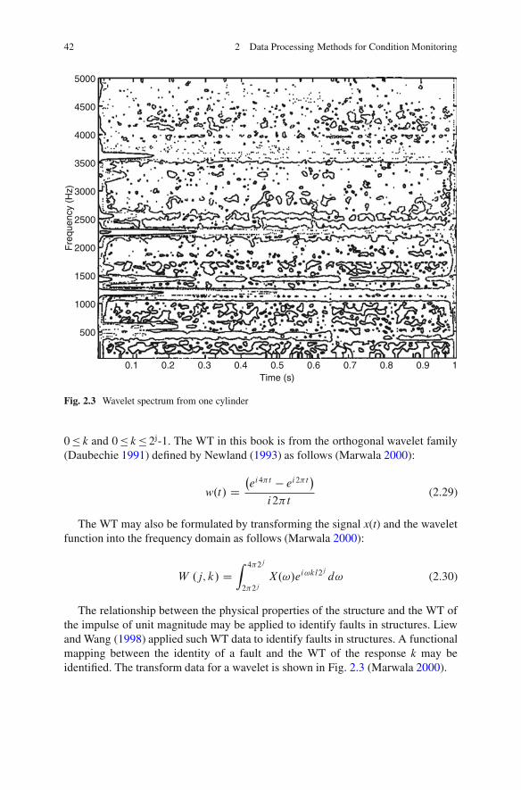
42 2 Data Processing Methods for Condition Monitoring
5000
4500
4000
3500
3000
2500
2000
1500
1000
500
0.1 0.2 0.3 0.4Time (s)
Fre
quen
cy (
Hz)
0.5 0.6 0.7 0.8 0.9 1
Fig. 2.3 Wavelet spectrum from one cylinder
0 � k and 0 � k � 2j-1. The WT in this book is from the orthogonal wavelet family(Daubechie 1991) defined by Newland (1993) as follows (Marwala 2000):
w.t/ D�ei4�t � ei2�t
�i2�t
(2.29)
The WT may also be formulated by transforming the signal x(t) and the waveletfunction into the frequency domain as follows (Marwala 2000):
W .j; k/ DZ 4�2j
2�2j
X.!/ei!kl2j
d! (2.30)
The relationship between the physical properties of the structure and the WT ofthe impulse of unit magnitude may be applied to identify faults in structures. Liewand Wang (1998) applied such WT data to identify faults in structures. A functionalmapping between the identity of a fault and the WT of the response k may beidentified. The transform data for a wavelet is shown in Fig. 2.3 (Marwala 2000).

2.11 Examples Used in This Book 43
2.10 Principal Component Analysis
For this book the principal component analysis (PCA) (Jolliffe 1986) was im-plemented to reduce the input data into independent components. The PCAorthogonalizes the components of the input vector so that they are uncorrelatedwith each other. When implementing the PCA for data reduction, correlations andinteractions among variables in the data are summarised in terms of a small numberof underlying factors. The PCA was introduced by Pearson (1901) to recast linearregression analysis into a new framework, and was developed further by Hotelling(1933) who applied it to Psychometry and it was subsequently generalized byLoeve (1963). The PCA has been successfully applied to reduce the dimensionof the data (Bishop 1995). Some researchers who have successfully applied thistechnique include Partridge and Calvo (1997) who applied the PCA to reduce thedimensions of two high-dimensional image databases, one of handwritten digitsand one of handwritten Japanese characters. The variant of the PCA used in thisbook finds the directions in which the data points have the most variance. Thesedirections are called principal directions. The data are then projected onto theseprincipal directions without the loss of significant information from the data. Herefollows a brief outline of the implementation of the PCA adopted in this book. Thecovariance matrix can be calculated as follows (Marwala 2001):
† DPX
pD1
.xp � �/ .xp � �/T (2.31)
Here † is the covariance matrix, T is for transpose, P is the number of vectorsin the training set, � is the mean vector of the data set taken over the number oftraining set and x is the input data. The second step is to calculate the eigenvalues andeigenvectors of the covariance matrix and arrange them from the largest eigenvalueto the smallest. The first N largest eigenvalues are chosen. In this book the first Neigenvalues were chosen in such a way that their sum constitutes at least 85% of thetotal sum of all the eigenvalues. By so doing at least 85% of the variance of the datawas retained. The data were then projected onto the eigenvectors corresponding tothe N most dominant eigenvalues.
2.11 Examples Used in This Book
This section reports on three examples: a rolling element bearing, a population ofcylindrical shells and transformer bushings.

44 2 Data Processing Methods for Condition Monitoring
Ball
Cage
Outer Raceway
DInner Raceway
Fig. 2.4 Ball bearing geometry, with diameter D
2.11.1 Rolling Element Bearing
Vibration measurement is important in an advanced conditioning monitoring ofmechanical systems. Most bearing vibrations are periodical movements. The ge-ometry of the bearing is shown in Fig. 2.4 (Purushothama et al. 2005; Li et al.2000; Nelwamondo et al. 2006a; Marwala et al. 2006). Generally, the rolling bearingcontains two concentric rings, which are called the inner and outer raceway (Li et al.2000). Furthermore, the bearing contains a set of rolling elements that run in thetracks of these raceways. There are number of standard shapes for the rollingelements such as the ball, the cylindrical roller, the tapered roller, needle rollers,the symmetrical and the unsymmetrical barrel roller (Li et al. 2000). For this book,a ball rolling element was used. Figure 2.4 also shows the cage, which ensuresuniform spacing and prevents mutual contact.
There were three faults studied for this book: an inner raceway fault, an outerraceway fault and a rolling element fault. A bearing fault increases the rotationalfriction of the rotor and therefore each fault generates vibration spectra withunique frequency components (Ericsson et al. 2004). It should be noted that thesefrequency components are a linear function of the running speed. Additionally,the two raceway frequencies are also linear functions of the number of balls. Themotor-bearing conditioning monitoring systems were implemented by analyzingthe vibration signal of all the bearing faults. The vibration signal was producedby the impact pulse generated when a ball roller hit a defect in the raceways or eachand every time the defect in the ball hit the raceways (Li et al. 2000).
The database used to validate new bearing fault diagnosis was developed at theRockwell Science Center by Loparo (Purushothama et al. 2005; Lou and Loparo2004) In this database, single point faults of diameters of 7 mils, 14 mils and 21mils (1 mil D 0.001 in.) were introduced using electro-discharge machining. Thesefaults were introduced separately at the inner raceway, rolling element (i.e., ball)and outer raceway. The experiments were performed for each fault diameter and

2.11 Examples Used in This Book 45
Accelerometer
Fault
Substructure 1
Substructure 2
Excitation position
Substructure 3
Sponge
Bubble wrap
Fig. 2.5 Illustration of the cylindrical shell showing the positions of the excitation impulse,accelerometer, substructures, fault position and supporting sponge
this was repeated for two load conditions, which were 1 and 2 horsepower. Theexperimentation was performed for vibration signals sampled at 12,000 samples persecond for the drive-end bearing faults. The vibration signals from this databasewere all divided into equal windows of four revolutions. Half of the resulting sub-signals were used for training and the other half were used for testing.
2.11.2 Population of Cylindrical Shells
The second experiment was performed on a population of cylinders, which weresupported by inserting a sponge rested on a bubble-wrap, to simulate a ‘free-free’environment (see Fig. 2.5). The impulse hammer test was performed on each of the20 steel seam-welded cylindrical shells. The impulse was applied at 19 differentlocations as indicated in Fig. 2.5. More details on this experiment may be found inMarwala (2001).
Each cylinder was divided into three equal substructures and holes of 10–15 mmdiameter were introduced at the centers of the substructures to simulate faults. Forone cylinder the first type of fault was a zero-fault scenario. This type of fault wasgiven the identity [000], indicating that there were no faults in any of the threesubstructures. The second type of fault was a one-fault-scenario, where a hole could

46 2 Data Processing Methods for Condition Monitoring
be located in any of the three substructures. Three possible one-fault-scenarios were[100], [010], and [001] indicating one hole in substructures 1, 2 or 3, respectively.The third type of fault was a two-fault scenario, where holes were located in twoof the three substructures. The three possible two-fault-scenarios were identified as[110], [101], and [011]. The final type of fault was a three-fault-scenario, where ahole was located in all three substructures. The identity of this fault was [111]. Eighttypes of fault-cases were considered (including [000]).
Each cylinder was measured three times under different boundary conditionsby changing the orientation of the rectangular sponge inserted inside the cylinder.The number of sets of measurements taken for undamaged population was 60 (20cylinders � 3 different boundary conditions). For the eight possible fault types, twofault types [000] and [111] had 60 occurrences while the rest had 24. It should benoted that the numbers of one- and two-fault cases were each 72. This was becauseas mentioned above, increasing the sizes of holes in the substructures and takingvibration measurements generated additional one- and two-fault cases.
2.11.3 Transformer Bushings
Bushings are an important component in electricity for transportation. They are usedin substation buildings, transformers, locomotives, and switchgear. Bushings causemore than 15% of transformer failures in Eskom (van Wyk 1997). Australasianreliability statistics on transformers over 1970–1995 concluded that bushingswere second to tap changers as the component initially involved in failure andwere amongst the top three contributors to costly transformer failures (Lord andHodge 2003). Figure 2.6 shows that the result of collateral damage and personnelinjury is a major concern, warranting the development of new and improved,affordable, reliable, and flexible diagnostics technologies to allow asset ownersto detect impending failures in a timely manner (Dhlamini and Marwala 2004a).Sokolov (2001) found that more than 46% of transformer defects were attributable tobushings, on-load tap changers, and the cooling system. The reliability of bushingsaffects the security of supply of electricity in an area and the economical operationof the area. Transformer failure research shows that bushings are among the top threemost frequent causes of transformer failure (Ward 2000; Lord and Hodge 2003;Vilakazi et al. 2005). Bushing failure is typically followed by a catastrophic eventsuch as a tank rupture, violent explosion of the bushing and fire (Lord and Hodge2003). With such consequences the major concern is collateral faults and personnelinjury. Numerous diagnostic tools exist such as on-line Partial Discharge analysis,on-line power factor, and infra-red scanning to detect an impending transformerfailure (Mojo 1997). In isolation, few of these approaches can offer all of the datathat a transformer operator needs to decide upon a course of action. Conditionmonitoring has many benefits such as: an unexpected failure can be avoidedthrough the possession of quality information relating to on-line condition of theplant and the resulting ability to identify faults in incipient levels of development.
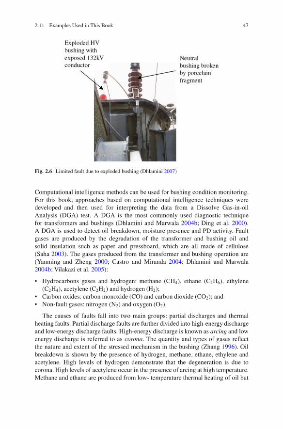
2.11 Examples Used in This Book 47
Fig. 2.6 Limited fault due to exploded bushing (Dhlamini 2007)
Computational intelligence methods can be used for bushing condition monitoring.For this book, approaches based on computational intelligence techniques weredeveloped and then used for interpreting the data from a Dissolve Gas-in-oilAnalysis (DGA) test. A DGA is the most commonly used diagnostic techniquefor transformers and bushings (Dhlamini and Marwala 2004b; Ding et al. 2000).A DGA is used to detect oil breakdown, moisture presence and PD activity. Faultgases are produced by the degradation of the transformer and bushing oil andsolid insulation such as paper and pressboard, which are all made of cellulose(Saha 2003). The gases produced from the transformer and bushing operation are(Yanming and Zheng 2000; Castro and Miranda 2004; Dhlamini and Marwala2004b; Vilakazi et al. 2005):
• Hydrocarbons gases and hydrogen: methane (CH4), ethane (C2H6), ethylene(C2H4), acetylene (C2H2) and hydrogen (H2);
• Carbon oxides: carbon monoxide (CO) and carbon dioxide (CO2); and• Non-fault gases: nitrogen (N2) and oxygen (O2).
The causes of faults fall into two main groups: partial discharges and thermalheating faults. Partial discharge faults are further divided into high-energy dischargeand low-energy discharge faults. High-energy discharge is known as arcing and lowenergy discharge is referred to as corona. The quantity and types of gases reflectthe nature and extent of the stressed mechanism in the bushing (Zhang 1996). Oilbreakdown is shown by the presence of hydrogen, methane, ethane, ethylene andacetylene. High levels of hydrogen demonstrate that the degeneration is due tocorona. High levels of acetylene occur in the presence of arcing at high temperature.Methane and ethane are produced from low- temperature thermal heating of oil but

48 2 Data Processing Methods for Condition Monitoring
high-temperature thermal heating produces ethylene and hydrogen plus methaneand ethane. The low-temperature thermal degradation of cellulose produces CO2
and high temperature heating produces CO.
2.12 Conclusions
In this chapter, the data processing techniques for condition monitoring in mechan-ical and electrical systems were reviewed. Approaches for acquiring data weredescribed and procedures for analyzing data were explained. Modal properties,pseudo-modal energies, wavelet, principal component analysis and Mel-frequencyCepstral Coefficients methods were described. Cases used in this book weredescribed: gearbox data, population of cylindrical shells data and transformerbushing data.
References
Adhikari S (1999) Rates of change of eigenvalues and eigenvectors in damped system. Am InstAeronaut Astronaut J 37:1452–1458
Altman J, Mathew J (2001) Multiple band-pass autoregressive demodulation for rolling elementbearing fault diagnosis. Mech Syst Signal Process 15(5):963–997
Antoni J (2006) The spectral kurtosis: a useful tool for characterising non-stationary signals. MechSyst Signal Process 20(2):282–307
Aydin N, Padayachee S, Markus HS (1999) The use of the wavelet transform to describe embolicsignals. Ultrasound Med Biol 25(6):953–958
Bishop CM (1995) Neural networks for pattern recognition. Oxford University Press, OxfordBoumahdi M (1996) Blind identification using the kurtosis with applications to field data. Signal
Process 48(3):205–216Castro ARG, Miranda V (2004) An interpretation of neural networks as inference engines with
application to transformer failure diagnosis. In: IEEE international conference on probabilisticmethods applied to power systems, Porto, Portugal, pp 997–1002
Cheng T, Rivard B, Sanchez-Azofeifa A (2011) Spectroscopic determination of leaf water contentusing continuous wavelet analysis. Remote Sens Environ 115(2):659–670
Cross SS (1994) The application of fractal geometric analysis to microscopic images. Micron25(1):101–113
Dathe A, Eins S, Niemeyer J, Gerold G (2001) The surface fractal dimension of the soil-poreinterface as measured by image analysis. Geoderma 103(1–2):203–229
Daubechie I (1991) The wavelet transform, time-frequency localization, and signal processing.IEEE Trans Inform Theory 36:961–1005
de la Rosa JJG, Moreno-Munoz A, Gallego A, Piotrkowski R, Castro E (2010) On-site non-destructive measurement of termite activity using the spectral kurtosis and the discrete wavelettransform. Measurement 43(10):1472–1488
Dhlamini SM (2007) Bushing diagnosis using artificial intelligence and dissolved gas analysis.PhD thesis, University of the Witwatersrand
Dhlamini SM, Marwala T (2004a) An application of SVM, RBF and MLP with ARD on bushings.In: Proceedings of the IEEE conference on cybernetics and intelligent systems, Singapore,pp 1245–1258
References 49
Dhlamini SM, Marwala T (2004b) Bushing monitoring using MLP and RBF. In: Proceedings ofthe IEEE Africon 2004, Gaborone, Botswana, pp 613–617
Ding X, Liu Y, Griffin PJ (2000) Neural nets and experts system diagnoses transformer faults.IEEE Comput Appl Power 13(1):50–55
Doebling SW, Farrar CR, Prime MB, Shevitz DW (1996) Damage identification and healthmonitoring of structural and mechanical systems from changes in their vibration characteristics:a literature review Los Alamos National Laboratory report LA-13070-MS
Dougherty G, Henebry GM (2001) Fractal signature and lacunarity in the measurement of thetexture of trabecular bone in clinical CT images. Med Eng Phys 23(6):369–380
El-Wardany TI, Gao D, Elbestawi MA (1996) Tool condition monitoring in drilling using vibrationsignature analysis. Int J Mach Tool Manufacture 36(6):687–711
Ericsson S, Grip N, Johansson E, Persson LE, Sjoberg R, Stromberg JO (2004) Towards automaticdetection of local bearing defects in rotating machines. Mech Syst Signal Process 19:509–535
Eritenel T, Parker RG (2009) Modal properties of three-dimensional helical planetary gears.J Sound Vib 325(1–2):397–420
Ewins DJ (1995) Modal testing: theory and practice. Research Studies Press, LetchworthFadili MJ, Bullmore ET (2004) A comparative evaluation of wavelet-based methods for hypothesis
testing of brain activation maps. NeuroImage 23(3):1112–1128Fahmy MMM (2010) Palmprint recognition based on Mel frequency Cepstral coefficients feature
extraction. Ain Shams Eng J 1(1):39–47Falconer K (1952) Fractal geometry; mathematical foundations and application. John Wiley, New
YorkGilliam X, Dunyak J, Doggett A, Smith D (2000) Coherent structure detection using wavelet
analysis in long time-series. J Wind Eng Ind Aerodyn 88(2–3):183–195Gradshteyn IS, Yyzhik IM (1994) Tables of integrals, series, and products. Academic, LondonHarris CM (1998) The Fourier analysis of biological transients. J Neurosci Meth 83(1):15–34Hotelling H (1933) Analysis of a complex of statistical variables into principal components. J Educ
Psychol 24:417–441Jolliffe IT (1986) Principal component analysis. Springer, New YorkKerut EK, Given MB, McIlwain E, Allen G, Espinoza C, Giles TD (2000) Echocardiographic
texture analysis using the wavelet transform: differentiation of early heart muscle disease.Ultrasound Med Biol 26(9):1445–1453
Kollo T (2008) Multivariate skewness and kurtosis measures with an application in ICA. J MultivarAnal 99(10):2328–2338
Lacarbonara W, Paolone A, Vestroni F (2007) Non-linear modal properties of non-shallow cables.Int J Non-Linear Mech 42(3):542–554
Li B, Chow MY, Tipsuwan Y, Hung JC (2000) Neural-network-based motor rolling bearing faultdiagnosis. IEEE Trans Ind Electron 47:1060–1068
Liew KM, Wang Q (1998) Application of wavelet theory for crack identification in structures.J Eng Mech ASCE 124(2):152–157
Lim J, Bienkiewicz B, Richards E (2011) Modeling of structural coupling for assessment of modalproperties of twin tall buildings with a skybridge. J Wind Eng Ind Aerodyn 99(5):615–623
Loeve M (1963) Probability theory, 3rd edn. Van Nostrand, New YorkLord T, Hodge G (2003) On-line monitoring technology applied to HV bushing. In: Proceedings
of the AVO conference, New Zealand, November (CD-ROM)Lou X, Loparo KA (2004) Bearing fault diagnosis based on wavelet transform and fuzzy inference.
J Mech Syst Signal Process 18:1077–1095Lunga D, Marwala T (2006) Time series analysis using fractal theory and online ensemble
classifiers, vol 4304/2006, Lectures notes in artificial intelligence. Springer, Berlin/Heidelberg,pp 312–321
Magosso E, Ursino M, Zaniboni A, Gardella E (1 January 2009) A wavelet-based energeticapproach for the analysis of biomedical signals: application to the electroencephalogram andelectro-oculogram. Appl Math Comput, Includes Special issue on Emergent Applications ofFractals and Wavelets in Biology and Biomedicine 207(1):42–62

50 2 Data Processing Methods for Condition Monitoring
Maia NMM, Silva JMM (1997) Theoretical and experimental modal analysis. Research StudiesPress, Letchworth
Manning R (1994) Damage detection in adaptive structures using neural networks. In: Proceedingsof the 35th AIAA/ASME/ASCE/AHS/ASC structures, structural dynamics, and materialsconference, Hilton Head, South Carolina, pp 160–172
Maragos P, Potamianos A (1999) Fractal dimensions of speech sounds: computation and applica-tion to automatic speech recognition. J Acoust Soc Am 105:1925–1932
Marwala T (2000) On damage identification using a committee of neural networks. AmericanSociety of Civil Engineers. J Eng Mech 126:43–50
Marwala T (2001) Fault identification using neural networks and vibration data. Doctor ofPhilosophy, University of Cambridge
Marwala T (2003) Fault classification using pseudo modal energies and neural networks. Am InstAeronaut Astronaut J 41(1):82–89
Marwala T, Heyns PS (1998) A multiple criterion method for detecting damage on structures. AmInst Aeronaut Astronaut J 195:1494–1501
Marwala T, Hunt HEM (1999) Fault identification using a committee of neural networks. In:Friswell MI, Mottershead JE, Lees AW (eds) Identification in engineering systems. SwanseaWales, UK, pp 102–111
Marwala T, Mahola U, Nelwamondo F (2006) Hidden Markov models and Gaussian mixturemodels for bearing fault detection using fractals. In: Proceedings of the IEEE internationaljoint conference on neural networks, Vancouver, BC, Canada, pp 5876–5881
Meruane V, Heylen W (2011) An hybrid real genetic algorithm to detect structural damage usingmodal properties. Mech Syst Signal Process 25(5):1559–1573
Mojo B (1997) Transformer condition monitoring (non-invasive Infrared Thermography Tech-nique). Masters thesis, Department of Electrical Engineering, University of the Witwatersrand
Nelwamondo FV, Marwala T, Mahola U (2006a) Early classifications of bearing faults usinghidden Markov models, Gaussian mixture models, Mel-frequency Cepstral coefficients andfractals. Int J Innov Comput Inform Control 2(6):1281–1299
Nelwamondo FV, Mahola U, Marwala T (2006b) Multi-scale fractal dimension for speakeridentification system. Trans Syst 5(5):1152–1157
Nelwamondo FV, Mahola U, Marwala T (2006c) Improving speaker identification rate usingfractals. In: Proceedings of the IEEE international joint conference on neural networks,Vancouver, BC, Canada, pp 5870–5875
Newland DE (1993) An introduction to random vibration, spectral and wavelet analysis, 3rd edn.Longman, Harlow, and John Wiley, New York
Nikravan B, Baul RM, Gill KF (1989) An experimental evaluation of normalised Fourierdescriptors in the identification of simple engineering objects. Comput Ind 13(1):37–47
Ovanesova AV, Suarez LE (2004) Applications of wavelet transforms to damage detection in framestructures. Eng Struct 26(1):39–49
Partridge MG, Calvo RA (1997) Fast dimensionality reduction and simple PCA. Intell Data Anal2(3):724–727
Pearson K (1901) On lines and planes of closest fit to systems of points in space. Philos Mag2:559–572
Purushothama V, Narayanana S, Prasadb SAN (2005) Multi-fault diagnosis of rolling bearingelements using wavelet analysis and hidden Markov model based fault recognition. NDT&EInt 38:654–664
Rizos PF, Aspragathos N, Dimarogonas AD (1990) Identification of crack location and magnitudein a cantilever beam from the vibration modes. J Sound Vib 138:381–388
Saha TK (2003) Review of modern diagnostic techniques for assessing insulation condition in agedtransformer. IEEE Trans Dielect Electr Insul 10(5):903–917
Sanchez I, Uzcategui G (2011) Fractals in dentistry. J Dent 39(4):273–292Sejdic E, Djurovic I, Stankovic L (2011) Fractional fourier transform as a signal processing tool:
an overview of recent developments, signal processing. Fourier Related Transforms for Non-Stationary Signals 91(6):1351–1369

References 51
Sokolov V (2001) Transformer life management, II workshop on power transformers-deregulationand transformers technical, economic, and strategical issues, Salvador, Brazil, 29–31 August
Sokolowska Z, Sokolowski S (2000) Influence of humic acid on surface fractal dimension ofkaolin: analysis of mercury porosimetry and water vapour adsorption data. In: Pachepsky Y,Crawford JW, Rawls WJ (eds) Fractals in soil science, vol 27, Developments in soil science.Elsevier, Amsterdam/New York, pp 143–159
Stamataki I, Kapsalis A, Mikroulis S, Syvridis D, Hamacher M, Troppenz U, Heidrich H (2009)Modal properties of all-active InGaAsP/InP microring lasers. Opt Commun 282(12):2388–2393
Stubbs NJ, Kim JT, Topole K (1992) An efficient and robust algorithm for damage localization inoffshore platforms. In: Proceeding of the American Society of Civil Engineers 10th structurescongress, San Antonio, pp 543–546
Surace C, Ruotolo R (1994) Crack detection of a beam using the wavelet transform. In: Proceedingsof the 12th international modal analysis conference, Honolulu, Hawaii, pp 1141–1148
Tufekci Z, Gowdy JN, Gurbuz S, Patterson E (2006) Applied mel-frequency discrete waveletcoefficients and parallel model compensation for noise-robust speech recognition. SpeechCommun 48(10):1294–1307
van Wyk S (1997) Transformer field performance in subSaharan Africa. Energize Magazine,Jul/Aug issue:44–47
Viale P, Fevrier S, Leproux P, Jaouen Y, Obaton A-F (2006) Modal properties of solid-corephotonic bandgap fibers. Photonics Nanostruct – Fundam Appl 4(2):116–122
Vilakazi CB, Mautla RP, Moloto EM, Marwala T (2005) On-line bushing condition monitoring. In:Garcia-Planas MI et al (eds) Proceedings of the 5th WSEAS/IASME international conferenceon electric power systems, high voltages, electric machines, Tenerife, Spain, pp 406–411
Wang F, Zheng F, Wu W (2000) A C/V segmentation for Mandarin speech based on multi-scalefractal dimension. In: International conference on spoken language processing, Beijing, China,pp 4:648–651
Wang J, Wang J, Weng Y (2002) Chip design of MFCC extraction for speech recognition. IntegrVLSI J 32(1–3):111–131
Wang Z, Willett P, DeAguiar PR, Webster Y (2001) Neural network detection of grinding burnfrom acoustic emission. Int J Mach Tool Manufacture 41(2):283–309
Ward B (2000) A survey of new techniques in insulation monitoring of power transformers. IEEEElectr Insul Mag 17(3):16–23
Yanming T, Zheng Q (2000) DGA based insulation diagnosis of power transformer via ANN.In: Proceedings of the 6th international conference on properties and application of dielectricmaterials, Winnipeg, Canada, pp 1:133–137
Zhang J, Xu Q, Lu X (2011) Propagation properties of Gaussian beams through the anamorphicfractional Fourier transform system with an eccentric circular aperture. Optik – Int J LightElectron Opt 122(4):277–280
Zhang Y (1996) An artificial neural network approach to transformer fault diagnosis. IEEE TransPower Deliv 11:1836–1841

Chapter 3Multi-Layer Perceptron for ConditionMonitoring in a Mechanical System
3.1 Introduction
It is important to identify faults before the occurrence of faults in a mechanicalsystem as it prevents the loss of life and reduces the machine down-time. Theprocess of fault identification entails the gathering of data, the processing of datato reveal vital features and the interpretation of the data. For this chapter, vibrationdata were measured and were processed as explained in Chap. 2. The data was thenanalyzed to identify the faults. The mechanism that was adopted to analyze the datain this chapter was the Multi-Layer Perceptron (MLP) neural network.
Dimla and Lister (2000) applied the MLP neural network for the monitoring ofthe condition of an on-line metal cutting tool. They performed test cuts on an EN24alloy steel using P15 and P25 coated cemented carbide inserts. Thereafter, cuttingforces and vibration data were measured online. Concurrently the wear sizes on thecutting boundaries were measured and these as well as the processed data were putinto a multi-layer perceptron neural network that had been trained to identify thetool state. When the proposed system was tested on a number of cutting types itwas able to classify tool state condition with an accuracy of 90%. However, theperformance worsened when the cutting types were altered considerably.
Mustapha et al. (2007) applied a vector of novelty indices for damage detectionand location in an isotropic plate. Their method was based on the novelty detectiontechnique, outlier analysis and a multi-layer perceptron neural network. To evaluatethe usefulness of the method, a thin rectangular plate with isotropic behavior wasexperimentally assessed. Additionally, a study was made of the scattering effect ofan ultrasonic guided wave on the investigated plate, for both a faulty and a healthystate of affairs. Wave propagation was successively communicated and measuredby 8 Piezo-electic Transducer (PzT) patches bonded on the plate, creating a sensornetwork on the tested isotropic rectangular structure. An 8-channel multiplexer wasincluded in the small scale, low-cost ‘structural health monitoring’ system to switchthe PzTs task from sensor to actuator. Fault identification software was developedto obtain the waveform responses. The scattering waveform responses indicating
T. Marwala, Condition Monitoring Using Computational Intelligence Methods:Applications in Mechanical and Electrical Systems, DOI 10.1007/978-1-4471-2380-4 3,© Springer-Verlag London Limited 2012
53

54 3 Multi-Layer Perceptron for Condition Monitoring
healthy and faulty conditions were transformed into a set of novelty indices thateventually define the conditions of the tested structure. The developed noveltyindices indicating the available sensor paths were applied as the inputs to the MLPneural network to identify faults on the tested isotopic plate.
Herzog et al. (2009) applied the MLP neural network for estimating the residuallife of a machine and its components. They trained and tested numerous neuralnetwork variations with data from two different reliability-related datasets. The firstdataset represented the renewal case where the failed unit was repaired and restoredto a good-as-new condition. Data were collected in the laboratory by subjecting aseries of similar test pieces to fatigue loading with a hydraulic actuator. The averageprediction error of the various neural networks being compared varied from 431to 841 s on this dataset, where test pieces had a characteristic life of 8971 s. Thesecond dataset was gathered from a collection of pumps used to circulate a waterand magnetite solution within a plant. The data was obtained from a repaired systemaffected by reliability degradation. When optimized, the multi-layer perceptronneural networks trained with the Levenberg-Marquardt procedure and the generalregression neural network gave a sums-of squares error within 11.1% of each otherfor the renewal dataset. The small number of inputs and poorly mapped input spaceon the second dataset indicated that much larger errors were verified on some ofthe test data. Nevertheless, the prospect of using neural networks for residual lifeprediction and the advantage of integrating condition-based data into the model wasdemonstrated in both examples.
Rafiee et al. (2007) applied a multi-layer perceptron neural network for theintelligent condition monitoring of a gearbox. The input to the MLP neural networkconsisted of the standard deviations of wavelet packet coefficients of vibration data.The gear conditions were classified as normal gearbox, slightly-worn, medium-worn, broken-teeth gear damage and a general bearing fault. The results indicatedan accurate identification of the faults.
Abu-Mahfouz (2003) successfully applied vibration data and multi-layer per-ceptron neural network for detection and classification of drilling wear. The studycompared several architectures and used a vibration signature as the source ofinformation from the machining process. Five different drill wear conditions weresimulated and used to train the neural network for fault identification. It wasobserved that the frequency domain features were more effective in training theneural network than were the time domain data.
Kim et al. (2006) applied wavelets with Daubechie’s four functions and multi-layer perceptron network neural networks to detect the toxic response behavior ofchironomids for water quality monitoring. The variables chosen were based onthe feature coefficients of Discrete Wavelet Transforms and were used as inputfor training the MLP network. The trained network capably detected changesin movement patterns before and after the treatments and it was shown thatthe application of the wavelets and artificial neural networks was useful for theautomatic monitoring of water quality.
Marwala and Hunt (1999) presented a committee of neural networks technique,which employed both frequency response functions and modal data simultaneously

3.2 Mathematical Framework 55
to identify faults in structures. They tested this technique on simulated data froma cantilevered beam, which was structured into five regions. It was observed thatirrespective of the noise levels in the data, the committee of neural networks gaveresults that had a lower mean-squares error and standard deviation than the twoexisting methods. It was found that the method could identify fault cases betterthan the two approaches used individually. It was established that for the problemanalyzed, giving equal weights to the frequency-response-based method and modal-properties-based method minimized the errors in identifying faults.
Bucolo et al. (2002) successfully applied multi-layer perceptron and neuro-fuzzysystems in predicting models for the corrosion phenomena in pulp and paper plant.The data was gathered in a Wisaforest pulp mill in Finland.
Caputo and Pelagagge (2002) successfully applied the MLP neural networkapproach for piping network monitoring to localize leakages based on pressure andflow rate information. Elsewhere Yella et al. (2009) successfully applied machinevision based method for the condition monitoring of wooden railway sleepers.Furthermore, Kwak et al. (2002) applied a multi-layer perceptron neural networkto recognize the movement tracks of medaka (Oryzias latipes) in response to sub-lethal treatments of an insecticide.
3.2 Mathematical Framework
In this section, the mathematical background of the multi-layer perceptron neuralnetworks is explained, including a review of background literature of successfulimplementations, an explanation of architectures, and a description of a method thatwas implemented to train the MLP.
A neural network is an information processing technique that is inspired by theway biological nervous systems, like the human brain, process information. It is acomputer based machine, designed to model the way in which the brain performsa particular function of interest (Haykin 1999). It is an extraordinarily powerfulmechanism that has found successful use in the diverse fields of mechanicalengineering (Marwala and Hunt 1999; Vilakazi and Marwala 2007), civil engi-neering (Marwala 2000), aerospace engineering (Marwala 2001a; Marwala 2003),biomedical engineering (Marwala 2007), and finance (Patel and Marwala 2006).In this chapter, a multi-layer perceptron neural network is viewed as generalizedregression model that can model both linear and non-linear data. The constructionof a neural network involves four main steps (Marwala and Lagazio 2011; Msizaet al. 2007):
1. the processing units uj, where each uj has a certain activation level aj(t) at anypoint in time;
2. weighted inter-connections between a number of processing units. These inter-connections govern how the activation of one unit leads to the input for anotherunit;

56 3 Multi-Layer Perceptron for Condition Monitoring
3. an activation rule, which acts on the set of input signals at a processing unit toproduce a new output signal; and
4. a learning rule that stipulates how to fine-tune the weights for a given input oroutput (Freeman and Skapura 1991).
Because they are capable of extracting meaning from complex data, neuralnetworks are engaged to extract patterns and detect trends that are too complexto be identified by many other computer techniques (Hassoun 1995). A trainedneural network can be viewed as an expert in the class of information that it hasbeen given to analyze (Yoon and Peterson 1990). This expert can then be applied tooffer predictions when presented with new circumstances. Because of their abilityto adapt to non-linear data, neural networks have been applied to model a numberof non-linear applications (Hassoun 1995; Leke et al. 2007).
The architecture of neural processing units and their inter-connections can have asignificant influence on the processing capabilities of neural networks. Accordingly,there are many different connections that define how data flows between the input,hidden and output layers. The next section gives details on the architecture of themulti-layer perceptron neural networks employed in this chapter.
3.2.1 Multi-Layer Perceptrons (MLP) for ClassificationProblems
In the past 30 years the MLP neural networks have successfully been appliedto both classification and regression problems. Ikuta et al. (2010) connected achaos glial network to the MLP to solve a two-spiral problem and found that theirmethod performed better than the conventional MLP. Zadeh et al. (2010) used theMLP to predict the daily flows from the Khosrow Shirin watershed, and observedthat precipitation and discharge with a 1 day time lag best predicted daily flows.Narasinga-Rao et al. (2010) applied the multi-layer perceptron to predicting thequality of life in diabetes patients using age, gender, weight, and fasting plasmaglucose as inputs.
Pasero et al. (2010) used the MLP for a time series analysis while Sug (2010)used a MLP for task classification. Zhang and Li (2009) used a hybrid of the HiddenMarkov Model (HMM) and the MLP for speech recognition and demonstrated thatthe hybrid model performed better than the HMM.
He et al. (2009) used the MLP for short-term demand forecasting using graphicsprocessing units. Bernardo-Torres and Gomez-Gil (2009) used the MLP to forecastseismograms while Sug (2009) applied the MLP to pilot sampling. Kushwaha andShakya (2009) successfully applied the MLP for predicting the helical content ofproteins while Karami et al. (2009) successfully applied it to decoding low-densityparity-check codes.
Other applications for the MLP include the work by Achili et al. (2009) inrobotics, Sancho-Gomez et al. (2009) for decision support systems with missing

3.2 Mathematical Framework 57
data, Krishna (2009) in an air data system, Hu and Weng (2009) in image processing,Duta and Duta (2009) in turbo-machinery optimization, Pontin et al. (2009) inpredicting the occurrence of stinging jellyfish, Yazdanmehr et al. (2009) for themodeling of nanocrystals, Watts and Worner (2009) for predicting the distributionof fungal crop diseases as well as Yilmaz and Ozer (2009) for pitch angle control inwind turbines above the rated wind speed.
In this book, neural networks are regarded as a broad structure for describing non-linear mappings between multi-dimensional spaces where the form of the mappingis overseen by a set of free parameters (Bishop 1995; Mohamed 2003; Mohamedet al. 2006) which have to be estimated from the data. There are two ways inwhich neural networks can be trained: supervised or unsupervised learning. Weconsider only supervised learning in this book. In supervised learning, the trainingdata involves both the input to the neural networks and a corresponding targetoutput. In this chapter, the input is a set of features that are deemed to influencethe health status of the structure such as vibration data and the output is the identityof the faults.
3.2.2 Architecture
The multi-layer perceptron neural network architecture was selected for mappingthe relationship between vibration data and the identity of faults. Each connectionbetween inputs and neurons was weighted by adjustable weight parameters. Inaddition, each neuron had an adjustable bias weight parameter which is denotedby a connection from a constant input x0 D 1 and z0 D 1 for the hidden neuronsand the output neuron, respectively. This group of two-layer multi-layer perceptronmodels can approximate any continuous function with arbitrary accuracy, as long asthe number of hidden neurons is sufficiently large (Bishop 1995; Mohamed 2006).
The advantage of the multi-layer perceptron network is the interconnected cross-coupling that occurs between the input variables and the hidden nodes, with thehidden nodes and the output variables. If we assume that x is the input to the multi-layer perceptron and y is the output of the MLP, a mapping function between theinput and the output may be written as follows (Bishop 1995):
y D foutput
0@ MX
jD1
wj fhidden
NX
iD0
wij xi
!C w0
1A (3.1)
Here N is the number of inputs units, M is the number of hidden neurons, xi is the ith
input unit, wij is the weight parameter between input i and hidden neuron j and wj isthe weight parameter between hidden neuron j and the output neuron. The activationfunction foutput.�/ is sigmoid and can be written as follows (Bishop 1995):
foutput .a/ D 1
1 C e�a(3.2)

58 3 Multi-Layer Perceptron for Condition Monitoring
In this chapter, we apply a neural network to classify the identity of fault. Inmodeling complex problems, care must be taken in the choice of the outputactivation function. For classification problems, as is the case in this chapter, thesigmoid function indicated in Eq. 3.2 is ideal (Bishop 1995). The activation functionfhidden.�/ is a hyperbolic tangent which can be written as (Bishop 1995):
fhidden.a/ D tanh.a/ (3.3)
3.2.3 Training of the Multi-Layer Perceptron
Once the activation function is defined and the sizes of the hidden nodes are selected,what remains is to approximate the network weights. The network weights areapproximated from the observed data through a method called training. There are anumber of critical matters that must be taken into account in training the networks.These include ensuring that, on identifying the network weights, the resultingnetwork must not just memorize the data but learn from it. There are methodsthat have been presented to deal with this specific matter, and they comprise cross-validation, early-stopping, and regularization.
Two common methods can be applied to train a neural network. These methodsare the maximum likelihood technique and the Bayesian method. The maximumlikelihood technique estimates the network weights that maximize the capacity of atrained network to estimate the observed data, while the Bayesian method createsthe probability distribution of the network model given the observed data. It shouldbe noted here that the maximum likelihood and Bayesian methods are the same andthe only difference is that the maximum likelihood technique identifies the networkvector of weights that is most likely in the posterior probability distribution function.The first undertaking in identifying a vector of network weights that maximizesthe predictive capacity of the neural network is to build a fitness function in theevolutionary programming perspective. The fitness function is a measure of thedifference between the approximations of the model and the observed data.
In a two-class classification problem, the fitness function is the differencebetween the neural network’s estimated output and the target output, t, given inEq. 3.1 for all training patterns. E is the cross-entropy error function given by(Bishop 1995; Marwala 2009; Marwala and Lagazio 2011):
E D �PX
pD1
˚tp ln.yp/ C .1 � tp/ ln.1 � yp/
�(3.4)
There are many advantages of the cross-entropy function. One of these includes thefact that it permits the output to be understood probabilistically without the necessityof invoking a Bayesian method. Neural networks are trained by iteratively adjustingthe weight parameters, w, to minimize the fitness function given by Eq. 3.4. This is

3.2 Mathematical Framework 59
accomplished by randomly initializing the network weights and then adjusting theweight parameters using the scaled conjugate gradient technique (Møller 1993). Thescaled conjugate gradient technique was selected over other optimization methodsfor the reason that it has efficient convergence properties.
Generalization is the capability of a trained neural network model to classifyinput patterns that were not observed during the training of the neural network. Es-sentially, on pursuing a network that generalizes, one identifies the balance betweenthe capabilities of a network to remember the training data with the capability ofthe network to estimate data not seen. The generalization of performance is a truereflection of the capacity of a neural network to classify faults. This can simply beproven by separating the data into training and testing data sets.
Bishop (1995) demonstrated that a minimization of the cross-entropy fitnessfunction in the neural network training with the activation function of a neuralnetwork results in the output of a neural network approximating the posteriorprobability of membership to a specific class, given the input fxg. In the present caseof modeling the identity of faults, the output estimates the posterior probability of aspecific identity of fault. If this class is represented by C1 and the pattern class fornot containing faults is represented by C2, the relations for the posterior probabilityof class membership can be written as (Bishop 1995; Tettey and Marwala 2007):
P .C1 jfxg / D y (3.5)
P .C2 jfxg / D 1 � y (3.6)
Equations 3.5 and 3.6 offer a probabilistic interpretation to the neural networkoutput. On the account of these relationships, it is obvious that the input vector has ahigh probability of being an element of class C1 when y is close to 1 and C2 when yis close to 0. If y is close to 0.5, then there is uncertainty in the class membership ofthe input vector. An elementary method to increase the efficacy of the classifier is todevise an upper and lower rejection threshold to the neural network output (Bishop1995; Mohamed 2003). This classification decision rule can be expressed as follows(Mohamed 2003):
Choose C1 if y > �;
choose C2 if y < .1 � �/ ;
otherwise do not classify fxg:(3.7)
The parameter � sets the level of the rejection threshold and permits the engineer tochoose the level at which a decision can be made.

60 3 Multi-Layer Perceptron for Condition Monitoring
3.2.4 Back-Propagation Method
To identify the network weights given the training data, an optimization techniquecan be applied, within the context of the maximum-likelihood framework. Ingeneral, the weights can be identified using the following iterative technique(Werbos 1974):
fwgiC1 D fwgi � �@E
@fwg .fwgi / (3.8)
In Eq. 3.8, the parameter � is the learning rate while fg represents a vector. Theminimization of the fitness function, E, is achieved by calculating the derivative ofthe errors, in Eq. 3.7, with respect to the network weight. The derivative of the erroris calculated with respect to the weight which connects the hidden layer to the outputlayer, and can be written using the chain rule as follows (Bishop 1995; Marwala2009):
@E
@wkj
D @E
@ak
@ak
@wkj
D @E
@yk
@yk
@ak
@ak
@wkj
DX
n
f0
outer.ak/@E
@ynk
zj
(3.9)
In Eq. 3.9, zj D finner.aj / and ak D PMjD0 w.2/
kj yj : The derivative of the error withrespect to weight which connects the hidden to the output layer may be written usingthe chain rule as (Bishop 1995):
@E
@wkj
D @E
@ak
@ak
@wkj
DX
n
f0
inner.aj /X
k
wkj f0
outer.ak/@E
@ynk
(3.10)
In Eq. 3.10, aj DdP
iD1
w.1/j i xi : The derivative of the fitness function in Eq. 3.4 may
thus be written as:
@E
@ynk
D tnk � ynk
ynk .ynk � 1/(3.11)
while that of the hyperbolic tangent function is:

3.2 Mathematical Framework 61
f0
inner.aj / D sec h2.aj /: (3.12)
The derivative of the logistic activation function is:
f0
outer .ak/ D f .ak/ .1 � f .ak// (3.13)
Given that it has been determined how to compute the gradient of the error withrespect to the network weights using back-propagation algorithms, Eq. 3.8 can beapplied to update the network weights using an optimization process until somepre-defined stopping condition is achieved. If the learning rate in Eq. 3.8 is fixedthen this is known as the steepest descent optimization method (Robbins and Monro1951). Alternatively, since the steepest descent technique is not computationallyefficient an improved technique needs to be developed, and in this chapter the scaledconjugate gradient method is implemented (Møller 1993), which is the concern ofthe next section.
3.2.5 Scaled Conjugate Gradient Method
The technique in which the network weights are inferred from the data is byapplying some non-linear optimization technique (Mordecai 2003), and for thischapter is the scaled conjugate gradient technique. Before the scaled conjugategradient technique is described, it is important to comprehend how it operates.As described before, the weight vector that gives the minimum error is attainedby taking successive steps through the weight space as shown in Eq. 3.8 untilsome stopping criterion is achieved. Different algorithms select this learningrate differently. In this section, the gradient descent technique will be discussed,followed by how it can be extended to the conjugate gradient technique (Hestenesand Stiefel 1952). For the gradient descent technique, the step size is defined as��@E=@w, where the parameter � is the learning rate and the gradient of the erroris calculated using the back-propagation method described in the previous section.
If the learning rate is adequately small, the value of error decreases at each stepuntil a minimum value is attained for the error between the model prediction andtraining target data. The disadvantage with this method is that it is computationallyexpensive when compared to other methods. For the conjugate gradient technique,the quadratic function of the error is minimized at each iteration over a progressivelyexpanding linear vector space that includes the global minimum of the error(Luenberger 1984; Fletcher 1987; Bertsekas 1995).
For the conjugate gradient technique, the following steps are followed (Haykin1999):
1. Choose the initial weight vector fwg0.2. Calculate the gradient vector @E
@fwg.fwg0/:

62 3 Multi-Layer Perceptron for Condition Monitoring
3. At each step n use a line search to find the �.n/ that minimizes E.�/ whichrepresents the cost function expressed in terms of � for fixed values of w and� @E
@fwg.fwng/:4. Check that the Euclidean norm of the vector � @E
@w .fwng/ is sufficiently less thanthat of � @E
@w .fw0g/:5. Update the weight vector using Eq. 3.8.6. For wnC1 compute the updated gradient @E
@fwg.fwgnC1/:
7. Use the Polak-Ribiere method to calculate:
ˇ.n C 1/ D rE.fwgnC1/T .rE.fwgnC1/ � rE.fwgn///
rE.fwgn/T rE.fwgn/
8. Update the direction vector
@E
@fwg .fwgnC2/ D @E
@fwg .fwgnC1/ � ˇ.n C 1/@E
@fwg .fwgn/:
9. Set n D n C 1 and go back to step 3.10. Stop when the following condition is satisfied: @E
@fwg .fwgnC2/ D " @[email protected]/
where " is a small number.
The scaled conjugate gradient method differs from the conjugate gradient methodin that it does not involve the line search explained in step 3. The step-size (see step3) can be calculated directly by using the following formula (Møller 1993):
�.n/ D 2
0BBBB@�.n/ �
�@E.n/
@fwg .n/
�T
H.n/
�@E.n/
@fwg .n/
�:::
C �.n/
�
@E.n/
@fwg .n/
� 2
, �
@E.n/
@fwg .n/
�
1CCCCA
2
(3.14)
Here H is the Hessian of the gradient. The scaled conjugate gradient method wasused because it has been found to solve the optimization problems encounteredwhen training an MLP network to be more computationally efficient than thegradient descent and conjugate gradient methods (Bishop 1995).
3.3 The Multifold Cross-Validation Method
In the example of cylindrical shells considered in this chapter and described in Chap.2 (Marwala 2001b), because there is a limited amount of data available, the trainingdata set was also applied as a validation data set by using a multifold cross-validation

3.3 The Multifold Cross-Validation Method 63
Partition K Partition 3 Partition 2 Partition 1
Training case 1
Training case 2
Training case 3
Training case K
Fig. 3.1 The multifold cross-validation technique applied where the network was trained K times,each time leaving out the data indicated by the shaded area and using the omitted data for validationpurposes. The validation error was acquired by averaging the squared error under validation overall the trials of the experiment
technique (Stone 1974; Kohavi 1995). The multifold method implemented in thepresent study is illustrated in Fig. 3.1 (Marwala 2001b). Each column in Fig. 3.1demonstrates a partition of the training data set and each row denotes a trainingcase. The shaded box for a given training case is the partition that is applied forvalidation purposes whereas the rest of the boxes in one row are applied to train thenetwork.
When the multifold cross-validation method is applied, the training data set withN examples is segmented into K partitions. Here it is assumed that N is divisibleby K and that K > 1. For each training process, the network is trained with the datafrom all partitions excluding one and the validation set is the subset that is left out.The partition that is left out for each training case is a shaded one. For example, infor Training case 1 the network is trained using Partitions 2 to K and Partition 1 isused as a validation set. The procedure is repeated for K training cases, by leavingthe shaded partition for validation and using the remaining partitions for training.It should be noted that the type of the multifold cross-validation technique appliedin this chapter resets the network once in Training case 1. The network-weightsattained after Training case 1 turn into initial network weights for Training case 2and so on. The performance of the resulting network is assessed by averaging themean squared errors or classification error over all the training cases.
If the amount of data is inadequate or stark, then a technique called the leave-one-out process, was applied, which is a distinct case of the multifold cross-validationtechnique, where all examples but one are used to train the network and the

64 3 Multi-Layer Perceptron for Condition Monitoring
model is validated on the remaining one. The research directed by Shao and Tu(1995) advises that the multifold cross-validation technique performs better thanthe leave-one-out scheme for approximating generalization errors. This is becausethe leave-one-out technique over-fits the data. For each training session there mustbe a stopping criterion. For this book, training was stopped after 50 scaled conjugategradient iterations had lapsed.
3.4 Application to Cylindrical Shells
For this chapter the multifold cross-validation technique was used to trainand validate the pseudo-modal-energy-network and modal-property-network.A pseudomodal-energy-network is a Multi-Layer Perceptron neural network thatwas trained using pseudo-modal energies while a modal-property-network usesmodal properties which were described in Chap. 2. The fault cases that were usedto train and test the networks are shown in Table 3.1 (Marwala 2001b).
In Table 3.1 the training data set, with 168 fault cases, has an equal numberof fault cases showing that the probabilities of incidence for the eight fault casesare equal. The remaining 96 fault cases were used to test the networks. The trainingdata set with 168 fault cases was subdivided into 21 subsets. Each partition had eightdifferent fault cases. This established that the training set was balanced in terms ofthe proportion of fault cases present. The first sets of networks, i.e., the pseudo-modal-energy-network and the modal-property-network (20 for each method), weretrained with 160 fault cases (from Partitions 2 to 21) and the networks were validatedon the remaining eight fault cases (from Partition 1). The network weights identifiedwere used as initial weights for Training case 2. The training for this case wasconducted using all partitions apart from Partition 2, which was used to validatethe trained networks. The complete training and validation of the networks wereconducted 21 times until all the validation partitions had been used. As alreadyrevealed, 20 pseudo-modal-energies with the number of hidden units randomlychosen to fall between 7 and 11 were trained and validated using the multifold cross-validation process. The same process was used to train 20 modal-property-networks.From these two sets of 20 trained networks, the pseudo-modal-energy-network andmodal-property-network that gave the least mean squared errors over the validationpartitions were selected. Each validation partition gave a mean squared error. Theaverage of the mean squared errors of all the partitions was the validation errorwas used to select the networks. The pseudo-modal-energy-network and modal-property-network that had the least mean squared errors had respectively 10 inputs
Table 3.1 Fault cases used to train, cross-validate and test the networks
Fault [000] [100] [010] [001] [110] [101] [011] [111]
Training set 21 21 21 21 21 21 21 21Test set 39 3 3 3 3 3 3 39

3.4 Application to Cylindrical Shells 65
Table 3.2 Confusion matrix from the classification of fault cases in the test data using thepseudo-modal-energy-network
Predicted
[000] [100] [010] [001] [110] [101] [011] [111]
Actual [000] 36 0 2 1 0 0 0 0[100] 0 3 0 0 0 0 0 0[010] 0 0 3 0 0 0 0 0[001] 0 0 0 3 0 0 0 0[110] 0 0 0 0 3 0 0 0[101] 0 0 0 0 0 3 0 0[011] 0 0 0 0 0 0 3 0[111] 0 0 1 0 4 3 6 25
Table 3.3 Confusion matrix from the classification of fault cases in the test data using themodal-property-network
Predicted
[000] [100] [010] [001] [110] [101] [011] [111]
Actual [000] 35 0 1 3 0 0 0 0[100] 0 3 0 0 0 0 0 0[010] 0 0 3 0 0 0 0 0[001] 0 0 0 3 0 0 0 0[110] 0 0 0 0 3 0 0 0[101] 0 0 0 3 0 0 0 0[011] 0 0 0 0 0 0 3 0[111] 0 0 0 0 8 1 2 28
and 8 hidden nodes as well as 10 inputs and 9 hidden nodes. The number of inputunits was chosen. Here 10 input units were selected using the principal componentanalysis as explained by Marwala (2001b).
Fault cases given by a network were rounded off to the nearest whole number,i.e., 0 and 1. To assess the predictive capabilities of the trained set of networks, aconfusion matrix was applied as shown in Table 3.2. In this table the predicted faultcases are displayed vertically and the actual fault cases are displayed horizontally.A row of this matrix indicates all fault cases present in the test data for thatparticular fault case. As an example, a row with a fault case [000] in Table 3.2signifies the number of [000] fault cases used in the test data set. From the confusionmatrix certain information may be derived. The diagonal components of this matrixdemonstrate fault cases classified correctly, while the off-diagonal components ofthis matrix represent fault cases classified wrongly. A perfect fault identificationprocedure indicates a diagonal matrix with all off-diagonal components equal tozero. A completely imperfect confusion matrix indicates zero diagonal componentsand non-zero off-diagonal components. The results showing the confusion matriceswhen the pseudo-modal-energy-network and modal-property-network were used,are given in Tables 3.2 and 3.3 respectively (Marwala 2001b).

66 3 Multi-Layer Perceptron for Condition Monitoring
In Table 3.2, 92.3% of [000] cases; all the one- and two-fault cases; and 64.1%of [111] cases were correctly classified. Of the three [000] fault cases that wereclassified wrongly using the pseudo-modal-energy-network, two were classified as[010] cases and one as a [001] case. Of the fourteen [111] cases that were classifiedwrongly by the pseudo-modal-energy-network, four were classified as [110] cases,three as [101] cases, six as [011] cases, and one as a [010] case.
The confusion matrix obtained when the modal-property-network was used isshown in Table 3.3 (Marwala 2001b). This table demonstrates that this networkclassifies 89.7% of [000] fault cases correctly; all one and two-fault cases with, theexception of three [101] cases correctly; and 71.8% of [111] fault cases correctly.Of the four [000] cases that were classified wrongly by the modal-property-network,one is classified as a [010] case and three as [001] cases. Of the eleven [111] casesthat were classified wrongly by the modal-property-network, eight were classifiedas [110] cases, one as a [101] case and two as [011] cases. The three [101] casesthat were misclassified by the modal-property-network were all classified wronglyas [001] cases.
The pseudo-modal-energy-network misclassified three cases and the modal-property-network misclassified four [000] cases. The pseudo-modal-energy-network classified all the one- and two- fault cases correctly, while the modal-property-network misclassified all [101] cases. The modal-property-network mis-classified eleven [111] cases and the pseudo-modal-energy-network misclassifiedfourteen [111] cases.
The results indicate that in classifying all fault cases, the pseudo-modal-energy-network was only marginally better than the modal-property-network. Nevertheless,if account is taken of the fact that the modal-property-network could not correctlyclassify an entire fault case, i.e., [101], where this was never the case for thepseudo-modal-energy-network, then it can be concluded that the pseudo-modal-energy-network was better than the modal-property-network.
3.5 Conclusion
In this chapter, modal properties and pseudo-modal energies data as well as themulti-layer perceptron network were applied to classify faults in a populationof cylindrical shells and were experimentally validated. A principal componentanalysis was applied to reduce the dimensions of the input data. The multifold crossvalidation technique was applied to choose the optimal number of hidden unitsamongst the 20 trained pseudo-modal-energy-networks and the 20 trained modal-property-networks. The pseudo-modal-energy-network and the modal-property-network were found to offer similar levels of accuracy on classifying faults.

References 67
References
Abu-Mahfouz I (2003) Drilling wear detection and classification using vibration signals andartificial neural network. Int J Mach Tools Manufacture 43(7):707–720
Achili B, Daachi B, Ali-Cherif A, Amirat Y (2009) Combined multi-layer perceptron neuralnetwork and sliding mode technique for parallel robots control: an adaptive approach. In:Proceedings of the international joint conference on neural network, Atlanta, Georgia, pp 28–35
Bernardo-Torres A, Gomez-Gil P (2009) One-step forecasting of seismograms using multi-layerperceptrons. In: Proceedings of the 6th international conference on electrical engineering,computer science and automatic control, Athens, Greece, pp 1–4
Bertsekas DP (1995) Non-linear programming. Athenas Scientific, BelmontBishop CM (1995) Neural networks for pattern recognition. Oxford University Press, OxfordBucolo M, Fortuna L, Nelke M, Rizzo A, Sciacca T (2002) Prediction models for the corrosion
phenomena in pulp & paper plant. Control Eng Pract 10(2):227–237Caputo AC, Pelagagge PM (2002) An inverse approach for piping networks monitoring. J Loss
Prev Process Ind 15(6):497–505Dimla DE, Lister PM (2000) On-line metal cutting tool condition monitoring: II: tool-state
classification using multi-layer perceptron neural networks. Int J Mach Tools Manufacture40(5):769–781
Duta MC, Duta MD (2009) Multi-objective turbomachinery optimization using a gradient-enhanced multi-layer perceptron. Int J Numer Methods Fluids 61:591–605
Fletcher R (1987) Practical methods of optimization, 2nd edn. Wiley, New YorkFreeman J, Skapura D (1991) Neural networks: algorithms, applications and programming
techniques. Addison-Wesley, ReadingHassoun MH (1995) Fundamentals of artificial neural networks. MIT Press, CambridgeHaykin S (1999) Neural networks. Prentice-Hall, Upper Saddle RiverHe T, Dong ZY, Meng K, Wang H, Oh YT (2009) Accelerating multi-layer perceptron based
short-term demand forecasting using graphics processing units. In: Transmision & distributionconference & exposition: Asia and Pacific, Seoul, Korea, pp 1–4
Herzog MA, Marwala T, Heyns PS (2009) Machine and component residual life estimation throughthe application of neural networks. Reliability Eng Syst Saf 94(2):479–489
Hestenes MR, Stiefel E (1952) Methods of conjugate gradients for solving linear systems. J ResNatl Bur Stand 6:409–436
Hu X, Weng Q (2009) Estimating impervious surfaces from medium spatial resolution imageryusing the self-organizing map and multi-layer perceptron neural networks. Remote SensEnviron 113:2089–2102
Ikuta C, Uwate Y, Nishio Y (2010) Chaos glial network connected to multi-layer perceptron forsolving two-spiral problem. In: Proceedings of IEEE international symposium on circuits andsystems: nano-bio circuit fabrics and systems, Paris, France, pp 1360–1363
Karami AR, Ahmadian-Attari M, Tavakoli H (2009) Multi-layer perceptron neural networksdecoder for LDPC codes. In: Proceedings of the 5th international conference on wirelesscommunications, networking and mobile computing, pp 1–4
Kim C-K, Kwak I-S, Cha E-Y, Chon T-S (2006) Implementation of wavelets and artificial neuralnetworks to detection of toxic response behavior of chironomids (Chironomidae: Diptera)for water quality monitoring. Ecol Model 195(1–2): 61–71, Selected Papers from the thirdconference of the International Society for Ecological Informatics (ISEI), 26–30 August, 2002,Grottaferrata, Rome, Italy
Kohavi R (1995) A study of cross-validation and bootstrap for accuracy estimation and modelselection. In: Proceedings of the 4th international joint conference on artificial intelligence,pp 1137–1143
Krishna HS (2009) Highly accurate multi-layer perceptron neural network for air data system. DefSci J 59:670–674

68 3 Multi-Layer Perceptron for Condition Monitoring
Kushwaha SK, Shakya M (2009) Multi-layer perceptron architecture for tertiary structureprediction of helical content of proteins from peptide sequences. In: Proceedings of theinternational conference on advances in recent technologies in communication and computing,pp 465–467
Kwak I-S, Chon T-S, Kang H-M, Chung N-I, Kim J-S, Koh SC, Lee S-K, Kim Y-S (2002) Patternrecognition of the movement tracks of medaka (Oryzias latipes) in response to sub-lethaltreatments of an insecticide by using artificial neural networks. Environ Pollut 120(3):671–681
Leke B, Marwala T, Tettey T (2007) Using inverse neural network for HIV adaptive control. IntJ Comput Intell Res 3:11–15
Luenberger DG (1984) Linear and non-linear programming, 2nd edn. Addison-Wesley, ReadingMarwala T (2000) On damage identification using a committee of neural networks. J Eng Mech
126:43–50Marwala T (2001a) Probabilistic fault identification using a committee of neural networks and
vibration data. J Aircraft 38:138–146Marwala T (2001b) Fault identification using neural networks and vibration data. Doctor of
Philosophy Topic, University of Cambridge, Cambridge, UKMarwala T (2003) Fault classification using pseudo modal energies and neural networks. Am Inst
Aeronaut Astronaut J 41:82–89Marwala T (2007) Bayesian training of neural network using genetic programming. Pattern
Recognit Lett 28:1452–1458Marwala T (2009) Computational intelligence for missing data imputation, estimation and
management: knowledge optimization techniques. IGI Global Publications, New YorkMarwala T, Hunt HEM (1999) Fault identification using finite element models and neural networks.
Mech Syst Signal Process 13:475–490Marwala T, Lagazio M (2011) Militarized conflict modeling using computational intelligence
techniques. Springer, LondonMohamed N (2003) Detection of epileptic activity in the EEG using artificial neural networks.
M.Sc. (Electrical Engineering) Thesis, University of the WitwatersrandMohamed N, Rubin D, Marwala T (2006) Detection of epileptiform activity in human EEG signals
using Bayesian neural networks. Neural Inf Process Lett Rev 10:1–10Mohamed S (2006) Dynamic protein classification: adaptive models based on incremental learning
strategies. Unpublished Master’s thesis, University of the Witwatersrand, JohannesburgMøller MF (1993) A scaled conjugate gradient algorithm for fast supervised learning. Neural Netw
6:525–533Mordecai A (2003) Non-linear programming: analysis and methods. Dover Publishing, New York,
USAMsiza IS, Nelwamondo FV, Marwala T (2007) Water demand forecasting using multi-layer
perceptron and radial basis functions. In: Proceedings of the IEEE international conferenceon neural networks, Orlando, Florida, pp 13–18
Mustapha F, Manson G, Worden K, Pierce SG (2007) Damage location in an isotropic plate usinga vector of novelty indices. Mech Syst Signal Process 21(4):1885–1906
Narasinga-Rao MR, Sridhar GR, Madhu K, Rao AA (2010) A clinical decision support systemusing multi-layer perceptron neural network to predict quality of life in diabetes. DiabetesMetab Syndr: Clin Res Rev 4:57–59
Pasero E, Raimondo G, Ruffa S (2010) MULP: a multi-layer perceptron application to long-term,out-of-sample time series prediction. Lect Notes Comput Sci LNCS6064:566–575
Patel P, Marwala T (2006) Neural networks, fuzzy inference systems and adaptive-neuro fuzzyinference systems for financial decision making. Lect Notes Comput Sci LNCS4234:430–439
Pontin DR, Worner SP, Watts MJ (2009) Using time lagged input data to improve prediction ofstinging jellyfish occurrence at New Zealand beaches by multi-layer perceptrons. Lect NotesComput Sci LNCS5506:909–916
Rafiee J, Arvani F, Harifi A, Sadeghi MH (2007) Intelligent condition monitoring of a gearboxusing artificial neural network. Mech Syst Signal Process 21(4):1746–1754
Robbins H, Monro S (1951) A stochastic approximation method. Ann Math Stat 22:400–407

References 69
Sancho-Gomez JL, Garcıa-Laencina PJ, Figueiras-Vidal AR (2009) Combining missing dataimputation and pattern classification in a multi-layer perceptron. Intell Autom Soft Comput15:539–553
Shao J, Tu D (1995) The jackknife and bootstrap. Springer, New YorkStone M (1974) Cross-validatory choice and assessment of statistical predictions. J Stat Soc
B36:111–113Sug H (2009) A pilot sampling method for multi-layer perceptrons. In: Proceedings of the 13th
WSEAS international conference on computers, Athens, Greece, pp 629–633Sug H (2010) Investigating better multi-layer perceptrons for the task of classification. WSEAS
Trans Comput 9:475–485Tettey T, Marwala T (2007) Conflict modelling and knowledge extraction using computational
intelligence methods. In: Proceedings of the 11th international conference on intelligentengineering systems, pp 161–166
Vilakazi BC, Marwala T (2007) Condition monitoring using computational intelligence. In: LahaD, Mandal P (eds) Handbook on computational intelligence in manufacturing and productionmanagement, illustrated edn. IGI Publishers, New York
Watts MJ, Worner SP (2009) Predicting the distribution of fungal crop diseases from abiotic andbiotic factors using multi-layer perceptrons. Lect Notes Comput Sci LNCS5506:901–908
Werbos PJ (1974) Beyond regression: new tool for prediction and analysis in the behavioralsciences. Doctoral dissertation, Harvard University
Yazdanmehr M, Anijdan SHM, Samadi A, Bahrami A (2009) Mechanical behavior modeling ofnanocrystalline NiAl compound by a feed-forward back-propagation multi-layer perceptronANN. Comput Mater Sci 44:1231–1235
Yella S, Dougherty M, Gupta NK (2009) Condition monitoring of wooden railway sleepers.Transportation Res C: Emerg Technol 17(1):38–55
Yilmaz AS, Ozer Z (2009) Pitch angle control in wind turbines above the rated wind speedby multi-layer perceptron and radial basis function neural networks. Expert Syst Appl36:9767–9775
Yoon Y, Peterson LL (1990) Artificial neural networks: an emerging new technique. In: Proceed-ings of the ACM SIGBDP conference on trends and direction in expert systems, Orlando,Florida, pp 7–422
Zadeh MR, Amin S, Khalili D, Singh VP (2010) Daily outflow prediction by multi layerperceptron with logistic sigmoid and tangent sigmoid activation functions. Water Res Manag24:2673–2688
Zhang P, Li H (2009) Hybrid model of continuous hidden Markov model and multi-layerperceptron in speech recognition. In: Proceedings of the 2nd international conference onintelligent computation technology and automation, Guangdong, China, pp 62–65
Chapter 4Bayesian Approaches to Condition Monitoring
4.1 Introduction
For this chapter, Bayesian networks were trained using the hybrid Monte Carlomethod with vibration data used for the application of monitoring the conditionof cylindrical shells. Weidl et al. (2005) applied generic object-oriented Bayesiannetworks for condition monitoring, root-cause analysis and decision support to theoperation of complex continuous processes. Their technique combined a decision-theoretic diagnostic with risk assessment of an industrial process control and wasimplemented for a pulp digesting and screening process. Their results showed thatthe system did perform reasoning under uncertainty and offered remedial actionsto the operators with reasons for the root causes and detailed operators’ activitiesfor related examples. The Bayesian network models were arranged to executesequential learning to increase its diagnostic performance.
Kohda and Cui (2005) applied Bayesian network for the risk-based reconfigura-tion of a safety monitoring system to avoid an atypical episode from progressing toan accident. Their safety monitoring system detected indicators of unusual incidentsand mitigated its influence. A case study of a three-sensor system demonstratedthe advantages of their technique.
Marwala (2007) applied Bayesian techniques for training of neural networksusing genetic programming. Bayesian neural network were trained using MarkovChain Monte Carlo (MCMC) and genetic programming in binary space withina Metropolis framework. The procedure proposed had the ability to learn usingsamples obtained from previous steps merged using concepts of natural evolutionwhich included mutation, crossover and reproduction. The reproduction functionwas the Metropolis framework; binary mutation and simple crossover were alsoused. Their algorithm was tested for condition monitoring of structures and theresults were compared to those of a classical MCMC method. The results confirmedthat Bayesian neural networks trained using genetic programming offered a betterperformance and efficiency than the classical approach.
T. Marwala, Condition Monitoring Using Computational Intelligence Methods:Applications in Mechanical and Electrical Systems, DOI 10.1007/978-1-4471-2380-4 4,© Springer-Verlag London Limited 2012
71

72 4 Bayesian Approaches to Condition Monitoring
Qi and Huang (2011) successfully applied Bayesian techniques for control loopdiagnosis in the presence of temporal dependent evidences. Traditional Bayesianapproaches usually assume that evidences are temporally independent but thiscondition does not apply in many engineering cases. By assuming that the evidencetransition information needs to be considered, the temporal information can bederived within the Bayesian framework to advance diagnosis performance. Qi andHuang (2011) solved the evidence dependency case by applying a data-drivenBayesian method with attention to the evidence transition probability.
Katsis et al. (2011) applied a wearable system for the affective monitoring ofcar racing drivers during simulated conditions. The wearable device was intendedto gather chosen biological signals, pre-process them and wirelessly transmit themfrom the site of the subject to the centralized system. The centralized system wasintended to conduct an assessment of the subject’s emotional state and project ageneric 3D face model where the facial expression of the subject could be observed.A two stage classification system was used. The system entailed a decision tree toclassify the subject’s emotional state as high stress, low stress and valence as wellas a Tree Augmented Naive Bayesian to classify into two classes: euphoria anddysphoria. The system was validated using a dataset obtained from ten subjects insimulated racing conditions and the overall classification rate achieved using tenfoldcross-validation was very good.
Droguett et al. (2008) applied a semi-Markov model with a Bayesian beliefnetwork based human error probability for assessing the availability of down-holeoptical monitoring of oil fields in Brazil. They developed a pressure-temperatureoptical monitoring systems by using an availability assessment model where sys-tem dynamics were described using a continuous-time semi-Markovian processquantified using probabilities, which was combined with a Bayesian belief networkdescribing the cause-effect relationships among features influencing the repairman’serror probability during maintenance.
Kim et al. (2011) successfully applied a Bayesian framework to identify faultsin a partially observable system subject to random failures. The deterioration of asystem was modeled with a hidden 3-state continuous time homogeneous Markovprocess with States 0 and 1 not being observable, signifying good and warningsituations respectively, and only State 2 being observable. The model’s parameterswere identified using an Expectation Maximization procedure and a cost-optimalBayesian fault prediction scheme was presented. The technique was validated usingreal data from a spectrometric analysis of oil samples from the transmission units ofheavy hauler trucks.
Yuen and Kuok (2010) studied the long-term monitoring of a 22-storey rein-forced concrete building. It is necessary to distinguish the inevitable variations inambient conditions resulting from the abnormal changes due to structural damageand deterioration. A Bayesian framework was implemented to quantify the uncertainparameters in the modal frequency-ambient condition model. The results showedthat direct attention to the ambient temperature and relative humidity was vital forlong-term structural health monitoring.

4.1 Introduction 73
Pollino et al. (2007) investigated conflicts and improved strategies for themanagement of an endangered Eucalypt species using Bayesian networks. Theirframework gave a procedure to guide future integrative and iterative monitoring andresearch.
Subrahmanya et al. (2010) applied a Bayesian machine learning technique forsensor choice and fusion in an on-board fault diagnostics process. They presenteda procedure for choosing groups of features during regression and classification.A hierarchical Bayesian framework introduced grouping for the parameters of ageneralized linear model and the model’s hyper-parameters were approximatedusing an empirical Bayes procedure. The performance of the procedure was firsttested on a synthetic regression example and applied to fault detection in dieselengines.
Willis (2010) applied a logistic Partial Least Squares method for the conditionmonitoring of vibrations in the centrifuge of a product treatment plant. A logisticPartial Least Squares model was obtained using wavelet coefficients to de-correlatethe time series data. The model offered a reference line to assess any developmentthrough kernel techniques. The kernel hypothesis was presented from a Bayesianviewpoint and applied to create a detector with considerably fewer false positivesand missed detections.
Nebot et al. (2007) applied Bayesian networks for the diagnosis of surfaceroughness and cutting tool-wear. They presented a multi-sensor system for indirectmonitoring. Their rationale for using a Bayesian network was its ability to handlethe stochastic characteristics of the machining process. Their results were thatmodels with a high discretization showed a reliability of 89.5% for the surfaceroughness prediction and 97.3% for the cutting tool wear diagnosis, whereas lowerdiscretizations gave better reliability but worse diagnosis.
Feng and Schlindwein (2009) applied normalized wavelet packets quantifiersfor tool condition monitoring. They used Acoustic Emission signals from faultybearings of rotating machines and demonstrated that localized defects and advancedcontamination faults can be successfully identified if a suitable quantifier wasselected. When the Bayesian classifier was applied to quantitatively analyze andevaluate the performance of their quantifiers it was shown that decreasing theDaubechies wavelet order or the length of the segment deteriorated the performanceof the quantifiers.
Hu et al. (2010) applied an integrated technique for safety pre-warning incomplex large-scale and industrial systems. They implemented an integrated tech-nique that combined degradation process modeling, a dynamic Bayesian network,condition monitoring, safety assessment and prognosis steps, taking into accountthe a priori knowledge of the interactions and dependencies among components andthe environment, the relationships between hazard causes and effects, and historicalfailure data and online real-time data from condition monitoring. Their applicationof the integrated safety pre-warning method to the gas turbine compressor systemrevealed how each phase of the proposed technique contributed to the accomplish-ment of the development of a safety pre-warning system in a systematic manner.

74 4 Bayesian Approaches to Condition Monitoring
Other successful applications of a Bayesian framework include studies in clinicaltrials by Daimon (2008), the dynamics of attentional control under conflict (Yu et al.2009), and in the analysis of plant colonization on an Arctic moraine since the endof the Little Ice Age (Moreau et al. 2005).
The next section describes the neural network which was used for the faultidentification of this chapter.
4.2 Neural Networks
For this chapter, as for the previous chapter, multi-layer perceptron neural networkmodels were expressed in the Bayesian context and trained through applying MonteCarlo methods (Marwala 2001; Marwala and Lagazio 2011). These techniques wereimplemented for the classification of faults in a population of cylindrical shells.Hence this section gives a summary of neural networks within the context of faultclassification problems. For this chapter, a multi-layer perceptron was applied tomap the modal properties and pseudo-modal energies (x) and the fault classificationin a population of cylindrical shells (y). The relationship between the kth identity offault, yk, and the pseudo-modal energies or modal properties, x, may be written asfollows (Bishop 1995; Marwala 2009; Marwala and Lagazio 2011):
yk D fouter
0@ MX
jD1
w.2/
kj finner
dX
iD1
w.1/j i xi C w.1/
j 0
!C w.2/
k0
1A (4.1)
Here w.1/j i and w.2/
kj indicate the weights in the first and second layers, respectively,going from input i to hidden unit j, M is the number of hidden units, d is the numberof output units, while w.1/
j 0 indicates the bias for the hidden unit j and w.2/
k0 indicatesthe bias for the output unit k.
Choosing an appropriate network architecture is an important prerequisite formodel construction. For this chapter, the architecture chosen was the Multi-LayeredPerceptron (MLP), and in Chap. 3 was trained by applying the scaled conjugategradient method (Moller 1993). When choosing an appropriate MLP model, anotherimportant decision lies in the choice of the correct number of hidden units (M),and the class of functional transformations that they accomplish. This is because alarge value of M will produce very flexible networks, which may learn not onlythe data configuration but also the noise in the data. Conversely, a small valueof M will produce networks that are unable to model complex relationships. Toidentify the optimal MLP structure, the network was trained various times throughapplying the scaled conjugate gradient technique. The problem of identifying theweights and biases in neural networks may be posed in the Bayesian framework as(MacKay 1991; Bishop 1995; Lagazio and Marwala 2005; Marwala 2009; Marwalaand Lagazio 2011):

4.3 Sampling Methods 75
P.wjŒD�/ D P.ŒD�jw/P.w/
P.ŒD�/(4.2)
Here P(w) is the probability distribution function of the weight-space in the absenceof any data, also called the prior distribution function and [D]�(y1, : : : ,yN) is amatrix containing the identity of fault data. The expression P(wj[D]) is the posteriorprobability distribution function after the data have been observed, P([Djw]) is thelikelihood function and P([D]) is the normalization function, also known as the“evidence”. For the MLP, Eq. 4.2 may be expanded by applying the cross-entropyerror function to give (MacKay 1992; Bishop 1995; Marwala 2009; Marwala andLagazio 2011):
P.wjŒD�/ D 1
Zs
exp
0@ˇ
NXn
KXk
ftnk ln.ynk/C.1 � tnk/ ln.1 � ynk/g �WXj
˛j
2w2
j
1A
(4.3)
where
ZS .˛; ˇ/ D�
2�
ˇ
�N=2
C�
2�
˛
�W=2
(4.4)
The cost-entropy error function was applied because of its classification advan-tages. Also a weight-decay was assumed for the prior distribution as it penalizesthe weights with large magnitudes. In Eq. 4.3, n is the index for the trainingpattern, hyper-parameter ˇ is the data contribution to the error, k is the index forthe output units, tnk is the target output corresponding to the nth training patternand kth output unit and ynk is the corresponding predicted output. The parameter’j is another hyper-parameter, which determines the relative contribution of theregularization term on the training error. In Eq. 4.3, the hyper-parameters may be setfor groups of weights. Equation 4.3 can be solved in two ways: by using the Taylorexpansion and through approximating it as a Gaussian distribution and applyingthe evidence framework; or by numerically sampling the posterior probability byapplying approaches such as the Monte Carlo technique, simulated annealing, thegenetic Monte Carlo method, or the hybrid Monte Carlo (Marwala 2010). Thefollowing section describes some of these sampling approaches.
4.3 Sampling Methods
In turn, this section describes the following sampling methods: the Monte CarloMethod, the Markov Chain Monte Carlo Method, the hybrid Monte Carlo method.These methods were also described in detail by Marwala and Lagazio (2011).

76 4 Bayesian Approaches to Condition Monitoring
4.3.1 Monte Carlo Method
Monte Carlo approaches are regularly used to simulate complex systems. MonteCarlo approaches are a type of numerical method that depends on repetitiverandom sampling to approximate the results. Due to their dependence on recurrentcomputation of random or simulated random numbers, these methods are well suitedfor approximate results using computers and are used when it is unrealistic toapproximate a solution using a deterministic method (Marwala and Lagazio 2011).
The Monte Carlo technique is a computational procedure that applies recurrentrandom sampling to compute a result (Mathe and Novak 2007; Akhmatskaya et al.2009; Ratick and Schwarz 2009: Marwala 2009, 2010; Marwala and Lagazio 2011).Monte Carlo techniques have been applied for simulating physical and mathematicalsystems. For instance, Lai (2009) applied the Monte Carlo technique to solvingmatrix and integral problems while McClarren and Urbatsch (2009) applied anadapted Monte Carlo technique for modeling time-dependent radiative transfer withadaptive material coupling.
Other recent applications of the Monte Carlo technique include its use inparticle coagulation (Zhao and Zheng 2009), in diffusion problems (Liu et al.2009), for the design of radiation detectors (Dunn and Shultis 2009), for modelingbacterial activities (Oliveira et al. 2009), for vehicle detection (Jia and Zhang 2009),for modeling the bystander effect (Xia et al. 2009), and for modeling nitrogenabsorption (Rahmati and Modarress 2009).
Kandela et al. (2010) applied the Monte Carlo technique to study the movementof tablets in a pan coater by using video imaging. They applied the technique totrack the motion of tablets and used coating variables of circulation time, surfacetime, projected surface area and surface velocity of the tablet. These parameterswere derived from video imaging experiments. Other applications of the MonteCarlo technique include Padilla Cabal et al. (2010) who applied the technique toapproximate the efficiency of an n-type HPGe detector as well as Fefelov et al.(2009) who applied the Monte Carlo technique to study a self-assembled monolayerwith a number of different orientations for the organic molecules.
Martin and Ayesa (2010) applied the Monte Carlo technique to calibrate waterquality models while Roskilly et al. (2010) applied it to examine the effect of shapeon particle separation. Do et al. (2010) applied Monte Carlo techniques to simulatethe vapor–liquid equilibrium properties of R134a and its liquid microscopic struc-ture and observed that the simulations agreed with experimental data. Ozaki et al.(2010) applied the Monte Carlo technique to develop a framework for data analysis,including a process to link and control data processing modules.
Monte Carlo simulation approaches are advantageous in analyzing systems witha large number of degrees of freedom and uncertain inputs in varied fields suchas fluid dynamics, materials science, and solid mechanisms (Robert and Casella

4.3 Sampling Methods 77
2004). The Monte Carlo technique normally follows the following practice (Robertand Casella 2004; Marwala and Lagazio 2011):
• Express the input space.• Randomly create inputs from the input space by applying a selected probability
distribution.• Apply the produced input for the deterministic calculation.• Integrate the results of the individual calculations to approximate the final result.
A simple example that has been used many times to explain the Monte Carlotechnique is the approximation of by drawing a square and putting a circle insideit. The area of the square is 4r2 while the area of the circle inside it is r2. The ratioof the area of the circle to the area of the square is /4. By applying the Monte Carlotechnique, the input space is any point inside the square. If data points are randomlyproduced to be located inside the square, the ratio of the number of points that arelocated inside the circle to the ratio of the points that are located inside the square isequal to /4. This way, the value of can be approximated experimentally.
4.3.2 Markov Chain Monte Carlo Method
An additional method of sampling the posterior probability is to use the MarkovChain Monte Carlo (MCMC) technique, which is a random walk Monte Carloroutine which is performed through generating a Markov chain to identify anequilibrium distribution. The MCMC comprises of a Markov process and a MonteCarlo simulation (Liesenfeld and Richard 2008). After many random walk steps,the retained states will converge to a desired posterior distribution. Technically,as the number of steps approach infinity, the accuracy of the estimated probabilitydistribution becomes ideal. Rodina et al. (2010) applied the MCMC to predict renaldisease, while Drugan and Thierens (2010) presented an evolutionary MCMC whereevolutionary methods were applied to exchange information between states. Wanget al. (2010) applied the MCMC for spectrum sensing in cognitive radio while Wangand Harrison (2010) applied the MCMC to describe a water distribution system.
Wong et al. (2011) applied the MCMC for stochastic image de-noising andfound that their technique achieved excellent results in terms of both peak signal-to-noise ratio and mean structural similarity metrics when compared to other publishedapproaches.
Nichols et al. (2011) applied the Markov Chain Monte Carlo technique for iden-tifying cracks in a plate and their results show that this technique can approximatethe state of damage in a cracked plate structure.
Deutch et al. (2011) successfully applied MCMC to play Trivia while Vrugt(2011) applied an adaptive Markov chain Monte Carlo simulation algorithm to solvediscrete, non-continuous, posterior parameter estimation problems.

78 4 Bayesian Approaches to Condition Monitoring
Wu and Drummond (2011) applied the MCMC technique for joint inference ofmicrosatellite mutation models, population history and genealogies while Wohlingand Vrugt (2011) applied the MCMC for multi-response multi-layer vadose zonemodel calibration.
Jing and Vadakkepat (2009) applied a Markov Chain Monte Carlo technique tothe tracking of maneuvering objects whereas Gallagher et al. (2009) applied theMarkov Chain Monte Carlo procedure to identify optimal models, model resolution,and model selection for earth science problems. Curran (2008) applied the MCMCtechnique in DNA profiling. Other successful applications of the Markov ChainMonte Carlo technique include its use in environmental modeling (Gauchere et al.2008), in medical imaging (Jun et al. 2008), in lake-water quality modeling (Malveet al. 2007), in economics (Jacquier et al. 2007), in statistics (Lombardi 2007), indecrypting classical cipher texts (Chen and Rosenthal 2011) and in robotics (Wanget al. 2011).
To apply the MCMC procedure, a system is considered whose evolution is char-acterized by a stochastic process consisting of random variables fx1, x2, x3, : : : , xig.A random variable xi occupies a state x at discrete time i. The assembly of allpossible states that all random variables can occupy is called a state space. If theprobability that the system is in state xiC1 at time i C 1 depends completely on thepoint that it was in state xi at time i, then the random variables fx1, x2, x3, : : : , xigform a Markov chain. In the Markov Chain Monte Carlo, the transition betweenstates is achieved by adding random noise (") to the current state as follows (Bishop1995; Marwala 2010; Marwala and Lagazio 2011):
xiC1 D xi C " (4.5)
When the current state has been attained, it is either accepted or rejected. In thischapter the acceptance of a state is decided by applying the Metropolis algorithm(Bedard 2008; Meyer et al. 2008). This algorithm, developed by Metropolis et al.(1953) has been applied widely to solve problems in statistical mechanics. Bazavovet al. (2009) used biased Metropolis algorithms for protein simulation. Otherapplications of the Metropolis algorithms were in nuclear power plants (Sacco et al.2008), in protein chains simulation (Tiana et al. 2007), and for the prediction offree Co-Pt nano-clusters (Moskovkin and Hou 2007). Restrepo-Parra et al. (2011)applied the Metropolis algorithm for the magnetic phase diagram simulation ofLa1-xCaxMnO3 system by using Metropolis algorithm while Beddard (2011) appliedthe Metropolis algorithm to calculate thermodynamic quantities in an undergraduatecomputational experiment. Santoso et al. (2011) applied a modified Metropolis-Hastings procedure with reduced chain correlation for efficient subset simulation forthe reliability estimation of soil slope with spatially variable properties while Zuevand Katafygiotis (2011) applied a modified Metropolis-Hastings algorithm withdelayed rejection to a subset simulation for computing small failure probabilitiesin high dimensions.
In conclusion, in the MCMC implementation, on sampling a stochastic processfx1, x2, x3, : : : , xig comprised of random variables, random changes to x are

4.3 Sampling Methods 79
presented by using Eq. 4.5 and they are either accepted or rejected, according tothe following Metropolis et al. (1953) criterion (Marwala 2009; Marwala 2010;Marwala and Lagazio 2011):
if Enew < Eold accept state .snew/
else
accept .snew/ with probability
exp f�.Enew � Eold/g (4.6)
Through a careful investigation of Eq. 4.6, it will be seen that states with highprobability form the majority of the Markov chain, and those with low probabilityform the minority of the Markov chain.
4.3.3 Hybrid Monte Carlo
This chapter implements the Hybrid Monte Carlo (HMC) technique to estimate theposterior probability of the weight vectors, given the training data. This MonteCarlo method implements the gradient of the error that is calculated by applyinga back-propagation technique. The usage of the gradient technique guarantees thatthe simulation does sample throughout the regions of higher probabilities and thusincreases the time it takes to converge on a stationary probability distributionfunction. This method is regarded as a type of a Markov chain with transitionbetween states attained by alternating between the ‘stochastic’ and ‘dynamicmoves’. The ‘stochastic’ moves permit the technique to explore states with differenttotal energy whereas the ‘dynamic’ moves are achieved by applying the Hamiltoniandynamics and allowing the technique to search for states with the total energy nearlyconstant. In its basic form, the HMC technique can be regarded as a combination ofMonte Carlo sampling technique which is steered by the gradient of the probabilitydistribution function at each state.
Ghoufi and Maurin (2010) implemented the HMC technique to estimate thestructural transitions of a porous Metal-organic framework material and confirmedthat hybridizing the hybrid osmotic Monte Carlo technique with a “phase mixture”model is an effective technique to estimate the adsorption behavior accurately. Reiet al. (2010) implemented a hybrid Monte Carlo technique in a single vehicle routingproblem with stochastic demands and their results showed that this technique iseffective. Aleksandrov et al. (2010) implemented the HMC technique to study thevapor–liquid equilibria of copper and observed that the simulation and experimentwere close. Zhang et al. (2010) implemented a hybrid Monte Carlo techniqueto simulate stress-induced texture evolution and used this result to construct aninternal variable rate equation which could calculate the time evolution. Bogaerts(2009) implemented the HMC technique to study the effects of oxygen additionto argon glow discharges and Qian et al. (2011) implemented the hybrid Monte

80 4 Bayesian Approaches to Condition Monitoring
Carlo technique to estimate the animal population affected by an environmentalcatastrophe. Kulak (2009) applied the HMC method to simulate fluorescenceanisotropy decay whereas Suzuki et al. (2010) applied this technique in fluorideion-water clusters.
Wendt et al. (2011) applied the hybrid Hybrid Monte Carlo technique ingraphics while Hoefling et al. (2011) applied the hybrid Monte Carlo techniquefor modeling structural heterogeneity and quantitative Forster Resonance EnergyTransfer efficiency distributions of polyprolines.
Cheng et al. (2011) applied hybrid Monte Carlo technique to study spacecraftthermal models and the results proved that it was superior to conventional ap-proaches and fulfilled the necessities for thermal model correction while Zhang et al.(2011) applied the hybrid Monte Carlo method in stress-induced texture evolutionwith inelastic effects to develop a macroscopic equation that predicted such textureevolution.
Other applications of the hybrid Monte Carlo technique include its use inmodeling probability distributions in Riemannian space (Paquet and Viktor 2011)and to estimate an animal population affected by an environmental catastrophe(Qian et al. 2011).
In statistical mechanics, the positions and the momentum of all molecules ata given time in a physical system is referred to as the state space of the system.The positions of the molecules describe the potential energy of the system andthe momentum expresses the kinetic energy of the system. In this chapter, what isreferred to in statistical mechanics as the canonical distribution of the ‘potentialenergy’ is the posterior distribution. The canonical distribution of the system’skinetic energy is (Neal 1993; Bishop 1995; Marwala 2009; Marwala and Lagazio2011):
P.fpg/ D 1
ZK
exp.�K.fpg//
D .2�/�n=2 exp
�1
2
Xi
p2i
!(4.7)
In molecular dynamics, pi is the momentum of the ith molecule. At this juncture, pis not to be confused with, P, which stipulates the probability. In neural networks,pi is a fictional parameter that is used to offer the method with molecular dynamicscharacteristics. It must be noted that the weight vector, fwg, and momentum vector,fpg, are of the same dimension and for that reason the superscript W is used inEq. 4.3. The sum of the kinetic and potential energy is known as the Hamiltonianof the system and can be mathematically designated as follows (Neal 1993; Bishop1995; Marwala 2009; Marwala and Lagazio 2011):
H.w; p/ D ˇ
NX KXk
fynk � tnkg2 C ˛
2
WXjD1
w2j C 1
2
WXi
p2i (4.8)

4.3 Sampling Methods 81
In Eq. 4.8, the first two expressions are the potential energy of the system, whichis the exponent of the posterior distribution, and the last term is the kinetic energy.The canonical distribution over the phase space, i.e., position and momentum, canbe mathematically designated as follows (Neal 1993; Bishop 1995; Marwala 2009;Marwala and Lagazio 2011):
P.w; p/ D 1
Zexp.�H.w; p// D P.wjD/P.p/ (4.9)
By sampling through the weight and momentum space, the posterior distribution ofweight is achieved by overlooking the distribution of the momentum vector, p. Thedynamics in the phase space may be stated in terms of the Hamiltonian dynamicsby articulating the derivative of the ‘position’ and ‘momentum’ in terms of fictionaltime . It should be recalled that the expression ‘position’ applied here is identicalto the network weights. The dynamics of the system may thus be expressed throughapplying the Hamiltonian dynamics as follows (Neal 1993; Bishop 1995; Marwala2009; Marwala and Lagazio 2010):
dwi
d D C@H
@pi
D pi (4.10)
dpi
dD C @H
@wi
D � @E
@pi
(4.11)
The dynamics, stated in Eqs. 4.10 and 4.11, cannot be achieved exactly. As a resultthese equations are discretized by applying a ‘leapfrog’ technique. The leapfrogdiscretization of Eqs. 4.10 and 4.11 may be defined as follows (Neal 1993; Bishop1995; Marwala 2009; Marwala and Lagazio 2011):
Opi
C "
2
�D Opi ./ � "
2
@E
@wi
. Ow.// (4.12)
Owi . C "/ D Owi ./ C " Opi
C "
2
�(4.13)
Opi . C "/ D Opi
C "
2
�� "
2
@E
@wi
. Ow. C "// (4.14)
By applying Eq. 4.12, the leapfrog takes a slight half step for the momentumvector, fpg, and, applying Eq. 4.13, takes a full step for the ‘position’, fwg,and, by applying Eq. 4.14, takes a half step for the momentum vector, fpg. Thecombination of these three steps produce a single leapfrog iteration that calculatesthe ‘position’ and ‘momentum’ of a system at time C " from the network weightvector and ‘momentum’ at time . The above discretization is reversible in time. Italmost conserves the Hamiltonian, representing the total energy, and preserves the

82 4 Bayesian Approaches to Condition Monitoring
volume in the phase space, as required by Liouville’s theorem (Neal 1993). Thevolume preservation is achieved since the moves that the leapfrog takes are sheartransformations.
One subject that should be taken into account is that following Hamiltoniandynamics do not sample through the canonical distribution ergodically becausethe total energy stays the same, but at most samples through the micro-canonicaldistribution for a given energy. One technique applied to assure that the simulation isergodic, is by applying ‘stochastic’ moves by changing the Hamiltonian, H, throughthe simulation and this is achieved by substituting the ‘momentum’ vector, fpg,before the next leapfrog iteration is attained. In this chapter, a normally distributedvector with a zero-mean alternates for the ‘momentum’ vector. The dynamic stepsdescribed in this section apply the gradient of the error with respect to the ‘position’,which is the network weight vector. The technique used to move from one stateto another called the hybrid Monte Carlo which applies Hamiltonian dynamics toachieve dynamic moves and randomly changes the ‘momentum’ vector to attainstochastic moves. Simulating a distribution by perturbing a single vector, fwg asis done in the MCMC is not practical because of the high dimensional nature ofthe state space and the variation of the posterior probability of the weight vector.A method that applies the gradient of the Hamiltonian with respect to the weightvector, fwg, was implemented to improve the Metropolis algorithm.
The Hybrid Monte Carlo method combines the stochastic dynamics model withthe Metropolis algorithm, and in so doing eliminates the bias resulting from theuse of a non-zero step size. The HMC technique operates by taking a series oftrajectories from an initial state, i.e., ‘positions’ and ‘momentum’, and moving insome direction in the state space for a given length of time and accepting the finalstate by applying the Metropolis algorithm. The validity of the hybrid Monte Carlorests on three properties of the Hamiltonian dynamics. These properties have beendescribed by Neal (1993), Bishop (1995), Marwala (2009) as well as Marwala andLagazio (2011) as follows:
• Time reversibility: it is invariant under t!-t, p!-p.• Conservation of energy: the H(w,p) is the same at all times.• Conservation of state space volumes due to Liouville’s theorem (Neal 1993).
For a given leapfrog step size, "0, and the number of leapfrog steps, L, thedynamic transition of the hybrid Monte Carlo procedure is conducted as describedby Neal (1993), Bishop (1995), Marwala (2009) as well as Marwala and Lagazio(2011):
1. Randomly choose the direction of the trajectory, �, to be either �1 for abackwards trajectory or C1 for forwards trajectory.
2. Starting from the initial state, (fwg, fpg), perform L leapfrog steps with the stepsize " D "0.1 C 0:1k/ resulting in state (fwg*, fpg*). Here "0 is a selected fixedstep size and k is a number selected from a uniform distribution and is between0 and 1.

4.3 Sampling Methods 83
3. Reject or accept (fwg*, fpg*) by applying the Metropolis criterion. If the state isaccepted then the new state becomes (fwg*, fpg*). If rejected the old state, (fwg,fpg), is retained as the new state.
After applying Step 3, the momentum vector is initiated before moving on togenerate the following state. In this chapter, the momentum vector was sampledfrom a Gaussian distribution before producing the subsequent state. This ensuresthat the stochastic dynamics model samples are not limited to the micro-canonicalensemble. By altering the momentums, the total energy is allowed to change becausethe momentums of the particles are restored.
A note about the HMC method is that it applies the gradient information inStep 2 above by applying the leapfrog steps. The advantages of using this gradientinformation is that the HMC trajectories move in the direction of high probabilities,resulting in an improved probability that the resulting state be accepted and thatthe accepted states are not highly correlated. In neural networks the gradient iscalculated using back-propagation (Bishop 1995).
The number of leapfrog steps, L, must be significantly higher than one topermit a fast exploration of the state space. The selection of "0 and L affectsthe speed at which the simulation converges to a stationary distribution andthe correlation between the states accepted. The leapfrog discretization does notintroduce systematic errors due to occasional rejection of states that result with theincrease of the Hamiltonian. In Step 2 of the application of the HMC method, thestep size " D "0.1 C 0:1k/ where k is uniformly distributed between 0 and 1 isnot fixed. In effect, this ensures that the definite step size for each trajectory ischanged so that the accepted states do not have a high correlation. The same effectcan be achieved by changing the leapfrog steps. In this chapter only the step sizewas changed. The application of the Bayesian approach to neural networks resultsin weight vectors that have a certain mean and standard deviation. As a result, theoutput parameters have a probability distribution. Following the rules of probabilitytheory, the distribution of the output vector fyg for a given input vector fxg may bewritten in the following form as explained in Bishop (1995), Marwala (2009) andMarwala and Lagazio (2011):
p.fygˇˇfxg; D/ D
Zp.fyg jfxg; fwg/p.fwg jD/d fwg (4.15)
In this chapter, the hybrid Monte Carlo method was implemented to determine thedistribution of the weight vectors, and afterwards, of the output parameters. Theintegral in Eq. 4.15 may be estimated as follows (Bishop 1995; Neal 1993; Marwala2009; Marwala and Lagazio 2011):
I � 1
L
LXiD1
f .fwgi / (4.16)

84 4 Bayesian Approaches to Condition Monitoring
In Eq. 4.16, L is the number of retained states and f is the MLP network. Anapplication of a Bayesian framework to the neural network results, with the mappingweight vector between the input and output having a probability distribution.
4.4 Fault Identification of Cylindrical Shells
In Chap. 3 the maximum-likelihood method was used to train the neural networkswhich were applied to identify faults in a population of cylindrical shells. In thesame way, the Bayesian-formulated networks which are trained using the HMCwere applied to classify faults in cylindrical shells. The networks were trained andtested using the data described in Chap. 3 and the architectures of the MLP networkswere the same as those in Chap. 3. On implementing the hybrid Monte Carlo methodto train the neural networks the following parameters were used (Marwala 2001):
• The number of initial states discarded, K, in the hope of reaching a stationarydistribution was set to 100.
• The number of steps in each hybrid Monte Carlo trajectory was set to 100;• The fixed step size was set to 0.001• The number of samples retained to form a distribution was set to 500
The number of inputs and hidden units used are the same as those that were usedin Chap. 3. The number of output units corresponds to the number of substructures.The data contribution to the error function was chosen arbitrarily. The fixed stepsize was selected through trial and error by examining how a selected step sizeinfluenced the acceptance rate of the states visited. This step size should be as closeto zero as possible and if the step size is too low, then the dynamics of the hybridMonte Carlo technique through the state space takes a long time to converge to astationary posterior distribution; while if it is too large, then the process can possiblymiss the stationary distribution.
The ability of the networks to detect the presence of faults and classify fault casesfrom the test data set is studied. When the trained networks are used to detect thepresence of fault in the test data set as described in Chap. 3, the results in Tables 4.1and 4.2 are obtained.
The confusion matrix attained when the pseudo-modal-energy-network was usedis shown in Table 4.1. In this table 94.9% of [000]; all the one- and two-fault-cases;and 82.1% of [111] cases were correctly classified. The confusion matrix obtainedwhen the modal-property-network was used is shown in Table 4.2. This table showsthat this network classified 97.4% [000] fault-cases correctly; all the one- and two-fault-cases; and 66.7% of [111] fault-cases were classified correctly. These resultsshow that the pseudo-modal-energy-network classifies fault-cases more accuratelythan the modal-property-network.

References 85
Table 4.1 Confusion matrix from the classification of fault cases in the test data using the pseudo-modal-energy-network
Predicted
[000] [100] [010] [001] [110] [101] [011] [111]
Actual [000] 37 2 0 0 0 0 0 0[100] 0 3 0 0 0 0 0 0[010] 0 0 3 0 0 0 0 0[001] 0 0 0 3 0 0 0 0[110] 0 0 0 0 3 0 0 0[101] 0 0 0 0 0 3 0 0[011] 0 0 0 0 0 0 3 0[111] 0 0 0 0 5 1 1 32
Table 4.2 Confusion matrix from the classification of fault cases in the test data using themodal-energy-network
Predicted
[000] [100] [010] [001] [110] [101] [011] [111]
Actual [000] 38 0 0 1 0 0 0 0[100] 0 3 0 0 0 0 0 0[010] 0 0 3 0 0 0 0 0[001] 0 0 0 3 0 0 0 0[110] 0 0 0 0 3 0 0 0[101] 0 0 0 0 0 3 0 0[011] 0 0 0 0 0 0 3 0[111] 0 0 0 0 5 2 6 26
4.5 Conclusion
Two Bayesian formulated neural networks were trained using pseudo-modal en-ergies and modal properties were successfully used to perform fault identificationin a population of cylindrical shells. The Bayesian networks were identified usingthe hybrid Monte Carlo technique. On average, it is found that the pseudo modalenergies detect and classify faults more reliably than the modal properties do.
References
Akhmatskaya E, Bou-Rabee N, Reich S (2009) A comparison of generalized hybrid Monte Carlomethods with and without momentum flip. J Comput Phys 228:2256–2265
Aleksandrov T, Desgranges C, Delhommelle J (2010) Vapor–liquid equilibria of copper usinghybrid Monte Carlo Wang-Landau simulations. Fluid Phase Equilibria 287:79–83
Bazavov A, Berg BA, Zhou H (2009) Application of biased metropolis algorithms: from protonsto proteins. Math Comput Simul. doi:10.1016/j.matcom.2009.05.005
Bedard M (2008) Optimal acceptance rates for metropolis algorithms: moving beyond 0.234. StochProcess Appl 118:2198–2222

86 4 Bayesian Approaches to Condition Monitoring
Beddard GS (2011) Using the metropolis algorithm to calculate thermodynamic quantities: anundergraduate computational experiment. J Chem Educ 88(5):574–580
Bishop CM (1995) Neural networks for pattern recognition. Oxford University Press, OxfordBogaerts A (2009) Effects of oxygen addition to argon glow discharges: a hybrid Monte Carlo-fluid
modeling investigation. Spectrochim Acta B: Atomic Spectrosc 64:1266–1279Chen J, Rosenthal JS (2011) Decrypting classical cipher text using Markov Chain Monte Carlo.
Stat Comput 22:397–413Cheng WL, Liu N, Li Z, Zhong Q, Wang AM, Zhang ZM, He ZB (2011) Application study of a
correction method for a spacecraft thermal model with a Monte-Carlo hybrid algorithm. ChinSci Bull 56(13):1407–1412
Curran JM (2008) A MCMC method for resolving two person mixtures. Sci Justice 48:168–177Daimon T (2008) Predictive checking for Bayesian interim analyses in clinical trials. Contemp
Clin Trials 29(5):740–750. doi:10.1016/j.cct.2008.05.005, ISSN 1551–7144Deutch D, Greenshpan O, Kostenko B, Milo T (2011) Using Markov Chain Monte Carlo to
play Trivia. In: Proceedings of international conference on data engineering, art. no. 5767941,Hannover, Germany, pp 1308–1311
Do H, Wheatley RJ, Hirst JD (2010) Microscopic structure of liquid 1-1-1-2-tetrafluoroethane(R134a) from Monte Carlo simulation. Phys Chem Chem Phys 12:13266–13272
Droguett EL, das Chagas Moura M, Jacinto CM, Silva MF Jr (2008) A semi-Markov model withBayesian belief network based human error probability for availability assessment of downholeoptical monitoring systems. Simul Model Pract Theory 16(10):1713–1727, The Analysis ofComplex Systems
Drugan MM, Thierens D (2010) Recombination operators and selection strategies for evolutionaryMarkov Chain Monte Carlo algorithms. Evol Intell 3:79–101
Dunn WL, Shultis JK (2009) Monte Carlo methods for design and analysis of radiation detectors.Radiat Phys Chem 78:852–858
Fefelov VF, Gorbunov VA, Myshlyavtsev AV, Myshlyavtseva MD (2009) The simplest self-assembled monolayer model with different orientations of complex organic molecules – MonteCarlo and transfer-matrix techniques. Chem Eng J 154:107–114
Feng Y, Schlindwein FS (2009) Normalized wavelet packets quantifiers for condition monitoring.Mech Syst Signal Process 23(3):712–723
Gallagher K, Charvin K, Nielsen S, Sambridge M, Stephenson J (2009) Markov Chain MonteCarlo (MCMC) sampling methods to determine optimal models, model resolution and modelchoice for earth science problems. Mar Pet Geol 26:525–535
Gauchere C, Campillo F, Misson L, Guiot J, Boreux JJ (2008) Parameterization of a process-based tree-growth model: comparison of optimization. MCMC and particle filtering algorithms.Environ Model Software 23:1280–1288
Ghoufi A, Maurin G (2010) Hybrid Monte Carlo simulations combined with a phase mixturemodel to predict the structural transitions of a porous metal-organic framework material uponadsorption of guest molecules. J Phys Chem C 114:6496–6502
Hoefling M, Lima N, Haenni D, Seidel CAM, Schuler B, Grubmuller H (2011) Structuralheterogeneity and quantitative FRET efficiency distributions of polyprolines through a hybridatomistic simulation and Monte Carlo approach. PLoS One 6(5):e19791
Hu J, Zhang L, Ma L, Liang W (2010) An integrated method for safety pre-warning of complexsystem. Saf Sci 48(5):580–597
Jacquier E, Johannes M, Polson N (2007) MCMC maximum likelihood for latent state models.J Econometrics 137:615–640
Jia Y, Zhang C (2009) Front-view vehicle detection by Markov Chain Monte Carlo method. PatternRecognit 42:313–321
Jing L, Vadakkepat P (2009) Interacting MCMC particle filter for tracking maneuvering target.Digit Signal Process. doi:10.1016/j.dsp. 2009.08.011
Jun SC, George JS, Kim W, Pare-Blagoev J, Plis S, Ranken DM, Schmidt DM (2008) Bayesianbrain source imaging based on combined MEG/EEG and fMRI using MCMC. Neuroimage40:1581–1594

References 87
Kandela B, Sheorey U, Banerjee A, Bellare J (2010) Study of tablet-coating parameters for a pancoater through video imaging and Monte Carlo simulation. Powder Technol 204:103–112
Katsis CD, Goletsis Y, Rigas G, Fotiadis DI (2011) A wearable system for the affective monitoringof car racing drivers during simulated conditions. Transportation Res C: Emerg Technol19(3):541–551
Kim MJ, Jiang R, Makis V, Lee C-G (2011) Optimal Bayesian fault prediction scheme for apartially observable system subject to random failure. Eur J Oper Res 214:331–339
Kohda T, Cui W (2007) Risk-based reconfiguration of safety monitoring system using dynamicBayesian network. Reliability Eng Syst Saf 92(12):1716–1723, Special Issue on ESREL 2005
Kulak L (2009) Hybrid Monte-Carlo simulations of fluorescence anisotropy decay in three-component donor-mediator-acceptor systems in the presence of energy transfer. Chem PhysLett 467:435–438
Lagazio M, Marwala T (2005) Assessing different Bayesian neural network models for militarizedinterstate dispute. Soc Sci Comput Rev 2005:1–12
Lai Y (2009) Adaptive Monte Carlo methods for matrix equations with applications. J ComputAppl Math 231:705–714
Liesenfeld R, Richard J (2008) Improving MCMC, using efficient importance sampling. ComputStat Data Anal 53:272–288
Liu X, Newsome D, Coppens M (2009) Dynamic Monte Carlo simulations of binary self-diffusionin ZSM-5. Microporous Mesoporous Mater 125:149–159
Lombardi MJ (2007) Bayesian inference for [alpha]-stable distributions: a random walk MCMCapproach. Comput Stat Data Anal 51:2688–2700
MacKay DJC (1991) Bayesian methods for adaptive models. PhD thesis, California Institute ofTechnology
MacKay DJC (1992) A practical Bayesian framework for backpropagation networks. NeuralComput 4:448–472
Malve O, Laine M, Haario H, Kirkkala T, Sarvala J (2007) Bayesian modelling of algal massoccurrences – using adaptive MCMC methods with a lake water quality model. Environ ModelSoftware 22:966–977
Martin C, Ayesa E (2010) An Integrated Monte Carlo Methodology for the calibration of waterquality models. Ecol Model 221:2656–2667
Marwala T (2001) Fault identification using neural networks and vibration data. PhD thesis,University of Cambridge
Marwala T (2007) Bayesian training of neural network using genetic programming. PatternRecognit Lett. doi:org/10.1016/j.patrec.2007.034
Marwala T (2009) Computational intelligence for missing data imputation, estimation andmanagement: knowledge optimization techniques. IGI Global Publications, New York
Marwala T (2010) Finite element model updating using computational intelligence techniques.Springer, London
Marwala T, Lagazio M (2010) Militarized conflict modeling using computational intelligence.Springer, London
Marwala T, Lagazio M (2011) Militarized conflict modeling using computational intelligencetechniques. Springer, London
Mathe P, Novak E (2007) Simple Monte Carlo and the metropolis algorithm. J Complex23:673–696
McClarren RG, Urbatsch TJ (2009) A modified implicit Monte Carlo method for time-dependentradiative transfer with adaptive material coupling. J Comput Phys 228:5669–5686
Metropolis N, Rosenbluth A, Rosenbluth M, Teller A, Telle E (1953) Equation of state calculationsby fast computing machines. J Chem Phys 21:1087–1092
Meyer R, Cai B, Perron F (2008) Adaptive rejection metropolis sampling using Lagrangeinterpolation polynomials of degree 2. Comput Stat Data Anal 52:3408–3423
Moller M (1993) A scaled conjugate gradient algorithm for fast supervised learning. Neural Netw6:525–533

88 4 Bayesian Approaches to Condition Monitoring
Moreau M, Laffly D, Joly D, Brossard T (2005) Analysis of plant colonization on an arctic morainesince the end of the Little Ice Age using remotely sensed data and a Bayesian approach. RemoteSens Environ 99(3):244–253. doi:10.1016/j.rse.2005.03.017, ISSN 0034–4257
Moskovkin P, Hou M (2007) Metropolis Monte Carlo predictions of free Co-Pt nanoclusters.J Alloys Compounds 434–435:550–554
Neal RM (1993) Probabilistic inference using Markov Chain Monte Carlo methods. University ofToronto technical report CRG-TR-93-1, Toronto, Canada
Nebot JVA, Morales-Menendez R, Guevara AJV, Rodriguez CA (2007) Surface roughness andcutting tool-wear diagnosis based on Bayesian networks. In: Zhang H-Y (ed) Fault detection,supervision and safety of technical processes 2006. Elsevier, Oxford, pp 408–413
Nichols JM, Moore EZ, Murphy KD (2011) Bayesian identification of a cracked plate using apopulation-based Markov Chain Monte Carlo method. Comput Struct 89(13–14):1323–1332
Oliveira RG, Schneck E, Quinn BE, Konovalov OV, Brandenburg K, Seydel U, Gill T, Hanna CB,Pink DA, Tanaka M (2009) Physical mechanisms of bacterial survival revealed by combinedgrazing-incidence X-ray scattering and Monte Carlo simulation. Comptes Rendus Chimie12:209–217
Ozaki M, Ohno M, Terada Y, Watanabe S, Mizuno T, Takahashi T, Kokubun M, Tsujimoto M,Yamasaki NY, Odaka H, Takei Y, Yuasa T, Furuzawa A, Mori H, Matsumoto H, Okajima T,Kilbourne CA, Tajima H, Ishisaki Y (2010) The Monte Carlo simulation framework of theASTRO-H X-Ray Observatory. In: Proceedings of SPIE – the international society for opticalengineering:7732, San Diego, California, art. no. 773239
Padilla Cabal F, Lopez-Pino N, Luis Bernal-Castillo J, Martinez-Palenzuela Y, Aguilar-MenaJ, D’Alessandro K, Arbelo Y, Corrales Y, Diaz O (2010) Monte Carlo based geometrical modelfor efficiency calculation of an N-type HPGe detector. Appl Radiat Isot 68:2403–2408
Paquet E, Viktor HL (2011) Probability distributions from Riemannian geometry, generalizedhybrid Monte Carlo sampling and path integrals. In: Proceedings of SPIE – the InternationalSociety for Optical Engineering, 7864, San Francisco, California, art. no. 78640X
Pollino CA, White AK, Hart BT (2007) Examination of conflicts and improved strategies for themanagement of an endangered Eucalypt species using Bayesian networks. Ecol Model 201(1):37–59, Management, control and decision making for ecological systems
Qi F, Huang B (2011) Bayesian methods for control loop diagnosis in the presence of temporaldependent evidences. Automatica 47(7):1349–1356
Qian G, Li N, Huggins R (2011) Using capture-recapture data and hybrid Monte Carlo samplingto estimate an animal population affected by an environmental catastrophe. Stat Data Anal55(1):655–666
Rahmati M, Modarress H (2009) Nitrogen adsorption on nanoporous zeolites studied by grandcanonical Monte Carlo simulation. J Mol Struct: Theochem 901:110–116
Ratick S, Schwarz G (2009) Monte Carlo simulation. In: Kitchin R, Thrift N (eds) Internationalencyclopedia of human geography. Elsevier, Oxford
Rei W, Gendreau M, Soriano P (2010) A hybrid Monte Carlo local branching algorithm for thesingle vehicle routing problem with stochastic demands. Trans Sci 44:136–146
Restrepo-Parra E, Salazar-Enrquez CD, Londoo-Navarro J, Jurado JF, Restrepo J (2011) Magneticphase diagram simulation of La1-xCaxMnO 3 system by using Monte Carlo, Metropolisalgorithm and Heisenberg model. J Magn Magn Mater 323(11):1477–1483
Robert CP, Casella G (2004) Monte Carlo statistical methods. Springer, LondonRodina A, Bliznakova K, Pallikarakis N (2010) End stage renal disease patients’ projections using
Markov Chain Monte Carlo simulation. Proc IFMBE 29:796–799Roskilly SJ, Colbourn EA, Alli O, Williams D, Paul KA, Welfare EH, Trusty PA (2010)
Investigating the effect of shape on particle segregation using a Monte Carlo simulation. PowderTechnol 203:211–222
Sacco WF, Lapa CMF, Pereira CMNA, Filho HA (2008) A metropolis algorithm applied to anuclear power plant auxiliary feedwater system surveillance tests policy optimization. ProgNucl Energy 50:15–21
Santoso AM, Phoon KK, Quek ST (2011) Modified Metropolis-Hastings algorithm with reducedchain correlation for efficient subset simulation. Probabilistic Eng Mech 26(2):331–341

References 89
Subrahmanya N, Shin YC, Meckl PH (2010) A Bayesian machine learning method for sensorselection and fusion with application to on-board fault diagnostics. Mech Syst Signal Proces24(1):182–192
Suzuki K, Tachikawa M, Shiga M (2010) Efficient ab initio path integral hybrid Monte Carlo basedon the fourth-order Trotter expansion: application to fluoride ion-water cluster. J Chem Phys132: art. no. 144108. doi:10.1063/1.3367724
Tiana G, Sutto L, Broglia RA (2007) Use of the metropolis algorithm to simulate the dynamics ofprotein chains. Phys A: Stat Mech Appl 380:241–249
Vrugt JA (2011) DREAM(D): an adaptive Markov Chain Monte Carlo simulation algorithm tosolve discrete, noncontinuous, posterior parameter estimation problems. Hydrol Earth Syst SciDiscuss 8(2):4025–4052
Wang H, Harrison KW (2010) Adaptive Bayesian contaminant source characterization in waterdistribution systems via a parallel implementation of Markov Chain Monte Carlo (MCMC). In:Proceedings of the World Environmental and Water Resources Congress, Providence, RhodeIsland, pp 4323–4329
Wang XY, Wong A, Ho P-H (2010) Spectrum sensing in cognitive radio using a Markov-ChainMonte-Carlo scheme. IEEE Commun Lett 14:830–832
Wang Y, Wu H, Handroos H (2011) Markov Chain Monte Carlo (MCMC) methods for parameterestimation of a novel hybrid redundant robot. Fusion Eng Des 86:1863–1867
Weidl G, Madsen AL, Israelson S (2005) Applications of object-oriented Bayesian networksfor condition monitoring, root cause analysis and decision support on operation of complexcontinuous processes. Comput Chem Eng 29(9):1996–2009
Wendt KA, Drut JE, Lahde TA (2011) Toward large-scale hybrid Monte Carlo simulations of theHubbard model on graphics processing units. Comput Phys Commun 182(8):1651–1656
Willis AJ (2010) Condition monitoring of centrifuge vibrations using kernel PLS. Comput ChemEng 34(3):349–353
Wohling T, Vrugt JA (2011) Multiresponse multilayer vadose zone model calibration usingMarkov Chain Monte Carlo simulation and field water retention data. Water Resour Res 47(4),art. no. W04510. doi:10.1029/2010WR009265
Wong A, Mishra A, Zhang W, Fieguth P, Clausi DA (2011) Stochastic image denoising based onMarkov-Chain Monte Carlo sampling. Signal Process 91(8):2112–2120
Wu CH, Drummond AJ (2011) Joint inference of microsatellite mutation models, populationhistory and genealogies using transdimensional Markov Chain Monte Carlo. Genetics 188:151–164
Xia J, Liu L, Xue J, Wang Y, Wu L (2009) Modeling of radiation-induced bystander effect usingMonte Carlo methods. Nucl Instrum Methods Phys Res Sect B: Beam Interact Mater Atoms267:1015–1018
Yu AJ, Dayan P, Cohen JD (2009) Dynamics of attentional selection under conflict: to-ward a rational Bayesian account. J Exp Psychol Hum Percept Perform 35(3):700–717.doi:10.1037/a0013553, ISSN 0096–1523
Yuen K-V, Kuok S-C (2010) Ambient interference in long-term monitoring of buildings. Eng Struct32(8):2379–2386
Zhang L, Bartel T, Lusk MT (2010) Parallelized hybrid Monte Carlo simulation of stress-inducedtexture evolution. Comput Mater Sci 48:419–425
Zhang L, Dingreville R, Bartel T, Lusk MT (2011) Hybrid Monte Carlo simulation of stress-induced texture evolution with inelastic effects. Metallurgical Mater Trans A: Phys MetallurgyMater Sci 42(3):575–581
Zhao H, Zheng C (2009) Correcting the multi-Monte Carlo method for particle coagulation.Powder Technol 193:120–123
Zuev KM, Katafygiotis LS (2011) Modified Metropolis-Hastings algorithm with delayed rejection.Probabilistic Eng Mech 26(3):405–412

Chapter 5The Committee of Networks Approachto Condition Monitoring
5.1 Introduction
The identification of faults in mechanical systems at the manufacturing stage offersconsiderable economic benefits. By identification, this book means that the fault isas (1) detected; (2) located; and (3) the extent of the fault is quantified. Vibrationmethods are some of the many techniques that have been implemented with varyingdegrees of success to identify mechanical faults (Friswell and Mottershead 1995;Doebling et al. 1996; Marwala 2000). It has been shown that the success of faultidentification methods depends on the type of signal implemented for diagnostics(Marwala and Heyns 1998; Marwala 2000). There are three types of signalsthat may be implemented for fault identification purposes and, as discussed inChap. 2, these are the modal properties (mode shapes, as well as damping andnatural frequencies), the Frequency Response Functions (FRFs), and the WaveletTransform (WT) data. Modal properties are the easiest to implement, but aremost suitable for detecting large faults. The modal properties approaches are notsuccessful when used to identify faults in structures that are highly damped. Theyalso necessitate measurements at many points and do not work well for nonlinearstructural diagnosis. One limitation of FRF data is that they contain a great dealof extra information between resonance peaks. It is not clear how best to selectthe frequency bandwidth of interest. Also, FRF data are normally noisy at the anti-resonance regions, and there is no technique for choosing how to process FRFsfor a specific problem. Nevertheless, FRF techniques have the following benefits(Imregun et al. 1995; Marwala 2000):
• Measurements at many points on the structure are not necessarily required.• Estimated modal properties are further from measured data (in the time domain)
than are FRFs. This is because modal properties are identified from FRFsusing modal analysis. Using FRFs directly avoids errors incurred during modalanalysis.
T. Marwala, Condition Monitoring Using Computational Intelligence Methods:Applications in Mechanical and Electrical Systems, DOI 10.1007/978-1-4471-2380-4 5,© Springer-Verlag London Limited 2012
91

92 5 The Committee of Networks Approach to Condition Monitoring
• The FRF approach is applicable to non-modal behavior, for example, in cases ofhigher damping and modal density.
• It is possible to check a given solution by generating another one, since theproblem is over determined due to the availability of FRFs at numerous excitationfrequencies. This offers the possibility of using statistical techniques to determineconfidence parameters and to interpret the results obtained.
The main limitation of the wavelet method is that there are many types ofwavelets and there is no systematic technique to select the most suitable WT forfault identification. Wavelets generate excessive information and may be appliedby monitoring a number of parameters. Wavelet techniques have the followingadvantages (Marwala 2000):
• WTs are relatively sensitive to local defects.• Measurements at many points on the structure are not necessarily required.• The WT approach is applicable to non-modal behavior, for example, in cases of
higher damping and modal density.• The problem is over-determined due to WT data at numerous frequencies and
time domains.• WTs are effective in the identification of damage that results in the loss of
linearity of a structure.
For this chapter, three independent back-propagation (multi-layer perceptron)neural networks (Bishop 1995) were trained using modal properties, FRFs, and WTdata. These were used in parallel to diagnose faults in a population of cylindricalshells. It was found that the committee technique was more reliable than using eachmethod in isolation. The idea of using neural networks in parallel was conceived byPerrone and Cooper (1993). Levin and Lieven (1998) implemented modal propertiesin conjunction with neural networks to identify faults on a cantilevered beam. Atallaand Inman (1998) implemented FRFs to identify faults in finite-element models.Marwala and Hunt (1999) implemented modal properties and FRFs simultaneouslyto identify faults. Paya et al. (1997) implemented WT data and neural networks toidentify faults on rotating machinery. The committee method is the subject of thenext section.
5.2 A Committee of Networks
For this chapter a committee of networks is applied for classification of fault ina population of cylinders. Du et al. (2007) successfully implemented a committeeof probabilistic radial basis function neural networks to identify palm prints, whileMarwala et al. (2001) applied a committee of agents and genetic programming toevolve a stock market prediction system. Anthony (2007) studied the generalizationerror of fixed combinations of classifiers, while Sheikh-Ahmad et al. (2007) usedthe committee of neural network for force prediction models in a milling process.

5.2 A Committee of Networks 93
Marwala (2001) applied a probabilistic fault identification process in structuresusing a committee of neural networks and vibration data.
Abdel-Aal (2005a) presented a three-member committee of multi-layerperceptron networks for improving electric load forecasts and observed that thecommittee decreases forecasting errors when compared with individual networks.Furthermore, the author extended the application of the committee of networksto the problem of modeling medical data, and found that the committee methodoffered a decrease in classification errors of up to 20% when compared to stand-alone networks. In the committee method, it is known that the existence ofdiversity within the members of the committee improves the performance of thecommittee. Abdel-Aal (2005b) presented diversity by training several members ofthe committee with different data.
Karimpouli et al. (2010) applied a committee of neural networks to predictthe permeability of petroleum reservoirs, while Kadkhodaie-Ilkhchi et al. (2009)applied a committee of neural networks for the prediction of normalized oil contentfrom logged oil-well data from South Pars Gas Field in the Persian Gulf.
Jafari et al. (2011) applied a committee of neural networks with a fuzzy geneticalgorithm to predict a reservoir parameter in the petroleum industry, while vanHinsbergen et al. (2009) applied a Bayesian committee of neural networks to predicttravel times.
Other successful implementations of the committee method that revealed im-provement over individual methods include an application for human face recogni-tion by Zhao et al. (2004), recognition of the swallow acceleration signal by Daset al. (2001), choosing salient features by Bacauskiene and Verikas (2004), speakerverification by Reddy and Buch (2003), automatic fire detection (Fernandes et al.2004) as well as permeability prediction by Chen and Lin (2006), and missing dataestimation (Marwala 2009).
The committee approach presented in this chapter falls within a family of tech-niques called ensembles of networks. There are many types of network ensembles,and these include the Bayes Optimal Classifier, Bayesian model averaging, bagging,boosting and stacking. Some of these techniques are described in the next section.
5.2.1 Bayes Optimal Classifier
The Bayes Optimal Classifier (BOC) is an optimal classification method which isan ensemble of all the hypotheses in the hypothesis space and, therefore, no otherensemble can perform better than it (Bishop 1995). The vote of each hypothesis isproportional to the likelihood that the training data set is sampled from a systemwhere that hypothesis is true. To enable training data of finite size, each hypothesis’vote is also multiplied by the prior probability of that hypothesis. The BOC can thenbe mathematically written as follows (Bishop 1995):
y D arg maxcj2C
Xhi2H
P�cj
ˇhi
�P .T jhi / P .hi / (5.1)

94 5 The Committee of Networks Approach to Condition Monitoring
Here y is the estimated class, C is a full set with all classes, H is the hypothesisspace, P is the probability, and T is the training data set. The BOC denotes ahypothesis that is not necessarily located in H. The hypothesis characterized by theBOC is the optimal hypothesis in the ensemble space; however, the BOC can onlybe applied to the simplest of problems. There are a number of explanations why theBOC cannot be practically applied, including the fact that the hypothesis spaces aretoo large to iterate over. Many hypotheses give only a predicted class instead of theprobability for each class. Calculating the unbiased estimate of the probability ofthe training set, given a hypothesis, is difficult and computing the prior probabilityfor each hypothesis is not feasible.
5.2.2 Bayesian Model Averaging
Bayesian model averaging is an ensemble method that aims to estimate theBOC by sampling hypotheses from the hypothesis space and combining thesehypotheses using a Bayes’ framework (Hoeting et al. 1999). As opposed to theBayes optimal classifier described in the last section, Bayesian model averagingcan be practically applied using procedures such as Monte Carlo sampling methods(Marwala 2009). It has been shown that, under certain conditions, when hypothesesare sampled and averaged according to Bayes’ theorem, this procedure produces anexpected error that is at most twice the expected error of the BOC (Haussler et al.1994). Nevertheless, Bayesian model averaging has the shortcoming of over-fittingand performs worse empirically than simple ensembles do, for instance bagging(Domingos 2000).
Park and Grandhi (2011) successfully applied the Bayesian model averaging tocombine the predictions of a system response into a single prediction and appliedthis to a nonlinear spring-mass system, a laser peening process, and a compositematerial.
Other successful applications of Bayesian model averaging include the esti-mation of the mortality risk associated with heat waves (Bobb et al. 2011), theforecasting of the monthly industrial production output of six countries (Feld-kircher 2011), the assessment of environmental stressors (Boone et al. 2011),the analysis of schizophrenia family data (Tsai et al. 2011), quantifying multipletypes of uncertainty in computer simulation (Park and Grandhi 2010), atmosphericdispersion studies (Potempski et al. 2010) and microarray data survival analysis(Bichindaritz and Annest 2010).
5.2.3 Bagging
Bagging, which is also called Bootstrap averaging, is a technique based on acombination of models fitted to bootstrap samples of a training data set to reduce

5.2 A Committee of Networks 95
the variance of the prediction model (Breiman 1996). Bagging essentially entailsrandomly choosing a part of the training data, using this part to train a model andthen repeating this process. Thereafter, all trained models are combined with equalweights to form an ensemble.
Pino-Mejias et al. (2008) applied a reduced bootstrap aggregating learningalgorithms to simulated classification and regression problems. They applied thereduced bootstrap for bagging unstable learning algorithms such as decision treesand neural networks and found that the technique reduced variance.
Kyung and Lee (1999) applied a bootstrap and aggregating classifier for speakerrecognition. Experiments were done on a closed set, text-independent and speakeridentification system using the TIMIT database and their method demonstratedsignificantly improved performance over the conventional classifier.
Louzada et al. (2011) applied poly-bagging predictors in classification modelingof credit scoring. Their bagging technique consisted of combining predictors overa succession of re-sampling and their results showed that the poly-bagging methodimproved the modeling performance measures while retaining a flexible structurewhich was easy to apply.
Jia et al. (2011) generalized the selective clustering ensemble procedure andpresented a selective spectral clustering ensemble where the component clusteringof the ensemble system were generated by spectral clustering capable of engender-ing diverse committees. The random scaling parameter, a Nystrom approximationwas applied to perturb spectral clustering for creating the components of theensemble system. Subsequent to the production of component clustering, thebagging method was applied to evaluate the component clustering. The resultsshowed that the method achieved improved results over the conventional clusteringensemble methods.
Yu (2011) presented weighted bagging for a regularization technique and appliedthis to some real data sets, while Hernandez-Lobato et al. (2011) conducted anempirical analysis and evaluated approximate techniques for pruning regressionbagging.
Other applications of bagging were for bi-clustering of gene expression data(Hanczar and Nadif 2011), while Hu et al. (2011) applied bagging in hybridmodeling for the prediction of leaching rate in a leaching process based on negativecorrelation learning, and Osawa et al. (2011) applied bagging in the analysis ofzero-inflated data.
5.2.4 Boosting
Boosting is a technique that incrementally builds an ensemble by training each newmodel with data that the previously trained model mis-classified. Then the ensemble,which is a combination of all trained models, is used for prediction. Jasra andHolmes (2011) applied stochastic boosting algorithms which used sequential MonteCarlo methods. It was observed that stochastic boosting provided better predictions

96 5 The Committee of Networks Approach to Condition Monitoring
for classification problems than the conventional boosting algorithm. Leitenstorferand Tutz (2011) applied boosting methods to estimate single-index models, whileBaras et al. (2011) applied Bayesian networks for the automatic boosting of cross-product coverage. Furthermore, Kajdanowicz and Kazienko (2011) studied thestructured output element ordering in boosting-based classification. Khoshgoftaaret al. (2011) compared boosting and bagging methods by applying these techniquesto noisy and imbalanced data and observed that the bagging methods usuallyoutperform boosting.
5.2.5 Stacking
The critical prior belief in the scientific method is that one can select from a setof models by comparing them on data that was not used to create the models. Thisprior belief can also be used to select amongst a set of models based on a single dataset by using a technique called cross-validation (Bishop 1995). This is conducted bydividing the data set into a held-in data set, which is used to create the models, anda held-out data set which is used to test the created models (Sill et al. 2009).
Stacking takes advantage of this prior belief further by using performance onthe held-out data to combine the models instead of selecting from them the bestperforming model when tested on the held-out data. This is done because theensemble usually performs better than any single one of the trained models (Wolpert1992). It has been successfully applied in both supervised learning (regression),unsupervised learning (density estimation) and to approximate Bagging’s error rate(Breiman 1996; Smyth and Wolpert 1999; Wolpert and Macready 1999; Rokach2010). The stacking method has been observed to perform better than the Bayesianmodel-averaging technique (Clarke 2003).
Drygajlo et al. (2011) applied a generalized stacking model for adult facerecognition in score-age-quality classification space, while Larios et al. (2011)applied a stacking in an object-class recognition method to combine scores fromrandom trees.
Shiraishi and Fukumizu (2011) presented a method for combining binaryclassifiers which trained a combining method of binary classifiers using statisticaltechniques such as penalized logistic regression, stacking, and a sparsity promotingpenalty. Their method outperformed conventional classifiers and approximatedconditional probability for each class.
Tang et al. (2010) applied re-ranking for stacking ensemble learning where thepredictive scores of the base classifiers were assembled by the meta-learner andre-ranked according to the scores. Their method could find the best linear combina-tion of the base classifiers on the training samples. When their method was testedon a number of public datasets, it was observed that the proposed algorithm outper-formed the baseline procedures and several state-of-the-art stacking processes.
Homayouni et al. (2010) presented a Lazy Stacking (LS) method for building aclassifier ensemble learner and tested this method against four rival procedures on

5.3 Theoretical Background 97
a large suite of ten real-world benchmark numeric datasets. The results obtainedconfirmed that LS can outperform other approaches.
Other successful applications of stacking include remote sensing (Huang et al.2011), credit scoring (Wang et al. 2011), and aging face verification (Li et al. 2010).
5.2.6 Evolutionary Committees
Evolutionary committees are techniques for making the construction of the commit-tee method adapt in line with the environment. This is usually done through evolvingthe weighting function that defines the contribution of each individual method, withrespect to the overall outcome of the committee.
Marwala (2009) introduced committees of networks for missing data estimation.The first committee of networks was made of Multi-Layer Perceptrons (MLPs),Support Vector Machines (SVMs), and Radial Basis Functions (RBFs); and entailedthe weighted combination of these three networks. The second, third, and fourthcommittees of networks were evolved using a genetic programming method andused the MLPs, RBFs and SVMs, respectively. The committees of networkswere applied, collectively, with a hybrid particle swarm optimization and geneticalgorithm technique for missing data estimation. When they were tested on anartificial taster as well as HIV datasets and then compared to the individualMLPs, RBFs, and SVMs for missing data estimation, the committee of networkapproach was observed to give better results than the three approaches acting inisolation. Nonetheless, this improvement came at a higher computational load thanthe individual methods. In addition, it was observed that evolving a committeetechnique was a good way of constructing a committee.
Evolving networks has been the topic of study for some time (Marwala 2009).Rajan and Mohan (2007) applied an evolutionary programming method which wasbased on simulated annealing to solve the unit commitment problem, while Basu(2004) applied an evolutionary programming technique to create an interactivefuzzy satisfying scheme and applied this to solve a multi-objective short-termhydrothermal scheduling. Shi and Xu (2001) applied a self-adaptive evolutionaryprogramming technique and used this to optimize the multi-objective operationof power systems and Cao et al. (2000) applied an evolutionary programmingtechnique to a mixed-variable optimization problem.
5.3 Theoretical Background
The dynamics of any structure may be expressed in terms of mass, damping, andstiffness matrices as well as the acceleration, velocity, and displacement vector(Ewins 1995). The structure may be excited using an impulse hammer and the

98 5 The Committee of Networks Approach to Condition Monitoring
response can be measured by using an accelerometer. These responses may betransformed into other properties, such as FRFs, modal properties, and WT data(Newland 1993; Maia and Silva 1997; Marwala 2000). The mass, damping, andstiffness matrices depend on physical parameters such as the density, Poisson’sratio, and the Young’s modulus of each structural member. Therefore, thereare relationships between physical properties of the structure and the frequencyresponse functions, modal properties, and wavelet transform (Marwala 1999, 2000).In the next section these relationships will be identified.
5.3.1 Pseudo Modal Energies Method
The Fast Fourier Transform (FFT) can be applied to both the excitation(i.e., acceleration) and the response to obtain the FRFs. The FRF is defined asthe ratio of the transformed response to the transformed excitation (Ewins 1995).The pseudo-modal energies, denoted ˛, are integrals of the real and imaginarycomponents of the frequency response functions over chosen frequency rangesthat bracket the natural frequencies (Marwala 2001), as explained in Chap. 2.The pseudo-modal energy matrix is related to the spatial properties of thestructure and if adequate, data that defines the relationship between changes inphysical parameters and changes in pseudo modal energies may be produced.From this set of data, a functional mapping between the identity of fault y1
and the pseudo modal energy vector ˛ may be represented in the followingform:
y1 D f .˛/ (5.2)
5.3.2 Modal Properties
From the FRF data, modal properties which are natural frequencies and modalproperties may be extracted using a process called modal analysis (Ewins 1995;Maia and Silva 1997). The modal properties data are related to the spatial propertiesof the structure and adequate data that defines the relationship between changes inphysical parameters and changes in modal properties may be produced. Similarly, afunctional mapping between the identity of fault y2 and the modal properties vector� may be quantified by the following equation:
y2 D f .�/ (5.3)

5.4 Theory of Committee of Networks 99
5.3.3 Wavelet Transforms (WT)
The wavelet transform of a signal is an illustration of a time-frequency decom-position, which highlights the local features of a signal (Daubechie 1991) andwas discussed in Chap. 2. The WT in this chapter is from the orthogonal waveletfamily (Daubechie 1991) defined by Newland (1993). The relationship between thephysical properties of the structure and the WT of the impulse of a unit magnitudemay be used to identify faults on structures. Liew and Wang (1998) applied WTdata to identify damage in structures. A functional mapping between the identity offault y3 and the WT of the response vector � may be quantified by the followingequation:
y3 D f .�/ (5.4)
5.3.4 Neural Networks
For this chapter, neural networks were viewed as parameterized graphs that makeprobabilistic assumptions about data. Learning algorithms were viewed as methodsfor finding parameter values that look probable in light of the data. Supervisedlearning is the case where the input and the output are available, and neural networksare used to approximate the functional mapping between the two. The type of neuralnetwork applied for this chapter was the multi-layer perceptron (Jordan and Bishop1996). The multi-layer perceptron can approximate any continuous function to anarbitrary accuracy if the number of hidden units is sufficiently large. For this chapter,the output units represent the identity of faults and the inputs are the pseudo-modalenergies, modal properties or wavelet transform.
5.4 Theory of Committee of Networks
For this chapter, a committee of networks technique, as illustrated in Fig. 5.1, wasintroduced. The committee method in this figure comprises three networks andthe output is the weighted average of the outputs of these three networks. Theideas presented in this section are the adaptation and the addition of the work byPerrone and Cooper (1993) who introduced the concept of a committee of networksand it was extended and applied to mechanical systems by Marwala and Hunt(1999), as well as Marwala (2000). It is confirmed that a committee of networksprovides results that are more reliable than when using networks in isolation forfault identification.
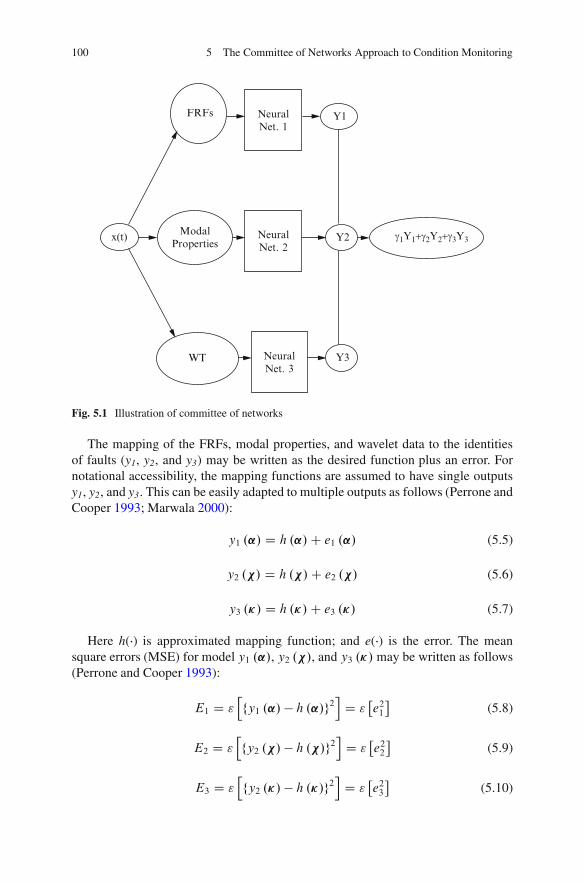
100 5 The Committee of Networks Approach to Condition Monitoring
FRFs NeuralNet. 1
NeuralNet. 2
NeuralNet. 3
ModalProperties
x(t)
WT Y3
Y2 g1Y1+g2Y2+g3Y3
Y1
Fig. 5.1 Illustration of committee of networks
The mapping of the FRFs, modal properties, and wavelet data to the identitiesof faults (y1, y2, and y3) may be written as the desired function plus an error. Fornotational accessibility, the mapping functions are assumed to have single outputsy1, y2, and y3. This can be easily adapted to multiple outputs as follows (Perrone andCooper 1993; Marwala 2000):
y1 .˛/ D h .˛/ C e1 .˛/ (5.5)
y2 .�/ D h .�/ C e2 .�/ (5.6)
y3 .�/ D h .�/ C e3 .�/ (5.7)
Here h(�) is approximated mapping function; and e(�) is the error. The meansquare errors (MSE) for model y1 .˛/, y2 .�/, and y3 .�/ may be written as follows(Perrone and Cooper 1993):
E1 D "hfy1 .˛/ � h .˛/g2
iD "
�e2
1
�(5.8)
E2 D "hfy2 .�/ � h .�/g2
iD "
�e2
2
�(5.9)
E3 D "hfy2 .�/ � h .�/g2
iD "
�e2
3
�(5.10)

5.4 Theory of Committee of Networks 101
Here " Œ� indicates the expected value and corresponds to integration over theinput data, and is defined as follows (Perrone and Cooper 1993):
"�e2
1
� �Z
e21 .˛/ p .˛/ d˛ (5.11)
"�e2
2
� �Z
e22 .�/ p .�/ d� (5.12)
"�e2
3
� �Z
e23 .�/ p .�/ d� (5.13)
Here p Œ� is the probability density function; and d Œ� is a differential operator.The average MSE of the three networks acting individually may be written asfollows (Perrone and Cooper 1993):
EAV D E1 .˛/ C E2 .�/ C E3 .�/
3
D 1
3
�"�e2
1
�C "�e2
2
�C "�e2
3
��(5.14)
5.4.1 Equal Weights
In this section, the concept of a committee is explained. The output of the committeeis the average of the outputs from the pseudo-modal energies, modal-property, andWT networks. The committee prediction may be written in the following form bygiving equal weighting functions (Perrone and Cooper 1993):
yCOM D 1
3.y1 .˛/ C y2 .�/ C y3 .�// (5.15)
The MSE of the committee can therefore be written as follows:
ECOM D "
"�1
3
�y1 .˛/ C y2 .�/ C y3 .�/
� 1
3Œh .˛/ C h .�/ C h .�/�
�2#
D "
"�1
3
�Œy1 .˛/ � h .˛/� C Œy2 .�/ � h .�/� C
�y3 .�/ � h .�/
��2#
D "
"�1
3fe1 C e2 C e3g
�2#
D 1
9
�"�e2
1
�C 2 ." Œe1e2� C " Œe2e3� C " Œe1e3�/ C "�e2
2
�C "�e2
3
��(5.16)

102 5 The Committee of Networks Approach to Condition Monitoring
If it is assumed that the errors (e1, e2, and e3) are uncorrelated then
" Œe1e2� D " Œe1e3� D " Œe2e3� D 0 (5.17)
Substituting Eq. 5.17 in Eq. 5.16, the error of the committee can be related to theaverage error of the networks acting individually as follows (Perrone and Cooper1993):
ECOM D 1
9
�"�e2
1
�C "�e2
2
�C "�e2
3
��
D 1
3EAV (5.18)
Equation 5.18 demonstrates that the MSE of the committee is one-third of theaverage MSE of the individual technique. From Eq. 5.18, it can be deduced that theMSE of the committee is always equal to or less than the average MSE of the threemethods acting individually.
5.4.2 Variable Weights
The three networks might not essentially have the same predictive capability. Thismight be because modal properties are extracted from the FRFs (Ewins 1995), theWT of the impulse response that is chosen is not ideal, or the parameters chosenfrom the pseudo-modal energies are not ideal. To accommodate the strength ofeach technique, the network should be given suitable weighting functions. It willbe explained later how these weighting functions will be evaluated when there is noprior knowledge of the strength of each approach.
The identity of fault may be defined as the combination of the three independentmethods with estimated weighting functions as (a modification of Eq. 5.15):
yCOM D �1y1 .˛/ C �2y2 .�/ C �3y3 .�/ (5.19)
Here �1, �2, and �3 are the weighting functions and �1 C �2 C �3 D 1. The MSEdue to the weighted committee can be written as follows (Marwala 2000):
ECOM D "h.�1y1 .˛/ C �2y2 .�/ C �3y3 .�/ � Œ�1h .˛/ C �2h .�/ C �3h .�/�/2
i
D "h.�1 Œy1 .˛/ � h .˛/� C �2 Œy2 .�/ � h .�/� C �3 Œy3 .�/ � h .�/�/2
i
D "h.�1e1 C �2e2 C �3e3/
2i
(5.20)

5.4 Theory of Committee of Networks 103
Equation 5.20 may be rewritten in Lagrangian form as follows (Perrone andCooper 1993):
ECOM D "h.�1e1 C �2e2 C �3e3/
2i
C � .1 � �1 � �2 � �3/ (5.21)
Here � is the Lagrangian multiplier. The derivative of error in Eq. 5.21 withrespect to �1, �2, �3 and � may be calculated and equated to zero as (Perrone andCooper 1993):
dECOM
d�1
D 2e1" Œ.�1e1 C �2e2 C �3e3/� � � D 0 (5.22)
dECOM
d�2
D 2e2" Œ.�1e1 C �2e2 C �3e3/� � � D 0 (5.23)
dECOM
d�3
D 2e3" Œ.�1e1 C �2e2 C �3e3/� � � D 0 (5.24)
dECOM
d�D 1 � �1 � �2 � �3 D 0 (5.25)
In solving Eqs. 5.21–5.25, the minimum error is obtained when the weights are(Perrone and Cooper 1993):
�1 D 1
1 C "Œe21 �
"Œe22�
C "Œe21 �
"Œe23 �
(5.26)
�2 D 1
1 C "Œe22 �
"Œe21�
C "Œe22 �
"Œe23 �
(5.27)
�3 D 1
1 C "Œe23 �
"Œe21�
C "Œe23 �
"Œe22 �
(5.28)
Equations 5.26–5.28 may be generalized for a committee with n-trained networksand may be written as follows (Perrone and Cooper 1993):
�i D 1nP
jD1
"Œe2i �
"he2
j
i(5.29)
From Eq. 5.29, the following conditions may be derived (Marwala 2000):
"�e2
1
� D "�e2
2
� D "�e2
3
� ) �1 D �2 D �3 D 1
3(5.30)

104 5 The Committee of Networks Approach to Condition Monitoring
"�e2
3
�< "
�e2
2
�< "
�e2
1
� ) �1 < �2 < �3I �3 >1
3(5.31)
"�e2
1
�< "
�e2
2
�< "
�e2
3
� ) �3 < �2 < �3I �1 >1
3(5.32)
These conditions show that if the predictive capacity of the pseudo-modal energynetwork, the modal-property network, and the WT network are equal, then eachmethod should be given equal weights. If the pseudo modal energy network is betterthan the other two, it should be given a higher weight. If the modal-property networkhas lower expected errors than the other two networks, it should be given a higherweight. If the WT network has smaller errors than the other two methods, it shouldbe given more weight. These conditions are trivial, but they have been derived toconfirm the effectiveness of the presented technique.
Because it is not known which network is more accurate in a given instance, theweighting functions were determined from the data that was used for training thenetworks (prior knowledge) and this is called stacking, as described in the previoussection.
Therefore, it can be concluded that if three independent (uncorrelated) methodsare used simultaneously, the reliability of the combination is at least as good aswhen the methods are used individually. Suppose the probabilities of success for thepseudo-modal energy network, the modal-property network, and the WT networkare P(x1), P(x2), and P(x3), respectively. The reliability of the three methods actingin parallel can be mathematically written as follows (Marwala 2001):
P .x1 [ x2 [ x3/ D P .x1/ C P .x2/ C P .x3/ � ŒP .x1 \ x2/
C P .x2 \ x3/ P .x1 \ x3/� :::
C P .x1 \ x2 \ x3/
(5.33)
From Eq. 5.33, it can be concluded that the reliability of the committee is alwayshigher than that of the individual methods.
5.5 Application to Cylindrical Shells
For this section, the committee procedure was applied to identify faults in apopulation of cylindrical shells. As described in Chap. 2, an impulse hammertest was performed on ten steel seam-welded cylindrical shells (1.75 ˙ 0.02 mmthickness, 101.86 ˙ 0.29 mm diameter, and height 101.50 ˙ 0.20 mm). Thesecylinders were resting on bubble wrap to simulate a free-free environment. Thedetails of this experiment may be found in Marwala (1999).

5.5 Application to Cylindrical Shells 105
Table 5.1 Confusion matrix from the classification of fault cases in the test data using thepseudo-modal-energy network
Predicted
[000] [100] [010] [001] [110] [101] [011] [111]
Actual [000] 37 2 0 0 0 0 0 0[100] 0 3 0 0 0 0 0 0[010] 0 0 3 0 0 0 0 0[001] 0 0 0 3 0 0 0 0[110] 0 0 0 0 3 0 0 0[101] 0 0 0 0 0 3 0 0[011] 0 0 0 0 0 0 3 0[111] 0 0 0 0 5 1 1 32
Each cylinder was divided into three substructures, and holes of 12 mm diameterwere drilled into each substructure. For one cylinder, the first type of fault was azero-fault scenario, and its identity was [000]. The second type of fault was a one-fault scenario; if it was located in substructure 1, its identity was [100]. The thirdtype of fault was a two-fault scenario, and if the faults were located in substructures1 and 2, the identity of this case was [110]. The final type of fault was a three-faultscenario, and the identity of this case was [111].
For each fault case, measurements were taken by measuring the acceleration at afixed position and roving the impulse position about. One cylinder gives four faultscenarios and 12 sets of measurements. The structure was vibrated at 19 differentlocations, nine on the upper ring of the cylinder and ten on the lower ring of thecylinder. Each measurement was taken three times to quantify the repeatability ofthe measurements. The total number of data points collected was 120.
From the measured data, pseudo-modal energies, modal properties, and waveletdata were identified and used to train three neural networks. The training processwas done in the same way as in Chap. 3. The WT network was trained using waveletdata. This network had 18 input parameters, 9 hidden units, and 3 output units. Thecommittee was applied using the weighting obtained from the validation data.
When the networks were evaluated using the data not used for training, theresults in Tables 5.1, 5.2, 5.3 and 5.4 were obtained. These results indicate thatthe committee approach gave the best results followed by the pseudo-modal energynetwork, and then the modal-property network. The wavelet-network performed theworst.
The neural networks were trained using the hybrid Monte Carlo method asdescribed in Chap. 4. The number of initial states discarded in the hope of reachinga stationary distribution was set to 100; the number of steps in each hybrid MonteCarlo trajectory was set to 100; the fixed step size was set to 0.001; and the numberof samples retained to form a distribution was set to 500.

106 5 The Committee of Networks Approach to Condition Monitoring
Table 5.2 Confusion matrix from the classification of fault cases in the test data using themodal-energy-network
Predicted
[000] [100] [010] [001] [110] [101] [011] [111]
Actual [000] 38 0 0 1 0 0 0 0[100] 0 3 0 0 0 0 0 0[010] 0 0 3 0 0 0 0 0[001] 0 0 0 3 0 0 0 0[110] 0 0 0 0 3 0 0 0[101] 0 0 0 0 0 3 0 0[011] 0 0 0 0 0 0 3 0[111] 0 0 0 0 5 2 6 26
Table 5.3 Confusion matrix from the classification of fault cases in the test data using thewavelet-network
Predicted
[000] [100] [010] [001] [110] [101] [011] [111]
Actual [000] 35 0 0 1 0 0 0 0[100] 0 1 0 0 0 0 0 0[010] 2 0 3 0 0 0 0 0[001] 0 2 0 2 0 0 0 0[110] 0 0 0 0 3 0 0 1[101] 0 0 0 1 0 3 0 0[011] 0 0 0 0 0 0 3 0[111] 1 0 0 0 5 2 6 25
Table 5.4 Confusion matrix from the classification of fault cases in the test data using thecommittee-network
Predicted
[000] [100] [010] [001] [110] [101] [011] [111]
Actual [000] 38 1 0 0 0 0 0 0[100] 0 3 0 0 0 0 0 0[010] 0 0 3 0 0 0 0 0[001] 0 0 0 3 0 0 0 0[110] 0 0 0 0 3 0 0 0[101] 0 0 0 0 0 3 0 0[011] 0 0 0 0 0 0 3 0[111] 0 0 1 0 3 0 1 34
5.6 Conclusions
In this study, the committee of neural networks method was presented and appliedto the structural diagnostics of a population of cylindrical shells. This methodused pseudo-modal energies, modal properties, and used wavelet transform datato simultaneously identify faults in structures. It was observed that the committee

References 107
approach gave the best results followed by the pseudo-modal energy networkand then the modal-property network, while the wavelet-network performed theworst.
References
Abdel-Aal RE (2005a) Improving electric load forecasts using network committees. Electric PowerSyst Res 74:83–94
Abdel-Aal RE (2005b) Improved classification of medical data using abductive network commit-tees trained on different feature subsets. Comput Methods Program Biomed 80:141–153
Anthony M (2007) On the generalization error of fixed combinations of classifiers. J Comput SystSci 73:725–734
Atalla MJ, Inman DJ (1998) On model updating using neural networks. Mech Syst Signal Process12:135–161
Bacauskiene M, Verikas A (2004) Selecting salient features for classification based on neuralnetwork committees. Pattern Recognit Lett 25:1879–1891
Baras D, Fine S, Fournier L, Geiger D, Ziv A (2011) Automatic boosting of cross-product coverageusing bayesian networks. Int J Software Tools Technol Transfer 13:247–261
Basu M (2004) An interactive fuzzy satisfying method based on evolutionary programmingtechnique for multiobjective short-term hydrothermal scheduling. Electric Power Syst Res69:277–285
Bichindaritz I, Annest A (2010) Case based reasoning with bayesian model averaging: an improvedmethod for survival analysis on microarray data. Lect Notes Comput Sci 6176:346–359
Bishop CM (1995) Neural networks for pattern recognition. Oxford University Press, OxfordBobb JF, Dominici F, Peng RD (2011) A bayesian model averaging approach for estimating the
relative risk of mortality associated with heat waves in 105 U.S. cities. Biometrics 67:1605–1616
Boone EL, Ye K, Smith EP (2011) Assessing environmental stressors via Bayesian modelaveraging in the presence of missing data. Environmetrics 22:13–22
Breiman L (1996) Bagging predictors. Mach Learn 24:123–140Cao YJ, Jiang L, Wu QH (2000) An evolutionary programming approach to mixed-variable
optimization problems. Appl Math Model 24:931–942Chen CH, Lin ZS (2006) A committee machine with empirical formulas for permeability
prediction. Comput Geosci 32:485–496Clarke B (2003) Comparing Bayes model averaging and stacking when model approximation error
cannot be ignored. J Mach Learn Res 4:683–712Das A, Reddy NP, Narayanan J (2001) Hybrid fuzzy logic committee neural networks for
recognition of swallow acceleration signals. Comput Methods Programs Biomed 64:87–99Daubechie I (1991) The wavelet transform, time-frequency localization and signal processing.
IEEE Trans Info Theory 36:961–1005Doebling SW, Farrar CR, Prime MB, Shevitz DW (1996) Damage identification and health
monitoring of structural and mechanical systems from changes in their vibration characteristics:a literature review. Los Alamos National Laboratory report LA-13070-MS, Los AlamosNational Laboratory, Los Alamos
Domingos P (2000) Bayesian averaging of classifiers and the overfitting problem. In: Proceedingsof the 17th international conference on machine learning, Stanford, California, pp 223–230
Drygajlo A, Li W, Qiu H (2011) Adult face recognition in score-age-quality classification space.Lect Notes Comput Sci 6583:205–216
Du J, Zhai C, Wan Y (2007) Radial basis probabilistic neural networks committee for palmprintrecognition. Lect Notes Comput Sci 4492:819–824

108 5 The Committee of Networks Approach to Condition Monitoring
Ewins DJ (1995) Modal testing: theory and practice. Research Studies Press, LetchworthFeldkircher M (2011) Forecast combination and Bayesian model averaging: a prior sensitivity
analysis. J Forecast doi:10.1002/for.1228Fernandes AM, Utkin AB, Lavrov AV, Vilar RM (2004) Development of neural network committee
machines for automatic forest fire detection using Lidar. Pattern Recognit 37:2039–2047Friswell MI, Mottershead JE (1995) Finite element model updating in structural dynamics. Kluwer
Academic Publishers, DordrechtHanczar B, Nadif M (2011) Using the bagging approach for biclustering of gene expression data.
Neurocomputing 74:1595–1605Haussler D, Kearns M, Schapire RE (1994) Bounds on the sample complexity of Bayesian learning
using information theory and the VC dimension. Mach Learn 14:83–113Hernandez-Lobato D, Martinez-Munoz G, Suarez A (2011) Empirical analysis and evaluation
of approximate techniques for pruning regression bagging ensembles. Neurocomputing 74:2250–2264
Hoeting JA, Madigan D, Raftery AE, Volinsky CT (1999) Bayesian model averaging: a tutorial.Stat Sci 14:382–401
Homayouni H, Hashemi S, Hamzeh A (2010) Instance-based ensemble learning algorithmwith stacking framework. In: Proceedings of the 2nd international conference on softwaretechnology and engineering, Puerto Rico, USA, pp 164–169
Hu G, Mao Z, He D, Yang F (2011) Hybrid modeling for the prediction of leaching rate in leachingprocess based on negative correlation learning bagging ensemble algorithm. Comput Chem Eng35(12):2611–2617
Huang X, Zhang L, Gong W (2011) Information fusion of aerial images and LIDAR data inurban areas: vector-stacking, re-classification and post-processing approaches. Int J RemoteSens 32:69–84
Imregun M, Visser WJ, Ewins DJ (1995) Finite element model updating using frequency responsefunction data I: theory and initial investigation. Mech Syst Signal Process 9:187–202
Jafari SA, Mashohor S, Jalali Varnamkhasti M (2011) Committee neural networks with fuzzygenetic algorithm. J Petrol Sci Eng 76:217–223
Jasra A, Holmes CC (2011) Stochastic boosting algorithms. Stat Comput 21:335–347Jia J, Xiao X, Liu B, Jiao L (2011) Bagging-based spectral clustering ensemble selection. Pattern
Recognit Lett 32:1456–1467Jordan MI, Bishop CM (1996) Neural networks. MIT technology report artificial intelligence.
Memo no. 1562, Massachusetts Institute of Technology, CambridgeKadkhodaie-Ilkhchi A, Reza Rezaee M, Rahimpour-Bonab H (2009) A committee neural network
for prediction of normalized oil content from well log data: an example from South Pars GasField, Persian Gulf. J Petrol Sci Eng 65:23–32
Kajdanowicz T, Kazienko P (2011) Structured output element ordering in boosting-based classifi-cation. Lect Notes Comput Sci 6679:221–228
Karimpouli S, Fathianpour N, Roohi J (2010) A new approach to improve neural networks’algorithm in permeability prediction of petroleum reservoirs using Supervised CommitteeMachine Neural Network (SCMNN). J Petrol Sci Eng 73:227–232
Khoshgoftaar TM, van Hulse J, Napolitano A (2011) Comparing boosting and bagging techniqueswith noisy and imbalanced data. IEEE Trans Syst Man Cybern A Syst Hum 41:552–568
Kyung YJ, Lee HS (1999) Bootstrap and aggregating VQ classifier for speaker recognition.Electron Lett 35:973–974
Larios N, Lin J, Zhang M, Lytle D, Moldenke A, Shapiro L, Dietterich T (2011) Stacked spatial-pyramid kernel: an object-class recognition method to combine scores from random trees.In: Proceedings of the IEEE workshop on application of computer vision, Kona, Hawaii,pp 329–335
Leitenstorfer F, Tutz G (2011) Estimation of single-index models based on boosting techniques.Stat Model 11:203–217
Levin RI, Lieven NAJ (1998) Dynamic finite element updating using neural networks. J Sound Vib210:593–608

References 109
Li W, Drygajlo A, Qiu H (2010) Aging face verification in score-age space using single referenceimage template. In: Proceedings of the IEEE 4th international conference on biometrics: theory,application and Systems, Washington, DC, pp 1–7
Liew KM, Wang Q (1998) Application of wavelet theory for crack identification in structures.J Eng Mech 124:152–157
Louzada F, Anacleto-Junior O, Candolo C, Mazucheli J (2011) Poly-bagging predictors forclassification modelling for credit scoring. Expert Syst Appl 38:12717–12720
Maia NMM, Silva JMM (1997) Theoretical and experimental modal analysis. Research StudiesPress, Letchworth
Marwala T (1999) Probabilistic damage identification using neural networks and modal properties.University of Cambridge Technical Report CUED/C-MECH/TR-76, University of Cambridge,Cambridge
Marwala T (2000) On damage identification using a committee of neural networks. J Eng Mech126:43–50
Marwala T (2001) Probabilistic fault identification using a committee of neural networks andvibration data. J Aircraft 38:138–146
Marwala T (2009) Computational intelligence for missing data imputation, estimation andmanagement: knowledge optimization techniques. IGI Global Publications, New York
Marwala T, Heyns PS (1998) Multiple-criterion method for determining structural damage.Am Inst Aeronaut Astronaut J 36:1494–1501
Marwala T, Hunt HEM (1999) Fault identification using finite element models and neural networks.Mech Syst Signal Process 13:475–490
Marwala T, de Wilde P, Correia L, Mariano P, Ribeiro R, Abramov V, Szirbik N, GoossenaertsJ (2001) Scalability and optimisation of a committee of agents using genetic algorithm.In: Proceedings of the international symposium on soft computing and intelligent systems forindustry, Paisley, Scotland, pp 1–6
Newland DE (1993) An introduction to random vibration, spectral and wavelet analysis. Long-man/John Wiley, New York/Harlow
Osawa T, Mitsuhashi H, Uematsu Y, Ushimaru A (2011) Bagging GLM: improved generalizedlinear model for the analysis of zero-inflated data. Ecol Info 6(5):270–275
Park I, Grandhi RV (2010) Quantification of multiple types of uncertainty in computer simulationusing bayesian model averaging. In: Proceedings of the 51st AIAA/ASME/ASCE/AHS/ASCstructures, structural dynamics and materials conference, Orlando, Florida, pp 1–6
Park I, Grandhi RV (2011) Quantifying multiple types of uncertainty in physics-based simulationusing Bayesian model averaging. Am Inst Aeronaut Astronaut J 49:1038–1045
Paya BA, Esat II, Badi MNM (1997) Artificial neural network based fault diagnostics of rotatingmachinery using wavelet transforms as a pre-processor. Mech Syst Signal Process 11:751–765
Perrone MP, Cooper LN (1993) When networks disagree: ensemble methods for hybrid neuralnetworks. In: Mammone RJ (ed) Artificial neural networks for speech and vision. Chapmanand Hall, London
Pino-Mejias R, Jimenez-Gamero MD, Cubiles-de-la-Vega MD, Pascual-Acosta A (2008) Reducedbootstrap aggregating of learning algorithms. Pattern Recognit Lett 29:265–271
Potempski S, Galmarini S, Riccio A, Giunta G (2010) Bayesian model averaging for emergencyresponse atmospheric dispersion multimodel ensembles: is it really better? How many data areneeded? Are the weights portable? J Geophys Res. doi:10.1029/2010JD014210
Rajan CCA, Mohan MR (2007) An evolutionary programming based simulated annealing methodfor solving the unit commitment problem. Int J Electric Power Energy Syst 29:540–550
Reddy NP, Buch OA (2003) Speaker verification using committee neural networks. ComputMethods Programs Biomed 72:109–115
Rokach L (2010) Ensemble-based classifiers. Artif Intell Rev 33:1–39Sheikh-Ahmad J, Twomey J, Kalla D, Lodhia P (2007) Multiple regression and committee neural
network force prediction models in milling FRP. Mach Sci Technol 11:391–412

110 5 The Committee of Networks Approach to Condition Monitoring
Shi L, Xu G (2001) Self-adaptive evolutionary programming and its application to multi-objectiveoptimal operation of power systems. Electric Power Syst Res 57:181–187
Shiraishi Y, Fukumizu K (2011) Statistical approaches to combining binary classifiers for multi-class classification. Neurocomputing 74:680–688
Sill J, Takacs G, Mackey L, Lin D (2009) Feature-weighted linear stacking. arXiv:0911.0460Smyth P, Wolpert DH (1999) Linearly combining density estimators via stacking. Mach Learn
J 36:59–83Tang B, Chen Q, Wang X, Wang X (2010) Reranking for stacking ensemble learning. Lect Notes
Comput Sci 6443:575–584Tsai MY, Hsiao CK, Chen WJ (2011) Extended bayesian model averaging in generalized linear
mixed models applied to schizophrenia family data. Ann Hum Genet 75:62–77van Hinsbergen CPIJ, van Lint JWC, van Zuylen HJ (2009) Bayesian committee of neural networks
to predict travel times with confidence intervals. Trans Res C Emerg Technol 17:498–509Wang G, Hao J, Ma J, Jiang H (2011) A comparative assessment of ensemble learning for credit
scoring. Expert Syst Appl 38:223–230Wolpert DH (1992) Stacked generalization. Neural Netw 5:241–259Wolpert DH, Macready WG (1999) An efficient method to estimate bagging’s generalization error.
Mach Learn J 35:41–55Yu Q (2011) Weighted bagging: a modification of adaboost from the perspective of importance
sampling. J Appl Stat 38:451–463Zhao ZQ, Huang DS, Sun BY (2004) Human face recognition based on multi-features using Neural
Networks Committee. Pattern Recognit Lett 25:1351–1358

Chapter 6Gaussian Mixture Models and Hidden MarkovModels for Condition Monitoring
6.1 Introduction
Rotating machines are widely used in industry for system operation and processautomation. Research shows that the failures of these machines are often linkedwith bearing failures (Lou et al. 2004). Bearing faults induce high bearing vibrationswhich generate noise that may even cause the entire rotating machine, such asthe electric motor, to function incorrectly. Thus, it is important to include bearingvibration fault detection and diagnosis in industrial motor rotational fault diagnosissystems (Lou et al. 2004). As a result, there is a high demand for cost effectiveautomatic monitoring of bearing vibrations in industrial motor systems.
A variety of fault bearing vibration feature detection techniques exist. Thesecan be classified into three domains, namely: frequency domain analysis, time-frequency domain analysis, and time domain analysis (Ericsson et al. 2004).The frequency domain methods often involve frequency analysis of the vibrationsignals and look at the periodicity of high frequency transients. This procedure iscomplicated by the fact that this periodicity may be suppressed (Ericsson et al.2004). The most commonly used frequency analysis technique for detection anddiagnosis of bearing fault is the envelope analysis. More details on this techniqueare found in McFadden and Smith (1984). The main disadvantage of the frequencydomain analysis is that it tends to average out transient vibrations and thereforebecomes more sensitive to background noise. To overcome this problem, the time-frequency domain analysis is used, which shows how the frequency contents ofthe signal changes with time. Examples of such analyses are: Short Time FourierTransform (STFT), the Wigner-Ville Distribution (WVD) and, most importantly,the Wavelet Transform (WT). These techniques are studied in detail in the work ofLi et al. (2000).
The last category of the feature detection is the time domain analysis. There are anumber of time domain methods that give reasonable results. These methods includethe time-series averaging method, the signal enveloping method, the Kurtosismethod, and others (Li et al. 2000). Research shows that, unlike the frequency
T. Marwala, Condition Monitoring Using Computational Intelligence Methods:Applications in Mechanical and Electrical Systems, DOI 10.1007/978-1-4471-2380-4 6,© Springer-Verlag London Limited 2012
111

112 6 Gaussian Mixture Models and Hidden Markov Models for Condition Monitoring
domain analysis, this technique is less sensitive to suppressions of the impact ofperiodicity (Ericsson et al. 2004; Li et al. 2000). This chapter introduces a new timedomain analysis method, known as fractal dimension analysis, which was originallyused in image processing and has been recently used in speech recognition (Maragosand Sun 1993; Maragos and Potamianos 1999; Wang et al. 2000). This method isexpected to give enormous improvement to the performance of the bearing faultdetection and diagnosis because it extracts the non-linear vibration features of eachbearing fault. The fractal dimension analysis is based on the Multi-scale FractalDimensions (MFD) of short-time bearing vibration segments, derived from non-linear theory (Wang et al. 2000).
Once the bearing vibration features are extracted using one of the three domainsmentioned above, then these features can be used for automatic motor bearing faultdetection and diagnosis by applying them to a non-linear pattern classifier. Themost popular classifier used in bearing fault detection is a Neural Network (NN).Nevertheless, other non-linear classifiers like Gaussian Mixture Model (GMM) andHidden Markov Model (HMM) have been shown to outperform NN in a numberof classification problems, in general, and in speech related problems in particular.Only recently, have researchers such as Purushothama et al. (2005) applied speechpattern classifiers, such as HMM, to the fault detection of mechanical systemsbecause of their success in speech recognition.
This chapter presents a comparative study of HMM and GMM, and introducestime-domain analysis based techniques using fractals to extract the features. Further-more, the ability of MFD to detect bearing faults was evaluated using both HMMand GMM non-linear pattern classifiers.
The rest of the chapter is arranged as follows: the next section presents thedifferent bearing faults studied in this chapter, followed by the mathematicalbackground to fractal dimensions, HMM, and GMM. Thereafter, the time domainbearing detection and diagnosis framework is presented.
6.2 Background
This section presents, in detail, the different bearing faults studied in this chapter,followed by the mathematical background to fractal dimensions, HMM, and GMM.
6.2.1 The Gaussian Mixture Model (GMM)
A GMM is a weighted sum of M component Gaussian densities, p(xj�) as given bythe equation (Reynolds 1992; Dempster et al. 1977):
p.xj�/ DMX
iD1
wi pi .x/ (6.1)

6.2 Background 113
with
pi .xt / D 1
.2�/D=2p†i
exp
��1
2.xk � �i /
t .†i /�1.xk � �i /
(6.2)
Here, x is a D-dimensional, continuous-valued data vector representing mea-surements from features, wi, i D 1, : : : , M, are the mixture weights, with meanvector �i and covariance matrix †i. The mixture weights, wi, satisfy the constraintPM
iD1 wi D 1.
The entire GMM is parameterized by the mean vectors, covariance matrices, andmixture weights from all component densities and these parameters are togetherrepresented by the notation (Reynolds and Rose 1995; Dempster et al. 1977):
� D fw; �; †g (6.3)
Here, � is the model, w, �, † are, respectively, the weights, means, andcovariance of the features. The covariance matrices can be full rank or constrainedto be diagonal but, in this chapter assumes that it is diagonal. The choice ofmodel architecture, which are the number of components, diagonal covariancematrices and parameter is usually determined by the amount of data available forapproximating the GMM parameters and how the GMM is applied in a specificfault identification problem. GMM has the advantage of being able to represent alarge class of sample distributions and to form smooth estimates to indiscriminatelyshaped probability densities.
Given a collection of training vectors, the parameters of this model are estimatedby a number of algorithms such as the Expectation-Maximization (EM) algorithmand K-means algorithm (Dempster et al. 1977; Reynolds et al. 2000). The EMalgorithm was used in this study because it has reasonably fast computational timewhen compared to other algorithms. The EM algorithm finds the optimum modelparameters by iteratively refining GMM parameters to increase the likelihood of theestimated model for the given bearing fault feature vector. More details on the EMalgorithm for training a GMM are in the work of Wang and Kootsookos (1998).
Bordes et al. (2007) applied the EM algorithm to image reconstruction. Theyfound that the results were within 10% of the experimental data. Dempster et al.(1977) applied the EM algorithm to missing data, while Ingrassia and Rocci (2007)generalized the EM algorithm to semi-parametric mixture models that, when testedon real data, showed that their method was easy to implement and computationallyefficient. Kauermann et al. (2007) used the EM algorithm to recognize polymor-phism in pharmacokinetic/pharmacodynamic (PK/PD) phenotypes, while Wangand Hu (2007) improved the EM algorithm’s computational load and successfullyapplied this to brain tissue segmentation. Another successful implementation ofthe EM algorithm includes binary text classification (Park et al. 2007). Otherimprovements of the EM algorithm include accelerating the computational speed byPatel et al. (2007). Further information on the implementation of the EM algorithmcan be found in Wang et al. (2007), as well as McLachlan and Krishnan (1997).
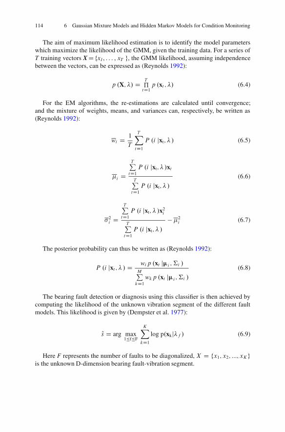
114 6 Gaussian Mixture Models and Hidden Markov Models for Condition Monitoring
The aim of maximum likelihood estimation is to identify the model parameterswhich maximize the likelihood of the GMM, given the training data. For a series ofT training vectors X D fx1, : : : , xT g, the GMM likelihood, assuming independencebetween the vectors, can be expressed as (Reynolds 1992):
p .X; �/ D T
…tD1
p .xt ; �/ (6.4)
For the EM algorithms, the re-estimations are calculated until convergence;and the mixture of weights, means, and variances can, respectively, be written as(Reynolds 1992):
wi D 1
T
TXtD1
P .i jxt; � / (6.5)
�i D
TPtD1
P .i jxt; � /xt
TPtD1
P .i jxt; � /
(6.6)
�2i D
TPtD1
P .i jxt; � /x2i
TPtD1
P .i jxt; � /
� �2i (6.7)
The posterior probability can thus be written as (Reynolds 1992):
P .i jxt ; � / D wi p .xt j�i ; †i /
MPkD1
wkp .xt j�i ; †i /
(6.8)
The bearing fault detection or diagnosis using this classifier is then achieved bycomputing the likelihood of the unknown vibration segment of the different faultmodels. This likelihood is given by (Dempster et al. 1977):
Os D arg max1�f�F
KXkD1
log p.xkj�f / (6.9)
Here F represents the number of faults to be diagonalized, X D fx1; x2; :::; xK gis the unknown D-dimension bearing fault-vibration segment.
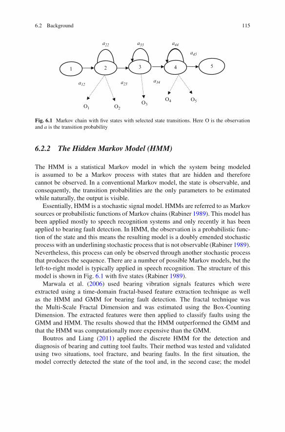
6.2 Background 115
2 3 41 5
O1 O2O3
O4 O5
a22 a33 a44
a34a12 a23
a45
Fig. 6.1 Markov chain with five states with selected state transitions. Here O is the observationand a is the transition probability
6.2.2 The Hidden Markov Model (HMM)
The HMM is a statistical Markov model in which the system being modeledis assumed to be a Markov process with states that are hidden and thereforecannot be observed. In a conventional Markov model, the state is observable, andconsequently, the transition probabilities are the only parameters to be estimatedwhile naturally, the output is visible.
Essentially, HMM is a stochastic signal model. HMMs are referred to as Markovsources or probabilistic functions of Markov chains (Rabiner 1989). This model hasbeen applied mostly to speech recognition systems and only recently it has beenapplied to bearing fault detection. In HMM, the observation is a probabilistic func-tion of the state and this means the resulting model is a doubly emended stochasticprocess with an underlining stochastic process that is not observable (Rabiner 1989).Nevertheless, this process can only be observed through another stochastic processthat produces the sequence. There are a number of possible Markov models, but theleft-to-right model is typically applied in speech recognition. The structure of thismodel is shown in Fig. 6.1 with five states (Rabiner 1989).
Marwala et al. (2006) used bearing vibration signals features which wereextracted using a time-domain fractal-based feature extraction technique as wellas the HMM and GMM for bearing fault detection. The fractal technique wasthe Multi-Scale Fractal Dimension and was estimated using the Box-CountingDimension. The extracted features were then applied to classify faults using theGMM and HMM. The results showed that the HMM outperformed the GMM andthat the HMM was computationally more expensive than the GMM.
Boutros and Liang (2011) applied the discrete HMM for the detection anddiagnosis of bearing and cutting tool faults. Their method was tested and validatedusing two situations, tool fracture, and bearing faults. In the first situation, themodel correctly detected the state of the tool and, in the second case; the model

116 6 Gaussian Mixture Models and Hidden Markov Models for Condition Monitoring
classified the severity of the fault seeded into two different engine bearings. Theresult obtained for fault severity classification was above 95%. In addition to thefault severity, a location index was developed to determine the fault location andgave an average success rate of 96%.
Wong and Lee (2010) successfully applied HMM for fault detection in theshell-and-tube heat exchanger. This method was viewed as a generalization of themixture-of-Gaussians method and was demonstrated through a problem.
Lee et al. (2010) applied HMM for online degradation assessment and adaptivefault detection of multiple failure modes. Their method, together with statisticalprocess control was used to detect the incidence of faults. This technique permittedthe hidden Markov state to be updated with the identification of new states. Theresults for a turning process showed that the tool wear processes can be successfullydetected, and the tool wear processes can be identified.
Calefati et al. (2006) successfully applied HMM for machine faults detectionand forecasting in gearboxes. Elsewhere, Zhou and Wang (2005) applied HMMand a principal component analysis to the on-line fault detection and diagnosis inindustrial processes, and applied these to case studies from the Tennessee Eastmanprocess.
Menon et al. (2003) applied HMM for incipient fault detection and diagnosisin turbine engines and the effectiveness of the HMM method was compared to aneural network method and a hybrid of principal component analysis and a neuralnetwork approach. Their HMM method was found to be more effective than theother methods.
Smyth (1994) applied HMM to fault detection in dynamic systems. It wasdemonstrated that a pattern recognition system combined with a finite-state HMMwas good at modeling temporal characteristics. The model was validated usinga real-world fault diagnosis problem and was demonstrated to offer substantialpractical advantages.
The complete parameter set needed to define the HMM can be written as (Rabiner1989; Caelli et al. 2001; Koski 2001):
� D fA; B; �g (6.10)
where � is the model, A D faij g, B D fbij .k/g and � D f�i gare the transitionprobability distribution, the observation probability distribution, and initial statedistribution, respectively. For example, if we assume that the distribution can berepresented by the Gaussian mixture model shown in Eq. 6.2, the equation can bewritten as:
� D fA; w; �; †; �g (6.11)

6.2 Background 117
These parameters of a given state, Si, are defined as (Rabiner 1989; Ching et al.2003; Purushothama et al. 2005; Ching and Ng 2006):
aij D P.qtC1 D Sj jqt D Si /; 1 � i; j � N (6.12)
bij .k/ D P.Okjqt D Si/; 1 � j � N; 1 � k � M (6.13)
and
�i D P.q1 D Si/; 1 � i � N (6.14)
Here, qt is the state at time t and N denotes the number of states. Additionally,Ok is the kth observation and M is the number of distinct observation.
The HMM can be used to simulate the observed state as follows (Rabiner1989):
1. Let t D 1.2. Create Ot D vk 2 V in accordance with the probability bi .k/.3. Create a transition of hidden state from qt D Si to qtC1 D Sj in accordance with
the transition probability aij.4. Let t D t C 1 and go to Step 2 if t < T or else terminate the algorithm.
There are three fundamental issues to be solved for this model to be applied inpractice. Firstly, we ought to identify the probability of the observation sequenceO D O1; O2; :::; OT of visible states generated by the model �. Secondly, we needa decoding process which identifies a state sequence that maximizes the probabilityof an observation sequence and this can be realized through the so-called Viterbialgorithm (Rabiner 1989). Thirdly, we need a training process which adjusts modelparameters to maximize the probability of the observed sequence.
The next step is to calculate the likelihood of the observed sequence as follows(Rabiner 1989; Ching et al. 2004):
P.O/ DX
all possible
�q1 bq1.O1/ � �q2 bq2.O2/ � ::: � �qn bqn.On/ (6.15)
To speed up the computation of this, the backward and the forward methods canbe applied (Baum 1972). To do this, we define the following (Baum 1972):
˛T .i/ D P.O1O2:::Ot ; qt D Si / (6.16)
The forward technique can be written as follows (Rabiner 1989; Tai et al.2009):
1. Initialize as follows:
˛1.i/ D �i bi .O1/ for 1 � i � N

118 6 Gaussian Mixture Models and Hidden Markov Models for Condition Monitoring
2. Apply the recursion step as follows:
˛t .j / D bj .Ot /
NXiD1
˛t�1.i/aij for 2 � t � T and 1 � j � N
3. Terminate as follows:
P.O/ DNX
iD1
˛T .i/
The backward technique can be written as follows by letting (Rabiner 1989; Taiet al. 2009):
ˇt .i/ D P.OtC1OtC2:::OT jqt D Si / (6.17)
1. Initialize as follows:
ˇT .i/ D 1 for 1 � i � N
2. Apply the recursion step as follows:
ˇt .i/ DNX
jD1
aij bj .OtC1/ˇtC1.j / for 1 � t � T � 1 and 1 � j � N
3. Terminate as follows:
P.O/ DNX
iD1
ˇ1.i/�i bi .O1/
The Baum-Welch estimation procedures with the Maximum Likelihood tech-nique can be used to approximate the model parameters (Rabiner 1989). To explainthe use of this procedure it is important to state the following definition (Rabiner1989; Ching et al. 2004):
�t .i; j / D P�qt D Si ; qtC1 D Sj jO; A; B; �
�(6.18)
This is the probability of being in state Si at time t and having a transition to stateSi at time t C 1 given the observed sequence and the model. This can be expanded

6.2 Background 119
as follows (Rabiner 1989; Ching et al. 2004):
�t .i; j / D ˛t .i/˛ij ˇtC1.j /bj .OtC1/Pi
Pj ˛t .i/˛ij ˇtC1.j /bj .OtC1/
(6.19)
We can also define that (Rabiner 1989; Ching et al. 2004):
�t .i/ D P.qt D Si jO; A; B; �/ (6.20)
This indicates the probability of being in state Si at time t given the observedsequence and the model. Therefore, we now have (Rabiner 1989; Ching et al. 2004):
�t DX
j
�t .i; j / (6.21)
This procedure can be written as follows (Baum 1972; Rabiner 1989):
1. Select a set of initial parameters � D fA; B; �g randomly2. Estimate the parameters using the following equations (Tai et al. 2009)
N�i D �1.i/ for 1 � i � N
Naij DPT�1
tD1 �t .i; j /PT�1tD1 �t .i/
for 1 � i � N; 1 � j � N
Nbj .k/ DPT
tD1 �t .j /IOtDkPTtD1 �t .j /
for 1 � j � N; 1 � k � M
Here IOtDk D�
1 if Ot D k
0 otherwise
3. Set NA D fNaij gij , NB D f Nbj .k/gjk and N� D f N�i g4. Set N� D f NA; NB; N�g5. If � D N�, end otherwise let � D N� and go to Step 2
A more detailed explanation of HMM training using the Baum-Welchre-estimation along with other features of HMM is presented by Rabiner (1989).
The estimation of the hidden state can be conducted using the Viterbi algorithm(Viterbi 1967) to calculate the probability of the hidden states given the HMMparameters and an observed sequence. To do this we can define the following(Rabiner 1989; Tai et al. 2009) which is the maximum probability within a singlepath:
ıt .i/ D maxq1;q2;:::;qt�1
P .q1; q2; :::; qt ; O1O2:::Ot I qt D Si/ (6.22)

120 6 Gaussian Mixture Models and Hidden Markov Models for Condition Monitoring
and define (Tai et al. 2009):
ıt .j / D bj .Ot / � maxi
fıt�1.i/aij g (6.23)
We can therefore solve this problem using dynamic programming as follows(Rabiner 1989; Tai et al. 2009):
1. Initialize ı1.i/ D �i bi .O1/ and 1.i/ D 0 for 1 � i � N
2. Solve the following recursion step
ıt .j / D max1�i�N
ıt�1.i/aij bj .Ot / for 2 � t � T and 1 � j � N
and
t .j / D arg max1�i�N
fıt�1.i/aij g for 2 � t � T and 1 � j � N
3. Terminate
P � D max1�i�N
ıT .i/ and q�T D arg max1�i�N
ıT .i/
Here P* is the most likely likelihood and q* is the most likely state at time T.4. Backtrack:
q�T D tC1.q�tC1/ for t D T � 1; T � 2; ::: ; 2; 1
6.2.3 Fractals
For this chapter, fractals were used to analyse the bearing data. A fractal is definedas a rough geometric shape that can be divided into various segments, each ofwhich is roughly a reduced-size copy of the whole. This characteristic is known asself-similarity (Mandelbrot 1982). The theory of fractals was described in detail,in Chap. 2. The basis of the idea of fractals extends back to the seventeenthcentury. There are numerous classes of fractals, characterized as displaying exactself-similarity, quasi self-similarity or statistical self-similarity (Briggs 1992). Eventhough fractals are a mathematical concept, they are seen in nature, and this has ledto their use in the arts they are useful in biomedical sciences, engineering sciences,and speech recognition. A fractal usually has the following characteristics (Falconer2003):
• It contains a fine structure at randomly small scales.• It is too irregular to be described using Euclidean geometry.• It is approximately self-similar.

6.3 Motor Bearing Faults 121
• It has a Hausdorff dimension (this explained in Chap. 2) which is more than itstopological dimension (Pickover 2009).
• It has a basic and recursive description.
Fractals are frequently viewed to be infinitely complex because they look similarat all levels of magnification (Batty 1985; Russ 1994). Examples of natural objectsthat can be approximated by fractals include clouds, mountain ranges, lightningbolts, and coastlines (Sornette 2004).
Zhang et al. (2010) successfully applied a combined wavelet and fractal methodfor the fault detection of the opening fault of power electronic circuits based on thesingularity of the fault signal from the power electronic equipment. Voltage wavesignals were analyzed by applying the wavelet transform and correlative dimensionsof the wavelet transform were estimated using fractals.
Yang et al. (2011) applied a fractal correlation dimension for the fault detectionin the supply air temperature sensors of air handling unit systems and the resultsobtained demonstrated that it was more efficient in detecting a relatively small biasfault under noise conditions.
Ikizoglu et al. (2010) applied a Hurst parameter and fractal dimension for faultthe detection of the bearings in electric motors. The vibration signals were obtained,analyzed in the frequency domain.
Ma (2009) successfully applied fractal analysis for fault detection in the weldingprocess while Shanlin et al. (2007) successfully applied wavelet fractal network forfault detection in a power system generator.
Other successful applications of the wavelet transform in fault detection includeits application for distributed power system short-circuit problems (Song et al.2007), robotics (Yan et al. 2007), short-circuit faults in low-voltage systems (Kanget al. 2006), and Direct Current system grounding (Li et al. 2005).
6.3 Motor Bearing Faults
Vibration measurement is important in advanced conditioning monitoring of me-chanical systems. Most bearing vibrations are periodical movements. In general,rolling bearing contains two concentric rings, which are called the inner and outerraceway and these were shown in Chap. 2 (Li et al. 2000). Furthermore, the bearingcontains a set of rolling elements that run in the tracts of these raceways. There is anumber of standard shapes for the rolling elements such as a ball, cylindrical roller,tapered roller, needle roller, symmetrical and unsymmetrical barrel roller and manymore as described by Ocak and Loparo (2004). In this chapter, a ball rolling elementis used as was done by Ocak and Loparo (2004).
Three faults are studied in this chapter. These are an inner raceway, an outerraceway, and a rolling element fault. A bearing fault increases the rotational frictionof the rotor and, therefore, each fault gives vibration spectra with unique frequencycomponents (Ericsson et al. 2004). It should be taken into account that these

122 6 Gaussian Mixture Models and Hidden Markov Models for Condition Monitoring
Time Domain vibration singal
Vibrationmeasurement
Pre-procesing andFeature Extraction
PCA
GMM
P0
Select Maximum Properbility
Bearing Condition
P1 P2 P3
l0 l1 l2 l3
HMM
Classification
Fig. 6.2 Motor bearing fault detection and diagnosis system
frequency components are a linear function of the running speed and that the tworaceway frequencies are also linear functions of the number of balls. The motorbearing condition monitoring systems was implemented by analyzing the vibrationsignal of all the bearing faults. The vibration signal was produced by Ocak andLoparo (2004) using the impact pulse generated when a ball roller knocks a defectin the raceways or when the defect in the ball knocks the raceways (Li et al. 2000).
The studied motor bearing fault detection and diagnosis system is displayed inFig. 6.2 (Marwala et al. 2006). The system consists of two major stages after thevibration signal measurement and these are the pre-processing which includes boththe feature extraction phase and classification phase.
The initial phase of an automatic fault detection and diagnosis system, asindicated in Fig. 6.3, is signal preprocessing and feature extraction (Marwala et al.2006). Faults cause a change in the machinery vibration levels and, consequently,the information regarding the health status of the monitored machine is largelycontained in the vibration time signal (McClintic et al. 2000). Figure 6.4 shows

6.3 Motor Bearing Faults 123
Box-CountingMFD1
O1 O2
Classification
OT
Box-CountingMFD2
Box-CountingMFDT
Fig. 6.3 Vibration signal pre-processing and feature extraction
0.5 Normal Condition
Inner Raceway Fault
Ball Fault
Outer Raceway Fault
−0.5
2
0
−2
0
0.5
−0.5
−5
5
0
0 0.02 0.04 0.06 0.08 0.1
Time(s)
Acc
eler
atio
n
0.12 0.14 0.16 0.18 0.2
0
Fig. 6.4 The first 2 s of the vibration signal of the normal, inner raceway fault, ball fault, and outerraceway fault

124 6 Gaussian Mixture Models and Hidden Markov Models for Condition Monitoring
that the signal is preprocessed by dividing the vibration signals into T windows ofequal lengths (Marwala et al. 2006). For this technique to be effective, it shouldbe noted that the width of the window must be more than one revolution of thebearing to ensure that the uniqueness of each vibration fault signal is captured. Thepreprocessing is followed by extraction of features of each window using the Box-Counting MFD, which forms the observation sequence to be used by the GMM orthe HMM classifier. The time domain analysis extracts the non-linear turbulenceinformation of the vibration signal and is expected to give enormous improvementon the performance of the bearing fault detection and diagnosis process.
Due to the large variations of the vibration signal, direct comparison of thesignals is difficult. Hence, non-linear pattern classification methods are used toclassify different bearing fault conditions. The features extracted were used as inputsto the classification phase of the framework. This chapter compares the performanceof the GMM and the HMM classifiers. For the GMM classifier, the principalcomponent analysis (PCA), which was described in Chap. 2, was applied to thefeature vector before training to reduce the dimensionality and remove redundantinformation (Jolliffe 1986). The principal concept behind PCA is to identify thefeatures that explain as much of the total variation in the data as possible with asfew of these features as possible. The calculation of the PCA data transformationmatrix is based on the eigenvalue decomposition.
The computation of the principal components was conducted as described below(Jolliffe 1986):
• Calculate the covariance matrix of the input data.• Compute the eigenvalues and eigenvectors of the covariance matrix.• Preserve the largest eigenvalues and their respective eigenvectors which contains
at least 90% of the data.• Transform the original data into the reduced eigenvectors and, therefore, decrease
the number of dimensions of the data.
For more information on the PCA used here to reduce the dimensionality of thefeature space, the reader is referred to the work of Jolliffe (1986). In Fig. 6.3, thediagnosis of the motor bearing fault was achieved by calculating the probability ofthe feature vector, given the entire previously constructed fault model and then theGMM or HMM with maximum probability determined the bearing condition.
This section discusses the experimental database used to evaluate the efficiencyof the proposed approach. The performance measure adopted during experimenta-tion is also briefly discussed. The database used to validate the new bearing faultdiagnosis discussed in the last section was developed at Rockwell Science Centreby Loparo in 2005. In this data set, single point faults of diameters of 7 mils,14 mils, and 21 mils (1 mil D 0.001 in.) were introduced using electro-dischargemachining. These faults were introduced separately at the inner raceway, rollingelement and outer raceway. A more detailed explanation of this data set is presentedin (Loparo 2006). The experiments were performed for each fault diameter and thiswas repeated for two load conditions, which were 1 and 2 hp. The experiment wasperformed for vibration signals sampled at 12,000 samples per second for the drive

6.3 Motor Bearing Faults 125
0 0.1 0.2 0.3 0.4 0.5 0.6 0.7 0.8 0.91
1.1
1.2
1.3
1.4
1.5
1.6
1.7
1.8
Normalized Time
Box
-cou
ntin
g M
FD
Normal Condition
InnerRacewayFault
OuterRacewayFault
BallFault
Fig. 6.5 MFD feature extraction comparison for the normal, inner, outer and ball fault for the 1 svibration
end bearing faults. The vibration signals from this database were divided into equalwindows of four revolutions. Half of the resulting sub-signals are used for trainingand the other half were used for testing.
The main concern was to measure the ability of the system to classify the bearingfaults. The performance of the system was measured using the Classification Rate(CR) which is the proportion of fault cases correctly classified.
The optimum HMM architecture, used in the experiment was a 2 state modelwith a diagonal covariance matrix that contained 10 Gaussian mixtures. The GMMarchitecture also used a diagonal covariance matrix with three centers. The mainadvantage of using the diagonal covariance matrix in both cases was that this de-correlated the feature vectors. This was necessary because fractal dimensions ofadjacent scales were highly correlated (Maragos and Potamianos 1999).
The first set of experiments measured the effectiveness of the time-domain fractaldimension based feature-extraction using vibration signal of the faults as shown inFig. 6.5 (Marwala et al. 2006).
Figure 6.5 shows the first 2 s of the vibration signals used. It can be clearly seenthat there is fault specific information which must be extracted. Figure 6.6 shows theMFD feature vector which extracts the bearing’s fault specific information (Marwalaet al. 2006). It should be noted that these features are only for the first second ofthe vibration signal. Figure 6.6 clearly shows that the presented feature extraction

126 6 Gaussian Mixture Models and Hidden Markov Models for Condition Monitoring
2 4 6 8 10 12 14 16 18 2030
40
50
60
70
80
90
100
MFD size
Cla
ssifi
catio
n A
ccur
acy
HMM
GMM
Optimumsize forGMM
Optimumsize forHMM
Fig. 6.6 The graph of the change classification rate with change in MFD size
Table 6.1 The classification rate for different loads and fault diameters forthe GMM and HMM classifier
Load 7 mils 14 mils 21 mils Load 7 mils 14 mils
HMM GMM HMM GMM HMM GMM1 100% 99.2% 100% 98.7% 100% 99%2 100% 99% 100% 99.1% 100% 99%
method does indeed extract the fault specific features which are used to classifydifferent bearing faults (Marwala et al. 2006). For this reason, the presented MFDfeature extraction is expected to give enormous improvement to the performanceof the bearing fault detection and diagnosis. Nevertheless, the optimum size ofthe MFD must be initially found. Figure 6.6 shows the graph of change of thesystem accuracy with the change of the MFD size. The figure shows that the GMMgenerally has a large optimum MFD size of 12 compared to 6 for HMM.
Having used the optimum HMM and GMM architecture discussed previously,the classification accuracy that was found for different bearing loads and differentbearing fault diameters appears in Table 6.1 for the GMM and the HMM classifier.
Table 6.1 shows that the HMM outperforms the GMM classifier for all cases, witha 100% and 99.2% classification rate for HMM and GMM, respectively. Table 6.1also shows that changing the bearing load or diameter does not significantly changethe classification rate.

References 127
Using a Pentium IV with 2.4 GHz processor speed, further experimentingshowed that the average training time of HMM was 19.5 s. This was more than20 times higher than the GMM training time, which was found to be 0.83 s. Insummary, even though HMM gave higher classification rate when compared toGMM it was time consuming to train the models when compared to GMM. It isprobably worth mentioning that, it was observed that using the PCA dimensionreduction technique does not affect the classification rate. Nevertheless, this reducedthe dimension from 84 to 11, which makes GMM training even more computation-ally efficient when compared to training the HMM.
This chapter presented the obtained using MFD short time feature extraction.The results demonstrated that this technique does extract fault specific features.Furthermore, the results showed that for the GMM classifier using PCA, theclassification rate was not affected; it simply reduced the dimensionality of the inputfeature vector which makes the GMM models less complex than the HMM models.Further experimentation revealed that there was an optimum MFD size which gavethe optimum classification rate. From the results obtained, it was found that theGMM generally had larger optimum MFD size than the HMM.
The second set of tests that were performed compared the performance of GMMand HMM in classifying the different bearing faults. The test revealed that the HMMoutperformed the GMM classifier with a classification rate of 100%. Further testingof these classifiers revealed that, the major disadvantage of the HMM classifier wasthat it took longer to train than the GMM classifier, even though GMM had largerMFD size than HMM. So, it is recommended that one use the GMM classifier whentime is the major issue in that particular application. It was further observed thatchanging the bearing load or diameter does not significantly affect the classificationrate of the presented framework.
6.4 Conclusions
A framework that used a time-domain fractal-based feature extraction methodto extract the non-linear turbulent information of the vibration signal has beenpresented. Using these features together with HMM and GMM classifiers, theresults showed that the HMM classifier outperformed the GMM classifier with theHMM giving 100% and the GMM 99.2% classification rate. Nevertheless, the majordrawback of the HMM classifier was that it was computationally expensive, taking20 times longer than the GMM classifier to train.
References
Batty M (1985) Fractals – geometry between dimensions. New Sci 105:31–35Baum L (1972) An inequality and associated maximization techniques in statistical estimation for
probabilistic function of Markov processes. Inequality 3:1–8

128 6 Gaussian Mixture Models and Hidden Markov Models for Condition Monitoring
Bordes L, Chauveau D, Vandekerkhove (2007) A stochastic EM algorithm for a semiparametricmixture model. J Comput Stat Data Anal 51:5429–5443
Boutros T, Liang M (2011) Detection and diagnosis of bearing and cutting tool faults using hiddenMarkov models. Mech Syst Signal Process 25:2102–2124
Briggs J (1992) Fractals: the patterns of chaos. Thames and Hudson, LondonCaelli T, McCabe A, Briscoe G (2001) Shape tracking and production using hidden Markov
models. In: Bunke H, Caelli T (eds) Hidden Markov models: applications in computer vision.World Scientific, Singapore
Calefati P, Amico B, Lacasella A, Muraca E, Zuo MJ (2006) Machinery faults detection andforecasting using hidden Markov models. In: Proceedings of the 8th biennial ASME conferenceon engineering systems design and analysis, Torino, Italy, pp 895–901
Ching WK, Ng M (2006) Markov chains: models, algorithms and applications, International serieson operations research and management science. Springer, New York
Ching WK, Ng M, Fung E (2003) Higher-order hidden Markov models with applications toDNA sequences. In: Liu J, Cheung Y, Yin H (eds) Intelligent data engineering and automatedlearning. Springer, New York
Ching WK, Ng M, Wong K (2004) Hidden Markov model and its applications in customerrelationship management. IMA J Manag Math 15:13–24
Dempster AP, Laird NM, Rubin DB (1977) Maximum likelihood from incomplete data via the EMalgorithm. J Roy Stat Soc B 39:1–38
Ericsson S, Grip N, Johansson E, Persson LE, Sjoberg R, Stromberg JO (2004) Towards automaticdetection of local bearing defects in rotating machines. Mech Syst Signal Process 19:509–535
Falconer K (2003) Fractal geometry: mathematical foundations and applications. Wiley, NewJersey
Ikizoglu S, Caglar R, Seker S (2010) Hurst parameter and fractal dimension concept for faultdetection in electric motors. Int Rev Electric Eng 5:980–984
Ingrassia S, Rocci R (2007) A stochastic EM algorithm for a semiparametric mixture model.Comput Stat Data Anal 51:5429–5443
Jolliffe IT (1986) Principal component analysis. Springer, New YorkKang S, Wang B, Kang Y (2006) Early detection for short-circuit fault in low-voltage systems
based on fractal exponent wavelet analysis. In: Proceedings of the SPIE – the internationalsociety for optical engineering: San Diego, California, art. no. 63574Z
Kauermann G, Xu R, Vaida F (2007) Nonlinear random effects mixture models: maximumlikelihood estimation via the EM algorithm. Comput Stat Data Anal 51:6614–6623
Koski T (2001) Hidden Markov models for bioinformatics. Kluwer Academic, DordrechtLee S, Li L, Ni J (2010) Online degradation assessment and adaptive fault detection using modified
hidden Markov model. J Manufacturing Sci Eng Trans ASME 132:0210101–02101011Li B, Chow MY, Tipsuwan Y, Hung JC (2000) Neural-network-based motor rolling bearing fault
diagnosis. IEEE Trans Ind Electron 47:1060–1068Li DH, Wang JF, Shi LT (2005) Application of fractal theory in DC system grounding fault
detection. Automation Electric Power Syst 29:53–56C84Loparo KA (2006) Bearing data center seeded fault test data. http://www.eecs.case.edu/-
laboratory/bearing/download.htm. Last accessed 01 June 2006Lou X, Loparo KA, Discenzo FM, Yoo J, Twarowski A (2004) A model-based technique for rolling
element bearing fault detection. Mech Syst Signal Process 18:1077–1095Ma J (2009) The application of fractal analysis to fault detection and diagnoses in course of welded.
In: Proceedings of the 2nd international conference on model and sim, Manchester, UK,pp 263–266
Mandelbrot BB (1982) The fractal geometry of nature. W.H. Freeman and Co, San FranciscoMaragos P, Potamianos A (1999) Fractal dimensions of speech sounds: computation and applica-
tion to automatic speech recognition. J Acoust Soc Am 105:1925–1932Maragos P, Sun FK (1993) Measuring the fractal dimension of signals: morphological covers and
iterative optimization. IEEE Trans Signal Process 41:108–121

References 129
Marwala T, Mahola U, Nelwamondo FV (2006) Hidden Markov models and Gaussian mixturemodels for bearing fault detection using fractals. In: Proceedings of the IEEE internationalconference on neural networks, Vancouver, Canada, pp 3237–3242
McClintic K, Lebold M, Maynard K, Byington C, Campbell R (2000) Residual and differencefeature analysis with transitional gearbox data. In: Proceedings of the 54th meeting of thesociety for machinery failure prevention technology, Virginia Beach, pp 635–645
McFadden PD, Smith JD (1984) Vibration monitoring of rolling element bearings by highfrequency resonance technique – a review. Tribol Int 77:3–10
McLachlan G, Krishnan T (1997) The EM algorithm and extensions, Wiley series in probabilityand statistics. Wiley, New Jersey
Menon S, Kim K, Uluyol O, Nwadiogbu EO (2003) Incipient fault detection and diagnosis inturbine engines using hidden Markov models. Am Soc Mech Eng Int Gas Turbine Inst, TurboExpo (Publication) IGTI:493–500
Ocak H, Loparo KA (2004) Estimation of the running speed and bearing defect frequencies of aninduction motor from vibration data. Mech Syst Signal Process 18:515–533
Park J, Qian GQ, Jun Y (2007) Using the revised EM algorithm to remove noisy data for improvingthe one-against-the-rest method in binary text classification. Info Process Manag 43:1281–1293
Patel AK, Patwardhan AW, Thorat BN (2007) Acceleration schemes with application to the EMalgorithm. Comput Stat Data Anal 51:3689–3702
Pickover CA (2009) The math book: from Pythagoras to the 57th dimension, 250 milestones in thehistory of mathematics. Sterling Publishing Company, New York
Purushothama V, Narayanana S, Suryana-rayana AN, Prasad B (2005) Multi-fault diagnosisof rolling bearing elements using wavelet analysis and hidden Markov model based faultrecognition. NDT&E Int 38:654–664
Rabiner LR (1989) A tutorial on hidden Markov models and selected applications in speechrecognition. Proc IEEE 77:257–286
Reynolds DA (1992) A Gaussian mixture modeling approach to text-independent speaker identifi-cation. PhD thesis, Georgia Institute of Technology
Reynolds DA, Rose RC (1995) Robust text-independent speaker identification using Gaussianmixture speaker models. IEEE Trans Acoust Speech Signal Process 3:72–83
Reynolds DA, Quatieri TF, Dunn RB (2000) Speaker verification using adapted Gaussian mixturemodels. Digit Signal Process 10:19–41
Russ JC (1994) Fractal surfaces. Springer, New YorkShanlin K, Baoshe L, Feng F, Songhua S (2007) Vibration fault detection and diagnosis method of
power system generator based on wavelet fractal network. In: Proceedings of the 26th Chinesecontrol conference, Zhangjiajie, China, pp 520–524
Smyth P (1994) Hidden Markov models for fault detection in dynamic systems. Pattern Recognit27:149–164
Song Y, Wang G, Chen X (2007) Fault detection and analysis of distributed power system short-circuit using wavelet fractal network. In: Proceedings of the 8th international conference onelectron measurement and instruments, Xi’an, China, pp 3422–3425
Sornette D (2004) Critical phenomena in natural sciences: chaos, fractals, selforganization, anddisorder: concepts and tools. Springer, New York
Tai AH, Ching WK, Chan LY (2009) Detection of machine failure: hidden Markov modelapproach. Comput Ind Eng 57:608–619
Viterbi A (1967) Error bounds for convolutional codes and an asymptotically optimum decodingalgorithm. IEEE Trans Info Theory 13:260–269
Wang F, Zheng F, Wu W (2000) A C/V segmentation method for Mandarin speech based on multi-scale fractal dimension. In: Proceedings of the international conference on spoken languageprocess, Beijing, China, pp 648–651
Wang H, Hu Z (2007) Speeding up HMRF EM algorithms for fast unsupervised image segmen-tation by bootstrap resampling: application to the brain tissue segmentation. Signal Process87:2544–2559

130 6 Gaussian Mixture Models and Hidden Markov Models for Condition Monitoring
Wang YF, Kootsookos PJ (1998) Modeling of low shaft speed bearing faults for conditionmonitoring. Mech Syst Signal Process 12:415–426
Wang X, Schumitzky A, D’Argenio DZ (2007) Constrained monotone EM algorithms for finitemixture of multivariate Gaussians. Comput Stat Data Anal 51:5339–5351
Wong WC, Lee JH (2010) Fault detection and diagnosis using hidden Markov disturbance models.Ind Eng Chem Res 49:7901–7908
Yan H, Zhang XC, Li G, Yin J, Cheng W (2007) Fault detection for wall-climbing robot usingcomplex wavelet packets transform and fractal theory. Acta Photonica Sinica 36:322–325
Yang XB, Jin XQ, Du ZM, Zhu YH (2011) A novel model-based fault detection method fortemperature sensor using fractal correlation dimension. Build Environ 46:970–979
Zhang HT, An Q, Hu ZK, Chen ZW (2010) Fault detection wavelet fractal method of circuitof three-phase bridge rectifier. In: Proceedings of the international conference on intelligentsystems design and engineering applications, Cairo, Egypt, pp 725–729
Zhou SY, Wang SQ (2005) On-line fault detection and diagnosis in industrial processes usinghidden Markov model. Dev Chem Eng Miner Process 13:397–406

Chapter 7Fuzzy Systems for Condition Monitoring
7.1 Introduction
Fuzzy set theory (FST) has been successfully applied in a number of applicationsin the past (Dhlamini and Marwala 2005; Dhlamini et al. 2006; Dhlamini 2007).Successful applications of FST include relating operators to chemical plants basedon their skill availability, health and age (Majozi and Zhu 2005), in control systems(Kubica et al. 1995), in pattern recognition (Flaig et al. 2000), applied FST inpattern recognition and in the evaluation of state government performance (Ammarand Wright 2000). The principal advantage of the FST is its capability to modeluncertain data that many systems and environments exhibit. FST enables theexploration of the interaction of variables which define a system, and how thevariables affect the system’s output.
This chapter applies FST for the condition monitoring of transformer bushings.In transformer bushings the IEC60599 standard can be applied to evaluate therange associated with normal, elevated and abnormal concentrations of gas. For thischapter the FST was applied to evaluate the extent of how high is too high (or toolow) so that the elevated (or depressed) condition must be classified as dangerousand require the transformer bushing to be decommissioned from service.
In essence, this chapter presents the application of FST to diagnose the conditionof high voltage bushings. This procedure applies Dissolved Gas Analysis (DGA)data from bushings based on the IEC60599, California State University Sacramento(CSUS) and IEEE C57-104 criteria for Oil Impregnated Paper (OIP) bushings.FST was applied to evaluate the interrelations that exist between each bushing’sidentifying attributes, i.e., the dissolved gases in oil. In DGA there is a relationshipbetween the resulting failure and the concurrent existence of oxygen with othergases, for instance, hydrogen, methane, ethane, ethylene, acetylene, and carbonmonoxide in a bushing. The incidence of combustible gases and the nonexistence ofoxygen is itself not a sign of imminent failure. Implementing FST on bushing datais essential because the degree to which the assessment standard is under the cut-off point for a safe operation is not uniform for each bushing. This inconsistency
T. Marwala, Condition Monitoring Using Computational Intelligence Methods:Applications in Mechanical and Electrical Systems, DOI 10.1007/978-1-4471-2380-4 7,© Springer-Verlag London Limited 2012
131

132 7 Fuzzy Systems for Condition Monitoring
can be accounted for in the assessment procedure by applying fuzzy set theory.Temperature is a vital measure in the evaluation process and denotes both to theoperating temperature of the oil and the difference between the ambient and the oiltemperature.
Bushings that constantly function at temperatures near or above the auto-ignitiontemperature of any of the gases or oil have a considerably higher probability ofexplosion than those that operate at lower temperatures with the same ratio ofgases (Dhlamini et al. 2006). The auto-ignition temperature of a substance is thetemperature at or above which a material will unexpectedly catch fire in the absenceof an external spark or flame.
Msiza et al. (2011) applied neural networks to the detection of transformerfaults and in particular for evaluating the relevance of the input space parameters.They applied a multi-layer neural network, initially populated with all the ten inputparameters (10 V-Model). A matrix containing causal information about the possiblerelevance of each input parameter was then obtained. The information from thismatrix was proven to be valid through the construction and testing of another two,separate, multilayer networks. One network’s input space was populated with thefive most relevant parameters (MRV-Model), while the other was populated withthe five least relevant parameters (LRV-Model). The obtained classification accuracyvalues were as follows: 100% for the 10 V-Model, 98.5% for the MRV-Model, and53.0% for the LRV-Model.
Auto-ignition temperature must not be mistaken for flash or fire points, whichare normally a couple of hundred degrees lower (Dhlamini et al. 2006). The flashpoint is the lowest temperature at which a liquid can create an ignitable mixturewith air near the surface of the liquid. In this regard, the lower the flash point, theeasier it is to ignite the material. Fire point is the minimum sample temperature atwhich vapor is formed at an adequate rate to sustain combustion and it is the lowesttemperature at which the ignited vapor continues to burn for at least 5 s (Dhlaminiet al. 2006).
Flash point is identified by the ASTM D 93 technique known as the “Flash Pointby Pensky-Martens Closed Tester” for fuel oils (Dhlamini et al. 2006) or otherwiseby the ASTM D 92 method known as the “Flash and Fire Points by Cleveland OpenCup”. At the fire point, the temperature of the flame goes into self-sustainabilityin order to continue burning the liquid, whereas at the flash point the flame doesnot require to be sustained. The fire point is typically a few degrees above the flashpoint.
In this chapter, ten identifying attributes were chosen to develop member-ship functions and these were the concentrations of hydrogen, oxygen, nitrogen,methane, carbon monoxide, carbon dioxide, ethylene, ethane, acetylene and totaldissolved combustibles gases.
Boesack et al. (2010) applied genetic algorithm and fuzzy logic for automaticgeneration control to rationalize the fuzzy inference rules and the appropriateselection of the input and output membership functions. They fed the fuzzy logiccontroller with certain parameters which can be optimized using a genetic algorithmto suit the specific application under control.
7.2 Computational Intelligence 133
Sainz Palmero et al. (2005) applied fuzzy ARTMAP for the detection of faults inAlternating Current motors. When the system was tested a good level of detectionand classification was obtained. Furthermore, the knowledge extracted had anacceptable degree of interpretability. Korbicz and Kowal (2007) applied fuzzysystems to the fault detection of valves in the industrial installation of the Lublinsugar factory. The results indicated the effectiveness of the technique. Mendoncaet al. (2009) applied a fuzzy system for the detection of faults and isolation ofan industrial valve and could detect and isolate the simulated abrupt and incipientfaults.
Razavi-Far et al. (2009) applied fuzzy systems for fault detection and isolation ina steam generator while elsewhere D’Angelo et al. (2011) applied fuzzy systemsfor the detection of incipient faults in induction machine stator-windings. Chenet al. (2008) applied fuzzy system for fault detection in railway track circuits andelsewhere, Evsukoff and Gentil (2005) applied fuzzy system for fault detectionand isolation in nuclear reactors. Other applications of fuzzy systems are in faultdetection of analogue circuits (Catelani et al. 2002), for condition monitoringof a packaging plant (Jeffries et al. 2001), for tool wear condition monitoring(Aliustaoglu et al. 2009), for monitoring water pipelines (Lau and Dwight 2011)and for machine condition monitoring (Javadpour and Knapp 2003a).
7.2 Computational Intelligence
Computational Intelligence has many tools in its toolbox. This section explains theuse of six of these tools: Basic Fuzzy Logic Theory, Membership Functions, FuzzyRules, Decisions Based on Fuzzy Rules, Aggregated Rules and Defuzzification.
7.2.1 Fuzzy Logic Theory
Fuzzy logic is a method of mapping an input space to an output space by meansof a list of linguistic rules that entail the if-then statements (Bih 2006; Marwalaand Lagazio 2011). Basic fuzzy logic is made up of four components: fuzzy sets,membership functions, fuzzy logic operators, and fuzzy rules (Von Altrock 1995;Biacino and Gerla 2002; Cox 1994; Marwala and Lagazio 2011).
In classical set theory, an object is either an element or is not an element of agiven set (Devlin 1993; Ferreiros 1999; Johnson 1972; Marwala and Lagazio 2011).Accordingly, it is conceivable to define if an object is an element of a given setsince a set has distinctive boundaries, providing that such an object cannot takeon fractional membership. An alternate method of seeing this is that an object’sbelonging to a set is either true or false. A characteristic function for a classical sethas a value of one if the object is an element of the set and a value of zero if the

134 7 Fuzzy Systems for Condition Monitoring
object is not an element of a set (Cantor 1874). For example, if a set X is definedto characterize the possible heights of all people, one could define a “tall” subsetfor any person who is above or equal to a specific height x, and anyone below xdoesn’t belong to the “tall” subset but belongs to a “short” subset. This is obviouslyinflexible as a person just below the boundary is categorized as being short whenthey are clearly “almost tall”. Here, vague values such as “reasonably tall” are notpermitted. Furthermore, such clear-cut defined boundaries can be very subjective interms of what different people may define as belonging to a specific set.
The crucial aim of fuzzy logic is to allow a more flexible representation of setsof objects by applying fuzzy sets. A fuzzy set does not have the perfect margins asdoes a classical set; the objects are characterized by a degree of membership to aspecific set (Hajek 1995; Halpern 2003; Wright and Marwala 2006; Hajek 1998).Accordingly, transitional values of objects can be characterized in a way that isnearer to the way that the human brain thinks, compared to the clear cut-off marginsin classical sets.
A membership function expresses the degree that an object is an element ofa certain set or class. The membership function is a curve that maps the inputspace variable to a number between 0 and 1, signifying the degree that a specificinput variable is an element of a specific set (Klir and Folger 1988; Klir et al.1997; Klir and Yuan 1995). A membership function can be a curve of any shape.Expanding the example above, there are two subsets: one for tall people and one forshort that overlap. In this way, a person can have a partial participation in each ofthese sets, consequently determining the degree to which the person is both tall andshort.
Logical operators are defined to produce new fuzzy sets from the existing fuzzysets. In classical set theory, there are three key operators used, permitting logicalexpressions to be defined: intersection, union, and the complement (Kosko 1993;Kosko and Isaka 1993). These operators are also used in fuzzy logic, but have beenmodified to deal with partial memberships. The intersection (AND operator) of twofuzzy sets is given by a minimum operation, and the union (OR operator) of twofuzzy sets is given by a maximum operation (Novak 1989, 2005; Novak et al. 1999).These logical operators are used in the rules and determination of the final outputfuzzy set.
Fuzzy rules express the conditional statements which are used to model theinput–output relationships of the system, and are articulated in natural language.These linguistic rules are in the form of if-then statements which use the logicaloperators and membership functions to produce an output. A vital characteristic offuzzy logic is the use of linguistic variables. Linguistic variables are variables thatuse words or sentences as their values as an alternative to numbers (Zadeh 1965;Zemankova-Leech 1983; Zimmermann 2001; Marwala and Lagazio 2011). Eachlinguistic variable takes on a linguistic value that corresponds to a fuzzy set. The setof values that it can take on is called the term set. For instance, a linguistic variableheight could have the following term set fvery tall, tall, medium, short, very shortg.A single fuzzy if-then rule assumes the form

7.2 Computational Intelligence 135
if x is A then y is B:
Here A and B are linguistic values defined by fuzzy sets on the ranges (universesof discourse) X and Y, respectively.
Every one of the rules is assessed for an input set, and the corresponding outputfor the rule is attained. If an input corresponds to two linguistic variable values thenthe rules associated with both these values will be assessed. Moreover, the rest of therules will be assessed; nevertheless they will not have an influence on the final resultas the linguistic variable will have a value of zero. Consequently, if the antecedentis true to some degree, the result will have to be true to some degree (Zadeh 1965).The degree of each linguistic output value is then calculated by performing a logicalsum for each membership function (Zadeh 1965), after which all the sums for aspecific linguistic variable can be combined. These last phases comprise the useof an inference technique which will map the result onto an output membershipfunction (Zadeh 1965).
Lastly the defuzzification process is accomplished where a single numeric outputis produced. One technique for computing the degree of each linguistic output valueis to take the maximum of all rules describing this linguistic output value, the outputis taken as the center of gravity of the area under the affected part of the outputmembership function. There are other inference techniques such as averaging andsum mean square. Figure 7.1 displays the stages involved in generating input–outputmapping using fuzzy logic.
The application of series of fuzzy rules and inference approaches to yieldsdefuzzified output constitute a Fuzzy Inference System (FIS). The final mannerin which the aggregation process takes place and the technique of defuzzificationdiffers, depending on the application of the selected FIS. The method explainedbelow is that of Mamdani (1974).
There are a number of kinds of fuzzy inference systems which differ accordingto the fuzzy reasoning and the form of the if-then statements applied. One ofthese approaches is the Takagi-Sugeno-Kang neuro-fuzzy technique (Takagi andSugeno 1985; Araujo 2008). This method is similar to the Mamdani methoddescribed above, except that the consequent part is of a different form and, asa result, the defuzzification technique is different. The if-then statement of aSugeno fuzzy system expresses the output of each rule as a function of the inputvariables (Sugeno and Kang 1988; Sugeno 1985; Takagi and Sugeno 1985; Babuska1991). Applications of neuro-fuzzy model include its use in modeling liquid-holdupprediction in horizontal Multiphase flows (El-Sebakhy 2010), in reinforcementgroup cooperation-based symbiotic evolution (Hsu and Lin 2009), in gene extractionfor cancer diagnosis (Huang and Kecman 2005), in control of nonlinear system(Iplikci 2010), for autonomous parallel parking (Demirli and Khoshnejad 2009), forconflict modeling (Tettey and Marwala 2006), and in constitutive modeling (Cabalaret al. 2010).
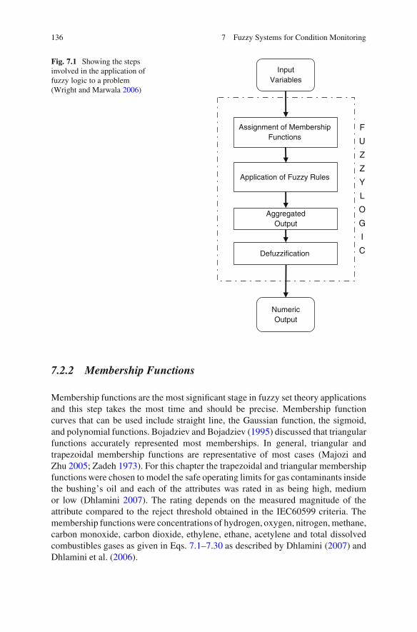
136 7 Fuzzy Systems for Condition Monitoring
F
U
Z
Z
Y
L
O
G
I
C
Assignment of Membership Functions
Application of Fuzzy Rules
AggregatedOutput
Defuzzification
InputVariables
NumericOutput
Fig. 7.1 Showing the stepsinvolved in the application offuzzy logic to a problem(Wright and Marwala 2006)
7.2.2 Membership Functions
Membership functions are the most significant stage in fuzzy set theory applicationsand this step takes the most time and should be precise. Membership functioncurves that can be used include straight line, the Gaussian function, the sigmoid,and polynomial functions. Bojadziev and Bojadziev (1995) discussed that triangularfunctions accurately represented most memberships. In general, triangular andtrapezoidal membership functions are representative of most cases (Majozi andZhu 2005; Zadeh 1973). For this chapter the trapezoidal and triangular membershipfunctions were chosen to model the safe operating limits for gas contaminants insidethe bushing’s oil and each of the attributes was rated in as being high, mediumor low (Dhlamini 2007). The rating depends on the measured magnitude of theattribute compared to the reject threshold obtained in the IEC60599 criteria. Themembership functions were concentrations of hydrogen, oxygen, nitrogen, methane,carbon monoxide, carbon dioxide, ethylene, ethane, acetylene and total dissolvedcombustibles gases as given in Eqs. 7.1–7.30 as described by Dhlamini (2007) andDhlamini et al. (2006).
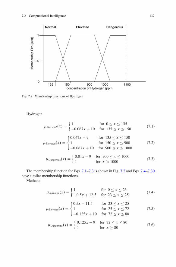
7.2 Computational Intelligence 137
Normal
1
0.5
0135 150 900
concentration of Hydrogen (ppm)
Mem
bers
hip
Fxn
(µ(
x))
1000 1100
Elevated Dangerous
Fig. 7.2 Membership functions of Hydrogen
Hydrogen
�Normal .x/ D�
1 for 0 � x � 135
�0:067x C 10 for 135 � x � 150(7.1)
�Elevated.x/ D8<:
0:067x � 9 for 135 � x � 150
1 for 150 � x � 900
�0:067x C 10 for 900 � x � 1000
(7.2)
�Dangerous.x/ D�
0:01x � 9 for 900 � x � 1000
1 for x > 1000(7.3)
The membership function for Eqs. 7.1–7.3 is shown in Fig. 7.2 and Eqs. 7.4–7.30have similar membership functions.
Methane
�Normal .x/ D�
1 for 0 � x � 23
�0:5x C 12:5 for 23 � x � 25(7.4)
�Elevated.x/ D8<:
0:5x � 11:5 for 23 � x � 25
1 for 25 � x � 72
�0:125x C 10 for 72 � x � 80
(7.5)
�Dangerous.x/ D�
0:125x � 9 for 72 � x � 80
1 for x 80(7.6)

138 7 Fuzzy Systems for Condition Monitoring
Ethane
�Normal.x/ D�
1 for 0 � x � 9
�x C 10 for 9 � x � 10(7.7)
�Elevated.x/ D8<:
x � 9 for 9 � x � 10
1 for 10 � x � 32
�0:333x C 11:66 for 32 � x � 35
(7.8)
�Dangerous.x/ D�
0:333x � 10:66 for 32 � x � 35
1 for x 35(7.9)
Ethylene
�Normal.x/ D�
1 for 0 � x � 18
�0:5x C 10 for 18 � x � 20(7.10)
�Elevated.x/ D8<:
0:5x � 9 for 18 � x � 20
1 for 20 � x � 90
�0:1x C 10 for 90 � x � 100
(7.11)
�Dangerous.x/ D�
0:1x � 9 for 90 � x � 100
1 for x 100(7.12)
Acetylene
�Normal.x/ D�
1 for 0 � x � 14
�x C 15 for 14 � x � 15(7.13)
�Elevated.x/ D8<:
x � 14 for 14 � x � 15
1 for 15 � x � 63
�0:142857x C 10 for 63 � x � 70
(7.14)
�Dangerous.x/ D�
0:142857x � 9 for 63 � x � 70
1 for x 70(7.15)
Carbon Monoxide
�Normal.x/ D�
1 for 0 � x � 450
�0:02x C 10 for 450 � x � 500(7.16)
�Elevated.x/ D8<:
0:02x � 9 for 450 � x � 500
1 for 500 � x � 900
�0:01x C 10 for 900 � x � 1000
(7.17)

7.2 Computational Intelligence 139
�Dangerous.x/ D�
0:01x � 9 for 900 � x � 1000
1 for x 1000(7.18)
Nitrogen
�Normal .x/ D�
1 for 0 � x � 0:9
�10x C 10 for 0:9 � x � 1(7.19)
�Elevated.x/ D8<:
10x � 9 for 0:9 � x � 1
1 for 1 � x � 9
�x C 10 for 9 � x � 10
(7.20)
�Dangerous.x/ D�
x � 9 for 9 � x � 10
1 forx 10(7.21)
Oxygen
�Normal.x/ D�
1 for 0 � x � 0:09
�100x C 10 for 0:09 � x � 0:1(7.22)
�Elevated.x/ D8<:
100x � 9 for 0:09 � x � 0:10
1 for 0:10 � x � 0:18
�50x C 10 for 0:18 � x � 0:20
(7.23)
�Dangerous.x/ D�
50x � 9 for 0:18 � x � 0:20
1 for x 0:20(7.24)
Carbon Dioxide
�Normal.x/ D�
1 for 0 � x � 9000
�0:001x C 10 for 9000 � x � 10000(7.25)
�Elevated.x/ D8<:
0:001x � 9 for 9000 � x � 10000
1 for 10000 � x � 13500
�0:00067x C 10 for 13500 � x � 15000
(7.26)
�Dangerous.x/ D�
0:00067x � 9 for 13500 � x � 15000
1 for x 15000(7.27)
Total Combustible Gases
�Normal .x/ D�
1 for 0 � x � 648
�0:01389x C 10 for 648 � x � 720(7.28)

140 7 Fuzzy Systems for Condition Monitoring
�Elevated.x/ D8<:
0:01389x � 9 for 648 � x � 720
1 for 720 � x � 4500
�0:002x C 10 for 4500 � x � 5000
(7.29)
�Dangerous.x/ D�
0:002x � 9 for 4500 � x � 5000
1 for x 5000(7.30)
7.2.3 Fuzzy Rules
Fuzzy rules represent the interrelation between all the inputs. This is a pointwhere user experience can be integrated in the mathematical modeling. It has beenestimated by many researchers before, that the number of rules is theoretically equalto the number of fuzzy categories raised to the power of the number of fuzzy criteria.Fuzzy categories used here were: the membership functions “dangerous”, “elevated”or “normal”. Fuzzy criteria applied here were the different gases that were present,i.e., hydrogen, methane, ethane, ethylene, acetylene, carbon monoxide, nitrogen,oxygen, carbon dioxide and total combustible gases. The rates of change of thegases were not used because the available data was taken on 1 day only.
Rules have an antecedent and a consequence. Rules can be expressed in the form(Ammar and Wright 2000; Wang 2000; Mamdani and Assilian 1975):
IF Attribute 1 is A1 AND Attribute 2 is A2 AND : : : AND Attribute N is AN ,THEN Consequent is Ci,
In the expression, Attribute 1, Attribute 2, : : : , Attribute N collectively forman Antecedent. Antecedents and Consequents are variables or concepts and A1,A2; : : : , Ci are linguistic terms or fuzzy sets of these variables, such as, “low”,“dangerous” or “high”, etc. (Bandemer and Gottwald 1995).
For the situation of bushing diagnosis, the amalgamation of the combustiblegases in the absence of oxygen does not generate a failure. With transformer oil,failure happens when oxygen is present in quantities above 0.2% at temperaturesabove 250ıC without any spark being present (auto-ignition) or at 156ıC if aspark is present (flash point). This condition decreases the number of fuzzy rulesmeaningfully, to only 81 fuzzy rules. The amalgamations were modeled in 81compartments. Two examples of fuzzy rules in written language are (1) If hydrogenis High only then Low Risk and (2) If hydrogen is High and Oxygen is High thenHigh Risk.
7.2.4 Decisions Based on Fuzzy Rules
By applying the rules, the bushing is given a risk rating for which certainmaintenance actions must be taken on the plant. For the safe operation of bushings
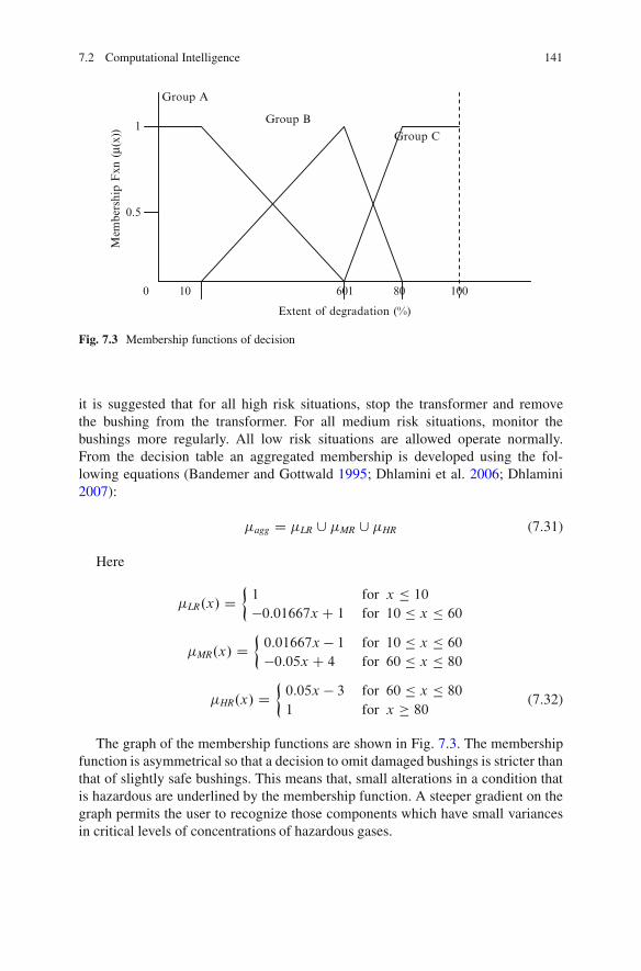
7.2 Computational Intelligence 141
1
10080100
0.5
601
Mem
bers
hip
Fxn
(µ(
x))
Extent of degradation (%)
Group A
Group B
Group C
Fig. 7.3 Membership functions of decision
it is suggested that for all high risk situations, stop the transformer and removethe bushing from the transformer. For all medium risk situations, monitor thebushings more regularly. All low risk situations are allowed operate normally.From the decision table an aggregated membership is developed using the fol-lowing equations (Bandemer and Gottwald 1995; Dhlamini et al. 2006; Dhlamini2007):
�agg D �LR [ �MR [ �HR (7.31)
Here
�LR.x/ D�
1 for x � 10
�0:01667x C 1 for 10 � x � 60
�MR.x/ D�
0:01667x � 1 for 10 � x � 60
�0:05x C 4 for 60 � x � 80
�HR.x/ D�
0:05x � 3 for 60 � x � 80
1 for x 80(7.32)
The graph of the membership functions are shown in Fig. 7.3. The membershipfunction is asymmetrical so that a decision to omit damaged bushings is stricter thanthat of slightly safe bushings. This means that, small alterations in a condition thatis hazardous are underlined by the membership function. A steeper gradient on thegraph permits the user to recognize those components which have small variancesin critical levels of concentrations of hazardous gases.

142 7 Fuzzy Systems for Condition Monitoring
7.2.5 Aggregated Rules
The table of fuzzy rules can additionally be streamlined by identifying cells withfeatures that are common within partitions. This procedure is known as aggregating.One can improve the following Aggregated Rules (AR) based on the underlinedpartition (Dhlamini et al. 2006).
(AR4) IF bushing has ‘Dangerous level of TDCG’ AND ‘NOT Normal Oxygen’AND ‘Not Normal Methane’, THEN the bushing belongs to ‘Group A (high riskor dangerous)’.
(AR5) IF bushing has ‘Dangerous TDCG’ AND ‘NOT Normal Oxygen’ AND‘Normal Methane’, THEN the bushing belongs to ‘Group B (medium risk orelevated)’.
(AR6) IF bushing has ‘Dangerous TDCG’ AND ‘Normal Oxygen’ AND ‘NotNormal Methane’, THEN the bushing belongs to ‘Group B (medium risk orelevated)’.
(AR7) IF bushing has ‘Dangerous TDCG’ AND ‘Normal Oxygen’ AND ‘NormalMethane’, THEN the bushing belongs to ‘Group C (low risk or normal)’.
In rule AR1, the result is ‘the bushing belongs to Group A’. The truth value ofthis consequence (CAR4) is displayed in Eq. 7.33 (Dhlamini 2007).
CAR4 D min .1; 1; 1/ D 1 (7.33)
When all the rules have been applied to a specific bushing, and different truthvalues of each consequence obtained, the maximum value of each consequenceamong all the rules that result in that consequence is taken as the degree to which thatconsequence applies to a given bushing. In the end this gives rise to an aggregatedfuzzy output as shown in Table 7.1 and the following equation (Bandemer andGottwald 1995):
AGDi D max .CAR1i \ CAR2i \ � � � \ CARni / (7.34)
Here, AGDi is the aggregated decision for category i, CAR is the consequence ofaggregated rules in a particular category i in a given partition.
7.2.6 Defuzzification
Defuzzification is intended at transforming fuzzy information into crisp data. Thetechnique used for defuzzification in this chapter is known as the weighted averageof maximum values of membership functions (Majozi and Zhu 2005). The techniquewas chosen since it is computationally economical. The result of this techniqueoffers the rank or level of risk of each bushing.
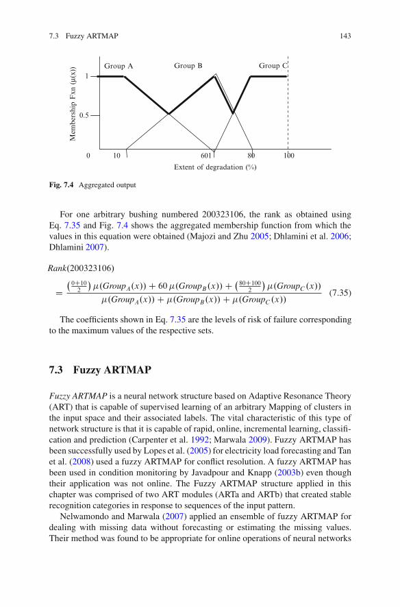
7.3 Fuzzy ARTMAP 143
1
10080100
0.5
601
Mem
bers
hip
Fxn
(µ(
x))
Extent of degradation (%)
Group A Group B Group C
Fig. 7.4 Aggregated output
For one arbitrary bushing numbered 200323106, the rank as obtained usingEq. 7.35 and Fig. 7.4 shows the aggregated membership function from which thevalues in this equation were obtained (Majozi and Zhu 2005; Dhlamini et al. 2006;Dhlamini 2007).
Rank.200323106/
D�
0C102
��.GroupA.x// C 60 �.GroupB.x// C �
80C1002
��.GroupC .x//
�.GroupA.x// C �.GroupB.x// C �.GroupC .x//(7.35)
The coefficients shown in Eq. 7.35 are the levels of risk of failure correspondingto the maximum values of the respective sets.
7.3 Fuzzy ARTMAP
Fuzzy ARTMAP is a neural network structure based on Adaptive Resonance Theory(ART) that is capable of supervised learning of an arbitrary Mapping of clusters inthe input space and their associated labels. The vital characteristic of this type ofnetwork structure is that it is capable of rapid, online, incremental learning, classifi-cation and prediction (Carpenter et al. 1992; Marwala 2009). Fuzzy ARTMAP hasbeen successfully used by Lopes et al. (2005) for electricity load forecasting and Tanet al. (2008) used a fuzzy ARTMAP for conflict resolution. A fuzzy ARTMAP hasbeen used in condition monitoring by Javadpour and Knapp (2003b) even thoughtheir application was not online. The Fuzzy ARTMAP structure applied in thischapter was comprised of two ART modules (ARTa and ARTb) that created stablerecognition categories in response to sequences of the input pattern.
Nelwamondo and Marwala (2007) applied an ensemble of fuzzy ARTMAP fordealing with missing data without forecasting or estimating the missing values.Their method was found to be appropriate for online operations of neural networks

144 7 Fuzzy Systems for Condition Monitoring
and was used for online condition monitoring. Their method was tested both onclassification and regression problems. An ensemble of fuzzy ARTMAPs wasimplemented for classification while an ensemble of multi-layer perceptions wasapplied for the regression problem. The results achieved using this ensemble-basedtechnique were compared to those attained using a combination of auto-associativeneural networks and genetic algorithms and they indicated that this techniqueperformed up to 9% better in regression problems.
Vilakazi and Marwala (2006) applied a fuzzy ARTMAP method for intrusiondetection and diagnosis. Their method applied a Sequential Backward FloatingSearch for feature selection and a fuzzy ARTMAP for detection and diagnosis ofattacks. The optimal vigilance parameter for the fuzzy ARTMAP was chosen usinga genetic algorithm. The reduced set of features decreased the computation time by0.789 s. A classification rate of 100% and 99.89% was obtained for the detectionstage and diagnosis stage, respectively.
Vilakazi and Marwala (2007a, b) applied a Fuzzy ARTMAP (FAM) for incre-mental learning for bushing condition monitoring. FAM was introduced since itcan incrementally learn from information as it becomes available. An ensembleof classifiers was used to improve the classification accuracy of the systems. Theresults showed that the FAM ensemble gave an accuracy of 98.5%. Additionally, theresults showed that the fuzzy ARTMAP can update its knowledge in an incrementalfashion without forgetting previously learned information.
Barszcz et al. (2011) applied a fuzzy ART neural network for wind turbinesstate classification and Chang et al. (2010b) applied a fuzzy ART for color-basedsemantic image retrieval. Wang and Zan (2010) applied a fuzzy ART for statisticalprocess control while Chen et al. (2010) successfully applied a fuzzy ART forinfrared target detection. Other successful applications of fuzzy ART include itsmedical application in the diagnosis of cancer (Hwang et al. 2010), for semanticimage retrieval (Chang et al. 2010a) and for personal credit scoring (Jiang and Lin2010).
The architecture of the FAM is shown in Fig. 7.5. The two ART modules wereinterconnected by a series of weighted connections between the F2 layers. Theconnection between the two ART modules formed the Map Field (Carpenter et al.1992). Various parameters needed to be set for the training process and this wasachieved in the ART Network. The vigilance parameter, �[0,1] is the only user-specified parameter. The vigilance parameter controls the network resonance. Thesecond parameter that is adjusted during training is the training rate ˇ[0,1] whichcontrols the adaptation speed. Here 0 implies a slow speed and 1 implies the fastest.The parameter ’ acts as a parameter to decide the category class and is always setsuch that 0 < ’ < 1.
During supervised learning, an analog signal vector X D (a, ac) was input into theARTa input layer F a
0 in the form of a complement code. Both the original input aand its complement ac were presented to the fuzzy ARTMAP network as explainedby Javadpour and Knapp (2003b).

7.3 Fuzzy ARTMAP 145
Inter-ART
Match Tracking
Fab
F2b
wkb
wkb
F1a
ARTaARTb
cF0
a (I = [aa ])
F1b
ra rb
waj wa
j
wjkab
F2a
r
- - cF0
b (I = [bb ])- -
Fig. 7.5 Architecture of the fuzzy ARTMAP
Each component in the input vector corresponds to a single node in F a1 . The key
function of this F a1 block was to compare the hypothesized class propagated from
the F a2 to the input signal. Simultaneously, a vector b was presented to ARTb and
this vector contained the desired outputs corresponding to the vector a in the ARTa.The network then used hypothesis testing to deduce which category the input patternshould belong to. Mapping was done in two steps. Firstly, the ARTa module alloweddata to be clustered into categories that were mapped to a class in the ARTb side ofthe module. The Fuzzy ARTMAP map field mapped the data cluster in the ‘A-side’to the label cluster in the ‘B-side’. During the learning process, each template fromthe ‘A-side’ was mapped to one template on the ‘B-Side’, ensuring a many-to-onemapping. The weights wAB
jk were used to control the association between the F2nodes on both sides. When the vectors a and b were presented to ARTa and ARTbrespectively, both models soon entered resonance.
When the vigilance criterion was respected, the map field learned the associationbetween vectors a and b by modifying its weights following the initial weight.A fuzzy ARTMAP has an internal controller that ensures autonomous systemoperation in real time. The inter-ART module has a self-regulatory mechanismnamed match tracking, whose objective was to maximize the generalization andminimize the network error. A complete description of the Fuzzy ARTMAP is

146 7 Fuzzy Systems for Condition Monitoring
Table 7.1 Classification results
Classifier Validation accuracy (%) Test accuracy (%)
Fuzzy set network 98.4 98.0Fuzzy ARTMAP 98.5 97.5
provided by Carpenter et al. (1992). The vigilance criterion is given by (Carpenteret al. 1992; Marwala 2009):
ˇybƒwab
JK
ˇyb
�ab (7.36)
Here the H vigilance criterion was reached by making a small increment in thevigilance parameter such that a certain category was excluded. This was done untilthe moment the active category corresponded to the desired output. After the inputhad completed the resonance state by the vigilance criterion, the weight adaptationwas accomplished. The adaptation of the ARTa and ARTb module weights is givenby (Carpenter et al. 1992; Marwala 2009):
wnewj ˇ.Iƒwold
j / C .1 � ˇ/woldj (7.37)
7.4 Results
Fuzzy sets technique and fuzzy ARTMAP were implemented to classify faults intransformer bushings using the dissolved gas analysis data based on the IEC60599,IEEE C57-104, and the California State University Sacramento (CSUS) criteria forOil Impregnated Paper (OIP) bushings, described in Chapter 2 by Vilakazi (2007).The networks were trained, validated and tested with 1,000 data points that consistedof 500 faulty and 500 healthy bushings. The results are shown in Table 7.1.
Table 7.1 shows that the fuzzy set network gave marginally better results than thefuzzy ARTMAP. However, the fuzzy set network was, however, able to factor intoaccount the user experience through the fuzzy rules.
7.5 Conclusion
In this chapter fuzzy set theory and fuzzy ARTMAP were implemented for faultidentification in transformer bushings based on the dissolved gas analysis (DGA)data and the IEC60599, IEEE C57-104, and California State University Sacramento(CSUS) criteria. The results showed that the fuzzy set theory and the fuzzyARTMAP gave an accuracy of 98% and 97.5%, respectively. The fuzzy set theorycan incorporate user experience through the use of fuzzy rules.

References 147
References
Aliustaoglu C, Metin Ertunc H, Ocak H (2009) Tool wear condition monitoring using a sensorfusion model based on fuzzy inference system. Mech Syst Signal Process 23(2):539–546
Ammar S, Wright R (2000) Applying fuzzy-set theory to performance evaluation. Socioecon PlannSci 34:285–302
Araujo E (2008) Improved Takagi-Sugeno fuzzy approach. In: Proceedings of the IEEE interna-tional conference on fuzzy systems, Hong Kong, China, pp 1154–1158
Babuska R (1991) Fuzzy modeling and identification. PhD thesis, Technical University of DelftBandemer H, Gottwald S (1995) Fuzzy sets, fuzzy logic, fuzzy methods with applications. Wiley,
New YorkBarszcz T, Bielecka M, Bielecki A, Wojcik M (2011) Wind turbines states classification by a fuzzy-
ART neural network with a stereographic projection as a signal normalization. Lect NotesComput Sci (including subseries Lecture Notes in Artificial Intelligence and Lecture Notesin Bioinformatics) 6594 LNCS (PART 2):225–234
Biacino L, Gerla G (2002) Fuzzy logic, continuity and effectiveness. Arch Math Logic 41:643–667Bih J (2006) Paradigm shift – an introduction to fuzzy logic. IEEE Potentials 25:6–21Boesack CD, Marwala T, Nelwamondo FV (2010) Application of GA-fuzzy controller design to
automatic generation control. In: 2010 Third international workshop on advanced computa-tional intelligence (IWACI), Suzhou, China, pp 227–232
Bojadziev G, Bojadziev M (1995) Fuzzy sets, fuzzy logic, applications. World Scientific PublishingCo. Pte. Ltd, Singapore/River Edge
Cabalar AF, Cevik A, Gokceoglu C, Baykal G (2010) Neuro-fuzzy based constitutive modeling ofundrained response of Leighton Buzzard sand mixtures. Expert Syst Appl 37:842–851
Cantor G (1874) Uber eine Eigenschaft des Inbegriffes aller reellen algebraischen Zahlen. CrellesJ Math 77:258–262
Carpenter GA, Grossberg S, Markuzon N, Reynolds JH, Rosen DB (1992) Fuzzy ARTMAP: aneural network architecture for incremental supervised learning of analog multidimensionalmaps. IEEE Trans Neural Netw 3:698–713
Catelani M, Fort A, Alippi C (2002) A fuzzy approach for soft fault detection in analog circuits.Measurement 32(1):73–83
Chang CY, Wang HJ, Jian RH (2010a) Semantic image retrieval with Fuzzy-ART. In: 2010International conference on system science and engineering, ICSSE 2010, Taipei, Taiwan, art.#5551705, pp 69–74
Chang CY, Wang HJ, Jian RH (2010b) Color-based semantic image retrieval with fuzzy-ART.In: Proceedings of 2010 6th international conference on intelligent information hiding andmultimedia signal processing, IIHMSP 2010, Darmstadt, Germany, art. #5635903, pp 426–429
Chen B, Wang W, Qin Q (2010) Infrared target detection based on fuzzy ART neural network. In:2010 2nd international conference on computational intelligence and natural computing, CINC2010, 2, Wuhan, China, art. no. 5643745, pp 240–243
Chen J, Roberts C, Weston P (2008) Fault detection and diagnosis for railway track circuits usingneuro-fuzzy systems. Control Eng Pract 16(5):585–596
Cox E (1994) The fuzzy systems handbook: a practitioner’s guide to building, using, maintainingfuzzy systems. AP Professional, Boston
D’Angelo MFSV, Palhares RM, Takahashi RHC, Loschi RH, Baccarini LMR, Caminhas WM(2011) Incipient fault detection in induction machine stator-winding using a fuzzy-Bayesianchange point detection approach. Appl Software Comput 11(1):179–192
Demirli K, Khoshnejad M (2009) Autonomous parallel parking of a car-like mobile robot by aneuro-fuzzy sensor-based controller. Fuzzy Sets Syst 160:2876–2891
Devlin K (1993) The joy of sets. Springer, BerlinDhlamini SM (2007) Bushing diagnosis using artificial intelligence and dissolved gas analysis.
University of the Witwatersrand PhD thesis
148 7 Fuzzy Systems for Condition Monitoring
Dhlamini SM, Marwala T (2005) Modeling inaccuracies from simulators for HV polymer Bushing.In: Proceedings of international symposium on high voltage, Beijing, Paper A18
Dhlamini SM, Marwala T, Majozi T (2006) Fuzzy and multilayer perceptron for evaluation ofHV bushings. In: Proceedings of the IEEE international conference on systems, man andcybernetics, Taiwan, pp 1331–1336
El-Sebakhy EA (2010) Flow regimes identification and liquid-holdup prediction in horizontalmultiphase flow based on neuro-fuzzy inference systems. Math Comput Simul 80:1854–1866
Evsukoff A, Gentil S (2005) Recurrent neuro-fuzzy system for fault detection and isolation innuclear reactors. Adv Eng Inform 19(1):55–66
Ferreiros J (1999) Labyrinth of thought: a history of set theory and its role in modern mathematics.Birkhauser, Basel
Flaig A, Barner KE, Arce GR (2000) Fuzzy ranking: theory and applications. Signal Process80:1017–1036
Hajek P (1995) Fuzzy logic and arithmetical hierarchy. Fuzzy Sets Syst 3:359–363Hajek P (1998) Metamathematics of fuzzy logic. Kluwer, DordrechtHalpern JY (2003) Reasoning about uncertainty. MIT Press, CambridgeHsu Y-C, Lin S-F (2009) Reinforcement group cooperation-based symbiotic evolution for recurrent
wavelet-based neuro-fuzzy systems. J Neurocomput 72:2418–2432Huang T-M, Kecman V (2005) Gene extraction for cancer diagnosis by support vector machinesan
improvement. Artif Intell Med 35:185–194Hwang JIG, Liu CE, Sokoll L, Adam BL (2010) Applying fuzzy ART in medical diagnosis of
cancers. In: 2010 international conference on machine learning and cybernetics, ICMLC 2010,Qingdao, 3, art. no. 5580939, pp 1084–1089
Iplikci S (2010) Support vector machines based neuro-fuzzy control of nonlinear systems.J Neurocomput 73:2097–2107
Javadpour R, Knapp GM (2003a) A fuzzy neural network approach to condition monitoring.Comput Ind Eng 45:323–330
Javadpour R, Knapp GM (2003b) A fuzzy neural network approach to machine conditionmonitoring. Comput Ind Eng 45(2):323–330, 25th international conference on computers andindustrial engineering, Limerick, Ireland, August 2003
Jeffries M, Lai E, Plantenberg DH, Hull JB (2001) A fuzzy approach to the condition monitoringof a packaging plant. J Mater Process Technol 109(1–2):83–89
Jiang M, Lin S (2010) A study of personal credit scoring models based on fuzzy ART. J ComputInfo Syst 6(9):2805–2811
Johnson P (1972) A history of set theory. Prindle, Weber & Schmidt, BostonKlir GJ, Folger TA (1988) Fuzzy sets, uncertainty, and information. Prentice Hall, Englewood
CliffsKlir GJ, Yuan B (1995) Fuzzy sets and fuzzy logic: theory and applications. Prentice Hall, Upper
Saddle RiverKlir GJ, St Clair UH, Yuan B (1997) Fuzzy set theory: foundations and applications. Prentice Hall,
Upper Saddle RiverKorbicz J, Kowal M (2007) Neuro-fuzzy networks and their application to fault detection of
dynamical systems. Eng Appl Artif Intell 20(5):609–617, Soft Computing Applications,August 2007
Kosko B (1993) Fuzzy thinking: the new science of fuzzy logic. Hyperion, New YorkKosko B, Isaka S (1993) Fuzzy logic. Sci Am 269:76–81Kubica EG, Wang D, Winter AD (1995) Modelling balance and posture control mechanisms of the
upper body using conventional and fuzzy techniques. Gait Posture 3(2):111Lau HCW, Dwight RA (2011) A fuzzy-based decision support model for engineering asset
condition monitoring – a case study of examination of water pipelines. Expert Syst Appl38(10):13342–13350
Lopes MLM, Minussi CR, Lotufo ADP (2005) Electric load forecasting using a fuzzyART&ARTMAP neural network. Appl Software Comput 5(2):235–244

References 149
Majozi T, Zhu XX (2005) A combined fuzzy set theory and MILP approach in integration ofplanning and scheduling of batch plants – personnel evaluation and allocation. Comput ChemEng 29:2029–2047, Elsevier Science, July 2005
Mamdani EH (1974) Application of fuzzy algorithms for the control of a dynamic plant. Proc IEE121:1585–1588
Mamdani EH, Assilian S (1975) An experiment in linguistic synthesis with a fuzzy logic controller.Int J Man–Mach Stud 7(1):1–13
Marwala T (2009) Computational intelligence for missing data imputation, estimation and man-agement: knowledge optimization techniques. IGI Global Publications, Information ScienceReference Imprint, New York
Marwala T, Lagazio M (2011) Militarized conflict modeling using computational intelligencetechniques. Springer, London
Mendonca LF, Sousa JMC, Sa da Costa JMG (2009) An architecture for fault detection andisolation based on fuzzy methods. Expert Syst Appl 36(2, Part 1):1092–1104
Msiza IS, Szewczyk M, Halinka A, Pretorius J-HC, Sowa P, Marwala T (2011) Neural networkson transformer fault detection: evaluating the relevance of the input space parameters. In: 2011IEEE/PES Power Systems Conference and Exposition, PSCE 2011, Phoenix, art. no. 5772567
Nelwamondo FV, Marwala T (2007) Fuzzy artmap and neural network approach to onlineprocessing of inputs with missing values. Trans S Afr Inst Electrical Eng 98(2):45–51
Novak V (1989) Fuzzy sets and their applications. Adam Hilger, BristolNovak V (2005) On fuzzy type theory. Fuzzy Sets Syst 149:235–273Novak V, Perfilieva I, Mockor J (1999) Mathematical principles of fuzzy logic. Kluwer, DordrechtRazavi-Far R, Davilu H, Palade V, Lucas C (2009) Model-based fault detection and isolation of a
steam generator using neuro-fuzzy networks. Neurocomputing 72(13–15):2939–2951, HybridLearning Machines (HAIS 2007)/Recent Developments in Natural Computation (ICNC 2007),August 2009
Sainz Palmero GI, Juez Santamaria J, Moya de la Torre EJ, Peran Gonzalez JR (2005) Faultdetection and fuzzy rule extraction in AC motors by a neuro-fuzzy ART-based system. EngAppl Artif Intell 18(7):867–874
Sugeno M (1985) Industrial applications of fuzzy control. Elsevier, AmsterdamSugeno M, Kang G (1988) Structure identification of fuzzy model. Fuzzy Sets Syst 28:15–33Takagi T, Sugeno M (1985) Fuzzy identification of systems and its applications to modeling and
control. IEEE Trans Syst Man Cybern 15:116–132Tan SC, Rao MVC, Lim Fuzzy CP (2008) ARTMAP dynamic decay adjustment: an improved
fuzzy ARTMAP model with a conflict resolving facility. Appl Software Comput 8(1):543–554Tettey T, Marwala T (2006) Neuro-fuzzy modeling and fuzzy rule extraction applied to conflict
management. Lect Notes Comput Sci 4234:1087–1094Vilakazi CB (2007) Machine condition monitoring using artificial intelligence: the incremen-
tal learning and multi-agent system approach, University of the Witwatersrand Mastersdissertation
Vilakazi CB, Marwala T (2006) Application of feature selection and fuzzy ARTMAP to intrusiondetection. In: IEEE international conference on systems, man and cybernetics, Vancouver,Canada, pp 4880–4885
Vilakazi CB, Marwala T (2007a) Incremental learning and its application to bushing conditionmonitoring. Lect Notes Comput Sci (including subseries Lecture Notes in Artificial Intelligenceand Lecture Notes in Bioinformatics) 4491 LNCS (PART 1):1237–1246
Vilakazi CB, Marwala T (2007b) Online incremental learning for high voltage bushing conditionmonitoring. In: IEEE international conference on neural networks – conference proceedings,Orlando, Florida, art. no. 4371355, pp 2521–2526
Von Altrock C (1995) Fuzzy logic and neurofuzzy applications explained. Prentice Hall, Engle-wood Cliffs
Wang M, Zan T (2010) Adaptively pattern recognition in statistical process control using fuzzyART neural network. In: Proceedings – 2010 international conference on digital manufacturingand automation, ICDMA 2010, 1, Changcha, China, art. no. 5701122, pp 160–163

150 7 Fuzzy Systems for Condition Monitoring
Wang Z (2000) Artificial intelligence applications in the diagnosis of power transformer incipientfaults, PhD thesis, Virginia Polytechnic Institute and State University
Wright S, Marwala T (2006) Artificial intelligence techniques for steam generator modelling.arXiv:0811.1711
Zadeh LA (1965) Fuzzy sets. Info Control 8:338–353Zadeh LA (1973) Outline of a new approach to the analysis of complex systems and decision
processes. IEEE Trans Syst Man Cybern 3(1):28–44Zemankova-Leech M (1983) Fuzzy relational data bases. PhD dissertation, Florida State UniversityZimmermann H (2001) Fuzzy set theory and its applications. Kluwer, Boston

Chapter 8Rough Sets for Condition Monitoring
8.1 Introduction
Rough set theory as put forward by Pawlak (1991) is a mathematical techniquewhich models vagueness and uncertainty. It permits one to estimate sets that aredifficult to explain even with accessible information. For this chapter, rough setswere applied to the condition monitoring of transformer bushings based on dissolvedgas analysis data. The advantages of rough sets, as with many other computationalintelligence methods, are that they do not necessitate inflexible a priori assumptionsabout the mathematical characteristics of such complex relationships, as normallyrequired for the multivariate statistical approaches (Machowski and Marwala 2005;Crossingham et al. 2008; Marwala and Lagazio 2011). Rough set theory is based onthe assumption that the information of interest is associated with some informationfrom its universe of discourse (Crossingham and Marwala 2008a, b; Tettey et al.2007; Marwala and Crossingham 2008, 2009; Crossingham et al. 2009).
Wang et al. (2006) applied rough set theory to handle uncertainty and therebydecreased the redundancy in evaluating the degree of malignancy in brain glioma,based on Magnetic Resonance Imaging findings as well as the clinical data beforean operation. Their data comprised unsuitable features, uncertainties and missingvalues. The rough set rules that were identified from these data were applied toevaluate the degree of the malignancy. Rough set based feature selection procedureswere used to select features so that the accuracy of classification based on decisionrules could be enhanced. These selected feature subsets were applied to givedecision rules for the classification task. The results obtained showed that theirtechnique identified reducts that produced decision rules with higher classificationrates than conventional methods.
Xie et al. (2011) used variable precision rough set for land use / land coverretrieval from remote sensing images. Their results showed a retrieval accuracy of87.32%. Chen et al. (2011) used a rough set method for the prediction of proteininteraction hot spots. Their results indicated that four features, viz. the change of
T. Marwala, Condition Monitoring Using Computational Intelligence Methods:Applications in Mechanical and Electrical Systems, DOI 10.1007/978-1-4471-2380-4 8,© Springer-Verlag London Limited 2012
151

152 8 Rough Sets for Condition Monitoring
accessible surface area, percentage of the change of accessible surface area, size ofa residue, and atomic contacts were vital in predicting the hot spots.
Salamo and Lopez-Sanchez (2011) used rough sets for selecting features inCase-Based Reasoning classifiers. Lin et al. (2011) applied a hybrid of roughset theory and flow network graphs to predict the customer churn in credit cardaccounts using 21,000 customer samples equally divided into three classes (survival,voluntary churn, and involuntary churn). The input data included demographic,psychographic, and transactional variables for studying and classifying customercharacteristics. Their results indicated that rough sets can forecast customer churnand offer valuable information for decision-makers.
Other applications of rough set theory include the work by Azadeh et al. (2011)who applied a rough set technique for assessing the efficiency of personnel, Zhanget al. (2010) for controlling reagents in an ionic reverse flotation process, Huanget al. (2011) who used rough sets in patent development with the emphasis onresource allocation, Zou et al. (2011) who used rough sets for distributor selectionin a supply chain management system, Wang et al. (2010) who used rough setsand a Tabu search for credit scoring, Gong et al. (2010) for a rare-earth extractionprocess, Chen et al. (2010a) for creating a diagnostic system based on Chinesetraditional medicine for the pneumonia in elderly, Yan et al. (2010) for predictingsoil moisture, and Liao et al. (2010) for a model that assessed brand trust. The mainconcept of rough set theory is an indiscernibility relation, where indiscernibilityindicates indistinguishable from one another. For knowledge attainment from datawith numerical attributes, special methods are applied. Most commonly a stepcalled discretization is taken before the main step of rule induction or decision treegeneration is applied (Crossingham and Marwala 2007). A number of approaches toachieve the goal of discretization are Boolean reasoning, Equal-Width-Bin (EWB)partitioning and Equal-Frequency-Bin (EFB) partitioning (Jaafar et al. 2006; Fayyadand Irani 1993).
For this chapter an ant colony optimization method and an EFB partitioningmethod was used to discretize the rough set partitions and apply these to conditionthe monitoring of transformer bushings (Mpanza and Marwala 2011). Zhao et al.(2010) applied a fuzzy preference based rough set technique and principal compo-nent analysis for condition monitoring. They implemented a Principal ComponentAnalysis (PCA) to reduce the input space. Their method was tested for damage leveldetection of an impeller in a slurry pump. Zhang et al. (2008) applied rough setsand mathematical morphology for intelligent condition monitoring. They used thetheory of image processing to analyze the flank faces and they used tool conditionmonitoring through measuring the area of tool wear. Their results indicated thattheir method was flexible and fast enough to be applied in real time for the conditionmonitoring of tool wear online. Li et al. (2005) applied rough sets for the conditionmonitoring of an engine. They created decision tables for each fault case and used arough set reduction to conduct intelligent fault diagnosis and obtained good results.
Shen et al. (2000) applied rough set theory for the fault diagnosis of a multi-cylinder diesel engine. When the reducts from the rough sets theory were analyzedit was observed that this method was effective for valve fault diagnosis. In addition

8.2 Rough Sets 153
a new discretization technique was presented and was found to be suitable fordiscretizing the attributes without a priori knowledge.
Xiang et al. (2009) applied the Walsh transform and rough sets for faultdiagnosis. Data processed by the Walsh transform was discretized and reducedby the rough sets theory, and diagnosis rules were extracted and used for faultdiagnosis. The results obtained showed a higher accuracy than other methods.
Wang and Li (2004) successfully applied a rough-set based fault-ranking proto-type system for fault diagnosis and achieved good results. Elsewhere, Tay and Shen(2003) applied rough set for fault diagnosis in a multi-cylinder diesel engine.
Other applications of rough set theory to the area of condition monitoring includethat for a mono-block centrifugal pump (Sakthivel et al. 2010), for fault linedetection of ineffectually grounded systems (An et al. 2011), nuclear power plants(Mu et al. 2011), in fault line detection for distribution networks (Pang et al. 2010),machines (Yu and Han 2010), and in diesel engines (Li et al. 2010).
8.2 Rough Sets
The primary objective of using rough sets is to produce estimates of various conceptsfrom the acquired data. Contrary to other approaches that are applied to handleuncertainty, rough set theory has its own exclusive benefits in that it does notnecessitate (Crossingham 2007; Nelwamondo 2008; Marwala and Lagazio 2011):
• any additional information about the experimental training data such as thestatistical probability; and
• basic probability assignment in fuzzy set theory (Pawlak and Munakata 1996).
Rough set theory deals with the estimation of sets that are hard to explainwith the available information (Ohrn 1999; Ohrn and Rowland 2000; Marwala andLagazio 2011). It is targeted mainly to the classification of imprecise, uncertain,or incomplete information. Two estimations, the upper and lower estimation aredeveloped to handle inconsistent information. The data are represented using aninformation table.
Rough set theory is based on a set of rules, which are described in terms oflinguistic variables. Rough sets are of essential significance to artificial intelligenceand cognitive science, and are well applied to the tasks of machine learningand decision analysis, particularly in the analysis of decisions in which there arecontradictions. Because they are rule-based, rough sets are highly transparent butthey are not as accurate. However, they are not good as universal estimators,since other machine learning techniques such as neural networks are better intheir predictions. Thus, in machine learning, there is always a trade-off betweenprediction accuracy and transparency.
Crossingham and Marwala (2007) presented a method to optimize the partitionsizes of rough set using various optimization methods. Three optimization methodswere applied to perform the granularization process: the genetic algorithm, hill
154 8 Rough Sets for Condition Monitoring
climbing, and simulated annealing. These optimization approaches maximize theclassification accuracy of the rough sets. Their rough set partition approacheswere tested on a demographic set. The three methods were compared for theircomputational time, accuracy, and number of rules produced and then applied toa HIV data set. The optimized technique results were then compared to a non-optimized discretization method, using Equal-Width-Bin (EWB) partitioning. Theaccuracies achieved after optimizing the partitions using a genetic algorithm (GA),hill climbing, and simulated annealing (SA) were 66.89%, 65.84%, and 65.48%,respectively, compared to the accuracy of the EWB partitioning of 59.86%. Inaddition to rough sets providing the plausibility of the estimated HIV status, theyalso provided the linguistic rules describing how demographic parameters drive therisk of HIV.
Rough set theory offers a method of reasoning from vague and imprecise data(Goh and Law 2003). The method is based on the assumption that some observedinformation is in some way associated with some information in the universeof the discourse (Komorowski et al. 1999; Yang and John 2006; Kondo 2006).This suggests that if some characteristics of the data are missing, then theycan be approximated from part of the information in the universe of discoursewhich is comparable with the observed part of that specific data. Objects withthe same information are indiscernible in the view of the available information.An elementary set consisting of indiscernible objects forms a basic granule ofknowledge. A union of an elementary set is referred to as a crisp set; or else, the setis considered to be rough. In the next sub-sections, rough set theory is described.
8.2.1 Information System
An information system (ƒ), is described as a pair (U, A) where U is a finite setof objects known as the universe and A is a non-empty finite set of attributes asdescribed as follows (Crossingham 2007; Yang and John 2006; Nelwamondo 2008;Marwala 2009; Marwala and Lagazio 2011).
ƒ D .U; A/ (8.1)
All attributes a 2 A have values, which are elements of a set Va of the attributesa (Dubois 1990; Crossingham 2007; Marwala and Lagazio 2011):
a W U ! Va (8.2)
A rough set is described with a set of attributes and the indiscernibility relationbetween them. Indiscernibility is explained in the next subsection.

8.2 Rough Sets 155
8.2.2 The Indiscernibility Relation
The indiscernibility relation is one of the central ideas of rough set theory(Grzymala-Busse and Siddhaye 2004; Zhao et al. 2007; Pawlak and Skowron 2007;Marwala and Lagazio 2011). Indiscernibility basically suggests similarity (Goh andLaw 2003) and, consequently, these sets of objects are indistinguishable. Given aninformation system ƒ and subsetB � A, B the indiscernibility defines a binaryrelation I(B) on U such that (Pawlak et al. 1988; Ohrn 1999; Wu et al. 2003; Ohrnand Rowland 2000; Nelwamondo 2008; Marwala and Lagazio 2011):
.x; y/ 2 I.B/
if and only if
a.x/ D a.y/ (8.3)
for all a 2 A where a(x) symbolizes the value of attribute a for element x.Equation 8.3 suggests that any two elements that are elements of I(B) should beidentical from the point of view of a. Supposing that U has a finite set of N objectsfx1,x2,..,xNg. Let Q be a finite set of n attributes fq1,q2,..,qng in the same informationsystem ƒ, then (Inuiguchi and Miyajima; 2007; Crossingham 2007; Nelwamondo2008; Marwala and Lagazio 2011):
ƒ D hU; Q; V; f i (8.4)
Here f is the total decision function, known as the information function. From theexplanation of the indiscernibility relation, two entities have a similarity relation toattribute a if they universally have the same attribute values.
8.2.3 Information Table and Data Representation
An information table is applied in rough sets theory as a technique for signifyingthe data. Data in the information table are organized, centered on their conditionattributes and decision attributes (D). Condition attributes and decision attributesare similar to the independent variables and dependent variable (Goh and Law2003). These attributes are divided into C [ D D Q and C [ D D 0. Data isindicated in the table and each object is characterized in an Information System(Komorowski et al. 1999).
8.2.4 Decision Rules Induction
Rough sets also require producing decision rules for a given information table. Therules are generally based on condition attributes values (Bi et al. 2003; Slezak and

156 8 Rough Sets for Condition Monitoring
Ziarko 2005). The rules are presented in an ‘if CONDITION(S)-then DECISION’format. Stefanowski (1998) applied a rough set technique for inference in decisionrules.
8.2.5 The Lower and Upper Approximation of Sets
The lower and upper approximations of sets are defined on the basis of theindiscernibility relation. The lower approximation is defined as the collection ofcases whose equivalent classes are confined in the cases that need to be estimated,while the upper approximation is defined as the collection of classes that areincompletely contained in the set that need to be estimated (Rowland et al. 1998;Degang et al. 2006; Witlox and Tindemans 2004). If the concept X is defined as aset of all cases defined by a specific value of the decision and that any finite unionof elementary set, associated with B called a B-definable set (Grzymala-Busse andSiddhaye 2004) then set X can be estimated by two B-definable sets, known as theB-lower estimation denoted by X and B-upper approximation BX: The B-lowerapproximation is defined as (Bazan et al. 2004; Crossingham 2007; Nelwamondo2008; Marwala and Lagazio 2011):
BX D fx 2 U jŒx�B � Xg (8.5)
and the B-upper approximation is defined as (Crossingham 2007; Nelwamondo2008; Marwala and Lagazio 2011):
BX D fx 2 U jŒx�B \ X ¤ 0g (8.6)
There are other approaches that have been described for defining the lower andupper approximations for a completely specified decision table. Some of the popularones include approximating the lower and upper approximation of X using Eqs. 8.7and 8.8, as follows (Grzymala-Busse 2004; Crossingham 2007; Nelwamondo 2008;Marwala and Lagazio 2011):
[ fŒx�B jx 2 U; Œx�B � Xg (8.7)
[ fŒx�B jx 2 U; Œx�B \ X ¤ 0g (8.8)
The definition of definability is revised in situations of incompletely specifiedtables. In this case, any finite union of characteristic sets of B is called a B-definableset. Three different definitions of approximations have been discussed by Grzymala-Busse and Siddhaye (2004). By letting B be a subset of A of all attributes and R(B)be the characteristic relation of the incomplete decision table with characteristic

8.2 Rough Sets 157
sets K(x), where x 2 U, the following can be defined (Grzymala-Busse 2004;Crossingham 2007; Nelwamondo 2008; Marwala and Lagazio 2011):
BX D fx 2 U jKB.x/ � Xg (8.9)
and
BX D fx 2 U jKB.x/ \ X ¤ 0 g (8.10)
Equations 8.9 and 8.10 are known as singletons. The subset lower and upperapproximations of incompletely specified data sets can then be mathematicallydefined as (Nelwamondo 2008; Marwala and Lagazio 2011):
[ fKB.x/ jx 2 U; KB.x/ � X g (8.11)
and
[ fKB.x/ jx 2 U; KB.x/ \ X D 0g (8.12)
Additional information on these approaches can be found in (Grzymala-Busseand Hu 2001; Grzymala-Busse and Siddhaye 2004; Crossingham 2007). It can bededuced from these properties that a crisp set is only defined if B.X/ D B.X/.Roughness is consequently defined as the difference between the upper and thelower approximation.
8.2.6 Set Approximation
A number of properties of rough sets have been presented in the work of Pawlak(1991). An important property of rough set theory is the definability of a roughset (Quafafou 2000). This was explained for the situation when the lower andupper approximations are equal. If this is not the situation, then the target set isun-definable. Some of the distinctive cases of definability are (Pawlak et al. 1988;Crossingham 2007; Nelwamondo 2008; Marwala 2009):
• Internally definable set: Here, BX ¤ 0and BX D U . The attribute set B hasobjects that certainly are elements of the target set X, even though there are noobjects that can definitively be excluded from the set X.
• Externally definable set: Here, BX D 0 and BX ¤ U . The attribute set B hasno objects that certainly are elements of the target set X, even though there areobjects that can definitively be excluded from the set X.
• Totally un-definable set: Here, BX D 0and BX D U . The attribute set B has noobjects that certainly are elements of the target set X, even though there are noobjects that can definitively be excluded from the set X.

158 8 Rough Sets for Condition Monitoring
8.2.7 The Reduct
An additional property of rough sets is the reduct which is a concept that defineswhether there are attributes B in the information system that are more significant tothe knowledge represented in the equivalence class structure than other attributes. Itis vital to identify whether there is a subset of attributes which could be completelydescribed by the knowledge in the database. This attribute set is known as the reduct.
Beynon (2001) concluded that the elementary feature of the variable precisionrough set model involved an exploration for subsets of condition attributes whichgive identical information for classification functions as the complete set of givenattributes. Beynon characterized these subsets as approximate reducts. Beynonexplained these subsets for an identified classification error represented by ˇ andthen identified the particular variances and showed interesting consequences foridentifying ˇ-reducts which ensure a general knowledge similar to that obtainedfrom the full set of attributes.
Terlecki and Walczak (2007) described the relations between rough set reductsand emerging patterns. Their study established a practical application for theseobservations for the minimal reduct problem, using these to test the differentiatingfactor of an attribute set. Shan and Ziarko (1995) properly defined a reduct as asubset of attributes RED � B such that:
• Œx�RED D Œx�B . That is, the equivalence classes that were induced by reducingthe attribute set RED are equal to the similar class structure that was induced bythe full attribute set B.
• Attribute set RED is minimal because Œx�.RED�A/ ¤ Œx�B for any attribute A 2RED. Simply, there is no attribute that can be taken away from the set REDwithout changing the equivalent classes Œx�B .
Therefore a reduct can be visualized as a suitable set of features that can ade-quately express the category’s structure. One property of a reduct in an informationsystem is that it is not unique since there may be other subsets of attributes whichmay still preserve the equivalence class structure conveyed in the informationsystem. The set of characteristics that are common in all reducts is called a core.
8.2.8 Boundary Region
The boundary region, which can be expressed as the difference BX�BX , is a regionwhich is composed of objects that cannot be included nor excluded as elements ofthe target set X. Simply, the lower approximation of a target set is an estimationwhich consists only of those objects which can be positively identified as elementsof the set. The upper approximation is a rough approximation and includes objectsthat may be elements of the target set. The boundary region is the area between theupper and lower approximation.

8.3 Discretization Methods 159
8.2.9 Rough Membership Functions
A rough membership function is a function �xA W U ! Œ0; 1� that, when applied
to object x, quantifies the degree of overlap between set X and the indiscernibilityset to which x belongs. The rough membership function is applied to estimate theplausibility and can be defined as (Pawlak 1991; Crossingham 2007; Nelwamondo2008; Marwala and Lagazio 2011):
�xA.X/ D jŒx�B \ X j
jŒx�B j (8.13)
The rough membership function can be understood as a fuzzification within thecontext of rough approximation. It confirms the translation from rough approxi-mation into membership function. The important aspect of a rough membershipfunction is that it is derived from data (Hoa and Son 2008; Crossingham 2007).
8.3 Discretization Methods
The methods which allow continuous data to be processed involve discretization.There are several methods available to perform discretization, but the two popularlyones – Equal-Width-Bin (EWB) partitioning and Equal-Frequency-Bin (EFB)partitioning – were investigated by Crossingham (2007). Details are given below.
8.3.1 Equal-Width-Bin (EWB) Partitioning
EWB partitioning divides the range of observed values of an attribute intokequallysized bins (Crossingham et al. 2009). For this chapter, kwas taken as four. Onenotable problem of this method is that it is vulnerable to outliers that may drasticallyskew the data range. This problem was eliminated through a pre-processing stepinvolving cleaning of the data. The manner in which data can be discretizedusing EWB follows (Grzymala-Busse 2004; Crossingham et al. 2009; Marwala andLagazio 2011):
• Evaluate the Smallest and Largest value for each attribute and label these valuesS and L.
• Write the width of each interval, W, as:
W D L � S
4(8.14)
• The interval boundaries can be determined as: S C W, S C 2W, S C 3W. Theseboundaries can be determined for any number of intervals k, up to the termS C .k � 1/W .

160 8 Rough Sets for Condition Monitoring
8.3.2 Equal-Frequency-Bin (EFB) Partitioning
EFB partitioning sorts the values of each attribute in ascending order and dividesthem intokbins where (givenminstances) each bin contains m/k adjacent values. Inmost instances duplicated values will probably exist. The EFB partitioning can beimplemented as follows (Grzymala-Busse 2004; Crossingham 2007; Marwala andLagazio 2011):
• Arrange the values of each attribute (va1; va
2; va3; :::; va
m) into intervals whereby mis the number of instances.
• Therefore each interval is made of the following sequential values:
� D m
4(8.15)
• The cut-off points may be computed using the following equation which is validfor i D 1, 2, 3 where k intervals can be calculated for i D 1, : : : , k-1:
ci D vi� C vi�C1
2(8.16)
8.4 Rough Set Formulation
The process of modeling the rough set can be classified into these five stages(Grzymala-Busse 2004; Crossingham 2007):
1. The first stage is to select the data.2. The second stage involves pre-processing the data to ensure that it is ready for
analysis. This stage involves discretizing the data and removing unnecessary data(cleaning the data).
3. If reducts are considered, the third stage is to use the cleaned data to generatereducts. A reduct is the most concise way in which we can discern object classes.In other words, a reduct is the minimal subset of attributes that enables the sameclassification of elements of the universe as the whole set of attributes. To copewith inconsistencies, lower and upper approximations of decision classes aredefined in this stage.
4. Stage four is where the rules are extracted or generated. The rules are usuallydetermined based on condition attribute values. Once the rules are extracted, theycan be presented in an ‘if CONDITION(S)-then DECISION’ format.
5. The fifth and final stage involves testing the newly created rules on a test set. Theaccuracy must be noted and sent back into the optimization method used in step 2and the process will continue until the optimum or highest accuracy is achieved.
The procedure for computing rough sets and extracting rules is given inAlgorithm 8.1 (Crossingham 2007). Once the rules are extracted, they can be tested

8.5 Optimized Rough Sets 161
Algorithm 8.1 Procedure to Generate a Rough Set Model
Input: Condition and Decision AttributesOutput: Certain and Possible Rules1 Obtain the data set to be used;2 Repeat3 forconditional attribute 1 to size of training datado4 Pre-process data to ensure that it is ready for analysis;5 Discretize the data according to the optimization technique;6 Compute the lower approximation, as defined in Eq. 8.5;7 Compute the upper approximation, as defined in Eq. 8.6;
8From the general rules, calculate plausibility measures for an object x belonging toset X, as defined by Eq. 8.13;
9 Extract the certain rules from the lower approximation generated for each subset;10 Similarly, extract the possible rules from the upper approximation of each subset;11 Remove the generated rules for the purposes of testing on unseen data;12 Compute the classifier performance using the AUC;13 End14 until Optimization technique termination condition;
using a set of testing data. The classification output is expressed as a decision valuewhich lies between 0 and 1. The accuracy of the rough set is determined using theArea Under the receiver operating characteristic Curve (AUC).
8.5 Optimized Rough Sets
This section of the chapter uses the ant colony optimization technique to discretizethe rough set partition. The general procedure pursued in this chapter is bestexpressed mathematically as follows (Marwala 2009; Marwala and Lagazio 2011):
y D f .x; RP / (8.17)
Here x is the input data � in this chapter it is the dissolved gas analysis data, RPis the rough set partition and y is the accuracy obtained when the model is tested onunseen data. For this chapter, the aim of the optimization process was to identify theRP parameters so that the accuracy y was maximized. To this end, the ant colonyoptimization method was applied and is the subject of the next section (Mpanza2011).
8.5.1 Ant Colony System
Ant Colony Optimization (ACO) is a meta-heuristic optimization technique forestimating solutions for combinatorial optimization problems (Blum 2005; Mpanzaand Marwala 2011; Mpanza 2011). It is a type of the swarm intelligence group.

162 8 Rough Sets for Condition Monitoring
Swarm intelligence is the emergent collective intelligence of groups of simpleagents. Ant colony system was first proposed by Dorigo (1992). It is inspired by thenatural behavior of ants as they work collectively sharing information to identifythe best possible route between their colony and the food source. This autonomy isachieved by ants depositing pheromone on their trail that acts as a signal for otherants. In the end, the path with the highest concentration of pheromone deposit is theoptimal path.
ACO is different from other optimization tools in that it explicitly incorporatesprior information on the structure of a good solution with a posteriori informationon the good solution that was attained earlier (Yaseen and AL-Slamy 2008; Mpanza2011; Mpanza and Marwala 2011). Different to the discretization techniques such asequal width or equal frequency types (Marwala and Lagazio 2011), ACO is a non-deterministic procedure. Non-deterministic procedures produce different solutionsfor different implementation because of their randomness (Thantulage 2009). ACOtechniques have been applied in estimating solutions for the traveling salesmenproblem (Dorigo and Gambardella 1997; Cheng and Mao 2007), the networkrouting problem (Di Caro and Dorigo 1997), flowshop scheduling (Tavares Neto andGodinho Filho 2011), seismic design (Kaveh et al. 2010), part-machine clustering(Xing et al. 2010a, b), for missing data estimation (Leke and Marwala 2006),feature selection (Chen et al. 2010b) and for attribute reduction (Ke et al. 2008).These applications have demonstrated that ACO is capable of estimating NP-hardproblems.
8.5.2 Artificial Ant
An artificial ant is a computational agent describing the behavior of a real ant byiteratively constructing a solution for the problem at hand. The current state, i, is anincomplete solution and an ant follows the pheromone trail to move to the followingstate, j, and a more complete solution (Carbonaro and Maniezzo 2003).
8.5.3 Ant Colony Algorithm
An ant colony algorithm tries to solve a problem by constructing a candidatesolution and using the current solution to drive the ant’s path towards a high qualitysolution (Dorigo and Blum 2004; Mpanza 2011). The full procedure can be asfollows (Mpanza 2011; Dorigo and Blum 2004):
1. Set the trail pheromone () and the heuristic function (�)2. Estimate the best possible path (T) based on the current £ and �,3. Update and � based on the best selected path T,4. Repeat step 1 until the termination condition is attained

8.5 Optimized Rough Sets 163
Trail pheromone ( ij) is an a posteriori desirability of selecting the path between iand j while heuristic function (�ij) is the attractiveness of selecting the path betweeni and j. Parameters ij and �ij are set to equal values to avoid biasing the solutionsearch.
8.5.4 Ant Routing Table
An ant routing table is an action choice rule. An ant at node i uses this table tochoose the best possible move to the next node j. The probability of ant k at nodei choosing node j as the next node is given by (Mpanza 2011; Dorigo and Blum2004):
P kj D
8ˆ<ˆ:
˛ij �
ˇij
nPm2N k
i
˛ij �
ˇij
if j 2 Ni
0 otherwise
(8.18)
Here Ni is the set of nodes available from node i. Parameters � and are tuningvariables. The solution identified by ant k is the path travelled Tk. The path isassessed by the objective function Lk.
8.5.5 Pheromone Update
The cost of the solution is identified by ant k in path Tk is Lk. This objective functionis applied to update the pheromone trail for reinforcement (Mpanza 2011; Dorigoand Blum 2004):
�kij D
8<:
1
Lk
if .i; j / 2 Tk
0 otherwise
(8.19)
The effect of updating the pheromone in this manner is so that large objectivefunctions result in small changes, whereas small objective functions result insignificant changes. This is to bias future searches towards the solution with thelowest objective function. After all the ants have identified their solution, thepheromone is updated as follows (Mpanza 2011; Dorigo and Blum 2004):
ij D .1 � �/ ij CmX
kD0
kij (8.20)

164 8 Rough Sets for Condition Monitoring
Fig. 8.1 Process followed in developing an ant colony optimization based rough set model(Mpanza 2011; Mpanza and Marwala 2011)
Discretise Data
Min Maxi j
Train and test the RSReturn the AUC
i ∈ [1,98], j ∈ [2,99] and i ≤ j .Fig. 8.2 The ant colonyoptimization discretization ofa continuous variable. HereRS stands for rough sets andAUC stands for the area underthe receiver operatingcharacteristics curve (Mpanza2011; Mpanza and Marwala2011)
where � is the pheromone evaporation constant. This constant is used to reduce thepheromone on paths that are not sampled.
Previous studies have shown a number of techniques applied for data discretiza-tion but none of which applied ant-colony optimization. For this section, a rough setmodel was developed from data discretized using the ACO technique. The objectiveof this study was to:
1. Establish if ant colony optimization could be applied to discretize data for thedetection of faults in bushings using rough set modeling.
2. Establish if ant colony optimization can contend with other discretizationapproaches. Figure 8.1 shows the process for developing an ant colony optimiza-tion model based on rough sets.
8.5.6 Ant Colony Discretization
Figure 8.2 shows the operation of ant colony optimization discretization (Mpanza2011; Dorigo and Blum 2004). Discretization in ant colony optimization is

8.6 Application to Transformer Bushings 165
Algorithm 8.2 Ant Colony Optimized Rough Sets (Mpanza 2011)
multivariate process and Fig. 8.2 shows a continuous variable being discretized ini and j, integer percentages of the range of a variable. To discretize a variable intothree sections, two division points are needed. These division points ensure that antsestimate a solution by choosing an (i; j) permutation in each variable that maximizesthe testing accuracy of the model. Algorithm 8.2 demonstrates the ACO rough setprocess.
For this chapter the ACO discretization process was compared with the equal-frequency-bin (EFB) partitioning method as investigated by Crossingham (2007).
8.6 Application to Transformer Bushings
The technique was applied to a set of 2,000 bushings which were divided intotraining and testing bushings. The inputs were each discretized into three sectionsusing the ACO and the EFB. Table 8.1 summarises the model’s performance. EFB

166 8 Rough Sets for Condition Monitoring
Table 8.1 Comparison of theACO and EFB (Mpanza2011)
Method Accuracy (%) AUC Number of rules
EFB 96.4 0.964 206Ant colony 96.1 0.961 45
had an accuracy of 96.4% while the ACO had 96.1% which is approximately thesame (Mpanza 2011). Nevertheless, the number of rules were substantially less inusing the ACO than the EFB. Consequently, the ACO model has roughly the samedegree of accuracy as the EFB, but is more transparent. The EFB surpasses the ACOin terms of computational time. However, this is barely a disadvantage for the ACObecause training is a once-off process. Invoking Occam’s razor, ACO is simpler andthus the better of the two classifiers.
8.7 Conclusion
This chapter presented a technique for discretizing input data for rough set modelingusing ant colony optimization, a metaheuristic optimization method. The theoriesof rough set and ant colony optimization method were described. The presentedtechnique was tested for the condition monitoring of transformer bushings. The antcolony optimization method was then compared to the equal frequency bin modeland was observed to be better in transparency and equal in accuracy even though itwas computationally expensive.
References
An YZ, Wen X, Li X, Xu Y, Long Y-K (2011) Morphological operator and rough set theory forfault line detection. In: 2011 Asia-Pacific Power and Energy Engineering Conference, APPEEC2011 – Proceedings, Wuhan, art. no. 5748966
Azadeh A, Saberi M, Moghaddam RT, Javanmardi L (2011) An integrated data envelopmentanalysis – artificial neural network-rough set algorithm for assessment of personnel efficiency.Expert Syst Appl 38:1364–1373
Bazan J, Nguyen HS, Szczuka M (2004) A view on rough set concept approximations. FundamInform 59:107–118
Beynon M (2001) Reducts within the variable precision rough sets model: a further investigation.Eur J Oper Res 134:592–605
Bi Y, Anderson T, McClean S (2003) A rough set model with ontologies for discovering maximalassociation rules in document collections. Knowl Based Syst 16:243–251
Blum C (2005) Ant colony optimization: introduction and recent trends. Phys Life Rev 2(4):353–373
Carbonaro A, Maniezzo V (2003) The ant colony optimization paradigm for combinatorialoptimization. Adv Evol Comput, 1:539–557
Chen C, Shen J, Chen B, Shang CX, Wang YC (2010a) Building symptoms diagnosis criteriaof traditional Chinese medical science treatment on the elderly’s pneumonia by the rough settheory. In: Proceedings of the 29th Chinese control conference, Beijing, China pp 5268–5271

References 167
Chen Y, Miao D, Wang R (2010b) A rough set approach to feature selection based on ant colonyoptimization. Pattern Recognit Lett 31(3):226–233
Chen R, Zhang Z, Wu D, Zhang P, Zhang X, Wang Y, Shi Y (2011) Prediction of protein interactionhot spots using rough set-based multiple criteria linear programming. J Theor Biol 269:174–180
Cheng CB, Mao CP (2007) A modified ant colony system for solving the travelling salesmanproblem with time windows. Math Comput Model 46(9–10):1225–1235
Crossingham B (2007) Rough set partitioning using computational intelligence approach. MScthesis, University of the Witwatersrand, Johannesburg
Crossingham B, Marwala T (2007) Using optimisation techniques to granulise rough set partitions.Comput Model Life Sci 952:248–257
Crossingham B, Marwala T (2008a) Using genetic algorithms to optimise rough set partition sizesfor HIV data analysis. Stud Comput Intell 78:245–250
Crossingham B, Marwala T (2008b) Using optimisation techniques for discretizing rough setpartitions. Int J Hybrid Intell Syst 5:219–236
Crossingham B, Marwala T, Lagazio M (2008) Optimised rough sets for modeling interstate con-flict. In: Proceedings of the IEEE international conference on systems, man, and cybernetics,Singapore, pp 1198–1204
Crossingham B, Marwala T, Lagazio M (2009) Evolutionarily optimized rough set partitions. ICICExpr Lett 3:241–246
Degang C, Wenxiu Z, Yeung D, Tsang ECC (2006) Rough approximations on a complete com-pletely distributive lattice with applications to generalized rough sets. Info Sci 176:1829–1848
Di Caro G, Dorigo M (1997) Antnet: a mobile agent approach to adaptive routing. Techincal reportIRIDIA/97-12. Universit Lubre de Bruxelles, Belgium
Dorigo M (1992) Optimization, learning and natural algorithms. PhD thesis, Politecnico di Milano,Milano
Dorigo M, Blum C (2004) Ant colony optimization. MIT Press, CambridgeDorigo M, Gambardella LM (1997) Ant colony system: a cooperative learning approach to the
traveling salesman problem. IEEE Trans Evol Comput 1:53–66Dubois D (1990) Rough fuzzy sets and fuzzy rough sets. Int J Gen Syst 17:191–209Fayyad U, Irani K (1993) Multi-interval discretization of continuous valued attributes for
classification learning. In: Proceedings of the 13th international joint conference on artificialintelligence, Los Alamos, CA, pp 1022–1027
Goh C, Law R (2003) Incorporating the rough sets theory into travel demand analysis. TourismManag 24:511–517
Gong J, Yang H, Zhong L (2010) Case-based reasoning based on rough set in rare-earth extractionprocess. In: Proceedings of the 29th Chinese control conference, Beijing, China, pp 70–1706
Grzymala-Busse JW (2004) Three approaches to missing attribute values – a rough set perspective.In: Proceedings of the IEEE 4th international conference on data mining, Brighton, UK,pp 57–64
Grzymala-Busse JW, Hu M (2001) A comparison of several approaches to missing attribute valuesin data mining. Lect Notes Artif Intell 205:378–385
Grzymala-Busse JW, Siddhaye S (2004) Rough set approaches to rule induction from incompletedata. In: Proceedings of the 10th international conference on infomation processing andmanagement of uncertainty in knowledge-based systems, vol 2, Perugia, pp 923–930
Hoa NS, Son NH (2008) Rough set approach to approximation of concepts from taxonomy. http://logic.mimuw.edu.pl/publikacje/SonHoaKDO04.pdf. Last Accessed 9 July 2011
Huang C-C, Liang W-Y, Shian-Hua L, Tseng T-L, Chiang H-Y (2011) A rough set basedapproach to patent development with the consideration of resource allocation. Expert Syst Appl38:1980–1992
Inuiguchi M, Miyajima T (2007) Rough set based rule induction from two decision tables. Eur JOper Res 181:1540–1553
Jaafar AFB, Jais J, Hamid MHBHA, Rahman ZBA, Benaouda D (2006) Using rough set as atool for knowledge discovery in DSS. In: Proceedings of the 4th international conference

168 8 Rough Sets for Condition Monitoring
on multimedia and information and communication technolgy in education, Seville, Spain,pp 1011–1015
Kaveh A, Farahmand Azar B, Hadidi A, Rezazadeh Sorochi F, Talatahari S (2010) Performance-based seismic design of steel frames using ant colony optimization. J Constr Steel Res66(4):566–574
Ke L, Feng Z, Ren Z (2008) An efficient ant colony optimization approach to attribute reductionin rough set theory. Pattern Recognit Lett 29(9):1351–1357
Komorowski J, Pawlak Z, Polkowski L, Skowron A (1999) A rough set perspective on data andknowledge. In: Klosgen W, Zytkow JM, Klosgen W, Zyt J (eds) The handbook of data miningand knowledge discovery. Oxford University Press, New York
Kondo M (2006) On the structure of generalized rough sets. Info Sci 176:589–600Leke BB, Marwala T (2006) Ant colony optimization for missing data estimation. In: Proceedings
of the Pattern Recognition Association of South Africa, 2006, Parys, South Africa, pp 183–188Li X, Li S, Xu Z (2005) Condition monitoring and fault diagnosis based on rough set theory. Yi Qi
Yi Biao XueBao/Chin J Sci Instrum 26(suppl):781–783Li L, Yang Z, He Z (2010) Research on intelligent fault diagnosis method based on rough set theory
and fuzzy petri nets. Appl Mech Mater 26–28:77–82Liao SH, Chen YJ, Chu PH (2010) Rough-set-based association rules applied to brand trust
evaluation model. Lect Notes Comput Sci 6443:634–641Lin CS, Tzeng GH, Chin YC (2011) Combined rough set theory and flow network graph to predict
customer churn in credit card accounts. Expert Syst Appl 38:8–15Machowski LA, Marwala T (2005) Using object oriented calculation process framework and neural
networks for classification of image shapes. Int J Innov Comput, Info Control 1:609–623Marwala T (2009) Computational intelligence for missing data imputation, estimation and
management: knowledge optimization techniques. IGI Global Publications, New YorkMarwala T, Crossingham B (2008) Neuro-rough models for modelling HIV. In: Proceedings of the
IEEE international conference on systems, man, and cybernetics, Singapore, pp 3089–3095Marwala T, Crossingham B (2009) Bayesian rough sets. ICIC Expr Lett 3:115–120Marwala T, Lagazio M (2011) Militarized conflict modeling using computational intelligence
techniques london. Springer, LondonMpanza LJ (2011) A rough set approach to bushings fault detection. University of Johannesburg
Master of Engineering ThesisMpanza LJ, Marwala T (2011) Artificial neural network and rough set for HV bushings condition
monitoring. In: Proceedings of the 15th IEEE international conference on intelligent engineer-ing systems, Poprad, Slovakia
Mu Y, Xia H, Liu Y-K (2011) Fault diagnosis method for nuclear power plant based on decisiontree and neighborhood rough sets. Yuanzineng Kexue Jishu/Atomic Energy Sci Technol45(1):44–47
Nelwamondo FV (2008) Computational intelligence techniques for missing data imputation. PhDthesis, University of the Witwatersrand, Johannesburg
Ohrn A (1999) Discernibility and rough sets in medicine: tools and applications. unpublished PhDthesis, Norwegian University of Science and Technology
Ohrn A, Rowland T (2000) Rough sets: a knowledge discovery technique for multifactorial medicaloutcomes. Am J Phys Med Rehabil 79:100–108
Pang Q, Liu X, Zhang M (2010) Improved neural network based on rough set and application infault line detection for distribution network. In: Proceedings of 2010 3rd international congresson image and signal processing, CISP 2010, 8, Yantai, China, art. no. 5646686, pp 3784–3788
Pawlak Z (1991) Rough sets – theoretical aspects of reasoning about data. Kluwer AcademicPublishers, Dordrecht
Pawlak Z, Munakata T (1996) Rough control application of rough set theory to control. In:Proceedings of the 4th European congress on intelligence techniques and soft computing,Aachen, pp 209–218
Pawlak Z, Skowron A (2007) Rough sets and boolean reasoning. Info Sci 177:41–73

References 169
Pawlak Z, Wong SKM, Ziarko W (1988) Rough sets: probabilistic versus deterministic approach.Int J Man Mach Stud 29:81–95
Quafafou M (2000) ’-RST: a generalization of rough set theory. Info Sci 124:301–316Rowland T, Ohno-Machado L, Ohrn A (1998) Comparison of multiple prediction models for
ambulation following spinal cord injury. In Chute 31:528–532Sakthivel NR, Sugumaran V, Nair BB (2010) Comparison of decision tree-fuzzy and rough set-
fuzzy methods for fault categorization of mono-block centrifugal pump. Mech Syst SignalProcess 24(6):1887–1906
Salamo M, Lopez-Sanchez M (2011) Rough set based approaches to feature selection for case-based reasoning classifiers. Pattern Recognit Lett 32:280–292
Shan N, Ziarko W (1995) Data-based acquisition and incremental modification of classificationrules. Comput Intell 11:357–370
Shen L, Tay FEH, Qu L, Shen Y (2000) Fault diagnosis using rough sets theory. Comput Ind43(1):61–72
Slezak D, Ziarko W (2005) The investigation of the Bayesian rough set model. Int J ApproxReasoning 40:81–91
Stefanowski J (1998) On rough set based approaches to induction of decision rules. In: PolkowskiL, Skowron A (eds) Rough sets in knowledge discovery 1: Methodology and applications.Physica-Verlag, Heidelberg
Tavares Neto RF, Godinho Filho M (2011) An ant colony optimization approach to a permutationalflowshop scheduling problem with outsourcing allowed. Comput Oper Res 38(9):1286–1293
Tay FEH, Shen L (2003) Fault diagnosis based on rough set theory. Eng Appl Artif Intell16(1):39–43
Terlecki P, Walczak K (2007) On the relation between rough set reducts and jumping emergingpatterns. Info Sci 177:74–83
Tettey T, Nelwamondo FV, Marwala T (2007) HIV data analysis via rule extraction using roughsets. In: Proceedings of the 11th IEEE international conference on intelligence engineeringsystems, Budapest, Hungary, pp 105–110
Thantulage GIF (2009) Ant colony optimization based simulation of 3d automatic hose /piperouting. PhD thesis, School of Engineering and Design, Brunel University, London, UK
Wang J, Guo K, Wang S (2010) Rough set and tabu search based feature selection for credit scoring.Proced Comput Sci 1:2433–2440
Wang QH, Li JH (2004) A rough set-based fault ranking prototype system for fault diagnosis. EngAppl Artif Intell 17(8):909–917
Wang W, Yang J, Jensen R, Liu X (2006) Rough set feature selection and rule inductionfor prediction of malignancy degree in brain glioma. Comput Methods Programs Biomed83:147–156
Witlox F, Tindemans H (2004) The application of rough sets analysis in activity based modelling:opportunities and constraints. Expert Syst Appl 27:585–592
Wu W, Mi J, Zhang W (2003) Generalized fuzzy rough sets. Info Sci 151:263–282Xiang X, Zhou J, Li C, Li Q, Luo Z (2009) Fault diagnosis based on walsh transform and rough
sets. Mech Syst Signal Process 23(4):1313–1326Xie F, Lin Y, Ren W (2011) Optimizing model for land use/land cover retrieval from remote sensing
imagery based on variable precision rough sets. Ecol Model 222:232–240Xing B, Gao WJ, Nelwamondo FV, Battle K, Marwala T (2010a) Ant colony optimization for
automated storage and retrieval system. In: IEEE CEC 2010, Barcelona, Spain, pp 1133–1139Xing B, Gao WJ, Nelwamondo FV, Battle K, Marwala T (2010b) Part-machine clustering: the
comparison between adaptive resonance theory neural network and Ant Colony System 2010.Lect Notes Electrical Eng 67:747–755, Springer
Yan W, Liu W, Cheng Z, Kan J (2010) The prediction of soil moisture based on rough set-neural network model. In: Proceedings of the 29th Chinese control conference, Beijing, China,pp 2413–2415
Yang Y, John R (2006) Roughness bound in set-oriented rough set operations. In: Proceedings ofthe IEEE international conference on fuzzy systems, Vancouver, Canada, pp 1461–1468

170 8 Rough Sets for Condition Monitoring
Yaseen SG, AL-Slamy NMA (2008) Ant colony optimization. Int J Comput Sci Netw Secur8(6):351–357
Yu Y, Han C (2010) Fault diagnosis of metro shield machine based on rough set & neural network.In: Proceedings – 3rd international conference on intelligent networks and intelligent systems,ICINIS 2010, Shenyang, China, art. no. 5693773, pp 588–591
Zhang L, Ji SM, Xie Y, Yuan QL, Zhang YD, Yao ZN (2008) Intelligent tool condition monitoringsystem based on rough sets and mathematical morphology. Appl Mech Mater 10–12:722–726
Zhang Y, Zhu J, Zhang Z-Y (2010) The research of reagent adding control in anionic reverseflotation process based on rough set theory. In: Proceedings of the 29th Chinese controlconference, Beijing, China, pp 3487–3491
Zhao X, Zuo MJ, Patel T (2010) Application of fuzzy preference based rough set model tocondition monitoring. Lect Notes Comput Sci (including subseries Lecture Notes in ArtificialIntelligence and Lecture Notes in Bioinformatics) 6086 LNAI:688–697
Zhao Y, Yao Y, Luo F (2007) Data analysis based on discernibility and indiscernibility. Info Sci177:4959–4976
Zou Z, Tseng T-L, Sohn H, Song G, Gutierrez R (2011) A rough set based approach to distributorselection in supply chain management. Expert Syst Appl 38:106–115
Chapter 9Condition Monitoring with IncompleteInformation
9.1 Introduction
Neural networks have been applied in together with vibration data to identify faultsin structures (Doebling et al. 1996; Marwala 2001, 2003, 2004; Zang and Imregun2001; Waszczyszyn and Ziemianski 2001; Marwala and Chakraverty 2006). Neuralnetworks estimate functions of arbitrary complexity using training data. Supervisedneural networks are applied to characterize a mapping from an input vector ontoan output vector, whereas unsupervised networks are applied to classify the datawithout prior knowledge of the classes involved. One of the the most used neuralnetwork architectures is the multi-layer perceptron (MLP) which is trained usingthe back-propagation technique (Marwala 2000; Bishop 1995). Another networktype is the radial basis function or RBF (Bishop 1995). Both the MLP and RBFhave been applied for fault identification in structures but it has been observed thatMLP generally performs better than RBF (Marwala 2000). This is because the RBFgenerally requires the application of the pseudo-inverse of a matrix for training,which is normally singular while the MLP applies optimization approaches that arestable (Marwala 2000).
Levin and Lieven (1998) used a RBF neural network and modal properties toidentify errors in a finite element model of a cantilevered beam. The techniquewas found to give a good identification of the faults even with a limited numberof experimentally measured degrees of freedom and modes.
Wu et al. (1992) applied an MLP neural network to identify the damage in amodel of a three-story building. Damage was modeled by reducing member stiffnessbetween 50% and 75%. The input to the neural network was a Fourier transform ofthe acceleration data and the output was the level of damage in each member. Thenetwork could diagnose damage within 25% accuracy.
Lopes et al. (2000) applied impedance techniques and neural networks forstructural health monitoring. Marwala (2001) applied a probabilistic committee ofneural networks to classify faults in a population of nominally identical cylindricalshells. The probabilistic neural networks were trained using the hybrid Monte Carlo
T. Marwala, Condition Monitoring Using Computational Intelligence Methods:Applications in Mechanical and Electrical Systems, DOI 10.1007/978-1-4471-2380-4 9,© Springer-Verlag London Limited 2012
171

172 9 Condition Monitoring with Incomplete Information
(Neal 1993) and an accuracy of 95% was observed in classifying the eight-classesfault cases. Chen et al. (2003) applied neural networks and response-only data forthe fault diagnosis of structures.
Atalla and Inman (1998) trained a RBF neural network using frequency responsefunctions to identify faults in structures. Marwala and Hunt (1999) applied multi-layer perceptron neural networks and finite element models to identify faults in acantilevered beam. Atalla and Inman (1998) trained a RBF neural network usingfrequency response functions to identify faults in structures. Suresh et al. (2004)used a modular neural network approach to identify crack location in a cantileverbeam and elsewhere Reddy and Ganguli (2003) used radial basis function neuralnetworks for a helicopter rotor blade. Pawar and Ganguli (2003) used a geneticfuzzy system for damage detection in beams and helicopter rotor blades.
When these neural networks are applied in a real life condition, one of the keyproblems faced is the issue of sensor failure. If one of the sensors fails, then theneural network is not capable of making a decision because it only works with acomplete input set. What is normally done is to use the average value of that sensorcalculated over some defined period in the past and hope that the next time aroundthe sensor will be available.
In the literature there is no method presented thus far that takes account ofthe absence of entries of inputs to the neural networks for fault classification instructures. It must be noted, nevertheless, that the issue of estimating missing datahas been applied in other areas in mechanical systems such as validating the gas-path sensor data (Lu and Hsu 2002). Consequently this chapter contributes to thefield of structural mechanics a technique that has been applied in gas dynamics.
This chapter explains a technique for approximating missing entries in thedatabase that is based on auto-associative models (Kramer 1992) combined withgenetic algorithm for data estimation and subsequently fault identification instructural mechanics (Marwala and Chakraverty 2006). This technique was testedon a classification of faults in a population of nominally cylindrical shells.
9.2 Mathematical Background
The mathematical background to neural networks and auto-associative networkswith Missing Data is explained in this section.
9.2.1 Neural Networks
This chapter we applied neural networks to construct auto-associative neuralnetworks. These are networks with inputs and output being the same (Kramer1992; Marwala and Chakraverty 2006). There are different types of neural networktopologies but this chapter focuses on the MLP. The MLP network implemented
9.2 Mathematical Background 173
in this chapter contains a hyperbolic tangent basis function in the hidden units andlinear basis functions in the output units (Bishop 1995). The relationship betweenthe output y and input x be written as follows (Bishop 1995):
yk DMX
jD0
w.2/
kj tanh
dX
iD0
w.1/j i xi
!(9.1)
where w.1/j i and w.2/
kj indicate weights in the first and second layer, respectively, goingfrom input i to hidden unit j, M is the number of hidden units, and d is the numberof output units.
The MLP model can take into account the intrinsic dimensionality of the data.Models of this nature can estimate any continuous function to arbitrary accuracy ifthe number of hidden units M is adequately large. A training of the neural networkidentifies the weights in Eq. 9.1. A cost or objective function must be selected toidentify the weights in Eq. 9.1. A cost function is a mathematical representation ofthe overall objective of the problem. In this chapter, the main objective is to constructthe cost function that identifies a set of neural network weights given the measureddata. If the training set D D fxk; tkgN
kD1 is used, and assuming that the targets y aresampled independently given the inputs xk and the weight parameters, wkj, then thecost function, E, may be written using the sum-of-squares of errors cost function(Bishop 1995):
E DNX
nD1
KXkD1
ftnk � ynkg2 (9.2)
here t is the target data, N is the number of training examples and K is the numberof outputs.
Before network training is performed, the network architecture needs to becreated by selecting the number of hidden units, M. If M is too small, the neuralnetwork will be inadequately flexible and will give a poor generalization of the databecause of high bias. Contrariwise, if M is too large, the neural network will beunnecessarily flexible and will give a poor generalization due to the phenomenonknown as over-fitting caused by high variance. In this study to minimize theequation, the scaled conjugate gradient technique was applied in conjunctionwith back-propagation (Møller 1993; Bishop 1995). The scaled conjugate gradienttechnique is an optimization method that is based on the conjugate gradienttechnique but uses optimized mathematical expressions to reduce the computationalintensity of the conjugate gradient method. It must however be noted that there isno material difference in accuracy of the results of the scaled conjugate gradient,conjugate gradient and other gradient based optimization methods. The onlydifference between these methods is the computational efficiency and so the scaledconjugate gradient method was selected because of its computational efficiency.

174 9 Condition Monitoring with Incomplete Information
9.2.2 Auto-Associative Networks with Missing Data
Auto-associative networks are models where the network is trained to recall itsinputs. This means that whenever an input is presented to the network the outputis the predicted input. These networks have been used in a number of applicationsincluding novelty detection, feature selection and data compression (Hines et al.1998; Kramer 1991; Upadhyaya and Eryurek 1992; Jensen et al. 2001; Reed andMarks II 1999).
There has been an increased interest in handling the missing data problem byestimation or imputation (Nelwamondo and Marwala 2007; Abdella and Marwala2006). The combination of the auto-associative neural network and the genetic al-gorithm (GA) has been demonstrated to be a successful method to estimate missingdata (Nelwamondo 2008; Abdella and Marwala 2006). The efficient and effectiveestimation of missing data relies on the extraction and storage of the relationshipsor correlations between the variables that make up the dataset (Nelwamondo 2008).Auto-associative neural networks allow this to be conducted well (Kramer 1991)Nevertheless, other methods such as a standard principal component analysis (PCA)can also be used successfully.
Other applications of auto-associative network includes its use in structuraldamage detection (Zhou et al. 2011), in autonomous single-pass end-memberapproximation (Ritter et al. 2009), in spoken cued recall (de Zubicaray et al. 2007)and in fault identification in rotating machinery (Sanz et al. 2007). Also, Amiri et al.(2008) analyzed the dynamical behaviour of a feedback auto-associative memory.
It must be borne in mind that on applying auto-associative neural networks fordata compression, the network has fewer nodes in the hidden layer. However, itmust be noted that for missing data estimation it is crucial that the network be asaccurate as possible and that this accuracy is not necessarily realized through fewhidden nodes as is the case when these networks are used for data compression.It is consequently vital that some process for identifying the optimal architecturemust be used. By using Eq. 9.1 in an auto-associative memory network, as shownin Fig. 9.1, an auto-associative memory network may be formulated by setting theinput x to be equal to the output y. Equation 9.1 may thus be re-written in simplifiedform as (Marwala 2009; Abdella and Marwala 2006):
fyg D f .fwg; fxg/ (9.3)
Here fyg is the output vector, fxg is the input vector, f is a function, and fwg is themapping weight vector. Given the fact that fxg D fyg, Eq. 9.3 may thus be re-writtenas follows (Marwala 2009; Abdella and Marwala 2006):
fxg D f .fwg; fxg/ (9.4)

9.2 Mathematical Background 175
x1
x2
xn
y1
y2
yK
f ({x},{w})
f({x},{w})
f({x},{w})
Fig. 9.1 An auto-associative MLP network having two layers of adaptive weights
For a perfectly mapped system, Eq. 9.4 holds. Nevertheless, for a realisticmapping there will be some error, and thus Eq. 9.4 may be re-written as (Marwala2009; Abdella and Marwala 2006):
feg D fxg � f .fwg; fxg/ (9.5)
The sum of squares of both the left hand side and the right hand side of Eq. 9.5will give (Marwala 2009; Abdella and Marwala 2006):
E DcX
iD1
.fxg � f .fwg; fxg//2 (9.6)
Here c is the size of the input vector. For a situation when not all the inputs areknown, the input data may be divided into known xkw and unknown components xu
and thus Eq. 9.6 may be written as follows (Marwala 2009; Abdella and Marwala2006):
E DcX
iD1
��xu
xkw
� f
�fwg ;
�xu
xkw
��2
(9.7)
From Eq. 9.7, the unknown component data xu is estimated from the knowncomponent xkw by minimizing the error in Eq. 9.7. It is essential that a globalminimum error be achieved because a local minimum error results from the incorrectestimation of the unknown component xu. For this chapter a global optimumtechnique, genetic algorithm, was applied to identify the global optimum solution(Holland 1975). The next section thus explains the genetic algorithm.

176 9 Condition Monitoring with Incomplete Information
9.3 Genetic Algorithms (GA)
The condition monitoring procedure presented in this chapter used a geneticalgorithm to estimate the missing data by minimizing Eq. 9.7. Different to variousoptimization procedures, a genetic algorithm technique has a higher probabilityof converging to a global optimal solution than does a gradient-based method(Marwala 2010). A genetic algorithm is a population-based, probabilistic methodthat operates to find a solution to a problem from a population of possible solutions(Goldberg 1989; Holland 1975; Kubalık and Lazansky 1999; Marwala 2009).It is applied to identify approximate solutions to difficult problems through theanalogy of the principles of evolutionary biology to computer science (Michalewicz1996; Mitchell 1996; Forrest 1996; Vose 1999; Tettey and Marwala 2006). Itwas inspired by Darwin’s theory of evolution where members of the populationcompete to survive and reproduce whereas the weaker are eliminated from thepopulation. Every individual is allocated a fitness value according to how wellit satisfies the objective of solving the problem. New and more evolutionary-fitindividual solutions are produced during a cycle of generations, where selectionand recombination operations take place, similar to how gene transfer happens tothe current individuals. This continues until a termination condition is satisfied, afterwhich the best individual thus far is considered to be the estimation for missing data.This chapter describes the application of a genetic algorithm to optimize Eq. 9.7.
Applications of genetic algorithm include those in structures (Marwala 2002),in helicopter rotor-blade design (Akula and Ganguli 2003), in artificial boundaryconditions (Tu and Lu 2008) and for material model parameter identificationfor low-cycle fatigue (Franulovic et al. 2009). Other recent applications of GAinclude Balamurugan et al. (2008) who evaluated the performance of a two-stageadaptive genetic algorithm, enhanced with island and adaptive features for structuraltopology optimization. Elsewhere, Kwak and Kim (2009) used a hybrid geneticalgorithm, improved by a direct search for optimum design of reinforced concreteframes. Canyurt et al. (2008) approximated the strength of a laser hybrid weldedjoint using a genetic-algorithm technique.
Perera et al. (2009) used a GA to evaluate the performance of a multi-criteria damage-identification system. Almeida and Awruch (2009) applied a GAto optimally design composite laminated structures. Their GA was adapted withparticular operators and variables codification for the definite class of compositelaminated structures.
Li and Du (2012) applied a method for handling the inequality constraint inGas, using a boundary simulation method. Elsewhere, Gladwin et al. (2011) appliedGA for hardware-in-the-loop experimentation. Mosalman Yazdi and Ramli Sulong(2001) applied a GA to the optimization of Off-Centre bracing, while Balin (2011)applied a GA in non-identical parallel machine scheduling, and Musharavati andHamoud (2011) applied a modified GA for manufacturing process planning inmanufacturing lines making multiple parts.

9.3 Genetic Algorithms (GA) 177
Crossover
Mutation
Fitness functioncalculation
reproduction
Stop
Does this satisfy the stopping
InitializationFig. 9.2 Flow chart of thegenetic algorithm method
Additional applications of a genetic algorithm for optimization structures includePaluch et al. (2008) as well as Roy and Chakraborty (2009). In addition, GA has alsobeen proven to be successful in a variety of applications including:
• finite-element analysis (Marwala 2003, 2010);• selecting optimal neural-network architecture (Arifovic and Gencay 2001);• training hybrid fuzzy neural networks (Oh and Pedrycz 2006);• solving job-scheduling problems (Park et al. 2003);• remote sensing (Stern et al. 2006);• missing-data estimation (Abdella and Marwala 2006; Marwala 2009); and• combinatorial optimization (Zhang and Ishikawa 2004).
Additionally, GA has been proven to be successful in complex optimization prob-lems such as wire-routing, scheduling, adaptive control, game-playing, cognitivemodeling, transportation problems, traveling salesman problems, optimal controlproblems and database-query optimization (Pendharkar and Rodger 1999; Marwalaet al. 2001; Marwala and Chakraverty 2006; Marwala 2007; Crossingham andMarwala 2007; Hulley and Marwala 2007). The MATLAB
®implementation of a
GA as described in Houck et al. (1995) was used as the GA in this chapter. To applya GA, the following steps are followed as shown in Fig. 9.2: initialization, crossover,mutation, selection, reproduction, and termination.

178 9 Condition Monitoring with Incomplete Information
In this chapter, the GA viewed learning as a competition between populations ofevolving candidate problem solutions. A fitness function, which in this chapter isrepresented by Eq. 9.4, evaluates each solution to decide whether it will contributeto the next generation of solutions. Through operations analogous to gene transfer insexual reproduction, the algorithm creates a new population of candidate solutions(Goldberg 1989). The three most important aspects of using a genetic algorithm arethe:
• definition of the objective function;• implementation of the genetic representation; and• implementation of the genetic operators.
The details of genetic algorithms are illustrated in Fig. 9.2.
9.3.1 Initialization
In the beginning, a large number of possible individual solutions are randomlygenerated to form an initial population. This initial population is sampled so thatit covers a good representation of the updating solution space. Within the context ofthis chapter, the size of the population should depend on the nature of the problem.
9.3.2 Crossover
The crossover operator fuses genetic information in the population by cutting pairsof chromosomes at random points along their length and swapping the cut sectionsover. This has a potential for assembling successful operators (Gwiazda 2006).
Crossover occurs with a certain probability. In many natural systems, the prob-ability of crossover occurring is higher than the probability of mutation occurring.An example is a simple crossover technique (Banzhaf et al. 1998; Goldberg 1989).
For simple crossover, one crossover point is chosen, a binary string from thebeginning of a chromosome to the crossover point is copied from one parent, andthe rest is copied from the second parent. For instance, if two chromosomes inbinary space a D 11001011 and b D 11011111 undertake a one-point crossover atthe midpoint, then the resulting offspring is c D 11001111. For arithmetic crossover,a mathematical operator is performed to make an offspring. For example, an ANDoperator can be executed on a D 11001011 and b D 11011111 to create an offspring11001011.
9.3.3 Mutation
The mutation operator chooses a binary digit in the chromosomes at random andinverts it. This has a potential of adding new information to the population, and

9.3 Genetic Algorithms (GA) 179
in so doing avoids the GA simulation from being trapped in a local optimumsolution. Mutation takes place with a certain probability. In many natural systems,the probability of mutation is low (i.e., less than 1%). For this chapter, binarymutation was applied (Goldberg 1989). When binary mutation is applied, a numberwritten in binary form was selected and one bit value was inverted. For instance: thechromosome 11001011 may become the chromosome 11000011.
Non uniform mutation operates by increasing the probability of mutation suchthat it will approximate 0 as the generation number increases adequately. It avoidsthe population from stagnating in the early stages of the evolution process, and thenallows the procedure to improve the solution in the end stages of the evolution.
9.3.4 Selection
For each generation, a selection of the proportion of the existing population isselected to breed a new population. This selection is accomplished by using thefitness-based procedure, where solutions that are fitter, as measured by Eq. 9.7, aregiven a higher probability of being chosen. Some selection approaches rank thefitness of each solution and select the best solutions, whereas other techniques ranka randomly selected sample of the population for computational efficiency.
Numerous selection functions have a tendency to be stochastic in nature andare therefore designed such that a selection procedure is performed on a smallproportion of less fit solutions. This ensures that diversity of the population ofpossible solutions is preserved at a high level and, consequently, avoids convergenceon poor and incorrect solutions. There are numerous selection techniques. Theseinclude roulette-wheel selection (Mohamed et al. 2008).
Roulette-wheel selection is a genetic operator applied for selecting potentiallyvaluable solutions in a GA optimization process. In this technique, each possibletechnique is assigned the fitness function that is applied to map the probability ofselection with each individual solution. Supposing the fitness fi is of individual i inthe population then the probability that this individual is selected is:
pi D fi
,NP
jD1
fj(9.8)
Here N is the total population size.This procedure guarantees that candidate solutions with a higher fitness have a
lower probability so that they may eliminate those with a lower fitness. In the sameway, solutions with low fitness have a low probability of surviving the selectionprocess. The advantage of this step is that although a solution may have low fitness,it may still have some components that may be beneficial in the future.
The process explained results in the following generation of a population ofsolutions that is different from the parent generation and that has an average fitnessthat is higher than the preceding generation.

180 9 Condition Monitoring with Incomplete Information
Algorithm 9.1 An Algorithm for Implementing a Genetic Algorithm
1. Choose the initial population2. Calculate the fitness of each chromosome in the population using Eq. 9.73. Repeat
a. Select chromosomes with higher fitness to reproduceb. Produce a new population using crossover and mutation to create offspringsc. Calculate the fitness of each offspringd. Subsitute the low fitness section of the population with offspring
4. Repeat until termination
9.3.5 Termination
The procedure explained is recurred until a termination criterion has been realized,either because a desired solution that meets the objective function in Eq. 9.7 wasidentified or because a stated number of generations has been achieved or thesolution’s fitness has converged (or any combination of these).
The procedure explained can be expressed in pseudo-code, as described in Algo-rithm 9.1 (Goldberg 1989; Marwala 2010). For instance, for a GA representation, achoice has to be made between a binary and a floating-point representation. For theinitialization procedure, a choice has to be made for the population size.
9.4 Missing Entry Methodology
The missing data methodology applied in this chapter combined the auto-associativeneural networks and with the optimization technique, viz. the genetic algorithm. Thetechnique is shown in Fig. 9.3. It was applied by determining the number of missingdata and calling this number N. Then, the missing entry objective function withN variables was constructed using Eq. 9.7. A Genetic algorithm was then appliedto minimize the missing entry objective function and the optimum solution is theapproximated values of the missing variables. The missing entry objective functionin the equation can also be solved using a gradient-based method because thegradient of the error function can be calculated simply by using back-propagation.Nevertheless, the gradient-based techniques are not global procedures and so werenot used for this chapter although they can be used to adjust the solution givenby the genetic algorithm. Nonetheless, it has been observed that fine-tuning thegenetic algorithm solution does not offer any advantage in the estimation of themissing entries nor in the accuracy of fault classification (Marwala and Chakraverty2006).

9.5 Dynamics 181
Let the number ofmissing entries be N
Construct the errorequation with N
unknown variables
Set genetic algorithmparameters such asthe population sizedepending on N
Has the solutionconverged?
Yes
The optimum variablesare the missing entries
No
Fig. 9.3 A diagramindicating the implementationof the missing data estimator
9.5 Dynamics
In this chapter, modal properties i.e., natural frequencies and mode shapes weeapplied for the fault classification of the population of cylinders which weredescribed in Chap. 2. Consequently these parameters are surveyed only briefly inthis section. Modal properties are related to the physical properties of the structure.All elastic structures may be defined in terms of their distributed mass, dampingand stiffness matrices in the time domain through the following expression (Ewins1995; Marwala 2010):
ŒM �fX 00g C ŒC �fX 0g C ŒK�gfXg D fF g (9.9)

182 9 Condition Monitoring with Incomplete Information
Here [M], [C] and [K] are the mass, damping and stiffness matrices respectively,and fXg, fX0g and fX00g are the displacement, velocity and acceleration vectors,respectively. Finally fFg is the applied force vector. If Eq. 9.9 is transformed into themodal domain to form an eigenvalue equation for the ith mode, then (Ewins 1995;Marwala 2010):
.�!2i ŒM � C j!i ŒC � C ŒK�/f'gi D f0g (9.10)
wherejDp�1, !i is the ith complex eigenvalue, with its imaginary part correspond-ing to the natural frequency !i, f0g is the null vector, and f'gi is the ith complexmode shape vector with the real part corresponding to the normalized mode shapef�gi. From Eq. 9.10 it may be assumed that changes in the mass and stiffnessmatrices cause changes in the modal properties of the structure. Consequently, themodal properties can be identified through the identification of the correct mass andstiffness matrices.
9.6 Example: A Cylindrical Structure
In this section the technique presented in this chapter was experimentally validated.The experiment was performed on a population of cylinders, which were supportedby inserting a sponge rested on bubble-wrap plastic sheet, to simulate a ‘free-free’environment. The particulars of this may be obtained in Marwala (2001) and wasdescribed in Chap. 2.
As described by Marwala (2001), each cylinder was divided into three equalsubstructures and holes 10–15 mm in diameter were introduced at the centers ofthe substructures to simulate faults. For one cylinder, the first type of fault was azero-fault scenario. This type of fault was given the identity [0 0 0], indicating thatthere were no faults in any of the three substructures. The second type of fault was aone-fault-scenario, where a hole might be located in any of the three substructures.The three possible one-fault-scenarios were [1 0 0], [0 1 0], and [0 0 1] indicatingone hole in substructures 1, 2, or 3 respectively. The third type of fault was a two-fault scenario, where a hole was located in two of the three substructures. The threepossible two-fault-scenarios were [1 1 0], [1 0 1], and [0 1 1]. The final type of faultwas a three-fault-scenario, where a hole was located in all three substructures, andthe identity of this fault was [1 1 1]. There were eight different types of fault-casesconsidered (including [0 0 0]).
Because the zero-fault scenarios and the three-fault scenarios are over-represented, 12 cylinders were picked at random and additional one- and two-faultcases were measured after increasing the magnitude of the holes. This was donebefore the next fault case was introduced to the cylinders. The reason why zero-faultand three-fault scenarios are over-represented was because all cylinders tested givethese fault-cases, whereas not all cylinders tested give all 3 one-fault and 3 two-fault

9.6 Example: A Cylindrical Structure 183
cases. Only a few fault-cases were selected because of the limited computationalstorage space available. For each fault-case, acceleration and impulse measurementswere taken. The types of faults that were introduced (i.e., drilled holes) do notinfluence damping.
Each cylinder was measured three times under different directions by changingthe orientation of a rectangular sponge inserted inside the cylinder. The numberof sets of measurements taken for undamaged population was 60 (20 cylinders � 3different directions).
The impulse and response data were processed using the Fast Fourier Transformto convert the time domain impulse history and response data into the frequencydomain. The data in the frequency domain was used to calculate the FRFs. TheFRF results from an ensemble of 20 undamaged cylinders indicated that the mea-surements were generally repeatable at low frequencies and were not repeatable athigh frequencies. Axi-symmetric structures such as cylinders have repeated modesdue to their symmetry (Royston et al. 2000). In the work for this chapter, thepresence of an accelerometer and the imperfection of cylinders destroy the axi-symmetry of the structures. Therefore, the problem of repeated natural frequencieswas neatly avoided thereby making the process of modal analysis easier (Maia andSilva 1997). The problem of uncertainty of high frequencies was avoided by onlyusing frequencies under 4,000 Hz.
From the measured data, 10 parameters were selected using the principalcomponent analysis described in Chap. 2. An auto-associative network with 10inputs and 10 outputs was constructed and several numbers of hidden units wereused as shown in Fig. 9.4 (Marwala and Chakraverty 2006). As shown in thisfigure, it was found that 10 hidden units was the optimal network that gives the bestprediction of the input data. However it must be noted that it is generally assumedthat the best auto-associative network is the one that has the lowest possible numberof hidden units. However, in this study, i.e., the case of missing data estimation, thisfactor was not taken for granted and it is recommended that a separate study, likethe one conducted here, be used to determine the optimal auto-associative network.This is because for missing data estimation it was found that the success of theprocedure was determined by how accurate the networks were and the accuracy didnot necessarily only occur when the size of hidden nodes was small. As indicatedbefore, the auto-associative network was trained using the scaled conjugate method.
The first experiment consisted of cases where one of the input to the neuralnetwork was assumed to be unknown and then estimated using a genetic algorithmmethod. To apply a genetic algorithm, an arithmetic cross-over, non-uniformmutation and normalized geometric selection were used. On applying the arithmeticcross-over, a number of parameters had to be selected. These were bounds andthe probability of cross-over. The bounds were determined from the maxima andminima of historical values of the particular data point, while the probability ofcross-over was selected to be 0.75 as suggested by Holland (1975). On implement-ing the mutation the parameters that needed to be chosen were the bounds, andthese were chosen as for cross-over, and the probability of mutation, was chosen
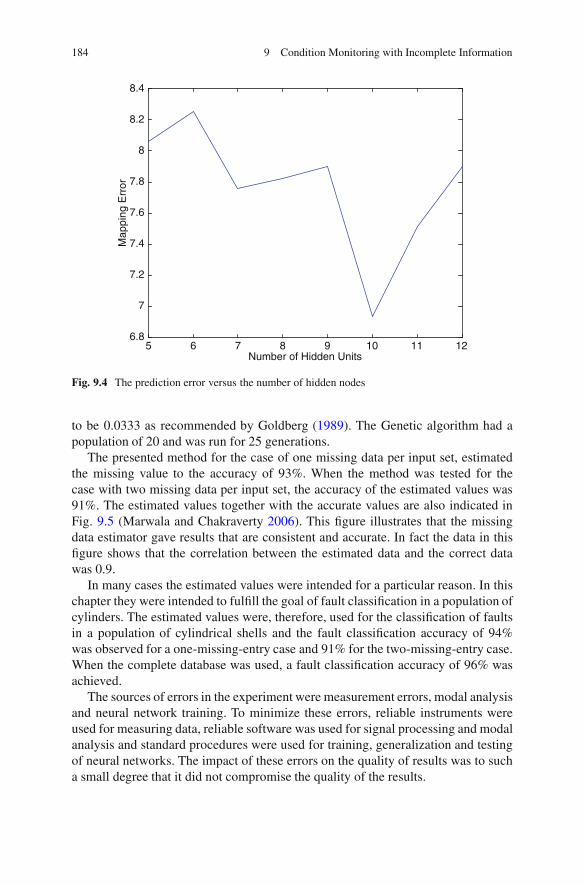
184 9 Condition Monitoring with Incomplete Information
Number of Hidden Units
8.4
8.2
8
7.8
7.6
7.4
7.2
7
6.85 6 7 8 9 10 11 12
Map
ping
Err
or
Fig. 9.4 The prediction error versus the number of hidden nodes
to be 0.0333 as recommended by Goldberg (1989). The Genetic algorithm had apopulation of 20 and was run for 25 generations.
The presented method for the case of one missing data per input set, estimatedthe missing value to the accuracy of 93%. When the method was tested for thecase with two missing data per input set, the accuracy of the estimated values was91%. The estimated values together with the accurate values are also indicated inFig. 9.5 (Marwala and Chakraverty 2006). This figure illustrates that the missingdata estimator gave results that are consistent and accurate. In fact the data in thisfigure shows that the correlation between the estimated data and the correct datawas 0.9.
In many cases the estimated values were intended for a particular reason. In thischapter they were intended to fulfill the goal of fault classification in a population ofcylinders. The estimated values were, therefore, used for the classification of faultsin a population of cylindrical shells and the fault classification accuracy of 94%was observed for a one-missing-entry case and 91% for the two-missing-entry case.When the complete database was used, a fault classification accuracy of 96% wasachieved.
The sources of errors in the experiment were measurement errors, modal analysisand neural network training. To minimize these errors, reliable instruments wereused for measuring data, reliable software was used for signal processing and modalanalysis and standard procedures were used for training, generalization and testingof neural networks. The impact of these errors on the quality of results was to sucha small degree that it did not compromise the quality of the results.

References 185
Fig. 9.5 The measured and estimated missing value
9.7 Conclusion
In this chapter, a technique based on auto-associative neural networks and geneticalgorithms was presented to approximate missing entries in data. This technique wastested on a population of cylindrical shells. The technique could approximate single-missing-entries to an accuracy of 93% and two-missing-entries to an accuracy of91%. Furthermore, a fault classification accuracy of 94% was obtained for single-missing-entry cases and 91% for two-missing-entry cases whereas the full databaseset gave a classification accuracy of 96%.
References
Abdella M, Marwala T (2006) The use of a genetic algorithm and neural networks to approximatemissing data in database. Comput Inform 24:1001–1013
Akula VR, Ganguli R (2003) Finite element model updating for helicopter rotor blade using agenetic algorithm. AIAA J. doi:10.2514/2.1983
Almeida FS, Awruch AM (2009) Design optimization of composite laminated structures using agenetic algorithm and finite element analysis. Compos Struct 88:443–454
Amiri M, Saeb S, Yazdanpanah MJ, Seyyedsalehi SA (2008) Analysis of the dynamical behaviorof a feedback auto-associative memory. Neurocomputing 71:486–494

186 9 Condition Monitoring with Incomplete Information
Arifovic J, Gencay R (2001) Using a genetic algorithms to select architecture of a feedforwardartificial neural network. Phys A: Stat Mech Appl 289:574–594
Atalla MJ, Inman DJ (1998) On model updating using neural networks. Mech Syst Signal Process12:135–161
Balamurugan R, Ramakrishnan CV, Singh N (2008) Performance evaluation of a two stageadaptive genetic algorithm (TSAGA) in structural topology optimization. Appl Soft Comput8:1607–1624
Balin S (2011) Non-identical parallel machine scheduling using genetic algorithm. Expert SystAppl 38:6814–6821
Banzhaf W, Nordin P, Keller R, Francone F (1998) Genetic programming – an introduction: on theautomatic evolution of computer programs and its applications. Morgan Kaufmann Publishers,San Francisco
Bishop CM (1995) Neural networks for pattern recognition. Oxford University Press, OxfordCanyurt OE, Kim HR, Lee KY (2008) Estimation of laser hybrid welded joint strength by using a
genetic algorithm approach. Mech Mater 40:825–831Chen Q, Chan YW, Worden K (2003) Structural fault diagnosis and isolation using neural networks
based on response only data. Comput Struct 81:2165–2172Crossingham B, Marwala T (2007) Using a genetic algorithms to optimise rough set partition sizes
for HIV data analysis. Stud Comput Intell 78:245–250de Zubicaray G, McMahon K, Eastburn M, Pringle AJ, Lorenz L, Humphreys MS (2007) Support
for an auto-associative model of spoken cued recall: evidence from fMRI. Neuropsychologia45:824–835
Doebling SW, Farrar CR, Prime MB, Shevitz DW (1996) Damage identification and healthmonitoring of structural and mechanical systems from changes in their vibration characteristics:a literature review. Los Alamos National Laboratory report LA-13070-MS
Ewins DJ (1995) Modal testing: theory and practice. Research Studies Press, LetchworthForrest S (1996) Genetic algorithms. ACM Comput Surv 28:77–80Franulovic M, Basan R, Prebil I (2009) A genetic algorithm in material model parameters’
identification for low-cycle fatigue. Comput Mater Sci 45:505–510Gladwin D, Stewart P, Stewart J (2011) A controlled migration genetic algorithm operator for
hardware-in-the-loop experimentation. Eng Appl Art Intell 24:586–594Goldberg DE (1989) Genetic algorithms in search, optimization and machine learning. Addison-
Wesley, ReadingGwiazda TD (2006) A genetic algorithms reference Vol.1 Cross-over for single-objective numeri-
cal optimization problems. Adobe eBook, LomiankiHines JW, Uhrig RE, Wrest DJ (1998) Use of autoassociative neural networks for signal validation.
J Intell Robot Syst 21:143–154Holland J (1975) Adaptation in natural and artificial systems. University of Michigan Press, Ann
ArborHouck CR, Joines JA, Kay MG (1995) A genetic algorithm for function optimisation: a MATLAB
implementation. Technical Report NCSU-IE TR 95–09, North Carolina State University,Raleigh
Hulley G, Marwala T (2007) A genetic algorithm based incremental learning for optimal weightand classifier selection. Comput Mod Life Sci Am Inst Phys Ser 952:258–267
Jensen CA, El-Sharkawi MA, Marks RJ II (2001) Power system security assessment using neuralnetworks: feature selection using fisher discrimination. IEEE Trans Energ Convers 16:757–763
Kramer MA (1991) Nonlinear principal component analysis using autoassociative neural networks.AIChE J 37:233–234
Kramer MA (1992) Autoassociative neural networks. Comput Chem Eng 16:313–328Kubalık J, Lazansky J (1999) Genetic algorithms and their testing. In: Proceedings of the AIP
Conference, New York, USA, pp 217–229Kwak HG, Kim J (2009) An integrated genetic algorithm complemented with direct search for
optimum design of RC frames. Comput Aid Des 41:490–500

References 187
Levin RI, Lieven NAJ (1998) Dynamic finite element model updating using simulated annealingand genetic algorithms. Mech Syst Signal Process 12:91–120
Li X, Du G (2012) Inequality constraint handling in genetic algorithms using a boundarysimulation method. Comput Oper Res 39:521–540
Lopes V, Park G, Cudney HH, Inman DJ (2000) Impedance-based structural health monitoringwith artificial neural networks. J Intell Mater Syst Struct 11:206–216
Lu PJ, Hsu TC (2002) Application of autoassociative neural network on gas-path sensor datavalidation. J Propul Power 18:879–888
Maia NMM, Silva JMM (1997) Theoretical and experimental modal analysis. Research StudiesPress, Letchworth
Marwala T (2000) Fault identification using neural networks and vibration data. PhD thesis,University of Cambridge
Marwala T (2001) Probabilistic fault identification using a committee of neural networks andvibration data. J Aircraft 38:138–146
Marwala T (2002) Finite element updating using wavelet data and a genetic algorithm. AIAAJ Aircraft 39:709–711
Marwala T (2003) Fault classification using pseudo modal energies and neural networks. Am InstAeronaut Astronaut J 41:82–89
Marwala T (2004) Fault classification using pseudo modal energies and probabilistic neuralnetworks. J Eng Mech 130:1346–1355
Marwala T (2007) Bayesian training of neural network using genetic programming. PatternRecognit Lett 28:1452–1458
Marwala T (2009) Computational intelligence for missing data imputation, estimation andmanagement: Knowledge optimization techniques. IGI Global Publications, New York
Marwala T (2010) Finite element model updating using computational intelligence techniques.Springer, London
Marwala T, Chakraverty S (2006) Fault classification in structures with incomplete measured datausing autoassociative neural networks and genetic algorithms. Curr Sci 90:542–548
Marwala T, Hunt HEM (1999) Fault identification using finite element models and neural networks.Mech Syst Signal Process 13:475–490
Marwala T, de Wilde P, Correia L, Mariano P, Ribeiro R, Abramov V, Szirbik N, GoossenaertsJ (2001) Scalability and optimisation of a committee of agents using a genetic algorithm. In:Proceedings of the 2001 international symposium on soft computing and intelligence systemsfor Industry, Scotland
Michalewicz Z (1996) Genetic algorithmsC data structuresD evolution programs. Springer,New York
Mitchell M (1996) An introduction to genetic algorithms. MIT Press, CambridgeMohamed AK, Nelwamondo FV, Marwala T (2008) Estimation of missing data: neural networks,
principal component analysis and genetic algorithms. In: Proceedings of the 12th world multi-conference on systems, cybern and inform, Orlando, Florida, pp 36–41
Møller M (1993) A scaled conjugate gradient algorithm for fast supervised learning. Neural Netw6:525–533
Mosalman Yazdi HA, Ramli Sulong NH (2001) Optimization of off-centre bracing system usinggenetic algorithm. J Constr Steel Res 67:1435–1441
Musharavati F, Hamoud ASM (2011) Modified genetic algorithms for manufacturing process plan-ning in multiple parts manufacturing lines. Expert Syst Appl. doi:10.1016/j.eswa.2011.01.129
Neal RM (1993) Probabilistic inference using Markov Chain Monte Carlo methods. TechnicalReport CRG-TR-93-1, University of Toronto, Toronto, Canada
Nelwamondo FV (2008) Computational intelligence techniques for missing data imputation. PhDthesis, University of the Witwatersrand
Nelwamondo FV, Marwala T (2007) Handling missing data from heteroskedastic and nonstation-ary data. Lect Notes Comput Sci 449:1297–1306
Oh S, Pedrycz W (2006) Genetic optimization-driven multi-layer hybrid fuzzy neural networks.Simulat Mod Pract Theory 14:597–613

188 9 Condition Monitoring with Incomplete Information
Paluch B, Grediac M, Faye A (2008) Combining a finite element programme and a geneticalgorithm to optimize composite structures with variable thickness. Compos Struct 83:284–294
Park BJ, Choi HR, Kim HS (2003) A hybrid genetic algorithm for the job shop schedulingproblems. Comput Ind Eng 45:597–613
Pawar PP, Ganguli R (2003) Genetic fuzzy system for damage detection in beams and helicopterrotor blades. Comput Meth Appl Mech Eng 192:2031
Pendharkar PC, Rodger JA (1999) An empirical study of non-binary genetic algorithm-basedneural approaches for classification. In: Proceedings of the 20th international conference oninformation systems, Charlotte, North Carolina, pp 155–165
Perera R, Ruiz A, Manzano C (2009) Performance assessment of multi-criteria damage identifica-tion genetic algorithms. Comput Struct 87:120–127
Reddy RRK, Ganguli R (2003) Structural damage detection in a helicopter rotor using radial basisfunction neural networks. Smart Struct Mater 12:232–241
Reed RD, Marks RJ II (1999) Neural smithing: supervised learning in feedforward artificial neuralnetworks. MIT Press, Cambridge
Ritter GX, Urcid G, Schmalz MS (2009) Autonomous single-pass end member approximationusing lattice auto-associative memories. Neurocomputing 72:2101–2110
Roy T, Chakraborty D (2009) Optimal vibration control of smart fiber reinforced composite shellstructures using improved a genetic algorithm. J Sound Vib 319:15–40
Royston TJ, Spohnholtz T, Ellington WA (2000) Use of non-degeneracy in nominally axisym-metric structures for fault detection with application to cylindrical geometries. J Sound Vibr230:791–808
Sanz J, Perera R, Huerta C (2007) Fault diagnosis of rotating machinery based on auto-associativeneural networks and wavelet transforms. J Sound Vibr 302:981–999
Stern H, Chassidim Y, Zofi M (2006) Multi-agent visual area coverage using a new geneticalgorithm selection scheme. Eur J Oper Res 175:1890–1907
Suresh S, Omkar SN, Ganguli R, Mani V (2004) Identification of crack location and depth in acentilever beam using a modular neural network approach. Smart Mater Struct 13:907–916
Tettey T, Marwala T (2006) Controlling interstate conflict using neuro-fuzzy modeling and agenetic algorithms. In: Proceedings of the 10th IEEE international conference on intelligentengineering systems, London, UK, pp 30–44
Tu Z, Lu Y (2008) Finite element model updating using artificial boundary conditions with geneticalgorithms. Comput Struct 86:714–727
Upadhyaya BR, Eryurek E (1992) Application of neural networks for sensor validation and plantmonitoring. Nuclear Technol 97:170–176
Vose MD (1999) The simple genetic algorithm: foundations and theory. MIT Press, CambridgeWaszczyszyn Z, Ziemianski L (2001) Neural networks in mechanics of structures and materials –
new results and prospects of applications. Comput Struct 79:2261–2276Wu X, Ghaboussi J, Garret JH (1992) Use of neural networks in the detection of structural damage.
Comput Struct 42:649–659Zang C, Imregun M (2001) Combined neural network and reduced FRF techniques for slight
damage detection using measured response data. Arch Appl Mech 71:525–536Zhang H, Ishikawa M (2004) A solution to combinatorial optimization with time-varying
parameters by a hybrid genetic algorithm. Int Congr Ser 1269:149–152Zhou HF, Ni YQ, Ko JM (2011) Structural damage alarming using auto-associative neural network
technique: exploration of environment-tolerant capacity and setup of alarming threshold. MechSyst Signal Process 25:1508–1526

Chapter 10Condition Monitoring Using SupportVector Machines and Extension NeuralNetworks Classifiers
10.1 Introduction
The condition monitoring of machines is very important in industry because of thenecessity to improve machine reliability and reduce the possible loss of productionfrom machine breakdowns. Condition monitoring is conducted when it is essentialto classify the state of a machine and to establish whether it is faulty through ob-servation and analysis (William et al. 1992; Marwala and Vilakazi 2007). Conditionmonitoring is a method of monitoring the operating characteristics of a machine sothat the changes and movements of the monitored signals can be used to predict theneed for maintenance before a breakdown does happen. Condition monitoring hasbecome progressively more vital in areas such as aerospace engineering where anunpredicted fault can result in a serious accident. Another application of conditionmonitoring is in manufacturing where manufacturers must identify methods to avoidfailures, decrease maintenance costs, minimize downtime, and increase the lifetimeof their equipment.
With a reliable condition monitoring procedure, machines can be employedin a more optimal fashion. A maintenance plan follows a schedule to selectwhen maintenance must be performed. This leads to inefficiencies because themaintenance process may be performed unnecessarily early or a failure may occurprior to scheduled maintenance taking place. However, condition monitoring can beapplied for condition based maintenance or for predictive maintenance.
Rotating machinery is employed in a number of industrial applications. A com-mon component of a modern rotating machinery is the rolling element bearing. Infact most machine failures are related to bearing failure (Lou and Loparo 2004),which frequently result in protracted downtimes that have economic consequences.As a result, an increasing amount of condition monitoring data are measured andpresented to engineers for analysis. However, because of the complexity and massof data generated relating to all plant items and their health, it is problematic forengineers to handle such data. Because the identification of the vital informationfrom such data is difficult, a reliable and automated diagnostic method permitting
T. Marwala, Condition Monitoring Using Computational Intelligence Methods:Applications in Mechanical and Electrical Systems, DOI 10.1007/978-1-4471-2380-4 10,© Springer-Verlag London Limited 2012
189

190 10 Condition Monitoring Using Support Vector Machines and Extension. . .
fairly unskilled operators is necessary to take significant decisions without the needfor a condition monitoring specialist. One of the most frequently applied conditionmonitoring techniques is the vibration-based condition monitoring procedure whichis grounded on the principle that all systems produce vibrations. When a machineis operating appropriately, the vibrations are small and constant; however, whenfaults progress and several dynamic processes change, the vibration spectrum alsochanges (Marwala 2001).
The robustness of a classification system depends on the usefulness of theextracted features and the reliability and effectiveness of a condition monitoringclassification system. This chapter presents three feature selection methods appliedfor bearing fault diagnosis (Nelwamondo et al. 2006a). These methods are theMel-frequency Cepstral Coefficients (MFCC) technique, which is a time-frequencydomain technique; kurtosis which is the time-domain procedure and a fractaldimension analysis which is also time-domain method that has been of benefit.This chapter also assesses the usefulness of the extracted features for bearing faultdiagnosis using the Support Vector Machine (SVM) and the Extension NeuralNetwork (ENN) classifiers. The SVM was selected because it has been appliedsuccessfully in many fault complex applications (Msiza et al. 2007; Patel andMarwala 2009; Marivate et al. 2008) and the ENN was selected because of itssuccess in pattern recognition of complex systems (Vilakazi and Marwala 2006;Mohamed et al. 2006).
10.2 Features
The success of a classification system depends on the usefulness of the extractedfeatures that represent a specific machine condition. Previously, substantial researchhas been conducted into the development of a number of feature extraction methodsand condition monitoring systems. Feature extraction methods can be categorizedinto three domains: the frequency, time-frequency and time-domains (Ericsson et al.2004). The frequency domain techniques usually include a frequency analysis of thevibration signals and investigate the periodicity of high frequency transients. In thisregard, frequency domain approaches explore a train of repetitions arising at any ofthe frequencies from the faulty regime (Ocak and Loparo 2004). This techniquebecomes complicated because the periodicity of the signal may be suppressed.These frequency domain methods include the frequency averaging procedure,adaptive noise cancellation and the High Frequency Resonance Technique (HFRT).The HFTR has been used widely for bearing fault detection and diagnosis (Ocakand Loparo 2004). The shortcoming of the HFTR method is that it requiresseveral impact tests to identify the bearing resonance frequency and thus it iscomputationally expensive (Ocak and Loparo 2004).
McFadden and Smith (1984) presented an envelope analysis, which is a fre-quency domain method for the detection and diagnosis of bearing faults. Theshortcoming of the frequency domain analysis is that it tends to average out transient

10.2 Features 191
vibrations. As a result it becomes more sensitive to background noise. To overcomethis problem, the time-frequency domain analysis was applied, which expresseshow the frequency content of the signal varies with time. Time-frequency domainanalysis methods include the Short Time Fourier Transform (STFT), the Wigner-Ville Distribution (WVD) and Wavelet Transform (WT). These techniques arestudied in detail in Li et al. (2000).
Time domain approaches normally involve indices that are sensitive to impulsiveoscillations, such as peak level, root mean square value, crest factor analysis,Kurtosis analysis, shock pulse counting, time series averaging techniques, and signalenveloping routines (Ocak and Loparo 2004; Li et al. 2000). Ericsson et al. (2004)and Li et al. (2000) demonstrated that the time-domain analysis is less sensitive tosuppressions of the periodicity.
A number of feature extraction methods have been applied to vibration-basedcondition monitoring. Ocak and Loparo (2004); Lou and Loparo (2004), as well asNikolaou and Antoniadis (2002) have applied wavelet transforms to detect and clas-sify different faults in bearings. Elsewhere, Rojas and Nandi (2006) implementedspectral and statistical features for the classification of bearing faults. Peng et al.(2005) compared the Hilbert-Huang transform with the wavelet transform for abearing fault diagnosis. Junsheng et al. (2006) presented a feature extraction tech-nique based on empirical mode decomposition process and autoregressive modelin roller bearings diagnosis. Baillie and Mathew (1996) applied an autoregressivemodeling that does not only classify, but also offers a one-step-ahead prediction ofthe vibration signal using the previous outputs. H. Yang et al. (2005) implementeda basis pursuit and obtained better results than with wavelet transforms. Altmanand Mathew (2001) also applied the discrete wavelet packet analysis to improve thedetection and diagnostic effectiveness of rolling element bearing faults. Prabhakaret al. (2002) demonstrated that the Discrete Wavelet Transform (DWT) can beapplied to enhance the detection of bearing faults and elsewhere, Antoni and Randall(2006) applied spectral kurtosis to the vibratory surveillance and diagnostics ofrotating machines.
The other vital component of a condition monitoring process is a classificationsystem that identifies the operating status of the machine as well as the type offailure. Such a classification system can be categorized into two groups: knowledge-based and data-based models.
Knowledge-based models depend on human-like knowledge of the process andits faults. Knowledge-based models (such as expert systems or decision trees)implement human-like knowledge of the process for fault diagnosis. In fault diag-nostics, the human expert could be a person who operates the machine and who hasexpertise in different categories of faults. The knowledge base can be constructedby conducting interviews with a human operator about fault incidences in thediagnosed machine. Expert systems are normally appropriate for such problems,where the human expert can linguistically explain the solution. Characteristically,human knowledge is imprecise, and how to treat such information has frequentlybeen a problem with traditional expert systems. For instance, the precise limit whenthe temperature in a sauna is too high is vague in human minds. In fact, it is very
192 10 Condition Monitoring Using Support Vector Machines and Extension. . .
difficult to attain sufficiently representative data for the complex and highly non-linear behavior of faulty system to make quantitative models. Knowledge-basedmodels may be applied collectively with simple signal-based diagnostics, if theexpert knowledge for the process is available. Nevertheless, it is frequently difficulteven for a human expert to differentiate faulty operation from healthy operation.Furthermore, multiple information sources may be needed for reliable decision-making. Therefore, data-based models are the most flexible method for automatedcondition monitoring.
Data-based models are implemented when the process model is unknown in ananalytical form and expert knowledge of the procedure performance under faultsis absent. Data-based models can be produced in numerous ways. Neural networkbased models like the Multilayer Perceptron (MLP) and the Radial Basis Function(RBF) have been applied extensively for bearing condition monitoring. Samanta andAl-Bushi (2003) applied neural networks with time-domain features for the detec-tion of rolling element bearing faults. Elsewhere Yang et al. (2004) implemented theART-KOHONEN technique for the fault diagnosis of rotating machinery. Kernel-based classifiers such as the Support Vector Machine (SVM) have been applied forbearing fault diagnosis. In this regard, Jack and Nandi (2002) compared supportvector machines and neural networks, enhanced by genetic algorithms for faultdetection. Samanta (2004) implemented both Artificial Neural Networks (ANN)and SVM with genetic algorithm for bearing fault detection. B.S. Yang et al. (2005)applied multi-class SVM for fault diagnosis of rotating machinery while Rojas andNandi (2006) applied the SVM for the detection and classification of faults in rollingelement bearings. Hu et al. (2007) applied a wavelet transform and SVM ensemblefor the fault diagnosis of rotating machines. Furthermore, data-based statisticalmethods have achieved success in speech recognition and have recently been appliedfor condition monitoring. Ertunc et al. (2001) applied the Hidden Markov model(HMM) in wear studies of drill bits in a drilling process. Ocak and Loparo (2004),Purushotham et al. (2005), Miao and Makis (2006) and Nelwamondo et al. (2006a)applied the HMM for bearing fault diagnosis.
10.3 Feature Extraction
This section describes a number of features that were extracted from vibrationsignals of bearing elements: fractal analysis, Mel-frequency cepstral coefficientsand kurtosis.
10.3.1 Fractal Dimension
As described in Chap. 2, a fractal dimension is a rough geometric shape thatcan be divided into parts, each of which is nearly a reduced copy of the whole

10.3 Feature Extraction 193
and this characteristic is known as self-similarity. Vibration signals are mostlyperiodic movements with some level of turbulence. To detect different bearing faultsthese non-linear, turbulence features must be identified. The non-linear turbulencefeatures of the vibration signal may be quantified using a fractal model (Maragosand Potamianos 1999). The fractal dimension of a compact planar set F, alsoknown as the Hausdorff dimension, has its value ranging between 1 and 2. It canbe approximated using techniques such as the Minkowski-Bouligand dimensionand Box-Counting dimension (Maragos and Potamianos 1999). Fractals have beensuccessfully applied to condition monitoring (Cui and Xu 1999).
Li et al. (2005) applied fractal theory in direct current system groundingfault detection. Elsewhere, Zhao and Guo (2005) applied the fractal dimensiontechnique for detecting a single-phase-to-earth faults. Other applications of thefractal technique were in phase selection (D. Yang et al. 2005), and in aircraft faultdetection (Zhang et al. 2001). For this chapter the Box-Counting dimension wasused as described in Chap. 2.
10.3.2 Mel-Frequency Cepstral Coefficients (MFCCs)
The Mel-frequency Cepstral Coefficients (MFCCs) are coefficients that are derivedfrom a sort of cepstral representation of the signal. They extract both linear andnon-linear properties. The frequency bands are evenly spread out on the mel scaleand this estimates the human auditory system’s response closer than linearly-spacedfrequency bands would.
The MFCCs have been applied to fields such as speech recognition and conditionmonitoring (Marwala and Vilakazi 2007; Nelwamondo et al. 2006b; Mahola et al.2005; Chen et al. 2011a). The MFCC used features extracted from vibration signals.It can be viewed as a category of wavelet in which frequency scales are put on alinear scale for frequencies less than 1 kHz and on a log scale for frequencies above1 kHz (Wang et al. 2002). The complex cepstral coefficients attained from this scaleare known as the MFCC (Wang et al. 2002). The MFCCs are represented in bothtime and frequency domains.
Saenz-Lechon et al. (2011) applied the mel-frequency cepstral analysis for anobjective evaluation of perceived roughness and breathiness while Arias-Londonoet al. (2011) applied the mel-frequency cepstral coefficients for the automaticdetection of pathological voices. Other applications of the mel-frequency cepstralcoefficients were for the classification of spoken letters (Rozali et al. 2011), and inthe low bit-rate coding of speech (Boucheron et al. 2011).
10.3.3 Kurtosis
Kurtosis is the quantification of the “peakedness” in the probability distribution ofa real-valued, random variable. In this chapter, kurtosis is intended to deal with

194 10 Condition Monitoring Using Support Vector Machines and Extension. . .
the occasional spiking of vibration data caused by some types of faults. Kurtosisfeatures of vibration data have been applied in the monitoring of tool condition byEl-Wardany et al. (1996). Elsewhere, Cai et al. (2011) successfully applied kurtosisin detecting roller bearing faults. Immovilli et al. (2009) successfully appliedkurtosis for the detection of generalized-roughness bearing faults. Elsewhere, Taoet al. (2008) applied Kurtosis for the detection of faults for one class of bearings.Finally, kurtosis was applied for fault detection and diagnosis in rolling elementbearings by Sawalhi et al. (2007).
The success of using kurtosis in vibration signals is a consequence of the fact thatthe vibration signals of a system under stress or having defects are different fromthose of a normal system. The spiking of the vibration signal changes when thereare faults in the system. Kurtosis is a quantification of the sharpness of the peak andis defined as the normalized fourth-order central moment of the signal (Wang et al.2001). The kurtosis value is beneficial in identifying transients and spontaneousevents within vibration signals (Wang 2001) and is an accepted criterion for faultdetection. The kurtosis value is computed as the normalized square of the secondmoment. A high value of kurtosis indicates a sharp distribution peak and shows thatthe signal is impulsive in nature (Altman and Mathew 2001).
10.4 Classification Techniques
For this chapter two classification techniques were applied, together with thefeatures described in the previous section for the detection of faults in bearings.These classification techniques are described in this section viz., the support vectormachines and extension neural networks.
10.4.1 Support Vector Machines (SVMs)
Support vector machines are supervised learning approaches applied mostly forclassification. They are derived from the theory of statistical learning and werefirst proposed by Vapnik (1995). Shen et al. (2005) applied a SVM-based colorimage watermarking method that operated by applying the information suppliedfrom the reference positions and the watermark, which was adaptively embeddedinto the blue channel of the host image, taking the human visual system into account.Other implementations of SVMs to model complicated systems include Marwalaet al. (2006) who applied SVMs in the fault classification of mechanical systems,Msiza et al. (2007) who used SVMs in forecasting a water-demand time-series andMarwala and Lagazio (2011) who applied SVMs in the modeling of militarizedinterstate conflict.
Chen et al. (2011b) used SVMs to approximate monthly solar radiation and theirresults demonstrated that SVMs perform better than traditional approaches (such as
10.4 Classification Techniques 195
neural networks) in predicting solar radiation. Yeh et al. (2011) applied SVMs in therecognition of counterfeit banknotes. Each banknote was separated into segmentsand the luminance histograms of the segments were used as the inputs to the SVMmodel with each segment was paired with its own kernels. When the technique wastested on Taiwanese banknotes, they showed that their technique performed betterthan methods such as the single-kernel SVM.
Tellaeche et al. (2009) used support vector machines and computer vision forweed identification. Elsewhere, Lin et al. (2011) applied SVMs to predict businessfailures based on previous financial data. Their results showed that their methodgave a good classification rate. Li-Xia et al. (2011) implemented SVMs and particleswarm optimization for tax forecasting and their results showed that the SVM modelperforms well.
The application of SVMs has also been extended to regression analysis problems,thus resulting in the term Support Vector Regression (SVR) (Gunn 1997; Chuang2008). Pires and Marwala (2004) applied SVMs for option pricing and extendedthese with a Bayesian framework. Elsewhere, Gidudu et al. (2007) used SVMs inimage classification.
Thissen et al. (2004) applied SVMs for spectral regression cases, and Ustun et al.(2007) visualized and interpreted SVM models. Other applications of SVMs includethe prediction of jet penetration depth (Wang et al. 2010), tool wear identification(Tao and Tao 2010), ozone concentration (Ortiz-Garcıa et al. 2010), the identifi-cation of people (Palanivel and Yegnanarayana 2008), chemical compound analysis(Zhou et al. 2006), response modeling (Kim et al. 2008), and the real-time predictionof order flow times (Alenezi et al. 2007).
For SVMs, a data point is conceptualized as a p-dimensional vector. Theobjective is to separate such points with a p-1-dimensional hyperplane, known asa linear classifier. There are many hyperplanes that can be created. Some of theseinclude the one that exhibits the largest separation, also called the margin, betweenthe two classes. The selected hyperplane can be chosen so that the distance fromit to the nearest data point on both sides is maximized. This is then known asthe maximum-margin hyperplane. The classification problem can then be statedas estimating a function f W RN ! f�1; 1g dependent on input-output trainingdata, where an independently distributed, unknown probability distribution P(x, y)is chosen such that f can classify unseen (x, y) data (Muller et al. 2001; Habtemariam2006; Marwala and Lagazio 2011). The ideal function minimizes the expected error(risk) and can be expressed mathematically as follows (Vapnik 1995; Habtemariam2006; Habtemariam et al. 2005; Marwala and Lagazio 2011):
RŒf � DZ
l.f .x/; y/dP.x; y/ (10.1)
Here, l indicates a loss function (Muller et al. 2001). Since the fundamentalprobability distribution P is unknown, Eq. 10.1 cannot be solved implicitly.

196 10 Condition Monitoring Using Support Vector Machines and Extension. . .
The best route is to identify an upper bound for the risk function which is givenmathematically as follows (Vapnik 1995; Muller et al. 2001; Marwala and Lagazio2011):
RŒf � D RŒf �emp Cs
h�ln 2n
hC 1
� � ln�
ı4
�n
(10.2)
Here h 2 NC is the Vapnik-Chervonenkis (VC) dimension of f 2 F and • > 0.The VC dimension of a function class F is defined as the biggest number of hcoordinates that can be divided in all possible ways by means of functions of thatclass (Vapnik 1995). The empirical error R[f ]emp is a training error given by (Vapnik1995; Habtemariam 2006; Marwala and Lagazio 2011):
RŒf �emp D 1
n
nXiC1
l.f .xi /; yi / (10.3)
This assumes that the training sample is linearly separable by a hyperplane of theform (Vapnik 1995; Habtemariam 2006; Marwala and Lagazio 2011):
f .x/ D hw; xi C b with w 2 �; b 2 < (10.4)
Here h:; :i denotes the dot product, w is an adjustable weight vector and b is anoffset (Muller et al. 2001). The objective of the learning process, as propounded byVapnik and Lerner (1963) is to identify the hyperplane with the maximum margin ofseparation from the class of dividing hyperplanes. Nonetheless, since practical datausually exhibit complex properties which cannot be divided linearly, more complexclassifiers are essential. To circumvent the complexity of the nonlinear classifiers,the concept of linear classifiers in a feature space can be introduced. SVMs attemptto identify a linear separating hyperplane by initially mapping the input space into ahigher dimensional feature space F. This suggests that each training example xi besubstituted with (xi) to give (Vapnik 1995; Habtemariam 2006):
Yi .w:ˆ.xi / C b/ ; i D 1; 2; :::; n (10.5)
The VC dimension,h, in the feature space F is constrained subject to h �jjW jj2R2 C 1 where R is the radius of the smallest sphere around the training data(Muller et al. 2001; Habtemariam 2006). Consequently, minimizing the expectedrisk can be expressed as an optimization problem as follows (Burges 1998; Mulleret al. 2001; Scholkopf and Smola 2003; Marwala and Lagazio 2011):
Minimize .W; b/1
2jjwjj2 (10.6)

10.4 Classification Techniques 197
subject to:
ci .w; xi � b/ 1; i D 1; :::; n (10.7)
Equations 10.6 and 10.7 are jointly called the quadratic programming problembecause it is the problem of optimizing a quadratic function of a number of variablessubject to linear constraints on these variables (Scholkopf and Smola 2003). Fromthe expressions:
kwk2 D w:w (10.8)
w DnX
iD0
˛i ci xi (10.9)
it can be shown that the dual nature of the support vector machines can, bymaximizing of ˛i, be written in Lagrangian form as follows (Scholkopf and Smola2003):
L .˛/ DnX
iD1
˛i � 1
2
Xi;j
˛i ˛j ci cj xTi xj
DnX
iD1
˛i � 1
2
Xi;j
˛i ˛j ci cj k�xi ; xj
�; i D 1; :::; n
(10.10)
Subject to:
˛i 0; i D 1; :::; n (10.11)
and to the constraint from the minimization in b:
˛i 0; i D 1; :::; n (10.12)
and subject to the following constraints:
nXiD1
˛i ci D 0 (10.13)
Here the kernel is (Muller et al. 2001):
k�xi ; xj
� D xi � xj (10.14)

198 10 Condition Monitoring Using Support Vector Machines and Extension. . .
10.4.1.1 Soft Margin
Cortes and Vapnik (1995) presented an improved maximum margin idea thatincorporated mislabeled data points. If there is no hyperplane that can exactly dividethe “yes” and “no” data points, the Soft Margin technique will select a hyperplanethat divides the data points as efficiently as possible, still maximizing the distance tothe nearest, neatly divided data points. The method incorporates slack variables, � i
which quantify the degree of misclassification of the data point as follows (Cortesand Vapnik 1995):
ci .w � xi � b/ 1 � �i ; 1 � i � n (10.15)
A function which penalizes non-zero ”i augments the objective and, conse-quently, the optimization exhibits a compromise between a large margin and a smallerror penalty. If a linear penalty function is assumed, the optimization problem canthen be written by minimizing w and ”i through the following function (Cortes andVapnik 1995):
1
2kwk2 C C
nXiD1
�i (10.16)
subject to:
ci .w � xi � b/ 1 � �i ; �i 0; i D 1; :::; n (10.17)
In Eq. 10.16, C is the capacity. Equations 10.16 and 10.17 can be expressed in aLagrangian form by optimizing the following equation in terms of w, ”, b, ’ and ˇ
(Cortes and Vapnik 1995):
minfwg;�;b
max˛;ˇ(
1
2kwk2 C C
nXiD1
�i �nX
iD1
˛i Œci .w � xi � b/ � 1 C �i � �nX
iD1
ˇi �i
)(10.18)
Here ˛i ; ˇi 0. The advantage of a linear penalty function is that the slackvariables are removed from the dual problem. As a result, C only appears as asupplementary constraint on the Lagrange multipliers. The application of non-linearpenalty functions to reduce the impact of outliers on the classifier has been appliedin the past, but it makes the optimization problem non-convex and it is difficult toidentify a global solution.

10.4 Classification Techniques 199
10.4.1.2 Non-Linear Classification
To apply the linear SVM technique for producing non-linear classifiers, the kerneltrick was applied (Aizerman et al. 1964) to the maximum-margin hyperplanes(Boser et al. 1992). In this method the dot product is substituted with a non-linearkernel function to fit the maximum-margin hyperplane in a transformed featurespace. Although this dot product transformation may be non-linear, the transformedspace may be of high dimensions. For instance, when a Gaussian radial basisfunction kernel is applied, the resultant feature space is a Hilbert space of infinitedimension. Some useful kernel functions include (Vapnik 1995; Muller et al. 2001;Marwala and Lagazio 2011):
The Radial Basis Function,
k�xi ; xj
� D exp�� xi � xj
2�; � > 0 (10.19)
The Polynomial (homogeneous),
k�xi ; xj
� D �xi � xj
�d(10.20)
The Polynomial (inhomogeneous),
k�xi ; xj
� D �xi � xj C 1
�d(10.21)
The Hyperbolic tangent,
k�xi ; xj
� D tanh�"xi � xj C b
�; " > 0I b < 0 (10.22)
The variables of the maximum-margin hyperplane can be identified by opti-mizing the objective equation through applying an interior point technique thatidentifies a solution for the Karush-Kuhn-Tucker (KKT) conditions of the primaland dual problems (Kuhn and Tucker 1951; Karush 1939). To avoid solving a linearsystem, including the large kernel matrix, a low rank approximation to the matrixcan be applied to apply the kernel trick. The Karush–Kuhn–Tucker conditions arenecessary to optimize a non-linear programming problem, for the satisfaction of aparticular regularity condition. For the given problem listed below:
Minimize W f .x/ (10.23)
subject to:
gi .x/ � 0I hj .x/ D 0 (10.24)
Here, gi is the ith inequality constraint and hi is the ith equality constraint. TheKarush–Kuhn–Tucker method allows the inequality constraints by generalizing

200 10 Condition Monitoring Using Support Vector Machines and Extension. . .
the technique of Lagrange multipliers which allow only equality constraints. Thenecessary conditions for the KKT are (Kuhn and Tucker 1951; Karush 1939;Marwala and Lagazio 2011):
Stationary,
rf�x��C
mXiD1
�i rgi
�x��C
lXjD1
�j rhj
�x�� D 0; i D 1; :::; mI j D 1; :::; l
(10.25)
Primal and dual feasibility as well as complementary slackness,
gi
�x�� � 0; i D 1; :::; m
hj
�x�� D 0I j D 1; :::; l
�i 0; i D 1; :::; m
�i gi
�x�� D 0; i D 1; :::; m (10.26)
The KKT method can be viewed as a generalized form of the Lagrangian methodobtained by setting m D 0. In some cases, the necessary conditions are also sufficientfor optimization. Nevertheless, in many circumstances the necessary conditions arenot sufficient for optimization and additional information, for instance the secondderivative, is necessary. The necessary conditions are sufficient for optimization ifthe cost function f and the inequality constraints gj are continuously differentiable,convex functions and the equality constraints gj are functions which have constantgradients.
10.4.2 Extension Neural Networks
An Extension Neural Network (ENN) is a classification system that is based onconcepts from neural networks and extension theory as shown in Fig. 10.1 (Wangand Hung 2003; Mohamed et al. 2006; Vilakazi and Marwala 2006). Lu (2010)successfully applied ENN for fault diagnosis, while Zhang et al. (2010) appliedextension neural networks for the condition monitoring of the equipment. Wanget al. (2009) applied extension neural networks for the classification of brain MRIwhile Chao et al. (2009) applied ENN for tracking the maximum power point. Otherapplications of ENN were in infringement lawsuits (Lai and Che 2009), in intelligenttraffic light control (Chao et al. 2008) and in the condition monitoring of transformerbushings (Miya et al. 2008).
The extension theory implements a distance measurement for classificationprocesses, and the neural network entrenches the relevant features of learningcapability. The classifier is ideal for classification problems where there are patternswith an extensive range of continuous inputs and a discrete output indicating which

10.4 Classification Techniques 201
Cluster Outputs
OutputLayer
NetworkWeights
InputLayer
Feature Pattern
nc
Oil
l k
l
wLll
wLkj
wUll
wUkj
j n
xil xij xin
Oik Oinc
Fig. 10.1 Extension neural network
class the pattern is an element of. ENN encompasses an input layer and an outputlayer. The input layer nodes accept an input feature pattern and use a set of weightedparameters to produce an image of the input pattern. There are two connectionweights between input nodes and output nodes: one connection represents the lowerbound for this classical domain of features and the other represents the upper bound.The complete network is therefore represented by a matrix of weights for the upperand lower limits of the features for each class. These are WU and WL, respectively.A third matrix representing the cluster centers is also defined as (Wang and Hung2003):
z D Wu C Wl
2(10.27)
The ENN applies supervised learning, which tunes the weights of the ENNto attain a good clustering performance by minimizing the clustering error. Thenetwork is trained by adjusting the network weights and recalculating the network

202 10 Condition Monitoring Using Support Vector Machines and Extension. . .
centers for each training pattern, subject to reducing the extension distance (ED) ofthat pattern to its labelled cluster. Each training pattern adjusts the network weightsand the centers by quantities that depend on the learning rate. Generally, the weightupdate for a variable xi is (Wang and Hung 2003):
wnew D wold � �.xi � wold/ (10.28)
Here, � is the learning rate and w can either be the upper or the lower weightmatrices of the network centers. It can be shown that for t training patterns for aparticular class C, the weight is given by (Mohamed et al. 2006):
wc.t/ D .1 � �/wc.0/ � �X
.1 � �/t�1xic (10.29)
This equation reveals how each training pattern reinforces the learning in thenetwork by having the most recent signal govern only a fraction of the current value.This equation demonstrates that there is no convergence of the weight values, asthe learning process is adaptive and reinforcing and indicates the significance ofthe learning rate, �. Small values of � necessitate many training iterations, whilehigh values may cause an oscillatory behavior of the network weights, causing poorclassification performance.
10.5 Example Vibration Data
The work for this chapter was based on the data obtained from the Case WesternReserve University website (Loparo 1998). The set-up for the correspondingexperiment was made up of a Reliance Electric 2HP IQPreAlert connected to adynamometer. Faults of size 0.007, 0.014, 0.021 and 0.028 in. were introduced intothe drive-end bearing of a motor using the Electric Discharge Machining (EDM)technique. These faults were introduced separately at the inner raceway, rollingelement and outer raceway. An impulsive force was applied to the motor shaft andthe resulting vibration was measured using two accelerometers, one mounted on themotor housing and the other on the outer race of the drive-end bearing. All signalswere recorded at a sampling frequency of 12 kHz.
10.6 Application to Bearing Condition Monitoring
Figure 10.2 shows samples of bearing vibration signals for the four bearingconditions (Marwala and Vilakazi 2007). Features were then extracted to classifyfaults.

10.6 Application to Bearing Condition Monitoring 203
0.5
0
−0.5
0.5
0
−0.5
5
0
0 0.02 0.04 0.06 0.08 0.12 0.14 0.16 0.18 0.20.1
Time(s)
Acc
eler
atio
n
−5
Outer Raceway Fault
Inner Raceway Fault
Normal Condition
Ball Fault
2
0
−2
Fig. 10.2 Vibration signals on the bearing under: normal conditions, with inner race fault, outerrace fault and ball fault
The optimal classifier parameters were identified using trial and error. Theoptimum SVM architecture applied a polynomial kernel function with a degree of 5.The ENN architecture with an optimal learning rate of 0.219 was used.
The first set of investigations assessed the effectiveness of the time-domain frac-tal dimension based feature-extraction using vibration signal condition monitoring.Figure 10.3 shows the Multi-scale Fractal Dimension (MFD) feature vector whichshows the bearing’s fault-specific information. Figure 10.3 shows that the presentedfeature extraction method does indeed extract fault defining features which can beapplied to classify the different bearing conditions. Nonetheless, the optimum sizeof the MFD must be found.
Figure 10.4 shows the change of the system accuracy with a change to theMFD size. This figure shows that the size of MFD does not affect the classificationaccuracy of SVM and ENN.
Using the optimum SVM and ENN architecture together with MFD, the confu-sion matrix that was obtained for different bearing faults is presented for the SVMand ENN classifiers in Table 10.1.
In further investigating the use of MFCC with SVM and ENN, it was observedthat varying the number of MFCCs has no impact on the classification rate of the
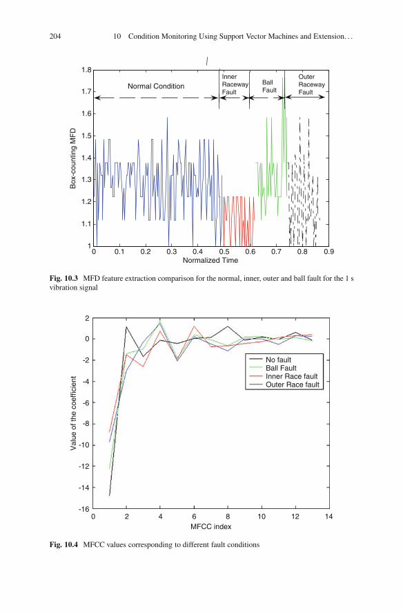
204 10 Condition Monitoring Using Support Vector Machines and Extension. . .
0 0.1 0.2 0.3 0.4 0.5 0.6 0.7 0.8 0.91
1.1
1.2
1.3
1.4
1.5
1.6
1.7
1.8
Normalized Time
Box
-cou
ntin
g M
FD
Normal ConditionInnerRacewayFault
OuterRacewayFault
BallFault
Fig. 10.3 MFD feature extraction comparison for the normal, inner, outer and ball fault for the 1 svibration signal
2
0
-2
-4
-6
-8
-10
-12
-14
-160 2 4 6 8
MFCC index
Val
ue o
f the
coe
ffici
ent
10 12 14
No faultBall FaultInner Race faultOuter Race fault
Fig. 10.4 MFCC values corresponding to different fault conditions

10.7 Conclusion 205
Table 10.1 The confusion matrix for the SVM, HMM, GMM, and ENN classi-fiers used with fractal features
SVM ENN
Normal Inner Outer Ball Normal Inner Outer Ball
Normal 100 0 0 0 100 0 0 0Inner 0 100 0 0 0 100 0 0Outer 0 0 100 0 0 0 100 0Ball 0 0 0 100 0 0 0 100
Table 10.2 The confusion matrix for the SVM and ENN classifiers used withMFCC features
SVM ENN
Normal Inner Outer Ball Normal Inner Outer Ball
Normal 100 0 0 0 100 0 0 0Inner 0 100 0 0 0 100 0 0Outer 0 0 100 0 0 0 100 0Ball 0 0 0 100 0 0 0 100
Table 10.3 Summary ofclassification results
SVM (%) ENN (%)
Fractal features 100 100MFCC 100 100MFCCC kurtosis 100 100
classifiers, as shown Fig. 10.4. It was also observed that 13 MFCCs gave optimalresults and that increasing the number of MFCC above 13 did not improve theclassification results Table 10.2.
The overall classification results are summarized in Table 10.3.
10.7 Conclusion
The chapter investigated two vital requirements for an automated condition monitor-ing system. The first requirement was for a feature-extraction procedure that couldsuccessfully extract the condition specific features. The second requirement wasfor a classification system that could effectively classify the machine conditions.This chapter gave a review of three feature extraction methods that are used forcondition monitoring. These methods are fractal analysis, mel-frequency cepstralcoefficients and kurtosis. The effectiveness of the extracted features were testedusing two classifiers. These were support vector machines and the extension neuralnetwork. The presented system gave very good results for the fault diagnosis ofbearings.

206 10 Condition Monitoring Using Support Vector Machines and Extension. . .
References
Aizerman M, Braverman E, Rozonoer L (1964) Theoretical foundations of the potential functionmethod in pattern recognition learning. Autom Remote Control 25:821–837
Alenezi A, Moses SA, Trafalis TB (2007) Real-time prediction of order flowtimes using supportvector regression. Comp Oper Res 35:3489–3503
Altman J, Mathew J (2001) Multiple band-pass autoregressive demodulation for rolling elementbearing fault diagnosis. Mech Syst Signal Process 15:963–997
Antoni J, Randall RB (2006) The spectral kurtosis: application to the vibratory surveillance anddiagnostics of rotating machines. Mech Syst Signal Process 20:308–331
Arias-Londono JD, Godino-Llorente JI, Markaki M, Stylianou Y (2011) On combining informa-tion from modulation spectra and mel-frequency cepstral coefficients for automatic detectionof pathological voices. Logoped Phoniatr Vocol 36:60–69
Baillie DC, Mathew J (1996) A comparison of autoregressive modeling techniques for faultdiagnosis of rolling element bearings. Mech Syst Signal Process 10:1–17
Boser BE, Guyon IM, Vapnik VN (1992) A training algorithm for optimal margin classifiers. In:Haussler D (ed) 5th annual ACM workshop on COLT. ACM Press, Pittsburgh
Boucheron LE, Leon PLD, Sandoval S (2011) Hybrid scalar/vector quantization of mel-frequencycepstral coefficients for low bit-rate coding of speech. In: Proceedings of the data compressionconference, Snowbird, Utah, pp 103–112
Burges C (1998) A tutorial on support vector machines for pattern recognition. Data Min KnowlDisc 2:121–167
Cai YP, Li AH, Shi LS, Bai XF, Shen JW (2011) Roller bearing fault detection using improved en-velope spectrum analysis based on EMD and spectrum kurtosis. J Vibr Shock 30:167–172C191
Chao KH, Lee RH, Wang MH (2008) An intelligent traffic light control based on extension neuralnetwork. Lect Notes Comput Sci 5177:17–24
Chao KH, Li CJ, Wang MH (2009) A maximum power point tracking method based on extensionneural network for PV systems. Lect Notes Comput Sci 5551:745–755
Chen JL, Liu HB, Wu W, Xie DT (2011a) Estimation of monthly solar radiation from measuredtemperatures using support vector machines – a case study. Renew Energ 36:413–420
Chen N, Xiao HD, Wan W (2011b) Audio hash function based on non-negative matrix factorisationof mel-frequency cepstral coefficients. IET Info Sec 5:19–25
Chuang CC (2008) Extended support vector interval regression networks for interval input–outputdata. Info Sci 178:871–891
Cortes C, Vapnik V (1995) Support-vector networks. Mach Learn 20:273–297Cui R, Xu D (1999) Detection of minor faults using both fractal and artificial neural network
techniques. J China Univ Min Technol 28:258–265El-Wardany TI, Gao D, Elbestawi MA (1996) Tool condition monitoring in drilling using vibration
signature analysis. Int J Mach Tool Manufact 36:687–711Ericsson S, Grip N, Johansson E, Persson LE, Sjoberg R, Stromberg JO (2004) Towards automatic
detection of local bearing defects in rotating machines. Mech Syst Signal Process 19:509–535Ertunc HM, Loparo KA, Ocak H (2001) Tool wear condition monitoring in drilling operations
using hidden Markov models. Int J Mach Tool Manufact 41:1363–1384Gidudu A, Hulley G, Marwala T (2007) Image classification using SVMs: one-against-one vs One-
against-all. In: Proceedings of the 28th Asian conference on remote sensing, CD-Rom, KualaLumpur, Malaysia
Gunn SR (1997) Support vector machines for classification and regression. ISIS technical report,University of Southampton
Habtemariam E (2006) Artificial intelligence for conflict management. MSc thesis, University ofthe Witwatersrand
Habtemariam E, Marwala T, Lagazio M (2005) Artificial intelligence for conflict management. In:Proceedings of the IEEE international joint conference on neural networks, Montreal, Canada,pp 2583–2588

References 207
Hu Q, He Z, Zhang Z, Zi Y (2007) Fault diagnosis of rotating machine based on improved waveletpackage transform and SVMs ensemble. Mech Syst Signal Process 21:688–705
Immovilli F, Cocconcelli M, Bellini A, Rubini R (2009) Detection of generalized-roughnessbearing fault by spectral-kurtosis energy of vibration or current signals. IEEE Trans IndElectron 56:4710–4717
Jack LB, Nandi AK (2002) Fault detection using support vector machines and artificial neuralnetworks, augmented by genetic algorithms. Mech Syst Signal Process 16:373–390
Junsheng C, Dejie Y, Yu Y (2006) A fault diagnosis approach for roller bearings based on EMDmethod and AR model. Mech Syst Signal Process 20:350–362
Karush W (1939) Minima of functions of several variables with inequalities as side constraints.MSc thesis, University of Chicago
Kim D, Lee H, Cho S (2008) Response modeling with support vector regression. Expert Syst Appl34:1102–1108
Kuhn HW, Tucker AW (1951) Nonlinear programming. In: Proceedings of the 2nd Berkeleysymposium, Berkeley, pp 481–492
Lai YH, Che HC (2009) Integrated evaluator extracted from infringement lawsuits using extensionneural network accommodated to patent assessment. Int J Comp Appl Technol 35:84–96
Li B, Chow MY, Tipsuwan Y, Hung JC (2000) Neural-network-based motor rolling bearing faultdiagnosis. IEEE Trans Ind Electron 47:1060–1068
Li DH, Wang JF, Shi LT (2005) Application of fractal theory in DC system grounding faultdetection. Autom Electric Power Syst 29:53–56C84
Lin F, Yeh CC, Lee MY (2011) The use of hybrid manifold learning and support vector machinesin the prediction of business failure. Knowledge-Based Syst 24:95–101
Li-Xia L, Yi-Qi Z, Liu XY (2011) Tax forecasting theory and model based on SVM optimized byPSO. Expert Syst Appl 38:116–120
Loparo KA (1998) Bearing data centre. Case Western Reserve University. http://www.eecs.cwru.edu/laboratory/bearing. Accessed 19 Nov 2005
Lou X, Loparo KA (2004) Bearing fault diagnosis based on wavelet transform and fuzzy inference.Mech Syst Signal Process 18:1077–1095
Lu M (2010) The study of fault diagnosis algorithm based on extension neural network. In:Proceedings of the 2nd IEEE international conference on information and financial engineering,Chongqing, China, pp 447–450
Mahola U, Nelwamondo FV, Marwala T (2005) HMM sub-band based speaker identification. In:Proceedings of the 16th annual symposium of the Pattern Recognition Society of South Africa,Langebaan, pp 123–128
Maragos P, Potamianos A (1999) Fractal dimensions of speech sounds: computation and applica-tion to automatic speech recognition. J Acoust Soc Am 105:1925–1932
Marivate VN, Nelwamondo VF, Marwala T (2008) Investigation into the use of autoencoderneural networks, principal component analysis and support vector regression in estimatingmissing HIV data. In: Proceedings of the 17th world congress of the international federation ofautomatic control, Seoul, Korea, pp 682–689
Marwala T (2001) Fault identification using neural network and vibration data. PhD thesis,University of Cambridge
Marwala T, Lagazio M (2011) Militarized conflict modeling using computational intelligencetechniques. Springer, London
Marwala T, Vilakazi CB (2007) Condition monitoring using computational intelligence. In: LahaD, Mandal P (eds) Handbook on computational intelligence in manufacturing and productionmanagement. IGI Publishers, Hershey
Marwala T, Chakraverty S, Mahola U (2006) Fault classification using multi-layer perceptrons andsupport vector machines. Int J Eng Simul 7:29–35
McFadden PD, Smith JD (1984) Vibration monitoring of rolling element bearings by highfrequency resonance technique – a review. Tribol Int 77:3–10
Miao Q, Makis V (2006) Condition monitoring and classification of rotating machinery usingwavelets and hidden Markov models. Mech Syst Signal Process 21:840–855

208 10 Condition Monitoring Using Support Vector Machines and Extension. . .
Miya WS, Mpanza LJ, Marwala T, Nelwamondo FV (2008) Condition monitoring of oil-impregnated paper bushings using extension neural network, Gaussian mixture and hiddenMarkov models. In: Proceedings of the IEEE international conference on systems, man, andcybernetics, Tucson, pp 1954–1959
Mohamed S, Tettey T, Marwala T (2006) An extension neural network and genetic algorithm forbearing fault classification. In: Proceedings of the IEEE international joint conference on neuralnetworks, Vancouver, Canada, pp 7673–7679
Msiza IS, Nelwamondo FV, Marwala T (2007) Artificial neural networks and support vectormachines for water demand time series forecasting. In: Proceedings of the IEEE internationalconference on systems, man, and cybernetics, Montreal, Canada, pp 638–643
Muller KR, Mika S, Ratsch G, Tsuda K, Scholkopf B (2001) An introduction to kernel-basedlearning algorithms. IEEE Trans Neural Netw 12:181–201
Nelwamondo FV, Mahola U, Marwala T (2006a) Multi-scale fractal dimension for speakeridentification system. WSEAS Trans Syst 5:1152–1157
Nelwamondo FV, Marwala T, Mahola U (2006b) Early classifications of bearing faults usinghidden Markov models, Gaussian mixture models, mel-frequency cepstral coefficients andfractals. Int J Innov Comput Info Control 2:281–1299
Nikolaou NG, Antoniadis LA (2002) Rolling element bearing fault diagnosis using waveletpackets. NDT&E Intl 35:197–205
Ocak H, Loparo KA (2004) Estimation of the running speed and bearing defect frequencies of aninduction motor from vibration data. Mech Syst Signal Process 18:515–533
Ortiz-Garcıa EG, Salcedo-Sanz S, Perez-Bellido AM, Portilla-Figueras JA, Prieto L (2010)Prediction of hourly O3 concentrations using support vector regression algorithms. AtmosEnviron 44:4481–4488
Palanivel S, Yegnanarayana B (2008) Multimodal person authentication using speech, face andvisual speech [modalities]. Comput Vis Image Underst 109:44–55
Patel PB, Marwala T (2009) Genetic algorithms, neural networks, fuzzy inference system, supportvector machines for call performance classification. In: Proceedings of the IEEE internationalconference on machine learning and applications, Miami, Florida, pp 415–420
Peng ZK, Tse PW, Chu FL (2005) A comparison study of improved Hilbert–Huang transform andwavelet transform: application to fault diagnosis for rolling bearing. Mech Syst Signal Process19:974–988
Pires M, Marwala T (2004) Option pricing using neural networks and support vector machines.In: Proceedings of the IEEE international conference on systems, man, and cybernetics, TheHague, Netherlands, pp 1279–1285
Prabhakar S, Mohanty AR, Sekhar AS (2002) Application of discrete wavelet transform fordetection of ball bearing race faults. Tribol Int 35:793–800
Purushotham V, Narayanana S, Prasadb SAN (2005) Multi-fault diagnosis of rolling bearingelements using wavelet analysis and hidden Markov model based fault recognition. NDT&EInt 38:654–664
Rojas A, Nandi AK (2006) Practical scheme for fast detection and classification of rolling-elementbearing faults using support vector machines. Mech Syst Signal Process 20:1523–1536
Rozali MF, Yassin IM, Zabidi A, Mansor W, Tahir NMD (2011) Application of Orthogonal LeastSquare (OLS) for selection of Mel frequency cepstrum coefficients for classification of spokenletters using MLP classifier. In: Proceedings of the IEEE 7th international colloquium on signalprocessing and its applications, Penang, Malaysia, pp 464–468
Saenz-Lechon N, Fraile R, Godino-Llorente JI, Fernandez-Baıllo R, Osma-Ruiz V, Gutierrez-Arriola JM, Arias-Londono JD (2011) Towards objective evaluation of perceived roughness andbreathiness: an approach based on mel-frequency cepstral analysis. Logoped Phoniatr Vocol36:52–59
Samanta B (2004) Gear fault detection using artificial neural network and vector machines withgenetic algorithms. Mech Syst Signal Process 18:625–644
Samanta B, Al-Bushi KR (2003) Artificial neural network based fault diagnostic of rollingelements bearing using time-domain features. Mech Syst Signal Process 17:317–328

References 209
Sawalhi N, Randall RB, Endo H (2007) The enhancement of fault detection and diagnosis in rollingelement bearings using minimum entropy deconvolution combined with spectral kurtosis. MechSyst Signal Process 21:2616–2633
Scholkopf B, Smola AJ (2003) A short introduction to learning with kernels. In: Mendelson S,Smola AJ (ed) Proceedings of the machine learning summer school. Springer, Berlin
Shen R, Fu Y, Lu H (2005) A novel image watermarking scheme based on support vectorregression. J Syst Software 78:1–8
Tao X, Tao W (2010) Cutting tool wear identification based on wavelet package and SVM.In: Proceedings of the world congress on intelligent control and automation, Shandong, China,pp 5953–5957
Tao XM, Du BX, Xu Y, Wu ZJ (2008) Fault detection for one class of bearings based on AR withself-correlation kurtosis. J Vibr Shock 27:120–124C136
Tellaeche A, Pajares G, Burgos-Artizzu XP, Ribeiro A (2009) A computer vision approach forweeds identification through support vector machines. Appl Soft Comput J 11:908–915
Thissen U, Pepers M, Ustun B, Melssen WJ, Buydens LMC (2004) Comparing support vectormachines to PLS for spectral regression applications. Chemometr Intell Lab Syst 73:169–179
Ustun B, Melssen WJ, Buydens LMC (2007) Visualisation and interpretation of support vectorregression models. Anal Chim Acta 595:299–309
Vapnik V (1995) The nature of statistical learning theory. Springer, New YorkVapnik V, Lerner A (1963) Pattern recognition using generalized portrait method. Automat Remote
Control 24:774–780Vilakazi CB, Marwala T (2006) Bushing fault detection and diagnosis using extension neural
network. In: Proceedings of the 10th IEEE international conference on intelligent engineeringsystems, London, UK, pp 170–174
Wang CM, Wu MJ, Chen JH, Yu CY (2009) Extension neural network approach to classificationof brain MRI. In: Proceedings of the 5th international conference on intelligent informationhiding and multimedia signal processing, Kyoto, Japan, pp 515–517
Wang CH, Zhong ZP, Li R, JQ E (2010) Prediction of jet penetration depth based on least squaresupport vector machine. Powder Technol 203:404–411
Wang J, Wang J, Weng Y (2002) Chip design of MFCC extraction for speech recognition. IntegrVLSI J 32:111–131
Wang MH (2001) Partial discharge pattern recognition of current transformers using an ENN. IEEETrans Power Deliv 20:1984–1990
Wang MH, Hung CP (2003) Extension neural network and its applications. Neural Netw16:779–784
Wang Z, Willett P, DeAguiar PR, Webster Y (2001) Neural network detection of grinding burnfrom acoustic emission. Int J Mach Tool Manufact 41:283–309
William JH, Davies A, Drake PR (1992) Condition-based maintenance and machine diagnostics.Chapman & Hall, London
Yang BS, Han T, An JL (2004) ART-KOHONEN neural network for fault diagnosis of rotatingmachinery. Mech Syst Signal Process 18:645–657
Yang BS, Han T, Hwang WW (2005) Fault diagnosis of rotating machinery based on multi-classsupport vector machines. J Mech Sci Technol 19:846–859
Yang D, Liu P, Wang DQ, Liu HF (2005) Detection of faults and phase-selection using fractaltechniques. Autom Electric Power Syst 29:35–39C88
Yang H, Mathew J, Ma L (2005) Fault diagnosis of rolling element bearings using basis pursuit.Mech Syst Signal Process 19:341–356
Yeh CY, Su WP, Lee SJ (2011) Employing multiple-kernel support vector machines for counterfeitbanknote recognition. Appl Soft Comput J 11:1439–1447
Zhang J, Qian X, Zhou Y, Deng A (2010) Condition monitoring method of the equipment basedon extension neural network. In: Chinese control and decision conference, Taiyan, China,pp 1735–1740
Zhang X, Jiang X, Huang W (2001) Aircraft fault detection based on fractal. J Vibr Shock 20:76–78

210 10 Condition Monitoring Using Support Vector Machines and Extension. . .
Zhao C, Guo Y (2005) Mesh fractal dimension detection on single-phase-to-earth fault in the non-solidly earthed network. In: IEEE power engineering society general meeting, San Francisco,California, pp 752–756
Zhou YP, Jiang JH, Lin WQ, Zou HY, Wu HL, Shen GL, Yu RQ (2006) Boosting supportvector regression in QSAR studies of bioactivities of chemical compounds. Eur J Pharm Sci28:344–353

Chapter 11On-line Condition Monitoring Using EnsembleLearning
11.1 Introduction
In Chap. 3 the Multi-Layer Perceptron (MLP) neural network was introduced forcondition monitoring of a population of cylindrical shells. The MLP technique wasexplained in detail and after a literature review was conducted the technique wasimplemented to identify faults in a population of cylindrical shells. In that chapter,modal properties and pseudo-modal energies data were applied to classify faults.The principal component analysis method was applied to reduce the dimensions ofthe input data. The multifold cross-validation method was used to select the optimalnumber of hidden units amongst the 20 trained pseudo-modal-energy-networks andthe 20 trained modal-property-networks. The pseudo-modal-energy-network andthe modal-property-network were found to give similar accuracy in classifyingfaults.
In Chap. 4, two Bayesian multi-layer perceptron neural networks were developedby applying the hybrid Monte Carlo technique, with one trained using pseudo-modalenergies while the other was trained using modal properties. They were then appliedto the condition monitoring of a population of cylindrical shells. The pseudo-modal-energy-network gave better results than the modal-property-network.
In Chap. 5, a committee of neural networks technique was presented. It appliedpseudo modal energies, modal properties and wavelet transform data simultaneouslyto identify faults in cylindrical shells. The technique was tested to identify faults ina population of ten steel seam-welded cylindrical shells and could identify faultsbetter than the three individual methods.
Next, Chap. 6 extracted bearing vibration signals features using time-domainfractal-based feature extraction. This method applied the Multi-Scale FractalDimension (MFD) which was approximated using the Box-Counting Dimension.The extracted features were then used to classify faults using the Gaussian MixtureModels (GMM) and the hidden Markov Models (HMM). The results showed thatthe feature extraction method revealed fault specific information. Additionally,the experiment demonstrated that HMM outperformed GMM. Nonetheless, the
T. Marwala, Condition Monitoring Using Computational Intelligence Methods:Applications in Mechanical and Electrical Systems, DOI 10.1007/978-1-4471-2380-4 11,© Springer-Verlag London Limited 2012
211

212 11 On-line Condition Monitoring
disadvantage of HMM was that it was more computationally expensive to trainwhen compared with the GMM. Consequently, it was concluded that the frameworkpresented gives an improvement in the performance of the bearing fault detectionand diagnosis, but it was recommended that the GMM classifier be used when thecomputational effort is a major issue of consideration.
Chapter 7 presented the application of Fuzzy Set Theory (FST) and fuzzyARTMAP to diagnose the condition of high voltage bushings. The diagnosis usedDissolved Gas Analysis (DGA) data from bushings based on IEC60599, IEEEC57-104, and the California State University Sacramento (CSUS) criteria for oilimpregnated paper (OIP) bushings. FST and fuzzy ARTMAP were compared withregards to accuracy. Both FST and fuzzy ARTMAP could diagnose the bushingscondition with 98% and 97.5% accuracy respectively.
Chapter 8 applied the rough set method and the ant colony optimizationtechnique for the condition monitoring of transformer bushings. The theories ofrough set and ant colony optimization technique were described and the presentedsystem was tested for the condition monitoring of transformer bushings. The roughset method that was optimized using the ant colony optimization method gave 96.1%accuracy, using 45 rules while the equal-frequency-bin partition model gave 96.4%accuracy, using 206 rules.
In Chap. 9 a technique for fault classification in mechanical systems in thepresence of missing data entries was introduced. The technique was based on auto-associative neural networks where the network was trained to recall the input datathrough some non-linear neural network mapping. From the trained network an errorequation with missing inputs as design variables was created. A genetic algorithmwas applied to solve for the missing input values. The presented technique wastested on a fault classification problem for a population of cylindrical shells. It wasobserved that the technique could estimate single-missing-entries to an accuracy of93% and two-missing-entries to an accuracy of 91%. The approximated values werethen applied to the classification of faults and a fault classification accuracy of 94%was observed for single-missing-entry cases and 91% for two-missing-entry cases,while the full database set was able to give a classification accuracy of 96%.
In Chap. 10 feature extraction and condition classification were considered.The feature extraction methods were fractals, Kurtosis and Mel-frequency CepstralCoefficients. The classification approaches that were applied were the supportvector machines (SVM) and extension neural networks (ENN). When applied thesetechniques gave good results.
Pan et al. (2008) created a remote online machine condition monitoring systemwhich was created using Borland CCC and communication via the internet.A number of signal-processing approaches, for instance time-frequency analysisand order-tracking for signal analysis and pattern recognition were applied using theBorland CCC Builder graphical user interface. The machine fault-diagnostic abilitywas improved by using the socket application program interface as the transmissioncontrol protocol / Internet protocol. The effectiveness of their remote diagnosticsystem was tested by monitoring a transmission-element test rig and good resultswere obtained.

11.2 Ensemble Methods 213
Bouhouche et al. (2010) presented a technique for process condition monitoringand evaluation which hybridized the online support vector machine regression andthe fuzzy sets approaches. Their technique was based on moving windows so that thepast and new data for the model to adapt to the time dependency. A fuzzy analysiswas then applied for condition monitoring. Their technique was then applied onlineto evaluate the quality of a rolling process. The results showed that their techniquewas simple and gave good results.
Oberholster and Heyns (2009) presented an online condition monitoring tech-nique and applied this to axial-flow turbo-machinery blades. They applied theEulerian application of laser Doppler vibrometry to accomplish this task. Whenthe method was tested it was found to be viable for the online blade conditionmonitoring when phase angles at reference frequencies were monitored using a non-harmonic Fourier analysis.
Loutas et al. (2009) presented a condition monitoring system for a single-stagegearbox with induced gear cracks using on-line vibration and acoustic emissionmeasurements. Special attention was paid to the signal processing of the measuredvibration and acoustic emission data with the intention of extracting conventionaland novel features of diagnostic value from the monitored waveforms. Wavelet-based features used the discrete wavelet transform. The evolution of the chosenfeatures against test time was presented, assessed and the parameters with the mostdiagnostic characteristics were selected. The advantages of acoustic emission overvibration data for the early diagnosis of natural wear in gear systems were presented.
11.2 Ensemble Methods
The online learning technique implemented in this chapter is based on ensemblelearning (Hansen and Salamon 1990; Jordan and Jacobs 1994; Kuncheva et al.2001). Ensemble learning is a technique where multiple models, such as classifiers,are intentionally created and combined to solve a particular problem (Rogova 1994;Polikar 2006). Ensemble learning is usually applied to increase the performance ofa model (Xu et al. 1992; Huang and Suen 1993; Dietterich 2000). In this sectionthree ensemble learning approaches are described: bagging, stacking, and adaptiveboosting. In particular, the AdaBoost method is described because it was the basisfor the creation of the Learn CC technique, which is the online method adopted forthis chapter.
11.2.1 Bagging
Bagging is a technique which is based on the combination of models fitted torandomly selected samples of a training data set to decrease the variance of theprediction model (Efron 1979; Breiman 1996). Bagging basically requires randomly
214 11 On-line Condition Monitoring
selecting a subset of the training data and using this subset to train a model andrepeating this process. Afterwards, all trained models are combined with equalweights to form an ensemble.
11.2.2 Stacking
In the area of modelling, one can choose from a set of models by comparing themusing the data that was not used to create the models (Polikar 2006). This priorbelief can also be applied to choose a model amongst a set of models, based on asingle data set by using a technique called cross-validation (Bishop 1995). This isconducted by dividing the data into a training data set, which is used to train themodels, and a test data set. Stacking takes advantage of this prior belief by using theperformance from the test data to combine the models instead of choosing amongthem the best performing model when tested on the test data set (Wolpert 1992).
11.2.3 AdaBoost
Boosting is a method that incrementally creates an ensemble by training each newmodel with data that the previously trained model misclassified. Then the ensemble,which is a combination of all trained models, is used for prediction.
Adaptive Boosting (AdaBoost) is an extension of boosting to multi-class prob-lems (Freund and Schapire 1997; Schapire et al. 1998). There are many types ofAdaBoost, for instance AdaBoost.M1, where each classifier can receive a weightederror of no more than ½, AdaBoost.M2 for those weak classifiers that cannot achievea weighted error of less than ½.
For AdaBoost.M1, samples are drawn from a distribution D that is updated insuch a way that successive classifiers concentrate on difficult cases. This is achievedby adjusting D in such a way that that the earlier, misclassified cases are likely to bepresent in the following sample. The classifiers are then combined through weightedmajority voting. The distribution begins as a uniform distribution so that all caseshave equal probability to be drawn into the first data subset S1.
As described by Polikar (2006), at each iteration t, a new training data subsetis sampled, and a weak classifier is trained to create a hypothesis ht. The errorgiven by this hypothesis with regards to the current distribution is estimated as thesum of distribution weights of the cases misclassified by ht. AdaBoost.M1 requiresthat this error is less than ½, and if this requirement is violated then the procedureterminates. The normalized error ˇt is then calculated so that the error that is inthe [0 0.5] interval is normalized into the [0 1] interval. The transformed error isimplemented in the distribution update rule, where Dt(i) is decreased by a factor ofˇt ; 0 < ˇt < 1, if xi is correctly classified by ht, or else it is left unaltered. Whenthe distribution is normalized so that DtC1(i) is a proper distribution, the weights of

11.3 The LearnCC On-line Method 215
those instances that are misclassified are increased. This update rule guarantees thatthe weights of all instances correctly classified and the weights of all misclassifiedinstances add up to ½. The requirement for the training error of the base classifier tobe less than ½ forces the procedure to correct the error committed by the previousbase model. When the training process is complete, the test data are classified bythis ensemble of T classifiers, by applying a weighted majority voting procedurewhere each classifier obtains a voting weight that is inversely proportional to itsnormalized error (Polikar 2006). The weighted majority voting then selects the class! allocated the majority vote of all classifiers. The procedure for Adaboost is shownin Algorithm 11.1 (Polikar 2006).
As described by Polikar (2006), the theoretical analysis of the AdaBoosttechnique shows that the ensemble training error E is bounded above by:
E < 2T
TYtD1
p"t .1 � "t / (11.1)
The "t < 1=2 ensemble error E is reduced when new classifiers are added. TheAdaBoost is resistant to overfitting, a characteristic that is explained by the margintheory (Schapire 1990; Polikar 2006).
11.3 The LearnCC On-line Method
On-line learning is appropriate for modelling dynamically time-varying systemswhere the operating conditions change with time. It is also appropriate when thedata set available is insufficient and does not completely characterize the system.Another benefit of on-line learning is that it can incorporate new conditions thatmay be presented by the incoming data.
An on-line bushing condition monitoring system must have incremental learningcapability if it is to be used for automatic and continuous on-line monitoring.An on-line bushing monitoring system improves the reliability, diminishes themaintenance cost and minimizes the out-of-service time for a transformer. Thebasis of on-line learning is incremental learning, which has been studied by amany researchers (Higgins and Goodman 1991; Fu et al. 1996; Yamaguchi et al.1999; Carpenter et al. 1992). The difficulty in on-line learning is the propensityof an on-line learner to forget the information learned during the initial stages ofthe learning process (McCloskey and Cohen 1989). The on-line learning techniqueadopted for this chapter was LearnCC (Polikar et al. 2001).
Vilakazi and Marwala (2007a) applied the on-line incremental learning techniquefor monitoring the condition of high voltage bushings. Two incremental learningtechniques were applied to the problem of condition monitoring. The first techniqueused was the incremental learning capability of the Fuzzy ARTMAP (FAM),and they investigated whether the ensemble approach can improve the performance

216 11 On-line Condition Monitoring
Algorithm 11.1 The AdaBoost algorithm.M1
Input:
• Training data X D fx1; x2; :::; xng with correct labels � D fy1; y2; :::; yng• Weak learn algorithm, known as Weaklearn• Integer T, speciying the number of classifiers
D1.i/ D 1=nI i D 1; :::; n
For tD 1,2, : : : ,T;
1. Sample a training subset St, according to the distribution Dt
2. Train Weaklearn with St, receive hypothesis ht W X ! �
3. Estimate the error of ht W "t DnP
iD1
I Œht .xi / ¤ yi � � Dt .i/ D PtWht .xi /¤yi
Dt .i/ If "t > 12
terminate.4. Estimate the normalized error ˇt D "t = .1� "t /) 0 � ˇt � 1
5. Update the distribution Dt: DtC1.i/ D Dt .i/
Zt��
ˇt ; if ht .xi /yi
1; otherwisewhere Zt is the normalization
constant so that DtC1 becomes a proper distribution function.
Test using majority voting given an unlabeled example z as follows:
1. Count the total vote from the classifiers Vj D PtWht .z/
log .1=ˇt /j D 1; :::; C
2. Select the class that receives the highest number of votes as the final classification.
of the FAM. The second technique applied was LearnCC that implemented anensemble of the multi-layer perceptron classifiers. Both methods were performedwell when tested for transformer bushing condition monitoring.
Mohamed et al. (2007) applied incremental learning for the classification ofprotein sequences. They used the fuzzy ARTMAP as an alternative machinelearning system with the ability to incrementally learn new data as it becomesavailable. The fuzzy ARTMAP was seen to be comparable to many other machinelearning systems. The application of an evolutionary strategy in the selection andcombination of individual classifiers into an ensemble system, coupled with theincremental learning capability of the fuzzy ARTMAP was shown to be suitableas a pattern classifier. Their algorithm was tested using the data from the G-CoupledProtein Receptors Database and it demonstrated a good accuracy of 83%.
Mohamed et al. (2006) applied fuzzy ARTMAP for multi-class protein sequenceclassification. They presented a classification system that used pattern recognitionmethod to produce a numerical vector representation of a protein sequence andthen classified the sequence into a number of given families. They applied fuzzyARTMAP classifiers and showed that, when coupled with a genetic algorithm

11.3 The LearnCC On-line Method 217
based feature subset selection, the system could classify protein sequences withan accuracy of 93%. This accuracy was then compared to other classificationtechniques and it was shown that the fuzzy ARTMAP was most suitable becauseof its high accuracy, quick training times and ability to incrementally learn.
Perez et al. (2010) applied a population-based, incremental learning approachto microarray gene expression feature selection. They evaluated the usefulness ofthe Population-Based Incremental Learning (PBIL) procedure in identifying a classdifferentiating gene set for sample classification. PBIL was based on iterativelyevolving the genome of a search population by updating a probability vector, guidedby the extent of class-separability demonstrated by a combination of features. ThePBIL was then compared to standard Genetic Algorithm (GA) and an Analysis ofVariance (ANOVA) method. The procedures were tested on a publically availablethree-class leukaemia microarray data set (n D 72). After running 30 repeats of bothGA and PBIL, the PBIL could identify an average feature-space separability of97.04%, while GA achieved an average class-separability of 96.39%. The PBILalso found smaller feature-spaces than GA, (PBIL – 326 genes and GA – 2652) thusexcluding a large percentage of redundant features. It also, on average, outperformedthe ANOVA approach for n D 2652 (91.62%), q < 0.05 (94.44%), q < 0.01 (93.06%)and q < 0.005 (95.83%). The best PBIL run (98.61%) even outperformed ANOVAfor n D 326 and q < 0.001 (both 97.22%). PBIL’s performance was credited to itsability to direct the search, not only towards the optimal solution, but also awayfrom the worst.
Hulley and Marwala (2007) applied GA-based incremental learning for opti-mal weight and classifier selection. They then compared LearnCC, which is anincremental learning algorithm to the new Incremental Learning Using GeneticAlgorithm (ILUGA). LearnCC demonstrated good incremental learning capabil-ities on benchmark datasets on which the new ILUGA technique was tested.ILUGA showed good incremental learning ability using only a few classifiers anddid not suffer from catastrophic forgetting. The results obtained for ILUGA onthe Optical Character Recognition (OCR) and Wine datasets were good, with anoverall accuracy of 93% and 94% respectively showing a 4% improvement overLearnCC.MT for the difficult multi-class OCR dataset.
Lunga and Marwala (2006a) applied a time series analysis using fractal theoryand on-line ensemble classifiers to model the stock market. The fractal analysis wasimplemented as a concept to identify the degree of persistence and self-similaritywithin the stock market data. This concept was carried out using the Rescaled rangeanalysis (R/S) technique. The R/S analysis outcome was then applied to an on-line incremental algorithm (LearnCC) that was built to classify the direction ofmovement of the stock market. The use of fractal geometry in this study provided away of determining quantitatively the extent to which the time series data could bepredicted. In an extensive test, it was demonstrated that the R/S analysis provided avery sensitive technique to reveal hidden long runs and short run memory trendswithin the sample data. A time series data that was measured to be persistent

218 11 On-line Condition Monitoring
was used in training the neural network. The results from the LearnCC algorithmshowed a very high level of confidence for the neural network to classify sampledata accurately.
Lunga and Marwala (2006b) applied incremental learning for the on-line fore-casting of stock market movement direction. In particular, they presented a specificapplication of the LearnCC algorithm, and investigated the predictability offinancial movement direction with LearnCC by forecasting the daily movementdirection of the Dow Jones. The framework was implemented using the Multi-LayerPerceptron (MLP) as a weak learner. First, a weak learning algorithm, which tried tolearn a class concept with a single input perceptron, was established. The LearnCCalgorithm was then applied to improve the weak MLP learning capacity and thusintroduced the concept of incremental on-line learning. The presented frameworkcould adapt as new data were introduced and could classify the data well.
Vilakazi and Marwala (2007b) applied incremental learning to bushing conditionmonitoring. They presented a technique for bushing fault condition monitoringusing the fuzzy ARTMAP. The fuzzy ARTMAP was introduced for bushingcondition monitoring because it can incrementally learn information as it becomesavailable. An ensemble of classifiers was used to improve the classification accuracyof the systems. The test results showed that the fuzzy ARTMAP ensemble gave anaccuracy of 98.5%. In addition, the results showed that the fuzzy ARTMAP couldupdate its knowledge in an incremental fashion without forgetting the previouslylearned information.
Nelwamondo and Marwala (2007) successfully applied a technique for handlingmissing data from heteroskedastic and non-stationary data. They presented acomputational intelligence approach for predicting missing data in the presenceof concept drift using an ensemble of multi-layered feed-forward neural networks.Six instances prior to the occurrence of missing data were used to approximate themissing values. The algorithm was applied to a simulated time series data sets thatresembled non-stationary data from a sensor. Results showed that the predictionof missing data in a non-stationary time series data was possible but was still achallenge. For one test, up to 78% of the data could be predicted within a 10%tolerance range of accuracy.
Other successful implementations of incremental learning techniques include itsuse in anomaly detection (Khreich et al. 2009), in human robot interaction (Okadaet al. 2009), for online handwriting recognition (Almaksour and Anquetil 2009), forpredicting human and vehicle motion (Vasquez et al. 2009) and in visual learning(Huang et al. 2009).
11.3.1 LearnCC
LearnCC is an incremental learning algorithm that was introduced by Polikar andco-workers (Polikar et al. 2000, 2001, 2002; Muhlbaier et al. 2004; Erdem et al.2005; Polikar 2006). It is based on AdaBoost and applies multiple classifiers to

11.3 The LearnCC On-line Method 219
enable the system to learn incrementally. The algorithm operates on the concept ofusing many classifiers that are weak learners to give a good overall classification.The weak learners are trained on a separate subset of the training data and thenthe classifiers are combined using a weighted majority vote. The weights for theweighted majority vote are chosen using the performance of the classifiers on theentire training dataset.
Each classifier is trained using a training subset that is drawn according toa specified distribution. The classifiers are trained using a weak learn algorithm(WeakLearn). The requirement for the WeakLearn algorithm is that it must give aclassification rate of less than 50% initially (Polikar et al. 2002). For each databaseDk that contains training sequence, S, where S contains learning examples and theircorresponding classes, LearnCC starts by initializing the weights, w, accordingto a specified distribution DT, where T is the number of hypothesis. Firstly theweights are initialized to be uniform, thereby giving equal probability for allcases selected for the first training subset and the distribution is given by (Polikaret al. 2002):
D D 1=m (11.2)
Here, m represents the number of training examples in S. The training data arethen divided into training subset TR and testing subset TE to ensure the WeakLearncapability. The distribution is then used to select the training subset TR and testingsubset TE from Sk. After the training and testing subset have been selected, theWeakLearn algorithm is implemented. The WeakLearner is trained using subset TR.A hypothesis, ht, obtained from a WeakLearner is tested using both the training andtesting subsets to obtain an error (Polikar et al. 2002):
"t DX
t Whi .xi /¤yi
Dt .i/ (11.3)
The error is required to be less than 0.5; a normalized error ˇt is computed using(Polikar et al. 2002):
Bt D "t=1 � "t(11.4)
If the error is greater than 0.5, the hypothesis is discarded and a new training andtesting subsets are selected according to a distribution DT and another hypothesisis computed. All classifiers generated are then combined using weighted majorityvoting to obtain the composite hypothesis, Ht (Polikar et al. 2002):
Ht D arg maxy2Y
Xt Wht .x/Dy
log1=ˇt
�(11.5)

220 11 On-line Condition Monitoring
Weighted majority voting gives higher voting weights to a hypothesis thatperforms well on the training and testing data subsets. The error of the compositehypothesis is computed as follows (Polikar et al. 2002):
Et DX
t WHi .xi /¤yi
Dt .i/ (11.6)
If the error is greater than 0.5, the current hypothesis is discarded and the newtraining and testing data are selected according to the distribution DT . Otherwise, ifthe error is less than 0.5, then the normalized error of the composite hypothesis iscomputed as follows (Polikar et al. 2002):
Bt D Et=1 � Et(11.7)
The error is used in the distribution update rule, where the weights of thecorrectly classified case are reduced, consequently increasing the weights of themisclassified instances. This ensures that the cases that were misclassified bythe current hypothesis have a higher probability of being selected for the subsequenttraining set. The distribution update rule is given by the following equation (Polikaret al. 2002):
wtC1 D wt .i / � B1�ŒjHt .xi /¤yi j�t (11.8)
After the T hypothesis has been created for each database, the final hypothesis iscomputed by combining the hypotheses using weighted majority voting as describedby the following equation (Polikar et al. 2002):
Ht D arg maxy2Y
KXkD1
Xt WHt .x/Dy
log1=ˇt
�(11.9)
The LearnCC algorithm is represented diagrammatically in Fig. 11.1.
11.3.2 Confidence Measurement
A technique is used to estimate the confidence of the algorithm about its owndecision. A majority of hypotheses agreeing on given instances can be interpretedas an indication of confidence on the decision proposed. If it is assumed that a totalof T hypotheses are generated in k training sessions for a C-class problem, then forany given example, the final classification class, the total vote class c receives isgiven by (Muhlbaier et al. 2004):

11.3 The LearnCC On-line Method 221
Fig. 11.1 Block diagram of a LearnCC algorithm
�c DX
t Wht .x/Dc
‰t (11.10)
where ‰t denotes the voting weights of the t th, hypothesis ht.Normalizing the votes received by each class can be performed as follows
(Muhlbaier et al. 2004):
�c D �c
CPcD1
�c
(11.11)
Here, �c can be interpreted as a measure of confidence on a scale of 0–1. A highvalue of �c shows high confidence in the decision and conversely, a low value of�c shows low confidence in the decision. It should be noted that the �c value doesnot represent the accuracy of the results, but the confidence of the system in its owndecision.

222 11 On-line Condition Monitoring
11.4 Multi-Layer Perceptrons
The architecture considered in this chapter to create the WeakLearn was the multi-layer perceptron (MLP) as described in great detail in Chap. 3. The MLP can bedefined as a feed-forward neural network model that approximates the relationshipbetween a set of input data and a set of appropriate output data. Its foundation is thestandard linear perceptron. It makes use of three or more layers of neurons usuallywith non-linear activation functions. This is because it can distinguish data that arenot linearly separable, or separable by a hyper-plane. The multi-layer perceptronhas been used to model many complex systems in areas such as mechanical andaerospace engineering as well as for modelling interstate conflict (Marwala 2007;Marwala 2009; Marwala 2010; Marwala and Lagazio 2011).
The MLP neural network consists of multiple layers of computational units,usually inter-connected in a feed-forward way (Bishop 1995). Each neuron inone layer is directly connected to the neurons of the subsequent layer. A fullyconnected two-layered MLP architecture was used for this chapter. A two-layeredMLP architecture was used because of the universal approximation theorem, whichstates that a two-layered architecture is adequate for MLP and, consequently, it canapproximate data of arbitrary complexity (Bishop 1995).
11.5 Experimental Investigation
A dissolved gas analysis is used to estimate the faulty gases in bushing oil. Theinformation from the dissolved gas analysis reflects the states of the transformerand bushing. Ten diagnostic gases are extracted: CH4, C2H6, C2H4, C2H2, H2,CO, CO2, N2, O2 and total dissolved combustible gases. The total dissolvedcombustible gas is given by the sum of methane, hydrogen, acetylene, ethane,ethylene and hydrogen. The faulty gases are analyzed using the IEEE C57.104standards. Data pre-processing is an integral part of neural network architecture.Data pre-processing makes it easier for the network to learn. Data are normalized tofall within 0 and 1.
The first experiment evaluated the incremental capability of the LearnCCalgorithm using a first-level fault diagnosis, which was aimed at classifying thepresence or the absence of faults in transformer bushings. The data used werecollected from bushings over a period of 2.5 years from bushings in service. Thealgorithm was implemented with 1,500 training examples and 4,000 validationexamples. The training data were divided into five databases each with 300 traininginstances. In each training session, LearnCC was provided with each database and20 hypotheses were generated. The WeakLearner used an MLP with 10 input layerneurons, 5 hidden layer neurons and one output layer neuron. To ensure that thetechnique retained previously learned data, the previous database was tested at eachtraining session.

11.5 Experimental Investigation 223
Table 11.1 Performance ofLearnCC for first levelonline condition monitoring(Key: SD dataset)
Dataset S1 S2 S3 S4 S5
S1 89.5 85.8 83.0 86.9 85.3S2 – 91.4 94.2 93.7 92.9S3 – – 93.2 90.1 91.4S4 – – – 92.2 94.5S5 – – – – 98.0LearnCC 65.7 79.0 85.0 93.5 95.8Testing (%)
Fig. 11.2 Performance of LearnCC on training data against the number of classifiers
The first row of Table 11.1 shows the performance of LearnCC on the trainingdata for different databases. On average, the WeakLearner gave 60% classificationrate on its training dataset, which improved to 98% when the hypotheses werecombined.
These results show the performance improvement of LearnCC with a singledatabase. Each column shows the performance of current and previous databases.This is to indicate that LearnCC did not forget the previously learned informationwhen new data were introduced.
The classifiers’ performance on the testing dataset steadily increased from65.7% to 95.8% as new databases became available, demonstrating the incrementalcapability of LearnCC as shown in Fig. 11.2.
A second experiment was performed to evaluate whether the frameworks canaccommodate new classes. The results appear in Table 11.2. The faulty data

224 11 On-line Condition Monitoring
Table 11.2 Performance ofLearnCC for second stagebushing condition monitoring
Dataset S1 S2 S3 S4 S5
S1 95.0 95.2 94.6 95.7 95.1S2 – 96.3 96.0 96.8 95.3S3 – – 97.0 96.4 96.5S4 – – – 97.8 96.8S5 – – – – 99.2LearnCC 60.0 65.2 76.0 83.0 95.3Testing (%)
were divided into 1,000 training examples and 2,000 validation examples, whichcontained all three classes. The training data were divided into five databases,each with 200 training instances. The first and second databases contained trainingexamples of partial discharges and thermal faults.
The data with unknown faults were introduced in training session three. In eachtraining session, LearnCC was provided with each database and 20 hypotheseswere generated. The classifiers performance increased from 60% to 95.3% asnew classes were introduced in subsequent training datasets. The final experimentaddressed the problem of bushing condition monitoring using a MLP network thatwas trained using batch learning. This was done to compare the classification rateof LearnCC with that of a MLP.
A MLP with the same set of training example as LearnCC was trained and thetrained MLP was tested with the same validation data as LearnCC. This test wasconducted for the first and second levels of fault classification. In the first level faultdiagnosis, the MLP gave a classification rate of 97.2% whereas the second levelMLP gave a classification rate of 96.0%. This was when the classifier had seenall the fault classes a priori. If the classifier had not seen all the fault cases, theperformance decreased from 65.7% for database 1–30.0% for databases 2–3 for thefirst level fault classification.
11.6 Conclusion
This chapter presented an on-line bushing condition monitoring approach, whichcan adapt to newly acquired data. This technique was capable of factoring intoaccount new classes that were introduced by incoming data and was implementedusing an incremental learning algorithm that used the MLP called LearnCC. Thetest results improved from 67.5% to 95.8% as new data were introduced andimproved from 60% to 95.3% as new conditions were introduced. On average, theconfidence value of the framework about its decision was 0.92.
References 225
References
Almaksour A, Anquetil E (2009) Fast incremental learning strategy driven by confusion reject foronline handwriting recognition. In: Proceedings of the international conference on documentanalysis and recognition, Barcelona, Spain, pp 81–85
Bishop CM (1995) Neural networks for pattern recognition. Oxford University Press, OxfordBouhouche S, Yazid LL, Hocine S, Bast J (2010) Evaluation using online support-vector-machines
and fuzzy reasoning. Application to condition monitoring of speeds rolling process. ControlEng Pract 18:1060–1068
Breiman L (1996) Bagging predictors. Mach Learn 24:123–140Carpenter GA, Grossberg S, Marhuzon N, Reynolds JH, Rosen DB (1992) ARTMAP: a neural
network architecture for incremental learning supervised learning of analog multidimensionalmaps. IEEE Trans Neural Netw 3:698–713
Dietterich TG (2000) Ensemble methods in machine learning. Lect Notes Comput Sci 1857:1–15Efron B (1979) Bootstrap methods: another look at the jackknife. Ann Stat 7:1–26Erdem Z, Polikar R, Gurgen F, Yumusak N (2005) Reducing the effect of out-voting problem in
ensemble based incremental support vector machines. Lect Notes Comput Sci 3697:607–612Freund Y, Schapire RE (1997) Decision-theoretic generalization of on-line learning and an
application to boosting. J Comput Syst Sci 55:119–139Fu L, Hsu HH, Principe JC (1996) Incremental backpropagation networks. IEEE Trans Neural
Netw 7:757–761Hansen LK, Salamon P (1990) Neural network ensembles. IEEE Trans Pattern Anal Mach Intell
12:993–1001Higgins CH, Goodman RM (1991) Incremental learning for rule based neural network. In:
Proceedings of the internatinal joint conference on neural networks, Seattle, Washington,pp 875–880
Huang YS, Suen CY (1993) Behavior-knowledge space method for combination of multipleclassifiers. In: Proceedings of the IEEE computer vision and pattern recognition conference,New York, USA, pp 347–352
Huang D, Yi Z, Pu X (2009) A new incremental PCA algorithm with application to visual learningand recognition. Neural Process Lett 30:171–185
Hulley G, Marwala T (2007) Genetic algorithm based incremental learning for optimal weight andclassifier selection. In: Proceedings of the AIP conference, Vancouver, Canada, pp 258–267
Jordan MJ, Jacobs RA (1994) Hierarchical mixtures of experts and the EM algorithm. NeuralComput 6:181–214
Khreich W, Granger E, Miri A, Sabourin RA (2009) A comparison of techniques for on-lineincremental learning of HMM parameters in anomaly detection. In: Proceedings of the IEEEsymposium on computational intelligence for security and defense applications, Ottawa, pp 1–8
Kuncheva LI, Bezdek JC, Duin R (2001) Decision templates for multiple classifier fusion: anexperimental comparison. Pattern Recognit 34:299–314
Loutas TH, Sotiriades G, Kalaitzoglou I, Kostopoulos V (2009) Condition monitoring of a single-stage gearbox with artificially induced gear cracks utilizing on-line vibration and acousticemission measurements. Appl Acoust 70:1148–1159
Lunga D, Marwala T (2006a) Online forecasting of stock market movement direction using theimproved incremental algorithm. Lect Notes Comput Sci 4234:440–449
Lunga D, Marwala T (2006b) Time series analysis using fractal theory and online ensembleclassifiers. Lect Notes Comput Sci 4304:312–321
Marwala T (2007) Computational intelligence for modelling complex systems. Research IndiaPublications, Delhi
Marwala T (2009) Computational intelligence for missing data imputation, estimation andmanagement: knowledge optimization techniques. IGI Global Publications, New York
Marwala T (2010) Finite element model updating using computational intelligence techniques.Springer, London

226 11 On-line Condition Monitoring
Marwala T, Lagazio M (2011) Militarized conflict modeling using computational intelligencetechniques. Springer, London
McCloskey M, Cohen N (1989) Catastrophic interference connectionist networks: the sequentiallearning problem. Psychol Learn Motiv 24:109–164
Mohamed S, Rubin D, Marwala T (2006) Multi-class protein sequence classification usingfuzzy ARTMAP. In: Proceedings of the IEEE international conference on systems, man, andcybernetics, Taipei City, pp 1676–1681
Mohamed S, Rubin D, Marwala T (2007) Incremental learning for classification of proteinsequences. In: Proceedings of the IEEE international joint conference on neural networks,Orlando, Florida, pp 19–24
Muhlbaier M, Topalis A, Polikar R (2004) LearnCC.MT: a new approach to incremental learning.Lect Notes Comput Sci 3077:52–61
Nelwamondo FV, Marwala T (2007) Handling missing data from heteroskedastic and nonstation-ary data. Lect Notes Comput Sci 4491:1293–1302
Oberholster AJ, Heyns PS (2009) Online condition monitoring of axial-flow turbomachineryblades using rotor-axial Eulerian laser Doppler vibrometry. Mech Syst Signal Process 23:1634–1643
Okada S, Kobayashi Y, Ishibashi S, Nishida T (2009) Incremental learning of gestures for human-robot interaction. AI Soc 25:155–168
Pan MC, Li PC, Cheng YR (2008) Remote online machine condition monitoring system.Measurement 41:912–921
Perez M, Featherston J, Marwala T, Scott LE, Stevens DM (2010) A population-based incrementallearning approach to microarray gene expression feature selection. In: Proceedings of the IEEE26th convention of electrical and electronic engineers, Eilat, Israel, pp 10–14
Polikar R (2006) Ensemble based systems in decision making. IEEE Circuit Syst Mag 6:21–45Polikar R, Udpa L, Udpa S, Honavar V (2000) LearnCC: an incremental learning algorithm for
multilayer perceptrons. In: Proceedings of IEEE 25th international conference on acoustics,speech and signal processing, Michigan, USA, pp 3414–3417
Polikar R, Udpa L, Udpaand S, Honavar V (2001) LearnCC: an incremental learning algorithmfor supervised neural networks. IEEE Trans Syst Man Cybern 31:497–508
Polikar R, Byorick J, Krause S, Marino A, Moreton M (2002) LearnCC: a classifier independentincremental learning algorithm for supervised neural networks. In: Proceedings of the interna-tional joint conference on neural networks, Honolulu, pp 1742–1747
Rogova G (1994) Combining the results of several neural network classifiers. Neural Netw 7:777–781
Schapire RE (1990) The strength of weak learnability. Mach Learn 5:197–227Schapire RE, Freund Y, Bartlett P, Lee WS (1998) Boosting the margin: a new explanation for the
effectiveness of voting methods. Ann Stat 26:51–1686Vasquez D, Fraichard T, Laugier C (2009) Growing hidden Markov models: an incremental tool
for learning and predicting human and vehicle motion. Int J Robot Res 28:1486–1506Vilakazi CB, Marwala T (2007a) Incremental learning and its application to bushing condition
monitoring. Lect Notes Comput Sci 4491:1237–1246Vilakazi CB, Marwala T (2007b) Online incremental learning for high voltage bushing condition
monitoring. In: Proceedings of the international joint conference on neural networks, Orlando,Florida, pp 2521–2526
Wolpert DH (1992) Stacked generalization. Neural Netw 5:241–259Xu L, Krzyzak A, Suen CY (1992) Methods for combining multiple classifiers and their
applications to handwriting recognition. IEEE Trans Syst Man Cybern 22:418–435Yamaguchi K, Yamaguchi N, Ishii N (1999) Incremental learning method with retrieving of
interfered patterns. IEEE Trans Neural Netw 10:1351–1365
Chapter 12Conclusion
12.1 Introduction
In Chap. 1, condition monitoring methods in mechanical and electrical systems werereviewed. A condition monitoring framework was discussed which entailed the do-main in which the data were visualized and in particular the time, modal, frequencyand time-frequency domains. A generalized condition monitoring framework whichencompasses the data acquisition device, data analysis device, feature selectiondevice, and decision making device was presented. Techniques for decision makingdevices were introduced: finite element models, correlation based methods andcomputational intelligence techniques.
Chapter 2 reviewed data processing methods for condition monitoring in me-chanical and electrical systems. Approaches for acquiring data were describedand techniques for analyzing data were explained. In particular, modal properties,pseudo-modal energies, wavelet and Mel-frequency Cepstral Coefficients tech-niques were described. Furthermore, the principal component analysis techniquewas described. In conclusion, examples that were followed for this book weredescribed. These examples were gearbox data, a population of cylindrical shellsdata and transformer bushing data. Additionally, Bayesian neural networks wereimplemented using the hybrid Monte Carlo method and trained using pseudo-modalenergies and modal properties data. The pseudo-modal-energy-network was foundto offer better results than the modal-property-network.
In Chap. 3 the multi-layer perceptron neural network was introduced for con-dition monitoring of a population of cylindrical shells. The multi-layer perceptronmethod was explained in detail and a literature review of the pertinent literature waspresented and applied to identify faults in a population of cylindrical shells. Themodal properties and pseudo-modal energies data were used to classify faults and aprincipal component analysis was applied to reduce the dimensions of the input data.The pseudo-modal-energy-network and the modal-property-network were found togive similar levels of accuracy in classifying faults.
T. Marwala, Condition Monitoring Using Computational Intelligence Methods:Applications in Mechanical and Electrical Systems, DOI 10.1007/978-1-4471-2380-4 12,© Springer-Verlag London Limited 2012
227

228 12 Conclusion
In Chap. 4, two Bayesian multi-layer perceptron neural networks were developedby applying the hybrid Monte Carlo technique with one trained using the pseudo-modal energies while the other trained using the modal properties. They were thenapplied for condition monitoring of a population of cylindrical shells. The pseudo-modal-energy-network gave better results than the modal-property-network.
In Chap. 5, a committee of neural networks method applied the pseudo modalenergies, modal properties and wavelet transform data simultaneously to identifyfaults in cylindrical shells. When tested to identify faults it could identify faultsbetter than the three individual methods.
In Chap. 6, bearing vibration signals features were extracted using the time-domain fractal-based feature extraction and the extracted features were then appliedto classify faults using Gaussian Mixture Models (GMMs) and hidden MarkovModels (HMMs). The HMM was found to out-perform GMM.
In Chap. 7, the Fuzzy Set Theory (FST) and fuzzy ARTMAP was applied todiagnose the condition of high voltage bushings. Both FST and fuzzy ARTMAPcould diagnose the bushing’s condition.
In Chap. 8, the rough set technique and ant colony optimization methodswere applied for the condition monitoring of transformer bushings. The rough setoptimized using the ant colony optimization method gave better results than theequal-frequency-bin partition model.
In Chap. 9, a method was introduced for fault classification in mechanicalsystems in the presence of missing data entries, based on auto-associative neuralnetworks and a genetic algorithm. The approximated values were then applied forthe classification of faults. A fault classification accuracy of 94% was observedfor single-missing-entry cases and 91% for two-missing-entry cases, while the fulldatabase set gave a classification accuracy of 96%.
In Chap. 10, feature extraction methods: fractals, Kurtosis and Mel-frequencyCepstral Coefficients were used as inputs to the Support vector machine (SVM) andextension neural network (ENN) and then applied for condition monitoring. Whentested for condition monitoring they were observed to give good results.
In Chap. 11, an on-line bushing condition monitoring technique was introduced,which was capable of adapting to newly acquired data. This method could accom-modate new classes that were introduced by incoming data. It was implementedusing an incremental learning algorithm that used the multi-layered perceptron. Thetesting results improved from 67.5% to 95.8% as new data were introduced and thetesting results improved from 60% to 95.3% as new conditions were introduced.
12.2 Future Studies
A multi-agent system uses intelligent software that can learn, adapt and actindependently to solve complex problems. For example, Marwala and Hurwitz(2009) applied a multi-agent system to design software that can bluff. Elsewhere,Pereira et al. (2001) applied a multi-agent system to simulate a trading system.

References 229
Marwala et al. (2001) applied a multi-agent system for stock market predictionwhile Abramov et al. (2001) studied the ontological basis of a multi-agent system.Teweldemedhin et al. (2004) applied a multi-agent system to study the infectioncharacteristics of the HIV epidemic. Elsewhere, Marivate et al. (2008) applied amulti-agent system for designing a neural network based recommender system.In the future an integrated study on how the multi-agent systems can be used incondition monitoring should be explored.
The ability of a classifier to take on new information and classes by evolvingthe classifier system without it having to be fully retrained is known as incrementallearning. In this book an incremental learning system, known as LearnCC, wassuccessfully applied to condition monitoring. For future studies a new method calledIncremental Learning Using a Genetic Algorithm (ILUGA) which was successfullyapplied to Optical Character Recognition (OCR) and Wine datasets could be appliedto condition monitoring and be compared to the LearnCC system (Hulley andMarwala 2007).
In this book, a committee of learning networks was applied to conditionmonitoring and was found to perform better than the individual methods. For futurestudies, a committee method should be adapted with the ability to autonomouslyevolve (Marwala 2009, 2010).
In this book, rough sets theory was applied for condition monitoring. For futurework a neuro-rough model can be a combination of neural networks with roughset theory for condition monitoring (Marwala and Crossingham 2008; Marwalaand Lagazio 2011). This model will naturally combine the accuracy of the neuralnetwork with the transparency of the rough set model.
References
Abramov VA, Szirbik NB, Goossenaerts JBM, Marwala T, de Wilde P, Correia L, Mariano P,Ribeiro R (2001) Ontological basis for open distributed multi-agent system. In: Proceedings ofthe symposium on adaptive agents and multi-agent systems, York, UK, pp 33–43
Hulley G, Marwala T (2007) Genetic algorithm based incremental learning for optimal weight andclassifier selection. Comput Model Life Sci 952:258–267
Marivate V, Ssali G, Marwala T (2008) An intelligent multi-agent recommender system for humancapacity building. In: Proceedings of the 14th IEEE mediterranean electrotechnical conference,Ajaccio, France, pp 909–915
Marwala T (2009) Computational intelligence for missing data imputation, estimation andmanagement: knowledge optimization techniques. IGI Global Publications, New York
Marwala T (2010) Finite element model updating using computational intelligence techniques.Springer, London
Marwala T, Crossingham B (2008) Neuro-rough models for modelling HIV. In: Proceedings of theIEEE international conference on man, systems, and cybernetics, Singapore, pp 3089–3095
Marwala T, Hurwitz E (2009) A multi-agent approach to bluffing. In: Ahmed S, Karsiti MN (eds)Multiagent systems. InTech Open Access Publisher, Vienna
Marwala T, Lagazio M (2011) Militarized conflict modeling using computational intelligencetechniques. Springer, London

230 12 Conclusion
Marwala T, de Wilde P, Correia L, Mariano P, Ribeiro R, Abramov V, Szirbik N, GoossenaertsJ (2001) Scalability and optimisation of a committee of agents using a genetic algorithm.In: Proceedings of the international symposium on soft computing and intelligent systems forindustry, Scotland, UK, pp 1–6
Pereira A, Correia L, Ribeiro R, Abramov V, Szirbik N, Goossenaerts J, Marwala T, de Wilde P,Mariano P (2001) Simulation of a trading multi-agent system. In: Proceedings of the IEEEinternational conference on systems, man, and cybernetics, Tucson, Arizona, pp 3378–3384
Teweldemedhin E, Marwala T, Mueller C (2004) Agent-based modelling: a case study in HIVepidemic. In: Proceedings of the IEEE 4th international conference in hybrid intelligentsystems, Kitakyushu, Japan, pp 154–159

Biography
Tshilidzi Marwala was born in Venda (Limpopo, South Africa) and is currentlythe Dean of Engineering at the University of Johannesburg. Previously he was aFull Professor of Electrical Engineering, the holder of the Carl and Emily FuchsChair of Systems and Control Engineering, as well as the holder of the DST/NRFSouth Africa Research Chair of Systems Engineering at the University of theWitwatersrand. He is a professor extraordinaire at the University of Pretoria andis on the boards of directors of Denel, EOH and City Power Johannesburg. Heis a Fellow of the following institutions: the Council for Scientific and IndustrialResearch, the South African Academy of Engineering, the South African Academyof Science, TWAS – The Academy of Science for the Developing World and theMapungubwe Institute for Strategic Reflection. He is a Senior Member of theIEEE and a Distinguished Member of the ACM. He is a Trustee of the BradlowFoundation as well as the Carl and Emily Fuchs Foundation. He is the recipientof the Order of Mapungubwe. He holds a Bachelor of Science in MechanicalEngineering (Magna Cum Laude) from Case Western Reserve University, a Masterof Engineering from the University of Pretoria, and a Ph.D. in Engineeringfrom the University of Cambridge. He was a post-doctoral research associate atImperial College (London) and was a visiting fellow at Harvard University andWolfson College (Cambridge). His research interests include the application ofcomputational intelligence to engineering, computer science, finance, social scienceand medicine. He has successfully supervised 36 masters and 6 Ph.D. students,published over 220 refereed papers, holds 3 patents and has authored 5 books.
T. Marwala, Condition Monitoring Using Computational Intelligence Methods:Applications in Mechanical and Electrical Systems, DOI 10.1007/978-1-4471-2380-4,© Springer-Verlag London Limited 2012
231

Index
AACO. See Ant colony optimization (ACO)Activation function, 57–59, 61, 222Adaboost, 213–215, 218Aggregated rules (AR), 133, 142Amplifiers, 29Ant colony algorithm, 162–163Ant colony optimization (ACO), 6, 152, 161,
162, 164, 165, 212, 228Ant routing table, 163AR. See Aggregated rules (AR)Artificial ant, 162Auto-associative networks, 172, 174–175, 183Auto-ignition temperature, 132
BBack-propagation method, 60, 61Bagging, 93–96, 213–214Bayesian framework, 72–74, 83, 195Bayesian method, 58, 72Bayesian model averaging, 93, 94, 96Bayesian neural network, 18, 71, 227Bayes optimal classifier (BOC), 93, 94BOC. See Bayes optimal classifier (BOC)Boosting, 93, 95–96, 213, 214Boundary region, 158–159Box-Counting dimension, 37, 38, 115, 193,
211
CCanonical distribution, 80, 81Committee of networks, 5, 18, 91–107Confidence measurement, 16, 220–221Conjugate gradient method, 61, 62, 173Correlation based methods, 14, 227
Cost function, 62, 173, 200Crossover, 71, 177, 178, 180, 183Cross-validation method, 62–64, 211Cylindrical shells, 18, 27–31, 43, 45–46, 48,
62, 64–66, 71, 74, 83–85, 92, 104–106,171, 172, 184, 185, 211, 212, 227, 228
DDamping ratio, 7, 9, 33, 35, 36Data-based models, 191, 192Decision rules induction, 155Decisions based on fuzzy rules, 133, 140–141Defuzzification, 133, 135, 142–143Discretization methods, 154, 159–160Dissolved gas-in-oil analysis, 3, 47, 131, 146,
212
EEM. See Expectation maximization (EM)Ensemble methods, 3, 94, 95, 213–215Equal-frequency-bin partition, 212, 228Equal-width-bin partition (EWB), 152, 154,
159Evolutionary committee, 97EWB partition. See Equal-width-bin (EWB)
partitionExpectation maximization (EM), 72, 113, 114Extension neural networks, 18, 189–205Externally definable, 157
FFAM. See Fuzzy ARTMAP (FAM)Fault classification, 5, 18, 74, 172, 180, 181,
184, 185, 194, 212, 224, 228
T. Marwala, Condition Monitoring Using Computational Intelligence Methods:Applications in Mechanical and Electrical Systems, DOI 10.1007/978-1-4471-2380-4,© Springer-Verlag London Limited 2012
233

234 Index
Filter, 4, 29, 40Finite element updating, 14–17Fire point, 132Fitness function, 58–60, 178, 179Flash point, 132, 140Fourier transform, 1, 4, 5, 7, 10, 12, 13, 17, 18,
30–31, 33, 171Fractal dimension, 37–39, 112, 115, 122, 125,
190, 192–193Frequency domain data, 7, 10–11Frequency response functions (FRF), 10, 11,
14–17, 27, 29–31, 33, 54, 91, 98, 172FRF. See Frequency response functions (FRF)Fuzzy ARTMAP (FAM), 3, 18, 133, 143–146,
212, 216–218, 228Fuzzy logic, 18, 132–136Fuzzy rules, 133–135, 140–142, 146
GGA. See Genetic algorithm (GA)Gaussian mixture models (GMM), 3, 18,
111–127, 205, 211, 212, 228Generalization, 59, 64, 92, 116, 145, 173,
184Generalized theory of condition monitoring,
4–5Genetic algorithm (GA), 10, 15, 18, 32, 93,
97, 132, 144, 153, 154, 172, 174–180,183–185, 192, 212, 216, 217, 228
GMM. See Gaussian mixture models(GMM)
HHamiltonian, 79–83Hidden Markov model (HMM), 3, 18, 56,
111–127, 192, 205, 211, 212, 228HMC. See Hybrid Monte Carlo (HMC)HMM. See Hidden Markov model (HMM)Hybrid Monte Carlo (HMC), 18, 71, 75,
79–85, 105, 171, 211, 227, 228Hyper-parameters, 73, 75
IIndiscernibility relation, 152, 154–156Inertance, 33–36Information system, 154, 155, 158Information table, 153, 155Initialization, 177, 178, 180Internally definable, 157
KKarush–Kuhn–Tucker condition, 199Knowledge-based models, 191, 192Kurtosis, 7, 40, 41, 111, 190–193, 205, 212,
228
LLearn CC, 213, 215–224, 229Lower approximation, 156–158, 161
MMamdani method, 135Markov chain Monte Carlo (MCMC), 71, 75,
77–79, 82Match tracking, 145Maximum likelihood technique, 18, 58, 118Maximum-margin hyperplane, 195, 199MCMC. See Markov chain Monte Carlo
(MCMC)Mel-frequency cepstral coefficients (MFCC),
39–40, 48, 190, 192, 193, 203–205,212, 227, 228
Membership function(s), 132–143, 159Metropolis algorithm, 78, 82MFCC. See Mel-frequency cepstral coefficients
(MFCC)MFD. See Multi-scale fractal dimension
(MFD)Missing data methodology, 180MLP. See Multi-layer perceptron (MLP)Modal domain data, 7–10, 18Modal properties, 7, 11, 15, 18, 27, 31–36, 48,
55, 64, 66, 74, 85, 91, 92, 98, 100, 102,105, 106, 171, 181, 182, 211, 227, 228
Mode shapes, 7, 9–10, 13–16, 32, 35, 91, 181,182
Monte Carlo, 18, 71, 74–77, 79–85, 94, 95,105, 171, 211, 227, 228
Motor bearing faults, 121–127Multi-layer perceptron (MLP), 2, 3, 5, 16–18,
53–66, 74, 75, 83, 84, 92, 93, 97, 99,171–173, 175, 192, 211, 216, 218, 222,224, 227, 228
Multi-scale fractal dimension (MFD), 38–39,112, 115, 124–127, 203, 204, 211
Mutation, 71, 77, 164, 177–180, 183
NNatural frequency, 8, 32, 34, 182Network weights, 58–61, 63, 64, 81, 173, 201,
202

Index 235
Neural network (NN), 10, 27, 53, 74, 92, 112,132, 171, 189, 211, 227
NN. See Neural network (NN)Non-linear classification, 199–200
OOptimized rough sets, 161–164, 166Over-fitting, 94, 173
PPCA. See Principal component analysis (PCA)Pheromone update, 163–164Posterior probability distribution function, 58,
75Principal component analysis (PCA), 1, 2, 5,
18, 27, 43, 48, 65, 66, 116, 124, 127,152, 174, 183, 211, 227
Prior distribution function, 75Prior probability distribution, 93, 94Pseudo modal energies, 18, 27, 33–36, 48, 64,
66, 74, 85, 98, 99, 101, 102, 105, 106,211, 227, 228
QQuadratic programming problem, 197
RReceptance, 33–36Reduct, 158, 160Rolling element bearing, 7, 43–45, 189, 191,
192, 194Rough membership function, 159Rough set(s), 5, 151–166, 212, 228,
229
SScaled conjugate gradient, 59, 61–62, 64, 74,
173Selection, 4, 5, 78, 83, 132, 144, 151, 152, 162,
174, 176, 177, 179, 183, 190, 193, 216,217, 227
Set approximation, 156–157Soft margin, 198Stacking, 93, 96–97, 104, 213, 214State space, 4, 78, 80, 82–84Support vector machines (SVMs), 2, 4, 5, 17,
97, 189–205, 212, 228SVMs. See Support vector machines (SVMs)
TTakagi-Sugeno neuro-fuzzy model, 135Termination, 161, 162, 176, 177, 180Time domain data, 7, 54Time-frequency data, 11–13Totally un-definable set, 157Training rate, 144Transformer bushing, 18, 19, 43, 46–48, 131,
146, 151, 152, 164–165, 200, 212, 216,222, 227, 228
UUpper approximation, 156–158, 160, 161
VVigilance parameter, 144, 146
WWavelet transform (WT), 12, 13, 18, 27, 41–42,
54, 91, 92, 98, 99, 101, 102, 104–106,111, 121, 191, 192, 211, 213, 228
WT. See Wavelet transform (WT)