Condition monitoring architecture for maintenance

of dynamical systems with unknown failure modes

A. Chammas ∗ M. Traore ∗∗ E. Duviella ∗ M. Sayed-Mouchaweh ∗

S. Lecoeuche ∗

∗ Univ Lille Nord de France, F-59000 Lille, FranceEMDouai, IA, F-59500 Douai, France (e-mail: {antoine.chammas,

eric.duviella, moamar.sayed-mouchaweh,stephane.lecoeuche}@mines-douai.fr).∗∗ (e-mail: moutraoree@gmail.com)

Abstract: In this paper, a condition monitoring architecture for maintenance of dynamical systems withunknown failure modes is proposed. In many real applications, dysfunctional analysis techniques donot allow the determination of the complete list of failures that may impact a system. Our proposedarchitecture allows us to update this a priori analysis. The considered faults are slowly evolving gradualfaults known also as drift. The architecture is based on dynamical clustering algorithm which leads tothe detection and characterization of drifts amongst the normal operating mode and failure operatingmodes. The method is highlighted on a case study of a tank system.

Keywords: Fault diagnosis, Maintenance, Drift, Dynamical Clustering.

1. INTRODUCTION

The main objective of predictive maintenance politics is to im-prove the availability and the reliability of industrial processes.Recently, for predictive maintenance, a unified architecture,the Condition-Based Maintenance (CBM) has been proposedby (Lebold and Thurston, 2001). It is based on six modulesgathering a set of tools which are necessary to perform thepredictive maintenance task. CBM uses a supervision system inorder to determine the equipment’s health (Muller et al., 2008b;Vachtsevanos et al., 2006). It has a sense when the processis subject to an incipient fault known also as drift. In thissituation, the process passes gradually from normal to failurethrough an intermediate state called degraded state (Isermann,2005). Byington et al proposed in (Byington et al., 2003), anOSA-CBM based on an Open System Architecture (OSA) toprovide a generic architecture for the development of prog-nostic systems. In (Muller et al., 2008a), an integrated systemof proactive maintenance (ISPM) based on three modules, i.e.supervision, prognosis and aid-decision making process, is pro-posed. Whatever are the maintenance strategies, a prelimenarydysfunctional analysis of the processes, as FMECA (FailureModes, Effets and Criticity Analysis), is generally required inorder to determine the critical components of the systems whichhave to be supervised. From the FMECA, failure trees of theprocess can be built to highlight graphically the propagationof failures on the process (Vesely et al., 1981). Then, staticProbability Functions by Episode (PFE) can be associated to theelements of the failure tree in order to determine the occurencerisks of failures (Desinde et al., 2006). In (Traore et al., 2009a;Chammas et al., 2011), supervision and pronostic tools havebeen developped to generate dynamic PFE. However, thesemethodes have been proposed with the assumption that all thefailures are identified. In fact, dysfunctional analysis techniquesdo not allow the determination of the complete list of failuresthat may impact a process. Several a priori not-considered

failures can occur during the operational time of a process.Thus, it is necessary to propose a methodology to detect driftstoward unknown failure modes, to give informations to theprocess supervisor, and to update the dysfunctional analysisof the process. It fits well with the need of developping anefficient risk assessment approach. To achieve these aims, weproposed a condition monitoring architecture which is based ona data-driven diagnosis approach. Unlike model-based methods(Isermann, 2005) which need analytical model of the studiedprocess, data-driven based methods (Venkatasubramanian et al.,2003; Markou and Singh, 2003; Jardine et al., 2006), use di-rectly historical data measured on the system for supervisionpurposes. Amongst them, appears the pattern recognition ap-proaches in which operating states of the system are representedby classes or clusters of similar patterns. These approachesconsist in building a decision model in the training phase givensets of data corresponding to normal modes and failure modes.Features are extracted from these data and a classifier is builton the feature space making the fault diagnosis a classificationproblem (Sayed-Mouchaweh, 2012). Since drift can cause achange in the distribution of data, dynamical clustering appearsto be an appropriate way to follow the evolution of a drift(Traore et al., 2009b; Boubacar et al., 2004; Iverson, 2004). Theidea behind this approach is to iteratively update the parametersof clusters in the feature space as new data arrive.

The condition monitoring architecture proposed herein allowsthe computation of indicators for detection and characterizationof drifts in a process. Its benefit is to improve the availability ofthe process by detection of drifts before occurrence of failures.The indicators we compute allow us to detect drift, pinpointthe fault behind this drift, and determine the drift direction, i.e.towards known or unknown failure modes. The health state ofthe process is reconstructed using metrics from a dynamicalclustering algorithm. In section 2, the essential characteristicsof incipient faults, i.e. drifts, the main functionalities of the

2nd IFAC Workshop on Advanced Maintenance Engineering,Services and TechnologyUniversidad de Sevilla, Sevilla, Spain. November 22-23, 2012

978-3-902823-17-5/12/$20.00 © 2012 IFAC 36 10.3182/20121122-2-ES-4026.00042

dynamical clustering algorithm, and the proposed architecture,are described. In section 3, the computation of the indicatorscharacterizing the drift are described. Finally, the proposedmethods are highlighted on a case study of a tank system insection 4.

2. SUPERVISION ARCHITECTURE

2.1 General scheme of the supervision architecture

The supervision architecture is composed of a module whichgathers the maintenance strategies of the process, and of adetection and diagnosis module which aim at detecting theoccurence of drifts and at determining the current state of theprocess (see figure 1). The several normal operating and faultymodes are a priori known and issued from the dysfunctionalanalysis method. This analysis is realized according to expertknowledge on the process and other informations about theprocess.

PROCESS

Data

base

MAINTENANCE STRATEGY

Current

State

Drift

Detection

Dysfunctional

Analysis

Methods

DETECTION

DIAGNOSTIC

Dri

Det

Current

State

ion

DE

Modes

Methods

Measured

Data

Fig. 1. supervision architecture structure.

One of the objectives of the detection and diagnosis module isto detect the drifts towards known failures modes. The otherone, is to detect the drifts towards unknown failures modes.In this case, it will be necessary to update the database of thesystem, and to give information to the supervisor of the processin order to reactualize the dysfunctional analysis of the process.

Thus, it is necessary to define the main characteristics of a drift,and then, to explain the dynamical clustering algorithm whichis used to perform the detection and diagnosis functions andfinally to detail the general scheme of the condition monitoring.

2.2 Drift characterization

A drift is the case when the process passes gradually from anormal operating mode to failure passing by faulty situation.This can be reflected in the feature space by a change in theparameters of the distribution of the patterns (Kuncheva, 2004).In the literature, many papers deal with the characterizationof drifts (Tsymbal, 2004; Zliobate, 2009; Minku and Yao,2011). Concerning condition monitoring, the criterias that areinteresting to fully characterize a drift are:

(1) Severity: it is an indicator that assesses the amplitude of adrift.

(2) Predictability/Direction: when drift occurs, the distribu-tion of the patterns starts to change. The patterns graduallystart appearing in new regions. When a known fault iscausing the drift, the patterns tend to move towards thefailure region defined for this fault. In the opposite case,

when an unknown fault is causing the drift, the patternstend to move towards an unknown region in space. Pre-dictability or direction criteria is the ability to say to-wards which region patterns are apporaching in the featurespace.

2.3 Dynamical clustering algorithm

Clusters are similar patterns in restricted regions in the featurespace. Our architecture is based on monitoring parameters ofclusters who are dynamically updated at each instant t. Thedynamical clustering algorithm we use is AuDyC and it standsfor Auto-Adaptive Dynamical Clustering. It is used to model,continuously, the operating modes of the process. It uses atechnique that is inspired from the mixed Gaussian model(Traore et al., 2009b; Boubacar et al., 2004). The featurescorresponding to different modes are modeled using Gaussianprototypes P j characterized by a center MP j and a covariancematrix ΣP j . Each cluster can be composed of several Gaussianprototypes, forming a class of similar points. In our case, weassume that each cluster is composed of only one Gaussianprototype. A minimum number of Nwin values are necessaryto define one cluster, where Nwin is a user defined threshold.The equation (1) show the density function g(x|µ,Σ) of amultivariate Gaussian distribution with mean µ and covariancematrix Σ:

g(x|µ,Σ) =1

(2π)d/2|Σ|0.5exp(−0.5 ∗ (x−µ)TΣ−1(x−µ)),

(1)where d is the dimensionality of the feature space. Each newfeature vector x ∈ R

d, is compared to existing clusters thenassigned to the cluster that is most similar to it. The metric toevaluate similarity is a membership function λ(x). It is givenby:

λ(x) = exp(−0.5 ∗ (x− µ)TΣ−1(x− µ)). (2)

If λ(x) ≥ λm, where λm is a user defined threshold, then thefeature vector x is assigned to that cluster. After assignment to acluster, the latter’s parameters are updated. The basic idea of theadaptation is to recalculate the mean and the covariance matrixof the newest Nwin values forming the new cluster. We notethat AuDyC contains a lot of other functionalities but we citedthose who are interesting for our application. For more detailson the functionalities and on the rules of recursive adaptationin AuDyC, please refer to (Traore et al., 2009b; Lecoeuche andLurette, 2003).It is important to say that the initial construction of the knowl-edge base is done using AuDyC. Given an initial set of data cor-responding to normal operating mode and different fault modes,and after feature extraction on these data, we start the trainingprocess with an empty cluster database. The first feature vectoris inserted in the database as the initial cluster. Each subsequentinput feature vector is compared to the contents of the databaseto find the cluster that is most similar to it. After assignmentto a cluster, the parameters (center and covariance matrix) ofthe latter are updated. The process iteratively continues on eachfeature vector of the training set. After a certain time, the clus-ters converge to regions in the feature space. The knowledgebase is thus constructed. In our case, it contains one Gaussianprototype CN describing normal mode and a set of nf Gaussianprototypes Cfi , i = 1, ..., nf describing failure modes. For driftdetection purpose, as we will see later, a sample of n1 cluster

2nd IFAC A-MESTSevilla, Spain. November 22-23, 2012

37

Feature vector

computation

Fig. 2. Condition monitoring structure.

centers (means) corresponding to normal operating regime afterconvergence are kept in memory.

2.4 General scheme of the condition monitoring

At this point, we can give an overview of our architecture in fig-ure 2. As each feature vector is available, it is compared to theknowledge base model constructed on the training set. Undernormal operating conditions, features will be assigned to CN .After each assignment, the parameters (mean and covariance)are updated, i.e. the cluster is updated and will be denoted Ce(t)as to say the evolving cluster at time t. Under normal operatingmode (without drift), Ce(t) ≈ CN . The assumption made isthat a drift will cause the mean of Ce(t) to move away fromthe inital cluster corresponding to normal mode. At this point,three possible cases (see figure 3) for the trajectory of the meanof Ce(t):

• Towards a known region in case fault is known,• Towards an unknown region in case of unknown fault,• Possible change in direction due to multiple faults; known

or unknown faults.

In the two last cases, Ce(t) reaches an unknown region. Afterthe detection of this type of drift, a dysfunctional analysis haveto be updated to take into account the new faulty modes. Thisis reflected in the feature space in the appearence of a newregion correpsponding to the new failure mode. This is doneafter interpretation by an expert. This new knowledge addedhelps the optimization of maintenance strategies.

3. DRIFT DETECTION AND CHARACTERIZATION

3.1 Drift detection

Methods for detecting drifts have been largely studied in theliterature. Under supervised learning, this problem is addressedas concept drift and it was highly aborded (Zliobate, 2009)(and the references therein). However, the problem of detectingchange is known as anomaly detection or statistical outlierdetection and it was also highly aborded in the literature. Ageneral review on anomaly detection can be found in (Chandolaet al., 2009). Example of these techniques are process qualitycontrol charts algorithms such as CUSUM test (Bassevilleand Nikiforov, 1993), SPRT (sequential probability ratio test)control charts (Kuncheva, 2009) and hypothesis tests (MvBain

NC

1FC

2FC

Unknown regions

NC

1FC

2FC

Unknown regions

Offline model: knowledge base Drifting towards a known region

NC

1FC

2FC

Drifting towards an unknown region

NC

1FC

2FC

Possible change of direction of a drift

NCCN

NCN

2F2

CCF

Trajectory

Trajectory

Fig. 3. Different possible drifting scenarios.

and Timusk, 2009; Li et al., 2010).Since we use a parametric technique (Gaussian model) to modelthe data in the feature space, a hypothesis test on the mean canbe used to detect drifts. The samples used for this test are:

• Sample S1: it is the sample of cluster means correspond-ing to normal operating mode that was kept in memoryfrom the training set; card(S1) = n1.

• Sample S2: it is the sample of most recent cluster meansfrom the online operating time. card(S2) = n2.

Let (µ1,Σ1) be the mean and the covariance matrix of thesample S1 and (µ2,Σ2) be the mean and the covariance matrixof sample S2 respectively. The null hypothesis is: Ho : µ1 =µ2. If there is no drift, then Ho will be accepted.Each of the samples S1 and S2 contains centers of clusterswhich themselves constitue the mean of Nwin features. Thus,each sample is a distribution of sample means. For this reason,the distribution of both samples can be considered normal. Thena Hoteling T 2 test can be conducted under the null hypothesis.The sizes of the samples (n1 and n2) influence the power ofthe test. The bigger the samples are, the more robust the testis. Statistical results show that under normality distribution,a sample larger than 30 samples is enough (Chandola et al.,2009). The T 2 statistic is:

T 2 = (µ1 − µ2)TΣ−1

pooled(µ1 − µ2), (3)

Σpooled =n1

n1 + n2Σ1 +

n2

n1 + n2Σ2. (4)

We know that n2+n1−d−1d(n1+n2−2)T

2 ∼ F(d,n2−d), where F(p,q) is the

Fisher distribution with p and q degrees of freedom. Thus, for agiven confidence level α, drift is confirmed if:

T 2 ≤d.(n1 + n2 − 2)

n2 + n1 − d− 1F(d,n2−d)|α, (5)

3.2 Drift characteristization indicators

Once drift is detected, computation of drift indicators at eachstep is necessary. In order to fully characterize a drift, twodrift indicators are required: direction indicator and severityindicator.

Direction indicator: It is used to pinpoint the cause ofthe fault (isolation) by studying the direction of the move-ment of the evolving clusters. For this reason, given Ce(t) =

2nd IFAC A-MESTSevilla, Spain. November 22-23, 2012

38

(µe(t),Σe(t)) and Ce(t − 1) = (µe(t − 1),Σe(t − 1)) theparameters of the evolving clusters at time t and (t − 1) re-spectively, and Cfi , i = 1, ..., nf the parameters of the faultyclusters corresponding to fault number i, we will define thefollowing vectors:

• De(t) =µe(t)−µe(t−1)||µe(t)−µe(t−1)|| , the unitary vector relating the

centroids of two consecutive clusters.

• Di(t) =µfi

(t)−µe(t)

||µfi(t)−µe(t)||

, the unitary vector relating the

centroids of the evolving cluster at time t, and the centroidof the failure cluster Cfi .

At each step, let p(t) = max(DTe (t)Di(t))

1≤i≤nf

, and Γ(t) =

arg(p(t)). p(t) is the maximum of the scalar product betweenDe(t) and all the vectors Di(t). The closer the value of p(t)is to 1, the more De(t) and Di(t) are closer to be colinear. Ifp(t) = 1, then the drift is linear, i.e. the trajectory of the centersof the clusters is a line. The values of the direction indicator andthe rules of assignment at each step follow this algorithm:

(1) First calculate p(t) and Γ(t),(2) If p(t) ≥ pM , where pM is a user-defined threshold, then

it is safe to say that the movement is towards the failurecluster whose number is Γ In this case, we give a valuefor direction such that direction = Γ. In the case wherep(t) < pM , the movement of the drift is considered to betowards an unknown region. The value of direction in thiscase is 0. The threshold pM is user defined and depends onthe application. The larger its value is, the more the useris assuming a linear drift.

Severity indicator: The severity indicator must reflect howfar the evolving class is from normal class and how close it isgetting to the failure class. Because the clusters are Gaussians,the Kullback-Leibler divergence metric is used to compare theclusters and is denoted by dKL. John and Olson (2007) gave theequation of this divergence between two multivariate Gaussianprototypes P1 = (µ1,Σ1) and P2 = (µ2,Σ2):

dKL(P1, P2) = 0.5 ∗ [ln(|ΣP2

|

|ΣP1|)− d+ tr(Σ−1

P2ΣP1

)

+ (µP1− µP2

)TΣ−1P2(µP1

− µP2)], (6)

Two cases are possible:

• The direction of drift is towards a known faulty clusterCfi : in this case, we define the severity indicator svi(t)by:

svi(t) =dKL(Cn, Ce)(t)

dKL(Cn, Ce)(t) + dKL(Ce, Cfi)(t). (7)

• The direction of the drift is towards an unknown region inspace: in this case, no severity indicator will be computedbecause of the lack of knowledge on a failure class.

From equation (7), it is clear that a severity indicator svi(t)can take values ranging from 0 to 1. Under normal operatingconditions, Ce(t) ≈ CN thus svi(t) → 0. Under failureoperating conditions, Ce(t) ≈ Cfi thus svi(t)→ 1.

4. CASE STUDY: TANK SYSTEM

The synthetic database used for the testing our architectureof drift was simulated using the benchmark of a tank system.

Different scenarios including known faults and unknown faultswere simulated and the results are shown. The tank systemis shown in figure 4. Under normal operating mode, the levelof water is kept between two thresholds, hHIGH

1 and hLOW1 .

When the level of water reaches hHIGH1 , P1 is closed and

V2 is opened. When the level of water reaches hLOW1 , P1 is

opened and V2 is closed. The valve V1 is used to simulate leakin the tank. The surface of the valves V1 and V2 is the same:SV1

= SV2= SV and the surface of the pump pipe is SP . The

instrumentation used consists of only one sensor for the level ofwater in the tank. It is denoted by h1.

0.5m 0.3m

mhHIGH

4.01

=

mhLOW

1.01

=

Pump P1

Valve V1

used to simulate

the leak

Valve V2 is the

normal operating

valve of the

system

Fig. 4. The tank system.

4.1 Considered faults

According to a dysfunctional analyis, two incipient faults areconsidered to be known:

(1) Fault1: gradual increase of the surface of the valve V1

leading to a gradual increase of the flow of water leakingfrom the tank. This surface increases from 0%.SV to30%.SV considered as the maximum intensity of leakage.At this stage, the system is considered in failure. Whenthe surface is between 0%.SV and 30%.SV , the system isfaulty (degraded operation).

(2) Fault2: clogging of the pump P1 meaning that the flow ofwater that the pump is delivering is decreasing with time.The same principle for the simulation of V1 is used. Aclogging of 30%.SP corresponds to failure.

In order to test our architecture, an unknown fault3 is con-sidered. Fault3 corresponds to clogging of the valve V2. Thesame principle for the simulation of V1 is used. A clogging of30%.SV means failure.

4.2 Feature extraction

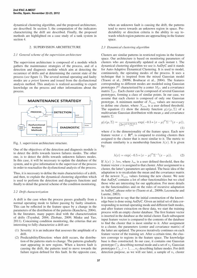
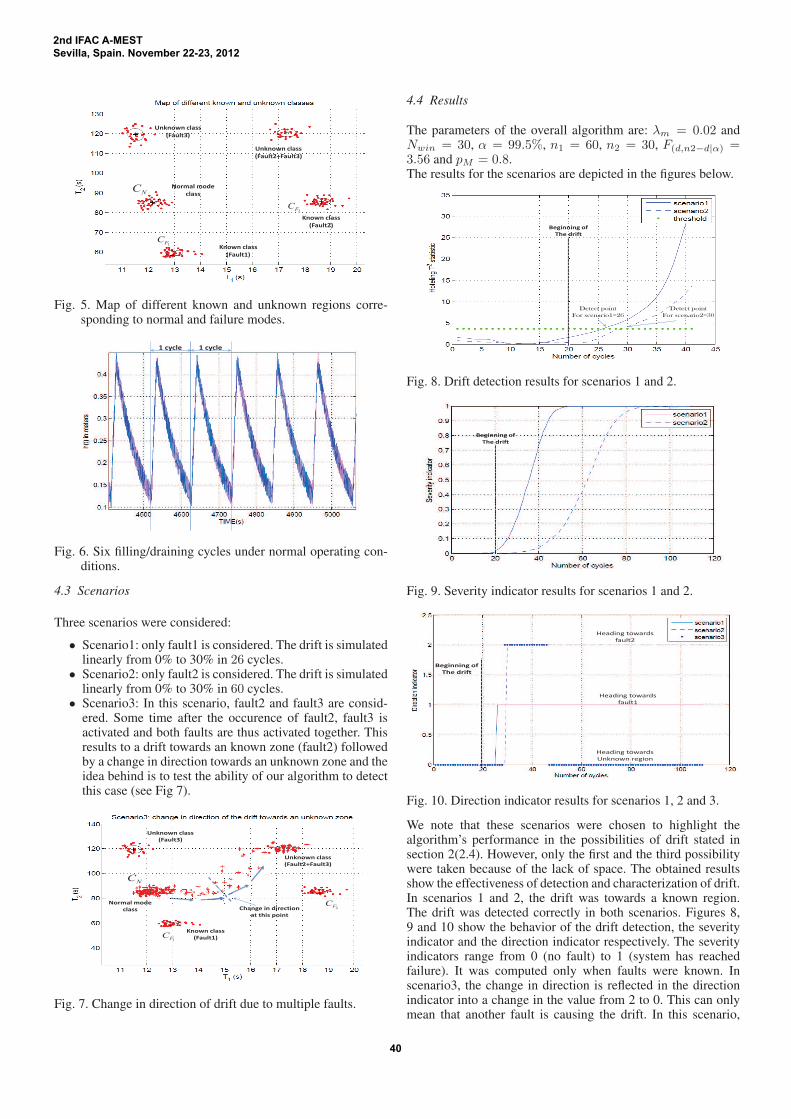
At the beginning, three data sets are given. One correspondingto normal operating mode, and two corresponding to fault1and fault2 operating modes respectively. In figure 6, we showthe sensor measurements under normal operating mode. Wecan clearly see that a cycle is a sequence of a filling periodfollowed by a draining period. The features extracted from thissignal are the time required for the filling T1 and the timerequired for draining T2. A cycle will be denoted cy. Themap showing normal mode and different known and unknownmodes is presented in figure 5.

2nd IFAC A-MESTSevilla, Spain. November 22-23, 2012

39

Known class

(Fault1)

Known class

(Fault2)

Unknown class

(Fault2+Fault3)

Unknown class

(Fault3)

Normal mode

class NC

1FC

2FC

Fig. 5. Map of different known and unknown regions corre-sponding to normal and failure modes.

1 cycle 1 cycle

Fig. 6. Six filling/draining cycles under normal operating con-ditions.

4.3 Scenarios

Three scenarios were considered:

• Scenario1: only fault1 is considered. The drift is simulatedlinearly from 0% to 30% in 26 cycles.

• Scenario2: only fault2 is considered. The drift is simulatedlinearly from 0% to 30% in 60 cycles.

• Scenario3: In this scenario, fault2 and fault3 are consid-ered. Some time after the occurence of fault2, fault3 isactivated and both faults are thus activated together. Thisresults to a drift towards an known zone (fault2) followedby a change in direction towards an unknown zone and theidea behind is to test the ability of our algorithm to detectthis case (see Fig 7).

2FC

NC

1FC

Unknown class

(Fault3)

Unknown class

(Fault2+Fault3)

Normal mode

class

Known class

(Fault1)

Change in direction

at this point

Fig. 7. Change in direction of drift due to multiple faults.

4.4 Results

The parameters of the overall algorithm are: λm = 0.02 andNwin = 30, α = 99.5%, n1 = 60, n2 = 30, F(d,n2−d|α) =3.56 and pM = 0.8.The results for the scenarios are depicted in the figures below.

Beginning of

The drift

Detect point

For scenario1=26

Detect point

For scenario2=30

Fig. 8. Drift detection results for scenarios 1 and 2.

Beginning of

The drift

Fig. 9. Severity indicator results for scenarios 1 and 2.

Beginning of

The drift

Heading towards

fault1

Heading towards

fault2

Heading towards

Unknown region

Fig. 10. Direction indicator results for scenarios 1, 2 and 3.

We note that these scenarios were chosen to highlight thealgorithm’s performance in the possibilities of drift stated insection 2(2.4). However, only the first and the third possibilitywere taken because of the lack of space. The obtained resultsshow the effectiveness of detection and characterization of drift.In scenarios 1 and 2, the drift was towards a known region.The drift was detected correctly in both scenarios. Figures 8,9 and 10 show the behavior of the drift detection, the severityindicator and the direction indicator respectively. The severityindicators range from 0 (no fault) to 1 (system has reachedfailure). It was computed only when faults were known. Inscenario3, the change in direction is reflected in the directionindicator into a change in the value from 2 to 0. This can onlymean that another fault is causing the drift. In this scenario,

2nd IFAC A-MESTSevilla, Spain. November 22-23, 2012

40

the unknown zone reflects the need to update the dysfunctionalanalysis using expert knowledge. The detection for this scenariois the same as for scenario 2 because fault 2 was simulated inthe beginning and so it wasn’t put on the figure 8.

5. CONCLUSION AND PERSPECTIVES

In this paper, we showed an architecture of supervision forcondition monitoring and diagnosis. A methodology for detect-ing and characterizing drifts was employed. The methodologywas based on the monitoring of the parameters of dynamicallyupdated clusters. Then, a diagnosis block was used to detectdrifts, and in case of positive detection, to compute directionand severity indicators to characterize the drift. This alloweddetecting new unknown zones and allows experts to updateinitial dysfunctional analysis made on a process. Results wereshown on a case study and confirm the efficiency of the archi-tecture.The indicators computed allowed the estimation of the condi-tion of the process. A future step could be the use of these indi-cators to compute the Remaining Useful Life (RUL) providingin this way more tools for the condition based maintenance. TheRUL could be estimated by a trend analysis of the trajectory ofthe severity indicators. Another interesting application will bethe use of real data sets in order to test our methodology in realworld applications.

REFERENCES

Basseville, M. and Nikiforov, I. (1993). Detection of AbruptChanges: Theory and Application. Prentice Hall, Inc.

Boubacar, H.A., Lecoueuche, S., and Maouche, S. (2004).Audyc neural network using a new gaussian densities mergemechanism. In 7th Conference on Adaptive and NeuralCmputing Algorithms, 155–158.

Byington, C., Watson, M., Roemer, M., and Galie, T. (2003).Prognostic enhancements to gas turbine diagnostic systems.In IEEE Aerospace Conference, 103, 137–143.

Chammas, A., Traore, M., Duviella, E., and Lecoeuche, S.(2011). Supervision of switching systems based on dynami-cal classification approach. In European Safety and Reliabil-ity Association ESREL’10.

Chandola, V., Banerjee, A., and Kumar, V. (2009). Anomalydetection : A survey. Technical report, ACM ComputingSurveys.

Desinde, M., Flaus, J.M., and Ploix, S. (2006). Tool andmethodology for online risk assessement of process. InLambda-Mu 15 /Lille.

Isermann, R. (2005). Model-based fault detection and diagnosis- status and applications. Annual Reviews in Control, 29, 71–85.

Iverson, D. (2004). Inductive system health monitoring. In Pro-ceedings of The 2004 International Conference on ArtificialIntelligence (IC-AI04), CSREA Press, Las Vegas, NV.

Jardine, A.K., Lin, D., and Banjevic, D. (2006). A reviewon machinery diagnostics and prognostics implementingcondition-based maintenance. Mechanical Systems and Sig-nal Processing, 20, 1483–1510.

John and Olson, P. (2007). Approximating the kullback leiblerdivergence between gaussian mixture models. In IEEEInternational Conference on Acoustics, Speech and SignalProcessing, ICASSP.

Kuncheva, L. (2009). Using control charts for detecting conceptchange in streaming data. Technical report, Technical ReportBCS-TR-001.

Kuncheva, L.I. (2004). Classifier ensembles for changingenvironments. Lecture Notes in Computer Science, 3077, 1–15.

Lebold, M. and Thurston, M. (2001). Open standards forcondition-based maintenance and prognosis systems. Inthe 5th Annual Maintenance and Reliability Conference,Gatlinburg, USA.

Lecoeuche, S. and Lurette, C. (2003). Auto-adaptive and dy-namical clustering neural network. In ICANN’03 Proceed-ings.

Li, G., Qin, J., Ji, Y., and Zhou, D.H. (2010). Reconstructionbased fault prognosis for continuous processes. ControlEngineering Practice, 18, 1211–1219.

Markou, M. and Singh, S. (2003). Novelty detection: a review–part i: statistical approaches. SIGNAL PROCESSING, 83,2481–2497.

Minku, L.L. and Yao, X. (2011). Ddd: A new ensemble ap-proach for dealing with concept drift. In IEEE Transactionson Knowledge and Data Engineering.

Muller, A., Suhner, M.C., and Iung, B. (2008a). Formalisationof a new prognosis model for supporting proactive main-tenance implementation on industrial system. ReliabilityEngineering and System Safety, 93, 234–253.

Muller, A., Marquez, A.C., and Iunga, B. (2008b). On theconcept of e-maintenance: Review and current research. Re-liability Engineering and System Safety, 93, 1165–1187.

MvBain, J. and Timusk, M. (2009). Fault detection in variablespeed machinery: Statistical parametrization. Journal ofSound and Vibration, 327, 623–646.

Sayed-Mouchaweh, M. (2012). Semi-supervised classificationmethod for dynamic applications. Fuzzy Sets and Systems,161, 544–563.

Traore, M., Duviella, E., and Lecoeuche, S. (2009a). Dynam-ical classification method to provide pertinent indicators forpredictive maintenance strategies. ICINCO’09, Milan, Italie.

Traore, M., Duviella, E., and Lecoueuche, S. (2009b). Com-parison of two prognosis methods based on neuro fuzzyinference system and clustering neural network. In SAFEPROCESS.

Tsymbal, A. (2004). The problem of concept drift: definitionsand related work. Trinity College, Dublin, Ireland, TCD-CS-2004-15.

Vachtsevanos, G., Lewis, F., Roemer, M., Hess, A., and Wu,B. (2006). Intelligent Fault Diagnosis and Prognosis forEngineering Systems. Jhon Wiley and Sons, Inc.

Venkatasubramanian, V., Rengaswamy, R., Yin, K., and Kavuri,S. (2003). A review of process fault detection and diagnosispart iii: Process history based methods. Computers andchemical Engineering, 27, 327–346.

Vesely, W.E., Goldberg, F.F., Robert, N.H., and Haasl, D.F.(1981). Fault Tree Handbook. US nuclear RegulatoryCommission, Washington D.C., USA.

Zliobate, I. (2009). Learning under concept drift: an overview.Technical report, Vilnius University.

2nd IFAC A-MESTSevilla, Spain. November 22-23, 2012

41