Conceptual Design of Jet Transport Aircraft with Energy ...
231
Conceptual Design of Jet Transport Aircraft with Energy Harvesting Structure By: Mahesa Akbar Supervisors: Dr. Jose Luis Curiel-Sosa Dr. Anton Krynkin A thesis submitted in partial fulfilment of the requirements for the degree of Doctor of Philosophy March 2019
-
Upload
khangminh22 -
Category
Documents
-
view
1 -
download
0
Transcript of Conceptual Design of Jet Transport Aircraft with Energy ...

Conceptual Design of Jet
Transport Aircraft with Energy
Harvesting Structure
By:
Mahesa Akbar
Supervisors:
Dr. Jose Luis Curiel-Sosa
Dr. Anton Krynkin
A thesis submitted in partial fulfilment of the requirements
for the degree of Doctor of Philosophy
March 2019

Abstract
Piezoelectric material has been utilised to construct a small scale (µW order) power
generator devices in recent years. In the case of aerial vehicles, some works have
presented its implementation on small unmanned aerial vehicles (UAV). However, an
application on larger aircraft structure has not yet been investigated. The present
work aimed to seek insight into the potential energy that could be harvested from a
large aircraft structure, i.e., wing. The alternative energy support may reduce fuel
consumption and improve flight performance. However, the computational procedure
fit for design purposes of an aircraft with energy harvesting capability also has not
yet been developed. Thus, the development of computational methods for energy
harvesting from an aircraft structure is also aimed in the present work.
As the first part of the present work, a novel hybrid mathematical/computational
scheme is built to evaluate the energy harvested by a mechanical system. The governing
voltage differential equations of the piezoelectric composite beam can be coupled with
the output from a numerical method, e.g. the Finite Element Method (FEM). The
scheme can evaluate various excitation forms concerning bending deformation including
dynamic force and base excitation. In this report, the capabilities and robustness of
the scheme are compared with results from the literature. Implementation to the
simulation of a notional jet aircraft wingbox with a piezoelectric skin layer is shown
in some detail. The results pointed out that the electrical power generated can be as
much as 39.13 kW for a 14.5 m wingspan.
The second part of the present work focused on the evaluation of alternative com-
posite material, namely the multiphase composite with active structural fiber. The
active structural fiber constructed of carbon fiber as a core with a piezoelectric shell as
the coating can be flexibly optimised in terms of weight and electromechanical coupling.
Hence, it may provide a lightweight benefit compared to the bulk piezoelectric material.
In the present work, for the first time, the multiphase composite is implemented for
energy harvesting purpose. An application to a notional jet aircraft wingbox is evalu-
ated. An analysis of the trade-off between the energy harvested, the weight reduction
and the fuel saving of the aircraft is shown in some detail.
Lastly, the third part of the present work is the development of a novel iterative
FEM for piezoelectric energy harvesting. The application of the present iterative FEM
to evaluate the piezoelectric energy harvesting of lifting structures under an aeroelastic
condition, i.e., gust load, is shown in some details. Furthermore, energy harvesting
potential from a transport aircraft wingbox is also investigated. The results pointed
out that the wingbox is still in a safe condition even when it is subjected to a 30 m/s
gust amplitude while harvesting 51 kW power. In addition, for the first time, stress and
failure analyses of the structure with an active energy harvesting layer are performed.

Acknowledgment
The author gratefully acknowledges Dr Jose Luis Curiel-Sosa and Dr Anton Krynkin
for their continuous support and the fruitful discussions. The author also acknowledges
the funding from Indonesia Endowment Fund for Education (LPDP).
The author also would like to thank Indonesia National Institute of Aeronautics and
Space (LAPAN), in particular, Mr Nanda Wirawan for the support in the engineering
analysis works. Lastly, I want to dedicate my deepest gratitude to my family and
friends.

List of Publications
During his PhD study, the author has published several journal articles in which some
of them are based on the works done for his PhD thesis. The main articles published
and submitted by the author during his PhD study are listed below:
Main publications
1. M. Akbar and J.L. Curiel-Sosa, ”Piezoelectric energy harvester composite under
dynamic bending with implementation to aircraft wingbox structure” Composite
Structures, vol. 153, pp. 193-203, 2016.
2. M. Akbar and J.L. Curiel-Sosa, ”Evaluation of piezoelectric energy harvester
under dynamic bending by means of hybrid mathematical/isogeometric analysis”
International Journal of Mechanics and Materials in Design, vol. 14(4), pp. 647-
667, 2018.
3. M. Akbar and J.L. Curiel-Sosa, ”Implementation of multiphase piezoelectric
composites energy harvester on aircraft wingbox structure with fuel saving eval-
uation” Composite Structures, vol. 202, pp. 1000-1020, 2018.
4. M. Akbar and J.L. Curiel-Sosa, ”An iterative finite element method for piezo-
electric energy harvesting composite with implementation to lifting structures
under gust load conditions”, Composite Structures, vol. 219, pp. 97-110, 2019.
5. M. Akbar and J.L. Curiel-Sosa, ”An iterative finite element method for piezo-
electric energy harvester and actuator with implementation to jet aircraft wing”
submitted to Composite Structures.
Meanwhile, other publications of the author are:
Other publications
1. N.A. Abdullah, J.L. Curiel-Sosa and M. Akbar, ”Aeroelastic assessment of
cracked composite plate by means of fully coupled finite element and Doublet
Lattice Method” Composite Structures, vol. 202, pp. 151-161, 2018.
2. M.I.M Ahmad, J.L. Curiel-Sosa, M. Akbar and N.A. Abdullah, ”Numerical
inspection based on quasi-static analysis using Rousselier damage model for alu-
minium wingbox aircraft structure” Journal of Physics: Conference Series, vol.
1106, pp. 012013, 2018.

3. N. Wirawan, N.A. Abdullah, M. Akbar and J.L. Curiel-Sosa, ”Analysis on
cracked commuter aircraft wing under dynamic cruise load by means of XFEM”
Journal of Physics: Conference Series, vol. 1106, pp. 012014, 2018.
4. N.A. Abdullah, J.L. Curiel-Sosa and M. Akbar, ”Structural integrity investi-
gation on cracked composites under aeroelastic condition by means of XFEM”
accepted for publication in Composite Structures, 2019.
5. N.A. Abdullah, J.L. Curiel-Sosa and M. Akbar, ”Structural integrity investi-
gation of commuter aircraft wing under discrete gust loads by means of XFEM”
submitted to AIAA Journal.
iv


Contents
Abstract . . . . . . . . . . . . . . . . . . . . . . . . . . . . . . . . . . . . . . i
Acknowledgment . . . . . . . . . . . . . . . . . . . . . . . . . . . . . . . . . ii
List of Publications . . . . . . . . . . . . . . . . . . . . . . . . . . . . . . . . iii
Table of Contents . . . . . . . . . . . . . . . . . . . . . . . . . . . . . . . . . vi
List of Figures . . . . . . . . . . . . . . . . . . . . . . . . . . . . . . . . . . . ix
List of Tables . . . . . . . . . . . . . . . . . . . . . . . . . . . . . . . . . . . xv
1 Introduction 1
1.1 Background and motivations . . . . . . . . . . . . . . . . . . . . . . . . 1
1.2 Research objectives . . . . . . . . . . . . . . . . . . . . . . . . . . . . . 3
1.3 Research work plan . . . . . . . . . . . . . . . . . . . . . . . . . . . . . 3
1.4 Thesis outline . . . . . . . . . . . . . . . . . . . . . . . . . . . . . . . . 5
2 Literature Review 6
2.1 Piezoelectric energy harvesting from lifting structure vibration . . . . . 6
2.2 Computational analysis of piezoaeroelastic energy harvesting . . . . . . 9
2.3 Multiphase composites with active structural fiber . . . . . . . . . . . . 15
3 Hybrid Analytical/ Computational Scheme for Piezoelectric Energy
Harvesting 18
3.1 Mathematical model . . . . . . . . . . . . . . . . . . . . . . . . . . . . 18
3.2 Code algorithm . . . . . . . . . . . . . . . . . . . . . . . . . . . . . . . 24
3.3 Validation against analytical solution . . . . . . . . . . . . . . . . . . . 26
3.4 Validation against experimental result . . . . . . . . . . . . . . . . . . 29
3.5 Validation against electro-mechanically coupled FEM . . . . . . . . . . 32
3.6 Investigation by higher-order elements . . . . . . . . . . . . . . . . . . 38
3.7 Summary . . . . . . . . . . . . . . . . . . . . . . . . . . . . . . . . . . 42
4 Implementation of The Hybrid Scheme on A Jet Aircraft Wingbox 44
4.1 Wingbox FEM analysis . . . . . . . . . . . . . . . . . . . . . . . . . . . 44
4.2 Wingbox energy harvesting simulation . . . . . . . . . . . . . . . . . . 48
4.3 Summary . . . . . . . . . . . . . . . . . . . . . . . . . . . . . . . . . . 52
vi

TABLE OF CONTENTS
5 Multiphase Piezoelectric Composites with Active Structural Fiber 54
5.1 The Double-Inclusion model . . . . . . . . . . . . . . . . . . . . . . . . 54
5.2 Evaluation procedure of the multiphase composite effective electro-elastic
properties . . . . . . . . . . . . . . . . . . . . . . . . . . . . . . . . . . 58
5.3 Case study and validation: Multiphase composite electro-elastic prop-
erties estimation . . . . . . . . . . . . . . . . . . . . . . . . . . . . . . . 60
5.3.1 Electro-elastic properties comparison against analytical model
and experimental results . . . . . . . . . . . . . . . . . . . . . . 60
5.3.2 Electro-elastic properties comparison against finite element model 66
5.3.3 Highlights on the effective electro-elastic properties concerning
energy harvesting analysis . . . . . . . . . . . . . . . . . . . . . 74
5.4 Summary . . . . . . . . . . . . . . . . . . . . . . . . . . . . . . . . . . 76
6 Application of The Multiphase Composites on A Jet Aircraft Wing-
box 77
6.1 Aircraft weight breakdown in conceptual design . . . . . . . . . . . . . 77
6.2 Evaluation procedure on the trade-off between aircraft weight and energy
harvested . . . . . . . . . . . . . . . . . . . . . . . . . . . . . . . . . . 79
6.3 Wingbox energy harvesting simulation with the multiphase composite . 81
6.4 Aircraft fuel saving evaluation . . . . . . . . . . . . . . . . . . . . . . . 85
6.5 Summary . . . . . . . . . . . . . . . . . . . . . . . . . . . . . . . . . . 88
7 Iterative Finite Element Method for Piezoelectric Energy Harvesting 90
7.1 The coupled electro-mechanical equations . . . . . . . . . . . . . . . . . 91
7.2 Computational scheme . . . . . . . . . . . . . . . . . . . . . . . . . . . 93
7.3 Unimorph plate under base excitation . . . . . . . . . . . . . . . . . . . 97
7.4 Discrete 1-cosine gust and unsteady aerodynamic loads . . . . . . . . . 101
7.5 Bimorph plate under gust load conditions . . . . . . . . . . . . . . . . . 103
7.6 UAV wingbox under gust load conditions . . . . . . . . . . . . . . . . . 109
7.7 Summary . . . . . . . . . . . . . . . . . . . . . . . . . . . . . . . . . . 115
8 Iterative Finite Element Method with Implementation to An Aircraft
Wingbox 116
8.1 Jet aircraft wingbox under Gust Load Condition . . . . . . . . . . . . . 116
8.2 Discussion on the power density and the flight performance . . . . . . . 128
8.3 Summary . . . . . . . . . . . . . . . . . . . . . . . . . . . . . . . . . . 134
9 Conclusion 136
9.1 On the hybrid piezoelectric energy harvester model . . . . . . . . . . . 139
9.2 On the multiphase piezoelectric composite . . . . . . . . . . . . . . . . 139
vii

TABLE OF CONTENTS
9.3 On the iterative FEM for piezoelectric energy harvesting . . . . . . . . 140
9.4 Future work . . . . . . . . . . . . . . . . . . . . . . . . . . . . . . . . . 142
Bibliography 143
APPENDIX A 155
APPENDIX B 157
APPENDIX C 160
APPENDIX D 168
APPENDIX E 181
APPENDIX F 187
APPENDIX G 193
APPENDIX H 195
APPENDIX I 197
APPENDIX J 199
APPENDIX K 202
APPENDIX L 208
viii
List of Figures
1.1 The research flow diagram . . . . . . . . . . . . . . . . . . . . . . . . . 4
2.1 2-DoF airfoil aeroelastic model . . . . . . . . . . . . . . . . . . . . . . . 9
2.2 2-DoF airfoil piezoaeroelastic model . . . . . . . . . . . . . . . . . . . . 10
3.1 Specimen loaded by voltage, V . . . . . . . . . . . . . . . . . . . . . . 19
3.2 Specimen loaded by force, F . . . . . . . . . . . . . . . . . . . . . . . . 20
3.3 A cantilevered multilayer beam with piezoelectric layer . . . . . . . . . 21
3.4 A cantilever beam loaded by bending moment, M . . . . . . . . . . . . 21
3.5 A cantilever beam with piezoelectric layer loaded by voltage, V . . . . 22
3.6 A cantilever beam with uniform cross-section . . . . . . . . . . . . . . . 22
3.7 A cantilevered piezoelectric energy harvester exerted by mechanical and
electrical loads . . . . . . . . . . . . . . . . . . . . . . . . . . . . . . . 25
3.8 Schematic diagram of the energy harvesting system evaluation process . 25
3.9 Bimorph 1 - Variation of the voltage amplitude with the resistance load 28
3.10 Bimorph 1 - Variation of the power amplitude with the resistance load 29
3.11 Bimorph 2 - Variation of the voltage amplitude with the resistance load 30
3.12 Bimorph 2 - Variation of the power amplitude with the resistance load 31
3.13 Variation of the thickness ratio, h*, with the length ratio, L*, of the spar 33
3.14 Variation of the (a) natural frequency, (b) critical damping ratio with
the length ratio of the spar . . . . . . . . . . . . . . . . . . . . . . . . . 34
3.15 Variation of the (a) maximum power amplitude and (b) optimum resis-
tance load with the length ratio of the spar . . . . . . . . . . . . . . . . 35
3.16 Variation of the power amplitude with the resistance load for various
length ratio of the spar . . . . . . . . . . . . . . . . . . . . . . . . . . . 35
3.17 Investigation by IGA: Voltage amplitude vs resistance . . . . . . . . . . 39
3.18 Investigation by IGA: Power amplitude vs resistance . . . . . . . . . . 40
3.19 Variation of the (a) tip displacement and (b) tip angle with the thickness
ratio, h0/h . . . . . . . . . . . . . . . . . . . . . . . . . . . . . . . . . . 41
3.20 Variation of the reverse piezoelectric parameter with the thickness ratio,
h0/h . . . . . . . . . . . . . . . . . . . . . . . . . . . . . . . . . . . . . 41
ix

LIST OF FIGURES
3.21 Bimorph 1 with h0/h = 103.75 - Variation of the (a) voltage amplitude
and (b) power amplitude with the resistance load . . . . . . . . . . . . 42
3.22 Bimorph 1 with h0/h = 104 - Variation of the (a) voltage amplitude and
(b) power amplitude with the resistance load . . . . . . . . . . . . . . . 43
4.1 Wingbox vertical stiffness distribution . . . . . . . . . . . . . . . . . . 45
4.2 Wingbox topside view layout . . . . . . . . . . . . . . . . . . . . . . . . 45
4.3 Wingbox model for finite element analysis . . . . . . . . . . . . . . . . 46
4.4 Sketch of the lift coefficient distribution on the wing . . . . . . . . . . . 48
4.5 Wingbox dynamic response amplitude along the span . . . . . . . . . . 48
4.6 Wingbox voltage amplitude vs resistance . . . . . . . . . . . . . . . . . 49
4.7 Wingbox power amplitude vs resistance . . . . . . . . . . . . . . . . . . 50
4.8 Wingbox voltage amplitude vs resistance, loglog scale . . . . . . . . . . 50
4.9 Wingbox power amplitude vs resistance, loglog scale . . . . . . . . . . . 51
5.1 Multiphase composite with active structural fiber (ASF) . . . . . . . . 56
5.2 Cross-section of energy harvester beam with multiphase composite as
an active layer . . . . . . . . . . . . . . . . . . . . . . . . . . . . . . . . 58
5.3 (a) Stiffness, C33, (b) Piezoelectric Constant, e33, (c) Compliance, S31,
and (d) Charge Constant, d31, vs ASF Volume Fraction of PZT-7A -
Carbon Fiber - Epoxy Composites . . . . . . . . . . . . . . . . . . . . . 63
5.4 (a) Density, ρ, (b) Charge Constant, d33, (c) Compliance, S11 + S12,
and (d) Dielectric Permittivity Ratio,εT33ε0
, vs ASF Volume Fraction of
PZT-7A-Carbon Fiber-Epoxy Composites . . . . . . . . . . . . . . . . 64
5.5 Charge Constant Ratio, dcomp31 /dbulk
31 , vs ASF Volume Fraction of BaTiO3
- SiC - LaRC-SI Composites . . . . . . . . . . . . . . . . . . . . . . . . 65
5.6 (a) Modulus Young, E3, (b) Relative Permittivity, εS33/ε0, (c) Modu-
lus Young, E1, and (d) Relative Permittivity, εS11/ε0, vs ASF Volume
Fraction of PZT-7A - Carbon Fiber - LaRC-SI Composites . . . . . . . 67
5.7 Charge Constant Ratio dcomp31 /dbulk
31 & dcomp33 /dbulk
33 , vs Aspect Ratio of
PZT-7A - Glass - Epoxy Composites . . . . . . . . . . . . . . . . . . . 69
5.8 Natural Frequency Comparison of PZT-5A - Carbon - LaRC-SI Compos-
ites for (a) Different Aspect Ratio at 50% Volume Fraction (b) Different
Volume Fraction at 0.3 Aspect Ratio . . . . . . . . . . . . . . . . . . . 70
5.9 (a) Detailed 3D FE eigenvector (structural mode shape), (b) Homogeni-
sation FE eigenvector (structural mode shape), (c) Detailed 3D FE
eigenvector (voltage mode shape), and (d) Homogenisation FE eigenvec-
tor (voltage mode shape) of the first bending mode, PZT-5A - Carbon
Fiber - LaRC-SI composites with Vf 50% and AR 0.3 . . . . . . . . . . 71
x

LIST OF FIGURES
5.10 (a) Detailed 3D FE displacement, (b) Homogenisation FE displacement,
(c) Detailed 3D FE voltage, and (d) Homogenisation FE voltage of the
static bending response, PZT-5A - Carbon Fiber - LaRC-SI unimorph
beam with Vf 50% - AR 0.3 and aluminium substrate . . . . . . . . . . 72
5.11 (a) Detailed 3D FE displacement, (b) Homogenisation FE displacement,
(c) Detailed 3D FE voltage, and (d) Homogenisation FE voltage of the
dynamic bending response at 0.6 frequency ratio, PZT-5A - Carbon
Fiber - LaRC-SI unimorph beam with Vf 50% - AR 0.3 and aluminium
substrate . . . . . . . . . . . . . . . . . . . . . . . . . . . . . . . . . . . 73
6.1 Schematic diagram of the weight change calculation . . . . . . . . . . . 80
6.2 Schematic diagram of the fuel saving evaluation . . . . . . . . . . . . . 81
6.3 Variation of voltage amplitude to the resistance load for wingboxes with
multiphase composite skin, AR 0.2, 0.4 & 0.6 at Vf 50%, and bulk PZT
skin . . . . . . . . . . . . . . . . . . . . . . . . . . . . . . . . . . . . . 85
6.4 Variation of power amplitude to the resistance load for wingboxes with
multiphase composite skin, AR 0.2, 0.4 & 0.6 at Vf 50%, and bulk PZT
skin . . . . . . . . . . . . . . . . . . . . . . . . . . . . . . . . . . . . . 86
6.5 Variation of power amplitude to the resistance load for wingboxes with
multiphase composite skin, Vf 50%, 60% & 70% at AR 0.2 and bulk
PZT skin . . . . . . . . . . . . . . . . . . . . . . . . . . . . . . . . . . 87
7.1 Illustration of the iterative FEM process . . . . . . . . . . . . . . . . . 93
7.2 The algorithm of the iterative FEM for a time domain problem . . . . 94
7.3 The algorithm of the iterative FEM for a frequency domain problem . . 95
7.4 The iteration histories of (a) voltage and (b) relative tip displacement
amplitudes of the unimorph modelled by solid elements . . . . . . . . . 99
7.5 The iteration histories of (a) voltage and (b) relative tip displacement
amplitudes of the unimorph modelled by shell elements . . . . . . . . . 99
7.6 The voltage output time history of the unimorph modelled by solid ele-
ments . . . . . . . . . . . . . . . . . . . . . . . . . . . . . . . . . . . . 100
7.7 Illustration of a lifting surface exposed to a freestream flow with airspeed
V∞ and 1-cosine gust with maximum gust speed Vg0 . . . . . . . . . . . 101
7.8 Configuration of the bimorph . . . . . . . . . . . . . . . . . . . . . . . 103
7.9 (a) Damping vs Airspeed, and (b) Frequency vs Airspeed graphs of the
bimorph . . . . . . . . . . . . . . . . . . . . . . . . . . . . . . . . . . . 104
7.10 Illustration of a lifting surface exposed to a freestream flow with airspeed
V∞ and an impulse gust with maximum gust speed Vg0 . . . . . . . . . 106
xi
LIST OF FIGURES
7.11 Time histories of the power output of the bimorph at 10 m/s airspeed
for different gust period . . . . . . . . . . . . . . . . . . . . . . . . . . 107
7.12 Time histories of (a) the tip displacement and (b) the power output of
the bimorph at 10 m/s airspeed . . . . . . . . . . . . . . . . . . . . . . 107
7.13 Time histories of (a) the tip displacement and (b) the power output of
the bimorph 30 m/s airspeed . . . . . . . . . . . . . . . . . . . . . . . . 108
7.14 Displacement contours at tg = 0.175 s of the bimorph with airspeeds (a)
10 m/s and (b) 30 m/s (displacement unit in mm) . . . . . . . . . . . . 109
7.15 Topside view of the UAV wingbox configuration: Wingbox only - Struc-
tural model (top), Wingbox and wing surface - Structural model and
aerodynamic panels (bottom) . . . . . . . . . . . . . . . . . . . . . . . 110
7.16 (a) Damping vs Airspeed, and (b) Frequency vs Airspeed graphs of the
UAV wingbox . . . . . . . . . . . . . . . . . . . . . . . . . . . . . . . . 111
7.17 Time histories of (a) the tip displacement and (b) the voltage output of
the UAV wingbox under 1-cosine gust . . . . . . . . . . . . . . . . . . . 112
7.18 The power output time history . . . . . . . . . . . . . . . . . . . . . . 113
7.19 Displacement contour of the UAV wingbox at tg = 0.0285 s(displacement
unit in mm) . . . . . . . . . . . . . . . . . . . . . . . . . . . . . . . . . 113
7.20 Voltage contour of the piezoelectric layer of the UAV wingbox at tg =
0.0285 s (voltage unit in µV) . . . . . . . . . . . . . . . . . . . . . . . . 114
7.21 The voltage output time histories at different iteration steps . . . . . . 114
8.1 Topside view of the aircraft wingbox configuration: Wingbox only -
Structural model (left), Wingbox and wing surface - Structural model
and aerodynamic panels (right) . . . . . . . . . . . . . . . . . . . . . . 117
8.2 Mode shapes the aircraft wingbox . . . . . . . . . . . . . . . . . . . . . 118
8.3 (a) Airspeed vs Damping (V −g), and (b) Airspeed vs Frequency (V −f)
graphs of the aircraft wingbox . . . . . . . . . . . . . . . . . . . . . . . 119
8.4 The time histories of (a) vertical tip displacment and (b) voltage output
of the aircraft wingbox for different gust gradient distances with gust
velocity 15 m/s . . . . . . . . . . . . . . . . . . . . . . . . . . . . . . . 120
8.5 The power output time history of the aircraft wingbox for different gust
gradient distance with gust velocity 15 m/s . . . . . . . . . . . . . . . . 120
8.6 The voltage output time history of the aircraft wingbox with gust gra-
dient distance 12.5 MAC at different iteration step . . . . . . . . . . . 121
8.7 The time histories of (a) vertical tip displacement and (b) voltage output
of the aircraft wingbox for different gust velocities with gust gradient
distance 12.5 MAC . . . . . . . . . . . . . . . . . . . . . . . . . . . . . 122
xii

LIST OF FIGURES
8.8 The power output time history of the aircraft wingbox for different gust
velocity with gust gradient distance 12.5 MAC . . . . . . . . . . . . . . 123
8.9 Displacement contours of the aircraft wingbox for 12.5 MAC gust gra-
dient distance with (a) 15 m/s and (b) 30 m/s gust velocities at tg =
0.3 s (displacement unit: mm) . . . . . . . . . . . . . . . . . . . . . . . 124
8.10 The stress contours with (a) Vg0 = 15 m/s, (b) Vg0 = 30 m/s of the
aircraft wingbox for Hg = 12.5 MAC at tg = 0.3 s (stress unit: kPa) . . 125
8.11 The failure indices with (a) Vg0 = 15 m/s, (b) Vg0 = 30 m/s of the
aircraft wingbox for Hg = 12.5 MAC at tg = 0.3 s . . . . . . . . . . . . 126
8.12 The time histories of (a) voltage output and (b) power output of the
aircraft wingbox with multiphase composite for different time step . . . 127
8.13 The time histories of (a) voltage output and (b) power output of the
aircraft wingbox with multiphase composite for different gust velocities
(Up gust) with gust gradient distance 12.5 MAC . . . . . . . . . . . . . 127
8.14 The time histories of (a) voltage output and (b) power output of the
aircraft wingbox with multiphase composite for different gust velocities
(Down gust) with gust gradient distance 12.5 MAC . . . . . . . . . . . 128
8.15 Mission profile of a typical jet transport aircraft . . . . . . . . . . . . . 131
8.16 Mission profile with energy harvesting system and extended cruise range
using the fuel saved . . . . . . . . . . . . . . . . . . . . . . . . . . . . . 132
8.17 (a) The number of gust occurrence per flight, and (b) Total energy
generated per flight as functions of the gust amplitude (Vg0) . . . . . . 132
G.1 The first bending mode of the jet aircraft wingbox with PZT-5A as
upper skin material . . . . . . . . . . . . . . . . . . . . . . . . . . . . . 193
G.2 The dynamic response at 0.5 frequency ratio of the jet aircraft wingbox
with PZT-5A as upper skin material (displacement unit: inch) . . . . . 193
G.3 The dynamic response at 0.7 frequency ratio of the jet aircraft wingbox
with PZT-5A as upper skin material (displacement unit: inch) . . . . . 194
G.4 The dynamic response at 0.9 frequency ratio of the jet aircraft wingbox
with PZT-5A as upper skin material (displacement unit: inch) . . . . . 194
H.1 The dynamic response at 0.9 frequency ratio of the jet aircraft wingbox
with multiphase composite at Vf 50% and AR 0.2 (displacement unit:
inch) . . . . . . . . . . . . . . . . . . . . . . . . . . . . . . . . . . . . . 195
H.2 The dynamic response at 0.9 frequency ratio of the jet aircraft wingbox
with multiphase composite at Vf 50% and AR 0.6 (displacement unit:
inch) . . . . . . . . . . . . . . . . . . . . . . . . . . . . . . . . . . . . . 195
xiii
LIST OF FIGURES
H.3 The dynamic response at 0.9 frequency ratio of the jet aircraft wingbox
with multiphase composite at Vf 60% and AR 0.2 (displacement unit:
inch) . . . . . . . . . . . . . . . . . . . . . . . . . . . . . . . . . . . . . 196
H.4 The dynamic response at 0.9 frequency ratio of the jet aircraft wingbox
with multiphase composite at Vf 70% and AR 0.2 (displacement unit:
inch) . . . . . . . . . . . . . . . . . . . . . . . . . . . . . . . . . . . . . 196
I.1 The flutter response of Xiang et al. UAV wingbox associated with the
third bending eigenvector at airspeed 150 m/s and frequency 174 Hz . . 197
I.2 The flutter response of Xiang et al. UAV wingbox associated with the
first torsion eigenvector at airspeed 150 m/s and frequency 207 Hz . . . 197
I.3 The flutter response of Xiang et al. UAV wingbox associated with the
fourth bending eigenvector at airspeed 150 m/s and frequency 336 Hz . 198
I.4 The flutter response of Xiang et al. UAV wingbox associated with the
mixed eigenvector (bending and torsion modes already coalesced) at
airspeed 210 m/s and frequency 90 Hz . . . . . . . . . . . . . . . . . . 198
J.1 Displacement contour of the aircraft wingbox for 12.5 MAC gust gradient
distance with gust velocities at tg = 0.225 s (displacement unit: mm) . 199
J.2 Displacement contour of the aircraft wingbox for 12.5 MAC gust gradient
distance with gust velocities at tg = 0.275 s (displacement unit: mm) . 199
J.3 Displacement contour of the aircraft wingbox for 12.5 MAC gust gradient
distance with gust velocities at tg = 0.325 s (displacement unit: mm) . 200
J.4 Displacement contour of the aircraft wingbox for 12.5 MAC gust gradient
distance with gust velocities at tg = 0.375 s (displacement unit: mm) . 200
J.5 Displacement contour of the aircraft wingbox for 12.5 MAC gust gradient
distance with gust velocities at tg = 0525 s (displacement unit: mm) . . 200
J.6 Displacement contour of the aircraft wingbox for 12.5 MAC gust gradient
distance with gust velocities at tg = 0.225 s (displacement unit: mm) . 201
J.7 Displacement contour of the aircraft wingbox for 12.5 MAC gust gradient
distance with gust velocities at tg = 1.275 s (displacement unit: mm) . 201
J.8 Displacement contour of the aircraft wingbox for 12.5 MAC gust gradient
distance with gust velocities at tg = 1.475 s (displacement unit: mm) . 201
xiv
List of Tables
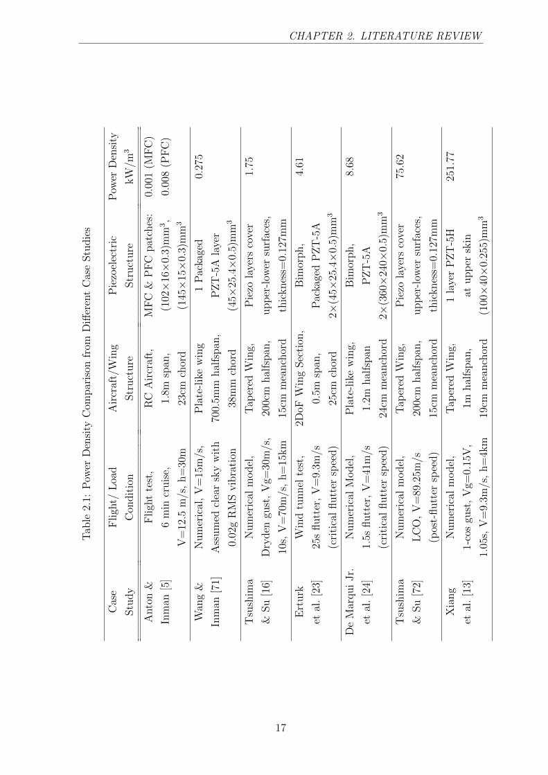
2.1 Power Density Comparison from Different Case Studies . . . . . . . . . 17
3.1 Bimorph 1 - Material properties and configuration . . . . . . . . . . . . 26
3.2 Bimorph 1 - Natural frequency comparison . . . . . . . . . . . . . . . . 27
3.3 Bimorph 1 - Relative tip displacement & tip angle comparison . . . . . 27
3.4 Bimorph 1 - Electrical parameters comparison . . . . . . . . . . . . . . 29
3.5 Bimorph 2 - Material properties and configuration . . . . . . . . . . . . 30
3.6 Bimorph 2 - Electrical parameters comparison at R = 6.7 kΩ . . . . . . 31
3.7 Material properties and geometry of the bimorph UAV wingspar . . . . 32
3.8 Natural frequency and maximum power comparison of De Marqui Jr. et
al - FEM and Present Model (FEM) . . . . . . . . . . . . . . . . . . . 36
3.9 Simulation time comparison . . . . . . . . . . . . . . . . . . . . . . . . 37
3.10 Electrical Parameters Comparison with h0/h = 104 . . . . . . . . . . . 42
4.1 Weight and tip displacement, Ztip, original model vs model A . . . . . . 47
4.2 Natural frequency comparison, model A vs model B . . . . . . . . . . . 47
4.3 Simulation time comparison for the wingbox model . . . . . . . . . . . 52
5.1 Material Properties of Piezoelectric Materials . . . . . . . . . . . . . . 60
5.2 Material Properties of Core Fiber Materials . . . . . . . . . . . . . . . 61
5.3 Material Properties of Matrix Materials . . . . . . . . . . . . . . . . . . 62
5.4 Comparison of The Present Model and Lin-Sodano Model against The
Experimental Results . . . . . . . . . . . . . . . . . . . . . . . . . . . . 66
5.5 Charge Constant Ratio Comparison: The Present Model vs XFEM -
Koutsawa et al. . . . . . . . . . . . . . . . . . . . . . . . . . . . . . . 70
5.6 Natural Frequency Comparison for Different Volume Fraction at 0.3 As-
pect Ratio of PZT-5A - Carbon - LaRC-SI Composites, Detailed 3D
Finite Element vs Finite Element with Homogenization Properties . . . 74
5.7 Natural Frequency Comparison of homogenised FE for Different Volume
Fraction at 50% Volume Fraction of PZT-5A - Carbon - LaRC-SI Com-
posites, Pure Mechanical Effect vs Activated Electro-mechanical Coupling 75
xv

LIST OF TABLES
5.8 Natural Frequency Comparison for The Unimorph Beam, Detailed 3D
Finite Element vs Finite Element with Homogenization Properties . . . 75
6.1 Wingbox Weight: Different Upper Skin Material . . . . . . . . . . . . . 82
6.2 Wingbox Weight: Multiphase Composites Upper Skin, PZT-5A - Car-
bon - LaRC-SI 50% Volume Fraction . . . . . . . . . . . . . . . . . . . 82
6.3 Wingbox Weight: Multiphase Composites Upper Skin, PZT-5A - Car-
bon - LaRC-SI 0.2 Aspect Ratio . . . . . . . . . . . . . . . . . . . . . . 82
6.4 Aircraft Empty Weight and Take-Off Weight: Different Wingbox Upper
Skin Material . . . . . . . . . . . . . . . . . . . . . . . . . . . . . . . . 83
6.5 Aircraft Empty Weight and Take-Off Weight: Multiphase Composite
Wingbox Upper Skin, PZT-5A - Carbon - LaRC-SI 50% Volume Fraction 83
6.6 Aircraft Empty Weight and Take-Off Weight: Multiphase Composite
Wingbox Upper Skin, PZT-5A - Carbon - LaRC-SI 0.2 Aspect Ratio . 83
6.7 1st Bending Natural Frequency of The Wingbox for Different Multiphase
Composite Composition . . . . . . . . . . . . . . . . . . . . . . . . . . 84
6.8 Maximum Power Amplitude and Resistance Load at Maximum Power
of The Wingbox for Different Multiphase Composite Composition with
0.9 Frequency Ratio Excitation . . . . . . . . . . . . . . . . . . . . . . 88
6.9 Aircraft Fuel Saving Evaluation: Wingbox with Bulk PZT-5A Upper Skin 88
6.10 Aircraft Fuel Saving Evaluation: Wingbox with PZT-5A - Carbon -
LaRC-SI Composite Upper Skin . . . . . . . . . . . . . . . . . . . . . . 89
7.1 Natural frequency comparison of the unimorph . . . . . . . . . . . . . . 98
7.2 Voltage amplitude for each iteration of the unimorph modelled by solid
elements . . . . . . . . . . . . . . . . . . . . . . . . . . . . . . . . . . . 100
7.3 Tip displacement amplitude for each iteration of the unimorph modelled
by solid elements . . . . . . . . . . . . . . . . . . . . . . . . . . . . . . 100
7.4 Voltage and relative tip displacement amplitudes comparison of the uni-
morph . . . . . . . . . . . . . . . . . . . . . . . . . . . . . . . . . . . . 101
7.5 Natural frequency comparison of the bimorph . . . . . . . . . . . . . . 104
7.6 Electrical energy comparison of the bimorph . . . . . . . . . . . . . . . 108
7.7 Electrical energy output of the UAV wingbox on each iteration step . . 115
8.1 Electrical energy output of the aircraft wingbox for different gust gradi-
ent distance with gust velocity 15 m/s . . . . . . . . . . . . . . . . . . 121
8.2 Electrical energy output of the aircraft wingbox on each iteration step . 122
8.3 Power Density Comparison from Different Case Studies . . . . . . . . . 129
xvi

Chapter 1
Introduction
1.1 Background and motivations
The interest in the implementation of the multifunctional structure has grown signifi-
cantly in the past decade. The terms multifunctional structures or defined as Mul-
tifunctional Material Systems by Christodoulou and Venables [1] possess not only
load-bearing capability but also other non-structural functions. The type of mul-
tifunctional structure classified in the structural power system [1], or so-called the
energy-storing/harvesting structure [2] is focused in the present work.
Despite numerous researches on small scale energy-storing/harvesting systems, only
a few have made successful implementation on aerial vehicles. The Wasp UAV [3,
4] and a study by Anton and Inman [5] are amongst the few of them. The WASP
UAV successfully implemented the concept of a multifunctional battery system. The
structural-battery system is rechargeable before the flight, served as the energy storing
system.
In contrast with the energy storing system of The WASP, Anton and Inman investi-
gated in-flight energy harvesting capability of a remote control aircraft embedded with
solar panels and piezoelectric patches [5]. During the flight test, both systems proven
could harvest the energy and support the power sources of the aircraft. This work was
followed by a series of analytical and experimental studies on the piezoelectric energy
harvesting system for UAV. One of the most cited works in this field were the studies
done by Erturk, Inman and colleagues [6, 7]. They successfully developed an analyt-
ical model of piezoelectric energy harvesting via structural vibration and validated it
experimentally.
The implementation of piezoelectric materials for energy harvesting purpose on
aerial vehicle shows the extended range of the multifunctional or smart structure ap-
plications. Targeted in the present work is the study of energy harvesting capabilities
of piezoelectric embedded civil jet transport aircraft. Even though there has been
1
CHAPTER 1. INTRODUCTION
significant development on the topic of piezoelectric energy harvesting from lifting
structures in the recent years [8], to the author′s knowledge, there has not been any
study concerning large aircraft structure.
In the present work, the focus on the transport aircraft structure is chosen due to
the potential benefit that could be obtained for the flight operation. If proven that
the energy harvested from the aircraft structure is promising to be used as alternative
energy, fuel efficiency and flight performance may be increased. Hence, it will be
profitable for the aircraft operator, i.e., airline.
The unique interaction between the aerodynamic loads and the structure in aircraft
could be used as one of the sources for energy harvesting. The aerodynamic loads acting
on aircraft are self-excited loads generated from the aircraft movement. These loads are
heavily influenced by the shape of the structure, i.e., airfoil shape on wing structure.
As the aircraft moves, the aerodynamic forces are generated; hence, the structure is
deformed, and further, the aerodynamic load is reformed, and so on. These interactive
coupling of aerodynamic and structure is called aeroelasticity phenomena [9].
The wing structure is focused as the primary object of investigation in the present
work. During the flight operation, the aircraft wings generated the most substantial
aerodynamic loads and their structures commonly exercised a significant amount of
deformation. Therefore, in the present work, the first concern arises in how much
energy could be harvested from this deformation.
De Marqui Jr. et al. in [10] provided one of the earliest models for energy harvesting
via aeroelastic vibration. The studies on this topic have been evolved since, and nu-
merous models have been developed [8]. However, there are only a few models [11–16]
that are applicable for aircraft′s normal flight operation. Moreover, those models are
only verified for small scale and simple geometries, i.e., plates, UAV wings. Hence, in
the present work, the second concern is how to evaluate the energy that is harvested
from a larger and more complex wing structure, i.e., jet aircraft wing. Therefore, the
development of computational methods to address this concern is an essential part of
the present work.
In the first part of the present work, the development of a novel scheme to evaluate
energy harvesting from an aircraft wing is conducted. A low computational cost scheme
which aimed for early aircraft design stage is proposed. Further, a novel piezoelectric
composite is also investigated in the present work. This new composite is purposed as
an alternative to the bulk piezoelectric material; thus, better optimisation on the struc-
tural weight can be achieved. Lastly, the present work is focused on the development
of a new finite element method for piezoelectric energy harvesting structure. This new
finite element method is dedicated to a higher-fidelity investigation concerning a more
realistic model on the aeroelastic vibration.
2

CHAPTER 1. INTRODUCTION
1.2 Research objectives
The research aims to provide a novel investigation on the energy harvesting potential
from an aircraft wing exerted by aeroelastic loading. The present work will utilise
existing commercial software augmented with computational coding as a means of
evaluation. Hence, the present work embarks on the following objectives:
Development of a new mathematical model or computational scheme concern-
ing the utilisation of existing commercial software supported by computational
code to perform aeroelastic simulation of an aircraft wing with energy harvesting
capability;
Modelling and analysis on a new piezoelectric composite for energy harvesting
application;
Investigation of piezoelectric energy harvesting feasibility on jet transport aircraft
wing from aeroelastic vibration.
1.3 Research work plan
In the process of completing this research, a research flow diagram is made to highlight
several essential processes as depicted in Figure 1.1.
The first part of this research focused on the study of a cantilevered piezoelectric
energy harvester model under dynamic bending excitation. A cantilevered beam model
is chosen due to it could be used as a simplified representation of an aircraft wing. A
new computational scheme for piezoelectric energy harvesting, so-called hybrid analyt-
ical/computational scheme, is developed in this first part. This model is implemented
to estimate the energy harvested from an aircraft wingbox structure.
A novel multiphase piezoelectric composite is investigated in the second part of
this research. For the first time, the evaluation of this composite for energy harvest-
ing purpose is conducted. The hybrid scheme is also applied to investigate the air-
craft wingbox with different multiphase composite configurations. An analysis of the
trade-off between the structural weight and energy harvested from different composite
configurations is conducted.
The last part of the research focused on the evaluation of the aircraft wingbox
exerted by aeroelastic conditions, i.e., cruise and gust loads. A new computational
scheme based on an iterative process involving finite element method (FEM) is devel-
oped. Analysis of the aircraft wingbox through this iterative FEM is conducted. Both
bulk piezoelectric material and multiphase composite are applied.
3

CHAPTER 1. INTRODUCTION
Pie
zoel
ectr
ic B
eam
Ben
din
g En
ergy
Har
vest
er M
od
el
Hyb
rid
Mat
hem
atic
al &
C
om
pu
tati
on
al S
chem
e
Pre
limin
ary
Ener
gy E
stim
atio
n
on
Air
craf
t W
ing
PAR
T 1
Mu
ltip
has
e P
iezo
elec
tric
Co
mp
osi
te
wit
h A
ctiv
e St
ruct
ura
l Fib
er
Mu
ltip
has
e C
om
po
site
Im
ple
men
tati
on
on
Air
craf
tW
ing
Eval
uat
ion
on
Wei
ght
and
Ener
gy H
arve
sted
Tra
de-
off
PAR
T 2
Elec
tro
mec
han
ical
A
nal
ysis
Pie
zoae
roel
asti
c En
ergy
Har
vest
er
An
alys
is f
rom
Lif
tin
g Su
rfac
esFl
igh
t Lo
ad/
Gu
st L
oad
PAR
T 3
Pie
zoae
roel
asti
cEn
ergy
H
arve
stin
g fr
om
Air
craf
t W
ing
un
der
Flig
ht
Load
/ G
ust
Lo
ad
Aer
od
ynam
ic
An
alys
is
Iter
ativ
e FE
MA
ero
-str
uct
ure
co
up
ling
Fig
ure
1.1:
The
rese
arch
flow
dia
gram
4

CHAPTER 1. INTRODUCTION
1.4 Thesis outline
This thesis presents the methods, results and discussions on the works conducted during
the research.
Chapter 1 provides the backgrounds, motivations, objectives and the workflow of
the current research.
Chapter 2 presents a detailed review of the significant researches on the piezoelec-
tric energy harvesting, which influenced and provided valuable insights to the current
research.
Chapter 3 depicts the derivation of the hybrid analytical/ computational scheme
for piezoelectric energy harvesting under dynamic bending. A computational algo-
rithm concerning this hybrid scheme is presented. Validations with the literature are
discussed.
Chapter 4 shows the implementation of the hybrid scheme for energy harvesting
evaluation of a notional jet aircraft wingbox. The results laid out the importance of
the following parts of the current research.
Chapter 5 presents an extended Double-Inclusion method to model the multi-
phase piezoelectric composites. Validations with the results obtained by the previous
researchers are discussed. Analyses of the electro-elastic properties of the composite
comprised of carbon fiber, piezoceramic and epoxy are also shown in some details.
Chapter 6 discusses the implementation of the multiphase composite on the air-
craft wingbox. An analysis of the structural weight, energy harvested and fuel saved
from various composite configurations is presented.
Chapter 7 presents the derivation of the iterative FEM for piezoelectric energy
harvesting structure. The algorithm of the computational work is explained. Investiga-
tions on lifting piezoelectric structures are discussed. Verifications with the literature
are also shown in some details.
Chapter 8 discusses the evaluation of the aircraft wingbox exerted by aeroelas-
tic loadings. The comparison of the power harvested with those from the literature
is presented. An analysis of the flight performance with active energy harvesting is
elaborated.
Chapter 9 concludes the findings and contributions of the current research in the
field of piezoelectric energy harvesting. Some potential future works are also discussed.
5
Chapter 2
Literature Review
In this chapter, a review of the published works in relation to the current research is
presented. The scope of the review is divided into three topics, as follows:
The development of piezoelectric energy harvesting method with implementation
to lifting structure;
The advance on the piezoaeroelastic energy harvesting by means of computational
analysis;
The established works on piezoelectric composites and multiphase piezoelectric
composites modelling.
2.1 Piezoelectric energy harvesting from lifting struc-
ture vibration
In the present work, the main interest is to study the potential of energy harvesting
from civil transport aircraft. The initiation of this research came from an idea to
convert structural vibration in aircraft to harvest the energy that can be utilised for
aircraft flight. However, yet there has not been many studies involving large structure,
especially transport aircraft. Numerous articles in energy harvesting topic have been
published in the last few years. Despite this fact, based on the reviews in [17–19] most
of the past researches only studied the level of power in microwatts to tens of watts.
In the case of a small-scale aerial vehicle, The Wasp UAV [3,4] is one of the success-
ful application for multifunctional structure in a power system category. A structural-
battery laminated wing skin reduced the weight and enhanced the endurance of the
UAV. However, this structural-battery was focused on the energy storing capability
rather than energy harvesting. Therefore, it was functioned to store the charged elec-
trical energy when it was on the ground, connected to a power source.
6
CHAPTER 2. LITERATURE REVIEW
Anton and Inman [5] performed one of the earliest and the most successful imple-
mentation of energy harvesting during flight operation. Solar panels and piezoelectric
plates were embedded to a remote control aircraft′s wings while a piezoelectric beam
was put inside the fuselage. The piezoelectric plates in the wings were attached to the
spars, harvesting energy via the wings′ vibration whereas the piezoelectric beam was
harvesting the energy from fuselage motion. They found that the piezoelectric-based
energy harvesters were able to supply the internal capacitor up to 70%. It is important
to remark that at their time, there has not been many established analytical model nor
computational work on the piezoelectric energy harvesting from structural vibration.
Erturk and Inman established one of the first analytical models on the piezoelectric
energy harvesting from vibration in [20]. They proposed a cantilevered piezoelectric
energy harvester model under base excitation load. This model was then extended for
the design of a so-called self-charging UAV wing spar in [6]. The self-charging system of
this wing spar consisted of piezoelectric layers, and thin-film batteries functioned as en-
ergy harvesters and energy storage component. The design itself has been successfully
tested experimentally [7].
The Erturk-Inman′s base excitation model provided solutions for structural (dis-
placement), and electrical (voltage and power) responses of the cantilever beam exerted
by transverse dynamic motions [20]. The structural deformations are evaluated con-
cerning the electromechanical coupling effect of the piezoelectric materials. Prior to
this model, several modelling issues of piezoelectric energy harvesters were discussed
by Erturk and Inman in [21].
Erturk and Inman stated that from the past researches, there had been a critical
issue in the lack of reverse piezoelectric effect on the analytical models of the energy
harvester. Based on [21], the absence of the reverse piezoelectric coupling from several
studies leads to misleading results. The experiment by Erturk and Inman in [22]
further confirmed the importance of the reverse piezoelectric effect. The inclusion
of this effect on the mathematical model yields good comparisons with experimental
results, whereas the model without the reverse effect overestimated the experimental
results. This reverse effect is essential as it provides counterbalancing deformation
to the deformation exerted by mechanical loads. In the present work, this reverse
piezoelectric effect also becomes an important parameter as later discussed in Chapter
3 and Chapter 7.
Furthermore, the base excitation model has inspired several other studies. The
piezoelectric energy harvester model via the vibration of two degrees of freedoms (2-
DoF) airfoil under flutter condition was proposed by Erturk et al. in [23]. This model
has also been successfully validated by wind tunnel testing. They also introduced
the term ”piezoaeroelastic” energy harvesting in [23]. This term is associated with
7

CHAPTER 2. LITERATURE REVIEW
piezoelectric energy harvesting via the vibration of an aeroelastic system. Hence, in
the piezoaeroelastic subject, involved not only the electrical and structural domains
but also the fluid dynamic/ aerodynamic field.
In line with the 2-DoF flutter model of Erturk et al., other notable piezoaeroelastic
models can be found [12, 24–26]. De Marqui Jr. et al. proposed a planar lifting
surface model with the unsteady aerodynamic load modelled via Vortex Lattice Method
in [24]. In addition, they also proposed a different model with unsteady aerodynamic
calculation via Doublet Lattice Method in [25]. The main difference of both models
is that the former is used in a time-domain analysis while the latter is applied in the
frequency domain. Furthermore, a coupled model considering the electromagnetic field
is proposed by [12]. Dias et al. in [26] extended the work of 2-DoF flutter model into
a three degree of freedoms (3-DoF) concerning an additional degree of freedom from
the control surface.
Detailed reviews on numerous studies of the piezoaeroelastic energy harvesting
within the period of 2004-2017 are given in [8,27–30]. One main concern that arises from
those review articles is the lack of study on a more practical aerodynamic loading. Al-
though significant attention was given to the piezoaeroelastic energy harvesting, mainly
the studies focused on resonance and instability phenomenon, i.e., Vortex-Induced Vi-
bration, flutter. To the author′ knowledge, apart from the works done by De marqui et
al. [11, 24], only a few articles [13–16] presented the evaluation of the lifting structure
under a more practical aerodynamic loading condition, i.e., cruise and gust loads.
Flutter and other instability problems are never meant to be encountered during a
typical flight of civil jet aircraft. The civil jet aircraft itself, based on the certification
process refer to FAR 25, is designed to have flutter speed much higher than cruise
speed. If an instability problem, i.e., flutter, is happened during a flight, it may
lead to catastrophic behaviour. Hence, concerning energy harvesting from an aircraft
structure, most of the available energy harvester models could not be implemented in
the case of normal flight. Furthermore, the aircraft structure constructed from a more
complicated configuration, i.e. skins, ribs and spars; thus, an airfoil model or a planar
lifting surface model also could not be utilised. In more detail, the author further
focused a review on the development of the computational and analytical model for
piezoeaeroelastic energy harvesting considering non-flutter or non-instability problem
as presented in Section 2.2.
8

CHAPTER 2. LITERATURE REVIEW
2.2 Computational analysis of piezoaeroelastic en-
ergy harvesting
The 2-DoF airfoil piezoaeroelastic model proposed by Erturk et al. in [23] laid a funda-
mental principle on the coupling between electrical response (voltage) and structural
responses exerted by unsteady aerodynamic loads during critical flutter condition. An
increase in the flutter instability limit due to additional damping in the system pro-
vided by the piezoelectric coupling effect, so-called shunt damping, was found from
their investigation.
In their analytical model, Erturk et al. treated the voltage response as an additional
degree of freedom to the 2-DoF aeroelastic system. The difference of a pure 2-DoF
aeroelastic model and a piezoaeroelastic model can be seen in Equations (2.1)-(2.2)
and Equations (2.3)-(2.5).
𝑘ℎ 𝑘𝛼
𝑑𝛼
𝑑ℎ
𝑐𝑒𝑛𝑡𝑒𝑟 𝑜𝑓𝑔𝑟𝑎𝑣𝑖𝑡𝑦
𝑎𝑒𝑟𝑜𝑑𝑦𝑛𝑎𝑚𝑖𝑐𝑐𝑒𝑛𝑡𝑒𝑟
𝑓𝑟𝑒𝑒𝑠𝑡𝑟𝑒𝑎𝑚𝑓𝑙𝑜𝑤
2𝑏
Figure 2.1: 2-DoF airfoil aeroelastic model
Equation (2.1) and Equation (2.2) define a set of equations for 2-DoF (airfoil) aeroe-
lastic system [9]. The coupled degree of freedoms are heaving and pitching motions.
These motions are denoted by h and α. The dot, ˙[ ], and double dots, [ ], define the
first and second derivative to the time. Meanwhile, m and I are the mass per unit
length and moment inertia per unit length of the airfoil. The terms b and xα define the
half-chord length and the dimensionless distance from the centroid to the elastic axis
of the airfoil, respectively. The stiffness and damping parameters per unit length for
both heaving and pitching motions are denoted by kh, kα, dh and dα. The aerodynamic
lift and moment are represented by L and M , respectively.
mh+mxαbα + dhh+ khh = −L (2.1)
mxαbh+ Iα + dαα + kαα = M (2.2)
9

CHAPTER 2. LITERATURE REVIEW
For flutter analysis, the 2-DoF aeroelastic system is commonly solved in the fre-
quency domain, by assuming harmonic oscillation motions, i.e., h = heiωt, α = αeiωt,
L = Leiωt, M = Meiωt where h, α, L and M denote the amplitudes. The unsteady
aerodynamic model based on the Theodorsen function [31] is often applied to find
the aerodynamic coefficients. The airfoil movement influences the surrounding flow,
and the aerodynamic loads affect the structural displacement; hence, the aerodynamic
loads, L and M , can be modelled as the functions of motions, h and α [9]. In addition,
based on the Theodorsen function, the aerodynamic coefficients are evaluated as func-
tions of the reduced frequency, the ratio of the excitation frequency to the freestream
airspeed times the airfoil′s half-chord.
Concerning the aerodynamic loads as the functions of motions, the right-hand side
terms of Equation (2.1) and Equation (2.2) can be moved to the left-hand side; hence,
the right-hand side becomes zero. Therefore, this set of equations becomes a complex
eigenvalue problem which is a function of the aerodynamic coefficients. This eigenvalue
problem is solved via the classic flutter determinant approach for various airspeed and
frequency or various reduced frequency [9]. The airspeed that makes the imaginary
part of the respective eigenvalue branch equal to zero is determined as the critical
flutter speed. At this speed, the damping of the aeroelastic system is zero. Physically,
at this point, the aerodynamic load which equivalent to the damping force, so-called
aerodynamic damping, eliminates the structural damping. Hence, further increasing
the airspeed may lead to unstable behaviour, causing a catastrophic effect.
𝑘ℎ 𝑘𝛼
𝑑𝛼
𝑑ℎ
𝑐𝑒𝑛𝑡𝑒𝑟 𝑜𝑓𝑔𝑟𝑎𝑣𝑖𝑡𝑦
𝑎𝑒𝑟𝑜𝑑𝑦𝑛𝑎𝑚𝑖𝑐𝑐𝑒𝑛𝑡𝑒𝑟
𝑓𝑟𝑒𝑒𝑠𝑡𝑟𝑒𝑎𝑚𝑓𝑙𝑜𝑤
2𝑏
𝑣
Figure 2.2: 2-DoF airfoil piezoaeroelastic model
Erturk et al. in [23] added the additional electrical degree of freedom to modify
the 2-DoF aeroelastic system. The voltage degree of freedom, v, is coupled with the
heaving motion, as shown in Equation (2.3) and Equation (2.5). Meanwhile, as the
pitching motion is not coupled with the voltage, Equation (2.4) remains the same as
10

CHAPTER 2. LITERATURE REVIEW
the 2-DoF aeroelastic system. The piezoelectric coupling term is defined by θ. The
capacitance of the piezoelectric structure and the resistance load are denoted by Cp
and R, respectively. It is important to note that in the 2-DoF aeroelastic system, the
parameters, i.e., mass, distances, loads, are mostly defined per unit length to represent
an airfoil, a two-dimensional object. However, as the electromechanical coupling term,
θ, usually evaluated for a specific length [23], the effect of the span length of the
piezoelectric plate, l, needs to be included as shown in Equation (2.3).
mh+mxαbα + dhh+ khh−θ
lv = −L (2.3)
mxαbh+ Iα + dαα + kαα = M (2.4)
Cpv +v
R+ θh = 0 (2.5)
Erturk et al. proposed an iterative solution procedure to solve the complex eigen-
value problem of Equations (2.3)-(2.5). The basic idea of this iterative process is to
solve the set of these three equations using a similar approach as the 2-DoF problem.
Although the voltage function of Equation (2.5) can be substituted to Equation (2.3)
to eliminate the voltage term, the complex eigenvalue problem could not be solved
using classical flutter determinant approach. There is another ω term as part of the
electromechanical coupling function in addition to the ω term in the eigenvalue term.
Hence, an iterative process was proposed by Erturk et al. concerning the convergence
of the voltage term in Equation (2.5) and Equation (2.3) [23].
An initial condition assuming the electromechanical coupling terms as zero in Equa-
tion (2.3) can be applied to start the iterative process. Then, Equations (2.3) and (2.4)
can be solved using the flutter determinant approach. Once the eigenvectors h and α
are known, the voltage eigenvector, v, can be obtained from Equation (2.5). This value
of v then become input for the next iteration, in which the electromechanical coupling
term in Equation (2.3) is not zero. The iteration is continued until the eigenvalue, and
the eigenvectors are converged.
Even though the model of Erturk et al. in [23] was proposed for solving a piezoaeroe-
lastic problem at the flutter boundary, this model provided important insights for the
present work. First, the piezoaeroelastic system of Equations (2.3)-(2.5) strengthen the
author′s understanding of the reverse piezoelectric effect. A comparison of Equation
(2.1) and Equation (2.3) shows that the voltage harvested will add equal force to the
system which acts against the mechanical force, i.e., aerodynamic force.
Furthermore, theoretically, it is possible to extend the system defined by Equations
(2.3)-(2.5) to a forced excitation problem by adding external mechanical forces or
disturbance. Lastly, the iterative process introduced by Erturk et al. in [23] to solve
the piezoaeroelastic system can be further developed for the more complex system, i.e.,
multi-degree of freedoms (MDOF) system.
11

CHAPTER 2. LITERATURE REVIEW
The airfoil flutter model of Erturk et al. [23] was further developed to a lifting
surface model in [11,24,25]. A preliminary model of the piezoaeroelastic planar lifting
surface was proposed by De Marqui Jr. and Jose Maria in [11]. This model utilises
the combination of an electromechanically coupled FEM and a time-domain unsteady
aerodynamic model via the Vortex-Lattice Method (VLM) of Katz and Plotkin [32].
De Marqui Jr. et al. further elaborated this preliminary model in [24] to evaluate the
energy harvesting potential of a plate-like wing under excitation of different airspeed
condition.
De Marqui Jr. et al. in [24] extended the piezoaeroelastic system of Erturk et
al. [23] by defining an external disturbance to the system, a sharp-edged gust. Hence,
the system became a forced excitation problem. Furthermore, the gust was defined
so that the plate had a small angle of attack to produce an additional lift. The gust
load was given within a very short period at the beginning of the analysis. Moreover,
De Marqui Jr. et al. utilised finite elements to model the structure of the plate, i.e.,
mass, damping and stiffness matrices. Thus, the piezoaeroelastic system comprised an
MDOF structure. Equations (2.6)-(2.7) depict the piezoaeroelastic system proposed
by De Marqui Jr. et al. in [24].
MΨ + GΨ + KΨ−ΘV = F (2.6)
ΘT Ψ + CpV +V
R= 0 (2.7)
The mechanical coordinates are represented by vector Ψ. The mass, structural
damping and stiffness matrices are defined by M, G and K, respectively. The elec-
tromechanical coupling vector is denoted by Θ. Meanwhile, V is the voltage generated
across the structure, i.e., plate. The force vector, F, represents the aerodynamic loads
obtained via the VLM. The effect of aerodynamic damping on the system was discussed
in [24]. They observed that by initially increasing the airspeed, the system reached a
point of the maximum damping. At this point, the maximum aerodynamic damping
occurred and supported the structural damping. However, as the airspeed was further
increased, the aerodynamic damping decreased until it vanished and even became neg-
ative damping. At the critical flutter speed, the aerodynamic loads produced negative
damping which eliminated the structural damping [24].
Concerning the energy harvesting case, the maximum aerodynamic damping gives
a rapidly damped vibration as shown in [24]. Hence, the case of maximum damping is
undesirable in the vibration-based energy harvesting, as the harvested energy will be
minimum. In contrast, at the critical flutter boundary, De Marqui Jr. et al. expected a
large deformation and sustained oscillation; thus, it gives the most benefit for the energy
harvesting [24]. Abdelkefi also strengthens this conclusion in his review article [8].
12

CHAPTER 2. LITERATURE REVIEW
He found that most of the studies in aeroelastic energy harvesting expected to gain
sustained energy by imposing the structure at the flutter boundary.
However, as previously discussed in Section 2.1, flutter is a catastrophic phe-
nomenon in the aircraft flight. Therefore, despite generating sustained deformation
and energy, the aircraft structure will be collapsed if flutter happens. Hence, energy
harvesting at the flutter condition is not an applicable practice for aircraft structure.
Nevertheless, the study by De marqui Jr. et al. in [24] provided a good insight that
an external disturbance, i.e., gust load, could be utilised to generate additional en-
ergy from a low airspeed. Despite a gust load is also an undesirable phenomenon in a
flight, it is very likely to occur during a routine flight. Therefore, firstly, in the present
work, the concern that arises is whether the electrical energy harvested at a regular
flight operation, i.e., cruise with gust disturbance, will be sufficient to be considered as
alternative energy to the aircraft.
De Marqui Jr et al. in [25] performed similar investigation to the plate-like wing
in [24] via a frequency-domain analysis. The frequency-domain unsteady aerodynamic
model, Doublet-Lattice Method (DLM) of Albano and Rodden [33], was used to per-
form the flutter analysis. In agreement with [23], they found that the shunt damping
effect increased the critical flutter speed of the system.
The structural model in [11,24,25] utilised the laminated quadrilateral shell element
developed by De Marqui Jr. et al. in [10]. Apart from the 3-DOF displacement, one
vertical translation and two rotations, on each node, a voltage degree of freedom is
added to each element. This model was further advanced for the analysis of energy
harvesting from functionally graded piezoelectric materials (FGPMs) in [34, 35]. The
FGPMs were implemented in order to enhance the mechanical performance of the
piezoelectric composites by avoiding stress concentration and crack propagation.
To the author′s knowledge, to this date, the work by De Marqui Jr. et al. in [10]
is one of the few that successfully modelled a plate-like energy harvester with three-
dimensional motion via an electromechanically coupled finite element model. However,
this shell model requires an effort in computational coding. Concerning large and
complicated structure, i.e., jet aircraft wing, the computational effort will significantly
increase. Geometry reconstruction and meshing considerably will need a high cost
if a self-made computational program is used. Hence, in the present work, another
concern also arises, whether an already established commercial software can be utilised
to perform the energy harvesting evaluation with minimum addition or modification
to complement the software.
In contrast with the finite element model of [10] which require numerical code de-
velopment, some efforts have been made to utilise commercial finite element and com-
putational fluid dynamic (CFD) software for the energy harvesting simulation such as
13

CHAPTER 2. LITERATURE REVIEW
presented in [36–40]. Although those models have been experimentally well-validated,
the analyses were only performed for short-circuit (no resistance load, R → 0) or
open-circuit (R→∞) problems. Thus, there was no variation to the resistance load.
An attempt of using 3D finite elements of commercial software to evaluate the effect
of the resistance load variation is given in [41]. However, validation by other methods
was not conducted in their investigation. Furthermore, the governing equation applied
to their finite element model depicted the full effect of the electromechanical coupling
and capacitance as the analogues of the stiffness. This approach is in contrast with the
model in [10,23], in which the capacitance and one part of electromechanical coupling
are the analogues of damping and associated with the velocity as shown in Equation
(2.5) and Equation (2.7).
Other efforts performed numerical investigation via the analogue of the piezoelectric
energy harvester structure with the electrical circuit model. In [42], parameter iden-
tification on a finite element model was conducted to construct an equivalent circuit
model which was simulated in an integrated circuit simulator software. In opposite,
the investigation in [43] constructed the equivalent of the structural model from the
electrical parameters, which was input to a commercial finite element software. Mean-
while, the investigation presented in [44] attempted to couple a finite element model
with a circuit modeller software.
Recent studies by [45, 46] proposed beam elements which comprise 3D effects to
model the piezoelectric energy harvester. Another use of beam element for fluid-
structure interaction is presented in [47]. Iterative scheme between beam elements
and aerodynamic loads modelled via the Reynolds-averaged Navier-stokes (RANS) was
developed. However, their simulation also concerned a resonance case, not a forced ex-
citation problem, where the wake of a cylinder exerted an energy harvester plate.
Xiang et al. [13] and Bruni et al. [14] investigated discrete gust loading conditions,
i.e., 1-cosine and square gusts. Xiang et al. [13] modelled a UAV wingbox structure
using beam elements with discrete masses and stiffnesses obtained from a step func-
tion. Whereas Bruni et al. [14] utilised lumped parameters to model the masses and
stiffnesses of a slender wing. Both investigations applied the aerodynamic loading via
the Strip theory. The unsteady aerodynamic model of Strip theory is the extension
of the Theodorsen aerodynamic model for airfoil [9]. In the Strip theory, the wing is
divided into panels in the spanwise direction, where the aerodynamic loads acting on
each panel are based on the Theodorsen theory. Meanwhile, Tsushima and Su in [15]
developed a model to evaluate random gust/ turbulence condition. Beam elements
were also used to discretise the structure and coupled with a 2D airfoil unsteady aero-
dynamic model. In [16], this model was extended to include active control function.
A highlight of these piezoaeroelastic studies concerning a flying structure is shown in
14
CHAPTER 2. LITERATURE REVIEW
Table 2.1.
The entries in Table 2.1 depict a couple of experimental efforts in [5, 23]. Despite
the fact that the models built in [11,13–16,24] provided the platforms to evaluate the
energy harvesting potential from the lifting structure under cruise/gust loads, to the
author′s knowledge, comparison of each method with other approaches have not yet
been conducted.
The proposed new computational method, the iterative FEM, is utilised to recon-
struct and to compare with some results depicted in Table 2.1. The detailed discussion
is given in Chapter 7. Furthermore, Chapter 8 provides a more detailed comparison of
the studies shown in Table 2.1 with some correlations to the present work.
2.3 Multiphase composites with active structural
fiber
A highlight on the results presented later in Chapter 4 depicts that the weight incre-
ment due to the use of piezoelectric material in aircraft is massive compared to the
power harvested. Thus, instead of benefits, it resulted in a loss due to weight incre-
ment. Hence, in the present work, an alternative to the bulk piezoelectric material
is concerned. A so-called multiphase composite is evaluated to provide a lightweight
energy harvesting structure.
Initially, Lin and Sodano in [48] introduced a concept of active structural fiber
(ASF) constructed of a piezoelectric shell and a core fiber. The primary structural
function, i.e., the load-bearing capability, is provided by the core fiber. In contrast,
the piezoelectric shell provided electromechanical coupling effect, i.e., actuating and
sensing. Lin and Sodano presented the fabrication methodology and the experimental
test validation of the ASF in [49, 50]. Furthermore, the multiphase composite model
was proposed by Lin and Sodano in [51]. The composite was depicted as the ASF with
a surrounding matrix material.
Lin and Sodano proposed the Double-Inclusion model in [51] to estimate the ef-
fective electro-elastic properties of the multiphase composite. The FEM simulation
was used to validate the model′s results. The Double-Inclusion model of the multi-
phase piezoelectric composite in [51] was based on the model proposed initially by
Dunn and Ledbetter [52]. Hori and Nemat-Nasser in [53] initially derived the Double-
Inclusion model. This model was generalised to a multi-inclusion model in [54]. How-
ever, both models in [52,53] were applicable only to obtain effective elastic properties,
non-piezoelectric material.
In order to incorporate the full electro-elastic properties, the piezoelectric analogue
Eshelby′s tensor of [55] was introduced to the Double-Inclusion model in [51]. Eshelby′s
15

CHAPTER 2. LITERATURE REVIEW
tensor [56] was initially established for an elastic material. The Eshelby tensor was fur-
ther developed to the homogenisation scheme, i.e., effective medium approximation, by
Hashin [57] and Mori-Tanaka [58]. Hashin and Mori-Tanaka methods provided trans-
formations of the heterogeneous materials′ microscopic properties to the macroscopic
properties based on the averaging techniques, or so-called homogenisation. One of the
most well-known and simplest homogenisation methods is the rule of mixture. The
implementation of the Eshelby′s tensor with the Mori-Tanaka method is more accurate
to estimate the effective composite properties with large volume fraction than the rule
of mixture [59].
Chan and Unsworth [60] derived one of the earliest analytical models to homogenise
the properties of the single piezoelectric fiber composite. Dunn and Taya [61] imple-
mented the piezoelectric Eshelby tensor with various homogenisation scheme, i.e., dilute
model, Mori-Tanaka method, self-consistent model, to predict the effective electro-
elastic properties of a single piezoelectric fiber composite. The model′s results were
compared with the experimental data of Chan and Unsworth [60]. It was found that
the best comparison with the experiment′s is provided by the Mori-Tanaka method.
Odegard [62] compared the results of FEM simulation with the homogenisation schemes
for the single inclusion piezoelectric composite. The Mori-Tanaka method was also
given the closest comparison with the FEM results.
Other related works with the multiphase piezoelectric composite can be found in
the development of the multi-inclusion piezoelectric composite models in [63–65] and
the multiphase magneto-electro-elastic composite model in [66–68]. The interested
reader is also referred to a review article in [69] which discussed various works on the
inclusion model. Even though the multiphase piezoelectric provide multifunctional
capability [51, 70], the implementation of energy harvesting structure is not found in
the literature.
16
CHAPTER 2. LITERATURE REVIEW
Tab
le2.
1:P
ower
Den
sity
Com
par
ison
from
Diff
eren
tC
ase
Stu
die
s
Cas
eF
ligh
t/L
oad
Air
craf
t/W
ing
Pie
zoel
ectr
icP
ower
Den
sity
Stu
dy
Con
dit
ion
Str
uct
ure
Str
uct
ure
kW
/m3
Anto
n&
Fligh
tte
st,
RC
Air
craf
t,M
FC
&P
FC
pat
ches
:0.
001
(MF
C)
Inm
an[5
]6
min
cruis
e,1.
8msp
an,
(102×
16×
0.3)
mm
3,
0.00
8(P
FC
)
V=
12.5
m/s
,h=
30m
23cm
chor
d(1
45×
15×
0.3)
mm
3
Wan
g&
Num
eric
al,
V=
15m
/s,
Pla
te-l
ike
win
g1
Pac
kage
d0.
275
Inm
an[7
1]A
ssum
edcl
ear
sky
wit
h70
0.5m
mhal
fspan
,P
ZT
-5A
laye
r
0.02
gR
MS
vib
rati
on38
mm
chor
d(4
5×25
.4×
0.5)
mm
3
Tsu
shim
aN
um
eric
alm
odel
,T
aper
edW
ing,
Pie
zola
yers
cove
r1.
75
&Su
[16]
Dry
den
gust
,V
g=30
m/s
,20
0cm
hal
fspan
,upp
er-l
ower
surf
aces
,
10s,
V=
70m
/s,
h=
15km
15cm
mea
nch
ord
thic
knes
s=0.
127m
m
Ert
urk
Win
dtu
nnel
test
,2D
oFW
ing
Sec
tion
,B
imor
ph,
4.61
etal
.[2
3]25
sflutt
er,
V=
9.3m
/s0.
5msp
an,
Pac
kage
dP
ZT
-5A
(cri
tica
lflutt
ersp
eed)
25cm
chor
d2×
(45×
25.4×
0.5)
mm
3
De
Mar
qui
Jr.
Num
eric
alM
odel
,P
late
-lik
ew
ing,
Bim
orph,
8.68
etal
.[2
4]1.
5sflutt
er,
V=
41m
/s1.
2mhal
fspan
PZ
T-5
A
(cri
tica
lflutt
ersp
eed)
24cm
mea
nch
ord
2×(3
60×
240×
0.5)
mm
3
Tsu
shim
aN
um
eric
alm
odel
,T
aper
edW
ing,
Pie
zola
yers
cove
r75
.62
&Su
[72]
LC
O,
V=
89.2
5m/s
200c
mhal
fspan
,upp
er-l
ower
surf
aces
,
(pos
t-flutt
ersp
eed)
15cm
mea
nch
ord
thic
knes
s=0.
127m
m
Xia
ng
Num
eric
alm
odel
,T
aper
edW
ing,
1la
yer
PZ
T-5
H25
1.77
etal
.[1
3]1-
cos
gust
,V
g=0.
15V
,1m
hal
fspan
,at
upp
ersk
in
1.05
s,V
=9.
3m/s
,h=
4km
19cm
mea
nch
ord
(100×
40×
0.25
5)m
m3
17

Chapter 3
Hybrid Analytical/ Computational
Scheme for Piezoelectric Energy
Harvesting
In this chapter, the mathematical model for the energy harvesting of a piezoelectric
cantilever beam under dynamic bending load is presented. The novel scheme to cal-
culate energy harvested involving hybrid analytical and computational procedure is
described. The governing voltage differential equations of the piezoelectric composite
beam are coupled with the output from the computational method, i.e., finite element
method.
This hybrid scheme is purposed to serve as a tool to evaluate energy harvesting
potential for a more complicated structure which could not be solved analytically. The
implementation of the hybrid scheme is aimed at a conceptual design level, to provide
a fast and cheap computational procedure. This hybrid scheme is validated with the
analytical method, numerical investigation, and experimental result from the literature.
An investigation through coupling with an advanced computational method, higher-
order elements, is also discussed in some details.
Some works and results presented in this chapter are parts of the author’s pub-
lished works in Composite Structures, Volume 153, 2016; and International Journal of
Mechanics and Materials in Design, Volume 14(4), 2018.
3.1 Mathematical model
The constitutive relationship of piezoelectric material is constructed from both the
electrical and mechanical domains. For an isotropic material, the description of the
electrical and mechanical characteristics are shown in Figures 3.1 and 3.2.
In Figure 3.1, when a voltage load is supplied to an electrically active specimen,
18
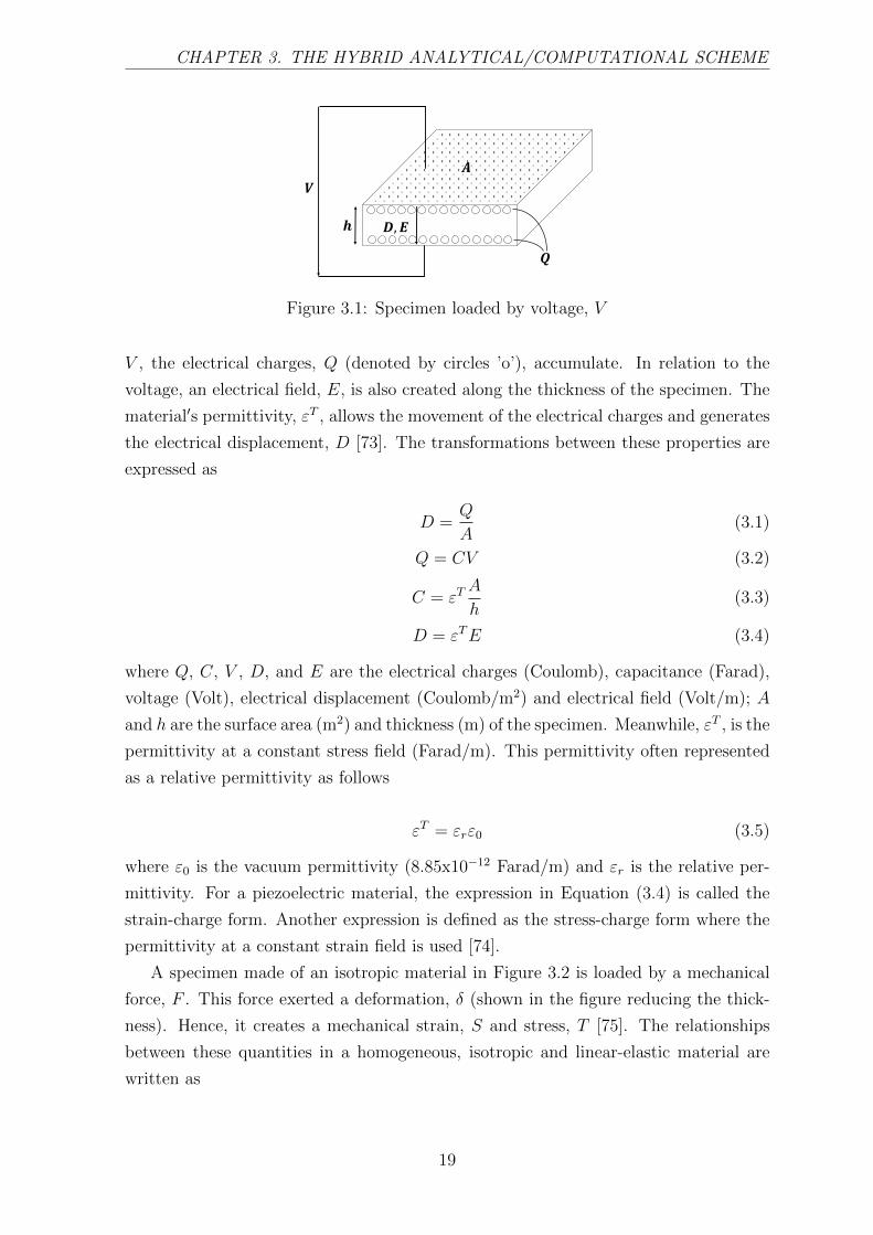
CHAPTER 3. THE HYBRID ANALYTICAL/COMPUTATIONAL SCHEME
𝑽
𝑨
𝑫,𝑬
𝑸
𝒉
Figure 3.1: Specimen loaded by voltage, V
V , the electrical charges, Q (denoted by circles ’o’), accumulate. In relation to the
voltage, an electrical field, E, is also created along the thickness of the specimen. The
material′s permittivity, εT , allows the movement of the electrical charges and generates
the electrical displacement, D [73]. The transformations between these properties are
expressed as
D =Q
A(3.1)
Q = CV (3.2)
C = εTA
h(3.3)
D = εTE (3.4)
where Q, C, V , D, and E are the electrical charges (Coulomb), capacitance (Farad),
voltage (Volt), electrical displacement (Coulomb/m2) and electrical field (Volt/m); A
and h are the surface area (m2) and thickness (m) of the specimen. Meanwhile, εT , is the
permittivity at a constant stress field (Farad/m). This permittivity often represented
as a relative permittivity as follows
εT = εrε0 (3.5)
where ε0 is the vacuum permittivity (8.85x10⁻¹² Farad/m) and εr is the relative per-
mittivity. For a piezoelectric material, the expression in Equation (3.4) is called the
strain-charge form. Another expression is defined as the stress-charge form where the
permittivity at a constant strain field is used [74].
A specimen made of an isotropic material in Figure 3.2 is loaded by a mechanical
force, F . This force exerted a deformation, δ (shown in the figure reducing the thick-
ness). Hence, it creates a mechanical strain, S and stress, T [75]. The relationships
between these quantities in a homogeneous, isotropic and linear-elastic material are
written as
19

CHAPTER 3. THE HYBRID ANALYTICAL/COMPUTATIONAL SCHEME
𝑨
𝑭
𝑻, 𝑺𝜹
𝒉
Figure 3.2: Specimen loaded by force, F
T =F
A(3.6)
S =δ
h(3.7)
S = sT (3.8)
In a piezoelectric material, the electrical and mechanical domains are coupled. Me-
chanical stress could generate an electrical displacement, and an electrical field could
create a mechanical strain. In a strain-charge form, this coupling is defined by a piezo-
electric charge constant, d. This charge constant relates the structural deformation
generated by a unit of voltage; and vice versa [73]. Based on the IEEE Standard
on Piezoelectricity [74], the constitutive relations in Equations (3.4) and (3.8) can be
coupled as a set of electromechanical equations and can be expressed as
D = εE + dT (3.9)
S = dE + sT (3.10)
Ballas [76] derived the mathematical models of a piezoelectric beam bending ac-
tuator exerted by static and dynamic bending loads. The composite beam made of
substrate layers (host structure; non-piezoelectric material) and electrically active lay-
ers (piezoelectric material) is concerned in [76]. The illustration of this beam is shown
in Figure 3.3.
The following assumptions were taken by Ballas in [76]:
1. The electrical field only generated in the thickness direction (poling direction)
E2 = E3 = 0 & E1 6= 0;
2. Only one mechanical stress component generated in the longitudinal direction
T1 = T2 = T4 = T5 = T6 = 0 & T3 6= 0;
3. All active layers are driven by the same voltage along the poling direction, V 1.
20

CHAPTER 3. THE HYBRID ANALYTICAL/COMPUTATIONAL SCHEME
𝒂𝒄𝒕𝒊𝒗𝒆 𝒍𝒂𝒚𝒆𝒓
𝒔𝒖𝒃𝒔𝒕𝒓𝒂𝒕𝒆 𝒍𝒂𝒚𝒆𝒓
𝒏𝒆𝒖𝒕𝒓𝒂𝒍 𝒂𝒙𝒊𝒔𝒙, 𝟑
𝒚, 𝟐
𝒛, 𝟏
Figure 3.3: A cantilevered multilayer beam with piezoelectric layer
Hence, Equations (3.9) and (3.10) can be rewritten as
D1 = εT11E1 + d31T3 (3.11)
S3 = d31E1 + s33T3 (3.12)
In Figure 3.4, illustration of a mechanical load in the form of bending moment, M ,
acting on a cantilever beam is shown. Here, the bending deformation can be quantified
by a transverse displacement, ζ, and a bending slope, θ. In addition, at an arbitrary
point,P , located at a distance, z, from the neutral axis, a strain is generated.
𝒙, 𝟑
𝒚, 𝟐
𝒛, 𝟏𝑷
𝑷′
𝑴
𝜁𝜃
𝑷𝑷′
𝜃
𝛿
𝑧
Figure 3.4: A cantilever beam loaded by bending moment, M
The mechanical strain at x-direction is written as
S3 = −z ∂2ζ
∂x2(3.13)
In the active layer, the electrical voltage, V , creates an electrical field, E, as depicted
in Figure 3.5.
V =
∫ hu
hl
E1dz (3.14)
Incorporating Equations (3.13) and (3.14) into Equations (3.11) and (3.12), yields
21

CHAPTER 3. THE HYBRID ANALYTICAL/COMPUTATIONAL SCHEME
𝑽
𝒙, 𝟑
𝒚, 𝟐
𝒛, 𝟏
𝒉
𝒉𝒍𝒉𝒖
𝑳
𝑫, 𝑬
Figure 3.5: A cantilever beam with piezoelectric layer loaded by voltage, V
D1 =V
h
(εT11 −
d231
s33
)− d31(h2
u − h2l )
2s33h
∂2ζ
∂x2(3.15)
Moreover, the electrical charges at a certain point, Q, is evaluated through the
Gauss′s theorem over an area, A, as
Q =
∮D1 dA (3.16)
Thus, considering a uniform cross section depicted in Figure 3.6, the electrical charges,
Q(x), from the root until a certain point at length x, could be defined as
Q(x) =V (x)bx
h
(εT11 −
d231
s33
)− d31(h2
u − h2l )b
2s33h
∂ζ(x)
∂x(3.17)
𝑨
𝒉
𝒙
𝒃
Figure 3.6: A cantilever beam with uniform cross-section
In the present work, two parameters are defined as
Γ1 =bx
h
(εT11 −
d231
s33
)(3.18)
and,
Γ2 =d31(h2
u − h2l )b
2s33h(3.19)
For a time-dependant motion, Equation (3.17) becomes
22

CHAPTER 3. THE HYBRID ANALYTICAL/COMPUTATIONAL SCHEME
Q(x, t) = Γ1(x)V (x, t)− Γ2(x)∂ζ(x, t)
∂x(3.20)
The parameter Γ2 defines an internal bending moment, Mpiezo, exerted by a unit of
voltage, V .
Mpiezo = Γ2V (3.21)
The concept of Mpiezo was applied by Ballas [76] to evaluate the static deformation
of a voltage-driven piezoelectric beam actuator. This concept has been well validated
experimentally [76].
In the present work, Equation (3.20) is further elaborated for the energy harvesting
purpose. An electrical circuit connected to the piezoelectric beam is considered.
dQ(x, t)
dt= I(x, t) =
V (x, t)
R(3.22)
where, I is the electrical current (Ampere) and R is the resistance load (Ohm, Ω).
Incorporating Equation (3.20) to Equation (3.22), yields a differential equation in
terms of V ,
Γ1dV (x, t)
dt− Γ2
d
dt
(∂ζ(x, t)
∂x
)=V (x, t)
R(3.23)
Assumes a harmonic oscillation motion
ζ(x, t) = Z(x)eiωt (3.24)
V (x, t) = V (x)eiωt (3.25)
where Z is the transverse displacement amplitude (meter) and V is the voltage
amplitude.
Equation (3.23) becomes
iωΓ1V − iωΓ2∂Z(x)
∂x=V
R(3.26)
Concerning the electromechanical coupling effect, it is critical to remark that the
displacement, Z(x), is comprised of the displacement exerted by a mechanical load,
Zmech, and an accumulated electrical load, Zelec. Thus,
∂Z
∂x=∂Zmech∂x
+∂Zelec∂x
(3.27)
The Zelec is generated by the internal forces due to the reverse piezoelectric effect.
By employing the concept of Mpiezo, the bending slope due to the electrical load is
defined as
23

CHAPTER 3. THE HYBRID ANALYTICAL/COMPUTATIONAL SCHEME
∂Zelec∂x
= HαmMpiezo (3.28)
or,∂Zelec∂x
= HαmΓ2V (3.29)
Here, Hαm is the admittance function (rad/Newton-meter) of the displacement
slope (rad) due to a unit of moment applied at the tip. This admittance function can
be obtained straightforwardly by analytical method [76] or via computational analysis.
As stated by Erturk and Inman in [20], early works in piezoelectric energy harvesting
as can be found in [77, 78], were lacking this reverse effect. Hence, the responses were
highly inaccurate and overestimated the experimental results.
As far as the author′s knowledge, the concept of Mpiezo had only been used for
the actuator case. Therefore, for energy harvesting purpose it is a novel concept to
evaluate the reverse piezoelectric effect.
Furthermore, incorporating Equations (3.27) and (3.29), then Equation (3.26) be-
comes
V (x) =iωΓ2(x)∂Zmech(x)
∂x
− 1R
+ iωΓ1(x)− iωΓ2(x)2Hαm(x)(3.30)
Concerning the voltage along the length of the beam (x = L), Equation (3.30) is
rewritten as
V (L) =iωΓ2(L)∂Zmech(L)
∂x
− 1R
+ iωΓ1(L)− iωΓ2(L)2Hαm(L)(3.31)
The maximum electrical power, Pmax (Watt), is given as
Pmax =V 2
R(3.32)
Figure 3.7 illustrates a cantilevered piezoelectric energy harvester exerted by two
types of loading. The bending moment, M , as the mechanical load and the resistance,
R, as the electrical load.
3.2 Code algorithm
In the present work, a computational code is built using MATLAB© to estimate the
voltage and power responses based on Equations (3.31) and (3.32). The algorithm of
the present code is depicted in Figure 3.8.
Two key inputs for the present code are
24

CHAPTER 3. THE HYBRID ANALYTICAL/COMPUTATIONAL SCHEME
𝒏𝒆𝒖𝒕𝒓𝒂𝒍 𝒂𝒙𝒊𝒔
𝑴
𝑹
𝒙, 𝟑𝒚, 𝟐
𝒛, 𝟏
𝒉
𝒉𝒍𝒉𝒖
𝑳
Figure 3.7: A cantilevered piezoelectric energy harvester exerted by mechanical and
electrical loads
Analytical / Computational model
Actual mechanical load (Force, Moment, etc.)
Dummy mechanical load(1 unit of Moment at beam’s neutral axis tip)
Complex conjugate bending angle, 𝜕𝑍𝑚𝑒𝑐ℎ
𝜕𝑥
Admittance function (complex conjugate bending angle per 1 unit
of moment), 𝐻𝛼𝑚
Material properties and geometry, Γ1 and Γ2
Set of Resistance load, 𝑅
Governing piezoelectric energy harvester voltage
equation
Voltage and Power for the set of 𝑅
Figure 3.8: Schematic diagram of the energy harvesting system evaluation process
1. the displacement slope (bending angle) function due to the (actual) mechanical
loading, ∂Zmech
∂x, and
2. the admittance function of bending angle due to a unit of moment, Hαm.
The admittance function, Hαm, can be obtained by applying a dummy load represented
by one unit (i.e. 1 Nm) of moment at the neutral axis of the beam′s tip.
In the current work, a computational method, i.e. finite element method (FEM),
is applied to obtain both of these inputs. Dynamic analysis via FEM is concerned
to evaluate a complex geometry. Hence, the scheme provided here is called a hybrid
analytical/computational scheme. Hereafter, for simplification, this scheme will also
be called the hybrid scheme. However, the hybrid is not limited to the inputs from
25
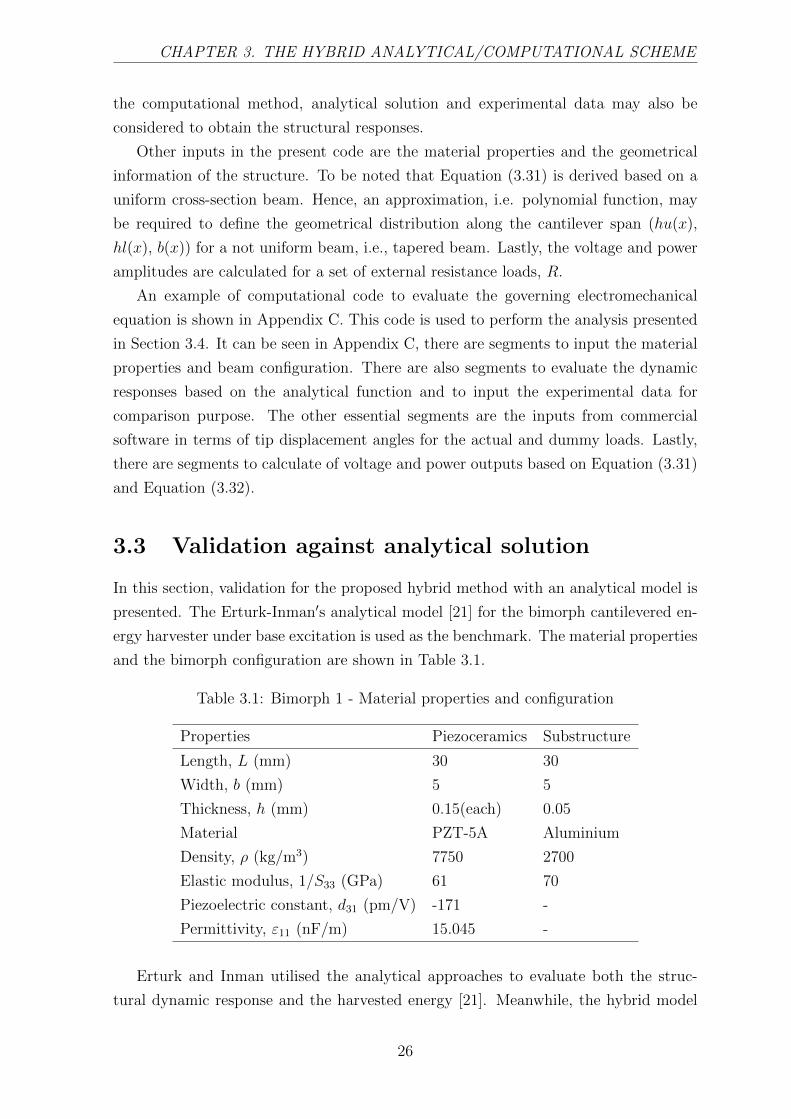
CHAPTER 3. THE HYBRID ANALYTICAL/COMPUTATIONAL SCHEME
the computational method, analytical solution and experimental data may also be
considered to obtain the structural responses.
Other inputs in the present code are the material properties and the geometrical
information of the structure. To be noted that Equation (3.31) is derived based on a
uniform cross-section beam. Hence, an approximation, i.e. polynomial function, may
be required to define the geometrical distribution along the cantilever span (hu(x),
hl(x), b(x)) for a not uniform beam, i.e., tapered beam. Lastly, the voltage and power
amplitudes are calculated for a set of external resistance loads, R.
An example of computational code to evaluate the governing electromechanical
equation is shown in Appendix C. This code is used to perform the analysis presented
in Section 3.4. It can be seen in Appendix C, there are segments to input the material
properties and beam configuration. There are also segments to evaluate the dynamic
responses based on the analytical function and to input the experimental data for
comparison purpose. The other essential segments are the inputs from commercial
software in terms of tip displacement angles for the actual and dummy loads. Lastly,
there are segments to calculate of voltage and power outputs based on Equation (3.31)
and Equation (3.32).
3.3 Validation against analytical solution
In this section, validation for the proposed hybrid method with an analytical model is
presented. The Erturk-Inman′s analytical model [21] for the bimorph cantilevered en-
ergy harvester under base excitation is used as the benchmark. The material properties
and the bimorph configuration are shown in Table 3.1.
Table 3.1: Bimorph 1 - Material properties and configuration
Properties Piezoceramics Substructure
Length, L (mm) 30 30
Width, b (mm) 5 5
Thickness, h (mm) 0.15(each) 0.05
Material PZT-5A Aluminium
Density, ρ (kg/m3) 7750 2700
Elastic modulus, 1/S33 (GPa) 61 70
Piezoelectric constant, d31 (pm/V) -171 -
Permittivity, ε11 (nF/m) 15.045 -
Erturk and Inman utilised the analytical approaches to evaluate both the struc-
tural dynamic response and the harvested energy [21]. Meanwhile, the hybrid model
26

CHAPTER 3. THE HYBRID ANALYTICAL/COMPUTATIONAL SCHEME
can use both the structural dynamic responses based on the analytical solution and
FEM simulation to estimate the harvested energy. An industrial finite element soft-
ware [79] is used in the present work. Bi-linear quadrilateral elements and the direct
frequency response module are applied. The meshes of 2 x 12 equal sized elements are
implemented. A MATLAB© code is written to obtain the analytical solution of the
structural dynamic response.
Table 3.2: Bimorph 1 - Natural frequency comparison
Natural frequency (Hz)
Mode Shape Erturk - Inman [21] Analytical - Present FEM - Present
1st Bending 185.1 185.1 187
2nd Bending 1159.8 1160.1 1162.3
3rd Bending 3247.6 3248.3 3238.5
Table 3.3: Bimorph 1 - Relative tip displacement & tip angle comparison
Parameter Erturk - Inman [21] Analytical - Present FEM - Present
Tip displacement (µm) 78.0 78.3 78.3
Tip angle (rad) 3.59e-3 3.60e-3 3.60e-3
Table 3.2 shows comparison of the natural frequencies for both the analytical solu-
tion and FEM results of the present work are in a good agreement with Erturk-Inman′s
results [21]. Meanwhile, Table 3.3 shows the comparison of the relative tip displace-
ments and angles due to 1 µm base excitation amplitude at the resonance frequency
of the first bending. The tip displacements and angles of all three procedures are also
well agreed.
For comparison purpose, a separate code via MATLAB© is built to reconstruct
Erturk and Inman′s electromechanical model for a bimorph cantilevered piezoelectric
energy harvester under base excitation [21]. Using the configuration from Table 3.1,
the harvested energy with series connection is evaluated.
Figure 3.9 and Figure 3.10 show the voltage and amplitudes of the 3 different
procedures at the first resonance′s excitation frequency. Denoted by ”Present Model
(Analytical)” is the result of the present hybrid model combined with the analytical
structural dynamic solutions. Meanwhile, the result via coupling with the FEM model
is denoted by ”Present Model (FEM)”.
The figures are in logarithmic to logarithmic scale, where both the voltage and
power are normalized per unit of g (9.81 m/s2) and g2, following the way it is presented
in [21]. Value of ”V per g” is obtained from the voltage amplitude divided by the base
27

CHAPTER 3. THE HYBRID ANALYTICAL/COMPUTATIONAL SCHEME
103 104 105 106 107
Resistance ( )
10-1
100
101
Vo
ltag
e (V
per
g)
Voltage Amplitude vs Resistance
Erturk-Inman ModelPresent Model (FEM)Present Model (Analytical)
8 8.5 9 9.5 10
105
5.4
5.45
5.5
5.55
Figure 3.9: Bimorph 1 - Variation of the voltage amplitude with the resistance load
acceleration ratio to g, i.e. base amplitude 1 µm and 150 Hz excitation equal with 0.89
m/s2 base acceleration or 0.09 acceleration ratio. Meanwhile, the electrical power is
normalized per unit g2, or power divided by the square of the acceleration ratio.
Figure 3.9 and Figure 3.10 depict that the voltage and power amplitude for the 3
procedures are almost coincide. In the enlarged view, in a smaller range of resistance
loads, it can be seen that the hybrid model results via FEM combination slightly over-
estimates the Erturk-Inman model′s as shown in figures 3.9 and 3.10. Meanwhile, the
hybrid model results via analytical structural response still coincide with the Erturk-
Inman model′s.
All the three procedures show the same trend of voltage and power functions. Ini-
tially, the voltage increases with the resistance load before it is going in asymptotic
behaviour as displayed in Figure 3.9. Mathematically, it can be explained via Equation
(3.30), as the resistance load is very large, close to the open circuit (R→∞), the effect
of the resistance load will vanish. Hence, the voltage function will be reduced as only
a function of material properties, configuration and displacements.
The power function, as a result of the voltage function′s asymptotic behaviour, will
initially increases with the resistance load until it reaches a maximum point. This
maximum point, is the point before the voltage goes asymptotic. Thus, beyond this
point, increasing the resistance load will only decrease the harvested power as the
voltage is almost constant. As it can be seen from Equation (3.32), if the voltage is
constant while the resistance load is getting closer to the open circuit (R → ∞), the
harvested power will be diminished (Pmax → 0).
Detailed comparison for the maximum voltage and power amplitude are given in
28

CHAPTER 3. THE HYBRID ANALYTICAL/COMPUTATIONAL SCHEME
103 104 105 106 107
Resistance ( )
100
101
102
103
Po
wer
(W
per
g2)
Power Amplitude vs Resistance
Erturk-Inman ModelPresent Model (FEM)Present Model (Analytical)
2.5 3 3.5 4 4.5 5
104
215
220
225
230
235
Figure 3.10: Bimorph 1 - Variation of the power amplitude with the resistance load
Table 3.4. It can be seen that the variances are insignificant (less than 2%).
Table 3.4: Bimorph 1 - Electrical parameters comparison
Electrical Erturk- Present Model Present Model
parameters Inman [80] (Analytical) (FEM)
Max Voltage (mV) 782.10 782.10 ∆=0.0% 782.80 ∆=0.09%
Max Power (µW) 4.35 4.35 ∆=0.0% 4.40 ∆=1.15%
R at Max Power (kΩ) 35.90 35.90 ∆=0.0% 35.96 ∆=0.17%
3.4 Validation against experimental result
This section presents the comparison of the results obtained via the present hybrid
method and the experiment done by Erturk - Inman [22]. Table 3.5 depicts the material
properties and the configuration of the investigated bimorph.
A case of 1 µm base excitation amplitude is evaluated. The first resonance frequency
is applied as the excitation frequency. The analytical and FEM model predicted 502.6
Hz as the fundamental first bending natural frequency. It is well agreed with the value
of 502.5 Hz obtained from the experiment done by Erturk and Inman [22].
Figure 3.11 and Figure 3.12 show the variations of voltage and power amplitudes
against the resistance loads for 4 different procedures. Both figures display the results
from the Erturk-Inman analytical model, the present hybrid methods via analytical
and FEM coupling, and lastly the experiment. The figures are also in logarithmic to
29

CHAPTER 3. THE HYBRID ANALYTICAL/COMPUTATIONAL SCHEME
Table 3.5: Bimorph 2 - Material properties and configuration
Properties Piezoceramics Substructure
Length, L (mm) 24.53 24.53
Width, b (mm) 6.4 6.4
Thickness, h (mm) 0.265(each) 0.140
Material PZT-5H Brass
Density, ρ (kg/m3) 7500 9000
Elastic modulus, 1/S33 (GPa) 60.6 105
Piezoelectric constant, d31 (pm/V) -274 -
Permittivity, ε11 (nF/m) 30.09 -
logarithmic scale, where both the voltage and power are normalized per unit of g (9.81
m/s2) and g2.
102 103 104 105 106 107
Resistance ( )
10-3
10-2
10-1
100
101
102
Vo
ltag
e (V
per
g)
Voltage Amplitude vs Resistance
Erturk-Inman ModelPresent Model (FEM)Present Model (Analytical)Erturk-Inman Experiment
6000 8000 10000
1.2
1.3
1.4
1.5
Figure 3.11: Bimorph 2 - Variation of the voltage amplitude with the resistance load
30

CHAPTER 3. THE HYBRID ANALYTICAL/COMPUTATIONAL SCHEME
102 103 104 105 106 107
Resistance ( )
10-1
100
101
102
103
104
Po
wer
(W
per
g2)
Power Amplitude vs Resistance
Erturk-Inman ModelPresent Model (FEM)Present Model (Analytical)Erturk-Inman Experiment
6000 8000 10000210
215
220
225
Figure 3.12: Bimorph 2 - Variation of the power amplitude with the resistance load
It can be seen that all 4 procedures are in a good agreement. In the enlarged view, it
is shown that the results from the present hybrid method via FEM coupling just slightly
overestimate the analytical and experimental results. Similar behaviours as presented
in Section 3.3 are also captured in Figures 3.11 and 3.12. The voltage functions for all
procedures go asymptotic towards the open circuit condition (R → ∞). Meanwhile,
the power functions achieved a maximum value before declining as the resistance going
towards the open circuit.
All the models predicted the value of resistance load at the maximum power ampli-
tude is 7.6 kΩ. The Erturk-Inman model estimates the maximum power of 224.89 µW.
Meanwhile, the present hybrid model via FEM coupling predicts as much as 227.64 µW,
overestimates Erturk-Inman model’s by only 1.22 %. In addition, both procedures are
also well agreed in the estimation of the maximum voltage, 2.62 V by Erturk-Inman’s
and 2.61 V via the present model (FEM), respectively. However, the resistance value
of 7.6 kΩ was not used in the experiment. The nearest value used was 6.7 kΩ [22].
Therefore, the output parameters obtained by the models and the experiment for 6.7
kΩ are compared as displayed in Table 3.6.
Table 3.6: Bimorph 2 - Electrical parameters comparison at R = 6.7 kΩ
Electrical Erturk-Inman Erturk-Inman Present Model
parameters Model [22] Experiment [22] (FEM)
Voltage (V) 1.225 1.230 ∆=0.41% 1.232 ∆=0.57%
Power (µW) 223.92 225.77 ∆=0.83% 226.63 ∆=1.21%
31

CHAPTER 3. THE HYBRID ANALYTICAL/COMPUTATIONAL SCHEME
It can be seen in Table 3.6, the variances of the voltage and power amplitudes
between the models’ and the experiment’s are insignificant. The maximum variance is
only 1.21 %, coming from the power comparison between the present model via FEM
coupling and the Erturk-Inman model.
3.5 Validation against electro-mechanically coupled
FEM
In this subsection, the comparison of the present hybrid method and the electro-
mechanically coupled FEM investigation of De Marqui Jr. et al. [10] is discussed.
Energy harvested from a UAV wing spar is evaluated. The spar is a bimorph plate
with the material properties and geometry as shown in Table 3.7. The piezoelectric
layer is connected as series configuration, and the load source is the base excitation
motion.
Table 3.7: Material properties and geometry of the bimorph UAV wingspar
Dimension of The Beam
Total Length, L (mm) 300
Total Width, b (mm) 30
Total Thickness, h (mm) 12
Piezoceramics
ρ (kg/m3) 7800
cE11 (GPa) 120.3
cE12 (GPa) 75.2
cE13 (GPa) 75.1
cE33 (GPa) 110.9
cE66 (GPa) 22.7
e31 (C/m2) -5.2
e33 (C/m2) 15.9
ε11 (nF/m) 15.93
Host-structure (Aluminum)
ρ (kg/m3) 2750
E (GPa) 70
In Table 3.7, the piezoelectric properties are shown in 3D orthotropic of the stress-
charge form [74]. The cE11, cE12, ..., c
E66 are the components of elastic stiffness of the
mechanical constitutive relations. The e31, e32, e33 are the components of piezoelectric
charge constant.
32

CHAPTER 3. THE HYBRID ANALYTICAL/COMPUTATIONAL SCHEME
De Marqui Jr. et al. [10] adopted Kirchhoff plate theory to develop the electrome-
chanically coupled finite element model of the piezoelectric energy harvester. The
piezoceramic layer is assumed poled in the thickness direction; thus, align with the
assumption used in Section 3.1. The piezoceramic layer is also assumed covered by a
continuous electrode and perfectly bonded to the host-structure. It is assumed very thin
and conductive electrode layers are on the top and bottom surfaces of the piezoceramic
layers. Hence, it is assumed that all finite elements generate the same voltage output.
Furthermore, one degree of freedom is used as the voltage output degree of freedom of
each element. The reader is referred to [10] for the detail of their formulation.
Rayleigh mechanical damping is used in the finite element formulation. The damp-
ing is assumed proportional to the mass and stiffness matrices with the constant of
proportionality α and β. Thus the critical damping ratio ζ is written as
ζ =α
2ωn+ωnβ
2(3.33)
where ωn is the natural frequency of the structure. In the case presented in this
subsection, α = 21.28 rad/s and β = 10−5 s/rad are used.
The configuration of the spar is limited to 10% additional mass of the full aluminum
spar mass. Therefore, a restriction of length and thickness of the piezoelectric layer, L∗
x h∗ ≤ 0.02723, is applied. L∗ is the ratio of piezoelectric length to the total length of
the beam and h∗ is the thickness ratio of one piezoelectric layer to the total thickness
of the beam. The relationship of L∗ × h∗ boundary is shown in Figure 3.13.
0.1 0.2 0.3 0.4 0.5 0.6 0.7 0.8 0.9 1
L* (Length Ratio)
0
0.05
0.1
0.15
0.2
0.25
0.3
h*
(Th
ickn
ess
Rat
io)
Length Ratio vs Thickness Ratio
Figure 3.13: Variation of the thickness ratio, h*, with the length ratio, L*, of the spar
As the length and thickness of the piezoelectric layers and the aluminum layer
are varied and not uniform along the span, thus, the analytical solution of [21] is not
applicable. Thus, in this subsection, the comparison is only applied to the hybrid model
with FEM combination. Figure 3.14 shows the variation of the 1st Bending natural
frequency and the critical damping ratio for various length ratio, L∗.
33

CHAPTER 3. THE HYBRID ANALYTICAL/COMPUTATIONAL SCHEME
0 0.2 0.4 0.6 0.8 1
L* (Length Ratio)
100
101
102
103
104
105
106
107
108
109
110
Fre
qu
ency
(H
z)
Length Ratio vs Short-circuit Resonance Frequency
De Marqui Jr. et al. - FEMPresent Model (FEM)
(a)
0 0.2 0.4 0.6 0.8 1
L* (Length Ratio)
0.0185
0.019
0.0195
0.02
0.0205
(D
amp
ing
Rat
io)
Length Ratio vs Critical Damping Ratio
De Marqui Jr. et al - FEMPresent Model (FEM)
(b)
Figure 3.14: Variation of the (a) natural frequency, (b) critical damping ratio with the
length ratio of the spar
It is seen from Figure 3.14 the trends of the natural frequency and damping ratio
for all three procedures are all in good comparison. The total mass of the beam is fixed
at 1.1 × full aluminum mass, and the cross section shape is maintained. Therefore, the
only variation that is affecting the change of the natural frequency is the composite
material properties along the span.
In general, the natural frequency is decreasing from L∗ = 0.1 to 1. However, from
L∗ = 0.25 to 0.4 a slight increment occurs, despite it is followed by a significant drop
from L∗ = 0.8 to 1. This trend is caused by a reduced stiffness of the piezo-aluminum
composite beam as the piezoceramics layers approaches L∗ = 1. In addition, for a
benchmark, analytically the natural frequency of a full aluminum spar is 108.79 Hz.
The maximum power and the optimum resistance load for various length ratio are
depicted in Figure 3.15a and Figure 3.15b. All of the three procedures are also in good
agreement. The maximum power increased at first and reached its highest point at L∗
= 0.225 before it significantly drops when L∗ approach 1. In contrast, the optimum
resistance load is decreased with the increment of L∗.
De Marqui Jr. et al. [10] concluded that for very thin piezoceramics, at L∗ >
0.5, the effect of increased dynamic flexibility (decreased natural frequency, Figure
3.14a) is not able to overcome the increased structural damping as shown in Figure
3.14b. Therefore, although the flexibility is increased, the amplitude of the vibration is
reduced. It resulted in the decrease of the power harvested as shown in Figure 3.15a.
This behavior is aligned with Equation (3.30) in which the energy output is influenced
by the displacement variation along the structural element.
Figure 3.16 depicts the variation of the power amplitude with the resistance load
for different length ratio. The black cross ”x” denoted L∗ = 1 and the blue plus ”+”
34

CHAPTER 3. THE HYBRID ANALYTICAL/COMPUTATIONAL SCHEME
0 0.2 0.4 0.6 0.8 1
L* (Length Ratio)
100
110
120
130
140
150
160
170
Po
wer
(m
W/g
2)
Length Ratio vs Maximum Power
De Marqui Jr. et al - FEMPresent Model (FEM)
(a)
0 0.2 0.4 0.6 0.8 1
L* (Length Ratio)
0
50
100
150
200
250
300
350
400
450
500
Res
ista
nce
Lo
ad (
k)
Length Ratio vs Resistance at Maximum Power
De Marqui Jr. et al - FEMPresent Model (FEM)
(b)
Figure 3.15: Variation of the (a) maximum power amplitude and (b) optimum resis-
tance load with the length ratio of the spar
denoted L∗ = 0.1. It can be seen that the Power-Resistance curve is shifting from left
to right as the L∗ decreases. In alignment with Equation (3.18), thinner and longer
piezoelectric layer means Γ1 parameter is increased. Thus, the voltage function reached
the asymptotic behavior at smaller resistance load.
102 103 104 105 106 107 108
Resistance ( )
101
102
103
104
105
106
Po
wer
(W
per
g2)
Power Amplitude vs Resistance
L*=0.1L*=0.2L*=0.4L*=0.6L*=0.8L*=1.0
L* decrease
Figure 3.16: Variation of the power amplitude with the resistance load for various
length ratio of the spar
In detail, the comparison of the natural frequency and maximum power obtained
from the present hybrid model and the results of [10] is presented in Table 3.8. The 1st
bending natural frequency is denoted by ”F” and the maximum power is denoted by
”P”. The subscripts ”DMJ” and ”Present” represent the results of [10] and the ones
35
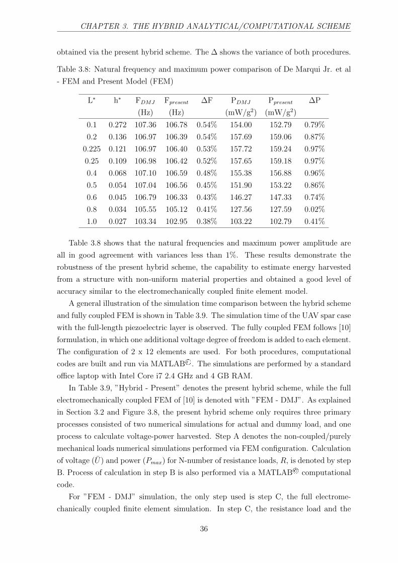
CHAPTER 3. THE HYBRID ANALYTICAL/COMPUTATIONAL SCHEME
obtained via the present hybrid scheme. The ∆ shows the variance of both procedures.
Table 3.8: Natural frequency and maximum power comparison of De Marqui Jr. et al
- FEM and Present Model (FEM)
L∗ h∗ FDMJ Fpresent ∆F PDMJ Ppresent ∆P
(Hz) (Hz) (mW/g2) (mW/g2)
0.1 0.272 107.36 106.78 0.54% 154.00 152.79 0.79%
0.2 0.136 106.97 106.39 0.54% 157.69 159.06 0.87%
0.225 0.121 106.97 106.40 0.53% 157.72 159.24 0.97%
0.25 0.109 106.98 106.42 0.52% 157.65 159.18 0.97%
0.4 0.068 107.10 106.59 0.48% 155.38 156.88 0.96%
0.5 0.054 107.04 106.56 0.45% 151.90 153.22 0.86%
0.6 0.045 106.79 106.33 0.43% 146.27 147.33 0.74%
0.8 0.034 105.55 105.12 0.41% 127.56 127.59 0.02%
1.0 0.027 103.34 102.95 0.38% 103.22 102.79 0.41%
Table 3.8 shows that the natural frequencies and maximum power amplitude are
all in good agreement with variances less than 1%. These results demonstrate the
robustness of the present hybrid scheme, the capability to estimate energy harvested
from a structure with non-uniform material properties and obtained a good level of
accuracy similar to the electromechanically coupled finite element model.
A general illustration of the simulation time comparison between the hybrid scheme
and fully coupled FEM is shown in Table 3.9. The simulation time of the UAV spar case
with the full-length piezoelectric layer is observed. The fully coupled FEM follows [10]
formulation, in which one additional voltage degree of freedom is added to each element.
The configuration of 2 x 12 elements are used. For both procedures, computational
codes are built and run via MATLAB©. The simulations are performed by a standard
office laptop with Intel Core i7 2.4 GHz and 4 GB RAM.
In Table 3.9, ”Hybrid - Present” denotes the present hybrid scheme, while the full
electromechanically coupled FEM of [10] is denoted with ”FEM - DMJ”. As explained
in Section 3.2 and Figure 3.8, the present hybrid scheme only requires three primary
processes consisted of two numerical simulations for actual and dummy load, and one
process to calculate voltage-power harvested. Step A denotes the non-coupled/purely
mechanical loads numerical simulations performed via FEM configuration. Calculation
of voltage (U) and power (Pmax) for N-number of resistance loads, R, is denoted by step
B. Process of calculation in step B is also performed via a MATLAB© computational
code.
For ”FEM - DMJ” simulation, the only step used is step C, the full electrome-
chanically coupled finite element simulation. In step C, the resistance load and the
36

CHAPTER 3. THE HYBRID ANALYTICAL/COMPUTATIONAL SCHEME
Table 3.9: Simulation time comparison
Simulation Time (s)
100 no. of R 10000 no. of R
Steps Hybrid-Present FEM-DMJ Hybrid-Present FEM-DMJ
A. Non-coupled 2 x 15 - 2 x 15 -
simulations
B. U and Pmax 5 - 15 -
calculations
C. Fully coupled - 100 - 10000
simulations x 20 x 20
TOTAL 35 2000 45 20000
mechanical load are both given as the excitation source on the finite elements, while
both the structural deformation and voltage responses are obtained directly as the
output of FEM simulation. It is assumed that for a set of N-numbers of R, N-times of
simulations is required.
As shown in Table 3.9, step A shows fixed simulation time, 2 x 15 seconds. The
elapsed time for the actual load (base excitation) and the dummy load ( the moment
at the tip) are around 15 seconds each and independent to the number of R. In step B,
shows an increment of computing time as the number of resistance loads is increasing.
For a set of 100 variances of R, the elapsed time is less than 5 seconds. While for
10000 numbers of R, around 15 seconds computing time is required. Therefore, in
total, ”Hybrid - Present” simulations require 35 seconds for 100 variances of R, and 45
seconds for 10000 numbers of R.
In contrast, the simulation time required for ”FEM - DMJ”, step C, is purely
dependent on the number of R observed. For a simulation with one resistance load, it
only requires less than 20 seconds. However, the simulation times are multiplied with
N-number of R investigated. Therefore, if 100 number of R used, then 2000 seconds
is required. Furthermore, if 10000 number of R used, then 200000 seconds or around
56 hours is required. Interesting to note that to produce a plot with the level of detail
such as shown in Figure 3.16, a set of R from 102 to 108 Ω with 100 Ω step is used.
Thus, to produce this plot utilizing the present hybrid scheme only need less than 1
minute, while with full electromechanically coupled FEM will require around 56 hours.
The independence on the number of simulations on the hybrid scheme is bene-
ficial especially in a preliminary/conceptual design stage, in which a faster iterative
design process to obtain an optimal harvester structural design and resistance load is
achievable. However, despite the higher computational cost, a full electromechanically
coupled FEM may provide more details for a particular area of interests, i.e., the region
37

CHAPTER 3. THE HYBRID ANALYTICAL/COMPUTATIONAL SCHEME
near optimum resistance load. Thus, the hybrid scheme may build the fundamental
sense of the best harvester design at the early design stage, while more detailed analy-
sis may be provided by fully coupled FEM at the later design phase. Furthermore, an
illustration is given in Chapter 4 to show the computational time of a larger structure,
i.e, aircraft wingbox, via the present hybrid scheme.
3.6 Investigation by higher-order elements
In this section, the robustness of the present hybrid scheme with higher-order elements
is elaborated to investigate very thin structural configurations. Isogeometric Analysis
(IGA) is implemented to perform the structural analysis. IGA was first proposed by
Hughes et al. [81]. They utilised Non-Uniform Rational B-Spline (NURBS) function to
construct a so-called basis function of IGA elements, analogous to the shape function
of finite element. The main attribute of NURBS-based IGA is the ability to estab-
lish numerical engineering analysis within the same model from the computational
engineering design/drawing. Hence, decreasing the cost of numerical analysis-design
interface and improving the accuracy compared to the standard finite element [81].
In the present work, another advantage of IGA is focused. In this section, the
advantage of IGA against shear locking phenomena on a thin shells and its effect on
the energy harvesting response is focused. Piezoelectric structures often manufactured
as thin-walled structures; hence a problem of shear locking may occur on the numer-
ical analysis. A study by Thai et al. [82] concluded that higher-order IGA elements
hardly suffer from shear locking phenomena. The shear locking phenomena have been
investigated since the early development of finite elements. It happens when the shear
energy becomes very dominant compared to the bending energy as the thickness of the
element is very small compared to its length [83]. A brief summary on the state-of-the-
art of IGA for solid mechanics is given in Appendix A. To be noted here, the literature
review on IGA is not given in this chapter nor Chapter 2 as the main focus of the work
here is the piezoelectric energy harvesting while IGA is one of supporting the tools to
provide the structural analysis similar to FEM.
In the present study, two different methods, i.e., analytical and numerical, are im-
plemented to perform the structural dynamic analysis. Nine-noded bi-quadratic (Q9)
and 25-noded bi-quartic (Q25) IGA shell elements are utilised. Full integration points,
3 × 3 for bi-quadratic and 5 × 5 for bi-quartic, are used. The same number of elements
as mentioned in Section 3.3, 2 x 12 equal sized elements, is used. Computational codes
are developed in MATLAB© to perform IGA structural dynamic analysis. The detail
of the IGA elements construction can be found in Appendix B. To be noted as well,
the IGA elements development is not discussed in this chapter to allow more focus on
38

CHAPTER 3. THE HYBRID ANALYTICAL/COMPUTATIONAL SCHEME
the piezoelectric energy harvesting aspect.
103 104 105 106 107
Resistance ( )
10-1
100
101
Vo
ltag
e (V
per
g)
Voltage Amplitude vs Resistance
Erturk-Inman ModelPresent Model (IGA Q9)Present Model (IGA Q25)Present Model (Analytical)
8 8.5 9 9.5 10
105
5.4
5.45
5.5
5.55
5.6
Figure 3.17: Investigation by IGA: Voltage amplitude vs resistance
The Bimorph 1 configuration from Table 3.1 is investigated. The energy harvesting
analysis from base excitation case is evaluated. Figure 3.17 and Figure 3.18 show the
generated voltage and maximum power amplitude for a set of resistance load obtained
via Erturk-Inman′s model and the present hybrid scheme. These figures are similar
to those shown in Section 3.3 with the exception of IGA-based analyses replacing the
FEM-based analysis.
It can be seen from Figure 3.17 and Figure 3.18, there is no significant difference
between the results obtained by IGA Q9 and Q25. In order to investigate the effect
of various thickness, the beam with the configuration on Table 3.1 is modified. The
thickness of the beam is varied with h is the investigated thickness and h0 is the
original thickness on Table 3.1. Thus, a ratio of thickness, h0/h is defined as the
non-dimensional parameter.
The thickness ratio of the beam is varied from h0/h = 1 to h0/h = 104. The number
of elements is kept the same. As the thickness ratio, h0/h increases, the investigated
thickness becomes smaller. At h0/h = 104, the length per thickness ratio of the element
is more than 7000 and considered as a very thin element. For comparison, eight-noded
standard finite elements (FEM Q8) are also used for the analysis.
The numerical investigation results show that IGA Q9, Q25, and FEM Q8 elements
are all maintained at a good level accuracy at small thickness ratio. In contrast, at the
larger thickness ratio, shear locking effect started influenced the FEM Q8 elements. The
variation of the tip displacement and tip angle with the thickness ratio are displayed
in Figure 3.19.
39
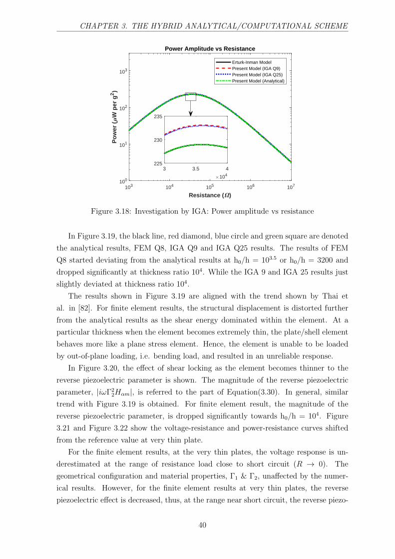
CHAPTER 3. THE HYBRID ANALYTICAL/COMPUTATIONAL SCHEME
103 104 105 106 107
Resistance ( )
100
101
102
103
Po
wer
(W
per
g2)
Power Amplitude vs Resistance
Erturk-Inman ModelPresent Model (IGA Q9)Present Model (IGA Q25)Present Model (Analytical)
3 3.5 4
104
225
230
235
Figure 3.18: Investigation by IGA: Power amplitude vs resistance
In Figure 3.19, the black line, red diamond, blue circle and green square are denoted
the analytical results, FEM Q8, IGA Q9 and IGA Q25 results. The results of FEM
Q8 started deviating from the analytical results at h0/h = 103.5 or h0/h = 3200 and
dropped significantly at thickness ratio 104. While the IGA 9 and IGA 25 results just
slightly deviated at thickness ratio 104.
The results shown in Figure 3.19 are aligned with the trend shown by Thai et
al. in [82]. For finite element results, the structural displacement is distorted further
from the analytical results as the shear energy dominated within the element. At a
particular thickness when the element becomes extremely thin, the plate/shell element
behaves more like a plane stress element. Hence, the element is unable to be loaded
by out-of-plane loading, i.e. bending load, and resulted in an unreliable response.
In Figure 3.20, the effect of shear locking as the element becomes thinner to the
reverse piezoelectric parameter is shown. The magnitude of the reverse piezoelectric
parameter, |iωΓ22Hαm|, is referred to the part of Equation(3.30). In general, similar
trend with Figure 3.19 is obtained. For finite element result, the magnitude of the
reverse piezoelectric parameter, is dropped significantly towards h0/h = 104. Figure
3.21 and Figure 3.22 show the voltage-resistance and power-resistance curves shifted
from the reference value at very thin plate.
For the finite element results, at the very thin plates, the voltage response is un-
derestimated at the range of resistance load close to short circuit (R → 0). The
geometrical configuration and material properties, Γ1 & Γ2, unaffected by the numer-
ical results. However, for the finite element results at very thin plates, the reverse
piezoelectric effect is decreased, thus, at the range near short circuit, the reverse piezo-
40
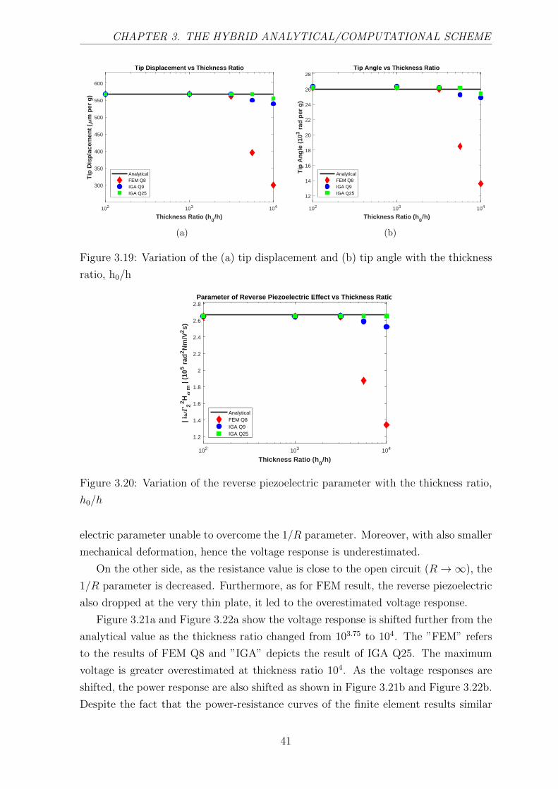
CHAPTER 3. THE HYBRID ANALYTICAL/COMPUTATIONAL SCHEME
102 103 104
Thickness Ratio (h0/h)
300
350
400
450
500
550
600T
ip D
isp
lace
men
t (
m p
er g
)
Tip Displacement vs Thickness Ratio
AnalyticalFEM Q8IGA Q9IGA Q25
(a)
102 103 104
Thickness Ratio (h0/h)
12
14
16
18
20
22
24
26
28
Tip
An
gle
(10
3 r
ad p
er g
)
Tip Angle vs Thickness Ratio
AnalyticalFEM Q8IGA Q9IGA Q25
(b)
Figure 3.19: Variation of the (a) tip displacement and (b) tip angle with the thickness
ratio, h0/h
102 103 104
Thickness Ratio (h0/h)
1.2
1.4
1.6
1.8
2
2.2
2.4
2.6
2.8
| i2
2H
m |
(105
rad
2N
m/V
2s)
Parameter of Reverse Piezoelectric Effect vs Thickness Ratio
AnalyticalFEM Q8IGA Q9IGA Q25
Figure 3.20: Variation of the reverse piezoelectric parameter with the thickness ratio,
h0/h
electric parameter unable to overcome the 1/R parameter. Moreover, with also smaller
mechanical deformation, hence the voltage response is underestimated.
On the other side, as the resistance value is close to the open circuit (R→∞), the
1/R parameter is decreased. Furthermore, as for FEM result, the reverse piezoelectric
also dropped at the very thin plate, it led to the overestimated voltage response.
Figure 3.21a and Figure 3.22a show the voltage response is shifted further from the
analytical value as the thickness ratio changed from 103.75 to 104. The ”FEM” refers
to the results of FEM Q8 and ”IGA” depicts the result of IGA Q25. The maximum
voltage is greater overestimated at thickness ratio 104. As the voltage responses are
shifted, the power response are also shifted as shown in Figure 3.21b and Figure 3.22b.
Despite the fact that the power-resistance curves of the finite element results similar
41

CHAPTER 3. THE HYBRID ANALYTICAL/COMPUTATIONAL SCHEME
103 104 105 106 107
Resistance ( )
10-1
100
101
Vo
ltag
e (V
per
g)
Voltage Amplitude vs Resistance
Erturk-Inman ModelPresent Model (FEM)Present Model (IGA)Present Model (Analytical)
8 8.5 9 9.5 10
105
5.4
5.45
5.5
5.55
5.6
(a)
103 104 105 106 107
Resistance ( )
100
101
102
103
Po
wer
(W
per
g2)
Power Amplitude vs Resistance
Erturk-Inman ModelPresent Model (FEM)Present Model (IGA)Present Model (Analytical)
2.5 3 3.5 4 4.5 5
104
215
220
225
230
235
(b)
Figure 3.21: Bimorph 1 with h0/h = 103.75 - Variation of the (a) voltage amplitude
and (b) power amplitude with the resistance load
to the trend of the analytical, the resistance values are overestimated.
Table 3.10: Electrical Parameters Comparison with h0/h = 104
Electrical Parameters Comparison
Parameter Erturk - Present Present Present
Inman (Analyt.) (FEM) (IGA)
Max Voltage 7.8 7.8 14.5 7.64
(nV) ∆=0.0% ∆=85.9% ∆=2.0%
Max Power 4.35e-10 4.35e-10 4.55e-10 4.17e-10
(pW) ∆=0.0% ∆=4.6% ∆=4.1%
R at Max 35.9 35.9 125.07 36.09
Power (kΩ) ∆=0.0% ∆=248% ∆=0.5%
In detail, Table 3.10 presents the comparison of maximum voltage and maximum
power amplitude with the resistance at maximum power for all procedures at h0/h
= 104. It can be seen that all of the methods are in good agreement except the one
combined with FEM. Although the maximum power obtained with FEM combination
is less than 5% variance (∆), however the resistance value at the maximum power is
overestimated by 2.5 times the analytical result.
3.7 Summary
A mathematical model and computational scheme to evaluate a cantilevered piezo-
electric energy harvester under dynamic bending have been developed. The energy
42

CHAPTER 3. THE HYBRID ANALYTICAL/COMPUTATIONAL SCHEME
103 104 105 106 107
Resistance ( )
10-1
100
101
Vo
ltag
e (V
per
g)
Voltage Amplitude vs Resistance
Erturk-Inman ModelPresent Model (FEM)Present Model (IGA)Present Model (Analytical)
8 8.5 9 9.5 10
105
5.4
5.45
5.5
5.55
5.6
(a)
103 104 105 106 107
Resistance ( )
100
101
102
103
Po
wer
(W
per
g2)
Power Amplitude vs Resistance
Erturk-Inman ModelPresent Model (FEM)Present Model (IGA)Present Model (Analytical)
2.5 3 3.5 4 4.5 5
104
215
220
225
230
235
(b)
Figure 3.22: Bimorph 1 with h0/h = 104 - Variation of the (a) voltage amplitude and
(b) power amplitude with the resistance load
harvesting investigations by means of the hybrid analytical/ computational scheme
have been discussed in this chapter. The capabilities and robustness of the scheme are
shown by comparison with results from the literature.
The results obtained via the present hybrid scheme are well agreed with those
obtained from analytical, numerical and experimental methods. It is shown in some
details that the present hybrid scheme provided a faster computational time compared
to an electro-mechanically coupled finite element method. Moreover, the hybrid scheme
provided ease to utilise commercial software with minimum addition of computational
coding for energy harvesting evaluation. By means of the hybrid scheme, the reverse
piezoelectric effect was obtained from the dummy load structural simulation via a
commercial software. Thus, full electromechanical coupling on the finite elements were
not required. Hence, it can be used as an alternative tool during an early design stage
to evaluate the harvester potential.
In relation to the aim of the present research to evaluate the energy harvesting
potential of a large aircraft wing, the hybrid scheme is further implemented to inves-
tigate a jet aircraft wingbox in Chapter 4. The investigation presented in Chapter 4
will serve to give some insights on the power harvested and concerns on the addition
of piezoelectric material concerning the aircraft structure.
43

Chapter 4
Implementation of The Hybrid
Scheme on A Jet Aircraft Wingbox
In this chapter, the implementation of the novel hybrid scheme on a notional jet aircraft
wingbox is presented. A typical long-ranged civil jet transport aircraft type is chosen.
It is expected that with this type of wing structure, the order of power is much larger
compared to those obtained from small lifting structure in the literature. A jet aircraft
wingbox with 14.5 m half span is used for the energy harvesting evaluation. A piezo-
electric material replaces the original upper skin′s material of the wingbox. A dynamic
cruise load is applied. The results pointed out that the electrical power generated can
be as much as 39.13 kW.
Some works and results presented in this chapter are parts of the author’s published
works in Composite Structures, Volume 153, 2016.
4.1 Wingbox FEM analysis
A test case for a notional civil jet aircraft wingbox is simulated in the present work.
The structural dynamic response is performed via FEM. A common practical case in
the operational flight is considered. The dynamic excitation forces is equal with the
cruise load. The excitation frequencies observed are around the 1st bending mode
natural frequency.
An aircraft wingbox model [84] is taken as the reference for the present simulation.
However due to some details of the wingbox are not given, the geometry is simplified
based on the available data.
Figure 4.1 shows the wingbox vertical stiffness distribution. Due to the detail of
the ribs cross section is not available from [84], it is assumed that the ribs are plates
with rectangular cross section. Figure 4.2 shows the wingbox layout from topside view.
The available data from [84] are the span length of the spar (570 in or 14.48 m), the
44

CHAPTER 4. HYBRID SCHEME IMPLEMENTATION ON WINGBOX
0 100 200 300 400 500 6000
0.5
1
1.5
2
2.51011
Figure 4.1: Wingbox vertical stiffness distribution
Figure 4.2: Wingbox topside view layout
distance between the front spar and the rear spar at the wing root (90 in or 2.29 m) and
at the wing tip (35 in or 0.88 m). For simplification, the front spar length is assumed
perpendicular to the ribs at the root and tip. The rear spar is assumed to be straight
connecting the trailing edge of the root and tip ribs. The ribs spacing are assumed
uniform. Hence, there are 20 ribs with 30 inches spacing in the simplified model.
Other simplifications made for the present simulation are
1. The skins, ribs and spars are assumed as rectangular plates with uniform thick-
ness. The thickness for the skins is 0.24 inches and for the ribs and the spars is
0.29 inches. These are maximum thickness values of the original model [84].
2. The stringers and spar caps are not modelled for the present simulation.
45
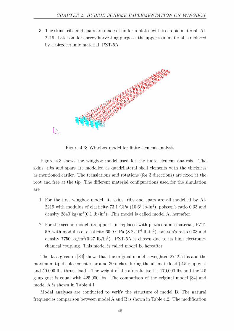
CHAPTER 4. HYBRID SCHEME IMPLEMENTATION ON WINGBOX
3. The skins, ribs and spars are made of uniform plates with isotropic material, Al-
2219. Later on, for energy harvesting purpose, the upper skin material is replaced
by a piezoceramic material, PZT-5A.
Figure 4.3: Wingbox model for finite element analysis
Figure 4.3 shows the wingbox model used for the finite element analysis. The
skins, ribs and spars are modelled as quadrilateral shell elements with the thickness
as mentioned earlier. The translations and rotations (for 3 directions) are fixed at the
root and free at the tip. The different material configurations used for the simulation
are
1. For the first wingbox model, its skins, ribs and spars are all modelled by Al-
2219 with modulus of elasticity 73.1 GPa (10.66 lb-in2), poisson′s ratio 0.33 and
density 2840 kg/m3(0.1 lb/in3). This model is called model A, hereafter.
2. For the second model, its upper skin replaced with piezoceramic material, PZT-
5A with modulus of elasticity 60.9 GPa (8.8x10⁶ lb-in2), poisson′s ratio 0.33 and
density 7750 kg/m3(0.27 lb/in3). PZT-5A is chosen due to its high electrome-
chanical coupling. This model is called model B, hereafter.
The data given in [84] shows that the original model is weighted 2742.5 lbs and the
maximum tip displacement is around 30 inches during the ultimate load (2.5 g up gust
and 50,000 lbs thrust load). The weight of the aircraft itself is 170,000 lbs and the 2.5
g up gust is equal with 425,000 lbs. The comparison of the original model [84] and
model A is shown in Table 4.1.
Modal analyses are conducted to verify the structure of model B. The natural
frequencies comparison between model A and B is shown in Table 4.2. The modification
46
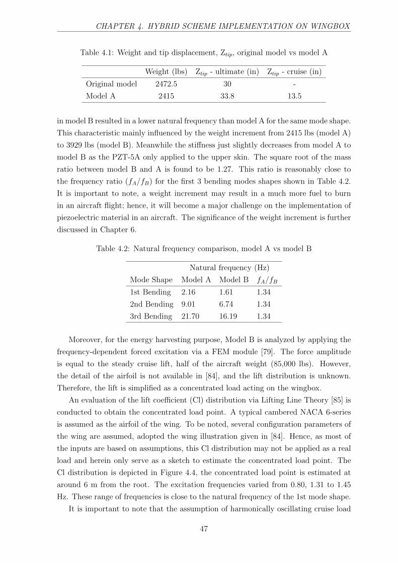
CHAPTER 4. HYBRID SCHEME IMPLEMENTATION ON WINGBOX
Table 4.1: Weight and tip displacement, Ztip, original model vs model A
Weight (lbs) Ztip - ultimate (in) Ztip - cruise (in)
Original model 2472.5 30 -
Model A 2415 33.8 13.5
in model B resulted in a lower natural frequency than model A for the same mode shape.
This characteristic mainly influenced by the weight increment from 2415 lbs (model A)
to 3929 lbs (model B). Meanwhile the stiffness just slightly decreases from model A to
model B as the PZT-5A only applied to the upper skin. The square root of the mass
ratio between model B and A is found to be 1.27. This ratio is reasonably close to
the frequency ratio (fA/fB) for the first 3 bending modes shapes shown in Table 4.2.
It is important to note, a weight increment may result in a much more fuel to burn
in an aircraft flight; hence, it will become a major challenge on the implementation of
piezoelectric material in an aircraft. The significance of the weight increment is further
discussed in Chapter 6.
Table 4.2: Natural frequency comparison, model A vs model B
Natural frequency (Hz)
Mode Shape Model A Model B fA/fB
1st Bending 2.16 1.61 1.34
2nd Bending 9.01 6.74 1.34
3rd Bending 21.70 16.19 1.34
Moreover, for the energy harvesting purpose, Model B is analyzed by applying the
frequency-dependent forced excitation via a FEM module [79]. The force amplitude
is equal to the steady cruise lift, half of the aircraft weight (85,000 lbs). However,
the detail of the airfoil is not available in [84], and the lift distribution is unknown.
Therefore, the lift is simplified as a concentrated load acting on the wingbox.
An evaluation of the lift coefficient (Cl) distribution via Lifting Line Theory [85] is
conducted to obtain the concentrated load point. A typical cambered NACA 6-series
is assumed as the airfoil of the wing. To be noted, several configuration parameters of
the wing are assumed, adopted the wing illustration given in [84]. Hence, as most of
the inputs are based on assumptions, this Cl distribution may not be applied as a real
load and herein only serve as a sketch to estimate the concentrated load point. The
Cl distribution is depicted in Figure 4.4, the concentrated load point is estimated at
around 6 m from the root. The excitation frequencies varied from 0.80, 1.31 to 1.45
Hz. These range of frequencies is close to the natural frequency of the 1st mode shape.
It is important to note that the assumption of harmonically oscillating cruise load
47

CHAPTER 4. HYBRID SCHEME IMPLEMENTATION ON WINGBOX
0 5 10 15
Location in semispan [m]
0
0.05
0.1
0.15
0.2
0.25
0.3
0.35
0.4
0.45
Lift
coef
ficie
nt
Lift distribution
Figure 4.4: Sketch of the lift coefficient distribution on the wing
may provide unrealistic loading condition in comparison to a typical cruise flight. One
of the main consequences that may need to be noted is the structural responses may
be overestimated. This is due to the vibration amplitude directly applies the load
equal to the aircraft weight and the excitation frequencies near the first bending mode.
Moreover, a continuous vibration, i.e., harmonic oscillation, may not occur on a normal
flight as the aeroelastic damping is sufficient to reduce the oscillation and stabilise the
response exerted by external disturbance, i.e., gust wing. Thus, the following evaluation
in Section 4.2 may only be interpreted as an extreme and rare case, serves as the upper
benchmark on the energy harvesting estimation.
4.2 Wingbox energy harvesting simulation
0 0.1 0.2 0.3 0.4 0.5 0.6 0.7 0.8 0.9 1
x/L
0
0.02
0.04
0.06
0.08
0.1
0.12
0.14
0.16
0.18
Zm
ech/L
Spanwise displacement
f1f2f3
Figure 4.5: Wingbox dynamic response amplitude along the span
Figure 4.5 shows the plot of model B displacement functions obtained via the FEM
48

CHAPTER 4. HYBRID SCHEME IMPLEMENTATION ON WINGBOX
simulation. The plot shows the non-dimensionalised amplitude, Zmech/L, with respect
to the neutral axis. The excitation frequencies below the first bending mode is observed.
The excitation frequencies applied, f1, f2 and f3, are 0.80, 1.31 and 1.45 Hz. These
values are 0.5, 0.7 and 0.9 times of the first bending frequency. It is shown in Figure
4.5 that all the displacement responses are mainly influenced by the first bending
mode shape. The displacements are all shown increasing from the root to the tip.
The excitation on 1.45 Hz provided the largest displacement as it is the closest to
the resonance frequency. Appendix G displays the first bending mode shape and the
displacements of the wing for different excitation frequencies.
The voltage amplitude responses are shown in Figure 4.6. It can be seen that
the voltage amplitudes resemble the behaviour of the structural dynamic responses.
At 1.45 Hz, the voltage amplitude is the largest amongst the other two frequencies.
The voltage responses in Figure 4.6 also exhibit the similar behaviour with the results
displayed in Chapter 3, Figure 3.9. The voltage responses at first are increasing with
the resistance load until at a certain point it undergo an asymptotic behaviour. Hence,
from this point, further increment of the resistance load is no more affecting the voltage
responses.
Meanwhile, the power amplitude responses are shown in Figure 4.7. The responses
are aligned with those of the voltage responses. The power amplitude at 1.45 Hz is
the largest amongst the other two frequencies. The power responses in Figure 4.7 also
exhibit similar behaviour with those previously shown for the base excitation model
in Chapter 3, Figure 3.10. The power responses at first is increasing proportionally
with the resistance load, but after reaching a certain point it is declining while the
resistance increased. The resistance load that gives the maximum power response is
the first resistance load before the voltage response goes asymptotic.
0 10 20 30 40 50 60 70 80 90 100
Resistance ( )
0
100
200
300
400
500
Vo
ltag
e (V
olt
)
Maximum Voltage vs Resistance
f1f2f3
Figure 4.6: Wingbox voltage amplitude vs resistance
49

CHAPTER 4. HYBRID SCHEME IMPLEMENTATION ON WINGBOX
0 10 20 30 40 50 60 70 80 90 100
Resistance ( )
0
0.5
1
1.5
2
2.5
3
3.5
4
4.5
Po
wer
(W
att)
104 Maximum Power vs Resistance
f1f2f3
Figure 4.7: Wingbox power amplitude vs resistance
10-2 10-1 100 101 102 103 104
Resistance ( )
10-1
100
101
102
103
Vo
ltag
e (V
olt
)
Maximum Voltage vs Resistance
f1f2f3
Figure 4.8: Wingbox voltage amplitude vs resistance, loglog scale
In a wider range of resistance loads, the voltage and power responses are plotted
by logarithmic to logarithmic scale in Figure 4.8 and Figure 4.9 (the responses are not
normalized to g such previously done for the base excitation model). In Figure 4.6 and
Figure 4.7, the range of resistance loads used are between 0-10 Ω. The resistance loads
at maximum power amplitude are around 6.59 Ω at 0.80 Hz, 4.46 Ω at 1.31 Hz and
2.73 Ω at 1.45 Hz. Figure 4.8 shows the voltage responses become asymptotic even
until the order of 104 Ω.
Figure 4.9 shows the optimum power is achieved in a small range of resistance loads,
around 10−1 Ω to 101 Ω. Within this range, electrical power in order of 102 watts to
103 watts is achievable. However, the power is dropped significantly outside of this
area. Therefore, the selection of the resistance loads is critical to design an optimum
harvester configuration.
For the purpose to evaluate the speed of computation, a comparison between the
50

CHAPTER 4. HYBRID SCHEME IMPLEMENTATION ON WINGBOX
10-2 10-1 100 101 102 103 104
Resistance ( )
100
101
102
103
104
105
Po
wer
(W
att)
Maximum Power vs Resistance
f1f2f3
Figure 4.9: Wingbox power amplitude vs resistance, loglog scale
hybrid scheme and fully coupled FEM is shown in in Table 4.3. However, it is important
to note that the fully coupled FEM developed in [10] is based on the 3-DoF quadrilateral
planar shell element (1 vertical translation and 2 rotations degree-of-freedoms). Hence,
it could not be used to construct the wingbox model as shown in Figure 4.3 as it requires
6-DoF shell element (3 translations and 3 rotations degree-of-freedoms). Therefore, for
comparison purpose, the computational time of the fully coupled FEM is based on a
rough estimation concerning the ratio to the non-coupled FEM.
In Table 3.9, it is shown that the simulation times for a standard non-coupled FEM
and a fully coupled FEM are 15 seconds and 20 seconds, respectively. Hence, there
is 33% additional time required to perform a fully coupled FEM simulation. In the
present case, for the wingbox model, a non-coupled FEM simulation requires around
2 minutes. The simulations is performed by a standard office laptop with Intel Core
i7 2.4 GHz and 4 GB RAM. Therefore, assuming 33% additional time, a fully coupled
FEM simulation needs around 2 minutes and 40 seconds.
Table 4.3 displays the same computational steps shown in Table 3.9. Step A de-
notes the non-coupled FEM simulations for the actual and dummy loads performed via
commercial software. Calculation of voltage (U) and power (Pmax) for N-number of
resistance loads, R, is denoted by step B. The process in step B is also performed via a
MATLAB© computational code. The only step used in the fully coupled FEM is step
C. It is assumed that for a set of N-numbers of R, N-times of simulations is required.
As can be seen in Table 4.3, the computation times of voltage and power outputs
in step B are the same with the ones shown in Table 3.9. Step B performs analytical
calculation based on Equation (3.30) and Equation (3.32); hence, independent to the
number of elements. Therefore, the gaps of simulation times between the hybrid scheme
and fully coupled FEM are much larger. Simulations times for 100 and 10000 variances
51

CHAPTER 4. HYBRID SCHEME IMPLEMENTATION ON WINGBOX
Table 4.3: Simulation time comparison for the wingbox model
Simulation Time (s)
100 no. of R 10000 no. of R
Steps Hybrid Scheme Fully Coupled Hybrid Scheme Fully Coupled
- Present FEM - Present FEM
A. Non-coupled 2 x 120 - 2 x 120 -
simulations
B. U and Pmax 5 - 15 -
calculations
C. Fully coupled - 100 - 10000
simulations x 160 x 160
TOTAL 245 16000 255 1600000
of R via the hybrid scheme are less than 3 minutes. In contrast, by means of fully
coupled FEM, simulation times for 100 and 10000 variances of R are more then 4
hours and 440 hours, respectively. Thus, for a large structure, the present hybrid
scheme may provide significant benefit in terms of computational time.
4.3 Summary
In this chapter, a simulation for a notional civil jet aircraft wingbox with piezoelectric
skin layer has been presented. Based on the simulation results, the voltage and power
responses could attain a promising level, in the order of 101 to 102 Volts and 102 to
104 Watts.
However, concerning an aircraft design process and flight operation, there are still
some issues to be addressed as follows:
1. One of the major issues is the weight increment on the aircraft structure due to
the existence of piezoelectric material. The commercially available piezoelectric
materials are three times heavier than the common aluminium alloy used in the
aircraft structure, i.e. Al-2219, Al-7075.
It has been shown in this chapter, by replacing the upper skin with a piezoelectric
material, the wingbox weight increased more than 60%. In a flight operation,
more weight means more lift force to produce; hence, more drag force generated
and more fuel is burnt. Therefore, this issue should be addressed in the design
process to gain the optimum weight-power exchange.
2. It has been shown in this chapter that a jet aircraft wingbox structure potentially
52
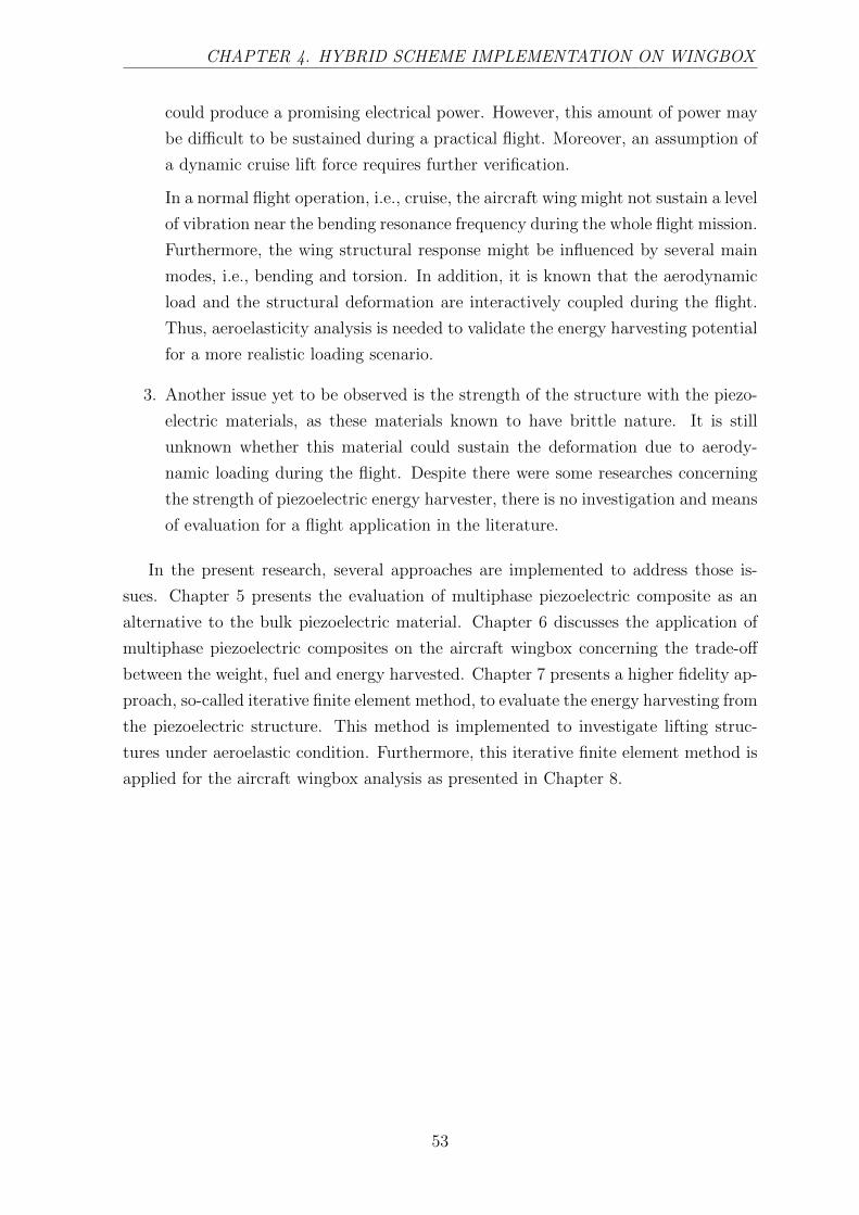
CHAPTER 4. HYBRID SCHEME IMPLEMENTATION ON WINGBOX
could produce a promising electrical power. However, this amount of power may
be difficult to be sustained during a practical flight. Moreover, an assumption of
a dynamic cruise lift force requires further verification.
In a normal flight operation, i.e., cruise, the aircraft wing might not sustain a level
of vibration near the bending resonance frequency during the whole flight mission.
Furthermore, the wing structural response might be influenced by several main
modes, i.e., bending and torsion. In addition, it is known that the aerodynamic
load and the structural deformation are interactively coupled during the flight.
Thus, aeroelasticity analysis is needed to validate the energy harvesting potential
for a more realistic loading scenario.
3. Another issue yet to be observed is the strength of the structure with the piezo-
electric materials, as these materials known to have brittle nature. It is still
unknown whether this material could sustain the deformation due to aerody-
namic loading during the flight. Despite there were some researches concerning
the strength of piezoelectric energy harvester, there is no investigation and means
of evaluation for a flight application in the literature.
In the present research, several approaches are implemented to address those is-
sues. Chapter 5 presents the evaluation of multiphase piezoelectric composite as an
alternative to the bulk piezoelectric material. Chapter 6 discusses the application of
multiphase piezoelectric composites on the aircraft wingbox concerning the trade-off
between the weight, fuel and energy harvested. Chapter 7 presents a higher fidelity ap-
proach, so-called iterative finite element method, to evaluate the energy harvesting from
the piezoelectric structure. This method is implemented to investigate lifting struc-
tures under aeroelastic condition. Furthermore, this iterative finite element method is
applied for the aircraft wingbox analysis as presented in Chapter 8.
53

Chapter 5
Multiphase Piezoelectric
Composites with Active Structural
Fiber
In this chapter, the evaluation of the multiphase composite with active structural fiber
(ASF) is discussed. The ASF is a multiphase fiber constructed of a core fiber which is a
non-electro-active coated by a piezoelectric material. By combining a matrix material
with the ASF, a so-called multiphase piezoelectric composite can be constructed. This
type of multiphase composite is investigated as the alternative of bulk piezoelectric
material for energy harvesting. From the literature, multiphase composites with ASF
has proven able to provide better optimisation between actuating and load bearing
capability compared to a pure piezoelectric material. However, application in energy
harvesting purpose has not been found in the literature.
The estimation of the electro-elastic or electromechanical properties of the multi-
phase composite is discussed in this chapter. The Double-Inclusion model combined
with the Mori-Tanaka method is implemented in a computational code to estimate the
effective electro-elastic properties of the multiphase composite. The effective composite
properties obtained via the present code are compared with the analytical, experimen-
tal and finite element results.
Some works and results presented in this chapter are parts of the author’s published
works in Composite Structures, Volume 202, 2018.
5.1 The Double-Inclusion model
In this section, the multiphase composite with electro-elastic constitutive matrix is con-
cerned. The constitutive matrix of piezoelectric material is adopted to the multiphase
composite. Two forms of the constitutive matrix, i.e., stress-charge, strain-charge,
54

CHAPTER 5. MULTIPHASE PIEZOELECTRIC COMPOSITES
are used. The stress-charge form is mainly used in The Double-Inclusion formulation.
While the strain-charge form is applied in the energy harvester model. In contrast
with the energy harvester model proposed in Chapter 3, the Double-Inclusion model
evaluates the material in three dimensional form (3D). Based on the IEEE standard
on piezoelectricity [74], the stress-charge form is expressed as
EiJMn =
C11 C12 C13 0 0 0 0 0 −e31
C12 C11 C13 0 0 0 0 0 −e31
C13 C13 C33 0 0 0 0 0 −e33
0 0 0 C44 0 0 0 −e15 0
0 0 0 0 C44 0 −e15 0 0
0 0 0 0 0 C66 0 0 0
0 0 0 0 e15 0 εS11 0 0
0 0 0 e15 0 0 0 εS11 0
e31 e31 e33 0 0 0 0 0 εS33
(5.1)
and the strain-charge form is written as
FAbiJ =
S11 S12 S13 0 0 0 0 0 d31
S12 S11 S13 0 0 0 0 0 d31
S13 S13 S33 0 0 0 0 0 d33
0 0 0 S44 0 0 0 d15 0
0 0 0 0 S44 0 d15 0 0
0 0 0 0 0 S66 0 0 0
0 0 0 0 d15 0 εT11 0 0
0 0 0 d15 0 0 0 εT11 0
d31 d31 d33 0 0 0 0 0 εT33
(5.2)
The contracted Voigt′s notation (i.e., 11 → 1, 22 → 2, 33 → 3, 23 → 4, 13 → 5,
12 → 6, 41 → 7, 42 → 8, 43 → 9) is applied in Equations (5.1) and (5.1). The four
subscripts define the row and column in a 9 × 9 matrix. Hence, for example E1111
denotes the first row - first column component of the EiJMn in a 9 × 9 matrix form,
refer to the elasticity component C11; F2343 is the fourth row - ninth column component
of the FAbiJ, refer to the piezoelectric coupling component d33; and so on. Important
to note that in Equations (5.1) and (5.2), an orthotropic characteristic is assumed.
Hence, the symmetries due to orthotropic, i.e., C11 = C22, d31 = d32, etc., are directly
implemented. Equations (5.1) and (5.2) can be written in a compact form as
EiJMn =
C −et
(6× 6) (6× 3)
e εS
(3× 6) (3× 3)
(5.3)
55
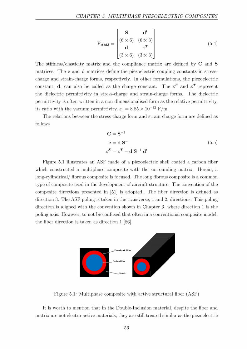
CHAPTER 5. MULTIPHASE PIEZOELECTRIC COMPOSITES
FAbiJ =
S dt
(6× 6) (6× 3)
d εT
(3× 6) (3× 3)
(5.4)
The stiffness/elasticity matrix and the compliance matrix are defined by C and S
matrices. The e and d matrices define the piezoelectric coupling constants in stress-
charge and strain-charge forms, respectively. In other formulations, the piezoelectric
constant, d, can also be called as the charge constant. The εS and εT represent
the dielectric permittivity in stress-charge and strain-charge forms. The dielectric
permittivity is often written in a non-dimensionalised form as the relative permittivity,
its ratio with the vacuum permittivity, ε0 = 8.85× 10⁻¹² F/m.
The relations between the stress-charge form and strain-charge form are defined as
follows
C = S−1
e = d S−1
εS = εT − d S−1 dt
(5.5)
Figure 5.1 illustrates an ASF made of a piezoelectric shell coated a carbon fiber
which constructed a multiphase composite with the surrounding matrix. Herein, a
long-cylindrical/ fibrous composite is focused. The long fibrous composite is a common
type of composite used in the development of aircraft structure. The convention of the
composite directions presented in [51] is adopted. The fiber direction is defined as
direction 3. The ASF poling is taken in the transverse, 1 and 2, directions. This poling
direction is aligned with the convention shown in Chapter 3, where direction 1 is the
poling axis. However, to not be confused that often in a conventional composite model,
the fiber direction is taken as direction 1 [86].
Piezoelectric Fiber
Carbon Fiber
Matrix
Figure 5.1: Multiphase composite with active structural fiber (ASF)
It is worth to mention that in the Double-Inclusion material, despite the fiber and
matrix are not electro-active materials, they are still treated similar as the piezoelectric
56
CHAPTER 5. MULTIPHASE PIEZOELECTRIC COMPOSITES
material. Later in Section 5.3, it is shown that the fiber and matrix materials do not
possess piezoelectric coupling constant. However, their permittivity are still considered.
Despite these materials do not generate electrical charge, the electrical charges could
still travel between the core fiber, the piezoelectric shell and the matrix. Hence, the
overall multiphase composite is an electro-active structure.
In the Double-Inclusion model, the effective electro-elastic matrix of the overall
composite, EiJMn, as a function of each phase properties is shown in Equation (5.6).
The electro-elastic matrices of each phase; the core fiber, the piezoelectric shell, and
the matrix are defined by EciJMn, Ep
iJMn and EmiJMn. In the following notations, the
components of the matrix, the piezoelectric shell and the core fiber are denoted by the
superscripts m, p and c, respectively.
EiJMn =(V c EciJMn Ac) + (V p Ep
iJMn Ap)+
(V m EmiJMn Am)
(5.6)
The volume fractions of each phase to the overall composite volume are defined by V c,
V p and V m. While the strain concentration tensors of each phase are denoted by Ac,
Ap and Am, respectively.
The concentration tensors in the dilute limit is used by Lin and Sodano in [51]
to obtain the effective electro-elastic properties of the multiphase composite. In the
present work, instead of only using the dilute limit, the Mori-Tanaka′s method is applied
to evaluate the concentration tensors. It is expected with this approach, a better
agreement with experimental and computational results can be achieved. The dilute
and Mori-Tanaka′s concentration tensors are estimated from the following formulations
Acdil = (I + (Sp
MnAb EmiJMn
−1 EcmiJMn))
−1
Apdil = (I + (Sc
MnAb EmiJMn
−1 EcpiJMn))
−1 (5.7)
AmMT = I ((V m I + V p Ap
dil + V c Acdil)−1
)
ApMT = Ap
dil ((V m I + V p Apdil + V c Ac
dil)−1
)
AcMT = Ac
dil ((V m I + V p Apdil + V c Ac
dil)−1
)
(5.8)
The concentration tensors in dilute limit, Adil, are calculated from Equation (5.7).
These dilute concentration tensors are used to evaluate the Mori-Tanaka′s concentra-
tion tensors, AMT, as given in Equation (5.8). In alignment with Equation (5.6),
the concentration tensors A = AMT. The identity matrix (9 x 9 size) is defined by
I. Meanwhile, the other components are obtained as EcmiJMn = Ec
iJMn − EmiJMn and
EcpiJMn = Ep
iJMn − EciJMn.
The tensor defined by SMnAb is the piezoelectric analog of the Eshelby′s tensor.
The analytical form of this tensor is derived in detail by Dunn and Taya [55]. In
the present work, the numerical form of SMnAb based on the work in [87] is applied.
57

CHAPTER 5. MULTIPHASE PIEZOELECTRIC COMPOSITES
Furthermore, for the case of circular cylindrical fibrous, if the fiber length is very large
(→∞) compared to its radius, a simplified form of SMnAb [61, 88] can also be used.
𝑨𝒄𝒕𝒊𝒗𝒆 𝑳𝒂𝒚𝒆𝒓
𝑺𝒖𝒃𝒔𝒕𝒓𝒂𝒕𝒆 𝑳𝒂𝒚𝒆𝒓
Figure 5.2: Cross-section of energy harvester beam with multiphase composite as an
active layer
5.2 Evaluation procedure of the multiphase com-
posite effective electro-elastic properties
The procedure to calculate the piezoelectric Eshelby′s tensor, SMnAb, is presented in
this section. As previously explained in Section 5.1, if the SMnAb tensor is known,
the concentration tensors can be calculated from Equations (5.7) and (5.8). Hence,
the effective electro-elastic properties of the composite can be evaluated from Equation
(5.6). Herein, the numerical form of SMnAb by applying Gauss integration procedure
in [87] is adopted. The elastic part of SMnAb is expressed as
SMnAb =EiJAb
8π
P∑p=1
Q∑q=1
(GpqMJin +Gpq
nJiM)W pW q
with M = 1, 2, 3;
(5.9)
and the electro-elastic part is given by
SMnAb =EmiJAb
4π
P∑p=1
Q∑q=1
(GpqMJin)W pW q
with M = 4
(5.10)
Where
GpqMJin = zpqi z
pqn (Kpq
MJ)−1
KpqMJ = Em
iJMnzpqi z
pqn
i = 1, 2, 3; n = 1, 2, 3; J = 1, 2, 3, 4
(5.11)
58
CHAPTER 5. MULTIPHASE PIEZOELECTRIC COMPOSITES
and
zpq3 = ξp3/a3
zpq1 =√
1− (ξp1) cos θq/a1
zpq2 =√
1− (ξp2) cos θq/a2
(5.12)
The contracted Voigt′s notation (i.e., 11 → 1, 22 → 2, 33 → 3, 23 → 4, 13 → 5, 12 →6, 41 → 7, 42 → 8, 43 → 9) is also applied in Equations (5.9), (5.10) and (5.11).
The number of the integration points are defined by the capital letters, P and Q.
Whereas the superscripts p and q are the numerical counters for the Gauss points, ξp3
and θq, and also for the weight coefficients, W p and W q. The ellipsoidal shape with
the semiaxes, a1, a2 and a3, is adopted as the inclusion shape [55]. In the longitudinal
direction, the semiaxis length is defined by a3. Meanwhile, the semiaxis lengths in the
transverse directions are a1 and a2. Therefore, for example, if the inclusion is a sphere-
shaped particle then all the semiaxis lengths are the same, a1 = a2 = a3. In the other
hand, if the inclusion is a long cylindrical fiber then the transverse semiaxis lengths
are equal, a1 = a2, and the longitudinal length is assumed very long, a3 >>> a1.
The SMnAb tensor is calculated via the following procedure
1. The properties of the matrix material, EmiJMn, and the shape aspect ratio a2/a1
and a3/a1 are used as the input. Then, the number of integration points P and Q
are determined. Hence, the Gauss points, ξp3 and θq, and the weight coefficients,
W p and W q can be obtained.
2. The zpq3 , zpq1 and zpq2 components are evaluated for each combination of the Gauss
points via Equation (5.12).
3. The KpqMJ matrix component is calculated for each combination of the Gauss
points via Equation (5.11). Then, the inverse of KpqMJ is used to evaluate Gpq
MJin.
4. The SMnAb matrix component is calculated via Equations (5.9) and (5.10).
A MATLAB© computational code is written to evaluate the SMnAb matrix and the
effective electro-elastic properties, EiJMn. The composite configuration is determined
from the combination of the ASF volume fraction to the overall composite, Vf , and
the aspect ratio of the piezoelectric shell thickness to the ASF radius, AR. In the
case of long-infinite fiber, the shape aspect ratio of the fiber is assumed very large,
a3/a1 = 106. In addition, in the present code, the linear summation of each phase
density fraction is used to determine the average density, ρ, of the composite.
59
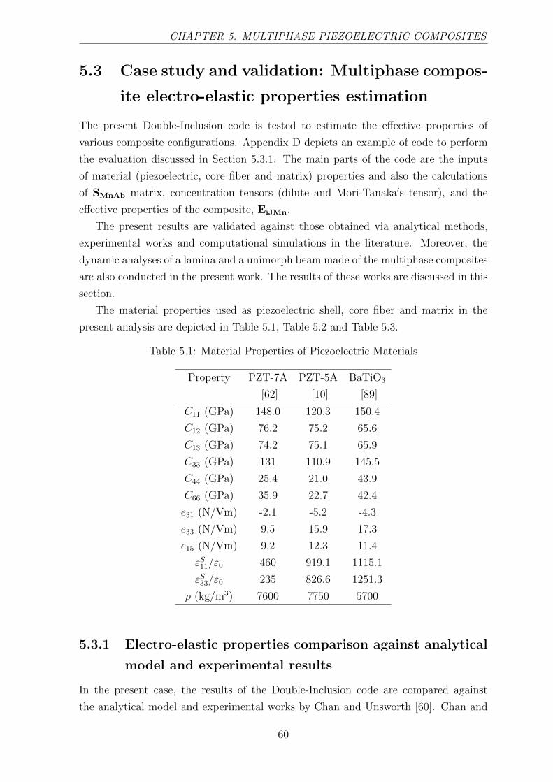
CHAPTER 5. MULTIPHASE PIEZOELECTRIC COMPOSITES
5.3 Case study and validation: Multiphase compos-
ite electro-elastic properties estimation
The present Double-Inclusion code is tested to estimate the effective properties of
various composite configurations. Appendix D depicts an example of code to perform
the evaluation discussed in Section 5.3.1. The main parts of the code are the inputs
of material (piezoelectric, core fiber and matrix) properties and also the calculations
of SMnAb matrix, concentration tensors (dilute and Mori-Tanaka′s tensor), and the
effective properties of the composite, EiJMn.
The present results are validated against those obtained via analytical methods,
experimental works and computational simulations in the literature. Moreover, the
dynamic analyses of a lamina and a unimorph beam made of the multiphase composites
are also conducted in the present work. The results of these works are discussed in this
section.
The material properties used as piezoelectric shell, core fiber and matrix in the
present analysis are depicted in Table 5.1, Table 5.2 and Table 5.3.
Table 5.1: Material Properties of Piezoelectric Materials
Property PZT-7A PZT-5A BaTiO3
[62] [10] [89]
C11 (GPa) 148.0 120.3 150.4
C12 (GPa) 76.2 75.2 65.6
C13 (GPa) 74.2 75.1 65.9
C33 (GPa) 131 110.9 145.5
C44 (GPa) 25.4 21.0 43.9
C66 (GPa) 35.9 22.7 42.4
e31 (N/Vm) -2.1 -5.2 -4.3
e33 (N/Vm) 9.5 15.9 17.3
e15 (N/Vm) 9.2 12.3 11.4
εS11/ε0 460 919.1 1115.1
εS33/ε0 235 826.6 1251.3
ρ (kg/m3) 7600 7750 5700
5.3.1 Electro-elastic properties comparison against analytical
model and experimental results
In the present case, the results of the Double-Inclusion code are compared against
the analytical model and experimental works by Chan and Unsworth [60]. Chan and
60

CHAPTER 5. MULTIPHASE PIEZOELECTRIC COMPOSITES
Table 5.2: Material Properties of Core Fiber Materials
Property Carbon SiC Glass
Fiber [62] Fiber [62] Fiber [90]
C11 (GPa) 24.0 483.7 88.8
C12 (GPa) 9.7 99.1 29.6
C13 (GPa) 6.7 99.1 29.6
C33 (GPa) 243.7 483.7 88.8
C44 (GPa) 27.0 192.3 29.6
C66 (GPa) 11.0 192.3 29.6
e31 (N/Vm) 0 0 0
e33 (N/Vm) 0 0 0
e15 (N/Vm) 0 0 0
εS11/ε0 12.0 10.0 6.4
εS33/ε0 12.0 10.0 6.4
ρ (kg/m3) 2000 4360 2550
Unsworth investigated single piezoelectric fiber composites in [60]. Hence, their model
serves as an upper benchmark when the piezoelectric thickness becomes very dominant
in the ASF.
In the work done by Chan and Unsworth [60], PZT-7A and Epoxy matrix are used
to construct the single fiber composites. In the present work, carbon fiber is added as
the core fiber of the ASF. The properties in Table 5.1, Table 5.2 and Table 5.3 are used.
However, to be noted that Chan and Unsworth found the d33 of the tested PZT-7A was
around 163-167 pm/V. Therefore, they used 167 pm/V in their analytical model [60].
Thus, in the present work, e33 is changed to 12.3 C/m2, so that d33 is 167 pm/V and
d31,d32 are kept as -60 pm/V.
The stiffness, compliance and piezoelectric coupling components of the multiphase
composite for various volume fraction, Vf, and aspect ratio, AR, are depicted in Figure
5.3. The results obtained from the present Double-Inclusion code are denoted by
”Present Code - DI MT”. Whereas ”AR1”, ”AR2”, ”AR3” and ”AR4” represent the
results for 0.50, 0.60, 0.70 and 0.95 aspect ratios. Meanwhile, the solid black lines show
the results of Chan-Unsworth′s analytical model for single fiber composites.
It can be seen in Figure 5.3, the present code′s results follow the similar trend with
the Chan-Unsworth model. In addition, as expected, the pattern of the multiphase
composite shifted closer to the results of single fiber model when the aspect ratio of
the piezoelectric shell increases. It is clearly seen at AR 0.95, the results of multiphase
composite and single fiber model are coincide. In this configuration, the ASF is made
of 99.75% piezoelectric material. Therefore, the multiphase composite closely behaves
61

CHAPTER 5. MULTIPHASE PIEZOELECTRIC COMPOSITES
Table 5.3: Material Properties of Matrix Materials
Property LaRC-SI Epoxy
[62] [90]
C11 (GPa) 8.1 8.0
C12 (GPa) 5.4 4.4
C13 (GPa) 5.4 4.4
C33 (GPa) 8.1 8.0
C44 (GPa) 1.4 1.4
C66 (GPa) 1.4 1.4
e31 (N/Vm) 0 0
e33 (N/Vm) 0 0
e15 (N/Vm) 0 0
εS11/ε0 2.8 4.2
εS33/ε0 2.8 4.2
ρ (kg/m3) 1360 1150
like a single fiber composite.
Figure 5.3a depicts the stiffness component of the composite in the fiber direction.
As the carbon fiber and PZT-7A stiffness components are larger than the epoxy matrix,
the composite stiffness increases with the ASF volume fraction for the same aspect
ratio. In contrast, as the carbon fiber stiffness is larger than PZT-7A, the composite
stiffness decreases while the aspect ratio increases.
The piezoelectric constant of stress-charge form, e33, is shown in Figure 5.3b. As
the aspect ratio increases, the PZT-7A composition is larger. Hence, the piezoelectric
constant of the composite increases. Whereas for the same aspect ratio, e33 increases
with the volume fraction.
Figures 5.3c and 5.3d present the components in strain-charge form, i.e., compliance,
S31, and piezoelectric charge constant, d31. Here, the negative (-) sign defines the cause
and effect in opposite direction. For example, if d31 becomes more negative, hence,
there is a larger deformation in negative direction (compression) exerted by a positive
voltage.
It is interesting to note that for both S31 and d31, the trend of the parameters for
large volume fraction (above 50%) are almost no longer affected by the volume fraction.
Hence, in relation to d31, further increasing the volume fraction above 50% may not
significantly increase the electrical response of the composite when a deformation is
applied.
Figure 5.4 shows the variation of the other material properties, compliance, piezo-
electric charge constants, dielectric permittivity and density of the composite. In addi-
62

CHAPTER 5. MULTIPHASE PIEZOELECTRIC COMPOSITES
0 0.1 0.2 0.3 0.4 0.5 0.6 0.7 0.8 0.9 1
Volume Fraction of ASF
0
2
4
6
8
10
12
14
C33
(10
10 N
/m2)
Stiffness C33 vs Volume Fraction of ASF
Present Code - DI MT AR1Present Code - DI MT AR2Present Code - DI MT AR3Present Code - DI MT AR4Chan-Unsworth Model
(a)
0 0.1 0.2 0.3 0.4 0.5 0.6 0.7 0.8 0.9 1
Volume Fraction of ASF
0
2
4
6
8
10
12
14
e 33 (
C/m
2)
Piezoelectric Constant e33 vs Volume Fraction of ASF
Present Code - DI MT AR1Present Code - DI MT AR2Present Code - DI MT AR3Present Code - DI MT AR4Chan-Unsworth Model
(b)
0 0.1 0.2 0.3 0.4 0.5 0.6 0.7 0.8 0.9 1
Volume Fraction of ASF
-60
-50
-40
-30
-20
-10
0
S31
(10
-12 m
2/N
)
Compliance S31 vs Volume Fraction of ASF
Present Code - DI MT AR1Present Code - DI MT AR2Present Code - DI MT AR3Present Code - DI MT AR4Chan-Unsworth Model
(c)
0 0.1 0.2 0.3 0.4 0.5 0.6 0.7 0.8 0.9 1
Volume Fraction of ASF
-70
-60
-50
-40
-30
-20
-10
d31
(10
-12 m
/V)
Charge Constant d31 vs Volume Fraction of ASF
Present Code - DI MT AR1Present Code - DI MT AR2Present Code - DI MT AR3Present Code - DI MT AR4Chan-Unsworth Model
(d)
Figure 5.3: (a) Stiffness, C33, (b) Piezoelectric Constant, e33, (c) Compliance, S31, and
(d) Charge Constant, d31, vs ASF Volume Fraction of PZT-7A - Carbon Fiber - Epoxy
Composites
tion, Figure 5.4 depicts the experimental results of Chan-Unsworth [60]. Similarly with
Figure 5.3, all the results obtained from the Double-Inclusion code follow the similar
trend with Chan-Unsworth′s results as displayed in Figure 5.4
It is clearly shown in Figures 5.4a and 5.4b that both the density, ρ, and the charge
constant, d33, of the composite at AR 0.95 are coincide with those estimated via Chan-
Unsworth model. Furthermore, their values are in an excellent agreement with the
experimental results. The density of the composite at the same aspect ratio increases
linearly with the volume fraction due to the densities of the ASFs are larger than
the matrix. Moreover, similarly to the trend of d31 depicted in Figure 5.3d, the charge
constant, d33, almost insensitive to the volume fraction increment at above 50% volume
fraction.
The variation of the compliance components, S11 + S12, is shown in 5.4c. Mathe-
matically, by inversing the stiffness matrices, it is found the carbon fiber′s compliance
63

CHAPTER 5. MULTIPHASE PIEZOELECTRIC COMPOSITES
0 0.1 0.2 0.3 0.4 0.5 0.6 0.7 0.8 0.9 1
Volume Fraction of ASF
1000
2000
3000
4000
5000
6000
7000
8000
(kg
/m3)
Density vs Volume Fraction of ASF
Present Code - DI MT AR1Present Code - DI MT AR2Present Code - DI MT AR3Present Code - DI MT AR4Chan-Unsworth ModelChan-Unsworth Experiment
(a)
0 0.1 0.2 0.3 0.4 0.5 0.6 0.7 0.8 0.9 1
Volume Fraction of ASF
20
40
60
80
100
120
140
160
180
d33
(10
-12 m
/V)
Charge Constant d33 vs Volume Fraction of ASF
Present Code - DI MT AR1Present Code - DI MT AR2Present Code - DI MT AR3Present Code - DI MT AR4Chan-Unsworth ModelChan-Unsworth Experiment
(b)
0 0.1 0.2 0.3 0.4 0.5 0.6 0.7 0.8 0.9 1
Volume Fraction of ASF
0
20
40
60
80
100
120
S11
+S12
(10
-12 m
2/N
)
Compliance S11+S12 vs Volume Fraction of ASF
Present Code - DI MT AR1Present Code - DI MT AR2Present Code - DI MT AR3Present Code - DI MT AR4Chan-Unsworth ModelChan-Unsworth Experiment
(c)
0 0.1 0.2 0.3 0.4 0.5 0.6 0.7 0.8 0.9 1
Volume Fraction of ASF
0
50
100
150
200
250
300
350
400
450
500
33T /
0
Permittivity Ratio 33T / 0 vs Volume Fraction of ASF
Present Code - DI MT AR1Present Code - DI MT AR2Present Code - DI MT AR3Present Code - DI MT AR4Chan-Unsworth ModelChan-Unsworth Experiment
(d)
Figure 5.4: (a) Density, ρ, (b) Charge Constant, d33, (c) Compliance, S11 + S12, and
(d) Dielectric Permittivity Ratio,εT33ε0
, vs ASF Volume Fraction of PZT-7A-Carbon
Fiber-Epoxy Composites
at 11-direction, S11, is more positive than the PZT-7A. In contrast, the compliance of
carbon fiber at 12-direction, S12, is more negative. Thus, the compliance components,
S11 and S12, of the ASF decrease and increase together with the increasing aspect ratio.
This is aligned with the trend displayed in Figure 5.4c, the summation of S11 and S12
almost not affected by the variation of aspect ratio.
Despite the fact that most of the parameters obtained via the Double-Inclusion
code are in good agreements Chan-Unsworth′s results as depicted in Figures 5.3 and
5.4, some discrepancies are still evident. Chan and Unsworth in [60] explained that the
differences occured between the analytical model and the experimental results due to
some properties of the tested materials had deviations with the supplied manufacturer
data. For example, as explained earlier, the charge constant, d33, for the present
and Chan-Unsworth models need to be adjusted closer to the properties of the tested
samples. However, the deviations data of other properties were not given in [60]; thus,
64
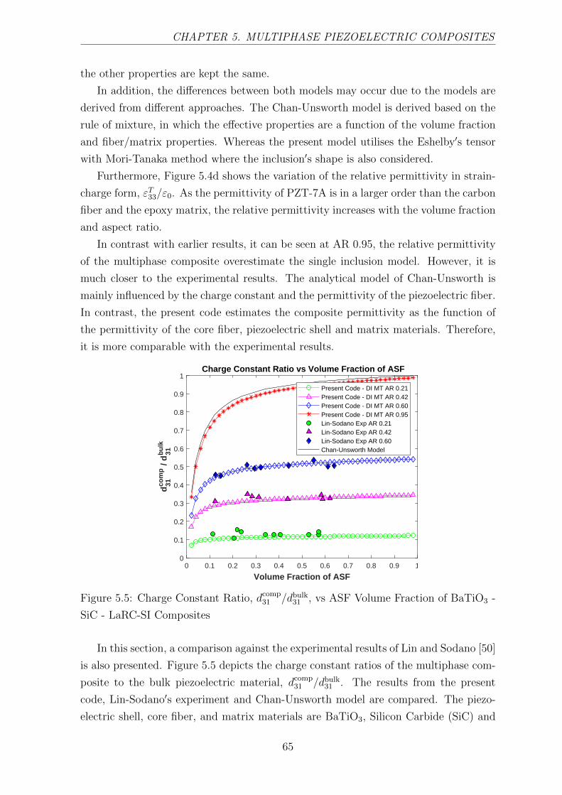
CHAPTER 5. MULTIPHASE PIEZOELECTRIC COMPOSITES
the other properties are kept the same.
In addition, the differences between both models may occur due to the models are
derived from different approaches. The Chan-Unsworth model is derived based on the
rule of mixture, in which the effective properties are a function of the volume fraction
and fiber/matrix properties. Whereas the present model utilises the Eshelby′s tensor
with Mori-Tanaka method where the inclusion′s shape is also considered.
Furthermore, Figure 5.4d shows the variation of the relative permittivity in strain-
charge form, εT33/ε0. As the permittivity of PZT-7A is in a larger order than the carbon
fiber and the epoxy matrix, the relative permittivity increases with the volume fraction
and aspect ratio.
In contrast with earlier results, it can be seen at AR 0.95, the relative permittivity
of the multiphase composite overestimate the single inclusion model. However, it is
much closer to the experimental results. The analytical model of Chan-Unsworth is
mainly influenced by the charge constant and the permittivity of the piezoelectric fiber.
In contrast, the present code estimates the composite permittivity as the function of
the permittivity of the core fiber, piezoelectric shell and matrix materials. Therefore,
it is more comparable with the experimental results.
0 0.1 0.2 0.3 0.4 0.5 0.6 0.7 0.8 0.9 1
Volume Fraction of ASF
0
0.1
0.2
0.3
0.4
0.5
0.6
0.7
0.8
0.9
1
d31co
mp /
d31b
ulk
Charge Constant Ratio vs Volume Fraction of ASF
Present Code - DI MT AR 0.21Present Code - DI MT AR 0.42Present Code - DI MT AR 0.60Present Code - DI MT AR 0.95Lin-Sodano Exp AR 0.21Lin-Sodano Exp AR 0.42Lin-Sodano Exp AR 0.60Chan-Unsworth Model
Figure 5.5: Charge Constant Ratio, dcomp31 /dbulk
31 , vs ASF Volume Fraction of BaTiO3 -
SiC - LaRC-SI Composites
In this section, a comparison against the experimental results of Lin and Sodano [50]
is also presented. Figure 5.5 depicts the charge constant ratios of the multiphase com-
posite to the bulk piezoelectric material, dcomp31 /dbulk
31 . The results from the present
code, Lin-Sodano′s experiment and Chan-Unsworth model are compared. The piezo-
electric shell, core fiber, and matrix materials are BaTiO3, Silicon Carbide (SiC) and
65
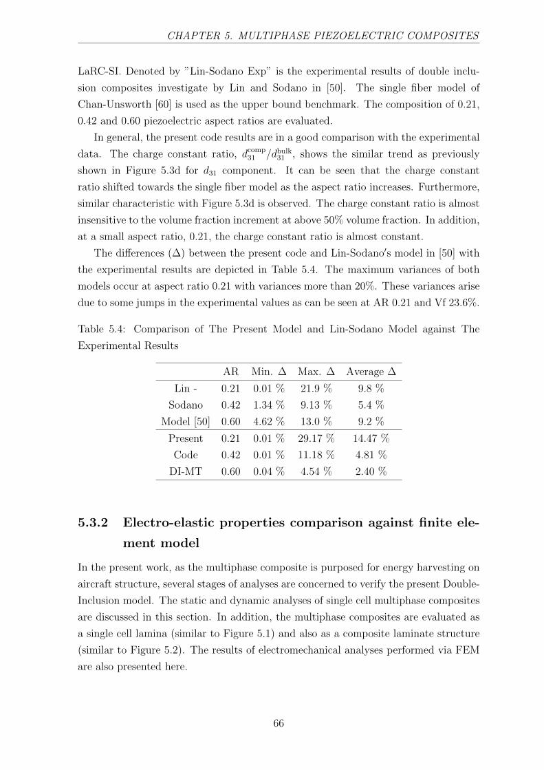
CHAPTER 5. MULTIPHASE PIEZOELECTRIC COMPOSITES
LaRC-SI. Denoted by ”Lin-Sodano Exp” is the experimental results of double inclu-
sion composites investigate by Lin and Sodano in [50]. The single fiber model of
Chan-Unsworth [60] is used as the upper bound benchmark. The composition of 0.21,
0.42 and 0.60 piezoelectric aspect ratios are evaluated.
In general, the present code results are in a good comparison with the experimental
data. The charge constant ratio, dcomp31 /dbulk
31 , shows the similar trend as previously
shown in Figure 5.3d for d31 component. It can be seen that the charge constant
ratio shifted towards the single fiber model as the aspect ratio increases. Furthermore,
similar characteristic with Figure 5.3d is observed. The charge constant ratio is almost
insensitive to the volume fraction increment at above 50% volume fraction. In addition,
at a small aspect ratio, 0.21, the charge constant ratio is almost constant.
The differences (∆) between the present code and Lin-Sodano′s model in [50] with
the experimental results are depicted in Table 5.4. The maximum variances of both
models occur at aspect ratio 0.21 with variances more than 20%. These variances arise
due to some jumps in the experimental values as can be seen at AR 0.21 and Vf 23.6%.
Table 5.4: Comparison of The Present Model and Lin-Sodano Model against The
Experimental Results
AR Min. ∆ Max. ∆ Average ∆
Lin - 0.21 0.01 % 21.9 % 9.8 %
Sodano 0.42 1.34 % 9.13 % 5.4 %
Model [50] 0.60 4.62 % 13.0 % 9.2 %
Present 0.21 0.01 % 29.17 % 14.47 %
Code 0.42 0.01 % 11.18 % 4.81 %
DI-MT 0.60 0.04 % 4.54 % 2.40 %
5.3.2 Electro-elastic properties comparison against finite ele-
ment model
In the present work, as the multiphase composite is purposed for energy harvesting on
aircraft structure, several stages of analyses are concerned to verify the present Double-
Inclusion model. The static and dynamic analyses of single cell multiphase composites
are discussed in this section. In addition, the multiphase composites are evaluated as
a single cell lamina (similar to Figure 5.1) and also as a composite laminate structure
(similar to Figure 5.2). The results of electromechanical analyses performed via FEM
are also presented here.
66

CHAPTER 5. MULTIPHASE PIEZOELECTRIC COMPOSITES
0 0.1 0.2 0.3 0.4 0.5 0.6 0.7 0.8 0.9 1
Volume Fraction of ASF
0
2
4
6
8
10
12
14
16
18
E3 (
1010
N/m
2)
Modulus Young E3 vs Volume Fraction of ASF
Present Code - DI MT AR1Present Code - DI MT AR2Present Code - DI MT AR3Present Code - DI MT AR4Lin-Sodano FEM AR1Lin-Sodano FEM AR2Lin-Sodano FEM AR3Lin-Sodano FEM AR4
(a)
0 0.1 0.2 0.3 0.4 0.5 0.6 0.7 0.8 0.9 1
Volume Fraction of ASF
0
50
100
150
200
250
33S /
0
Permittivity Ratio 33S / 0 vs Volume Fraction of ASF
Present Code - DI MT AR1Present Code - DI MT AR2Present Code - DI MT AR3Present Code - DI MT AR4Lin-Sodano FEM AR1Lin-Sodano FEM AR2Lin-Sodano FEM AR3Lin-Sodano FEM AR4
(b)
0 0.1 0.2 0.3 0.4 0.5 0.6 0.7 0.8 0.9 1
Volume Fraction of ASF
0
1
2
3
4
5
6
7
8
E1 (
1010
N/m
2)
Modulus Young E1 vs Volume Fraction of ASF
Present Code - DI MT AR1Present Code - DI MT AR2Present Code - DI MT AR3Present Code - DI MT AR4Lin-Sodano FEM AR1Lin-Sodano FEM AR2Lin-Sodano FEM AR3Lin-Sodano FEM AR4
(c)
0 0.1 0.2 0.3 0.4 0.5 0.6 0.7 0.8 0.9 1
Volume Fraction of ASF
0
50
100
150
11S /
0
Permittivity Ratio 11S / 0 vs Volume Fraction of ASF
Present Code - DI MT AR1Present Code - DI MT AR2Present Code - DI MT AR3Present Code - DI MT AR4Lin-Sodano FEM AR1Lin-Sodano FEM AR2Lin-Sodano FEM AR3Lin-Sodano FEM AR4
(d)
Figure 5.6: (a) Modulus Young, E3, (b) Relative Permittivity, εS33/ε0, (c) Modulus
Young, E1, and (d) Relative Permittivity, εS11/ε0, vs ASF Volume Fraction of PZT-7A
- Carbon Fiber - LaRC-SI Composites
5.3.2.1 Static analysis of single lamina composite
The results of Lin-Sodano [51] for the single cell multiphase composite is used as the
first benchmark for the static analysis. The multiphase composites made of Carbon
fiber, PZT-7A, and LaRC SI matrix were investigated by Lin and Sodano [51]. They
applied eight unique electrical and mechanical boundary conditions to the single cell
FEM model to evaluate each electro-elastic properties of the composite. Those unique
properties are four stiffness components, two permittivity components, and two piezo-
electric coupling components. Static load condition was applied. Therefore, for one
composite configuration, eight static FEM simulations were required. In more details,
those electro-mechanical boundary conditions can be found in [51,62].
The modulus and relative permittivity at the transversal and longitudinal directions
of the composites are depicted in Figure 5.6. The solid lines denotes the present code
67
CHAPTER 5. MULTIPHASE PIEZOELECTRIC COMPOSITES
results. Meanwhile, the FEM results from Lin-Sodano are depicted by the star, circle,
triangle, and diamond symbols. ”AR1”, ”AR2”, ”AR3” and ”AR4” represent 0.2, 0.4,
0.6 and 0.8 aspect ratios.
The composite properties at longitudinal/fiber direction, E3 and εS33/ε0 are shown
in Figures 5.6a and 5.6b. It can be seen that the present code and FEM results
possesses the same trends and the variances are insignificant. At the same aspect
ratio, the Young′s modulus, E3, increases linearly with the volume fraction. This can
be explained as the composite becomes stiffer with larger fractions of carbon fiber and
PZT-7A. In contrast, at the same volume fraction, the E3 decreases as the aspect
ratio increases. In this case, the carbon fiber fraction becomes smaller; hence the ASF
stiffness is lesser. However, the relative permittivity, εS33/ε0, increases with both the
aspect ratio and volume fraction. The PZT-7A has the largest permittivity compared
to the carbon fiber and matrix. Therefore, more permittivity is gained with larger
fraction of PZT-7A.
Figures 5.6c and 5.6d depict the composite properties at the transversal direction,
E1 and εS11/ε0. Important to note that orthotropic condition is assumed, thus, the
properties at direction 1 and direction 2 are the same. In contrast with the longitudinal
properties, at the transversal direction, the properties grow exponentially with the
volume fraction. This characteristic occurs as the stiffness components of the PZT-
7A at the transversal direction are in a larger magnitude than the carbon fiber, i.e.,
hundreds GPa compare to tens GPA. Hence, when the fraction of PZT-7A becomes
larger, its stiffness rapidly dominates the effective stiffness of the overall composite. A
similar condition also applied to the permittivity at transversal direction.
However, it can be seen there are some discrepancies occur between the FEM and
the present code results for the transversal properties estimation. Both for E1 and
εS11/ε0, as the volume fraction increases, the FEM results show different increment rate
with the present code results. The FEM results show a larger increment rate of E1 at
the large volume fraction (>50%). In contrast, for the relative permittivity, εS11/ε0, the
FEM results have almost a steady increment rate with the increasing volume fraction.
These results aligned with the phenomena observed by Lin and Sodano in [51].
At AR 0.8 and Vf 70%, the maximum variance of E1 was observed, their FEM model
overestimated the Double-Inclusion model by 31%. Whereas at AR 0.2 and Vf 70%, the
FEM model overestimated the εS11/ε0 value by 39%. Despite the maximum variances
occur at the same composite configuration for the present code, a closer agreement is
obtained with the FEM results. At AR 0.8 and Vf 70%, the E1 estimation from the
present code has 12% variance with the FEM results. Whereas at AR 0.2 and Vf 70%,
the estimation of εS11/ε0 from the present code differs by 28% with the FEM′s.
The second investigation for static analysis used the XFEM results of Koutsawa et
68

CHAPTER 5. MULTIPHASE PIEZOELECTRIC COMPOSITES
al. [91] as benchmark. The multiphase composite materials are PZT-7A, glass fiber and
epoxy matrix. By means of XFEM, Koutsawa et al. modelled the different material
regions and boundaries of the composite via enrichment functions and level set method.
Thus, the finite element meshes are independent to the composite phases [91]. The
comparison of the present code with their XFEM results is shown in Figure 5.7.
0.1 0.2 0.3 0.4 0.5 0.6 0.7 0.8 0.9
Aspect Ratio of Piezo Shell
0.1
0.2
0.3
0.4
0.5
0.6
0.7
0.8
0.9
1C
har
ge
Co
nst
ant
Rat
io Charge Constant Ratio at 50 % ASF Volume Fraction
Present Code d31comp / d
33bulk
Present Code d33comp / d
33bulk
XFEM Koutsawa et al. d31comp / d
33bulk
XFEM Koutsawa et al. d33comp / d
33bulk
Figure 5.7: Charge Constant Ratio dcomp31 /dbulk
31 & dcomp33 /dbulk
33 , vs Aspect Ratio of PZT-
7A - Glass - Epoxy Composites
Excellent agreement between the present code and XFEM results can be seen in
Figure 5.7. Both charge constant ratios at 33-directions and 31-directions show the
same trend. At small aspect ratio, the charge constant ratio almost linearly increases
with the aspect ratio. However, at a larger aspect ratio (>40%), the increment rate
decreases. These trends aligned with the earlier results depicted in Figures 5.3d, 5.4b
and 5.5. Table 5.5 shows the discrepancies of d31 ratios from both methods in more
details.
5.3.2.2 Dynamic analysis of single lamina composite and unimorph beam
In this section, the dynamic analyses of single cell lamina and unimorph structure
made of the multiphase composite are discussed. Two different models are used in the
FEM simulations. The first model is a long cube/unit-cell constructed from different
materials. The model consists of detailed and distinct 3D elements for each phase. In
contrast, the second model is a simpler shape, only a long cube without any detail of
each phase. The effective electro-elastic properties obtained from the Double-Inclusion
code are the only material input. The analyses focused to compare the displacement
69

CHAPTER 5. MULTIPHASE PIEZOELECTRIC COMPOSITES
Table 5.5: Charge Constant Ratio Comparison: The Present Model vs XFEM - Kout-
sawa et al.
Charge Constant Ratio (dcomp31 /dbulk31 )
AR Present Code XFEM [91] ∆ (%)
0.1 0.19 0.18 5.56%
0.2 0.35 0.33 6.06%
0.3 0.49 0.46 6.52%
0.4 0.61 0.59 3.39%
0.5 0.71 0.69 2.90%
0.6 0.79 0.78 1.28%
0.7 0.85 0.84 1.19%
0.8 0.89 0.88 1.14%
0.9 0.91 0.90 1.11%
and voltage distributions of the lamina. Herein, the first and the second models are
called as the ”Detailed 3D FE” and the ”homogenised FE” models, respectively.
0.1 0.2 0.3 0.4 0.5 0.6 0.7
Piezoelectric Shell Aspect Ratio
0
0.5
1
1.5
2
2.5
3
3.5
Nat
ura
l Fre
qu
ency
(H
z)
Natural Frequency Comparison at 50 % Volume Fraction
1B-Detailed 3D FE1B-Homogenized FE2B-Detailed 3D FE2B-Homogenized FE3B-Detailed 3D FE3B-Homogenized FE
(a)
0.3 0.4 0.5 0.6 0.7 0.8 0.9
ASF Volume Fraction
0
0.5
1
1.5
2
2.5
3
3.5
Nat
ura
l Fre
qu
ency
(H
z)
Natural Frequency Comparison at 0.3 Aspect Ratio
1B-Detailed 3D FE1B-Homogenized FE2B-Detailed 3D FE2B-Homogenized FE3B-Detailed 3D FE3B-Homogenized FE
(b)
Figure 5.8: Natural Frequency Comparison of PZT-5A - Carbon - LaRC-SI Composites
for (a) Different Aspect Ratio at 50% Volume Fraction (b) Different Volume Fraction
at 0.3 Aspect Ratio
The FEM simulations are conducted using COMSOL Multiphysics© with the piezo-
electric devices module. Due to the software limitation, only linear tetrahedral elements
are used. The observed composites are made of PZT-5A, Carbon fiber, and LaRC-SI
matrix. Fixed boundary conditions are applied at one end of the lamina. The FEM
models are evaluated by means of modal analysis.
Figures 5.8a and 5.8b depict the natural frequencies of the composite at Vf 50% and
70
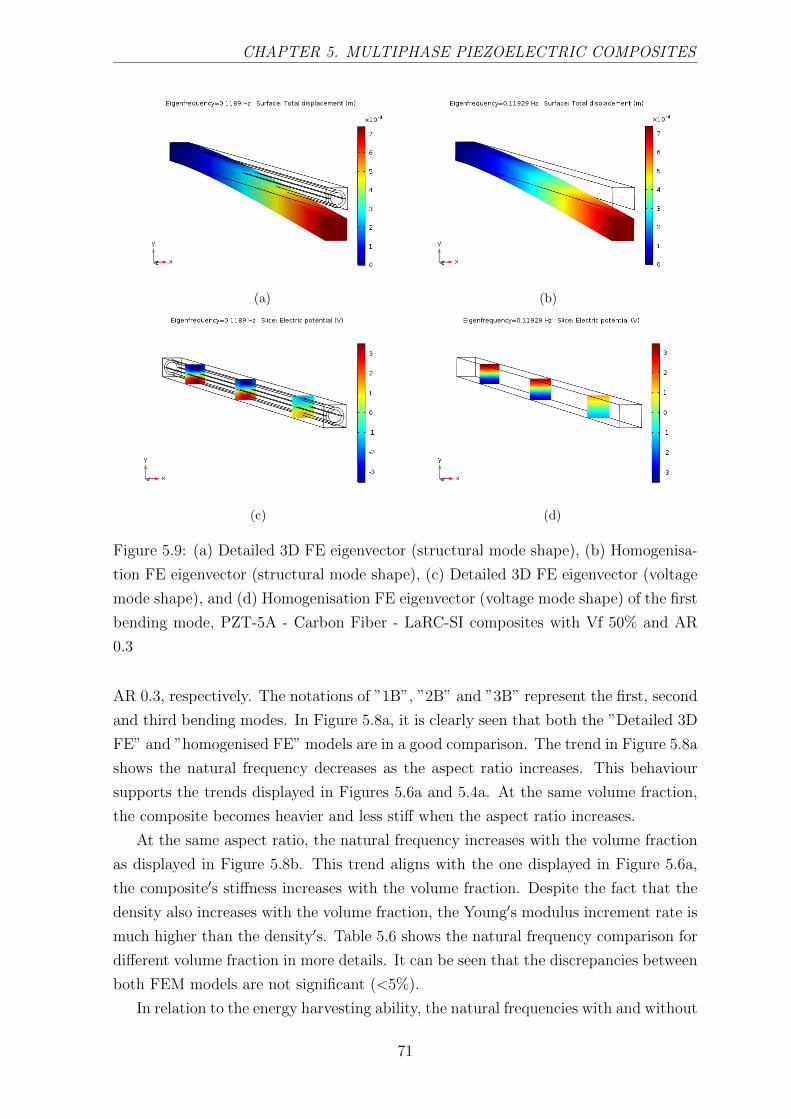
CHAPTER 5. MULTIPHASE PIEZOELECTRIC COMPOSITES
(a) (b)
(c) (d)
Figure 5.9: (a) Detailed 3D FE eigenvector (structural mode shape), (b) Homogenisa-
tion FE eigenvector (structural mode shape), (c) Detailed 3D FE eigenvector (voltage
mode shape), and (d) Homogenisation FE eigenvector (voltage mode shape) of the first
bending mode, PZT-5A - Carbon Fiber - LaRC-SI composites with Vf 50% and AR
0.3
AR 0.3, respectively. The notations of ”1B”, ”2B” and ”3B” represent the first, second
and third bending modes. In Figure 5.8a, it is clearly seen that both the ”Detailed 3D
FE” and ”homogenised FE” models are in a good comparison. The trend in Figure 5.8a
shows the natural frequency decreases as the aspect ratio increases. This behaviour
supports the trends displayed in Figures 5.6a and 5.4a. At the same volume fraction,
the composite becomes heavier and less stiff when the aspect ratio increases.
At the same aspect ratio, the natural frequency increases with the volume fraction
as displayed in Figure 5.8b. This trend aligns with the one displayed in Figure 5.6a,
the composite′s stiffness increases with the volume fraction. Despite the fact that the
density also increases with the volume fraction, the Young′s modulus increment rate is
much higher than the density′s. Table 5.6 shows the natural frequency comparison for
different volume fraction in more details. It can be seen that the discrepancies between
both FEM models are not significant (<5%).
In relation to the energy harvesting ability, the natural frequencies with and without
71
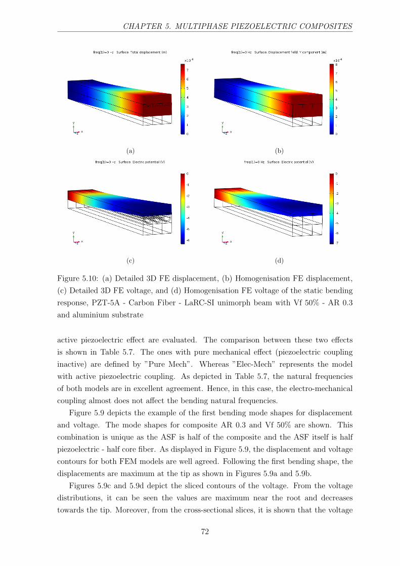
CHAPTER 5. MULTIPHASE PIEZOELECTRIC COMPOSITES
(a) (b)
(c) (d)
Figure 5.10: (a) Detailed 3D FE displacement, (b) Homogenisation FE displacement,
(c) Detailed 3D FE voltage, and (d) Homogenisation FE voltage of the static bending
response, PZT-5A - Carbon Fiber - LaRC-SI unimorph beam with Vf 50% - AR 0.3
and aluminium substrate
active piezoelectric effect are evaluated. The comparison between these two effects
is shown in Table 5.7. The ones with pure mechanical effect (piezoelectric coupling
inactive) are defined by ”Pure Mech”. Whereas ”Elec-Mech” represents the model
with active piezoelectric coupling. As depicted in Table 5.7, the natural frequencies
of both models are in excellent agreement. Hence, in this case, the electro-mechanical
coupling almost does not affect the bending natural frequencies.
Figure 5.9 depicts the example of the first bending mode shapes for displacement
and voltage. The mode shapes for composite AR 0.3 and Vf 50% are shown. This
combination is unique as the ASF is half of the composite and the ASF itself is half
piezoelectric - half core fiber. As displayed in Figure 5.9, the displacement and voltage
contours for both FEM models are well agreed. Following the first bending shape, the
displacements are maximum at the tip as shown in Figures 5.9a and 5.9b.
Figures 5.9c and 5.9d depict the sliced contours of the voltage. From the voltage
distributions, it can be seen the values are maximum near the root and decreases
towards the tip. Moreover, from the cross-sectional slices, it is shown that the voltage
72

CHAPTER 5. MULTIPHASE PIEZOELECTRIC COMPOSITES
(a) (b)
(c) (d)
Figure 5.11: (a) Detailed 3D FE displacement, (b) Homogenisation FE displacement,
(c) Detailed 3D FE voltage, and (d) Homogenisation FE voltage of the dynamic bending
response at 0.6 frequency ratio, PZT-5A - Carbon Fiber - LaRC-SI unimorph beam
with Vf 50% - AR 0.3 and aluminium substrate
of the bottom and top parts are in the opposite values. This is occurred as the bottom
part exhibits compression and the top part exhibits tension. Whereas at the neutral
axis, the voltage is zero.
The results from a unimorph beam analyses are also presented here. The unimorph
beam commonly consisted of a piezoelectric material as the electro-active layer. In
the present case, the bulk piezoelectric material is substituted with the multiphase
composite.
In the present case, the active layer consisted of three multiphase composite lam-
ina arranged in a row. The substrate (non-active) layer at the bottom is made of
aluminium. Table 5.8 depicts the natural frequencies comparison of the unimorph
modelled with the ”Detailed 3D FE” and the ”homogenised FE”. The first bending,
second bending and the first torsion modes are defined by ”1B”, ”2B” and ”1T”. As
shown in Table 5.8, the natural frequencies of both FEM models are reasonably agreed.
A sensor-like problem is evaluated in the dynamic response cases. An external me-
chanical load is given at the unimorph′s tip. The responses at 0 Hz excitation frequency
73

CHAPTER 5. MULTIPHASE PIEZOELECTRIC COMPOSITES
Table 5.6: Natural Frequency Comparison for Different Volume Fraction at 0.3 Aspect
Ratio of PZT-5A - Carbon - LaRC-SI Composites, Detailed 3D Finite Element vs
Finite Element with Homogenization Properties
Natural frequency (Hz)
Vf Mode Detailed 3D homogenised ∆ (%)
1B 0.1189 0.1192 0.31%
50% 2B 0.7423 0.7513 1.32%
3B 2.0662 2.1166 2.44%
1B 0.1323 0.1281 3.14%
60% 2B 0.8254 0.8062 2.32%
3B 2.2950 2.2684 1.16%
1B 0.1556 0.1540 1.02%
80% 2B 0.9695 0.9657 0.40%
3B 2.6902 2.7037 0.50%
(static condition) are shown in Figure 5.10. It is depicted that the deformation of the
”Homogenised FE” model is slightly higher than the ”Detailed 3D FE” model. This
behaviour may occur due to the utilisation of the tetrahedral elements. The tetrahedral
element is known to have a stiff character in a bending case. The mesh construction for
the ”Detailed 3D FE” model is much more difficult as the elements need to be carefully
defined in each phase. Thus, despite that coarse meshes are used for both models, the
”Detailed 3D FE” converges at a higher number of elements.
As the natural frequencies of both FEM models are slightly differing, a ratio of the
excitation frequency to the first bending frequency is used to define the load. It is
known that when the excitation is near the natural frequency, the resonance occurs,
and the amplitude can be extremely amplified. Hence, it is considered reasonable to
compare the responses at the excitation below the natural frequency. Figure 5.11 shows
the unimorph responses for 0.6 frequency ratio. In the case of the ”Detailed 3D FE”,
this ratio defines an excitation at 0.6 × 1.5618 Hz or 0.9371 Hz. It is shown in Figure
5.11 that the displacement and voltage amplitudes of both FEM models are in a good
agreement.
5.3.3 Highlights on the effective electro-elastic properties con-
cerning energy harvesting analysis
In relation to the energy harvested under dynamic bending, the following effective
electro-elastic properties of the multiphase composite are highlighted.
74
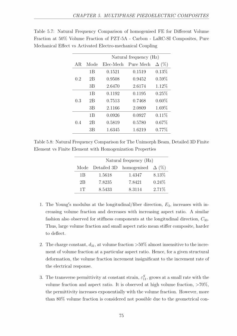
CHAPTER 5. MULTIPHASE PIEZOELECTRIC COMPOSITES
Table 5.7: Natural Frequency Comparison of homogenised FE for Different Volume
Fraction at 50% Volume Fraction of PZT-5A - Carbon - LaRC-SI Composites, Pure
Mechanical Effect vs Activated Electro-mechanical Coupling
Natural frequency (Hz)
AR Mode Elec-Mech Pure Mech ∆ (%)
1B 0.1521 0.1519 0.13%
0.2 2B 0.9508 0.9452 0.59%
3B 2.6470 2.6174 1.12%
1B 0.1192 0.1195 0.25%
0.3 2B 0.7513 0.7468 0.60%
3B 2.1166 2.0809 1.69%
1B 0.0926 0.0927 0.11%
0.4 2B 0.5819 0.5780 0.67%
3B 1.6345 1.6219 0.77%
Table 5.8: Natural Frequency Comparison for The Unimorph Beam, Detailed 3D Finite
Element vs Finite Element with Homogenization Properties
Natural frequency (Hz)
Mode Detailed 3D homogenised ∆ (%)
1B 1.5618 1.4347 8.13%
2B 7.8235 7.8421 0.24%
1T 8.5433 8.3114 2.71%
1. The Young′s modulus at the longitudinal/fiber direction, E3, increases with in-
creasing volume fraction and decreases with increasing aspect ratio. A similar
fashion also observed for stiffness components at the longitudinal direction, C33.
Thus, large volume fraction and small aspect ratio mean stiffer composite, harder
to deflect.
2. The charge constant, d31, at volume fraction >50% almost insensitive to the incre-
ment of volume fraction at a particular aspect ratio. Hence, for a given structural
deformation, the volume fraction increment insignificant to the increment rate of
the electrical response.
3. The transverse permittivity at constant strain, εS11, grows at a small rate with the
volume fraction and aspect ratio. It is observed at high volume fraction, >70%,
the permittivity increases exponentially with the volume fraction. However, more
than 80% volume fraction is considered not possible due to the geometrical con-
75

CHAPTER 5. MULTIPHASE PIEZOELECTRIC COMPOSITES
straint. Therefore, for all possible material composition, a low permittivity or a
low capacitance in the structure is expected.
In addition, although the density is not explicitly shown in the governing energy
harvester formulation, it influences the natural frequencies and dynamic response of the
structure. Moreover, in the aircraft design case, density is a significant parameter in a
weight-energy evaluation. The density increases with the volume fraction and aspect
ratio. Hence, with larger volume fraction and aspect ratio, the structure is heavier and
more fuel is required.
5.4 Summary
In this chapter, a method of evaluating electro-elastic properties of multiphase com-
posites with active structural fiber has been presented. A computational code based
on the Double-Inclusion model extended with the Mori-Tanaka method has been de-
veloped. The numerical code has been applied to estimate the effective electro-elastic
properties of multiphase composites with various material compositions. The results of
the present work have been well validated with the analytical, experimental and finite
element results from the literature.
Static and dynamic electromechanical analyses for a single lamina and a unimorph
beam via FEM has also been performed in the present work. The effective properties
obtained from the present Double-Inclusion code has been verified with a detailed 3D
FEM model. Therefore, the present Double-Inclusion model can be used as one of the
preliminary tools to provide an estimation on the properties of multiphase composites
for energy harvesting evaluation. Later in Chapter 6 and Chapter 8, the composites′
properties evaluated here are utilised as the substitution of the bulk piezoelectric ma-
terial in energy harvesting structures.
76

Chapter 6
Application of The Multiphase
Composites on A Jet Aircraft
Wingbox
In the present work, the multiphase composites with ASF are applied to a notional jet
aircraft wingbox. The same wingbox presented in Chapter 4 is used for the investiga-
tion. The energy harvesting analysis of this wingbox is discussed in this chapter. The
novel hybrid scheme presented in Chapter 3 is used. The Double-Inclusion model is
implemented to evaluate the electro-elastic properties of the multiphase composites.
In addition, a new procedure is developed to investigate the trade-off between the
aircraft weight, the fuel saving and the energy harvested for different composite config-
urations. A conceptual aircraft design approach concerning the aircraft weight break-
down is adopted for this procedure. The description and implementation of this pro-
cedure for the aircraft wingbox are presented in this chapter.
Some works and results presented in this chapter are parts of the author’s published
works in Composite Structures, Volume 202, 2018.
6.1 Aircraft weight breakdown in conceptual design
In this section an aircraft′s weight breakdown is presented. The weight breakdown
concerning a conceptual aircraft design stage [92] is adopted. This weight breakdown
is used to establish the relationship due to the changes caused by the piezoelectric/
multiphase composites to the aircraft weight. The main weight components concerned
here can be classified as follows:
1. The empty weight, WE, which consisted of the aircraft structure and the installed
systems/equipments/interiors.
77

CHAPTER 6. APPLICATION OF MULTIPHASE COMPOSITES ON THEWINGBOX
2. The crew weight, WC , and the payload weight, WP . The crews are the pilots,
the flight attendants and any other staffs, i.e., engineers. The payloads are the
passengers, the baggages and also the cargo. These components are usually a
pre-determined requirements in the conceptual aircraft design.
3. The fuel weight, Wfuel, which consisted of the fuel to accomplish the flight mission
with some extras, i.e., 5% reserve fuel. It is estimated based on the flight mission
profile, i.e., take-off, climb, cruise, descent, landing.
4. The take-off weight, WTO, which is the total of all the weight components as
presented in Equation (6.1).
WTO = WE +WC +WP +Wfuel (6.1)
In the conceptual aircraft design, the WTO is initially estimated from a historical
data or an empirical formulation. The ratio of WE to the WTO can be determined from
the following empirical formulation.
WE
WTO
= A WCTO KV S (6.2)
The constants A and C are defined based on the aircraft type. For a jet transport
aircraft, A = 1.02 and C = -0.06. Whereas KV S is the variable sweep constant, for a
fixed-sweep wing, KV S = 1, and for a variable-sweep wing, KV S = 1.04. Hence, in the
present case, Equation (6.2) can be rewritten as
WE
WTO
= 1.02 W−0.06TO (6.3)
However, it is important to note that the constants in Equation (6.3) are defined based
on the historical data of conventional jet transport aircraft.
To the author′s knowledge, composites have just started been used as main ma-
terials for the commercial aircraft in the past decade [93]. Hence, the historical data
is not sufficient to develop an empirical weight function for a transport aircraft with
composites. Therefore, for the study purpose, the weight fraction based on Equation
(6.3) is applied to evaluate the aircraft with multiphase composite in the present work.
However, in a more detailed design stage, some correction factors need to be applied to
accomodate the influence of advanced composites. For reader′s reference, some efforts
have been reviewed in [94] concerning the prospect of composite implementation on
future aircraft.
Commonly, an iterative procedure is required in the initial weight estimation as
WE, Wfuel and WTO are unknown. Thus, Equation (6.1) and Equation (6.2) are solved
iteratively. However, a reference aircraft is known in the present work. The WE, Wfuel
and WTO components have been defined. Therefore, the concern is addressing the
effects due to a material replacement. The detail of procedure to evaluate these effects
is explained in the next section.
78

CHAPTER 6. APPLICATION OF MULTIPHASE COMPOSITES ON THEWINGBOX
6.2 Evaluation procedure on the trade-off between
aircraft weight and energy harvested
In this section, firstly, the increment or reduction of the aircraft weight due to a material
replacement is discussed. Further, this modified weight is used to evaluate the trade
off between the aircraft weight and the harvested energy. The empty weight, WE,
and the take-off weight, WTO, are directly influenced by a material replacement as the
structural weight changes. Thus, the aerodynamic load required to lift the aircraft will
change, as well as the drag force that occurred due to lift and also the thrust required
to move the aircraft forward. Hence, the fuel weight, Wfuel, is affected and a new
aerodynamic load may be applied for the structural response and energy harvesting
evaluations. The scheme to quantify these effects is given in Figure 6.1 and can be
described as follows:
1. The weight components of a reference aircraft are defined. The superscript ”Ref”
in Figure 6.1 denotes these components.
2. The change in structural weight, ∆WStructural, due to material replacement is
calculated.
3. The new empty weight, WNewE , is obtained from the summation of the reference
empty weight, WRefE , and the ∆WStructural.
4. Once WNewE is found, Equation (6.3) can be used to estimate the new take-off
weight, WNewTO .
5. In a steady level flight, a new lift cruise load may be defined equal to the WNewTO .
6. There is no change in the payload and crew weights as these components are
considered as requirements.
7. After the new weight components are obtained, the new fuel weight WNewfuel is
calculated via Equation (6.1).
In the current case study, the upper skin material of the aircraft wingbox is replaced
(refer to Chapter 4). Important to note that the aircraft has two wings; hence, the
∆WStructural is twice the weight change of a wingbox. In the present study, the electrical
power harvested from the wingbox is associated with the APU generated power in order
to have an equivalent parameter for the trade off between weight and energy. The
scheme to estimate the fuel saving from the material replacement and the harvested
power is depicted in Figure 6.2 and can be explained as follows:
79

CHAPTER 6. APPLICATION OF MULTIPHASE COMPOSITES ON THEWINGBOX
𝑊𝑇𝑂𝑅𝑒𝑓
,𝑊𝐸𝑅𝑒𝑓
,
𝑊𝐶𝑅𝑒𝑓
,𝑊𝑃𝑅𝑒𝑓
,𝑊𝑓𝑢𝑒𝑙𝑅𝑒𝑓
𝑊𝐸𝑁𝑒𝑤 = 𝑊𝐸
𝑅𝑒𝑓+ ∆𝑊𝑆𝑡𝑟𝑢𝑐𝑡𝑢𝑟𝑎𝑙
Material Replacement
∆𝑊𝑆𝑡𝑟𝑢𝑐𝑡𝑢𝑟𝑎𝑙
𝑊𝑇𝑂𝑁𝑒𝑤 = 𝑓 (𝑊𝐸
𝑁𝑒𝑤)
Empty Weight
Fraction
𝑊𝑓𝑢𝑒𝑙𝑁𝑒𝑤
= 𝑊𝑇𝑂𝑁𝑒𝑤 − (𝑊𝐸
𝑁𝑒𝑤 +𝑊𝐶𝑁𝑒𝑤 +𝑊𝑝
𝑁𝑒𝑤)
𝑊𝐶𝑅𝑒𝑓
= 𝑊𝐶𝑁𝑒𝑤
𝑊𝑃𝑅𝑒𝑓
= 𝑊𝑃𝑁𝑒𝑤
Cruise Lift
= 𝑊𝑇𝑂𝑁𝑒𝑤
Figure 6.1: Schematic diagram of the weight change calculation
1. The power generated (kW) and the fuel consumption rate (kg/s or lbs/hour) of
the APU are determined.
2. An operation time, tAPU , is defined. The energy generated by the APU, JAPU
(Joule), and its consumed fuel consumed are estimated.
3. The ratio of the energy to the consumed fuel, J∗ (Joule/kg-fuel or Joule/lbs-fuel),
is calculated.
4. In relation to the hybrid scheme discussed in Chapter 4, a steady-state harmonic
oscillation is assumed. Hence, the average power, PAve, can be defined as half
the maximum harvested power Pmax.
5. For a certain vibration time, tHarvest, the energy generated by the harvester,
JHarvest (Joule), is obtained from the integration of power to time.
6. The equivalent fuel saved due to the energy harvested, ∆Wfuel−Pwr, is determined
based on the J∗ ratio.
7. The fuel change due to the direct effect of structural weight increment/reduction,
80

CHAPTER 6. APPLICATION OF MULTIPHASE COMPOSITES ON THEWINGBOX
∆Wfuel−Str, is the difference between the new fuel weight, WNewfuel , and the refer-
ence fuel weight, WReffuel .
8. The TOTAL ∆Wfuel, is the summation of ∆Wfuel−Pwr and ∆Wfuel−Str.
APU power,
fuel consumption rate
𝐽𝐴𝑃𝑈 = 𝑃𝐴𝑃𝑈 × 𝑡𝐴𝑃𝑈
𝑡𝐴𝑃𝑈
𝑻𝑶𝑻𝑨𝑳 ∆𝑾𝒇𝒖𝒆𝒍
= ∆𝑾𝒇𝒖𝒆𝒍−𝑺𝒕𝒓 + ∆𝑾𝒇𝒖𝒆𝒍−𝑷𝒘𝒓
𝐽∗ =𝐽𝐴𝑃𝑈
𝑓𝑢𝑒𝑙 𝑐𝑜𝑛𝑠𝑢𝑚𝑒𝑑
𝐽𝐻𝑎𝑟𝑣𝑒𝑠𝑡
= 𝑃𝑎𝑣𝑒 × 𝑡𝐻𝑎𝑟𝑣𝑒𝑠𝑡∆𝑾𝒇𝒖𝒆𝒍−𝑺𝒕𝒓
= 𝑊𝑓𝑢𝑒𝑙𝑁𝑒𝑤 −𝑊𝑓𝑢𝑒𝑙
𝑅𝑒𝑓
∆𝑾𝒇𝒖𝒆𝒍−𝑷𝒘𝒓
= 𝐽𝐻𝑎𝑟𝑣𝑒𝑠𝑡 × 𝐽∗
Figure 6.2: Schematic diagram of the fuel saving evaluation
To be noted that the formulation of maximum power in Chapter 3, Equation (3.32)
is derived for one cantilever beam. In Chapter 4, one cantilever beam is associated
with one aircraft wing. Hence, the total power harvested from the aircraft is twice the
power harvested from a wing. Thus, PAve, needs to be considered for two wings.
6.3 Wingbox energy harvesting simulation with the
multiphase composite
In this section, the investigation on the energy harvesting potential from the typical jet
transport aircraft is presented. The same wingbox configuration discussed in Chapter
4 is evaluated. In addition to PZT-5A, multiphase composites with different configura-
tions are analysed as the replacement material on the upper skin of the wingbox. The
81

CHAPTER 6. APPLICATION OF MULTIPHASE COMPOSITES ON THEWINGBOX
similar composites evaluated in Chapter 5, Section 5.3.2.2 which consisted of PZT-5A,
carbon fiber and LaRC SI matrix are used.
The fiber orientation is along the span of the wingbox, from the root to the tip.
The material properties of the multiphase composites in 3D form is reduced to 2D form
as input for the quadrilateral shell elements. The detailed transformation scheme of
the properties is referred to [10]. Table 6.1 shows the wingbox weight with different
bulk materials. Whereas, the wingbox weight with embedded multiphase composites
are depicted in Tables 6.2 and 6.3. Here, the aerodynamic lift during cruise is assumed
equal to the take-off weight, WTO. Therefore, the lift load is dependent to the materials′
weight.
Table 6.1: Wingbox Weight: Different Upper Skin Material
Material Al-2219 PZT-5A
Weight (lbs) 2415 3929
Table 6.2: Wingbox Weight: Multiphase Composites Upper Skin, PZT-5A - Carbon -
LaRC-SI 50% Volume Fraction
Aspect Ratio 0.2 0.4 0.6
Weight (lbs) 2373 2622 2800
Table 6.3: Wingbox Weight: Multiphase Composites Upper Skin, PZT-5A - Carbon -
LaRC-SI 0.2 Aspect Ratio
Volume Fraction 50% 60% 70%
Weight (lbs) 2373 2457 2541
The WTO and WE of the aircraft is determined via Equation (6.1) and Equation
(6.3) for each material configuration. Firstly, the weight components of a reference
aircraft is calculated. The reference aircraft′s WTO is 170000 lbs with Wfuel is 41000
lbs [84]. Hence, it is found that the WE is 84183 lbs. Therefore, the payload and
crew weight, WC + WP is 44817 lbs. In association with the scheme in Figure 6.1,
these weight components are the ones with superscript ”Ref”. Hence, by following the
procedure in Figure 6.1, the new aircraft weights for various material configurations
can be calculated.
The WTO and WE for aircraft with different bulk materials are depicted in Table
6.4. Whereas Tables 6.5 and 6.6 show the WTO and WE for aircraft with different
composites configurations. It is obviously seen in Table 6.4 the maximum WE and
82

CHAPTER 6. APPLICATION OF MULTIPHASE COMPOSITES ON THEWINGBOX
WTO are obtained with bulk piezoelectric material. In contrast, the aircraft with the
composite composition of the smallest volume fraction and aspect ratio, AR 0.2 and
Vf 50%, gains the minimum WE and WTO.
Table 6.4: Aircraft Empty Weight and Take-Off Weight: Different Wingbox Upper
Skin Material
Material Al-2219 PZT-5A
WE (lbs) 84183 87211
WTO (lbs) 170000 176513
Table 6.5: Aircraft Empty Weight and Take-Off Weight: Multiphase Composite Wing-
box Upper Skin, PZT-5A - Carbon - LaRC-SI 50% Volume Fraction
Aspect Ratio 0.2 0.4 0.6
WE (lbs) 84099 84597 84593
WTO (lbs) 169820 170890 171656
Table 6.6: Aircraft Empty Weight and Take-Off Weight: Multiphase Composite Wing-
box Upper Skin, PZT-5A - Carbon - LaRC-SI 0.2 Aspect Ratio
Volume Fraction 50% 60% 70%
WE (lbs) 84099 84267 84435
WTO (lbs) 169820 170181 170542
Concerning the energy harvesting evaluation, the same loading condition as de-
scribed in Chapter 4 is applied. The steady lift is modelled as a concentrated force
acting on the wing. This force is used as the amplitude to form a harmonic load excita-
tion. Initially, modal analyses is performed to the wingboxes. The natural frequencies
are used to define the excitation frequencies acting on the structures. Similar to the one
presented in Chapter 4, the excitation lower than the first bending natural frequency
are also used here. Table 6.7 depicts the first bending frequencies for the wingboxes.
The first bending natural frequencies for the wingboxes are quite low, around 1.6-
2.3 Hz. The frequency ratio defined in Chapter 4 is used. The loads with 0.5, 0.7,
0.9 frequency ratios are applied. In accordance to the implementation of the hybrid
scheme in Chapter 4, the lift cruise load and a unit of moment are used as the actual
and dummy loads. Appendix H shows the displacements of the wing with different
composite configurations. The responses from the lift loads represent the displacement
due to mechanical load. The responses from the dummy loads are used to obtain the
reverse piezoelectric effect.
83

CHAPTER 6. APPLICATION OF MULTIPHASE COMPOSITES ON THEWINGBOX
Table 6.7: 1st Bending Natural Frequency of The Wingbox for Different Multiphase
Composite Composition
Vf AR Natural frequency (Hz)
0.5 0.2 2.21
0.5 0.4 1.99
0.5 0.6 1.76
0.6 0.2 2.32
0.7 0.2 2.35
Bulk PZT-5A 1.61
Figure 6.3 shows the voltage amplitude responses for wingboxes with bulk PZT-5A
and the multiphase composites at Vf 50%. The excitation at 0.5, 0.7, 0.9 frequency
ratios are represented by ”f1”, ”f2” and ”f3”, respectively. The trend of the voltage
responses similar with shown earlier in Chapter 4. Initially, the voltage increases with
the resistance load. However, at a particular point, it starts to undergo an asymptotic
behaviour.
The wingbox with bulk PZT-5A has the small resistance load when the voltage
starts to become asymptotic. In contrast, the wingbox with the composite at Vf 50%
and AR 0.2 aspect ratio has the largest resistance load when the voltage starts to
become asymptotic. Although a larger piezoelectric coupling comes with a higher
aspect ratio, the voltage goes asymptotic at a smaller resistance; thus, it resulted in a
smaller maximum voltage. Furthermore, in alignment with the discussion in Chapter
4, the largest excitation frequency provided the highest level of the maximum voltage
as it exerts the highest displacement amplitude.
The power amplitude responses for wingboxes with bulk PZT-5A and the multi-
phase composites at Vf 50 %. are depicted in Figure 6.4. Similar characteristics as
presented in Chapter 4 are also observed. Initially, the power increases with the re-
sistance load before it reaches a maximum point and starts to decline. An interesting
characteristic is found as the powers from all configurations, including the bulk PZT-
5A, could reach a similar maximum level as can be seen in Table 6.8. This finding
could become a positive insight for the study on the energy harvesting material and
its weight issue.
It is a positive value to remark as the multiphase composites are lighter than the
bulk PZT and yet it can produce a similar level of power. In accordance with the
findings highlighted in Chapter 5, Section 5.3.3, this behaviour may occur as the per-
mittivity (capacitance) and the piezoelectric coupling constants of the composites are
smaller than the bulk PZT. A smaller coupling constant may result in a smaller elec-
trical field. However, a smaller capacitance may also result in a larger voltage for the
84

CHAPTER 6. APPLICATION OF MULTIPHASE COMPOSITES ON THEWINGBOX
0 100 200 300 400
Resistance ( )
0
1000
2000
3000V
olt
age
(Vo
lt)
AR = 0.2
0 100 200 300 400
Resistance ( )
0
1000
2000
3000
Vo
ltag
e (V
olt
)
AR = 0.4
0 100 200 300 400
Resistance ( )
0
1000
2000
3000
Vo
ltag
e (V
olt
)
AR = 0.6
0 100 200 300 400
Resistance ( )
0
1000
2000
3000
Vo
ltag
e (V
olt
)
Bulk PZT
f1f2f3
Figure 6.3: Variation of voltage amplitude to the resistance load for wingboxes with
multiphase composite skin, AR 0.2, 0.4 & 0.6 at Vf 50%, and bulk PZT skin
same amount of charges.
In addition, Figure 6.5 shows the power amplitude responses for wingboxes with
bulk PZT-5A and the composites at AR 0.2. It can be seen that the level of maximum
power decreases as the volume fraction increases. This characteristic is caused by
an increasing stiffness at the longitudinal/fiber direction for a composite at a higher
volume fraction.
6.4 Aircraft fuel saving evaluation
In this section, the equivalent fuel saving from the implementation of the multiphase
composites on the wingbox is discussed. The power responses obtained from the ear-
lier section are equivalenced with the fuel used for an APU operation. The scheme
presented in Figure 6.2 is applied.
The APU used as reference is a typical APU for a medium-long ranged jet trans-
port aircraft, i.e., the B737 or the A320. Based on the data in [95, 96], the APU can
85
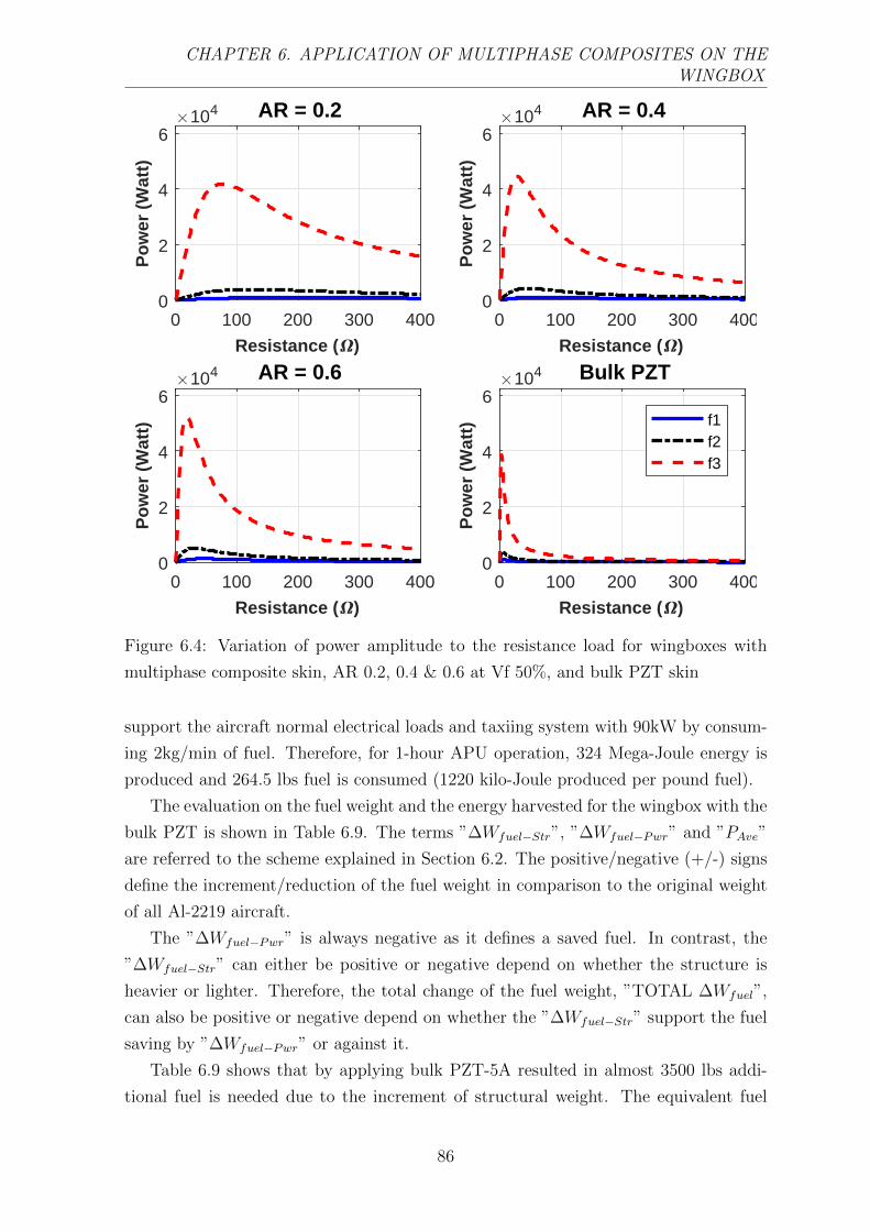
CHAPTER 6. APPLICATION OF MULTIPHASE COMPOSITES ON THEWINGBOX
0 100 200 300 400
Resistance ( )
0
2
4
6P
ow
er (
Wat
t)104 AR = 0.2
0 100 200 300 400
Resistance ( )
0
2
4
6
Po
wer
(W
att)
104 AR = 0.4
0 100 200 300 400
Resistance ( )
0
2
4
6
Po
wer
(W
att)
104 AR = 0.6
0 100 200 300 400
Resistance ( )
0
2
4
6
Po
wer
(W
att)
104 Bulk PZT
f1f2f3
Figure 6.4: Variation of power amplitude to the resistance load for wingboxes with
multiphase composite skin, AR 0.2, 0.4 & 0.6 at Vf 50%, and bulk PZT skin
support the aircraft normal electrical loads and taxiing system with 90kW by consum-
ing 2kg/min of fuel. Therefore, for 1-hour APU operation, 324 Mega-Joule energy is
produced and 264.5 lbs fuel is consumed (1220 kilo-Joule produced per pound fuel).
The evaluation on the fuel weight and the energy harvested for the wingbox with the
bulk PZT is shown in Table 6.9. The terms ”∆Wfuel−Str”, ”∆Wfuel−Pwr” and ”PAve”
are referred to the scheme explained in Section 6.2. The positive/negative (+/-) signs
define the increment/reduction of the fuel weight in comparison to the original weight
of all Al-2219 aircraft.
The ”∆Wfuel−Pwr” is always negative as it defines a saved fuel. In contrast, the
”∆Wfuel−Str” can either be positive or negative depend on whether the structure is
heavier or lighter. Therefore, the total change of the fuel weight, ”TOTAL ∆Wfuel”,
can also be positive or negative depend on whether the ”∆Wfuel−Str” support the fuel
saving by ”∆Wfuel−Pwr” or against it.
Table 6.9 shows that by applying bulk PZT-5A resulted in almost 3500 lbs addi-
tional fuel is needed due to the increment of structural weight. The equivalent fuel
86

CHAPTER 6. APPLICATION OF MULTIPHASE COMPOSITES ON THEWINGBOX
0 100 200 300 400
Resistance ( )
0
2
4P
ow
er (
Wat
t)104 Vf = 0.5
0 100 200 300 400
Resistance ( )
0
2
4
Po
wer
(W
att)
104 Vf = 0.6
0 100 200 300 400
Resistance ( )
0
2
4
Po
wer
(W
att)
104 Vf = 0.7
0 100 200 300 400
Resistance ( )
0
2
4
Po
wer
(W
att)
104 Bulk PZT
f1f2f3
Figure 6.5: Variation of power amplitude to the resistance load for wingboxes with
multiphase composite skin, Vf 50%, 60% & 70% at AR 0.2 and bulk PZT skin
saving from the power harvested even unable to overcome the effect of this increasing
weight. Hence, the total addition of fuel around 3300-3500 lbs is required. However,
the structural weight can be reduced significantly by substituting the bulk PZT with
the multiphase composites.
Table 6.10 depicts the fuel saving evaluation by applying the multiphase composites.
The fuel weight due to structural changes is reduced. The composite with Vf 50% and
AR 0.2 gives the largest total fuel saved. The aircraft weight is lighter. Thus, it saves
the fuel weight by almost 100 lbs due to the reduction in the structural weight. In
addition, the equivalent fuel saving up to 240 lbs can be achieved. Hence, the total
fuel saved is around 340 pounds and it is more than sufficient to support 1 hour APU
operation.
Based on the results depicted in Table 6.10, a composite with large aspect ratio
and volume fraction is not beneficial for aircraft operation as it may require more fuel.
The composite with Vf 50% and AR 0.6 resulted in the heaviest structure, hence, it
needs the most fuel. However, a large volume fraction may be optimised with small
87
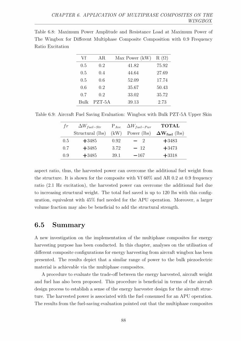
CHAPTER 6. APPLICATION OF MULTIPHASE COMPOSITES ON THEWINGBOX
Table 6.8: Maximum Power Amplitude and Resistance Load at Maximum Power of
The Wingbox for Different Multiphase Composite Composition with 0.9 Frequency
Ratio Excitation
Vf AR Max Power (kW) R (Ω)
0.5 0.2 41.82 75.92
0.5 0.4 44.64 27.69
0.5 0.6 52.09 17.74
0.6 0.2 35.67 50.43
0.7 0.2 33.02 35.72
Bulk PZT-5A 39.13 2.73
Table 6.9: Aircraft Fuel Saving Evaluation: Wingbox with Bulk PZT-5A Upper Skin
fr ∆Wfuel−Str PAve ∆Wfuel−Pwr TOTAL
Structural (lbs) (kW) Power (lbs) ∆Wfuel (lbs)
0.5 +++3485 0.92 −−− 2 +++3483
0.7 +++3485 3.72 −−− 12 +++3473
0.9 +++3485 39.1 −−−167 +++3318
aspect ratio, thus, the harvested power can overcome the additional fuel weight from
the structure. It is shown for the composite with Vf 60% and AR 0.2 at 0.9 frequency
ratio (2.1 Hz excitation), the harvested power can overcome the additional fuel due
to increasing structural weight. The total fuel saved is up to 120 lbs with this config-
uration, equivalent with 45% fuel needed for the APU operation. Moreover, a larger
volume fraction may also be beneficial to add the structural strength.
6.5 Summary
A new investigation on the implementation of the multiphase composites for energy
harvesting purpose has been conducted. In this chapter, analyses on the utilisation of
different composite configurations for energy harvesting from aircraft wingbox has been
presented. The results depict that a similar range of power to the bulk piezoelectric
material is achievable via the multiphase composites.
A procedure to evaluate the trade-off between the energy harvested, aircraft weight
and fuel has also been proposed. This procedure is beneficial in terms of the aircraft
design process to establish a sense of the energy harvester design for the aircraft struc-
ture. The harvested power is associated with the fuel consumed for an APU operation.
The results from the fuel-saving evaluation pointed out that the multiphase composites
88
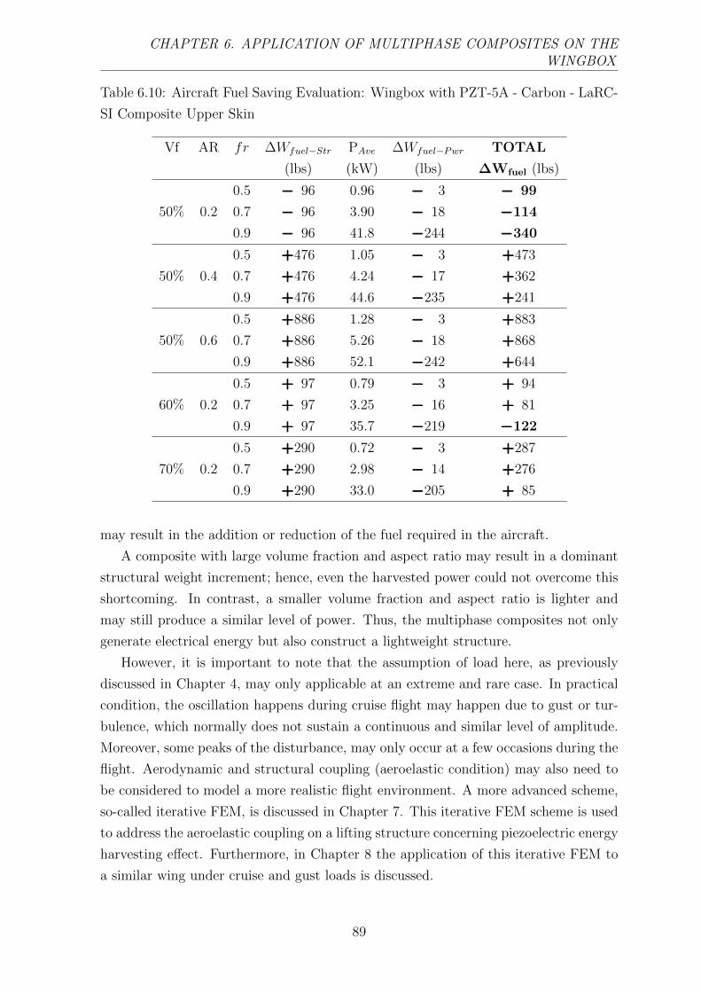
CHAPTER 6. APPLICATION OF MULTIPHASE COMPOSITES ON THEWINGBOX
Table 6.10: Aircraft Fuel Saving Evaluation: Wingbox with PZT-5A - Carbon - LaRC-
SI Composite Upper Skin
Vf AR fr ∆Wfuel−Str PAve ∆Wfuel−Pwr TOTAL
(lbs) (kW) (lbs) ∆Wfuel (lbs)
0.5 −−− 96 0.96 −−− 3 −−− 99
50% 0.2 0.7 −−− 96 3.90 −−− 18 −−−114
0.9 −−− 96 41.8 −−−244 −−−340
0.5 +++476 1.05 −−− 3 +++473
50% 0.4 0.7 +++476 4.24 −−− 17 +++362
0.9 +++476 44.6 −−−235 +++241
0.5 +++886 1.28 −−− 3 +++883
50% 0.6 0.7 +++886 5.26 −−− 18 +++868
0.9 +++886 52.1 −−−242 +++644
0.5 +++ 97 0.79 −−− 3 +++ 94
60% 0.2 0.7 +++ 97 3.25 −−− 16 +++ 81
0.9 +++ 97 35.7 −−−219 −−−122
0.5 +++290 0.72 −−− 3 +++287
70% 0.2 0.7 +++290 2.98 −−− 14 +++276
0.9 +++290 33.0 −−−205 +++ 85
may result in the addition or reduction of the fuel required in the aircraft.
A composite with large volume fraction and aspect ratio may result in a dominant
structural weight increment; hence, even the harvested power could not overcome this
shortcoming. In contrast, a smaller volume fraction and aspect ratio is lighter and
may still produce a similar level of power. Thus, the multiphase composites not only
generate electrical energy but also construct a lightweight structure.
However, it is important to note that the assumption of load here, as previously
discussed in Chapter 4, may only applicable at an extreme and rare case. In practical
condition, the oscillation happens during cruise flight may happen due to gust or tur-
bulence, which normally does not sustain a continuous and similar level of amplitude.
Moreover, some peaks of the disturbance, may only occur at a few occasions during the
flight. Aerodynamic and structural coupling (aeroelastic condition) may also need to
be considered to model a more realistic flight environment. A more advanced scheme,
so-called iterative FEM, is discussed in Chapter 7. This iterative FEM scheme is used
to address the aeroelastic coupling on a lifting structure concerning piezoelectric energy
harvesting effect. Furthermore, in Chapter 8 the application of this iterative FEM to
a similar wing under cruise and gust loads is discussed.
89

Chapter 7
Iterative Finite Element Method
for Piezoelectric Energy Harvesting
In this chapter, a novel iterative finite element method (FEM) for energy harvesting
purpose is presented. The development of this iterative FEM is purposed for further
evaluation of the energy harvesting potential from the aircraft wing. Hence, aerody-
namic loading and aero-structure coupling (aeroelasticity) are concerned. This itera-
tive FEM may serve as a higher fidelity approach to verify the results from the hybrid
computational/analytical scheme.
In this iterative FEM, the electromechanical coupling in the governing piezoelectric
energy harvesting equation is separated into two parts. One part is an actuator-like
problem and can be evaluated with ease via commercial software. The solution of the
other part, for voltage generation, is obtained straightforward utilising the structural
response of the earlier part. Hence, aero-structure and electro-mechanical couplings
are evaluated. These two parts are solved iteratively until the convergence in voltage
and structural responses is reached.
The new iterative FEM is implemented to solve the dynamic problems of piezoelectric-
based energy harvester in the frequency and time domains. The frequency-domain
scheme can be applied for a harmonic oscillation motion. Whereas the time-domain
scheme can be used for much broader time-dependent cases. The application of the
present iterative FEM to evaluate the piezoelectric energy harvesting of lifting struc-
tures under an aeroelastic condition, i.e., gust load, is shown in some details. The
validation against other methods from the literature shows the robustness and capa-
bilities of the iterative FEM.
Some works and results presented in this chapter are parts of the author’s published
works in Composite Structures, Volume 219, 2019.
90

CHAPTER 7.ITERATIVE FEM
7.1 The coupled electro-mechanical equations
In the present work, the piezoelectric electromechanical equilibrium in a dynamic prob-
lem is concerned. The governing equation of a coupled mechanical - electrical actuation
problem for piezoelectric finite elements [97] is modified to obtain the energy harvesting
solution. This actuation problem can be written as follows
[M 0
0 0
]U
V
+
[G 0
−Kvu Kvv
]U
V
+
[Kuu Kuv
0 0
]U
V
=
F
Q
(7.1)
The sizes of the matrices in Equation (7.1) are defined by the number of degrees
of freedom in mechanical, nm, and electrical, ne, domains [10]. The first and second
derivatives with respect to the time are denoted by the dot, ˙[ ], and the double dots,¨[ ]. Here, U (nm × 1), V (ne × 1), F (nm × 1) and Q (ne × 1), respectively, are the
global nodal displacement, electrical voltage, mechanical force and electrical current
vectors of the element. M (nm × nm) and G (nm × nm) represent the global mass and
mechanical damping matrices. The global stiffness and dampring matrices concerning
the electromechanical system are denoted by Kuu (nm × nm), Kuv (nm × ne), Kvu
(ne×nm) and Kvv (ne×ne). These global matrices are assembled from the associated
element′s matrices as follows [98]
Keuu =
∫V ol
BT C B dV ol (7.2)
Kevv =
∫V ol
BET εS BE dV ol (7.3)
Keuv =
∫V ol
BT eT BE dV ol (7.4)
Kevu =
∫V ol
BET e B dV ol (7.5)
Me =
∫V ol
NT ρ N dV ol (7.6)
Equations (7.2-7.6) represent the element′s volume integral of the electro-elastic
properties of the material. The density of the material is defined as ρ. The superscript
e denotes the matrix of an element. The structural stiffness matrix, Keuu, is constructed
from the elasticity matrix. Whereas Kevv is the capacitance of the piezoelectric element.
The electromechanical coupling of the piezoelectric element is represented by Keuv and
Kevu matrices. B and BE involves the shape functions, N, of the element based on the
type of discretisation [99]. In the present work, the poling of the piezoelectric layer
is assumed in the thickness direction. Hence, the component inside the integral of
Equation (7.3) can be expressed as [10]
91

CHAPTER 7.ITERATIVE FEM
BETεSBE =
εS33
h2(7.7)
In the present work, the polling of the piezoelectric layer is assumed in the thick-
ness direction. In addition, the piezoelectric materials usually manufactured as a thin
plate and sandwiched between very thin and conductive electrodes. Therefore, if the
continuous electrodes are used on the whole surfaces, all elements can be assumed to
generate the same voltage. Thus, vector V reduces to a voltage V [10]. Hence,
KuvV = Kuv[1 1...1]TV = K∗uvV (7.8)
where the size of the ones vector [1 1...1]T is ne×1, and the electromechanical coupling
is now defined by the vector K∗uv (nm × 1).
To modify the actuation problem in Equation (7.1), the current, I = Q, is defined
not as an input, but, as the function of the voltage output from the piezoelectric
harvester. The electrical load, however, comes from an external circuit connected to
the structure as shown in Figure 3.7. In the present work, the resistance load, R, is
applied as the the electrical load, thus, Q = −VR
. Therefore, Equation (7.1) can be
written as
MU + GU + KuuU = F−K∗uvV (7.9)
, and
−K∗vuU +KvvV +V
R= 0 (7.10)
where vector K∗vu = K∗uvT and Kvv is the capacitance of the piezoelectric layer.
The idea of the present iterative FEM is to obtain the solution of the displacement
vector U of the structure and the voltage output, V , of the piezoelectric layer through
an iterative process between Equations (7.9) and (7.10). This iteration process allows
Equation (7.9) to be separately solved as if it is an ”actuation” problem with the
mechanical force, F, and the voltage, V , as the actuating load to deform the structure.
In the iteration process, Equation (7.10) will update the value of the voltage V on each
iteration based on the displacement vector solved by Equation (7.9). A more detailed
algorithm of the present iterative FEM is described in Section 7.2. In addition, the
harvested power, P , is expressed as
P =V 2
R(7.11)
For a harmonic oscillation motion, the displacement, voltage and force are assumed
as the function of an excitation frequency, ω (rad/s) and can be written as
U = Ueiωt
F = Feiωt
V = V eiωt
(7.12)
92

CHAPTER 7.ITERATIVE FEM
where i =√−1 and the bar above a parameter denotes the amplitude. Hence, Equa-
tions (7.9) and (7.10) become
−ω2MU + KuuU = F−K∗uvV (7.13)
V =iωK∗vuU
iωKvv + 1R
(7.14)
Therefore, in this case, the iteration process will involve Equations (7.13) and (7.14).
7.2 Computational scheme
1st Equation→ Actuator-like Problem → Available in most commercial software
2nd Equation→Input of Resistance Loading→Numerical Coding
→Key Variables: 𝑲𝒗𝒖∗ = 𝑲𝒖𝒗
∗ 𝑇; 𝐾𝑣𝑣 = 𝐶𝑝
𝑴 ሷ𝑼 + 𝑮 ሶ𝑼 + 𝑲𝒖𝒖𝑼 = 𝑭 − 𝑲𝒖𝒗∗ 𝑉
−𝑲𝒗𝒖∗ ሶ𝑼 + 𝐾𝑣𝑣 ሶ𝑉 + ൗ𝑉 𝑅 = 0
ሶ𝑼𝒊
ሶ𝑼𝒊, 𝑅
𝑉𝑖
𝑉𝑖 , 𝑭 ሶ𝑼𝒊+𝟏
Next Iteration
Figure 7.1: Illustration of the iterative FEM process
In the present iterative FEM, one of the unique features is the seclusion of Equation
(7.9) to be solved as if it is an actuator problem. Figure 7.1 depicts the illustration of
the iterative FEM process based on Equation (7.9) and Equation (7.10). The actuator
problem is already a matured problem in the structural analysis field, and the module
is readily available in many commercial finite element software, i.e., Abaqus, Ansys,
MSC Nastran [100]. Therefore, the present iterative FEM provides excellent ease for
utilising the standard commercial software. In addition, Equation (7.10) can be solved
with minimum computational coding.
Moreover, the ease of solving Equation (7.9) via an already established computa-
tional software is that the mechanical force, F, may have a wide range of form, i.e.,
concentrated force, pressure, relative motion, or combination of several load types.
93

CHAPTER 7.ITERATIVE FEM
Commercial Software Computational CodeEquation (7.15)
𝑲𝒖𝒗∗
Equation (7.9)
Displacement Velocityሶ𝑼𝟎
Harvested Voltageሶ𝑉(𝑡)𝑖
Displacement Velocityሶ𝑼𝒊
Set tolerance∆
Converge ?
𝐽𝑖 − 𝐽𝑖−1 < ∆
Harvested Energy
𝐽𝑖 = න𝑡0
𝑡𝑒𝑛𝑑
𝑃(𝑡)𝑖 𝑑𝑡
Harvested Voltageሶ𝑉(𝑡)1
Equation (7.10)
Equation (7.9)
Equation (7.10)
IterationSTOP
NO𝒊 = 𝒊 + 𝟏
YES
INITIATION
𝑉0 = 0
𝑉 = 1
Co
mm
erc
ial
Soft
war
eC
om
pu
tati
on
al C
od
e
Figure 7.2: The algorithm of the iterative FEM for a time domain problem
Sections 7.3-7.6 present the works which demonstrate the implementation of base exci-
tation motion and unsteady aerodynamic loads as the mechanical force. Moreover, the
mechanical damping, G, can also be modelled with various form [79], i.e., proportional
to the structural stiffness matrix (structural damping), the linear combination of struc-
tural mass and stiffness matrix (Rayleigh damping), the function of natural frequency
(modal damping).
However, it is worth to note that the procedure to solve the electromechanical prob-
lem for energy harvesting as depicted in Equations (7.9) and (7.10) is not limited to
the present iterative process. Most notably, concerning unsteady aerodynamic loading,
several works in [13, 24] solved the aeroelastic and electromechanical coupling by con-
structing a state-space matrix; thus, iterative process was not required. Despite this
fact, their procedures require more elaborated effort in computational coding, i.e., nu-
merical codes to evaluate the structure (FEM), unsteady aerodynamic and piezoaeroe-
lastic coupling. Moreover, the selection of elements were limited to beam and planar
(3-DoF) elements [13, 24].
Meanwhile, in the present iterative scheme, the need of computational code is min-
imum. The choice to maximise the utilisation of the commercial software is due to
the focus of the present research which as a jet aircraft wing. This type of wing is
much more complex and larger structure compared to the lifting structures evaluated
in [13,24]. Hence, it is expected that the construction of elements, aerodynamic loads
and the aero-structure coupling could be handled by the commercial software with only
concern on the computational coding is to incorporate the electromechanical effect.
94
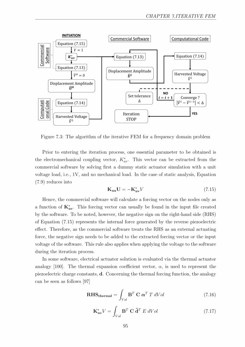
CHAPTER 7.ITERATIVE FEM
Commercial Software Computational CodeEquation (7.15)
𝑲𝒖𝒗∗
Equation (7.13)
Displacement Amplitudeഥ𝑼𝟎
Harvested Voltageത𝑉𝑖
Displacement Amplitudeഥ𝑼𝒊
Set tolerance∆
Converge ?ത𝑉𝑖 − ത𝑉𝑖−1 < ∆
Harvested Voltageത𝑉1
Equation (7.14)
Equation (7.13) Equation (7.14)
IterationSTOP
NO𝒊 = 𝒊 + 𝟏
YES
INITIATION
ത𝑉0 = 0
𝑉 = 1
Co
mm
erc
ial
Soft
war
eC
om
pu
tati
on
al C
od
e
Figure 7.3: The algorithm of the iterative FEM for a frequency domain problem
Prior to entering the iteration process, one essential parameter to be obtained is
the electromechanical coupling vector, K∗uv. This vector can be extracted from the
commercial software by solving first a dummy static actuator simulation with a unit
voltage load, i.e., 1V, and no mechanical load. In the case of static analysis, Equation
(7.9) reduces into
KuuU = −K∗uvV (7.15)
Hence, the commercial software will calculate a forcing vector on the nodes only as
a function of K∗uv. This forcing vector can usually be found in the input file created
by the software. To be noted, however, the negative sign on the right-hand side (RHS)
of Equation (7.15) represents the internal force generated by the reverse piezoelectric
effect. Therefore, as the commercial software treats the RHS as an external actuating
force, the negative sign needs to be added to the extracted forcing vector or the input
voltage of the software. This rule also applies when applying the voltage to the software
during the iteration process.
In some software, electrical actuator solution is evaluated via the thermal actuator
analogy [100]. The thermal expansion coefficient vector, α, is used to represent the
piezoelectric charge constants, d. Concerning the thermal forcing function, the analogy
can be seen as follows [97]
RHSthermal =
∫V ol
BT C αT T dV ol (7.16)
K∗uvV =
∫V ol
BT C dT E dV ol (7.17)
95

CHAPTER 7.ITERATIVE FEM
where the electrical field is E = V/h and the piezoelectric charge constants matrix d
(3 × 6) is collapsed to the vector d (1 × 6). This vector is expressed as
dT = [d31 d32 d33 0 0 0]T (7.18)
which analogous to the thermal expansion coefficient vector as
αT = [α1 α2 α3 α4 α5 α6]T (7.19)
Hence, in the case thermal actuator module is used, the piezoelectric charge constants
per layer thickness are input as the thermal expansion coefficients, i.e., d31/h = α1,
and the voltage as the temperature, i.e., V = T , to the commercial software.
The algorithm of the time-domain iterative FEM is depicted in Figure 7.2. In
the present work, the computational code to solve Equation (7.10) is built using
MATLAB©. The ordinary differential equation (ODE) solver of MATLAB© is used to
obtain the solution of V (t) for each iteration. The iteration procedure can be described
as follows:
1. Initially, Equation (7.9) is solved in the commercial software by assuming no
voltage applied, V 0 = 0.
2. The initial value of velocity vector, U0, is then used as input to the computational
code to obtain the first solution of the harvested voltage, V (t)1, via Equation
(7.10).
3. This first solution, V (t)1, is input to Equation (7.9) to obtain the new velocity
vector of iteration.
4. This new velocity vector then inputs again to solve Equation (7.10). This process
is repeated until the solution is converged.
In the present work, the convergence criteria for the time domain simulation is
based on the variance of energy from the current iteration and the previous iteration,
J i− J i−1 < ∆. In addition, the trend of the voltage function, V (t), is also observed to
ensure that the patterns are similar and in reasonable shape on each iteration.
The iteration process for the frequency domain is shown in Figure 7.3. In this
case, Equations (7.13) and (7.14) are the main governing equations. In addition, the
iterative variables for the frequency domain case are the amplitudes, U and V . Hence,
the convergence criteria is also much simpler by comparing the variance of the voltage
from each iteration, V i − V i−1 < ∆.
Appendices E and F show the examples of code to perform the frequency-domain
and time-domain analyses. Both codes have similar segments to extract the data from
96

CHAPTER 7.ITERATIVE FEM
a commercial software to construct the coupling matrix, Kuv, and the displacement
amplitude vector, U, or the velocity vector, U. The frequency-domain code, as shown
in Appendix E, calculates the voltage amplitude based on Equation (7.14). Mean-
while, the time-domain code, as depicted in Appendix F evaluates the voltage based
on Equation (7.10).
In the present work, the commercial software used is MSC Nastran©. It can be
seen in Appendices E and F, there are segments written for exchanging data between
the codes and the commercial software for each iteration. The displacement vector or
velocity vector is obtained from the analysis of dynamic responses via MSC Nastran©.
The iterative process involves offline files exchange between the inputs and outputs
from the code and the software. Appendix K depicts an example of input for gust
analysis performed via MSC Nastran©. This Nastran input is used for the jet wingbox
analysis presented in Chapter 8. The set of voltage input shown in Appendix K is
obtained from the calculation performed in Appendix F. An example of velocity vector
output from MSC Nastran© is shown in Appendix L. This data of velocity vector is
used as input to the code in Appendix F.
7.3 Unimorph plate under base excitation
In this section, the energy harvesting evaluation of a unimorph exerted by base excita-
tion is presented in [21]. The iterative FEM for frequency and time domain is utilised.
Comparison against the result of Erturk-Inman′s analytical model [21] is also shown in
some details.
The unimorph plate consisted of a host structure (isotropic metal) and a piezoelec-
tric layer (PZT-5A) covering the top surface of the plate similar to the configuration
shown in Figure 3.7. The size of the plate is 100 × 20 × 0.9 mm3 (length × width
× thickness), with PZT covering 44% of the thickness. The details of the material
properties for a beam-type formulation can be found in [21]. However, as solid and
shell elements are used here, the 3D and 2D material properties of PZT-5A in [101] are
utilised.
The verification of the unimorph structural models is performed using modal anal-
ysis. The unimorph is modelled by 25 × 5 elements, in the spanwise and the chordwise
directions, respectively. For a solid model, each layer on thickness direction is made
of their own respective material (PZT or metal). However, for the shell model, the
laminated composite module is used to represent the lay-up sequence.
The natural frequencies and the mode shapes of the present structural models are
depicted in Table 7.1. The results of Erturk-Inman′s analytical model is displayed in the
column ”Analytical”, while the present models′ are shown in columns ”Present-Solid”
97

CHAPTER 7.ITERATIVE FEM
and ”Present-Shell”. The first, second and third bending modes are denoted by ”1B”,
”2B” and ”3B”, respectively. It can be seen that both solid and shell models natural
frequencies are in a good agreement against analytical results in [21] with insignificant
variances, ∆ ≤ 1%.
Table 7.1: Natural frequency comparison of the unimorph
Natural Frequency (Hz)
Mode Analytical Present ∆ Present ∆
Shape [21] - Solid - Shell
1B 47.8 47.8 0.00% 47.5 0.63%
2B 299.6 299.3 0.10% 296.9 1.00%
3B 838.2 841.1 0.35% 831.9 0.75%
In the frequency domain investigation, 1µm amplitude of vertical displacement is
applied at the root as the base excitation load. The excitation frequency is equal with
the first bending natural frequency. Resistance load of 15 kΩ is used as the exter-
nal electrical load. As previously explained in Section 7.2, initially a pure structural
dynamic response without voltage load is performed to start the iteration process. Fol-
lowing the iterative procedure in Section 7.2, on each iteration step, the voltage output
and the structural responses are updated.
The voltage and relative tip amplitudes on each iteration step for both solid and
shell models are depicted in Figures 7.4 and 7.5. The dotted line with green circles
denote the results of the iterative FEM on each iteration step. The references′ values
denoted by the straight red line and the black dashed line are obtained via Erturk-
Inman model [21] and the present hybrid analytical/computational scheme. However,
with the hybrid scheme, only the voltage amplitude can be compared as the struc-
tural displacement after affected by voltage response could not be obtained from this
approach.
It can be seen in Figures 7.4a and 7.5a, initial value of voltage amplitude, V , is
zero. This condition resulted in a pure mechanical structural response with relative
tip displacement, Zrel, around 0.08 mm as depicted in Figures 7.4b and 7.5b. The first
iteration updated these values with the existence of voltage output and a much lower
tip displacement around 0.03 mm. The iteration histories shown in Figures 7.4 and 7.5
display the fluctuation on both voltage and tip displacement amplitudes around the
references′ values until they converge to some particular points.
The fluctuation happens as the electromechanical coupling tries to balance the
responses exerted by the mechanical load and the reverse piezoelectric effect. Initially,
a small voltage at an iteration step, i, resulted in a large displacement caused mainly
by the mechanical load, Zimech >>> Zi
elec, hence, Zitotal ≈ Zi
mech. However, large
98
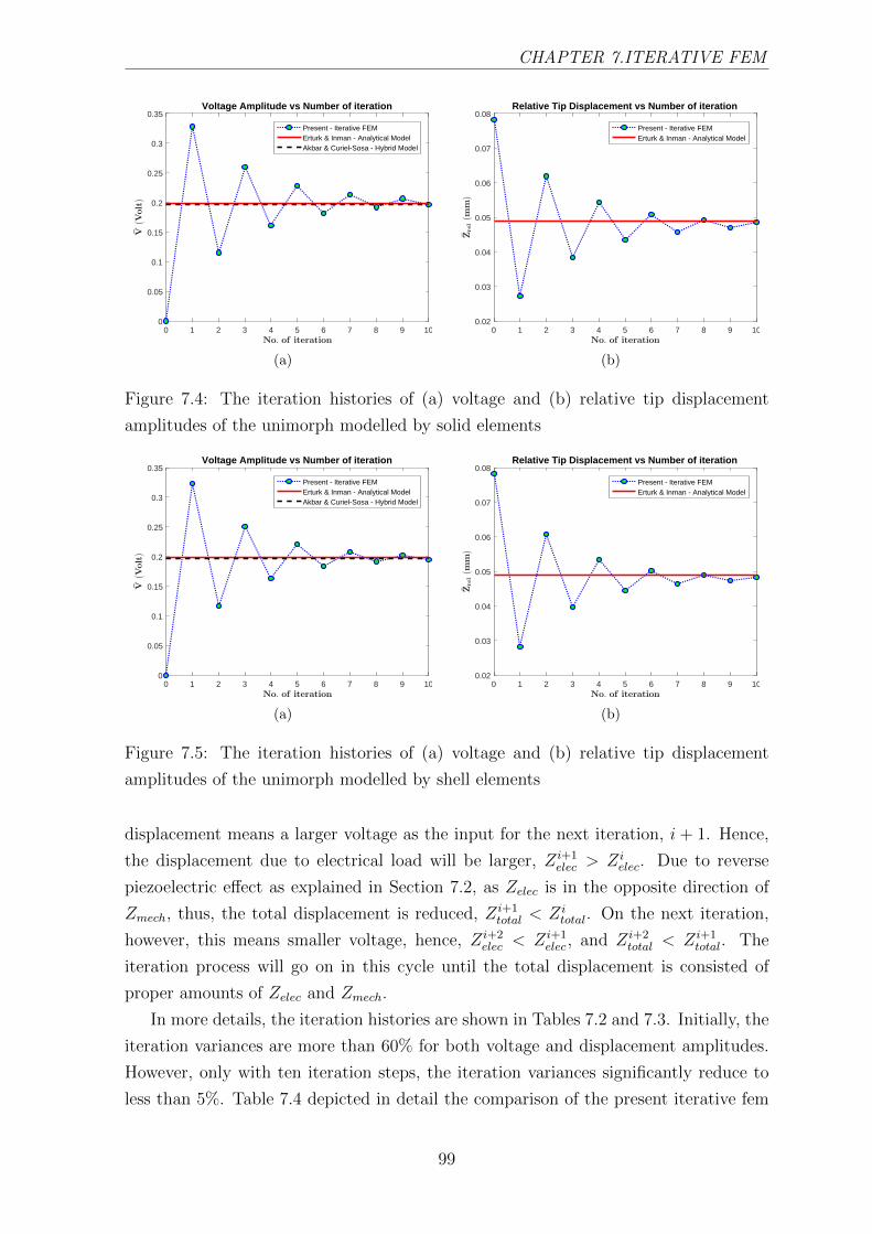
CHAPTER 7.ITERATIVE FEM
0 1 2 3 4 5 6 7 8 9 100
0.05
0.1
0.15
0.2
0.25
0.3
0.35Voltage Amplitude vs Number of iteration
Present - Iterative FEMErturk & Inman - Analytical ModelAkbar & Curiel-Sosa - Hybrid Model
(a)
0 1 2 3 4 5 6 7 8 9 100.02
0.03
0.04
0.05
0.06
0.07
0.08Relative Tip Displacement vs Number of iteration
Present - Iterative FEMErturk & Inman - Analytical Model
(b)
Figure 7.4: The iteration histories of (a) voltage and (b) relative tip displacement
amplitudes of the unimorph modelled by solid elements
0 1 2 3 4 5 6 7 8 9 100
0.05
0.1
0.15
0.2
0.25
0.3
0.35Voltage Amplitude vs Number of iteration
Present - Iterative FEMErturk & Inman - Analytical ModelAkbar & Curiel-Sosa - Hybrid Model
(a)
0 1 2 3 4 5 6 7 8 9 100.02
0.03
0.04
0.05
0.06
0.07
0.08Relative Tip Displacement vs Number of iteration
Present - Iterative FEMErturk & Inman - Analytical Model
(b)
Figure 7.5: The iteration histories of (a) voltage and (b) relative tip displacement
amplitudes of the unimorph modelled by shell elements
displacement means a larger voltage as the input for the next iteration, i + 1. Hence,
the displacement due to electrical load will be larger, Zi+1elec > Zi
elec. Due to reverse
piezoelectric effect as explained in Section 7.2, as Zelec is in the opposite direction of
Zmech, thus, the total displacement is reduced, Zi+1total < Zi
total. On the next iteration,
however, this means smaller voltage, hence, Zi+2elec < Zi+1
elec, and Zi+2total < Zi+1
total. The
iteration process will go on in this cycle until the total displacement is consisted of
proper amounts of Zelec and Zmech.
In more details, the iteration histories are shown in Tables 7.2 and 7.3. Initially, the
iteration variances are more than 60% for both voltage and displacement amplitudes.
However, only with ten iteration steps, the iteration variances significantly reduce to
less than 5%. Table 7.4 depicted in detail the comparison of the present iterative fem
99
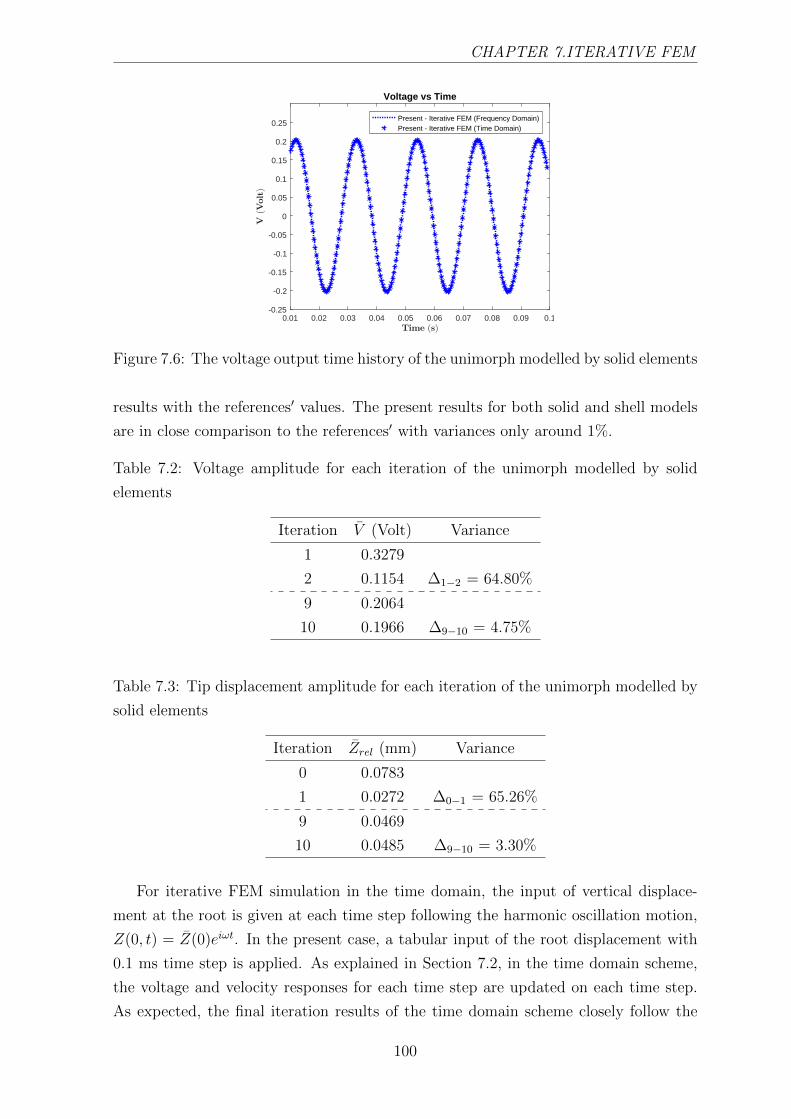
CHAPTER 7.ITERATIVE FEM
0.01 0.02 0.03 0.04 0.05 0.06 0.07 0.08 0.09 0.1-0.25
-0.2
-0.15
-0.1
-0.05
0
0.05
0.1
0.15
0.2
0.25
Voltage vs Time
Present - Iterative FEM (Frequency Domain)Present - Iterative FEM (Time Domain)
Figure 7.6: The voltage output time history of the unimorph modelled by solid elements
results with the references′ values. The present results for both solid and shell models
are in close comparison to the references′ with variances only around 1%.
Table 7.2: Voltage amplitude for each iteration of the unimorph modelled by solid
elements
Iteration V (Volt) Variance
1 0.3279
2 0.1154 ∆1−2 = 64.80%
9 0.2064
10 0.1966 ∆9−10 = 4.75%
Table 7.3: Tip displacement amplitude for each iteration of the unimorph modelled by
solid elements
Iteration Zrel (mm) Variance
0 0.0783
1 0.0272 ∆0−1 = 65.26%
9 0.0469
10 0.0485 ∆9−10 = 3.30%
For iterative FEM simulation in the time domain, the input of vertical displace-
ment at the root is given at each time step following the harmonic oscillation motion,
Z(0, t) = Z(0)eiωt. In the present case, a tabular input of the root displacement with
0.1 ms time step is applied. As explained in Section 7.2, in the time domain scheme,
the voltage and velocity responses for each time step are updated on each time step.
As expected, the final iteration results of the time domain scheme closely follow the
100
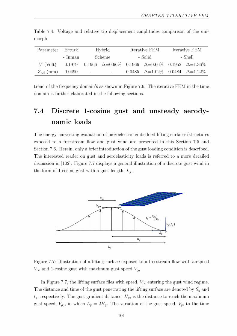
CHAPTER 7.ITERATIVE FEM
Table 7.4: Voltage and relative tip displacement amplitudes comparison of the uni-
morph
Parameter Erturk Hybrid Iterative FEM Iterative FEM
- Inman Scheme - Solid - Shell
V (Volt) 0.1979 0.1966 ∆=0.66% 0.1966 ∆=0.66% 0.1952 ∆=1.36%
Zrel (mm) 0.0490 - - 0.0485 ∆=1.02% 0.0484 ∆=1.22%
trend of the frequency domain′s as shown in Figure 7.6. The iterative FEM in the time
domain is further elaborated in the following sections.
7.4 Discrete 1-cosine gust and unsteady aerody-
namic loads
The energy harvesting evaluation of piezoelectric embedded lifting surfaces/structures
exposed to a freestream flow and gust wind are presented in this Section 7.5 and
Section 7.6. Herein, only a brief introduction of the gust loading condition is described.
The interested reader on gust and aeroelasticity loads is referred to a more detailed
discussion in [102]. Figure 7.7 displays a general illustration of a discrete gust wind in
the form of 1-cosine gust with a gust length, Lg.
𝑉𝑔0
𝐻𝑔
𝐿𝑔
𝑉∞
𝑡𝑔 = ൘𝑆𝑔
𝑉∞
𝑉𝑔(𝑡𝑔)
𝑆𝑔0
Figure 7.7: Illustration of a lifting surface exposed to a freestream flow with airspeed
V∞ and 1-cosine gust with maximum gust speed Vg0
In Figure 7.7, the lifting surface flies with speed, V∞ entering the gust wind regime.
The distance and time of the gust penetrating the lifting surface are denoted by Sg and
tg, respectively. The gust gradient distance, Hg, is the distance to reach the maximum
gust speed, Vg0 , in which Lg = 2Hg. The variation of the gust speed, Vg, to the time
101

CHAPTER 7.ITERATIVE FEM
tg is defined as
Vg =Vg02
(1− cos
(2πV∞tgLg
))(7.20)
To be noted, herein and hereafter, the letter V with subscripts ”∞”, ”g” and ”g0” will
be associated with speed. Therefore, it is important to note, the terms V∞, Vg and
Vg0 always refer to airspeed and gust speed. Meanwhile, the terms V and V always
associated with voltage or voltage amplitude.
Evaluating Equation (7.9) in the electromechanical coupling equations, the equilib-
rium equation concerning the aerodynamic load due to freestream flow and gust wind
can be written as
MU + GU + KuuU = F∞ + Fg −K∗uvV (7.21)
where F∞ and Fg are the aerodynamic loads due to airspeed, V∞, and gust speed,
Vg. Considering the coupling between the aerodynamic load and the structural de-
formation, F∞ can be written as the function of structural displacement, velocity and
acceleration. Hence, F∞ can be written equivalent with the component of mass, damp-
ing and stiffness. Therefore, Equation (7.21) can be rearranged with the aerodynamic
mass, M∞, aerodynamic damping, G∞, and aerodynamic stiffness, K∞.
(M−M∞)U + (G−G∞)U + (Kuu −K∞)U = Fg −K∗uvV (7.22)
In the present work, the Doublet-Lattice Method (DLM) of Albano and Rodden [33]
for subsonic flow is applied to model the aerodynamic loads acting on the lifting sur-
face. The DLM of Albano and Rodden is a well-established approach and commonly
implemented in the aircraft industries to evaluate the aeroelastic conditions for certifi-
cation, i.e., flutter instability and gust loads [102]. In addition, this approach is readily
available in commercial software, i.e., MSC Nastran [103].
In brief, Albano and Rodden [33] derived the aerodynamic force, F∞, as a dis-
tributed pressure, p, acting on the lifting surface. This pressure is evaluated numeri-
cally in matrix form as
p = D−1w (7.23)
The DLM discretises the lifting surface into panels in which the aerodynamic forces
modelled via doublets concentrated on the quarter chord line of each panel. The aero-
dynamic influence coefficient, D, is obtained from the doublet strength of each panel
and modelled as a function of the panel′s geometry, location, and the flight condition.
Meanwhile, the upwash velocity, w, is evaluated from the structure′s oscillatory mode
shapes, φ.
w =∂φ
∂x+ ikrφ (7.24)
Thus, concerning Equation (7.24), the investigation of the mode shapes are essential
to the aeroelastic evaluation. Moreover, the imaginary part of Equation (7.24) requires
102

CHAPTER 7.ITERATIVE FEM
the evaluation of the reduced frequency, kr, which defined as the ratio of excitation
frequency and freestream airspeed times the lifting surface′s half-chord.
7.5 Bimorph plate under gust load conditions
In this section, a plate-like wing with bimorph piezoelectric configuration in [24] is
elaborated as the case study. The bimorph plate configuration is depicted in Figure
7.8. Piezoelectric layers are made of PZT-5A with each covering 30% of the length
and 17% of the thickness. The host structure is made of Aluminum and sandwiched
between the piezoelectric layers in the region near the root. The PZT-5A layers and
Aluminum layers are represented with blue and red regions in Figure 7.8. The detailed
material properties are given in [24].
3mm
𝑉∞
Figure 7.8: Configuration of the bimorph
The PZT-5A layers are combined in a series circuit with each poled in the thickness
direction opposite to the other′s. A resistance load of 10 kΩ is used to complete the
electrical circuit. The whole bimorph plate is assumed as the lifting surface, exposed
to a uniform freestream flow at the sea level condition with airspeed, V∞, parallel to
the chordwise direction. The direction from the leading edge to trailing edge is defined
as the x-positive direction.
Both solid and shell elements are also applied to model the bimorph plate. The
solid finite element model of the bimorph is also shown in Figure 7.8. The configuration
of 40 × 8 elements is used in spanwise and chordwise directions. The same division
also applied to the shell model with the difference lies in the implementation of the
laminated composite module to represent the lay-up sequence. In order to validate
the structural model, the natural frequencies and mode shapes of the solid and shell
models are compared against the results in [24] as depicted in Table 7.5.
103
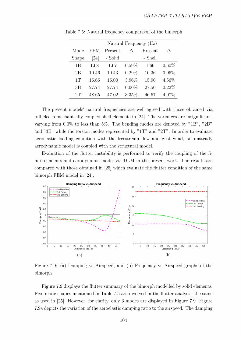
CHAPTER 7.ITERATIVE FEM
Table 7.5: Natural frequency comparison of the bimorph
Natural Frequency (Hz)
Mode FEM Present ∆ Present ∆
Shape [24] - Solid - Shell
1B 1.68 1.67 0.59% 1.66 0.60%
2B 10.46 10.43 0.29% 10.36 0.96%
1T 16.66 16.00 3.96% 15.90 4.56%
3B 27.74 27.74 0.00% 27.50 0.22%
2T 48.65 47.02 3.35% 46.67 4.07%
The present models′ natural frequencies are well agreed with those obtained via
full electromechanically-coupled shell elements in [24]. The variances are insignificant,
varying from 0.0% to less than 5%. The bending modes are denoted by ”1B”, ”2B”
and ”3B” while the torsion modes represented by ”1T” and ”2T”. In order to evaluate
aeroelastic loading condition with the freestream flow and gust wind, an unsteady
aerodynamic model is coupled with the structural model.
Evaluation of the flutter instability is performed to verify the coupling of the fi-
nite elements and aerodynamic model via DLM in the present work. The results are
compared with those obtained in [25] which evaluate the flutter condition of the same
bimorph FEM model in [24].
0 5 10 15 20 25 30 35 40 45 50-0.5
-0.4
-0.3
-0.2
-0.1
0
0.1
0.2
0.3
0.4
0.5Damping Ratio vs Airspeed
2nd Bending1st Torsion3rd Bending
(a)
5 10 15 20 25 30 35 40 45 500
5
10
15
20
25
30Frequency vs Airspeed
2nd Bending1st Torsion3rd Bending
(b)
Figure 7.9: (a) Damping vs Airspeed, and (b) Frequency vs Airspeed graphs of the
bimorph
Figure 7.9 displays the flutter summary of the bimorph modelled by solid elements.
Five mode shapes mentioned in Table 7.5 are involved in the flutter analysis, the same
as used in [25]. However, for clarity, only 3 modes are displayed in Figure 7.9. Figure
7.9a depicts the variation of the aeroelastic damping ratio to the airspeed. The damping
104
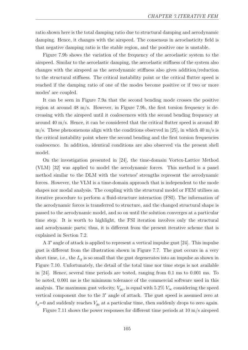
CHAPTER 7.ITERATIVE FEM
ratio shown here is the total damping ratio due to structural damping and aerodynamic
damping. Hence, it changes with the airspeed. The consensus in aeroelasticity field is
that negative damping ratio is the stable region, and the positive one is unstable.
Figure 7.9b shows the variation of the frequency of the aeroelastic system to the
airspeed. Similar to the aeroelastic damping, the aeroelastic stiffness of the system also
changes with the airspeed as the aerodynamic stiffness also gives addition/reduction
to the structural stiffness. The critical instability point or the critical flutter speed is
reached if the damping ratio of one of the modes become positive or if two or more
modes′ are coupled.
It can be seen in Figure 7.9a that the second bending mode crosses the positive
region at around 48 m/s. However, in Figure 7.9b, the first torsion frequency is de-
creasing with the airspeed until it coalescences with the second bending frequency at
around 40 m/s. Hence, it can be considered that the critical flutter speed is around 40
m/s. These phenomenons align with the conditions observed in [25], in which 40 m/s is
the critical instability point where the second bending and the first torsion frequencies
coalescence. In addition, identical conditions are also observed via the present shell
model.
On the investigation presented in [24], the time-domain Vortex-Lattice Method
(VLM) [32] was applied to model the aerodynamic forces. This method is a panel
method similar to the DLM with the vortexes′ strengths represent the aerodynamic
forces. However, the VLM is a time-domain approach that is independent to the mode
shapes nor modal analysis. The coupling with the structural model or FEM utilises an
iterative procedure to perform a fluid-structure interaction (FSI). The information of
the aerodynamic forces is transferred to structure, and the changed structural shape is
passed to the aerodynamic model, and so on until the solution converges at a particular
time step. It is worth to highlight, the FSI iteration involves only the structural
and aerodynamic parts; thus, it is different from the present iterative scheme that is
explained in Section 7.2.
A 3° angle of attack is applied to represent a vertical impulse gust [24]. This impulse
gust is different from the illustration shown in Figure 7.7. The gust occurs in a very
short time, i.e., the Lg is so small that the gust degenerates into an impulse as shown in
Figure 7.10. Unfortunately, the detail of the total time nor time steps is not available
in [24]. Hence, several time periods are tested, ranging from 0.1 ms to 0.001 ms. To
be noted, 0.001 ms is the minimum tolerance of the commercial software used in this
analysis. The maximum gust velocity, Vg0 , is equal with 5.2% V∞ considering the speed
vertical component due to the 3° angle of attack. The gust speed is assumed zero at
tg=0 and suddenly reaches Vg0 at a particular time, then suddenly drops to zero again.
Figure 7.11 shows the power responses for different time periods at 10 m/s airspeed
105

CHAPTER 7.ITERATIVE FEM
𝑉∞
𝑉𝑔0
𝐿𝑔
𝑉𝑔(𝑡𝑔)
Figure 7.10: Illustration of a lifting surface exposed to a freestream flow with airspeed
V∞ and an impulse gust with maximum gust speed Vg0
obtained via shell elements. It is found that 0.01 ms period gives the closest results
to the reference, total energy 0.0927 µJ compared to 0.0865 µJ in [24]. In contrast,
0.1 ms resulted in a more overestimated result, 0.0970 µJ, and 0.001 ms provides
underestimated result with 0.0594 µJ. Therefore, for the current analysis, 0.01 ms is
selected as the time period. Further, the comparison of the current results with the
reference′s is shown in Table 7.6.
Figures 7.12 and 7.13 depict time histories of the bimorph′s tip displacements and
harvested powers from the piezoelectric layers at 10 m/s and 30 m/s freestream con-
ditions, respectively. The red dashed-dotted lines denote the results of De Marqui Jr.
et al. [24]. The final iteration′s results obtained via the present iterative FEM method
by the shell and solid models are denoted by the black straight lines and the blue
dotted lines. The iterative processes for both models rapidly converge in less than five
iterations as the harvested voltages do not greatly affect the structural responses. This
phenomenon aligns with the results in [24], in which the structural responses from the
range of short circuit to open circuit are identical. Thus, showing that the displacement
due to mechanical load is much more dominant than the one exerted by the electrical
load.
The computational simulations are done via a standard office laptop with Intel
Core i7 2.4 GHz and 4GB RAM. Less than 5 minutes are required for the aeroelastic
evaluation and around 2-3 minutes for the electromechanical evaluation in MATLAB.
Adding a couple of minutes for text editing of the aeroelastic result data to MATLAB,
106
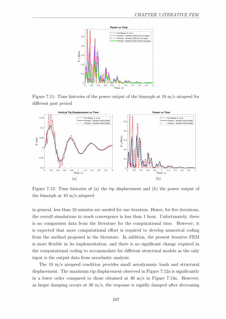
CHAPTER 7.ITERATIVE FEM
0 0.2 0.4 0.6 0.8 1 1.2 1.4 1.6 1.8 20
0.1
0.2
0.3
0.4
0.5
Power vs Time
De Marqui Jr. et al.Present - Iterative FEM (0.01 ms gust)Present - Iterative FEM (0.1 ms gust)Present - Iterative FEM (0.001 ms gust)
Figure 7.11: Time histories of the power output of the bimorph at 10 m/s airspeed for
different gust period
0 0.2 0.4 0.6 0.8 1 1.2 1.4 1.6 1.8 2-0.1
-0.05
0
0.05
0.1
0.15
Vertical Tip Displacement vs Time
De Marqui Jr. et al.Present - Iterative FEM (Shell)Present - Iterative FEM (Solid)
(a)
0 0.2 0.4 0.6 0.8 1 1.2 1.4 1.6 1.8 20
0.1
0.2
0.3
0.4
0.5
Power vs Time
De Marqui Jr. et al.Present - Iterative FEM (Shell)Present - Iterative FEM (Solid)
(b)
Figure 7.12: Time histories of (a) the tip displacement and (b) the power output of
the bimorph at 10 m/s airspeed
in general, less than 10 minutes are needed for one iteration. Hence, for five iterations,
the overall simulations to reach convergence is less than 1 hour. Unfortunately, there
is no comparison data from the literature for the computational time. However, it
is expected that more computational effort is required to develop numerical coding
from the method proposed in the literature. In addition, the present iterative FEM
is more flexible in its implementation, and there is no significant change required in
the computational coding to accommodate for different structural models as the only
input is the output data from aeroelastic analysis.
The 10 m/s airspeed condition provides small aerodynamic loads and structural
displacement. The maximum tip displacement observed in Figure 7.12a is significantly
in a lower order compared to those obtained at 30 m/s in Figure 7.13a. However,
as larger damping occurs at 30 m/s, the response is rapidly damped after decreasing
107

CHAPTER 7.ITERATIVE FEM
0 0.2 0.4 0.6 0.8 1 1.2 1.4 1.6 1.8 2
0
0.2
0.4
0.6
0.8
1
Vertical Tip Displacement vs Time
De Marqui Jr. et al.Present - Iterative FEM (Shell)Present - Iterative FEM (Solid)
(a)
0 0.2 0.4 0.6 0.8 1 1.2 1.4 1.6 1.8 20
10
20
30
40
50
60
70
Power vs Time
De Marqui Jr. et al.Present - Iterative FEM (Shell)Present - Iterative FEM (Solid)
(b)
Figure 7.13: Time histories of (a) the tip displacement and (b) the power output of
the bimorph 30 m/s airspeed
from the maximum point. In contrast, the one at 10 m/s still oscillating after the first
maximum response, showing moderate damping of the system.
The harvested power responses are aligned with the trends of the tip displacements
as shown in Figures 7.12b and 7.13b. The harvested power at 10 m/s still oscillating
after the first maximum response. However, at 30 m/s, the power response quickly
vanishes along with the damped structural response. The VLM simulation and both
present models are all in agreement and show similar behaviours. However, it can
be seen that the results of the VLM fluctuate with the time due to the FSI iterative
process on each time step [32].
Table 7.6: Electrical energy comparison of the bimorph
Energy (µJ)
Speed FEM Present ∆ Present ∆
(m/s) [10] - Solid - Shell
10 0.0865 0.0880 1.73% 0.0927 7.17%
30 5.5295 5.7258 3.55% 5.5838 0.98%
In more details, the energy harvested by the three approaches are compared in
Table 7.6. Total time of 2s is used to calculate the energy harvested. The energies
obtained from all approaches are in a good comparison. The present results only vary
less than 10% to the results by De Marqui Jr. et al. [24], in which mostly vary between
1% to 4%. Nevertheless, for a preliminary engineering design phase, these variances
are considered acceptable.
The displacement contours of the solid bimorph at tg = 0.175 s are depicted in
Figures 7.14a and 7.14b. At tg = 0.175 s, the loads causes the maximum structural
108
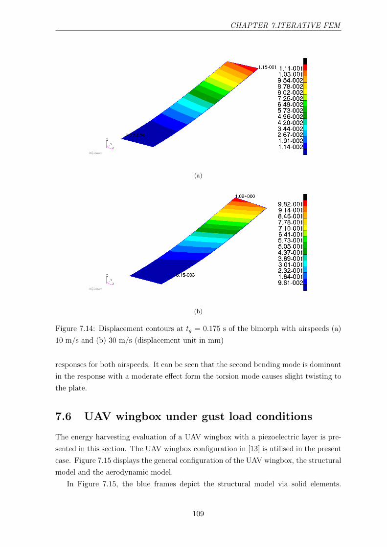
CHAPTER 7.ITERATIVE FEM
(a)
(b)
Figure 7.14: Displacement contours at tg = 0.175 s of the bimorph with airspeeds (a)
10 m/s and (b) 30 m/s (displacement unit in mm)
responses for both airspeeds. It can be seen that the second bending mode is dominant
in the response with a moderate effect form the torsion mode causes slight twisting to
the plate.
7.6 UAV wingbox under gust load conditions
The energy harvesting evaluation of a UAV wingbox with a piezoelectric layer is pre-
sented in this section. The UAV wingbox configuration in [13] is utilised in the present
case. Figure 7.15 displays the general configuration of the UAV wingbox, the structural
model and the aerodynamic model.
In Figure 7.15, the blue frames depict the structural model via solid elements.
109
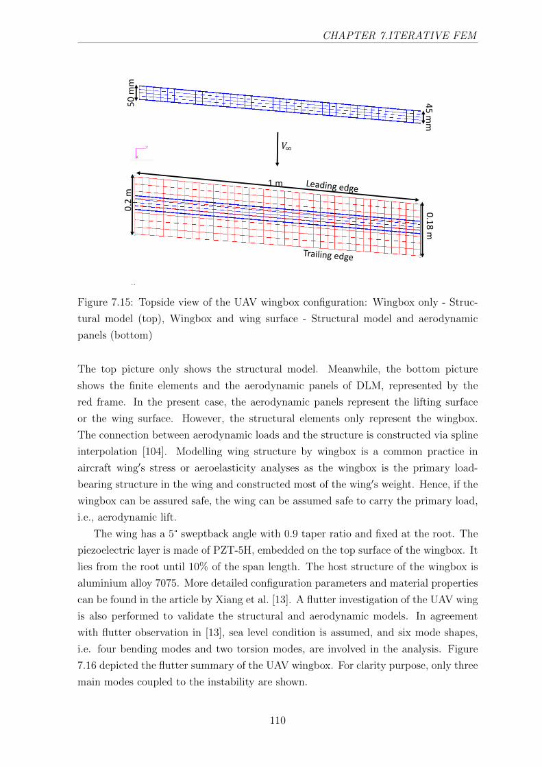
CHAPTER 7.ITERATIVE FEM
50
mm
45
mm
1 m
0.2
m
0.1
8 m
𝑉∞
Figure 7.15: Topside view of the UAV wingbox configuration: Wingbox only - Struc-
tural model (top), Wingbox and wing surface - Structural model and aerodynamic
panels (bottom)
The top picture only shows the structural model. Meanwhile, the bottom picture
shows the finite elements and the aerodynamic panels of DLM, represented by the
red frame. In the present case, the aerodynamic panels represent the lifting surface
or the wing surface. However, the structural elements only represent the wingbox.
The connection between aerodynamic loads and the structure is constructed via spline
interpolation [104]. Modelling wing structure by wingbox is a common practice in
aircraft wing′s stress or aeroelasticity analyses as the wingbox is the primary load-
bearing structure in the wing and constructed most of the wing′s weight. Hence, if the
wingbox can be assured safe, the wing can be assumed safe to carry the primary load,
i.e., aerodynamic lift.
The wing has a 5° sweptback angle with 0.9 taper ratio and fixed at the root. The
piezoelectric layer is made of PZT-5H, embedded on the top surface of the wingbox. It
lies from the root until 10% of the span length. The host structure of the wingbox is
aluminium alloy 7075. More detailed configuration parameters and material properties
can be found in the article by Xiang et al. [13]. A flutter investigation of the UAV wing
is also performed to validate the structural and aerodynamic models. In agreement
with flutter observation in [13], sea level condition is assumed, and six mode shapes,
i.e. four bending modes and two torsion modes, are involved in the analysis. Figure
7.16 depicted the flutter summary of the UAV wingbox. For clarity purpose, only three
main modes coupled to the instability are shown.
110

CHAPTER 7.ITERATIVE FEM
0 50 100 150 200 250-2
-1.5
-1
-0.5
0
0.5
1
1.5
2Airspeed vs Damping Ratio
3rd Bending1st Torsion4th Bending
(a)
50 100 150 200 2500
50
100
150
200
250
300
350
Airspeed vs Frequency
3rd Bending1st Torsion4th Bending
(b)
Figure 7.16: (a) Damping vs Airspeed, and (b) Frequency vs Airspeed graphs of the
UAV wingbox
Figures 7.16a and 7.16a shows the variations of the damping ratio and frequency
to the airspeed of the UAV wingbox. It can be seen that the first torsion crosses
the positive damping (unstable) region at 220 m/s in Figure 7.16a. However, the
frequency evolution in Figure 7.16b displays the three modes coalesce at around 140-
150 m/s. Appendix I shows the flutter responses of the UAV wingbox at 150 m/s
for different modes. The frequencies of the third and fourth bending coalesce first at
140 m/s followed by the other intersections. These complete intersections of the three
frequencies may lead to violent instability. This case is also known as a hard flutter
condition, while the one for the bimorph in Section 7.5 is called soft flutter as the
frequencies only approach each other at a very short gap [102]. This condition agrees
with the critical flutter speed at 150.2 m/s obtained by Xiang et al. [13].
For the gust load condition, the wing is observed at cruise state with V∞ = 100 m/s
and flight altitude 4000 m above sea level. The maximum gust velocity, Vg0 , is 15 m/s.
The gust gradient distance, Hg, is 12.5 mean aerodynamic chord (MAC). This typical
gust gradient is one of the parameters set by FAR for time-dependant gust analysis as
it normally gives the maximum structural response. Thus, the total gust time, tg, is
0.0475 s. Extra 1 s observation time is given by Xiang et al. [13] to allow the dynamic
response finishes. It can be seen, however, the displacement is completely damped after
0.2 s as shown in Figure 7.17a.
In Figures 7.17a and 7.17b the responses of both the present result and those ob-
tained in [13] are in a good agreement at the beginning until it reaches the maximum
responses. However, some discrepancies can be seen after the first maximum responses.
The displacement obtained by Xiang et al. [13] is damped quickly without any oscilla-
tion after it reaches the first amplitude. In contrast, the present result shows at least
111
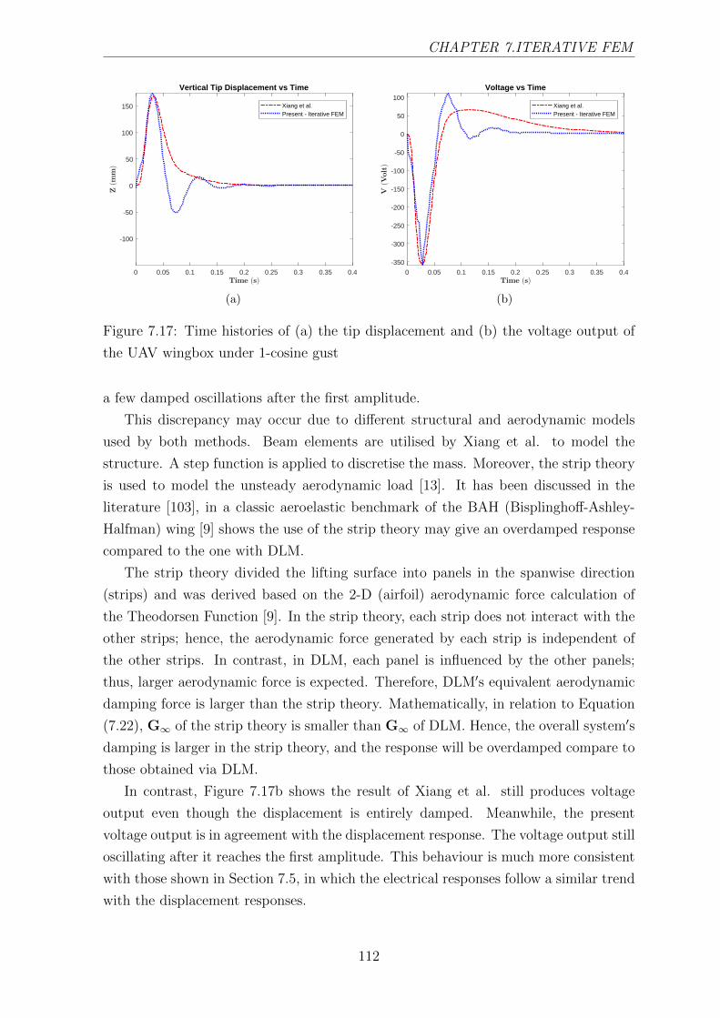
CHAPTER 7.ITERATIVE FEM
0 0.05 0.1 0.15 0.2 0.25 0.3 0.35 0.4
-100
-50
0
50
100
150
Vertical Tip Displacement vs Time
Xiang et al.Present - Iterative FEM
(a)
0 0.05 0.1 0.15 0.2 0.25 0.3 0.35 0.4
-350
-300
-250
-200
-150
-100
-50
0
50
100
Voltage vs Time
Xiang et al.Present - Iterative FEM
(b)
Figure 7.17: Time histories of (a) the tip displacement and (b) the voltage output of
the UAV wingbox under 1-cosine gust
a few damped oscillations after the first amplitude.
This discrepancy may occur due to different structural and aerodynamic models
used by both methods. Beam elements are utilised by Xiang et al. to model the
structure. A step function is applied to discretise the mass. Moreover, the strip theory
is used to model the unsteady aerodynamic load [13]. It has been discussed in the
literature [103], in a classic aeroelastic benchmark of the BAH (Bisplinghoff-Ashley-
Halfman) wing [9] shows the use of the strip theory may give an overdamped response
compared to the one with DLM.
The strip theory divided the lifting surface into panels in the spanwise direction
(strips) and was derived based on the 2-D (airfoil) aerodynamic force calculation of
the Theodorsen Function [9]. In the strip theory, each strip does not interact with the
other strips; hence, the aerodynamic force generated by each strip is independent of
the other strips. In contrast, in DLM, each panel is influenced by the other panels;
thus, larger aerodynamic force is expected. Therefore, DLM′s equivalent aerodynamic
damping force is larger than the strip theory. Mathematically, in relation to Equation
(7.22), G∞ of the strip theory is smaller than G∞ of DLM. Hence, the overall system′s
damping is larger in the strip theory, and the response will be overdamped compare to
those obtained via DLM.
In contrast, Figure 7.17b shows the result of Xiang et al. still produces voltage
output even though the displacement is entirely damped. Meanwhile, the present
voltage output is in agreement with the displacement response. The voltage output still
oscillating after it reaches the first amplitude. This behaviour is much more consistent
with those shown in Section 7.5, in which the electrical responses follow a similar trend
with the displacement responses.
112

CHAPTER 7.ITERATIVE FEM
0 0.05 0.1 0.15 0.2 0.25 0.3 0.35 0.40
0.2
0.4
0.6
0.8
1
1.2
Power vs Time
Xiang et al.Present - Iterative FEM
Figure 7.18: The power output time history
Figure 7.19: Displacement contour of the UAV wingbox at tg = 0.0285 s(displacement
unit in mm)
Figure 7.18 shows the power response of the present model still has fluctuations after
the first maximum power although the second largest fluctuation only sustained around
0.05 s. Meanwhile, after the first amplitude, the result from Xiang et al. sustained a
lower maximum power which sustained much longer, around 0.15 s. This behaviour
resulted in a discrepancy of the total energy output. The present result only achieves
25.3 mJ compared to the one obtained by Xiang et al., 35.1 mJ.
A detailed displacement contour of the UAV wingbox at tg = 28.5 ms is depicted
in Figure 7.19. At tg = 28.5 ms, the maximum displacement response is exerted by the
combined mechanical and electrical loads. The displacement is mostly dominated by
the first bending mode where the maximum is observed at the tip. Figure 7.20 shows
the voltage contour on the wingbox. It is seen that the voltage only occurs at the thin
top layer near the root in which the piezoelectric is located. An amount of 363 Volt
113

CHAPTER 7.ITERATIVE FEM
Figure 7.20: Voltage contour of the piezoelectric layer of the UAV wingbox at tg =
0.0285 s (voltage unit in µV)
is observed at tg = 28 ms. Meanwhile, the other parts of the wingbox do not produce
the voltage as there is no electromechanical coupling.
0 0.05 0.1 0.15 0.2 0.25 0.3 0.35 0.4
-350
-300
-250
-200
-150
-100
-50
0
50
100Voltage vs Time
Iteration 2Iteration 3Iteration 4
0.01 0.02 0.03 0.04 0.05
-350
-300
-250
-200
Figure 7.21: The voltage output time histories at different iteration steps
Figure 7.21 displays the voltage responses at different iteration steps. It can be seen
that the responses for all the steps almost coincide. In the enlarged view, the result
from the second iteration is shown slightly overestimates the other results. The third
and the fourth iteration results, however, still almost coincide even in the enlarged
view. In more details, the iterative process is shown in Table 7.7.
The harvested energy even only after the third iteration provided less than 5% iter-
ation variance. After ten iterations, the iteration variance even lower, with a value less
than 1%. This shows that the displacement due to electrical load is also insignificant
to the one exerted by the mechanical load. This behaviour is similar to the results
114

CHAPTER 7.ITERATIVE FEM
observed in Section 7.5. In this case, it might be considered that the normal flight op-
eration with active piezoelectric energy harvesting may not provide a significant change
to the structural deformation while still may produce voltage response.
Table 7.7: Electrical energy output of the UAV wingbox on each iteration step
Iteration Energy (J) Variance
1 0.0250
2 0.0263 ∆1−2 = 5.60%
3 0.0250 ∆2−3 = 4.94%
4 0.0256 ∆3−4 = 2.40%
9 0.0251
10 0.0253 ∆9−10 = 0.79%
7.7 Summary
A novel iterative finite element method (FEM) for energy harvesting purpose has been
developed. This iterative FEM scheme involves the utilisation of commercial software
to create and evaluate the structure, aerodynamic, and aeroelastic models. A computa-
tional code based on this new iterative FEM has been built as the augmentation for the
commercial software to solve the electromechanical coupling for energy harvesting case.
Validation with the classical benchmark of piezoelectric energy harvester plate under
base excitation shows an excellent agreement both in frequency and time domains.
Two different lifting structures, i.e., a plate-like wing and a UAV wingbox, with
active energy harvesting layer(s) subjected to 1-cosine gusts have been investigated
via the time-domain iterative FEM. Based on the case studies, the iterative processes
are considerably fast, and convergences are achieved in less than ten iterations. The
present results are all showing similar behaviours with the references′ results.
From the observation on the iterative processes, an exciting finding is taken, the
mechanically-exerted displacements dominate the responses of all the lifting structures.
Thus, based on these results, the influences of the reverse piezoelectric effect are min-
imum. Hence, for normal flight operation, it may occur that the displacement is not
significantly affected by the harvested voltage.
In the present work, the iterative FEM is further implemented to a notional jet
aircraft wingbox exerted by gust and cruise loading. Chapter 8 discusses the energy
harvesting evaluation of the wingbox for different gust load conditions.
115
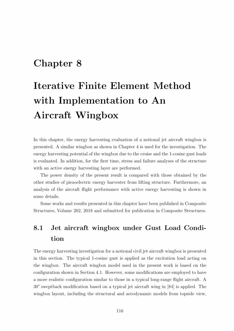
Chapter 8
Iterative Finite Element Method
with Implementation to An
Aircraft Wingbox
In this chapter, the energy harvesting evaluation of a notional jet aircraft wingbox is
presented. A similar wingbox as shown in Chapter 4 is used for the investigation. The
energy harvesting potential of the wingbox due to the cruise and the 1-cosine gust loads
is evaluated. In addition, for the first time, stress and failure analyses of the structure
with an active energy harvesting layer are performed.
The power density of the present result is compared with those obtained by the
other studies of piezoelectric energy harvester from lifting structure. Furthermore, an
analysis of the aircraft flight performance with active energy harvesting is shown in
some details.
Some works and results presented in this chapter have been published in Composite
Structures, Volume 202, 2018 and submitted for publication in Composite Structures.
8.1 Jet aircraft wingbox under Gust Load Condi-
tion
The energy harvesting investigation for a notional civil jet aircraft wingbox is presented
in this section. The typical 1-cosine gust is applied as the excitation load acting on
the wingbox. The aircraft wingbox model used in the present work is based on the
configuration shown in Section 4.1. However, some modifications are employed to have
a more realistic configuration similar to those in a typical long-range flight aircraft. A
30° sweptback modification based on a typical jet aircraft wing in [84] is applied. The
wingbox layout, including the structural and aerodynamic models from topside view,
116
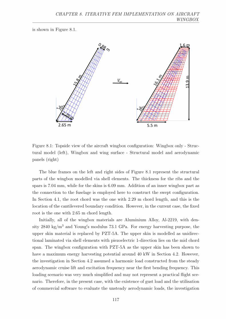
CHAPTER 8. ITERATIVE FEM IMPLEMENTATION ON AIRCRAFTWINGBOX
is shown in Figure 8.1.
𝑉∞
5.5 m
1.6 m
30o
13
.9 m
2.65 m
30o
Figure 8.1: Topside view of the aircraft wingbox configuration: Wingbox only - Struc-
tural model (left), Wingbox and wing surface - Structural model and aerodynamic
panels (right)
The blue frames on the left and right sides of Figure 8.1 represent the structural
parts of the wingbox modelled via shell elements. The thickness for the ribs and the
spars is 7.04 mm, while for the skins is 6.09 mm. Addition of an inner wingbox part as
the connection to the fuselage is employed here to construct the swept configuration.
In Section 4.1, the root chord was the one with 2.29 m chord length, and this is the
location of the cantilevered boundary condition. However, in the current case, the fixed
root is the one with 2.65 m chord length.
Initially, all of the wingbox materials are Aluminium Alloy, Al-2219, with den-
sity 2840 kg/m3 and Young′s modulus 73.1 GPa. For energy harvesting purpose, the
upper skin material is replaced by PZT-5A. The upper skin is modelled as unidirec-
tional laminated via shell elements with piezoelectric 1-direction lies on the mid chord
span. The wingbox configuration with PZT-5A as the upper skin has been shown to
have a maximum energy harvesting potential around 40 kW in Section 4.2. However,
the investigation in Section 4.2 assumed a harmonic load constructed from the steady
aerodynamic cruise lift and excitation frequency near the first bending frequency. This
loading scenario was very much simplified and may not represent a practical flight sce-
nario. Therefore, in the present case, with the existence of gust load and the utilisation
of commercial software to evaluate the unsteady aerodynamic loads, the investigation
117
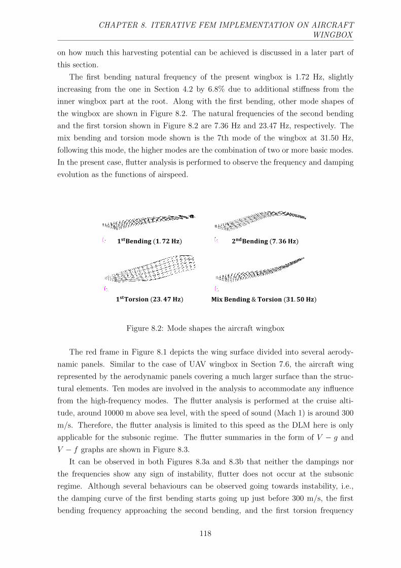
CHAPTER 8. ITERATIVE FEM IMPLEMENTATION ON AIRCRAFTWINGBOX
on how much this harvesting potential can be achieved is discussed in a later part of
this section.
The first bending natural frequency of the present wingbox is 1.72 Hz, slightly
increasing from the one in Section 4.2 by 6.8% due to additional stiffness from the
inner wingbox part at the root. Along with the first bending, other mode shapes of
the wingbox are shown in Figure 8.2. The natural frequencies of the second bending
and the first torsion shown in Figure 8.2 are 7.36 Hz and 23.47 Hz, respectively. The
mix bending and torsion mode shown is the 7th mode of the wingbox at 31.50 Hz,
following this mode, the higher modes are the combination of two or more basic modes.
In the present case, flutter analysis is performed to observe the frequency and damping
evolution as the functions of airspeed.
𝟏𝐬𝐭𝐁𝐞𝐧𝐝𝐢𝐧𝐠 (𝟏. 𝟕𝟐 𝐇𝐳) 𝟐𝐧𝐝𝐁𝐞𝐧𝐝𝐢𝐧𝐠 (𝟕. 𝟑𝟔 𝐇𝐳)
𝟏𝐬𝐭𝐓𝐨𝐫𝐬𝐢𝐨𝐧 (𝟐𝟑. 𝟒𝟕 𝐇𝐳) 𝐌𝐢𝐱 𝐁𝐞𝐧𝐝𝐢𝐧𝐠 & 𝐓𝐨𝐫𝐬𝐢𝐨𝐧 (𝟑𝟏. 𝟓𝟎 𝐇𝐳)
Figure 8.2: Mode shapes the aircraft wingbox
The red frame in Figure 8.1 depicts the wing surface divided into several aerody-
namic panels. Similar to the case of UAV wingbox in Section 7.6, the aircraft wing
represented by the aerodynamic panels covering a much larger surface than the struc-
tural elements. Ten modes are involved in the analysis to accommodate any influence
from the high-frequency modes. The flutter analysis is performed at the cruise alti-
tude, around 10000 m above sea level, with the speed of sound (Mach 1) is around 300
m/s. Therefore, the flutter analysis is limited to this speed as the DLM here is only
applicable for the subsonic regime. The flutter summaries in the form of V − g and
V − f graphs are shown in Figure 8.3.
It can be observed in both Figures 8.3a and 8.3b that neither the dampings nor
the frequencies show any sign of instability, flutter does not occur at the subsonic
regime. Although several behaviours can be observed going towards instability, i.e.,
the damping curve of the first bending starts going up just before 300 m/s, the first
bending frequency approaching the second bending, and the first torsion frequency
118
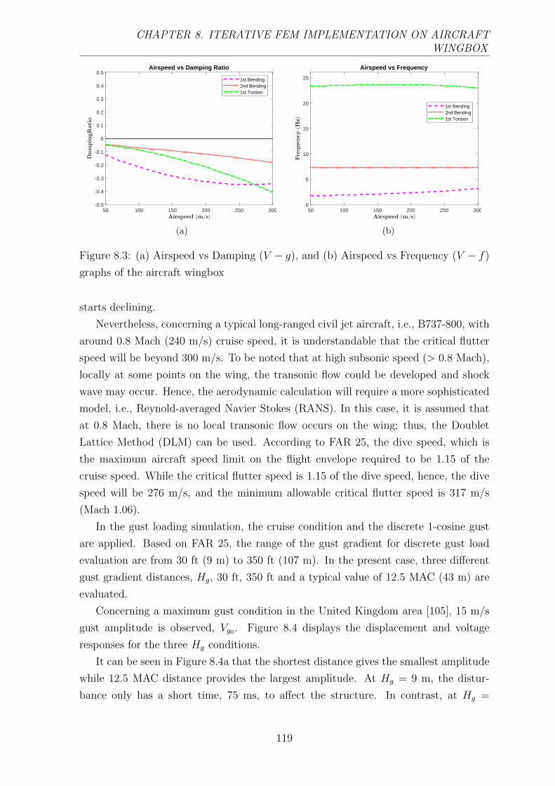
CHAPTER 8. ITERATIVE FEM IMPLEMENTATION ON AIRCRAFTWINGBOX
50 100 150 200 250 300-0.5
-0.4
-0.3
-0.2
-0.1
0
0.1
0.2
0.3
0.4
0.5Airspeed vs Damping Ratio
1st Bending2nd Bending1st Torsion
(a)
50 100 150 200 250 3000
5
10
15
20
25
Airspeed vs Frequency
1st Bending2nd Bending1st Torsion
(b)
Figure 8.3: (a) Airspeed vs Damping (V − g), and (b) Airspeed vs Frequency (V − f)
graphs of the aircraft wingbox
starts declining.
Nevertheless, concerning a typical long-ranged civil jet aircraft, i.e., B737-800, with
around 0.8 Mach (240 m/s) cruise speed, it is understandable that the critical flutter
speed will be beyond 300 m/s. To be noted that at high subsonic speed (> 0.8 Mach),
locally at some points on the wing, the transonic flow could be developed and shock
wave may occur. Hence, the aerodynamic calculation will require a more sophisticated
model, i.e., Reynold-averaged Navier Stokes (RANS). In this case, it is assumed that
at 0.8 Mach, there is no local transonic flow occurs on the wing; thus, the Doublet
Lattice Method (DLM) can be used. According to FAR 25, the dive speed, which is
the maximum aircraft speed limit on the flight envelope required to be 1.15 of the
cruise speed. While the critical flutter speed is 1.15 of the dive speed, hence, the dive
speed will be 276 m/s, and the minimum allowable critical flutter speed is 317 m/s
(Mach 1.06).
In the gust loading simulation, the cruise condition and the discrete 1-cosine gust
are applied. Based on FAR 25, the range of the gust gradient for discrete gust load
evaluation are from 30 ft (9 m) to 350 ft (107 m). In the present case, three different
gust gradient distances, Hg, 30 ft, 350 ft and a typical value of 12.5 MAC (43 m) are
evaluated.
Concerning a maximum gust condition in the United Kingdom area [105], 15 m/s
gust amplitude is observed, Vg0 . Figure 8.4 displays the displacement and voltage
responses for the three Hg conditions.
It can be seen in Figure 8.4a that the shortest distance gives the smallest amplitude
while 12.5 MAC distance provides the largest amplitude. At Hg = 9 m, the distur-
bance only has a short time, 75 ms, to affect the structure. In contrast, at Hg =
119

CHAPTER 8. ITERATIVE FEM IMPLEMENTATION ON AIRCRAFTWINGBOX
0 0.2 0.4 0.6 0.8 1 1.2 1.4 1.6 1.8 2
-600
-400
-200
0
200
400
600
800
1000
1200
Vertical Tip Displacement vs Time
Gust Gradient = 30 FeetGust Gradient = 12.5 MACGust Gradient = 350 Feet
(a)
0 0.2 0.4 0.6 0.8 1 1.2 1.4 1.6 1.8 2
-2000
-1000
0
1000
2000
3000
Voltage vs Time
Gust Gradient = 30 FeetGust Gradient = 12.5 MACGust Gradient = 350 Feet
(b)
Figure 8.4: The time histories of (a) vertical tip displacment and (b) voltage output of
the aircraft wingbox for different gust gradient distances with gust velocity 15 m/s
0 0.2 0.4 0.6 0.8 1 1.2 1.4 1.6 1.8 20
2000
4000
6000
8000
10000
12000
Power vs Time
Gust Gradient = 30 FeetGust Gradient = 12.5 MACGust Gradient = 350 Feet
Figure 8.5: The power output time history of the aircraft wingbox for different gust
gradient distance with gust velocity 15 m/s
107 m, the gust load penetrates the structure almost around 1 s, allowing a sloping
displacement gradient or a low-velocity response. In this case, the dynamic effect is
relatively small (almost like steady) compared to the other cases. However, at Hg =
12.5 MAC, the disturbance is sustained long enough to gives the maximum amplitude.
While it still keeps a steep displacement gradient or a high-velocity response; hence,
it allows some oscillations after the gust ended. In a more detail, Appendix J displays
the displacements of the wingbox at Hg = 12.5 MAC for different times, tg.
In Figure 8.4b, it is interesting to see that the shortest and the longest distances
resulted in a similar level of the maximum voltage. The shortest distance gives the
smallest displacement amplitude; hence, small voltage. A sloping response exerted by
the longest distance resulted in the smallest velocity amplitude; thus, small voltage as
120

CHAPTER 8. ITERATIVE FEM IMPLEMENTATION ON AIRCRAFTWINGBOX
well. Moreover, at Hg = 12.5 MAC, the maximum voltage amplitude is achieved as it
gives the maximum displacement and velocity.
The power output as depicted in Figure 8.5 also reflected similar behaviours as the
shortest and the longest distances give a similar level of amplitude, while at Hg = 12.5
MAC, the maximum power amplitude is obtained. As expected, the largest energy is
harvested at Hg = 12.5 MAC as shown in Table 8.1.
Table 8.1: Electrical energy output of the aircraft wingbox for different gust gradient
distance with gust velocity 15 m/s
Hg Energy (kJ)
30 ft (9 m) 0.3767
12.5 MAC (43 m) 2.4921
350 ft (107 m) 0.7639
The voltage outputs at different iteration steps are shown in Figure 8.6. It can
be seen that the responses from three iteration steps are hardly distinguished. In the
enlarged view, the first iteration, denoted by the pink dashed line, slightly overestimates
the second and third iterations. After the first iteration, the responses declined at the
second iteration, and then slightly going up again at the third iteration.
0 0.2 0.4 0.6 0.8 1 1.2 1.4 1.6 1.8 2
-2000
-1000
0
1000
2000
3000
4000
5000Voltage vs Time
Iteration 1Iteration 2Iteration 3
0.4 0.45 0.5 0.553000
3500
4000
Figure 8.6: The voltage output time history of the aircraft wingbox with gust gradient
distance 12.5 MAC at different iteration step
In more details, Table 8.2 displays the iteration process in terms of energy output.
The first to the second iteration variance is only around 5%, followed by less than 1%
variance after the third iteration. This trend is in agreement with the one shown in
Section 7.6. In this case, the mechanical load dominated the displacement response,
and the reverse piezoelectric effect may not be significant effects on the structural
response.
121

CHAPTER 8. ITERATIVE FEM IMPLEMENTATION ON AIRCRAFTWINGBOX
Table 8.2: Electrical energy output of the aircraft wingbox on each iteration step
Iteration Energy (kJ) Variance
1 2.6093
2 2.4752 ∆1−2 = 5.14%
3 2.4991 ∆2−3 = 0.97%
4 2.4884 ∆3−4 = 0.43%
5 2.4921 ∆4−5 = 0.15%
At tg = 0.3 s, the gust loading exerted the maximum displacement response of the
wingbox, and a maximum of 3.95 kV is generated at the upper skin made of PZT-5A.
The maximum power achieved for Hg = 12.5 MAC and Vg0 = 15 m/s, is around 12 kW.
Considering a more extreme condition in the United Kingdom area, 30 m/s [105], is
also observed as the Vg0 . The displacement and voltage responses for the two different
gust amplitudes are depicted in Figure 8.7.
0 0.2 0.4 0.6 0.8 1 1.2 1.4 1.6 1.8 2
-1000
-500
0
500
1000
1500
2000
2500
Vertical Tip Displacement vs Time
Gust Speed 15 m/sGust Speed 30 m/s
(a)
0 0.2 0.4 0.6 0.8 1 1.2 1.4 1.6 1.8 2
-4000
-2000
0
2000
4000
6000
8000Voltage vs Time
Gust Speed 15 m/sGust Speed 30 m/s
(b)
Figure 8.7: The time histories of (a) vertical tip displacement and (b) voltage output of
the aircraft wingbox for different gust velocities with gust gradient distance 12.5 MAC
It is easily seen from Figure 8.7 that with the same gust gradient distance, both gust
speeds possess a similar pattern of time histories. However, with a larger gust speed
amplitude, 30 m/s, the amplitudes of the displacement and voltage are also higher. As
displayed in Figure 8.8, In agreement with these trends, the power output for Vg0 = 30
m/s is also higher than the one obtained for 15 m/s.
In the present work, concerning the structural strength, for the first time, the
stress and failure analyses of the structure due to the flight condition and the harvested
electrical power are performed. The present iterative FEM provides ease of commercial
software utilisation; hence, several analysis modules can be explored to support the
observation of the energy harvesting structure. In the present case, the gust and
122
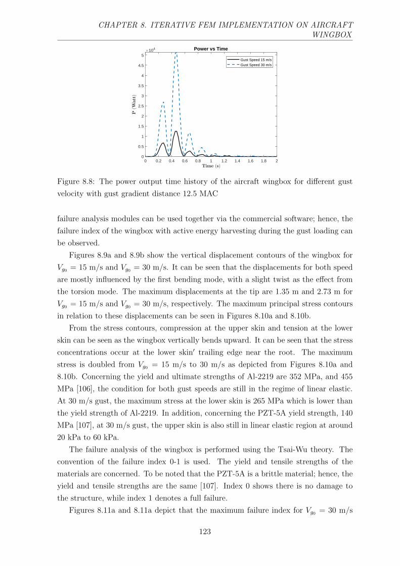
CHAPTER 8. ITERATIVE FEM IMPLEMENTATION ON AIRCRAFTWINGBOX
0 0.2 0.4 0.6 0.8 1 1.2 1.4 1.6 1.8 20
0.5
1
1.5
2
2.5
3
3.5
4
4.5
5104 Power vs Time
Gust Speed 15 m/sGust Speed 30 m/s
Figure 8.8: The power output time history of the aircraft wingbox for different gust
velocity with gust gradient distance 12.5 MAC
failure analysis modules can be used together via the commercial software; hence, the
failure index of the wingbox with active energy harvesting during the gust loading can
be observed.
Figures 8.9a and 8.9b show the vertical displacement contours of the wingbox for
Vg0 = 15 m/s and Vg0 = 30 m/s. It can be seen that the displacements for both speed
are mostly influenced by the first bending mode, with a slight twist as the effect from
the torsion mode. The maximum displacements at the tip are 1.35 m and 2.73 m for
Vg0 = 15 m/s and Vg0 = 30 m/s, respectively. The maximum principal stress contours
in relation to these displacements can be seen in Figures 8.10a and 8.10b.
From the stress contours, compression at the upper skin and tension at the lower
skin can be seen as the wingbox vertically bends upward. It can be seen that the stress
concentrations occur at the lower skin′ trailing edge near the root. The maximum
stress is doubled from Vg0 = 15 m/s to 30 m/s as depicted from Figures 8.10a and
8.10b. Concerning the yield and ultimate strengths of Al-2219 are 352 MPa, and 455
MPa [106], the condition for both gust speeds are still in the regime of linear elastic.
At 30 m/s gust, the maximum stress at the lower skin is 265 MPa which is lower than
the yield strength of Al-2219. In addition, concerning the PZT-5A yield strength, 140
MPa [107], at 30 m/s gust, the upper skin is also still in linear elastic region at around
20 kPa to 60 kPa.
The failure analysis of the wingbox is performed using the Tsai-Wu theory. The
convention of the failure index 0-1 is used. The yield and tensile strengths of the
materials are concerned. To be noted that the PZT-5A is a brittle material; hence, the
yield and tensile strengths are the same [107]. Index 0 shows there is no damage to
the structure, while index 1 denotes a full failure.
Figures 8.11a and 8.11a depict that the maximum failure index for Vg0 = 30 m/s
123

CHAPTER 8. ITERATIVE FEM IMPLEMENTATION ON AIRCRAFTWINGBOX
(a)
(b)
Figure 8.9: Displacement contours of the aircraft wingbox for 12.5 MAC gust gradient
distance with (a) 15 m/s and (b) 30 m/s gust velocities at tg = 0.3 s (displacement
unit: mm)
are four times the index for Vg0 = 15 m/s, from 0.143 to 0.575. Despite this fact, the
maximum failure indices are still less than 1. Hence, even at an extreme condition,
with 30 m/s gust amplitude, the wingbox structure is considered safe. In addition, the
failure indices at the upper skin also relatively small, less than 0.1. Therefore, it can
be assumed that the piezoelectric layer is in a very safe condition. However, despite
the wing could withstand the loads while harvesting the energy, the displacements that
occur are quite high, i.e., almost 10% of half span at 15 m/s gust amplitude. Hence, it
is not practical in a routine flight.
Based on the data from ESDU [108], 15 m/s and 30 m/s gust amplitudes are
quite extreme and very rare to occur during a normal flight. The data from ESDU
[108], depicts empirical functions on the gust probability based on the altitude and
124
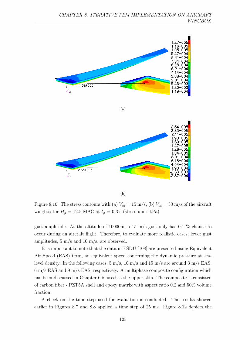
CHAPTER 8. ITERATIVE FEM IMPLEMENTATION ON AIRCRAFTWINGBOX
(a)
(b)
Figure 8.10: The stress contours with (a) Vg0 = 15 m/s, (b) Vg0 = 30 m/s of the aircraft
wingbox for Hg = 12.5 MAC at tg = 0.3 s (stress unit: kPa)
gust amplitude. At the altitude of 10000m, a 15 m/s gust only has 0.1 % chance to
occur during an aircraft flight. Therefore, to evaluate more realistic cases, lower gust
amplitudes, 5 m/s and 10 m/s, are observed.
It is important to note that the data in ESDU [108] are presented using Equivalent
Air Speed (EAS) term, an equivalent speed concerning the dynamic pressure at sea-
level density. In the following cases, 5 m/s, 10 m/s and 15 m/s are around 3 m/s EAS,
6 m/s EAS and 9 m/s EAS, respectively. A multiphase composite configuration which
has been discussed in Chapter 6 is used as the upper skin. The composite is consisted
of carbon fiber - PZT5A shell and epoxy matrix with aspect ratio 0.2 and 50% volume
fraction.
A check on the time step used for evaluation is conducted. The results showed
earlier in Figures 8.7 and 8.8 applied a time step of 25 ms. Figure 8.12 depicts the
125

CHAPTER 8. ITERATIVE FEM IMPLEMENTATION ON AIRCRAFTWINGBOX
(a)
(b)
Figure 8.11: The failure indices with (a) Vg0 = 15 m/s, (b) Vg0 = 30 m/s of the aircraft
wingbox for Hg = 12.5 MAC at tg = 0.3 s
results using different time steps (dt) for the multiphase composite case. It can be seen
that at time steps 25 ms, 12.5 ms and 6.25 ms the results coincide. For these time
steps, the energy converges at around 2.39 kJ. Meanwhile at dt = 50 ms, despite the
trends closely follow the ones with 25 ms, the energy is slightly underestimated with
2.37 kJ. However, using the largest time step, 100 ms, the responses are quite distinct.
The power response despite does not reach the same maximum level with the others,
the energy is overestimated with 2.41 kJ.
The voltage and power responses of the multiphase composites for different gust
amplitudes are shown in Figure 8.13. As expected, lower gust amplitudes give smaller
voltage and power outputs. For 15 m/s gust amplitude, the wing with multiphase
composite can generate more voltage as the permittivity is much lower than the bulk
piezoelectric material. This characteristic aligns with the discussions in Chapter 5 and
126

CHAPTER 8. ITERATIVE FEM IMPLEMENTATION ON AIRCRAFTWINGBOX
0 0.2 0.4 0.6 0.8 1 1.2 1.4 1.6 1.8 2
-3000
-2000
-1000
0
1000
2000
3000
4000
Voltage vs Time
dt = 0.00625 sdt = 0.0125 sdt = 0.025 sdt = 0.050 sdt = 0.100 s
(a)
0 0.2 0.4 0.6 0.8 1 1.2 1.4 1.6 1.8 20
5000
10000
15000
Power vs Time
dt = 0.00625 sdt = 0.0125 sdt = 0.025 sdt = 0.050 sdt = 0.100 s
(b)
Figure 8.12: The time histories of (a) voltage output and (b) power output of the
aircraft wingbox with multiphase composite for different time step
Chapter 6. However, similar to Figures 8.7 and 8.8, it can be seen that the responses
during cruise speed are quickly damped.
0 0.2 0.4 0.6 0.8 1 1.2 1.4 1.6 1.8 2
-3000
-2000
-1000
0
1000
2000
3000
4000
Voltage vs Time
Gust Speed 3 m/s (EAS)Gust Speed 6 m/s (EAS)Gust Speed 9 m/s (EAS)
(a)
0 0.2 0.4 0.6 0.8 1 1.2 1.4 1.6 1.8 20
5000
10000
15000
Power vs Time
Gust Speed 3 m/s (EAS)Gust Speed 6 m/s (EAS)Gust Speed 9 m/s (EAS)
(b)
Figure 8.13: The time histories of (a) voltage output and (b) power output of the
aircraft wingbox with multiphase composite for different gust velocities (Up gust) with
gust gradient distance 12.5 MAC
The electrical energies generated from each discrete gust amplitudes are 0.28 kJ,
1.13 kJ and 2.39 kJ for 3 m/s EAS, 6 m/s EAS and 9 m/s EAS, respectively. These
outputs are much lower than those obtained in Chapter 6. It shows that the assump-
tion used with harmonically oscillating cruise load resulted in overestimated responses
and may happen only in a rare case, i.e., extreme (≥ 30 m/s) and continuous gust
disturbance. Nevertheless, both the hybrid scheme and the iterative FEM have shown
that it could successfully provide an estimation on the energy harvesting of a complex
structure, i.e., wing. However, in a future study, it is essential to re-evaluate the loading
127

CHAPTER 8. ITERATIVE FEM IMPLEMENTATION ON AIRCRAFTWINGBOX
assumption for the application in the hybrid method. As an example, the amplitude
of load may be corrected by considering a small amount of load as the oscillating part
to represent the disturbance by gust; while the steady lift cruise load serves as a static
pre-loaded case providing an initial deformation to the wing.
Based on the data from ESDU, the probability of gust at a specific amplitude
not only could happen with an upward direction (up-gust) but also may happen with
a downward direction (down-gust). Thus, similar gust amplitudes with downward
direction are also evaluated. As it can be seen in Figure 8.14, the responses of the
down-gust are similar to the up-gust with the only significant difference is the direction
of the voltage.
0 0.2 0.4 0.6 0.8 1 1.2 1.4 1.6 1.8 2
-4000
-3000
-2000
-1000
0
1000
2000
3000
Voltage vs Time
Gust Speed 3 m/s (EAS)Gust Speed 6 m/s (EAS)Gust Speed 9 m/s (EAS)
(a)
0 0.2 0.4 0.6 0.8 1 1.2 1.4 1.6 1.8 20
5000
10000
15000
Power vs Time
Gust Speed 3 m/s (EAS)Gust Speed 6 m/s (EAS)Gust Speed 9 m/s (EAS)
(b)
Figure 8.14: The time histories of (a) voltage output and (b) power output of the
aircraft wingbox with multiphase composite for different gust velocities (Down gust)
with gust gradient distance 12.5 MAC
8.2 Discussion on the power density and the flight
performance
In this section, a comparison with the result from the references is depicted in Table
8.3. The selected cases provided studies on the different structural size with different
flight/load condition, i.e., gust load, cruise flight, flutter. The maximum RMS or
average power densities, power per volume of the piezoelectric layer(s), of different
cases are compared. Table 8.3 ranked the power density from the lowest to the highest.
128

CHAPTER 8. ITERATIVE FEM IMPLEMENTATION ON AIRCRAFTWINGBOX
Table 8.3: Power Density Comparison from Different Case Studies
Case Aircraft/Wing Piezoelectric Power Density
Study Structure Structure kW/m3
Anton & RC Aircraft, MFC & PFC patches: 0.001 (MFC)
Inman [5] 1.8m span, (102×16×0.3)mm3, 0.008 (PFC)
23cm chord (145×15×0.3)mm3
Wang & Plate-like wing 1 Packaged 0.275
Inman [71] 700.5mm halfspan, PZT-5A layer
38mm chord (45×25.4×0.5)mm3
Tsushima Tapered Wing, Piezo layers cover 1.75
& Su [16] 200cm halfspan, upper-lower surfaces,
15cm meanchord thickness=0.127mm
Present Jet Aircraft Wing, Multiphase composite 1.90
Work 13.5m halfspan as the upper wingbox skin
3.55m MAC 24.5m2 × 0.006m
Erturk 2DoF Wing Section, Bimorph, 4.61
et al. [23] 0.5m span, Packaged PZT-5A
25cm chord 2×(45×25.4×0.5)mm3
De Marqui Jr. Plate-like wing, Bimorph, 8.68
et al. [24] 1.2m halfspan PZT-5A
24cm meanchord 2×(360×240×0.5)mm3
Tsushima Tapered Wing, Piezo layers cover 75.62
& Su [72] 200cm halfspan, upper-lower surfaces,
15cm meanchord thickness=0.127mm
Xiang Tapered Wing, 1 layer PZT-5H 251.77
et al. [13] 1m halfspan, at upper skin
19cm meanchord (100×40×0.255)mm3
The current case study with multiphase composite (AR 0.2, Vf 50%) is right in the
middle of the table, provides the fifth-highest power density. The case with 3 m/s gust
amplitude is used in the comparison as it has the highest probability of occurrence
amongst the other amplitudes. The first and the second highest power densities were
obtained by a gust load case [13] and a post-flutter speed LCO case [72] which could
reach hundreds and tens of kW/m3.
129

CHAPTER 8. ITERATIVE FEM IMPLEMENTATION ON AIRCRAFTWINGBOX
The study by Xiang et al. in [13] observed an extreme 15 m/s gust which is 15%
of the cruise speed. Hence, it provided a large power output. However, based on the
ESDU data [108], the occurrence of this gust is very unlikely, less than 0.1% probability.
The work discussed by Tsushima and Su in [72] evaluated the responses from a Limit-
Cycle Oscillation (LCO) at a post flutter speed. Theoretically, an LCO phenomenon
exerts a sustained oscillation after the lifting structure pass the critical flutter point.
However, as has been discussed earlier in Chapter 2, in a practical flight condition,
flutter is a catastrophic phenomenon in which the structure may have been collapsed
after the flutter point.
Meanwhile, Anton and Inman [5] obtained the smallest power density. They were
the first researchers who did the flight experiment for piezoelectric energy harvesting.
At the time they conducted the flight test, the mathematical/numerical model to es-
timate/design the energy harvester has not yet been developed. They used an already
available piezoelectric patches in the market and did not optimise the design of the
structure, the location of the piezoelectric nor the electrical load. Hence, it is under-
standable that they got significantly smaller order than the other studies compared in
Table 8.3.
Wang and Inman implemented the most conventional approach in [71]. They ap-
proximated a cruise flight in a clear sky with a transient base excitation function. The
aerodynamic load and aero-structure coupling were not modelled. The load was given
as the base acceleration so that the tip displacement had a similar pattern to the re-
sponse of a flight. They also obtained a small level of power density compared to the
other′s. It can be seen that the power density mostly varies from the order of 100
kW/m3 to 102 kW/m3. The variations are most likely influenced by the assumption
taken to simulate the load acting on the wings.
Different gust types were observed in the literature, discrete 1-cosine gust [13] and
Dryden gust/turbulence [16] resulted in different scale of power densities. The differ-
ences may also occur due to various resistance load. Despite the 1-cosine gust acting
at a much slower speed than the Dryden gust, but the power density is more than
a hundred times of the Dryden gust case. Most of the selected case study used the
optimum resistance load; however, the studies in [16, 72] did not mention whether the
optimum resistance load was used.
Moreover, the studies in [16] and [72] despite using the same wing structure, due
to different loads, i.e., Dryden gust and post-flutter limit cycle oscillation (LCO) vi-
bration, different level of power densities are obtained. The vibration amplitude due
to the Dryden gust is not constant over time; however, at the flutter and LCO case,
a persistent oscillation is expected. Hence, despite the author’s effort to normalised
the power by comparing the power densities as depicted in Table 8.3, it remains chal-
130

CHAPTER 8. ITERATIVE FEM IMPLEMENTATION ON AIRCRAFTWINGBOX
lenging to have an equivalent parametric comparison for the case of piezoaeroelastic
energy harvesting. Nevertheless, Table 8.3 still provide an insight that the power esti-
mated from the present work is still in a reasonable order compared to those from the
literature.
Considering overall flight performance, for instance, a typical jet transport aircraft′s
mission profile with the weight fractions of each flight phase is shown in Figure 8.15.
Meanwhile, an illustration of the mission profile with active energy harvesting is de-
picted in Figure 8.16. The range is initially assumed to be the same for both mission
profiles. The same aircraft’s velocity, specific fuel consumption, and lift to drag ratio
are assumed. As WTO is known and W5 is assumed as the operational empty weight
with 5% reserved fuel, hence W2 and W3 can be calculated. The range at cruise phase is
evaluated using the Breguet′s formula [92]. The range is proportional to the ln(W2/W3)
based on the Breguet′s formula.
𝑾𝟎 = 𝑾𝑻𝟎
𝑾𝟏
𝑾𝟎= 𝟎. 𝟗𝟖
𝑾𝟐
𝑾𝟏= 𝟎. 𝟗𝟕
𝑾𝟒
𝑾𝟑= 𝟎. 𝟗𝟗
𝑾𝟓
𝑾𝟒= 𝟎. 𝟗𝟗𝟕
𝑾𝟎 𝑾𝟏
𝑾𝟐 𝑾𝟑
𝑾𝟒 𝑾𝟓
𝑻𝒂𝒙𝒊 & 𝑻𝒂𝒌𝒆 𝒐𝒇𝒇 𝑳𝒂𝒏𝒅𝒊𝒏𝒈 & 𝑻𝒂𝒙𝒊
𝑪𝒓𝒖𝒊𝒔𝒆
𝑹𝒂𝒏𝒈𝒆 ∝ 𝐥𝐧𝑾𝟐
𝑾𝟑
𝑹𝒂𝒏𝒈𝒆
Figure 8.15: Mission profile of a typical jet transport aircraft
In the current case, the aircraft has the WTO=169820 lbs and WE=84099 lbs (refer
to Chapter 6, Section 6.4). Hence, the weight breakdown for each phase can be found
as follows:
W1 = 166424 lbs;
W2 = 161431 lbs;
W3 = 89546 lbs;
W4 = 88651 lbs;
W5 = 88385 lbs;
ln(W2/W3) = 0.589;
131

CHAPTER 8. ITERATIVE FEM IMPLEMENTATION ON AIRCRAFTWINGBOX
𝑾𝟎 = 𝑾𝑻𝟎
𝑾𝟏
𝑾𝟎= 𝟎. 𝟗𝟖
𝑾𝟐
𝑾𝟏= 𝟎. 𝟗𝟕
𝑾𝟒
𝑾𝟑∗ = 𝟎. 𝟗𝟗 𝑾𝟑
∗ = 𝑾𝟑 − ∆𝑾𝒇𝒖𝒆𝒍−𝑷𝒘𝒓
𝑾𝟎 𝑾𝟏
𝑾𝟐 𝑾𝟑
𝑾𝟒 𝑾𝟓
𝑻𝒂𝒙𝒊 & 𝑻𝒂𝒌𝒆 𝒐𝒇𝒇 𝑳𝒂𝒏𝒅𝒊𝒏𝒈 & 𝑻𝒂𝒙𝒊
𝑪𝒓𝒖𝒊𝒔𝒆
𝑹𝒂𝒏𝒈𝒆 ∝ 𝐥𝐧𝑾𝟐
𝑾𝟑
∆𝑹𝒂𝒏𝒈𝒆
𝑾𝟑∗
𝑷𝑨𝒗𝒆𝒔𝒖𝒑𝒑𝒐𝒓𝒕 𝒕𝒂𝒙𝒊𝒊𝒏𝒈
∆𝑹𝒂𝒏𝒈𝒆 ∝ 𝐥𝐧𝑾𝟑
𝑾𝟑∗
∆𝑾𝒇𝒖𝒆𝒍−𝑷𝒘𝒓
𝑬𝒏𝒆𝒓𝒈𝒚 𝑯𝒂𝒓𝒗𝒆𝒔𝒕𝒊𝒏𝒈𝑨𝒄𝒕𝒊𝒗𝒆
Figure 8.16: Mission profile with energy harvesting system and extended cruise range
using the fuel saved
From the aircraft weight breakdown, then, it can be estimated that the fuel required
during landing and taxi is 266 lbs. This amount of fuel is equivalent with 324 Mega-
Joule of energy produced by the APU. If the energy harvesting ability is activated and
the harvested power is used to support taxiing system, then the equivalent fuel saved
from the harvested power can be used to extend the cruise range as shown in Figure
8.16.
2.5 3 3.5 4 4.5 50
5
10
15
20
25
30
35Gust Amplitude vs Number of Occurence
(a)
2.5 3 3.5 4 4.5 50.5
1
1.5
2
2.5
3
3.5
4
4.5Gust Amplitude vs Energy
(b)
Figure 8.17: (a) The number of gust occurrence per flight, and (b) Total energy gen-
erated per flight as functions of the gust amplitude (Vg0)
Based on the data from ESDU [108], considering an aircraft with cloud warning
radar, at an altitude of 10000 m above sea level, the average distance flew to meet an
up- or down- gust is around 2800 nautical miles or 5200 km. This average distance is
equal to the cruising distance of a long-range aircraft with 240 m/s speed and 6 hours
132

CHAPTER 8. ITERATIVE FEM IMPLEMENTATION ON AIRCRAFTWINGBOX
cruise (for 7-8 hours flight time). The ratio of up-gust and down-gust at this altitude
is around one [108]; thus, the chance to meet an up-gust or a down-gust is the same.
The probability of meeting a gust, however, is unique for a certain gust amplitude.
The chances to encounter a 5 m/s (3 m/s EAS), 10 m/s (6 m/s EAS) and 15 m/s
(9 m/s EAS) are 100%, 3% and 0.1%, respectively [108]. Therefore, there is only one
chance to meet a gust with 5 m/s amplitude during a cruise flight of a typical jet
aircraft observed in Section 8.1. Moreover, there are only three times a 10 m/s gust
could be encountered in 100 flights and only one time a 15 m/s gust occurs in 1000
flights. Hence, the most realistic scenario between the three gusts is the one with 5
m/s gust amplitude.
Considering both wings of the aircraft generate the energy, then, around 0.56 kJ can
be harvested during the flight if there is only a 5 m/s gust. If lower gust amplitude is
concerned, there is a higher probability that the gust could occur more than once during
this flight. Figure 8.17a depicts the number of occurrence for lower gust amplitudes
based on the ESDU data [108]. It can be seen that the lowest gust amplitude, 2.5 m/s,
could occur more than 30 times during this flight. Unfortunately, lower gust speed
could not be evaluated as the data is not available, and extrapolating the data may
lead to invalid result [108].
Figure 8.17b shows the variation of total energy per flight to the gust amplitude. It
can be seen that lower gust amplitude does not necessary means lower energy during
the flight. Smaller gust amplitude may result in higher number of encounter during
the flight. Hence, may provide higher total energy per flight. However, despite this
fact, the maximum energy harvested per flight is only around 4.3 kJ (from 2.5 m/s
gusts). This amount of energy is still in a much lower order compared to the fuel-
energy ratio of the APU, 1220 kJ per pound fuel. Therefore, the improvement in the
flight performance, i.e., range, as shown in Figure 8.16 will not be significant or may
even be negligible.
Nevertheless, the evaluation concerning discrete gust load disturbance during cruise
flight provides more realistic results compared to the ones given in Chapter 6. The
analyses based on the assumption of harmonically oscillating cruise load discussed in
Chapter 6 lead to overestimated total energies. In a typical flight, as shown in the
current analysis, the load does not continuously oscillate with the same amplitude,
even when there is a disturbance, i.e., gust, the oscillation is quickly damped and
each disturbance may occur only at a certain distance. In addition, the excitation
near the first bending frequency as assumed in Chapter 6 may only valid to estimate
the maximum power amplitude in such an extreme and rare case, i.e., very high gust
amplitude.
133
CHAPTER 8. ITERATIVE FEM IMPLEMENTATION ON AIRCRAFTWINGBOX
8.3 Summary
Implementation of the iterative FEM scheme to a transport aircraft wingbox exerted by
gust and cruise loads provide a more realistic approach to the flight loading condition.
The analyses presented in this chapter have incorporated the aero-structure coupling
with unsteady aerodynamics and structural dynamics models.
The utilisation of the commercial software in the iterative FEM has given the flex-
ibility to evaluate several types of structural analysis, i.e., gust and failure modules.
In the present work, the stress and failure analyses of the aircraft wingbox while sub-
jected to the gust load and harvesting the energy have been conducted. The failure
analysis depicts that the wingbox is safe even when it is subjected to an extreme load,
30 m/s gust amplitude while harvesting the energy. These results have shown that the
multidisciplinary problems, i.e., aeroelastic vibration, energy harvesting and structural
strength, as mentioned in the literature Chapter 4 can be overcome with this iterative
FEM approach.
A more realistic load model concerning gust and cruise load has also shown a more
grounded result. The responses exerted by the gust have shown that the structural
vibration was quickly damped in a routine flight; thus, the maximum power was only
attained at a very short time. Moreover, a gust with a particular amplitude may only
occur once at a certain distance; hence, continuous vibration and power generation may
not be feasible during a typical flight. Therefore, an earlier assumption of harmonically
oscillating flight load as discussed in Chapter 4 and Chapter 6 may only apply to an
extreme and rare condition; thus not realistic in a typical flight.
Nevertheless, a much simpler and faster approach as discussed in Chapter 4 and
Chapter 6 can be beneficial to evaluate a conceptual design of energy harvesting imple-
mentation on an aircraft structure. The hybrid scheme may be used to provide more
realistic investigation if the assumption of the loading condition considers much more
constraints, i.e., level and occurrence of disturbance during flight. Hence, from the
present work, two different approaches for evaluation of piezoelectric energy harvest-
ing, namely the hybrid analytical/ computational scheme and the iterative FEM, can
be utilised for different stages of design and engineering analyses.
A comparison with the power densities from other piezoeaeroelastic energy harvest-
ing studies has also been conducted. The selected cases provided studies on different
structural sizes and varied flight/load conditions. The result obtained from the present
work reasonably falls in the range obtained from the literature.
The results presented in this chapter pointed out that the energy harvested during
a normal cruise flight with gust disturbance is rather small compared to the energy
provided by the aircraft system, i.e., the APU. Hence, it may not be recommended
to consider the piezoelectric energy harvesting structure as an option to support the
134

CHAPTER 8. ITERATIVE FEM IMPLEMENTATION ON AIRCRAFTWINGBOX
main or auxiliary power system of the aircraft. The flight performance improvement,
however, may be achieved if the harvested energy from the piezoelectric structure is
used for improving the efficiency of other aircraft systems. As an example, it can be
utilised to construct a self-powered actuating system for control surfaces or providing
an active disturbance control, i.e., gust alleviation system. Thus, in the future works, it
is worth to highlight that the research on the piezoelectric energy harvesting structure
for aircraft can be focused on the evaluation of these kinds of systems.
135

Chapter 9
Conclusion
In the present research, for the first time, investigations on the potential of piezoelectric-
based energy harvesting from a civil jet transport aircraft wing have been conducted.
The piezoelectric-based structure has been proven could harvest the electrical energy
from the structural vibration, i.e., aeroelastic vibration. Hence, it has the prospect to
become an alternative energy source in aircraft flight as the aircraft always encountered
aeroelastic vibration. From the literature, as has been discussed in Chapter 2, many
researchers have done studies in piezoaeroelastic energy harvesting. However, there
are not many who dedicated their research concerning normal flight loads. In addition,
their focuses are limited to small-scale lifting structures, i.e., small plate, UAV wing.
Therefore, the main questions on the piezoaeroelastic energy harvesting from large
aircraft structure are rather basics yet has not been answered prior to the present
research. Those questions are:
how much energy can be harvested from an aircraft structure, and
how this energy can be estimated.
Therefore, the essential part from the present research has been the development
of computational methods to quantify the energy harvesting potential from an aircraft
structure. The wing structure as the primary part in flight operation has been focused
as the object of the present work. The wing also the part where the aeroelastic vibration
is always concerned in the aircraft. Hence, the first computational method proposed in
this research is based on one of the most common simplifications of a wing structure,
i.e., a cantilevered beam.
Numerous researchers have studied beam-based piezoelectric energy harvesting.
However, most of them either analytical or experimental. The base excitation model of
Erturk and Inman [6] is one of the infamous analytical models in this subject. Despite
this fact, there is no model which could handle the complexity of wing geometry. There
is one electromechanical finite element model by De Marqui Jr. et al. [10] which has
136
CHAPTER 9. CONCLUSION
the potential to be applied for wing analysis. However, the shell-based element will
need a great effort on the coding development. Moreover, as previously said, there is
even still a concern about how much energy the wing can generate. Therefore, the
focus on this research has been on the early engineering analysis level.
The initial concept on the computational work in this research was always rooting
on the utilisation of a commercial software as much as possible. The use of commercial
software has been proven a significant benefit in this research, i.e., the ease of con-
structing wing structure and performing dynamic analyses. However, the commercial
software readily available in the market are not capable of conducting electromechan-
ical analysis for piezoelectric energy harvesting. Therefore, an augmentation from a
manually built computational code was required in the current work. Namely, a novel
hybrid analytical/ computational scheme has been proposed in the present research.
The so-called hybrid scheme combines the procedures from an analytically-solved
electromechanical equation and a structural dynamic analysis done by commercial soft-
ware. In the present work, a FEM-based commercial software was dedicated to the
computational analysis. However, as has been presented in Chapter 3, it is also possi-
ble to provide information from an analytical solution or an advanced computational
analysis, i.e., isogeometric analysis. This hybrid scheme has been successfully applied
to estimate the energy harvesting potential from a typical jet aircraft wingbox as has
been discussed in Chapter 4.
The results obtained via the hybrid scheme pointed out that the jet aircraft wingbox
with 14.5 m half span could harvest as much as 40 kW of electrical power. This
power came only from the implementation of a piezoelectric material as its upper
skin. The level of power is indeed promising; however, there were some concerns
found from this investigation. The weight of the piezoelectric material was one of the
shortcomings found in the analysis. The wingbox weight increased significantly, thus,
may result in additional fuel to consume. Secondly, the assumption of harmonic cruise
load may not be suitable for a practical flight, i.e., concerning aero-structure coupling
and disturbance occurrence during the flight. Moreover, the scaling of the load acted
on the wingbox was only based on the bending frequency. Lastly, the strength of the
wingbox exerted by flight loads while harvesting electrical energy was also one of the
concerns.
In the current work, in order to address the weight issue, multiphase composites
with active structural fiber (ASF) has been proposed as an alternative to the bulk
piezoelectric materials. To this date, there has not been any study on the application of
this type of multiphase composite for energy harvesting. Hence, several investigations
were conducted to obtain insights on the characteristic of this composite concerning
the energy harvesting analysis. Chapter 5 presented the Double-Inclusion model with
137

CHAPTER 9. CONCLUSION
Mori Tanaka method as the approach to estimating the electromechanical properties
of the multiphase composites. The investigations done employing the Double-Inclusion
model have been well validated with the findings from other researchers. In addition,
verification of the dynamic responses has been successfully conducted via FEM.
The similar investigation on the jet aircraft wingbox was then conducted by utilis-
ing the properties estimated via the Double-Inclusion model. The hybrid scheme was
also applied. As presented in Chapter 6, various configurations of the multiphase com-
posites have been tested. An interesting finding is that the wingboxes with multiphase
composites could generate the same level of power compared to the one with the bulk
piezoelectric material. Hence, by selecting a particular composition of the composite,
a lightweight energy harvesting wing can be constructed. In the current case, with the
combination of carbon fiber in the composite, not only lightweight but also an increase
in strength can be expected.
In order to address a more realistic loading on the aircraft wing, another compu-
tational method has been developed in the present work. An iterative FEM has been
proposed. Similar to the hybrid scheme, the idea of utilising commercial software was
also the root of this iterative FEM. An interesting concept to separate the electrome-
chanical coupling effect from piezoelectric structure was implemented. The commercial
software was dedicated to solving the actuator-like part of the electromechanical cou-
pling. In the other hand, a computational code was built to solve the part induced
by the electrical resistance. These two parts were solved iteratively until the response
from both parts converged.
Another ease of using commercial software was found during the investigation with
the iterative FEM. Structural dynamic analysis, unsteady aerodynamic loads calcula-
tion and aero-structure coupling evaluation were done via a commercial software. A
computational code was built and applied to evaluate the electromechanical coupling
effect. Therefore, piezoaeroelastic energy harvesting concerning gust load analysis can
be performed. Verification with the results from literature has been performed and
depicted good agreements. The detail has been discussed in Chapter 7. The iterative
FEM was then implemented to analyse the energy harvesting from the jet aircraft wing.
The investigations by means of iterative FEM have shown a level of maximum
power similar to those obtained via the hybrid scheme is achievable. However, different
natures on the gust load and harmonic cruise load proved to be the distinctive aspect.
The analyses from discrete gust load conditions depicted a certain level of maximum
power could not be sustained in the long term. As discussed in Chapter 8, a long
flight hour may be needed to extract a considerable amount of energy. Nevertheless,
via the iterative FEM, for the first time, failure analyses on piezoaeroelastic energy
harvesting structure have been conducted. The failure index of the wingbox shown
138
CHAPTER 9. CONCLUSION
that the structure could endure both the aerodynamics and electrical loads.
In addition, several notable findings and contributions of the present work are
highlighted in the following sections.
9.1 On the hybrid piezoelectric energy harvester
model
A mathematical model and computational scheme to evaluate a cantilevered piezoelec-
tric energy harvester under dynamic bending to enable the hybrid analytical/ compu-
tational scheme have been proposed. The detailed derivation on the governing elec-
tromechanical equation and the algorithm of the hybrid scheme have been presented
in Chapter 3.
The validation against the analytical base excitation model of Erturk and Inman [6],
the experimental results of Erturk and Inman [22] and the electromechanical finite el-
ement model of De Marqui Jr. et al. [10] have been conducted and shown excellent
agreements. In addition, the comparison against the electromechanical FEM has de-
picted significant benefits in terms of computational cost by means of the hybrid scheme
(refer to Table 3.8 in Chapter 3, Section 3.5). Moreover, the robustness of the hybrid
scheme has also been tested by replacing finite element analysis with isogeometric
analysis.
A simulation for a notional civil jet aircraft wingbox with piezoelectric skin layer
has been conducted in the present work. An assumption of a harmonic cruise loading
was taken on the investigation. A steady cruise load equal to the weight of the aircraft
was varied with different excitation frequencies. Excitation lower than the first bending
frequency was considered. Based on the simulation results, the power responses could
achieve the level of 102 to 104 watts. The estimated maximum power reached around
40 kW (refer to Figure 4.7 in in Chapter 4, Section 4.2).
9.2 On the multiphase piezoelectric composite
The implementation of the multiphase composite with active structural fiber for energy
harvesting structure has been proposed in the present work. The multiphase composite
was designated as the substitute for the bulk piezoelectric material. This purpose was
addressed to the weight issue which has been highlighted from the first study on the
aircraft wingbox (refer to Chapter 4, Section 4.3).
The application of multiphase composites for energy harvesting has never been
elaborated before the present work. Hence, a means of analysis was required to give
139

CHAPTER 9. CONCLUSION
more understanding to the properties of the multiphase composite concerning the en-
ergy harvesting structure. A computational homogenisation method based on The
Double-Inclusion model combined with the Mori-Tanaka method has been proposed in
the present work. A computational code has also been built for the present Double-
Inclusion model. The detailed derivation and computational procedure of this method
have been presented in Chapter 5.
Benchmark analyses against the analytical model and experimental results of the
piezoelectric-based single fiber composite by Chan and Unsworth [60] has been success-
fully conducted. Comparison against the finite element model of Lin and Sodano [50]
and their experiment [51] have also shown a good agreement. Concerning the energy
harvesting characteristic, dynamic analyses against detailed 3D FEM models have also
been performed. The FEM models contained effective electro-elastic properties esti-
mated via Double-Inclusion model were well agreed with the detailed 3D FEM models.
The hybrid scheme has also been applied to evaluate the energy harvesting po-
tential from the jet aircraft wingbox embedded with the multiphase composite. The
multiphase composites with various compositions have been applied to replace the bulk
piezoelectric material as the wingbox upper skin. The results pointed out that differ-
ent compositions of the composite were still able to generate similar level of maximum
power with the bulk piezoelectric material (refer to Figure 6.4, Figure 6.5 and Table
6.8 in Chapter 6, Section 6.3).
Although the composites were able to harvest a similar order of power with the
bulk material, different compositions may result in an increment or reduction of the
structural weight. Hence, a specific composition has to be selected so that it could
construct a lightweight structure while still able to harvest the energy. In order to
satisfy this requirement, the composite needs to produce an equivalent electrical power
which could save a considerable amount of fuel.
In the present work, a new procedure to investigate the trade-off between the aircraft
weight, the fuel saved and the harvested energy has been developed. Based on the
investigation results, 340 pounds of fuel potentially could be saved as the equivalence
of the harvested power of the wingbox with a multiphase composite (refer to Table
6.10). Based on the comparison with a typical APU of a long-range aircraft, this
amount of fuel saved may support an hour operation of the APU.
9.3 On the iterative FEM for piezoelectric energy
harvesting
A novel iterative finite element method (FEM) for energy harvesting purpose has been
developed in the present work. This iterative FEM was designated to resolve the
140

CHAPTER 9. CONCLUSION
piezoelectric energy harvesting analysis considering aeroelastic condition. The main
feature of this iterative FEM is the separation of the electromechanical coupling parts
of the piezoelectric energy harvester. In which, one part is solved via a standard finite
element software with the augmentation of a computational code to solve the other
part. Iterative scheme to achieve convergence from both parts has been proposed. A
computational code concerning the electromechanical coupling has been built and has
been used together with a commercial software to conduct the iterative process. The
mathematical background and computational scheme of this iterative FEM have been
presented in Chapter 7.
The utilisation of commercial software has enabled the iterative FEM to assess
aeroelastic problems conveniently. Three different lifting structures, i.e., a plate-like
wing of De Marqui Jr. et al. [24], a UAV wingbox of Xiang et al. [13], and the jet
transport aircraft wing, with active energy harvesting layer(s) subjected to 1-cosine
gusts, have been investigated via the time-domain iterative FEM. Based on the study
cases, the iterative processes are considerably fast, and convergences are achieved in
less than ten iterations (refer to Figure 7.4, Figure 7.5, Figure 7.21, and Figure 8.6 in
Chapter 7 and Chapter 8).
The energy harvesting analysis of the transport aircraft wing employing iterative
FEM pointed out that the output up to 4.3 kJ could be achieved (refer to Chapter
8, Section 8.2). This result are much lower than the one obtained via the hybrid
analytical/computational scheme. It is critical to remark that the response due to
discrete gust were quickly damped during a cruise flight. Moreover, the occurrence
probability of the gust is also an essential factor to be considered. A higher gust
amplitude has a lower chance to be encountered. It was found that a gust with 15
m/s amplitude is very unlikely to happen (less than 0.1% chance), a gust with 5 m/s
amplitude may occur only once during a cruise flight. Nevertheless, these results much
more representing a practical flight condition than the assumption of harmonic cruise
load as presented in Chapter 4.
In addition, the utilisation of the commercial software in the iterative FEM has
given the flexibility to evaluate several types of structural analysis, i.e., gust and failure
modules. In the present work, the stress and failure analyses of the aircraft wing while
subjected to the gust load and harvesting the energy have been conducted. The failure
index of the wing depicted that the structure is still safe even when subjected to
cruise and gust loads while harvesting the electrical energy (refer to Figure 8.11a and
Figure 8.11b). Therefore, the present iterative FEM has covered the multi-discipline
analysis concerned in the early investigation of the current work. The hybrid scheme,
nonetheless, was able to provide fast estimation on the energy harvesting potential;
however, the iterative FEM enhanced the level of analysis for a more complex scope.
141

CHAPTER 9. CONCLUSION
9.4 Future work
Continuation of the present work can be further developed in the manners of:
A higher fidelity approach, i.e., a multiscale approach, can be considered for
further verification of the effective electro-elastic properties. On a much complex
configuration, in which a laminated composite consisted of thousands of fiber,
the multiscale modelling approach could be much more efficient.
In the current iterative FEM, to be noted that a continuous electrode is assumed,
thus, uniform voltage distribution is expected. In a real case, manufacturing
capability and materials availability may need to be considered. Hence, a discrete
segmentation of the piezoelectric layer may be required.
In relation to the flight operation, an evaluation on a continuous gust or turbu-
lence disturbance may also be considered for the future works. The present work
evaluated a discrete 1-cosine gust, which may represent a spike of atmospheric
disturbance. However, it is also worth to investigate the effect of continuous
disturbance during the flight which further can be used to verify the model of a
discrete gust.
Considering the failure analysis, fracture and delamination in the piezoelectric
structure may need to be addressed in the future. Moreover, concerning a routine
flight operation, apart from a failure due to maximum load condition, fatigue
analysis is also important to be conducted in the future. It will be essential
to see how the implementation of energy harvesting structure could affect the
lifetime of an aircraft.
A parametric scaling, i.e., non-dimensionalised parameters, are required in the
future. Examples for these parameters are the Reynold number (aerodynamic
analysis) and the Strouhal number (vortex-induced vibration case). These non-
dimensional parameters could give senses to represent different scales of analysis
for their respective cases. As depicted in Table 8.3, currently, it is still diffi-
cult to compare the piezoaeroelastic-based energy harvesting for various size of
structures and different airspeed conditions. Hence, a scaled-down model for an
experimental test could be done in the future.
Lastly, employing the harvested energy for other applications in wing structure,
i.e., control surface and morphing skin, might potentially enhance the aerody-
namic efficiency, i.e., gust alleviation, drag reduction. Therefore, it could lead to
other schemes to save fuel, instead of directly using the harvested power as an
alternative to the primary power source.
142

Bibliography
[1] L. Christodoulou and J. D. Venables, “Multifunctional material systems: The
first generation,” The Journal of The Minerals, Metals & Materials Society
(TMS), vol. 55, no. 12, pp. 39–45, 2003.
[2] R. F. Gibson, “A review of recent research on mechanics of multifunctional com-
posite materials and structures,” Composite Structures, vol. 92, no. 12, pp. 2793
– 2810, 2010.
[3] J. P. Thomas, M. Keennon, A. DuPasquier, M. A. Qidwai, and P. Matic, “Mul-
tifunctional structure-battery materials for enhanced performance in small un-
manned air vehicles,” American Society of Mechanical Engineers, Materials Di-
vision (Publication) MD, vol. 98, pp. 289–292, 2003.
[4] J. P. Thomas and M. A. Qidwai, “The design and application of multifunctional
structure-battery materials systems,” The Journal of The Minerals, Metals &
Materials Society (TMS), vol. 57, no. 3, pp. 18–24, 2003.
[5] S. R. Anton and D. J. Inman, “Vibration energy harvesting for unmanned aerial
vehicles,” Proceedings of SPIE - The International Society for Optical Engineer-
ing, vol. 6928, p. 692824, 2008.
[6] A. Erturk, S. R. Anton, and D. J. Inman, “Piezoelectric energy harvesting from
multifunctional wing spars for UAVs - Part 1: Coupled modeling and preliminary
analysis,” Proceedings of SPIE - The International Society for Optical Engineer-
ing, vol. 7288, p. 72880C, 2009.
[7] S. R. Anton, A. Erturk, and D. J. Inman, “Piezoelectric energy harvesting from
multifunctional wing spars for UAVs - Part 2: Experiments and storage applica-
tions,” Proceedings of SPIE - The International Society for Optical Engineering,
vol. 7288, p. 72880D, 2009.
[8] A. Abdelkefi, “Aeroelastic energy harvesting: A review,” International Journal
of Engineering Science, vol. 100, pp. 112–135, 2016.
143

BIBLIOGRAPHY
[9] R. L. Bisplinghoff, H. Ashley, and R. L.Halfman, Aeroelasticity. Dover Publica-
tions, Inc., 1983.
[10] C. De Marqui Jr., A. Erturk, and D. J. Inman, “An electromechanical finite
element model for piezoelectric energy harvester plates,” Journal of Sound and
Vibration, vol. 327, no. 1, pp. 9 – 25, 2009.
[11] C. De Marqui Jr. and M. J. Maria, “Effect of piezoelectric energy harvesting on
the response of a generator wing to a turbulence gust,” in 27th Congress of The
International Council of The Aeronautical Sciences, 2010.
[12] C. De Marqui Jr. and A. Erturk, “Electroaeroelastic analysis of airfoil-based
wind energy harvesting using piezoelectric transduction and electromagnetic in-
duction,” Journal of Intelligent Material Systems and Structures, vol. 24, no. 7,
pp. 846–854, 2013.
[13] J. Xiang, Y. Wu, and D. Li, “Energy harvesting from the discrete gust response
of a piezoaeroelastic wing: Modeling and performance evaluation,” Journal of
Sound and Vibration, vol. 343, pp. 176–193, 2015.
[14] C. Bruni, J. Gibert, G. Frulla, E. Cestino, and P. Marzocca, “Energy harvesting
from aeroelastic vibrations induced by discrete gust loads,” Journal of Intelligent
Material System and Structure, vol. 28, no. 1, pp. 47–62, 2017.
[15] N. Tsushima and W. Su, “Modeling of highly flexible multifunctional wings for
energy harvesting,” Journal of Aircraft, vol. 53, no. 4, pp. 1033–1044, 2016.
[16] N. Tsushima and W. Su, “Concurrent active piezoelectric control and energy
harvesting of highly flexible multifunctional wings,” Journal of Aircraft, vol. 54,
no. 2, pp. 724–736, 2017.
[17] J. P. Thomas, M. A. Qidwai, and J. C. Kellogg, “Energy scavenging for small-
scale unmanned systems,” Journal of Power Sources, vol. 159, no. 2, pp. 1494 –
1509, 2006.
[18] S. R. Anton and H. A. Sodano, “A review of power harvesting using piezoelectric
materials (2003-2006),” Smart Materials and Structures, vol. 16, no. 3, p. R1,
2007.
[19] K. V. Selvan and M. S. Mohamed Ali, “Micro-scale energy harvesting devices:
Review of methodological performances in the last decade,” Renewable and Sus-
tainable Energy Reviews, vol. 54, pp. 1035 – 1047, 2016.
144

BIBLIOGRAPHY
[20] A. Erturk and D. J. Inman, “Issues in mathematical modeling of piezoelectric
energy harvesters,” Smart Materials and Structures, vol. 17, no. 6, p. 065016,
2008.
[21] A. Erturk and D. J. Inman, “A distributed parameter electromechanical model for
cantilevered piezoelectric energy harvesters,” Journal of Vibration and Acoustics,
Transactions of the ASME, vol. 130, no. 4, p. 041002, 2008.
[22] A. Erturk and D. J. Inman, “An experimentally validated bimorph cantilever
model for piezoelectric energy harvesting from base excitations,” Smart Materials
and Structures, vol. 18, no. 2, p. 025009, 2009.
[23] A. Erturk, W. G. R. Vieira, C. De Marqui Jr., and D. J. Inman, “On the energy
harvesting potential of piezoaeroelastic systems,” Applied Physics Letters, vol. 96,
no. 18, p. 184103, 2010.
[24] C. De Marqui Jr., A. Erturk, and D. J. Inman, “Piezoaeroelastic modeling and
analysis of a generator wing with continuous and segmented electrodes,” Journal
of Intelligent Material Systems and Structures, vol. 21, no. 10, pp. 983–993, 2010.
[25] C. De Marqui Jr., W. G. R. Vieira, A. Erturk, and D. J. Inman, “Modeling and
analysis of piezoelectric energy harvesting from aeroelastic vibrations using the
doublet-lattice method,” Journal of Vibration and Acoustics, Transactions of the
ASME, vol. 133, no. 1, p. 011003, 2011.
[26] J. A. C. Dias, C. De Marqui Jr., and A. Erturk, “Three-degree-of-freedom hybrid
piezoelectric-inductive aeroelastic energy harvester exploiting a control surface,”
AIAA Journal, vol. 53, no. 2, pp. 394–404, 2015.
[27] D. Li, Y. Wu, A. D. Ronch, and J. Xiang, “Energy harvesting by means of
flow-induced vibrations on aerospace vehicles,” Progress in Aerospace Sciences,
vol. 86, pp. 28 – 62, 2016.
[28] A. B. Rostami and M. Armandei, “Renewable energy harvesting by vortex-
induced motions: Review and benchmarking of technologies,” Renewable and
Sustainable Energy Reviews, vol. 70, pp. 193 – 214, 2017.
[29] C. Wei and X. Jing, “A comprehensive review on vibration energy harvesting:
Modelling and realization,” Renewable and Sustainable Energy Reviews, vol. 74,
pp. 1 – 18, 2017.
[30] M. Bashir, P. Rajendran, and S. Khan, “Energy harvesting from aerodynamic
instabilities: Current prospect and future trends,” IOP Conference Series: Ma-
terial Science, vol. 290, p. 012054, 01 2018.
145
BIBLIOGRAPHY
[31] T. Theodorsen, “General theory of aerodynamic instability and mechanism of
flutter,” Tech. Rep. 496, Langley Memorial Aeronautical Laboratory, NACA.
[32] J. Katz and A. Plotkin, Low Speed Aerodynamics. Cambridge University Press,
2001.
[33] E. Albano and W. P. Rodden, “A doublet-lattice method for calculating lift
distributions on oscillating surfaces in subsonic flows,” AIAA Journal, vol. 7,
no. 2, pp. 279–285, 1969.
[34] Y. Amini, H. Emdad, and M. Farid, “Finite element modeling of functionally
graded piezoelectric harvesters,” Composite Structures, vol. 129, pp. 165–176,
2015.
[35] Y. Amini, P. Fatehi, M. Heshmati, and H. Parandvar, “Time domain and fre-
quency domain analysis of functionally graded piezoelectric harvesters subjected
to random vibration: Finite element modeling,” Composite Structures, vol. 136,
pp. 384–393, 2016.
[36] Y. Shindo and F. Narita, “Dynamic bending/torsion and output power of s-
shaped piezoelectric energy harvesters,” International Journal of Mechanics and
Materials in Design, vol. 10, pp. 305–311, Sep 2014.
[37] H. Lee, N. Sharpes, H. Abdelmoula, A. Abdelkefi, and S. Priya, “Higher power
generation from torsion-dominant mode in a zigzag shaped two-dimensional en-
ergy harvester,” Applied Energy, vol. 216, pp. 494 – 503, 2018.
[38] A. G. Muthalif and N. D. Nordin, “Optimal piezoelectric beam shape for single
and broadband vibration energy harvesting: Modeling, simulation and experi-
mental results,” Mechanical Systems and Signal Processing, vol. 54-55, pp. 417 –
426, 2015.
[39] Y. Chen, X. Mu, T. Wang, W. Ren, Y. Yang, Z. L. Wang, C. Sun, and A. Y. Gu,
“Flutter phenomenon in flow driven energy harvester–a unified theoretical model
for “stiff” and “flexible” materials,” Scientific Reports, vol. 6, October 2016.
[40] A. I. Aquino, J. K. Calautit, and B. R. Hughes, “Evaluation of the integration
of the wind-induced flutter energy harvester (wifeh) into the built environment:
Experimental and numerical analysis,” Applied Energy, vol. 207, pp. 61 – 77,
2017.
[41] E. Meiling Zhu, J. Worthington, and J. Njuguna, “Analyses of power output
of piezoelectric energy-harvesting devices directly connected to a load resistor
146

BIBLIOGRAPHY
using a coupled piezoelectric-circuit finite element method,” IEEE Transonics,
Ultrasonics, and Ferroelectrics, vol. 56, no. 7, pp. 1309–1318, 2009.
[42] Y. Yang and L. Tang, “Equivalent circuit modeling of piezoelectric energy har-
vesters,” Journall of Intelligent Material Systems and Structures, vol. 20, no. 18,
pp. 2223–2235, 2009.
[43] P. H. Wu and Y. C. Shu, “Finite element modeling of electrically rectified
piezoelectric energy harvesters,” Smart Materials and Structures, vol. 24, no. 9,
p. 094008, 2015.
[44] D. Gedeon and S. J. Rupitsch, “Finite element based system simulation for piezo-
electric vibration energy harvesting devices,” Journal of Intelligent Material Sys-
tems and Structures, vol. 29, no. 7, pp. 1333–1347, 2018.
[45] G. Gafforelli, R. Ardito, and A. Corigliano, “Improved one-dimensional model of
piezoelectric laminates for energy harvesters including three dimensional effects,”
Composite Structures, vol. 127, pp. 369 – 381, 2015.
[46] I. Fattahi and H. R. Mirdamadi, “Novel composite finite element model for piezo-
electric energy harvesters based on 3D beam kinematics,” Composite Structures,
vol. 179, pp. 161 – 171, 2017.
[47] Y. Amini, H. Emdad, and M. Farid, “An accurate model for numerical predic-
tion of piezoelectric energy harvesting from fluid structure interaction problems,”
Smart Materials and Structures, vol. 23, no. 9, p. 095034, 2014.
[48] Y. Lin and H. A. Sodano, “Concept and model of a piezoelectric structural fiber
for multifunctional composites,” Composites Science and Technology, vol. 68,
no. 7, pp. 1911 – 1918, 2008.
[49] Y. Lin and H. A. Sodano, “Fabrication and electromechanical characterization of
a piezoelectric structural fiber for multifunctional composites,” Advanced Func-
tional Materials, vol. 19, no. 4, pp. 592–598, 2009.
[50] Y. Lin and H. A. Sodano, “Electromechanical characterization of a active struc-
tural fiber lamina for multifunctional composites,” Composites Science and Tech-
nology, vol. 69, no. 11, pp. 1825 – 1830, 2009.
[51] Y. Lin and H. A. Sodano, “A double inclusion model for multiphase piezoelectric
composites,” Smart Materials and Structures, vol. 19, no. 3, p. 035003, 2010.
147
BIBLIOGRAPHY
[52] M. L. Dunn and H. Ledbetter, “Elastic moduli of composites reinforced by mul-
tiphase particles,” Journal of Applied Mechanics, vol. 62, no. 4, pp. 1023–1028,
1995.
[53] M. Hori and S. Nemat-Nasser, “Double-inclusion model and overall moduli of
multi-phase composites,” Mechanics of Materials, vol. 14, no. 3, pp. 189 – 206,
1993.
[54] M. Hori and S. Nemat-Nasser, “Double-inclusion model and overall moduli
of multi-phase composites,” Journal of Engineering Materials and Technology,
vol. 116, no. 3, pp. 305–309, 1994.
[55] M. L. Dunn and M. Taya, “An analysis of piezoelectric composite materials
containing ellipsoidal inhomogeneities,” Proceedings of the Royal Society London
A, vol. 443, no. 1918, pp. 265–287, 1993.
[56] J. Eshelby, “The determination of the field of an ellipsoidal inclusion and related
problems,” Proceedings of the Royal Society London, vol. 241, pp. 376–396, 1957.
[57] Z. Hashin, “The elastic moduli of heterogeneous materials,” Journal of Applied
Mechanics, vol. 29, pp. 143 – 150, 1962.
[58] T. Mori and K. Tanaka, “Average stress in matrix and average elastic energy of
materials with misfitting inclusions,” Acta Metallurgica, vol. 21, no. 5, pp. 571 –
574, 1973.
[59] N. A. Abdullah, J. L. Curiel-Sosa, and M. Akbar, “Aeroelastic assessment of
cracked composite plate by means of fully coupled finite element and doublet
lattice method,” Composite Structures, 2018.
[60] H. L. W. Chan and J. Unsworth, “Simple model for piezoelectric ceramic/polymer
1-3 composites used in ultrasonic transducer applications,” IEEE T Ultrason
Ferr, vol. 36, pp. 434–441, July 1989.
[61] M. L. Dunn and M. Taya, “Micromechanics predictions of the effective electroe-
lastic moduli of piezoelectric composites,” International Journal of Solids and
Structures, vol. 30, no. 2, pp. 161 – 175, 1993.
[62] G. Odegard, “Constitutive modeling of piezoelectric polymer composites,” Acta
Materialia, vol. 52, no. 18, pp. 5315 – 5330, 2004.
[63] R. Hashemi, G. Weng, M. Kargarnovin, and H. Shodja, “Piezoelectric composites
with periodic multi-coated inhomogeneities,” International Journal of Solids and
Structures, vol. 47, no. 21, pp. 2893 – 2904, 2010.
148

BIBLIOGRAPHY
[64] H.-Y. Kuo, “Multicoated elliptic fibrous composites of piezoelectric and piezo-
magnetic phases,” International Journal of Engineering Science, vol. 49, no. 7,
pp. 561 – 575, 2011.
[65] M. H. Malakooti and H. A. Sodano, “Multi-inclusion modeling of multiphase
piezoelectric composites,” Composites Part B: Engineering, vol. 47, pp. 181 –
189, 2013.
[66] J. Y. Li and M. L. Dunn, “Micromechanics of magnetoelectroelastic composite
materials: Average fields and effective behavior,” Journal of Intelligent Material
Systems and Structures, vol. 9, no. 6, pp. 404–416, 1998.
[67] F. Dinzart and H. Sabar, “Magneto-electro-elastic coated inclusion problem
and its application to magnetic-piezoelectric composite materials,” International
Journal of Solids and Structures, vol. 48, no. 16, pp. 2393 – 2401, 2011.
[68] H.-Y. Kuo and K. Bhattacharya, “Fibrous composites of piezoelectric and piezo-
magnetic phases,” Mechanics of Materials, vol. 60, pp. 159 – 170, 2013.
[69] K. Zhou, H. J. Hoh, X. Wang, L. M. Keer, J. H. Pang, B. Song, and Q. J. Wang,
“A review of recent works on inclusions,” Mechanics of Materials, vol. 60, pp. 144
– 158, 2013.
[70] K. Sairajan, G. Aglietti, and K. Mani, “A review of multifunctional structure
technology for aerospace applications,” Acta Astronautica, vol. 120, pp. 30 – 42,
2016.
[71] Y. Wang and D. J. Inman, “Simultaneous energy harvesting and gust allevia-
tion for a multifunctional composite wing spar using reduced energy control via
piezoceramics,” Journal of Composite Material, vol. 47, no. 1, pp. 125–146, 2013.
[72] N. Tsushima and W. Su, “Flutter suppression for highly flexible wings using
passive and active piezoelectric effects,” Aerospace Science Technology, vol. 65,
pp. 78 – 89, 2017.
[73] A. Lenk, R. G. Ballas, R. Werthschutzky, and G. Pfeifer, Electromechanical Sys-
tems in Microtechnology and Mechatronics: Electrical, Mechanical and Acous-
tic Networks, their Interactions and Applications. Microtechnology and MEMS,
Springer Berlin Heidelberg, 2010.
[74] Standards Committee of the IEEE Ultrasonics, Ferroelectrics, and Frequency
Control Society, “IEEE Standard on Piezoelectricity,” ANSI/IEEE Std 176-
1987, 1988.
149
BIBLIOGRAPHY
[75] A. Lenk, R. G. Ballas, R. Werthschutzky, and G. Pfeifer, Electromechanical Sys-
tems in Microtechnology and Mechatronics: Electrical, Mechanical and Acoustic
Networks, their Interactions and Applications, ch. 9, pp. 313–412. Microtechnol-
ogy and MEMS, Springer Berlin Heidelberg, 2010.
[76] R. G. Ballas, Piezoelectric Multilayer Beam Bending Actuators: Static and Dy-
namic Behavior and Aspects of Sensor Integration. Microtechnology and MEMS,
Springer Berlin Heidelberg, 2007.
[77] F. Lu, H. Lee, and S. Lim, “Modeling and analysis of micro piezoelectric power
generators for micro-electromechanical-systems applications,” Smart Materials
and Structures, vol. 13, no. 1, pp. 57–63, 2004.
[78] S. Beeby, M. Tudor, and N. White, “Energy harvesting vibration sources for mi-
crosystems applications,” Measurement Science and Technology, vol. 17, no. 12,
pp. R175–R195, 2006.
[79] MSC Software Corporation, MSC Nastran 2014 Dynamic Analysis User’s Guide.
Springer Berlin Heidelberg, 2014.
[80] A. Erturk and D. J. Inman, Piezoelectric Energy Harvesting, ch. 3, pp. 49–96.
John Wiley & Sons, 2011.
[81] T. Hughes, J. Cottrell, and Y. Bazilevs, “Isogeometric analysis: CAD, finite
elements, NURBS, exact geometry and mesh refinement,” Computer Methods
in Applied Mechanics and Engineering, vol. 194, no. 39–41, pp. 4135 – 4195,
2005.
[82] C. H. Thai, H. Nguyen-Xuan, N. Nguyen-Thanh, T.-H. Le, T. Nguyen-Thoi, and
T. Rabczuk, “Static, free vibration, and buckling analysis of laminated composite
Reissner-Mindlin plates using NURBS-based isogeometric approach,” Interna-
tional Journal for Numerical Methods in Engineering, vol. 91, no. 6, pp. 571–603,
2012.
[83] Y. Kwon and H. Bang, The Finite Element Method Using MATLAB, Second
Edition. Mechanical and Aerospace Engineering Series, CRC Press, 2000.
[84] J. Ainsworth, C. Collier, P. Yarrington, R. Lucking, and J. Locke, “Airframe
wingbox preliminary design and weight prediction,” in 69th Annual Conference
on Mass Properties, Virginia Beach, Virginia, p. 41, 05/2010 2010.
[85] M. H. Sadraey, Aircraft Design A System Engineering Approach. John Wiley &
Sons, 2013.
150

BIBLIOGRAPHY
[86] G. Voyiadjis and P. Kattan, Mechanics of Composite Materials with MATLAB.
Springer Berlin Heidelberg, 2005.
[87] J. Y. Li, “Magnetoelectroelastic multi-inclusion and inhomogeneity problems and
their applications in composite materials,” International Journal of Engineering
Science, vol. 38, no. 18, pp. 1993 – 2011, 2000.
[88] Y. Mikata, “Determination of piezoelectric eshelby tensor in transversely
isotropic piezoelectric solids,” International Journal of Engineering Science,
vol. 38, no. 6, pp. 605 – 641, 2000.
[89] H.-Y. Kuo and C.-Y. Peng, “Magnetoelectricity in coated fibrous composites of
piezoelectric and piezomagnetic phases,” International Journal of Engineering
Science, vol. 62, pp. 70 – 83, 2013.
[90] F. Dinzart and H. Sabar, “Electroelastic behavior of piezoelectric composites
with coated reinforcements: Micromechanical approach and applications,” In-
ternational Journal of Solids and Structures, vol. 46, no. 20, pp. 3556 – 3564,
2009.
[91] Y. Koutsawa, S. Belouettar, A. Makradi, and S. Tiem, “X-FEM implementation
of VAMUCH: Application to active structural fiber multi-functional composite
materials,” Composite Structures, vol. 94, no. 4, pp. 1297 – 1304, 2012.
[92] D. P. Raymer, Aircraft Design: A Conceptual Approach. AIAA Education Series,
American Institute of Aeronautics and Astronautics, Inc., 1992.
[93] M. Wagner and G. Norris, Boeing 787 Dreamliner. MBI Publishing Company,
2009.
[94] O. Gohardani, M. C. Elola, and C. Elizetxea, “Potential and prospective imple-
mentation of carbon nanotubes on next generation aircraft and space vehicles: A
review of current and expected applications in aerospace sciences,” Progress in
Aerospace Sciences, vol. 70, pp. 42 – 68, 2014.
[95] N. Yann, eTaxi – Taxiing aircraft with engines stopped, pp. 2–10. AIRBUS
S.A.S., 01/2013 2013.
[96] D. Scholz, “An optional APU for passenger aircraft,” in 5th Council of Eu-
ropean Aerospace Societies Air and Space Conference: Challenges in European
Aerospace, Delft, 11/2015 2015.
151
BIBLIOGRAPHY
[97] B. D. Freed and V. Babuska, “Finite element modeling of composite piezoelectric
structures with MSC/NASTRAN,” Proceeding of SPIE, vol. 3041, pp. 676–688,
1997.
[98] F. Cote, P. Masson, N. Mrad, and V. Cotoni, “Dynamic and static mod-
elling of piezoelectric composite structures using a thermal analogy with
MSC/NASTRAN,” Composite Structures, vol. 65, no. 3, pp. 471 – 484, 2004.
[99] S. Rao, The Finite Element Method in Engineering. Elsevier Butterworth Heine-
mann, 2005.
[100] M. Staworko and T. Uhl, “Modeling and simulation of piezoelectric elements-
comparison of available methods and tools,” Mechanics, vol. 27, no. 4, pp. 161–
171, 2008.
[101] A. Erturk and D. J. Inman, Piezoelectric Energy Harvesting. 2011.
[102] J. R. Wright and J. E. Cooper, Introduction to Aircraft Aeroelasticity and Loads.
John Wiley & Sons, Ltd., 2007.
[103] MSC Nastran Version 68 Aeroelastic Analysis User’s Guide. MSC Software Cor-
poration, 2002.
[104] R. Harder and R. Desmarais, “Interpolation using surface splines,” Journal of
Aircraft, vol. 9, no. 2, pp. 189–191, 1972.
[105] R. Hewston and S. R. Dorling, “An analysis of observed daily maximum wind
gusts in the uk,” Journal of Wind Engineering and Industrial Aerodynamics,
vol. 99, no. 8, pp. 845 – 856, 2011.
[106] http://asm.matweb.com/, Accessed: June 2018.
[107] S. R. Anton, A. Erturk, and D. J. Inman, “Bending strength of piezoelectric
ceramics and single crystals for multifunctional load-bearing applications,” IEEE
Transonics, Ultrasonics and Ferroelectrics, vol. 59, no. 6, pp. 1085 – 1092, 2012.
[108] ESDU, “IHS ESDU 69023 Average gust frequencies subsonic transport aircraft,”
tech. rep., 1969.
[109] J. Cottrell, A. Reali, Y. Bazilevs, and T. Hughes, “Isogeometric analysis of struc-
tural vibrations,” Computer Methods in Applied Mechanics and Engineering,
vol. 195, no. 41–43, pp. 5257 – 5296, 2006. John H. Argyris Memorial Issue.
Part II.
152

BIBLIOGRAPHY
[110] Y. Bazilevs, V. M. Calo, T. J. R. Hughes, and Y. Zhang, “Isogeometric fluid-
structure interaction: theory, algorithms, and computations,” Computational
Mechanics, vol. 43, no. 1, pp. 3–37, 2008.
[111] J. Cottrell, T. Hughes, and Y. Bazilevs, Isogeometric Analysis: Toward Integra-
tion of CAD and FEA. Wiley, 2009.
[112] D. Rypl and B. Patzak, “From the finite element analysis to the isogeometric
analysis in an object oriented computing environment,” Advances in Engineering
Software, vol. 44, no. 1, pp. 116 – 125, 2012.
[113] R. Sevilla, S. Fernandez-Mendez, and A. Huerta, “NURBS-enhanced finite ele-
ment method (NEFEM),” International Journal for Numerical Methods in En-
gineering, vol. 76, no. 1, pp. 56–83, 2008.
[114] D. J. Benson, Y. Bazilevs, E. De Luycker, M.-C. Hsu, M. Scott, T. J. R. Hughes,
and T. Belytschko, “A generalized finite element formulation for arbitrary ba-
sis functions: From isogeometric analysis to XFEM,” International Journal for
Numerical Methods in Engineering, vol. 83, no. 6, pp. 765–785, 2010.
[115] J. Kiendl, K.-U. Bletzinger, J. Linhard, and R. Wuchner, “Isogeometric shell
analysis with Kirchhoff–Love elements,” Computer Methods in Applied Mechan-
ics and Engineering, vol. 198, no. 49–52, pp. 3902 – 3914, 2009.
[116] D. Benson, Y. Bazilevs, M. Hsu, and T. Hughes, “Isogeometric shell analysis:
The Reissner–Mindlin shell,” Computer Methods in Applied Mechanics and En-
gineering, vol. 199, no. 5–8, pp. 276 – 289, 2010.
[117] R. Echter, B. Oesterle, and M. Bischoff, “A hierarchic family of isogeometric
shell finite elements,” Computer Methods in Applied Mechanics and Engineering,
vol. 254, pp. 170 – 180, 2013.
[118] S. Shojaee, N. Valizadeh, E. Izadpanah, T. Q. Bui, and T.-V. Vu, “Free vibration
and buckling analysis of laminated composite plates using the NURBS-based iso-
geometric finite element method,” Composite Structures, vol. 94, no. 5, pp. 1677
– 1693, 2012.
[119] S. Yin, T. Yu, T. Q. Bui, S. Xia, and S. Hirose, “A cutout isogeometric analysis for
thin laminated composite plates using level sets,” Composite Structures, vol. 127,
pp. 152 – 164, 2015.
153
BIBLIOGRAPHY
[120] T. Yu, S. Yin, T. Q. Bui, S. Xia, S. Tanaka, and S. Hirose, “NURBS-based
isogeometric analysis of buckling and free vibration problems for laminated com-
posites plates with complicated cutouts using a new simple FSDT theory and
level set method,” Thin-Walled Structures, vol. 101, pp. 141 – 156, 2016.
[121] V. P. Nguyen, C. Anitescu, S. P. Bordas, and T. Rabczuk, “Isogeometric analysis:
An overview and computer implementation aspects,” Mathematics and Comput-
ers in Simulation, vol. 117, pp. 89 – 116, 2015.
[122] G. Beer and S. Bordas, Isogeometric Methods for Numerical Simulation. CISM
International Centre for Mechanical Sciences, Springer Vienna, 2015.
[123] C. de Falco, A. Reali, and R. Vazquez, “GeoPDEs: A research tool for isoge-
ometric analysis of PDEs,” Advances in Engineering Software, vol. 42, no. 12,
pp. 1020 – 1034, 2011.
[124] R. Vazquez, “A new design for the implementation of isogeometric analysis in
Octave and Matlab: GeoPDEs 3.0,” Computers and Mathematics with Applica-
tions, vol. 72, no. 3, pp. 523 – 554, 2016.
154

APPENDIX A
A brief state-of-the-art of isogeometric analysis for
structural analysis
Computational methods have become one of the major core on numerous engineering
analysis. Research in both integral and differential equation based methods has grown
over the past few decades. However, despite of these growth, there is always a gap
between the engineering design geometry and the engineering analysis based on this
geometry. In conventional engineering analysis, it is required to construct a discrete
representation of the design geometry by some approximation objects, i.e. meshed
elements. Thus, the accuracy of the engineering analysis result depends on how close
this discrete representation approximate the design geometry. Hence, errors due to
redundant geometry approximation is unavoidable. In order to bridge this concern, an
alternate approach has been introduced by Hughes and colleagues [81], it is isogeometric
analysis (IGA).
The concept of IGA integrates CAD (Computer Aided Design) process with compu-
tational engineering analysis by means of spline functions. Practically, in commercial
CAD software, spline-based geometry construction technique has been established for
engineering design and manufacturing. Hughes and colleagues utilised NURBS (Non-
Uniform Rational B-splines) based geometry and applied the spline functions as the
basis for engineering analysis [81]. Hence, the design geometry is directly applicable
for engineering analysis.
Hughes and colleagues [81] NURBS-based IGA has been successfully implemented
on a number of structural and fluid analyses. Furthermore, the extension of Hughes
et. al work [81],can be seen in the works of Cotrell et. al [109] and Bazilevs et. al [110]
with focuses on structural vibration problems and fluid-structure interaction problems.
The reader is refered to [111] for more details of these works.
Rypl and Patzak [112] compare IGA and Finite Element Method (FEM) highlight-
ing significant differences. Rypl and Patzak stated that one of the major differences
is the ability of IGA to represent the exact geometry rather than to approximate the
geometry. Thus, there is no interpolation between nodes as NURBS (or B-spline func-

APPENDIX A
tions) are used to construct the shape function. NURBS-based isogeometric element
also proven to provide better accuracy compare to polynomial-based isoparametric
element [113,114].
IGA offers more flexibility on the use of a higher order methodology by simply
elevating the orders of the basis functions [112]. A two dimensional (2D) IGA module
for plane stress case is described by Rypl and Patzak [112]. Furthermore, in the
field of IGA for 2D solid mechanics, aside of plane stress/strain problems, focus on
the development of 2D shell/plate analysis has also been a great interest in recent
years [115–117].
The development of IGA in plate analysis follows the development on the laminated
composite analysis. One of the earliest articles on IGA for laminated composites was
developed by means of the Classical Plate Theory [118]. Based on the classical plate
theory, the IGA integrated with the level sets for capturing the defects or cutouts in
the thin laminated composite plates have been presented in [119]. More recently the
NURBS based IGA with level sets has also been applied tto buckling and vibration
analysis of laminated composite plates with complicated cutouts, but using a new
simple first-order shear deformation plate theory (FSDT) instead [120].
An overview of recent developments in the field of isogeometric analysis can be
found in Nguyen et. al [121]. In this review, guidelines and development of an IGA
computational code written in MATLAB© is described. The strategy applied to this
computational code for extended isogeometric analysis (XIGA) has been detailed in
[122]. To the author′s knowledge, there are only a few published articles describing in
details the guidelines for computational coding of IGA, e.g., see [123,124].
156

APPENDIX B
Isogeometric analysis formulation for laminated com-
posite
The isogeometric formulation for laminated composite based on First Shear Deforma-
tion Theory (FSDT) and Reissner-Mindlin Plate is presented here. In the isoparama-
teric finite element formulation, a particular point in an element is associated with the
shape functions and the locations of all the nodes.
R(x, y) =nn∑A=1
NA(t, s)RA(xA, yA) (B.1)
where R is a point in the element with coordinate (x, y). While, nn is the number
of nodes in an element and NA(t, s) is the shape function of a particular node, RA,
associated with the point R.
In the NURBS-based isogeometric formulation, the surface or element, is also rep-
resented by the NURBS function. Hence, the shape functions, Nii, are associated with
the basis functions and the control points of the NURBS surface [82]. Considering
a NURBS surface with control net BA and weighting value wA, the point R can be
written as
R(t, s) =
(n+1)×(m+1)∑A=1
NA(t, s)BA (B.2)
where the shape function ,
NA(t, s) =NA(t, s)wAw(t, s)
(B.3)
and
NA(t, s) = Ni,k(t)Mj,l(s) (B.4)
Hence, the displacement at a particular point on the element is written as
u(t, s) =
(n+1)×(m+1)∑A=1
NA(t, s)uA (B.5)

APPENDIX B
where u = [ux uy uz θxz θyz]T is the displacement associated with 3 translational and
2 rotational degree of freedoms.
Adopting the formulation of Reissner-Mindlin plate with FSDT assumption, the
shape function derivatives for membrane, bending and shear component are written as
BmA =
NA,x 0 0 0 0
0 NA,y 0 0 0
NA,x NA,y 0 0 0
(B.6)
BbA =
0 0 0 NA,x 0
0 0 0 0 NA,y
0 0 0 NA,x NA,y
(B.7)
BsA =
[0 0 NA,x NA 0
0 0 NA,y 0 NA
](B.8)
The stiffness matrix of the plate element ,Ke, then obtained as
Ke =
∫Ωe
(Bm)TAcBmdΩe +
∫Ωe
(Bm)TBcBbdΩe+∫
Ωe
(Bb)TBcBmdΩe +
∫Ωe
(Bb)TDcBbdΩe+∫
Ωe
(Bs)THcBsdΩe
(B.9)
where Ωe is the domain of the element. The Ac,Bc,Dc and Hc matrices are the elastic
of the laminate properties which represent the in-plane, bending-extension coupling,
bending and inter-laminar shear components. These matrices often called as one set,
the A-B-D-H matrices, and are the function of the material constitutive matrix and
the orientation of the lamina. Furthermore, the mass matrix of the element, Me, is
written as
Me =
∫Ωe
(NA)TmNAdΩe (B.10)
with
m = ρ
he 0 0 0 0
0 he 0 0 0
0 0 he 0 0
0 0 0 he3/12 0
0 0 0 0 he3/12
(B.11)
where ρ and he are the material density and the thickness of the element.
For the free vibration analysis, the eigenvalue problem is written as
(K− ω2nM)u = 0 (B.12)
158

APPENDIX B
and for dynamic response problem,
(K− ω2M)u = f (B.13)
where K, M, ωn, u are the global stiffness matrix, global mass matrix, the natural
frequency and the eigenvector. While u is the displacement vector exerted by the force
vector f.
159

APPENDIX C
Example of MATLAB code for the hybrid computa-
tional/ analytical method
% Erturk-Inman bimorph with experimental validation
close all;
clear all;
clc;
%% Input Beam Layer Properties
nlay=3;%number of layers
layprop=zeros(7,nlay);%layer properties initiation
lb=(24.53e-3);%meter - beam length
wb=(6.4e-3);%meter - beam width
% Assume uniform cross section
for i=1:nlay
layprop(1,i)=lb;%meter - layers’s length
layprop(2,i)=wb;%meter - layers’s width
end
layprop(3,1)=0.265e-3;%meter - thickness - material 1 (PZT 5H)
layprop(3,2)=0.140e-3;%meter - thickness - material 2 (Aluminium)
layprop(3,3)=0.265e-3;%meter - thickness - material 3 (PZT 5H)
layprop(4,1)=(1/60.6)*1e-9;%m2/N - compliance (s11) - PZT 5H
layprop(4,2)=(1/105)*1e-9;%m2/N - compliance (s11) - Aluminium
layprop(4,3)=(1/60.6)*1e-9;%m2/N - compliance (s11) - PZT 5H
layprop(5,1)=0;% should be -274e-12 m/V;% - charge constant (d31) - PZT 5H
%...this is to avoid cancellation at sum of the voltage
%...effect of series or parallel connection with this layer
%...will be incorporated in electromechanical coupling calculation
layprop(5,2)=0;%m/V - charge constant (d31) - Aluminium
layprop(5,3)=-274e-12;%m/V - charge constant (d31) - PZT 5H
layprop(6,1)=0;% should be 3400*8.85*(10-12);%Farad/m - permitvty - PZT 5H

APPENDIX C
%...this is to avoid cancellation at sum of the voltage
%...effect of series or parallel connection with this layer
%...will be incorporated in electromechanical coupling calculation
layprop(6,2)=0;%Farad/m - permitvty - Aluminium
layprop(6,3)=3400*8.85*(10-12);%Farad/m - permitvty - PZT 5H
layprop(7,1)=7500;%kg/(m3) - density - PZT 5H
layprop(7,2)=9000;%kg/(m3) - density - Aluminium
layprop(7,3)=7500;%kg/(m3) - density - PZT 5H
%% Neutral axis, beam flexural stiffness and mpiezo calculations
l=zeros(1,nlay);%array of layers’s length
w=zeros(1,nlay);%array of layers’s width
h=zeros(1,nlay);%array of layers’s thickness
s11=zeros(1,nlay);%array of layers’s material compliance
d31=zeros(1,nlay);%array of layers’s piezoelectric charge constant
eps33=zeros(1,nlay);%array of layers’s permitivitty (at constant stress)
rho=zeros(1,nlay);%array of layers’s density
for i=1:nlay
l(i)=layprop(1,i);
w(i)=layprop(2,i);
h(i)=layprop(3,i);
s11(i)=layprop(4,i);
d31(i)=layprop(5,i);
eps33(i)=layprop(6,i);
rho(i)=layprop(7,i);
end
z1=0;hj=0;z2=0;z3=0;
for i=1:nlay
z1= z1+(w(i)*(h(i)2)/s11(i));
hj= hj+h(i);
z2= z2+((w(i)*h(i)/s11(i))*hj);
z3= z3+(w(i)*h(i)/s11(i));
end
zbar=-((z1)-(2*z2))/(2*z3);%meter (measured from bottom) - neutral axis
clay=zeros(1,nlay);hu=0;
mlay=zeros(1,nlay);
for i=1:nlay
hu = hu+h(i);
hl = hu-h(i);
161

APPENDIX C
clay(i)=(w(i)/s11(i))*((3*h(i)*(zbar-hu)*(zbar-hl))+(h(i)3));
mlay(i)=(w(i)*d31(i)/(s11(i)*h(i)))*... ((2*zbar*h(i))-(2*h(i)*hu)+(h(i)2));
end
C=sum(clay)/3;%Nm2 - Beam flexural stiffness
mpiezo=sum(mlay)/2;%Nm/V - internal moment due to piezo per unit volt
%% Dynamic bending modes and natural frequencies (clamped-free beam)
%The first five solutions of characteristic equation
%(not calculated here, taken from reference)
nmod=2;%number of modeshapes
kl =[1.8751 4.6941 7.8548 10.9955 14.137];
k =kl./lb;%1/m - characteristic solution per unit length
mass=0;
for i=1:nlay
mass = mass+(l(i)*w(i)*h(i)*rho(i));%kg - mass of the beam
end
miu=mass/lb;
for i=1:nmod
natomg(i)= ((kl(i)2)/(lb2))*(sqrt(C/miu));%rad/s - angular natural freq
natfrq(i)= natomg(i)/(2*pi);%Hz - natural freq
end
%% Spanwise location
dx=1e-4;
x=(0:dx:lb)’;%spanwise location along the beam
nx=numel(x);
%%Rayleigh function
ckx=(cosh(x*k)-cos(x*k))/2;
skx=(sinh(x*k)-sin(x*k))/2;
ckl=(cosh(kl)+cos(kl))/2;
skl=(sinh(kl)+sin(kl))/2;
for i=1:nmod
csl(i)=ckl(i)/skl(i);
Zmod(:,i)=ckx(:,i)-(skx(:,i)*csl(i));%mode shapes
end
for i=1:nmod
dz(:,i)=gradient(Zmod(:,i),dx);
dzl(i)=dz(nx,i);
am(i)=(sin(kl(i)).*sinh(kl(i)))./(sinh(kl(i))+sin(kl(i)));
kla(i)=kl(i).*am(i);
162

APPENDIX C
h11(i)=-4.*kla(i).*dzl(i)/((lb2)*(miu));
end
%%Erturk - Technique
sigma = (sin(kl)-sinh(kl))./(cos(kl)+cosh(kl));
for i=1:nmod
Phimod(:,i)=sqrt(1/(miu*lb))*...
((cos(k(i)*x)-cosh(k(i)*x))+ (sigma(i)*(sin(k(i)*x)-sinh(k(i)*x))));
end
%%Slope of mode shapes along the span
for i=1:nmod
dphi(:,i)=gradient(Phimod(:,i),dx);
end
figure(1)
for i=1:nmod
plot((x*1000),(Zmod(:,i))*(-2)*sqrt(1/(miu*lb)),’*’)
hold on
plot((x*1000),(Phimod(:,i)))
hold on
end
xlabel(’x(mm)’);
ylabel(’Zmodes’);
title(’Mode Shapes’);
grid on
%% Admittance matrix and dynamic response of base exc, m.Wo(omg2) cos omg*t
zeta=[0.00874 0.00874 0.00874 0.00874 0.00874];%damping ratio
frq=natfrq(1);%Hz - input excitation frequency
omg=2*pi*frq;%rad/s - input angular excitation frequency
W0=1e-6;%meter - base displacement amplitude
j=sqrt(-1);
for i=1:nmod
Trtip(i)=abs(2*sigma(i)*(cos(kl(i))-cosh(kl(i))+(sigma(i)*(sin(kl(i))-sinh(kl(i)))))...
/(kl(i)*((natomg(i)2)-(omg2)+(j*2*zeta(i)*natomg(i)*omg))));
end
%%Relative tip displacement(absolute value)
wrtip=W0*(omg2)*sum(Trtip);
for i=1:nmod
for o=1:nx
if Phimod(o,i)¡0
163
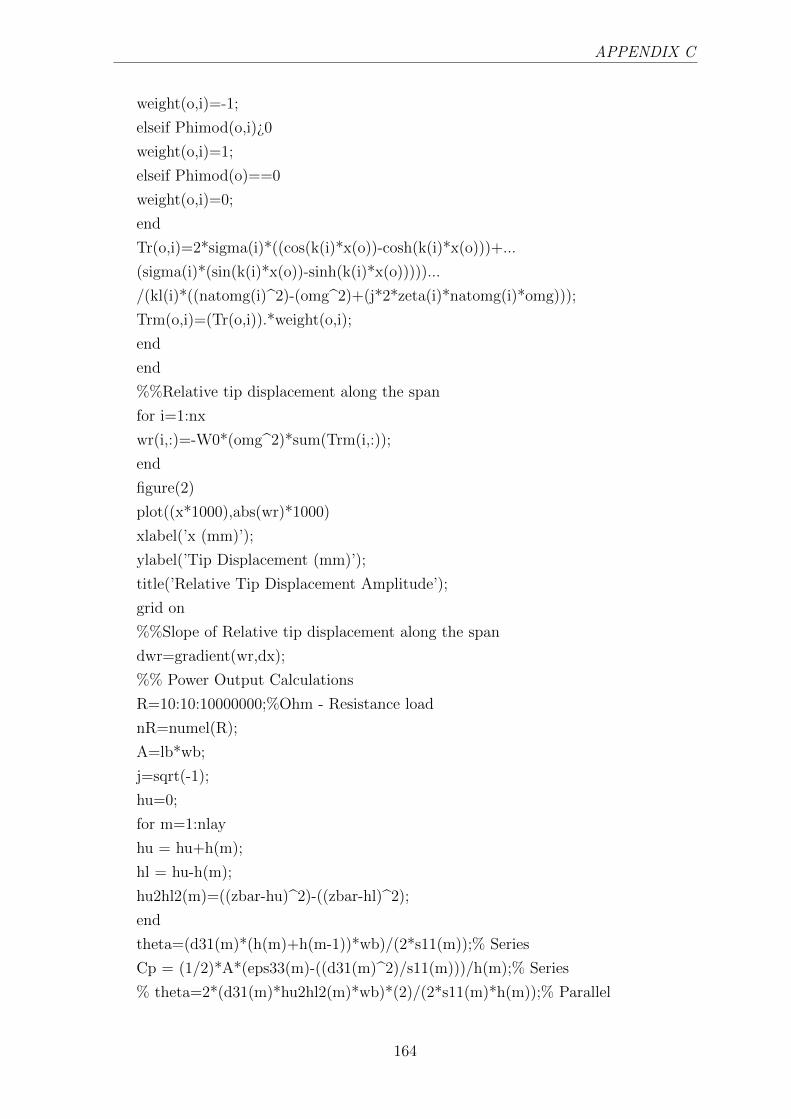
APPENDIX C
weight(o,i)=-1;
elseif Phimod(o,i)¿0
weight(o,i)=1;
elseif Phimod(o)==0
weight(o,i)=0;
end
Tr(o,i)=2*sigma(i)*((cos(k(i)*x(o))-cosh(k(i)*x(o)))+...
(sigma(i)*(sin(k(i)*x(o))-sinh(k(i)*x(o)))))...
/(kl(i)*((natomg(i)2)-(omg2)+(j*2*zeta(i)*natomg(i)*omg)));
Trm(o,i)=(Tr(o,i)).*weight(o,i);
end
end
%%Relative tip displacement along the span
for i=1:nx
wr(i,:)=-W0*(omg2)*sum(Trm(i,:));
end
figure(2)
plot((x*1000),abs(wr)*1000)
xlabel(’x (mm)’);
ylabel(’Tip Displacement (mm)’);
title(’Relative Tip Displacement Amplitude’);
grid on
%%Slope of Relative tip displacement along the span
dwr=gradient(wr,dx);
%% Power Output Calculations
R=10:10:10000000;%Ohm - Resistance load
nR=numel(R);
A=lb*wb;
j=sqrt(-1);
hu=0;
for m=1:nlay
hu = hu+h(m);
hl = hu-h(m);
hu2hl2(m)=((zbar-hu)2)-((zbar-hl)2);
end
theta=(d31(m)*(h(m)+h(m-1))*wb)/(2*s11(m));% Series
Cp = (1/2)*A*(eps33(m)-((d31(m)2)/s11(m)))/h(m);% Series
% theta=2*(d31(m)*hu2hl2(m)*wb)*(2)/(2*s11(m)*h(m));% Parallel
164
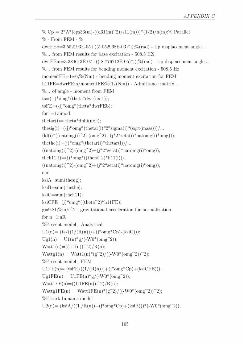
APPENDIX C
% Cp = 2*A*(eps33(m)-((d31(m)2)/s11(m)))*(1/2)/h(m);% Parallel
% - From FEM - %
dwrFEb=3.552193E-05+((5.052968E-03)*j);%(rad) - tip displacement angle...
%... from FEM results for base excitation - 508.5 HZ
dwrFEm=3.384613E-07+((-8.776712E-05)*j);%(rad) - tip displacement angle...
%... from FEM results for bending moment excitation - 508.5 Hz
momentFE=1e-6;%(Nm) - bending moment excitation for FEM
h11FE=dwrFEm/momentFE;%(1/(Nm)) - Admittance matrix...
%... of angle - moment from FEM
ts=(-j)*omg*(theta*dwr(nx,1));
tsFE=(-j)*omg*(theta*dwrFEb);
for i=1:nmod
thetar(i)= theta*dphi(nx,i);
thesig(i)=(-j)*omg*(thetar(i)*2*sigma(i)*(sqrt(mass)))/...
(kl(i)*((natomg(i)2)-(omg2)+(j*2*zeta(i)*natomg(i)*omg)));
thethe(i)=(j)*omg*(thetar(i)*thetar(i))/...
((natomg(i)2)-(omg2)+(j*2*zeta(i)*natomg(i)*omg));
theh11(i)=(j)*omg*((theta2)*h11(i))/...
((natomg(i)2)-(omg2)+(j*2*zeta(i)*natomg(i)*omg));
end
ksiA=sum(thesig);
ksiB=sum(thethe);
ksiC=sum(theh11);
ksiCFE=(j)*omg*((theta2)*h11FE);
g=9.81;%m/s2 - gravitational acceleration for normalization
for n=1:nR
%Present model - Analytical
U1(n)= (ts/((1/(R(n)))+(j*omg*Cp)-(ksiC)));
Ug1(n) = U1(n)*g/(-W0*(omg2));
Watt1(n)=((U1(n)).2)/R(n);
Wattg1(n) = Watt1(n)*(g2)/((-W0*(omg2))2);
%Present model - FEM
U1FE(n)= (tsFE/((1/(R(n)))+(j*omg*Cp)+(ksiCFE)));
Ug1FE(n) = U1FE(n)*g/(-W0*(omg2));
Watt1FE(n)=((U1FE(n)).2)/R(n);
Wattg1FE(n) = Watt1FE(n)*(g2)/((-W0*(omg2))2);
%Erturk-Inman’s model
U2(n)= (ksiA/((1./R(n))+(j*omg*Cp)+(ksiB)))*(-W0*(omg2));
165

APPENDIX C
Ug2(n) = U2(n)*g/(-W0*(omg2));
Watt2(n)=((U2(n)).2)/R(n);
Wattg2(n) = Watt2(n)*(g2)/((-W0*(omg2))2);
end
%Erturk-Inman’s experiment
Rexp = 1e3*[0.47 1.2 6.7 9.9 21.5 44.9 90.9 247.8 319.2 403.9 498.7 995.0];
Ugexp = [0.15 0.35 1.21 1.46 1.90 2.20 2.37 2.49 2.51 2.52 2.53 2.55];
Wattgexp = [4.72e-05 1.02e-04 2.17e-04 2.14e-04 1.68e-04 1.08e-04...
6.19e-05 2.51e-05 1.97e-05 1.57e-05 1.28e-05 6.53e-06];
figure(3)
subplot(1,1,1);
loglog((R)’,(abs(Ug2))’,’-k’,’linewidth’,2)
hold on
loglog((R)’,(abs(Ug1FE))’,’–r’,’linewidth’,2)
loglog((R)’,(abs(Ug1))’,’-.g’,’linewidth’,2)
loglog((Rexp)’,(abs(Ugexp))’,’ob’,’linewidth’,2)
xlabel(’Resistance (Ohm)’);
ylabel(’Voltage (V per g)’);
title(’Voltage Amplitude vs Resistance’);
legend(’Erturk-Inman Model’,’Present Model (FEM)’,’Present Model (Analytical)’,...
’Erturk-Inman Experiment’)
axis ([1e2 1e7 1e-3 1e2]);
grid off
annotation(’rectangle’,[0.40 0.60 0.05 0.05])
annotation(’arrow’,[0.45 0.55],[0.60 0.55])
axes(’position’, [.55, .25, .3, .3])
plot((R)’,(abs(Ug2))’,’-k’,’linewidth’,2)
hold on
plot((R)’,(abs(Ug1FE))’,’–r’,’linewidth’,2)
plot((R)’,(abs(Ug1))’,’-.g’,’linewidth’,2)
plot((Rexp)’,(abs(Ugexp))’,’ob’,’linewidth’,2)
axis ([0.60*(104) 1.05*(104) 1.15*(100) 1.55*(100)]);
figure(4)
subplot(1,1,1);
loglog((R)’,(abs(Wattg2)*1e6)’,’-k’,’linewidth’,2)
hold on
loglog((R)’,(abs(Wattg1FE)*1e6)’,’–r’,’linewidth’,2)
loglog((R)’,(abs(Wattg1)*1e6),’-.g’,’linewidth’,2)
166

APPENDIX C
loglog((Rexp)’,(abs(Wattgexp)*1e6)’,’ob’,’linewidth’,2)
xlabel(’Resistance (Ohm)’);
ylabel(’Power (micro-Watts per g2)’);
title(’Power Amplitude vs Resistance’);
legend(’Erturk-Inman Model’,’Present Model (FEM)’,’Present Model (Analytical)’,...
’Erturk-Inman Experiment’)
axis ([1e2 1e7 1e-1 1e4]);
grid off
annotation(’rectangle’,[0.4 0.625 0.05 0.05])
annotation(’arrow’,[0.425 0.425],[0.625 0.525])
axes(’position’, [.30, .225, .3, .3])
plot((R)’,(abs(Wattg2)*1e6)’,’-k’,’linewidth’,2)
hold on
plot((R)’,(abs(Wattg1FE)*1e6)’,’–r’,’linewidth’,2)
plot((R)’,(abs(Wattg1)*1e6)’,’-.g’,’linewidth’,2)
plot((Rexp)’,(abs(Wattgexp)*1e6)’,’ob’,’linewidth’,2)
axis ([0.60*(104) 1.05*(104) 2.10*(102) 2.25*(102)]);
grid off
167

APPENDIX D
Example of MATLAB code for the Double-Inclusion
model with Mori-Tanaka method
% Chan - Unsworth: analytical and experimental validation
close all;
clear all;
clc;
%% Input piezo fiber and matrix properties
% Piezo Fiber: PZT-7A Chan - Unsworth
rho p = 7600;% kg/m3
C11 p = 148E09;% Pa
C12 p = 76.2E09;% Pa
C13 p = 74.2E09;% Pa
C21 p = 76.2E09;% Pa
C22 p = 148E09;% Pa
C23 p = 74.2E09;% Pa
C31 p = 74.2E09;% Pa
C32 p = 74.2E09;% Pa
C33 p = 131E09;% Pa
C44 p = 25.4E09;% Pa
C55 p = 25.4E09;% Pa
C66 p = 35.9E09;% Pa
C p = [C11 p C12 p C13 p 0 0 0;...
C21 p C22 p C23 p 0 0 0;...
C31 p C32 p C33 p 0 0 0;...
0 0 0 C44 p 0 0;...
0 0 0 0 C55 p 0;...
0 0 0 0 0 C66 p ;];
S p = inv(C p);
e15 p = 9.2;% C/m2

APPENDIX D
e31 p = -2.1;% C/m2
e32 p = -2.1;% C/m2
e33 p = 12.3; %9.5;% C/m2
e p = [0 0 0 0 e15 p 0;...
0 0 0 e15 p 0 0;...
e31 p e32 p e33 p 0 0 0;];
d p = e p*S p;
k0 = 8.85E-12;% C2/Nm2 - Standard Vacuum Permittivity
k1 p = 460 * k0;% C2/Nm2
k2 p = 460 * k0;% C2/Nm2
k3 p = 235 * k0;% C2/Nm2
k p = [k1 p 0 0;...
0 k2 p 0;...
0 0 k3 p;];
EiJMn p = [C p, -e p’;...
e p, k p;];
% Matrix: Araldite - Epoxy
rho m = 1150;% kg/m3
C11 m = 8.0E09;% Pa
C12 m = 4.4E09;% Pa
C13 m = 4.4E09;% Pa
C21 m = 4.4E09;% Pa
C22 m = 8.0E09;% Pa
C23 m = 4.4E09;% Pa
C31 m = 4.4E09;% Pa
C32 m = 4.4E09;% Pa
C33 m = 8.0E09;% Pa
C44 m = 1.8E09;% Pa
C55 m = 1.8E09;% Pa
C66 m = 1.8E09;% Pa
C m = [C11 m C12 m C13 m 0 0 0;...
C21 m C22 m C23 m 0 0 0;...
C31 m C32 m C33 m 0 0 0;...
0 0 0 C44 m 0 0;...
0 0 0 0 C55 m 0;...
0 0 0 0 0 C66 m ;];
S m = inv(C m);
e15 m = 0.0;% C/m2
169

APPENDIX D
e31 m = 0.0;% C/m2
e32 m = 0.0;% C/m2
e33 m = 0.0;% C/m2
e m = [0 0 0 0 e15 m 0;...
0 0 0 e15 m 0 0;...
e31 m e32 m e33 m 0 0 0;];
k0 = 8.85E-12;% C2/Nm2 - Standard Vacuum Permittivity
k1 m = 4.2 * k0;% C2/Nm2
k2 m = 4.2 * k0;% C2/Nm2
k3 m = 4.2 * k0;% C2/Nm2
k m = [k1 m 0 0;... 0 k2 m 0;... 0 0 k3 m;];
EiJMn m = [C m, -e m’;...
e m, k m;];
% Core Fiber: Graphite Carbon Fiber
rho c = 2000;% kg/m3
C11 c = 24.0E09;% Pa
C12 c = 9.7E09;% Pa
C13 c = 6.7E09;% Pa
C21 c = 9.7E09;% Pa
C22 c = 24.0E09;% Pa
C23 c = 6.7E09;% Pa
C31 c = 6.7E09;% Pa
C32 c = 6.7E09;% Pa
C33 c = 243.7E09;% Pa
C44 c = 27.0E09;% Pa
C55 c = 27.0E09;% Pa
C66 c = 11.0E09;% Pa
C c = [C11 c C12 c C13 c 0 0 0;...
C21 c C22 c C23 c 0 0 0;...
C31 c C32 c C33 c 0 0 0;...
0 0 0 C44 c 0 0;...
0 0 0 0 C55 c 0;...
0 0 0 0 0 C66 c ;];
S c = inv(C c);
e15 c = 0.0;% C/m2
e31 c = 0.0;% C/m2
e32 c = 0.0;% C/m2
e33 c = 0.0;% C/m2
170

APPENDIX D
e c = [0 0 0 0 e15 c 0;...
0 0 0 e15 c 0 0;...
e31 c e32 c e33 c 0 0 0;];
k0 = 8.85E-12;% C2/Nm2 - Standard Vacuum Permittivity
k1 c = 12 * k0;% C2/Nm2
k2 c = 12 * k0;% C2/Nm2
k3 c = 12 * k0;% C2/Nm2
k c = [k1 c 0 0;... 0 k2 c 0;...
0 0 k3 c;];
EiJMn c = [C c, -e c’;...
e c, k c;];
EiJMn pm = EiJMn p - EiJMn m;
EiJMn cp = EiJMn p - EiJMn c;
EiJMn cm = EiJMn c - EiJMn m;
%% Geometry of inclusion (fiber in the matrix) and concentration tensor
alfa = 1;% long-infinite cylindrical inclusion
V cp = 0.02:0.02:0.98;% volume fraction of piezo+core fiber (ASF)
V ASF = V cp;
AR p = [0.5, 0.6, 0.7, 0.95] ;% aspect ratio of piezo shell thickness
for i=1:numel(V cp)
for j=1:numel(AR p)
r cASF(j) = 1-AR p(j);% ratio of core radius to ASF radius
V cASF(j) = (1-AR p(j))2;% volume fraction of core fiber to the ASF
V pASF(j) = 1-V cASF(j);% volume fraction of piezo to the ASF
V m(i)= 1-V cp(i);% volume fraction of matrix to the composite
V c(i,j)= V cASF(j)*V cp(i);% volume fraction of core fiber to the composite
V p(i,j)= 1-V c(i,j)-V m(i);% volume fraction of piezo to the composite
end
end
SMnAb c = zeros(9,9);
SMnAb p = zeros(9,9);
if alfa == 1
% Concentration Tensor for Piezo fiber
S1111 p = ((5*C11 m)+C12 m)/(8*C11 m);
S2222 p = S1111 p;
S1212 p = ((3*C11 m)-C12 m)/(8*C11 m);
S2121 p = S1212 p;
S1221 p = S1212 p;
171

APPENDIX D
S2112 p = S1212 p;
S1313 p = 1/4;
S3131 p = S1313 p;
S1331 p = S1313 p;
S3113 p = S1313 p;
S2323 p = S1313 p;
S3232 p = S1313 p;
S2332 p = S1313 p;
S3223 p = S1313 p;
S1122 p = ((3*C12 m)-C11 m)/(8*C11 m);
S2211 p = S1122 p;
S1133 p = C13 m/(2*C11 m);
S2233 p = S1133 p;
S1143 p = e31 m/(2*C11 m);
S2243 p = S1143 p;
S4141 p = 1/2;
S4242 p = S4141 p;
SMnAb p(1,1) = S1111 p;
SMnAb p(1,2) = S1122 p;
SMnAb p(1,3) = S1133 p;
SMnAb p(1,9) = S1143 p;
SMnAb p(2,1) = S2211 p;
SMnAb p(2,2) = S2222 p;
SMnAb p(2,3) = S2233 p;
SMnAb p(2,9) = S2243 p;
SMnAb p(4,4) = S2323 p;
SMnAb p(5,5) = S1313 p;
SMnAb p(6,6) = S1212 p;
SMnAb p(7,7) = S4141 p;
SMnAb p(8,8) = S4242 p;
% Concentration Tensor for Core fiber
S1111 c = ((5*C11 m)+C12 m)/(8*C11 m);
S2222 c = S1111 c;
S1212 c = ((3*C11 m)-C12 m)/(8*C11 m);
S2121 c = S1212 c;
S1221 c = S1212 c;
S2112 c = S1212 c;
S1313 c = 1/4;
172

APPENDIX D
S3131 c = S1313 c;
S1331 c = S1313 c;
S3113 c = S1313 c;
S2323 c = S1313 c;
S3232 c = S1313 c;
S2332 c = S1313 c;
S3223 c = S1313 c;
S1122 c = ((3*C12 m)-C11 m)/(8*C11 m);
S2211 c = S1122 c;
S1133 c = C13 m/(2*C11 m);
S2233 c = S1133 c;
S1143 c = e31 m/(2*C11 m);
S2243 c = S1143 c;
S4141 c = 1/2;
S4242 c = S4141 c;
SMnAb c(1,1) = S1111 c;
SMnAb c(1,2) = S1122 c;
SMnAb c(1,3) = S1133 c;
SMnAb c(1,9) = S1143 c;
SMnAb c(2,1) = S2211 c;
SMnAb c(2,2) = S2222 c;
SMnAb c(2,3) = S2233 c;
SMnAb c(2,9) = S2243 c;
SMnAb c(4,4) = S2323 c;
SMnAb c(5,5) = S1313 c;
SMnAb c(6,6) = S1212 c;
SMnAb c(7,7) = S4141 c;
SMnAb c(8,8) = S4242 c;
end
I=eye(9,9);
A dil c=inv(I+(SMnAb p*inv(EiJMn m)*EiJMn cm));
A dil p=inv(I+(SMnAb c*inv(EiJMn m)*EiJMn cp));
deltaS=SMnAb c-SMnAb p;
F c = inv(EiJMn cm)*EiJMn m;
F p = inv(EiJMn pm)*EiJMn m;
for i=1:numel(V cp) for j=1:numel(AR p)
A MT m(:,:,i,j)=I*inv((V m(i)*I)+(V p(i,j)*A dil p(:,:))+...
(V c(i,j)*A dil c(:,:)));% Mori-Tanaka Concentration Tensor - matrix
173
APPENDIX D
A MT p(:,:,i,j)=A dil p(:,:)*inv((V m(i)*I)+(V p(i,j)*A dil p(:,:))+...
(V c(i,j)*A dil c(:,:)));% Mori-Tanaka Concentration Tensor - piezo
A MT c(:,:,i,j)=A dil c(:,:)*inv((V m(i)*I)+(V p(i,j)*A dil p(:,:))+...
(V c(i,j)*A dil c(:,:)));% Mori-Tanaka Concentration Tensor - carbon
EiJMn MT(:,:,i,j)=(V m(i)*EiJMn m*A MT m(:,:,i,j))+...
(V p(i,j)*EiJMn p*A MT p(:,:,i,j))+(V c(i,j)*EiJMn c*A MT c(:,:,i,j));
C(:,:,i,j)=EiJMn MT(1:6,1:6,i,j);
e(:,:,i,j)=EiJMn MT(7:9,1:6,i,j);
k(:,:,i,j)=EiJMn MT(7:9,7:9,i,j);
S(:,:,i,j)=inv(C(:,:,i,j));
d(:,:,i,j)=e(:,:,i,j)*S(:,:,i,j);
kt(:,:,i,j)=k(:,:,i,j)+(d(:,:,i,j)*C(:,:,i,j)*d(:,:,i,j)’);
rho(i,j)=rho m*V m(i)+rho p*V p(i,j)+rho c*V c(i,j);
end
end
for i=1:numel(V cp)
C33 AR1(i)=C(3,3,i,1);
C31 AR1(i)=C(3,1,i,1);
e33 AR1(i)=e(3,3,i,1);
e31 AR1(i)=e(3,1,i,1);
d33 AR1(i)=d(3,3,i,1);
d31 AR1(i)=d(3,1,i,1);
S33 AR1(i)=S(3,3,i,1);
S31 AR1(i)=S(3,1,i,1);
rho AR1(i)=rho(i,1);
S11 AR1(i)=S(1,1,i,1);
S12 AR1(i)=S(1,2,i,1);
S11S12 AR1(i)=S11 AR1(i)+S12 AR1(i);
k33s AR1(i)=k(3,3,i,1);
k33t AR1(i)=kt(3,3,i,1);
C11 AR1(i)=C(1,1,i,1);
C33 AR2(i)=C(3,3,i,2);
C31 AR2(i)=C(3,1,i,2);
e33 AR2(i)=e(3,3,i,2);
e31 AR2(i)=e(3,1,i,2);
d33 AR2(i)=d(3,3,i,2);
d31 AR2(i)=d(3,1,i,2);
S33 AR2(i)=S(3,3,i,2);
174

APPENDIX D
S31 AR2(i)=S(3,1,i,2);
rho AR2(i)=rho(i,2);
S11 AR2(i)=S(1,1,i,2);
S12 AR2(i)=S(1,2,i,2);
S11S12 AR2(i)=S11 AR2(i)+S12 AR2(i);
k33s AR2(i)=k(3,3,i,2);
k33t AR2(i)=kt(3,3,i,2);
C11 AR2(i)=C(1,1,i,2);
C33 AR3(i)=C(3,3,i,3);
C31 AR3(i)=C(3,1,i,3);
e33 AR3(i)=e(3,3,i,3);
e31 AR3(i)=e(3,1,i,3);
d33 AR3(i)=d(3,3,i,3);
d31 AR3(i)=d(3,1,i,3);
S33 AR3(i)=S(3,3,i,3);
S31 AR3(i)=S(3,1,i,3);
rho AR3(i)=rho(i,3);
S11 AR3(i)=S(1,1,i,3);
S12 AR3(i)=S(1,2,i,3);
S11S12 AR3(i)=S11 AR3(i)+S12 AR3(i);
k33s AR3(i)=k(3,3,i,3);
k33t AR3(i)=kt(3,3,i,3);
C11 AR3(i)=C(1,1,i,3);
C33 AR4(i)=C(3,3,i,4);
C31 AR4(i)=C(3,1,i,4);
e33 AR4(i)=e(3,3,i,4);
e31 AR4(i)=e(3,1,i,4);
d33 AR4(i)=d(3,3,i,4);
d31 AR4(i)=d(3,1,i,4);
S33 AR4(i)=S(3,3,i,4);
S31 AR4(i)=S(3,1,i,4);
rho AR4(i)=rho(i,4);
S11 AR4(i)=S(1,1,i,4);
S12 AR4(i)=S(1,2,i,4);
S11S12 AR4(i)=S11 AR4(i)+S12 AR4(i);
k33s AR4(i)=k(3,3,i,4);
k33t AR4(i)=kt(3,3,i,4);
C11 AR4(i)=C(1,1,i,4);
175
APPENDIX D
% Chan and Unsworth Model (1989)
cv(i) = C p(1,1)+C p(1,2)+((V ASF(i)*(C m(1,1)+C m(1,2)))/(1-V ASF(i)));
sv(i) =(V ASF(i)*S m(1,1))+ ((1-V ASF(i))*(S p(3,3)));
c33v(i) = (V ASF(i)*(C p(3,3)-(2*((C p(1,3)-C m(1,2))2)/cv(i))))+...
((1-V ASF(i))*C m(1,1));
e33v(i) = V ASF(i)*(e p(3,3)-(2*e p(3,1)*(C p(1,3)-C m(1,2))/cv(i)));
c31v(i) = ((C m(1,2)*(C p(1,1)+C p(1,2)))+...
(V ASF(i)*C p(1,3)*(C m(1,1)+C m(1,2))/(1-V ASF(i))))/cv(i);
e31v(i) = e p(3,1)*(1-((C p(1,1)+C p(1,2))/cv(i)));
s31v(i) = ((S p(3,3)*S m(1,2)*(1-V ASF(i)))+...
(V ASF(i)*S m(1,1)*S p(1,3)))/sv(i);
s33v(i) = S m(1,1)*S p(3,3)/sv(i);
d33v(i) = V ASF(i)*S m(1,1)*d p(3,3)/sv(i);
d31v(i) = (V ASF(i)*d p(3,1))-((V ASF(i)*(1-V ASF(i))*d p(3,3)*...
(S p(1,3)-S m(1,2)))/sv(i));
rhov(i) = rho m*V m(i)+rho p*(1-V m(i));
s11s12v(i) = (V ASF(i)*(S p(1,1)+S p(1,2)))+...
((1-V ASF(i))*(S m(1,1)+S m(1,2)))-...
((2*V ASF(i)/sv(i))*(1-V ASF(i))*((S m(1,3)-S p(1,2))2));
k33tv(i) = (V ASF(i)*425*k0)-(V ASF(i)*(1-V ASF(i))*d p(3,3)2/sv(i))+...
((1-V ASF(i))*(k m(1,1)));
end
expdata=[0.2, 0.3, 0.42, 0.55, 0.65, 0.82;...
90, 100, 210, 240, 300, 420;...
125, 150, 160, 160, 167, 167;...
100, 75, 55, 45, 32, 20;...
2440, 3085, 3860, 4700, 5340, 6440;];
figure (1)
plot (V cp,C33 AR1*1E-10,’r-*’, V cp,C33 AR2*1E-10,’g-o’,...
V cp,C33 AR3*1E-10,’m-’,V cp,C33 AR4*1E-10,’b-d’,...
V cp,c33v*1E-10,’k-’)
xlabel(’Volume Fraction of ASF’);
ylabel(’C 33 (1010 N/m2)’);
title(’Stiffness C 33 vs Volume Fraction of ASF’);
legend(’Present Code - DI MT AR1’,’Present Code - DI MT AR2’,...
’Present Code - DI MT AR3’,’Present Code - DI MT AR4’,...
’Chan-Unsworth Model’,’Location’,’Best’)
figure (2)
176
APPENDIX D
plot (V cp,C31 AR1*1E-10,’r-*’,V cp,C31 AR2*1E-10,’g-o’,...
V cp,C31 AR3*1E-10,’m-’,V cp,C31 AR4*1E-10,’b-d’,...
V cp,c31v*1E-10,’k-’)
xlabel(’Volume Fraction of ASF’);
ylabel(’C 31 (1010 N/m2)’);
title(’Stiffness C 31 vs Volume Fraction of ASF’);
legend(’Present Code - DI MT AR1’,’Present Code - DI MT AR2’,...
’Present Code - DI MT AR3’,’Present Code - DI MT AR4’,...
’Chan-Unsworth Model’,’Location’,’Best’)
figure (3)
plot (V cp,e33 AR1,’r-*’,V cp,e33 AR2,’g-o’,...
V cp,e33 AR3,’m-’,V cp,e33 AR4,’b-d’,...
V cp,e33v,’k-’)
xlabel(’Volume Fraction of ASF’);
ylabel(’e 33 (C/m2)’);
title(’Piezoelectric Constant e 33 vs Volume Fraction of ASF’);
legend(’Present Code - DI MT AR1’,’Present Code - DI MT AR2’,...
’Present Code - DI MT AR3’,’Present Code - DI MT AR4’,...
’Chan-Unsworth Model’,’Location’,’Best’)
figure (4)
plot (V cp,e31 AR1,’r-*’,V cp,e31 AR2,’g-o’,...
V cp,e31 AR3,’m-’,V cp,e31 AR4,’b-d’,...
V cp,e31v,’k-’)
xlabel(’Volume Fraction of ASF’);
ylabel(’e 31 (C/m2)’);
title(’Piezoelectric Constant e 31 vs Volume Fraction of ASF’);
legend(’Present Code - DI MT AR1’,’Present Code - DI MT AR2’,...
’Present Code - DI MT AR3’,’Present Code - DI MT AR4’,...
’Chan-Unsworth Model’,’Location’,’Best’)
figure (5)
plot (V cp,d33 AR1*1E12,’r-*’,V cp,d33 AR2*1E12,’g-o’,...
V cp,d33 AR3*1E12,’m-’,V cp,d33 AR4*1E12,’b-d’,...
V cp,d33v*1E12,’k-’)
hold on
plot(expdata(1,:),expdata(3,:),’ks’,’MarkerFaceColor’,’k’)
xlabel(’Volume Fraction of ASF’);
ylabel(’d 33 (10-12 m/V)’);
title(’Charge Constant d 33 vs Volume Fraction of ASF’);
177
APPENDIX D
legend(’Present Code - DI MT AR1’,’Present Code - DI MT AR2’,...
’Present Code - DI MT AR3’,’Present Code - DI MT AR4’,...
’Chan-Unsworth Model’,’Chan-Unsworth Experiment’,’Location’,’Best’)
figure (6)
plot (V cp,d31 AR1*1E12,’r-*’,V cp,d31 AR2*1E12,’g-o’,...
V cp,d31 AR3*1E12,’m-’,V cp,d31 AR4*1E12,’b-d’,...
V cp,d31v*1E12,’k-’)
xlabel(’Volume Fraction of ASF’);
ylabel(’d 31 (10-12 m/V)’);
title(’Charge Constant d 31 vs Volume Fraction of ASF’);
legend(’Present Code - DI MT AR1’,’Present Code - DI MT AR2’,...
’Present Code - DI MT AR3’,’Present Code - DI MT AR4’,...
’Chan-Unsworth Model’,’Location’,’Best’)
figure (7)
plot (V cp,S33 AR1*1E12,’r-*’,V cp,S33 AR2*1E12,’g-o’,...
V cp,S33 AR3*1E12,’m-’,V cp,S33 AR4*1E12,’b-d’,...
V cp,s33v*1E12,’k-’)
xlabel(’Volume Fraction of ASF’);
ylabel(’S 33 (10-12 m2/N)’);
title(’Compliance S 33 vs Volume Fraction of ASF’);
legend(’Present Code - DI MT AR1’,’Present Code - DI MT AR2’,...
’Present Code - DI MT AR3’,’Present Code - DI MT AR4’,...
’Chan-Unsworth Model’,’Location’,’Best’)
figure (8)
plot (V cp,S31 AR1*1E12,’r-*’,V cp,S31 AR2*1E12,’g-o’,...
V cp,S31 AR3*1E12,’m-’,V cp,S31 AR4*1E12,’b-d’,...
V cp,s31v*1E12,’k-’)
xlabel(’Volume Fraction of ASF’);
ylabel(’S 31 (10-12 m2/N)’);
title(’Compliance S 31 vs Volume Fraction of ASF’);
legend(’Present Code - DI MT AR1’,’Present Code - DI MT AR2’,...
’Present Code - DI MT AR3’,’Present Code - DI MT AR4’,...
’Chan-Unsworth Model’,’Location’,’Best’)
figure (9)
plot (V cp,rho AR1,’r-*’,V cp,rho AR2,’g-o’,...
V cp,rho AR3,’m-’,V cp,rho AR4,’b-d’,...
V cp,rhov,’k-’)
hold on
178
APPENDIX D
plot(expdata(1,:),expdata(5,:),’ks’,’MarkerFaceColor’,’k’)
xlabel(’Volume Fraction of ASF’);
ylabel(’Density (kg/m3)’);
title(’Density vs Volume Fraction of ASF’);
legend(’Present Code - DI MT AR1’,’Present Code - DI MT AR2’,...
’Present Code - DI MT AR3’,’Present Code - DI MT AR4’,...
’Chan-Unsworth Model’,’Chan-Unsworth Experiment’,’Location’,’Best’)
figure (10)
plot (V cp,S11 AR1*1E12,’r-*’,V cp,S11 AR2*1E12,’g-o’,...
V cp,S11 AR3*1E12,’m-’,...
V cp,S11 AR4*1E12,’b-d’)
xlabel(’Volume Fraction of ASF’);
ylabel(’S 11 (10-12 m2/N)’);
title(’Compliance S 11 vs Volume Fraction of ASF’);
legend(’Present Code - DI MT AR1’,’Present Code - DI MT AR2’,...
’Present Code - DI MT AR3’,’Present Code - DI MT AR4’,’Location’,’Best’)
figure (11)
plot (V cp,C11 AR1*1E-10,’r-*’,V cp,C11 AR2*1E-10,’g-o’,...
V cp,C11 AR3*1E-10,’m-’,...
V cp,C11 AR4*1E-10,’b-d’)
xlabel(’Volume Fraction of ASF’);
ylabel(’C 11 (1010 m2/N)’);
title(’Stiffness C 11 vs Volume Fraction of ASF’);
legend(’Present Code - DI MT AR1’,’Present Code - DI MT AR2’,...
’Present Code - DI MT AR3’,’Present Code - DI MT AR4’,’Location’,’Best’)
figure (12)
plot (V cp,S11S12 AR1*1E12,’r-s’,V cp,S11S12 AR2*1E12,’g-o’,...
V cp,S11S12 AR3*1E12,’m-’,V cp,S11S12 AR4*1E12,’b-d’,...
V cp,s11s12v*1E12,’k-’)
hold on
plot(expdata(1,:),expdata(4,:),’ks’,’MarkerFaceColor’,’k’)
xlabel(’Volume Fraction of ASF’);
ylabel(’S 11+S 12 (10-12 m2/N)’);
title(’Compliance S 11+S 12 vs Volume Fraction of ASF’);
legend(’Present Code - DI MT AR1’,’Present Code - DI MT AR2’,...
’Present Code - DI MT AR3’,’Present Code - DI MT AR4’,...
’Chan-Unsworth Model’,’Chan-Unsworth Experiment’,’Location’,’Best’)
figure (13)
179

APPENDIX D
plot (V cp,k33t AR1*(1/k0),’r-*’,V cp,k33t AR2*(1/k0),’g-o’,...
V cp,k33t AR3*(1/k0),’m-’,V cp,k33t AR4*(1/k0),’b-d’,...
V cp,k33tv*(1/k0),’k-’)
hold on
plot (expdata(1,:),expdata(2,:),’ks’,’MarkerFaceColor’,’k’)
xlabel(’Volume Fraction of ASF’);
ylabel(’\epsilon 33T / \epsilon 0’);
title(’Permittivity Ratio \epsilon 33T / \epsilon 0 vs Volume Fraction of ASF’);
legend(’Present Code - DI MT AR1’,’Present Code - DI MT AR2’,...
’Present Code - DI MT AR3’,’Present Code - DI MT AR4’,...
’Chan-Unsworth Model’,’Chan-Unsworth Experiment’,’Location’,’Best’)
%% Output 2D Plane Stress Constitutive
for i=1:numel(V cp)
for j=1:numel(AR p)
C11 2D(i,j) = C(1,1,i,j) - ((C(1,3,i,j)2)/C(3,3,i,j));
C12 2D(i,j) = C(1,2,i,j) - ((C(1,3,i,j)*C(2,3,i,j))/C(3,3,i,j));
C22 2D(i,j) = C(2,2,i,j) - ((C(2,3,i,j)2)/C(3,3,i,j));
C66 2D(i,j) = C(6,6,i,j);
C 2D(:,:,i,j) = [C11 2D(i,j) C12 2D(i,j) 0;...
C12 2D(i,j) C22 2D(i,j) 0;... 0 0 C66 2D(i,j);];
S 2D(:,:,i,j) = inv(C 2D(:,:,i,j));
e31 2D(i,j) = e(3,1,i,j) - ((C(1,3,i,j)*e(3,3,i,j))/C(3,3,i,j));
e32 2D(i,j) = e(3,2,i,j) - ((C(2,3,i,j)*e(3,3,i,j))/C(3,3,i,j));
e 2D(:,:,i,j) = [e31 2D(i,j) e32 2D(i,j) 0];
d 2D(:,:,i,j) = e 2D(:,:,i,j)*S 2D(:,:,i,j);
k3 2D(i,j) = k(3,3,i,j) +((e(3,3,i,j)2)/C(3,3,i,j));
k 2D(i,j) = k3 2D(i,j);
EiJMn 2D(:,:,i,j) = [C 2D(:,:,i,j), -e 2D(:,:,i,j)’;...
e 2D(:,:,i,j), k 2D(i,j);];
end
end
180

APPENDIX E
Example of MATLAB code for the Iterative FEM in
frequency domain
% Marqui unimorph base excitation - solid element
close all
clear all
clc
%% Input read XLS from Nastran PCH
j=sqrt(-1);
Kuv(:,1)=-xlsread(’marqui uni3d pch’,’FX’,’B:B’);
nnod=length(Kuv);
Kuv(nnod+1:2*nnod,1)=-xlsread(’marqui uni3d pch’,’FY’,’B:B’);
Kuv((2*nnod)+1:3*nnod,1)=-xlsread(’marqui uni3d pch’,’FZ’,’B:B’);
U(:,1)=xlsread(’marqui uni3d pch’,’UX r0’,’B:B’)+...
(j*xlsread(’marqui uni3d pch’,’UX i0’,’B:B’)); % mm
U(nnod+1:2*nnod,1)=xlsread(’marqui uni3d pch’,’UY r0’,’B:B’)+...
(j*xlsread(’marqui uni3d pch’,’UY i0’,’B:B’)); % mm
U((2*nnod)+1:3*nnod,1)=xlsread(’marqui uni3d pch’,’UZ r0’,’B:B’)+...
(j*xlsread(’marqui uni3d pch’,’UZ i0’,’B:B’)); % mm
%% Input geometry and material properties
n lay=2;%number of layers
lay prop=zeros(7,n lay);%layer properties initiation
lb=(100);%mm - beam length
wb=(20);%mm - beam width
% Assume uniform cross section
for i=1:n lay
lay prop(1,i)=lb;%mm - layers’s length
lay prop(2,i)=wb;%mm - layers’s width
end
lay prop(3,1)=0.5;%mm - thickness - material 1 (metal)

APPENDIX E
lay prop(3,2)=0.4;%mm - thickness - material 2 (PZT 5A)
lay prop(4,1)=(1/100)*1e-6;%mm.s/kg - compliance (s 11) - metal
lay prop(4,2)=(1/66)*1e-6;%mm.s/kg - compliance (s 11) - PZT 5A
lay prop(5,1)=0;% C/(kg.mm/s2) - charge constant (d 31) - metal
lay prop(5,2)=-190e-15;% C/(kg.mm/s2) - charge constant (d 31) - PZT 5A
lay prop(6,1)=0;%Farad/mm - permittivity - metal
lay prop(6,2)=2069*8.85*(10-15);%Farad/mm - permittivity - PZT 5A
lay prop(7,1)=7800e-9;%kg/(mm3) - density - metal
lay prop(7,2)=7165e-9;%kg/(mm3) - density - PZT 5A
%% neutral axis, beam flexural stiffness and m piezo calculations
l=zeros(1,n lay);%array of layers’s length
w=zeros(1,n lay);%array of layers’s width
h=zeros(1,n lay);%array of layers’s thickness
s 11=zeros(1,n lay);%array of layers’s material compliance
d 31=zeros(1,n lay);%array of layers’s piezoelectric charge constant
eps 33=zeros(1,n lay);%array of layers’s permitivitty (at constant stress)
rho=zeros(1,n lay);%array of layers’s density
for i=1:n lay
l(i)=lay prop(1,i);
w(i)=lay prop(2,i);
h(i)=lay prop(3,i);
s 11(i)=lay prop(4,i);
d 31(i)=lay prop(5,i);
eps 33(i)=lay prop(6,i);
rho(i)=lay prop(7,i);
end
z1=0;hj=0;z2=0;z3=0;
for i=1:n lay
z1= z1+(w(i)*(h(i)2)/s 11(i));
hj= hj+h(i);
z2= z2+((w(i)*h(i)/s 11(i))*hj);
z3= z3+(w(i)*h(i)/s 11(i));
end
z bar=-((z1)-(2*z2))/(2*z3);%meter (measured from bottom) - neutral axis
c lay=zeros(1,n lay);hu=0;
m lay=zeros(1,n lay);
for i=1:n lay
hu = hu+h(i);
182

APPENDIX E
hl = hu-h(i);
c lay(i)=(w(i)/s 11(i))*((3*h(i)*(z bar-hu)*(z bar-hl))+(h(i)3));
m lay(i)=(w(i)*d 31(i)/(s 11(i)*h(i)))*...
((2*z bar*h(i))-(2*h(i)*hu)+(h(i)2));
end
C=sum(c lay)/3;%Nm2 - Beam flexural stiffness
m piezo=sum(m lay)/2;%Nm/V - internal moment due to piezo per unit volt
A=lb*wb;
Cp = A*(eps 33(2)-((d 31(2)2)/s 11(2)))/h(2);% unimorph
%% Dynamic bending modes and natural frequencies (clamped-free beam)
%The first five solutions of characteristic equation
%(not calculated here, taken from reference)
n mod=5;%number of modeshapes
kl =[1.8751 4.6941 7.8548 10.9955 14.137];%dimensionless
k =kl./lb;%1/m - characteristic solution per unit length
mass=0;
for i=1:n lay
mass = mass+(l(i)*w(i)*h(i)*rho(i));%kg - mass of the beam
end
miu=mass/lb;
for i=1:n mod
natomg(i)= ((kl(i)2)/(lb2))*(sqrt(C/miu));%rad/s - angular natural freq
natfrq(i)= natomg(i)/(2*pi);%Hz - natural freq
end
%% Electrical Equation - Iteration 0
R = 15000; % Ohm
Volt1=j*natomg(1)*(Kuv’*U)*(1/((j*natomg(1)*Cp)+(1/R)));
%% Electrical Equation - Iteration 1
Uiter1(:,1)=xlsread(’marqui uni3d pch’,’UX r1’,’B:B’)+...
(j*xlsread(’marqui uni3d pch’,’UX i1’,’B:B’)); % mm
Uiter1(nnod+1:2*nnod,1)=xlsread(’marqui uni3d pch’,’UY r1’,’B:B’)+...
(j*xlsread(’marqui uni3d pch’,’UY i1’,’B:B’)); % mm
Uiter1((2*nnod)+1:3*nnod,1)=xlsread(’marqui uni3d pch’,’UZ r1’,’B:B’)+...
(j*xlsread(’marqui uni3d pch’,’UZ i1’,’B:B’)); % mm
Volt2=j*natomg(1)*(Kuv’*Uiter1)*(1/((j*natomg(1)*Cp)+(1/R)));
%% Electrical Equation - Iteration 2
Uiter2(:,1)=xlsread(’marqui uni3d pch’,’UX r2’,’B:B’)+...
(j*xlsread(’marqui uni3d pch’,’UX i2’,’B:B’)); % mm
183

APPENDIX E
Uiter2(nnod+1:2*nnod,1)=xlsread(’marqui uni3d pch’,’UY r2’,’B:B’)+...
(j*xlsread(’marqui uni3d pch’,’UY i2’,’B:B’)); % mm
Uiter2((2*nnod)+1:3*nnod,1)=xlsread(’marqui uni3d pch’,’UZ r2’,’B:B’)+...
(j*xlsread(’marqui uni3d pch’,’UZ i2’,’B:B’)); % mm
Volt3=j*natomg(1)*(Kuv’*Uiter2)*(1/((j*natomg(1)*Cp)+(1/R)));
%% Electrical Equation - Iteration 3
Uiter3(:,1)=xlsread(’marqui uni3d pch’,’UX r3’,’B:B’)+...
(j*xlsread(’marqui uni3d pch’,’UX i3’,’B:B’)); % mm
Uiter3(nnod+1:2*nnod,1)=xlsread(’marqui uni3d pch’,’UY r3’,’B:B’)+...
(j*xlsread(’marqui uni3d pch’,’UY i3’,’B:B’)); % mm
Uiter3((2*nnod)+1:3*nnod,1)=xlsread(’marqui uni3d pch’,’UZ r3’,’B:B’)+...
(j*xlsread(’marqui uni3d pch’,’UZ i3’,’B:B’)); % mm
Volt4=j*natomg(1)*(Kuv’*Uiter3)*(1/((j*natomg(1)*Cp)+(1/R)));
%% Electrical Equation - Iteration 4
Uiter4(:,1)=xlsread(’marqui uni3d pch’,’UX r4’,’B:B’)+...
(j*xlsread(’marqui uni3d pch’,’UX i4’,’B:B’)); % mm
Uiter4(nnod+1:2*nnod,1)=xlsread(’marqui uni3d pch’,’UY r4’,’B:B’)+...
(j*xlsread(’marqui uni3d pch’,’UY i4’,’B:B’)); % mm
Uiter4((2*nnod)+1:3*nnod,1)=xlsread(’marqui uni3d pch’,’UZ r4’,’B:B’)+...
(j*xlsread(’marqui uni3d pch’,’UZ i4’,’B:B’)); % mm
Volt5=j*natomg(1)*(Kuv’*Uiter4)*(1/((j*natomg(1)*Cp)+(1/R)));
%% Electrical Equation - Iteration 5
Uiter5(:,1)=xlsread(’marqui uni3d pch’,’UX r5’,’B:B’)+...
(j*xlsread(’marqui uni3d pch’,’UX i5’,’B:B’)); % mm
Uiter5(nnod+1:2*nnod,1)=xlsread(’marqui uni3d pch’,’UY r5’,’B:B’)+...
(j*xlsread(’marqui uni3d pch’,’UY i5’,’B:B’)); % mm
Uiter5((2*nnod)+1:3*nnod,1)=xlsread(’marqui uni3d pch’,’UZ r5’,’B:B’)+...
(j*xlsread(’marqui uni3d pch’,’UZ i5’,’B:B’)); % mm
Volt6=j*natomg(1)*(Kuv’*Uiter5)*(1/((j*natomg(1)*Cp)+(1/R)));
%% Electrical Equation - Iteration 6
Uiter6(:,1)=xlsread(’marqui uni3d pch’,’UX r6’,’B:B’)+...
(j*xlsread(’marqui uni3d pch’,’UX i6’,’B:B’)); % mm
Uiter6(nnod+1:2*nnod,1)=xlsread(’marqui uni3d pch’,’UY r6’,’B:B’)+...
(j*xlsread(’marqui uni3d pch’,’UY i6’,’B:B’)); % mm
Uiter6((2*nnod)+1:3*nnod,1)=xlsread(’marqui uni3d pch’,’UZ r6’,’B:B’)+...
(j*xlsread(’marqui uni3d pch’,’UZ i6’,’B:B’)); % mm
Volt7=j*natomg(1)*(Kuv’*Uiter6)*(1/((j*natomg(1)*Cp)+(1/R)));
%% Electrical Equation - Iteration 7
184

APPENDIX E
Uiter7(:,1)=xlsread(’marqui uni3d pch’,’UX r7’,’B:B’)+...
(j*xlsread(’marqui uni3d pch’,’UX i7’,’B:B’)); % mm
Uiter7(nnod+1:2*nnod,1)=xlsread(’marqui uni3d pch’,’UY r7’,’B:B’)+...
(j*xlsread(’marqui uni3d pch’,’UY i7’,’B:B’)); % mm
Uiter7((2*nnod)+1:3*nnod,1)=xlsread(’marqui uni3d pch’,’UZ r7’,’B:B’)+...
(j*xlsread(’marqui uni3d pch’,’UZ i7’,’B:B’)); % mm
Volt8=j*natomg(1)*(Kuv’*Uiter7)*(1/((j*natomg(1)*Cp)+(1/R)));
%% Electrical Equation - Iteration 8
Uiter8(:,1)=xlsread(’marqui uni3d pch’,’UX r8’,’B:B’)+...
(j*xlsread(’marqui uni3d pch’,’UX i8’,’B:B’)); % mm
Uiter8(nnod+1:2*nnod,1)=xlsread(’marqui uni3d pch’,’UY r8’,’B:B’)+...
(j*xlsread(’marqui uni3d pch’,’UY i8’,’B:B’)); % mm
Uiter8((2*nnod)+1:3*nnod,1)=xlsread(’marqui uni3d pch’,’UZ r8’,’B:B’)+...
(j*xlsread(’marqui uni3d pch’,’UZ i8’,’B:B’)); % mm
Volt9=j*natomg(1)*(Kuv’*Uiter8)*(1/((j*natomg(1)*Cp)+(1/R)));
%% Electrical Equation - Iteration 9
Uiter9(:,1)=xlsread(’marqui uni3d pch’,’UX r9’,’B:B’)+...
(j*xlsread(’marqui uni3d pch’,’UX i9’,’B:B’)); % mm
Uiter9(nnod+1:2*nnod,1)=xlsread(’marqui uni3d pch’,’UY r9’,’B:B’)+...
(j*xlsread(’marqui uni3d pch’,’UY i9’,’B:B’)); % mm
Uiter9((2*nnod)+1:3*nnod,1)=xlsread(’marqui uni3d pch’,’UZ r9’,’B:B’)+...
(j*xlsread(’marqui uni3d pch’,’UZ i9’,’B:B’)); % mm
Volt10=j*natomg(1)*(Kuv’*Uiter9)*(1/((j*natomg(1)*Cp)+(1/R)));
%% Electrical Equation - Iteration 10
Uiter10(:,1)=xlsread(’marqui uni3d pch’,’UX r10’,’B:B’)+...
(j*xlsread(’marqui uni3d pch’,’UX i10’,’B:B’)); % mm
Uiter10(nnod+1:2*nnod,1)=xlsread(’marqui uni3d pch’,’UY r10’,’B:B’)+...
(j*xlsread(’marqui uni3d pch’,’UY i10’,’B:B’)); % mm
Uiter10((2*nnod)+1:3*nnod,1)=xlsread(’marqui uni3d pch’,’UZ r10’,’B:B’)+...
(j*xlsread(’marqui uni3d pch’,’UZ i10’,’B:B’)); % mm
Volt11=j*natomg(1)*(Kuv’*Uiter10)*(1/((j*natomg(1)*Cp)+(1/R)));
%% Plot Umax and Volt vs No. Iter.
Iter = 0:1:10;
Volt = [0 Volt1 Volt2 Volt3 Volt4 Volt5 Volt6 Volt7 Volt8 Volt9 Volt10];
Volt EIM = ones(1,11)*0.1979;
Volt ACS = ones(1,11)*0.1966;
Umax = [max(abs(U)) max(abs(Uiter1)) max(abs(Uiter2)) max(abs(Uiter3)) ...
max(abs(Uiter4)) max(abs(Uiter5)) max(abs(Uiter6)) max(abs(Uiter7))...
185

APPENDIX E
max(abs(Uiter8)) max(abs(Uiter9)) max(abs(Uiter10))];% mm
Umax EIM = ones(1,11)*49e-3;% mm
figure(1)
plot(Iter,abs(Volt),’:ob’,’linewidth’,1.5,’MarkerFaceColor’,’g’)
hold on
plot(Iter,Volt EIM,’-r’,’linewidth’,2)
plot(Iter,Volt ACS,’–k’,’linewidth’,2)
xlabel(’No. of iteration’, ’interpreter’,’latex’);
ylabel(’V (Volt)’, ’interpreter’,’latex’);
title(’Voltage Amplitude vs Number of iteration’);
legend(’Present - Iterative FEM’,’Erturk and Inman - Analytical Model’,...
’Akbar and Curiel-Sosa - Hybrid Model’)
figure(2)
plot(Iter,Umax,’:ob’,’linewidth’,1.5,’MarkerFaceColor’,’g’)
hold on
plot(Iter,Umax EIM,’-r’,’linewidth’,2)
% plot(Iter,Umax ACS,’–k’,’linewidth’,2)
xlabel(’No. of iteration’, ’interpreter’,’latex’);
ylabel(’Zrel (mm)’, ’interpreter’,’latex’);
title(’Relative Tip Displacement vs Number of iteration’);
legend(’Present - Iterative FEM’,’Erturk and Inman - Analytical Model’,...
’Akbar and Curiel-Sosa - Hybrid Model’)
186

APPENDIX F
Example of MATLAB code for the Iterative FEM in
time domain
% Jet aircraft wing PZT-5A gust load - shell element
close all
clear all
clc
%% Input read XLS from Nastran PCH
j=sqrt(-1);
Kuv(:,1)=-xlsread(’SAWEswept pzt5a pch’,’FX’,’B:B’);
nnod=length(Kuv);
Kuv(nnod+1:2*nnod,1)=-xlsread(’SAWEswept pzt5a pch’,’FY’,’B:B’);
Kuv((2*nnod)+1:3*nnod,1)=-xlsread(’SAWEswept pzt5a pch’,’FZ’,’B:B’);
Kuv((3*nnod)+1:4*nnod,1)=-xlsread(’SAWEswept pzt5a pch’,’MX’,’B:B’);
Kuv((4*nnod)+1:5*nnod,1)=-xlsread(’SAWEswept pzt5a pch’,’MY’,’B:B’);
Kuv((5*nnod)+1:6*nnod,1)=-xlsread(’SAWEswept pzt5a pch’,’MZ’,’B:B’);
nt=200;% no of increment + 1, from Nastran BDF
dt=2.500000E-02;% time step, from Nastran BDF
nonzero=find(Kuv =0);
nnzeronod=length(nonzero)/2;
Kuv red=Kuv(nonzero);
% F06 needs to be modified, delete all lines before and after the displacement results
ni=nt/50;% iteration parameter, 50 is total numeric lines in 1 page of SOL 146 F06
for i=1:ni*nnzeronod
datah43(:,i,1)=dlmread(’saweswept ptz5a sol146 h43 vel 0.txt’,”,...
[(7*i)+(50*(i-1)) 0 ((7*i)-1)+(50*i) 0]);% Time data
datah43(:,i,2)=dlmread(’saweswept ptz5a sol146 h43 vel 0.txt’,”,...
[(7*i)+(50*(i-1)) 1 ((7*i)-1)+(50*i) 1]);% Velocity x data
datah43(:,i,3)=dlmread(’saweswept ptz5a sol146 h43 vel 0.txt’,”,...
[(7*i)+(50*(i-1)) 2 ((7*i)-1)+(50*i) 2]);% Velocity y data
APPENDIX F
% 50 is total numeric lines in 1 page of SOL 146 F06
% 7 is total non-numeric lines in 1 page of SOL 146 F06
end
time=(reshape(datah9(:,:,1),[nt,nnzeronod]))’;% Time data, (nnzeronod x nt) size
Uh43(:,:)=(reshape(datah43(:,:,2),[nt,nnzeronod]))’;...
% Velocity x, (nnzeronod x nt) size
Uh43(nnzeronod+1:2*nnzeronod,:)=(reshape(datah43(:,:,3),[nt,nnzeronod]))’;...
% Velocity y, (nnzeronod x nt) size
%% Material and beam properties
L = 14480;%mm - halfspan length
h = 6.096;%mm - piezo layer thickness
A = 24.5243*(106);%mm2 - piezo layer surface area
b = 1587.5;%mm - piezo layer average width
s 11 = 16.4e-09;%mm.s/kg - piezo material compliance (E 11 = 1/s 11)
d 31 = -171e-15;%C/(kg.mm/s2) - piezoelectric charge constant
eps 33 = 15051.8e-15;%Farad/mm - permittivity at constant stress
Cp = A*(eps 33-((d 312)/s 11))/h;% unimorph
%% Electrical Equation - Iteration 0
R = 1250; % Ohm
tspan=[0 4.975000E+00];
KUth43=Kuv red’*Uh43;
[t1h43,V1h43] = ode45(@(t1h43,V1h43) ((-V1h43/R) +...
interp1(time(1,:),KUth43,t1h43))/Cp, tspan, 0);
% t1, V1 will not have the same length with nt, because automatically
% calculated by the ode45.
Volt1h43 = interp1(t1h43,V1h43,time(1,:));% interpolate V1, so,...
% size Volt1 = nt x 1
P1h43=(Volt1h43.2)*(1/R);
tVolt1h43(1,1:2:2*nt) = time(1,:);
tVolt1h43(1,2:2:2*nt) = Volt1h43;
tVolt1h43=reshape(tVolt1h43,8,[])’;
% dlmwrite(’tVolt1h43.dat’,tVolt1h43,’precision’,’%.4f’)
%% Electrical Equation - Iteration 1
for i=1:ni*nnzeronod
data1h43(:,i,1)=dlmread(’saweswept ptz5a sol146 h43 vel 1.txt’,”,...
[(7*i)+(50*(i-1)) 0 ((7*i)-1)+(50*i) 0]);% Time data
data1h43(:,i,2)=dlmread(’saweswept ptz5a sol146 h43 vel 1.txt’,”,...
[(7*i)+(50*(i-1)) 1 ((7*i)-1)+(50*i) 1]);% Velocity x data
188

APPENDIX F
data1h43(:,i,3)=dlmread(’saweswept ptz5a sol146 h43 vel 1.txt’,”,...
[(7*i)+(50*(i-1)) 2 ((7*i)-1)+(50*i) 2]);% Velocity y data
% 50 is total numeric lines in 1 page of SOL 146 F06
% 7 is total non-numeric lines in 1 page of SOL 146 F06
end
U1h43(:,:)=(reshape(data1h43(:,:,2),[nt,nnzeronod]))’;...
% Velocity x, (nnzeronod x nt) size
U1h43(nnzeronod+1:2*nnzeronod,:)=(reshape(data1h43(:,:,3),[nt,nnzeronod]))’;...
% Velocity y, (nnzeronod x nt) size
KUt1h43=Kuv red’*U1h43;
[t2h43,V2h43] = ode45(@(t2h43,V2h43) ((-V2h43/R) +...
interp1(time(1,:),KUt1h43,t2h43))/Cp, tspan, 0);
Volt2h43 = interp1(t2h43,V2h43,time(1,:));% interpolate V1, so,...
% size Volt1 = nt x 1
P2h43=(Volt2h43.2)*(1/R);
tVolt2h43(1,1:2:2*nt) = time(1,:);
tVolt2h43(1,2:2:2*nt) = Volt2h43;
tVolt2h43=reshape(tVolt2h43,8,[])’;
% dlmwrite(’tVolt2h43.dat’,tVolt2h43,’precision’,’%.4f’)
%% Electrical Equation - Iteration 2
for i=1:ni*nnzeronod
data2h43(:,i,1)=dlmread(’saweswept ptz5a sol146 h43 vel 2.txt’,”,...
[(7*i)+(50*(i-1)) 0 ((7*i)-1)+(50*i) 0]);% Time data
data2h43(:,i,2)=dlmread(’saweswept ptz5a sol146 h43 vel 2.txt’,”,...
[(7*i)+(50*(i-1)) 1 ((7*i)-1)+(50*i) 1]);% Velocity x data
data2h43(:,i,3)=dlmread(’saweswept ptz5a sol146 h43 vel 2.txt’,”,...
[(7*i)+(50*(i-1)) 2 ((7*i)-1)+(50*i) 2]);% Velocity y data
% 50 is total numeric lines in 1 page of SOL 146 F06
% 7 is total non-numeric lines in 1 page of SOL 146 F06 end
U2h43(:,:)=(reshape(data2h43(:,:,2),[nt,nnzeronod]))’;...
% Velocity x, (nnzeronod x nt) size
U2h43(nnzeronod+1:2*nnzeronod,:)=(reshape(data2h43(:,:,3),[nt,nnzeronod]))’;...
% Velocity y, (nnzeronod x nt) size
KUt2h43=Kuv red’*U2h43;
[t3h43,V3h43] = ode45(@(t3h43,V3h43) ((-V3h43/R) +...
interp1(time(1,:),KUt2h43,t3h43))/Cp, tspan, 0);
Volt3h43 = interp1(t3h43,V3h43,time(1,:));% interpolate V1, so,...
% size Volt1 = nt x 1
189

APPENDIX F
P3h43=(Volt3h43.2)*(1/R);
tVolt3h43(1,1:2:2*nt) = time(1,:);
tVolt3h43(1,2:2:2*nt) = Volt3h43;
tVolt3h43=reshape(tVolt3h43,8,[])’;
% dlmwrite(’tVolt3h43.dat’,tVolt3h43,’precision’,’%.4f’)
%% Electrical Equation - Iteration 3
for i=1:ni*nnzeronod
data3h43(:,i,1)=dlmread(’saweswept ptz5a sol146 h43 vel 3.txt’,”,...
[(7*i)+(50*(i-1)) 0 ((7*i)-1)+(50*i) 0]);% Time data
data3h43(:,i,2)=dlmread(’saweswept ptz5a sol146 h43 vel 3.txt’,”,...
[(7*i)+(50*(i-1)) 1 ((7*i)-1)+(50*i) 1]);% Velocity x data
data3h43(:,i,3)=dlmread(’saweswept ptz5a sol146 h43 vel 3.txt’,”,...
[(7*i)+(50*(i-1)) 2 ((7*i)-1)+(50*i) 2]);% Velocity y data
% 50 is total numeric lines in 1 page of SOL 146 F06
% 7 is total non-numeric lines in 1 page of SOL 146 F06
end
U3h43(:,:)=(reshape(data3h43(:,:,2),[nt,nnzeronod]))’;...
% Velocity x, (nnzeronod x nt) size
U3h43(nnzeronod+1:2*nnzeronod,:)=(reshape(data3h43(:,:,3),[nt,nnzeronod]))’;...
% Velocity y, (nnzeronod x nt) size
KUt3h43=Kuv red’*U3h43;
[t4h43,V4h43] = ode45(@(t4h43,V4h43) ((-V4h43/R) +...
interp1(time(1,:),KUt3h43,t4h43))/Cp, tspan, 0);
Volt4h43 = interp1(t4h43,V4h43,time(1,:));% interpolate V1, so,...
% size Volt1 = nt x 1
P4h43=(Volt4h43.2)*(1/R);
tVolt4h43(1,1:2:2*nt) = time(1,:);
tVolt4h43(1,2:2:2*nt) = Volt4h43;
tVolt4h43=reshape(tVolt4h43,8,[])’;
% dlmwrite(’tVolt4h43.dat’,tVolt4h43,’precision’,’%.4f’)
%% Electrical Equation - Iteration 4
for i=1:ni*nnzeronod
data4h43(:,i,1)=dlmread(’saweswept ptz5a sol146 h43 vel 4.txt’,”,...
[(7*i)+(50*(i-1)) 0 ((7*i)-1)+(50*i) 0]);% Time data
data4h43(:,i,2)=dlmread(’saweswept ptz5a sol146 h43 vel 4.txt’,”,...
[(7*i)+(50*(i-1)) 1 ((7*i)-1)+(50*i) 1]);% Velocity x data
data4h43(:,i,3)=dlmread(’saweswept ptz5a sol146 h43 vel 4.txt’,”,...
[(7*i)+(50*(i-1)) 2 ((7*i)-1)+(50*i) 2]);% Velocity y data
190

APPENDIX F
% 50 is total numeric lines in 1 page of SOL 146 F06
% 7 is total non-numeric lines in 1 page of SOL 146 F06 end
U4h43(:,:)=(reshape(data4h43(:,:,2),[nt,nnzeronod]))’;...
% Velocity x, (nnzeronod x nt) size
U4h43(nnzeronod+1:2*nnzeronod,:)=(reshape(data4h43(:,:,3),[nt,nnzeronod]))’;...
% Velocity y, (nnzeronod x nt) size
KUt4h43=Kuv red’*U4h43;
[t5h43,V5h43] = ode45(@(t5h43,V5h43) ((-V5h43/R) +...
interp1(time(1,:),KUt4h43,t5h43))/Cp, tspan, 0);
Volt5h43 = interp1(t5h43,V5h43,time(1,:));% interpolate V1, so,...
% size Volt1 = nt x 1
P5h43=(Volt5h43.2)*(1/R);
tVolt5h43(1,1:2:2*nt) = time(1,:);
tVolt5h43(1,2:2:2*nt) = Volt5h43;
tVolt5h43=reshape(tVolt5h43,8,[])’;
% dlmwrite(’tVolt5h43.dat’,tVolt5h43,’precision’,’%.4f’)
%% Plot results and references
for i=1:ni
wzh43(:,i,1)=dlmread(’saweswept ptz5a sol146 h43 wz 4.txt’,”,...
[(7*i)+(50*(i-1)) 3 ((7*i)-1)+(50*i) 3]);% Tip Displacement z data
% 50 is total numeric lines in 1 page of SOL 146 F06
% 7 is total non-numeric lines in 1 page of SOL 146 F06
end
wzh43=(reshape(wzh43,[nt,1]))’;% Disp z, (1 x nt) size
figure(1)
plot(time(1,:),wzh43,’-k’,’linewidth’,1.5’)
xlabel(’Time (s)’, ’interpreter’,’latex’);
ylabel(’Z (mm)’, ’interpreter’,’latex’);
title(’Vertical Tip Displacement vs Time’);
legend(’Gust Gradient = 12.5 MAC’,’Location’,’northeast’)
axis ([0 2 -inf inf])
figure(2)
plot(ttime(1,:),Volt5h43,’-k’,’linewidth’,1.5’)
xlabel(’Time (s)’, ’interpreter’,’latex’);
ylabel(’V (Volt)’, ’interpreter’,’latex’);
title(’Voltage vs Time’);
legend(’Gust Gradient = 12.5 MAC’,’Location’,’northeast’)
axis ([0 2 -inf inf])
191
APPENDIX F
figure(3)
plot(time(1,:),P5h43,’-k’,’linewidth’,1.5’)
xlabel(’Time (s)’, ’interpreter’,’latex’);
ylabel(’P (Watt)’, ’interpreter’,’latex’);
title(’Power vs Time’);
legend(’Gust Gradient = 12.5 MAC’,’Location’,’northeast’)
axis ([0 2 -inf inf])
figure(4)
plot(time(1,:),Volt1h43,’–m’,time(1,:),Volt2h43,’-.g’,time(1,:),Volt3h43,’-k’,...
’linewidth’,1.5’)
xlabel(’Time (s)’, ’interpreter’,’latex’);
ylabel(’V (Volt)’, ’interpreter’,’latex’);
title(’Voltage vs Time’);
legend(’Iteration 1’,’Iteration 2’,’Iteration 3’,’Location’,’northeast’)
axis ([0 2 -inf 5000])
annotation(’arrow’,[0.33 0.38],[0.80 0.80])
axes(’position’, [.40, .55, .3, .3])
plot(time(1,:),Volt1h43,’–m’,time(1,:),Volt2h43,’-.g’,time(1,:),Volt3h43,’-k’,...
’linewidth’,1.5’)
axis ([0.40 0.55 3000 4000]);
figure(5)
plot(time(1,:),P1h43,’–m’,time(1,:),P2h43,’-.g’,time(1,:),P3h43,’-k’,’linewidth’,1.5’)
xlabel(’Time (s)’, ’interpreter’,’latex’);
ylabel(’P (Watt)’, ’interpreter’,’latex’);
title(’Power vs Time’);
legend(’Iteration 1’,’Iteration 2’,’Iteration 3’,’Location’,’northeast’)
axis ([0 2 -inf inf])
annotation(’arrow’,[0.35 0.45],[0.75 0.70])
axes(’position’, [.5, .4, .3, .3])
plot(time(1,:),P1h43,’–m’,time(1,:),P2h43,’-.g’,time(1,:),P3h43,’-k’,’linewidth’,1.5’)
axis ([0.40 0.55 11000 13000]);
192
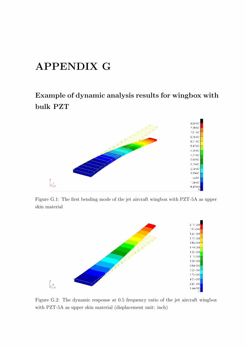
APPENDIX G
Example of dynamic analysis results for wingbox with
bulk PZT
Figure G.1: The first bending mode of the jet aircraft wingbox with PZT-5A as upper
skin material
Figure G.2: The dynamic response at 0.5 frequency ratio of the jet aircraft wingbox
with PZT-5A as upper skin material (displacement unit: inch)
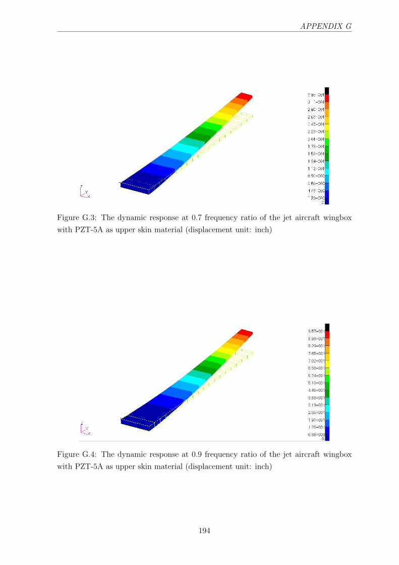
APPENDIX G
Figure G.3: The dynamic response at 0.7 frequency ratio of the jet aircraft wingbox
with PZT-5A as upper skin material (displacement unit: inch)
Figure G.4: The dynamic response at 0.9 frequency ratio of the jet aircraft wingbox
with PZT-5A as upper skin material (displacement unit: inch)
194

APPENDIX H
Example of dynamic analysis results for wingbox with
multiphase composite
Figure H.1: The dynamic response at 0.9 frequency ratio of the jet aircraft wingbox
with multiphase composite at Vf 50% and AR 0.2 (displacement unit: inch)
Figure H.2: The dynamic response at 0.9 frequency ratio of the jet aircraft wingbox
with multiphase composite at Vf 50% and AR 0.6 (displacement unit: inch)

APPENDIX H
Figure H.3: The dynamic response at 0.9 frequency ratio of the jet aircraft wingbox
with multiphase composite at Vf 60% and AR 0.2 (displacement unit: inch)
Figure H.4: The dynamic response at 0.9 frequency ratio of the jet aircraft wingbox
with multiphase composite at Vf 70% and AR 0.2 (displacement unit: inch)
196

APPENDIX I
Example of flutter analysis results
Figure I.1: The flutter response of Xiang et al. UAV wingbox associated with the third
bending eigenvector at airspeed 150 m/s and frequency 174 Hz
Figure I.2: The flutter response of Xiang et al. UAV wingbox associated with the first
torsion eigenvector at airspeed 150 m/s and frequency 207 Hz

APPENDIX I
Figure I.3: The flutter response of Xiang et al. UAV wingbox associated with the
fourth bending eigenvector at airspeed 150 m/s and frequency 336 Hz
Figure I.4: The flutter response of Xiang et al. UAV wingbox associated with the
mixed eigenvector (bending and torsion modes already coalesced) at airspeed 210 m/s
and frequency 90 Hz
198
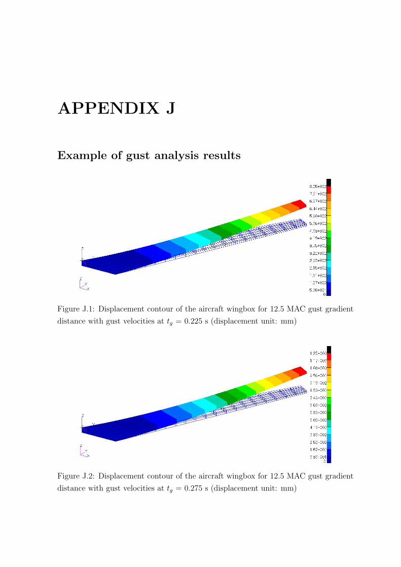
APPENDIX J
Example of gust analysis results
Figure J.1: Displacement contour of the aircraft wingbox for 12.5 MAC gust gradient
distance with gust velocities at tg = 0.225 s (displacement unit: mm)
Figure J.2: Displacement contour of the aircraft wingbox for 12.5 MAC gust gradient
distance with gust velocities at tg = 0.275 s (displacement unit: mm)

APPENDIX J
Figure J.3: Displacement contour of the aircraft wingbox for 12.5 MAC gust gradient
distance with gust velocities at tg = 0.325 s (displacement unit: mm)
Figure J.4: Displacement contour of the aircraft wingbox for 12.5 MAC gust gradient
distance with gust velocities at tg = 0.375 s (displacement unit: mm)
Figure J.5: Displacement contour of the aircraft wingbox for 12.5 MAC gust gradient
distance with gust velocities at tg = 0525 s (displacement unit: mm)
200

APPENDIX J
Figure J.6: Displacement contour of the aircraft wingbox for 12.5 MAC gust gradient
distance with gust velocities at tg = 0.225 s (displacement unit: mm)
Figure J.7: Displacement contour of the aircraft wingbox for 12.5 MAC gust gradient
distance with gust velocities at tg = 1.275 s (displacement unit: mm)
Figure J.8: Displacement contour of the aircraft wingbox for 12.5 MAC gust gradient
distance with gust velocities at tg = 1.475 s (displacement unit: mm)
201

APPENDIX K
Example of NASTRAN input for gust analysis with
voltage load
The following pages show the NASTRAN input for gust analysis with additional voltage
load. The main input for the unsteady aerodynamic/ gust analysis and voltage load are
depicted. However, for displaying purpose only in this appendix, the FEM structural
input has been shortened.

SAWEswept_ptz5a_sol146_H43_vel_4SOL 146CEND$ Direct Text Input for Global Case Control DataTITLE = WINGBOX_GUSTSUBTI = CANTILEVERED, DOUBLET-LATTICE AERODYNAMICSLABEL = 1-COSINE GUSTECHO = BOTHLOADSET = 1SPC = 1 $ FUSELAGE CONSTRAINTSDAMP = 2000 $ STRUCTURAL DAMPINGMETHOD= 1 $ LANCZOS METHODSVEC = NONE $ PRINT VIBRATION MODESGUST = 1000 $ AERODYNAMIC LOADING (1-COS GUST)DLOAD = 999 $ COMBINED LOADFREQ = 40 $ FREQUENCY LISTTSTEP = 41 $ SOLUTION TIME STEPSSET 999 = 1 THRU 10MODESELECT = 999OUTPUTSET 1 = 1 THRU 104VELOCITY = 1 $ VELOCITY RESPONSE FOR GRID IN SET 1$ DISP = ALL $ PRINT GUST RESPONSEBEGIN BULK$ Direct Text Input for Bulk DataTEMPD 4 0PARAM GRDPNT 0PARAM POST 1PARAM PRTMAXIM YES$ * * STRUCTURAL DAMPING * * $$ $$ THE PARAMETER KDAMP DETERMINES THE MANNER OF INCLUSION $$ OF STRUCTURAL DAMPING IN EQUATIONS OF MOTION (SEE HANDBOOK $$ FOR DYNAMIC ANALYSIS, SECT. 3.2.2). IF SET TO -1, MODAL $$ DAMPING IS PUT INTO COMPLEX STIFFNESS MATRIX AS STRUCTURAL $$ DAMPING. $$ $$ N V1 V2PARAM KDAMP +1$ $$ THE TABDMP1 ENTRY DEFINES MODAL DAMPING AS A TABULAR $$ FUNCTION OF FREQUENCY. THE DAMPING LEVELS ARE LINEAR $$ BETWEEN THE FREQUENCY AND DAMPING PAIRS AND ARE EXTRAP- $$ OLATED OUTSIDE THE TABULATED FREQUENCY RANGE. $$ $$ ID +TDPTABDMP1 2000 +T2000$ F1 G1 F2 G2 ETC ENDT+T2000 0.0 0.02 1000. 0.02 ENDT$ $$ $$ * * * AERODYNAMIC DATA * * * $$ $$ (SNAIL-IN-SEC SYSTEM) $$ $$ * * ELEMENT GEOMETRY * * $$ $$ THE AERO ENTRY SPECIFIES THE AERO COORDINATE SYSTEM, THE $$ VELOCITY (USED FOR DATA RECOVERY), THE REFERENCE CHORD $$ AND FLUID DENSITY, PLUS SYMMETRY KEYS. SYMXZ=1 INDICATES $$ THAT THE MODEL IS MOUNTED WITH A ROOT REFLECTION PLANE; $$ SYMXY = 0 INDICATES THAT THE MODEL IS MOUNTED FAR ENOUGH $$ FROM THE FLOOR SO THAT REFLECTION EFFECTS ARE NEGLIGIBLE. $$$234567 1234567 1234567 1234567 1234567 1234567 1234567 $ ACSID VELOCITY REFC RHOREF SYMXZ SYMXYAERO 0 240000. 3500. .4615E-9 1$ THE CAERO1 ENTRY IS USED FOR DOUBLET-LATTICE AERODYNAMICS. $$ LISTED ARE ITS PAERO ENTRY ID AND THE COORDINATE SYSTEM $$ FOR LOCATING THE INBOARD AND OUTBOARD LEADING EDGE POINTS $$ (1 AND 4). NSPAN AND NCHORD, OR LSPAN AND LCHORD, ARE $$ USED TO PARTITION THE WING INTO AERODYNAMIC BOXES, THE $$ FORMER FOR UNIFORMLY SPACED BOXES AND THE LATTER FOR $$ NON-UNIFORMLY SPACED BOXES. IGID IS THE ID OF ITS $$ ASSOCIATED INTERFERENCE GROUP. THE CONTINUATION ENTRY $$ DEFINES POINTS 1 AND 2, THE ROOT CHORD AND THE TIP CHORD. $$ THE BOXES FORMED BY THE GRID LINES WILL BE NUMBERED $$ BEGINNING WITH EID, SO A NUMBER SHOULD BE CHOSEN THAT IS $$ UNIQUE, AND IS GREATER THAN ALL STRUCTURAL GRID, SCALAR $$ AND EXTRA POINT IDS. $$$234567 1234567 1234567 1234567 1234567 1234567 1234567 1234567 1234567 $$ EID PID CP NSPAN NCHORD LSPAN LCHORD IGID CAERO1 3001 1000 0 40 8 1 +CC1$234567 1234567 1234567 1234567 1234567 1234567 1234567 1234567 1234567$ (FWD INBOARD POINT) ROOTCHORD (FWD OUTBOARD POINT) TIP CHORD
Page 1
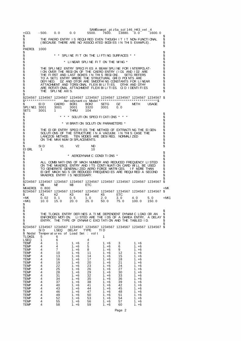
SAWEswept_ptz5a_sol146_H43_vel_4+CC1 -500. 0.0 0.0 5500. 7600. 13880. 0.0 1600.0$ $$ THE PAERO ENTRY IS REQUIRED EVEN THOUGH IT IT NON-FUNCTIONAL $$ (BECAUSE THERE ARE NO ASSOCIATED BODIES IN THIS EXAMPLE). $$ $PAERO1 1000$ $$ * * SPLINE FIT ON THE LIFTING SURFACES * * $$ $$ * LINEAR SPLINE FIT ON THE WING * $$ $$ THE SPLINE2 ENTRY SPECIFIES A BEAM SPLINE FOR INTERPOLAT- $$ ION OVER THE REGION OF THE CAERO ENTRY (ID1 AND ID2 ARE $$ THE FIRST AND LAST BOXES IN THIS REGION). SETG REFERS $$ TO A SET1 ENTRY WHERE THE STRUCTURAL GRID POINTS ARE $$ DEFINED. DZ AND DTOR ARE SMOOTHING CONSTANTS FOR LINEAR $$ ATTACHMENT AND TORSIONAL FLEXIBILITIES. DTHX AND DTHY $$ ARE ROTATIONAL ATTACHMENT FLEXIBILITIES. CID IDENTIFIES $$ THE SPLINE AXIS. $$$234567 1234567 1234567 1234567 1234567 1234567 1234567 1234567 1234567 $$**************** Aerodynamics Model******************************$$ EID CAERO BOX1 BOX2 SETG DZ METH USAGESPLINE1 3001 3001 3001 3320 3001 0.0 SET1 3001 1 THRU 104$ $$ * * * SOLUTION SPECIFICATIONS * * * $$ $$ * VIBRATION SOLUTION PARAMETERS * $$ $$ THE EIGR ENTRY SPECIFIES THE METHOD OF EXTRACTING THE EIGEN- $$ SOLUTIONS OF THE STRUCTURE IN A VACUUM, IN THIS CASE THE $$ LANCZOS METHOD. TEN MODES ARE DESIRED, NORMALIZED $$ ON THE MAXIMUM DISPLACEMENTS. $$ $$ SID V1 V2 ND $EIGRL 1 10$ $$ * AERODYNAMIC CONDITIONS * $$ $$ ALL COMBINATIONS OF MACH NUMBER AND REDUCED FREQUENCY LISTED $$ ON THE MKAERO1 ENTRY AND ITS CONTINUATION CARD WILL BE USED $$ TO GENERATE GENERALIZED AERO FORCE MATRICES. IF MORE THAN $$ EIGHT MACH NO.S OR REDUCED FREQUENCIES ARE REQUIRED A SECOND $$ MKAERO1 ENTRY IS NECESSARY. $$ $$234567 1234567 1234567 1234567 1234567 1234567 1234567 1234567 1234567 $$ M1 M2 M3 ETCMKAERO1 0.800 +MK$234567 1234567 1234567 1234567 1234567 1234567 1234567 1234567 1234567 $$ K1 K2 K3 K4 K5 ETC
+MK 0.02 0.1 0.5 1.0 2.0 3.0 4.0 5.0 +MK1+MK1 10.0 15.0 20.0 25.0 50.0 75.0 100.0 150.0$$$ $$ THE TLOAD1 ENTRY DEFINES A TIME DEPENDENT DYNAMIC LOAD OR AN $$ ENFORCED MOTION. LISTED ARE THE IDS OF A DAREA ENTRY, A DELAY $$ ENTRY, THE TYPE OF DYNAMIC EXCITATION AND THE TABLED ID. $$ $$234567 1234567 1234567 1234567 1234567 1234567 1234567 1234567 1234567 $$ SID LSEQ DELAY TYPE TID$ Nodal Temperatures of Load Set : voltTLOAD1 5 6 1LSEQ 1 6 4TEMP 4 1 1.+6 2 1.+6 3 1.+6TEMP 4 4 1.+6 5 1.+6 6 1.+6TEMP 4 7 1.+6 8 1.+6 9 1.+6TEMP 4 10 1.+6 11 1.+6 12 1.+6TEMP 4 13 1.+6 14 1.+6 15 1.+6TEMP 4 16 1.+6 17 1.+6 18 1.+6TEMP 4 19 1.+6 20 1.+6 21 1.+6TEMP 4 22 1.+6 23 1.+6 24 1.+6TEMP 4 25 1.+6 26 1.+6 27 1.+6TEMP 4 28 1.+6 29 1.+6 30 1.+6TEMP 4 31 1.+6 32 1.+6 33 1.+6TEMP 4 34 1.+6 35 1.+6 36 1.+6TEMP 4 37 1.+6 38 1.+6 39 1.+6TEMP 4 40 1.+6 41 1.+6 42 1.+6TEMP 4 43 1.+6 44 1.+6 45 1.+6TEMP 4 46 1.+6 47 1.+6 48 1.+6TEMP 4 49 1.+6 50 1.+6 51 1.+6TEMP 4 52 1.+6 53 1.+6 54 1.+6TEMP 4 55 1.+6 56 1.+6 57 1.+6TEMP 4 58 1.+6 59 1.+6 60 1.+6
Page 2

SAWEswept_ptz5a_sol146_H43_vel_4TEMP 4 61 1.+6 62 1.+6 63 1.+6TEMP 4 64 1.+6 65 1.+6 66 1.+6TEMP 4 67 1.+6 68 1.+6 69 1.+6TEMP 4 70 1.+6 71 1.+6 72 1.+6TEMP 4 73 1.+6 74 1.+6 75 1.+6TEMP 4 76 1.+6 77 1.+6 78 1.+6TEMP 4 79 1.+6 80 1.+6 81 1.+6TEMP 4 82 1.+6 83 1.+6 84 1.+6TEMP 4 85 1.+6 86 1.+6 87 1.+6TEMP 4 88 1.+6 89 1.+6 90 1.+6TEMP 4 91 1.+6 92 1.+6 93 1.+6TEMP 4 94 1.+6 95 1.+6 96 1.+6TEMP 4 97 1.+6 98 1.+6 99 1.+6TEMP 4 100 1.+6 101 1.+6 102 1.+6TEMP 4 103 1.+6 104 1.+6 $ $INCLUDE 'tVolt4h43.dat'$$$* * * * * * * * * * * * * * * * * * * * * * * * * * * * * * * * * * * * * * *$$ * * DYNAMIC LOAD AND RESPONSE DATA * *$$ GUST DEFINES A STATIONARY VERTICAL GUST. LISTED ARE T/RLOAD ENTRY$ ID, GUST ANGLE OF ATTACK (I.E., THE RATIO OF GUST VELOCITY TO THE$ VEHICLE VELOCITY), LOCATION OF THE GUST WITH RESPECT TO THE ORIGIN$ OF THE AERO COORDINATE SYSTEM, AND THE VEHICLE VELOCITY.$234567 1234567 1234567 1234567 1234567 1234567 1234567 1234567 1234567 $$ SID DLOAD WG X0 VGUST 1000 1001 .0625 0. 240000.$$ TLOAD1 DEFINES A TIME DEPENDENT DYNAMIC LOAD OR ENFORCED MOTION.$ LISTED ARE THE ID, DAREA ID, DELAY ID, TYPE OF DYNAMIC EXCITATION,$ AND TABELDi ID.$$ SID DAREA DELAY TYPE TIDTLOAD1 1001 1002 1003$$ DAREA DEFINES THE DOF WHERE THE LOAD IS APPLIED AND A SCALE FACTOR.$ NOTE: THIS IS JUST DUMMY CARD REQUIRED BY TLOAD CARD BUT$ NOT AFFECTING THE ACTUAL LOAD$$ SID P C ADAREA 1002 11 1 0.$$ TABLED1 DEFINES A TABULAR FUNCTION OF A TIME-DEPENDENT LOAD.$$ SIDTABLED1 1003 +TAB1$ X1 Y1 X2 Y2 X3 Y3 X4 Y4+TAB1 0. 0. 0.03646 .09549 0.07292 .34549 0.10938 .65451 +TAB2$ X5 Y5 Xn... Yn... +TAB2 0.14584 .90451 0.1823 1. 0.21876 .90451 0.25522 .65451 +TAB3$ X9 Y9 Xn... Yn... +TAB3 0.29168 .34549 0.32814 .09549 0.3646 0. ENDT $234567 1234567 1234567 1234567 1234567 1234567 1234567 1234567 1234567 $$ PARAM,GUSTAERO,-1 IS REQUIRED IF GUST LOADS ARE TO BE COMPUTED.$PARAM GUSTAERO -1$$ PARAM,MACH SPECIFIES MACH NUMBER.$PARAM MACH 0.800$$ PARAM,Q SPECIFIES DYNAMIC PRESSURE.$PARAM Q 13.291$$ PARAM,LMODES,N SPECIFIES THAT N MODES ARE TO BE USED IN$ THE GUST ANALYSIS.$PARAM LMODES 10$$ FREQ1 DEFINES THE SET OF FREQUENCIES USED TO OBTAIN$ THE FREQUENCY RESPONSE SOLUTION. LISTED ARE THE STARTING$ FREQUENCY, FREQUENCY INCREMENT AND NUMBER OF INCREMENTS.$$234567 1234567 1234567 1234567 1234567 1234567 1234567 1234567 1234567 $$ SID F1 DF NDFFREQ1 40 0. 0.2 350$$ TSTEP DEFINES TIME STEP INTERVALS AT WHICH THE TRANSIENT$ RESPONSES ARE DESIRED. LISTED ARE THE NUMBER OF STEPS,$ THE TIME INTERVAL AND SKIP FACTOR FOR OUTPUT.$ T = 1/DF
Page 3

SAWEswept_ptz5a_sol146_H43_vel_4$ SID N DT NOTSTEP 41 199 .025 1$$DLOAD 999 1. 1. 5 1. 1001$$ ALL THE STRUCTURAL MODEL FROM FEM IS COPIED BELOW$ Elements and Element Properties for region : skin_upper$ Composite Property Reference Material: piezo_comp$ Composite Material Description :PCOMP 1 2 .01 0. YES 1 6.09 0. YES$ Pset: "skin_upper" will be imported as: "pcomp.1"CQUAD4 1 1 1 2 6 5CQUAD4 2 1 2 3 7 6CQUAD4 3 1 3 4 8 7CTRIA3 4 1 4 9 8CQUAD4 5 1 5 6 11 10CQUAD4 6 1 6 7 12 11CQUAD4 7 1 7 8 13 12CQUAD4 8 1 8 9 14 13CQUAD4 9 1 10 11 16 15CQUAD4 10 1 11 12 17 16CQUAD4 11 1 12 13 18 17CQUAD4 12 1 13 14 19 18CQUAD4 13 1 15 16 21 20CQUAD4 14 1 16 17 22 21CQUAD4 15 1 17 18 23 22CQUAD4 16 1 18 19 24 23CQUAD4 17 1 20 21 26 25CQUAD4 18 1 21 22 27 26CQUAD4 19 1 22 23 28 27CQUAD4 20 1 23 24 29 28CQUAD4 21 1 25 26 31 30CQUAD4 22 1 26 27 32 31CQUAD4 23 1 27 28 33 32CQUAD4 24 1 28 29 34 33CQUAD4 25 1 30 31 36 35CQUAD4 26 1 31 32 37 36CQUAD4 27 1 32 33 38 37CQUAD4 28 1 33 34 39 38CQUAD4 29 1 35 36 41 40CQUAD4 30 1 36 37 42 41CQUAD4 31 1 37 38 43 42CQUAD4 32 1 38 39 44 43CQUAD4 33 1 40 41 46 45CQUAD4 34 1 41 42 47 46CQUAD4 35 1 42 43 48 47CQUAD4 36 1 43 44 49 48CQUAD4 37 1 45 46 51 50CQUAD4 38 1 46 47 52 51CQUAD4 39 1 47 48 53 52CQUAD4 40 1 48 49 54 53CQUAD4 41 1 50 51 56 55CQUAD4 42 1 51 52 57 56CQUAD4 43 1 52 53 58 57CQUAD4 44 1 53 54 59 58CQUAD4 45 1 55 56 61 60CQUAD4 46 1 56 57 62 61CQUAD4 47 1 57 58 63 62CQUAD4 48 1 58 59 64 63CQUAD4 49 1 60 61 66 65CQUAD4 50 1 61 62 67 66CQUAD4 51 1 62 63 68 67CQUAD4 52 1 63 64 69 68CQUAD4 53 1 65 66 71 70CQUAD4 54 1 66 67 72 71CQUAD4 55 1 67 68 73 72CQUAD4 56 1 68 69 74 73CQUAD4 57 1 70 71 76 75CQUAD4 58 1 71 72 77 76CQUAD4 59 1 72 73 78 77CQUAD4 60 1 73 74 79 78CQUAD4 61 1 75 76 81 80CQUAD4 62 1 76 77 82 81CQUAD4 63 1 77 78 83 82CQUAD4 64 1 78 79 84 83CQUAD4 65 1 80 81 86 85CQUAD4 66 1 81 82 87 86CQUAD4 67 1 82 83 88 87CQUAD4 68 1 83 84 89 88CQUAD4 69 1 85 86 91 90CQUAD4 70 1 86 87 92 91CQUAD4 71 1 87 88 93 92CQUAD4 72 1 88 89 94 93
Page 4
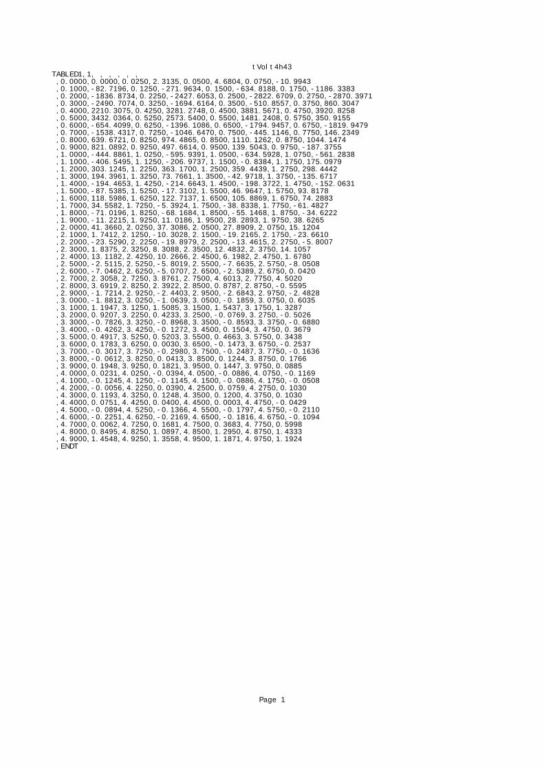
tVolt4h43TABLED1,1, , , , , , ,0.0000,0.0000,0.0250,2.3135,0.0500,4.6804,0.0750,-10.9943 ,0.1000,-82.7196,0.1250,-271.9634,0.1500,-634.8188,0.1750,-1186.3383 ,0.2000,-1836.8734,0.2250,-2427.6053,0.2500,-2822.6709,0.2750,-2870.3971 ,0.3000,-2490.7074,0.3250,-1694.6164,0.3500,-510.8557,0.3750,860.3047 ,0.4000,2210.3075,0.4250,3281.2748,0.4500,3881.5671,0.4750,3920.8258 ,0.5000,3432.0364,0.5250,2573.5400,0.5500,1481.2408,0.5750,350.9155 ,0.6000,-654.4099,0.6250,-1396.1086,0.6500,-1794.9457,0.6750,-1819.9479 ,0.7000,-1538.4317,0.7250,-1046.6470,0.7500,-445.1146,0.7750,146.2349 ,0.8000,639.6721,0.8250,974.4865,0.8500,1110.1262,0.8750,1044.1474 ,0.9000,821.0892,0.9250,497.6614,0.9500,139.5043,0.9750,-187.3755 ,1.0000,-444.8861,1.0250,-595.9391,1.0500,-634.5928,1.0750,-561.2838 ,1.1000,-406.5495,1.1250,-206.9737,1.1500,-0.8384,1.1750,175.0979 ,1.2000,303.1245,1.2250,363.1700,1.2500,359.4439,1.2750,298.4442 ,1.3000,194.3961,1.3250,73.7661,1.3500,-42.9718,1.3750,-135.6717 ,1.4000,-194.4653,1.4250,-214.6643,1.4500,-198.3722,1.4750,-152.0631 ,1.5000,-87.5385,1.5250,-17.3102,1.5500,46.9647,1.5750,93.8178 ,1.6000,118.5986,1.6250,122.7137,1.6500,105.8869,1.6750,74.2883 ,1.7000,34.5582,1.7250,-5.3924,1.7500,-38.8338,1.7750,-61.4827 ,1.8000,-71.0196,1.8250,-68.1684,1.8500,-55.1468,1.8750,-34.6222 ,1.9000,-11.2215,1.9250,11.0186,1.9500,28.2893,1.9750,38.6265 ,2.0000,41.3660,2.0250,37.3086,2.0500,27.8909,2.0750,15.1204 ,2.1000,1.7412,2.1250,-10.3028,2.1500,-19.2165,2.1750,-23.6610 ,2.2000,-23.5290,2.2250,-19.8979,2.2500,-13.4615,2.2750,-5.8007 ,2.3000,1.8375,2.3250,8.3088,2.3500,12.4832,2.3750,14.1057 ,2.4000,13.1182,2.4250,10.2666,2.4500,6.1982,2.4750,1.6780 ,2.5000,-2.5115,2.5250,-5.8019,2.5500,-7.6635,2.5750,-8.0508 ,2.6000,-7.0462,2.6250,-5.0707,2.6500,-2.5389,2.6750,0.0420 ,2.7000,2.3058,2.7250,3.8761,2.7500,4.6013,2.7750,4.5020 ,2.8000,3.6919,2.8250,2.3922,2.8500,0.8787,2.8750,-0.5595 ,2.9000,-1.7214,2.9250,-2.4403,2.9500,-2.6843,2.9750,-2.4828 ,3.0000,-1.8812,3.0250,-1.0639,3.0500,-0.1859,3.0750,0.6035 ,3.1000,1.1947,3.1250,1.5085,3.1500,1.5437,3.1750,1.3287 ,3.2000,0.9207,3.2250,0.4233,3.2500,-0.0769,3.2750,-0.5026 ,3.3000,-0.7826,3.3250,-0.8968,3.3500,-0.8593,3.3750,-0.6880 ,3.4000,-0.4262,3.4250,-0.1272,3.4500,0.1504,3.4750,0.3679 ,3.5000,0.4917,3.5250,0.5203,3.5500,0.4663,3.5750,0.3438 ,3.6000,0.1783,3.6250,0.0030,3.6500,-0.1473,3.6750,-0.2537 ,3.7000,-0.3017,3.7250,-0.2980,3.7500,-0.2487,3.7750,-0.1636 ,3.8000,-0.0612,3.8250,0.0413,3.8500,0.1244,3.8750,0.1766 ,3.9000,0.1948,3.9250,0.1821,3.9500,0.1447,3.9750,0.0885 ,4.0000,0.0231,4.0250,-0.0394,4.0500,-0.0886,4.0750,-0.1169 ,4.1000,-0.1245,4.1250,-0.1145,4.1500,-0.0886,4.1750,-0.0508 ,4.2000,-0.0056,4.2250,0.0390,4.2500,0.0759,4.2750,0.1030 ,4.3000,0.1193,4.3250,0.1248,4.3500,0.1200,4.3750,0.1030 ,4.4000,0.0751,4.4250,0.0400,4.4500,0.0003,4.4750,-0.0429 ,4.5000,-0.0894,4.5250,-0.1366,4.5500,-0.1797,4.5750,-0.2110 ,4.6000,-0.2251,4.6250,-0.2169,4.6500,-0.1816,4.6750,-0.1094 ,4.7000,0.0062,4.7250,0.1681,4.7500,0.3683,4.7750,0.5998 ,4.8000,0.8495,4.8250,1.0897,4.8500,1.2950,4.8750,1.4333 ,4.9000,1.4548,4.9250,1.3558,4.9500,1.1871,4.9750,1.1924 ,ENDT
Page 1
APPENDIX L
Example of NASTRAN output for gust analysis with
voltage load
The following pages show the NASTRAN output for gust analysis with additional
voltage load. The output defines voltage responses for a node (point) at 6-DoF (3
translations and 3 rotations) within a time range. This output used as input in the
MATLAB code for the iterative FEM. However, for displaying purpose only in this
appendix, the data has been shortened.

saweswept_ptz5a_sol146_h43_vel_41 TESTPLATE_FLUTTER JULY 8, 2018 MSC Nastran 11/13/14 PAE 76 CANTILEVERED, DOUBLET-LATTICE AERODYNAMICS AT MACH NO. 0.0 0 1-COSINE UST POINT-ID = 1 V E L O C I T Y V E C T O R TIME T1 T2 T3 R1 R2 R3 0.0 0.0 0.0 0.0 0.0 0.0 0.0 2.500000E-02 0.0 0.0 0.0 0.0 0.0 0.0 5.000000E-02 0.0 0.0 0.0 0.0 0.0 0.0 7.500000E-02 0.0 0.0 0.0 0.0 0.0 0.0 1.000000E-01 0.0 0.0 0.0 0.0 0.0 0.0 1.250000E-01 0.0 0.0 0.0 0.0 0.0 0.0 1.500000E-01 0.0 0.0 0.0 0.0 0.0 0.0 1.750000E-01 0.0 0.0 0.0 0.0 0.0 0.0 2.000000E-01 0.0 0.0 0.0 0.0 0.0 0.0 2.250000E-01 0.0 0.0 0.0 0.0 0.0 0.0 2.500000E-01 0.0 0.0 0.0 0.0 0.0 0.0 2.750000E-01 0.0 0.0 0.0 0.0 0.0 0.0 3.000000E-01 0.0 0.0 0.0 0.0 0.0 0.0 3.250000E-01 0.0 0.0 0.0 0.0 0.0 0.0 3.500000E-01 0.0 0.0 0.0 0.0 0.0 0.0 3.750000E-01 0.0 0.0 0.0 0.0 0.0 0.0 4.000000E-01 0.0 0.0 0.0 0.0 0.0 0.0 4.250000E-01 0.0 0.0 0.0 0.0 0.0 0.0 4.500000E-01 0.0 0.0 0.0 0.0 0.0 0.0 4.750000E-01 0.0 0.0 0.0 0.0 0.0 0.0 5.000000E-01 0.0 0.0 0.0 0.0 0.0 0.0 5.250000E-01 0.0 0.0 0.0 0.0 0.0 0.0 5.500000E-01 0.0 0.0 0.0 0.0 0.0 0.0 5.750000E-01 0.0 0.0 0.0 0.0 0.0 0.0 6.000000E-01 0.0 0.0 0.0 0.0 0.0 0.0 6.250000E-01 0.0 0.0 0.0 0.0 0.0 0.0 6.500000E-01 0.0 0.0 0.0 0.0 0.0 0.0 6.750000E-01 0.0 0.0 0.0 0.0 0.0 0.0 7.000000E-01 0.0 0.0 0.0 0.0 0.0 0.0 7.250000E-01 0.0 0.0 0.0 0.0 0.0 0.0 7.500000E-01 0.0 0.0 0.0 0.0 0.0 0.0 7.750000E-01 0.0 0.0 0.0 0.0 0.0 0.0 8.000000E-01 0.0 0.0 0.0 0.0 0.0 0.0 8.250000E-01 0.0 0.0 0.0 0.0 0.0 0.0 8.500000E-01 0.0 0.0 0.0 0.0 0.0 0.0 8.750000E-01 0.0 0.0 0.0 0.0 0.0 0.0 9.000000E-01 0.0 0.0 0.0 0.0 0.0 0.0
Page 1

saweswept_ptz5a_sol146_h43_vel_4 9.250000E-01 0.0 0.0 0.0 0.0 0.0 0.0 9.500000E-01 0.0 0.0 0.0 0.0 0.0 0.0 9.750000E-01 0.0 0.0 0.0 0.0 0.0 0.0 1.000000E+00 0.0 0.0 0.0 0.0 0.0 0.0 1.025000E+00 0.0 0.0 0.0 0.0 0.0 0.0 1.050000E+00 0.0 0.0 0.0 0.0 0.0 0.0 1.075000E+00 0.0 0.0 0.0 0.0 0.0 0.0 1.100000E+00 0.0 0.0 0.0 0.0 0.0 0.0 1.125000E+00 0.0 0.0 0.0 0.0 0.0 0.0 1.150000E+00 0.0 0.0 0.0 0.0 0.0 0.0 1.175000E+00 0.0 0.0 0.0 0.0 0.0 0.0 1.200000E+00 0.0 0.0 0.0 0.0 0.0 0.0 1.225000E+00 0.0 0.0 0.0 0.0 0.0 0.01 TESTPLATE_FLUTTER JULY 8, 2018 MSC Nastran 11/13/14 PAE 77 CANTILEVERED, DOUBLET-LATTICE AERODYNAMICS AT MACH NO. 0.0 0 1-COSINE UST POINT-ID = 1 V E L O C I T Y V E C T O R TIME T1 T2 T3 R1 R2 R3 1.250000E+00 0.0 0.0 0.0 0.0 0.0 0.0 1.275000E+00 0.0 0.0 0.0 0.0 0.0 0.0 1.300000E+00 0.0 0.0 0.0 0.0 0.0 0.0 1.325000E+00 0.0 0.0 0.0 0.0 0.0 0.0 1.350000E+00 0.0 0.0 0.0 0.0 0.0 0.0 1.375000E+00 0.0 0.0 0.0 0.0 0.0 0.0 1.400000E+00 0.0 0.0 0.0 0.0 0.0 0.0 1.425000E+00 0.0 0.0 0.0 0.0 0.0 0.0 1.450000E+00 0.0 0.0 0.0 0.0 0.0 0.0 1.475000E+00 0.0 0.0 0.0 0.0 0.0 0.0 1.500000E+00 0.0 0.0 0.0 0.0 0.0 0.0 1.525000E+00 0.0 0.0 0.0 0.0 0.0 0.0 1.550000E+00 0.0 0.0 0.0 0.0 0.0 0.0 1.575000E+00 0.0 0.0 0.0 0.0 0.0 0.0 1.600000E+00 0.0 0.0 0.0 0.0 0.0 0.0 1.625000E+00 0.0 0.0 0.0 0.0 0.0 0.0 1.650000E+00 0.0 0.0 0.0 0.0 0.0 0.0 1.675000E+00 0.0 0.0 0.0 0.0 0.0 0.0 1.700000E+00 0.0 0.0 0.0 0.0 0.0 0.0 1.725000E+00 0.0 0.0 0.0 0.0 0.0 0.0 1.750000E+00 0.0 0.0 0.0 0.0 0.0 0.0 1.775000E+00 0.0 0.0 0.0 0.0 0.0 0.0 1.800000E+00 0.0 0.0 0.0 0.0 0.0 0.0 1.825000E+00 0.0 0.0 0.0 0.0 0.0 0.0
Page 2

saweswept_ptz5a_sol146_h43_vel_4Nastran 11/13/14 PAE 125 CANTILEVERED, DOUBLET-LATTICE AERODYNAMICS AT MACH NO. 0.0 0 1-COSINE UST POINT-ID = 13 V E L O C I T Y V E C T O R TIME T1 T2 T3 R1 R2 R3 1.250000E+00 3.018021E-01 8.914543E-01 -2.888492E+00 -4.913677E-03 1.665195E-03 -3.359958E-04 1.275000E+00 8.877153E-02 1.155595E-01 -3.545005E-01 -6.718423E-04 3.785901E-04 -4.561735E-05 1.300000E+00 -1.223534E-01 -5.788389E-01 1.938026E+00 3.169167E-03 -8.158363E-04 2.209204E-04 1.325000E+00 -3.025409E-01 -1.131719E+00 3.854096E+00 6.320012E-03 -1.795745E-03 4.247121E-04 1.350000E+00 -4.113624E-01 -1.454886E+00 5.006360E+00 8.194306E-03 -2.394885E-03 5.341288E-04 1.375000E+00 -4.284621E-01 -1.484951E+00 5.109393E+00 8.370501E-03 -2.498593E-03 5.335273E-04 1.400000E+00 -3.661546E-01 -1.236316E+00 4.210274E+00 6.939012E-03 -2.125072E-03 4.434834E-04 1.425000E+00 -2.573636E-01 -8.056436E-01 2.659308E+00 4.471546E-03 -1.442272E-03 3.054965E-04 1.450000E+00 -1.271670E-01 -3.292407E-01 1.021461E+00 1.795806E-03 -6.579097E-04 1.370932E-04 1.475000E+00 3.215468E-03 1.091150E-01 -4.269446E-01 -6.288690E-04 8.245922E-05 -3.444303E-05 1.500000E+00 1.174433E-01 4.692566E-01 -1.578425E+00 -2.597314E-03 7.102106E-04 -1.840826E-04 1.525000E+00 1.994102E-01 7.328935E-01 -2.463925E+00 -4.069112E-03 1.179349E-03 -2.777597E-04 1.550000E+00 2.412568E-01 8.608315E-01 -2.942354E+00 -4.826362E-03 1.425715E-03 -3.105939E-04 1.575000E+00 2.404300E-01 8.230457E-01 -2.843774E+00 -4.653131E-03 1.398350E-03 -2.932292E-04 1.600000E+00 1.977613E-01 6.371763E-01 -2.182087E+00 -3.600478E-03 1.113966E-03 -2.348866E-04 1.625000E+00 1.237009E-01 3.673314E-01 -1.197876E+00 -2.033526E-03 6.730634E-04 -1.438171E-04 1.650000E+00 3.921142E-02 8.971892E-02 -2.335192E-01 -4.508116E-04 2.052376E-04 -3.498167E-05 1.675000E+00 -3.395760E-02 -1.547981E-01 5.601961E-01 8.880699E-04 -2.091430E-04 6.060499E-05 1.700000E+00 -8.644745E-02 -3.431142E-01 1.146403E+00 1.887968E-03 -5.307549E-04 1.269509E-04 1.725000E+00 -1.218678E-01 -4.616550E-01 1.542002E+00 2.544439E-03 -7.461493E-04 1.646513E-04 1.750000E+00 -1.411848E-01 -4.944018E-01 1.689832E+00 2.776473E-03 -8.286189E-04 1.798798E-04 1.775000E+00 -1.368041E-01 -4.390366E-01 1.524904E+00 2.505644E-03 -7.608862E-04 1.677081E-04 1.800000E+00 -1.032517E-01 -3.168100E-01 1.087741E+00 1.800223E-03 -5.634433E-04 1.210885E-04 1.825000E+00 -5.108851E-02 -1.580824E-01 5.005932E-01 8.537362E-04 -2.927354E-04 5.400764E-05 1.850000E+00 -1.452706E-03 2.521327E-03 -5.727227E-02 -6.198284E-05 -2.102941E-05 -8.695444E-06 1.875000E+00 3.296999E-02 1.406697E-01 -4.940124E-01 -7.923287E-04 2.058966E-04 -5.003075E-05 1.900000E+00 5.574218E-02 2.361913E-01 -7.802777E-01 -1.281118E-03 3.670648E-04 -7.663096E-05 1.925000E+00 7.399895E-02 2.796990E-01 -9.300632E-01 -1.537032E-03 4.562878E-04 -9.791497E-05 1.950000E+00 8.423702E-02 2.736187E-01 -9.424017E-01 -1.555310E-03 4.686965E-04 -1.082069E-04 1.975000E+00 7.626593E-02 2.272394E-01 -7.981332E-01 -1.315526E-03 4.026972E-04 -9.404814E-05 2.000000E+00 4.906438E-02 1.529777E-01 -5.211948E-01 -8.624854E-04 2.739423E-04 -5.493709E-05 2.025000E+00 1.582801E-02 6.095287E-02 -1.750975E-01 -3.023870E-04 1.129281E-04 -1.145806E-05 2.050000E+00 -9.048259E-03 -3.285731E-02 1.416910E-01 2.152304E-04 -4.193599E-05 1.783951E-05 2.075000E+00 -2.353648E-02 -1.096115E-01 3.712469E-01 5.986382E-04 -1.636158E-04 3.255460E-05 2.100000E+00 -3.490832E-02 -1.538016E-01 5.013138E-01 8.236037E-04 -2.401674E-04 4.545476E-05 2.125000E+00 -4.587012E-02 -1.629479E-01 5.458346E-01 9.038811E-04 -2.704811E-04 6.013416E-05 2.150000E+00 -4.978830E-02 -1.468430E-01 5.155519E-01 8.530853E-04 -2.583958E-04 6.477133E-05 2.175000E+00 -4.008333E-02 -1.147921E-01 4.058519E-01 6.703204E-04 -2.072791E-04
Page 65
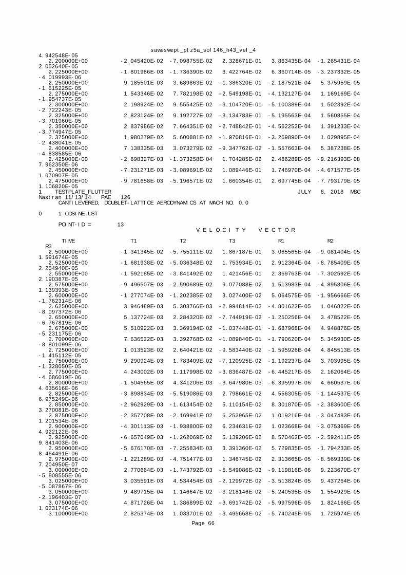
saweswept_ptz5a_sol146_h43_vel_44.942548E-05 2.200000E+00 -2.045420E-02 -7.098755E-02 2.328671E-01 3.863435E-04 -1.265431E-04 2.052640E-05 2.225000E+00 -1.801986E-03 -1.736390E-02 3.422764E-02 6.360714E-05 -3.237332E-05 -4.019993E-06 2.250000E+00 9.185501E-03 3.689863E-02 -1.386320E-01 -2.187521E-04 5.375959E-05 -1.515225E-05 2.275000E+00 1.543346E-02 7.782198E-02 -2.549198E-01 -4.132127E-04 1.169169E-04 -1.954737E-05 2.300000E+00 2.198924E-02 9.555425E-02 -3.104720E-01 -5.100389E-04 1.502392E-04 -2.722243E-05 2.325000E+00 2.823124E-02 9.192727E-02 -3.134783E-01 -5.195563E-04 1.560855E-04 -3.701960E-05 2.350000E+00 2.837986E-02 7.664351E-02 -2.748842E-01 -4.562252E-04 1.391233E-04 -3.774947E-05 2.375000E+00 1.980279E-02 5.600881E-02 -1.970816E-01 -3.269890E-04 1.029895E-04 -2.438041E-05 2.400000E+00 7.138335E-03 3.073279E-02 -9.347762E-02 -1.557663E-04 5.387238E-05 -4.838585E-06 2.425000E+00 -2.698327E-03 -1.373258E-04 1.704285E-02 2.486289E-05 -9.216393E-08 7.962350E-06 2.450000E+00 -7.231271E-03 -3.089691E-02 1.089446E-01 1.746970E-04 -4.671577E-05 1.070907E-05 2.475000E+00 -9.781658E-03 -5.196571E-02 1.660354E-01 2.697745E-04 -7.793179E-05 1.106820E-051 TESTPLATE_FLUTTER JULY 8, 2018 MSC Nastran 11/13/14 PAE 126 CANTILEVERED, DOUBLET-LATTICE AERODYNAMICS AT MACH NO. 0.0 0 1-COSINE UST POINT-ID = 13 V E L O C I T Y V E C T O R TIME T1 T2 T3 R1 R2 R3 2.500000E+00 -1.341345E-02 -5.755111E-02 1.867187E-01 3.065565E-04 -9.081404E-05 1.591674E-05 2.525000E+00 -1.681938E-02 -5.036348E-02 1.753934E-01 2.912364E-04 -8.785409E-05 2.254940E-05 2.550000E+00 -1.592185E-02 -3.841492E-02 1.421456E-01 2.369763E-04 -7.302592E-05 2.190387E-05 2.575000E+00 -9.496507E-03 -2.590689E-02 9.077088E-02 1.513983E-04 -4.895806E-05 1.139393E-05 2.600000E+00 -1.277074E-03 -1.202385E-02 3.027400E-02 5.064575E-05 -1.956666E-05 -1.762314E-06 2.625000E+00 3.946489E-03 5.303766E-03 -2.994814E-02 -4.801622E-05 1.046822E-05 -8.097372E-06 2.650000E+00 5.137724E-03 2.284320E-02 -7.744919E-02 -1.250256E-04 3.478522E-05 -6.767819E-06 2.675000E+00 5.510922E-03 3.369194E-02 -1.037448E-01 -1.687968E-04 4.948876E-05 -5.231175E-06 2.700000E+00 7.636522E-03 3.392768E-02 -1.089840E-01 -1.790620E-04 5.345930E-05 -8.801099E-06 2.725000E+00 1.013523E-02 2.640421E-02 -9.583440E-02 -1.595926E-04 4.845513E-05 -1.415112E-05 2.750000E+00 9.290924E-03 1.783409E-02 -7.120925E-02 -1.192237E-04 3.703995E-05 -1.328050E-05 2.775000E+00 4.243002E-03 1.117998E-02 -3.836487E-02 -6.445217E-05 2.162064E-05 -4.686019E-06 2.800000E+00 -1.504565E-03 4.341206E-03 -3.647980E-03 -6.395997E-06 4.660537E-06 4.635616E-06 2.825000E+00 -3.898834E-03 -5.519086E-03 2.798661E-02 4.556305E-05 -1.144537E-05 6.975249E-06 2.850000E+00 -2.962929E-03 -1.613454E-02 5.110154E-02 8.301870E-05 -2.383600E-05 3.270081E-06 2.875000E+00 -2.357708E-03 -2.169941E-02 6.253965E-02 1.019216E-04 -3.047483E-05 1.201534E-06 2.900000E+00 -4.301113E-03 -1.938800E-02 6.234631E-02 1.023668E-04 -3.075369E-05 4.922122E-06 2.925000E+00 -6.657049E-03 -1.262069E-02 5.139206E-02 8.570462E-05 -2.592411E-05 9.841403E-06 2.950000E+00 -5.676170E-03 -7.255834E-03 3.391360E-02 5.729835E-05 -1.794233E-05 8.464491E-06 2.975000E+00 -1.221289E-03 -4.751477E-03 1.346745E-02 2.313665E-05 -8.569339E-06 7.204950E-07 3.000000E+00 2.770664E-03 -1.743792E-03 -5.549086E-03 -9.119816E-06 9.223670E-07 -5.808555E-06 3.025000E+00 3.035591E-03 4.534454E-03 -2.129972E-02 -3.513824E-05 9.437264E-06 -5.087867E-06 3.050000E+00 9.489715E-04 1.146647E-02 -3.218146E-02 -5.240535E-05 1.554929E-05 -2.196403E-07 3.075000E+00 4.871726E-04 1.386899E-02 -3.691742E-02 -5.997596E-05 1.824166E-05 1.023174E-06 3.100000E+00 2.825374E-03 1.033701E-02 -3.495668E-02 -5.740245E-05 1.725974E-05
Page 66

saweswept_ptz5a_sol146_h43_vel_4 POINT-ID = 104 V E L O C I T Y V E C T O R TIME T1 T2 T3 R1 R2 R3 3.750000E+00 3.195991E-02 -2.052107E-02 9.144466E-02 1.480380E-05 -6.432360E-06 -3.882778E-06 3.775000E+00 2.872361E-01 -1.585655E-01 -3.399534E-01 -2.278181E-05 2.712839E-05 -3.501218E-05 3.800000E+00 1.704479E-01 -8.459052E-02 -6.793213E-01 -6.324151E-05 4.660745E-05 -2.035578E-05 3.825000E+00 -1.563228E-01 1.066188E-01 -8.590188E-01 -9.126713E-05 4.849045E-05 2.015978E-05 3.850000E+00 -2.665188E-01 1.696859E-01 -8.619423E-01 -9.267431E-05 4.262465E-05 3.379988E-05 3.875000E+00 -2.355909E-02 2.725387E-02 -7.264923E-01 -7.029758E-05 3.830412E-05 3.662041E-06 3.900000E+00 2.509679E-01 -1.343785E-01 -5.127407E-01 -4.262735E-05 3.394094E-05 -3.043947E-05 3.925000E+00 2.017643E-01 -1.105395E-01 -2.610786E-01 -2.255467E-05 2.122426E-05 -2.458094E-05 3.950000E+00 -1.026348E-01 5.924448E-02 7.499449E-03 -6.134869E-06 -9.631411E-07 1.270125E-05 3.975000E+00 -2.678051E-01 1.487879E-01 2.640849E-01 1.690030E-05 -2.215617E-05 3.271375E-05 4.000000E+00 -8.745309E-02 4.105816E-02 4.593306E-01 4.455392E-05 -3.095563E-05 1.019899E-05 4.025000E+00 1.966733E-01 -1.237156E-01 5.489387E-01 6.142191E-05 -2.778364E-05 -2.484382E-05 4.050000E+00 2.163467E-01 -1.342064E-01 5.291392E-01 5.730867E-05 -2.319973E-05 -2.711175E-05 4.075000E+00 -4.724709E-02 1.909298E-02 4.347475E-01 3.922313E-05 -2.354622E-05 5.464358E-06 4.100000E+00 -2.480887E-01 1.365661E-01 3.040114E-01 2.282438E-05 -2.336912E-05 3.019810E-05 4.125000E+00 -1.286805E-01 7.056681E-02 1.509815E-01 1.400785E-05 -1.426322E-05 1.556059E-05 4.150000E+00 1.513786E-01 -8.686364E-02 -2.257291E-02 4.969327E-06 2.178083E-06 -1.867354E-05 4.175000E+00 2.303163E-01 -1.284842E-01 -1.992796E-01 -1.251741E-05 1.530538E-05 -2.809735E-05 4.200000E+00 1.328749E-02 -9.957608E-04 -3.425493E-01 -3.438179E-05 1.827542E-05 -1.248478E-06 4.225000E+00 -2.126808E-01 1.300722E-01 -4.233594E-01 -4.777685E-05 1.553950E-05 2.651976E-05 4.250000E+00 -1.565715E-01 9.793471E-02 -4.435534E-01 -4.609960E-05 1.572000E-05 1.954990E-05 4.275000E+00 1.030413E-01 -5.147516E-02 -4.267159E-01 -3.651198E-05 2.057882E-05 -1.235764E-05 4.300000E+00 2.279808E-01 -1.236060E-01 -3.892858E-01 -3.114907E-05 2.367662E-05 -2.764114E-05 4.325000E+00 6.085704E-02 -2.852717E-02 -3.256041E-01 -3.196169E-05 1.916279E-05 -7.094159E-06 4.350000E+00 -1.773425E-01 1.063022E-01 -2.235016E-01 -2.895216E-05 9.187196E-06 2.203379E-05 4.375000E+00 -1.800225E-01 1.050586E-01 -8.853387E-02 -1.399587E-05 1.640557E-06 2.216542E-05 4.400000E+00 4.955968E-02 -2.946150E-02 5.504843E-02 7.589428E-06 7.597289E-07 -6.126533E-06 4.425000E+00 2.100646E-01 -1.236941E-01 1.882280E-01 2.328112E-05 1.825256E-06 -2.581812E-05 4.450000E+00 9.602978E-02 -6.019597E-02 3.156094E-01 2.963177E-05 -3.247071E-06 -1.185401E-05 4.475000E+00 -1.407424E-01 7.312045E-02 4.517425E-01 3.589924E-05 -1.542380E-05 1.702251E-05 4.500000E+00 -1.946238E-01 1.010371E-01 5.915315E-01 5.051499E-05 -2.650806E-05 2.342351E-05 4.525000E+00 -2.076759E-03 -1.182051E-02 7.035817E-01 6.871821E-05 -3.015162E-05 -3.045990E-07 4.550000E+00 1.827056E-01 -1.187903E-01 7.534439E-01 7.797959E-05 -2.993055E-05 -2.301285E-05 4.575000E+00 1.218864E-01 -8.352202E-02 7.261918E-01 7.256576E-05 -3.404317E-05 -1.564216E-05 4.600000E+00 -1.009016E-01 4.581758E-02 6.167808E-01 5.744177E-05 -4.185558E-05 1.160793E-05 4.625000E+00 -1.954223E-01 1.031724E-01 4.088509E-01 3.830896E-05 -4.443343E-05 2.325238E-05 4.650000E+00 -4.220985E-02 2.086093E-02 7.109596E-02 1.259657E-05 -3.500421E-05 4.632816E-06 4.675000E+00 1.583661E-01 -8.569200E-02 -4.193067E-01 -2.800680E-05 -1.615577E-05 -1.974162E-05 4.700000E+00 1.512873E-01 -7.023248E-02 -1.055757E+00 -8.884124E-05 6.840753E-06 -1.849989E-05 4.725000E+00 -4.435500E-02 5.571879E-02 -1.800161E+00 -1.660403E-04 3.306436E-05
Page 543

saweswept_ptz5a_sol146_h43_vel_46.113950E-06 4.750000E+00 -1.666747E-01 1.407199E-01 -2.595703E+00 -2.471692E-04 6.495756E-05 2.183972E-05 4.775000E+00 -5.343694E-02 9.044844E-02 -3.380996E+00 -3.195818E-04 1.077864E-04 8.668092E-06 4.800000E+00 1.520215E-01 -1.383798E-02 -4.074815E+00 -3.823109E-04 1.585389E-04 -1.578365E-05 4.825000E+00 1.913422E-01 -2.510236E-02 -4.562643E+00 -4.388892E-04 2.085523E-04 -1.969794E-05 4.850000E+00 2.415948E-02 7.606084E-02 -4.688665E+00 -4.741055E-04 2.367621E-04 1.395856E-06 4.875000E+00 -1.269008E-01 1.585610E-01 -4.332330E+00 -4.523290E-04 2.529605E-04 2.023599E-05 4.900000E+00 -6.853218E-02 1.100816E-01 -3.410939E+00 -3.825924E-04 2.218790E-04 1.224584E-05 4.925000E+00 1.090501E-01 -1.529681E-02 -2.077428E+00 -3.355566E-04 3.771772E-05 -1.296418E-05 4.950000E+00 1.435650E-01 -6.493582E-02 -1.286726E+00 -3.865468E-04 -5.247009E-04 -2.819376E-05 4.975000E+00 -4.971029E-02 4.613657E-02 -3.939311E+00 -2.766407E-04 -7.760281E-04 -7.778375E-06
Page 544