Computational Analysis of Transcript Interactions and Variants ...

Computational Analysis of Transcript Interactions andVariants in Cancer

A THESIS

SUBMITTED TO THE FACULTY OF THE GRADUATE SCHOOL

OF THE UNIVERSITY OF MINNESOTA

BY

Wei Zhang

IN PARTIAL FULFILLMENT OF THE REQUIREMENTS

FOR THE DEGREE OF

Doctor of Philosophy

Rui Kuang

November, 2015

c© Wei Zhang 2015

ALL RIGHTS RESERVED

Acknowledgements

There are many people that have earned my gratitude for their contribution to my time

in graduate school.

First and foremost, I would like to express my sincerest gratitude and appreciation

to my advisor Dr. Rui Kuang for his invaluable support and guidance throughout my

graduate study. His motivation, enthusiasm, immense knowledge and dedication to

research trigger my interests on research. This thesis would not have been possible

without his support and encouragement.

Second, I would like to extend my appreciation to my co-advisor Dr. Baolin Wu and

my collaborator Dr. Jeongsik Yong. I appreciate all their contributions of time, ideas

to make my Ph.D. experience productive.

Third, I am grateful to our computational biology group formal and current mem-

bers, Dr. Taehyun Hwang, Dr. Ze Tian, Huanan Zhang, Dr. Maoqiang Xie, Raphael

Petegrosso, David Roe, Zhuliu Li, Catherine Lee, and Nishitha Paidimukkala, and col-

laborator from University of Kansas Cancer Center, Dr. Jeremy Chien.

My sincere thanks also go to Dr. Bin Li, who I have worked with during my summer

internship. His supervision and support truly helped the progress and smoothness of

my internship program.

For this thesis I would like to thank my committee members Dr. Vipin Kumar and

Dr. Chad Myers for their time, interest, insightful questions and helpful comments.

Finally, I would like to thank all my friends, family and professors who have helped

me grow and become the person I am today. Especially my wife, Shiyang Su and my

parents, I would not be here without all of their love, support, and encouragement.

i

Dedication

To my parents.

ii

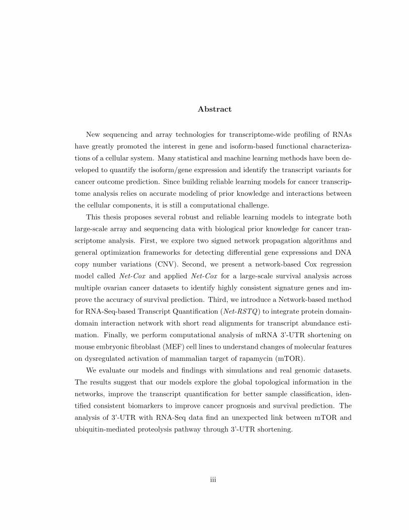
Abstract

New sequencing and array technologies for transcriptome-wide profiling of RNAs

have greatly promoted the interest in gene and isoform-based functional characteriza-

tions of a cellular system. Many statistical and machine learning methods have been de-

veloped to quantify the isoform/gene expression and identify the transcript variants for

cancer outcome prediction. Since building reliable learning models for cancer transcrip-

tome analysis relies on accurate modeling of prior knowledge and interactions between

the cellular components, it is still a computational challenge.

This thesis proposes several robust and reliable learning models to integrate both

large-scale array and sequencing data with biological prior knowledge for cancer tran-

scriptome analysis. First, we explore two signed network propagation algorithms and

general optimization frameworks for detecting differential gene expressions and DNA

copy number variations (CNV). Second, we present a network-based Cox regression

model called Net-Cox and applied Net-Cox for a large-scale survival analysis across

multiple ovarian cancer datasets to identify highly consistent signature genes and im-

prove the accuracy of survival prediction. Third, we introduce a Network-based method

for RNA-Seq-based Transcript Quantification (Net-RSTQ) to integrate protein domain-

domain interaction network with short read alignments for transcript abundance esti-

mation. Finally, we perform computational analysis of mRNA 3’-UTR shortening on

mouse embryonic fibroblast (MEF) cell lines to understand changes of molecular features

on dysregulated activation of mammalian target of rapamycin (mTOR).

We evaluate our models and findings with simulations and real genomic datasets.

The results suggest that our models explore the global topological information in the

networks, improve the transcript quantification for better sample classification, iden-

tified consistent biomarkers to improve cancer prognosis and survival prediction. The

analysis of 3’-UTR with RNA-Seq data find an unexpected link between mTOR and

ubiquitin-mediated proteolysis pathway through 3’-UTR shortening.

iii

Contents

Acknowledgements i

Dedication ii

Abstract iii

List of Tables viii

List of Figures ix

1 Introduction 1

1.1 Background . . . . . . . . . . . . . . . . . . . . . . . . . . . . . . . . . . 1

1.2 Previous Methods . . . . . . . . . . . . . . . . . . . . . . . . . . . . . . 4

1.2.1 Network propagation . . . . . . . . . . . . . . . . . . . . . . . . . 4

1.2.2 Cox proportional hazard model . . . . . . . . . . . . . . . . . . . 5

1.2.3 Base EM model for transcript quantification . . . . . . . . . . . . 6

1.3 Challenges and Objectives . . . . . . . . . . . . . . . . . . . . . . . . . . 7

1.4 Contributions . . . . . . . . . . . . . . . . . . . . . . . . . . . . . . . . . 8

1.5 Data Repositories . . . . . . . . . . . . . . . . . . . . . . . . . . . . . . . 9

1.6 Outline . . . . . . . . . . . . . . . . . . . . . . . . . . . . . . . . . . . . 10

2 Signed Network Propagation for Consistent Cancer Biomarker Detec-

tion 12

2.1 Introduction . . . . . . . . . . . . . . . . . . . . . . . . . . . . . . . . . . 12

2.2 Method . . . . . . . . . . . . . . . . . . . . . . . . . . . . . . . . . . . . 13

iv

2.2.1 Signed Network Propagation . . . . . . . . . . . . . . . . . . . . 14

2.2.2 Propagation on Signed Bipartite Graph . . . . . . . . . . . . . . 15

2.2.3 Learning with Gene Correlation Graph . . . . . . . . . . . . . . . 15

2.2.4 Learning with Sample-Feature Bipartite Graph . . . . . . . . . . 17

2.3 Experiments . . . . . . . . . . . . . . . . . . . . . . . . . . . . . . . . . . 18

2.3.1 Biomarker Identification from Gene Correlation Graph . . . . . . 18

2.3.2 Genomic Feature Selection on Sample-feature Bipartite Graphs . 22

2.4 Discussion . . . . . . . . . . . . . . . . . . . . . . . . . . . . . . . . . . . 26

3 Network-based Survival Analysis on Ovarian Cancer 27

3.1 Introduction . . . . . . . . . . . . . . . . . . . . . . . . . . . . . . . . . . 27

3.2 Results . . . . . . . . . . . . . . . . . . . . . . . . . . . . . . . . . . . . . 30

3.2.1 Net-Cox identifies consistent signature genes . . . . . . . . . . . 31

3.2.2 Net-Cox improves survival prediction . . . . . . . . . . . . . . . . 32

3.2.3 Statistical assessment . . . . . . . . . . . . . . . . . . . . . . . . 34

3.2.4 Evaluation by whole gene expression data . . . . . . . . . . . . . 36

3.2.5 Signature genes are ECM components or modulators . . . . . . . 37

3.2.6 Enriched PPI subnetworks and GO terms . . . . . . . . . . . . . 39

3.2.7 Laboratory experiment validates FBN1’s role . . . . . . . . . . . 41

3.3 Materials and Methods . . . . . . . . . . . . . . . . . . . . . . . . . . . . 42

3.3.1 Gene relation network construction . . . . . . . . . . . . . . . . . 42

3.3.2 Gene expression dataset preparation . . . . . . . . . . . . . . . . 44

3.3.3 Cox proportional hazard model . . . . . . . . . . . . . . . . . . . 44

3.3.4 Network-constrained Cox regression . . . . . . . . . . . . . . . . 45

3.3.5 Alternating optimization algorithm . . . . . . . . . . . . . . . . . 46

3.3.6 Cross validation and parameter tuning . . . . . . . . . . . . . . . 47

3.3.7 Evaluation measures . . . . . . . . . . . . . . . . . . . . . . . . . 48

3.3.8 Tumor array preparation . . . . . . . . . . . . . . . . . . . . . . 49

3.4 Discussion . . . . . . . . . . . . . . . . . . . . . . . . . . . . . . . . . . . 50

4 Network-based Isoform Quantification with RNA-Seq Data 53

4.1 Introduction . . . . . . . . . . . . . . . . . . . . . . . . . . . . . . . . . . 53

4.2 Materials and Methods . . . . . . . . . . . . . . . . . . . . . . . . . . . . 56

v

4.2.1 Transcript network construction . . . . . . . . . . . . . . . . . . 57

4.2.2 Network-based transcript quantification model . . . . . . . . . . 58

4.2.3 The Net-RSTQ algorithm . . . . . . . . . . . . . . . . . . . . . . 60

4.2.4 EM algorithm in Net-RSTQ . . . . . . . . . . . . . . . . . . . . . 61

4.2.5 qRT-PCR experiment design . . . . . . . . . . . . . . . . . . . . 63

4.2.6 RNA-Seq data preparation . . . . . . . . . . . . . . . . . . . . . 64

4.3 Results . . . . . . . . . . . . . . . . . . . . . . . . . . . . . . . . . . . . . 66

4.3.1 Isoform co-expressions correlate with protein DDI . . . . . . . . 66

4.3.2 Protein domain-domain interactions enrich KEGG pathways . . 70

4.3.3 Net-RSTQ captures network prior in simulations . . . . . . . . . 70

4.3.4 qRT-PCR experiments confirmed improved transcript quantification 73

4.3.5 Net-RSTQ improved overall cancer outcome predictions . . . . . 75

4.3.6 Running time . . . . . . . . . . . . . . . . . . . . . . . . . . . . . 78

4.4 Discussion . . . . . . . . . . . . . . . . . . . . . . . . . . . . . . . . . . . 79

5 Detecting mRNA 3’-UTR shortening in mTORC1 activated MEFs 82

5.1 Introduction . . . . . . . . . . . . . . . . . . . . . . . . . . . . . . . . . . 82

5.2 Results . . . . . . . . . . . . . . . . . . . . . . . . . . . . . . . . . . . . . 84

5.2.1 3’-UTR shortening of mRNAs is caused by mTOR activation and

is a down stream target of mTORC1 . . . . . . . . . . . . . . . . 84

5.2.2 3’-UTR shortening activates ubiquitin-mediated proteolysis . . . 89

5.3 Method . . . . . . . . . . . . . . . . . . . . . . . . . . . . . . . . . . . . 91

5.3.1 RNA-Seq and alignments . . . . . . . . . . . . . . . . . . . . . . 91

5.3.2 ApA analysis . . . . . . . . . . . . . . . . . . . . . . . . . . . . . 92

5.3.3 Scatter plot for differential expression and ApA analysis . . . . . 92

5.3.4 Measurement of RSI . . . . . . . . . . . . . . . . . . . . . . . . . 93

5.4 Discussion . . . . . . . . . . . . . . . . . . . . . . . . . . . . . . . . . . . 93

6 Conclusion and Discussion 95

6.1 Conclusion . . . . . . . . . . . . . . . . . . . . . . . . . . . . . . . . . . 95

6.2 Future Work . . . . . . . . . . . . . . . . . . . . . . . . . . . . . . . . . 97

6.2.1 Transfer learning across cancers . . . . . . . . . . . . . . . . . . . 97

vi

6.2.2 Improving transcript quantification by integrating RNA-Seq and

NanoString/qRT-PCR data . . . . . . . . . . . . . . . . . . . . . 98

6.2.3 Identify 3’-UTR shortening by integrating RNA-Seq and PAS-Seq

data . . . . . . . . . . . . . . . . . . . . . . . . . . . . . . . . . . 99

References 100

vii

List of Tables

2.1 Samples in five breast cancer datasets. . . . . . . . . . . . . . . . . . . . 18

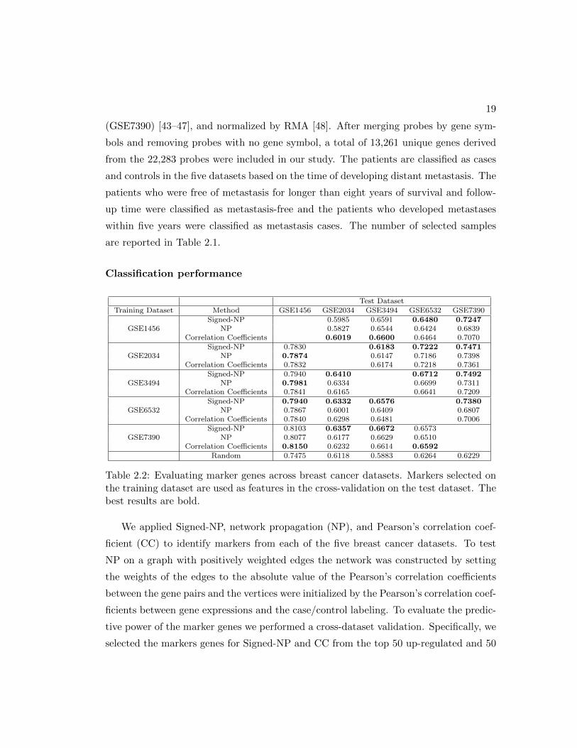
2.2 Evaluating marker genes across breast cancer datasets. . . . . . . . . . . 19

2.3 Enriched GO terms by the signature genes. . . . . . . . . . . . . . . . . 23

2.4 AUC scores of classifying patients on gene expression datasets. . . . . . 24

2.5 AUC scores of classifying patients on CNV datasets. . . . . . . . . . . . 24

3.1 Patient samples in the ovarian cancer datasets. . . . . . . . . . . . . . . 30

3.2 Log-rank test p−values in cross-dataset evaluation. . . . . . . . . . . . . 32

3.3 Top-15 signature genes. . . . . . . . . . . . . . . . . . . . . . . . . . . . 38

3.4 Literature review of the candidate ovarian cancer genes. . . . . . . . . . 38

4.1 Notations . . . . . . . . . . . . . . . . . . . . . . . . . . . . . . . . . . . 56

4.2 Network characteristics. . . . . . . . . . . . . . . . . . . . . . . . . . . . 58

4.3 Summary of patient samples in TCGA datasets. . . . . . . . . . . . . . 65

4.4 Classification performance on the small cancer gene list. . . . . . . . . . 77

4.5 Classification performance on the large cancer gene list. . . . . . . . . . 77

viii

List of Figures

1.1 Alternative splicing, alternative polyadenylation, and PPI subnetworks . 3

2.1 Running Signed-NP on a gene correlation graph. . . . . . . . . . . . . . 16

2.2 Running Signed-NPBi on sample-feature bipartite graph. . . . . . . . . 17

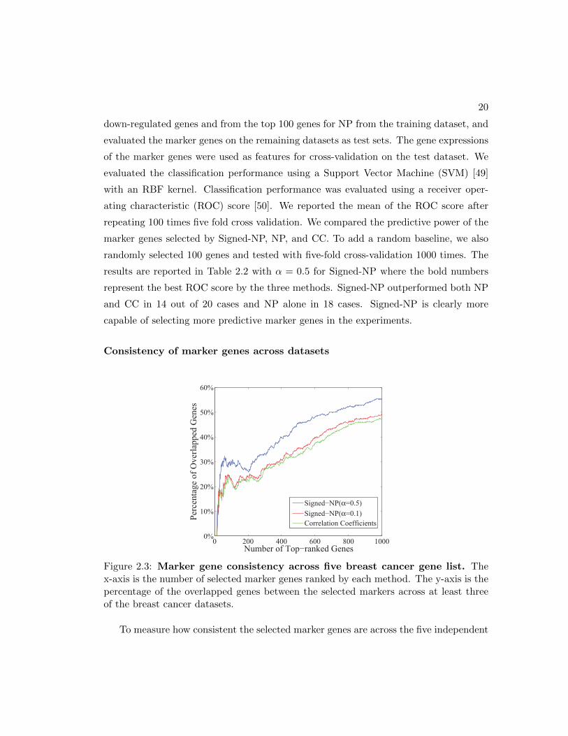
2.3 Marker gene consistency across five breast cancer gene list. . . . . . . . 20

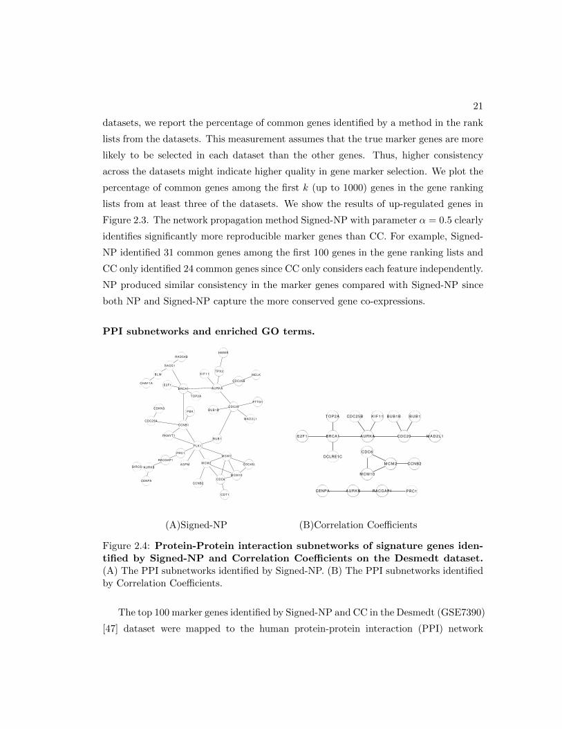
2.4 Protein-Protein interaction subnetworks of signature genes. . . . . . . . 21

2.5 CNV weights learned by Signed-NPBi. . . . . . . . . . . . . . . . . . . . 25

3.1 Overview of Net-Cox . . . . . . . . . . . . . . . . . . . . . . . . . . . . . 28

3.2 Consistency of signature genes. . . . . . . . . . . . . . . . . . . . . . . . 31

3.3 Cross-dataset survival prediction. . . . . . . . . . . . . . . . . . . . . . . 33

3.4 Consistency of signature genes on randomized co-expression networks. . 35

3.5 Statistical analysis of log-partial likelihood. . . . . . . . . . . . . . . . . 36

3.6 Statistical analysis of cross-validation log-partial likelihood. . . . . . . . 37

3.7 Protein-Protein interaction subnetworks of signature genes. . . . . . . . 40

3.8 Various levels of FBN1 expression in ovarian tumor arrays. . . . . . . . 41

3.9 Kaplan-Meier survival plots on FBN1 expression groups. . . . . . . . . . 43

4.1 An transcript network based on protein domain-domain interactions. . . 55

4.2 Transcript interaction neighborhood. . . . . . . . . . . . . . . . . . . . . 59

4.3 Correlation between transcript co-expression and protein DDI. . . . . . 68

4.4 Compare estimated expressions and ground truth in simulation. . . . . . 72

4.5 Validation by comparison with qRT-PCR results. . . . . . . . . . . . . . 74

4.6 Statistical analysis with randomized networks. . . . . . . . . . . . . . . . 78

4.7 Net-RSTQ running time. . . . . . . . . . . . . . . . . . . . . . . . . . . 79

5.1 mTOR activation leads to genome-wide 3’-UTR shortening. . . . . . . . 84

5.2 3’-UTR shortening is a downstream target of mTORC1. . . . . . . . . . 87

ix

5.3 3’-UTR shortening due to mTOR activation targets specific pathways. . 89

x

Chapter 1

Introduction

1.1 Background

Messenger RNA (mRNA) is a large family of RNA molecules. It carries codes from

the DNA and translated into proteins. Since mRNA expression is strongly correlated

with protein activities, it is often used as a signature in cancer analysis. Transcriptomic

technologies such as mRNA-Sequencing (RNA-Seq) and Microarrays have given us the

ability to analyze cellular mRNA levels globally, which enable effective molecular phe-

notyping of cancers, providing novel insights into the disease. Some pioneer works have

shown that the mRNA expression patterns caused by BRCA1 or BRCA2 mutation are

associated with either a poor prognosis or a good prognosis of breast cancer and ovarian

cancer [1–3] by analysing microarray gene expression data.

In the human transcriptome, there are ∼21,000 protein coding genes and many of

these genes can encode multiple protein isoforms. Besides transcript isoforms, there are

other transcript variants such as gene fusion and alterative polyadenylation can still

be introduced into mRNA and affect the expression of gene and isoforms. Moreover,

as a complex disease, cancer is believed to be caused by a combination of the effects

of multiple transcript variants. Therefore, analyzing cancer trascriptomes is still a

challenge. In this thesis, we focus on three specific problems in understanding cancer

trascriptome and list them below.

1

2

Alternative splicing A single gene contains numerous exons and introns, the exons

can be spliced together in different ways. Recent studies have estimated that alternative

splicing events exist in 92-94% of multi-exon genes in human, resulting in more than

one transcript per gene [4]. An example of an alternative splicing event is illustrated

in Figure 1.1(A). The gene contains 5 exons, one of the mRNA transcribed from that

gene contains exons 1-4 and another contains exons 1-3, and exon 5, which produce

two protein isoforms from the same gene. Alternative splicing provides cells with the

opportunity to create protein isoforms of differing functions from a single gene. Can-

cer cells often take advantage of this flexibility that promote growth and survival [5].

Many isoforms produced in this way are developmentally regulated and preferentially

re-expressed in tumor [5,6]. Therefore, accurate transcript quantification is crucial and

enables us to detect the differences of the alternative transcripts in the gene under differ-

ent conditions. Its downstream application in detecting molecular signature for cancer

can greatly impact biomedical study.

Alternative polyadenylation The 3’ end of most protein-coding genes and non-

coding RNAs is polyadenylated. Recent studies using transcriptome-wide techniques

have revealed that most human or mouse genes contain more than one poly(A) site, in-

dicating alternative polyadenylation (ApA) [7]. Tandem 3’ untranslated region (UTR)

ApA, illustrated in Figure 1.1(B), involves the occurrence of alternative poly(A) sites

within the same terminal exon is one of the most frequent ApA forms. 3’-UTR ApA

generates multiple isoforms with different 3’-UTR length without affecting the protein

encoded by the gene. It potentially regulates the stability, cellular localization and

translation efficiency of target RNAs as 3’-UTR provides a binding platform for mi-

croRNAs and RNA-binding proteins. A recently recognized mechanism of oncogene

activation is the loss of microRNA complementary sites [8, 9]. Therefore, identifying

cancer relevant 3’-UTR shortening events can possibly improve disease prognosis and

diagnosis.

Interactions It is well known that gene, transcript or protein isoforms do not function

in isolation in the cell, but are integrated together as a network of interactions between

3

Figure 1.1: (A) Alternative Splicing, (B)Tandem 3’-UTR AlternativePolyadenylation, and (C) Protein-Protein interaction subnetworks.

cellular components. Two human protein-protein interaction (PPI) subnetworks ob-

tained from HPRD [10] are shown in Figure 1.1(C). Cancer, as a complex disease,

reflects the perturbations or breakdown of specific functional modules in the complex

cellular network, rather than a consequence of an abnormality in a single gene [11].

Thus, instead of considering the gene or transcript variant individually in the cancer

transcriptome analysis, integrating network and high-throughput information together

could probably improve the quality of the analysis [12]. However, due to the complex

4

and heterogeneous nature of these large-scale datasets, efficient and reliable computa-

tional methods that integrate network information for cancer transcriptome analysis are

crucially needed.

1.2 Previous Methods

We will review a few fundamental modeling techniques that have been widely used in

cancer transcriptome analysis. Our models proposed in this thesis are developed based

on these base models. 1) Network propagation, a popular method for feature section by

integrating network information into analysis [13–15]; 2) Cox proportional hazard model

[16], widely used in survival analysis for biomarker identification and survival prediction;

3) A base Expectation-Maximization(EM) model [17, 18] for transcript quantification

with RNA-Seq data.

1.2.1 Network propagation

Let G = (V,W ) denote an undirected graph with vertex set V and positive adjacency

matrix W ∈ R+|V |×|V |. In network propagation, the vertex set V is initialized by a

vector y which is the +1/− 1 label on training vertices and 0 on test vertices in binary

classification. In the regularization framework proposed by [13], the objective is to learn

a label assignment function f : V → R to assign labels to the test vertices. The cost

function is defined as follows,

Ω(f) =∑i,j

Wij(fi√Dii− fj√

Djj

)2 + %‖f − y‖2, (1.1)

where D is a diagonal matrix with Dii =∑

jWij and % ≥ 0 is a parameter to weight the

two terms in the cost function. The first term in Eqn. (1.1) is the smoothness constraint,

which encourages assigning similar labels to strongly connected vertices. The second

term is the fitting constraint, which encourages consistency between predictions and

training labels. The first term can be rewritten as

f ′(I − (D)−12W (D)−

12 )f,

where I − (D)−12W (D)−

12 is the normalized graph Laplacian, which is positive semi-

definite. Thus Eqn. (1.1) is a quadratic problem with a closed-form solution.

5

In transcriptome analysis, G denotes a gene correlation graph, each vertex represent

a gene, and the edge represent the relation between two genes. The initial labels, y,

provide the differential expression of each individual gene in the case/control study as

the starting point of propagation. After convergence, f gives a new ranking of the genes.

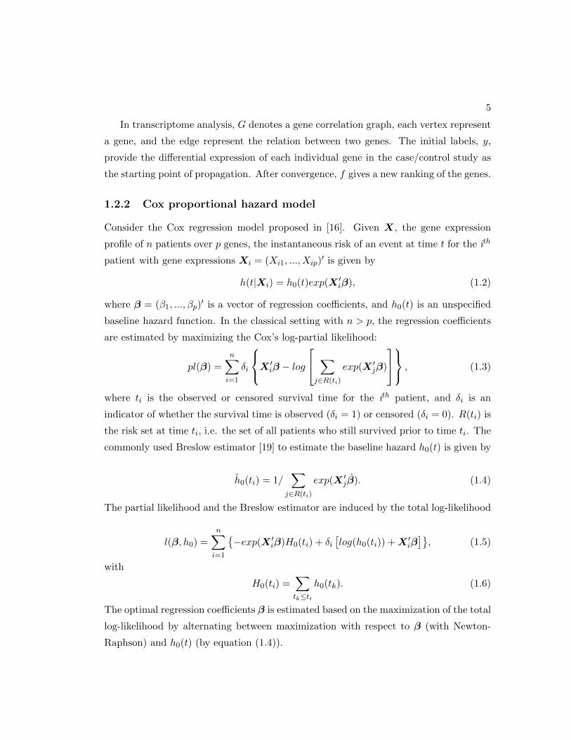
1.2.2 Cox proportional hazard model

Consider the Cox regression model proposed in [16]. Given X, the gene expression

profile of n patients over p genes, the instantaneous risk of an event at time t for the ith

patient with gene expressions Xi = (Xi1, ..., Xip)′ is given by

h(t|Xi) = h0(t)exp(X ′iβ), (1.2)

where β = (β1, ..., βp)′ is a vector of regression coefficients, and h0(t) is an unspecified

baseline hazard function. In the classical setting with n > p, the regression coefficients

are estimated by maximizing the Cox’s log-partial likelihood:

pl(β) =n∑i=1

δi

X ′iβ − log ∑j∈R(ti)

exp(X ′jβ)

, (1.3)

where ti is the observed or censored survival time for the ith patient, and δi is an

indicator of whether the survival time is observed (δi = 1) or censored (δi = 0). R(ti) is

the risk set at time ti, i.e. the set of all patients who still survived prior to time ti. The

commonly used Breslow estimator [19] to estimate the baseline hazard h0(t) is given by

h0(ti) = 1/∑

j∈R(ti)

exp(X ′jβ). (1.4)

The partial likelihood and the Breslow estimator are induced by the total log-likelihood

l(β, h0) =

n∑i=1

−exp(X ′iβ)H0(ti) + δi

[log(h0(ti)) +X ′iβ

], (1.5)

with

H0(ti) =∑tk≤ti

h0(tk). (1.6)

The optimal regression coefficients β is estimated based on the maximization of the total

log-likelihood by alternating between maximization with respect to β (with Newton-

Raphson) and h0(t) (by equation (1.4)).

6

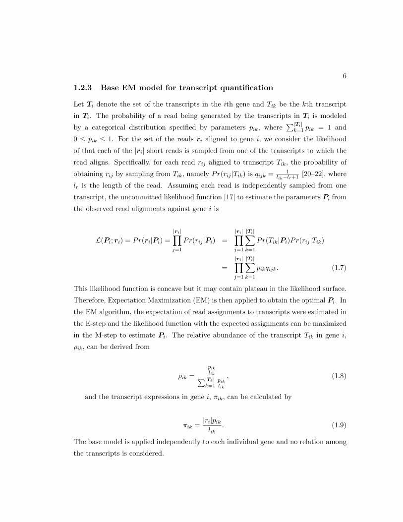
1.2.3 Base EM model for transcript quantification

Let Ti denote the set of the transcripts in the ith gene and Tik be the kth transcript

in Ti. The probability of a read being generated by the transcripts in Ti is modeled

by a categorical distribution specified by parameters pik, where∑|Ti|

k=1 pik = 1 and

0 ≤ pik ≤ 1. For the set of the reads ri aligned to gene i, we consider the likelihood

of that each of the |ri| short reads is sampled from one of the transcripts to which the

read aligns. Specifically, for each read rij aligned to transcript Tik, the probability of

obtaining rij by sampling from Tik, namely Pr(rij |Tik) is qijk = 1lik−lr+1 [20–22], where

lr is the length of the read. Assuming each read is independently sampled from one

transcript, the uncommitted likelihood function [17] to estimate the parameters Pi from

the observed read alignments against gene i is

L(Pi; ri) = Pr(ri|Pi) =

|ri|∏j=1

Pr(rij |Pi) =

|ri|∏j=1

|Ti|∑k=1

Pr(Tik|Pi)Pr(rij |Tik)

=

|ri|∏j=1

|Ti|∑k=1

pikqijk. (1.7)

This likelihood function is concave but it may contain plateau in the likelihood surface.

Therefore, Expectation Maximization (EM) is then applied to obtain the optimal Pi. In

the EM algorithm, the expectation of read assignments to transcripts were estimated in

the E-step and the likelihood function with the expected assignments can be maximized

in the M-step to estimate Pi. The relative abundance of the transcript Tik in gene i,

ρik, can be derived from

ρik =

piklik∑|Ti|k=1

piklik

, (1.8)

and the transcript expressions in gene i, πik, can be calculated by

πik =|ri|piklik

. (1.9)

The base model is applied independently to each individual gene and no relation among

the transcripts is considered.

7

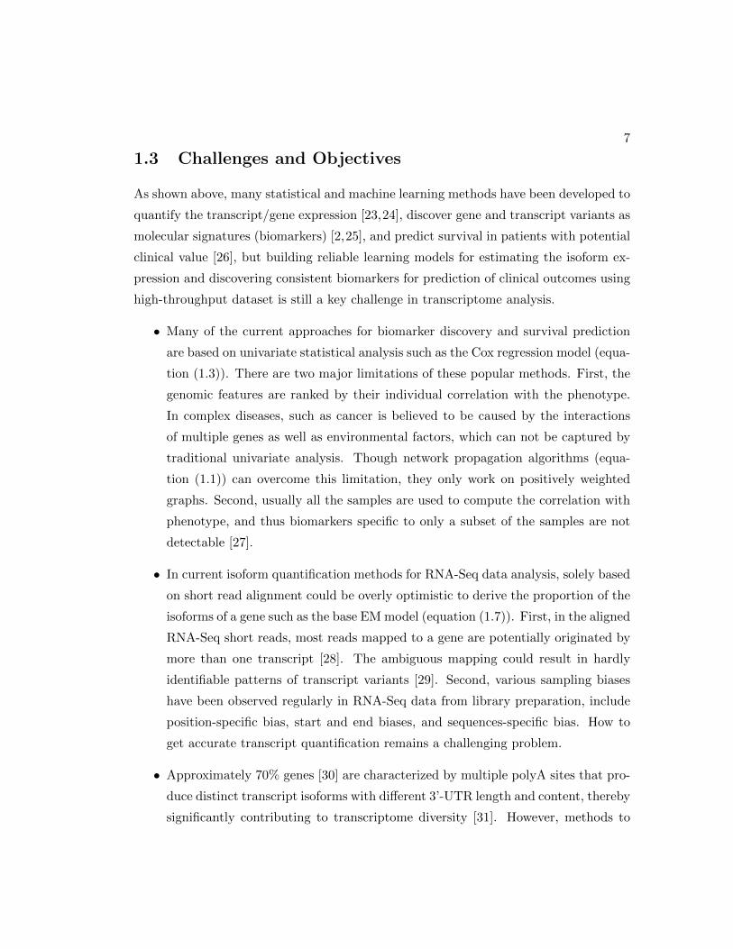
1.3 Challenges and Objectives

As shown above, many statistical and machine learning methods have been developed to

quantify the transcript/gene expression [23,24], discover gene and transcript variants as

molecular signatures (biomarkers) [2,25], and predict survival in patients with potential

clinical value [26], but building reliable learning models for estimating the isoform ex-

pression and discovering consistent biomarkers for prediction of clinical outcomes using

high-throughput dataset is still a key challenge in transcriptome analysis.

• Many of the current approaches for biomarker discovery and survival prediction

are based on univariate statistical analysis such as the Cox regression model (equa-

tion (1.3)). There are two major limitations of these popular methods. First, the

genomic features are ranked by their individual correlation with the phenotype.

In complex diseases, such as cancer is believed to be caused by the interactions

of multiple genes as well as environmental factors, which can not be captured by

traditional univariate analysis. Though network propagation algorithms (equa-

tion (1.1)) can overcome this limitation, they only work on positively weighted

graphs. Second, usually all the samples are used to compute the correlation with

phenotype, and thus biomarkers specific to only a subset of the samples are not

detectable [27].

• In current isoform quantification methods for RNA-Seq data analysis, solely based

on short read alignment could be overly optimistic to derive the proportion of the

isoforms of a gene such as the base EM model (equation (1.7)). First, in the aligned

RNA-Seq short reads, most reads mapped to a gene are potentially originated by

more than one transcript [28]. The ambiguous mapping could result in hardly

identifiable patterns of transcript variants [29]. Second, various sampling biases

have been observed regularly in RNA-Seq data from library preparation, include

position-specific bias, start and end biases, and sequences-specific bias. How to

get accurate transcript quantification remains a challenging problem.

• Approximately 70% genes [30] are characterized by multiple polyA sites that pro-

duce distinct transcript isoforms with different 3’-UTR length and content, thereby

significantly contributing to transcriptome diversity [31]. However, methods to

8

quantify relative ApA usage are still limited. Besides that, very few RNA-seq

reads contain polyA tails, challenging our ability to identify ApA events in gene.

For example, an ultra-deep sequencing study [32] only identified ∼40 thousand pu-

tative polyA reads (∼0.003%) from 1.2 billion total RNA-seq reads [33]. Moreover,

the precise mechanism(s) of ApA events is unknown [34].

1.4 Contributions

To address the challenges described above, we propose four different models and studies

in this thesis.

First, we introduce signed network propagation frameworks for detecting consistent

biomarkers [27]. The first framework runs network propagation on a gene graph weighted

by both positive and negative gene co-expression for gene selection from gene expression

datasets. It integrates gene co-expression and differential expression to explore gene

modules which overcome the limitation of the biomarker identification models based

on univariate statistical analysis. The second framework runs network propagation on

sample-feature bipartite graphs linked by both positive and negative features to identify

gene or CNV markers. The framework explores bi-clusters between patients and features

to find biomarkers specific to subsets of patient samples.

Second, we propose a network-based Cox proportional hazard model to explore the

co-expression or functional relation among gene expression features for survival anal-

ysis [35], which to our knowledge is among the first models that directly incorporate

network information in survival analysis. A gene relation network constructed by co-

expression analysis or prior knowledge of gene functional relations models the relation-

ship between genes. In the model, a graph Laplacian constraint is introduced as a

smoothness requirement on the gene features linked in the gene relation network. The

model identified consistent signature genes across the three ovarian cancer datasets, and

because of the better generalization across the datasets, the model also consistently im-

proved the accuracy of survival prediction over the Cox models regularized by L2-norm

or L1-norm.

Third, we examine the possibility of using protein domain-domain interactions as

9

prior knowledge in isoform transcript quantification to overcome the limitation of sam-

pling bias from RNA-Seq data [36]. We first made the observation that protein domain-

domain interactions positively correlate with isoform co-expressions in TCGA data and

then designed a probabilistic EM approach to integrate domain-domain interactions with

short read alignments for estimation of isoform proportions. In simulation, the approach

effectively improved isoform transcript quantifications when isoform co-expressions cor-

relate with their interactions. qRT-PCR results on 25 multi-isoform genes in a stem cell

line, ovarian cancer cell line, and a breast cancer cell line also showed that the approach

estimated more consistent isoform proportions with RNA-Seq data. In the experiments

on the RNA-Seq data in TCGA, the transcript abundances estimated by the approach

are more informative for patient sample classification of ovarian cancer, breast cancer

and lung cancer.

Last, we developed a pipeline to identify the transcriptome-wide ApA events with

RNA-Seq data in mouse embryonic fibroblast (MEF) [34]. To detect the events, we

evaluated candidate polyA signal (PAS) motifs in the 3’-UTR of the transcript by con-

trasting the short-read coverage up/downstream of the site across wild-type (WT) and

TSC1−/− MEFs with χ2-test. To our knowledge, this is one of the first comprehen-

sive analysis of transcriptome-wide ApA events with RNA-Seq data. Besides that, in

this study we investigate the molecular signatures of mammalian target of rapamycin

(mTOR) activated transcriptome and discovered widespread 3’-UTR shortening due to

dysregulated mTOR activation. Moreover, we found almost all known 3’-end process-

ing factors alter their expression on changes in cellular mTOR activity in TSC1−/−

compared with WT MEF.

1.5 Data Repositories

In this thesis, we utilized public high-throughput genomic data from several sources. All

the processed RNA-Seq and microarray data were downloaded from The Cancer Genome

Atlas (TCGA) data portal and the Gene Expression Omnibus (GEO) repository. The

raw RNA-Seq fastq files were downloaded from Cancer Genomics Hub (CGHub) under

National Cancer Institute (NCI) and Sequence Read Archive (SRA) under National

Center for Biotechnology Information (NCBI).

10

• TCGA project (http://cancergenome.nih.gov/) profiled and analyzed large

numbers of human tumors to discover molecular aberrations at the DNA, RNA,

protein and epigenetic levels. The resulting rich data provide a whole picture

to understand the molecular basis of cancer. TCGA data portal (https://

tcga-data.nci.nih.gov/tcga/dataAccessMatrix.htm) provides a platform for

researchers to search, download, and analyze data sets generated by TCGA. We

downloaded the normalized RNA-Seq and microarray gene expression and tran-

script expression data of four cancer types from the data portal.

• CGHub (https://cghub.ucsc.edu/) is the online repository of the sequencing

programs of the NCI, including The Cancer Genomics Atlas (TCGA) project [37].

The raw RNA-Seq fastq files of the cancer patients in four cancer types listed in

TCGA were downloaded from the CGHub online repository.

• GEO (http://www.ncbi.nlm.nih.gov/geo/) is a public repository that archives

and freely distributes microarray, next-generation sequencing, and other forms of

high-throughput functional genomic data submitted by the scientific community

[38]. We downloaded two ovarian cancer microarray gene expression datasets, five

breast cancer microarray gene expression datasets from the GEO repository.

• SRA (http://www.ncbi.nlm.nih.gov/sra) stores raw sequence data from next-

generation sequencing technologies. Two raw RNA-Seq fastq files of breast cancer

cell line and stem cell line were downloaded from the SRA database.

Besides above, our collaborators at University of Kansas Medical Center and University

of Minnesota also provided in-house data of ovarian cancer cell line and mouse cell line

for the studies.

1.6 Outline

The rest of the thesis is organized as follows:

• In Chapter 2, we describe two signed network propagation algorithms, Signed-NP

and Signed-NPBi, consider both positive and negative relation in graphs to model

http://cancergenome.nih.gov/

https://tcga-data.nci.nih.gov/tcga/dataAccessMatrix.htm

https://tcga-data.nci.nih.gov/tcga/dataAccessMatrix.htm

https://cghub.ucsc.edu/

http://www.ncbi.nlm.nih.gov/geo/

http://www.ncbi.nlm.nih.gov/sra

11

gene up/down-regulation or amplification/deletion CNV events for detecting dif-

ferential gene expressions and DNA CNVs.

• In Chapter 3, we describe a network-based Cox regression model called Net-Cox,

integrates gene network information into the Cox’s proportional hazard model

to explore the co-expression or functional relation among high-dimensional gene

expression features in the gene network for biomarker identification and survival

prediction.

• In Chapter 4, we describe a network-based probabilistic EM approach, Net-RSTQ,

to integrate domain-domain interations with short read alignments for estimation

of isoform proportions.

• In Chapter 5, we identifie 3’-UTR shortening of mRNAs as an additional molecular

signature of mTOR activation and show that 3’-UTR shortening enhances the

translation of specific mRNAs.

• In Chapter 6, we summarize the findings of the thesis and suggesting directions

for future work.

Chapter 2

Signed Network Propagation for

Cancer Biomarker Analysis

2.1 Introduction

Powered by high-throughput genomic technologies, it is now a common practice to per-

form genome-scale experiments for measuring gene expressions, copy number variations

(CNVs), single nucleotide polymorphisms, and other molecular information for cancer

studies. Correlating these high-dimensional genomic features with cancer phenotypes

as molecular signatures (biomarkers) can possibly improve prognosis and diagnosis over

current clinical measures for risk assessment of patients [2,39,40]. The most widely used

statistical methods to detect biomarkers are Pearson correlation coefficients [2] and hy-

pothesis test methods such as student t-test. There are two major limitations of these

popular methods. First, the genomic features are ranked by their individual correlation

with the phenotype, and thus relations among features, for example co-expressed genes

under certain conditions and adjacent probes involved in the same CNV events, are

ignored. Second, usually all the samples are used to compute the correlation with phe-

notype, and thus biomarkers specific to only a subset of the samples are not detectable.

Network propagation is a graph-based learning algorithm [13] similar to PageRank

12

13

used by Google. It has been shown that network propagation is capable of captur-

ing the dependence among genomic features to detect correlated features as biomark-

ers [14, 15]. An efficient network propagation algorithm on bipartite graphs was in-

troduced to explore sample-feature bi-clusters for feature selection and cancer outcome

classification [41]. In the network propagation regularization framework, a quadratic

term with a normalized graph Laplacian matrix as hessian is combined with a square-

loss on the predictions to explore the global graph structure for capturing correlation

between all genomic features. The graph Laplacian matrix is only defined for positively

weighted graphs which poses a significant limitation on the applicability of network

propagation to the analysis of genomic data. For example, gene expression data could

require a precise representation of up-regulated expression or down-regulated expres-

sion, and CNV data require a precise representation of amplification or deletion events.

In these real computational biology problems, genomic data are represented by signed

graphs to incorporate both positive and negative relations and thus the existing network

propagation algorithms are not applicable.

To address the problem, we propose two signed network propagation algorithms

and regularization frameworks for detecting differential gene expressions and DNA copy

number variations. In the frameworks, we introduce signed graph Laplacians into net-

work propagation. The first algorithm, Signed-NP, runs network propagation on a gene

graph weighted by both positive and negative gene co-expressions for gene selection from

gene expression datasets. Signed-NP integrates gene co-expressions and differential ex-

pressions to explore gene modules. The second algorithm, Signed-NPBi, runs network

propagation on sample-feature bipartite graphs linked by both positive and negative

features to identify gene or CNV markers. Signed-NPBi explores bi-clusters between

patients and features to find biomarkers specific to subsets of patient samples.

2.2 Method

Based on the network propagation model described in section 1.2.1. We first introduce

signed network propagation (Signed-NP) in section 2.2.1 and its extension for propa-

gation on bipartite graphs (Signed-NPBi) in section 2.2.2. In section 2.2.3 and section

14

2.2.4 we apply Signed-NP on gene correlation graphs for detecting differential gene ex-

pressions, and Signed-NPBi on sample-feature bipartite graphs for gene selection or

CNV detection respectively.

2.2.1 Signed Network Propagation

To allow both positive and negative edges for network propagation, we introduce signed

graph Laplacian [42] into the regularization framework. Given a signed graph G =

(V,W ) with vertices V and adjacency matrix W ∈ R|V |×|V |. The cost function of the

regularization framework is modified as follows,

Ω(f) =∑i,j

|Wij |(fi√Dii− sgn(Wij)

fj√Djj

)2 + %‖f − y‖2, (2.1)

where Dii =∑

j |Wij |. The first term in Eqn.(2.1) is the normalized signed graph

Laplacian I − S, where S = D−12 ∗ W ∗ D−

12 . It has been shown in [42] that the

signed graph Laplacian is always positive semi-definite. The first cost term encourages

assigning similar labels to vertices connected by positive edges and opposite labels to

the vertices connected by negative edges. Empirically, the eigenvalues of S can be very

small. For better performance in network propagation, we rescale S by dividing the

largest eigenvalue such that S’s eigenvalues are in the range [−1, 1]. Similar to the

algorithm proposed by [13], the optimization framework in Eqn.(2.1) can be solved with

an iterative label propagation algorithm,

f t = (1− α)y + αSf t−1, (2.2)

where t denotes the propagation step and α = 1/(1 +%). The parameter α balances the

weights between initial label and network structure. The larger the α, the more we trust

the network structure. This algorithm simply propagates labels among the neighbors

in the graph. The algorithm will converge to the closed-form solution

f∗ = (1− α)(I − αS)−1 ∗ y, (2.3)

where f∗ assigns labels to the vertices.

15

2.2.2 Propagation on Signed Bipartite Graph

We next extend the framework in Eqn.(2.1) for signed bipartite graphs. Let G =

(V,U,E,W ) denote a signed bipartite graph, where V and U represent two disjoint

vertex sets, E is a set of weighted edges, and W ∈ RV×U is the wighted adjacency

matrix. Each edge (v, u) ∈ E connects two vertices v and u with weight Wvu. The

initialization function y for the two vertex sets are denoted by y(v) and y(u). In this

context, the cost function over G = (V,U,E,W ) is defined as

Ω(f) = 2∑

(v,u)∈E

|Wvu|(f(v)√Dvv

− sgn(Wvu)f(u)√D′uu

)2

+%‖f(v)− y(v)‖2 + %‖f(u)− y(u)‖2, (2.4)

where % ≥ 0 is a parameter for balancing the cost terms, and D and D′ are diagonal

matrices with Dvv =∑

u∈U |w(v, u)| and D′uu =∑

v∈V |w(v, u)|. The first cost term

encourages similar labeling on positively connected vertex pairs and opposite labeling on

negatively connected pairs. The second term and the third term constrain the new label

assignment to be consistent with the initial labeling. To solve the optimization problem

in Eqn.(2.4), we can also use a similar network propagation algorithm to compute

the closed-form solution. The propagation algorithm iteratively performs propagation

between the two vertex sets in both directions as follow,

f(v)t = (1− α)y(v) + αSf(u)t−1

f(u)t = (1− α)y(u) + αSf(v)t−1

where α = 1/(1+%), S = D−12 ∗W ∗D′−

12 , and t denotes the propagation step. S is also

similarly rescaled by dividing the largest eigenvalue. Label information is propagated

through neighbors in the bipartite graph. The algorithm will converge to the closed-form

solution as in Eqn.(2.3).

2.2.3 Learning with Gene Correlation Graph

We first apply Signed-NP to a gene correlation graph for identifying differentially ex-

pressed genes. An illustrative example of network propagation on a gene correlation

graph G = (V,W ) is shown in Figure 2.1. Each vertex in V represents a gene which

16

0.29

0.21

0.490.52

-0.47

0.30

0.380.430.37

0.40

-0.46

0.310.44

0.39

0.37

-0.31

0.32

-0.500.42

0.360.31

0.39

0.47

0.51

0.37

0.42

0.050.41

0.42

0.120.34

-0.35

0.47-0.23

-0.24

-0.49

0.37

0.29

-0.37

0.53

-0.38

-0.27

-0.14

-0.34

-0.35

0.43

0.52

0.37

0.40

-0.46

0.49

-0.47

0.30

0.380.29

0.31 0.210.44

-0.50

0.39

0.470.36

0.31

0.320.39

0.37

0.37

0.42

-0.31

0.51

0.42

0.34

0.35

0.38-0.28 -0.07

0.21

0.31-0.18

0.19

0.56

-0.33-0.35

-0.25

-0.32

-0.24-0.41

0.39

-0.43

-0.26

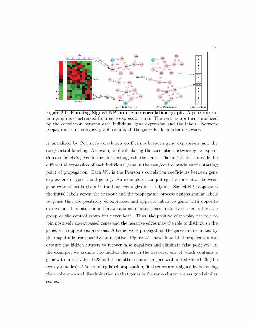
Figure 2.1: Running Signed-NP on a gene correlation graph. A gene correla-tion graph is constructed from gene expression data. The vertices are then initializedby the correlation between each individual gene expression and the labels. Networkpropagation on the signed graph re-rank all the genes for biomarker discovery.

is initialized by Pearson’s correlation coefficients between gene expressions and the

case/control labeling. An example of calculating the correlation between gene expres-

sion and labels is given in the pink rectangles in the figure. The initial labels provide the

differential expression of each individual gene in the case/control study as the starting

point of propagation. Each Wij is the Pearson’s correlation coefficients between gene

expressions of gene i and gene j. An example of computing the correlation between

gene expressions is given in the blue rectangles in the figure. Signed-NP propagates

the initial labels across the network and the propagation process assigns similar labels

to genes that are positively co-expressed and opposite labels to genes with opposite

expression. The intuition is that we assume marker genes are active either in the case

group or the control group but never both. Thus, the positive edges play the role to

join positively co-expressed genes and the negative edges play the role to distinguish the

genes with opposite expressions. After network propagation, the genes are re-ranked by

the magnitude from positive to negative. Figure 2.1 shows how label propagation can

capture the hidden clusters to recover false negatives and eliminate false positives. In

the example, we assume two hidden clusters in the network, one of which contains a

gene with initial value -0.23 and the another contains a gene with initial value 0.29 (the

two cyan nodes). After running label propagation, final scores are assigned by balancing

their coherence and discrimination so that genes in the same cluster are assigned similar

scores.

17

2.2.4 Learning with Sample-Feature Bipartite Graph

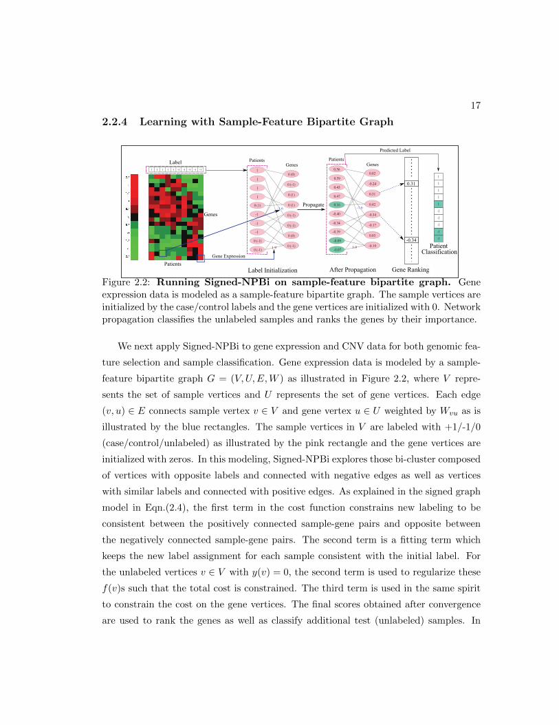
Figure 2.2: Running Signed-NPBi on sample-feature bipartite graph. Geneexpression data is modeled as a sample-feature bipartite graph. The sample vertices areinitialized by the case/control labels and the gene vertices are initialized with 0. Networkpropagation classifies the unlabeled samples and ranks the genes by their importance.

We next apply Signed-NPBi to gene expression and CNV data for both genomic fea-

ture selection and sample classification. Gene expression data is modeled by a sample-

feature bipartite graph G = (V,U,E,W ) as illustrated in Figure 2.2, where V repre-

sents the set of sample vertices and U represents the set of gene vertices. Each edge

(v, u) ∈ E connects sample vertex v ∈ V and gene vertex u ∈ U weighted by Wvu as is

illustrated by the blue rectangles. The sample vertices in V are labeled with +1/-1/0

(case/control/unlabeled) as illustrated by the pink rectangle and the gene vertices are

initialized with zeros. In this modeling, Signed-NPBi explores those bi-cluster composed

of vertices with opposite labels and connected with negative edges as well as vertices

with similar labels and connected with positive edges. As explained in the signed graph

model in Eqn.(2.4), the first term in the cost function constrains new labeling to be

consistent between the positively connected sample-gene pairs and opposite between

the negatively connected sample-gene pairs. The second term is a fitting term which

keeps the new label assignment for each sample consistent with the initial label. For

the unlabeled vertices v ∈ V with y(v) = 0, the second term is used to regularize these

f(v)s such that the total cost is constrained. The third term is used in the same spirit

to constrain the cost on the gene vertices. The final scores obtained after convergence

are used to rank the genes as well as classify additional test (unlabeled) samples. In

18

Figure 2.2 the optimal labels are given in parentheses. After running network propaga-

tion, the genes in bi-clusters will receive more significant values. Note that if connected

by negative edges, the sample and the gene will receive opposite labels. Since the im-

portant genes are strongly connected to either the case group or the control group we

can consider the genes with significant scores within the bi-clusters as biomarkers. The

unlabeled samples are also classified to different groups based on the sign of the final

score for each sample.

Similarly, we can also apply the signed bipartite graph model to copy number varia-

tion data. Each probe feature is represented by a vertex in U connected to the samples

with an edge weighted by the log intensity ratio of the probe. After network propaga-

tion, those probes with high scores are selected as important CNV regions. In CNV

analysis the adjacent probes tend to be strongly correlated, thus the bi-clusters in the

bipartite graph represent a continuous CNV regions across a subset of samples.

2.3 Experiments

In the experiments, we tested Signed-NP on 5 breast cancer gene expression datasets

to detect differentially expressed genes and Signed-NPBi on two breast cancer gene ex-

pression datasets and one bladder cancer arrayCGH dataset to detect both differentially

expressed genes and copy number variations.

2.3.1 Biomarker Identification from Gene Correlation Graph

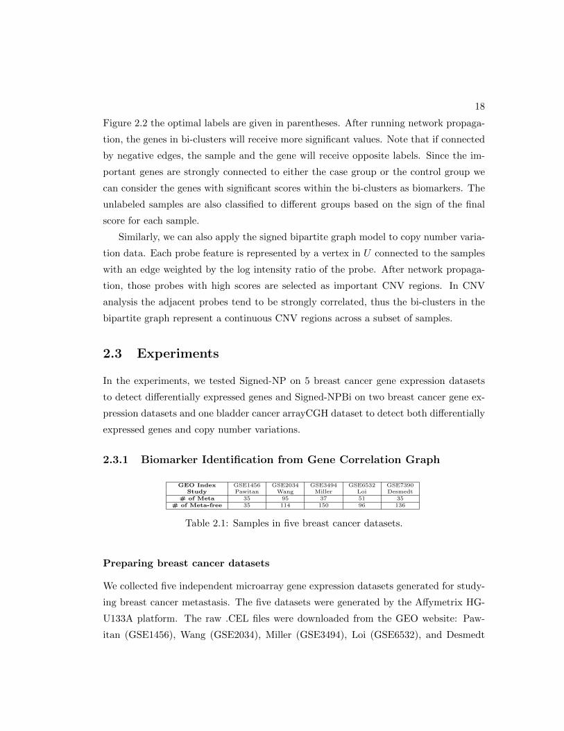
GEO Index GSE1456 GSE2034 GSE3494 GSE6532 GSE7390Study Pawitan Wang Miller Loi Desmedt

# of Meta 35 95 37 51 35# of Meta-free 35 114 150 96 136

Table 2.1: Samples in five breast cancer datasets.

Preparing breast cancer datasets

We collected five independent microarray gene expression datasets generated for study-

ing breast cancer metastasis. The five datasets were generated by the Affymetrix HG-

U133A platform. The raw .CEL files were downloaded from the GEO website: Paw-

itan (GSE1456), Wang (GSE2034), Miller (GSE3494), Loi (GSE6532), and Desmedt

19

(GSE7390) [43–47], and normalized by RMA [48]. After merging probes by gene sym-

bols and removing probes with no gene symbol, a total of 13,261 unique genes derived

from the 22,283 probes were included in our study. The patients are classified as cases

and controls in the five datasets based on the time of developing distant metastasis. The

patients who were free of metastasis for longer than eight years of survival and follow-

up time were classified as metastasis-free and the patients who developed metastases

within five years were classified as metastasis cases. The number of selected samples

are reported in Table 2.1.

Classification performance

Test DatasetTraining Dataset Method GSE1456 GSE2034 GSE3494 GSE6532 GSE7390

GSE1456Signed-NP 0.5985 0.6591 0.6480 0.7247

NP 0.5827 0.6544 0.6424 0.6839Correlation Coefficients 0.6019 0.6600 0.6464 0.7070

GSE2034Signed-NP 0.7830 0.6183 0.7222 0.7471


GSE3494Signed-NP 0.7940 0.6410 0.6712 0.7492


GSE6532Signed-NP 0.7940 0.6332 0.6576 0.7380


GSE7390Signed-NP 0.8103 0.6357 0.6672 0.6573


Random 0.7475 0.6118 0.5883 0.6264 0.6229

Table 2.2: Evaluating marker genes across breast cancer datasets. Markers selected onthe training dataset are used as features in the cross-validation on the test dataset. Thebest results are bold.

We applied Signed-NP, network propagation (NP), and Pearson’s correlation coef-

ficient (CC) to identify markers from each of the five breast cancer datasets. To test

NP on a graph with positively weighted edges the network was constructed by setting

the weights of the edges to the absolute value of the Pearson’s correlation coefficients

between the gene pairs and the vertices were initialized by the Pearson’s correlation coef-

ficients between gene expressions and the case/control labeling. To evaluate the predic-

tive power of the marker genes we performed a cross-dataset validation. Specifically, we

selected the markers genes for Signed-NP and CC from the top 50 up-regulated and 50

20

down-regulated genes and from the top 100 genes for NP from the training dataset, and

evaluated the marker genes on the remaining datasets as test sets. The gene expressions

of the marker genes were used as features for cross-validation on the test dataset. We

evaluated the classification performance using a Support Vector Machine (SVM) [49]

with an RBF kernel. Classification performance was evaluated using a receiver oper-

ating characteristic (ROC) score [50]. We reported the mean of the ROC score after

repeating 100 times five fold cross validation. We compared the predictive power of the

marker genes selected by Signed-NP, NP, and CC. To add a random baseline, we also

randomly selected 100 genes and tested with five-fold cross-validation 1000 times. The

results are reported in Table 2.2 with α = 0.5 for Signed-NP where the bold numbers

represent the best ROC score by the three methods. Signed-NP outperformed both NP

and CC in 14 out of 20 cases and NP alone in 18 cases. Signed-NP is clearly more

capable of selecting more predictive marker genes in the experiments.

Consistency of marker genes across datasets

0 200 400 600 800 10000%

10%

20%

30%

40%

50%

60%

Number of Top−ranked Genes

Perc

enta

ge o

f Ove

rlapp

ed G

enes

Signed−NP(α=0.5)Signed−NP(α=0.1)Correlation Coefficients

Figure 2.3: Marker gene consistency across five breast cancer gene list. Thex-axis is the number of selected marker genes ranked by each method. The y-axis is thepercentage of the overlapped genes between the selected markers across at least threeof the breast cancer datasets.

To measure how consistent the selected marker genes are across the five independent

21

datasets, we report the percentage of common genes identified by a method in the rank

lists from the datasets. This measurement assumes that the true marker genes are more

likely to be selected in each dataset than the other genes. Thus, higher consistency

across the datasets might indicate higher quality in gene marker selection. We plot the

percentage of common genes among the first k (up to 1000) genes in the gene ranking

lists from at least three of the datasets. We show the results of up-regulated genes in

Figure 2.3. The network propagation method Signed-NP with parameter α = 0.5 clearly

identifies significantly more reproducible marker genes than CC. For example, Signed-

NP identified 31 common genes among the first 100 genes in the gene ranking lists and

CC only identified 24 common genes since CC only considers each feature independently.

NP produced similar consistency in the marker genes compared with Signed-NP since

both NP and Signed-NP capture the more conserved gene co-expressions.

PPI subnetworks and enriched GO terms.

KIF11

BRCA1

RAD51

CHAF1A

B L M

RAD54B

TOP2A

E2F1CDC25B

BUB1B

MELK

M A D 2 L 1

TPX2

PTTG1

H M M R

AURKA

CDC20

M C M 1 0

B U B 1

CCNB2

PLK1

CDC6

CDT1

CDC45L

M C M 7

M C M 2

CDC25A

CENPA

BIRC5 AURKB

CCNB1

RACGAP1

PRC1

CDKN3

PKMYT1

ASPM

PBK

TOP2A

AURKA

KIF11

BRCA1

CDC25B

E2F1

B U B 1

M C M 2

CDC20

BUB1B

RACGAP1

M A D 2 L 1

PRC1

CCNB2

DCLRE1C

AURKB

CDC6

CENPA

M C M 1 0

(A)Signed-NP (B)Correlation Coefficients

Figure 2.4: Protein-Protein interaction subnetworks of signature genes iden-tified by Signed-NP and Correlation Coefficients on the Desmedt dataset.(A) The PPI subnetworks identified by Signed-NP. (B) The PPI subnetworks identifiedby Correlation Coefficients.

The top 100 marker genes identified by Signed-NP and CC in the Desmedt (GSE7390)

[47] dataset were mapped to the human protein-protein interaction (PPI) network

22

obtained from HPRD [10] and also analyzed with the DAVID functional annotation

tool [51]. We report the densely connected PPI subnetworks constructed from the top

100 up-regulated genes selected by Signed-NP in Figure 2.4(A). The subnetwork con-

tains 37 genes and 43 connections between the genes. Compared with the PPI subnet-

work generated from the marker genes selected by CC in Figure 2.4(B), which contain

19 genes and 17 connections, the subnetwork is larger and denser. In Figure 2.4(A),

HMMR and RAD51 were reported as oncogenes of breast cancer in Online Mendelian

Inheritance in Man (OMIM) [52], neither of which was detected by CC. Women with a

variation in the HMMR gene had a higher risk of breast cancer even after accounting

for mutations in the BRCA1 or BRCA2 genes. In particular, the risk of breast can-

cer in women under age 40 who carry the HMMR variation was 2.7 times higher than

the risk in women without this variation [53]. RAD51 interacts with the evolutionar-

ily conserved BRC motifs in the human breast cancer susceptibility gene BRCA2 [54].

In addition, the genes MAD2L1, RAD51, AURKA, BRCA1, BUB1, BUB1B, CDT1,

and PTTG1 are listed on the breast cancer gene list in Genetic Association Database

(GAD) [55]. Furthermore, the 37 marker genes in the subnetwork are also enriched by

cell cycle process, nuclear division, DNA replication, DNA metabolic process, and ATP

binding, all of which are well-known cancer relevant GO functions.

The top 100 signature genes identified by Signed-NP enriched 83 GO functions (p-

value¡0.01) and the ones identified by CC only enriched 47 GO functions. The most

significantly enriched GO functions are listed in Table 2.3. It is clear that Signed-NP

identified signature genes that are more functionally coherent.

2.3.2 Genomic Feature Selection on Sample-feature Bipartite Graphs

Data Preparation

We prepared two microarray gene expression datasets [1,2] to study breast cancer metas-

tasis and one arrayCGH dataset to study bladder cancer [56]. The dataset (Rosetta)

in [2] measures expression profiles of 24,481 genes generated by Agilent oligonucleotide

Hu25K microarrays. This dataset contains 97 patient samples among which 51 patients

were free of disease after their diagnosis for an interval of at least 5 years (good outcome)

and 46 patients had developed distant metastasis within 5 years (poor outcome). The

23GO terms Signed-NP

CorrelationCoefficients

cell cycle 38.382 21.419cell cycle process 34.078 19.295cell cycle phase 32.805 17.377M phase 32.329 17.547mitotic cell cycle 31.849 17.468mitosis 27.777 15.157nuclear division 27.777 15.157M phase of mitotic cell cycle 27.534 14.994organelle fission 27.236 14.794cell division 19.805 12.449organelle organization 19.072 13.072spindle 18.723 12.557microtubule cytoskeleton 14.743 Xchromosome 14.389 Xnuclear part 14.028 Xregulation of cell cycle 13.611 Xcellular component organization 13.389 XDNA replication 12.282 Xintracellular non-membrane-bounded organelle 12.091 Xnon-membrane-bounded organelle 12.091 Xintracellular organelle part 11.667 Xorganelle part 11.530 Xcondensed chromosome 10.774 Xnucleus 10.529 Xchromosomal part 10.397 X

Table 2.3: Enriched GO terms by the signature genes. The p-values in −log10

scale are shown for the enriched GO terms. A “X” denotes a p-value larger than1× 10−10.

Vijver [1] dataset contains microarray gene expressions produced by the same technique

for generating the Rosetta dataset on 295 samples (194 with good outcome and 101

with poor outcome). The two datasets were chosen for the experiment because Agilent

array data by default report up/down-gene expression with positive and negative values

for testing Signed-NPBi. The RMA normalized Affymetrix arrays used in the previous

experiments usually contain absolute intensities. To avoid additional processing of the

data, the five Affymetrix datasets were not used in this experiment. The arrayCGH

dataset Blaveri [56] was generated with a HumanArray 2.0 array consisting of 2,464

probes at 1.5Mb resolution. After pruning, the dataset contained 98 samples and 2,142

probes. We classified the patient samples by the tumor stage.

Signed-NPBi was compared against SVM with linear and RBF kernels and the

bipartite network propagation algorithm (NPBi) [41]. To apply NPBi, each feature in

the datasets was split into two features to represent the positive portion and the negative

portion in the original features. The parameter α for both Signed-NPBi and NPBi was

chosen from 0.95, 0.5, 0.1 in the analysis.

24

Algorithm Rosetta Vijver

Signed-NPBi 0.7374 0.6682NPBi 0.7290 0.6162SVM(linear) 0.7072 0.6708SVM(RBF) 0.7030 0.6830

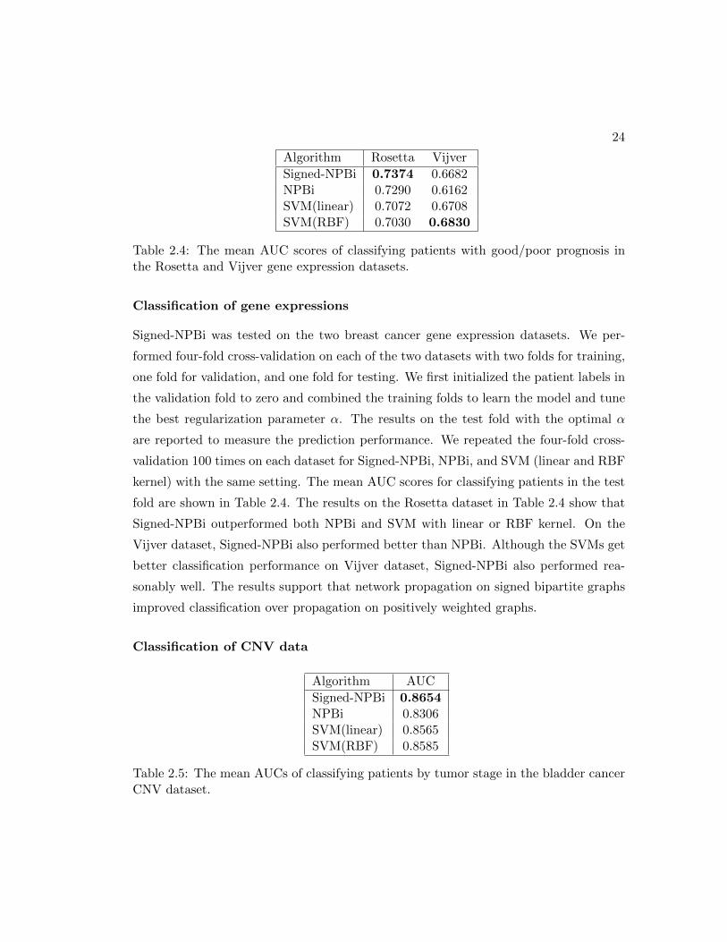
Table 2.4: The mean AUC scores of classifying patients with good/poor prognosis inthe Rosetta and Vijver gene expression datasets.

Classification of gene expressions

Signed-NPBi was tested on the two breast cancer gene expression datasets. We per-

formed four-fold cross-validation on each of the two datasets with two folds for training,

one fold for validation, and one fold for testing. We first initialized the patient labels in

the validation fold to zero and combined the training folds to learn the model and tune

the best regularization parameter α. The results on the test fold with the optimal α

are reported to measure the prediction performance. We repeated the four-fold cross-

validation 100 times on each dataset for Signed-NPBi, NPBi, and SVM (linear and RBF

kernel) with the same setting. The mean AUC scores for classifying patients in the test

fold are shown in Table 2.4. The results on the Rosetta dataset in Table 2.4 show that

Signed-NPBi outperformed both NPBi and SVM with linear or RBF kernel. On the

Vijver dataset, Signed-NPBi also performed better than NPBi. Although the SVMs get

better classification performance on Vijver dataset, Signed-NPBi also performed rea-

sonably well. The results support that network propagation on signed bipartite graphs

improved classification over propagation on positively weighted graphs.

Classification of CNV data

Algorithm AUC

Signed-NPBi 0.8654NPBi 0.8306SVM(linear) 0.8565SVM(RBF) 0.8585

Table 2.5: The mean AUCs of classifying patients by tumor stage in the bladder cancerCNV dataset.

25

We then evaluated Signed-NPBi on the bladder cancer CNV dataset (Blaveri). The

cross-validation setup in this experiment was the same as the setup in section 2.3.2.

The mean AUCs are reported in Table 2.5. Signed-NPBi also outperformed NPBi and

SVMs.

Interpretation of CNV Detection with Signed-NPBi

−0.5

0

0.5 Correlation Coefficients (CC)

CC

−0.02

0

Signed−NPBi(α=0.1)

Wei

ghts

−0.03

0

0.03

Wei

ghts Signed−NPBi(α=0.8)

0 20 40 60 80 100 120 140 160 180 200−0.03

0

0.03

Probe Index

Wei

ghts Signed−NPBi(α=0.95)

Chromosome 17

Probe Index

Posi

tive

Gro

up

Neg

ativ

e G

roup

20 40 60 80 100 120 140 160 180

−1−1−1−1−1−1−1−1−1−1−1−1−1−1−1−1−1−111111111111111111111−8

−6

−4

−2

0

2

4

6

8

x 10−4

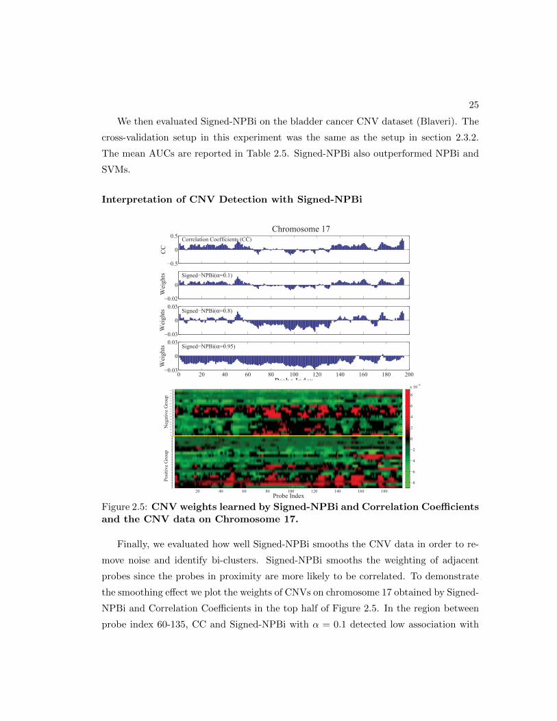
Figure 2.5: CNV weights learned by Signed-NPBi and Correlation Coefficientsand the CNV data on Chromosome 17.

Finally, we evaluated how well Signed-NPBi smooths the CNV data in order to re-

move noise and identify bi-clusters. Signed-NPBi smooths the weighting of adjacent

probes since the probes in proximity are more likely to be correlated. To demonstrate

the smoothing effect we plot the weights of CNVs on chromosome 17 obtained by Signed-

NPBi and Correlation Coefficients in the top half of Figure 2.5. In the region between

probe index 60-135, CC and Signed-NPBi with α = 0.1 detected low association with

26

tumor stage while Signed-NPBi with α = 0.8 and α = 0.95 detected a negative asso-

ciation. By examining the probe log-intensity-ratios across the patients shown in the

bottom half of Figure 2.5, we can confirm an amplification bi-cluster within the negative

group in this region which was not captured by CC or Signed-NPBi with small α. This

example shows the strength of Signed-NPBi to recover hidden bi-clusters in CNV data

by taking into account the dependence between nearby probes.

2.4 Discussion

In this study, we present network propagation models on signed graphs for feature selec-

tion and classification in high-dimensional microarray gene expression and copy number

variation data. Network propagation is a promising approach to explore modular struc-

tures such as clusters or bi-clusters hiding in high-dimensional data. The signed network

propagation models are a useful and important generalization for modeling positive and

negative relations in biological networks.

Since network propagation methods explore graph structures they are usually more

computationally demanding compared with other simpler feature selection methods.

Our future work will focus on developing approximations based on sparse structures to

improve efficiency. In addition, we also plan to further investigate other regularizations

of the signed graph Laplacian to improve the applicability and flexibility of the models.

Chapter 3

Network-based Survival Analysis

on Ovarian Cancer

3.1 Introduction

Survival analysis is routinely applied to analyzing microarray gene expressions to as-

sess cancer outcomes by the time to an event of interest [57–59]. By uncovering the

relationship between gene expression profiles and time to an event such as recurrence

or death, a good survival model is expected to achieve more accurate prognoses or

diagnoses, and in addition, to identify genes that are relevant to or predictive of the

events [60,61]. The Cox proportional hazard model [16] is widely used in survival anal-

ysis because of its intuitive likelihood modeling with both uncensored patient samples

and censored patient samples who are event-free by the last follow-up. Due to the high

dimensionality of typical microarray gene expressions, the Cox regression model is usu-

ally regularized with penalties such as L2 penalty in ridge regression [62–65], L1 Lasso

regularization [26,66–70] and L2 regularization in Hilbert space [71]. While those penal-

ties were designed as a statistical or algorithmic treatment for the high-dimensionality

problem, these Cox models are still prone to noise and overfitting to the low sample

size. An important prior information that has been largely ignored in survival analy-

sis is the modular relations among gene expressions. Groups of genes are co-expressed

under certain conditions or their protein products interact with each other to carry

out a biological function. It has been shown that protein-protein interaction network

27

28

or co-expressions can provide useful prior knowledge to remove statistical randomness

and confounding factors from high-dimensional data for several classification and regres-

sion models [72–75]. The major advantage of these network-based models is the better

generalization across independent studies since the network information is consistent

with the conserved patterns in the gene expression data. For example, previous studies

in [72, 74] discovered that more consistent signature genes of breast cancer metastasis

can be identified from independent gene expression datasets by network-based classifi-

cation models. The observations also motivated several graph algorithms for detecting

cancer causal genes in protein-protein interaction network [76,77].

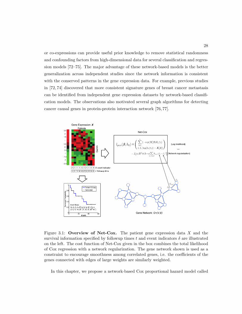
Figure 3.1: Overview of Net-Cox. The patient gene expression data X and thesurvival information specified by followup times t and event indicators δ are illustratedon the left. The cost function of Net-Cox given in the box combines the total likelihoodof Cox regression with a network regularization. The gene network shown is used as aconstraint to encourage smoothness among correlated genes, i.e. the coefficients of thegenes connected with edges of large weights are similarly weighted.

In this chapter, we propose a network-based Cox proportional hazard model called

29

Net-Cox to explore the co-expression or functional relation among gene expression fea-

tures for survival analysis. The relation between gene expressions are modeled by a gene

relation network constructed by co-expression analysis or prior knowledge of gene func-

tional relations. In the Net-Cox model, a graph Laplacian constraint is introduced as a

smoothness requirement on the gene features linked in the gene relation network. Figure

3.1 illustrates the general framework of Net-Cox for utilizing gene network information

in survival analysis. In the framework, the cost function of Net-Cox, shown in the box,

combines the total likelihood of Cox regression with a network regularization. The total

log-likelihood is a function of the linear regression coefficients β and the base hazard

h0(t) on each followup time t1, t2, ..., t10, represented by the likelihood ratios with the

patient gene expression data and the survival information specified by followup times

and event indicators. The gene network is either constructed with gene co-expression

information or a given gene functional linkage network. The gene network is modeled

as a constraint to encourage smoothness among correlated genes, for example gene i

and j in the network, such that the coefficients of the genes connected with edges of

large weights are similarly weighted. The cost function of Net-Cox can be solved by

alternating optimization of β and h0(t) by iterations. An algorithm that solves the

Net-Cox model in its dual representation is also introduced to improve the efficiency.

The complete model is explained in detail in Section 3.3.

In this study, we applied Net-Cox to identify gene expression signatures associated

with the outcomes of death and recurrence in the treatment of ovarian carcinoma.

Ovarian cancer is the fifth-leading cause of cancer death in US women [59]. Identifying

molecular signatures for patient survival or tumor recurrence can potentially improve

diagnosis and prognosis of ovarian cancer. Net-Cox was applied on three large-scale

ovarian cancer gene expression datasets [59, 78, 79] to predict survivals or recurrences

and to identify the genes that may be relevant to the events. Our study is fundamentally

different from previous survival analysis on ovarian cancer [59, 78–80], which are based

on univariate Cox regression. For example, in [59], gene expression profiles from 215

stage II-IV ovarian tumors from TCGA were used to identify a prognostic gene signature

(univariate Cox p−value < 0.01) for overall survival, including 108 genes correlated with

poor (worse) prognosis and 85 genes correlated with good (better) prognosis. In [78], a

Cox score is defined to measure the correlation between gene expression and survival.

30

The genes with a Cox score that exceeds an empirically optimized threshold in leave-

one-out cross-validation were reported as signature genes. Similarly, in [79] and [80], a

univariate Cox model was applied to identify association between gene expressions and

survival (univariate Cox p−value < 0.01). Our study is based on gene networks enriched

by co-expression and functional information and thus identifies subnetwork signatures

for predicting survival or recurrence in ovarian cancer treatment.

3.2 Results

In the experiments, Net-Cox was applied to analyze three ovarian cancer gene expres-

sion datasets listed in Table 3.1. Net-Cox (equation (3.4)) was compared with L2−Cox

(equation (3.1)) and L1−Cox (equation (3.2)) with performance evaluation in survival

prediction and gene signature identification for the analysis of patient survival and tu-

mor recurrence. First, for evaluation with a better focus on cancer-relevant genes, the

expressions of a list of 2647 genes that are previously known to be related to cancer

(Sloan-Kettering cancer genes) are used. On the data of these 2647 genes, Net-Cox,

L2−Cox and L1−Cox were evaluated by consistency of signature gene selection across

the three datasets, accuracy of survival prediction and assessment of statistical sig-

nificance. Next, more comprehensive experiments on all 7562 mappable genes were

conducted to identify novel signature genes associated with ovarian cancer. Finally, we

further analyzed and validated ovarian cancer signatures by an additional tumor array

experiment and literature survey. In all the experiments, gene co-expression networks

and a gene functional linkage network were used to derive the network constraints for

Net-Cox. The details of data preparation and the algorithms are described in Section

3.3.

Dataset (GEO ID) TCGA (N/A) Tothill (GSE9899) Bonome (GSE26712)Death # of Censored 227 160 24

# of Uncensored 277 111 129Recurrence # of Censored 241 86 N/A

# of Uncensored 263 185 N/A

Table 3.1: Patient samples in the ovarian cancer datasets. The number of pa-tients categorized by censoring and uncensoring for the death and recurrent events isreported in each dataset. Note that the Bonome dataset does not provide informationon recurrence.

31

3.2.1 Net-Cox identifies consistent signature genes across independent

datasets

To evaluate the generalization of the models, we first measured the consistency among

the signature genes selected from the three independent datasets by each method.

Specifically, we report the percentage of common genes in the three rank lists identified

by a method. This measurement assumes that even under the presence of biological

variability in gene expressions and patient heterogeneities in each dataset, genes that

are selected in multiple datasets are more likely to be true signature genes. Thus, higher

consistency across the datasets might indicate higher quality in gene selection.

Figure 3.2: Consistency of signature genes (Sloan-Kettering cancer genes).The x-axis is the number of selected signature genes ranked by each method. The y-axis is the percentage of the overlapped genes between the selected genes across theovarian cancer datasets. The plots show the results for the death outcome (A) and thetumor recurrence outcome (B).

In Figure 3.2, we plot the number of common genes among the first k (up to 300)

genes in the gene ranking lists from all of the three datasets for the death event and

two datasets (TCGA and Tothill) for the recurrence event. For the parameter setting

of Net-Cox, we fixed λ to be the optimal parameter in the five-fold cross-validation (see

Section Materials and Methods and report the results with α = 0.01 and 0.5. Since

the ranking lists of Net-Cox with α = 0.95 are nearly identical to those of L2−Cox, they

are not reported for better clarity in the figure. The first observation is that the gene

32

rankings by Net-Cox are more consistent than those by L2−Cox and L1−Cox at all

the cutoffs. Moreover, Net-Cox with α = 0.01 identified more common signature genes

than Net-Cox with α = 0.5. For example, for the tumor recurrence outcome, Net-Cox

(Co-expression) with α = 0.01 and 0.5 identified 36 and 29 common genes among the

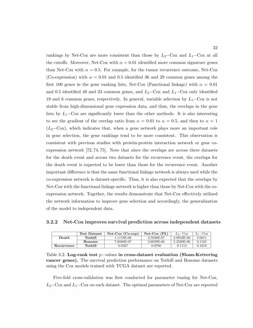
first 100 genes in the gene ranking lists, Net-Cox (Functional linkage) with α = 0.01

and 0.5 identified 49 and 23 common genes, and L2−Cox and L1−Cox only identified

19 and 6 common genes, respectively. In general, variable selection by L1−Cox is not

stable from high-dimensional gene expression data, and thus, the overlaps in the gene

lists by L1−Cox are significantly lower than the other methods. It is also interesting

to see the gradient of the overlap ratio from α = 0.01 to α = 0.5, and then to α = 1

(L2−Cox), which indicates that, when a gene network plays more an important role

in gene selection, the gene rankings tend to be more consistent. This observation is

consistent with previous studies with protein-protein interaction network or gene co-

expression network [72, 74, 75]. Note that since the overlaps are across three datasets

for the death event and across two datasets for the recurrence event, the overlaps for

the death event is expected to be lower than those for the recurrence event. Another

important difference is that the same functional linkage network is always used while the

co-expression network is dataset-specific. Thus, it is also expected that the overlaps by

Net-Cox with the functional linkage network is higher than those by Net-Cox with the co-

expression network. Together, the results demonstrate that Net-Cox effectively utilized

the network information to improve gene selection and accordingly, the generalization

of the model to independent data.

3.2.2 Net-Cox improves survival prediction across independent datasets

Test Dataset Net-Cox (Co-exp) Net-Cox (FL) L2−Cox L1−CoxDeath Tothill 1.1178E-06 2.5938E-07 2.9932E-06 0.0011

Bonome 7.6088E-07 3.6039E-06 5.2590E-06 0.1165Recurrence Tothill 0.0567 0.0786 0.1115 0.4219

Table 3.2: Log-rank test p−values in cross-dataset evaluation (Sloan-Ketteringcancer genes). The survival prediction performance on Tothill and Bonome datasetsusing the Cox models trained with TCGA dataset are reported.

Five-fold cross-validation was first conducted for parameter tuning for Net-Cox,

L2−Cox and L1−Cox on each dataset. The optimal parameters of Net-Cox are reported

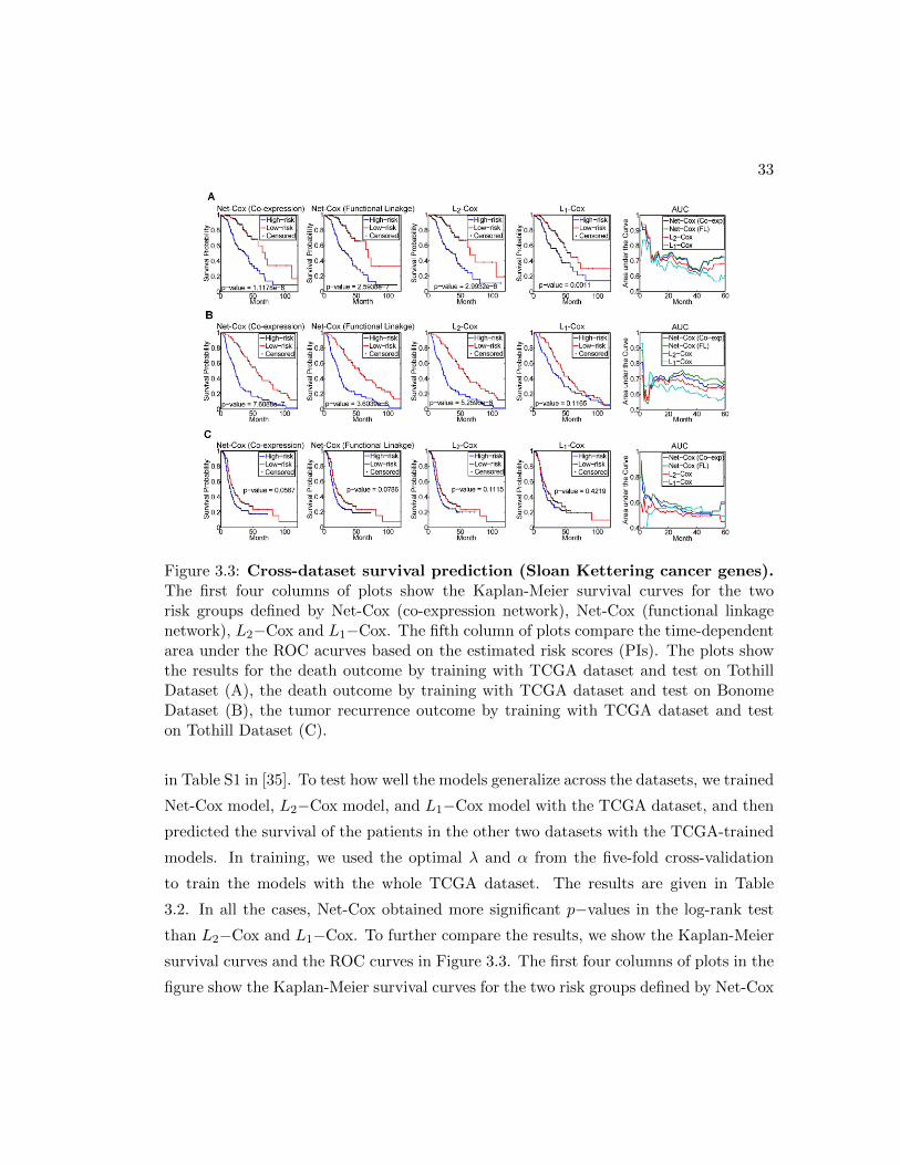
33

Figure 3.3: Cross-dataset survival prediction (Sloan Kettering cancer genes).The first four columns of plots show the Kaplan-Meier survival curves for the tworisk groups defined by Net-Cox (co-expression network), Net-Cox (functional linkagenetwork), L2−Cox and L1−Cox. The fifth column of plots compare the time-dependentarea under the ROC acurves based on the estimated risk scores (PIs). The plots showthe results for the death outcome by training with TCGA dataset and test on TothillDataset (A), the death outcome by training with TCGA dataset and test on BonomeDataset (B), the tumor recurrence outcome by training with TCGA dataset and teston Tothill Dataset (C).

in Table S1 in [35]. To test how well the models generalize across the datasets, we trained

Net-Cox model, L2−Cox model, and L1−Cox model with the TCGA dataset, and then

predicted the survival of the patients in the other two datasets with the TCGA-trained

models. In training, we used the optimal λ and α from the five-fold cross-validation

to train the models with the whole TCGA dataset. The results are given in Table

3.2. In all the cases, Net-Cox obtained more significant p−values in the log-rank test

than L2−Cox and L1−Cox. To further compare the results, we show the Kaplan-Meier

survival curves and the ROC curves in Figure 3.3. The first four columns of plots in the

figure show the Kaplan-Meier survival curves for the two risk groups defined by Net-Cox

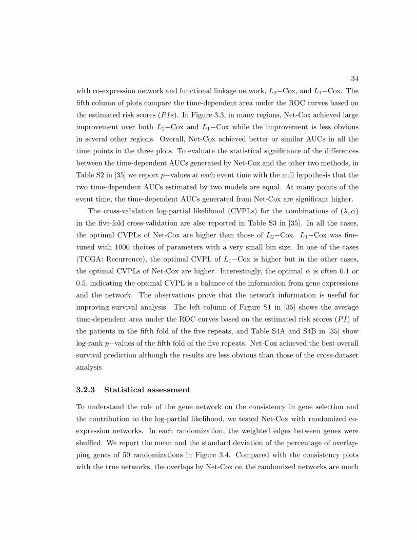
34

with co-expression network and functional linkage network, L2−Cox, and L1−Cox. The

fifth column of plots compare the time-dependent area under the ROC curves based on

the estimated risk scores (PIs). In Figure 3.3, in many regions, Net-Cox achieved large

improvement over both L2−Cox and L1−Cox while the improvement is less obvious

in several other regions. Overall, Net-Cox achieved better or similar AUCs in all the

time points in the three plots. To evaluate the statistical significance of the differences

between the time-dependent AUCs generated by Net-Cox and the other two methods, in

Table S2 in [35] we report p−values at each event time with the null hypothesis that the

two time-dependent AUCs estimated by two models are equal. At many points of the

event time, the time-dependent AUCs generated from Net-Cox are significant higher.

The cross-validation log-partial likelihood (CVPLs) for the combinations of (λ, α)

in the five-fold cross-validation are also reported in Table S3 in [35]. In all the cases,

the optimal CVPLs of Net-Cox are higher than those of L2−Cox. L1−Cox was fine-

tuned with 1000 choices of parameters with a very small bin size. In one of the cases

(TCGA: Recurrence), the optimal CVPL of L1−Cox is higher but in the other cases,

the optimal CVPLs of Net-Cox are higher. Interestingly, the optimal α is often 0.1 or

0.5, indicating the optimal CVPL is a balance of the information from gene expressions

and the network. The observations prove that the network information is useful for

improving survival analysis. The left column of Figure S1 in [35] shows the average

time-dependent area under the ROC curves based on the estimated risk scores (PI) of

the patients in the fifth fold of the five repeats, and Table S4A and S4B in [35] show

log-rank p−values of the fifth fold of the five repeats. Net-Cox achieved the best overall

survival prediction although the results are less obvious than those of the cross-dataset

analysis.

3.2.3 Statistical assessment

To understand the role of the gene network on the consistency in gene selection and

the contribution to the log-partial likelihood, we tested Net-Cox with randomized co-

expression networks. In each randomization, the weighted edges between genes were

shuffled. We report the mean and the standard deviation of the percentage of overlap-

ping genes of 50 randomizations in Figure 3.4. Compared with the consistency plots

with the true networks, the overlaps by Net-Cox on the randomized networks are much

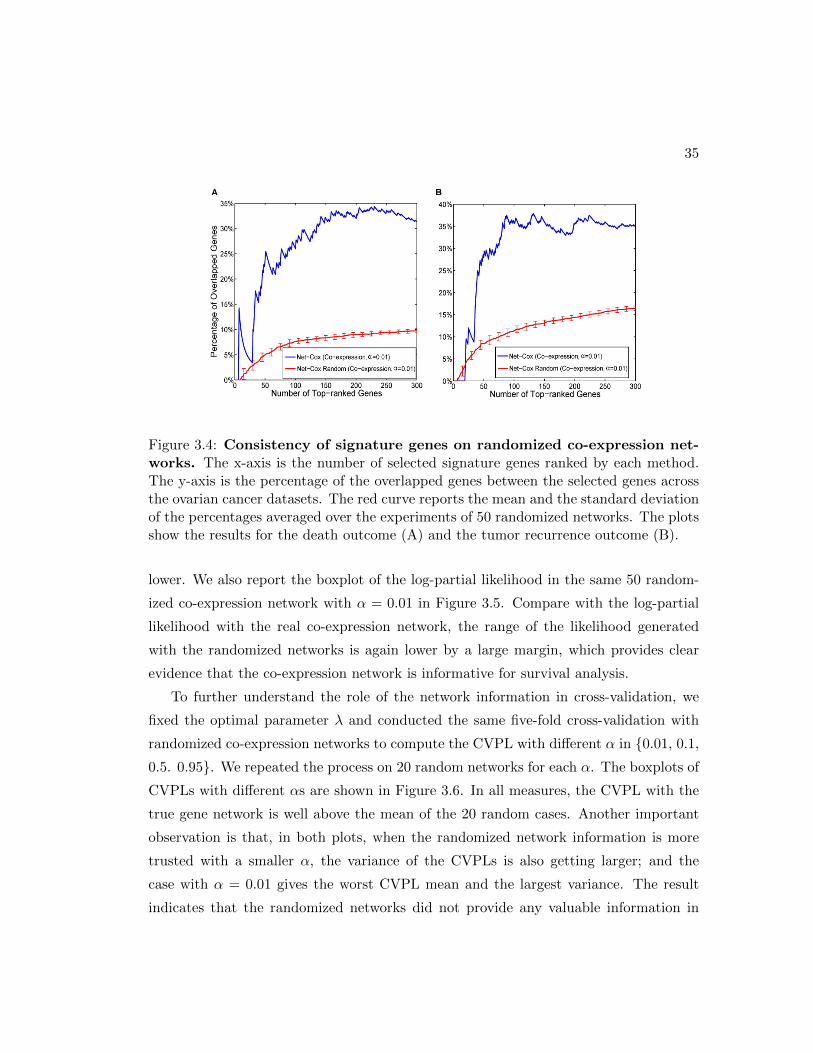
35

Figure 3.4: Consistency of signature genes on randomized co-expression net-works. The x-axis is the number of selected signature genes ranked by each method.The y-axis is the percentage of the overlapped genes between the selected genes acrossthe ovarian cancer datasets. The red curve reports the mean and the standard deviationof the percentages averaged over the experiments of 50 randomized networks. The plotsshow the results for the death outcome (A) and the tumor recurrence outcome (B).

lower. We also report the boxplot of the log-partial likelihood in the same 50 random-

ized co-expression network with α = 0.01 in Figure 3.5. Compare with the log-partial

likelihood with the real co-expression network, the range of the likelihood generated

with the randomized networks is again lower by a large margin, which provides clear

evidence that the co-expression network is informative for survival analysis.

To further understand the role of the network information in cross-validation, we

fixed the optimal parameter λ and conducted the same five-fold cross-validation with

randomized co-expression networks to compute the CVPL with different α in 0.01, 0.1,

0.5. 0.95. We repeated the process on 20 random networks for each α. The boxplots of

CVPLs with different αs are shown in Figure 3.6. In all measures, the CVPL with the

true gene network is well above the mean of the 20 random cases. Another important

observation is that, in both plots, when the randomized network information is more

trusted with a smaller α, the variance of the CVPLs is also getting larger; and the

case with α = 0.01 gives the worst CVPL mean and the largest variance. The result

indicates that the randomized networks did not provide any valuable information in

36

Figure 3.5: Statistical analysis of log-partial likelihood. The optimal λ was fixedand α = 0.01 is set to allow better evaluation of the network information. The log-partial likelihood computed by Net-Cox on the real co-expression network and on therandomized co-expression network are reported against tumor recurrence in the TCGAand Tothill datasets. The stars represent the results with the real co-expression net-works, and the boxplots represent the results with the randomized networks.

survival prediction. In contrast, with the true gene network, CVPLs generated from

α = 0.01 and α = 0.1 are much higher than the ones from α = 0.95 and L2−Cox

(α = 1). Again, these results convincingly support the importance of using the network

information in survival prediction.

3.2.4 Evaluation by whole gene expression data

Besides the 2647 Sloan-Kettering genes, all the 7562 mappable genes were also tested

to evaluate Net-Cox, L2−Cox and L1−Cox by consistency of signature gene selection

across the three datasets and accuracy of survival prediction in similar experiments.

For the signature gene consistency, Figure S2 in [35] reports the percentage of common

genes identified by each method in the ranking lists from the datasets. For the cross-

dataset validation, Table S5 in [35] shows the log-rank test p−values by training the

TCGA datasets and test on the other two datasets, and Figure S3 in [35] shows the

Kaplan-Meier survival curves for the two risk groups defined by Net-Cox, L2−Cox

and L1−Cox and compares the time-dependent area under the ROC curves. For the

37

Figure 3.6: Statistical analysis of cross-validation log-partial likelihood(CVPL). The optimal λ was fixed and α is varied from 0.01 to 1. The CVPL offive-fold cross-validation on the real co-expression network and on the randomized co-expression network are reported against tumor recurrence in TCGA dataset (A) andTothill dataset (B). The stars represent the results with the real co-expression networks,and the boxplots represent the results with the randomized networks.

five-fold cross-validation, the right column of Figure S1 in [35] shows the average time-

dependent area under the ROC curves based on the estimated risk scores (PI) of the

patients in the fifth fold of the five repeats, and Table S4C and S4D in [35] report log-

rank test p−values of the fifth fold of the five repeats. Overall, similar observations are

made in experimenting with all the genes, though the improvements are less significant

compared with the results by experimenting with the Sloan-Kettering cancer genes. One

possible explanation is that, since the genes in the Sloan-Kettering gene list are more

cancer relevant, the gene expressions may be more readily integrated with the network

information.

3.2.5 Signature genes are ECM components or modulators

To analyze the signature genes identified by Net-Cox and L2−Cox, we created consensus

rankings across the three datasets by re-ranking the genes with the lowest rank by Net-

Cox and L2−Cox in the three datasets. Specifically, for each gene, a new ranking score

is assigned as the lowest of its ranks in the three datasets, and then, all the genes were

re-ranked by the new ranking score. The top-15 genes selected by Net-Cox and L2−Cox

in the consensus rankings are shown in Table 3.3. For the death outcome, nine signature

38Death Recurrence

Net-Cox (Co-exp) Net-Cox (FL) L2−Cox Net-Cox (Co-exp) Net-Cox (FL) L2−CoxFBN1 COL11A1 COL11A1 COL5A2 COL11A1 COL11A1

COL5A2 MFAP4 FABP4 COL1A1 COL10A1 NLRP2VCAN TIMP3 MFAP4 COL5A1 CRYAB CRYABSPARC MFAP5 COMP THBS2 NPY PTX3AEBP1 COL5A2 BCHE FAP IGF1 COL10A1AOC3 THBS2 FAP COL3A1 COMP CXCL12

COL3A1 FAP COL5A2 COL11A1 KLK5 THBS2THBS2 CXCL12 MFAP5 FBN1 THBS2 NPY

PLN AEBP1 TIMP3 VCAN PI3 KLK5ADIPOQ RYR3 THBS2 INHBA CXCL12 COMPCOL5A1 LOX HOXA5 CTSK MFAP5 FAPCNN1 COL5A1 NUAK1 COL1A2 VGLL1 MFAP5

COL6A2 EDNRA COL5A1 SPARC CCL11 PI3COL1A2 NUAK1 SLIT2 AEBP1 EPHB1 PDGFD

DCN LPL CXCL12 SERPINE1 OXTR CHRDL1

Table 3.3: Top-15 signature genes. The table lists the genes with over-expressionindicating higher hazard of death or recurrence, identified by Net-Cox and L2−Cox inthe consensus ranking across the three datasets.

genes, FBN1, VCAN, SPARC, ADIPOQ, CNN1, DCN, LOX, EDNRA, LPL, known to

be related to ovarian cancer [81–89] are only discovered by Net-Cox. Among the ten

common genes highly ranked by both Net-Cox and L2−Cox, three are collagen genes,

and MFAP5, TIMP3, THBS2, and CXCL12 are previously known to be relevant to

ovarian cancer [90–93]. For the recurrence outcome, there are eleven common signature

genes detected by both Net-Cox and L2−Cox. Net-Cox identified six additional ovarian

cancer related signature genes [81–83,94–96].

Gene Sym Reference DescriptionADIPOQ [84] ADIPOQ 45T/G and 276G/T polymorphisms is associated with susceptibility to polycystic ovary syndrome(PCOS).CCL11 [96] CCL11 signaling plays an important role in proliferation and invasion of ovarian carcinoma cells.CNN1 [85] CCN1 plays a role in ovarian carcinogenesis by stimulating survival and antiapoptotic signaling pathways.

CRYAB [97] Low expression of lens crystallin CRYAB is significantly associated with adverse ovarian patient survival.CXCL12 [93] CXCL12 and vascular endothelial growth factor synergistically induce neoangiogenesis in human ovarian cancers.

DCN [86] Ovarian DCN is an ECM-associated component, which acts as a multifunctional regulator of GF signaling in the primate ovary.EDNRA [88] Endothelin peptide is produced before ovulation and the contractile action of EDN2 within the ovary is facilitated via EDNRA.FBN1 [81] FBN1 controls the bioactivity of TGFβs and associate with polycystic ovary syndrome (PCOS).IGF1 [95] Ovarian follicular growth is controlled by the production of intraovarian growth regulatory factors such as IGF1.

INHBA [94] INHBA is the promoter of TAF4B; TAF4B in the ovary is essential for proper follicle development.LOX [87] Inhibition of LOX expression portends worse clinical parameters for ovarian cancer.LPL [89] LPL is differentially expressed between preoperative samples of ovarian cancer patients and those of healthy controls.

MFAP5 [90] MAGP2 is an independent predictor of survival in advanced serous ovarian cancer.NPY [98] NPY receptor is expressed in human primary ovarian neoplasms.

SPARC [83] SPARC expression in ovarian cancer cells is inversely correlated with the degree of malignancy.THBS2 [92] In ovarian cancer an aberrant methylation process is responsible for down-regulation of THBS2.TIMP3 [91] TIMP2 and TIMP3 play functional role in LPA-induced invasion as negative regulators.VCAN [82] VCAN V1 isoform is overexpressed in ovarian cancer stroma compared with normal ovarian stroma and ovarian cancer cells.

Table 3.4: Literature review of the candidate ovarian cancer genes. This tablereports the citations that describe relevance of the signature genes with over-expressionindicating higher hazard of death or recurrence, identified by Net-Cox across the threedatasets.

The intersection of the 60 genes identified by Net-Cox in Table 3.3 contains 41

39

unique genes. We performed a literature survey of the 41 genes, out of which eigh-

teen are supported by literature to be related to ovarian cancer shown in Table 3.4.

Most of the genes whose over-expression is associated with poor outcome are stromal

or extracellular-related proteins. The genes such as VCAN, TIMP3, THBS2, ADIPOQ,

PARC, NPY, MFAP5, DCN, LOX, FBN1, EDNRA, and CXCL12 are either compo-

nents or modulators of extracellular matrix. In particular, LOX protein is involved in

extracellular matrix remodeling by cross-linking collagens. Extracellular matrix remod-

eling through over-expression of collagens has been shown to contribute to platinum

resistance, and platinum resistance is the main factor in chemotherapy failure and poor

survival of ovarian cancer patients. Therefore, the identification of these extracellular

matrix proteins as biomarkers of early recurrence and poor survival outcome in patients

with ovarian cancer is consistent with the suggested pathobiological role of some of these

proteins in platinum resistance.

3.2.6 Enriched PPI subnetworks and GO terms

The top-100 signature genes with the largest regression coefficients by Net-Cox and

L2−Cox learned from the TCGA dataset were mapped to the human protein-protein

interaction (PPI) network obtained from HPRD [10] and also analyzed with DAVID

functional annotation tool [51]. We report the densely connected PPI subnetworks con-

structed from the 100 genes selected by Net-Cox in Figure 3.7. Compared with the PPI

subnetworks generated from the 100 genes selected by L2−Cox, which contain 10 genes

in the death subnetwork and 6 genes in the recurrence subnetworks (shown in Figure

S4 in [35]), the subnetworks are both larger and denser. The subnetworks identified

from the co-expression networks in Figure 3.7(A) are also larger than the subnetworks

identified by the functional linkage network in Figure 3.7(B) although many genes are

shared. In the recurrence subnetworks, DCN, THBS1, and THBS2 are members of the

TGF−β signaling KEGG pathway, and FBN1 controls the bioactivity of TGFβs and

relates to polycystic ovary syndrome [81]. In addition, ten genes are members of the

focal adhesion KEGG pathway. These results point to a possibility that extracellular

matrix signaling through focal adhesion complexes may constitute a pathway by which

tumor cells escape chemotherapy and produce recurrence in chemotherapy [99]. Nine

genes in the death subnetworks are members of the extracellular matrix(ECM)-receptor

40

Figure 3.7: Protein-Protein interaction subnetworks of signature genes iden-tified by Net-Cox on the TCGA dataset. (A) The PPI subnetworks identified byNet-Cox on the co-expression network. (B) The PPI subnetworks identified by Net-Coxon the functional linkage network.

interaction KEGG pathway, and eighteen genes are annotated as ECM component. It

was shown that ECM acts as a model substratum for the preferential attachment of

human ovarian tumor cells in vitro [100]. FOS and JUN constitutes a nuclear signal-

ing components downstream of extracellular signal-regulated kinases (ERK1/2) that

are mediators of growth factor and adhesion-related signaling pathways [101]. In addi-

tion, the genes are also enriched by regulation of gene expression, positive regulation

of cellular process, developmental process, transcription regulator activity, and growth

factor binding, all of which are well-known cancer relevant functions. The significantly

enriched GO functions are listed in Table S6 and Table S7 in [35]. Extracellular matrix,

41

extracellular region, and extracellular structure organization are consistently the most

significantly enriched in the analysis.

3.2.7 Laboratory experiment validates FBN1’s role in chemo-resistance

FBN1 was ranked 1st and 8th by Net-Cox with co-expression network in death and re-

currence outcomes while L2−Cox only ranked FBN1 at 27th and 42nd, respectively. It

is interesting to note that in the PPI subnetworks in Figure 3.7(A), FBN1 is connected

with VCAN and DCN, both of which bear the annotation of extracellular matrix. The

dense subnetwork boosted the ranking of FBN1 when Net-Cox was applied. We fur-

ther validated the role of FBN1 in ovarian cancer recurrence using tumor microarrays

(TMAs) consisting of a cohort of 78 independent patients (see Section Materials and

Methods). The expression level of FBN1 in ovarian cancer was scored by one observer

who is blinded to the clinical outcome and described as: absent (0), moderate (1), and

high (2) as illustrated by Figure 3.8.

Figure 3.8: Representative photomicrographs showing various levels of FBN1expression in ovarian tumor arrays. The brown regions are stromal area showingexpression of FBN1.

In Figure S5A in [35], the Kaplan-Meier survival curve shows the recurrence for

groups by the FBN1 staining scores. At the initial 12 month, there is no difference in

the recurrence rate between the groups with high and low FBN1 staining. After 12

month, the recurrence rate is lower in the low staining group. The similar patterns are

also observed in the re-examination of the gene expression datasets in Figure S5B-E

in [35]. Except the TCGA dataset on the Affymetrix platform (Figure S5E in [35]),

the pattern is clearly observed on the other two platforms, exon arrays and Agilent

arrays. The discrepancy in the Affymetrix data could be related to data pre-processing

or experimental noise. The plots suggest that FBN1 plays a role on platinum-sensitive

42

ovarian cancer, and it could be developed as a target for platinum-sensitive patients

with high FBN1 expression after about 12 month of the treatment.

In the context of ovarian cancer treatment, a platinum-sensitive patient group can

be defined as the group of patients who was free of recurrence or developed a recurrence

after k month of the treatment, where k ≥ 14 depends on the treatment plan and the

follow-up. To better evaluate the role of FBN1, we plot the Kaplan-Meier survival curve

only for the platinum-sensitive patients in Figure 3.9, i.e. we removed all the patients

who developed recurrence before k month and considered the follow-ups up to 72 month

after the treatment. Due to the small sample size of the Mayo Clinic data, we set k = 14

while k = 20 for the gene expression datasets. In Figure 3.9A, the difference between the

survival curves of low FBN1 staining and high staining patient groups is more significant.

Similarly, Figure 3.9B-E show the survival curves for the platinum-sensitive patients

for groups by the expression value of FBN1 in gene expression datasets. Compare to

the matched curves in Figure S5 in [35], the log-rank test p−values are more significant

except the TCGA dataset on the Affymetrix platform. Overall, the observations strongly

support the hypothesized role of FBN1 in platinum-sensitive ovarian cancer patients.

3.3 Materials and Methods

3.3.1 Gene relation network construction

We denote gene relation network by G = (V ,W ), where V is the vertex set, each

element of which represents a gene, and W is a |V |× |V | positively weighted adjacency

matrix. D is a diagonal matrix with Dii =∑

jWij and S = D−12WD−

12 is the

normalized weighted adjacency matrix by dividing the square root of the column sum

and the row sum. Two gene relation networks were used with Net-Cox, the gene co-

expression network and the gene functional linkage network.

Gene co-expression network: A gene co-expression network was generated from a gene

correlation graph model. In the weighted adjacency matrixW , each Wij is the reliability

score [102] based on the absolute value of the Pearson’s correlation coefficients between

genes vi and vj , calculated as Wij = 1Ri,j×Rj,i , where Ri,j is gene vi’s rank among all

the genes with respect to the correlation with gene vj and Rj,i is gene vj ’s rank with

43

Figure 3.9: Kaplan-Meier survival plots on FBN1 expression groups. (A)Kaplan-Meier survival curve of recurrence between 14 to 72 month by FBN1 staininggroups on Mayo Clinic dataset. (B) Kaplan-Meier survival curve of recurrence between20 to 72 month by the expression of FBN1 on Tothill dataset. (C)-(E) Kaplan-Meiersurvival curves of recurrence between 20 to 72 month by the expression of FBN1 onTCGA dataset with AgilentG4502A platform, HuEx-1 0-st-v2 platform, and AffymetrixHG-U133A platform, respectively. In plot(A), the groups with FBN1 staining score 1and 2 are combined into the high-expression group. In plots(B)-(E), the patients aredivided into two groups of the same size by the expression of FBN1.

respect to the correlation with gene vi. Note that the gene co-expression network is

directly inferred from the gene expression dataset. Thus, a gene co-expression network

is specific to the dataset used for computing the co-expression network.

Gene functional linkage network: A human gene functional linkage network was con-

structed by a regularized Bayesian integration system [103]. The network contains maps

of functional activity and interaction networks in over 200 areas of human cellular bi-

ology with information from 30,000 genome-scale experiments. The functional linkage

network summarizes information from a variety of biologically informative perspectives:

prediction of protein function and functional modules, cross-talk among biological pro-

cesses, and association of novel genes and pathways with known genetic disorders [103].

Each edge in the network is weighted between [0,1] to quantify the functional relation

between two genes. Thus, the functional linkage network provides much more compre-

hensive information than Human protein-protein interaction network, which was more

frequently used as the network prior knowledge.

44

3.3.2 Gene expression dataset preparation

Three independent microarray gene expression datasets for studying ovarian carcinoma

were used in the experiments [59, 78, 79]. The information of patient samples in each

dataset is given in Table 3.1. All the three datasets were generated by the Affymetrix

HG-U133A platform. The raw .CEL files of two datasets were downloaded from GEO

website (Tothill: GSE9899) and (Bonome: GSE26712) [78, 79]. The TCGA dataset

was downloaded from The Cancer Genome Atlas data portal [59]. The raw files were

normalized by RMA [48]. After merging probes by gene symbols and removing probes

with no gene symbol, a total of 7562 unique genes were derived from the 22,283 probes

and overlapped with the functional linkage network for this study. Note that the Bonome

dataset does not provide information on recurrence. Thus, only TCGA and Tothill

datasets were used for studying recurrence while all the three datasets were used for

studying death. In cross-dataset validation, the batch effects among the three datasets

were removed by applying ComBat [104]. Besides testing all the genes, for a better

focus on genes that are more likely to be cancer relevant, we derived a set of 2647 genes

from the cancer gene list compiled by Sloan-Kettering Cancer Center (SKCC) [105].

The TCGA datasets with AgilentG4502A platform (gene expression array) and

HuEx-1 0-st-v2 (exon expression array) were used to evaluate the signature gene FBN1

in Figure 3.9. The processed level 3 data with expression calls for gene/exon were

downloaded from the TCGA data portal.

3.3.3 Cox proportional hazard model

In the analysis of microarray gene expressions, the number of gene features p is larger

than the number of subjects n by several magnitudes (pn). Fitting the Cox regression

model proposed in section 1.2.2 will lead to large regression coefficients, which are not

reliable. One possible solution is to introduce a L2−norm constraint to shrink regres-

sion coefficients estimates towards zero [62, 65]. In the L2−Cox model, the regression

coefficients are estimated by maximizing the penalized total log-likelihood:

lpen(β, h0) =n∑i=1



]− 1

2λ

p∑j=1

βj2, (3.1)

45

where λ∑p

j=1 βj2 is the penalty term and λ is the parameter controlling the amount

of shrinkage. Another possibility is to introduce a L1−norm constraint for variable

selection [26, 66]. The L1−Cox model penalizes the log-partial likelihood (equation

(1.3)) by λ∑p

j=1 |βj | leading to:

plpen(β) =

n∑i=1

δi

X ′iβ − log ∑j∈R(ti)

exp(X ′jβ)

− λp∑j=1

|βj |. (3.2)

In our experiments, R package “glmnet” [106] was used in the implementation of

L1−Cox.

3.3.4 Network-constrained Cox regression (Net-Cox)

We introduce a network-constraint to the Cox model as follows,

lpen(β, h0) = l(β, h0)− 1

2λβ′[(1− α)L+ αI]β, (3.3)

where L is a positive semidefinite matrix derived from network information, I is an

identity matrix, and λ is the parameter controlling the weighting between the total

likelihood and the network constraint. α ∈ (0, 1] is another parameter weighting the

network matrix and the identity matrix in the network constraint. For convenience, we

define Γ = (1− α)L+ αI and rewrite the object function as

lpen(β, h0) =n∑i=1



]− 1

2λβ′Γβ. (3.4)

The term λβ′[(1− α)L+ αI]β in equation (3.3) is a network Laplacian constraint to

encode prior knowledge from a network. Given a normalized graph weight matrix S,

we assume that co-expressed (related) genes should be assigned similar coefficients by

defining the following cost term over the coefficients,

Ψ(β) =1

2

p∑i,j=1

Si,j(βi − βj)2

= β′(I − S)β = β′Lβ. (3.5)

As illustrated in Figure 3.1, the Laplacian constraint encourages a smoothness among

the regression coefficients in the network. Specifically, for any pair of genes connected

46

by an edge, there is a cost proportional to both the difference in the coefficients and

the edge weight. Large difference between coefficients on two genes connected with a

highly weighted edge will result in a large cost in the objective function. Thus, the

objective function encourages assigning similar weights to genes connected by edges of

larger weights. By adding an additional L2−norm constraint to Ψ(β) weighted by α,

we obtain the network constraint (1 − α)β′Lβ + α|β|2=β′Γβ in equation (3.3) and

(3.4). The L2−norm of β similarly regularizes the uncertainty in the network con-

straint, which could have a singular Hessian matrix, and the α parameter balances

between the L2−norm and the “Laplacian-norm”. The smaller the α parameter, the

more importance put on the network information.

3.3.5 Alternating optimization algorithm

The objective function defined by equation (3.4) can be solved by alternating optimiza-

tion of β and h0(t). The maximization with respect to β is done by Newton-Raphson

method. The derivative of equation (3.4) is

∂lpen(β, h0)

∂β=

n∑i=1

[δi − exp(X ′iβ)H0(ti)

]Xi − λΓβ

= X′∆− λΓβ, (3.6)

where ∆i = δi − exp(X ′iβ)H0(ti), and the second derivative is

∂2lpen(β, h0)

∂β∂β′= −

[n∑i=1

exp(X ′iβ)H0(ti)XiX′i

]− λΓ

= −X′DX − λΓ, (3.7)

where D is the diagonal matrix with Dii = exp(X ′iβ)H0(ti). Thus, the full algorithm

to solve the Net-Cox model is given below.

47

1 Initialization: β = 0; Compute L = I − S.

2 Do until convergence

(a) Do Newton-Raphson iteration

i. Compute the first derivative l′pen(β, h0) =∂lpen(β,h0)

∂β

ii. Compute the second derivative l′′pen(β, h0) =∂2lpen(β,h0)

∂β∂β′

iii. Update β = β − l′′pen(β, h0)−1l′pen(β, h0)

(b) Update h0(ti) = 1/∑

j∈R(ti)exp(X ′jβ)

3 Return β

Using Newton-Raphson method to update β requires inverting the Hessian matrix,

which is time consuming and often inaccurate. An alternative approach is to reduce the

covariant space from p to n, which relates to singular value decomposition that exploits

the low rank of the gene expression matrix X [65]. The equation

∂lpen(β, h0)

∂β=

n∑i=1

[δi − exp(X ′iβ)H0(ti)

]Xi − λΓβ

= X′∆− λΓβ = 0 (3.8)

implies that β = Γ−1X ′η for some η. Thus, the dual form of equation (3.4) with

respect to η is

lpen(η, h0) =

n∑i=1

−exp(Z ′iη)H0(ti) + δi

[log(h0(ti)) +Z ′iη

]− 1

2λη′Zη (3.9)

with Zi = XΓ−1Xi and Z = XΓ−1X′. In its dual form, it is clear that the new object

function (3.9) is equivalent to equation (3.4) but the problem dimension is reduced from

p to n.

3.3.6 Cross validation and parameter tuning

To determine the optimal tuning parameters λ and α, we performed five-fold cross-

validation following the procedure proposed by [65] on each of the three datasets. In

the cross-validation, four folds of data are used to build a model for validation on the

48

fifth fold, cycling through each of the five folds in turn, and then the (λ, α) pair that

maximizes the cross-validation log-partial likelihood (CVPL) are chosen as the optimal

parameters. CVPL is defined as

CV PL(λ, α) =

5∑i=1

[pl(β

(−i)(λ,α))− pl

(−i)(β(−i)(λ,α))

](3.10)

where β(−i) is the optimal β learned from the data without the ith fold. In the equation,

pl() denotes the log-partial likelihood on all the samples and pl(−i)() denotes the log-

partial likelihood on samples excluding the ith fold. We performed a grid search for the

optimal (λ, α) maximizing the sum of the contributions of each fold to the log-partial

likelihood in CVPL. In particular, λ was chosen from 1e-5, 1e-4, 1e-3, 1e-2, 1e-1, 1(λs larger than 1 do not change the ranking of β anymore), and α was chosen from

0.01, 0.1, 0.5, 0.95. Note that, when α = 1, Net-Cox ignores the network information

and is reduced to L2−Cox. For L1−Cox, the optimal λ was chosen from 1000 λs by the

“glmnet” parameter setting with the largest CVPL.

3.3.7 Evaluation measures

The Log-rank test [107] and time-dependent ROC [108] were used to evaluate mea-

surements of the prediction performance by a survival model. For the gene expression

profile X in the test set, the prognostic indexes PI=X′β is computed, where β is the

regression coefficients of the survival model, to rank the patients by descending order.

We assigned the top 40% of the patients as the high-risk group and the bottom 40% as

the low-risk group.

The Log-rank test is a statistical hypothesis test for comparison of two Kaplan-

Meier survival curves with the null hypothesis that there is no difference between the

population survival curves, i.e. the probability of an event occurring at any time point

is the same for each population. The test statistic is compared with a χ2 distribution

with one degree of freedom to derive the significance p−value reflecting the difference

between two survival curves. The log-rank test only evaluates whether the patients

are assigned to the “right group” but not how well the patients are ranked within the

group by examining the PI. A more refined approach is afforded by the time-dependent

ROC curves [108,109]. Time-dependent ROC curves evaluate how well the PI classifies

49

the patients into high-risk and low-risk prognosis groups. Letting f(X)=X′β, we can

define time-dependent sensitivity and specificity functions at a cutoff point c as

sensitivity[c, t|f(X)] = Pr f(X) > c|δ(t) = 1 ,

specificity[c, t|f(X)] = Pr f(X) ≤ c|δ(t) = 0

with δ(t) being the event indicator at time t [109]. The corresponding ROC curve for any

time t, ROC[t|f(X)], is the plot of sensitivity[c, t|f(X)] versus 1−specificity[c, t|f(X)]

with different cutoff point c. AUC[t|f(X)] is denoted as the area under theROC[t|f(X)]

curve. A larger AUC[t|f(X)] indicates better prediction of time to event at time t, as

measured by sensitivity and specificity evaluated at time t. We plot the AUCs at each

time t to compare the methods.

To select gene variables in the multi-variate scenario by Net-Cox and L2−Cox, we

ranked the genes by the magnitude of the coefficients β. To justify this simple ranking

method, we examined the relation between the magnitude of the coefficients for each

gene and the contribution of the gene to the log-partial likelihood in Figure S6 in [35].

It is clear in the plot that the genes towards the two tails of the ranking list contributes

most of the likelihood, and the proportion of the contributions are consistent with the

ranking. For L1−Cox, we ranked the genes by the first-time jump into the active set

when decreasing the tuning parameter λ in the solution path.

3.3.8 Tumor array preparation

With approval by the Mayo Clinic Institutional Review Board, archived ovarian ep-

ithelial tumor specimens from patients with advanced-stage, high-grade serous, or en-

dometrioid tumors obtained prior to exposure to any chemotherapy were utilized to

construct the TMA array. The array was constructed using a custom-fabricated device

that utilizes a 0.6-mm tissue corer and a 240-capacity recipient block. Triplicate cores

from each tumor were included, as were cores of liver as fiducial markers and controls

for immunohistochemistry reactions. Five-micrometer-thick sections were cut from the

TMA blocks. Immunohistochemistry was performed essentially as described in [110].

Sections of tissue arrays were deparaffinized, rehydrated, and submitted to antigen re-

trieval by a steamer for 25 minutes in target retrieval solution (Dako, Carpinteria, CA,

USA). Endogenous peroxide was diminished with 3% H2O2 for 30 min. Slides were

50

blocked in protein block solution for 30 min and then blocked with avidin and biotin

for 10 min each, followed by overnight incubation with 1:1000 diluted Anti-FBN1 an-

tibody (HPA021057, Sigma-Aldrich) at 4C. The sections were then incubated with

biotinylated universal link for 15 min and streptavidin for 25 min at 25C. Slides were

developed in diaminobenzine and counterstained with hematoxylin.

3.4 Discussion

Many methods were proposed for survival analysis on high-dimensional gene expression

data with highly correlated variates [60, 61]. In this study, we propose Net-Cox, a

network-based survival model, which to our knowledge is among the first models that

directly incorporate network information in survival analysis. The graph Laplacian

constraint introduced in Net-Cox is positive definite and thus, the Net-Cox model can

be solved as efficiently as solving the L2−Cox model. In the dual form of Net-Cox,

the model is scalable to genomic data with p n. Net-Cox not only makes survival

predictions but also generate densely connected subnetworks enriched by genes with

large regression coefficients.

Net-Cox is most related to the Lp shrinkage-based Cox models typically with L1

(Lasso) and L2 (ridge) penalties [61]. The purpose of applying L1 regularization is to

obtain a sparse estimate of the linear coefficients for solving the high-dimensionality

problem. A Ridge penalty results in small regression coefficients to avoid overfitting

problem with the small sample size. Compared with Net-Cox, neither Lasso nor ridge

regularized Cox regression models are designed to incorporate any prior information

among genes in the objective function for survival analysis. Another alternative solu-

tion in the literature is to apply dimension reduction methods to obtain a small num-

ber of features for subsequent survival analysis such as principal components analysis

(PCA) [111–113] and partial least squares (PLS) [114–117]. These methods first com-

pute the principle components to capture the maximal covariance with the outcomes or

the maximal variance in the gene expression data, and then project the original high-

dimensional gene expressions into a space of the directions of the principle components.

Typically, these methods do not utilize any prior information. It is also usually difficult

51

to interpret the results since the features in the project space are not directly map-

pable to any particular gene expression. There are also tree-based ensemble methods

for survival analysis such as bagging of survival trees and random forests [118,119]. The

tree-based methods usually also require a variable selection step to reduce the dimen-

sionality. Multiple trees are then built from different samplings of training data and the

results of the individual trees are aggregated for making predictions. Since the trees are

built from random sampling, the resulted forests consist of different trees. Thus, the

interpretation of the trees can be very difficult [60].

In [120], a supervised group Lasso approach (SGLasso) is proposed to account for

the cluster structure in gene expression data as prior information in survival analysis. In

this approach, gene clusters are first identified with clustering. Important genes are then

identified with Lasso model within each cluster and finally, the clusters are selected with

group Lasso. More recently, the method in [121] combined a group Lasso constraint with

Lasso Cox regression (sparse-group Lasso). An additional parameter is introduced to

balance between Lasso and group Lasso constraints. There are two major discrepancies

between Net-Cox and the graph Lasso methods. First, while group Lasso assumes non-

overlapping cluster structures among gene expressions, the gene network introduced in

Net-Cox captures more global relation among all the genes. Specifically, beyond the

cluster partition of genes into co-expression groups, a gene network represents pair-

wise relationships between genes, which contain information of modularities, subgraph

structures and other global properties such as centralities and closenesses. Second,

while SGLasso adopts an unsupervised strategy to cluster genes as predefined groups

for selection, Net-Cox identifies subnetwork signatures in a supervised manner, in which

the selected subnetworks are enriched by genes with large regression coefficients by the

design of the network constraint. In Table S3(g) in [35], we reported the results of

group Lasso and sparse-group Lasso in the five-fold cross-validation with the R package

“SGL” [121]. Compared with the CVPLs by the other methods in Table S3(a)-(f), the

CVPLs in Table S3(g) in [35] for group Lasso and sparse-group Lasso are consistently

lowest when 25 or 100 gene clusters are used as groups. Thus, we did not further

compare and analyze other results by the group Lasso models.

The experiments in this study clearly demonstrated that the network information is

52

useful for improving the accuracy of survival prediction as well as increasing the consis-

tency in discovering signature genes across independent datasets. Since the signature

genes were discovered based on their relation in the networks, they enrich dense PPI

subnetworks, which are useful for pathway analysis. It is also interesting to note that

the PPI subnetworks of signature genes identified by Net-Cox on the TCGA dataset

is enriched by extracellular matrix proteins such as collagens, fibronectin, and decorin.

Previous gene expression studies had identified stromal gene signatures in ovarian tu-

mors to be associated with poor survival outcome [78]. Therefore, our observation that

the stromal subnetwork enriched by extracellular matrix proteins and stromal-related

proteins is consistent with the role of stromal gene signature in poor prognosis. Finally,

collagen matrix remodelling has been linked to platinum resistance, and ovarian cancer

cells grown on collagens are more resistant to platinum agents than their counterpart

grown on non-collagen substratum [122]. The tumor array validation indicates that

FBN1 can serve as a biomarker for predicting recurrence of platinum-sensitive ovarian

cancer.

Chapter 4

Network-based Isoform

Quantification with RNA-Seq

Data for Cancer Transcriptome

Analysis

4.1 Introduction

Application of next generation sequencing technologies to mRNA sequencing (RNA-Seq)

is a widely used approach in transcriptome study [123–125]. Compared with microarray

technologies, RNA-Seq provides information for expression analysis at transcript level

and avoids the limitations of cross-hybridization and restricted range of the measured

expression levels. Thus, RNA-Seq is particularly useful for quantification of isoform

transcript expressions and identification of novel isoforms. Accurate RNA-Seq-based

transcript quantification is a crucial step in other downstream transcriptome analy-

ses such as isoform function prediction in the pioneer work in [126], and differential

gene expression analysis [127] or transcript expression analysis [25]. Detecting biomark-

ers from transcript quantifications by RNA-Seq is also a frequent common practice in

biomedical research. However, transcript quantification is challenging since a variety

53

54

of systematical sampling biases have been observed in RNA-Seq data as a result of li-

brary preparation protocols [21, 28, 128, 129]. Moreover, in the aligned RNA-Seq short

reads, most reads mapped to a gene are potentially originated by more than one tran-

script. The ambiguous mapping could result in hardly identifiable patterns of transcript

variants [28,29].

A useful prior knowledge that has been largely ignored in RNA-Seq transcriptome

quantification is the relation among the isoform transcripts by the interactions between

their protein products. The protein products of different isoforms coded by the same

gene may contain different domains interacting with the protein products of the tran-

scripts in other genes. Previous studies suggested that alternative splicing events tend to

insert or delete complete protein domains/functional motifs [130] to mediate key linkages

in protein interaction networks by removal of protein domain-domain interactions [131].

The work in [126, 132] also suggested unique patterns in isoform co-expressions. Thus,

the abundance of an isoform transcript in a gene can significantly impact the quantifica-

tion of the transcripts in other genes when their protein products interact with each other

to accomplish a common function as illustrated by a real subnetwork in Figure 4.1, which

is constructed based on domain-domain interaction databases [133,134] and Pfam [135].

Motivated by our observation that the protein products of highly co-expressed tran-

scripts are more likely to interact with each other by protein domain-domain binding

in four TCGA RNA-Seq datasets (see the section Results), we constructed two hu-

man transcript interaction networks of different sizes based on protein domain-domain

interactions to improve transcript quantification. Based on the constructed transcript

network, we propose a network-based transcript quantification model called Net-RSTQ

to explore domain-domain interaction information for estimating transcript abundance.

In the Net-RSTQ model, Dirichlet prior representing prior information in the tran-

script interaction network is introduced into the likelihood function of observing the

short read alignments. The new likelihood function of Net-RSTQ can be alternating-

optimized over each gene with expectation maximization (EM). It is important to note

that the Dirichlet prior from the neighboring isoforms play two possible roles. On one

hand, for the isoforms in the same gene but with different interacting partners, the dif-

ferent prior information will help differentiate their expressions to reflect their different

functional roles. On the other hand, for the isoforms in the same gene with the same

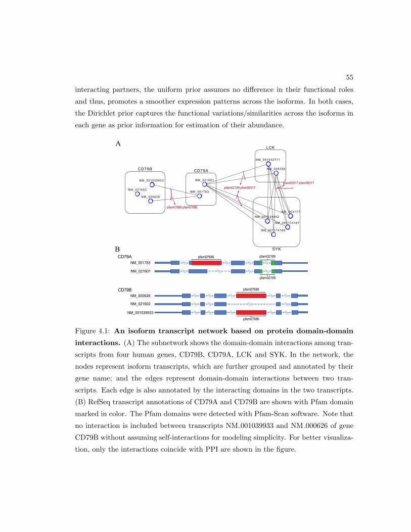
55

interacting partners, the uniform prior assumes no difference in their functional roles

and thus, promotes a smoother expression patterns across the isoforms. In both cases,

the Dirichlet prior captures the functional variations/similarities across the isoforms in

each gene as prior information for estimation of their abundance.

NM_001783

CD79B

NM_001039933

NM_000626

CD79A

NM_021601

NM_021602

LCK

NM_001174167

NM_001174168

NM_001042771

NM_001135052

NM_003177

NM_005356

SYK

NM_021601

NM_001783

NM_001039933

NM_021602

NM_000626

CD79B

CD79A pfam07686

pfam07686

pfam07686

pfam02189

pfam07686:pfam07686

pfam02189:pfam00017pfam00017:pfam00017

pfam02189

A

B

Figure 4.1: An isoform transcript network based on protein domain-domain

interactions. (A) The subnetwork shows the domain-domain interactions among tran-

scripts from four human genes, CD79B, CD79A, LCK and SYK. In the network, the

nodes represent isoform transcripts, which are further grouped and annotated by their

gene name; and the edges represent domain-domain interactions between two tran-

scripts. Each edge is also annotated by the interacting domains in the two transcripts.

(B) RefSeq transcript annotations of CD79A and CD79B are shown with Pfam domain

marked in color. The Pfam domains were detected with Pfam-Scan software. Note that

no interaction is included between transcripts NM 001039933 and NM 000626 of gene

CD79B without assuming self-interactions for modeling simplicity. For better visualiza-

tion, only the interactions coincide with PPI are shown in the figure.

56

The chapter is organized as following. In the section Materials and Methods,

we describe the procedure to construct protein domain-domain interaction networks,

the mathematic description of the probabilistic model and the Net-RSTQ algorithm,

qRT-PCR experiment design, and RNA-Seq data preparation. In the section Results,

we first demonstrate the correlation between protein domain-domain interactions and

isoform transcript co-expressions across samples in four cancer RNA-Seq datasets from

The Cancer Genome Atlas (TCGA) to justify using domain-domain interactions as

prior knowledge. We then compared the predicted isoform proportions with qRT-PCR

experiments on 25 multi-isoform genes in three cell lines, H9 stem cell line, OVCAR8

ovarian cancer cell line and MCF7 breast cancer cell line. Net-RSTQ was also applied to

four cancer RNA-Seq datasets to quantify isoform expressions to classify patient samples

by the survival or relapse outcomes. In addition, simulations were also performed to

measure the statistical robustness of Net-RSTQ over randomized networks.

4.2 Materials and Methods

In this section, we first describe the construction of the transcript interaction network.

We then introduce the network-based transcript quantification model (Net-RSTQ) by

applying the protein domain-domain interaction information as prior knowledge based

on the base EM model mentioned in section 1.2.3. The notations used in the equations

are summarized in Table 4.1. At last, qRT-PCR experiment design and RNA-Seq data

preparation are explained.

Notation DescriptionN total # of genes

T set of transcripts; Tik is the kth transcript of the ith gene; Ti denotes the transcripts of the ith genelik length of transcript Tik

r set of reads; rij is the jth read aligned to the ith gene; ri is the read set aligned to the ith gene

pik the probability of a read generated by transcript Tik in the ith gene

Pi the probability of a read generated by transcript Ti in the ith gene, specifically, [pi1, ..., pi,|Ti|]P concatenate of all Pi, specifically, [P1,P2, ...,PN ]

ρik relative abundance of the transcript Tik in the ith gene

π transcript expression; πik is the expression of the kth transcript of the ith geneφik average expressions (normalized) of transcript Tik’s neighbors in the transcript networkα parameters of Dirichlet distribution; αik = λφik + 1 is the parameter of the Dirichlet distribution of pikqijk read sampling probability, qijk = 1

lik−lr+1if read rij is aligned to transcript Tik, otherwise qijk = 0

S binary matrix for transcript interaction network

Table 4.1: Notations.

57

4.2.1 Transcript network construction

Two binary transcript networks were constructed by measuring the protein domain-

domain interactions (DDI) between the domains in each pair of transcripts in four

steps. First, the translated transcript sequences of all human genes were obtained

from RefSeq [136]. Second, Pfam-Scan was used to search Pfam databases for the

matched Pfam domains on each transcript with 1e-5 e-value cutoff [135]. Note that

only high quality, manually curated Pfam-A entries in the database were used in the

search. Third, domain-domain interactions were obtained from several domain-domain

interaction databases, and if any domain-domain interaction exists between a pair of

transcripts, the two transcripts are connected in the transcript network. Specifically,

6634 interactions between 4346 Pfam domain families from two 3D structure-based DDI

datasets (iPfam [133] and 3did [134]) inferred from the protein structures in Protein

Data Bank (PDB) [137] were used in the experiments. Besides these highly confident

structure-based DDIs, transcript interactions constructed from 2989 predicted high-

confidence DDIs and 2537 predicted medium-confidence DDIs in DOMINE [138] were

also included if the transcript interaction agrees with protein-protein interactions (PPI)

in HPRD [139].

In the experiments, we focused on the transcripts from two cancer gene lists from

the literature for better reliability in annotations. The first smaller transcript network

consists of 11736 interactions constructed from the 3D structure-based DDIs and 421

interactions constructed from the predicted DDIs among the 898 transcripts in 397 genes

from the first gene list [140]. The second larger transcript network contains 711,516

interactions constructed from the 3D structure-based DDIs among 5599 transcripts in

2551 genes in a larger gene list [141]. Since inclusion of the predicted DDIs results in a

much higher density in the large network, the large network does not include predicted

DDIs to prevent too many potential false positive interactions. The characteristics of the

two transcript networks are summarized in Table 4.2. The density of the two networks

are 3.02% and 4.54% respectively, which are in similar scale with the PPI network.

Both networks show high clustering coefficients, suggesting modularity of subnetworks.

Note that self-interactions (interactions between transcript(s) in the same gene) are not

considered since Net-RSTQ only utilizes positive correlation between the expressions

of neighboring transcripts in different genes. For simplicity, Net-RSTQ assumes that

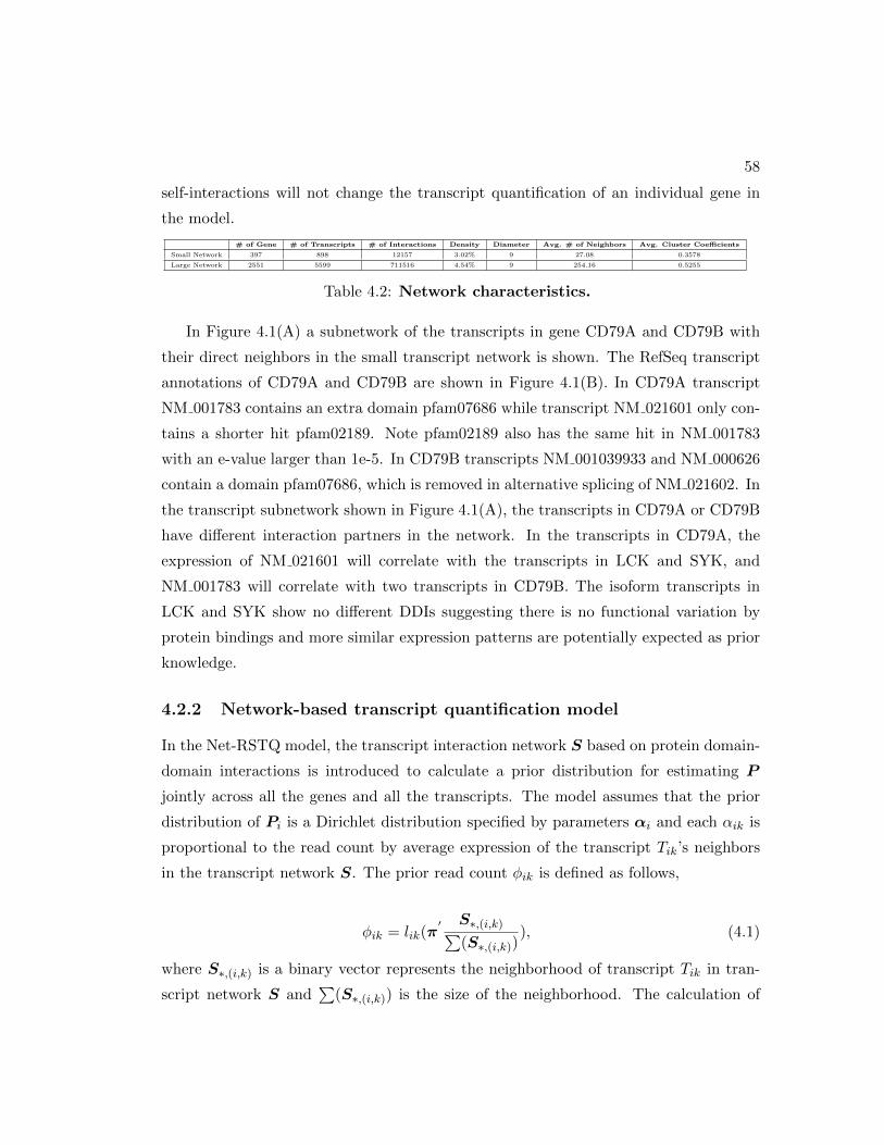
58

self-interactions will not change the transcript quantification of an individual gene in

the model.

# of Gene # of Transcripts # of Interactions Density Diameter Avg. # of Neighbors Avg. Cluster Coefficients

Small Network 397 898 12157 3.02% 9 27.08 0.3578

Large Network 2551 5599 711516 4.54% 9 254.16 0.5255

Table 4.2: Network characteristics.

In Figure 4.1(A) a subnetwork of the transcripts in gene CD79A and CD79B with

their direct neighbors in the small transcript network is shown. The RefSeq transcript

annotations of CD79A and CD79B are shown in Figure 4.1(B). In CD79A transcript

NM 001783 contains an extra domain pfam07686 while transcript NM 021601 only con-

tains a shorter hit pfam02189. Note pfam02189 also has the same hit in NM 001783

with an e-value larger than 1e-5. In CD79B transcripts NM 001039933 and NM 000626

contain a domain pfam07686, which is removed in alternative splicing of NM 021602. In

the transcript subnetwork shown in Figure 4.1(A), the transcripts in CD79A or CD79B

have different interaction partners in the network. In the transcripts in CD79A, the

expression of NM 021601 will correlate with the transcripts in LCK and SYK, and

NM 001783 will correlate with two transcripts in CD79B. The isoform transcripts in

LCK and SYK show no different DDIs suggesting there is no functional variation by

protein bindings and more similar expression patterns are potentially expected as prior

knowledge.

4.2.2 Network-based transcript quantification model

In the Net-RSTQ model, the transcript interaction network S based on protein domain-

domain interactions is introduced to calculate a prior distribution for estimating P

jointly across all the genes and all the transcripts. The model assumes that the prior

distribution of Pi is a Dirichlet distribution specified by parameters αi and each αik is

proportional to the read count by average expression of the transcript Tik’s neighbors

in the transcript network S. The prior read count φik is defined as follows,

φik = lik(π′ S∗,(i,k)∑

(S∗,(i,k))), (4.1)

where S∗,(i,k) is a binary vector represents the neighborhood of transcript Tik in tran-

script network S and∑

(S∗,(i,k)) is the size of the neighborhood. The calculation of

59

each φik is illustrated in Figure 4.2. The Dirichlet parameter αi is defined as a function

of φik as

αik = λφik + 1, (4.2)

where λ > 0 is a tuning parameter balancing the belief between the prior-read count

and the aligned-read count.

λαik=

C

0

C 11

1

1

0

′ik

Tik:

Tg1a

Tg3c

:

:

×0…

…

g1a

=

g2b

g3c

g4dNeighbor(Tik) = Tg1a,Tg2b,Tg3c,Tg4d

Tg2b :

Tg4d :

g1a g2b

g4dg3c

ik+1

αik

( ) lik

Figure 4.2: Transcript interaction neighborhood. In this toy example, transcript

Tik has four neighbor transcripts Tg1a, Tg2b, Tg3c, Tg4d, which are transcripts from g1,

g2, g3 and g4, respectively. The neighborhood expression φik of Tik is then calculated as

the average of its neighbor transcripts’ expressions and further normalized by transcript

length, represented as the vector product between π and S∗,(ik) normalized by the

number of neighbors∑S∗,(ik) and the transcript length lik in the figure.

To obtain the optimal P jointly for all genes, we introduce a pseudo-likelihood model

to estimate P iteratively in each iteration. Assuming uniform Pr(ri), the pseudo-

likelihood function is defined as,

L(P ,α; r) =

N∏i=1

L(Pi,αi; ri) =

N∏i=1

Pr(Pi|αi)Pr(ri|Pi)

Pr(ri)∝

N∏i=1

Pr(Pi|αi)Pr(ri|Pi). (4.3)

Note that the pseudo-likelihood model relies on the independence assumption among the

likelihood functions of each individual gene when theα parameters of the Dirichlet priors

are pre-computed. Thus, the model simply takes the product of the likelihood function

from each gene. Each prior distribution Pr(Pi|αi) follows the Dirichlet distribution,

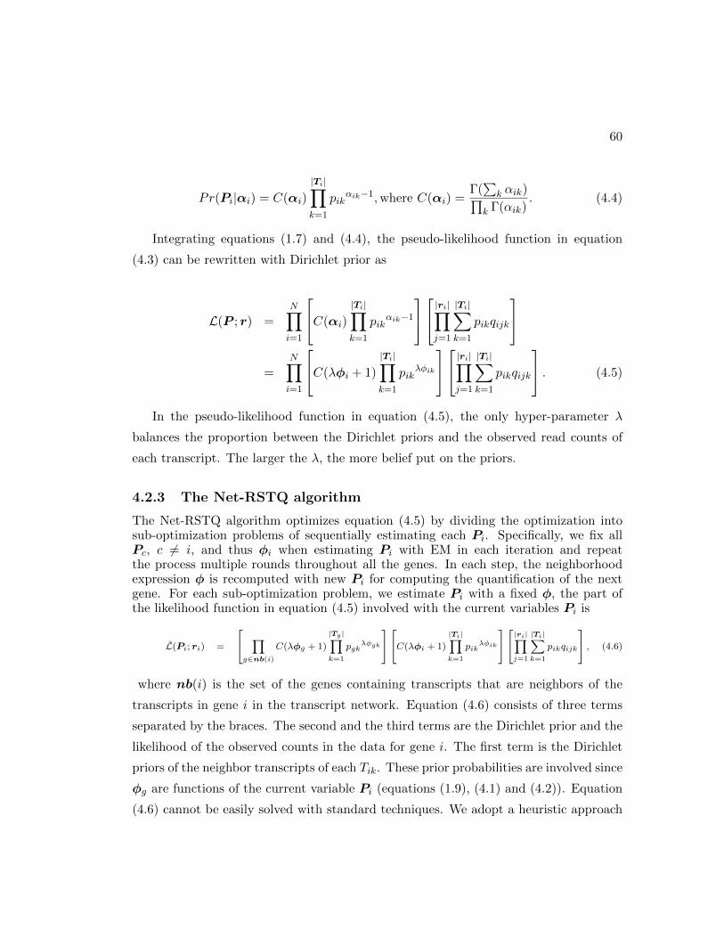
60

Pr(Pi|αi) = C(αi)

|Ti|∏k=1

pikαik−1,where C(αi) =

Γ(∑

k αik)∏k Γ(αik)

. (4.4)

Integrating equations (1.7) and (4.4), the pseudo-likelihood function in equation

(4.3) can be rewritten with Dirichlet prior as

L(P ; r) =

N∏i=1

C(αi)

|Ti|∏k=1

pikαik−1

|ri|∏j=1

|Ti|∑k=1

pikqijk

=

N∏i=1

C(λφi + 1)

|Ti|∏k=1

pikλφik

|ri|∏j=1

|Ti|∑k=1

pikqijk

. (4.5)

In the pseudo-likelihood function in equation (4.5), the only hyper-parameter λ

balances the proportion between the Dirichlet priors and the observed read counts of

each transcript. The larger the λ, the more belief put on the priors.

4.2.3 The Net-RSTQ algorithm

The Net-RSTQ algorithm optimizes equation (4.5) by dividing the optimization intosub-optimization problems of sequentially estimating each Pi. Specifically, we fix allPc, c 6= i, and thus φi when estimating Pi with EM in each iteration and repeatthe process multiple rounds throughout all the genes. In each step, the neighborhoodexpression φ is recomputed with new Pi for computing the quantification of the nextgene. For each sub-optimization problem, we estimate Pi with a fixed φ, the part ofthe likelihood function in equation (4.5) involved with the current variables Pi is

L(Pi; ri) =

∏g∈nb(i)

C(λφg + 1)

|Tg|∏k=1

pgkλφgk

C(λφi + 1)

|Ti|∏k=1

pikλφik

|ri|∏j=1

|Ti|∑k=1

pikqijk

, (4.6)

where nb(i) is the set of the genes containing transcripts that are neighbors of the

transcripts in gene i in the transcript network. Equation (4.6) consists of three terms

separated by the braces. The second and the third terms are the Dirichlet prior and the

likelihood of the observed counts in the data for gene i. The first term is the Dirichlet

priors of the neighbor transcripts of each Tik. These prior probabilities are involved since

φg are functions of the current variable Pi (equations (1.9), (4.1) and (4.2)). Equation

(4.6) cannot be easily solved with standard techniques. We adopt a heuristic approach

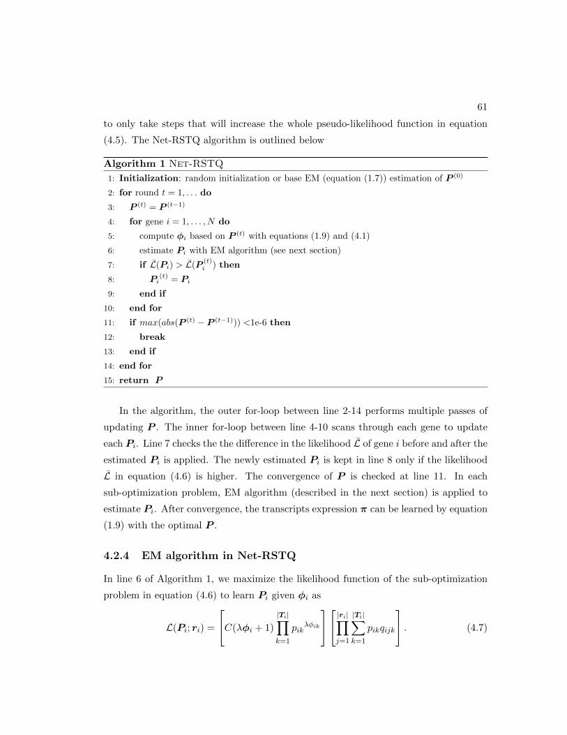
61

to only take steps that will increase the whole pseudo-likelihood function in equation

(4.5). The Net-RSTQ algorithm is outlined below

Algorithm 1 Net-RSTQ

1: Initialization: random initialization or base EM (equation (1.7)) estimation of P (0)

2: for round t = 1, . . . do

3: P (t) = P (t−1)

4: for gene i = 1, . . . , N do

5: compute φi based on P (t) with equations (1.9) and (4.1)

6: estimate Pi with EM algorithm (see next section)

7: if L(Pi) > L(P(t)i ) then

8: Pi(t) = Pi

9: end if

10: end for

11: if max(abs(P (t) − P (t−1))) <1e-6 then

12: break

13: end if

14: end for

15: return P

In the algorithm, the outer for-loop between line 2-14 performs multiple passes of

updating P . The inner for-loop between line 4-10 scans through each gene to update

each Pi. Line 7 checks the the difference in the likelihood L of gene i before and after the

estimated Pi is applied. The newly estimated Pi is kept in line 8 only if the likelihood

L in equation (4.6) is higher. The convergence of P is checked at line 11. In each

sub-optimization problem, EM algorithm (described in the next section) is applied to

estimate Pi. After convergence, the transcripts expression π can be learned by equation

(1.9) with the optimal P .

4.2.4 EM algorithm in Net-RSTQ

In line 6 of Algorithm 1, we maximize the likelihood function of the sub-optimization

problem in equation (4.6) to learn Pi given φi as

L(Pi; ri) =

C(λφi + 1)

|Ti|∏k=1

pikλφik

|ri|∏j=1

|Ti|∑k=1

pikqijk

. (4.7)

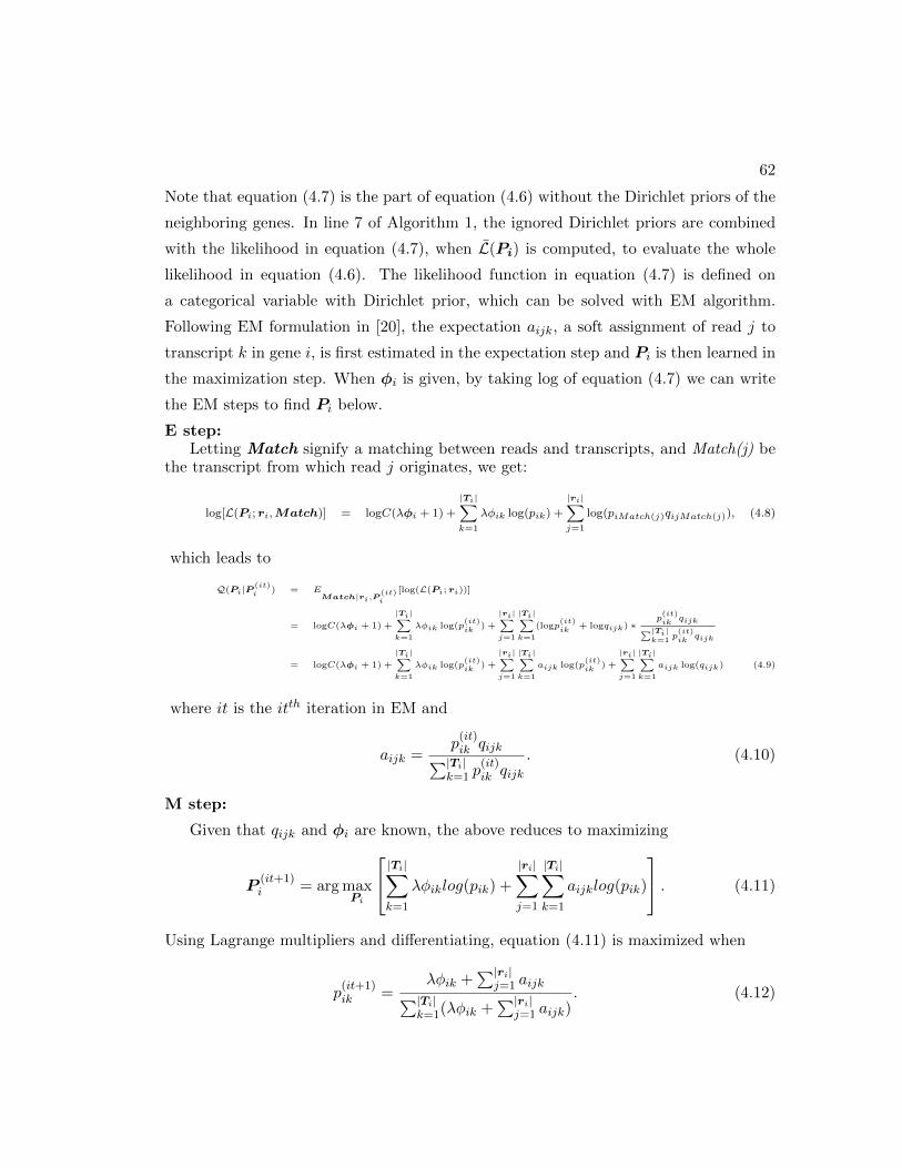
62

Note that equation (4.7) is the part of equation (4.6) without the Dirichlet priors of the

neighboring genes. In line 7 of Algorithm 1, the ignored Dirichlet priors are combined

with the likelihood in equation (4.7), when L(Pi) is computed, to evaluate the whole

likelihood in equation (4.6). The likelihood function in equation (4.7) is defined on

a categorical variable with Dirichlet prior, which can be solved with EM algorithm.

Following EM formulation in [20], the expectation aijk, a soft assignment of read j to

transcript k in gene i, is first estimated in the expectation step and Pi is then learned in

the maximization step. When φi is given, by taking log of equation (4.7) we can write

the EM steps to find Pi below.

E step:Letting Match signify a matching between reads and transcripts, and Match(j) be

the transcript from which read j originates, we get:

log[L(Pi; ri,Match)] = logC(λφi + 1) +

|Ti|∑k=1

λφik log(pik) +

|ri|∑j=1

log(piMatch(j)qijMatch(j)), (4.8)

which leads to

Q(Pi|P(it)i ) = E

Match|ri,P(it)i

[log(L(Pi; ri))]

= logC(λφi + 1) +

|Ti|∑k=1

λφik log(p(it)ik

) +

|ri|∑j=1

|Ti|∑k=1

(logp(it)ik

+ logqijk) ∗p(it)ik

qijk∑|Ti|k=1

p(it)ik

qijk

= logC(λφi + 1) +

|Ti|∑k=1

λφik log(p(it)ik

) +

|ri|∑j=1

|Ti|∑k=1

aijk log(p(it)ik

) +

|ri|∑j=1

|Ti|∑k=1

aijk log(qijk) (4.9)

where it is the itth iteration in EM and

aijk =p

(it)ik qijk∑|Ti|

k=1 p(it)ik qijk

. (4.10)

M step:

Given that qijk and φi are known, the above reduces to maximizing

P(it+1)i = arg max

Pi

|Ti|∑k=1

λφiklog(pik) +

|ri|∑j=1

|Ti|∑k=1

aijklog(pik)

. (4.11)

Using Lagrange multipliers and differentiating, equation (4.11) is maximized when

p(it+1)ik =

λφik +∑|ri|

j=1 aijk∑|Ti|k=1(λφik +

∑|ri|j=1 aijk)

. (4.12)

63

After EM algorithm converges, we update P with the newly estimated Pi only if the

update leads to increase of equation (4.6). It can be seen from equation (4.12) that the

role of λ is a parameter controlling the balance between the prior-read count and the

aligned-read count. To see that, recall φik is the prior-read count of transcript Tik by

the average expression of its neighbors (equation (4.1)) and∑|ri|

j=1 aijk is the expected

aligned-read count of transcript Tik. λ directly balances the contributions from the two

terms. Therefore, a reasonable choice of λ should apply to RNA-Seq data with similar

level of noise or bias in general.

4.2.5 qRT-PCR experiment design

Three qRT-PCR experiments are designed to measure the isoform proportions of 25

multi-isoform genes in three cell lines, H9 stem cell line, OVCAR8 ovarian cancer cell

line and MCF7 breast cancer cell line. The cell lines were selected based on the available

of both RNA-Seq data and cell culture in our labs. The qRT-PCR experiments focused

on the gene with most different quantification results reported by Net-RSTQ and other

compared methods. Due to the limitations in time and cost of running qRT-PCR

experiments, only the 25 genes in the three cell lines were tested with all the results

reported in the experiments. Quantitation of the real-time PCR results was done on

the data from H9 human embryonic stem cells to obtain the absolute expressions for

comparing more than two transcripts and comparative Ct method was done on the data

from OVCAR8 ovarian cancer cells and MCF7 breast cancer cells to obtain the ratio

between a pair of transcripts.

H9 Stem cell line

Total RNA was extracted from human embryonic stem (ES) H9 cells by using TRIzol

(Invitrogen). To repeat the experiments of triplicate three times, 5µg RNA was used

to synthesize complementary DNA with ReverTra Ace (Toyobo) and oligo-dT (Takara)

according to the manufacturer’s instructions. Transcript levels of genes were determined

by using Premix Ex Taq (Takara) and analysed with a CFX-96 Real Time system (Bio-

Rad). The templates for different transcripts were generated with PCR by using the

template primers in S1 Table in [36]. After isolation and purification, the templates were

used to generate the standard curves with qRT-PCR by using the qRT-PCR primers for

64

different transcripts. The generated standard curves have coefficient of determination

(R2) over 0.999. The qRT-PCR primers were then applied to determine the expression

levels of different transcripts in H9 ES cells by calculating with the standard curves.

The expressions were carried out in three independent replications and the standard

deviations were provided after the average.

Ovarian cancer cell line

1µg of total RNAs were isolated from untreated OVCAR8 cells using Trizol (Invitrogen).

RNA was reverse-transcribed using Superscript II reverse transcriptase (Invitrogen)

according to manufacture protocol. Real-time PCR was performed on CFX384 Real-

time system (Bio-Rad) with FastStart SYBR Green Master (Roche) with the primer

sets in S2 Table in [36]. PCR conditions are 10 min at 95C and 40 cycles of 95C for

45 sec and 60C for 45 sec. Quantitation of the real-time PCR results was done using

comparative Ct method. Two replicates of qRT-PCR were performed using total RNAs

isolated.

Breast cancer cell line

0.5µg of total RNAs purified from MCF7 cells was used for oligo d(T)20-primed reverse

transcription (Superscript III; Life Technologies). SYBR Green was used to detect and

quantitate PCR products in real-time reactions with the primer sets in S3 Table in [36].

PCR conditions for qRT-PCR analysis are 2 min 94C and 40 cycles of 94C for 30 sec,

60C for 20 sec and 72C for 30 sec. Quantitation of the real-time PCR results was done

using comparative Ct method. GAPDH mRNA was used as a normalization control for

quantitation. Three replicates of qRT-PCR were performed using total RNAs isolated.

4.2.6 RNA-Seq data preparation

Three cell line RNA-Seq datasets were used for evaluating the accuracy of transcript

quantification by comparison with qRT-PCR results. The first dataset is the H9 em-

bryonic stem cell line data from [142]. The raw RNA-Seq fastq file were downloaded

from SRA website (SRR1015682) under GEO accession GSE51607. The second dataset

65

is an in-house dataset from the ovarian cancer cell line OVCAR8 prepared at Uni-

versity of Kansas Medical Center. The third dataset is the MCF7 breast cancer cell

line data from [143]. The raw RNA-Seq fastq file was downloaded from SRA website

(SRR925723) under GEO accession GSE48213. There are 23,397,325 single-end 34bp

reads in the stem cell line dataset, 19,892,473 paired-end 100bp reads in the OVCAR8,

and 21,855,632 paired-end 76bp reads in the MCF7 mapped to the human hg19 refer-

ence genome by TopHat2.0.9 [144] with up to 2 mismatches allowed. Exon coverages

and read counts of exon-exon junctions were generated by SAMtools [145] to be utilized

with Net-RSTQ and base EM (equation (1.7)). Cufflinks [23] directly infers transcript

expressions based on the alignment by TopHat with the min isoform fraction set to 0

for better sensitivity.

TCGA RNA-Seq datasets of Ovarian serous cystadenocarcinoma (OV), Breast in-

vasive carcinoma (BRCA), Lung adenocarcinoma (LUAD) and Lung squamous cell

carcinoma (LUSC) were analyzed for patient outcome prediction with transcript expres-

sions estimated by Net-RSTQ, base EM (equation (1.7)), RSEM [24] and Cufflinks [23].

Both the gene expression and transcript expression data reported by RSEM [24] in

TCGA (level 3 data) were utilized as two baselines for cancer outcome prediction. The

raw RNA-Seq fastq files (level 1 data) were downloaded from Cancer Genomics Hub

(CGHub) and processed by TopHat for use with Net-RSTQ, base EM and Cufflinks.

The patient samples in each dataset were classified into cases and controls based on the

survival and relapse outcomes as shown in Table 4.3. The command lines for preparing

the data with RSEM and Cufflinks are available in the S3 Text in [36].

Cancer Type Event # of Patients by years

Ovarian serous cystadenocarcinoma(OV) Survival 76(<3 ys) vs 62(>4 ys)Relapse 79(<1.5 ys) vs 68(>2 ys)

Breast invasive carcinoma(BRCA) Survival 66(<5 ys) vs 57(>8 ys)Relapse 42(<5 ys) vs 38(>8 ys)

Lung adenocarcinoma(LUAD) Survival 47(<2 ys) vs 56(>3 ys)

Lung squamous cell carcinoma(LUSC) Survival 67(<2 ys)vs 77 (>3 ys)

Table 4.3: Summary of patient samples in TCGA datasets. The samples are clas-sified by cutoffs on survival and relapse time based on the available clinical informationin each dataset.

66

4.3 Results

There are six major results in this section, 1) isoform co-expression analysis on TCGA

data to show the correlation with protein domain-domain interactions; 2) overlapping

the DDIs and KEGG pathways to understand the transcript networks; 3) simulations

for model validation and statistical analysis; 4) qRT-PCR experiments to measure the

performance of transcript quantification; 5) cancer outcome prediction on TCGA data

to measure the quality of transcript quantification as molecular markers; and 6) running

time of Net-RSTQ.

Net-RSTQ was compared with base EM (the base model in equation (1.7)), Cuf-

flinks [23] and RSEM (isoform expression or gene expression) [24]. The accuracy of

transcript quantification was directly measured on the simulated data with ground-truth

expressions and qRT-PCR data from the three cell lines. Cancer outcome prediction

on four TCGA cancer datasets evaluates the potential of using isoform expressions as

predictive biomarkers in clinical settings. Statistical assessment was also performed on

randomized transcript networks to evaluate the significance of the results.

4.3.1 Isoform co-expressions correlate with protein domain-domain in-

teractions

To investigate the correlation between protein domain-domain interactions and isofrom

transcript co-expressions, we calculated the number of transcript pairs that are both

nearby (being neighbors or having a distance up to 2) in the transcript network and

highly co-expressed in the TCGA samples. The transcript co-expressions were calculated

by Pearson’s correlation coefficients of each pair of transcripts across all the samples

in each dataset with the isoform transcript quantification by Cufflinks. The transcript

pairs were then sorted by the correlation coefficients from the largest to the smallest

and grouped into bins of size 1000. The number of transcript pairs that are nearby in

the transcript networks out of 1000 pairs are calculated within each bin and plotted

in Figure 4.3(A) and Figure 4.3(B) for the two cancer gene lists, respectively. In both

Figure 4.3(A) and Figure 4.3(B), the left column shows the plots of the number of pairs

that are neighbors in the transcript network, and the right column shows the plots of

the number of transcript pairs with a distance up to 2 in the transcript network, among

67

the 1000 pairs in each bin. In all the plots, similar trends are observed in all the four

cancer datasets: there are more interacting isoform pairs in the bins with higher co-

expressions. For example, among the 1000 transcript pairs with the highest correlation

coefficients, there are 73 interactions in the transcript network in OV dataset and thus,

73 interactions (y-axis) for bin index 1 (x-axis) is plotted in the left column of Figure

4.3(A). In all the plots, there is a clear pattern that the numbers of matched nearby

transcripts in the transcript network among the 1000 pairs in the first few bins are

higher than the expected average of 30 in the small network of density 3.02%, 114 in

the small network of density 11.41% (with distance up to 2), 45 in the larger network

of density 4.54%, and 203 in the larger network of density 20.33% (with distance up

to 2). Moreover, the 2-step walk clearly promoted the number of overlaps with the

pairs of higher co-expressions in the small network. For example, the significant overlap

is extended from the first 25 bins to approximately the first 50 bins or more in the

four datasets. The observation suggests that higher co-expressions exist not only in the

direct neighbors in the transcript network but also the nearby nodes by a small distance.

By exploring the network structure with prior information through neighbors by many

steps in iterations, Net-RSTQ model is expected to propagate the expression values from

each transcript to its nearby nodes in the network to capture the co-expressions. Note

that considering the neighboring pairs with distance up to 2 in the larger network will

result in a graph of density 20.33%, which is likely to contain too many false relations

by the two-step walk. Thus, the plots of the larger network of distance-2 pairs are only

included for the completeness of the analysis.

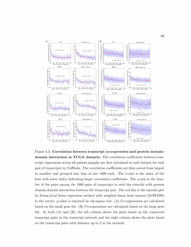
68

0 50 100 150 200 250 30080

100

120

140

160

180

200

Index of Sorted CC by Magnitude

# of

Ove

rlapp

ed T

rans

crip

t Int

erac

tions

OV (dist<=2)

p−value = 4.72e−65

0 50 100 150 200 25080

100

120

140

160

180

200


# of

Ove

rlapp

ed T

rans

crip

t Int

erac

tions

BRCA (dist<=2)

p−value = 3.55e−21

0 50 100 150 200 250 30060

80

100

120

140

160

180

200


# of

Ove

rlapp

ed T

rans

crip

t Int

erac

tions

LUAD (dist<=2)

p−value = 1.20e−40

0 50 100 150 200 250 30080

100

120

140

160

180

200


# of

Ove

rlapp

ed T

rans

crip

t Int

erac

tions

LUSC (dist<=2)

p−value = 1.11e−79

0 50 100 150 200 250 30010

20

30

40

50

60

70

80


# of

Ove

rlapp

ed T

rans

crip

t Int

erac

tions

OV

A

0 50 100 150 200 25010

20

30

40

50

60

70


# of

Ove

rlapp

ed T

rans

crip

t Int

erac

tions

BRCA

0 50 100 150 200 250 30010

20

30

40

50

60

70

80


# of

Ove

rlapp

ed T

rans

crip

t Int

erac

tions

LUAD

0 50 100 150 200 250 30010

20

30

40

50

60

70


# of

Ove

rlapp

ed T

rans

crip

t Int

erac

tions

LUSC

0 2000 4000 6000 8000 10000 120000

10

20

30

40

50

60

70

80

90

100


# of

Ove

rlapp

ed T

rans

crip

t Int

erac

tion

OV

0 2000 4000 6000 8000 100000

10

20

30

40

50

60

70

80

90

100

110


# of

Ove

rlapp

ed T

rans

crip

t Int

erac

tion

BRCA

0 2000 4000 6000 8000 10000 120000

10

20

30

40

50

60

70

80

90

100


# of

Ove

rlapp

ed T

rans

crip

t Int

erac

tion

LUAD

0 2000 4000 6000 8000 100000

10

20

30

40

50

60

70

80

90

100


# of

Ove

rlapp

ed T

rans

crip

t Int

erac

tion

LUSC

A B

0 2000 4000 6000 8000 10000 12000140

160

180

200

220

240

260

280


# of

Ove

rlapp

ed T

rans

crip

t Int

erac

tions

OV (dist<=2)

p−value = 1.75e−22

0 2000 4000 6000 8000 10000100

150

200

250

300

350


# of

Ove

rlapp

ed T

rans

crip

t Int

erac

tions

BRCA (dist<=2)

p−value = 1.53e−133

0 2000 4000 6000 8000 10000 12000140

160

180

200

220

240

260


# of

Ove

rlapp

ed T

rans

crip

t Int

erac

tions

LUAD (dist<=2)

p−value = 2.81e−21

0 2000 4000 6000 8000 10000140

160

180

200

220

240

260


# of

Ove

rlapp

ed T

rans

crip

t Int

erac

tions

LUSC (dist<=2)

p−value = 0.2359

p-value = 4.40e-49

p-value = 5.48e-15

p-value = 2.29e-36

p-value = 1.80e-38

p-value = 2.59e-40

p-value = 1.16e-94

p-value = 4.04e-20

p-value =1.18e-07

Figure 4.3: Correlation between transcript co-expression and protein domain-

domain interaction in TCGA datasets. The correlation coefficients between tran-

script expressions across all patient samples are first calculated in each dataset for each

pair of transcripts by Cufflinks. The correlation coefficients are then sorted from largest

to smallest and grouped into bins of size 1000 each. The x-axis is the index of the

bins with lower index indicating larger correlation coefficients. The y-axis is the num-

ber of the pairs among the 1000 pairs of transcripts in each bin coincide with protein

domain-domain interaction between the transcript pair. The red line is the smooth plot

by fitting local linear regression method with weighted linear least squares (LOWESS)

to the curves. p-value is reported by chi-square test. (A) Co-expressions are calculated

based on the small gene list. (B) Co-expressions are calculated based on the large gene

list. In both (A) and (B), the left column shows the plots based on the connected

transcript pairs in the transcript network and the right column shows the plots based

on the transcript pairs with distance up to 2 in the network.

69

The canonical 2x2 chi-square test was also applied to compare the number of the

domain-domain interactions in the first 10,000 transcript pairs (first 10 bins) with the

number in the rest of the pairs. In all the four datasets in both Figure 4.3(A) and

Figure 4.3(B) with one exception in the LUSC dataset on the large network of distance-

2 relation, there is a significant difference that the highly co-expressed transcripts are

more likely to interact with each other in the transcript network, confirmed by the

significant p-values. As explained previously, the exception is likely due to the large

number of false-positive pairs in the dense network. The observation further support the

hypothesis that protein domain-domain interactions correlate transcript co-expressions

reported in previous studies [130,131].

To further understand the specificity of the domain-domain interactions in the highly

co-expressed transcripts, we calculated the number of domain-domain pairs that con-

struct the DDIs in the top 10,000 co-expressed transcript pairs. The statistics suggest

high diversity of the type of DDIs. For example, there are 547 interacting transcript

pairs among the 201 out of 898 transcripts in the top 10,000 co-expressed transcript

pairs in OV dataset for small network. The 547 interacting transcript pairs represent

770 different domain-domain interactions (There might be more than one DDIs between

a pair of transcripts). There are 739 interacting transcript pairs among the 538 out of

5599 transcripts in the top 10,000 co-expressed transcript pairs in OV dataset for large

network. The 739 interacting transcript pairs represent 1277 different domain-domain

interactions. The statistics suggest that the correlation between protein domain-domain

interactions and transcript co-expressions is not a bias due to a few highly spurious DDIs.

It is a general correlation in many different DDIs and co-expressed transcripts. Very

similar statistics were observed in all the datasets and both networks.

To further demonstrate the co-expression relations in the transcript network, two ex-

amples are shown in S1 Figure in [36]. In S1(A) Figure, WHSC1L1 contains two isoforms

connected with different interactions in the transcript network. Isoform NM 017778

interacts with 12 transcripts with average correlation coefficients 0.22 and the other

isoform NM 023034 interacts with 13 more transcripts with average correlation coef-

ficients 0.30 compared with the average correlation coefficient 0.188 against the other

unconnected isoforms across the samples in the OV dataset. In S1(B) Figure, gene

BRD4 contains two isoforms both of which are connected with the same 14 neighbors

70

in the network. The average correlation coefficients between these two isoforms and

the 14 neighboring isoforms are both above 0.26 compared with the average correlation

coefficient less than 0.15 against the other unconnected isoforms across the samples on

the BRCA dataset. In both examples, we observed high degree of agreement between

co-expressions and DDIs.

4.3.2 Protein domain-domain interactions enrich KEGG pathways

To further understand the transcript networks, we overlapped the DDIs between genes

in the two networks with the 294 human KEGG pathways [146]. Among the 397 genes

in the small network, 10.97%(17284) of the pairs are co-members in at least one KEGG

pathway. The 10.97% KEGG co-member pairs covers 42.70%(2122) of the DDIs among

the genes while the other 89.03%(140352) non-co-member pairs covers 57.30%(2748) of

the DDIs. By these numbers, there is about 6-fold enrichment of DDIs in the KEGG

co-member genes in the small network. Among the 2551 genes in the large network,

the 5.15%(335372) KEGG co-member pairs covers 12.45%(40812) of the DDIs among

genes while the other 94.85%(6172229) non-co-member pairs covers 87.55%(287090) of

the DDIs. By these numbers, there is about 2.6-fold enrichment of DDIs in the KEGG

co-member genes in the large network. We also list the KEGG pathways that are highly

enriched with DDIs in the large network in S4 Table in [36]. Specifically, we consider

the subnetwork of genes that are members of one KEGG pathway and calculated the

density of DDIs in the subnetwork to compare to the overall density of 5.04% in the

whole network. Interestingly, most of the enriched pathways are signaling pathways and

disease pathways with very high DDI densities.

4.3.3 Net-RSTQ captures network prior in simulations

In the simulations, we applied flux-simulator [147] to generate paired-end short reads

simulating real RNA-Seq experiment in silico based on a ground truth transcript expres-

sion profile, using hg19 reference human genome and RefSeq annotations downloaded

from UCSC Genome Browser. To generate the ground-truth expression profiles, the

gene expressions were sampled from a poisson distribution and the proportions of the

isoforms in each gene were derived based on a neighbor average expression in the small

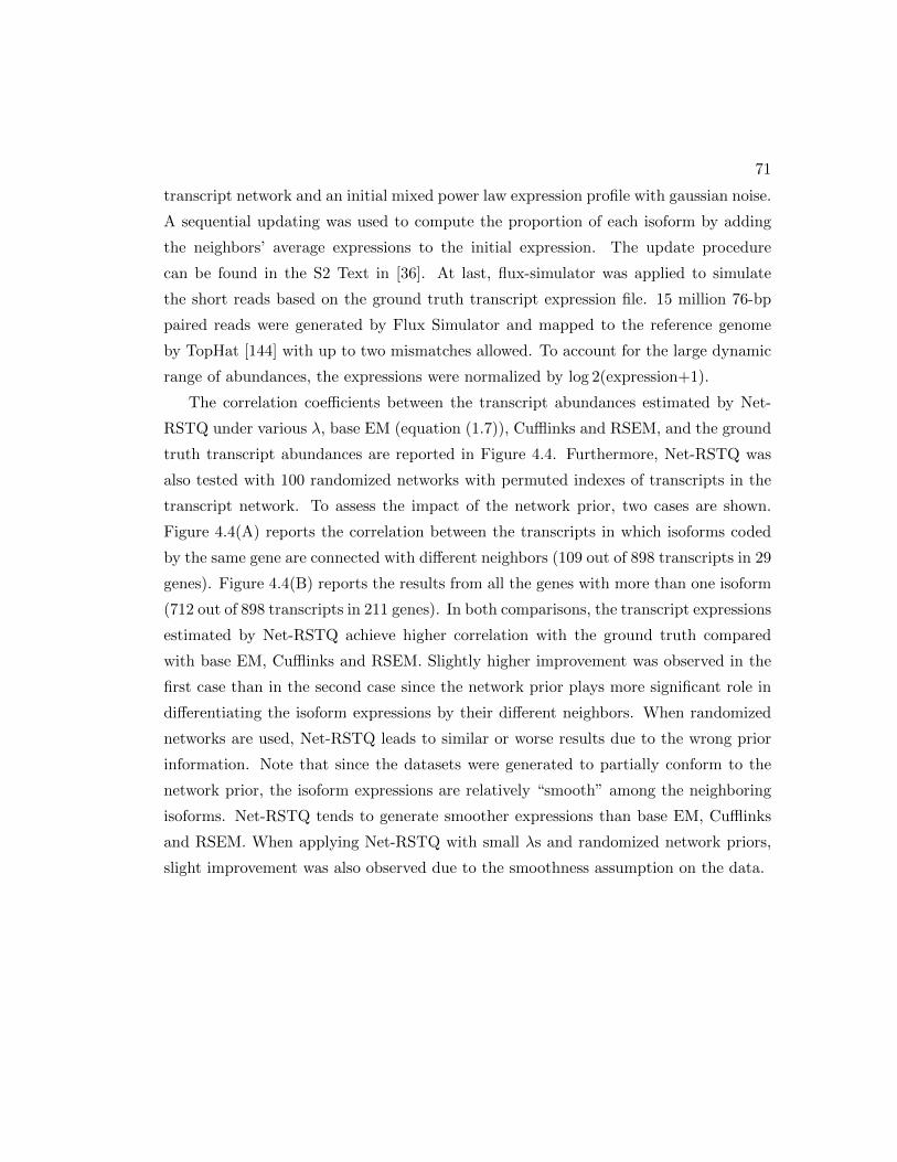
71

transcript network and an initial mixed power law expression profile with gaussian noise.

A sequential updating was used to compute the proportion of each isoform by adding

the neighbors’ average expressions to the initial expression. The update procedure

can be found in the S2 Text in [36]. At last, flux-simulator was applied to simulate

the short reads based on the ground truth transcript expression file. 15 million 76-bp

paired reads were generated by Flux Simulator and mapped to the reference genome

by TopHat [144] with up to two mismatches allowed. To account for the large dynamic

range of abundances, the expressions were normalized by log 2(expression+1).

The correlation coefficients between the transcript abundances estimated by Net-

RSTQ under various λ, base EM (equation (1.7)), Cufflinks and RSEM, and the ground

truth transcript abundances are reported in Figure 4.4. Furthermore, Net-RSTQ was

also tested with 100 randomized networks with permuted indexes of transcripts in the

transcript network. To assess the impact of the network prior, two cases are shown.

Figure 4.4(A) reports the correlation between the transcripts in which isoforms coded

by the same gene are connected with different neighbors (109 out of 898 transcripts in 29

genes). Figure 4.4(B) reports the results from all the genes with more than one isoform

(712 out of 898 transcripts in 211 genes). In both comparisons, the transcript expressions

estimated by Net-RSTQ achieve higher correlation with the ground truth compared

with base EM, Cufflinks and RSEM. Slightly higher improvement was observed in the

first case than in the second case since the network prior plays more significant role in

differentiating the isoform expressions by their different neighbors. When randomized

networks are used, Net-RSTQ leads to similar or worse results due to the wrong prior

information. Note that since the datasets were generated to partially conform to the

network prior, the isoform expressions are relatively “smooth” among the neighboring

isoforms. Net-RSTQ tends to generate smoother expressions than base EM, Cufflinks

and RSEM. When applying Net-RSTQ with small λs and randomized network priors,

slight improvement was also observed due to the smoothness assumption on the data.

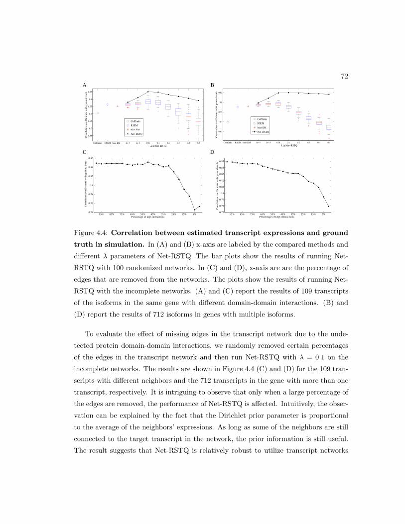
72

95% 85% 75% 65% 55% 45% 35% 25% 15% 5%0.77

0.78

0.79

0.8

0.81

0.82

0.83

0.84

0.85

Percentage of kept interactionsC

orre

lati

on c

oeff

icie

nts

wit

h gr

ound

tru

th

Cufflinks RSEM base EM 1e−4 1e−3 0.01 0.1 0.2 0.3 0.4 0.5

0.55

0.6

0.65

0.7

0.75

0.8

0.85

λ in Net−RSTQ

Cor

rela

tion

coe

ffic

ient

s w

ith

grou

nd tr

uth

Cufflinks

RSEM

base EM

Net−RSTQ

Cufflinks RSEM base EM 1e−4 1e−3 0.01 0.1 0.2 0.3 0.4 0.5

0.65

0.7

0.75

0.8

0.85

λ in Net−RSTQ

Cor

rela

tion

coe

ffic

ient

s w

ith

grou

nd tr

uth

Cufflinks

RSEM

base EM

Net−RSTQ

95% 85% 75% 65% 55% 45% 35% 25% 15% 5%0.74

0.76

0.78

0.8

0.82

0.84

0.86

Percentage of kept interactions

Cor

rela

tion

coe

ffic

ient

s w

ith

grou

nd tr

uth

A B

C D

Figure 4.4: Correlation between estimated transcript expressions and ground

truth in simulation. In (A) and (B) x-axis are labeled by the compared methods and

different λ parameters of Net-RSTQ. The bar plots show the results of running Net-

RSTQ with 100 randomized networks. In (C) and (D), x-axis are are the percentage of

edges that are removed from the networks. The plots show the results of running Net-

RSTQ with the incomplete networks. (A) and (C) report the results of 109 transcripts

of the isoforms in the same gene with different domain-domain interactions. (B) and

(D) report the results of 712 isoforms in genes with multiple isoforms.

To evaluate the effect of missing edges in the transcript network due to the unde-

tected protein domain-domain interactions, we randomly removed certain percentages

of the edges in the transcript network and then run Net-RSTQ with λ = 0.1 on the

incomplete networks. The results are shown in Figure 4.4 (C) and (D) for the 109 tran-

scripts with different neighbors and the 712 transcripts in the gene with more than one

transcript, respectively. It is intriguing to observe that only when a large percentage of

the edges are removed, the performance of Net-RSTQ is affected. Intuitively, the obser-

vation can be explained by the fact that the Dirichlet prior parameter is proportional

to the average of the neighbors’ expressions. As long as some of the neighbors are still

connected to the target transcript in the network, the prior information is still useful.

The result suggests that Net-RSTQ is relatively robust to utilize transcript networks

73

potentially constructed with a large percentage of undetected protein domain-domain

interactions.

4.3.4 Three qRT-PCR experiments confirmed overall improved tran-

script quantification

The isoform proportions estimated by Net-RSTQ, base EM, RSEM, and Cufflinks were

compared to the qRT-PCR results on the three cell lines. Parameter λ = 0.1 was fixed

in all the Net-RSTQ experiments. Among the genes that Net-RSTQ, base EM, RSEM,

and Cufflinks report most different quantification results, qRT-PCR experiments were

performed to test the genes with relatively higher coverage of RNA-Seq data, coding

two to three isoforms, and the feasibility of designing isoform-specific primers in the

qRT-PCR products (see S1, S2 and S3 Tables in [36]). Twenty-five genes in total

were tested in the three cell lines: seven in H9 stem cell line, five in OVCAR8 ovarian

cancer cell line, and thirteen in MCF7 breast cancer cell line. The scatter plots of the

relative abundance of the first transcript in each gene estimated by Net-RSTQ, base

EM, Cufflinks and RSEM were compared to the qRT-PCR results in Figure 4.5(A) and

(E). In the scatter plot, the estimated relative abundance by Net-RSTQ were closer

to qRT-PCR results measured by the accuracy of various thresholds and Root Mean

Square Errors. Net-RSTQ achieved the lowest Root Mean Square Error of 0.291, which

is more than 0.05 less than 0.3435, the second best achieved by RSEM. In the 20%

confidence region, Net-RSTQ puts 59.3% of the pairs in the region compared with 37%,

29.6%, and 51.9% by base EM, Cufflink, and RSEM, respectively. RSEM performed

well by putting 37.0% of the pairs within 10% confidence regions but performed poorly

in about half of the pairs with more than 25% error.

7418

(A) All three cell lines (B) H9 stem cell line

(C) OVCAR8 ovarian cancer cell line (D) MCF7 breast cancer cell line

Accuracy

Cut-off Net-RSTQ base EM Cufflink RSEM0.1 29.6% 18.5% 18.5% 37.0%0.15 44.4% 33.3% 22.2% 40.7%0.2 59.3% 37.0% 29.6% 51.9%0.25 74.4% 44.4% 33.3% 51.9%

Root Mean Square Error 0.2915 0.3701 0.4111 0.3435

(E) Accuracy and correlation

Figure 5. Validation by comparison with qRT-PCR results. (A) The scatter plots compare thereported relative proportion of each pair of the isoforms of each gene between the computational methods(Net-RSTQ, EM and Cufflinks) and qRT-PCR experiments. The proportions of the two compared isoforms in apair are normalized to adding to 1. The x-axis and y-axis are the relative proportion of one of the two isoform(the other is 1 minus the proportion) reported by qRT-PCR and the computational methods, respectively. Thescatter points aligning closer to the diagonal line indicate better estimations by a computational methodmatching to the qRT-PCR results. The unshaded gradient around the diagonal line shows the regions withscatter differences less than 0.1, 0.15, 0.2 and 0.25, within which the estimations are more similar to theqRT-PCR results. (B)-(D) The scatter plots on each individual dataset. (E) The table shows the percentage ofpredictions by each method within the unshaded regions and the overall correlation coefficients between thepredictions by each method and the qRT-PCR results.

Figure 4.5: Validation by comparison with qRT-PCR results. (A) The scatter

plots compare the reported relative proportion of each pair of the isoforms of each gene

between the computational methods (Net-RSTQ, base EM, Cufflinks, and RSEM) and

qRT-PCR experiments. The proportions of the two compared isoforms in a pair are

normalized to adding to 1. The x-axis and y-axis are the relative proportion of one of

the two isoform (the other is 1 minus the proportion) reported by qRT-PCR and the

computational methods, respectively. The scatter points aligning closer to the diagonal

line indicate better estimations by a computational method matching to the qRT-PCR

results. The unshaded gradient around the diagonal line shows the regions with scatter

differences less than 0.1, 0.15, 0.2 and 0.25, within which the estimations are more

similar to the qRT-PCR results. (B)-(D) The scatter plots on each individual dataset.

(E) The table shows the percentage of predictions by each method within the unshaded

regions and the overall Root Mean Square Error of the predictions by each method

compared to the qRT-PCR results.

75

The relative abundance of the seven genes in H9 stem cell line is shown in Fig-

ure 4.5(B), S2(A) Figure and S5 Table in [36]. In all seven genes tested, the relative

abundance estimated by Net-RSTQ is closer to the qRT-PCR results compare to that

by base EM and Cufflinks. RSEM performed similarly well on four genes and worse

on the other three genes, CBLC, TCF3 and NPM1. The same comparison on the five

selected genes in OVCAR8 ovarian cancer cell line is shown in Figure 4.5(C), S2(B)

Figure and S6 Table in [36]. Cufflinks reports very low expressions in the first tran-

script in four genes, three of which do not agree with the highly expressed transcript

in the qRT-PCR results. While base EM performed better for two genes (NSD1 and

HNRNPA2B1), Net-RSTQ performed better on the other three genes (HRAS, TSC2,

and WHSC1L1). Net-RSTQ correctly predicted the overall enrichment of isoforms of

HNRNPA2B1 and NSD1 (NM 031243 > NM 002137 in HNRNPA2B1 and NM 022455

> NM 172349 in NSD1). It is possible that the expressions of NM 002137 transcript in

gene HNRNPA2B1 and NM 172349 in gene NSD1 were slightly over-smoothed by net-

work information in Net-RSTQ with the fixed λ parameter. RSEM performed slightly

better on WHSC1L1 and NSD1 but much worse in the other three genes. The same

comparison on the thirteen genes in MCF7 breast cancer cell line is shown in Figure

4.5(D), S2(C) Figure and S7 Table in [36]. Cufflinks performed poorly on 8 genes with

more than 25% error while RSEM, base EM and Net-RSTQ performed poorly on 5,

4 and 3 genes, respectively. Overall, Net-RSTQ performed better than base EM and

Cufflinks and slightly better than RSEM. In summary, Net-RSTQ improved the overall

isoform quantification significantly in the H9 stem cell data and predicted more consis-

tent cases in OVCAR8 and MCF7 cancer cell lines data. Note that there could be more

uncertainties in primer designs due to somatic DNA variations and cell differentiation

and proliferation in cancer cell lines, potentially a larger variation in the qRT-PCR

experiments on the cancer cell lines is expected than H9 stem cell line.

4.3.5 Net-RSTQ improved overall cancer outcome predictions

To provide an additional evaluation of the quality of transcript quantification, we de-

signed six cancer outcome prediction tasks by the assumption that better transcript

quantification always leads to better isoform markers for cancer outcome prediction.

Net-RSTQ was compared with base EM, RSEM [24], and Cufflinks [23] by classification

76

with the quantification of isoform transcripts in two cancer gene lists (397 and 2551

genes) on four cancer datasets. Each dataset is divided into four folds with two folds for

training, one fold for validation (parameter tuning), and one fold for test in a four-fold

cross-validation. Support Vector Machine (SVM) with RBF kernel [49] were chosen as

the classifier. We repeated the four-fold cross-validation 100 times by each method in

each dataset.

The average area under the curve (AUC) of receiver operating characteristic of the

100 repeats are reported in Table 4.4 when the small gene list was used and Table 4.5

when the large gene list was used. The transcript expressions estimated by Net-RSTQ

consistently achieved better average classification results than those by the base EM.

To evaluate the statistical significance of the differences between the AUCs generated

by Net-RSTQ and the base EM in the 100 repeats, we also report the p-values by a

binomial test on the number of wins/loses in all the experiments between Net-RSTQ

and the base EM in Table 4.4 and Table 4.5. When the small gene list was tested, three

cases were significant with low p-values less than 0.001 and two cases were significant

with p-values just below 0.02 while in the BRCA (survival) data, the p-value is only

moderately significant even though the average by Net-RSTQ is higher. Overall, Net-

RSTQ outperformed the base EM significantly. When the larger gene list was tested,

the improvements are not as significant. The improvement was only significant in one

dataset, BRCA (survival), and slightly significant in two datasets, OV (relapse) and

LUSC (survival). In the other three datasets, the improvements are not significant.

Net-RSTQ also outperformed Cufflinks and RSEM (transcript or gene) in five cases

except the experiment on BRCA (relapse) dataset in Table 4.4. In Table 4.5, the

improvements are less obvious. Moreover, the isoform expression features are not more

informative than gene expression features. Overall, the classification performance with

the small gene list in Table 4.4 is generally better than or similar to the large gene list

in Table 4.5 possibly suggesting less relevance to survival and relapse in the large gene

list.

77Dataset OV(Survival) OV(Relapse) BRCA(Survival) BRCA(Relapse) LUAD(Survival) LUSC(Survival)

Net-RSTQ(Isoform) 0.5973 0.6070 0.6826 0.5902 0.6353 0.5666

base EM(Isoform) 0.5696 0.5886 0.6727 0.5419 0.5789 0.5496

RSEM(Isoform) 0.5865 0.5501 0.6510 0.6156 0.6132 0.5362

Cufflinks(Isoform) 0.5630 0.5770 0.6762 0.5933 0.5554 0.5563

RSEM(Gene) 0.5911 0.5804 0.6513 0.5581 0.6151 0.5585

p-value(Net-RSTQ vs base EM) 0.0011 0.0198 0.1356 2.248e-5 1.948e-8 0.0167

Table 4.4: Classification performance of estimated transcript expressions and

gene expression on the small cancer gene list. The mean AUC scores of classifying

patients by estimated transcript (gene) expression in four-fold cross-validation for each

dataset are reported. The best AUCs across the five models using isoforms as features

are bold.

Dataset OV(Survival) OV(Relapse) BRCA(Survival) BRCA(Relapse) LUAD(Survival) LUSC(Survival)

Net-RSTQ(Isoform) 0.5989 0.5852 0.6793 0.5920 0.6038 0.5662

base EM(Isoform) 0.5901 0.5720 0.6509 0.5710 0.5971 0.5555

RSEM(Isoform) 0.5842 0.5694 0.6629 0.5935 0.5867 0.5432

Cufflinks(Isoform) 0.5623 0.5819 0.6825 0.5800 0.5834 0.5591

RSEM(Gene) 0.6041 0.5766 0.6746 0.5980 0.6266 0.5535

p-value(Net-RSTQ vs base EM) 0.3798 0.0967 0.0018 0.3822 0.6178 0.1356

Table 4.5: Classification performance of estimated transcript expressions and

gene expression on the large cancer gene list. The mean AUC scores of classifying

patients by estimated transcript (gene) expression in four-fold cross-validation for each

dataset are reported. The best AUCs across the five models are bold.

The parameter λ was tuned by the AUC on the validation set and the optimal

λ was used to train the Net-RSTQ model to be tested on the test set. The process

is repeated for each fold in 100 repeats. To show the effect of varying the λ on the

classification performance in Net-RSTQ, we plotted the average AUC on the validation

set across the 100 repeats on the BRCA (survival) dataset with small gene list in S3(A)

Figure in [36]. The optimal λ was 0.1 in this experiment. The local gradient around the

optimal λ suggesting that the transcript network is playing an important role in inferring

better transcript quantification from the RNA-Seq data. In S3(B) Figure in [36], the

convergence of Net-RSTQ is also illustrated by each update through all the genes in each

iteration. After less than 10 overall iterations across 397 genes, Net-RSTQ converged

well to a local optimum. Similar convergence patterns were observed in all other TCGA

samples.

To understand the role of the transcript network in the transcript expression esti-

mation, we used 100 randomized networks to learn the transcript proportion in each

experiment with λ fixed to be 0.1. In each randomization, the edges were shuffled

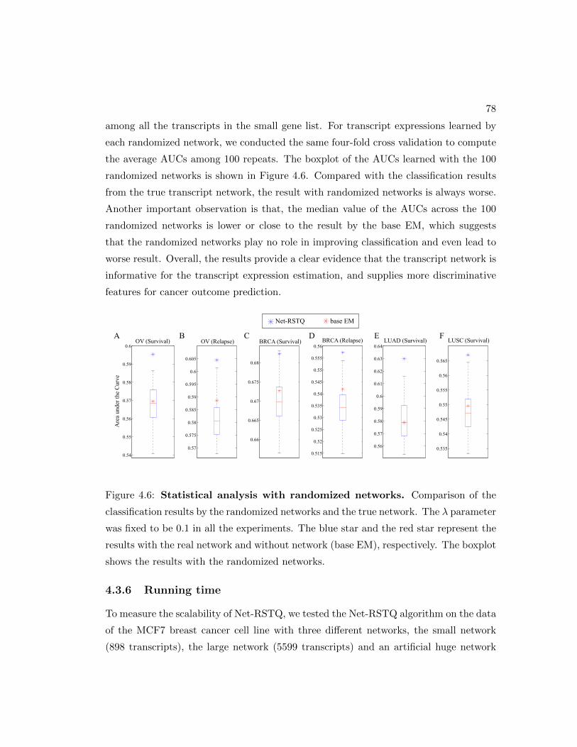
78

among all the transcripts in the small gene list. For transcript expressions learned by

each randomized network, we conducted the same four-fold cross validation to compute

the average AUCs among 100 repeats. The boxplot of the AUCs learned with the 100

randomized networks is shown in Figure 4.6. Compared with the classification results

from the true transcript network, the result with randomized networks is always worse.

Another important observation is that, the median value of the AUCs across the 100

randomized networks is lower or close to the result by the base EM, which suggests

that the randomized networks play no role in improving classification and even lead to

worse result. Overall, the results provide a clear evidence that the transcript network is

informative for the transcript expression estimation, and supplies more discriminative

features for cancer outcome prediction.

0.54

0.55

0.56

0.57

0.58

0.59

0.6

Net2RSTQdddddddddddddddbasedEM

0.57

0.575

0.58

0.585

0.59

0.595

0.6

0.605

0.66

0.665

0.67

0.675

0.68

0.535

0.54

0.545

0.55

0.555

0.56

0.565

0.515

0.52

0.525

0.53

0.535

0.54

0.545

0.55

0.555

0.56OVd7Survival8 OVd7Relapse8 BRCAd7Survival8 BRCAd7Relapse8

0.56

0.57

0.58

0.59

0.6

0.61

0.62

0.63

0.64LUADd7Survival8 LUSCd7Survival8

Are

adun

derd

thed

Cur

ve

A B C D E F

Figure 4.6: Statistical analysis with randomized networks. Comparison of the

classification results by the randomized networks and the true network. The λ parameter

was fixed to be 0.1 in all the experiments. The blue star and the red star represent the

results with the real network and without network (base EM), respectively. The boxplot

shows the results with the randomized networks.

4.3.6 Running time

To measure the scalability of Net-RSTQ, we tested the Net-RSTQ algorithm on the data

of the MCF7 breast cancer cell line with three different networks, the small network

(898 transcripts), the large network (5599 transcripts) and an artificial huge network

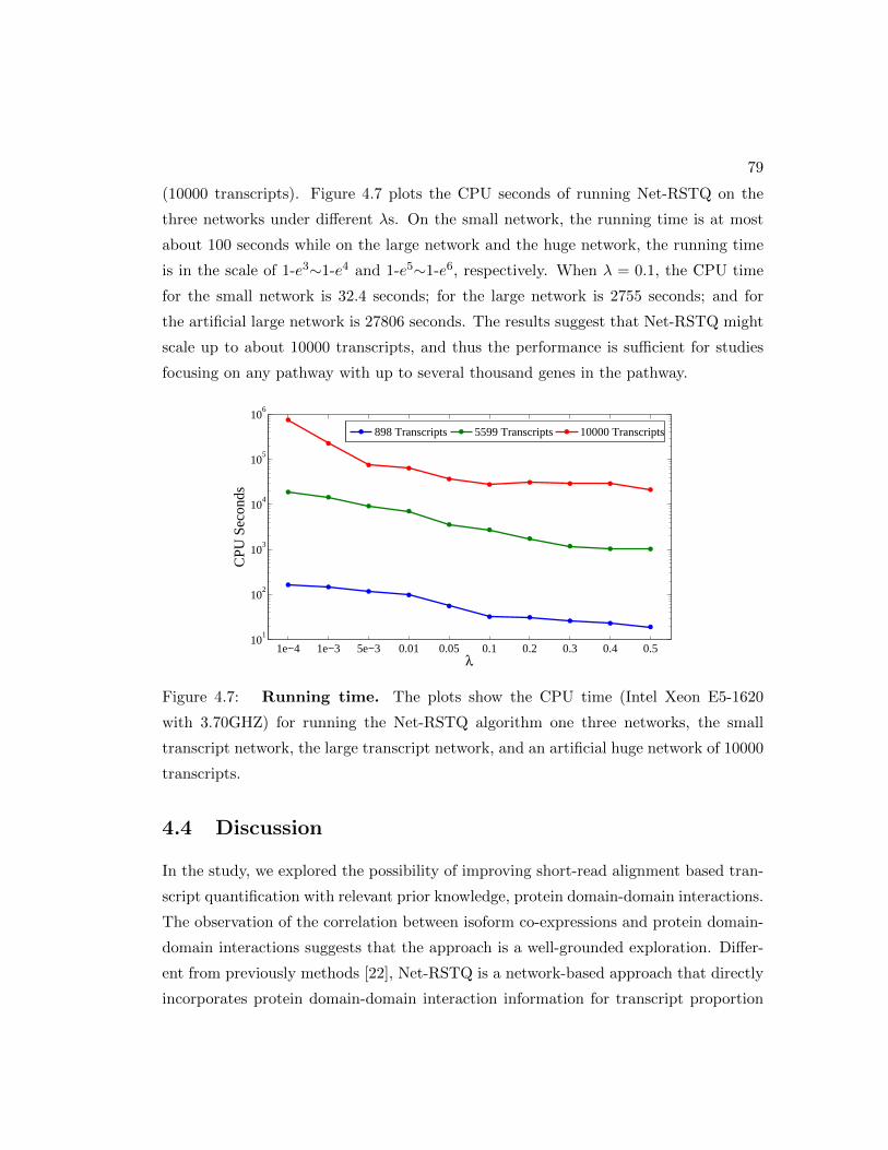
79

(10000 transcripts). Figure 4.7 plots the CPU seconds of running Net-RSTQ on the

three networks under different λs. On the small network, the running time is at most

about 100 seconds while on the large network and the huge network, the running time

is in the scale of 1-e3∼1-e4 and 1-e5∼1-e6, respectively. When λ = 0.1, the CPU time

for the small network is 32.4 seconds; for the large network is 2755 seconds; and for

the artificial large network is 27806 seconds. The results suggest that Net-RSTQ might

scale up to about 10000 transcripts, and thus the performance is sufficient for studies

focusing on any pathway with up to several thousand genes in the pathway.

1e−4 1e−3 5e−3 0.01 0.05 0.1 0.2 0.3 0.4 0.510

1

102

103

104

105

106

λ

CPU

Sec

onds

898 Transcripts 5599 Transcripts 10000 Transcripts

Figure 4.7: Running time. The plots show the CPU time (Intel Xeon E5-1620

with 3.70GHZ) for running the Net-RSTQ algorithm one three networks, the small

transcript network, the large transcript network, and an artificial huge network of 10000

transcripts.

4.4 Discussion

In the study, we explored the possibility of improving short-read alignment based tran-

script quantification with relevant prior knowledge, protein domain-domain interactions.

The observation of the correlation between isoform co-expressions and protein domain-

domain interactions suggests that the approach is a well-grounded exploration. Differ-

ent from previously methods [22], Net-RSTQ is a network-based approach that directly

incorporates protein domain-domain interaction information for transcript proportion

80

estimation. The experiments suggested a great potential of exploring protein domain-

domain interactions to overcome the limitations of short-read alignments and improve

transcript quantification for better sample classification.

The Dirichlet prior from the neighboring isoforms play two different roles: differ-

entiating isoform expressions to reflect different functional roles or smoothing isoform

expressions to reflect similar functional roles, depending on whether the isoforms of a

gene share the same or different interacting partners. This principle in modeling is

based on the hypothesis that isoforms playing different functional roles (e.g. containing

different protein domains) are more likely to behavior differently than isoforms with

the same or similar functional roles (e.g. containing the same protein domains). When

the isoforms of a gene interact with different partners, their expressions correlates with

their partners’ expressions. And, when the isoforms of a gene interact with the same

partners, there is no benefit on differentiating their proportions to drive the function-

ality. A limitation is that when the functional difference among the isoforms are not

captured by domain content, the smoothing role might under-estimate the difference in

their proportions. Thus, our future goal is to bring in other type of functional infor-

mation to distinguish their functional roles in cancer such as preferential adoption of

post-transcriptional regulations.

Currently, Net-RSTQ does not directly model multi-hits reads in multiple loci. In the

TCGA experiments, around 5-10% of the aligned reads in four datasets have multiple

alignments reported by TopHat and only one of the best alignments is considered.

To check the effect of the multiple-alignment reads in transcript quantification, we

allow up to 20 best alignments by TopHat and normalized the read assignment qijk

by the number of loci that the reads aligned to. The correlation coefficients between

the estimated gene expressions before and after the normalization are above 0.98 in all

the datasets. A potential rigorous solution is to add iteratively reassignment of the

reads to the potential origins based on updated abundance of the involved isoforms.

The modification will significantly decrease the computational efficiency and make it

impractical on large RNA-Seq datasets.

There is also another alternative of integrating the network information directly as a

regularization term on the joint likelihood function of all the genes. We also explored this

model in the S1 Text in [36]. In the preliminary experiments, we observed very similar

81

outputs between the alternative model and the Net-RSTQ model shown in S8 Table

in [36]. However, since the alternative model directly works with one large optimization

problem across all the genes, the convergence is much slower as shown in S4 Figure

in [36] and the optimization package used in the experiments ran into numerical issues.

Thus, we believe the Net-RSTQ model is more scalable and robust in comparison.

Currently, Net-RSTQ can scale on transcript network with up to around 5000 tran-

scripts, which is sufficient for more focused analysis of several thousand genes. The

running time of Net-RSTQ on such large transcript network is below 2 hours on each

TCGA sample, compared with 5-8 hours needed for aligning the short reads. To fur-

ther scale up Net-RSTQ, we will investigate other faster strategies of utilizing short

read information, such as Sailfish [148] which directly estimates isoform expressions by

counting k-mer occurrences in reads rather than reads from the alignments. This will

be our future direction.

Chapter 5

Detecting mRNA 3’-UTR

shortening in mTORC1 activated

MEFs

5.1 Introduction

In eukaryotes, a large portion of mRNAs contains multiple polyadenylation signals

(PASs) in their 3’-untranslated region (3’-UTR). Alternating the usage of PAS, namely

alternative cleavage and polyadenylation (ApA), produces mRNA isoforms with the

same coding capacity but with various lengths of 3’-UTR [7,149–151]. As 3’-UTR pro-

vides a binding platform for microRNAs and RNA-binding proteins, it serves as an im-

portant determinant for mRNA fate such as translation and stability [149,150,152,153].

Therefore, ApA provides an additional layer of complexity in regulating gene expres-

sion at the posttranscriptional level. Powerful high-profiling technologies focusing on

3’-UTRs of mRNAs provided high-resolution snap shots of alternatively polyadenylated

mRNA isoforms in various tissues and cells across many species [4,153–157]. An impor-

tant insight that emerged from these studies is that 3’-UTR length undergoes dynamic

changes under pathogenic conditions such as cancer and in diverse biological processes

such as cell proliferation, differentiation and development [23, 149, 153, 154, 158, 159].

Although the information on alternative polyadenylation sites in transcriptomes across

82

83

different species and tissues is rapidly accumulating, it is not clear what cellular mech-

anism(s) controls the switches between proximal and distal polyadenylation sites and

how this process is regulated.

The mammalian target of rapamycin (mTOR) pathway is crucial for regulating cell

proliferation/growth and its dysregulation causes many human diseases [160]. mTOR

exists as two distinctive multi-protein complexes, mTORC1 and mTORC2. Raptor and

Rictor are specific components of mTORC1 and mTORC2, respectively, and they are

essential for cellular function of each mTOR complex [160,161]. mTORC1 is negatively

regulated by tuberous sclerosis complexes (TSC1 and TSC2) and is an evolutionarily

conserved kinase that phosphorylates the ribosomal protein S6 kinases and the eu-

karyotic initiation factor 4E-binding proteins for efficient translation [160,161]. Recent

studies identified cis-acting elements in mRNAs such as 5’-terminal oligopyrimidine tract

(TOP) or 5’-pyrimidine-rich translational element (PRTE) that render the association

of a transcript with polysomes. mRNAs containing these elements in their 5’-UTRs

encode proteins for cellular pathways including translation, cell invasion and metasta-

sis, suggesting their relevance in cancer pathogenesis [162, 163]. mTOR also plays an

important role for activating transcriptional networks and regulates multiple cellular

pathways for lipid and nucleotide metabolism [164,165]. Recently, mTOR was shown to

play a role in the regulation of proteasome activity by upregulating a transcription fac-

tor Nrf-1 (ref. [166]). Although these studies were mainly focusing on the role of mTOR

in the synthesis of proteins, lipids and nucleic acids through transcriptional networks,

whether mTOR is involved in other cellular processes by modulating gene expression at

posttranscriptional level is relatively unclear.

In this study, we used isogenic non-cancerous mouse embryonic fibroblast (MEF) cell

lines to understand changes of molecular features on dysregulated activation of mTOR.

We employed RNA sequencing (RNA-seq) and two-dimensional liquid chromatography

tandem mass spectrometry (2D LC-MS/MS) approaches to investigate the changes at

high resolution and found an unexpected link between mTOR and ubiquitin-mediated

proteolysis pathway through 3’-UTR shortening. These findings expand our under-

standing of mTOR to regulation of RNA processing and protein degradation pathways.

84

5.2 Results

5.2.1 3’-UTR shortening of mRNAs is caused by mTOR activation

and is a down stream target of mTORC1

Figure 5.1: mTOR activation leads to genome-wide 3’-UTR shortening. (a)

RNA-seq reads from WT and TSC1−/− are aligned to mouse genome mm10 RefSeq.

Representative examples of transcripts with 3’-UTR shortening are presented. Anno-

tated gene structures are at the bottom of the alignment. The yellow boxes highlight

the aligned reads in 3’-UTRs. (b) Scatter plot of RNA-seq data. Red dots represent

individual transcripts in the analysis. Horizontal blue-dashed lines represent the cutoff

values for twofold changes in differential gene expression. Vertical green-dashed lines

represent the cutoff values for log10 (p-value) of 3’-UTR shortening (1.3 corresponds to

p-value=0.05) in TSC1−/− and WT, which was determined by χ2-test. (c) A schematic

presenting primer sets for RT-qPCR and the RSI determination. Pairs of primers were

used to detect a total (short+long) or a long-specific transcript. The RSI was calculated

to determine the 3-UTR shortening in a target cell line by RT-qPCR. (d) Validation of

RNA-seq data. Error bars represent s.e. from three repeats of experiments. Student’s

t-tests are done for statistical significance. ∗p-value <0.0025.

85

To explore mTOR function in gene expression at a single nucleotide resolution, we

performed RNA-seq experiments (Supplementary Table 1 in [34]) using Tsc1 knockout

(TSC1−/−) and wild-type (WT) MEF cells [167]. Knockout of Tsc1, a negative regulator

of mTOR, leads to uncontrolled mTOR hyperactivation compared with WT [167,168].

One of the striking features in our data set was that many transcripts in TSC1−/−

showed an abrupt signal drop only for a segment of the 3’-most exon of an annotated

gene compared with WT (Fig.1a and Supplementary Fig.1a in [34]). For example, the

read signal for Dicer1 in TSC1−/− dropped after the termination codon in the 3’-most

exon, although the signal from upstream exons increased (Fig.1a). In some cases, up-

stream exons showed either similar (for example, Mecp2 and Tomm20) or decreased (for

example, Anxa7 and Timp2) signal, although we observed the same pattern of signal

drop in the 3’-most exon from TSC1−/− (Fig.1a and Supplementary Fig.1a in [34]). Fur-

ther sequence analysis revealed that canonical or non-canonical PAS(s) exists around the

regions showing the signal drop. This indicates that the synthesis of these transcripts

terminated early in the 3’-most exon using the proximal PASs for polyadenylation, sug-

gesting a predominant production of mRNA isoforms with a shorter 3’-UTR in the

mTOR-activated transcriptome (Fig.1a and Supplementary Fig.1a in [34], yellow box,

and Supplementary Data 1 in [34]). For some transcripts such as Tomm20 and Nampt,

3’-UTR-shortened transcripts were already present in WT where the mTOR activity is

low but not entirely absent (Fig.1a and Supplementary Fig.1a in [34]). These 3’-UTR-

shortened transcripts increased significantly in TSC1−/− (Fig.1a and Supplementary

Fig.1a in [34]), indicating that individual transcripts differ in the regulation of their

3’-UTR length in response to cellular mTOR activity. As the signals from upstream ex-

ons reflecting the amount of transcripts varied among the 3’-UTR-shortened transcripts,

we examined whether 3’-UTR shortening in the mTOR-activated transcriptome corre-

lates to differential gene expression. To this end, we enriched 5,160 transcripts in our

data set that are eligible for combined analysis of 3’-UTR shortening and differential

expression (see Methods for details). Next, each transcript was plotted by fold changes

in the differential gene expression (y axis in Fig.1b) and the significance of 3’-UTR

shortening (x axis in Fig.1b). This approach identified 846 3’-UTR-shortened tran-

scripts (about 16.4%) out of 5,160 transcripts in TSC1−/− (Fig.1b). Although 26.3%

(223/846) of the 3’-UTR-shortened transcripts either increased (147/846) or decreased

86

(76/846) their expression level, a significant proportion (73.7%) of them in the mTOR-

activated transcriptome remained unchanged (Fig.1b), indicating no strong correlation

between the differential gene expression and the 3’-UTR shortening in the mTOR-

activated transcriptome. Of note, only a small percentage (1.3%) of transcripts showed

3’-UTR shortening in WT over TSC1−/− MEFs. To confirm the RNA-seq data, we

developed a method to determine 3’-UTR shortening or lengthening by calculating rel-

ative shortening index (RSI) (see Methods for details; Fig.1c). Twelve genes, covering

a wide range of p-values, were randomly selected from the 3’-UTR shortening data set;

all showed the RSI >0 in TSC1−/− (Fig.1d and see also Supplementary Fig.1d,e in [34]

for alternative presentations of the data using different experimental and calculation

methods), validating our RNA-seq data analysis. Together, these data strongly suggest

that mTOR activation in cells leads to a preferred usage of proximal PAS in the 3’-most

exon of mRNAs and results in transcriptome-wide 3’-UTR shortening.

To determine whether 3’-UTR shortening due to ApA is a previously uncharac-

terized cellular target downstream of mTOR pathway, our collaborator established a

stable mTOR knockdown cell line TSC1−/− MEFs (TSC1−/− mTOR kd; Supplemen-

tary Fig.2a in [34]). The tested transcripts showed the RSI <0 in TSC1−/− mTOR

kd MEFs as compared with a control knockdown cell line, indicating the enrichment

of 3’-UTR-lengthened transcripts in mTOR-deficient cells (Fig.2a and Supplementary

Fig.2b in [34]), thus supporting the idea that mTOR functions in 3’-UTR length regula-

tion. Consistently, the same results were observed in a human embryonic kidney stable

cell line and a bladder cancer cell line with the same treatment [169,170]. These results

suggest that the function of mTOR in 3’-UTR shortening is a general phenomenon and

evolutionarily conserved between human and mouse (Supplementary Fig.2c-e in [34]).

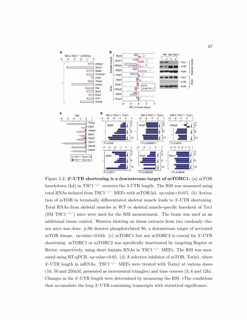
87

Figure 5.2: 3’-UTR shortening is a downstream target of mTORC1. (a) mTOR

knockdown (kd) in TSC1−/− recovers the 3-UTR length. The RSI was measured using

total RNAs isolated from TSC1−/− MEFs with mTOR kd. ∗p-value<0.015. (b) Activa-

tion of mTOR in terminally differentiated skeletal muscle leads to 3’-UTR shortening.

Total RNAs from skeletal muscles in WT or skeletal muscle-specific knockout of Tsc1

(SM TSC1−/−) mice were used for the RSI measurement. The brain was used as an

additional tissue control. Western blotting on tissue extracts from two randomly cho-

sen mice was done. p-S6 denotes phosphorylated S6, a downstream target of activated

mTOR kinase. ∗p-value<0.016. (c) mTORC1 but not mTORC2 is crucial for 3’-UTR

shortening. mTORC1 or mTORC2 was specifically deactivated by targeting Raptor or

Rictor, respectively, using short hairpin RNAs in TSC1−/− MEFs. The RSI was mea-

sured using RT-qPCR. ∗p-value<0.05. (d) A selective inhibitor of mTOR, Torin1, alters

3’-UTR length in mRNAs. TSC1−/− MEFs were treated with Torin1 at various doses

(10, 50 and 250nM, presented as incremental triangles) and time courses (3, 6 and 12h).

Changes in the 3’-UTR length were determined by measuring the RSI. ∗The conditions

that accumulate the long 3’-UTR-containing transcripts with statistical significance.

88

Proliferative cells are known to carry short 3’-UTRs in their transcriptome and

terminally differentiated tissues are known to produce transcripts with long 3’-UTRs

[153,154,157]. We asked whether mTOR activation could be an underlying reason that

explains these observations. The experiments done by our collaborator on a mouse

model with skeletal muscle provide evidence that the mTOR activation is sufficient

to drive 3’-UTR shortening in terminally differentiated skeletal muscles (Fig.2b and

Supplementary Fig.2m in [34]).

To address which mTOR complex regulates 3’-UTR shortening, our collaborator es-

tablished stable cell lines using short hairpin RNA that specifically knocks down Raptor

(a component of mTORC1) or Rictor (a component of mTORC2) in TSC1−/− MEFs

(Supplementary Fig.2g in [34]). The knockdown of Raptor but not Rictor resulted in

the RSI <0 when compared with control knockdown cells, suggesting that mTORC1

plays an important role in 3’-UTR shortening (Fig.2c and Supplementary Fig.2h in [34]).

mTOR is a key therapeutic target for many human disease treatments [160] and several

versions of selective mTOR inhibitors have been developed including Torin1 (ref. [171]).

The experiments done by our collaborator shows that the cellular ApA pattern changes

drastically on the pharmacological inhibition of mTOR (Fig.2d and Supplementary

Fig.2i,j,n in [34]). Furthermore, our collaborator proved that the 3’-UTR lengthening

after Torin1 treatment is not caused by the inhibition of cell proliferation but rather

from the inactivation of mTOR (Supplementary Fig.2r,s in [34]). Taken together, we

conclude that the mTOR pathway is an upstream regulator for ApA process and deter-

mines the 3’-UTR length in the transcriptome independent of cell proliferation status.

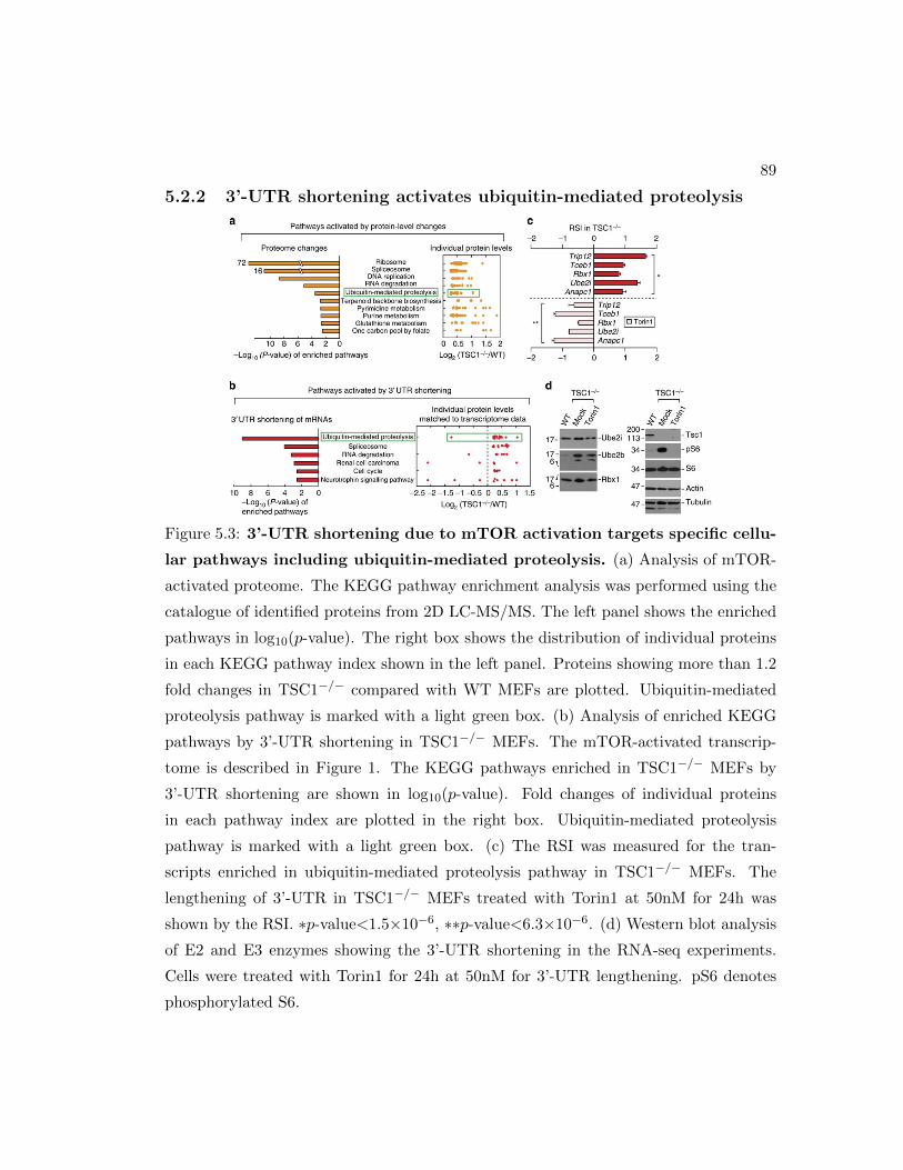
89

5.2.2 3’-UTR shortening activates ubiquitin-mediated proteolysis

Figure 5.3: 3’-UTR shortening due to mTOR activation targets specific cellu-

lar pathways including ubiquitin-mediated proteolysis. (a) Analysis of mTOR-

activated proteome. The KEGG pathway enrichment analysis was performed using the

catalogue of identified proteins from 2D LC-MS/MS. The left panel shows the enriched

pathways in log10(p-value). The right box shows the distribution of individual proteins

in each KEGG pathway index shown in the left panel. Proteins showing more than 1.2

fold changes in TSC1−/− compared with WT MEFs are plotted. Ubiquitin-mediated

proteolysis pathway is marked with a light green box. (b) Analysis of enriched KEGG

pathways by 3’-UTR shortening in TSC1−/− MEFs. The mTOR-activated transcrip-

tome is described in Figure 1. The KEGG pathways enriched in TSC1−/− MEFs by

3’-UTR shortening are shown in log10(p-value). Fold changes of individual proteins

in each pathway index are plotted in the right box. Ubiquitin-mediated proteolysis

pathway is marked with a light green box. (c) The RSI was measured for the tran-

scripts enriched in ubiquitin-mediated proteolysis pathway in TSC1−/− MEFs. The

lengthening of 3’-UTR in TSC1−/− MEFs treated with Torin1 at 50nM for 24h was

shown by the RSI. ∗p-value<1.5×10−6, ∗∗p-value<6.3×10−6. (d) Western blot analysis

of E2 and E3 enzymes showing the 3’-UTR shortening in the RNA-seq experiments.

Cells were treated with Torin1 for 24h at 50nM for 3’-UTR lengthening. pS6 denotes

phosphorylated S6.

90

Activation of mTOR increases global protein synthesis by controlling multiple down-

stream events such as ribosome biogenesis and cap-dependent translation initiation and

elongation [160,161]. Especially, mTOR promotes the translation of a subset of mRNAs

carrying 5’-UTR sequences such as 5’TOP, 5’TOP-like motif and 5’PRTE [162, 163].

Similar to 5’-UTR, 3’-UTR in mRNA also plays an important role in the regulation

of gene expression. In particular, 3’-UTR shortening in a transcript has been shown

to increase protein production [150, 153, 154, 172]. Therefore, we asked whether the

mTOR-activated 3’-UTR shortening contributes to mTOR-mediated upregulation of

protein synthesis and influences mTOR-related biology. To this end, our collaborator

first conducted quantitative proteomic studies using tandem mass tag (TMT)-labelled

total cell lysates prepared from WT and TSC1−/− MEFs, to quantitatively profile the

changes in the cellular proteome due to mTOR activation. They identified a total of

2,754 proteins that were found in either cell line by two or more unique peptides via

2D LC-MS/MS (Supplementary Data 2 in [34]). I did the KEGG (Kyoto Encyclopedia

of Genes and Genomes) enrichment analysis on the catalogue of proteins with >20%

increase (1,014 proteins) in abundance (TSC1−/− compared with WT) and found that

multiple cellular pathways are activated in TSC1−/− (Fig.3a). We also performed the

KEGG pathway analysis using the catalogue of 846 3’-UTR-shortened transcripts (Sup-

plementary Data 1 in [34]) and the differentially expressed transcripts in TSC1−/− MEFs

(Supplementary Fig.3a and Supplementary Data 3 in [34]). By comparing the enriched

pathways from these three data sets, we found that multiple pathways in the mTOR-

activated proteome such as spliceosome (mmu03040) and RNA degradation (mmu03018)

are upregulated by both 3’-UTR shortening and differential gene expression, whereas

other enriched pathways such as DNA replication (mmu03030) and pyrimidine/purine

metabolism (mmu00240/mmu00230) are attributable solely to the differential gene ex-

pression (Fig.3a and Supplementary Fig.3a,b in [34]).

Intriguingly, among those enriched pathways in the quantitative proteome analy-

sis, ribosome- (mmu03010) and ubiquitin-mediated proteolysis pathways (mmu04120)

did not appear in the differential gene expression data set (Fig.3a and Supplementary

Fig.3b,c in [34]). This indicates that these two pathways are most likely to be ac-

tivated by other mTOR-mediated regulatory mechanisms rather than transcriptional

regulation. It is known that the ribosome pathway is activated by mTOR through the

91

translational regulation of mTOR-responsive 5’-UTR cis-elements such as 5’TOP and

5’PRTE in the mRNAs [162,163,173]. On the other hand, mTOR-responsive 5’-UTR se-

quence elements do not exist in most transcripts from the ubiquitin-mediated proteolysis

pathway, supporting the idea that 3’-UTR shortening could be an explanation for the

activation of ubiquitin-mediated proteolysis pathway in the mTOR-activated proteome

(the light green box in Fig.3a,b and Supplementary Fig.3d in [34]). All transcripts from

the ubiquitin-mediated proteolysis pathway containing short 3’-UTR encode the com-

ponents of E2 ubiquitin-conjugating enzymes and E3 ubiquitin ligases such as Anapc1,

Rbx1, Trip12, Ube2i and Tceb1. Consistent with our findings in this study, these tran-

scripts carry an mTOR-dependent short 3’-UTR in TSC1−/− MEFs as determined by

the RSI in the presence or the absence of Torin1 treatment (Fig.3c). As shown by

western blotting (Fig.3d), the expression of Ube2i, Ube2b and Rbx1 proteins matched

the progression of 3’-UTR shortening in these transcripts, supporting our conclusions

from quantitative proteomics studies and 3’-UTR-shortening analysis. Together, these

results suggest that 3’-UTR shortening by mTOR activation plays an important role in

altering gene expression. These results also identify the ubiquitin-mediated proteolysis

pathway as an additional cellular target of mTOR. Thus, mTOR-driven 3’-UTR short-

ening might explain part of cellular phenotypic changes in TSC1−/− over WT MEFs.

5.3 Method

5.3.1 RNA-Seq and alignments

To evaluate transcriptome features under mTOR hyperactivation at nucleotide-wise

resolution, we performed RNA-seq analysis of poly(A+) RNAs isolated from WT and

TSC1−/− MEFs. In total, 63,742,790 paired-end reads for WT and 74,251,891 paired-

end reads for TSC1−/− MEFs were produced from Hi-Seq pipeline with length of 50bp of

each end. The short reads were aligned to the mm10 reference genome by TopHat [174],

with up to two mismatches allowed. The unmapped reads were first trimmed to remove

poly-A/T tails (repeats of [A/N]s or [T/N]s) from read ends/starts and then aligned to

the reference genome. It is worth noting that we only retained the reads with at least

30bp in both ends after trimming. Finally, 87.1% of short reads from WT and 87.5% of

sequence reads from TSC1−/− MEFs were mapped to the reference genome by TopHat

92

for ApA analysis in the study.

5.3.2 ApA analysis

To detect the potential alternative PAS of a transcript between WT and TSC1−/−

MEFs, we evaluated candidate PAS motifs (AATAAA, ATTAAA, AGTAAA, CATAAA,

TATAAA, GATAAA, ACTAAA, AATACA, AATATA, AAGAAA, AATAGA, AAT-

GAA, TTTAAA, AAAATA, TATATA, AGATAA, ATTACA, AGAATA) [31, 175] in

the 3’-UTR of the transcript by contrasting the short-read coverage up/downstream of

the site across WT and TSC1−/− samples with χ2-test. Specifically, we first scanned

the 3’-UTR of a transcript (by mm10 annotation) to identify PAS motifs as candidates

of alternative PAS. For each candidate PAS, we calculated the mean coverage upstream

of the site (N and M) and downstream of the site (n and m) with (N, n) denoting the

coverage in WT and (M, m) denoting the coverage in TSC1−/−. In the calculation, the

upstream region starts at the beginning of the last coding exon adjacent to the 3’-UTR

of the transcript and ends at the beginning of the PAS motif site. Next, a canonical

2×2 χ2-test was applied to report a p-value for each candidate site. The candidate PAS

with the most significant p-value ≤0.05 was considered for further analysis. It is note-

worthy that the χ2-test will report shortening events in both WT (when N/n>M/m)

and TSC1−/− (when N/n<M/m). Out of the 5,160 transcripts, 846 (16.4%) show a

p-value ≤0.05 in TSC1−/− MEFs and 69 (1.3%) a show p-value ≤0.05 in WT MEFs.

5.3.3 Scatter plot for differential expression and ApA analysis

To select candidate transcripts with sufficient signal for reliable differential expression

analysis and 3’-UTR-shortening identification, we first analysed the short-read align-

ments of the RNA-seq data against mouse mm10 reference genome using Cufflink [23].

In the alignments, 14,378 and 14,175 transcripts are considered ‘expressed’ in WT and

TSC1−/− cell lines, respectively, with a FPKM (fragments per kilobase of transcript per

million mapped reads) cutoff=0.17. The union of the two sets gives 15,340 transcripts

that are expressed in at least one of the cell lines. We further filtered out the transcripts

with positional short-read coverage ≤25 in the entire 3’-UTR in both cell lines. In ad-

dition, transcripts with 3’-UTR overlapping exons in the strand in opposite direction

93

were removed to avoid mingled short-read signals that might lead to inaccurate 3’-UTR-

shortening identification. Finally, to allow precise PAS analysis, only transcripts with

at least two occurrences of the 18 PAS motifs in the 3’-UTR are retained in the study.

The entire pruning procedure left 5,160 transcripts for further analysis.

5.3.4 Measurement of RSI

A numerical presentation of 3’-UTR shortening was developed by calculating the RSI of

a given transcript. A relative expression of total or longer 3’-UTR-containing transcripts

was measured by normalizing to total amount of RNAs used in RT-qPCR analysis. The

following equation was used to determine the RSI.

LI=[normalized expression of longer 3’-UTR-containing transcript]/[normalized ex-

pression of total (long+short) transcript]

RSI=log2(LI/[LI in reference cell line]); thus, RSI=0 for a reference cell line.

If RSI >0 in a target cell line, then there is a 3’-UTR shortening. If RSI <0 in a

target cell line, then there is a 3’-UTR lengthening. The RSI contains the information

about the changes in the proportion of a longer 3’-UTR-containing transcript in a given

cellular context compared with a reference cell. For example, a value of 1 in the RSI of

a transcript indicates that the proportion of the longer 3’-UTR-containing transcript of

the total (long+short) transcript decreases by 50% compared with that of the reference

cell line, indicating an enrichment of 3’-UTR-shortened transcript (that is, 3’-UTR

shortening).

5.4 Discussion

In this study, we used genetically well-defined MEFs to investigate the molecular signa-

tures of mTOR-activated transcriptome and discovered widespread 3’-UTR shortening

due to dysregulated mTOR activation. Although a precise mechanism(s) of how mTOR

activation leads to the 3’-UTR shortening in selected transcripts is unknown, we found

that almost all known 3’-end processing factors alter their expression on changes in cel-

lular mTOR activity in TSC1−/− compared with WT MEFs, suggesting that mTOR-

mediated 3’-UTR shortening occurs by multiple factors (Supplementary Data 3 in [34]).

94

Analysis on pathways enriched in 3’-UTR-shortened transcripts and quantitative pro-

teomics on mTOR activation identified ubiquitin-mediated proteolysis as an additional

target pathway of mTOR. Considering the well-documented function of mTOR in the

activation of cellular anabolic metabolism for rapid cell proliferation [176], the newly dis-

covered function of mTOR in ubiquitin-mediated proteolysis through 3’-UTR shortening

is surprising. A recent study suggests a role of mTOR in the activation of proteasome

through the modulation of a transcriptional network [166]. This study argued that the

promotion of protein degradation pathway on mTOR activation is required for a con-

tinuous supply of amino acids to cellular systems, to maintain the steady-state protein

synthesis. Our data set also indicates a marginal increase in the proteasome activity

through a transcriptional upregulation of several proteasomal subunits (Supplementary

Fig.4d in [34]) and an increase in the polyubiquitination of proteins on mTOR activation

(Supplementary Fig.4i in [34]). Moreover, our data demonstrate that mTOR-promoted

3’-UTR shortening leads to the overexpression of selected E2 and E3 components in ubiq-

uitin ligase complexes (Figs 3b,d), which is known to increase polyubiquitination of their

substrates [177–183]. Therefore, it is possible that the enrichment of polyubiquitination

in cellular proteins on mTOR activation could come from selective polyubiquitination of

those E2 and E3 substrates. Together, our study proposes the molecular mechanism of

how mTOR pathway selects proteins to degrade through 3’-UTR shortening of a subset

of mRNAs. The E2 and E3 enzymes upregulated by mTOR-driven 3’-UTR shortening

mostly target cell cycle regulators, tumour suppressors and pro-apoptotic proteins for

ubiquitin-proteasome system [178,184]. For instance, Rbx1, Trip12 or Anapc1/5 are all

components of E3 ligase complexes that selectively polyubiquitinate Arf and Cyclins,

and Birc6 E3 ligase targets Caspase 3/7 for degradation [178, 184, 185]. For rapidly

proliferating cells, a timely removal of cell cycle regulators such as Arf and Cyclins is a

key step for rapid progression of the cell cycle [178]. Therefore, our findings are particu-

larly important, because unlike a previous argument it explains how upregulated mTOR

and consequent proteasome activation recycles proteins that are only needed to foster

a cellular environment favourable to rapid cell proliferation. Thus, we suggest that this

selective proteolysis not only provides a surplus of amino acids to cellular systems but

also makes cells proliferate rapidly by efficient modulation of the cellular levels of cell

cycle regulators.

Chapter 6

Conclusion and Discussion

This thesis has presented several network-based learning methods and a pipeline for uti-

lize high-dimensional microarray gene expression and RNA-Sequencing genomic data

that integrate biological prior knowledge for cancer transcriptome analysis. We ap-

proached this problem with three consecutive directions. (1) Accurate quantification of

the molecular features in the genomic data. (2) Develop reliable methods to identify

the reproducible cancer relevant biomarkers from all the candidate genomic features.

(3) Develop robust predictive models for patient samples classification. In this chapter,

we summarized the works present in the thesis based on the three directions mentioned

above and then a discussion of possible extensions of the works.

6.1 Conclusion

Accurate quantification of molecular features is the crucial step in other downstream

transciptome analysis such as isoform function prediction, biomarker identification, and

patient samples classification. In the thesis, (1) we described a network-based method

Net-RSTQ integrate protein domain-domain interaction network with short read align-

ments for transcript abundance estimation in Chapter 4. Compared to the existing

methods, Net-RSTQ is proven a useful tool for isoform-based analysis in functional

genomes and systems biology validated by qRT-PCR experiments, simulation and clas-

sification of TCGA patient samples. All the experiments suggested a great potential of

exploring protein domain-domain interactions to overcome the limitations of short-read

95

96

alignments. (2) We developed a pipeline for the study in Chapter 5 to quantify the

different polyadenylation sites in the 3’-UTR region for the same gene with RNA-Seq

data. We then identified ApA events between TSC1−/− and WT based on the quantified

polyadenylation with χ2-test. The experiments support the accuracy of the identified

ApA events.

Discovered biomarkers can possibly provide better prognosis and diagnosis than the

current available clinical measures for risk assessment of cancer patients. Building re-

liable computational methods to identify reproducible cancer relevant biomarkers from

high-throughput genomic data is a challenge problem. In the thesis, (1) we present

network propagation models Signed-NP for feature selection in high-dimensional mi-

croarray gene expression for detecting differentially expressed genes in Chapter 2. (2)

We introduce a network-based Cox regression model Net-Cox to identify relevant fea-

tures for survival analysis in cancer genomics in Chapter 3. Both models presented in

these two chapters introduce a graph Laplacian matrix as a smoothness requirement

on the gene features linked in the gene relation network. The gene relation network is

constructed by co-expression analysis or prior knowledge of gene functional relations.

Compared to the existing models, introducing a gene relation network in the model

capture more global relation among all the genes, such as centralities, closenesses, mod-

ularities, and subgraph structures. The experiments in Chapter 2 and 3 show that

the network-based methods identified highly consistent signature genes across several

datasets for the same study purpose. Moreover, the identified signature genes contain

more discriminative power for cancer prediction and survival prediction compared with

the marker genes identified by the other methods. One of the marker genes, FBN1,

which was detected as a signature gene of high confidence by Net-Cox with network

information, was validated as a biomarker for predicting early recurrence in platinum-

sensitive ovarian cancer patients in laboratory.

Developing a predictive model based on the identified molecular features or the

whole feature space for cancer patient survival prediction or classification is critical

for cancer treatment and etiology. The classification model, Signed-NPBi, which is

described in Chapter 2, is a semi-supervised learning algorithm on bipartite graphs was

introduced to explore sample-feature bi-clusters for feature selection and cancer outcome

classification. Large scale experiments on several microarray gene expression datasets

97

and CNV datasets validated that Signed-NPBi performed better classification of gene

expression and CNV data than the existing methods. The survival prediction model,

Net-Cox, which is described in Chapter 3 also consistently improved the accuracy of

survival prediction over the Cox models regularized by L2-norm or L1-norm.

In summary, all models proposed in this thesis showed promising results in both

simulations and experiments on real high-throughput genomic data, and the findings

are useful for the cancer studies.

6.2 Future Work

In this section, we will discuss several future directions extending the work presented in

this thesis.

6.2.1 Transfer learning across cancers

We introduce a transfer learning framework to discover common genomic features shared

across different cancer types and cancer specific features to extend the work proposed

in Chapter 2.

Suppose we have δ datasets (studies/cancer types) measured from the same p ge-

nomic features, each dataset i contains ni samples. We can learn the common genomic

features across the datasets and datasets specific features from

L(fc,fi) =

δ∑i=1

[α(fc + fi)

TLi(fc + fi) + (1− α)‖fc + fi − yi‖22 + γ1‖fi‖1]

+γ2‖fc‖1, (6.1)

where fc is the common feature vector and fi is the feature vector specific in dataset

i. Alternating optimize fc and fc can solve the problem in equation 6.1. When fc is

fixed, we can learn one fi at a time, which is equivalent to solve a lasso penalized linear

regression problem. The same for updating fc.

We can also extend the framework in equation 6.1 on a bipartite graph as a semi-

supervised learning model to identify common cancer genomic features, cancer specific

features, and classify the samples in each study simultaneously. Suppose we have δ

98

studies and i is the index of the studies. S(i) = D− 1

2v(i)∗W ∗D−

12

u(i).

L(fv(c),fv(i)

,fu(i)) =

δ∑i=1

‖fv(c)+ fv(i)

‖22 + ‖fu(i)‖22 − 2(fv(c)

+ fv(i))TS(i)fu(i)

+α‖fv(c)+ fv(i)

− yv(i)‖22 + α‖fu(i)

− yu(i)‖22

+λ1‖fv(i)‖1+ λ2‖fv(c)

‖1 (6.2)

where fv(c)is the common feature vector, fv(i)

is the feature vector specific in dataset

i, and fu(i)is the label vector for the samples in dataset i.

6.2.2 Improving transcript quantification by integrating RNA-Seq and

NanoString/qRT-PCR data

We introduce an integrative model to learn the transcript expression by integrating

RNA-Seq data and NanoString/qRT-PCR to provide the accurate transcript quantifi-

cation with the same purpose of the algorithm, Net-RSTQ described in Chapter 4.

Instead of providing all the individual isoform expression in the gene, NanoString or

qRT-PCR only need to provide the expression of the isoform groups in the gene as a

reference. For example, suppose there are five transcripts in gene A, we only need to

design the primers for NanoString(or qRT-PCR) to separate the five transcripts into at

least two groups, the groups can be overlapped with each other. The objective function

can be formulated to learn the probability pik of a read generated by transcript Tik in

the ith gene as follow,

Pi = arg maxPi

|ri|∑j=1

log(

|Ti|∑k=1

pikqijk)− λ‖Gi|ri| − αEi‖2 , (6.3)

where Pi is the probability of a read generated by transcript Ti in the ith gene, specif-

ically, Pi = [pi1, ..., pi,|Ti|]. Ei is the expression of the isoform groups in the ith gene

estimated from NanoString(or qRT-PCR). α is a parameter make the expressions esti-

mated by RNA-Seq and NanoString(or qRT-PCR) are comparable. Gi is the relative

abundance of the isoform groups in the ith gene which is a function of pik.

Equation 6.3 consists of two terms. The first term is the log-likelihood of the observed

read counts in the data for gene i, and the second term encourages consistency between

the expressions reported by RNA-Seq and NanoString (or qRT-PCR).

99

6.2.3 Identify 3’-UTR shortening by integrating RNA-Seq and PAS-

Seq data

The pipeline to identify the ApA events presented in Chapter 5 is solely based on the

candidate PAS motifs since the exact polyadenylation sites in the 3’-UTR region are not

available. It may not accurately estimate the cleavage position from the candidate PAS

to identify the ApA events. A recently developed deep sequencing-based method called

Poly(A) Site Sequencing (PAS-Seq) for quantitatively profiling RNA polyadenylation

at the transcriptome level [186] is available. PAS-Seq not only accurately and com-

prehensively identifies polyadenylation sites in mRNAs and noncoding RNAs, but also

provides quantitative information on the relative abundance of polyadenylated RNAs.

By integrating PAS-Seq data with RNA-Seq data, we can improve the pipeline presented

in Chapter 5 with an integrative model to identify 3’-UTR shortening events.

The integrative model can be formulated to learn the probability pik of a read

generated by the polyadenylated RNA Cik in the ith gene as follow,

Pi = arg maxPi

|ri|∑j=1

log(

|Ci|∑k=1

pikqijk)− λ‖Pi|ri|Li

− αEi‖2 , (6.4)

where Pi is the probability of a read generated by the polyadenylated RNA Ci in the ith

gene, specifically, Pi = [pi1, ..., pi,|Ci|]. Li is a vector contains the length of the 3’-UTRs

for polyadenylated RNAs in the ith gene. Ei is the expression of the polyadenylated

RNAs in the ith gene estimated from PAS-Seq. α is a parameter to make the expression

estimated by RNA-Seq and PAS-Seq comparable.

References

[1] van de Vijver MJ, He YD, van ’t Veer LJ, et al. (2002) A gene-expression signature

as a predictor of survival in breast cancer. New England Journal of Medicine 347:

1999-2009.

[2] Van’t Veer L, Dai H, Van de Vijver M, He Y, Hart A, et al. (2001) Gene expression

profiling predicts clinical outcome of breast cancer. Nature 415: 530-536.

[3] Jazaeri AA, Yee CJ, Sotiriou C, Brantley KR, Boyd J, et al. (2002) Gene expres-

sion profiles of brca1-linked, brca2-linked, and sporadic ovarian cancers. Journal

of the National Cancer Institute 94: 990-1000.

[4] Wang ET, Sandberg R, Luo S, Khrebtukova I, Zhang L, et al. (2008) Alternative

isoform regulation in human tissue transcriptomes. Nature 456: 470–476.

[5] David CJ, Manley JL (2010) Alternative pre-mrna splicing regulation in cancer:

pathways and programs unhinged. Genes & development 24: 2343–2364.

[6] Silvera D, Formenti SC, Schneider RJ (2010) Translational control in cancer. Na-

ture Reviews Cancer 10: 254–266.

[7] Elkon R, Ugalde AP, Agami R (2013) Alternative cleavage and polyadenylation:

extent, regulation and function. Nature Reviews Genetics 14: 496–506.

[8] Mayr C, Hemann MT, Bartel DP (2007) Disrupting the pairing between let-7 and

hmga2 enhances oncogenic transformation. Science 315: 1576–1579.

[9] Lee YS, Dutta A (2007) The tumor suppressor microrna let-7 represses the hmga2

oncogene. Genes & development 21: 1025–1030.

100

101

[10] Peri S, Navarro JD, Amanchy R, Kristiansen TZ, Jonnalagadda CK, et al. (2003)

Development of human protein reference database as an initial platform for ap-

proaching systems biology in humans. Genome Res 13: 2363-2371.

[11] Barabasi AL, Gulbahce N, Loscalzo J (2011) Network medicine: a network-based

approach to human disease. Nature Reviews Genetics 12: 56–68.

[12] Ulitsky I, Shamir R (2007) Identification of functional modules using network

topology and high-throughput data. BMC systems biology 1: 8.

[13] Zhou D, Bousquet O, Lal T, Weston J, Scholkopf B (2004) Learning with local

and global consistency. Advances in Neural Information Processing Systems 16:

321-328.

[14] Zhang W, Hwang B, Wu B, et al. (2010) Network propagation models for gene

selection. In: Genomic Signal Processing and Statistics (GENSIPS), 2010 IEEE

International Workshop on. pp. 1-4. doi:10.1109/GENSIPS.2010.5719689.

[15] Winter C, Kristiansen G, Kersting S, et al. (2012) Google goes cancer: Improving

outcome prediction for cancer patients by network-based ranking of marker genes.

PLoS Comput Biol 8: e1002511.

[16] Cox DR (1972) Regression Models and Life-Tables. Journal of the Royal Statistical

Society Series B (Methodological) 34: 187-220.

[17] Xing Y, Yu T, Wu YN, Roy M, Kim J, et al. (2006) An expectation-maximization

algorithm for probabilistic reconstructions of full-length isoforms from splice

graphs. Nucleic acids research 34: 3150-3160.

[18] Li B, Ruotti V, Stewart RM, Thomson JA, Dewey CN (2010) RNA-Seq gene

expression estimation with read mapping uncertainty. Bioinformatics 26: 493-

500.

[19] Breslow NE (1972) Discussion of professor cox’s paper. J R Statist Soc : 216-217.

[20] Rozov R, Halperin E, Shamir R (2012) MGMR: leveraging RNA-Seq population

data to optimize expression estimation. BMC Bioinformatics 13: S2.

102

[21] Li B, Ruotti V, Stewart RM, Thomson JA, Dewey CN (2010) RNA-Seq gene

expression estimation with read mapping uncertainty. Bioinformatics 26: 493-

500.

[22] Pachter L (2011) Models for transcript quantification from RNA-Seq. ArXiv :

1104.3889.

[23] Trapnell C, Williams BA, Pertea G, Mortazavi A, Kwan G, et al. (2010) Transcript

assembly and quantification by RNA-Seq reveals unannotated transcripts and

isoform switching during cell differentiation. Nat Biotech 28: 511-515.

[24] Li B, Dewey CN (2011) RSEM: accurate transcript quantification from RNA-Seq

data with or without a reference genome. BMC Bioinformatics 12: 323.

[25] Trapnell C, Hendrickson DG, Sauvageau M, Goff L, Rinn JL, et al. (2012) Differ-

ential analysis of gene regulation at transcript resolution with RNA-Seq. Nature

Biotechnology : 46–53.

[26] Gui J, Li H (2005) Penalized cox regression analysis in the high-dimensional and

low-sample size settings, with applications to microarray gene expression data.

Bioinformatics 21: 3001-3008.

[27] Zhang W, Johnson N, Wu B, Kuang R (2012) Signed Network Propagation for

Detecting Differential Gene Expressions and DNA Copy Number Variations. In:

Proceedings of the ACM Conference on Bioinformatics, Computational Biology

and Biomedicine. New York, NY, USA: ACM, BCB ’12, pp. 337–344. doi:10.1145/

2382936.2382979.

[28] Huang Y, Hu Y, Jones CD, MacLeod JN, Chiang DY, et al. (2013) A Robust

Method for Transcript Quantification with RNA-Seq Data. Journal of Computa-

tional Biology 20: 167-187.

[29] Jiang H, Wong WH (2009) Statistical inferences for isoform expression in RNA-

Seq. Bioinformatics 25: 1026-1032.

103

[30] Derti A, Garrett-Engele P, MacIsaac KD, Stevens RC, Sriram S, et al. (2012)

A quantitative atlas of polyadenylation in five mammals. Genome Research 22:

1173-1183.

[31] Tian B, Hu J, Zhang H, Lutz CS (2005) A large-scale analysis of mrna polyadeny-

lation of human and mouse genes. Nucleic Acids Res 33: 201-212.

[32] Pickrell JK, Marioni JC, Pai AA, Degner JF, Engelhardt BE, et al. (2010) Un-

derstanding mechanisms underlying human gene expression variation with RNA

sequencing. Nature 464: 768–772.

[33] Xia Z, Donehower LA, Cooper TA, Neilson JR, Wheeler DA, et al. (2014) Dy-

namic analyses of alternative polyadenylation from rna-seq reveal a 3-utr land-

scape across seven tumour types. Nature communications 5.

[34] Chang JW, Zhang W, Yeh HS, de Jong EP, Jun S, et al. (2015) mRNA 3’UTR

shortening is a molecular signature of mTORC1 activation. Nature Communica-

tions 6: 7218.

[35] Zhang W, Ota T, Shridhar V, Chien J, Wu B, et al. (2013) Network-based Sur-

vival Analysis Reveals Subnetwork Signatures for Predicting Outcomes of Ovarian

Cancer Treatment. PLoS Comput Biol 9: e1002975.

[36] Zhang W, Chang JW, Lin L, Minn K, Wu B, et al. (2015) Network-based Isoform

Quantification with RNA-Seq Data for Cancer Transcriptome Analysis. PLoS

Comput Biol 9: e1004465.

[37] Wilks C, Cline MS, Weiler E, Diehkans M, Craft B, et al. (2014) The cancer

genomics hub (cghub): overcoming cancer through the power of torrential data.

Database 2014.

[38] Barrett T, Wilhite SE, Ledoux P, Evangelista C, Kim IF, et al. (2013) Ncbi

geo: archive for functional genomics data setsupdate. Nucleic Acids Research 41:

D991-D995.

104

[39] Gevaert O, Smet FD, Timmerman D, et al. (2006) Predicting the prognosis of

breast cancer by integrating clinical and microarray data with bayesian networks.

Bioinformatics 22: 184-190.

[40] Rebbeck TR, Khoury MJ, Potter JD (2007) Genetic association studies of cancer:

Where do we go from here? Cancer Epidemiology Biomarkers and Prevention 16:

864-865.

[41] Hwang T, Sicotte H, Tian Z, et al. (2008) Robust and efficient identification of

biomarkers by classifying features on graphs. Bioinformatics 24: 2023–2029.

[42] Kunegis J, Schmidt S, Lommatzsch A, et al. (2010) Spectral analysis of signed

graphs for clustering, prediction and visualization. Proceedings of the Eleventh

SIAM International Conference on Data Mining, SDM2010 : 559-570.

[43] Pawitan Y, Bjohle J, Amler L, Borg A, Egyhazi S, et al. (2005) Gene expression

profiling spares early breast cancer patients from adjuvant therapy: derived and

validated in two population-based cohorts. Breast Cancer Res 7: R953-R964.

[44] Wang Y, Klijn JGM, Zhang Y, Sieuwerts A, Look M, et al. (2005) Gene-expression

profiles to predict distant metastasis of lymph-node-negative primary breast can-

cer. The Lancet 365: 671-679.

[45] Miller L, Smeds J, George J, Vega V, Vergara L, et al. (2005) An expression

signature for p53 status in human breast cancer predicts mutation status, tran-

scriptional effects, and patient survival. Proceedings of the National Academy of

Sciences 102: 13550-13555.

[46] Loi S, Haibe-Kains B, Desmedt C, Lallemand F, Tutt A, et al. (2007) Defini-

tion of clinically distinct molecular subtypes in estrogen receptor-positive breast

carcinomas through genomic grade. Journal of Clinical Oncology 25: 1239-1246.

[47] Desmedt C, Piette F, Loi S, Wang Y, Lallemand F, et al. (2007) Strong time

dependence of the 76-gene prognostic signature for node-negative breast cancer

patients in the transbig multicenter independent validation series. Clinical Cancer

Research 13: 3207.

105

[48] Irizarry RA, Hobbs B, Collin F, Beazer-Barclay YD, Antonellis KJ, et al. (2003)

Exploration, normalization, and summaries of high density oligonucleotide array

probe level data. Biostatistics 4: 249-264.

[49] Vapnik VN (1998) Statistical Learning Theory. Wiley-Interscience.

[50] Gribskov M, Robinson NL (1996) Use of receiver operating characteristic (ROC)

analysis to evaluate sequence matching. Computers and Chemistry 20: 25-33.

[51] Huang DW, Sherman BT, Lempicki RA (2009) Systematic and integrative analysis

of large gene lists using david bioinformatics resources. Nature Protocols 4: 44-57.

[52] Hamosh A, Scott AF, Amberger JS, et al. (2005) Online mendelian inheritance

in man (omim), a knowledgebase of human genes and genetic disorders. Nucleic

Acids Research 33: D514-D517.

[53] Pujana M, Han J, Starita L, et al. (2007) Network modeling links breast cancer

susceptibility and centrosome dysfunction. Nat Genet 39: 1338-1349.

[54] Wong AKC, Pero R, Ormonde PA, et al. (1997) Rad51 interacts with the evo-

lutionarily conserved brc motifs in the human breast cancer susceptibility gene

brca2. Journal of Biological Chemistry 272: 31941-31944.

[55] Becker KG, Barnes KC, Bright TJ, et al. (2004) The genetic association database.

Nat Genet 36: 431-432.

[56] Blaveri E, Brewer JL, Roydasgupta R, et al. (2005) Bladder cancer stage and

outcome by array-based comparative genomic hybridization. Clinical Cancer Re-

search 11: 7012-7022.

[57] Rosenwald A, Wright G, Chan WC, Connors JM, Campo E, et al. (2002) The use

of molecular profiling to predict survival after chemotherapy for diffuse large-b-cell

lymphoma. New England Journal of Medicine 346: 1937-1947.

[58] Bøvelstad HM, Nygard S, Størvold HL, Aldrin M, Borgan Ø, et al. (2007) Pre-

dicting survival from microarray data-a comparative study. Bioinformatics 23:

2080-2087.

106

[59] Cancer Genome Atlas Research Network (2011) Integrated genomic analyses of

ovarian carcinoma. Nature 474: 609-615.

[60] Van Wieringen W, Kun D, Hampel R, Boulesteix A (2009) Survival prediction

using gene expression data: a review and comparison. Computational statistics

& data analysis 53: 1590-1603.

[61] Witten D, Tibshirani R (2010) Survival analysis with high-dimensional covariates.

Stat Methods Med Res 19: 29-51.

[62] Hoerl AE, Kennard RW (1970) Ridge regression: biased estimation for non-

orthogonal problems. Technometrics 12: 55-67.

[63] Pawitan Y, Bjohle J, Wedren S, Humphreys K, Skoog L, et al. (2004) Gene ex-

pression profiling for prognosis using cox regression. Stat Med 23: 1767-1780.

[64] Hastie T, Tibshirani R (2004) Efficient quadratic regularization for expression

arrays. Biostatistics 5: 329-340.

[65] Van Houwelingen HC, Bruinsma T, Hart AAM, Van’t Veer LJ, Wessels LFA (2006)

Cross-validated cox regression on microarray gene expression data. Statistics in

Medicine 25: 3201-3216.

[66] Tibshirani R (1997) The lasso method for variable selection in the cox model. Stat

Med 16: 385-395.

[67] Efron B, Hastie T, Johnstone I, Tibshirani R (2004) Least angle regression. The

Annals of statistics 32: 407-499.

[68] Segal MR (2006) Microarray gene expression data with linked survival phenotypes:

diffuse large-b-cell lymphoma revisited. Biostatistics 7: 268-285.

[69] Park M, Hastie T (2007) L1-regularization path algorithm for generalized linear

models. Journal of the Royal Statistical Society: Series B (Statistical Methodol-

ogy) 69: 659-677.

[70] Sohn I, Kim J, Jung SH, Park C (2009) Gradient lasso for cox proportional hazards

model. Bioinformatics 25: 1775-1781.

107

[71] Li H, Luan Y (2003) Kernel cox regression models for linking gene expression

profiles to censored survival data. Pac Symp Biocomput : 65-76.

[72] Chuang HY, Lee E, Liu YT, Lee D, Ideker T (2007) Network-based classification

of breast cancer metastasis. Mol Syst Biol 3: 140.

[73] Li C, Li H (2008) Network-constrained regularization and variable selection for

analysis of genomic data. Bioinformatics 24: 1175-1182.

[74] Hwang T, Sicotte H, Tian Z, Wu B, Kocher J, et al. (2008) Robust and efficient

identification of biomarkers by classifying features on graphs. Bioinformatics 24:

2023-2029.

[75] Tian Z, Hwang T, Kuang R (2009) A hypergraph-based learning algorithm for

classifying gene expression and arraycgh data with prior knowledge. Bioinformat-

ics 25: 2831-2838.

[76] Vandin F, Upfal E, Raphael B (2011) Algorithms for detecting significantly mu-

tated pathways in cancer. J Comput Biol 18: 507-522.

[77] Kim Y, Wuchty S, Przytycka T (2011) Identifying causal genes and dysregulated

pathways in complex diseases. PLoS Comput Biol 7: e1001095.

[78] Tothill RW, Tinker AV, George J, Brown R, Fox SB, et al. (2008) Novel molecular

subtypes of serous and endometrioid ovarian cancer linked to clinical outcome.

Clinical Cancer Research 14: 5198-5208.

[79] Bonome T, Levine DA, Shih J, Randonovich M, Pise-Masison CA, et al. (2008)

A gene signature predicting for survival in suboptimally debulked patients with

ovarian cancer. Cancer research 68: 5478-5486.

[80] Crijns APG, Fehrmann RSN, Jong SD, Gerbens F, Meersma GJ, et al. (2009)

Survival-related profile, pathways, and transcription factors in ovarian cancer.

PLoS Med 6: e1000024.

[81] Hatzirodos N, Bayne RA, Irving-Rodgers HF, Hummitzsch K, Sabatier L, et al.

(2011) Linkage of regulators of tgf-β activity in the fetal ovary to polycystic ovary

syndrome. FASEB J 25: 2256-2265.

108

[82] Ghosh S, Albitar L, LeBaron R, Welch WR, Samimi G, et al. (2010) Up-regulation

of stromal versican expression in advanced stage serous ovarian cancer. Gyneco-

logic oncology 119: 114-120.

[83] Yiu GK, Chan WY, Ng SW, Chan PS, Cheung KK, et al. (2001) Sparc (secreted

protein acidic and rich in cysteine) induces apoptosis in ovarian cancer cells. The

American journal of pathology 159: 609-622.

[84] Xian L, He W, Pang F, Hu Y (2012) Adipoq gene polymorphisms and suscepti-

bility to polycystic ovary syndrome: a huge survey and meta-analysis. European

Journal of Obstetrics & Gynecology and Reproductive Biology 161: 117-124.

[85] Gery S, Xie D, Yin D, Gabra H, Miller C, et al. (2005) Ovarian carcinomas:

Ccn genes are aberrantly expressed and ccn1 promotes proliferation of these cells.

Clinical Cancer Research 11: 7243-7254.

[86] Adam M, Saller S, Strobl S, Hennebold J, Dissen G, et al. (2012) Decorin is a

part of the ovarian extracellular matrix in primates and may act as a signaling

molecule. Human Reproduction 27: 3249-3258.

[87] Rocconi RP, Kirby TO, Seitz RS, Beck R, Straughn Jr JM, et al. (2008) Lipoxy-

genase pathway receptor expression in ovarian cancer. Reproductive Sciences 15:

321-326.

[88] Bridges PJ, Jo M, Al Alem L, Na G, Su W, et al. (2010) Production and binding

of endothelin-2 (edn2) in the rat ovary: endothelin receptor subtype a (ednra)-

mediated contraction. Reproduction, Fertility and Development 22: 780-787.

[89] Sutphen R, Xu Y, Wilbanks GD, Fiorica J, Grendys Jr EC, et al. (2004)

Lysophospholipids are potential biomarkers of ovarian cancer. Cancer Epidemiol-

ogy Biomarkers & Prevention 13: 1185-1191.

[90] Mok SC, Bonome T, Vathipadiekal V, Bell A, Johnson ME, et al. (2009) A gene

signature predictive for outcome in advanced ovarian cancer identifies a survival

factor: microfibril-associated glycoprotein 2. Cancer cell 16: 521-532.

109

[91] Sengupta S, Kim KS, Berk MP, Oates R, Escobar P, et al. (2006) Lysophosphatidic

acid downregulates tissue inhibitor of metalloproteinases, which are negatively

involved in lysophosphatidic acid-induced cell invasion. Oncogene 26: 2894-2901.

[92] Czekierdowski A, Czekierdowska S, Danilos J, Czuba B, Sodowski K, et al. (2008)

Microvessel density and cpg island methylation of thbs2 gene in malignant ovarian

tumors. J Physiol Pharmacol 59: 53-65.

[93] Kryczek I, Lange A, Mottram P, Alvarez X, Cheng P, et al. (2005) Cxcl12 and

vascular endothelial growth factor synergistically induce neoangiogenesis in human

ovarian cancers. Cancer research 65: 465-472.

[94] Geles KG, Freiman RN, Liu WL, Zheng S, Voronina E, et al. (2006) Cell-type-

selective induction of c-jun by taf4b directs ovarian-specific transcription networks.

Proc Natl Acad Sci U S A 103: 2594-2599.

[95] Richards JS, Russell DL, Ochsner S, Hsieh M, Doyle KH, et al. (2002) Novel

signaling pathways that control ovarian follicular development, ovulation, and

luteinization. Recent Prog Horm Res 57: 195-220.

[96] Levina V, Nolen BM, Marrangoni AM, Cheng P, Marks JR, et al. (2009) Role of

eotaxin-1 signaling in ovarian cancer. Clinical Cancer Research 15: 2647-2656.

[97] Stronach EA, Sellar GC, Blenkiron C, Rabiasz GJ, Taylor KJ, et al. (2003) Iden-

tification of clinically relevant genes on chromosome 11 in a functional model of

ovarian cancer tumor suppression. Cancer research 63: 8648-8655.

[98] Korner M, Waser B, Reubi JC (2003) Neuropeptide y receptor expression in hu-

man primary ovarian neoplasms. Laboratory investigation 84: 71-80.

[99] Sood AK, Coffin JE, Schneider GB, Fletcher MS, DeYoung BR, et al. (2004)

Biological significance of focal adhesion kinase in ovarian cancer: role in migration

and invasion. Am J Pathol 165: 1087-1095.

[100] Allen HJ, Sucato D, Woynarowska B, Gottstine S, Sharma A, et al. (1990) Role

of galaptin in ovarian carcinoma adhesion to extracellular matrix in vitro. J Cell

Biochem 43: 43-57.

110

[101] Yang X, Kovalenko OV, Tang W, Claas C, Stipp CS, et al. (2004) Palmitoylation

supports assembly and function of integrintetraspanin complexes. The Journal of

Cell Biology 167: 1231-1240.

[102] Ucar D, Neuhaus I, Ross-MacDonald P, Tilford C, Parthasarathy S, et al. (2007)

Construction of a reference gene association network from multiple profiling data:

application to data analysis. Bioinformatics 23: 2716-2724.

[103] Huttenhower C, Haley EM, Hibbs MA, Dumeaux V, Barrett DR, et al. (2009)

Exploring the human genome with functional maps. Genome Research 19: 1093-

1106.

[104] Johnson WE, Li C, Rabinovic A (2007) Adjusting batch effects in microarray

expression data using empirical bayes methods. Biostatistics 8: 118-127.

[105] Higgins ME, Claremont M, Major JE, Sander C, Lash AE (2007) Cancergenes:

a gene selection resource for cancer genome projects. Nucleic Acids Research 35:

D721-D726.

[106] Simon N, Friedman J, Hastie T, Tibshirani R (2011) Regularization paths for

cox’s proportional hazards model via coordinate descent. Journal of Statistical

Software 39: 1-13.

[107] Mantel N (1966) Evaluation of survival data and two new rank order statistics

arising in its consideration. Cancer chemotherapy reports 50: 163-170.

[108] Heagerty PJ, Lumley T, Pepe MS (2000) Time-dependent roc curves for censored

survival data and a diagnostic marker. Biometrics 56: 337-344.

[109] Li H, Gui J (2004) Partial cox regression analysis for high-dimensional microarray

gene expression data. Bioinformatics 20: i208-i215.

[110] Chien J, Aletti G, Baldi A, Catalano V, Muretto P, et al. (2006) Serine protease

htra1 modulates chemotherapy-induced cytotoxicity. J Clin Invest 116: 1994-

2004.

[111] Bair E, Tibshirani R (2004) Semi-supervised methods to predict patient survival

from gene expression data. PLoS Biology 2: e108.

111

[112] Bair E, Hastie T, Paul D, Tibshirani R (2006) Prediction by supervised principal

components. Journal of the American Statistical Association 101: 119-137.

[113] Li L, Li H (2004) Dimension reduction methods for microarrays with application

to censored survival data. Bioinformatics 20: 3406-3412.

[114] Nguyen D, Rocke D (2002) Partial least squares proportional hazard regression

for application to dna microarray survival data. Bioinformatics 18: 1625-1632.

[115] Bastien P (2004) Pls-cox model: application to gene expression. Proceedings in

Computational Statistics : 655-662.

[116] Bastien P, Vinzi V, Tenenhaus M (2005) Pls generalised linear regression. Com-

putational Statistics & Data Analysis 48: 17-46.

[117] Boulesteix A, Strimmer K (2007) Partial least squares: a versatile tool for the

analysis of high-dimensional genomic data. Briefings in bioinformatics 8: 32-44.

[118] Hothorn T, Lausen B, Benner A, Radespiel-Troger M (2004) Bagging survival

trees. Stat Med 23: 77-91.

[119] Hothorn T, Buhlmann P, Dudoit S, Molinaro A, van der Laan M (2006) Survival

ensembles. Biostatistics 7: 355-373.

[120] Ma S, Song X, Huang J (2007) Supervised group lasso with applications to mi-

croarray data analysis. BMC Bioinformatics 8: 60.

[121] Simon N, Friedman J, Hastie T, Tibshirani R (2012) A sparse-group lasso. Journal

of Computational and Graphical Statistics, DOI 10: 681250.

[122] Sherman-Baust C, Weeraratna A, Rangel L, Pizer E, Cho K, et al. (2003) Remod-

eling of the extracellular matrix through overexpression of collagen vi contributes

to cisplatin resistance in ovarian cancer cells. Cancer Cell 3: 377-386.

[123] Mortazavi A, Williams BA, McCue K, Schaeffer L, Wold B (2008) Mapping and

quantifying mammalian transcriptomes by RNA-Seq. Nat Meth 5: 621-628.

[124] Wang ET, Sandberg R, Luo S, Khrebtukova I, Zhang L, et al. (2008) Alternative

isoform regulation in human tissue transcriptomes. Nature 456: 470-476.

112

[125] Li JJ, Jiang CR, Brown JB, Huang H, Bickel PJ (2011) Sparse linear modeling

of next-generation mRNA sequencing (RNA-Seq) data for isoform discovery and

abundance estimation. Proceedings of the National Academy of Sciences 108:

19867-19872.

[126] Li W, Kang S, Liu CC, Zhang S, Shi Y, et al. (2014) High-resolution functional

annotation of human transcriptome: predicting isoform functions by a novel mul-

tiple instance-based label propagation method. Nucleic Acids Research 42: e39.

[127] Yang EW, Girke T, Jiang T (2013) Differential Gene Expression Analysis Using

Coexpression and RNA-Seq Data. Bioinformatics 29: 2153-2161.

[128] Roberts A, Trapnell C, Donaghey J, Rinn J, Pachter L (2011) Improving RNA-Seq

expression estimates by correcting for fragment bias. Genome Biology 12: R22.

[129] Turro E, Su SY, Goncalves A, Coin L, Richardson S, et al. (2011) Haplotype

and isoform specific expression estimation using multi-mapping RNA-seq reads.

Genome Biology 12: R13.

[130] Kriventseva EV, Koch I, Apweiler R, Vingron M, Bork P, et al. (2003) Increase

of functional diversity by alternative splicing. Trends in Genetics 19: 124 - 128.

[131] Resch A, Xing Y, Modrek B, Gorlick M, Riley R, et al. (2004) Assessing the impact

of alternative splicing on domain interactions in the human proteome. Journal of

Proteome Research 3: 76-83.

[132] Tseng YT, Li W, Chen CH, Zhang S, Chen J, et al. (2015) IIIDB: a database for

isoform-isoform interactions and isoform network modules. BMC Genomics 16:

S10.

[133] Finn RD, Marshall M, Bateman A (2005) iPfam: visualization of protein–protein

interactions in PDB at domain and amino acid resolutions. Bioinformatics 21:

410-412.

[134] Stein A, Ceol A, Aloy P (2011) 3did: identification and classification of domain-

based interactions of known three-dimensional structure. Nucleic Acids Research

39: 718-723.

113

[135] Punta M, Coggill PC, Eberhardt RY, Mistry J, Tate JG, et al. (2012) The Pfam

protein families database. Nucleic Acids Research 40: 290-301.

[136] Pruitt KD, Tatusova TA, Brown GR, Maglott DR (2012) NCBI Reference Se-

quences (RefSeq): current status, new features and genome annotation policy.

Nucleic Acids Research 40: 130-135.

[137] Berman HM, Westbrook JD, Feng Z, Gilliland G, Bhat TN, et al. (2000) The

Protein Data Bank. Nucleic Acids Research 28: 235-242.

[138] Yellaboina S, Tasneem A, Zaykin DV, Raghavachari B, Jothi R (2011) DOMINE:

a comprehensive collection of known and predicted domain-domain interactions.


[139] Prasad TSK, Goel R, Kandasamy K, Keerthikumar S, Kumar S, et al. (2009)

Human Protein Reference Database–2009 update. Nucleic Acids Research 37:

767-772.

[140] Futreal PA, Coin L, Marshall M, Down T, Hubbard T, et al. (2004) A census of

human cancer genes. Nature Reviews Cancer 4: 177-183.

[141] Higgins ME, Claremont M, Major JE, Sander C, Lash AE (2007) Cancergenes:

a gene selection resource for cancer genome projects. Nucleic Acids Research 35:

D721-D726.

[142] Tanaka Y, Kim KY, Zhong M, Pan X, Weissman SM, et al. (2014) Transcriptional

regulation in pluripotent stem cells by methyl CpG-binding protein 2 (MeCP2).

Human Molecular Genetics 23: 1045-1055.

[143] Daemen A, Griffith O, Heiser L, Wang N, Enache O, et al. (2013) Modeling

precision treatment of breast cancer. Genome Biology 14: R110.

[144] Kim D, Pertea G, Trapnell C, Pimentel H, Kelley R, et al. (2013) TopHat2:

accurate alignment of transcriptomes in the presence of insertions, deletions and

gene fusions. Genome Biology 14: R36.

[145] Li H, Handsaker B, Wysoker A, Fennell T, Ruan J, et al. (2009) The Sequence

Alignment/Map format and SAMtools. Bioinformatics 25: 2078-2079.

114

[146] Kanehisa M, Goto S (2000) KEGG: Kyoto Encyclopedia of Genes and Genomes.


[147] Griebel T, Zacher B, Ribeca P, Raineri E, Lacroix V, et al. (2012) Modelling and

simulating generic RNA-Seq experiments with the flux simulator. Nucleic Acids

Research 40: 10073-10083.

[148] Patro R, Mount SM, Kingsford C (2014) Sailfish enables alignment-free isoform

quantification from RNA-seq reads using lightweight algorithms. Nat Biotech 32:

462–464.

[149] Tian B, Manley JL (2013) Alternative cleavage and polyadenylation: the long and

short of it. Trends Biochem Sci 38: 312-320.

[150] Gruber AR, Martin G, Keller W, Zavolan M (2014) Means to an end: mechanisms

of alternative polyadenylation of messenger rna precursors. Wiley Interdiscip Rev

RNA 5: 183-196.

[151] Shi Y (2012) Alternative polyadenylation: new insights from global analyses. RNA

18: 2105-2117.

[152] Lutz CS, Moreira A (2011) Alternative mrna polyadenylation in eukaryotes: an

effective regulator of gene expression. Wiley Interdiscip Rev RNA 2: 22-31.

[153] Sandberg R, Neilson JR, Sarma A, Sharp PA, Burge CB (2008) Proliferating cells

express mrnas with shortened 3[prime] untranslated regions and fewer microrna

target sites. Science 320: 1643-1647.

[154] Mayr C, Bartel DP (2009) Widespread shortening of 3[prime]utrs by alternative

cleavage and polyadenylation activates oncogenes in cancer cells. Cell 138: 673-

684.

[155] Shepard PJ (2011) Complex and dynamic landscape of rna polyadenylation re-

vealed by pas-seq. RNA 17: 761-772.

[156] Hoque M (2013) Analysis of alternative cleavage and polyadenylation by 3’ region

extraction and deep sequencing. Nat Methods 10: 133-139.

115

[157] Lianoglou S, Garg V, Yang JL, Leslie CS, Mayr C (2013) Ubiquitously transcribed

genes use alternative polyadenylation to achieve tissue-specific expression. Genes

Dev 27: 2380-2396.

[158] Ji Z, Lee JY, Pan Z, Jiang B, Tian B (2009) Progressive lengthening of 3’ untrans-

lated regions of mrnas by alternative polyadenylation during mouse embryonic

development. Proc Natl Acad Sci USA 106: 7028-7033.

[159] Singh P (2009) Global changes in processing of mrna 3’ untranslated regions

characterize clinically distinct cancer subtypes. Cancer Res 69: 9422-9430.

[160] Laplante M, Sabatini DM (2012) mtor signaling in growth control and disease.

Cell 149: 274-293.

[161] Ma XM, Blenis J (2009) Molecular mechanisms of mtor-mediated translational

control. Nat Rev Mol Cell Biol 10: 307-318.

[162] Hsieh AC (2012) The translational landscape of mtor signalling steers cancer ini-

tiation and metastasis. Nature 485: 55-61.

[163] Thoreen CC (2012) A unifying model for mtorc1-mediated regulation of mrna

translation. Nature 485: 109-113.

[164] Laplante M, Sabatini DM (2013) Regulation of mtorc1 and its impact on gene

expression at a glance. J Cell Sci 126: 1713-1719.

[165] Lamming DW, Sabatini DM (2013) A central role for mtor in lipid homeostasis.

Cell Metab 18: 465-469.

[166] Zhang Y (2014) Coordinated regulation of protein synthesis and degradation by

mtorc1. Nature 513: 440-443.

[167] Kwiatkowski DJ (2002) A mouse model of tsc1 reveals sex-dependent lethality

from liver hemangiomas, and up-regulation of p70s6 kinase activity in tsc1 null

cells. Hum Mol Genet 11: 525-534.

[168] Tee AR, Manning BD, Roux PP, Cantley LC, Blenis J (2003) Tuberous sclerosis

complex gene products, tuberin and hamartin, control mtor signaling by acting

as a gtpase-activating protein complex toward rheb. Curr Biol 13: 1259-1268.

116

[169] Knowles MA, Habuchi T, Kennedy W, Cuthbert-Heavens D (2003) Mutation spec-

trum of the 9q34 tuberous sclerosis gene tsc1 in transitional cell carcinoma of the

bladder. Cancer Res 63: 7652-7656.

[170] Guo Y (2013) Tsc1 involvement in bladder cancer: diverse effects and therapeutic

implications. J Pathol 230: 17-27.

[171] Guertin DA, Sabatini DM (2009) The pharmacology of mtor inhibition. Sci Signal

2: pe24.

[172] Filipowicz W, Bhattacharyya SN, Sonenberg N (2008) Mechanisms of post-

transcriptional regulation by micrornas: are the answers in sight? Nat Rev Genet

9: 102-114.

[173] Shimobayashi M, Hall MN (2014) Making new contacts: the mtor network in

metabolism and signalling crosstalk. Nat Rev Mol Cell Biol 15: 155-162.

[174] Trapnell C, Pachter L, Salzberg SL (2009) TopHat: discovering splice junctions

with RNA-Seq. Bioinformatics 25: 1105-1111.

[175] Beaudoing E, Freier S, Wyatt JR, Claverie JM, Gautheret D (2000) Patterns of

variant polyadenylation signal usage in human genes. Genome Res 10: 1001-1010.

[176] Howell JJ, Ricoult SJ, Ben-Sahra I, Manning BD (2013) A growing role for mtor

in promoting anabolic metabolism. Biochem Soc Trans 41: 906-912.

[177] Chio II (2012) Tradd contributes to tumour suppression by regulating ulf-

dependent p19arf ubiquitylation. Nat Cell Biol 14: 625-633.

[178] Teixeira LK, Reed SI (2013) Ubiquitin ligases and cell cycle control. Annu Rev

Biochem 82: 387-414.

[179] Yanagiya A (2012) Translational homeostasis via the mrna cap-binding protein,

eif4e. Mol Cell 46: 847-858.

[180] Chen D, Shan J, Zhu WG, Qin J, Gu W (2010) Transcription-independent arf

regulation in oncogenic stress-mediated p53 responses. Nature 464: 624-627.

117

[181] Hagting A (2002) Human securin proteolysis is controlled by the spindle check-

point and reveals when the apc/c switches from activation by cdc20 to cdh1. J

Cell Biol 157: 1125-1137.

[182] Zhou L (2013) The role of ring box protein 1 in mouse oocyte meiotic maturation.

PLoS One 8: e68964.

[183] Kraft C (2003) Mitotic regulation of the human anaphase-promoting complex by

phosphorylation. EMBO J 22: 6598-6609.

[184] Jia L, Sun Y (2009) Rbx1/roc1-scf e3 ubiquitin ligase is required for mouse em-

bryogenesis and cancer cell survival. Cell Div 4: 16-21.

[185] Bartke T, Pohl C, Pyrowolakis G, Jentsch S (2004) Dual role of bruce as an

antiapoptotic iap and a chimeric e2/e3 ubiquitin ligase. Mol Cell 14: 801-811.

[186] Shepard PJ, Choi EA, Lu J, Flanagan LA, Hertel KJ, et al. (2011) Complex and

dynamic landscape of rna polyadenylation revealed by pas-seq. Rna 17: 761–772.

Computational Analysis of Transcript Interactions and Variants ...

Documents

Transcript of Computational Analysis of Transcript Interactions and Variants ...