arX

iv:m

ath-

ph/0

6020

46v3

23

Feb

2010

Computation of Invariants of Lie Algebras

by Means of Moving Frames

Vyacheslav Boyko †, Jiri Patera ‡ and Roman Popovych †§

† Institute of Mathematics of NAS of Ukraine, 3 Tereshchenkivs’ka Str., Kyiv-4, 01601 UkraineE-mail: boyko@imath.kiev.ua, rop@imath.kiev.ua

‡ Centre de Recherches Mathematiques, Universite de Montreal,C.P. 6128 succursale Centre-ville, Montreal (Quebec), H3C 3J7 CanadaE-mail: patera@CRM.UMontreal.CA

§ Fakultat fur Mathematik, Universitat Wien, Nordbergstraße 15, A-1090 Wien, Austria

Abstract

A new purely algebraic algorithm is presented for computation of invariants (generalized Casimiroperators) of Lie algebras. It uses the Cartan’s method of moving frames and the knowledge ofthe group of inner automorphisms of each Lie algebra. The algorithm is applied, in particular,to computation of invariants of real low-dimensional Lie algebras. A number of examples arecalculated to illustrate its effectiveness and to make a comparison with the same cases in theliterature. Bases of invariants of the real solvable Lie algebras up to dimension five, the realsix-dimensional nilpotent Lie algebras and the real six-dimensional solvable Lie algebras withfour-dimensional nilradicals are newly calculated and listed in tables.

1 Introduction

Real low-dimensional Lie algebras are finding numerous applications in many parts of mathematicsand physics. Although a substantive review of these efforts would be desirable, it is well beyondthe scope of the present article. Such applications provide a general motivation for this work.Result of a smaller and more specific problem, namely classification of isomorphism classes oflow-dimensional algebras, is the playground and test bed for the method proposed in this article,although our method is not constrained to such Lie algebras only (see Example 6 below).

Many authors encountered the need to use a list of isomorphism classes of the low-dimensionalreal Lie algebras. In various degrees of completeness, such lists are available in the literature[3, 5, 15, 21, 22, 23, 24, 25, 26, 31, 33, 34, 37, 44] (for review of results on classification of low-dimensional algebras see Table 1 in preprint math-ph/0301029v7). Unfortunately, it is a laboriousand thankless task to unify and correct these lists. Number of entries in such lists rapidly increaseswith growing dimension, even if each parameter-dependent family of non-isomorphic Lie algebras iscounted as a single entry. Indeed, different choices of bases of the algebras and ranges of continuousparameters, not mentioning occasional misprints and errors, make it difficult to compare suchresults. Rigorously speaking, the problem of classification of (solvable) Lie algebras is wild since itincludes, as a subproblem, the problem on reduction of pairs of matrices to a canonical form [19].

The goal of this paper is to introduce an original method for calculating invariant operators(“generalized Casimir operators”) of the Lie algebras. In our opinion its main advantage is in thatit is purely algebraic. Unlike the conventional methods, it eliminates the need to solve systemsof differential equations, replacing them by algebraic equations. Efficient exploitation of the newmethod imposes certain constraints on the choice of bases of the Lie algebras. That then automat-ically yields simpler expressions for the invariants. In some cases the simplification is considerable.

The interest in finding all independent invariants of the real low-dimensional Lie algebras wasrecognized a few decades ago [1, 4, 31, 35, 40, 45]. Let us point out that invariants, which are

1

polynomial operators in the Lie algebra elements, are called here the Casimir operators, whilethose which are not necessarily polynomials are called generalized Casimir operators.

At present it looks impossible to construct theory of generalized Casimir operators in the generalcase. There are, however, quite a few papers on properties of such operators, on estimation of theirnumber, on computing methods and on application of invariants of various classes of Lie algebras,or even a particular Lie algebra which appears in physical problems. In particular, functional basesof invariants were calculated for all three-, four-, five-dimensional and nilpotent six-dimensionalreal Lie algebras in [31]. The same problem was considered in [27] for the six-dimensional real Liealgebras with four-dimensional nilradicals. In [32] the subgroups of the Poincare group together withtheir invariants were found. The unique (up to independence) Casimir operator of the unimodularaffine group SA(4,R) which appears, along with the double covering group SA(4,R), as a symmetrygroup of the spectrum of particles in various gravity-related theories (metric-affine theory of gravity,particles in curved space-time, QCD-induced gravity effects on hadrons) is calculated in [20] andthen applied to explicit construction of the unitary irreducible representations of SA(4,R).

Existence of bases consisting entirely of Casimir operators (polynomial invariants) is importantfor the theory of generalized Casimir operators and for their applications. It was shown that it isthe case for the nilpotent and for perfect Lie algebras [1]. A Lie algebra A is perfect if [A,A] = A;the derived algebra equals A. (Let us note that the same name is also used for another class ofLie algebras [18].) Properties of Casimir operators of some perfect Lie algebras and estimations fortheir number were investigated recently in [10, 11, 29].

Invariants of Lie algebras with various additional structural restrictions are also found in theliterature. Namely the solvable Lie algebras with the nilradicals isomorphic to the Heisenbergalgebras [41], with Abelian nilradicals [28, 30], with nilradicals containing Abelian ideals of codi-mension 1 [42], solvable triangular algebras [43], some solvable rigid Lie algebras [8, 9], solvable Liealgebras with graded nilradical of maximal nilindex and a Heisenberg subalgebra [2].

In [38] the Casimir operators of a number of series of inhomogeneous classical groups wereexplicitly constructed. The applied method is based on a particular fiber bundle structure of thegeneric orbits generated by the coadjoint representation of a semidirect product.

In this paper, after short review of necessary notions and results, we formulate a simple algo-rithm for finding the generalized Casimir operators of Lie algebras. The algorithm makes use of theCartan’s method of moving frames in the Fels–Olver version ([16, 17] and reference therein). It dif-fers from existing methods in that it allows one to avoid integration of systems of partial differentialequations. Then six examples are described in detail. They are selected to illustrate various aspectsof our method. Finally we present a complete list of corrected and conveniently modified bases ofinvariants of the real solvable Lie algebras up to dimension five, the real six-dimensional nilpotentLie algebras and the real six-dimensional solvable Lie algebras with four-dimensional nilradicals.

2 Preliminaries

Consider a Lie algebra A of dimension dimA = n < ∞ over the complex or real field and thecorresponding connected Lie group G. The results presented in this paper refer to real Lie algebras.

Any (fixed) set of basis elements e1, . . . , en of A satisfies the commutation relations

[ei, ej ] = ckijek,

where ckij are components of the tensor of structure constants of A in the chosen basis. Hereafterindices i, j and k run from 1 to n and we use the summation convention for repeated indices.

To introduce the notion of invariants of a Lie algebra, consider the dual space A∗ of the vectorspace A. The map Ad∗ : G → GL(A∗) defined for any g ∈ G by the relation 〈Ad∗gf, a〉 = 〈f,Adg−1a〉

2

for all f ∈ A∗ and a ∈ A is called the coadjoint representation of the Lie group G. Here Ad: G →GL(A) is the usual adjoint representation of G in A, and the image AdG of G under Ad is theinner automorphism group Int(A) of the Lie algebra A. The image of G under Ad∗ is a subgroupof GL(A∗) and is denoted by Ad∗G.

A function F ∈ C∞(A∗) is called an invariant of Ad∗G if F (Ad∗gf) = F (f) for all g ∈ G andf ∈ A∗.

Our task here is to determine the basis of the functionally independent invariants for Ad∗G andthen to transform these invariants to the invariants of the algebra A. Any other invariant of A isa function of the independent ones.

Let x = (x1, . . . , xn) be the coordinates in A∗ associated with the dual basis to the basise1, . . . , en. Any invariant F (x1, . . . , xn) of Ad∗G is a solution of the linear system of first-orderpartial differential equations, see e.g. [4, 1, 36],

XiF = 0, i.e. ckijxkFxj= 0, (1)

where Xi = ckijxk∂xjis the infinitesimal generator of the one-parameter group {Ad∗G(exp εei)}

corresponding to ei. The mapping ei → Xi gives a representation of the Lie algebra A. It isfaithful iff the center of A consists of zero only.

It was noted already in [4, 35] that the maximal possible number NA of functionally independentinvariants F l(x1, . . . , xn), l = 1, . . . , NA, coincides with the number of functionally independentsolutions of system (1). It is given by the difference

NA = dimA− rankA. (2)

Here

rankA = sup(x1,...,xn)

rank (ckijxk)ni,j=1.

The rank of the Lie algebra A is a bases-independent characteristic of the algebra A. An interpre-tation of NA from the differential form point of view can be found in [12].

Given any invariant F (x1, . . . , xn) of Ad∗G, one finds the corresponding invariant of the Liealgebra A as symmetrization, SymF (e1, . . . , en), of F . It is often called a generalized Casimiroperator of A. If F is a polynomial, SymF (e1, . . . , en) is a usual Casimir operator. More precisely,the symmetrization operator Sym acts only on the monomials of the forms ei1 · · · eir , where thereare non-commuting elements among ei1 , . . . , eir , and is defined by the formula

Sym(ei1 · · · eir) =1

r!

∑

σ∈Sr

eiσ1 · · · eiσr ,

where i1, . . . , ir take values from 1 to n, r ∈ N, the symbol Sr denotes the permutation group of relements.

The sets of invariants of Ad∗G and invariants of A are denoted by Inv(Ad∗G) and Inv(A), respec-tively. A set of functionally independent invariants F l(x1, . . . , xn), l = 1, . . . , NA, forms a functionalbasis (fundamental invariant) of Inv(Ad∗G), i.e. any invariant F (x1, . . . , xn) can be uniquely pre-sented as a function of F l(x1, . . . , xn), l = 1, . . . , NA. Accordingly the set of SymF l(e1, . . . , en),l = 1, . . . , NA, is called a basis of Inv(A).

If the Lie algebra A is decomposable into the direct sum of Lie algebras A1 and A2 then theunion of bases of Inv(A1) and Inv(A2) is a basis of Inv(A). Therefore, for classification of invariantsof Lie algebras from a given class it is really enough for one to describe only invariants of theindecomposable algebras from this class.

3

3 The algorithm

The standard method of construction of generalized Casimir operators consists of integration ofthe system of linear differential equations (1). It turns out to be rather cumbersome calculation,once the dimension of Lie algebra is not one of the lowest few. Alternative methods use matrixrepresentations of Lie algebras, see e.g. [13]. They are not much easier and are valid for a limitedclass of representations.

The algebraic method of computation of invariants of Lie algebras presented in this paper issimpler and generally valid. It extends to our problem the exploitation of the Cartan’s method ofmoving frames [16, 17].

Let us recall some facts from [16, 17] and adapt them to the particular case of the coadjoint actionof G on A∗. Let A = Ad∗G × A∗ denote the trivial left principal Ad∗G-bundle over A∗. The rightregularization R of the coadjoint action of G on A∗ is the diagonal action of Ad∗G on A = Ad∗G×A∗.It is provided by the maps

Rg(Ad∗h, f) = (Ad∗h ·Ad

∗g−1 ,Ad

∗gf), g, h ∈ G, f ∈ A∗,

where the action on the bundle A = Ad∗G × A∗ is regular and free. We call Rg the lifted coad-joint action of G. It projects back to the coadjoint action on A∗ via the Ad∗G-equivariant pro-jection πA∗ : A → A∗. Any lifted invariant of Ad∗G is a (locally defined) smooth function from Ato a manifold, which is invariant with respect to the lifted coadjoint action of G. The functionI : A → A∗ given by I = I(Ad∗g, f) = Ad∗gf is the fundamental lifted invariant of Ad∗G, i.e. Iis a lifted invariant and any lifted invariant can be locally written as a function of I. Using anarbitrary function F (f) on A∗, we can produce the lifted invariant F ◦ I of Ad∗G by replacing fwith I = Ad∗gf in the expression for F . Ordinary invariants are particular cases of lifted invariants,where one identifies any invariant formed as its composition with the standard projection πA∗.Therefore, ordinary invariants are particular functional combinations of lifted ones that happen tobe independent of the group parameters of Ad∗G.

In view of the above consideration, the proposed algorithm for construction of invariants of Liealgebra A can be briefly formulated in the following four steps.

1. Construction of generic matrix B(θ) of Ad∗G. It is calculated from the structure constantsof the Lie algebra by exponentiation. B(θ) is the matrix of an inner automorphism of the Liealgebra A in the the given basis e1, . . . , en, θ = (θ1, . . . , θr) are group parameters (coordinates)of Int(A), and

r = dimAd∗G = dim Int(A) = n− dimZ(A),

Z(A) is the center of A. Generally that is a quite straightforward problem if n = dimA is a smallinteger, and it can be solved by means of using symbolic calculation packages (we have usedMaple 9.0). Computing time may essentially depend on choose of basis of the Lie algebra A.

2. Finite transformations. The transformations from Ad∗G can be presented in the coordinateform as

(x1, . . . , xn) = (x1, . . . , xn) ·B(θ1, . . . , θr), (3)

or briefly x = x · B(θ). The right-hand member x · B(θ) of equality (3) is the explicit form of thefundamental lifted invariant I of Ad∗G in the chosen coordinates (θ, x) in Ad∗G ×A∗.

3. Elimination of parameters from system (3). According to [16, 17], there are exactly NA inde-pendent algebraic consequences of (3), which do not contain the parameters θ (θ-free consequences).They can be written in the form

F l(x1, . . . , xn) = F l(x1, . . . , xn), l = 1, . . . , NA.

4

4. Symmetrization. The functions F l(x1, . . . , xn) which form a basis of Inv(Ad∗G), are sym-metrized to SymF l(e1, . . . , en). It is desired a basis of Inv(A).

Let us give some remarks on steps of the algorithm.In the first step we use second canonical coordinates on IntA and present the matrix B(θ) as

B(θ) =r∏

i=1

exp(θiaden−r+i), (4)

where e1, . . . , en−r are assumed to form a bases of Z(A); adv denotes the adjoint representation ofv∈A in GL(A): advw = [v,w] for all w∈A, and the matrix of adv in the basis e1, . . . , en is denotedas adv. In particular, adei = (ckij)

nj,k=1. Sometimes the parameters θ are additionally transformed

in a light manner (signs, renumbering etc) for simplification of final presentation of B(θ).Since B(θ) is a general form of matrices from IntA, we should not adopt it in any way for the

second step.In fact, the third step of our algorithm involves only preliminaries of the moving frame method,

namely, the procedure of invariant lifting [16, 17]. Instead, other closed techniques can be usedwithin the scope of the moving frame method, which are also based on using an explicit form offinite transformations (3). One of them is the normalization procedure [16, 17]. Following it, wecan reformulate the third step of the algorithm.

3′. Elimination of parameters from lifted invariants. We find a nonsingular submatrix

∂(Ij1 , . . . ,Ijρ)

∂(θk1 , . . . , θkρ)(ρ = rankA)

in the Jacobian matrix ∂I/∂θ and solve the equations Ij1 = c1, . . . , Ijρ = cρ with respect toθk1 , . . . , θkρ . Here the constants c1, . . . , cρ are chosen to lie in the range of values of Ij1 , . . . , Ijρ.After substituting the found solutions to the other lifted invariants, we obtain NA = n − ρ usualinvariants F l(x1, . . . , xn).

In conclusion, let us underline that the search of invariants of the Lie algebra A, which has beendone by solution of system PDEs (1), is replaced here by construction of the matrix B(θ) of innerautomorphisms and by excluding the parameters θ from the algebraic system (3) in some way.

4 Exploitation of the algorithm

The six examples shown in this Section are selected to give us an opportunity to make importantcomments and comparison with analogous results elsewhere. The Lie algebras are of dimensionfour, five and six in examples 1–5 and of general finite dimension in the last example. In some casesthe algebras contain continuous parameters, hence they stand for continuum of non-isomorphic Liealgebras. For each algebra only the non-zero commutation relations are shown.

Let us point out that simplicity of the form of invariants as well as simplicity of computationoften depend on the choice of bases of Lie algebras. The idea of an appropriate choice of bases forsolvable Lie algebras consists in making evident the chain of solvable subalgebras Ai = 〈e1, . . . , ei〉 ofascending dimensions, such that Ai is an ideal in Ai+1, i = 1, . . . , n−1. The above basis e1, . . . , enis called K-canonical one [24] which corresponds to the composition series K = {Ai, i = 1, . . . , n}.K-canonical bases corresponding to the same composition series K are connected to each other vialinear transformations with triangular matrices. In particular, we needed to modify bases of solvableLie algebras in classification of nilpotent six-dimensional Lie algebras [23] and in classification ofsix-dimensional Lie algebras with four-dimensional nilradical [44].

Other criteria of optimality of bases can be used additionally.

5

Example 1. The Lie algebra in this example is one of the complicate ones among four-dimensionalsolvable Lie algebras. On this example we shown all details of our method.

The non-zero commutation relations are the following

[e1, e4] = ae1, [e2, e4] = be2 − e3, [e3, e4] = e2 + be3, a > 0, b ∈ R.

It is the Lie algebra Aa,b4.6 in [24, 31, 33, 39]. According to (2), we have NA = 2, i.e. the algebra Aa,b

4.6

has two functionally independent invariants. The matrices of the adjoint representation adei of thebasis elements e1, e2, e3 and e4 correspondingly have the form

0 0 0 a0 0 0 00 0 0 00 0 0 0

,

0 0 0 00 0 0 b0 0 0 −10 0 0 0

,

0 0 0 00 0 0 10 0 0 b0 0 0 0

,

−a 0 0 00 −b −1 00 1 −b 00 0 0 0

.

The product of their exponentiations is the matrix B of inner automorphisms of the first stepof our algorithm

4∏

i=1

exp(−θiadei) = B(θ) =

eaθ4 0 0 −aθ10 ebθ4 cos θ4 ebθ4 sin θ4 −bθ2 − θ30 −ebθ4 sin θ4 ebθ4 cos θ4 θ2 − bθ30 0 0 1

.

Substitution B(θ) into system (3) yields the system of linear equations with coefficients dependingexplicitly on the parameters θ1, θ2, θ3 and θ4

x1 = x1eaθ4 ,

x2 = ebθ4(x2 cos θ4 − x3 sin θ4),

x3 = ebθ4(x2 sin θ4 + x3 cos θ4),

x4 = −ax1θ1 − x2(bθ2 + θ3) + x3(θ2 − bθ3) + x4.

Combining the first three equations of the system, one gets

x1x1

= eaθ4 , x22 + x23 = e2bθ4(x22 + x23),x3x2

= tan

(arctan

x3x2

+ θ4

).

Finally, obvious further combinations lead to the two θ-free relations

xb1(x22 + x23)

a=

xb1(x22 + x23)

a,

(x22 + x23) exp

(−2b arctan

x3x2

)= (x22 + x23) exp

(−2b arctan

x3x2

).

Symmetrization of two expressions does not require any further computation. Consequently, wehave our final results: the two invariants

eb1(e22 + e23)

aand (e22 + e23) exp

(−2b arctan

e3e2

)

which form a basis of Inv(Aab4.6). It is equivalent to the one constructed in [31], but it contains no

complex numbers.

6

Example 2. The solvable Lie algebra A5.27 [25, 31] has the following commutation relations

[e3, e4] = e1, [e1, e5] = e1, [e2, e5] = e1 + e2, [e3, e5] = e2 + e3.

Here we have modified the basis to the K-canonical form [24], i.e. now 〈e1, . . . , ei〉 is an ideal in〈e1, . . . , ei, ei+1〉 for any i = 1, 2, 3, 4. The inner automorphisms of A5.27 are then described by thetriangular matrix

B(θ) =

eθ5 θ5eθ5 (θ4 +

12θ

25)e

θ5 θ3 θ1 + θ20 eθ5 θ5e

θ5 0 θ2 + θ30 0 eθ5 0 θ30 0 0 1 00 0 0 0 1

.

Combining the first and the second equations of the corresponding system (3), we can exclude theparameter θ5 and obtain the relation

x1 exp

(−x2x1

)= x1 exp

(−x2x1

).

Since NA = 1, there are no other possibilities for construction of θ-free relations. As a result, wehave the basis of Inv(A5.27), which consists of the unique element

e1 exp

(−e2e1

).

Example 3. The solvable Lie algebra A5.36 [25, 31] is defined by the commutation relations

[e2, e3] = e1, [e1, e4] = e1, [e2, e4] = e2, [e2, e5] = −e2, [e3, e5] = e3.

System (3) for A5.36 has the following form

x1 = x1eθ4 ,

x2 = −x1θ3eθ4eθ5 + x2e

θ4eθ5 ,

x3 = x1θ2e−θ5 + x3e

−θ5 ,

x4 = x1θ1 + x2θ2 + x4,

x5 = x1θ2θ3 − x2θ2 + x3θ3 + x5.

We multiply the second and third equations and divide the result by the first equation. Thenadding the fifth one, we get

x5 +x2x3x1

= x5 +x2x3x1

.

Therefore, the right-side member of the latter equality gives an invariant of coadjoint representationof the Lie group corresponding to A5.36. It is unique up to functional independence since NA = 1.After symmetrization, which is quite non-trivial here in contrast to the other examples, we obtainthe basis of Inv(A5.36), formed by the single invariant

e5 +e2e3 + e3e2

2e1.

7

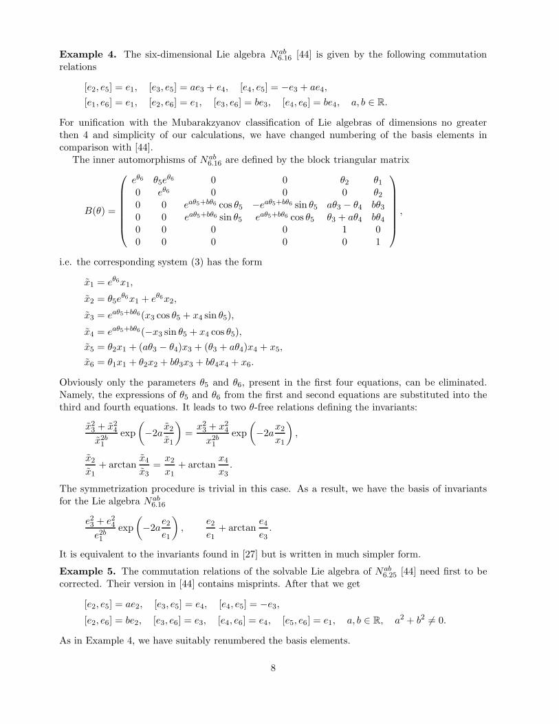
Example 4. The six-dimensional Lie algebra Nab6.16 [44] is given by the following commutation

relations

[e2, e5] = e1, [e3, e5] = ae3 + e4, [e4, e5] = −e3 + ae4,

[e1, e6] = e1, [e2, e6] = e1, [e3, e6] = be3, [e4, e6] = be4, a, b ∈ R.

For unification with the Mubarakzyanov classification of Lie algebras of dimensions no greaterthen 4 and simplicity of our calculations, we have changed numbering of the basis elements incomparison with [44].

The inner automorphisms of Nab6.16 are defined by the block triangular matrix

B(θ) =

eθ6 θ5eθ6 0 0 θ2 θ1

0 eθ6 0 0 0 θ20 0 eaθ5+bθ6 cos θ5 −eaθ5+bθ6 sin θ5 aθ3 − θ4 bθ30 0 eaθ5+bθ6 sin θ5 eaθ5+bθ6 cos θ5 θ3 + aθ4 bθ40 0 0 0 1 00 0 0 0 0 1

,

i.e. the corresponding system (3) has the form

x1 = eθ6x1,

x2 = θ5eθ6x1 + eθ6x2,

x3 = eaθ5+bθ6(x3 cos θ5 + x4 sin θ5),

x4 = eaθ5+bθ6(−x3 sin θ5 + x4 cos θ5),

x5 = θ2x1 + (aθ3 − θ4)x3 + (θ3 + aθ4)x4 + x5,

x6 = θ1x1 + θ2x2 + bθ3x3 + bθ4x4 + x6.

Obviously only the parameters θ5 and θ6, present in the first four equations, can be eliminated.Namely, the expressions of θ5 and θ6 from the first and second equations are substituted into thethird and fourth equations. It leads to two θ-free relations defining the invariants:

x23 + x24x2b1

exp

(−2a

x2x1

)=

x23 + x24x2b1

exp

(−2a

x2x1

),

x2x1

+ arctanx4x3

=x2x1

+ arctanx4x3

.

The symmetrization procedure is trivial in this case. As a result, we have the basis of invariantsfor the Lie algebra Nab

6.16

e23 + e24e2b1

exp

(−2a

e2e1

),

e2e1

+ arctane4e3

.

It is equivalent to the invariants found in [27] but is written in much simpler form.

Example 5. The commutation relations of the solvable Lie algebra of Nab6.25 [44] need first to be

corrected. Their version in [44] contains misprints. After that we get

[e2, e5] = ae2, [e3, e5] = e4, [e4, e5] = −e3,

[e2, e6] = be2, [e3, e6] = e3, [e4, e6] = e4, [e5, e6] = e1, a, b ∈ R, a2 + b2 6= 0.

As in Example 4, we have suitably renumbered the basis elements.

8

After computing the inner automorphism group of Nab6.25, we get the system (3):

x1 = x1,

x2 = eaθ4+bθ5x2,

x3 = eθ5(x3 cos θ4 + x4 sin θ4),

x4 = eθ5(−x3 sin θ4 + x4 cos θ4),

x5 = θ5x1 + aθ1x2 − θ3x3 + θ2x4 + x5,

x6 = −θ4x1 + bθ1x2 + θ2x3 + θ3x4 + x6. (5)

Here the parameter θi correspond to ei+1, i = 1, . . . , 5. The number NA of independent invariantsof Nab

6.25 equals 2. It is obvious that e1 generating the center Z(Nab6.25) is one of the invariants. The

second invariant is found by elimination of θ4 and θ5 from the second, third and fourth equationsof system (5):

(x23 + x24)b

x22exp

(2a arctan

x4x3

)=

(x23 + x24)b

x22exp

(2a arctan

x4x3

).

Therefore, we have the following basis of Inv(Nab6.25):

e1,(e23 + e24)

b

e22exp

(2a arctan

e4e3

).

The three examples above show that, even for higher dimensional algebras of relative complicatedstructure, our method admits hand calculations, provided convenient bases are used.

Example 6. In this example the Lie algebra is of general dimension n < ∞. Consider a classformed by Lie algebras of finite dimensions without an upper bound, namely by the nilpotentLie algebras nn,1, n = 3, 4, . . ., with the (n − 1)-dimensional Abelian ideal 〈e1, e2, . . . , en−1〉. Thenon-zero commutation relations of nn,1 have the form [42]

[ek, en] = ek−1, k = 2, . . . , n− 1.

The inner automorphisms of nn,1 are described by the triangular matrix

B(θ) =

1 θ112!θ

21

13!θ

31 · · · 1

(n−2)!θn−21 θ2

0 1 θ112!θ

21 · · · 1

(n−3)!θn−31 θ3

0 0 1 θ1 · · · 1(n−4)!θ

n−41 θ4

· · · · · · · · · · · · · · · · · · · · ·0 0 0 0 · · · θ1 θn−1

0 0 0 0 · · · 1 00 0 0 0 · · · 0 1

,

i.e. the complete set of lifted invariants has the form

Ik =k∑

j=1

1

(k − j)!θk−j1 xj, k = 1, . . . , n− 1, In = xn +

n−2∑

j=1

θj+1xj .

It is obvious that the basis element e1 generating the center of nn,1 is one of the invariants(I1 = x1). Other (n− 3) invariants are found by the normalization procedure applied to the lifted

9

invariants I2, . . . , In−1. Namely, we solve the equation I2 = 0 with respect to θ1 and substitute theobtained expression θ1 = −x2/x1 to the other I’s. To construct polynomial invariants finally, wemultiply the derived invariants by powers of the invariant x1. Since the symmetrization procedureis trivial for this algebra, we get the following complete set of generalized Casimir operators whichare classical Casimir operators:

e1,k∑

j=1

(−1)k−j

(k − j)!ej−21 ek−j

2 ej , k = 3, . . . , n − 1.

This set completely coincides with the one determined in Lemma 1 of [30] and Theorem 4 of [42].

5 Concluding remarks

It is likely that the moving frame method, combined with knowledge of the groups of inner auto-morphisms, will allow one to investigate invariants and other characteristics of special classes of Liealgebras, such as solvable Lie algebras with given structures of nilradicals (see Example 6 and [7]).

In the course of testing our method of computing the bases of invariants, we recalculated invari-ants of real low-dimensional Lie algebras available in the literature. A detailed account of this workis to be presented elsewhere. More precisely, a complete verified list of invariants and other charac-teristics, such as the groups of inner automorphisms of low-dimensional Lie algebras of dimensionno greater than six, will be presented in [6].

The invariants of Lie algebras of dimension 3, 4, 5, as well as nilpotent Lie algebras of dimension 6of [31] are correct. Note however, that using our new method, all invariants can be written avoidingintroduction of complex numbers (cf. Table 1 and [31]). As an illustration, compare Example 1above with the case of the Lie algebra Aab

4.6 of [31]. The same claims are true for invariants of thesix-dimensional solvable Lie algebras with five-dimensional nilradials, which are calculated in [14].

Our computation of invariants of the six-dimensional solvable Lie algebras with four-dimensionalnilradials is presented in Table 2. The same algebras were considered in [27]. Besides correctingseveral misprints/errors (for example in the entries Na

6.3, Nab6.12, N

a6.21, N

ab6.25, N6.31, N

ab6.35 and N6.38),

we found that, for most of the algebras, the bases of invariants can be reduced to a simpler formjust by choosing another (K-canonical) bases of the algebras.

Contents of Tables. A symbol An.k in the first column of Table 1 denotes the indecomposablen-dimensional Lie algebra numbered k in the classifications by Mubarakzyanov [24, 25] if n 6 5or in the classification by Morozov [23] if the algebra is nilpotent and six-dimensional. (Thisalgebra numeration slightly differs from that in [31]). Analogously, in the first column the symbolfrom [44] is shown, denoting six-dimensional solvable Lie algebras with four-dimensional nilradials.If a symbol has superscripts, it denotes a series of Lie algebras with parameters indicated in thesuperscripts. The parameters a, b, c and d are real. The non-zero commutation relations are in thesecond column. In all cases we have renumbered the basis elements of the algebras in comparisonwith [23, 44] in order to have bases in K-canonical forms. Bases of invariants are listed in the thirdcolumn. Algebras are collected in correspondence with structure of their nilradicals and centers.The algebras N6.1–N6.19 contain the Abelian nilradicals (∼ 4A1) and the centers of dimension zero;the algebras N6.20–N6.27 have the Abelian nilradicals (∼ 4A1) and one-dimensional centers; thenilradical of N6.28 is isomorphic to A4.1; the nilradicals of N6.29–N6.40 are isomorphic to A3.1 ⊕A1.

Acknowledgments. The work was partially supported by the National Science and Enginee-ring Research Council of Canada, by MITACS. The research of R.P. was supported by AustrianScience Fund (FWF), Lise Meitner project M923-N13. Two of us, V. B. and R.P., are grateful forthe hospitality extended to us at the Centre de Recherches Mathematiques, Universite de Montreal.

10

References

[1] Abellanas L. and Martinez Alonso L. A general setting for Casimir invariants, J. Math. Phys., 1975,V.16, 1580–1584.

[2] Ancochea J.M., Campoamor-Stursberg R. and Garcia Vergnolle L. Solvable Lie algebras with nat-urally graded nilradicals and their invariants, J. Phys. A: Math. Gen., 2006, V.39, 1339–1355;math-ph/0511027.

[3] Andrada A., Barberis M.L., Dotti I. and Ovando G. Product structures on four dimensional solvableLie algebras, Homology Homotopy Appl., 2005, V.7, 9–37; math.RA/0402234.

[4] Beltrametti E.G. and Blasi A. On the number of Casimir operators associated with any Lie group,Phys. Lett., 1966, V.20, 62–64.

[5] Bianchi L. Lezioni sulla teoria dei gruppi continui finiti di transformazioni, Pisa, Spoerri, 1918.

[6] Boyko V., Nesterenko M., Patera J. and Popovych R. Real low-dimensional Lie algebras, in preparation.

[7] Boyko V., Patera J. and Popovych R. Invariants of Lie algebras with fixed structure of nilradicals,J. Phys. A: Math. Theor., 2007, V.40, 113–130; math-ph/0606045.

[8] Campoamor-Stursberg R. Invariants of solvable rigid Lie algebras up to dimension 8, J. Phys. A: Math.Gen., 2002, V.35, 6293–6306; math.RA/0202006.

[9] Campoamor-Stursberg R. On the invariants of some solvable rigid Lie algebras, J. Math. Phys., 2003,V.44, 771–784; math.RA/0204074.

[10] Campoamor-Stursberg R. The structure of the invariants of perfect Lie algebras, J. Phys. A: Math.Gen., 2003, V.36, 6709–6723; Corrigendum, J. Phys. A: Math. Gen., 2003, V.36, 7977; The structureof the invariants of perfect Lie algebras II, J. Phys. A: Math. Gen., 2004, V.37, 3627–3643.

[11] Campoamor-Stursberg R. An extension based determinantal method to compute Casimir operators ofLie algebras, Phys. Lett. A, 2003, V.312, 211–219.

[12] Campoamor-Stursberg R. An alternative interpretation of the Beltrametti–Blasi formula by means ofdifferential forms, Phys. Lett. A, 2004, V.327, 138–145.

[13] Campoamor-Stursberg R. A new matrix method for the Casimir operators of the Lie algebras wsp(N,R)and Isp(2N,R), J. Phys. A: Math. Gen., 2005, V.38, 4187–4208.

[14] Campoamor-Stursberg R., Some remarks concerning the invariants of rank one solvable real Lie algeb-ras, Algebra Colloq., 2005, V.12, 497–518.

[15] de Graaf W.A. Classification of solvable Lie algebras, Experiment. Math., 2005, V.14, 15–25;math.RA/0404071.

[16] Fels M. and Olver P. Moving coframes: I. A practical algorithm, Acta Appl. Math., 1998, V.51, 161–213.

[17] Fels M. and Olver P. Moving coframes: II. Regularization and theoretical foundations, Acta Appl.Math., 1999, V.55, 127–208.

[18] Jacobson N. Lie algebras, New York, Interscience, 1955.

[19] Kirillov A.A. Elements of the theory of representations, Grundlehren der Mathematischen Wis-senschaften, Band 220, Berlin – New York, Springer-Verlag, 1976.

[20] Lemke J., Ne’eman Y. and Pecina-Cruz J. Wigner analysis and Casimir operators of SA(4,R), J. Math.Phys., 1992, V.33, 2656–2659.

[21] Lie S. Theorie der Transformationsgruppen, Vol. 1–3, Leipzig, 1888, 1890, 1893.

[22] MacCallum M.A.H. On the enumeration of the real four-dimensional Lie algebras, in On Einstein’sPath: essays in honor of Engelbert Schucking, Editor A.L. Harvey, New York, Springer Verlag, 1999,299–317 (first version circulated as a preprint in 1979).

[23] Morozov V.V. Classification of nilpotent Lie algebras of sixth order, Izv. Vys. Ucheb. Zaved. Mate-matika, 1958, N 4 (5), 161–171 (in Russian).

11

[24] Mubarakzyanov G.M. On solvable Lie algebras, Izv. Vys. Ucheb. Zaved. Matematika, 1963, N 1 (32),114–123 (in Russian).

[25] Mubarakzyanov G.M. The classification of the real structure of five-dimensional Lie algebras, Izv. Vys.Ucheb. Zaved. Matematika, 1963, N 3 (34), 99–106 (in Russian).

[26] Mubarakzyanov G.M. Classification of solvable Lie algebras of sixth order with a non-nilpotent basiselement, Izv. Vys. Ucheb. Zaved. Matematika, 1963, N 4 (35), 104–116 (in Russian).

[27] Ndogmo J.C. Invariants of solvable Lie algebras of dimension six, J. Phys. A: Math. Gen., 2000, V.33,2273–2287.

[28] Ndogmo J.C. Properties of the invariants of solvable Lie algebras, Canad. Math. Bull., 2000, V.43,459–471.

[29] Ndogmo J.C. Invariants of a semi-direct sum of Lie algebras, J. Phys. A: Math. Gen., 2004, V.37,5635–5647.

[30] Ndogmo J.C. and Winternitz P. Generalized Casimir operators of solvable Lie algebras with Abeliannilradicals, J. Phys. A: Math. Gen., 1994, V.27, 2787–2800.

[31] Patera J., Sharp R.T., Winternitz P. and Zassenhaus H. Invariants of real low dimension Lie algebras,J. Math. Phys., 1976, V.17, 986–994.

[32] Patera J., Sharp R.T., Winternitz P. and Zassenhaus H. Subgroups of the Poincare group and theirinvariants, J. Math. Phys., 1976, V.17, 977–985.

[33] Patera J. and Winternitz P. Subalgebras of real three and four-dimensional Lie algebras, J. Math. Phys.,1977, V.18, 1449–1455.

[34] Patera J. and Zassenhaus H. Solvable Lie algebras of dimension 6 4 over perfect fields, Linear AlgebraAppl., 1990, V.142, 1–17.

[35] Pauri M. and Prosperi G.M. On the construction of the invariants operators for any finite-parameterLie group, Nuovo Cimento A, 1966, V.43, 533–537.

[36] Pecina-Cruz J.N. An algorithm to calculate the invariants of any Lie algebra, J. Math. Phys., 1994,V.35, 3146–3162.

[37] Petrov A.Z. New methods in general relativity, Moscow, Nauka, 1966 (in Russian).

[38] Perroud M. The fundamental invariants of inhomogeneous classical groups, J. Math. Phys., 1983, V.24,1381–1391.

[39] Popovych R., Boyko V., Nesterenko M. and Lutfullin M. Realizations of real low-dimensional Liealgebras, J. Phys. A: Math. Gen., 2003, V.36, 7337–7360; see math-ph/0301029 for the revised andextended version.

[40] Racah G. Sulla caratterizzazione delle rappresentazioni irriducibili dei gruppi semisemplici di Lie, AttiAccad. Naz. Lincei. Rend. Cl. Sci. Fis. Mat. Nat. (8), 1950, V.8, 108–112.

[41] Rubin J.L. and Winternitz P. Solvable Lie algebras with Heisenberg ideals, J. Phys. A: Math. Gen.,1993, V.26, N 5, 1123–1138.

[42] Snobl L. and Winternitz P. A class of solvable Lie algebras and their Casimir invariants, J. Phys. A:Math. Gen., 2005, V.38, 2687–2700; math-ph/0411023.

[43] Tremblay S. and Winternitz P. Invariants of the nilpotent and solvable triangular Lie algebras,J. Phys. A: Math. Gen., 2001, V.34, 9085–9099.

[44] Turkowski P. Solvable Lie algebras of dimension six, J. Math. Phys., 1990, V.31, 1344–1350.

[45] Zassenhaus H. On the invariants of a Lie group. I, in Computers in Nonassociative Rings and Algebras(Special Session, 82nd Annual Meeting Amer. Math. Soc., San Ontario, 1976), Editors R.E. Beck andB. Kolman, New York, Academic Press, 1977, 139–155.

12

Table 1. Invariants of the real indecomposable Lie algebras up to dimension 5and nilpotent Lie algebras of dimension 6

Algebra Nonzero commutation relations Invariants

A1 e1

A2.1 [e1, e2] = e1 none

A3.1 [e2, e3] = e1 e1

A3.2 [e1, e3] = e1, [e2, e3] = e1 + e2 e1 exp(

−e2e1

)

A3.3 [e1, e3] = e1, [e2, e3] = e2 e2/e1

Aa3.4, |a| 6 1, [e1, e3] = e1, [e2, e3] = ae2 e−a

1 e2

a 6= 0, 1

Ab3.5, b > 0 [e1, e3] = be1 − e2,

(e21 + e22) exp(

−2b arctane2e1

)

[e2, e3] = e1 + be2

sl(2,R) [e1, e2] = e1, [e2, e3] = e3, [e1, e3] = −2e2 e1e3 + e3e1 + 2e22

so(3) [e2, e3] = e1, [e3, e1] = e2, [e1, e2] = e3 e21 + e22 + e23

A4.1 [e2, e4] = e1, [e3, e4] = e2 e1, e22 − 2e1e3

Aa4.2, a 6= 0 [e1, e4] = ae1, [e2, e4] = e2, [e3, e4] = e2 + e3 ea2

e1, e2 exp

(

−e3e2

)

A4.3 [e1, e4] = e1, [e3, e4] = e2 e2, e1 exp(

−e3e2

)

A4.4 [e1, e4] = e1, [e2, e4] = e1 + e2,e1 exp

(

−e2e1

)

,e22 − 2e1e3

e21[e3, e4] = e2 + e3

Aa,b,c4.5 , [e1, e4] = ae1, [e2, e4] = be2, [e3, e4] = ce3 ea3

ec1,ea2eb1abc 6= 0

Aa,b4.6, [e1, e4] = ae1, [e2, e4] = be2 − e3,

(e22 + e23) exp

(

−2b arctane3e2

)

,(e22 + e23)

a

eb1a > 0 [e3, e4] = e2 + be3

A4.7 [e2, e3] = e1, [e1, e4] = 2e1,none

[e2, e4] = e2, [e3, e4] = e2 + e3

Aa4.8, |a| 6 1 [e2, e3] = e1, [e1, e4] = (1 + a)e1, only for a = −1:

[e2, e4] = e2, [e3, e4] = ae3 e1, e2e3 + e3e2 − 2e1e4

Aa4.9, a > 0 [e2, e3] = e1, [e1, e4] = 2ae1, only for a = 0:

[e2, e4] = ae2 − e3, [e3, e4] = e2 + ae3 e1, 2e1e4 + e22 + e23

A4.10 [e1, e3] = e1, [e2, e3] = e2, [e1, e4] = −e2, [e2, e4] = e1 none

A5.1 [e3, e5] = e1, [e4, e5] = e2 e1, e2, e2e3 − e1e4

A5.2 [e2, e5] = e1, [e3, e5] = e2, [e4, e5] = e3 e1, e22 − 2e1e3, e

32 + 3e21e4 − 3e1e2e3

A5.3 [e3, e4] = e2, [e3, e5] = e1, [e4, e5] = e3 e1, e2, e23 + 2e2e5 − 2e1e4

A5.4 [e2, e4] = e1, [e3, e5] = e1 e1

A5.5 [e3, e4] = e1, [e2, e5] = e1, [e3, e5] = e2 e1

A5.6 [e3, e4] = e1, [e2, e5] = e1, [e3, e5] = e2, [e4, e5] = e3 e1

Aabc5.7 , [e1, e5] = e1, [e2, e5] = ae2, [e3, e5] = be3, ea1

e2,eb1e3

,ec1e4abc 6= 0 [e4, e5] = ce4

Aa5.8, [e2, e5] = e1, [e3, e5] = e3, [e4, e5] = ae4

e1,ea3e4

, e3 exp(

−e2e1

)

0 < |a| 6 1

Aab5.9, [e1, e5] = e1, [e2, e5] = e1 + e2, ea1

e3,eb1e4

, e1 exp(

−e2e1

)

0 6= b 6 a [e3, e5] = ae3, [e4, e5] = be4

A5.10 [e2, e5] = e1, [e3, e5] = e2, [e4, e5] = e4 e1, e22 − 2e1e3, e4 exp

(

−e2e1

)

Aa5.11, a 6= 0 [e1, e5] = e1, [e2, e5] = e1 + e2, ea1

e3, e1 exp

(

−e2e1

)

,e22 − 2e1e3

e21[e3, e5] = e2 + e3, [e4, e5] = ae4

13

Algebra Nonzero commutation relations Invariants

A5.12 [e1, e5] = e1, [e2, e5] = e1 + e2,e1 exp

(

−e2e1

)

,e22−2e1e3

e21,e32+3e21e4−3e1e2e3

e31[e3, e5] = e2 + e3, [e4, e5] = e3 + e4

Aabc5.13, |a| 6 1, [e1, e5] = e1, [e2, e5] = ae2, ea1

e2,e23 + e24e2b1

, ec1 exp(

− arctane4e3

)

ac 6= 0 [e3, e5] = be3 − ce4, [e4, e5] = ce3 + be4

Aa5.14 [e2, e5] = e1, [e3, e5] = ae3 − e4,

e1, (e23 + e24) exp

(

−2ae2e1

)

,e2e1

− arctane4e3[e4, e5] = e3 + ae4

Aa5.15, |a| 6 1 [e1, e5] = e1, [e2, e5] = e1 + e2, ea1

e3, e1 exp

(

−e2e1

)

, e3 exp(

−e4e3

)

[e3, e5] = ae3, [e4, e5] = e3 + ae4

Aab5.16, b 6= 0 [e1, e5] = e1, [e2, e5] = e1 + e2,

e1 exp(

−e2e1

)

,e23 + e24e2a1

,e2e1

− arctane4e3[e3, e5] = ae3 − be4, [e4, e5] = be3 + ae4

Aabc5.17, c 6= 0 [e1, e5] = ae1 − e2, [e2, e5] = e1 + ae2, (e21 + e22) exp

(

−2a arctane2e1

)

,(e21 + e22)

b

(e23 + e24)a,

(e23 + e24) exp(

−2b

carctan

e4e3

)

[e3, e5] = be3 − ce4, [e4, e5] = ce3 + be4

Aa5.18, a > 0 [e1, e5] = ae1 − e2, [e2, e5] = e1 + ae2, (e21+e22) exp

(

−2a arctane2e1

)

,e1e4 − e2e3e21 + e22

,

(e21 + e22) exp(

−2ae1e3 + e2e4e21 + e22

)

[e3, e5] = e1 + ae3 − e4, [e4, e5] = e2 + e3 + ae4

Aab5.19, b 6= 0 [e2, e3] = e1, [e1, e5] = ae1, [e2, e5] = e2, eb1

ea4[e3, e5] = (a− 1)e3, [e4, e5] = be4

Aa5.20 [e2, e3] = e1, [e1, e5] = ae2, [e2, e5] = e2,

e1 exp(

−ae4e1

)

[e3, e5] = (a− 1)e3, [e4, e5] = e1 + ae4

A5.21 [e2, e3] = e1, [e1, e5] = 2e1, [e2, e5] = e2 + e3, e24e1[e3, e5] = e3 + e4, [e4, e5] = e4

A5.22 [e2, e3] = e1, [e2, e5] = e3, [e4, e5] = e4 e1

Aa5.23, a 6= 0 [e2, e3] = e1, [e1, e5] = 2e1, [e2, e5] = e2 + e3, ea1

e24[e3, e5] = e3, [e4, e5] = ae4

A±

5.24 [e2, e3] = e1, [e1, e5] = 2e1, [e2, e5] = e2 + e3,e1 exp

(

∓2e4e1

)

[e3, e5] = e3, [e4, e5] = ±e1 + 2e4

Aab5.25, b 6= 0 [e2, e3] = e1, [e1, e5] = 2ae1, [e2, e5] = ae2 + e3, eb1

e2a4[e3, e5] = −e2 + ae3, [e4, e5] = be4

A±a5.26 [e2, e3] = e1, [e1, e5] = 2ae1, [e2, e5] = ae2 + e3,

e1 exp(

∓2ae4e1

)

[e3, e5] = −e2 + ae3, [e4, e5] = ±e1 + 2ae4

A5.27 [e2, e3] = e1, [e1, e5] = e1, [e3, e5] = e3 + e4,e1 exp

(

−e4e1

)

[e4, e5] = e1 + e4

Aa5.28 [e2, e3] = e1, [e1, e5] = ae1, [e2, e5] = (a− 1)e2, ea4

e1[e3, e5] = e3 + e4, [e4, e5] = e4

A5.29 [e2, e4] = e1, [e1, e5] = e1, [e2, e5] = e2, [e4, e5] = e3 e3

Aa5.30 [e2, e4] = e1, [e3, e4] = e2, [e1, e5] = (a+ 1)e1, (e22 − 2e1e3)

a+1

e2a1[e2, e5] = ae2, [e3, e5] = (a− 1)e3, [e4, e5] = e4

A5.31 [e2, e4] = e1, [e3, e4] = e2, [e1, e5] = 3e1, (e22 − 2e1e3)3

e41[e2, e5] = 2e2, [e3, e5] = e3, [e4, e5] = e3 + e4

Aa5.32 [e2, e4] = e1, [e3, e4] = e2, [e1, e5] = e1,

e2a1 expe22 − 2e1e3

e21[e2, e5] = e2, [e3, e5] = ae1 + e3

Aab5.33, [e1, e4] = e1, [e3, e4] = ae3, [e2, e5] = e2, ea1e

b2

e3a2 + b2 6= 0 [e3, e5] = be3

Aa5.34 [e1, e4] = ae1, [e2, e4] = e2, [e3, e4] = e3, ea2

e1exp

e3e2[e1, e5] = e1, [e3, e5] = e2

14

Algebra Nonzero commutation relations Invariants

Aab5.35, [e1, e4] = ae1, [e2, e4] = e2, [e3, e4] = e3, e21

(e22 + e23)aexp

(

−2b arctane3e2

)

a2 + b2 6= 0 [e1, e5] = be1, [e2, e5] = −e3, [e3, e5] = e2

A5.36 [e2, e3] = e1, [e1, e4] = e1, [e2, e4] = e2, e2e3 + e3e2 + 2e1e5e1[e2, e5] = −e2, [e3, e5] = e3

A5.37 [e2, e3] = e1, [e1, e4] = 2e1, [e2, e4] = e2, e22 + e23 + 2e1e5e1[e3, e4] = e3, [e2, e5] = −e3, [e3, e5] = e2

A5.38 [e1, e4] = e1, [e2, e5] = e2, [e4, e5] = e3 e3

A5.39 [e1, e4] = e1, [e2, e4] = e2, [e1, e5] = −e2,e3

[e2, e5] = e1, [e4, e5] = e3

sl(2,R)+⊂ 2A1 [e1, e2] = 2e1, [e1, e3] = −e2, [e2, e3] = 2e3, {

e1e24 − e2e4e5 − e3e

25

}

symmetrized[e1, e4] = e5, [e2, e4] = e4, [e2, e5] = −e5, [e3, e5] = e4

A6.1 [e3, e6] = e1, [e4, e6] = e2, [e5, e6] = e4 e1, e2, e1e4 − e2e3, 2e2e5 − e24

A6.2 [e2, e6] = e1, [e3, e6] = e2, [e4, e6] = e3, e1, 2e1e3 − e22, 2e1e5 − 2e2e4 + e23,

[e5, e6] = e4 3e21e4 − 3e1e2e3 + e32

A6.3 [e4, e5] = e1, [e4, e6] = e2, [e5, e6] = e3 e1, e2, e3, e1e6 + e3e4 − e2e5

A6.4 [e3, e5] = e1, [e4, e6] = e1, [e5, e6] = e2 e1, e2

Aa6.5, [e3, e5] = e1, [e4, e5] = ae2, [e3, e6] = e2,

e1, e2a 6= 0 [e4, e6] = e1

A6.6 [e4, e5] = e1, [e3, e6] = e1, [e4, e6] = e2,e1, e2

[e5, e6] = e3

A6.7 [e4, e5] = e1, [e3, e6] = e2, [e4, e6] = e3 e1, e2

A6.8 [e3, e5] = e1, [e4, e6] = e2, [e5, e6] = e3 + e4 e1, e2

A6.9 [e4, e5] = e1, [e3, e6] = e1, [e4, e6] = e2,e1, e2

[e5, e6] = e4

Aa6.10, [e3, e5] = e1, [e4, e5] = ae2, [e3, e6] = e2,

e1, e2a 6= 0 [e4, e6] = e1, [e5, e6] = e4

A6.11 [e5, e6] = e4, [e4, e6] = e3, [e3, e6] = e2,e1, e2

[e4, e5] = e1

A6.12 [e2, e5] = e1, [e3, e6] = e1, [e4, e6] = e3 e1, 2e1e4 − e23

A6.13 [e2, e5] = e1, [e3, e6] = e1, [e4, e6] = e3,e1, 2e1e4 − e23[e5, e6] = e2

Aa6.14, [e2, e5] = ae2, [e4, e5] = e2, [e3, e6] = e1,

e1, e22 + ae23 − 2ae1e4

a 6= 0 [e4, e6] = e3

A6.15 [e2, e5] = e1, [e3, e6] = e1, [e4, e6] = e3,e1, 2e1e4 − e23[e5, e6] = e2 + e4

A6.16 [e3, e5] = e1, [e4, e5] = e2, [e2, e6] = e1,e1, e

32 + 3e21e4 − 3e1e2e3

[e3, e6] = e2, [e4, e6] = e3

A6.17 [e2, e5] = e1, [e3, e6] = e1, [e4, e6] = e3,e1, 2e1e4 − e23[e5, e6] = e4

Aa6.18, [e2, e5] = ae1, [e4, e5] = e2, [e3, e6] = e1,

e1, e22 + ae23 − 2ae1e4

a 6= 0 [e4, e6] = e3, [e5, e6] = e4

A6.19 [e4, e5] = e1, [e2, e6] = e1, [e3, e6] = e2,e1, e

22 − 2e1e3

[e4, e6] = e3, [e5, e6] = e4

A6.20 [e3, e5] = e1, [e4, e5] = e2, [e2, e6] = e1,e1, e

32 + 3e21e4 − 3e1e2e3

[e3, e6] = e2, [e4, e6] = e3, [e5, e6] = e4

A6.21 [e3, e4] = e1, [e3, e5] = e2, [e4, e5] = e3,e1, e

23 + 2e1e5 − 2e2e4

[e2, e6] = e1, [e5, e6] = e4

A6.22 [e3, e4] = e1, [e3, e5] = e2, [e4, e5] = e3,e1, 2e

32 + 3e1e

23 + 6e21e5 − 6e1e2e4

[e2, e6] = e1, [e4, e6] = e2, [e5, e6] = e4

15

Table 2. Invariants of the real six-dimensional solvable Lie algebras with four-dimensional nilradials

Algebra Non-zero commutation relations Invariants

Nabcd6.1 [e1, e5] = ae1, [e2, e5] = be2, [e4, e5] = e4,

ec3ea4

e1,ed3e

b4

e2[e1, e6] = ce1, [e2, e6] = de2, [e3, e6] = e3,

ac 6= 0, b2 + d2 6= 0

Nabc6.2 [e1, e5] = ae1, [e2, e5] = e2, [e4, e5] = e3,

ea2eac−b3

e1, e2e

c3 exp

e4e3

[e1, e6] = be1, [e2, e6] = ce2, [e3, e6] = e3,

[e4, e6] = e4, a2 + b2 6= 0

Na6.3 [e1, e5] = e1, [e2, e5] = e2, [e4, e5] = e3,

e3 exp(

−e2e1

)

, e1 exp(

−e4e3

− ae2e1

)

[e1, e6] = ae1, [e2, e6] = e1 + ae2,

[e3, e6] = e3, [e4, e6] = e4

Nab6.4 [e1, e5] = e1, [e2, e5] = e2, [e4, e5] = e3, e2b3 (e21 + e22)

a exp(

−2ae4e3

)

,

e3 exp(

a arctane2e1

)[e1, e6] = e2, [e2, e6] = −e1, [e3, e6] = ae3,

[e4, e6] = be3 + ae4, a 6= 0

Nab6.5 [e1, e5] = ae1, [e3, e5] = e3, [e4, e5] = e3 + e4, eb2e

a3

e1, e3 exp

(

−e4e3

)

[e1, e6] = be1, [e2, e6] = e2, ab 6= 0

Nab6.6 [e1, e5] = ae1, [e2, e5] = ae2, [e3, e5] = e3,

ea3e1

expe2e1

, e3 exp(

be2e1

−e4e3

)

[e4, e5] = e3 + e4, [e1, e6] = e1, [e2, e6] = e1 + e2,

[e4, e6] = be3, a2 + b2 6= 0

Nabc6.7 [e1, e5] = ae1, [e2, e5] = ae2, [e3, e5] = e3, e3 exp

(

−e4e3

− c arctane2e1

)

,

(e21 + e22)e−a3 exp

(

2b arctane2e1

)[e4, e5] = e3 + e4, [e1, e6] = be1 + e2,

[e2, e6] = −e1 + be2, [e4, e6] = ce3, a2 + c2 6= 0

N6.8 [e1, e5] = e1, [e4, e5] = e2, [e2, e6] = e2,e1 exp

(

−e4e2

)

, e2 exp(

−e3e2

)

[e3, e6] = e2 + e3, [e4, e6] = e4

Na6.9 [e1, e5] = e1, [e4, e5] = e2, [e2, e6] = e2,

e2a1 exp

(

e23 − 2ae2e4e22

)

, ea2 exp(

−e3e2

)

[e3, e6] = ae2 + e3, [e4, e6] = e3 + e4

Nab6.10 [e1, e5] = ae1, [e2, e5] = e2, [e3, e5] = e3,

ea2e1

expe3e2

, e2b2 exp

(

e23 − 2e2e4e22

)

[e4, e5] = be2 + e4, [e1, e6] = e1, [e3, e6] = e2,

[e4, e6] = e3

Na6.11 [e2, e5] = e1, [e3, e5] = e3, [e4, e5] = e3 + e4, e4

e3−

e2e1

,ea1e3

expe2e1[e1, e6] = e1, [e2, e6] = e2, [e3, e6] = ae3, [e4, e6] = ae4

Nab6.12 [e1, e5] = e1, [e2, e5] = e1 + e2, [e3, e5] = e3,

[e4, e5] = e3 + e4, [e1, e6] = e3, [e2, e6] = ae1 − be3 + e4,

e1e4 − e2e3e21 + e23

+ b arctane3e1

,

e1e2 + e3e4e21 + e23

+ a arctane3e1

+1

2ln(e21 + e23)[e3, e6] = −e1, [e4, e6] = be1 − e2 + ae3

Nabcd6.13 [e1, e5] = ae1, [e2, e5] = be2, [e3, e5] = e4, [e4, e5] = −e3, e21(e

23 + e24)

−c exp(

2a arctane4e3

)

,

e22(e23 + e24)

−d exp(

2b arctane4e3

)[e1, e6] = ce1, [e2, e6] = de2, [e3, e6] = e3, [e4, e6] = e4,

a2 + c2 6= 0, b2 + d2 6= 0

Nabc6.14 [e1, e5] = ae1, [e3, e5] = be3 + e4, [e4, e5] = −e3 + be4, e1e

−c2 exp

(

a arctane4e3

)

,

(e23 + e24) exp(

2b arctane4e3

)[e1, e6] = ce1, [e2, e6] = e2, ac 6= 0

Nabcd6.15 [e1, e5] = e1, [e2, e5] = e2, [e3, e5] = ae3 + be4, (e21 + e22) exp

(2

barctan

e4e3

+ 2c arctane2e1

)

,

(e23+e24) exp(2a

barctan

e4e3

+2d arctane2e1

)[e4, e5] = −be3 + ae4, [e1, e6] = ce1 + e2,

[e2, e6] = −e1 + ce2, [e3, e6] = de3, [e4, e6] = de4, b 6= 0

Nab6.16 [e2, e5] = e1, [e3, e5] = ae3 + e4, [e4, e5] = −e3 + ae4,

(e23 + e24)e−2b1 exp

(

−2ae2e1

)

,e2e1

+ arctane4e3[e1, e6] = e1, [e2, e6] = e2, [e3, e6] = be3, [e4, e6] = be4

Na6.17 [e1, e5] = ae1, [e2, e5] = e1 + ae2, [e3, e5] = e4,

e1 exp(

−ae2e1

)

,e2e1

+ arctane4e3[e4, e5] = −e3, [e3, e6] = e3, [e4, e6] = e4

16

Algebra Nonzero commutation relations Invariants

Nabc6.18 [e1, e5] = e2, [e2, e5] = −e1, [e3, e5] = ae3 + be4, arctan

e4e3

− b arctane2e1

,

(e23 + e24)(e21 + e22)

−c exp(

2a arctane4e3

)[e4, e5] = −be3 + ae4, [e1, e6] = e1, [e2, e6] = e2,

[e3, e6] = ce3, [e4, e6] = ce4, b 6= 0

N6.19 [e1, e5] = e2, [e2, e5] = −e1, [e3, e5] = e1 + e4,e1e4 − e2e3e21 + e22

,e1e3 + e2e4e21 + e22

+ arctane4e3

[e4, e5] = e2 − e3, [e1, e6] = e1, [e2, e6] = e2,

[e3, e6] = e3, [e4, e6] = e4

Nab6.20 [e2, e5] = ae2, [e4, e5] = e4, [e2, e6] = be2,

e1,eb3e

a4

e2[e3, e6] = e3, [e5, e6] = e1

Na6.21 [e2, e5] = e2, [e4, e5] = e3, [e2, e6] = ae2,

e1,ea3e2

expe4e3[e3, e6] = e3, [e4, e6] = e4, [e5, e6] = e1

Naε6.22 [e2, e5] = e1, [e4, e5] = e4, [e3, e6] = e3,

e1,ea3e4

expe2e1[e4, e6] = ae4, [e5, e6] = εe1, ε = 0, 1, a2 + ε2 6= 0

Naε6.23 [e2, e5] = e1, [e3, e5] = e3, [e4, e5] = e4, [e2, e6] = ae1,

e1, (e23 + e24) exp

(

−2e2e1

− 2a arctane4e3

)

[e3, e6] = e4, [e4, e6] = −e3, [e5, e6] = εe1, ε = 0, 1

N6.24 [e3, e5] = e3, [e4, e5] = e3 + e4, [e2, e6] = e2, [e5, e6] = e1 e1, e3 exp(

−e4e3

)

Nab6.25 [e2, e5] = ae2, [e3, e5] = e4, [e4, e5] = −e3, [e2, e6] = be2,

e1, e22(e

23 + e24)

−b exp(

−2a arctane4e3

)

[e3, e6] = e3, [e4, e6] = e4, [e5, e6] = e1, a2 + b2 6= 0

Na6.26 [e3, e5] = ae3 + e4, [e4, e5] = −e3 + ae4, [e2, e6] = e2,

e1, (e23 + e24) exp

(

2a arctane4e3

)

[e5, e6] = e1

Nε6.27 [e2, e5] = e1, [e3, e5] = e4, [e4, e5] = −e3, [e3, e6] = e3,

e1,e2e1

+ arctane4e3[e4, e6] = e4, [e5, e6] = εe2, ε = 0, 1

N6.28 [e2, e4] = e1, [e3, e4] = e2, [e1, e5] = e1, [e3, e5] = −e3, none

[e4, e5] = e4, [e2, e6] = e2, [e3, e6] = 2e3, [e4, e6] = −e4

Nab6.29 [e2, e3] = e1, [e1, e5] = e1, [e2, e5] = e2, [e4, e5] = ae4, none

[e1, e6] = e1, [e3, e6] = e3, [e4, e6] = be4, a2 + b2 6= 0

Na6.30 [e2, e3] = e1, [e1, e5] = 2e1, [e2, e5] = e2, [e3, e5] = e3, none

[e4, e5] = ae4, [e3, e6] = e2, [e4, e6] = e4

N6.31 [e2, e3] = e1, [e2, e5] = e2, [e3, e5] = −e3, [e1, e6] = e1,e1 exp

(

−e4e1

)

, e5 −e2e3 + e3e2

2e1[e3, e6] = e3, [e4, e6] = e1 + e4

Na6.32 [e2, e3] = e1, [e2, e5] = e2, [e3, e5] = −e3, [e4, e5] = e1, none

[e1, e6] = e1, [e2, e6] = ae2, [e3, e6] = (1−a)e3, [e4, e6] = e4

N6.33 [e2, e3] = e1, [e1, e5] = e1, [e2, e5] = e2, [e1, e6] = e1, none

[e3, e6] = e3 + e4, [e4, e6] = e4

Na6.34 [e2, e3] = e1, [e1, e5] = e1, [e2, e5] = e2, [e3, e5] = e4, none

[e1, e6] = ae1, [e2, e6] = (a−1)e2, [e3, e6] = e3, [e4, e6] = e4

Nab6.35 [e2, e3] = e1, [e2, e5] = e3, [e3, e5] = −e2, [e4, e5] = ae4, eb1

e24, 2e5 −

e22 + e23e1

if a = 0,

none if a 6= 0

[e1, e6] = 2e1, [e2, e6] = e2, [e3, e6] = e3, [e4, e6] = be4,

a2 + b2 6= 0

N6.36 [e2, e3] = e1, [e2, e5] = e3, [e3, e5] = −e2, [e1, e6] = 2e1,e1 exp

(

−2e4e1

)

, 2e5 −e22 + e23

e1[e2, e6] = e2, [e3, e6] = e3, [e4, e6] = e1 + 2e4

Na6.37 [e2, e3] = e1, [e2, e5] = e3, [e3, e5] = −e2, [e4, e5] = e1, none

[e1, e6] = 2e1, [e2, e6] = e2 + ae3, [e3, e6] = −ae2 + e3,

[e4, e6] = 2e4

N6.38 [e2, e3] = e1, [e1, e5] = e1, [e2, e5] = e2, [e1, e6] = e1,e4,

e2e3 + e3e22e1

− e5 + e6 + e4 ln e1[e3, e6] = e3, [e5, e6] = e4

N6.39 [e2, e3] = e1, [e2, e5] = e3, [e3, e5] = −e2, [e1, e6] = 2e1,e4,

e22 + e23e1

− 2e5 + e4 ln e1[e2, e6] = e2, [e3, e6] = e3, [e5, e6] = e4

N6.40 [e2, e3] = e1, [e2, e5] = e3, [e3, e5] = −e2, [e4, e6] = e4,e1,

e22 + e23e1

− 2e5 + 2e1 ln e4[e5, e6] = e1

17