1

Compressed Ultrasound Imaging:from Sub-Nyquist Rates to Super-Resolution

Oded Drori, Alon Mamistvalov, Oren Solomon, Yonina C. Eldar, Fellow, IEEE

I. INTRODUCTION

The multi-billion dollar, worldwide medical ultrasound (US)market continues to grow annually. Its non-ionizing nature,real-time capabilities and relatively low cost, compared toother imaging modalities, have led to significant applicationsin many different fields, including cardiology, angiology,obstetrics and emergency medicine. Facilitated by ongoinginnovations, US continues to change rules and norms re-garding patient screening, diagnosis and surgery. This hugeand promising market is constantly driven by new imagingand processing techniques. From 3D images to sophisticatedsoftware, hardware and portability improvements, it is clearthat the status of US as one of the leading medical imagingtechnologies is ensured for many years ahead. However, asimaging systems evolve, new engineering challenges emerge.Acquisition, transmission and processing of huge amounts ofdata are common for all ultrasound-based imaging modali-ties. Moreover, achieving higher resolution is constantly ondemand, as improved diagnosis could be achieved by bettervisualization of organs and blood vessels deep within tissues.

In this article, our goal is to motivate further interest andresearch in emerging processing techniques, as well as theirapplications in medical ultrasound, enabled by recent advance-ments in signal processing algorithms and deep learning [1].We address some of the primary challenges and potentialremedies from a signal processing perspective, by exploitingthe inherent structure of the received US signal [2], [3]. Inparticular, we discuss the mathematical models which underliethe received signals and show how prior information can beexploited to achieve unprecedented improvements in both dataacquisition trade-offs and resolution. We begin by detailingthe processing steps necessary to obtain an ultrasound imagein the most commonly used schemes today. Once these areestablished, we turn to the challenges inherent to this process,focusing on data rates, access to the actual signal returns, andresolution.

The first challenge we address is that of the data-ratebottleneck in US imaging. The formation of a US imagerequires large amounts of data due mostly to two factors: Highsampling rates, multiples or even magnitudes of order beyondthe Nyquist rate to ensure high resolution beamforming, and alarge number of data channels (and corresponding receivers),typically tens to hundreds, to enable high spatial resolution.These high data rates constrain advanced processing algo-rithms and portable hardware [3]. Typically, to enable realtime imaging, a significant amount of the processing is done inhardware, with only reduced-dimensional digital images beingexported from the device. This inability to access the original,

raw signals (‘channel data’) limits the ability to take advantageof advanced, digital processing and machine learning methods[4]. Additionally, processing in hardware means that bulky andcostly systems must be used, housing all required electronics,limiting portability and increasing cost. Currently, wheneverreducing system costs becomes a priority, an unnecessaryreduction in performance follows.

To address the problem of data-rate reduction, we reviewmethods brought upon by the ideas of compressed sensing [2],[3], [5], where prior knowledge about the frequency contentand structure of ultrasound signals may be used to representit using a reduced set of samples. In particular, we exploitthe fact that the recived signal is sparse, centered aroundthe transmitted frequency, and that the beamformed signalused to form an image corresponds to time-shifted and scaledreflections of the transmitted pulse, thus obeying the FiniteRate of Innovation model [6]. The result is an ability toreconstruct an equivalent image using fewer samples, reducingrequired sampling rates by orders of magnitude, even belowthe Nyquist limit of the transmitted pulse [6].

To reduce the number of channels used in US probes,we turn to the field of sparse array design [7], [8]. Withan appropriate choice of sparse array and post processing,the performance of a large physical array, as characterizedby the beam pattern, can be achieved using fewer elementsenabling a reduction in the number of elements without loss ofperformance. Algorithms such as Convolutional Beamforming[9], can be used to reconstruct an equivalent image with fourto ten times fewer channels.

Addressing the data bottleneck leads to the availabilityof US channel data, enabling the application of emergingdeep learning techniques directly on the raw channel returns.This approach can improve a seemingly limitless array ofapplications, including noise reduction, enhanced resolution,advanced diagnostic tools, addressing technician dependence,and rapid image formation, to name a few [4], [10]. Wedemonstrate two such deep learning algorithms: the LISTAalgorithm [11], used to perform efficient recovery of an ultra-sound signal from a small set of samples given its sparse rep-resentation [12], and the ABLE algorithm [13], used to formhigh resolution US images from their channel data. Moreover,reducing the data size and computational load needed intoday’s traditional US machines, paves the way for over-WIFI,efficient, wireless US imaging, bringing US machines closerto the patients, independent of their geographical location.

Finally, we turn to address the challenge of increasing USimage resolution [14]. As a wave-based imaging modality,conventional spatial resolution for US signals is on the orderof its wavelength, ranging from a few tenths of a millimeter

arX

iv:2

107.

1126

3v1

[ee

ss.S

P] 2

3 Ju

l 202

1

2

to a few millimeters, depending on application [15]. Thisprohibits the use of traditional US imaging in applicationswhere the features being imaged are of microscopic scale, suchas the microscopic blood vessels developing around malignantcancerous tumors, or around inflamed regions such as theabdomen in Crohn’s disease. Adressing this challenge maylead to unprecedented, non-invasive, non-radiative diagnosticcapabilities for early detection and/or treatment of many newlydetectable pathologies.

This challenge is addressed by reviewing techniques inthe field of Contrast-Enhanced UltraSound (CEUS) imaging,where the injection of designated agents into the blood streamallows for the exploitation of prior knowledge about theirfrequency domain behaviour, as well as their sparsity inseveral domains [16]. This results in an ability to map sub-wavelength features such as the microscopic vessels (micro-vasculature) created near malignant tumors. We review the useof sparsity and deep learning in this context, and demonstratethe improved resolution that can be obtained by algorithmsutilizing them, such as the SUSHI method [17].

We conclude our review by discussing several outstandingchallenges related to signal processing and image processing,and the exciting benefits their solution may enable. We hopethis review will inspire further work by the signal processingcommunity to bring ultrasound closer to the patient side andpave the way to high quality and portable ultrasound imagingat the home and primary care.

II. BASICS OF ULTRASOUND IMAGING

We begin by detailing the stages taken to perform ultrasoundimaging. The most common mode of US imaging is referredto as Brightness mode, or B-mode. In B-mode, a gray-scaleimage of a desired plane (or volume in the case of 3D) isgenerated, with the brightness at each point representing itsacoustic reflectivity. Scanning is performed using a designatedsystem with a probe (transducer) moved around to determinethe imaging region.

The typical stages of B-mode formation include: Trans-mission, where the imaging plane is insonified by ultrasonicpulses emitted by the probe; Reception, where their echoes arereceived in the transducer elements; Delay, where geometriccalculations are used to match the timing of the recordedsignals across the elements; and Sum, where the signals of allelements are summed (or averaged) to yield a brightness valueat each point. The Delay and Sum stages are often lumpedtogether in an algorithm termed Delay-and-Sum (DAS) Beam-forming.

Once summed, the signal is referred to as RF data andundergoes further processing to enhance the resulting image,such as envelope detection, up-sampling, dynamic range com-pression, contrast adjustment and edge enhancement [18], be-fore being stored as digital image data. In most commerciallyavailable US systems, the sheer size of data before summingusually means that only RF data, or even image data, isexported digitally, with prior stages performed in hardware.

In transmit stage, the imaging region is insonified withacoustic energy, most commonly by the formations of thin,

focused, axial beams, transmitted one at a time and sweptlaterally across the imaging region. In receive stage, the signalsacquired from each such beam are referred to as an image‘line’, since they are each used to form the brightness along aline in the beam axis. To mitigate the effect of echoes from onebeam to the reception of another, a beam is transmitted onlyafter the previous line’s echoes are acquired. Once a line isreceived, its data may be described as a set of signals ϕm(t; θ),where m denotes the channel number, t denotes time and θthe lateral coordinate of the beam. In this form, the data isreferred to as channel data.

In the delay stage, an appropriate time delay is applied toeach channel so that the signals are aligned in time to yieldthe delayed signal

ϕm(t, θ) = ϕm(τm(t; θ)), (1)

where ϕm(t, θ) is the delayed signal for channel m at time tand τm(t; θ) is the time delay for the same channel, given by

τm(t, θ) =1

2(t+

√t2 − 4(δm/c)t sin θ + 4(δm/c)2). (2)

Here c = 1540m/sec is the effective speed of sound in tissueand δm is the distance between the beam origin and receivingelement m. In the Sum stage, the signals are summed to yieldthe brightness-mode value at each point in the line:

Φ(t; θ) =∑m

ϕm(τm(t; θ)), (3)

where Φ(t; θ) denotes the beamformed data. Repeating theprocess for each line yields a brightness value for each pointin the imaging region. In practice, the delay is performed inthe digital domain after sampling on a sufficiently dense grid,to enable implementation of (2) in digital.

Many improvements upon this basic DAS scheme have beendeveloped over the years, such as apodization and adaptivebeamforming. See box ”Advanced Beamforming” for moreinformation. In practice, DAS remains the most commonlyused beamforming technique, thanks to its simplicity andapplicability for real-time imaging.

Although the method of focused-beam, line-based beam-forming described above is the most common in US imaging,other techniques have been developed for various settings.Plane wave and diverging wave schemes insonify the entirescan region with a single pulse allowing for high frame rate[19], [20]. M-Mode imaging narrows the scan region to asingle line, monitoring axial movements at a high refreshrate [21]. Finally, various versions of Doppler ultrasound usedesignated transmit schemes to improve spectral resolution andestimate flow velocities [22].

III. DATA-RATE REDUCTION

As previously described, the standard approach to digitalbeamforming is through DAS, thanks to its relatively lowcomputational load. The delays applied in DAS typically areon the order of nanoseconds, which results in high samplingrate requirements [23]. For practical reasons, US signals aresampled at lower rates, in the order of tens of megahertz,

3

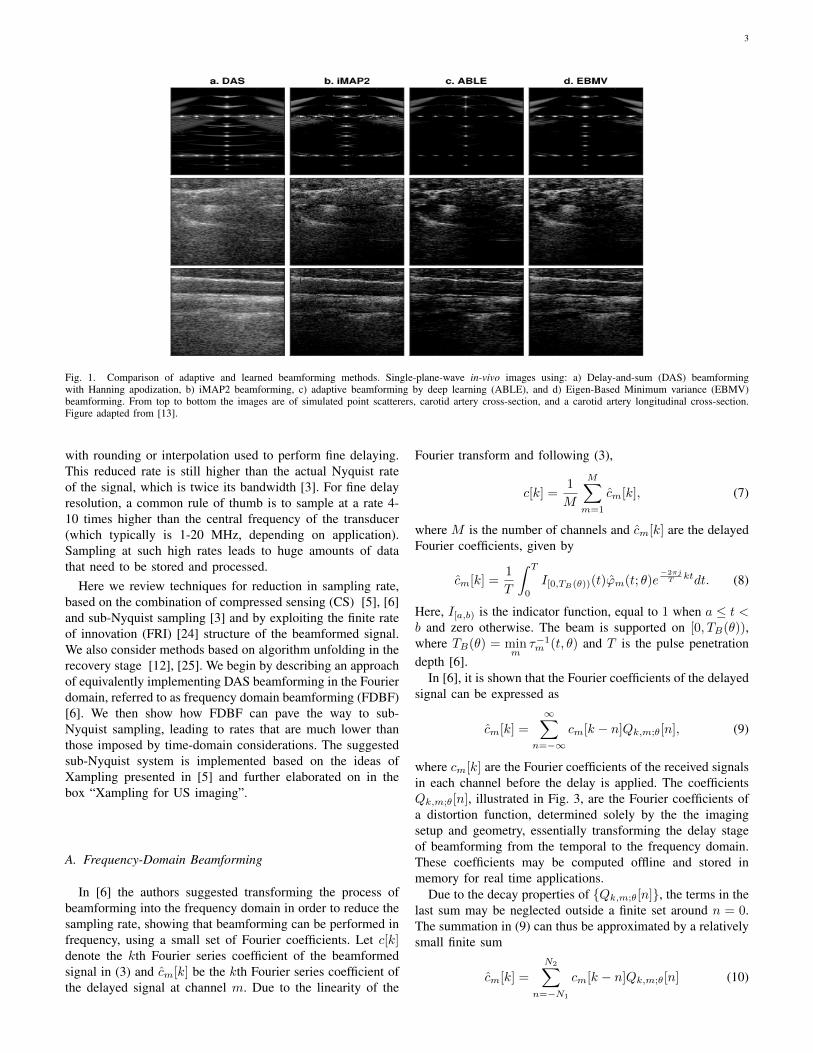
Fig. 1. Comparison of adaptive and learned beamforming methods. Single-plane-wave in-vivo images using: a) Delay-and-sum (DAS) beamformingwith Hanning apodization, b) iMAP2 beamforming, c) adaptive beamforming by deep learning (ABLE), and d) Eigen-Based Minimum variance (EBMV)beamforming. From top to bottom the images are of simulated point scatterers, carotid artery cross-section, and a carotid artery longitudinal cross-section.Figure adapted from [13].

with rounding or interpolation used to perform fine delaying.This reduced rate is still higher than the actual Nyquist rateof the signal, which is twice its bandwidth [3]. For fine delayresolution, a common rule of thumb is to sample at a rate 4-10 times higher than the central frequency of the transducer(which typically is 1-20 MHz, depending on application).Sampling at such high rates leads to huge amounts of datathat need to be stored and processed.

Here we review techniques for reduction in sampling rate,based on the combination of compressed sensing (CS) [5], [6]and sub-Nyquist sampling [3] and by exploiting the finite rateof innovation (FRI) [24] structure of the beamformed signal.We also consider methods based on algorithm unfolding in therecovery stage [12], [25]. We begin by describing an approachof equivalently implementing DAS beamforming in the Fourierdomain, referred to as frequency domain beamforming (FDBF)[6]. We then show how FDBF can pave the way to sub-Nyquist sampling, leading to rates that are much lower thanthose imposed by time-domain considerations. The suggestedsub-Nyquist system is implemented based on the ideas ofXampling presented in [5] and further elaborated on in thebox “Xampling for US imaging”.

A. Frequency-Domain Beamforming

In [6] the authors suggested transforming the process ofbeamforming into the frequency domain in order to reduce thesampling rate, showing that beamforming can be performed infrequency, using a small set of Fourier coefficients. Let c[k]denote the kth Fourier series coefficient of the beamformedsignal in (3) and cm[k] be the kth Fourier series coefficient ofthe delayed signal at channel m. Due to the linearity of the

Fourier transform and following (3),

c[k] =1

M

M∑m=1

cm[k], (7)

where M is the number of channels and cm[k] are the delayedFourier coefficients, given by

cm[k] =1

T

∫ T

0

I[0,TB(θ))(t)ϕm(t; θ)e−2πjT ktdt. (8)

Here, I[a,b) is the indicator function, equal to 1 when a ≤ t <b and zero otherwise. The beam is supported on [0, TB(θ)),where TB(θ) = min

mτ−1m (t, θ) and T is the pulse penetration

depth [6].In [6], it is shown that the Fourier coefficients of the delayed

signal can be expressed as

cm[k] =

∞∑n=−∞

cm[k − n]Qk,m;θ[n], (9)

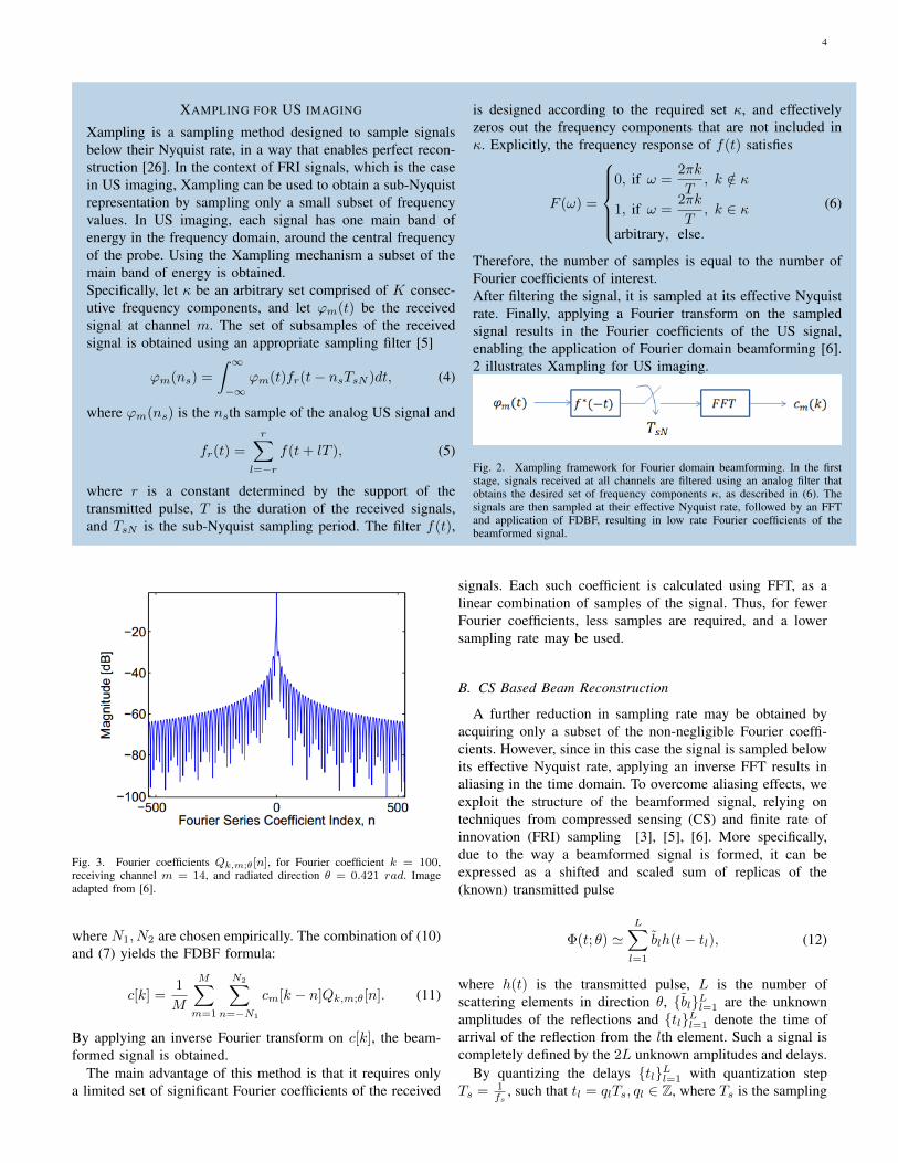
where cm[k] are the Fourier coefficients of the received signalsin each channel before the delay is applied. The coefficientsQk,m;θ[n], illustrated in Fig. 3, are the Fourier coefficients ofa distortion function, determined solely by the the imagingsetup and geometry, essentially transforming the delay stageof beamforming from the temporal to the frequency domain.These coefficients may be computed offline and stored inmemory for real time applications.

Due to the decay properties of {Qk,m;θ[n]}, the terms in thelast sum may be neglected outside a finite set around n = 0.The summation in (9) can thus be approximated by a relativelysmall finite sum

cm[k] =

N2∑n=−N1

cm[k − n]Qk,m;θ[n] (10)

4

XAMPLING FOR US IMAGING

Xampling is a sampling method designed to sample signalsbelow their Nyquist rate, in a way that enables perfect recon-struction [26]. In the context of FRI signals, which is the casein US imaging, Xampling can be used to obtain a sub-Nyquistrepresentation by sampling only a small subset of frequencyvalues. In US imaging, each signal has one main band ofenergy in the frequency domain, around the central frequencyof the probe. Using the Xampling mechanism a subset of themain band of energy is obtained.Specifically, let κ be an arbitrary set comprised of K consec-utive frequency components, and let ϕm(t) be the receivedsignal at channel m. The set of subsamples of the receivedsignal is obtained using an appropriate sampling filter [5]

ϕm(ns) =

∫ ∞−∞

ϕm(t)fr(t− nsTsN )dt, (4)

where ϕm(ns) is the nsth sample of the analog US signal and

fr(t) =

r∑l=−r

f(t+ lT ), (5)

where r is a constant determined by the support of thetransmitted pulse, T is the duration of the received signals,and TsN is the sub-Nyquist sampling period. The filter f(t),

is designed according to the required set κ, and effectivelyzeros out the frequency components that are not included inκ. Explicitly, the frequency response of f(t) satisfies

F (ω) =

0, if ω =

2πk

T, k /∈ κ

1, if ω =2πk

T, k ∈ κ

arbitrary, else.

(6)

Therefore, the number of samples is equal to the number ofFourier coefficients of interest.After filtering the signal, it is sampled at its effective Nyquistrate. Finally, applying a Fourier transform on the sampledsignal results in the Fourier coefficients of the US signal,enabling the application of Fourier domain beamforming [6].2 illustrates Xampling for US imaging.

Fig. 2. Xampling framework for Fourier domain beamforming. In the firststage, signals received at all channels are filtered using an analog filter thatobtains the desired set of frequency components κ, as described in (6). Thesignals are then sampled at their effective Nyquist rate, followed by an FFTand application of FDBF, resulting in low rate Fourier coefficients of thebeamformed signal.

Fig. 3. Fourier coefficients Qk,m;θ[n], for Fourier coefficient k = 100,receiving channel m = 14, and radiated direction θ = 0.421 rad. Imageadapted from [6].

where N1, N2 are chosen empirically. The combination of (10)and (7) yields the FDBF formula:

c[k] =1

M

M∑m=1

N2∑n=−N1

cm[k − n]Qk,m;θ[n]. (11)

By applying an inverse Fourier transform on c[k], the beam-formed signal is obtained.

The main advantage of this method is that it requires onlya limited set of significant Fourier coefficients of the received

signals. Each such coefficient is calculated using FFT, as alinear combination of samples of the signal. Thus, for fewerFourier coefficients, less samples are required, and a lowersampling rate may be used.

B. CS Based Beam Reconstruction

A further reduction in sampling rate may be obtained byacquiring only a subset of the non-negligible Fourier coeffi-cients. However, since in this case the signal is sampled belowits effective Nyquist rate, applying an inverse FFT results inaliasing in the time domain. To overcome aliasing effects, weexploit the structure of the beamformed signal, relying ontechniques from compressed sensing (CS) and finite rate ofinnovation (FRI) sampling [3], [5], [6]. More specifically,due to the way a beamformed signal is formed, it can beexpressed as a shifted and scaled sum of replicas of the(known) transmitted pulse

Φ(t; θ) 'L∑l=1

blh(t− tl), (12)

where h(t) is the transmitted pulse, L is the number ofscattering elements in direction θ, {bl}Ll=1 are the unknownamplitudes of the reflections and {tl}Ll=1 denote the time ofarrival of the reflection from the lth element. Such a signal iscompletely defined by the 2L unknown amplitudes and delays.

By quantizing the delays {tl}Ll=1 with quantization stepTs = 1

fs, such that tl = qlTs, ql ∈ Z, where Ts is the sampling

5

period and fs is the sampling frequency, we may write theFourier coefficients of the beamformed signal as:

c[k] = h[k]

N−1∑l=0

ble−i 2πN kl, (13)

where N = bT/Tsc, h[k] are the Fourier coefficients of thetransmitted pulse, and

bl =

{bl, if l = ql0, otherwise.

(14)

Defining an M -length measurement vector c with kth entryc[k], (13) may be rewritten as

c = HDb = Ab, (15)

where H is an M×M diagonal matrix with h[k] as its entries,D is an M ×N matrix formed by taking a set of rows froman N×N Fourier matrix, and b is a vector of length Nst withlth entry bl, where Nst is the number of samples required forstandard DAS beamforming.

Once formulated this way, the problem is that of recoveringa sparse vector b, given measurements c. A typical beam-formed ultrasound signal is comprised of a relatively smallnumber of strong reflections and many scattered echoes. Thus,the vector b defined in (15), is typically not strictly sparse,but rather compressible. This property can be captured byusing the l1 norm as an objective function in an optimizationproblem:

minb‖b‖1 subject to ‖Ab− c‖2 ≤ ε, (16)

with ε a parameter representing a noise level. Problem (16)can be solved using second-order methods such as interiorpoint methods [27], or first-order methods, based on iterativeshrinkage ideas such as the NESTA algorithm [6], which wasshown to be highly suitable for US signals.

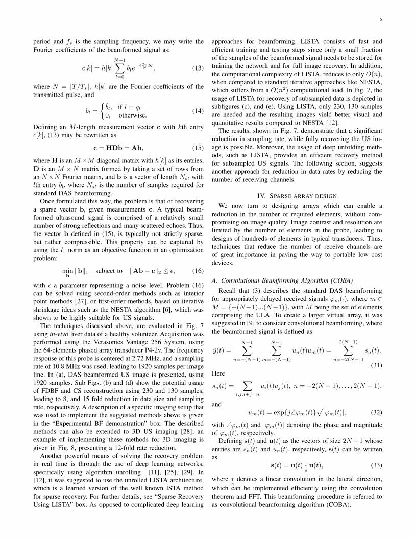
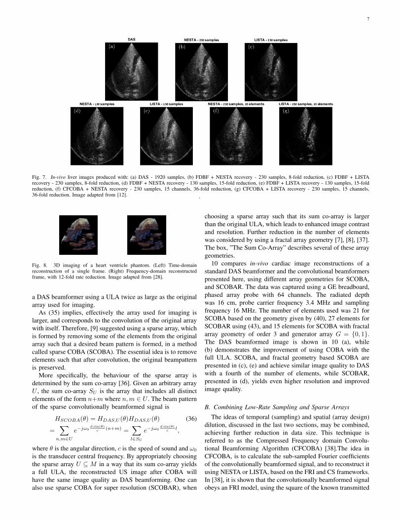
The techniques discussed above, are evaluated in Fig. 7using in-vivo liver data of a healthy volunteer. Acquisition wasperformed using the Verasonics Vantage 256 System, usingthe 64-elements phased array transducer P4-2v. The frequencyresponse of this probe is centered at 2.72 MHz, and a samplingrate of 10.8 MHz was used, leading to 1920 samples per imageline. In (a), DAS beamformed US image is presented, using1920 samples. Sub Figs. (b) and (d) show the potential usageof FDBF and CS reconstruction using 230 and 130 samples,leading to 8, and 15 fold reduction in data size and samplingrate, respectively. A description of a specific imaging setup thatwas used to implement the suggested methods above is givenin the “Experimental BF demonstration” box. The describedmethods can also be extended to 3D US imaging [28]; anexample of implementing these methods for 3D imaging isgiven in Fig. 8, presenting a 12-fold rate reduction.

Another powerful means of solving the recovery problemin real time is through the use of deep learning networks,specifically using algorithm unrolling [11], [25], [29]. In[12], it was suggested to use the unrolled LISTA architecture,which is a learned version of the well known ISTA methodfor sparse recovery. For further details, see “Sparse RecoveryUsing LISTA” box. As opposed to complicated deep learning

approaches for beamforming, LISTA consists of fast andefficient training and testing steps since only a small fractionof the samples of the beamformed signal needs to be stored fortraining the network and for full image recovery. In addition,the computational complexity of LISTA, reduces to only O(n),when compared to standard iterative approaches like NESTA,which suffers from a O(n2) computational load. In Fig. 7, theusage of LISTA for recovery of subsampled data is depicted insubfigures (c), and (e). Using LISTA, only 230, 130 samplesare needed and the resulting images yield better visual andquantitative results compared to NESTA [12].

The results, shown in Fig. 7, demonstrate that a significantreduction in sampling rate, while fully recovering the US im-age is possible. Moreover, the usage of deep unfolding meth-ods, such as LISTA, provides an efficient recovery methodfor subsampled US signals. The following section, suggestsanother approach for reduction in data rates by reducing thenumber of receiving channels.

IV. SPARSE ARRAY DESIGN

We now turn to designing arrays which can enable areduction in the number of required elements, without com-promising on image quality. Image contrast and resolution arelimited by the number of elements in the probe, leading todesigns of hundreds of elements in typical transducers. Thus,techniques that reduce the number of receive channels areof great importance in paving the way to portable low costdevices.

A. Convolutional Beamforming Algorithm (COBA)

Recall that (3) describes the standard DAS beamformingfor appropriately delayed received signals ϕm(·), where m ∈M = {−(N−1)...(N−1)}, with M being the set of elementscomprising the ULA. To create a larger virtual array, it wassuggested in [9] to consider convolutional beamforming, wherethe beamformed signal is defined as

y(t) =

N−1∑n=−(N−1)

N−1∑m=−(N−1)

un(t)um(t) =

2(N−1)∑n=−2(N−1)

sn(t).

(31)Here

sn(t) =∑

i,j:i+j=n

ui(t)uj(t), n = −2(N − 1), . . . , 2(N − 1),

andum(t) = exp{j∠ϕm(t)}

√|ϕm(t)|, (32)

with ∠ϕm(t) and |ϕm(t)| denoting the phase and magnitudeof ϕm(t), respectively.

Defining s(t) and u(t) as the vectors of size 2N −1 whoseentries are sn(t) and un(t), respectively, s(t) can be writtenas

s(t) = u(t) ∗su(t), (33)

where ∗s

denotes a linear convolution in the lateral direction,which can be implemented efficiently using the convolutiontheorem and FFT. This beamforming procedure is referred toas convolutional beamforming algorithm (COBA).

6

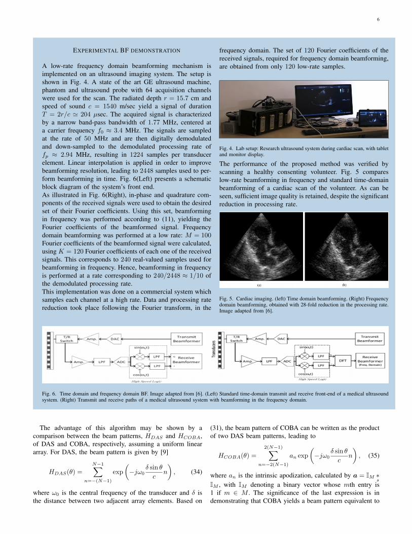
EXPERIMENTAL BF DEMONSTRATION

A low-rate frequency domain beamforming mechanism isimplemented on an ultrasound imaging system. The setup isshown in Fig. 4. A state of the art GE ultrasound machine,phantom and ultrasound probe with 64 acquisition channelswere used for the scan. The radiated depth r = 15.7 cm andspeed of sound c = 1540 m/sec yield a signal of durationT = 2r/c ' 204 µsec. The acquired signal is characterizedby a narrow band-pass bandwidth of 1.77 MHz, centered ata carrier frequency f0 ≈ 3.4 MHz. The signals are sampledat the rate of 50 MHz and are then digitally demodulatedand down-sampled to the demodulated processing rate offp ≈ 2.94 MHz, resulting in 1224 samples per transducerelement. Linear interpolation is applied in order to improvebeamforming resolution, leading to 2448 samples used to per-form beamforming in time. Fig. 6(Left) presents a schematicblock diagram of the system’s front end.As illustrated in Fig. 6(Right), in-phase and quadrature com-ponents of the received signals were used to obtain the desiredset of their Fourier coefficients. Using this set, beamformingin frequency was performed according to (11), yielding theFourier coefficients of the beamformed signal. Frequencydomain beamforming was performed at a low rate: M = 100Fourier coefficients of the beamformed signal were calculated,using K = 120 Fourier coefficients of each one of the receivedsignals. This corresponds to 240 real-valued samples used forbeamforming in frequency. Hence, beamforming in frequencyis performed at a rate corresponding to 240/2448 ≈ 1/10 ofthe demodulated processing rate.This implementation was done on a commercial system whichsamples each channel at a high rate. Data and processing ratereduction took place following the Fourier transform, in the

frequency domain. The set of 120 Fourier coefficients of thereceived signals, required for frequency domain beamforming,are obtained from only 120 low-rate samples.

Fig. 4. Lab setup: Research ultrasound system during cardiac scan, with tabletand monitor display.

The performance of the proposed method was verified byscanning a healthy consenting volunteer. Fig. 5 compareslow-rate beamforming in frequency and standard time-domainbeamforming of a cardiac scan of the volunteer. As can beseen, sufficient image quality is retained, despite the significantreduction in processing rate.

Fig. 5. Cardiac imaging. (left) Time domain beamforming. (Right) Frequencydomain beamforming, obtained with 28-fold reduction in the processing rate.Image adapted from [6].

Fig. 6. Time domain and frequency domain BF. Image adapted from [6]. (Left) Standard time-domain transmit and receive front-end of a medical ultrasoundsystem. (Right) Transmit and receive paths of a medical ultrasound system with beamforming in the frequency domain.

The advantage of this algorithm may be shown by acomparison between the beam patterns, HDAS and HCOBA,of DAS and COBA, respectively, assuming a uniform lineararray. For DAS, the beam pattern is given by [9]

HDAS(θ) =

N−1∑n=−(N−1)

exp

(−jω0

δ sin θ

cn

), (34)

where ω0 is the central frequency of the transducer and δ isthe distance between two adjacent array elements. Based on

(31), the beam pattern of COBA can be written as the productof two DAS beam patterns, leading to

HCOBA(θ) =

2(N−1)∑n=−2(N−1)

an exp

(−jω0

δ sin θ

cn

), (35)

where an is the intrinsic apodization, calculated by a = IM ∗s

IM , with IM denoting a binary vector whose mth entry is1 if m ∈ M . The significance of the last expression is indemonstrating that COBA yields a beam pattern equivalent to

7

Fig. 7. In-vivo liver images produced with: (a) DAS - 1920 samples, (b) FDBF + NESTA recovery - 230 samples, 8-fold reduction, (c) FDBF + LISTArecovery - 230 samples, 8-fold reduction, (d) FDBF + NESTA recovery - 130 samples, 15-fold reduction, (e) FDBF + LISTA recovery - 130 samples, 15-foldreduction, (f) CFCOBA + NESTA recovery - 230 samples, 15 channels, 36-fold reduction, (g) CFCOBA + LISTA recovery - 230 samples, 15 channels,36-fold reduction. Image adapted from [12]. .

Fig. 8. 3D imaging of a heart ventricle phantom. (Left) Time-domainreconstruction of a single frame. (Right) Frequency-domain reconstructedframe, with 12-fold rate reduction. Image adapted from [28].

a DAS beamformer using a ULA twice as large as the originalarray used for imaging.

As (35) implies, effectively the array used for imaging islarger, and corresponds to the convolution of the original arraywith itself. Therefore, [9] suggested using a sparse array, whichis formed by removing some of the elements from the originalarray such that a desired beam pattern is formed, in a methodcalled sparse COBA (SCOBA). The essential idea is to removeelements such that after convolution, the original beampatternis preserved.

More specifically, the behaviour of the sparse array isdetermined by the sum co-array [36]. Given an arbitrary arrayU , the sum co-array SU is the array that includes all distinctelements of the form n+m where n,m ∈ U . The beam patternof the sparse convolutionally beamformed signal is

HSCOBA(θ) = HDAS,U (θ)HDAS,U (θ) (36)

=∑

n,m∈Ue−jω0

d sin(θ)c (n+m) =

∑l∈SU

e−jω0d sin(θ)

c l,

where θ is the angular direction, c is the speed of sound and ω0

is the transducer central frequency. By appropriately choosingthe sparse array U ⊆M in a way that its sum co-array yieldsa full ULA, the reconstructed US image after COBA willhave the same image quality as DAS beamforming. One canalso use sparse COBA for super resolution (SCOBAR), when

choosing a sparse array such that its sum co-array is largerthan the original ULA, which leads to enhanced image contrastand resolution. Further reduction in the number of elementswas considered by using a fractal array geometry [7], [8], [37].The box, ”The Sum Co-Array” describes several of these arraygeometries.

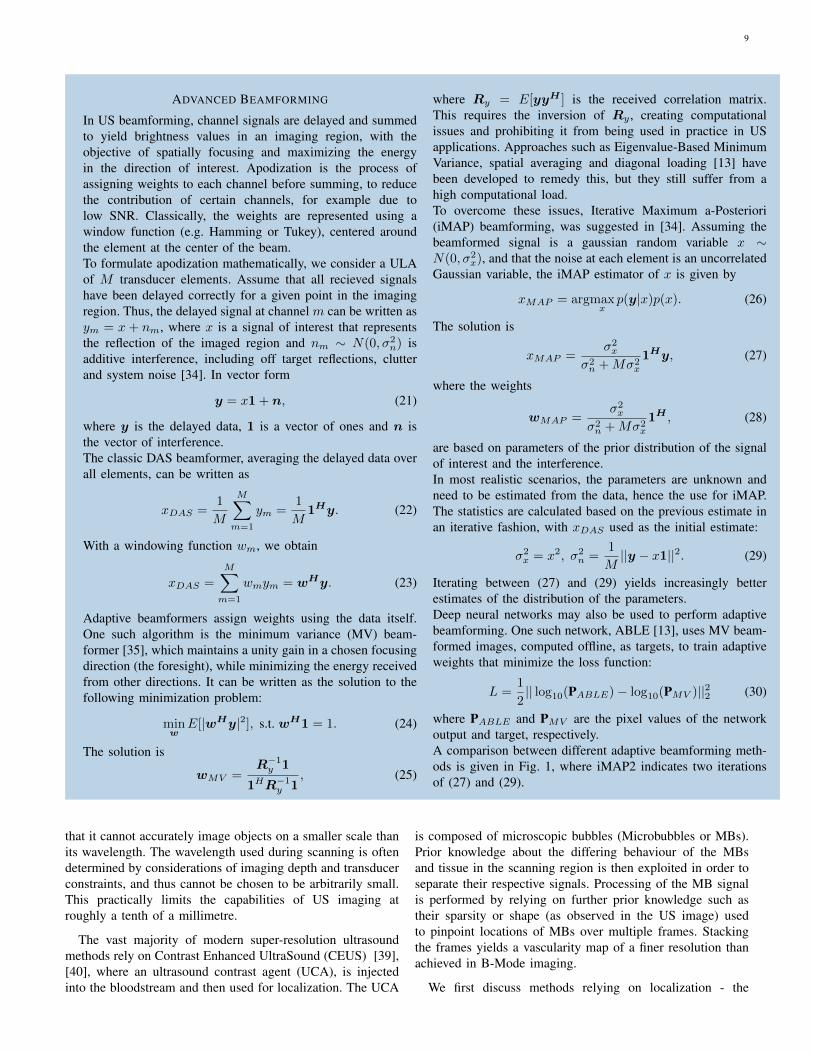
10 compares in-vivo cardiac image reconstructions of astandard DAS beamformer and the convolutional beamformerspresented here, using different array geometries for SCOBA,and SCOBAR. The data was captured using a GE breadboard,phased array probe with 64 channels. The radiated depthwas 16 cm, probe carrier frequency 3.4 MHz and samplingfrequency 16 MHz. The number of elements used was 21 forSCOBA based on the geometry given by (40), 27 elements forSCOBAR using (43), and 15 elements for SCOBA with fractalarray geometry of order 3 and generator array G = {0, 1}.The DAS beamformed image is shown in 10 (a), while(b) demonstrates the improvement of using COBA with thefull ULA. SCOBA, and fractal geometry based SCOBA arepresented in (c), (e) and achieve similar image quality to DASwith a fourth of the number of elements, while SCOBAR,presented in (d), yields even higher resolution and improvedimage quality.

B. Combining Low-Rate Sampling and Sparse Arrays

The ideas of temporal (sampling) and spatial (array design)dilution, discussed in the last two sections, may be combined,achieving further reduction in data size. This technique isreferred to as the Compressed Frequency domain Convolu-tional Beamforming Algorithm (CFCOBA) [38].The idea inCFCOBA, is to calculate the sub-sampled Fourier coefficientsof the convolutionally beamformed signal, and to reconstruct itusing NESTA or LISTA, based on the FRI and CS frameworks.In [38], it is shown that the convolutionally beamformed signalobeys an FRI model, using the square of the known transmitted

8

SPARSE RECOVERY USING LISTA

Learned ISTA (LISTA) [11], [25] is a data-driven, learnedcounterpart of the widely used iterative shrinkage/thresholdingalgorithm (ISTA) [30] for sparse recovery.Consider a sparse recovery problem

minx

=1

2||y− Ax||22 + λ||x||1 (17)

where y is the measured signal, A is the measurement matrix,both known, λ a regularization parameter and x is the underly-ing sparse vector to be recovered. ISTA solves (17) iterativelythrough the iterations

xk+1 = Sλ(Wey + Wtxk), x0 = 0, (18)

where xk+1, xk are subsequent approximations of the solution,We = µAT ,Wt = I − µATA for some chosen step sizeparameter µ, and Sλ is a soft thresholding operator withthreshold λ.Adapting ISTA to a learning-based framework is performed byunrolling: cascading layers of a deep network, each mimickingan iteration in the iterated algorithm [25]. In the unfolded ver-sion of LISTA, the layers consist of trainable convolutions Wk

e ,Wkt , and a trainable shrinkage parameter λk, corresponding

to the threshold in ISTA, for 1 ≤ k ≤ K, where K is thetotal number of layers. The thresholding operation in LISTAis replaced by a smooth approximation (though other smoothapproximations are possible)

Sλ(x) =x

1 + e−(|x|−λ), (19)

with the operations performed element-wise.Training LISTA is done in a supervised manner, by firstrecovering a set of sparse codes xi, 1 ≤ i ≤ N , given aset of measurements yi and the known measurement matrixA. This recovery is typically performed using an iterativesparse solver, e.g. ISTA, FISTA, and NESTA [30], [31].Training is typically performed by minimizing the mean-squared-error (MSE) between the unrolled network’s output,given the measurements yi and their respective latent codesxi,

L(We,Wt, λ) =1

N

N∑i=1

||xi(yi; We,Wt, λ)− xi||22, (20)

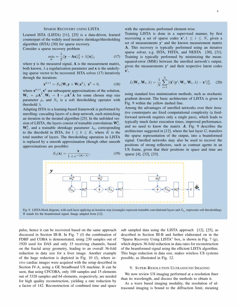
using standard loss minimization methods, such as stochasticgradient descent. The basic architecture of LISTA is given inFig. 9 within the yellow dashed line.Among the advantages of unrolled networks over their itera-tive counterparts are fixed computational complexity (a feed-forward network requires only a single pass), which leads totypically much faster execution times, improved performance,and no need to know the matrix A. Fig. 9 describes thearchitecture suggested in [12], where the last layer G, transfersthe sparse representation of the output, into a beamformedsignal. Unrolled networks may also be used to recover thepositions of strong reflectors, such as contrast agents in anUS frame, given that their positions in space and time aresparse [4], [32], [33].

Fig. 9. LISTA block diagram, with each layer applying an iteration step (rectangles represent trainable convolutional layers and Sλi represents soft thresholding).Φ stands for the beamformed signal. Image adapted from [12].

pulse, hence it can be recovered based on the same approachdiscussed in Section III-B. In Fig. 7 (f) the combination ofFDBF and COBA is demonstrated, using 230 samples out of1920 used for DAS and only 15 receiving channels, basedon the fractal array geometry, leading to an overall 36-foldreduction in data size for a liver image. Another exampleof the huge reduction is depicted in Fig. 10 (f), where in-vivo cardiac images were acquired with the setup described inSection IV-A, using a GE breadboard US machine. It can beseen, that using CFCOBA, only 100 samples and 15 elementsout of 3328 samples and 64 elements, respectively, are neededfor high quality reconstruction, yielding a rate reduction bya factor of 142. Reconstruction of combined time and space

sub sampled data using the LISTA approach [12], [25], asdescribed in Section III-B and further elaborated on in the“Sparse Recovery Using LISTA” box, is shown in Fig. 7 (g),which depicts 36-fold reduction in data rates for reconstructionof the beamformed signal using the efficient LISTA algorithm.This huge reduction in data size, makes wireless US systemspossible, as illustrated in Fig. 12.

V. SUPER-RESOLUTION ULTRASOUND IMAGING

We now review US imaging performed at a resolution finerthan its wavelength, and discuss the methods to obtain it.

As a wave based imaging modality, the resolution of ul-trasound imaging is bound to the diffraction limit, meaning

9

ADVANCED BEAMFORMING

In US beamforming, channel signals are delayed and summedto yield brightness values in an imaging region, with theobjective of spatially focusing and maximizing the energyin the direction of interest. Apodization is the process ofassigning weights to each channel before summing, to reducethe contribution of certain channels, for example due tolow SNR. Classically, the weights are represented using awindow function (e.g. Hamming or Tukey), centered aroundthe element at the center of the beam.To formulate apodization mathematically, we consider a ULAof M transducer elements. Assume that all recieved signalshave been delayed correctly for a given point in the imagingregion. Thus, the delayed signal at channel m can be written asym = x + nm, where x is a signal of interest that representsthe reflection of the imaged region and nm ∼ N(0, σ2

n) isadditive interference, including off target reflections, clutterand system noise [34]. In vector form

y = x1 + n, (21)

where y is the delayed data, 1 is a vector of ones and n isthe vector of interference.The classic DAS beamformer, averaging the delayed data overall elements, can be written as

xDAS =1

M

M∑m=1

ym =1

M1Hy. (22)

With a windowing function wm, we obtain

xDAS =

M∑m=1

wmym = wHy. (23)

Adaptive beamformers assign weights using the data itself.One such algorithm is the minimum variance (MV) beam-former [35], which maintains a unity gain in a chosen focusingdirection (the foresight), while minimizing the energy receivedfrom other directions. It can be written as the solution to thefollowing minimization problem:

minw

E[|wHy|2], s.t. wH1 = 1. (24)

The solution is

wMV =R−1y 1

1HR−1y 1, (25)

where Ry = E[yyH ] is the received correlation matrix.This requires the inversion of Ry , creating computationalissues and prohibiting it from being used in practice in USapplications. Approaches such as Eigenvalue-Based MinimumVariance, spatial averaging and diagonal loading [13] havebeen developed to remedy this, but they still suffer from ahigh computational load.To overcome these issues, Iterative Maximum a-Posteriori(iMAP) beamforming, was suggested in [34]. Assuming thebeamformed signal is a gaussian random variable x ∼N(0, σ2

x), and that the noise at each element is an uncorrelatedGaussian variable, the iMAP estimator of x is given by

xMAP = argmaxx

p(y|x)p(x). (26)

The solution is

xMAP =σ2x

σ2n +Mσ2

x

1Hy, (27)

where the weights

wMAP =σ2x

σ2n +Mσ2

x

1H , (28)

are based on parameters of the prior distribution of the signalof interest and the interference.In most realistic scenarios, the parameters are unknown andneed to be estimated from the data, hence the use for iMAP.The statistics are calculated based on the previous estimate inan iterative fashion, with xDAS used as the initial estimate:

σ2x = x2, σ2

n =1

M||y − x1||2. (29)

Iterating between (27) and (29) yields increasingly betterestimates of the distribution of the parameters.Deep neural networks may also be used to perform adaptivebeamforming. One such network, ABLE [13], uses MV beam-formed images, computed offline, as targets, to train adaptiveweights that minimize the loss function:

L =1

2|| log10(PABLE)− log10(PMV )||22 (30)

where PABLE and PMV are the pixel values of the networkoutput and target, respectively.A comparison between different adaptive beamforming meth-ods is given in Fig. 1, where iMAP2 indicates two iterationsof (27) and (29).

that it cannot accurately image objects on a smaller scale thanits wavelength. The wavelength used during scanning is oftendetermined by considerations of imaging depth and transducerconstraints, and thus cannot be chosen to be arbitrarily small.This practically limits the capabilities of US imaging atroughly a tenth of a millimetre.

The vast majority of modern super-resolution ultrasoundmethods rely on Contrast Enhanced UltraSound (CEUS) [39],[40], where an ultrasound contrast agent (UCA), is injectedinto the bloodstream and then used for localization. The UCA

is composed of microscopic bubbles (Microbubbles or MBs).Prior knowledge about the differing behaviour of the MBsand tissue in the scanning region is then exploited in order toseparate their respective signals. Processing of the MB signalis performed by relying on further prior knowledge such astheir sparsity or shape (as observed in the US image) usedto pinpoint locations of MBs over multiple frames. Stackingthe frames yields a vascularity map of a finer resolution thanachieved in B-Mode imaging.

We first discuss methods relying on localization - the

10

Fig. 10. Cardiac ultrasound images beamformed with (a) DAS - 64 elements (ULA), 3328 samples, (b) COBA - full ULA, 3328 samples, (c) SCOBA -21 elements, 3328 samples, (d) SCOBAR - 27 elements, 3328 samples, (e) fractal geometry - 15 elements, 3328 samples, (f) CFCOBA - 15 elements, 100samples. The US signals are obtained with different number of receiving channels, and images are produced using COBA, and the compressed frequencydomain COBA approach. Images adapted from [9], [38].

tracking of, and subsequent replacement of MBs with pointobjects. Then, we show how sparsity in different domains canbe exploited to yield non-localization based techniques.

A. Ultrasound Localization Microscopy

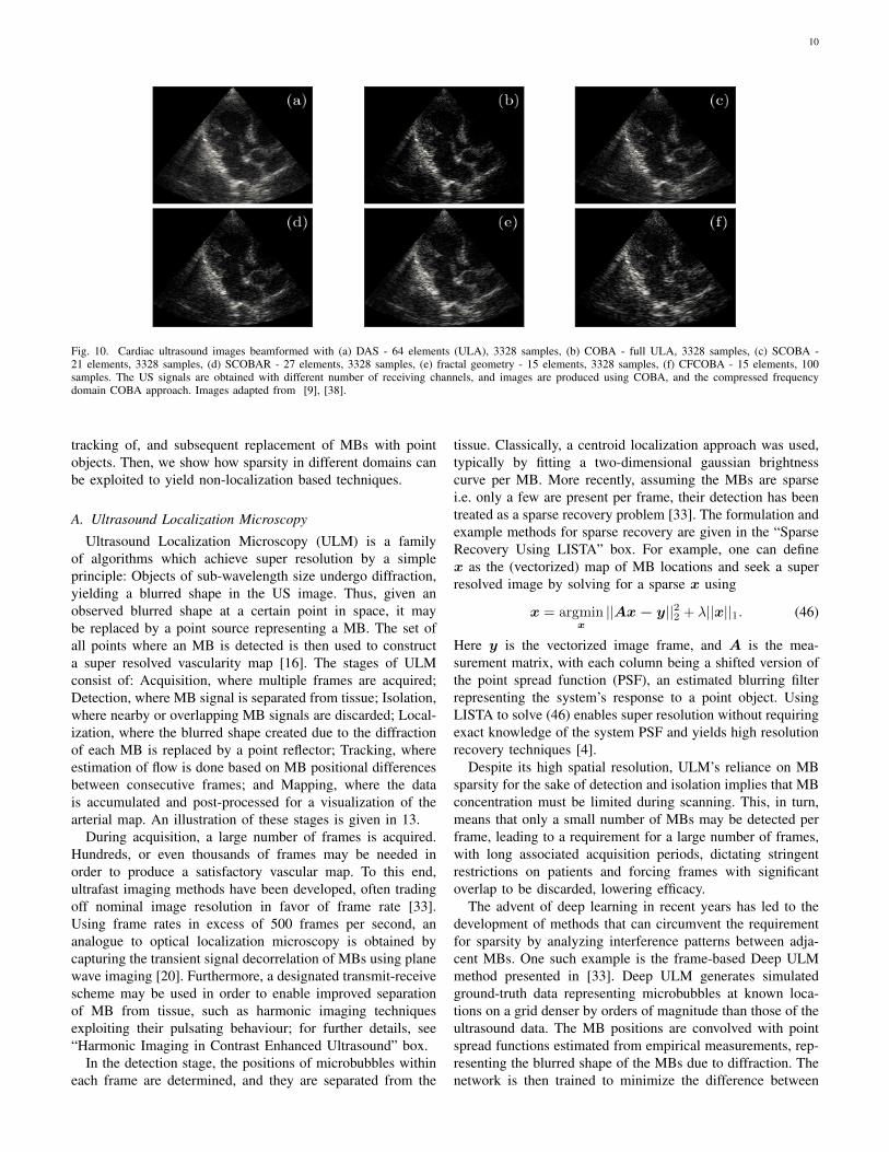
Ultrasound Localization Microscopy (ULM) is a familyof algorithms which achieve super resolution by a simpleprinciple: Objects of sub-wavelength size undergo diffraction,yielding a blurred shape in the US image. Thus, given anobserved blurred shape at a certain point in space, it maybe replaced by a point source representing a MB. The set ofall points where an MB is detected is then used to constructa super resolved vascularity map [16]. The stages of ULMconsist of: Acquisition, where multiple frames are acquired;Detection, where MB signal is separated from tissue; Isolation,where nearby or overlapping MB signals are discarded; Local-ization, where the blurred shape created due to the diffractionof each MB is replaced by a point reflector; Tracking, whereestimation of flow is done based on MB positional differencesbetween consecutive frames; and Mapping, where the datais accumulated and post-processed for a visualization of thearterial map. An illustration of these stages is given in 13.

During acquisition, a large number of frames is acquired.Hundreds, or even thousands of frames may be needed inorder to produce a satisfactory vascular map. To this end,ultrafast imaging methods have been developed, often tradingoff nominal image resolution in favor of frame rate [33].Using frame rates in excess of 500 frames per second, ananalogue to optical localization microscopy is obtained bycapturing the transient signal decorrelation of MBs using planewave imaging [20]. Furthermore, a designated transmit-receivescheme may be used in order to enable improved separationof MB from tissue, such as harmonic imaging techniquesexploiting their pulsating behaviour; for further details, see“Harmonic Imaging in Contrast Enhanced Ultrasound” box.

In the detection stage, the positions of microbubbles withineach frame are determined, and they are separated from the

tissue. Classically, a centroid localization approach was used,typically by fitting a two-dimensional gaussian brightnesscurve per MB. More recently, assuming the MBs are sparsei.e. only a few are present per frame, their detection has beentreated as a sparse recovery problem [33]. The formulation andexample methods for sparse recovery are given in the “SparseRecovery Using LISTA” box. For example, one can definex as the (vectorized) map of MB locations and seek a superresolved image by solving for a sparse x using

x = argminx||Ax − y||22 + λ||x||1. (46)

Here y is the vectorized image frame, and A is the mea-surement matrix, with each column being a shifted version ofthe point spread function (PSF), an estimated blurring filterrepresenting the system’s response to a point object. UsingLISTA to solve (46) enables super resolution without requiringexact knowledge of the system PSF and yields high resolutionrecovery techniques [4].

Despite its high spatial resolution, ULM’s reliance on MBsparsity for the sake of detection and isolation implies that MBconcentration must be limited during scanning. This, in turn,means that only a small number of MBs may be detected perframe, leading to a requirement for a large number of frames,with long associated acquisition periods, dictating stringentrestrictions on patients and forcing frames with significantoverlap to be discarded, lowering efficacy.

The advent of deep learning in recent years has led to thedevelopment of methods that can circumvent the requirementfor sparsity by analyzing interference patterns between adja-cent MBs. One such example is the frame-based Deep ULMmethod presented in [33]. Deep ULM generates simulatedground-truth data representing microbubbles at known loca-tions on a grid denser by orders of magnitude than those of theultrasound data. The MB positions are convolved with pointspread functions estimated from empirical measurements, rep-resenting the blurred shape of the MBs due to diffraction. Thenetwork is then trained to minimize the difference between

11

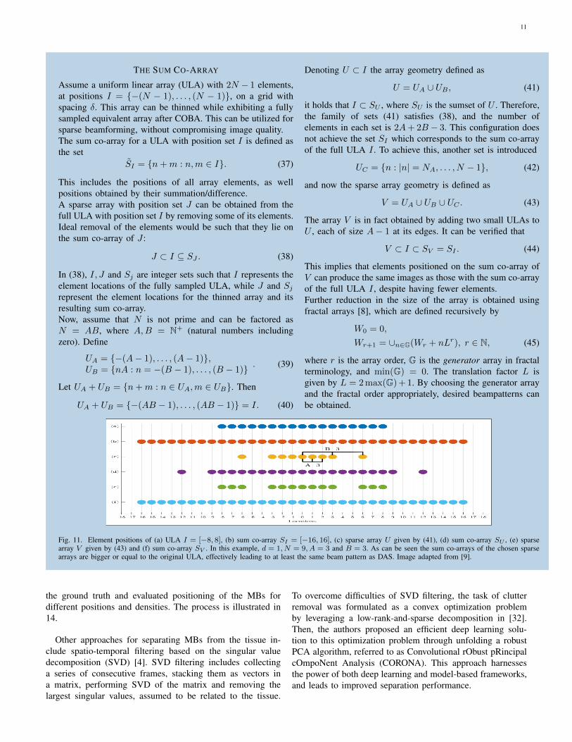
THE SUM CO-ARRAY

Assume a uniform linear array (ULA) with 2N − 1 elements,at positions I = {−(N − 1), . . . , (N − 1)}, on a grid withspacing δ. This array can be thinned while exhibiting a fullysampled equivalent array after COBA. This can be utilized forsparse beamforming, without compromising image quality.The sum co-array for a ULA with position set I is defined asthe set

SI = {n+m : n,m ∈ I}. (37)

This includes the positions of all array elements, as wellpositions obtained by their summation/difference.A sparse array with position set J can be obtained from thefull ULA with position set I by removing some of its elements.Ideal removal of the elements would be such that they lie onthe sum co-array of J :

J ⊂ I ⊆ SJ . (38)

In (38), I, J and Sj are integer sets such that I represents theelement locations of the fully sampled ULA, while J and Sjrepresent the element locations for the thinned array and itsresulting sum co-array.Now, assume that N is not prime and can be factored asN = AB, where A,B = N+ (natural numbers includingzero). Define

UA = {−(A− 1), . . . , (A− 1)},UB = {nA : n = −(B − 1), . . . , (B − 1)} . (39)

Let UA + UB = {n+m : n ∈ UA,m ∈ UB}. Then

UA + UB = {−(AB − 1), . . . , (AB − 1)} = I. (40)

Denoting U ⊂ I the array geometry defined as

U = UA ∪ UB , (41)

it holds that I ⊂ SU , where SU is the sumset of U . Therefore,the family of sets (41) satisfies (38), and the number ofelements in each set is 2A+ 2B − 3. This configuration doesnot achieve the set SI which corresponds to the sum co-arrayof the full ULA I . To achieve this, another set is introduced

UC = {n : |n| = NA, . . . , N − 1}, (42)

and now the sparse array geometry is defined as

V = UA ∪ UB ∪ UC . (43)

The array V is in fact obtained by adding two small ULAs toU , each of size A− 1 at its edges. It can be verified that

V ⊂ I ⊂ SV = SI . (44)

This implies that elements positioned on the sum co-array ofV can produce the same images as those with the sum co-arrayof the full ULA I , despite having fewer elements.Further reduction in the size of the array is obtained usingfractal arrays [8], which are defined recursively by

W0 = 0,

Wr+1 = ∪n∈G(Wr + nLr), r ∈ N, (45)

where r is the array order, G is the generator array in fractalterminology, and min(G) = 0. The translation factor L isgiven by L = 2 max(G) + 1. By choosing the generator arrayand the fractal order appropriately, desired beampatterns canbe obtained.

Fig. 11. Element positions of (a) ULA I = [−8, 8], (b) sum co-array SI = [−16, 16], (c) sparse array U given by (41), (d) sum co-array SU , (e) sparsearray V given by (43) and (f) sum co-array SV . In this example, d = 1, N = 9, A = 3 and B = 3. As can be seen the sum co-arrays of the chosen sparsearrays are bigger or equal to the original ULA, effectively leading to at least the same beam pattern as DAS. Image adapted from [9].

the ground truth and evaluated positioning of the MBs fordifferent positions and densities. The process is illustrated in14.

Other approaches for separating MBs from the tissue in-clude spatio-temporal filtering based on the singular valuedecomposition (SVD) [4]. SVD filtering includes collectinga series of consecutive frames, stacking them as vectors ina matrix, performing SVD of the matrix and removing thelargest singular values, assumed to be related to the tissue.

To overcome difficulties of SVD filtering, the task of clutterremoval was formulated as a convex optimization problemby leveraging a low-rank-and-sparse decomposition in [32].Then, the authors proposed an efficient deep learning solu-tion to this optimization problem through unfolding a robustPCA algorithm, referred to as Convolutional rObust pRincipalcOmpoNent Analysis (CORONA). This approach harnessesthe power of both deep learning and model-based frameworks,and leads to improved separation performance.

12

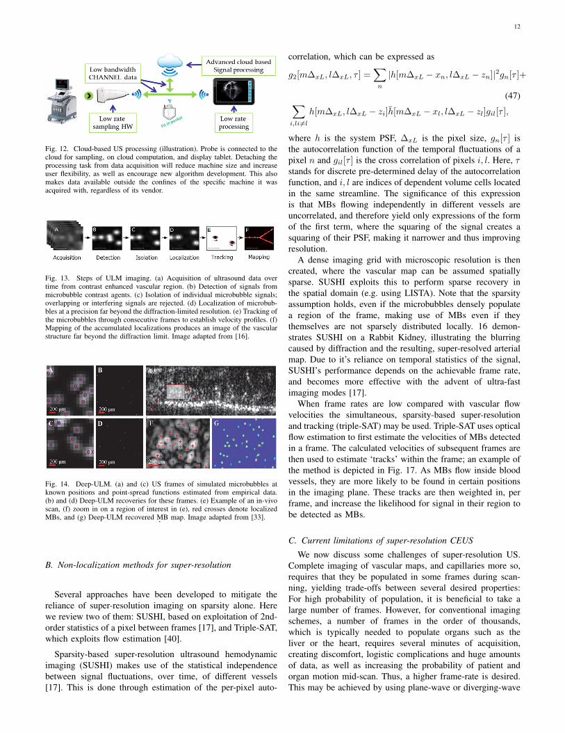
Fig. 12. Cloud-based US processing (illustration). Probe is connected to thecloud for sampling, on cloud computation, and display tablet. Detaching theprocessing task from data acquisition will reduce machine size and increaseuser flexibility, as well as encourage new algorithm development. This alsomakes data available outside the confines of the specific machine it wasacquired with, regardless of its vendor.

Fig. 13. Steps of ULM imaging. (a) Acquisition of ultrasound data overtime from contrast enhanced vascular region. (b) Detection of signals frommicrobubble contrast agents. (c) Isolation of individual microbubble signals;overlapping or interfering signals are rejected. (d) Localization of microbub-bles at a precision far beyond the diffraction-limited resolution. (e) Tracking ofthe microbubbles through consecutive frames to establish velocity profiles. (f)Mapping of the accumulated localizations produces an image of the vascularstructure far beyond the diffraction limit. Image adapted from [16].

Fig. 14. Deep-ULM. (a) and (c) US frames of simulated microbubbles atknown positions and point-spread functions estimated from empirical data.(b) and (d) Deep-ULM recoveries for these frames. (e) Example of an in-vivoscan, (f) zoom in on a region of interest in (e), red crosses denote localizedMBs, and (g) Deep-ULM recovered MB map. Image adapted from [33]..

B. Non-localization methods for super-resolution

Several approaches have been developed to mitigate thereliance of super-resolution imaging on sparsity alone. Herewe review two of them: SUSHI, based on exploitation of 2nd-order statistics of a pixel between frames [17], and Triple-SAT,which exploits flow estimation [40].

Sparsity-based super-resolution ultrasound hemodynamicimaging (SUSHI) makes use of the statistical independencebetween signal fluctuations, over time, of different vessels[17]. This is done through estimation of the per-pixel auto-

correlation, which can be expressed as

g2[m∆xL, l∆xL, τ ] =∑n

|h[m∆xL − xn, l∆xL − zn]|2gn[τ ]+

(47)∑i,li6=l

h[m∆xL, l∆xL − zi]h[m∆xL − xl, l∆xL − zl]gil[τ ],

where h is the system PSF, ∆xL is the pixel size, gn[τ ] isthe autocorrelation function of the temporal fluctuations of apixel n and gil[τ ] is the cross correlation of pixels i, l. Here, τstands for discrete pre-determined delay of the autocorrelationfunction, and i, l are indices of dependent volume cells locatedin the same streamline. The significance of this expressionis that MBs flowing independently in different vessels areuncorrelated, and therefore yield only expressions of the formof the first term, where the squaring of the signal creates asquaring of their PSF, making it narrower and thus improvingresolution.

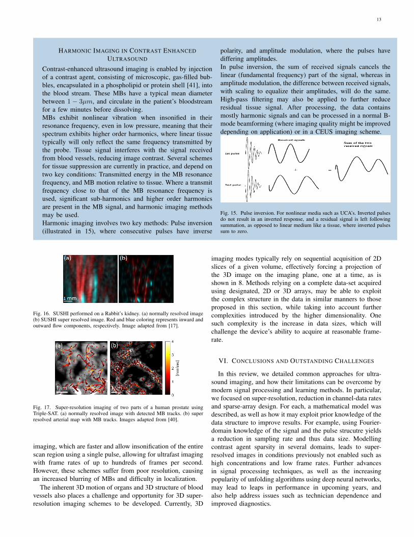
A dense imaging grid with microscopic resolution is thencreated, where the vascular map can be assumed spatiallysparse. SUSHI exploits this to perform sparse recovery inthe spatial domain (e.g. using LISTA). Note that the sparsityassumption holds, even if the microbubbles densely populatea region of the frame, making use of MBs even if theythemselves are not sparsely distributed locally. 16 demon-strates SUSHI on a Rabbit Kidney, illustrating the blurringcaused by diffraction and the resulting, super-resolved arterialmap. Due to it’s reliance on temporal statistics of the signal,SUSHI’s performance depends on the achievable frame rate,and becomes more effective with the advent of ultra-fastimaging modes [17].

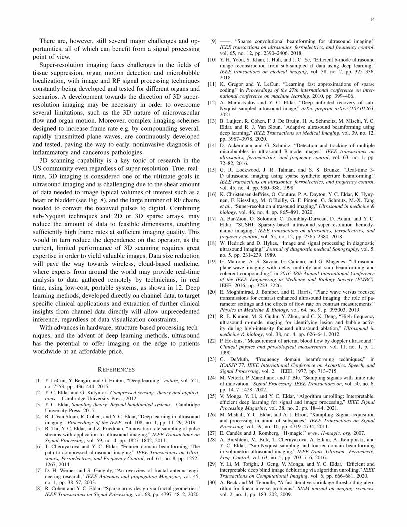
When frame rates are low compared with vascular flowvelocities the simultaneous, sparsity-based super-resolutionand tracking (triple-SAT) may be used. Triple-SAT uses opticalflow estimation to first estimate the velocities of MBs detectedin a frame. The calculated velocities of subsequent frames arethen used to estimate ‘tracks’ within the frame; an example ofthe method is depicted in Fig. 17. As MBs flow inside bloodvessels, they are more likely to be found in certain positionsin the imaging plane. These tracks are then weighted in, perframe, and increase the likelihood for signal in their region tobe detected as MBs.

C. Current limitations of super-resolution CEUS

We now discuss some challenges of super-resolution US.Complete imaging of vascular maps, and capillaries more so,requires that they be populated in some frames during scan-ning, yielding trade-offs between several desired properties:For high probability of population, it is beneficial to take alarge number of frames. However, for conventional imagingschemes, a number of frames in the order of thousands,which is typically needed to populate organs such as theliver or the heart, requires several minutes of acquisition,creating discomfort, logistic complications and huge amountsof data, as well as increasing the probability of patient andorgan motion mid-scan. Thus, a higher frame-rate is desired.This may be achieved by using plane-wave or diverging-wave

13

HARMONIC IMAGING IN CONTRAST ENHANCEDULTRASOUND

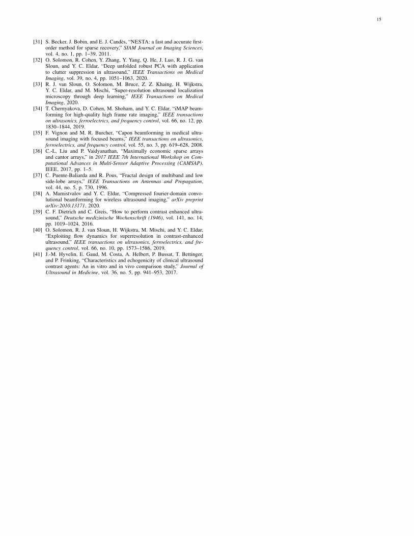
Contrast-enhanced ultrasound imaging is enabled by injectionof a contrast agent, consisting of microscopic, gas-filled bub-bles, encapsulated in a phospholipid or protein shell [41], intothe blood stream. These MBs have a typical mean diameterbetween 1 − 3µm, and circulate in the patient’s bloodstreamfor a few minutes before dissolving.MBs exhibit nonlinear vibration when insonified in theirresonance frequency, even in low pressure, meaning that theirspectrum exhibits higher order harmonics, where linear tissuetypically will only reflect the same frequency transmitted bythe probe. Tissue signal interferes with the signal receivedfrom blood vessels, reducing image contrast. Several schemesfor tissue suppression are currently in practice, and depend ontwo key conditions: Transmitted energy in the MB resonancefrequency, and MB motion relative to tissue. Where a transmitfrequency close to that of the MB resonance frequency isused, significant sub-harmonics and higher order harmonicsare present in the MB signal, and harmonic imaging methodsmay be used.Harmonic imaging involves two key methods: Pulse inversion(illustrated in 15), where consecutive pulses have inverse

polarity, and amplitude modulation, where the pulses havediffering amplitudes.In pulse inversion, the sum of received signals cancels thelinear (fundamental frequency) part of the signal, whereas inamplitude modulation, the difference between received signals,with scaling to equalize their amplitudes, will do the same.High-pass filtering may also be applied to further reduceresidual tissue signal. After processing, the data containsmostly harmonic signals and can be processed in a normal B-mode beamforming (where imaging quality might be improveddepending on application) or in a CEUS imaging scheme.

Fig. 15. Pulse inversion. For nonlinear media such as UCA’s. Inverted pulsesdo not result in an inverted response, and a residual signal is left followingsummation, as opposed to linear medium like a tissue, where inverted pulsessum to zero.

Fig. 16. SUSHI performed on a Rabbit’s kidney. (a) normally resolved image(b) SUSHI super resolved image. Red and blue coloring represents inward andoutward flow components, respectively. Image adapted from [17].

Fig. 17. Super-resolution imaging of two parts of a human prostate usingTriple-SAT. (a) normally resolved image with detected MB tracks. (b) superresolved arterial map with MB tracks. Images adapted from [40].

imaging, which are faster and allow insonification of the entirescan region using a single pulse, allowing for ultrafast imagingwith frame rates of up to hundreds of frames per second.However, these schemes suffer from poor resolution, causingan increased blurring of MBs and difficulty in localization.

The inherent 3D motion of organs and 3D structure of bloodvessels also places a challenge and opportunity for 3D super-resolution imaging schemes to be developed. Currently, 3D

imaging modes typically rely on sequential acquisition of 2Dslices of a given volume, effectively forcing a projection ofthe 3D image on the imaging plane, one at a time, as isshown in 8. Methods relying on a complete data-set acquiredusing designated, 2D or 3D arrays, may be able to exploitthe complex structure in the data in similar manners to thoseproposed in this section, while taking into account furthercomplexities introduced by the higher dimensionality. Onesuch complexity is the increase in data sizes, which willchallenge the device’s ability to acquire at reasonable frame-rate.

VI. CONCLUSIONS AND OUTSTANDING CHALLENGES

In this review, we detailed common approaches for ultra-sound imaging, and how their limitations can be overcome bymodern signal processing and learning methods. In particular,we focused on super-resolution, reduction in channel-data ratesand sparse-array design. For each, a mathematical model wasdescribed, as well as how it may exploit prior knowledge of thedata structure to improve results. For example, using Fourier-domain knowledge of the signal and the pulse strucutre yieldsa reduction in sampling rate and thus data size. Modellingcontrast agent sparsity in several domains, leads to super-resolved images in conditions previously not enabled such ashigh concentrations and low frame rates. Further advancesin signal processing techniques, as well as the increasingpopularity of unfolding algorithms using deep neural networks,may lead to leaps in performance in upcoming years, andalso help address issues such as technician dependence andimproved diagnostics.

14

There are, however, still several major challenges and op-portunities, all of which can benefit from a signal processingpoint of view.

Super-resolution imaging faces challenges in the fields oftissue suppression, organ motion detection and microbubblelocalization, with image and RF signal processing techniquesconstantly being developed and tested for different organs andscenarios. A development towards the direction of 3D super-resolution imaging may be necessary in order to overcomeseveral limitations, such as the 3D nature of microvascularflow and organ motion. Moreover, complex imaging schemesdesigned to increase frame rate e.g. by compounding several,rapidly transmitted plane waves, are continuously developedand tested, paving the way to early, noninvasive diagnosis ofinflammatory and cancerous pathologies.

3D scanning capability is a key topic of research in theUS community even regardless of super-resolution. True, real-time, 3D imaging is considered one of the ultimate goals inultrasound imaging and is challenging due to the shear amountof data needed to image typical volumes of interest such as aheart or bladder (see Fig. 8), and the large number of RF chainsneeded to convert the received pulses to digital. Combiningsub-Nyquist techniques and 2D or 3D sparse arrays, mayreduce the amount of data to feasible dimensions, enablingsufficiently high frame rates at sufficient imaging quality. Thiswould in turn reduce the dependence on the operator, as thecurrent, limited performance of 3D scanning requires greatexpertise in order to yield valuable images. Data size reductionwill pave the way towards wireless, cloud-based medicine,where experts from around the world may provide real-timeanalysis to data gathered remotely by technicians, in realtime, using low-cost, portable systems, as shown in 12. Deeplearning methods, developed directly on channel data, to targetspecific clinical applications and extraction of further clinicalinsights from channel data directly will allow unprecedentedinference, regardless of data visualization constraints.

With advances in hardware, structure-based processing tech-niques, and the advent of deep learning methods, ultrasoundhas the potential to offer imaging on the edge to patientsworldwide at an affordable price.

REFERENCES

[1] Y. LeCun, Y. Bengio, and G. Hinton, “Deep learning,” nature, vol. 521,no. 7553, pp. 436–444, 2015.

[2] Y. C. Eldar and G. Kutyniok, Compressed sensing: theory and applica-tions. Cambridge University Press, 2012.

[3] Y. C. Eldar, Sampling theory: Beyond bandlimited systems. CambridgeUniversity Press, 2015.

[4] R. J. Van Sloun, R. Cohen, and Y. C. Eldar, “Deep learning in ultrasoundimaging,” Proceedings of the IEEE, vol. 108, no. 1, pp. 11–29, 2019.

[5] R. Tur, Y. C. Eldar, and Z. Friedman, “Innovation rate sampling of pulsestreams with application to ultrasound imaging,” IEEE Transactions onSignal Processing, vol. 59, no. 4, pp. 1827–1842, 2011.

[6] T. Chernyakova and Y. C. Eldar, “Fourier domain beamforming: Thepath to compressed ultrasound imaging,” IEEE Transactions on Ultra-sonics, Ferroelectrics, and Frequency Control, vol. 61, no. 8, pp. 1252–1267, 2014.

[7] D. H. Werner and S. Ganguly, “An overview of fractal antenna engi-neering research,” IEEE Antennas and propagation Magazine, vol. 45,no. 1, pp. 38–57, 2003.

[8] R. Cohen and Y. C. Eldar, “Sparse array design via fractal geometries,”IEEE Transactions on Signal Processing, vol. 68, pp. 4797–4812, 2020.

[9] ——, “Sparse convolutional beamforming for ultrasound imaging,”IEEE transactions on ultrasonics, ferroelectrics, and frequency control,vol. 65, no. 12, pp. 2390–2406, 2018.

[10] Y. H. Yoon, S. Khan, J. Huh, and J. C. Ye, “Efficient b-mode ultrasoundimage reconstruction from sub-sampled rf data using deep learning,”IEEE transactions on medical imaging, vol. 38, no. 2, pp. 325–336,2018.

[11] K. Gregor and Y. LeCun, “Learning fast approximations of sparsecoding,” in Proceedings of the 27th international conference on inter-national conference on machine learning, 2010, pp. 399–406.

[12] A. Mamistvalov and Y. C. Eldar, “Deep unfolded recovery of sub-Nyquist sampled ultrasound image,” arXiv preprint arXiv:2103.01263,2021.

[13] B. Luijten, R. Cohen, F. J. De Bruijn, H. A. Schmeitz, M. Mischi, Y. C.Eldar, and R. J. Van Sloun, “Adaptive ultrasound beamforming usingdeep learning,” IEEE Transactions on Medical Imaging, vol. 39, no. 12,pp. 3967–3978, 2020.

[14] D. Ackermann and G. Schmitz, “Detection and tracking of multiplemicrobubbles in ultrasound B-mode images,” IEEE transactions onultrasonics, ferroelectrics, and frequency control, vol. 63, no. 1, pp.72–82, 2016.

[15] G. R. Lockwood, J. R. Talman, and S. S. Brunke, “Real-time 3-D ultrasound imaging using sparse synthetic aperture beamforming,”IEEE transactions on ultrasonics, ferroelectrics, and frequency control,vol. 45, no. 4, pp. 980–988, 1998.

[16] K. Christensen-Jeffries, O. Couture, P. A. Dayton, Y. C. Eldar, K. Hyny-nen, F. Kiessling, M. O’Reilly, G. F. Pinton, G. Schmitz, M.-X. Tanget al., “Super-resolution ultrasound imaging,” Ultrasound in medicine &biology, vol. 46, no. 4, pp. 865–891, 2020.

[17] A. Bar-Zion, O. Solomon, C. Tremblay-Darveau, D. Adam, and Y. C.Eldar, “SUSHI: Sparsity-based ultrasound super-resolution hemody-namic imaging,” IEEE transactions on ultrasonics, ferroelectrics, andfrequency control, vol. 65, no. 12, pp. 2365–2380, 2018.

[18] W. Hedrick and D. Hykes, “Image and signal processing in diagnosticultrasound imaging,” Journal of diagnostic medical Sonography, vol. 5,no. 5, pp. 231–239, 1989.

[19] G. Matrone, A. S. Savoia, G. Caliano, and G. Magenes, “Ultrasoundplane-wave imaging with delay multiply and sum beamforming andcoherent compounding,” in 2016 38th Annual International Conferenceof the IEEE Engineering in Medicine and Biology Society (EMBC).IEEE, 2016, pp. 3223–3226.

[20] E. Moghimirad, J. Bamber, and E. Harris, “Plane wave versus focusedtransmissions for contrast enhanced ultrasound imaging: the role of pa-rameter settings and the effects of flow rate on contrast measurements,”Physics in Medicine & Biology, vol. 64, no. 9, p. 095003, 2019.

[21] R. E. Kumon, M. S. Gudur, Y. Zhou, and C. X. Deng, “High-frequencyultrasound m-mode imaging for identifying lesion and bubble activ-ity during high-intensity focused ultrasound ablation,” Ultrasound inmedicine & biology, vol. 38, no. 4, pp. 626–641, 2012.

[22] P. Hoskins, “Measurement of arterial blood flow by doppler ultrasound,”Clinical physics and physiological measurement, vol. 11, no. 1, p. 1,1990.

[23] G. DeMuth, “Frequency domain beamforming techniques,” inICASSP’77. IEEE International Conference on Acoustics, Speech, andSignal Processing, vol. 2. IEEE, 1977, pp. 713–715.

[24] M. Vetterli, P. Marziliano, and T. Blu, “Sampling signals with finite rateof innovation,” Signal Processing, IEEE Transactions on, vol. 50, no. 6,pp. 1417–1428, 2002.

[25] V. Monga, Y. Li, and Y. C. Eldar, “Algorithm unrolling: Interpretable,efficient deep learning for signal and image processing,” IEEE SignalProcessing Magazine, vol. 38, no. 2, pp. 18–44, 2021.

[26] M. Mishali, Y. C. Eldar, and A. J. Elron, “Xampling: Signal acquisitionand processing in union of subspaces,” IEEE Transactions on SignalProcessing, vol. 59, no. 10, pp. 4719–4734, 2011.

[27] E. Candes and J. Romberg, “l1-magic,” www. l1-magic. org, 2007.[28] A. Burshtein, M. Birk, T. Chernyakova, A. Eilam, A. Kempinski, and

Y. C. Eldar, “Sub-Nyquist sampling and fourier domain beamformingin volumetric ultrasound imaging,” IEEE Trans. Ultrason., Ferroelectr.,Freq. Control, vol. 63, no. 5, pp. 703–716, 2016.

[29] Y. Li, M. Tofighi, J. Geng, V. Monga, and Y. C. Eldar, “Efficient andinterpretable deep blind image deblurring via algorithm unrolling,” IEEETransactions on Computational Imaging, vol. 6, pp. 666–681, 2020.

[30] A. Beck and M. Teboulle, “A fast iterative shrinkage-thresholding algo-rithm for linear inverse problems,” SIAM journal on imaging sciences,vol. 2, no. 1, pp. 183–202, 2009.

15

[31] S. Becker, J. Bobin, and E. J. Candes, “NESTA: a fast and accurate first-order method for sparse recovery,” SIAM Journal on Imaging Sciences,vol. 4, no. 1, pp. 1–39, 2011.

[32] O. Solomon, R. Cohen, Y. Zhang, Y. Yang, Q. He, J. Luo, R. J. G. vanSloun, and Y. C. Eldar, “Deep unfolded robust PCA with applicationto clutter suppression in ultrasound,” IEEE Transactions on MedicalImaging, vol. 39, no. 4, pp. 1051–1063, 2020.

[33] R. J. van Sloun, O. Solomon, M. Bruce, Z. Z. Khaing, H. Wijkstra,Y. C. Eldar, and M. Mischi, “Super-resolution ultrasound localizationmicroscopy through deep learning,” IEEE Transactions on MedicalImaging, 2020.

[34] T. Chernyakova, D. Cohen, M. Shoham, and Y. C. Eldar, “iMAP beam-forming for high-quality high frame rate imaging,” IEEE transactionson ultrasonics, ferroelectrics, and frequency control, vol. 66, no. 12, pp.1830–1844, 2019.

[35] F. Vignon and M. R. Burcher, “Capon beamforming in medical ultra-sound imaging with focused beams,” IEEE transactions on ultrasonics,ferroelectrics, and frequency control, vol. 55, no. 3, pp. 619–628, 2008.

[36] C.-L. Liu and P. Vaidyanathan, “Maximally economic sparse arraysand cantor arrays,” in 2017 IEEE 7th International Workshop on Com-putational Advances in Multi-Sensor Adaptive Processing (CAMSAP).IEEE, 2017, pp. 1–5.

[37] C. Puente-Baliarda and R. Pous, “Fractal design of multiband and lowside-lobe arrays,” IEEE Transactions on Antennas and Propagation,vol. 44, no. 5, p. 730, 1996.

[38] A. Mamistvalov and Y. C. Eldar, “Compressed fourier-domain convo-lutional beamforming for wireless ultrasound imaging,” arXiv preprintarXiv:2010.13171, 2020.

[39] C. F. Dietrich and C. Greis, “How to perform contrast enhanced ultra-sound,” Deutsche medizinische Wochenschrift (1946), vol. 141, no. 14,pp. 1019–1024, 2016.

[40] O. Solomon, R. J. van Sloun, H. Wijkstra, M. Mischi, and Y. C. Eldar,“Exploiting flow dynamics for superresolution in contrast-enhancedultrasound,” IEEE transactions on ultrasonics, ferroelectrics, and fre-quency control, vol. 66, no. 10, pp. 1573–1586, 2019.

[41] J.-M. Hyvelin, E. Gaud, M. Costa, A. Helbert, P. Bussat, T. Bettinger,and P. Frinking, “Characteristics and echogenicity of clinical ultrasoundcontrast agents: An in vitro and in vivo comparison study,” Journal ofUltrasound in Medicine, vol. 36, no. 5, pp. 941–953, 2017.