Complete validation for classification and class modeling procedures with selection of variables...

Chemometrics and Intelligent Laboratory Systems 102 (2010) 110–122

Contents lists available at ScienceDirect

Chemometrics and Intelligent Laboratory Systems

j ourna l homepage: www.e lsev ie r.com/ locate /chemolab

Complete validation for classification and class modeling procedures with selectionof variables and/or with additional computed variables

M. Forina ⁎, P. Oliveri, M. CasaleDipartimento di Chimica e Tecnologie Farmaceutiche ed Alimentari, Università di Genova, Via Brigata Salerno 13, I-16147 Genova, Italy

⁎ Corresponding author. Tel.: +39 010 3532630; fax:E-mail address: [email protected] (M. Forina).

0169-7439/$ – see front matter © 2010 Elsevier B.V. Adoi:10.1016/j.chemolab.2010.04.011

a b s t r a c t
a r t i c l e i n f o
Article history:Received 23 October 2009Received in revised form 25 March 2010Accepted 14 April 2010Available online 27 April 2010

Keywords:ValidationClassificationClass modeling

The evaluation of the predictive ability of a model, is an essential moment of all the chemometricaltechniques. So it must be performed very carefully. However, in the case of selection of relevant variables (anessential step in the case of data sets with many, frequently thousands, variables) the selection is generallyperformed using all the available objects. In some recent classification and class modeling techniques, fromthe original or from the selected variables the Mahalanobis distances of the leverages from the centroids ofthe categories in the problem are computed, and then added to the original variables. Also here theMahalanobis distances are computed with all the objects. The consequence is an overestimate of theprediction ability, very large when the ratio between the number of the objects and that of the variables israther low, so that the variance-covariance matrix is unstable.In this paper the correct validation procedures are described for the cases of selection of variables and of theaddition of Mahalanobis distances computed on the original variables or the selected variables. The estimatesof the prediction ability are compared with those obtained with insufficient validation strategies.

+39 010 3532684.

ll rights reserved.

© 2010 Elsevier B.V. All rights reserved.

1. Introduction

Validation, i.e. the evaluation of the predictive ability of a model, isan essential moment of all the chemometrical techniques. Validationmeans that the model is built with a fraction of the objects (thetraining set), and the remaining objects are used to evaluate theprediction performance of the model. It seems obvious that

Validation rule 1: “All final or intermediate parameters of themodel(s)must be obtained with only the data in the trainingset”.

Nevertheless the above statement is very frequently ignored, andvalidation is performed more or less roughly. Moreover the predictiveability is an experimental result, therefore with uncertainty. Chemistsare used to present experimental resultswith a confidence interval, but,in the case of the predictive ability no people compute the uncertainty.

So, we call here “complete validation” just the validation performedwith the use of Rule 1 and possibly with that of

Validation rule 2: “The predictive ability and associated quantitiesmustbe accompanied by their uncertainty”.

Validation can be performed by means of Leave-One-Out validation(LOO), Cross Validation (CV), or validation with a single evaluation set.In the case of a single evaluation set, frequently people use a random

assignment of the objects; sometimes the assignment is made to haveboth representative training and test sets, e.g. by means of twinKennard–Stone design [1,2]. The use of a single test set remembers thebeginnings of Chemometrics. CV appeared only in a second time, withthe leave-one-out procedure or with a number of validation groups.Rarely repeated evaluation set, also calledMontecarlo validation (MV) isused. In this strategy, a large number of evaluation sets are randomlycreated, with the exploration of different combination of objects in thetraining and in the evaluation sets, and with the evaluation of theuncertainty in the measure of the predictive ability. The evaluation ofthis uncertainty is possible also with cross validation, by repeating theprediction with different number of CV groups and with different orderof the objects. Also BootstrapValidation is used rarely. Bootstrap createsmany training sets. Each time, n random objects from the original dataset of N objects are selected, with replacement. This means that afterselecting an object, this object returns to the pool from which obser-vations are randomly chosen. Thus, a single objectmaybe selectedmorethan once in any single training set. The evaluation set constitutes all theobjects not found in the training set. The numberof training setsmustbelarge, 200 or more. They have the same number of objects. Theestimated error rate is the average of the error rates in the evaluationsets.

The single test set with a non-representative or too poor test setincreases the risk of over or under-evaluation of the predictive ability. Inthe cases of heavy optimizations, like in the use of Artificial NeuralNetworks (ANN), there are frequently three sets: the training set, themonitoring or predictive optimization set, and the test or finalevaluation set.

mailto:[email protected]

http://dx.doi.org/10.1016/j.chemolab.2010.04.011

http://www.sciencedirect.com/science/journal/01697439

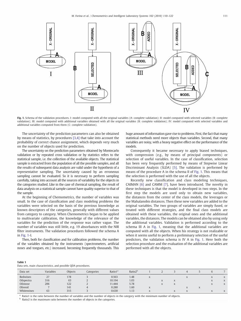
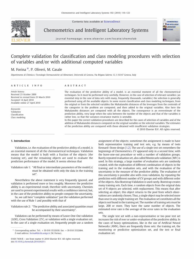
Fig. 1. Schema of the validation procedures. I: model computed with all the original variables (A: complete validation); II: model computed with selected variables (B: completevalidation); III: model computed with additional variables obtained with all the original variables (B: complete validation); IV: model computed with selected variables andadditional variables computed from them (C: complete validation).

111M. Forina et al. / Chemometrics and Intelligent Laboratory Systems 102 (2010) 110–122

The uncertainty of the prediction parameters can also be obtainedby means of statistics, by procedures [3,4] that take into account theprobability of correct chance assignment, which depends very muchon the number of objects used for prediction.

The uncertainty on the prediction parameters obtained by Montecarlovalidation or by repeated cross validation or by statistics refers to thestatistical sample, i.e. the collection of the available objects. The statisticalsample is extracted from the population of all the possible samples, and allthe results of subsequent data analysis are valid under the hypothesis of arepresentative sampling. The uncertainty caused by an erroneoussampling cannot be evaluated. So it is necessary to perform samplingcarefully, taking into account all the sources of variability for the objects inthe categories studied. Like in the case of chemical sampling, the result ofdata analysis on a statistical sample cannot have quality superior to that ofthe sample.

At the beginning of Chemometrics, the number of variables wassmall. In the case of classification and class modeling problems thevariables were selected on the basis of the previous knowledge asknown descriptors of the categories, generally with different valuesfrom category to category. When Chemometrics began to be appliedto multivariate calibration, the knowledge of the relevance of thevariables for the prediction of the response was rather vague. Thenumber of variables was still little, e.g. 19 absorbances with the NIRfilter instruments. The validation procedures followed the schema Ain Fig. 1-I.

Then, both for classification and for calibration problems, the numberof the variables obtained by the instruments (spectrometers, artificialnoses and tongues, etc.) increased, becoming frequently thousands. This

Table 1Data sets, main characteristics, and possible QDA procedures.

Data set Variables Objects Categories Ratio1a

Redwines 27 178 3 0.563Oilspectra 316 63 2 10.194Oilsnose 206 122 2 11.444Oliveoil 7 141 4 0.280Whitewines 63 315 3 0.630

a Ratio1 is the ratio between the number of variables and the number of objects in the cb Ratio2 is the maximum ratio between the number of objects in the categories.

huge amount of information gave rise to problems. First, the fact thatmanystatistical methods need more objects than variables. Second, that manyvariables are noisy, with a heavy negative effect on the performance of themodels.

Consequently it became necessary to apply biased techniques,with compression (e.g., by means of principal components) orselection of useful variables. In the case of classification, selectionhas been very frequently performed by means of Stepwise LinearDiscriminant Analysis (SLDA) [5]. The validation is performed bymeans of the procedure A in the schema II of Fig. 1. This means thatthe selection is performed with the use of all the objects.

Recently new classification and class modeling techniques,CAIMAN [6] and CAMM [7], have been introduced. The novelty inthese techniques is that the model is developed in two steps. In thefirst step the models are used only to obtain new variables,the distances from the center of the class models, the leverages orthe Mahalanobis distances. Then these new variables are added to theoriginal variables. The two groups of variables are simply fused, ortreated with different strategies, and the final class models areobtained with these variables, the original ones and the additionalvariables, the distances. Themodels can be obtained also by using onlythe additional variables. Validation is performed according to theschema III A in Fig. 1, meaning that the additional variables arecomputed with all the objects. When his strategy is not realizable orwhen it seems useful to perform a preliminary selection of the usefulpredictors, the validation schema is IV A in Fig. 1. Here both theselection procedure and the evaluation of the additional variables areperformed with all the objects.

Ratio2b 1 2 3 4 5 6 7

1.48 x x x x1.03 x x x x5.78 x x x x1.60 x x x1.13 x x x x x

ategory with the minimum number of objects.

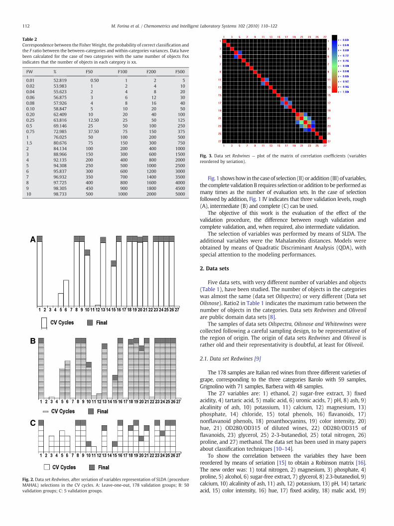
Table 2Correspondence between the FisherWeight, the probability of correct classification andthe F ratio between the between-categories and within-categories variances. Data havebeen calculated for the case of two categories with the same number of objects Fxxindicates that the number of objects in each category is xx.

FW % F50 F100 F200 F500

0.01 52.819 0.50 1 2 50.02 53.983 1 2 4 100.04 55.623 2 4 8 200.06 56.875 3 6 12 300.08 57.926 4 8 16 400.10 58.847 5 10 20 500.20 62.409 10 20 40 1000.25 63.816 12.50 25 50 1250.5 69.146 25 50 100 2500.75 72.985 37.50 75 150 3751 76.025 50 100 200 5001.5 80.676 75 150 300 7502 84.134 100 200 400 10003 88.966 150 300 600 15004 92.135 200 400 800 20005 94.308 250 500 1000 25006 95.837 300 600 1200 30007 96.932 350 700 1400 35008 97.725 400 800 1600 40009 98.305 450 900 1800 450010 98.733 500 1000 2000 5000

Fig. 2. Data set Redwines, after seriation of variables representation of SLDA (procedureMAHAL) selections in the CV cycles. A: Leave-one-out, 178 validation groups; B: 50validation groups; C: 5 validation groups.

Fig. 3. Data set Redwines — plot of the matrix of correlation coefficients (variablesreordered by seriation).

112 M. Forina et al. / Chemometrics and Intelligent Laboratory Systems 102 (2010) 110–122

Fig. 1 showshowin thecaseof selection (II) or addition (III) of variables,the complete validation B requires selection or addition to be performed asmany times as the number of evaluation sets. In the case of selectionfollowed by addition, Fig. 1 IV indicates that three validation levels, rough(A), intermediate (B) and complete (C) can be used.

The objective of this work is the evaluation of the effect of thevalidation procedure, the difference between rough validation andcomplete validation, and, when required, also intermediate validation.

The selection of variables was performed by means of SLDA. Theadditional variables were the Mahalanobis distances. Models wereobtained by means of Quadratic Discriminant Analysis (QDA), withspecial attention to the modeling performances.

2. Data sets

Five data sets, with very different number of variables and objects(Table 1), have been studied. The number of objects in the categorieswas almost the same (data set Oilspectra) or very different (Data setOilsnose). Ratio2 in Table 1 indicates the maximum ratio between thenumber of objects in the categories. Data sets Redwines and Oliveoilare public domain data sets [8].

The samples of data sets Oilspectra, Oilsnose and Whitewines werecollected following a careful sampling design, to be representative ofthe region of origin. The origin of data sets Redwines and Oliveoil israther old and their representativity is doubtful, at least for Oliveoil.

2.1. Data set Redwines [9]

The 178 samples are Italian red wines from three different varieties ofgrape, corresponding to the three categories Barolo with 59 samples,Grignolino with 71 samples, Barbera with 48 samples.

The 27 variables are: 1) ethanol, 2) sugar-free extract, 3) fixedacidity, 4) tartaric acid, 5) malic acid, 6) uronic acids, 7) pH, 8) ash, 9)alcalinity of ash, 10) potassium, 11) calcium, 12) magnesium, 13)phosphate, 14) chloride, 15) total phenols, 16) flavanoids, 17)nonflavanoid phenols, 18) proanthocyanins, 19) color intensity, 20)hue, 21) OD280/OD315 of diluted wines, 22) OD280/OD315 offlavanoids, 23) glycerol, 25) 2-3-butanediol, 25) total nitrogen, 26)proline, and 27) methanol. The data set has been used in many papersabout classification techniques [10–14].

To show the correlation between the variables they have beenreordered by means of seriation [15] to obtain a Robinson matrix [16].The new order was: 1) total nitrogen, 2) magnesium, 3) phosphate, 4)proline, 5) alcohol, 6) sugar-free extract, 7) glycerol, 8) 2.3-butanediol, 9)calcium, 10) alcalinity of ash, 11) ash, 12) potassium, 13) pH, 14) tartaricacid, 15) color intensity, 16) hue, 17) fixed acidity, 18) malic acid, 19)

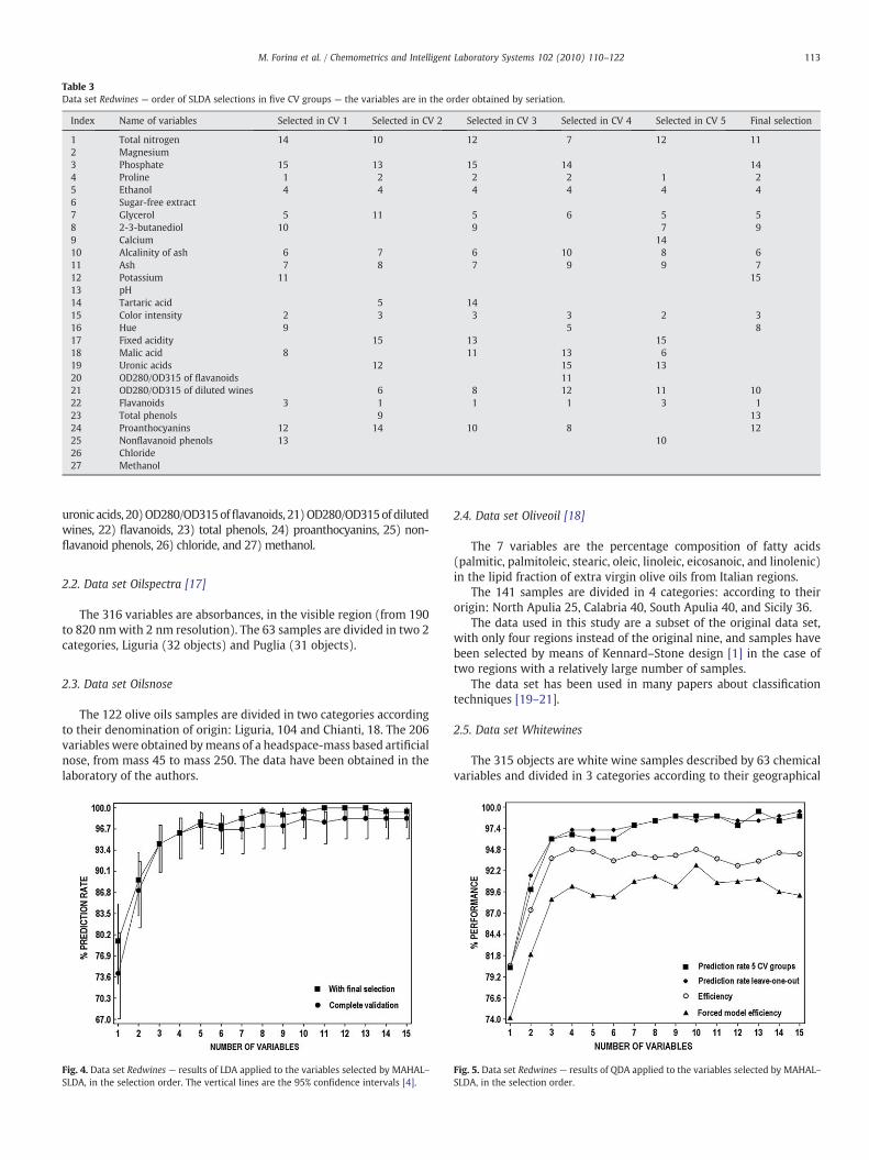
Table 3Data set Redwines — order of SLDA selections in five CV groups — the variables are in the order obtained by seriation.

Index Name of variables Selected in CV 1 Selected in CV 2 Selected in CV 3 Selected in CV 4 Selected in CV 5 Final selection

1 Total nitrogen 14 10 12 7 12 112 Magnesium3 Phosphate 15 13 15 14 144 Proline 1 2 2 2 1 25 Ethanol 4 4 4 4 4 46 Sugar-free extract7 Glycerol 5 11 5 6 5 58 2-3-butanediol 10 9 7 99 Calcium 1410 Alcalinity of ash 6 7 6 10 8 611 Ash 7 8 7 9 9 712 Potassium 11 1513 pH14 Tartaric acid 5 1415 Color intensity 2 3 3 3 2 316 Hue 9 5 817 Fixed acidity 15 13 1518 Malic acid 8 11 13 619 Uronic acids 12 15 1320 OD280/OD315 of flavanoids 1121 OD280/OD315 of diluted wines 6 8 12 11 1022 Flavanoids 3 1 1 1 3 123 Total phenols 9 1324 Proanthocyanins 12 14 10 8 1225 Nonflavanoid phenols 13 1026 Chloride27 Methanol


uronic acids, 20)OD280/OD315offlavanoids, 21)OD280/OD315of dilutedwines, 22) flavanoids, 23) total phenols, 24) proanthocyanins, 25) non-flavanoid phenols, 26) chloride, and 27) methanol.

2.2. Data set Oilspectra [17]

The 316 variables are absorbances, in the visible region (from 190to 820 nmwith 2 nm resolution). The 63 samples are divided in two 2categories, Liguria (32 objects) and Puglia (31 objects).

2.3. Data set Oilsnose

The 122 olive oils samples are divided in two categories accordingto their denomination of origin: Liguria, 104 and Chianti, 18. The 206variables were obtained bymeans of a headspace-mass based artificialnose, from mass 45 to mass 250. The data have been obtained in thelaboratory of the authors.

Fig. 4. Data set Redwines — results of LDA applied to the variables selected by MAHAL–SLDA, in the selection order. The vertical lines are the 95% confidence intervals [4].

2.4. Data set Oliveoil [18]

The 7 variables are the percentage composition of fatty acids(palmitic, palmitoleic, stearic, oleic, linoleic, eicosanoic, and linolenic)in the lipid fraction of extra virgin olive oils from Italian regions.

The 141 samples are divided in 4 categories: according to theirorigin: North Apulia 25, Calabria 40, South Apulia 40, and Sicily 36.

The data used in this study are a subset of the original data set,with only four regions instead of the original nine, and samples havebeen selected by means of Kennard–Stone design [1] in the case oftwo regions with a relatively large number of samples.

The data set has been used in many papers about classificationtechniques [19–21].

2.5. Data set Whitewines

The 315 objects are white wine samples described by 63 chemicalvariables and divided in 3 categories according to their geographical

Fig. 5. Data set Redwines — results of QDA applied to the variables selected by MAHAL–SLDA, in the selection order.

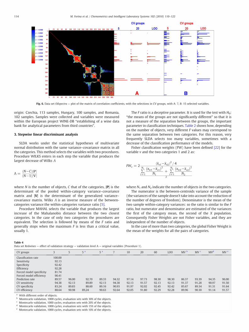
Fig. 6. Data set Oilspectra — plot of the matrix of correlation coefficients, with the selections in CV groups, with A: 7, B: 15 selected variables.


origin: Czechia, 113 samples, Hungary, 100 samples, and Romania,102 samples. Samples were collected and variables were measuredwithin the European project WINE-DB “establishing of a wine databank for analytical parameters from third countries”.

3. Stepwise linear discriminant analysis

SLDA works under the statistical hypotheses of multivariatenormal distribution with the same variance–covariance matrix in allthe categories. This method selects the variables with two procedures.Procedure WILKS enters in each step the variable that produces thelargest decrease of Wilks Λ

Λ =N−Cð ÞjPjN−1ð ÞjVj

where N is the number of objects, C that of the categories, |P| is thedeterminant of the pooled within-category variance–covariancematrix and |V| is the determinant of the generalized variance–covariance matrix. Wilks Λ is an inverse measure of the between-categories variance:the within-categories variance ratio [5].

Procedure MAHAL selects the variable that produces the largestincrease of the Mahalanobis distance between the two closestcategories. In the case of only two categories the procedures areequivalent. The selection is followed by means of the F ratio andgenerally stops when the maximum F is less than a critical value,usually 1.

Table 4Data set Redwines — effect of validation strategy — validation level A — original variables (

CV groups 3 5 5 a 5 a 7

Classification rate 100.00Sensitivity 92.13Specificity 92.42Efficiency 92.28Forced model specificity 81.74Forced model efficiency 90.41Prediction rate 89.57 96.00 92.70 89.33 94.32CV sensitivity 94.38 92.13 89.89 92.13 94.38CV specificity 83.24 89.83 88.60 89.16 90.93CV efficiency 88.64 90.98 89,24 90.63 92.64

a With different order of objects.b Montecarlo validation, 1000 cycles, evaluation sets with 30% of the objects.c Montecarlo validation, 1000 cycles, evaluation sets with 20% of the objects.d Montecarlo validation, 1000 cycles, evaluation sets with 15% of the objects.e Montecarlo validation, 1000 cycles, evaluation sets with 10% of the objects.

The F ratio is a deceptive parameter. It is used for the test with H0:“the means of the groups are not significantly different” so that it isnot a measure of the separation between the groups, the importantparameter in classification techniques. Table 2 shows how, dependingon the number of objects, very different F values may correspond tothe same separation between two categories. For this reason, veryfrequently SLDA selects too many variables, sometimes with adecrease of the classification performance of the models.

Fisher classification weights (FW) have been defined [22] for thevariable v and the two categories 1 and 2 as:

FWv = 2xv1−xv2ð Þ2 = 4

∑N1

i=1

xiv1−xv1� �2

N1+ ∑

N2

i=1

xiv2−xv2� �2

N22

where N1 and N2 indicate the number of objects in the two categories.The numerator is the between-centroids variance of the sample

(the variances of the sample doesn't take into account the reduction ofthe number of degrees of freedom). Denominator is the mean of thetwo sample within-category variances: so the ratio is similar to the Fratio, but numerator and denominator are estimated of the variancesthe first of the category mean, the second of the X population.Consequently Fisher Weights are not Fisher variables, and they areindependent of the number of objects.

In the case of more than two categories, the global FisherWeight isthe mean of the weights for all the pairs of categories.

Procedure 1).

10 20 60 LOO MV b MV c MVd MV e

97.14 97.73 98.30 98.30 86.37 93.39 94.35 96.0092.13 91.57 92.13 92.13 91.37 91.28 90.97 91.5091.97 92.02 92.45 92.42 85.67 89.34 91.31 91.6492.05 91.80 92.29 92.28 89.96 90.30 91.14 91.57

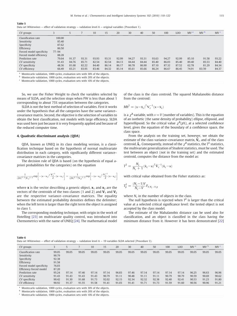
Table 5Data set Whitewines — effect of validation strategy — validation level A — original variables (Procedure 1).

CV groups 3 5 7 10 15 20 30 40 50 100 LOO MV a MV b MV c

Classification rate 100.00Sensitivity 85.40Specificity 87.62Efficiency 86.50Forced model specificity 77–94Forced model efficiency 88.28Prediction rate 79.64 91.37 93.31 93.93 93.31 92.99 94.27 93.31 93.63 94.27 92.99 85.10 91.58 93.22CV sensitivity 91.43 84.76 85.71 82.54 82.54 84.13 84.44 84.44 85.40 86.03 85.40 89.40 85.53 84.40CV specificity 48.36 81.68 82.22 84.40 86.14 86.17 86.78 86.90 87.10 87.32 87.52 62.78 81.29 84.34CV efficiency 66.49 83.21 83.95 83.46 84.32 85.14 85.61 85.66 86.24 86.67 86.45 74.91 83/39 84.37

a Montecarlo validation, 1000 cycles, evaluation sets with 30% of the objects.b Montecarlo validation, 1000 cycles, evaluation sets with 20% of the objects.c Montecarlo validation, 1000 cycles, evaluation sets with 10% of the objects.


So, we use the Fisher Weight to check the variables selected bymeans of SLDA, and the selection stops when FW is less than about 1corresponding to about 75% separation between the categories.

SLDA is not the best method of selection of variables. First it worksunder the hypothesis that all the categories have the same variance–covariancematrix. Second, the objective is the selection of variables toobtain the best classification, not models with large efficiency. SLDAwas used here just because it is very frequently applied and because ofthe reduced computer time.

4. Quadratic discriminant analysis (QDA)

QDA, known as UNEQ in its class modeling version, is a classi-fication technique based on the hypothesis of normal multivariatedistribution in each category, with significantly different variance–covariance matrices in the categories.

The decision rule of QDA is based (on the hypothesis of equal a-priori probabilities for the categories) on the equation

12πð ÞV =2jV1j1=2

exp − x−x1ð ÞT V−11

2x−x1ð Þ

" #=

12πð ÞV =2jV2j1=2

exp − x−x2ð ÞT V−12

2x−x2ð Þ

" #

where x is the vector describing a generic object, x1 and x2 are thevectors of the centroids of the two classes (1 and 2) and V1 and V2

are the respective variance–covariance matrices. The equalitybetween the estimated probability densities defines the delimiter;when the left term is larger than the right term the object is assignedto class 1.

The corresponding modeling technique, with origin in the work ofHotelling [23] on multivariate quality control, was introduced intoChemometrics with the name of UNEQ [24]. The mathematical model

Table 6Data set Whitewines — effect of validation strategy — validation level A — 19 variables SLDA

CV groups 3 5 7 10 15 20

Classification rate 99.05 99.05 99.05 99.05 99.05 99.05Sensitivity 90.79Specificity 92.38Efficiency 91.58Forced model specificity 76.03Efficiency forced model 87.20Prediction rate 95.24 97.14 97.46 97.14 97.14 96.83CV sensitivity 91.43 91.43 91.43 91.43 90.79 91.11CV specificity 90.42 91.30 91.68 91.73 92.02 92.15CV efficiency 90.92 91.37 91.55 91.58 91.41 91.03

a Montecarlo validation, 1000 cycles, evaluation sets with 30% of the objects.b Montecarlo validation, 1000 cycles, evaluation sets with 20% of the objects.c Montecarlo validation, 1000 cycles, evaluation sets with 10% of the objects.

of the class is the class centroid. The squared Mahalanobis distancefrom the centroid:

Mh2 = x−xcð ÞTV−1c x−xcð Þ

is a χ2 variable, with ν=V (number of variables). This is the equationof an isothetic (the same density of probability) ellipse, ellipsoid, andhyperellipsoid. So the critical value χ2(p%), at a selected confidencelevel, gives the equation of the boundary of a confidence space, theclass space.

From the analysis on the training set, however, we obtain theestimate of the class variance–covariance matrix, Vc, and of the classcentroid, xc. Consequently, instead of the χ2 statistics, the T2 statistics,themultivariate generalization of Student statistics, must be used. Thetest between an object (not in the training set) and the estimatedcentroid, computes the distance from the model as:

T2 =Nc

Nc + 1xc−xð ÞTV−1

c xc−xð Þ

with critical value obtained from the Fisher statistics as:

T2p =

Nc−1ð ÞVNc−V

FV ;Nc−V ;p

where Nc in the number of objects in the class.The null hypothesis is rejected when T2 is larger than the critical

value at a selected critical significance level: the tested object is notaccepted by the class model.

The estimate of the Mahalanobis distance can be used also forclassification, and an object is classified in the class having theminimum distance from it. However it has been demonstrated [22]

selected (Procedure 3).

30 40 50 100 LOO MV a MV b MV c

99.05 99.05 99.05 99.05 99.05 99.05 99.05 99.05

97.46 97.14 97.14 97.14 97.14 96.25 96.63 96.9690.48 91.11 91.11 90.79 90.79 90.59 90.69 90.6292.34 92.32 92.38 92.40 92.41 90.53 91.23 91.8091.41 91.71 91.73 91.59 91.60 90.56 90.96 91.21


that this classification criterion is worse than that based on theestimate of the probability density.

A class model is characterized by two parameters: the sensitivity,percent measure of Correct I decisions, i.e. of type I errors, and by thespecificity, percent measure of correct II decisions:

Fv
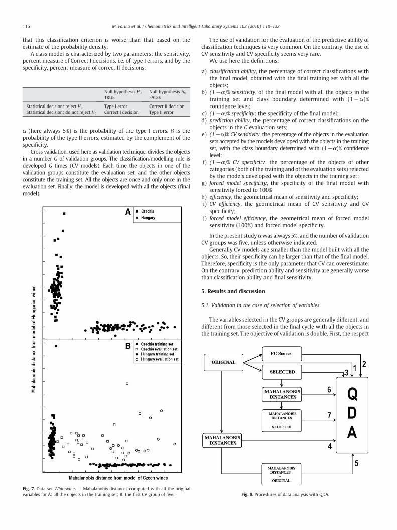
ig. 7. Data set Whitewines — Mahalanobariables for A: all the objects in the train
Null hypothesis H0

TRUE

is distances computeding set; B: the first CV

Null hypothesis H0

FALSE

Statistical decision: reject H0
Type I error Correct II decision Statistical decision: do not reject H0 Correct I decision Type II error
α (here always 5%) is the probability of the type I errors. β is theprobability of the type II errors, estimated by the complement of thespecificity.

Cross validation, used here as validation technique, divides the objectsin a number G of validation groups. The classification/modelling rule isdeveloped G times (CV models). Each time the objects in one of thevalidation groups constitute the evaluation set, and the other objectsconstitute the training set. All the objects are once and only once in theevaluation set. Finally, the model is developed with all the objects (finalmodel).

with all the originalgroup of five.

The use of validation for the evaluation of the predictive ability ofclassification techniques is very common. On the contrary, the use ofCV sensitivity and CV specificity seems very rare.

We use here the definitions:

a) classification ability, the percentage of correct classifications withthe final model, obtained with the final training set with all theobjects;

b) (1−α)% sensitivity, of the final model with all the objects in thetraining set and class boundary determined with (1−α)%confidence level;

c) (1−α)% specificity: the specificity of the final model;d) prediction ability, the percentage of correct classifications on the

objects in the G evaluation sets;e) (1−α)% CV sensitivity, the percentage of the objects in the evaluation

sets accepted by themodels developedwith the objects in the trainingset, with the class boundary determined with (1−α)% confidencelevel;

f) (1−α)% CV specificity, the percentage of the objects of othercategories (both of the training and of the evaluation sets) rejectedby the models developed with the objects in the training set;

g) forced model specificity, the specificity of the final model withsensitivity forced to 100%

h) efficiency, the geometrical mean of sensitivity and specificity;i) CV efficiency, the geometrical mean of CV sensitivity and CV

specificity;j) forced model efficiency, the geometrical mean of forced model

sensitivity (100%) and forced model specificity.

In the present study αwas always 5%, and the number of validationCV groups was five, unless otherwise indicated.

Generally CV models are smaller than the model built with all theobjects. So, their specificity can be larger than that of the final model.Therefore, specificity is the only parameter that CV can overestimate.On the contrary, prediction ability and sensitivity are generally worsethan classification ability and final sensitivity.

5. Results and discussion

5.1. Validation in the case of selection of variables

The variables selected in the CV groups are generally different, anddifferent from those selected in the final cycle with all the objects inthe training set. The objective of validation is double. First, the respect

Fig. 8. Procedures of data analysis with QDA.

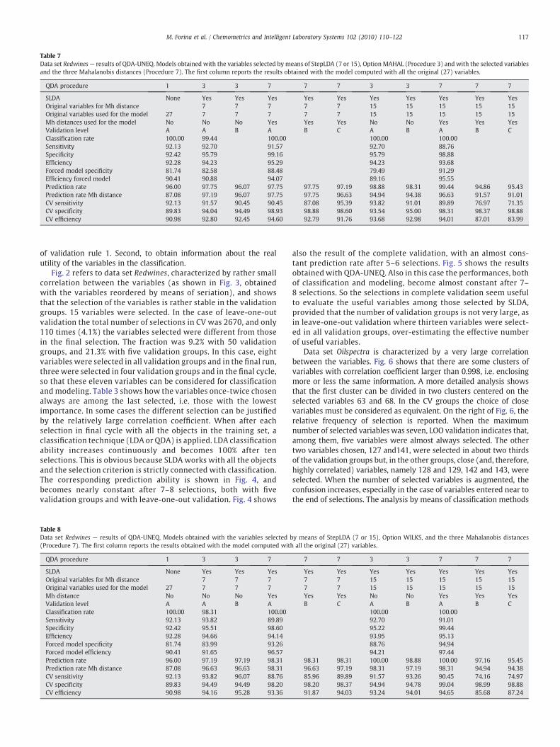
Table 7Data set Redwines— results of QDA-UNEQ. Models obtained with the variables selected by means of StepLDA (7 or 15), Option MAHAL (Procedure 3) and with the selected variablesand the three Mahalanobis distances (Procedure 7). The first column reports the results obtained with the model computed with all the original (27) variables.

QDA procedure 1 3 3 7 7 7 3 3 7 7 7

SLDA None Yes Yes Yes Yes Yes Yes Yes Yes Yes YesOriginal variables for Mh distance 7 7 7 7 7 15 15 15 15 15Original variables used for the model 27 7 7 7 7 7 15 15 15 15 15Mh distances used for the model No No No Yes Yes Yes No No Yes Yes YesValidation level A A B A B C A B A B CClassification rate 100.00 99.44 100.00 100.00 100.00Sensitivity 92.13 92.70 91.57 92.70 88.76Specificity 92.42 95.79 99.16 95.79 98.88Efficiency 92.28 94.23 95.29 94.23 93.68Forced model specificity 81.74 82.58 88.48 79.49 91.29Efficiency forced model 90.41 90.88 94.07 89.16 95.55Prediction rate 96.00 97.75 96.07 97.75 97.75 97.19 98.88 98.31 99.44 94.86 95.43Prediction rate Mh distance 87.08 97.19 96.07 97.75 97.75 96.63 94.94 94.38 96.63 91.57 91.01CV sensitivity 92.13 91.57 90.45 90.45 87.08 95.39 93.82 91.01 89.89 76.97 71.35CV specificity 89.83 94.04 94.49 98.93 98.88 98.60 93.54 95.00 98.31 98.37 98.88CV efficiency 90.98 92.80 92.45 94.60 92.79 91.76 93.68 92.98 94.01 87.01 83.99


of validation rule 1. Second, to obtain information about the realutility of the variables in the classification.

Fig. 2 refers to data set Redwines, characterized by rather smallcorrelation between the variables (as shown in Fig. 3, obtainedwith the variables reordered by means of seriation), and showsthat the selection of the variables is rather stable in the validationgroups. 15 variables were selected. In the case of leave-one-outvalidation the total number of selections in CV was 2670, and only110 times (4.1%) the variables selected were different from thosein the final selection. The fraction was 9.2% with 50 validationgroups, and 21.3% with five validation groups. In this case, eightvariables were selected in all validation groups and in the final run,three were selected in four validation groups and in the final cycle,so that these eleven variables can be considered for classificationand modeling. Table 3 shows how the variables once-twice chosenalways are among the last selected, i.e. those with the lowestimportance. In some cases the different selection can be justifiedby the relatively large correlation coefficient. When after eachselection in final cycle with all the objects in the training set, aclassification technique (LDA or QDA) is applied. LDA classificationability increases continuously and becomes 100% after tenselections. This is obvious because SLDA works with all the objectsand the selection criterion is strictly connected with classification.The corresponding prediction ability is shown in Fig. 4, andbecomes nearly constant after 7–8 selections, both with fivevalidation groups and with leave-one-out validation. Fig. 4 shows

Table 8Data set Redwines — results of QDA-UNEQ. Models obtained with the variables selected b(Procedure 7). The first column reports the results obtained with the model computed wit

QDA procedure 1 3 3 7

SLDA None Yes Yes YesOriginal variables for Mh distance 7 7 7Original variables used for the model 27 7 7 7Mh distance No No No YesValidation level A A B AClassification rate 100.00 98.31 100.00Sensitivity 92.13 93.82 89.89Specificity 92.42 95.51 98.60Efficiency 92.28 94.66 94.14Forced model specificity 81.74 83.99 93.26Forced model efficiency 90.41 91.65 96.57Prediction rate 96.00 97.19 97.19 98.31Prediction rate Mh distance 87.08 96.63 96.63 98.31CV sensitivity 92.13 93.82 96.07 88.76CV specificity 89.83 94.49 94.49 98.20CV efficiency 90.98 94.16 95.28 93.36

also the result of the complete validation, with an almost cons-tant prediction rate after 5–6 selections. Fig. 5 shows the resultsobtained with QDA-UNEQ. Also in this case the performances, bothof classification and modeling, become almost constant after 7–8 selections. So the selections in complete validation seem usefulto evaluate the useful variables among those selected by SLDA,provided that the number of validation groups is not very large, asin leave-one-out validation where thirteen variables were select-ed in all validation groups, over-estimating the effective numberof useful variables.

Data set Oilspectra is characterized by a very large correlationbetween the variables. Fig. 6 shows that there are some clusters ofvariables with correlation coefficient larger than 0.998, i.e. enclosingmore or less the same information. A more detailed analysis showsthat the first cluster can be divided in two clusters centered on theselected variables 63 and 68. In the CV groups the choice of closevariables must be considered as equivalent. On the right of Fig. 6, therelative frequency of selection is reported. When the maximumnumber of selected variables was seven, LOO validation indicates that,among them, five variables were almost always selected. The othertwo variables chosen, 127 and141, were selected in about two thirdsof the validation groups but, in the other groups, close (and, therefore,highly correlated) variables, namely 128 and 129, 142 and 143, wereselected. When the number of selected variables is augmented, theconfusion increases, especially in the case of variables entered near tothe end of selections. The analysis by means of classification methods

y means of StepLDA (7 or 15), Option WILKS, and the three Mahalanobis distancesh all the original (27) variables.

7 7 3 3 7 7 7

Yes Yes Yes Yes Yes Yes Yes7 7 15 15 15 15 157 7 15 15 15 15 15Yes Yes No No Yes Yes YesB C A B A B C

100.00 100.0092.70 91.0195.22 99.4493.95 95.1388.76 94.9494.21 97.44

98.31 98.31 100.00 98.88 100.00 97.16 95.4596.63 97.19 98.31 97.19 98.31 94.94 94.3885.96 89.89 91.57 93.26 90.45 74.16 74.9798.20 98.37 94.94 94.78 99.04 98.99 98.8891.87 94.03 93.24 94.01 94.65 85.68 87.24

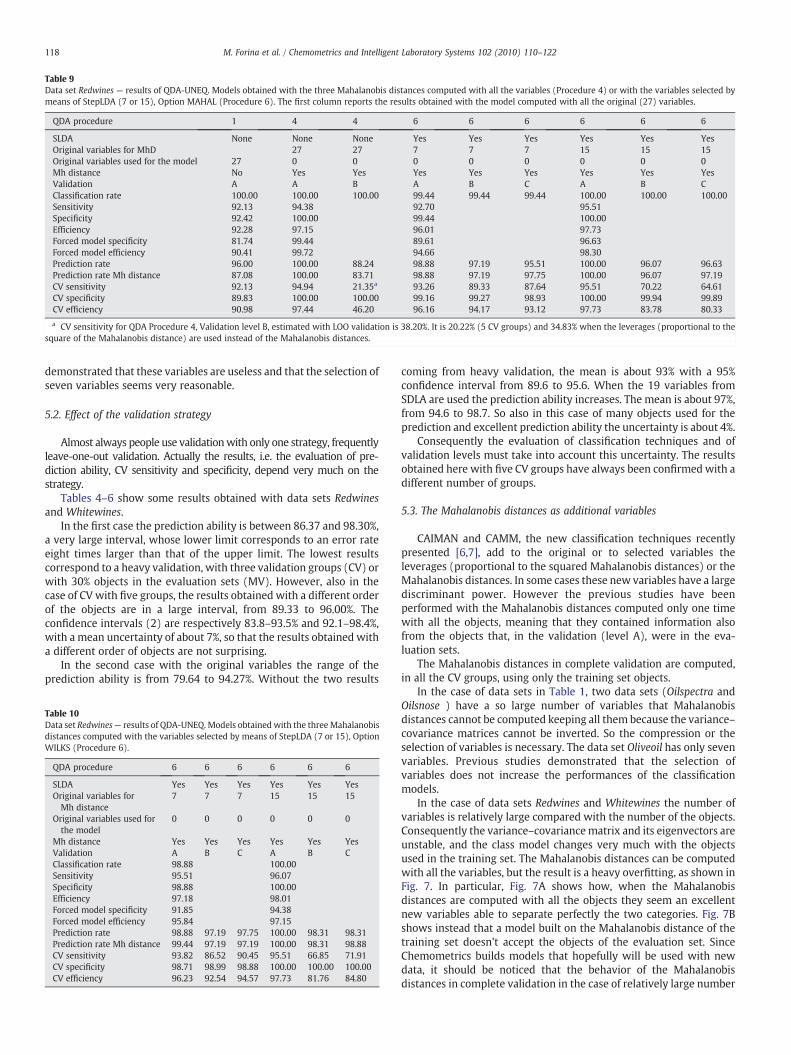
Table 9Data set Redwines — results of QDA-UNEQ. Models obtained with the three Mahalanobis distances computed with all the variables (Procedure 4) or with the variables selected bymeans of StepLDA (7 or 15), Option MAHAL (Procedure 6). The first column reports the results obtained with the model computed with all the original (27) variables.

QDA procedure 1 4 4 6 6 6 6 6 6

SLDA None None None Yes Yes Yes Yes Yes YesOriginal variables for MhD 27 27 7 7 7 15 15 15Original variables used for the model 27 0 0 0 0 0 0 0 0Mh distance No Yes Yes Yes Yes Yes Yes Yes YesValidation A A B A B C A B CClassification rate 100.00 100.00 100.00 99.44 99.44 99.44 100.00 100.00 100.00Sensitivity 92.13 94.38 92.70 95.51Specificity 92.42 100.00 99.44 100.00Efficiency 92.28 97.15 96.01 97.73Forced model specificity 81.74 99.44 89.61 96.63Forced model efficiency 90.41 99.72 94.66 98.30Prediction rate 96.00 100.00 88.24 98.88 97.19 95.51 100.00 96.07 96.63Prediction rate Mh distance 87.08 100.00 83.71 98.88 97.19 97.75 100.00 96.07 97.19CV sensitivity 92.13 94.94 21.35a 93.26 89.33 87.64 95.51 70.22 64.61CV specificity 89.83 100.00 100.00 99.16 99.27 98.93 100.00 99.94 99.89CV efficiency 90.98 97.44 46.20 96.16 94.17 93.12 97.73 83.78 80.33

a CV sensitivity for QDA Procedure 4, Validation level B, estimated with LOO validation is 38.20%. It is 20.22% (5 CV groups) and 34.83% when the leverages (proportional to thesquare of the Mahalanobis distance) are used instead of the Mahalanobis distances.


demonstrated that these variables are useless and that the selection ofseven variables seems very reasonable.

5.2. Effect of the validation strategy

Almost always people use validationwith only one strategy, frequentlyleave-one-out validation. Actually the results, i.e. the evaluation of pre-diction ability, CV sensitivity and specificity, depend very much on thestrategy.

Tables 4–6 show some results obtained with data sets Redwinesand Whitewines.

In the first case the prediction ability is between 86.37 and 98.30%,a very large interval, whose lower limit corresponds to an error rateeight times larger than that of the upper limit. The lowest resultscorrespond to a heavy validation, with three validation groups (CV) orwith 30% objects in the evaluation sets (MV). However, also in thecase of CV with five groups, the results obtained with a different orderof the objects are in a large interval, from 89.33 to 96.00%. Theconfidence intervals (2) are respectively 83.8–93.5% and 92.1–98.4%,with a mean uncertainty of about 7%, so that the results obtained witha different order of objects are not surprising.

In the second case with the original variables the range of theprediction ability is from 79.64 to 94.27%. Without the two results

Table 10Data set Redwines— results of QDA-UNEQ. Models obtained with the three Mahalanobisdistances computed with the variables selected by means of StepLDA (7 or 15), OptionWILKS (Procedure 6).

QDA procedure 6 6 6 6 6 6

SLDA Yes Yes Yes Yes Yes YesOriginal variables forMh distance

7 7 7 15 15 15

Original variables used forthe model

0 0 0 0 0 0

Mh distance Yes Yes Yes Yes Yes YesValidation A B C A B CClassification rate 98.88 100.00Sensitivity 95.51 96.07Specificity 98.88 100.00Efficiency 97.18 98.01Forced model specificity 91.85 94.38Forced model efficiency 95.84 97.15Prediction rate 98.88 97.19 97.75 100.00 98.31 98.31Prediction rate Mh distance 99.44 97.19 97.19 100.00 98.31 98.88CV sensitivity 93.82 86.52 90.45 95.51 66.85 71.91CV specificity 98.71 98.99 98.88 100.00 100.00 100.00CV efficiency 96.23 92.54 94.57 97.73 81.76 84.80

coming from heavy validation, the mean is about 93% with a 95%confidence interval from 89.6 to 95.6. When the 19 variables fromSDLA are used the prediction ability increases. The mean is about 97%,from 94.6 to 98.7. So also in this case of many objects used for theprediction and excellent prediction ability the uncertainty is about 4%.

Consequently the evaluation of classification techniques and ofvalidation levels must take into account this uncertainty. The resultsobtained here with five CV groups have always been confirmed with adifferent number of groups.

5.3. The Mahalanobis distances as additional variables

CAIMAN and CAMM, the new classification techniques recentlypresented [6,7], add to the original or to selected variables theleverages (proportional to the squared Mahalanobis distances) or theMahalanobis distances. In some cases these new variables have a largediscriminant power. However the previous studies have beenperformed with the Mahalanobis distances computed only one timewith all the objects, meaning that they contained information alsofrom the objects that, in the validation (level A), were in the eva-luation sets.

The Mahalanobis distances in complete validation are computed,in all the CV groups, using only the training set objects.

In the case of data sets in Table 1, two data sets (Oilspectra andOilsnose ) have a so large number of variables that Mahalanobisdistances cannot be computed keeping all them because the variance–covariance matrices cannot be inverted. So the compression or theselection of variables is necessary. The data set Oliveoil has only sevenvariables. Previous studies demonstrated that the selection ofvariables does not increase the performances of the classificationmodels.

In the case of data sets Redwines and Whitewines the number ofvariables is relatively large compared with the number of the objects.Consequently the variance–covariancematrix and its eigenvectors areunstable, and the class model changes very much with the objectsused in the training set. The Mahalanobis distances can be computedwith all the variables, but the result is a heavy overfitting, as shown inFig. 7. In particular, Fig. 7A shows how, when the Mahalanobisdistances are computed with all the objects they seem an excellentnew variables able to separate perfectly the two categories. Fig. 7Bshows instead that a model built on the Mahalanobis distance of thetraining set doesn't accept the objects of the evaluation set. SinceChemometrics builds models that hopefully will be used with newdata, it should be noticed that the behavior of the Mahalanobisdistances in complete validation in the case of relatively large number

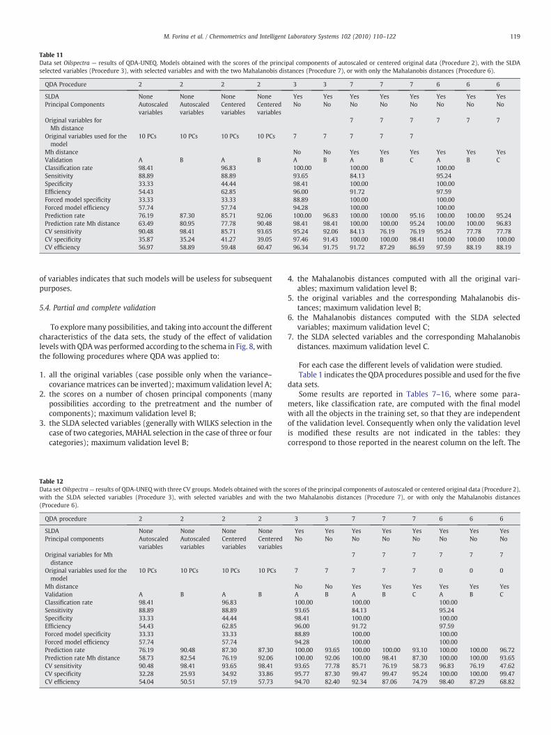
Table 11Data set Oilspectra — results of QDA-UNEQ. Models obtained with the scores of the principal components of autoscaled or centered original data (Procedure 2), with the SLDAselected variables (Procedure 3), with selected variables and with the two Mahalanobis distances (Procedure 7), or with only the Mahalanobis distances (Procedure 6).

QDA Procedure 2 2 2 2 3 3 7 7 7 6 6 6

SLDA None None None None Yes Yes Yes Yes Yes Yes Yes YesPrincipal Components Autoscaled

variablesAutoscaledvariables

Centeredvariables

Centeredvariables

No No No No No No No No

Original variables forMh distance

7 7 7 7 7 7

Original variables used for themodel

10 PCs 10 PCs 10 PCs 10 PCs 7 7 7 7 7

Mh distance No No Yes Yes Yes Yes Yes YesValidation A B A B A B A B C A B CClassification rate 98.41 96.83 100.00 100.00 100.00Sensitivity 88.89 88.89 93.65 84.13 95.24Specificity 33.33 44.44 98.41 100.00 100.00Efficiency 54.43 62.85 96.00 91.72 97.59Forced model specificity 33.33 33.33 88.89 100.00 100.00Forced model efficiency 57.74 57.74 94.28 100.00 100.00Prediction rate 76.19 87.30 85.71 92.06 100.00 96.83 100.00 100.00 95.16 100.00 100.00 95.24Prediction rate Mh distance 63.49 80.95 77.78 90.48 98.41 98.41 100.00 100.00 95.24 100.00 100.00 96.83CV sensitivity 90.48 98.41 85.71 93.65 95.24 92.06 84.13 76.19 76.19 95.24 77.78 77.78CV specificity 35.87 35.24 41.27 39.05 97.46 91.43 100.00 100.00 98.41 100.00 100.00 100.00CV efficiency 56.97 58.89 59.48 60.47 96.34 91.75 91.72 87.29 86.59 97.59 88.19 88.19


of variables indicates that such models will be useless for subsequentpurposes.

5.4. Partial and complete validation

To explore many possibilities, and taking into account the differentcharacteristics of the data sets, the study of the effect of validationlevels with QDAwas performed according to the schema in Fig. 8, withthe following procedures where QDA was applied to:

1. all the original variables (case possible only when the variance–covariancematrices can be inverted); maximum validation level A;

2. the scores on a number of chosen principal components (manypossibilities according to the pretreatment and the number ofcomponents); maximum validation level B;

3. the SLDA selected variables (generally with WILKS selection in thecase of two categories, MAHAL selection in the case of three or fourcategories); maximum validation level B;

Table 12Data set Oilspectra— results of QDA-UNEQ with three CV groups. Models obtained with the swith the SLDA selected variables (Procedure 3), with selected variables and with the(Procedure 6).


SLDA None None None NonePrincipal components Autoscaled


Centeredvariables

Centeredvariables

Original variables for Mhdistance


10 PCs 10 PCs 10 PCs 10 PCs

Mh distanceValidation A B A BClassification rate 98.41 96.83Sensitivity 88.89 88.89Specificity 33.33 44.44Efficiency 54.43 62.85Forced model specificity 33.33 33.33Forced model efficiency 57.74 57.74Prediction rate 76.19 90.48 87.30 87.30Prediction rate Mh distance 58.73 82.54 76.19 92.06CV sensitivity 90.48 98.41 93.65 98.41CV specificity 32.28 25.93 34.92 33.86CV efficiency 54.04 50.51 57.19 57.73

4. the Mahalanobis distances computed with all the original vari-ables; maximum validation level B;

5. the original variables and the corresponding Mahalanobis dis-tances; maximum validation level B;

6. the Mahalanobis distances computed with the SLDA selectedvariables; maximum validation level C;

7. the SLDA selected variables and the corresponding Mahalanobisdistances. maximum validation level C.

For each case the different levels of validation were studied.Table 1 indicates the QDA procedures possible and used for the five

data sets.Some results are reported in Tables 7–16, where some para-

meters, like classification rate, are computed with the final modelwith all the objects in the training set, so that they are independentof the validation level. Consequently when only the validation levelis modified these results are not indicated in the tables: theycorrespond to those reported in the nearest column on the left. The

cores of the principal components of autoscaled or centered original data (Procedure 2),two Mahalanobis distances (Procedure 7), or with only the Mahalanobis distances

3 3 7 7 7 6 6 6

Yes Yes Yes Yes Yes Yes Yes YesNo No No No No No No No

7 7 7 7 7 7

7 7 7 7 7 0 0 0

No No Yes Yes Yes Yes Yes YesA B A B C A B C100.00 100.00 100.0093.65 84.13 95.2498.41 100.00 100.0096.00 91.72 97.5988.89 100.00 100.0094.28 100.00 100.00100.00 93.65 100.00 100.00 93.10 100.00 100.00 96.72100.00 92.06 100.00 98.41 87.30 100.00 100.00 93.6593.65 77.78 85.71 76.19 58.73 96.83 76.19 47.6295.77 87.30 99.47 99.47 95.24 100.00 100.00 99.4794.70 82.40 92.34 87.06 74.79 98.40 87.29 68.82

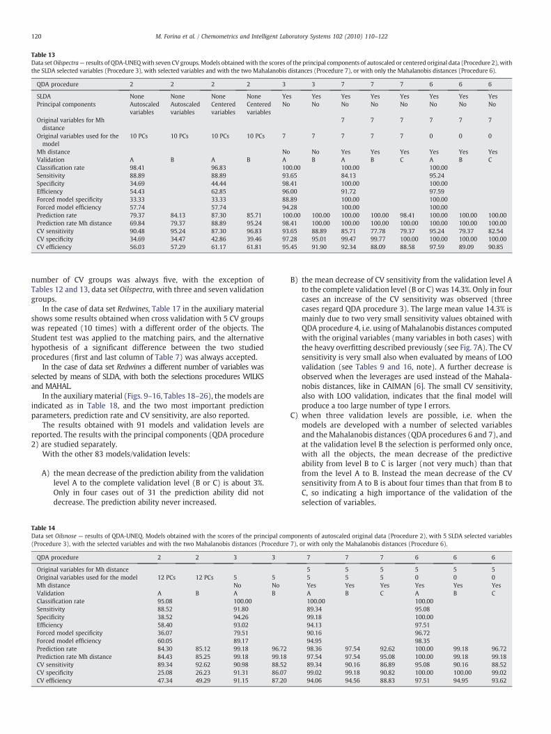
Table 13Data setOilspectra— results of QDA-UNEQwith seven CV groups. Models obtainedwith the scores of the principal components of autoscaled or centered original data (Procedure 2), withthe SLDA selected variables (Procedure 3), with selected variables and with the two Mahalanobis distances (Procedure 7), or with only the Mahalanobis distances (Procedure 6).

QDA procedure 2 2 2 2 3 3 7 7 7 6 6 6

SLDA None None None None Yes Yes Yes Yes Yes Yes Yes YesPrincipal components Autoscaled


Centeredvariables

Centeredvariables

No No No No No No No No

Original variables for Mhdistance

7 7 7 7 7 7


10 PCs 10 PCs 10 PCs 10 PCs 7 7 7 7 7 0 0 0

Mh distance No No Yes Yes Yes Yes Yes YesValidation A B A B A B A B C A B CClassification rate 98.41 96.83 100.00 100.00 100.00Sensitivity 88.89 88.89 93.65 84.13 95.24Specificity 34.69 44.44 98.41 100.00 100.00Efficiency 54.43 62.85 96.00 91.72 97.59Forced model specificity 33.33 33.33 88.89 100.00 100.00Forced model efficiency 57.74 57.74 94.28 100.00 100.00Prediction rate 79.37 84.13 87.30 85.71 100.00 100.00 100.00 100.00 98.41 100.00 100.00 100.00Prediction rate Mh distance 69.84 79.37 88.89 95.24 98.41 100.00 100.00 100.00 100.00 100.00 100.00 100.00CV sensitivity 90.48 95.24 87.30 96.83 93.65 88.89 85.71 77.78 79.37 95.24 79.37 82.54CV specificity 34.69 34.47 42.86 39.46 97.28 95.01 99.47 99.77 100.00 100.00 100.00 100.00CV efficiency 56.03 57.29 61.17 61.81 95.45 91.90 92.34 88.09 88.58 97.59 89.09 90.85


number of CV groups was always five, with the exception ofTables 12 and 13, data set Oilspectra, with three and seven validationgroups.

In the case of data set Redwines, Table 17 in the auxiliary materialshows some results obtained when cross validation with 5 CV groupswas repeated (10 times) with a different order of the objects. TheStudent test was applied to the matching pairs, and the alternativehypothesis of a significant difference between the two studiedprocedures (first and last column of Table 7) was always accepted.

In the case of data set Redwines a different number of variables wasselected by means of SLDA, with both the selections procedures WILKSand MAHAL.

In the auxiliary material (Figs. 9–16, Tables 18–26), the models areindicated as in Table 18, and the two most important predictionparameters, prediction rate and CV sensitivity, are also reported.

The results obtained with 91 models and validation levels arereported. The results with the principal components (QDA procedure2) are studied separately.

With the other 83 models/validation levels:

A) the mean decrease of the prediction ability from the validationlevel A to the complete validation level (B or C) is about 3%.Only in four cases out of 31 the prediction ability did notdecrease. The prediction ability never increased.

Table 14Data set Oilsnose — results of QDA-UNEQ. Models obtained with the scores of the principal(Procedure 3), with the selected variables and with the two Mahalanobis distances (Proced


Original variables for Mh distanceOriginal variables used for the model 12 PCs 12 PCs 5 5Mh distance No NoValidation A B A BClassification rate 95.08 100.00Sensitivity 88.52 91.80Specificity 38.52 94.26Efficiency 58.40 93.02Forced model specificity 36.07 79.51Forced model efficiency 60.05 89.17Prediction rate 84.30 85.12 99.18 96Prediction rate Mh distance 84.43 85.25 99.18 99CV sensitivity 89.34 92.62 90.98 88CV specificity 25.08 26.23 91.31 86CV efficiency 47.34 49.29 91.15 87

B) the mean decrease of CV sensitivity from the validation level Ato the complete validation level (B or C) was 14.3%. Only in fourcases an increase of the CV sensitivity was observed (threecases regard QDA procedure 3). The large mean value 14.3% ismainly due to two very small sensitivity values obtained withQDA procedure 4, i.e. using of Mahalanobis distances computedwith the original variables (many variables in both cases) withthe heavy overfitting described previously (see Fig. 7A). The CVsensitivity is very small also when evaluated by means of LOOvalidation (see Tables 9 and 16, note). A further decrease isobserved when the leverages are used instead of the Mahala-nobis distances, like in CAIMAN [6]. The small CV sensitivity,also with LOO validation, indicates that the final model willproduce a too large number of type I errors.

C) when three validation levels are possible, i.e. when themodels are developed with a number of selected variablesand the Mahalanobis distances (QDA procedures 6 and 7), andat the validation level B the selection is performed only once,with all the objects, the mean decrease of the predictiveability from level B to C is larger (not very much) than thatfrom the level A to B. Instead the mean decrease of the CVsensitivity from A to B is about four times than that from B toC, so indicating a high importance of the validation of theselection of variables.

components of autoscaled original data (Procedure 2), with 5 SLDA selected variablesure 7), or with only the Mahalanobis distances (Procedure 6).

7 7 7 6 6 6

5 5 5 5 5 55 5 5 0 0 0Yes Yes Yes Yes Yes YesA B C A B C100.00 100.0089.34 95.0899.18 100.0094.13 97.5190.16 96.7294.95 98.35

.72 98.36 97.54 92.62 100.00 99.18 96.72

.18 97.54 97.54 95.08 100.00 99.18 99.18

.52 89.34 90.16 86.89 95.08 90.16 88.52

.07 99.02 99.18 90.82 100.00 100.00 99.02

.20 94.06 94.56 88.83 97.51 94.95 93.62

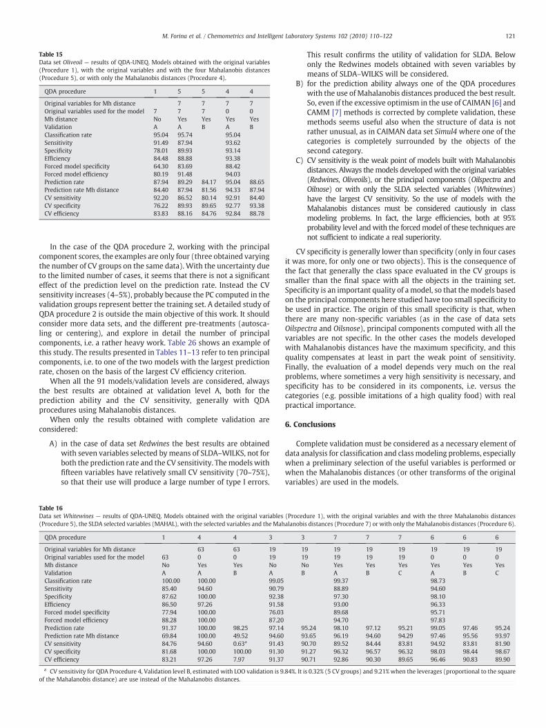
Table 15Data set Oliveoil — results of QDA-UNEQ. Models obtained with the original variables(Procedure 1), with the original variables and with the four Mahalanobis distances(Procedure 5), or with only the Mahalanobis distances (Procedure 4).

QDA procedure 1 5 5 4 4

Original variables for Mh distance 7 7 7 7Original variables used for the model 7 7 7 0 0Mh distance No Yes Yes Yes YesValidation A A B A BClassification rate 95.04 95.74 95.04Sensitivity 91.49 87.94 93.62Specificity 78.01 89.93 93.14Efficiency 84.48 88.88 93.38Forced model specificity 64.30 83.69 88.42Forced model efficiency 80.19 91.48 94.03Prediction rate 87.94 89.29 84.17 95.04 88.65Prediction rate Mh distance 84.40 87.94 81.56 94.33 87.94CV sensitivity 92.20 86.52 80.14 92.91 84.40CV specificity 76.22 89.93 89.65 92.77 93.38CV efficiency 83.83 88.16 84.76 92.84 88.78


In the case of the QDA procedure 2, working with the principalcomponent scores, the examples are only four (three obtained varyingthe number of CV groups on the same data). With the uncertainty dueto the limited number of cases, it seems that there is not a significanteffect of the prediction level on the prediction rate. Instead the CVsensitivity increases (4–5%), probably because the PC computed in thevalidation groups represent better the training set. A detailed study ofQDA procedure 2 is outside the main objective of this work. It shouldconsider more data sets, and the different pre-treatments (autosca-ling or centering), and explore in detail the number of principalcomponents, i.e. a rather heavy work. Table 26 shows an example ofthis study. The results presented in Tables 11–13 refer to ten principalcomponents, i.e. to one of the two models with the largest predictionrate, chosen on the basis of the largest CV efficiency criterion.

When all the 91 models/validation levels are considered, alwaysthe best results are obtained at validation level A, both for theprediction ability and the CV sensitivity, generally with QDAprocedures using Mahalanobis distances.

When only the results obtained with complete validation areconsidered:

A) in the case of data set Redwines the best results are obtainedwith seven variables selected by means of SLDA–WILKS, not forboth the prediction rate and the CV sensitivity. Themodels withfifteen variables have relatively small CV sensitivity (70–75%),so that their use will produce a large number of type I errors.

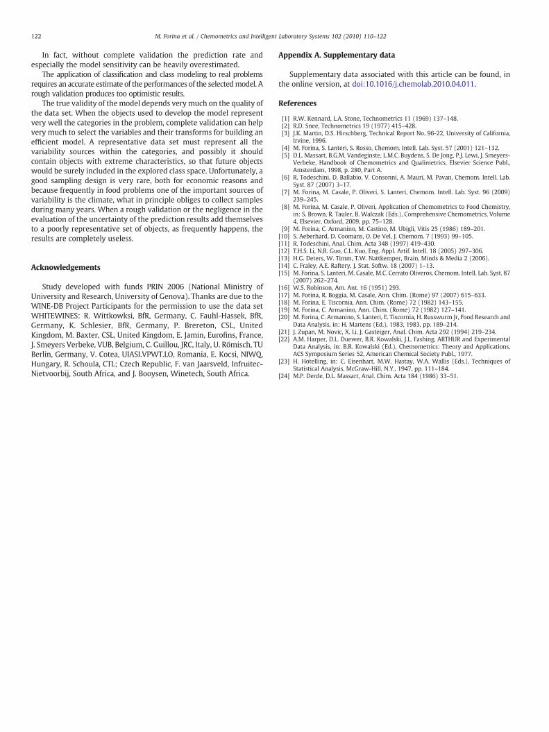
Table 16Data set Whitewines — results of QDA-UNEQ. Models obtained with the original variables(Procedure 5), the SLDA selected variables (MAHAL), with the selected variables and the Mah


Original variables for Mh distance 63 63 19Original variables used for the model 63 0 0 19Mh distance No Yes Yes NoValidation A A B AClassification rate 100.00 100.00 99.05Sensitivity 85.40 94.60 90.79Specificity 87.62 100.00 92.38Efficiency 86.50 97.26 91.58Forced model specificity 77.94 100.00 76.03Forced model efficiency 88.28 100.00 87.20Prediction rate 91.37 100.00 98.25 97.14Prediction rate Mh distance 69.84 100.00 49.52 94.60CV sensitivity 84.76 94.60 0.63a 91.43CV specificity 81.68 100.00 100.00 91.30CV efficiency 83.21 97.26 7.97 91.37

a CV sensitivity for QDA Procedure 4, Validation level B, estimated with LOO validation is 9of the Mahalanobis distance) are use instead of the Mahalanobis distances.

This result confirms the utility of validation for SLDA. Belowonly the Redwines models obtained with seven variables bymeans of SLDA–WILKS will be considered.

B) for the prediction ability always one of the QDA procedureswith the use of Mahalanobis distances produced the best result.So, even if the excessive optimism in the use of CAIMAN [6] andCAMM [7] methods is corrected by complete validation, thesemethods seems useful also when the structure of data is notrather unusual, as in CAIMAN data set Simul4 where one of thecategories is completely surrounded by the objects of thesecond category.

C) CV sensitivity is the weak point of models built with Mahalanobisdistances. Always themodels developedwith the original variables(Redwines, Oliveoils), or the principal components (Oilspectra andOilnose) or with only the SLDA selected variables (Whitewines)have the largest CV sensitivity. So the use of models with theMahalanobis distances must be considered cautiously in classmodeling problems. In fact, the large efficiencies, both at 95%probability level andwith the forcedmodel of these techniques arenot sufficient to indicate a real superiority.

CV specificity is generally lower than specificity (only in four casesit was more, for only one or two objects). This is the consequence ofthe fact that generally the class space evaluated in the CV groups issmaller than the final space with all the objects in the training set.Specificity is an important quality of amodel, so that themodels basedon the principal components here studied have too small specificity tobe used in practice. The origin of this small specificity is that, whenthere are many non-specific variables (as in the case of data setsOilspectra and Oilsnose), principal components computed with all thevariables are not specific. In the other cases the models developedwith Mahalanobis distances have the maximum specificity, and thisquality compensates at least in part the weak point of sensitivity.Finally, the evaluation of a model depends very much on the realproblems, where sometimes a very high sensitivity is necessary, andspecificity has to be considered in its components, i.e. versus thecategories (e.g. possible imitations of a high quality food) with realpractical importance.

6. Conclusions

Complete validation must be considered as a necessary element ofdata analysis for classification and class modeling problems, especiallywhen a preliminary selection of the useful variables is performed orwhen the Mahalanobis distances (or other transforms of the originalvariables) are used in the models.

(Procedure 1), with the original variables and with the three Mahalanobis distancesalanobis distances (Procedure 7) or with only theMahalanobis distances (Procedure 6).

3 7 7 7 6 6 6

19 19 19 19 19 19 1919 19 19 19 0 0 0No Yes Yes Yes Yes Yes YesB A B C A B C

99.37 98.7388.89 94.6097.30 98.1093.00 96.3389.68 95.7194.70 97.83

95.24 98.10 97.12 95.21 99.05 97.46 95.2493.65 96.19 94.60 94.29 97.46 95.56 93.9790.70 89.52 84.44 83.81 94.92 83.81 81.9091.27 96.32 96.57 96.32 98.03 98.44 98.6790.71 92.86 90.30 89.65 96.46 90.83 89.90

.84%. It is 0.32% (5 CV groups) and 9.21% when the leverages (proportional to the square


In fact, without complete validation the prediction rate andespecially the model sensitivity can be heavily overestimated.

The application of classification and class modeling to real problemsrequires an accurate estimate of the performances of the selectedmodel. Arough validation produces too optimistic results.

The true validity of the model depends very much on the quality ofthe data set. When the objects used to develop the model representvery well the categories in the problem, complete validation can helpvery much to select the variables and their transforms for building anefficient model. A representative data set must represent all thevariability sources within the categories, and possibly it shouldcontain objects with extreme characteristics, so that future objectswould be surely included in the explored class space. Unfortunately, agood sampling design is very rare, both for economic reasons andbecause frequently in food problems one of the important sources ofvariability is the climate, what in principle obliges to collect samplesduring many years. When a rough validation or the negligence in theevaluation of the uncertainty of the prediction results add themselvesto a poorly representative set of objects, as frequently happens, theresults are completely useless.

Acknowledgements

Study developed with funds PRIN 2006 (National Ministry ofUniversity and Research, University of Genova). Thanks are due to theWINE-DB Project Participants for the permission to use the data setWHITEWINES: R. Wittkowksi, BfR, Germany, C. Fauhl-Hassek, BfR,Germany, K. Schlesier, BfR, Germany, P. Brereton, CSL, UnitedKingdom, M. Baxter, CSL, United Kingdom, E. Jamin, Eurofins, France,J. Smeyers Verbeke, VUB, Belgium, C. Guillou, JRC, Italy, U. Römisch, TUBerlin, Germany, V. Cotea, UIASI.VPWT.LO, Romania, E. Kocsi, NIWQ,Hungary, R. Schoula, CTL; Czech Republic, F. van Jaarsveld, Infruitec-Nietvoorbij, South Africa, and J. Booysen, Winetech, South Africa.

Appendix A. Supplementary data

Supplementary data associated with this article can be found, inthe online version, at doi:10.1016/j.chemolab.2010.04.011.

References

[1] R.W. Kennard, L.A. Stone, Technometrics 11 (1969) 137–148.[2] R.D. Snee, Technometrics 19 (1977) 415–428.[3] J.K. Martin, D.S. Hirschberg, Technical Report No. 96-22, University of California,

Irvine, 1996.[4] M. Forina, S. Lanteri, S. Rosso, Chemom. Intell. Lab. Syst. 57 (2001) 121–132.[5] D.L. Massart, B.G.M. Vandeginste, L.M.C. Buydens, S. De Jong, P.J. Lewi, J. Smeyers-

Verbeke, Handbook of Chemometrics and Qualimetrics, Elsevier Science Publ.,Amsterdam, 1998, p. 280, Part A.

[6] R. Todeschini, D. Ballabio, V. Consonni, A. Mauri, M. Pavan, Chemom. Intell. Lab.Syst. 87 (2007) 3–17.

[7] M. Forina, M. Casale, P. Oliveri, S. Lanteri, Chemom. Intell. Lab. Syst. 96 (2009)239–245.

[8] M. Forina, M. Casale, P. Oliveri, Application of Chemometrics to Food Chemistry,in: S. Brown, R. Tauler, B. Walczak (Eds.), Comprehensive Chemometrics, Volume4, Elsevier, Oxford, 2009, pp. 75–128.

[9] M. Forina, C. Armanino, M. Castino, M. Ubigli, Vitis 25 (1986) 189–201.[10] S. Aeberhard, D. Coomans, O. De Vel, J. Chemom. 7 (1993) 99–105.[11] R. Todeschini, Anal. Chim. Acta 348 (1997) 419–430.[12] T.H.S. Li, N.R. Guo, C.L. Kuo, Eng. Appl. Artif. Intell. 18 (2005) 297–306.[13] H.G. Deters, W. Timm, T.W. Nattkemper, Brain, Minds & Media 2 (2006).[14] C. Fraley, A.E. Raftery, J. Stat. Softw. 18 (2007) 1–13.[15] M. Forina, S. Lanteri, M. Casale, M.C. Cerrato Oliveros, Chemom. Intell. Lab. Syst. 87

(2007) 262–274.[16] W.S. Robinson, Am. Ant. 16 (1951) 293.[17] M. Forina, R. Boggia, M. Casale, Ann. Chim. (Rome) 97 (2007) 615–633.[18] M. Forina, E. Tiscornia, Ann. Chim. (Rome) 72 (1982) 143–155.[19] M. Forina, C. Armanino, Ann. Chim. (Rome) 72 (1982) 127–141.[20] M. Forina, C. Armanino, S. Lanteri, E. Tiscornia, H. Russwurm Jr, Food Research and

Data Analysis, in: H. Martens (Ed.), 1983, 1983, pp. 189–214.[21] J. Zupan, M. Novic, X. Li, J. Gasteiger, Anal. Chim. Acta 292 (1994) 219–234.[22] A.M. Harper, D.L. Duewer, B.R. Kowalski, J.L. Fashing, ARTHUR and Experimental

Data Analysis, in: B.R. Kowalski (Ed.), Chemometrics: Theory and Applications,ACS Symposium Series 52, American Chemical Society Publ., 1977.

[23] H. Hotelling, in: C. Eisenhart, M.W. Hastay, W.A. Wallis (Eds.), Techniques ofStatistical Analysis, McGraw-Hill, N.Y., 1947, pp. 111–184.

[24] M.P. Derde, D.L. Massart, Anal. Chim. Acta 184 (1986) 33–51.

http://dx.doi.org/10.1016/j.chemolab.2010.04.011

Complete validation for classification and class modeling procedures with selection of variables...

Documents

Transcript of Complete validation for classification and class modeling procedures with selection of variables...