
Competent Design by Castings - VTT
391
ESPOO 2005 VTT SYMPOSIUM 237 Competent Design by Castings Improvements in a Nordic project
-
Upload
khangminh22 -
Category
Documents
-
view
0 -
download
0
Transcript of Competent Design by Castings - VTT

VTT SY
MPO
SIUM
237Com
petent Design by Castings. Improvem
ents in a Nordic project
Tätä julkaisua myy Denna publikation säljs av This publication is available from
VTT TIETOPALVELU VTT INFORMATIONSTJÄNST VTT INFORMATION SERVICEPL 2000 PB 2000 P.O.Box 2000
02044 VTT 02044 VTT FI–02044 VTT, FinlandPuh. 020 722 4404 Tel. 020 722 4404 Phone internat. +358 20 722 4404Faksi 020 722 4374 Fax 020 722 4374 Fax +358 20 722 4374
ISBN 951– 38– 6298– 4 (soft back ed.) ISBN 951– 38– 6299– 2 (URL: http://www.vtt.fi/inf/pdf/)ISSN 0357– 9387 (soft back ed.) ISSN 1455– 0873 (URL: http://www.vtt.fi/inf/pdf/)
ESPOO 2005 VTT SYMPOSIUM 237
Competent Design by CastingsImprovements in a Nordic project
This symposium summarises the achievements within a joint R&D project"GJUTDESIGN2005 – Design kvalitet och NDT för gjutna utmattningsbelastadekomponenter". It brought together 25 Nordic organisations aiming to coordinated development of improved methods and tools for fatigue design of caststructures and components. The partners include 10 industrial companies thatdesign and manufacture construction machinery, trucks, robots, windmills, papermachines and ship engines, 5 foundries, engineering consulting firm, researchorganisations and universities.
Selected 20 papers deal with mechanisms, understanding, practicalassessment and specific industrial challenges in fields of
optimisation of casting process, material properties and component design,
influence of defects and crack growth mechanisms on fatigue resistance,
inspection and quality assurance to control of defects, and complex service loading in terms of variable amplitude and
multiaxiality.Experiments were performed for small test pieces and real components. NDE
methods were studied to assess the current state of the art in industry andresearch. Numerical modelling, simulation and analysis of complex structureswas applied to design of experiments and for optimisation of products.


VTT SYMPOSIUM 237 Keywords: cast structures, cast materials, cast quality, design, complex fatigue loads, fracture mechanics, fatigue assessment, modelling, Nordic countries, graphite
Competent Design by Castings Improvements in a Nordic project
GJUTDESIGN-2005 final seminar Espoo, 13.14.6.2005
Edited by
Jack Samuelsson Gary Marquis
Jussi Solin
Organised by
Nordic Innovation Center, Volvo, Componenta, VATTU, LUT and VTT

ISBN 9513862984 (soft back ed.) ISSN 03579387 (soft back ed.)
ISBN 9513862992 (URL:http://www.vtt.fi/inf/pdf/) ISSN 14550873 (URL: http://www.vtt.fi/inf/pdf/ )
Copyright © VTT Technical Research Centre of Finland 2005
JULKAISIJA UTGIVARE PUBLISHER
VTT, Vuorimiehentie 5, PL 2000, 02044 VTT puh. vaihde 020 722 111, faksi 020 722 4374
VTT, Bergsmansvägen 5, PB 2000, 02044 VTT tel. växel 020 722 111, fax 020 722 4374
VTT Technical Research Centre of Finland Vuorimiehentie 5, P.O.Box 2000, FI02044 VTT, Finland phone internat. +358 20 722 111, fax + 358 20 722 4374
VTT Tuotteet ja tuotanto, Kemistintie 3, PL 1704, 02044 VTT puh. vaihde 020 722 111, faksi 020 722 7002, 020 722 7010, 020 722 5875
VTT Industriella System, Kemistvägen 3, PB 1704, 02044 VTT tel. växel 020 722 111, fax 020 722 7002, 020 722 7010, 020 722 5875
VTT Industrial Systems, Kemistintie 3, P.O.Box 1704, FI02044 VTT, Finland phone internat. +358 20 722 111, fax +358 20 722 7002, +358 20 722 7010, +358 20 722 5875
Valopaino Oy, Helsinki 2005

3
Preface The research work reported in these proceedings has been performed within the Nordic R&D project GJUTDESIGN-2005 Design kvalitet och NDT för gjutna utmattningsbelastade komponenter. The project started in 2001 and involved 25 Nordic organisations from Sweden, Finland, Denmark and Iceland aiming to co-ordinated development of improved methods and tools for fatigue design of cast structures and components.
The main objective was to improve the reliability and reduce the time and effort required to design complex fatigue loaded cast structures by developing design guidelines, quality rules and cost-effective NDE systems. Work on the project has proceeded simultaneously along several fronts such as fatigue testing of small test pieces and real components, application of different NDE-systems, modelling and analysis of complex structures, and quantitative examination of factors influencing cast quality.
Important steps have been made in order to better implement fracture mechanics based fatigue assessment procedures for cast materials. Progress has been made in cast process modeling and control to avoid major defects and avoidance of chunky graphite that is often associated with high silicon iron. Several potential tools for reliable NDE have been investigated.
The impact of the project on the design of cast structures within the Nordic countries is significant. The participants are involved with most of the major Nordic companies where integrity of fatigue loaded cast structures is a design concern. The partners include 10 industrial companies that design and manufacture complex structures such as construction machinery, trucks, robots, windmills, paper machines and ship engines. The consortium also included five foundries, one engineering consulting firm, five research organisations and four universities.
More than 50 individuals were involved in collaboration within this project, which has both maintained and strengthened Nordic networking between industry, universities and research organisations.

4
The GJUTDESIGN-2005 project was partly sponsored by the Nordic Innovation Center (NiCe), the Swedish Vehicle Research Program (PFF) and Tekes (National Technology Agency of Finland). However, the major part of the budget was covered by technical and financial support from the participating companies and institutes. The programme was designed as collaboration between industry, research organisations and universities with appr. 60 % of the budget being provided by the industrial partners, 20 % from national funding and 20 % from NiCe. See Appendix A for description of the financing organisations.
We consider the high quality of papers in this book as evidence of success in both collaboration and individual R&D efforts. This would not have been possible without targeted financial support of the sponsors. Financial support and encouragement received from all financing organisations is gratefully acknowledged. However, today our primary thanks are directed toward the authors. Their voluntary contributions are remarkable and deserve our sincere appreciation.
Stockholm, Lappeenranta and Espoo in May, 2005
Jack Samuelsson Gary Marquis Jussi Solin

5
Sponsors of the project
Funding organisations: The Nordic Innovation Center (NiCe)
The Swedish Vehicle Research Program (PFF)
Tekes (National Technology Agency of Finland)
Denmark: Valdemar Birn AS
Finland: Componenta Oyj
Componenta Pistons
Metso Drives
Metso Papers
VTT (Technical Research Center of Finland)
Wärtsilä Technology
Iceland: ICETEC
Sweden: ABB Corporate Research
ABB Robotics
Arvika Gjuteri
DNV (Det Norske Veritas) KEYCAST (Sweden)
Svenska Gjuteriföreningen
Volvo Articulated Haulers Volvo Buss
Volvo Construction Equipment Components
Volvo Truck
Volvo Wheel Loaders

6
Project management
Project leader: Prof. Jack Samuelsson, Volvo CE
Steering group: Prof. Anders Blom, FOI, Sweden chairman
Prof. Gary Marquis, LUT, Finland Prof. Jack Samuelsson, Volvo CE, Sweden Dr. Roger Rabb, Wärtsilä, Finland Mr. Lars-Erik Björkegren, Svenska Gjuteriföreningen Mrs. Liese Sund, NiCe
Contract monitors: Mrs. Liese Sund, NiCe Mr. Gunnar Lindstedt, PFF Mr. Tapani Nummelin, Tekes
Seminar organisers
Chairmen Prof. Jack Samuelsson, Volvo CE & KTH, Sweden Prof. Gary Marquis, LUT, Finland
Local organisers: Mr. Matti Johansson, Componenta, Finland Mr. Panu Ukkonen, VATTU, Finland Mr. Jussi Solin, VTT, Finland

7
Contents
Preface, sponsors and organisers 3
Improving competence by designing cast components Gjutdesign 2005 9
CASTING TECHNOLOGY AND OPTIMISATION
Optimization of cast components in the development process 25
Structural optimization of castings by using ABAQUS and Matlab 39
Simulation of the foundry process 53
Chunky graphite formation and influence on mechanical properties in ductile cast iron 63
INSPECTION AND QUALITY ASSURANCE
Development of a high resolution X-ray radiographic technique, optimized for on-site testing in radioactive environments 89
Filtering technique applied to synthetic radiograms and images from a high resolution digital radiographic system 101
Ultrasonic assessment of material degradation by thermal fatigue 123
Evaluation of near surface defects and fatigue properties of cast iron 133
Round robin on NDT evaluation of a cast truck component 157
Quality assurance of cast pistons for large diesel engines 169
8
FATIGUE ASSESSMENT
Defect tolerance for castings 185
Analysis of defects and failure risk of cast components 205
Influence of occasional underloads on fatigue 229
On the prediction of crack propagation in cast steel specimens 251
Conventional vs. closure free crack growth in nodular iron 273
Fatigue crack growth in ductile iron 287
Fatigue assessment of a cast axle 311
COMPLEX LOADING
Multiaxial fatigue tests of a component in nodular cast iron 331
Fracture mechanics evaluation of a nodular cast iron component by 3D modelling 351
Multiaxial fatigue analysis in ABAQUS environment 375
APPENDIX
A: Financing organisations
9
Improving competence by designing cast components GJUTDESIGN-2005
Jack Samuelsson, Volvo Wheel Loader, Sweden Gary Marquis LUT, Finland
Kenneth Hamberg CTH, Sweden Lars Hammar CTH, Sweden
Abstract
Cast materials are widely used in drive trains, in cars, trucks, wind mills, ship engines, construction machinery and many other mechanical components. In 2000 a consortium of 21 industrial companies, universities and research institutes representing all Nordic countries initiated a joint research project with the goal developing improved methods and tools for fatigue design of cast structures and components. Consortium partners represent machinery, construction, manufacturing, energy production, ground transportation and shipping industries. The main objective of the initiative was to improve the reliability and reduce the time and effort required to design complex fatigue loaded cast structures by developing design guidelines, quality rules and cost-effective NDE systems. Work on the project has proceeded simultaneously along several fronts such as fatigue testing of small test pieces and real components, application of different NDE-systems, modelling and analysis of complex structures, and quantitative examination of factors influencing cast quality. All
structures considered represent actual components from the participating industries. The analysis and testing include both multi-axial and linear elastic fracture mechanics (LEFM). During the project a broad analysis of the design process of cast components is started.
1. Participants and organisation
There are 21 major participants in the project from Sweden, Finland, Denmark and Iceland. 15 companies, 4 university and 2 research organisations are among the active partners. In all 25 organisations has been involved in the project. 8 of

10
the companies develop and manufacture fatigue loaded cast structures as construction machinery, trucks, windmills, paper rolls, robots, cranes and large ship engines, 5 are foundry companies and 1 are consultancy, se Table 1.
Table 1. Participants and management of the Gjutdesign 2005 project.
Company/Institution Company/Institution
(Volvo CE) Volvo Articulated Haulers CHL (Chalmers Lindholmen)
Volvo Construction Equipment Components, Volvo Wheel Loaders.
CTH (Chalmers University)
Volvo Truck, Volvo Buss
KTH Dep of Aeronautical and Vehicle Engineering
ABB Research, ABB Robotics Metso Papers, Metso Drives
DNV (Det Norske Veritas) Componenta OY, Componenta Pistons
Arvika Gjuteri Wärtsilä Technology
KEYCAST (Sweden) VTT (Technical Research Center of Finland)
Svenska Gjuteriföreningen LUT (Lappeenranta University of Technology)
Alfgam Optimering AB Valdemar Birn AS
FOI (Försvarets Forsknings Institut) ICETEC
Project leader: Prof. Jack Samuelsson Volvo CE
Steering group chairman: Prof. Anders Blom FOI
Steering group: Prof. Anders Blom FOI, Prof. Gary Marquis LUT, Prof. Jack Samuelsson Volvo CE, Dr Roger Rabb Wärtsilä, Lars-Erik Björkegren Svenska Gjuteriföreningen and Liese Sund NiCe

11
2. Introduction
2.1 Background
Cast materials are widely used in drive trains and in structures of cars, trucks, wind mills, ship engines, construction machinery and many other mechanical components. The main reasons for the use of castings are the possibility to achieve an optimal geometry and good machining properties.
Cast aluminium is used in transmission cases and engine blocks for cars. Grey iron is used in engine blocks in heavy vehicles and ship engines. Nodular cast iron is used in axle cases, transmission cases, hubs, attachments and linkages in as well trucks as construction machinery and in hubs of windmills. Cast steel is used in the welded structures of construction machinery and also in some offshore platforms. All these components and structures are required to sustain fatigue loading and the number of significant load cycles can be significant varying from 107 109 during their economical life of the structure.
A general problem with casting is the existence of defects. The fatigue strength of defect free materials is governed by ultimate strength, surface finish and residual stress levels and there is proportionality between fatigue strength and ultimate strength for polished specimens. With increasing surface roughness, the proportionality between fatigue and ultimate strength is lost and for rough surfaces, the roughness rather than the material strength controls fatigue. At this stage the life is mainly dominating by crack propagation and the fatigue strength is inverse proportional to the defect size (crack, roughness depth, and inclusions a. o.). The size and location of different type of defects govern the fatigue strength of the actual component and it is important to reduce or remove defects or remove defect components from production lines.
For cast materials there is a number of different quality standards, 9 different external standards were identified in a 1997 Volvo CE-project dealing with acceptance criteria. All these standards have a systematic error in common, the absences of a connection between acceptance limits and fatigue design strength.
Existing NDT-technology require time, knowledge and investments regardless type of material. Simple, fast and cost effective systems are not in general use or exist in the market causing difficulties in serial production of fatigue sensitive

12
components to guarantee a certain level of defects in cast materials. Detailed strength and fatigue analysis is the slowest link in the chain leading from new design concept to realisation. For critical fatigue loaded components, target failure rates are in the range 1x10⁴ during their economical life. Lack of precision in the fatigue analysis can raise this figure by one or two decades.
In 2000 a consortium of 21 industrial companies, universities and research institutes representing all Nordic countries initiated a joint research project with the goal developing improved methods and tools for fatigue design of cast structures and components Consortium partners represent machinery, construction, manufacturing, energy production, ground transportation and shipping industries. The main objective of the initiative was to improve the reliability and reduce the time and effort required to design complex fatigue loaded cast structures by developing design guidelines, quality rules and cost-effective NDE systems.
Work on the project has proceeded simultaneously along several fronts such as fatigue testing of small test pieces and real components, application of different NDE-systems, modelling and analysis of complex structures, and quantitative examination of factors influencing cast quality. All structures considered represent actual components from the participating industries. The analysis and testing include both multi-axial and linear elastic fracture mechanics (LEFM).
In some cases alternate life prediction strategies are used and, when possible, compared to measured fatigue lives. During dynamic testing of structures attention was given to the location and orientation of fatigue damage in addition to the number of load cycles to failure
2.2 Fatigue analysis methods
For cast materials there are three main methods available for fatigue analysis, the SN-approach which is based on fatigue testing of smalls scale specimens or components, the local stress strain method which is based on fatigue testing of small scale specimen in displacement control and finally LEFM based on fatigue test of cracked specimen. In multi-axial situations the complexity increases and these methods needs modifications and introduction of equivalent measures or analysis in different planes in the structure.

13
The majority of mechanical industries, except the aeronautical and nuclear industries, are working with the SN-approach. Since the fatigue strength is related to both defect size and defect location in the component, the scatter can be extremely large. The scatter is also emphasized by the blasting operation, which cast components are subject to as part of the cleaning operation. The blasting is, in most cases of intensity greater than in shot peening and causes compressive residual stresses on the cast surface.
The local stress strain method rely on more or less defect free material and should be used only on cast components which undergo 100 % NDE or other means to guarantee the quality. The availability of relatively cheap software on the market is a risk for miss-use of the method.
Linear elastic fracture mechanics, LEFM, is an accepted and established way to predict fatigue failure due to propagating cracks. It is widely used within the aeronautical, space and nuclear industry. Yet, there are difficulties regarding the incorporation of LEFM in order to estimate length of life for specific components. The application of LEFM in mechanical industry such as car, truck and construction machinery industry are limited and often only connected to failure investigations. One reason for the limited use of LEFM is that the area is new and the education at university level started just 30 years ago. Another reason is that it is still a very time consuming exercise to handle crack growth in complex geometry. The problems with complex boundary conditions, large models and concentrated loads, should not be underestimated. A third reason is the lack of research in crack growth of cast materials in comparison to steel, titanium and aluminium. The lack of research may be a result of lack of demand from the sectors using cast materials.
One major problem in connection with nodular cast iron is the scatter in LEFM-material data. For mild and medium strength rolled steel there is a general consensus about LEFM data and they are also introduced in international design guidelines as IIW (1). For nodular cast iron the scatter in terms of slope and position of the LEFM-data is large in the literature

14
2.3 Defects
Microstructures that develop during solidification of a ductile iron casting are to a great extent influenced by the specific foundry process. The casting itself affects the solidification by its thickness and complexity. Properties of a casting in ductile iron can however never be characterised by the microstructure alone when a cast component never can be delivered free from defects. There are always isolated micro shrinkages in the vicinity and in hotspots and dross defects near surfaces. An investigation conducted at Volvo1 show that leading foundries in Europe always deliver cast components with dross defects close to the surface every now and then. Therefore a perfect microstructure must be defined as a microstructure that contains small isolated defects i.e. micro shrinkages. The only thing the foundry can granite is small volumes that are free from defects. These volumes must be located close the critical section where the stresses are at maximum and where a fatigue crack is likely to initiate. The foundry must find a way to design the ingate-system and feeders in a way that the critical volumes are free from defects and all defects are located in areas that has a low load. A practical tool here is filling and solidification simulation of the casting. As a cast component becomes more optimised with thin walls the significant of the defects increase. The obvious question is how serious the defect is and how large it can bee. In an earlier project2 investigations on specimens taken from real cast components and from rig tested components under spectrum loads showed that a Kitagawa plot was a practical tool to predict in a defect of a certain size could imitate a fatigue crack. Here the conclusion was that defects as small as 0,30,4 mm in maximum dimension can cause initiation of a fatigue crack. This corresponds to a stress intensity range (∆K) of 4 mMPa . In a more practical situation, estimated from a rig test on real components under spectrum load a stress intensity (∆K) of 10 mMPa is more realistic. This means in practical terms that a defects with maximum length of 0,5 mm subjected to a load (∆σ) of 100 MPa must bee considered as a potent danger. In the literature3 it is also possible to determine the risk different types of defects put on the stressed component. Dross defects are for instant more dangerous than shrinkages.

15
2.4 NDE
To perform non destructive testing (NDT) on cast material there is some key properties of the test object that has to be taken under consideration. These are mainly surface roughness, varying thickness and high acoustic damping. The NDT methods can be divided into two categories, surface- and volumetric methods. Since the main objective (in this specific NDT situation) has been to detect subsurface defects in steel castings, no surface NDT method has been under consideration. The two major volumetric methods are ultrasonic and radiographic testing. Due to the properties of the grain structure of cast material tends to introduce grain scattering and thus also difficulties in penetration.
For high reliability components, reliable NDE will increasingly become part of the manufacturing quality inspection process. Implementation of NDE systems for many mechanical engineering components remains a relatively expensive process. Normally it is limited to ultra high reliability systems like aerospace or nuclear installations where high costs can be justified or to ultra-high volume production where dedicated systems can be used. Flexible systems that can be used inexpensively for numerous components each with yearly production runs of several hundred or several thousand units are not available
2.5 Design process
Design and manufacturing of complex mechanical structures for use in transport equipment, vehicles and similar will require that attention be given to a number of critical issues. The competing demands associated with lead-time, cost, quality and fuel consumption need to be set against those of durability and structural integrity. For cast structures this is a difficult process including many different steps and the lead-time and performance rely on success in all steps. The function and the assembly of the structure affect the basic geometry and the stress distributions control the local geometries. Since fatigue life is a results of different combinations of stress levels, residual stresses and defects (in a fatigue loaded structure), simultaneous engineering together with manufacturing is required.
There is a need to develop a robust design process for cast components were the major requirements must be assessed as early and correct as possible. Such

16
process needs guidelines, simulation tools, robust fatigue assessment methods, and quality systems. To achieve adequate quality in serial production there is a need to improve weld quality system and base it on a more scientific ground and automate NDE at reasonable cost
3. Outline of the work
The project has been conducted in Sweden and Finland within 4 main areas. A number of investigations within different aspects of cast material in fatigue loaded components. The topics studied can be grouped under defect development, defect detection (NDE), critical fatigue issues and design process for cast material
4. Results and discussion
4.1 Defect development
In this project another type of foundry defect is investigated, chunky graphite. Chunky graphite is a form of degenerate graphite, which often develops in the final regions to solidification in heavy castings4. Of special interest in this project is the influence of silicon as the newly developed ductile iron, ISO GJS-50010 has a silicon level of 3,7 %. Components cast in this alloy sometimes show a slight tendency to form chunky graphite. The graphite degeneration can significantly reduce the mechanical properties of the casting, especially fracture toughness and other measures of ductility. This is especially dangerous for components exposed to fatigue loads. The threshold is more or less unaffected but in combination with the lowered fracture toughness can cause a lowered lifetime for the component. According to the literature the foundry must concentrate on accomplish as short solidification time as possible and as high nodular cont as possible in hot spots of the component. These actions will reduce the segregation of the chemical elements, especially the tramp elements of the melt. The project initiated a deeper study in this area. A PhD student is now working with the assignment to verify the findings the literature survey found. This study is financed outside this project
17
4.2 NDE
Surface ultrasound examination and real-time X-ray systems have been investigated as part of this project. Technically the systems are promising, but rapid processing of the vast amount of data that is produced remains a challenge. Flexibility of the systems must also improve.
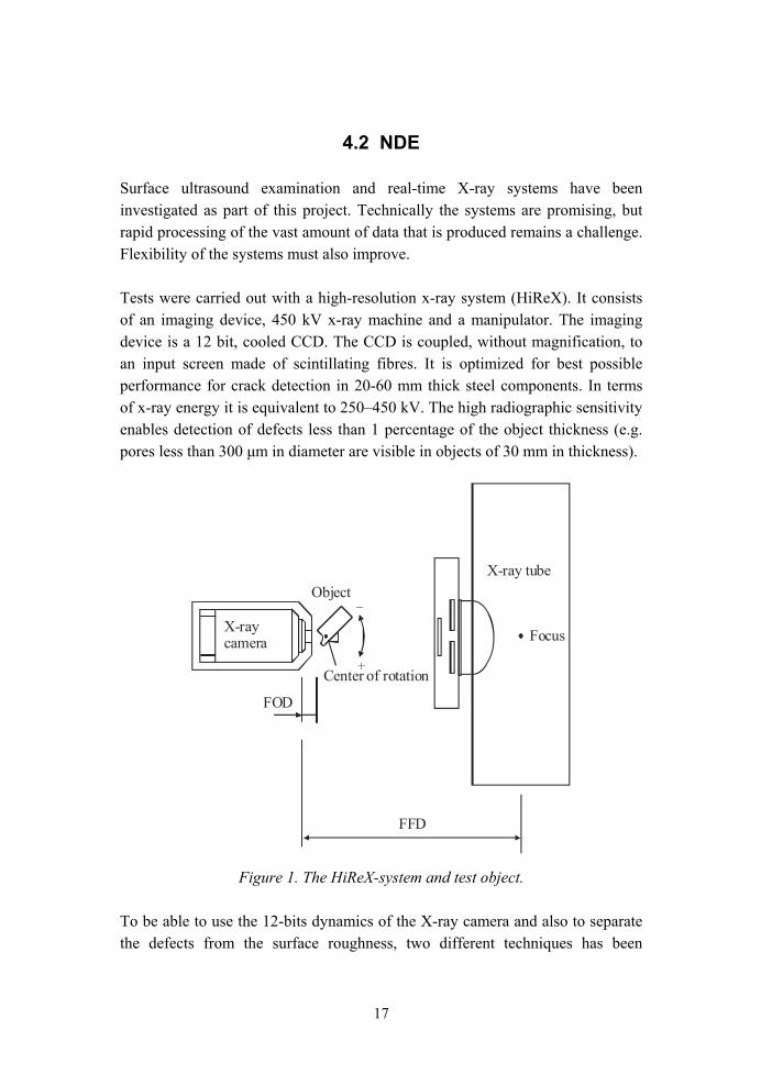
Tests were carried out with a high-resolution x-ray system (HiReX). It consists of an imaging device, 450 kV x-ray machine and a manipulator. The imaging device is a 12 bit, cooled CCD. The CCD is coupled, without magnification, to an input screen made of scintillating fibres. It is optimized for best possible performance for crack detection in 20-60 mm thick steel components. In terms of x-ray energy it is equivalent to 250450 kV. The high radiographic sensitivity enables detection of defects less than 1 percentage of the object thickness (e.g. pores less than 300 µm in diameter are visible in objects of 30 mm in thickness).
Object
Center of rotation+
_
FOD
FFD
FocusX-raycamera
X-ray tube
Figure 1. The HiReX-system and test object.
To be able to use the 12-bits dynamics of the X-ray camera and also to separate the defects from the surface roughness, two different techniques has been
18
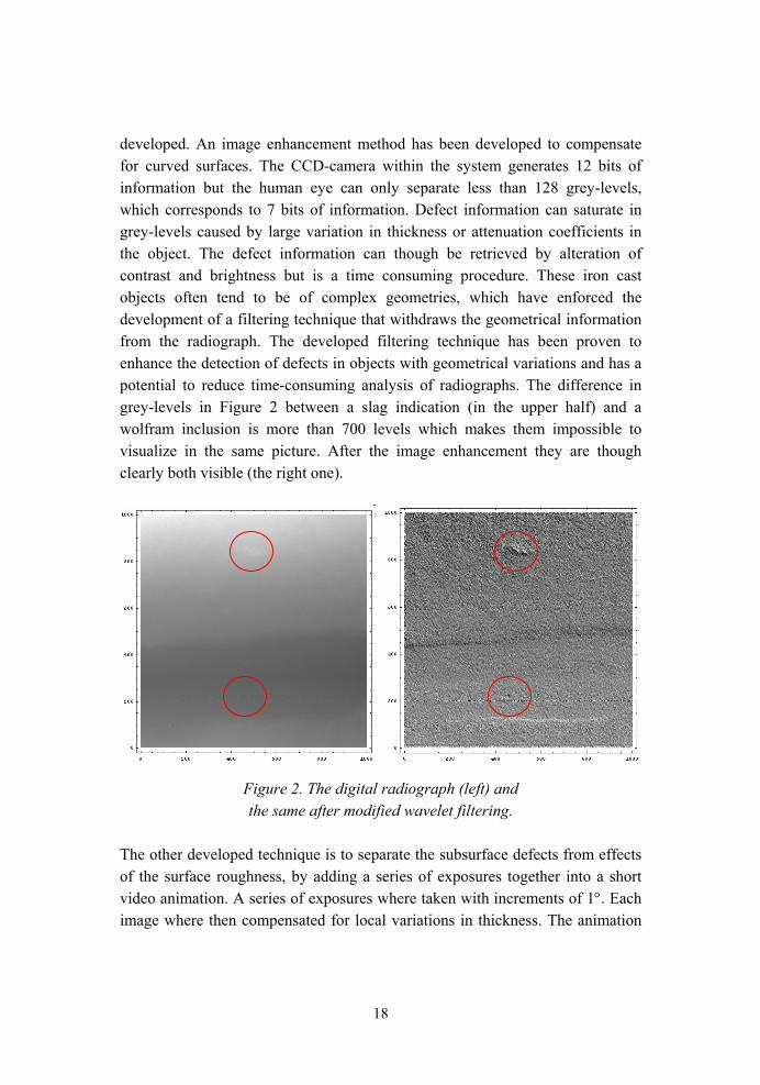
developed. An image enhancement method has been developed to compensate for curved surfaces. The CCD-camera within the system generates 12 bits of information but the human eye can only separate less than 128 grey-levels, which corresponds to 7 bits of information. Defect information can saturate in grey-levels caused by large variation in thickness or attenuation coefficients in the object. The defect information can though be retrieved by alteration of contrast and brightness but is a time consuming procedure. These iron cast objects often tend to be of complex geometries, which have enforced the development of a filtering technique that withdraws the geometrical information from the radiograph. The developed filtering technique has been proven to enhance the detection of defects in objects with geometrical variations and has a potential to reduce time-consuming analysis of radiographs. The difference in grey-levels in Figure 2 between a slag indication (in the upper half) and a wolfram inclusion is more than 700 levels which makes them impossible to visualize in the same picture. After the image enhancement they are though clearly both visible (the right one).
Figure 2. The digital radiograph (left) and the same after modified wavelet filtering.
The other developed technique is to separate the subsurface defects from effects of the surface roughness, by adding a series of exposures together into a short video animation. A series of exposures where taken with increments of 1°. Each image where then compensated for local variations in thickness. The animation

19
is produced in conventional AVI-file format. The subsurface defects where then visible in the animations.
4.3 Critical fatigue issues
Nodular cast iron. The fatigue test of small scale specimen with and without chunky graphite show that the da/dN curve is not affected to any extent by the chunky graphite, but the fracture toughness is reduced in same order of magnitude as the elongation.
The fatigue strength of machine components that are subject nominally to constant amplitude load can be drastically reduced by only a few rare r under-load events. These events are in many cases part of the normal duty cycle and are the result of thermal transients during start-ups and shut-downs or due to maintenance. Critical experimental measurements of this overload effect have been made for grey and nodular iron and for QT steel.
For complex parts, loading is often multi-axial and in some cases is also highly non-proportional. Fatigue damage models have primarily been developed for materials that fail predominantly by shear crack growth. Cast materials, however, fail predominantly by tensile mode crack growth. There is a need to develop models for this class of material and verify the results for large and often complex components
4.4 Design process
For cast load-carrying and work producing components and structures there is a need to integrate efficient FE based analysis tools, reliable information on defect size, shape and location, and expertise on how complex variable amplitude and multi-axial loading influence fatigue damage in cast materials. In terms of assessing the significance of defects in different regions of a component, fracture mechanics methods are a valuable too, but are not often applied to cast components. Reliability of these methods, especially in regards to material parameters, is needed and has been a valuable contribution of this project.

20
To get a simple tool for the designers and to make the communication easier between the buyer and the deliverer of castings a special standard has been developed. The standard classifies and defines different type of defects in ductile iron seen from size, number and location. Further on demands are given when the component can be accepted after correcting measures.
5. Conclusions
In order to gain a competitive advantage in the world marketplace, Nordic industries need to press forward in several critical research areas. For cast load-carrying and work producing components and structures there is a need to integrate efficient FE based analysis tools, reliable information on defect size, shape and location, and expertise on how complex variable amplitude and multi-axial loading influence fatigue damage in cast materials. Important steps have been made in order to better implement fracture mechanics based fatigue assessment procedures for cast materials. Progress has been made in cast process modeling and control to avoid major defects and avoidance of chunky graphite that is often associated with high silicon iron. Several potential tools for reliable NDE have been investigated.
Acknowledgements
This project is funded by Nordic Innovation Center (NiCe), The Swedish Vehicle research Programme (PFF), Tekes and the participating organisations which is greatly acknowledged.
References
1. Hobbacher, A. Fatigue Design of Welded Joints and Components. Recommendations of IIW, XIII-1539/XV-8454-96. Abington Publishing 1996.
2. Björkegren, L.-E. Slutrapport, Vamp-7, Dimensionering av gjutna komponenter med avseende på defekter, korta ledtider och lättviktskonstruktion, 1999.
21
3. Robertsson, Defect Sensitivity in Nodular Cast Iron for Safety Critical Components. Volvo internal report LM-500245, 1993.
4. Einarsson, Sinander, M. and Smedendahl, S. Defect Sensivity in Cast Materials. Examensarbete vid Chalmers Lindholmen, Institutionen för Maskinteknik, Rapport Mi3-40-2002.
5. Swedish Standard SS-EN 1563.
6. Björkblad, A. Conventional vs. closure free crack growth in nodular iron. To be published at the 15th European Conference of Fracture (ECF 2004), August 2004, Stockholm, Sweden.
7. Mörtsell, M, Hamberg, K. and Wasén, J. Crack Initiation in Ductile Cast Irons. In: Proc. 7th Int. Conf of Cast materials, Barcelona, 2002.
8. Hamberg, K. and Björkegren, L.-E. Chunky Graphite a literature survey. Report 300930 at the Swedish Foundry Association.
9. Björkblad, A. On the prediction of crack propagation in cast steel specimens. 9th Portuguese Conference of Fracture, Setûbal, 2004. Pp. 167175.
10. Hamberg, K. and Stenfor, S.-E. Defekter i järngjutgods, ett förslag till ny standard. Gjuteriet, Nr 3, 2002, pp. 1015.
11. Björkegren, L.-E. and Hamberg, K. Lätta segjärnskonstuktioner genom optimering av materialegenskaper och konstruktiv utformning. Svenska Gjuteriföreningensskrift 970930.
12. Kaufmann, H. Zur schwingfesten Bemessung dickwandiger Bauteile aus GGG-40 unter Berücksichtigung giesstechnisch bedingter Gefügeugänzen, LBF Bericht Nr. FB-214, 1998.
13. Hamberg, K. Björkegren, L.-E. and Sun Z. X. Chunky Graphite in Ductile Iron. A literature survey. Gjuteriföreningspublikation, 2003.

22
14. Rabb, B. R. Influence of occasional underloads on fatigue. European Congress on Computational Methods in Applied Science and Engineering, ECCOMAS 2004, 24-28.7.2004, Jyväskylä.
15. Marquis, G. B., Rabb, B. R. and Karjalainen-Roikonen, P. High Cycle Variable Amplitude Fatigue of a Nodular Cast Iron. J. of ASTM International, ASTM International, West Conshohocken, PA, 2004.
16. Marquis, G. and Karjalainen-Roikonen, P. Long-Life Multiaxial Fatigue of a Nodular Cast Iron. In: ESIS Special Technical Publication on biaxial/multiaxial fatigue and fracture, A. Carpentieri, M. de Freitas, and A. Spagnoli (eds.). 2003.
17. Marquis, G. Fatigue assessment and future trends in multiaxial fatigue. 7th Intl Conf. Biaxial and Multiaxial Fatigue and Fracture, 28.6.1.7.2004, DVM Publishers, Berlin. 12 p.
18. Marquis, G. and Murakami, Y. Scatter in the Fatigue Limit of Nodular Iron. Materials Science Research International, Special Technical Publication, Kyoto, Japan, 2001, T. Hoshide (ed.). Pp. 9296.
19. Wirdelius, H. and Hammar, Lars. Modeling of a high resolution digital radiographic system and development of a filtering technique based on wavelet transforms. NDT & E International, 37:1 (2004), pp. 7381.
20. Hammar, L. and Wirdelius, H. HiReX-development of a high resolution digital X-ray system. Proc. 16th WCNDT, Montreal, 2004.
21. Hammar, L. Inspection of steel casting fatigue specimens with High Resolution Digital X-ray (HiReX). Comm. SCeNDT-0401, Göteborg 2004.
22. Israelsson, B. Kvalitetsstyrning vid framställning av stålgjutgods En genomgång av processen vid svenska gjuterier, Gjuteriföringsskrift 040913, 2004.
23. Bahta, S. Analysis of Impact of Weld Repair on Complex Steel Castings. Examenensarbete Volvo CE.

Casting technology and optimisation
Optimization of cast components in the development process.......... 25 Andreas Holmström, Stefan Edlund, Fredrik Larsson & Kenneth Runesson
Structural optimization of castings by using ABAQUS and Matlab ... 39 Erik Gustafsson & Niclas Strömberg
Simulation of the foundry process ..................................................... 53 Kenneth Åsvik
Chunky graphite – formation and influence on mechanical properties in ductile cast iron ............................................................ 63
Rikard Källbom, Kenneth Hamberg & Lars-Erik Björkegren

25
Optimization of cast components in the development process
Andreas Holmström, Stefan Edlund Volvo Trucks, Sweden
Fredrik Larsson, Kenneth Runesson Chalmers University of Technology, Gothenburg, Sweden
Abstract
Well-known customer requirements on commercial vehicles (trucks) are better fuel economy, more load-capacity, better safety and higher reliability. Further, there are normally a number of functional demands, often contradictory, that the development team must take into account when designing the structural components. Examples are high reliability, good stability and low structural weight. Many of these demands have ties into several different physical fields. This is combined with the requirement that less time and resources should be used in the development. In the development of a component it is often impossible to evaluate every possible solution since it is not obvious from the demands if a solution is feasible. For a cast component the mechanical behaviour depends on the casting process, and it must be taken into account that strong couplings exist between the geometry, the production process and the material properties. These couplings must therefore be analysed at different stages of the development process. As a result, one is faced with a complex multidisciplinary optimisation problem.
In this contribution a generic process for optimising complex multi-physics problems is presented using a succession of more complex analyses. The strategy that we propose is to use low-level analyses to scan a large number of different solutions in order to find the most viable ones. These are then further narrowed down during a chain of analyses with successively higher level of detail, while trying not to remove good solutions. During the very latest stages of the analysis only a few solutions are considered and therefore time and resource-consuming analyses can be used in order to fully investigate the properties of the component.

26
A principal problem of a cast component is discussed for a given set of mechanical load demands and with consideration to the production process in order to exemplify the process and some possible pitfalls. The explicit computational procedure, based on FE-analysis, is applied to simplified mechanical and thermal problems involved in the casting of a typical load-bearing structural component.
1. Introduction
There is always a demand for developing new products with increased performance to less cost and in shorter time to market. This requires a product development process that utilizes the possibilities in simulating the product in as early stage as possible. Significant research effort has recently been devoted to the use of optimisation in the development process.
In this article the focus is on how to use optimisation techniques and different models in a development process in order to develop optimal components, whereby optimal refers to cost-effectiveness. In particular, the focus is the development of a cast component where demands and behaviour are functions of the casting process. How this can be analysed at different stages of the process?
The demands that are imposed on the truck are mostly functional. During the development process the demands on components might be altered in order to get a better compliance with demands on the truck level. Since some of the demands will be dependent on the resulting solution and what trucks it shall be used in, the process has to be adaptable enough so new demands can be incorporated when they arise.
2. Optimisation strategy
The development is usually started with a proposed solution. Based on analysis, and/or prior knowledge of previous solutions, this solution is deemed acceptable or a new solution is developed. If a better solution appears, it will most often be used even if the current solution is acceptable. The development process can thus be seen as an optimisation process, not very different from an evolutionary algorithm, even if it is not strictly a mathematical optimisation, see Figure 1.

27
Manual
Initial parameter values
Analysis
Analysis
Analysis
Optimised product/process
Parameter update
Evaluation
Analysis
Analysis
Analysis
AutomaticManual
Initial parameter values
Analysis
Analysis
Analysis
Analysis
AnalysisAnalysis
Optimised product/process
Parameter update
Evaluation
Optimised product/processOptimised product/process
Parameter update
Evaluation
Parameter update
Evaluation
Analysis
Analysis
Analysis Analysis
Analysis
Analysis
Automatic
Figure 1. Generic flowchart for optimisation.
The functional demands must be reformulated so they can be measured. Further, we only do a detailed examination on a few solutions, due to the analysis effort involved. Therefore, a strategy for how and when demands should be investigated is needed.
2.1 Strategies
The strategy that we propose is to use simplified models to scan a large number of different solutions in order to find the most viable ones. These are then further narrowed down during a chain of analyses with successively better precision. During the very latest stages of the analysis only a few solutions are considered and therefore thorough time and resource consuming analyses can be used in order to fully investigate the properties of the component. With this approach, combined with a process improvement, we believe an effective development against several multi-physical demands is possible. In order to structure this somewhat we introduce the concept of different levels of detail for the analysis.

28
2.2 Level of detail LOD
The analysis done in the development process is divided into high and low LOD analysis. The low LOD is quick analysis that can be made in order to rank a large number of different solutions. The high levels should be able to predict whether the component fulfils the (often) functional demands.
These simplified models must not predict whether a solution strictly satisfies the demands, but rather can give an indication. Even so the simpler problem obviously needs to have a resembling behaviour for this analysis to be of any value. The higher levels of analyses can then be more time and labour intensive. One can use several levels of detail in the analysis in order to minimize the number of times the most expensive analyses are made. Often the case is that only the most time consuming analyses can give reliable predictions on some of the most important questions.
The different levels of detail in the analysis also mean that the demands must be changed accordingly, e.g. a stress level is considered as criterion in a FE calculation and in a rig testing the specimen is inspected after the load cycle. Since the high-level analysis is not done results from earlier designs are used in order to correlate acceptance levels.
It might be of value if the low level analysis can be modified to better fit the finding of the high level analysis because the errors that comes from simplifications can be hard to quantify.
In our opinion it would be worthwhile to develop low-level methods to evaluate e.g. casting. The focus not being to develop a physical model, but rather to develop a locally correct model that can be used to examine how small changes influence the solution. Possible solutions are, for instance, to use linear cooling models, enthalpy calculations or to use neural networks.

29
3. Abstract formulation of the multidisciplinary optimisation problem
We now turn to formulate a mathematical framework for the optimization. First we consider the general optimization of finding the solution such that
where is a (scalar) goal function and is the parameter space of all admissible solutions. In this setting, is restricted by the demands on the problem. Assuming that is a natural parameter space, i.e., is a space that defines some set of parameters, dimensions and more, sufficient to define the solution. We construct the parameter space as
In the definition above, we introduced a set of constraints . A common approach is to use the larger parameter space, , and specify the constraints in the minimization problem. We thus formulate the problem as that of finding that solves
We assume that the goal-function and constraints are formulated implicitly in terms of the solutions to a set of engineering problems such as mechanical load cases, manufacturing etc. Clearly, the constraints , as well as the goal function , can be described with different LOD. Choosing suitable goal functions and
constraints based on the requirements on the product governs how the problem is solved.
In order to construct an explicit mathematical formulation we introduce constraints and goal-function approximating the physical events in some way. We formulate problems describing physical events as

30
The solutions, or states, hence depend indirectly on . Finally, we construct the goal-function . The constraints can now be partitioned as follows.
Assuming that the state equations hold, we obtain the following equalities:
Finally, we present the expanded optimization problem as follows:
In this expanded setting we identify 4 different types of constraints to the minimization problem:
1. The space restricts the problem in terms of dimension and types, i.e., defines the degrees of freedom.
2. State-independent constraints define more complex relations for admissible , yet in an explicit fashion.
3. State-dependent constraints define requirements on the system in terms of response to certain events, e.g. mechanical loading.
4. State equations describe the events for which the state-dependent constrains are formulated. These relations are indeed themselves constraints to the problem of minimizing .

31
3.1 Approximations in the optimisation problem
3.1.1 Approximating the goal-functional
Defining the goal-function is a crucial task. Approximations in the goal-function can be those of basing the value on the results of more or less complex state equations. It might be problematic to formulate the goal-function in a mathematical framework as a function of all possible solutions. Therefore the solutions are restricted to be of a certain type, e.g. only one specific casting-method is considered. There might also be problems in specifying the goal-functions in terms of parameter space. Instead, additional constraints can be added in order to bound the solution, e.g. maintenance-cost.
3.1.2 Approximate constraints
In many cases, the first approximation of a constraint is that of formulating a constraint in a mathematical framework rather than functional constraints. Even the mathematical model may be too expensive to evaluate, requiring expensive-to-solve state equations. Some of the constraints might also involve several coupled effects that need to be decoupled in order to be modelled. Note that the choice of constraints strongly affect both goal-function and what type of parameterisation that should be used.
3.1.3 Approximate state equations
The choice of goal-function and constraint equations governs the required state equations to be solved. Within those boundaries, further approximations are possible. For instance, model approximations and approximate solutions. In particular, we often turn to numerical methods in order to solve the state equations, and thus introducing discretization errors from the numerical approximation. For an in depth view on the error in optimization due FE-discretization, cf. [1]. For analysis on error control and model adaptivity in the FE-context, cf. [2]. The constraints that involve coupled and/or sequential effects might also be problematic/expensive to solve without introducing further approximations.
32
3.1.4 Restricting the parameter space
It is important to note that if the natural parameter space does not include a solution it will not be found by the optimisation.
Typically, we introduce a reduced (finite) subset of the natural parameter space, , in order for the optimisation to be efficient. The effects are, in general,
that we do not obtain the true optima for the problem. However, this does not affect the validity of our constraint equations. For further reading on error control w.r.t. parameter space, cf. [1]
4. Example
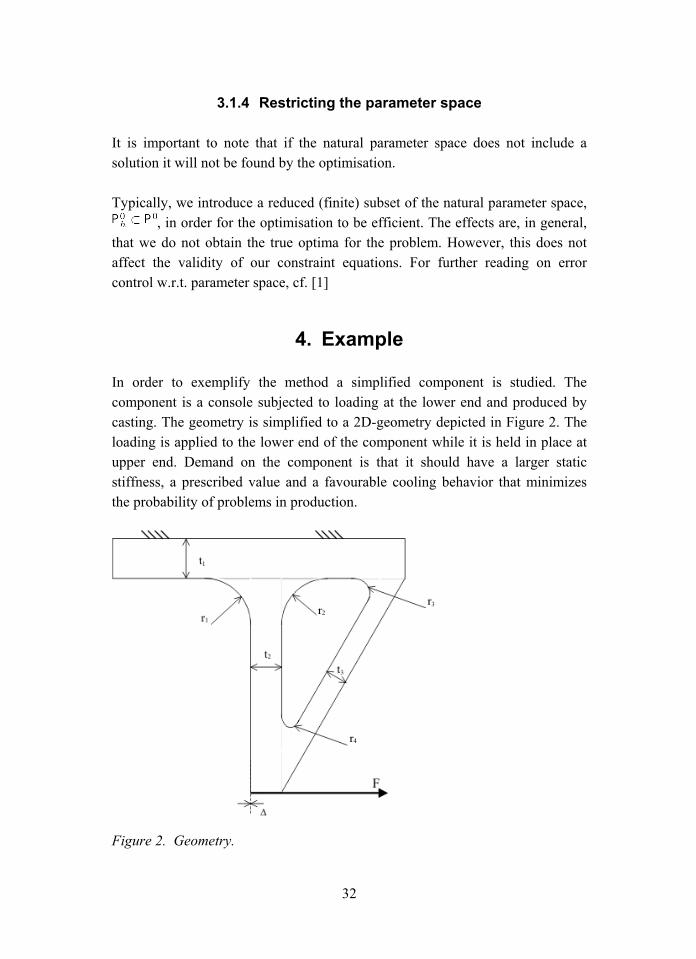
In order to exemplify the method a simplified component is studied. The component is a console subjected to loading at the lower end and produced by casting. The geometry is simplified to a 2D-geometry depicted in Figure 2. The loading is applied to the lower end of the component while it is held in place at upper end. Demand on the component is that it should have a larger static stiffness, a prescribed value and a favourable cooling behavior that minimizes the probability of problems in production.
Figure 2. Geometry.

33
In the example problem the parameter space is the parameters we need to describe the solution and the geometry we allow is restricted be the parameters we choose. We chose three lengths and four radii to describe our solutions, see Figure 2. We also have fixed upper and lower bounds for the variables
Meaning:
- Minimization of volume
- Bounded parameter values
- Deflection due to applied forces less than $\Delta_0$
- Favorable cooling profile
Table 1. Approximations used in level I and level II.
Strength evaluated by linear elasticity
Strength evaluated by linear elasticity
Material evaluated from linear cooling
Material evaluated from non-linear cooling
Geometry is modelled without radii
Geometry is modelled with radii

34
So in order to asses these demands at different levels we need to decide on analysis and measures. As level I approximation of the strength of the component we examine the stiffness calculated from linear elasticity and simplify the geometry by not including the radii in the model. At level II we include the radii.
For the thermal problem we make assessment of the material based on cooling history, essentially saying that the cooling should be as uniform as possible. At LOD I we asses this from linear cooling analysis and at LOD II we use a non-linear cooling analysis to get the temperature history.
We restrict the current analysis to the uncoupled problem and solve the dual instead of the primal problem. This means that instead of finding the geometry with minimal area that still complies with demand, we find the solution that have the most favorable geometry, given a certain area.
4.1 Implementation
The state problems are solved using an experimental FE platform. For further reading on FE implementation, cf. [3], [4]. In this way we have control over the discretization and approximations made. This is combined with a Nealder-Mead search method (MATLAB Optimization Toolbox).
4.2 Results
For the mechanical problem we see that the inclusion of (small) radii has not made any significant difference to the overall geometry, Figures 34.
For the thermal problem we see that similar geometry is optimal for both linear and non-linear cooling, Figures 56.

35
0.5
1
1.5
2
2.5
x 105
Figure 3. No radii.
0.5
1
1.5
2
2.5
3x 10
5
Figure 4. With radii.

36
200
250
300
350
400
450
500
550
Figure 5. Linear cooling
150
200
250
300
350
400
450
Figure 6. Non-linear cooling

37
5. Discussion
When optimising a product with multiple complex constraints it is hard to develop a model that is both accurate and generic enough to allow for a large number of different solutions. In this article an approach based on a succession of different models is proposed, where the first models have a large freedom in design and the late models have a good correlation to the real application of the product. Many engineering problems are solved in a similar manner, as identified by researchers such as [5].
We want to point out the possibility to use models that only give quantitative estimation of the properties by correlating these models to later models used, or old solutions to similar problems. It is also important that models that do not work can be eliminated from the process. The models do not have to be mathematical, they can be based on experience, but such models are highly dependent on the skills of the person doing the evaluation.
It varies how hard it is to model at different stages of the development process, e.g. a low level estimation of stiffness can easily be formulated but a good estimation of strength is hard to do at low levels.
6. Conclusions
It is possible to develop simplified models, (low LOD), that still have a sufficient resemblance with the true problem to be used in the development process. It can also be noted that non-localized effects can more readily be modelled with a low LOD.
References
1. Johansson, H. and Runesson, K. Parameter identification in constitutive models via optimization with a posteriori error control. Chalmers, 2005. International Journal for Numerical Methods in Engineering. In preparation.

38
2. Larsson, F. and Runesson, K., Modeling and discretization errors in hyperelasto-(visco-)plasticity with a view to hierarchical modeling, Chalmers, 2005. Computer Methods in Applied Mechanics and Engineering, Submitted.
3. Ottosen, N. and Pettersen, H. Introduction to the finite element method, New York: Prentice Hall, 1992. 410 p.
4. Holmström, A., Larsson, F., Runesson, K. and Edlund, S. Efficient space-time FE for a simplified thermo-metallurgical problem relevant to casting. Chalmers, 2005. In preparation.
5. Isaksson, O. Computational support in product development: applications from high temperature design and development, Luleå University of Technology, 1998. Doctoral thesis. 31 p.

39
Structural optimization of castings by using ABAQUS and Matlab
Erik Gustafsson Swedish Foundry Association, Jönköping, Sweden
Niclas Strömberg Jönköping University, School of Engineering, Jönköping, Sweden
Abstract
In this work a general method for structural optimization of nonlinear structures is implemented using FE-analysis. The method utilizes the response surface methodology with polynomial surfaces and nonlinear programming. In such manner a method that is applicable for a large number of different classes of nonlinear problems is obtained. In this paper, the method is utilized to minimize weight of castings by including residual stresses from solidification. This is performed by first determine the residual stresses by a thermomechanical analysis of a metal structure that is cooled from a temperature above liquidus temperature down to room temperature. The thermomechanical analysis is uncoupled where the temperature distribution within the casting as a function of time is determined first and is later on used for residual stress calculations. These residual stresses are then included when the mechanical load is applied to the structure and the problem of minimum of weight is formulated. The structure shown in this paper is an example of a two dimensional geometry. The shape of the structures will of course affect the residual stress distribution during the optimization. The nonlinear models are then solved using ABAQUS/Standard. A set of solutions are generated by solving the model for a pre-defined set of parameters. In order to minimize the number of simulations and still achieve good surface approximations these parameters are taken to be D-optimal. The sets of solutions and parameters are in turn exported to Matlab where general quadratic response surfaces are fitted by the least square method. By utilizing these surfaces the problem of minimum of weight subjected to constraints on stresses is formulated. Finally, the nonlinear optimization problem is solved by sequential linear programming.
40
1. Introduction
The work that has been conducted within simulation of the casting process has so far to a wide extent been concerning flow simulation and solidification simulation. Due to complexity of the material properties at high temperature, the research within the area of residual stresses built up in a structure that solidifies has been kept at a modest level. Early work that studied the stress in elasto-plastic material was done by (Weiner et al., 1963) and (Perzyna, 1966). As an example of what have been done in recent years one can mention (Lee et al., 1996) who developed a hybrid model of FVM and FEM that is used for calculating thermal distribution and stresses within a solidifying body. The works by Weiner and Perzyna have been the grounds for what has been done in the area of residual stresses in castings. (Samonds et al., 2005) has presented one way of implementing the theory of Perzyna. (Jacot et al., 2000) has done studies on residual stresses in cast iron with ABAQUS. (Hattel, 1997) has shown results from residual stress calculation based on a finite volume approach. In (Petersen, 2003) a comparison between a FVM calculation and a FEM calculation of residual stresses is made. In this work we simulate residual stresses by an uncoupled thermomechanical analysis. First the classical heat equation for constant parameters is solved. Then, a quasi-static rate independent plastic analysis is performed for the resulting temperature history. In this model we let Lame´s coefficients, the yield stress and the hardening modulus depend on the temperature. The theory of computational plasticity and viscoplasticity can be found in (Simo and Hughes, 1998)
Response Surface Method (RSM) has been widely used in several optimization problems where the optimal solution to non-linear thermal and mechanical problem is the goal. (Box and Wilson, 1951) was the first to introduce RSM in 1951. The book by (Myers and Montgomery, 2002) gives an extensive information about RSM. RSM has for example been used for optimization of multibody-systems, (Etman, 1997), and optimization of crashworthiness, (Rehde, 2004). An extensive list of RSM activities since 1989 can be found in (Myers et al., 2004). In (Kok et al., 1998) an optimization of a thermoelastic problem is described that is closely related to the work presented here. In this work an optimization routine for a two-dimensional problem is created. The reason why a two-dimensional beam is chosen as an object to study is because a clear understanding of residual stresses is obtained. The analytical solution to this problem is also already well known and its easy to compare simulations

41
with expectations. The objective is to minimize weight of a beam subjected to a pressure load under the constraint that the stresses will not exceed a given value. The beam has been cooled down from a temperature above liquidus temperature and therefore residual stresses will be present in the beam. These residual stresses are included in the optimization. RSM has been used for optimization where the design variables are D-optimally chosen. Sequential linear programming is used in every interval to obtain an optimal solution.
2. Governing equations
Let us consider a beam subjected to an external line load t, see Figure 1. We are interested in minimizing weight of this beam under a constraint on stresses by changing the shape at the bottom of the beam. This is a classical problem in structural optimization. However, in this work we will also include that the beam is manufactured by casting. This is done by including the residual stresses from the casting process in the optimization problem. The residual stresses are of course influenced by the shape of the beam, which in turn will influence the constraint on stresses. The problem is formulated by utilizing symmetry. The shape at the bottom is given by a B-spline that is defined by two variables x1 and x2. The residual stresses are obtained by solving two problems (P1 and P2). In the first problem the temperature history is solved by cooling down the beam. Then, in the second problem, this prescribed temperature history is utilized to find the corresponding residual stresses by an elastoplastic analysis. Finally, in problem P3, these residual stresses are included in the structural analysis when the external line load is applied. The governing equations of each problem are presented below.
2
1
Γq
Ω Γq0
P1
ΩΓs
p
P2 tΓt
ΩΓu
Γs
P3
tΓt
1x2x
h
w
2/w
2
1
2
1
Γq
Ω Γq0
P1
Γq
Ω Γq0
P1
Γq
Ω Γq0
P1
ΩΓs
p
P2
ΩΓs
p
P2
ΩΓs
p
P2 tΓt
ΩΓu
Γs
P3 tΓt
ΩΓu
Γs
P3 tΓt
ΩΓu
Γs
P3
tΓt
tΓt
tΓt
1x2x
h
w
2/w 1x2x
h
w
2/w 1x2x
h
w
2/w Figure 1. The beam, the B-spline and the three problems (P1P3).
42
P1: First an uncoupled thermal problem is solved in order to determine the temperature distribution as function of time in the beam. This is obtained by solving the heat equation
[ ]TkdivtT
TE
∇=∂∂
∂∂ρ
where ρ is the density, E(T) is the enthalpy, k is the conductivity, T is the temperature and t represents the time. E(T) is a function of temperature, which encompasses the effects of specific and latent heat.
∫ −+=T
sp TfLcTE0
))(1()( dT
where cp is specific heat, L is latent heat and fs(T) is fraction solid according to
⎪⎪⎩
⎪⎪⎨
⎧
>
≤≤−−
<
=
L
LssL
s
s
s
TTfor
TTTforTTTT
TTfor
Tf
1
0
)(
where TL is the liquidus temperature and TS is the solidus temperature. The heat equation is solved for the following boundary conditions:
( )BA TTkq −= 2 on Γq
0=q on Γq0
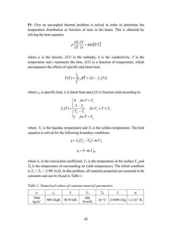
where k2 is the convection coefficient, TA is the temperature at the surface Γq and TB is the temperature of surrounding air (sink temperature). The initial condition is T0 = TL = 1190o in Ω. In this problem, all material properties are assumed to be constants and can be found in Table 1.
Table 1. Numerical values of constant material parameters.
ρ cp k k2 TB L α 7000 kg/m3 800 J/kgK 40 W/mK 400
W/m2K 20 °C 215000 J/kg 1.2⋅10-5 /K
43
P2: The residual stresses are obtained by an elastoplastic analysis. The equilibrium equation reads
0σ =div in Ω
where σ is the stress tensor. The boundary conditions are
u1=0 on Γs
u2 = 0 at p
The constitutive laws are given by temperature dependent J2-plasticity. That is,
( )[ ]Tuuε ∇+∇=21
( )Tp εεεDσ −−=
)( 0TTT −= Iε α
( ) 0:23),( 0
2/1 ≤+−= YHTf pεssσ
σε
∂∂
=fp γ&
dtt
p ∫=0 3
2 pε&ε
Here, u is the displacement, D=D(T) is the elastic tensor, α is the thermal expansion parameter, s is the deviatoric stress, H=H(T) is the linear hardening parameter, Y0= Y0 (T) is the initial yield stress and γ is the plastic multiplier which is governed by the following Karush-Kuhn-Tucker conditions: 0≥γ ,
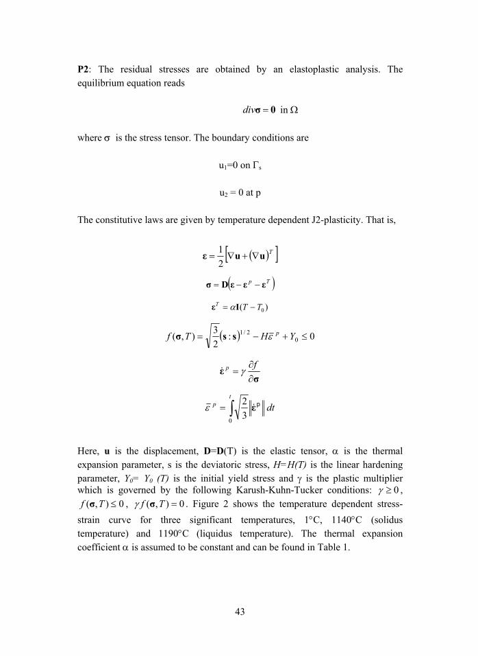
0),( ≤Tf σ , 0),( =Tf σγ . Figure 2 shows the temperature dependent stress-strain curve for three significant temperatures, 1°C, 1140°C (solidus temperature) and 1190°C (liquidus temperature). The thermal expansion coefficient α is assumed to be constant and can be found in Table 1.
44
T = 1 °C
To tal strain, ε0 0,050,040,0 30,020,0 1
100
700
600
500
400
300
200
Str
ess,
σ[M
Pa
] T = 1 °C
To tal strain, ε0 0,050,040,0 30,020,0 1
100
700
600
500
400
300
200
Str
ess,
σ[M
Pa
]
To tal strain, ε0 0,050,040,0 30,020,0 1
100
700
600
500
400
300
200
0 0,050,040,0 30,020,0 10 0,050,040,0 30,020,0 1
100
700
600
500
400
300
200
100
700
600
500
400
300
200
Str
ess,
σ[M
Pa
] T = 1140 °C
Total strain, ε0 0,050,040,0 30,020,0 1
2
14
12
10
8
6
4
Str
ess,
σ[M
Pa
]
T = 1140 °C
Total strain, ε0 0,050,040,0 30,020,0 1
2
14
12
10
8
6
4
Str
ess,
σ[M
Pa
]
T = 1140 °C
Total strain, ε0 0,050,040,0 30,020,0 1
2
14
12
10
8
6
4
Str
ess,
σ[M
Pa
]
To tal strain, ε0 0,050,040,0 30,020,0 10 0,050,040,0 30,020,0 1
2
14
12
10
8
6
4
2
14
12
10
8
6
4
Str
ess,
σ[M
Pa
]
T = 1190 °C
To tal strain, ε0 0,050,040,0 30,020,0 1
Str
ess,
σ[M
Pa
]
0 ,2
0 ,4
0 ,6
0 ,8
1 ,0
1 ,2
1 ,4
1 ,6
1 ,8
2 ,0
T = 1190 °C
To tal strain, ε0 0,050,040,0 30,020,0 10 0,050,040,0 30,020,0 1
Str
ess,
σ[M
Pa
]
0 ,2
0 ,4
0 ,6
0 ,8
1 ,0
1 ,2
1 ,4
1 ,6
1 ,8
2 ,0
0 ,2
0 ,4
0 ,6
0 ,8
1 ,0
1 ,2
1 ,4
1 ,6
1 ,8
2 ,0
T = 1 °C
To tal strain, ε0 0,050,040,0 30,020,0 1
100
700
600
500
400
300
200
Str
ess,
σ[M
Pa
] T = 1 °C
To tal strain, ε0 0,050,040,0 30,020,0 1
100
700
600
500
400
300
200
Str
ess,
σ[M
Pa
]
To tal strain, ε0 0,050,040,0 30,020,0 1
100
700
600
500
400
300
200
0 0,050,040,0 30,020,0 10 0,050,040,0 30,020,0 1
100
700
600
500
400
300
200
100
700
600
500
400
300
200
Str
ess,
σ[M
Pa
] T = 1140 °C
Total strain, ε0 0,050,040,0 30,020,0 1
2
14
12
10
8
6
4
Str
ess,
σ[M
Pa
]
T = 1140 °C
Total strain, ε0 0,050,040,0 30,020,0 1
2
14
12
10
8
6
4
Str
ess,
σ[M
Pa
]
T = 1140 °C
Total strain, ε0 0,050,040,0 30,020,0 1
2
14
12
10
8
6
4
Str
ess,
σ[M
Pa
]
To tal strain, ε0 0,050,040,0 30,020,0 10 0,050,040,0 30,020,0 1
2
14
12
10
8
6
4
2
14
12
10
8
6
4
Str
ess,
σ[M
Pa
]
T = 1190 °C
To tal strain, ε0 0,050,040,0 30,020,0 1
Str
ess,
σ[M
Pa
]
0 ,2
0 ,4
0 ,6
0 ,8
1 ,0
1 ,2
1 ,4
1 ,6
1 ,8
2 ,0
T = 1190 °C
To tal strain, ε0 0,050,040,0 30,020,0 10 0,050,040,0 30,020,0 1
Str
ess,
σ[M
Pa
]
0 ,2
0 ,4
0 ,6
0 ,8
1 ,0
1 ,2
1 ,4
1 ,6
1 ,8
2 ,0
0 ,2
0 ,4
0 ,6
0 ,8
1 ,0
1 ,2
1 ,4
1 ,6
1 ,8
2 ,0
Figure 2. Temperature dependent stress-strain curves for the material used.
P3: The governing equations are very similar to the ones of problem P2. Now, of course, Tε =0 and the boundary conditions are given by
tnσ = on Γt
u = 0 on Γu u1=0 on Γs
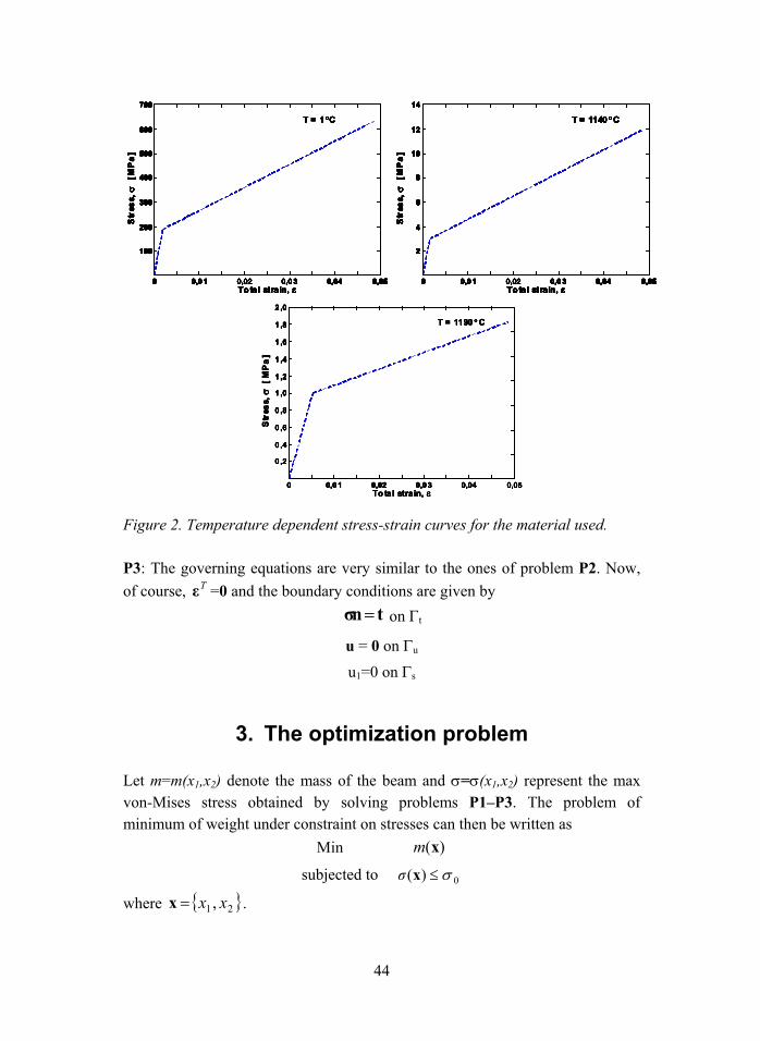
3. The optimization problem
Let m=m(x1,x2) denote the mass of the beam and σ=σ(x1,x2) represent the max von-Mises stress obtained by solving problems P1P3. The problem of minimum of weight under constraint on stresses can then be written as
Min )(xm
subjected to 0)( σ≤xσ
where 21, xx=x .

45
The actual representation of the response of m and σ are assumed to be a polynomial of any degree suitable. This polynomial contains a number of unknown parameters β that must be adjusted to match the function to be approximated. For a general quadratic surface approximation the function will be
i
j k
ik
ijjk
j
ijj
i xxxy εβββ +++= ∑∑∑0 , i = 1, 2, , N
where xi are the design points in the region of interest, εi is the error and N is the number of evaluations. In order to determine the unknown variables β the above equation is written in matrix notation as
εβxXy += )(
The function is then calculated at the design points xi and the error is minimized by a least square method. The solution to this problem is governed by the normal equation, i.e.
( ) yxXxXxXβ )()()(1* TT −
=
The quadratic approximation implies that the optimization problem is non-linear. In this work this is solved by sequential linear programming. In a point *x our problem is approximated by
Min )()()( *** xxxx −∇+ Tmm
subjected to 0*** )()()( σσσ ≤−∇+ xxxx T
iiii UBDxxLBD ≤−≤ * i = 1,2
The last set of constraint is called move limits, with LBD being the lower bound and UBD being the upper bound, on the allowed change of xi. This problem is solved using linear programming in Matlab. A presentation of sequential linear programming can be found in (Luenberger, 2004).

46
4. Numerical examples
Two optimal solutions are presented in this section. The dimensions of the beam are
h = 0.1m
w = 0.2m
xi ∈ [0, 0.09] m
see Figure 1. These geometric conditions are valid for both optimization problems. The optimal shape of the beam when the residual is neglected is shown in Figure 4. The corresponding mass as function of iterations is presented in Figure 3. Figure 5 shows the optimal shape when residual stresses are included in the analysis. The corresponding residual stresses are depicted in Figure 6. Figure 8 then shows the corresponding mass as function of iterations for the case where residual stresses are included. Finally, in Figure 7, the optimal shaped beam according to structural load only is loaded with the same thermal load that is used to obtain the optimal solution presented in Figure 5. It can then be seen that the maximum stress is more then 10% higher compared to Figure 4 where residual stresses are neglected.
Figure 4. Mass of beam as a function of iterations.

47
Figure 3. Optimal shape and von-Mises stress in beam due to structural load.
Figure 5. Optimal shape and von-Mises stress in beam after thermal load and structural load.

48
Figure 6. Von-Mises stress in beam due to thermal load.
Figure 7. Von-Mises stress in beam after thermal load and structural load.

49
Figure 8. Mass of beam as a function of iterations.
Figure 9. Relative error of response value for stress vs. actual value as a function of iterations.

50
In Figure 8 one can see how the volume changes as the iterations proceeds. There is a large dip on the curve at iteration 11 and 12. The optimization at this level is not continued, instead the volume at iteration 13 is higher. One can see in Figure 9, where the relative error between the response, y(x*) of the stress and the correct stress σ(x*) for the optimal solution x* is computed at each iteration, that the stress at iteration 12 is overestimated by the response. Therefore the optimal solution at iteration 12 is valid but still abandoned in iteration 13. The calculation of the relative error is done according to the following formula
)()()(
*
**
xxx
i
iii
ye
σσ−
= , i = 1, 2, , M
where x* is the optimal solution at iteration i, M is the number of iterations, yi is the response for the solution x* and σi is the actual stress for the optimal solution x*.
The reason why the optimal solution in iteration 12 is abandoned has to do with the response approximation in iteration 13. The response in iteration 13 is such that it finds another optimal solution x* and by doing this the optimization routine never finds the optimal solution at iteration 12 again. Future work will, among other things, be concentrated on implementing a routine that never abandons an optimal solution due to a worse response at the next iteration. For instance, we will implement the panning and zooming technique by (Stander and Craig, 2002).
5. Concluding remarks
An optimization routine is created where RSM is used to obtain the optimal solution to a thermomechanical problem. The variables within the optimization are chosen in a D-optimal manner. The optimal solution from the thermomechanical problem is then compared with the optimal solution of the same problem when thermal load is excluded. The difference in optimal shape between the pure structural problem and the thermomechanical problem was not that significant. The reason for this is that the major part of the plastic strain develops at the center of the beam during solidification. Therefore, the residual stresses of significance will be found at the center. Of course, these stresses will

51
not superpose with the stresses caused by the structural load. Future work will be concentrated on improving the optimization routine, the thermal stress calculation and the material data as well as applying the method to more complex geometries.
Acknowledgement
This project is supported by the Knowledge Foundation (KK-Stiftelsen) in Sweden.
References
1. Box, G. E. P., and Wilson, K. B. On the Experimental Attainment of Optimum Conditions. Journal of the Royal Statistical Society. 1951. Vol. 13, No. 1, pp. 145.
2. Etman, L. F. P. Optimization of Multibody Systems using Approximation Concepts. Ph.D. Thesis, Technical University Eindhoven, The Netherlands, 1997.
3. Hattel, J. Numerical Modelling of Stresses and Deformations in Casting Process. International ADI and Simulation Conference, May 2830, 1997.
4. Jacot, A., Maijer, D. and Cockcroft, S. Modeling of Microstructure and Residual Stress in Cast Iron Calender Rolls. Metallurgical and Materials Transactions A. 2000. Vol. 31A, April, pp. 12011211.
5. Kok, S., Stander, N. and Roux, W. Thermal Optimization in Transient Thermoelasticity Using Response Surface Approximations. International Journal for Numerical Methods in Engineering. 1998. Vol. 43, pp. 121.
6. Lee, J. and Hwang, K.-I. A Hybrid Numerical Analysis of Heat Transfer and Thermal Stress in a Solidifying Body Using FVM and FEM. International Journal of Engineering Science. 1996. Vol. 34, No. 8, pp. 901922.
7. Luenberger, D. G. Introduction to Linear and Nonlinear Programming. Kluwer Academic Publishers, 2004.

52
8. Myers, R. H. and Montgomery, D. C. Response Surface Methodology Process and Product Optimization Using Designed Experiments. Wiley, New York, 2002.
9. Myers, R. H., Montgomery, D. C., Vining, G. G., Borror, C. M. and Kowalski, S. M. Response Surface Methodology: A Retrospective and Literature Survey. Journal of Quality Technology: a quaterly journal of methods applications and related topics. 2004. Vol. 36, No. 1, pp. 5377.
10. Perzyna, P. Fundamental Problems in Viscoplasticity. Advance in Applied Mechanics, 1966. Vol 9, pp. 243377.
11. Petersen, A. Validation of Plasticity Models for Residual Stresses in Casting Processes. M.Sc. Thesis, Institut for Produktion og Ledelse, DTU, Denmark, 2003.
12. Rehde, M. On Vehicle Crashworthiness Design Using Structural Optimization. Ph.D. Thesis, Division of Solid Mechanics, Department of Mechanical Engineering, Linköpings Universitet, Sweden, 2004.
13. Samonds, M. and Zhu, J. Z. Coupled Thermal-fluids-stress Analysis of Casting. http://www.calcom.ch/HomeWebCalcom/News&Events/actives/S.%20Stress-MCWASP.pdf , 2005-02-17.
14. Simo, J. C. and Hughes, T. J. R. Computational Inelasticity. Springer, New York, 1998.
15. Stander, N. and Craig, K. J. On the Robustness of Simple Domain Reduction Scheme for Simulation-Based Optimization. Engineering Computations. 2002. Vol. 19 (4), pp 431450.
16. Weiner, J. H. and Boley, B. A. Elasto-plastic Thermal Stress in a Solidifying Body. Journal of Mechanical Physics and Solids. 1963. Vol. 11, pp. 145154.

53
Simulation of the foundry process
Kenneth Åsvik, Volvo Wheel Loaders
Eskilstuna, Sweden
Abstract
Simulation of the foundry process is a very useful tool for foundries to improve quality and reduce lead-time. Presented in this paper are some case-studies where simulations have played an important roll to be able to understand the foundry process and produce good quality castings.
1. Introduction
Simulation software for foundries has been on the market for about 20 years but the first versions were perhaps not made for foundry men, they were not easy to use and very slow. But the development in both computer hardware and software has made the systems both quicker and easier to use.
The first programs were made to be able to detect shrinkage and did only calculate the solidification but now the systems can calculate both mould filling and solidification. A lot of data , regarding both solidification and flow but also about stresses and displacements.
The obvious reasons for using simulations are to improve casting quality and by that improve lead-time and save costs, but there are other advantages in using simulations for instance it gives you a deeper understanding of what actually is happening in the mould.
This paper describes three cases where simulations were used to be able to produce high quality castings.
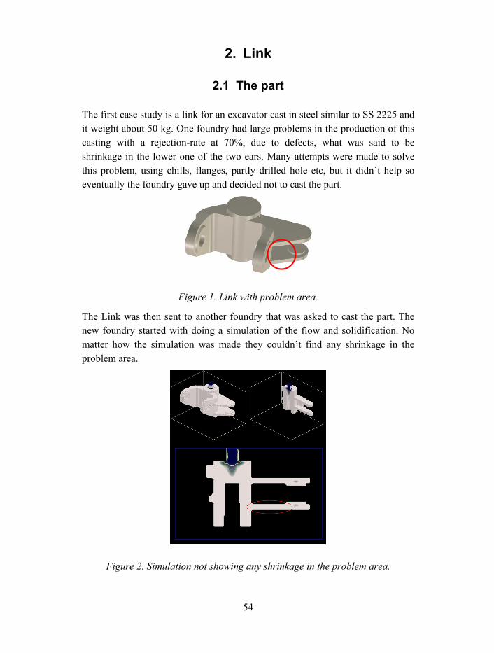
54
2. Link
2.1 The part
The first case study is a link for an excavator cast in steel similar to SS 2225 and it weight about 50 kg. One foundry had large problems in the production of this casting with a rejection-rate at 70%, due to defects, what was said to be shrinkage in the lower one of the two ears. Many attempts were made to solve this problem, using chills, flanges, partly drilled hole etc, but it didnt help so eventually the foundry gave up and decided not to cast the part.
Figure 1. Link with problem area.
The Link was then sent to another foundry that was asked to cast the part. The new foundry started with doing a simulation of the flow and solidification. No matter how the simulation was made they couldnt find any shrinkage in the problem area.
Figure 2. Simulation not showing any shrinkage in the problem area.

55
The foundry then started to look for another reason for the defects and when looking at the filling of the mould they found something interesting. When the problem-area was filling the connection to the rest of the mould-cavity was filled by the melted steel so all the air and gases had nowhere to go but out of the mould walls. It looked like a lot of gas that might be too much gas to get out of the mould walls. So perhaps the defects were gas porosity due to trapped gas and not shrinkage.
Figure 3. Simulaion of flow into the mould.
The foundry then put a connection between the ears that was used as a chimney for the gases in the mould. The part was cast and the casting was OK and after two years production the rejection-rate is 0%.
Figure 4. Showing new way of pouring casting.

56
Another interesting thing seen on this simulation is if you look at the contact surface between the sand and the steel, se Fig. 5. This part is cast using olivine sand which has a sintering temperature of 1380°C and when looking at the simulation it is seen that the temperature in the sand in some areas are over 1380°C which should mean sintered sand. And when you look at the castings in these areas it clearly show sintered sand. This can be solved by the foundry by either lower the temperature of the steel or use another kind of sand or coating in these areas. In this case it was solved by using chromite sand and coating.
Figure 5. Simulation of temperature in the sand.
Figure 6. Sintered and burnt-on sand.
2.2 Discussion
Clearly the simulations used in this case helped the foundry to produce a casting with acceptable quality. There is of course a possibility to come to the same conclusions by using destructive or non-destructive testing but that would probably have been much more expensive to cast some samples to do the testing

57
and that would have taken longer time. Here the first castings poured was Ok and delivered to the customer.
It is not easy to understand how the filling of the mould is done so it is not sure that the problem is recognized as a mould filling problem. But the simulation helped to visualize the problem and gave the foundry a better understanding of what kind of problems a bad ingatesystem can lead to and this has helped the foundry with other similar products.
3. Pin
3.1 The part
This casting is a simple pin used in fishing boats cast in a high strength steel similar to SS2225. This high grade hardened and tempered steels are sensitive for cracks, especially thick-walled castings. This casting is about two meters long and weights about 1500 kg.
Figure 7. Pin.
The foundry have had problems with cracks in this material so when a casting with defects was found it was thought of as cracks due to bad material properties.

58
Figure 8. Defects looking like cracks.
To be able to find a good solution to the problem a deeper investigation was made. In the investigation it was found that the defects were on the side facing down in the mould which doesnt make sense if the problems were due to the material properties, because then the defects should have been on the thickest part of the casting I e in or close to the feeder.
After making an exact study of how the part was poured a simulation was made and it showed shrinkage in the lower part of the casting. This was strange and there were first a lot of doubts if the simulation showed the right result. But after looking at what the reason for these defects was it made more sense. The foundry used chills in the mould to start the cooling of the casting at the right place, which can be a problem for round castings. Unfortunately they had used too big chills and not placed them good so they actually caused the problem. By cooling off the connection to the feeder and leaving the lower parts of the casting unfed they led to shrinkage defects. And when taking closer look at some of the defects they found some that looked more like shrinkage than cracks.
Figure 8. Showing the way the pin was poured.

59
Figure 9. Simulation showing shrinkage in lower parts of the casting.
Figure 10. Simulation showing cooling of pin.
Figure 11. Defects looking more like shrinkage than cracks.

60
3.2 Discussion
The simulation of this part didnt just help the foundry to solve the problem with the part it also helped creating a better understanding for how chills work and that it is important to use the right size of chills in the right place. Due to the good visualization that the simulation gives it was much easier to show the staff what has happened and why.
There had been some doubts at the foundry if the simulation program could handle chills and do proper calculations with them but this example shows that it is possible.
It also shows that it is very important to have the right data for all material used in the foundry process when doing the simulation to get the right result. Due to this reason it is the authors opinion that it is best, if the foundry does the simulation, not the buyer of the casting, since the foundry have more knowledge of the different parameters.
4. Wheel
4.1 The part
This casting is a small wheel used in a machine for making paper. It is cast in stainless steel according to SS2343 and is a case similar to the first one in this paper.
Figure 12. Wheel.
The foundry producing this casting achieved information from their customer that the casting delivered had defects, gjutmästarbostäder as they said.

61
As gjutmästarbostäder is a nickname for shrinkage the foundry started doing changes to avoid shrinkages but just to be sure X-rays were made and it showed a completely different thing. No shrinkage was seen but a large gasporosity, so simulations were made to try to figure out why the gasporosity was there. When looking at the flow into the mould it was seen that there was trapped gas in this part too and by changing the ingate system this problem was solved and now the foundry are producing castings with no defects.
Figure 13. X-ray showing gasporosity.
Figure 14. Simulation of flow into the mould.

62
4.2 Discussion
Simulations and different NDT-methods are both very good tools for quality assurance in a foundry but if they are combined they are even better. If they are combined tendencies can be seen and better conclusions can be made, even if there are no real problems. The knowledge where defects might occur and what kind of defects is expected to be found during NDT-testing improve the analysis and the simulation tools can be used much more efficient.
5. Summary
It is clear that simulation of the foundry process can help foundries to produce castings with higher quality reducing both cost and lead time. This is done by reducing trials but also through optimizing casting layouts and easier testing of new ideas.
But it is also a good tool to get a better understanding what actually is happening during the foundry process and for that reason very useful for education.
The simulation should also be an integrated part of the foundry and not used in a separate department, as it often is today. If it is more integrated with all parts of the foundry, such as moulding and NDT-testing, and that you have a constant flow of information and knowledge and a good understanding from both parts of each others methods and results then simulation can be an excellent tool for quality assurance in a foundry.
6. Acknowledgements
This work is funded by Nordic Innovation Center (NiCe), The Swedish Vehicle research Programme (PFF) and Volvo which is greatly acknowledged.
63
Chunky graphite formation and influence on mechanical properties
in ductile cast iron
Rikard Källbom1, Kenneth Hamberg2, Lars-Erik Björkegren1 1Swedish Foundry Association, Jönköping, Sweden
2Chalmers University of Technology, Göteborg, Sweden
Abstract
A literature review followed by confirming experimental work regarding chunky graphite formation and growth in ductile cast iron has been carried out. Chunky graphite is branched and interconnected in a network within eutectic cells. The ultimate tensile strength and especially the elongation are severely lowered when chunky graphite appears in the microstructure while hardness and yield strength remains unaffected. Low carbon equivalent, non-excessive amount of rare earth elements and the use of chills prevent chunky graphite formation to a great extent. The purity of the charge material has to be related to the amount of rare earth elements in the sense that high purity charges in combination with excessive amount of RE will promote chunky graphite formation. In the case of excessive amount of Ce it is unified opinion in the literature that Sb is most suitable to add from the elements that remedy chunky graphite formation. Because of the degradation of mechanical properties in chunky graphite containing ductile cast iron and the fact that no unified theory for its formation has yet been proposed, further research is important to fully understand the formation mechanism of chunky graphite. Especially since the industrial use of heavy section ductile cast irons is increasing.
1. Introduction
Ductile cast iron is a very important construction material within the cast iron family. Due to expansion of the windmill and the heavy automotive industry as well as the production of canisters for terminal storage of nuclear waste, the manufacturing of heavy section ductile cast iron is increasing. The need of heavy

64
section castings increase and future applications seems to require even bigger wall-thicknesses. The quality demand on the mechanical properties will be further escalating in these castings leading to greater importance than before of the excellence of spherical graphite morphology especially.
Several different graphite morphologies like vermicular-, spiky-, coral-, exploded- and chunky graphite have been observed to form in thermal centre of heavy ductile iron sections during solidification [1]. The presence of chunky graphite decreases the mechanical strength, especially ductility and consequently fracture toughness. Kaufman concluded that the ultimate strength is strongly reduced [2]; Cox found that in zones with chunky graphite the tensile strength was reduced by 2025% and elongation by as much as 50% compared to sections with normal graphite nodules [3]. Further on, Breitkreutz has shown that the ductility decreases linearly with the amount of fracture surface showing chunky graphite [4]. Compared to normal graphite nodules, chunky graphite causes about 25% reduction in fatigue strength at fully reversed loading. The m- and the threshold values, seems to be more or less unaffected when specimens with and without chunky graphite are compared. The greatest difference is found in the Kc-value (corresponds with fracture toughness). The Kc-value for the microstructure containing chunky graphite is about 50% lower compared to normal nodules [2]. The risk for reduced lifetime is thereby increased and also the possibility for brittle fracture.
This paper aims to make a thoroughly literature review and to evaluate theories presented regarding chunky graphite formation and growth. Some confirming experimental work has been carried out as well.
2. Literature review
Many different, often contradictory, conclusions have been drawn regarding the origin of chunky graphite and the literature ranks several factors to be of importance to chunky graphite formation. It seems that there is no single main factor promoting chunky graphite alone but several factors act together. Alternatively, the main factor has still not been determined or the mechanism has not been fully understood.

65
2.1 Observations/ Appearance
Chunky graphite is an intercrystalline eutectic graphite [5, 6, 7, 8, 9]. The eutectic cells show a radial growth, starting from a central nucleus [9]. Within each eutectic cell the graphite is extensively branched and interconnected [6, 7, 10, 11]. The average size of a chunky graphite cell is much bigger compared to other types of graphite and, according to Itofuji and Uchikawa, chunky graphite cells is approximately 0.8 mm3 [6]. Chunky graphite can often be seen along austenite dendrite arms [9] and the site between austenite dendrites and between austenite shell and dendrites, as well as Mg-Ca-Si-S-O system inclusions in a carbon-rich area, might act as nucleation site for chunky graphite [6].
During growth, the tips of chunky graphite are in direct contact with the melt from the beginning to the end [5, 6, 8, 9]. No unified results weather chunky graphite forms in the bulk iron melt or in the rest melt areas has been presented though. Itofuji showed by quenching experiments that the growth of nodules was almost ended when the chunky graphite began to nucleate and grow [12]. Further quenching experiments by Zhang et al showed that chunky graphite first formed at the austenite/liquid interface, in the middle or at the end of the eutectic solidification, then grew into the remains of molten iron [8]. This conclusion was also drawn by Yingyi et al [5]. The later the sample was quenched, the more chunky graphite appeared in the remaining molten iron during the solidification process [8]. On the other hand, by microsond analysis Zhou, Schmitz and Engler found that negatively segregated elements such as Si and Cu was to a greater extend found in austenite and less in the last solidified areas [9]. The amounts of those elements were in the chunky graphite areas somewhere in between. The positive segregated elements (Cr, Mn, V, Mg) was concentrated in the last solidified areas near the austenite but not in the chunky graphite areas. Together with color etching results, the difference in concentration of elements lead Zhou et al to the conclusion that chunky graphite does not have its origin in the last solodified areas [9]. Xi et al explained the contradictory conclusions of the time sequence of chunky graphite growth by using metallographic etching, realized with oxidizing etchant very sensitive to silicon microsegregation. The result indicated that chunky graphite occurs after nodular graphite when RE are added, and before nodular graphite in any other case [10].

66
The formation of chunky graphite is connected a strong recalesence close to the eutectic equilibrium temperature [13]. Results of thermal analyze by Prinz et al showed that crystallization always starts with a comparatively strong supercooling despite slow heat transfer rate [13]. Gagné and Argo [11] agree and stated that, besides a low carbon equivalent, the most efficient action to prevent chunky graphite formation is to generate a low level of constitutional supercooling in the thermal center of the casting.
2.2 Factors discussed in the literature
Chunky graphite is more prevalent in irons having a high carbon equivalent and/or high silicon content. Literature recommendation mainly states that the carbon equivalent (CE = %C + 1/3 (%Si+%P)) should be somewhere in the range of 4.04.3 to avoid chunky graphite in the thermal center of heavy section castings [7, 11, 14, 15]. If high purity charge materials are used, CE is even recommended to be below 4.0 [10]. Silicon content is recommended to be in the range 2.02.2 % [7, 15]. When high Si content is desired, the greatest part of this element should be added with charge materials [10].
Buhr suggested that the cause of chunky graphite is thermal currents inside the still liquid core of the casting. Accordingly, excluding thermal currents through unidirectional solidification would lead to spheroidal graphite structure [16]. Several researchers agree that increased solidification cooling rate or high temperature gradients during solidification is beneficial to avoid chunky graphite [7, 10, 11, 12, 14, 15]. This is achieved by the use of chills or molding material with good heat transfer capacity like zircon- or chromitesand. Large risers should be avoided in order to eliminate hot spot areas where chunky graphite easily could form.
The temperature is a factor that shows incongruous results in the literature. Strizik and Jeglitsch suggested the use of casting temperature as low as possible, preferable about 1400 °C [14]. Itofuji also suggested low pouring temperature about 100150 °C over liquidus [12]. Karsay and Campomanes determined that neither nodule count or chunky graphite content was significantly altered by changing pouring temperature within the range of 12931410 °C [16]. Gagné and Argo showed by experiments that in the temperature range of 13451425 °C, 72%

67
of heats poured at 1380°C or less exhibited chunk graphite while 75% of heats poured at a temperature higher than 1380°C were free of chunky graphite [11].
High nodule counts generally reduce the tendency for all types of non-spherical graphite formation [7]. To avoid chunky graphite inoculants containing Sb or Bi is recommended [15] while Ca, Al or Sr bearing FeSi alloys should be avoided, especially in connection to late addition [10, 15]. When using inoculants containing Ce it is important to control the total added amount of Mg + RE. If necessary, MgFeSi-addition has to be reduced to keep total amount of Mg + RE constant. Less than 0.2 %, late mould or stream, inoculation is recommended in the literature depending on the composition of the inoculant [12, 14, 15].
In the literature it has been suggested to work with a rather impure initial charge material [14] as well as pure charge material [15] and it has also been suggested that the purity level is not a determinant factor for chunky graphite formation at all [11]. Those contradictory opinions seems to be explained by that the factor of the purity of the charge material has to be related to the amount of RE in the sense that high purity charges in combination with excessive amount of RE will promote chunky graphite formation [10]. Even if Gagné and Argo [11] stated there was no significant difference, literature generally reports that Ce, as well as other rare earths, promote chunky graphite. The detrimental effect of RE are determined by how well balance is achieved between the presence of RE and those elements which are subversive [7]. Karsay started to divide the chemical elements into two groups and reported that elements that promote flake graphite could be used as remedy for chunky graphite and vice versa [17]. Many investigations have proven that this assumption is right. Moore and Pritsker classified the elements that work as remedy for chunky graphite formation as elements forming oxides with a low melting point below the temperature of the liquidus/solidus range for nodular iron [18]. Prinz et al reported that elements that raise the eutectic equilibrium temperature apparently benefit the formation of chunky graphite, while elements that decrease the eutectic temperature stabilize nodular solidification [13].
Nickel has been reported in the literature to both increase chunky graphite and increase the amount of Si that can be tolerated without forming chunky graphite [1, 10]. Isolated materials such as a riser sleeve or riser neck would cause chunky graphite precipitation if they contain Al2O3 and metallic Al over a certain level [12]. The use of Cu has shown ambiguous results.

68
Most of the elements recommended to be added to neutralize the excessive rare earths, such as Sb, Sn, Bi or As, are strong pearlite promoters. They promote pearlite formation by creating a diffusion barrier around the graphite nodules. Therefore, according to Gagné and Argo, these elements slow down the diffusion of carbon to the graphite particles and lower the carbon supersaturation level on the basal plane of the graphite, essential to the accelerated growth observed in chunky graphite [11]. Strizik and Jeglitsch stated that introducing Sn or Sb combined with Ce, in amounts that do not form carbides, increases the solubility of carbon in the austenite that in turn would prevent occurrence of chunky graphite [14]. Sb is most suitable to add from the elements that remedy chunky graphite. According to Gagné and Argo, Sb concentrates around the graphite particles, and its action on the prism plane balances the rapid growth on the basal plane of the crystals to produce spheroidal graphite [11]. Before using Sb as a remedy for chunky graphite, effort should be made to modify the carbon equivalent or heat exchange parameters [19]. Literature recommendation mainly states that the Sb addition should be somewhere in the range of 0.0020.005 % to avoid chunky graphite [1, 7, 10, 11, 15]. Deleterious effects of Sb on the nodular shape of graphite would be avoided if Sb only is used in combination with a balancing content of cerium [11, 19]. The result of Sb addition is reported to be best when added before or during the spheroidization treatment [10] or with the inoculant [1].
Table 1. Elements affecting chunky graphite formation.
Chunky group Remedy group
Cerium Ce Arsenic As
Calcium Ca Bismuth Bi
Nickel Ni Boron B
Silicon Si Antimony Sb
Aluminium Al Tin Sn
Copper Cu Lead Pb
Rare Earths RE Copper Cu

69
2.3 Formation and growth theories
There have been many studies of chunky graphite but no unified theory for its formation has yet been proposed. Different and partly contradictory theories have been discussed though.
2.3.1 Broken off pieces (Karsay and Campomanes)
The early theory of Karsay and Campomanes stated that chunky graphite had its origin in small pieces broken off the ordinary graphite nodules [11, 14]. Due to thermal currents and growth stresses, the nodules would break into sectors and be distributed into the interdendritic spaces. Carbon diffusing from the melt could then deposit on the chunks changing their appearance and causing the characteristic chunky graphite interconnection [11]. Today chunky graphite is not considered to consist of broken pieces of graphite spheroids, but it might nucleate in a manner similar to spheroidal graphite [7].
2.3.2 Pyramidal model (Liu et al.) [7]
Liu et al said that chunky graphite is a deteriorated form of spheroidal graphite, and they observed a number of graphite forms that were intermediate between chunky and spheroidal graphite. These intermediate graphite forms can be observed in chunky graphite zones of certain heavy section ductile iron castings. A possible growth model was proposed, where chunky graphite was characterized by a series of clustered, sector-shaped graphite segments, see Figure 1. According to Liu et al, branching is probably due to the micro segregation of certain elements, i.e. Ce etc. [7].
Figure 1. Pyramidal model (Liu et al.) [7].
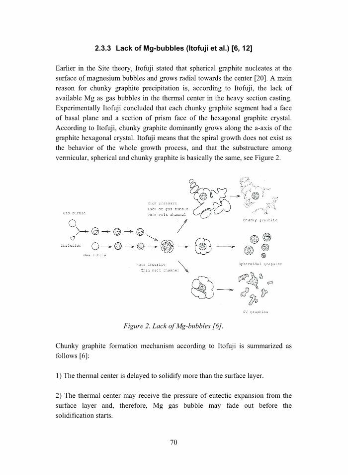
70
2.3.3 Lack of Mg-bubbles (Itofuji et al.) [6, 12]
Earlier in the Site theory, Itofuji stated that spherical graphite nucleates at the surface of magnesium bubbles and grows radial towards the center [20]. A main reason for chunky graphite precipitation is, according to Itofuji, the lack of available Mg as gas bubbles in the thermal center in the heavy section casting. Experimentally Itofuji concluded that each chunky graphite segment had a face of basal plane and a section of prism face of the hexagonal graphite crystal. According to Itofuji, chunky graphite dominantly grows along the a-axis of the graphite hexagonal crystal. Itofuji means that the spiral growth does not exist as the behavior of the whole growth process, and that the substructure among vermicular, spherical and chunky graphite is basically the same, see Figure 2.
Figure 2. Lack of Mg-bubbles [6].
Chunky graphite formation mechanism according to Itofuji is summarized as follows [6]:
1) The thermal center is delayed to solidify more than the surface layer.
2) The thermal center may receive the pressure of eutectic expansion from the surface layer and, therefore, Mg gas bubble may fade out before the solidification starts.
71
3) Small numbers of Mg gas bubbles can exist in the melt under such a circumstance and graphite precipitates into them as spherical graphite at the early stage of the solidification.
4) Liquid Mg, caused by the pressure of eutectic expansion, segregates at austenite shell or dendrite-residual melt interface. The critical pressure is a few atoms at near-solidification temperature and the eutectic expansion has reported 5060 atoms in eutectic composition.
5) At the middle stage of the solidification, after spherical graphite has precipitated, chunky graphite starts to precipitate. If inclusions exist, for example Mg-Ca-Si-S-O system inclusions, at a carbon-rich area, graphite would precipitate at melt inclusion interface. The site between austenite dendrites and between austenite shell and dendrite might also act as the nucleation site for chunky graphite. During growth, chunky graphite ends have contact with residual melt through thin melt channels.
2.3.4 Loose coupling between eutectic phases (Zhou et al.) [9]
Zhou, Schmitz and Engler´s theory on chunky graphite formation is based on heterogeneous nucleation of graphite and loose coupling between the eutectic phases. According to Zhou et al., different graphite morphologies can be ascribed to the degree of coupling between the graphite and the austenite phases during the eutectic solidification. The chunky graphite grows with looser coupling between the austenite compared to flake graphite but not as loose as for spherical graphite. The graphite can twist, arch or branch undisturbed due to the relaxed/loose coupling with the crystallizing austenite [9], see Figure 3.

72
Figure 3. Coupling between austenite and graphite [9].
Schematic representation of the development process of chunky graphite in hypereutectic spheroidal cast iron, according to Zhou et al, can be seen in figure 4. The process is divided into four different parts:
1) Shortly before reaching the eutectic temperature primary graphite nodules are formed. Independently austenite dendrites are formed at the same time.
2) Shortly after reaching the eutectic temperature the crystallization of chunky graphite starts near by the austenite dendrites.
3) After nucleation, eutectic chunky graphite cells continue to grow in the melt during eutectic solidification. The precipitation of graphite and austenite take place parallel with loose coupling between graphite and austenite. During the eutectic solidification the chunky graphite cells will bump into segregated elements in the melt (Mg, Mn, Mo, Cr, V, B, Ti). New chunky graphite cells are formed during the eutectic solidification. The growth of chunky graphite proceeds by precipitation of carbon directly from melt.
4) The eutectic growth is ended at a certain size. Elements insoluble in graphite as well as austenite segregates to the rest melt areas. Those elements affect the solidification process in the rest melt area. For example the available Mg in this area will favor the formation of spherical shaped graphite. Also carbides will easily form in the grain boundaries.

73
Figure 4. Chunky graphite formation (Zhou et al.) [9].
2.3.5 Constitutional supercooling (Gagné and Argo) [11]
According to Gagné and Argo, the growth mechanism of chunky graphite is of spiral type on the basal plane. They revealed that the diameter of the strings was relatively constant along its length, which implies that the growth rate on the basal plane has a much higher magnitude compared to the growth rate on the prism plane of the graphite crystals. Spiral crystal growth on the basal plane proceeds as would a screw dislocation and can be achieved only in presence of a high driving force. Considering the solidification of ductile iron, Gagné and Argo concluded that the major driving forces that could be responsible for such a spiral crystal growth pattern are carbon supersaturation and large supercooling level. Other variables could be complimentary.
In regions displaying carbon supersaturation, caused by a high carbon equivalent, chunky graphite strings extend very rapidly because of the availability of the carbon atoms to precipitate on the basal planes of the graphite crystals.
Carbon supersaturation cannot be the only factor ensuring the formation of chunky graphite, but in combination with high supercooling level Gagné and Argo found a strong driving force that favored the spiral growth. A large constitutional supercooling in the center of a heavy section ductile iron casting may be caused by several factors:

74
• Low nucleation potential.
• As the casting solidifies the concentration of solute atoms in the liquid just ahead of the solid/liquid interface should tend to increase. Consequently, lower and lower temperatures are required for continued solidification.
• The temperature at the center of the casting tends to approach that of the interface as the latter get closer together. This effectively flattens out the contour of the temperature-distance curve in the liquid generating a high degree of supercooling in the center of a casting.
• The supercooling should be enhanced in sand-cast ductile iron castings. As the solidification front advances, the heat extraction at the interface metal-sand eventually exceeds the latent heat of solidification of the remaining liquid metal. It results in a rapid cooling of the remaining liquid and in a high degree of localized supercooling.
The mechanism by which branching of chunky graphite occurs remains obscure to Gagné and Argo. However, they recalled that branching during growth on the basal plane has been reported to be due to the occurrence of crystal defects on the growing crystallographic planes that serve as nucleating sites for new graphite strings. The rapid growth of the chunky graphite filaments should favor the occurrence of such defects [11].
2.3.6 Theory of vermicular graphite iron formation (Deng et al.) [21]
Literature reports that chunky graphite shows a partly coupled growth between graphite and austenite phases and that its morphology is similar to vermicular graphite. The chunky graphite can be separated from the vermicular graphite by its finer structure and its only local appearance [13, 15]. The theory of structure and formation of vermicular graphite formulated by Deng, Zhu and Liu is interesting in comparison to the chunky graphite formation. Deng et al reported that necessary conditions to obtain vermicular graphite should be the insufficient modifier addition or the presence of interfering elements. The modifiers need a dissolving period. Therefore there can be some areas of rich modifier even after its complete dissolution. Spheroidal graphite may be formed in these areas, but in the insufficient areas, flake graphite will mainly be produced. Various types

75
of graphite can co-exist in the iron. It was found that vermicular graphite was formed mainly in two ways. In the first, it grew out from flake graphite; in the second it degenerated from spheroidal graphite, Figure 5. The growth direction of vermicular graphite often changes from a-, to c-direction, or vice versa. Because of the influence of modifying elements, the vermicular graphite is twisted severely, changing its growth direction continually and branching frequently. It was suggested that redistribution and uneven distribution of modifying elements play an important role in the formation of vermicular graphite. The mechanism on which the graphite transfers its growth direction due to the effect of modifiers has been explained with the unstability of (10T0) growth interface. During the whole process of eutectic solidification, the tips of the vermicular graphite are always in contact with the melt and grow coupled with austenite [21].
Figure 5 Vermicular graphite formation (Deng et al.) [21].
3. Experimental work
In order to confirm some of the facts reported in the literature experimental work has been carried out. A geometry consisting of five 200 x 200 mm plates with thickness ranging from 10 mm to 200 mm were used, Figure 6. Several melts were produced in a 250-kg induction furnace and cast in furan bonded sand moulds in order to attain chunky graphite containing microstructures. Varying amounts of chunky graphite was achieved by changing parameters as inoculation, Mg-content and casting temperature, Table 2.

76
Figure 6. Pattern for experimental work.
Table 2. Parameters for experimental work.
MELT: A B C D E
Pouring temperature (°C) 1555 1547 1550 1556 1540
Mg-content (%) 0,058 0,052 0,057 0,045 0,063
Casting temperature (°C) 1400 1400 1400 1400 1340
Mould inoculation (%)
0,07 (X*) 0 0 0,07
(X*) 0,07 (X*)
Stream inoculation (%)
0,10 (Y*)
0,15 (Y*)
0,10 (Z*)
0,10 (Y*)
0,10 (Z*)
*See table 3
Chemical analyses of the three different inoculants used are shown in table 3. The C content in the castings were adjusted to 3.23.4 % and Si to 3.23.4 %.

77
Table 3. Chemical composition (%) of inoculants used in experimental work.
Si
Mg
Al
Ca
Mn
Zr
Ba
Ce)
Size (mm)
X (in mould) 64 1,10 1,20 1,20 3,30 3,90 - - block
Y (stream) 73 - 1,20 1,20 - - 1,10 - 0,2-
0,7
Z (stream) 73 - 1,0 1,0 - - - 1,7
Mechanical properties was determined by tensile tests according to SS 11 21 27 14Q70. Test bars were machined out from the castings located as shown in Figure 7. The microstructure in the vicinity of the fracture surface of the tensile test bars was investigated under optical and scanning electron microscope (SEM). The graphite morphology was further revealed by deep etching technique using 1:3 HCl + HNO3 for approximately 20 minutes.
Figure 7. Location of thermocouples and test bars.
4. Results
4.1 Mechanical properties
Evaluation of the mechanical properties showed that the ultimate tensile strength (Rm) and the elongation (A) decreased as chunky graphite was present. The yield strength (Rp02) and the Brinell hardness (HBW) were hardly affected though. The ruthless affect of chunky graphite morphology on the elongation value is
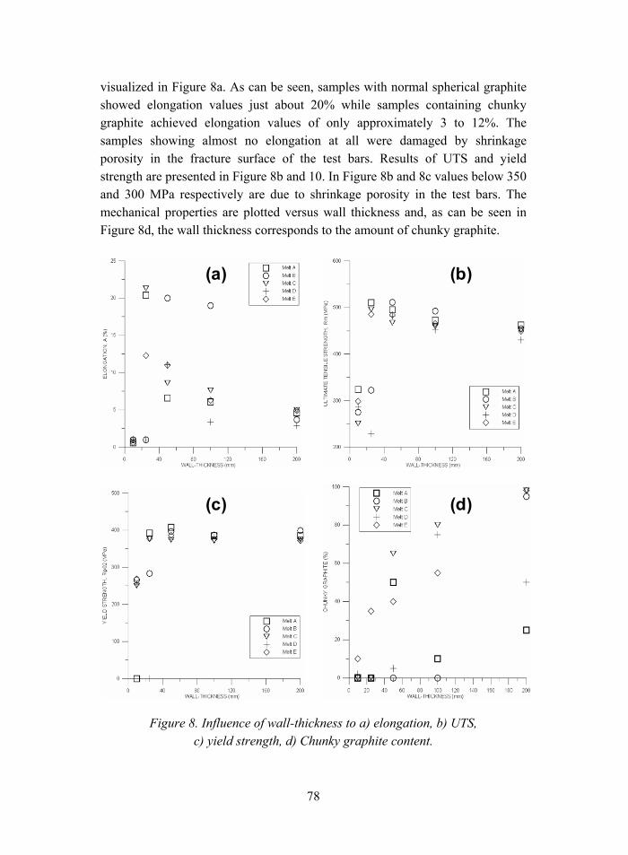
78
visualized in Figure 8a. As can be seen, samples with normal spherical graphite showed elongation values just about 20% while samples containing chunky graphite achieved elongation values of only approximately 3 to 12%. The samples showing almost no elongation at all were damaged by shrinkage porosity in the fracture surface of the test bars. Results of UTS and yield strength are presented in Figure 8b and 10. In Figure 8b and 8c values below 350 and 300 MPa respectively are due to shrinkage porosity in the test bars. The mechanical properties are plotted versus wall thickness and, as can be seen in Figure 8d, the wall thickness corresponds to the amount of chunky graphite.
(a)
(d)(c)
(b)(a)
(d)(c)
(b)
Figure 8. Influence of wall-thickness to a) elongation, b) UTS, c) yield strength, d) Chunky graphite content.

79
The macro structure of chunky graphite causes a localized darkening of the surface of a sectioned casting that makes the degenerated graphite easily detected. While investigating the fracture surfaces of tensile test bars local dark areas of various sizes were detected. Comparisons to the microstructure show that the size of the dark areas corresponds very well to the amount of chunky graphite, Figure 9.
Figure 9. Fracture surfaces of test bars (14 mm diameter). Black areas correspond to the amount of chunky graphite in the microstructure.
4.2 Microstructure
Microscope examination of the microstructure confirmed that the chunky graphite forms eutectic cells, most often located in the vicinity of austenite dendrites, Figure 10. Scanning electron microscope examination of deep etched samples showed that the graphite is widely branched and interconnected in a network within each eutectic cell, Figure 11. At the outer boundary of each eutectic cell an obvious coarsening of the graphite was detected, Figure 10. The amount of chunky graphite was visually approximated through area analyses of the microstructure, Table 4.

80
Figure 10. Eutectic chunky cell.
Figure 11. Chunky morphology.

81
Table 4. Amount (%) of chunky graphite in fracture surface of test bars.
Plate (mm)
Melt A Melt B Melt C Melt D Melt E
10 0 0 0 2 10
25 0 0 0 0 35
50 50 0 65 5 40
100 10 0 80 75 55
200 25 95 98 50 98
5. Discussion
Opinions in the literature are reasonably well uniform regarding the importance of low carbon equivalent, non-excessive amount of rare earth elements and of the use of chills to prevent chunky graphite formation. It is also accepted knowledge that the chunky graphite grows in direct contact with the melt forming eutectic cells and that the graphite are heavily branched and interconnected within each eutectic cell.
Depending on weather the chunky graphite forms before or after the spherical graphite, the opinion that high nodule counts reduce the potential risk of chunky graphite formation may or may not be a cause-and-effect relationship [16]. The difficult task to manage though is that every factor that increases the number of nodules, such as high carbon equivalent, use of Ca, Ce, Al or RE bearing inoculants etc., also seems to promote chunky graphite formation [10, 16]. The experimental work in this paper confirmed that the use of inoculants containing Ce increased the amount of chunky graphite and a minimized use of inoculants containing Al, Ca, decreased the amount of chunky graphite. The results from different researchers imply that the pouring temperature is not a main significant factor of chunky graphite formation. Experiments in this paper using low casting temperature resulted in more chunky graphite even in thin sections but the result is not excluding clear since Ce containing inoculant and higher Mg level were used as well.

82
The purity of the charge material has to be related to the amount of RE in the sense that high purity charges in combination with excessive amount of RE will promote chunky graphite formation [10]. While the use of RE is highly recommended in the production of ductile cast iron (improved nodule count, improved nodularity, reduced magnesium requirement) the presence of RE in amounts greater than that required to improve nucleation and to react with subversive elements promotes chunky graphite. It is unified opinion in the literature that Sb is most suitable to add from the elements that remedy chunky graphite. The Sb addition should mainly be made to balance excessive amounts of Ce.
In the different theories regarding chunky graphite formation and growth it has been suggested that chunky graphite nucleate and grow in a manner similar to, or as a degenerated form of spheroidal graphite. Theories state both the a- and c-directions as the main growth directions. Since the chunky graphite resembles the vermicular graphite morphology it is interesting to compare the theory of Deng et al where the vermicular graphite either grow out from flake graphite or degenerates from spheroidal graphite. The growth direction of vermicular graphite often changes from a- to c-direction, or vice versa. The influence of various amount of modifying elements during the solidification sequence makes the graphite twist and change growth direction resulting in the branched morphology. The presence of modifying elements as Mg and RE as well as other surface active elements as S or O influence the growth of graphite. The solid solubility of these elements is small in austenite and those elements will gradually move and enrich into residual molten iron and at the freezing front [5, 8]. The atomic dimension of RE is about 1.5 times as large as that of iron. Usually, RE atoms diffuse with difficulty in a solid phase, but the condition of slow solidification of heavy section ductile iron contributes to the diffusion of RE, according to the principle of chemical equilibrium distribution. Therefore, with slow solidification, the elements of RE, Mg, S and O should enrich at the freezing front more and more [5]. The nodulizing effect of Mg and RE makes the eutectic graphite grow up with screw dislocations along the crystal orientation (0001), leading to the eutectic graphite to possess the growing characteristics of spherical graphite. On the other side, S, O and RE promote the eutectic graphite to branch frequently, making the eutectic graphite become chunky graphite [5]. At the interface, on which chunky graphite begins to appear, not only the elements of RE, Mg, S and O but also carbon enriches. Carbon reaches the state of supersaturation. The enrichment of RE might

83
obstruct carbon to expand through austenite shell and to deposit on spherical graphite. RE-oxides and RE-sulfides may become cores to graphite at interface of solid-liquid when carbon is in the state of supersaturation in liquid. All of these may promote the formation of intercrystalline eutectic graphite [5].
The hypothesis of constitutional supercooling as the main driving force for chunky graphite formation is vindicated by the fact that increased heat exchange rate by using chills and maintaining a uniform temperature by thermal mixing, impede constitutional supercooling and chunky graphite formation [11]. The fact that chunky graphite sometimes resembles ATM type D flake graphite also support the theory that some kind of supercooling take place as well as the growth certainly can be out from flake graphite.
Because of the degradation of mechanical properties in chunky graphite containing ductile cast iron and the fact that no unified theory for its formation has yet been proposed, further research is important to fully understand the formation mechanism of chunky graphite. Especially since the industrial use of heavy section ductile cast irons is increasing. From the work in this paper it will be interesting to further investigate the role of constitutional supercooling and the presence of surface active elements as S an O in the chunky graphite regions.
6. Conclusions
• Chunky graphite is branched and interconnected in a network within eutectic cells.
• The ultimate tensile strength and especially the elongation are severely lowered when chunky graphite appears in the microstructure while hardness and yield strength are not affected.
• Low carbon equivalent, non-excessive amount of rare earth elements and the use of chills prevents chunky graphite formation to a great extent.
• The purity of the charge material has to be related to the amount of RE in the sense that high purity charges in combination with excessive amount of RE will promote chunky graphite formation.

84
• It is unified opinion in the literature that antimony is most suitable to add from the elements that remedy chunky graphite. The Sb addition should mainly be made to balance excessive amounts of Ce.
• Chunky graphite seems to grow alternating in a- and c-direction and changes to constant spherical like growth at the outer boundary of the eutectic cells.
• No single unified theory of chunky graphite formation and growth has yet been proposed.
Acknowledgements
Acknowledgements to Arvika Foundry in Sweden for providing the charge material used in the experimental work and to the Scandinavian Foundry School for carrying out the melt and casting work.
References
1. Hoover, H. W. Jr. A literture Survey on Degenerate Graphite in Heavy Section Ductile Iron. Colt Ind./Fairbanks Morse Engineering Division, Beloit. AFS Transactions 86-102, 1986, pp. 601608.
2. Kaufmann, H. Zur schwingfesten Bemessung dickwandiger Bauteile aus GGG-50 unter Berücksichtigung hiesstechnisch bedingter Gefügeungänzen. 1998. LBF-Bericht NR. FB-214.
3. Cox, G. J. Giesserei-Praxis (Germany). Vol. 18, Sept. 1992, pp. 274276.
4. Breitkreutz, K., Frenz, H., Portella, P. D. Zur quantitativen Bestimmung des Chunky-Graphits in Gusseisen. Prakt Met. 28, 1991, pp. 523541.
5. Niu, Y. and Zhu, Z. A study of the rare earth effect on chunky graphite formation in heavy section ductile iron. China. The Foundryman, August 1988.

85
6. Itofuji, H. and Uchikawa, H. Formation Mechanism of Chunky Graphite in Heavy-section Ductile Cast Irons. Ube Steel Co., Ltd., Japan. AFS Transactions 90-42, 1990, pp. 429448.
7. Liu, P.C., Li, C.L., Wu, D.H. and Loper, Jr. SEM Study of Chunky Graphite in Heavy Section Ductile Iron. AFS Transactions 83-51, 1983, pp. 119126.
8. Zhang, Z., Flower, H. M. and Niu, Y. Classification of degenerate graphite and its formation processes in heavy section ductile iron. China. Materials Science and Technology, July 1989, Vol. 5, pp. 657664.
9. Zhou, J., Schmitz W. and Engler, S. Untersuchung der Gefügebildung von Gusseisen mit Kugelgraphit bei langsamer Erstarrung. Giessereiforschung, 39 Heft 2, 1987, pp. 5570.
10. Xi, T. C., Fargues, J., Hecht M. and Margerie J.C. Formation and prevention of chunky graphite in slowly cooled nodular irons. Mat. Res. Soc. Symp. Proc. Vol. 34, 1985, pp. 6776.
11. Gagné, M. and Argo D. Heavy Section Ductile Iron Castings Part I and Part II. Canada. Proceedings of an International Conference on Advanced Casting Technology, Kalamazoo, Michigan, USA, 1214 November 1989. Pp. 231256.
12. Itofuji, H. and Masutani, A. Nucleation and growth behaviour of chunky graphite. Ube Steel Co., Ltd., Japan. Int. J. Cast Metals Res., 14, 2001, pp. 114.
13. Prinz, B., Reifferscheid, K.J., Schulze, T., Döpp, R. and Schürman, E. Untersuchung von Ursachen von Graphitentartungen bei Gusseisen mit Kugelgraphit in Form von Chunky-Graphit. Germany. Giessereigorschung 43, 1991, Nr. 3, pp. 107115.
14. Strizik, P. and Jeglitsch, F. Contribution to the Mechanism of Formation of Chunky Graphite. Austria. AFS International Cast Metals Journal, September 1976, pp. 2330.
15. Chunky-Graphit, Internal publication ÖGI, 1998.

86
16. Karsay, S.I., Campomanes E. Control of Graphite Structure in Heavy Ductile Iron Castings. Canada. AFS Transactions, pp. 85-92.
17. Karsay I. S. Ductile Iron Production I. 1976. QIT Corporation.
18. Moore, W.H. and Pritsker, L. Influence of Antimony on nodular cast iron in various castings sections. Meehanite Worldwide Report No. E. 1307.
19. The Sorelmetal Book of Ductile Iron. 2004. Rio Tinto Iron & Titanium. Canada.
20. Itofuji, H. Proposal of Site Theory. Ube Steel Co., Ltd., Japan. AFS Transactions 96-131, 1996, pp. 7987.
21. Deng, X. J., Zhu, P. Y. and Liu, Q. F. Structure and Formation of Vermicular Graphite. China. AFS Transactions 86-173, 1986, pp. 927934.

Inspection and quality assurance
Development of a high resolution X-ray radiographic technique, optimized for on-site testing in radioactive environments ................. 89
L. Hammar & H. Wirdelius
Filtering technique applied to synthetic radiograms and images from a high resolution digital radiographic system........................... 101
H. Wirdelius & L. Hammar
Ultrasonic assessment of material degradation by thermal fatigue 123 Jorma Pitkänen, Pentti Kauppinen & Harri Jeskanen
Evaluation of near surface defects and fatigue properties of cast iron ....................................................................................... 133
Jouni Alhainen, Jussi Solin & Matti Johansson
Round robin on Nondestructive Testing evaluation of a cast truck component ....................................................................................... 157
Ulla Boman
Quality assurance of cast pistons for large diesel engines ............. 169 Sakari Pisilä

89
Development of a high resolution X-ray radiographic technique, optimized for on-site testing in radioactive environments
L. Hammar, H. Wirdelius Chalmers University of Technology
Gothenburg, Sweden.
Abstract
A high resolution x-ray radiographic system has been developed, based upon scintillation fibre optics. One of the goals in the design process was to achieve as high overall system resolution as possible. Another was to restrict the size of the components. Hence the system is optimized for sizing and characterization of cracks in nuclear power plants.
The first part of this paper describes the components of the system. Such as the high resolution x-ray image detector and how the parameters of the system has been chosen during the design process.
The system is able to scan the test object from different directions and angles. The second part of the paper describes a mathematical model for the two separate, manipulating robots that handles the x-ray tube and the x-ray image detector. It is a general model that is applicable to any arbitrary configurations. A technique to calibrate theirs absolute positions relative to each other has been developed and is also included.
The third part is highlighting the problems associated with scintillating fibre optics and how to solve this problem.
The last section is about a method to use filters, based on statistical methods, to remove noise induced from the radioactive environment.

90
1. Introduction
A radiographic system optimized for crack characterization in nuclear power plats has been developed. One common type is inter-granular stress corrosion cracking (IGSCC) [Fig. 1]. This kind of cracks characterized by quiet narrow width and it contains of major part with branches. A typical 5 mm deep crack has a crack opening width in the range of 25-50 µm.
Figure 1. Cross section of an typical IGSCC.
The main idea in the design process was achieve as high radiographic sensitivity in the system as possible. To make the system suitable for on-site testing it had to have a limited physical size. The NDT-system (x-ray machine, x-ray image detector and the manipulating robot) was optimized as follows. The first step was to develop a suitable x-ray image detector. The requirements were high spatial resolution and dynamics at high energies to make it suitable for object thicknesses equivalent to 60 mm steel. Next step was to choose a radiation source. In an early stage isotopes were excluded due to their lack of intensity. A 450 kV x-ray machine with a small focus size found to be the optimum for our needs. The x-ray tube was then equipped with a diaphragm to restrict the primary beam in order to only radiate the imaging area of the detector. To be able to take exposures in different angles around cracks, demands on the manipulating system concerning stiffness and relative position accuracy were postulated.

91
2. X-ray image detector optimization
In traditional x-ray converters as phosphor, spatial resolution and detection efficiency are in conflict. An improvement is to use structured CsI(Tl). The best approach to achieve high spatial resolution and high detection efficiency is to utilise a scintillating glass fibre optic faceplate (FOP) [1]. It is obvious that a traditional phosphor cant combine resolution and detection efficiency.
How a columnar CsI(Tl) is compared with scintillating FOP is not highlighted in this paper but interesting result has been achieved with 700 µm thick CsI(Tl)-screens [2]. When our system was designed (1995) there were only earlier versions of FOP available commercially. Since then both CsI(Tl) and FOP have been improved. There is also a difference between those two in light yield. Normally it is an advantage with high light yield, but if the lens is effective it produce too much light and will saturate the CCD-chip without reaching maximum contrast. In our solution a low light yield is preferable. To produce an x-ray image with high contrast is it the number of detected photons that is important (not to detect light only). To optimize the image detector we have tried to tune the light yield to the A/D-converter. As we use a 12-bit A/D-converter, full well capacity in the CCD should correspond to the amount of the available digitization levels. As we use a 12-bit (4096 levels) A/D-converter a saturated CCD correspond to about 4000 detected photons/pixel.
First we decided to optimize the system for an object thickness equal to 60 mm steel. Calculations of x-ray output and attenuation coefficients were made with software [3] to simulate filtered spectrum from a 450 kV x-ray tube. The diagram shows the filtered x-ray spectrum after a 60 mm thick steel object. The simulation is with maximum power of a 450 kV constant potential x-ray tube (Philips MG451).
The detection efficiency is about 33% and corresponds to 73 000 detected photons in the diagram [Fig. 2]. Data to simulate the detection efficiency for our scintillating FOP (a glass material named LG9) were available in reference [1].

92
10 40 70 100 130 160 190 220 250 280 310 340 370 400 430kV
0
2000
4000
6000
8000
10000
12000
14000
Phot
ons
/ mm
2 /s
Filtered spectrumAttenuatedAbsorbed450 kV, 2 mAFFD=500 mm60 mm steel
10 40 70 100 130 160 190 220 250 280 310 340 370 400 430kV
0
2000
4000
6000
8000
10000
12000
14000
Phot
ons
/ mm
2 /s
Filtered spectrumAttenuatedAbsorbed450 kV, 2 mAFFD=500 mm60 mm steel
10 40 70 100 130 160 190 220 250 280 310 340 370 400 430kV
0
2000
4000
6000
8000
10000
12000
14000
Phot
ons
/ mm
2 /s
10 40 70 100 130 160 190 220 250 280 310 340 370 400 430kV
0
2000
4000
6000
8000
10000
12000
14000
Phot
ons
/ mm
2 /s
10 40 70 100 130 160 190 220 250 280 310 340 370 400 430kV
10 40 70 100 130 160 190 220 250 280 310 340 370 400 430kV
0
2000
4000
6000
8000
10000
12000
14000
Phot
ons
/ mm
2 /s
0
2000
4000
6000
8000
10000
12000
14000
0
2000
4000
6000
8000
10000
12000
14000
Phot
ons
/ mm
2 /s
Filtered spectrumAttenuatedAbsorbed
Filtered spectrumAttenuatedAbsorbed450 kV, 2 mAFFD=500 mm60 mm steel
450 kV, 2 mAFFD=500 mm60 mm steel
Figure 2. Simulated filtered spectrum and detection efficiency of a 10 mm scintillating FOP.
tca T·T TDE ⋅= (1) DE = scintillating output energy / photon input energy Ta = 0,33 (absorbed photon energy / incident photon energy) Tc = 0,09 (generated scintillating light / absorbed photon energy) Tt = 0,04 (output scintillating light / generated scintillating light)
If equation (1) is modified it will calculate the amount of light photons for each detected photon rather then the detection efficiency it can be used for optimizing the hole chain from the input scintillating FOP to the signal to the A/D-converter.
6,3
2ccdrtce QEFTTPh
CE⋅⋅⋅⋅
= (2)
CE = number of electrons / incident photon energy Phe = 300 [keV] (incident photon energy) Fr = 0,7 (Fresnel losses in coupling interfaces) QEccd = 0,25 (quantum efficiency in CCD)
As a pixel size of 22,5 · 22,5 µm2 is used is 35 photons are detected (/pixel/s). The final solution for the x-ray image detector was then ordered after discussion with the delivering company, Photonic Science [4]. The ordered x-ray image detector was a modified standard image detector (XIOS 1:1) with an

93
interchangeable scintillating FOP as input screen. The material in the FOP is a Tb2O3 activated, fused glass fibre optic, with 20 µm fibre diameter. The FOP is connected to a fibre optic lens with a length of 100 mm and 6 µm fibre diameter. The fibre optic lens is manufactured from a heavier glass material then the FOP to protect the CCD from primary radiation. In the end of the lens is the CCD-chip mounted. It is a full frame CCD (EEV-0530 MPP) of 1:th grade with a size of 1320 · 1150 pixels. The full well capacity is 300 000 e-. The readout circuit works at 200 kHz and the read out time for a full image is 7 s.
Electronics
Cooling andtungsten shield CCD
Scintillating FOP
Light guide
Tungsten shield
Inputwindow
Electronics
Cooling andtungsten shield CCD
Scintillating FOP
Light guide
Tungsten shield
Inputwindow
Electronics
Cooling andtungsten shield CCD
Scintillating FOP
Light guide
Tungsten shield
Inputwindow
Figure 3. Schematic sketch of the x-ray imaging detector.
The CCD-chip is cooled with two stage (Peltier) cooling. The CCD-chip and the readout electronics is also protected from background radiation with wolfram blocks. The front is covered with tungsten shielding with an input window with an area of 28 · 26 mm2. The overall length of the x-ray camera is 240 mm and the diameter is 120 mm. Tests to measure the resolution of the system at 400 kV was carried out according to EN 462-5. The result is in figure below [Figure 4]. The image quality indicator is made of platinum and the diameter of the smallest wires is 50 µm with the same distance between them.

94
Line Profile
Distance (Pi xel)
Intensity
0 10 20 30 4090
100
110
120
130
Line Profile
Distance (Pi xel)
Intensity
0 10 20 30 4090
100
110
120
130
Line Profile
Distance (Pi xel)
Intensity
0 10 20 30 4090
100
110
120
130
Line Profile
Distance (Pi xel)
Intensity
0 10 20 30 4090
100
110
120
130
Line Profile
Distance (Pi xel)
Intensity
0 10 20 30 4090
100
110
120
130
Line Profile
Distance (Pi xel)
Intensity
0 10 20 30 4090
100
110
120
130
Figure 4. Resolution measured according to EN 462-5 (400 kV, 20 mm steel).
3. Positioning equipment
To be able to detect cracks with an x-ray system, the x-ray beam has to be fairly parallel to the crack. The relationship between the depth and width of a crack with the viewing angle and the performance of the x-ray system can be analyzed. A classical formula [5] has been used for traditional film radiography and is a useful tool to predicting crack sensitivity.
( ) ⎟⎟⎠
⎞⎜⎜⎝
⎛++Θ+Θ⋅=⋅
D
ST I
IUWdConstWd 1)cos()sin( (3)
ID = Primary radiation IS = Scattered radiation µ = Attenuation coefficient UT = Total un-sharpness
( )22 / SFDtfUU FT +≥ Uf = Inherent un-sharpness f = Focus spot size SFD = Source to film distance t = Object thickness
Θ
Wd
To optimize each parameter in equation (3), best possible result can be achieved. Some factors are not relevant to digital x-ray system, but relationship between width and depth to the angle is the same. The constant on right hand in equation (3), is only available for film radiography and should be replaced by a corresponding factor for the contrast sensitivity of the image detector. To be sure

95
that a crack will be detected it is necessary to make a series of exposures with a small displacement in angle between each exposure. From our experience a series of exposures from -15º to +15º with an angular displacement of 1º is very effective to be shore that most parts of a crack, including sub-branches in the case of IGSCC, will be detected. Based on this theoretically considerations the positioning equipment was developed [Fig. 5].
To make the system easy to use we decided in an early stage to make the manipulating in two, separate units. The reason was to make it more versatile and avoid specially designed, object specific, manipulating units. A very important aspect with NDT examinations in nuclear environments is the background radiation level. The time for NDT technicians to stay in the radioactive environments has to be minimized. To minimize that time a technique to calibrate the relative positions of each manipulating unit is developed. A hair-cross like device is mounted in the front of the image detector during calibration procedure. By moving the x-ray tube into a numbers of positions and line up the image detector so that the hair-cross verifies that the focus of the x-ray tube is on the vector in the centre of the x-ray image detector. When this is done it is possible to transform the coordinate system of the manipulating unit for the x-ray tube into the coordinate system of the x-ray image detector. When the internal calibration is done it is possible to rotate around any arbitrary point with high accuracy e.g. the opening of a crack inside the object to be examined.
4. Scintillating fibre optics
The fibre scintillating fibre optics used is non-uniform in the sense that the individual fibre has different conversion efficiency. A chicken- wire pattern is visible in the raw image. To compensate for this effect a standard image operation, background compensation, is used (4). An exposure with a background image is made from the same material and thickness as the object of interest. To avoid negative values a zero-image with no radiation is also needed since the zero-level in the A/D-converter is adjusted slightly over zero.
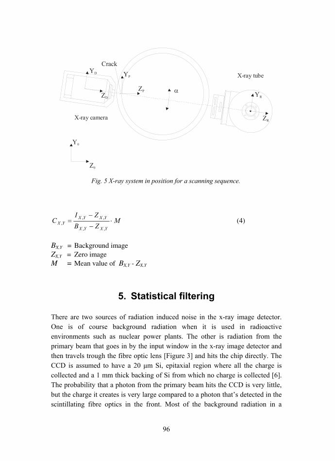
96
X-ray camera
X-ray tube
ZD
YD
ZP
YP
Crack
ZR
YR
Z0
Y0
α
Fig. 5 X-ray system in position for a scanning sequence.
MZBZI
CYXYX
YXYXYX ⋅
−
−=
,,
,,, (4)
BX,Y = Background image ZX,Y = Zero image M = Mean value of BX,Y - ZX,Y
5. Statistical filtering
There are two sources of radiation induced noise in the x-ray image detector. One is of course background radiation when it is used in radioactive environments such as nuclear power plants. The other is radiation from the primary beam that goes in by the input window in the x-ray image detector and then travels trough the fibre optic lens [Figure 3] and hits the chip directly. The CCD is assumed to have a 20 µm Si, epitaxial region where all the charge is collected and a 1 mm thick backing of Si from which no charge is collected [6]. The probability that a photon from the primary beam hits the CCD is very little, but the charge it creates is very large compared to a photon thats detected in the scintillating fibre optics in the front. Most of the background radiation in a

97
nuclear power plant, when it is accessible for non destructive examinations, consists of radiation from 60Co contaminations. The background radiation gives the same effect as from the photons from the primary beam. It is complicated to simulate the deposition of charge from an attenuated x-ray in the CCD. The photons from the primary beam thats hit the CCD has high energy due to the filtration trough the test object (usually 4060 mm of steel) and the fibre optic lens. The dominant attenuation process at that energy in Si is the Compton-effect. There is only a part of the energy that will absorb the rest of the energy will scatter away. The dominate direction is forward and the energy that will be deposit is from the Compton electron. If the radiation originates from 60Co it will have higher energy when it hits the CCD.
Instead of simulate the process a series of test has been done to measure the energy that will be deposit in the pixels. The mean range from a secondary electron in the CCD is short. It means that when a pixel is hit by an x-ray it deposit most of the energy in one single pixel and its neighbours.
By dividing each exposure in sub-exposures with identical exposures data can they be compared pixel by pixel. To distinguish between light generated in the scintillating FOP and charge directly deposited n the CCD a special type median filter has been developed (5). By sorting the data with the same pixel from each sub-image, in a vector and then take the median value from the vector, can a criterion be used to separate values originated from primary radiation and radiation induced noise in the CCD.
)),...,2,1(( , nPMax YX will be rejected if (5)
)),...,2,1(()),...,2,1(()),...,2,1(( ,,, nPMedianCnPMediannPMax YXYXYX ⋅>−
then it continues with
)),..,2,1(()),..,2,1(())1,..,2,1(( ,,, nPMedianCnPMediannPMax YXYXYX ⋅>−−
until no more values will be rejected. The pixel value (PX,Y), is the mean value of all accepted values from the sub-images. The constant (Const) is the confidence interval of the normal distribution. Const = 1,96 (95% confidence) Const = 2,58 (99% confidence)

98
P(1,x-1,y) P(1,x-1,y+1)P(1,x-1,y-1)
P(1,x+1,y) P(1,x+1,y+1)P(1,x+1,y-1)
P(1,x,y) P(1,x,y+1)P(1,x,y-1)
P(1, , )
P(2, , )
P(n, , )
Fig. 6 Pixel notation in sub-images.
Instead of simulating the phenomenon a series of tests has been carried out. The tests were done without the scintillating FOP, with the energy set to 400 kV and a steel object with 50 mm in thickness, were used. From our test it was obvious that about 0,1% of the values from the sub-pixels, were rejected. To make the algorithm more efficient, the neighbour pixel [Figure 6] to those how are rejected are also excluded.
6. Discussion
The system has been working well and despite that the imaging detector has been heavily exposed for more than 1000 hours at high energies, the CCD have not been damaged. In the next version of the image detector, a new construction will be used in order to avoid exposure of the CCD with primary radiation. The scintillating fibre optic will also be replaced with one with improved quality alternatively with a thicker CsI(Tl) if this gives better resolution [3]. The image sequences from the scanning around the cracks have given a new dimension to crack characterisation. It is planned to be developed refined methods for sizing

99
of crack by using spatio-temporal filtering methods. The needs for filtering methods [7] to eliminate problems from variations of thicknesses and attenuations in objects has been highlighted when it is difficult to present image with more than 8 bits.
References
1. Shao, Hua, Miller, Don W. and Pearsall, Robert C. Scintillating Fiber Optics and Their Applications in Radiographic Systems. IEEE Trans. Nucl. Sci., April 1991. Vol. 38, no. 2, pp. 845857.
2. Nagarkar, V. V., Gordon, J. S., Vasile, S., Gothoskar, P. and Hopkins, F. High Resolution X-Ray Sensors for Non Destructive Evaluation. IEEE Trans. Nucl. Sci., June 1996. Vol. 43, no. 3, pp. 15591563.
3. Harmonex X-Ray, 2369 Laura Lane Mtn. View, CA, USA, +94043 (415) 968 13 56.
4. Photonic Science, Millham, Mountfield, Robertsbridge, East Sussex, TN32 5LA, England, +44 1580 881199.
5. Halmshaw, R. Industrial Radiology. Applied Science Publisher, London, England, 1982.
6. Flynn, M. J., Hames, S. M., Wilderman, S. J. and Ciarelli, J. J. Quantum Noise in Digital X-Ray Image Detectors with Optically Coupled Scintillators. IEEE Trans. Nucl. Sci., August 1996. Vol. 43, no. 4, pp. 23202324.
7. Wirdelius, H. and Hammar, L. Modelling of a High Resolution Radiographic System and Development of a Filtering Technique Based on Wavelet Transforms. NDT&E International, 2004. Vol. 37, pp. 7381.

101
Filtering technique applied to synthetic radiograms and images from a high
resolution digital radiographic system
H. Wirdelius, L. Hammar Chalmers University of Technology
Gothenburg, Sweden.
Abstract
The first part of this paper describes a geometrical model of an iron cast object with a number of simple defects included in the volume. This model, together with a model of a specific digital X-ray system and procedure, is used to generate a simulated radiograph of the volume. This is then employed in the development of a filtering technique that extracts the grey-level information related to the existence of anomalies in the object. The wavelet-technique is applied in two different ways in order to identify the large-scale of a matrix (i.e. a radiograph). It turns out that both methods are able to remove the geometrical based information from the greyscale in the simulated radiographs.
The techniques are also verified with real radiographs taken from a number of welds and iron cast objects with different kinds of defects and defect sizes. The high-resolution digital X-ray system (HiReX) is able to detect defects less than one percentage of the object-thickness in the range of 2560 mm steel. The developed filtering technique is proven to enhance the detection of defects in objects with geometrical variations and has a potential to reduce time-consuming analysis of radiographs.
1. Introduction
According to the Swedish Nuclear Power Inspectorates requirements in the regulations concerning structural components in nuclear installations, in-service inspection must be performed using inspection methods that have been qualified. The qualification is based on a technical justification that provides evidence

102
about the reliability of the proposed NDT-system and a qualification of the testing personnel working according to a well-specified procedure. A high resolution digital X-ray system was developed [1] as a collaboration between a testing company (SAQ Kontroll AB) and Linköping Institute of Technology and this system was later qualified (1998) to detect, size and characterize stress corrosion cracks in thick walled steel components in nuclear plants.
In a number of occasions testing personnel have been qualified to detect according to their procedure but fail when it comes to characterization and sizing of the defects. This in view of the fact that utilized techniques (ultrasonic or in some case eddy-current) tends to be sensitive in their application as sizing tools when it comes to objects with complex combination of materials and geometries. The X-ray system applied in this project has a potential to be a supplement to NDT-systems that are able to detect the defects but are less successful in sizing of them. The development of the technique described in this paper indicates how to make this NDT technique independent any complex combination of materials or the geometry of the object.
Within a project that addresses standardization and quality control of large cast iron objects that will be exposed to fatigue stress this high resolution X-ray system (HiReX) has been used as reference system. The CCD-camera within the system generates 12 bits of information but the human eye can only separate less than 128 grey-levels, which corresponds to 7 bits of information. Defect information can saturate in grey-levels caused by large variation in thickness or attenuation coefficients in the object. The defect information can though be retrieved by alteration of contrast and brightness but is a time consuming procedure. These iron cast objects often tend to be of complex geometries, which have enforced the development of a filtering technique that withdraws the geometrical information from the radiograph.
Automated X-ray inspection systems in manufacturing industries often utilize CAD-based models in order to generate a perfect radiograph without any defects. This is then subtracted from the actual radiograph with the intention of extracting defect information, geometrical irregularities or to calibrate the system [2, 3]. These systems are most suited in production lines with a high degree of automation and products in large series. For in-service inspections and other applications where the inspected objects are more or less unique (e.g. iron cast objects, large scale components, food and humans) the radiograph itself can

103
instead be utilized to filter out the geometry within the image [4, 5]. The wavelet technique has turned out to be a very useful tool in image processing and noise reduction. As such it has been used in an automated crack detection system [6, 7]. In this paper the wavelet transform is instead used to identify the large scale information which is thereafter subtracted from the original radiograph. The described technique is developed for manual inspection. However it is believed to be applicable in automated system but with other crack identifying criteria than those described in [6, 7].
The first part of the paper, found in Section 2, describes a geometrical model of an iron cast object with a number of simple defects included in the volume. In Section 3 a model of a digital X-ray system is used to generate a simulated radiograph of this volume and the filtering techniques are validated against the model. In Section 4 the techniques are verified with real radiographs taken from a number of welds and iron cast objects with different kinds of defects. Concluding remarks are provided in Section 5.
2. A simplified geometric model of an iron cast object
The dark grey part in figure 1 is the part of the iron cast object that is to be tested with a digital X-ray system. If the object is assumed to be symmetric
( )((),( 22 yxzyxz += with the coordinate system defined according to the
lower part of figure 1) we can let the thickness of that particular part be defined as:
])([1])(([))(((
])([1])(([)(((2),(
722
422222
62
5
422
322
322
21
VVVV
VVVVV
cyxHcyxHyxcc
cyxHcyxHcyxccyxz
−+−−++−−+
−+−−+−++=(1)
with ),( yxH as the heaviside unit step function and VVV ccc 721 ..., are constants
fited to the modeled object.

104
Figure 1. The object and the simplified geometrical model (Mathematica® [8]).
The CCD-camera in the used NDT system only covers a minor part in each projection ( 2525× mm), which is indicated in Figure 1. The iron cast object has been manufactured by sand cocill technique which tends to provide the surface with more or less severe roughness and in order to include this, a surface roughness model was added. The surface roughness is modelled by adding the following contribution:
)])20()10()((sin[)(),( 22210
1
1 yngxngngngyxz rrrn
rroughness ++++∑==
π (2)

105
with )(2 ngr randomly distributed between 0 and 1 while the )(1 ngr coefficients are randomly distributed within a specified region in order to control the rms-value of the surface roughness. In this specific case a rms-value of 140µm was chosen in order to correlate to the actual object and also to be at the same scale as the defects.
In the volume, specified above, we introduce six different defects (coordinates ix0 and iy0 ). Four spherical cavities with diameters of 100µm and 200µm
( ic2 ) are located along the diagonal (see Figure 3). They are defined in equation (3) and could be stated to be equivalent to ideal shaped pores.
]))()([1)()()(((2),( 20
20
20
20
2iiiiiii cyyxxHyyxxcyxz −−+−−−+−−=∆ (3)
Other common defects among these kinds of objects are slag or intrusions. In order to model this kind of defect we introduce a circular cavity with a diameter of 500µm, but with the thickness randomly distributed between 100µm and 500µm (i.e. 1
ig in equation (4)). Since the model assume homogeneous attenuation coefficient the variation of thickness represents the variation in their product.
]))()([1(),( 20
20
1iiiii cyyxxHgyxz −−+−−=∆ (4)
The different types of defects described above are initiated in the material due to the manufacturing process but service induced cracks such as fatigue cracks also tend to appear. As a consequence of this, a simulated crack is also modelled. Its definition is found in equation (5) and in this specific case it is provided with a length of 4mm ( 02 y∆ ) and a height of 1mm ( ic ).
)])([)]([]2/)([(cos)])([)]([]2/)((cos[),(
0000008
000000xxxHxxxHxxx
yyyHyyyHyyycyxz
iii
iiiii∆+−∆−−∆−
⋅∆+−∆−−∆−=∆ππ
(5)
When the models of surface roughness and the defects are included, the thickness of the object as function of coordinates x and y is described by:
∑∆−+==
6
1),(),(),(),(
iiroughnessobject yxzyxzyxzyxz (6)

106
Figure 2. Six different defects are placed within the volume.
3. Simulation of Digital Radiography and reduction of information based on the geometry
The model of the NDT situation will only be used in the development of a filtering technique, which justify all the simplifications and idealisations it includes. Hence it does not include any beam hardening or secondary scattering effects. Mathematical models that do include these effects are however available in the literature [9, 10]. An equation that relates the properties of the used X-ray source, the material properties of the tested object and the resulting grey-levels can be found in [11].
The signal level ),( jiyccd (grey-level) in the CCD-camera pixel (i, j):
),(),(),,,(σtf)(),( jinnjmixjinmrAjiy em n
zCCD +−−∑∑= (7)

107
with )(rA as the aperture damping function, ),( jine is added electronic noise and ),,,(σtf jinmz is the overall imaging systems optical transfer function.
Equation (7) was developed for an X-ray image intensifier and since the NDT technique used in this case is based on the use of a cooled high resolution CCD camera operating with a 1:1 scintillator utilizing fibre optics technique, it can be simplified into:
),(),(σtf),( jixjijiy zCCD = (8)
Each individual pixel is also normalized with the corresponding zero energy value:
0000 )],(),()[,(σtf),(),(),( CCDzCCDCCDCCDnormCCD yjixjixjiyjiyjiyjiy +−=+−= (9)
with 0CCDy as the average zero energy grey level.
In order to level out the individual variance in the overall imaging systems optical transfer function, a background picture is produced for each individual object and the related energy level. This is produced by using a homogeneous object without any defects and with the same thickness and attenuation coefficient as the object of interest:
00 )],(),()[,(σtf),( CCDback
zbackCCD yjixjixjijiy +−= (10)
The normalized original picture is then background corrected according to [12]:
000
0
000
0.
]][),(),(
),(),([
]][),(
),([),(
CCDCCDbackCCDback
CCDCCDbackCCD
CCDbackCCD
CCDnormCCDcorrb
CCD
yyyjixjix
jixjix
yyyyjiy
yjiyjiy
+−−
−=
+−−
−=
(11)
The detector input signal )),( jix is determined by the X-ray energy, applied filter, object and shutter time. For each area, represented by a pixel in the CCD-camera, the input signal can be simplified as (i.e. if the X-ray linear attenuation

108
coefficients, µ, are constant within a narrow range and I0 represents amount of photons impinging the object):
),(),(0
0 ),(),(),( jidjiejiIjixjix µ−≈− (12)
and
backback dback ejiIjixjix µ−≈− ),(),(),( 00 (13)
If these relations (equations (12) and (13)) are inserted into equation (11) a model can be defined that gives the relative grey level variation as a function of the thickness variation:
))(),((0
model ),( jyixzCCD
objecteyjiy µ−= (14)
Equation (6) has been inserted into equation (14) and the corresponding theoretical digital radiograph has been calculated ( 10241024× pixels). As can be deduced from figure 3, the geometrical variation makes it necessary to adjust contrast and brightness in order to analyse each separate region of thickness in the image.
The objective is to develop a technique that identifies the most significant information within a radiograph. This information should only include information due to the actual geometry of the object and this will then be subtracted from the original radiograph. An image can be viewed as composed of a smooth background together with fluctuations or details. The distinction between what is to be defined as smooth background or detail is determined by the resolution, i.e., by the scale below which the details of a picture cannot be discerned. If an approximation of a function f(t) on resolution level j is fj(t) the next level of resolution includes details dj(t), i.e., fj+1(t)= fj(t)+ dj(t). The original function is recovered when the resolution goes to infinity:
∑+=∞
= jkkj tdtftf )()()( (15)

109
Figure 3. Simulated radiograph of the modelled volume(above) and the same after adjustment of contrast and brightness (below).

110
The L2( ) space can be composed of a sequence of subspaces Ζ∈jjW and
Ζ∈jjV such that for a specific level of resolution j, details dj(t) are found in Wj
(detail space) and correspondingly fj(t) in Vj (approximation space).
Definition of multiresolution analysis
A multiresolution analysis (MRA) of L2( ) is a nested sequence of subspaces Ζ∈jjV ( is the set of integers) with the following properties ([10][13]):
1. ⊂⊂ + ...1jj VV L2( ).
2. 1)2()( +∈⇔∈ jj VtfVtf
3. 00 )()( VktfVtf ∈−⇒∈
4. 0=∩ jj V , =∪ jj V L2( ).
5. There exist a scaling function 0V∈ϕ , such that )( kt −ϕ is an orthonormal basis of 0V .
The first condition specifies that functions in Vj+1 contain more details than functions in Vj and the second condition defines the difference. This requirement of scale or dilation invariance states that Vj+1 approximates functions at twice a finer scale than Vj. The third condition is the corresponding requirement of translation or shift invariance of the space Vj. The fourth condition states that the only function that can be approximated at an arbitrarily coarse scale is the zero function ( 0lim =−∞→ jj V ) and if the resolution instead goes to infinity the entire L2( )) space should be recovered ( →∞→ jj Vlim L2( )).
The fifth condition requires the approximation spaces Vj to be spanned by scaling functions. If the dilated, translated and normalized scaling function is defined as )2(2)( 2 ktt jj
jk −= ϕϕ , then )(tjkϕ forms an orthonormal basis
for Vj ( )()( ttjk ϕϕ = ). Since 10 VV ⊂ , any function in V0 can be expanded in
terms of the basis function of V1. The dilation equation relates the scaling function at two consecutive scales:

111
∑ ∑ ∫ −=−==∞
∞−k kkkkk dtktthkththt )2()(2 ),2(2)()( 1 ϕϕϕϕϕ (16)
For a multiresolution analysis the detail space Wj has an orthonormal basis )(tjkψ , where )2(2)( 2 ktt jj
jk −= ψψ is the dilated and translated wavelet. The function )(tψ that generates all the basis functions of the Wj space is referred to as the mother wavelet. Since )( kt −ψ is in W0 and 10 VW ⊂ , )(tψ can be expanded in basis functions )(1 tkϕ which gives the wavelet equation:
∫ −=∑ ∑ −==∞
∞−dtkttgktgtgt k
k kkkk )2()(2 ,)2(2)()( 1 ϕψϕϕψ (17)
The detail space Wj is defined by the functions ∑=k
jkjkj twtd )()( ψ and the
forward wavelet transformation of the function f(t) on resolution level J , with the coarsest level defined as j0 , can be expressed as:
⎪⎪⎩
⎪⎪⎨
⎧
∫=
∫=∑+∑ ∑=≈ ∞
∞−
∞
∞−−
= dtttfs
dtttfwtstwtftf
jkjk
jkjk
kkjkj
J
jj kjkjkJ
)()(
)()( with ,)()()()( 00
0
1
ϕ
ψϕψ (18)
The fast forward wavelet transformation is based on a recursive scheme that utilizes the following relations between scaling and wavelet coefficients:
∑=∑= +−+−l
ljkljkl
ljkljk sgwshs 1212 and (19,20)
and the corresponding relation that is used in the inverse wavelet transform:
) ( 221 jkkll
jkkllj wgshs −−+ ∑ += (21)
The above description of the one-dimensional wavelet transformation has no intention of being complete as such (for deeper understanding see [13][14]) but indicates the motivation to use this technique for this specific filtering problem. The most forward way of applying the corresponding two-dimensional wavelet technique is to transform the digital picture ( 0
CCDY ) and then withdraw

112
information from the matrices that represents the details (i.e. 0 then if =≤ jkjk ww τ ). The compressed information is then inverse
transformated which therafter represents a coarser picture than the original one. This is then subtracted from the original digital radiograph which produces a picture that only represents the small scale information (i.e. the defects):
]InvWT[WT 000-
→≤−= τjkwCCDCCDscalesmall
CCD YYY (22)
This technique (equation (22)) has been applied to the simulated digital radiograph in Figure 3 and the result is visualized as the upper picture in Figure 4. All the simulated defects can be identified within the simulated radiograph even though the detection of the smaller pores more or less demands some pre-knowledge of their existence. One drawback with the described filtering technique is to find the right level of compression (i.e. τ). This level is individual for each detection situation and if the parameter τ is chosen too low it will render in a loss of defect information. Another approach is to violate the transformation in order to get an enough bad reconstruction of the original picture. This technique does not include any identification of parameters that are due to the individual picture and will be less dependent upon the specific detection situation.
][WTInvWT 012
0-CCDffCCD
scalesmallCCD YYY −= (23)
The lower picture in Figure 4 shows the result when the forward transformation is based on Daubechies wavelet of order 6 followed by an inverse transformation utilizing Daubechies wavelet of order 5 (equation (23)). We have also reduced the number of decompositions from 10 to 9 by reducing the number of pixels ( 1021000 < ) in the picture ( 10001000× ). The reconstruction is obviously strongly distorted but the resulting picture includes information from the total volume. Despite the distortions the defects actually becomes more visible and easy to detect when this technique is chosen.

113
Figure 4. Conventional (above) and modified (below) application of the wavelet technique.

114
4. Application of wavelet filtering technique on real data
A test piece of stainless steel includes a weld of nickel-based alloy (Inconel 182). As can be deduced from the drawings below, the geometry of the object is not complex but the attenuation coefficient of the weld is 20% larger than within the base material. All radiographs are each built up by five radiographs (integrated) and are thereafter normalized and background corrected (equations (9) and (11)). The dominant part of the grey-level variation in the radiographs (Figures 6 and 7) are due to the difference in attenuation coefficient.
Figure 5. The experimental set-up.
As in the previously described theoretical exemplification, wavelet technique is utilized to render a radiograph that captures the most significant information (the geometry and the attenuation coefficient). This information is thereafter subtracted from the original radiograph. In the included examples in Figures 8, 9, 10 and 11 the technique described by equation (23) has been applied. The conventional way of filtering with wavelet transformation technique (equation
X-ray camera
Object
X-ray tube
X
Y
Z
Test- volume
100 mm
XY
Z

115
(22)) was also exploited (upper pictures in Figures 8 and 9) but the correct level of the parameter, τ was a time-consuming task to identify in some cases.
The stainless steel is found in the upper part of the pictures (Figures 6 to 9) with significant less attenuation than in the welded region. This part is followed by the projection of the fusion line. The almost horizontal lines visible in figures 8 and 9, due to the welding beads, identify this. The almost constant darker grey level found in the lower regions of radiographs in Figures 6 and 7 is due to a fraction of the pieces that includes solely welded material. The texture perpendicular to the welding direction (visible in Figures 8 and 9) indicates some kind of segregation of alloying elements in the weld. This is probably correlates to the orientation of the dendrites in the weld.
It is easy to identify a large number of pores in the filtered radiographs in Figure 8 even though instability in the CCD chip has generated noise. This can be identified as almost horizontal lines in the pictures. The filtered information was used as detection technique and any indication of anomalies was subsequently sized and positioned in the volume by a number of projections with unfiltered radiographs. The smallest pore that were detected and sized was found to be 200 µm in diameter, which is less than one percentage of the thickness of the object. The appearance of star-shaped discontinuities in the lower pictures in Figures 8 and 9 are caused by dead pixels and includes no defect information. However, these dead pixels are easy to identify in the original radiograph and could there be replaced by some mean value using neighbouring pixel values.
Some pores are also visible in Figure 9 but more significant are the two cracks that are visible in the pictures. A stress corrosion crack that stretches from the fusion line can be distinguished. In the lower part of the picture (within the welded volume) this crack encounters a perpendicular crack (parallel to the welding direction) that has a slightly different character. This has been identified as a service induced crack (hot crack). Both these defects have later been confirmed by destructive examinations.

116
Figure 6. Digital radiograph of the welded test piece number 1(see Figure 5).
Figure 7. Digital radiograph of the welded test piece number 2(see Figure 5).
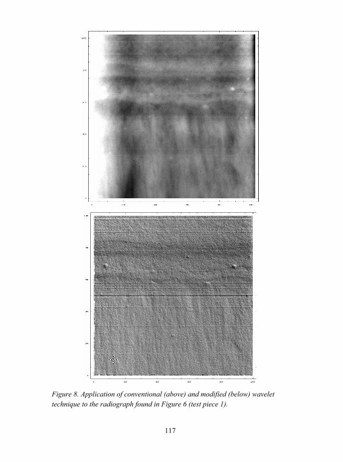
117
Figure 8. Application of conventional (above) and modified (below) wavelet technique to the radiograph found in Figure 6 (test piece 1).

118
Figure 9. Application of conventional (above) and modified (below) wavelet technique to the radiograph found in Figure 7 (test piece 2).

119
Figure 10. The digital radiograph (above) and corresponding after using modified wavelet filtering.

120
In an iron cast material without any major geometrical variation a giant combination of pore and slag is clearly visual in the original radiograph (Figure 10). The visible cross is made of gold and is attached to the object and used as reference in order to position any subsurface defect. The defected area is nearly 16 mm in diameter and the actual surface structure of the defect, i.e. the projection of the two, becomes visible after applying the filtering technique (lower picture in Figure 10). This indicates that the suggested technique is rather insensitive to the actual size of the defect.
5. Conclusions
Two different ways of applying wavelet-filtering technique in order to remove geometrical based information from a radiograph has been developed. The techniques were validated against an X-ray model with a simple geometrical defined volume and a number of simplified defects. Both methods were able to remove the geometrical based information from the greyscale. However, the conventional way of applying the wavelet technique introduced a cumbersome procedure to identify the optimum degree of resolution.
The techniques were also verified with real radiographs taken from a number of welds and iron cast objects with different kinds of defects and defect sizes. The high-resolution digital X-ray system (HiReX) was able to detect defects less than one percentage of the object-thickness in the range of 2560 mm steel. The developed filtering technique has been proven to enhance the detection of defects in objects with geometrical variations and has a potential to reduce time-consuming analysis of radiographs.
Acknowledgements
The authors are grateful to Jack Samuelsson, KTH, and Tom Stenfjell, Ringhals AB, for their support and their effort to provide us with interesting objects to radiograph. We also wish to thank Nordisk Industrifond for their part in financing our research presented in this paper.

121
References
[1] Hammar, L. Qualification of Radiographic Technique. NDE Techniques Capability Demonstrations and Inspection Qualification, Petten, 1113 March, 1997.
[2] Noble, A., Gupta, R., Mundy, J. and Schmitz, A. High Precision X-ray Stereo for Automated 3-D CAD-Based Inspection. IEEE Transactions on Robotics and Automation, 1998. Vol. 14, no. 2, pp. 292302.
[3] Mery, D. Explicit Geometrical Model of a Radioscopic Imaging System. NDT & E International. In Press, 2003.
[4] Hanke, R., Hassler, U. and Heil, K. Fast Automatic X-ray Image Processing by means of a New Multistage Filter for Background Modelling. IEEE International Conference on Image Processing, Austin, 1316 November, 1994.
[5] Oeckl, S. Hassler, U., Wenzel, T. and Hanke, R. Automatische Auswertung von 3D-CT Daten ohne CAD-Information. DGZfP JAHRESTAGUNG 2001, Berlin, 2123 May, 2001.
[6] Jacobsen, C. and Zscherpel, U. Automated Evaluation of Digitized Radiographs with Neuronal Methods. Computerized Tomography for Industrial Applications and Image Processing in Radiology, Berlin, 1517 March, 1999.
[7] Jacobsen, C., Zscherpel, U. and Nockemann, C. Crack Detection in Digitized Radiographs with Neuronal Methods. 7th European Conference on Non-Destructive Testing, Copenhagen, 2629 May, 1998.
[8] Wolfram, S. The Mathematica® Book. 4th ed. Cambridge University Press, Cambridge, 1999.
[9] Tillack, G.R., Nockemann, C. and Bellon, C. X-ray Modelling for Industrial Applications. NDT & E International, 2000. Vol. 33, no. 7, pp. 481488.

122
[10] Duvauchelle, R., Freud, N., Kaftandjian, V. and Babot, D., A Computer Code to Simulate X-ray Imaging Techniques, Nuclear Instruments and Methods in Physics Research B, 2000. Vol. 170, pp. 245258.
[11] Mångård, M. and Hammersberg, P. Modelling of an X-ray image-intensifier-based radiography system. Journal of X-ray Science and Technology, 1998. 8(1), pp. 3150.
[12] Image-Pro® Plus Reference Guide, version 4.5. Media Cybernetics Inc., Silver Spring, 2001.
[13] Bergh, J., Ekstedt, F. and Lindberg, M. Wavelets. Studentlitteratur, Lund, 1999.
[14] Daubechies, I. Ten Lectures on Wavelets. SIAM, 1992.

123
Ultrasonic assessment of material degradation by thermal fatigue
Jorma Pitkänen, Pentti Kauppinen and Harri Jeskanen VTT
Espoo, Finland
Abstract
Near surface areas can contain many types of defects, material changes and degradation. Materials subjected to thermal fatigue or annealing have been evaluated with a special ultrasonic probe optimised for surface measurements, and with a 0° longitudinal wave probe. Combining measured data from a large area and calculating depths of interest in the sound path (RF-signal) information provides improved estimation of degradation levels. The technique is using a combination of three factors: (1) back-scattered ultrasonic signals and induced leaky Rayleigh wave information), and (2) simple statistical data analysis in combination with (3) an optimised ultrasonic transducer. The back-scattered ultrasonic signal is a measure of the effect of geometrical reflectors such as micro-pores, inclusions, precipitates, segregation, micro-cracks and cracks as well as of back-scattering from phase boundaries during fatigue damaging and increase of degradation inside the material. The leaky Rayleigh wave component is sensitive to surface properties, and especially to cracks. Deep cracks will totally cancel the leaky Rayleigh wave signal.
1. Introduction
The ageing of conventional as well as nuclear power plants gives motivation to non-destructive detection of degradation of materials. Many NDE techniques have potential for detection of degradation. These methods offer the possibility of studying these effects on-site reliably. The information gained using this type of techniques gives background for evaluation of the lifetime of a component. This helps power plant operators to plan more accurately their in-service tasks and to reduce costs.
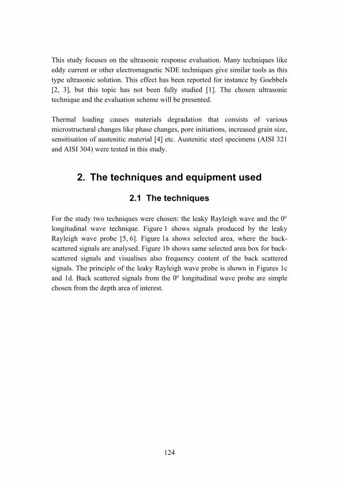
124
This study focuses on the ultrasonic response evaluation. Many techniques like eddy current or other electromagnetic NDE techniques give similar tools as this type ultrasonic solution. This effect has been reported for instance by Goebbels [2, 3], but this topic has not been fully studied [1]. The chosen ultrasonic technique and the evaluation scheme will be presented.
Thermal loading causes materials degradation that consists of various microstructural changes like phase changes, pore initiations, increased grain size, sensitisation of austenitic material [4] etc. Austenitic steel specimens (AISI 321 and AISI 304) were tested in this study.
2. The techniques and equipment used
2.1 The techniques
For the study two techniques were chosen: the leaky Rayleigh wave and the 0° longitudinal wave technique. Figure 1 shows signals produced by the leaky Rayleigh wave probe [5, 6]. Figure 1a shows selected area, where the back-scattered signals are analysed. Figure 1b shows same selected area box for back-scattered signals and visualises also frequency content of the back scattered signals. The principle of the leaky Rayleigh wave probe is shown in Figures 1c and 1d. Back scattered signals from the 0° longitudinal wave probe are simple chosen from the depth area of interest.
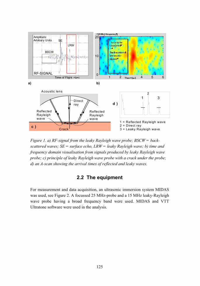
125
a) b)
Acoustic lens
Crack
Directray
ReflectedRayleighwave
c )
31
3 = Leaky Rayleigh wave
1 = Reflected Rayleigh wave2 = Direct ray
2
d )
ReflectedRayleighwave
Figure 1. a) RF-signal from the leaky Rayleigh wave probe; BSCW = back- scattered waves; SE = surface echo, LRW = leaky Rayleigh wave; b) time and frequency domain visualisation from signals produced by leaky Rayleigh wave probe; c) principle of leaky Rayleigh wave probe with a crack under the probe; d) an A-scan showing the arrival times of reflected and leaky waves.
2.2 The equipment
For measurement and data acquisition, an ultrasonic immersion system MIDAS was used, see Figure 2. A focussed 25 MHz-probe and a 15 MHz leaky-Rayleigh wave probe having a broad frequency band were used. MIDAS and VTT Ultratone software were used in the analysis.

126
Figure 2. Arrangement for measurement (left) MIDAS ultrasonic immersion testing equipment (right).
2.3 Measured data
Amplitude data were calculated from raw data and compared with different loading factors. As a comparison, a reference material was used with either zero loading or exactly known reference loading. The calculated amplitude values are obtained from the following equation:
))/,/(/),(log(20
maxmax
10
10 iAiAfAAfV
i
ii
i
iiii ∑∑
==∆∆=

127
where Ai is the computed statistical amplitude value from specimen i, ∆Ai is the computed statistical amplitude variation from specimen i, A0i is the computed statistical amplitude from the reference specimen
i with reference loading, ∆A0i is the computed statistical amplitude variation from the
reference specimen i with reference loading.
3. Measurements and results
Austenitic steel specimens (AISI 321) were loaded with low cycle thermal fatigue. The specimens were measured after loading with leaky Rayleigh wave technique, measuring only the back-scattered area shown earlier. The statistical amplitude values (rms) were calculated for each measurement point. The number of measurement points for each specimen was about 10000. The computed rms-values are shown in a C-scan form in Figure 3. The rms-value increases with increasing thermal low cycle fatigue. Figure 3 shows results from measured specimen of 5 different loads with increasing degradation from left to right. The lower row shows the specimen with highest degradation. From these specimens the effect of degradation is clearly seen. The amplitude increase was in best cases about 1014 dB and the reference material was material, which was not subjected to low cycle fatigue. In the degraded material micro-cracks and even macro-cracks were already seen in some specimens.
This back-scattered noise technique was also applied also to measure grain boundary precipitation. Specimens of overlay welded austenitic steel (AISI 304) were studied for the effects of welding and ageing (sensitisation and grain growth). Thermal ageing for low temperature sensitisation (LTS) was conducted at 400°C for 69 days (specimen A) and for 650 days (specimen B). Ageing treatment caused increase in the degree of sensitisation (DOS) due to growth of carbides (M23C6) during the weld cycle at LWR operation temperature within the heat affected zone (HAZ), see Figure 4 [4].

128
Figure 3. C-scan from computed rms-values for back-scattered ultrasonic signals showing degradation caused by low cycle fatigue.
The measured C-scans of computed rms-values are shown in Figure 5, as well the rms-frequency distribution from the studied volume. Rms-amplitude of the frequency distribution is increasing with increasing heat treatment time. Table 1 shows the determined amplitude values from the two specimens. Unlike specimen A, the specimen B with a longer ageing treatment showed a detectable increase in the rms-amplitude from RF-signal (Rms_A) and from power spectrum amplitude (Rms_F) of back-scattered ultrasonic signals.

129
S p e c i m e n B S p e c i m e n A
´H A Z ´H A Z
W e l d W e l d
B A
Figure 4. Micrographs [4] from two austenitic steel specimens showing different carbide grain sizes in the heat affected zone.
S p e c i m e n A
S p e c i m e n B
B AB A
Figure 5. Rms-frequency distribution from the studied volume on the left and the measured C-scans of computed amplitude rms-values on the right (A = Rms C-scan from specimen A; B = Rms C-scan from specimen B).
Table 1. Statistical characteristics from measurements of two heat treated austenitic steel specimens.
Material RMS_A RMS_F RMS_t X (mm) Y (mm) Z (mm) f (MHz)
B 5.61± 0.72 4.68± 0.72 2.54 ± 0.36 7082 0.538.5 610 214
A 5.01 ± 0.63 4.15± 0.62 2.62 ± 0.36 107119 0.538.5 610 214

130
4. Discussion and conclusions
The following conclusions have been drawn from the inspections of different materials. The surface condition has an effect on the results and this has to be considered in the evaluation of data. Ultrasonic back scattering showed correla-tion with degradation of studied austenitic materials. Effects of heat treatment on M23C6 carbides in the heat-affected zone was detectable as increasing noise in the back-scattered ultrasonic signals. The analysis of rms-values of a large measurement area can be a useful method for determining degradation in austenitic materials. Calibration standards are needed for analysis. Frequency analysis of the measured data gives supplementary information for degradation analysis. Noise measurement based on the back scattering of ultrasonic waves shows potential to determine material characteristics and its changes.
References
1. Thompson, R. B. Use of elastodynamic theories in the stochastic description of the effects microstructure on ultrasonic flaw and noise signals. Wave motion 36 (2002), pp. 47365.
2. Vary, A. Ultrasonic measurement of materials properties by scattered ultrasonic radiation. In: Research Technique in Nondestructive Testing, Volume IV. Ed. R. S. Sharpe. London: Academic Press, 1980. Pp. 159204.
3. Goebbels, K. Structure analysis by scattered ultrasonic radiation. In: Research Technique in Nondestructive Testing, Volume IV. Ed. R. S. Sharpe. London: Academic Press, 1980. Pp. 87157.
4. Kekkonen, T. Sensitation of austenitic stainless steel weld in low temperatures. Master of Science Thesis, Helsinki University of Technology, Espoo, Finland, 1983. 85 p.
5. Jeskanen, H., Pitkänen, J. & Kauppinen, P. Applications of materials property ultrasonic probe. ECNDT, Barcelona, Spain, 1721 June, 2002. 7 p.

131
6. Kauppinen, P. The evaluation of integrity and elasticity of thermally sprayed coatings by ultrasonics. Dissertation Thesis. Helsinki University of Technology, Espoo, Finland, 1997. 130 p.
7. Pitkänen, J., Kauppinen, P. & Jeskanen, H. Materials degradation and altering influence on ultrasonic scattering by light statistical approach in austenitic thermal loaded materials. Review of progress in quantitative nondestructive evaluation, Vol. 23. D. O. Thompson; D. E. Chimenti, 2004. 5 p.
133
Evaluation of near surface defects and fatigue properties of cast iron
Jouni Alhainen, Jussi Solin VTT, Espoo, Finland
Matti Johansson Componenta Oyj, Karkkila, Finland
Abstract
This research work aimed to find out means to ensure fatigue strength of cast components. Componenta carries out R&D to avoid casting defects which have detrimental effect on the fatigue properties. Extensive metallographic studies and fatigue experiments were herein performed to support this development work. Clear differences in the amount of degenerated graphite and defects near the casting surface were seen in the micrographs at different surface positions. An ultrasound scanning microscope was used to evaluate applicability of Rayleigh wave velocity measurements to detect and classify small surface defects. This technology was investigated as a candidate method for non-destructive quality control. Some fatigue crack initiation sites could be correlated with the detected surface defects, but the influence of defects on the fatigue properties could not be evaluated. The fatigue strengths of the studied variants were within a common scatter band. But the results of ultrasonic measurements are in perfect agreement with the microstructural measurements. They are also fully in line with the trends in fatigue lives and scatters.
1. Introduction
One of the most important challenges when designing a new component is to minimise its weight. One possibility is to use high strength materials, but fatigue strength does not always increase along with static strength. It is a widely accepted fact that surface defects have detrimental effect on the fatigue properties of the castings. Small defects are usually allowed because of the difficulties in detection and characterisation.

134
1.1 Goals
The aim of this research work was to find out the means to ensure fatigue strength of cast components. A challenge would be to match the fatigue strength of machined components. One of the most important tasks is to avoid defects which have detrimental effect on the fatigue properties. Extensive metallographic studies and fatigue experiments were performed to support this development work.
Another important task was to test applicability of non-destructive quality control methods. Nowadays many foundries are doing destructive testing to manufactured parts on a frequency that is defined either by standard or by a contract with the client. Cutting and examining the surfaces of the castings in a traditional way is time consuming, expensive and still one cant be absolutely convinced about the quality of the whole casting. If the surface quality of the casting could be measured reliably, effectively and quantitatively with a non-destructive method, it could be a very useful tool to control the foundry process. Such enhancement would give considerable benefits both to the foundries and to the clients.
1.2 Previous work
Fatigue resistance of heavy section nodular iron was studied in a previous project [1]. An attempt to correlate propagation of ultrasound to fatigue resistance of the material was made by measuring velocities and attenuation of longitudinal, shear and Rayleigh waves in fatigue specimens taken from large ingots. A weak inverse correlation of fatigue life with the shear wave velocity was then observed, but in general, the test material was considered too homogeneous for the purpose. Furthermore, knowing that fatigue cracks normally initiate at or near the surface, the bulk material properties are not ideal for fatigue life prediction. A new approach was thus needed and therefore, the ultrasound experiments in this project were focused in Rayleigh waves propagating at a controllable depth near the component surface.
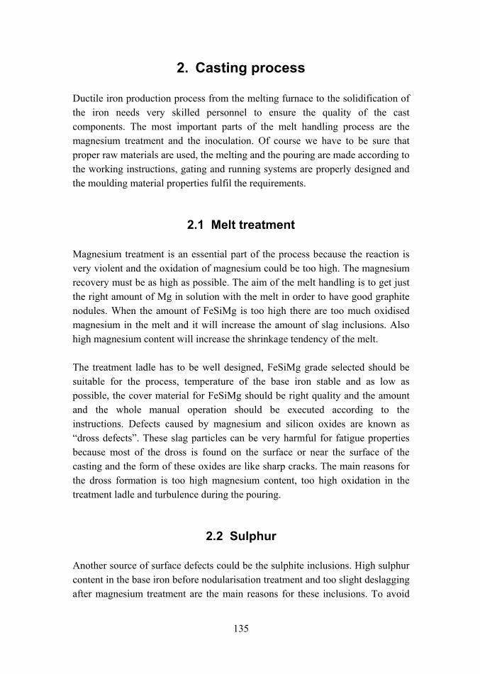
135
2. Casting process
Ductile iron production process from the melting furnace to the solidification of the iron needs very skilled personnel to ensure the quality of the cast components. The most important parts of the melt handling process are the magnesium treatment and the inoculation. Of course we have to be sure that proper raw materials are used, the melting and the pouring are made according to the working instructions, gating and running systems are properly designed and the moulding material properties fulfil the requirements.
2.1 Melt treatment
Magnesium treatment is an essential part of the process because the reaction is very violent and the oxidation of magnesium could be too high. The magnesium recovery must be as high as possible. The aim of the melt handling is to get just the right amount of Mg in solution with the melt in order to have good graphite nodules. When the amount of FeSiMg is too high there are too much oxidised magnesium in the melt and it will increase the amount of slag inclusions. Also high magnesium content will increase the shrinkage tendency of the melt.
The treatment ladle has to be well designed, FeSiMg grade selected should be suitable for the process, temperature of the base iron stable and as low as possible, the cover material for FeSiMg should be right quality and the amount and the whole manual operation should be executed according to the instructions. Defects caused by magnesium and silicon oxides are known as dross defects. These slag particles can be very harmful for fatigue properties because most of the dross is found on the surface or near the surface of the casting and the form of these oxides are like sharp cracks. The main reasons for the dross formation is too high magnesium content, too high oxidation in the treatment ladle and turbulence during the pouring.
2.2 Sulphur
Another source of surface defects could be the sulphite inclusions. High sulphur content in the base iron before nodularisation treatment and too slight deslagging after magnesium treatment are the main reasons for these inclusions. To avoid

136
rich sulphite inclusions to flow into the mould ceramic filters should be used. But the high sulphur content can exist also in the mould and core materials. Sulphur content should be controlled so that the formation of the flake or compacted graphite at the casting surface will be avoided.
2.3 Surface condition
Many authors have published papers concerning the effect of surface defects on the fatigue strength. Final failure crack often initiates from the casting defects at the as cast surface. It has also been reported in these papers that sand blasting or shot peening improves the fatigue strength because of the compressive stress produced to the surface but that does not help if there are deep dross defects at the surface of the casting.
2.4 Good practice
Surface defects are minimised by optimised nodularisation treatment, simulation of the melt flow and good foundry practise respecting work instructions based on research and experience.
Some important rules to remember to make better castings [2]:
- Keep ladles clean - Control the magnesium reaction - Take slag off carefully after magnesium treatment - Use optimised pouring times and hold the melt in the ladle for the shortest
possible time - Avoid turbulence during pouring and adjust the pouring temperature - Keep the elements which strongly react with oxygen as low as possible, e.g.
Mg, Mn, Al and if necessary reduce them - Keep sulphur content low in sand moulds and cores.

137
3. Experimental
3.1 Test Material
Slag and oxides are lighter than the iron melt and surface defects are enriched at the upper part of the castings. Special test piece was made where one can examine not only green sand surfaces but also core surfaces. The aim of this primary stage of the project was also to make the ductile iron castings for the fatigue tests. The test castings were done at three Componenta foundries (Karkkila, Pori and Pietarsaari) with their normal production processes and control systems.
Microstructures were examined and analysed after pouring and the results were also utilized to improve the process control. Castings with different surface qualities were selected for further examination to find out the effects of the defects on the NDT testing results and the fatigue properties.
The grade GJS-500-7 ductile iron was produced. Chemical composition of test castings are presented in Table 1 and mould sand properties in Table 2. Part of the test casting series 2 was heat treated to the class GJS-900-7. The shape of the test casting is presented in Figure 1 and the pattern used is shown in Figure 2.
Table 1. The chemical composition of the test material.
Series C Si Mn P S Mg Cu Mo Ni 1 3,74 2,42 0,27 0,021 0,008 0,038 0,32 - 0,03 2 3,76 2,19 0,32 0,018 0,010 0,052 0,30 0,02 0,04
Table 2. The sand properties in the moulding lines.
Series 1 Series 2
Permeability 120 98 Compactability (%) 39 37 Moisture content (%) 3,0 3,1 Green compression strength (p/cm2) 205 227 Temperature (°C) 38 24 VOL (%) 1,8 2,3 C (%) 3,5 3,5 S (%) 0,05 0,09

138
Figure 1. The test casting for fatigue test.
Figure 2. The top half of the pattern.
3.2 Microstructure examination
The test specimens were cut from the middle part of the casting along the longitudinal direction. The microstructure observations were made from the polished specimens by optical microscope. Specimen polishing for optical microscopy was carried out conventionally. The top part, side part and bottom part of the casting were examined by optical microscope Nikon TME. The microstructures of the castings near the outer surface were in contact with sand mould and the inner surface contact with a cold-box core.

139
3.3 Fatigue testing
Fatigue testing of 4-point bending test was performed using a programmable resonant test machine manufactured by RUMUL. This machine can perform constant amplitude testing at frequencies between 80 and 300 Hz. The specimens tested in this project were fatigued at a frequency of about 80 Hz.
3.4 Ultrasonic measurements
Another important task in the project was to test applicability of non-destructive quality control methods. For that purpose, experiments utilising Rayleigh wave propagation at a controllable depth near the component surface were performed. A novel type of ultrasonic material characterisation probe developed at VTT was applied in an ultrasound scanning microscope [3, 4]. The technique is also briefly described by Pitkänen et al. in the previous paper in this proceedings.
The ultrasound probe sends signal to the material. The time of flight across a pretemined distance is then measured with high accuracy. The depth of the Rayleigh wave can be controlled by frequency. 4, 8 and 12 Mhz were used in preliminary tests and 8 MHz was selected for further measurements. The ultrasound is thus screening the material to the depth of 300350 µm below the surface.
This measurement technique was considered potentially capable to detect and classify small sub-surface defects. More importantly, it was also considered a candidate method for routine use in a foundry environment. This kind of measurement is relatively fast and, if desired, it could be automated or simply mechanised for routine use in quality control. Results can be immediately handled and displayed in a graphical form on computer screen.
With ultrasound it is possible to measure in a minute relatively large area on the cast surface and thus receive quantitative information about the surface quality. The benefits would be obvious when compared to the traditional destructive examination. But applicability of the technology needs to be investigated first. The herein reported experiments were performed in that aim.

140
4. Test Results
4.1 Microstructural studies
The optical micrographs in Figures 38 show the microstructures with different levels of defects at different positions of the casting and poured in different foundries. Material 2 (Figures 68) presents generally more slag inclusions and degenerated graphite compared to material 1 even though ceramic filters were used. The optical micrographs in Figures 35 show very little amount of slag inclusions and degenerated graphite near the surfaces. In general, there are more slag inclusions and degenerated graphite near the outer and inner surfaces of the side part in the casting, as well as near the outer surface of the top part in the casting than that in other positions.
When taking into account the process parameters one can see that in test material 2 there are higher magnesium content in the melt and also higher sulphur content in the sand. Despite of the use of the ceramic filters there are more oxides and degenerated graphite in the castings. Some of the oxides and sulphites can go through the filter or oxides/sulphites are formed in the mould cavity. Especially sulphur in the sand can have negative effect on the graphite morphology.
a) b) Figure 3. The optical micrograph of the material 1 a) near the outer surface of the top part shows a small amount of slag inclusions and degenerated graphite, b) near the inner surface of the top part shows a very little amount of slag inclusions and degenerated graphite.

141
a) b) Figure 4. The optical micrograph of the material 1 a) near the outer surface of the side part shows slag inclusions and degenerated graphite, b) near the inner surface of the side part shows slag inclusions and degenerated graphite.
a) b) Figure 5. The optical micrograph of the material 1 a) near the outer surface of the bottom part shows a very little amount of slag inclusions and degenerated graphite, b) near the inner surface of the bottom part shows a very little amount of slag inclusions and degenerated graphite.
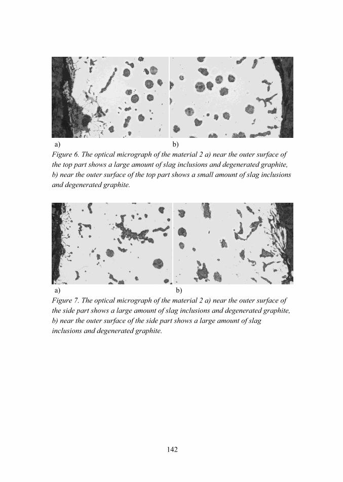
142
a) b)
Figure 6. The optical micrograph of the material 2 a) near the outer surface of the top part shows a large amount of slag inclusions and degenerated graphite, b) near the outer surface of the top part shows a small amount of slag inclusions and degenerated graphite.
a) b) Figure 7. The optical micrograph of the material 2 a) near the outer surface of the side part shows a large amount of slag inclusions and degenerated graphite, b) near the outer surface of the side part shows a large amount of slag inclusions and degenerated graphite.

143
a) b) Figure 8. The optical micrograph of the material 2 a) near the outer surface of the bottom part shows some slag inclusions and degenerated graphite, b) near the outer surface of the bottom part shows a large amount of slag inclusions and degenerated graphite.
4.2 Preliminary NDE of test materials
Several test castings made from material series 1 and 2 were NDT tested. The Rayleigh wave velocity at the test castings upper and lower surfaces were measured at nine constant measurement points. Results are presented at figures 9. Conclusion of this preliminary test was that for both test materials the velocity of the Rayleigh wave was systematically lower at the upper surfaces where more defects were expected to be found.
The effect of the machining of the defected surface layer was tested by machining 100, 200, 300, 400, 500 and 2000 µm away from the as cast surface. It can be seen in Figure 11 that at upper surfaces there must be more material machined away until the Rayleigh time-of-flight value is stabilised which could mean that there is a thicker layer of defected material at the upper surfaces. In this case defected material can mean for example shrinkage, inclusions, dross, unwanted graphite morphology etc. It can also be seen from Figure 10 a that Rayleigh-wave value is quite constant for lower surface of test castings made of test material 1 which means that the defected layer was probably machined away by 100 µm removal.

144
2400
2500
2600
2700
2800
2900
3000
1 2 3 4 5 6 7 8 9measurement point
Rayl
eigh
spee
d, [
m/s
]Upper surfaceLower surface( a )
2400
2500
2600
2700
2800
2900
3000
1 2 3 4 5 6 7 8 9measurement point
Rayl
eigh
spee
d, [
m/s
]Upper surfaceLower surface
2400
2500
2600
2700
2800
2900
3000
1 2 3 4 5 6 7 8 9measurement point
Rayl
eigh
spee
d, [
m/s
]Upper surfaceLower surface
2400
2500
2600
2700
2800
2900
3000
2400
2500
2600
2700
2800
2900
3000
1 2 3 4 5 6 7 8 91 2 3 4 5 6 7 8 9measurement point
Rayl
eigh
spee
d, [
m/s
]Upper surfaceLower surfaceUpper surfaceLower surfaceUpper surfaceLower surface( a )
2400
2500
2600
2700
2800
2900
3000
1 2 3 4 5 6 7 8 9measurement point
Rayl
eigh
spee
d, [
m/s
]
Upper surfaceLower surface( b )
2400
2500
2600
2700
2800
2900
3000
1 2 3 4 5 6 7 8 9measurement point
Rayl
eigh
spee
d, [
m/s
]
Upper surfaceLower surface
2400
2500
2600
2700
2800
2900
3000
1 2 3 4 5 6 7 8 9measurement point
Rayl
eigh
spee
d, [
m/s
]
Upper surfaceLower surface
2400
2500
2600
2700
2800
2900
3000
2400
2500
2600
2700
2800
2900
3000
1 2 3 4 5 6 7 8 91 2 3 4 5 6 7 8 9measurement point
Rayl
eigh
spee
d, [
m/s
]
Upper surfaceLower surfaceUpper surfaceLower surfaceUpper surfaceLower surface( b )
Figure 9. Rayleigh wave velocities for a) material 2 and b) material 1 test castings.

145
570575
580585590
595600
605610615
620625
0 500 1000 1500 2000 2500
Machined from surface, µm
Tim
e-of
-flig
ht, n
sUpper surface
Lower surface
a)
570
580
590
600
610
620
630
640
650
660
0 500 1000 1500 2000 2500Machined from surface, µm
Tim
e-of
-flig
ht, n
s
Upper surfaceLower surface
b) Figure 10. Effect of machining of the as cast surface on the Rayleigh wave time-of-flight measurements of a) material 1 and b) material 2.

146
4.3 Fatigue testing
Four different surface types were selected for 4-point bending testing: 1. Material 1 lower surface (GJS500, less defects) 2. Material 1 machined surface (GJS500). 3. Material 2 upper surface (ADI, most defects) 4. Material 2 lower surface (ADI, some defects).
4-point bending test bar used can be seen in Figure 11. All the test specimens were surface scanned with a material characterisation probe before fatigue testing. Fatigue testing of all samples was made with the load of 240±225 MPa. Results of fatigue tests are presented in Figure 12.
Figure 11. 4-point bending test specimen.
According to these fatigue tests machining of the surface doesnt necessarily improve the fatigue strength of the material. One possible explanation for this is the compressive state produced to the surface of the casting during the shot peening. However machining seems to reduce the standard deviation considerably. The mean life values and standard deviations for different materials and surface qualities are presented in Table 3.
Other interesting phenomena is the GJS500 grades higher average Nf-value when compared to the ADI upper surface. This confirms the assumption that the surface defects can cause very harmful effects on fatigue properties and one should be very careful with the production practices used. On the other hand the mean life of ADI lower surface which has less defects has clearly higher average Nf value.
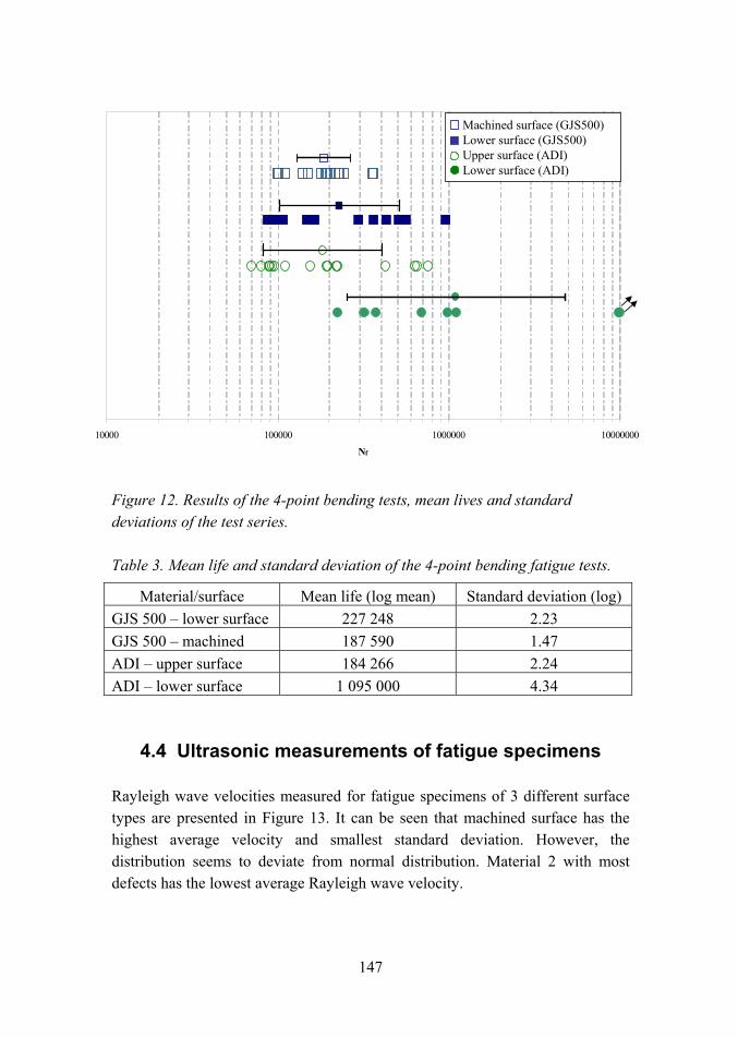
147
22010000 100000 1000000 10000000
Nf
Machined surface (GJS500)Lower surface (GJS500)Upper surface (ADI)Lower surface (ADI)
22010000 100000 1000000 10000000
Nf
Machined surface (GJS500)Lower surface (GJS500)Upper surface (ADI)Lower surface (ADI)
Figure 12. Results of the 4-point bending tests, mean lives and standard deviations of the test series.
Table 3. Mean life and standard deviation of the 4-point bending fatigue tests.
Material/surface Mean life (log mean) Standard deviation (log) GJS 500 lower surface 227 248 2.23 GJS 500 machined 187 590 1.47 ADI upper surface 184 266 2.24 ADI lower surface 1 095 000 4.34
4.4 Ultrasonic measurements of fatigue specimens
Rayleigh wave velocities measured for fatigue specimens of 3 different surface types are presented in Figure 13. It can be seen that machined surface has the highest average velocity and smallest standard deviation. However, the distribution seems to deviate from normal distribution. Material 2 with most defects has the lowest average Rayleigh wave velocity.

148
It should be noted that each point in Figure 13 represents thousands of measurements in one fatigue specimen. Fatigue strength would not necessarily correlate with the average velocity, but perhaps rather with the minimum velocity. The variability of test material properties did not allow direct comparison of fatigue strength and Rayleigh wave velocities in this study.
2200
2400
2600
2800
3000
3200
Velo
city
m/s
maxaveragemin
Material 2 Material 1 Machined ± 1x σ2200
2400
2600
2800
3000
3200
Velo
city
m/s
maxaveragemin
Material 2 Material 1 Machined ± 1x σ
Figure 13. Measured Rayleigh wave velocities for the studied material variants: upper surface of material 2, lower surface of material 1 and machined surface of material 1. Each point represents thousands of measurements in one fatigue specimen. Minimum, maximum and average values are given. Standard deviations represent variation between specimens.
Rayleigh wave velocity measurements can be presented as C-scans a kind of maps of the measured surface. Because defects retard Rayleigh waves, it should be possible to detect the sub-surface defects from the C-scans. Some examples of typical C-scans of the 4-point bending test bars are presented in Figures 1417 together with the corresponding fracture surfaces. Dark blue areas present potential defect areas in these C-scans. Sub-surface defects found on the fracture surfaces correlate well with the C-scan images.

149
Figure 14. C-scan plot of fatigue specimen with notable defects or other areas retarding Rayleigh waves (dark blue). White dotted line marks the location of the fatigue crack plane. Fracture surface is shown below. The sub-surface defect on the crack surface can be seen also in the C-Scan.

150
Figure 15. C-scan plot of fatigue specimen with notable defects or other areas retarding Rayleigh waves (dark blue). White dotted line marks the location of the fatigue crack plane. Fracture surface is shown below. Two sub-surface defects on the crack surface can be seen also in the C-Scan.

151
Figure 16. C-scan plot of fatigue specimen with notable defects or other areas retarding Rayleigh waves (dark blue). White dotted line marks the location of the fatigue crack plane. Fracture surface is shown below. The defect on the crack surface can be seen also in the C-Scan.
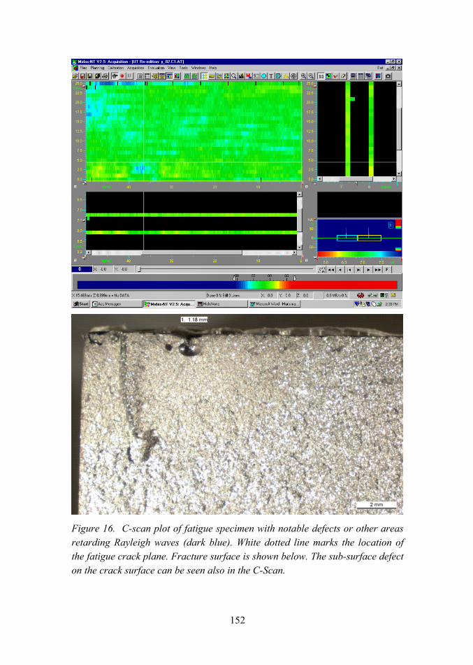
152
Figure 16. C-scan plot of fatigue specimen with notable defects or other areas retarding Rayleigh waves (dark blue). White dotted line marks the location of the fatigue crack plane. Fracture surface is shown below. The sub-surface defect on the crack surface can be seen also in the C-Scan.

153
5. Conclusions
In this work the efforts were concentrated to investigation of surface defects and their detrimental effect on fatigue strength of cast iron components. Surface defects are minimised by optimised nodularisation treatment, simulation of the melt flow and good foundry practise respecting work instructions based on research and experience.
Four material variants were studied by metallography, ultrasonic measurements and fatigue tests. The following conclusions were drawn:
• Detrimental effects of high sulphur content in sand and high residual magnesium content in melt were confirmed by wide metallographic evidence. They increase amount of dross defects at cast surface.
• The upper and lower surfaces of both studied casting series were identical in visual inspection, but clear differences could be seen in optical micrographs (Figures 38) and in preliminary ultrasonic measurements (Figure 9).
• Removal of as-cast surface by machining systematically increases velocity of ultrasonic Rayleigh wave (Figure 10). Sub-surface defects reduce the velocity of the 8 MHz Rayleigh wave, which penetrates approximately 300 µm below the surface.
• The 500 µm depth of machining where improvement is scaling off, correlates well with the microstructure. This supports applicability of ultrasonic measurement for characterisation of surface quality.
• Differences in fatigue lives of the tested four variants were not significant. The scatter bands were large, but not exceptional for cast irons in high cycle regime.
• Material 2 upper surface was of higher strength (ADI), but it was ranked to the worst surface quality in both metallographic and ultrasonic measurements. Consequently, the shortest mean fatigue life was measured to upper surface of material 2.
154
• The lower surface of higher strength material 2 (ADI) was ranked to the second best surface quality in metallographic investigation. Highest mean fatigue life was measured to this material variant. This material was excluded from the ultrasound measurements.
• Machining of the as-cast surface did not increase mean fatigue life, but it reduced the scatter. This could be explained by controversial effects of removal of defects and residual stresses. Removal of defects should increase life and reduce scatter. Removal of residual stresses should decrease life.
• The results of ultrasonic measurements (Figure 17) are in perfect agreement with the microstructural measurements. They are also fully in line with the trends in fatigue lives and scatters.
• The Rayleigh wave C-scans revealed spots of reduced velocity, which gave reason to suspect that there were large defects (Figures 1316). They were considered as potential fatigue initiation sites. Later on, large defects were in many cases found from the same areas on the fracture surfaces.
The results do not yet confirm applicability of the studied techniques for industrial use. However, they encourage further attempts to develop non-destructive quality assurance methods for competent design by castings.
If further R&D is considered, special attention should be paid to design of material variants. The test matrix should provide a wide range of fatigue properties due to variable sub-surface defect distributions only.
Acknowledgements
The reported work was financed by the Nordic Innovation Centre, Tekes, VTT and Finnish industry as part of the Gjutdesign-2005 project. Matti Johansson of Componenta Oyj was in primary charge of controlling this subproject. Research planning was initiated by Gary Marquis, when still at VTT, Päivi Karjalainen-Roikonen took charge of the work at VTT until her parential leave and Jouni Alhainen since beginning of 2004. Ultrasonic measurements were performed by
155
Harri Jeskanen, metallography by Jouni Alhainen and fatigue tests by Heikki Laukkanen. Jorma Pitkänen ja Jussi Solin supervised the NDE and fatigue experiments.
References
1. Marquis, G. and Solin, J. 2000. Long-life fatigue design of GRP 500 nodular cast iron components. Espoo 2000. VTT Research Notes 2043. 70 p.
2. Bauer, W., 2001. Einfluss der Gusshaut auf das Biegewechselverhalten von Werkstücken aus Gusseisen mit Kugelgraphit. Konstruiren + Giessen 26 (2001) Nr. 4.
3. Jeskanen, H., Kauppinen, P., Pitkänen, J. and Tähtinen, S. Material characterization probe. 15th World Conference on Non-Destructive Testing. Rome, IT, 1521 Oct. 2000. 4 p.
4. Jeskanen, H., Pitkänen, J. and Kauppinen, P. Applications of materials property ultrasonic probe. 8th European Conference on Non-destructive Testing. Barcelona, 1721 June 2002. CD-Rom. Asociacion Espanola de Ensayos No Destructivos. 7 p.

157
Round robin on Nondestructive Testing evaluation of a cast truck component
Ulla Boman Volvo Powertrain, Materials Technology
Gothenburg, Sweden
Abstract
To get an understanding of the general possibilities to detect casting defects with Nondestructive Testing (NDT) a Round Robin exercise was set up. The participants were 4 Swedish and 2 Finnish companies, either foundries or companies buying castings. Two nodular iron castings used for Volvo trucks were circulated between the participants. The participating companies could freely choose between the NDT methods they regularly use. As a reference the castings were tested at Chalmers University of Technology using a high-resolution X-ray radiographic system based on scintillation fibre optics.
Magnetic particle testing was the test method in the Round Robin that gave most defect indications. However, there was a big scatter in the test results. Several companies found indications in the same areas but the correlation with the results of the high resolution X-ray examination is however rather vague.
The indications that one of the companies found with ultrasonic testing did not correspond with the inner defects found with high resolution X-ray.
This Round Robin exercise indicates that there is a big scatter in nondestuctive test results when utilised for defect detection in an iron casting.

158
1. Introduction
The fatigue limit of cast materials is strongly influenced by casting defects [1]. It has been shown that near surface defects are much more dangerous with regard to the fatigue limit than internal defects [2]. Slag stringers of different origin are common surface-close defects in iron castings.
For weight optimisation of a casting the designer needs reliable material data but the influence of casting defects also needs to be taken into account. The biggest allowed defects in the areas with highest stress should be specified. There are many measures a foundry has to take to minimise the risk for slag defects, e.g. careful design of the in-gate system, good temperature control and strict slag-off routines. For control of the achieved defect level micro samples can be extracted from the critical areas, but it is also essential that the foundry can perform nondestructive testing.
2. Experimental
To get an understanding of the general possibilities to detect casting defects with Nondestructive Testing (NDT) a Round Robin exercise was set up. The participants were 4 Swedish and 2 Finnish companies, either foundries or companies buying castings.
2.1 Test Material
Two pieces, designated K1 and K2, of a Volvo truck nodular iron casting were circulated between the participants. The castings had been rejected by Volvo Truck Corporation, as they did not fulfil the drawing demands regarding casting quality. The castings were not painted. The appearance of the casting is shown in Figure 1. The material corresponds to EN-GJS-600-3.

159
Figure 1. Truck casting used for NDT Round Robin.
2.2 Test Methods
The participating companies could freely choose between the NDT methods they regularly use, see Table 1.
One page of instructions and standard test forms for each method were sent to the participants. In the forms the test parameters were given together with information on used references etc. No markings were made on the castings. The positions of the found indications were marked on photos or on simple sketches.
Some of the chosen test parameters for magnetic particle and ultrasonic testing are given in Table 2 and 3 below. For liquid penetrant testing company 1 used red penetrant. To X-ray the castings company 5 used 275 kV and five films for each casting.
As a reference the castings were tested at Chalmers University of Technology using a high-resolution X-ray radiographic system based on scintillation fibre optics. The whole castings were scanned. Voltage used was 300 kV, current 3 mA, focus spot size 1 mm2 and the exposure time was 40 s. According to EN473 the radiography sensitivity is approximately 0,5%, which is better than film radiography.
239 mm

160
Table 1. NDT methods chosen by the participating companies.
Company Used Methods
1 Magnetic Particle Testing
Ultrasonic Testing
2 Magnetic Particle Testing
Ultrasonic Testing
Liquid Penetrant Testing
3 Magnetic Particle Testing
Ultrasonic Testing
4 Magnetic Particle Testing
Ultrasonic Testing
5 Magnetic Particle Testing
Radiographic Testing
6 Magnetic Particle Testing
Table 2. Test parameters magnetic particle testing.
Company Magnetic Particles
1 Wet
2 Wet
3 Black
4 Wet, Fluorescent
5 Wet, Fluorescent
6 Wet, Fluorescent
Table 3. Test parameters Ultrasonic Testing.
Company Probe Angle of refraction
1 MSEB4H 90°
2 Double 4MHz
3 S12W2 0°
4 Sonatest GEM 510, 911/03 0°
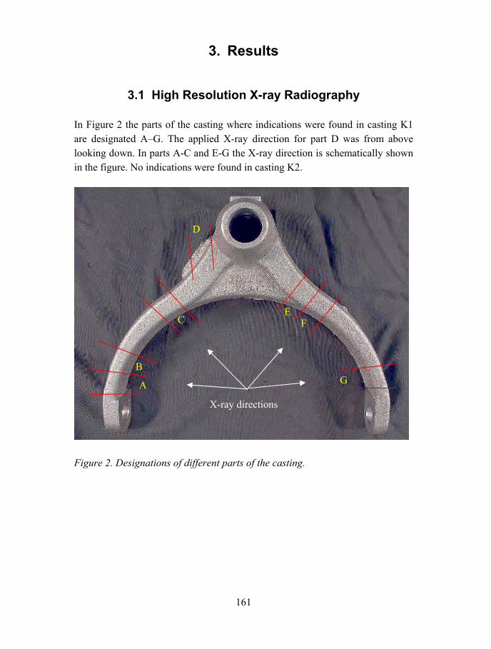
161
3. Results
3.1 High Resolution X-ray Radiography
In Figure 2 the parts of the casting where indications were found in casting K1 are designated AG. The applied X-ray direction for part D was from above looking down. In parts A-C and E-G the X-ray direction is schematically shown in the figure. No indications were found in casting K2.
Figure 2. Designations of different parts of the casting.
A
E
D
C
B
F
G
X-ray directions

162
Table 4. Indications found in casting K1 with High Resolution X-ray Radiography.
Part Indication
A, upper Small porosity, possibly surface irregularity
B, upper Small elongated porosity and a slag
B, lower Slag
C, lowest Small porosity
D, lowest Small porosity
E, middle Defects looking like porosities
F, lowest Big porosity, probably surface irregularity
G, lower Slags
3.2 Magnetic Particle Testing
The areas where indications were found are marked in Figures 35 and the results are presented in Tables 5 and 6. In Figures 6 and 7 the appearance of some indications is shown.

163
Figure 3. Areas where indications have been found.
Figure 4. Areas where indications have been found.
1
52
34
6
7
1 2

164
Figure 5. Areas where indications have been found.
3.2.1 Casting K1
Table 5. Indications found in casting K1 with magnetic particle testing.
Company Indications 1 1 indication Fig. 5, area 2 2 No indications 3 1 indication Fig. 3, area 4
1 indication Fig. 3, area 5 1 indication Fig. 4, area 2
4 1 indication Fig. 3, area 4 1 indication Fig. 5, area 2
5 Several indications Fig. 5, area 1 1 indication Fig. 5, area 2
6 1 indication Fig. 3, area 1 1 indication Fig. 3, area 3 1 indication Fig. 3, area 4 2 indication Fig. 3, area 5
2
1

165
Figure 6. Indications on casting K1. Photographed in UV light.
3.2.2 Casting K2
Table 6. Indications found in casting K2 with magnetic particle testing.
Company Indications 1 No indications 2 No indications 3 No indications 4 2 indications Fig. 3, area 3
2 indications Fig. 3, area 6 5 No indications 6 1 indication Fig. 3, area 2
1 indication Fig. 3, area 3
Indications

166
Figure 7. Indications on casting K2.
3.3 Ultrasonic Testing
Only one of the companies found any indications with ultrasonic testing, see Table 7.
Table 7. Indications found with Ultrasonic Testing.
Company Test piece Indications
1 K1, K2 No indications
2 K1, K2 No indications
3 K1, K2 No indications
4 K1 No indications
4 K2 1 inner defect Fig. 3, position 7 1 inner defect Fig. 4, position 1
Indications

167
3.4 Liquid Penetrant Testing
Only company 2 used the method. No indications were found.
3.5 Radiographic Testing
Company 5 did not find any indications in the test pieces.
3.6 Time Consumed
In Table 8 the consumed time is given.
Table 8. Time consumed for the testing.
Method Company No. Time Consumed (hours)
Magnetic Particle Testing 1 0,75
2 2,0
3 1,0
4 1,0
5 2,0
6 1,0
Ultrasonic Testing 1 0,5
2 2,0
4 1,0
Liquid Penetrant Testing 2 2,0
Radiographic Testing 5 3,0
168
4. Discussion
Magnetic particle testing was the test method in the Round Robin that gave most defect indications. However, there was a big scatter in the test results. Several companies found indications in the same areas of Figures 2 and 4. The correlation with the results of the high resolution X-ray examination is however rather vague.
The indications that one of the companies found with ultrasonic testing did not correspond with the inner defects found with high resolution X-ray.
Liquid penetrant only migrates into cracks and cavities that are open to the surface. No indications were found. The film radiography that one company used gave no indications.
5. Conclusion
This Round Robin exercise indicates that there is a big scatter in nondestuctive test results when utilised for defect detection in an iron casting.
Acknowledgements
The contribution from the companies that took part in the Round Robin exercise and Lars Hammar at Chalmers University is gratefully acknowledged.
References
[1] Murakami, Y. Metal fatigue: effect of small defects and non-metallic inclusions. Elsevier; 2002. ISBN: 0-08-044064-9.
[2] Nadot, Y., Mendez, J. and Ranganathan, N. Influence of casting defects on the fatigue limit of nodular cast iron. Int. Journal of Fatigue 26 (2004), pp. 311319.

169
Quality assurance of cast pistons for large diesel engines
Sakari Pisilä
Componenta Pistons Pietarsaari, Finland
Abstract
Several different inspection methods are applied in everyday quality assurance of the cast components at Componenta Pistons Oy. The main methods are presented in this paper. Measurements with manual gauges in each machining stage and quality control operations performed at subcontractor of antifriction coating and heat treatment plants are omitted in this presentation.
1. Introduction
Componenta Pistons designs, manufactures and markets large bore pistons for medium speed diesel engine manufacturers. Annual production volume at Componenta Pistons is approximately 3500 pistons per year. Main components of the composite type pistons are steel piston crown and nodular cast iron piston skirt. It is well known that castings tend to have variable amounts defects and especially surface defects can have detrimental effect on fatigue properties. Pistons at power stations and marine diesel engines are under a heavy load during operation. Quality demands are extremely high for these types of pistons. Thus inspection of the pistons must be done in a proper and reliable way. Several different inspection and measurement methods are applied at Componenta Pistons. Radioscopic inspection of the cast iron piston skirts is one of the inspection methods and annually 175000 X-ray images are taken.

170
2. Products
2.1 The Piston
Product family of Componenta Pistons Oy consists of the four different piston models and three different bore sizes (Figure 1). Overview of the piston design is presented at Figure 2.
Figure 1. Medium speed diesel engine pistons.
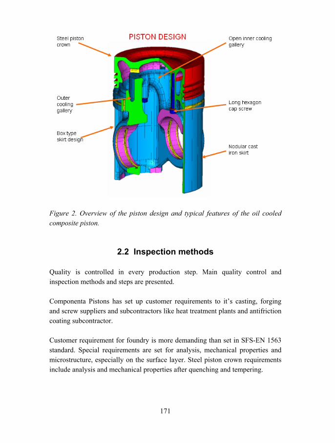
171
Figure 2. Overview of the piston design and typical features of the oil cooled composite piston.
2.2 Inspection methods
Quality is controlled in every production step. Main quality control and inspection methods and steps are presented.
Componenta Pistons has set up customer requirements to its casting, forging and screw suppliers and subcontractors like heat treatment plants and antifriction coating subcontractor.
Customer requirement for foundry is more demanding than set in SFS-EN 1563 standard. Special requirements are set for analysis, mechanical properties and microstructure, especially on the surface layer. Steel piston crown requirements include analysis and mechanical properties after quenching and tempering.

172
Ultrasonic inspection of the castings is made for pistons skirt castings at normal sampling rate set at the quality system of the foundry. Addition to that certain areas of the piston skirt castings are inspected to 100%. These are the thickest parts of the castings where X-ray penetration is limited. Steel piston crown material goes through ultrasonic inspection at the steel mill, when its geometry is the most suitable for inspection method.
All piston skirt castings go through radioscopic inspection at 100% coverage. Inspection program for piston skirt consist of 50 X-ray images in average depending on the piston model. Inspection is performed after first turning operation when the outer surface has been machined away. First machining operation before inspection is necessary for the inspection program to move and position the casting accurately before each image taken. Internal defects found in the radioscopic inspection are rare. The lost machining time is not significant for cases when the casting is so seriously defected that it had to be scraped. Inspection time is approximately 15 minutes. The following machining operation takes longer time than radioscopic inspection. CNC-machine operators are trained for the inspection and they do the inspection while the horizontal machining centre is machining automatically already inspected casting.
Dimensional measurements with coordinate measurement machine are very detailed. In average 65 measurements (diameter, length, straightness, perpendicularity, flatness, inclination etc.) are made for each piston crown and each piston skirt. Addition to that 15002000 measurement points (amount depends on the piston model) are scanned with CMM to verify the shape of each piston skirt sliding surface. Measurement results are part of the product. Measurement summary containing 15 measurement results of each piston skirt and piston crown and 6 measurement results of each piston assembly are included into the delivery documents of the piston supply.
Magnetic particle inspection is performed for piston skirts and piston crowns after CMM measurements to find surface defects like dross, cracks and inclusions. Applied inspection system is computer controlled and it monitors automatically magnetization current, uv-light, fluorescence and translucency of the inspection liquid.

173
In the assembly process piston skirts and piston crowns will get serial numbers. Before assembly parts are traceable by their unique production numbers. Piston crowns are fastened to piston skirts with screw joint. Screw joint fastening sequence is specified. The fastening reliability system is applied to fasten the screws. Angle is controlled and torque is monitored by the fastening reliability system in final fastening. Fastening data of each screw joint is stored in the computer. Assembled pistons are weighted.
Traceability of the pistons is covered from the melting of iron in the foundry and steel in the steel mill through the whole production process with all measurements and inspections to screw fastening data. All data can be found from the traceability database by the piston serial number.
- material analysis, mechanical properties, microstructures
- ultrasonic inspection (Figure 3)
- radioscopic inspection (Figure 4)
- dimensional measurements, CMM (Figure 5)
- magnetic particle inspection (Figure 6)
- screw fastening data (Figure 7)
- traceability

174
Figure 3. Ultrasonic testing of a piston casting and schematic view of the ultrasonic testing of the steel bar.
Figure 4. Radioscopic inspection image of the piston casting.

175
Figure 5. Piston skirt sliding surface cross section deviation graph and dimensional measurement of piston skirt.
Figure 6. Magnetic particle inspection of piston skirt.

176
Figure 7. Screw fastening at the piston assembly shell. Fastening data (angle and torque) is recorded and data is transferred in computer.
2.2.1 Radioscopic inspection
Radioscopic inspection of the piston skirt castings is made with Seifert DP 406P inspection system (Figure 8). Main specifications of the inspection system are:
- X-ray tube: 450 kV - Focal spots: 0.8 / 1.5 mm - X-ray image intensifier: Vistalux 9S3-CCD - Image enhacement system: Vistaplus II - Control: Siemens PLC - Programmable axis: 10 - Max work piece weight: 250 kg - Protection cabinet: 12 200 kg - Manufacturer: Rich. Seifert & Co GmbH & Co. KG - Made in: Germany - Manufactured: 1999
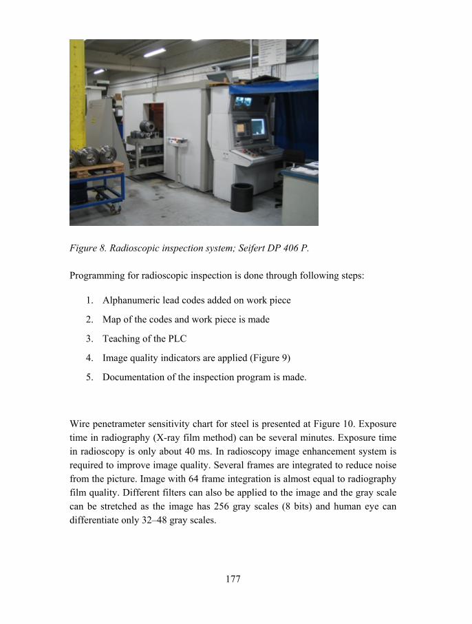
177
Figure 8. Radioscopic inspection system; Seifert DP 406 P.
Programming for radioscopic inspection is done through following steps:
1. Alphanumeric lead codes added on work piece
2. Map of the codes and work piece is made
3. Teaching of the PLC
4. Image quality indicators are applied (Figure 9)
5. Documentation of the inspection program is made.
Wire penetrameter sensitivity chart for steel is presented at Figure 10. Exposure time in radiography (X-ray film method) can be several minutes. Exposure time in radioscopy is only about 40 ms. In radioscopy image enhancement system is required to improve image quality. Several frames are integrated to reduce noise from the picture. Image with 64 frame integration is almost equal to radiography film quality. Different filters can also be applied to the image and the gray scale can be stretched as the image has 256 gray scales (8 bits) and human eye can differentiate only 3248 gray scales.

178
Figure 9. Image quality indicator.
Figure 10. Wire penetrameter sensitivity chart for steel.

179
Wire penetrameter sensitivity chart shows the size of the defects that is possible to find from steels with various thickness. Also the difference between live image and image with 64 frame integration is shown.
When a defect is found from the image and the decision to reject the casting or accept it is not clear, evaluation of the image is made by comparing the images to the reference images in the library. Reference images are originally evaluated by cutting the casting in pieces the castings where the indications are found. At Figures 1113 there are some examples of radioscopic images.
Figure 11. Acceptable defect.
Figure 12. Slight shrinkage porosity.

180
Figure 13. Not acceptable defect.
2.2.2 Surface defects
Surface defects can be found with:
- radioscopic inspection (Figure 14)
- visual inspection
- magnetic particle inspection.
Figure 14. Surface defects detected through radioscopic inspection.

181
Majority of the defects found with the radioscopic inspection turns out to be on the surface of the casting and can also be seen visually.
Componenta Pistons quality system instructs where and how much can be grinded to remove the surface defect (Figure 15). Instructions are based on finite element model calculations and fatigue analysis of the one quarter model of piston, gudgeon pin and upper part of the connecting rod. Quality instruction is made simple to follow. There are only two colors defining how much material in percentage of the wall thickness or absolutely can be removed from colored area. Originally picture presents fatigue safety fringe plot of the fatigue analyses.
Figure 15. Limits for removal of surface defects.

182
3. Conclusions
Different inspection and measurement methods are applied to control quality of pistons manufactured by Componenta Pistons.
Reliability requirements set for diesel engine pistons are extremely high. The integrity of cast components must be verified to meet the imposed quality requirements.
The inspection procedures and acceptance criteria are designed for optimised fitness for purpose. Coverage of inspection at critical parts is 100%.
To meet the high quality standards Componenta Pistons analyses 175 000 X-ray images annually, i.e. about 50 images per piston. Quality assurance is an essential part of the manufacturing process of large bore pistons.

Fatigue assessment
Defect tolerance for castings .......................................................... 185 Jussi Solin
Analysis of defects and failure risk of cast components ................. 205 Jan Persson
Influence of occasional underloads on fatigue ................................ 229 B. Roger Rabb
On the prediction of crack propagation in cast steel specimens ..... 251 Anders Björkblad
Conventional vs. closure free crack growth in nodular iron ............ 273 Anders Björkblad
Fatigue crack growth in ductile iron ................................................ 287 Kenneth Hamberg, Marie Mörtsell, Anders Björkblad & Jack Samuelsson
Fatigue assessment of a cast axle .................................................. 311 Janne Lepistö

185
Defect tolerance for castings
Jussi Solin VTT Technical Research Centre of Finland
Espoo, Finland
Abstract
Heavy section cast GJS 400 nodular iron was studied. In ultrasonic factory inspection rejected and acceptable material blocks were evaluated by further ultrasonic measurements, radiography and fatigue testing. Radiography was capable to recognize porosity, but the sizes of individual pores could not be assessed. The defected area map of factory inspection resembles the C-scan image produced by semi-manual inspection using BAT method.
Fatigue tests show a notable difference in fatigue resistance of the acceptable and rejected materials for 50 % failure probability, but the scatter was clearly higher in the acceptable material batch, meaning that reduction of safe fatigue design curve may be much smaller than the difference at 50 % failure probability.
1. Introduction
The effect of large clusters of internal casting defects on fatigue endurance of heavy section nodular cast iron was studied. Centerline porosity may form in the last solidifying volume of heavy castings. To some extent it can be in-avoidable and acceptable, in particular, if service stresses are lower at the centerline. However, fatigue cracks may also initiate in less stressed internal areas, if the porosity lowers the fatigue strength significantly.

186
1.1 Background
Fatigue performance of heavy section nodular iron was studied in a previous project [1]. Normal quality castings were studied already then by both ultrasonic measurements and fatigue tests. Correlations between NDE results and fatigue resistance were sought for, but less successfully. It was concluded that the material was too homogeneous and difference could not be seen. The test material was considered defect free.
However, to obtain some insight to the applied NDT criteria, nodular iron samples with known defects were tested. Those tests were conducted in 4 point bending on 20 x 20 mm cross section specimens. The test material did not meet a φ5 mm reference hole criteria. The fatigue test results are shown in Fig. 1. The fatigue limit stress for the specimens with defects was about 50 % of the fatigue limit stress for the defect free material.
Figure 1. Bending fatigue data for specimens of cast nodular iron GJS 500 with defects exceeding a criteria of φ5 mm reference hole [1].

187
1.2 Scope of the study
Metso Paper designs and manufactures paper machines. Some rolls are manufactured from very large castings. The castings are subjected to ultrasound inspection and excessive centreline porosity is sometimes found, Fig. 2. The cost of each casting is high and delivery time is long. Re-melting of a casting may cause problems for delivery schedule of the whole project. The economic and delivery schedule concerns, together with the high reliability requirements for integrity and fatigue endurance of the rolls, set pressure on well justified decisions on rejection or acceptance of the castings.
Figure 2. Rejected nodular cast iron roll after US inspection.
A final purpose for Metso Paper is to refine instructions to evaluate acceptability of detected defects in a cast roll. Information about location and size of the defected area and the severity of the defect from ultrasonic inspection should be correlated with the material properties data of defected cast roll material. Porosity may affect also other properties, but this study was focussed to determination of fatigue strength reduction and applicability of ultrasonic inspection to predict such reduction.

188
Results of strength calculations of the roll under operational loads are needed for judging case by case the acceptability of NDE indications. The herein studied defects clusters of shrinkage pores are forming in the areas of last solidification near the material mid-plane of the hull. Fortunately, the internals of the hull are less severely stressed and less sensitive for fatigue crack initiation than the outer surface of the roll. However, macroscopic bending of a roll causes quite even tension/compression hoop stresses across the hull thickness.
2. Experimental
2.1 Test material
Fatigue testing of both rejected and acceptable cast nodular iron was included in a subproject within this Gjutdesign-2005 project. Test material is cut from the cast nodular iron, GJS 400, roll where a large shrinkage pore area had been detected. The size of the defected area is about 250 x 900 mm. Cutting plan of a rejected roll is shown in Fig. 3. About half meter long cylinder part from the 140 mm thick roll was cut in four pieces for the investigations. A large area of porosity was extracted as a whole. For comparison adjacent material of the same roll was also tested.
Figure 3. Cutting plan for the studied roll.
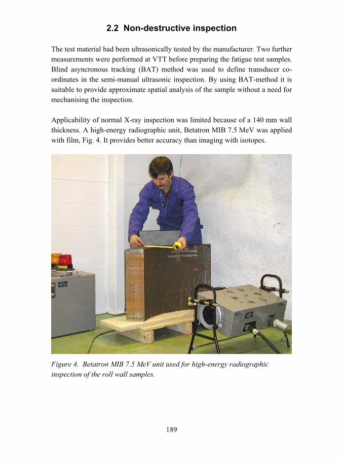
189
2.2 Non-destructive inspection
The test material had been ultrasonically tested by the manufacturer. Two further measurements were performed at VTT before preparing the fatigue test samples. Blind asyncronous tracking (BAT) method was used to define transducer co-ordinates in the semi-manual ultrasonic inspection. By using BAT-method it is suitable to provide approximate spatial analysis of the sample without a need for mechanising the inspection.
Applicability of normal X-ray inspection was limited because of a 140 mm wall thickness. A high-energy radiographic unit, Betatron MIB 7.5 MeV was applied with film, Fig. 4. It provides better accuracy than imaging with isotopes.
Figure 4. Betatron MIB 7.5 MeV unit used for high-energy radiographic inspection of the roll wall samples.
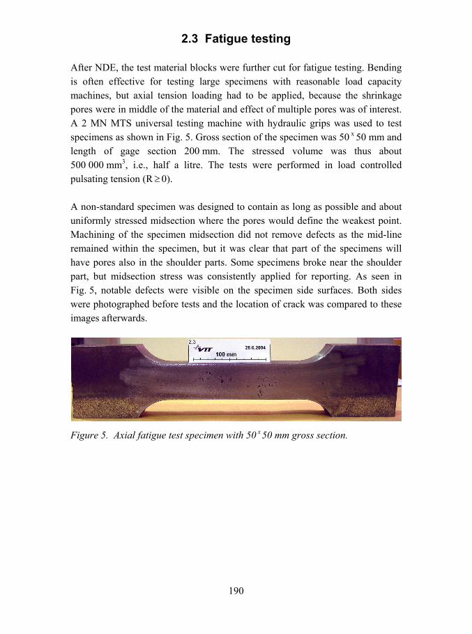
190
2.3 Fatigue testing
After NDE, the test material blocks were further cut for fatigue testing. Bending is often effective for testing large specimens with reasonable load capacity machines, but axial tension loading had to be applied, because the shrinkage pores were in middle of the material and effect of multiple pores was of interest. A 2 MN MTS universal testing machine with hydraulic grips was used to test specimens as shown in Fig. 5. Gross section of the specimen was 50 x 50 mm and length of gage section 200 mm. The stressed volume was thus about 500 000 mm3, i.e., half a litre. The tests were performed in load controlled pulsating tension (R ≥ 0).
A non-standard specimen was designed to contain as long as possible and about uniformly stressed midsection where the pores would define the weakest point. Machining of the specimen midsection did not remove defects as the mid-line remained within the specimen, but it was clear that part of the specimens will have pores also in the shoulder parts. Some specimens broke near the shoulder part, but midsection stress was consistently applied for reporting. As seen in Fig. 5, notable defects were visible on the specimen side surfaces. Both sides were photographed before tests and the location of crack was compared to these images afterwards.
Figure 5. Axial fatigue test specimen with 50 x 50 mm gross section.
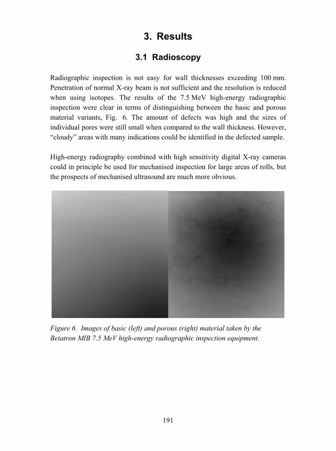
191
3. Results
3.1 Radioscopy
Radiographic inspection is not easy for wall thicknesses exceeding 100 mm. Penetration of normal X-ray beam is not sufficient and the resolution is reduced when using isotopes. The results of the 7.5 MeV high-energy radiographic inspection were clear in terms of distinguishing between the basic and porous material variants, Fig. 6. The amount of defects was high and the sizes of individual pores were still small when compared to the wall thickness. However, cloudy areas with many indications could be identified in the defected sample.
High-energy radiography combined with high sensitivity digital X-ray cameras could in principle be used for mechanised inspection for large areas of rolls, but the prospects of mechanised ultrasound are much more obvious.
Figure 6. Images of basic (left) and porous (right) material taken by the Betatron MIB 7.5 MeV high-energy radiographic inspection equipment.

192
3.2 Ultrasonic inspection
The material was already inspected in the factory by Metso Paper. A map of classified indications is shown in Fig. 7. These results were used as a basis for selection of the test material and cutting of fatigue test samples.
VTT performed comparative ultrasonic measurements with blind asyncronous tracking (BAT). This technology combines the simplicity of manual inspection and quantitative data processing for 3d mapping of the sample. The BAT-system traces and stores the transducers co-ordinates together with the US measurements. A C-scan of post processed data is shown in Fig. 8. Porosity is seen as black and dark blue in this C-scan. The scanning was performed in two phases. Unfortunately, slightly different dB-scales were used to construct the graphs, from 23,0 to 56 dB for the left side and from 26,5 to 57,2 dB for the right hand side (this could be still redone, but would not change the conclusions). On the other hand, the co-ordinate systems seem to be quite accurate, because the two graphs coincide pretty well.
Comparison of Figs 7 and 8 shows good repeatability of the measurements. The exact dimensions should not be compared as the factory inspections are reported to a hand drawn grid with approximately 35 mm cell size, in average. However, a closer look reveals that a certain pattern of indications was accurately revealed already in the factory inspection and then reproduced by different people, equipment and method. Even the reported reference reflector sizes (flat bottom holes) correlate with the C-scan analysis.
The BAT-system with post processing can provide approximate spatial analysis of the sample. The results are presented as cross section projections in Fig. 8. In these graphs the colour scale is inversed so that red colour corresponds to indications. We can see most of the indications at the predicted depth (only midsection is shown). The indications correlate also with the C-scan and factory inspections (Figs 7 and 8) in the X and Y coordinate directions.

193
A B C D E F G H I J K L M N O
900X
[mm]
72
144
216
288
360
432
504
576
648
720
792
0A B C D E F G H I J K L M N O
900X
[mm]
72
144
216
288
360
432
504
576
648
720
792
0
900X
[mm]
72
144
216
288
360
432
504
576
648
720
792
0
72
144
216
288
360
432
504
576
648
720
792
0
Figure 7. A map of factory ultrasonic inspection results as reference flat bottom hole sizes representative for indications. Two highest classes are highlighted by colour (inspection performed by Metso Paper).

194
Z
Z
50
90
50 90
100
200
300
400
500
600
700
800
0 100 200 300 400
X Y
Z
Z
50
90
50 90
100
200
300
400
500
600
700
800
0 100 200 300 400
Z
Z
50
90
50 90
100
200
300
400
500
600
700
800
0 100 200 300 400
Z
Z
50
90
50
90
50
90
50 9050 90
100
200
300
400
500
600
700
800
100
200
300
400
500
600
700
800
100
200
300
400
500
600
700
800
0 100 200 300 4000 100 200 300 400
XX YY
Figure 8. C-scan image of the same porosity area as in Fig. 7. The C-scan is composed of two parts with slightly different dB scales as presented in colours. Dark blue corresponds to defects. Gross section projections (right, below) show the distribution of porous areas (this time red) as through the X and Y directions.

195
3.3 Fatigue S-N curves
Eleven specimen of the basic material were all tested at nominal 100 ± 105 MPa. Twelve specimen taken from the porous blank were tested at different stress amplitudes: 100 ± 105 MPa; 80 ± 75 MPa; 67,5 ± 65 MPa and 55 ± 52,5 MPa.
The results of fatigue tests are shown in Fig. 9. Geometric mean lives for each stress amplitudes and arbitrary regression fits are also shown. An equation with asymptotic exponent of -1/4 for short lives and a smooth transition to fatigue limit was adopted for regression:
Sa = α ⋅ 1 + ( Nf / 100 000 ) -0,25 . (1)
The resulting α parameters ( fatigue limit and α = Sa, 100 000 / 2 ) are 54,8 MPa for basic material and 34,4 MPa for the porous material, i.e., the fatigue strength of the defected material would be about 63 % of the basic material fatigue strength. The mean fatigue life for the defected material would be 4 % of the life for the basic material at Sa = 105 MPa and only 1 % at Sa = 75 MPa. These values should be considered just as rough estimates. Furthermore, one specimen was excluded from the defects sample, as explained later.
25
50
75
100
125
150Basic
Defects
Defect ?
mean (B)
mean (D)
103 104 105 106 107
150
125
100
75
50
25
Stre
ss a
mpl
itude
[ M
Pa ]
N f25
50
75
100
125
150Basic
Defects
Defect ?
mean (B)
mean (D)
103 104 105 106 107
150
125
100
75
50
2525
50
75
100
125
150Basic
Defects
Defect ?
mean (B)
mean (D)
25
50
75
100
125
150Basic
Defects
Defect ?
mean (B)
mean (D)
103 104 105 106 107103 104 105 106 107
150
125
100
75
50
25
150
125
100
75
50
25
Stre
ss a
mpl
itude
[ M
Pa ]
N f
Figure 9. Fatigue lives for materials outside and in the porous area.

196
3.4 Fracture surfaces
Fractographic evaluation of the fatigue tested specimens was performed using stereo microscope and macrogaphs, Figs 1012. For some specimens it turned out very difficult to locate crack initiation sites and their growth paths.
Many specimens had multiple crack initiation sites and in some cases the cracks had grown on different planes beyond each other before the final failure occurred. Even distinguishing between casting defects and sound iron is not so easy. Some fracture surfaces had very large areas, which might be considered as defected. However, the surfaces are still macroscopically planar and the defected areas cannot be considered as single defects, but rather as dense clusters of smaller porosity.
Figure 10. Fracture surface of the specimen with the poorest fatigue endurance (1.1). Left is a detail from the defected area in the left lower corner.
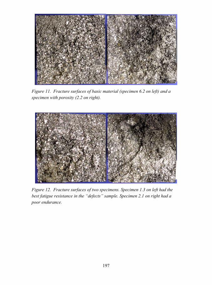
197
Figure 11. Fracture surfaces of basic material (specimen 6.2 on left) and a specimen with porosity (2.2 on right).
Figure 12. Fracture surfaces of two specimens. Specimen 1.3 on left had the best fatigue resistance in the defects sample. Specimen 2.1 on right had a poor endurance.
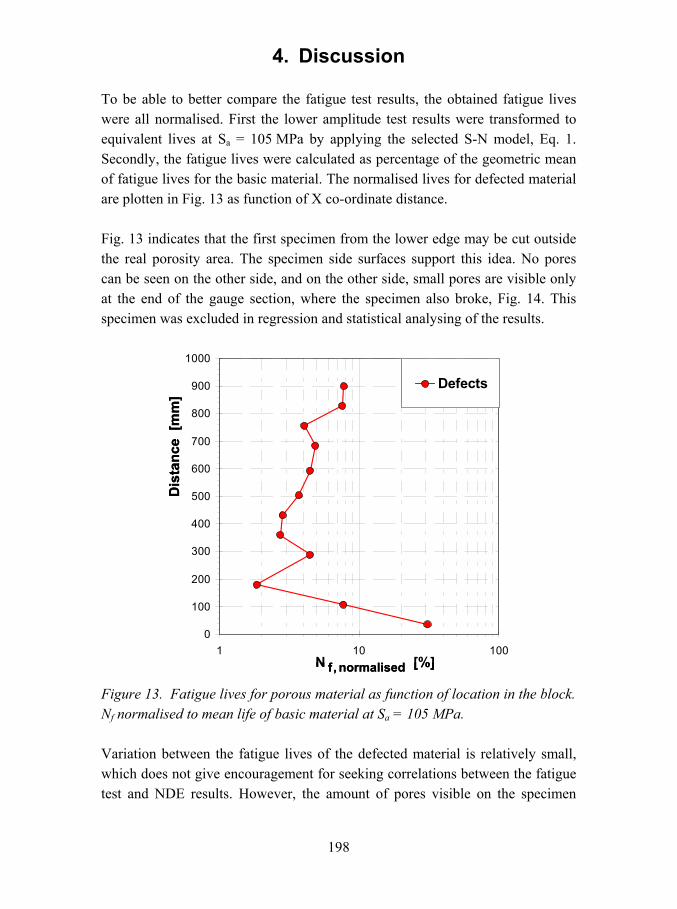
198
4. Discussion
To be able to better compare the fatigue test results, the obtained fatigue lives were all normalised. First the lower amplitude test results were transformed to equivalent lives at Sa = 105 MPa by applying the selected S-N model, Eq. 1. Secondly, the fatigue lives were calculated as percentage of the geometric mean of fatigue lives for the basic material. The normalised lives for defected material are plotten in Fig. 13 as function of X co-ordinate distance.
Fig. 13 indicates that the first specimen from the lower edge may be cut outside the real porosity area. The specimen side surfaces support this idea. No pores can be seen on the other side, and on the other side, small pores are visible only at the end of the gauge section, where the specimen also broke, Fig. 14. This specimen was excluded in regression and statistical analysing of the results.
0
100
200
300
400
500
600
700
800
900
1000
1 10 100
Defects
Dis
tanc
e [m
m]
N f, normalised [%]
0
100
200
300
400
500
600
700
800
900
1000
1 10 100
Defects
Dis
tanc
e [m
m]
N f, normalised [%]
Figure 13. Fatigue lives for porous material as function of location in the block. Nf normalised to mean life of basic material at Sa = 105 MPa.
Variation between the fatigue lives of the defected material is relatively small, which does not give encouragement for seeking correlations between the fatigue test and NDE results. However, the amount of pores visible on the specimen

199
surfaces was found to be qualitatively in line with the ultrasound measurement results. Also the local deviation to better fatigue resistance at X = 300 mm in Fig. 13 happens to coincide with a gap in severe porosity along the X -axis in the longitudinal gross section of Fig. 8. Specimen 2.2 in Fig. 15 was cut from an area of high porosity.
Figure 14. The first specimen from the lower edge of the defected material block. Small pores are visible only on one side at the end of the gauge section, where the specimen also broke as marked with the pile.
Figure 15. A specimen with porosity visible on surface and low fatigue strength. The specimen broke along with the plane marked with pile.
4.1 Scatter in fatigue results
Another interesting way of presenting the results is shown in Figs 16 and 17. Both data sets are ordered according to the rank probability and plotted to show extreme value statistics distributions of normalised fatigue lives (Fig. 16) and according to log-normal distribution (Fig. 17). The fatigue lives are usually assumed to follow log-normal distribution. On the other hand, statistics controlled by weakest links tend to follow extreme value statistics distributions.

200
We can see that the two data sets follow quite different statistics. Perhaps one would not assume that the scatter is lower for the material containing more defects. However, this is clearly the case. And as a consequence, the difference between the two data sets gets smaller when comparison is done at lower failure probability, i.e., for more reliable designs. According to Fig. 16 the ratio of (normalised) fatigue lives for the compared materials is 35 at 50 % failure probability. But the ratio is extrapolated only to 5 at 1 % failure probability.
The before mentioned influence of selected failure probability should be considered, when deciding on the acceptability criteria for porosity. On the other hand, this observation supports the idea of adopting design criteria allowing for large defects even for material, which has passed NDE.
The material with defects seems to follow log-normal distribution quite well, but the basic material doesnt. There seems to be kind of scaling off behaviour limiting the distribution from the upper edge of fatigue resistance. A possible explanation for such behaviour would be, for example, if there were two different kinds of defects controlling the fatigue resistance. If shrinkage pores vanish, another type of defects will cause initiation.
This kind of situation is typical for nodular iron. Graphite nodules would always be able to provide fatigue crack initiation sites in perfect castings without shrinkage pores or other kind of defects.
On the other hand, it is important to consider, whether the lower tail of the fatigue strength distribution is generally wider. In laboratory testing it results to low fatigue resistance only for minority of the material samples, but in practice the situation may be quite different, because the stressed volume in a roll is much higher than in the test specimen. If the herein studied acceptable material is representative, the lower tail of the distribution should be carefully estimated. However, this material was taken adjacent to a large concentration of casting defects and it may be not generally representative material sample.
The previous tests shown in Fig. 1 were not directly comparable to the present results, but they are in line with them.
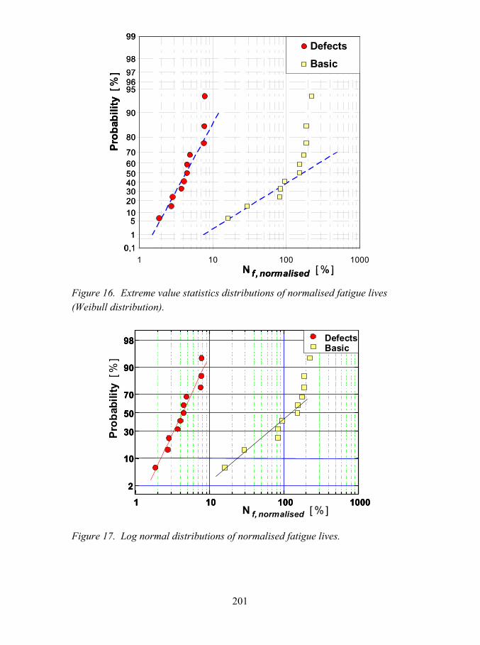
201
1 10 100 1000
DefectsBasic
50
70
95
90
98
99
403020105
1
97
80
0,1
60
96
Prob
abili
ty [
%]
N f , normalised [ % ]1 10 100 1000
DefectsBasic
50
70
95
90
98
99
403020105
1
97
80
0,1
60
96
1 10 100 1000
DefectsBasic
1 10 100 1000
DefectsBasic
50
70
95
90
98
99
403020105
1
97
80
0,1
60
96
50
70
95
90
98
99
403020105
1
97
80
0,1
60
96
Prob
abili
ty [
%]
N f , normalised [ % ]
Figure 16. Extreme value statistics distributions of normalised fatigue lives (Weibull distribution).
Prob
abili
ty [
%]
N f, normalised [ % ]1 10 100 1000
2
10
30
50
70
90
98 DefectsBasic
Prob
abili
ty [
%]
N f, normalised [ % ]1 10 100 1000
2
10
30
50
70
90
98 DefectsBasic
1 10 100 1000
2
10
30
50
70
90
98
1 10 100 1000
2
10
30
50
70
90
98 DefectsBasic
Figure 17. Log normal distributions of normalised fatigue lives.

202
5. Conclusions
In ultrasonic factory inspection rejected and acceptable GJS 400 nodular iron samples taken from heavy casting were studied by further ultrasonic measurements, radiography and fatigue testing. The following conclusions can be drawn:
• Radiography was capable to recognize porosity, but the sizes of individual pores could not be assessed.
• Repeatability of ultrasonic measurements is good. The defected area map of factory inspection resembles the C-scan image produced by semi-manual inspection using BAT method.
• Fatigue tests show a notable difference in fatigue resistance of the acceptable and rejected materials. For 50 % failure probability the difference was about 40 % ( from 100 % to 63 %) in stress amplitude and about 95 % ( from 100 % to 4 %) in fatigue life.
• The scatter was higher in the acceptable material. This means that reduction of safe fatigue design curve may be smaller than 40 %.
• The fatigue resistance of the studied acceptable material was not log-normally distributed. The lower tail of the distribution was wider than the upper end.
• If the studied acceptable material is representative, the lower tail of the distribution should be carefully estimated, because the stressed volume in a roll is much higher than in the test specimen and failure probabilities are more controlled by the lower tail of the distribution.
It shall be noted that the wall thickness of the test material was 140 mm and that the studied shrinkage pore areas were located near midline inside the roll shell. It can be assumed that much better quality of material is obtained at the surface of the roll.
203
Acknowledgements
The reported work was financed by the Nordic Innovation Centre, Tekes, VTT and Finnish industry as part of the Gjutdesign-2005 project. Together with Eerikki Mäkinen and Juhani Vestola, Erkki Kiiski of Metso Paper Ltd was in primary charge of controlling this subproject. Research planning was initiated by Gary Marquis, when still at VTT. Päivi Karjalainen-Roikonen took charge of the work at VTT until her parential leave and Jouni Alhainen since beginning of 2004. Ultrasonic measurements at VTT were performed by Jorma Pitkänen, High energy X-ray by Markku Hirn and fatigue tests by Heikki Laukkanen.
References
1. Marquis, G. and Solin, J., 2000. Long-life fatigue design of GRP 500 nodular cast iron components. Espoo 2000. VTT Research Notes 2043. 70 p.

205
Analysis of defects and failure risk of cast components
Jan Persson VOLVO Construction Equipment Components AB
Eskilstuna, Sweden
Abstract
The objective of this work has been to determine the fatigue life of hubs containing defects as a result of casting. The defects arise from shrinkage in the material. A survey of non-destructive testing methods has been made in order to detect the casting defects. The conclusion is that no good method exist that can be used to detect small internal defects beneath the surface. A visual examination of the surfaces was conducted. Test specimens cut out from the hubs were fatigue tested in a rig. Approximately 11% of the examined hubs contained larger defects on or beneath the surface. The fatigue life from the testing was then compared with the calculated life for the test specimens. The calculated (LEFM) fatigue life was approximately 7580 % of the fatigue life, obtained at the fatigue test.
A fatigue life conversion from the test specimens to the hubs was made. The fatigue life of hubs containing the larger defects is approximately 18·106 cycles at the dimensioning load (corresponds to 18000 operating hours). The larger defects found were located in the low stressed area.
This work has been preformed as a master thesis work in cooperation with LiTH.
1. Introduction
This report shows part of the Master thesis work Analysis of casting defects and assessment of failure [1]. The work was performed at the department for Analysis and Structural Strength testing, Volvo Construction Equipment Components AB.

206
1.1 Background
In connection with the introduction of a new casting method for hubs of nodular cast iron SS0727-02, casting defects (porosity) on a larger or lesser extent have been noticed in a limited volume beneath the inlet, probably caused by bad performance of the feeder. The defects arise from shrinkage in the material. The defects were discovered for a batch of hubs after the machining process. The majority of those hubs probably are defect free, but a small number with a varying degree of cast defects is likely to occur. To get a base for a judgment about the failure risk for those hubs, if mounted in machines, we have examined 60 of them.
1.2 Objective
The main objective of this work was to
• examine the use of non-destructive testing to discover defects on and beneath the surface.
• determine the fatigue life and verify strength values for the hubs containing defects as a result of casting, by life prediction testing of small test specimens, cut out from the hubs.
• perform fracture mechanic calculation with assumed defect size, defect "distribution" and stress gradient.
1.3 Delimitations
In this work the defects have been considered to be two dimensional fractures. Life prediction calculations have only been done for surface braking defects. The possible presence of residual stresses on the surface (from machining) has been disregarded.

207
2. Selection of hubs
2.1 Visual inspection
A thorough visual inspection (light from a halogen lamp) of the hubs was carried out to determine the size and magnitude of the defects on the surface. (The casting defects are in the area near the machined outer radii, where the inlets are assumed to have been located during the casting.) The positions, size, appearance and distribution of the defects were noted.
Figure 1. Cross section of the hub as cast.
2.2 Non-destructive testing
One hub was sent for material testing. Two hubs with small defects were sent for non-destructive testing one to DNV and one (for x-ray examination) to Chalmers-Lindholmen.

208
Figure 2. Cross section of the hub. The defects are found in the marked area.
Test methods were eddy current testing, magnetic particle inspection, ultra sonic testing, penetrant testing and radiographic testing. Penetrant testing was the only method that could detect small surface pores. There is no good method to detect defects beneath the surface when the size of the defects is small. Also the shape of the defects and the location in the hub may cause trouble to detect defects. For surface-braking defects, visual inspection is probably the best method.
2.3 Destructive testing
From hubs without or with minor surface-braking defects (2r < 0,5 mm) some test specimens were made to define reference values. From the hubs with surface-braking defects 16 test specimens were made for rig tests. After fracture 8 test specimens were classified having small starting defects (0,5 mm < 2r < 1 mm). Those are considered to be the size of normal casting defects, witch were used to define normal values. 8 test specimens were classified having significant starting defects (2r > 1 mm). Those were used to define strength values as a function of defect size. (2r is the equivalent poor diameter, see chapter 4.2.)

209
3. Fatigue testing
3.1 Test objects
3.1.1 Geometry
The test specimens were cut out from the hubs, symmetrically around one of the internal stiffening ribs. (It is assumed that the thicker material at the ribs solidifies last and contributed to the forming of defects in the volume.) The sides of the specimens are milled to be parallel and have a thickness of 50 mm.
Figure 3. Model of test specimen.
3.1.2 Material, loads and constraints
The hubs are made of nodular cast iron SS0727-02. The loads in the fatigue testing are chosen to give life of approximately 5·105 to 5·106 cycles for defect free material. The fastening and load application points are seen in Figure 4.
3.2 Test method
Constant amplitude tests were performed with R = 0 at different loads in a test rig.

210
3.3 Test rig
A test rig was designed using FE-simulations. A model of the test specimens was imported from Solid Edge into Ansys Workbench Structural. Different fastenings and load application points were tested to generate maximum stress in the area where the defects were found. The data generated was used in the design of the test rig.
This support and point of load application produced a relatively evenly distributed stress over the area where defects were indicated. It is assumed that the stress concentration is substantially increased at the defects, so that the fracture is assumed to occur there. The maximum stress is found in the 10 mm radius.
Figure 4. Test rig with load application points and constraints.

211
Figure 5. Test rig.
Figure 6. Maximum principal stress (see Figure 17 for reproduction in color).

212
3.4 Testing
One of the reference test specimens was equipped with strain gauges in two perpendicular directions, to compare the stresses from FEM calculation and stresses from rig test. Hookes general law was used to calculate the principal stress. A linear behaviour can be assumed and the stress appeared to be 10% higher in the FE-model compared to the rig test. The calculated stress gradients from the FE-simulation were multiplied by 0,9.
Test specimens from all the groups (see chapter 2.3) were fatigue tested with constant amplitude to determine the influence that casting defects have on strength. The tests were performed with R = 0 at different loads.
3.5 Material strength
The life of a component can be assessed using fatigue testing with cyclic load at a certain R-value (σmin/σmax). The stress range is plotted against the number of cycles in a Wöhler diagram/S-N diagram (log-log scale). Because of the large scatter in life it is necessary to test a large number of specimens to determine a reference curve. The assumption made here is that specimens with similar defects will follow the same Wöhler curve.
The Capacity-value (C) is a measure of the material fatigue strength. The C-value is calculated according to equation 1.
C = ∆σk ·N (1)
where: ∆σ = stress range k = slope factor (inverse slope in Wöhler diagram) N = cycles to failure.
The Design Curve (see Figures 13 and 14) for nodular cast iron components is according to Volvo CE standards. The slope factor have earlier been k = 4,7. In this project k = 5 has been used for the tested material.
The results for all the groups are presented in Wöhler diagrams in chapter 5.

213
4. Fracture surfaces
4.1 Examination
In order to calculate the fatigue life of the test specimens the size of the initial crack has to be known. It was determined through examination of the fracture surfaces. The examination was done using both macro-scope and scanning electron microscope (SEM). The macro-scope provided a good overview of the fracture initiation point. If several initiation points have been found, the largest one was chosen. With SEM the size of the defects could be determined more exactly. Figures 7 and 8 shows a material inspection of the hub.
Figure 7. Section throw hub with typical defects in the shrinkage area.
Figure 8. Chunky graphite and fatigue cracks in the shrinkage area.

214
The defects are distinguished by the presence of dendrites, se Figure 9. The image to the left shows large dendrite with branches that has grown from a major defect with great lack of feeder material. The image to the right shows minor dendrite where the branching is minimized.
Figure 9. Dendrites.

215
4.2 Evaluation of defect sizes
Due to the absence of round smooth edges on the defects the shapes have been estimated in order to calculate life with the fatigue calculation (fracture propagation) program AFGROW [2]. Since AFGROW only handles calculations of circular and elliptic cracks the defects have been approximated into those shapes. Used method see [3]. Some defect areas have been very hard to estimate when there has been coherent material between the defects. On some fracture surfaces the defects were just below the surface (approximately 0,2 mm), see for example Figure 10.
These defects have nevertheless been considered as surface braking defects while the number of cycles until surface braking is supposedly very low. If two cracks are positioned close to each other interference is likely to occur. The stress intensity will in this case get higher than if the cracks had been isolated from each other. If the space between the cracks is larger than the size of the smaller crack the stress intensity will not be noticeably influenced. If the distance between the cracks is less, a common area can be calculated as the sum of the crack area plus the space between them. An example can be seen in Figure 11 where the white ellipse shows the estimation of the defect.
Test specimens no 23, 25 and 30 are shown in Figure 12. In the first two images the defect is situated on the edges where the fracture has started. The third image shows a very extended and deep defect.

216
Figure 10. Defect that is situated just beneath the surface. Surface on top of image.
Figure 11. The ellipse shows an example of estimation of a half-elliptic surface crack.

217
Figure 12. Images of fracture surfaces that contain major defects.
5. Results of rig test of specimens
To develop a Reference Curve requires a large amount of data points. The Reference Curve in Figure 13 is only based on 4 points. That was done since the scatter in this case was considered to be very small. After calculating a mean value for the C-value of the reference items (defect free material) an approximated curve with the slope factor k = 5 was drawn. The rig test was performed with R = 0.
Figure 14 shows the Wöhler diagram of the specimens with defects. The group with small (normal) defects are in good agreement with the Design Curve.
(The Wöhler curve have to be justified for the hubs with R = -1. That is done according to equations 2 and 3, according to Volvo CE design rules.
CR=-1 = CR=0·KRk (2)
KR = 1 0,33·R (R≤ 0) (3)
where k is the slope factor of the Wöhler curve.)

218
104 105 106 107 108
Cycles to Failure
Design Curve
Reference itemsReference Curve
Stre
ss R
ange
[MP
a]
100
1000
200
800
400
600
104 105 106 107 108
Cycles to Failure
Design Curve
Reference itemsReference Curve
Stre
ss R
ange
[MP
a]
100
1000
200
800
400
600
104 105 106 107 108104 105 106 107 108
Cycles to Failure
Design Curve
Reference itemsReference Curve
Stre
ss R
ange
[MP
a]
100
1000
200
800
400
600
100
1000
200
800
400
600
Figure 13. Reference items compared to the Design Curve (R=0).
104 105 106 107 108
Cycles to Failure
Stre
ss R
ange
[MP
a]
100
1000
200
800
400
600 Design CurveRefer. Curve
Small DefectsNo 21 & 35No 26 & 34No 36No 23No 25 & 30
104 105 106 107 108
Cycles to Failure
Stre
ss R
ange
[MP
a]
100
1000
200
800
400
600
104 105 106 107 108104 105 106 107 108
Cycles to Failure
Stre
ss R
ange
[MP
a]
100
1000
200
800
400
600
100
1000
200
800
400
600 Design CurveDesign CurveRefer. CurveRefer. Curve
Small DefectsNo 21 & 35No 26 & 34No 36No 23No 25 & 30
Figure 14. Wöhler diagram showing test specimens with defects (R=0).
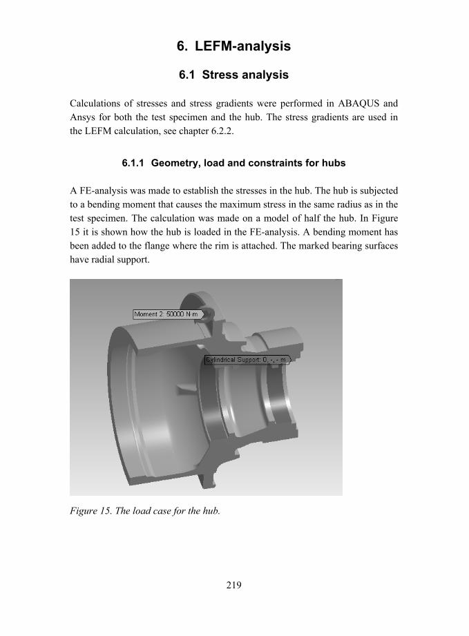
219
6. LEFM-analysis
6.1 Stress analysis
Calculations of stresses and stress gradients were performed in ABAQUS and Ansys for both the test specimen and the hub. The stress gradients are used in the LEFM calculation, see chapter 6.2.2.
6.1.1 Geometry, load and constraints for hubs
A FE-analysis was made to establish the stresses in the hub. The hub is subjected to a bending moment that causes the maximum stress in the same radius as in the test specimen. The calculation was made on a model of half the hub. In Figure 15 it is shown how the hub is loaded in the FE-analysis. A bending moment has been added to the flange where the rim is attached. The marked bearing surfaces have radial support.
Figure 15. The load case for the hub.

220
6.1.2 Stress gradients
The hubs are subjected to cyclic positive and negative stress (R = -1). In Figure 16 (to the left) there is positive stress on the upper part and negative on the lower. Figure 16 (to the right) and Figure 17 shows how the stress gradient locations L3, L7, L2 and L1 are selected (the same lines as in the test specimens). In the following calculations the equivalent bending moment for the highest loaded axle was used.
Figure 18 shows the stress gradient through the thickness when subjected to the equivalent bending moment. It is only in the radius (L1) that the gradient is high. (Distance 0 means upper surface.)
Figure 18. Stress gradients for the hub.
(For the test specimens the gradients look different.)
0 0,01 0,02 0,03 0,04 0,05 Distance [m]
Stre
ss R
ange
[MPa
]
L1
L3 L2
L7

221
Figure 16. Maximum principal stresses in the hub.

222
Figure 17. Location of sections for calculation of stress gradients in the hub.
Reproduction of Figure 6. Maximum principal stress in test specimen.
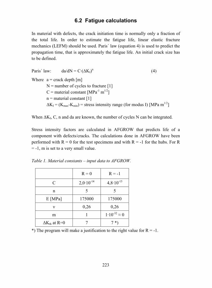
223
6.2 Fatigue calculations
In material with defects, the crack initiation time is normally only a fraction of the total life. In order to estimate the fatigue life, linear elastic fracture mechanics (LEFM) should be used. Paris´ law (equation 4) is used to predict the propagation time, that is approximately the fatigue life. An initial crack size has to be defined.
Paris´ law: da/dN = C·(∆KI)n (4)
Where a = crack depth [m] N = number of cycles to fracture [1] C = material constant [MPa-1 m1/2] n = material constant [1] ∆KI = (Kmax-Kmin) = stress intensity range (for modus I) [MPa m1/2]
When ∆KI, C, n and da are known, the number of cycles N can be integrated.
Stress intensity factors are calculated in AFGROW that predicts life of a component with defects/cracks. The calculations done in AFGROW have been performed with R = 0 for the test specimens and with R = -1 for the hubs. For R = -1, m is set to a very small value.
Table 1. Material constants input data to AFGROW.
R = 0 R = -1
C 2,0·10-14 4,8·10-15
n 5 5
E [MPa] 175000 175000
ν 0,26 0,26
m 1 1·10-32 ≈ 0
∆Kth at R=0 7 7 *)
*) The program will make a justification to the right value for R = -1.

224
An elementary case, that describes the crack position in the specimen, was chosen in the program. To be able to state a stress gradient the calculation has to be done using weight functions. The gradients are collected from the FEM-calculations (chapter 6.1.2) and their position is shown in Figures 1617.
The cases found during the examination of defect sizes have been approximated with semi-elliptical surface cracks or edge cracks. The dimensions of both the cross sections and the cracks have been stated in the program. With the help of submitted data (Table 1), AFGROW calculates, in small steps, the growth of cracks in both directions in relation to the stress intensity factors.
Estimation of the starting defects size is done according to the rules in reference [3] (see chapter 4.2). Table 2 shows the life predictions made in AFGROW.
Table 2. Estimation of defect size.
Defect size [mm] Test no c a
Position
4 0.3 0.5 0.49 L1 6 0.23 0.63 0.48 L1
27 0.25 0.35 0.37 L1 28 0.2 0.4 0.35 L1 21 0.35 0.6 0.57 L1 35 0.4 0.8 0.71 L1 26 0.7 2.6 1.2 L7 34 0.5 0.4 1.4 edge L7 36 1.5 8 4.34 L2 23 4.5 4.5 3.99 edge L2 25 3 15 8.41 L2 30 8 8 7.09 edge L2
areadefect
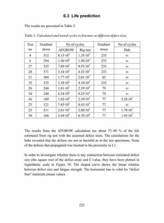
225
6.3 Life prediction
The results are presented in Table 3.
Table 3. Calculated and tested cycles to fracture at different defect sizes.
No of cycles No of cycles Test no
Gradient stress AFGROW Rig test
Gradient stress Hub
4 512 8.13·104 1.35·105 233 ∞ 6 294 1.20·106 1.50·106 233 ∞
27 335 7.89·105 9.53·105 233 ∞ 28 371 3.34·105 4.52·105 233 ∞ 21 384 1.77·105 2.01·105 83 ∞ 35 335 3.38·105 4.10·105 233 ∞ 26 260 1.81·105 2.39·105 79 ∞ 34 240 6.34·104 8.25·104 79 ∞ 36 189 1.92·105 2.39·105 77 5.28·107 23 121 7.45·105 8.43·105 77 ∞ 25 211 2.01·104 2.80·104 77 1.79·107 30 166 5.44·104 6.70·104 77 1.92·107
The results from the AFGROW calculation are about 7580 % of the life estimated from rig test with the assumed defect sizes. The calculations for the hubs revealed that the defects are not as harmful as in the test specimens. None of the defects that propagated was located in the proximity to L1.
In order to investigate whether there is any connection between estimated defect size (the square root of the defect area) and C-value, they have been plotted in logarithmic scale in Figure 19. The sloped curve shows the linear relation between defect size and fatigue strength. The horizontal line is valid for defect free materials (mean value).

226
1,E+15
1,E+16
1,E+17
1,E+18
1,E+19
1,E+20
0,1 1,0 10,0Defect size
Cap
acity
Figure 19. Relationship between the C-value and the square root of the defect area.
7. Discussion
The results from the life calculations is about 7580 % of the life estimated from rig test. It is of course difficult to estimate the size of the starting defects these estimations needs experience and training. Also the material data that are needed for the calculation have a large scatter, see Hamberg et al. [4], depending on the sources. Another reason for this discrepancy could be that AFGROW only handle 2-dimensional crack propagation.
227
AFGROW predicts that 3 test specimens had defects that should have propagated, with the dimensioning stress. This is only about 6 % of the hubs (even if the figure is uncertain). That means that relatively large defects can be allowed in the hubs without risk for failures. If the defects instead had been located in the radius with much higher stresses, the life could be drastically shortened.
8. Conclusions
The investigation of different non-destructive test methods gave a negative result. There is no good method to find the defects. This depends among other things on the defects size, shape and also where in the hubs they are located.
The life assessment for hubs with the largest defects found is about 18·106 cycles for the design load time history, which is equivalent to 18000 h. Approximately 3 % of the examined hubs contained defects of this size.
Further work
The defects arise from shrinkage in the material of casting. Since a casting simulation of the hubs couldnt be performed it has been hard to determine what parts of the hub that solidified last. To verify the location of the defects more exactly a simulation of the casting process should be conducted with the data needed retrieved from the foundry. Such a simulation would show if there are any risk for the defects to be located in the highly stressed area.
Acknowledgements
I would like to thank Åse Löfstrand (LiTH), Therése Eklund (LiTH), Kjell Eriksson (VOLVO CE Components), Nenad Mrden (VOLVO CE Components), Anders Björkblad (KTH), Magnus Byggnevi (Volvo Wheel Loaders) and Jack Samuelsson (Volvo Wheel Loaders/ KTH) for contributions to this work.

228
References
1. Löfstrand Å. and Eklund, T. Analysis of casting defects and assessment of failure, LITH-IKP-EX--05/2236--SE, 2005, Linköping Technical High School, Linköping.
2. AFGROW (http://afgrow.wpafb.af.mil/about/history.php)
3. Murakami, Y. Metal Fatigue: Effects of Small Defects and Non-metallic Inclusions, (Publication year missing), Department of Mechanical Science & Engineering, Faculty of Engineering, Kyushu University Japan.
4. Hamberg, K. Mörtsell, M. Björkblad, A. and Samuelsson, J. Fatigue Crack growth in Ductile Iron. In this proceedings, 2005.
INFLUENCE OF OCCASIONAL UNDERLOADS ON FATIGUE
B. Roger Rabb
Department of Calculation & Simulation/Wärtsilä Finland – Engine DivisionP.O. Box 125, FIN-65101 Wärtsilä Finland Oy, Finland
e-mail: [email protected]
Key words. Fatigue, variable amplitude load, cumulative damage
Abstract. The fatigue strength of a machine part, nominally subjected to a con-stant amplitude load and designed for an infinite lifetime, can suffer greatly by afew occasional peak loads if they cause stress amplitudes beyond the fatigue limit.This phenomenon has been given much attention by researchers in recent years.Interest in this question at the author’s company was aroused in the 1980’s whenthe cylinder liner of a medium speed diesel engine tested in the company labora-tory developed fatigue cracks in the orifices of the cooling bores. These crackswere found to be caused by large underloads as a result of temperature stress var-iations during engine start-up and stopping. Underloads are especially detrimen-tal for the fatigue limit because of the residual tension stresses caused in a notchby them. These residual stresses cause a decaying acceleration of the damage ac-cumulation. A surprisingly low number of underloads can be enough to initiate apropagating fatigue crack, although the basic dynamic stress amplitude is well be-low the fatigue limit. The effect of occasional underloads is highlighted in this pa-per by presenting the results of extensive fatigue testing with a constant amplitudestress containing a few large periodic underloads on three different materialtypes, i.e. grey cast iron, nodular cast iron, and quenched and tempered steel.
1 INTRODUCTION
Medium speed diesel engines are mostly operated at a virtually constant poweroutput. The fatigue analysis of most engine parts can therefore be made, assuminga constant amplitude load. However, due to engine start-ups and stoppings, engineparts affected by temperature stresses, i.e., the cylinder head and liner, can thenexperience a much higher stress amplitude. Also some other engine parts, such asthe screws of the cylinder head and the connecting rod, will be subjected to largestress amplitudes due to regularly repeated engine overhauls.
A section through an in line medium speed diesel engine is shown in Figure 1.This engine operates at a nominal speed of 750 rpm. During an engine lifetime of
229

about 200 000 operational hours it can be estimated that the engine will be startedand stopped about 20 000 to 40 000 times. The cylinder head is made of nodularcast iron, and particularly its flame deck is exposed to a variable amplitude stresshistory consisting of about 4.5 billion high cycle loads due to the firing pressure,as well as a maximum of 40 000 low cycle loads due to engine start-ups and stop-pings. The high cycle stress amplitude, which can be considered to be quite con-stant, must of course be below the fatigue limit. Cumulative damage will resultwhen the low cycle amplitude, which can also be considered constant, is muchlarger than the high cycle amplitude and exceeds the fatigue limit. The cylinderliner is made of centrifugally cast grey cast iron. Due to wear it has to be replacedat least once during the lifetime of the engine. Accordingly, the number of loadcycles on the liner is only half the amount of load cycles on the cylinder head.
The typical load spectrum in Figure 1b for a cylinder liner, for example, is sim-ple to handle. It consists of a number of high cycle loads with mean stress
and amplitude level . Correspondingly, it has a number of lowcycles with mean stress and amplitude level . The cycle ratio in oneblock of the spectrum test is thus .
The cumulative fatigue damage caused by a variable amplitude load has longbeen known, and much research has been done on this issue. Already in the1920’s, the Swedish researcher, A. Palmgren, examined the fatigue life of bearingrollers [1]. But not until M. A. Miner published his investigations [2] in the 1940’s
a) section through the engine b) one block of the stress history in the test
Figure 1. Wärtsilä Vasa 32 medium speed diesel engine. Definitions of thequantities in the stress history with high cycle and low cycle loads in thetest of nodular cast iron grade 500-7/ISO 1083.
nhcσmean hc, σa hc, nl c
σmean lc, σa lc,nhc nl c⁄
σo = 10
230

on this subject did this phenomenon become more known.The linear damage rule according to Miner is quite simple and in its original
form it only considered amplitudes over the fatigue limit. If denotes the numberof cycles with amplitude and denotes the lifetime taken from the constantamplitude S-N curve at this stress amplitude, the Miner rule is as follow:
(1)
However, it has long been known that cycles with amplitudes below the fatiguelimit must also be included in some way to this damage sum. Many attempts havebeen made to construct a correction of the constant amplitude S-N curve to ac-count for amplitudes below the fatigue limit. H. T. Corten and T. J. Dolan [3] wereamong the firsts to attempt a correction, which was basically an extension of theconstant amplitude S-N curve with the same slope into the high cycle domain.Also the correction suggested by E. Haibach [4] deserves a mention. He suggestedthat the slope exponent in the power expression for the S-N curve of steelsshould be replaced in the high cycle domain by the slope exponent . Ifdenotes the life in the number of cycles at amplitude , and if is the numberof cycles where the S-N curve reaches the fatigue limit , then this correctionis as follows for steel.
basic S-N curve for (2)
extended S-N curve for (3)
However, the linear damage rule has many weaknesses. It is not possible, for ex-ample, to consider the sequence of load amplitudes. More crucially still, in caseswhere the number of under- or overloads are few, it fails to give the correct esti-mates of the expected lifetime. It is known from many experiments, References[5], [6] and [7], that an occasional overload tends to retard the crack growth dueto the generated compression residual stresses in the crack wake. In the same man-ner, an occasional underload will accelerate the crack growth due to the tensionresidual stresses it will generate.
The modern understanding of fatigue, References [5] and [8], makes no strictdistinction between crack nucleation and crack propagation. Also the crack nucle-ation phase consists of a growth of small inherent defects, whether it starts froman internal material flaw or from a slip band intersecting the surface in a bad di-rection. In principle the whole fatigue process with crack nucleation and propaga-tion can be illustrated in a plot as in Figure 2.
The vast majority of the testing in question was performed using a programma-ble resonant test machine manufactured by RUMUL. This machine can performconstant amplitude testing at frequencies between 80 and 300 Hz. The axial spec-imens tested in these projects were fatigued at a frequency of about 150 Hz.
niσai Ni
D ni Ni⁄i
∑=
k2k 1– N
σa Nafσaf
N Naf
σaf
σa--------
k
= σa σaf≥
N Naf
σaf
σa--------
2k 1–
= σa σaf<
da dN⁄ ∆K–
231

Figure 2. Crack nucleation and propagation at a certain stress intensityrange, Refs. [5] and [8].
2 TESTS ON NODULAR CAST IRON
The fatigue tests made to determine the behaviour of nodular cast iron grade 500-7/ISO 1083 in the high cycle regime when occasional underloads are present aregiven in detail in Reference [9]. The geometry and dimensions of the smooth testspecimens are shown in Figure 3a. The effective stress area of this specimen at acertain relative standard deviation of the fatigue strength is given in this figure tofacilitate the application of the test data to actual components with different effec-tive stress areas. The important concepts effective stress area and the related con-cept statistical size factor are explained in References [10] and [11].
To be able to determine the appropriate high cycle stress amplitudes in the fa-tigue test with occasional underloads, the fatigue limit at high cycle mean stresshad first to be tested with a staircase test. The basic S-N curve at high cycle meanstress also had to be tested to be able to compare it with its extension into the highcycle domain.
On the one hand, actual stresses should be used in a modern fatigue analysissince these are the stresses that are calculated in a FE analysis, and their transfor-mation to nominal stresses are both unnecessary and sometimes even impossible.On the other hand, in order to calculate the effective stress area, the actual stressdistributions must be used. Because the test specimen in Figure 3a has a simplegeometry, it is easy to calculate the actual stresses from the nominal stresses bymultiplying the nominal stresses by the theoretical stress concentration factor,
. In the following, actual stresses are therefore mostly used. Onthe other hand, it is more convenient to conduct the tests using nominal stresses.σactual K tσnom=
crack growth in m/cycle
stress intensity in MN/m3/2
threshold value for a growing crack at a certain stress intensity
range
stress intensity due to an ap-plied external load
stress intensity due to internalstresses
Crack growth when the maximum stress in-tensity factor exceeds the threshold at a giv-en stress intensity range:
da dN⁄K
K th
Kapp
K i nt
Kapp K i nt+ K th>
232
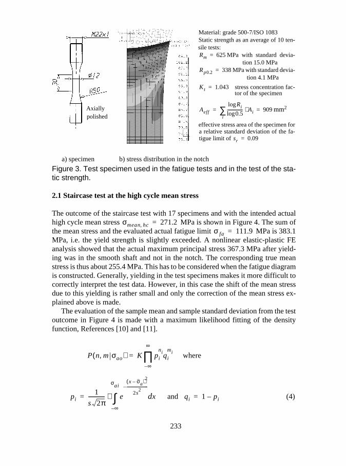
a) specimen b) stress distribution in the notch
Figure 3. Test specimen used in the fatigue tests and in the test of the sta-tic strength.
2.1 Staircase test at the high cycle mean stress
The outcome of the staircase test with 17 specimens and with the intended actualhigh cycle mean stress MPa is shown in Figure 4. The sum ofthe mean stress and the evaluated actual fatigue limit MPa is 383.1MPa, i.e. the yield strength is slightly exceeded. A nonlinear elastic-plastic FEanalysis showed that the actual maximum principal stress 367.3 MPa after yield-ing was in the smooth shaft and not in the notch. The corresponding true meanstress is thus about 255.4 MPa. This has to be considered when the fatigue diagramis constructed. Generally, yielding in the test specimens makes it more difficult tocorrectly interpret the test data. However, in this case the shift of the mean stressdue to this yielding is rather small and only the correction of the mean stress ex-plained above is made.
The evaluation of the sample mean and sample standard deviation from the testoutcome in Figure 4 is made with a maximum likelihood fitting of the densityfunction, References [10] and [11].
where
and (4)
Axiallypolished
σmean hc, 271.2=σ fa 111.9=
P n m σao,( ) K pi
niqi
mi
∞–
∞
∏=
pi1
s 2π------------- e
x σa–( )2
2s2
-----------------------–
xd∞–
σai
∫⋅= qi 1 pi–=
Material: grade 500-7/ISO 1083Static strength as an average of 10 ten-sile tests:
MPa with standard devia-tion 15.0 MPa
MPa with standard devia-tion 4.1 MPa
stress concentration fac-tor of the specimen
mm2
effective stress area of the specimen fora relative standard deviation of the fa-tigue limit of
Rm 625=
Rp0.2 338=
K t 1.043=
Aeff
Rilog
0.5log--------------- Ai⋅
i∑ 909= =
sr 0.09=
233

In Equation (4) the meaning of is the number of failures on the level with stressamplitude and is the corresponding number of runouts. The lowest validamplitude level is . The constantK is neither dependent on the mean, nor onthe standard deviation. The mean of the trial density function is and its stand-ard deviation . The cutoff limit in this staircase test was cycles, which is theusual value. The evaluated standard deviation cannot really be trusted in this casebecause of the small number of specimens in this test, Reference [11].
In order to construct the entire fatigue diagram in this case, use was made ofan earlier test on nodular cast iron grade 500-7, Reference [11]. The same speci-mens as in Figure 3a were used in this test, but they were taken from a batch withan average tensile strength of MPa. The fatigue ratio, i.e. the ratio be-tween the fatigue limit in fully reversed tension compression to the average tensilestrength was then evaluated to . The Haigh diagram in Figure 5 hasbeen constructed using this fatigue ratio and the evaluated data in Figure 4. How-ever, according to the tested S-N curve at zero mean stress, see Figure 8, the fa-tigue ratio could be a little lower, or about 0.37. It is worth noting how steep thediagram in fact is. The Haigh diagram for nodular cast iron is often presentedwrongly, i.e. much flatter, in older literature.
Figure 4. Staircase test with the specimens of nodular cast iron at a truemean stress considering also the yielding of about 255.4 MPa.
Figure 5. Haigh diagram for nodular cast iron. The dotted line correspondsto the 90 % confidence value to be used in the fatigue analysis and is validfor 25 test specimens and for a typical sample standard deviation of 10 % .
niσai mi
σaoσa
s 107
Rm 517=
f R 0.378=
= σao
Estimated Haigh diagram for asample consisting of 25 speci-mens according to Figure 3a.Evaluated relative sample stand-ard deviation .
mm2
for
sr 0.10=
Aeff 909=
sr 0.09=
Nodular cast iron grade 500-7/ISO1083Evaluated sample values at a truemean stress of about 255.4 MPa:
MPa sample mean fa-tigue limit
MPa sample standard de-viation
σa 111.9=
s 10.6=
234

2.2 Basic S-N curves
Most of the tests of the basic S-N curve at a nominal high cycle mean stress of 260MPa were made at three different nominal stress amplitude levels, i.e. 110, 130,and 240 MPa. Because a different amount of yielding in the specimens will takeplace at each different level, the actual mean stress will shift more downwards forhigher amplitude levels. Because the basic S-N curve is used only as a reference,this shift will not be considered here, but the evaluation is made as if the actualmean stress at each level would be the same and equal to =255.4 MPa. The outcome of this test is shown in Figure 6.
In Figure 6, the symbol denotes the standard deviation of the lifetime log-arithm. The symbol denotes the corresponding approximate standard deviationof the fatigue strength according to Equation (5).
(5)
The curve fitting of the S-N curve to the test outcome is done with the method ofleast squares, Reference [12]. It is worth noting that the scatter in the S-N curveincreases towards the fatigue limit. Because the allowed stress amplitude in the fa-tigue analysis is decided by a reduction of the mean fatigue limit to the maximumallowed probability of failure, this means that it perhaps could be possible to usesmaller safety factors in the finite lifetime domain than when designing in relationto the fatigue limit. However, the S-N curve obtained by excluding the observa-tions on the lowest test level indicates that the S-N curve has started to plain outon this level. Accordingly, the relative standard deviation on the lowest level couldin fact be less than the one determined with Equation (5).
Figure 6. S-N curve for nodular cast iron grade 500-7/ISO 1083 at the ac-tual high cycle mean stress 255.4 MPa.
σmean σmean hc,=
sNsr
sr 1 1
10sN k⁄---------------–≈
235

It is seen in Figure 1b that the actual mean stress 190.3 MPa used in the test of theS-N curve corresponding to the low cycle mean stress will slightly change depend-ing on the high cycle stress amplitude. The outcome of a test of the S-N curve cor-responding to this mean stress is shown in Figure 7. Especially on the highest testlevel, with a maximum stress , the yield stress hasbeen exceeded. The small shift of the mean stress due to this exceeding has notbeen considered in this evaluation.
A test of the S-N curve in fully reversed tension compression was also made,see Figure 8. The scatter of the lifespans in this test is very high. Especially, the
Figure 7. S-N curve for grade 500-7/ISO 1083 at the approximate actuallow cycle mean stress of 190.3 MPa
.
Figure 8. S-N curve for grade 500-7/ISO 1083 at fully reversed tensioncompression.
σmax σmean lc, σa+ 427.6= =
runout
236
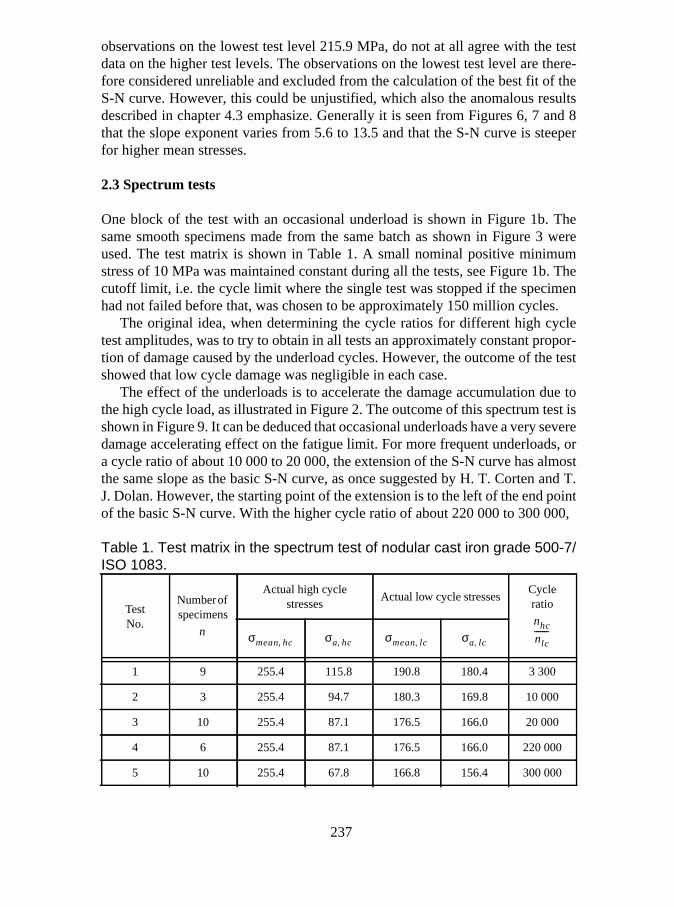
observations on the lowest test level 215.9 MPa, do not at all agree with the testdata on the higher test levels. The observations on the lowest test level are there-fore considered unreliable and excluded from the calculation of the best fit of theS-N curve. However, this could be unjustified, which also the anomalous resultsdescribed in chapter 4.3 emphasize. Generally it is seen from Figures 6, 7 and 8that the slope exponent varies from 5.6 to 13.5 and that the S-N curve is steeperfor higher mean stresses.
2.3 Spectrum tests
One block of the test with an occasional underload is shown in Figure 1b. Thesame smooth specimens made from the same batch as shown in Figure 3 wereused. The test matrix is shown in Table 1. A small nominal positive minimumstress of 10 MPa was maintained constant during all the tests, see Figure 1b. Thecutoff limit, i.e. the cycle limit where the single test was stopped if the specimenhad not failed before that, was chosen to be approximately 150 million cycles.
The original idea, when determining the cycle ratios for different high cycletest amplitudes, was to try to obtain in all tests an approximately constant propor-tion of damage caused by the underload cycles. However, the outcome of the testshowed that low cycle damage was negligible in each case.
The effect of the underloads is to accelerate the damage accumulation due tothe high cycle load, as illustrated in Figure 2. The outcome of this spectrum test isshown in Figure 9. It can be deduced that occasional underloads have a very severedamage accelerating effect on the fatigue limit. For more frequent underloads, ora cycle ratio of about 10 000 to 20 000, the extension of the S-N curve has almostthe same slope as the basic S-N curve, as once suggested by H. T. Corten and T.J. Dolan. However, the starting point of the extension is to the left of the end pointof the basic S-N curve. With the higher cycle ratio of about 220 000 to 300 000,
Table 1. Test matrix in the spectrum test of nodular cast iron grade 500-7/ISO 1083.
TestNo.
Number ofspecimens
Actual high cyclestresses
Actual low cycle stressesCycleratio
1 9 255.4 115.8 190.8 180.4 3 300
2 3 255.4 94.7 180.3 169.8 10 000
3 10 255.4 87.1 176.5 166.0 20 000
4 6 255.4 87.1 176.5 166.0 220 000
5 10 255.4 67.8 166.8 156.4 300 000
nnhc
nl c-------σmean hc, σa hc, σmean lc, σa l c,
237

Figure 9. Extension of the S-N curve for grade 500-7/ISO 1083 due to oc-casional underloads at a high cycle mean stress of 255.4 MPa.
Table 2. Life and scatter (sample values) at different test levels and withdifferent cycle ratios in the spectrum test on nodular cast iron grade 500-7/ISO 1083.
TestNo.
Averagenumber ofhigh cycles
Number oflow cycles Average
amount of lowcycle damage
Unbias.standarddeviat.
oflogarith-mic life
Relative standarddeviation of the fatigue
strength
Average
Min.Comm-
ent
1 544000 164 90 0.137 0.051 6.08
2 278 170 0.292 0.105 6.08
3 232 39 0.343 0.122 6.08
4 62 9 0.609 0.155 8.32
5 366 54 0.374 0.098 8.32
Basic S-N curve
N 10Nlog
=
nl c
nl c
3.9 106 143.6
σa l c,--------------
9.3⋅
-------------------------------------------------
sN
sr 1 1
10sN k⁄
--------------------–≈
k
5.3 104–⋅
2.79 106⋅ 5.3 10
4–⋅
4.64 106⋅ 3.6 10
4–⋅
13.7 106⋅ 9.6 10
5–⋅
109.9 106⋅ 3.3 10
4–⋅
238
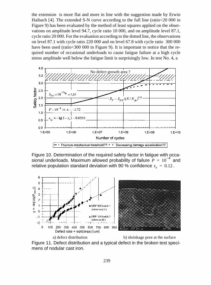
the extension is more flat and more in line with the suggestion made by ErwinHaibach [4]. The extended S-N curve according to the full line (ratio<20 000 inFigure 9) has been evaluated by the method of least squares applied on the obser-vations on amplitude level 94.7, cycle ratio 10 000, and on amplitude level 87.1,cycle ratio 20 000. For the evaluation according to the dotted line, the observationson level 87.1 with cycle ratio 220 000 and on level 67.8 with cycle ratio 300 000have been used (ratio<300 000 in Figure 9). It is important to notice that the re-quired number of occasional underloads to cause fatigue failure at a high cyclestress amplitude well below the fatigue limit is surprisingly low. In test No. 4, a
Figure 10. Determination of the required safety factor in fatigue with occa-sional underloads. Maximum allowed probability of failure andrelative population standard deviation with 90 % confidence .
a) defect distribution b) shrinkage pore at the surfaceFigure 11. Defect distribution and a typical defect in the broken test speci-mens of nodular cast iron.
No defect growth area ?
P 104–
=sr 0.12=
239

minimum number of 9 underloads has been enough to cause fatigue failure in onespecimen. The failure of the cumulative linear Miner rule to predict this phenom-enon is illustrated in Table 2 by the calculated low cycle damage, which in itselfis negligible. The calculated standard deviations are quite high. This must be con-sidered when the appropriate factor of safety is determined in the fatigue analysis.Much testing must still be done to be able to determinate the correct safety factorin variable amplitude conditions with occasional underloads, especially in the ul-tra high cycle regime with up to one billion cycles or more. The present situationwith its open questions is sketched in Figure 10. It seems logical to assume thatthere must be some limit to the required safety factor. In addition to testing in theultra high cycle domain, this limit could perhaps also be estimated by using thefracture mechanical stress intensity threshold value and some upper limit of thepossible initial defect, see Figure 11.
3 TESTS ON GREY CAST IRON
The fatigue tests that were made on specimens of grey cast iron grade 300/ISO 185and their evaluation are explained in more detail in References [12] and [13].Therefore, only a brief summary of these tests will be given here. These tests werethe first spectrum tests ever planned by the author, and therefore due to lack of ex-perience they are not as complete as the corresponding tests on nodular cast iron.The biggest weakness is that the cycle ratio was different on all the three testedlevels and exact information about how the cycle ratio will influence the slope ex-ponent was not obtained. The same specimens as those according to Figure 3awere also used in these tests. The ultimate tensile strength, as an average of 10 ten-sile tests, of these specimens was MPa with an unbiased standard de-viation of 18.6 MPa. The same type of spectrum as shown in Figure 1b, but withthe values given in Table 3, was used in these fatigue tests with occasional over-loads.
The basic S-N curve measured in this test at the actual high cycle mean stressof 166.9 MPa is shown in Figure 12. Staircase tests were also made to obtain the
Table 3: Test matrix in the spectrum test of grey cast iron grade 300/ISO185.
TestNo.
Number ofspecimens
Actual high cycle stresses Actual low cycle stresses Cycle ratio
1 5 166.9 31.8 104.6 94.1 5000
2 5 166.9 29.2 103.3 92.8 27 500
3 5 166.9 26.6 102.0 91.5 200 000
Rm 339=
n
nhc
nl c-------σmean hc, σa hc, σmean lc, σa lc,
240

Haigh diagram of the specimens in this material, see Figure 13. The outcome ofthe fatigue tests with occasional underloads according to Table 3 is sketched inFigure 14. It can be seen that also in this case a very low number of occasional un-derloads will promote an acceleration of the damage caused by the high cycleloads. Besides, it is also evident that the cycle ratio will influence the slope of theextended S-N curve. A summary of the outcome of this test is given in Table 4.The amount of low cycle damage is also in this case negligible. The scatter in thelifetime logarithm is comparable to the one found for nodular cast iron. However,the corresponding scatter in the fatigue amplitude is much smaller due to the flattercurve . This fact can be utilized when the appropriate safety factor with regard tothe fatigue limit is defined. To determine the population standard deviation it is
Figure 12. S-N curve for grey cast iron grade 300/ISO 185 at the actualhigh cycle mean stress 166.9 MPa.
a) staircase test b) Haigh diagram
Figure 13. Haigh diagram for grey cast iron grade 300/ISO 185. Staircasetest at the actual high cycle mean stress 166.9 MPa.
241

Figure 14. Extension of the S-N curve for grey cast iron grade 300/ISO 185due to occasional underloads at a high cycle mean stress of 166.9 MPa.
Table 4. Life and scatter (sample values) at different test levels and withdifferent cycle ratios in the spectrum test on grey cast iron grade 300/ISO185.
recommended to put a 90 % confidence on the sample value. The distribution ofthe sample standard deviation is characterised by the Chi squared distribution, seeReference [11]. Because there have only been 5 specimens per level, the followingpopulation standard deviation can be calculated, e.g., for level 2, Table 4:
TestNo.
Averagenumber ofhigh cycles
Number oflow cycles
Averageamount of lowcycle damage,
ref. [12]
Unbias.standarddeviat.
oflogarith-mic life
Relative standarddeviation of the fatigue
strength
Average
Min.Comm-
ent
1 379 186 0.229 0.036 14.36
2 332 75 0.453 0.039 26.49
3 452 75 0.411 0.035 26.49
Basic S-N curve
N 10Nlog
=
nl c
nl c
3.7 106 54.6
σa l c,--------------
7.3⋅
-------------------------------------------------
sN
sr 1 1
10sN k⁄
--------------------–≈
k
1.70 106⋅ 4.0 10
3–⋅
5.78 106⋅ 3.2 10
3–⋅
6.84 107⋅ 3.9 10
3–⋅
242

(6)
The required safety factor, at e.g. a maximum allowed probability of failurewhich corresponds to a standard normal variable , is then as
follows:
and (7)
For instance, at a high cycle number , the extended S-N curve in Figure14 gives a fatigue amplitude of MPa, and the allowed value is hence
= 17.9 MPa. Calculated in relation to the fatigue limit the equiv-alent safety factor would then be .
4 TESTS ON QUENCHED AND TEMPERED STEEL
These fatigue tests with occasional underloads were planned in the recently fin-ished fatigue testing project FADEL (Fatigue Design for Long Life). ProjectFADEL was a joint project between 5 Finnish companies and the testing wasmainly made at VTT, the Technical Research Centre of Finland, and partly at theLappeenranta University of Technology. The material in the specimens shown inFigure 15 is quenched and tempered steel EN 10083-1 - 34CrNiMo6+QT. TheHaigh diagram for this material had first to be tested, and the resulting diagram isshown in Figure 16 with the actual high cycle test points and the approximate lowcycle test point of the spectrum test sketched.
As seen in Figure 16, the stress amplitude of the low cycle load of the test spec-trum is rather high. The reason for this choice of load spectrum is that it in factresembles the load spectrum in the thread roots of pretensioned screws. For in-stance, the connecting rod and cylinder head screws will experience even higherlow cycle stress amplitudes due to the loosening and tightening during periodic en-gine overhauls. One of the main purposes of this test was to determine whetherthere is a risk that the already low number of such overhauls during the engine life-time could initiate this kind of accelerated fatigue crack nucleation. The final testmatrix for the tests with occasional underloads is given in Table 5 and sketched inFigure 17.
4.1 Staircase tests
The Haigh diagram for the chosen material EN 10083-1 - 34CrNiMo6+QT hadfirst to be determined by two staircase tests, one at the high cycle mean stress andthe other at the low cycle mean stress. The outcome of these staircase tests areshown in Figure 18. Due to a perhaps too large stress increment in the tests at the
srC90n 1–h1
------------ sr⋅ 5 1–1.064------------- 0.039⋅ 0.076= = =
P 104–
= λ 3.72–=
sl g lg 1 srC90–( )–≈ 0.0343= SF 10λslg–
1.34= =
nhc 109
=σa hc, 24.0=
σal l σa hc, SF⁄=SF 32.4 17.9⁄ 1.81= =
243

a) specimen b) stress distribution in the notchFigure 15. Test specimen used in the fatigue tests and in the test of thestatic strength.
Figure 16. Haigh diagram with the approximate test points for the spectrumtests sketched. The dotted line corresponds to the 90 % confidence valueto be used in the fatigue analysis. The confidence line is valid for 25 spec-imens and a typical sample standard deviation of 7 %. This diagram is test-ed with specimens according to figure 15a.
Axiallypolished
σa 597 0.304σm–=
R = 0
Material: EN 10083-1 - 34CrNiMo6+QT.Static strength as an average of 2 ten-sile tests:
MPa
MPa
theoretical stress concen-tration factor of the spec-imen
mm2
effective stress area of the specimenfor a relative standard deviation of thefatigue limit of
Rm 1165=
Rp0.2 1064=
K t 1.036=
Aeff
Rilog
0.5log--------------- Ai⋅
i∑ 367= =
sr 0.07=
244

high cycle mean stress, there is a distribution of failures and runouts on only thelevel in the middle. It is not possible to calculate any sensible standard deviationfrom such an outcome. However, the evaluated actual fatigue limitMPa at the high cycle mean stress can be trusted. The staircase test at an actualmean stress of 207.2 MPa, which is close to the low cycle mean stress looks rathergood. The calculated sample standard deviation in this test is 34.2 MPa, i.e. therelative sample standard deviation is , which is quite typical forquenched and tempered steels. However, it should be considered that the evalua-tion of staircase test outcomes of this type can systematically lead to a somewhattoo small sample standard deviation, see Reference [11]. Therefore, based on alsoother tests on quenched and tempered steel of the same type, a value ofhas been used in Figure 16. This value is thought as quite typical for a staircase test
Table 5. Test matrix in the spectrum test of quenched and tempered steelEN 10083-1 - 34CrNiMo6+QT.
Figure 17. Stress history in one block of the spectrum test on quenchedand tempered steel specimens.
TestNo.
Number ofspecimens
Actual high cycle stresses Actual low cycle stresses Cycle ratio
1 5 556 400.4 167.4 789.0 10 000
2 5 556 400.4 167.4 789.0 100 000
3 5 556 373 153.7 775.3 10 000
4 5 556 373 153.7 775.3 100 000
5 5 556 321.2 127.8 749.4 100 000
σ fa 428.0=
sr 0.064=
sr 0.07=
n
nhc
nl c-------σmean hc, σa hc, σmean lc, σa lc,
σa,hc
σmean,hc
σmean.lc
σa,lc
245
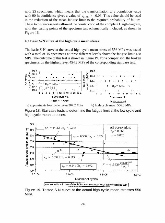
with 25 specimens, which means that the transformation to a population valuewith 90 % confidence gives a value of 0.09. This value should be usedin the reduction of the mean fatigue limit to the required probability of failure.These two staircase tests allowed the construction of the complete Haigh diagram,with the testing points of the spectrum test schematically included, as shown inFigure 16.
4.2 Basic S-N curve at the high cycle mean stress
The basic S-N curve at the actual high cycle mean stress of 556 MPa was testedwith a total of 15 specimens at three different levels above the fatigue limit 428MPa. The outcome of this test is shown in Figure 19. For a comparison, the brokenspecimens on the highest level 454.8 MPa of the corresponding staircase test,
a) approximate low cycle mean 207.2 MPa b) high cycle mean 556.0 MPa
Figure 18. Staircase tests to determine the fatigue limit at the low cycle andhigh cycle mean stresses.
Figure 19. Tested S-N curve at the actual high cycle mean stresses 556MPa.
srC90 ≈
σaf = 534.2s= 34.2
σaf = 428.0
sN 0.112 sr∧ 0.015= =
sN 0.560 sr∧ 0.074= =
N 4.15 106 428
σa---------
16.8⋅=
sN 0.892 sr∧ 0.115= =
sN 0.541 sr∧ 0.072= =
All observation:
sr = 0.075sN = 0.566
246

Figure 18b, are also included to this figure.It is seen from Figure 19 that the scatter increases towards the fatigue limit,
from a standard deviation of the lifetime logarithm on the highest testlevel to a value of on the lowest level at 476.6 MPa. It is clear thatthis can be considered when the appropriate safety factors are determined. A morealarming fact is that the scatter in the S-N curve close to the fatigue limit is largerthan the one calculated in the corresponding staircase test. This was also true fornodular cast iron, Figure 6, and it will arouse fears that it is wrong, as is now com-mon, to estimate the standard deviation to be used in the fatigue analysis only fromthe staircase test.
4.3 Spectrum tests
The outcome of the tests with occasional underloads is shown in Figure 20 and Ta-ble 6.Quenched and tempered steel 34CrNiMo6+QT will, according to the test re-sults in Figure 20 and Table 6, be extremely sensitive to such kinds of occasionalunderloads. This came as a total surprise, because it had been assumed beforethese tests that E. Haibach’s suggestion should work quite well. However, the ex-tension of the S-N curve starts shifted one decade or more to the left in comparisonto the end point of the basic S-N curve. The extension of the S-N curve continueseven somewhat steeper than the basic curve for a cycle ratio of 10 000 and withconsiderable sensitivity to the different cycle ratios 10 000 and 100 000. Moreo-ver, an extremely low number of occasional underloads, on average about 30 andat a minimum of only 3 pcs, is needed to initiate this accelerating damage.
Regrettably, the S-N curve corresponding to the low cycle mean stress was nottested. Therefore the damage due to the underloads is calculated using the sameslope exponent as for the tested S-N curve for the high cycle mean stress. Calcu-lated in this way the low cycle damage, is negligible but because the tests on nod-ular cast iron show that the slope exponent grows with decreasing mean stress theactual damage could be somewhat bigger. The scatter in the extension is quite highand it must be concluded that it is necessary to use at least the same relative stand-ard deviation as for the fatigue limit in the fatigue analysis. The outcome on thelowest test level 321.2 MPa is very alarming due to unexpectedly short lifetimes.This is illustrated with the steep extension obtained by fitting it to all the three testlevels with cycle ratio 100 000. Because only 5 specimens have been tested oneach level it could perhaps be a slump, but it could also be that this combinationof low cycle and high cycle stress amplitudes will give the most unfavourable in-ternal residual stresses.
5 CONCLUSIONS
It has been shown above with spectrum tests on three different material types,namely, nodular cast iron, grey cast iron, and quenched and tempered steel that the
sN 0.112=sN 0.892=
247
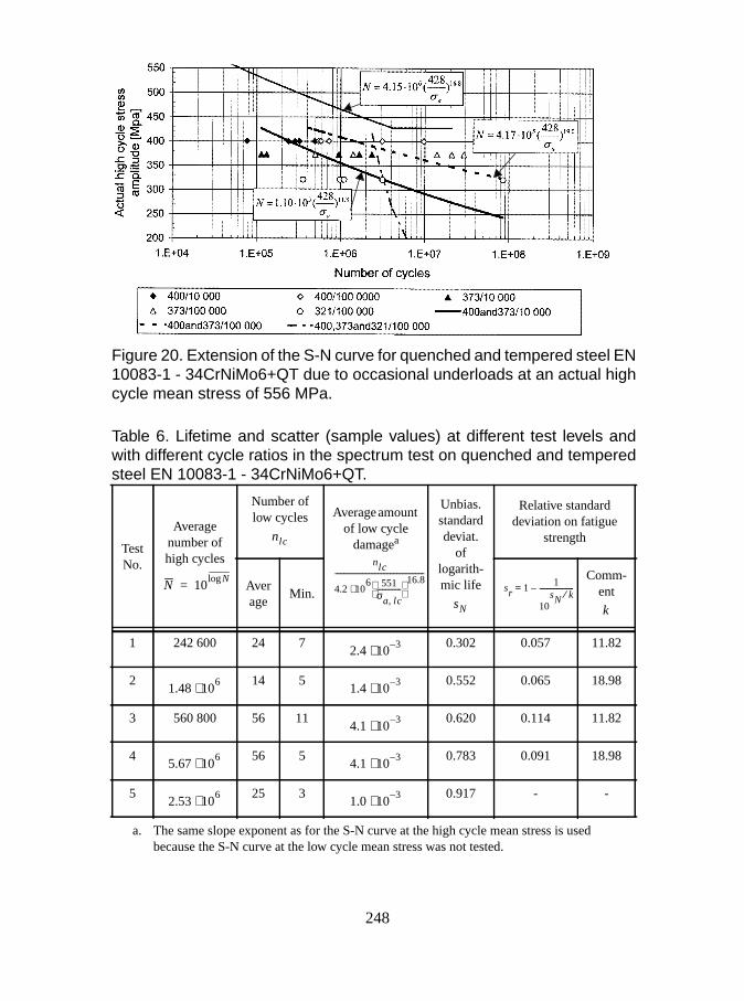
Figure 20. Extension of the S-N curve for quenched and tempered steel EN10083-1 - 34CrNiMo6+QT due to occasional underloads at an actual highcycle mean stress of 556 MPa.
Table 6. Lifetime and scatter (sample values) at different test levels andwith different cycle ratios in the spectrum test on quenched and temperedsteel EN 10083-1 - 34CrNiMo6+QT.
a. The same slope exponent as for the S-N curve at the high cycle mean stress is usedbecause the S-N curve at the low cycle mean stress was not tested.
TestNo.
Averagenumber ofhigh cycles
Number oflow cycles Average amount
of low cycledamagea
Unbias.standarddeviat.
oflogarith-mic life
Relative standarddeviation on fatigue
strength
Average
Min.Comm-
ent
1 242 600 24 7 0.302 0.057 11.82
2 14 5 0.552 0.065 18.98
3 560 800 56 11 0.620 0.114 11.82
4 56 5 0.783 0.091 18.98
5 25 3 0.917 - -
N 10Nlog
=
nl c
nl c
4.2 106 551
σa lc,--------------
16.8⋅
----------------------------------------------------
sN
sr 1 1
10sN k⁄
--------------------–≈
k
2.4 103–⋅
1.48 106⋅ 1.4 10
3–⋅
4.1 103–⋅
5.67 106⋅ 4.1 10
3–⋅
2.53 106⋅ 1.0 10
3–⋅
248

damage accelerating effect due to occasional underloads with amplitudes beyondthe fatigue limit is a very real problem. The severity of this phenomenon seems toincrease with increasing strength. The extension of the S-N curve for grey cast ironis much flatter than the basic curve. Nodular cast iron is more sensitive and the ex-tended S-N curve has about the same slope as the basic curve. However, the ex-tension of the S-N curve due to occasional underloads for quenched and temperedsteels can be even steeper than the basic curve.
These findings cannot be explained by any old theory about cumulative dam-age. It is even hard to quantitatively explain it with the fracture mechanical rea-soning in chapter 1. Before a consistent theory can be developed it is necessary toconduct more testing on the three decisive factors, namely a) the influence of thecycle ratio, b) the influence of the total life, i.e., will the extended curve flattenduring ultralong lifetimes, and c) the influence of the amplitude of the underload.
In general, the scatter in the extended S-N curves are quite high and when thesafety factor corresponding to the maximum allowed probability of failure is de-termined, it is recommended to use the same relative standard deviation as for thefatigue limit, at least for nodular cast iron and quenched and tempered steels.
REFERENCES
[1] A. Palmgren. Die Lebensdauer von Kugellagern. VDI-Z 69 (1924). pp. 339-341.
[2] M. A. Miner. Cumulative damage in fatigue. Trans. ASME. J. Appl. Mech.12 (1945) A159-A169.
[3] H. T. Corten and T. J. Dolan. Cumulative fatigue damage. Proc. Int. Conf.Fatigue of Metals, Inst. Mech. London. New York 1956. pp. 235-246.
[4] Prof. Dr.-Ing. Erwin Haibach. Betriebsfestigkeit. Verfahren und Daten zurBauteilberechnung. 2. Auflage. Springer-Verlag Berlin Heidelberg 2002.
[5] A. K. Vasudevan, K. Sadananda and G. Glinka. Critical parameters for fa-tigue damage. International Journal of Fatigue 23 (2001) S39-S53.
[6] Gary B. Marquis, B. Roger Rabb and Päivi Karjalainen-Roikonen. High Cy-cle Variable Amplitude Fatigue of a Nodular Cast Iron. “Fatigue Testing andAnalysis Under Variable Amplitude Loading Conditions”. ASTM STP1439. P. C. McKeighan and N. Ranganathan, Eds., American Society forTesting and Materials, West Conshohocken, PA, 2003.
[7] J. C. Newman, Jr. and E. P. Phillips. Prediction of Crack Growth under Var-iable-Amplitude and Spectrum Loading in a Titanium Alloy. “Fatigue Test-ing and Analysis Under Variable Amplitude Loading Conditions”. ASTMSTP 1439. P. C. McKeighan and N. Ranganathan, Eds., American Societyfor Testing and Materials, West Conshohocken, PA, 2003.
[8] K. Sadananda, A. K. Vasudevan, R. L. Holtz and E. U. Lee. Analysis ofoverload effects and related phenomena. International Journal of Fatigue 21(1999) S233-S246.
249

[9] Gary Marquis & Jussi Solin. Long-life fatigue design of GRP 500 nodularcast iron components. VTT Technical Research Centre of Finland, ResearchNotes 2043, ESPOO 2000.
[10] B. Roger Rabb. Interpretation and Evaluation of the Statistical Size Effect.Proceedings Vol. 3 from the 23rd CIMAC World Congress on CombustionEngine Technology, May 7-10, 2001 Hamburg, pp.1125-1140.
[11] B. Roger Rabb. Staircase testing - confidence and reliability. Fatigue Dam-age of Materials. Experiment and Analysis. Editors: A. Varvani-Farahaniand C. A. Brebbia. WITpress 2003.
[12] B. Roger Rabb. Fatigue Testing and Its Statistical Evaluation into DesignRules. Tampere University of Technology. Publications 253. Doctoral the-sis, Tampere April 1999.
[13] Roger Rabb. Fatigue Life Evaluation of Grey Cast Iron Machine Compo-nents under Variable Amplitude Loading. ESIS Publication 23, Fatigue De-sign and Reliability. Editors: G. Marquis & J. Solin. 1999 Elsevier ScienceLtd.
[14] Chr. Boller and T. Seeger. Materials Data for Cyclic Loading. Part B: Low-alloy Steels. Elsevier 1987.
250

251
On the prediction of crack propagation in cast steel specimens
Anders Björkblad Department of Aeronautical & Vehicle Engineering
Royal Institute of Technology, KTH 100 44 Stockholm
SWEDEN
Abstract
This investigation deals with the fatigue behaviour of cast steel with respect to defects, crack initiation, crack growth and material parameters. It constitutes the initial part of a larger work in cast materials. The main objectives have been to validate calculations made by FEM and Paris law with data from fatigue tests and to confirm material parameters for Paris law. Furthermore, the results where put against calculations obtained from the fracture mechanic software AF-GROW. During the accomplishment some difficulties was experienced concerning the initiation of the crack, with result that there where just a few specimens suitable for evaluation by LEFM. However, some conclusions concerning the crack growth behaviour could yet be done. The results in general showed good correspondence, the results from AF-GROW included. Most divergences could be explained by residual stresses and, to some extent, the initiation problems.

252
1. Introduction
Linear elastic fracture mechanics, LEFM [1][2], is an accepted and established way to predict fatigue failure due to propagating cracks within aeronautical, space and nuclear industry. Yet, there are difficulties regarding the incorporation of LEFM in order to estimate length of life for specific components. The application of LEFM in mechanical industry such as truck and construction machinery are limited and often connected to failure investigations. If one deals with components that are supposed to have infinite life, it might be appropriate to use a classical fatigue approach. However, concerning the majority of the vehicle and machinery components, finite life is the most current condition. The finite life approach is mainly controlled by propagating cracks, implicating LEFM to be a much suitable tool. The amount of cast materials is as high as 1020% by weight for trucks and construction machinery. Keeping in mind that fatigue is the most important damage parameter, the amount of cast material in fatigue loaded structural components constitutes a fertile soil for fatigue damage. It can be considered as a shortage not to use LEFM as a rule, especially for cast materials that are extra sensitive to fatigue damage due to their amount of internal cast defects.
The literature shows a broad spectrum of material parameters for use in connection with LEFM. Unfortunately, data for one and the same alloy is widely scattered and seem to be dependent of test conditions and geometry of the test object. For example, the Swedish foundry association has made a parameter list [3] that establishes the Paris exponent (m) to between 2 and 3.5, and the Paris parameter (c) to between 1e-7 and 1e-9 [1/MNm^(3/2) mm/cycle]. Presumed constant R-value, the variations are more narrow. An investigation by Sahli and Albrecht [4] show similar values. An approximate mean value from those investigations are m=3 and c=5e-9 presuming medium strength steel and R=0. As a starting point, it is assumed that those values are convenient. This investigation has then in view to confirm equality between experimental results and LEFM calculation and to confirm the validity of the Paris parameters (m) and (c) for a common cast steel. Further, the investigation is intended to validate and confirm the capability of producing accurate FE models for fracture mechanic calculations.

253
2. Specimens
Two different designs of specimens where used for the investigation. The first specimen design had an hourglass-formed shape from one face and parallel shape from the other face, see Figure 1. One of the parallel sides where left as cast while the other was machined. At the midsection, a stress riser in shape of a hole where located with dimensions diameter 1 mm and dept 1 mm. For most of the specimens the hole where drilled from the machined side, but some of the specimen was drilled from the as cast side. All type 1 specimens where cut from production components i.e. the material where representative of normal production quality.
Table 1. Chemical composition [weight %.]
C Mn Si S P Mo V Ni Cr Cu
12MDV6 max 0.15
1.21.5 0.6 0.035 0.04 0.20.4
0.050.1
max 0.05
max 0.5
max0.5
SS2225 0.220.29
0.50.8 0.30.6
0.020.035
00.035
0.150.25
- 00.3
0.91.2
-
The second specimen design where plane-parallel with grip tabs at the ends, see Figure 1.

254
Figure 1. Specimen type 1 and type 2.
The surfaces where machined all over with exception of the edges of the waist. At the midsection a stress riser in shape of a true thickness hole with various diameters where drilled. Those specimens where cut from cast rod-shaped test samples with a square dimension of 40 x 40mm.
Table 2. Material properties.
Material 12MDV6-M SS2225-24
Rm [Mpa] 600 (min) 800 (min)
Rp0.2 [Mpa] 500 (min) 600 (min)
A5 [%] 15 10
E [GPa] 207 207
Hardness [HB] 160210 210250

255
The material was cast steel 12MDV6 for the first specimen type and SS2225 for the latter specimen type, see Table 1. The surface smoothness has not been regarded since no cracks initiated from the surface. Mechanical properties according to Table 2.
3. Numerical model
The K-solutions for the type I specimen have been produced by FEM. The K-solutions for the type II specimens where obtained from basic solutions [9]. All finite element calculations were made in the software ANSYS 5.7. The model was built as a one-fourth model utilizing the symmetry attribute of the X-Y-plane, see Figure 2.
Figure 2. Model with notch and initial crack.
Boundary conditions
The two symmetry planes needed for the model where created by locking respectively X- and Y degrees of freedom. The axial load was emulated by stress acting at the end area of the model. The tests was carried out in a servo-hydraulic test rig which had a diameter of the spindles of about 80 mm.

256
Compared to the dimensions of the specimen waist (11 x 13 mm) the test rig can be considered as infinitely stiff. By that reason, it has been no compensation made for any flexibility or load-induced displacement of the boundaries in the finite element model. Consequently, all degrees of freedom but the elongation where locked at the grip areas of the specimen at the simulations.
Crack location and development
The crack was supposed to initiate at the circumference of the stress rising hole from near the outer surface of the specimen and inwards, perpendicular from the lengthwise direction of the specimen. Emanating from the initiation area the crack was expected to grow inwards the bottom of the hole. During the growth to the bottom of the hole, the crack has to pass two discontinuous areas.
Figure 3. Crack initiation site and discontinuous areas at artificial defect.
The first are located at the changeover from the circumference of the hole to the bottom flank and the other at the bottom centre of the hole, see Figure 3. Modelling the crack when it passes the discontinuities is a complicated issue that will not be profitable because of the local extent of the singularity. Furthermore, the use of a symmetric model results in the fact that the crack also is supposed to be symmetric, i.e. the reach of the centre of the hole means that the crack will take the shape of a half ellipse.

257
Figure 4. Continued crack development in FE model.
In consequence of this the passage of the singularities where omitted during the modelling process. Accordingly, the crack jumps direct from the circumference of the hole to a fully developed half semicircular crack. The same goes for the corner area of the specimen waist, see Figure 4. When the crack reaches the outer corner, there is a singularity in stress intensity. This area is consequently also omitted in the crack modelling. After it has passed the outer corner the crack was modelled as a gradually transition to a line crack. The stress intensities between the omitted regions where then calculated by interpolation. See Figure 4 for the course of events. The correctness of this way of handling the model was later confirmed by test data, showing only 520 cycles in total for the passage of these regions. This should be compared to the total fatigue life of 5002,000 cycles. He shape of the propagating crack (Figure 4) was confirmed at tests, see Figure 10.
Paris law
In this investigation the standard formulation of Paris law have been used. No compensation has been done for crack closure or anything else, implying that all kinds of influences are included in the Paris parameter c. Because of the use of a fixed R-value R=0, the full K-range is used for ∆K.
( )mKCdNda
∆∗= (1)
Equation 1. Paris law.

258
4. AF-Grow
The AF-GROW [5] software was applied in order to compare the results obtained from the stress intensity solutions and the Paris law integration in this investigation. AF-GROW were developed by the US Air Force and the Air Vehicles Directorate, US. The program uses analytical solutions and weight functions for the fatigue calculations. It is referred to official website of AF-GROW for specified information.
Parameters
In this investigation the Walker [5][8] equation was used within AF-Grow. The Walker Equation was essentially an enhancement of the Paris Equation that includes a means to account for the effect of Stress Ratio (Minimum Stress/Maximum Stress) on crack growth rate The parameter n varies between 0 and 1 for that purpose.
( )( )[ ] 0;1 1 ≥−∆∗= − RRKCdNda mn (2)
Equation 2. The Walker equation.
As only stress ratio R=0 has been used in this investigation, the parameter n=0 will reduce the Walker equation to the original Paris Equation (used within the linear domain).
Table 3. Parameters used in AF-GROW.
Stress ratio, R Constant C Coefficient m
0 5e-12 3

259
5. Experimental procedure
General conditions
The testing was performed in a servo-hydraulic test machine of type Schenck Hydropuls PSB. The load capacity for the machine was 250 kN. The specimens where loaded with stress ratio R=0 and test frequency between 22 and 28 Hz throughout the testing.
Figure 5. Test arrangement.
Measurement of the crack
To measure the propagation during the testing a microscope where mounted in front of the specimen on a guide so it was possible to move laterally. The crack propagation where then measured with the help of a calliper mounted at the microscope guide, see Figure 5. Estimated accuracy was ±0.02 mm.

260
Residual stresses
The residual stress state in two specimens where measured with X-ray diffraction at both as cast (shoot blasted) surface and at machined side down to a deep of 700 µm.
Figure 6. Residual stresses.
As expected the result showed a significant level of compressive residual stress at as cast side, see figure 6. Near the surface the level is as high as 250 Mpa and at a dept of 400500 µm there is still about 100 Mpa compressive residual stress. The residual stresses, which are caused mainly by the shoot blasting, can normally be expected to remain down to a depth of 500800 µm under the surface. This is also confirmed, see figure 6. Also for the machined side there where some residual stresses although in tension, however that layer was considerably thinner, only about 50 µm, and will therefore probably not interfere too much with the initiation.
Crack initiation
The intention with the artificial defect, i.e. the drilled hole, was to apply a stress riser that would initiate the fatigue crack at the desired location. In practice, the initiation showed up to be not that easy to bring about. For the as cast side it was

261
not surprisingly regarding the residual stress, but for the machined side. In order to circumvent this problem the specimen was loaded in compression at a high nominal stress. This measure will activate the same mechanism as for tension, but it is possible to use a much higher stress level without having a uncontrollable crack growth [6][8]. As soon as the crack initiation where established the stress was altered to tension.
Initial defects
For this investigation, the initiation phase was not at focus. The presence of initial defect at the walls inside the hole was therefore presumed, but the absence of crack initiation required a sub-investigation on defect occurrences. The circumference surface inside the hole was then examined at 25 experimentally drilled holes of sizes 13 mm. The holes where drilled in a few pieces, see Figure 7, all of which where cut out from a specimen. The pieces where grinded and polished and after that microscope examined in 2D, showing the potential initiation points as cracks and flaws having its origin in the drilling operation. Examples of such flaws can be seen in Figure 8.
The grinding and polishing procedure was then repeated, generating a new 2D section to examine. Totally one hundred 2D snapshots of the hole sections was examined.
Figure 7. Initial crack examination in 2D.

262
Figure 8. Example of initiation flaw.
Table 4. Occurrence of possible initiation points.
Number of defects at circumference Frequency Percent of total
0 68 65
1 23 22
2 6 6
3 5 5
4 0 -
5 1 1
6 0 -
7 1 1

263
Tab. x shows that 33/104=32% of the sections contains initial flaws of sizes from 1020 µm up to 6070 µm. The average numbers of flaws are 1.75 per section. If one of these shall be able to propagate, it must be located within an area that is highly stressed. The load-affected area of the circumference in the hole can be approximated to a sector of 40° at each side of the hole, i.e. a total of 80/360= 22% of a turn. Assuming uniform distribution, the probability that an initial flaw will be located in a critical position is then 0.22*1.75=38% or about 1:2.5 for the 2D case. In 3D, it is harder to prophesy about the occurrence of a suitable located initiation crack. The absence of initiation points will anyway promote general cast defects to initiate and propagate although they are not located at the most highly stressed areas. This might explain some of the deviation from the expected initiation behaviour that has been experienced.
Considerations regarding the compressive load
By the use of compression loads, residual tension stresses will occur at the stress concentration and, when the crack has established, at the crack tip. It has earlier been showed that a residual tension stress at the crack tip will accelerate the crack propagating speed as long as the crack tip is within the plastic zone created by the compression stress[6][8]. Therefore, the first part of the crack propagation is not regarded for in the subsequent calculations. It was assumed that the part of the crack that one have to disregard is of the same size as the plastic zone. Figure 9 shows a FEM-calculation of the artificial defect with the distribution of first principal stress. It can be seen that the influence of the notch goes no longer than approximately 0.8 times the radius from the edge of the hole. Beyond that distance, the material is no longer exposed for any plastic deformation. Therefore, one can assume that beyond one radius of length, the crack propagation rate, da/dN, is the same as for virgin material despite the former compressive stresses.
6. Results
The total number of specimens was 16ps. of type I and 6ps. of type II. The type I specimen was mainly used for LEFM while the type II specimen was used for da/dN evaluation and crack propagation characteristics.

264
Figure 9. Boundary of plastic strain exposed area (arrow).
Table 5. Total test plan and the number of successful tests.
Type I Type II
Total number of specimens 16 6
da/dN 2 2
LEFM 3 -
AF-GROW 7 -
Because of the initiation problem experienced during the fatigue tests it was only 3 specimens that where suitable for fatigue life calculation by LEFM and 4 in total for calculation by AF-Grow, see Table 5. All other specimens where of no use because of cracks emanating from a non-convenient location, accidents during the testing etc. In Table 6 it is shown the test results for those specimens and the corresponding calculated values. As seen in Table 6 the predictions is in reasonable agreement to test results, although not always conservative.

265
Table 6. Specimens of type I: Calculated and tested fatigue life.
Tests Paris law AF-Grow
No.2 2162 2129 1808
No.3 1580 1636 1541
No.6 1138 - 1130
No.8 360 - 182
No.10 392 166 452
No.11 656 - 513
No.15 665 - 344
In Figure 10 the beach marks after the crack development is visible, although the contrast is poor. Figure 11 is a close up of the circumference of the defect, showing the initiation site. Both the initiation and the propagation indicated to occur as expected.
da/dN-curves
There are several standards for the preparation of LEFM parameters, for instance ASTM-standards [7]. Although one follows a standard procedure, the result seems to be more or less dependent of the local test conditions applied, geometry and type of crack, material state etc. However, it seems to be an assent that the slope of the curve at the section II in Paris law should have the magnitude 3 on average for medium strength steels [3][4]. This value was used as an initial value for the da/dN-curve.

266
Figure 10. Crack development around defect.
Figure 11. Beach marks and initiation site.
Specimen type 1 showed to be of unsuitable design for evaluating da/dN curves. Great difficulties to read off the crack increment resulted in a non-smooth curve. The second specimen type gave significantly better data resulting in a smooth, clearly defined da/dN-curve. In Figure 12 it can be seen both set of curves and a nominal curve with a slope of magnitude 3 (red colour). For an additional comparison, the NASGRO curve [5] for ASTM A469 C15 steel (similar material properties) is also added (cyan colour). The rough curves (magenta and green) at the lower part of the diagram are from the first specimen type. They

267
indicate that the position with respect to the nominal curve became as expected and that they strive to a slope about 3. No other conclusions were made from those curves. From Figure 12 one can conclude that the slope m=3 corresponds well to test data for specimen of type II. Provided slope 3 for the da/dN-curve, average test data will give parameter c= 4.8e-9, which could be rounded off to 5e-9. This confirms the presumed values for Paris parameters c and m. The conformity for the curves from type II specimens is very good.
Figure 12. da/dN-curves.

268
Threshold level
The threshold level for cast steel is given by various investigations to 9-10 [Mpa(m)^0.5], [3][9]. It has then been assumed R=0 and long crack behaviour, i.e. with an apparent amount of crack closure. This has also been observed during the investigation. A specimen that did not fail for 4.7 million cycles at a nominal stress of 180 Mpa did fail (in fatigue) in a new test after 0.6 million cycles at 250 Mpa. The 0.6 million fatigue cycles corresponds exactly to the LEFM propagation phase for the specimen. When the specimen was examined after the failure, a sharp slag inclusion of size 0.3 mm was found. If one place the inclusion on equal foot with a crack of the same size and recalculate for stress intensity this means that a range of ∆K=5.5 did not start the crack propagation but the range ∆K=7.7 did start the propagation at once. This indicates that the threshold level should be something in between 5.5 and 7.7, i.e about 6.5 [Mpa(m)^0.5] for this crack length. Another specimen had the artificial notch at the as cast side, and when the crack was initiated it became arrested as soon as it had left the area of increased stress (caused by the notch). The specimen was loaded with a nominal stress of 300 Mpa and the residual stress average to 180 Mpa. When the crack was arrested, its length was 0.6 mm. At that point the notch causes the stress 411 Mpa [9]. Included the residual compressive stress this results in a stress intensity of (411180)*(π*0.6e-3)^0.5=10 [Mpa*m^0.5]. The two values, about 6 respectively 10 [Mpa*m^0.5], seem to correspond well to respectively low and high crack closure level caused by residual stresses [3].
Propagation characteristics for cracks emanating from cast defects vs. already established cracks
It is a well-known fact that a solidification shrink cavity is a most dangerous defect due to its sharp inner edges [10]. It has been noticed during the testing that a shrink cavity is to be considered not only as a dangerous defect, but as a crack already being in the propagation phase. Furthermore, the initial crack that will emanate from the defect has not been cycled and has consequently not developed any plastic zone at the crack tip.

269
Table 7. Tests vs. LEFM for cast defects.
Ntest NAF-Grow Ntest/NAF-Grow
1 11 900 10 500 1.13
2 60 000 38 000 1.58
3 137 000 74 000 1.85
4 600 000 247 000 2.43
Table 7 point out the similarities between pure crack propagation and propagation from cast defects. The specimens at row 1 and 2 represent fatigue life for pure propagation from an already founded crack. The figures at row 3 and 4 represent the entire fatigue life for those specimens, including initiation from a defect and the following propagation. Especially note that data from specimen 2 and 3 indicate that in some cases (worst case) a cast defect is almost as dangerous as an already propagating crack i.e. negligible initiation phase. This implies that the fatigue life should be possible to calculate by only defect size and location, and thereby facilitated. The same result has been reported from other investigations [10].

270
7. Conclusions
Although it is doubtful to make extensive conclusions from such a small number of successful tests, some findings can be settled.
• The calculation of stress intensity factors is found to prove satisfactory. This means that the prediction of crack development path also is satisfactory modelled and the calculation capability for LEFM overall is confirmed.
• Calculated results from FE-model show reasonably agreement both to tests and to results from AF-Grow. This is also valid for da/dN-curves.
• The presumed initiation values for Paris law parameters c=5e-9 and m=3 where validated.
• Cast defects (pores, slag etc.) can be as serious as an already founded crack. Fatigue life is then governed by defect size, defect location and LEFM for material containing defects.
• Threshold levels indicate correlation to earlier investigations.
• Observing an arbitrary 2D section of a drilled hole there is in average 38% chance/risk of having an initiation flaw located at a highly stressed location, presumed 1D stress state. There is a significant difference in initiation time for separate specimens, most surely depending of presence or not of initiation flaws.
8. Discussion and further work
During the testing several problems has occurred that has affected the evaluation. The most significant problems have been crack initiation and the possibility to follow the crack throughout the whole propagation sequence. The difficulties with the initiation gave rise to the idea to use compressive stresses instead of tension. The benefit was that it was possible to use a much higher

271
stress level and thereby considerably shorten the initiation time. The main drawback was the establishment of a plastic zone that will affect subsequent fatigue testing. The other main problem was more complicated to handle. In practise, it prevented a complete evaluation of both the experiments and the subsequent calculations. In order to manage this problem a new design of the specimen was developed.
The residual stress problem made the fatigue life evaluation impossible for a number of specimens. The initiation showed up to be impossible within normal stress levels, or in other cases, the crack becomes arrested after a short while of propagation. Further, some crack paths was unsymmetrical despite a symmetric load. This behaviour occurred most time at as cast side of the specimens. To summarise, the present case showed up a palette of failure modes. Most of them seems to be created by residual stress and/or cast defects. Then several specimens went broke at a non-expected location. From this, it will naturally follow that further work will be focused at the two issues residual stress and cast defects. As it was said in the intro, this work constitutes the first part in a larger project about cast materials. Next in turn will be a LFEM study of nodular iron.
Acknowledgements
The author would like to thank Jack Samuelsson, Volvo CE, and Kenneth Hamberg, Chalmers Lindholmen, for being sources of inspiration and for supervision. Further, Kjell Eriksson, Volvo CE, and Mirsattar Hejazifar, Materials technology Volvo 3P, for material investigations. Last, but not least, Nordic Industrial Found (NI), National Council for Technical Research and Vehicle Engineering (PFF) and Volvo for founding.

272
References
1. Anderson, T. L. Fracture Mechanics, fundamentals and applications. 2nd ed. CRC Press LCC, Florida, USA, 1995. ISBN 0-8493-4260-0
2. Bäcklund, J. Brottmekanik. Publication 82-18, Royal Institute of Technology (KTH), Stockholm, Sweden, 1982.
3. Lindeborg, B. and Nilsson, J. Fracture mechanicaldata for ductile iron, malleable iron and cast steel. Sveriges mekanförbund, Stockholm, Sweden, 1985. ISBN 91-524-0791-8
4. Sahli, A. and Albrecht, P. Fatigue life of welded stiffeners with known initial cracks, ASTM STP 833, Philadelphia, pp. 193217.
5. Official website for AF-GROW software, http://afgrow.wpafb.af.mil/index.php
6. Pippan, R. The growth of short cracks under cyclic compression, Fatigue Frac. Engng. Mater. Struct., 1987. Vol. 9, no 5, pp. 319328.
7. ASTM E-647, Measurement of fatigue crack growth rate, American Society for Testing and Materials, Philadelphia.
8. Suresh, S. Fatigue of materials, 2nd ed, Camebridge university press, Camebridge, UK, 1998. ISBN 0-521-57847-7
9. Sundström, B. et al. Handbook in solid mechanics, Royal Institute of Technology (KTH), Stockholm, Sweden, 1998.
10. Skallerud, B., Ivelend, T. and Härkegård, G. Fatigue life assessment of aluminium alloys with casting defects, Engng. Fract. Mech., 1993. 44(6), pp. 857874.
273
Conventional vs. closure free crack growth in nodular iron
Anders Björkblad Department of Aeronautical and Vehicle Engineering, KTH
Teknikringen 8, 111 11 STOCKHOLM [email protected]
Abstract
This investigation deals with the fatigue properties and material parameters for a silicon alloyed nodular cast iron. The material follows the Swedish standard SS 140725. The objectives for this investigation where to evaluate properties of the material in a fracture mechanic sense of view. In this part, the attention was paid to the basic fracture mechanic properties, i.e. da/dN-curves and Paris law parameters. It also include R-dependence behaviour evaluated for R-values from R= 0 and R= 0.8. The main incitement for using the closure free approach is that it produces the fastest crack propagation rate that can be found at given conditions and load levels. This investigation of nodular iron will be followed by subsequent parts. The investigation in total is a part of the nordic project Cast Design 2005.
1. Introduction
Nodular iron is a material that is widely used for heavy construction equipment. The material has a number of attractive properties that makes it convenient for instance in the automotive industry. The properties are in general similar to grey iron but with a far better toughness. This makes the material suitable for all the same applications as grey iron but also for application that requires resistance against shock loadings. It is also relatively easy to found, an important property with respect to productivity. As being used for moving structural parts, it will also be exposed for fatigue. The issue of fatigue strength for cast materials is mainly governed by the presence of cast defects, Nadot et al. [1]. The main
274
reason for this is that cast defects generally have an irregular, sharp interior geometry that facilitate crack establishment. The notch effect of those defects is often so severe that the initiation phase can be more or less disregarded, thus leaving the fatigue life for the fracture mechanics [1]. Normally the initiation phase constitutes a main part of the fatigue life, so by losing it one will miss a great deal of the service life for a component. Under those conditions, it became extra important to manage the fracture mechanic tool in order to perform reliable forecasts.
One of the themes of this work is to relate the crack growth that will occur during closure free conditions to the crack growth rate that can be expected under closure. It is a quite interesting note that during closure free conditions the highest crack growth rate is expected to take place in a certain material provided equal load level. This is valid also for internal cracks, there are only some more conditions to consider. For example the stress field and the stress intensity take another appearance, but the most significant difference from surface cracks is that they are developed under vacuum which imply other crack propagation rates, closure effects etc. [1]. The presumption is, for all cases, that once the closure free crack growth rate for a material is known, all other fatigue conditions will result in an equal or minor crack growth rate. By the use of the closure free crack growth rate, one will therefore produce only conservative fatigue life times. It is then, if desirable, possible to develop empirical correction factors for different load conditions. The approach is particular suitable for nodular iron because of the widely spread crack growth parameters that have been reported in the literature [1], Lindeborg, B. & Nilsson, J. [2], Sundström, B. et al. [3].
( )mKCdNda
∆∗= (1)
The evaluation of the fatigue behaviour is made by LEFM, Anderson, T. L [4]. For the fracture mechanic characterisation the standard form of Paris law was used, Eq. (1).

275
2. Specimen
The most common specimen type for mode I crack analysis is maybe the CT-specimen. It has some advantageous properties such as single determined crack path, reliable compliance behaviour, it is easy to pre-crack and have an extensive crack length. However, despite those good points, one can object that not many components have a shape similar to the CT-specimen. Much more common are the scenario with some kind of centre crack in the component. On top of that, since this investigation is about cast material, the probability is substantial that a fatigue crack will start at a cast defect below the surface of the component, and an initiation point in the bulk will not form a crack development similar to the CT-specimen crack. Instead, a centre crack specimen design was applied, furnished with a central stress concentration. The geometry of the specimen is shown in Figure 1.
Figure 1. Specimen appearance and measures [mm].
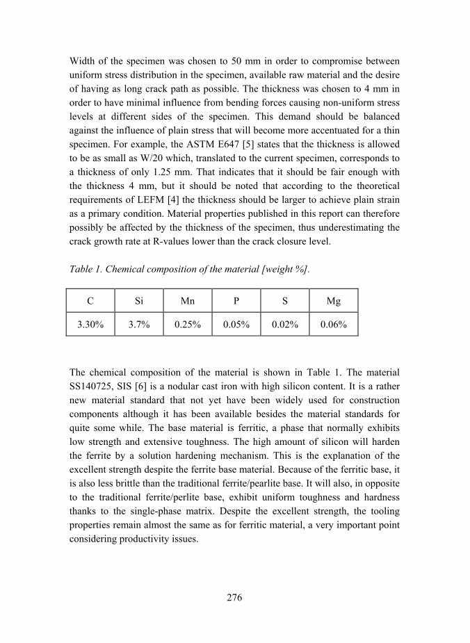
276
Width of the specimen was chosen to 50 mm in order to compromise between uniform stress distribution in the specimen, available raw material and the desire of having as long crack path as possible. The thickness was chosen to 4 mm in order to have minimal influence from bending forces causing non-uniform stress levels at different sides of the specimen. This demand should be balanced against the influence of plain stress that will become more accentuated for a thin specimen. For example, the ASTM E647 [5] states that the thickness is allowed to be as small as W/20 which, translated to the current specimen, corresponds to a thickness of only 1.25 mm. That indicates that it should be fair enough with the thickness 4 mm, but it should be noted that according to the theoretical requirements of LEFM [4] the thickness should be larger to achieve plain strain as a primary condition. Material properties published in this report can therefore possibly be affected by the thickness of the specimen, thus underestimating the crack growth rate at R-values lower than the crack closure level.
Table 1. Chemical composition of the material [weight %].
C Si Mn P S Mg
3.30% 3.7% 0.25% 0.05% 0.02% 0.06%
The chemical composition of the material is shown in Table 1. The material SS140725, SIS [6] is a nodular cast iron with high silicon content. It is a rather new material standard that not yet have been widely used for construction components although it has been available besides the material standards for quite some while. The base material is ferritic, a phase that normally exhibits low strength and extensive toughness. The high amount of silicon will harden the ferrite by a solution hardening mechanism. This is the explanation of the excellent strength despite the ferrite base material. Because of the ferritic base, it is also less brittle than the traditional ferrite/pearlite base. It will also, in opposite to the traditional ferrite/perlite base, exhibit uniform toughness and hardness thanks to the single-phase matrix. Despite the excellent strength, the tooling properties remain almost the same as for ferritic material, a very important point considering productivity issues.

277
Table 2. Material properties.
E (Gpa) Rp0.2 (MPa) Rm (Mpa) A5 (%) HB
Typical values* 173 422 523 15 195
SS 140725-00** 160175 360 500 10 185215
*) Typical values from cast components
**) Lower limits and intervals established in standard
3. Numerical model
The specimen was modelled in finite element as a half-model utilizing symmetry. Two cracks where supposed to emanate from the stress riser, perpendicular from the load and from the lengthwise direction of the specimen. The cracks could be propagated independent of each other in order to model any non-symmetric behaviour of the cracks. The symmetry plane needed for the model where created by locking the lengthwise degree of freedom at the midsection. The axial load was emulated by stress acting at the end area of the model and finally all degrees of freedom but the lengthwise was locked at the grip tabs.
Figure 2. Half model of the specimen and a close up at the notch and the crack fronts.

278
The tests was carried out in a servo-hydraulic test rig which had a diameter of the spindles of about 70 mm. Compared to the dimensions of the specimen waist (4 mm of thickness) the test rig can be considered as infinitely stiff. Therefore it has been no compensation made for any flexibility or load-induced displacement of the boundaries in the finite element model. The correctness of this was confirmed by measurements with strain gauges during the testing.
Figure 3. Stress intensity as a function of crack length for FEM vs. analytical solution for σ0=100 MPa.
The finite element calculations where made in the software ANSYS. The K-solutions where calculated by built-in routines utilizing wedge formed singular crack tip elements with displaced node locations (1/4th position) [4]. Stress intensity factors for both plain stress at the surface and plain strain in the bulk of the specimen where calculated.
4. Experimental procedure
The testing was performed in a servo-hydraulic test machine of type Schenck Hydropuls PSB. The load capacity for the machine was 50 kN. Sinusoidal curve shape at frequencies between 20 and 30 Hz where used during the testing. All tests where made in air at room temperature.

279
To measure the propagation during the testing a travelling microscope was used. Estimated accuracy was ±0.02 mm in total.
Constant load was used during all tests; accordingly the crack tip was exposed for strict increased stress intensity. The procedure helps to avoid accumulation of residual stresses at the crack tip, thus creating as little as possible of crack closure, Suresh, S [7]. The constant load condition is also the most usual for real components, often combined with a load spectrum. Since a spectrum load tend to demolish the residual stresses at the crack tip, it is even more important not to use a test sequence that promotes the build-up of residual stresses. All testing was conducted step-by-step in small increments with reading in between. The crack increments were typical from 0.050.1 mm of length at the beginning of the propagation and up to 12 mm at the end of the crack path just before rupture. The stress intensity and the da/dN-values where then calculated as mean values over the current crack increment.
In this investigation no attention was paid to the initiation phase. The crack initiation was established by cycling the specimens between σ0=225 Mpa and σ0=25 Mpa, thus at R= 0.11 for approximately 30-35000 cycles. Corrected for the effect of the notch, the stress would become +675 Mpa to 75 Mpa at the initation site, i.e. 1.6 times the yield stress. This will explain the low cycle count for crack initiation. At complete crack initiation, the cracks where about 0.20.3 mm of length.
2
11⎟⎟⎠
⎞⎜⎜⎝
⎛=
yp
Krσπ
(2)
The first part of the propagation was disregarded because of the remaining plastic zone after initiation cycling at high stress level. The extension of the plastic zone was estimated according to the Irwin approximation for plane stress, Eq. (2), [7]. This is the condition which produces the largest plastic zone size and the situation that is predominant at the surface where the observations of the propagating crack where made. Assuming an average size of 0.3 mm for the initial crack, the size of the plastic zone was calculated using the stress intensity from the initiation cycling. The crack was then propagated beyond the plastic

280
zone using the same load level as for the subsequent testing before any crack rate measurements where made.
5. Initiation site establishment from machining
Even if the initiation phase was not at focus for this investigation, it is interesting from an engineering point of view to have some knowledge about factors that affect the initiation. The presence of initial defect at the walls inside the hole is one such issue. Macroscopic fatigue cracks often initiate in microscopic flaws. The material around boltholes is usually pretensioned by the mounted bolts and consequently stress released. Under such conditions, the surface smoothness inside the holes is not crucial. In other cases, when the holes are to be free from clamp loads during service, the surface character inside the holes can be of vital importance. Note that it can be of great difference how the holes are manufactured. In this investigation drilled holes are considered, but it is likely that an inclination for micro crack development due to machining is general for a certain material.
The circumference surface inside the hole was examined in 31 experimentally drilled holes of diameters 1.5, 2.5 and 3.5mm. The holes where drilled in three small test specimens, see Figure 4, all of which where cut out from one of the nodular iron specimens. The holes were drilled under different conditions such as sharp drill and low feeding, sharp drill and high feeding and finally blunt drill and medium feeding. The test specimens was moulded in plastic and then grinded and polished and after that microscope examined in 2D, showing the presumptive initiation points as cracks and flaws originating in the drilling operation.
The grinding and polishing procedure was then repeated, generating a new 2D section to examine. Totally four 2D hole sections of each test specimen was examined, i.e. 124 hole sections in total.

281
Figure 4. Test specimens for investigation of machined surfaces inside holes.
The range of flaw size that is of interest was estimated to be from 1020 µm and upwards. In contrast to steel, Björkblad, A. [8] this ferritic nodular iron does not give rise to any initiation flaws inside bored holes. The average numbers of flaws where less than one per section an no one of the rare flaws that were found was bigger than 20 µm. The only present type of surface braking cracks where at the nodules that was located near under the surface. That type of cracks are still not menacing as they end up in a nodule with a radius at bottom, and therefore can be placed on an equal footing with all other surface braking nodules. All other irregularities that where found was only embrace the surface.
This sub investigation shows that this material is not sensitive to crack initiation emanating from machining operations. Only the surface from bore operations has been investigated, but it is likely, most because of the tough character of the material and the large amount of nodules that will cut off the chips, that the characteristics is the same for other machining operations.
6. Chunky graphite
The so-called chunky graphite is a type of cast error, which show up as degenerated graphite origin in the solidification process. It occurs mainly in silicon alloyed nodular iron, especially in thick sections with a relative slow cooling rate during the solidification. Instead of spherical nodules (which is the normal graphite form in nodular iron), the chunky graphite has the form of irregular lumps branched and spread in 3D.

282
A recent report of the work done at the subject, Hamberg et al. [9], indicates that the mechanical properties are affected by the chunky graphite. The most affected properties are the elongation, the ultimate strength and the fracture toughness, all of which was decreased up to 50 percent or more. However, the material used in [9] is not of the same chemical composition as the material in this investigation. Since the slope of the Paris curve seems to be slightly different for the silicon alloyed material compared to other nodular irons, [2], it is of great interest to evaluate also the Paris parameters for silicon alloyed nodular iron containing chunky graphite.
The specimens containing chunky that was used in this investigation was of the same type as for the perfect material except for the thickness that was 6 mm instead of 4 mm. This will produce conservative results because of the accentuated plane strain condition that will prevail (compared to the other type of specimen). The share of chunky was about 95 percent throughout the specimen, which is more or less the highest amount that normally will be found in regular goods. This brings that the test results are supposed to be the worst possible for this type of abnormal microstructure. The normal situation is scattered areas with chunky and normal material in between, leaving the chunky content for 3090 percent.
It should also be pointed out that even if the fatigue characteristics are quite satisfactory for the chunky graphite, it has yet lost a great deal of its toughness.
7. Results
The results that have been achieved are mainly the Paris parameters m and c, see Figure 5. These are for R=0: m=5.25, c=4.5e-12 and for R=0.8: m=5.25, c=1.5e-10 provided da/dN in [mm/cycle] and ∆K in [Mpa(m)1/2]. The middle curve in Fig. 5, [2] is an average curve for R=0 [2] for a ferritic/perlitic nodular iron. Paris data for this curve (ref) are m=5 and c=3e-11 and the curve is often used as a mean curve for ferritic/perlitic nodular iron.
Figure 6 shows the result for the material containing chunky graphite. It should be noted that the chunky graphite does not degenerate the crack propagation properties as much as one could expect. The propagation rate is approximately
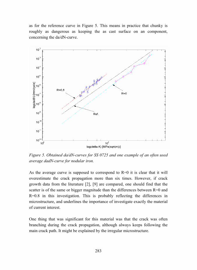
283
as for the reference curve in Figure 5. This means in practice that chunky is roughly as dangerous as keeping the as cast surface on an component, concerning the da/dN-curve.
Figure 5. Obtained da/dN-curves for SS 0725 and one example of an often used average dadN-curve for nodular iron.
As the average curve is supposed to correspond to R=0 it is clear that it will overestimate the crack propagation more than six times. However, if crack growth data from the literature [2], [9] are compared, one should find that the scatter is of the same or bigger magnitude than the differences between R=0 and R=0.8 in this investigation. This is probably reflecting the differences in microstructure, and underlines the importance of investigate exactly the material of current interest.
One thing that was significant for this material was that the crack was often branching during the crack propagation, although always keeps following the main crack path. It might be explained by the irregular microstructure.
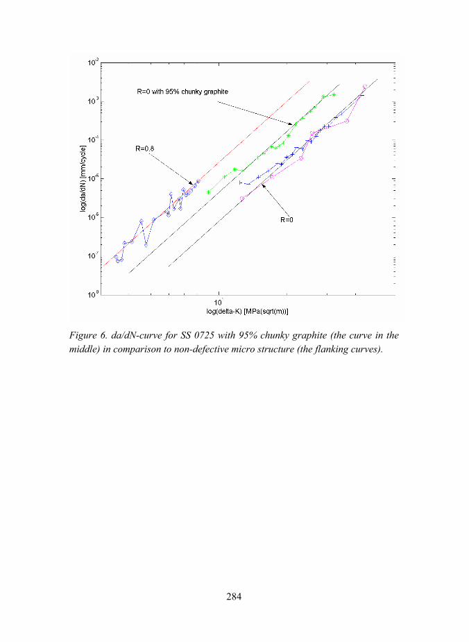
284
Figure 6. da/dN-curve for SS 0725 with 95% chunky graphite (the curve in the middle) in comparison to non-defective micro structure (the flanking curves).

285
8. Conclusions
The fatigue material properties for nodular iron SS 140725 where investigated. Additionally fatigue material properties were determined for a type of cast defect, chunky graphite. The investigation is based on stress intensities from FE-calculations and fatigue testing of a center crack specimen.
The general conclusions can be drawn as follows:
• Stress intensity solutions from FEM are in good correlation with analytical solutions
• The material shows a relatively smooth and uniform crack rate behavior despite the irregular micro structure
• The crack is often branching during the crack propagation, although always keep following the main crack path
• The difference in crack growth rate between R=0 and R=0.8, i.e. propagation with respectively without crack closure, is more than 33 times
• The testing shows a Paris law slope that are equal for different R-values
• No sensitivity for crack establishment from machining can be discerned
• The chunky graphite does not affect the da/dN fatigue curve in any serious matter, although the fracture toughness will be notably lowered.

286
Acknowledgements
The author would like to thank Jack Samuelsson, Volvo CE, and Kenneth Hamberg, Chalmers Lindholmen, for being sources of inspiration and for supervision. Further, Kjell Eriksson, Volvo CE, for material investigations and Rickard Kjellbom, Swedish foundry association, for supplying the material with chunky graphite. Last, but not least, Nordic Industrial Found (NI), National Council for Technical Research and Vehicle Engineering (PFF) and Volvo for founding.
References
1. Nadot, Y. Mendez, J. and Ranganathan, N. Influence of casting defects on the fatigue limit of nodular cast iron, 2004. Int. J. of Fatigue. Vol. 26, pp. 311–319.
2. Lindeborg, B. and Nilsson, J. Fracture mechanical data for ductile iron, malleable iron and cast steel. Sveriges mekanförbund, Stockholm, Sweden, 1985. ISBN 91-524-0791-8.
3. Sundström, B. et al. Handbook in solid mechanics. Royal Institute of Technology (KTH), Stockholm, Sweden, 1998.
4. Anderson, T. L. Fracture Mechanics, fundamentals and applications. 2nd ed. CRC Press LCC, Florida, USA, 1995. ISBN 0-8493-4260-0.
5. ASTM E-647. Measurement of fatigue crack growth rate. American Society for Testing and Materials, Philadelphia.
6. Swedish standard Institute, SIS. SS 140725 spheriodal graphite cast iron. 1st ed. Stockholm, Sweden, 1998.
7. Suresh S. Fatigue of materials. 2nd ed. Came bridge University Press, Camebridge, UK, 1998, ISBN 0-521-57847-7.
8. Bjökblad, A. In: Proceedings of the 9th Portuguese Conference of Fracture, edited by C.M. Branco. IST, Lisbon, Portugal, 2004. Pp. 167–175.
9. Hamberg, K., Björkegren, L.-E. and Sun, Z. X. Chunky graphite in ductile iron. Swedish foundry association, report number 030930, Sweden, 2003.

287
Fatigue crack growth in ductile iron
Kenneth Hamberg, Chalmers University of Technology Marie Mörtsell, Volvo Truck, Gothenburg
Anders Björkblad, KTH, Stockholm Jack Samuelsson, Volvo Wheel Loaders, Eskilstuna
Abstract
Crack initiation and propagation of two ductile irons are studied. The main reason for the study is to propose a common set of reliable fatigue data based on fracture mechanics. Material in this investigation is one standard feritic/pearlitic ductile iron (SGJ 500-7) and one silicon alloyed ductile iron with a solution hardened ferritic matrix (SS 140725). Basically the threshold value and the scaling constants in Paris equation are evaluated. The data used at Volvo Truck has been gathered and re-evaluated. Complementary experiments have been conducted. All experiments have been in accordance with ASTM-647. Scaling constants in Paris equation is set to m= 4,5 and C= 9,4 10-14 (m/cycle)/MNm-3/2
for the standard grade material and m= 5,0 and C= 1,9 10-14 (m/cycle)/MNm-3/2
for the silicon alloyed material. These results are valid for -1<R<0,5. The difference in the slope between the materials is due to different fracture behaviour. Threshold values for the materials can be found in Tables 2 and 3. Crack closure and the influence on crack propagation is expressed in a in a new algorithm. The new algorithm is valid for -1<R< 0,5 but should be used with caution due to meagre statistical foundation.
1. Introduction The usage of nodular cast iron (also referred to as ductile iron) is increasing in the automotive industry today. The main cause for this is due to the possibility of receiving a wide range of mechanical properties that could fulfill desirable component requirements [1]. Other advantages are great design freedom and a low cost production method. In the automotive industry the usage of nodular iron is therefore increasing [24] especially in the truck sector. As a consequence the designer creates more shape and weight optimized components. This fact

288
calls for more reliable materials data for accurate fatigue assessments. Today a common view of the material properties in ductile iron is still lacking. Especially for fatigue loadings a more united front is needed. One of the aims of this paper is to collect and verify some of the fatigue properties for ductile iron and recommend a set of reliable data.
In particular the combination of crack propagation rate and fracture mechanics has proven to bee especially fruitful to use. The method offers a relatively easy way for lifetime calculation. What is more important is that the defects that always are present in a casting can be incorporated in the calculation in a simple manner. Another very important characteristic of the fracture mechanic approach is that it is very compatible with the Wöhler approach of high cycle fatigue. The usage of Whöler curves is well known and familiar to most designers, the fracture mechanic approach is not. All designs in a vehicle must however be based on fracture mechanics even if they are presented in the form of Wöhler curves.
In the field of crack propagation a great amount of work has been published and many attempts have been made to summarise the published information. Ritchie [5] among others have made a more successful attempt when he published the graph that is reproduced in Figure 1.
Figure 1. The crack propagation rate as a function of stress intensity.
dNdalog
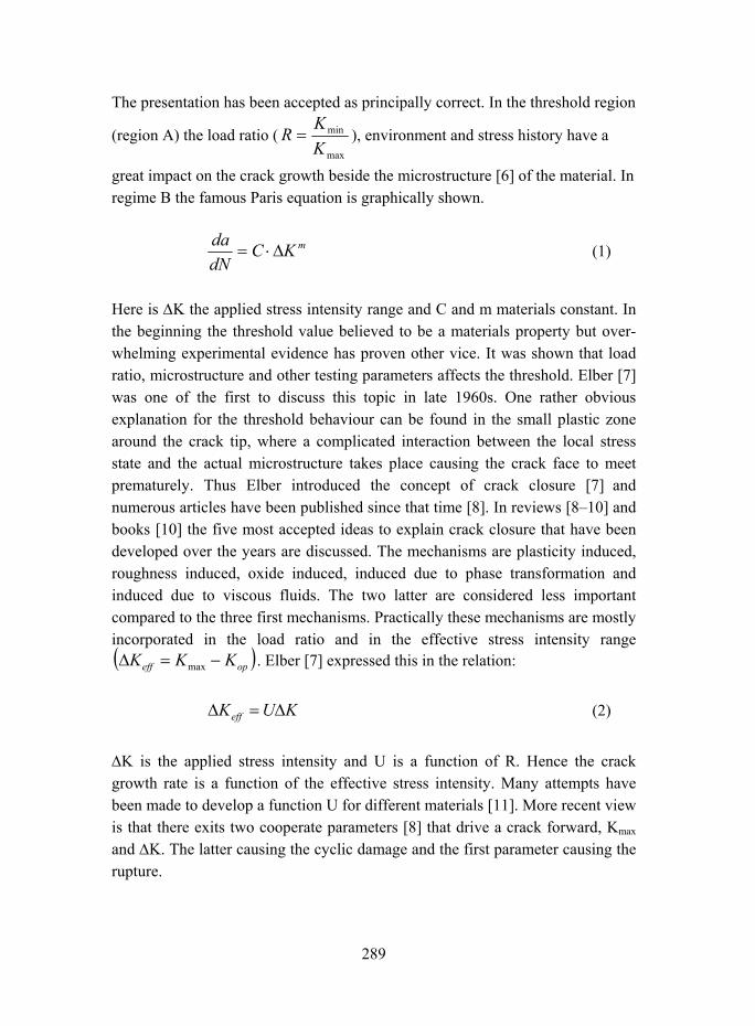
289
The presentation has been accepted as principally correct. In the threshold region
(region A) the load ratio (max
min
KKR = ), environment and stress history have a
great impact on the crack growth beside the microstructure [6] of the material. In regime B the famous Paris equation is graphically shown.
mKCdNda
∆⋅= (1)
Here is ∆K the applied stress intensity range and C and m materials constant. In the beginning the threshold value believed to be a materials property but over- whelming experimental evidence has proven other vice. It was shown that load ratio, microstructure and other testing parameters affects the threshold. Elber [7] was one of the first to discuss this topic in late 1960s. One rather obvious explanation for the threshold behaviour can be found in the small plastic zone around the crack tip, where a complicated interaction between the local stress state and the actual microstructure takes place causing the crack face to meet prematurely. Thus Elber introduced the concept of crack closure [7] and numerous articles have been published since that time [8]. In reviews [810] and books [10] the five most accepted ideas to explain crack closure that have been developed over the years are discussed. The mechanisms are plasticity induced, roughness induced, oxide induced, induced due to phase transformation and induced due to viscous fluids. The two latter are considered less important compared to the three first mechanisms. Practically these mechanisms are mostly incorporated in the load ratio and in the effective stress intensity range ( )opeff KKK −=∆ max . Elber [7] expressed this in the relation:
KUKeff ∆=∆ (2)
∆K is the applied stress intensity and U is a function of R. Hence the crack growth rate is a function of the effective stress intensity. Many attempts have been made to develop a function U for different materials [11]. More recent view is that there exits two cooperate parameters [8] that drive a crack forward, Kmax and ∆K. The latter causing the cyclic damage and the first parameter causing the rupture.

290
In spite of all this quantitative understanding little information can be found in the literature on how a specific microstructure especially for ductile iron reacts under cyclic loading. For practical use a way of incorporate crack closure in a simple and consistent way is needed for ductile iron. For instance no mathematical expression, U exists for ductile iron. Particular for loading in compression data is uncommon. A recent thesis by Mörtsell [12] deals partly with this problem. Examples of published results in tension-tension loading (R>0) in ductile iron is the work of Tokaji [13] and Bulloch [14]. An attempt will be made in this work to find an expression U for ductile iron. One of the problems that arise when analysing published work is that it is rare to find systematic work on ductile iron that can be used in a new kind of analysis.
In compression the problem with the driving force of the crack must be sorted out. According to ASTM E647 only the tension part of the loading cycle is active as a crack driving process. This leaves Kmax as the crack driving parameter in compression. In some recent articles [1517] the situation in compression is under discussion. Here they conclude that an additional contribution to Kmax is possible. This contribution comes from local internal stresses that develop under the fatigue process. Contribution of the local stresses can be both negative and positive depending on the local situation. The nature and variation of the local stress state must therefore be analysed in some detail.
2. Experiments
Before any tests were preformed all relevant crack growth data at Volvo Truck was gathered and reevaluated according to standard. Additional tests were thereafter preformed to fill the information gaps.
Fatigue tests were performed with a sinusoidal waveform of 40 Hz with load ratios R=0 and R= -1. These load ratios were chosen because they have the most practical relevance for designers at Volvo Truck. The tests were performed in room temperature using an Instron 8500 servo-hydraulic testing machine. All the mechanical testing was performed according to standard procedure (ASTM E647-96).

291
2.1 Quantitative fractography
By making a study of the surface topography, the microstructural feature that has the greatest impact on the crack propagation path can be identified. The fracture surface of the fatigued specimens is geometrically quantified by the aid of profile analysis. The profiles are taken from vertical sections through the interior of the specimens parallel to the crack propagation direction. High-resolution optical micrographs are used for computer aided digitising of the profiles. In the measurement a chain of cords replaces the genuine profile with an individual length given by the resolution of the digitalisation, in this case 0,5 µm. The parameters used to characterise the profile describes the direction and the location of the cords related to a suitable reference line. Such parameters are the height distribution and the angular distribution. The precise procedure is described elsewhere [12].
2.2 In situ experiments
More knowledge is needed on what parameters that controls the local properties in the material at a macroscopic high tensile load. During the components life there are some cycles that reaches 300400 MPa [12] or higher. This is above the yield stress for these specific cast irons. The experiments are thus performed under high static load and that is because the high load is thought to be equal to a single shock load on the component. It is also theoretical possible that a static tensile test is comparable to the first ¼ cycle at dynamic loading. To be able to study the local microstructure during static loading, polished test specimens are placed within a unique Scanning Electron Microscope (SEM). There are two types of specimen and also two different aims with this examination. One specimen is notched and pre cycled outside the SEM to allow a crack to start grow out of the plastic zone region of the notch. Then the local microstructures effect on the crack tip and the area in front of the crack is studied during load. Again the specimen is cycled and then investigated in the SEM. This technique [12] is developed by Davidson, S. W. Research Institute, San Antonio, Texas.

292
2.3 Material
Two nodular cast irons are investigated; the first one is standard ferritic/pearlitic grade, 500-7, denoted SS 140727. The other alloy is a fully ferritic (SS 140725) material with roughly the same tensile strength as SS 140727 (the yield strength is 100 MPa higher for SS 140725). Chemical compositions of the materials are given in Table 1. Both materials are produced under production like conditions on a Künkel Wagner green sand moulding line. For the two materials the base iron differs slightly. The ferritic grade has a clean base iron made from pig iron and sheet material scrap and the ferritic/pearlitic grade is made from a standard base iron.
A completely ferritic matrix in material SS 140725 can be accomplished by alloying with silicon. Silicon also solid solution hardens the matrix and gives static mechanical properties comparable to the ferritic/pearlitic SS 140727.
Table 1. Chemical composition of the tested irons (Ceq =C+Si/4 + P/2).
Material C % Si % Mn % P % S % Cu % Sn % Ceq
SS140727 3.59 2.35 0.37 0.009 0.008 0.27 0.005 4.18
SS140725 3.22 3.36 0.23 0.004 0.004 0.03 0.005 4.13
Both materials have well shaped graphite nodules that are evenly distributed in the matrix with a nodularity larger than 95 %. Examples of the microstructure are shown in Figure 2.
Figure 2. The microstructure of SS-EN-GJS-500-7( left) and SS-140725 (right).

293
Even if the nodularity ranking is high in both materials the graphite/matrix phase boundary is more serrated in SS 140727. A more detailed study of the two materials reveals two sets of graphite surfaces, one smooth and one rough. In SS 140725 the surface is smooth while in SS 140727 the surface is much coarser. Figure 3 shows typical examples of different graphite nodule morphologies. These morphologies have an impact on the closure behavior of the material.
Figure 3. Graphite nodules in SS 140725 (left) and in SS 140727 (right). The samples are deep etched in 50 v/o HCl and 50 v/o ethanol.
2.4 Casting defects
A problem with cast iron is the defects present in the components. Casting simulations have during the last years given the foundry technicians a better opportunity to locate casting defects to low stress areas in the component. Therefore small volumes in a component can be virtually defect free. These areas are often highly stressed. In this work a defect free area in ductile iron is defined as a microstructure that contains isolated micro shrinkages, graphite nodules and the matrix. It is of great importance to identify the properties of such a material and to identify the micro mechanisms that control the fracture mechanisms. The damage evolution in this microstructure has been discussed in several articles, see i.e. Tokaij [13] et al., Nadot [18] et al. A simple and easy to use model is still lacking.
One way of investigate the influence of defects is to make test specimens of material taken from suitable cast components. Thus the specimen contain a real cast surface with the residual stresses left intact from the cleaning operations.
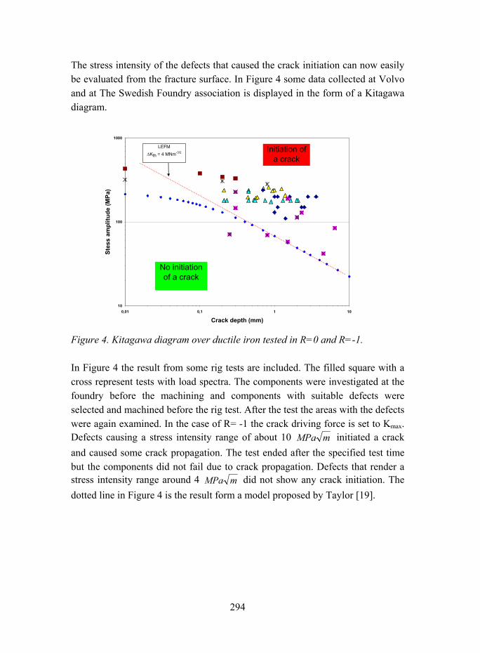
294
The stress intensity of the defects that caused the crack initiation can now easily be evaluated from the fracture surface. In Figure 4 some data collected at Volvo and at The Swedish Foundry association is displayed in the form of a Kitagawa diagram.
10
100
1000
0,01 0,1 1 10
Crack depth (mm)
Stes
s am
plitu
de (M
Pa)
No initiation of a crack
Initiation of a crack
LEFM∆Kth = 4 MNm-3/2
Figure 4. Kitagawa diagram over ductile iron tested in R=0 and R=-1.
In Figure 4 the result from some rig tests are included. The filled square with a cross represent tests with load spectra. The components were investigated at the foundry before the machining and components with suitable defects were selected and machined before the rig test. After the test the areas with the defects were again examined. In the case of R= -1 the crack driving force is set to Kmax. Defects causing a stress intensity range of about 10 mMPa initiated a crack and caused some crack propagation. The test ended after the specified test time but the components did not fail due to crack propagation. Defects that render a stress intensity range around 4 mMPa did not show any crack initiation. The dotted line in Figure 4 is the result form a model proposed by Taylor [19].

295
3. Results
3.1 Crack propagation and threshold data
All results from the testing and from the revaluated old results are presented in Table 2 and Table 3 below. For R=0 where a comparison with old and new data could be made a very good agreement exists with the new tests and older investigations [20].
In table 3 one applied threshold value is not verified according to the standard procedure, it is a good estimate form the test done, the opening value is also a fairly good extrapolation.
Table 2 Fatigue crack growth data for R=0.
Material R m C
( )⎥⎥⎥⎥
⎦
⎤
⎢⎢⎢⎢
⎣
⎡
− mMNmCycle
m
2/3
∆Kth
(MNm-3/2)
Kop
(MNm-3/2)
SS 140727 -1 4,9 1,7 10-13 9.6 5.3
SS 140727 0 4,4 1,5 10-13 7,4 5,3
SS 140727[20] 0,5 4,3 3,6 10-13 4,4 ---
In the case of R= 0,5 the crack opening stress intensity is lacking, due to the fact that the crack was completely opened during the test and consequently the value of the opening intensity is not possible to measure.
Further experimental work is needed for load ratios R < 0. This indicates that stress intensities with Kmin less than zero must be discussed. According to ASTM recommends that ∆K = Kmax when compression loads do not influence the crick driving process. Sadananda [17], Holtz [21] and Kujawski [15] have debated this in a series of articles and come to the conclusion that local stresses that develop in the microstructure affect the process. They can give both a positive and a negative contribution to the crack driving parameters Kmax and ∆K.

296
Table 3. Fatigue crack growth tested at R= -1.
Material R m C
( )⎥⎥⎥⎥
⎦
⎤
⎢⎢⎢⎢
⎣
⎡
− mMNmCycle
m
2/3
∆Kth
(MNm-3/2)
Kop
(MNm-3/2)
SS 140725 -1 5,4 2,5 10-14 9,5* 3,2*
SS 140725 0 5,1 3,8 10-14 7,4 3,7
3.2 Fatigue crack propagation in ductile iron containing chunky graphite
In this project one of the assignments was to investigate the formation of chunky graphite in the newly developed ductile iron SS 14 0725. This iron that is solid solution hardened with silicon is prone to form chunky graphite due to the high silicon content. The unwanted graphite form appears in the hot spots of relatively coarse sections in some castings. Some fatigue experiments was conducted in iron containing 100 % chunky graphite. The material for the specimens was taken from castings specially designed to facilitate formation of chunky graphite. Details are published elsewhere [22]. In Figure 5 the crack propagation rate is presented. Here are also some data from Kaufmann [26] as comparison to the own trials. From the Figure 5 the conclusion is that there is a fair correspondence with the two experiments.
The own experiments (triangles and squares) show a slope of m = 5,2 with a C-value of 1,5 10- 14 [m/cycle/(MNm-3/2)]. Comparison with Kaufmanns [26] experiment show a slightly higher crack propagation rate for his specimen. Kaufmann made his experiments on SGJ 450 material. This is a ductile iron with ferritic matrix and with a tensile strength of at least 450 MPa. The test materials has 100 % chunky graphite. Compared with normal nodules the chunky graphite show a slope in average around 5,5, see Table 4.

297
1,0E-10
1,0E-09
1,0E-08
1,0E-07
1,0E-06
1,0E-05
1,0E+00 1,0E+01 1,0E+02
Stress Intensity (MPa, m)
Cra
ck P
ropa
gatio
n (m
/cyc
le) This Study (specimen 1)
This Study (specimen 3) Kaufmann (ref. 26)
1,0E-10
1,0E-09
1,0E-08
1,0E-07
1,0E-06
1,0E-05
1,0E+00 1,0E+01 1,0E+02
Stress Intensity (MPa, m)
Cra
ck P
ropa
gatio
n (m
/cyc
le) This Study (specimen 1)
This Study (specimen 3) Kaufmann (ref. 26)
Figure 5. Crack propagation data for SS 14 0725 containing 100% chunky graphite.
4. Discussion
4.1 Threshold region
In the threshold region (regime A, Figure 1) the load ratio, environment and stress history have a great influence on the crack growth besides microstructure. It is generally believed that the microstructure have the strongest influence in this region. Major factors are material strength [10, 12], grain size and morphology/distribution of the microconstituents. In several articles by Sadananda and Vasudevan [8, 16, 17, 23], they have argued that the driving force for a short or a long crack is ∆K and Kmax simultaneously, the first causing the cyclic damage and the latter is responsible for the rupture at the crack tip. Accordingly there exists two intrinsic threshold values [23] but Kmax seems to bee the more important parameter. One rather obvious explanation for this behaviour can be found in the small plastic zone around the crack tip, where a complicated interaction between the local stress state and the actual microstructure takes place. In the plastic zone the local stresses due to microstructure and other external notches, as well as residual stresses of all kind, join forces to affect crack initiation and crack growth. Most of the time all these effects are gathered in the term crack closure. Vaudevan and Sadananda

298
incorporate all premature contacts between the two fracture surfaces in the two terms ∆K and Kmax without discussing crack closure, they deal instead with local stresses and local strains.
Mörtsell [24] have discussed the influence of microstructure in her theses. In an experiment with an even distribution of graphite nodules in a ferritic matrix the local strain distribution was measured.
-400-300-200-1000100200300400
0
100
200
300
400
500
0
1
2
3
4
5
Figure 6. The local strain distribution in the microstructure due to the graphite. The global strain is 0 ,7%.
The specimen was given a nominal strain of 0,7% witch gave a local strain variation between 0 and 4,1%. Figure 6 displays this variation. The results point at the importance of an even distribution of small graphite nodules. Crack initiation is likely to appear at a spot with a high strain and after initiation the crack will propagate in the direction of the highest strains. The distribution and size of the graphite nodules is therefore of great interest. Other results by Mörtsell [13] have shown that voids or cracks appear at the graphite matrix interface when the nominal stress reaches the yield stress of the material.
In material SS 140725, solid solution hardened with silicon, the influence of the graphite seems to bee less pronounced. Normally the graphite is guiding the crack due to the void formation around the graphite. Recent work [25] indicates that the matrix-graphite interface can affect the micro mechanism of deformation. The higher yield strength of material SS 140725 can thus affect

299
both the initiation and propagation of the crack. The described effect can be one contribution to the variation in the threshold value that has been seen in the literature. The scatter increases with lower load ratio. As known the intrinsic threshold lies around 4 MNm-3/2, which corresponds to a R value of around 0,5 [20] to 0,7 [18]. Interesting to note is the experimental finding of Mörtsell in ref. 25 where a small micro shrinkage gave rise to a stress intensity of the intrinsic threshold level, consequently a crack was initiated.
4.2 Crack propagation
When crack propagation rate is a bit higher the linear region is entered (regime B in fig. 1). Here Paris have stated the best known and in most cases confirmed crack propagation law:
mKCdNda )(∆= (3)
C and m are experimentally determined scaling constants, generally reported as having no direct relation with each other. The constants are of prime importance especially in cases of spectrum loading where the threshold value is less urgent. This type of loading is important for most practical situations in the automotive industry where random loading situations predominate. It is therefore essential that the designers can agree on a common set of reliable data that can be applied on ductile iron.
In the literature m can take any value between 1,5 and 10 [27] for steel, depending on the material, microstructure, environment. Ritchie [28] and Tanaka [27] have not surprisingly observed that crack propagation at high m-values have a different fracture mechanism compared to crack propagation at low m-values. Normally the slope lies between 3 and 5 for steel.
When the fracture surfaces on the two ductile irons in this study are compared a difference comes into view that can justify two different slopes. One reason is that the high silicon alloy has little less graphite than the other alloy. Another reason is the microstructure. The standard GJS 500-7 material has a ferritic/perlitic microstructure with a soft ferrite and a hard perlite while the high

300
silicon alloy got a hard ferritic matrix. If the slope m of the two alloys are compared a difference exists. The slope increases from 4,5 to 5 when the perlite vanish and the ferrite is solid solution hardened with silicon. Reasons for the difference may lie in the crack closure level, witch depends on the microstructure that makes the crack meander. In figure 7 some data for plain mild steel with various microstructures [30] are displayed for comparison.
0
1
2
3
4
5
6
0 20 40 60 80 100
Surface roughness (mm)
Cra
ck c
losu
re le
vel
(MPa
m0,
5)
SS 0727
SS 0725
0
1
2
3
4
5
6
0 20 40 60 80 100
Surface roughness (mm)
Cra
ck c
losu
re le
vel
(MPa
m0,
5)
SS 0727
SS 0725
SS 0727
SS 0725
Figure 7. Crack closure as a function of surface roughness.
Ogawa et al. [31] suggested that graphite could be deposited in the wake of the growing crack, but he did not show any experimental evidence of the phenomenon. Mörtsell [12] has shown that the graphite is leading the crack propagation due to the localised plasticity and shear band that develop between the mediate nodules and thus leads the crack. On the fracture surface the volume fraction of graphite is more than 30%. A random surface through the specimen should contain 1014% depending on the carbon content. From Table 1 one can see that there is a slight difference in the carbon content, witch is the reason for the graphite variation. The distribution and size of the graphite is therefore of prime importance. Experimental evidence exists [24] that show how graphite is chipped of the nodules when the crack is advancing. Graphite with rougher surfaces generates more closure than the smoother graphite surfaces on the silicon alloyed material does.
From a practical point of view there is a need to compare how C and m values affect the life of a component and to judge that from the crack propagation plot. Therefore a modified variant of Paris equation is derived. From a set of 200 C

301
and m values gathered from the literature (R= 0) the conclusion was drawn that there exist a relation between C and m which can be expressed as:
Cmmm log10 += (4)
The relationship have been reported for steels [32, 33], aluminium alloys [34, 35], copper alloys and titanium alloys. Immediately one great advantage is offered; Paris equation can be expressed with only one dependent variable, C or m. Further analysis suggests that m also can be expressed as a function of Youngs modulus, E.
Emmmo log32 += (5)
In Principle C in Paris equation can be expressed as a function of m as equation 4 postulates.
mk kEkC
3
1 12
= (6)
This means that Paris equation can be expressed with just one parameter m.
mk
m
kK
EkKC
dNda )()(
3
12
∆=∆= (7)
A simple regression analysis can now be performed with the experimentally determined values of C and m by applying the equation 5. The result is shown below:
mKEdN
da )3,23
(9,126,3
∆= (8)
Equation 8 points towards the importance of Youngs modulus. The equation is valid for materials with different elastic modulus, the modulus span between 45 to 210 GPa. In ductile iron the parameter can vary with the microstructure as it can be regarded as a composite. The local variation in the graphite distribution

302
affects the elastic modulus and thus crack propagation rate. Again this calls for a close control of the graphite distribution and the importance of a small nodule size and evenly distributed graphite.
In table 4 the m and C values are slightly changed compared to tables 2 and 3 in the result paragraph.
Table 4. Recommended fatigue crack growth data for ductile iron.
Material R m C
( )⎥⎥⎥⎥
⎦
⎤
⎢⎢⎢⎢
⎣
⎡
− mMNmCycle
m
2/3
SS 140727 -1 4,5 9,4 10-14
SS 140727 0 4,5 9,4 10-14
SS 140727 0,5 4,5 9,4 10-14
SS 140725 -1 5 1,9 10-14
SS 140725 0 5 1,9 10-14
SS 140725* 0 5,5 4,1 10-15
*/ Results from chunky graphite
The values are grouped in this way due to practical reasons. It is convenient to have one set of data for ductile iron in spite of changes in the R value. The influence of R is small in the linear region and do not affect the outcome of the life calculation in a significant way. Another justification for the choice of slope is the practical difficulties to evaluate the slope.

303
4.3 Compensation for local stresses
From a point of simplicity a function that takes care of the variation in load ratio and transforms a crack the ∆K dependence to ∆Keff is needed. Elber [7] was the first to make such an approach. He defined a function U according to the formula below.
KK
U eff
∆∆
= (9)
He postulated that for his aluminium material the famous function 24,01,05,0 RRU ++= and -0,1 ≤R< 0,5. Kumar and Singh[11] have gathered
such functions for different type of alloys but only for R> 0, except for Elbers formula mentioned above. If lower R-values are incorporated in the analysis the definitions of ∆K must be considered. By definition the driving force for the crack, ∆K, is the difference between Kmax and Kmin. This works well if the fracture surfaces dont com into contact before Kmin is reached. In figure 7 the threshold value is principally sketched as a function of R. For positive R-values the threshold is diminished with increasing R to a certain point where the line levels of into a plateau, here is the intrinsic threshold value for the material. For R< 0 ASTM recommend Kmax as the crack driving force, the reason is simply that a negative K do not contribute to crack propagation. This is under the assumption that no contacts exists between the fracture surfaces as long as K> Kmin. In the literature one can also find that the whole stress intensity range (∆K) is used for negative R values. Such an approach suggests that the negative part of the stress intensity have the same crack driving capability as the positive part of the stress intensity. In Figure 7 both these assumptions are indicated with broken lines. A suggestion to a more plausible function is the straight line in the Figure 7.

304
Figure 7. The threshold value as a function of R.
There have been many attempts to make such an analysis and many formulas are published in the literature. Kumar [11] have gathered such formulas for a number of commercial alloys mostly for steel and aluminium alloys. For ductile iron there is no expression available, though there has been a number of attempts, see Dahlberg [36] to find one. In the literature there are many published sets of data for R> O, but data for negative load ratios are rare. Just for a trial the data in hand from the literature [36, 20] and the own experimental findings was grouped and normal regression analysis gave the following relation:
242,064,056,0 RRU ++= for -1 ≤ R < 0,5 (10)
The analysis show that ASTMs recommendation seems to hold relatively well in this case, but the data that is the base for the regression analysis is rather meagre and additional data is needed to make the conclusions more reliable.
R +1-1
∆Kth
0

305
1,0E-10
1,0E-09
1,0E-08
1,0E-07
1,0E-06
1 10 100
Stress intensity (MPa, m)
Cra
ck p
ropa
gatio
n (m
/cyc
le)
R = 0,1R = 0,5R = -1
Figure 8. Crack propagation data for ductile iron 0727 at various R values.
If the algorithm is applied on the data in Figure 8, witch is supplied by ABB Robotics the following picture emerges.
On this data the algorithm seems to hold, as well on the own data with the same good correlation. Trials on other literature data can give a slightly higher scatter. A cause for this might be the meagre data for negative R values. The algorithm must be supported with more reliable experimental data.
1E-10
1E-09
1E-08
1E-07
0,000001
0,00001
1 10 100Stress Intensity * U
Cra
ck P
ropa
gatio
n
R=0,5R=0R=-1
Figure 9. The crack propagation data in Figure 8 corrected for crack closure.
306
4.4 Influence of defects
Defects are the foremost cause for crack initiation and thus crack propagation and failure. Kitagawa diagrams like in Figure 4 show basically two way of interpret fatigue. The horizontal line that predicts no influence of defects is the Wöhler approach. Linear fracture mechanics take defects into account and show the possibility of predicting the influence of defects. If a small defect is contained in the structure a high load can be applied and thus a big defect a small load. This is shown by the inclining line in Figure 4. The point where the two lines intersect is a rough estimate of the smallest defect that must be taken into account in order to endure the fatigue limit due to the Wöhler approach. As seen this is a small defect, roughly 0,20,3 mm in dimension. Only in the most stressed region on a component such a demand can be of interest. Thus zone marking of a whole component is not justifiable. One reason is that not all defects ends up on a high stressed area, most defects are stuck in regions where they are acceptable. Thus only small areas must be controlled with NDT-testing, but still it is challenging to find that size in serial production in complicated structures.
5. Conclusions
Following conclusions has been drawn for this study:
• Analysis of the fracture surfaces can support the difference of the slopes in the table below.
• Crack closure for the standard grade is greater compared to the iron solution hardened with silicon. It is proposed that the chipping of pieces of the graphite nodules in the standard iron is the mechanism that enhances crack closure.
• The scaling constants in Paris formula can be expressed with one dependent parameter, m, according the formula:
mk kEkC
3
1 12
=
• Paris equation can be expressed according to:

307
mKEdN
da )3,23
(9,126,3
∆=
• The following set of design data is recommended for ductile iron:
Material R ∆Kth m C
( )⎥⎥⎥⎥
⎦
⎤
⎢⎢⎢⎢
⎣
⎡
− mMNmCycle
m
2/3
SS 140727 -1 9,6 4,5 9,43 10-14
SS 140727 0 7,4 4,5 9,43 10-14
SS 140727 0,5 4,4 4,5 9,49 10-14
SS 140725 -1 9,5 5 1,95 10-14
SS 140725 0 7,4 5 1,95 10-14
SS 140725* 0 --- 5,5 4,05 10-15
*/ Results from chunky graphite
The proposed constants in the table are based on practical convenience, due to the fact that the influence of R on the constants is small.
• The influence of crack closure can be summarized with a classical Elber analysis:
( ) KRRKUKeff ∆⋅++=∆⋅=∆ 242,064,056,0 , for -1< R < 0,5R
The expression is based on a relatively poor statistical foundation and more experimental support is needed for negative R values.
Acknowledgements
The financial support from the Nordic Industrial Found (NI), Vehicle Research Program (PFF), together with Swedish industry (Volvo AB, Volvo CE, ABB Robotics, Arvika Foundry AB) is gratefully acknowledged.

308
References
1. Dahlberg, M. Fatigue in Nodular Cast Iron. Litentiate Thesis, Department of Solid Mechanics, Royal Institute of Technology, 1997.
2. Foundry man, West European Overview, No. 8 (Aug), 1999, pp. 221228.
3. Yaacoub, A., Béranger, A. S., Billardon, R. and Hild, F. High Cycle Fatigue Behavior of Spheroidal Graphite Cast Iron. Fatigue and Fracture of Engineering Materials and Structures. Vol. 21, 1998, pp. 287296.
4. Zuidema, J., Wijnmaaln, L. & Eldijk, C. Fatigue of Nodular Cast Iron. Bejing, China. Fatigue 99, pp. 20712076.
5. Ritchie, R. O. Influence of Microstructure on Near-Threshold Fatigue-Crack Propagation in Ultra-High Strength Steel. Met. Sci., 1977. Vol. 11, No. 8/9, pp. 368381.
6. Schindler, H.-J. On the Significance of Crack Tip Shilding in Fatigue Thresholds-Theoretical Relations and Experimental Implications, 2000, ASTM STP 1372. Pp. 4662.
7. Elber, W. The significance of fatigue crack closure. ASTM STP 486, 1971. Pp. 230242.
8. Vasudevan, A.K. and Sadananda, K. A review of crack closure, fatigue crack threshold and related phenomena, Materials Science and Engineering, 1994. A188, pp. 122.
9. Newman, J. C. and Piascik, R. S. Fatigue Crack Growth Thresholds, endurance limits and design. ASTM STP 1372, 2000. ISBN 0-8031-2624-7
10. Suresh, S. Fatigue of Materials. Cambridge University Press, 1991. ISBN 0 521 36510 4
11. Kumar, R. and Singh, K. Influence of stress ratio on fatigue crack growth in mild steel. Engineering Fracture Mechanics, 1995. Vol. 50, No. 3, pp. 377384.
12. Mörtsell, M. Crack Initiation in Nodular Cast Iron. Lic. Thesis, To be published, 2005.

309
13. Tokaji, K., Ogawa T. and Shamoto, K. Fatigue crack growth in spheroidal-graphite cast irons with different microstructures. Fatigue, 1994. Vol. 16, July, pp. 344350.
14. Bulloch, D. J. and Bulloch, J. H. Influence of R-ratio and microstructure on the Threshold Fatigue Growth Characteristics of Spheroidal Graphite Cast Iron. Int. J. Pres. Ves. & Piping, 1989. Vol. 36, pp. 289314.
15. Kujawski, K. ∆Keff parameter under re-examination. Int. J. Fatigue, 2003. Vol. 25, pp. 793800.
16. Sadananda K., Vasudevan A. K. and Kang, I. W., Effect of superimposed monotonic fracture modes on the ∆K and ∆Kmax parameters of fatigue propagation. Acta Materialia, 2003. Vol. 51, pp. 33004314.
17. Sadananda, K. and Vasudevan, A. K. Application of unified fatigue damage approach to compression-region. Int. J. Fatigue, 1999. Vol. 21, pp. S263S273.
18. Nadot, Y., Mendez, J. and Ranganathan, N. Influence of casting defects on the fatigue limit of nodular cast iron. Int. J. Fatigue, 2004. Vol. 26, pp. 311319.
19. Tailor, D. Geometrical effects in fatigue: a unifying theoretical model, Int. J. Fatigue, 1999. Vol. 12, pp. 413420.
20. Ljungwald, N. and Näslund P. Methods for Fatigue Life Time Prediction. LM-500570 (Internal Volvo report), 1994.
21. Holtz, R. L. Phenomenology of the effective stress intensity related to fatigue crack growth thresholds. Int. J Fatigue, 2003. Vol. 25, pp. 891897.
22. Källbom, R. Avoiding chunky graphite in ductile iron. To be Published, 2005.
23. Sadananda, K. and Vasudevan, A. K. Crack driving force and crack growth representation under fatigue. Int. J. Fatigue, 2004. Vol. 26, pp. 3947.
24. Mörtsell, M., Hamberg, K. and Wasén, J. The Effect of Graphite nodules on the Fatigue Threshold in two Ductile Irons. 2002, In Proc. Fatigue 2005.

310
25. Mörtsell M., Hamberg K., Wasén J. 2003, Crack Initiation in Ductile Cast, 2002. Irons. In: Proc. 7th. Int. Conf of Cast Materials, Barcelona.
26. Kaufmann, H. 1998, Zur schwingfesten Bemessung dickwandiger Bauteile aus GGG-40 unter Berücksichtigung giesstechnisch bedingter Gefügeungänzen. Bericht Nr FB-214, Fraunhofer Institut für Betriebs- festigkeit.
27. Tanaka, K. Tentative Explanation for Two Parameters, C and m, in the Paris Equation of Fatigue Crack Growth. Int. J. Fracture, 1977. Vol 13, p. 563.
28. Ritchie, R. O., Suresh, S. and Moss, C. M. Near-Threshold Fatigue Crack Growth in 2.25Cr-1Mo Pressure Vessel Steel in Air and Hydrogen. J. Eng. Met. Tech, 1980. Vol. 102, p. 293.
29. Ritchie, R. O. and Knott J. F. Acta. Met, 1973. Vol. 21, p. 69.
30. Hamberg, K. Microstructural Influence on the Fatigue Properties of Steel. Ph D theses, Chalmers University of Technology, 1986.
31. Ogawa, T. and Kobayashi, H. Near-threshold Crack Growth and Crack Closure in a Nodular Cast Iron. Fatigue of Engineering Materials and Structures, 1987. Vol. 10, No. 4, pp. 273280.
32. Benson, J. P. and Edmonds, D. V. Relationship Between the Parameters C and m of Paris' Law for Fatigue Crack Growth in a Low-Alloy Steel. Scr. Met. 1978. Vol. 12, p. 645.
33. McCarter, L. M. and Irving, P. E. Comments on A Correlation for Fatigue Crack Growth Rate. Scr. Met. 1977. Vol 11, p. 181.
34. Nicolls, E. H. Scr. Met. 1976. Vol. 10, p. 295.
35. Bilon, J. P. and Masounave J. Relationship Between the Parameters of Paris' Law for Fatigue Crack Growth in Al Alloys. Scr. Met. 1977. Vol. 11, p. 1101.
36. Dahlberg, M. and Stenfors, S.-E. Examination of the Fracture Mechanics Approach to Fatigue Design of Nodular Cast Iron Components. In: Proc. Fatigue 2002, Vol. 4, pp. 23022400.

311
Fatigue assessment of a cast axle
Janne Lepistö Lappeenranta University of Technology
Lappeenranta, Finland
Abstract
In this paper, some results of fatigue tests carried out for a cast axle are presented. The axle is a large thick walled structure fabricated from nodular cast iron. In addition to fatigue tests, static measurements and FE-analyses were performed. The results from static measurements were also compared with the results obtained from FE-analysis. The FE-results were in good agreement with the static measurements. Several different load cases were studied. These involved bending-only, torsion-only, combinations of bending and torsion and constant and variable amplitude loading. In total, 10 fatigue tests were done. Based on these tests, a mean SN curve was determined. For the two test cases in which variable amplitude loading was used, the fatigue strength was significantly lower than that observed in constant amplitude loading.
1. Introduction
Cast components are widely used in such applications, which require rather complex geometry. One of these applications is a cast axle studied in this paper. This component is typically subjected to quite complex loading. A typical load could consist for example of mainly torsion added with some bending force. Usually the loading is alternating and can be either proportional or non-proportional. The presence of several load components makes the axle to be subjected to a multi-axial stress state.
The critical spot regarding to fatigue is the shoulder made on it due to the bearing. The groove on shoulder has rather tight radius, which causes especially in bending loading a significant stress concentration. The loading in question (torsion plus bending) makes the stress state to be bi-axial on the bottom of the groove.

312
Both static and fatigue tests were performed. In order to estimate and determine the stress level at the groove, also FE-analyses were carried out. This had to be done because of the fact, that no strain gauges etc. could be attached on that spot. The FE-analyses were made using a 2D-model utilising axisymmetric elements. Bending was analysed in 2D models by means of Fourier series. This feature was included in software used (MSC Marc and ABAQUS). The results of the FE-analysis were compared with static test results.
Two different constructions were used in tests. The original structure had to be modified, since it appeared that the failure comes to a wrong part of the test system. The torsion axle of the test system was too weak. In total, ten fatigue tests were performed including the run-out tests. The studied cases were as follows:
• Constant amplitude bending (2) • Constant amplitude torsion (2) • Constant amplitude torsion-bending (2) • Constant amplitude torsion-bending, non-proportional loading (2) • Variable amplitude torsion-bending (2). Most tests were carried out using a min-max stress ratio of R = 0, meaning that some mean stress was included in results. The load spectrum in variable amplitude tests was very simple; one over- underload cycle in 10000 cycles.
2. FE-analyses
FE-analyses were performed using MSC Marc and ABAQUS software. The original construction was analysed using Marc and the modified one with ABAQUS. A 2D-model was used with axisymmetric elements. This approach was chosen since the region of the groove wanted to model with a fine element mesh enough. This goal in mind, a 3D model would have become far too large. The element size used in these models was approximately 0.2x0.2 mm at the vicinity of the groove. Element models consisted approximately 3500 elements. When the loading is bending, axisymmetric elements normally cannot be used, because they require the load in addition to the geometry also to be axisymmetric. However, both of named software supported the use of Fourier series when analysing a bending case. This was done by different means, though.
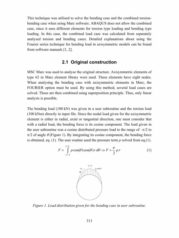
313
This technique was utilised to solve the bending case and the combined torsion-bending case when using Marc software. ABAQUS does not allow the combined case, since it uses different elements for torsion type loading and bending type loading. In this case, the combined load case was calculated from separately analysed torsion and bending cases. Detailed explanations about using the Fourier series technique for bending load in axisymmetric models can be found from software manuals [1, 2].
2.1 Original construction
MSC Marc was used to analyse the original structure. Axisymmetric elements of type 62 in Marc element library were used. These elements have eight nodes. When analysing the bending case with axisymmetric elements in Marc, the FOURIER option must be used. By using this method, several load cases are solved. These are then combined using superposition principle. Thus, only linear analysis is possible.
The bending load (100 kN) was given in a user subroutine and the torsion load (100 kNm) directly in input file. Since the nodal load given for the axisymmetric element is either in radial, axial or tangential direction, one must consider that with a radial load, the bending force is its cosine component. The load given in the user subroutine was a cosine distributed pressure load to the range of π/2 to π/2 of angle θ (Figure 1). By integrating its cosine component, the bending force is obtained, eq. (1). The user routine used the pressure term p solved from eq.(1).
/ 2
/ 2
cos( )cos( )2
F p r d F p rπ
π
πθ θ θ−
= ⇒ =∫ (1)
Figure 1. Load distribution given for the bending case in user subroutine.

314
2.2 Modified construction
The modified construction was analysed with ABAQUS software. In the model, the inner diameter of the cast axle was enlarged, thus the wall thickness was reduced. In addition, the bending arm length with respect to the groove differed from the original construction model. In ABAQUS, the bending case using axisymmetric elements can be also nonlinear. In this case, however, the analysis was linear.
Both bending case and torsion case were solved separately. A combined case can then be calculated afterwards using equations (2)(4). In the bending case, an element of type CAXA8R2 was used. This is an eight-node element with Fourier series expansions. The torsion case was analysed using an element CGAX8R, which is also an eight-node element included with a degree of freedom in circumferential direction. Both elements use reduced integration. The given loads were 100 kN in bending and 100 kNm in torsion.
( )
( )
2 21
2 22
1 421 42
x y x y
x y x y
σ σ σ σ σ τ
σ σ σ σ σ τ
⎧ ⎛ ⎞= + + − +⎜ ⎟⎪⎪ ⎝ ⎠⎨
⎛ ⎞⎪ = + − − +⎜ ⎟⎪ ⎝ ⎠⎩
(2)
2 2 23vm x y x yσ σ σ σ σ τ= + − + (3)
1b 2b 1Tb b
bFEA bFEA FEA
, ,x yF F TF F Tσ σ σσ σ τ= = = (4)
In the equation (4), stresses σ1b and σ2b are principal stresses obtained from FE-analysis for the bending case and the force FbFEA is the force used in the analysis. Accordingly, the stress σ1T is the principal stress from torsion case and TFEA is the torsion moment used in the analysis. Fb and T are the bending force and torsion moment of the combination in question.

315
3. Experimental All tests were carried out in LUT laboratory of fatigue and strength. Test specimens were modified after few first tests since the torsion shaft of the test system was broken instead of the cast axle itself. Consequently, the diameter of the torsion shaft was enlarged as well as the inner diameter of the cast axle accordingly. By this means, the stress level at the cast axle groove was increased and the critical spot was moved at a location under investigation. The test arrangement is presented in Figure 2.
Figure 2. The test arrangement of the cast axle fatigue tests.
3.1 Test material
Test specimens were fabricated from nodular cast iron. For each specimen, strength values of the casting were determined. These are presented in Table 1. The modulus of the elasticity and the Poisson ratio used in FE-analyses and stress calculations in static tests were E = 175000 MPa ν = 0.275 respectively.
Table 1. Yield strength and ultimate strength values of tested specimens [MPa].
Specimen
1 2 3 4 5 6 7 8 9 10
Rp0.2 498 511 467 467 519 506 506 475 467 467
Rm 862 910 838 835 817 878 878 806 835 835
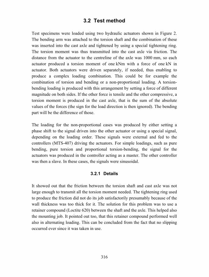
316
3.2 Test method
Test specimens were loaded using two hydraulic actuators shown in Figure 2. The bending arm was attached to the torsion shaft and the combination of these was inserted into the cast axle and tightened by using a special tightening ring. The torsion moment was thus transmitted into the cast axle via friction. The distance from the actuator to the centreline of the axle was 1000 mm, so each actuator produced a torsion moment of one kNm with a force of one kN in actuator. Both actuators were driven separately, if needed, thus enabling to produce a complex loading combination. This could be for example the combination of torsion and bending or a non-proportional loading. A torsion-bending loading is produced with this arrangement by setting a force of different magnitude on both sides. If the other force is tensile and the other compressive, a torsion moment is produced in the cast axle, that is the sum of the absolute values of the forces (the sign for the load direction is then ignored). The bending part will be the difference of those.
The loading for the non-proportional cases was produced by either setting a phase shift to the signal driven into the other actuator or using a special signal, depending on the loading order. These signals were external and fed to the controllers (MTS-407) driving the actuators. For simple loadings, such as pure bending, pure torsion and proportional torsion-bending, the signal for the actuators was produced in the controller acting as a master. The other controller was then a slave. In these cases, the signals were sinusoidal.
3.2.1 Details
It showed out that the friction between the torsion shaft and cast axle was not large enough to transmit all the torsion moment needed. The tightening ring used to produce the friction did not do its job satisfactorily presumably because of the wall thickness was too thick for it. The solution for this problem was to use a retainer compound (Loctite 620) between the shaft and the axle. This helped also the mounting job. It pointed out too, that this retainer compound performed well also in alternating loading. This can be concluded from the fact that no slipping occurred ever since it was taken in use.

317
For each test specimen, some static tests were carried out before the fatigue test. Specimens were instrumented with strain gauge rosettes. The angle between the grids A and B as well as B and C was 45 degrees. One of the strain gauges was located as near the groove as possible, Figure 3. This means, that the gauge had to be placed under the bearing. Therefore, a space for the gauge was machined on the inner ring of the bearing. The orientation of the gauges with respect to the cast axle axis was as shown in Figure 3. In the first tests, the orientation was like on the left side and later the orientation like on the right side was used. The strain values were measured for each grid separately. Principal strains and stresses can then be calculated using equations (5)(8). It must be noted, that the result of the angle of the principal strains (and stresses) will be in the coordinate system based on the gauge. In this system, the first axis is the direction of the grid A and the second axis in the direction of the grid C. If one is using Mathcad program for calculations, it is convenient to replace the equation (8) with the eq. (9), which gives the result measured from the first axis of the gauge coordinate system.
( ) ( )( )( ) ( )( )
2 21 A C A C B A C
2 22 A C A C B A C
1 221 22
ε ε ε ε ε ε ε ε
ε ε ε ε ε ε ε ε
⎧ = + + − + − −⎪⎪⎨⎪ = + − − + − −⎪⎩
(5)
( ) ( )
( ) ( )
2 2A C1 A C B A C
2 2A C2 A C B A C
1 22 1 1
1 22 1 1
E
E
ε εσ ε ε ε ε εν ν
ε εσ ε ε ε ε ε
ν ν
⎧ +⎛ ⎞= + − + − −⎜ ⎟⎪ − +⎪ ⎝ ⎠⎨
+⎛ ⎞⎪ = − − + − −⎜ ⎟⎪ − +⎝ ⎠⎩
(6)
( ) ( ) ( )2 2 1 2
max A C B A C22 1 2
E σ στ ε ε ε ε εν
−= − + − − =
+ (7)
B A C
A C
21 arctan2
ε ε εθε ε
⎛ ⎞− −= ⎜ ⎟−⎝ ⎠
(8)
A C B A C1 angle[( ), (2 )]2
θ ε ε ε ε ε= − − − (9)

318
Figure 3. The orientation of the strain gauges on test specimens.
Some of the fatigue tests were aborted before the cast axle totally broke. In those cases, however, the presence of a crack was obvious based on the output of the strain gauge. The occurrence of a crack on the cast axle was considered as a failure. The load level for the actuators was determined based on the FE-analysis results at the axle groove. Loading sequences for the non-proportional cases is shown in Figure 4. On the left side is presented the sequence for the first case. Loading starts from zero and executes anticlockwise (bending on, torsion on, bending off, torsion off). On the right side of the Figure 4, is shown the sequence for the second case. Again, loading starts from zero, goes up and then right, finally returning along the same path (torsion on, bending on, bending off, torsion off). The load spectrum for variable amplitude fatigue tests is presented in Figure 5. Here, F denotes the loading combination (torsion with slight bending).
0 20 400
100
200
Tor t( )
kNm
Ben t( )
kN
0 20 400
100
200
Tor t( )
kNm
Ben t( )
kN
Figure 4. Loading sequences for the non-proportional test cases.
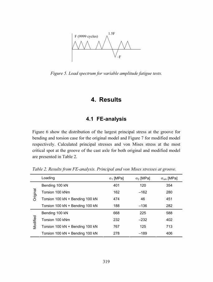
319
Figure 5. Load spectrum for variable amplitude fatigue tests.
4. Results
4.1 FE-analysis
Figure 6 show the distribution of the largest principal stress at the groove for bending and torsion case for the original model and Figure 7 for modified model respectively. Calculated principal stresses and von Mises stress at the most critical spot at the groove of the cast axle for both original and modified model are presented in Table 2.
Table 2. Results from FE-analysis. Principal and von Mises stresses at groove.
Loading σ1 [MPa] σ2 [MPa] σvm [MPa]
Bending 100 kN 401 120 354
Torsion 100 kNm 162 162 280
Torsion 100 kN + Bending 100 kN 474 46 451 Orig
inal
Torsion 100 kN + Bending 100 kN 188 136 282
Bending 100 kN 668 225 588
Torsion 100 kNm 232 232 402
Torsion 100 kN + Bending 100 kN 767 125 713 Mod
ified
Torsion 100 kN + Bending 100 kN 278 189 406
1.5F
F
F (9999 cycles)
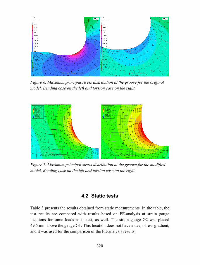
320
Figure 6. Maximum principal stress distribution at the groove for the original model. Bending case on the left and torsion case on the right.
Figure 7. Maximum principal stress distribution at the groove for the modified model. Bending case on the left and torsion case on the right.
4.2 Static tests
Table 3 presents the results obtained from static measurements. In the table, the test results are compared with results based on FE-analysis at strain gauge locations for same loads as in test, as well. The strain gauge G2 was placed 49.5 mm above the gauge G1. This location does not have a deep stress gradient, and it was used for the comparison of the FE-analysis results.

321
Table 3. Static test results for both constructions and the comparison of the results with the FE-analysis results at same locations.
Loading, gauge
σ1 [MPa]
σ2 [MPa]
τmax [MPa]
σ1 / σ1,fea
σ2 / σ2,fea
τmax / τmax,fea
B, G1 102 34 34 0.94 1.06 0.89
B, G2 70 6 32 1.00 0.86 1.00
Orig
inal
T, G2 85 78 81 1.05 0.96 1.00
B, G1 119 61 29 1.05 1.28 0.88
B, G2 44 2 21 1.01 1.73 0.93
T, G1 134 110 122 1.14 0.93 1.04 Mod
ified
T, G2 119 106 113 1.06 0.95 1.00
Original structure, bending case: Fb = 100 kN, T = 0 kNm Original structure, torsion case: T = 99.8 kNm, Fb = 0.2 kN Modified structure, bending case: Fb = 51.8 kN, T = 0 kNm Modified structure, torsion case: T = 95.1 kNm, Fb = 0.1 kN
4.3 Fatigue tests
The fatigue test results are presented in Table 4. In the table, σ1a and σ1m are the stress amplitude and mean stress of the largest principal stress, respectively. The term λ is the biaxial principal stress amplitude ratio and R is min-max ratio of σ1a. The value Nf is the number of cycles to failure. The specimens were considered as failed, when a crack was observed. The presence of the crack was judged based on the output of the strain gauge near the groove. When a change of approximately five to ten percent in maximum strain level of one grid was noticed, the breaking point was set on that location.
Figure 8 shows a typical crack for bending loading. Figure 9 presents a typical failure when the loading is fully reversed torsion. Finally, Figure 10 shows a typical crack for torsion-bending loading cases with R = 0. The direction of the crack is very close to the normal of the largest principal stress (usually approximately 40 degrees from the centreline of the cast axle for these cases). Often several small cracks at the groove were observed. These were typically in a direction that is normal to largest tensile principal stress.

322
Table 4. Fatigue test results for the cast axle.
Spec σ1a σ1m λ=σ2a/σ1a R Nf Type Note
1 181 221 0.30 0.1 1000561 B RO
1 238 277 0.30 0.07 328000 B
5 123 124 1.00 0 2138000 T RO
2 230 0 0.55 1 991400 T+B RO
10 279 0 1.00 1 395000 T
9 229 229 0.50 0 225000 T+B
8 229 230 0.47 0 625000 T+B NP1
4 233 233 0.49 0 170000 T+B NP2
6 160/395 160/78 0.61 0/0.67 669000 T+B SP
7 160/395 160/78 0.61 0/0.67 720000 T+B SP
RO means run-out result, test was aborted before failure NP means non-proportional loading SP means spectrum loading Specimens 1, 5 and 2 are original, the rest are modified.
5. Discussion
Finite element analysis results are in good agreement with the static measurements. For example in the bending load case, the difference between the results of the largest principal stress lies within six percent. For maximum shear stress in torsion case, the difference of the results lies within four percent. For the second principal stress, there are cases with large percentage difference. One must remember, however, that the absolute values in these cases are small, meaning that large percentage difference can arise due to rather small measurement error. On the other hand, the FE-model in this case is somewhat idealised, so it cannot always describe the real construction right.
The occurrence of the crack could be observed relatively early in the fatigue tests from the output of the strain gauge placed near the groove. The gauge was usually placed near the expected site of the crack initiation. Even a rather small crack seemed to change the gauge output five to ten percent. However, even after the crack initiation was observed, the structure still had significant residual life being longer in the original construction than in modified one.
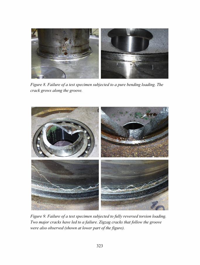
323
Figure 8. Failure of a test specimen subjected to a pure bending loading. The crack grows along the groove.
Figure 9. Failure of a test specimen subjected to fully reversed torsion loading. Two major cracks have led to a failure. Zigzag cracks that follow the groove were also observed (shown at lower part of the figure).
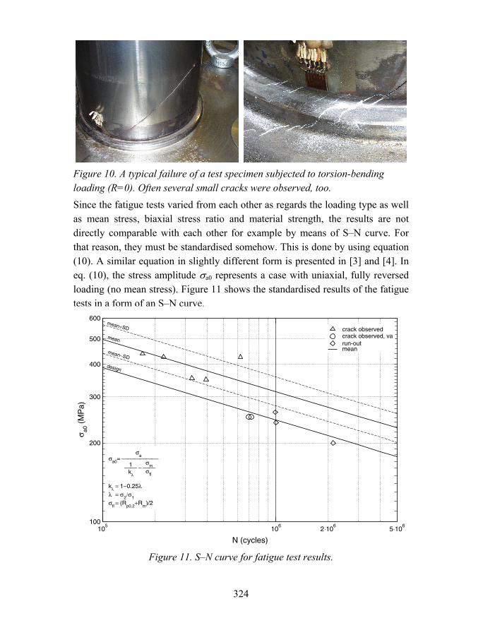
324
Figure 10. A typical failure of a test specimen subjected to torsion-bending loading (R=0). Often several small cracks were observed, too. Since the fatigue tests varied from each other as regards the loading type as well as mean stress, biaxial stress ratio and material strength, the results are not directly comparable with each other for example by means of SN curve. For that reason, they must be standardised somehow. This is done by using equation (10). A similar equation in slightly different form is presented in [3] and [4]. In eq. (10), the stress amplitude σa0 represents a case with uniaxial, fully reversed loading (no mean stress). Figure 11 shows the standardised results of the fatigue tests in a form of an SN curve.
N (cycles)
100
200
300
400
500
600
σ a0 (
MP
a)
105
106
2⋅106
5⋅106
crack observedcrack observed, varun-outmean
mean+SD
mean−SD
σa0= ⎯⎯⎯⎯⎯⎯σa
⎯⎯ − ⎯⎯1kλ
σmσfl
kλ = 1−0.25λλ = σ2/σ1σfl = (Rp0.2+Rm)/2
design
mean
Figure 11. SN curve for fatigue test results.

325
( )
aa0
m
λ fl
λ
2 1
fl p0.2 m
, where1
1 0.25/
12
k
k
R R
σσσσ
λλ σ σ
σ
=−
= −=
= +
(10)
The solid line without any markings represent the mean fatigue capacity m a0
bC Nσ= of the results. The mean fatigue capacity being a geometric mean of the fatigue capacities of each test result is calculated from eq. (11). Only results leading to a failure are included. The slope of the curve used here is b = 5. The line marked as design is calculated from the mean by subtracting two standard deviations (mean 2⋅sd). The standard deviation in log(C) is obtained from eq. (12). The calculated values for mean fatigue capacity and standard deviation are Cm = 3.089⋅1018 and sd = 0.27, respectively.
m
1
0
nn i
i
bi i a i
C C
C N σ
=
=
=
∏ (11)
( )2
m1
log( ) log( )
1
n
ii
C Csd
n=
−=
−
∑ (12)
The modified Haigh diagram in Figure 12 presents the same matter than Figure 11, but seen from different direction. This kind of presentation can be found from references [3, 4], too. The line drawn in figure cuts the ordinate axis at a point defined from the mean curve in Figure 11 at one million cycle endurance and average σfl. This diagram shows also the fact, that the cases with occasional over- underload cycles were worse compared with the others.
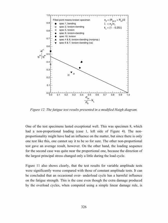
326
0.0 0.1 0.2 0.3 0.4 0.5 0.6 0.7 0.8 0.9 1.0σm⎯⎯σfl
kλ
0.0
0.1
0.2
0.3
0.4
0.5
0.6
0.7
0.8
0.9
1.0
σ a⎯
⎯σ fl
kλ
spec 1, bendingspec 2, torsion+bendingspec 5, torsionspec 9, torsion+bendingspec 10, torsionspec 4 & 8, torsion+bending (nonprop.)spec 6 & 7, torsion+bending (va)
σfl = (Rp0.2 + Rm)/2
λ = σ2/σ1
kλ = (1 − 0.25λ)
Filled point means broken specimen
Figure 12. The fatigue test results presented in a modified Haigh diagram.
One of the test specimens lasted exceptional well. This was specimen 8, which had a non-proportional loading (case 1, left side of Figure 4). The non-proportionality might have had an influence on the matter, but since there is only one test like this, one cannot say it to be so for sure. The other non-proportional test gave an average result, however. On the other hand, the loading sequence for the second case was quite near the proportional one, because the direction of the largest principal stress changed only a little during the load cycle.
Figure 11 also shows clearly, that the test results for variable amplitude tests were significantly worse compared with those of constant amplitude tests. It can be concluded that an occasional over- underload cycle has a harmful influence on the fatigue strength. This is the case even though the extra damage produced by the overload cycles, when computed using a simple linear damage rule, is

327
negligible. The larger over- underload cycle has no significant influence on the computed equivalent stress amplitude.
6. Conclusions
The FE-model calculated using axisymmetric elements gave good agreement with the static test results.
The occurrence of small cracks could be observed relatively early in the fatigue tests based on output of the strain gauge located near the expected site of crack initiation. By using the occurrence of the crack as a criterion for the failure, the fatigue strength of alternate axle constructions could be compared to each other. However, even after crack initiation was observed, the structure still had significant residual life.
Usually several small cracks nucleated at the bottom of the groove in a direction normal to the largest principal stress (when R = 0). With torsion case (R = 1), also zigzag cracks along the bottom of the groove were observed.
The test results for different loading cases could be reduced to a single design line using eq. (10) to standardise the principal stress amplitude. This takes into account different mean stresses, principal stress ratios and materials in each test.
The test results show clearly, that an occasional over- underload cycle is harmful and reduces the fatigue strength significantly. This is the case even though the extra damage produced by the overload cycles, when computed using a simple linear damage rule, is negligible. The larger over- underload cycle has no significant influence on the computed equivalent stress amplitude.
Acknowledgements
This work was partially supported through a grant from the Finnish Academy and the project Fadel/Gjutdesign, which is funded by the Nordic Industrial Fund, Wärtsilä Technology, Metso Corp. Componenta Corp. and VTT Industrial systems. All involved persons will also be gratefully acknowledged.

328
References
1. MSC.Marc. Volume A: Theory and User Information, Version 2001. Revision April 2001. MSC.Software Corporation 2001.
2. ABAQUS Theory Manual, Version 6.4. ABAQUS inc. 2003.
3. Marquis, G. B. and Karjalainen-Roikonen, P. Long-life multiaxial fatigue of nodular graphite cast iron. In: Carpinteri, A., Freitas, M. and Spagnoli, A. (eds.). Biaxial/Multiaxial Fatigue and Fracture. ESIS Publication 31. Elsevier Science Ltd 2003. P. 105122.
4. Marquis, G and Solin, J. Long-life fatigue design of GRP 500 nodular cast iron components. Espoo 2000. Technical Research Centre of Finland, VTT Tiedotteita Meddelanden Research Notes 2043. 70 p.

Complex loading
Multiaxial fatigue tests of a component in nodular cast iron ........... 331 Tormod Dahle, Tommy Thors & Magnus Hellberg
Fracture mechanics evaluation of a nodular cast iron component by 3D modelling .............................................................................. 351
Anders Björkblad
Multiaxial fatigue analysis in ABAQUS environment ....................... 375 B. Roger Rabb

331
Multi-axial fatigue tests of a component in nodular iron
Tormod Dahle Aros Mechanics, Västerås, Sweden
E-mail: [email protected]
Tommy Thors ABB Automation Technologies AB
Robotics, S-721 68 Västerås, Sweden E-mail: [email protected]
Magnus Hellberg
ABB Automation Technologies AB Robotics, S-721 68 Västerås, Sweden E-mail: [email protected]
Abstract
Multi-axial fatigue tests of a (fictitious) robot constructional component made in nodular iron have been performed in order to test the adjusted normal stress hy-pothesis suggested in the literature as a design stress criterion.
The test results show the relevance of the normal stress hypothesis for nodular iron subjected to multi-axial stress conditions as one expects in robot applica-tions. It is further concluded that application of the von Mises stress is conserva-tive and to a greater extent the larger the ratio between torsion and bending.
An engineering crack propagation model is used to successfully simulate the fa-tigue strength of the component used in this investigation.

332
1. Introduction.
The object of this work was to test alternatives to the von Mises stress criterion in design of robots made of nodular iron. Besides, there is a strong wish to use local criteria, which are better suited in companion with finite element analyses (FEA) and which have been applied conventionally in every days design of mechanical components. Local stresses are a natural goal for the future to study. However, using FEA and nominal material criteria of today leads almost inevitably to too conservative design.
The von Mises stress is a scalar and used as design criterion against plastic de-formation in multi-axial (quasi-static) stress states. By convention and conven-ience, this criterion has also been applied in dynamically loaded details where loads change both magnitude and direction. Therefore, criteria, which are more physically conformed, are sought. In this particular case, the combination of ten-sion or bending with torsion, the modified normal stress hypothesis suggested by Grubisic & Sonsino [1] is tested.
This study is one part of a project to introduce new criteria in the design of vari-ous details of robots made of nodular iron, but also to reduce weight and further to lighter metallic materials along with development of loading models without jeopardizing the safe and economic design in the near future.
2. Theory
In components subjected to fatigue loading a crack nearly always initiates at the surface and propagates until fracture occurs. Therefore, we can approximately in-troduce the stress condition in two dimensions in instead of three (i.e. plane stress) through the stress tensor as follows
[ ] ( )⎥⎦⎤
⎢⎣
⎡=
tttt
tyxy
xyx
σττσ
σ)(
)()()( (1)
where each stress is a (cyclic) time variable. Each stress component can be writ-ten as

333
)sin()(
)sin()()sin()(
xyxyaxymxy
yyaymy
xaxmx
tt
tttt
δωτττ
δωσσσωσσσ
−⋅+=
−⋅+=⋅+=
(2)
where σxm .are time constant variables and/or stresses, σxa . are amplitudes and δy are phase shifts in radians or degrees. Often the stresses σy(t) and σx(t) are synchronous variables and can be written
)()( tAt xy σσ ⋅=
The normal stress hypothesis (modified with a mean stress anticipation) has been suggested as relevant for brittle or semi-ductile materials [2]. One can regard a point on the surface where the stresses according to equation (2) are acting through which a plane with angle ϕ exists. On this plane is acting a normal stress σn(ϕ) and a shear stress τn(ϕ). Thus, the normal stress can be written as
)2sin()()2cos(2
)()(2
)()())(( ϕτϕ
σσσσϕσ ⋅+⋅
−+
+= t
ttttt xy
yxyxn (3)
For every angle ϕ one can find as a result of the time variation a maximum value and a minimum value of that normal stress. From these extreme values one can find for every plane with angle ϕ a mean stress and a stress amplitude:
2/)()( min,max,, nnmn σσϕσ += (4)
2/)()( min,max,, nnan σσϕσ −±= (5)
For every plane the following expression for the dynamic stress is valid as:
)()()( ,, ϕσϕσϕσ anmnn ±= (6)
The critical combination of mean stress and amplitude stress can be determined by using the materials Haigh diagram. This procedure is easy to program which is indicated in [1].

334
3. Experimental
3.1 Test material and test method
The material was nodular iron SS-EN GJS 500-7 with chemical composition as in Table 1. The hardness was measured to 205 HV10 on a polished cross section and the typical structure is shown in Figure 1.
Figure 1. Structure in the surface region of the nodular iron used.
Table 1. Chemical composition of tested SS-EN GJS 500-7 (wt-%)
C Si Mn P S Cr Ni Cu 3.54 1.9 0.25 0.019 0.007 0.03 0.04 0.21
50 test components (see Figure 2) were manufactured industrially through sand casting. After casting the test pieces were cleaned by shot blasting with steel thread pieces, 1.8 mm in diameter, length 1.4-2.0 mm with Vickers hardness 400-515 HV, blasting time 5 minutes which is the suppliers conventional procedure. The surfaces on the main part of the test pieces were kept intact (i.e. as cast sur-face) after surface painting, apart from the outer and inner surfaces to the right (as seen on Figure 2), which were turned to obtain a tight grip to avoid backlash dur-ing the testing. A few components were stress relieved at 600oC for 2 hours fol-lowed by furnace cooling.

335
Figure 2. Test object with crack after torsion test. The total length of the object is 170 mm.
A longitudinal cross section of the above test component is shown in Figure 3.
Figure 3. Longitudinal cross section through the test object with gripping arrangement at the loading position in the test fixture.
Torsion
Bending
Critical section
Tapered fastener
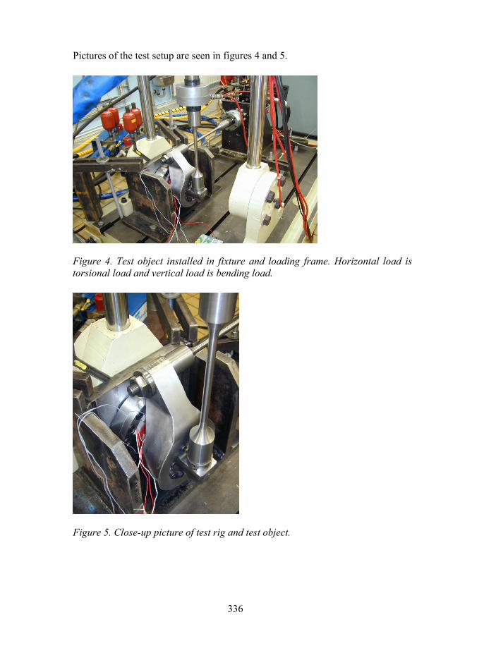
336
Pictures of the test setup are seen in figures 4 and 5.
Figure 4. Test object installed in fixture and loading frame. Horizontal load is torsional load and vertical load is bending load.
Figure 5. Close-up picture of test rig and test object.

337
The test rig was tightened with tapered fasteners on the loading table on the floor (see Figure 4). Both loading arms, bending and torsion, were coupled to the testing machines respective actuator to a moment free and slender transmission arm with torsional stiff bolted joints (see Figures 4 and 5). The testing machine was built with separate cylinders (actuators) and an electro-hydraulic computer controlled testing system. The computer system contained a computer program to control the two from each other independent channels with PID-regulators for amplitude control. In this fashion at a testing frequency of 510 Hz the ampli-tudes were held within 1%. The controller had also the ability to control the phase between bending and torsion at any desired level.
The testing was performed in load control. The time to failure was measured as the number of cycles to a certain percentage increase of the controller s error signal. This percentage was determined to be 8%, which resulted in, by naked eye, a clear detection of cracks of several mm in length. This uncertainty was es-timated as marginal, in any case not more than approximately 25% of the regis-tered fatigue life.
3.2 Calibration of test fixture and test object
An FE model was made of the test object fit into the load frame. After this analy-sis the frame had to be stiffened so that difference between the model and analyti-cal calculations and strain measurements could be minimized. However, it was stated that the FE model gave 10% higher stresses at the bottom (i.e. 6 oclock) of the test object due to unsymmetrical stiffness of the frame. This was accepted. Figure 6 shows a cross section of the part in the case of pure bending.

338
Figure 6. Maximum principal stress around the critical section in the case of pure bending.
4. Results
4.1 General
From the FEA the stress concentration factor in bending was determined to 2.63 and in torsion 1.26. For most of the bending tests the fatigue cracks appeared as expected according to the FEA, i.e. at the 6 oclock position as stated while for most of the torsion tests at the 3 oclock position. The following test series are re-ported here, see Table 2.

339
Table 2. Tests made in this investigation.
Type of testing Test Test condition Bending only B1 As delivered, R=-1. 10 pieces. B2 Stress relieved, R=-1. 3 pieces. B3 As delivered, R=-1. B3a. Turned outside and
B3b. Turned outside and inside. 5 pieces. B4 As delivered, R=-1. Drilled holes 0.5 mm and
1.0 mm in diameter. 3 pieces. Torsion only T1 As delivered, R=-1. 5 pieces. T2 Stress relieved, R=-1. 3 pieces. Bending and torsion com-bined in-phase
C1 As delivered, R=-1. Torsion/Bending=0.47-0.71. 6 pieces.
C2 Stress relieved, R=-1. Torsion/Bending=0.48. 2 pieces.
C3 Stress relieved, Smean=55.8 MPa. Tor-sion/Bending=1.01. 1 piece.
4.2 Assessment of pure bending and torsion results
Since FEA was used here in the pre-analyses and also used in design situations all results below will be shown as function of the local stress calculated elastically (in contrast to nominal stress commonly used) with a calibrated finite element model using 20 node, quadratic elements. This model was calibrated to be correct within 5% of the strain measurements during the pre-analyses. The local elastic stresses calculated are in reality expected to be relaxed due to local plastic yield-ing.

340
Figure 7. Results from pure bending and torsion tests, tests performed on as re-ceived, stress relieved (SR), machined components and one component with a 1 mm diameter drilled hole.
As a reference to the experimental data a number of estimated material properties are indicated in Figure 7. These are the following: estimated (nominal) fatigue limit of bending fatigue of a smooth bar (test bar bending) [5], estimated fatigue limit of tension-compression on a smooth bar (test bar tension/comp, after test-ing at ABB) and torsion fatigue limit estimated from the Marquis et al. [3] inves-tigation (torsion expected). The approximate fatigue limit is here defined as the fatigue strength at 106 cycles.
It is obvious that stress relieving has approximately the same effect as machining, i.e. turning (Ra ≈ 24) in this case, which means that surface material is removed

341
even though stress relieved material has a thin, hard skin (230250 HV relative to 205 HV in the core). Anyhow, the effect of the cleaning by shot blasting can be roughly estimated by comparing the as cast material and machined/stress-relieved material, which for this particular component is about 50% for bending as indicated in Figure 7. It implies that shot blasting introduces beneficial residual stresses in compression corresponding to a stress level of about 125 MPa.
The fatigue limit of the virgin stress relieved material (332 MPa, nominally 332/2.63=126.2) lies approximately 3035% above the bending fatigue limit on smooth specimens of 260 MPa as depicted in Figure 7. This size effect may be an ef-fect of the stress gradient and (stressed) volume, which appears both for bending and torsion. Firstly, the amount 3035% should be reduced (say 5%) due to the fact that the fatigue limit is estimated at 106 cycles rather than at 107 cycles. Additionally, the effect of the raw cast surface would have reduced the smooth bending fatigue limit a certain amount. According to [6] the surface factor (=kgradient,bending) for nodular iron due to the roughness is 0.86 for bending according to the following formula
)400
6.1(log)4(log128.00.1
)400
2(log)4(log16.00.1
1010,
1010,
matorsionr
mabendingr
RRk
RRk
⋅⋅⋅−=
⋅⋅⋅⋅−= (7)
when using Rm=550 MPa and Ra=25 (by surface measurements). This means, using 35%, that the total effect of the stress gradient can be estimated to (1.350.05)*1/0.86 = 1.51 to be compared with the fatigue notch factor, Kf = 1.81 (=260*0.86/(332/2.63)).
The fatigue limit in torsion for an un-notched component has been estimated to 170 MPa [3]. The stress relieved (notched) components tested here in torsion the fatigue limit is determined to 218 MPa (nominally 218/1.26=173). The estimated effect of the gradient/volume is also 1.3 as for bending. Further, for torsion the effect of shot blast-ing has been determined to a benefit of 20%.
4.3 Results from bending and torsion in combination
Figure 8 shows the results from the in-phase bending and torsion in combination. The experimental results are illustrated as maximum principal stress as function of number of cycles. In this case, using the maximum principal stress (for the ease of calculation) corresponds to the modified normal stress without any phase-shift or mean stress. It is stated that the data follow the trend line from the pure

342
uni-axial bending. Thus, the principal stress (or normal stress) seems justified for multi-axial stress states. Some few data from stress-relieved components are also shown.
Figure 8. Results from the bending and torsion tests in combination. Tests are run in-phase. Stresses are local stress elastically calculated.
The data are also assessed using the von Mises stress, which yields an overesti-mation of around 5%. There seems, however, a tendency that this overestima-tion increases with the Torsion/Bending (T/B)-ratio, which varies between 0.270.44 for the as cast components to 0.280.65 for the stress relieved com-ponents as illustrated in Figure 8. The triangular points in this diagram are simu-lated using the normal stress hypothesis algorithm, see section 2, so that the al-

343
gorithm can be used to predict the gain in using the normal stress or the princi-pal stress over the von Mises stress.
Figure 9. Overestimation using von Mises stress as function of T/B-ratio.
4.4 Fractographic investigation
Some of the test components fractured surfaces were investigated using SEM to study details about the position and form of the defects. It may be interesting to compare these real defects with artificially introduced defects and discuss how they relate to the initiation and propagation of the fatigue cracks.

344
Figure 10. Test component 4. N=18722 cycles. Red arrow indicates bending direction. Crack site 6 oclock. Pure bending, S=520 MPa.
Figure 11. Test component 4. Defect size: D1420/L970 µm.
The defect shown in Figures 1011 has a great influence on the fatigue life. With N=18722 cycles it is the shortest life ranging from 18722 to 200000 cycles on the (local elastic) stress level of 520 MPa and with a defect size of depth=1.42 mm and length/width=0.97 mm.

345
Figure 12. Test component with drilled hole (at the arrow, hole diameter Ø 1 mm). Pure bending. Local stress level 459 MPa. N=555 980 cycles.
Figure 13. As above. Size: depth= 1100 /Width = 900 µm.
In Figures 1213 photos from the component with a drilled hole with nominally 1 mm drill. As seen in Figure 12 the drilled hole is the origin of the fracture. The fatigue life of the drilled component has been depicted in Figure 7. The question is if it is possible to use crack propagation and fracture mechanics to predict the fatigue life using engineering models since cracks are long cracks and stresses

346
are pure bending and to illustrate and explain the results attained. An engineering model (valid only for stress relieved material) is used below to illustrate the use of such a model.
5. Crack propagation model
5.1 Model
In Figure 14 the conventional crack propagation properties of the nodular iron are shown (tested earlier at ABB). Figure 15 shows the same data transformed into an effective stress intensity factor. The model used is showed in the fol-lowing.
Figure 14. Crack propagation data of nodular iron SS 0727 tested at R=0.1, 0.5 and R=-1 (ABB 1995).
The effective stress intensity factor is transformed from applied to effective by collapsing the above data by using the following approximation:
appliedappliedeff KRH
KUK ∆−
=∆⋅=∆1
; -1 ≥ R ≤ 0.1 (8)

347
The result of this is shown in Figure 15. Here H is a material constant and R is stress ratio.
Figure 15. Data collapsed to effective stress intensity factor. Curve 2 is ex-plained in the text below.
The above relation is only used for bending loads where R-values are between 1 and 0.1 and only for constant amplitude loading, which corresponds to curve 2 in Figure 15. In this mode the da/dN-curve is represented by one bilinear curve with adjustment for the R-ratio by equation (8). The stress intensity factor is cal-culated by the function (taking account of a two-dimensional behavior, p(a/c), see later in the text) as
)/( capgYaSK nomapplied ⋅⋅⋅⋅⋅∆=∆ π (9)
Here Y is the geometrical function for an un-notched cylinder with an external radial through the thickness crack given by Mettu et al. [4] and g is a factor tak-ing into account that the crack lies in a stress concentration stress field in bend-ing and called gradient factor. The gradient factor has been determined earlier at ABB by an approximate weight-function method verified by FEM computa-tions. Figure 15 shows the stress gradient through the critical section (without the crack).

348
Figure 16. The bending and torsion gradients (normalized).
The fatigue life of a robot component is simulated with the above method by in-tegrating between the initial crack 0.5 mm respectively 1.0 mm to through the wall crack by using the (bilinear) Paris equation
meffKC
dNda
∆⋅= (10)
and by using the above indicated material properties and the stress intensity fac-tors. The results of such calculations are depicted in Figure 17.

349
Figure 17. Simulated crack propagation fatigue life compared with experiments for stress relieved components subjected to constant amplitude bending, R=-1, in nodular iron SS 0727.
When performing crack propagation calculation in hollow cylinders (=pipes, axles) it is important to take into account the change in the depth-length (a/c-) ratio of the crack itself due to the in-plane differences in the stress intensity fac-tor. In an engineering sense an effective method is to use a mapping technique in which the a/c-ratio is mapped with the appearance of a known fatigue crack of the same geometry. The mapping data (i.e. the function p(a/c), equation (9) is a table of crack depth to width ratio with crack depth. The results are relatively insensitive to changes in this function. The same kind of analysis is not per-formed for the shot blasted material. This is due to lack of modeling by taking care of mean stresses in compression and is, therefore, left for the future.
6. Conclusions
It has been shown in this investigation that a normal cleaning operation applied after casting operation in nodular iron introduces considerable residual stresses in compression which are beneficial to the fatigue strength of the component. This beneficial effect is normally not taken into account in design.

350
The properties of the tested component can be explained in the light of the me-chanical properties of the base material.
It has also been stated that the combination of bending and torsion in nodular iron can be rationalized by the normal stress hypothesis instead of the von Mises stress. The von Mises stress is conventionally used by the industry in de-sign which inevitably leads to un-economical usage of the material.
Further and finally, it is shown by using an engineering crack propagation model that it is possible to simulate the fatigue strength of a typical defect-governed material like nodular iron. This has also been verified experimentally in this investigation.
References
1 Grubisic, V. and Neugebauer, J. Festigkeitsverhalten von Gusseisen mit Kugelgraphit unter mehrachsiger Schwingbeanspruchung, Giesserifor-schung, 1979, 31 (4), pp. 123128.
2 Sonsino, C. M. and Grubisic, V., Mechanik von Schwingbruchen an ge-gossenen und gesinterten Konstruktionswerkstoffen unter mehrachsiger Beanspruchung, Konstruktion, (1985), 37, H7, pp. 261269.
3 Marquis, G. and Karjalainen-Roikonen, P., Long-life multiaxial fatigue of SG cast iron, VTT Manufacturing Technology, P.O. Box 1705, FIN-02044 VTT, Finland.
4 Mettu, S. R., Raju, I. S. and Forman, G., Stress intensity factors for part-through surface cracks in hollow cylinders, JSC 25685 (LESC 300236), NASA job order 85-130, 1992.
5 Hück, M., Schück, W. and Walter, H. Moderne Schwingfestigkeits- unterlagen für die Bemessung von Bauteilen aus Sphäroguss und Temperguss Teil 1, ATZ 86, 1984, 7/8, pp. 325331.
6 Hänel, B. and Wegerth, G. Festigkeitsnachweis. Vorhaben 154. Rechne-rischer Festigkeitsnachweis für Maschinenbauteile. Institut für Machi-nelle Anlagentechnik und Betriebsfestigkeit, T. Univ. Claustahl, Institut für Stahlbau und Werkstoffmechanik, T. Univ. Darmstadt, 1993.

351
Fracture mechanics evaluation of a nodular cast iron component by 3d modelling
Anders Björkblad Department of Aeronautical and Vehicle Engineering, KTH
Teknikringen 8, 100 44 STOCKHOLM [email protected]
Abstract
The object of this paper was fracture mechanic modelling of solids using finite element (FEM). The main tool that has been utilized was the software Mcrack which is a group of macros intended for use jointly with ANSYS finite element program. One major advantage of the Mcrack software is that it supports solid modelling with a crack located at an arbitrary location. This implies that it is possible to calculate also torsion and mixed mode cases within a most reasonable work effort. However, Mcrack was developed to cover complex weld geometries. Utilizing Mcrack for general solid modelling requires an analysis of the possibility of development for arbitrary crack paths. As test object a cast sleeve made of nodular iron has been used. Previous to this investigation the component was submitted to a test program and a subsequent evaluation according to S/N criterias at ABB, Sweden. This paper is thus a continuation of the ABB work, and at the same time an extension of the field of application for the Mcrack software. For validation purposes the software AF-Grow as well as elementary cases has been used in parallel. The investigation is a part of the nordic project Cast Design 2005.
352
1. Introduction
Linear fracture mechanics (LEFM) is a most powerful tool for analysis of many fatigue processes. As the applicability range is from crack initiation to failure the initiation period is not covered. However, due to the problem at issue it can be a considerable amount of the life time left for the crack propagation phase. For practical use, nowadays it is more or less compulsory to utilize finite element method (FEM) for structural analysis. Yet, the application of LEFM within FEM is a very demanding task. In fact, it is probably one of the main reasons why LEFM is not utilized in a larger extent. This is a pity considering that the LEFM is capable of analysing intricate geometries and complex load cases. The present paper proposes a method for solid modelling of LEFM. It is based on a group of macros that onwards will be called Mcrack, Martinsson, J, [1], and which are supposed to be used in conjunction with ANSYS [2]. Mcrack was originally developed for weld analysis and is well suited to exact follow a weld geometry. When considering an arbitrary solid body this is not possible, but one will have to accept a certain degree of misalignment between global model and sub model. The theme in this paper was thus to show that it is possible to apply Mcrack to arbitrary solid models despite the modelling issue. In order to cover the matter of validation, the software AF-Grow [3] as well as elementary cases and ordinary solid modelling where used in parallel. It should also be known that the applicability was intended to serve practical industrial purposes.
The component that was used for the application of Mcrack was a nodular iron cast sleeve. The nodular iron is a material that is widely used in load carrying components as axles housings, transmission housings, hubs, linkage, brackets and attachments in both trucks and heavy construction equipment. It is also used in the main structure in robotics and in hubs in wind mills. The material has a number of attractive properties that makes it convenient for instance in the automotive industry. Both the strength and the toughness can be varied in wide ranges depending on current demands. This makes the material suitable for all the same applications as grey iron but also for application that requires resistance against shock- and fatigue loadings. It is also relatively easy to found and machine, important matters with respect to productivity. As being used for moving structural parts, it will be exposed for fatigue. The issue of fatigue strength for cast materials is mainly governed by the presence of cast defects, Nadot et al.[4], Björkblad, A.[5], Mörtsell et al.[6]. Cast materials always contain

353
(relatively) large amounts of contaminations. The size of the defects emanating from those impurities comprises the whole range from micrometer up to several millimetres. On top of this there are also the more pronounced defects emanating from the cast process. Those are most often different kinds of porosity, e.g. shrinkage pours. The common property for all of the impurities and defects are that they generally form an irregular, sharp interior geometry that will give rise to stress concentrations. The stress concentrations in its turn facilitates crack establishment and this mechanism is often so severe that the fatigue crack initiation phase can be more or less disregarded, thus leaving the fatigue life for the crack propagating phase. Commonly (for a continuum like material) the initiation phase constitutes a main part of the fatigue life, so by omitting it one will miss a substantial part of the service life for a component. Under such conditions, it became extra important to manage fracture mechanic calculations in order to perform reliable forecasts.
The preliminary work which preceded this investigation was performed by ABB in Västerås, Sweden. ABB have also designed the component and made all the testing, see ABB report[7]. Originally the intention was to investigate mixed mode behaviour of the GJS500-7[8] material under alternating load (R=-1), and the evaluation was planned to be made by a classic fatigue approach, i.e. S/N-curves.
One of the main themes of this work was to make a fracture mechanic evaluation of the component life by aid of the FEM. The other main theme was the application of the fracture mechanic macro collection Mcrack which was developed at the department of aeronautical and vehicle engineering, KTH. This line of action will not only produce a solution for this specific component, but also point out a user friendly way of utilizing FEM for fracture problems. It is a well-known fact that the fracture mechanics in FEM is not a very simple manoeuvrable technique, yet it constitutes a powerful tool. The Mcrack software offers, along with other aids as AF-Grow, a great extent of simplifying in the analyse work. In order to verify the correctness of the Mcrack calculation capability comparisons where made between the calculated results and elementary cases.

354
2. Component
The component was a cast iron sleeve designed solely for fatigue testing. The dimensions are given in Figure 1 and the appearance of the component is given in Figure 5. Total material thickness at the critical area was 6 mm. The material was GJS 500-7 (european standard SS-EN 1563) [8], a medium strength nodular iron. The chemical composition of the material is given in Table 1. Mechanical properties are given in Table 2.
Figure 1. The nodular cast iron component.
The components where all around shot blasted with cut steel wires and most of them were tested in that condition. In order to determine the influence of the residual stresses that origin from the shot blasting a minor number of sleeves where annealed or machined (just at the very surface) before testing.
Measurement of the residual stress field were performed by x-ray diffraction technique, see Figure 8 for stress profile.
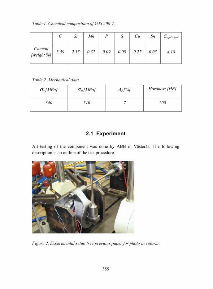
355
Table 1. Chemical composition of GJS 500-7.
C Si Mn P S Cu Sn Cequivalent
Content [weight %]
3.59 2.35 0.37 0.09 0.08 0.27 0.05 4.18
Table 2. Mechanical data.
σy [MPa] σB [MPa] A5 [%] Hardness [HB]
340 510 7 200
2.1 Experiment
All testing of the component was done by ABB in Västerås. The following description is an outline of the test procedure.
Figure 2. Experimental setup (see previous paper for photo in colors).

356
The component was mounted with the flange attached against an angle shelf. The shelf in its turn was bolted to the test machine base. In order to apply torque there was an arm attached at the outer diameter at the cylindrical outer end of the sleeve. This arm was designed so it would not give any bending moment with respect to the most highly stressed areas at the sleeve, i.e. only torque and shear force where applied at the critical location. A bending arm was inserted inside the inner diameter of the outer end in order to apply bending moment. The torsion and the moment arms where connected to the sleeve by a friction attachment. Two servo hydraulic cylinders where then connected to respectively torque arm and bending arm by push-pull rods. The complete appearance of the test set up is shown in Figure 2.
Figure 3. Front view and side view of FEM model including support. Load introduction for torsion respectively bending.
The testing was accomplished by stress ratio R= -1 for both bending and torsion. Also mixed mode tests were conducted, then with phase relations between bending and torsion of 0 and 90 degrees respectively. Load frequency during the tests was 5 Hz.
2.2 Experimental results
The original evaluation was made at ABB in connection with the tests. A classical fatigue approach with S/N-curves was planned. It was expected that the measured life should be in accordance with results extruded from testing of

357
smooth, straight cast specimens. The test results showed something quite different. Although the local stress was over the yield limit at the stress concentration, the measured life was longer than expected from the S/N approach, see report from ABB [7].
Figure 4. S/N-curves from tests for bending and torsion (ABB).
It turned out that the stress gradient seriously affects the crack initiation and the crack growth. In Figure 4 it can be seen the outcome from the tests. Extracted data from Figure 4 shows that the difference between expected fatigue level and true fatigue level in bending is about 80 MPa or ~33% at 1e6 cycles, which corresponds to a factor of about three for the total life. It can also be seen that the shot blasting affects the fatigue limit about 30% at the same number of cycles. In Figure 6 the typical bending respectively torsion crack faces is shown.

358
Figure 5. Critical location at the component.
Both the bending and the torsion case exhibit evident multi crack initiation with ridges and x-crack formations respectively. Using the stress ratio R= -1 the load will also act in two directions, and consequently there will form line cracks at both upper and lower side for the bending case and multiple x-formed cracks for the torsion case.
Figure 6. Typical crack faces from bending (left) and torsion (right).
It can however be questioned how to evaluate the outlook from the testing since the maximal stress was to be considered more or less as overload. In all cases the bending will behave different from the usual defect initiated semi elliptical crack development, meanwhile the torsion shows a normal appearance despite the high load level.

359
3. Simulation
The analyses in this investigation are based on LEFM for determination of stress intensities and Paris law, Eq. 1, for life calculations.
( )mKCdNda
∆∗= (1)
maxKK =∆ ; K<0 (2)
2
1*5.2),,,( ⎟⎟⎠
⎞⎜⎜⎝
⎛>
y
Ktwcaσ
(3)
5=m 115.2 −= eC [mm/cycle] [9]
The Paris parameters m=5 and C=2.5e-11 (valid for R=0) was chosen as medium range values representing a broad variety of cast components from various foundries. The variation range of published data is relatively large and, just to cite one source, m-values of 4.08-5.65 and C-values between 9.6e-12 and 4e-10 [mm/cycle] are reported for R=0 [10]. This is presumably a major part of the explanation to the discrepancies between individual test components, and underlines the importance of using valid material parameters.
The present form of Paris law uses nominal K-range and assumes the crack closure to be included in parameter c. Further, in consistence with the unity of parameter c, ∆K=Kmax was used according to Eq. 2. Because of the non-symmetric boundaries there was a slight difference in between the upwards- and the downwards bending solution. For stress ratio R= -1 the test object will experience both those stress levels, and it was presumed that the higher level (S1max) was constituting upper bound and therefore used for calculations.
For the rest the regular conditions for LEFM where presumed, i.e. small scale yielding according to ASTM [11] directions, see Eq. 3, which is considered as a general limit for LEFM validity. The value 2.5 is however in practice not a sharp limit, Ljustell, P.[12], has shown that the LEFM can remain applicable for loads

360
as high as 15 times the criterion limit for certain materials. The implication is that LEFM is likely to be valid also for the highest loads in the present investigation as the fracture toughness anyway is quite low for nodular iron.
The presumed crack front evolution was perpendicular to the first principal stress, S1, due to the maximum principal stress criterion [13]. The cracks were thus modeled consequently which means that there where neither mode II nor mode III crack growth for any of the cracks. The initiation position directly in an angle corresponding to first principal stress is most plausible in cast materials since there are small internal defects everywhere and in any direction. The shear stress for the two cases where also small in comparison to the stresses from the bending and torsion and therefore neglected. The approach was confirmed by numerical results since almost only mode I stress intensity factors (SIF) where present after locating the crack perpendicular to S1.
In the bending analysis the local stress at the stress concentration (radius) was between 1.2 and 1.68 times the yield limit for the material. In Fig. 7 the normalized stress gradient through the thickness can be seen. Stresses at such levels will quickly relax residual stresses for what reason they where neglected in analyses. This substantial overload will also seriously affect the behavior of the material so that the fatigue initiation mechanism will be switched away from being ruled by defects.

361
Figure 7. The stress profile for bending. Normalized maximum principal stress through the thickness at the critical location.
The strain will be in such level that the Coffin-Manson [14] relationship is valid, see Eq. 4, which will rule the initiation at the most highly stressed areas of the sleeve. First thereafter, with an established crack as deep and long as the overstrained material, the LEFM will determine the process.
( )Cffp N2
2'ε
ε=
∆ (4)
540648.0' =fε 675431.0−=c (5)
The material parameters for Coffin-Manson, Eq. 5, are retrieved from Samuelsson, J [15]. In Tab. 3 it can be seen the low number of cycles to crack initiation as a result of the high strain level. Mörtsell et al. [6] have showed that for nodular cast iron this severe strain state cause immediate crack initiation in the matrix around nodules and at micro pores even at the first load cycle. This

362
implies that the damage is made at a very early stage and the crack establishment will continue fast in the affected volume, circumstances that where confirmed by the current test results.
Table 3. Crack initiation phases due to Coffin-Manson for present load levels.
Stress level [MPa] 408 459 520 571
Number of cycles 26,000 14,200 8,000 5,400
The dept of the initiated crack is hard to predict as the behavior is unclear at the transition point between strain govern fatigue and the following crack propagation, but it is probable that the dept will be about the same size as the extent of the overstrained material. With respect to the present stress gradient it means an initiation crack dept between 0.5 and 1.1 mm depending on the load. It could be worth noting that normally the low-cycle regime is not applicable for mechanical design because of the resulting low service life. Herein it is utilized only by necessity for initiation at a stress concentration.
In the numerical model no concern has been taken to multiple initiations. At current load levels this is not relevant for the bending load seeing that a line crack will establish, but for lower load levels it would be much appropriate. It would certainly be much appropriate also for the torsion case, but unfortunately the available software is yet not suited for that kind of modeling. The result, however, should possibly be a lower stiffness with higher SIF as consequence. It is also an irrefutable fact that the 32 bit operative system can not really model multi crack initiation because of the file size created. The matter may be reissued at a future date.
3.1 Numerical model
The FE model of the component was modelled with solid 20-node brick elements. It was a full model and also the surrounding fixing shelf and load introduction devices where made by solid modelling. There where no contact elements in the model between the different parts since it was supposed that the
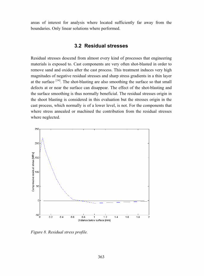
363
areas of interest for analysis where located sufficiently far away from the boundaries. Only linear solutions where performed.
3.2 Residual stresses
Residual stresses descend from almost every kind of processes that engineering materials is exposed to. Cast components are very often shot-blasted in order to remove sand and oxides after the cast process. This treatment induces very high magnitudes of negative residual stresses and sharp stress gradients in a thin layer at the surface [14]. The shot-blasting are also smoothing the surface so that small defects at or near the surface can disappear. The effect of the shot-blasting and the surface smoothing is thus normally beneficial. The residual stresses origin in the shoot blasting is considered in this evaluation but the stresses origin in the cast process, which normally is of a lower level, is not. For the components that where stress annealed or machined the contribution from the residual stresses where neglected.
Figure 8. Residual stress profile.

364
The characteristic appearance of the stress gradient curve is obtained from an investigation on cast steel [5]. Nadot and Denier [4] report the residual stress magnitude 300 MPa for the current material and state. This is a value for flat easily accessible surfaces, but as the critical area at the present component is a little difficult to access, the residual stress magnitude for this investigation is set to 75% of 300 or 225 MPa. This is also in order to make conservative estimations.
The residual stress profile was used as input load in AF-Grow. The output SIFs from AF-Grow, origin in the residual stress and valid for respectively crack size, was then subtracted from the SIF of the applied load. For the calculation of the residual K-distribution the weight functions available in AF-Grow were utilized.
Figure 9. Distribution of (specific) residual stress induced negative K-contribution through the thickness. The curve fit where used for the FEM simulations.
The strain state of the present test conditions give rise to a quick relaxation of residual stresses. The difference between included residual stresses or not is only a few thousand of cycles (plus or minus depending of load level). The residual stresses are therefore neglected in this evaluation.

365
3.3 Software tools
The finite element program used was ANSYS 8.1 [2]. As a supplementing tool Mcrack [1] was utilized. Mcrack is a collection of macros intended for use in conjunction with ANSYS. Mcrack enables immediate sub-modelling of complex fracture mechanic weld problems. In this paper it was showed that it might be utilized also for arbitrary solid modelling. For validation purpose and for handling small cracks (i.e. closely after initiation phase) the software AF-Grow was used.
The Mcrack macro collection is founded on a sub modelling technique. Schematically it replaces a part of the finite element structure with a sub model. All original elements located within the sub model will be deleted and the resulting boundary is joined with the sub model by constraint equations. Then the global problem is solved, thus involving the current crack size in the stiffness calculation. This line of action implies that the correct stiffness, including redistribution of stresses, is catch. After the displacement solution is available there will be another sub model consisting of singular quarter point crack elements laid out along the crack front. From this second sub model the K-solutions are then derived. When used for weld geometries Mcrack also include the option of automatically move the crack front forward. In such case both crack front deviation (because of mode II load) and individual crack increment is considered. By geometrical reasons it is not possible to utilize this option for solid modelling carrying semi elliptical cracks. In case of semi elliptical cracks one has to perform separate, discreet K-solutions.
3.4 Verification
Mcrack was developed especially for complex weld geometries. In that application the sub models that the program creates encompass the geometry of the weld. When using Mcrack for solid modelling it is not always possible to exactly follow the geometry of the global model. Instead, the beginning and/or the ending of the sub model is situated with some angle against the surface or slightly below/above the surface. This raises the question of the correctness of the K-solution and therefore a number of comparisons were made between an exact model of a specimen and specimens with different types of misaligned sub models.

366
In order to verify the correctness of the SIF calculations a number of comparisons where made between elementary cases [16], Mcrack [1], AF-Grow [3] and solid crack modelled solutions. The specimen model for this purpose was a centre semi elliptic surface crack specimen with dimensions 10 x 20 x 200 mm, see Figure 10. The dimension of the crack was a=3mm and c=3mm. The crack was located perpendicular except for one model where an angle (bias) of 10 degrees was applied. The load was set to 100 MPa and the SIF was evaluated at surface and at middle bottom of the crack. The alignment between global model and sub model, which in parallel with the overall SIF solution was the object of the convergence study, was supposed to range from -0.5 mm below up to +1.5 mm above the surface, see Figures 1114.
Figure 10. Centre semi elliptic crack specimen used for the verification study.
Also, one simulation was made with a sub model bias of 10 degrees from the perpendicular position. As seen in Figure 15, if one holds within ±0.25mm, there is a consensus within 515 percent between the SIF from the different models, a number that must be considered fairly good keeping in mind all other sources that may contribute to the discrepancy. Another thing to note is that the SIF solution is almost unaffected at centre of crack.

367
Figure 11. Exactly aligned with surface. Figure 12. Below surface.
Figure 13. Above surface. Figure 14. Non perpendicular to surface.
In Table 4 it can be seen that the Mcrack sub modelling technique, as well as homogeneous solid modelling, is in excellent agreement with analytical solutions. This implies that the type of fracture mechanics evaluation where the growth at crack centre is at issue, which perhaps is the most common for crack propagation, is practically unaffected of the sub model alignment. Disregarded the mode II and mode III SIF that appears, even the biased model shows the same accuracy. The conclusion is that the accuracy is most sufficient for practical use.

368
Table 4. Verification of SIF solutions for perfectly aligned sub model. Units in MPa(mm)1/2.
Figure 15. SIF solutions for varying misaligned sub models compared with exactly aligned sub model.
ANSYS/Mcrack
ANSYS pure solid modelling
AF-Grow Analytical [16 ]
K (at surface)
230 225.5 238 235
K (at middle bottom)
203 202.8 210 208

369
4. Results
4.1 Bending
The bending solution is somewhat cumbersome at present load levels. As the maximum principal stress clearly exceeds the yield stress for all loads the resulting fatigue damage will obey the CoffinManson relationship. This means an overload situation and a short initiation phase. In this specific case the stress level is caused by a stress concentration and therefore it is not as severe as it should be without the stress gradient through the thickness, but in general such circum stances is not applicable in engineering design. Yet, the approach is necessary for this analysis.
Figure 16. Predicted life for bending load corresponding to max S1=520MPa.
The consequence of the local overload is a line crack covering roughly a 45 degree arc at top and bottom of the critical stress location. The initial crack dept

370
is hard to predict exactly (see reasoning in section 3), but it should be between 0.5 and 1.1 for the load levels at issue. In Figure 16 it can be seen that the test results for an initial line crack are quite well arranged around a crack size of about 1 mm, which in fact is exactly the expected size for the current load level. Further it can be noted that the difference between the line crack and the semi elliptical approach is vanishing at a crack size of roughly 1.5 mm. This is a most natural effect as the stress concentration rapidly will force the semi elliptic crack to spread out along the surface and approach the line solution. It deserves once again to point out that the prediction for the elliptical solution is not valid at those stress levels. Assuming a significantly higher yield stress for the material, the predictions would be true also for the elliptical solution.
4.2 Torsion and mixed mode
The torsion case tests shows pronounced multiple crack initiation in line with knowledge of cast material behaviour, i.e. initiation at several defects as the stress was about uniform along the highly stressed area. In a cast material there exist is no preferred crack path, so for the present case it will immediate form a factory-roof appearance. In this work an initiative was taken to model the torsion crack propagation by a single crack, see Figure 17.
Figure 17. Single crack in torsion load, perpendicular to 1st principal stress.
As expected, the simulation result divagated from test results due to higher stiffness, see fig. 18. It is evident that it has to be defects of size 2.53.5 mm present to cause the predicted result, but there where no one larger than 0.30.4

371
mm found. It must further be kept in mind that also the applied torsion loads where at equal or over the yield stress level for the material, which implies that the initiation maybe was govern by another mechanism. However, the path indicated by the maximum principal stress criteria agree very well with test results, and this is valid also for the test components subjected to bi-axial load i.e. both bending and torsion, though one have to consider any sequence effects for mixed mode loading. The Mcrack software was unfortunately at this stage not suited for modelling torsion induced multiple cracks. This is partly because of computer memory limitations, but mainly because the crack surfaces have to be adjacent as they will experience contact during the load cycle. By the same reasons the mixed mode solutions is not treated. Still, the concept seems worth to develop, and the issue has been added to the list of future work. It should be noted that also for the torsion case the loads where very high.
Figure 18. Predicted life time for torsion load compared with test results.
372
5. Conclusions
In this paper a fracture mechanics evaluation of a nodular cast iron sleeve was made. During the course of action it has been showed that the software Mcrack, which was used as main tool for the crack modelling, is a powerful and versatile tool not only for crack modelling in welds, but also for solid modelling of cracks. The evaluation also points out the importance of thorough planning before accomplishing a test program. The expected S/N-evaluation of the present study became non relevant because of the oversight about stress levels above yield limit.
The most significant conclusions of the work (not classified):
• It is of greatest importance to take a local approach for evaluations. All calculations should be made as local analysis with local stresses, local R-values, local material behaviour etc, etc.
• The field of application for the Mcrack software has been extended. The relative error caused by non exact sub modelling was relatively small, within 5-10% for about 0.25 mm misalignment.
• The timesaving utilization of AF-Grow for implementing residual stresses was very successful. It contributes greatly to the improvement of prediction capability without consuming non proportional amounts of resources, yet it was not crucial for this particular evaluation.
• Fracture mechanics has once more showed to be well suited for analysing troublesome, complexly loaded components. The predictions made for semi elliptical cracks are not possible to verify through current test results, but the agreement with the line crack solution confirm its correctness.
• The maximum principal stress criterion has shown to be in good agreement to test results for cast components exposed to various multiaxial loads. Therefore the possibilities to model multiple initiations should be improved, e.g. the ability to model multiple cracks in torsion loaded cast components, would be much useful.

373
Acknowledgements
The author would like to thank Jack Samuelsson, Volvo CE, and Kenneth Hamberg, Chalmers Lindholmen, for being sources of inspiration and for supervision. Johan Martinsson for fruitful discussions and for support with Mcrack. Further, Tommy Thors and Magnus Hellberg, ABB, for underlying test results, tested components and general support. Gunnar Åkerström, Volvo Truck, for material investigations. Last, but not least, Nordic Industrial Found (NI), Vehicle Research Program (PFF) and Volvo for funding.
References
1. Martinsson, J. Fatigue Assessment of Complex Welded Steel Structures, Doctoral thesis. Department of Aeronautical and Vehicle Engineering, KTH, Sweden 2005. ISBN 91-2783-968-6.
2. ANSYS official web page, http://www.ansys.com/
3. AF-Grow official web page, http://afgrow.wpafb.af.mil/index.php
4. Nadot, Y. and Denier, V. Fatigue failure of suspension arm: experimental analysis and multiaxial criterion. Engineering Failure Analysis, 2004. No. 11, pp. 485499.
5. Björkblad, A. On the Prediction of crack propagation in Cast Steel Specimens. In: Proceedings of the 9th Portuguese Conference of Fracture, edited by C. M. Branco, IST, Lisbon, Portugal, 2004. Pp. 167175.
6. Mörtsell, M. et al. Fatigue crack initiation in ductile cast irons, International Journey of Cast Metal Research, 2003. Vol. 16, No. 13, pp. 245250.
7. Dahle, T. et al. Multi-axial fatigue tests of a component in nodular iron. In: Proceedings of Cast Design 2005 Final seminar, VTT, Finland, 2005.

374
8. Swedish Standard Institute, SIS, SS-EN 1563 spheriodal graphite cast iron. 1st ed. Stockholm, Sweden, 1997.
9. Lindeborg, B. and Nilsson, J. Fracture mechanical data for ductile iron, malleable iron and cast steel. Sveriges mekanförbund, Stockholm, Sweden, 1985. ISBN 91-524-0791-8.
10. Nadot, Y., Mendez, J. and Ranganathan, N. Influence of casting defects on the fatigue limit of nodular cast iron. Int. J. of Fatigue, 2004. Vol. 26, pp. 311319.
11. ASTM E-647, Measurement of fatigue crack growth rate. American Society for Testing and Materials, Philadelphia.
12. Ljustell, P. On Predictions of Fatigue Crack Growth Rate. licentiate thesis. Solid mechanics, KTH, Sweden, 2005.
13. Keesecker, A. L. et al. Crack path bifurcation at a tear strap in a pressurized shell. Computers and structures, 2003, pp. 16331642.
14. Suresh, S. Fatigue of materials. 2nd ed. Cambridge University Press. Cambridge, UK, 1998. ISBN 0-521-57847-7.
15. Samuelsson, J. Fatigue Design of Vehicle Components: Methodology and applications. PhD Thesis. Dept. of Aeronautical Structures and Materials, Report 88-23. The Royal Institute of Technology, Stockholm, 1988.
16. Andersen, T. L. Fracture mechanics, fundamentals and applications. 2nd ed. CRC Press LCC, Florida,USA, 1995. ISBN 0-8493-4260-0.

375
Multiaxial fatigue analysis in abaqus environment
B. Roger Rabb
Department of Calculation & Simulation/Wärtsilä Finland Engine Division P.O. Box 125, FIN-65101 Wärtsilä Finland Oy, Finland
e-mail: [email protected]
Keywords. Fatigue, Multiaxial fatigue, Size effect, Fatigue testing, Confidence
Abstract. In the fatigue analysis of most medium speed diesel engine parts, it is customary to assume a constant amplitude load and, in principle, calculate for an infinite lifetime. Diesel engine components often have a complex geometry, and a multiaxial stress state will arise at many places in these parts. Because of the size of these engine parts, component testing of the fatigue limit is not possible, and it is necessary to rely on specimen testing. The correct transformation of the test data to the corresponding component data will therefore be of utmost importance, i.e. the correct interpretation and evaluation of the statistical size factor become especially important. ABAQUS is used in the stress analysis, and to speed up the fatigue analysis, an in-house program has been developed for the automatic multiaxial fatigue analysis according to the Findley criterion. The statistical size factor is calculated according to the theory of the weakest link, using the tested standard deviation of the fatigue limit and the calculated effective stress area. The effective stress area is also calculated with the theory of the weakest link utilizing the calculated surface stress distribution. The ratio of this stress area to the effective stress area of the reference specimen used in the testing of the fatigue limit will be the number of links to be used in the calculation of the statistical size factor.
1. Introduction
The development of computers and sophisticated software such as ABAQUS has made it possible to calculate stresses in an engine part very accurately. Although the efficient use of a code like ABAQUS requires a good theoretical knowledge of the investigated physical phenomena, it is often the lack of knowledge about the strength of the material in different loading conditions that will constitute the bottleneck for a correct sizing of the component. A good knowledge of fatigue issues is of special importance to guarantee a reliable and economic operation of a modern medium speed diesel engine as the ones shown in Figure 1.

376
The importance of also mastering fatigue analysis is constantly growing because of the need to continuously increase the power output and performance of the engine. Although there are a lot of books and articles on fatigue available, there remain, however, many badly known and even controversial questions. For instance, one such question is the correct interpretation and evaluation of the statistical size factor, (Rabb, 2001). Another important question is the accurate determination of the fatigue limit, (Rabb, 2003). As can be seen in Figure 1, the engine parts of a medium speed diesel engine can be very big and it is not possible to conduct component testing. It is therefore necessary to rely on fatigue testing of small specimens. The importance of a fatigue analysis based on the probability theory is thus emphasized because a good knowledge of the standard deviation of the fatigue limit is needed both for the calculation of the statistical size factor and for the reduction of the mean fatigue limit to a value corresponding to the maximum allowed probability of failure. In this connection, the transformation of the sample mean and standard deviation found in the fatigue test to the corresponding population values by applying appropriate confidence limits is of the utmost importance. Usually engine parts are exposed to a multiaxial stress state. Some excellent multiaxial failure criteria, as e.g. the Findley criterion, (Findley, 1959), have existed for almost half a century. However, their application in the sizing of medium speed diesel engines has been limited up to now since their efficient use requires good software and a big computer. Therefore, in the past pseudo-criteria as the signed von Mises criterion or the worst principal stress combination were frequently used. However, their use will lead to contradictions in some cases, and moreover, especially the use of the worst principal stress criterion can lead to a nonconservative sizing. Today, a lot of different multiaxial failure criteria exist and the choice of the most suitable can be difficult to assess. Since the different
Figure 1. V and in-line medium speed diesel engines type Wärtsilä W46.
4800 5500

377
criteria are also of different complexities, the choice of the most suitable will not always depend only on functionality but also on how fast the analysis can be made in an automatized fatigue analysis of the stress output from the analysis.
2. Staircase testing sample and population values
The required lifetime of a medium speed diesel engine is at least 200 000 operational hours. The total number of high cycles, e.g. the number of pressure pulses from the firing in the combustion chamber can accordingly be from one to ten billion. Consequently, it is common practice to size the engine parts for a nominally infinite life using the nominal design values including still some possible overload margins. The allowable stress is hence determined by reducing the mean fatigue limit to a level corresponding to the maximum allowed probability of failure P. This reduction is usually carried out using a 90 % confidence limit on both the sample mean and the sample standard deviation, (Rabb, 2003). The fatigue limit can be determined with a staircase test using small test specimens. The cutoff limit in these tests is usually ten million cycles. However, it is nowadays known that the fatigue limit will also gradually decrease in the ultralong life regime and it should be considered, (Murakami, 2002). An actual staircase test using stress ratio R = -1 made on plain specimens of nodular cast iron grade 500-7/ISO 1083 is shown in Figure 2. The static strength values Rm = 517 MPa and Rp0.2 = 307 MPa were determined as an average of 10 tensile tests. The effective stress area of this specimen is Aref = 909 mm2 at a relative standard deviation of the fatigue limit of sr = 0.09. Actual stresses should be used in a modern fatigue analysis based on the probability theory as is hinted at in Figure 2. The evaluation of the sample mean and standard deviation is made by maximizing the value of Equation 1, (Dixon et al., 1948).
∏∞
∞−
= ii mi
niao qpKmnP ),( σ (1)
where ∫∞−
−−
⋅=ai a
dxes
p sx
i
σ σ
π2
2
2)(
21 and ii pq −= 1 (2)
and aσ sample mean fatigue limit
s sample standard deviation

378
Figure 2. Staircase test on nodular cast iron grade 500-7/ISO 1083.
K constant neither dependent on the mean, nor on the standard deviation
ni number of failures on amplitude level i
mi number of runouts on amplitude level i
pi probability of failure on level i
qi probability of survival on level i.
The lowest valid amplitude level is σao. When Equations 1 and 2 are applied on the test outcome in Figure 2, a sample mean fatigue limit of 5.195=aσ MPa and a sample standard deviation of s = 17.6 MPa are obtained. The relative sample standard deviation (coefficient of variation) is thus sr = 0.090. To obtain the population values, confidence limits should be defined on the sample values. The sample mean value theoretically follows the Students t distribution with a number of degrees of freedom equal to n-1, where n is the number of specimens in the staircase test. The sample standard deviation is characterized by the Chi squared distribution. Regrettably, due to the weaknesses in the staircase test, the actual distributions differ more or less from the theoretical ones. This is illustrated in Figure 3 by comparing the theoretical distributions for the staircase test in Figure 2 to the actual distributions evaluated with 10 000 Monte Carlo simulations of this staircase test. Fairly conservative population values are obtained by requiring a 90 % confidence level to be put on both the sample mean and standard deviation. A confidence limit of 90 % means that in repeated tests only10 % of the sample means are below this value and only10 % of the sample standard deviations are larger than this value. Only 2 423 simulated tests of the 10 000 total had observations on only four levels as in the actual test in Figure 2. Considering this and the definitions of confidence given above, the following population values were evaluated with this simulation; mean fatigue limit σaR=-1 = σaC90 = 186.9 MPa, standard deviation sC90 = 25.2 MPa, i.e. srC90 = 0.13, and the fatigue ratio fR = σaR=-1/Rm = 0.362.
Axially polished
Stress concen-tration factor Kt = 1.043
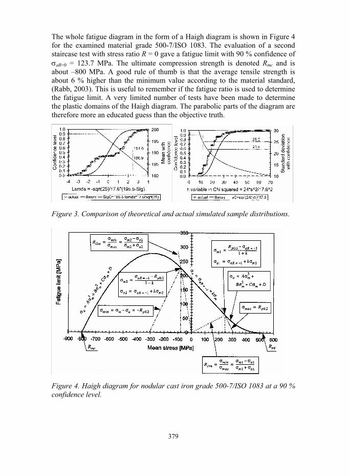
379
The whole fatigue diagram in the form of a Haigh diagram is shown in Figure 4 for the examined material grade 500-7/ISO 1083. The evaluation of a second staircase test with stress ratio R = 0 gave a fatigue limit with 90 % confidence of σaR=0 = 123.7 MPa. The ultimate compression strength is denoted Rmc and is about 800 MPa. A good rule of thumb is that the average tensile strength is about 6 % higher than the minimum value according to the material standard, (Rabb, 2003). This is useful to remember if the fatigue ratio is used to determine the fatigue limit. A very limited number of tests have been made to determine the plastic domains of the Haigh diagram. The parabolic parts of the diagram are therefore more an educated guess than the objective truth.
Figure 3. Comparison of theoretical and actual simulated sample distributions.
Figure 4. Haigh diagram for nodular cast iron grade 500-7/ISO 1083 at a 90 % confidence level.

380
3. Statistical size factor
Waloddi Weibull already published a statistical theory approximately 55 years ago explaining the influence of the component size on the fatigue limit, (Weibull, 1949). Despite this, the issue is still often misunderstood and much confusion is prevailing among calculation engineers. Also the higher fatigue strength observed in notches are not due to any supporting effect but can be interpreted as mainly dependent on the statistical size effect. It is possible to derive a consistent and physically meaningful definition of the statistical size factor by using the theory of the weakest link. The number of links is determined as the ratio of the effective stress areas of the examined part and of the test specimen in the fatigue test. The calculation of the size effect more as an area effect than a volume effect is motivated by the observation that most fatigue cracks initiate at the surface. The evaluation of the effective stress area and the statistical size factor is illustrated in Figure 5, which shows a staircase test made with notched specimens made from the same batch of material as the plain specimens in Figure 2. This staircase was also made in fully reversed tension compression, i.e. with the stress ratio R = -1. The stress concentration factor is Kt = 1.669 as seen in Figure 5. The evaluation of this test gave a sample mean fatigue limit of σaR=-
1,notch = 249.5 MPa. The observed size factor with regard to the plain specimen is thus as follows:
276.1/ ,1,1, == −=−= plainaRnotchaRobssizeK σσ
Both the effective stress area Aeff and the statistical size factor Ksize are calculated with the theory of the weakest link and the following equations can be derived when the surface area with a stress distribution with the maximum stress amplitude σamax at the critical point is divided into sub areas Ai with a decreasing average stress amplitude σai , (Rabb, 2001).
∑ ⋅=i
ii
eff ARA5.0log
log where ∫∞
−⋅=
i
dxeRx
iλπ
2
2
21 and )1(1
max
−=a
ai
ri s σ
σλ (3)
Figure 5. Staircase test on notched specimens of grade 500-7 with R = -1.

381
Ri probability of survival (reliability) at the average stress amplitude σai when σamax is assumed to correspond to a reliability of 0.5
λi value of the standard normal variable at a reliability of Ri
The number of links n in the calculation of the statistical size factor is equal to the ratio of the effective stress areas. The number of links should be greater than one, so if the effective stress area of the reference specimen Aref is smaller than that of the examined part, then
refeff AAn /= else effref AAn /= (4)
To obtain the expected fatigue limit of the part with the larger stress area the fatigue limit of the part with the smaller effective stress has to be reduced to a level with the following reliability R and corresponding λ value, which has to be iterated with the probability integral:
r
size
xn
sKdxeR
λπ λ +=⇒⋅== ∫
∞−
11
215.0 2
2
(5)
To always remain conservative, a large confidence limit, e.g. C = 90 %, should be applied on the relative standard deviation srC if the effective stress area of the examined part is larger than that of the reference specimen, otherwise a small confidence limit, e.g. 10 % should be used. An effective stress area of Aeff = 21.8 mm2 can be calculated for the notched specimen at a relative standard deviation of sr = 0.09. Since Aeff < Aref = 909 mm2, the fatigue limit of the reference specimens has to be increased with the statistical size factor to obtain the expectation value for the notched specimens. If the relative sample standard deviation sr = 0.09 directly evaluated in the test with the plain specimens is used, then the following expectation value can be calculated:
239.109.014.21
114.2984.07.418.21/909 =⋅−
=⇒−=⇒=⇒== sizeKRn λ
The calculated size factor is slightly less than the observed, but when the calculation is repeated with sr = 0.101 then the agreement is exact between the observed size factor and the size factor calculated. In fact, the determination of the standard deviation with the help of the observed size factor is a very reliable way of finding the correct sample standard deviation. The upper and lower confidence limit on this sample standard deviation 0.101 can now be calculated by combining the appropriate fatigue limits. Because of the small difference between the theoretical and simulated distributions of the sample mean, this can be done using the theoretical Students t distribution and observing that the two staircase tests have different numbers of degrees of freedom:
12.0)11(1352.1 9090
10 =−=⇒==size
rCplainC
notchCsize K
sKλσ
σ

382
08.0204.1 1010
90 =⇒== rCplainC
notchCsize sK
σσ
4. Multiaxial failure criterion in fatigue
Nowadays, there are a lot of suggested multiaxial failure criteria in fatigue. The suggested criteria can roughly be divided into critical plane based and energy based criteria. In this work, only certain different critical plane based criteria were examined and compared, namely the Findley, the McDiarmid, the Dang Van and the Papadopoulos criteria, (Socie et al., 2000) and (Papadopoulos, 2001). The Dang Van and Papadopoulos criteria are quite similar, and in fact they provide the same results for proportional loadings. The meaning of proportional and nonproportional loadings is illustrated in Figure 6 for a biaxial stress state on which the Findley criterion has been applied. The examination of these four criteria showed some definite advantages for the Findley criterion, among others the following; a) the observed anisotropy in the fatigue limit can be understood, b) provides realistic results also for cast iron, c) consistent with the theory of the statistical size effect, d) is usually slightly more conservative compared to the other criteria and e) the three other criteria can lead to contradictions under certain conditions. The Findley criterion was therefore chosen as the best alternative for an automatized fatigue analysis of the ABAQUS stress files although it has the disadvantage of requiring the most complicated and therefore the slowest algorithm of these four criteria. The critical plane of the Findley criterion is the plane where the sum of the shear stress amplitude and a certain fraction of the
a) proportional b) nonproportional
Figure 6. Biaxial proportional and nonproportional loadings.
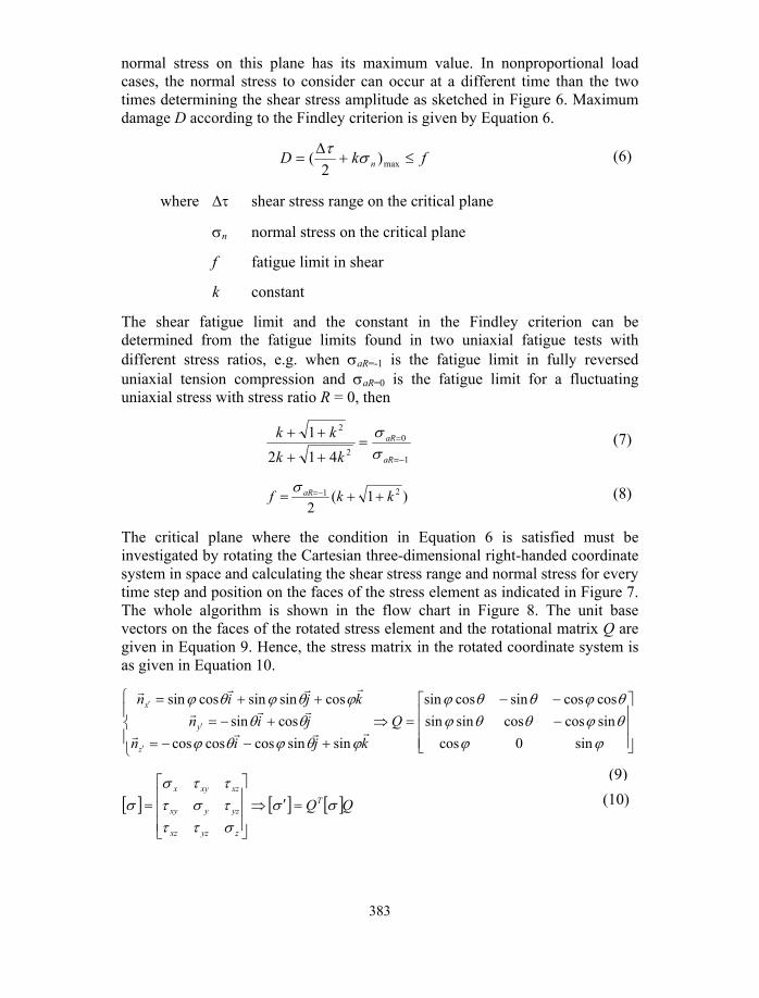
383
normal stress on this plane has its maximum value. In nonproportional load cases, the normal stress to consider can occur at a different time than the two times determining the shear stress amplitude as sketched in Figure 6. Maximum damage D according to the Findley criterion is given by Equation 6.
fkD n ≤+∆
= max)2
( στ (6)
where ∆τ shear stress range on the critical plane
σn normal stress on the critical plane
f fatigue limit in shear
k constant
The shear fatigue limit and the constant in the Findley criterion can be determined from the fatigue limits found in two uniaxial fatigue tests with different stress ratios, e.g. when σaR=-1 is the fatigue limit in fully reversed uniaxial tension compression and σaR=0 is the fatigue limit for a fluctuating uniaxial stress with stress ratio R = 0, then
1
02
2
4121
−=
==++
++
aR
aR
kkkk
σσ (7)
)1(2
21 kkf aR ++= −=σ (8)
The critical plane where the condition in Equation 6 is satisfied must be investigated by rotating the Cartesian three-dimensional right-handed coordinate system in space and calculating the shear stress range and normal stress for every time step and position on the faces of the stress element as indicated in Figure 7. The whole algorithm is shown in the flow chart in Figure 8. The unit base vectors on the faces of the rotated stress element and the rotational matrix Q are given in Equation 9. Hence, the stress matrix in the rotated coordinate system is as given in Equation 10.
⎪⎩
⎪⎨
⎧
⎥⎥⎥
⎦
⎤
⎢⎢⎢
⎣
⎡−−−
=⇒+−−=
+−=++=
′
′
′
ϕϕθϕθθϕθϕθθϕ
ϕθϕθϕθθ
ϕθϕθϕ
sin0cossincoscossinsincoscossincossin
sinsincoscoscoscossin
cossinsincossinQ
kjinjin
kjin
z
y
x
rrrr
rrr
rrrr
[ ] [ ] [ ]QQT
zyzxz
yzyxy
xzxyx
σσστττστττσ
σ =′⇒⎥⎥⎥
⎦
⎤
⎢⎢⎢
⎣
⎡
= (10) (9)

384
Figure 7. Rotation of the Cartesian coordinate system in a spherical coordinate system.
4.1 Safety factor and equivalent uniaxial stress state
Furthermore considering the surface factor KR and the life factor KN , the following safety factor SF can be calculated by directly applying the Findley criterion:
)
2( nsize
RN
size
RNF
kK
fKKDK
fKKSστ
+∆
== when refeff AA ≥ (11)
DfKKKS RNsizeF /= when refeff AA ≤ (12)
Both the surface factor and the life factor are still the subject of much research, (Murakami, 2002). However, it is recommended to decrease the fatigue limit of steels and cast irons by about 5 % per decade of cycles between two million and ten billion cycles, (Kaufmann et al., 2002).
[ ] 05.0)102lg(lg1 6 ⋅⋅−−= NKN , 106 10102 ≤≤⋅ N (13)
If the ten point height of irregularities of the profile is denoted Rz , a conservative estimate is obtained for the surface factor with Equation 14, (Gudehus et al., 1995)
53.064.0 )(lg45.0lg)(lg22.01 zmzR RRRK +⋅−= (14)

385
Figure 8. Flowchart for the multiaxial fatigue analysis according to Findley.
The definition of the safety factor in Equations 11 and 12 has two large drawbacks. One is that it is hard to know how to apply this equation in the plastic domains. The other is that it presupposes that both the shear stress amplitude and the normal stress vary in the same way. This is about the same as to assume in a uniaxial stress case that the stress ratio is constant. However, usually it is assumed that the mean stress is constant when the fatigue limit is

386
taken from the Haigh diagram. To eliminate these difficulties, the use of the equivalent uniaxial stress case can be considered. It is clear that equally large damages, regardless of the stress state, whether multiaxial or uniaxial, must have the same safety factor. It is therefore always possible to change the calculated damage, i.e. ∆τ and σn to an equivalent uniaxial stress state. This is illustrated in Figure 9. The damage for the equivalent uniaxial stress state is given by Equation 17. By differentiating this equation and putting the derivative equal to zero, the direction of the critical plane will be found. Thus, there are three conditions, equations 15, 16 and 18 for an iterative solution of the three unknowns σx,min, σx,max and the direction of the critical plane α.
σx,max = σn/cos2α (15)
σx,min = σx,max-2∆τ/sin(2α) (16)
ασασσ α 2
max,min,max, cos2sin
4 xxx kD +⋅
−= (17)
⎥⎦⎤
⎢⎣⎡ −=⇒= − )1(21tan
210 1 R
kddD αα
when 1≤≤∞− R where max,min, / xxR σσ=
and ⎥⎦⎤
⎢⎣⎡ −+= − )1(21tan
2190 1 R
koα when ∞≤≤ R1 (18)
After first solving the equivalent maximum and minimum stresses, it is subsequently possible to calculate the equivalent uniaxial mean stress and amplitude and to carry out the calculation of the safety factor in the traditional way. However, when both σx,min and σx,max are negative and approaching each other, the direction of the critical plane approaches 90 degrees. The denominatorof Equation 15 will then go towards zero, which might cause numerical problems.
Figure 9. Equivalent uniaxial stress state.

387
There is evidence that nonproportional loadings will lead to a decrease of the fatigue limit, much in the way reported for loading cases involving occasional underloads, (Rabb, 2004). Situations with nonproportional loads should therefore be treated carefully.
4.2 Probability of failure
There is no sense in mentioning a safety factor without mentioning the probability of failure or at least the standard deviation of the fatigue limit. The log normal distribution is well suited for the reduction of the mean fatigue limit to correspond to the maximum allowed probability of failure. Equation 19 gives the relation between the safety factor and the probability of failure in the form of the number λ of logarithmic standards deviations
bslog to be reduced from the
mean value. A logarithm with base b is then assumed. The use of either the normal or the log normal distribution should lead to approximately the same probability of failure for small λ−values. Therefore Equation 20 corresponding to λ = -1 can be derived for the approximate relation between sr and
bslog :
Table 1. Recommended failure probabilities and safety factors.
Material and surface Relative standard de-viation srC at confidence limit C
Safety factor SF at probability of failure P
C = 0.1 C = 0.9 P = 10-3 and λ = -3.09
P = 10-4 and λ = -3.72
Machined steel surface with parallel grain flow
0.05 0.08 1.29 1.36
Machined steel surface with perpendicular grain flow
0.085 0.12 1.48 1.61
Machined large cast iron castings
0.08 0.12 1.48 1.61
Shot peened cast iron castings
- 0.18 1.85 2.09
Castings with Chunky graphite
- 0.22 2.15 2.52

388
bsF bS logλ−= (19)
)1(log)1(log1log rbrsmallb
small
sssb
−−→+≈ λλ
when 1−→smallλ (20)
Some typical relative standard deviations and corresponding safety factors at the chosen maximum allowed probabilities of failure are shown in Table 1.
5. Facts in favor of the Findley criterion
- Findley can explain anisotropy
The observed anisotropy in the fatigue limit, i.e. the fact that the fatigue limit is higher when a fluctuating uniaxial stress acts in the direction of the grain flow than when it is perpendicular to the grain flow can be understood with the Findley criterion. This is illustrated in Figure 10, which shows the direction of the critical plane for both a parallel grain flow and a perpendicular one. This figure is drawn for a quenched and tempered steel with a tensile strength of 1165 MPa and for a stress ratio R = 0. It is important to note that according to the three other examined criteria there should not be any difference.
Figure 10. Findley explains material anisotropy.
- Findley can be applied on cast iron
Most of the critical plane approaches will provide more or less wrong results when applied on cast iron, but Findley will provide quite satisfying results. This is illustrated in Table 2 with the result of a fatigue test made in torsion on the tubular specimens of nodular cast iron grade 500-7 shown in Figure 11, (Marquis et al., 2000). Two torsional tests were conducted, one in fully reversed torsion

389
and the other with stress ratio R = 0. The evaluated fatigue limits in torsion are not more accurate than at best 5± % because a very small number of specimens were used in these tests. However, the evaluated fatigue limits in torsion were as follows: 1831 ≈−=aRτ MPa and 1250 ≈=aRτ MPa. The evaluation of these torsional stresses with the four examined criteria provided the results shown in Table 2. It can be seen that only the Findley criterion provides satisfying results.
Figure 11. Specimen in the torsion test.
Table 2. Findley criterion can also be applied on cast iron.
Safety factor SF at torsional loads ±183 MPa (R = -1) and 0250 MPa (R = 0)
McDiarmid based on the uniaxial fatigue limit
Stress ratio
Findley
Dang Van and Papadopoulos 2361 ≈−=aRσ 1560 ≈=aRσ
R = -1 0.946 1.324 0.712 0.487
R = 0 1.077 1.938 1.042 0.713
All the other three criteria fail more or less to give credible results. The tensile strength of these specimens was 625 MPa, which has been considered when the uniaxial fatigue limits were estimated using the sample fatigue ratio 0.378 given in chapter 2.
- Findley is consistent with the theory for the statistical size effect
The Findley criterion considers only the axial stress σz when the maximum damage is calculated for the notch shown in Figure 12. There is no support effect due to the biaxial stress state! The calculated values in Figure 12 are valid for nodular cast iron and with the stress ratio R = 0.

390
Figure 12. Maximum damage in the notch is determined only by σz.
References 1. Dixon, W. J. and Mood, A. M. A Method for obtaining and Analyzing
Sensitivity Data. Journal of the American Statistical Association, 1948. 43, pp. 108126.
2. Findley, W. N. A Theory for the Effect of Mean Stress on Fatigue of Metals Under Combined Torsion and Axial Load or Bending. Journal of Engineering for Industry. November 1959, pp. 301306.
3. Gudehus, H. und Zenner, H. Leitfaden für eine Betriebsfestigkeitsrechnung, 3. Auflage. Verlag Stahleisen mbH, Düßeldorf 1995.
4. Kaufmann, H. und Wolters, H. Zyklische Beanspruchbarkeit dickwandiger Bauteile aus ferritischem Gußeisen mit Kugelgraphit. Konstruieren+gießen 27 (2002) Nr. 1.
5. Marquis, G. and Solin, J. Long-life fatigue design of GRP 500 nodular cast iron components. VTT (Technical Research Centre of Finland), Research Notes 2043, Espoo 2000.
6. Murakami, Y. Metal Fatigue: Effects of Small Defects and Nonmetallic Inclusions. Elsevier Science Ltd. 2002.
7. Papadopoulos, I. V. Long life fatigue under multiaxial loading. International Journal of Fatigue 23 (2001), pp. 839849.
391
8. Rabb, B. R. Interpretation and Evaluation of the Statistical Size Effect. Proceedings, of the 23rd CIMAC World Congress on Combustion Engine Technology. Vol. 3. May 710, 2001, Hamburg Germany. Pp. 11251138.
9. Rabb, B. R. Staircase testing confidence and reliability. Fatigue Damage of Materials, Experiment and Analysis. Editors: A. Varvani-Farahani and C. A. Brebbia. WITpress 2003. Pp. 447464.
10. Rabb, B. R. Influence of Occasional Underloads on Fatigue. European Congress on Computational Methods in Applied Sciences and Engineering ECCOMAS 2004, Jyväskylä, 2428 July 2004.
www.mit.jyu.fi/eccomas2004/proceedings/proceed.html.
11. Socie, D. F. and Marquis G. B. Multiaxial Fatigue. Society of Automotive Engineers, Inc. 2000.
12. Weibull, W. A Statistical Representation of Fatigue Failures in Solids. Transactions of the Royal Institute of Technology Stockholm, Sweden. No. 27, 1949. Elanders Boktryckeri Ab, Göteborg 1949.

A/1
Appendix A: Financing organisations
The following financing organisations have provided funding for the GJUTDESIGN-2005 project.1 Short descriptions of the organisations were obtained from their web sites:
http://www.nordicinnovation.net htpp://www.tekes.fi htpp://www.pff.nu
Nordic Innovation Centre
Tekes, National Technology Agency of Finland
PFF The Program Board for Automotive Research (PFF)
1 The seminar itself was jointly financed by the participants.

A/2
Nordic Innovation Centre
The Nordic Innovation Centre is the Nordic Council of Ministers single most important instrument for promoting an innovative and knowledge-intensive Nordic business sector.
Our basic assumption is that each of the Nordic countries possesses knowledge, which through increased co-operation significantly will improve innovation capabilities and competitiveness for Nordic businesses.
Building knowledge platforms
Today, the Nordic Innovation Centre is an important player in Nordic knowledge platforms within the areas of innovation policy, creative industries, biotechnology, food safety and innovative building & construction. Establishing common Nordic knowledge platforms on strategically important areas give Nordic businesses access to the best knowledge possible and greatly enhance their innovation capabilities. We believe that building common Nordic knowledge markets are vital to all Nordic business life, enabling them to compete on a global market which is becoming more and more knowledge driven.
Investments
The total project portfolio of the Nordic Innovation Centre consists of approximately 120 ongoing projects and networks. Together with several hundred completed projects of great value to Nordic businesses, these projects involve the Centre in nearly all strategically important Nordic areas.

A/3
Tekes
Tekes, the National Technology Agency is the main public financing and expert organisation for research and technological development in Finland. Tekes finances industrial R&D projects as well as projects in universities and research institutes. Tekes especially promotes innovative, risk-intensive projects.
The primary objective of Tekes is to promote the competitiveness of Finnish industry and the service sector by assisting in the creation of world-class technology and technological know-how. Specifically, Tekes activities aim to diversify production structures, increase production and exports, and create a foundation for employment and social wellbeing.
Tekes funds come from the state budget via the Ministry of Trade and Industry. Tekes has a budget of 400 million euros, a source of funding for 2000 projects annually.
How does Tekes operate?
Tekes works in close cooperation with its clients in companies, universities and research institutes. Tekes is headquartered in Helsinki, with regional offices throughout Finland and abroad. Over 300 dedicated personnel support Tekes activities.

A/4
The Program Board for Automotive Research (PFF)
The PFF is a research body that is unique to Sweden and that is comprised of the automotive industry and those authorities that conduct research in the automotive field. The PFF is a forum for cooperation between its various parties and it is also responsible for the implementation of four different research programs in the field of automotive technology.
The Vehicle Research Program (ffp)
The aim of the Vehicle Research Program is to strengthen the ability of the Swedish automotive industry to compete on an international basis. This is done by supporting technological automotive research in the fields of safety, the environment and cost/quality. The aim is the creation in the country of a skills and recruiting basis at the hig-hest international level and to see that high-quality research results are generated. Research is governed entirely by the needs of the automotive industry, something that is ensured by the project being initiated and required by a company within the automotive indu-stry, while, at the same time, work involving a university/industrial research institute is a precondition of any project.
The program has been evaluated on two occasions. Impressions from the latest evaluation of the ffp include the following:
• the projects are relevant in terms of research, industry and society
• there is a functioning network structure that has led to close contact within industry and real problems for the researchers to solve
• this network structure has allowed the companies to achieve an improved basis for recruitment and useable research results
• strong groups have been created that carry out fundamental research that is of long-term interest for the automotive indu-stry.The latest evaluation can be viewed at www.pff.nu

Published by
Series title, number and report code of publication
VTT Symposium 237 VTTSYMP237
Author(s) Samuelsson, Jack, Marquis, Gary & Solin, Jussi (eds) Title
Competent Design by Castings Improvements in a Nordic project
Abstract This symposium summarises the achievements within a joint R&D project GJUTDESIGN-2005 Design kvalitet och NDT för gjutna utmattningsbelastade komponenter. It brought together 25 Nordic organisations aiming to co-ordinated development of improved methods and tools for fatigue design of cast structures and components. The partners include 10 industrial companies that design and manufacture construction machinery, trucks, robots, windmills, paper machines and ship engines, 5 foundries, engineering consulting firm, research organisations and universities. Selected 20 papers deal with mechanisms, understanding, practical assessment and specific industrial challenges in fields of optimisation of casting process, material properties and component design, influence of defects and crack growth mechanisms on fatigue resistance, inspection and quality assurance to control of defects, and complex service loading in terms of variable amplitude and multiaxiality. Keywords cast structures, cast materials, cast quality, design, complex fatigue loads, fracture mechanics, fatigue assessment, modelling, Nordic countries, graphite
Activity unit VTT Industrial Systems, Kemistintie 3, P.O.Box 1704, FI02044 VTT, Finland
ISBN Project number 9513862984 (soft back ed.) 9513862992 (URL: http://www.vtt.fi/inf/pdf/)
Date Language Pages Price May 2005 English 391 p. + app. 4 p. H
Name of project Commissioned by
Series title and ISSN Sold by VTT Symposium 03579387 (soft back ed.) 14550873 (URL: http://www.vtt.fi/inf/pdf/)
VTT Information Service P.O.Box 2000, FI02044 VTT, Finland Phone internat. +358 20 722 4404 Fax +358 20 722 4374

VTT SY
MPO
SIUM
237Com
petent Design by Castings. Improvem
ents in a Nordic project
Tätä julkaisua myy Denna publikation säljs av This publication is available from
VTT TIETOPALVELU VTT INFORMATIONSTJÄNST VTT INFORMATION SERVICEPL 2000 PB 2000 P.O.Box 2000
02044 VTT 02044 VTT FI–02044 VTT, FinlandPuh. 020 722 4404 Tel. 020 722 4404 Phone internat. +358 20 722 4404Faksi 020 722 4374 Fax 020 722 4374 Fax +358 20 722 4374
ISBN 951– 38– 6298– 4 (soft back ed.) ISBN 951– 38– 6299– 2 (URL: http://www.vtt.fi/inf/pdf/)ISSN 0357– 9387 (soft back ed.) ISSN 1455– 0873 (URL: http://www.vtt.fi/inf/pdf/)
ESPOO 2005 VTT SYMPOSIUM 237
Competent Design by CastingsImprovements in a Nordic project
This symposium summarises the achievements within a joint R&D project"GJUTDESIGN2005 – Design kvalitet och NDT för gjutna utmattningsbelastadekomponenter". It brought together 25 Nordic organisations aiming to coordinated development of improved methods and tools for fatigue design of caststructures and components. The partners include 10 industrial companies thatdesign and manufacture construction machinery, trucks, robots, windmills, papermachines and ship engines, 5 foundries, engineering consulting firm, researchorganisations and universities.
Selected 20 papers deal with mechanisms, understanding, practicalassessment and specific industrial challenges in fields of
optimisation of casting process, material properties and component design,
influence of defects and crack growth mechanisms on fatigue resistance,
inspection and quality assurance to control of defects, and complex service loading in terms of variable amplitude and
multiaxiality.Experiments were performed for small test pieces and real components. NDE
methods were studied to assess the current state of the art in industry andresearch. Numerical modelling, simulation and analysis of complex structureswas applied to design of experiments and for optimisation of products.