TGRS-2009-00082.R2

1

Abstract— The emission of bare soils at microwave L-band (1

– 2 GHz) frequencies is known to be correlated with surface soil moisture. Roughness plays an important role in determining soil emissivity although it is not clear which roughness length scales are most relevant. Small-scale (i.e. smaller than the resolution limit) inhomogenities across the soil surface and with soil depth, caused by both, spatially varying soil properties and topographic features may affect soil emissivity. In this study, roughness effects were investigated by comparing measured brightness temperatures of well-characterized bare soil surfaces with the results from two reflectivity models. The selected models are the Air-to-Soil (A2S) transition model and Shi’s parameterization of the Integral Equation Model (IEM). The experimental data taken from the Surface Monitoring Of the Soil Reservoir Experiment (SMOSREX) consist of surface profiles, soil permittivities and temperatures, and brightness temperatures at 1.4 GHz with horizontal and vertical polarization.

The types of correlation functions of the rough surfaces were investigated as required to evaluate Shi’s parameterization of the IEM. The correlation functions were found to be clearly more Exponential than Gaussian. Over the experimental period the diurnal mean RMS-height decreased, while the correlation length and the type of correlation function did not change. Comparing the reflectivity models with respect to their sensitivities to the surface RMS-height and correlation length revealed distinct differences. Modeled reflectivities were tested against reflectivities derived from measured brightness, which showed that the two models perform differently depending on the polarization and the observation angle.

Index Terms— electromagnetic scattering by rough surfaces, microwave radiometry, permittivity, soil moisture

Manuscript received February 6, 2009. This work was supported in part by

the Swiss Federal Institute for Forest, Snow and Landscape Research (Eidgenösische Forschungsanstalt für Wald, Schnee und Landschaft (WSL)).

M. Schwank and I. Völksch are with the Swiss Federal Institute for Forest, Snow and Landscape Research, 8903 Birmensdorf, Switzerland (mike.schwank@wsl.ch).

J.-P. Wigneron and Y. H. Kerr are with the INRA, EPHYSE, Villenave d'Ornon, France (jpwigner@bordeaux.inra.fr, yann.kerr@cesbio.cnes.fr).

A. Mialon and P. de Rosnay are with the CESBIO, CNRS/CNES/IRD/UPS, BPI 2801, Toulouse, France (mialon@cesbio.cnes.fr). P. de Rosnay is also with the European Centre for Medium Range Weather Forecasts (ECMWF), Berkshire, UK (Patricia.Rosnay@ecmwf.int).

C. Mätzler is with the Institute of Applied Physics (IAP), University of Bern, 3012 Bern, Switzerland, (christian.matzler@iap.unibe.ch).

I. INTRODUCTION nergy fluxes through the terrestrial surface layer are

major drivers of climate. For land areas with sparse or no vegetation, the amount of this energy exchange is fundamentally linked with the moisture in the soil. Techniques for monitoring the surface moisture on the spatial scales relevant for climate and meteorological research are therefore of particular interest [1-5]. One such technique is passive microwave remote sensing at L-band (1 - 2 GHz), which has an almost 25-year long history [6, 7]. It is used in the European Space Agency’s (ESA) Soil Moisture and Ocean Salinity (SMOS) mission, which deduces soil surface moisture from thermal brightness at 1.4 GHz with near global coverage every three days and a spatial resolution of approximately 40 × 40 km2 [8, 9]. NASA’s Soil Moisture Active and Passive (SMAP) mission will use a combined radiometer and high-resolution radar to measure surface soil moisture and freeze-thaw state. The mission is recommended by the U.S. National Research Council Committee on Earth Science and Applications from Space for launch between 2010 and 2013 [10].

Retrieving soil moisture from thermal microwave radiation is significantly affected by soil roughness [11-16]. Hence, the surface emission model used for interpreting measured radiance is one of the essential components in a retrieval algorithm. The text books [17-20] give an exhaustive review of the commonly used surface emission models relevant for passive microwave remote sensing. Most of the physical models, however, require significant computing effort and detailed ground truth information, which hampers their operative usage in retrieving algorithms. For this reason, easy to use semi-empirical approaches such as the Q/H model [21, 22] are usually employed in retrieval algorithms.

This study aims to test the application of two surface reflectivity models for retrieving the surface moisture of bare soils from measured L-band radiation. The two approaches studied are the so-called Air-to-Soil (A2S) transition model ([12] and chapter 4.7 in [23]) and the physical Integral Equation Model (IEM) [17]. With regard to the application in a retrieval algorithm, the IEM model is evaluated using Shi’s parameterization of a large database of IEM simulations. The A2S model describes the effect of soil roughness by matching

Comparison of Two Bare Soil Reflectivity Models and Validation with L-Band Radiometer

Measurements M. Schwank , I. Völksch, J.-P. Wigneron, Y. H. Kerr, A. Mialon, P. de Rosnay, and C. Mätzler

E

TGRS-2009-00082.R2

2

the impedance between the dielectric constants of air and the topsoil. The gradual dielectric transition from air to soil is represented using a semi-empirical effective medium approach. As demonstrated in [24-26], a similar approach can also be used for modeling the reflectivity of soils covered with sparse vegetation or litter provided that scattering is not dominant.

The A2S and the IEM model are compared in this study and the model results are tested against the L-band signatures measured. The steps involved in the comparison are explained in section II, and the experimental dataset is presented in section III. Results and discussion are the content of section IV and conclusions are provided in section V.

II. MODELS AND METHODS

A. Review of Existing Surface Reflectivity Models The emissivity of a bare soil surface at horizontal (p = H) or

vertical polarization (p = V) is described as 1 – RpRM, where

RpRM is the surface reflectivity determining the brightness

temperature TpB measured with a RadioMeter (RM). Two

categories of surface reflectivity model can be distinguished: i) physical approaches that seek solutions to Maxwell’s equations by considering the boundary conditions on the rough surface; ii) empirical approaches that rely exclusively on observations.

The fast model developed by Shi et al. (2002) [27] can be considered physical, as it is a representation of reflectivities computed with the physical Integral Equation Model (IEM) [17]. The Air-to-Soil (A2S) transition model ([12] and chapter 4.7 in [23]) can be classified somewhere in between the physical and the empirical approaches. The physical aspect of the A2S model is the concept of a vertically extended dielectric transition zone to model the gradual increase from the air to the bulk soil permittivity (impedance matching). The more empirical part of the A2S model is the representation of this dielectric transition zone by considering exclusively topographic features smaller than the resolution limit in combination with an empirical dielectric (refractive) mixing model.

According to [27] soil moisture can be retrieved with an accuracy of ≈ 3 % if Shi’s fast model is used. An analysis of horizontally polarized L-band signatures by means of the Shi reflectivity model and the A2S transition model is described in [12]. Mean deviations between the modeled and measured soil reflectivities were found to be 0.079 if the Shi model is applied and 0.029 if the A2S transition model is applied.

1) Shi’s Parameterization of the IEM Model Shi’s fast model is used for the efficient computation of

surface reflectivities predicted by the Integral Equation Model (IEM). The fast model uses simulated reflectivity data derived from an advanced version of the IEM [28]. The IEM-simulated database consists of rough surface reflectivities for 1.4 GHz with horizontal (p = H) and vertical (p = V) polarization and of reflectivities computed for Exponential (S = E) and Gaussian (S = G) auto-correlation functions CS(r) of

the rough surfaces. Further input parameters to Shi’s fast model are the surface Root Mean Square (RMS) height h, the correlation length lc, the surface permittivity εs, and the observation angle α relative to the vertical. The ranges of the IEM model parameters included in Shi’s parameterization are: 2.5 mm ≤ h ≤ 35 mm; 25 mm ≤ lc ≤ 300 mm; 20° ≤ α ≤ 60°; and 3.3 ≤ εs ≤ 28.9 (corresponding to the soil moisture range 0.02 m3m-3 ≤ θ ≤ 0.44 m3m-3 if the empirical relation [29] is used).

Shi fast model uses a parameterization of IEM-simulated reflectivities Rp

IEM, consisting of a coherent (Rpcoh.) and a non-

coherent term (Rpnon-coh.) [27]:

IEM coh. non-coh. F F4exp cos

pp p p p p p BR R R R h A Rπ αλ

⎡ ⎤⎛ ⎞= + = ⋅ − +⎜ ⎟⎢ ⎥⎝ ⎠⎣ ⎦ (1)

RpF is the Fresnel reflectivity, λ is the wavelength (≈

0.21 m), and Ap, Bp are parameters given in [27] that depend on p, α, h, lc and on the type of correlation function. As can be seen from (1), the coherent part Rp

coh. does not depend on the correlation length lc while the non-coherent part Rp

non-coh. depends on h and lc.

The hexagons depicted in the flow chart in Fig. 1 show the inputs h, S, lc, εs, α, and p to be specified in Shi’s parametrization and how they relate to the A2S model described below.

2) Air-to-Soil Model (A2S) The uppermost soil horizon exhibits a highly complex

three-dimensional structure in terms of the dielectric properties with feature sizes in the range of centimeters. These dielectric heterogeneities result not only from the surface roughness, but also from spatial variations in moisture, texture, and structure.

The evaluation procedure and the basic ideas implemented in the A2S transition model are shown in the diagrams in Fig. 1 and 2. The model takes into account how many of the soil topographic features are smaller than the resolution limit at L-band frequencies, which can be estimated by the Bragg limit ΛBragg (λ = wavelength, α = observation angle):

Bragg 2 sinλ

αΛ = (2)

The Bragg limit ΛBragg, however, is not a sharp criterion to distinguish between the small features to be treated in the sense of full wave electromagnetism and the larger features that can be modeled with geometric optics. The resolution limit ΛBragg gives the order of magnitude of the spatial dimension in which the intermediate method of physical optics applies. From now on the expression “small-scale” is used for feature sizes with dimensions smaller than the resolution limit.

Dielectric small-scale heterogeneities (cross-section shown in Fig. 2a) can therefore be treated in the sense of the quasi-static limit, where the mean field is homogeneous and extends over a region much larger than the feature size. This makes it possible to postulate an A2S transition zone (Fig. 2b) matching the impedance between the air and bulk soil. Within

TGRS-2009-00082.R2

3

this zone, the effective permittivity ε(z) [30] gradually increases from the air value (εa = 1) to the permittivity εs > εa of the bulk surface soil.

The apparent dielectric profile ε(z) depicted in Fig. 2d is modeled with the refractive mixing model [30, 31], taking into account the bulk soil and air phases:

( ) ( ) ( )[ ] 21 2 1 2s a1z z zε ν ε ν ε⎡ ⎤= ⋅ + − ⋅⎣ ⎦ (3)

Thereby, the volume fraction ν(z) of the bulk soil phase (Fig. 2c) increases with depth z, whereas the air fraction 1 - ν(z) decreases to zero within the air-to-soil transition zone. In [23] (chapter 4.7), where the A2S model is explained in detail, ν(z) is represented by an empirical relation comprising its vertical extent. For our study, either measured or synthetically generated topography data are available, allowing ν(z) to be modeled as the cumulated probability density of the small-scale surface height (see section C).

Imaginary parts of bulk soil permittivities εs used in (3)

were not considered as only real parts were available from the capacitive in-situ measurements (see section III). Finally, once the dielectric depth profile ε(z) is modeled from the small-scale topography, the rough soil reflectivities Rp

A2S (p = H, V) are calculated by applying a coherent radiative-transfer model for layered dielectric media. A matrix formulation of the boundary conditions at the layer interfaces derived from Maxwell’s equations is used [32]. This coherent model was evaluated for dielectric layers with thickness d = 0.1 mm << λ, making the reflectivities Rp

A2S independent of d.

B. Microwave Radiative Transfer L-band brightness temperatures Tp

B with horizontal (p = H) and vertical (p = V) polarization measured with the RadioMeter (RM) are used for deriving soil reflectivities Rp

RM (thin-line boxes in Fig. 1). This requires a radiative transfer model expressing Tp

B by means of RpRM, the effective physical

temperature T [33] of the soil surface layer, and the mean sky brightness temperature TB,sky ≈ 6.3 K [34]:

( )B RM B,sky RM1p p pT T R T R= − + (4) Equation (4) fulfills Kirchhoff’s law and can easily be

solved for RpRM. Validations of the reflectivity models

presented in section IV.C are performed by means of daily mean values ⟨Rp

RM⟩ computed from instantaneous RpRM. This

approach was chosen as reliable topography information, which is required as input to the reflectivity models, was available on a daily basis only.

C. Rough Surfaces The purpose of the following sub-sections 1) - 5) is to

describe the modeling steps depicted in Fig. 1. Following this, reflectivities Rp

M (p = H, V; M = A2S, IEM) at the observation angles α are modeled from topography profiles f(x) of random rough soil surfaces with permittivities εs. The surface topography f(x) is either measured directly (see section III), or artificially generated (see section II.C.1)). To derive Rp

A2S, the small-scale (SS) topography fss(x) is extracted from f(x) (section II.C.2)), and then the soil fraction profile ν(z) is determined (section II.C.3)), leading to the dielectric profile ε(z) (3) used for computing Rp

A2S. The computation of the RMS-height h, the correlation function C(r), and the

Fig. 1. Illustration of the procedures applied for deriving rough surface reflectivities Rp

M (p = H, V; M = IEM, A2S, RM). Hexagons indicate model inputs. Reflectivities Rp

IEM computed with the IEM model (dashed-lineboxes) require the topography parameters h, lc, S = E, G (either pre-set or derived from topography profiles f(x)). Reflectivities Rp

A2S computed with the A2S model (solid-line boxes) directly use f(x) as input. Reflectivities Rp

RM

(thin-line boxes) are derived from measured brightness and soil temperaturesTp

B and T.

Fig. 2. Illustration of the ideas implemented in the A2S transition model. A cross-section of the small-scale topography is shown as a sketch in a); the postulated air-to-soil transition zone is shown in b); the volumetric soil fraction ν(z) and the dielectric profile ε(z) computed with (3) are shown in c) and d), respectively.

TGRS-2009-00082.R2

4

correlation length lc of f(x) required for computing RpIEM is

described in section II.C.4). Section II.C.5) introduces the quantity EG used for rating the type of measured correlation function to be specified in Shi’s fast model.

1) Generating Surface Topographies As the flow-chart in Fig. 1 shows with the solid-line boxes,

modeling RpA2S requires the topography data of a rough

dielectric surface. For this purpose, one-dimensional random rough surface profiles fS(x) with either Gaussian (S = G) or Exponential (S = E) correlation functions CS(r) are generated:

( )2

G 2exp rC r

lc⎛ ⎞

= −⎜ ⎟⎝ ⎠

and ( )E expr

C rlc

⎛ ⎞= −⎜ ⎟⎜ ⎟

⎝ ⎠ (5)

Thereby, r denotes the horizontal distance in x between two points of the surface and CS(r) evaluated at r expresses the statistical correlation between the surface heights fS(x) and fS(x + r). From CG(lc) = CE(lc) = e-1 ≈ 0.37, it follows that the correlation between two surface heights at the characteristic distance r = lc is the same for the Exponential and the Gaussian surface type.

For generating Exponential and Gaussian profiles fS(x) of length L, zero mean ⟨fS(x)⟩ = 0, RMS-heights h, and correlation lengths lc, the approach described in [35] (chapter 4) was implemented. The power spectral densities [19] (chapter 4, section 1.4):

( )2 2 2

G exp42

h lc k lcW kπ

⎛ ⎞⋅= −⎜ ⎟

⎝ ⎠ and ( ) ( )

2

E 2 21h lcW k

k lcπ=

+ (6)

associated with the two surface types express the abundance of features with a certain spatial wave number k = 2π / Λ present in fS(x) (Λ = spatial wavelength). As a consequence of the exponential form of WG(k) associated with the Gaussian surface fG(x), the spectral components with k ≥ klc ≡ 2π / lc (corresponding to Λ ≤ lc) are clearly less present in a Gaussian than in an Exponential surface generated for the same lc and h. Quantitatively this can be expressed by the fraction EGS, weighting the spectral components with spatial wavelengths Λ shorter than lc:

( )

( )

5

1

0

1 Erf 10 for G2 ArcCot2 10 for E

lc

Sk

S

S

W k dkS

EGSW k dk

π

π π

∞

−

∞ −

⎧ − ≈ =⎪≡ = ⎨≈ =⎪⎩

∫

∫

(7)

The distinct difference between EGG and EGE suggests that this quantity can be applied to measured topography data to decide whether the surface is Exponential or Gaussian. This will be pursued in section II.C.5) and applied in section IV.A 4.1 to investigate whether the type of correlation function changes with time as a consequence of progressive weathering of the soil surface.

2) Filtering of Small-Scale Features The A2S transition model uses exclusively small-scale

surface features fss(x) with spatial dimensions smaller than the resolution limit (Fig. 1 and 2) to compute Rp

A2S. As mentioned in section II.A.2), the Bragg resolution limit ΛBragg is not an

exact lower limit for the dimension of features that can be electromagnetically resolved. Considering this, it has to be emphasized that defining “small-scale” as features with dimensions smaller than ΛBragg means there is a certain model uncertainty.

However, a discrete Fourier high-pass filter with the Bragg resolution limit (2) chosen for the cut-off wavelength is applied to extract the Small-Scale (SS) features fss(x) with Λ ≤ ΛBragg from f(x). Applying discrete Fourier transformations to a profile of length L requires first transforming the data into an equidistant form [xj, zj] (j = 1,…,N) with increments Δx = L / (N - 1) along the horizontal direction x. Subsequently, the data [L+j⋅Δx, zN-j] (j = 1,…,N-1) are appended to [xj, zj], resulting in a periodic sequence 2L in length and N0 = 2N-1 data points. This complemented periodic dataset can now be represented by its Fourier series:

( )0 1

0 0

1exp 2

N

j kk

k jz c i

Nπ

−

=

⎛ ⎞⋅ −= ⎜ ⎟⎜ ⎟

⎝ ⎠∑ , (8)

with the complex Fourier coefficients ck given by: ( )0

10 0

11 exp 2N

k jj

k jc z i

N Nπ

=

⎛ ⎞−= ⋅ −⎜ ⎟⎜ ⎟

⎝ ⎠∑ (9)

Then, the small-scale features [xj, zjss] (j = 1,…,N) required

to compute the soil fraction ν(z) are extracted by evaluating the Fourier series (8) with ck computed from (9) for Λ = 2L / k ≤ ΛBragg, and otherwise with ck = 0.

3) Soil Fraction in the A2S Transition Zone The soil fraction ν(z) within the air-to-soil transition zone

(Fig. 2) is computed from the discrete small-scale topography data [xj, zj

ss] (j = 1,…,N) by using the “Quantile” function implemented in “Mathematica 5.2”. Calling this function with the vector zj

ss and a certain probability P between 0 and 1 yields the height z at which the air fraction 1 - ν(z) equals P. Thus, the discrete dataset [zj, νj] considering N – 1 evenly spaced soil fraction levels 0 < νj < 1 is constructed. The corresponding continuous interpolation function 0 < ν(z) < 1 is then used in the refractive dielectric mixing model (3) to describe the apparent dielectric profile ε(z) used to compute the reflectivity Rp

A2S with the A2S model. 4) Correlation Function and Correlation Length

When topography profiles f(x) are measured, they are characterized by their correlation length lc and RMS-heights h. For an equally spaced topography dataset [xj, zj] (j =1,…,N), h is simply computed as the standard deviation of the heights zi. To derive lc of a profile with length L, the correlation function C(r) has to be computed numerically:

( ) ( ) ( )20

1 L

C r f x f f x r f dxLh

≡ ⎡ − ⎤ ⎡ + − ⎤⎣ ⎦ ⎣ ⎦∫ (10)

To enable the evaluation of (10) for each r in the range of 0 ≤ r ≤ L considering the given integration limits, the data [xj, zj] must be supplemented with their mirrored sequence (compare section II.C.2)). The resulting continuous correlation function C(r) associated with [xj, zj] is then used to compute the correlation length lc by solving C(lc) = 1/e numerically for the

TGRS-2009-00082.R2

5

smallest solution. At this point it should be noted that the length L of a profile

may have a significant influence on the estimated h and lc. Monte-Carlo simulations showed that the 95% confidence limits for h and lc of individual transects come into ±10% margin of error when L are around 240⋅lc and 460⋅lc [36]. The same investigation showed that mean values ⟨h⟩ and ⟨lc⟩ derived from a set of realizations are much more reliable. Considering these findings, and in view of the fact that measured profiles were available for L = 2 m, it is expected that h and lc derived from the individual profiles are rather error-prone. Their daily mean values ⟨h⟩ and ⟨lc⟩ derived from the 11 to 16 profiles available per day, however, are expected to be much more representative of the surface state on a particular day.

5) Correlation Function Type Reflectivities Rp

IEM computed with Shi’s parameterization of IEM reflectivities are rather sensitive to the type of the correlation function of the topography. Therefore, indicator values EG are calculated that allow systematic trends in time in surface correlation function type to be identified (section IV):

2

2

2

kk lc

kk

cEG

cπ≥≡

∑

∑ (11)

In analogy with (7), EG weighs the sum of the squared absolute values of the Fourier coefficients ck (9) with wave numbers k ≥ 2π / lc (corresponding to spatial wavelengths Λ ≤ lc) with respect to the total sum of ⎪ck⎪2. Consequently EG defined by (11) weights the spectral components with spatial wavelengths Λ shorter than lc, and can therefore be used to rate the type of correlation function measured as either more Exponential or Gaussian.

III. SMOSREX DATASET The two reflectivity models were validated with a long-term

dataset acquired in the framework of the Surface Monitoring Of the Soil Reservoir EXperiment (SMOSREX), which has been in full operation since January 2003 [37]. L-band brightness temperatures Tp

B (p = H, V) of a bare soil site are acquired by the L-band radiometer for Estimating Water In Soils (LEWIS), installed near Toulouse in the south of France [38]. The LEWIS radiometer is mounted at the top of a 13.7 m vertical structure and provides Tp

B with an accuracy of ± 0.2 K. The field of view of the horn antenna is 13.5° at -3 dB. Every 3 hours, elevation scans at α = 20°, 30°, 40°, 50°, and 60° are performed over the bare soil and a plot with vegetation. The bare soil was rather smooth until January 13th, 2006, which we refer to as DoY = 13, where DoY is the Day of Year. On that date, it was ploughed and the surface roughness was distinctly increased. Up until that date, the soil structure had not been modified artificially and had just changed gradually with climatic events (rainfall, wind, etc.).

After ploughing, changes in the soil topography were

monitored by regularly measuring the soil mechanically. For this purpose, a needle board 2 m in length L, consisting of N = 201 movable (in the vertical direction) needles 1 cm apart, is used to follow the soil elevation profile. Photos of the board are taken, digitized manually, and finally used to compute soil topography profiles f = [xj, zj] (j = 1,…,N). Measurements were performed parallel and perpendicular to the soil rows produced through ploughing. After the ploughing, eleven assessments were conducted in 2006: DoY = 13, 20, 32, 51, 75, 93, 124, 150, 181, 328 and one in 2007 (DoY = 71).

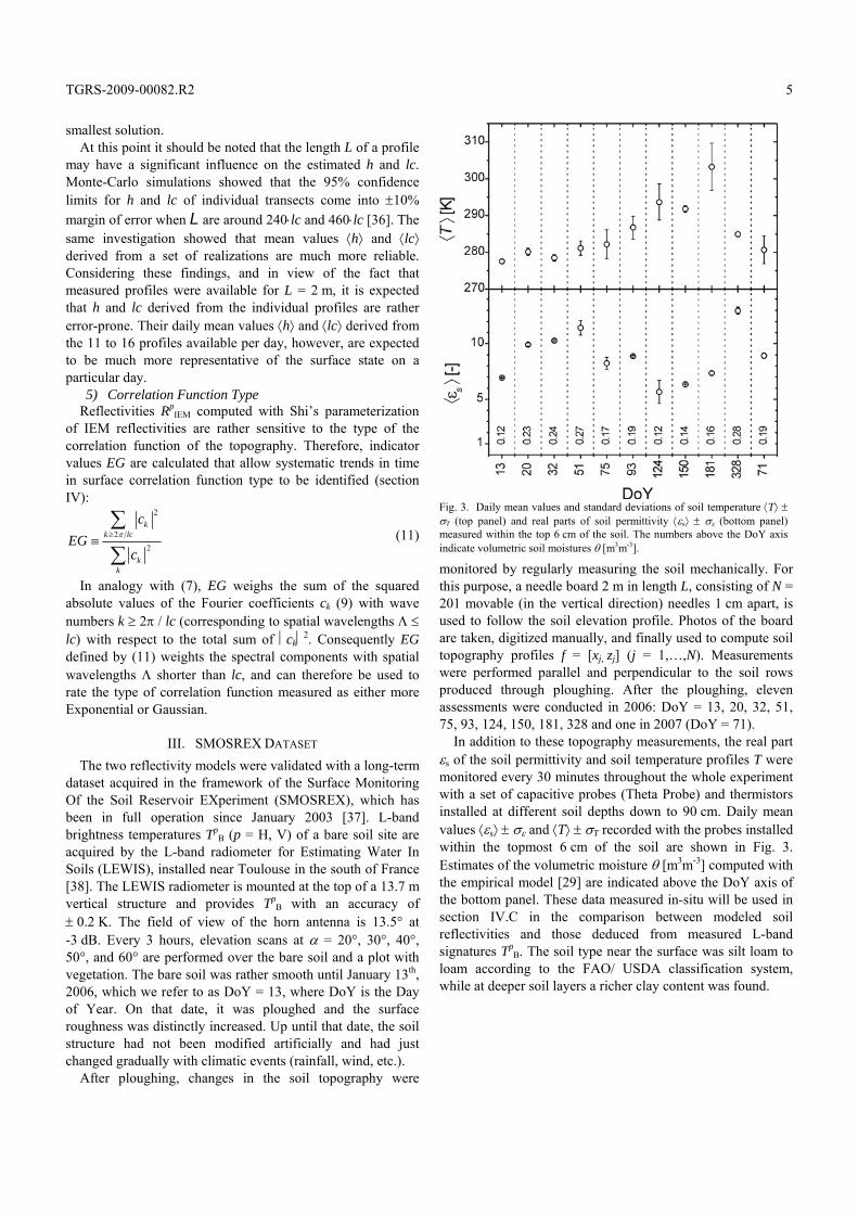
In addition to these topography measurements, the real part εs of the soil permittivity and soil temperature profiles T were monitored every 30 minutes throughout the whole experiment with a set of capacitive probes (Theta Probe) and thermistors installed at different soil depths down to 90 cm. Daily mean values ⟨εs⟩ ± σε and ⟨T⟩ ± σT recorded with the probes installed within the topmost 6 cm of the soil are shown in Fig. 3. Estimates of the volumetric moisture θ [m3m-3] computed with the empirical model [29] are indicated above the DoY axis of the bottom panel. These data measured in-situ will be used in section IV.C in the comparison between modeled soil reflectivities and those deduced from measured L-band signatures Tp

B. The soil type near the surface was silt loam to loam according to the FAO/ USDA classification system, while at deeper soil layers a richer clay content was found.

Fig. 3. Daily mean values and standard deviations of soil temperature ⟨T⟩ ±σT (top panel) and real parts of soil permittivity ⟨εs⟩ ± σε (bottom panel)measured within the top 6 cm of the soil. The numbers above the DoY axis indicate volumetric soil moistures θ [m3m-3].

TGRS-2009-00082.R2

6

IV. RESULTS AND DISCUSSION

A. Soil Topographies Surfaces fE(x) with Exponential correlation functions are

associated with non-differentiable topographies. This is typical for granular media with loose crumbs and cracks at the surface. Gaussian surfaces fG(x), by contrast, are differentiable and thus locally smooth, as is sometimes the case with the surface of a liquid. With regard to the soil topographies measured, it was hypothesized that the surfaces measured during the first days after ploughing would be mostly Exponential. The second hypothesis was that the surfaces would become more Gaussian after several rain events. These two hypotheses will be discussed in the following sub-sections 1) and 2).

1) Topography and how it Changes with Time To illustrate how the topography of the soil changed after it

was ploughed until the end of the experiment, an early topography profile and one of the last profiles taken from the SMOSREX dataset (section III) were analyzed. The RMS-height h and the correlation length lc derived from the two single profiles are not necessarily representative of the surface state on the corresponding days. As discussed in section II.C.4), the surface statistical parameters h and lc could be disputed due to the limited profile length (L = 2 m).

The top panels of Fig. 4a and b show surface profiles f for January 13th 2006 (DoY 13 = day of ploughing) and June 30th 2006 (DoY 181). The middle panels show the corresponding correlation functions C(r), and the bottom panels show the surface power spectra ⎟ck⎟2 (9) plotted versus the spatial wavelength Λ = 2L / k.

The topography of the freshly ploughed field (DoY 13) clearly differs from that measured 5.5 months later on DoY 181. This change is conveyed by the RMS-height decreasing

Fig. 4. Topography profiles f measured with the needle board (N = 201 measuring points and length L = 2 m) on DoY 13 (a) and on DoY 181 (b). Surface RMS-heights are h = 40 mm and h = 25 mm. The middle panels show the associated correlation functions C(r) with lc = 68 mm and lc = 104 mm (dashed lines). The power spectra of f (ck = Fourier coefficients (9)) plotted versus the spatial wavelengths Λ are shown in the bottom panels with EG (defined in (11)) indicated.

TGRS-2009-00082.R2

7

from h = 40 mm (DoY 13) to h = 25 mm (DoY 181), and the correlation length increasing from lc = 68 mm (DoY 13) to lc = 104 mm (DoY 181). The values EG ≈ 0.05 for DoY 13 and EG ≈ 0.06 for DoY 181 are similar and of the same order of magnitude as the EGE ≈ 10-1 for Exponential surfaces. By contrast, Gaussian surfaces reveal significantly smaller EGG ≈ 10-5 (7). This implies that the two topography profiles measured, comprise a rather large fraction of features smaller than lc, which suggests that the topographies are more likely to be Exponential than Gaussian. However, just two surface profiles are not sufficient to determine this.

2) Daily Mean Soil Surface Properties To test the results of Fig. 4 further, an extended database,

consisting of profiles f = [xj, zj] measured on DoY = 13, 20, 32, 51, 75, 93, 124, 150, 181, 328 in 2006 and DoY = 71 in 2007, was analyzed. In this database, 11 to 16 profiles are available for each of the 11 days. Daily mean values ⟨h⟩ ± σh, ⟨lc⟩ ± σlc, and ⟨EG⟩ ± σEG with their corresponding standard deviations are shown in Fig. 5 a, b, and c. The bold dots represent h, lc, and EG of the two single profiles in Fig. 4. As mentioned in section II.C.4), unlike h, lc, and EG, the daily mean values ⟨h⟩, ⟨lc⟩, and ⟨EG⟩ can be expected to be representative of the soil topography on the days considered.

As can be seen in Fig. 5a, ⟨h⟩ gradually decreased from ⟨h⟩ = 39 mm on the day of ploughing (DoY 13, 2006) to approximately ⟨h⟩ = 20 mm 14 months later (DoY 71, 2007). This confirms the hypothesis that soil roughness decreases with time due to progressive weathering and concretion caused by successive rain events. The standard deviations σh and σlc of the surface RMS-height h and the correlation length lc do not, however, decrease with time. This indicates that the wide variation in h on the meter-scale tends to be rather persistent despite weathering processes. Furthermore, it corroborates the difficulty of assigning a distinct correlation length to a soil surface based on relatively short topography profiles. Considering the consistently large σlc, no clear temporal trend can be identified for ⟨lc⟩. This means that the increase of lc = 68 mm deduced from the profile on DoY 13 to lc =104 mm for the profile on DoY 181 (Fig. 4) is not representative, and therefore the hypothesis that the correlation length of the soil surface increases with time is not confirmed.

The daily values ⟨EG⟩ ± σEG computed to infer the suspected temporal trend in the correlation function type from Exponential (EGE ≈ 10-1 ,(7)) to more Gaussian (EGG ≈ 10-5) remained at the same level over the entire observation period. According to definition (11), this implies that the proportion of surface features with spatial wavelengths Λ < lc does not change with time. However, the A2S model uses exclusively small-scale features with dimensions smaller than the resolution limit ΛBragg (2), which is important to bear in mind with regard to the temporal evolution of the daily mean reflectivities ⟨Rp

A2S⟩. Given the finding that ⟨EG⟩ does not reveal a clear trend

over the 14 months after ploughing the field, a mean value

⟨EGtot⟩ can be assigned. The overall mean ⟨EGtot⟩ = 0.17 is in agreement with EGE ≈ 10-1 (7) associated with an ideal Exponential surface fE(x). This implies that Shi’s fast model should be evaluated for the Exponential surface type to generate IEM reflectivities potentially reproducing remotely sensed soil reflectivities.

B. Comparison of Modeled Rough Surface Reflectivities In this section we present the modeled reflectivities Rp

IEM and Rp

A2S (p = H, V) at 1.4 GHz of rough dielectric surfaces. Evaluations were performed for the soil permittivity εs = 10 (corresponding to the soil moisture θ ≈ 0.20 m3m-3 if the model [29] is used). The observation angles, α = 35° and 55°, were chosen to be consistent with the radiometer observations presented in section IV.C.

To explore the model responses with respect to h and lc, the reflectivities shown in Fig. 6 and 7 were computed for the parameter ranges: i) Rp

A2S(h) (open dots) and RpIEM(h) (solid

dots) for h ≤ 100 mm and constant lc = 100 mm; and ii)

Fig. 5. a) Daily mean surface RMS-height ⟨h⟩ ± σh, b) correlation length ⟨lc⟩± σlc, and c) ⟨EG⟩ ± σEG defined in (11) derived from topographies measured on the indicated days (open dots, ). The bold dots ( ) on DoY 13 and DoY 181 are h, lc and EG of the profiles from Fig. 4.

TGRS-2009-00082.R2

8

RpA2S(lc) (open dots) and Rp

IEM(lc) (solid dots) for lc ≤ 490 mm and constant h = 20 mm. The panels a) show reflectivities for horizontal polarization (p = H), and the panels b) for vertical polarization (p = V). Reflectivities Rp

A2S are derived from surface profiles f(x) = [xj, zj] generated for the set points h and lc. As these profiles are random in nature, a Monte-Carlo approach is used to compute the ranges Rp

A2S ± σR

pA2S representative of the h and lc considered. Each Rp

A2S ±

σRpA2S depicted in Fig. 6 and 7 is computed from the particular

reflectivities deduced from 100 profiles f(x) = [xj, zj] (j = 1,…,N = 201) with length L = 2 m.

The gray shaded areas indicate the sensitivity of RpA2S with

respect to the choice of the maximum spatial wavelength Λ used to extract the small-scale roughness with feature sizes smaller than the resolution limit. As discussed in section II.C.2), the cut-off Λ = ΛBragg is normally used to evaluate the

Fig. 6. Rough surface reflectivities Rp

A2S(h) (open dots, ) and RpIEM(h) (solid dots, ) plotted versus h for lc = 100 mm, εs = 10, and α = 35°, 55°. Gray shaded

areas are RpA2S(h) computed with different assumptions about the resolution limit Λ ranging from ΛBragg / 2 ≤ Λ ≤ ΛBragg ⋅ 2. The panels a) are for horizontal

polarization (p = H) and the panels b) for vertical polarization (p = V).

Fig. 7. Rough surface reflectivities Rp

A2S(lc) (open dots, ) and RpIEM(lc) (solid dots, ) plotted versus lc for h = 20 mm, εs = 10 and α = 35°, 55°. Gray shaded

areas are RpA2S(lc), computed with resolution limits Λ ranging from ΛBragg / 2 ≤ Λ ≤ ΛBragg ⋅ 2. The dashed lines are the corresponding Fresnel reflectivities Rp

F. The panels a) are for horizontal polarization (p = H) and the panels b) for vertical polarization (p = V).

TGRS-2009-00082.R2

9

A2S model, which implies that topography features with Λ ≤ ΛBragg are exclusively considered. The upper boundaries of the gray areas in Fig. 6 and 7 are Rp

A2S, computed with Λ = ΛBragg / 2 and the lower boundaries are for Λ = ΛBragg ⋅ 2.

As can be seen in Fig. 6, the two reflectivity models give identical results for the specular case (h → 0 mm). As expected, they also coincide with the Fresnel reflectivities Rp

F computed for εs = 10 and α = 35°, 55°. For horizontal polarization RH

IEM(h) and RHA2S(h) are in agreement within the

A2S model uncertainty associated with the choice of the cut-off wavelength ΛBragg / 2 ≤ Λ ≤ ΛBragg ⋅ 2 used. With vertical polarization, however, the differences between RV

IEM(h) and RV

A2S(h) cannot be explained with this model uncertainty. Generally, for larger h the A2S model predicts lower reflectivities than the IEM model, before both models asymptotically approach zero reflectivity for h >> 100 mm. For the observation angles considered, Rp

A2S(h) monotonically decrease with increasing h, starting from values equal to Rp

F. The behavior of Rp

IEM(h) with respect to h, however, shows different regimes. Except for p = V and α = 55°, the reflectivities Rp

IEM(h) decrease in a manner similar to that of Rp

A2S(h) for small h, but for intermediate h, RpIEM(h) decrease

much less distinctly or even increase. This is most pronounced for α = 55° and vertical polarization, where RV

IEM(h) increases between h = 0 mm and h = 60 mm to values exceeding the corresponding Fresnel reflectivity RV

F ≈ 0.1. These differing model responses with respect to h result in

regimes where RpA2S(h) exceeds Rp

IEM(h) and vice versa. This observation can be explained as arising from polarization crosstalk effects, which changes a horizontally or a vertically polarized wave into an elliptically polarized wave. Such effects are accounted for in the IEM model but ignored in the A2S model. Polarization crosstalk is thought to be most pronounced with vertical polarization and with observation angles close to the Brewster angle αB = ArcTan(εs

0.5) ≈ 72° for εs = 10. At these angles, RH

F are considerably higher than RV

F, which can cause RVIEM(h) > RV

F. However, as will be discussed in section IV.C, this effect is rarely observed in the reflectivities RV

RM presented, which were derived from L-band brightness temperatures measured over bare soil. This indicates that the effect of polarization crosstalk might be overrated by the IEM model.

The results of the calculations for the model responses Rp

A2S(lc) and RpIEM(lc) on the correlation length lc are shown

in Fig. 7 for α = 35° and 55°. Distinct differences between Rp

A2S(lc) (open dots) and RpIEM(lc) (solid dots) can be

observed here as well. Rp

A2S(lc) increase monotonically with increasing lc at H- and V polarization. By contrast, Rp

IEM(lc) are almost constant within the parameter range investigated. This can be demonstrated by (1) showing that: i) the coherent part Rp

coh. of Rp

IEM(lc) is independent of lc, and ii) the dependency of the non-coherent part Rp

non-coh is minor for α = 35° and 55° and the exponential correlation function.

For lc much larger than the wavelength λ ≈ 210 mm,

RpA2S(lc) asymptotically approach values slightly smaller than

the Fresnel reflectivities RpF (dashed lines). This is reasonable

as their behavior approaches geometrical optics, which allows the footprint reflectivity to be represented as independent specular dielectric boundaries observed under a narrow range of locally varying observation angles (tangent-plane approximation). As the A2S model exclusively uses the small-scale roughness (Λ = ΛBragg, (2)) to represent the dielectric transition zone ε(z) (3), increasing Rp

A2S(lc) with increasing lc is inherently part of this model.

C. Comparison of Measured and Modeled Reflectivities Using the dataset presented in section III the IEM and the

A2S models were tested against reflectivities derived from the L-band brightness temperatures Tp

B measured. The comparisons were made for the 11 days for which topography profiles, in-situ soil permittivities εs and temperatures T, as well as Tp

B are available. For these days, the mean reflectivities ⟨Rp

A2S⟩ and ⟨RpIEM⟩

with corresponding standard deviations σRpA2S and σR

pIEM

were modeled on the basis of the 11 to 16 needle board profiles available per day. As can be seen from the Fig. 3 and 5 the daily mean values of εs, h, and lc are well within the validity ranges of Shi’s parameterization of IEM reflectivities (see section II.A.1)). The ranges ⟨Rp

A2S⟩ ± σRp

A2S and ⟨RpIEM⟩ ±

σRpIEM were derived from the sets of daily reflectivities Rp

A2S and Rp

IEM, modeled following the procedures depicted in Fig. 1. Since the type of correlation function was found to be persistently Exponential for the entire observation period, only the Exponential correlation function was considered when evaluating Shi’s parameterization of the IEM model.

The ranges of measured reflectivities ⟨RpRM⟩ ± σR

pRM were

computed from 5 to 16 samples of RpRM, each deduced from

the particular TpB measured. The sky brightness TB,sky = 6.3 K

[34] was used in the radiative transfer model (4) and the soil temperature T used in (4) was derived from the mean values measured 1 cm and 5 cm below the soil surface. Although Tp

B are available for a wider range of α, the data presented are reduced to α = 35° and 55° by averaging Tp

B over the adjacent observation angles (30°, 40° and 50°, 60°). This approach was chosen to simplify the visualization of the reflectivity data shown in Fig. 8. As the antenna field of view (13.5° at -3 dB) is of the same order of magnitude as the difference between the adjacent observation angles, no relevant information is lost by applying averaging. The reflectivities ⟨Rp

A2S⟩, ⟨RpIEM⟩ and

⟨RpRM⟩, as well as the diurnal mean Fresnel reflectivities ⟨Rp

F⟩ computed using the daily mean soil permittivities ⟨εs⟩ from Fig. 3, are shown in Fig. 8.

The results show that ⟨RpF⟩ (solid squares) mostly

significantly exceed the radiometrically derived ⟨RpRM⟩ values

(crosses). This indicates that it is surface roughness that mostly reduces the reflectivity. This experimental finding means that surface roughness should be considered when interpreting thermal L-band signatures, even though the RMS-surface height h is smaller than the Frauenhofer criterion [39].

TGRS-2009-00082.R2

10

It is only with vertical polarization that ⟨RVRM⟩ is found to be

comparable with ⟨RVF⟩. For α = 35°, this is true solely for

DoY 328, whereas for α = 55°, the results show ⟨RVF⟩ ≈

⟨RVRM⟩ for most days or even ⟨RV

RM⟩ > ⟨RVF⟩. The latter

phenomenon is in accordance with the finding (see section IV.B), that polarization crosstalk starts to dominate when the observation angle α approaches the Brewster angle αB = ArcTan(εs

0.5). Table 1 shows how δM and OKM can be used to rate the

performances of the A2S, IEM, and Fresnel models and compare them with the measurements ⟨Rp

RM⟩ ± σRpRM shown

in Fig. 8. The values OKM indicate the number of days out of the total

nDOY = 11 days for which the modeled ranges ⟨RpM⟩ ± σR

pM (M

= A2S, IEM, F) overlap with the measured ⟨RpRM⟩ ± σR

pRM.

The mean relative deviations δM [%] given in Table 1 are computed as:

DoY RM

1DoY RM

100p pn M i i

M pi

i

R R

n Rδ

=

−= ∑ (12)

For α = 35° and horizontal polarization (p = H), the A2S model explains the measurements ⟨RV

RM⟩ ± σRV

RM adequately on OKA2S = 7 of the nDOY = 11 days, the IEM model on OKIEM = 10 days, and the Fresnel model on OKF = 0, i.e. on no days.

The corresponding mean relative errors are δA2S = 24 %, δIEM = 12 % and δF = 97 %.

If α = 35° and polarization is vertical (p = V), the measurements are explained at OKA2S = OKIEM = 9 days by both the A2S and the IEM models with δA2S = 24 % and δIEM = 12 %. Again, the Fresnel model is inaccurate on most days except for DoY 328.

At the larger observation angle α = 55°, the agreement between the measured daily reflectivities and the corresponding model predictions differ significantly depending on the polarization. If the polarization is horizontal, ⟨RH

A2S⟩ systematically overshoots the measurements ⟨RVRM⟩

(OKA2S = 0, δA2S = 51 %), whereas ⟨RHIEM⟩ is consistent with

the measurements ⟨RVRM⟩ on OKIEM = 7 days with δIEM =

23 %. Obviously, for p = H and α = 55°, the IEM model performs better than the A2S model. However, with vertical polarization and α = 55°, the reverse is true. In this case ⟨RV

IEM⟩ systematically overshoots the observations ⟨RVRM⟩,

yielding OKIEM = 0 and δIEM = 102 %, whereas ⟨RVA2S⟩

reproduces the generally low ⟨RVRM⟩ clearly better (OKA2S = 2

and δA2S = 26 %). Although ⟨RVA2S⟩ and ⟨RV

RM⟩ show close agreement for α = 55° and p = V, the value OKA2S = 2 is low due to the corresponding small standard deviations σR

VA2S ≤ 0.009 and σR

VRM ≤ 0.014. It is interesting to note that

Fig. 8. aily reflectivity ranges ⟨Rp

M⟩ ± σpM at α = 35° and 55° for the 11 days indicated. Crosses (×) represent the reflectivities derived from the radiometer

measurements (M = RM), open dots ( ) are modeled with the A2S model (M = A2S), solid dots ( ) are IEM predictions (M = IEM), and solid squares ( ) are the diurnal mean Fresnel reflectivities (M = F). Panels a) are for horizontal polarization (p = H) and the panels b) are for vertical polarization (p = V).

TGRS-2009-00082.R2

11

σRp

A2S associated with the A2S predictions are significantly smaller for α = 55° than for α = 35°. This can be explained by the way the L-band Bragg limit (2) decreases with increasing α (evaluating (2) for λ = 21 cm yields ΛBragg ≈ 18 cm for α = 35° and ΛBragg ≈ 13 cm for α = 55°), which leads to increasingly restrictive spatial filtering for increasing α. The resolution limit Λ = ΛBragg used in the Fourier high-pass filter is not, however, an exact criterion (see section IV.B), which implies that OKA2S and σR

VA2S for α = 55° and p = V could be

optimized by changing the cut-off wavelength Λ. The fact the A2S model tends to overestimate the measured

reflectivities with horizontal polarization and slightly underestimates them with vertical polarization can be explained by the presence or absence of polarization crosstalk. This effect is not accounted for in the A2S model, but it is incorporated in the IEM model. The systematic overestimates of the IEM reflectivities for α = 55° and p = V, however, show that polarization crosstalk effects might be exaggerated in the IEM model. Polarization crosstalk is generally expected to gain in importance when α approaches the Brewster angle, which is in the range 67° ≤ αB ≤ 74°, corresponding to the daily mean permittivities 5.7 ≤ ⟨εs⟩ ≤ 13 of the measuring period. The A2S model was found to perform better than the IEM model for p = V and α = 55°, which provides further support for this claim.

V. CONCLUSIONS The impact of roughness on reflectivity was analyzed by

comparing the results of the A2S model [23], Shi’s parameterization [27] of the IEM model [17], and measurements in the field. The measurements were taken from the SMOSREX dataset [37], consisting of L-band brightness temperatures Tp

B [38], in-situ soil temperatures T and real parts of permittivities εs, and mechanically measured topography profiles f(x) on 11 days between January 2006 and February 2007.

The diurnal mean values of surface RMS-height ⟨h⟩, of correlation length ⟨lc⟩, and of ⟨EG⟩, expressing the ratio of surface features with spatial wavelengths smaller than lc were investigated. During the 14-month experimental period after ploughing the soil on DoY 13 in 2006, ⟨h⟩ was reduced from approximately 40 mm to almost half its value, while ⟨lc⟩ and ⟨EG⟩ remained at the same level over the experimental period. From this it can be concluded that weathering reduces the

coarse surface features distinctly, while the fine textures behave rather persistently. The finding that the measured ⟨EG⟩ (11) were of the same order of magnitude as EGE of an ideal Exponential surface (7) led us to conclude that the correlation function of a naturally weathered bare soil surface is Exponential. Assuming that Shi’s fast model is used in an operational data assimilation algorithm, this is important as Shi’s parameterization requires specification of the type of surface auto-correlation function.

The responses of the two reflectivity models revealed distinct differences. Polarization crosstalk, which was not considered in the A2S model, was identified as one possible reason. Such effects could be considered in the A2S model by replacing the empirical effective medium approach (equation (3)) with a more realistic dielectric mixing model that takes anisotropies into account. Such a refinement would make it possible to consider not only the impact of topography on the reflectivity, but also the impact of small-scale dielectric anisotropies of the bulk soil within the air-to-soil transition zone. This refinement would take into account the observation that, depending on the moisture level, such small-scale dielectric heterogeneities can have a dominant impact on the reflectivity of bare soil ([11], chapter 4.7 in [23], and [40]). It can then be assumed that the discrepancies between the measurements presented and the model predictions are associated with such volume effects occurring in the top few centimeters of the soil.

To sum up, the two roughness models performed reasonably in comparison with the measurements, although partly in complementary parameter ranges. The A2S model introduces some uncertainty by using a somewhat empirical spatial cut-off wavelength Λ to extract the small-scale topography. Nevertheless, the performances of the A2S and the IEM model were very similar for α = 35°. The study revealed that detailed knowledge of the soil topography might still not be sufficient for good predictions of the soil reflectivity as the dielectric heterogeneities and anisotropies of the bulk soil in the topmost centimeters can have more impact.

To assess conclusively the implications of roughness model imperfections on the soil moisture retrieval from the upcoming SMOS and SMAP data, further model comparisons are required. These investigations should be conducted for different soil types and under different meteorological conditions, preferably utilizing corresponding satellite data.

ACKNOWLEDGMENTS The author would like to thank the SMOSREX team

members (N.E.D. Fritz, P. Waldteufel, R. Durbe, G. Cherel, J.-C. Poussière, M.J. Escorihuela, and C. Gruhier) for their valuable work on the fertile SMOSREX dataset used in this work and J.-C. Calvet who coordinated the Météo-France Team. I am also grateful to the “Deutsche Bahn AG” for permitting me to work on the manuscript undisturbed for many hours commuting between work and my family. Many thanks also to S. Dingwall for the editorial work on the

TABLE I QUANTITIES δM AND OKM USED FOR RATING THE MODEL PERFORMANCES

AGAINST THE MEASUREMENTS ⟨RPRM⟩ ± σR

PRM SHOWN IN FIGURE 8. OKM IS

THE NUMBER OF DAYS, OUT OF THE TOTAL NDOY = 11 DAYS, ON WHICH EACH OF THE MODELS M = A2S, IEM, F (FRESNEL) CAN EXPLAIN THE

MEASUREMENT. δM IS THE RELATIVE MODEL PREDICTION ERROR (12). α [°]

p [-]

OKA2S

[-] δA2S

[%] OKIEM

[-]

δIEM

[%] OKF

[-] δF

[%] 35 H 7 24 10 12 0 97 35 V 9 20 9 16 1 68 55 H 0 51 7 23 0 92 55 V 2 26 0 102 3 16

TGRS-2009-00082.R2

12

manuscript. This study was supported by the Swiss Federal Institute for Forest, Snow and Landscape Research (WSL Birmensdorf).

REFERENCES [1] 1. Jackson, T.J., D.M. LeVine, A.Y. Hsu, A. Oldak, P.J. Starks, and

C.T. Swift, et al., Soil moisture mapping at regional scales using microwave radiometry: the Southern Great Plains Hydrology Experiment. IEEE Trans. Geosci. Remote Sensing, 1999. 37: p. 2136−2150.

[2] 2. Njoku, E.G., T.J. Jackson, V. Lakshmi, C.T. K., and S.V. Nghiem, Soil moisture retrieval from AMSR-E. IEEE Trans. Geosci. Remote Sensing, 2003. 41(2): p. 215−229.

[3] 3. Schmugge, T., Applications of passive microwave observations of surface soil moisture. Journal of Hydrology, 1998. 212–213: p. 188−197.

[4] 4. Wigneron, J.-P., Y. Kerr, P. Waldteufel, K. Saleh, M.-J. Escorihuela, P. Richaume, P. Ferrazzoli, P.d. Rosnay, R. Gurney, J.-C. Calvet, J.P. Grant, M. Guglielmetti, B. Hornbuckle, C. Mätzler, T. Pellarin, and M. Schwank, L-band Microwave Emission of the Biosphere (L-MEB) Model: Description and calibration against experimental data sets over crop fields. Remote Sensing of Environment, 2007. 107: p. 639–655.

[5] 5. Grant, J.P., K. Saleh, A.A. Van de Griend, J.-P. Wigneron, M. Guglielmetti, Y. Kerr, M. Schwank, and N. Skou, Calibration of the L-MEB Model over a Coniferous and a Deciduous Forest. IEEE Transactions on Geoscience and Remote Sensing, 2008. 46(3): p. 808-818.

[6] 6. Schmugge, T., Remote sensing of soil moisture, in In Hydrological Forecasting, M.A.a.T. Burt, Editor. 1985, John Wiley & Sons Ltd. p. 101-124.

[7] 7. Shutko, A.M., Microwave Radiometry of Lands under Natural and Arificial Moistening. IEEE Trans. Geosci. Remote Sensing, 1982. GE-20(1): p. 18-26.

[8] 8. SMOS Earth Explorers. Available from: http://www.esa.int/esaLP/LPsmos.html, 2000 - 2007.

[9] 9. Kerr, Y., P. Waldteufel, J.-P. Wigneron, J.-M. Martinuzzi, J. Font, and M. Berger, Soil moisture retrieval from space: The soil moisture and ocean salinity (SMOS) mission. IEEE Trans. Geosci. Remote Sensing, 2001. 39: p. 1729-1735.

[10] 10. Committee on Earth Science and Applications from Space: A Community Assessment and Strategy for the Future, N.R.C., Earth Science and Applications from Space: National Imperatives for the Next Decade and Beyond. Vol. chapter 2 "The Next Decade of Earth Observations from Space". 2007, Washington, D.C.: The national scademies press.

[11] 11. Escorihuela, M.-J., Y. Kerr, P. de Rosnay, J.-P. Wigneron, J.-C. Calvet, and F. Lemaitre, A Simple Model of the Bare Soil Microwave Emission at L-Band. IEEE Trans. Geosci. Remote Sensing, 2007. 45(7): p. 1978-1987.

[12] 12. Schneeberger, K., M. Schwank, C. Stamm, P.d. Rosnay, C. Mätzler, and H. Flühler, Topsoil structure influencing soil water retrieval by microwave radiometry. Vadose Zone Journal, 2004. 3: p. 1169-1179.

[13] 13. Wigneron, J.-P., L. Laguerre, and Y. Kerr, A simple parameterization of the L-band microwave emission from rough agricultural soils. IEEE Trans. Geosci. Remote Sensing, 2001. 39(8): p. 1697-1707.

[14] 14. Mo, T. and T. Schmugge, A Parameterization of the Effect of Surface roughness on Microwave Emission IEEE Trans. Geosci. Remote Sensing, 1987. GE-25(4): p. 481-487.

[15] 15. Monerris, A., A. Camps, and M. Vall-llossera. Empirical determination of the soil emissivity at L-band: Effects of soil moisture, soil roughness, vine canopy, and topography. in Geoscience and Remote Sensing Symposium, 2007. IGARSS 2007. IEEE International. 23-28 July 2007.

[16] 16. Saleh, K., J.-P. Wigneron, P.d. Rosnay, M.J. Escorihuela, Y. Kerr, J.-C. Calvet, M. Schwank, and P. Waldteufel. Estimates of surface soil moisture in prairies using L- band passive microwaves. in Geoscience and Remote Sensing Symposium, 2007. IGARSS 2007. IEEE International. 23-28 July 2007.

[17] 17. Fung, A.K., Microwave Scattering and Emission Models and Their Application. 1994: Artech House Inc. Boston.

[18] 18. Tsang, L., J.A. Kong, K.-H. Ding, and C.O. Ao, Scattering of Electromagnetic Waves: Theories And Applications. Vol. I. 2000: John Wiley and Sons, Inc.

[19] 19. Tsang, L., J.A. Kong, K.-H. Ding, and C.O. Ao, Scattering of Electromagnetic Waves: Numerical Simulations. Vol. II. 2001: John Wiley and Sons, Inc.

[20] 20. Tsang, L., J.A. Kong, K.-H. Ding, and C.O. Ao, Scattering of Electromagnetic Waves: Advanced Topics. Vol. III. 2001: John Wiley and Sons, Inc.

[21] 21. Choudhury, B.J., T.J. Schmugge, A. Chang, and R.W. Newton, Effect of surface roughness on the microwave emission from soil. J. Geophys. Res., Ocean and Atmospheres, 1979. 84(C9): p. 5699–5706.

[22] 22. Wang, J.R. and B.J. Choudhury, Remote-sensing of soil-moisture content over bare field at 1.4 GHz frequency. J. Geophys. Res., Ocean and Atmospheres, 1981. 86(NC6): p. 5277-5282.

[23] 23. Mätzler, C., Thermal Microwave Radiation-Applications for Remote Sensing,, ed. P.W. Rosenkranz, A. Battaglia, and J.P.W. (eds.). Vol. 52. 2006: IEE Electromagnetic Waves Series No. 52, London, UK.

[24] 24. Grant, J.P., A.A. Van de Griend, M. Schwank, and J.-P. Wigneron, Observations and Modeling of a Pine Forest Floor at L-Band. IEEE Transactions on Geoscience and Remote Sensing, 2009. 47(7): p. 2024-2036.

[25] 25. Schwank, M., M. Guglielmetti, C. Mätzler, and H. Flühler, Testing a New Model for the L-band Radiation of Moist Leaf Litter. IEEE Trans. Geosci. Remote Sensing, 2008. 46(7): p. 1982-1994.

[26] 26. Schwank, M., C. Mätzler, M. Guglielmetti, and H. Flühler, L-Band Radiometer Measurements of Soil Water under Growing Clover Grass. IEEE Trans. Geosci. Remote Sensing, 2005. 43(10): p. 2225-2237.

[27] 27. Shi, J., K.S. Chen, Q. Li, T. Jackson, P.E. O'Neill, and L. Tsang, A Parameterized Surface Reflectivity Model and Estimation of Bare-Surface Soil Moisture with L-Band Radiometer. IEEE Trans. Geosci. Remote Sensing, 2002. 40(12): p. 2674-2686.

[28] 28. Wu, T.D., K.S. Chen, J. Shi, and A.K. Fung, A transition model for the reflection coefficient in surface scattering. IEEE Trans. Geosci. Remote Sensing, 2001. 39(9): p. 2040–2050.

[29] 29. Topp, G.C., J.L. Davis, and A.P. Annan, Electromagnetic determination of soil water content: Measurements in coaxial transmission lines. Water Resources Research, 1980. 16(3): p. 574-582.

[30] 30. Sihvola, A., Electromagnetic mixing formulas and applications. Electromagnetic Waves Series 47. 1999, London: The Institution of Electrical Engeneers.

[31] 31. Birchak, J.R., C.G. Gardner, J.E. Hipp, and J.M. Victor, High dielectric constant microwave probes for sensing soil moisture. Proceedings IEEE, 1974. 62: p. 93-98.

[32] 32. Bass, M., E.W.V. Stryland, R. Williams, and W.L.W. (Eds.), Optical Properties of Films and Coatings, Part 11, in Handbook of Optics. 1995, McGraw-Hill, Inc.: Inc. New York, San Francisco, Washingtion D.C. p. 42.9 - 42.14.

[33] 33. Chanzy, A., Y. Kerr, J.-P. Wigneron, and J.-C. Calvet., Soil moisture estimation under sparse vegetation using microwave radiometry at C-band. Geoscience and Remote Sensing, 1997. IGARSS '97. Remote Sensing - A Scientific Vision for Sustainable Development., 1997 IEEE International, 1997. 3(3-8): p. 1090–1092.

[34] 34. Pellarin, T., J.-P. Wigneron, J.C. Calvet, M. Berger, H. Douville, P. Ferrazzoli, Y.H. Kerr, E. Lopez-Baesa, J. Pulliainen, L.P. Simmonds, and P. Waldteufel, Two-year global simulation of L-band brightness temperatures over land. IEEE Transactions on Geoscience and Remote Sensing, 2003. 41(9): p. 2135-2139.

[35] 35. Tsang, L., J.A. Kong, K.-H. Ding, and C.O. Ao, Scattering of Electromagnetic Waves: Numerical Simulations. 2001: John Wiley and Sons, Inc.

[36] 36. Nishimoto, M. Error analysis of soil rougness parameters estimated from measured surface profile data. in IGARSS. 2008. Boston, Massachusetts, U.S.A.: IEEE International Geoscience & Remote Sensing Symposium.

[37] 37. de Rosnay, P., J.-C. Calvet, Y. Kerr, J.-P. Wigneron, F. Lemaître, M.-J. Escorihuela, S.J. M., K. Saleh, J. Barrié, G. Bouhours, L. Coret, G. Cherel, G. Dedieu, R. Durbe, F.N.E. Dine, F. Froissard, J. Hoedjes, A. Kruszewski, F. Lavenu, D. Suquia, and P. Waldteufel, SMOSREX: A long term field campaign experiment for soil moisture and land surface processes remote sensing. Remote Sensing of Environment, 2006. 102: p. 377−389.

TGRS-2009-00082.R2

13

[38] 38. Lemaître, F., J.C. Poussière, Y.H. Kerr, M. Déjus, R. Durbe, P.d. Rosnay, and J.C. Calvet, Design and Test of the Ground-Based L-Band Radiometer for Estimating Water in Soils (LEWIS). IEEE Trans. Geosci. Remote Sensing, 2004. 42(8): p. 1666-1676.

[39] 39. Ulaby, F.T., R. Moore, and A.K. Fung, Microwave remote sensing, active and passive, Vol I, Microwave remote sensing fundamentals and radiometry(1981), Vol II, Radar remote sensing and surface scattering and emission theory (1982), Vol III, From theory to applications’ (1986): Artech House Inc., Noorwood, MA.

[40] 40. Schanda, E., On randomly absorbing and scattering surface layers. IEEE Trans. Geosci. Remote Sensing, 1982. GE-20(1): p. 72-76.

Dr. Mike Schwank received a Ph.D. degree in Physics from the Swiss Federal Institute of Technology Zürich (ETH) in 1999. The topic of his Ph.D was “nano-lithography using a high-pressure scanning-tunneling microscope”. In the following three years he gained experience in the industrial

environment, where he worked as a research and development engineer in the field of micro-optics. Since 2003 he works in the research field of microwave remote sensing applied to soil moisture detection. Currently he works as a senior research assistant at the Swiss Federal Institute for Forest, Snow and Landscape Research (WSL). His research involves practical and theoretical aspects of microwave radiometry. In addition to his research at the WSL he works for the company Gamma Remote Sensing (Gümligen, Switzerland) where he is involved in the production of microwave radiometers to be deployed for ground based SMOS calibration / validation purposes.

Ingo Völksch studied Geology at the University of Jena, Germany and Earth Sciences with a special focus on Glaciology at the Swiss Federal Institute of Technology (ETH) Zürich, Switzerland. He received his degree in 2004 for his thesis entitled "Monitoring and modelling of small-scale spatial

variations of mountain permafrost properties". In the following year he gained further experience in

permafrost modelling and snow hydrology working as a research assistant at the Swiss Federal Institute of Snow and Avalanche Research (SLF) Davos, Switzerland.

He then turned his focus towards passive microwave radiometry and is currently pursuing his Ph.D. degree in the mountain hydrology group of the Swiss Federal Institute for Forest, Snow and Landscape Research (WSL). His work focuses on L-band signatures of soils with oriented surface structures.

Dr. Jean-Pierre Wigneron (SM’03) received the Engineering degree from SupAéro, Ecole Nationale Supérieure de l’Aéronautique et de l’Espace (ENSAE), Toulouse, France, in 1987 and the Ph.D. degree from University of Toulouse, France, in 1993. He is currently a Senior Research Scientist at the Institut

National de Recherche Agronomiques (INRA), Bordeaux, France, and the Head of the remote sensing team at EPHYSE, Bordeaux. He coordinated the development of the L-MEB model for soil and vegetation in the Level-2 inversion algorithm of the ESA-SMOS Mission. His research interests are in microwave remote sensing of soil and vegetation, radiative transfer, and data assimilation. He has been a member of the Editorial Board of Remote Sensing of Environment since 2005.

Dr. Yann H. Kerr (M’88, SM ’01) received the engineering degree from Ecole Nationale Supérieure de l'Aéronautique et de l'Espace (ENSAE), the M.Sc. from Glasgow University in E&EE, and Ph.D from Université Paul Sabatier. From 1980 to

1985 he was employed by CNES. In 1985 he joined LERTS; for which he was director in 1993-1994. He spent 19 months at JPL, Pasadena in 1987-88. He has been working at CESBIO since 1995 (deputy director and director since 2007). His fields of interest are in the theory and techniques for microwave and thermal infrared remote sensing of the Earth, with emphasis on hydrology, water resources management and vegetation monitoring.

He has been involved with many Space missions. He was an EOS principal investigator (interdisciplinary investigations) and PI and precursor of the use of the SCAT over land. In 1990 he started to work on the interferometric concept applied to passive microwave earth observation and was subsequently the science lead on the MIRAS project for ESA with MMS and OMP. He was also a Co investigator on IRIS, OSIRIS and HYDROS for NASA. He was science advisor for MIMR and Co I on AMSR.

In 1997 he first proposed the natural outcome of the previous MIRAS work with what was to become the SMOS Mission which was eventually selected by ESA in 1999 with him as the SMOS mission Lead-Investigator and Chair of the Science Advisory Group. He is also in charge of the SMOS science activities coordination in France. He has organised all the SMOS Science workshops.

TGRS-2009-00082.R2

14

Dr. Arnaud Mialon received the M.S. degree in climate and physics-chemistry of the atmosphere from the Université Joseph Fourier (Grenoble, France) in 2002. He received his Ph.D. degree in ocean-atmosphere-hydrology from the Université Joseph Fourier de Grenoble (France) and in remote sensing from the Université de

Sherbrooke, Sherbrooke (Québec, Canada), in 2005. He joined the Centre d'Etudes Spatiales de la Biosphère, Toulouse, France, in 2006. His fields of interest are focused on passive microwave remote sensing of continental surfaces. He is involved in the SMOS (Soil Moisture and Ocean Salinity) mission as well as the SMOSREX field experiment.

Patricia de Rosnay received her Ph.D degree from the University Pierre et Marie Curie (Paris 6, France) in 1999. She is currently a Research Scientist with the European Centre for Medium-Range Weather Forecasts (ECMWF) where she works on land surface data

assimilation for Numerical Weather Prediction applications. Her current research interests are focused on the use of passive and active microwave data for soil moisture analysis in weather forecasts models. She is involved in the SMOS Validation and Retrieval Team and she participates to the EUMETSAT H-SAF project. She has been also involved in land surface modelling activities such as the African Monsoon Multidisciplinary Analysis (AMMA) Land Surface Model Inter-comparison Project (ALMIP) and the microwave component of the project ALMIP-MEM (Microwave Emission Model). She initiated the validation of the future SMOS soil moisture products over West Africa. She has been working four years with the French Centre National de la Recherche Scientifiques (CNRS) at Centre d'Etudes Spatiales de la Biosphère (CESBIO), Toulouse, France, where she has been having an active contribution to the SMOSREX field experiment for soil moisture remote sensing with the SMOS project. Her research topic at the Laboratoire de Météorologie Dynamique (LMD) from 1994 to 2001 was focused on global scale land surface processes understanding and parameterisation developments for climate modelling.

Prof. Christian Mätzler studied physics at the University of Bern with minors in mathematics and geography, MSc in 1970, and PhD in solar radio astronomy in 1974. After post-doctoral research at NASA GSFC in Maryland and at ETHZ in Zurich, Switzerland, he returned to

the Institute of Applied Physics (IAP) at the University of Bern in 1978 as a research-group leader for terrestrial and atmospheric radiometry and remote sensing. He received the habilitation in applied physics with emphasis on remote sensing methods in 1986, and the title of a Titular Professor in the same field in 1992. He spent sabbaticals in 1996 at the Universities of Colorado and Washington, and in 2004 at the Paris Observatory. His studies have been concentrated on microwave (1-100 GHz) signatures for active and passive remote sensing of the atmosphere, snow, ice, soil and vegetation, as well as the development of methods for dielectric and propagation measurements for such media, while complementary work has been done in his group at infrared and optical wavelengths. He is interested in the understanding of the observed processes and in the interactions between surface and atmosphere. Based on the experimental work, he has contributed to the development of radiative transfer models, on methods for retrieving geophysical parameters from microwave remote sensors, and on the assessment of optimum sensor parameters. He is a Senior Member of IEEE and editor of a book on thermal microwave emission with applications for remote sensing.