Comparison of Satellite Reflectance Algorithms for Estimating ...

remote sensing

Article

Comparison of Satellite Reflectance Algorithms forEstimating Phycocyanin Values and CyanobacterialTotal Biovolume in a Temperate Reservoir UsingCoincident Hyperspectral Aircraft Imagery andDense Coincident Surface Observations

Richard Beck 1,*, Min Xu 1, Shengan Zhan 1, Hongxing Liu 1, Richard A. Johansen 1,Susanna Tong 1, Bo Yang 1, Song Shu 1, Qiusheng Wu 1, Shujie Wang 1, Kevin Berling 1,Andrew Murray 1, Erich Emery 2, Molly Reif 3, Joseph Harwood 3, Jade Young 4, Mark Martin 5,Garrett Stillings 5, Richard Stumpf 6, Haibin Su 7, Zhaoxia Ye 8 and Yan Huang 9

1 Department of Geography, University of Cincinnati, Cincinnati, OH 45221, USA;[email protected] (M.X.); [email protected] (S.Z.); [email protected] (H.L.);[email protected] (R.A.J.); [email protected] (S.T.); [email protected]; (B.Y.);[email protected] (S.S.); [email protected] (Q.W.); [email protected] (S.W.);[email protected] (K.B.); [email protected] (A.M.);

2 U.S. Army Corps of Engineers, Great Lakes and Ohio River Division, Cincinnati, OH 45202, USA;[email protected]

3 U.S. Army Corps of Engineers, ERDC, JALBTCX, Kiln, MS 39556, USA; [email protected] (M.R.);[email protected] (J.H.)

4 U.S. Army Corps of Engineers, Louisville District, Water Quality, Louisville, KY 40202, USA;[email protected]

5 Kentucky Department of Environmental Protection, Division of Water, Frankfort, KY 40601, USA;[email protected] (M.M.); [email protected] (G.S.)

6 National Oceanic and Atmospheric Administration, National Ocean Service, Silver Spring, MD 20910, USA;[email protected]

7 Department of Physics and Geosciences, Texas A & M Kingsville, Kingsville, TX 78363-8202, USA;[email protected]

8 State Key Laboratory of Desert and Oasis Ecology, Xinjiang Institute of Ecology and Geography,Chinese Academy of Sciences, Urumqi 830011, China; [email protected]

9 School of Geographic Sciences, Key Laboratory of Geographic Information Science,East China Normal University, Shanghai 200241, China; [email protected]

* Correspondence: [email protected]; Tel.: +1-513-556-3249; Fax: +1-513-556-3370

Academic Editors: Raphael M. Kudela, Deepak R. Mishra and Prasad S. ThenkabailReceived: 1 March 2017; Accepted: 3 May 2017; Published: 29 May 2017

Abstract: We analyzed 27 established and new simple and therefore perhaps portable satellitephycocyanin pigment reflectance algorithms for estimating cyanobacterial values in a temperate8.9 km2 reservoir in southwest Ohio using coincident hyperspectral aircraft imagery and densecoincident water surface observations collected from 44 sites within 1 h of image acquisition.The algorithms were adapted to real Compact Airborne Spectrographic Imager (CASI), syntheticWorldView-2, Sentinel-2, Landsat-8, MODIS and Sentinel-3/MERIS/OLCI imagery resulting in184 variants and corresponding image products. Image products were compared to the cyanobacterialcoincident surface observation measurements to identify groups of promising algorithms foroperational algal bloom monitoring. Several of the algorithms were found useful for estimatingphycocyanin values with each sensor type except MODIS in this small lake. In situ phycocyaninmeasurements correlated strongly (r2 = 0.757) with cyanobacterial sum of total biovolume (CSTB)allowing us to estimate both phycocyanin values and CSTB for all of the satellites considered exceptMODIS in this situation.

Remote Sens. 2017, 9, 538; doi:10.3390/rs9060538 www.mdpi.com/journal/remotesensing

http://www.mdpi.com/journal/remotesensing

http://www.mdpi.com

http://dx.doi.org/10.3390/rs9060538

http://www.mdpi.com/journal/remotesensing

Remote Sens. 2017, 9, 538 2 of 30

Keywords: cyanobacteria; total biovolume; blue-green algae; BGA; phycocyanin; algal bloom; harmfulalgal bloom; algorithm; aircraft; satellite; hyperspectral; multispectral; coincident surface observations

1. Introduction

1.1. Background

Algal blooms, including some toxic or “harmful” algal blooms (HABs), are increasing and affectinginland rivers, lakes and reservoirs, many of which are used as a source of drinking water [1,2]. HABsare often associated with prokaryotic cyanobacteria (i.e., blue-green algae (BGA)) [1]. These HABs havemade the development of satellite reflectance algorithms for the estimation of the chlorophyll-a (Chl-a)and phycocyanin (PC) pigments associated with cyanobacterial biomass a high research priority formonitoring and warning efforts [3–6]. Chlorophyll-a is less specific to cyanobacterial blooms thanphycocyanin because it occurs in both prokaryotic and eukaryotic phytoplankton, although Chl-a ismore easily sensed by a variety of current and near-future satellite imaging systems because mostcurrent electro-optical satellite imaging systems are also designed to sense Chl-a in land plants [5].

Phycocyanin is a spectrally active accessory pigment specific to cyanobacteria that is commonlyused as a proxy for cyanobacterial (BGA) biomass [4,7–23]. Phycocyanin pigment is therefore a keyindicator of water quality [11,16]. Phycocyanin is more specific to cyanobacteria but is more difficult tosense because its spectral features are subtler and overlap with Chlorophyll-a, b and c as well as otherpigments and water quality parameters [24]. Satellite reflectance algorithms for estimating BGA valueswith algorithms focused on phycocyanin reflectance signatures in temperate inland water bodies havebeen reviewed and evaluated by many researchers [10,11,14,16,22]. The large amount of previous BGAalgorithm research has resulted in numerous algorithm options for algal bloom monitoring.

1.2. Rationale

The goal of this research is to find relatively simple, semi-analytical (spectral signature-based)phycocyanin and chlorophyll-a reflectance algorithms that are adaptable to a variety of satellite imagers(i.e., portable). A main objective is to maximize the utility of multiple current and near-future satelliteimaging systems to counter the frequent cloud cover occurring over many small inland water bodiesto estimate BGA/PC values. We conducted a case study using Harsha Lake, a 2000-acre (8.9 km2)drinking water reservoir in southwestern Ohio experiencing HABs. We began this research witha comparison of real aircraft and simulated satellite data imager/algorithm combinations againstchlorophyll-a (Chl-a) coincident water surface observations [6]. We focus on BGA/PC estimation inthis paper.

1.3. Study Area

For the sake of brevity, most of the details of our approach, study area (Figure 1), aircraft campaign,pre-processing, synthetic satellite data construction, image analysis, statistical regression techniques,combined error budgets, and coincident surface observations (Figure 2) are available in our companionChl-a study [6].

Remote Sens. 2017, 9, 538 3 of 30Remote Sens. 2017, 9, 538 3 of 30

(a)

(b)

Figure 1. Location maps of Harsha (East Fork) Lake near Cincinnati, Ohio: location in Ohio (a); and

in detail (b). Figure 1. Location maps of Harsha (East Fork) Lake near Cincinnati, Ohio: location in Ohio (a); and indetail (b).


Figure 2. Image of Harsha (East Fork) Lake acquired with a CASI-1500 imager on 27 June 2014 with

44 coincident surface observation locations used in this study.

1.4. Approach

Phycocyanin is a light blue organic compound more specific to cyanobacterial (BGA/PC) values

than chlorophyll-a [16]. The phycocyanin reflectance signature when compared to that of Chl-a is

both weaker [24] and more difficult to sense directly with most imagers due to the interfering

reflectance of chlorophyll-a and other spectrally active substances in water with abundant

phytoplankton and/or sediment [7,8] (Figure 3). This interference makes the width and spacing of

spectral bands for each imager important with regard to avoiding other spectral components

[7,8,10,11,13,14,16,24–26].

Figure 3. Averaged reflectance spectra of an intense cyanobacterial (Microcystis) bloom over visible

and near-infrared (NIR) wavelengths, with location of Sentinel-3/MERIS/OLCI red and NIR bands

showing phycocyanin absorption at 620 nm, chlorophyll-a absorption at 670 nm and chlorophyll-a

reflectance peak at 724 nm [27]. X-axis is wavelength in nanometers, and Y-axis is relative reflectance.

Only a few of the existing satellite imaging systems can measure the depth of the approximately

620 nm phycocyanin absorption feature relative to other parts of the visible to near-infrared spectrum.

Image via IEEE Earthzine: “Satellite Monitoring of Toxic Cyanobacteria for Public Health”

https://earthzine.org/2014/03/26/satellite-monitoring-of-toxic-cyanobacteria-for-public-health/.

Figure 2. Image of Harsha (East Fork) Lake acquired with a CASI-1500 imager on 27 June 2014 with44 coincident surface observation locations used in this study.

1.4. Approach

Phycocyanin is a light blue organic compound more specific to cyanobacterial (BGA/PC) valuesthan chlorophyll-a [16]. The phycocyanin reflectance signature when compared to that of Chl-a is bothweaker [24] and more difficult to sense directly with most imagers due to the interfering reflectance ofchlorophyll-a and other spectrally active substances in water with abundant phytoplankton and/orsediment [7,8] (Figure 3). This interference makes the width and spacing of spectral bands for eachimager important with regard to avoiding other spectral components [7,8,10,11,13,14,16,24–26].

Remote Sens. 2017, 9, 538 4 of 30

Figure 2. Image of Harsha (East Fork) Lake acquired with a CASI-1500 imager on 27 June 2014 with

44 coincident surface observation locations used in this study.

1.4. Approach

Phycocyanin is a light blue organic compound more specific to cyanobacterial (BGA/PC) values

than chlorophyll-a [16]. The phycocyanin reflectance signature when compared to that of Chl-a is

both weaker [24] and more difficult to sense directly with most imagers due to the interfering

reflectance of chlorophyll-a and other spectrally active substances in water with abundant

phytoplankton and/or sediment [7,8] (Figure 3). This interference makes the width and spacing of

spectral bands for each imager important with regard to avoiding other spectral components

[7,8,10,11,13,14,16,24–26].

Figure 3. Averaged reflectance spectra of an intense cyanobacterial (Microcystis) bloom over visible

and near-infrared (NIR) wavelengths, with location of Sentinel-3/MERIS/OLCI red and NIR bands

showing phycocyanin absorption at 620 nm, chlorophyll-a absorption at 670 nm and chlorophyll-a

reflectance peak at 724 nm [27]. X-axis is wavelength in nanometers, and Y-axis is relative reflectance.

Only a few of the existing satellite imaging systems can measure the depth of the approximately

620 nm phycocyanin absorption feature relative to other parts of the visible to near-infrared spectrum.

Image via IEEE Earthzine: “Satellite Monitoring of Toxic Cyanobacteria for Public Health”

https://earthzine.org/2014/03/26/satellite-monitoring-of-toxic-cyanobacteria-for-public-health/.

Figure 3. Averaged reflectance spectra of an intense cyanobacterial (Microcystis) bloom over visibleand near-infrared (NIR) wavelengths, with location of Sentinel-3/MERIS/OLCI red and NIR bandsshowing phycocyanin absorption at 620 nm, chlorophyll-a absorption at 670 nm and chlorophyll-areflectance peak at 724 nm [27]. X-axis is wavelength in nanometers, and Y-axis is relative reflectance.Only a few of the existing satellite imaging systems can measure the depth of the approximately620 nm phycocyanin absorption feature relative to other parts of the visible to near-infrared spectrum.Image via IEEE Earthzine: “Satellite Monitoring of Toxic Cyanobacteria for Public Health” https://earthzine.org/2014/03/26/satellite-monitoring-of-toxic-cyanobacteria-for-public-health/.

https://earthzine.org/2014/03/26/satellite-monitoring-of-toxic-cyanobacteria-for-public-health/

https://earthzine.org/2014/03/26/satellite-monitoring-of-toxic-cyanobacteria-for-public-health/

Remote Sens. 2017, 9, 538 5 of 30

BGA algorithms based on the reflectance spectrum of phycocyanin should be better indicatorsof cyanobacteria than Chl-a algorithms because of their specificity, but are more difficult to adapt toexisting satellite imaging systems due to much of the phycocyanin reflectance spectrum being maskedby Chl-a and other pigments [11]. Only those imagers that sense a narrow absorption feature near620 nm are well suited for the direct estimation of phycocyanin and BGA (Table 1). We have focusedon relatively simple algorithms for BGA/PC estimation accordingly. Other water quality parameterssuch as Chl-a often co-occur and may co-vary with BGA and may be used as proxies for BGA in somewater bodies [3,6–11,14,15,17,23,24,28–30].

Even with direct BGA estimation based on phycocyanin spectral features, not all species ofcyanobacteria produce toxins and even the same species of BGA may or may not produce toxinsdepending upon environmental conditions. Therefore, remote sensing of algal blooms and especiallyBGA blooms is a first-cut technology that can “red flag” cyanobacterial blooms but cannot assesstoxicity directly [24].

In this study we balance accuracy with portability across a variety of satellite imagers to counterfrequent cloud cover issues during the humid temperate summers of southwest Ohio, and to create apractical first-cut capability for potential HAB monitoring. The target users for this technology arewater quality managers of smaller inland water bodies less than a few km across. Given that no currentremote sensing technology can actually detect the toxins in algal blooms [24], our operational goalis to find groups of imager/algorithm combinations that appear promising for the detection of algalblooms. Once a significant algal bloom is detected it will be necessary to collect water samples toevaluate toxicity. Therefore we are not concerned about detecting very low values of chlorophyll-aor phycocyanin nor are we concerned about saturation at high Chl-a/BGA values or differentiatinghigh Chl-a/BGA values from surface algal scums for the purposes of this near-term warning andmonitoring system. Characterizing Chl-a [6] and/or BGA/PC (this study) values as low, medium orhigh will be sufficient in this context of smaller inland water bodies in temperate climates like thatof Ohio due to frequent summer cloud cover. Interpretation of low, medium or high will depend onthe algorithm index and imager in a regional context. Regional water quality managers will then beable to use their experience in combination with field-based toxicity data to determine thresholds andappropriate responses to algal blooms.

Several studies have used high spectral resolution surface point and imaging spectroradiometerswith numerous and narrow (“hyperspectral”) band configurations to collect reflectance signaturesof BGA laden inland waters in order to formulate algorithms to estimate BGA values based on thephycocyanin reflectance signature [7,8,10,11,13,14,17,31,32]. We have favored simple algorithms for thereasons above. In several cases, we have followed the band choices of previous workers in simplifiedversions of their algorithms [7,8,10] or transferred their band choices to new or variants of existingalgorithms [7–9,11,17].

Surface phytoplankton values are influenced by wind (mixing and drifting) as well as changesin the nutrient flux and water temperature, among other variables. Phytoplankton communities,in general, are dynamic on the scale of days and sometimes hours [29–39]. Moderate resolution satellitessuch as Landsat-8 can provide affordable sources of imagery for water quality monitoring in inlandreservoirs [40]; however, their fixed revisit times, fixed observation angles and small constellations(usually a single satellite) limit their temporal resolution (e.g., 16 days for Landsat-8). It is thereforedesirable to use a variety of low-cost sources of moderate spatial resolution satellite imagery fromdifferent satellites to increase temporal resolution and maximize the chances of successful imageacquisition. Moderate resolution satellites such as Landsat-8, Sentinel-3/MERIS/OLCI, the ModerateResolution Imaging Spectrometer (MODIS), and the new Sentinel-2 A&B constellation have a varietyof both spatial resolutions and band configurations [33–40]. Not all satellite BGA/PC algorithms canbe applied to all existing moderate resolution satellite imagers accordingly.

Remote Sens. 2017, 9, 538 6 of 30

2. Methods

The methods used in this comparison of phycocyanin algorithms are similar to those of thecompanion study on chlorophyll-a [6]. This section is abbreviated accordingly. Our research used thefollowing key datasets: airborne visible and near-infrared (VNIR) hyperspectral imagery of HarshaLake and extensive, coincident surface spectral observations, laboratory measurements of water qualityparameters and in situ water sensors. YSI BGA probe data were used to develop and calibrate a set ofnumerical algorithms for rapid and economical quantitative estimation of BGA values in this study.

2.1. Coincident Surface Observations of BGA

Twenty-seven established and new algorithms for BGA/PC estimation, either directly or via Chl-aproxy, were tested against the BGA/PC YSI probe (sonde) data for the real CASI aircraft hyperspectralimagery and for synthetic versions of several multispectral satellites. As stated above, our goal isthe regional to local operational use of decades of previous work by others on reflectance algorithmsfor HAB detection. For this reason, we have focused our coincident surface observations on YSIBGA/PC relative fluorescence unit (BGA_PC_RFU) values to provide water quality managers witha rapid, affordable and common method for surface BGA/PC calibration for the most promisingreflectance algorithms discussed below. This approach is adequate for our task because even BGA/PCconcentrations (as opposed to BGA_PC_RFU values) are not a direct indicator of toxicity. Determinationof toxicity requires at least limited and focused water sampling followed by laboratory analyses [5].

Given the variety of band center wavelengths and bandwidths for these different real and syntheticimagers, 184 variants of the initial 27 algorithm/imager combinations were created for this companionstudy in which we used the same aircraft imaging spectrometer dataset and field methods describedin Beck et al. [6]. We then evaluated the initial set of Chl-a algorithms [6], several published BGA/PCalgorithms as well as some new BGA/PC algorithms and their observed image-derived indices against(field/measured/observed) BGA estimates from in-situ fluorometry using a YSI brand BGA probefor measuring PC in the field and laboratory microscope-based BGA cell counts from water samplescollected within 1 h of aircraft hyperspectral imager (imaging spectrometer) acquisition.

2.2. Atmospheric Correction of CASI Hyperspectral Aircraft Imagery

All of the synthetic imagery used for the following performance analysis with regard to theestimation of BGA is derived from VNIR CASI data atmospherically corrected to reflectance [6].Atmospheric correction is usually incomplete, especially in regions of high humidity, nonetheless,we observed strong visual similarity of our pixel reflectance and Analytical Spectral Devices (ASD)reflectance spectra, very strong visual similarity of spatial pattern between image derived Chl-aindices and our coincident surface observations and strong (r2 > 0.6; p < 0.001) to very strong (r2 > 0.7;p < 0.001) observed vs. predicted Pearson’s r2 values depending on coincident surface observationtype. The visual similarity of our surface and aircraft relative reflectance spectra is also confirmedstatistically. For example, we averaged all 16 United States Army Corps of Engineers (USACE) surfaceASD and USACE CASI (FLAASH) reflectance spectra from 16 locations from Harsha Lake and thennormalized the CASI data to the ASD data in the Spectral Analysis and Management System (SAMS)at 550 nm in Figure 4 for comparison.

We then resampled the averaged ASD reflectance spectrum to the averaged CASI reflectancespectrum to obtain relative reflectance values at the same scale at the same wavelengths (Figure 5).

Our study used wavelengths from 425 to 865 nm (Table 2) so we created an observed vs. predicted(OP) Pearson’s regression (ASD surface vs. CASI aircraft relative reflectance) for all reflectance valuepairs between those wavelengths. We verified this atmospheric correction by normalizing CASIto ASD spectroradiometer relative reflectance values at 550 nm at 16 locations and then evaluatedtheir similarity with a linear regression of the relative reflectance value pairs for the 425 to 865 nmwavelengths used in this study with excellent results (Figure 6).


Figure 4. Averaged Analytical Spectral Devices (ASD) surface relative reflectance spectra (red) vs.

Averaged CASI reflectance spectra (n = 16) (black) for Harsha Lake with CASI data normalized to

ASD at 550 nm. Wavelength in nm. They correspond well over the 425 and 865 nm wavelength range

used in our study. One can even see a slight depression in the CASI spectra at 620 nm that corresponds

to the phycocyanin absorption feature.

Figure 5. Averaged ASD surface relative reflectance spectra (red) resampled to the same wavelengths

as our CASI data vs. Averaged CASI reflectance spectra (n = 16) (black) for Harsha Lake with CASI

data normalized to ASD at 550 nm. Wavelength in nm.

Figure 6. Pearson’s test of linear correlation for ASD vs. CASI relative reflectance values at 32

wavelengths (n = 32). r2 = 0.89, p < 0.001, degrees of freedom = 30, slope = 1.265, intercept = −0.024.

Figure 4. Averaged Analytical Spectral Devices (ASD) surface relative reflectance spectra (red) vs.Averaged CASI reflectance spectra (n = 16) (black) for Harsha Lake with CASI data normalized to ASDat 550 nm. Wavelength in nm. They correspond well over the 425 and 865 nm wavelength range usedin our study. One can even see a slight depression in the CASI spectra at 620 nm that corresponds tothe phycocyanin absorption feature.

Remote Sens. 2017, 9, 538 7 of 30










wavelengths (n = 32). r2 = 0.89, p < 0.001, degrees of freedom = 30, slope = 1.265, intercept = −0.024.

Figure 5. Averaged ASD surface relative reflectance spectra (red) resampled to the same wavelengthsas our CASI data vs. Averaged CASI reflectance spectra (n = 16) (black) for Harsha Lake with CASI datanormalized to ASD at 550 nm. Wavelength in nm.

Remote Sens. 2017, 9, 538 7 of 30










wavelengths (n = 32). r2 = 0.89, p < 0.001, degrees of freedom = 30, slope = 1.265, intercept = −0.024. Figure 6. Pearson’s test of linear correlation for ASD vs. CASI relative reflectance values at 32 wavelengths(n = 32). r2 = 0.89, p < 0.001, degrees of freedom = 30, slope = 1.265, intercept = −0.024.

Remote Sens. 2017, 9, 538 8 of 30

Figures 5 and 6 show some overestimation of reflectance by the atmospherically corrected CASIdata, although the spectral shapes are similar. Therefore, the following algorithm/imager vs. coincidentsurface water observation regression results are for atmospherically corrected imagery for all of thereal aircraft and synthetic satellite sensors considered below.

The atmospherically corrected (relative reflectance) CASI airborne hyperspectral imagery wasupscaled to synthesize moderate resolution satellite data to develop specifications for a prototypemulti-satellite monitoring system for HABs in our case study lake, Harsha Lake, in SouthwestOhio [6]. The band characteristics of our synthetic satellite imagers are summarized in Table 1.The original established algorithms, authors and band math with the original wavelength centers forChl-a (indirect) and BGA/PC (direct) phycocyanin/BGA estimation algorithms are listed in Table 2.The algorithm/imager combinations and our 184 adaptations of the original algorithms to newwavelength centers for several synthetic satellite imagers are listed in Table S1. It is important tonote that most of the existing algorithms were designed for different water bodies, including someCASE 1 water bodies [25] with different imagers. Imagers often have differing band centers, widthsand spacing so the performance of the adapted algorithms here reflects our attempts at portability tonew imagers in this circumstance only (a smaller temperate inland reservoir and perhaps some similarCASE 2 [25] waters) and does not reflect on the scientific talent of the original authors. Indeed, someestablished algorithms perform poorly with our narrow band real aircraft CASI data and better withspectral (and spatial) binning in our synthetic satellite data or vice-versa, as will be described below.

Remote Sens. 2017, 9, 538 9 of 30

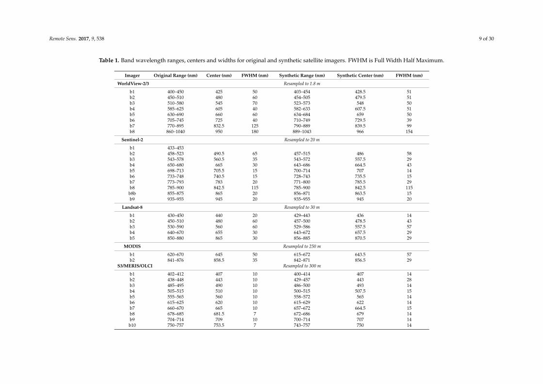
Table 1. Band wavelength ranges, centers and widths for original and synthetic satellite imagers. FWHM is Full Width Half Maximum.

Imager Original Range (nm) Center (nm) FWHM (nm) Synthetic Range (nm) Synthetic Center (nm) FWHM (nm)

WorldView-2/3 Resampled to 1.8 m

b1 400–450 425 50 403–454 428.5 51b2 450–510 480 60 454–505 479.5 51b3 510–580 545 70 523–573 548 50b4 585–625 605 40 582–633 607.5 51b5 630–690 660 60 634–684 659 50b6 705–745 725 40 710–749 729.5 39b7 770–895 832.5 125 790–889 839.5 99b8 860–1040 950 180 889–1043 966 154

Sentinel-2 Resampled to 20 m

b1 433–453b2 458–523 490.5 65 457–515 486 58b3 543–578 560.5 35 543–572 557.5 29b4 650–680 665 30 643–686 664.5 43b5 698–713 705.5 15 700–714 707 14b6 733–748 740.5 15 728–743 735.5 15b7 773–793 783 20 771–800 785.5 29b8 785–900 842.5 115 785–900 842.5 115

b8b 855–875 865 20 856–871 863.5 15b9 935–955 945 20 935–955 945 20

Landsat-8 Resampled to 30 m

b1 430–450 440 20 429–443 436 14b2 450–510 480 60 457–500 478.5 43b3 530–590 560 60 529–586 557.5 57b4 640–670 655 30 643–672 657.5 29b5 850–880 865 30 856–885 870.5 29

MODIS Resampled to 250 m

b1 620–670 645 50 615–672 643.5 57b2 841–876 858.5 35 842–871 856.5 29

S3/MERIS/OLCI Resampled to 300 m

b1 402–412 407 10 400–414 407 14b2 438–448 443 10 429–457 443 28b3 485–495 490 10 486–500 493 14b4 505–515 510 10 500–515 507.5 15b5 555–565 560 10 558–572 565 14b6 615–625 620 10 615–629 622 14b7 660–670 665 10 657–672 664.5 15b8 678–685 681.5 7 672–686 679 14b9 704–714 709 10 700–714 707 14

b10 750–757 753.5 7 743–757 750 14

Remote Sens. 2017, 9, 538 10 of 30

Table 1. Cont.

Imager Original Range (nm) Center (nm) FWHM (nm) Synthetic Range (nm) Synthetic Center (nm) FWHM (nm)

S3/MERIS/OLCI Resampled to 300 m

b11 757–762 759.5 5 750–764 757 14b12 772–787 779.5 15 757–800 778.5 43b13 855–875 865 20 842–885 863.5 43b14 880–890 885 10 871–899 885 28b15 895–905 900 10 885–913 899 28

Table 2. Band math and original specified wavelengths in nm for each algorithm used for blue-green algae/phycocyanin (BGA/PC) relative fluorescence unit (RFU)estimation at Harsha Lake. Float refers to floating point values of relative reflectance in the ENVI band math we used in this study at the specified wavelengths in nmfrom atmospherically corrected imagery. Float is not a variable; it is an IDL function used to prevent byte overflow errors during calculation. Asterisk after algorithmdenotes design specifically for phycocyanin detection.

Algorithm Reference ENVI Band Math with Original Specified Wavelengths

(Numerical Value = Wavelength in nm)

Al10SABI Alawadi et al. (2010) [41] (float(857) − float(644))/(float(458) + float(529))Am092Bsub Amin et al. (2009) [42] (float(678)) − (float(667))Am09KBBI Amin et al. (2009) [42] (float(686) − float(658))/(float(686) + float(658))Be162Bdiv This paper (float(681))/(float(665))

Be162Bsub * This paper (float(700)) − (float(622))Be16FLHblue Beck et al. (2016) [6] (float(529)) − [float(644) + (float(458) − float(644))]Be16FLHPhy * This paper (float(620)) − [float(709) + (float(560) − float(709))]Be16FLHviolet Beck et al. (2016) [6] (float(529)) − [float(644) + (float(5) − float(644))]Be16NDPhyI * This paper (float(700) − float(622))/(float(700) + float(622))

DE933BDA Dekker (1993) [26] ((float(600)) − (float(648))) − (float(625))Gi033BDA Gitelson et al. (2003) [43] ((1/float(672)) − (1/float(715))) × (float(757))Go04MCI Gower et al. (2004) [44] (((float(709)) − (float(681)) − ((float(753)) − (float(681)))))

HU103BDA * Hunter et al. (2008) [29] ((1/float(615)) − (1/float(600))) − (float(725))Kn07KIVU Kneubuhler et al. (2007) [45] (float(458) − float(644))/(float(529))Ku15PhyCI Kudela et al. (2015) [17] −1 × (((float(681)) − (float(665)) − ((float(709)) − (float(665)))))MI092BDA Mishra et al. (2009) [11] (float(700))/(float(600))

MM092BDA Mishra et al. (2009) [11] (float(724))/(float(600))MM12NDCI Mishra and Mishra (2012) [32] (float(700) − float(665))/(float(700) + float(665))

MM143BDAopt * Mishra and Mishra (2014) [16] ((1/float(629)) − (1/float(659))) × (float(724))MM143BDAver3merisver * Mishra and Mishra (2014) [16] ((1/float(620)) − (1/float(665))) × (float(778))

SI052BDA * Simis et al. (2005) [7] (float(709))/(float(620))SM122BDA S. Mishra (2012) [46] (float(709))/(float(600))SY002BDA * Schalles and Yacobi (2000) [47] (float(650))/(float(625))

Stu16Phy Stumpf et al. (2016) [24] (float(665) − float(620)) + ((float(620) − float(681)) × 0.74)Stu16PhyFLH * Stumpf et al. (2016) [24] (float(665)) − (float(681) + (float(620) − float(681)))

Wy08CI Wynne et al. (2008) [19] −1 × (((float(686)) − (float(672)) − ((float(715)) − (float(672)))))Zh10FLH Zhao et al. (2010) [48] (float(686)) − [float(715) + (float(672) − float(715))]

Remote Sens. 2017, 9, 538 11 of 30

3. Results

Single-band output from the Band Math function in ENVI for each BGA algorithm (ENVI BandMath Field in Table 2 and Table S1) was point sampled using the coincident surface observationlocations (Figure 2) to extract BGA index (image) values for comparison with measured YSI sondeBGA/PC relative fluorescence unit values (BGA_PC_RFU) collected within 1 h of the CASI overflight.Strong correlations (Pearson’s r2 > 0.6; p < 0.001) between image derived indices and densecoincident surface observations of BGA during this experiment indicate that Be162BsubPhy, SI052BDA,Be162B700sub601, Be16NDPhyI, Gi033BDA, Da052BDA, SM122BDA, Ku15PhyCI, MM092BDA,MI092BDA, Wy08CI, Zh10FLH, and MM12NDCI BGA algorithms worked well with CASI imagery.The Be162BsubPhy, SI052BDA, Am092Bsub, Be16NDPhyI, Mi092BDA, and MM12NDCI BGAalgorithms worked well (Pearson’s r2 > 0.6; p < 0.001) with simulated WorldView-2 and -3, imagery; theBe162Bsub algorithm with simulated Sentinel-2 imagery; the Be16FLHviolet with simulated Landsat-8imagery; and the MM092BDA, Be16NDPhyI, MM12NDCI, Go04MCI, Ku15PhyCI, Wy08CI, SI052BDA,Be162BsubPhy, and Hu103BDA BGA algorithms with simulated Sentinel-3/MERIS/OLCI imagery.The Be162BsubPhy algorithm was the most widely applicable BGA algorithm with good performancefor CASI, WorldView-2 and -3, Sentinel-2 and MERIS-like imagery and limited performance withMODIS imagery. The Be16FLHviolet “greenness” algorithm yielded the best (although poor) BGA/PCestimates with simulated Landsat-8 imagery.

We also conducted an extensive survey of other water quality parameters in the lake at the timeof acquisition in order to determine why some proxy indices such as Chl-a may also work with regardto BGA estimation. Details of our statistical treatment of the data are available in Beck et al. [6]. Type 1(Pearson’s) r2 values were used to evaluate algorithm performance with raw index values vs. BGA/PCrelative fluorescence units (BGA_PC_RFU) values measured with YSI BGA optical sondes in the water(Table S2) and as index values normalized to BGA values vs. BGA_PC_RFU values (Table S3) tofacilitate comparison.

We used a critical p-value of 0.001 for all Pearson’s r Type 1 regression tests. Some researchersprefer Standard Error of Regression (Standard Error of Estimate or S) values to Type 1 (Pearson’s)r2 values so we have also included them for the top performing algorithms from Table S3 forcomparison (Table 3). Other researchers prefer Type 2 regressions [48] to test correlations of observedvs. measured values [49] in natural systems. Therefore, we also applied the Type 2 geometric meanmethod of Peltzer [48] to BGA estimation at Harsha (East Fork) Lake with all results again normalizedto calculated BGA values for top performing algorithms for each imager by Type 1 regression tests [17](Table 4). A combined error budget for radiometry and multispectral image synthesis is presented inthe chlorophyll-a companion paper [6].

Examples of promising algorithms as applied to real CASI aircraft hyperspectral imagery andsynthetic multispectral satellite imagery are discussed below.

Remote Sens. 2017, 9, 538 12 of 30

Table 3. Performance of Algorithms for BGA Estimation at Harsha (East Fork) Lake with all results normalized to calculated BGA values with additional Type 1Regression tests for Standard Error of Regression (Standard Error of Estimate or S values) and associated statistics. Float refers to floating point values of relativereflectance in the ENVI band math we used in this study at the specified wavelengths in nm from atmospherically corrected imagery. Float is not a variable; it is anIDL function used to prevent byte overflow errors during calculation.

Algorithms By Satellite/Sensor R-Squared Adj. R-Sqr. Std. Err. Reg. Std. Dev. n Residual Mean Square p Conf. Level

S

CASIBe152BsubPhy715sub615 0.763 0.754 1.974 3.978 29 3.896 <0.001 95.0%(float(715)) − (float(615))

WV2Be162Bsub 0.790 0.782 1.871 4.007 29 3.500 <0.001 95.0%(float(730)) − (float(608))

S2Be162Bsub 0.704 0.693 2.219 4.007 29 4.924 <0.001 95.0%(float(736)) − (float(665))

L8Be15Flhviolet 0.339 0.314 3.318 4.007 29 11.011 <0.001 95.0%(float(530)) − [float(640) + (float(430) − float(640))]

MODISMM12NDCI4 0.183 0.066 2.938 3.040 9 8.632 0.251 95.0%(float(857) − float(644))/(float(857) + float(644))

MERISMM092BDA 0.863 0.843 1.203 3.040 9 1.448 <0.001 95.0%(float(707))/(float(679))

Table 4. Performance of Algorithms for BGA Estimation at Harsha (East Fork) Lake with all results normalized to calculated BGA values with additional Type 2Geometric Mean Tests for top performing algorithms by Type 1 Regression tests.

Algorithms By Satellite/Sensor Spatial n Geometric Geometric Geometric Geometric Standard Standard

(Band Math in nm) Res. (m) Mean Mean Mean Mean Deviation of Deviation of

Slope Intercept Correlation Correlation Slope Y-intercept

Coefficient Coefficient

Squared

CASIBe152BsubPhy715sub615 1 29 1.141 −1.500 0.881 0.777 0.107 1.199(float(715)) − (float(615))

WV2Be162Bsub 1.8 29 1.128 −1.376 0.889 0.790 0.102 1.150(float(730)) − (float(608))

S2Be162Bsub 20 29 1.194 −2.087 0.839 0.704 0.130 1.456(float(736)) − (float(665))

L8Be15Flhviolet 30 29 1.708 −7.773 0.582 0.339 0.301 3.317(float(530)) − [float(640) + (float(430) − float(640))]

MODISMM12NDCI412 250 9 2.339 −13.716 0.428 0.183 0.946 9.760(float(857) − float(644))/(float(857) + float(644))

MERISMM092BDA 300 9 1.077 −0.783 0.929 0.863 0.153 1.624(float(707))/(float(679))

Remote Sens. 2017, 9, 538 13 of 30

3.1. CASI Imagery

We applied 27 algorithms in the form of 70 variants to the 1-m, 48-band CASI VNIR hyperspectralreflectance image mosaic (Tables S1, S2 and S4 and Figure 7). CASI has a narrow band capableof measuring the 620 nm phycocyanin absorption feature. The performance of each algorithm inTables 2 and 3 applied to the CASI reflectance imagery was then evaluated using 29 coincidentsurface observations for the sake of consistency with synthetic WorldView-2 and -3, Sentinel-2 andLandsat-8 imagery (other sub-30 m imagery). Simple subtraction, ratio-based and shape metric (secondderivative) algorithms that include the 620 nm phycocyanin absorption feature and/or reflectance inthe near-infrared suppress illumination variation well and had the best performance with regardto BGA estimation. In decreasing order of performance (Pearson’s r2), the CASIBe152BsubPhy,CASISI052BDA, CASIBe162B700sub601, CASIBe16NDPhyI, CASIGi033BDA, CASIDa052BDA,CASISM122BDA, CASIKu15PhyCI, CASIMM092BDA, CASIMi092BDA, CASIWy08CI, CASIZh10FLH,and CASIMM12NDCI algorithms worked well (Pearson’s r2 > 0.600) for BGA estimation with CASIimagery. Index imagery with raw and normalized index Type 1 (Pearson’s r) linear regressions areshown for the best performing algorithm (CASIBe152BsubPhy) in Figure 7.

Remote Sens. 2017, 9, x FOR PEER REVIEW 13 of 30

3.1. CASI Imagery

We applied 27 algorithms in the form of 70 variants to the 1-m, 48-band CASI VNIR

hyperspectral reflectance image mosaic (Tables S1, S2 and S4 and Figure 7). CASI has a narrow band

capable of measuring the 620 nm phycocyanin absorption feature. The performance of each algorithm

in Tables 2 and 3 applied to the CASI reflectance imagery was then evaluated using 29 coincident

surface observations for the sake of consistency with synthetic WorldView-2 and -3, Sentinel-2 and

Landsat-8 imagery (other sub-30 m imagery). Simple subtraction, ratio-based and shape metric

(second derivative) algorithms that include the 620 nm phycocyanin absorption feature and/or

reflectance in the near-infrared suppress illumination variation well and had the best performance

with regard to BGA estimation. In decreasing order of performance (Pearson’s r2), the

CASIBe152BsubPhy, CASISI052BDA, CASIBe162B700sub601, CASIBe16NDPhyI, CASIGi033BDA,

CASIDa052BDA, CASISM122BDA, CASIKu15PhyCI, CASIMM092BDA, CASIMi092BDA,

CASIWy08CI, CASIZh10FLH, and CASIMM12NDCI algorithms worked well (Pearson’s r2 > 0.600)

for BGA estimation with CASI imagery. Index imagery with raw and normalized index Type 1

(Pearson’s r) linear regressions are shown for the best performing algorithm (CASIBe152BsubPhy) in

Figure 7.

(a)

(b)

Figure 7. Cont.

Remote Sens. 2017, 9, 538 14 of 30Remote Sens. 2017, 9, x FOR PEER REVIEW 14 of 30

(c)

Figure 7. Results of CASIBe152BsubPhy (715sub615) algorithm (this paper) as raw index values as

applied to original CASI imagery with brighter pixels in the reservoir indicating higher BGA/PC

values (a). Evaluation via observed (Y axis = BGA_PC_RFU) vs. predicted (calculated) raw

CASIBe152BsubPhy (715sub615) index value with Pearson’s r2 (r2 = 0.776 p < 0.001, n = 29 to avoid

shorelines) (b). Evaluation via observed (Y axis = BGA_PC_RFU) vs. normalized predicted

(calculated) BGA values (CASIBe152BsubPhyPHY) with Pearson’s r2 (r2 = 0.776, p < 0.001, n = 29 to

avoid shorelines) (c). Details of the synthetic bands and band math are available in Tables 1 and 2,

respectively.

Excellent results for several algorithms with CASI high resolution aircraft imagery for

BGA_PC_RFU value estimation and their resulting index maps (Figure 7a) reveal considerable spatial

heterogeneity at the 1 m scale in Harsha Lake at the time of aircraft image acquisition. This spatial

heterogeneity of BGA/PC values in the imagery is supported by strong correlations with dense

coincident surface observations (Figure 7b,c). Figure 5a also shows a strong correlation between the

locations of the inflow from the East Fork of the Little Miami River in the NE corner of the image and

the largest region of high BGA_PC_RFU values. In general the east basin of Harsha Lake has higher

BGA/PC values than the west basin (Figure 7a). One can also see gyre-like structures associated with

the dissipation of the BGA/PC-rich waters from east to west across the lake. The spatial heterogeneity

displayed by the processed CASI images is masked to varying degrees in the coarser spatial

resolution synthetic satellite data derived from this real CASI relative reflectance data as shown

below. This masking of spatial heterogeneity in the east and west basins in coarse resolution satellite

imagery also appears to exaggerate the contrast in BGA/PC values between the east and west basins

of Harsha Lake. We view the high correlations of coincident surface observations with predicted

BGA/PC values with coarse resolution synthetic MERIS/OLCI data presented below with some

caution accordingly.

3.2. WorldView-2 (Synthetic)

We applied 11 existing and two new algorithms in the form of 25 variants to synthetic 1.8-m,

WorldView-2 imagery to examine the degree of portability of some of the simpler algorithms between

(synthetic) satellite imaging systems (Tables S1, S2 and 5 and Figure 8). WorldView-2 has a narrow

band capable of measuring the 620 nm phycocyanin absorption feature. We also applied a new

subtraction algorithm (Be162Bsub) and a new modified NDCI algorithm [32] (Be16NDPhyI) tuned to

the 620 nm phycocyanin absorption feature. In decreasing order of performance, seven algorithms,

WV2Be162Bsub, WV2SiO52BDA, WV2Am092Bsub, WV2Be16NDPhyI WV2Mi092BDA, and

WV2MM12NDCI, had acceptable performance (Pearson’s r2 > 0.6; p < 0.001) with this sensor in this

exercise (Figure 8). The performance of each algorithm in Tables 2 and S1 applied to the synthetic

WorldView-2 imagery was evaluated using 29 coincident surface observations (Tables S2 and 5). As

with CASI, simple subtraction and ratio-based algorithms that include the 620 nm phycocyanin

absorption feature and/or reflectance in the near-infrared suppress illumination variation well and

had the best performance with regard to BGA/PC value estimation. Index imagery with raw and

Figure 7. Results of CASIBe152BsubPhy (715sub615) algorithm (this paper) as raw index values asapplied to original CASI imagery with brighter pixels in the reservoir indicating higher BGA/PC values(a). Evaluation via observed (Y axis = BGA_PC_RFU) vs. predicted (calculated) raw CASIBe152BsubPhy(715sub615) index value with Pearson’s r2 (r2 = 0.776 p < 0.001, n = 29 to avoid shorelines) (b).Evaluation via observed (Y axis = BGA_PC_RFU) vs. normalized predicted (calculated) BGA values(CASIBe152BsubPhyPHY) with Pearson’s r2 (r2 = 0.776, p < 0.001, n = 29 to avoid shorelines) (c). Detailsof the synthetic bands and band math are available in Tables 1 and 2, respectively.

Excellent results for several algorithms with CASI high resolution aircraft imagery forBGA_PC_RFU value estimation and their resulting index maps (Figure 7a) reveal considerable spatialheterogeneity at the 1 m scale in Harsha Lake at the time of aircraft image acquisition. This spatialheterogeneity of BGA/PC values in the imagery is supported by strong correlations with densecoincident surface observations (Figure 7b,c). Figure 5a also shows a strong correlation between thelocations of the inflow from the East Fork of the Little Miami River in the NE corner of the image andthe largest region of high BGA_PC_RFU values. In general the east basin of Harsha Lake has higherBGA/PC values than the west basin (Figure 7a). One can also see gyre-like structures associated withthe dissipation of the BGA/PC-rich waters from east to west across the lake. The spatial heterogeneitydisplayed by the processed CASI images is masked to varying degrees in the coarser spatial resolutionsynthetic satellite data derived from this real CASI relative reflectance data as shown below. Thismasking of spatial heterogeneity in the east and west basins in coarse resolution satellite imagery alsoappears to exaggerate the contrast in BGA/PC values between the east and west basins of HarshaLake. We view the high correlations of coincident surface observations with predicted BGA/PC valueswith coarse resolution synthetic MERIS/OLCI data presented below with some caution accordingly.

3.2. WorldView-2 (Synthetic)

We applied 11 existing and two new algorithms in the form of 25 variants to synthetic 1.8-m,WorldView-2 imagery to examine the degree of portability of some of the simpler algorithms between(synthetic) satellite imaging systems (Tables S1, S2 and S4 and Figure 8). WorldView-2 has anarrow band capable of measuring the 620 nm phycocyanin absorption feature. We also applieda new subtraction algorithm (Be162Bsub) and a new modified NDCI algorithm [32] (Be16NDPhyI)tuned to the 620 nm phycocyanin absorption feature. In decreasing order of performance, sevenalgorithms, WV2Be162Bsub, WV2SiO52BDA, WV2Am092Bsub, WV2Be16NDPhyI WV2Mi092BDA,and WV2MM12NDCI, had acceptable performance (Pearson’s r2 > 0.6; p < 0.001) with this sensor in thisexercise (Figure 8). The performance of each algorithm in Table 2 and Table S1 applied to the syntheticWorldView-2 imagery was evaluated using 29 coincident surface observations (Table S2 and S4).As with CASI, simple subtraction and ratio-based algorithms that include the 620 nm phycocyaninabsorption feature and/or reflectance in the near-infrared suppress illumination variation well and

Remote Sens. 2017, 9, 538 15 of 30

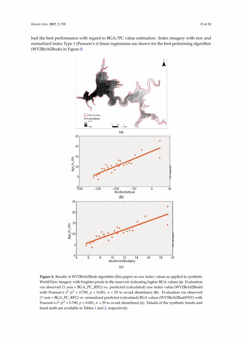
had the best performance with regard to BGA/PC value estimation. Index imagery with raw andnormalized index Type 1 (Pearson’s r) linear regressions are shown for the best performing algorithm(WV2Be162Bsub) in Figure 8.


normalized index Type 1 (Pearson’s r) linear regressions are shown for the best performing algorithm

(WV2Be162Bsub) in Figure 8.

(a)

(b)

(c)

Figure 8. Results of WV2Be162Bsub algorithm (this paper) as raw index values as applied to synthetic

WorldView imagery with brighter pixels in the reservoir indicating higher BGA values (a). Evaluation

via observed (Y axis = BGA_PC_RFU) vs. predicted (calculated) raw index value (WV2Be162Bsub)

with Pearson’s r2 (r2 = 0.790, p < 0.001, n = 29 to avoid shorelines) (b). Evaluation via observed (Y axis

= BGA_PC_RFU) vs. normalized predicted (calculated) BGA values (WV2Be162BsubPHY) with

Pearson’s r2 (r2 = 0.790, p < 0.001, n = 29 to avoid shorelines) (c). Details of the synthetic bands and

band math are available in Tables 1 and 2, respectively.

Figure 8. Results of WV2Be162Bsub algorithm (this paper) as raw index values as applied to syntheticWorldView imagery with brighter pixels in the reservoir indicating higher BGA values (a). Evaluationvia observed (Y axis = BGA_PC_RFU) vs. predicted (calculated) raw index value (WV2Be162Bsub)with Pearson’s r2 (r2 = 0.790, p < 0.001, n = 29 to avoid shorelines) (b). Evaluation via observed(Y axis = BGA_PC_RFU) vs. normalized predicted (calculated) BGA values (WV2Be162BsubPHY) withPearson’s r2 (r2 = 0.790, p < 0.001, n = 29 to avoid shorelines) (c). Details of the synthetic bands andband math are available in Tables 1 and 2, respectively.

Remote Sens. 2017, 9, 538 16 of 30

3.3. Sentinel-2 (Synthetic)

We applied eight existing and five new algorithms in the form of 23 variants to the 20-m,synthetic Sentinel-2 imagery. Sentinel-2 lacks a narrow band capable of measuring the 620 nmphycocyanin absorption feature. The performance of each algorithm in Tables 2 and 3 applied to thesynthetic Sentinel-2 imagery was evaluated using 29 coincident surface observations coincident surfaceobservations chosen to avoid pixels that mixed land and water at 20 and 30 m spatial resolutions(Tables S2 and S4). Six algorithms, S2Be162Bsub, S2SiO52BDA, S2Am092Bsub, S2MM12NDCI,S2Mi092BDA, and S2Be16NDPhyI, had acceptable performance (Pearson’s r2 > 0.6; p < 0.001) withthis sensor in this experiment. The S2Be162Bsub, S2SiO52BDA, S2MM12NDCI, S2Mi092BDA, andS2Be16NDPhyI algorithms also appear to have good portability between CASI, WorldView-2/-3 andSentinel-2 imagery (Tables S2 and S4 and Figure 9). The strong performance of these algorithms withsynthetic Sentinel-2 imagery and their wide swaths and dual constellation suggest that Sentinel-2satellites will play a key role in future BGA monitoring systems for inland water quality. Indeximagery with raw and normalized index Type 1 (Pearson’s r) linear regressions are shown for the bestperforming algorithm (S2Be162Bsub) in Figure 9.


3.3. Sentinel-2 (Synthetic)

We applied eight existing and five new algorithms in the form of 23 variants to the 20-m,

synthetic Sentinel-2 imagery. Sentinel-2 lacks a narrow band capable of measuring the 620 nm

phycocyanin absorption feature. The performance of each algorithm in Tables 2 and 3 applied to the

synthetic Sentinel-2 imagery was evaluated using 29 coincident surface observations coincident

surface observations chosen to avoid pixels that mixed land and water at 20 and 30 m spatial

resolutions (Tables S2 and 5). Six algorithms, S2Be162Bsub, S2SiO52BDA, S2Am092Bsub,

S2MM12NDCI, S2Mi092BDA, and S2Be16NDPhyI, had acceptable performance (Pearson’s r2 > 0.6; p

< 0.001) with this sensor in this experiment. The S2Be162Bsub, S2SiO52BDA, S2MM12NDCI,

S2Mi092BDA, and S2Be16NDPhyI algorithms also appear to have good portability between CASI,

WorldView-2/-3 and Sentinel-2 imagery (Tables S2 and 5 and Figure 9). The strong performance of

these algorithms with synthetic Sentinel-2 imagery and their wide swaths and dual constellation

suggest that Sentinel-2 satellites will play a key role in future BGA monitoring systems for inland

water quality. Index imagery with raw and normalized index Type 1 (Pearson’s r) linear regressions

are shown for the best performing algorithm (S2Be162Bsub) in Figure 9.

(a)

(b)

Figure 9. Cont.


(c)

Figure 9. Results of S2Be162Bsub algorithm (this paper) converted to BGA values as applied to

synthetic Sentinel-2 imagery with brighter pixels in the reservoir indicating higher BGA values (a).

Evaluation via observed (Y axis = BGA_PC_RFU) vs. predicted (calculated) raw index value

(S2Be162Bsub) with Pearson’s r2 (r2 = 0.704, p < 0.001, n = 29 to avoid shorelines) (b). Evaluation via

observed (Y axis = BGA_PC_RFU) vs. normalized predicted (calculated) BGA values

(S2Be162BsubPHY) with Pearson’s r2 (r2 = 0.704, p value < 0.001, n = 29 to avoid shorelines) (c). The

CASI data allowed the synthesis of Sentinel-2 bands 2 through 9 only. Details of the synthetic bands

and band math are available in Tables 1 and 2, respectively.

3.4. Landsat-8 (Synthetic)

We applied nine existing algorithms in the form of 17 variants to the 30-m, synthetic Landsat-8

imagery. Landsat-8 lacks a narrow band capable of measuring the 620 nm phycocyanin absorption

feature. All of the algorithms applied here were indirect Chl-a proxy algorithms [6] accordingly.

Moreover, the widths and positions of Landsat-8 bands also make the application of shape metrics

for the Chl-a NIR reflectance peak feature infeasible and the application of some of the simple band

ratio algorithms challenging (Tables 2 and S1, Figure 10). The best performing algorithm was the

green peak FLH Violet algorithm that incorporated the new ultra blue (“violet”) coastal band for this

sensor in this experiment [6].

(a)

Figure 9. Results of S2Be162Bsub algorithm (this paper) converted to BGA values as applied to syntheticSentinel-2 imagery with brighter pixels in the reservoir indicating higher BGA values (a). Evaluationvia observed (Y axis = BGA_PC_RFU) vs. predicted (calculated) raw index value (S2Be162Bsub)with Pearson’s r2 (r2 = 0.704, p < 0.001, n = 29 to avoid shorelines) (b). Evaluation via observed(Y axis = BGA_PC_RFU) vs. normalized predicted (calculated) BGA values (S2Be162BsubPHY) withPearson’s r2 (r2 = 0.704, p value < 0.001, n = 29 to avoid shorelines) (c). The CASI data allowed thesynthesis of Sentinel-2 bands 2 through 9 only. Details of the synthetic bands and band math areavailable in Tables 1 and 2, respectively.


We applied nine existing algorithms in the form of 17 variants to the 30-m, synthetic Landsat-8imagery. Landsat-8 lacks a narrow band capable of measuring the 620 nm phycocyanin absorptionfeature. All of the algorithms applied here were indirect Chl-a proxy algorithms [6] accordingly.Moreover, the widths and positions of Landsat-8 bands also make the application of shape metrics forthe Chl-a NIR reflectance peak feature infeasible and the application of some of the simple band ratioalgorithms challenging (Table 2 and Table S1, Figure 10). The best performing algorithm was the greenpeak FLH Violet algorithm that incorporated the new ultra blue (“violet”) coastal band for this sensorin this experiment [6].


(c)

Figure 9. Results of S2Be162Bsub algorithm (this paper) converted to BGA values as applied to

synthetic Sentinel-2 imagery with brighter pixels in the reservoir indicating higher BGA values (a).

Evaluation via observed (Y axis = BGA_PC_RFU) vs. predicted (calculated) raw index value

(S2Be162Bsub) with Pearson’s r2 (r2 = 0.704, p < 0.001, n = 29 to avoid shorelines) (b). Evaluation via

observed (Y axis = BGA_PC_RFU) vs. normalized predicted (calculated) BGA values

(S2Be162BsubPHY) with Pearson’s r2 (r2 = 0.704, p value < 0.001, n = 29 to avoid shorelines) (c). The

CASI data allowed the synthesis of Sentinel-2 bands 2 through 9 only. Details of the synthetic bands

and band math are available in Tables 1 and 2, respectively.


We applied nine existing algorithms in the form of 17 variants to the 30-m, synthetic Landsat-8

imagery. Landsat-8 lacks a narrow band capable of measuring the 620 nm phycocyanin absorption

feature. All of the algorithms applied here were indirect Chl-a proxy algorithms [6] accordingly.

Moreover, the widths and positions of Landsat-8 bands also make the application of shape metrics

for the Chl-a NIR reflectance peak feature infeasible and the application of some of the simple band

ratio algorithms challenging (Tables 2 and S1, Figure 10). The best performing algorithm was the

green peak FLH Violet algorithm that incorporated the new ultra blue (“violet”) coastal band for this

sensor in this experiment [6].

(a)

Figure 10. Cont.


(b)

(c)

Figure 10. Results of new FLH Violet algorithm [6] as raw index values as applied to synthetic Landsat

8 imagery with brighter pixels in the reservoir indicating higher BGA values (a). Evaluation via

observed (Y axis = BGA_PC_RFU) vs. predicted (calculated) raw index value (L8Be15Flhviolet) with

Pearson’s r2 (r2 = 0.339, p < 0.001, n = 29 to avoid shorelines) (b). Evaluation via observed (Y axis =

BGA_PC_RFU) vs. normalized predicted (calculated) BGA values (L8_FlhvioletPHY) with Pearson’s

r2 (r2 = 0.339, p < 0.001, n = 29 to avoid shorelines) (c). Details of the synthetic bands and band math

are available in Tables 1 and 2, respectively.

None of the simple spectrally-oriented semi-analytical algorithms (based at least in part on

known spectral features associated with known water quality parameters) considered here had

acceptable performance (Pearson’s r2 > 0.6; p < 0.001) with regard to BGA estimation with Landsat-8

in this exercise due to its design for land vegetation (Chl-a) rather than BGA/PC in water. Index

imagery with raw and normalized index Type 1 (Pearson’s r) linear regressions are shown for the

best performing algorithm (L8Be15Flhviolet) in Figure 10. Local empirical algorithms based on other

water quality parameters such as Chl-a and turbidity with local calibration and validation are

required for use with Landsat-8 for reliable BGA estimation because Landsat-8 cannot sense the 620

nm phycocyanin absorption feature [22].

3.5. MODIS (Synthetic)

We applied three existing algorithms (NDCI, 2BDA and Am092Bsub) in the form of six variants

to synthetic MODIS bands 1 and 2 [43] for BGA estimation with limited success (Tables S1, S2 and 5,

Figure 11). None of the spectrally-oriented semi-analytical algorithms considered here had acceptable

performance (Pearson’s r2 > 0.6; p < 0.001) with regard to BGA estimation with this sensor in this

experiment due to the wide MODIS bands. While MODIS could be a part of operational monitoring

systems, its wide bands and coarse spatial resolution suggest that it will have limited value in

operational monitoring systems for inland water quality, especially for smaller water bodies less than

Figure 10. Results of new FLH Violet algorithm [6] as raw index values as applied to synthetic Landsat 8imagery with brighter pixels in the reservoir indicating higher BGA values (a). Evaluation via observed(Y axis = BGA_PC_RFU) vs. predicted (calculated) raw index value (L8Be15Flhviolet) with Pearson’s r2

(r2 = 0.339, p < 0.001, n = 29 to avoid shorelines) (b). Evaluation via observed (Y axis = BGA_PC_RFU)vs. normalized predicted (calculated) BGA values (L8_FlhvioletPHY) with Pearson’s r2 (r2 = 0.339,p < 0.001, n = 29 to avoid shorelines) (c). Details of the synthetic bands and band math are available inTables 1 and 2, respectively.

None of the simple spectrally-oriented semi-analytical algorithms (based at least in part on knownspectral features associated with known water quality parameters) considered here had acceptableperformance (Pearson’s r2 > 0.6; p < 0.001) with regard to BGA estimation with Landsat-8 in thisexercise due to its design for land vegetation (Chl-a) rather than BGA/PC in water. Index imagery withraw and normalized index Type 1 (Pearson’s r) linear regressions are shown for the best performingalgorithm (L8Be15Flhviolet) in Figure 10. Local empirical algorithms based on other water qualityparameters such as Chl-a and turbidity with local calibration and validation are required for usewith Landsat-8 for reliable BGA estimation because Landsat-8 cannot sense the 620 nm phycocyaninabsorption feature [22].

3.5. MODIS (Synthetic)

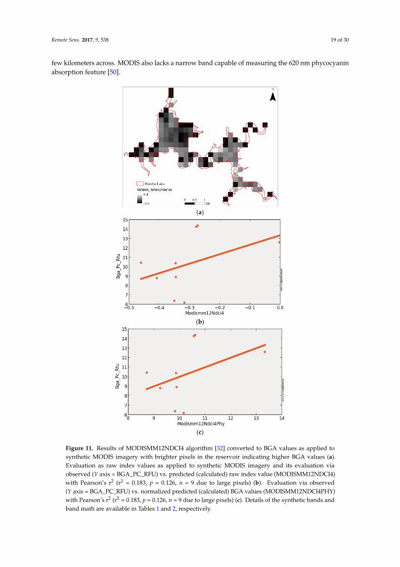
We applied three existing algorithms (NDCI, 2BDA and Am092Bsub) in the form of six variantsto synthetic MODIS bands 1 and 2 [43] for BGA estimation with limited success (Tables S1, S2 and S4,Figure 11). None of the spectrally-oriented semi-analytical algorithms considered here had acceptableperformance (Pearson’s r2 > 0.6; p < 0.001) with regard to BGA estimation with this sensor in thisexperiment due to the wide MODIS bands. While MODIS could be a part of operational monitoringsystems, its wide bands and coarse spatial resolution suggest that it will have limited value inoperational monitoring systems for inland water quality, especially for smaller water bodies less than a

Remote Sens. 2017, 9, 538 19 of 30

few kilometers across. MODIS also lacks a narrow band capable of measuring the 620 nm phycocyaninabsorption feature [50].


a few kilometers across. MODIS also lacks a narrow band capable of measuring the 620 nm

phycocyanin absorption feature [50].

(a)

(b)

(c)

Figure 11. Results of MODISMM12NDCI4 algorithm [32] converted to BGA values as applied to

synthetic MODIS imagery with brighter pixels in the reservoir indicating higher BGA values (a).

Evaluation as raw index values as applied to synthetic MODIS imagery and its evaluation via

observed (Y axis = BGA_PC_RFU) vs. predicted (calculated) raw index value (MODISMM12NDCI4)

with Pearson’s r2 (r2 = 0.183, p = 0.126, n = 9 due to large pixels) (b). Evaluation via observed (Y axis =

BGA_PC_RFU) vs. normalized predicted (calculated) BGA values (MODISMM12NDCI4PHY) with

Pearson’s r2 (r2 = 0.183, p = 0.126, n = 9 due to large pixels) (c). Details of the synthetic bands and band

math are available in Tables 1 and 2, respectively.

Figure 11. Results of MODISMM12NDCI4 algorithm [32] converted to BGA values as applied tosynthetic MODIS imagery with brighter pixels in the reservoir indicating higher BGA values (a).Evaluation as raw index values as applied to synthetic MODIS imagery and its evaluation viaobserved (Y axis = BGA_PC_RFU) vs. predicted (calculated) raw index value (MODISMM12NDCI4)with Pearson’s r2 (r2 = 0.183, p = 0.126, n = 9 due to large pixels) (b). Evaluation via observed(Y axis = BGA_PC_RFU) vs. normalized predicted (calculated) BGA values (MODISMM12NDCI4PHY)with Pearson’s r2 (r2 = 0.183, p = 0.126, n = 9 due to large pixels) (c). Details of the synthetic bands andband math are available in Tables 1 and 2, respectively.

Remote Sens. 2017, 9, 538 20 of 30

The performance of each algorithm in Table 2 and Table S1 applied to the synthetic MODISimagery was evaluated using nine coincident surface observations. These nine points were chosen toavoid pixels that mixed land and water at 250 and 300 m spatial resolutions. MODIS bands 1 and 2were simulated with the CASI data at 250 m spatial resolution to facilitate comparison of algorithmperformance. MODIS bands 1 and 2 are commonly available at the 250 m spatial resolution and arepart of the better performing algorithm (NDCI). This suggests that MODIS NDCI may have somemodest utility with regard to BGA estimation and algal bloom monitoring in some larger inland waterbodies. The large pixel sizes associated with MODIS make it more appropriate for relatively largewater bodies using other water quality parameters such as Chl-a or turbidity as proxies for BGA/PC.MODIS imagery will also require severe masking to avoid shorelines (mixed land and water pixels)(Figure 9a). Index imagery with raw and normalized index Type 1 (Pearson’s r) linear regressions areshown for the best performing algorithm (MODISMM12NDCI4) in Figure 11.

3.6. MERIS (Synthetic)

We applied the 13 existing and four new algorithms in the form of 35 variants for BGA estimationto synthetic Sentinel-3/MERIS/OLCI data for Harsha Lake with limited success (Tables S1, S2 and S4,Figure 12) before severe masking (Figure 12a). MERIS has a narrow band capable of measuringthe 620 nm phycocyanin absorption feature. Ten of the BGA (direct) and Chl-a (indirect or proxy)spectrally-oriented semi-analytical algorithms considered here had acceptable performance (Pearson’sr2 > 0.6; p < 0.001) when tested against in situ YSI BGA probe data (BGA_PC_RFU) with this sensor inthis experiment after severe masking. In order of decreasing performance, the MERISMM092BDA,MERISBe16NDPhyI, MERISMM12NDCI, MERISGo04MCI, MERISWy08CI and MERISKu15PhyCI,MERISSi052BDA, MERISBe162Bsub, MERISHu103BDA, and MERISMM143BDAopt algorithms allestimated BGA well in this exercise. We agree that MERIS/OLCI can be a part of operational waterquality monitoring systems [20]. However, high-spatial resolution CASI data show that there wassignificant spatial heterogeneity in the values of BGA on a scale much finer than either Sentinel-3/MERIS/OLCI (300 m) or MODIS (250 m) pixels. Index imagery with raw and normalized index Type 1(Pearson’s r) linear regressions are shown for the best performing algorithm (MERISMMO92BDA) inFigure 12.

Type 1 Standard Error of Regression (Standard Error of Estimate or S) values track our Pearson’sr2 values (Table 3). The Type 2 geometric mean regressions [41] show an ordering of correlation similarto those of Type 1 regressions [17,49] with somewhat poorer results for Landsat-8 (Table 4).


The performance of each algorithm in Tables 2 and S1 applied to the synthetic MODIS imagery

was evaluated using nine coincident surface observations. These nine points were chosen to avoid

pixels that mixed land and water at 250 and 300 m spatial resolutions. MODIS bands 1 and 2 were

simulated with the CASI data at 250 m spatial resolution to facilitate comparison of algorithm

performance. MODIS bands 1 and 2 are commonly available at the 250 m spatial resolution and are

part of the better performing algorithm (NDCI). This suggests that MODIS NDCI may have some

modest utility with regard to BGA estimation and algal bloom monitoring in some larger inland

water bodies. The large pixel sizes associated with MODIS make it more appropriate for relatively

large water bodies using other water quality parameters such as Chl-a or turbidity as proxies for

BGA/PC. MODIS imagery will also require severe masking to avoid shorelines (mixed land and water

pixels) (Figure 9a). Index imagery with raw and normalized index Type 1 (Pearson’s r) linear

regressions are shown for the best performing algorithm (MODISMM12NDCI4) in Figure 11.

3.6. MERIS (Synthetic)

We applied the 13 existing and four new algorithms in the form of 35 variants for BGA

estimation to synthetic Sentinel-3/MERIS/OLCI data for Harsha Lake with limited success (Tables S1,

S2 and 5, Figure 12) before severe masking (Figure 12a). MERIS has a narrow band capable of

measuring the 620 nm phycocyanin absorption feature. Ten of the BGA (direct) and Chl-a (indirect

or proxy) spectrally-oriented semi-analytical algorithms considered here had acceptable performance

(Pearson’s r2 > 0.6; p < 0.001) when tested against in situ YSI BGA probe data (BGA_PC_RFU) with

this sensor in this experiment after severe masking. In order of decreasing performance, the

MERISMM092BDA, MERISBe16NDPhyI, MERISMM12NDCI, MERISGo04MCI, MERISWy08CI and

MERISKu15PhyCI, MERISSi052BDA, MERISBe162Bsub, MERISHu103BDA, and

MERISMM143BDAopt algorithms all estimated BGA well in this exercise. We agree that

MERIS/OLCI can be a part of operational water quality monitoring systems [20]. However, high-

spatial resolution CASI data show that there was significant spatial heterogeneity in the values of

BGA on a scale much finer than either Sentinel-3/MERIS/OLCI (300 m) or MODIS (250 m) pixels.

Index imagery with raw and normalized index Type 1 (Pearson’s r) linear regressions are shown for

the best performing algorithm (MERISMMO92BDA) in Figure 12.

Type 1 Standard Error of Regression (Standard Error of Estimate or S) values track our Pearson’s

r2 values (Table 3). The Type 2 geometric mean regressions [41] show an ordering of correlation

similar to those of Type 1 regressions [17,49] with somewhat poorer results for Landsat-8 (Table 4).

(a)

Figure 12. Cont.


(b)

(c)

Figure 12. Results of MERISMM092BDA algorithm (Mishra and Mishra, 2009) as raw BGA index

values as applied to synthetic MERIS imagery with brighter pixels in the reservoir indicating higher

BGA values (a). Evaluation via observed (Y axis = BGA_PC_RFU) vs. predicted (calculated) raw BGA

index values (MERISMM092BDA) values with Pearson’s r2 (r2 = 0.863, p < 0.001, n = 9 due to large

pixels) (b). Evaluation via observed (Y axis = BGA_PC_RFU) vs. normalized predicted (calculated)

BGA (MERISMM092BDA) values with Pearson’s r2 (r2 = 0.863, p < 0.001, n = 9 due to large pixels) (c).

Details of the synthetic bands and band math are available in Tables 1 and 2, respectively.

4. Discussion

The focus of this study is on simple, portable, semi-analytical algorithms based on the

phycocyanin and Chl-a spectral signatures. CASI, WorldView and MERIS are capable of sensing the

narrow 620 nm phycocyanin absorption feature (Figure 1, Table 1). Algorithms specifically tuned to

this phycocyanin feature had the best performance for 1 m CASI imagery (CASIBe152BsubPhy, r2 =

0.776) and 1.8 m WorldView imagery (WV2Be162Bsub, r2 = 0.790) and the second best for 300 m

MERIS imagery (MERISBe16NDPhyI, r2 = 0.852) (Table S4). An indirect BGA index algorithm,

MERISMM092BDA (r2 = 0.863), designed to measure Chl-a had the best performance with regard to

BGA estimation with simulated MERIS/OLCI imagery.

Wheeler et al. [30] observed similar results for MERIS in Lake Champlain, New York, USA, with

a stronger correlation of BGA to NIR reflectance than 620 nm absorption. They ascribed this result to

non-linear absorption at 620 nm, spectral interference of Chl and other pigments with the 620 nm

feature, due in part to surface scums, and temporal/environmental differences in phycocyanin

absorption efficiency. Our results suggest that the large pixel sizes of MERIS may contribute to the

Figure 12. Results of MERISMM092BDA algorithm (Mishra and Mishra, 2009) as raw BGA indexvalues as applied to synthetic MERIS imagery with brighter pixels in the reservoir indicating higherBGA values (a). Evaluation via observed (Y axis = BGA_PC_RFU) vs. predicted (calculated) raw BGAindex values (MERISMM092BDA) values with Pearson’s r2 (r2 = 0.863, p < 0.001, n = 9 due to largepixels) (b). Evaluation via observed (Y axis = BGA_PC_RFU) vs. normalized predicted (calculated)BGA (MERISMM092BDA) values with Pearson’s r2 (r2 = 0.863, p < 0.001, n = 9 due to large pixels) (c).Details of the synthetic bands and band math are available in Tables 1 and 2, respectively.

4. Discussion

The focus of this study is on simple, portable, semi-analytical algorithms based on the phycocyaninand Chl-a spectral signatures. CASI, WorldView and MERIS are capable of sensing the narrow 620 nmphycocyanin absorption feature (Figure 1, Table 1). Algorithms specifically tuned to this phycocyaninfeature had the best performance for 1 m CASI imagery (CASIBe152BsubPhy, r2 = 0.776) and 1.8 mWorldView imagery (WV2Be162Bsub, r2 = 0.790) and the second best for 300 m MERIS imagery(MERISBe16NDPhyI, r2 = 0.852) (Table S4). An indirect BGA index algorithm, MERISMM092BDA(r2 = 0.863), designed to measure Chl-a had the best performance with regard to BGA estimation withsimulated MERIS/OLCI imagery.

Wheeler et al. [30] observed similar results for MERIS in Lake Champlain, New York, USA,with a stronger correlation of BGA to NIR reflectance than 620 nm absorption. They ascribed thisresult to non-linear absorption at 620 nm, spectral interference of Chl and other pigments with the620 nm feature, due in part to surface scums, and temporal/environmental differences in phycocyanin

Remote Sens. 2017, 9, 538 22 of 30

absorption efficiency. Our results suggest that the large pixel sizes of MERIS may contributeto the masking of the 620 nm phycocyanin absorption feature, although the phycocyanin-tunedMERISBe16NDPhyI algorithm still had excellent performance (r2 = 0.852) probably due to the strongalgal and turbidity contrasts between the eastern and western basins of Harsha Lake at the time ofaircraft image acquisition. In addition, MERIS does not capture the spatial variation observed in higherresolution imagery discussed above accordingly [6]. We conclude that phycocyanin specific algorithmswith strong performance are available for CASI, WorldView and MERIS-like imagers.

In contrast, Sentinel-2, Landsat-8 and MODIS are not capable of sensing the narrow 620 nmphycocyanin absorption feature (Figure 1, Table 1). We relied on Chl-a proxy algorithms summarizedin [6] for BGA estimation with these imagers accordingly. The best performing Chl-a proxy algorithmsfor BGA were S2Be16Bsub for Sentinel-2 (r2 = 0.704), L8Be15Flhviolet for Landsat-8 (r2 = 0.339) andMODISMMNDCI12 for MODIS (r2 = 0.183). The strong performance of Sentinel-2 for BGA estimationvia the S2Be16Bsub Chl-a algorithm makes it a valuable component for cyanobacterial monitoring in atleast some inland water bodies similar to Harsha Lake. The poor performance of these semi-analyticalChl-a proxy algorithms for BGA estimation with Landsat-8 and MODIS mirrors their poor performancefor Chl-a estimation due to their wide bands relative to distinctive parts of the Chl-a spectral signaturein water [6]. Indirect empirical local algorithms based on one or several other co-varying water qualityparameters may be necessary for Landsat-8 and MODIS algorithms accordingly and will requirelocal tuning.

Ogashawara et al. [14] completed a performance review of reflectance based algorithms forpredicting phycocyanin values in waters with both field and laboratory fluorometry. For this study weused field-based fluorometery using a calibrated YSI BGA probe. Despite our differences in approaches(surface remote sensing reflectance (Rrs) vs. aircraft relative reflectance) our results are remarkablysimilar. Ogashawara et al. [14] simulated Hyperion, CHRIS and HyspIRI narrow band imager datafrom their surface spectroradiometer data. They found the SI05, MM09, and MI09 algorithms allperformed well (strong r2 values with modest RMSE values) with more modest results for the SC00(SY00 in our study) [47] algorithm in their study. Our real calibrated aircraft relative reflectancebased imagery showed the same pattern (Table S4). In fact, we found only one simple subtraction(Be162BsubPhy715sub615) algorithm that exceeds the performance of the simplified Simis algorithm [7]in our study. This simple subtraction algorithm leverages the band choices of Mishra et al. [11] forminimizing the Chl-a spectral overlap with that of the 620 nm phycocyanin absorption feature in theirMI09 band ratio algorithm.

The strong performance of our simple subtraction algorithm in this particular “snap-shot” studywith real narrow band CASI data may not hold for time-series imagery with illumination variationbetween dates of acquisition. Like Mishra et al. [11] we expect their MI09 ratio-based algorithm(and other band ratio and shape metric algorithms) to be more robust across time-series imagerybecause they inherently damp variations in illumination. In addition, similar to Mishra et al. [11],we used the simplified version of the Simis et al. [7] algorithm because we are trying to evaluatethe portability of relatively simple algorithms between narrow, moderate and broad band satelliteimagers [6], some of which have relatively limited band choices in order to create meta-constellationsof current and near-term imagers for operational algal bloom monitoring. The performance of thesealgorithms with real imagers will vary due to differences in their on-orbit radiometry and for otherwater bodies due to variable values of BGA/PC and co-occurring water quality parameters includingthose described below.

This study measured 41 water quality parameters (Table 5) at each of the 44 coincident surfaceobservation sites during the hyperspectral overpass used to construct the coincident synthetic imageryfor the satellite imaging systems considered above. These data helped to determine when andwhy some proxy algorithms such as those for Chl-a also work for BGA estimation. Of primaryimportance was quantifying the output of our YSI BGA fluorescence probes which recorded in BGAphycocyanin (PC) relative fluorescence units (BGA_PC_RFU) vs. total laboratory BGA cell counts

Remote Sens. 2017, 9, 538 23 of 30

(Figure 13). A comparison of these optical sonde BGA values (BGA-PC-RFU) vs. laboratory determinedCyanobacterial Sum of Total Biovolume (CSTB) values measured on the same day resulted in Pearson’sr2 = 0.757 with p < 0.001 and n = 39 (Figure 13). We are confident in the validity of using optical sondeBGA_PC_RFU values as the basis for our coincident BGA surface observations accordingly.


of using optical sonde BGA_PC_RFU values as the basis for our coincident BGA surface observations

accordingly.

Figure 13. Comparison of optical sonde BGA values (Bga-PC-RFU) vs. laboratory determined

Cyanobacterial Sum of Total Biovolume values measured in Harsha and a nearby reservoir on the

same days with Pearson’s r2 (r2 = 0.757, p < 0.001, n = 39).

Our normalized phycocyanin index values for the best performing algorithms for all imagers

except MODIS allow us to predict phycocyanin values (BGA_PC_RFU) and in turn cyanobacterial

sum of total biovolume (CSTB). For example if we were to determine that a CASI pixel has an

estimated normalized index value of 12 (Figure 7c) this would correspond to a BGA_PC_RFU value

of 12 as well. This BGA_PC_RFU value of 12 would in turn correspond with a CSTB value of

approximately 1.2 µm3/L. One can make similar phycocyanin value estimates with WorldView-2

(Figure 8c), Sentinel-2 (Figure 9c), Landsat-8 (Figure 10c), and perhaps Sentinel-3/MERIS/OLCI

(Figure 11c) and then CSTB estimates from Figure 13, respectively. We expect slopes and intercepts

for normalized phycocyanin index values for the best performing algorithms derived from real

WorldView-2, Sentinel-2, Landsat-8 (Figure 10c), and perhaps Sentinel-3/MERIS/OLCI reflectance

imagery to differ somewhat from the synthetic results here. Once we have calibrated the time-series

imagery from these imagers for the most promising algorithms identified here we will be able to

make similar phycocyanin values and CSTB estimates for real satellite imagery.

Operational use of this method for estimating phycocyanin values (BGA_PC_RFU) and CSTB

will be facilitated by the use of multiple satellite imaging platforms that will improve revisit times

and help to alleviate summer cloud cover which limits the utility of single satellite HAB monitoring

systems. For example cloud free images of Harsha Lake from Landsat-8 are available for perhaps 1

out of 4 overpasses. We hope to improve our temporal resolution by using the technique described

above to approximately every two weeks by using Landsat-8 in combination with Sentinel-2a and -

2b at a minimum. We will augment this coverage with WorldView-2 and -3 imagery when it is

available to us. Larger water bodies should be able to use Sentinel-3/MERIS/OLCI imagery as well.

Figure 13. Comparison of optical sonde BGA values (Bga-PC-RFU) vs. laboratory determined CyanobacterialSum of Total Biovolume values measured in Harsha and a nearby reservoir on the same days withPearson’s r2 (r2 = 0.757, p < 0.001, n = 39).

Our normalized phycocyanin index values for the best performing algorithms for all imagersexcept MODIS allow us to predict phycocyanin values (BGA_PC_RFU) and in turn cyanobacterial sumof total biovolume (CSTB). For example if we were to determine that a CASI pixel has an estimatednormalized index value of 12 (Figure 7c) this would correspond to a BGA_PC_RFU value of 12 aswell. This BGA_PC_RFU value of 12 would in turn correspond with a CSTB value of approximately1.2 µm3/L. One can make similar phycocyanin value estimates with WorldView-2 (Figure 8c), Sentinel-2(Figure 9c), Landsat-8 (Figure 10c), and perhaps Sentinel-3/MERIS/OLCI (Figure 11c) and then CSTBestimates from Figure 13, respectively. We expect slopes and intercepts for normalized phycocyaninindex values for the best performing algorithms derived from real WorldView-2, Sentinel-2, Landsat-8(Figure 10c), and perhaps Sentinel-3/MERIS/OLCI reflectance imagery to differ somewhat from thesynthetic results here. Once we have calibrated the time-series imagery from these imagers for themost promising algorithms identified here we will be able to make similar phycocyanin values andCSTB estimates for real satellite imagery.

Operational use of this method for estimating phycocyanin values (BGA_PC_RFU) and CSTBwill be facilitated by the use of multiple satellite imaging platforms that will improve revisit timesand help to alleviate summer cloud cover which limits the utility of single satellite HAB monitoringsystems. For example cloud free images of Harsha Lake from Landsat-8 are available for perhaps 1 outof 4 overpasses. We hope to improve our temporal resolution by using the technique described aboveto approximately every two weeks by using Landsat-8 in combination with Sentinel-2a and -2b at aminimum. We will augment this coverage with WorldView-2 and -3 imagery when it is available to us.Larger water bodies should be able to use Sentinel-3/MERIS/OLCI imagery as well.

Remote Sens. 2017, 9, 538 24 of 30

Table 5. Water Quality Parameters Investigated for covariation with BGA.

Constituent (unit) Description

Alkalinity mg as CaCO3 as isBGA-PC-Cells/mL BlueGreen Algae (Cyanobacteria) probe response as cell density

BGA-PC-RFU BlueGreen Algae (Cyanobacteria) probe response as relative fluorescence unitChl-µg/L Chlorophyll probe response as concentrationChl-RFU Chlorophyll probe response as relative fluorescence unitDepth-m as is

DNH4 (ugN/L) Dissolved AmmoniumDNO2-3 (ugN/L) Dissolved Nitrite-Nitrate

DOC (mg/L) Dissolved organic CarbonDRP (ugP/L) Dissolved Reactive Phosphorous (or filtered Ortho-P)

hardness mg as CaCO3 as isHCO3- (est) (ppm) Bicarbonate ion

MC-LR CV Coefficient of variation of environmental sample run in triplicateMC-LR Stdev (3reps) Standard deviation of environmental sample run in triplicate

Microcystin-LR equivalent Microcystin LR equivalents measured by ELISA as concentration (PPB)ODO-mg/L Optical Dissolved Oxygen probe measurement as concentrationODO Sat % Optical Dissolved Oxygen probe measurement as percent saturation

OM percent (% OM) % organic matter of suspended solidspH as is

pH (@Alkalinity measurement) as isPN (ugN/L) Particulate NitrogenPOC (mg/L) Particulate Organic CarbonPP (ugP/L) Particulate Phosphorous

PRP (ugP/L) Particulate Reactive Phosphorous

RCe,a (ug/L) Phaephyton Corrected Chlorophyll A measured as absorbance on filtered andextracted samples

RCHLa (ug/L) Uncorrected Chlorophyll A measured as absorbance on filtered and extracted samplesRCHLb (ug/L) Uncorrected Chlorophyll B measured as absorbance on filtered and extracted samplesRCHLc (ug/L) Uncorrected Chlorophyll C measured as absorbance on filtered and extracted samplesRPe,a (ug/L) Phaephyton measured as absorbance on filtered and extracted samples

Sonde Number as isSpCond-uS/cm Specific Conductance in microsemens per cm

TDN (ugNL) Total Dissolved NitrogenTDP (ugP/L) Total Dissolved Phosphorous

Temp-◦C as isTime as is

TN (ugN/L) Total NitrogenTNH4 (ugN/L) Total Ammonium

TOC (mg/L) Total Organic CarbonTP (ugP/L) Total Phosphorous

TRP (ugP/L) Total Reactive Phosphorous (or Unfiltered Ortho-P)TSS (mg/L) Total Suspended Solids

Turbidity-NTU as isVSS (mg/L) Volatile Suspended Solids

Our results show that several other water quality parameters were also correlated withBGA_PC_RFU values in Harsha reservoir at the time of hyperspectral image acquisition (Table 6).Thirteen water quality parameters had Pearson’s r2 values greater than 0.500. They were, in orderof decreasing correlation, Turbidity (NTU) (r2 = 0.852), total suspended solids (TSS) (r2 = 0.789),total phosphorous (TP) (r2 = 0.724), particulate phosphorous (PP) (r2 = 0.697), volatile suspendedsolids (VSS) (r2 = 0.666), dissolved reactive phosphorous (DRP) (r2 = 0.661), total nitrogen (TN)(r2 = 0.656), Chlorophyll as concentration and as RFU (r2 = 0.651 and 0.640, respectively), totaldissolved phosphorous (TDP) (r2 = 0.610), particulate nitrogen (PN) (r2 = 0.591), bicarbonate (HCO3-)(r2 = 0.551) and alkalinity as mg of CaCO3 (r2 = 0.542) (Tables 5 and 6). Of these parameters, onlyTurbidity (NTU), TSS, VSS, and CHL, are spectrally active. Nonetheless, their strong co-variancewith spectrally inactive water constituents explains why local empirical regressions against bandreflectance values may be used to locally estimate a number of water quality parameters after localcalibration [14,23,30] although their portability may be limited.

In summary, there are several excellent semi-analytical spectrally based algorithm/imagercombinations capable of estimating BGA values and cyanobacterial total volumes in smallerinland water bodies either directly via the phycocyanin signature with CASI, WorldView-2/-3, and

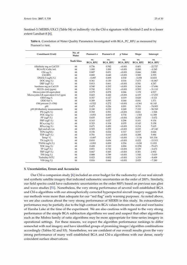
Remote Sens. 2017, 9, 538 25 of 30

Sentinel-3/MERIS/OLCI (Table S4) or indirectly via the Chl-a signature with Sentinel-2 and to a lesserextent Landsat-8 [6].

Table 6. Correlation of Water Quality Parameters Investigated with BGA_PC_RFU as measured byPearson’s r test.

Constituent (Unit) No. ofWater Pearson’s r Pearson’s r2 p Value Slope Intercept

Truth Sites vs.BGA_RFU

vs.BGA_RFU

vs.BGA_RFU

vs.BGA_RFU

vs.BGA_RFU

Alkalinity mg as CaCO3 44 0.736 0.542 <0.001 0.401 −22.727BGA-PC-Cells/mL 44 1.000 1.000 <0.001 0.000 −0.245

Chl-µg/L 44 0.807 0.651 <0.001 0.666 3.889Chl-RFU 44 0.800 0.640 <0.001 3.500 2.555

DNO2-3 (ugN/L) 44 −0.097 0.009 0.530 −0.058 10.833DOC (mg/L) 44 0.361 0.130 0.016 7.673 −41.867DRP (ugP/L) 44 0.813 0.661 <0.001 0.541 4.247

hardness mg as CaCO3 44 0.540 0.292 <0.001 0.264 −17.696HCO3- (est) (ppm) 44 0.742 0.551 <0.001 0.593 −31.110

Microcystin-LR equivalent 44 0.279 0.078 0.066 1.178 4.917Microcystin-LR equivalent 2–6.5 ppm 44 0.665 0.442 <0.001 6.105 −17.233

ODO-mg/L 44 0.357 0.127 0.019 0.628 −0.121ODO Sat % 44 0.309 0.095 0.044 0.041 1.571

OM percent (% OM) 44 −0.522 0.272 <0.001 −0.361 41.143pH 44 0.475 0.226 0.001 8.531 −74.903

pH (@Alkalinity measurement) 44 0.180 0.032 0.249 7.193 −58.769PN (ugN/L) 44 0.769 0.591 <0.001 0.021 −1.928POC (mg/L) 44 −0.053 0.003 0.734 −1.503 11.308PP (ugP/L) 44 0.835 0.697 <0.001 0.200 −3.672

PRP (ugP/L) 44 0.163 0.027 0.296 0.101 9.154RCe,a (ug/L) 44 0.323 0.104 0.035 0.143 5.158RPe,a (ug/L) 44 0.671 0.450 <0.001 0.214 7.615

SpCond-uS/cm 44 0.505 0.255 <0.001 0.225 −47.140TDN (ugNL) 44 0.156 0.024 0.317 0.017 0.626TDP (ugP/L) 44 0.781 0.610 <0.001 0.288 5.984

Temp-◦C 44 −0.497 0.247 <0.001 −3.136 101.334TN (ugN/L) 44 0.810 0.656 <0.001 0.022 −15.515

TNH4 (ugN/L) 44 −0.093 0.009 0.554 −0.030 11.033TOC (mg/L) 44 0.428 0.183 0.004 12.258 −79.471TP (ugP/L) 44 0.851 0.724 <0.001 0.129 −0.672

TRP (ugP/L) 44 0.667 0.445 <0.001 0.301 2.952TSS (mg/L) 44 0.888 0.789 <0.001 1.545 −5.619

Turbidity-NTU 44 0.923 0.852 <0.001 1.319 −8.609VSS (mg/L) 44 0.816 0.666 <0.001 2.025 −7.280

5. Uncertainties, Errors and Accuracies

Our Chl-a companion study [6] included an error budget for the radiometry of our real aircraftand synthetic satellite imagery that indicated radiometric uncertainties on the order of 200%. Similarly,our field spectra could have radiometric uncertainties on the order 800% based on previous sun glintand wave studies [51]. Nonetheless, the very strong performance of several well established BGAand Chl-a algorithms with our atmospherically corrected hyperspectral aircraft imagery suggests thatour methods were more than adequate for our “red flag” early warning purposes. As noted above,we are also cautious about the very strong performance of MERIS in this study. Its extraordinaryperformance may be partially due to the high contrast in BGA values between the east and west basinsof Harsha Lake at the time of the experiment. We are also cautious with regard to the very strongperformance of the simple BGA subtraction algorithms we used and suspect that other algorithmssuch as the Mishra family of ratio algorithms may be more appropriate for time-series imagery inoperational settings. For these reasons, we expect the algorithm performance rankings to differsomewhat with real imagery and have identified groups of promising imager/algorithm combinationsaccordingly (Tables S2 and S3). Nonetheless, we are confident of our overall results given the verystrong performance of many well established BGA and Chl-a algorithms with our dense, nearlycoincident surface observations.

Remote Sens. 2017, 9, 538 26 of 30

6. Conclusions

This study used atmospherically corrected high-spatial and high-spectral resolution VNIRCASI hyperspectral imagery to construct synthetic WorldView-2, Sentinel-2, Landsat-8, MODIS andSentinel-3/MERIS/OLCI image datasets with dense coincident surface observations in the form ofin situ water quality sonde and laboratory measurements to evaluate the performance of reflectancealgorithms for estimating BGA values in a 8.9 km2 temperate inland reservoir. The study focused oncurrently operational and near-future imaging satellite constellations that may be suitable contributorsto an operational water quality monitoring system for smaller inland reservoirs, lakes and rivers.

6.1. Best Performing Imager/Algorithm Combinations for BGA Estimation

We found that several established algorithms for the estimation of BGA values performed well(Pearson’s r2 > 0.6; p < 0.001) for most of the real aircraft and synthetic satellite datasets considered here.The Be162BsubPhy, SI052BDA, Be162B700sub601, Be16NDPhyI, Gi033BDA, Da052BDA, SM122BDA,Ku15PhyCI, MM092BDA, MI092BDA, Wy08CI, Zh10FLH, and MM12NDCI BGA algorithms workedwell with CASI imagery. The Be162BsubPhy, SI052BDA, Am092Bsub, Be16NDPhyI, Mi092BDA,and MM12NDCI BGA algorithms worked well with WorldView-2 and -3; the Be162Bsub algorithmwith Sentinel-2; and the MM092BDA, Be16NDPhyI, MM12NDCI, Go04MCI, Ku15PhyCI, Wy08CI,SI052BDA, Be162BsubPhy, and Hu103BDA BGA algorithms with MERIS-like imagery. Be162BsubPhywas the most widely applicable BGA algorithm (Table S4). The Be16FLHviolet “greenness” algorithmyielded the best (albeit poor) BGA estimates with simulated Landsat-8 imagery.

Algorithm/imager combinations listed in the preceding paragraph that include the phycocyaninreflectance minimum at 620 nm had slightly better performance with regard to BGA estimationthan Chl-a algorithms for CASI and WorldView-2 and were only slightly less effective than Chl-aalgorithms for Sentinel-3/MERIS/OLCI as predicted by Simis et al. [7] and Mishra et al. [11] (Table S4).For imagers without a narrow band at 620 nm, we used Chl-a proxy algorithms to estimate BGA withgood results for simulated Sentinel-2 and poor results for simulated Landsat-8 and MODIS for thiswater body at the time of hyperspectral image acquisition.

6.2. Portability of Algorithms between Imagers

The simple phycocyanin spectrum-based, semi-analytical Be162Bsub subtraction algorithmshad the highest portability between the CASI, WorldView-2 and MERIS-like imaging systems. Othersimple band ratio-based algorithms also suppress illumination variation between scenes and estimateBGA values well after imager and environment specific calibration (Table S4). This is especiallyeffective when these simple subtraction and band ratio algorithms are applied to imagers withrelatively narrow bands that capture the 620 nm phycocyanin reflectance minimum (Si052BDA forCASI, WorldView and MERIS) or near-infrared/red Chl-a reflectance contrast (MM092BDA also forMERIS). The normalized difference phycocyanin index (Be16NDPhyI for CASI, WorldView and MERIS)and normalized difference chlorophyll index [32] (MMNDCI12 for CASI, WorldView, Sentinel-2, andMERIS) algorithms also performed well with regard to BGA estimation (Table S4). Landsat-8 requiresan alternative algorithm such the Chl-a “greenness” FLH Violet algorithm [6]. MERIS and MODISdo not capture the spatial heterogeneity in BGA observed in this study due to their large pixels.MODIS has wide bands that do not target the “veg edge” or BGA absorption feature well and haslow performance accordingly (Tables S2 and S4) although it may be useful with NDCI for largerwater bodies.

6.3. Implications for Operational BGA Monitoring with Existing and Near-Future Satellites

For imagers with appropriate bandwidths and positions relative to the BGA phycocyaninreflectance signature and pixel sizes appropriate for smaller inland water bodies less than a few kmacross, simple algorithms that subtract or ratio bands and therefore inherently normalize reflectance

Remote Sens. 2017, 9, 538 27 of 30

performed well and appear to be relatively portable between most satellite imaging systems for theestimation of BGA in smaller inland water bodies. Therefore, near-term steps toward operational waterquality monitoring systems for inland water bodies smaller than a few kilometers across should focuson Sentinel-2 A and B and to a lesser extent Landsat-8 with augmentation from WorldView-2 and -3 orhyperspectral imagery when required. Good performance of both BGA and Chl-a algorithms for BGAestimation suggests that early efforts to operationalize regional algal monitoring can use whichever setof algorithms are most appropriate for the sources of imagery at hand (Sentinel-2/3, WorldView-2/3and to a lesser extent Landsat-8). Sentinel-3/MERIS/OLCI may also be useful for heavily maskedtime-series monitoring but will capture very little of the spatial heterogeneity of BGA and CSTB valuesin smaller inland water bodies.

The somewhat better performance of phycocyanin specific semi-analytical algorithms for BGAand CSTB estimation suggests that future satellite imaging systems for cyanobacterial monitoring insmaller inland water bodies that are often sources of drinking water should include a narrow bandfocused on the 620 nm absorption feature [7,8,11,22] and spatial resolutions of 20–90 m. Such systemsshould also include “water vapor” bands at 770–870 nm and 870–1020 nm to facilitate atmosphericcorrection to reflectance [52] for real time monitoring of smaller inland water bodies [53].

Supplementary Materials: The following are available online at www.mdpi.com/2072-4292/9/6/538/s1,Table S1. Band math with band number and band wavelengths in nm for each algorithm used for BGA/PCrelative fluorescence unit (BGA_PC_RFU) estimation at Harsha Lake using phycocyanin indices and nearestcenter band wavelengths in current and near-future satellite imaging systems. Float refers to floating pointvalues of relative reflectance in the ENVI band math we used in this study at the specified wavelengths innm from atmospherically corrected imagery. Float is not a variable, it is an IDL function used to preventbyte overflow errors during calculation. Band number and band wavelengths are listed for each algorithmsequentially, Table S2. Performance of algorithms for BGA estimation at Harsha Lake using image derivedphycocyanin indices according to Pearson’s r test (Type 1) linear regressions. Satellite/Algorithm combinationswith asterisk measure the 620 nm phycocyanin absorption feature directly. Y-axis (dependent variable) andintercept have units of BGA_PC_RFU. X-axis is a unit less numerical index, Slope has units of BGA_PC_RFU,Table S3. Performance of Algorithms for BGA Estimation at Harsha (East Fork) Lake with all results normalizedto calculated BGA/PC values. Satellite/Algorithm combinations with asterisk measure the 620 nm phycocyaninabsorption feature directly. Y-axis (dependent variable) and intercept have units of BGA_PC_RFU. X-axis alsohas units of BGA_PC_RFU. Slope is unit less, Table S4. Direct and Indirect BGA Indices Ranked by Performance(Pearson’s r2). Satellite/Algorithm combinations with asterisk measure the 620 nm phycocyanin absorptionfeature directly. Y-axis (dependent variable) and intercept have units of BGA_PC_RFU. X-axis also has units ofBGA_PC_RFU. Slope is unit less.

Acknowledgments: This study was funded by the U.S. Army Corps of Engineers. The U.S. EnvironmentalProtection Agency and the Kentucky Department of Environmental Protection, Division of Water providedvaluable in-kind services. Christopher Nietch and Dana Macke of US EPA performed the laboratory water qualityparameter analyses and calibrated the in situ water quality sondes. Any use of trade, product, or firm names is fordescriptive purposes only and does not imply endorsement by the U.S. Government. This article expresses onlythe personal views of the U.S. Army Corps of Engineers employees listed as authors and does not necessarilyreflect the official positions of the Corps or of the Department of the Army.

Author Contributions: All authors played major roles in one of the most extensive coincident aircraft imaging,coincident surface observation and biogeochemical analysis campaigns for the evaluation of remote sensingalgorithms for the estimation of water quality to date.

Conflicts of Interest: The authors declare no conflict of interest.

References

1. Graham, J.L. Harmful Algal Blooms; USGS Fact Sheet, 2006-3147; USGS: Reston, VA, USA, 2006.2. Linkov, I.; Satterstrom, F.K.; Loney, D.; Steevans, J.A. The Impact of Harmful Algal Blooms on USACE Operations;

ANSRP Technical Notes Collection; ERDC/TN ANSRP-09-1; U.S. Army Engineer Research and DevelopmentCenter: Vicksburg, MS, USA, 2009.

3. Matthews, M.W.; Bernard, S. Characterizing the absorption properties for remote sensing of three smalloptically-diverse South African reservoirs. Remote Sens. 2013, 5, 4370–4404. [CrossRef]

4. Matthews, M.W.; Odermatt, D. Improved algorithm for routine monitoring of cyanobacteria and eutrophicationin inland and near-coastal waters. Remote Sens. Environ. 2015, 156, 374–382. [CrossRef]

www.mdpi.com/2072-4292/9/6/538/s1


http://dx.doi.org/10.1016/j.rse.2014.10.010

Remote Sens. 2017, 9, 538 28 of 30

5. Stumpf, R.P.; Wynne, T.T.; Baker, D.B.; Fahnenstiel, G.L. Interannual Variability of Cyanobacterial Blooms inLake Erie. PLoS ONE 2012, 7, e42444. [CrossRef] [PubMed]

6. Beck, R.A.; Zhan, S.; Liu, H.; Tong, S.; Yang, B.; Xu, M.; Ye, Z.; Huang, Y.; Wu, Q.; Wang, S.; et al. Comparisonof satellite reflectance algorithms for estimating chlorophyll-a in a temperate reservoir using coincidenthyperspectral aircraft imagery and dense coincident surface observations. Remote Sens. Environ. 2016, 178,15–30. [CrossRef]

7. Simis, S.G.H.; Peters, S.W.M.; Gons, H.J. Remote sensing of the cyanobacteria pigment phycocyanin in turbidinland water. Limnol. Oceanogr. 2005, 50, 237–245. [CrossRef]

8. Simis, S.G.H.; Ruiz-Verdu, A.; Dominguez, J.A.; Pena-Martinez, R.; Peters, S.W.M.; Gons, H.J. Influence ofphytoplankton pigment composition on remote sensing of cyanobacterial biomass. Remote Sens. Environ.2007, 106, 414–427. [CrossRef]

9. Randolph, K.; Wilson, J.; Tedesco, L.; Li, L.; Lani Pascual, D.; Soyeux, E. Hyperspectral remote sensing ofcyanobacteria in turbid productive water using optically active pigments, chlorophyll a and phycocyanin.Remote Sens. Environ. 2008, 112, 4009–4019. [CrossRef]

10. Ruiz-Verdu, A.; Simis, S.G.H.; de Hoyos, C.; Gons, H.J.; Pena-Martinez, R. An evaluation of algorithms forthe remote sensing of cyanobacterial biomass. Remote Sens. Environ. 2008, 112, 3996–4008. [CrossRef]

11. Mishra, S.; Mishra, D.R.; Schluchter, W.M. A novel algorithm for predicting PC concentrations incyanobacteria: A proximal hyperspectral remote sensing approach. Remote Sens. 2009, 1, 758–775. [CrossRef]

12. Klemas, V. Remote sensing of algal blooms: An overview with case studies. J. Coast. Res. 2012, 28, 34–43.[CrossRef]

13. Mishra, S.; Mishra, D.R.; Lee, Z.P. Bio-optical inversion in highly turbid and cyanobacteria dominated waters.IEEE Trans. Geosci. Remote Sens. 2014, 52, 375–388. [CrossRef]

14. Ogashawara, I.; Misra, D.R.; Mishra, S.; Curtarelli, M.P.; Stech, J.L. A performance review of reflectance basedalgorithms for predicting phycocyanin concentrations in inland waters. Remote Sens. 2013, 5, 4774–4798.[CrossRef]

15. Lyu, H.; Wang, Q.; Wu, C.; Zhu, L.; Yin, B.; Li, Y.; Huang, J. Retrieval of phycocyanin concentration fromremote-sensing reflectance using a semi-analytic model in eutrophic lakes. Ecol. Inform. 2013, 18, 178–187.[CrossRef]

16. Mishra, S.; Mishra, D.R. A novel remote sensing algorithm to quantify phycocyanin in cyanobacterial algalblooms. Environ. Res. Lett. 2014, 9, 114003. [CrossRef]

17. Kudela, R.M.; Palacios, S.L.; Austerberry, D.C.; Accorsi, E.K.; Guild, L.S.; Torres-Perez, J. Application ofhyperspectral remote sensing to cyanobacterial blooms in inland waters. Remote Sens. Environ. 2015, 167,196–205. [CrossRef]

18. Lunetta, R.S.; Schaeffer, B.A.; Stumpf, R.P.; Keith, D.; Jacobs, S.A.; Murphy, M.S. Evaluation of cyanobacterialcell count detection derived from MERIS imagery across the eastern USA. Remote Sens. Environ. 2015, 157,24–34. [CrossRef]

19. Wynne, T.T.; Stumpf, R.P.; Tomlinson, M.C.; Warner, R.A.; Tester, P.A.; Dyble, J. Relating spectral shape tocyanobacterial blooms in the Laurentian Great Lakes. Int. J. Remote Sens. 2008, 29, 3665–3672. [CrossRef]

20. Wynne, T.T.; Stumpf, R.P.; Tomlinson, M.C.; Dyble, J. Characterizing a cyanobacterial bloom in western LakeErie using satellite imagery and meteorological data. Limnol. Oceanogr. 2012, 55, 2025–2036. [CrossRef]

21. Wynne, T.T.; Stumpf, R.P. Spatial and Temporal Patterns in the Seasonal Distribution of Toxic Cyanobacteriain Western Lake Erie from 2002–2014. Toxins 2015, 7, 1649–1663. [CrossRef] [PubMed]

22. Sun, D.; Hu, C.; Qiu, Z.; Shi, K. Estimating phycocyanin pigment concentration in productive inland watersusing Landsat measurements: A case study in Lake Dianchi. Opt. Express 2015, 23, 3055–3074. [CrossRef][PubMed]

23. Wozniak, M.; Bradtke, K.M.; Darecki, M.; Krezel, A. Empirical Model for Phycocyanin ConcentrationEstimation as an Indicator of Cyanobacterial Bloom in the Optically Complex Coastal Waters of the BalticSea. Remote Sens. 2016, 8, 1–23. [CrossRef]

24. Stumpf, R.P.; Davis, T.W.; Wynne, T.T.; Graham, J.L.; Loftin, K.A.; Johengen, T.H.; Gossiaux, D.; Palladino, D.;Burtner, A. Challenges for mapping cyanotoxin patterns from remote sensing of cyanobacteria. Harmful Algae2016, 54, 160–173. [CrossRef] [PubMed]

25. Morel, A.; Prieur, L. Analysis of variations in ocean color. Limnol. Oceanogr. 1977, 22, 709–722. [CrossRef]

http://dx.doi.org/10.1371/journal.pone.0042444

http://www.ncbi.nlm.nih.gov/pubmed/22870327


http://dx.doi.org/10.4319/lo.2005.50.1.0237





http://dx.doi.org/10.2112/JCOASTRES-D-11-00051.1

http://dx.doi.org/10.1109/TGRS.2013.2240462


http://dx.doi.org/10.1016/j.ecoinf.2013.09.002

http://dx.doi.org/10.1088/1748-9326/9/11/114003



http://dx.doi.org/10.1080/01431160802007640

http://dx.doi.org/10.4319/lo.2010.55.5.2025

http://dx.doi.org/10.3390/toxins7051649


http://dx.doi.org/10.1364/OE.23.003055



http://dx.doi.org/10.1016/j.hal.2016.01.005


http://dx.doi.org/10.4319/lo.1977.22.4.0709

Remote Sens. 2017, 9, 538 29 of 30

26. Dekker, A. Detection of the Optical Water Quality Parameters for Eutrophic Waters by High ResolutionRemote Sensing. Ph.D. Thesis, Free University, Amsterdam, The Netherlands, 1993.

27. Stumpf, R.P. Satellite Monitoring of Toxic Cyanobacteria for Public Health. Earthzine. 2014. Available online:http://earthzine.org/2014/03/26/satellite-monitoring-of-toxic-cyanobacteria-for-public-health/ (accessedon 7 April 2016).

28. Augusto-Silva, P.B.; Ogashawara, I.; Barbosa, C.C.F.; de Carvalho, L.A.S.; Jorge, D.S.F.; Fornari, C.I.; Stech, J.L.Analysis of MERIS reflectance algorithms for estimating chlorophyll-a concentration in a Brazilian Reservoir.Remote Sens. 2014, 6, 11689–11707. [CrossRef]

29. Hunter, P.D.; Tyler, A.N.; Willby, N.J.; Gilvear, D.J. The spatial dynamics of vertical migration byMicrocystis aeruginosa in a eutrophic shallow lake: A case study using high spatial resolution time-seriesairborne remote sensing. Limnol. Oceanogr. 2008, 53, 2391–2406. [CrossRef]

30. Wheeler, S.M.; Morrissey, L.A.; Levine, S.N.; Livingston, G.P.; Vincent, W.F. Mapping cyanobacterial bloomsin Lake Champlain’s Missisquoi Bay using QuickBird and MERIS satellite data. J. Great Lakes Res. 2012, 38,68–75. [CrossRef]

31. Lee, Z.P.; Carder, K.L. Absorption spectrum of phytoplankton pigments derived from hyperspectralremote-sensing reflectance. Remote Sens. Environ. 2004, 89, 361–368. [CrossRef]

32. Mishra, S.; Mishra, D.R. Normalized difference chlorophyll index: A novel model for remote estimation ofchlorophyll-a concentration in turbid productive waters. Remote Sens. Environ. 2012, 117, 394–406. [CrossRef]

33. Shen, L.; Xu, H.; Guo, X. Satellite remote sensing of harmful algal blooms (HABs) and a Potential SynthesizedFramework. Sensors 2012, 12, 7778–7803. [CrossRef] [PubMed]

34. Verbyla, D.L. Satellite Remote Sensing of Natural Resources; CRC Lewis: Boca Raton, FL, USA, 1995; p. 199.35. Gitelson, A.A.; Garbuzov, G.; Szilagyi, F.; Mittenzwey, K.H.; Karnieli, A.; Kaiser, A. Quantitative remote

sensing methods for real-time monitoring of inland waters quality. Int. J. Remote Sens. 1993, 14, 1269–1295.[CrossRef]

36. Fraser, R.N. Hyperspectral remote sensing of turbidity and chlorophyll a among Nebraska Sand Hills lakes.Int. J. Remote Sens. 1998, 19, 1579–1589. [CrossRef]

37. Glasgow, H.B.; Burkholder, J.M.; Reed, R.E.; Lewitus, A.J.; Kleinman, J.E. Real-time remote monitoring ofwater quality: A review of current applications, and advancements in sensor technology, telemetry, andcomputing technologies. J. Exp. Mar. Biol. Ecol. 2004, 300, 409–448. [CrossRef]

38. Binding, C.E.; Greenberg, T.A.; Bukata, R.P. The MERIS Maximum Chlorophyll Index; its merits andlimitations for inland water algal bloom monitoring. J. Great Lakes Res. 2013, 39, 100–107. [CrossRef]

39. Sawaya, K.E.; Olmanson, L.G.; Heinart, N.J.; Brezonik, P.L.; Bauer, M.E. Extending satellite remote sensing tolocal scales: Land and water resource monitoring using high-resolution imagery. Remote Sens. Environ. 2003,88, 144–156. [CrossRef]

40. Mayo, M.; Gitelson, A.A.; Yacobi, Y.Z.; Ben-Avraham, Z. Chlorophyll distribution in Lake Kinneretdetermined from Landsat Thematic Mapper data. Int. J. Remote Sens. 1995, 16, 175–182. [CrossRef]

41. Alawadi, F. Detection of surface algal blooms using the newly developed algorithm surface algal bloomindex (SABI). Proc. SPIE 2010, 7825. [CrossRef]

42. Amin, R.; Zhou, J.; Gilerson, A.; Gross, B.; Moshary, F.; Ahmed, S. Novel optical techniques for detecting andclassifying toxic dinoflagellate Karenia brevis blooms using satellite imagery. Opt. Express 2009, 17, 9126–9144.[CrossRef] [PubMed]

43. Gitelson, A.A.; Gritz, U.; Merzlyak, M.N. Relationships between leaf chlorophyll content and spectralreflectance and algorithms for non-destructive chlorophyll assessment in higher plant leaves. J. Plant Phys.2003, 160, 271–282. [CrossRef] [PubMed]

44. Gower, J.; King, S.; Goncalves, P. Global monitoring of plankton blooms using MERIS MCI. Int. J. Remote Sens.2008, 29, 6209–6216. [CrossRef]

45. Kneubuhler, M.; Frank, T.; Kellenberger, T.W.; Pasche, N.; Schmid, M. Mapping chlorophyll-a in Lake Kivuwith remote sensing methods. In Proceedings of the Envisat Symposium 2007, Montreux, Switzerland,23–27 April 2007.

46. Mishra, S. Remote Sensing of Harmful Algal Bloom. PhD Thesis, Mississippi State University, Starkville, MI,USA, 2012.

47. Schalles, J.; Yacobi, Y. Remote detection and seasonal patterns of phycocyanin, carotenoid and chlorophyll-apigments in eutrophic waters. Arch. Hydrobiol. Adv. Limnol. 2000, 55, 153–168.

http://earthzine.org/2014/03/26/satellite-monitoring-of-toxic-cyanobacteria-for-public-health/

http://dx.doi.org/10.3390/rs61211689

http://dx.doi.org/10.4319/lo.2008.53.6.2391

http://dx.doi.org/10.1016/j.jglr.2011.06.009



http://dx.doi.org/10.3390/s120607778


http://dx.doi.org/10.1080/01431169308953956

http://dx.doi.org/10.1080/014311698215360

http://dx.doi.org/10.1016/j.jembe.2004.02.022

http://dx.doi.org/10.1016/j.jglr.2013.04.005


http://dx.doi.org/10.1080/01431169508954386

http://dx.doi.org/10.1117/12.862096

http://dx.doi.org/10.1364/OE.17.009126


http://dx.doi.org/10.1078/0176-1617-00887


http://dx.doi.org/10.1080/01431160802178110

Remote Sens. 2017, 9, 538 30 of 30

48. Peltzer, E.T. Model 1 and Model 2 Regressions. 2015. Available online: http://www.mbari.org/staff/etp3/regress.htm (accessed on 27 April 2015).

49. Pinero, G.; Perelman, S.; Guerschman, J.P.; Paruleo, J.M. How to evaluate models: Observed vs. predicted orpredicted vs. observed. Ecol. Model. 2008, 216, 316–322. [CrossRef]

50. Lindsey, R.; Herring, D. Modis; 2001; pp. 1–23. Available online: https://modis.gsfc.nasa.gov/about/media/modis_brochure.pdf (accessed on 24 May 2017).

51. Lee, Z.; Ahn, Y.-H.; Mobley, C.; Arnone, R. Removal of surface-reflected light for the measurement ofremote-sensing reflectance from an above-surface platform. Opt. Express 2010, 18, 26313–26324. [CrossRef][PubMed]

52. Gao, B.; Montes, M.J.; Davis, C.O.; Goetz, A.H. Atmospheric correction algorithms for hyperspectral remotesensing data of land and ocean. Remote Sens. Environ. 2009, 113, S17–S24. [CrossRef]

53. Reif, M. Remote Sensing for Inland Water Quality Monitoring: A U.S. Army Corps of Engineers Perspective;Engineer Research and Development Center/Environmental Laboratory Technical Report (ERDC/ELTR)-11-13; Engineer Research and Development Center/Environmental Laboratory: Vicksburg, MS,USA, 2011.

© 2017 by the authors. Licensee MDPI, Basel, Switzerland. This article is an open accessarticle distributed under the terms and conditions of the Creative Commons Attribution(CC BY) license (http://creativecommons.org/licenses/by/4.0/).

http://www.mbari.org/staff/etp3/regress.htm

http://www.mbari.org/staff/etp3/regress.htm

http://dx.doi.org/10.1016/j.ecolmodel.2008.05.006

https://modis.gsfc.nasa.gov/about/media/modis_brochure.pdf

https://modis.gsfc.nasa.gov/about/media/modis_brochure.pdf

http://dx.doi.org/10.1364/OE.18.026313



http://creativecommons.org/

http://creativecommons.org/licenses/by/4.0/.

Comparison of Satellite Reflectance Algorithms for Estimating ...

Documents

Transcript of Comparison of Satellite Reflectance Algorithms for Estimating ...