061213-012 1

Abstract—In this paper, we present some results obtained with the Shadows system, the new synthetic aperture sonar, by IXSEA. First sections are a slight presentation where we expose the performances and specifications of Shadows. We present the results obtained on the lateral sonar by using first the algorithm of DPCA, second the simulation of DPCA parameters by using the navigation data. Hence we present some results obtained by comparing the two methods. The data were recorded by the Shadows system in La Ciotat Bay during summer 2006.

Index Terms—Signal processing, sonar navigation, synthetic aperture sonar.

I. INTRODUCTION HADOWS is a new synthetic Aperture Sonar System developed by IXSEA (Fig.1.). It provides real-time SAS

processing on a 600 meters swath at a resolution of 15cm. The side-scan synthetic aperture sonar is completed with a front-looking sonar imaging the gap at nadir. The optimal working speed is 5 knots.

Fig.1. Shadows Synthetic Aperture Sonar, by IXSEA. The system computes directly a georeferenced map with SAS images in real-time. Images are displayed through a map server and the visualization is done on the NASA WorldWind

program (Fig. 3.).

II. PRESENTATION OF SHADOWS SYSTEM

A. Acoustic Specifications With the design of Shadows (Fig. 2.), the resolution

reaches 15cm at a maximum range of 300m and the maximum speed to form a non lacunar synthetic aperture is theoretically 5 knots. The coverage rate reaches 5.56 square km per hour.

Each side is composed of a receiver array of 24 hydrophones and of three transmitters. Two of the transmitters are located at each extremity of the physical antenna in order to perform ping-pong DPCA. The six transmitters are identical. The length of those transmitters is 14 cm, therefore the theoretical along track resolution is 7cm. We assume the practical resolution to be twice this figure i.e. 14cm all along the swath.

The central working frequency is 100kHz and the usable bandwidth of the transducers is 30kHz. This bandwidth is divided in three. One main part which width is at least 20kHz is used for imagery on the central transmitter. Two other narrower parts are used for the ping-pong DPCA. Those two auxiliary pulses are emitted alternatively on the fore end and backend transmitters.

The signal is recorded and demodulated for each receiver. The separation of the different transmitted pulses is done by three different convolutions.

Shadows is also equipped with an accurate and highly synchronized Inertial Navigation System.

Comparison between DPCA Algorithm and Inertial Navigation on the Ixsea Shadows SAS

Michel Legris, Frédéric Jean

S

1-4244-0635-8/07/$20.00 ©2007 IEEE

061213-012 2

Fig.2. Shadows Synthetic Aperture Sonar, by IXSEA.

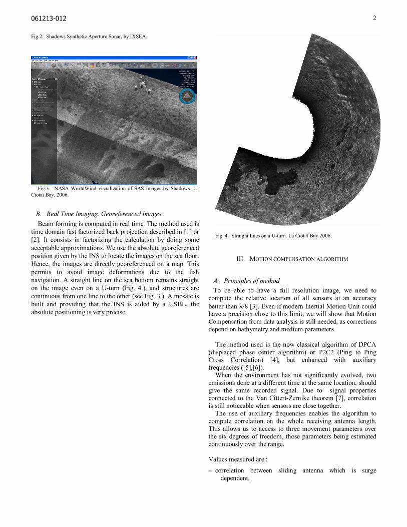
Fig.3. NASA WorldWind visualization of SAS images by Shadows. La

Ciotat Bay, 2006.

B. Real Time Imaging. Georeferenced Images. Beam forming is computed in real time. The method used is

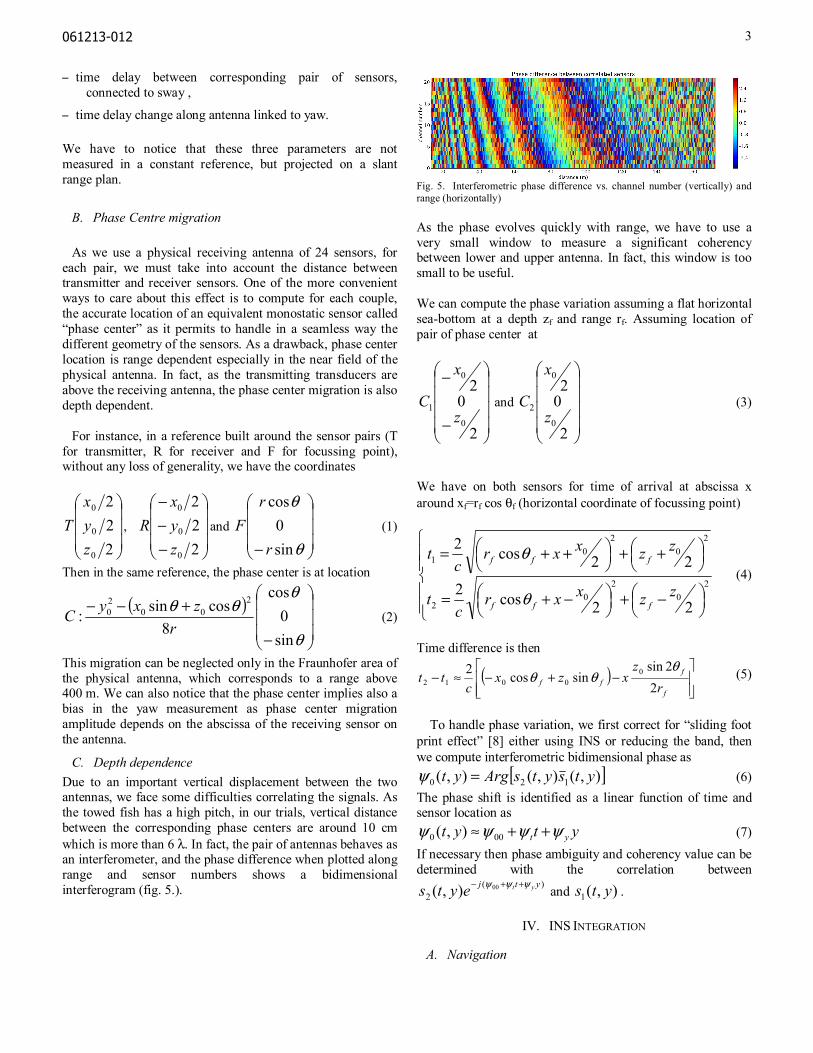
time domain fast factorized back projection described in [1] or [2]. It consists in factorizing the calculation by doing some acceptable approximations. We use the absolute georeferenced position given by the INS to locate the images on the sea floor. Hence, the images are directly georeferenced on a map. This permits to avoid image deformations due to the fish navigation. A straight line on the sea bottom remains straight on the image even on a U-turn (Fig. 4.), and structures are continuous from one line to the other (see Fig. 3.). A mosaic is built and providing that the INS is aided by a USBL, the absolute positioning is very precise.

Fig. 4. Straight lines on a U-turn. La Ciotat Bay 2006.

III. MOTION COMPENSATION ALGORITHM

A. Principles of method To be able to have a full resolution image, we need to

compute the relative location of all sensors at an accuracy better than λ/8 [3]. Even if modern Inertial Motion Unit could have a precision close to this limit, we will show that Motion Compensation from data analysis is still needed, as corrections depend on bathymetry and medium parameters. The method used is the now classical algorithm of DPCA (displaced phase center algorithm) or P2C2 (Ping to Ping Cross Correlation) [4], but enhanced with auxiliary frequencies ([5],[6]).

When the environment has not significantly evolved, two emissions done at a different time at the same location, should give the same recorded signal. Due to signal properties connected to the Van Cittert-Zernike theorem [7], correlation is still noticeable when sensors are close together.

The use of auxiliary frequencies enables the algorithm to compute correlation on the whole receiving antenna length. This allows us to access to three movement parameters over the six degrees of freedom, those parameters being estimated continuously over the range. Values measured are :

– correlation between sliding antenna which is surge dependent,

061213-012 3

– time delay between corresponding pair of sensors, connected to sway ,

– time delay change along antenna linked to yaw. We have to notice that these three parameters are not measured in a constant reference, but projected on a slant range plan.

B. Phase Centre migration

As we use a physical receiving antenna of 24 sensors, for each pair, we must take into account the distance between transmitter and receiver sensors. One of the more convenient ways to care about this effect is to compute for each couple, the accurate location of an equivalent monostatic sensor called “phase center” as it permits to handle in a seamless way the different geometry of the sensors. As a drawback, phase center location is range dependent especially in the near field of the physical antenna. In fact, as the transmitting transducers are above the receiving antenna, the phase center migration is also depth dependent.

For instance, in a reference built around the sensor pairs (T for transmitter, R for receiver and F for focussing point), without any loss of generality, we have the coordinates

222

0

0

0

zyx

T ,

−−−

222

0

0

0

zyx

R and

− θ

θ

sin0

cos

r

rF (1)

Then in the same reference, the phase center is at location

( )

−

+−−

θ

θθθ

sin0

cos

8cossin:

200

20

rzxyC (2)

This migration can be neglected only in the Fraunhofer area of the physical antenna, which corresponds to a range above 400 m. We can also notice that the phase center implies also a bias in the yaw measurement as phase center migration amplitude depends on the abscissa of the receiving sensor on the antenna.

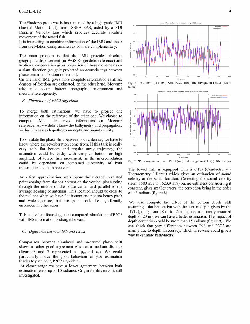
C. Depth dependence Due to an important vertical displacement between the two antennas, we face some difficulties correlating the signals. As the towed fish has a high pitch, in our trials, vertical distance between the corresponding phase centers are around 10 cm which is more than 6 λ. In fact, the pair of antennas behaves as an interferometer, and the phase difference when plotted along range and sensor numbers shows a bidimensional interferogram (fig. 5.).

Fig. 5. Interferometric phase difference vs. channel number (vertically) and range (horizontally) As the phase evolves quickly with range, we have to use a very small window to measure a significant coherency between lower and upper antenna. In fact, this window is too small to be useful. We can compute the phase variation assuming a flat horizontal sea-bottom at a depth zf and range rf. Assuming location of pair of phase center at

−

−

2

02

0

0

1z

x

C and

2

02

0

0

2z

x

C (3)

We have on both sensors for time of arrival at abscissa x around xf=rf cos θf (horizontal coordinate of focussing point)

−+

−+=

++

++=

20

20

2

20

20

1

22cos2

22cos2

zzxxrc

t

zzxxrc

t

fff

fff

θ

θ (4)

Time difference is then

( )

−+−≈−

f

fff r

zxzx

ctt

22sin

sincos2 00012

θθθ (5)

To handle phase variation, we first correct for “sliding foot

print effect” [8] either using INS or reducing the band, then we compute interferometric bidimensional phase as

[ ]),(),(),( 120 ytsytsArgyt =ψ (6) The phase shift is identified as a linear function of time and sensor location as

ytyt yt ψψψψ ++≈ 000 ),( (7) If necessary then phase ambiguity and coherency value can be determined with the correlation between

)(2

00),( ytj yteyts ψψψ ++− and ),(1 yts .

IV. INS INTEGRATION

A. Navigation

061213-012 4

The Shadows prototype is instrumented by a high grade IMU (Inertial Motion Unit) from IXSEA SAS, aided by a RDI Doppler Velocity Log which provides accurate absolute movement of the towed fish. It is interesting to combine information of the IMU and those from the Motion Compensation as both are complementary. The main problem is that the IMU provides absolute geographic displacement (in WGS 84 geodetic reference) and Motion Compensation gives projection of these movements on a slant direction (roughly projected on acoustic rays between phase center and bottom reflection). On one hand, IMU gives more complete information as all six degrees of freedom are estimated, on the other hand, Mocomp take into account bottom topographic environment and medium heterogeneity.

B. Simulation of P2C2 algorithm To merge both estimations, we have to project one information on the reference of the other one. We choose to compute IMU characterized information on Mocomp reference. As we didn’t know the bathymetry and propagation, we have to assess hypotheses on depth and sound celerity. To simulate the phase shift between both antennas, we have to know where the reverberation come from. If this task is really easy with flat bottom and regular array trajectory, the estimation could be tricky with complex bottom or high amplitude of towed fish movement, as the intercorrelation could be dependant on combined directivity of both transmitters and both receivers. As a first approximation, we suppose the average correlated point coming from the sea bottom on the vertical plane going through the middle of the phase center and parallel to the average heading of antennas. This location should be close to the real one when we have flat bottom and not too heavy pitch and wide aperture, but this point could be significantly erroneous in other cases. This equivalent focussing point computed, simulation of P2C2 with INS information is straightforward.

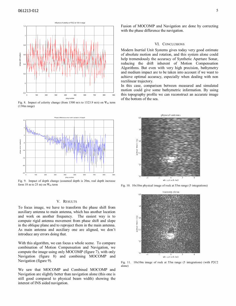
C. Difference between INS and P2C2 Comparison between simulated and measured phase shift shows a rather good agreement when at a medium distance (figure 6 and 7 represented as ψ00 and ψt). We could particularly notice the good behaviour of yaw estimation thanks to ping pong P2C2 algorithm. At closer range we have a lower agreement between both estimation (error up to 10 radians). Origin for this error is still investigated.

-20

-10

0

10

20

30

40

0 100 200 300 400 500 600 700 800 900

phase

shift

(radia

ns)

ping number

phase difference between consecutive ping at 130 m range

MocompNavigation

Fig. 6. Ψ00 term (see text) with P2C2 (red) and navigation (blue) (130m range)

-0.6

-0.5

-0.4

-0.3

-0.2

-0.1

0

0.1

0.2

0 100 200 300 400 500 600 700 800 900

phas

e sh

ift s

lope

per

sen

sor

(rad

ians

)

ping number

apparent phase shift slope between consecutive ping at 130 m range

from mocompfrom navigation

Fig. 7. Ψy term (see text) with P2C2 (red) and navigation (blue) (130m range) The towed fish is equipped with a CTD (Conductivity / Thermometry / Depth) which gives an estimation of sound celerity at the sonar location. Correcting the sound celerity (from 1500 m/s to 1523.9 m/s) but nevertheless considering it constant, gives smaller errors, the correction being in the order of 0.5 radians (figure 8). We also compute the effect of the bottom depth (still assuming a flat bottom but with the current depth given by the DVL (going from 18 m to 26 m against a formerly assumed depth of 20 m), we can have a better estimation. The impact of depth correction could be more than 15 radians (figure 9) . We can check that yaw differences between INS and P2C2 are mainly due to depth inaccuracy, which in reverse could give a way to estimate bathymetry.

061213-012 5

-0.2

0

0.2

0.4

0.6

0.8

1

1.2

0 100 200 300 400 500 600 700 800 900

phas

e sh

ift (r

adia

n)

ping number

influence of celerity on P2C2 at 130 m range

Fig. 8. Impact of celerity change (from 1500 m/s to 1523.9 m/s) on Ψ00 term (130m range)

-25

-20

-15

-10

-5

0

5

10

0 100 200 300 400 500 600 700 800 900

phas

e er

ror

(rad

ians

)

ping number

Phase difference error with variation of depth

Fig. 9. Impact of depth change (assumed depth is 20m, real depth increase form 18 m to 25 m) on Ψ00 term

V. RESULTS To focus image, we have to transform the phase shift from auxiliary antenna to main antenna, which has another location and work on another frequency. The easiest way is to compute rigid antenna movement from phase shift and slope in the oblique plane and to reproject them in the main antenna. As main antenna and auxiliary one are aligned, we don’t introduce any errors doing that.

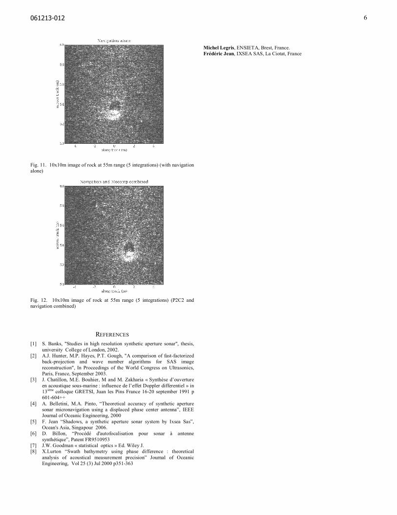
With this algorithm, we can focus a whole scene. To compare combination of Motion Compensation and Navigation, we compute the image using only MOCOMP (figure 7), with only Navigation (figure 8) and combining MOCOMP and Navigation (figure 9). We saw that MOCOMP and Combined MOCOMP and Navigation are slightly better than navigation alone (this one is still good compared to physical beam width) showing the interest of INS aided navigation.

Fusion of MOCOMP and Navigation are done by correcting with the phase difference the navigation.

VI. CONCLUSIONS Modern Inertial Unit Systems gives today very good estimate of absolute motion and rotation, and this system alone could help tremendously the accuracy of Synthetic Aperture Sonar, reducing the drift inherent of Motion Compensation Algorithms. But even with very high precision, bathymetry and medium impact are to be taken into account if we want to achieve optimal accuracy, especially when dealing with non rectilinear trajectory. In this case, comparison between measured and simulated motion could give some bathymetric information. By using this topography profile we can reconstruct an accurate image of the bottom of the sea.

Fig. 10. 10x10m physical image of rock at 55m range (5 integrations)

Fig. 11. 10x10m image of rock at 55m range (5 integrations) (with P2C2 alone)

061213-012 6

Fig. 11. 10x10m image of rock at 55m range (5 integrations) (with navigation alone)

Fig. 12. 10x10m image of rock at 55m range (5 integrations) (P2C2 and navigation combined)

REFERENCES [1] S. Banks, "Studies in high resolution synthetic aperture sonar", thesis,

university College of London, 2002. [2] A.J. Hunter, M.P. Hayes, P.T. Gough, "A comparison of fast-factorized

back-projection and wave number algorithms for SAS image reconstruction", In Proceedings of the World Congress on Ultrasonics, Paris, France, September 2003.

[3] J. Chatillon, M.E. Bouhier, M and M. Zakharia « Synthèse d’ouverture en acoustique sous-marine : influence de l’effet Doppler differentiel » in 13ième colloque GRETSI, Juan les Pins France 16-20 september 1991 p 601-604++

[4] A. Belletini, M.A. Pinto, “Theoretical accuracy of synthetic aperture sonar micronavigation using a displaced phase center antenna”, IEEE Journal of Oceanic Engineering, 2000

[5] F. Jean “Shadows, a synthetic aperture sonar system by Ixsea Sas”, Ocean's Asia, Singapour 2006.

[6] D. Billon, “Procédé d'autofocalisation pour sonar à antenne synthétique”, Patent FR9510953

[7] J.W. Goodman « statistical optics » Ed. Wiley J. [8] X.Lurton “Swath bathymetry using phase difference : theoretical

analysis of acoustical measurement precision” Journal of Oceanic Engineering, Vol 25 (3) Jul 2000 p351-363

Michel Legris, ENSIETA, Brest, France. Frédéric Jean, IXSEA SAS, La Ciotat, France