IN DEGREE PROJECT ELECTRONICS AND COMPUTER ENGINEERING,FIRST CYCLE, 15 CREDITS

, STOCKHOLM SWEDEN 2021

Comparing machine learning models for predicting stock market volatility using social media sentiment

A comparison of the predictive power of the Artificial Neural Network, Support Vector Machine and Decision Trees models on price volatility using social media sentiment

MAX PERSSON

ARASH DABIRI

KTH ROYAL INSTITUTE OF TECHNOLOGYSCHOOL OF ELECTRICAL ENGINEERING AND COMPUTER SCIENCE

Comparing machine learningmodels for predicting stockmarket volatility using socialmedia sentiment

MAX PERSSONARASH DABIRI

Degree project, first cycle (15 hp)Date: August 18, 2021Supervisor: Daniel BoskExaminer: Pawel HermanSchool of Electrical Engineering and Computer ScienceSwedish title: Komparativ analys av sentimentbaserademaskininlärningsmodeller för förutsägelse av volatilitet påaktiemarknaden

iii

AbstractWe aimed to explore how the machine learning models Artificial Neu-

ral Network (ANN), Support Vector Machine (SVM) and Decision tree (DT)compared in analyzing the effects of investor sentiment (from the forumwww.reddit.com/r/wallstreetbets) in conjunction with other key parameters, topredict asset price volatility of major US corporations. The paper explores theeffect on asset price volatility that the addition of sentiment based indicatorshad on companies listed in the S&P500 index since 2012.

None of themodels we used could accurately predict the volatility of stocksusing our collected sentiment and financial data. While social media sentimenthas been shown by previous research to impact parts of financial markets, themarket as a whole does not seem to be as susceptible to this interference assome analysts have suggested. Therefore, the training data for the algorithmshad too much noise to find strong relationship.

Furthermore we believe that more research is required in order to betterunderstand which financial (or other) indicators play a role in shaping onlinesentiment.

iv

SammanfattningI den här rapporten ämnade vi att undersöka hur väl maskininlärningsmo-

dellerna Artificial Neural Network (ANN), Support Vector Machine (SVM)och Decision trees (DT) kan förutspå prisvolatilitet av enskilda aktier medhjälp av historiskt användarsentiment och finansiella nyckelindikatorer. Vi haranvänt det historiska sentimentet på forumet www.reddit.com/r/wallstreetbetsoch historisk prisdata för det Amerikanska börsindexet S&P500.

Ingen modell kunde exakt förutspå prisvolatilitet av enskilda med hjälp avsentiment och den finansiella datan. Det indikerar att även om enskilda företagkan påverkas starkt så har marknaden som helhet inte påverkats i signifikantgrad av den sentimentkälla vi undersökt. Därför hade träningsdatan för algo-ritmerna för mycket brus för att hitta starka relationer i datan.

Vidare anser vi att mer forskning krävs för att etablera en länk mellan vilkafinansella (eller andra) nyckeltal som påverkar sentimentet på social media.

Glossary

Abnormal Return Abnormal return is difference between the expected re-turn of an investor compared to the actual return produced by a security.With return we refer to an increase in value of a security. We use theCapital Asset Pricing Model (CAPM) to calculate the expected return.

Beta-Number The beta-number is a measure of volatility of a security com-pared to an index such as the S&P500. A beta number closer to 0 meansthat a specific security is less volatile than the market average while abeta-number higher than 1 indicates that the security is more volatilethan the comparative index.

Emoji Pictorial representation of emotion. Frequently used in online com-munication. Also called smiley..

Market Capitalization Market Capitalization or market cap for short is ameasurement of a publicly traded company’s value on the stock mar-ket.

Meme Online joke, often satirical. Used extensively on social media..

Momentum Momentum is the historical returns of a security. In other wordsit’s a measurement of how the price of a security has changed recently.

SP500 S&P500 stands for Standard and Poor’s 500 wich is an index of the500 largest companies (in terms of market cap) traded in United Statesstock exchanges.

Security A security is a financial instrument that holds monetary value. Thisincludes but is not limited to stocks, bonds or options. When we referto securities in this text we primarily mean publicly traded shares.

v

vi Glossary

Sentiment With sentiment we mean the attitude expressed in some text. Thisis typically measured in a range between -1.0 and 1.0 where -1.0 is com-pletely negative and 1.0 is completely positive.

Subreddit A subforum of the hugely popular online communications plat-form and forum www.reddit.com.

Volatility Volatility is a measurement of how much the price of a securityfluctuates. In this text we primarily use the term volatility to mean intra-day price fluctuations, and it is often measured by the standard deviationof the prices.

Contents

1 Introduction 11.1 Problem Statement . . . . . . . . . . . . . . . . . . . . . . . 11.2 Purpose . . . . . . . . . . . . . . . . . . . . . . . . . . . . . 21.3 Scope . . . . . . . . . . . . . . . . . . . . . . . . . . . . . . 21.4 Approach . . . . . . . . . . . . . . . . . . . . . . . . . . . . 31.5 Thesis Outline . . . . . . . . . . . . . . . . . . . . . . . . . . 3

2 Background 42.1 Sentiment Based Market Research . . . . . . . . . . . . . . . 42.2 Previous Research . . . . . . . . . . . . . . . . . . . . . . . . 52.3 Novelty . . . . . . . . . . . . . . . . . . . . . . . . . . . . . 62.4 Sentiment Scoring . . . . . . . . . . . . . . . . . . . . . . . . 62.5 Data Sources . . . . . . . . . . . . . . . . . . . . . . . . . . 7

3 Methods 83.1 Data collection . . . . . . . . . . . . . . . . . . . . . . . . . 9

3.1.1 Alpha Vantage . . . . . . . . . . . . . . . . . . . . . 93.1.2 Sentiment analysis . . . . . . . . . . . . . . . . . . . 9

3.2 Data Parsing . . . . . . . . . . . . . . . . . . . . . . . . . . . 103.2.1 Input Parameter Computations . . . . . . . . . . . . . 103.2.2 Provided Parameters . . . . . . . . . . . . . . . . . . 103.2.3 Computed Parameters . . . . . . . . . . . . . . . . . 113.2.4 Resulting ML-Algorithm Input Structure . . . . . . . 12

3.3 Machine learning algorithms . . . . . . . . . . . . . . . . . . 133.3.1 Decision tree . . . . . . . . . . . . . . . . . . . . . . 133.3.2 Neural network . . . . . . . . . . . . . . . . . . . . . 143.3.3 Support Vector Machine . . . . . . . . . . . . . . . . 16

3.4 Evaluating algorithms . . . . . . . . . . . . . . . . . . . . . . 193.4.1 Performance metrics . . . . . . . . . . . . . . . . . . 20

vii

viii CONTENTS

4 Results 224.1 Individual Algorithmic Performance . . . . . . . . . . . . . . 23

4.1.1 Decision tree . . . . . . . . . . . . . . . . . . . . . . 234.1.2 Support Vector Machine . . . . . . . . . . . . . . . . 244.1.3 Artifical Neural Network . . . . . . . . . . . . . . . . 25

4.2 Comparative Algorithmic Performance . . . . . . . . . . . . . 26

5 Discussion 305.1 Analysis of the Result . . . . . . . . . . . . . . . . . . . . . . 30

5.1.1 Reflections on the Quality of Data . . . . . . . . . . . 335.1.2 Further Research . . . . . . . . . . . . . . . . . . . . 35

6 Conclusion 36

Bibliography 37

Chapter 1

Introduction

1.1 Problem StatementThere is a long standing academic debate about the degree of influence

that investor sentiment can have on the development of the price of securities.Brown and Cliff (2005) drew the conclusion that investor sentiment accuratelypredicts stock market prices in the time span of one to three years. Thus in-vestor sentiment towards a specific security or an entire market is a key aspectin how much capital is aggregated to that security or across that market.

This means that communication and actions by key stakeholders in themarketplace has the potential to significantly affect the volatility of any givensecurity. For that reason there are rules and regulations in place to prohibitor mandate stakeholder communication. Such stakeholders have traditionallybeen executives of publicly traded companies, managers of large funds andjournalists employed by large publications.

Today, the advent of social media provides new opportunities for largegroups of small investors to create great volatility in the marketplace. Thiswas evidenced by the meteoric rise and subsequent fall and reemergence ofthe heavily shorted Gamestop (GME) stock in late January of 2021, whichaccording to Lyócsa, Baumöhl, and Vyrost (2021) was due to a decentralizedshort squeeze concentrated around the subreddit r/Wallstreetbets.

High volatility in individual securities introduces significant and unpre-dictable risk for investors. Thus studying the patterns of online sentiment andits impact on volatility is crucial in understanding modern challenges in themarketplace. When looking to establish patterns and links in large sets ofdata between some parameters, such as sentiment scores, and some depen-dent variable, such as asset price volatility, machine learning models are often

1

2 CHAPTER 1. INTRODUCTION

used. However there is today no clear consensus over which machine learningmodels that should be used (N. Li, Liang, X. Li, C. Wang, and We (2009),Renault (2019)). We therefore set out to compare popular machine learningmodels utilized by previous researchers to see which ones that most accuratelycan link sentiment from r/Wallstreetbets and price volatility of stocks.

1.2 PurposeThis research project aims to compare the popular machine learning mod-

els Artificial Neural Network, Support Vector Machine and Decision tree tosee if the aggregated sentiment of unregulated and rapid online communica-tion on social media can accurately predict stock market volatility. The threemodels are chosen since they have been successfully utilized in several previ-ous research projects.

• How well do popular machine learning algorithms compare when relat-ing social media sentiment to market volatility of individual companies?

1.3 ScopeOur aim is to make the results as generalized as possible in order for the

findings to accurately explore the relationship between sentiment and volatil-ity. This means that we look at publicly traded companies whose market capi-talization is large enough to limit the impact of confounding market conditionsunrelated to sentiment. Such confounding factors include but are not limitedto:

• A single large investing entity driving up the price.

• Large groups of small investors driving up the price over the span of 1-2days (a so called pump and dump.)

The securities we look at need to be large enough to have a substantialdigital communication present online for us to build our sentiment corpus on.Therefore, we have decided to use the S&P500 index as the base for our work.

We use popular machine learning algorithms that has been used success-fully in previous research to predict volatility using sentiment-based and fi-nancial indicators. (N. Li, Liang, X. Li, C. Wang, and We (2009), Gu, Kelly,and Xiu (2020), Renault (2019), Rundo, Trenta, Luigi di Stallo, and Battiato(2019))

CHAPTER 1. INTRODUCTION 3

1.4 ApproachTo compare the different machine learningmodels, sentiment data from the

online community ofWallstreetbets and financial data is fed into three differentmachine learning models (Artificial Neural Network, Support Vector Machineand Decision tree) for these to predict price volatility of stocks on a day to daybasis. Then the predictions are compared using the mean absolute error, root-mean-squared-error and the coefficient of determination to see which machinelearning model best can predict the volatility of stocks.

1.5 Thesis OutlineChapter 2 provides background information and accounts for a review of

previous work in the field. Chapter 3 presents the methods and mathematicalformulas we use in this work as well as a brief introduction to the machinelearning methods. Chapter 4 showcases the results of the individual machinelearning methods as well as a comparative table and diagrams. Chapter 5contains a discussion of the result and reflections on the quality of the dataused. Chapter 6 contains our conclusion and final remarks.

Chapter 2

Background

2.1 Sentiment Based Market ResearchSentiment analysis is a young science. In its infancy the primary source of

data was public opinion polls in the United States. This slowly grew to includemore natural language and morphed into the field of computational linguisticsin the 1990’s. The field however demanded a high degree of manual labouras raw data had to be collected largely by hand. This changed with the adventof the web and the availability of customer reviews of products being placedonline. The sentiment in the customer’s reviews could impact future salesand thus there was a strong incentive to understand and categorize the data(Mäntylä, Graziotin, and Kuutila 2018).

More than 99% of the scientific articles written on the subject has beenpublished after 2004. Since then the use of sentiment analysis has broadenedand come to include uses in finance, medicine and entertainment (Mäntylä,Graziotin, and Kuutila 2018). The popularization of smartphones and low-feeinvestment apps have according to S. Wang (2021) opened the world of in-vestment to new audiences who primarily rely on digital media for financialinformation. Furthermore Wang argues that these so called "retail investors"are less informed in financial matters than the institutional investors they com-pete against. In an attempt to bridge this informational gap retail investors mayseek out online forums such as r/wallstreetbets to receive guidance and discusswith like minded investors. Bradley, Hanousek, Jame, and Xiao (2021) hasshown that the users and posters are skilled, meaning that they overperform incomparison to a broad market index fund. On average, a buy-recommendationon r/wallstreetbets results in a 1.1% return over a two day period.

Several different machine learning algorithms have been used to link senti-

4

CHAPTER 2. BACKGROUND 5

ment based indicators, which have shown to have an effect to market volatility,to the market volatility of individual companies. There is however no consen-sus on the comparative performance, although several different models havebeen shown to work (N. Li, Liang, X. Li, C. Wang, and We (2009), Gu, Kelly,and Xiu (2020)).

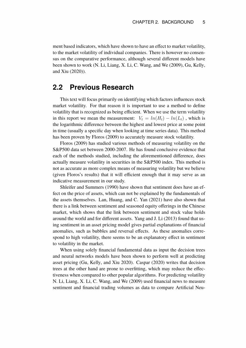
2.2 Previous ResearchThis text will focus primarily on identifying which factors influences stock

market volatility. For that reason it is important to use a method to definevolatility that is recognized as being efficient. When we use the term volatilityin this report we mean the measurement: Vt = ln(Ht) − ln(Lt) , which isthe logarithmic difference between the highest and lowest price at some pointin time (usually a specific day when looking at time series data). This methodhas been proven by Floros (2009) to accurately measure stock volatility.

Floros (2009) has studied various methods of measuring volatility on theS&P500 data set between 2000-2007. He has found conclusive evidence thateach of the methods studied, including the aforementioned difference, doesactually measure volatility in securities in the S&P500 index. This method isnot as accurate as more complex means of measuring volatility but we believe(given Floros’s results) that it will efficient enough that it may serve as anindicative measurement in our study.

Shleifer and Summers (1990) have shown that sentiment does have an ef-fect on the price of assets, which can not be explained by the fundamentals ofthe assets themselves. Lan, Huang, and C. Yan (2021) have also shown thatthere is a link between sentiment and seasoned equity offerings in the Chinesemarket, which shows that the link between sentiment and stock value holdsaround the world and for different assets. Yang and J. Li (2013) found that us-ing sentiment in an asset pricing model gives partial explanations of financialanomalies, such as bubbles and reversal effects. As these anomalies corre-spond to high volatility, there seems to be an explanatory effect in sentimentto volatility in the market.

When using solely financial fundamental data as input the decision treesand neural networks models have been shown to perform well at predictingasset pricing (Gu, Kelly, and Xiu 2020). Caspar (2020) writes that decisiontrees at the other hand are prone to overfitting, which may reduce the effec-tiveness when compared to other popular algorithms. For predicting volatilityN. Li, Liang, X. Li, C. Wang, and We (2009) used financial news to measuresentiment and financial trading volumes as data to compare Artificial Neu-

6 CHAPTER 2. BACKGROUND

ral Networks (ANN) with Support Vector Machines (SVM). They found thatSVM’s outperformANN’s for volatility forecasts, but that ANN’s perform bet-ter at predicting volatility trends. The paper also shows that there is a strongcorrelation between information sentiment, trading volume and volatility.

Bradley, Hanousek, Jame, and Xiao (2021) studied the due diligence re-ports on the subreddit Wallstreetbets. Average buy recommendations lead tolarger trading volumes in the intraday window following the publication. Also,on average the reports lead to larger returns for the buyers as the returns on av-erage are 5% over the subsequent quarter after the post. Rao and Srivastava(2012) studied the correlation between sentiment on Twitter and stock priceson big cap technological stocks, and found a strong correlation between these.

2.3 NoveltyEarlier research such as that done by Brown and Cliff (2005) primarily re-

lied on physical surveys to gather investor sentiment. More modern researchsuch as that done by Mankar, Hotchandani, Madhwani, Chidrawar, and Lifna(2018) relied on training a classifier on a corpus of tweets. Lyócsa, Baumöhl,and Vyrost (2021) has used sentiment data from r/wallstreetbets while N. Li,Liang, X. Li, C. Wang, and We (2009) has compared different machine learn-ing methods.

Our aim, on the other hand, is to study the impact of sentiment from thesubreddit reddit.com/r/wallstreetbets using multiple machine learning meth-ods and financial indicators.

2.4 Sentiment ScoringFor sentiment analysis we use the deep language representation Distil-

BERT to grade the sentiment of our collected data. DistilBERT is a pretrainedmodel that is commonly used to perform natural language analysis. Buyukoz,Hurriyetoglu, and Arzucan (2020) et al found that DistilBERT is better thanother state of the art deep contextual representations at grading sentiment, ata lower computational cost.

DistilBERT takes natural language as input and provides a score between-1.0 and 1.0 where -1.0 means that the sentiment is completely negative and1.0 means that the sentiment is completely positive.

CHAPTER 2. BACKGROUND 7

2.5 Data SourcesWe have sourced our financial data (time series data, shares outstanding,

debt, etc.) fromAlphaVantage, which is a vendor that offers extensive financialdata to both private businesses and as part of academic endeavours.

In order to gauge online sentiment from social media we have collectedapproximately three million comments from the subforum "/r/wallstreetbets"of the social media platform "www.reddit.com", where it currently has over 10million members. This subforum has in recent years caused significant volatil-ity in several securites such as GME, NOK and AMC, as Lyócsa, Baumöhl,and Vyrost (2021) et al. have found.

Chapter 3

Methods

In our work, data has been collected, parsed and fed to machine learningalgorithms. The data took a path from collection from financial informationproviders and Wallstreetbets, through parsing and analysis to the final results,as can be seen in Figure 3.1, where the arrows symbolize the paths of data.

We chose our data source on the basis of availability and the quality of dataprovided.

Figure 3.1: The path from raw unstructured data to the result.

8

CHAPTER 3. METHODS 9

3.1 Data collection

3.1.1 Alpha VantageAlphaVantage offers a limited public API and a more extensive API for

academic purposes upon request. We chose this API among others because ofits support for academic research, highly set data transfer limitation rates andbuilt in support for calculations of certain financial metrics. We have used anacademic license to source data from the following endpoints, which are usedto calculate input for machine learning algorithms:

TIME_SERIES_DAILY

Contains the daily open, close, high and low prices of the requested secu-rity.

MOM

This endpoint returns a time series which maps dates to the momentumindicator.

OVERVIEW

This endpoint returns an overview of the requested security. We have usedthis to collect the number of shares outstanding.

3.1.2 Sentiment analysisUtilizing the fact that Reddit does not delete old data we have been able to

collect comments from the subreddit ’/r/wallstreetbets’ since 2012. The com-ments were downloaded as raw text data, including emojis, split with newlinecharacters. We have parsed the comments by iterating through them, splittingthem up into individual items in a collection and then storing that collectionas JSON.

Utilizing this collection we have been able to extract all comments men-tioning a specific security symbol by utilizing case insensitive regular expres-sions. These comments were sorted into a dictionary that maps between a dateand all comments made about that security on that specific day. This processwas repeated for all symbols in the S&P500.

This construction allowed us to process each comment individually usingthe distilBERT neural network to create an aggregated sentiment score per day

10 CHAPTER 3. METHODS

for any symbol. DistilBERT is used as Buyukoz, Hurriyetoglu, and Arzucan(2020) found that DistilBERT is better than other state of the art deep contex-tual representations at grading sentiment, while having a lower computationalcost.

3.2 Data Parsing

3.2.1 Input Parameter ComputationsIn order to create input for the machine learning algorithms we have com-

puted several values to serve as data points for input to the models. The com-putations of these data points have been made from the raw data calculatedfrom the collected financial and sentiment data. Other parameters were notcomputed by us, but given by the data provider Alpha Vantage. The collecteddata points were then inserted into a vector before being fed into the machinelearning algorithms for training.

3.2.2 Provided ParametersThe following parameters were provided to us pre-calculated by Alpha

Vantage:

Momentum

Momentum is the difference between the latest price of a security and theprice 10 days previously (Hayes 2021). We have used the following equationto calculate the momentum of our securities:

M = V − Vx

Momentum was chosen as a parameter as Arena, Haggard, and X. Yan(2008) have shown that there is a positive time-series relation between idiosyn-cratic volatility and momentum. Also, K. Wang and Xu (2015) showed thatvolatility is a significant power when forecasting momentum. There thus exista correlation between volatility and momentum, and therefore historic mo-mentum should be used as a financial metric to correct for the effect it has onvolatility.

CHAPTER 3. METHODS 11

3.2.3 Computed ParametersThe following financial and accounting values were computed by us using

raw financial data provided by Alpha Vantage or computed by the sentimentanalysis model:

Market Cap

Themarket cap has been computed using the number of shares outstandingfor the company multiplied with the share price (Shobhit 2020). LetMc be themarket cap, P be the daily closing price of the company’s shares and S be thenumber of total shares outstanding.

Mc = P ∗ S

This parameter was included to limit the impact of confounding factorssuch as market manipulation that were unrelated to broader investor sentiment.Serkan and Bedri (2013) and Riyanto and Arifin (2018) showed that smallercompanies with a lower free float tends to be more prone to manipulation.

Abnormal Return

The abnormal return was calculated by comparing the expected return ofan average investor to the actual return that the security has produced oversome period (Barone 2021). We have chosen a period of 60 days. We havecomputed the abnormal return as follows:

rab = ra − reWherein rab is defined as the abnormal return, ra is the actual return on

investment and re is expected return. The expected return is computed as:

re = rf + β(rm − rf )

Here rf is the risk free rate of return. We have settled for a rate of 2%which is the average of the 10 year United States Treasury bond yield between2016-2021. β is beta-number for the particular security and rm is averagemarket return. We have used a rough figure of 8% which is the average growthof the S&P500 index between 2016-2021.

The actual return on investment has been calculated as follows:

ra =ct1 − ct2ct1

12 CHAPTER 3. METHODS

Where ct1 is the market cap at a given date and ct2 is the market cap 60days previous.

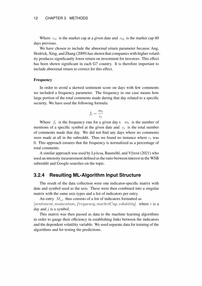
We have chosen to include the abnormal return parameter because Ang,Hodrick, Xing, and Zhang (2009) has shown that companieswith higher volatil-ity produces significantly lower return on investment for investors. This effecthas been shown significant in each G7 country. It is therefore important toinclude abnormal return to correct for this effect.

Frequency

In order to avoid a skewed sentiment score on days with few commentswe included a frequency parameter. The frequency in our case means howlarge portion of the total comments made during that day related to a specificsecurity. We have used the following formula:

ft =mt

ct

Where ft is the frequency rate for a given day t. mt is the number ofmentions of a specific symbol at the given date and ct is the total numberof comments made that day. We did not find any days where no commentswere made at all in the subreddit. Thus we found no instance where ct was0. This approach ensures that the frequency is normalized as a percentage oftotal comments.

A similar approach was used by Lyócsa, Baumöhl, and Vyrost (2021) whoused an intensitymeasurement defined as the ratio between interest in theWSBsubreddit and Google-searches on the topic.

3.2.4 Resulting ML-Algorithm Input StructureThe result of the data collection were one indicator-specific matrix with

date and symbol used as the axis. These were then combined into a singularmatrix with the same axis types and a list of indicators per entry.

An entry Mi,j thus consists of a list of indicators formatted as[sentiment,momentum, frequency,marketCap, volatility] where i is aday and j is a symbol.

This matrix was then passed as data to the machine learning algorithmsin order to gauge their efficiency in establishing links between the indicatorsand the dependent volatility variable. We used separate data for training of thealgorithms and for testing the predictions.

CHAPTER 3. METHODS 13

This structure was chosen as all machine learning libraries used expectedmatrices as input, and as it was compatible with the Pandas package for ma-trices.

3.3 Machine learning algorithms

3.3.1 Decision treeThe decision tree algorithm is a relatively straightforward algorithm to

gauge relations in structured data. We chose this method given the successof Gu, Kelly, and Xiu (2020) in modeling security prices through decisiontrees. In this model the data flows through a tree-like structure wherein thenodes are boolean statements. This is done through sequentially asking ques-tions about the attributes of each observation in each node, where differentanswers lead to different child-nodes. At the end each observation comes to aleaf where the prediction of the decision tree stands for the observation.

During construction of the decision tree, the structure of the tree dependson which statement has the highest Gini-impurity, which is a measure of pre-dictability. The basic principle of this method is to keep organizing the treeinto sections with low Gini-impurity so that the resulting leaf-nodes will be aspure of impurity as possible. Another way to see this is that each node asksthe question which gives us the most information about the sample, which iswhen the entropy of the answer is reduced most.

Figure 3.2: Example of how a subsection of the decision tree could be ordered.

In order to create and execute the creation of the decision tree we have usedthe XGBoost library implementation for Python. XGBoost is broadly used inmachine learning competitions and by data scientists, and uses less compu-tational power than its competitors (Chen and Guestrin 2016). As we lack

14 CHAPTER 3. METHODS

computational power, XGBoost thus allows us to train on more data than itscompetitors while not sacrificing prediction power. Also, as we try to comparepopular machine learning algorithms, using the libraries most widely used byprofessionals for each method is fitting.

We used the default tree parameters of the XGBoost library, which meansthat some parameters are optimized automatically by heuristics. All machinelearning algorithms ran 100 times to collect statistical data, and each individualrun used a random 5% of the data in the total data set, which in total consistedof almost one million data points. Unfortunately more training data couldnot be used due to computational limitations, especially as the computationalcomplexity seemed to increase faster than linearly in regards to the amount ofinput data.

3.3.2 Neural networkWe chose this model for our work because N. Li, Liang, X. Li, C. Wang,

and We (2009) successfully used it to predict volatility in the stock marketusing sentiment data. We have used the Keras Python wrapper for the Ten-sorFlow library to simulate an artificial neural network. The input is a set ofnodes which is put through layers of differently weighted connections whichmaps to nodes containing degrees of volatility in the output. We have chosenthe TensorFlow library because it offers extensive functionality through thewrapper Keras and is frequently used in other academic projects.

For this project we have utilized a very simple sequential neural networkconsisting of two hidden layers, which means that it is a multilayer perceptronas the number of hidden layers is more than or equal to one. The first hid-den layer consists of 16 neurons and the second layer consists of 32 neurons.The output layer is a single neuron which is the degree of volatility, and theinput layer consists of four neurons as there are four features in the input data.Using a multilayer perceptron means that the ANN can approximate almostall smooth functions, even highly non-linear functions (Gardner and Dorling1998).

G. Panchal, Ganatra, Kosta, and D. Panchal (2011) writes that whereasone hidden layer is sufficient for most problems, it cannot model discontin-uous functions. As the function between the input data and stock volatilitymay contain discontinuities such as saw tooth patterns, two hidden layers wereused. However, more hidden layers seldom improves predictions and insteadintroduces a risk of converging to a local minimum.

Using toomany neurons in each layer introduces risk of overfitting, whereas

CHAPTER 3. METHODS 15

using too fewmay lead to underfitting (G. Panchal, Ganatra, Kosta, andD. Pan-chal 2011). There are rules of thumbs however as to the amount of neuronsused, but ultimately it becomes a question of trial and error to find which con-figuration of neurons best can model the data. After testing different amountof neurons in each layer we concluded in the current ANN network.

In order to use the Keras wrapper we took our generalized input matrix andnormalized the data, ensuring that all data is represented on the scale [0.0-1.0].

The computations were performed with the following settings:

Optimizer AdamLearning Rate 1 ∗ 10−4

Loss Function Sparse Categorical CrossentropyEpochs 30

Batch Size 10Hidden Layer Activation Function (both layers) Relu

The optimizer Adam was chosen as it is the standard optimizer for thesci-kit learn implementation of the ANN. The number of epochs was set to30 to improve the model’s accuracy in each iteration without sacrificing toomuch computational time. The Relu activation function was chosen as it isrecommended by the library authors.

16 CHAPTER 3. METHODS

Figure 3.3: Example showcasing the basic structure of the neural networksetup.

3.3.3 Support Vector MachineSupport Vector Machine (SVM) is a machine learning model which at-

tempts to classify objects based on their characteristics through segmentation.Our aim is to be able to segment different securities into categories of volatil-ity to accurately predict which of our key indicators leads to high volatility.This model was been shown to yield good results in predicting asset volatilitywith sentiment based parameters (N. Li, Liang, X. Li, C.Wang, andWe 2009),which therefore makes it relevant for this study.

CHAPTER 3. METHODS 17

Figure 3.4: Example of linear SVM hyperplanes. H1 does not separate theclasses, whereas H2 and H3 does. H3 separates the classes with the widestmargins. Picture from Wikipedia.

In Figure 3.4 X1 and X2 would be different dimensions of data on theobservations we have used. An example could be that one axle is Momen-tum, and the other Frequency of mentions on Wallstreetbets. Also, the linesof a SVM are seldom linear, and will in our example be in more dimensions.Computing SVMs in high dimensions is however costly in regards of calcula-tions, which is why a kernel is used. A kernel allows SVMs to operate in highdimension spaces without calculating all coordinates. The kernel we use isthe Radial Basis Function (RBF), which was previously used by N. Li, Liang,X. Li, C. Wang, and We (2009) to classify clusters. The RBF needs a gamma-value which dictates how much the algorithm will fit the line after individualobservations. The larger the gamma, the more closely the fit of the line to in-dividual data points, as can be seen in figure 3.5 and 3.6. The thicker blackline is a hyperplane in a RBF kernel, which more closely follows individualdata points in Figure 3.5.

18 CHAPTER 3. METHODS

Figure 3.5: Example of higher gammavalue.

Figure 3.6: Example of lower gammavalue.

In order to more accurately allow the model to find the best fit we are usinga built-in feature of the Scikit-learn library which utilizes machine learning todetermine an optimal gamma-value.

The computations were performed with the following settings:

Class Weight NoneCoefficient 0 0.0

Decision Function Shape OVRPolynomial Degree 3

Gamma AutoPolynomial Kernel RBFMax Iterations -1Probability False

Random State 7Shrinking TrueTolerance 20

These settings are primarily standard settings of the sci-kit learn library.The RBF-kernel however was chosen on the basis of having been used by N.Li, Liang, X. Li, C. Wang, and We (2009) and ’Random State 7’ was chosenarbitrarily to provide a seed for the pseudo random number generator. Thepolynomial degree was chosen as 3 rather than the standard 2 with the intentto expose more possible segmentation patterns of the data without sacrificingtoo much computation time. The other settings were default settings, whichwe kept as we did not need to limit computational resources used and as theproblem did not require changed settings.

CHAPTER 3. METHODS 19

3.4 Evaluating algorithmsWe use machine learning algorithms to predict outcomes using continuous

variables, similar to regressionmodels. Therefore, Handelman et al. (2019) ar-gues that the performance of the machine learning algorithms should be mea-sured using coefficient of determination (R2), Mean Squared Error (MSE)or Mean Absolute Error (MAE). Other evaluation metrics used for machinelearning algorithms using continuous variables as input are Mean AbsolutePercentage Error (MAPE) and Root Mean Squared Error (RMSE) (Rundo,Trenta, Luigi di Stallo, and Battiato 2019). Also, the amount of measuresvaries between two or three measures where at least one measure evaluatesthe absolute error and another measures the root, percentage or relative error(Handelman et al. (2019), Rundo, Trenta, Luigi di Stallo, and Battiato (2019),Osisanwo, Akinsola, Awodele, Hinmikaiye, Olakanmi, and Akinjobi (2017)).

This study will therefore use the measures Mean Absolute Error (MAE),Root Mean Squared Error (RMSE) and the coefficient of determination (R2).We use MAE to measure the average error of the predictions, which tells usthe magnitude of the error. RMSE at the other hand varies with the size ofthe variability of the error magnitudes as well as the average error of the pre-dictions (Willmott and Matsuura 2005). Willmott and Matsuura (2005) alsoshow that the RMSE can not be smaller than MAE, instead a large differencebetween the RMSE and MAE values indicate a high amount of variability ofthe size of the errors. Therefore algorithms where the size of the errors dif-ferentiates highly will have a significantly higher RMSE value than the MAEvalue, which discerns algorithms which may have a low MAE but at timeshas very large errors from those which have a consistent rate of error. Lastly,whereas MAE and RMSE is useful to compare algorithms, the coefficient ofdetermination is used to detect the quality of the algorithms as it describesthe proportion of the variance of the dependent variable which is determinedby the independent variable (Chicco, Warrens, and Jurman 2021). Togetherthese measures give a picture over the size of the average error, the variabil-ity of errors and a measure over the explanatory value of the algorithms. Wehave chosen the coefficient of determination as the measure for the explana-tory power instead of measures like the Symmetric Mean Absolute PercentageError (SMAPE) as Chicco, Warrens, and Jurman (2021) argue thatR2 is moreinformative and truthful than SMAPE in several use cases.

The results will be statistically tested by running each machine learningalgorithm 100 times and for each run collect the MAE, RMSE and R2 valuesfor the test through comparing predicted and test values. Each individual run

20 CHAPTER 3. METHODS

will use a random 5% of the data in the total dataset, which in total consistsof almost one million data points. Two thirds of the randomly chosen data isused for training the algorithms, and one third for calculating the measureswe use to compare the algorithms. More training data and test runs couldnot be completed due to limitations in computing power. Lastly, the median,average and variance of each measure will be calculated and the results of thecalculated measures will be visualized using box plots to show the distributionof each measure.

3.4.1 Performance metricsThe basis of these definitions were primarily sourced from Chicco, War-

rens, and Jurman (2021).

Mean Absolute Error (MAE)

MAE =Σni=1|ei|n

Here n is the number of datapoints, i the current datapoint and |ei| is de-fined as the difference between the predicted and actual values for a datapoint.

Root-Mean-Square Error (RMSE)

RMSE =

√Σni=1e

2i

n

Here n is the number of datapoints, ei is the difference between betweenthe predicted and actual values for the datapoint i.

Coefficient of Determination (R2)

The coefficient of determination is, in our case, a measurement of howwellwe can predict the volatility given our input parameters. A negative R2 valueindicates that the trend curve a model has fit to the training data has an inverserelationship with the testing data.

R2 = 1− SSresSStot

SSres = Σni e

2i

CHAPTER 3. METHODS 21

where n is the number of datapoints and e2i is the squared error between apredicted value and the actual value.

SStot = Σnim

2i

where m2i is the squared distance between the actual value of a datapoint

and the mean value of all the datapoints.

Chapter 4

Results

This section details the results we obtained by feeding our sourced data intoour three machine learning methods. Lower Mean Absolute Error (MAE) in-dicates better prediction power as the average value of the errors is lower, how-ever a error very close to zero indicates a possible case of overfitting the modelto the data. The Root Mean Squared Error (RMSE) can not be lower than theMAE, however a RMSE which is only slightly higher than the MEA indicatesa low variance of the error distribution, which generally is preferrable.

The coefficient of determination (R2) is the proportion of variance of pricevolatility that is predictable from financial and sentiment based data. A coef-ficient of determination closer to one indicates high predictive power. A zero,or negative coefficient indicates that a model does not model the trend of thedata.

The volatility parameter is measured as a percentage of the fluctuation inthe price of a security. The average overall volatility for all companies in theindex was 0.0222 or 2.22%. The average variance in volatility was 0.00028.

22

CHAPTER 4. RESULTS 23

4.1 Individual Algorithmic Performance

4.1.1 Decision treeName Average Median VarianceMAE 4.6417 4.6092 0.2201RMSE 11.3720 10.5557 10.1519R2 -0.3499 -0.2046 0.1723

Table 4.1: Table over averages, medians and variances of the MAE, RMSEand R2 measures on the predictions of the decision tree algorithm. N=100

Figure 4.1: Boxplot over the R2 of the predictions results after 100 runs ofdecision trees.

The R2 result in Table 4.1 indicates that utilizing the decision tree modelwith our parameters does not reliably produce a result that holds predictivepower greater than a chance-based model. Also, the R2 value being less thanzero implies that the decision tree models found relationships between inputand output which were erroneous. Figure 4.1 shows that no test run reached aR2 score of higher than zero. Also, as the RMSE is significantly higher thanthe MAE in Table 4.1 there is an indication that there exists large errors in thedecision tree algorithm, rather than a consistent error rate in the predictions.Also, as the average MAE is significantly larger than the variance of the aver-age volatility of companies the volatility predictions seem to be far from thetrue volatility values of companies.

24 CHAPTER 4. RESULTS

Figure 4.2: Boxplot over the R2 values after 100 runs of the SVM algorithm

4.1.2 Support Vector MachineName Average Median VarianceMAE 10.7313 10.6969 0.4443RMSE 19.2126 18.5888 20.0850R2 -0.3071 -0.3071 0.0088

Table 4.2: Table over averages, medians and variances of the MAE, RMSEand R2 measures on the predictions of the SVM algorithm. N=100

The results obtained from testing the data with the Support VectorMachinemodel using our specified parameters did not show any significant predictivepower. The negative R2 value, as depicted in Figure 4.2, clearly indicates thatwe were not able to explain data that the model was not trained on. Instead themodels found erroneous relationships which does not model the trends of thedata. In fact, not a single test run had a positive R2 value. Also, as the RMSEin Table 4.2 is significantly higher than the MAE there is an indication of ahigh variability of the errors in the predictions of the SVM algorithm. TheMAE at the other hand is relatively stable with a low variance, which impliesthat the absolute average error rate is similar between each run of the algo-rithm.

CHAPTER 4. RESULTS 25

4.1.3 Artifical Neural NetworkName Average Median VarianceMAE 4089855483 983818915 4.4763E + 19

RMSE 15673566608 2938017159 9.9998E + 20

R2 −4.9532E + 24 -3.3046E + 22 4.1332E + 50

Table 4.3: Table over averages, medians and variances of the MAE, RMSEand R2 measures of the ANN algorithm. N=100

The ANN algorithm performed very poorly with significantly higher av-erage RMSE values than MAE values in table 4.3, which indicates that theprediction errors were not of a similar size. There is instead a high disper-sion of prediction errors within each test run, as well as a high variance inMAE which implies that the average size of the prediction errors varies highlybetween each test run.

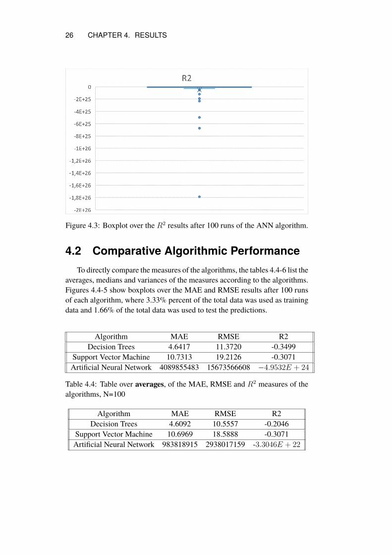
The average and median R2 value of ANN is highly negative, as can beseen in table 4.3. Figure 4.3 also shows that the number of R2 value outliersis high. ANN thus has a very high span of its predictions.

26 CHAPTER 4. RESULTS

Figure 4.3: Boxplot over the R2 results after 100 runs of the ANN algorithm.

4.2 Comparative Algorithmic PerformanceTo directly compare the measures of the algorithms, the tables 4.4-6 list the

averages, medians and variances of the measures according to the algorithms.Figures 4.4-5 show boxplots over the MAE and RMSE results after 100 runsof each algorithm, where 3.33% percent of the total data was used as trainingdata and 1.66% of the total data was used to test the predictions.

Algorithm MAE RMSE R2Decision Trees 4.6417 11.3720 -0.3499

Support Vector Machine 10.7313 19.2126 -0.3071Artificial Neural Network 4089855483 15673566608 −4.9532E + 24

Table 4.4: Table over averages, of the MAE, RMSE and R2 measures of thealgorithms, N=100

Algorithm MAE RMSE R2Decision Trees 4.6092 10.5557 -0.2046

Support Vector Machine 10.6969 18.5888 -0.3071Artificial Neural Network 983818915 2938017159 -3.3046E + 22

CHAPTER 4. RESULTS 27

Table 4.5: Table over medians, of the MAE, RMSE and R2 measures of thealgorithms, N=100

Algorithm MAE RMSE R2Decision Trees 0.2201 10.1519 0.1723

Support Vector Machine 0.4443 20.0850 0.0088Artificial Neural Network 4.4763E + 19 9.9998E + 20 4.1332E + 50

Table 4.6: Table over variance, of the MAE, RMSE and R2 measures of thealgorithms, N=100

The results obtained point to the fact that the parameters based on senti-ment and financial data supplied the model with have little to none predictivepower in relation to predictive abnormal volatility for the broader stock mar-ket. This is due to the on average negative R2 value, showed in Table 4.4.Also, figures 4.1-3 show that the theR2 value never reached positive values inany test runs using any algorithm.

There are however differences between the algorithms. Whereas the De-cision Tree (DT) and the Support Vector Machine (SVM) on average haveonly a slightly negative R2 value, the Artifical Neural Network (ANN) hasan extremely negative R2. The negative R2 value indicates that the DT andSVM models routinely follow erroneous relationships between input and out-put, which can be due to overfitting during the training phase. The extremelynegative average R2 value as well as the excessively high average and medianMAE of ANN suggests that the predictions are far outside the span of the cor-rect answers.

Even though table 4.4 shows that DT on average has a lower R2 valuethan SVM, table 4.5 shows that the median value of R2 is higher on DT. Thisindicates that there are highly negative outliers of the R2 on decision trees,which also is illustrated in figure 4.1. Also, the variance of R2 is higher forDT than for SVM. Thus, DT can at certain runs have higher prediction errors,while SVM has a lower and more consistent amount of prediction errors.

Tables 4.4-5 show that DT has a consistently lower Mean Absolute Error(MAE) as well as a lower variance of the MAE than both SVM and ANN.Figure 4.4 also shows that the lower MAE of the DT is also reached with fewoutliers, whereas ANN has a high amount of outliers. This shows that DT onaverage has a lower and more stable average error size than SVM, which isturn has a lower and stabler average error size than ANN.

The relatively low amount of outliers and lower average variance of SVMand DT in MAE and RMSE ,shown in figure 4.4-5 as well as the table 4.5,

28 CHAPTER 4. RESULTS

Figure 4.4: Boxplot over the MAE results of the machine learning algorithmsafter 100 runs.

Figure 4.5: Boxplot over the RMSE results of the machine learning algorithmsafter 100 runs.

CHAPTER 4. RESULTS 29

show that these algorithms have more stable predictions than ANN. This in-dicates that DT and SVM consistently follow models with a certain span onthe predictions, whereas the ANN has a much larger span on the values of thepredictions. Also, as the average MAE, RMSE and R2 is considerably higherfor ANN it seems to have considerably more disordered predictions.

Chapter 5

Discussion

5.1 Analysis of the ResultThe resulting inaccuracy of all the machine learning models surveyed sur-

prised us. Previous research had indicated that the algorithms we used couldbe used to find relationships between investor sentiment and market volatil-ity. N. Li, Liang, X. Li, C. Wang, and We (2009) for example successfullyused the SVM-model to predict stock market volatility based on sentimentsourced from financial news. Therefore we expected that this model couldyield significant results inmodeling volatility as a consequence of Reddit senti-ment, as Lyócsa, Baumöhl, and Vyrost (2021) found that activity on the forumr/wallstreetbets had an impact on price variation on the companies involved inthe short squeeze of 2020/2021.

N. Li, Liang, X. Li, C. Wang, andWe (2009) also used an ANN to forecastvolatility in the stock market with the previously mentioned sentiment datasourced from financial news. N. Li, Liang, X. Li, C. Wang, and We (2009)found the ANN to be less efficient than the SVM to predict volatility for in-dividual securities, but still capable of achieving favorable predicting results.For this reason we expected that an ANNwould hold relatively high predictivepower when sourcing the sentiment data from Reddit.

Based on this research and the consistent research results by Gu, Kelly,and Xiu (2020) we expected the aforementioned models to produce a gradualincrease in predictive power where the decision tree model would be the leasteffective, the SVM-model would follow and the ANNwould be the best suited.

Our results however did not produce this result. While we had expected theANN to produce the best results, the numbers did not support this. Our errorsrates were extremely high and the coefficient of determination was extremely

30

CHAPTER 5. DISCUSSION 31

negative. This we believe to be a sign that the model was not able to find anyconfiguration of weights between the nodes that produced a satisfying result.It could also be that the network was malformed and did not have the sufficientdepth, or that the sentiment data we sourced did not carry the same predictivepower as the financial news previous research utilized. Another reason whywe did not achieve the same success that N. Li, Liang, X. Li, C. Wang, andWe (2009) did while using the ANN is that we utilized a construction withtwo hidden layers instead of one. This may have introduced a higher degree ofvariance in the MAE and RMSE values given that there were more weightedconnections between the neurons to tune while fitting the model to the data.

The inaccuracies of the DT could be due to the fact that the model is proneto overfitting (Caspar 2020). The negative average R2 value for the model is,according to Caspar (2020), a usual side effect of overfitting. The compara-tively bad R2 value for the SVM-model we believe hints at the same problem.

DT did on average perform worse than SVM, in regards to R2, but had aslightly less worse median R2 than SVM. Together with the higher varianceof DT’s R2 value. Thus, our research shows that the DTs are less stable thanSVMs and more prone to outliers, but otherwise produce predictions with ahigher median R2 value as well as a lower MAE. The sensitivity of decisiontrees may be due to the fact that it for every node uses the attribute with thehighest explanation or information value to create the node question. If twoattributes therefore have similar information values the decision tree will lookhighly different between test runs as the variables by chance will have differentinformation values in each run. This problem could become more prevalentif there exist more attributes, as each attribute inserts a new dimension whichthe decision tree has to partition. If several attributes have weak informationvalue the decision trees will therefore look highly different between each testrun.

The weakness of the SVM algorithm could be due to an incorrectly cho-sen kernel function. However, as we chose the same kernel function as N. Li,Liang, X. Li, C. Wang, and We (2009) who succesfully used SVM to pre-dict similar data there might be other factors behind the weak performance.A potential factor behind the weak performance might be a high amount ofnoise in the data, which hinders class separation as classes overlap. Bradley,Hanousek, Jame, andXiao (2021) found that sentiment on r/wallstreetbets onlyaffected certain companies, while the training data for SVM was based on allcompanies in the S&P500. There should therefore be high amounts of noisein the data as the sentiment data does not correlate with volatility for mostcompanies, which negatively affects class separation of SVMs.

32 CHAPTER 5. DISCUSSION

The ANN showcased a high variance in the MAE and RMSE rates andaverage absolute value of the error rates that were higher than the other twomodels by an order of magnitude. This could be due to how the models arefundamentally arranged. The SVM for example works by lifting the data into ahigher order dimension in order to place it into categories. This means that themodel will categorize the data into the same broad categories as the trainingdata in each run. The segmentation between the values thus ended up beingsimilar between the runs. The Decision Tree model is built on a similar prin-ciple of segmenting data points into broader categories, and thus keeps thepredictions in the same order of magnitude as the training data. It stands toreason that the DT-model would segment the data into similar sections eachpass given the same configurations. We believe that the similarly sized MAEand RMSE reflects this.

The ANN, however, tries highly different weighted settings in each itera-tion, resulting in the high variance we see in the result. Thus, ANN predictionsare not necessarily of the same magnitude as the training data when ANN cannot find a clear relation between the dependent and target variables. Thus,the differences between the algorithms, when looking at MAE, RMSE andR2 could simply be due to different fundamental behaviours when not findingadequate relationships.

Given that sentiment from r/wallstreetbets have been shown to have pre-dictive power in previous research, and the models used in our research alsohave previously been shown to work with newspaper sentiment there is somediscrepancy with our results. This discrepancy could be the result of theamount of capital allocated to different subsets of investors. The sentimentin r/wallstreetbets and the financial news could cater to different audiences,where the investors that gets their news from the financial press have a broadermarket presence. This could possibly explain why Bradley, Hanousek, Jame,and Xiao (2021) saw a clear positive trend in the asset price of popular com-panies on r/wallstreetbets while we did not see this effect on the market as awhole. Lyócsa, Baumöhl, and Vyrost (2021) however used an intensity andsentiment based model to gauge the effect on the market as a whole and foundno impact which would be consistent with our result.

Therefore, we believe that the results of the explored models could bevastly improved by conducting thorough experimentation on smaller subsetsof the data as previous research did find connections between the sentimentof an asset and fluctuations in price on popular companies on r/wallstreetbets.This would lead to less noise in the data, which improves the performance ofmachine learning algorithms. It is also possible that we could have seen im-

CHAPTER 5. DISCUSSION 33

proved result if we had excluded non sentiment based parameters as modelslike DT often perform worse when more parameters are included.

5.1.1 Reflections on the Quality of DataIt is very difficult for us to gauge the impact of weaknesses in our data given

the lack of previous research. We can however make reasonable conclusionsbased on the performance of related research which is what we have attemptedto do.

One of our main challenges while conducting this research has been en-suring the quality of the data used for the prediction models. There are severalproblems with the quality of the financial data we have been able to sourcefrom Alpha Vantage and here we aim to describe them and their potential im-pact in detail.

Averaging of Key Indicators

Some of the key indicators we have used as input data in this report are notreadily available from the API we have utilized and therefore we have had toaverage them out over the period we’ve looked at. One such indicator is the10-year United States bond yield. We have used the figure of 2% which couldbe problematic given that it has fluctuated somewhat during the period fromwhich the data has been collected.

Another example of this is our usage of the 8%-figure in computing theexpected return of an investor. This figure is based on the long term averagegrowth of stock market indexes but could potentially affect the results on ayear-on-year basis.

Usage of Non-Adjusted Time Series Data

There is a well established link between the day that a stock is purchasedwithout the right to participate in the dividend (the so called X-day) and highvolatility. Often the drop in asset price matches the yield attained from thedividend. It is possible that such days with naturally high volatility is con-founded with sentiment based price action in our results. We believe this to bean insignificant factor however as it would rely on the repeated intersection ofstrong sentiment changes on Reddit and X-days.

34 CHAPTER 5. DISCUSSION

Time Sensitive Datapoints

Some datapoints that we have used in our calculations have fluctuated overtime. For example some of the companies present in the S&P500 index haschanged over the period that we’ve covered.

This problem is also evident in the usage of a set number of shares out-standing in calculating themarket capitalization of each securitywe have lookedat. We have not accounted for the issuance of new equity of the S&P500 com-panies. Instead we have used a set figure from 2021. This was a limitation ofthe API we have used. The problem however is somewhat mitigated by the factthat the companies on the S&P500 index is large and do not issue new equityregularly.

The Issue of Meme-Based Sentiment Determination

Apart from problematic financial data one of our largest challenges wasthe ability to accurately gauge the sentiment of the often meme-based com-munication that occurs on Reddit. It is difficult to use traditional methods ofsentiment-analysis when key parts of the message is delivered in emojis. Wehave experimented with using a neural network to identity the different emojis,but it left us with the problem of trying to determine a ranking between theemojis in the evaluation of the sentiment. In the end we have settled on onlyanalyzing the natural language of the posts. However, even the sentiment ofthe natural language of the community has been difficult to interpret due to thespecial language used. Often foul language and insider jokes have been inter-preted as negative sentiment, while they in fact have communicated positivemessages. Examples can be read below.

• "I’m broke and never invested in GME (still retarded), but this sub islike fucking crack. Mad props to all of you holding, i’m fucking pullingfor each and everyone of you. (Four rocket emojis)" - This commentis positive about GME as it describes how courageous people who ownGME are, and thus should be interpreted as positive sentiment towardsGME. Distilbert however ranked this comment as -0.9236, which almostis as bad as a sentiment can get.

• "Stop buying Reddit awards you idiots, buy GME! (Two rocket emojis)"- This comment describes how forum members should not pay to buyawards on Reddit, but should instead buy GME. This comment is highlypositive towards GME as it is a direct order to buy GME, but Distilbertranked it as -0.9995, where -1 is as negative as it can get.

CHAPTER 5. DISCUSSION 35

5.1.2 Further ResearchFuture research might benefit from having access to larger and continually

calculated data to more accurately reflect market conditions. The predictivepower of the models we utilized we believe could be further reinforced by theaddition of a larger set of technical indicators and a more thorough investi-gation of which parameters that are best suited to perform similar analysis.Furthermore we recommend future researchers to add sentiment-based vari-ables such as sentiment data from multiple sources.

A separate study on the topic of what factors accurately reflects the senti-ment of social media-based investors ought to be performed to give qualitativeindicators on which further research could be based.

We also believe that there needs to be research performed on the degree ofcorrelation between the sentiment on social media and the actions of the rest ofthe market. It is our belief that when the link between social-media sentimentand asset prices continues to be popularized this will affect the actions of largergroups of people and form a self-perpetuating cycle. Therefore such linksought to be investigated thoroughly.

Chapter 6

Conclusion

We have determined that none one of the three models tested, using ourspecific configurations, held any predictive power over the development ofvolatility on the S&P500 index. Our conclusion is that while certain compa-niesmay experience high degrees of short term volatility based on r/wallstreetbetssentiment the market as a whole shows no signs of being highly susceptible.The machine learning algorithms were therefore trained on noisy data whichlead to difficulties for the algorithms to find patterns.

Even though none of the machine learning algorithms had any predictivepower, the average error rates differed between the relatively lower averageerror rates of decision trees and support vector machines, and the relativelyhigher average error rates of the artificial neural networks. This disparityseems to be caused by the underlying structure of the algorithms. Thereforethe differences in error rates between the algorithms are simply due to how thealgorithms respond differently to noisy data, and not stronger predictive powerin some algorithms.

36

Bibliography

Brown, G. and Cliff, M. (2005). “Investor Sentiment and Asset Valuation”. In:The Journal of Business 78.2, pp. 405–440. doi: 10.1086/427633.

Lyócsa, Š., Baumöhl, E., and Vyrost, T. (2021). YOLO trading: Riding withthe herd during the GameStop episode. Tech. rep. doi: 10419/230679.

Li, N., Liang, X., Li, X., Wang, C., and We, D. (2009). “Network Environ-ment and Financial Risk Using Machine Learning and Sentiment Analy-sis”. In:Human and Ecological Risk Assessment: An International Journal15, pp. 227–252. doi: 10.1086/427633.

Renault, T. (2019). “Sentiment analysis and machine learning in finance: acomparison of methods and models on one million messages”. In: DigitalFinance 2, pp. 1–13. doi: 10.1007/s42521-019-00014-x.

Gu, S., Kelly, B., and Xiu, D. (2020). “Empirical Asset Pricing via MachineLearning”. In: The Review of Financial Studies 33, pp. 2223–2273. doi:10.1093/rfs/hhaa009.

Rundo, F., Trenta, F., Luigi di Stallo, A., and Battiato, S. (2019). “MachineLearning for Quantitative Finance Applications: A Survey”. In: AppliedSciences 24. doi: 10.3390/app9245574.

Mäntylä, M., Graziotin, D., and Kuutila, M. (2018). “The evolution of sen-timent analysis—A review of research topics, venues, and top cited pa-pers”. In: Computer Science Review 27, pp. 16–32. doi: 10.1016/j.cosrev.2017.10.002.

Wang, S. (2021). “Consumers Beware: How Are Your Favorite "Free" Invest-ment Apps Regulated?” In:Duke Law&Technology Review 19, pp. 43–58.url: https://scholarship.law.duke.edu/dltr/vol19/iss1/3/ (visited on 07/28/2021).

Bradley, D., Hanousek, J., Jame, R., and Xiao, Z. (2021). “Place Your Bets?The Market Consequences of Investment Advice on Reddit’s Wallstreet-bets”. In: SSRN Electronic Journal. doi: 10.2139/ssrn.3806065.

37

38 BIBLIOGRAPHY

Floros, C. (2009). “Modelling volatility using high, low, open and closingprices: evidence from four SP indices”. In: International Research Journalof Finance and Economics 28, pp. 198–206. issn: 1450-2887.

Shleifer, A. and Summers, L. (1990). “The Noise Trader Approach to Fi-nance”. In: Journal of Economic Perspectives 4, pp. 19–33. doi: 10 .1257/jep.4.2.19.

Lan, Y., Huang, Y., and Yan, C. (Jan. 2021). “Investor sentiment and stockprice: Empirical evidence from Chinese SEOs”. In: Economic Modelling94, pp. 703–714. doi: 10.1016/j.econmod.2020.02.012.

Yang, C. and Li, J. (2013). “Investor sentiment, information and asset pricingmodel”. In: Economic Modelling 35, pp. 436–442. doi: 10.1016/j.econmod.2013.07.015.

Caspar, L. (2020). “Exploring heterogeneity usingMetaForest”. In: Small Sam-ple Size Solutions. Ed. by R. van de Schoot and M. Miočević. New York:Routledge. Chap. 13, pp. 186–202.

Rao, T. and Srivastava, S. (2012). “Analyzing Stock Market Movements Us-ing Twitter Sentiment Analysis”. In: 2012 International Conference on Ad-vances in Social Networks Analysis andMining. doi:10.1109/ASONAM.2012.30.

Mankar, T., Hotchandani, T., Madhwani, M., Chidrawar, A., and Lifna, S.(2018). “Stock Market Prediction based on Social Sentiments using Ma-chine Learning”. In: 2018 International Conference on Smart City andEmerging Technology (ICSCET), pp. 1–3. doi: 10 . 1109 / ICSCET .2018.8537242.

Buyukoz, B., Hurriyetoglu, A., and Arzucan, O. (2020). “Analyzing ELMoand DistilBERT on Socio-political News Classification”. In: Language Re-sources and Evaluation Conference. url: https://www.aclweb.org/anthology/2020.aespen-1.4.pdf (visited on 07/25/2021).

Hayes, A. (2021).MarketMomentum.url:https://www.investopedia.com/terms/m/momentum.asp (visited on 07/26/2021).

Arena, M., Haggard, S., and Yan, X. (2008). “Price Momentum and Idiosyn-cratic Volatility”. In: The Financial Review 43, pp. 159–190. doi: 10.1111/j.1540-6288.2008.00190.x.

Wang, K. and Xu, J. (2015). “Market volatility andmomentum”. In: Journal ofEmpirical Finance 30, pp. 79–91. doi: 10.1016/j.jempfin.2014.11.009.

Shobhit, S. (2020). Market Capitalization Defined. url: https://www.investopedia.com/investing/market-capitalization-defined/ (visited on 07/26/2021).

BIBLIOGRAPHY 39

Serkan, I. and Bedri, T. (2013). “Which firms are more prone to stock marketmanipulation?” In: Emerging Markets Review 16, pp. 119–130. doi: 10.1016/j.ememar.2013.04.003.

Riyanto, A. and Arifin, Z. (2018). “Pump-Dump manipulation analysis: theinfluence of market capitalization and its impact on stock price volatilityat Indonesia stock exchange”. In: Review of Integrative Business and Eco-nomics Research 7, pp. 129–142. issn: 2304-1013.

Barone, A. (2021).Abnormal Return.url:https://www.investopedia.com/terms/a/abnormalreturn.asp (visited on 07/26/2021).

Ang, A., Hodrick, R., Xing, Y., and Zhang, X. (2009). “High idiosyncraticvolatility and low returns: International and further U.S. evidence”. In:Journal of Financial Economics 91.1, pp. 1–23. doi: 10 . 1016 / j .jfineco.2007.12.005.

Chen, T. and Guestrin, C. (2016). “XGBoost: A Scalable Tree Boosting Sys-tem”. In: KDD ’16: Proceedings of the 22nd ACM SIGKDD InternationalConference on Knowledge Discovery and Data Mining, pp. 785–794. doi:10.1145/2939672.2939785.

Gardner, M. and Dorling, S. (1998). “Artificial neural networks (the multilayerperceptron)—a review of applications in the atmospheric sciences”. In: At-mospheric Environment 32.14, pp. 2627–2636. doi: 10.1016/S1352-2310(97)00447-0.

Panchal, G., Ganatra, A., Kosta, Y., and Panchal, D. (2011). “Behaviour Anal-ysis of Multilayer Perceptrons with Multiple Hidden Neurons and HiddenLayers”. In: International Journal of Computer Theory and Engineering3.2, pp. 332–337. doi: 10.7763/ijcte.2011.v3.328.

Handelman, G. et al. (2019). “Peering Into the Black Box of Artificial Intelli-gence: Evaluation Metrics of Machine Learning Methods”. In: AmericanJournal of Roentgenology, pp. 38–43. doi: 10.2214/AJR.18.20224.

Osisanwo, F., Akinsola, J., Awodele, O., Hinmikaiye, J., Olakanmi, O., andAkinjobi, J. (2017). “Supervised Machine Learning Algorithms: Classi-fication and Comparison”. In: International Journal of Computer Trendsand Technology 48, pp. 128–138. doi:10.14445/22312803/IJCTT-V48P126.

Willmott, C. and Matsuura, K. (2005). “Advantages of the mean absolute er-ror (MAE) over the root mean square error (RMSE) in assessing aver-age model performance”. In: Climate Research 30, pp. 79–82. doi: 10.3354/cr030079.

Chicco, D., Warrens, M., and Jurman, G. (2021). “The coefficient of determi-nation R-squared is more informative than SMAPE, MAE, MAPE, MSE

40 BIBLIOGRAPHY

and RMSE in regression analysis evaluation”. In: PeerJ Computer Science7. doi: 10.7717/peerj-cs.623.

www.kth.se

TRITA -EECS-EX-2021:661