Co

Ma

b

a

ARR1A

KVEESLAPVPM

1

smAbinc(e

tr

v

h1

Ecological Indicators 52 (2015) 300–310

Contents lists available at ScienceDirect

Ecological Indicators

jo ur nal ho me page: www.elsev ier .com/ locate / ecol ind

omparing environmental vulnerability in the montane cloud forestf eastern Mexico: A vulnerability index

anuel Esperón-Rodrígueza,b, Víctor L. Barradasb,∗

Posgrado en Geografia, Universidad Nacional Autónoma de México, 04510, México, D.F., MexicoLaboratorio de Ecofisiología Tropical, Instituto de Ecología, Universidad Nacional Autónoma de México, 04510, México, D.F., Mexico

r t i c l e i n f o

rticle history:eceived 10 June 2014eceived in revised form1 December 2014ccepted 12 December 2014

eywords:ulnerability indexnvironmental vulnerabilitynvelope function methodtomatal conductanceeaf water potentialir temperaturehotosynthetically active radiation

a b s t r a c t

The montane cloud forest (MCF) is one of the most threatened ecosystems, in spite of its high strate-gic value for sustainable development, the role it plays in the hydrological cycle maintenance, and asreservoir of endemic biodiversity. For Mexico, this forest is considered the most threatened terrestrialecosystem at national level because of land-use changes and the effects of global climate change. Tocompare and assess the environmental vulnerability in the MCF we measured two physiological traits(stomatal conductance and leaf water potential), four climate variables (air temperature, photosyntheti-cally active radiation, vapor pressure deficit, water availability) and the potential geographic distributionof eleven tree species from this forest. We evaluated stomatal conductance responses using the envelopefunction method (EFM), and after analyzing these responses we developed a vulnerability index thatallowed us to compare the environmental vulnerability among species. We proposed the EFM as a usefultool to assess regional environmental vulnerability by comparing species. Our results showed differentialspecies responses to all the studied variables; however, the vulnerability index allowed us to conclude

apor pressure deficitotential distributionontane cloud forest

that the most vulnerable species was Liquidambar styraciflua, and the least vulnerable Persea longipes. Wealso found that temperatures above 34 ◦C, and vapor pressure deficit above 2.9 kPa with relative humiditybelow 30% jeopardized the stomatal conductance performance of all species. We also found leaf waterpotential as the most influential variable over the studied species followed by vapor pressure deficit,showing that even in the MCF water is a determinant factor for species’ development.

© 2014 Elsevier Ltd. All rights reserved.

. Introduction

The montane cloud forest (MCF) posses high strategic value forustainable development, plays a key role in the hydrological cycleaintenance, and is a reservoir of endemic biodiversity (Toledo-ceves et al., 2011). For Mexico, this forest is one of the mostio-diverse ecosystem (González-Espinosa et al., 2012); however,

t is also considered the most threatened terrestrial ecosystem atational level because of changes in land-use, the effects of global

limate change, and local and regional environmental changese.g. CONABIO, 2010; Toledo-Aceves et al., 2011; Calderón-Aguilerat al., 2012).

Abbreviations: gS, stomatal conductance; TA, air temperature; PAR, photosyn-hetically active radiation; VPD, vapor pressure deficit; � , leaf water potential; RH,elative humidity.∗ Corresponding author.

E-mail addresses: orcacomefoca@ciencias.unam.mx (M. Esperón-Rodríguez),barrada@ecologia.unam.mx (V.L. Barradas).

ttp://dx.doi.org/10.1016/j.ecolind.2014.12.019470-160X/© 2014 Elsevier Ltd. All rights reserved.

Globally, climate and environmental changes are increasinglyrecognized as a complex phenomenon involving shifts in manydimensions of Earth’s atmospheric functions (Houghton et al.,1995). Three general expectations exist for species’ responses tothese changes: movement, adaptation (evolutionary change orphysiological acclimatization), or extinction (Holt, 1990). If speciesare sufficiently mobile, they may track the geographic positionof their ecological niches; if species are capable of rapid evolu-tionary change or have a wide range of physiological tolerances,adjustment to changing conditions and landscapes may be possi-ble. Failing mobility and adaptability, extinction is the likely result(Holt, 1990; Melillo et al., 1995). Changes on climate are expected toshift the species’ distribution along environmental gradients if theircurrent environmental tolerance is exceeded (Miller and Urban,1999).

Modeling can be used to predict shifts in vegetation’s distribu-

tion under climatic change and to simulate vegetation responses(Zolbrod and Peterson, 1999). In theory, species presence/absenceand abundance is highest where optimal conditions exist (Gauchet al., 1974). However, global vegetation patterns are already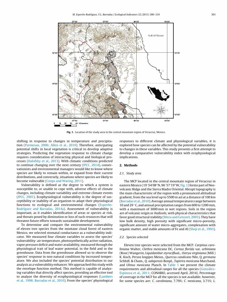

M. Esperón-Rodríguez, V.L. Barradas / Ecological Indicators 52 (2015) 300–310 301

centra

stpsrctvsdb

sc(cfRiat

oMcvvpgsaatite

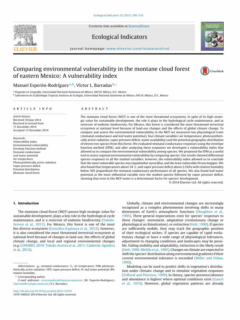
Fig. 1. Location of the study area in the

hifting in response to changes in temperature and precipita-ion (Parmesan, 2006; Allen et al., 2010). Therefore, anticipatingotential shifts in local vegetation is critical to develop adaptivetrategies. Predicting the vegetation response to climate changeequires consideration of interacting physical and biological pro-esses (Halofsky et al., 2013). With climatic conditions predictedo continue changing over the next century (IPCC, 2014), conser-ationists and environmental managers would like to know wherepecies are likely to remain within, or expand from their currentistributions, and conversely, situations where species are likely toecome vulnerable (Coops and Waring, 2011).

Vulnerability is defined as the degree to which a system isusceptible to, or unable to cope with, adverse effects of climatehanges, including climate variability and extreme climate eventsIPCC, 2001). Ecophysiological vulnerability is the degree of sus-eptibility or inability of an organism to adapt their physiologicalunctions to ecological and environmental changes (Esperón-odríguez and Barradas, 2014a). Assessment of vulnerability is

mportant, as it enables identification of areas or species at risk,nd threats posed by diminution or loss of such resources that willhreaten future efforts towards sustainable development.

To determine and compare the environmental vulnerabilityf eleven tree species from the montane cloud forest of easternexico, we selected stomatal conductance as a vulnerability indi-

ator. We measured four climate variables to assess the species’ulnerability: air temperature, photosynthetically active radiation,apor pressure deficit and water availability, measured through thehysiological trait of leaf water potential, in the field and in thereenhouse. Data from the greenhouse allowed us to observe thepecies’ response in non-natural conditions by increased temper-ture. We also included the species’ potential distribution to ournalysis as a vulnerability enhancer. We approached this study with

he envelope function method. This method is capable of analyz-ng variables that directly affect species, providing an effective toolo analyze the diversity of ecophysiological responses (Lamberst al., 1998; Barradas et al., 2010). From the species’ physiological

l mountain region of Veracruz, Mexico.

responses to different climate and physiological variables, it isexplored how species can be affected by the potential vulnerabilityto changes in these variables. This study presents a first attempt todevelop a comparative vulnerability index with ecophysiologicalimplications.

2. Methods

2.1. Study area

The MCF located in the central mountain region of Veracruz ineastern Mexico (19◦54′08′′N, 96◦57′19′′W, Fig. 1) forms part of Neo-volcanic Ridge and the Sierra Madre Oriental. Abrupt topography isthe main characteristic of the region with a pronounced altitudinalgradient, from the sea level up to 5500 m asl at a distance of 100 km(Barradas et al., 2010). Average annual temperatures range between10 and 29 ◦C, and annual precipitation ranges from 600 to 1200 mm,with a maximum of 3000 mm in wet regions. Soils in the regionare of volcanic origin or Andisols, with physical characteristics thatfavor good structural stability (Meza and Geissert, 2003). They havelow bulk density, high porosity with significant micro-porosity,significant amount of water micro-aggregates, complexation withorganic matter, and stable amounts of Fe and Al (Shoji et al., 1993).

2.2. Species selected

Eleven tree species were selected from the MCF: Carpinus caro-liniana Walter, Clethra mexicana DC, Cornus florida var. urbiniana(Rose) Wangerin, Liquidambar styracifluaL., Ostrya virginiana (Mill.)K. Koch, Persea longipes Meisn., Quercus candicans Née, Q. germanaSchltdl. & Cham., Q. xalapensis Bonpl., Tapirira mexicana Marchand,and Ulmus mexicana Planch. In Table 1 we present the climate

requirements and altitudinal ranges for all the species (González-Espinosa et al., 2011; CONABIO, accessed April, 2014). Percentageof coverage in the MCF for all the species is not available; however,for some species are: C. caroliniana, 7.79%; C. mexicana, 3.71%; L.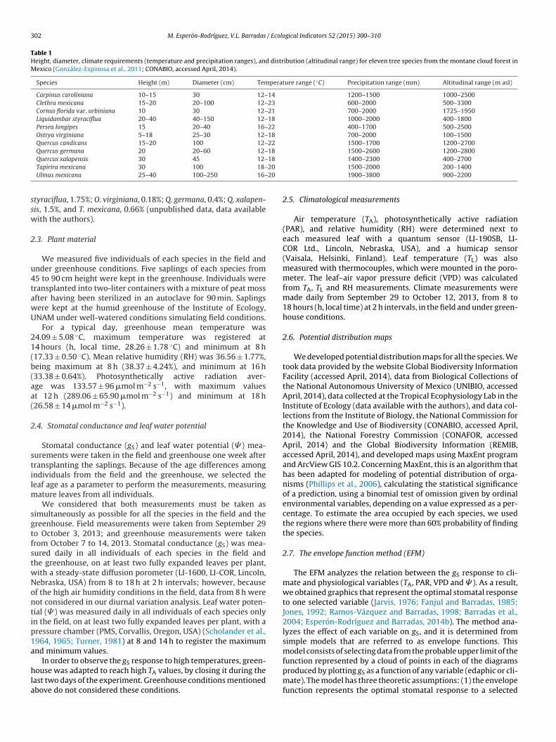

302 M. Esperón-Rodríguez, V.L. Barradas / Ecological Indicators 52 (2015) 300–310

Table 1Height, diameter, climate requirements (temperature and precipitation ranges), and distribution (altitudinal range) for eleven tree species from the montane cloud forest inMexico (González-Espinosa et al., 2011; CONABIO, accessed April, 2014).

Species Height (m) Diameter (cm) Temperature range (◦C) Precipitation range (mm) Altitudinal range (m asl)

Carpinus caroliniana 10–15 30 12–14 1200–1500 1000–2500Clethra mexicana 15–20 20–100 12–23 600–2000 500–3300Cornus florida var. urbiniana 10 30 12–21 700–2000 1725–1950Liquidambar styraciflua 20–40 40–150 12–18 1000–2000 400–1800Persea longipes 15 20–40 16–22 400–1700 500–2500Ostrya virginiana 5–18 25–30 12–18 700–2000 100–1500Quercus candicans 15–20 100 12–22 1500–1700 1200–2700Quercus germana 20 20–60 12–18 1500–2600 1200–2800

18

20

20

ssw

2

u4tawU

21(b(aa(

2

stilm

sgtfstwNontip1a

hla

Quercus xalapensis 30 45 12–Tapirira mexicana 30 100 18–Ulmus mexicana 25–40 100–250 16–

tyraciflua, 1.75%; O. virginiana, 0.18%; Q. germana, 0.4%; Q. xalapen-is, 1.5%, and T. mexicana, 0.66% (unpublished data, data availableith the authors).

.3. Plant material

We measured five individuals of each species in the field andnder greenhouse conditions. Five saplings of each species from5 to 90 cm height were kept in the greenhouse. Individuals wereransplanted into two-liter containers with a mixture of peat mossfter having been sterilized in an autoclave for 90 min. Saplingsere kept at the humid greenhouse of the Institute of Ecology,NAM under well-watered conditions simulating field conditions.

For a typical day, greenhouse mean temperature was4.09 ± 5.08 ◦C, maximum temperature was registered at4 hours (h, local time, 28.26 ± 1.78 ◦C) and minimum at 8 h17.33 ± 0.50 ◦C). Mean relative humidity (RH) was 36.56 ± 1.77%,eing maximum at 8 h (38.37 ± 4.24%), and minimum at 16 h33.38 ± 0.64%). Photosynthetically active radiation aver-ge was 133.57 ± 96 �mol m−2 s−1, with maximum valuest 12 h (289.06 ± 65.90 �mol m−2 s−1) and minimum at 18 h26.58 ± 14 �mol m−2 s−1).

.4. Stomatal conductance and leaf water potential

Stomatal conductance (gS) and leaf water potential (� ) mea-urements were taken in the field and greenhouse one week afterransplanting the saplings. Because of the age differences amongndividuals from the field and the greenhouse, we selected theeaf age as a parameter to perform the measurements, measuring

ature leaves from all individuals.We considered that both measurements must be taken as

imultaneously as possible for all the species in the field and thereenhouse. Field measurements were taken from September 29o October 3, 2013; and greenhouse measurements were takenrom October 7 to 14, 2013. Stomatal conductance (gS) was mea-ured daily in all individuals of each species in the field andhe greenhouse, on at least two fully expanded leaves per plant,ith a steady-state diffusion porometer (LI-1600, LI-COR, Lincoln,ebraska, USA) from 8 to 18 h at 2 h intervals; however, becausef the high air humidity conditions in the field, data from 8 h wereot considered in our diurnal variation analysis. Leaf water poten-ial (� ) was measured daily in all individuals of each species onlyn the field, on at least two fully expanded leaves per plant, with aressure chamber (PMS, Corvallis, Oregon, USA) (Scholander et al.,964, 1965; Turner, 1981) at 8 and 14 h to register the maximumnd minimum values.

In order to observe the gS response to high temperatures, green-ouse was adapted to reach high TA values, by closing it during the

ast two days of the experiment. Greenhouse conditions mentionedbove do not considered these conditions.

1400–2300 400–27001500–2000 200–14001900–3800 900–2200

2.5. Climatological measurements

Air temperature (TA), photosynthetically active radiation(PAR), and relative humidity (RH) were determined next toeach measured leaf with a quantum sensor (LI-190SB, LI-COR Ltd., Lincoln, Nebraska, USA), and a humicap sensor(Vaisala, Helsinki, Finland). Leaf temperature (TL) was alsomeasured with thermocouples, which were mounted in the poro-meter. The leaf–air vapor pressure deficit (VPD) was calculatedfrom TA, TL and RH measurements. Climate measurements weremade daily from September 29 to October 12, 2013, from 8 to18 hours (h, local time) at 2 h intervals, in the field and under green-house conditions.

2.6. Potential distribution maps

We developed potential distribution maps for all the species. Wetook data provided by the website Global Biodiversity InformationFacility (accessed April, 2014), data from Biological Collections ofthe National Autonomous University of Mexico (UNIBIO, accessedApril, 2014), data collected at the Tropical Ecophysiology Lab in theInstitute of Ecology (data available with the authors), and data col-lections from the Institute of Biology, the National Commission forthe Knowledge and Use of Biodiversity (CONABIO, accessed April,2014), the National Forestry Commission (CONAFOR, accessedApril, 2014) and the Global Biodiversity Information (REMIB,accessed April, 2014), and developed maps using MaxEnt programand ArcView GIS 10.2. Concerning MaxEnt, this is an algorithm thathas been adapted for modeling of potential distribution of orga-nisms (Phillips et al., 2006), calculating the statistical significanceof a prediction, using a binomial test of omission given by ordinalenvironmental variables, depending on a value expressed as a per-centage. To estimate the area occupied by each species, we usedthe regions where there were more than 60% probability of findingthe species.

2.7. The envelope function method (EFM)

The EFM analyzes the relation between the gS response to cli-mate and physiological variables (TA, PAR, VPD and � ). As a result,we obtained graphics that represent the optimal stomatal responseto one selected variable (Jarvis, 1976; Fanjul and Barradas, 1985;Jones, 1992; Ramos-Vázquez and Barradas, 1998; Barradas et al.,2004; Esperón-Rodríguez and Barradas, 2014b). The method ana-lyzes the effect of each variable on gS, and it is determined fromsimple models that are referred to as envelope functions. Thismodel consists of selecting data from the probable upper limit of the

function represented by a cloud of points in each of the diagramsproduced by plotting gS as a function of any variable (edaphic or cli-mate). The model has three theoretic assumptions: (1) the envelopefunction represents the optimal stomatal response to a selected

/ Ecolo

ctTv1e

e

g

wdsaa(tdrp

ph

g

wt

g

g

wts

a

g

wct

tc

2

fthvcsvv

pg(en(

M. Esperón-Rodríguez, V.L. Barradas

limate variable (e.g. PAR); (2) the points below the selected func-ion are the result of a change in any of the other variables (e.g.A and VPD), and (3) there are no synergistic interactions betweenariables (edaphic or climate) (Jarvis, 1976; Fanjul and Barradas,985; Jones, 1992; Ramos-Vázquez and Barradas, 1998; Barradast al., 2004).

The relation of gS in terms of air temperature (TA) is given by thenvelope values that fit a quadratic equation:

S = A + BTA + CT2A (1)

here A, B and C are parameters of the parable, being possible toetermine the optimum temperature (TO) at which the maximumtomatal conductance (gSMAX) occurs, and the cardinal temper-tures (minimum and maximum). From the plot TA vs. gS welso obtained the optimal thermic interval (TR) for all the speciesconsidering this interval from the maximum stomatal opening upo 30% closure), and the maximum temperature (TMAX) before gSecrease by 50%, because we considered that this decrease rep-esented potential vulnerability and stress to jeopardize stomatalerformance.

Envelope values of stomatal conductance (gS) as a function ofhotosynthetically active radiation (PAR) are consistent with ayperbolic function:

S =[

aPAR(b + PAR)

](2)

here a is the asymptotic value of gS or gSMAX, and b is gS sensitivityo changes in PAR.

While the gS function in relation to vapor pressure deficit (VPD)enerates a simple linear equation.

S = a + bVPD (3)

here b is gS sensitivity to the VPD, and a is the zero drift. Usinghe plots, we calculated the minimum VPD value (VPDmin) beforetomatal conductance decrease by 50%.

Similarly, the stomatal response to leaf water potential (� ) islso a simple linear equation:

S = a + b� (4)

here b is gS sensitivity to the � , and a is the zero drift. We alsoalculated the maximum � value (� MAX) before stomatal conduc-ance decrease by 50%.

We used data of all variables (gS, TA, PAR, VPD and � ) fromhe field and the greenhouse to estimate all the functions and theoefficients mentioned above.

.8. Vulnerability index

For our study we considered the parameter b from the envelopeunction model as a vulnerability indicator. Parameter b representshe slope of the equations of the variables PAR, VPD and � . Theigher the b, the greater the slope. High b values indicate that theseariables (PAR, VPD and � ) limit and affect more the gS response,ompared with lower slopes where the variables’ effects on thetomatal response is minor. The higher the b value, the greater theulnerability, this because small changes in climate or physiologicalariables represent bigger changes in the gS response.

We developed a vulnerability index that can be used to com-are vulnerability among species (Isp), but also among functionalroups or species from different altitudinal ranges or ecosystems

IV) by obtaining the average values of all the individuals Isp ofach group. The index is composed by five vulnerability compo-ents: air temperature (VTA ), photosynthetically active radiationVPAR), vapor pressure deficit (VVPD), leaf water potential (V�) and

gical Indicators 52 (2015) 300–310 303

distribution (VD). The vulnerability index is the average of all thesecomponents:

Isp = (VTA + VPAR + VVPD + V� + VD)5

(5)

IV =n∑

n=1

Isp

n(6)

As for the vulnerability components, VTA is obtained by dividingthe temperature from the optimal range of each species (TRspn) bythe broadest thermal range of all the species (TRMAX):

VTA = 1 −(

TRspn

TRMAX

)(7)

Regarding the components VPAR, VVPD, V� , these are obtained bydividing the resulting parameter b of each species (bspn) from thecorresponding envelope function (PAR, VPD and � ) by the maxi-mum b value of all the species (bMAX):

VPAR, VVPD, V� = bspn

bMAX(8)

The component VD, was obtained by dividing the distribution ofeach species (Dspn) by the broadest distribution of all the speciesDMAX.

VD = 1 −(

Dspn

DMAX

)(9)

The highest vulnerability level corresponds to values close to 1and the lowest to values close to 0.

2.9. Statistical analysis

Statistical analyses were conducted using software R version3.0.1 (R Core Team, 2014). We used the non-parametrical testKruskal–Wallis to evaluate our data whether there were significantdifferences for three cases: (i) to compare the climatological vari-ables of TA, PAR and VPD between greenhouse and field conditions;(ii) to compare for each species the variables of gS, TA, PAR, VPDbetween greenhouse and field conditions, and (iii) to compare thevariables of gS, TA, PAR, VPD, � among all the species under green-house and field conditions. Statistical significance was consideredat 95% for all cases.

Influence of each variable (TA, PAR, VPD, � ) across the elevenspecies was evaluated through a Principal Components Analysis(PCA). For this purpose, the dataset was organized into a single 4variable × 11 species matrix, and the PCA was based on the correla-tion matrix of variables (Jongman et al., 1987). The PCA was used toidentify the principal sources of variability. We calculated the rel-ative importance (RI) of each component by measuring the lengthof each vector (Legendre and Legendre, 1998). The RI values esti-mated were multiplied for the vulnerability components (VTA , VPAR,VVPD, V�) of all the species to obtain weighted or adjusted values.

3. Results

To compare the species’ response to the drifting variables weincluded in the comparison of climatological conditions betweenfield and greenhouse the values of high TA and VPD reached dur-ing the last days of the experiment (when the greenhouse wasclosed). We found no differences between greenhouse and fieldwhen comparing TA (Kruskal–Wallis H = 1.5504, df = 1, P = 0.2131);

whilst VPD (Kruskal–Wallis H = 11.0253, df = 1, P < 0.001) andPAR (Kruskal–Wallis H = 5.890, df = 1, P = 0.015) had significantdifferences. Greenhouse mean temperature was 25.62 ± 5.88 ◦C,whereas mean temperature in the field was 24.02 ± 3.87 ◦C.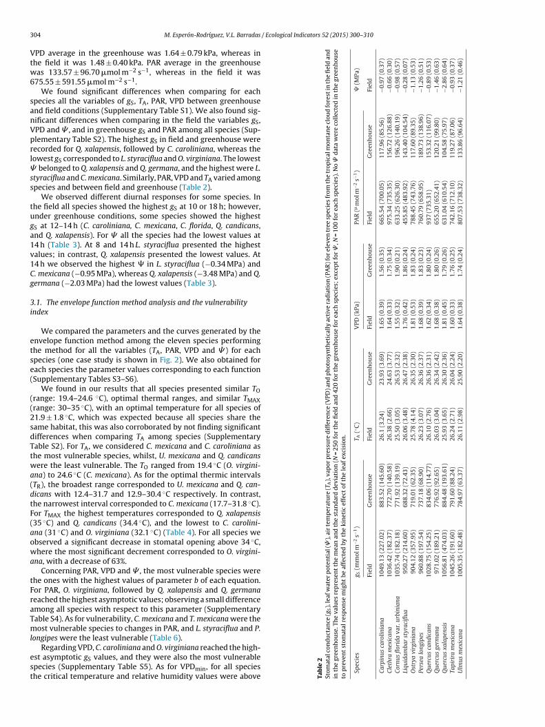

3 / Ecological Indicators 52 (2015) 300–310

Vtw6

sanVprl�ss

tuga1v1Cg

3i

etse(

((2sdTtwa(dtF(aowa

tFraTml

est

du

ctan

ce

(gS),

leaf

wat

er

pot

enti

al

(�

),

air

tem

per

atu

re

(TA),

vap

or

pre

ssu

re

dif

fere

nce

(VPD

) an

d

ph

otos

ynth

etic

ally

acti

ve

rad

iati

on

(PA

R) f

or

elev

en

tree

spec

ies

from

the

trop

ical

mon

tan

e

clou

d

fore

st

in

the

fiel

d

and

ouse

. Th

e

valu

es

rep

rese

nt

the

mea

n

and

the

stan

dar

d

dev

iati

on

(N

=

250

for

the

fiel

d

and

420

for

the

gree

nh

ouse

for

each

spec

ies;

exce

pt

for

�

, N

=

100

for

each

spec

ies)

. No

�

dat

a

wer

e

coll

ecte

d

in

the

gree

nh

ouse

omat

al

resp

onse

mig

ht

be

affe

cted

by

the

kin

etic

effe

ct

of

the

leaf

exci

sion

.

g S(m

mol

m−2

s−1)

T A(◦ C

)

VPD

(kPa

)

PAR

(�m

ol

m−2

s−1)

�

(MPa

)

Fiel

d

Gre

enh

ouse

Fiel

d

Gre

enh

ouse

Fiel

d

Gre

enh

ouse

Fiel

d

Gre

enh

ouse

Fiel

d

rolin

iana

1049

.13

(227

.02)

883.

52

(145

.60)

26.1

(3.2

4)

23.9

3

(3.6

9)

1.65

(0.3

9)

1.56

(0.3

5)

665.

54

(700

.05)

117.

96

(85.

56)

−0.9

7

(0.3

7)ic

ana

1036

.42

(182

.37)

772.

70

(140

.58)

26.3

8

(2.6

6)

24.6

3

(3.7

7)

1.64

(0.3

3)

1.75

(0.3

4)

975.

34

(735

.35)

156.

72

(126

.88)

−0.6

6

(0.3

0)da

var.

urbi

nian

a10

35.7

4

(182

.18)

771.

92

(139

.19)

25.5

0

(3.0

5)

26.5

3

(2.3

2)

1.55

(0.3

2)

1.90

(0.2

1)

633.

25

(626

.30)

196.

26

(140

.19)

−0.9

8

(0.5

7)r

styr

acifl

ua

950.

27

(214

.60)

688.

32

(72.

43)

26.0

6

(3.4

8)

26.4

7

(2.3

8)

1.76

(0.4

2)

1.86

(0.2

4)

455.

85

(483

.92)

143.

40

(104

.54)

−0.2

8

(0.0

7)in

iana

904.

12

(357

.95)

719.

01

(62.

35)

25.7

8

(4.1

4)

26.3

5

(2.3

0)

1.81

(0.5

3)

1.83

(0.2

4)

788.

45

(743

.76)

117.

60

(89.

35)

−1.1

3

(0.5

3)ip

es

960.

88

(197

.54)

737.

18

(68.

90)

26.2

3 (3

.07)

26.3

6

(2.3

7)

1.68

(0.3

9)

1.83

(0.2

3)

760.

79

(658

.95)

189.

73

(138

.96)

−1.2

6

(0.5

1)di

cans

1028

.75

(154

.25)

834.

06

(114

.77)

26.1

0 (2

.76)

26.3

6

(2.3

1)

1.62

(0.3

4)

1.80

(0.2

4)

937

(735

.31)

153.

32

(116

.07)

−0.8

9

(0.5

3)m

ana

971.

02

(189

.21)

776.

92

(92.

65)

26.0

3

(3.0

4)

26.3

4

(2.4

2)

1.68

(0.3

8)

1.80

(0.2

6)

655.

20

(652

.41)

120.

21

(99.

80)

−1.4

6

(0.6

3)ap

ensi

s

1056

.81

(474

.03)

884.

48

(193

.61)

25.9

3

(3.6

5)

26.3

0

(2.3

6)

1.81

(0.4

5)

1.79

(0.2

6)

631.

04

(610

.54)

104.

58

(75.

97)

−2.8

6

(0.6

4)xi

cana

1045

.26

(191

.60)

791.

60

(88.

24)

26.2

4

(2.7

1)

26.0

4

(2.2

4)

1.60

(0.3

3)

1.76

(0.2

5)

742.

16

(712

.10)

119.

27

(87.

06)

−0.9

3

(0.3

7)ic

ana

1005

.35

(182

.48)

784.

97

(63.

37)

26.1

1

(2.9

8)

25.9

0

(2.2

0)

1.64

(0.3

8)

1.74

(0.2

4)

807.

53

(738

.32)

133.

86

(96.

64)

−1.2

1

(0.4

6)

04 M. Esperón-Rodríguez, V.L. Barradas

PD average in the greenhouse was 1.64 ± 0.79 kPa, whereas inhe field it was 1.48 ± 0.40 kPa. PAR average in the greenhouseas 133.57 ± 96.70 �mol m−2 s−1, whereas in the field it was

75.55 ± 591.55 �mol m−2 s−1.We found significant differences when comparing for each

pecies all the variables of gS, TA, PAR, VPD between greenhousend field conditions (Supplementary Table S1). We also found sig-ificant differences when comparing in the field the variables gS,PD and � , and in greenhouse gS and PAR among all species (Sup-lementary Table S2). The highest gS in field and greenhouse wereecorded for Q. xalapensis, followed by C. caroliniana, whereas theowest gS corresponded to L. styraciflua and O. virginiana. The lowest

belonged to Q. xalapensis and Q. germana, and the highest were L.tyraciflua and C. mexicana. Similarly, PAR, VPD and TA varied amongpecies and between field and greenhouse (Table 2).

We observed different diurnal responses for some species. Inhe field all species showed the highest gS at 10 or 18 h; however,nder greenhouse conditions, some species showed the highestS at 12–14 h (C. caroliniana, C. mexicana, C. florida, Q. candicans,nd Q. xalapensis). For � all the species had the lowest values at4 h (Table 3). At 8 and 14 h L. styraciflua presented the highestalues; in contrast, Q. xalapensis presented the lowest values. At4 h we observed the highest � in L. styraciflua (−0.34 MPa) and. mexicana (−0.95 MPa), whereas Q. xalapensis (−3.48 MPa) and Q.ermana (−2.03 MPa) had the lowest values (Table 3).

.1. The envelope function method analysis and the vulnerabilityndex

We compared the parameters and the curves generated by thenvelope function method among the eleven species performinghe method for all the variables (TA, PAR, VPD and � ) for eachpecies (one case study is shown in Fig. 2). We also obtained forach species the parameter values corresponding to each functionSupplementary Tables S3–S6).

We found in our results that all species presented similar TOrange: 19.4–24.6 ◦C), optimal thermal ranges, and similar TMAXrange: 30–35 ◦C), with an optimal temperature for all species of1.9 ± 1.8 ◦C, which was expected because all species share theame habitat, this was also corroborated by not finding significantifferences when comparing TA among species (Supplementaryable S2). For TA, we considered C. mexicana and C. caroliniana ashe most vulnerable species, whilst, U. mexicana and Q. candicansere the least vulnerable. The TO ranged from 19.4 ◦C (O. virgini-

na) to 24.6 ◦C (C. mexicana). As for the optimal thermic intervalsTR), the broadest range corresponded to U. mexicana and Q. can-icans with 12.4–31.7 and 12.9–30.4 ◦C respectively. In contrast,he narrowest interval corresponded to C. mexicana (17.7–31.8 ◦C).or TMAX the highest temperatures corresponded to Q. xalapensis35 ◦C) and Q. candicans (34.4 ◦C), and the lowest to C. carolini-na (31 ◦C) and O. virginiana (32.1 ◦C) (Table 4). For all species webserved a significant decrease in stomatal opening above 34 ◦C,here the most significant decrement corresponded to O. virgini-

na, with a decrease of 63%.Concerning PAR, VPD and � , the most vulnerable species were

he ones with the highest values of parameter b of each equation.or PAR, O. virginiana, followed by Q. xalapensis and Q. germanaeached the highest asymptotic values; observing a small differencemong all species with respect to this parameter (Supplementaryable S4). As for vulnerability, C. mexicana and T. mexicana were theost vulnerable species to changes in PAR, and L. styraciflua and P.

ongipes were the least vulnerable (Table 6).

Regarding VPD, C. caroliniana and O. virginiana reached the high-

st asymptotic gS values, and they were also the most vulnerablepecies (Supplementary Table S5). As for VPDmin, for all specieshe critical temperature and relative humidity values were above Ta

ble

2St

omat

al

con

in

the

gree

nh

to

pre

ven

t

st

Spec

ies

Carp

inus

caCl

ethr

a

mex

Corn

us

flori

Liqu

idam

baO

stry

a

virg

Pers

ea

long

Que

rcus

can

Que

rcus

ger

Que

rcus

xal

Tapi

rira

me

Ulm

us

mex

M. Esperón-Rodríguez, V.L. Barradas / Ecological Indicators 52 (2015) 300–310 305

TA (ºC)

10 15 20 25 30 35 40 45

g S (m

mol

m-2

s-1

)

400

600

800

1000

1200

1400

PAR (�mol s-1 m-2)

0 500 1000 1500 2000

g S (m

mol

m-2

s-1

)

400

600

800

1000

1200

1400

VPD (kPa)

1.0 1.5 2.0 2.5 3.0 3.5 4.0 4.5

g S (m

mol

m-2

s-1

)

400

600

800

1000

1200

1400

� (MPa)

-3.0 -2 .5 -2 .0 -1 .5 -1 .0 -0 .5 0.0

g S (m

mol

m-2

s-1

)

400

600

800

1000

1200

1400

F ) plottp

3ttal

alLa

TLwt(

ig. 2. Scatter diagrams and probable boundary-line of stomatal conductance (gS

ressure deficit (VPD), and leaf water potential (� ) for Quercus candicans.

3.8 ◦C and less than 30% of humidity, where Q. germana presentedhe lowest VPDmin and Q. candicans the highest (Table 5). Accordingo this parameter, the most vulnerable species were C. carolinianand O. virginiana, and the least vulnerable were Q. candicans and P.ongipes (Table 6).

For � , C. caroliniana and Q. xalapensis reached the highest

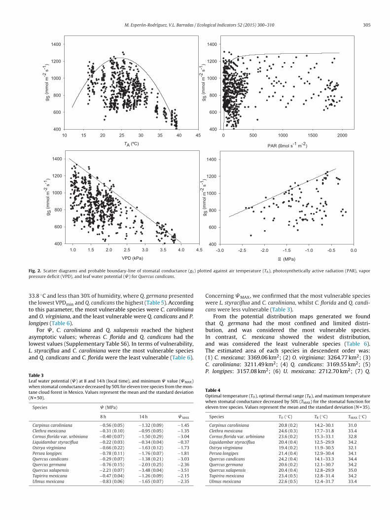
symptotic values; whereas C. florida and Q. candicans had theowest values (Supplementary Table S6). In terms of vulnerability,. styraciflua and C. caroliniana were the most vulnerable speciesnd Q. candicans and C. florida were the least vulnerable (Table 6).

able 3eaf water potential (� ) at 8 and 14 h (local time), and minimum � value (� MAX)hen stomatal conductance decreased by 50% for eleven tree species from the mon-

ane cloud forest in Mexico. Values represent the mean and the standard deviationN = 50).

Species � (MPa)

8 h 14 h � MAX

Carpinus caroliniana −0.56 (0.05) −1.32 (0.09) −1.45Clethra mexicana −0.31 (0.10) −0.95 (0.05) −1.35Cornus florida var. urbiniana −0.40 (0.07) −1.50 (0.29) −3.04Liquidambar styraciflua −0.22 (0.03) −0.34 (0.04) −0.37Ostrya virginiana −0.66 (0.22) −1.63 (0.12) −1.73Persea longipes −0.78 (0.11) −1.76 (0.07) −1.81Quercus candicans −0.29 (0.07) −1.38 (0.21) −3.03Quercus germana −0.76 (0.15) −2.03 (0.25) −2.36Quercus xalapensis −2.21 (0.07) −3.48 (0.04) −3.51Tapirira mexicana −0.47 (0.04) −1.26 (0.09) −2.15Ulmus mexicana −0.83 (0.06) −1.65 (0.07) −2.35

ed against air temperature (TA), photosynthetically active radiation (PAR), vapor

Concerning � MAX, we confirmed that the most vulnerable specieswere L. styraciflua and C. caroliniana, whilst C. florida and Q. candi-cans were less vulnerable (Table 3).

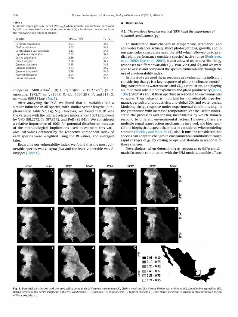
From the potential distribution maps generated we foundthat Q. germana had the most confined and limited distri-bution, and was considered the most vulnerable species.In contrast, C. mexicana showed the widest distribution,and was considered the least vulnerable species (Table 6).The estimated area of each species in descendent order was:

(1) C. mexicana: 3369.06 km2; (2) O. virginiana: 3264.77 km2; (3)C. caroliniana: 3211.49 km2; (4) Q. candicans: 3169.55 km2; (5)P. longipes: 3157.08 km2; (6) U. mexicana: 2712.70 km2; (7) Q.

Table 4Optimal temperature (TO), optimal thermal range (TR), and maximum temperaturewhen stomatal conductance decreased by 50% (TMAX) for the stomatal function foreleven tree species. Values represent the mean and the standard deviation (N = 35).

Species TO (◦C) TR (◦C) TMAX (◦C)

Carpinus caroliniana 20.8 (0.2) 14.2–30.1 31.0Clethra mexicana 24.6 (0.3) 17.7–31.8 33.4Cornus florida var. urbiniana 23.6 (0.2) 15.3–33.1 32.8Liquidambar styraciflua 20.4 (0.4) 12.5–29.9 34.2Ostrya virginiana 19.4 (0.2) 11.9–30.5 32.1Persea longipes 21.4 (0.4) 12.9–30.4 34.1Quercus candicans 24.2 (0.4) 14.1–33.3 34.4Quercus germana 20.6 (0.2) 12.1–30.7 34.2Quercus xalapensis 20.4 (0.4) 12.8–29.9 35.0Tapirira mexicana 23.4 (0.5) 12.8–31.4 34.2Ulmus mexicana 22.6 (0.5) 12.4–31.7 33.4

306 M. Esperón-Rodríguez, V.L. Barradas / Ecolo

Table 5Minimum vapor pressure deficit (VPDmin) when stomatal conductance decreasedby 50%, and associated values of air temperature (TA) for eleven tree species fromthe montane cloud forest in Mexico.

Species VPDmin (kPa) TA (◦C)

Carpinus caroliniana 2.93 34.4Clethra mexicana 3.02 34.8Cornus florida var. urbiniana 3.13 34.9Liquidambar styraciflua 2.87 34.2Ostrya virginiana 2.86 34.4Persea longipes 2.96 34.2Quercus candicans 3.18 34.8Quercus germana 2.83 34.2Quercus xalapensis 2.88 34.0

xmg

sptbaoael

nl

FOo

Tapirira mexicana 2.94 34.4Ulmus mexicana 2.86 33.8

alapensis: 2408.90 km2; (8) L. styraciflua: 2013.27 km2; (9) T.exicana: 1872.71 km2; (10) C. florida: 1504.29 km2, and (11) Q.

ermana: 906.88 km2 (Fig. 3).After analyzing the PCA, we found that all variables had a

imilar influence in all species, with similar vector lengths (Sup-lementary Table S7, Fig. S1). However, we found that � washe variable with the highest relative importance (100%), followedy VPD (99.27%), TA (97.85%), and PAR (82.94%). We considered

relative importance of 100% for potential distribution becausef the methodological implications used to estimate this vari-ble. All values obtained by the respective component index ofach species were weighted using the RI values, and averaged

ater.

Regarding our vulnerability index, we found that the most vul-erable species was L. styraciflua and the least vulnerable was P.

ongipes (Table 6).

ig. 3. Potential distribution and the probability color scale of Carpinus caroliniana (A),

strya virginiana (E), Persea longipes (F), Quercus candicans (G), Q. germana (H), Q. xalapenf Veracruz, Mexico.

gical Indicators 52 (2015) 300–310

4. Discussion

4.1. The envelope function method (EFM) and the importance ofstomatal conductance (gS)

To understand how changes in temperature, irradiance, andsoil water balances actually affect photosynthesis, growth, and inour particular case gS, we used the EFM which allowed us to pre-dict plant performance outside a species’ native range (Rodríguezet al., 2002; Dye et al., 2004), it also allowed us to describe the gSresponses to different variables (TA, PAR, VPD, and � ), and we wereable to assess and compared the species’ vulnerability through theuse of a vulnerability index.

In this study we used the gS response as a vulnerability indicator,considering that gS is a key response of plants to climate, control-ling transpiration (water status) and CO2 assimilation, and playingan important role in photosynthesis and plant productivity (Jones,1992). Stomata adjust their aperture in response to environmentalvariables. Their behavior is important for individual plant perfor-mance, agricultural productivity, and global CO2 and water cycles.Modeling the gS response under experimental conditions (e.g. inthe greenhouse with increased temperature) can be used to under-stand the processes and sensing mechanisms by which stomatarespond to different environmental factors. However, there aremultiple signal transduction mechanisms involved, and biochemi-cal and biophysical aspects that must be considered when modelingstomata (Buckley and Mott, 2013). Also, it must be considered thatspecies can adapt to changes in environmental conditions through

rapid changes of gS, by closing or opening stomata in response tothese changes.

Nevertheless, when determining gS responses to different cli-matic factors in combination with the EFM models, possible effects

Clethra mexicana (B), Cornus florida var. urbiniana (C), Liquidambar styraciflua (D),sis (I), Tapirira mexicana (J), and Ulmus mexicana (K) in the central mountain region

M. Esperón-Rodríguez, V.L. Barradas / Ecological Indicators 52 (2015) 300–310 307

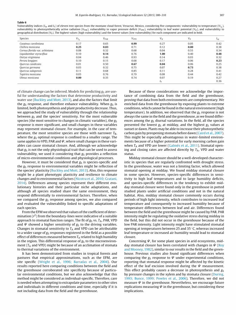
Table 6Vulnerability indices (Isp and IV) of eleven tree species from the montane cloud forest, Veracruz, Mexico, considering five components: vulnerability to temperature (VTA ),vulnerability to photosynthetically active radiation (VPAR), vulnerability to vapor pressure deficit (VVPD), vulnerability to leaf water potential (V�), and vulnerability togeographical distribution (VD). The highest values (high vulnerability) and the lowest values (low vulnerability) for each component are indicated in bold.

Species VTA VPAR VVPD V� VD Isp

Carpinus caroliniana 0.17 0.65 0.99 0.27 0.05 0.42Clethra mexicana 0.25 0.83 0.71 0.12 0.00 0.38Cornus florida var. urbiniana 0.08 0.32 0.68 0.04 0.55 0.34Liquidambar styraciflua 0.10 0.14 0.76 1.00 0.40 0.48Ostrya virginiana 0.04 0.46 0.93 0.14 0.03 0.32Persea longipes 0.10 0.15 0.68 0.17 0.06 0.23Quercus candicans 0.01 0.50 0.67 0.04 0.06 0.25Quercus germana 0.03 0.32 0.75 0.07 0.73 0.38Quercus xalapensis 0.11 0.68 0.85 0.11 0.28 0.41

ofwtlwbsrmpwsatvo

ttmc2larwae

maaCteimt

psrtlmian

Tapirira mexicana 0.03 0.76

Ulmus mexicana 0.00 0.35

f climate change can be inferred. Models for predicting gS are use-ul for understanding the factors that determine productivity andater use (Buckley and Mott, 2013), and also the factors that limit

he gS response, and therefore enhance vulnerability. When gS isimited, both photosynthesis and plant productivity decrease. Thus,

e approached the study of vulnerability through the relationshipetween gS and the species’ sensitivity. For the most vulnerablepecies (the most sensitive to changes in climatic variables), the gSesponse is more significant, and small changes in these variablesay represent stomatal closure. For example, in the case of tem-

erature, the most sensitive species are those with narrower TR,here the gS optimal response is confined to a smaller range. The

ame applies to VPD, PAR and � , where small changes in these vari-bles can cause stomatal closure. And, although we acknowledgehat gS is not the only physiological trait that can be used to assessulnerability, we used it considering that gS provides a reflectionf micro-environmental conditions and physiological processes.

However, it must be considered that gS is species-specific andhe gS response to environmental variables might be reflection ofhe species’ plasticity (Buckley and Mott, 2013). Also, this response

ight be a plant phenotypic plasticity and resilience to climatehanges and to environmental factors (Nicotra et al., 2010; Gratani,014). Differences among species represent their different evo-

utionary histories and their particular niche adaptations, andlthough all species studied share the same environment, theyespond differentially to environmental factors. Therefore, whene compared the gS response among species, we also compared

nd evaluated the vulnerability linked to specific adaptations ofach species.

From the EFM we observed that values of the coefficient of deter-ination (r2) from the boundary-lines were indicative of a suitable

pproach to stomatal function ranges. The fit of gS vs. TA, PAR, VPDnd � showed a higher sensitivity of gS to the driving variables.hanges in stomatal sensitivity to TA and VPD can be attributableo a wider range of gS responses registered in the field as a possibleffect of differences measured between TA related to high humidityn the region. This differential response of gS to the microenviron-

ent (TA and VPD) might be because of an acclimation of stomatao thermal variations of the environment.

It has been demonstrated from studies in tropical forests andastures that empirical approximations, such as the EFM, areite specific (Wright et al., 1996; Barradas et al., 2004). Ouresults reported here comparing conditions between the field andhe greenhouse corroborated site specificity because of particu-ar environmental conditions, but we also acknowledge that this

ethod might be considered as individual-specific. Therefore, cares needed when attempting to extrapolate parameters to other sitesnd individuals in different conditions and time, especially if it isot including data from the field and the greenhouse.

0.79 0.08 0.44 0.420.74 0.07 0.19 0.27

IV 0.36

Because of these considerations we acknowledge the impor-tance of combining data from the field and the greenhouse,proving that data from both environments are complementary. Weenriched data from the greenhouse by exposing plants to extremeconditions, which cannot be found in the natural environment (hightemperature). In addition, we observed that the gS response is notalways the same in the field and the greenhouse, as we found differ-ences among the gS diurnal variations. In the field, all the speciespresented the lowest gS at midday, and the highest gS values atsunset or dawn. Plants may be able to increase their photosyntheticcarbon gain by preopening stomata before dawn (Caird et al., 2007).This might be especially advantageous in water-limited environ-ments because of a higher potential for early morning carbon gainwhen TA and VPD are lower (Galmés et al., 2011). Stomatal open-ing and closing rates are affected directly by TA, VPD and waterstatus.

Midday stomatal closure should be a well-developed character-istic in species that are regularly confronted with drought stress.In the greenhouse, water was not a limiting factor, which allowedstomatal opening at midday. We found midday stomatal closurein some species. However, species-specific differences in sensi-tivity to high leaf temperatures and to large humidity deficits,and species-specific differences in the tendency to exhibit mid-day stomatal closure were found only in the greenhouse in pottedstudied plants under artificial conditions and not in the naturalhabitat. Also, midday stomatal closure commonly occurs duringperiods of high light intensity, which contributes to increased leaftemperature and consequently to increased humidity because oftemperature differences between leaf and air. Differences foundbetween the field and the greenhouse might be caused by PAR. PARintensity might be regulating the oxidative stress during midday inthe field, but this did not occur in the greenhouse because of thelow PAR intensity. Light intensity might have stimulated stomatalopening at temperatures between 25 and 35 ◦C, whereas increasedleaf temperature or increased air humidity would lead to stomatalclosure.

Concerning � , for some plant species in arid ecosystems, mid-day stomatal closure has been correlated with changes in � (Royand Mooney, 1982), similar to our results in the field and the green-house. Previous studies also found significant differences whencomparing the gS response to � under experimental conditions,reporting that stomatal response might be affected by the kineticeffect of the leaf excision involved during the � measurement.This effect probably causes a decrease in photosynthesis and gSby pressure changes in the xylem and by stomata closure (During,

1993; Bunce, 1999; Powles et al., 2006). Therefore, we did notmeasure � in the greenhouse. Nevertheless, we encourage futurereplications measuring � in the greenhouse, but considering theseimplications.

3 / Ecolo

4

vaC2ca�wmcTtd2umilctt

tpdtmdcpaabCaTwom

4

psapewc

pRtacacitSmo

08 M. Esperón-Rodríguez, V.L. Barradas

.2. Species vulnerability

In this study, we found that temperatures above 34 ◦C, and VPDalues above 2.9 kPa with RH below 30% limited gS performance ofll species. Decrease in gS has been attributed to a decrease in � (e.g.omstock and Mencuccini, 1998; Esperón-Rodríguez and Barradas,014a), to increasing VPD and TA (e.g. Maroco et al., 1997), or to aombination of these factors; but if we consider species individu-lly we observed differences among the gS responses. Concerning

, the most important variable according to the RI from the PCA,e found significant differences, especially when comparing theost vulnerable species (L. styraciflua) and the least vulnerable (Q.

andicans). Stomatal conductance was highly correlated to VPD andA but not as much to � . This suggests that the control of stoma-al opening is mainly a function of the atmospheric evaporativeemand rather than a response to the plant water status (Meinzer,002), may be because water is not a limiting factor in the MCF andnder greenhouse conditions. However, � should not be underesti-ated, particularly in arid environments or in regions where water

s a limiting factor. Also, changes in � are not necessary related toow � values; this was corroborated in our results, where Q. candi-ans was the least vulnerable species, whilst Q. xalapensis reachedhe lowest � (Table 3). Opposite to this finding, L. styraciflua washe most vulnerable species with the highest � (Table 3).

Concerning the geographical distribution, we considered thathe species’ distribution is an accurate and complementary com-onent for our vulnerability analysis. Species with more confinedistributions are more likely to suffer impacts of environmen-al and climate changes, particularly those species that require

ore specific micro- and climatic conditions. The potential species’istribution represents an indirect reflection of temperature, pre-ipitation and other climate parameters that establishes theresence/absence of a given species. As for the coverage percent-ge, we found that seven species represent 15.98% of the MCF (therere no data for all species). We considered this a high percentage,ecause of the high biodiversity of this ecosystem. Interestingly,. caroliniana was the species with the highest coverage percent-ge and also was one of the most vulnerable species (Table 6).his increases the ecosystem vulnerability, because if a speciesith wide coverage decreases in number of individuals because

f climate or environmental changes, the ecosystems compositionight be affected.

.3. The vulnerability index: ecological relevance and limitations

In this work we considered the sensitivity of the species, thearameter b from the EFM, as a vulnerability indicator, reflecting gSensitivity to changes in the variables of each species. As a result,

species with a broader thermal range, and lower values of thearameter b, was considered to be better fitted to face and toleratenvironmental changes, whereas a species whose thermal rangeas narrower, and the vulnerability parameter was higher, was

onsidered less tolerant and more vulnerable to disturbances.The use of sensitivity as a vulnerability indicator has been

roposed previously by other authors (e.g. Tremblay-Boyer andoss-Anderson, 2007; Young et al., 2010; Loehle, 2014). The impor-ance of sensitivity relies on its capacity to explain the species’daptations to external factors as a means of identifying whatauses vulnerability differences (Berry et al., 2006). Also, vulner-bility is a function of the character, magnitude and rate of climatehange and variation to which a system is exposed, its sensitiv-ty, and its adaptive capacity (IPCC, 2001). Predicted sensitivity to

emperature and precipitation changes is of particular importance.pecies requiring specific precipitation and temperature regimesay be less likely to find similar areas as climate change and previ-

usly associated temperature and precipitation patterns uncouple

gical Indicators 52 (2015) 300–310

(e.g. Hawkins et al., 2008; Laidre et al., 2008). Species dependent onhabitats that are maintained by regular disturbances (e.g. fires orflooding) are vulnerable to changes in the frequency and intensityof these disturbances (IPCC, 2001; Archer and Predick, 2008), alsospecies with more confined distributions are more vulnerable.

We acknowledge that our index has some limitations. It onlyconsiders two physiological traits, gS and � , three climate vari-ables, TA, PAR and VPD, and the species’ distribution, and althoughwe recognize that there are other traits and variables relevant todescribe species vulnerability, we considered our index accurate,because of the gS importance, and because it is useful to comparevulnerability among species. Also, the evaluated climate variableshelped us to understand the species’ response to climate variabil-ity, by measuring directly the effect of TA, and indirectly the effectof water availability through � . Changes in PAR and VPD are alsoaffected indirectly by TA and water availability; where PAR incre-ment will concur with the substrate temperature and water lossfrom the soil, and changes in TA and humidity will cause effects onVPD. Due to these interactions we considered that the five com-ponents of our index (VTA , VPAR, VVPD, V� , VD) could provide anaccurate vulnerability status of a given species.

Another limitation of our index is the fact that it is only compar-ative; however, we found it efficient because it gathers informationabout variables that might be affected by environmental changes.Another consideration concerning diurnal variation, is that TA, PARand VPD are not the only variables that vary during day. The antiox-idant capacity of leaves also varies during the day and seasonally(Ni et al., 2012), and although this variable was not considered forour study, it should be addressed its importance, considering thatthis variable might jeopardize the gS response if, in a future sce-nario of climate change, this variable changes at different times ofthe day. Nevertheless, we do not consider that these considerationsdetract the effectiveness and assertiveness of the index.

The index allows to prioritize the approach of vulnerability stud-ies by telling which species are most vulnerable. Also, the indexmight be used to compare species, functional groups or speciesfrom different ecosystems, taking into account the limitations men-tioned above. Our index links physiological responses to climatevariables. We encourage future replications in other ecosystemsusing other physiological traits and climate variables. We alsoencourage the development of a homonym index for other taxo-nomical groups.

4.4. Future implications

Gradual increases in temperature, changes in rainfall patterns,or modification in solar radiation will likely impact on growth,regeneration and natural rates of mortality (Chapin et al., 2010).Previous studies from our study region revealed negative precip-itations and positive temperature trends (Esperón-Rodríguez andBarradas, 2014a,b), suggesting a possible regional climate change,implying potential reductions in precipitation of as much as 50% bythe year 2023, and increment of consecutive dry days by the year2099 (Cervantes-Pérez et al., 2001; Barradas et al., 2010; Esperón-Rodríguez and Barradas, 2014a). Also, decreased rainfall and fogfrequency is expected (Barradas et al., 2010, 2011). These changesalso have repercussions on other climatic variables such as solarradiation, which is expected to be more intense where both rainfalland fog frequency decreased (Barradas et al., 2011).

It is also important to consider that species’ interactions underclimate change will probably be altered, thus influencing potentialdistributions (Davis et al., 1998). We must consider the expected

change in the species’ distributions regarding dispersal abilities.Dispersal abilities will play an important role for the species toreach places where environmental conditions will be more favor-able for their establishment, growth, and eventual reproduction.

/ Ecolo

Irrwiaeatwtsuiaa

5

edopdiLwg

saTarmvpeva

A

BgVJtOaPttav2s

A

f2

M. Esperón-Rodríguez, V.L. Barradas

ncreases in temperature predicted by climate change modelseflect species’ vulnerability against these changes. Species mightespond to this vulnerability by migrating to higher elevationshere temperature is lower. Management plans and policies that

ncorporate the response of species and ecosystems are required tossist species to respond to rapid environmental changes (del Barriot al., 2006). It must be considered that if a species does not have thebility to migrate to higher elevations because of the lack of effec-ive seed dispersal, this migration process could be assisted, startingith the most vulnerable species. However, it is important to men-

ion that climate variables are not the only parameters delimitingpecies’ distribution. Factors such as deforestation, agriculture andrban growth, counteract species’ conservation. Scientists and pol-

cymakers must work together to implement proper plans andctions that not only guarantee the preservation of the species butlso benefit the local communities.

. Conclusions

We proposed the EFM as a useful tool for assessing regionalnvironmental vulnerability by comparing species through theevelopment of a vulnerability index in a case study in the MCFf eastern Mexico. This method allowed us to integrate climate andhysiological variables. Our results showed that species respondedifferentially to TA, PAR, VPD and � . However, the vulnerability

ndex allowed us to conclude that the most vulnerable species was. styraciflua. In terms of temperature C. mexicana and C. carolinianaere also vulnerable, and in terms of geographical distribution, Q.

ermana and C. florida were the most vulnerable species.Finding � as the variable with more influence over the species

tudied followed by VPD, showed that even in the MCF water is determinant factor for species’ establishment and development.he EFM needs to be considered with caution because of differencesmong species and sites. Further use with other species, in otheregions and ecosystems should pay attention to what microcli-atic conditions are important in determining local environmental

ulnerability and how is the impact of each variable on the com-lex environment. Our vulnerability index can be considered as ancophysiological index, which evaluates and compares the species’ulnerability through the link of physiological traits, climate vari-bles and geographical distribution.

cknowledgements

We thank Juan Pablo Ruíz Córdova, Alejandro Morales, Martínonifacio and Alfredo Zamora for their help during the field andreenhouse work. We thank MSc. Carlos G. Iglesias Delfín and MSc.íctor Elías Luna Monterrojo from the Jardín Botánico Francisco

avier Clavijero, Instituto de Ecología A.C. for his help and assis-ance to get the plant material. A special thank you to Dr. Marklson. We thank Dr. Alexander Correa Metrio for his invaluablessistance and thoughtful contributions. We thank to David Gómezalacios for his contribution in the data analysis. Also, we thanko the anonymous reviewers for their critical observations and inhoughtful contributions for the improving of this work. The firstuthor thanks the Postgraduate School of Geography of the Uni-ersidad Nacional Autónoma de México and CONACyT-México (no.09767) for the received grants. The experiments performed in thistudy do not violate any environmental laws of Mexico.

ppendix A. Supplementary data

Supplementary data associated with this article can beound, in the online version, at http://dx.doi.org/10.1016/j.ecolind.014.12.019.

gical Indicators 52 (2015) 300–310 309

References

Allen, C.D., Macalady, A.K., Chenchouni, H., Bachelet, D., McDowell, N., Vennetier, M.,Kitzberger, T., Rigling, A., Breshears, D.D., Hogg, E.H., Gonzalez, P., Fensham, R.,Zhang, Z., Castro, J., Demidova, N., Lim, J., Allard, G., Running, S.W., Semerci, A.,Cobb, N., 2010. A global overview of drought and heat-induced tree mortalityreveals emerging climate change risks for forests. Forest Ecology and Manage-ment 259, 660–684.

Archer, S.R., Predick, K.I., 2008. Climate change and ecosystems of the southwesternUnited States. Rangelands 30, 23–28.

Barradas, V.L., Ramos-Vázquez, A., Orozco-Segovia, A., 2004. Stomatal conductancein a tropical xerophilous shrubland at a lava substratum. International Journalof Biometeorology 48, 119–127.

Barradas, V.L., Cervantes-Pérez, J., Ramos-Palacios, R., Puchet-Anyul, C., Vázquez-Rodríguez, P., Granados-Ramirez, R., 2010. Meso-scale climate change in thecentral mountain region of Veracruz State, Mexico. In: Bruijnzeel, L.A., Scatena,F.N., Hamilton, L.S. (Eds.), Tropical Montane Cloud Forests. Science for Con-servation and Management. Cambridge University Press, Cambridge, UK, pp.549–556.

Barradas, V.L., Tapia-Vargas, L.M., Cervantes-Pérez, J., 2011. Consecuencias del cam-bio climático en la ecofisiologiı́a vegetal de un bosque templado en Veracruz.Revista Mexicana de Ciencias Agrícolas 21, 183–194.

Berry, P.M., Rounsevell, M.D.A., Harrisona, P.A., Audsley, E., 2006. Assessing the vul-nerability of agricultural land use and species to climate change and the roleof policy in facilitating adaptation. Environmental Science & Policy 9, 189–204.

Buckley, T., Mott, K., 2013. Modelling stomatal conductance in response to environ-mental factors. Plant, Cell & Environment 36 (9), 1691–1699.

Bunce, J.A., 1999. Leaf and root control of stomatal closure during drying in soybean.Physiologia Plantarum 106, 190–195.

Caird, M.A., Richards, J.H., Donovan, L.A., 2007. Nighttime stomatal conductance andtranspiration in C3 and C4 plants. Plant Physiology 143, 4–10.

Calderón-Aguilera, L.E., Rivera-Monroy, V.H., Porter-Bolland, L., Martiı́nez-Yriı́zar,A., Ladah, L.B., Martiı́nez-Ramos, M., Alcocer, J., Santiago-Pérez, A.L., Hernández-Arana, H.A., Reyes-Goı́mez, V.M., Pérez-Salicrup, D., 2012. An assessment ofnatural and human disturbance effects on Mexican ecosystems: current trendsand research gaps. Biodiversity Conservation 21, 589–617.

Cervantes-Pérez, J., Barradas, V.L., Tejeda-Martínez, A., Pereyra, D., 2001. Climaurbano, bioclima humano, hidrología superficial y evaluación de riesgos porhidrometeoros en Xalapa. In: Capitanachi-Moreno, C., Utrera Barillas, E.M.,Smith, C.B. (Coord.), Unidades Ambientales Urbanas: Bases Metodológicas parala Comprensión Integrada del Espacio Urbano, pp. 1–57.

Chapin, F.S., McGuire, A.D., Ruess, R.W., Hollingsworth, T.N., Mack, M.C., Johnstone,J.F., Kasischke, E.S., Euskirchen, E.S., Jones, J.B., Jorgenson, M.T., Kielland, K., Kofi-nas, G.P., Turetsky, M.R., Yarie, J., Lloyd, A.H., Taylor, D.L., 2010. Resilience ofAlaska’s boreal forest to climate change. Canadian Journal of Forest Research 40,1360–1370.

Comstock, J.P., Mencuccini, M.M., 1998. Control of stomatal conductance by leafwater potential in Hymenoclea salsola (T&G), a desert subshrub. Plant, Cell andEnvironment 21, 1029–1238.

CONABIO, 2010. El Bosque Mesoı́filo de Montan˜a en México: Amenazas y Oportu-nidades para su Conservacioı́n y Manejo Sostenible. Comisioı́n Nacional para elConocimiento y Uso de la Biodiversidad, México D.F., México.

Coops, N.C., Waring, R.H., 2011. Estimating the vulnerability of fifteen tree speciesunder changing climate in Northwest North America. Ecological Modelling 222(13), 2119–2129.

Davis, A., Jenkinson, L., Lawton, J.H., Shorrocks, B., Wood, S., 1998. Making mistakeswhen predicting shifts in species range in response to global warming. Nature391, 783–786.

del Barrio, G., Harrison, P.A., Berry, P.M., Butt, N., Sanjuan, M.E., Pearson, R.G.,Dawson, T., 2006. Integrating multiple modelling approaches to predict thepotential impacts of climate change on species’ distributions in contrastingregions: comparison and implications for policy. Environmental Science Policy 9,129–147.

During, H., 1993. Rapid stomatal and photosynthetic responses of Vitis berlandierileaves after petiole excision in water. Vitis 32, 63–68.

Dye, P.J., Jacobs, S., Drew, D., 2004. Verification of 3-PG growth and water-use pre-diction in twelve Eucalyptus plantation stands in Zululand South Africa. ForestEcology Managment 193, 197–218.

Esperón-Rodríguez, M., Barradas, V.L., 2014a. Ecophysiological vulnerability toclimate change: water stress responses in four tree species from the cen-tral mountain region of Veracruz, Mexico. Regional Environmental Change,http://dx.doi.org/10.1007/s10113-014-0624-x.

Esperón-Rodríguez, M., Barradas, V.L., 2014b. Potential vulnerability to climatechange of four tree species from the central mountain region of Veracruz,Mexico. Climate Research, http://dx.doi.org/10.3354/cr01231.

Fanjul, L., Barradas, V.L., 1985. Stomatal behaviour of two heliophile understoreyspecies of a tropical deciduous forest in Mexico. Journal of Applied Ecology 22,943–954.

Galmés, J., Conesa, M.A., Ochogavía, J.M., Perdomo, J.A., Francis, D.M., Ribas-Carbo, M., Save, R., Flexas, J., Medrano, H., Cifre, J., 2011. Physiological and

morphological adaptations in relation to water use efficiency in Mediter-ranean accessions of Solanum lycopersicum. Plant, Cell & Environment 34,245–260.

Gauch, H.G.J., Chase, G.B., Whittaker, R.H., 1974. Ordination of vegetation samplesby Gaussian species distributions. Ecology 55 (6), 1382–1390.

3 / Ecolo

G

G

G

H

H

H

H

I

I

J

JJ

L

L

LL

M

M

M

10 M. Esperón-Rodríguez, V.L. Barradas

onzález-Espinosa, M., Meave, J.A., Lorea-Hernández, F.G., Ibarra-Manríquez, G.,Newton, A.C., 2011. The Red List of Mexican Cloud Forest Trees. Fauna & FloraInternational, Cambridge, UK.

onzález-Espinosa, M., Meave, J.A., Ramiı́rez-Marcial, N., Toledo-Aceves, T., Lorea-Hernández, F.G., Ibarra-Manriı́quez, G., 2012. Los bosques de niebla de Meéxico:conservación y restauración de su componente arbóreo. Ecosistemas 21 (1–2),36–54.

ratani, L., 2014. Plant Phenotypic Plasticity in Response to EnvironmentalFactors. Advances in Botany, http://dx.doi.org/10.1155/2014/208747 (articleID 208747).

alofsky, J.E., Hemstrom, M.A., Conklin, D.R., Halofsky, J.S., Kerns, B.K., Bachelet, D.,2013. Assessing potential climate change effects on vegetation using a linkedmodel approach. Ecological Modelling 266 (24), 131–143.

awkins, B., Sharrock, S., Havens, K., 2008. Plants and Climate Change: WhichFuture? Botanic Gardens Conservation International, Richmond, United King-dom.

olt, R.D., 1990. The microevolutionary consequences of climate change. Trends inEcology & Evolution 5, 311–315.

oughton, J.T., Meira Filho, L.G., Callander, B.A., Harris, N., Kattenberg, A., Maskell,K., 1995. Climate Change 1995. The Science of Climate Change. Cambridge Uni-versity Press, Cambridge.

PCC, 2001. Climate change 2001: Impacts, adaptation, and vulnerability. In:McCarthy, J.J., Canziani, O.F., Leary, N.A., Dokken, D.J., White, K.S. (Eds.),Contribution of Working Group II to the Third Assessment Report of theIntergovernmental Panel on Climate Change. Cambridge University Press, UK,Cambridge.

PCC, 2014. Climate Change 2013: The Physical Science Basis. In: Stocker, T.F., Qin,D., Plattner, G.-K., Tignor, M., Allen, S.K., Boschung, J., Nauels, A., Xia, Y., Bex,V., Midgley, P.M. (Eds.), Contribution of Working Group I to the Fifth Assess-ment Report of the Intergovernmental Panel on Climate Change. Changes tothe Underlying Scientific/Technical Assessment. Cambridge University Press,Cambridge, United Kingdom/New York, NY, USA.

arvis, P.G., 1976. The interpretation of the variation in leaf water potential andstomatal conductance found in canopies in the field. Philosophical Transactionsof the Royal Society B 273, 593–610.

ones, H.G., 1992. Plant and Microclimate. Cambridge University Press, Cambridge.ongman, R.H.G., ter Braak, C.J.F., van Tongeren, O.F.R., 1987. Data Analysis in Com-

munity and Landscape Ecology. Pudoc, Wageningen, NL.aidre, K.L., Stirling, I., Lowry, L.F., Wiig, O., Heide-Jørgensen, M.P., Ferguson, S.H.,

2008. Quantifying the sensitivity of arctic marine mammals to climate-inducedhabitat change. Ecological Applications 18, S97–S125.

ambers, H., Chapin III, F.S., Pons, T.L., 1998. Plant Physiological Ecology. Springer,NY, USA.

egendre, P., Legendre, L., 1998. Numerical Ecology. Elsevier Scientific, Oxford.oehle, C., 2014. A minimal model for estimating climate sensitivity. Ecological

Modelling 276, 80–84.aroco, J.P., Pereira, J.S., Chaves, M.M., 1997. Stomatal responses to leaf-to-air

vapour pressure deficit in sahelian species. Australian Journal of Plant Physiology24, 381–387.

einzer, F.C., 2002. Co-ordination of vapour and liquid phase water transport prop-

erties in plants. Plant, Cell & Environment 25, 265–274.

elillo, J.M., Prentice, I.C., Farquhar, G.D., Schulze, E.D., Sala, O.E., 1995. Terres-trial biotic responses to environmental change and feedbacks to climate. In:Houghton, J.T., Meira Filho, L.G., Callander, B.A., Harris, N., Kattenberg, A.,Maskell, K. (Eds.), Climate Change 1995: The Science of Climate Change.

gical Indicators 52 (2015) 300–310

Meza, P.E., Geissert, D., 2003. Estructura, agregación y porosidad en suelos forestalesy cultivados de origen volcánico del Cofre de Perote, Veracruz, México. ForestaVeracruzana 5, 57–60.

Miller, C., Urban, D.L., 1999. Forest pattern, fire, and climatic change in the SierraNevada. Ecosystems 2, 76–87.

Ni, Q., Xu, G., Wang, Z., Gao, Q., Wang, S., Zhang, Y., 2012. Seasonal variationsof the antioxidant composition in ground bamboo Sasa argenteastria-tus leaves. International Journal of Molecular Sciences 13 (2), 249–262,http://dx.doi.org/10.3390/ijms13022249.

Nicotra, A.B., Atkin, O.K., et al., 2010. Plant phenotypic plasticity in a changing cli-mate. Trends in Plant Science 15 (12), 684–692.

Parmesan, C., 2006. Ecological and evolutionary responses to recent climate change.Annual Review of Ecology, Evolution, and Systematics 37, 637–669.

Phillips, S.J., Anderson, R.P., Schapire, R.E., 2006. Maximum entropy modeling ofspecies geographic distributions. Ecological Modelling 190, 231–259.

Powles, J.E., Buckley, T.N., Nicotra, A.B., Farquhar, G.D., 2006. Dynamics of stomatalwater relations following leaf excision. Plant, Cell & Environment 29, 981–992.

R Core Team, 2014. R: A Language and Environment for Statistical Computing. RFoundation for Statistical Computing, Vienna, Austria.

Ramos-Vázquez, A., Barradas, V.L., 1998. El efecto del microambiente en la conduc-tividad estomática de Buddleia cordata H. B. K., en la reserva del Pedregal de SanÁngel. Boletín de la Sociedad Botánica Mexicana 62, 63–71.

Rodríguez, R., Espinosa, M., Real, P., Inzunza, J., 2002. Analysis of productivity ofradiata pine plantations under different silvicultural regimes using the 3-PGprocess-based model. Australian Forestry 65, 165–172.

Roy, J., Mooney, H.A., 1982. Physiological adaptation and plasticity to water stressof coastal and desert populations of Heliotropium curassavicum L. Oecologia 52,370–375.

Scholander, P.F., Hammel, H.T., Hemmingsen, E.A., Bradstreet, E.D., 1964. Hydrostaticpressure and osmotic potential in leaves of mangroves and some other plants.Proceedings of the National Academy of Sciences of the United States of America52, 119–125.

Scholander, P.F., Hammel, H.T., Bradstreet, E.D., Hemmingsen, E.A., 1965. Sap pres-sure in vascular plants. Science 148, 339–346.

Shoji, S., Nanzyo, M., Dahlgren, R., Volcanic ash soils: genesis, properties and utiliza-tion, 1993, Developments in Soil Science 21. Elsevier, Amsterdam.

Toledo-Aceves, T., Meave, J.A., González-Espinosa, M., Ramírez-Marcial, N., 2011.Tropical montane cloud forests: current threats and opportunities for their con-servation and sustainable management in Mexico. Journal of EnvironmentalManagement 92 (3), 974–981.

Tremblay-Boyer, L., Ross-Anderson, E., 2007. A Preliminary Assessment of EcosystemVulnerability to Climate Change in Panama. McGill University and the Smithson-ian Tropical Research Institution, Panama.

Turner, N.C., 1981. Techniques and experimental approaches for the measurementof the plant water status. Plant and Soil 58, 339–366.

Wright, I.R., Gash, J.H.C., Rocha, H.R., Roberts, J.M., 1996. Modelling stomatal conduc-tance for Amazonian pasture and forest. In: Gash, J.H.C., Nobre, C.A., Roberts, J.M.,Victoria, R.L. (Eds.), Amazonian Deforestation and Climate. Institute of Hydrol-ogy, Wallingford, pp. 437–457.

Young, B., Byers, E., Gravuer, K., Hall, K., Hammerson, G., Redder, A., 2010. Guidelines

for Using the NatureServe Climate Change Vulnerability Index. NatureServe,Arlington, VA.

Zolbrod, A.N., Peterson, D.L., 1999. Response of high-elevation forests in theOlympic Mountains to climatic change. Canadian Journal of Forest Research 29,1966–1978.