Comparative evaluation of mathematical functions to describe growth and efficiency of phosphorus...

FranceE. Kebreab, M. Schulin-Zeuthen, S. Lopez, J. Soler, R. S. Dias, C. F. M. de Lange and J.

of phosphorus utilization in growing pigsComparative evaluation of mathematical functions to describe growth and efficiency

published online June 12, 2007J ANIM SCI

http://jas.fass.org/content/early/2007/06/12/jas.2006-738.citationthe World Wide Web at:

The online version of this article, along with updated information and services, is located on

www.asas.org

by guest on May 18, 2011jas.fass.orgDownloaded from

http://jas.fass.org/

Growth and phosphorus intake analysis in pigs1

2

Comparative evaluation of mathematical functions to describe 3

growth and efficiency of phosphorus utilization in growing pigs14

5

E. Kebreab,*†2 M. Schulin-Zeuthen,* S. Lopez,‡ J. Soler,§ R. S. Dias,* C. F. M. de6

Lange,* and J. France*7

8

*Centre for Nutrition Modelling, Department of Animal and Poultry Science, University of 9

Guelph, Guelph, N1G 2W1, Canada; †National Centre for Livestock and Environment, 10

Department of Animal Science, University of Manitoba, Winnipeg, Manitoba R3T 2N2, 11

Canada; ‡Departmento Produccion Animal, Universidad de León, 24071 Leon, Spain; §IRTA, 12

Centre de Control Porcí, 17121 Monells, Girona, Spain13

14

15

16

17

18

1This research was undertaken, in part, thanks to funding from the Canada Research Chairs19

Program20

Corresponding author: [email protected]

Page 1 of 31 Journal of Animal Science

Published Online First on June 12, 2007 as doi:10.2527/jas.2006-738 by guest on May 18, 2011jas.fass.orgDownloaded from


2

ABSTRACT: Success of pig production depends on maximizing return over feed costs and 22

addressing potential nutrient pollution to the environment. Mathematical modeling has been 23

used to describe many important aspects of inputs and outputs of pork production. This study 24

was undertaken to compare 4 mathematical functions for best fit in describing specific datasets 25

on pig growth, and to compare these 4 functions for describing P utilization for growth in a 26

separate experiment. Two datasets with growth data were used to conduct growth analysis and 27

another dataset was used for P efficiency analysis. All datasets were constructed from 28

independent trials that measured BW, age, and intake. Four growth functions representing 29

diminishing returns (monomolecular), sigmoidal with fixed point of inflection (Gompertz),30

and sigmoidal with variable point of inflection (Richards and von Bertalanffy) were used. 31

Meta-analysis of data was conducted to identify the most appropriate functions for growth and 32

P utilization. Based on Bayesian Information Criteria, the Richards equation described BW vs. 33

age data best. The additional parameter of Richards equation was necessary because the data 34

required a lower point of inflection (138 d) than the Gompertz (189 d) could accommodate,35

being fixed at 1/e times the final weight and was a limitation to accurate prediction. The 36

monomolecular equation was best at determining efficiencies of P utilization for weight gain37

compared to the sigmoidal functions. The parameter estimate for the rate constant in all 38

functions decreased as available P intake increases. Average efficiencies during different 39

stages of growth were calculated and offer insight into targeting stages where high feed40

(nutrient) input is required and when adjustments are needed to accommodate loss of 41

efficiency and reduction of potential pollution problems. It is recommended that the Richards 42

and monomolecular equations be included in future growth and nutrient efficiency analyses.43

Key words: functions, growth, phosphorus, pigs44

Page 2 of 31Journal of Animal Science



3

INTRODUCTION45

Traditionally, growth functions have been used to describe increase in BW over time. 46

One of the outputs of generating growth curves is to have the ability to predict accurately the 47

time at which pigs will be ready for market. A useful growth function should describe data 48

well and contain biologically and physically meaningful parameters (France et al., 1996). 49

Protein accretion (Ferguson et al., 1994), BW (Bridges et al., 1992), and mineral deposition 50

(Mahan and Shields, 1998) are among attributes to be quantified using growth functions. In 51

swine nutrition, Schinckel and de Lange (1996) identified protein accretion, partitioning of 52

energy, maintenance requirement, and feed intake as primary requirements in developing 53

growth models. Growth functions can be grouped into 3 categories: those that represent 54

diminishing returns behavior (e.g., monomolecular), sigmoidal behavior with a fixed point of 55

inflection (e.g., Gompertz, logistic), and those encompassing sigmoidal behavior with a 56

flexible point of inflection (e.g., Richards, von Bertalanffy). The flexible functions are often 57

generalized models that encompass simpler models for particular values of certain additional 58

parameters. Although the Gompertz has been applied widely, other functions have been used 59

to describe growth in nonruminant animals (e.g., Darmani Kuhi et al., 2003a).60

Another application of growth curves is to relate BW to cumulative nutrient intake. It is 61

useful to examine intake in order to assess genetic improvements (Bermejo et al., 2003) or to 62

increase return over feed costs. Phosphorus is an essential nutrient that has received attention 63

for environmental reasons such as limited supply and pollution of ponds and streams (Schulin-64

Zeuthen et al., 2005). Therefore, optimizing P intake and understanding factors affecting P 65

utilization in pigs have environmental and economic benefits. Growth functions can be used to 66

determine efficiency of nutrient utilization (Darmani Kuhi et al., 2003b), which is the 67




https://www.researchgate.net/publication/13734115_Macro-_and_Micromineral_Composition_of_Pigs_from_Birth_to_145_Kilograms_of_Body_Weight?el=1_x_8&enrichId=rgreq-03f6e798d70c160b42fe890da560fe75-XXX&enrichSource=Y292ZXJQYWdlOzYyNzIxMzM7QVM6MTAxNzAyNzMyNjE1NjkwQDE0MDEyNTkyMjk3Nzk=

4

derivative of the relationship between BW and cumulative nutrient intake. The aim of this68

study was to evaluate 4 candidate mathematical functions for best fit in describing specific 69

datasets on pig growth, and to evaluate these 4 functions for describing P utilization for70

growth in a separate experiment.71

72

MATERIALS AND METHODS 73

Data Sources74

A total of 2,450 observations from 102 pigs originating from 3 independent datasets 75

(Table 1) was used in this study. All 3 datasets had data on individual pigs and were derived 76

from experiments conducted in Denmark, Spain, and Canada. Separate analyses were 77

undertaken to relate BW to time and BW to cumulative P intake. Datasets 1 and 2 were used 78

for growth analysis, and dataset 3 for P efficiency analysis.79

Growth analysis. Two datasets with a total of 1,120 observations from 48 pigs were used 80

to compare 4 equations to describe growth in pigs. Dataset 1 consisted of birth to maturity 81

records from 5 castrated, 5 male, and 5 female pigs. The pigs were crossbred ¼ Danish 82

Landrace, ¼ Yorkshire, and ½ Duroc (LYxD). Individual BW was recorded weekly and feed 83

intake twice a wk. All pigs received 7 different diets (based on barley and soybean) during 84

their lifespan in order to maximize growth based on Danish standards. The pigs were raised 85

between 1996 and 2001 (Schulin-Zeuthen, 2000; Schulin-Zeuthen and Danfær, 2001).86

Dataset 2 consisted of data collected from 33 Spanish grower-finisher pigs (25 to 140 87

kg) of 2 sexes (females and castrated males) with BW and feed intake recorded every third 88

week. The pigs were crossbred ¼ Large White, ¼ Landrace, and ½ Large White or Pietrain. 89

They received a grower and a finisher diet, based on corn (32.6 and 28.5 %), soybean meal 90




5

(24.5 and 21 %), barley (10 and 15 %), and wheat (10 and 10 %) for grower and finisher diets, 91

respectively (Tibau et al., 2002; Jondreville et al., 2004).92

Phosphorus efficiency analysis. Dataset 3 with 1,330 observations was used to test the 93

fit of 4 functions to describe efficiency of P utilization (dW/dP) in growing pigs. An 94

experiment using 54 Yorkshire pigs (30 males and 24 females), with an initial BW of 25 kg95

conducted at the University of Guelph (Swidersky et al., 2003), was used to construct Dataset96

3. The pigs were randomly assigned to 1 of the 4 dietary P levels. The treatments were low, 97

medium, recommended, and high available P intakes corresponding to 52, 78, 105 and 130%,98

respectively, of the NRC (1998) requirements for grower and finisher pigs. Pigs had ad libitum 99

access to feed and feed intake was recorded automatically. For individual pigs housed in 100

groups, 2 diets were prepared for grower and finisher phases, based on corn (73.1 and 80%) 101

and soybean meal (24.0 and 17.3%) (Swidersky et al., 2003). The dataset was selected because 102

of the wide range of P intakes. The 4 functions can also describe Ca efficiency, as Ca was 103

varied in tandem with P because of their close association; however, diets were formulated to 104

be first-limiting in P.105

Mathematical Models106

Growth analysis. The growth equations chosen in the study represent diminishing 107

returns behavior (monomolecular), sigmoidal with a fixed point of inflection (Gompertz), and 108

sigmoidal with a variable point of inflection (von Bertalanffy and Richards) as described in 109

Chapter 5 of Thornley and France (2007).110

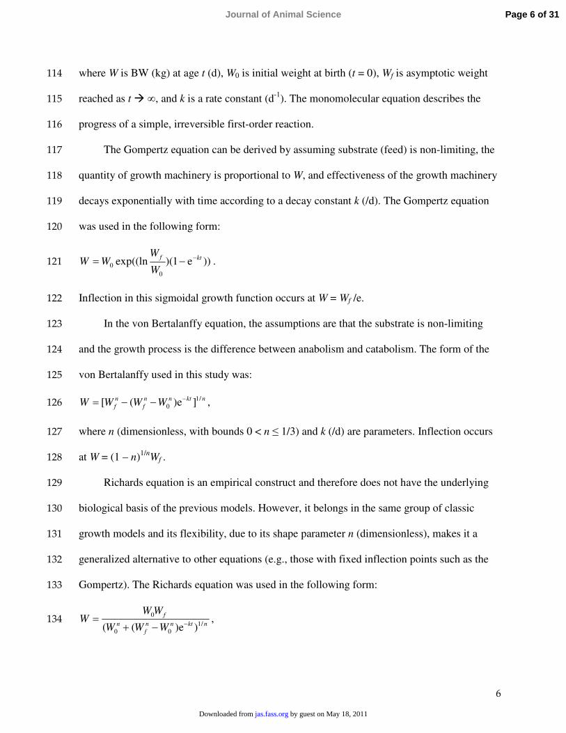
The monomolecular equation, the simplest equation used in this study, was used in the 111

following form with 3 parameters:112

W = Wf – (Wf – W0)e–kt,113




6

where W is BW (kg) at age t (d), W0 is initial weight at birth (t = 0), Wf is asymptotic weight 114

reached as t � ∞, and k is a rate constant (d-1). The monomolecular equation describes the 115

progress of a simple, irreversible first-order reaction.116

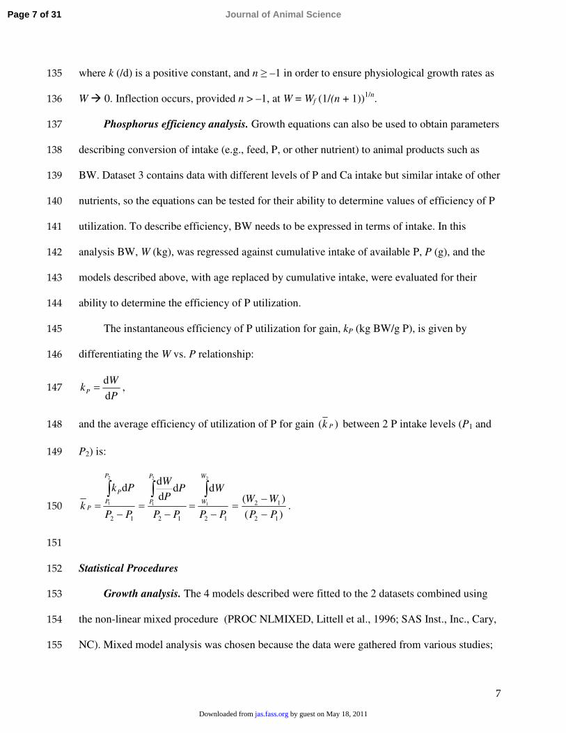
The Gompertz equation can be derived by assuming substrate (feed) is non-limiting, the 117

quantity of growth machinery is proportional to W, and effectiveness of the growth machinery 118

decays exponentially with time according to a decay constant k (/d). The Gompertz equation 119

was used in the following form:120

))e1)(exp((ln0

0ktf

W

WWW −−= .121

Inflection in this sigmoidal growth function occurs at W = Wf /e. 122

In the von Bertalanffy equation, the assumptions are that the substrate is non-limiting123

and the growth process is the difference between anabolism and catabolism. The form of the 124

von Bertalanffy used in this study was:125

nktnnf

nf WWWW /1

0 ]e)([ −−−= , 126

where n (dimensionless, with bounds 0 < n ≤ 1/3) and k (/d) are parameters. Inflection occurs 127

at W = (1 – n)1/nWf .128

Richards equation is an empirical construct and therefore does not have the underlying 129

biological basis of the previous models. However, it belongs in the same group of classic 130

growth models and its flexibility, due to its shape parameter n (dimensionless), makes it a 131

generalized alternative to other equations (e.g., those with fixed inflection points such as the 132

Gompertz). The Richards equation was used in the following form:133

nktnnf

n

f

WWW

WWW

/100

0

)e)(( −−+= ,134




7

where k (/d) is a positive constant, and n ≥ –1 in order to ensure physiological growth rates as 135

W � 0. Inflection occurs, provided n > –1, at W = Wf (1/(n + 1))1/n.136

Phosphorus efficiency analysis. Growth equations can also be used to obtain parameters 137

describing conversion of intake (e.g., feed, P, or other nutrient) to animal products such as 138

BW. Dataset 3 contains data with different levels of P and Ca intake but similar intake of other 139

nutrients, so the equations can be tested for their ability to determine values of efficiency of P 140

utilization. To describe efficiency, BW needs to be expressed in terms of intake. In this 141

analysis BW, W (kg), was regressed against cumulative intake of available P, P (g), and the 142

models described above, with age replaced by cumulative intake, were evaluated for their 143

ability to determine the efficiency of P utilization.144

The instantaneous efficiency of P utilization for gain, kP (kg BW/g P), is given by145

differentiating the W vs. P relationship: 146

P

WkP d

d= ,147

and the average efficiency of utilization of P for gain )( Pk between 2 P intake levels (P1 and 148

P2) is:149

12

d2

1

PP

Pk

k

P

P

P

P−

=∫

1212

2

1

2

1

dddd

PP

W

PP

PP

WW

W

P

P

−=

−=

∫∫)(

)(

12

12

PP

WW

−−

= .150

151

Statistical Procedures152

Growth analysis. The 4 models described were fitted to the 2 datasets combined using 153

the non-linear mixed procedure (PROC NLMIXED, Littell et al., 1996; SAS Inst., Inc., Cary, 154

NC). Mixed model analysis was chosen because the data were gathered from various studies;155




8

therefore, it was necessary to consider analyzing not only fixed effects of the dependent 156

variable but also random effects (because the studies represent a random sample of a larger 157

population of studies). For this analysis, a nonlinear mixed procedure based on Craig and 158

Schinckel (2001) and Schinckel and Craig (2002) was employed. Forward selection was used 159

to find the optimum model with lowest value of Bayesian Information Criterion (BIC) 160

(Leonard and Hsu, 2001). Trial was coded as a random effect and between-pig variability was 161

modeled by introducing a parameter (c) to vary the mature BW which was also a random 162

effect (Craig and Schinckel, 2001). For example, for the monomolecular equation, the model 163

fitted was W = (c + µ)*(Wf – (Wf – W0)e–kt) where µ is the random effect of each pig. 164

Introducing sex as a fixed source of variation in the model did not improve the performance of 165

the models because most of the variability associated with differences in sex had been 166

explained by the between-pig variability parameter.167

Phosphorus efficiency analysis. Nonlinear mixed model analysis was also used in 168

determining efficiency of P utilization. First, the equations were fitted to the data and then 169

derivatives of the growth curves were calculated. In fitting the equations, fixed effects of 170

available P intake level and sex were considered. The NLMIXED procedure in SAS does not 171

support directly the concept of an independent discrete (class) variable, so the analysis was 172

performed using dummy variables to represent treatments, sex, or both. Each parameter was 173

considered individually at first and then a combination of parameters used. Model comparison 174

using an F-test showed that the rate parameter (k) was significantly affected by treatment (P < 175

0.01) and inclusion of other parameters did not improve the overall model performance. 176

Therefore, the model with separate k values but a common W0, Wf and n was fitted.177




9

Distribution of random effects was assumed to be normal and the dual quasi-Newton 178

technique was used for optimization with adaptive Gaussian quadrature as the integration 179

method. Performance of the models was evaluated using significance level of the parameters 180

estimated, variance of error estimate, and its approximate SE. Comparison of models was 181

based on BIC which are model-order selection criteria centered on parsimony and imposing a 182

penalty on more complicated models for inclusion of additional parameters. Bayesian 183

Information Criterion combines the maximum likelihood (data fitting) and the choice of model 184

by penalizing the (log) maximum likelihood with a term related to model complexity as 185

follows:186

BIC = –2 log(Ĵ) + Klog (N),187

where Ĵ is the maximum likelihood, K is number of free parameters in the model and N is 188

sample size. A smaller numerical value of BIC indicates a better fit when comparing models.189

Both analyses were performed with the assumption that variance distribution for the 190

fixed factor was normal. Random effects were assumed to be normally distributed.191

192

RESULTS193

Growth Analysis194

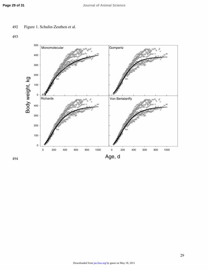
In general, all the equations fitted BW vs. age data well below approximately 350 kg 195

(Figure 1). The non-linear analysis of the pooled datasets showed that W0 estimates were close 196

to zero for all of the models compared. The estimate of W0 from the monomolecular equation197

was highest compared to the other equations. The von Bertalanffy equation estimated W0 to be 198

decreased compared to the other equations (Table 2). Estimates of Wf were within a 0.07-kg 199

range for the sigmoidal equations. More importantly, the random effect multiplier based on 200




10

BW, (c), was also within a narrow range. Due to the introduction of a random effect of 201

between-pig variation, the parameter estimate of ‘mature’ pig weights (Wf) as described above 202

is not absolute. Therefore, to aid comparison between models, the estimated mature weight 203

was calculated by multiplying Wf and c (Table 2) with the monomolecular and Gompertz 204

equations showing highest and the lowest estimates, respectively. The rate constant parameter 205

estimates (k) ranged between 0.0028 and 0.0067, and were significantly different from zero for206

all models. Finally, the parameter n estimates were –0.40 and 0.33 for Richards and von207

Bertalanffy equations, respectively.208

Comparison of models based on BIC suggested an advantage in using a more complex 209

model (Richards) compared with simpler models such as the Gompertz or monomolecular. 210

The von Bertalanffy equation also appeared to improve predictions (Figure 1) compared with 211

the monomolecular equation. However, the addition of an extra parameter in the von 212

Bertalanffy equation did not result in significant improvement in goodness-of-fit with this 213

model compared with the Gompertz equation, as reflected by their similar BIC values. 214

Phosphorus Efficiency Analysis215

Cumulative available dietary P intake was calculated from feed intake measurements and 216

corresponding available P content of the diet. For a given weight, the amount of available P 217

consumed up to that particular time was entered in the database. 218

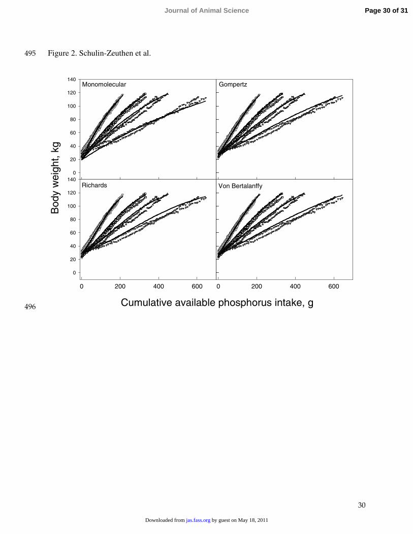
Fitting the equations to plots of BW vs. cumulative available dietary P intake (Figure 2) 219

showed that the parameter estimate for initial weight at zero P intake ranged from 19.2 for the 220

monomolecular equation to 28.7 kg for Richards equation (Table 3). Final weight estimates221

ranged from 131.9 (Richards) to 193.3 kg (monomolecular). All initial and final weight 222

estimates for all 4 models were significant parameters in the model. Rate constant estimates 223




11

ranged from 0.0009 to 0.0082; n parameter estimates were –0.87 and 0.33 for the Richards and 224

von Bertalanffy equations, respectively.225

The model with separate rate constant values for each treatment category significantly 226

improved on the general model in all equations compared. However, comparisons of the 227

models using t-tests of parameter values failed to reject the null hypothesis that BW gain was 228

not significantly different between sexes (P > 0.05). Animals fed high levels of available P 229

showed the lowest estimates of rate constants, which increased as the levels of available P 230

decreased. In all models, the differences in the estimate of rate constants among dietary P 231

levels were significant (Table 3).232

Comparison of models based on BIC did not show any advantage in using a more 233

complex equation than the monomolecular (Table 3). The 3 sigmoidal equations did not do as 234

well as the monomolecular equation, but their BIC values were within a narrow range. The 235

Richards equation was marginally improved compared to the other sigmoidal equations and its 236

parameter estimates were close to those of the monomolecular equation, with a point of 237

inflection at a very small weight over the range of cumulative P intake. The Gompertz and von238

Bertalanffy equations were the least suitable for analyzing efficiency of P utilization.239

Calculations of maximum efficiency of P utilization showed wide variation between 240

models. Maximum efficiency was at a considerably lower weight for Richards (8.0 kg) than 241

for von Bertalanffy (56.5 kg) and Gompertz (57.9 kg) equations. The monomolecular equation 242

assumes the efficiency is continuously decreasing until an asymptote is reached, when 243

efficiency becomes zero.244

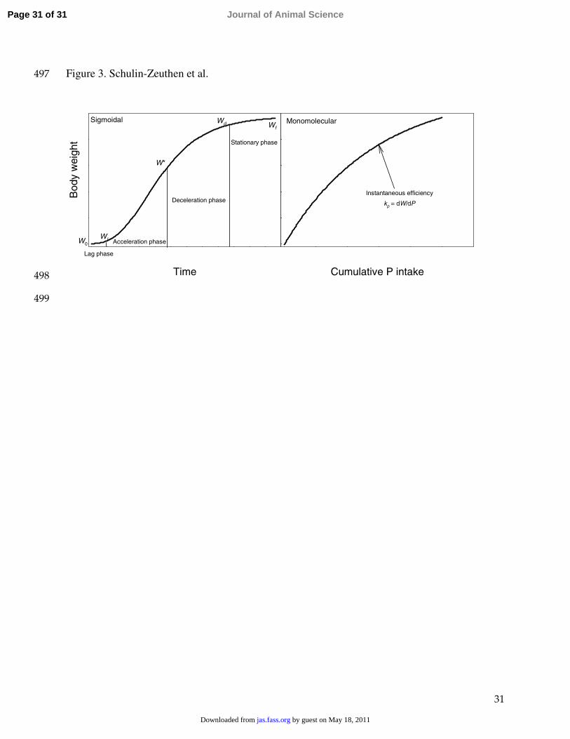
The growth curve was divided into 4 phases as shown in Figure 3. The ‘lag’ phase was 245

defined as time from the initial weight estimate until the animal attains 10% of its final weight, 246




12

the ‘accelerating’ phase continues from the end of lag phase until maximum growth rate (point 247

of inflection) is achieved, then the animal goes into the ‘deceleration’ phase until it reaches248

90% of its mature weight, and finally into the ‘stationary’ phase which continues until the 249

approach of asymptotic final weight. Figure 3 also depicts graphically instantaneous efficiency 250

of P utilization taking the monomolecular equation as an example.251

Average efficiency of P utilization for gain in the stages described above is given in 252

Table 4. The calculations were made by taking into account the significant differences in the 253

rate constant. Averages from 25 to 100 kg, 25 to 50 kg, and 50 to 100 kg (weight intervals254

covering the growing-finishing periods) are also given, as these could have implications for 255

commercial production systems. As expected, the greatest average weight gain and efficiency 256

of P utilization for the monomolecular equation was during the first phase, while for the 257

Gompertz and von Bertalanffy equations, greatest weight gain was during the acceleration258

phase. For all the equations, P efficiency approaches zero in the stationary phase.259

260

DISCUSSION261

Weight gain has been described using growth equations, and in nonruminants, the 262

Gompertz has traditionally been the model of choice (Wellock et al., 2004). In this study, a 263

simpler model (monomolecular) and others without the limitation of a fixed point of inflection264

(which occurs at 1/e times the final weight in the Gompertz), such as Richards and von265

Bertalanffy equations, were evaluated. The analyses showed that, in general, all 4 growth 266

equations fitted the data reasonably well (Figures 1 and 2).267

Performance of the equations in describing the datasets was evaluated using BIC, which 268

suggested differences in model choice for growth in BW and efficiency of P utilization. A 269




13

notable difference in parameter estimates in both sets of analyses was for W0. Estimates of W0270

were lower in the growth analysis because the data contained information on birth weights 271

while birth weight data were not available for the P efficiency analysis. The W0 estimates were 272

within the range of 0.042 and 9.5 kg in the first and second analyses, respectively. Wf273

estimates in growth analysis have to be looked at in conjunction with the c parameter, which 274

was within 18 kg for the sigmoidal curves. The introduction of random effect of mature weight 275

increased the goodness-of-fit (lower BIC value) compared to a generalized model with only 276

experiment as the random element in the model. It has also improved the approximate SE of 277

the parameter estimates.278

Comparison of BIC values for the growth analysis revealed that the Richards equation, 279

perhaps due to the broad limits on its additional parameter, was superior to the other 280

equations. As parameter n approaches particular values, the Richards equation encompasses 281

other simpler models, such as the monomolecular (n = –1), Gompertz (n = 0), and logistic (n = 282

1). Table 2 shows that n estimate was about halfway between the monomolecular and 283

Gompertz equations. The flexibility of the Richards equation increased the accuracy of 284

prediction, and the need for an additional parameter was justified because the shape of the 285

curve could not be described as well by either the monomolecular (because it is not a 286

sigmoidal equation) or the Gompertz (due to its fixed inflection point).287

Four phases were arbitrarily assigned to evaluate weight gain (Figure 3), and the average 288

efficiency of BW gain with time within the phases was calculated. The values based on289

generalized sigmoidal equations were close to each other but different from those based on the 290

monomolecular equation. The importance of this kind of calculation is to identify periods of 291

greatest weight gain so that inputs can be adjusted accordingly. More crucially, by recognizing 292




14

the rate of decline in growth during the stationary phase, more informed decisions can be 293

made about the impact of varying slaughter weight on nutrient use and income over diet costs.294

From the Richards equation, it can be calculated that the pigs were expected to gain nearly 1 295

kg/d during the accelerating phase, which goes down by about 40% in the next phase; by the 296

time they reach the stationary phase, the animals were 97% less efficient in gaining BW. The 297

data also show that there was uniformity up to the end of the accelerating phase (d 300 of age);298

then, as animals matured, there were greater differences among animals, due to the weight 299

gains being mainly attributable to fat deposition.300

Apart from describing the pattern of growth, non-linear equations can be used to 301

investigate efficiency of utilization of individual nutrients for BW gain. Usually, mineral 302

requirements in pigs are estimated by empirical methods based on feeding a range of dietary 303

concentrations of each mineral element and examining the response in terms of certain304

performance (weight gain) or physiological (mineral balance) attributes to assess the most 305

adequate dietary concentration (i.e., the one resulting in maximum response). In general, as P 306

intake is increased, there is an increase in weight gain, feed intake, and feed efficiency (gain to 307

feed ratio); this relationship is curvilinear, such that maximum response is reached at a certain 308

level of P intake, which is variable depending upon animal characteristics (genotype, sex) and 309

the growing stage (Ketaren et al., 1993; Ekpe et al., 2002; Hastad et al., 2004). The response is 310

less pronounced as the animal grows, hence in animals of greater weight the level of P intake 311

required to reach the maximum response is lower (Ketaren et al., 1993; Hastad et al., 2004).312

From this approach, requirements have been mostly expressed as percentage of the mineral in 313

the diet (or alternatively per unit of energy in the diet) (ARC, 1981). However, in order to 314

assess optimal requirements for a given growth rate, it is important to express requirements of315




15

P (and any other mineral) directly in relation to protein and fat gain, but this goal cannot be 316

achieved with the information currently available in the literature.317

Alternatively, the use of non-linear equations to describe the relationship between BW318

and cumulative available P intake can be used to estimate the efficiency of P utilization in 319

terms of weight gain per unit of available P intake at any stage of growth, provided that other 320

nutrients are not limiting expression of nutrient retention rates. Using this approach, 4 non-321

linear equations were examined. The Richards equation seemed to yield as good a fit as the322

Gompertz, given the almost identical BIC values. However, in this case, the estimate of 323

parameter n was close to –1 (Table 3), approaching diminishing returns behavior without a324

point of inflection, so that the simple monomolecular equation was adequate to describe the 325

relationship between BW and cumulative available P intake in pigs, which is confirmed by the 326

lowest BIC value of the model. Most of the rate parameter estimates of the Richards and 327

monomolecular equations were not significantly different from each other, which further 328

proves the flexibility of the Richards equation and the suitability of the monomolecular 329

equation to fit these profiles, without the need for an additional parameter. The same equation 330

(Richards) can be used for both growth analysis and efficiency of nutrient utilization, and can 331

yield different growth patterns for each of the 4 dietary P levels. Therefore, only 1 equation is 332

required for all levels to assess the optimum level.333

Calculations for efficiency of P utilization based on the best performing model 334

(monomolecular equation) showed that the average efficiency is greatest during the 2 initial 335

phases and slows down as the pig’s cumulative consumption of available P increases. By the 336

time the pig reaches the stationary phase, efficiency approaches zero. This trend is the same in 337

pigs fed low or high levels of P (Table 4). The steady decline in efficiency of P utilization 338




16

observed as a pig grows agrees with the lower P requirements recommended (ARC, 1981; 339

NRC, 1998) for different growth phases (decreasing from weaning to 100 kg) and can be 340

attributed to a number of reasons. The amount of P required for maintenance is greater in341

larger pigs, and thus relatively less P is used for growth (ARC, 1981; NRC, 1998). Also, it is 342

important to examine variations in P deposition in the weight gain. Considering the principles 343

of skeletal tissue growth, there is a steady and progressive increase in the rate of P 344

accumulation per unit of fat-free BW from birth to slaughtering weight (Mahan and Shields, 345

1998). However, given the exponential increase in fat deposition in adipose tissue, the rate of 346

increment of P content in empty BW is inversely related to BW, as demonstrated by Mudd et 347

al. (1969) in trials using carcass analysis, reporting values of 8.1, 5.3, and 1.6 g P/kg weight 348

gain at 20, 50, and 90 kg of empty BW, respectively. Our analysis also shows that as BW 349

increases, the proportion of P retained decreases. The ARC (1981) suggested that the rate of 350

storage of Ca and P (g/kg weight gain) with growth could be represented by a linear fall 351

between birth and 50 kg BW (with a linear relationship between that rate and BW) and a 352

constant rate thereafter. Calculations of efficiency of P utilization as d(BW)/d(P intake) using 353

non-linear methods takes into account the relationship between BW and P as described by 354

different classical growth equations. It is noteworthy that the levels of Ca and P resulting in 355

maximum growth rate and efficiency of gain are not necessarily adequate for maximum 356

growth mineralization (ARC, 1981). To achieve maximum deposition of Ca and P, and 357

increase the bone mineral content, a greater mineral supply would be required (NRC, 1998; 358

Hastad et al., 2004). The approach suggested herein could be used not only to quantify the 359

trend in efficiency of P utilization throughout the lifespan of the animal, but also to examine 360

differences between genotypes with different lean growth rate (Bertram et al., 1994) or the 361




17

effects of sex (comparison among gilts, barrows, or boars; Thomas and Kornegay, 1981; Epke 362

et al., 2002). This information could also be used to estimate P requirements in pigs at various 363

stages of the life cycle, adjusting P input levels during the finishing stages of pig production.364

Non-linear mixed analysis can give reliable parameter estimates and is a useful tool 365

when analyzing data from multiple studies. Although the Gompertz equation has been used 366

extensively, the Richards equation was superior in describing growth over time and it is 367

recommended for use in data analysis in nonruminant animals. The extra parameter in the 368

model improved the predictions and therefore was required as indicated by lower BIC values. 369

The non-linear relationship between BW and cumulative available P intake was best described 370

by the simpler monomolecular equation. Calculations of average or instantaneous efficiency of 371

P utilization can be used to predict the animals’ response to changes in intake and the potential 372

to reduce excess P excretion to the environment. It is recommended that future studies on 373

growth and nutrient intake analyses consider other models such as the monomolecular and 374

flexible equations such as the Richards as well as the Gompertz.375




18

LITERATURE CITED376

377

Andersen P. E., and A. Just. 1983. Tabeller over Foderstoffers Sammensætning m.m. Kvæg. 378

Svin. Jordbrugsforlaget, DK, Copenhagen, Denmark.379

ARC. 1981. The Nutrient Requirements of Pigs. Commonwealth Agric. Bureaux, Slough, 380

U.K.381

Bermejo, J. L., R. Roehe, G. Rave, and E. Kalm. 2003. Comparison of linear and nonlinear 382

functions and covariance structures to estimate feed intake pattern in growing pigs. 383

Livest. Prod. Sci. 82:15-26.384

Bertram, M. J., T. S. Stahly, and R. C. Ewan. 1994. Impact of lean growth genotype and 385

dietary phosphorus regimen on rate and efficiency of growth and carcass characteristics 386

of pigs. J. Anim Sci. 72 (Suppl. 2):68 (Abstr.).387

Bridges, T. C., L. W. Turner, T. S. Stahly, J. L. Usry, and O. J. Loewer. 1992. Modeling the 388

physiological growth of swine part I: Model logic and growth concepts. Trans. ASAE389

35:1019-1028.390

Craig, B. A., and A. P. Schinckel. 2001. Nonlinear mixed effects model for swine growth. 391

Prof. Anim. Scientist 17:256-260.392

Darmani Kuhi, H., E. Kebreab, S. Lopez, and J. France. 2003a. An evaluation of different 393

growth functions for describing the profile of live weight with time (age) in meat and 394

egg strains of chicken. Poult. Sci. 82:1536-1543.395

Darmani Kuhi, H., E. Kebreab, S. Lopez, and J. France. 2003b. A comparative evaluation of 396

functions for the analysis of growth in male broilers. J. Agric. Sci. 140:451-459.397




19

Ekpe, E. D., R. T. Zijlstra, and J. F. Patience. 2002. Digestible phosphorus requirement of 398

grower pigs. Canadian J. Anim. Sci. 82:541-549.399

Ferguson, N. S., R. M. Gous, and G. C. Emmans. 1994. Preferred components for the 400

construction of a new simulation model of growth, feed intake and nutrient requirements 401

of growing pigs. South African J. Anim. Sci. 24:10-17.402

France, J., J. Dijkstra, and M. S. Dhanoa. 1996. Growth functions and their application in 403

animal science. Ann. Zootech. 45:165-174.404

Hastad, C. W., S. S. Dritz, M. D. Tokach, R. D. Goodband, J. L. Nelssen, J. M. DeRouchey, 405

R. D. Boyd, and M. E. Johnston. 2004. Phosphorus requirements of growing-finishing 406

pigs reared in a commercial environment. J. Anim. Sci. 82:2945-2952.407

Jondreville, C., P.-S. Revy, J.-Y. Dourmad, Y. Nys, S. Hillion, F. Pontrucher, J. Gonzalez, J. 408

Soler, R. Lizardo, and J. Tibau. 2004. Influence of genotype and sex on minerals (Ca, P, 409

K, N, Mg, Fe, Zn, Cu) content and retention in the body of pigs from 25 to 135 kg of 410

body weight. J. Recherche Porcine 36:17-24.411

Ketaren, P. P., E. S. Batterham, E. White, D. J. Farrell, and B. K. Milthorpe. 1993. Phosphorus 412

studies in pigs .1. Available phosphorus requirements of grower finisher pigs. Br. J. 413

Nutr. 70:249-268.414

Leonard, T., and S. J. Hsu. 2001. Bayesian Methods: An Analysis for Statisticians and 415

Interdisciplinary Researchers. Cambridge Series in Statistical & Probabilistic 416

Mathematics. Cambridge Univ. Press, Cambridge U.K., 348 pp. 417

Littell, R. C., G. A. Milliken, W. W. Stroup, and R. D. Wolfinger. 1996. SAS® System for 418

Mixed Models. SAS Institute Inc., Cary, NC.419



http://www.amazon.co.uk/exec/obidos/search-handle-url/index=books-uk&field-author=Hsu%2C John S. J./026-5030605-3694019

http://www.amazon.co.uk/exec/obidos/search-handle-url/index=books-uk&field-author=Leonard%2C Thomas/026-5030605-3694019

http://0-wos02.isiknowledge.com.catoute.unileon.es/CIW.cgi?SID=CE@FLc3jfLIlhpiH15l&Func=OneClickSearch&field=AU&val=MILTHORPE+BK&curr_doc=3/1&Form=FullRecordPage&doc=3/1

http://0-wos02.isiknowledge.com.catoute.unileon.es/CIW.cgi?SID=CE@FLc3jfLIlhpiH15l&Func=OneClickSearch&field=AU&val=FARRELL+DJ&curr_doc=3/1&Form=FullRecordPage&doc=3/1

http://0-wos02.isiknowledge.com.catoute.unileon.es/CIW.cgi?SID=CE@FLc3jfLIlhpiH15l&Func=OneClickSearch&field=AU&val=WHITE+E&curr_doc=3/1&Form=FullRecordPage&doc=3/1

http://0-wos02.isiknowledge.com.catoute.unileon.es/CIW.cgi?SID=CE@FLc3jfLIlhpiH15l&Func=OneClickSearch&field=AU&val=BATTERHAM+ES&curr_doc=3/1&Form=FullRecordPage&doc=3/1

http://0-wos02.isiknowledge.com.catoute.unileon.es/CIW.cgi?SID=CE@FLc3jfLIlhpiH15l&Func=OneClickSearch&field=AU&val=KETAREN+PP&curr_doc=3/1&Form=FullRecordPage&doc=3/1

http://0-wos02.isiknowledge.com.catoute.unileon.es/CIW.cgi?SID=gNB2aokN3mKLiAKMpJk&Func=OneClickSearch&field=AU&val=Johnston+ME&curr_doc=8/8&Form=FullRecordPage&doc=8/8

http://0-wos02.isiknowledge.com.catoute.unileon.es/CIW.cgi?SID=gNB2aokN3mKLiAKMpJk&Func=OneClickSearch&field=AU&val=Boyd+RD&curr_doc=8/8&Form=FullRecordPage&doc=8/8

http://0-wos02.isiknowledge.com.catoute.unileon.es/CIW.cgi?SID=gNB2aokN3mKLiAKMpJk&Func=OneClickSearch&field=AU&val=DeRouchey+JM&curr_doc=8/8&Form=FullRecordPage&doc=8/8

http://0-wos02.isiknowledge.com.catoute.unileon.es/CIW.cgi?SID=gNB2aokN3mKLiAKMpJk&Func=OneClickSearch&field=AU&val=Nelssen+JL&curr_doc=8/8&Form=FullRecordPage&doc=8/8

http://0-wos02.isiknowledge.com.catoute.unileon.es/CIW.cgi?SID=gNB2aokN3mKLiAKMpJk&Func=OneClickSearch&field=AU&val=Goodband+RD&curr_doc=8/8&Form=FullRecordPage&doc=8/8

http://0-wos02.isiknowledge.com.catoute.unileon.es/CIW.cgi?SID=gNB2aokN3mKLiAKMpJk&Func=OneClickSearch&field=AU&val=Tokach+MD&curr_doc=8/8&Form=FullRecordPage&doc=8/8

http://0-wos02.isiknowledge.com.catoute.unileon.es/CIW.cgi?SID=gNB2aokN3mKLiAKMpJk&Func=OneClickSearch&field=AU&val=Dritz+SS&curr_doc=8/8&Form=FullRecordPage&doc=8/8

http://0-wos02.isiknowledge.com.catoute.unileon.es/CIW.cgi?SID=gNB2aokN3mKLiAKMpJk&Func=OneClickSearch&field=AU&val=Hastad+CW&curr_doc=8/8&Form=FullRecordPage&doc=8/8

http://0-wos02.isiknowledge.com.catoute.unileon.es/CIW.cgi?SID=gNB2aokN3mKLiAKMpJk&Func=OneClickSearch&field=AU&val=Zijlstra+RT&curr_doc=6/26&Form=FullRecordPage&doc=6/26

http://0-wos02.isiknowledge.com.catoute.unileon.es/CIW.cgi?SID=gNB2aokN3mKLiAKMpJk&Func=OneClickSearch&field=AU&val=Ekpe+ED&curr_doc=6/26&Form=FullRecordPage&doc=6/26


20

Mahan, D. C., and Jr. R. Shields. 1998. Macro- and micromineral composition of pigs from 420

birth to 145 kilograms of body weight. J. Anim. Sci. 76:506-512.421

Mudd, A. J., W. C. Smith, and D. G. 1969. Retention of certain minerals in pigs from birth to 422

90-kg live weight. J. Agric. Sci., Camb. 73: 181-188.423

NRC. 1998. Nutrient Requirements of Swine. 10th rev. ed. Natl. Acad. Press, Washington, DC.424

Schinckel, A. P., and C. F. de Lange. 1996. Characterization of growth parameters needed as 425

inputs for pig growth models. J. Anim. Sci. 74:2021-2036.426

Schinckel, A. P., and B. A. Craig. 2002. Evaluation of alternative nonlinear mixed effects 427

models of swine growth. Prof. Anim. Scientist 18:219-226.428

Schulin-Zeuthen, M. 2000. Capacity for retention of macro nutrients in growing pigs. M.Sc.429

Diss., Royal Veterinary and Agricultural Univ., Copenhagen, Denmark.430

Schulin-Zeuthen, M., and A. Danfær. 2001. Descriptions of the capacity of macro nutrient 431

retention in growing pigs. Page 7 in Proc. 52nd Ann. Meeting Europ. Assoc. Anim.432

Prod., Budapest, Hungary. 433

Schulin-Zeuthen, M., J. B. Lopes, E. Kebreab, D. M. S. S. Vitti, A. L. Abdalla, M. DeL. 434

Haddad, L. A. Crompton, and J. France. 2005. Effects of phosphorus intake on 435

phosphorus flow in growing pigs: Application and comparison of two models. J. Theor. 436

Biol. 236:115-125.437

Swidersky, A., J. Atkinson, and C. F. M. de Lange. 2003. Optimum dietary phosphorus levels 438

for grower-finisher pigs. Ontario Swine Research Review. Ontario Min. Agric. Fisheries, 439

Guelph, Canada.440



http://0-wos02.isiknowledge.com.catoute.unileon.es/CIW.cgi?SID=CE@FLc3jfLIlhpiH15l&Func=OneClickSearch&field=AU&val=SMITH+WC&curr_doc=1/21&Form=FullRecordPage&doc=1/21


21

Thomas, H. R., and E. T. Kornegay. 1981. Phosphorus in swine. I. Influence of dietary 441

calcium and phosphorus levels and growth rate on feedlot performance of barrows, gilts 442

and boars. J. Anim. Sci. 52:1041-1048.443

Thornley, J. H. M., and J. France. 2007. Mathematical Models in Agriculture. 2nd ed. CABI444

Int., Wallingford, U.K. 923 pp.445

Tibau, J., J. Gonzalez, J. Soler, M. Gispert, R. Lizardo, and J. Mourot. 2002. Influence du 446

poids à l'abattage du porc entre 25 et 140 kg de poids vif sur la composition chimique de 447

la carcasse: effets du génotype et du sexe. J. Recherche Porcine 34:121-127.448

Wellock, I. J., G. C. Emmans, and I. Kyriazakis. 2004. Describing and predicting potential 449

growth in the pig. Anim. Sci. 78:379-388.450

451




22

Table 1. Data sources used in the study452

Dataset Source Number of pigs

Growth period (d)

Genotype Diet (% of as fed)1

1 Schulin-Zeuthen, (2000);

Schulin-Zeuthen and

Danfær (2001)

911 Birth to

1007

(Landrace × Yorkshire) ×Duroc

DM 89.9, dCP 14.3, NE 9.26, P 0.586, aP 0.378DM 89.6, dCP 13.1, NE 9.11, P 0.551, aP 0.317DM 88.9, dCP 11.9, NE 8.96, P 0.517, aP 0.256DM 88.2, dCP 12.7, NE 8.49, P 0.507, aP 0.241DM 89.0, dCP 11.2, NE 8.18, P 0.497, aP 0.244DM 88.8, dCP 10.7, NE 7.87, P 0.458, aP 0.224DM 88.4, dCP 9.56, NE 7.87, P 0.450, aP 0.224

2 Jondreville et al. (2004);

Tibau et al. (2002)

209 68 to 210 (Large White × Landrace) ×Pietrain or (Large White× Landrace) × Large White

DM 89.6, CP 20.0, NE 9.55, Ca 1.07, P 0.845, aP 0.406DM 87.3, CP 18.5, NE 9.21, Ca 1.02, P 0.817, aP 0.378

3 Swidersky et al. (2003) 1,330 70 to 155 Yorkshire DM 88.3, dCP 13.2, Ca 0.348, P 0.377, aP 0.122DM 87.2, dCP 13.5, Ca 0.521, P 0.436, aP 0.183DM 87.1, dCP 13.2, Ca 0.685, P 0.493, aP 0.240DM 88.9, dCP 13.1, Ca 0.858, P 0.553, aP 0.301

1CP = 6.25 × N (NRC, 1998;), dCP = digestible protein, NE (Net Energy, MJ/kg) = 7.72 Scandinavian Feed Units (Andersen and 453

Just, 1983), NE = 0.75 digestible energy (Andersen and Just, 1983), aP = available phosphorus.454


by guest on May 18, 2011

jas.fass.orgD

ownloaded from


23

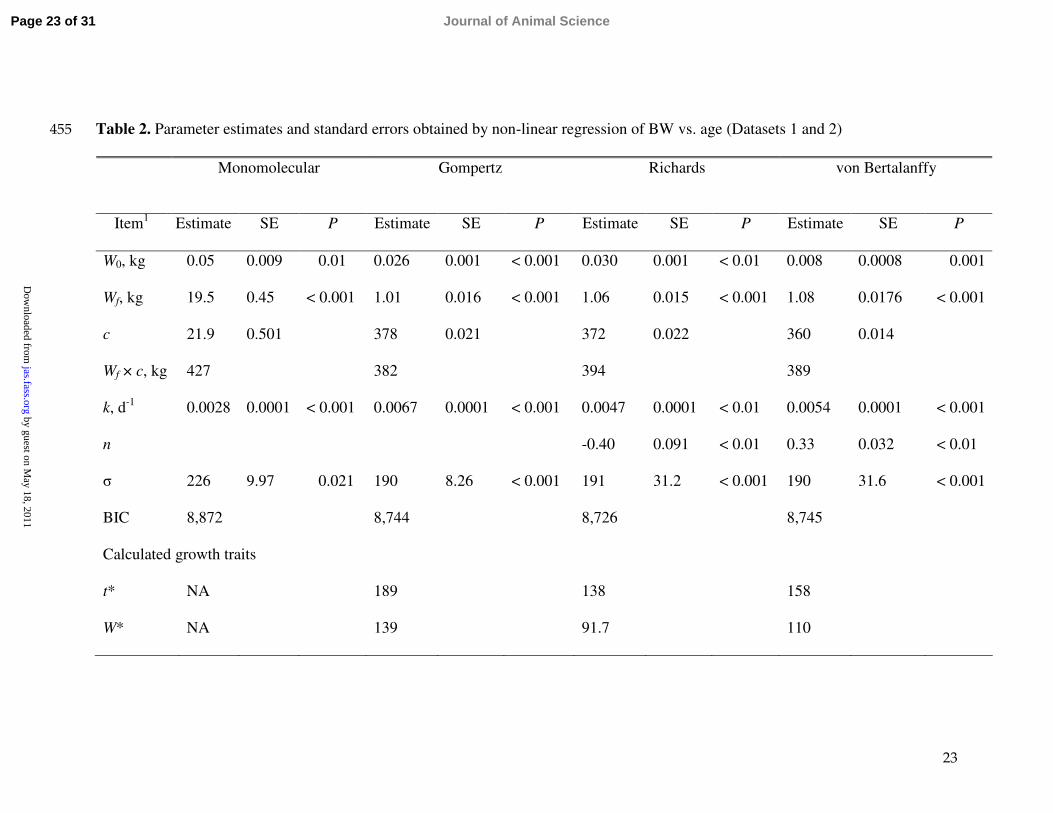
Table 2. Parameter estimates and standard errors obtained by non-linear regression of BW vs. age (Datasets 1 and 2)455

Monomolecular Gompertz Richards von Bertalanffy

Item1 Estimate SE P Estimate SE P Estimate SE P Estimate SE P

W0, kg 0.05 0.009 0.01 0.026 0.001 < 0.001 0.030 0.001 < 0.01 0.008 0.0008 0.001

Wf, kg 19.5 0.45 < 0.001 1.01 0.016 < 0.001 1.06 0.015 < 0.001 1.08 0.0176 < 0.001

c 21.9 0.501 378 0.021 372 0.022 360 0.014

Wf × c, kg 427 382 394 389

k, d-1 0.0028 0.0001 < 0.001 0.0067 0.0001 < 0.001 0.0047 0.0001 < 0.01 0.0054 0.0001 < 0.001

n -0.40 0.091 < 0.01 0.33 0.032 < 0.01

σ 226 9.97 0.021 190 8.26 < 0.001 191 31.2 < 0.001 190 31.6 < 0.001

BIC 8,872 8,744 8,726 8,745

Calculated growth traits

t* NA 189 138 158

W* NA 139 91.7 110



jas.fass.orgD

ownloaded from


24

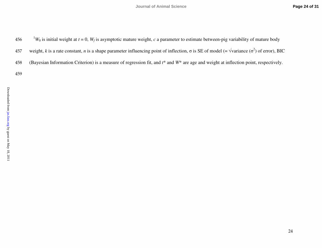
1W0 is initial weight at t = 0, Wf is asymptotic mature weight, c a parameter to estimate between-pig variability of mature body 456

weight, k is a rate constant, n is a shape parameter influencing point of inflection, σ is SE of model (= √variance (σ2) of error), BIC 457

(Bayesian Information Criterion) is a measure of regression fit, and t* and W* are age and weight at inflection point, respectively.458

459



jas.fass.orgD

ownloaded from


25

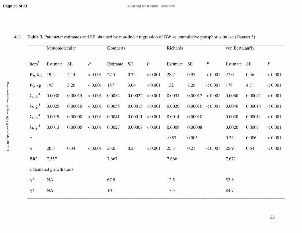
Table 3. Parameter estimates and SE obtained by non-linear regression of BW vs. cumulative phosphorus intake (Dataset 3)460

Monomolecular Gompertz Richards von Bertalanffy

Item1 Estimate SE P Estimate SE P Estimate SE P Estimate SE P

W0, kg 19.2 2.14 < 0.001 27.5 0.34 < 0.001 28.7 0.97 < 0.001 27.0 0.36 < 0.001

Wf, kg 193 5.26 < 0.001 157 3.04 < 0.001 132 7.26 < 0.001 178 4.71 < 0.001

k1, g-1 0.0038 0.00015 < 0.001 0.0082 0.00022 < 0.001 0.0031 0.00017 < 0.001 0.0060 0.00021 < 0.001

k2, g-1 0.0025 0.00010 < 0.001 0.0055 0.00015 < 0.001 0.0020 0.00016 < 0.001 0.0040 0.00014 < 0.001

k3, g-1 0.0019 0.00008 < 0.001 0.0041 0.00011 < 0.001 0.0014 0.00010 0.0030 0.00011 < 0.001

k4, g-1 0.0013 0.00005 < 0.001 0.0027 0.00007 < 0.001 0.0009 0.00008 0.0020 0.0007 < 0.001

n -0.87 0.005 0.33 0.006 < 0.001

σ 20.5 0.34 < 0.001 25.6 0.25 < 0.001 25.3 0.21 < 0.001 25.9 0.64 < 0.001

BIC 7,557 7,667 7,666 7,671

Calculated growth traits

t1* NA 67.9 12.5 52.8

t2* NA 101 17.3 84.7



jas.fass.orgD

ownloaded from


26

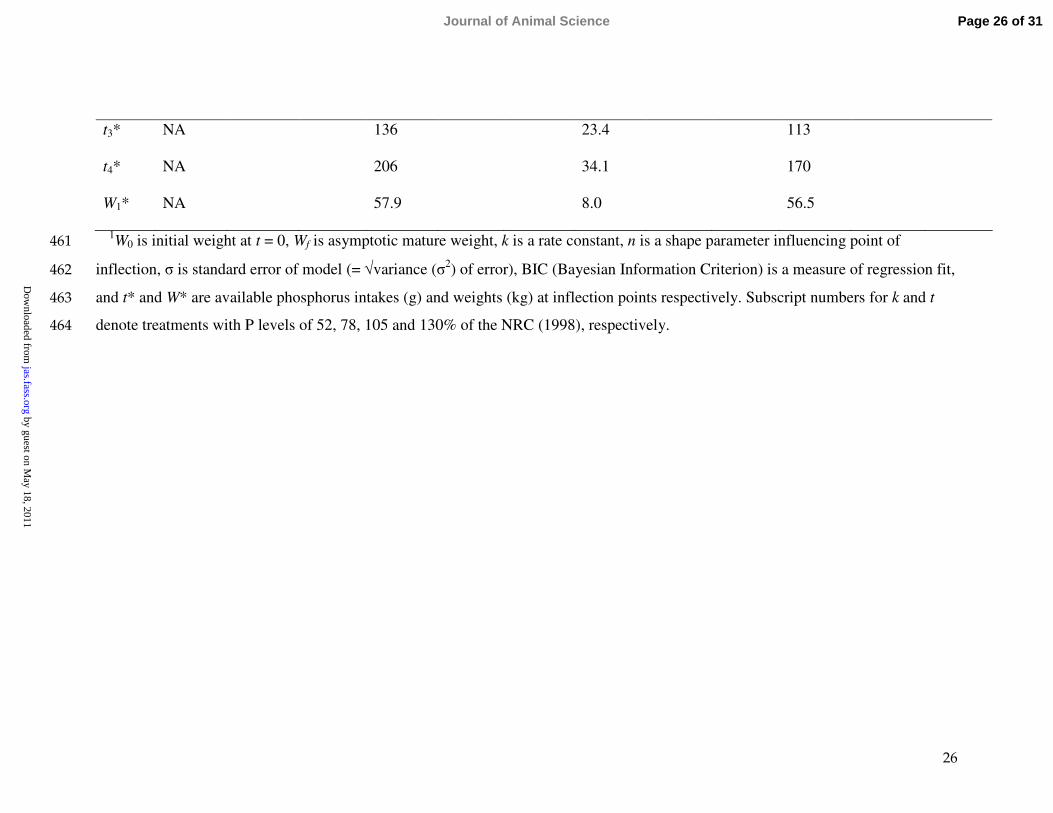
t3* NA 136 23.4 113

t4* NA 206 34.1 170

W1* NA 57.9 8.0 56.5

1W0 is initial weight at t = 0, Wf is asymptotic mature weight, k is a rate constant, n is a shape parameter influencing point of 461

inflection, σ is standard error of model (= √variance (σ2) of error), BIC (Bayesian Information Criterion) is a measure of regression fit, 462

and t* and W* are available phosphorus intakes (g) and weights (kg) at inflection points respectively. Subscript numbers for k and t463

denote treatments with P levels of 52, 78, 105 and 130% of the NRC (1998), respectively.464



jas.fass.orgD

ownloaded from


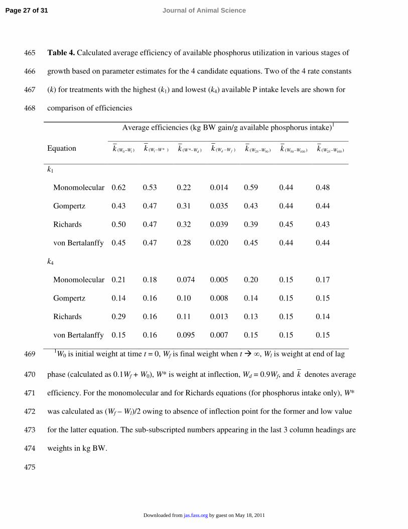
Table 4. Calculated average efficiency of available phosphorus utilization in various stages of 465

growth based on parameter estimates for the 4 candidate equations. Two of the 4 rate constants 466

(k) for treatments with the highest (k1) and lowest (k4) available P intake levels are shown for467

comparison of efficiencies468

Average efficiencies (kg BW gain/g available phosphorus intake)1

Equation )( 0 lWWk − )*( WWlk − )*( dWWk − )( fd WWk − )( 5025 WWk − )( 10050 WWk − )( 10025 WWk −

k1

Monomolecular 0.62 0.53 0.22 0.014 0.59 0.44 0.48

Gompertz 0.43 0.47 0.31 0.035 0.43 0.44 0.44

Richards 0.50 0.47 0.32 0.039 0.39 0.45 0.43

von Bertalanffy 0.45 0.47 0.28 0.020 0.45 0.44 0.44

k4

Monomolecular 0.21 0.18 0.074 0.005 0.20 0.15 0.17

Gompertz 0.14 0.16 0.10 0.008 0.14 0.15 0.15

Richards 0.29 0.16 0.11 0.013 0.13 0.15 0.14

von Bertalanffy 0.15 0.16 0.095 0.007 0.15 0.15 0.15

1W0 is initial weight at time t = 0, Wf is final weight when t � ∞, Wl is weight at end of lag 469

phase (calculated as 0.1Wf + W0), W* is weight at inflection, Wd = 0.9Wf, and k denotes average 470

efficiency. For the monomolecular and for Richards equations (for phosphorus intake only), W* 471

was calculated as (Wf – Wl)/2 owing to absence of inflection point for the former and low value 472

for the latter equation. The sub-subscripted numbers appearing in the last 3 column headings are 473

weights in kg BW.474

475




28

Figure legends:476

477

Figure 1. Relationship between BW (kg) and age (d) in Datasets 1 and 2. Symbols represent 478

observed values and the lines are regression lines fitted using the different functions.479

480

Figure 2. Relationship between BW (kg) and cumulative available phosphorus intake (g) in 481

Dataset 3. Symbols represent observed values (circle, square, triangle, inverted triangle 482

correspond to treatments with available P intakes of 52, 78, 105 and 130% of the NRC (1998), 483

respectively) and the lines are regression lines fitted using the 4 candidate equations.484

485

Figure 3. Growth stages for a representative sigmoidal curve and graphical representation of 486

instantaneous efficiency for the monomolecular equation. W0 is initial weight at time t = 0, Wf is 487

final weight when t � ∞, Wl is weight at the end of lag phase (calculated as W0 + 0.1Wf), W* is 488

weight at inflection, Wd = 0.9Wf, and kP is instantaneous efficiency of phosphorus utilization for 489

growth.490

491




29

Figure 1. Schulin-Zeuthen et al.492

493

Monomolecular

Bod

y w

eigh

t, kg

0

100

200

300

400

500Gompertz

Richards

Age, d

0 200 400 600 800 1000

0

100

200

300

400

Von Bertalanffy

0 200 400 600 800 1000

494




30


Monomolecular

Bod

y w

eigh

t, kg

0

20

40

60

80

100

120

140Gompertz

Richards

0 200 400 600

0

20

40

60

80

100

120

140Von Bertalanffy

Cumulative available phosphorus intake, g

0 200 400 600

496




31


Sigmoidal

Time

Bod

y w

eigh

t

Monomolecular

Cumulative P intake

Instantaneous efficiency

kp = dW/dP

Stationary phase

Acceleration phase

Lag phase

Deceleration phase

Wf

W*

WlW0

Wd

498

499




Citations

cleshttp://jas.fass.org/content/early/2007/06/12/jas.2006-738.citation#otherartiThis article has been cited by 1 HighWire-hosted articles:



Comparative evaluation of mathematical functions to describe growth and efficiency of phosphorus...

Documents

Transcript of Comparative evaluation of mathematical functions to describe growth and efficiency of phosphorus...