arX

iv:1

502.

0300

7v1

[co

nd-m

at.m

es-h

all]

10

Feb

2015

Comparative analysis of electric field influence

on the quantum wells with different boundary

conditions. II. Thermodynamic properties

O. Olendski∗

February 11, 2015

Abstract

Thermodynamic properties of the one-dimensional (1D) quantumwell (QW) with miscellaneous permutations of the Dirichlet (D) andNeumann (N) boundary conditions (BCs) at its edges in the perpen-dicular to the surfaces electric field E are calculated. For the canonicalensemble, analytical expressions involving theta functions are foundfor the mean energy and heat capacity cV for the box with no appliedvoltage. Pronounced maximum accompanied by the adjacent min-imum of the specific heat dependence on the temperature T for thepure Neumann QW and their absence for other BCs are predicted andexplained by the structure of the corresponding energy spectrum. Ap-plied field leads to the increase of the heat capacity and formation ofthe new or modification of the existing extrema what is qualitativelydescribed by the influence of the associated electric potential. A re-markable feature of the Fermi grand canonical ensemble is, at any BCcombination in zero fields, a salient maximum of cV observed on theT axis for one particle and its absence for any other number N of cor-puscles. Qualitative and quantitative explanation of this phenomenonemploys the analysis of the chemical potential and its temperature de-pendence for different N . It is proved that critical temperature Tcr ofthe Bose-Einstein (BE) condensation increases with the applied volt-age for any number of particles and for any BC permutation except

∗King Abdullah Institute for Nanotechnology, King Saud University, P.O. Box 2455,Riyadh 11451 Saudi Arabia; E-mail: oolendski@ksu.edu.sa

1

the ND case at small intensities E what is explained again by themodification by the field of the interrelated energies. It is shown thateven for the temperatures smaller than Tcr the total dipole moment〈P 〉 may become negative for the quite moderate E . For either Fermior BE system, the influence of the electric field on the heat capacity isshown to be suppressed with N growing. Different asymptotic casesof, e.g., the small and large temperatures and low and high voltagesare derived analytically and explained physically. Parallels are drawnto the similar properties of the 1D harmonic oscillator, and similaritiesand differences between them are discussed.

1 Introduction

Preceding paper [1] discovered, among other findings, the independence ofthe sign of the polarization Pn on the boundary conditions (BCs) for the one-dimensional (1D) quantum well (QW) of the width L placed into the uniformelectric field E that is directed perpendicular to its confining surfaces locatedat x = ±L/2: the polarization P0(E ) of the ground state for any permutationof the Dirichlet (D),

Ψ

(

±L

2

)

= 0, (1)

and Neumann (N),

Ψ′

(

±L

2

)

= 0, (2)

edge requirements imposed on the wavefunction Ψ(x) is positive for all ap-plied voltages while its excited-state counterparts Pn(E ), n ≥ 1, for thesmall growing fields decrease from zero at E = 0 to the negative values,pass through the minimum and only after this start to increase crossing zeroat the n- and BC-dependent intensity E

extn . Immediately, one wonders: for

any kind of the particles, is it possible to observe the total statistically av-eraged polarization that is negative at the small electric forces? Analysisbelow answers this question together with the thermodynamic calculationsof the corresponding energy E and heat capacity cV . Following the previousresearch [1], the QW with the particular distribution of the BCs will be de-noted by the two characters, where the first (second) one corresponds to theedge condition at the left (right) interface. Similar to the discussion of thespectrum En(E ) and polarizations Pn(E ) [1], all energies will be measured, if

2

not specified otherwise, in units of π2~2/(2mL2), which is a ground-state en-

ergy of the DD QW, while the unit of the electric field will be π2~2/(2emL3),

and that of the polarization - eL, with m being the particle mass and e de-noting the absolute value of the electronic charge. In addition, heat capacityis expressed below in terms of Boltzmann constant kB. Discussion considerscanonical as well as grand canonical ensembles. In this last case, the prop-erties are calculated both for fermions and bosons. Also, frequently we drawparallels with the 1D harmonic oscillator (HO) with the potential (in regularunits) [2]

VHO(x) =1

2mω2x2 (3)

whose energies EHOn , upon application of the electric voltage, are

EHOn = ~ω

(

n+1

2

)

− 1

2

e2E 2

mω2. (4)

For this configuration, the natural units that will be used below are: for theenergy, ~ω; for the length, x0 ≡ [~/(mω)]1/2; for the electric field, ~ω/(ex0);and for the polarization, ex0.

2 Canonical Ensemble

This type of the statistical ensemble assumes that the system under consid-eration is in the thermal equilibrium with the much larger bath characterizedby the thermodynamic temperature T . The fundamental quantity here is thepartition function

Z =∑

n

e−βEn , (5)

where the summation runs over all possible quantum states, and the param-eter β is (in regular, unnormalized units) β = 1/(kBT ). The probability wn

of finding particle in the state n depends on the temperature and the energyEn as

wn =1

Ze−βEn. (6)

As a result, the mean value 〈I〉can of any physical quantity I is calculated as

〈I〉can =1

Z

∑

n

wnIn =

∑

n Ine−βEn

∑

n e−βEn

. (7)

3

For the N particles in the system, this equation has to be multiplied by N .Applying these general results to the QW with the different BCs in the elec-tric field E , one derives the mean values of the energy 〈E〉 and polarization〈P 〉

〈E〉can(β, E ) =

∑

∞

n=0Ene−βEn

∑

∞

n=0 e−βEn

(8a)

〈P 〉can(β, E ) =

∑

∞

n=0 Pne−βEn

∑

∞

n=0 e−βEn

, (8b)

where in the left-hand side we have explicitly underlined that they are func-tions of the temperature T (through the parameter β) and electric field[through the corresponding dependence of En(E ) and Pn(E )]. Equivalently,Eq. (8a) can be written as:

〈E〉can = − ∂

∂βlnZ. (9)

Heat capacity at the constant volume cV is a work that has to be doneto change the temperature of the system by one degree and, as a result ofthis, it is calculated as a derivative of the total energy with respect to thetemperature T :

cV =∂

∂T〈E〉 = −kBβ

2 ∂

∂β〈E〉, (10)

where regular, unnormalized units have been used. Applying this genericdefinition to the canonical distribution from Eq. (8a), one gets fluctuation-dissipation theorem [2]

ccan(β, E ) = β2(

〈E2〉can − 〈E〉2can)

, (11)

where, for convenience of the notation, the subscript V has been dropped.Energies En and polarizations Pn for the QW were calculated before [1] whilefor the HO they are:

EHOn = n +

1

2− 1

2E

2 (12a)

PHOn = −dEHO

n

dE= E . (12b)

Note that, contrary to the hard-wall QW [1], for its HO counterpart thepolarization is at any voltage a linear function of the field and is the same

4

for all levels. Accordingly, its mean value for the one particle is equal to E

too while the energy becomes:

⟨

EHO⟩

can=

1

2+

1

eβ − 1− 1

2E

2. (13)

As a result, the electric field does not affect the HO canonical heat capacity,which reads [2]:

cHOcan (β) = β2 eβ

(eβ − 1)2. (14)

One can derive limiting cases of these dependencies:for the small temperatures (β → ∞):

⟨

EHO⟩

can=

1

2+ e−β + e−2β + e−3β + . . .− 1

2E

2 (15a)

cHOcan = β2

(

e−β + 2e−2β + 3e−3β + . . .)

, (15b)

for the large temperatures (β → 0):

⟨

EHO⟩

can=

1

β+

1

12β − 1

720β3 + . . .− 1

2E

2 (16a)

cHOcan = 1− 1

12β2 +

1

240β4 − . . . . (16b)

Before discussing the electric field influence on the thermodynamic prop-erties of the hard-wall QW, let us address first the voltage-free configuration.Plugging in the well known expressions for the zero-field energies

EDDn (0) = (n+ 1)2, END

n (0) =

(

n+1

2

)2

, ENNn (0) = n2 (17)

into Eq. (9), one gets after some algebra:

⟨

EDD⟩

can=

1

1− θ3(0, e−β)

d

dβθ3(

0, e−β)

(18a)

⟨

END⟩

can= − 1

θ2(0, e−β)

d

dβθ2(

0, e−β)

(18b)

⟨

ENN⟩

can= − 1

1 + θ3(0, e−β)

d

dβθ3(

0, e−β)

. (18c)

5

1 2 3 40.0

0.5

1.0

1.5

2.0

2.5

(b)

E

-1

DD NN ND

E=00.0

0.1

0.2

0.3

0.4

0.5

(a)

E=0

c V

DD NN ND

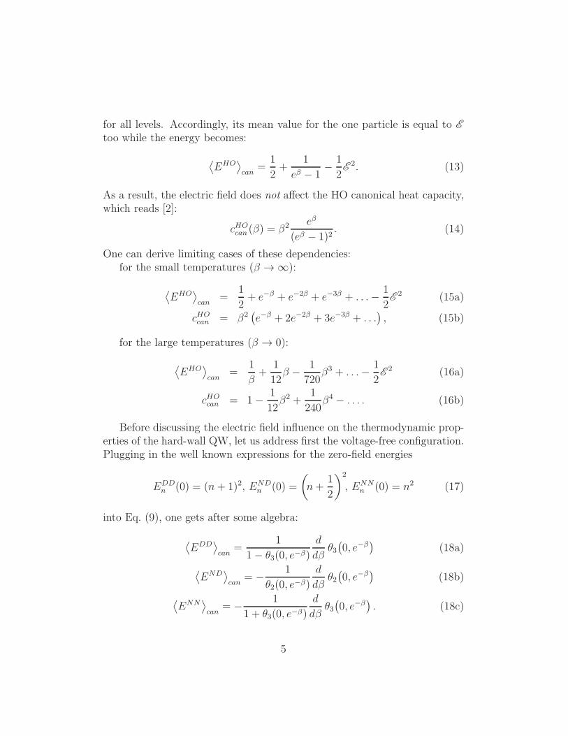
Figure 1: (a) Heat capacity cV and (b) mean energy 〈E〉 as a function of thenormalized temperature β−1 for the canonical ensemble and pure Dirichlet(dotted line), Neumann (solid curve) and ND (dashed line) QW at zeroelectric field.

6

Here, θi(z, q), i = 1, 2, 3, 4, are Theta functions [3, 4]. For small temperatures,β → ∞, these equations degenerate to

⟨

EDD⟩

can= 1 + 3e−3β − 3e−6β + 8e−8β + 3e−9β + . . . (19a)

⟨

END⟩

can=

1

4+ 2e−2β − 2e−4β + 8e−6β − 10e−8β + . . . (19b)

⟨

ENN⟩

can= e−β − e−2β + e−3β + 3e−4β − 4e−5β

+5e−6β − 6e−7β + 3e−8β + . . . . (19c)

Utilizing transformation properties of the Theta functions [3]

θ3(

0, e−β)

=

√

π

βθ3

(

0, e−π2/β)

(20a)

θ2(

0, e−β)

=

√

π

βθ4

(

0, e−π2/β)

, (20b)

one derives the energies in the opposite limit of the high temperatures:

⟨

EDDNN

⟩

can=

1

2β± 1

2π1/2β1/2+

1

βe−π2/β, β → 0 (21a)

⟨

END⟩

can=

1

2β− 2π2

β2e−π2/β, β → 0. (21b)

The corresponding heat capacities cV are calculated by applying the right-most part of Eq. (10) to the above dependencies; in particular, one has

for the “cold” QW, β → ∞:

cDDcan = β2

(

9e−3β − 18e−6β + 64e−8β + . . .)

(22a)

cNDcan = β2

(

4e−2β − 8e−4β + 48e−6β − 80e−8β + . . .)

(22b)

cNNcan = β2

(

e−β − e−2β + e−3β + 3e−4β − 4e−5β

+ 5e−6β −6e−7β+ 3e−8β+ . . .)

; (22c)

for the hot thermal bath:

cDD,NNcan =

1

2± 1

4π1/2β1/2 − π2

βe−π2/β, β → 0 (23a)

cNDcan =

1

2− 4π2

βe−π2/β +

2π4

β2e−π2/β , β → 0. (23b)

7

010

2030

40500

510

1520

-15

-10

-5

0

5

10 ND

-1 E

010

2030

40500

510

1520

-15

-10

-5

0

5

10 NN

-1 E

010

2030

40500

510

1520

-15

-10

-5

0

5

10 DD

-1 EE

010

2030

40500

510

1520

-15

-10

-5

0

5

10 DN

-1 E

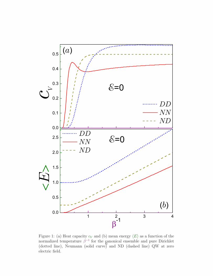
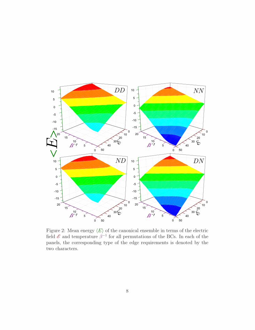
Figure 2: Mean energy 〈E〉 of the canonical ensemble in terms of the electricfield E and temperature β−1 for all permutations of the BCs. In each of thepanels, the corresponding type of the edge requirements is denoted by thetwo characters.

8

Statistically averaged energies and corresponding heat capacities are shownin Fig. 1. At the zero temperature, the total internal energy reduces to theground-state energy and the heat capacity is zero, as it should be. As itfollows from Eqs. (19) and (22), their avalanche growth from the T = 0 val-ues for the purely Neumann QW takes place at the smaller temperatures ascompared to the mixed BCs, which, in turn, is followed by the quantities forthe Dirichlet structure. This is explained by the growing difference betweenthe two lowest energies for just consecutively mentioned BC configurations:the quantity

∆n(E ) = En+1(E )− En(E ) (24)

at the zero field is the smallest (largest) for the Neumann (Dirichlet) struc-ture:

∆NNn (0) = 2n+ 1, ∆ND

n (0) = 2n+ 2, ∆DDn (0) = 2n+ 3. (25)

A remarkable feature of the heat capacity dependence is its nonmonotonicbehaviour for the Neumann QW: at β−1

max = 0.4342 (βmax = 2.3031) it reachesa pronounced maximum cNN

max = 0.4455 that is followed by the minimum ofcNNmin = 0.3818 located at β−1

min = 0.9420 (βmin = 1.0616). If the maximum isobserved quite exactly by keeping only the first term in the parentheses ofthe right-hand side of Eq. (22c), the emergence and precision of the locationand magnitude of the second extremum are described better by keeping moreterms in the same expansion. Physically, this nonmonotonicity of the heatcapacity is attributed to the structure of the energy spectrum, see Eqs. (17)and (25); namely, very small temperature promotes the particle mainly to thefirst excited level that is only one unit above the ground state, ∆NN

0 (0) = 1,with the contribution of the other levels being negligibly small due to thealmost vanishing exponents in Eq. (8a) or, equivalently, in Eqs. (19c) and(22c); as a result, the heat capacity grows rapidly. For the larger tempera-tures, the occupations of the higher lying levels become essential; however,the transitions to them are more difficult since the difference between, e.g.,second and first excited states ∆NN

1 (0) = 3 is three times larger than thatbetween the latter and the ground level. Accordingly, the same speed ofthe heat capacity change can not be sustained what results in the observedmaximum. For the other BCs, the ratio ∆1(0)/∆0(0) is smaller than forthe Neumann QW, as it follows from Eq. (25): ∆ND

1 (0)/∆ND0 (0) = 2 and

∆DD1 (0)/∆DD

0 (0) = 5/3; as a result, for them no extrema are observed onthe cV − T dependence at β−1 . 1. Mathematically, the drop of the NN

9

specific heat is caused by the interplay between the counterbalancing termsβ2 and e−β in Eq. (22c) as the temperature grows. Keeping only the firstexponent in the parentheses of the right-hand side of this equation produces

βNN(1)max = 2 while the same procedure applied to the other BCs, see Eqs. (22a)

and (22b), results in βDD(1)max = 2/3 and β

ND(1)max = 1, which are, respectively,

three and two times smaller and lie beyond the range of the validity of theseexpansions. Accordingly, for the latter two configurations, it is essential tokeep other items in the corresponding series in order for them to be correctat the decreasing β, and these extra exponents eliminate the resonance of thefirst-term approximation while for the Neumann QW the (negative) secondcomponent simply improves the previous result. Note that the HO leading

term of the capacity expansion from Eq. (15b) also results in βHO(1)max = 2; how-

ever, the subsequent (all positive) items in the series wipe out the extremum.Very broad and gentle asymmetric maximum is observed at β−1 & 2.5 for theDirichlet QW while for the mixed BC the heat capacity is a monotonicallyincreasing function of the temperature, which, at quite large T , rapidly ap-proaches the asymptotic value of one half. On the contrary, the heat capacityof the symmetric QWs reaches the same limit much slower, as Eq. (23a) as-serts and panel (a) of Fig. 1 exemplifies. Note that the HO internal energyfor the high temperatures is twice of that for the hard-wall QW: kBT and12kBT in regular units, respectively. From point of view of classical equilib-

rium statistics that is applicable for T → ∞, this difference is explained bythe fact that in the former case the kinetic and potential parts of the motionmake equal contributions of 1

2kBT to the total energy [2] while for the latter

system it is the kinetic energy only that determines 〈E〉 as the QW potentialis zero. As a direct consequence of this, the QW heat capacities in the samelimit are one half of their HO counterpart.

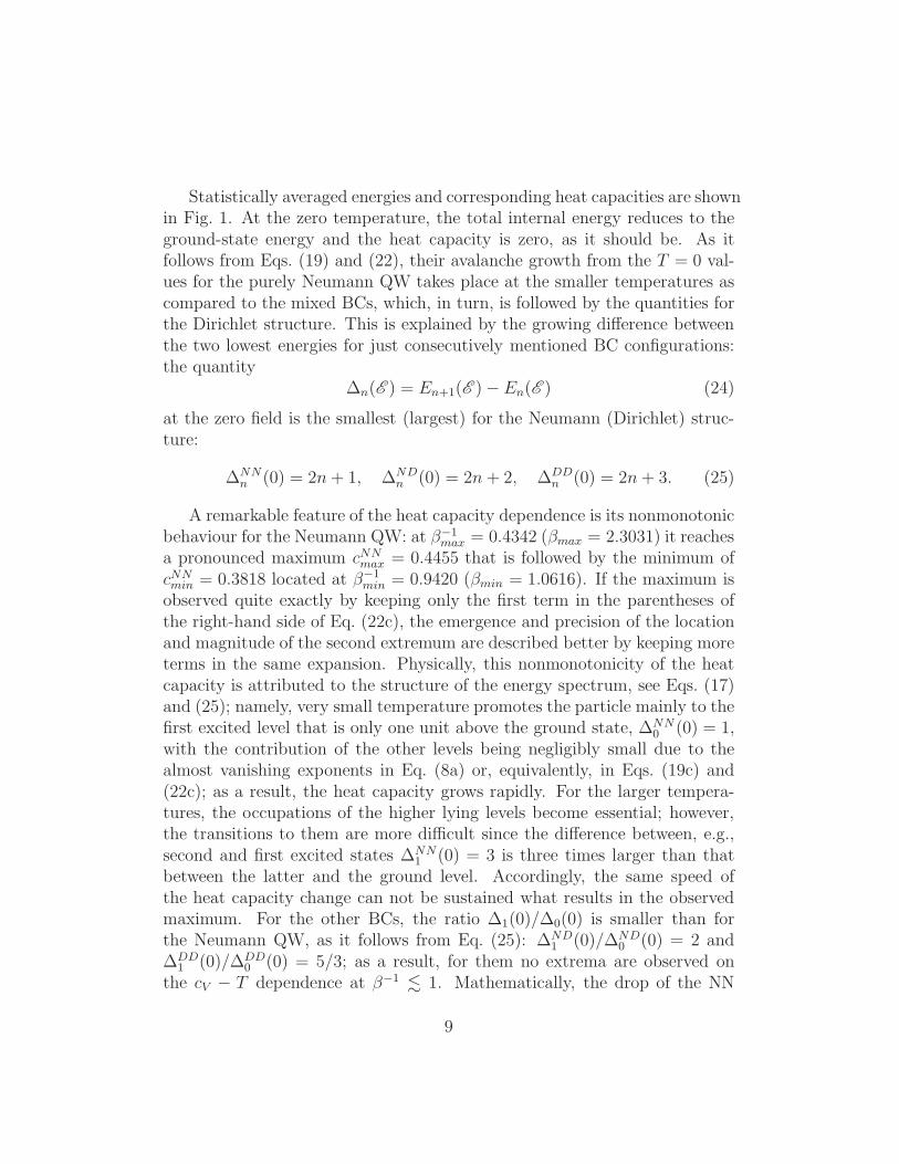
Applied electric field modifies the energy spectrum what, in turn, affectsthe thermodynamic properties of the wells. It was shown that the voltageincreases the difference ∆1(E ) between the ground and first excited levelsfor any permutation of the BCs (the only exception is the ND case at thesmall fields, see equations (33) in [1]); accordingly, the larger temperatureis needed to push out the electron from its lowest state. This is reflected inFigs. 2 and 3 where the energy 〈E(β, E )〉can and heat capacity 〈cV (β, E )〉can,respectively, are shown. It is seen that the β−1 range where the mean energydoes not change appreciably from the ground-state value gets wider for thestronger intensities E . The same is true for the heat capacity where the

10

c V

03

69

12

010

2030

4050

0.0

0.2

0.4

0.6

0.8

1.0DN

E

-10

36

912

010

2030

4050

0.0

0.2

0.4

0.6

0.8

1.0ND

E

-1

03

69

12

010

2030

4050

0.0

0.2

0.4

0.6

0.8

1.0NN

E

-10

36

912

010

2030

4050

0.0

0.2

0.4

0.6

0.8

1.0DD

E

-1

Figure 3: The same as in Fig. 2 but for the heat capacity cV .

11

plateau with its almost zero value grows with the field. The increasing voltagewipes out the NN minimum of the heat capacity simultaneously moving themaximum to the higher temperatures and increasing its magnitude. Foreach of the mixed BCs, it also creates a maximum that was absent at E = 0.Mentioned above DD extremum of the heat capacity gets narrower and itspeak increases with the field growing. Recalling again the language of theclassical statistical mechanics [2], one qualitatively explains the larger heatcapacities at the nonzero fields by the contribution of the electric potential;namely, the thermally averaged value of the potential energy 〈−E x〉 is:

〈−E x〉 = 1

β

(

1− 1

2βE coth

1

2βE

)

. (26)

This classical expression is applicable to our quantum system for the largetemperatures only:

〈−E x〉 ≈ − 1

12E

2β +1

720E

4β3 − . . . , β → 0. (27)

Then, the potential contribution to the heat capacity reads:

cpotV ≈ 1

12(βE )2 − 1

240(βE )4 + . . . , β → 0. (28)

Note that, contrary to the HO, the kinetic and potential contributions tothe heat capacity in this case, generally, are not equal to each other. Let usalso mention once again that the electric field does not affect at all the HOheat capacity, see Eq. (14), since it simply shifts all the levels by the sameamount, according to Eq. (12a).

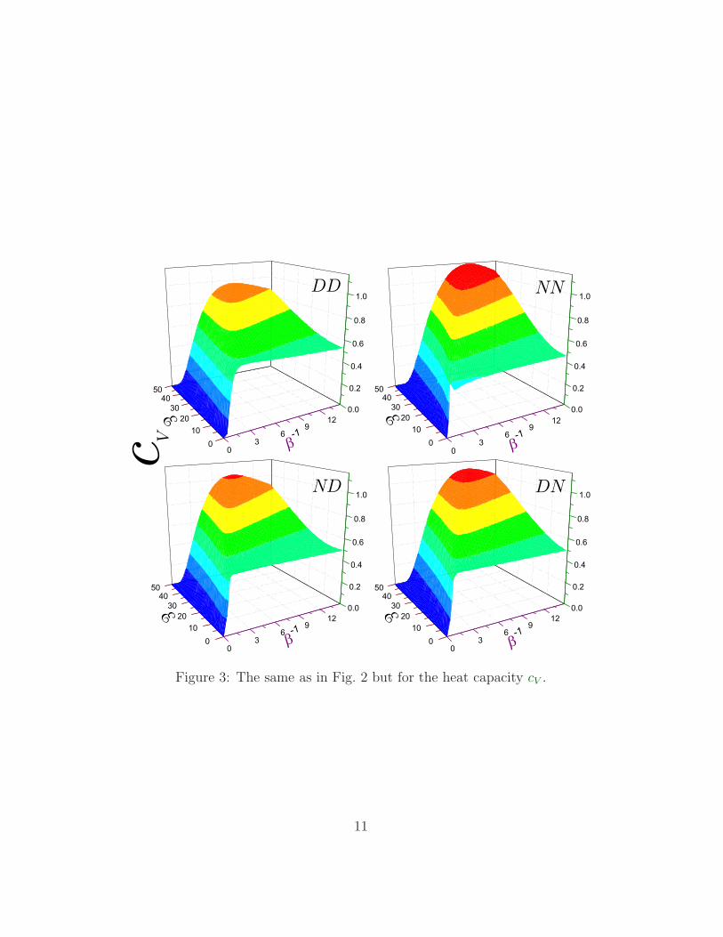
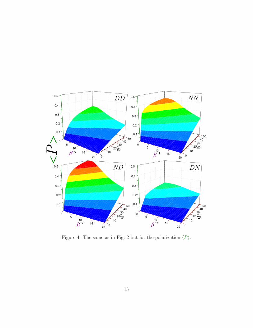
Fig. 4 depicts statistically averaged polarizations 〈P 〉can in terms of E

and β−1. Growing temperature leads to the decrease of 〈P 〉can for all electricfields; however, thermal energy is not strong enough to make the total dipolemoment negative: for any BC the polarization stays positive. To understandthe statistical properties better, it is instructive to consider the case of the lowtemperatures. For the small voltages, as a first approximation, we also acceptundisturbed by the field energies from Eq. (17). Then, one has following

12

05

1015

20

0.1

0.2

0.3

0.4

0.5

010

2030

4050

DN

E

-1

05

1015

20

0.1

0.2

0.3

0.4

0.5

010

2030

4050

ND

-1

E

05

1015

20

0.1

0.2

0.3

0.4

0.5

010

2030

4050

NN

E

-1

05

1015

20

0.1

0.2

0.3

0.4

0.5

010

2030

4050

DD

E-1P

Figure 4: The same as in Fig. 2 but for the polarization 〈P 〉.

13

dependencies:

〈PDD〉 = P0 + (P1 − P0)(

e−3β − e−6β)

+ (P2 − P0) e−8β + . . . , β → ∞ (29a)

〈PND〉 = P0 + (P1 − P0)(

e−2β − e−4β)

+ (P2 − 2P0 + P1) e−6β + . . . , β → ∞ (29b)

〈PNN〉 = P0 + (P1 − P0)(

e−β − e−2β + e−3β)

+ (P2 −P1) e−4β + . . . , β → ∞. (29c)

These equations were derived under the assumption of E ≪ 1, but the generalproperty stating that the first-order temperature correction is determined byP1−P0, holds for any electric intensities. For the small fields, this differenceis negative [1] what naturally explains the decrease of the total polarizationwith the temperature growing. In the opposite limit of the high voltages,the polarizations of the QW with the uniform BCs tend to the same level-independent value of one-half [1] what requires larger temperatures in orderto see the deviation of 〈P 〉 from its T = 0 value. This is exemplified in Fig. 4where the temperature-independent plateau at T = 0 widens with the fieldgrowing. For the mixed edge requirements, this limiting quantity is supple-mented by the term that is proportional to ±(n+ 1/2)−2 with its sign beingdetermined by the orientation of the BCs [1]; so, for the DN case it is actu-ally possible to observe the increase of the polarization with the temperaturegrowing from zero. This feature is now shown in the corresponding panel ofthe figure since it takes place beyond the figure range 0 ≤ E ≤ 50.

3 Grand Canonical Ensemble

Grand canonical distribution is used for the description of the quantum sys-tem that, in addition to the thermal balance with the external reservoir, isalso in the chemical equilibrium with it. Accordingly, the structure can ex-change the energy as well as particles with the heat bath. So, the numberof the quantum corpuscles N in it can be changed. The fundamental rolein this case is played by the chemical potential µ, which is defined from thecondition

N =∑

n

1

e(En−µ)β ± 1, (30)

14

where the upper sign corresponds to the Fermi-Dirac (FD) distribution whilethe lower one describes Bose-Einstein (BE) particles. Physically, the differ-ence between these two statistics is in the fact that each quantum level cannot be occupied by more than one fermion (Pauli exclusion principle) whilethe arbitrary number of bosons can coexist in the same state. The distri-bution function now depends not only on the energies En but also on thenumber of the particles in the system N ; namely, for the physical quantityI its grand canonical average value 〈I〉gc is

〈I〉gc =∑

n

In

e(En−µ)β ± 1. (31)

Applying the distribution from Eq. (31) for the calculation of the heat ca-pacity, Eq. (10), one finds that its grand canonical value cgc is

cgc = β2∑

n

En

(

En − µ− β ∂µ∂β

)

[e(En−µ)β ± 1]2 e(En−µ)β , (32)

where the chemical potential, which, in the case of fermions, is also frequentlycalled the Fermi level, is calculated, as stated above, from Eq. (30). Phys-ically, the value of µ corresponds to the energy that is needed for changingby one the number of the particles in the system:

µ =

(

∂〈E〉∂N

)

T,V

. (33)

For calculating its partial derivative with respect to the temperature, oneshould consider Eq. (30) as a condition of zeroing of the implicit functionF (µ, β,N) of the chemical potential in terms of the variables β and N :

F (µ(β,N), β, N) = 0. (34)

The rule of differentiating implicit functions states [9]:

∂µ

∂β= −∂F/∂β

∂F/∂µ. (35)

As a result, one finds:

β∂µ

∂β=

∑

nEn−µ

[e(En−µ)β±1]2 e

(En−µ)β

∑

n1

[e(En−µ)β±1]2 e(En−µ)β

. (36)

15

The boson statistics is used for the particles with the integer spin suchas photons or Cooper pairs in superconductors while the FD distribution isapplied for the system of the constituents with the half integer spins; forexample, the electron with its spin of 1/2 has, for the same energy, twoprojections of its spin equal to ±1/2. However, in our discussion below wewill neglect this fact and will assume that the number of the fermions foreach energy En is not larger than one.

Fig. 5 depicts the FD chemical potential for the pure Dirichlet QW as afunction of the electric field and temperature for several numbers N . Quali-tatively, the same features are characteristic for other BC permutations too.There are several distinct regions of the Fermi energy µN dependence on thetemperature. From its EN−1 value at T = 0 it rapidly grows as

µN = EN−1 −1

βln

1 +√1− 4e−∆N−1β

2, β → ∞, (37)

until it reaches and stays exactly at the value of

µN−1 =1

2(EN−1 + EN) , β & 1, (38)

which is due to the interaction of the two corresponding levels that, at thezero temperature, were the highest occupied and lowest unoccupied states.The width of this T -independent plateau is determined by the number of theparticles N and electric field E . For the still higher temperatures, the chem-ical potential for N = 1 decreases while for the larger number of particles,N ≥ 2, it grows with β−1, reaches maximum and only after that decreases,passes zero at β(0) and continues to decline into the negative part of thespectrum. For the nonpositive chemical potentials, µN ≤ 0, Eq. (30) can becast into the form

∞∑

m=0

(∓1)meµβ(m+1)∞∑

n=0

e−β(m+1)En = N, µ ≤ 0. (39)

For the zero field, E = 0, the energy spectrum from Eqs. (12a) and (17)simplifies this equation as follows:

16

04

812

16

010

2030

4050

100

102

104

106

108

110

112

114

N=10

E

-1

04

812

1620

010

2030

4050

26

28

30

32

34

N=5

E

-1

04

812

16

010

2030

4050

16

17

18

19

20

21

22

23

N=4

E

-10

48

1216

010

2030

4050

9

10

11

12

13

14

N=3

E-1

04

812

1620

-2

0

2

4

6

010

2030

4050

N=2

E

-1

04

812

1620

-20

-15

-10

-5

0

010

2030

4050

N=1

E

-1

Figure 5: Chemical potential µN for the FD distribution of the pure DirichletQW as a function of the electric field E and temperature β−1 for differentnumber of fermions N that is depicted in each panel. Note different µ scalefor each plot. Viewing perspectives for the upper two panels are differentfrom those for the other subplots. 17

for the HO:

1

2

∞∑

m=0

(∓1)meµβ(m+1)

sinh 12β(m+ 1)

= N, µ ≤ 0 (40a)

and, for example, for the mixed BCs:

1

2

∞∑

m=0

(∓1)meµβ(m+1)θ2(

0, e−β(m+1))

= N, µ ≤ 0. (40b)

Putting here the chemical potential equal to zero, µ = 0, leads to the cal-culation of β(0). In known to us literature [3–8], there are no analyticalexpressions for these infinite series. However, for the very small β, the m = 0terms in the above equations make the most significant contributions pro-ducing the following dependencies:

for the HO:

µHO(β)∣

∣

E=0=

1

βln(Nβ), β → 0 (41a)

and, for the hard-wall QW with the arbitrary BCs:

µIJ(β)∣

∣

E=0=

1

βln

(

2N

√

β

π

)

, β → 0. (41b)

Superscripts I and J in Eq. (41b) stand for any of the values of D and/orN . Fig. 5 manifests that, for the larger N , these asymptotics are achievedat the higher temperatures. As a result, the grand canonical mean energy〈E〉gc reads in the same limit:

〈EHO〉gc(β)∣

∣

E=0=

N

β, β → 0 (42a)

〈EIJ〉gc(β)∣

∣

E=0=

1

2

N

β, β → 0, (42b)

what, by means of Eq. (10), immediately leads to the associated heat capac-ities cgc:

cHOgc (β)

∣

∣

E=0= N, β → 0 (43a)

cIJgc (β)∣

∣

E=0=

N

2, β → 0. (43b)

A comparison of these remarkable results with Eqs. (16), (21) and (23) con-firms the general property, which states that for the large temperatures there

18

is no difference between canonical and grand canonical distributions [2]. How-ever, for the small T these two statistics produce very different features.Fig. 6 shows the FD heat capacity of the pure Dirichlet QW in terms ofthe temperature and electric field for the different N corresponding to theircounterparts from Fig. 5. It is seen that, for the larger number of the par-ticles, the asymptotics from Eq. (43b) is achieved at the higher T . At thezero field, a prominent characteristic of the heat capacity dependence for theone particle (top left panel of Fig. 6) is a salient maximum cmax = 0.882observed at β−1

max = 0.633, i.e., at the right edge of the plateau from Eq. (38).Accordingly, we attribute this extremum to the different behaviour of thechemical potential for N = 1 and N ≥ 2; namely, as it was mentioned duringdiscussion of Fig. 5, for one particle the Fermi energy decreases after the flatpart from Eq. (38) while for any other number N it grows with T . Thus, theircontributions to the heat capacity from Eq. (32) are opposite to each otherwhat results in the resonance that is observed for the one particle only. Eventhough the shape of this maximum is quite similar to its NN counterpartfor the canonical ensemble, see Sec. 2, its physical explanation is completelydifferent. First, we point out that the very similar extrema are calculatedalso for the ND (with cmax = 0.879 and β−1

max = 0.418) and pure Neumann(cmax = 0.878 and β−1

max = 0.208) QWs too. The fact that the three cmax arealmost the same and the ratios of the three temperatures Tmax are practicallyequal to those of ∆0(0) from Eq. (25), undoubtedly proves that the origin ofthis effect is the BC independent one and that the interplay between the twolowest states plays a dominant role in it. To understand these resonances, letus recall that, for the very small temperatures, the properties of the FD wellare determined only by the highest occupied level and its interaction with thenearest (empty at T = 0) above lying state, what is reflected in the extremelyrapid approach by the chemical potential to the energy from Eq. (38) thatis located exactly in the middle between them. For N ≥ 2, a contributionfrom the lower lying members in this regime is negligibly small and can besafely neglected, while for the one-electron QW this addition is absent bydefinition. Further growth of the temperature increases thermal energy butit is still too “weak” to compel the corpuscles, which at T = 0 lied below theFermi energy, to contribute to the heat capacity. Only at the right edge ofthe plateau, the thermodynamic quantum kBT becomes strong enough andforces other particles to donate to µN and cN . Therefore, for N ≥ 2 the heatcapacity is a quite smoothly varying function of the temperature. However,for N = 1 there are no such additional donors that aid to support the con-

19

tinuous growth of the heat capacity, which can not be sustained by the oneparticle only. As a result, the specific heat reaches maximum and drops.

This qualitative physical reasoning can be corroborated by the simplequantitative mathematical analysis. Fermi level from Eq. (37) defines thecorresponding mean energy and heat capacity as:

〈E〉 =

N−2∑

n=0

En +1

2EN−1 + ENe

−∆N−1β, β → ∞ (44a)

cV = EN∆N−1β2e−∆N−1β, β → ∞. (44b)

On the other hand, for the chemical potential from Eq. (38) these quantitiesfor one fermion, N = 1, become:

〈E〉 =E0

1 + e−∆0β/2+

E1

1 + e∆0β/2, β & 1 (45a)

cV =1

2∆0β

2

[

E1e∆0β/2

(1 + e∆0β/2)2

− E0e−∆0β/2

(1 + e−∆0β/2)2

]

, β & 1, (45b)

where we take into consideration only the two lowest states. For the pureNeumann QW without the field, this last expression takes an especially sim-ple form:

cNN1

∣

∣

E=0=

1

2β2 eβ/2

(1 + eβ/2)2 . (46)

This function has a pronounced maximum of cmax = 0.878 at βmax = 4.799. Aperfect coincidence with the provided above exact results justifies a validity ofthe two-level approximation and proves that the electron transitions betweenthem determine the specific heat resonance. It is also very instructive tocontrast Eq. (46) with its canonical counterpart from Eq. (22c) in sec. 2.The comparison shows that the magnitude of the grand canonical Neumannextremum is almost two times larger and it is achieved at more than twotimes lower temperature.

Applied field E smooths out and widens this maximum simultaneouslyincreasing the heat capacity. Similar to the canonical ensemble, this growthis explained by the contribution of the electrostatic potential. However, the

20

04

812

16

010

2030

4050

0.0

0.5

1.0

1.5

2.0

2.5

3.0

-1

N=10

E

04

812

16

010

2030

4050

0.0

0.5

1.0

1.5

2.0

2.5

3.0

N=5

E

-1

04

812

16

010

2030

4050

0.0

0.5

1.0

1.5

2.0

2.5

N=4

E

-1

04

812

16

010

2030

4050

0.0

0.5

1.0

1.5

2.0

N=3

E-1

02

46

810

010

2030

4050

0.0

0.4

0.8

1.2

1.6

N=2

E-1

02

46

010

2030

4050

0.0

0.2

0.4

0.6

0.8

1.0

N=1

E

-1

c N

Figure 6: The same as in Fig. 5 but for the heat capacity cN . Note differentc and β−1 scales for different panels.

21

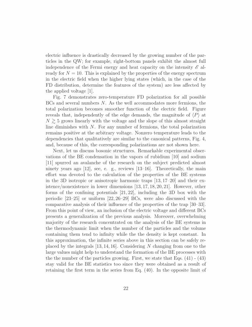
electric influence is drastically decreased by the growing number of the par-ticles in the QW; for example, right-bottom panels exhibit the almost fullindependence of the Fermi energy and heat capacity on the intensity E al-ready for N = 10. This is explained by the properties of the energy spectrumin the electric field when the higher lying states (which, in the case of theFD distribution, determine the features of the system) are less affected bythe applied voltage [1].

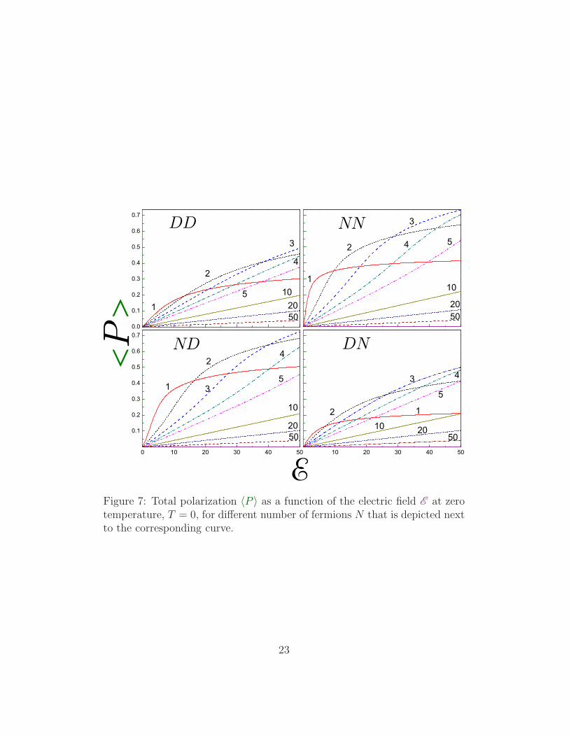
Fig. 7 demonstrates zero-temperature FD polarization for all possibleBCs and several numbers N . As the well accommodates more fermions, thetotal polarization becomes smoother function of the electric field. Figurereveals that, independently of the edge demands, the magnitude of 〈P 〉 atN & 5 grows linearly with the voltage and the slope of this almost straightline diminishes with N . For any number of fermions, the total polarizationremains positive at the arbitrary voltage. Nonzero temperature leads to thedependencies that qualitatively are similar to the canonical patterns, Fig. 4,and, because of this, the corresponding polarizations are not shown here.

Next, let us discuss bosonic structures. Remarkable experimental obser-vations of the BE condensation in the vapors of rubidium [10] and sodium[11] spurred an avalanche of the research on the subject predicted almostninety years ago [12], see, e. g., reviews [13–16]. Theoretically, the maineffort was devoted to the calculation of the properties of the BE systemsin the 3D isotropic or anisotropic harmonic traps [13, 17–20] and their ex-istence/nonexistence in lower dimensions [13, 17, 18, 20, 21]. However, otherforms of the confining potentials [21, 22], including the 3D box with theperiodic [23–25] or uniform [22, 26–29] BCs, were also discussed with thecomparative analysis of their influence of the properties of the trap [30–33].From this point of view, an inclusion of the electric voltage and different BCspresents a generalization of the previous analysis. Moreover, overwhelmingmajority of the research concentrated on the analysis of the BE systems inthe thermodynamic limit when the number of the particles and the volumecontaining them tend to infinity while the the density is kept constant. Inthis approximation, the infinite series above in this section can be safely re-placed by the integrals [13, 14, 16]. Considering N changing from one to thelarge values might help to understand the formation of the BE processes withthe the number of the particles growing. First, we state that Eqs. (41) - (43)stay valid for the BE statistics too since they were obtained as a result ofretaining the first term in the series from Eq. (40). In the opposite limit of

22

0.0

0.1

0.2

0.3

0.4

0.5

0.6

0.7

DD

5020

105

4

3

2

1

10 20 30 40 50

DN

502010

5

43

2 1

0 10 20 30 40 50

0.1

0.2

0.3

0.4

0.5

0.6

0.7

ND

5020

10

5

4

3

2

1

NN

5020

10

54

3

2

1

P

EFigure 7: Total polarization 〈P 〉 as a function of the electric field E at zerotemperature, T = 0, for different number of fermions N that is depicted nextto the corresponding curve.

23

the very small temperatures, it is elementary to derive:

µN = E0 −1

βln

(

1 +1

N

)

, β → ∞, (47a)

what leads to the mean energy and heat capacity:

〈E〉N = NE0 +N

N + 1E1e

−∆0β, β → ∞, (47b)

cN =N

N + 1E1∆0β

2e−∆0β, β → ∞. (47c)

An important characteristic of the BE system is its critical temperatureTcr. It corresponds to the situation when the chemical potential is equal tothe energy of the lowest level, µ = E0, and the number of the particles inthis state N0 is zero what leads to the implicit mathematical equation forfinding βcr

∑

n=1

1

e(En−E0)βcr − 1= N. (48)

Physically, it is the largest temperature at which the BE condensation stillcan be observed, and at the lower T the fraction N0/N of the particles in theground state will increase until at T = 0 it becomes unity:

N0/N |T=0 = 1. (49)

Fig. 8(a) shows dependencies of the critical parameter β−1cr on the applied

voltage for all possible BCs and several numbers N . In accordance with theprevious results [13], the temperature Tcr increases with N . In the absenceof the fields, the lowest (highest) temperature is observed for the pure Neu-mann (Dirichlet) QW what is a reflection of the corresponding spectrum fromEq. (17) and the energy difference between the affiliated states, see Eq. (25).Electric field leads to the modification of the mutual location of the levelson the energy axis; in particular, at the small voltages, the two lowest statesmove closer to each other for the ND geometry while the difference E1 −E0

grows with the field for all E and any other BC configuration [1]. As a result,the critical temperature for the former edge requirement decreases with thegrowing from zero field, passes through minimum and then unrestrictedlygrows with the electric intensity while for all other BCs it is a continuouslyincreasing function of E . At the high voltages, the energy spectrum is de-termined mainly by the condition at the right wall [1] what leads to almost

24

-0.6

-0.4

-0.2

0.0

0.2

0.4(b) N=5

N=1

P DD

NN DN ND

cr

0 10 20 30 40 50

5

10

15

20

25

30

35

(a)

N=5

-1

E

DD NN DN ND

cr

N=1

Figure 8: (a) Critical temperatures β−1cr and (b) corresponding to them po-

larizations 〈Pcr〉 from Eq. (50) as functions of the applied electric field E

for different number N of bosons that are depicted near the correspondingcurves. Solid (dotted) lines are for the pure Dirichlet (Neumann) BC whiletheir dash (dash-dotted) counterparts denote DN (ND) geometry. In panel(b), thin horizontal line is zero polarization.

25

the same critical temperature for, e. g., the NN and DN wells. Note thatin this regime, contrary to the zero fields, the Dirichlet requirement is morefavorable to the formation of the BE condensate as compared to the Neu-mann interface. This is explained by the larger level separation for the lattergeometry at the high voltages [1].

As the ground-state polarization is positive for all fields and BCs [1], onecan expect that at the onset of the BE condensation the total statisticallyaveraged dipole moment will, at the small voltages, be negative. This isexactly what is observed in panel (b) of Fig. 8 that shows the polarizations〈Pcr〉 corresponding to the critical temperatures β−1

cr from panel (a). Theywere calculated from equation

〈Pcr〉 =∞∑

n=1

Pn

e(En−E0)βcr − 1, (50)

and, as stated above, the critical temperature β−1cr was found from Eq. (48).

The characteristic features of the critical polarizations basically follow theproperties of the first excited state: from zero they decrease with the growthof the field, reach minimum after which they increase. However, for the largevoltages many upper lying states are occupied and contribute to the totaldipole moment. As a result, the high-field 〈Pcr〉 for one boson is considerablysmaller than P1. The absolute value of the negative polarization at theextremum grows with the number of the particles with the largest one, atthe fixed N , being observed for the pure Neumann QW followed by its NDcounterpart what is a replica of the similar behaviour for the first excitedlevel [1]. For the temperatures below Tcr, the nonzero occupation of theground state contributes a positive term to the polarization what leads tothe gradual disappearance of the negative region of the total dipole moment〈P 〉 with the decreasing temperature until at T = 0 it becomes NP0, whichis positive for any BC and arbitrary fields [1].

As a final example, Fig. 9 exhibits evolution of the heat capacity andchemical potential with the varying electric field and temperature for thepure Neumann QW. It is seen that for the small number of bosons, say,N = 3 in panel (a), the applied voltage leads, at quite warm sample, to theincrease of cV while at the small T , the width of the temperature-independentzero-capacity plateau increases with the field. These features were discussedbefore for the canonical ensemble. Increasing the number of the particlesin the well leads to the suppression of the voltage dependence, as a tran-

26

01

23

45

6

010

2030

4050

-40

-30

-20

-10

0

N=105

(d)

cr

E

01

23

45

010

2030

4050

0.000

0.002

0.004

0.006

0.008

0.010

N=105

(c)

N

E

c

cr

04

812

16

010

2030

4050 0.0

0.5

1.0

1.5

2.0

2.5

N=3c

V

(a)

E -1

01

23

45

010

2030

4050

0.00

0.02

0.04

0.06

0.08

N

(b)

N=1000E

c

cr

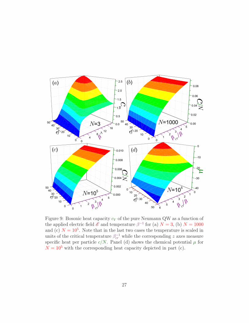
Figure 9: Bosonic heat capacity cV of the pure Neumann QW as a function ofthe applied electric field E and temperature β−1 for (a) N = 3, (b) N = 1000and (c) N = 105. Note that in the last two cases the temperature is scaled inunits of the critical temperature β−1

cr while the corresponding z axes measurespecific heat per particle c/N . Panel (d) shows the chemical potential µ forN = 105 with the corresponding heat capacity depicted in part (c).

27

sition from panel (a) to (b) with N = 1000 and (c) for N = 105 vividlydemonstrates. No any noticeable field dependence is seen there in the range0 ≤ E ≤ 50. It is well known that for some potentials, such as, e.g., the 3Disotropic harmonic trap [14, 16, 18, 19, 34, 35], the heat capacity has a cusp-like peculiarity as it passes through the critical temperature while for the 1Dquadratic potential it is a smooth function of T [16, 18, 35]. Fig. 9 exempli-fies that no any peculiarity is observed for the 1D hard-wall potential withNeumann surfaces and arbitrary applied electric fields. Our calculations con-firm that the same is true for any other BCs. Finally, panel (d) shows thatthe chemical potential µ is a monotonically decreasing function of both theelectric field E and temperature T . It is seen that the growing temperaturediminishes the voltage influence on the chemical potential.

4 Concluding remarks

Rigorous mathematical treatment of the QW with miscellaneous BCs underthe applied voltage revealed a strong influence of the interplay between themon the thermodynamic properties of the structure. In particular, without thefield the differences of the energy spectrum lead, for the canonical ensemble,to the conspicuous maximum followed by the minimum of the heat capacitycV on the temperature axis for the NN quantum box while for the otheredge requirements no such adjacent extrema are observed. Modification ofthe specific heat and statistically averaged polarization in the field is quali-tatively explained by the influence of the associated electrostatic potential.Numerical calculations, which predicted, for the flat potential with the arbi-trary BC, a salient maximum of cV as a function of T for one fermion andits absence for the larger N , were corroborated by the two-level model thatallows simple analytical treatment with its predictions perfectly coincidingwith the exact results. From this, a clear physical explanation of this phe-nomenon follows that is based on the analysis of the associated Fermi energy.It is predicted that the applied field, in general, favors the formation of theBE condensate, and the differences and similarities of this process for the dif-ferent BCs are discussed. The thermally averaged dipole moment is shownto take the negative values in some ranges of the fields and temperatures.It is also argued that for the larger number of either fermions or bosons inthe QW, the influence of the electric field on the thermodynamic propertiesdiminishes.

28

Dirichlet and Neumann conditions are the limiting cases of the so calledRobin BC [36]

n∇Ψ|S=

1

ΛΨ

∣

∣

∣

∣

S

, (51)

where n is an inward unit normal to the surface, and the parameter Λ has adimension of length and is called the extrapolation distance. Its variation al-lows a continuous transformation from the Dirichlet (Λ = 0) to the Neumann(Λ = ∞) situation. Without the field, especially intriguing are the propertiesof the QW at the small negative Robin lengths, Λ → −0, when, in additionto the positive spectrum, two almost degenerate odd and even levels with theenergies E ∼ −1/(πΛ)2 are created [37]. Analysis of the Robin QW in theelectric field might present an interesting extension of the present research.

5 Acknowledgement

This project was supported by Deanship of Scientific Research, College ofScience Research Center, King Saud University.

References

[1] O. Olendski, Preceding paper (accepted for publication in Annalen derPhysik).

[2] N. Dalarsson, M. Dalarsson, and L. Golubovic, Introductory StatisticalThermodynamics (Academic, Amsterdam, 2011).

[3] R. Bellman, A Brief Introduction to Theta Functions (Holt, Rinehartand Wilson, New York, 1961).

[4] M. Abramowitz and I. A. Stegun, Handbook of Mathematical Func-tions (Dover, New York, 1964).

[5] I. S. Gradshteyn and I. M. Ryzhik, Table of Integrals, Series, andProducts, 8th edn. (Academic, Amsterdam, 2014).

[6] A. P. Prudnikov, Y. A. Brychkov, and O. I. Marichev, Integrals andSeries, vol. 1 (Gordon and Breach, New York, 1986).

29

[7] A. P. Prudnikov, Y. A. Brychkov, and O. I. Marichev, Integrals andSeries, vol. 2 (Gordon and Breach, New York, 1990).

[8] Y. A. Brychkov, Handbook of Special Functions: Derivatives, Integrals,Series and Other Formulas (Chapman & Hall, Boca Raton, 2008).

[9] W. Rudin, Principles of Mathematical Analysis, 3rd edn. (McGraw-Hill, New-York, 1976).

[10] M. H. Anderson, J. R. Ensher, M. R. Matthews, C. E. Wieman, andE. A. Cornell, Science 269, 198 (1995).

[11] K. B. Davis, M.-O. Mewes, M. R. Andrews, N. J. van Druten, D. S.Durfee, D. M. Kurn, and W. Ketterle, Phys. Rev. Lett. 75, 3969 (1995).

[12] S. N. Bose, Z. Phys. 26, 178 (1924).

[13] F. Dalfovo, S. Giorgini, L. P. Pitaevskii, and S. Stringari, Rev. Mod.Phys. 71, 463 (1999).

[14] L. Pitaevskii and S. Stringari, Bose-Einstein Condensation (Clarendon,Oxford, 2003).

[15] A. J. Leggett, Rev. Mod. Phys. 73, 307 (2001).

[16] C. J. Pethick and H. Smith, Bose-Einstein Condensation in DiluteGases (Cambridge, Cambridge, 2004).

[17] W. Ketterle and N. J. van Druten, Phys. Rev. A 54, 656 (1996).

[18] N. J. van Druten and W. Ketterle, Phys. Rev. Lett. 79, 549 (1997).

[19] R. Napolitano, J. De Luca, V. S. Bagnato, and G. C. Marques, Phys.Rev. A 55, 3954 (1997).

[20] W. J. Mullin, J. Low Temp. Phys. 106, 615 (1997).

[21] V. Bagnato and D. Kleppner, Phys. Rev. A 44, 7439 (1991).

[22] V. Bagnato, D. E. Pritchard, and D. Kleppner, Phys. Rev. A 35, 4354(1987).

30

[23] E. B. Sonin, Zh. Eksp. Teor. Fiz. 56, 963 (1969) [Sov. Phys. - JETP29, 520 (1969)].

[24] S. Greenspoon and R. K. Pathria, Phys. Rev. A 9, 2103 (1974).

[25] C. S. Zasada and R. K. Pathria, Phys. Rev. A 14, 1269 (1976).

[26] D. F. Goble and L. E. H. Trainor, Can. J. Phys. 44, 27 (1966).

[27] D. F. Goble and L. E. H. Trainor, Phys. Rev. 157, 167 (1967).

[28] D. F. Goble and L. E. H. Trainor, Can. J. Phys. 46, 1867 (1968).

[29] S. Grossmann and M. Holthaus, Z. Phys. B 97, 319 (1995).

[30] R. K. Pathria, Phys. Rev. A 5, 1451 (1972).

[31] S. Greenspoon and R. K. Pathria, Phys. Rev. A 8, 2657 (1973).

[32] M. N. Barber and M. E. Fisher, Phys. Rev. A 8, 1124 (1973).

[33] Z. R. Hasan and D. F. Goble, Phys. Rev. A 10, 618 (1974).

[34] H. Haugerud, T. Haugset, and F. Ravndal, Phys. Lett. A 225, 18(1997).

[35] T. Haugset, H. Haugerud, and J. O. Andersen, Phys. Rev. A 55, 2922(1997).

[36] K. Gustafson and T. Abe, Math. Intell, 20(1), 63 (1998).

[37] O. Olendski and L. Mikhailovska, Phys. Rev. E 81, 036606 (2010).

31