Productivity index of multilateral wells
118
Graduate Theses, Dissertations, and Problem Reports 2006 Productivity index of multilateral wells Productivity index of multilateral wells Upender Naik Nunsavathu West Virginia University Follow this and additional works at: https://researchrepository.wvu.edu/etd Recommended Citation Recommended Citation Nunsavathu, Upender Naik, "Productivity index of multilateral wells" (2006). Graduate Theses, Dissertations, and Problem Reports. 1740. https://researchrepository.wvu.edu/etd/1740 This Thesis is protected by copyright and/or related rights. It has been brought to you by the The Research Repository @ WVU with permission from the rights-holder(s). You are free to use this Thesis in any way that is permitted by the copyright and related rights legislation that applies to your use. For other uses you must obtain permission from the rights-holder(s) directly, unless additional rights are indicated by a Creative Commons license in the record and/ or on the work itself. This Thesis has been accepted for inclusion in WVU Graduate Theses, Dissertations, and Problem Reports collection by an authorized administrator of The Research Repository @ WVU. For more information, please contact [email protected].
-
Upload
khangminh22 -
Category
Documents
-
view
1 -
download
0
Transcript of Productivity index of multilateral wells

Graduate Theses, Dissertations, and Problem Reports
2006
Productivity index of multilateral wells Productivity index of multilateral wells
Upender Naik Nunsavathu West Virginia University
Follow this and additional works at: https://researchrepository.wvu.edu/etd
Recommended Citation Recommended Citation Nunsavathu, Upender Naik, "Productivity index of multilateral wells" (2006). Graduate Theses, Dissertations, and Problem Reports. 1740. https://researchrepository.wvu.edu/etd/1740
This Thesis is protected by copyright and/or related rights. It has been brought to you by the The Research Repository @ WVU with permission from the rights-holder(s). You are free to use this Thesis in any way that is permitted by the copyright and related rights legislation that applies to your use. For other uses you must obtain permission from the rights-holder(s) directly, unless additional rights are indicated by a Creative Commons license in the record and/ or on the work itself. This Thesis has been accepted for inclusion in WVU Graduate Theses, Dissertations, and Problem Reports collection by an authorized administrator of The Research Repository @ WVU. For more information, please contact [email protected].

PRODUCTIVITY INDEX OF MULTILATERAL WELLS
Upender Naik Nunsavathu
Thesis Submitted to the
College of Engineering and Mineral Resources At West Virginia University
In partial fulfillments of the requirements For the degree of
Master of Science In
Petroleum and Natural Gas Engineering
Dr. H. Ilkin Bilgesu, Chair of Committee Prof. Samuel Ameri
Dr. Daniel E. Della-Giustina
Department of Petroleum and Natural Gas Engineering Morgantown, West Virginia
2006
Keywords: Petroleum & Natural Gas Engineering, Multilateral wells, Productivity index, Dimensionless time, Dimensionless pressure.

ii
Abstract
Productivity Index of Multilateral wells
Upender Naik Nunsavathu
In the history of petroleum science there are a vast variety of productivity solutions for different
well types, well configurations and flow regimes. The main well types that were considered for
calculating the productivity indexes were vertical wells and horizontal wells. The configurations
considered were multilayer perforations, dual lateral wells with laterals at same depths, stacked
wells etc. There are few solutions to estimate the well productivity for complex configurations like
multilateral wells.
The main objective of this work is to identify a numerical solution method for calculating
productivity indexes for different well configurations like single vertical well, single horizontal well,
dual lateral well with laterals at same depth, dual laterals with laterals at different depths and four
laterals well. A three-phase, three-dimensional black oil reservoir simulator (ECLIPSE) is used in
this thesis. Apart from comparing the productivity indexes of different well configurations,
dimensionless pressure derivatives with respect to dimensionless time is also compared for all
the above well configurations.

iii
ACKNOWLEDGEMENTS
At the first place, I would like to express my deepest gratitude and appreciation to my advisor
Dr. Ilkin Bilgesu. Throughout his support, guidance and encouragements during my graduate
program, I have completed my studies and the thesis, which culminated in the achievement of my
degree. He entirely changed my life and without him this would never be possible.
Sincerely thanks to Professor and Department Chair Samuel Ameri for guidance and support
during my graduate studies at West Virginia University. I also appreciate his enthusiasm to be on
my committee.
I sincerely thank Dr. Daniel E. Della-Giustina for his guidance, support in my research work and
for being on my committee.
Many thanks to my professors in the Department of West Virginia University for the knowledge
they shared with me.
I would like to acknowledge Schlumberger for providing the software (ECLIPSE) used in this
study.
Great portion of help and encouragements that I had during my graduate studies I owe to all my
friends. Thank you for the time you spent with me.
Great thanks to my family, especially to my brother Aravind Nunsavathu, for the constant
encouragement and support. He is the best friend I have ever had in my life.
Finally, I dedicate my work to my loving parents, wife and to my brother for all of their belief,
guidance, support, and encouragement.

iv
TABLE OF CONTENTS Page
ABSTRACT ii
ACKNOWLEDGEMENTS iii
TABLE OF CONTENTS iv
LIST OF FIGURES vi
LIST OF TABLES xi
CHAPTER I. INTRODUCTION 1
1.1. Overview 1
1.1.1. Background 1
1.1.2. General Definition 3
1.1.3. Geometry of Multi-Lateral and Multi-branched wells 3
1.1.4. Classification System (TAML) 4
1.1.5. Advantages of Multilateral wells 6
1.1.6. Drawbacks of Multilateral wells 6
CHAPTER II. THEORY 7
2.1. Unsteady state 8
2.2. Pseudo – steady State 9
2.3. Steady State 10
2.4. Late Transient State 10
CHAPTER III. PREDICTION OF PRODUCTIVITY METHODS 11
3.1 Steady-state PI 11
3.1.1 Borisov method 11
3.1.2 The Giger – Reiss – Jourdan method 11

v
3.1.3 Joshi’s method 12
3.1.4 The Renard – Dupuy method 13
3.2 Pseudo-Steady State PI 14
3.2.1 Babu – Odeh method 14
3.2.2 Kuchuk method 14
3.2.3 Economides method 15
3.3 Literature Review 15
3.3.1 Analytical Solution 16
CHAPTER IV. RESERVOIR SIMULATIONS 18
4.1 Numerical Simulation Models for Multilateral wells 18
CHAPTER V. RESULTS AND DISCUSSION 53
CHAPTER VI. CONCLUSION AND FUTURE WORK 101
APPENDIX 103
REFERENCES 104

vi
LIST OF FIGURES Page
Figure 1.1 Russia’s first Multilateral well 2
Figure 1.2 Different Well Configurations 3
Figure 2.1 Representation of Infinite – acting (or) Transient state 8
Figure 2.2 Representation of Pseudo – steady state 9
Figure 2.4 Representation of Late Transient state 10
Figure 4.1 500 ft. Single Lateral Well 19
Figure 4.2 Grid structure for the 500 ft. Single Lateral Well 20
Figure 4.3 1000 ft. Single Lateral Well 21
Figure 4.4 Grid structure for the 1000 ft. Single Lateral Well 22
Figure 4.5 1500 ft. Single Lateral Well 23
Figure 4.6 Grid structure for the 1500 ft. Single Lateral Well 24
Figure 4.7 2000 ft. Single Lateral Well 25
Figure 4.8 Grid structure for the 2000 ft. Single Lateral Well 26
Figure 4.9 500 ft. Dual Lateral Well 27
Figure 4.10 Grid structure for the 500 ft. Dual Lateral Well 28
Figure 4.11 1000 ft. Dual Lateral Well 29
Figure 4.12 Grid structure for the 1000 ft. Dual Lateral Well 30
Figure 4.13 1500 ft. Dual Lateral Well 31
Figure 4.14 Grid structure for the 1500 ft. Dual Lateral Well 32
Figure 4.15 2000 ft. Dual Lateral Well 33
Figure 4.16 Grid structure for the 2000 ft. Dual Lateral Well 34
Figure 4.17 500 ft. Dual Lateral Well with laterals at different depths 35
Figure 4.18 Grid structure for the 500 ft. Dual Lateral Well with laterals
at different depths 36
Figure 4.19 1000 ft. Dual Lateral Well with laterals at different depths 37
Figure 4.20 Grid structure for the 1000 ft. Dual Lateral Well with laterals
at different depths 38
Figure 4.21 1500 ft. Dual Lateral Well with laterals at different depths 39
Figure 4.22 Grid structure for the 1500 ft. Dual Lateral Well with laterals
at different depths 40
Figure 4.23 2000 ft. Dual Lateral Well with laterals at different depths 41

vii
Figure 4.24 Grid structure for the 2000 ft. Dual Lateral Well with laterals
at different depths 42
Figure 4.25 500 ft. 4-Laterals Well 43
Figure 4.26 Grid structure for the 500 ft. 4-Laterals Well 44
Figure 4.27 1000 ft. 4-Laterals Well 45
Figure 4.28 Grid structure for the 1000 ft. 4-Laterals Well 46
Figure 4.29 1500 ft. 4-Laterals Well 47
Figure 4.30 Grid structure for the 1500 ft. 4-Laterals Well 48
Figure 4.31 2000 ft. 4-Laterals Well 49
Figure 4.32 Grid structure for the 2000 ft. 4-Laterals Well 50
Figure 4.33 Single Vertical well 51
Figure 4.34 Grid structure for the Vertical Well 52
Figure 5.1 Variation of Productivity Index with time for a Single lateral
well with 500 ft lateral length 56
Figure 5.2 Variation of dimensionless pressure and its derivative with
dimensionless time for a Single lateral well with 500 ft lateral
length 57
Figure 5.3 Variation of Productivity Index with time for a Single lateral
well with 1000 ft lateral length 58
Figure 5.4 Variation of dimensionless pressure and its derivative
with dimensionless time for a Single lateral well with
1000 ft lateral length 59
Figure 5.5 Variation of Productivity Index with time for a Single lateral
well with 1500 ft lateral length 60
Figure 5.6 Variation of dimensionless pressure and its derivative
with dimensionless time for a Single lateral well with
1500 ft lateral length. 61
Figure 5.7 Variation of Productivity Index with time for a Single lateral
well with 2000 ft lateral length 62
Figure 5.8 Variation of dimensionless pressure and its derivative
with dimensionless time for a Single lateral well with
2000 ft lateral length 63
Figure 5.9 Variation of Productivity Index with time for a Dual Lateral well

viii
with 500 ft lateral lengths, which are at the same depth 64
Figure 5.10 Variation of dimensionless pressure and its derivative
with dimensionless time for a Dual Lateral well with
500 ft lateral lengths, which are at the same depth 65
Figure 5.11 Variation of Productivity Index with time for a Dual Lateral well
with 1000 ft lateral lengths, which are at the same depth 66
Figure 5.12 Variation of dimensionless pressure and its derivative
with dimensionless time for a Dual Lateral well with
1000 ft lateral lengths, which are at the same depth 67
Figure 5.13 Variation of Productivity Index with time for a Dual Lateral well
with 1500 ft lateral lengths, which are at the same depth 68
Figure 5.14 Variation of dimensionless pressure and its derivative
with dimensionless time for a Dual Lateral well with
1500 ft lateral lengths, which are at the same depth 69
Figure 5.15 Variation of Productivity Index with time for a Dual Lateral well
with 2000 ft lateral lengths, which are at the same depth 70
Figure 5.16 Variation of dimensionless pressure and its derivative
with dimensionless time for a Dual Lateral well with
2000 ft lateral lengths, which are at the same depth 71
Figure 5.17 Variation of Productivity Index with time for a Dual Lateral well
with 500 ft lateral lengths, which are at different depths 72
Figure 5.18 Variation of dimensionless pressure and its derivative
with dimensionless time for a Dual Lateral well with
500 ft lateral lengths, which are at different depths 73
Figure 5.19 Variation of Productivity Index with time for a Dual Lateral well
with 1000 ft lateral lengths, which are at different depths 74
Figure 5.20 Variation of dimensionless pressure and its derivative
with dimensionless time for a Dual Lateral well with
1000 ft lateral lengths, which are at different depths 75
Figure 5.21 Variation of Productivity Index with time for a Dual Lateral well
with 1500 ft lateral lengths, which are at different depths 76
Figure 5.22 Variation of dimensionless pressure and its derivative
with dimensionless time for a Dual Lateral well with

ix
1500 ft lateral lengths, which are at different depths 77
Figure 5.23 Variation of Productivity Index with time for a Dual Lateral well
with 2000 ft lateral lengths, which are at different depths 78
Figure 5.24 Variation of dimensionless pressure and its derivative
with dimensionless time for a Dual Lateral well with
2000 ft lateral lengths, which are at different depths 79
Figure 5.25 Variation of Productivity Index with time for a 4-lateral well
with 500 ft lateral lengths, which are at the same depth 80
Figure 5.26 Variation of dimensionless pressure and its derivative
with dimensionless time for a 4-lateral well with
500 ft lateral lengths, which are at the same depth 81
Figure 5.27 Variation of Productivity Index with time for a 4-lateral well
with 1000 ft lateral lengths, which are at the same depth 82
Figure 5.28 Variation of dimensionless pressure and its derivative
with dimensionless time for a 4-lateral well with
1000 ft lateral lengths, which are at the same depth 83
Figure 5.29 Variation of Productivity Index with time for a 4-lateral well
with 1500 ft lateral lengths, which are at the same depth 84
Figure 5.30 Variation of dimensionless pressure and its derivative
with dimensionless time for a 4-lateral well with
1500 ft lateral lengths, which are at the same depth 85
Figure 5.31 Variation of Productivity Index with time for a 4-lateral well
with 2000 ft lateral lengths, which are at the same depth 86
Figure 5.32 Variation of dimensionless pressure and its derivative
with dimensionless time for a 4-lateral well with
2000 ft lateral lengths, which are at the same depth 87
Figure 5.33 Variation of Productivity Index with time for a single Vertical
Well 88
Figure 5.34 Variation of dimensionless pressure and its derivative
with dimensionless time for a single Vertical Well 89
Figure 5.35 Variation of Productivity Index with time for a single lateral
well with 500 ft, 1000 ft, 1500 ft and 2000 ft lateral lengths 90
Figure 5.36 Variation of Productivity Index with time for a dual lateral

x
well with 500 ft, 1000 ft, 1500 ft and 2000 ft lateral lengths,
which are at the same depth 91
Figure 5.37 Variation of Productivity Index with time for a dual lateral
well with 500 ft, 1000 ft, 1500 ft and 2000 ft lateral lengths,
which are at different depths 92
Figure 5.38 Variation of Productivity Index with time for a 4-lateral well
with 500 ft, 1000 ft, 1500 ft and 2000 ft lateral lengths, which
are at the same depth 93
Figure 5.39 Variation of dimensionless pressure and its derivative
with dimensionless time for a single lateral well with 500 ft,
1000 ft, 1500 ft and 2000 ft lateral lengths 94
Figure 5.40 Variation of dimensionless pressure and its derivative
with dimensionless time for a dual lateral well with 500 ft,
1000 ft, 1500 ft and 2000 ft lateral lengths, which are at the same
depth 95
Figure 5.41 Variation of dimensionless pressure and its derivative
with dimensionless time for a dual lateral well with 500 ft,
1000 ft, 1500 ft and 2000 ft lateral lengths, which are at different
depths 96
Figure 5.42 Variation of dimensionless pressure and its derivative
with dimensionless time for a 4-lateral well with 500 ft,
1000 ft, 1500 ft and 2000 ft lateral lengths, which are at the same
depth 97

xi
LIST OF TABLES Page
Table 1.1 Complexity raking of multilateral wells 5

1
CHAPTER I. INTRODUCTION
1.1 Overview 1.1.1 Background
Deliverability of wells is the main focus of petroleum industry anywhere in the world. Advances in
science and technology applied to drilling and production engineering resulted in a modern well
design, ability to drill and complete a well with complicated trajectory in order to reach a certain
part of the reservoir. As most of the oil and gas reserves are much more extensive in their
horizontal dimensions than in their vertical (thickness) dimensions, the concept of horizontal
drilling technology came into existence. Advances in computer hardware and software
development triggered a new approach to the reservoir enabling a more detailed and better
quality analysis and selection of the drainage strategy and field development concept. Multilateral
wells are the part of advanced horizontal drilling technology. The first multilateral well was drilled
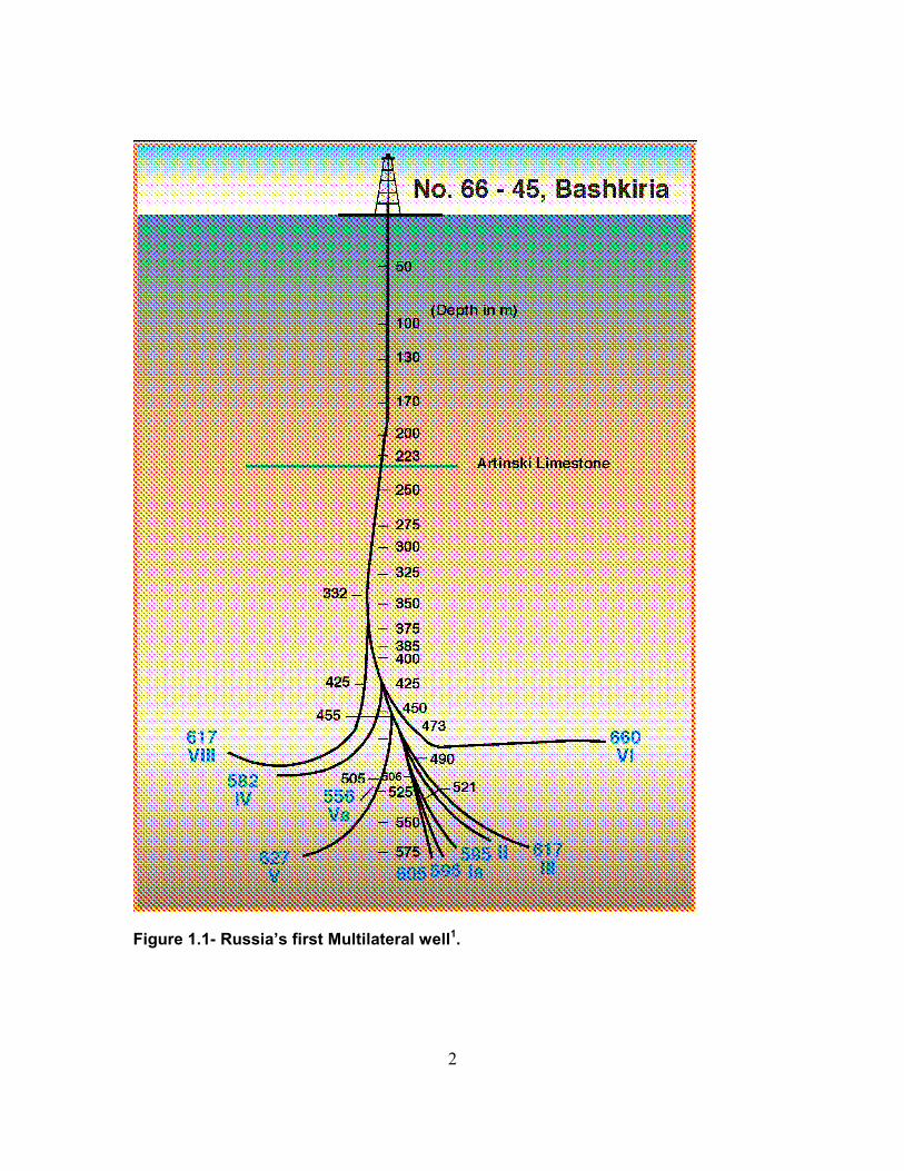
in Russia in 1950’s (Figure 1.1)1. Europe’s first multi-lateral wells were completed by Elf Aquitaine
in 1984 in the Paris Basin, France. Norsk Hydro completed successfully the first ever Level 5
multilateral well in the Oseburg Field, North Sea during 1996. In USA, Shell successfully
completed its first Level 6 multilateral well during 1998.
2
Figure 1.1- Russia’s first Multilateral well1.

3
1.1.2 General Definition
A multilateral well as defined by TAML1 group (Technical Advancements of Multilaterals)
is one in which there will be more than one horizontal or near horizontal lateral well drilled from a
single side (mother-bore) and connected back to a single bore.
1.1.3 Geometry of Multi-Lateral and Multi-branched wells
Well geometry of multi-lateral wells named according to their configuration and number of
laterals. e.g. Stacked Tri-lateral, Radial Quadrilateral etc.
Different well configurations are shown in Figure 1.21
Figure 1.2 - Different Well Configurations

4
1.1.4 Classification System (TAML)
There are two tiers of TAML classifications:
• Complexity ranking.
• Functional classification.
� Complexity ranking
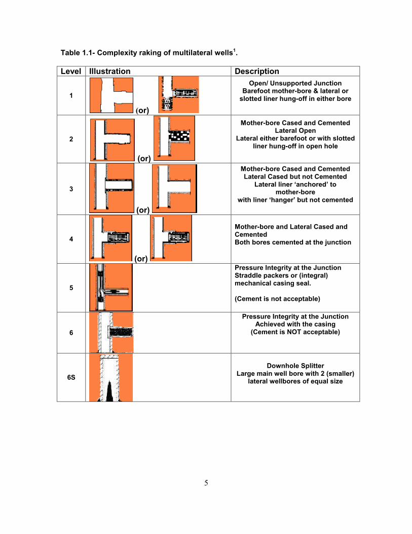
A number between 1 and 6 defines multilateral junction complexity. Table 1.1 illustrates the
complexity ratings.
� Functionality classification
This provides more technical detail on the major Multilateral/Multi-branched well attributes. This is
divided into two sections:
1. Well description.
2. Junction description.
5
Table 1.1- Complexity raking of multilateral wells1.
Level Illustration Description
1
(or)
Open/ Unsupported Junction Barefoot mother-bore & lateral or
slotted liner hung-off in either bore
2
(or)
Mother-bore Cased and Cemented Lateral Open
Lateral either barefoot or with slotted liner hung-off in open hole
3
(or)
Mother-bore Cased and Cemented Lateral Cased but not Cemented
Lateral liner ‘anchored’ to mother-bore
with liner ‘hanger’ but not cemented
4
(or)
Mother-bore and Lateral Cased and Cemented Both bores cemented at the junction
5
Pressure Integrity at the Junction Straddle packers or (integral) mechanical casing seal. (Cement is not acceptable)
6
Pressure Integrity at the Junction Achieved with the casing
(Cement is NOT acceptable)
6S
Downhole Splitter Large main well bore with 2 (smaller)
lateral wellbores of equal size

6
1.1.5 Advantages2 of Multilateral wells
The advantages of multilateral wells are:
• Higher productivity indexes.
• Relatively thin layer drainage can be accomplished.
• Decreased water and gas conning.
• Exposure to natural fractures will be high.
• In secondary and EOR applications, long horizontal injection wells provide higher
injectivity rates.
• Better vertical and areal sweep (particularly for irregular or odd-shaped drainages).
• These are alternative to infill drilling operations because existing surface installations can
be utilized.
• In heterogeneous reservoirs, more oil and gas pockets can be exploited and an
increased number of fissures can be intersected.
1.1.6 Disadvantages2 of Multilateral wells
The disadvantages of multilateral wells are:
• Higher costs.
• Highly sensitive to heterogeneities and anisotropies (both stress and permeability).
• Very complicated drilling, completion and production technologies are used.
• Complicated and expensive stimulation techniques are used.
• Selection of appropriate candidates is difficult.
• Interference of well branches may occur (Cross flow may take place).
7
CHAPTER II. THEORY
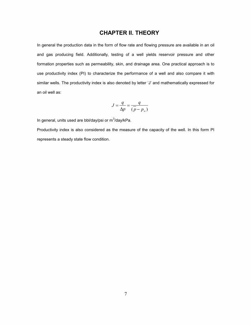
In general the production data in the form of flow rate and flowing pressure are available in an oil
and gas producing field. Additionally, testing of a well yields reservoir pressure and other
formation properties such as permeability, skin, and drainage area. One practical approach is to
use productivity index (PI) to characterize the performance of a well and also compare it with
similar wells. The productivity index is also denoted by letter ‘J’ and mathematically expressed for
an oil well as:
( )w
q qJ
p p p= =
∆ −
In general, units used are bbl/day/psi or m3/day/kPa.
Productivity index is also considered as the measure of the capacity of the well. In this form PI
represents a steady state flow condition.

8
During the operational life, the hydrocarbon producing well passes through various stages. These
stages mainly depend on the pressure drop and the boundary conditions. There are four different
flow scenarios, which occur during the operational life of the well. They are:
• Unsteady state.
• Pseudo – steady state.
• Steady state.
• Late Transient.
2.1. Unsteady state:
This is the condition of the well when the pressure disturbance caused by the flow has not
reached any of the reservoir boundaries. This is also known as Infinite – acting or Transient
state (Figure 2.1).
Figure 2.1. – Representation of Infinite – acting (or) Transient state.
Mathematically, unsteady state is defined as:
( , )P
f r tt
∂=
∂
Well
Reservoir Pressure Disturbance

9
2.2. Pseudo – steady State:
This is the condition of the well in a bounded reservoir when the pressure disturbance caused
by the flow has reached all of the reservoir boundaries. During this flow regime the reservoir
behaves like a tank. The pressure throughout the reservoir decreases at the same constant
rate. (Figure 2.2)
Figure 2.2. - Representation of Pseudo – steady state. Mathematically, pseudo-steady state is given as:
constantP
t
∂=
∂
Well
Reservoir Pressure Disturbance

10
2.3. Steady state:
This condition occurs during the late time region when a constant pressure boundary exists.
Constant pressure boundaries arise when the reservoir has aquifer support or gas cap expansion
support.
Mathematically, steady state is given as:
0P
t
∂=
∂
2.4. Late Transient State:
This is the state between unsteady state and pseudo – steady state. During this regime the
pressure distribution reaches some of the boundaries but not all of it. (Figure 2.4)
Figure 2.4. - Representation of Late Transient state.
Reservoir
Well
Pressure Disturbance

11
CHAPTER III. PREDICTION OF PRODUCTIVITY METHODS There are different methods for predicting Productivity Index (PI) of both types of wells (Vertical
wells and Horizontal wells). In this study, multilateral wells are considered as horizontal wells.
3.1 Steady State PI
There are different methods3 for predicting the PI for Steady state Horizontal wells. They are:
� Borisov’s method.
� The Giger – Reiss – Jourdan method.
� Joshi’s method.
� The Renard – Dupuy method.
3.1.1 Borisov’s method
Borisov proposed the following expression for predicting the productivity index of a horizontal
well in an isotropic reservoir, i.e., k v = k h.
0.00708
4ln ln
2
hh
eho o
w
hkJ
r L hB
L h rµ
π
=
+
3.1.2 The Giger – Reiss – Jourdan method
Giger – Reiss – Jourdan proposed the following expression for predicting the productivity
index of a horizontal well in an isotropic reservoir, i.e., k v = k h.
0.00708
ln( ) ln2
hh
o o
w
LkJ
L hB X
h rµ
=
+

12
( )
2
1 12
/ 2
eh
eh
L
rX
L r
+ +
=
For reservoir anisotropy, he proposed the following relationships:
2
0.00708
1ln( ) ln
2
hh
o o
w
kJ
B hB X
h L rµ
=
+
h
v
kB
k=
3.1.3 Joshi’s method
Joshi proposed the following expression for estimating the productivity index of a horizontal
well in an isotropic reservoir:
0.00708
ln( ) ln2
hh
o o
w
hkJ
h hB R
L rµ
=
+
2 2( / 2)
( / 2)
a a LR
L
+ −=
Here ‘a’ is half the major axis of the drainage ellipse and is given by:
0.54( / 2) 0.5 0.25 (2 / )eha L r L = + +
For the reservoir anisotropy, he proposed following relationships with vertical permeability, kv:

13
2
0.00708
ln( ) ln2
hh
o o
w
hkJ
B h hB R
L rµ
=
+
h
v
kB
k=
2 2( / 2)
( / 2)
a a LR
L
+ −=
Here ‘a’ is half the major axis of the drainage ellipse and is given by:
0.54( / 2) 0.5 0.25 (2 / )eha L r L = + +
3.1.4 The Renard – Dupuy method
For an isotropic reservoir, Renard and Dupuy proposed the following expression:
1
0.00708
2cosh ln
2
hh
o o
w
hkJ
a h hB
L L rµ
π−
=
+
Here ‘a’ is half the major axis of the drainage ellipse and is given by:
0.54( / 2) 0.5 0.25 (2 / )eha L r L = + +
For anisotropic reservoirs, these authors proposed the following relationship:
1
'
0.00708
2cosh ln
2
hh
o o
w
hkJ
a Bh hB
L L rµ
π−
=
+
where
(1 )
'2
ww
Brr
B
+= , h
v
kB
k=
14
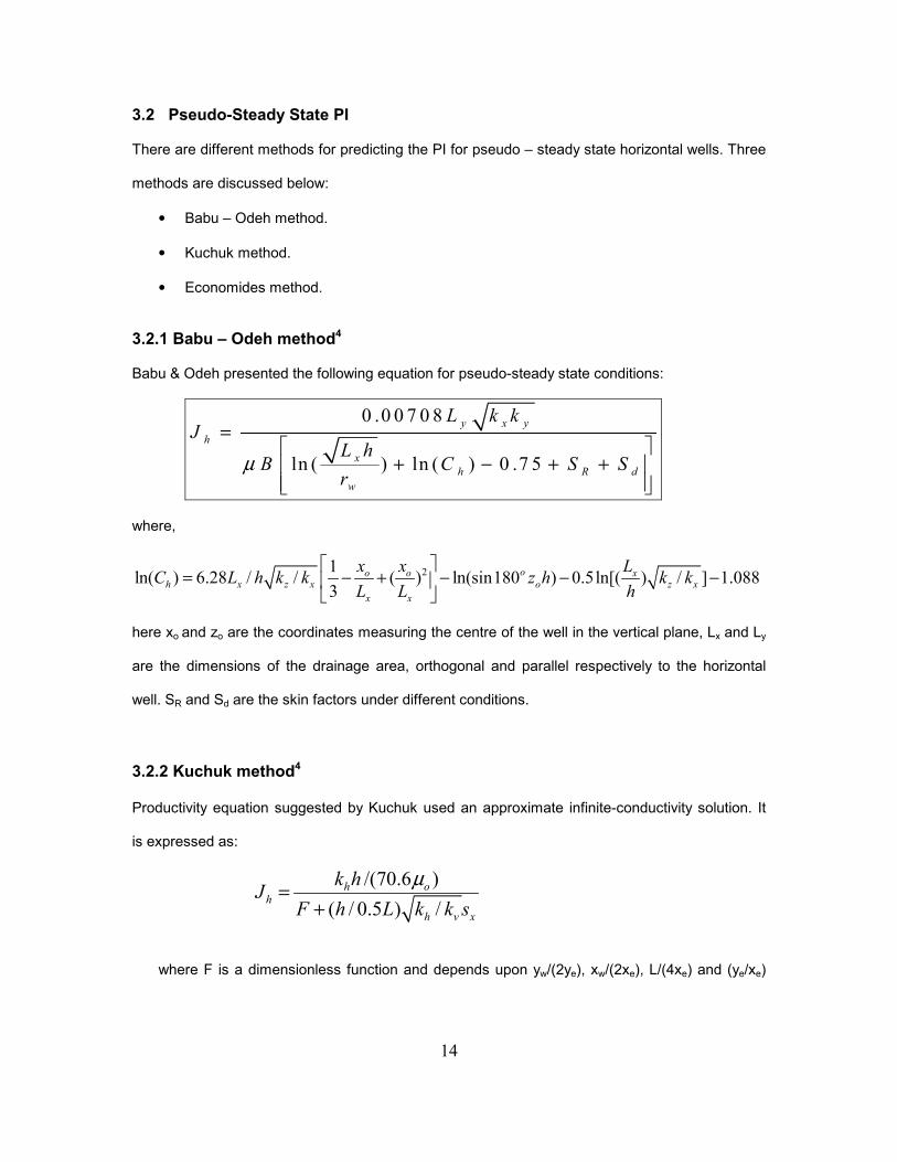
3.2 Pseudo-Steady State PI There are different methods for predicting the PI for pseudo – steady state horizontal wells. Three
methods are discussed below:
• Babu – Odeh method.
• Kuchuk method.
• Economides method.
3.2.1 Babu – Odeh method4 Babu & Odeh presented the following equation for pseudo-steady state conditions:
0 .0 0 7 0 8
ln ( ) ln ( ) 0 .7 5
y x y
h
x
h R d
w
L k kJ
L hB C S S
rµ
=
+ − + +
where,
21ln( ) 6.28 / / ( ) ln(sin180 ) 0.5ln[( ) / ] 1.088
3
oo o xh x z x o z x
x x
x x LC L h k k z h k k
L L h
= − + − − −
here xo and zo are the coordinates measuring the centre of the well in the vertical plane, Lx and Ly
are the dimensions of the drainage area, orthogonal and parallel respectively to the horizontal
well. SR and Sd are the skin factors under different conditions.
3.2.2 Kuchuk method4
Productivity equation suggested by Kuchuk used an approximate infinite-conductivity solution. It
is expressed as:
/(70.6 )
( / 0.5 ) /
h oh
h v x
k hJ
F h L k k s
µ=
+
where F is a dimensionless function and depends upon yw/(2ye), xw/(2xe), L/(4xe) and (ye/xe)

15
/x yk k . The value of sx is calculated using the following equation:
22 1
ln 1 sin3
w v w h w wx
h v
r k z k z zhs
h k h k L h h
π π = + − − +
3.2.3 Economides Method5
Economides suggested the following equation for calculating the PI:
( ) 887.22 ( )
2
o e
ewfD
q kxJ
xp p B p sL
µπ
= =− + ∑
where,
4 2
e H eD x
x C xp s
h Lπ π= +
s∑ - is the summation of all damage and pseudo-skin factors.
Skin effect sx is:
ln( )2 6
x e
w
h hs s
r Lπ= − +
where,
22 21 1
ln sin( )2 2
w w we
z z zhs
L h h h
π = − − −
16
3.3 Literature Review
3.3.1 Analytical Solutions
There are two main categories under which any oil or gas well is classified according to
their design as a vertical well or a horizontal well. An unstimulated horizontal well can generate
production rates of two to five times to that of an unstimulated vertical well at a similar pressure
drawdown. Apart from this main advantage there are also few disadvantages of horizontal wells.
Some of the disadvantages of horizontal wells are the less effectiveness in thicker reservoirs
(>500 ft), reservoirs with low vertical permeability (relative to horizontal permeability) and in
stratified reservoirs with impermeable shale barriers. Improvement of well completion and
stimulation technology can overcome these disadvantages. The use of hydraulic fractures to
enhance horizontal well productivity is explained by Giger et al6 and Giger
7.
There have been several attempts to describe and estimate horizontal well productivity
and/or injectivity indexes and several models have been used for this purpose. A widely used
approximation for the well drainage is a parallelepiped model with no-flow or constant-pressure
boundaries at the top or bottom, and either no-flow or infinite-acting boundaries at the sides.
One of the earliest models was introduced first by Borisov8, which assumed a constant
pressure drainage ellipse whose dimensions depend on the well length. Using this configuration
Joshi9 came up with an equation, which accounted for vertical-to-horizontal permeability
anisotropy. Then Economides et al.,10
modified it for a wellbore in elliptical coordinates. This
model does not account for either early-time or late-time phenomena nor, more importantly,
actual well and reservoir configurations.
Babu & Odeh11
used an expression, which was complicated and cumbersome to
calculate, for the pressure drop at any point by integrating appropriate point source (Green’s)
functions in space and time. Their work assumes that the well is parallel to the y-axis of the
parallelepiped model. Goode and Thambynayagam12
solved a model for horizontal well pressure
transient response in Laplace space and inverted solution using a numerical inverter. Kuchuk et

17
al.13
extended the Goode and Thambynayagam12
approach by including constant pressure (at the
top and/or bottom) boundaries.
In general it is believed that the productivity of a horizontal well is proportional to the well
length. But as the length increases, drilling and well control becomes more difficult. Apart from
this, transportation of large volumes of liquid along a long horizontal borehole results in
considerable pressure losses in the wellbore. Wellbore pressure loss yields a decrease in well
productivity. Multilateral wells provide an alternative to drilling long single horizontal wells.
There are many publications, which have discussed the flow into multilaterals. These can be
grouped into three categories: productivity models14 – 17
, transient flow models17-25
and field
applications 26 – 30
.

18
CHAPTER IV. APPROACH USING RESERVOIR SIMULATION
4.1 Numerical Simulation Models for Multilateral wells
To evaluate the productivity index of multilateral wells, reservoir simulation software, ECLIPSE
from Schlumberger, is used in this thesis. The ECLIPSE simulator is used to generate different
models in this thesis with version 2005A for black oil (ECLIPSE 100). ECLIPSE 100 is a fully
implicit, three-phase, three-dimensional black oil simulator. The black oil model considers the
reservoir fluids consisting of reservoir oil, solvent gas and water. The reservoir oil and solvent gas
components are assumed to be miscible in all proportions.
In this study, five different horizontal completions were considered. Namely:
1. Single Lateral.
2. Dual Lateral (with laterals at same depth).
3. Dual Lateral (with laterals at different depths).
4. Four Laterals (with laterals perpendicular to each other).
5. Single Vertical Well.
Additionally, four different lengths of 500 ft,. 1000 ft., 1500 ft., and 2000 ft. were considered for all
lateral completions.
In all cases, the following wellbore configurations were used:
Main borehole diameter : 12 in.
Casing Inner diameter : 8.4 in.
Casing Outer diameter : 9 in.
Casing Roughness : 0.001 in.
Tubing Inner diameter : 2.0 in.
Tubing Outer diameter : 2.441 in.
Tubing Inner roughness : 0.012 in.
Tubing Outer roughness : 0.012 in.
Packer set at a vertical depth : 4950 ft.

19
GRID STRUCTURE:
Direction Minimum cell size Maximum cell size Growth factor
X – direction 1 ft. 500 ft. 2
Y – direction 1 ft. 500 ft. 2
Z – direction 1 ft. 500 ft. 2
All of the above-mentioned configurations, which were generated using ECLIPSE, are described
below. All runs were conducted for 30 years.
Single Lateral:
Figure 4.1 is the schematic of a 500 ft Single Lateral Well. Figure 4.2 shows grid structure used
for the 500 ft Single Lateral Well.
Figure 4.1: 500 ft. Single Lateral Well.
Well
Lateral

20
Figure 4.2: Grid structure of 500 ft. Single Lateral Well.

21
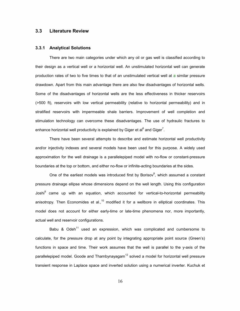
Figure 4.3 is the schematic of a 1000 ft Single Lateral Well. Figure 4.4 shows grid structure used
for the 1000 ft Single Lateral Well.
Figure 4.3: 1000 ft. Single Lateral Well.
22
Figure 4.4: Grid structure of 1000 ft. Single Lateral Well.

23
Figure 4.5 is the schematic of a 1500 ft Single Lateral Well. Figure 4.6 shows grid structure used
for the 1500 ft Single Lateral Well.
Figure 4.5: 1500 ft. Single Lateral Well.

24
Figure 4.6: Grid structure of 1500 ft. Single Lateral Well.

25
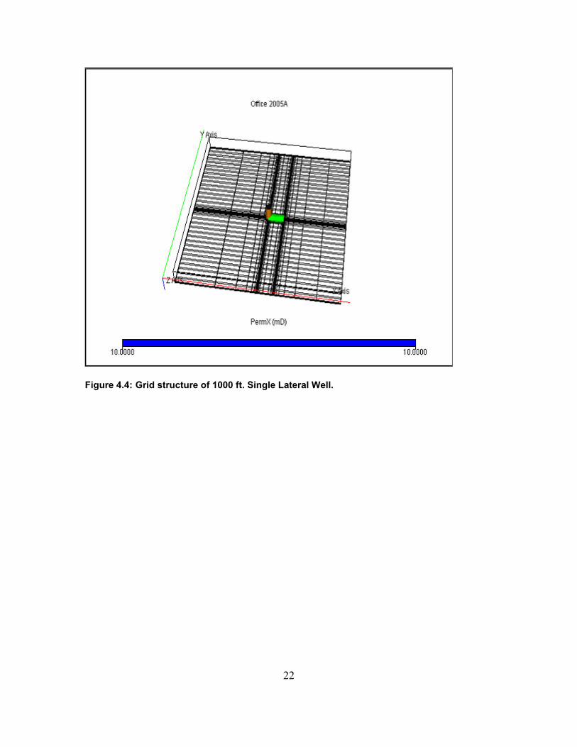
Figure 4.7 is the schematic of a 2000 ft Single Lateral Well. Figure 4.8 shows grid structure used
for the 2000 ft Single Lateral Well.
Figure 4.7: 2000 ft. Single Lateral Well.
26
Figure 4.8: Grid structure of 2000 ft. Single Lateral Well.

27
Dual Lateral:
Figure 4.9 is the schematic of a 500 ft Dual Lateral Well and Figure 4.10 shows grid structure
used for the 500 ft Dual Lateral well.
Figure 4.9: 500 ft. Dual Lateral Well.

28
Figure 4.10: Grid structure of 500 ft. Dual Lateral Well.

29
Figure 4.11 is the schematic of a 1000 ft Dual Lateral Well and Figure 4.12 shows grid structure
used for the 1000 ft Dual Lateral well.
Figure 4.11: 1000 ft. Dual Lateral Well.

30
Figure 4.12: Grid structure for the1000 ft. Dual Lateral Well.

31
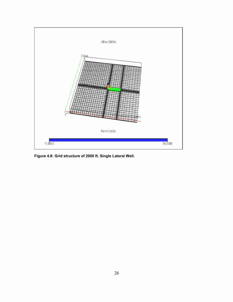
Figure 4.13 is the schematic of a 1500 ft Dual Lateral Well and Figure 4.14 shows grid structure
used for the 1500 ft Dual Lateral well.
Figure 4.13: 1500 ft. Dual Lateral Well.
32
Figure 4.14: Grid structure for the 1500 ft. Dual Lateral Well.

33
Figure 4.15 is the schematic of a 2000 ft Dual Lateral Well and Figure 4.16 shows grid structure
used for the 2000 ft Dual Lateral well.
Figure 4.15: 2000 ft. Dual Lateral Well.

34
Figure 4.16: Grid structure for the 2000 ft. Dual Lateral Well.

35
Dual Lateral well with laterals at different depths:
Figure 4.17 is the schematic of a 500 ft Dual Lateral Well with laterals at different depths and
Figure 4.18 shows grid structure used for this 500 ft Dual Lateral well.
Figure 4.17: 500 ft. Dual Lateral Well with laterals at different depths.

36
Figure 4.18: Grid structure for the 500 ft. Dual Lateral Well with laterals at different depths.

37
Figure 4.19 is the schematic of a 1000 ft Dual Lateral Well with laterals at different depths and
Figure 4.20 shows grid structure used for this 1000 ft Dual Lateral well.
Figure 4.19: 1000 ft. Dual Lateral Well with laterals at different depths.

38
Figure 4.20: Grid structure for the 1000 ft. Dual Lateral Well with laterals at different depths.
39
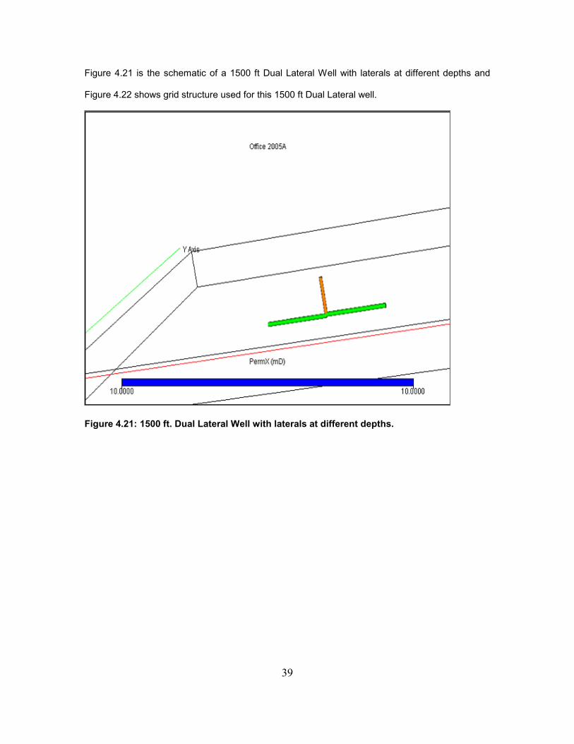
Figure 4.21 is the schematic of a 1500 ft Dual Lateral Well with laterals at different depths and
Figure 4.22 shows grid structure used for this 1500 ft Dual Lateral well.
Figure 4.21: 1500 ft. Dual Lateral Well with laterals at different depths.

40
Figure 4.22: Grid structure for the 1500 ft. Dual Lateral Well with laterals at different depths.

41
Figure 4.23 is the schematic of a 2000 ft dual lateral well with laterals at different depths and
Figure 4.24 shows grid structure used for this 2000 ft Dual Lateral well.
Figure 4.23: 2000 ft. Dual Lateral Well with laterals at different depths.

42
Figure 4.24: Grid structure for the 2000 ft. Dual Lateral Well with laterals at different depths.

43
Four Laterals:
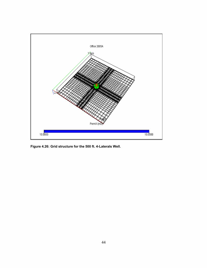
Figure 4.25 is the schematic of a 500 ft four lateral well with laterals at same depths and Figure
4.26 shows grid structure used for this 500 ft Four Lateral well.
Figure 4.25: 500 ft. 4-Laterals Well.
44
Figure 4.26: Grid structure for the 500 ft. 4-Laterals Well.

45
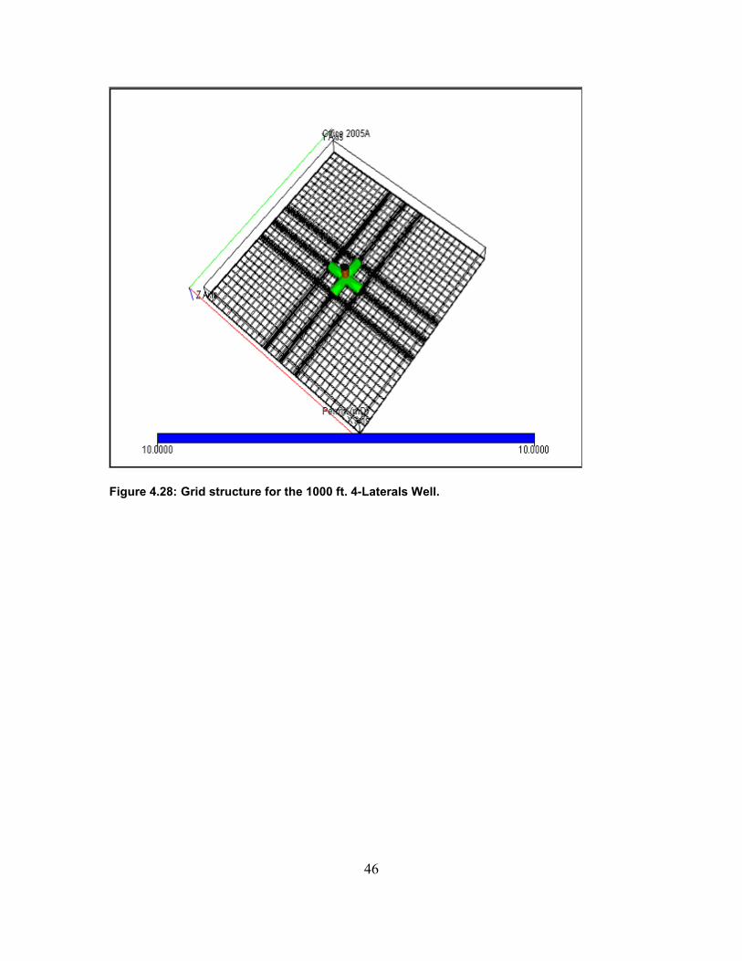
Figure 4.27 is the schematic of a 1000 ft four lateral well with laterals at same depths and Figure
4.28 shows grid structure used for this 1000 ft Four Lateral well.
Figure 4.27: 1000 ft. 4-Laterals Well.
46
Figure 4.28: Grid structure for the 1000 ft. 4-Laterals Well.

47
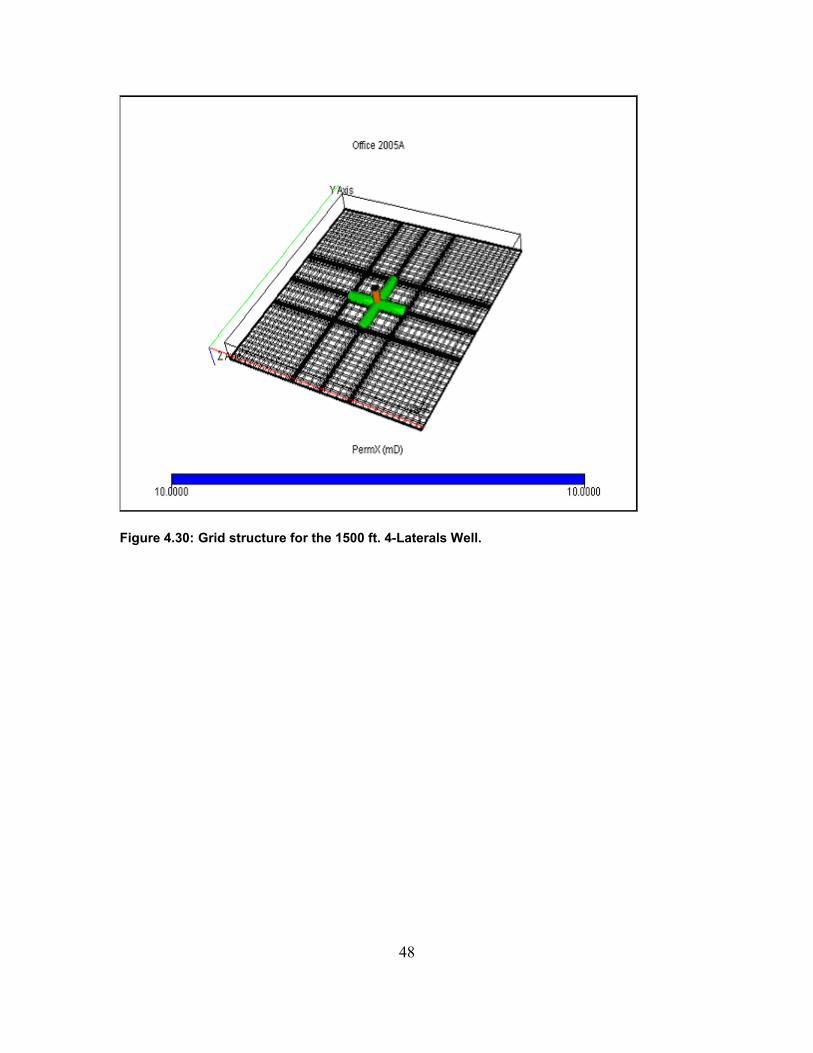
Figure 4.29 is the schematic of a 1500 ft four lateral well with laterals at same depths and Figure
4.30 shows grid structure used for this 1500 ft Four Lateral well.
Figure 4.29: 1500 ft. 4-Laterals Well.
48
Figure 4.30: Grid structure for the 1500 ft. 4-Laterals Well.
49
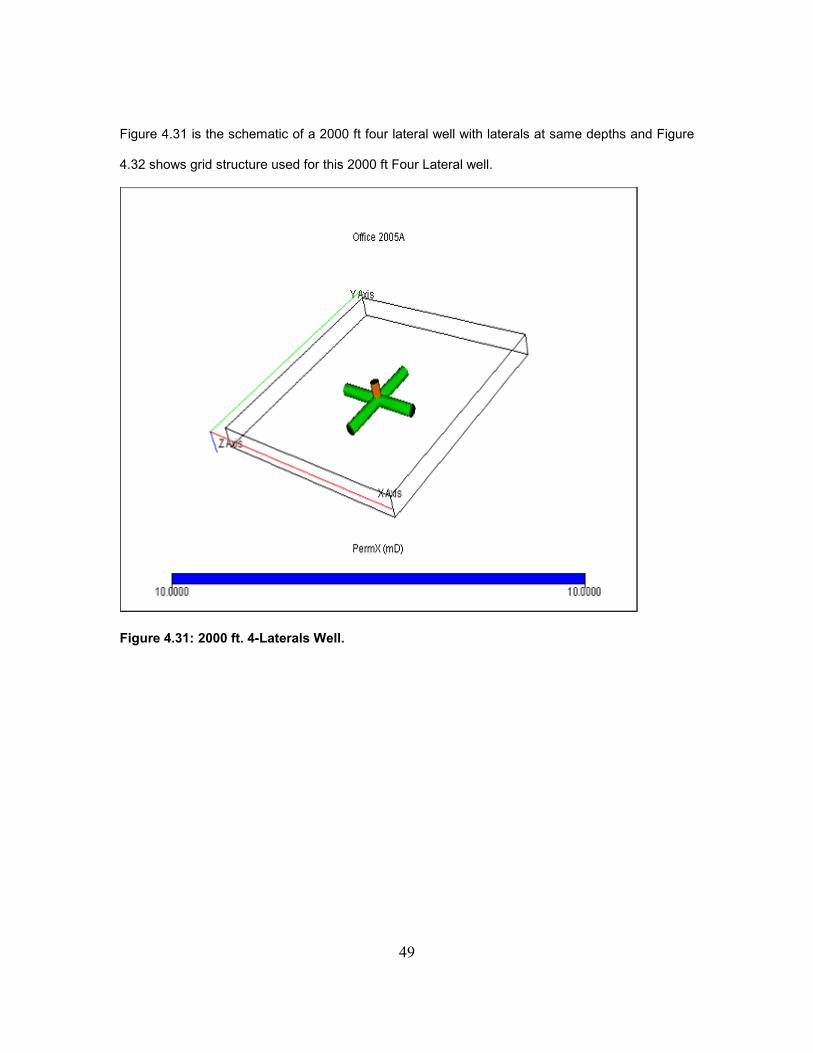
Figure 4.31 is the schematic of a 2000 ft four lateral well with laterals at same depths and Figure
4.32 shows grid structure used for this 2000 ft Four Lateral well.
Figure 4.31: 2000 ft. 4-Laterals Well.

50
Figure 4.32: Grid structure for the 2000 ft. 4-Laterals Well.
51
Vertical Well:
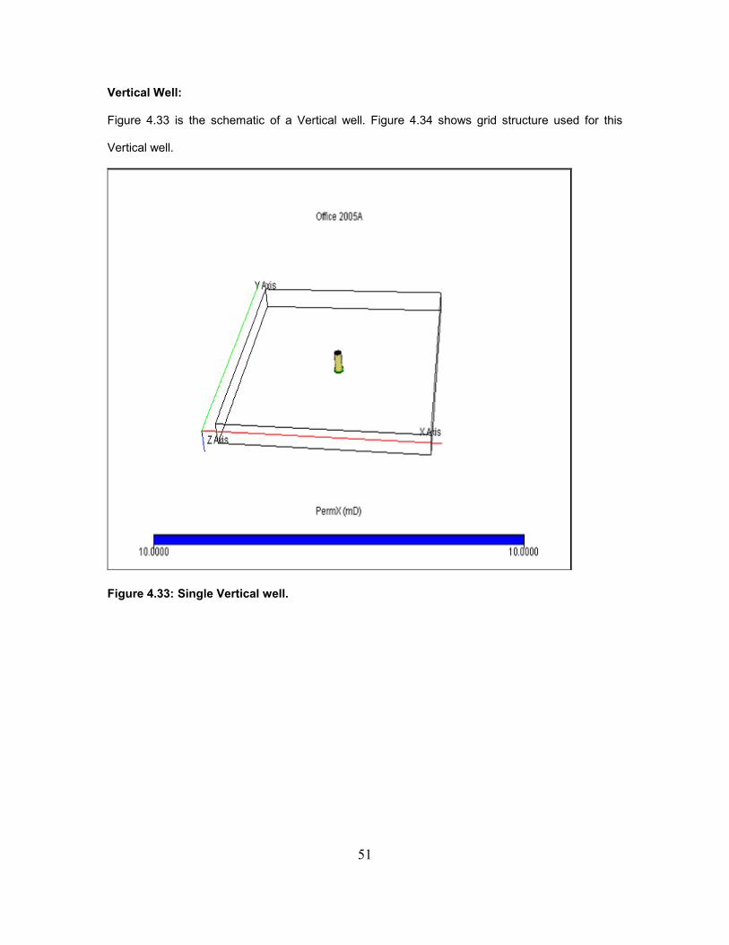
Figure 4.33 is the schematic of a Vertical well. Figure 4.34 shows grid structure used for this
Vertical well.
Figure 4.33: Single Vertical well.

52
Figure 4.34: Grid structure for the Vertical Well.
53
CHAPTER V: RESULTS AND DISCUSSION
For all the configurations that were described in the previous chapter had the following:
Reservoir description:
Length of the reservoir : 10000 ft.
Width of the reservoir : 10000 ft.
Thickness : 100 ft.
Porosity : 0.25
Permeability:
X- Direction : 10 mD.
Y- Direction : 10 mD.
Z- Direction : 1 mD.
Compressibility : 1E-6 /psi.
Initial reservoir pressure : 3500 psia.
Datum Depth (TVDSS) : 5180 ft.
Fluid Properties:
Oil density at surface : 49.9 lb/ft3.
Oil formation volume factor : 1.25 rb/stb.
Oil compressibility : 3E-6 /psi.
Oil Viscosity : 1 cp.
Total GOR : 0.00697224 Mscf/stb.
Bubble point pressure : 50 psia.
Gas Gravity : 0.7
Skin : 2
Runs were conducted using the above data with the configurations given in Chapter IV (with
different lateral lengths), field pressure rates, field oil production rates, well bottom hole pressure
and field pressure variations are tabulated. Using these values, Productivity Index, J for each
configuration (for different lateral lengths) is calculated with the following equation:

54
( )field WBHP
q qJ
p p p= =
∆ −
The basic equation that governs single-phase flow of a slightly compressible fluid in a porous
medium is given by:
2 2 2
2 2 2
D D D D
D D D D
p p p p
x y z t
∂ ∂ ∂ ∂+ + =
∂ ∂ ∂ ∂ (in dimensionless variables).
To convert the space coordinates or lengths to their dimensionless equivalent, they are scaled by
the reservoir length in the x-direction, xe and the following forms were used:
xD = x/ xe,
yD = y/ xe,
zD = z/ xe.
The following dimensionless time is used:
4
2
2.637 10D
t e
k tt
C xφ µ
−× × ×=
× × ×,
where 2.637x10⁻⁴ is the conversion factor for time measured in hours, and field units for k, xe, µ,
and Ct.
The dimensionless variables pD, tD are tabulated for each configuration. Dimensionless well-bore
pressure is calculated with,
141.2
D field WBHP
t o
k hp p p
q Bµ
× = − × × ×
After calculating the dimensionless pressure and time differences, dimensionless pressure
derivative values are calculated and tabulated for all the configurations. The pressure derivative is
given by:
( )D D Ddp dt t

55
Using above values, different plots are generated to check the variation of productivity index with
respect to time and dimensionless pressure derivative with respect to dimensionless time. The
plots are prepared for the following configurations:
1. Single lateral well.
2. Dual lateral well.
3. Dual Lateral well with laterals at different depths.
4. Four lateral well.
5. Single Vertical Well.
Lateral lengths of 500 ft, 1000 ft, 1500 ft, 2000 ft are considered for all these configurations.
Single Lateral Well:
The results for the 500 ft. single lateral well for productivity index values are presented in
Figure 5.1. As shown in Figure 5.1 the productivity index value shows a linear trend for 10 years 9
months. Compared to a vertical well completed in the same reservoir the productivity values are
57% greater indicating a larger production.

56
0.0000001
0.000001
0.00001
0.0001
0.001
0.01
0.1
1
10
0.01 0.10 1.00 10.00 100.00 1000.00 10000.00 100000.00
t, days
PI
Figure 5.1: Variation of Productivity Index with time for a Single lateral well with 500 ft
lateral length.

57
Figure 5.2 shows the variation of dimensionless pressure and its derivative with dimensionless
time for a Single lateral well with 500 ft lateral length.
0.010
0.100
1.000
10.000
100.000
0.0001 0.001 0.01 0.1 1 10 100 1000
tD
PD
and (dP
D/d
tD)tD
Figure 5.2: Variation of dimensionless pressure and its derivative with dimensionless time
for a Single lateral well with 500 ft lateral length.
58
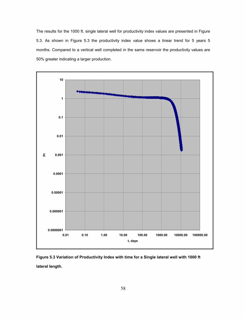
The results for the 1000 ft. single lateral well for productivity index values are presented in Figure
5.3. As shown in Figure 5.3 the productivity index value shows a linear trend for 5 years 5
months. Compared to a vertical well completed in the same reservoir the productivity values are
50% greater indicating a larger production.
0.0000001
0.000001
0.00001
0.0001
0.001
0.01
0.1
1
10
0.01 0.10 1.00 10.00 100.00 1000.00 10000.00 100000.00
t, days
PI
Figure 5.3 Variation of Productivity Index with time for a Single lateral well with 1000 ft
lateral length.

59
Figure 5.4 shows the variation of dimensionless pressure and its derivative with dimensionless
time for a Single lateral well with 1000 ft lateral length.
0.010
0.100
1.000
10.000
100.000
0.0001 0.001 0.01 0.1 1 10 100 1000
tD
PD
and (dP
D/d
tD)tD
Figure 5.4: Variation of dimensionless pressure and its derivative with dimensionless time
for a Single lateral well with 1000 ft lateral length.
60
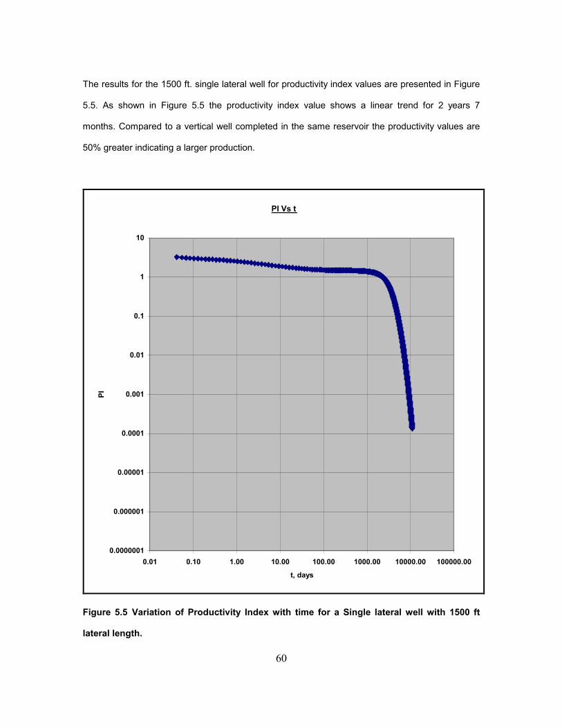
The results for the 1500 ft. single lateral well for productivity index values are presented in Figure
5.5. As shown in Figure 5.5 the productivity index value shows a linear trend for 2 years 7
months. Compared to a vertical well completed in the same reservoir the productivity values are
50% greater indicating a larger production.
PI Vs t
0.0000001
0.000001
0.00001
0.0001
0.001
0.01
0.1
1
10
0.01 0.10 1.00 10.00 100.00 1000.00 10000.00 100000.00
t, days
PI
Figure 5.5 Variation of Productivity Index with time for a Single lateral well with 1500 ft
lateral length.

61
Figure 5.6 shows the variation of dimensionless pressure and its derivative with dimensionless
time for a Single lateral well with 1500 ft lateral length.
0.010
0.100
1.000
10.000
100.000
0.0001 0.001 0.01 0.1 1 10 100 1000
tD
PD
and (dP
D/d
tD)tD
Figure 5.6: Variation of dimensionless pressure and its derivative with dimensionless time
for a Single lateral well with 1500 ft lateral length.

62
The results for the 2000 ft. single lateral well for productivity index values are presented in Figure
5.7. As shown in Figure 5.7 the productivity index value shows a linear trend for 1 year 9 months.
Compared to a vertical well completed in the same reservoir the productivity values are 46%
greater indicating a larger production.
PI Vs t
0.0000001
0.000001
0.00001
0.0001
0.001
0.01
0.1
1
10
0.01 0.10 1.00 10.00 100.00 1000.00 10000.00 100000.00
t, days
PI
Figure 5.7: Variation of Productivity Index with time for a Single lateral well with 2000 ft
lateral length.

63
Figure 5.8 shows the variation of dimensionless pressure and its derivative with dimensionless
time for a Single lateral well with 2000 ft lateral length.
0.010
0.100
1.000
10.000
100.000
0.0001 0.001 0.01 0.1 1 10 100 1000
tD
PD
and (dP
D/d
tD)tD
Figure 5.8: Variation of dimensionless pressure and its derivative with dimensionless time
for a Single lateral well with 2000 ft lateral length.

64
Dual Lateral Well with Laterals at same height:
The results for the 500 ft. Dual Lateral (laterals at same depth) well for productivity index values
are presented in Figure 5.9. As shown in Figure 5.9 the productivity index value shows a linear
trend for 4 years 1 month. Compared to a vertical well completed in the same reservoir the
productivity values are 49% greater indicating a larger production.
PI Vs t
0.0000001
0.000001
0.00001
0.0001
0.001
0.01
0.1
1
10
0.01 0.10 1.00 10.00 100.00 1000.00 10000.00 100000.00
t, days
PI
Figure 5.9: Variation of Productivity Index with time for a Dual Lateral well with 500 ft
lateral lengths, which are at the same depth.

65
Figure 5.10 shows the variation of dimensionless pressure and its derivative with dimensionless
time for a Dual Lateral well with 500 ft lateral length, which are at same depth.
0.010
0.100
1.000
10.000
100.000
0.0001 0.001 0.01 0.1 1 10 100 1000
tD
PD
and (dP
D/d
tD)tD
Figure 5.10: Variation of dimensionless pressure and its derivative with dimensionless
time for a Dual Lateral well with 500 ft lateral lengths, which are at the same depth.

66
The results for the 1000 ft. Dual Lateral (laterals at same depth) well for productivity index values
are presented in Figure 5.11. As shown in Figure 5.11 the productivity index value shows a linear
trend for 2 years 7 month. Compared to a vertical well completed in the same reservoir the
productivity values are 46% greater indicating a larger production.
PI Vs t
0.0000001
0.000001
0.00001
0.0001
0.001
0.01
0.1
1
10
0.01 0.10 1.00 10.00 100.00 1000.00 10000.00 100000.00
t, days
PI
Figure 5.11 Variation of Productivity Index with time for a Dual Lateral well with 1000 ft
lateral lengths, which are at the same depth.

67
Figure 5.12 shows the variation of dimensionless pressure and its derivative with dimensionless
time for a Dual Lateral well with 1000 ft lateral length, which are at same depth.
0.010
0.100
1.000
10.000
100.000
0.0001 0.001 0.01 0.1 1 10 100 1000
tD
PD
and (dP
D/d
tD)tD
Figure 5.12: Variation of dimensionless pressure and its derivative with dimensionless
time for a Dual Lateral well with 1000 ft lateral lengths, which are at the same depth.

68
The results for the 1500 ft. Dual Lateral (laterals at same depth) well for productivity index values
are presented in Figure 5.13. As shown in Figure 5.13 the productivity index value shows a linear
trend for 1 year 9 months and decreases to zero at the end of a dimensionless time of 11000
days. Compared to a vertical well completed in the same reservoir the productivity values are
43% greater indicating a larger production.
PI Vs t
0.0000001
0.000001
0.00001
0.0001
0.001
0.01
0.1
1
10
0.01 0.10 1.00 10.00 100.00 1000.00 10000.00 100000.00
t, days
PI
Figure 5.13: Variation of Productivity Index with time for a Dual Lateral well with 1500 ft
lateral lengths, which are at the same depth.
69
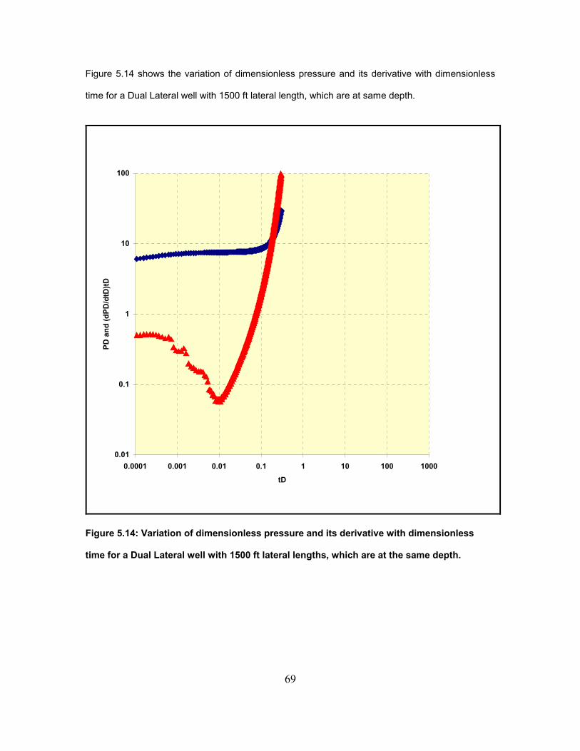
Figure 5.14 shows the variation of dimensionless pressure and its derivative with dimensionless
time for a Dual Lateral well with 1500 ft lateral length, which are at same depth.
0.01
0.1
1
10
100
0.0001 0.001 0.01 0.1 1 10 100 1000
tD
PD
and (dP
D/d
tD)tD
Figure 5.14: Variation of dimensionless pressure and its derivative with dimensionless
time for a Dual Lateral well with 1500 ft lateral lengths, which are at the same depth.

70
The results for the 2000 ft. Dual Lateral (laterals at same depth) well for productivity index values
are presented in Figure 5.15. As shown in Figure 5.15 the productivity index value shows a linear
trend for 1 year 6 months and decreases to zero at the end of a dimensionless time of 9500 days.
Compared to a vertical well completed in the same reservoir the productivity values are 34%
greater indicating a larger production.
PI Vs t
0.0000001
0.000001
0.00001
0.0001
0.001
0.01
0.1
1
10
0.01 0.10 1.00 10.00 100.00 1000.00 10000.00 100000.00
t, days
PI
Figure 5.15: Variation of Productivity Index with time for a Dual Lateral well with 2000 ft
lateral lengths, which are at the same depth.

71
Figure 5.16 shows the variation of dimensionless pressure and its derivative with dimensionless
time for a Dual Lateral well with 2000 ft lateral length, which are at same depth.
0.01
0.1
1
10
100
0.0001 0.001 0.01 0.1 1 10 100 1000
tD
PD
and (dP
D/d
tD)tD
Figure 5.16: Variation of dimensionless pressure and its derivative with dimensionless
time for a Dual Lateral well with 2000 ft lateral lengths, which are at the same depth.

72
Dual Lateral Well with Laterals at different height:
The results for the 500 ft. Dual Lateral (laterals at different depths separated by 50 ft) well for
productivity index values are presented in Figure 5.17. As shown in Figure 5.17 the productivity
index value shows a linear trend for 2 years 7 months Compared to a vertical well completed in
the same reservoir the productivity values are 49% greater indicating a larger production.
PI Vs t
0.0000001
0.000001
0.00001
0.0001
0.001
0.01
0.1
1
10
0.01 0.1 1 10 100 1000 10000 100000
t, days
PI
Figure 5.17: Variation of Productivity Index with time for a Dual Lateral well with 500 ft
lateral lengths, which are at different depths.

73
Figure 5.18 shows the variation of dimensionless pressure and its derivative with dimensionless
time for a Dual Lateral well with 500 ft lateral length, which are at different depths.
0.010
0.100
1.000
10.000
100.000
0.0001 0.001 0.01 0.1 1 10 100 1000
tD
PD
and (dP
D/d
tD)tD
Figure 5.18: Variation of dimensionless pressure and its derivative with dimensionless
time for a Dual Lateral well with 500 ft lateral lengths, which are at different depths.
74
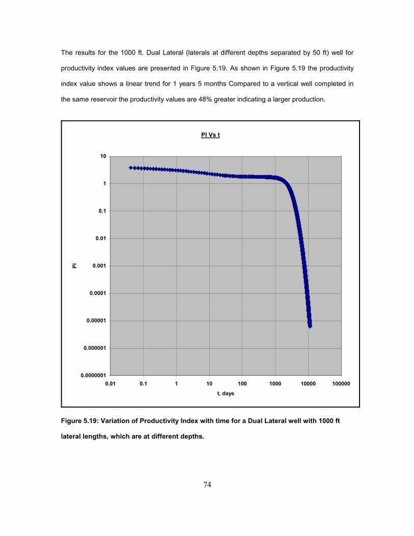
The results for the 1000 ft. Dual Lateral (laterals at different depths separated by 50 ft) well for
productivity index values are presented in Figure 5.19. As shown in Figure 5.19 the productivity
index value shows a linear trend for 1 years 5 months Compared to a vertical well completed in
the same reservoir the productivity values are 48% greater indicating a larger production.
PI Vs t
0.0000001
0.000001
0.00001
0.0001
0.001
0.01
0.1
1
10
0.01 0.1 1 10 100 1000 10000 100000
t, days
PI
Figure 5.19: Variation of Productivity Index with time for a Dual Lateral well with 1000 ft
lateral lengths, which are at different depths.
75
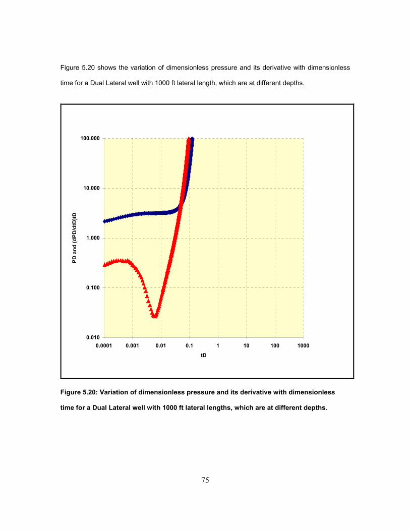
Figure 5.20 shows the variation of dimensionless pressure and its derivative with dimensionless
time for a Dual Lateral well with 1000 ft lateral length, which are at different depths.
0.010
0.100
1.000
10.000
100.000
0.0001 0.001 0.01 0.1 1 10 100 1000
tD
PD
and (dP
D/d
tD)tD
Figure 5.20: Variation of dimensionless pressure and its derivative with dimensionless
time for a Dual Lateral well with 1000 ft lateral lengths, which are at different depths.

76
The results for the 1500 ft. Dual Lateral (laterals at different depths separated by 50 ft) well for
productivity index values are presented in Figure 5.21. As shown in Figure 5.21 the productivity
index value shows a linear trend for 1 year 3 months and decreases to zero at the end of a
dimensionless time of 11000 days. Compared to a vertical well completed in the same reservoir
the productivity values are 43% greater indicating a larger production.
PI Vs t
0.0000001
0.000001
0.00001
0.0001
0.001
0.01
0.1
1
10
0.01 0.1 1 10 100 1000 10000 100000
t, days
PI
Figure 5.21: Variation of Productivity Index with time for a Dual Lateral well with 1500 ft
lateral lengths, which are at different depths.

77
Figure 5.22 shows the variation of dimensionless pressure and its derivative with dimensionless
time for a Dual Lateral well with 1500 ft lateral length, which are at different depths.
0.001
0.010
0.100
1.000
10.000
100.000
0.0001 0.001 0.01 0.1 1 10 100 1000
tD
PD
and (dP
D/d
tD)tD
Figure 5.22: Variation of dimensionless pressure and its derivative with dimensionless
time for a Dual Lateral well with 1500 ft lateral lengths, which are at different depths.

78
The results for the 2000 ft. Dual Lateral (laterals at different depths separated by 50 ft) well for
productivity index values are presented in Figure 5.23. As shown in Figure 5.23 the productivity
index value shows a linear trend for 1 years 6 months and decreases to zero at the end of a
dimensionless time of 9500 days. Compared to a vertical well completed in the same reservoir
the productivity values are 34% greater indicating a larger production.
PI Vs t
0.0000001
0.000001
0.00001
0.0001
0.001
0.01
0.1
1
10
0.01 0.1 1 10 100 1000 10000 100000
t, days
PI
Figure 5.23: Variation of Productivity Index with time for a Dual Lateral well with 2000 ft
lateral lengths, which are at different depths.

79
Figure 5.24 shows the variation of dimensionless pressure and its derivative with dimensionless
time for a Dual Lateral well with 2000 ft lateral length, which are at different depths.
0.010
0.100
1.000
10.000
100.000
0.0001 0.001 0.01 0.1 1 10 100 1000
tD
PD
and (dP
D/d
tD)tD
Figure 5.24: Variation of dimensionless pressure and its derivative with dimensionless
time for a Dual Lateral well with 2000 ft lateral lengths, which are at different depths.

80
Four Laterals well:
The results for the 500 ft. Four Laterals (laterals at same depth) well for productivity index values
are presented in Figure 5.25. As shown in Figure 5.25 the productivity index value shows a
linear trend for 1 year 3 months. Compared to a vertical well completed in the same reservoir the
productivity values are 47% greater indicating a larger production.
PI Vs t
0.0000001
0.000001
0.00001
0.0001
0.001
0.01
0.1
1
10
0.01 0.1 1 10 100 1000 10000 100000
t, days
PI
Figure 5.25: Variation of Productivity Index with time for a 4-lateral well with 500 ft lateral
lengths, which are at the same depth.
81
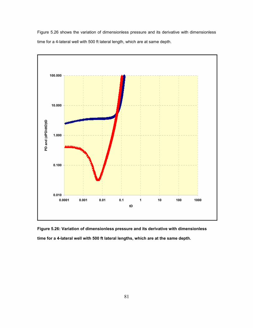
Figure 5.26 shows the variation of dimensionless pressure and its derivative with dimensionless
time for a 4-lateral well with 500 ft lateral length, which are at same depth.
0.010
0.100
1.000
10.000
100.000
0.0001 0.001 0.01 0.1 1 10 100 1000
tD
PD
and (dP
D/d
tD)tD
Figure 5.26: Variation of dimensionless pressure and its derivative with dimensionless
time for a 4-lateral well with 500 ft lateral lengths, which are at the same depth.

82
The results for the 1000 ft. Four Laterals (laterals at same depth) well for productivity index
values are presented in Figure 5.27. As shown in Figure 5.27 the productivity index value shows
a linear trend for 1 year 3 months and decreases to zero at the end of a dimensionless time of
11000 days. Compared to a vertical well completed in the same reservoir the productivity values
are 35% greater indicating a larger production.
PI Vs t
0.0000001
0.000001
0.00001
0.0001
0.001
0.01
0.1
1
10
0.01 0.1 1 10 100 1000 10000 100000
t, days
PI
Figure 5.27: Variation of Productivity Index with time for a 4-lateral well with 1000 ft lateral
lengths, which are at the same depth.

83
Figure 5.28 shows the variation of dimensionless pressure and its derivative with dimensionless
time for a 4-lateral well with 1000 ft lateral length, which are at same depth.
0.001
0.010
0.100
1.000
10.000
100.000
0.0001 0.001 0.01 0.1 1 10 100 1000
tD
PD
and (dP
D/d
tD)tD
Figure 5.28: Variation of dimensionless pressure and its derivative with dimensionless
time for a 4-lateral well with 1000 ft lateral lengths, which are at the same depth.

84
The results for the 1500 ft. Four Laterals (laterals at same depth) well for productivity index
values are presented in Figure 5.29. As shown in Figure 5.29 the productivity index value shows
a linear trend for 1 year and decreases to zero at the end of a dimensionless time of 7500 days.
Compared to a vertical well completed in the same reservoir the productivity values are 32%
greater indicating a larger production.
PI Vs t
0.0000001
0.000001
0.00001
0.0001
0.001
0.01
0.1
1
10
0.01 0.1 1 10 100 1000 10000
t, days
PI
Figure 5.29: Variation of Productivity Index with time for a 4-lateral well with 1500 ft lateral
lengths, which are at the same depth.

85
Figure 5.30 shows the variation of dimensionless pressure and its derivative with dimensionless
time for a 4-lateral well with 1500 ft lateral length, which are at same depth.
0.001
0.010
0.100
1.000
10.000
100.000
0.0001 0.001 0.01 0.1 1 10 100 1000
tD
PD
and (dP
D/d
tD)tD
Figure 5.30: Variation of dimensionless pressure and its derivative with dimensionless
time for a 4-lateral well with 1500 ft lateral lengths, which are at the same depth.

86
The results for the 2000 ft. Four Laterals (laterals at same depths) well for productivity index
values are presented in Figure 5.31. As shown in Figure 5.31 the productivity index value shows
a linear trend for 8 months and decreases to zero at the end of a dimensionless time of 6500
days. Compared to a vertical well completed in the same reservoir the productivity values are
29% greater indicating a larger production.
PI Vs t
0.0000001
0.000001
0.00001
0.0001
0.001
0.01
0.1
1
10
0.01 0.1 1 10 100 1000 10000
t, days
PI
Figure 5.31: Variation of Productivity Index with time for a 4-lateral well with 2000 ft lateral
lengths, which are at the same depth.

87
Figure 5.32 shows the variation of dimensionless pressure and its derivative with dimensionless
time for a 4-lateral well with 2000 ft lateral length, which are at same depth.
0.001
0.010
0.100
1.000
10.000
100.000
0.0001 0.001 0.01 0.1 1 10 100 1000
tD
PD
and (dP
D/d
tD)tD
Figure 5.32: Variation of dimensionless pressure and its derivative with dimensionless
time for a 4-lateral well with 2000 ft lateral lengths, which are at the same depth.

88
The results for the single Vertical well for productivity index values are presented in Figure 5.33.
As shown in Figure 5.33 the productivity index value shows a linear trend for 6 years.
PI Vs t
0.0000001
0.000001
0.00001
0.0001
0.001
0.01
0.1
1
0.01 0.1 1 10 100 1000 10000 100000
t, days
PI
Figure 5.33 Variation of Productivity Index with time for a single Vertical Well.
89
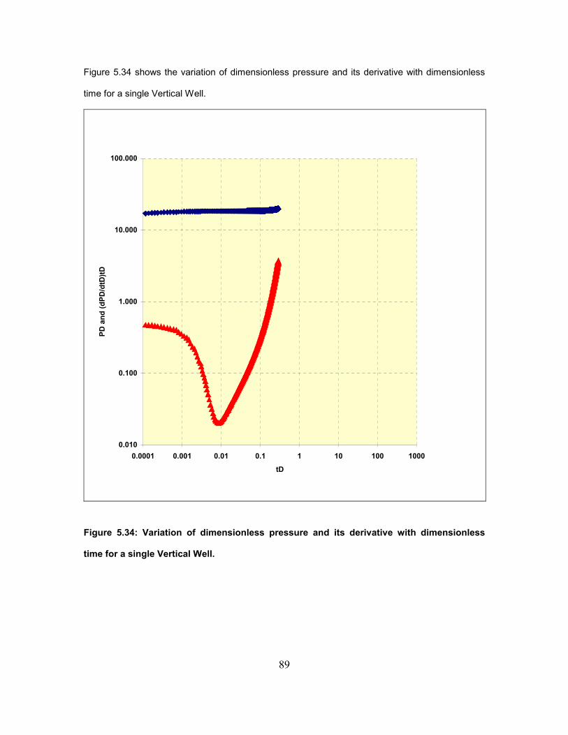
Figure 5.34 shows the variation of dimensionless pressure and its derivative with dimensionless
time for a single Vertical Well.
0.010
0.100
1.000
10.000
100.000
0.0001 0.001 0.01 0.1 1 10 100 1000
tD
PD
and (dP
D/d
tD)tD
Figure 5.34: Variation of dimensionless pressure and its derivative with dimensionless
time for a single Vertical Well.

90
Figure 5.35 shows the variation of Productivity Index with time for a single lateral well with 500 ft,
1000 ft, 1500 ft and 2000 ft lateral lengths.
Figure 5.35: Variation of Productivity Index with time for a single lateral well with 500 ft,
1000 ft, 1500 ft and 2000 ft lateral lengths.

91
Figure 5.36 shows the variation of Productivity Index with time for a dual lateral well with 500 ft,
1000 ft, 1500 ft and 2000 ft lateral lengths, which are at the same depth.
Figure 5.36: Variation of Productivity Index with time for a dual lateral well with 500 ft, 1000
ft, 1500 ft and 2000 ft lateral lengths, which are at the same depth.

92
Figure 5.37 shows the variation of Productivity Index with time for a dual lateral well with 500 ft,
1000 ft, 1500 ft and 2000 ft lateral lengths, which are at the different depth.
Figure 5.37: Variation of Productivity Index with time for a dual lateral well with 500 ft, 1000
ft, 1500 ft and 2000 ft lateral lengths, which are at the different depth.

93
Figure 5.38 shows the variation of Productivity Index with time for a 4-lateral well with 500 ft, 1000
ft, 1500 ft and 2000 ft lateral lengths, which are at the same depth.
Figure 5.38: Variation of Productivity Index with time for a 4-lateral well with 500 ft, 1000 ft,
1500 ft and 2000 ft lateral lengths, which are at the same depth.

94
Figure 5.39 shows the variation of dimensionless pressure and its derivative with dimensionless
time for a single lateral well with 500 ft, 1000 ft, 1500 ft and 2000 ft lateral lengths.
Figure 5.39: Variation of dimensionless pressure and its derivative with dimensionless
time for a single lateral well with 500 ft, 1000 ft, 1500 ft and 2000 ft lateral lengths.
0.010
0.100
1.000
10.000
100.000
1000.000
10000.000
100000.000
0.0001 0.001 0.01 0.1 1
tD
PD
and (dP
D/d
tD)tD
500 ft
500 ft
1000 ft
1000 ft
1500 ft
1500 ft
2000 ft
2000 ft

95
Figure 5.40 shows the variation of dimensionless pressure and its derivative with dimensionless
time for a dual lateral well with 500 ft, 1000 ft, 1500 ft and 2000 ft lateral lengths, which are at
same depths.
Figure 5.40: Variation of dimensionless pressure and its derivative with dimensionless
time for a dual lateral well with 500 ft, 1000 ft, 1500 ft and 2000 ft lateral lengths, which are
at the same depth.
0.001
0.010
0.100
1.000
10.000
100.000
1000.000
10000.000
100000.000
1000000.000
10000000.000
100000000.000
1000000000.000
10000000000.000
0.0001 0.001 0.01 0.1 1
tD
PD
and (dP
D/d
tD)tD
500 ft
500 ft
1000 ft
1000 ft
1500 ft
1500 ft
2000 ft
2000 ft

96
Figure 5.41 shows the variation of dimensionless pressure and its derivative with dimensionless
time for a dual lateral well with 500 ft, 1000 ft, 1500 ft and 2000 ft lateral lengths, which are at
different depths.
Figure 5.41: Variation of dimensionless pressure and its derivative with dimensionless
time for a dual lateral well with 500 ft, 1000 ft, 1500 ft and 2000 ft lateral lengths, which are
at different depths.
0.001
0.010
0.100
1.000
10.000
100.000
1000.000
10000.000
100000.000
1000000.000
10000000.000
100000000.000
1000000000.000
10000000000.000
0.0001 0.001 0.01 0.1 1
tD
PD
and (dP
D/d
tD)tD
500 ft
500 ft
1000 ft
1000 ft
1500 ft
1500 ft
2000 ft
2000 ft
97
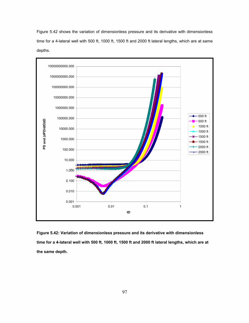
Figure 5.42 shows the variation of dimensionless pressure and its derivative with dimensionless
time for a 4-lateral well with 500 ft, 1000 ft, 1500 ft and 2000 ft lateral lengths, which are at same
depths.
Figure 5.42: Variation of dimensionless pressure and its derivative with dimensionless
time for a 4-lateral well with 500 ft, 1000 ft, 1500 ft and 2000 ft lateral lengths, which are at
the same depth.
0.001
0.010
0.100
1.000
10.000
100.000
1000.000
10000.000
100000.000
1000000.000
10000000.000
100000000.000
1000000000.000
10000000000.000
0.001 0.01 0.1 1
tD
PD
and (dP
D/d
tD)tD
500 ft
500 ft
1000 ft
1000 ft
1500 ft
1500 ft
2000 ft
2000 ft
98
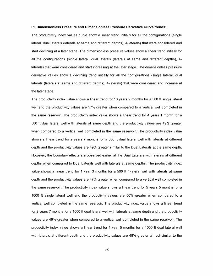
PI, Dimensionless Pressure and Dimensionless Pressure Derivative Curve trends: The productivity index values curve show a linear trend initially for all the configurations (single
lateral, dual laterals (laterals at same and different depths), 4-laterals) that were considered and
start declining at a later stage. The dimensionless pressure values show a linear trend initially for
all the configurations (single lateral, dual laterals (laterals at same and different depths), 4-
laterals) that were considered and start increasing at the later stage. The dimensionless pressure
derivative values show a declining trend initially for all the configurations (single lateral, dual
laterals (laterals at same and different depths), 4-laterals) that were considered and increase at
the later stage.
The productivity index value shows a linear trend for 10 years 9 months for a 500 ft single lateral
well and the productivity values are 57% greater when compared to a vertical well completed in
the same reservoir. The productivity index value shows a linear trend for 4 years 1 month for a
500 ft dual lateral well with laterals at same depth and the productivity values are 49% greater
when compared to a vertical well completed in the same reservoir. The productivity index value
shows a linear trend for 2 years 7 months for a 500 ft dual lateral well with laterals at different
depth and the productivity values are 49% greater similar to the Dual Laterals at the same depth.
However, the boundary effects are observed earlier at the Dual Laterals with laterals at different
depths when compared to Dual Laterals well with laterals at same depths. The productivity index
value shows a linear trend for 1 year 3 months for a 500 ft 4-lateral well with laterals at same
depth and the productivity values are 47% greater when compared to a vertical well completed in
the same reservoir. The productivity index value shows a linear trend for 5 years 5 months for a
1000 ft single lateral well and the productivity values are 50% greater when compared to a
vertical well completed in the same reservoir. The productivity index value shows a linear trend
for 2 years 7 months for a 1000 ft dual lateral well with laterals at same depth and the productivity
values are 46% greater when compared to a vertical well completed in the same reservoir. The
productivity index value shows a linear trend for 1 year 5 months for a 1000 ft dual lateral well
with laterals at different depth and the productivity values are 48% greater almost similar to the

99
Dual Laterals at the same depth. However, the boundary effects are observed earlier at the Dual
Laterals with laterals at different depths when compared to Dual Laterals well with laterals at
same depths. The productivity index value shows a linear trend for 1 year 3 months for a 1000 ft
4-lateral well with laterals at same depth and the productivity values are 35% greater when
compared to a vertical well completed in the same reservoir. The productivity index value shows
a linear trend for 2 years 7 months for a 1500 ft single lateral well and the productivity values are
50% greater when compared to a vertical well completed in the same reservoir. The productivity
index value shows a linear trend for 1 year 9 months for a 1500 ft dual lateral well with laterals at
same depth and the productivity values are 43% greater when compared to a vertical well
completed in the same reservoir. The productivity index value shows a linear trend for 1 year 3
months for a 1500 ft dual lateral well with laterals at different depth and the productivity values
are 43% greater similar to the Dual Laterals at the same depth. However, the boundary effects
are observed earlier at the Dual Laterals with laterals at different depths when compared to Dual
Laterals well with laterals at same depths. The productivity index value shows a linear trend for 1
year for a 1500 ft 4-lateral well with laterals at same depth and the productivity values are 32%
greater when compared to a vertical well completed in the same reservoir. The productivity index
value shows a linear trend for 1 year 9 months for a 2000 ft single lateral well and the productivity
values are 46% greater when compared to a vertical well completed in the same reservoir. The
productivity index value shows a linear trend for 1 year 6 months for a 2000 ft dual lateral well
with laterals at same depth and the productivity values are 34% greater when compared to a
vertical well completed in the same reservoir. The productivity index value shows a linear trend
for 1 year 6 months for a 2000 ft dual lateral well with laterals at different depth and the
productivity values are 34% greater similar to the Dual Laterals at the same depth. However, the
boundary effects are observed earlier at the Dual Laterals with laterals at different depths when
compared to Dual Laterals well with laterals at same depths. The productivity index value shows
a linear trend for 8 months for a 2000 ft 4-lateral well with laterals at same depth and the
productivity values are 29% greater when compared to a vertical well completed in the same

100
reservoir.

101
CHAPTER VI: CONCLUSION AND FUTURE WORK
The main focus of this work is to calculate the productivity indexes for different types of
configurations using a numerical solution method and examine the variation of dimensionless
pressure with respect to dimensionless time for all these configurations. To achieve the above
mentioned objective five different types of configurations were considered. They were single
vertical well, single horizontal well (for lateral length of 500 ft, 1000 ft, 1500 ft, 2000 ft), dual
lateral well with laterals at same depth (for lateral lengths of 500 ft, 1000 ft, 1500 ft, 2000 ft), dual
lateral well with laterals at different depths (for lateral lengths of 500 ft, 1000 ft, 1500 ft, 2000 ft),
4-lateral well with laterals at same depth (for lateral lengths of 500 ft, 1000 ft, 1500 ft, 2000 ft).
Using a three-phase black oil simulator (ECLIPSE) configurations were created and runs were
conducted for a period of 30 years. Results of these runs were tabulated and productivity indexes
for these configurations were calculated and plotted. Along with this dimensionless pressure,
dimensionless time and derivative of dimensionless pressure are also calculated and plotted.
Based on results, the following conclusions were drawn from this research:
1. Productivity Indexes show a linear trend until the boundary effects are felt. This linear
trend sections are shorter for longer laterals as a result of oil recoveries in a shorter time.
2. All lateral configurations show increase in PI values when compared to the PI value
obtained from a vertical well completed in the same reservoir.
3. PI values show a decreasing trend with increase in time while the dimensionless PI
values show decreasing trend with increase in dimensionless time.
4. The derivative curves for the dimensionless PI values show a minimum value. And the
dimensionless times corresponding to the minimum point exhibit similar values for all
configurations considered in this study.
5. In the case of wells with two lateral configurations where one considers both laterals at
same depths and the second one considers laterals extending from vertical at different
depths, PI values are similar. Thus, the location of deviation points for laterals do not
affect the PI values for the two configurations used in the runs.

102
FUTURE WORK:
Future work can include the following:
• More configurations (like 4 or more lateral well with laterals at different depths, 4-lateral
well with laterals placed at some angle etc.) should be considered and productivity index
should be calculated for all the configurations.
• For all configurations, runs should be made with different skin factors and permeabilities.
• Runs should be conducted to show the effect of well completion effects such as hole size
and completion intervals.

103
Appendix
Nomenclature
h = formation thickness, ft.
kh = horizontal permeability, md
kv = vertical permeability, md
L = length of the horizontal well, ft.
reh = drainage radius of the horizontal well, ft.
rw = wellbore radius, ft.
Jh = productivity index, STB/day/psi.
q = flow rate, STB/day.
µ = Viscosity, cp.
Bo = Formation Volume factor, bbls/STB.

104
References
1. Technical Advancements of Multilaterals (TAML) – URL: www.taml.net.
2. Retnanto, A, Frick, T.P, Brand, C.W., and Economides, M.J.: “Optimal Configurations
of Multiple-Lateral Horizontal Wells,” SPE Paper 35712, (1996).
3. Ahmed, T.: “Reservoir Engineering Handbook,”: Butterworth – Heinemann (March 15, 2000).
4. Kuppe, F. and Settari, A.: “A Practical Method for Determining the Productivity of
Multi-fractured Horizontal wells”, paper 96-22, presented at the 47th Annual
Technical Meeting of the Petroleum Society of CIM, Calgary, 10–12 June (1996).
5. Economides, M.J., Brand, C.W., and Frick, T.P.: “Well Configurations in Anisotropic
Reservoirs,” SPE Paper 27980, (1996).
6. Giger, F.M., Reiss, L.H. and Jourdan, A.P.,: “The Reservoir Engineering Aspects of
Horizontal Drilling”, SPE 13024, (September 1984).
7. Giger, F.M.,: “Horizontal Wells Production Techniques in Heterogeneous Reservoirs,”
Middle East Oil Technical Conference and Exhibition, Bahrain, (March 1985).
8. Borisov, J.P.: Oil Production using Horizontal and Multiple Deviation Wells, Nedra,
Moscow (1964). Translated by J. Strauss, S.D. Josh (ed.), Phillips Petroleum Co., the
R&D library translation, Bartlesville, Oklahoma (1984).
9. Joshi, S.D.: “Augmentation of Well Productivity with Slant and Horizontal Wells,” JPT
729-739, (June 1988).
10. Economides, M.J., Deimbacher, F.X., Brand, C.W., and Heinemann, Z.E.:
“Comprehensive simulation of Horizontal well Performance,” SPEFE, 418-426
(December 1991).

105
11. Babu, D.K. and Odeh, A.S.,: “Productivity of a Horizontal Well,” SPERE, 417-421,
(November 1989).
12. Goode, P.A. and Thambynayagam, R.K.M.: “Pressure Drawdown and Build-up
analysis of Horizontal wells in Anisotropic Media,” SPEFE, 683-697 (December
1987).
13. Kuchuk, F.J and Goode, P.A., Brice , B.W., Sherrard, D.W., and Thambynayagam,
R.K.M.: “Pressure Transient Analysis and Inflow Performance of Horizontal wells,”
paper SPE 18300, (1988).
14. Salas, J.R., Clifford, P.J., and Jenkins, D.P.: “Brief multilateral well Performance
Predictions,” JPT, (May 1996).
15. Economides, M.J., Smith, J. and Frick, T.P.: “Reducing economic risk in Areally
Anisotropic Formations with Multi-Lateral Horizontal Wells,” paper SPE 30647,
(1995).
16. Retnanto, A., Economides, M.J.: “Performance of Multiple Horizontal Well Laterals in
Low- to Medium-Permeability Reservoirs,” SPE Paper 29647, (1996).
17. Madden, M.V. and Vo, D.T.: “Performance Evaluation of Trilateral Wells: Field
Examples,” SPERE, (February 1995).
18. Karakas, M., Yokoyama, Y.M., and Arima, E.M.: “ Well Test Analysis of a Well with
Multiple Horizontal drain holes,” paper SPE 21424, (1991).
19. Raghavan, R. and Ambashta, A.K.: “ An Assessment of Productivity of Multilateral
Completions,” Journal of Canadian Petroleum Technology, V.37, No.10, (October
1998).
20. Ozkan, E., Yildiz, T., and Kuchuk, F.J.:”Transient Pressure Behavior of Dual-Lateral

106
Wells,” SPEJ, (June 1998).
21. Basquet, R et al: “ A Semianalytical Approach for Productivity Evaluation of Complex
Wells in Multi-layered Reservoirs,” SPERE, (December 1999).
22. Larsen, L.: “Pressure-Transient Behavior of Multibranched Wells in Layered
Reservoirs,” SPERE, 68-73, (February 2000).
23. Ding, Y.: “ Transient Pressure Solution in the Presence of Pressure Drop in the
Wellbore,” paper SPE 56614, (1999).
24. Ouyang, L.B. and Aziz, K.: “A General Single-Phase Wellbore/Reservoir Coupling
Model for Multilateral Wells,” SPERE, 327-335, (August 2001).
25. Yildiz, T.: “Multilateral Pressure-Transient Response,” SPEJ, (March 2003).
26. Hall, S.D.:” Multi-Lateral Horizontal Wells Optimizing a 5-Spot Waterflood,” paper
SPE 35210, (1996).
27. Longbottom, J.R.: “ Development and Testing of a Multi-Lateral System.” Paper SPE
35545, (1996).
28. Lee, S.S., Veeken, C.A.M., and Frens, A.M.: “ Multi-Lateral Well Modeling to
Optimize Well Design and Cost,” paper SPE 68728, (2001).
29. Stalder, J.L. et al.: “ Multilateral-Horizontal Wells Increase Rate and Lower Cost per
Barrel in the Zuata Field, Faja, Venezuela” paper SPE 69700, (2001).
30. Yaliz, A.: “ Case Study of a Quard-Lateral Horizontal well in the Lennox Field: A
Triassic Oil-Rim Reservoir,” paper SPE 75249, (2002).