Petrophysical interpretation of selected wells near Liverpool ...
44
OR/17/037; Draft 0.1 Last modified: 2017/05/04 10:09 Petrophysical interpretation of selected wells near Liverpool for the UK Geoenergy Observatories project Energy Programme Open Report OR/17/037
-
Upload
khangminh22 -
Category
Documents
-
view
1 -
download
0
Transcript of Petrophysical interpretation of selected wells near Liverpool ...
OR/17/037; Draft 0.1 Last modified: 2017/05/04 10:09
Petrophysical interpretation of selected wells near Liverpool for the UK Geoenergy Observatories project
Energy Programme
Open Report OR/17/037

OR/17/037; Draft 0.1 Last modified: 2017/05/04 10:09
OR/17/037; Draft 0.1 Last modified: 2017/05/04 10:09
BRITISH GEOLOGICAL SURVEY
ENERGY PROGRAMME
OPEN REPORT OR/17/037
The National Grid and other Ordnance Survey data © Crown Copyright and database rights 2017. Ordnance Survey Licence No. 100021290 EUL.
Keywords
ESIOS, petrophysics, porosity, clay volume, Thornton.
Front cover
Refer to Figure 1
Bibliographical reference
HANNIS, S., GENT, C. 2017. Petrophysical interpretation of selected wells near Liverpool for the UK Geoenergy Observatories project. British Geological Survey Open Report, OR/17/037. 44pp.
Copyright in materials derived from the British Geological Survey’s work is owned by the Natural Environment Research Council (NERC) and/or the authority that commissioned the work. You may not copy or adapt this publication without first obtaining permission. Contact the BGS Intellectual Property Rights Section, British Geological Survey, Keyworth, e-mail [email protected]. You may quote extracts of a reasonable length without prior permission, provided a full acknowledgement is given of the source of the extract.
Maps and diagrams in this book use topography based on Ordnance Survey mapping.
Petrophysical interpretation of selected wells near Liverpool for the UK Geoenergy Observatories project
S Hannis; C Gent
Contributor
N Smith; C Waters
© NERC 2017. All rights reserved Keyworth, Nottingham British Geological Survey 2017

OR/17/037; Draft 0.1 Last modified: 2017/05/04 10:09
The full range of our publications is available from BGS shops at Nottingham, Edinburgh, London and Cardiff (Welsh publications only) see contact details below or shop online at www.geologyshop.com
The London Information Office also maintains a reference collection of BGS publications, including maps, for consultation.
We publish an annual catalogue of our maps and other publications; this catalogue is available online or from any of the BGS shops.
The British Geological Survey carries out the geological survey of Great Britain and Northern Ireland (the latter as an agency service for the government of Northern Ireland), and of the surrounding continental shelf, as well as basic research projects. It also undertakes programmes of technical aid in geology in developing countries.
The British Geological Survey is a component body of the Natural Environment Research Council.
British Geological Survey offices
BGS Central Enquiries Desk
Tel 0115 936 3143 Fax 0115 936 3276
email [email protected]
Environmental Science Centre, Keyworth, Nottingham NG12 5GG
Tel 0115 936 3241 Fax 0115 936 3488 email [email protected]
The Lyell Centre, Research Avenue South, Edinburgh EH14 4AP
Tel 0131 667 1000 Fax 0131 668 2683 email [email protected]
Natural History Museum, Cromwell Road, London SW7 5BD
Tel 020 7589 4090 Fax 020 7584 8270 Tel 020 7942 5344/45 email [email protected]
Columbus House, Greenmeadow Springs, Tongwynlais, Cardiff CF15 7NE
Tel 029 2052 1962 Fax 029 2052 1963
Maclean Building, Crowmarsh Gifford, Wallingford OX10 8BB
Tel 01491 838800 Fax 01491 692345
Geological Survey of Northern Ireland, Department of Enterprise, Trade & Investment, Dundonald House, Upper Newtownards Road, Ballymiscaw, Belfast, BT4 3SB
Tel 028 9038 8462 Fax 028 9038 8461
www.bgs.ac.uk/gsni/
Parent Body
Natural Environment Research Council, Polaris House, North Star Avenue, Swindon SN2 1EU
Tel 01793 411500 Fax 01793 411501 www.nerc.ac.uk
Website www.bgs.ac.uk Shop online at www.geologyshop.com
BRITISH GEOLOGICAL SURVEY

OR/17/037; Draft 0.1 Last modified: 2017/05/04 10:09
i
Foreword
New and emerging subsurface energy technologies and the extent to which they might make a major contribution to the energy security of the UK, the UK economy and to jobs is a subject of close debate. The complexity of geological conditions in the UK means that there is a need to better understand the impacts of energy technologies on the subsurface environment. Our vision is that the research facilities at the UK Geoenergy Observatories will allow us to carry out ground-breaking scientific monitoring, observation and experimentation to gather critical evidence on the impact on the environment (primarily in terms of the sub-surface and linking to the wider environment) of a range of geoenergy technologies.
The Natural Environment Research Council (NERC) through the British Geological Survey, the UK environmental science base and in collaboration with industry, will deliver the UK Geoenergy Observatories project comprised of two new world-class subsurface research facilities. These facilities will enable rigorous, transparent and replicable observations of subsurface processes, framed by the Energy Security Innovation and Observing System for the sub surface Science Plan. The two facilities will form the heart of a wider distributed network of sensors and instrumented boreholes for monitoring the subsurface across the UK. Scientific research will generate knowledge applicable to a wide range of energy technologies including: shallow geothermal energy, shale gas, underground gas storage, coal bed methane, underground coal gasification, and carbon capture and storage.
The UK Geoenergy Observatories project will create a first-of-its-kind set of national infrastructure research and testing facilities capable of investigating the feasibility of innovative unconventional and emerging energy technologies. Specifically, the project will allow us to:
deploy sensors and monitoring equipment to enable world-class science and understanding of subsurface processes and interactions
develop real-time, independent data capable of providing independent evidence to better inform decisions relating to unconventional, emerging and innovative energy technologies policy, regulatory practice and business operations in these technology areas.
This report is a published product of the UK Geoenergy Observatories project (formerly known as the ESIOS project), by the British Geological Survey (BGS) and forms part of the geological characterisation of the Cheshire site. The report describes the petrophysical evaluation of 2 onshore wells near Liverpool UK. These wells penetrate strata from Triassic to Carboniferous age. New interpretations of the stratigraphy are documented in this report. Key results include interpretations of clay volume, coal presence, porosity of the reservoir intervals and for one well, the total organic carbon (TOC) of the shale intervals.
OR/17/037; Draft 0.1 Last modified: 2017/05/04 10:09
ii
Contents
Foreword ......................................................................................................................................... i
Contents .......................................................................................................................................... ii
Summary ........................................................................................................................................ 1
1 Introduction ............................................................................................................................ 3
2 Method .................................................................................................................................... 4
2.1 Data types and sources ................................................................................................... 4
2.2 Data preparation ............................................................................................................. 6
2.3 Petrophysical interpretation of lithology and porosity ................................................... 8
2.4 Petrophysical interpretation of Total Organic Carbon content (TOC) ........................... 9
3 Results ................................................................................................................................... 10
3.1 Interpreted curves ......................................................................................................... 10
3.2 Calculation of thicknesses, average values and ranges ................................................ 11
3.3 Summary of reservoir petrophysical results ................................................................. 12
3.4 Total Organic Carbon (TOC) calculation results ......................................................... 15
3.5 Summary of parameters and quality of the output interpreted curves .......................... 18
4 Discussion .............................................................................................................................. 19
4.1 Lithology and permeability in Kemira 1 ...................................................................... 19
5 Conclusions ........................................................................................................................... 21
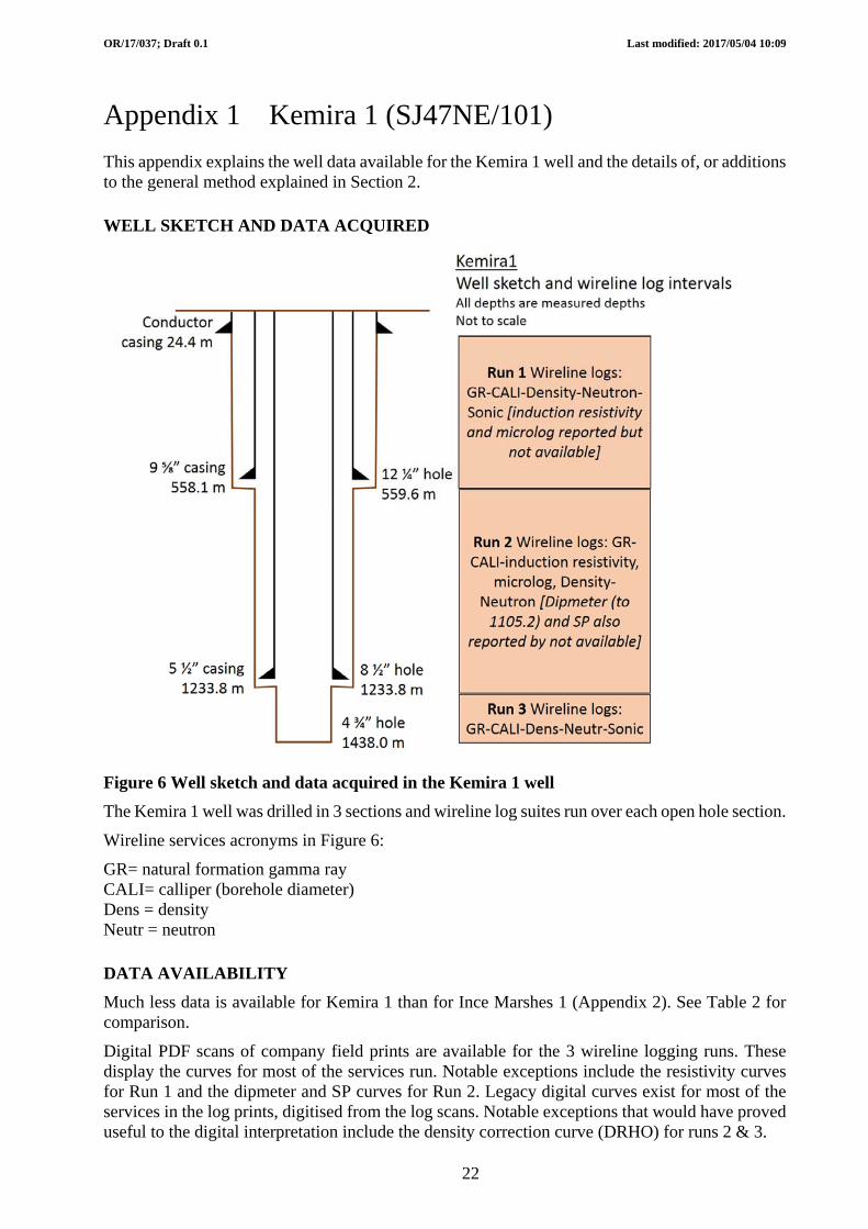
Appendix 1 Kemira 1 (SJ47NE/101) .................................................................................... 22
Well sketch and data acquired ................................................................................................ 22
Data availability ..................................................................................................................... 22
Data loading and quality checks ............................................................................................ 23
Petrophysical interpretation and results ................................................................................. 23
Appendix 2 Ince Marshes 1 (SJ47NE/100) .......................................................................... 25
Well sketch and data acquired ................................................................................................ 25
Data availability ..................................................................................................................... 26
Data loading and quality checks ............................................................................................ 26
Petrophysical interpretation and results ................................................................................. 27
Appendix 3 Stratigraphic interpretations ........................................................................... 32
Appendix 4 Temperature gradient ...................................................................................... 34
Appendix 5 Technical information for BGS internal use .................................................. 36
5.1 Ancillary information available: ................................................................................... 36
5.2 Ancillary information available for BGS reference ONLY: ........................................ 36
References .................................................................................................................................... 36

OR/17/037; Draft 0.1 Last modified: 2017/05/04 10:09
iii
FIGURES
Figure 1 Location of wells deeper than 1 km in the vicinity of the study area (pink circle). The two wells interpreted in this report are inside the pink circle. .................................................. 3
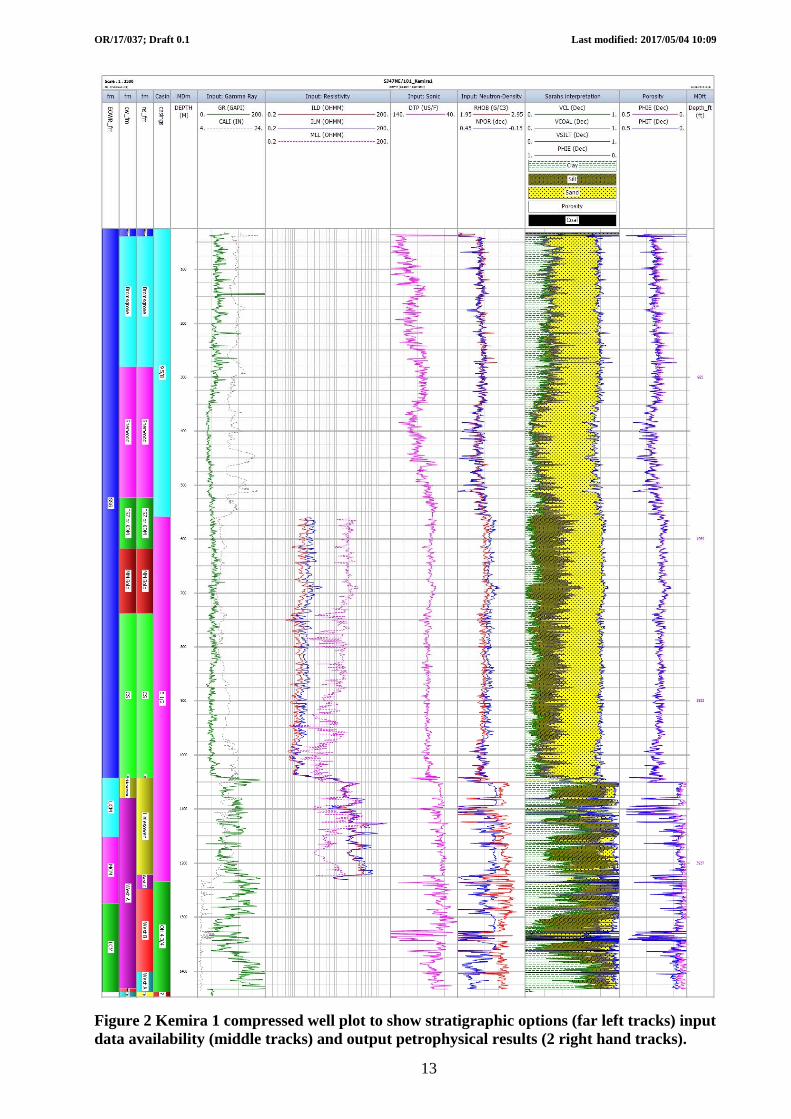
Figure 2 Kemira 1 compressed well plot to show stratigraphic options (far left tracks) input data availability (middle tracks) and output petrophysical results (2 right hand tracks). .............. 13
Figure 3 Ince Marshes 1 compressed well plot to show stratigraphic options (far left tracks) input data availability (middle tracks) and output petrophysical results (2 right hand tracks). ....... 14
Figure 4 Mature TOC rich shale intervals at 875 m and 900 m in the Westphalian A. The black line in the track on the right is the calculated TOC with a maximum value of 9.2 wt%. Grey shading indicates intervals with TOC >1.5 wt%. ................................................................... 16
Figure 5 Ince Marshes 1 section of well plot to show the calculated TOC curve (pink) and TOC rich (>1.5 wt%) intervals (grey shading in track 8). Measured TOC values are represented by black dots. Interpretation guide diagram available in Passey et al. 1990 (and Appendix 5, Section 5.2). ............................................................................................................................ 17
Figure 6 Well sketch and data acquired in the Kemira 1 well ...................................................... 22
Figure 7 Plot to show VCOAL cut off parameters and results. Coal bed labels in Table 10 ........... 24
Figure 8 Well sketch and data acquired in the Ince Marshes 1 well ............................................. 25
Figure 9 Ince Marshes 1 compressed well plot to broadly indicate data availability ................... 29
Figure 10 Ince Marshes 1 compressed well plot to show data comparisons: (XRD sample analysis vs ECS curves vs interpreted lithological curves) .................................................... 30
Figure 11 Histograms of calculated TOC for the Westphalian A (grey, left) and Millstone Grit (green, right) for Ince Marshes 1. ........................................................................................... 31
Figure 12 A cross-plot of measured TOC against calculated TOC in Ince Marshes 1 ................. 31
Figure 13 Temperature data for the wells in this study plotted with regional data. Pale blue arrows represent the correction of the maximum wireline recorded temperatures for the time since drilling mud circulation ceased. Data point and trend codes are listed in Table 15. ..... 34
TABLES
Table 1 Summary of data available for the wells studied ............................................................... 4
Table 2 Data available for each well. More details are provided in the appendix for each well (1 & 2 respectively) ...................................................................................................................... 5
Table 3 Data load, depth and quality checks for each well. More details are provided in the appendix for each well (1 & 2 respectively) ............................................................................. 6
Table 4 Core and analysis available for Ince Marshes 1 ................................................................. 7
Table 5 curves included in output *.LAS files .............................................................................. 11
Table 6 Results of petrophysical calculations listed by formation for each well (See Section 3.2 for an explanation of the column headings). For each column, the best and worst values are highlighted on the colour spectrum from dark green to dark red respectively. ...................... 12
Table 7 Shale thickness and TOC rich shale thickness to Gross Formation thickness summary for Ince Marshes 1. (No minimum shale thickness). .................................................................... 15
OR/17/037; Draft 0.1 Last modified: 2017/05/04 10:09
iv
Table 8 Shale thickness and TOC rich shale thickness to Gross Formation thickness summary for Ince Marshes 1. (2 m minimum shale thickness). .................................................................. 15
Table 9 Summary of VCOAL parameters and interpretation comments ......................................... 18
Table 10 Depths of coal intervals in Kemira 1 well, from the end of well report. Plot numbers refer to Figure 7. ..................................................................................................................... 24
Table 11 showing interpreted curves and corresponding XRD and ECS data used for comparison. (Arrows and boxes indicate where some minerals were grouped for comparison with combined curves). ........................................................................................................... 27
Table 12 Two stratigraphic interpretations for the 2 wells studied and some nearby wells. All depths in metres. ..................................................................................................................... 32
Table 13 Stratigraphy taken from the company composite logs or end of well reports. In addition, Coal seam depths were taken from the End of Well Report, these are shown in Table 10. For explanation of the formation codes, see Table 12. ................................................................. 33
Table 14 Stratigraphy loaded into interpretation software for this study and depth ranges of outputs. For explanation of the formation codes, see Table 12. ............................................. 33
Table 15 Sources of temperature data in Figure 13 ...................................................................... 35

OR/17/037; Draft 0.1 Last modified: 2017/05/04 10:09
1
Summary
This report details the petrophysical evaluation of 2 onshore wells near Liverpool UK: Kemira 1 (SJ47NE/101) and Ince Marshes 1 (SJ47NE/100). The results contribute to the geological characterisation for a monitoring experiment in Cheshire for the UK Geoenergy Observatories project.
The evaluation is based on the petrophysical interpretation of available digital wireline log curve data for the two wells across the whole logged interval (according to reinterpreted stratigraphic formations defined and correlated for this project). Associated digitised sample data (XRD, XRF, TOC data) is available to help cross-validate the interpretation for 1 of the 2 wells.
Outputs for this evaluation include continuous (along borehole) interpretations of clay volume, porosity, and total organic carbon (TOC). These interpreted curves were used to examine the proportions of reservoir rock and shale for each formation in each well and their respective properties. Net reservoir intervals were defined by those intervals where the clay volume was less than 50%, the porosity was more than 5% and no coal intervals were present. Net Shale intervals were defined by those intervals where the clay volume was more than 50% and no coal intervals were present.
The Kemira 1 well was logged from the Triassic Bromsgrove Sandstone Formation down to the Carboniferous Westphalian A unit, the base of which is not penetrated (~1400 m logged between 32-1433 m). Data is somewhat limited compared to the Ince Marshes 1 well, comprising parts of a standard log suite, and the curve data is machine-digitised from the legacy log field prints. (Resistivity curves are only available over part of the well; the neutron log was recorded in sandstone matrix units and the specific transformation to limestone matrix units (required for the interpretation) is unknown and has been guessed at; there is less data available for this well in terms of ancillary curves or sample analysis to cross check results than for the Ince Marshes 1 well). The results of the interpretation for this well should therefore be treated with appropriate caution.
The Ince Marshes 1 well was logged over the Carboniferous interval comprising the Westphalian C-A and the Millstone Grit Group, the base of which may be drilled through, but was unable to be logged due to hole difficulties (~1084 m logged between 368-1452 m). This well was drilled and logged more recently than the Kemira 1 well and has much more associated data including more advanced logging tools such as image logs, dipole sonic, and elemental spectroscopy to give formation mineral compositions. Sidewall cores were also collected and these and drill cuttings were analysed using various techniques to determine mineral, elemental and total organic carbon contents at the sample depths. There is therefore much more data available with which to cross check and verify results and as such the results of the interpretation can be regarded with a higher level of confidence than those of the Kemira 1 well.
The Kemira 1 well contains strata of Permian and Triassic age. These have high reservoir net to gross (NTG) values of 0.99 or 1 (i.e. 100% net reservoir). Their average porosities range from 18-25% and the Sherwood Sandstone Formation shows the highest average porosity at 25%. Both wells contain older, Carboniferous rocks and these have much lower NTG values, all containing less than 50% reservoir rocks (NTG ranging from 0.08-0.41). Their porosities are also lower, ranging from 8-15%, apart from the Westphalian C unit in the Kemira 1 well, which are anomalously high (23%) resulting from the presence of coal intervals and porosity artefacts adjacent to them (a software/parameter selection limitation
Total organic carbon (TOC) was calculated for the rocks beneath the Westphalian B unit in the Ince Marshes 1 well. Shales with TOC values calculated as greater than 1.5 wt% were considered ‘TOC-rich’. The ratio of these to the total formation thicknesses are generally very low: 0.08-0.15 for the Westphalian A and 0.11-0.24 for the Millstone Grit. The lower end of the range is where a

OR/17/037; Draft 0.1 Last modified: 2017/05/04 10:09
2
minimum shale thickness cut-off of 2 m is considered. The TOC rich shale in the Westphalian A has an average of 3.38 wt% TOC. However, individual intervals within the unit show typical curve responses for a mature source interval containing hydrocarbons and reach TOC values up to 9.18 wt%. The TOC rich shales in the Millstone Grit have an average of 2.9 wt% TOC. The TOC values measured in samples from sidewall cores and cuttings extend beneath the base of the geophysical well logs to 1575 m. There are 44 measured values averaging 2.89 wt% TOC with a maximum of 6.93 wt% TOC.
OR/17/037; Draft 0.1 Last modified: 2017/05/04 10:09
3
1 Introduction
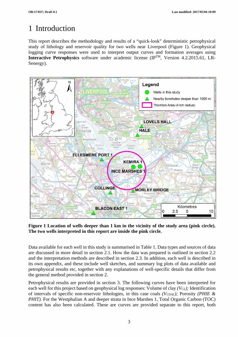
This report describes the methodology and results of a “quick-look” deterministic petrophysical study of lithology and reservoir quality for two wells near Liverpool (Figure 1). Geophysical logging curve responses were used to interpret output curves and formation averages using Interactive Petrophysics software under academic license (IPTM, Version 4.2.2015.61, LR-Senergy).
Figure 1 Location of wells deeper than 1 km in the vicinity of the study area (pink circle). The two wells interpreted in this report are inside the pink circle.
Data available for each well in this study is summarised in Table 1. Data types and sources of data are discussed in more detail in section 2.1. How the data was prepared is outlined in section 2.2 and the interpretation methods are described in section 2.3. In addition, each well is described in its own appendix, and these include well sketches, and summary log plots of data available and petrophysical results etc, together with any explanations of well-specific details that differ from the general method provided in section 2.
Petrophysical results are provided in section 3. The following curves have been interpreted for each well for this project based on geophysical log responses: Volume of clay (VCL); Identification of intervals of specific non-reservoir lithologies, in this case coals (VCOAL); Porosity (PHIE & PHIT). For the Westphalian A and deeper strata in Ince Marshes 1, Total Organic Carbon (TOC) content has also been calculated. These are curves are provided separate to this report, both

OR/17/037; Draft 0.1 Last modified: 2017/05/04 10:09
4
digitally as *.LAS files and as PDF log summary plots at 1:500 scale. More details can be found in section 3.1.
From these curves and the wellbore stratigraphy (Appendix 3), reservoir properties were output by formation: Gross thickness; Net, Net to Gross and Average porosity and porosity range (across the net intervals) (Section 3.3, Table 6). The derivation of these outputs are described in section 3.2.
Section 3.5 documents parameters used and gives a summary of the output data quality (Table 9). This, together with knowledge of the methods used to derive the outputs explained elsewhere in the report, should enable the reader to get an idea of the confidence that should be placed in the output results.
The reservoir quality and potential permeability is discussed in Section 4. The potential of the shale intervals as unconventional reservoir or source rock is discussed in Section 3.4.
Well Wireline logging services
Inp
ut c
urve
s
Tot
al lo
gged
inte
rval
(m
)
Tot
al le
ngt
h o
f co
re
cut
(m)
Side
wal
l cor
es
reco
vere
d
# of samples for each analysis
TV
D s
urve
y &
max
. d
evia
tion
(°)
Further details…
XR
D
TO
C
XR
F
…in Tables 2, 3, 4 and 7
and…
Kemira 1 (SJ47NE/101)
GR, density, neutron, sonic over most, resistivity middle section
only. 9 1405.7. 0 0 0 0 0 N, 6
Appendix 1
Ince Marshes 1 (SJ47NE/100)
Standard quad-combo, DSI, FMI, ECS
45+ 1085.7 198.7 98 47 82 8 Y, 9 Appendix
2
Table 1 Summary of data available for the wells studied
2 Method
Data for the wells was sourced and prepared for interpretation (Section 2.1) and then interpreted in specific software (Interactive Petrophysics (IPTM, Version 4.2.2015.61, LR-Senergy software, used under academic licence). This describes the general method. The process required for individual each well is recorded in the relevant appendix, as they may have incorporated fewer, or additional steps, from those listed here, depending on data availability, and any anomalies discovered and dealt with during the data checks.
2.1 DATA TYPES AND SOURCES
A number of data types and sources are required for, or contribute to, the petrophysical interpretation of each well. Specific data available by well are reported in the appendix for each well. The main data types and sources used for the ESIOS project are listed here, tabulated in Table 2 and more details including compressed log plots are shown in the relevant appendix for each well (Appendix 1 for Kemira 1 (SJ47NE/101) and Appendix 2 for Ince Marshes 1 (SJ47NE/100)).
a) Digital geophysical log curve data, mainly in LAS format (or sometimes LIS or DLIS) were extracted from the BGS storage holdings. Data origin includes company data via the DECC data storage agreement and also legacy BGS data e.g. curves machine-digitised from company field prints.
b) Associated well data from scanned company reports available from the DECC data store, mainly in *.PDF or *.Gif format:

OR/17/037; Draft 0.1 Last modified: 2017/05/04 10:09
5
Composite logs. Used to check well location, depths, curves scales, spliced intervals etc
End of well reports. Used to cross check well location, logged intervals etc Tabulated core sample analysis (available as excel sheets or digitised for this
project from report PDFs). Includes laboratory measured values such as Total Organic Carbon (TOC) content, mineralogical or elemental concentrations (from X-ray Ray Diffraction (XRD) and X-ray Fluorescence (XRF) analysis respectively) as well as porosity and permeability measurements. Used to cross check or, in some cases, calibrate log curve responses, depending on sample density and analysis results available.
Borehole orientation data (available as excel sheets or digitised for this project from report PDFs). These are usually tables recording borehole depth, borehole inclination and azimuth. Used to be able to accurately position subsurface features such as the location of formation tops intersecting the well bore.
c) Stratigraphy, i.e. formation tops (known as “well tops”) from various sources (Appendix 3):
Interpreted by BGS geologists for this (and previous) projects based on correlation with multiple wells in the region and in some cases in combination with examination of borehole rock core sections. 2 iterations available, one by N. Smith, one by C Waters (Table 12). These were compared with:
The company stratigraphy, as recorded on the composite log, or in the end of well report (Table 13).
The digital seismic interpretation, i.e. picked formation tops (identified using synthetic seismic sections using stratigraphy from surrounding wells (in PetrelTM, e.g. by J Williams, J White, D Evans).
d) Cored intervals based on BGS digital core-holdings database query. This was used to indicate core locations on log plots to help to distinguish intervals where data was derived from core, or from, for example, side wall cores or cuttings, where this information was not readily available in the material in b).
Well General indication of amount of data available
Origin of digital curves used in the interpretation
Company composite log?
Stratigraphy
Kemira 1 (SJ47NE/101)
Full log suite only available over part of the main hole. Partial data for the remainder. No core or supplementary analysis.
Company (via BGS storage of DECC data).
Composite log scan, basic end of well report, field prints of most (not all) services. No borehole orientation data.
3 interpretations available (Appendix 3):
BGS (Table 12)
1 Company (Table 13)
Edited BGS (N Smith version) used to output results (Table 14).
Ince Marshes 1 (SJ47NE/100)
Full log suite over main hole section including ancillary services and core sample analysis.
Legacy BGS, digitised from company field prints.
Composite log scan, end of well report and core sample reports. Multiple other reports, including TVD survey.
Table 2 Data available for each well. More details are provided in the appendix for each well (1 & 2 respectively)

OR/17/037; Draft 0.1 Last modified: 2017/05/04 10:09
6
2.2 DATA PREPARATION
Steps to import and prepare the data prior to interpretation (Section 2.3) are described:
2.2.1 Data load, depth and quality checks
a) Geophysical log curve data was loaded (to match the seismic petrel project). These were loaded and displayed in metres, but depth in feet was also calculated and displayed to help compare depths on the company logs.
b) The loaded curve types and intervals were checked against the company data (Section 2.1,b) to ensure that the expected curves were present. Curve response values at selected depths were then cross checked in more detail to ensure that data from each run was “on depth”, i.e. that the data had loaded and displayed at the correct value and depth.
c) Loaded LAS headers were compared to company data (Section 2.1,b) to ensure that the well location data matched and that elevations of the ground and the depth or height of the log starting position (usually “kelly bushing” or “drill floor”) also matched.
d) Curves were examined more generally that their responses were within the normal “expected range” and any possible log quality issues were noted. Any small data gaps were filled (to allow software calculation of Net to Gross and curve averages, Section 2.3).
e) Company data was checked for mud type (water or oil-based) and other parameters. If no opposing information was provided, it was assumed that suitable environmental corrections had already been applied to logs. Table 3 and Table 9 include some quality control comments and assumptions for individual wells.
f) Where sample data was available (see Table 2 and Table 4) this was formatted appropriately and loaded, checked against the source data for values and depths.
g) Stratigraphic interpretations were examined and discussed to select the most appropriate to output Petrophysical summaries for (Appendix 3). N Smith’s interpretations were used and slightly modified to match the intervals with petrophysical results (Table 14).
Well Curve type and intervals loaded?
Curve values and depths OK?
Location/ elevation data match?
Curve response “normal”?
Parameter availability?
Core data?
Kemira 1 (SJ47NE/101)
Run 2 Sonic inserted from more recently machine-digitised data. DRHO not available digitally for runs 2 &3. No resistivity curves available over runs 1 & 3.
Yes. Given the machine-digitised nature of the data in this well is perhaps less precise than the original
Some minor discrepancies.
Broadly yes (see parameter availability column)
Reasonable. Neutron recorded in sandstone units not limestone.
None acquired
Ince Marshes 1 (SJ47NE/100)
All main curves available in standard and high resolution modes. Also data from FMI, DSI and ECS services
Yes Some minor discrepancies.
Yes Good Available as excel sheets. Reformatted (and depths converted to m) for IP load
Table 3 Data load, depth and quality checks for each well. More details are provided in the appendix for each well (1 & 2 respectively)
2.2.2 Core sample data notes
The usual procedure for matching core and logs on a field - scale would be to first depth shift the core to the logs and then if necessary correct the core measurements for downhole in-situ

OR/17/037; Draft 0.1 Last modified: 2017/05/04 10:09
7
conditions (particularly applies to porosity and permeability measurements, to allow for the different fluid phases and different confining pressures, for example, to understand the degree of overburden stress correction to apply). Core data could then be used to aid the interpretation as per Section 2.1,b). However, for the wells examined here with core data available, (Ince Marshes 1, (SJ47NE/100)), details about core treatment, depth shifts to apply and the measurement method(s) were not generally captured. Therefore, within this report scope, the “usual” steps to correct the core data described above are not fully implemented. Other points of note for log-core matching include:
Sample scale - the vertical resolution of geophysical logs are much larger than the few centimetres-across core samples retrieved. Thus in very heterogeneous formations, average log response over an interval may be very different to the “point” data measurements on core;
Core treatment history: once the cores are removed from their downhole environment, depending on their treatment, fluids and other core features (e.g. clay structures etc) may not always be usefully preserved. This is because of technical difficulties in preserving or simulating the down hole temperatures and pressures in a core. Preparation of the core prior to analysis may also include cleaning and drying processes, which can further alter the measured parameters from downhole conditions (this can apply particularly to porosity and permeability measurements).
Core collection method: Sidewall core samples (wells 112/15-1 and 110/09a-2) of sandstones are often more affected by damage and drilling mud contamination than full cores (because of their smaller size relative to conventional core, which may also be affected by drilling and mud invasion damage around the outsides).
Well Core types Analysis and number of measurement depths
Comments
Ince Marshes 1 (SJ47NE/100)
~200m of conventionally drilled core. ~98 sidewall cores recovered
47 XRD 8 XRF 82 TOC
Analysis appears to be on a combination of sidewall cores and rock cuttings. Depth shifting for sidewall cores should not be necessary (shot on wireline). Sample density and lack of logs over the lower section means the cuttings derived samples cannot be depth checked (or depth shifted if necessary).
Table 4 Core and analysis available for Ince Marshes 1
2.2.3 Temperature gradient derivation
The software requires a temperature profile down the well for the processing (to allow recalculation of water and mud filtrate resistivities at downhole temperatures). Temperature data for each well and for the region was examined to determine a suitable temperature gradient to apply. Data sources include the “Maximum Recorded Temperature” from the wireline logging tools, coupled with “time since circulation”. This can be used to calculate the downhole temperature undisturbed by drilling (e.g. using methods described in ZetaWare, 2016). In some cases downhole fluid production temperatures may also be available. Busby et al. (2011) examined temperatures in the top 1000 m of the UK based on data from a variety of sources and produced contour maps for the results. Results from the closest contours at each depth was included as was the UK-wide average temperature gradient (Appendix 4). This was 2.8 °C per kilometre and as this provided a broad fit to the few data points available for the wells examined, it was used in this interpretation.
OR/17/037; Draft 0.1 Last modified: 2017/05/04 10:09
8
2.3 PETROPHYSICAL INTERPRETATION OF LITHOLOGY AND POROSITY
Curves describing reservoir parameters were interpreted using deterministic petrophysics workflows. The curves were used in combination to identify appropriate reservoir cut offs for the calculation of Net to Gross and average porosity values for the main formations (Section 3.2) and for the TOC interpretation (Section 3.4).
2.3.1 Volume of clay curve (VCL)
A Volume of Clay (VCL) curve was interpreted for each well. This gives a continuous, geophysical log-derived volume of clay for the intervals investigated. Input curves were the Gamma Ray (GR) and a combination of the Neutron, Density and Sonic curves where available and of suitable quality. These curves were used to select end points representing 0% clay and 100% clay for zones of the log, subdivided based on changing log character and curve responses with depth, to create a VCL log scaled from 0 (0% clay, i.e. 100% clean reservoir) to 1 (100% clay). This “quick-look”, interpretation of clay volume is based on curve responses only for Kemira 1, but for Ince Marshes 1, additional curves were available from the elemental capture spectroscopy (ECS) log and also sample analysis data for particular depths. This was used to help guide parameter selection. More details are described in the appendix for each well.
2.3.2 Coal identification curve (VCOAL)
A coal identification curve (VCOAL) was interpreted for each well, where “coal indicated” = 1, and “no coal indicated” = 0. This gives an indication of whether coal is thought to be present at each depth, based on the log response, and certain cut off values. This is because coal intervals could otherwise by mistakenly identified as part of the “net” reservoir intervals by the other cut-off criteria. See Section 3.2.1. The cut off values were selected based on a combination of the curve responses (based on knowledge of expected responses in coal and other minerals) and where the composite log lithology track indicated coal to be present. Thus slightly different cut offs were used in each well (see Table 9, Section 3.5). The additional ECS data for the Ince Marshes 1 well was used to cross-verify identification parameters. Well-specific details are described in the appendix for each well.
2.3.3 Porosity curves
Porosity curves were interpreted for each well. Input curves included the VCL curves (Section 3.2), Neutron, Density and Sonic curves. (Resistivity and Photoelectric Factor curves were used as visual aids to interpretation where required and data appeared to be reading within expected ranges). Areas of poor log quality were identified using primarily the Density Correction and Calliper curves.
Effective Porosity (PHIE) and Total Porosity (PHIT) curves were computed using the Neutron – Density method*. Where Density or Neutron data was unavailable, or its quality was poor, porosity was calculated using the sonic curve. These computations take into account tool measurements and interpretations of clay, mud filtrate and rock matrix properties.
*Using IP variable matrix density logic. IP solves the tool response equations for PHIE (corrected for wet clay volume). PHIT is then back-calculated by adding back in the clay bound water. Intervals that required sonic porosity calculations utilized the Wyllie equation.
Well-specific details are described in the appendix for each well.
2.3.4 Other curves: lithology curves and permeability indicators
Where suitable curves exist (i.e. dependent on data availability and pre-calculation of some curves) it may be possible to derive likely lithology from the curve responses. For example, the ‘multi-mineral lithology’ interpretation workflow in IP requires curves for the photo electric effect (Pef), and invaded zone resistivity (Rxo) curves. This interpretation was therefore only implemented for

OR/17/037; Draft 0.1 Last modified: 2017/05/04 10:09
9
the Ince Marshes 1 well and the results were compared to ECS processed lithology output curves (see Appendix 2). However, the “simple” mixed lithology calculations were also used to be able to cross compare results with the Kemira 1 well, which did not have the required curves available for the “multi-min” interpretation. The mixed mineral plot is derived from the VCL, VCOAL, VSALT and PHIE curves already described, and a Vsilt curve, a silt index, created by the software to indicate silt content (i.e. it is not an accurate, calculated volume. It is purely for display in the plot, to indicate that the rock can be thought of as containing clean sand of a certain porosity, non-porous silt and clay and it is not used in the interpretation methodology).
Permeability can be inferred by the relative responses of particular curves, for example, by observations in the Spontaneous Potential (SP) curve deflections (not available for either well) or by separation in resistivity curves which have different depths of investigation away from the borehole (see Section 3.5 for discussion on this). If hydrocarbon exists in the well and a water zone beneath it is also present, then residual water saturation can be interpreted from log responses and permeability calculated using various empirical relationships e.g. Timur Coates equations etc. This method was also not applicable to the wells in this study.
2.4 PETROPHYSICAL INTERPRETATION OF TOTAL ORGANIC CARBON CONTENT (TOC)
The Total Organic Carbon TOC was calculated using the Passey-method inbuilt into the IP TOC calculator for the shale intervals of Ince Marshes 1, in a similar methodology to those used by Gent et al. 2014. In the Passey method, scaled sonic and deep resistivity curves were made to overlay giving a vertically continuous wt % TOC curve (Passey et al. 1990). Ince Marshes was split into two maturity zones to represent the increasing maturity with depth based on the vitrinite reflectance profile (Harriman, 2011). The bulk density and neutron porosity curve overlay plots were used to verify those of the sonic.
Kemira 1 was not chosen for TOC calculations as the required resistivity curve only covers a 640 m interval over typically reservoir and barren units. Further to this there is a lack of geochemistry data with which to calibrate the TOC calculation.
The objective of this study was to produce TOC curves Ince Marshes 1 accompanied by statistical TOC outputs for the well. To be able to calculate the TOC, level of maturity (LOM) values had to be established. In addition, clay volume curves (VCl) with a suitable cut-off value were required to be able to distinguish potential shale source rocks from clean reservoir rock. Coal identifiers and TOC curve cut off values were also applied to the final calculations Volume of Clay (VCl): As discussed in Section 2.3.1. The VCl curve was used as a discriminator in subsequent calculations, to remove intervals with less than 50% clay (i.e. those considered unlikely to be a source rock). Coal Discriminator: The Passey method is accurate for calculating TOC in shale intervals but not in coals; if coals are not removed they give inaccurate spikes on the calculated TOC curve. The coal signal has to be removed using discriminators discussed in Section 2.3.2. The final results presented do not incorporate coals and account only for shale intervals. Level of Maturity (LOM): A key parameter in the Passey equation for calculating TOC is the level of maturity (LOM). This can be calculated from Ro values, measured on core and cuttings samples (Hood et al. 1975). The Ro values were taken from released geochemical reports (Harriman, 2011).
2.4.1 Assumptions and Limitations
The following assumptions and limitations should be considered when analysing the results and graphical TOC log plots:
OR/17/037; Draft 0.1 Last modified: 2017/05/04 10:09
10
The Level of Maturity parameter required for the Passey method TOC calculation is well defined from the Ro values in the geochemical report (Harriman, 2011; Appendix 5, Section 5.2). It is assumed that these values are correct, no sensitivity analysis has been run on these values in this study.
The Passey method also requires the selection of a ‘lean shale’ point where a shale is assumed to have no organic carbon. No sensitivity on this parameter has been done for this study, so this should be taken into consideration when examining the absolute TOC values reported here.
A volume of clay (VCl) cut-off of 0.5 has been arbitrarily applied to remove intervals with a low clay content.
The vertical resolution of the calculated TOC is limited by the resolution of logging tools. This means that, for example, sharply varying TOC values across thinly interbedded shales, coals and sands intervals may not be distinguishable and is likely to be presented as a smoother “average” TOC curve response. By contrast, each TOC measurement from cores or cuttings samples represent a single point in the succession. In addition it was not always possible to precisely depth shift the core depths to log depths. Therefore there may be some small depth differences between core TOC measurement points and the calculated TOC curve. The sample-derived TOC measurements are assumed to be correct, but these in themselves may have their own limitations, which are not discussed here.
Petrophysical log analysis has been used as a screening tool to highlight potential TOC rich source rock intervals (shales), over larger depth ranges than is available for core/cuttings sample data. Given time constraints, data availability and the variable nature of the Carboniferous sedimentation, kerogen types have not been taken into consideration. To further the work presented in this report, investigation of the kerogen type in conjunction with the calculated TOC will give a more complete understanding of the hydrocarbon sources
Units shallower than the Westphalian A (<700 m TVD) have not been assessed for TOC wt% as they are immature for hydrocarbon production and also have no measured TOC values for calibration.
3 Results
Results are based on the method broadly described in Section 2, using Interactive Petrophysics (IPTM, Version 4.2.2015.61) LR-Senergy software, used under academic licence. Output log plots are shown by well in the relevant appendices to this report. Output digital *.LAS files, excel tables of input data and 1:200 log plots are provided separately. All outputs should take into account the data quality comments provided in Table 9. This can give an indication of the confidence in output curve results.
3.1 INTERPRETED CURVES
Digital output curves were interpreted using the method described in Section 2. These were:
Volume of Clay curve (VCL); Coal Identification curve (VCOAL); Evaporite Identification curve (VSALT); Effective Porosity curve (PHIE); Total Porosity curve (PHIT); Total Organic Carbon content curve (TOC).

OR/17/037; Draft 0.1 Last modified: 2017/05/04 10:09
11
Plots of data for each well are available as a “quick-look” output in Figure 2 and Figure 9 (in Appendix 2). Table 5 lists the curves included in the output *.LAS files (Appendix 5, Section 5.1).
Track in Figure 2 &
Figure 3
Well/file name Curve name
Kemira 1 (SJ47NE/101)
Ince Marshes 1 (SJ47NE/100)
Kemira1_m.LAS InceMarshes1_m.LAS InceMarshes1_TOC_m.
LAS
Inp
ut c
urv
e
1 Gamma Ray GR HGR
Calliper CALI HCAL
2
Micro resistivity MLL RXO8
Shallow resistivity ILM RLA0, 1, 2
Deep resistivity ILD RLA3, 4, 5
3 Sonic (compressional) DTP DTCO
4
Neutron NPOR NPHI
Density RHOB RHO8
Density correction - HDRA
Photo electric factor - PEF8
Inte
rpre
ted
cu
rve
5
Clay volume VCL VCL
Coal interval VCOAL VCOAL
Salt interval VSALT VSALT
6 Effective porosity PHIE PHIE
Total porosity PHIT PHIT
Track in Figure 5
5 Gamma Ray HSGR
8 Calculated TOC - TOC
Table 5 curves included in output *.LAS files
3.2 CALCULATION OF THICKNESSES, AVERAGE VALUES AND RANGES
Gross and net are in metres, measured depth. This means that they represent measured depth thicknesses along the borehole, which is not necessarily the true stratigraphic, or true vertical thickness. Net to gross and porosities are provided as fractions.
3.2.1 Gross and net thicknesses
The total thickness of the interval of interest along the borehole is the “Gross” provided here.
The Net interval is the sum of the thicknesses of those parts of the reservoir that meet a set of cut-off criteria (applied to one or more curves). These parameters (the cut off criteria that define the Net) will, at the field scale, be based on operator preferences or field observations of reservoir productivity that may be refined through time. However, for this “quick-look”, generic cut-offs have been applied to give a broad indication of the Net where:
Clay volume is less than 50% (i.e. where VCL <0.5); Porosity is more than 5% (i.e. where PHIE > 0.05); No coal or salt intervals are identified (i.e. where VCOAL = 0, or VSALT = 0).
3.2.2 Net to gross
Net to Gross (NTG) in this report gives an indication of the amount of reservoir (Net) within an interval of interest (Gross). It is expressed as a fraction from 0 to 1, where a NTG of 0 means that no reservoir has been interpreted within the interval and a NTG of 1 means that all of the rock
OR/17/037; Draft 0.1 Last modified: 2017/05/04 10:09
12
within the interval has been interpreted to be composed of 100% reservoir. The NTG equation is shown below.
Net to Gross (NTG) = Total thickness of reservoir” (net)
Total thickness of interval (gross)
NTG values were calculated for each stratigraphic unit in each well (and by stratigraphic unit (for all wells) and by well (for all stratigraphic units)).
3.2.3 Average porosity and range
Average porosities and ranges were calculated for each stratigraphic unit in each well. These are based on arithmetic average calculations and curve statistics of the interpreted effective porosity (PHIE) curve (Section 2.3.3 over the intervals defined as net reservoir (Net: see NTG, Section 3.2.1)).
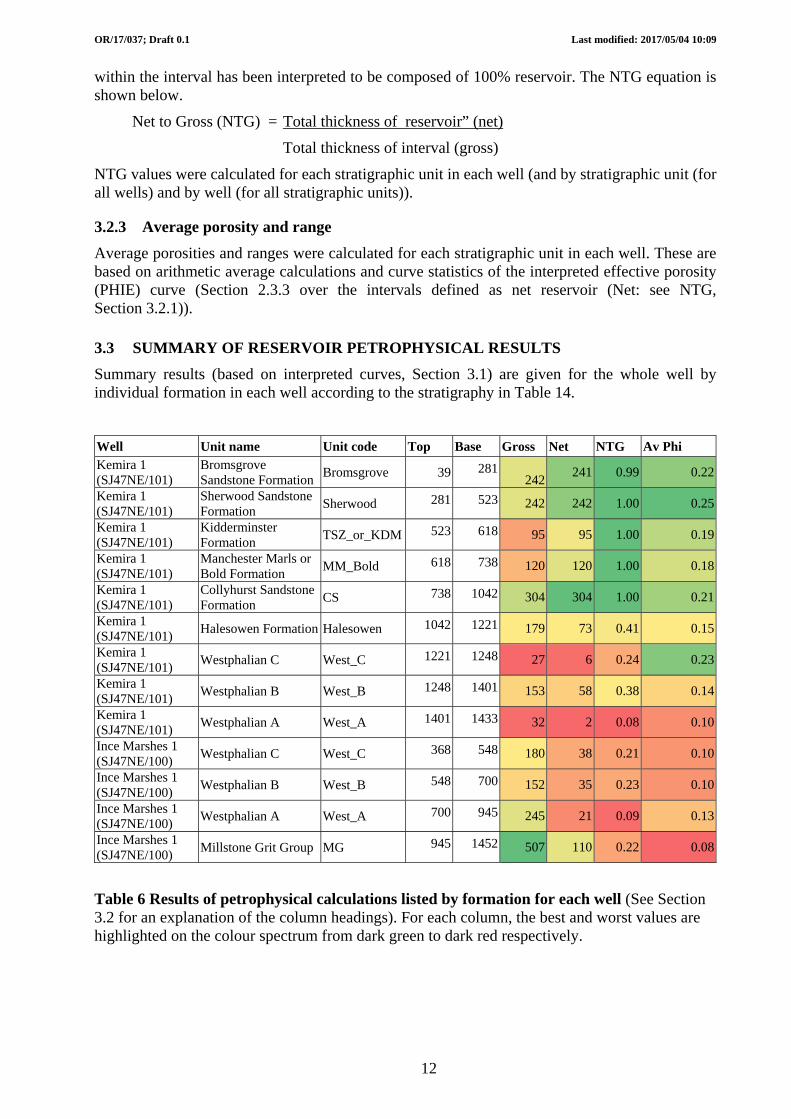
3.3 SUMMARY OF RESERVOIR PETROPHYSICAL RESULTS
Summary results (based on interpreted curves, Section 3.1) are given for the whole well by individual formation in each well according to the stratigraphy in Table 14.
Well Unit name Unit code Top Base Gross Net NTG Av Phi Kemira 1 (SJ47NE/101)
Bromsgrove Sandstone Formation
Bromsgrove 39 281242
241 0.99 0.22
Kemira 1 (SJ47NE/101)
Sherwood Sandstone Formation
Sherwood 281 523 242 242 1.00 0.25
Kemira 1 (SJ47NE/101)
Kidderminster Formation
TSZ_or_KDM 523 618 95 95 1.00 0.19
Kemira 1 (SJ47NE/101)
Manchester Marls or Bold Formation
MM_Bold 618 738 120 120 1.00 0.18
Kemira 1 (SJ47NE/101)
Collyhurst Sandstone Formation
CS 738 1042 304 304 1.00 0.21
Kemira 1 (SJ47NE/101)
Halesowen Formation Halesowen 1042 1221 179 73 0.41 0.15
Kemira 1 (SJ47NE/101)
Westphalian C West_C 1221 1248 27 6 0.24 0.23
Kemira 1 (SJ47NE/101)
Westphalian B West_B 1248 1401 153 58 0.38 0.14
Kemira 1 (SJ47NE/101)
Westphalian A West_A 1401 1433 32 2 0.08 0.10
Ince Marshes 1 (SJ47NE/100)
Westphalian C West_C 368 548 180 38 0.21 0.10
Ince Marshes 1 (SJ47NE/100)
Westphalian B West_B 548 700 152 35 0.23 0.10
Ince Marshes 1 (SJ47NE/100)
Westphalian A West_A 700 945 245 21 0.09 0.13
Ince Marshes 1 (SJ47NE/100)
Millstone Grit Group MG 945 1452 507 110 0.22 0.08
Table 6 Results of petrophysical calculations listed by formation for each well (See Section 3.2 for an explanation of the column headings). For each column, the best and worst values are highlighted on the colour spectrum from dark green to dark red respectively.
OR/17/037; Draft 0.1 Last modified: 2017/05/04 10:09
13
Figure 2 Kemira 1 compressed well plot to show stratigraphic options (far left tracks) input data availability (middle tracks) and output petrophysical results (2 right hand tracks).

OR/17/037; Draft 0.1 Last modified: 2017/05/04 10:09
14
Figure 3 Ince Marshes 1 compressed well plot to show stratigraphic options (far left tracks) input data availability (middle tracks) and output petrophysical results (2 right hand tracks).
OR/17/037; Draft 0.1 Last modified: 2017/05/04 10:09
15
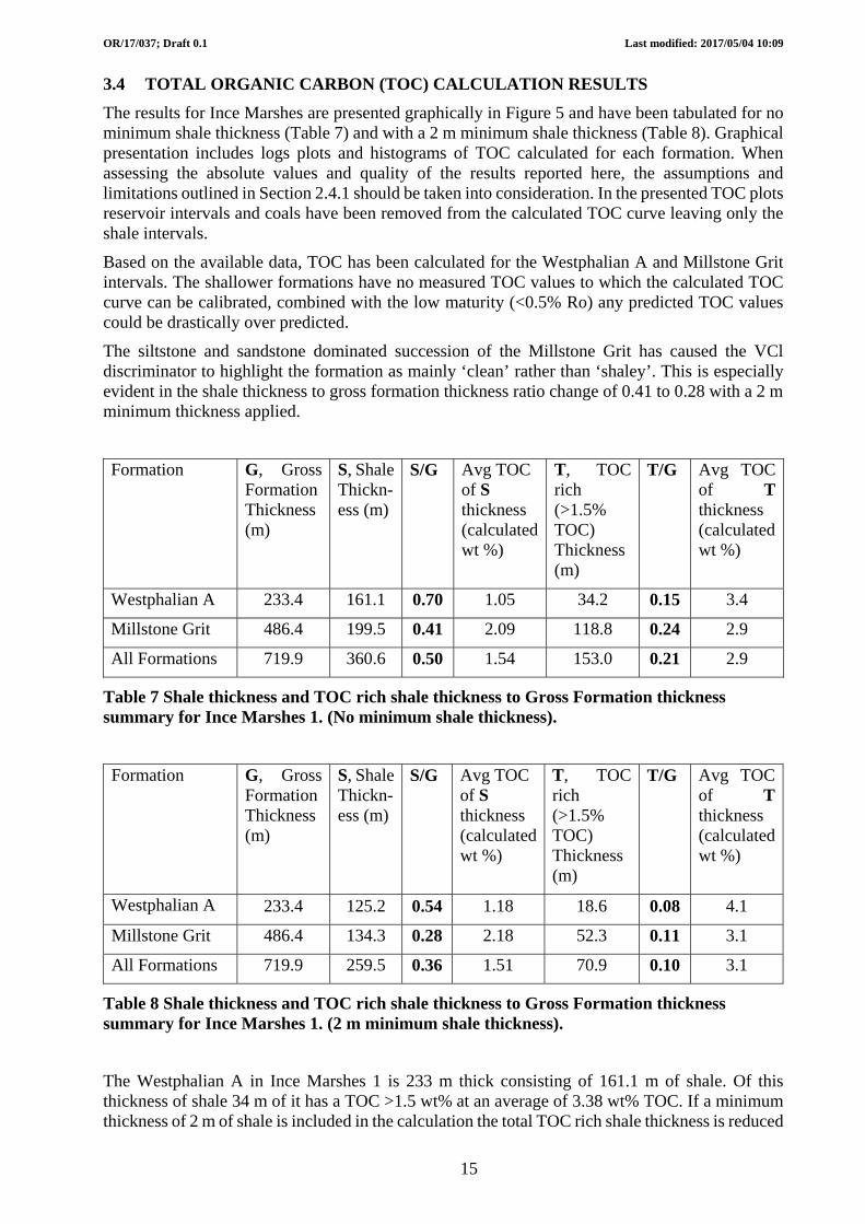
3.4 TOTAL ORGANIC CARBON (TOC) CALCULATION RESULTS
The results for Ince Marshes are presented graphically in Figure 5 and have been tabulated for no minimum shale thickness (Table 7) and with a 2 m minimum shale thickness (Table 8). Graphical presentation includes logs plots and histograms of TOC calculated for each formation. When assessing the absolute values and quality of the results reported here, the assumptions and limitations outlined in Section 2.4.1 should be taken into consideration. In the presented TOC plots reservoir intervals and coals have been removed from the calculated TOC curve leaving only the shale intervals.
Based on the available data, TOC has been calculated for the Westphalian A and Millstone Grit intervals. The shallower formations have no measured TOC values to which the calculated TOC curve can be calibrated, combined with the low maturity (<0.5% Ro) any predicted TOC values could be drastically over predicted.
The siltstone and sandstone dominated succession of the Millstone Grit has caused the VCl discriminator to highlight the formation as mainly ‘clean’ rather than ‘shaley’. This is especially evident in the shale thickness to gross formation thickness ratio change of 0.41 to 0.28 with a 2 m minimum thickness applied.
Formation G, Gross Formation Thickness (m)
S, Shale Thickn-ess (m)
S/G Avg TOC of S thickness (calculated wt %)
T, TOC rich (>1.5% TOC) Thickness (m)
T/G Avg TOC of T thickness (calculated wt %)
Westphalian A 233.4 161.1 0.70 1.05 34.2 0.15 3.4
Millstone Grit 486.4 199.5 0.41 2.09 118.8 0.24 2.9
All Formations 719.9 360.6 0.50 1.54 153.0 0.21 2.9
Table 7 Shale thickness and TOC rich shale thickness to Gross Formation thickness summary for Ince Marshes 1. (No minimum shale thickness).
Formation G, Gross Formation Thickness (m)
S, Shale Thickn-ess (m)
S/G Avg TOC of S thickness (calculated wt %)
T, TOC rich (>1.5% TOC) Thickness (m)
T/G Avg TOC of T thickness (calculated wt %)
Westphalian A 233.4 125.2 0.54 1.18 18.6 0.08 4.1
Millstone Grit 486.4 134.3 0.28 2.18 52.3 0.11 3.1
All Formations 719.9 259.5 0.36 1.51 70.9 0.10 3.1
Table 8 Shale thickness and TOC rich shale thickness to Gross Formation thickness summary for Ince Marshes 1. (2 m minimum shale thickness).
The Westphalian A in Ince Marshes 1 is 233 m thick consisting of 161.1 m of shale. Of this thickness of shale 34 m of it has a TOC >1.5 wt% at an average of 3.38 wt% TOC. If a minimum thickness of 2 m of shale is included in the calculation the total TOC rich shale thickness is reduced

OR/17/037; Draft 0.1 Last modified: 2017/05/04 10:09
16
to 18.6 m. Subsequently reducing the overall formation thickness to TOC rich shale thickness, fraction from 0.15 to 0.08.
Intervals within the Westphalian A at 870-876 m, 897-901 m and possibly 790-795 m show typical curve responses for a mature source interval containing hydrocarbons (Passey et al. 1990 schematic, Appendix 5, Section 5.2), these reach TOC values up to 9.2 wt% (Figure 4).
Figure 4 Mature TOC rich shale intervals at 875 m and 900 m in the Westphalian A. The black line in the track on the right is the calculated TOC with a maximum value of 9.2 wt%. Grey shading indicates intervals with TOC >1.5 wt%.
The Millstone Grit has been split into two for the calculation based on the increasing maturity outlined in Harriman, 2011 (Appendix 5, Section 5.2).
As a complete unit the Millstone Grit in Ince Marshes 1 is 486.4 m thick consisting of 199.5 m of shale. Of this thickness of shale, 118.8 m of it has a TOC >1.5 wt% at an average of 2.9 wt% TOC. If a minimum thickness of 2 m of shale is included in the calculation the total TOC rich shale thickness is reduced to 52.3 m. The resultant change in the T/G (TOC rich shale thickness (T) to gross formation thickness (G) fraction) is a reduction from 0.24 to 0.11.
The measured sidewall core and cuttings TOC values in this well extend beneath the base of the geophysical well logs to 1575 m (MD). There are 44 measured values averaging 2.89 wt% TOC with a maximum of 6.93 wt% TOC.

OR/17/037; Draft 0.1 Last modified: 2017/05/04 10:09
17
Figure 5 Ince Marshes 1 section of well plot to show the calculated TOC curve (pink) and TOC rich (>1.5 wt%) intervals (grey shading in track 8). Measured TOC values are represented by black dots. Interpretation guide diagram available in Passey et al. 1990 (and Appendix 5, Section 5.2).
Ince Marshes 1Scale : 1 : 4000TOC:DEPTH (699.97M - 1449.93M) 04/11/2016 16:21DB : DECC (34)
1 2
DEPTH(M)
3
TVD(M)
4
Coal
5
Caliper (IN)6. 16.
Gamma Ray (GAPI)0. 200.
6
Volume of Clay (Dec)0. 1.
Shaley
Clean
7
LogRT-1. 3.
DTovl (uSec/ft)-1. 3.
TOC
8
Calculated TOC (wt%)0. 12.Measured TOC (wt%)0 12
TOC > 1.5wt%
700
800
900
1000
1100
1200
1300
1400
700
800
900
1000
1100
1200
1300
1400
1431

OR/17/037; Draft 0.1 Last modified: 2017/05/04 10:09
18
3.5 SUMMARY OF PARAMETERS AND QUALITY OF THE OUTPUT INTERPRETED CURVES
Table 9 documents key log interpretation and quality notes regarding each well. Individual data quality checks by well are expanded on in the relevant appendix, as referred to in the table below. Parameter sets for VCOAL are also included. Parameters for VCL and porosity modules for each well are available separately as *.set files (Appendix 5, Section 5.1).
Well
Coal ID parameters General interpretation/data quality comments.
Density Neutron Sonic Comments refer to the “fixed logs”, i.e, once the data load & preparation processes have prepared the best possible starting dataset.
It was assumed that appropriate borehole corrections had already been applied to all curves, (except where otherwise mentioned)
IP defaults: 1.8 0.5 120
Density correction curve (DRHO or HDRA) in tolerance was assumed to be -0.1 to 0.1
Calliper logs (HCAL or CALI etc) were compared to bit size to identify washouts or zones of potential poor pad-tool contact.
All curves were compared to their expected responses and to the company composite pdf logs where available.
Kemira 1 (SJ47NE/101)
2.1 0.45 75
Outputs are lower confidence for this well than for Ince Marshes 1, resulting from initial input data quality and lack of additional data to cross-validate output curves during the interpretation process. There is low confidence in absolute neutron porosity (NPOR) values, relating to its transformation to limestone units (see Appendix 1, data load notes). This affects both VCL and PHI outputs. The density correction curve (DRHO) was not available digitally (although shown in field prints), so it was not possible to auto-replace porosities derived using the poor quality density data, with sonic derived porosities, which in any case did not match with the neutron-density derived porosities particularly well over the parts of the log (see Appendix 1, PHIE interpretation notes). Calliper data shows that the hole was rugose and washed out in places, but callipers are rarely open to their maximum extent (i.e. pad tools are mainly not “floating” and assumed to be in contact with borehole wall, suggesting that density-neutron data should be otherwise reasonable). No other information is available to cross check results apart from the lithology plot of the company composite log. Selection of VCOAL parameters was guided by the coal bed list in the end of well report (it is not known by what method these were identified). The cut-off parameters selected were able to detect 4 of the 15 recorded coal beds (see Appendix 1, PHIE interp notes). High porosity spikes occur either side of identified coal beds, because porosity is nulled over the identified coal, but the coal content of adjacent coal-rich sediments (below the VCOAL cut-off criteria parameters) is not able to be accounted for in the software.
Ince Marshes 1 (SJ47NE/100)
1.8 0.5 70
Data quality for this well appears to be not too bad from CALI and HDRA evidence. A few washouts, hole rugosity (CALI spikes) and areas where HDRA is out of tolerance, in some cases correspond to coals (e.g. around 620 m), but not always. The calliper doesn’t appear to be open to its maximum extent anywhere, i.e. pad tools were not "floating" suggesting that density-neutron data should be otherwise reasonable. The hole is ovalised in the top section above 434 m to casing shoe (378 m) based on the FMI dual callipers, C1, C2) but the data generally appears to be OK. Ancillary data from the Elemental Spectroscopy Log (ECS) provided a processed output for a suite of minerals. In addition, XRD, XRF analysis was available from samples at some of the sidewall core depths, or from rock cuttings Both these datasets were used to cross check input and interpreted output curves and in some cases used to guide parameter selection. VCOAL created porosity spikes where porosity is nulled over the identified coal bed. (see Appendix 2, Interpreted output data quality check notes and PHIE interpretation notes).
Table 9 Summary of VCOAL parameters and interpretation comments

OR/17/037; Draft 0.1 Last modified: 2017/05/04 10:09
19
4 Discussion
4.1 LITHOLOGY AND PERMEABILITY IN KEMIRA 1
Distinguishing the stratigraphy, structure and rock properties in the Kemira 1 well is challenging (Figure 2). The interval identified as the Manchester Marl Formation is generally predominantly a calcareous mudstone to the west of Kemira 1 in the East Irish Sea Basin. It is considered to be a non-reservoir rock, sealing to upward fluid migration. The formation is known to transition to a sandy facies east of Kemira 1. However, if the formation is correctly identified in Kemira 1, then it appears from the log responses that the Manchester Marl has already transitioned to the sandy facies at that location and, given the separation in resistivity curves, it appears to be permeable. An alternative explanation could be that the interval could be the Chester Formation (Formerly known as the Chester Pebble Beds) overlying the Kinnerton Sandstone Formation (rather than the Collyhurst Sandstone Formation). This is based on interpretation of core from a borehole called Speke north of the river Mersey and could fit with the cuttings logs described below:
When a well is drilled, the rock chippings (cuttings) are brought to the surface by the circulating drilling fluid. These are sieved out, examined and described to help with the geological interpretation. The company cuttings logs for Kemira 1 over the interval identified as the Manchester Marl Formation reports predominantly sandstone. The deciphering the description of the cuttings, it appears the sandstone is generally moderately to poorly consolidated with silica cement. Some loose grains, moderately well sorted and some siltstone frags are also reported, with a thin pebble conglomerate at the base.
The cuttings logs over the interval identified as the Collyhurst Sandstone Formation report a mixture of sandstone and siltstone, both moderately consolidated to friable with dolomitic and/or silica cement. More consolidated bands are reported at around 3050 ft and this roughly corresponds to a thin interval where the resistivity curves converge.
From the resistivity log response, the Collyhurst Sandstone Formation in Kemira 1 appears permeable, based on the separation in resistivity curves. The resistivity curves are slightly closer together over the basal part (below 980 m depth), which could suggest that this lower part is perhaps less permeable than the rest. When drilling a well, the drilling fluid (‘mud’) invades permeable formations during drilling until flow is capped off by the solids in the mud coating the borehole wall. When the mud is a different resistivity to the formation water, this invasion creates a transition in the overall resistivity from close to the borehole wall, outwards to the un-invaded formation. The resistivity tools measure resistivity at different distances into the formation from the borehole itself, so the invasion of drilling fluid is recorded by the separation in the output curve readings. When a formation is impermeable, no mud invasion can occur and so there is no transition in the resistivity away from the borehole wall. The resistivity curves reading at different depths into the formation therefore overlay each other.
This is considered to be the most likely scenario. However, there are a couple of alternative possibilities to this interpretation to be taken into consideration, given the limitations on data quality and data availability for this well:
1) The calliper is open to its maximum extent below 980 m, so the geophysical tools are likely to be outside their normal operating range. We don’t know the hole size, but it could be larger than the ILD's (deep resistivity curve) reach into the formation. i.e. both ILD & ILM (medium resistivity curve) could be reading mud in the borehole or at shallower depths into the formation than they are designed to, so they would not ‘see’ the full span of the invasion zone.
2) It could be that the uninvaded formation resistivity is the same as the invading drilling fluid resistivity below 980 m. The resistivities look to be similar, so the curve overlay could represent a
OR/17/037; Draft 0.1 Last modified: 2017/05/04 10:09
20
(very) slight fluid or rock matrix change that would bring the mud and formation resistivities to become identical.
2a) Fluid related changes could incorporate changes in the formation water salinity or hydrocarbon content. It is feasible that that the water in the shales and rocks below the Collyhurst Sandstone Formation (CS) are a different salinity to the CS, and there could therefore be a salinity gradient. It appears that the water in the shales beneath the CS is more resistive (less saline, or it could be hydrocarbon content). However, it seems unlikely that less saline water or small amounts of hydrocarbon would stay in a "block" at the base of the sandy CS because of the density contrast, unless this is also reflecting a vertical permeability change.
2b) Rock matrix related changes could be that the lower part of the CS formation (below 980 m) has slightly less conductive minerals than higher up e.g. pyrite (traces of which are reported in the cuttings log). Any lithological changes are difficult to detect, given that the enlarged hole is likely to have adversely affected the density-neutron curves, combined with the neutron curve processing difficulties (see Table 9 and Appendix 1).
Without examining data from nearby wells to verify whether a similar curve response is in evidence it is not possible to improve confidence in the permeability or lithological analysis. Other nearby boreholes that could be assessed include Morley Bridge, Collinge, Lovels Hall, Hale, Knutsford and Blacon East 1. However, a quick look suggests that the geophysical log data quality and availability may also limit further interpretation in those wells.

OR/17/037; Draft 0.1 Last modified: 2017/05/04 10:09
21
5 Conclusions
Two onshore wells near Liverpool UK were petrophysically evaluated to contribute to the geological characterisation of a Cheshire site for the UK Geoenergy Observatories project. The two wells are Kemira 1 (SJ47NE/101) and Ince Marshes 1 (SJ47NE/100).
Different types, quality and amounts of data were available for the two wells. Far less data is available for the evaluation of Kemira 1. For both wells, various limitations and assumptions are taken into account during the interpretation (particularly for the TOC calculations) and these should be taken into account when examining the petrophysical results.
The Kemira 1 well was logged from the Triassic Bromsgrove Sandstone Formation down to the Carboniferous Westphalian A unit, the base of which is not penetrated (~1400 m logged between 32-1433 m). Data available comprises parts of a standard log suite, machine-digitised from the legacy log field prints
The Ince Marshes 1 well was logged over the Carboniferous interval comprising the Westphalian C-A and the Millstone Grit Group, the base of which may be drilled, but was unable to be logged due to hole difficulties (~1084 m logged between 368-1452 m). In addition to standard log suites, data from more advanced logging tools such as imaging, dipole sonic, and elemental spectroscopy tools were also recorded. Sidewall cores were collected and analysed using various techniques to determine mineral, elemental and total organic carbon content.
Outputs for this evaluation include interpretations of clay volume and porosity. These interpreted curves were used to examine the proportions of reservoir rock and shale for each formation in each well and their respective properties. Net reservoir intervals were defined by those intervals where the clay volume was less than 50%, the porosity was more than 5% and no coal intervals were present.
Permian and Triassic age formations were only present in Kemira 1. These all have high reservoir net to gross (NTG) values of 0.99 or 1 (i.e. 100% net reservoir). Their average porosities range from 18-25% and the Sherwood Sandstone Formation shows the highest average porosity at 25%. The older, Carboniferous formations have much lower NTG values, all containing less than 50% reservoir rocks (NTG ranging from 0.08-0.41). Their porosities are also lower, ranging from 8-15%, apart from the Westphalian C unit in the Kemira 1 well, which are anomalously high (23%) resulting from the presence of coal intervals and porosity artefacts adjacent to them (a software/parameter selection limitation).
Total organic carbon (TOC) was calculated for the rocks beneath the Westphalian B unit in Ince Marshes 1. Shales with TOC values calculated as greater than 1.5 wt% were considered ‘TOC-rich’. The ratio of these to the total formation thicknesses are generally low: 0.08-0.15 for the Westphalian A and 0.11-0.24 for the Millstone Grit. The lower end of the range represents the ratio when a minimum shale thickness cut offs of 2 m is considered. The TOC rich shale in the Westphalian A has an average of 3.38 wt% TOC. However, individual intervals within the unit show typical curve responses for a mature source interval containing hydrocarbons and reach TOC values up to 9.18 wt%. The TOC rich shales in the Millstone Grit have an average of 2.9 wt% TOC. The measured sidewall core and cuttings TOC values extend beneath the base of the geophysical well logs to 1575 m. There are 44 measured values averaging 2.89 wt% TOC with a maximum of 6.93 wt% TOC.
OR/17/037; Draft 0.1 Last modified: 2017/05/04 10:09
22
Appendix 1 Kemira 1 (SJ47NE/101)
This appendix explains the well data available for the Kemira 1 well and the details of, or additions to the general method explained in Section 2.
WELL SKETCH AND DATA ACQUIRED
Figure 6 Well sketch and data acquired in the Kemira 1 well
The Kemira 1 well was drilled in 3 sections and wireline log suites run over each open hole section.
Wireline services acronyms in Figure 6:
GR= natural formation gamma ray CALI= calliper (borehole diameter) Dens = density Neutr = neutron
DATA AVAILABILITY
Much less data is available for Kemira 1 than for Ince Marshes 1 (Appendix 2). See Table 2 for comparison.
Digital PDF scans of company field prints are available for the 3 wireline logging runs. These display the curves for most of the services run. Notable exceptions include the resistivity curves for Run 1 and the dipmeter and SP curves for Run 2. Legacy digital curves exist for most of the services in the log prints, digitised from the log scans. Notable exceptions that would have proved useful to the digital interpretation include the density correction curve (DRHO) for runs 2 & 3.

OR/17/037; Draft 0.1 Last modified: 2017/05/04 10:09
23
The PDF scans of the end of well report and mud (cuttings) log is also available to provide ancillary data.
DATA LOADING AND QUALITY CHECKS
The data was checked according to the summary in Section 2.2.
Data load and quality summary notes
Sourced and spliced in missing data in vicinity of casing shoes from the previously merged data from individual run files. Fixed off-depth run 2 sonic (off depth in field print cf N-D and GR-res run 2s. Added 1.635m) and spliced in (needed to improve Vcoal picks – so sonic and N-D curves line up). Filled remaining gaps with straight line. Low confidence in absolute NPOR values. Field print states it was recorded in sandstone units. Needed in limestone units for petrophysical interp: Used IP conversion Neutron to "limestone matrix" (BPB transformation unavailable, used median of those available, i.e. the Schlumberger one). Therefore additional error on neutron absolute values, but curve shape OK. DRHO not available digitally (but shown in field prints).
PETROPHYSICAL INTERPRETATION AND RESULTS
The data was interpreted according to the summary in Section 2.2.
Vclay interpretation notes
Used GR for the interpretation. Also displayed for comparison (but did not use) Neutron-Density and Son-Den. Match OK, but not great between GR and N-D methods, but poor confidence in neutron data (resulting from sandstone-limestone matrix conversion, see load quality checks) and potentially parts of density data as there is no DRHO digitised for auto-“bad hole”-removal of poor-quality density. CALI shows rugose hole, but callipers don’t appear to be open to their maximum extent anywhere (i.e. pad tool probably not “floating” and assumed to be in contact with borehole wall). No other info available to cross check results.
PHIE interpretation notes
InterpS set – sonic porosity model, to calibrate/cross check if SPOR ok to use where HDRA suggests density quality poor. No resistivity curves used as they are only available for run 2.
Interp_noRes set – neutron-density porosity model. “Preferred”/best IP porosity output, plus most consistent to use between the two wells. No resistivity curves used as they are only available for run 2, and otherwise the output curves are only output over the run 2 interval (see Interp_ND set).
Interp_ND set – resistivity curves used. They are only available for run 2, so interpretation is only output over run 2 interval. Porosity used N-D method. (Output porosities comparable to those output in the Interp_noRes set). “Preferred”/best IP Vclay module output in this set.
Reasonable to good sonic and ND derived porosity methods match for zones 2 & 3 (collyhurst sandstone acc to CW strat), but underestimated sonic poro cf ND in zones beneath. Overestimated in zones above (i.e. zone 1), with some v high porosities output, probably resulting from the larger hole (and washouts up to 20” – the tool set up and sizes of centralisers is unknown) – which would make the amplitude of the returning signal weak and increase the likely hood of cycle skipping, which could look like higher porosity spikes. Some spikes in the porosity output can be seen as a result of proximity to coals (in the lower section) and hole washouts (see CALI curve).
VCOAL parameters were selected based on log responses in coal and compared to the list of coal seams in the end of well report (. (Note that sonic parameter selection was much easier once the curve had been put “on depth”, see data load/fixing section). Doesn’t detect 4 of the 15 coals

OR/17/037; Draft 0.1 Last modified: 2017/05/04 10:09
24
because log response does not reach the cut off criteria. If cut off criteria is decreased, then coals appear where they are probably not (according to the comp log scan).
Figure 7 Plot to show VCOAL cut off parameters and results. Coal bed labels in Table 10
Interpreted coal intervals on RHS in black, cut off used shown on LHS: turquoise = DTP cut off, pink = RHOB cut off, yellow = NPOR cut off. Actual cut off parameters listed in Table 9.
Label on plot Name Top Base Label on plot Name Top Base
1 INCE 1222.2 1222.9 9 WIGAN 1334.7 1335.8
2 CRANK 1235.2 1237.2 10 UNAMED 1336.5 1337.8
3 QUAKER 1239.9 1240.7 11 FIRECLAY 1340.2 1341.1
4 BLACKBED 1243.0 1243.0 12 STONE 1341.4 1343.4
5 MAIN 1284.9 1287.2 13 WALLBENCH 1361.2 1363.1
6 KEMIRA 1325.6 1327.7 14 QUEEN 1402.7 1403.8
7 CARB1 1329.1 1330.5 15 CARB3 1405.0 1405.7
8 CARB2 1332.9 1333.5
Table 10 Depths of coal intervals in Kemira 1 well, from the end of well report. Plot numbers refer to Figure 7.

OR/17/037; Draft 0.1 Last modified: 2017/05/04 10:09
25
Appendix 2 Ince Marshes 1 (SJ47NE/100)
This appendix explains the well data available for the Ince Marshes 1 well and the details of, or additions to the general method explained in Section 2.
WELL SKETCH AND DATA ACQUIRED
Figure 8 Well sketch and data acquired in the Ince Marshes 1 well
The Ince Marshes 1 well was drilled in 2 main sections and wireline log suites run over the lower section. Almost 200 m of core was drilled over part of this section and 98 sidewall cores were recovered from the section beneath the full core. XRD analysis samples appear to be from depths corresponding to some of the sidewall cores and also depths beneath that, suggesting that the analysis must have also been on cuttings (rock chips brought up in the mud during the drilling).
Wireline services acronyms in Figure 8:
FMI= Formation micro-imaging DSI= dipole sonic ECS= elemental capture spectroscopy HRLA= laterolog resistivity PEX=platform express (neutron, density, gamma ray) HNGS=spectral gamma ray

OR/17/037; Draft 0.1 Last modified: 2017/05/04 10:09
26
DATA AVAILABILITY
Figure 9 shows a summary plot of the data available for this well. Much more data is available for Ince Marshes 1 than for Kemira 1 (Appendix 1). See Table 2 for comparison.
Digital PDF scans of company field prints are available for each of the wireline logging services. Digital data is also available for each tool suite as *.DLIS files.
A PDF scan of the company composite logs is also available, along with various reports. Excel sheets tabulating sample analysis data is also available.
DATA LOADING AND QUALITY CHECKS
The data was loaded and checked according to the summary in Section 2.2.
Data load and input data quality summary notes
Data loaded from BGS Petrel –project *.LAS file and DECC *.DLIS file. Selected appropriate curves to use for the interpretation and ensured data available over all expected intervals. Ran TVD computation using reformatted, digitised PDF scan of TVD survey. Loaded sample analysis data after converting sample depths to metres and reformatting for IP load. Compared to core and sidewall core depths, also digitised and loaded from PDF report/log scans. Loaded Fault depths extracted from Petrel project from previous BGS FMI interpretation.
Data quality appears to be not too bad from CALI and HDRA curve evidence and curves responding as expected. A few washouts, rugosity (CALI spikes) and areas where HDRA is out of tolerance, in some cases corresponding to coals (e.g. around 620m), but not always. CALI not open to maximum extent anywhere, i.e. pad tools not "floating". Hole ovalised in top section above 434 m to casing shoe (378m) (from FMI dual calipers, C1, C2) but data generally OK.
Interpreted output data quality check notes
ECS log and XRD, XRF sample data used to cross check input and interpreted curves and for parameter selection. VCOAL created porosity spikes where porosity is nulled over the coal bed.
1) Comparisons of core sample data with ECS log results and interpreted lithological volume curves (VCLAY etc).
User calculations were written and implemented in IP to add XRD sample values together to make them more comparable to the ECS curve outputs and the interpreted lithology curves. The groupings and main comparisons are indicated in Table 11 by boxes and arrows respectively.

OR/17/037; Draft 0.1 Last modified: 2017/05/04 10:09
27
Interpreted curves (for this project) XRD results (results of company analysis of sidewall core
samples/cuttings) (vol%) (wt%)
ECS curves (from company wireline logging tool processing (dry weight fraction from “Spectrolith Walk 2
model”) Vclay
Vsand
Vlime
Vdol
Vcoal
Illite/Smectite
Illite+Mica
Kaolinite
Chlorite
Quartz
K Feldspar
Plagioclase
Calcite
Dolomite
Siderite
Pyrite
Clay (WCLA)
Quartz Feldspar, Mica (WQFM)
Carbonate (WCAR)
Siderite (WSID)
Pyrite (WPYR)
Coal (WCOA)
Anhydrite/Gypsum (WANH)
Salt (WEVA)
Table 11 showing interpreted curves and corresponding XRD and ECS data used for comparison. (Arrows and boxes indicate where some minerals were grouped for comparison with combined curves).
The comparisons were made by eye, and just used as a cross-check for the data quality, precision and accuracy. When the interpreted curves were produced these were also used visually as a cross check to help calibrate the outputs, particularly for determining VCLAY and VCOAL parameters. A plot of the comparisons is shown in Error! Reference source not found.. Some of the parameters selected are tabulated in Table 9.
2) High porosity spikes created adjacent to identified coal beds.
In the case of the VCOAL parameters in the IP software these are either “coal” (and all other curves are made zero) or “not coal”, rather than the wt% coal provided by the ECS tool processed outputs. Therefore, coal “kill” parameters were adjusted to allow for this. Unfortunately this creates spike artefacts in the porosity around the coal picks, where the rock either side of a coal bed may also have a high percentage of coal and therefore appear to have a high porosity, whereas the adjacent coal bed is assigned a porosity of zero. This creates “spikes” in the porosity log around the coal beds. Coal and salt “kill” parameters are recorded in Table 9.
PETROPHYSICAL INTERPRETATION AND RESULTS
The data was interpreted according to the summary in sections 2.2 and 2.3. Interpretation parameter sets are saved in the IP database and exported as *.set files (Appendix 5).
Vclay interpretation notes
Used GR, Neutron-Density for the interpretation. Also displayed (but did not use) Son-Den, and XRD data points. XRD vol% data for all clays was summed (using user formula) i.e. the data points for chlorite, illite+mica, illite/smectite and kaolinite were summed.
The log was zoned initially according to the stratigraphic options and Neutron – Density cross plots were produced for each to select clay points. Max and min GR parameters were also selected for the same zones based on curve responses. Son-Dens cross plots were also selected for comparison. The HDRA curve was used to indicate intervals of poor or suspect density data and remove Vcl from the Neutron-Density output Vclay. Once best possible parameters were selected,

OR/17/037; Draft 0.1 Last modified: 2017/05/04 10:09
28
all output curves and clay XRD data points matched satisfactorily by eye (i.e. “quick-look”). Deviations between N-D and GR derived Vclay curves towards the base of the log are caused by U content of basal sands (by examination of HGNS data) e.g. deeper than ~1418 m.
PHIE interpretation notes
InterpMultiMin set – density porosity model, U/Rho 3 mineral plot. Requires Pef, Rxo etc. OK match/cross check of log interpreted curves with sample & ECS data for clay (sample data used to help guide input params for clay), pyrite and coal. Sand appears underestimated in MultiMin interp cf ECS and sample data, and carbonates appear to be generally over estimated (although some samples have higher carbonate values than log interp predicts. Limestone-dolomite split not examined closely due to time constraints). See Figure 10.
InterpSonic set – sonic porosity model, to calibrate/cross check if SPOR ok to use where HDRA suggests density quality poor.
InterpND set – neutron-density porosity model. “Preferred”/best IP porosity output, plus most consistent to use between the two wells.
The presence of the XRD, XRF and ECS data, together with HGNS data means that the Ince Marshes 1 dataset could lend itself to probabilistic petrophysics methods, if a more detailed lithological study is required with uncertainty analysis. (Deterministic petrophyics means 1 possible solution for each set of parameters s elected).
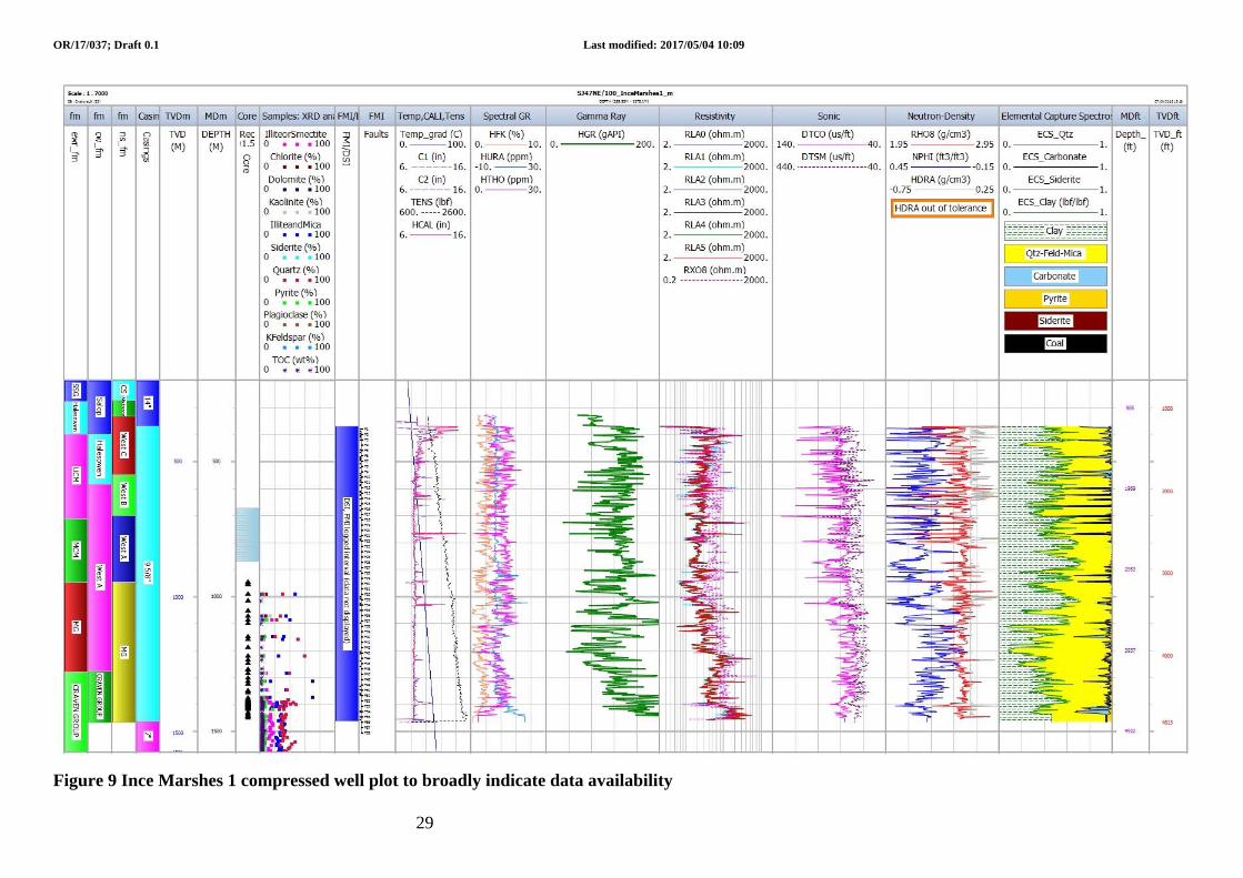
OR/17/037; Draft 0.1 Last modified: 2017/05/04 10:09
29
Figure 9 Ince Marshes 1 compressed well plot to broadly indicate data availability

OR/17/037; Draft 0.1 Last modified: 2017/05/04 10:09
30
Figure 10 Ince Marshes 1 compressed well plot to show data comparisons: (XRD sample analysis vs ECS curves vs interpreted lithological curves)

OR/17/037; Draft 0.1 Last modified: 2017/05/04 10:09
31
Figure 11 Histograms of calculated TOC for the Westphalian A (grey, left) and Millstone Grit (green, right) for Ince Marshes 1.
Figure 12 A cross-plot of measured TOC against calculated TOC in Ince Marshes 1

OR/17/037; Draft 0.1 Last modified: 2017/05/04 10:09
32
Appendix 3 Stratigraphic interpretations Borehole Kemira 1 Ince Marshes Morley Bridge Collinge Hale Lovel's Hall
Easting (m) 347586 346211 346181 341429 347077 347964 Northing (m) 376421 376439 371455 371112 383134 384935
Well top short name and explanation Interpreter NS CW NS CW NS CW NS CW NS CW NS CW OD level Ordnance datum 8.99 8.99 14.33 17.22 14.8 9.79 12.8 Bromsgrove Bromsgrove Sandstone Formation 39 39 Sherwood Sherwood Sandstone Group 281 281
TSZ/?KDM Kidderminster Formation, conglomerate, pebble beds.
523 523 60 30 36
MM/Bold Manchester Marls Formation, Bold Formation
618 618 22 165 91 100
CS Collyhurst Sandstone Formation 738 738 200 56 233 268 165 UVAR Variscan unconformity 1042 1042 272 526 848 557 344 Salop Salop Formation 200 526 848 870 30 344 Halesowen Halesowen Formation 1042 1042 272 398a 700 786b 930 1012c 557 NP 400 Etruria Etruria Formation (ETM) 668 Npe 599 NP
West C Westphalian C. CW lists Pennine Upper Coal Measures Formation (PUCM)
1221 NP 331 NP 675 700g
West B Westphalian B. CW lists Pennine Middle Coal Measures Formation (PMCM)
1248 NP 548 NP 969 1172 1169d 708 NP 741 795h
West A Westphalian A. CW lists Pennine Lower Coal Measures Formation (PLCM)
1401 1079 700 582 1078 1256 745 700f 933.1
MG Millstone Grit Group (MG) 1432 944.9 1124 CRAVEN GP Craven Group 1276 TD Total depth: deepest well penetration depth 1438 1438 1577 1577
WAWK Warwickshire Group (Calculated from depths West B-UVAR)
205.6 276 443 324 151 397
PT Permian-Triassic (Calculated from depths UVAR-top of log depth)
1003.4 272 504 788 527 308
Table 12 Two stratigraphic interpretations for the 2 wells studied and some nearby wells. All depths in metres.
Table notes: NS = Nigel Smith (partly chronostratigraphic), CW = Colin Waters (lithostratigraphic). Blue shading indicates the top of the log, yellow indicates a fault. Table notes by CW: a Base of red beds; b At marked change in GR log & appearance of red beds; c At big change in GR & LD logs & near transition to red beds; d Similar to NS interpretation; e Salop above reddened PMCM; f In part reddened; g Top PUCM at fault at 700m- big change in GR log; h Top PMCM taken at 795m at Cambriense MB. Base West B would be lower.
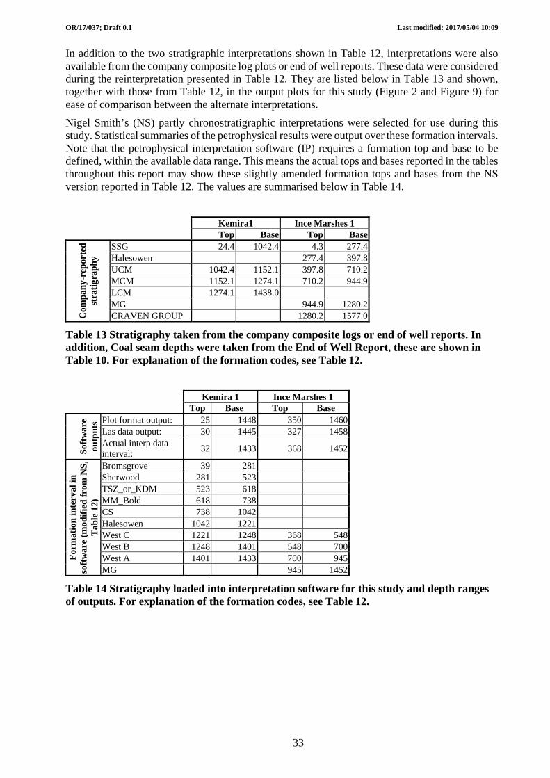
OR/17/037; Draft 0.1 Last modified: 2017/05/04 10:09
33
In addition to the two stratigraphic interpretations shown in Table 12, interpretations were also available from the company composite log plots or end of well reports. These data were considered during the reinterpretation presented in Table 12. They are listed below in Table 13 and shown, together with those from Table 12, in the output plots for this study (Figure 2 and Figure 9) for ease of comparison between the alternate interpretations.
Nigel Smith’s (NS) partly chronostratigraphic interpretations were selected for use during this study. Statistical summaries of the petrophysical results were output over these formation intervals. Note that the petrophysical interpretation software (IP) requires a formation top and base to be defined, within the available data range. This means the actual tops and bases reported in the tables throughout this report may show these slightly amended formation tops and bases from the NS version reported in Table 12. The values are summarised below in Table 14.
Kemira1 Ince Marshes 1
Top Base Top Base
Com
pan
y-re
por
ted
st
rati
grap
hy
SSG 24.4 1042.4 4.3 277.4Halesowen 277.4 397.8UCM 1042.4 1152.1 397.8 710.2MCM 1152.1 1274.1 710.2 944.9LCM 1274.1 1438.0 MG 944.9 1280.2CRAVEN GROUP 1280.2 1577.0
Table 13 Stratigraphy taken from the company composite logs or end of well reports. In addition, Coal seam depths were taken from the End of Well Report, these are shown in Table 10. For explanation of the formation codes, see Table 12.
Kemira 1 Ince Marshes 1
Top Base Top Base
Soft
war
e ou
tput
s Plot format output: 25 1448 350 1460Las data output: 30 1445 327 1458Actual interp data interval:
32 1433 368 1452
For
mat
ion
inte
rval
in
soft
war
e (m
odif
ied
fro
m N
S,
Tab
le 1
2)
Bromsgrove 39 281 Sherwood 281 523 TSZ_or_KDM 523 618 MM_Bold 618 738 CS 738 1042
Halesowen 1042 1221
West C 1221 1248 368 548West B 1248 1401 548 700West A 1401 1433 700 945MG 945 1452
Table 14 Stratigraphy loaded into interpretation software for this study and depth ranges of outputs. For explanation of the formation codes, see Table 12.
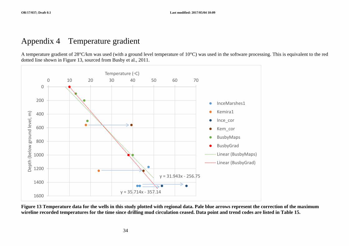
OR/17/037; Draft 0.1 Last modified: 2017/05/04 10:09
34
Appendix 4 Temperature gradient
A temperature gradient of 28°C/km was used (with a ground level temperature of 10°C) was used in the software processing. This is equivalent to the red dotted line shown in Figure 13, sourced from Busby et al., 2011.
Figure 13 Temperature data for the wells in this study plotted with regional data. Pale blue arrows represent the correction of the maximum wireline recorded temperatures for the time since drilling mud circulation ceased. Data point and trend codes are listed in Table 15.
y = 31.943x ‐ 256.75
y = 35.714x ‐ 357.14
0
200
400
600
800
1000
1200
1400
1600
0 10 20 30 40 50 60 70
Dep
th (below ground level, m)
Temperature (◦C)
InceMarshes1
Kemira1
Ince_cor
Kem_cor
BusbyMaps
BusbyGrad
Linear (BusbyMaps)
Linear (BusbyGrad)

OR/17/037; Draft 0.1 Last modified: 2017/05/04 10:09
35
well Depth, m Temp, °C Comments/source InceMarshes1 1453 43.33 FMI run
InceMarshes1 1453 43.33 Comp log header, Pex run, individual field prints used to find time since circ Maximum recorded temp
InceMarshes1 1453 42.22 p20 of geological End of Well Report (EOWR) Maximum recorded temp
InceMarshes1 1175.9 47.5 p9 of geological EOWR flow line
Kemira1 1230.78 23.89 Log header, Density_neutron_run_2.pdf No temp data in run 3 logs to 4708ft. TVD max 6 deg at 4037ft, no survey data reported. Assumed "vertical"
Kemira1 559.61 17.78 Log header, Density_neutron_run_1.pdf
Ince_cor 1453 65.51 Time since circ: 5.45 hrs. 3.30 11th dec to 9.16 11th dec
Simple method: http://www.zetaware. com/utilities/bht/timesince.html
Ince_cor 1453 53.86 Time since circ: 27.5 hrs. 3.30 11dec to 7.00 12dec
Kem_cor 1230.78 45.1 Time since circ: 6hrs 47 mins. 16.00 13 feb to 22:47 13 feb
Kem_cor 559.61 39.4 Time since circ: 6 hrs 13 mins. 19:30 28 jan to 1:43 on 29th Jan
BusbyMaps 100 13 12‐14 contour, Busby et al., 2011
BusbyMaps 200 17 16‐18 contour, Busby et al., 2011
BusbyMaps 500 18.5 17‐20 contour, Busby et al., 2011
BusbyMaps 1000 40 38‐42 contour, Busby et al., 2011
BusbyGrad 0 10 Reported gradient for UK (abstract, Busby et al., 2011)
BusbyGrad 1000 38 Reported gradient for UK (abstract, Busby et al., 2011)
Table 15 Sources of temperature data in Figure 13

OR/17/037; Draft 0.1 Last modified: 2017/05/04 10:09
36
Appendix 5 Technical information for BGS internal use
The technical appendix is for BGS internal use only and not included here. However, for reference, the contents is listed here:
5.1 ANCILLARY INFORMATION AVAILABLE:
1 to 500 scale PDF output logs for each well LAS files for each well containing input and output curves Parameter set IP files (*.set) recording all interpretation parameters
5.2 ANCILLARY INFORMATION AVAILABLE FOR BGS REFERENCE ONLY:
Excel sheet of stratigraphy and petrophysical results BGS tracking: IP set names for source and final data Kemira 1 (SJ47NE/101): source data and load notes Ince Marshes 1 (SJ47NE/100): source data and load notes Ince Marshes 1 (SJ47NE/100) TOC parameter selection and interpretation guide Notes relating to Section 4.1 discussion
References
British Geological Survey holds most of the references listed below, and copies may be obtained via the library service subject to copyright legislation (contact [email protected] for details). The library catalogue is available at: http://geolib.bgs.ac.uk.
BUSBY, J., KINGDON A., AND WILLIAMS, J. 2011. The measured shallow temperature field in Britain. Quarterly Journal of Engineering Geology and Hydrogeology, Vol. 44, 373–387.
GENT, C. M. A., HANNIS, S, D., AND ANDREWS, I. J. 2014. Estimation of total organic carbon in the Jurassic shales of the Weald area by log analysis. Appendix D In: ANDREWS, I. J., 2014. The Jurassic shales of the Weald Basin: geology and shale oil and shale gas resource estimation. British Geological Survey for Department of Energy and Climate Change, London, UK.
HARRIMAN, G. 2011. Ince Marshes-1 VR report Modified.pdf. A GHGeochem Ltd report for iGas.
HOOD. A., GUTJAHR. C. C. M., AND HEACOCK. R. L. 1975. Organic Metamorphism and the Generation of Petroleum. AAPG:Bulletin. 59. 986-996
PASSEY. Q.R, CREANEY. S., KULLA. J. B., MORETTI. F.J. AND STROUD. J.D. 1990, A Practical Model for Organic Richness from Porosity and Resistivity Logs. AAPG Bulletin. 74. 1777-1794
SCHLUMBERGER, 2009. Log Interpretation Charts. 2009 Edition. Available from http://www.slb.com
SERRA, O. 2007.Well logging and reservoir evaluation (Paris: Editions Technip) ISBN 978 2 7108 0881 7
ZETAWARE UTILITIES. Accessed August 2016. BHT correction. Available from http://www.zetaware.com/utilities/bht/timesince.html