Thermodynamic Optimization of Steam Boiler Parameter ...

Innovative Systems Design and Engineering www.iiste.org

ISSN 2222-1727 (Paper) ISSN 2222-2871 (Online)

Vol.6, No.11, 2015

53

Thermodynamic Optimization of Steam Boiler Parameter Using

Genetic Algorithm

Darlington Egeonu *

Chukwumaobi Oluah Patrick Okolo Howard Njoku

Department of Mechanical Engineering, University of Nigeria, Nsukka, Enugu State, Nigeria

Abstract

In this paper, genetic algorithm implemented in Matlab is used for the optimization of the boiler unit at Egbin

power plant. Based on thermodynamic consideration of a boiler, the thermal efficiency of the boiler for 2008 and

2009 is computed. The thermal efficiency is defined as the objective function and is maximized using genetic

algorithms subject to a list of constraints for obtaining the numerical values of the optimum operating

parameters. These determined optimum operating parameters will serve as basis for improving the performance

of the power plant and this is the significance of this study. The effects of genetic algorithm options (such as

initial population, elite children, and crossover ratio) on the optimization results are also established. It is

observed that applying genetic algorithm in the thermodynamic optimization of a case study (Egbin power plant)

boiler, the percentage increase in the thermal efficiency is 4.76% and 3.89% in comparison with the existing

values for the studied boiler at Egbin thermal power plant for 2008 and 2009 respectively.

Keywords: Thermodynamics, Optimization, Genetic Algorithm, Steam Boiler, Power Plant.

1.0 INTRODUCTION

Thermodynamic optimization is primarily concerned with determining the thermodynamically

optimum size or operating regime of a certain engineering system, ‘optimum’ here means the

condition in which the system loses the least power while still performing its fundamental

engineering function (Buljubasic and Delalic, 2008). It turns out that in many systems,

various mechanisms and design features that account for irreversibility compete with one

another. Accordingly, the thermodynamic optimization of interest here is the operating

condition of a steam boiler that will yield the best thermal efficiency of the boiler.

A steam boiler in its original meaning is a pressurized system in which thermal energy,

resulting from combustion of organic fuels, is transferred through heat surfaces to a working

fluid which evaporates in the system with the steam further overheated to a certain

temperature, steam under pressure is then usable for transferring the heat to a process.

The basic element of a steam boiler is furnace, in which fuel combustion takes place in

presence of oxygen, usually from air, releasing energy of a chemical reaction which raises

enthalpy of a heat receiver to a level suitable for transferring the heat to a heat exchanger

surface. In other elements of a steam boiler, flue gas is being cooled giving heat to heat

further receivers through heat surfaces. Those elements are: economizers, evaporators, steam

super-heaters and reheaters as well as air heaters. The most common working fluid (heat

receiver) is water which evaporates in the boiler, and is being further over heated so the final

brought to you by COREView metadata, citation and similar papers at core.ac.uk

provided by International Institute for Science, Technology and Education (IISTE): E-Journals

https://core.ac.uk/display/234643827?utm_source=pdf&utm_medium=banner&utm_campaign=pdf-decoration-v1



Vol.6, No.11, 2015

54

product is saturated or super-heated steam (Buljubasic and Delalic, 2008).

The performance parameters of boiler, like efficiency and evaporation ratio reduces with time

due to poor combustion, heat transfer surface fouling and poor operation and maintenance.

Even for a new boiler, reasons such as deteriorating fuel quality, water quality etc. can result

in poor boiler performance. Most power plants have highly nonlinear dynamics with

numerous uncertainties. However, no mathematical model can exactly describe such a

complicated physical process, and there will always be modeling errors due to un-modeled

dynamics and parametric uncertainties (Weng et al., 1996).

To properly characterize the essential dynamic behavior of power plants with accurate

representation of plant components/parts, detailed models are needed (Maffezzoni, 1997).

Besides, detailed modeling of plants dynamics is often not efficient for control synthesis.

There are complicated models based on finite element approximations to partial differential

equations. These models are in the form of large simulation codes for plant design, simulators

and commissioning. However, they are not normally used in control design approach because

of their complexity (Astrom and Bell, 2000).

The analytical plant model can be formulated based on the fundamental laws of physics such

as mass conservation, momentum, and energy semi-empirical laws for heat transfer and

thermodynamics state conversion (Astrom and Bell, 2000). In order to build such analytical

models, it is necessary to define their parameters with respect to boundaries, inputs, and

outputs. Generally, the developed models need to be tuned by performing tests to validate for

steady state and transient responses (Lu and Hogg, 2000; De Mello, 1991).

When the identified model for system component is nonlinear in the parameters, using

conventional methods like standard least squares technique will not provide superior results.

In these cases, evolutionary algorithm based methodologies are investigated as potential

solutions to obtain good estimation of the model parameters (Horst et al., 2000). Genetic

algorithms have an advantage that it does not require a complete system model and can be

employed to globally search for the optimal solution (Borsi, 1974).



Vol.6, No.11, 2015

55

In this paper, energy analysis will be used to determine the thermal efficiency of steam boiler

and optimize it using genetic algorithm with Egbim power plant as a case study.

1.1 GENETIC ALGORITHMS (GAs)

The GAs is a stochastic global search method that mimics the metaphor of natural biological

evolution (Gen and Cheng, 2000). GAs operate on a population of potential solutions

applying the principle of survival of the fittest to produce (hopefully) better and better

approximations to a solution. At each generation, a new set of approximations is created by

the process of selecting individuals according to their level of fitness in the problem domain

and breeding them together using operators borrowed from natural genetics. This process

leads to the evolution of populations of individuals that are better suited to their environment

than the individuals that they were created from, just as in natural adaptation.

Genetic Algorithms is an optimization technique that is based on the evolution theory. Instead

of searching for a solution to a problem in the "state space" (like the traditional search

algorithms do), a GA works in the "solution space" and builds (or better, "breeds") new,

hopefully better solutions based on existing ones (Haupt and Haupt, 2004).

The general idea behind GAs is that we can build a better solution if we somehow combine

the "good" parts of other solutions (schemata theory), just like nature does by combining the

DNA of living beings.

Individuals, or current approximations, are encoded as strings, chromosomes, composed over

some alphabet(s), so that the genotypes (chromosome values) are uniquely mapped onto the

decision variable (phenotypic) domain. The most commonly used representation in GAs is the

binary alphabet {0, 1} although other representations can be used, e.g. ternary, integer, real-

valued etc.

The search process will operate on the encoding of the decision variables, rather than the

decision variables themselves, except, where real-valued genes are used.

Having decoded the chromosome representation into the decision variable domain, it is

possible to assess the performance, or fitness, of individual members of a population. This is

done through an objective function that characterizes an individual’s performance in the

problem domain. In the natural world, this would be an individual’s ability to survive in its

present environment. Thus, the objective function establishes the basis for selection of pairs of

individuals that will be mated together during reproduction.



Vol.6, No.11, 2015

56

During the reproduction phase, each individual is assigned a fitness value derived from its raw

performance measure given by the objective function. This value is used in the selection to

bias towards more fit individuals. Highly fit individuals, relative to the whole population,

have a high probability of being selected for mating whereas less fit individuals have a

correspondingly low probability of being selected.

Once the individuals have been assigned a fitness value, they can be chosen from the

population, with a probability according to their relative fitness, and recombined to produce

the next generation. Genetic operators manipulate the characters (genes) of the chromosomes

directly, using the assumption that certain individual’s gene codes, on average, produce fitter

individuals. The recombination operator is used to exchange genetic information between

pairs, or larger groups, of individuals. The simplest recombination operator is that of single-

point crossover. A further genetic operator, called mutation, is subsequently applied to the new

chromosomes. Mutation causes the individual genetic representation to be changed according

to some probabilistic rule. In the binary string representation, mutation will cause a single bit

to change its state, 0 ⇒ 1 or 1 ⇒ 0. Mutation is generally considered to be a background

operator that ensures that the probability of searching a particular subspace of the problem

space is never zero. This has the effect of tending to inhibit the possibility of converging to a

local optimum, rather than the global optimum.

After recombination and mutation, the individual strings are then, if necessary, decoded, the

objective function evaluated, a fitness value assigned to each individual and individuals

selected for mating according to their fitness, and so the process continues through subsequent

generations. In this way, the average performance of individuals in a population is expected to

increase, as good individuals are preserved and bred with one another and the less fit

individuals die out. The GA is terminated when some criteria are satisfied, e.g. a certain

number of generations, a mean deviation in the population, or when a particular point in the

search space is encountered. A flow chart of the operations of genetic algorithm is shown in

figure 1.



Vol.6, No.11, 2015

57

Generate the initial population,

creating random fixed size string

Termination criterion satisfied ?Display best

answer

End

Applying selection and reproduction

operator to create a new population

Apply objective function and fitness

measure

Apply the crossover operator to the

pairs of strings of the new population

Apply the mutation operator to each

string of the new population

Replace the old population with the

Newly created population

NO

YES

Figure 1: GENETIC ALGORITHMS FLOW CHART (Hassanein, Aly and Abo-Ismail,

2012).

1.2 CASE STUDY DESCRIPTION

This study is on the steam boiler of a 220MW steam power plant which converts the feed

water at temperature 204oC to superheated steam at pressure 12,990 kPa and temperature

541oC, and also converts cold reheat steam to hot reheat steam at pressure 3,398 kPa and

temperature 541oC. The steam boiler, shown in figure 2, comprises the following major

elements: Burners (B), furnace (F), secondary super heater (SSH), primary super heater

(PSH), re-heater (RH), drum (D), economizer (ECO) and air heater (AH). The burners are

dual fuel firing as they could operate on HPFO (high pour fuel oil), LPFO (low pour fuel oil),

or gas. They are of three levels; A, B & C, LEVELS A&C has six burners each while level B

has three burners .The Water enters at ECO where it is heated at temperatures below the

boiling point. Heated water is sent to D of which any steam formed is removed by the hydro-

cyclone separators in the drum. Heated water then flows to F through down-comers by natural



Vol.6, No.11, 2015

58

circulation where water turns into steam. The steam water mixture rises into a steam boiler

drum where water separates from steam (by cyclone separators) and generation of dry

saturated steam is ensured by passing the steam through knockout drums and scrubbers. Dry

saturated steam then moves to primary super heater and then to the secondary super heater,

from that point superheated steam at 12,990kPa and 541oC leaves the steam boiler to High

pressure turbine. Cold reheat steam leaves the high pressure turbine back to the boiler re-

heater (RH) and leaves the boiler as hot reheat steam at 3,398kPa and 541oC to the

intermediate pressure turbine. Steam leaves intermediate pressure turbine to low pressure

turbine from where it moves to the condenser where it condensed to water at very low

pressure. Make up water is now added to the condensed water (when necessary) which passes

through series of low pressure heaters, de-aerator, boiler feed pump, high pressure heaters and

then moves back to the economizer.

The schematics of the boiler and the flow diagram of the plant are shown in figure 2 below.

Figure 2: Schematics of Boiler Unit (Source: Egbin Power Plant Catalogue, 1985)

2.0 ANALYSIS

In this study, two years (2008-2009) daily operational data of Egbin power plant was

collected and used in the analysis and optimization of steam boiler using genetic algorithm

tool box in Matlab.

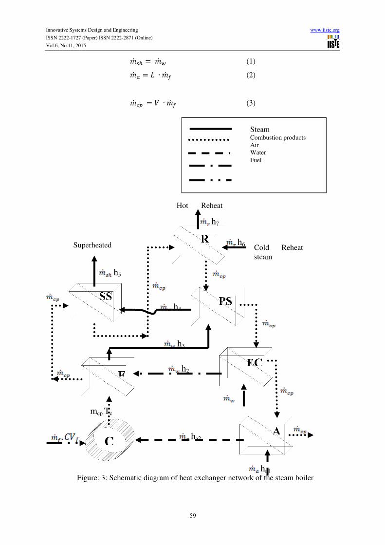
The mathematical representation of the mass and energy flow consists of a set of equations.

Figure 3 shows the heat exchanger network used to model the energy system of the steam

boiler of figure 2.

2.1 MASS AND ENERGY FLOWS:

Mass balance of the mathematical model of the system is as follows:



Vol.6, No.11, 2015

59

�� (1)

�� ∙ �� (2)

�� ∙ �� (3)

h4

h7

Hot Reheat

steam

h6

h2

ha1

ha2

mcp Tc

h5

h3

PS

EC

A

R

SS

F

C

Superheated

steam Cold Reheat

steam

Steam Combustion products

Air

Water

Fuel

Figure: 3: Schematic diagram of heat exchanger network of the steam boiler



Vol.6, No.11, 2015

60

Where

�� [kg/s] is the mass flow of water or steam, �� [kg/s] is the mass flow of air, �� [kg/s] is

the mass flow of reheat steam, L [kg/kg] is the mass of air required for combustion products

for 1 kg of fuel, �� [kg/s] is the consumption of fuel, �� [kg/s] is the mass flow of

combustion products, V [kg/kg] is the mass of combustion products for 1 kg of fuel, ��

[kg/s] is the mass flow of steam at a superheater exit, �� [kJ/kg] is the heating value of the

fuel,

Equation (2) presents the mass balance of air for combustion; Equation (3) presents mass

balance of product of combustion.

Energy balance of the mathematical model of the system is as follows:

Furnace F:

�� . �� − � �� (h� − h�) (4)

SSH : (pressure = 12990kPa)

�� . �� − � �� (h� − h�) (5)

RH : (pressure = 3398kPa)

�� . �� − � �� (h� − h ) (6)

PSH :

�� . �� − � �� (h� − h�) (7)

Economizer , Eco:

�� . �� − � �� (h� − h�) (8)

Air heater, AH

�� . �� − � �� (h!� − h!�) (9)

The constraints of the mathematical model are given by the following equations

� > � ��; � � > � ��; � �� > � ��; � �� > � ��; � �� > � ��; � �� > � �� (10)

where �� [J/kgK] is the specific heat of combustion products, � [K] is the temperature of

combustion, � �$[K] is the temperature of combustion products, ��[K] is the temperature of

cold air, ��[K] is the temperature of heated air, ℎ�[kJ/kg] is the specific enthalpy of heated

water, ℎ� [kJ/kg] is the specific enthalpy of saturated steam, ℎ� [kJ/kg] is the specific

enthalpy of superheated steam at exit of the steam boiler and temperatures of water and steam

at actual place of the steam boiler.

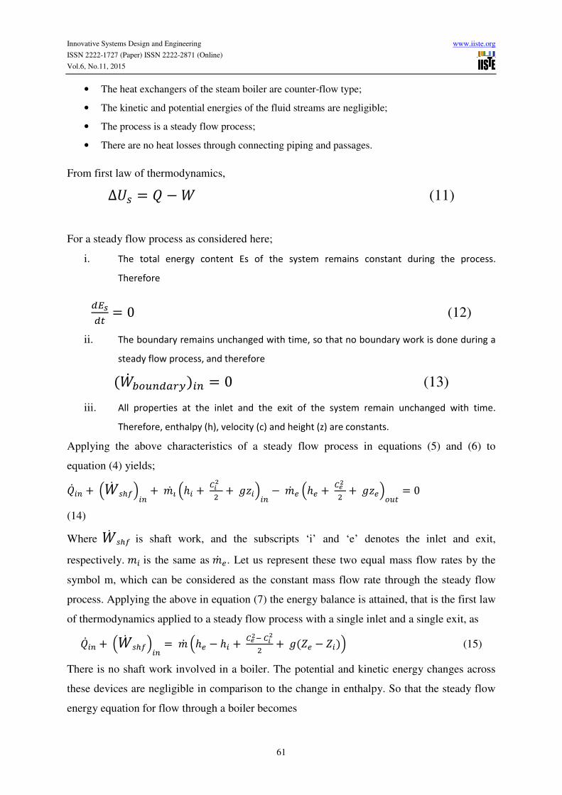
In order to determine the efficiency of the boiler, the following assumptions were made:



Vol.6, No.11, 2015

61

• The heat exchangers of the steam boiler are counter-flow type;

• The kinetic and potential energies of the fluid streams are negligible;

• The process is a steady flow process;

• There are no heat losses through connecting piping and passages.

From first law of thermodynamics,

∆'� � ( −) (11)

For a steady flow process as considered here;

i. The total energy content Es of the system remains constant during the process.

Therefore

*+,*- � 0 (12)

ii. The boundary remains unchanged with time, so that no boundary work is done during a

steady flow process, and therefore

()� /012*�3)$2 � 0 (13)

iii. All properties at the inlet and the exit of the system remain unchanged with time.

Therefore, enthalpy (h), velocity (c) and height (z) are constants.

Applying the above characteristics of a steady flow process in equations (5) and (6) to

equation (4) yields;

(� $2 +5)� ��6$2 +�7� 5ℎ$ +89:� + ;<$6$2 −�� = 5ℎ= +

8>:� + ;<=601- � 0

(14)

Where )� �� is shaft work, and the subscripts ‘i’ and ‘e’ denotes the inlet and exit,

respectively. �$ is the same as �� =. Let us represent these two equal mass flow rates by the

symbol m, which can be considered as the constant mass flow rate through the steady flow

process. Applying the above in equation (7) the energy balance is attained, that is the first law

of thermodynamics applied to a steady flow process with a single inlet and a single exit, as

(� $2 +5)� ��6$2 �� 5ℎ= − ℎ$ +8>:?89:� + ;(@= − @$)6 (15)

There is no shaft work involved in a boiler. The potential and kinetic energy changes across

these devices are negligible in comparison to the change in enthalpy. So that the steady flow

energy equation for flow through a boiler becomes



Vol.6, No.11, 2015

62

(� � �� (ℎ= − ℎ$)

(16)

ABCDEFGHHCICEJIK � L=-M1-�1-L=-N2�1- (17)

Where heat input (Qin) is the heat supplied by the fuel and heat output (Qout) is the heat gained

by water and steam.

O � PQRSP9T (18)

Which can be written as

O � �� (ℎE−ℎC)U� V×8XV (19)

Applying these to our case study boiler

O � U� ,Y(�Z?�[)\U� ](�^?�_)U� V×8XV

(20)

2.2 Genetic Algorithm Optimization

For the thermodynamic optimization, the objective function which is to be maximized is the

thermal efficiency of the steam boiler given by

E = -((x(1)*(x(2)- x(3))) + (x(4)*(x(5)- x(6))))/ (x(7) * x(8)) (21)

Subject to the following constraints:

For 2008 data;

x(5) > x(6), x(2) > x(3), x(5) > x(1); 174.3 ≤ x(1) ≤ 174.3;

3386 ≤ x(2) ≤ 3449; 599.2 ≤ x(3) ≤ 1085; 157.7 ≤ x(4) ≤ 157.7;

3489 ≤ x(5) ≤ 3550; 3166 ≤ x(6) ≤ 3166; 11.94 ≤ x(7) ≤ 12.5;

48851.036 ≤ x(8) ≤ 48851.036

(22)



Vol.6, No.11, 2015

63

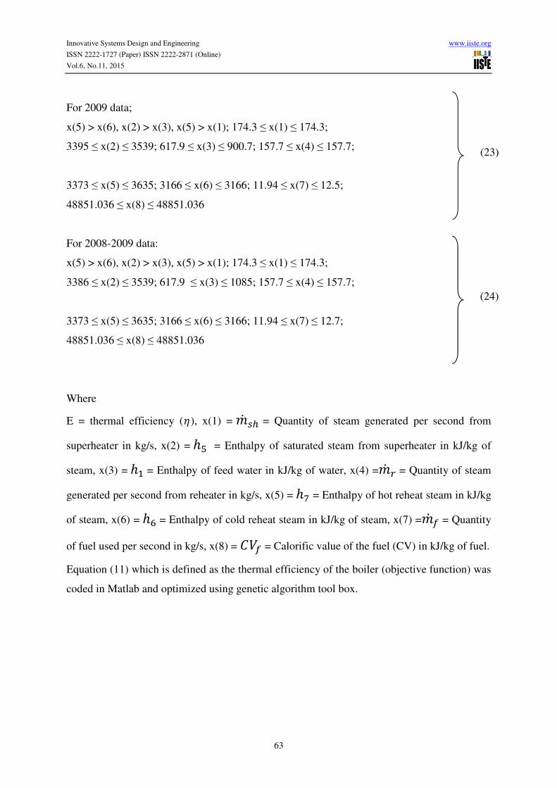
For 2009 data;

x(5) > x(6), x(2) > x(3), x(5) > x(1); 174.3 ≤ x(1) ≤ 174.3;

3395 ≤ x(2) ≤ 3539; 617.9 ≤ x(3) ≤ 900.7; 157.7 ≤ x(4) ≤ 157.7;

3373 ≤ x(5) ≤ 3635; 3166 ≤ x(6) ≤ 3166; 11.94 ≤ x(7) ≤ 12.5;

48851.036 ≤ x(8) ≤ 48851.036

For 2008-2009 data:

x(5) > x(6), x(2) > x(3), x(5) > x(1); 174.3 ≤ x(1) ≤ 174.3;

3386 ≤ x(2) ≤ 3539; 617.9 ≤ x(3) ≤ 1085; 157.7 ≤ x(4) ≤ 157.7;

3373 ≤ x(5) ≤ 3635; 3166 ≤ x(6) ≤ 3166; 11.94 ≤ x(7) ≤ 12.7;

48851.036 ≤ x(8) ≤ 48851.036

Where

E = thermal efficiency (O), x(1) = �� = Quantity of steam generated per second from

superheater in kg/s, x(2) = ℎ� = Enthalpy of saturated steam from superheater in kJ/kg of

steam, x(3) = ℎ� = Enthalpy of feed water in kJ/kg of water, x(4) =�� = Quantity of steam

generated per second from reheater in kg/s, x(5) = ℎ = Enthalpy of hot reheat steam in kJ/kg

of steam, x(6) = ℎ� = Enthalpy of cold reheat steam in kJ/kg of steam, x(7) =�� = Quantity

of fuel used per second in kg/s, x(8) = �� = Calorific value of the fuel (CV) in kJ/kg of fuel.

Equation (11) which is defined as the thermal efficiency of the boiler (objective function) was

coded in Matlab and optimized using genetic algorithm tool box.

(23)

(24)



Vol.6, No.11, 2015

64

3.0 RESULTS / DISCUSSION

3.1 RESULTS

Thermal efficiency of the boiler for the 365 days of years 2008 and 2009 has been calculated

using equation (10) and the results plotted (see figures 4 and 5 respectively). From the plot of

Variation of Thermal Efficiency with Days shown in figures 4 and 5 respectively, the

maximum thermal efficiencies are 86.8% (on the 90th

day) and 87.67% (on the 216th

day),

while the average thermal efficiencies are 78% and 84.32% .

Figure 4: Variation of Thermal Efficiency with Days for 2008

Figure 5: Variation of Thermal Efficiency with Days for 2009



Vol.6, No.11, 2015

65

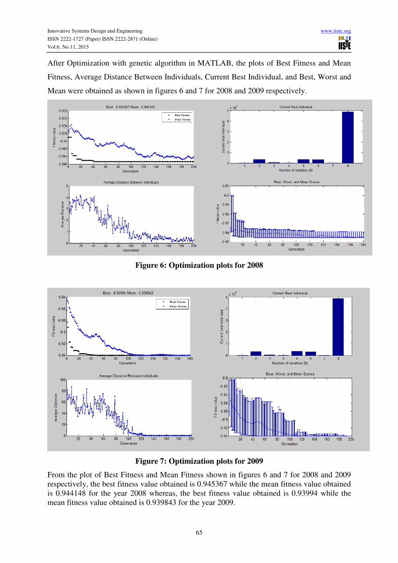
After Optimization with genetic algorithm in MATLAB, the plots of Best Fitness and Mean

Fitness, Average Distance Between Individuals, Current Best Individual, and Best, Worst and

Mean were obtained as shown in figures 6 and 7 for 2008 and 2009 respectively.

Figure 6: Optimization plots for 2008

Figure 7: Optimization plots for 2009

From the plot of Best Fitness and Mean Fitness shown in figures 6 and 7 for 2008 and 2009

respectively, the best fitness value obtained is 0.945367 while the mean fitness value obtained

is 0.944148 for the year 2008 whereas, the best fitness value obtained is 0.93994 while the

mean fitness value obtained is 0.939843 for the year 2009.



Vol.6, No.11, 2015

66

From the plot of Average Distance Between Individuals for 2009 shown in figure 7, the

overall average distance between individuals is 88, it decreases as optimization progresses.

The average distance between successive individuals decrease and increase as optimization

progresses, it is approximately zero from 130th

generation. From the plot of Average Distance

Between Individuals for 2008 shown in figure 6, the overall average distance between

individuals is 4.5, it follows similar trend as that of figure 7.

From the plot of Best, Worst and Mean scores shown in figure 6 and 7, there is an

improvement in all the scores as the optimization progresses, the difference between the best

score and the worst score is also reduced for both plots. The scores are approximately equal as

optimum point is reached at about 195th

generation for 2009 while the difference is negligible

for 2008.

Figures 6 and 7 for 2008 and 2009 respectively; show a plot of Current Best Individual, which

is the best individual after optimization. The best individual could be said to be a vector

whose length is the number of variables (or chromosomes) in the problem, applying the

fitness function to the best individual results to the score of the best individual which is the

value of the best fitness function. The best individual varies as optimization progresses. The

genes (vector entries) and score of the best individual are recorded in tables 1 and 3.

Tables 1 and 3 show a comparison of results, for 2008 & 2009 respectively, between values of

decision variables before and after optimization, the optimized values of decision variables

are based on the GA parameter values.

Table 1: Comparison of Results Between Values of Decision Variables Before and After

Optimization for 2008

Variables

Before Optimization After Optimization

Average Maximum Mean Best

x(1) �� (kg/s) 174.3 174.3 174.3 174.3

x(2) ℎ� (kJ/kg) 3423.81 3423 3433.13 3433.13

x(3) ℎ� (kJ/kg) 966.37 655.5 559.20 559.20

x(4) �� (kg/s) 157.7 157.7 157.7 157.7

x(5) ℎ (kJ/kg) 3522.15 3522 3533.018 3533.02

x(6) ℎ� (kJ/kg) 3166.0 3166.0 3166.0 3166.0

x(7) �� (kg/s) 12.7 12.7 12.7 12.7

x(8) �� (kj/kg) 48851.036 48851.036 48851.036 48851.036

E Η 0.78 0.868 0.944148 0.945367

The enthalpy values have been converted to temperatures at operating pressures for optimized

mean values and shown in Table 2;



Vol.6, No.11, 2015

67

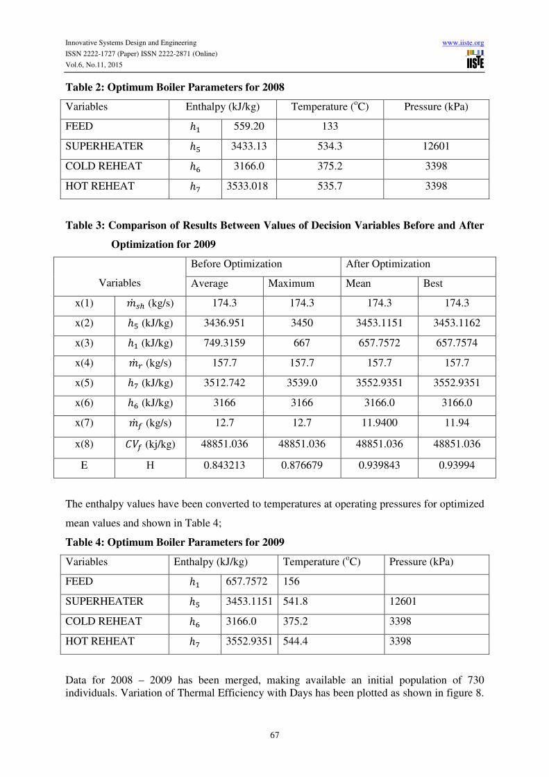
Table 2: Optimum Boiler Parameters for 2008

Variables Enthalpy (kJ/kg) Temperature (oC) Pressure (kPa)

FEED ℎ� 559.20 133

SUPERHEATER ℎ� 3433.13 534.3 12601

COLD REHEAT ℎ� 3166.0 375.2 3398

HOT REHEAT ℎ 3533.018 535.7 3398


Optimization for 2009

Variables


Average Maximum Mean Best

x(1) �� (kg/s) 174.3 174.3 174.3 174.3

x(2) ℎ� (kJ/kg) 3436.951 3450 3453.1151 3453.1162

x(3) ℎ� (kJ/kg) 749.3159 667 657.7572 657.7574

x(4) �� (kg/s) 157.7 157.7 157.7 157.7

x(5) ℎ (kJ/kg) 3512.742 3539.0 3552.9351 3552.9351

x(6) ℎ� (kJ/kg) 3166 3166 3166.0 3166.0

x(7) �� (kg/s) 12.7 12.7 11.9400 11.94

x(8) �� (kj/kg) 48851.036 48851.036 48851.036 48851.036

E Η 0.843213 0.876679 0.939843 0.93994

The enthalpy values have been converted to temperatures at operating pressures for optimized

mean values and shown in Table 4;

Table 4: Optimum Boiler Parameters for 2009


FEED ℎ� 657.7572 156

SUPERHEATER ℎ� 3453.1151 541.8 12601

COLD REHEAT ℎ� 3166.0 375.2 3398

HOT REHEAT ℎ 3552.9351 544.4 3398

Data for 2008 – 2009 has been merged, making available an initial population of 730

individuals. Variation of Thermal Efficiency with Days has been plotted as shown in figure 8.



Vol.6, No.11, 2015

68

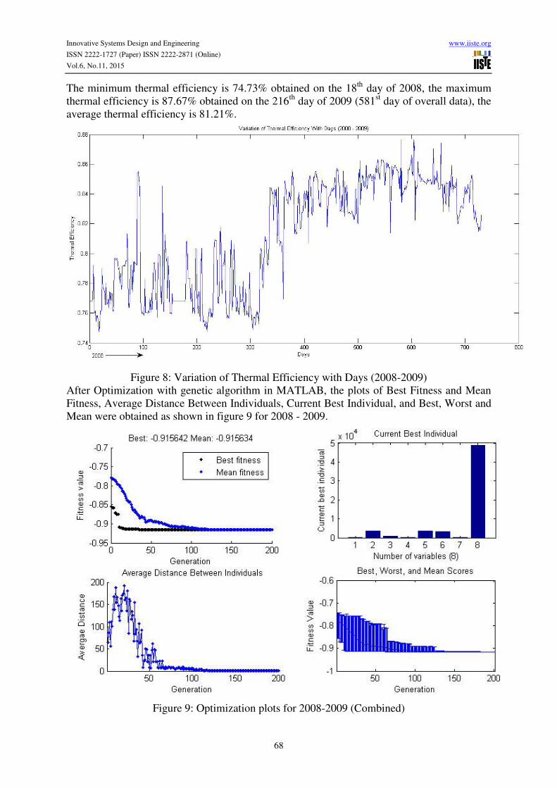
The minimum thermal efficiency is 74.73% obtained on the 18th

day of 2008, the maximum

thermal efficiency is 87.67% obtained on the 216th

day of 2009 (581st day of overall data), the

average thermal efficiency is 81.21%.

Figure 8: Variation of Thermal Efficiency with Days (2008-2009)

After Optimization with genetic algorithm in MATLAB, the plots of Best Fitness and Mean

Fitness, Average Distance Between Individuals, Current Best Individual, and Best, Worst and

Mean were obtained as shown in figure 9 for 2008 - 2009.

Figure 9: Optimization plots for 2008-2009 (Combined)



Vol.6, No.11, 2015

69

From the plot of Best Fitness and Mean Fitness shown in figure 9, the best fitness value

obtained is 0.915642 while the mean fitness value obtained is 0.915634.

From the plot of Average Distance Between Individuals shown in figure 9, the overall average

distance between individuals is 200 and reduces to 60 from the 42nd

generation, it decreases as

optimization progresses. The average distance between successive individuals decrease as

optimization progresses, it is approximately zero from 120th

generation.

From the plot of Best, Worst and Mean scores shown in figure 9, there is an improvement in

all the scores as the optimization progresses, the difference between the best score and the

worst score is also reduced. The scores are approximately equal as optimum point is reached

at about 190th

generation.

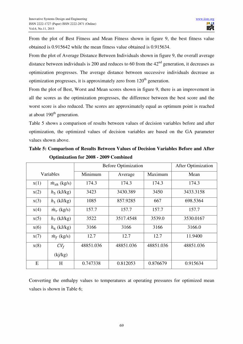
Table 5 shows a comparison of results between values of decision variables before and after

optimization, the optimized values of decision variables are based on the GA parameter

values shown above.


Optimization for 2008 - 2009 Combined

Variables


Minimum Average Maximum Mean

x(1) �� (kg/s) 174.3 174.3 174.3 174.3

x(2) ℎ� (kJ/kg) 3423 3430.389 3450 3433.3158

x(3) ℎ� (kJ/kg) 1085 857.9285 667 698.5364

x(4) �� (kg/s) 157.7 157.7 157.7 157.7

x(5) ℎ (kJ/kg) 3522 3517.4548 3539.0 3530.0167

x(6) ℎ� (kJ/kg) 3166 3166 3166 3166.0

x(7) �� (kg/s) 12.7 12.7 12.7 11.9400

x(8) ��

(kj/kg)

48851.036 48851.036 48851.036 48851.036

E Η 0.747338 0.812053 0.876679 0.915634

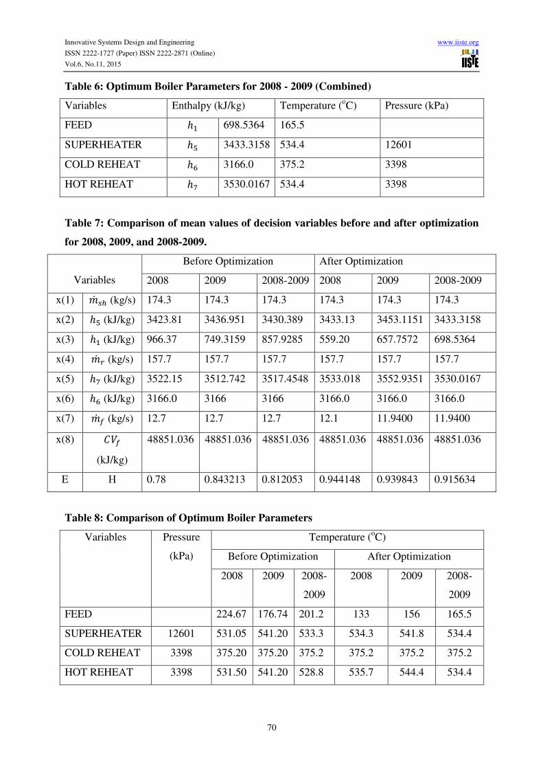
Converting the enthalpy values to temperatures at operating pressures for optimized mean

values is shown in Table 6;



Vol.6, No.11, 2015

70

Table 6: Optimum Boiler Parameters for 2008 - 2009 (Combined)


FEED ℎ� 698.5364 165.5

SUPERHEATER ℎ� 3433.3158 534.4 12601

COLD REHEAT ℎ� 3166.0 375.2 3398

HOT REHEAT ℎ 3530.0167 534.4 3398

Table 7: Comparison of mean values of decision variables before and after optimization

for 2008, 2009, and 2008-2009.

Variables


2008 2009 2008-2009 2008 2009 2008-2009

x(1) �� (kg/s) 174.3 174.3 174.3 174.3 174.3 174.3

x(2) ℎ� (kJ/kg) 3423.81 3436.951 3430.389 3433.13 3453.1151 3433.3158

x(3) ℎ� (kJ/kg) 966.37 749.3159 857.9285 559.20 657.7572 698.5364

x(4) �� (kg/s) 157.7 157.7 157.7 157.7 157.7 157.7

x(5) ℎ (kJ/kg) 3522.15 3512.742 3517.4548 3533.018 3552.9351 3530.0167

x(6) ℎ� (kJ/kg) 3166.0 3166 3166 3166.0 3166.0 3166.0

x(7) �� (kg/s) 12.7 12.7 12.7 12.1 11.9400 11.9400

x(8) ��

(kJ/kg)

48851.036 48851.036 48851.036 48851.036 48851.036 48851.036

E Η 0.78 0.843213 0.812053 0.944148 0.939843 0.915634

Table 8: Comparison of Optimum Boiler Parameters

Variables Pressure

(kPa)

Temperature (oC)


2008 2009 2008-

2009

2008 2009 2008-

2009

FEED 224.67 176.74 201.2 133 156 165.5

SUPERHEATER 12601 531.05 541.20 533.3 534.3 541.8 534.4

COLD REHEAT 3398 375.20 375.20 375.2 375.2 375.2 375.2

HOT REHEAT 3398 531.50 541.20 528.8 535.7 544.4 534.4



Vol.6, No.11, 2015

71

3.2 DISCUSSION

Before GA is used as an optimizing tool, the problem above has to be modeled in MATLAB

and a script (M-file) is written to represent the objective function of the problem together with

all other governing equations. Once this is done, it is a matter of calling up the M-file with

GA to begin the optimization.

In the optimization plots for 2009, the algorithm generates the best individual that it can,

using the genes at generation number 50, where the best fitness plot becomes level. After this,

it creates new copies of the best individual, which are then are selected for the next

generation. By generation number 170, all individuals in the population are the same, namely;

the best and mean individual. When this occurs, the average distance between individuals is 0.

Since the algorithm cannot improve the best fitness value after generation 170, it stalls after

30 more generations, because generation is set to 200.

From the curve of Best Fitness and Mean Fitness, as the number of generations increase, the

mean fitness converges to the best fitness, this shows that optimization is actually taking

place. It could also be seen that the best fitness is also reduced.

From the plot of average distance between individuals, it is obvious that the population

converges, since the average distance between individuals in terms of the fitness is

reduced, as the generations pass. This is a measure of the diversity of a population. With the

average distance between individuals much lower in 2008, gotten with a reduced elite count

and increased mutation in the GA options as compared with those of 2009, it is evident that

the results of optimization for 2008 is better than that obtained for 2009.

From table 1, the thermal efficiency at optimum condition is 94.54% indicating a 16.54%

improvement, compared to the existing mean operating value 78%%.


improvement, compared to the existing mean operating value 84.32%.

Combining the data for 2008 and 2009 provides a larger initial population, its effect is seen as

the optimization plots for 2009-2009 is analyzed and compared with the previous plots.


improvement, compared to the existing mean operating value 81.21%, and a 3.7% increase,

compared to the existing maximum operating value of 87.67%.

From table 8, the superheat temperature and hot reheat temperature are equal (534.4OC) only

for 2008-2009 optimized data, this can also be seen in the raw data for 2009 and 2009 as it is

the design specification for the boiler. With these analysis and comparisons, it is evident that



Vol.6, No.11, 2015

72

the optimization for 2008-2009 is the best of the three optimized data (i.e. 2008, 2009, and

2008-2009).

GA can work in many ways depending on how the objective function, constraints and GA

options are defined in the program. In the thermodynamic optimization of steam boiler, the

objective function is defined in equation (21), the constraints are defined in equations (22-24),

while Genetic Algorithm options as set in GA toolbox in MATLAB for the results obtained

are detailed below.

GA OPTIONS

The optimization of the steam boiler with GA was done with the following GA options:

For 2009 data:

Population size: 200; Initial range: [0.82;0.92]; Scaling function : Rank;

Selection function: Uniform; Elite count: 5; Crossover fraction: 0.5;

Mutation function: Constraint dependent; Crossover function: Scattered

Generations: 200; Stall generation: 200.

For 2008 and 2008-2009 data:

Same as those for 2009 data with the following changes:

Elite count: 2; Crossover fraction: 0.8.

4.0 CONCLUSION

Efficiency increase and pollutant emission control are the most significant projects of the

world. In the present investigation, an optimization has been done to one of the boilers in

Egbin steam power plant to increase boiler efficiency. Ensuring that the operation of a steam

turbine power plant is at an optimum level is rather complicated. There are too many factors

to be considered and a wrong decision might increase the cost of operation. It has been

demonstrated that genetic algorithm (GA) can be successfully implemented as an optimization

tool for a boiler unit in a steam turbine power plant.

For 2008 and 2009 the average thermal efficiency of the boiler has been determined to be

78% and 84.32% respectively, while the maximum thermal efficiency was calculated to be

86.8% and 87.67% respectively as shown in the plot of Variation of Thermal Efficiency with

Days (figures 1 and 2).

It has been established that increasing the initial population, reducing the number of elite

children and increasing the crossover fraction increases the probability of getting a more

accurate result of optimization using genetic algorithm.



Vol.6, No.11, 2015

73

After optimization with genetic algorithm, the mean fitness value obtained for 2008-2009 was

91.56%. The individual with this mean fitness value, whose chromosomes are

(�� , ℎ�, ℎ�, �� , ℎ , ℎ�, �� , ��), has genes (174.3, 3433.3158, 698.5364, 157.7, 3530.0167,

3166.0, 11.94, 48851.04).

From the above it is evident that if the boiler is operated at �� = 174.3kg/s, feed temperature

= 165.5OC, superheat temperature/pressure = 534.4

OC/12601kPa, cold reheat

temperature/pressure = 375.2OC/3398kPa, and hot reheat temperature/pressure =

534.4OC/3398kPa, �� = 157.7kg/s, �� = 11.94kg/s, �� = 48851.04kJ/kg, its thermal

efficiency would be 91.56% which amounts to 4.76% and 3.89% increase in boiler thermal

efficiency compared to maximum thermal efficiency obtained in 2008 and 2009 respectively.

It is recommended that future research should use hybrid models to optimize power plants.

Genetic algorithm together with artificial neural network should be used in power plant

modeling and optimization.

REFERENCES

Astrom, K.J. and Bell, R. D. (2000) Drum-Boiler Dynamics, Journal of Automatica. vol. 36

(3), pp.363-378.

Borsi, L. (1974) Extended Linear Mathematical Model of a Power Station Unit with a Once-

Through Boiler, Siemens Forschungs und Entwicklingsberichte, vol. 3 (5), pp. 274-280.

Buljubašić, I. and Delalić, S. (2008). Improvement of steam boiler plant efficiency based

on results of on-line performance monitoring. Tehnički vjesnik, 15(3), 29-33.

De Mello, F. P. (1991) Boiler Models for System Dynamic PerformanceStudies, IEEE

Transaction on Power Systems, vol. 6 (1), pp. 66-74.

Gen, M. and Cheng, R. (2000). Genetic algorithms and engineering optimization (Vol. 7).

John Wiley & Sons.

Hassanein, O. I. Aly, A. A. and Abo-Ismail, A. A. (2012). Parameter tuning via genetic

algorithm of fuzzy controller for fire tube boiler. International Journal of Intelligent

Systems and Applications (IJISA), 4(4), 9.

Haupt, R. L., & Haupt, S. E. (2004). Practical genetic algorithms. John Wiley & Sons.

Horst, R., Pardalos, P. and Thoai, N. (2000) Introduction to Global Optimization, Second

Edition, Kluwer Academic Publishers, Dordrech, pp. 34-36.

Lu, S. and Hogg, B. W. (2000) Dynamic Nonlinear Modelling of Power Plant by Physical

Principles and Neural Networks, Journal of Electrical Power and Energy Systems, vol.

22, pp. 67-78.

Maffezzoni, C. (1997) Boiler-Turbine Dynamics in Power Plant Control, Control Engineering

Practice. vol. 5, pp. 301-312.

Weng, C. K., Ray A. and Dai, X. (1996) Modeling of Power Plant Dynamics and

Uncertainties for Robust Control Synthesis, Application of Mathematical Modeling, vol.

20, pp. 501-512.

Thermodynamic Optimization of Steam Boiler Parameter ...

Documents

Transcript of Thermodynamic Optimization of Steam Boiler Parameter ...