Comparative analysis of electric field influence on the quantum wells with different boundary...

Orig

inal

Pape

rAnn. Phys. (Berlin) 527, No. 3–4, 296–310 (2015) / DOI 10.1002/andp.201400229

Comparative analysis of electric field influence on the quantumwells with different boundary conditionsII. Thermodynamic properties

Oleg Olendski∗

Received 29 December 2014, revised 9 February 2015, accepted 10 February 2015Published online 18 March 2015

Thermodynamic properties of the one-dimensional (1D) quan-tum well (QW) with miscellaneous permutations of the Dirich-let (D) and Neumann (N) boundary conditions (BCs) at itsedges in the perpendicular to the surfaces electric field E arecalculated. For the canonical ensemble, analytical expres-sions involving theta functions are found for the mean en-ergy and heat capacity cV for the box with no applied volt-age. Pronounced maximum accompanied by the adjacentminimum of the specific heat dependence on the tempera-ture T for the pure Neumann QW and their absence for otherBCs are predicted and explained by the structure of the corre-sponding energy spectrum. Applied field leads to the increaseof the heat capacity and formation of the new or modifica-tion of the existing extrema what is qualitatively described bythe influence of the associated electric potential. A remark-able feature of the Fermi grand canonical ensemble is, at anyBC combination in zero fields, a salient maximum of cV ob-served on the T axis for one particle and its absence for any

other number N of corpuscles. Qualitative and quantitativeexplanation of this phenomenon employs the analysis of thechemical potential and its temperature dependence for differ-ent N. It is proved that critical temperature Tcr of the Bose-Einstein (BE) condensation increases with the applied volt-age for any number of particles and for any BC permutationexcept the ND case at small intensities E what is explainedagain by the modification by the field of the interrelated ener-gies. It is shown that even for the temperatures smaller thanTcr the total dipole moment 〈P〉 may become negative forthe quite moderate E . For either Fermi or BE system, the in-fluence of the electric field on the heat capacity is shown tobe suppressed with N growing. Different asymptotic casesof, e.g., the small and large temperatures and low and highvoltages are derived analytically and explained physically. Par-allels are drawn to the similar properties of the 1D harmonicoscillator, and similarities and differences between them arediscussed.

1 Introduction

The preceding paper [1] discovered, among other find-ings, the independence of the sign of the polariza-tion Pn on the boundary conditions (BCs) for the one-dimensional (1D) quantum well (QW) of the width Lplaced into the uniform electric field E that is directedperpendicular to its confining surfaces located at x =±L/2: the polarization P0(E ) of the ground state for anypermutation of the Dirichlet (D),

�

(± L

2

)= 0, (1)

and Neumann (N),

� ′(

± L2

)= 0, (2)

edge requirements imposed on the wavefunction �(x)is positive for all applied voltages while its excited-state counterparts Pn(E ), n ≥ 1, for the small growingfields decrease from zero at E = 0 to the negative values,pass through the minimum and only after this start to

∗ Corresponding author E-mail: [email protected] Abdullah Institute for Nanotechnology, King Saud University,P.O. Box 2455, Riyadh 11451, Saudi Arabia

This is an open access article under the terms of the CreativeCommons Attribution-NonCommercial-NoDerivs License, whichpermits use and distribution in any medium, provided the orig-inal work is properly cited, the use is non-commercial and nomodifications or adaptations are made.

296 C© 2015 The Authors. Annalen der Physik published by Wiley-VCH Verlag GmbH & Co. KGaA Weinheim

OriginalPaper

Ann. Phys. (Berlin) 527, No. 3–4 (2015)

increase crossing zero at the n- and BC-dependent in-tensity E ext

n . Immediately, one wonders: for any kind ofthe particles, is it possible to observe the total statisticallyaveraged polarization that is negative at the small elec-tric forces? Analysis below answers this question togetherwith the thermodynamic calculations of the correspond-ing energy E and heat capacity cV . Following the previ-ous research [1], the QW with the particular distributionof the BCs will be denoted by the two characters, wherethe first (second) one corresponds to the edge conditionat the left (right) interface. Similar to the discussion ofthe spectrum En(E ) and polarizations Pn(E ) [1], all en-ergies will be measured, if not specified otherwise, inunits of π2

�2/(2mL2), which is a ground-state energy of

the DD QW, while the unit of the electric field will beπ2

�2/(2emL3), and that of the polarization - eL, with m

being the particle mass and e denoting the absolute valueof the electronic charge. In addition, heat capacity is ex-pressed below in terms of Boltzmann constant kB . Dis-cussion considers canonical as well as grand canonicalensembles. In this last case, the properties are calculatedboth for fermions and bosons. Also, frequently we drawparallels with the 1D harmonic oscillator (HO) with thepotential (in regular units) [2]

VHO(x) = 12

mω2x2 (3)

whose energies E HOn , upon application of the electric

voltage, are

E HOn = �ω

(n + 1

2

)− 1

2e2E 2

mω2. (4)

For this configuration, the natural units that will beused below are: for the energy, �ω; for the length, x0 ≡[�/(mω)]1/2; for the electric field, �ω/(ex0); and for the po-larization, ex0.

2 Canonical ensemble

This type of the statistical ensemble assumes that thesystem under consideration is in the thermal equilib-rium with the much larger bath characterized by thethermodynamic temperature T . The fundamental quan-tity here is the partition function

Z =∑

n

e−β En, (5)

where the summation runs over all possible quantumstates, and the parameter β is (in regular, unnormalized

units) β = 1/(kB T). The probability wn of finding particlein the state n depends on the temperature and the energyEn as

wn = 1Z

e−β En. (6)

As a result, the mean value 〈I 〉can of any physical quan-tity I is calculated as

〈I 〉can = 1Z

∑n

wnIn =∑

n Ine−β En∑n e−β En

. (7)

For the N particles in the system, this equation has to bemultiplied by N. Applying these general results to the QWwith the different BCs in the electric field E , one derivesthe mean values of the energy 〈E〉 and polarization 〈P〉

〈E〉can(β, E ) =∑∞

n=0 Ene−β En∑∞n=0 e−β En

(8a)

〈P〉can(β, E ) =∑∞

n=0 Pne−β En∑∞n=0 e−β En

, (8b)

where in the left-hand side we have explicitly underlinedthat they are functions of the temperature T (throughthe parameter β) and electric field [through the corre-sponding dependence of En(E ) and Pn(E )]. Equivalently,Eq. (8a) can be written as:

〈E〉can = − ∂

∂βln Z. (9)

Heat capacity at the constant volume cV is a work thathas to be done to change the temperature of the systemby one degree and, as a result of this, it is calculated as aderivative of the total energy with respect to the temper-ature T :

cV = ∂

∂T〈E〉 = −kBβ2 ∂

∂β〈E〉, (10)

where regular, unnormalized units have been used. Ap-plying this generic definition to the canonical distribu-tion from Eq. (8a), one gets fluctuation-dissipation theo-rem [2]

ccan(β, E ) = β2 (〈E 2〉can − 〈E〉2can

), (11)

where, for convenience of the notation, the subscript Vhas been dropped. Energies En and polarizations Pn forthe QW were calculated before [1] while for the HO theyare:

E HOn = n + 1

2− 1

2E 2 (12a)

C© 2015 The Authors. Annalen der Physik published by Wiley-VCH Verlag GmbH & Co. KGaA Weinheim 297www.ann-phys.org

Orig

inal

Pape

rO. Olendski: Quantum well with different boundary conditions in electric field. II.

PHOn = −dE HO

n

dE= E . (12b)

Note that, contrary to the hard-wall QW [1], for its HOcounterpart the polarization is at any voltage a linearfunction of the field and is the same for all levels. Accord-ingly, its mean value for the one particle is equal to E toowhile the energy becomes:

⟨E HO⟩

can = 12

+ 1eβ − 1

− 12

E 2. (13)

As a result, the electric field does not affect the HOcanonical heat capacity, which reads [2]:

cHOcan(β) = β2 eβ

(eβ − 1)2. (14)

One can derive limiting cases of these dependencies: forthe small temperatures (β → ∞):

⟨E HO⟩

can = 12

+ e−β + e−2β + e−3β + · · · − 12

E 2 (15a)

cHOcan = β2 (

e−β + 2e−2β + 3e−3β + · · · ) , (15b)

for the large temperatures (β → 0):

⟨E HO⟩

can = 1β

+ 112

β − 1720

β3 + · · · − 12

E 2 (16a)

cHOcan = 1 − 1

12β2 + 1

240β4 − · · · . (16b)

Before discussing the electric field influence on thethermodynamic properties of the hard-wall QW, let usaddress first the voltage-free configuration. Plugging inthe well known expressions for the zero-field energies

E DDn (0) = (n + 1)2, E ND

n (0) =(

n + 12

)2

, E NNn (0) = n2

(17)

into Eq. (9), one gets after some algebra:

⟨E DD⟩

can = 1

1 − θ3(0, e−β

) ddβ

θ3(0, e−β

)(18a)

⟨E ND⟩

can = − 1

θ2(0, e−β

) ddβ

θ2(0, e−β

)(18b)

⟨E NN⟩

can = − 1

1 + θ3(0, e−β

) ddβ

θ3(0, e−β

). (18c)

Here, θi(z, q), i = 1, 2, 3, 4, are Theta functions [3, 4]. Forsmall temperatures, β → ∞, these equations degenerateto

⟨E DD⟩

can = 1 + 3e−3β − 3e−6β + 8e−8β + 3e−9β + · · ·(19a)

⟨E ND⟩

can = 14

+ 2e−2β − 2e−4β + 8e−6β − 10e−8β + · · ·

(19b)

⟨E NN⟩

can = e−β − e−2β + e−3β + 3e−4β − 4e−5β

+ 5e−6β − 6e−7β + 3e−8β + · · · . (19c)

Utilizing transformation properties of the Theta func-tions [3]

θ3(0, e−β

) =√

π

βθ3

(0, e−π2/β

)(20a)

θ2(0, e−β

) =√

π

βθ4

(0, e−π2/β

), (20b)

one derives the energies in the opposite limit of the hightemperatures:

⟨E

DDNN

⟩can

= 12β

± 12π1/2β1/2

+ 1β

e−π2/β, β → 0 (21a)

⟨E ND⟩

can = 12β

− 2π2

β2e−π2/β, β → 0. (21b)

The corresponding heat capacities cV are calculatedby applying the right-most part of Eq. (10) to the abovedependencies; in particular, one has for the “cold” QW,β → ∞:

cDDcan = β2 (

9e−3β − 18e−6β + 64e−8β + · · · ) (22a)

cNDcan = β2 (

4e−2β − 8e−4β + 48e−6β − 80e−8β + · · · ) (22b)

cNNcan = β2 (

e−β − e−2β + e−3β + 3e−4β − 4e−5β

+ 5e−6β −6e−7β+ 3e−8β + · · · ) ; (22c)

for the hot thermal bath:

cDD,NNcan = 1

2± 1

4π1/2β1/2 − π2

βe−π2/β, β → 0 (23a)

cNDcan = 1

2− 4π2

βe−π2/β + 2π4

β2e−π2/β, β → 0. (23b)

298 C© 2015 The Authors. Annalen der Physik published by Wiley-VCH Verlag GmbH & Co. KGaA Weinheimwww.ann-phys.org

OriginalPaper


Figure 1 (a) Heat capacity cV and (b) mean energy 〈E〉 as a func-tion of the normalized temperature β−1 for the canonical ensem-ble and pure Dirichlet (dotted line), Neumann (solid curve) and ND(dashed line) QW at zero electric field.

Statistically averaged energies and correspondingheat capacities are shown in Fig. 1. At the zero tempera-ture, the total internal energy reduces to the ground-stateenergy and the heat capacity is zero, as it should be. As itfollows from Eqs. (19) and (22), their avalanche growthfrom the T = 0 values for the purely Neumann QW takesplace at the smaller temperatures as compared to themixed BCs, which, in turn, is followed by the quantitiesfor the Dirichlet structure. This is explained by the grow-ing difference between the two lowest energies for justconsecutively mentioned BC configurations: the quan-tity

�n(E ) = En+1(E ) − En(E ) (24)

at the zero field is the smallest (largest) for the Neumann(Dirichlet) structure:

�NNn (0) = 2n + 1, �ND

n (0) = 2n + 2,

�DDn (0) = 2n + 3. (25)

A remarkable feature of the heat capacity depen-dence is its nonmonotonic behavior for the NeumannQW: at β−1

max = 0.4342 (βmax = 2.3031) it reaches a pro-nounced maximum cNN

max = 0.4455 that is followed bythe minimum of cNN

min = 0.3818 located at β−1min = 0.9420

(βmin = 1.0616). If the maximum is observed quite ex-actly by keeping only the first term in the parenthesesof the right-hand side of Eq. (22c), the emergence andprecision of the location and magnitude of the secondextremum are described better by keeping more termsin the same expansion. Physically, this nonmonotonicityof the heat capacity is attributed to the structure ofthe energy spectrum, see Eqs. (17) and (25); namely,very small temperature promotes the particle mainlyto the first excited level that is only one unit above theground state, �NN

0 (0) = 1, with the contribution of theother levels being negligibly small due to the almostvanishing exponents in Eq. (8a) or, equivalently, inEqs. (19c) and (22c); as a result, the heat capacity growsrapidly. For the larger temperatures, the occupationsof the higher lying levels become essential; however,the transitions to them are more difficult since thedifference between, e.g., second and first excited states�NN

1 (0) = 3 is three times larger than that between thelatter and the ground level. Accordingly, the same speedof the heat capacity change can not be sustained whatresults in the observed maximum. For the other BCs,the ratio �1(0)/�0(0) is smaller than for the NeumannQW, as it follows from Eq. (25): �ND

1 (0)/�ND0 (0) = 2 and

�DD1 (0)/�DD

0 (0) = 5/3; as a result, for them no extremaare observed on the cV − T dependence at β−1 � 1.Mathematically, the drop of the NN specific heat iscaused by the interplay between the counterbalancingterms β2 and e−β in Eq. (22c) as the temperature grows.Keeping only the first exponent in the parentheses ofthe right-hand side of this equation produces β

NN(1)max = 2

while the same procedure applied to the other BCs,see Eqs. (22a) and (22b), results in β

DD(1)max = 2/3 and

βND(1)max = 1, which are, respectively, three and two times

smaller and lie beyond the range of the validity of theseexpansions. Accordingly, for the latter two configura-tions, it is essential to keep other items in the corre-sponding series in order for them to be correct at thedecreasing β, and these extra exponents eliminate theresonance of the first-term approximation while forthe Neumann QW the (negative) second componentsimply improves the previous result. Note that the HOleading term of the capacity expansion from Eq. (15b)also results in β

H O(1)max = 2; however, the subsequent (all

positive) items in the series wipe out the extremum. Verybroad and gentle asymmetric maximum is observed atβ−1 � 2.5 for the Dirichlet QW while for the mixed BC


Orig

inal

Pape


Figure 2 Mean energy 〈E〉 of thecanonical ensemble in terms of theelectric field E and temperature β−1

for all permutations of the BCs. In eachof the panels, the corresponding typeof the edge requirements is denoted bythe two characters.

the heat capacity is a monotonically increasing func-tion of the temperature, which, at quite large T , rapidlyapproaches the asymptotic value of one half. On the con-trary, the heat capacity of the symmetric QWs reaches thesame limit much slower, as Eq. (23b) asserts and panel(a) of Fig. 1 exemplifies. Note that the HO internal energyfor the high temperatures is twice of that for the hard-wall QW: kB T and 1

2 kB T in regular units, respectively.From point of view of classical equilibrium statistics thatis applicable for T → ∞, this difference is explained bythe fact that in the former case the kinetic and potentialparts of the motion make equal contributions of 1

2 kB Tto the total energy [2] while for the latter system it isthe kinetic energy only that determines 〈E〉 as the QWpotential is zero. As a direct consequence of this, the QWheat capacities in the same limit are one half of their HOcounterpart.

Applied electric field modifies the energy spectrumwhat, in turn, affects the thermodynamic properties ofthe wells. It was shown that the voltage increases thedifference �0(E ) between the ground and first excitedlevels for any permutation of the BCs (the only excep-tion is the ND case at the small fields, see equations (50)in [1]); accordingly, the larger temperature is needed topush out the electron from its lowest state. This is re-flected in Figs. 2 and 3 where the energy 〈E(β, E )〉can and

heat capacity 〈cV (β, E )〉can, respectively, are shown. It isseen that the β−1 range where the mean energy doesnot change appreciably from the ground-state value getswider for the stronger intensities E . The same is truefor the heat capacity where the plateau with its almostzero value grows with the field. The increasing voltagewipes out the NN minimum of the heat capacity simul-taneously moving the maximum to the higher tempera-tures and increasing its magnitude. For each of the mixedBCs, it also creates a maximum that was absent at E = 0.Mentioned above DD extremum of the heat capacity getsnarrower and its peak increases with the field growing.Recalling again the language of the classical statisticalmechanics [2], one qualitatively explains the larger heatcapacities at the nonzero fields by the contribution of theelectric potential; namely, the thermally averaged valueof the potential energy 〈−E x〉 is:

〈−E x〉 = 1β

(1 − 1

2βE coth

12βE

). (26)

This classical expression is applicable to our quantumsystem for the large temperatures only:

〈−E x〉 ≈ − 112

E 2β + 1720

E 4β3 − · · · , β → 0. (27)


OriginalPaper


Figure 3 The same as in Fig. 2 but forthe heat capacity cV .

Then, the potential contribution to the heat capacityreads:

c potV ≈ 1

12(βE )2 − 1

240(βE )4 + · · · , β → 0. (28)

Note that, contrary to the HO, the kinetic and poten-tial contributions to the heat capacity in this case, gen-erally, are not equal to each other. Let us also mentiononce again that the electric field does not affect at all theHO heat capacity, see Eq. (14), since it simply shifts all thelevels by the same amount, according to Eq. (12a).

Fig. 4 depicts statistically averaged polarizations〈P〉can in terms of E and β−1. Growing temperature leadsto the decrease of 〈P〉can for all electric fields; however,thermal energy is not strong enough to make the to-tal dipole moment negative: for any BC the polarizationstays positive. To understand the statistical propertiesbetter, it is instructive to consider the case of the lowtemperatures. For the small voltages, as a first approxi-mation, we also accept undisturbed by the field energiesfrom Eq. (17). Then, one has following dependencies:

〈P DD〉 = P0 + (P1 − P0)(e−3β − e−6β

)+ (P2 − P0) e−8β + · · · , β → ∞ (29a)

〈P ND〉 = P0 + (P1 − P0)(e−2β − e−4β

)+ (P2 − 2P0 + P1) e−6β + · · · , β → ∞ (29b)

〈P NN〉 = P0 + (P1 − P0)(e−β − e−2β + e−3β

)+ (P2 − P1) e−4β + · · · , β → ∞. (29c)

These equations were derived under the assumptionof E � 1, but the general property stating that the first-order temperature correction is determined by P1 − P0,holds for any electric intensities. For the small fields,this difference is negative [1] what naturally explains thedecrease of the total polarization with the temperaturegrowing. In the opposite limit of the high voltages, thepolarizations of the QW with the uniform BCs tendto the same level-independent value of one-half [1]what requires larger temperatures in order to see thedeviation of 〈P〉 from its T = 0 value. This is exemplifiedin Fig. 4 where the temperature-independent plateau atT = 0 widens with the field growing. For the mixed edgerequirements, this limiting quantity is supplementedby the term that is proportional to ±(n + 1/2)−2 with itssign being determined by the orientation of the BCs [1];so, for the DN case it is actually possible to observethe increase of the polarization with the temperature


Orig

inal

Pape


Figure 4 The same as in Fig. 2 but forthe polarization 〈P〉.

growing from zero. This feature is not shown in thecorresponding panel of the figure since it takes placebeyond the figure range 0 ≤ E ≤ 50.

3 Grand canonical ensemble

Grand canonical distribution is used for the descriptionof the quantum system that, in addition to the thermalbalance with the external reservoir, is also in the chemi-cal equilibrium with it. Accordingly, the structure can ex-change the energy as well as particles with the heat bath.So, the number of the quantum corpuscles N in it canbe changed. The fundamental role in this case is playedby the chemical potential μ, which is defined from thecondition

N =∑

n

1e(En−μ)β ± 1

, (30)

where the upper sign corresponds to the Fermi-Dirac(FD) distribution while the lower one describes Bose-Einstein (BE) particles. Physically, the difference betweenthese two statistics is in the fact that each quantum levelcan not be occupied by more than one fermion (Pauli ex-clusion principle) while the arbitrary number of bosonscan coexist in the same state. The distribution function

now depends not only on the energies En but also onthe number of the particles in the system N; namely, forthe physical quantity I its grand canonical average value〈I 〉gc is

〈I 〉gc =∑

n

In

e(En−μ)β ± 1. (31)

Applying the distribution from Eq. (31) for the cal-culation of the heat capacity, Eq. (10), one finds that itsgrand canonical value cgc is

cgc = β2∑

n

En

(En − μ − β

∂μ

∂β

)[e(En−μ)β ± 1

]2 e(En−μ)β, (32)

where the chemical potential, which, in the case offermions, is also frequently called the Fermi level, is cal-culated, as stated above, from Eq. (30). Physically, thevalue of μ corresponds to the energy that is neededfor changing by one the number of the particles in thesystem:

μ =(

∂〈E〉∂ N

)T,V

. (33)

For calculating its partial derivative with respect tothe temperature, one should consider Eq. (30) as a con-dition of zeroing of the implicit function F (μ, β, N) of the


OriginalPaper


Figure 5 Chemical potential μN for theFD distribution of the pure Dirichlet QWas a function of the electric field E andtemperature β−1 for different numberof fermions N that is depicted in eachpanel. Note different μ scale for eachplot. Viewing perspectives for the uppertwo panels are different from those forthe other subplots.

chemical potential in terms of the variables β and N:

F (μ(β, N), β, N) = 0. (34)

The rule of differentiating implicit functions states[9]:

∂μ

∂β= − ∂ F/∂β

∂ F/∂μ. (35)

As a result, one finds:

β∂μ

∂β=

∑n

En−μ

[e(En−μ)β±1]2 e(En−μ)β

∑n

1

[e(En−μ)β±1]2 e(En−μ)β. (36)

The boson statistics is used for the particles with theinteger spin such as photons or Cooper pairs in super-conductors while the FD distribution is applied for the

system of the constituents with the half integer spins;for example, the electron with its spin of 1/2 has, for thesame energy, two projections of its spin equal to ±1/2.However, in our discussion below we will neglect this factand will assume that the number of the fermions for eachenergy En is not larger than one.

Fig. 5 depicts the FD chemical potential for the pureDirichlet QW as a function of the electric field and tem-perature for several numbers N. Qualitatively, the samefeatures are characteristic for other BC permutations too.There are several distinct regions of the Fermi energy μN

dependence on the temperature. From its E N−1 value atT = 0 it rapidly grows as

μN = E N−1 − 1β

ln1 + √

1 − 4e−�N−1β

2, β → ∞, (37)


Orig

inal

Pape


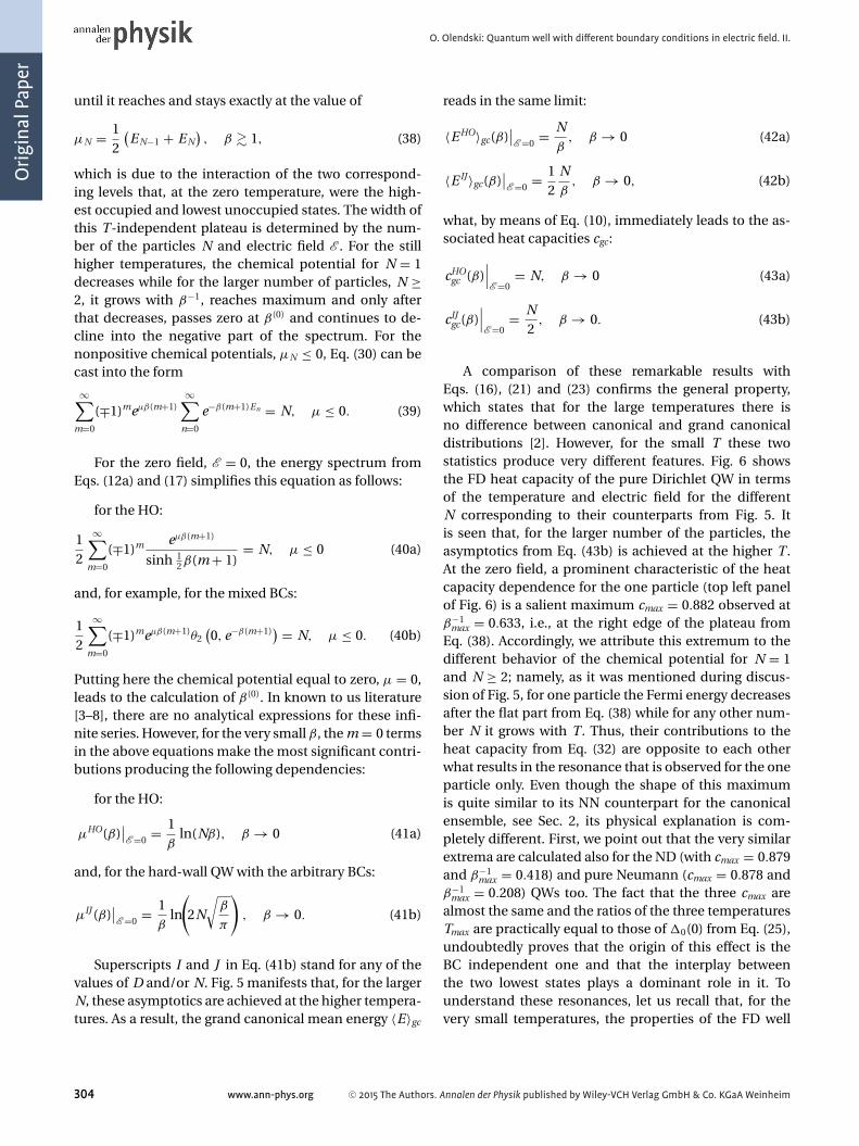
until it reaches and stays exactly at the value of

μN = 12

(E N−1 + E N

), β � 1, (38)

which is due to the interaction of the two correspond-ing levels that, at the zero temperature, were the high-est occupied and lowest unoccupied states. The width ofthis T-independent plateau is determined by the num-ber of the particles N and electric field E . For the stillhigher temperatures, the chemical potential for N = 1decreases while for the larger number of particles, N ≥2, it grows with β−1, reaches maximum and only afterthat decreases, passes zero at β(0) and continues to de-cline into the negative part of the spectrum. For thenonpositive chemical potentials, μN ≤ 0, Eq. (30) can becast into the form

∞∑m=0

(∓1)meμβ(m+1)∞∑

n=0

e−β(m+1)En = N, μ ≤ 0. (39)

For the zero field, E = 0, the energy spectrum fromEqs. (12a) and (17) simplifies this equation as follows:

for the HO:

12

∞∑m=0

(∓1)m eμβ(m+1)

sinh 12 β(m + 1)

= N, μ ≤ 0 (40a)

and, for example, for the mixed BCs:

12

∞∑m=0

(∓1)meμβ(m+1)θ2(0, e−β(m+1)) = N, μ ≤ 0. (40b)

Putting here the chemical potential equal to zero, μ = 0,leads to the calculation of β(0). In known to us literature[3–8], there are no analytical expressions for these infi-nite series. However, for the very small β, the m = 0 termsin the above equations make the most significant contri-butions producing the following dependencies:

for the HO:

μHO(β)∣∣E =0 = 1

βln(Nβ), β → 0 (41a)

and, for the hard-wall QW with the arbitrary BCs:

μIJ (β)∣∣E =0 = 1

βln

(2N

√β

π

), β → 0. (41b)

Superscripts I and J in Eq. (41b) stand for any of thevalues of D and/or N. Fig. 5 manifests that, for the largerN, these asymptotics are achieved at the higher tempera-tures. As a result, the grand canonical mean energy 〈E〉gc

reads in the same limit:

〈E HO〉gc(β)∣∣E =0 = N

β, β → 0 (42a)

〈E IJ 〉gc(β)∣∣E =0 = 1

2Nβ

, β → 0, (42b)

what, by means of Eq. (10), immediately leads to the as-sociated heat capacities cgc:

cHOgc (β)

∣∣∣E =0

= N, β → 0 (43a)

cIJgc(β)

∣∣∣E =0

= N2

, β → 0. (43b)

A comparison of these remarkable results withEqs. (16), (21) and (23) confirms the general property,which states that for the large temperatures there isno difference between canonical and grand canonicaldistributions [2]. However, for the small T these twostatistics produce very different features. Fig. 6 showsthe FD heat capacity of the pure Dirichlet QW in termsof the temperature and electric field for the differentN corresponding to their counterparts from Fig. 5. Itis seen that, for the larger number of the particles, theasymptotics from Eq. (43b) is achieved at the higher T .At the zero field, a prominent characteristic of the heatcapacity dependence for the one particle (top left panelof Fig. 6) is a salient maximum cmax = 0.882 observed atβ−1

max = 0.633, i.e., at the right edge of the plateau fromEq. (38). Accordingly, we attribute this extremum to thedifferent behavior of the chemical potential for N = 1and N ≥ 2; namely, as it was mentioned during discus-sion of Fig. 5, for one particle the Fermi energy decreasesafter the flat part from Eq. (38) while for any other num-ber N it grows with T . Thus, their contributions to theheat capacity from Eq. (32) are opposite to each otherwhat results in the resonance that is observed for the oneparticle only. Even though the shape of this maximumis quite similar to its NN counterpart for the canonicalensemble, see Sec. 2, its physical explanation is com-pletely different. First, we point out that the very similarextrema are calculated also for the ND (with cmax = 0.879and β−1

max = 0.418) and pure Neumann (cmax = 0.878 andβ−1

max = 0.208) QWs too. The fact that the three cmax arealmost the same and the ratios of the three temperaturesTmax are practically equal to those of �0(0) from Eq. (25),undoubtedly proves that the origin of this effect is theBC independent one and that the interplay betweenthe two lowest states plays a dominant role in it. Tounderstand these resonances, let us recall that, for thevery small temperatures, the properties of the FD well


OriginalPaper


Figure 6 The same as in Fig. 5 but forthe heat capacity cN. Note different cand β−1 scales for different panels.

are determined only by the highest occupied level and itsinteraction with the nearest (empty at T = 0) above lyingstate, what is reflected in the extremely rapid approachby the chemical potential to the energy from Eq. (38) thatis located exactly in the middle between them. For N ≥ 2,a contribution from the lower lying members in thisregime is negligibly small and can be safely neglected,while for the one-electron QW this addition is absent bydefinition. Further growth of the temperature increasesthermal energy but it is still too “weak” to compel thecorpuscles, which at T = 0 lied below the Fermi energy,to contribute to the heat capacity. Only at the rightedge of the plateau, the thermodynamic quantum kB Tbecomes strong enough and forces other particles to do-nate to μN and cN. Therefore, for N ≥ 2 the heat capacityis a quite smoothly varying function of the temperature.However, for N = 1 there are no such additional donorsthat aid to support the continuous growth of the heat

capacity, which can not be sustained by the one particleonly. As a result, the specific heat reaches maximum anddrops.

This qualitative physical reasoning can be corrob-orated by the simple quantitative mathematical analy-sis. Fermi level from Eq. (37) defines the correspondingmean energy and heat capacity as:

〈E〉 =N−2∑n=0

En + 12

E N−1 + E Ne−�N−1β, β → ∞ (44a)

cV = E N�N−1β2e−�N−1β, β → ∞. (44b)

On the other hand, for the chemical potentialfrom Eq. (38) these quantities for one fermion, N = 1,become:

〈E〉 = E0

1 + e−�0β/2+ E1

1 + e�0β/2, β � 1 (45a)


Orig

inal

Pape


Figure 7 Total polarization 〈P〉 as a func-tion of the electric field E at zero tem-perature, T = 0, for different number offermions N that is depicted next to thecorresponding curve.

cV = 12�0β

2

[E1

e�0β/2(1 + e�0β/2

)2

− E0e−�0β/2(

1 + e−�0β/2)2

], β � 1, (45b)

where we take into consideration only the two loweststates. For the pure Neumann QW without the field, thislast expression takes an especially simple form:

cNN1

∣∣E =0 = 1

2β2 eβ/2(

1 + eβ/2)2 . (46)

This function has a pronounced maximum ofcmax = 0.878 at βmax = 4.799. A perfect coincidence withthe provided above exact results justifies a validity of thetwo-level approximation and proves that the electrontransitions between them determine the specific heatresonance. It is also very instructive to contrast Eq. (46)with its canonical counterpart from Eq. (22c) in sec. 2.The comparison shows that the magnitude of the grandcanonical Neumann extremum is almost two timeslarger and it is achieved at more than two times lowertemperature.

Applied field E smooths out and widens this maxi-mum simultaneously increasing the heat capacity. Sim-ilar to the canonical ensemble, this growth is explainedby the contribution of the electrostatic potential. How-ever, the electric influence is drastically decreased by thegrowing number of the particles in the QW; for exam-

ple, right-bottom panels exhibit the almost full indepen-dence of the Fermi energy and heat capacity on the in-tensity E already for N = 10. This is explained by theproperties of the energy spectrum in the electric fieldwhen the higher lying states (which, in the case of the FDdistribution, determine the features of the system) areless affected by the applied voltage [1].

Fig. 7 demonstrates zero-temperature FD polariza-tion for all possible BCs and several numbers N. As thewell accommodates more fermions, the total polariza-tion becomes smoother function of the electric field. Fig-ure reveals that, independently of the edge demands, themagnitude of 〈P〉 at N � 5 grows linearly with the voltageand the slope of this almost straight line diminishes withN. For any number of fermions, the total polarizationremains positive at the arbitrary voltage. Nonzero tem-perature leads to the dependencies that qualitatively aresimilar to the canonical patterns, Fig. 4, and, because ofthis, the corresponding polarizations are not shown here.

Next, let us discuss bosonic structures. Remarkableexperimental observations of the BE condensation inthe vapors of rubidium [10] and sodium [11] spurredan avalanche of the research on the subject predictedalmost ninety years ago [12], see, e. g., reviews [13–16].Theoretically, the main effort was devoted to the cal-culation of the properties of the BE systems in the 3Disotropic or anisotropic harmonic traps [13, 17–20] andtheir existence/nonexistence in lower dimensions [13,17, 18, 20, 21]. However, other forms of the confiningpotentials [21, 22], including the 3D box with the pe-riodic [23–25] or uniform [22, 26–29] BCs, were also


OriginalPaper


discussed with the comparative analysis of their influ-ence of the properties of the trap [30–33]. From this pointof view, an inclusion of the electric voltage and differentBCs presents a generalization of the previous analy-sis. Moreover, overwhelming majority of the researchconcentrated on the analysis of the BE systems in thethermodynamic limit when the number of the particlesand the volume containing them tend to infinity whilethe the density is kept constant. In this approximation,the infinite series above in this section can be safelyreplaced by the integrals [13, 14, 16]. Considering Nchanging from one to the large values might help tounderstand the formation of the BE processes with thethe number of the particles growing. First, we state thatEqs. (41)–(43) stay valid for the BE statistics too sincethey were obtained as a result of retaining the first termin the series from Eq. (40). In the opposite limit of thevery small temperatures, it is elementary to derive:

μN = E0 − 1β

ln(

1 + 1N

), β → ∞, (47a)

what leads to the mean energy and heat capacity:

〈E〉N = NE0 + NN + 1

E1e−�0β, β → ∞, (47b)

cN = NN + 1

E1�0β2e−�0β, β → ∞. (47c)

An important characteristic of the BE system is itscritical temperature Tcr . It corresponds to the situationwhen the chemical potential is equal to the energy of thelowest level, μ = E0, and the number of the particles inthis state N0 is zero what leads to the implicit mathemat-ical equation for finding βcr

∑n=1

1e(En−E0)βcr − 1

= N. (48)

Physically, it is the largest temperature at which theBE condensation still can be observed, and at the lowerT the fraction N0/N of the particles in the ground statewill increase until at T = 0 it becomes unity:

N0/N|T=0 = 1. (49)

Fig. 8(a) shows dependencies of the critical parameterβ−1

cr on the applied voltage for all possible BCs and severalnumbers N. In accordance with the previous results [13],the temperature Tcr increases with N. In the absence ofthe fields, the lowest (highest) temperature is observedfor the pure Neumann (Dirichlet) QW what is a reflection

Figure 8 (a) Critical temperatures β−1cr and (b) corresponding to

them polarizations 〈Pcr 〉 from Eq. (50) as functions of the appliedelectric field E for different number N of bosons that are depictednear the corresponding curves. Solid (dotted) lines are for the pureDirichlet (Neumann) BC while their dash (dash-dotted) counter-parts denote DN (ND) geometry. In panel (b), thin horizontal lineis zero polarization.

of the corresponding spectrum from Eq. (17) and the en-ergy difference between the affiliated states, see Eq. (25).Electric field leads to the modification of the mutual lo-cation of the levels on the energy axis; in particular, atthe small voltages, the two lowest states move closer toeach other for the ND geometry while the differenceE1 − E0 grows with the field for all E and any other BCconfiguration [1]. As a result, the critical temperature forthe former edge requirement decreases with the growingfrom zero field, passes through minimum and then un-restrictedly grows with the electric intensity while for allother BCs it is a continuously increasing function of E .At the high voltages, the energy spectrum is determinedmainly by the condition at the right wall [1] what leadsto almost the same critical temperature for, e. g., the NNand DN wells. Note that in this regime, contrary to thezero fields, the Dirichlet requirement is more favorable tothe formation of the BE condensate as compared to the


Orig

inal

Pape


Figure 9 Bosonic heat capacity cV ofthe pure Neumann QW as a function ofthe applied electric field E and temper-ature β−1 for (a) N = 3, (b) N = 1000and (c) N = 105. Note that in the lasttwo cases the temperature is scaled inunits of the critical temperature β−1

cr

while the corresponding z axes measurespecific heat per particle c/N. Panel (d)shows the chemical potential μ for N =105 with the corresponding heat capac-ity depicted in part (c).

Neumann interface. This is explained by the larger levelseparation for the latter geometry at the high voltages [1].

As the ground-state polarization is positive for allfields and BCs [1], one can expect that at the onset of theBE condensation the total statistically averaged dipolemoment will, at the small voltages, be negative. This isexactly what is observed in panel (b) of Fig. 8 that showsthe polarizations 〈Pcr 〉 corresponding to the critical tem-peratures β−1

cr from panel (a). They were calculated fromequation

〈Pcr 〉 =∞∑

n=1

Pn

e(En−E0)βcr − 1, (50)

and, as stated above, the critical temperature β−1cr was

found from Eq. (48). The characteristic features of thecritical polarizations basically follow the properties ofthe first excited state: from zero they decrease with thegrowth of the field, reach minimum after which they in-crease. However, for the large voltages many upper ly-ing states are occupied and contribute to the total dipolemoment. As a result, the high-field 〈Pcr 〉 for one bosonis considerably smaller than P1. The absolute value ofthe negative polarization at the extremum grows with thenumber of the particles with the largest one, at the fixedN, being observed for the pure Neumann QW followed byits ND counterpart what is a replica of the similar behav-

ior for the first excited level [1]. For the temperatures be-low Tcr , the nonzero occupation of the ground state con-tributes a positive term to the polarization what leads tothe gradual disappearance of the negative region of thetotal dipole moment 〈P〉 with the decreasing tempera-ture until at T = 0 it becomes NP0, which is positive forany BC and arbitrary fields [1].

As a final example, Fig. 9 exhibits evolution of the heatcapacity and chemical potential with the varying electricfield and temperature for the pure Neumann QW. It isseen that for the small number of bosons, say, N = 3 inpanel (a), the applied voltage leads, at quite warm sam-ple, to the increase of cV while at the small T , the width ofthe temperature-independent zero-capacity plateau in-creases with the field. These features were discussed be-fore for the canonical ensemble. Increasing the numberof the particles in the well leads to the suppression of thevoltage dependence, as a transition from panel (a) to (b)with N = 1000 and (c) for N = 105 vividly demonstrates.No any noticeable field dependence is seen there in therange 0 ≤ E ≤ 50. It is well known that for some poten-tials, such as, e.g., the 3D isotropic harmonic trap [14,16, 18, 19, 34, 35], the heat capacity has a cusp-like pecu-liarity as it passes through the critical temperature whilefor the 1D quadratic potential it is a smooth function ofT [16, 18, 35]. Fig. 9 exemplifies that no any peculiarity isobserved for the 1D hard-wall potential with Neumann


OriginalPaper


surfaces and arbitrary applied electric fields. Our calcu-lations confirm that the same is true for any other BCs.Finally, panel (d) shows that the chemical potential μ isa monotonically decreasing function of both the elec-tric field E and temperature T . It is seen that the grow-ing temperature diminishes the voltage influence on thechemical potential.

4 Concluding remarks

Rigorous mathematical treatment of the QW with miscel-laneous BCs under the applied voltage revealed a stronginfluence of the interplay between them on the thermo-dynamic properties of the structure. In particular, with-out the field the differences of the energy spectrum lead,for the canonical ensemble, to the conspicuous maxi-mum followed by the minimum of the heat capacity cV

on the temperature axis for the NN quantum box whilefor the other edge requirements no such adjacent ex-trema are observed. Modification of the specific heat andstatistically averaged polarization in the field is qualita-tively explained by the influence of the associated elec-trostatic potential. Numerical calculations, which pre-dicted, for the flat potential with the arbitrary BC, asalient maximum of cV as a function of T for one fermionand its absence for the larger N, were corroborated bythe two-level model that allows simple analytical treat-ment with its predictions perfectly coinciding with theexact results. From this, a clear physical explanation ofthis phenomenon follows that is based on the analysis ofthe associated Fermi energy. It is predicted that the ap-plied field, in general, favors the formation of the BE con-densate, and the differences and similarities of this pro-cess for the different BCs are discussed. The thermallyaveraged dipole moment is shown to take the negativevalues in some ranges of the fields and temperatures. It isalso argued that for the larger number of either fermionsor bosons in the QW, the influence of the electric field onthe thermodynamic properties diminishes.

Dirichlet and Neumann conditions are the limitingcases of the so called Robin BC [36]

n∇�|S = 1

�

∣∣∣∣S

, (51)

where n is an inward unit normal to the surface, andthe parameter has a dimension of length and is calledthe extrapolation distance. Its variation allows a contin-uous transformation from the Dirichlet ( = 0) to theNeumann ( = ∞) situation. Without the field, espe-cially intriguing are the properties of the QW at the small

negative Robin lengths, → −0, when, in addition tothe positive spectrum, two almost degenerate odd andeven levels with the energies E ∼ −1/(π)2 are created[37]. Analysis of the Robin QW in the electric field mightpresent an interesting extension of the present research.

Acknowledgement. This project was supported by Deanship of Sci-entific Research, College of Science Research Center, King SaudUniversity.

Key words. Electric field, quantum well, boundary conditions,Bose-Einstein condensation, Fermi-Dirac statistics, heat capacity.

References

[1] O. Olendski, Ann. Phys. (Berlin), 527, 278–295(2015).

[2] N. Dalarsson, M. Dalarsson, and L. Golubovic, Intro-ductory Statistical Thermodynamics (Academic, Am-sterdam, 2011).

[3] R. Bellman, A Brief Introduction to Theta Functions(Holt, Rinehart and Wilson, New York, 1961).

[4] M. Abramowitz and I. A. Stegun, Handbook of Mathe-matical Functions (Dover, New York, 1964).

[5] I. S. Gradshteyn and I. M. Ryzhik, Table of Integrals,Series, and Products, 8th edn. (Academic, Amsterdam,2014).

[6] A. P. Prudnikov, Y. A. Brychkov, and O. I. Marichev,Integrals and Series Vol. 1 (Gordon and Breach, NewYork, 1986).

[7] A. P. Prudnikov, Y. A. Brychkov, and O. I. Marichev,Integrals and Series Vol. 2 (Gordon and Breach, NewYork, 1990).

[8] Y. A. Brychkov, Handbook of Special Functions:Derivatives, Integrals, Series and Other Formulas(Chapman & Hall, Boca Raton, FL, 2008).

[9] W. Rudin, Principles of Mathematical Analysis, 3rdedn. (McGraw-Hill, New-York, 1976).

[10] M. H. Anderson, J. R. Ensher, M. R. Matthews, C. E.Wieman, and E. A. Cornell, Science 269, 198 (1995).

[11] K. B. Davis, M.-O. Mewes, M. R. Andrews, N. J. vanDruten, D. S. Durfee, D. M. Kurn, and W. Ketterle, Phys.Rev. Lett. 75, 3969 (1995).

[12] S. N. Bose, Z. Phys. 26, 178 (1924).[13] F. Dalfovo, S. Giorgini, L. P. Pitaevskii, and S. Stringari,

Rev. Mod. Phys. 71, 463 (1999).[14] L. Pitaevskii and S. Stringari, Bose-Einstein Conden-

sation (Clarendon, Oxford, 2003).[15] A. J. Leggett, Rev. Mod. Phys. 73, 307 (2001).[16] C. J. Pethick and H. Smith, Bose-Einstein Con-

densation in Dilute Gases (Cambridge, Cambridge,2004).

[17] W. Ketterle and N. J. van Druten, Phys. Rev. A 54, 656(1996).

[18] N. J. van Druten and W. Ketterle, Phys. Rev. Lett. 79,549 (1997).


Orig

inal

Pape


[19] R. Napolitano, J. De Luca, V. S. Bagnato, and G. C. Mar-ques, Phys. Rev. A 55, 3954 (1997).

[20] W. J. Mullin, J. Low Temp. Phys. 106, 615 (1997).[21] V. Bagnato and D. Kleppner, Phys. Rev. A 44, 7439

(1991).[22] V. Bagnato, D. E. Pritchard, and D. Kleppner, Phys. Rev.

A 35, 4354 (1987).[23] E. B. Sonin, Zh. Eksp. Teor. Fiz. 56, 963 (1969) [Sov.

Phys. - JETP 29, 520 (1969)].[24] S. Greenspoon and R. K. Pathria, Phys. Rev. A 9, 2103

(1974).[25] C. S. Zasada and R. K. Pathria, Phys. Rev. A 14, 1269

(1976).[26] D. F. Goble and L. E. H. Trainor, Can. J. Phys. 44, 27

(1966).[27] D. F. Goble and L. E. H. Trainor, Phys. Rev. 157, 167

(1967).

[28] D. F. Goble and L. E. H. Trainor, Can. J. Phys. 46, 1867(1968).

[29] S. Grossmann and M. Holthaus, Z. Phys. B 97, 319(1995).

[30] R. K. Pathria, Phys. Rev. A 5, 1451 (1972).[31] S. Greenspoon and R. K. Pathria, Phys. Rev. A 8, 2657

(1973).[32] M. N. Barber and M. E. Fisher, Phys. Rev. A 8, 1124

(1973).[33] Z. R. Hasan and D. F. Goble, Phys. Rev. A 10, 618 (1974).[34] H. Haugerud, T. Haugset, and F. Ravndal, Phys. Lett. A

225, 18 (1997).[35] T. Haugset, H. Haugerud, and J. O. Andersen, Phys.

Rev. A 55, 2922 (1997).[36] K. Gustafson and T. Abe, Math. Intell. 20(1), 63 (1998).[37] O. Olendski and L. Mikhailovska, Phys. Rev. E 81,

036606 (2010).


Comparative analysis of electric field influence on the quantum wells with different boundary...

Documents

Transcript of Comparative analysis of electric field influence on the quantum wells with different boundary...