Companion for “Statistics for Business and Economics” by Paul Newbold, William L. Carlson and...

1

Companion

for “Statistics for Business and

Economics”

by Paul Newbold, William L. Carlson and

Betty Thorne

Kairat T. Mynbaev

International School of Economics

Kazakh-British Technical University

Tolebi 59, Almaty 050000, Kazakhstan

2

CHAPTER 0 PREFACE ............................................................................................................... 7

Unit 0.1 What is the difference between the textbook and this companion? ............................................. 7

Unit 0.2 Why study math? .......................................................................................................................... 7

Unit 0.3 Exposition ...................................................................................................................................... 9

Unit 0.4 Formatting conventions................................................................................................................. 9

Unit 0.5 Best ways to study ......................................................................................................................... 9

CHAPTER 1 HOW TO STUDY STATISTICS? ..................................................................... 11

Unit 1.1 The structure of mathematics (definitions, axioms, postulates, statements) ............................... 11

Unit 1.2 Studying a definition (natural, even, odd, integer and real numbers; sets) .................................. 11

Unit 1.3 Ways to think about things (commutativity rules, quadratic equation, real line, coordinate plane,

Venn diagrams) .............................................................................................................................................. 12

CHAPTER 2 DESCRIBING DATA: GRAPHICAL ................................................................ 14

Unit 2.1 Classification of variables (definitions: intuitive, formal, working, simplified, descriptive,

complementary; variables: numerical, categorical, discrete, continuous) ...................................................... 14

Unit 2.2 Frequencies and distributions (Bernoulli variable, binomial variable, sample size, random or

stochastic variable, absolute and relative frequencies, frequency distributions) ........................................... 15

Unit 2.3 Visualizing statistical data (coordinate plane; argument, values, domain and range of a function;

independent and dependent variables; histogram, Pareto diagram, time series, time series plot, stem-and-

leaf display, scatterplot) ................................................................................................................................ 17 2.3.1 Histogram short definition: plot frequencies against values. ........................................................... 18 2.3.2 Pareto diagram: same as a histogram, except that the observations are put in the order of

decreasing frequencies. ................................................................................................................................... 18 2.3.3 Time series plot: plot values against time.......................................................................................... 19 2.3.4 Stem-and-leaf display ........................................................................................................................ 19 2.3.5 Scatterplot: plot values of one variable against values of another. .................................................. 20

Unit 2.4 Questions for repetition .............................................................................................................. 20

CHAPTER 3 DESCRIBING DATA: NUMERICAL ............................................................... 21

Unit 3.1 Three representations of data: raw, ordered and frequency representation ............................... 21

Unit 3.2 Measures of central tendency (sample mean, mean or average, median, mode; bimodal and

trimodal distributions; outliers) ..................................................................................................................... 21

Unit 3.3 Shape of the distribution (symmetry; positive and negative skewness; tails) .............................. 23

Unit 3.4 Measures of variability (range, quartiles, deciles, percentiles; interquartile range or IQR; five-

number summary, sample variance, deviations from the mean, sample standard deviation) ....................... 23

Unit 3.5 Measures of relationships between variables (sample covariance, sample correlation coefficient;

positively correlated, negatively correlated and uncorrelated variables; perfect correlation) ....................... 25

3


CHAPTER 4 PROBABILITY ................................................................................................... 29

Unit 4.1 Set operations (set, element, union, intersection, difference, subset, complement, symmetric

difference; disjoint or nonoverlapping sets, empty set) ................................................................................. 29

Unit 4.2 Set identities (distributive law, de Morgan laws, equality of sets) ............................................... 30

Unit 4.3 Correspondence between set terminology and probabilistic terminology (random experiment;

impossible, collectively exhaustive and mutually exclusive events; sample space; basic outcomes or

elementary events; occurrence of an event, disjoint coverings) .................................................................... 30

Unit 4.4 Probability (inductive and deductive arguments; induction, probability, nonnegativity, additivity,

completeness axiom, complement rule, assembly formula, impossible and sure events) .............................. 31

Unit 4.5 Ways to find probabilities for a given experiment (equally likely events, classical probability,

addition rule) ................................................................................................................................................. 34 4.5.1 Equally likely outcomes (theoretical approach) ................................................................................ 34

Unit 4.6 Combinatorics (factorial, orderings, combinations) ..................................................................... 35

Unit 4.7 All about joint events (joint events, joint and marginal probabilities, cross-table, contingency

table) 37

Unit 4.8 Conditional probabilities (multiplication rule, independence of events, prior and posterior

probability) .................................................................................................................................................... 39 4.8.1 Independence of events .................................................................................................................... 40

Unit 4.9 Problem solving strategy ............................................................................................................. 42

Unit 4.10 Questions for repetition .......................................................................................................... 43

CHAPTER 5 DISCRETE RANDOM VARIABLES AND PROBABILITY

DISTRIBUTIONS ............................................................................................................................. 44

Unit 5.1 Random variable (random variable, discrete random variable) ................................................... 44

Unit 5.2 General properties of means (expected value, mean, average, mathematical expectation,

uniformly distributed discrete variable, grouped data formula, weighted mean formula)............................. 44

Unit 5.3 Linear combinations of random variables (linear combination, vector, parallelogram rule) ........ 46

Unit 5.4 Linearity (portfolio, portfolio value, universal statements, existence statements, homogeneity of

degree 1, additivity) ....................................................................................................................................... 47

Unit 5.5 Independence and its consequences (independent and dependent variables, multiplicativity of

means) 48

Unit 5.6 Covariance (linearity, alternative expression, uncorrelated variables, sufficient and necessary

conditions, symmetry of covariances) ............................................................................................................ 50

Unit 5.7 Variance (interaction term, variance of a sum, homogeneity of degree 2, additivity of variance) 52

Unit 5.8 Standard deviation (absolute value, homogeneity, Cauchy-Schwarz inequality) ......................... 54

4

Unit 5.9 Correlation coefficient (unit-free property, positively and negatively correlated variables,

uncorrelated variables, perfect correlation) .................................................................................................. 55

Unit 5.10 Standardization (standardized version) ................................................................................... 56

Unit 5.11 Bernoulli variable (population, sample, sample size, sampling with replacement, ex-post and

ex-ante treatment of random variables, identically distributed variables, parent population, binomial

variable, number of successes, proportion of successes, standard error) ...................................................... 57 5.11.1 Some facts about sampling not many people will tell you ........................................................... 57 5.11.2 An obvious and handy result ........................................................................................................ 59

Unit 5.12 Distribution of the binomial variable ...................................................................................... 60

Unit 5.13 Distribution function (cumulative distribution function, monotonicity, interval formula,

cumulative probabilities) ............................................................................................................................... 62

Unit 5.14 Poisson distribution (monomials, Taylor decomposition) ....................................................... 63

Unit 5.15 Poisson approximation to the binomial distribution ............................................................... 65

Unit 5.16 Portfolio analysis (rate of return) ............................................................................................ 66

Unit 5.17 Questions for repetition .......................................................................................................... 67

CHAPTER 6 CONTINUOUS RANDOM VARIABLES AND PROBABILITY

DISTRIBUTIONS ............................................................................................................................. 68

Unit 6.1 Distribution function and density (integral, lower and upper limits of integration, variable of

integration, additivity with respect to the domain of integration, linear combination of functions, linearity of

integrals, order property) .............................................................................................................................. 68 6.1.1 Properties of integrals ....................................................................................................................... 68

Unit 6.2 Density of a continuous random variable (density, interval formula in terms of densities) ......... 69

Unit 6.3 Mean value of a continuous random variable (mean) ................................................................. 71

Unit 6.4 Properties of means, covariance, variance and correlation ......................................................... 72

Unit 6.5 The uniform distribution (uniformly distributed variable, primitive function, integration rule) .. 73

Unit 6.6 The normal distribution (parameter, standard normal distribution, normal variable and

alternative definition, empirical rule) ............................................................................................................ 75 6.6.1 Parametric distributions .................................................................................................................... 75 6.6.2 Standard normal distribution ............................................................................................................ 76 6.6.3 Normal distribution ........................................................................................................................... 77

Unit 6.7 Normal approximation to the binomial (point estimate, interval estimate, confidence interval,

confidence level, left and right tails, significance level, convergence in distribution, central limit theorem) . 78

Unit 6.8 Joint distributions and independence (joint distribution function, marginal distribution function,

independent variables: continuous case) ....................................................................................................... 79


CHAPTER 7 SAMPLING AND SAMPLING DISTRIBUTION ........................................... 81

5

Unit 7.1 Sampling distribution (simple random sample, quota sampling, statistic, sampling distribution,

estimator, unbiasedness, upward and downward bias,) ................................................................................ 81

Unit 7.2 Sampling distributions of sample variances (chi-square distribution, degrees of freedom) ......... 83

Unit 7.3 Monte Carlo simulations ............................................................................................................. 84


CHAPTER 8 ESTIMATION: SINGLE POPULATION ......................................................... 87

Unit 8.1 Unbiasedness and efficiency ........................................................................................................ 87

Unit 8.2 Consistency (consistent estimator, Chebyshov inequality) .......................................................... 88

Unit 8.3 Confidence interval for the population mean. Case of a known σ (critical value, margin of error)

89

Unit 8.4 Confidence interval for the population mean. Case of an unknown σ (t-distribution) ................. 90

Unit 8.5 Confidence interval for population proportion ............................................................................ 91


CHAPTER 9 ESTIMATION: ADDITIONAL TOPICS ......................................................... 93

Unit 9.1 Matched pairs ............................................................................................................................. 93

Unit 9.2 Independent samples. Case I: σX, σY known ................................................................................ 93

Unit 9.3 Independent samples. Case II: σX, σY unknown but equal (pooled estimator) ............................ 94

Unit 9.4 Independent samples. Case III: σX, σY unknown and unequal (Satterthwaite’s approximation) . 95

Unit 9.5 Confidence interval for the difference between two population proportions .............................. 97


CHAPTER 10 HYPOTHESIS TESTING ................................................................................... 98

Unit 10.1 Concepts of hypothesis testing (null and alternative hypotheses, Type I and Type II errors,

Cobb-Douglas production function; increasing, constant and decreasing returns to scale) ............................ 98

Unit 10.2 Tradeoff between Type I and Type II errors (significance level, power of a test) ..................... 99

Unit 10.3 Using confidence intervals for hypothesis testing (decision rule, acceptance and rejection

regions, simple and composite hypotheses) ................................................................................................ 100

Unit 10.4 p-values ................................................................................................................................ 101

Unit 10.5 Power of a test ...................................................................................................................... 102

Unit 10.6 Questions for repetition ........................................................................................................ 104

6

CHAPTER 11 HYPOTHESIS TESTING II ............................................................................ 105

Unit 11.1 Testing for equality of two sample variances (F-distribution) ............................................... 105


CHAPTER 12 LINEAR REGRESSION .................................................................................. 107

Unit 12.1 Algebra of sample means ...................................................................................................... 107

Unit 12.2 Linear model setup (linear model, error term, explanatory variable, regressor) ................... 107

Unit 12.3 Ordinary least squares estimation (OLS estimators, normal equations, working formula) .... 108 12.3.1 Derivation of OLS estimators ...................................................................................................... 108 12.3.2 Unbiasedness of OLS estimators................................................................................................. 109

Unit 12.4 Variances of OLS estimators (homoscedasticity, autocorrelation, standard errors) .............. 110 12.4.1 Statistics for testing hypotheses ................................................................................................. 112

Unit 12.5 Orthogonality and its consequences (fitted value, residual vector, orthogonality, Pythagorean

theorem, Total Sum of Squares, Explained Sum of Squares, Residual Sum of Squares) ................................ 112

Unit 12.6 Goodness of fit (coefficient of determination) ...................................................................... 114


LITERATURE ................................................................................................................................ 115

LIST OF FIGURES ......................................................................................................................... 115

LIST OF TABLES ........................................................................................................................... 115

INDEX OF TERMS ........................................................................................................................ 116

LIST OF EXERCISES ..................................................................................................................... 119

LIST OF EXAMPLES ..................................................................................................................... 120

LIST OF THEOREMS ................................................................................................................... 120

7

Chapter 0 Preface

Unit 0.1 What is the difference between the textbook and this companion?

I am going to call the book NCT, by the last initials of the authors. All references are to the sixth edition of NCT.

On the good side, the book has a lot of intuitive explanations and plenty of exercises, which is especially handy for instructors. The coverage of statistical topics is wide, so that most instructors will not need to look for other sources. Statistics requires a lot of math. The authors have done their best to hide the mathematical complexities and make the book accessible to those who are content using formulas without having to derive them.

This last advantage, looked at from a different angle, becomes a major drawback. If you have to remember just five formulas, after applying each once or twice perhaps you will memorize them. But how about 100 formulas? This is an approximate number of equations and verbal definitions (which eventually translate to equations) contained in the first six chapters of NCT. Some formulas are given more than once, in different forms and contexts. For example, different types of means are defined in Sections 3.1, 3.3, 5.3, 6.2 and 18.2, and it takes time and effort to relate them to one another. For your information, all types of means are special cases of just one, population mean. The origin of most equations is not explained. When most formulas fall out of the blue sky, after a while you get lost. When it is necessary to systematize testing procedures scattered over several sections or chapters, the situation becomes even more complex. Look at Figure 10.10 that describes the decision rule for choosing an appropriate testing procedure. If you are comfortable using it and all the relevant formulas without understanding the links between them, then you don’t need this companion.

Now suppose that you are an ordinary human, who cannot mechanically memorize a bunch of formulas, like me or my students, who feel completely lost after the first six chapters if I follow the book’s approach. Suppose you want to see a harmonious, coherent picture instead of a jigsaw puzzle of unrelated facts. Then I am going to try to convince you that studying formulas with proofs and derivations is the best option.

Unit 0.2 Why study math?

Firstly, it’s not that much. You don’t need to dig all the math you’ve forgotten from high school. Just study what I give (which is directly related to the course), and then you’ll see that all properties of means make great sense and fit just two pages, with all the intuition, special cases and derivations. The same goes for variances, covariances, confidence intervals etc.

Secondly, knowing the logic (the links between theoretical facts) significantly reduces the burden on your memory. For example, just being familiar with the general principle of linearity will allow you to deduce all properties of covariances and variances in the logical chain

means → covariances → variances

from the properties of the first link (means). This is especially important in case of confidence intervals (and there are dozens of them) all of which are based on a few general ideas. My students love my handouts because instead of reading 30-40 pages in NCT they have to read just 9 pages (on average) for each chapter.

8

Thirdly, the knowledge cemented by logic stays in the memory much longer than mechanically memorized facts. Being able to derive equations you studied in the beginning of the semester will give you confidence when applying them during the final exam.

Fourthly, because in our brain everything is linked it has a wonderful property that can be called an icebreaker principle: as you develop one particular capability, many other brain activities enjoy a positive spillover effect. The logic and imagination you develop while studying math will give a comparative advantage in all your current and future activities that require analytical abilities. This influence on your skills and aptitude will be even more important than the knowledge of statistics as a subject.

Fifthly, the school approach to studying formulas through their application is not going to work with NCT. At high school you had to study a small number of different applications and had enough time to solve many exercises for each application type. In statistics, the number of different typical applications is so large that you will not have time to solve more than two exercises for each.

Sixthly, some students avoid math remembering their dreadful experience struggling with it at high school. Their fear of math continues well into college years, and they think: If I failed to learn math at high school, how can I learn it in just one semester (or year) at a university? I have a soothing and encouraging answer for such students. Most likely, you fell victim to a wrong teaching methodology, and I would not rely on your grades at high school to judge your math abilities. Some of your misunderstandings and problems with math may have come from your early age (when you saw for the first time, say, fractions or algebra rules). At that time your cognitive abilities were underdeveloped. Now you are an adult and, if you are reading this, you are a completely normal person with adequate cognitive abilities. You can comprehend everything much faster than when you were at elementary school. It’s like with a human embryo, which in 9 months passes all the stages of evolution that took the humans ages to become who they are now. There are a couple of rules to follow though. Forget your fears, do not rely on that scanty information you are not sure about and look for common

sense in everything you see. Relying on logic instead of memory is the best rule − this is why I prefer to teach people with work experience. Unlike fresh high-school graduates, they don’t take anything for granted and are sincere about their lack of math background.

The seventh and the most important reason has been overlooked by all those who recommend to sidestep all formula derivation and concentrate on mastering formulas through their applications. See, some of us are endowed with good logic and imagination from birth. For such people, indeed, it is enough to see a formula and a model exercise for its application to be able to apply the formula on their own in a slightly different situation. But most of us mortals are not that bright. I’ve seen many people who understand well the statement of the exercise and know all the required theory and yet do not see the solution. In this case there is only one verdict: such individual’s logic and imagination are not good enough. Explaining the solution to him/her usually doesn’t help because that doesn’t improve their logic and imagination and in a similar situation they will be lost again.

Logic and imagination are among the most advanced functions of our brain. Most people think that you either possess them or you don’t and it is not possible to develop them. I can tell you a big secret that this is wrong, at least in math. Study mathematical facts and theories WITH the pertaining logic, and with time your own logic will start working (this is how your humble servant has become a mathematician). More about how to do this will be said later. For now let me state the main recommendation. Some of the exercises in NCT are pretty tricky and their diversity is amazing. Don’t even hope to learn the solutions of a dozen model exercises and then be able to solve the rest of them.

9

Your sure bet is to develop your own logic and imagination and the best way to achieve this purpose is to study mathematical facts with proofs and derivations.

OK, suppose I have convinced you that studying math is worthwhile and you are ready to give it a try. Then why not combine reading NCT with reading one of the extant mathematical texts? In what way is this manuscript different or better than the pile on the market? Well, this manuscript is not just another math text. It’s the teaching philosophy that makes the difference. I talk about the learning strategy almost as much as about the subject itself. The exposition and study units are designed to develop your self-learning skills. There are comments on psychological aspects of the study process for students, teachers and even (present or future) parents.

Unit 0.3 Exposition

This manual is by no means a replacement for NCT. If I leave out some material, it means that it is well explained in NCT or it is not essential.

The order of definitions and statements in NCT does not reflect their logical sequence. Sometimes logically interrelated facts are scattered over different sections or even chapters in NCT. I do the opposite: the material is organized in study units, which combine logically linked information. This made necessary to give some material earlier or later than in NCT. Therefore placement of a study unit in a certain chapter is approximate. The heading of a unit contains the list of terms defined in it. Those headings and the index of terms allow you to establish the correspondence between NCT and this manual. I want my students to be able to answer questions of certain difficulty. Those questions determine the sizes of study units.

Unit 0.4 Formatting conventions

The level of difficulty of a unit is indicated by a line on the left side.

The dashed line on the left means something you are supposed to know from high school or math prerequisites.

There is no line on the left if the level roughly corresponds to NCT.

A single continuous line on the left means a higher level, which is desirable to study because it highlights important ideas. Sometimes it is included just to feed information-hungry students.

The text to type in Excel is shown in Courier font.

Italic indicates a new term even though the word “definition” may not be there.

The most important methodological recommendations are framed like this.

Unit 0.5 Best ways to study

First best way. Study a theoretical problem, the existing approaches to its solution, try to improve or generalize upon them and write a publishable article. This way is not accessible to most students.

Second best way. As you study, write your own book or manual, in your own words and the way you understand it. For example, Joon Kang uploads to scribd.com his supplements to NCT with his own vision of the subject. This way is as rewarding as it is time-consuming (but quite accessible to some students). When I was 32, I wrote a book with my major professor M. Otelbaev. In one year I learned more than in the previous three years.

10

Third best way. After reading some material, close the book and write down the main points explaining the accompanying logic. The luckiest of you may have a classmate to retell the material to (I am a stickler of team-based learning). This way is quite feasible for most students. I call it active recalling, as opposed to passive repetition, when after reading the material you just skim it to see what you remember and what you don’t. This way may be time-consuming initially but after a while you’ll get used and your speed will increase. Many things you did not understand before will become simple. Try to work in the evenings when you are so tired that your memory refuses to function but your logic still works.

In the end the 1980’s I had to give an intensive course in functional analysis. I gave 10 hours of lectures a week, 6 hours in a row in one day and 4 hours in another. As this all was high level stuff, the course was very useful for me (and a disaster for students).

Secret to success. Actively recall the material, in increasingly large chunks (not necessarily limited to my study units) and at an increasingly high speed.

If you don’t do this, I don’t guarantee anything. In my classes, I make sure that students actively repeat the material by arranging competitions among student teams.

Explanation. Nobody knows exactly what creative imagination means, in terms of neural activity. Let’s talk about internal vision by which I mean the ability to see a large and complex picture at once. Internal vision can be compared to a ray of a flashlight. If the ray of your flashlight is narrow and the picture is big, you can see only a part of it. The wider the ray, the more of the picture you see. When you see the whole picture, you can solve the problem.

Active recalling of increasingly large amounts of material forces the brain to adjust and gradually increase internal vision.

Increasing the speed of recalling (or writing) is important for two reasons. In addition to widening internal vision, it also strengthens the degree of excitation of neurons. Your thoughts become clearer and the speed of formation of new synapses (intra-neuron links) increases. The second reason is that high recalling speed reduces the degree of verbalization of the thinking process.

In most cases, in math too much bla-bla-bla is harmful!

Send me feedback through LinkedIn.

Kairat Mynbaev

June 4, 2010

11

Chapter 1 How to Study Statistics?

Most of the material of the first two chapters of NCT can be safely skipped, not only because it is unimportant but primarily because our brain tries to systematize the incoming information, and there is very little systematic content in the first two chapters. Also, some issues from Chapters 1-2 are better taken up in subsequent chapters, when you are ready for their solution. I use this space to discuss some issues deeper than in the book and at the level you will need later. High-school material or the stuff you are supposed to remember from math prerequisites is reviewed. Solve the relevant exercises in the book only when you find my explanations insufficient.

Unit 1.1 The structure of mathematics (definitions, axioms, postulates, statements)

Math consists of definitions, axioms and statements. Definitions are simply names of objects. They don’t require proofs. Axioms (also called postulates) are statements that we believe in; they don’t require proofs and are in the very basement of a theory. Statements have to be proved. Depending on the situation and the tastes of the researcher, they may have different other names: theorem, lemma, proposition, criterion etc. Statements are a way to economize on space and thinking efforts. They summarize sometimes very long arguments and serve as building bricks in subsequent constructions.

In math texts definitions take up at most 5 to 10% of space. A common error of students of quantitative subjects is to jump to statements without thinking enough about definitions1. Definitions not only give names to objects but they also give direction to the theory and reflect the researcher’s point of view. Often understanding definitions well allows you to guess or even prove some results.

Unit 1.2 Studying a definition (natural, even, odd, integer and real numbers; sets)

A definition starts with a preamble which sets a background and allows you to see the existence of objects with distinct properties. Most of the time the preamble is not even mentioned but there are cases when it contains a complex logical argument. After you

understand the preamble understanding the definition proper − that is giving the name − becomes easy. Studying a definition is concluded by considering possible equivalent definitions and deriving immediate consequences.

Example 1.1 (1) Preamble. Let us consider natural numbers (these are numbers 1, 2, 3, … that naturally arise when counting things). We can notice that some of them are divisible by 2 (for example, 4/2 = 2 is an integral number) and others are not (e.g., 3/2 is a fractional number).

(2) Definition proper. The natural numbers that are divisible by 2 (2, 4, 6, …) are called even. The natural numbers that are not divisible by 2 (1, 3, 5, …) are called odd.

1 When I was young I also committed this error.

12

(3) Immediate consequences. (i) Any natural number is either even or odd. (ii) If a natural number is even and divisible by 3 at the same time, then it is divisible by 6.

Some basic objects cannot be defined or their precise definitions are too complex for this course. In such cases it is better to give equivalent (descriptive) names or simply list the objects we name (as it has been done in case of natural numbers).

Example 1.2 The following names are used interchangeably: set = collection = family = array.

Example 1.3 Natural numbers are members of the set {1, 2, 3, ...}N = . Integer numbers are

members of the set {0, 1, 2, ...}Z = ± ± . In some applications (see Unit 5.12 and Unit 5.15)

we shall need nonnegative integer numbers listed in {0, 1, 2, ...}Z+= .

Example 1.4 The next type of numbers we need, real numbers, cannot be put in a list. As a convenient working definition, we call real numbers those numbers that can be written in a

decimal form. For example, the famous number π, is, by definition, the ratio of the length of a

circumference to its diameter. Its decimal form, is, up to approximation, π = 3.1415926… Integer numbers fall into this category: for example, 1 = 1.000… The set of all real numbers

is denoted R .

Unit 1.3 Ways to think about things (commutativity rules, quadratic equation, real line, coordinate plane, Venn diagrams)

(i) When you study a definition, don’t think about a single representative of a class of objects; try to think about the whole class. Thinking in terms of sets will systematize your knowledge.

(ii) In algebra, when we denote numbers by letters, we mean that whatever rules we write with letters are of universal character and apply to all numbers in a given set. For example, the commutativity rules for summation and multiplication a b b a+ = + , ab ba= hold for all

real numbers and not just for those specific ones you may plug in. Simple algebra rules, like the ones we have just seen, are easy to formulate verbally. Verbal formulation and derivation of complex algebra rules is a nightmare. For example, try to verbalize the rule for finding the

roots of the quadratic equation 20ax bx c+ + = . This is what people did before 1637, when

René Descartes introduced modern algebraic notation. This is what people still do in the beginning and intermediate micro- and macroeconomic courses. Excuse me, but this is a stone age! This tradition persists for the only reason that the teaching methodology at secondary and high school fails. With the right methodology, every normal person can learn algebra2.

(iii) Believe me, even with zero math background you can quickly learn algebra if you follow a few simple rules:

(a) Pay attention to small details, like the usage of upper- and lower-case letters, the difference between parentheses (), brackets [] and braces {}, punctuation and

arithmetic signs (+, −, ×, /).

2 I studied early education issues, experimented with my children and know what I am talking about.

13

(b) Try to find a tangible (or intuitive) interpretation for each element in a mathematical construction. Usually, geometry clarifies many things. For example, a real number can be uniquely identified with a point on a straight line (called a real line in this case); a pair of real numbers can be uniquely identified with a point on a coordinate plane; Venn diagrams help when working with sets.

(c) Similarly, explain for yourself each step in a long algebraic transformation. Don’t trust the book or the professor.

Your knowledge of and interest in the subject will directly depend on the percentage of the material you can explain.

(d) Initially it helps to translate formulas to verbal statements and back. Verbalization can also help in case of long, complex definitions and statements (we’ll return to this

when discussing p -values, see Unit 10.4). With time you’ll be able to do without

verbalization, and in complex situations the best thing to do is shut up and concentrate3.

(e) In such a theoretical subject as statistics it is not possible to provide real-life motivating examples for absolutely all parts of the theory. In fact, many theoretical problems are prompted by the internal logic of the theory; even more often the solutions to the problems are based on mathematical intuition. We are not computers; we need some level of interest in the subject and some level of satisfaction from our efforts to continue our studies. It may be relieving to learn that

We tend to like what we understand.

Try to keep your level of understanding high (say, at 80 to 90%) and the interest in the subject will ensue.

(f) If your ambition is to get a high mark in statistics, follow what I call a 110% rule. We inevitably forget a part of what we’ve studied.

To know all 100% of the material, you have to study 110%.

3 When I brought my son to the USA and put him to the 7

th grade, he did not speak English. The math teacher

would explain to the students the solution for half an hour, they would diligently write down his explanations

and my son would sit doing nothing. The teacher would ask why he wasn’t writing anything and my son would

show a one-line solution to the problem.

14

Chapter 2 Describing Data: Graphical

Unit 2.1 Classification of variables (definitions: intuitive, formal, working, simplified, descriptive, complementary; variables: numerical, categorical, discrete, continuous)

An important part of working with definitions consists in comparing related definitions. This is the right time to discuss the choice from among different definitions of the same object. An intuitive definition gives you the main idea and often helps you come up with the formal definition, which is mostly a formula4. Formal definitions may have different forms. The one which is easier to apply is called a working definition. Some complex definitions may be difficult to understand on the first push. In this case it is better to start with simplified definitions. They usually are also shorter. We also distinguish between descriptive definitions (when properties of an object are described) and complementary definitions (instead of saying what an object is we can say what it is not).

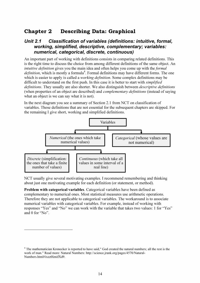
In the next diagram you see a summary of Section 2.1 from NCT on classification of variables. Those definitions that are not essential for the subsequent chapters are skipped. For the remaining I give short, working and simplified definitions.

NCT usually give several motivating examples. I recommend remembering and thinking about just one motivating example for each definition (or statement, or method).

Problem with categorical variables. Categorical variables have been defined as complementary to numerical ones. Most statistical measures use arithmetic operations. Therefore they are not applicable to categorical variables. The workaround is to associate numerical variables with categorical variables. For example, instead of working with responses “Yes” and “No” we can work with the variable that takes two values: 1 for “Yes” and 0 for “No”.

4 The mathematician Kronecker is reported to have said," God created the natural numbers; all the rest is the

work of man." Read more: Natural Numbers: http://science.jrank.org/pages/4570/Natural-

Numbers.html#ixzz0lznifXd9.

Variables

Numerical (the ones which take numerical values)

Discrete (simplification: the ones that take a finite

number of values)

Continuous (which take all values in some interval of a

real line)

Categorical (whose values are not numerical)

15

Unit 2.2 Frequencies and distributions (Bernoulli variable, binomial variable, sample size, random or stochastic variable, absolute and relative frequencies, frequency distributions)

One of the implicit purposes of Chapter 2 is to show you that real-life data are huge and impossible to grasp without certain graphical tools or summary measures. I think at this point it is important for you to get an idea of how the data arrive and how they are transformed for the purposes of statistical data processing. Using an Excel spreadsheet will give you the feeling of the data generation process in real time5.

Exercise 2.1 We are going to simulate a numerical two-valued variable (in Unit 7.3 it will be identified as the Bernoulli variable). In cell A1 type the name Bernoulli. In cell A2 enter the formula

=IF(RAND()>1/4,0,1)

exactly as it is (no blanks) 6. You can use lower-case letters but Excel will convert them to upper-case. In Tools/Options/Calculations select “Manual” and click OK. Now press F9 several times to see some realized values of the Bernoulli variable.

Exercise 2.2 This example models a variable with 4 integer values (we’ll see in Unit 7.3 that it’s a binomial variable). Copy the formula you entered in A2 to cells A3, A4 (you can select cell A2, pick with a mouse a small square in the lower right corner of the cell and pull it down for the selection to include cells A3, A4; the formula will be copied). In cell B1 type Binomial and in cell B2 enter the formula

=SUM(A2:A4)

By pressing F9 you can observe the realized values of the binomial variable. Many students consider it quite a headache. It will be, if you jump to the conclusions.

Exercise 2.3 This is the main exercise. We are going to collect a sample of observations on

the binomial variable. By definition, the sample size, n , is the number of observations.

(a) Choose n , press F9 n times and write down the values observed in cell B2:

1 2

..., ..., ..., ...

nb b b= = = (2.1)

Don’t be lazy and use at least 30n = .

(b) After having pressed F9 n times do you think you can predict what will show up next time? Intuitive definition of a random variable: a variable is called random (or stochastic) if its values cannot be predicted.

(c) Alternatively, do you think you can tell what is NOT likely to show up next time? The answer I am pushing for is that any number except 0, 1, 2, 3 is not likely to appear.

5 I am using Office 2003; all simulations are done in the same file; for new examples I use the cells to the right

of the filled ones.

6 The explanation of all Excel functions we use can be found in Excel Help. The mathematical side of what we

do will be explained in Unit 7.3.

16

(d) Denote ix distinct values in your sample. Most probably, they are

1 2 3 30, 1, 2, 3x x x x= = = = . Count the number of times

ix appears in your sample and denote

it in , 1, 2,3,4.i = These numbers are called absolute frequencies. Do you think their total is

n :

1 2 3 4

?n n n n n+ + + = (2.2)

(e) The numbers /i ir n n= , 1,2,3, 4,i = are called relative frequencies.

1r , for example, shows

the percentage of times the value 1x appears in your sample. Do you think the relative

frequencies sum to 1:

1 2 3 4

1?r r r r+ + + = (2.3)

You can get this equation from (2.2) by dividing both sides by n .

(f) Summarize your findings in a table:

Table 2.1 Table of absolute and relative frequencies (discrete variable)

Values of the variable Absolute frequencies Relative frequencies

10x =

1...n =

1...r =

21x =

2...n =

2...r =

32x =

3...n =

3...r =

40x =

4...n =

4...r =

Total = n Total = 1

Conclusions. Suppose somebody else works with a different sample size. Your and that person’s absolute frequencies will not be comparable because their totals are different. On the other hand, comparing relative frequencies will make sense because they sum to 1. Relative frequencies are better also because they are percentages. The columns of frequencies show how totals are distributed over the values of the variable. Therefore they are called absolute and relative frequency distributions, respectively. For convenience reasons, most of the time the last column of Table 2.1 is used and the adjective “relative” is omitted. Once you understand this basic situation, it is easy to understand possible variations, which we consider next.

Categorical variables. For example, suppose that at a given university there are four instructor ranks: lecturer, assistant professor, associate professor and full professor. Then instead of Table 2.1 we have

Table 2.2 Table of absolute and relative frequencies (categorical variable)


Lecturer 1

...n = 1

...r =

Assistant professor 2

...n = 2

...r =

Associate professor 3

...n = 3

...r =

Full professor 4

...n = 4

...r =

Total = n Total = 1

Exercise 2.4 Here we model a continuous variable. See Unit 7.3 for the theory.

(a) To model summer temperatures in my city, type in cell C1 Temperature and in cell C2 the formula

17

=NORMINV(RAND(),25,8)

The resulting numbers are real and may have many nonzero digits. Usually nobody reports temperatures with high precision. In Format/Cells/Number select “Number” as the category and 1 decimal place in “Decimal places” and click OK.

(b) Select the sample size and write down the observed values in form (2.1). Since the elements in the sample are real numbers, none may be repeated and in that case all absolute frequencies are equal to 1. What is worse, if you obtain another sample, it may have very few common elements with the first one. To achieve stability over samples and reduce the table size, in such cases the observations are joined in ranges (groups, clusters). In case of temperatures you can use intervals of length 1:

min max

10 11, ..., 39 40t t t t= ≤ < ≤ < = (2.4)

(the valuesmin max,t t will in fact depend on the sample and may be different from the ones you

see here). In this approach the values in the first column will be intervals (2.4).

(c) For each observation, you calculate the number of observations falling into that interval to find the absolute frequency. Since observed values are replaced by the intervals they fall into, under this approach a part of the information contained in the sample is lost. However, if the lengths of the intervals are decreased, the loss decreases and the resulting frequencies

represent the variables very well. Denoting k the number of intervals, we obtain a table of type:

Table 2.3 Table of absolute and relative frequencies (continuous variable)


10 11t≤ < 1

...n = 1

...r =

… … …

39 40t≤ < ...

kn = ...

kr =

Total = n Total = 1

Unit 2.3 Visualizing statistical data (coordinate plane; argument, values, domain and range of a function; independent and dependent variables; histogram, Pareto diagram, time series, time series plot, stem-and-leaf display, scatterplot)

Some graph types used by statisticians are readily available in Excel. Others require some data manipulation to produce results equivalent to those available in Minitab. Alternatively, you can buy SPC XL, a statistical add-in for Excel. But I think discussing definitions of main graph types is more important than seeing them.

In the coordinate plane, we have two axes. x-values are put on the horizontal axis. y-values

are put on the vertical axis. A point with coordinates ( , )x y is located at the intersection of

two straight lines: one of them is drawn vertically through point ( ,0)x (which is on the x-

axis); the other is drawn horizontally through point (0, )y (which is on the y-axis).

A graph is the best tool to visualize a functional relationship. The rough-and-tough approach

to graphing a function ( )y f x= is to (a) select several values of the argument1, ...,

nx x , (b)

calculate the corresponding values of the function 1 1

( ), ..., ( )n n

y f x y f x= = , (c) put the

18

points 1 1

( , ), ..., ( , )n n

x y x y on the coordinate plane and (d) draw a smooth line through these

points. If you have never done this, do it at least once, say, for 22 1y x= + .

Keep in mind the terminology introduced here: x is the argument, ( )f x is the value. The set

of all arguments of the given function is called its domain. The set of all values is called its range. As the argument runs over the domain, the value runs over the range.

When working with functions, it’s better to use words that emphasize motion. The notion of a function is one of the channels through which motion is introduced in mathematics.

The argument is also called an independent variable, while the value − a dependent variable. It is customary to plot the dependent variable on the y-axis and the independent one on the x-axis, the most notable exceptions being the plots of demand and supply in economics.

In order to be at sea with statistical graphs, you have to be clear about what is the argument and what is the value in each case. The short way to express this is: plot this … (values) against that … (arguments).

2.3.1 Histogram short definition: plot frequencies against values.

Explanations. (i) In case of numerical values, put them on the x-axis. Atop each of them show the corresponding frequency with a vertical bar whose height is equal to the frequency. The width of the bar doesn’t matter, as long as the bars have the same widths and don’t overlap. You can use either absolute or relative frequencies. I prefer relative frequencies and from now on talk only about them.

(ii) When values are intervals, we know from Exercise 2.4 that intervals of type (2.4) are adjacent. Bars showing frequencies are plotted against centers of the intervals. Regarding the heights and widths of the bars there are two possibilities:

(iia) The heights express frequencies. The widths don’t matter as long as the bars don’t overlap.

(iib) The areas of the bars are equal to frequencies. In this case the widths are equal to the lengths of the intervals on the x axis (the bars stand shoulder to shoulder) and the heights are calculated from the usual area rule

area = height × width.

The second possibility is used when, as in our case, the sample is obtained from a continuous variable. As we’ll see in Unit 6.2, for a continuous variable there is an equivalent of relative frequencies, and that equivalent hinges upon area rather than height.

(iii) Suppose the values are categories other than ranges of numerical values, like instructor ranks. You put them on the x-axis at arbitrary points and plot the bars as in case (i).

2.3.2 Pareto diagram: same as a histogram, except that the observations are put in the order of decreasing frequencies.

Example 2.1 In this case it is important to remember the motivation. Suppose there are too many traffic jams in the city and the mayor is determined to eliminate them. Among the reasons of traffic jams there are: lack of parking space in the center of the city, car accidents, absence of car junctions in critical areas, rush hours etc. It makes sense to start dealing with problems that have the highest impact on traffic jams frequency. Such problems (categories) on the histogram should be put first.

19

2.3.3 Time series plot: plot values against time.

Exercise 2.5 A time series is a sequence of observations on a variable along time. For

example, a sequence of daily observations on Microsoft stock can be written as 1,...,

ns s . The

observations are plotted in their raw form, without calculating any frequencies. We model them in Excel as follows. In D1 type Stock and in D2 enter the formula

=NORMINV(RAND(),25,8)

Copy it to cells D3-D21 (which corresponds to 20n = ). Select column D and in the Chart Wizard select “Line” for the plot type. When you press F9, you see various realizations of the time series. Time series plots are good to see if there are any tendencies or trends in a series and how volatile it is. Financial time series are among the most volatile.

2.3.4 Stem-and-leaf display

Firstly, this is not a graphical display. It is a tabular representation of the data where the observations are grouped according to their leading digits and the final digits (remainders) are used to show frequencies in each group. Secondly, going from the usual decimal representation to the stem-and-leaf display and back is drudgery. Given its very limited use in statistical data processing and availability of computers, having students do it by hand is a stone age. The only reason I give the next exercise is that in NCT it is not explained how you go from the stem-and-leaf display back to the decimal representation.

Example 2.2 Let’s say we have a sample of lengths of 10 fish:

1 2 3 4 5

6 7 8 9 10

9.8, 10.1, 14.5, 10.5, 13.2,

11.1, 9.2, 11.7, 15.0, 10.2.

x x x x x

x x x x x

= = = = =

= = = = =

We take the integer part (the number before the decimal point) as the stem (leading digits) and the digit after the decimal point as the leaf (final digits). The lengths

2 4 1010.1, 10.5, 10.2x x x= = = fall into one group. The stems are shown in the second

column and the leaves in the third column. The first column contains cumulative frequencies. To obtain them, you start counting the absolute frequencies from the upper and lower ends until the cumulative frequencies are about the same (in the middle). The cumulative frequency in the first row is the absolute frequency in that row; the cumulative frequency in the second row is the sum of absolute frequencies in that row and the preceding row. You go like that and stop at row 4 because if you count similarly the cumulative frequencies starting from the bottom, in row 5 you will have 8.

Table 2.4 Stem-and-leaf display

Cumulative frequencies Stem Leaf

2 9 2, 8 5 10 1, 5, 6 7 11 1, 7 7 12 8 13 2 6 14 5 1 15 0

Total = n Total = 1

Note four features of this display.

(i) The stems are ordered, unlike the original data.

20

(ii) The number of leaves readily shows absolute frequencies in each group.

(iii) You can restore the original values from this display if you know how much one unit in

the stem is worth. In our example it is worth 1w= so, for example, the first line gives two values

9 2 0.1 9 0.2 9.2, 9 8 0.1 9 0.2 9.8.w w w w⋅ + ⋅ ⋅ = + = ⋅ + ⋅ ⋅ = + =

(iv) If we considered young fish, instead of 9.2 and 9.8 we could have 0.92 and 0.98 and each

unit in the stem would have been worth 0.1w= . The above calculation would have given the right values.

2.3.5 Scatterplot: plot values of one variable against values of another.

Be alert when you see a discussion of pairs of variables. Most students find this topic difficult.

Exercise 2.6 We want to see a rough dependence between the weight and height of an adult.

For a sample of n adults we write down their weights 1, ...,

nw w and heights

1, ...,

nh h . The

first thing to note is that these observations should be written in pairs because it doesn’t make sense to correlate one person’s weight with another person’s height. The second thing is that, logically, it is the height that determines the weight and not the other way around. Therefore the right way to write the observations is

1 1( , ), ..., ( , ).

n nh w h w

(2.5)

A scatterplot just shows these points on the coordinate plane. Now we proceed with simulating them.

(i) In cell E1 type Heights and in cell E2 put the formula

=NORMINV(RAND(),170,30) (heights are measured in centimeters and weights in kilos). In cell F1 type Weights and in cell F2 put the formula

=E2-100+NORMINV(RAND(),0,20)

Select cells E2, F2 and by pulling down the small square in the lower right corner of cell F2 copy the contents of E2, F2 to sufficiently many cells, including E21, F21 (for future exercises).

(ii) Select columns E, F and use the plot type X,Y (Scatter) without lines connecting the points to see the scatterplot. To make it nicer, in Step 3 of the Chart Wizard on the tab “Titles” type Heights for Value (X) axis and Weights for Value (Y) axis; on the tab “Legend” uncheck “Show legend”.

(iii) You can see on the plot that there is, on average, a positive relationship between weight and height, as expected. If you press F9, the sample and plot will change.

Unit 2.4 Questions for repetition

1. Describe verbally how you get Table 2.1.

2. Give short definitions of a histogram, Pareto diagram, time series plot, stem-and-leaf display, scatterplot and indicate when they are appropriate.

21

Chapter 3 Describing Data: Numerical

Unit 3.1 Three representations of data: raw, ordered and frequency representation

In this chapter we consider numerical characteristics of data sets. As you think about the definitions given here, keep in mind three possible representations of observations on a real random variable:

(i) Raw representation. You write down the data in the order you observe them:

1, ...,

nx x (3.1)

(ii) Ordered representation. You put the observations on the real line and renumber them in an ascending order:

1

...n

y y≤ ≤ (3.2)

These are the same points as in (3.1), just the order is different, so the number of points is the same.

(iii) Frequency representation. This is a table similar to Table 2.1. That is, you see how

many distinct values there are among the observed points and denote them 1

...m

z z≤ ≤

(obviously, m does not exceed n ). For each iz you find its absolute frequency

in and

relative frequency ir . The result will be

Table 3.1 Absolute and relative frequencies distribution


1z

1n

1r

… … …

mz

mn

mr

Total = n Total = 1

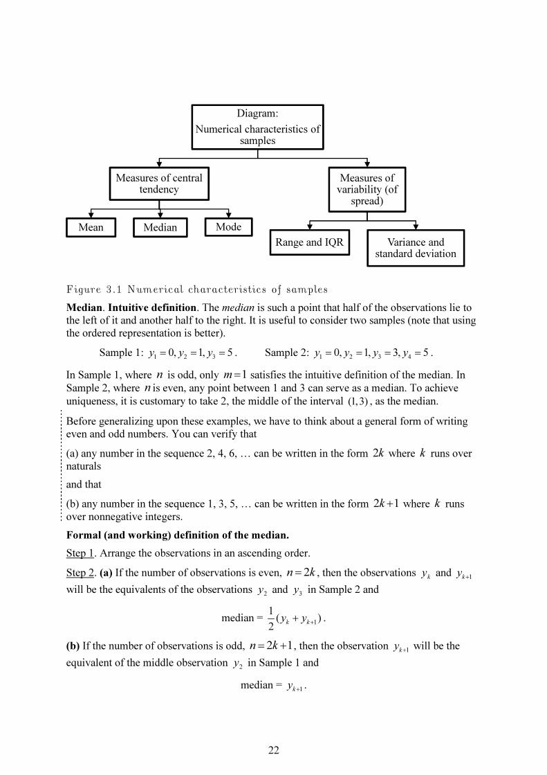
Our plan is to detail Figure 3.1 (below).

Unit 3.2 Measures of central tendency (sample mean, mean or average, median, mode; bimodal and trimodal distributions; outliers)

Mean. The sample mean (or simply mean or average) is the usual arithmetic mean

1...

nx x

x

n

+ +

= (3.3)

Does it change if instead of the raw representation one uses the ordered representation?

22

Figure 3.1 Numerical characteristics of samples

Median. Intuitive definition. The median is such a point that half of the observations lie to the left of it and another half to the right. It is useful to consider two samples (note that using the ordered representation is better).

Sample 1: 1 2 3

0, 1, 5y y y= = = . Sample 2: 1 2 3 4

0, 1, 3, 5y y y y= = = = .

In Sample 1, where n is odd, only 1m= satisfies the intuitive definition of the median. In

Sample 2, where n is even, any point between 1 and 3 can serve as a median. To achieve

uniqueness, it is customary to take 2, the middle of the interval (1,3) , as the median.

Before generalizing upon these examples, we have to think about a general form of writing even and odd numbers. You can verify that

(a) any number in the sequence 2, 4, 6, … can be written in the form 2k where k runs over naturals

and that

(b) any number in the sequence 1, 3, 5, … can be written in the form 2 1k + where k runs over nonnegative integers.

Formal (and working) definition of the median.

Step 1. Arrange the observations in an ascending order.

Step 2. (a) If the number of observations is even, 2n k= , then the observations ky and

1ky+

will be the equivalents of the observations 2y and

3y in Sample 2 and

median = 1

1( )

2k ky y

++ .

(b) If the number of observations is odd, 2 1n k= + , then the observation 1k

y+ will be the

equivalent of the middle observation 2y in Sample 1 and

median = 1k

y+.

Diagram:

Numerical characteristics of samples

Measures of central tendency

Mean Median Mode

Measures of variability (of

spread)

Range and IQR Variance and standard deviation

23

Mode. The mode is the most frequent observation. Obviously, in this case the frequency representation must be used. Note that it is possible for a frequency distribution to have more than one most frequent observation. In that case all of them will be modes. In the literature you can see names like bimodal, trimodal distributions.

Which of the measures of central tendency to use depends on the context and data.

Table 3.2 Exemplary comparison of measures of central tendency

Measure Pros Cons

Sample mean Has the best theoretical properties (to be discussed in Unit 5.2 through Unit 5.5).

Can be applied only to numerical variables.

Median Not sensitive to outliers. Good for income measurement.

Is not sensitive to where the bulk of the points lies.

Mode Can be used for categorical variables. Good when only most frequent observation matters.

Insensitive to all but the most frequent observation.

Don’t try to memorize this table. Think about the examples in NCT. Try to feel the definitions. Don’t think about observations as something frozen. Try to move them around. For example, you can fix the median, and move the points to the left of it back and forth. As you do that, do the sample mean and mode change? Or you can think about dependence on outliers, which, by definition, are points which lie far away from the bulk of the observations. If you move them further away, which of the measures of central tendency may change and which do not?

Unit 3.3 Shape of the distribution (symmetry; positive and negative skewness; tails)

The definitions of symmetry and skewness must be given in terms of the histogram.

The distribution is called symmetric if the histogram is symmetric about the mean (that is, observations equidistant from the mean to the left and right must have equal frequencies), see Figure 10.21 in NCT. Empirical distributions rarely are exactly symmetric, and judgments about approximate symmetry are subjective.

We don’t need the mathematical definition of skewness. The approximate definition of positive skewness given in NCT (that the mean should be greater than the median) is too often at variance with the precise definition. As a rule of thumb, it is better to talk about tails. We say that a distribution is positively skewed if the right tail is heavier than the left (think about the bars of the histogram as made of a heavy substance).

Unit 3.4 Measures of variability (range, quartiles, deciles, percentiles; interquartile range or IQR; five-number summary, sample variance, deviations from the mean, sample standard deviation)

Range. The smallest observation, denoted minix , in terms of the ordered representation is,

obviously, the leftmost point 1y . Similarly, the largest observation max

ix is the rightmost

point ny . Thus,

1min , max

i i nx y x y= = .

24

(i) Sometimes people call by the range the difference 1

Rangeny y= − .

(ii) It also makes sense to use this name for the segment 1

Range [ , ]n

y y= . This is the smallest

segment containing the sample.

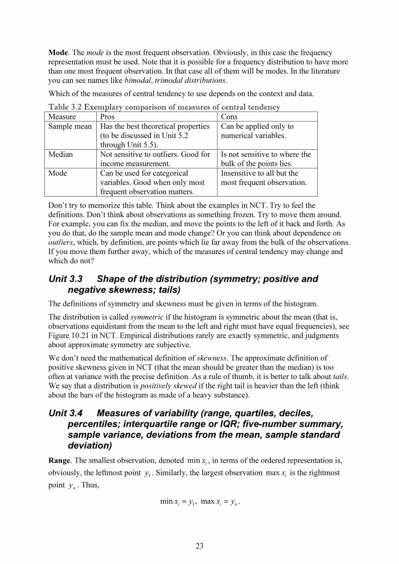
Definition of quartiles, deciles, percentiles. The idea behind them is the same as with the median: certain intervals should contain certain fractions of the total number of observations. For example, in case of quartiles we want the picture in Figure 3.2 where each of the

intervals 0 1 1 2 2 3 3 4

( , ), ( , ), ( , ), ( , )Q Q Q Q Q Q Q Q contains 25% of all observation.

Figure 3.2 Five number summary

This leads to the following definition:

1Q = observation numbered 0.25( 1)n +

3Q = observation numbered 0.75( 1)n + .

Actually, one has to take integer parts of the numbers 0.25( 1)n + , 0.75( 1)n + to apply this

definition. Similarly,

kth decile is the observation numbered ( 1)10

kn+

kth percentile is the observation numbered ( 1)100

kn + .

In the literature you can see other definitions and none of them is perfect because all are approximate. Think about it: if you have just 20 observations, how can you divide them in 100 equal parts?

Definition of IQR. As explained in NCT, the range depends on outliers. When this is a problem, the spread of the middle 50% of the data may be preferable. This gives us the definition of the interquartile range, or IQR:

3 1IQR Q Q= − .

A five-number summary is the set of numbers in Figure 3.2:

0 1 2 3 4min max .

i ix Q Q Q median Q Q x= < < = < < =

Variance. The sample variance is defined by

2 2 2

1

1( ) ... ( ) .

1x ns x x x x

n

= − + + − − (3.4)

A few names will help you understand this construction. 1,...,

nx x are the observed points. The

differences ix x− are called deviations (from the mean). 2

( )ix x− are squared deviations.

Their average would be

Q0

= y1

Q1

Q2

= median Q3

Q4

= yn

25

2 2

1

1( ) ... ( ) .

nx x x x

n

− + + −

In the definition of 2

xs there is division by 1n− instead of n for reasons to be explained in

Unit 7.2.

Exercise 3.1 If you can’t tell directly from the definition how to calculate 2

xs , I insist that you

do everything on the computer.

(i) If you are using the same Excel file as before, in cells D2-D21 you should have simulated observations on stock price. In cell G1 type Mean and in G2 enter the formula

=SUM($D$2:$D$21)/20

This is the average of the values 1 20,...,s s ; the dollar signs will prevent the addresses from

changing when you copy the formula to other cells.

(ii) Copy the formula to G2-G21. We want the same constant in G2-G21 to produce a horizontal line of the graph.

(iii) Select columns D, G and the line plot in the Chart Wizard. The time series plot is good to see the variability in the series. The sample mean is shown by a horizontal line. Some observations are above and others are below the mean, therefore some deviations from the mean are positive and others are negative.

(iv) In H1 type Deviations, in H2 type =D2-G2 and copy this to H3-H21. In I1 type Squared deviations, in I2 enter =H2^2 and copy this to I3-I21. You can notice that deviations have alternating signs and squared deviations are nonnegative.

(v) In H22 type =SUM(H2:H21)/20 and in I22 enter the formula =SUM(I2:I21)/19. The value in H22, the average of deviations, will be close to zero showing that the mean

deviation is not a good measure of variability. The value in I22 is 2

xs .

Standard deviation. The quantity 2

x xs s= is called a sample standard deviation.

Lessons to be learned. Both sample variance and sample standard deviation are used to measure variability (or volatility, or spread). Both are based on deep mathematical ideas and for now you have to accept them as they are. Unlike the range or IQR, both depend on all observations in the sample.

Once I took a course in Financial Management in a Business Department. Several equations from Corporate Finance were used without explanations of the underlying theories. The whole course was about using formulas on the calculator. The Business students were happy and I was horrified. Read again the above procedure and make sure you see the forest behind the trees. You should be able to reproduce the definitions and, if necessary, use the calculator instead of Excel.

Exercise 3.2 (a) What happens to 2

xs if all observations are increased by 5? Try to give two

different explanations.

(b) Can the sample variance be negative?

(c) If the sample variance is zero, what can you say about the variable?

Unit 3.5 Measures of relationships between variables (sample covariance, sample correlation coefficient; positively

26

correlated, negatively correlated and uncorrelated variables; perfect correlation)

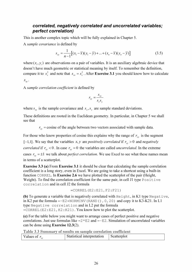
This is another complex topic which will be fully explained in Chapter 5.

A sample covariance is defined by

[ ]1 1

1( )( ) ... ( )( )

1xy n ns x x y y x x y y

n= − − + + − −

−

(3.5)

where ( , )i ix y are observations on a pair of variables. It is an auxiliary algebraic device that

doesn’t have much geometric or statistical meaning by itself. To remember the definition,

compare it to 2

xs and note that 2

xx xs s= . After Exercise 3.1 you should know how to calculate

xys .

A sample correlation coefficient is defined by

xy

xy

x y

s

r

s s

=

wherexys is the sample covariance and ,

x ys s are sample standard deviations.

These definitions are rooted in the Euclidean geometry. In particular, in Chapter 5 we shall see that

xyr = cosine of the angle between two vectors associated with sample data.

For those who know properties of cosine this explains why the range of xyr is the segment

[ 1,1]− . We say that the variables ,x y are positively correlated if 0xyr > and negatively

correlated if 0xyr < . In case 0

xyr = the variables are called uncorrelated. In the extreme

cases 1xyr = ± we talk about perfect correlation. We use Excel to see what these names mean

in terms of a scatterplot.

Exercise 3.3 (a) From Exercise 3.1 it should be clear that calculating the sample correlation coefficient is a long story, even in Excel. We are going to take a shortcut using a built-in function CORREL. In Exercise 2.6 we have plotted the scatterplot of the pair (Height, Weight). To find the correlation coefficient for the same pair, in cell J1 type Positive correlation and in cell J2 the formula

=CORREL(E2:E21,F2:F21)

(b) To generate a variable that is negatively correlated with Height, in K1 type Negative, in K2 put the formula =-E2+NORMINV(RAND(),0,20) and copy it to K3-K21. In L1 type Negative correlation and in L2 put the formula =CORREL(E2:E21,K2:K21). You know how to plot the scatterplot.

(c) For the table below you might want to arrange cases of perfect positive and negative correlations. Just use formulas like =2*E2 and =-E2. Simulation of uncorrelated variables can be done using Exercise 12.3(2).

Table 3.3 Summary of results on sample correlation coefficient

Values of xyr Statistical interpretation Scatterplot

27

1xyr =

There is an exact linear relationship between

,

i iy x in the form

i iy a bx= + with a

positive b .

0 1

xyr< <

There is an approximate linear relationship

between ,

i iy x in the

form i iy a bx≈ + with a

positive b .

0

xyr =

There is no definite pattern in the dependence.

1 0

xyr− < <

There is an approximate linear relationship

between ,

i iy x in the

form i iy a bx≈ + with a

negative b .

1

xyr = −

There is an exact linear relationship between

,

i iy x in the form

i iy a bx= + with a

negative b .

Exercise 3.4 Form some pairs of variables: inflation, unemployment, aggregate income, investment, government expenditures, per capita income and birth rate. For each pair you form indicate the expected sign of the correlation coefficient.

Least-squares regression is one of important topics of this chapter. I am not discussing it because with the knowledge we have I cannot say about it more than the book, and what we have done should be enough for you to understand what the book says. End-of-chapter exercises 3.46-3.56 is the minimum you should be able to solve. The full theory is given in Chapter 12.


1. Give in one block all definitions related to the five-number summary

0

100

200

300

400

500

0 50 100 150 200 250

Height

Ex

ac

t p

os

itiv

e

-20

0

20

40

60

80

100

120

140

0 100 200 300

Heights

Weights

Z

-90

-80

-70

-60

-50

-40

-30

-20

-10

0

0 10 20 30 40

X

Y

-250

-200

-150

-100

-50

0

0 100 200 300

Heights

Negative

-250

-200

-150

-100

-50

0

0 50 100 150 200 250

Height

Exa

ct

ne

ga

tive

28

2. An expression for the sample variance equivalent to (3.4) is

( )2

2 21 1.

1 ( 1)X i is x x

n n n

= −

− −

∑ ∑ Which one is easier to apply on a hand calculator?

3. Solve Exercise 3.45 from NCT.

29

Chapter 4 Probability

The way uncertainty is modeled in the theory of probabilities is complex: from sets to probabilities to random variables and their characteristics.

Unit 4.1 Set operations (set, element, union, intersection, difference, subset, complement, symmetric difference; disjoint or nonoverlapping sets, empty set)

Recall that the notion of a set is not defined. We just use equivalent names (collection, family, or array) and hope that, with practice, the right intuition will develop.

In the examples in the next table S denotes the set of all students of a particular university,

A denotes the set of students taking an anthropology class and B is the set of students taking

a biology class. We write x A∈ to mean that x is an element of A ( x belongs to A ). x A∉

means that x is not an element of A .

Table 4.1 Set operations: definitions, visualization and logic

Definition Visualization on Venn diagram

Logical interpretation and/or comments

The union A B∪ is the set of elements which belong to

A , to B or both.

Figure 4.2 in NCT

Logically, the union corresponds to

nonexclusive “or”7. A B∪ means all students who study anthropology or biology (or both).

The intersection A B∩ is the set of elements common

to A and B .

Figure 4.1(a) in NCT

Logically, the intersection corresponds

“and”. A B∩ is the set of students who study both anthropology and biology.

The difference \A B is the

set of elements of A which

do not belong to B .

\A B is the set of students who study anthropology but not biology. Don’t use “–“ (minus) or “|” (pipe) instead of the backslash “\”.

We say that A is a subset

of S and write A S⊂ if all

elements of A belong to .S

In applications S will be fixed, while its subsets will be changing.

A complement A is defined

as the difference \A S A=

and includes elements of S

outside A .

Figure 4.3 in NCT.

A is the set of students who do not study anthropology.

The set

( \ ) ( \ )A B A B B A= ∪△ is

called a symmetric

difference of A and B .

(lightly shaded

The symmetric difference logically

corresponds to “either or”. A B△ is the set

of students who study A or B but not both.

7 In English “or” is nonexclusive whereas “either or” is exclusive. In some other languages there is only one

“or” and one has to specify whether it is exclusive or nonexclusive.

BA

BA

A S

30

area)

For convenience, people introduce the empty set ∅ (the set without elements). A andB are

called disjoint (or nonoverlapping) if A B∩ =∅ (they have no common elements).

Unit 4.2 Set identities (distributive law, de Morgan laws, equality of sets)

To solve some exercises in NCT you need to use certain set relations. All of them can be established using Venn diagrams. There is no need to remember them but try to understand the logic which will help you pick the right relation for the exercise at hand.

Result 1. A set B can be obtained as a union of two disjoint sets, ( ) ( )B A B A B= ∩ ∪ ∩ ,

where A B∩ is the common part of A and B and A B∩ is the common part of A and B .

Try to express verbally the other results.

Result 2. ( )A B A A B∪ = ∪ ∩ .

Result 3. Distributive law: ( ) ( ) ( )A B C A B A C∩ ∪ = ∩ ∪ ∩ .

Result 4. De Morgan’s laws: ,A B A B A B A B∪ = ∩ ∩ = ∪ (you pass to complements by

interchanging unions and intersections).

These equations can be established using Venn diagrams but there is a more powerful method

which works when using the Venn diagrams would be infeasible. We say that two sets, U

and V , are equal, U V= , when and U V V U⊂ ⊂ (that is each element of U belongs to V

and vice versa). To prove the first de Morgan law, denote U A B= ∪ , V A B= ∩ .

Suppose x U∈ . By definition, \ ( )x S A B∈ ∪ which means two things: x S∈ , x A B∉ ∪ .

Hence, ,x A x B∈ ∈ and x A B∈ ∩ . Since the implication x U x V∈ ⇒ ∈ is true for any

element of U , we have proved that U V⊂ . The proof of V U⊂ is left as an exercise.

Unit 4.3 Correspondence between set terminology and probabilistic terminology (random experiment; impossible, collectively exhaustive and mutually exclusive events; sample space; basic outcomes or elementary events; occurrence of an event, disjoint coverings)

Definition of a random experiment: A random experiment is a process leading to two or more possible outcomes, with uncertainty as to which outcome will occur.

The example of rolling a die is sufficient to illustrate this intuitive definition.

If you stay at the intuitive level, you will never really understand the true meaning of most mathematical constructions.

The next table helps you establish ways to think about outcomes. When more than one term exists to express the same thing, try to use the more geometric term.

Table 4.2 Set terminology and probabilistic terminology

Set terminology Probabilistic terminology

1 Set Outcome or event, such as getting 1 on a die. Getting an even number is another example.

31

2 Empty set Impossible event

3 Disjoint sets Mutually exclusive events

4 S (universal set which contains all other sets of interest)

The widest possible event, called a sample

space S . In case of the die, {1,2,3,4,5,6}S =

5 Sets 1,...,

nA A S⊂ form a

covering if 1

...n

S A A= ∪ ∪ .

Events 1,...,

nA A S⊂ such that

1...

nS A A= ∪ ∪

are called collectively exhaustive.

6 Elements of S . Basic outcomes, or elementary events, are the simplest possible events.

Comments. (1) In case of the die the basic outcomes are the sets {1},{2},{3},{4},{5},{6} . All

other events can be obtained from these 6. For example, the event E that an even number turns up equals {2,4,6}E = . Of course, these numbers cannot turn up at the same time (this is

expressed as {2} {4} {6}∩ ∩ =∅ ). We say that E occurs when one of the numbers 2, 4, 6

turns up.

(2) We distinguish a number 2 from a set {2} . Arithmetic operations apply to numbers, while

for sets we use set operations.

In some problems we need disjoint coverings. For motivation, think about a jigsaw puzzle. Its pieces possess two properties: any two pieces are disjoint and together the pieces cover (comprise) the whole image. Departing from this geometric example, we say that events

1,...,

nA A S⊂ are mutually exclusive and collectively exhaustive if

(a) any pair ,

i jA A is disjoint and

(b) 1

...n

S A A= ∪ ∪ .

Unit 4.4 Probability (inductive and deductive arguments; induction, probability, nonnegativity, additivity, completeness axiom, complement rule, assembly formula, impossible and sure events)

Before proceeding with the formal definitions, try to answer the following questions (in parentheses I give the answers I usually hear from my students).

Exercise 4.1 (a) Intuitively, what do you think is the probability of getting a head when tossing a coin? (Some say 0.5, others say 50%. There are also answers like: on average, 50 times out of 100).

(b) When rolling a die, what do you think is the probability of getting 1? (Most say 1/6).

(c) Recall Table 2.1. Suppose you obtain a large sample and calculate that the variable takes values listed in the first column with relative frequencies listed in the third column. For the purposes of predicting the values in future samples would you accept the relative frequencies as the probabilities of the respective values? (Most say “Yes”).

The answers to parts (a) and (b) suggest that the coin and die are described by the following tables:

Table 4.3 Probability tables for C (Coin) and D (Die)

Values of C Probabilities Values of D Probabilities

H 1/2 {1} 1/6

T 1/2 {2} 1/6

32

{3} 1/6

{4} 1/6

{5} 1/6

{6} 1/6

Denoting ( )P A the probability of event A , from Table 4.3 we can surmise that

({2,4,6}) ({2}) ({4}) ({6}) 3 / 6 1 / 2.P P P P= + + = =

This makes sense because {1,2,3,4,5,6} {1,3,5} {2,4,6}= + . Generalizing upon Table 2.1 and

Table 4.3, in case of a variable with n values the following should be true:

Table 4.4 Probability table in case of a variable with n values

Values of the variable Probabilities

1x

1 1( )p P X x= =

… …

nx ( )

n np P X x= =

Here the sample space is 1

{ ,..., }n

S x x= . Since the numbers i

p mean percentages, they

should satisfy the conditions

(i) 0 1ip< <

for all i and

(ii) 1

... 1n

p p+ + = (completeness axiom).

The completeness axiom means that we have listed in the table all possible basic outcomes. If that axiom were not satisfied, we would have a smaller sample space.

Until this point I have been using what is called an inductive argument: by analyzing a simple situation and using an element of guessing, try to come up with definition that could be a base of a theory. When a definition is difficult to understand, try to pinpoint the underlying inductive argument. In the times of Karl Gauss it was common to show inductive arguments. These days they are mostly omitted, partly to save on paper and time. By skipping inductive arguments, you are not saving your time. You are complicating your task.

Before turning to a deductive argument, in which everything is deduced logically from a few basic definitions and postulates, a brush up on functions is necessary. Whenever you talk

about a function ( )f x , you have to realize what type of objects you can substitute as

arguments and what type of objects you can get as values. Right now we need to discuss dependence of area on a surface and of volume on a body. In both cases the arguments are sets and the values are numbers. Most importantly, the functions are additive. For instance, if

we denote ix pieces of a jigsaw puzzle, then

1 1( ... ) ( ) ... ( )

n narea x x area x area x∪ ∪ = + + .

Similarly, if ir denotes a room in a building, then

1 1( ... ) ( ) ... ( )

n nvolume r r volume r volume r∪ ∪ = + + .

Note the importance, for these equations to hold, of the facts that the pieces 1,...,

nx x do not

overlap and the rooms 1,...,

nr r are disjoint. Put it simply, if A B∩ =∅, as in the diagram

33

then ( ) ( ) ( )area A B area A area B∪ = + . If, on the other hand, A B∩ ≠∅ , as in the more

general case

then ( ) ( ) ( ) ( )area A B area A area B area A B∪ = + − ∩ because in the sum ( ) ( )area A area B+

the area of A B∩ is counted twice.

Definition. Let S be a sample space. By probability on S we mean a numerical function

( )P A of events A S⊂ such that

(a) if ,A B are mutually exclusive, then ( ) ( ) ( )P A B P A P B∪ = + (additivity),

(b) for any A , ( )P A is nonnegative, and

(c) ( ) 1P S = (completeness axiom).

Any definition as complex as this needs some chewing and digesting. This includes going back, to the motivating examples, going forward, to the consequences, and going sideways, to look at variations or cases when it is not satisfied.

Going back. To put the example from Table 4.4 into the general framework, for any event

A S⊂ define

( ) ({ })i

i

x A

P A P x

∈

=∑ (read like this: sum of probabilities of those

ix which belong to A ).

For example, 1 2 3 1 2 3

({ , , }) ({ }) ({ }) ({ })P x x x P x P x P x= + + . Later on we are going to use more

summation signs, and you will get used to them. Always write out the sums completely if you

don’t understand summation signs. As an exercise, try to show that the ( )P A defined here is

additive, nonnegative and satisfies the completeness axiom.

Going forward. (1) One way to understand a property is to generalize it. In the case under

consideration, additivity is generalized to the case of n events. If 1,...,

nA A are disjoint, then

from item (a) in the definition of probability we have

1 1 1 1 1

1 2 1 1

( ... ) (( ... ) ) ( ... ) ( )

( ... ) ( ) ( ) ( ) ... ( ).

n n n n n

n n n n

P A A P A A A P A A P A

P A A P A P A P A P A

− −

− −

∪ ∪ = ∪ ∪ ∪ = ∪ ∪ +

= ∪ ∪ + + = + +

This type of derivation of a general statement from its special case is called induction.

(2) The complement rule. Representing S as S A A= ∪ , from items (a) and (c) we deduce

( ) ( ) ( ) 1P A P A P S+ = = (4.1)

which implies the complement rule:

( ) 1 ( )P A P A= − .

B A

B A

34

(3) From (b) we know that ( ) 0P A ≥ . In addition, since in (4.1) ( ) 0P A ≥ , we have ( ) 1P A ≤ .

(4) Assembly formula. Fix some event B . If 1,...,

nA A are disjoint, then pieces

1,...,

nB A B A∩ ∩ are also disjoint. Further, if

1,...,

nA A are collectively exhaustive, then those

pieces comprise B . Therefore by additivity

1

( ) ( ) ... ( )n

P B P B A P B A= ∩ + + ∩ . (4.2)

Going sideways. While area and volume are additive and nonnegative, they generally do not satisfy condition (c).

When a definition is long, after chewing and digesting it you should formulate its short-and-easy-to-remember version.

Short definition. A probability is a nonnegative additive function defined on some sample

space S and such that ( ) 1P S = .

An impossible event can be defined by ( ) 0P A = . When ( ) 1P A = , we say that A is a sure

event. In the discrete case we are considering the only impossible event is A=∅ and the only sure event is the sample space.

In many practical applications it is not necessary or possible to check that all requirements of probabilistic definitions are satisfied.

Exercise 4.2 (a) What is the probability that tomorrow the sun will rise?

(b) What is the probability of you being at home and at the university at the same time?

(c) Probability of which event is higher: that tomorrow’s temperature at noon will not exceed 19°C or that it will not exceed 25°C?

Unit 4.5 Ways to find probabilities for a given experiment (equally likely events, classical probability, addition rule)

4.5.1 Equally likely outcomes (theoretical approach)

(1) In case of a fair coin, the head and tail are equally likely, so ( ) ( )P H P T= . Since these

events are mutually exclusive and collectively exhaustive, by additivity and completeness

axiom ( ) ( ) 1P H P H+ = . It follows that ( ) ( ) 1/ 2P H P T= = . We have rigorously proved the

first Table 4.3.

(2) In case of a fair die the events {1},...,{6} are equally likely, so they all have the same

probability p . By additivity and completeness axiom 6 1p = , so 1/ 6p = . We have derived

the second Table 4.3.

(3) More generally, suppose that there are N basic outcomes and suppose the basic

outcomes are equally likely. Then, as above, the probability of one basic outcome is 1/ N .

Now consider some condition that separates an event A S⊂ (in case of a die the condition

could be that the outcome is even). Denote AN the number of basic outcomes satisfying the

condition. Then by additivity

times

1 1( ) ...

A

A

N

NP A

N N N= + + =

��

.

35

This formula is called classical probability in the book. Many students remember the formula but don’t think about the conditions under which it is true. Reread the above derivation and state the result in the form: if … then…

(4) Frequentist approach. After observing relative frequencies in an experiment, one can take those frequencies as probabilities. The larger the sample size, the better will be the approximation to the truth. This is a general statistical fact. Statistics is mostly about large sample properties.

Exercise 4.3 We are going to simulate a large number of tossings of a fair coin. To work with numbers instead of heads and tails, we introduce a numerical variable

1 if head

0 if tailC

=

In a large number of trials n we calculate the proportion of heads. As n increases, n

p

should approach ½.

Step 1. In cell A1 put the formula

=IF(RAND()>1/2,0,1)

Copy it to cells A2-A100. These will be observations on the coin.

Step 2. In B1 type

=SUM($A$1:A1)/ROW(A1)

and copy this formula to B2-B100. The result in, say, B100 will be

=SUM($A$1:A100)/ROW(A100)

This is the sum of the contents of the cells A1 through A100 divided by the number of these

cells. Thus, in cells B1-B100 we have averages of the first n observations, 1,...,100n = .

Step 3. Select column B and see on the line plot the behavior of averages. They approach ½. To see the picture better, on the plot right-click the vertical axis and select “Format Axis”. On the Scale tab check Minimum and enter 0 for the value, uncheck Maximum and enter 1 for the value and check Major Unit and enter 0.1 for the value. Click OK. By pressing F9 you

will change realizations of the means for sample sizes 100n ≤ . Sometimes the speed of convergence of averages to ½ is not very good. This is a general probabilistic fact (see Unit 8.2 for the theory).

(5) Expert opinions. When the theoretical and frequentist approaches are not applicable, one can use subjective probabilities assigned by experts. For example, performance of economic projects depends on overall macroeconomic conditions. In project evaluation the resulting statements sound like this: with probability 0.6 the economy will be on the rise, and then the profitability of the project will be this much and so on.

Exercise 4.4 Generalize the addition rule ( ) ( ) ( ) ( )P A B P A P B P A B∪ = + − ∩ to the case of

three events ( ) ...P A B C∪ ∪ =

Unit 4.6 Combinatorics (factorial, orderings, combinations)

Definition. For a natural number n denote ! ( 1)...2 1n n n= ⋅ − ⋅ . This number is called n

factorial.

What do you think grows faster (as n increases): , ! or n n

e n n ?

36

Combinatorics is a wide area but we need only two results, one about orderings and the other about combinations. In order not to confuse them, remember just two motivating examples.

Example 4.1 There are three contestants in a competition, denoted 1 2 3, ,A A A , and three

prizes of different values (the possibility of ties is excluded). How many prize distributions are possible?

Solution. Let “>” stand for “better”. The ordering 1 2 3A A A> > is not the same as, say,

2 1 3A A A> > because the prizes are different. The number of prize distributions equals the

number of orderings and can be found as follows. Any of the three contestants can get the first prize, which gives us 3 possibilities. After the first prize is awarded, any of the remaining two contestants can get the second prize, which gives us 2 possibilities. After the second prize is awarded, there is only one possibility for the third prize. Any of these possibilities (3, 2 and 1) can be combined with any other, so the total number of possibilities

is 3⋅2⋅1 = 3! To see why the possibilities must be multiplied, you can use a tree (see NCT).

Exercise 4.5 To internalize the above argument, consider the case of n contestants and n

prizes. The number of orderings is the number of ways n elements can be ordered and it

equals !n .

Example 4.2 There are three new professors on campus and the IT department has 5 new identical computers, 3 of which will be distributed among the new professors. In how many different ways this is possible to do?

Solution. Denote 1 2 3, ,A A A the professors and

1 2 5, ,...,C C C the computers. Since the

computers are identical, the computer assignment

1 1

2 2

3 3

C A

C A

C A

→

→

→

is as good as, say,

1 1

3 2

5 3

C A

C A

C A

→

→

→

.

To make use of Example 4.1 let us introduce two fictitious persons 1 2,F F . As we know,

1 2 3 1 2, , , ,A A A F F can be assigned computers in 5! different ways, if the order matters. Now we

take into account that real persons can be ordered in 3! ways. Fictitious persons can be ordered in 2! ways. Five people can be ordered in 3!2! ways. Thus, the number of computer

assignments to real persons when the order doesn’t matter is 5!

3!2!

Definition. The number of different choices of x objects out of n identical objects is called

the number of combinations of x elements out ofn and denoted n

xC (here 0 x n≤ ≤ ).

Exercise 4.6 Generalize the above argument to show that !

!( )!

n

x

nC

x n x=

−

Comments. (1) When the order matters, use orderings and when it does not, apply combinations.

37

(2) In case of combinations I find it more practical to read n

xC as “the number of choices of x

elements out of n ”.

(3) For the choices formula to work in the extreme cases 0,x x n= = we put formally 0! = 1.

Exercise 4.7 Write out sequences 1 1 2 2 2 3 3 3 3

0 1 0 1 2 0 1 2 3{ , }, { , , }, { , , , }C C C C C C C C C . Note that they first

grow and then decline, the first and last elements being 1.

Unit 4.7 All about joint events (joint events, joint and marginal probabilities, cross-table, contingency table)

These notions are interrelated but in NCT they are given in different places and without discussing the relationships between them. The discussion will be long, and if you are stuck with something, read everything from the start.

Example 4.3 In Kazakhstan the profits of wheat producers critically depend on weather conditions during summer (a lot of rain results in an abundant crop; there is always a lot of sun) and the weather during the harvesting time (just three rainy days in September are

enough for the quality of wheat to plunge). Let us denote by S the event that the weather is

good in summer and by H the event that it is good during the harvesting time. The farmers are happy when ( )P S H∩ is high.

Definition. The event A B∩ is called a joint event and its probability ( )P A B∩ is called a

joint probability.

Comments. (1) Following the recommendation made earlier, remember that A and B may

vary and ( )P A B∩ is a function of two sets.

(2) In the wheat example we have four possible states of nature (the basic events) H S∩ ,

H S∩ , H S∩ , H S∩ and, correspondingly, four probabilities ( )P H S∩ , ( )P H S∩ ,

( )P H S∩ , ( )P H S∩ . By the completeness axiom, these probabilities sum to 1. As usual,

this information can be displayed in a table.

Table 4.5 1-D table of joint events and probabilities

Events Probabilities

H S∩ ( )P H S∩

H S∩ ( )P H S∩

H S∩ ( )P H S∩

H S∩ ( )P H S∩

Total = 1

Note that by the complement rule ( ) ( ) 1, ( ) ( ) 1.P S P S P H P H+ = + = Therefore we have two

more tables

Table 4.6 Separate probability tables

Events Probabilities Events Probabilities

S ( )P S H ( )P H

S ( )P S H ( )P H

1 1

38

It is convenient to call the numbers ( )P S and ( )P S own probabilities of the pair { S , S }

and the numbers ( )P H and ( )P H own probabilities of the pair {H ,H }.

(3) It is better to replace a 1-D table Table 4.5 by a 2-D table, in order to see better its link to Table 4.6.

Table 4.7 Joint probability table

H H Right margin

S ( )P S H∩ ( )P S H∩ ( )P S

S ( )P S H∩ ( )P S H∩ ( )P S

Lower margin ( )P H ( )P H 1

In a 2-D table it is easier to form pairs of individual events S , S , H and H . The probabilities from Table 4.5 have migrated to the central part of Table 4.7 (circumscribed with a double line). By the assembly formula

( ) ( ) ( ), ( ) ( ) ( )P S H P S H P S P S H P S H P S∩ + ∩ = ∩ + ∩ = .

Thus, row sums of the probabilities in the central part of Table 4.7 are equal to own

probabilities of the pair { S , S } (displayed in the right margin). Similarly, column sums of

the probabilities in the central part of Table 4.7 are equal to own probabilities of the pair {H

,H } (displayed in the lower margin). The customary name for own probabilities, marginal probabilities, reflects their placement in the table but not their role.

(4) The unity in the lower right corner of Table 4.7 is

(a) the sum of joint probabilities in the central part,

(b) the sum of own probabilities in the right margin and

(c) the sum of own probabilities in the lower margin.

(5) A cross-table (also called a contingency table) is similar to the joint probabilities table, except that instead of probabilities absolute frequencies are used.

Exercise 4.8 (a) List and prove 7 identities which hold for a joint probabilities table.

(b) Draw a joint probabilities table for the case when in the first column there are events 1A ,

…, n

A and in the first row there are events 1

B , …, m

B (n is not necessarily equal to m ).

Summation signs. Because of importance of the last exercise, we’ll do it together. This is the place to learn the techniques of working with summation signs. The sum

1

...n

a a+ + (4.3)

(in which the three points mean “and so on”) is written as

1

n

i

i

a

=

∑ (4.4)

(4.3) can be referred to as an extended expression and (4.4) is a short expression. In the short

expression we indicate the index that changes, i , and that it runs from the lower limit of

summation, 1, to the upper one, n . If you have problems working with summation signs, replace them with extended expressions, do the algebra, and then convert everything back. For the beginning remember two things:

39

(i) The sum (4.4) does not depend on i , as one can see from the extended expression. In

particular, the summation index can be replaced by anything else, for example, 1

n

j

j

a

=

∑ is the

same thing as (4.4).

(ii) When more than one different indices are involved, it is better to use different notations for them.

The answer to Exercise 4.8(b) looks as follows:

Table 4.8 Joint probability table (general case)

1

B … m

B Right margin

1A

1 1( )P A B∩ …

1( )

mP A B∩

1( )P A

… … … … …

nA

1( )

nP A B∩ … ( )

n mP A B∩ ( )

nP A

Lower margin 1

( )P B … ( )m

P B 1

Each of the families {1A , …,

nA } and {

1B , …,

mB } is mutually exclusive and collectively

exhaustive.

Identities:

(i) Sums across rows: 11 1

( ) ( ),..., ( ) ( )m m

i j n j nj jP A B P A P A B P A

= =

∩ = ∩ =∑ ∑ .

(ii) Sums across columns: 1

( ) ( ), 1,..., .n

i j jiP A B P B j m

=

∩ = =∑

(iii) Sums of own probabilities: 1 1

( ) 1, ( ) 1m n

j ij iP B P A

= =

= =∑ ∑ .

(iv) Sum of joint probabilities: 1 1

( ) 1.m n

i jj iP A B

= =

∩ =∑ ∑

Unit 4.8 Conditional probabilities (multiplication rule, independence of events, prior and posterior probability)

Example 4.4 In the wheat example (Example 4.3), suppose the summer is over, the weather has been good and the harvesting time is approaching. We are left with one line of Table 4.7:

Table 4.9 Leftover joint probabilities

H H Right margin

S ( )P S H∩ ( )P S H∩ ( )P S

Here the sum

( ) ( ) ( )P S H P S H P S∩ + ∩ = (4.5)

is not 1 and the completeness axiom is not satisfied. But we know that there are no missing

events. To satisfy the completeness axiom, we can divide both sides of (4.5) by ( )P S ,

( ) ( )1

( ) ( )

P S H P S H

P S P S

∩ ∩+ =

40

and treat ( ) / ( )P S H P S∩ and ( ) / ( )P S H P S∩ as probabilities of events H and H ,

provided that S has occurred.

Definition. Let ( ) 0P S > . The probability ( )

( | )( )

P H SP H S

P S

∩

= is called probability of H

conditional on S .

Comments. (1) If we are interested in probabilities of H and H , why not use simply ( )P H

and ( )P H ? The reason is that occurrence of S provides us with additional information.

There may be some dependence between events S and H , in which case conditional

probabilities ( | )P H S and ( | )P H S will be a better reflection of reality than own

probabilities of the pair {H ,H }. This process of updating our beliefs as new information arrives is one of the fundamental ideas of the theory of probabilities.

(2) Often random variables are introduced axiomatically. That is, take any numbers i

p

satisfying 0 1ip< < and

1... 1

np p+ + = and you can be sure that there is a random variable

whose values have probabilities exactly equal to those i

p ’s. Conditional probabilities are

defined axiomatically and the subsequent theory justifies their introduction.

Multiplication rule. The definition of ( | )P H S immediately implies

( ) ( | ) ( )P H S P H S P S∩ = .

Try to see the probabilistic meaning of this equation. Denote M the event that you obtain a

passing grade in Math and by S the event that you obtain a passing grade in Stats. Suppose

that Math is a prerequisite for Stats. Then the equation ( ) ( | ) ( )P S M P S M P M∩ = basically

tells us that to obtain a passing grade in both Math and Stats you have to pass Math first and, with that prerequisite satisfied, to obtain a passing grade in Stats. The fact that you have not failed Math tells something about your abilities and increases the chance of passing Stats.

4.8.1 Independence of events

Intuitive definition. Events A and B are called independent if occurrence of one of them does not influence in any way the chances of occurring of the other. For example, what happens to the coin has nothing to do with what happens to the die.

Formal definition. Events A and B are called independent if ( ) ( ) ( )P A B P A P B∩ = . When

( ) 0P B > , this can be equivalently written as ( | ) ( )P A B P A= .

This definition is applied in two ways.

(1) From independence to equation. If you know that A and B are independent, you can multiply ( )P A and ( )P B to get ( )P A B∩ . For example,

( 1, 1) ( 1) ( 1) 1 /12.P Coin Die P Coin P Die= = = = = =

(2) From equation to independence (or dependence). If you find that ( ) ( ) ( )P A B P A P B∩ ≠ ,

you conclude that A and B are dependent.

Exercise 4.9 Prove that if A and B are independent, then their complements are also independent.

41

Solution. Always write down what is given and what you need to get. We know that

( ) ( ) ( )P A B P A P B∩ = and we need to prove that ( ) ( ) ( )P A B P A P B∩ = . When rearranging

expressions indicate what rule you are applying, until everything becomes trivial.

( ) ( ) (complement rule)

[1 ( )][1 ( )] (multiplying out)

1 ( ) ( ) ( ) ( ) (by independence)

1 ( ) ( ) ( ) (additivity rule)

P A P B

P A P B

P A P B P A P B

P A P B P A B

=

= − −

= − − +

= − − + ∩

1 ( ) (complement rule)

( ) (de Morgan)

( )

P A B

P A B

P A B

= − ∪

=

= ∩

∪

A tangible example of independent events

Take the square [0,1] [0,1]S = × as the sample space, see Figure 4.1. For any set A S⊂

define its probability to be its area: ( ) ( )P A area A= . Since area is additive, nonnegative and

( ) 1P S = , this will be really a probability.

Figure 4.1 Example of independent events

For any [ , ] [0,1]a b ⊂ define A as the vertical strip {( , ) : ,0 1}A x y a x b y= ≤ ≤ ≤ ≤ . For any

[ , ] [0,1]c d ⊂ define B as the horizontal strip {( , ) : 0 1, }B x y x c y d= ≤ ≤ ≤ ≤ . Then

( ) , ( ) ,

{( , ) : , },

( ) ( )( ) ( ) ( )

P A b a P B d c

A B x y a x b c y d

P A B b a d c P A P B

= − = −

∩ = ≤ ≤ ≤ ≤

∩ = − − =

Thus, A and B are independent. Now try to move the strip A left and right and the strip B up and down. Independence takes a physical meaning: movements in mutually orthogonal directions do not affect each other.

y

1

10 x

d

c

ba

A

B

42

Theorem 4.1 (Bayes theorem) This theorem is one of realizations of the idea about updating one’s beliefs on the basis of new information. The easiest way to remember it is to express

( | )P B A through ( | )P A B :

( ) ( ) ( ) ( )( | ) ( | ) .

( ) ( ) ( ) ( )

P B A P B A P B P BP B A P A B

P A P B P A P A

∩ ∩

= = =

Interpretation in terms of subjective probabilities. Before occurrence of the event A , an

expert forms an opinion about likelihood of the event B . That opinion, embodied in ( )P B , is

called a prior probability. After occurrence of A , the expert’s belief is updated to obtain

( | )P B A , called a posterior probability. By the Bayes theorem, updating is accomplished

through multiplication of the prior probability by the factor ( | )

( )

P A B

P A.

A simple way to complicate the matters. Suppose 1,...,

KB B form a disjoint covering of the

sample space. By the Bayes theorem for each i

B

( | ) ( )( | ) .

( )

i i

i

P A B P BP B A

P A=

Here ( )P A can be replaced by

1

1 1

( ) (assembly formula)

( ) ... ( ) (multiplication rule)

( | ) ( ) ... ( | ) ( )

K

K K

P A

P A B P A B

P A B P B P A B P B

=

= ∩ + + ∩

= + +

The result is

1 1

( | ) ( )( | ) .

( | ) ( ) ... ( | ) ( )

i i

i

K K

P A B P BP B A

P A B P B P A B P B=

+ +

(4.6)

To me this is a good proof that knowing the derivation is better than remembering the result.

Unit 4.9 Problem solving strategy

Make sure that you can solve at least two typical exercises from each section. Have a look at Exercises (in NCT) 4.5, 4.6, 4.13, 4.14, 4.27, 4.28, 4.33, 4.35, 4.66, 4.76, 4.85, and 4.86. In the end of each chapter, starting from this one, there is a unit called Questions for Repetition, where, in addition to theoretical questions, I indicate a minimum of exercises from NCT.

To write down the conditions, you need a good notation. Avoid abstract notation and use

something that reminds you of what you are dealing with, like A for Anthropology class.

When looking for a solution of a problem, write down all the relevant theoretical facts. Don’t limit yourself to conclusions; repeat everything with proofs and derivations. Omit only what is easy; after a while everything will become easy. If you still don’t see the solution, go back by one or two steps and solve simpler similar exercises.

Exercises in the end of Sections 4.4 and 4.5 are easier than they look. This is where writing down all the relevant equations is particularly useful. Remember what you need to find. In

general, to find n unknowns it is sufficient to have n equations involving them. One of my students was able to solve those exercises without any knowledge of conditional and joint probabilities, just using common sense and the percentage interpretation of probabilities.

43

When you clearly see the idea, don’t calculate the numbers. Learn to save your time by concentrating on ideas.

If section exercises are too simple, don’t waste your time and go directly to end-of-chapter exercises.

Everybody finds difficult exercises that require orderings and combinations (there are many of them in the end of Section 4.3 and Chapter 4). Solve more of them, until you feel comfortable. However, it’s not a good idea to solve all of them.

Don’t go wide, go deep!


1. What do we mean by set operations?

2. Prove de Morgan laws.

3. Prove and illustrate on a Venn diagram equation (4.2).

4. Prove ( ) ( ) ( ) ( )P A B P A P B P A B∪ = + − ∩ .

5. Prove the formulas for orderings and combinations

6. Using a simple example, in one block give all definitions and identities related to joint and marginal probabilities.

7. Solve Exercise 4.9.

8. Derive the complex form of the Bayes theorem (4.6).

9. The minimum required: Exercises 4.5, 4.13, 4.27, 4.37, 4.47, 4.67, 4.88, 4.91, 4.93, 4.97, 4.107 from NCT.

44

Chapter 5 Discrete Random Variables and

Probability Distributions

At some point you may feel that the amount of new information is overwhelming and you forget many facts. Then it’s the time to arrange a global repetition. Repeat everything with proofs. Look for those minor or significant details you missed earlier. Make a list of facts in a logical order. This chapter will be more challenging than all the previous taken together, and you will need to be in a perfect shape to conquer it.

Unit 5.1 Random variable (random variable, discrete random variable)

Intuitive definition. A random variable is a variable whose values cannot be predicted.

For example, we can associate random variables with the coin and die. On the other hand, to

know the value of sin x it suffices to plug the argument x in. sin x or the number of days in a year are not random variables.

Short formal definition. A random variable is a pair: values plus probabilities.

Working definition of a discrete random variable. A discrete random variable is defined by Table 5.1:

Table 5.1 Discrete random variable with n values

Values of X Probabilities

1x

1p

… …

nx

np

Comments. (1) Most of the time, when people talk about random variables, they assume real-valued variables. Thus, in the first column we have real numbers. This is important to be able to use arithmetic operations.

(2) Capital X is used for the variable and lower-case x ’s for its values. The complete form

of writing i

p is ( )

iP X x= .

(3) Without the second column we would have a deterministic variable.

(4) In the table X takes a finite number of values. This is a simplification. In Unit 5.14 we’ll see an example of a discrete random variable that takes an infinite number of values.

Unit 5.2 General properties of means (expected value, mean, average, mathematical expectation, uniformly distributed discrete variable, grouped data formula, weighted mean formula)

Example 5.1 With probability 0.001 a strong earthquake destroys your house this year and then your loss is $200,000. Otherwise, your loss is just normal wear and tear, estimated at $4,000 per year. What is your expected loss?

Sometimes I ask questions before giving formal definitions, to prompt you to guess. Guessing and inductive reasoning are important parts of our thinking process. In economics there is a French term “tâtonnement” (groping one’s way in the dark). There are cases when you

45

clearly see the idea and the solution is straightforward. In more complex situations there may be several competing ideas, and some of them may not be clear, looking like unfamiliar creatures in the dark. Looking for them and nurturing them until they shape up so that you can test them is a great skill. This is where you need to collect all the relevant information, mull it over again and again, until it becomes your second nature. This process is more time-consuming than getting a ready answer from your professor or classmate but the rewards are also greater.

The expected loss is (-4,000)×0.999 + (-200,000)×0.001 = -4,196. The general idea is that it is a weighted sum of the values of the variable of interest (the loss function). We attach a higher importance to the value that has a higher probability.

In research ideas go before definitions.

Expected value of a discrete random variable. Using the working definition of a random

variable, we define the expected value of X (also called a mean, or an average, or mathematical expectation) to be

1 1

... .

n nEX x p x p= + + (5.1)

Comments. (1) Expected value is a function whose argument is a complex object (it is

described by Table 5.1) and the value is simple: EX is just a number. And it is not a product

of E and X !

(2) Relation to the sample mean. A discrete random variable is said to be uniformly

distributed if 1

... 1/n

p p n= = = . In this case the expected value is just the sample mean:

1

1

...1 1... .

n

n

x xEX x x X

n n n

+ +

= + + = =

(3) Grouped data formula. Recall the procedure for finding relative frequencies. Denote

1,...,

ny y the values in the sample. Equal values are joined in groups. Let

1,...,

mx x denote the

distinct values and 1,...,

mn n their absolute frequencies. Their total is, clearly, n . The sample

mean is

1

1

times times

1 1

1 1

... (sorting out 's into groups with equal values)

... ... ...

... (dividing through by and using relative freq

m

n

nn

m m

m m

y yY y

n

x x x x

n

n x n xn

n

+ +

=

+ + + + + +

=

+ +

=

��

1 1

uencies)

... .m m

r x r x EX= + + =

(5.2)

In this context, the sample mean Y , the grouped data formula (in the third line) and the expected value are the same thing. The weighted mean formula from NCT (see their equation

(3.12)) is the same thing as the grouped data formula with i in w= and

in w=∑ . Note also

that when data are grouped by intervals, as in Table 3.5 of NCT, in the grouped data formula

the midpoints i

m of the intervals are taken as the values of the variables.

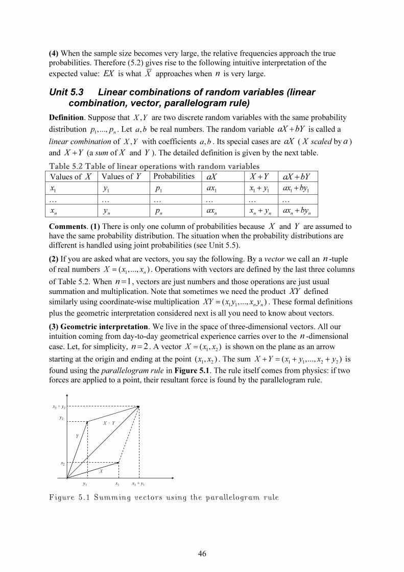
46

(4) When the sample size becomes very large, the relative frequencies approach the true probabilities. Therefore (5.2) gives rise to the following intuitive interpretation of the

expected value: EX is what X approaches when n is very large.

Unit 5.3 Linear combinations of random variables (linear combination, vector, parallelogram rule)

Definition. Suppose that ,X Y are two discrete random variables with the same probability

distribution 1,...,

np p . Let ,a b be real numbers. The random variable aX bY+ is called a

linear combination of ,X Y with coefficients ,a b . Its special cases are aX ( X scaled by a )

and X Y+ (a sum of X and Y ). The detailed definition is given by the next table.

Table 5.2 Table of linear operations with random variables

Values of X Values of Y Probabilities aX X Y+ aX bY+

1x

1y

1p

1ax

1 1x y+

1 1ax by+

… … … … … …

nx

ny

np

nax

n nx y+

n nax by+

Comments. (1) There is only one column of probabilities because X and Y are assumed to have the same probability distribution. The situation when the probability distributions are different is handled using joint probabilities (see Unit 5.5).

(2) If you are asked what are vectors, you say the following. By a vector we call an n -tuple

of real numbers 1

( ,..., )n

X x x= . Operations with vectors are defined by the last three columns

of Table 5.2. When 1n = , vectors are just numbers and those operations are just usual

summation and multiplication. Note that sometimes we need the product XY defined

similarly using coordinate-wise multiplication 1 1

( ,..., )n n

XY x y x y= . These formal definitions

plus the geometric interpretation considered next is all you need to know about vectors.

(3) Geometric interpretation. We live in the space of three-dimensional vectors. All our

intuition coming from day-to-day geometrical experience carries over to the n -dimensional

case. Let, for simplicity, 2n = . A vector 1 2

( , )X x x= is shown on the plane as an arrow

starting at the origin and ending at the point 1 2

( , )x x . The sum 1 1 2 2

( ,..., )X Y x y x y+ = + + is

found using the parallelogram rule in Figure 5.1. The rule itself comes from physics: if two forces are applied to a point, their resultant force is found by the parallelogram rule.

Figure 5.1 Summing vectors using the parallelogram rule

X

X + Y

Y

x2

x2

+ y2

y2

x1

+ y1

x1

y1

47

Scaling X by a positive number a means lengthening it in case 1a > and shortening in case

1a < . Scaling by a negative number means, additionally, reverting the direction of X .

Figure 5.2 Scaling a vector

To obtain a linear combination aX bY+ you first scale X and Y and then add the results.

Unit 5.4 Linearity (portfolio, portfolio value, universal statements, existence statements, homogeneity of degree 1, additivity)

Linearity is one of those many properties in which both the statement of the problem and its solution are mathematical.

Problem statement. What is the relation between ( )E aX bY+ and ,EX EY ?

Answer. For any random variables ,X Y and any numbers ,a b one has

( )E aX bY aEX bEY+ = + .

Proof. This is one of those straightforward proofs when knowing the definitions and starting with the left-hand side is enough to arrive at the result. Using the definitions in Table 5.2 the mean of the linear combination is

1 1 1

1 1 1 1

1 1 1 1

( ) ( ) ... ( ) (multiplying out)

... ... (grouping by variables)

( ... ) ( ... )

.

n n n

n n n n

n n n n

E aX bY ax by p ax by p

ax p by p ax p by p

ax p ax p by p by p

aEX bEY

+ = + + + +

= + + + + +

= + + + + +

= +

Chewing and digesting

Going back. A portfolio contains 1n shares of stock 1 whose price is

1S and

2n shares of

stock 2 whose price is 2S . Stock prices fluctuate and are random variables. Numbers of

shares are assumed fixed and are deterministic. What is the expected value of the portfolio?

Answer. The portfolio value is its market price 1 1 2 2

V n S n S= + . Since this is a linear

combination, the expected value is 1 1 2 2

EV n ES n ES= + .

Going sideways. (1) Rewrite the proof of linearity of means using summation signs.

(2) Do you think 2( )E X is the same as 2

( )EX ? Hint: It should be clear that 2 2 2

1( ,..., )

nX x x=

and 2 2 2

1 1...

n nEX x p x p= + + , see Unit 5.3.

(3) While I don’t give an answer for the previous question, I want to use it to discuss the difference between universal statements (which should be true for a class of objects) and existence statements (which assert existence of objects with special properties). If you say:

Yes, I think that 2 2( ) ( )E X EX= , it should be a universal statement: for ANY random

variable X one has 2 2( ) ( )E X EX= . If, on the other hand, you say: No, I don’t think so, then

it should be an existence statement: I am producing X such that 2 2( ) ( )E X EX≠ (whereas

X

2X2X

X

2X

0.5X

X

–X

X

48

for other variables the equation may be true). Pay attention to the order of words when you use “for every” and “there exists”. In the next two propositions the words are the same, just their order is different:

(i) In the city of X, for every man M there is a woman W such that W is a girlfriend of M.

(ii) In the city of X, there is a woman W such that W is a girlfriend of M for every man M.

Going forward. (1) Letting in the linearity property 0b = we get ( )E aX aEX= . This

property is called homogeneity of degree 1 (you can pull the constant out of the expected value sign).

(2) Letting 1a b= = in the linearity property we get ( )E X Y EX EY+ = + . This is called

additivity.

(3) Use induction to prove the generalization to the case of a linear combination of n variables:

1 1 1 1( ... ) ...

n n n nE a X a X a EX a EX+ + = + +

(4) Expected value of a constant. The mean of a constant is that constant,

1 1... ( ... ) 1

n nEc cp cp c p p= + + = + + = , because a constant doesn’t change, rain or shine.

Unit 5.5 Independence and its consequences (independent and dependent variables, multiplicativity of means)

Background. You have to recall the definition of independence of two events

( ) ( ) ( )P A B P A P B∩ = and realize that a random variable is a much more complex object

than an event. Visually, a random variable is a 1-D table with values and probabilities. A pair of random variables is represented by a 2-D table similar to Table 4.8. Since we want to work with variables whose probability distributions are not necessarily the same, a table of type Table 5.2 is insufficient. We deal with two random variables separately represented by the following tables

Table 5.3 Separate probability tables

Values of X Probabilities Values of Y Probabilities

1x

1

Xp

1y

1

Yp

… … … …

nx X

np

my Y

mp

In general, n is different from m . The probabilities are also different, that’s why they are provided with superscripts. If you remember, in this situation we cannot directly define the

sum X Y+ and the product XY . This is why we need to work with the pair ( , )X Y which

has values ( , ), 1,..., , 1,...,i jx y i n j m= = (you can think about throwing a coin and die at the

same time; any value on the coin can occur in combination with any value on the die). The

probabilities of these values are denoted , 1,..., , 1,...,ijp i n j m= = . Now we arrange a 2-D

table putting a pair of values ( , )i jx y and corresponding probability

ijp in the same cell:

Table 5.4 Joint values and probabilities

1y …

my Right margin

49

1x

1 1( , )x y ,

11p …

1( , )

mx y ,

1mp

1

Xp

… … … … …

nx

1( , )

nx y ,

1np … ( , )

n mx y ,

nmp X

np

Lower margin 1

Yp … Y

mp 1

Exercise 5.1 One and the same random variable can have many different (equivalent)

realizations. The variable X is realized in Table 5.3 on the sample space 1

{ ,..., }n

x x . What is

its realization in terms of Table 5.4 (what are the sample space, probability distribution and values)?

Exercise 5.2 You can refresh your memory by rewriting in this notation the identities following Table 4.8.

Intuitive definition. We say that X and Y are independent if what happens to X does not

influence Y in any way.

Formal definition. We say that X and Y are independent if the events independence condition is satisfied for every pair of their values:

, 1,..., , 1,...,X Y

ij i jp p p i n j m= = = (5.3)

Comments. (1) This is an opportune moment to discuss the relation between universal statements and existence statements. Consider a universal statement: all students in a given class are younger than 30. Its opposite is: there are students in a given class who are at least 30 years old, which is an existence statement. This is a general rule of logic: rejecting a universal statement you obtain an existence one, and vice versa.

(2) Rejecting the definition of independence, we obtain the definition of dependence, and it

should be an existence statement. Thus, we say that X and Y are dependent if at least one of the equations (5.3) is not true.

Definition. The sum X Y+ and the product XY are defined by the tables

Table 5.5 General definitions of the sum and product

Definition of X Y+ Definition of XY

1y …

my

1y …

my

1x

1 1x y+ …

1 mx y+

1x

1 1x y …

1 mx y

… … … … … … … …

nx

1nx y+ …

n mx y+

nx

1nx y …

n mx y

Exercise 5.3 How is the definition related to the earlier one?

Multiplicativity of expected values. If ,X Y are independent, then their mean is

multiplicative: ( )( )EXY EX EY= .

Proof. Earlier you were asked to rewrite the proof of linearity of means using summation signs. Here we need a special case of that property:

1 1

m m

j j

j j

az a z

= =

=∑ ∑ .

Using Table 5.5 and probabilities from Table 5.4 we have

50

1 1

1 1

1 1

(using independence assumption)

( is a constant for the inner sum)

( )( ).

n m

i j ij

i j

n mX Y X

i j i j i i

i j

n mX Y

i i j j

i j

EXY x y p

x y p p a x p

x p y p EX EY

= =

= =

= =

=

= =

= =

∑∑

∑∑

∑ ∑

Comments. (1) If you don’t understand this, take 2n m= = , write out everything without summation signs and then write out equivalents with summation signs.

(2) Multiplicativity is not a linear property. All operators in math that are linear may have nonlinear properties only under special conditions. Independence is such a special condition.

Recapitulating, ( )E aX bY aEX bEY+ = + is true for ANY ,X Y and ( )( )EXY EX EY= holds

ONLY under independence.

(3) The complete notation for the fact that X takes the value ix with probability X

ip is

( )X

i iP X x p= = . Similarly, the complete expression for the probabilities from Table 5.4 is

( , )i j ij

P X x Y y p= = = . This formalism is necessary to understand some equations in NCT.

(4) Two other characteristics of random variables, variance and covariance, are defined in terms of means. Therefore we shall be using linearity of means very often.

Unit 5.6 Covariance (linearity, alternative expression, uncorrelated variables, sufficient and necessary conditions, symmetry of covariances)

Definition. For two random variables ,X Y their covariance is defined by

cov( , ) ( )( )X Y E X EX Y EY= − − .

Comments. (1) Covariance has two complex arguments, whereas its value is simple – just a number.

(2) X EX− is the deviation of X from its mean; Y EY− is the deviation of Y from its mean. Therefore cov( , )X Y is the expected value of the product of these two deviations.

Explain all formulas for yourself in this way.

(3) The book says that covariance is a measure of relationship between two variables. This is true with some caveats. We keep covariance around mainly for its algebraic properties.

Property 1. Linearity. Covariance is linear in the first argument when the second argument

is fixed: for any random variables , ,X Y Z and numbers ,a b one has

cov( , ) cov( , ) cov( , ).aX bY Z a X Z b Y Z+ = + (5.4)

Proof. We start by writing out the left side of (5.4):

51

cov( , )

[( ) ( )]( ) (using linearity of means)

( )( ) (collecting similar terms)

[ ( ) ( )]( ) (multiplying

aX bY Z

E aX bY E aX bY Z EZ

E aX bY aEX bEY Z EZ

E a X EX b Y EY Z EZ

+

= + − + −

= + − − −

= − + − − out)

[ ( )( ) ( )( )] (using linearity of means)

( )( ) ( )( ) (by definition of covariance)

cov( , ) cov( , ).

E a X EX Z EZ b Y EY Z EZ

aE X EX Z EZ bE Y EY Z EZ

a X Z b bY Z

= − − + − −

= − − + − −

= +

Exercise 5.4 Covariance is also linear in the second argument when the first argument is fixed. Write out and prove this property. You can notice the importance of using parentheses and brackets.

Learning longer proofs will develop your logic and intuition to the extent that you’ll be able to produce results like this on demand.

Property 2. Alternative expression: cov( , ) ( )( )X Y EXY EX EY= − .

Proof.

cov( , )

( )( ) (multiplying out)

[ ( ) ( )( )] ( , are constants; use linearity)

( )( ) ( )( ) ( )( )

( )( ).

X Y

E X EX Y EY

E XY XEY EX Y EX EY EX EY

EXY EX EY EX EY EX EY

EXY EX EY

= − −

= − − +

= − − +

= −

Definition. Random variables ,X Y are uncorrelated if cov( , ) 0X Y = . Uncorrelatedness is

close to independence, so the intuition is the same: one variable does not influence the other. You can also say that there is no statistical relationship between uncorrelated variables.

Property 3. Independent variables are uncorrelated: if ,X Y are independent, then

cov( , ) 0X Y = .

Proof. By the alternative expression of covariance and multiplicativity of means for

independent variables cov( , ) ( )( ) 0X Y EXY EX EY= − = .

Comments. (1) This is a good place to discuss necessary and sufficient conditions. We say

that condition A is sufficient for condition B if A implies B: A ⇒ B. When this is true, we also say that B is necessary for A. Visually, the set of all objects satisfying A is a subset of all objects satisfying B when A is sufficient for B. For example, the statement on relationship between independence and uncorrelatedness is visualized like this:

52

Figure 5.3 Independent versus uncorrelated pairs of variables

(2) When A is both necessary and sufficient for B, we say that A is equivalent to B and write

A ⇔ B. An interesting question is whether independence is equivalent to uncorrelatedness or, put it differently, if there exist uncorrelated pairs which are not independent. The answer is

Yes. Take any variable X such that 30EX EX= = and put 2

Y X= . This Y is not

independent of X because knowledge of the latter implies knowledge of the former. However, they are uncorrelated:

3cov( , ) ( )( ) ( )( ) 0.X Y EXY EX EY EX EX EY= − = − =

(3) Here we show that the condition 30EX EX= = is satisfied for any random variable that

is symmetric around zero. The symmetry definition implies that any negative value ix− can be

written as i ix x− +

= − where ix+ is a positive value of the same variable and the probabilities

are the same: ( ) ( )i i

P X x P X x− +

= = = . Therefore

0 0

0

(sorting out positive and negative values)

(replacing negative values and their probabilities)

[( ) ] ( ) (

i i

i

i i

i i i i

x x

i i i

x

EX x p

x p x p

x x P X x

− +

+

− +

< >

+ + +

>

=

= +

= − + =

∑

∑ ∑

∑ the two terms cancel out)

0.=

The proof of 30EX = is similar.

Property 4. Correlation with a constant. Any random variable is uncorrelated with any constant: cov( , ) ( )( ) 0.X c E X EX c Ec= − − =

Property 5. Symmetry. Covariance is a symmetric function of its arguments:

cov( , ) cov( , )X Y Y X= .

Unit 5.7 Variance (interaction term, variance of a sum, homogeneity of degree 2, additivity of variance)

Definition. For a random variable X , its variance is defined by 2( ) ( )V X E X EX= − .

Comments. (1) Variance measures the spread of X around its mean.

All uncorrelated

pairs X,Y

All

independent

pairs X,Y

53

(2) For linear operations, like the mean EX , it is common to write the argument without parentheses, unless it is complex, as in ( )E aX bY+ . For nonlinear operations, of type ( )V X ,

the argument must be put in parentheses.

Property 1. Relation to covariance: ( ) cov( , )V X X X= .

Property 2. Variance of a linear combination. For any random variables ,X Y and

numbers ,a b one has

2 2( ) ( ) 2 cov( , ) ( ).V aX bY a V X ab X Y b V Y+ = + + (5.5)

The term 2 cov( , )ab X Y in (5.5) is called an interaction term.

Proof. Use Property 1:

2 2

( ) cov( , )

(using linearity with respect to the first variable)

cov( , ) cov( , )

(using linearity with respect to the second variable)

cov( , ) cov( , ) cov( , ) cov( ,

V aX bY aX bY aX bY

a X aX bY b Y aX bY

a X X ab X Y ab Y X b Y

+ = + +

= + + +

= + + +

2 2

)

(using symmetry of covariance and collecting similar terms)

( ) 2 cov( , ) ( ).

Y

a V X ab X Y b V Y= + +

Exercise 5.5 (1) Prove the property directly, without appealing to covariance.

(2) How do you obtain from this property two special cases:

(i) ( ) ( ) 2cov( , ) ( )V X Y V X X Y V Y+ = + + (variance of a sum)

and

(ii) 2( ) ( )V aX a V X= (homogeneity of degree 2)?

(3) What do you think is larger: ( )V X Y+ or ( )V X Y− ?

(4) If we add a constant to a variable, does its variance change?

Property 3. Variance of a constant: 2( ) ( ) 0V c E c Ec= − = .

Property 4. Nonnegativity: ( ) 0V X ≥ for any X .

Proof. By definition,

2 2 2

1 1( ) ( ) ( ) ... ( ) .

n nV X E X EX p x EX p x EX= − = − + + − (5.6)

This is a weighted sum of squared deviations, each of which is nonnegative, and the weights are positive, so the whole thing is nonnegative.

Property 5. Characterization of all variables with vanishing variance. We want to know exactly which variables have zero variance. We know that constants have this property, so

X c= is sufficient for ( ) 0V X = . Conversely, suppose that ( ) 0V X = . Since all probabilities

are positive, from (5.6) we see that 1

... 0n

x EX x EX− = = − = . This implies that all values are

equal to the mean, which is a constant. Conclusion: ( ) 0V X = if and only if X c= .

54

Property 6. Additivity of variance: if ,X Y are independent, then ( ) ( ) ( )V X Y V X V Y+ = +

(the interaction terms disappears).

Since variance is a nonlinear operator, it is additive only under special circumstances, when the variables are uncorrelated or, in particular, when they are independent.

Unit 5.8 Standard deviation (absolute value, homogeneity, Cauchy-Schwarz inequality)

Definition. For a random variable X , the quantity ( ) ( )X V Xσ = is called its standard

deviation.

In general, there are two square roots of a positive number, one positive and the other negative. The positive one is called an arithmetic square root. An arithmetic root is applied

here to ( ) 0V X ≥ , so standard deviation is always nonnegative.

Absolute values. An absolute value of a real number is defined by

, if is nonnegative| |

, if is negative

a a

a

a a

=

− (5.7)

It is introduced to measure the distance from point a to the origin. For example, dist(3,0) =

|3| = 3 and dist(–3,0) = |–3| = 3. More generally, for any points ,a b on the real line the

distance between them is given by dist( , ) | |a b a b= − .

The distance interpretation of the absolute value makes it clear that

(i) the condition [ , ]a b b∈ − is equivalent to | |a b≤

and

(ii) the condition [ , ]a b b∉ − is equivalent to | |a b> .

By squaring both sides in (5.7) we get 2 2| |a a= . Application of the arithmetic square root

gives 2| |a a= . This is the equation we need right now.

Property 1. Standard deviation is homogeneous of degree 1: 2( ) ( ) ( ) | | ( )aX V aX a V X a Xσ = = = σ .

Property 2. Cauchy-Schwarz inequality. (1) For any random variables ,X Y one has

| cov( , ) | ( ) ( )X Y X Y≤ σ σ .

(2) If the inequality sign turns into equality, | cov( , ) | ( ) ( )X Y X Y= σ σ , thenY is a linear

function of X : Y aX b= + .

Proof. (1) If at least one of the variables is constant, both sides of the inequality are 0 and

there is nothing to prove. To exclude the trivial case, let ,X Y be nonconstant. Consider a

real-valued function of a real number t defined by ( ) ( )f t V tX Y= + . Here we have variance

of a linear combination: 2( ) ( ) 2 cov( , ) ( )f t t V X t X Y V Y= + + .

We see that ( )f t is a parabola with branches looking upward (because the senior coefficient

( )V X is positive). By nonnegativity of variance, ( ) 0f t ≥ and the parabola lies above the

horizontal axis in the ( , )f t plane. Hence, the quadratic equation ( ) 0f t = may have at most

55

one real root. This means that the discriminant of the equation is non-positive: 2

[cov( , )] ( ) ( ) 0.D X Y V X V Y= − ≤ Applying square roots to both sides of 2

[cov( , )] ( ) ( )X Y V X V Y≤ we finish the proof of the first part.

(2) In case of the equality sign the discriminant is 0. Therefore the parabola touches the

horizontal axis where ( ) ( ) 0f t V tX Y= + = . But we know that this implies tX Y c+ = which

is just another way of writing Y aX b= + .

Do you think this proof is tricky? During the long history of development of mathematics mathematicians have invented many tricks, small and large. No matter how smart you are, you cannot reinvent all of them. If you want to learn a lot of math, you’ll have to study the existing tricks. By the way, the definition of what is tricky and what is not is strictly personal

and time-dependent.

Unit 5.9 Correlation coefficient (unit-free property, positively and negatively correlated variables, uncorrelated variables, perfect correlation)

Definition. Suppose random variables ,X Y are not constant. Then their standard deviations

are not zero and we can define

cov( , )( , )

( ) ( )

X YX Y

X Yρ =

σ σ

which is called a correlation coefficient between X and Y .

Property 1. Range of the correlation coefficient: for any ,X Y one has 1 ( , ) 1X Y− ≤ ρ ≤ .

Proof. By the properties of absolute values the Cauchy-Schwarz inequality can be written as

( ) ( ) cov( , ) ( ) ( ).X Y X Y X Y−σ σ ≤ ≤ σ σ

It remains to divide this inequality by ( ) ( )X Yσ σ .

Property 2. Interpretation of extreme cases. (1) If ( , ) 1X Yρ = , then Y aX b= + with 0.a >

(2) If ( , ) 1X Yρ = − , then Y aX b= + with 0a < .

Proof. (1) ( , ) 1X Yρ = implies

cov( , ) ( ) ( )X Y X Y= σ σ (5.8)

which, in turn, implies that Y is a linear function of X : Y aX b= + . Further, we can

establish the sign of the number a . By the properties of variance and covariance

cov( , ) cov( , ) cov( , ) cov( , ) ( ),

( ) ( ) ( ) | | ( ).

X Y X aX b a X X X b aV X

Y aX b aX a X

= + = + =

σ = σ + = σ = σ

Plugging this in (5.8) we get 2( ) | | ( )aV X a X= σ and see that a is positive.

The proof of (2) is left as an exercise.

Property 3. Suppose we want to measure correlation between weight W and height H of

people. The measurements are either in kilos and centimeters ,

k cW H or in pounds and feet

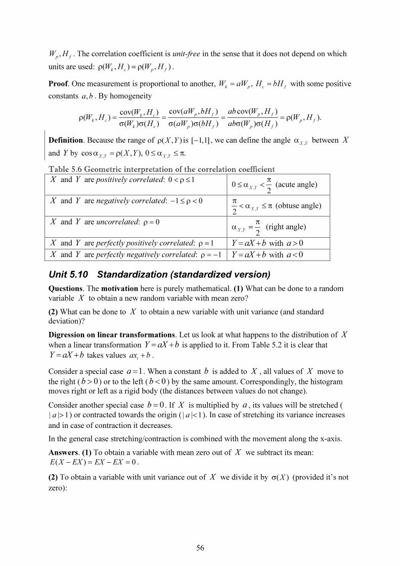
56

,p fW H . The correlation coefficient is unit-free in the sense that it does not depend on which

units are used: ( , ) ( , )k c p fW H W Hρ = ρ .

Proof. One measurement is proportional to another, ,k p c fW aW H bH= = with some positive

constants ,a b . By homogeneity

cov( , ) cov( , )cov( , )( , ) ( , ).

( ) ( ) ( ) ( ) ( ) ( )

p f p fk ck c p f

k c p f p f

aW bH ab W HW HW H W H

W H aW bH ab W Hρ = = = = ρ

σ σ σ σ σ σ

Definition. Because the range of ( , )X Yρ is [ 1,1]− , we can define the angle ,X Yα between X

and Y by , ,

cos ( , ), 0 .X Y X Y

X Yα = ρ ≤ α ≤ π

Table 5.6 Geometric interpretation of the correlation coefficient

X and Y are positively correlated: 0 1< ρ ≤ ,

02

X Y

π≤ α < (acute angle)

X and Y are negatively correlated: 1 0− ≤ ρ < ,

2X Y

π< α ≤ π (obtuse angle)

X and Y are uncorrelated: 0ρ = ,

2X Y

π

α = (right angle)

X and Y are perfectly positively correlated: 1ρ = Y aX b= + with 0a >

X and Y are perfectly negatively correlated: 1ρ = − Y aX b= + with 0a <

Unit 5.10 Standardization (standardized version)

Questions. The motivation here is purely mathematical. (1) What can be done to a random

variable X to obtain a new random variable with mean zero?

(2) What can be done to X to obtain a new variable with unit variance (and standard deviation)?

Digression on linear transformations. Let us look at what happens to the distribution of X

when a linear transformation Y aX b= + is applied to it. From Table 5.2 it is clear that

Y aX b= + takes values i

ax b+ .

Consider a special case 1a = . When a constant b is added to X , all values of X move to

the right ( 0b > ) or to the left ( 0b < ) by the same amount. Correspondingly, the histogram moves right or left as a rigid body (the distances between values do not change).

Consider another special case 0b = . If X is multiplied by a , its values will be stretched (

| | 1a > ) or contracted towards the origin ( | | 1a < ). In case of stretching its variance increases

and in case of contraction it decreases.

In the general case stretching/contraction is combined with the movement along the x-axis.

Answers. (1) To obtain a variable with mean zero out of X we subtract its mean:

( ) 0E X EX EX EX− = − = .

(2) To obtain a variable with unit variance out of X we divide it by ( )Xσ (provided it’s not

zero):

57

2

1(by homogeneity) ( ) 1.

( ) ( )

XV V X

X X

= = =

σ σ

To satisfy both requirements we combine the two transformations:

.( )

X EXY

X

−

=

σ

(5.9)

Definition. The transformation of X defined in (5.9) is called standardization and Y is

called a standardized version of X .

Exercise 5.6 Check that (5.9) has mean zero and unit variance.

In NCT the mean, variance and standard deviation are denoted by 2, and µ σ σ , respectively.

Always put a subscript to reflect the variable in question in this notation: 2, ( ), ( ) ( ).

X X XEX V X V X Xµ = σ = σ = = σ

Unit 5.11 Bernoulli variable (population, sample, sample size, sampling with replacement, ex-post and ex-ante treatment of random variables, identically distributed variables, parent population, binomial variable, number of successes, proportion of successes, standard error)

Intuitive definition. A Bernoulli variable is the variable that describes an unfair coin.

Formal definition. A Bernoulli variable is defined by the table:

Table 5.7 Bernoulli variable definition

Values of B Probabilities

1 p

0 1 p−

where 0 1p< < . Often it is convenient to denote 1q p= − .

Property 1. Mean of the Bernoulli variable: 1 0 (1 )EB p p p= ⋅ + ⋅ − = .

Property 2. Variance of the Bernoulli variable. Using the alternative expression for variance,

2 2

2 2 2 2

( ) ( )

1 0 (1 ) (1 ).

V B EB EB

p p p p p p p

= −

= + − − = − = −

Note that ( )V B is a parabola with branches looking downward. It vanishes at 0 and 1p p= =

and is maximized at 1/ 2p = , which corresponds to a fair coin.

5.11.1 Some facts about sampling not many people will tell you

Here we provide an example of an unfair coin and use it to discuss the notions of population and sample.

Take any book in English. All alphabetic characters in it are categorized as either consonants

or vowels. Denote by p the percentage of consonants. We assign 1 to a consonant and 0 to a

vowel. The experiment consists in randomly selecting an alphabetic character from the book.

Then the outcome is 1 with probability p and 0 with probability q . We have a random

58

variable described by Table 5.7. In this context, the population is the set of consonants and

vowels, along with their percentages p and q . This description fits the definition from

Section 1.2 of NCT: a population is a complete set of all items that interest the investigator.

Another definition from the same section says: a sample is an observed subset of population

values with sample size given by n . It is important to imagine the sampling process step by

step. To obtain a sample in our example we can randomly select n characters and write the sample as

1,...,

nX X

where some X ’s are unities and others are zeros. The problem is that “random selection” can be understood in different ways. We consider the most important two.

Case I. We randomly select 1

X from the whole book. Suppose it’s the first character in the

table of contents, which is “C” in NCT. Then 11X = . Then we randomly select

2X , again

from the whole book. It may well be the same “C” in the table of contents, in which case

21X = . We continue like this following two rules: (1) each selection is random and (2) the

selection is made from the whole book. The second condition defines what is called a sampling with replacement: to restore the population, selected elements are returned to it.

After we have obtained a sample of size n , we can form a sum of the observed values

1

...

n nS X X= + + (5.10)

and a sample mean

1...

.

n nX X S

Xn n

+ +

= = (5.11)

After we obtain an actual sample, there will be nothing random. n

S , being a sum of unities

and zeros, will be some integer from the range [0, ]n and X will be some fraction from

[0,1].

The subtlety of the theoretical argument in statistics is that 1,...,

nX X are treated not as

realized (ex-post) values but as theoretical (ex-ante) random variables that are associated with the drawings from the population.

Let us rewind the movie and think about the selection process again. The first time you don’t actually select a character, you just THINK about randomly selecting it from the whole book.

The associated random variable is denoted 1

X and, clearly, is described by the same table as

B . Similarly, you think about what possibilities you would face in all other cases and come to the conclusion that all drawings are described by the same table, just the names of the variables will be different.

Definition. Random variables that have the same distributions (that is, values plus probabilities) are called identically distributed.

Comments. (1) Since values plus probabilities is all one needs to find the mean and variance of a random variable, identically distributed variables have identical means and variances.

(2) Instead of saying “1,...,

nX X are identically distributed” we can equivalently say “

1,...,

nX X are drawn from the same population”. In this case the population we draw the

sample from is called a parent population.

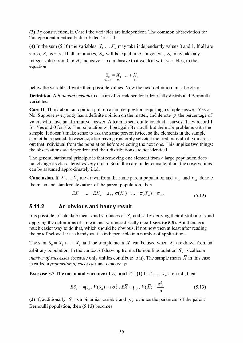
59

(3) By construction, in Case I the variables are independent. The common abbreviation for “independent identically distributed” is i.i.d.

(4) In the sum (5.10) the variables 1,...,

nX X may take independently values 0 and 1. If all are

zeros, n

S is zero. If all are unities, n

S will be equal to n . In general, n

S may take any

integer value from 0 to n , inclusive. To emphasize that we deal with variables, in the equation

10,10,..., 0,1

...

n n

n

S X X= + +

below the variables I write their possible values. Now the next definition must be clear.

Definition. A binomial variable is a sum of n independent identically distributed Bernoulli variables.

Case II. Think about an opinion poll on a simple question requiring a simple answer: Yes or

No. Suppose everybody has a definite opinion on the matter, and denote p the percentage of

voters who have an affirmative answer. A team is sent out to conduct a survey. They record 1 for Yes and 0 for No. The population will be again Bernoulli but there are problems with the sample. It doesn’t make sense to ask the same person twice, so the elements in the sample cannot be repeated. In essence, after having randomly selected the first individual, you cross out that individual from the population before selecting the next one. This implies two things: the observations are dependent and their distributions are not identical.

The general statistical principle is that removing one element from a large population does not change its characteristics very much. So in the case under consideration, the observations can be assumed approximately i.i.d.

Conclusion. If 1,...,

nX X are drawn from the same parent population and

Xµ and

Xσ denote

the mean and standard deviation of the parent population, then

1 1... , ( ) ... ( ) .

n X n XEX EX X X= = = µ σ = = σ = σ

(5.12)

5.11.2 An obvious and handy result

It is possible to calculate means and variances of and n

S X by deriving their distributions and

applying the definitions of a mean and variance directly (see Exercise 5.8). But there is a much easier way to do that, which should be obvious, if not now then at least after reading the proof below. It is as handy as it is indispensable in a number of applications.

The sum 1

...

n nS X X= + + and the sample mean X can be used when

iX are drawn from an

arbitrary population. In the context of drawing from a Bernoulli population n

S is called a

number of successes (because only unities contribute to it). The sample mean X in this case

is called a proportion of successes and denoted p .

Exercise 5.7 The mean and variance of n

S and X . (1) If 1,...,

nX X are i.i.d., then

2

2, ( ) , , ( ) .X

n X n X XES n V S n EX V X

n

σ= µ = σ = µ = (5.13)

(2) If, additionally, n

S is a binomial variable and X

p denotes the parameter of the parent

Bernoulli population, then (5.13) becomes

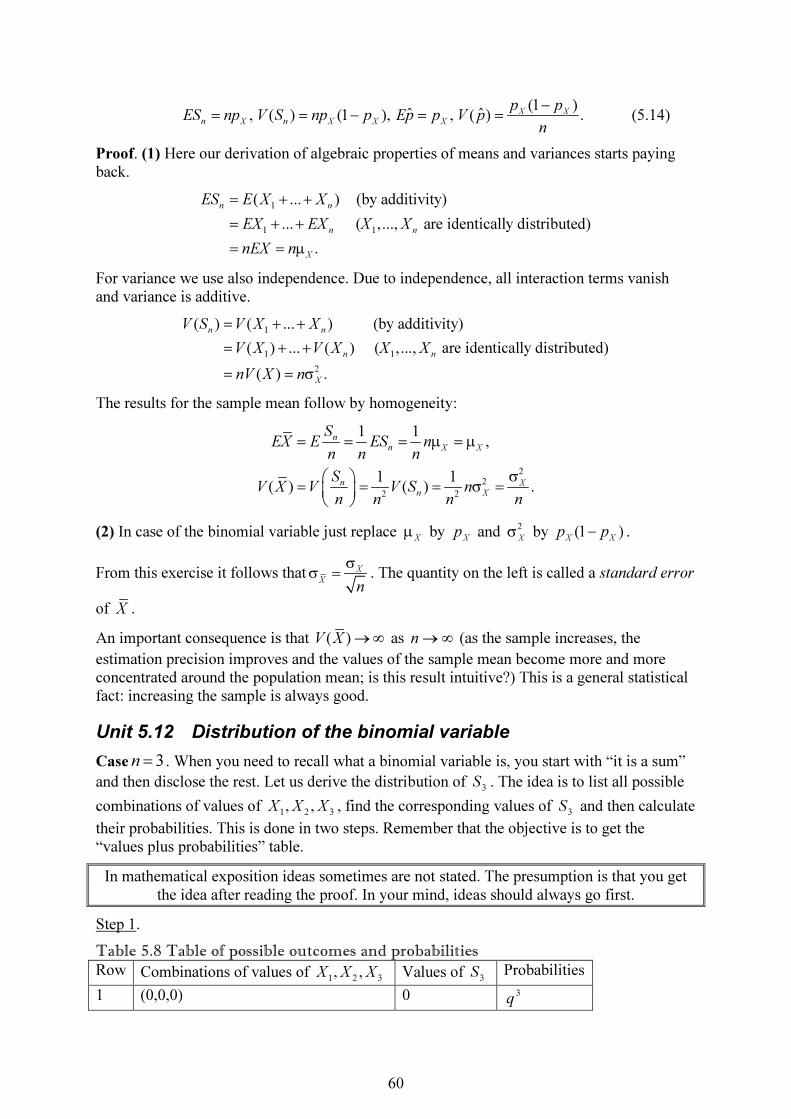
60

(1 )

ˆ ˆ, ( ) (1 ), , ( ) .X X

n X n X X X

p pES np V S np p Ep p V p

n

−

= = − = = (5.14)

Proof. (1) Here our derivation of algebraic properties of means and variances starts paying back.

1

1 1

( ... ) (by additivity)

... ( ,..., are identically distributed)

.

n n

n n

X

ES E X X

EX EX X X

nEX n

= + +

= + +

= = µ

For variance we use also independence. Due to independence, all interaction terms vanish and variance is additive.

1

1 1

2

( ) ( ... ) (by additivity)

( ) ... ( ) ( ,..., are identically distributed)

( ) .

n n

n n

X

V S V X X

V X V X X X

nV X n

= + +

= + +

= = σ

The results for the sample mean follow by homogeneity:

2

2

2 2

1 1,

1 1( ) ( ) .

n

n X X

n X

n X

SEX E ES n

n n n

SV X V V S n

n n n n

= = = µ = µ

σ = = = σ =

(2) In case of the binomial variable just replace X

µ by X

p and 2

Xσ by (1 )

X Xp p− .

From this exercise it follows that X

X

n

σ

σ = . The quantity on the left is called a standard error

of X .

An important consequence is that ( )V X →∞ as n→∞ (as the sample increases, the

estimation precision improves and the values of the sample mean become more and more concentrated around the population mean; is this result intuitive?) This is a general statistical fact: increasing the sample is always good.

Unit 5.12 Distribution of the binomial variable

Case 3n = . When you need to recall what a binomial variable is, you start with “it is a sum”

and then disclose the rest. Let us derive the distribution of 3

S . The idea is to list all possible

combinations of values of 1 2 3, ,X X X , find the corresponding values of

3S and then calculate

their probabilities. This is done in two steps. Remember that the objective is to get the “values plus probabilities” table.

In mathematical exposition ideas sometimes are not stated. The presumption is that you get the idea after reading the proof. In your mind, ideas should always go first.

Step 1.

Table 5.8 Table of possible outcomes and probabilities

Row Combinations of values of 1 2 3, ,X X X Values of

3S Probabilities

1 (0,0,0) 0 3q

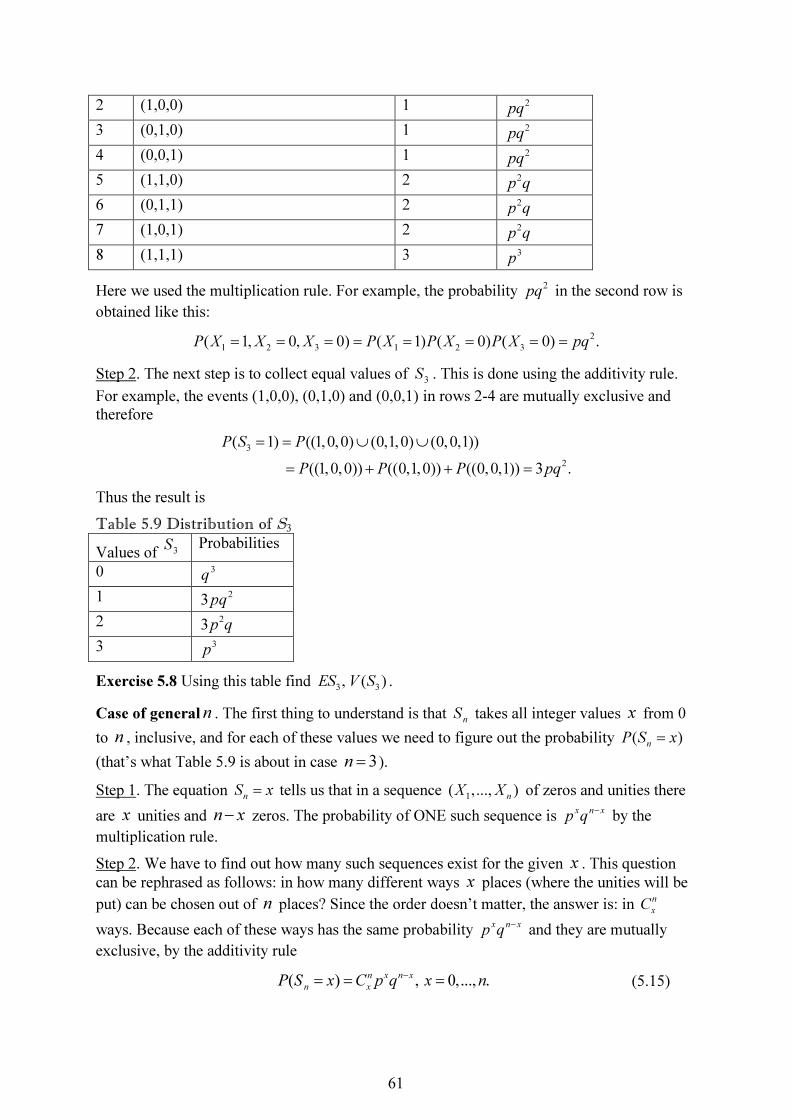
61

2 (1,0,0) 1 2pq

3 (0,1,0) 1 2pq

4 (0,0,1) 1 2pq

5 (1,1,0) 2 2p q

6 (0,1,1) 2 2p q

7 (1,0,1) 2 2p q

8 (1,1,1) 3 3p

Here we used the multiplication rule. For example, the probability 2pq in the second row is

obtained like this:

2

1 2 3 1 2 3( 1, 0, 0) ( 1) ( 0) ( 0) .P X X X P X P X P X pq= = = = = = = =

Step 2. The next step is to collect equal values of 3

S . This is done using the additivity rule.

For example, the events (1,0,0), (0,1,0) and (0,0,1) in rows 2-4 are mutually exclusive and therefore

3

2

( 1) ((1,0,0) (0,1,0) (0,0,1))

((1,0,0)) ((0,1,0)) ((0,0,1)) 3 .

P S P

P P P pq

= = ∪ ∪

= + + =

Thus the result is

Table 5.9 Distribution of S3

Values of 3S Probabilities

0 3q

1 23pq

2 23p q

3 3p

Exercise 5.8 Using this table find 3 3, ( )ES V S .

Case of generaln . The first thing to understand is that n

S takes all integer values x from 0

to n , inclusive, and for each of these values we need to figure out the probability ( )n

P S x=

(that’s what Table 5.9 is about in case 3n = ).

Step 1. The equation n

S x= tells us that in a sequence 1

( ,..., )n

X X of zeros and unities there

are x unities and n x− zeros. The probability of ONE such sequence is x n x

p q− by the

multiplication rule.

Step 2. We have to find out how many such sequences exist for the given x . This question

can be rephrased as follows: in how many different ways x places (where the unities will be

put) can be chosen out of n places? Since the order doesn’t matter, the answer is: in n

xC

ways. Because each of these ways has the same probability x n x

p q− and they are mutually

exclusive, by the additivity rule

( ) , 0,..., .n x n x

n xP S x C p q x n

−

= = = (5.15)

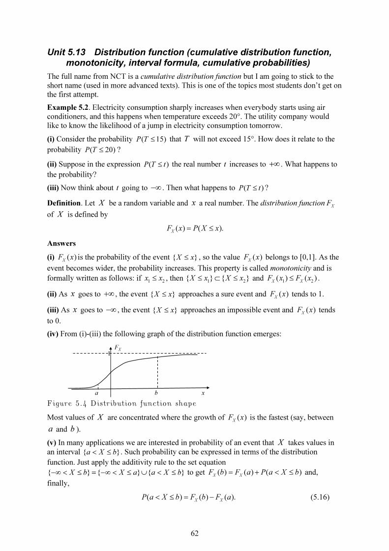
62

Unit 5.13 Distribution function (cumulative distribution function, monotonicity, interval formula, cumulative probabilities)

The full name from NCT is a cumulative distribution function but I am going to stick to the short name (used in more advanced texts). This is one of the topics most students don’t get on the first attempt.

Example 5.2. Electricity consumption sharply increases when everybody starts using air conditioners, and this happens when temperature exceeds 20°. The utility company would like to know the likelihood of a jump in electricity consumption tomorrow.

(i) Consider the probability ( 15)P T ≤ that T will not exceed 15°. How does it relate to the

probability ( 20)P T ≤ ?

(ii) Suppose in the expression ( )P T t≤ the real number t increases to +∞ . What happens to

the probability?

(iii) Now think about t going to −∞ . Then what happens to ( )P T t≤ ?

Definition. Let X be a random variable and x a real number. The distribution functionXF

of X is defined by

( ) ( ).X

F x P X x= ≤

Answers

(i) ( )X

F x is the probability of the event { }X x≤ , so the value ( )X

F x belongs to [0,1]. As the

event becomes wider, the probability increases. This property is called monotonicity and is

formally written as follows: if 1 2x x≤ , then

1 2{ } { }X x X x≤ ⊂ ≤ and

1 2( ) ( )

X XF x F x≤ .

(ii) As x goes to +∞ , the event { }X x≤ approaches a sure event and ( )X

F x tends to 1.

(iii) As x goes to −∞ , the event { }X x≤ approaches an impossible event and ( )X

F x tends

to 0.

(iv) From (i)-(iii) the following graph of the distribution function emerges:

Figure 5.4 Distribution function shape

Most values of X are concentrated where the growth of ( )X

F x is the fastest (say, between

a and b ).

(v) In many applications we are interested in probability of an event that X takes values in

an interval { }a X b< ≤ . Such probability can be expressed in terms of the distribution

function. Just apply the additivity rule to the set equation

{ } { } { }X b X a a X b−∞ < ≤ = −∞ < ≤ ∪ < ≤ to get ( ) ( ) ( )X X

F b F a P a X b= + < ≤ and,

finally,

( ) ( ) ( ).X X

P a X b F b F a< ≤ = − (5.16)

a

1

b

FX

x

63

This equation can be called an interval formula.

(vi) The definition of ( )X

F x equally applies to discrete and continuous variables. However,

in case of a discrete random variable the argument x is often restricted to the values taken by the variable. From the working definition of a discrete random variable it should be clear that, if the values are ordered, then

1 1 1 1

2 2 1 2 1 2

1

( ) ( ) ( ) ,

( ) ( ) ( ) ( ) ,

...

( ) ... .

X

X

X n n

F x P X x P X x p

F x P X x P X x P X x p p

F x p p

= ≤ = = =

= ≤ = = + = = +

= + +

The sums arising here are called cumulative probabilities. We summarize our findings in a table:

Table 5.10 Table of probabilities and cumulative probabilities

Values of X Probabilities Cumulative probabilities

1x

1p

1 1c p=

2x

2p

2 1 2c p p= +

… …

nx

np

1...

n nc p p= + +

Note that probabilities can be restored from the cumulative probabilities:

1 1 2 2 1 1, ,

n n np c p c c p c c

−

= = − = −

(vii) In Unit 6.2, Property 2, we shall see that a continuous random variable takes any fixed

value with probability zero. Therefore for such variables ( ) ( ) ( )X

F x P X x P X x= ≤ = < .

Unit 5.14 Poisson distribution (monomials, Taylor decomposition)

The derivation of the Poisson distribution from primitive assumptions would be even more difficult than for the binomial variable. Therefore we introduce it axiomatically and then start looking for real-world applications.

Taylor decomposition. The functions 0 1 21, , ,...x x x x= = are called monomials. Unlike

marsupials, they are considered simple. The idea is to represent other functions as linear

combinations of monomials. For example, a polynomial 0 1

( ) ...n

np x a a x a x= + + + is such a

combination. Linear and quadratic functions are special cases of polynomials. If infinite linear combinations, called Taylor decompositions, are allowed, then the set of functions representable using monomials becomes much wider. We are interested in the decomposition of the exponential function

2

0

1 1 1 11 ... ... .

1! 2! ! !

n x

x

e

n x

∞

λ

=

= + λ + λ + + λ + = λ∑ (5.17)

Here λ is any real number (see calculus texts for more information).

Definition. Take 0λ > and divide both sides of (5.17) by eλ to obtain

2

0

1 1 1 11 ... ... .

1! 2! ! !

n x

x

e e e e e

n x

∞

−λ −λ −λ −λ −λ

=

= + λ + λ + + λ + = λ∑

64

We see that quantities 1

!

x

xp e

x

−λ= λ satisfy the probability postulate. Hence, we can define a

random variable X by

1( ) , 0, 1, 2,...

!

x

P X x e xx

−λ= = λ =

This variable is called a Poisson distribution.

Comments. (1) This is a discrete random variable with an infinite number of values. An application should be a variable which can potentially take nonnegative integer values, including very large ones. Normally, a mobile network operator, such as T-Mobile, has a very

large number of subscribers. Let X denote the number of all customers of T-Mobile who use their mobile service at a given moment. It is random, it takes nonnegative integer values and the number of customers using their mobile phones simultaneously can be very large. Finally, decisions by customers to use their cell phones can be considered independent, unless there is a disaster.

(2) Compare this definition with what is written in Section 5.6 of NCT. “Assumptions of the Poisson Probability Distribution” from that section is an attempt to show how this distribution is derived from primitive assumptions. Since all the accompanying logic has been cut off, the result is a complete mystery.

Exercise 5.9 Calculate the mean and variance of the Poisson distribution.

Solution. In the definition of the mean the sum is, naturally, extended over all nonnegative integers:

0 0

1

1

1

1

!

(the term with 0 is actually 0, so summation starts with 1)

1

( 1)!

(we pull out , to obtain matching 1 in the power and factorial)

1

( 1)!

(repl

x

x

x x

x

x

x

x

EX xp x ex

x x

ex

x

ex

∞ ∞

−λ

= =

∞

−λ

=

∞

− −λ

=

= = λ

= =

= λ−

λ −

= λ λ−

∑ ∑

∑

∑

0 0

ace 1, to get Poisson probabilities)

1.

!

y

y

y y

y x

e py

∞ ∞

−λ

= =

= −

= λ λ = λ = λ∑ ∑

With the view to apply the alternative expression for variance, we calculate first

65

2 2 2

0 0

1

1

1 1

1

!

1

( 1)!

(this time it is possible to cancel out only one , so we replace 1 1)

1( 1 1)

( 1)!

1 1( 1)

( 1)! ( 1)!

(the idea is

x

x

x x

x

x

x

x

x x

x x

EX x p x ex

x ex

x x x

x ex

x e ex x

∞ ∞

−λ

= =

∞

−λ

=

∞

−λ

=

∞ ∞

−λ −λ

= =

= = λ

= λ−

= − +

= − + λ−

= − λ + λ− −

∑ ∑

∑

∑

∑ ∑

2 2 1 2

2 1

again to obtain Poisson probabilities)

1 1.

( 2)! ( 1)!

x x

x x

e ex x

∞ ∞

− −λ − −λ

= =

= λ λ +λ λ = λ + λ− −

∑ ∑

As a result, 2 2 2 2( ) ( )V X EX EX= − = λ + λ −λ = λ .

Conclusion. The Poisson distribution is special in that its mean and variance are the same,

( )EX V X= = λ . This is another indication as to where it can be applied.

Unit 5.15 Poisson approximation to the binomial distribution

The Poisson distribution is applied directly (see Examples 5.11 and 5.12 in NCT) or indirectly, via the binomial distribution. Before taking up the last point, we look at an example.

Exercise 5.10 An insurance company holds fraudulence insurance policies on 6,000 firms. In any given year the probability that any single policy will result in a claim is 0.001. Find the probability that at least three claims are made in a given year.

Solution. (a) Using the binomial.

On the exam you may not have enough time to calculate the answer. Show that you know the material by introducing the right notation and telling the main idea. Ideas go first!

Put 1X = if a claim is made and 0X = if it is not. This is a Bernoulli variable,

( 1) 0.001P X p= = = . Denote nS the binomial variable. By the additivity rule

( 3) 1 ( 2) 1 ( 0) ( 1) ( 2).n n n n n

P S P S P S P S P S≥ = − ≤ = − = − = − =

From this equation and the general formula ( ) n x n x

n xP S x C p q

−

= =

6000 5999 2 5998

6000 5999 2 5998

6000 5999 5998

6000! 6000!( 3) 1 0.999 0.001 0.999 0.001 0.999

1!5999! 2!5998!

1 0.999 6000 0.001 0.999 3000 5999 0.001 0.999

1 0.999 6 0.999 3 5.999 0.999 .

nP S ≥ = − − ⋅ − ⋅

= − − ⋅ ⋅ − ⋅ ⋅ ⋅

= − − ⋅ − ⋅ ⋅

(5.18)

You will die before you finish raising 0.999 to the power 6000 by hand. The trick is to use

the properties of the exponential function and natural logarithm: ln aa e= and ln ln

ba b a=

for any positive number a and real number b . In our case

66

60006000 ln0.999 6000ln0.999 6000( 0.0010005)0.999 0.00247e e e

−

= = = = .

Eventually we get ( 3) 0.93812n

P S ≥ = .

(b) Using the Poisson distribution. The distinctive feature of (5.18) is that 0.999 raised to a high power may become so small that a simple calculator will identify the result with zero.

This small number is multiplied by combinations n

xC which, when n is very large, may be

for a simple calculator the same thing as infinity. However, the product of the two numbers, one small and another large, may be manageable.

Mathematicians are reasonably lazy. When they see such numbers as in (5.18), they prefer to develop a theory than apply brute force. The device for the problem at hand is called a

Poisson approximation to the binomial distribution and sounds as follows. Suppose p is

small and n is large but their product npλ = is moderate (the book says 7λ ≤ ). Then the

probability of the binomial taking the value x can be approximated by the probability of the Poisson taking the same value:

( ) (Poisson ) .!

x

n

eP S x P x

x

−λλ

= ≈ = =

This result gives a reasonably good approximation ( 3) 0.938031n

P S ≥ = .

Unit 5.16 Portfolio analysis (rate of return)

In Unit 5.4 we already defined the portfolio value, and that definition corresponds to what the book has. In fact, the portfolio analysis is a little bit different. To explain the difference, we start with fixing two points of view.

(i) I hold a portfolio of stocks. If I want to sell it, I am interested in knowing its market value. In this situation the numbers of shares in my portfolio, which are constant, and the market prices of stocks, which are random, determine the market value of the portfolio, defined in Unit 5.4. The value of the portfolio is a linear combination of stock prices.

(ii) I have a certain amount of money 0M to invest. Being a gambler, I am not interested in

holding a portfolio. I am thinking about buying a portfolio of stocks now and selling it, say,

in a year at price 1M . In this case I am interested in the rate of return defined by

1 0

0

M Mr

M

−

= .

0M is considered deterministic (current prices are certain) and 1

M is random (future prices are unpredictable). The rate of return thus is random.

Main result. The rate of return on the portfolio is a linear combination of the rates of return on separate assets.

Proof. As it often happens in economics and finance, this result depends on how one

understands the things. The initial amount 0M is invested in n assets. Denoting 0

iM the

amount invested in asset i , we have0 0

1

n

i

i

M M

=

=∑ . Denoting 0 0/

i is M M= the share

(percentage) of 0

iM in the total investment 0

M , we have

67

0 0 0 0

1

, .

n

i i i

i

M sM M s M

=

= =∑ (5.19)

The sharesis are deterministic. Denote 1

iM what becomes of 0

iM in one year and by

1 1

1

n

i

i

M M

=

=∑ the value of the total investment at the end of the year. Since different assets

change at different rates, generally it is not true that 1 1

i iM s M= . Denote

1 0

0

i i

i

i

M Mr

M

−

= (5.20)

the rate of return on asset i . Then using (5.19) and (5.20) we get

0 0 0 01 0

0 0 0 0

(1 ).

i i i i i i i

i i

r M M rM rs MM Mr s r

M M M M

+ −−= = = = =

∑ ∑ ∑ ∑∑

This is the main result. Once you know this equation you can find the mean and variance of the rate of return on the portfolio in terms of shares and rates of return on assets.


1. List and prove all properties of means.

2. List and prove all properties of covariances.

3. List and prove all properties of variances.

4. List and prove all properties of standard deviations.

5. List and prove all properties of the correlation coefficient including the statistical interpretation from Table 3.3.

6. How and why do you standardize a variable?

7. Define and derive the properties of the Bernoulli variable.

8. Explain the term “independent identically distributed”.

9. Define a binomial distribution and derive its mean and variance with explanations.

10. Prove equation (5.15).

11. Define a distribution function, describe its geometric behavior and prove the interval formula.

12. Define the Poisson distribution and describe (without proof) how it is applied to the binomial distribution.

13. Minimum required: Exercises 5.13, 5.23, 5.37, 5.47, 5.67, 5.68, 5.82, 5.91, 5.97.

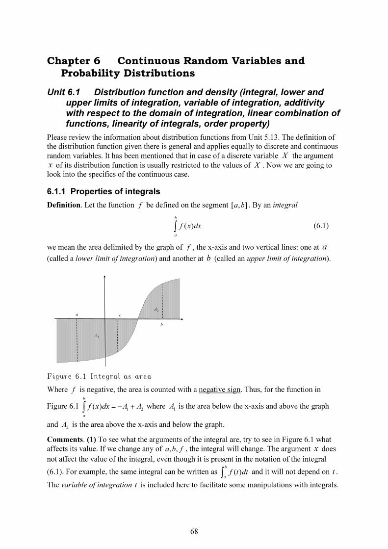
68

Chapter 6 Continuous Random Variables and

Probability Distributions

Unit 6.1 Distribution function and density (integral, lower and upper limits of integration, variable of integration, additivity with respect to the domain of integration, linear combination of functions, linearity of integrals, order property)

Please review the information about distribution functions from Unit 5.13. The definition of the distribution function given there is general and applies equally to discrete and continuous

random variables. It has been mentioned that in case of a discrete variable X the argument

x of its distribution function is usually restricted to the values of X . Now we are going to look into the specifics of the continuous case.

6.1.1 Properties of integrals

Definition. Let the function f be defined on the segment [ , ]a b . By an integral

( )

b

a

f x dx∫ (6.1)

we mean the area delimited by the graph of f , the x-axis and two vertical lines: one at a

(called a lower limit of integration) and another at b (called an upper limit of integration).

Figure 6.1 Integral as area

Where f is negative, the area is counted with a negative sign. Thus, for the function in

Figure 6.1 1 2

( )

b

a

f x dx A A= − +∫ where 1A is the area below the x-axis and above the graph

and 2

A is the area above the x-axis and below the graph.

Comments. (1) To see what the arguments of the integral are, try to see in Figure 6.1 what

affects its value. If we change any of , ,a b f , the integral will change. The argument x does

not affect the value of the integral, even though it is present in the notation of the integral

(6.1). For example, the same integral can be written as ( )b

a

f t dt∫ and it will not depend on t .

The variable of integration t is included here to facilitate some manipulations with integrals.

a

b

A1

A2

c

69

(2) Instead of changing separately a or b we can think of the whole segment [ , ]a b as

changing, and then we can ask what properties the integral has as a function of a segment

(when f is fixed). Its fundamental and geometrically obvious property is additivity with

respect to the domain of integration: if a c b< < , then

( ) ( ) ( )

b c b

a a c

f x dx f x dx f x dx= +∫ ∫ ∫

(see Figure 6.1).

(3) Since the area of a segment is equal to zero, for any a we have

( ) 0.

a

a

f x dx =∫ (6.2)

(4) We can also ask how the integral changes when the segment [ , ]a b is fixed and the

function f changes. Let ,f g be two functions and let ,c d be two numbers. The function

( ) ( )cf x dg x+ is called a linear combination of ,f g with coefficients ,c d . The linearity

property states that

[ ( ) ( )] ( ) ( ) .

b b b

a a a

cf x dg x dx c f x dx d g x dx+ = +∫ ∫ ∫

This property is quite similar to linearity of means and its applications are along the same lines but the proof requires a different level of math. This is one of those cases when you can use the cow-and-goat principle: here is a cow and there is a goat; they are quite similar and can be used, to a certain extent, for the same purposes. When it’s time to tell you how the cow is different from the goat, I will.

(5) The order property of integrals is immediate from their interpretation as area: if the graph

of the function f is above that of the function g , ( ) ( ) for all [ , ]f x g x x a b≥ ∈ , then

( ) ( ) .

b b

a a

f x dx g x dx≥∫ ∫

Unit 6.2 Density of a continuous random variable (density, interval formula in terms of densities)

Recall the short definition of a discrete random variable: values plus probabilities. Regarding the probabilities, we have established two properties: they are percentages and they satisfy the completeness axiom. We want an equivalent of these notions and properties in the continuous case.

Definition. Let X be a continuous random variable and let X

F be its distribution function.

If there exists a function X

p such that

( ) ( ) for all ,

x

X XF x p t dt x

−∞

= −∞ < < ∞∫ (6.3)

then we say that the function X

p is the density of X .

70

Comments. (1) Please follow my practice of attaching subscripts to emphasize that X

F and

Xp pertain to X .

(2) The definition appeals to existence of a function X

p satisfying (6.3). All continuous

random variables that do not satisfy this existence requirement are left out in this course.

Property 1. From (6.3) we can obtain a more general equation (an interval formula in terms

of densities):

( ) ( ) .

b

X

a

P a X b p t dt< ≤ = ∫ (6.4)

Proof. Use the interval formula (5.16) and additivity of integrals to get

( ) ( ) ( ) ( ) ( ) ( ) .

b a b

X X X X X

a

P a X b F b F a p t dt p t dt p t dt−∞ −∞

< ≤ = − = − =∫ ∫ ∫

Property 2. The probability of X taking any specific value is zero because by (6.2)

( ) ( ) ( ) ( ) 0.

a

X

a

P X a P X a P X a p t dt= = ≤ − < = =∫

For this reason ( )P X x≤ is the same as ( )P X x< and ( )P a X b< ≤ is the same as

( )P a X b≤ ≤ .

Property 3. ( ) 0X

p t ≥ for all t .

Proof. If the density is negative at some point 0x , we can take a and b close to that point

and then by the interval formula (6.4) ( )P a X b< ≤ will be negative, which is impossible.

Property 4. Any density satisfies the completeness axiom in the form

( ) 1X

p t dt

+∞

−∞

=∫

(the total area under the graph is 1).

Proof. This is because { }X−∞ < < +∞ is a sure event and ( ) 1XF +∞ = .

Differences between the cow and goat. (i) In the discrete case the variable takes its values

with positive probabilities ( )i i

P X x p= = . In the continuous case ( ) 0P X x= = for any x .

(ii) In the discrete case the numbers i

p are probabilities (percentages). In the continuous case

the values of the density ( )X

p t mean nothing and can be larger than 1. It’s the area ( )

b

X

a

p t dt∫

that means probability!

Exercise 6.1 Take two related continuous random variables and draw what you think would be their densities. For example, you can take: (i) distributions of income in a wealthy neighborhood and in a poor neighborhood, (ii) distributions of temperature in winter and summer in a given geographic location; (iii) distributions of electricity consumption in two different locations at the same time of the year. Don’t forget that the total density is 1!

71

Unit 6.3 Mean value of a continuous random variable (mean)

This whole section is about the definition of EX . In the preamble of the definition you will see the argument of type used in the times of Newton and Leibniz, the fathers of calculus. It is still used today in inductive arguments by modern mathematicians.

Figure 6.2 Approximation of an integral

Approximation of integrals by integral sums. The idea of the next construction is

illustrated in Figure 6.2. The segment [ , ]a b is divided into many small segments, denoted

0 1 1

[ , ], ...., [ , ]m m

t t t t−

(6.5)

where the leftmost point 0t coincides with a and the rightmost point

mt is b . By additivity

of integrals, the integral over the whole segment is a sum of integrals over subsegments:

1

0 1

( ) ( ) ... ( ) .m

m

ttb

a t t

f x dx f x dx f x dx

−

= + +∫ ∫ ∫ (6.6)

When m is large and the subsegments are small, for each of them the area

1

( )i

i

t

t

f x dx

−

∫ of a

curvilinear figure can be approximated by the area 1

( )( )i i i

f t t t−

− of a rectangle. Therefore

(6.6) is approximately

1 1 0 1

( ) ( )( ) ... ( )( ).

b

m m m

a

f x dx f t t t f t t t−

≈ − + + −∫ (6.7)

In particular, if the segment [ , ]a b itself is small, then

( ) ( )( ).

b

a

f x dx f b b a≈ −∫ (6.8)

Preamble. Let X be a continuous random variable that takes values in [ , ]a b . Let us divide

[ , ]a b into equal parts (6.5). If we have a sample of n observations on X , they can be

grouped in batches depending on which subsegment they fall into. Let 1n be the number of

observations falling into the first subsegment 0 1

[ , ]t t , …, mn the number of observations

a = t0

t1

t2

t3 b = t

4

f(t1)

f(t2)

f(t3)

f(t4)

72

falling into the last one 1

[ , ]m mt t−

. All observations falling into 1

[ , ]i it t−

are approximately

equal to the right end it of this subsegment. Then

1...

mn n n+ + = and by the mean of

grouped data formula (see the third line in (5.2))

1 1...

.

m mn t n t

EXn

+ +

≈

(6.9)

In the frequentist interpretation, in

n

approximates the probability that X takes values in

1[ , ]i it t−

. By the interval formula (6.4) and approximation (6.8)

1

1

1 1

( ) ( )

( )( )

i

i

t

i

i i X

t

X i i i

nP t X t p t dt

n

p t t t

−

−

− −

≈ < ≤ =

≈ −

∫

(6.10)

when the subsegments are short enough. (6.9) and (6.10) imply that

1 1 1 0 1( )( ) ... ( )( ).

X m X m m mEX t p t t t t p t t t

−

≈ − + + − (6.11)

From (6.7) and (6.11) we see that

( )

b

X

a

EX tp t dt≈ ∫

where the approximation improves as the partitioning into subsegments becomes finer.

Definition. The mean of a continuous random variable is defined by

( ) .

b

X

a

EX tp t dt= ∫

Extending the density by zero outside [ , ]a b we can with equal success define the mean by

( ) .X

EX tp t dt

+∞

−∞

= ∫ (6.12)

Unit 6.4 Properties of means, covariance, variance and correlation

It might be relieving to know that it’s only the definition of the mean that is different from the discrete case. All properties of means, covariance and variance derived from that definition are absolutely the same as in the discrete case. Here is the list of properties that will be constantly used:

(1) Linearity of means: ( )E aX bY aEX bEY+ = + .

(2) Expected value of a constant: Ec c= .

(3) Multiplicativity of expected values: ( )( )EXY EX EY= for independent ,X Y .

(4) Linearity of covariance: for example, for the first argumentcov( , ) cov( , ) cov( , ).aX bY Z a X Z b Y Z+ = +

(5) Alternative expression for covariance: cov( , ) ( )( )X Y EXY EX EY= − .

73

(6) Independent variables are uncorrelated: cov( , ) 0X Y = .

(7) Covariance with a constant: cov( , ) 0.X c =

(8) Symmetry of covariance: cov( , ) cov( , )X Y Y X= .

(9) Link between variance and covariance: ( ) cov( , )V X X X= .

(10) Alternative expression for variance: 2 2( ) ( )V X EX EX= − .

(11) Variance of a linear combination: 2 2( ) ( ) 2 cov( , ) ( ).V aX bY a V X ab X Y b V Y+ = + +

(12) Variance of a constant: ( ) 0V c = .

(13) Nonnegativity: ( ) 0V X ≥ .

(14) Variables with vanishing variance: ( ) 0V X = if and only if X c= .

(15) Additivity of variance: ( ) ( ) ( )V X Y V X V Y+ = + for independent ,X Y .

(16) Standard deviation is homogeneous: ( ) | | ( )aX a Xσ = σ .

(17) Range of the correlation coefficient: 1 ( , ) 1X Y− ≤ ρ ≤ for any ,X Y .

(18) Standardization: ( )

X EXY

X

−

=

σ

has mean zero and unit variance.

Here only property (3) requires additional definitions: joint density, independence etc. Also, for (10) we need the definition of a function of a random variable, and this is better explained following the cow-and-goat principle.

Table 6.1 Definition of a function of a random variable

The variable has values

Probability/Density A function of a variable has values

Discrete case ix

ip ( )

if x

Continuous case t ( )X

p t ( )f t

Example 6.12

X takes values 2t . sinX takes values sin t . Therefore

2 2 ( ) , sin (sin ) ( ) .X X

EX t p t dt E X t p t dt

+∞ +∞

−∞ −∞

= =∫ ∫

Unit 6.5 The uniform distribution (uniformly distributed variable, primitive function, integration rule)

You might want to review the definition of a uniformly distributed discrete variable in Unit 5.2.

Example 6.2 Take the power cable of your computer and stretch it along the real line. How would you describe the probability of the cable failing at any fixed point (plugs don’t count)? Do you think this probability at some points is higher than at others?

Intuitive definition. Fix some segment [ , ]a b . We say that a random variable U is uniformly

distributed over [ , ]a b if

(a) U does not take values outside [ , ]a b and

74

(b) its values inside [ , ]a b are equally likely.

After having heard the motivating example and the intuitive definition most students are able

to formally define the density of U .

Formal definition. U is such a variable that its density is

(a) null outside [ , ]a b and

(b) constant inside [ , ]a b .

Denoting

0 if t [ , ]( )

1 if t [ , ]U

a bp t

a b

∉=

∈

we can find the constant using the fact that the total density must be 1:

( ) (using additivity of integrals)

( ) ( ) ( ) (using density definition)

U

a b

U U U

a b

b

a

p t dt

p t dt p t dt p t dt

cdt

+∞

−∞

+∞

−∞

= + +

=

∫

∫ ∫ ∫

∫ (this is area of a rectangle)

( ) 1c b a= − =

so 1

cb a=

−

. The result is

0 if [ , ]

( ) 1 if [ , ]

U

t a b

p tt a b

b a

∉

= ∈ −

(6.13)

Important. In the interval formulas (5.16) and (6.4) the segment [ , ]a b is arbitrary, whereas

in the definition of U it is fixed. To remember this, sometimes it’s useful to denote [ , ]a bU the

variable which is uniformly distributed over [ , ]a b .

Property 1. Usually students can guess that [ , ]

2a b

a bEU

+= .

Proof. Using definitions (6.12) and (6.13) we get

[ , ]

1( ) ( ) .

b b

a b U U

a a

EU tp t dt tp t dt tdtb a

+∞

−∞

= = =

−∫ ∫ ∫ (6.14)

The last integral can be found using two steps from calculus.

Step 1. We have to find what is called a primitive function. ( )F x is called a primitive function

of ( )f x if '( ) ( ).F x f x= The primitive of ( )f t t= is 2

( )2

tF t = .

Step 2 is to use the primitive according to the integration rule

75

( ) ( ) ( ).

b

a

f t dt F b F a= −∫

In our case 2 2 ( )( )

.2 2 2

b

a

b a b a a btdt

− += − =∫ This together with (6.14) implies

[ , ]

1 ( )( ).

2 2a b

b a a b a bEU

b a

− + += =

−

(6.15)

Property 2. ( )2

[ , ]

( )

12a b

b aV U

−

= .

Proof. There is no need to try to guess or remember this result. We start with the alternative expression:

( ) ( )

22

[ , ] [ , ] [ , ] .

a b a b a bV U EU EU= −

(6.16)

Here the first term is

2 2 2

[ , ]

1( ) .

b

a b U

a

EU t p t dt t dtb a

+∞

−∞

= =

−∫ ∫

The primitive of 2( )f t t= is

3

( )3

tF t = . We can continue the previous display as

3 3 2 2 2 2

2

[ , ]

1 1 ( )( ).

3 3 3 3a b

b a b a b ab a b ab aEU

b a b a

− + + + += − = =

− − (6.17)

The equation 3 3 2 2( )( )b a b a b ab a− = − + + we have used can be verified directly. Combining

(6.15), (6.16) and (6.17) yields

( )22 2 2 2 2

[ , ]

2 ( ).

3 2 12 12a b

b ab a a b b ab a b aV U

+ + + − + − = − = =

Exercise 6.2 The distribution function of [ , ]a bU is

0 if

( ) if

1 if .

U

t a

t aF t a t b

b a

t b

< −

= ≤ ≤−

>

Unit 6.6 The normal distribution (parameter, standard normal distribution, normal variable and alternative definition, empirical rule)

6.6.1 Parametric distributions

Following the general recommendation to think in terms of sets rather than elements, let us think about families of similar distributions. One element of a family of similar distributions can be thought of as a function. The argument of the function is called a parameter. This

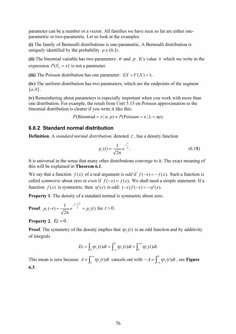
76

parameter can be a number or a vector. All families we have seen so far are either one-parametric or two-parametric. Let us look at the examples.

(i) The family of Bernoulli distributions is one-parametric. A Bernoulli distribution is

uniquely identified by the probability (0,1)p∈ .

(ii) The binomial variable has two parameters: n and p . It’s value x which we write in the

expression ( )n

P S x= is not a parameter.

(iii) The Poisson distribution has one parameter: ( )EX V X= = λ .

(iv) The uniform distribution has two parameters, which are the endpoints of the segment

[ , ]a b .

(v) Remembering about parameters is especially important when you work with more than one distribution. For example, the result from Unit 5.15 on Poisson approximation to the binomial distribution is clearer if you write it like this:

(Binomial | , ) (Poisson | ).P x n p P x np= ≈ = λ =

6.6.2 Standard normal distribution

Definition. A standard normal distribution, denoted z , has a density function

2

21

( ) .2

t

zp t e

−

=

π

(6.18)

It is universal in the sense that many other distributions converge to it. The exact meaning of this will be explained in Theorem 6.1.

We say that a function ( )f x of a real argument is odd if ( ) ( ).f x f x− = − Such a function is

called symmetric about zero or even if ( ) ( ).f x f x− = We shall need a simple statement: If a

function ( )f x is symmetric, then ( )xf x is odd: ( ) ( ) ( ).x f x xf x− − = −

Property 1. The density of a standard normal is symmetric about zero.

Proof.

2( )

21

( ) ( )2

t

z zp t e p t

−

−

− = =

π

for 0t > .

Property 2. 0Ez = .

Proof. The symmetry of the density implies that ( )z

tp t is an odd function and by additivity

of integrals

0

0

( ) ( ) ( ) .z z z

R

Ez tp t dt tp t dt tp t dt+∞

−∞

= = +∫ ∫ ∫

This mean is zero because 0

( )z

A tp t dt+∞

= ∫ cancels out with 0

( )z

A tp t dt−∞

− = ∫ , see Figure

6.3.

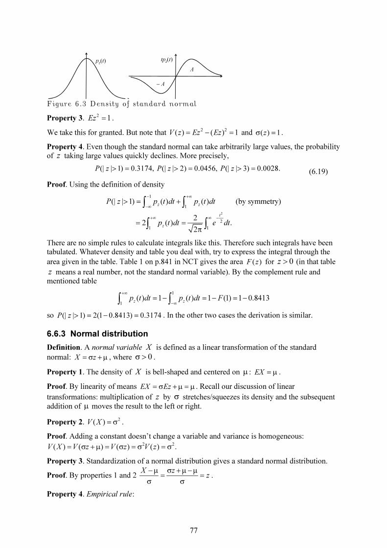
77

Figure 6.3 Density of standard normal

Property 3. 21Ez = .

We take this for granted. But note that 2 2( ) ( ) 1V z Ez Ez= − = and ( ) 1zσ = .

Property 4. Even though the standard normal can take arbitrarily large values, the probability of z taking large values quickly declines. More precisely,

(| | 1) 0.3174, (| | 2) 0.0456, (| | 3) 0.0028.P z P z P z> = > = > = (6.19)

Proof. Using the definition of density

2

1

1

2

1 1

(| | 1) ( ) ( ) (by symmetry)

2 2 ( ) .

2

z z

t

z

P z p t dt p t dt

p t dt e dt

− +∞

−∞

+∞ ∞ −

> = +

= =

π

∫ ∫

∫ ∫

There are no simple rules to calculate integrals like this. Therefore such integrals have been tabulated. Whatever density and table you deal with, try to express the integral through the

area given in the table. Table 1 on p.841 in NCT gives the area ( )F z for 0z > (in that table

z means a real number, not the standard normal variable). By the complement rule and mentioned table

1

1

( ) 1 ( ) 1 (1) 1 0.8413z z

p t dt p t dt F+∞

−∞

= − = − = −∫ ∫

so (| | 1) 2(1 0.8413) 0.3174P z > = − = . In the other two cases the derivation is similar.

6.6.3 Normal distribution

Definition. A normal variable X is defined as a linear transformation of the standard

normal: X z= σ +µ , where 0σ > .

Property 1. The density of X is bell-shaped and centered on µ : EX = µ .

Proof. By linearity of means EX Ez= σ +µ = µ . Recall our discussion of linear

transformations: multiplication of z by σ stretches/squeezes its density and the subsequent

addition of µ moves the result to the left or right.

Property 2. 2( )V X = σ .

Proof. Adding a constant doesn’t change a variable and variance is homogeneous:2 2

( ) ( ) ( ) ( ) .V X V z V z V z= σ +µ = σ = σ = σ

Property 3. Standardization of a normal distribution gives a standard normal distribution.

Proof. By properties 1 and 2 X z

z−µ σ +µ −µ

= =σ σ

.

Property 4. Empirical rule:

− A

tpz(t)

A

pz(t)

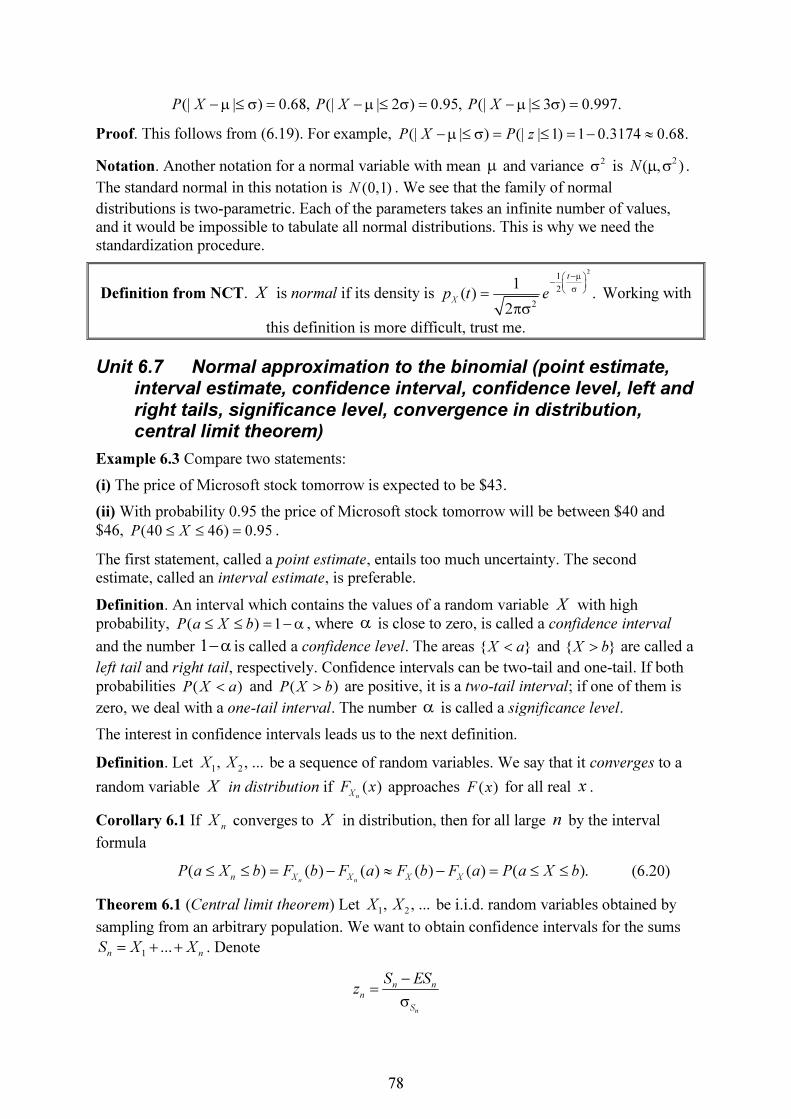
78

(| | ) 0.68, (| | 2 ) 0.95, (| | 3 ) 0.997.P X P X P X−µ ≤ σ = −µ ≤ σ = −µ ≤ σ =

Proof. This follows from (6.19). For example, (| | ) (| | 1) 1 0.3174 0.68.P X P z−µ ≤ σ = ≤ = − ≈

Notation. Another notation for a normal variable with mean µ and variance 2σ is 2

( , )N µ σ .

The standard normal in this notation is (0,1)N . We see that the family of normal

distributions is two-parametric. Each of the parameters takes an infinite number of values, and it would be impossible to tabulate all normal distributions. This is why we need the standardization procedure.

Definition from NCT. X is normal if its density is

21

2

2

1( ) .

2

t

Xp t e

−µ − σ =

πσ

Working with

this definition is more difficult, trust me.

Unit 6.7 Normal approximation to the binomial (point estimate, interval estimate, confidence interval, confidence level, left and right tails, significance level, convergence in distribution, central limit theorem)

Example 6.3 Compare two statements:

(i) The price of Microsoft stock tomorrow is expected to be $43.

(ii) With probability 0.95 the price of Microsoft stock tomorrow will be between $40 and

$46, (40 46) 0.95P X≤ ≤ = .

The first statement, called a point estimate, entails too much uncertainty. The second estimate, called an interval estimate, is preferable.

Definition. An interval which contains the values of a random variable X with high probability, ( ) 1P a X b≤ ≤ = −α , where α is close to zero, is called a confidence interval

and the number 1−α is called a confidence level. The areas { }X a< and { }X b> are called a

left tail and right tail, respectively. Confidence intervals can be two-tail and one-tail. If both

probabilities ( )P X a< and ( )P X b> are positive, it is a two-tail interval; if one of them is

zero, we deal with a one-tail interval. The number α is called a significance level.

The interest in confidence intervals leads us to the next definition.

Definition. Let 1 2, , ...X X be a sequence of random variables. We say that it converges to a

random variable X in distribution if ( )n

XF x approaches ( )F x for all real x .

Corollary 6.1 If n

X converges to X in distribution, then for all large n by the interval

formula

( ) ( ) ( ) ( ) ( ) ( ).n n

n X X X XP a X b F b F a F b F a P a X b≤ ≤ = − ≈ − = ≤ ≤ (6.20)

Theorem 6.1 (Central limit theorem) Let 1 2, , ...X X be i.i.d. random variables obtained by

sampling from an arbitrary population. We want to obtain confidence intervals for the sums

1...

n nS X X= + + . Denote

n

n n

n

S

S ESz

−

=

σ

79

the standardized versions of nS .

nz in general are not standard normal but they converge in

distribution to a standard normal distribution.

Corollary 6.2 Let nS be a binomial distribution. Then for any numbers ,a b and large n one

has

( ) .

n n

n n

n

S S

a ES b ESP a S b P z

− −≤ ≤ ≈ ≤ ≤

σ σ (6.21)

Proof. We need two properties of ordering of real numbers:

(1) the inequality u v≤ is equivalent to the inequality u c v c+ ≤ + for any constant c ,

(2) the inequality u v≤ is equivalent to the inequality uc vc≤ for any positive constant c .

It follows that the next three inequalities are equivalent:

(i) , (ii) , (iii) .

n n n

n n n n

n n n n n

S S S

a ES S ES b ESa S b a ES S ES b ES

− − −≤ ≤ − ≤ − ≤ − ≤ ≤

σ σ σ

Hence, probabilities of these events are the same. Now by the central limit theorem

( ) .

n n n n

n n n n

n n

S S S S

a ES b ES a ES b ESP a S b P z P z

− − − −≤ ≤ = ≤ ≤ ≈ ≤ ≤

σ σ σ σ

Exercise 6.3 Obtain an approximate confidence interval for ˆ nS

pn= .

Unit 6.8 Joint distributions and independence (joint distribution function, marginal distribution function, independent variables: continuous case)

All definitions in this section had precedents.

Consider vectors ( , )X Y and ( , )x y ( ( , )X Y is a pair of random variables and ( , )x y is a pair

of real numbers). The function ( , ) ( , ) ( , )X Y

F x y P X x Y y= ≤ ≤ is called a joint distribution

function of the vector ( , )X Y . The marginal distribution functions are defined to be

( , ) ( , )( , ), ( , )X Y X Y

F x F y∞ ∞ . They satisfy ( , ) ( , )( , ) ( ), ( , ) ( )X Y X X Y Y

F x F x F y F y∞ = ∞ = (marginal

distributions coincide with own distributions). We say that a function ( , ) 1 2( , )X Y

p t t is a joint

density of ( , )X Y if

( , ) ( , ) 1 2 1 2( , ) ( , ) .

yx

X Y X YF x y p t t dt dt

−∞ −∞

= ∫ ∫

Suppose X and Y have densities X

p and Yp , respectively. X and Y are called

independent if the joint density decomposes into a product of own densities:

( , ) 1 2 1 2( , ) ( ) ( )X Y X Y

p t t p t p t= . With these definitions we can prove Property 3) from Unit 6.4.

Exercise 6.4 For independent continuous random variables we have multiplicativity of

means: ( )( )EXY EX EY= .

Proof. Everything follows from definitions:

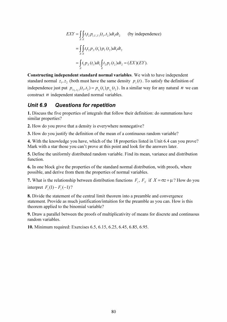
80

1 2 ( , ) 1 2 1 2

1 2 1 2 1 2

1 1 1 2 2 2

( , ) (by independence)

( ) ( )

( ) ( ) ( )( ).

X Y

R R

X Y

R R

X Y

R R

EXY t t p t t dt dt

t t p t p t dt dt

t p t dt t p t dt EX EY

=

=

= =

∫ ∫

∫ ∫

∫ ∫

Constructing independent standard normal variables. We wish to have independent

standard normal 1 2,z z (both must have the same density ( )

zp t . To satisfy the definition of

independence just put 1 2 1 2

( , ) 1 2 1 2( , ) ( ) ( )z z z z

p t t p t p t= . In a similar way for any natural n we can

construct n independent standard normal variables.


1. Discuss the five properties of integrals that follow their definition: do summations have similar properties?

2. How do you prove that a density is everywhere nonnegative?

3. How do you justify the definition of the mean of a continuous random variable?

4. With the knowledge you have, which of the 18 properties listed in Unit 6.4 can you prove? Mark with a star those you can’t prove at this point and look for the answers later.

5. Define the uniformly distributed random variable. Find its mean, variance and distribution function.

6. In one block give the properties of the standard normal distribution, with proofs, where possible, and derive from them the properties of normal variables.

7. What is the relationship between distribution functions ,

z XF F if X z=σ +µ ? How do you

interpret (1) ( 1)z zF F− − ?

8. Divide the statement of the central limit theorem into a preamble and convergence statement. Provide as much justification/intuition for the preamble as you can. How is this theorem applied to the binomial variable?

9. Draw a parallel between the proofs of multiplicativity of means for discrete and continuous random variables.

10. Minimum required: Exercises 6.5, 6.15, 6.25, 6.45, 6.85, 6.95.

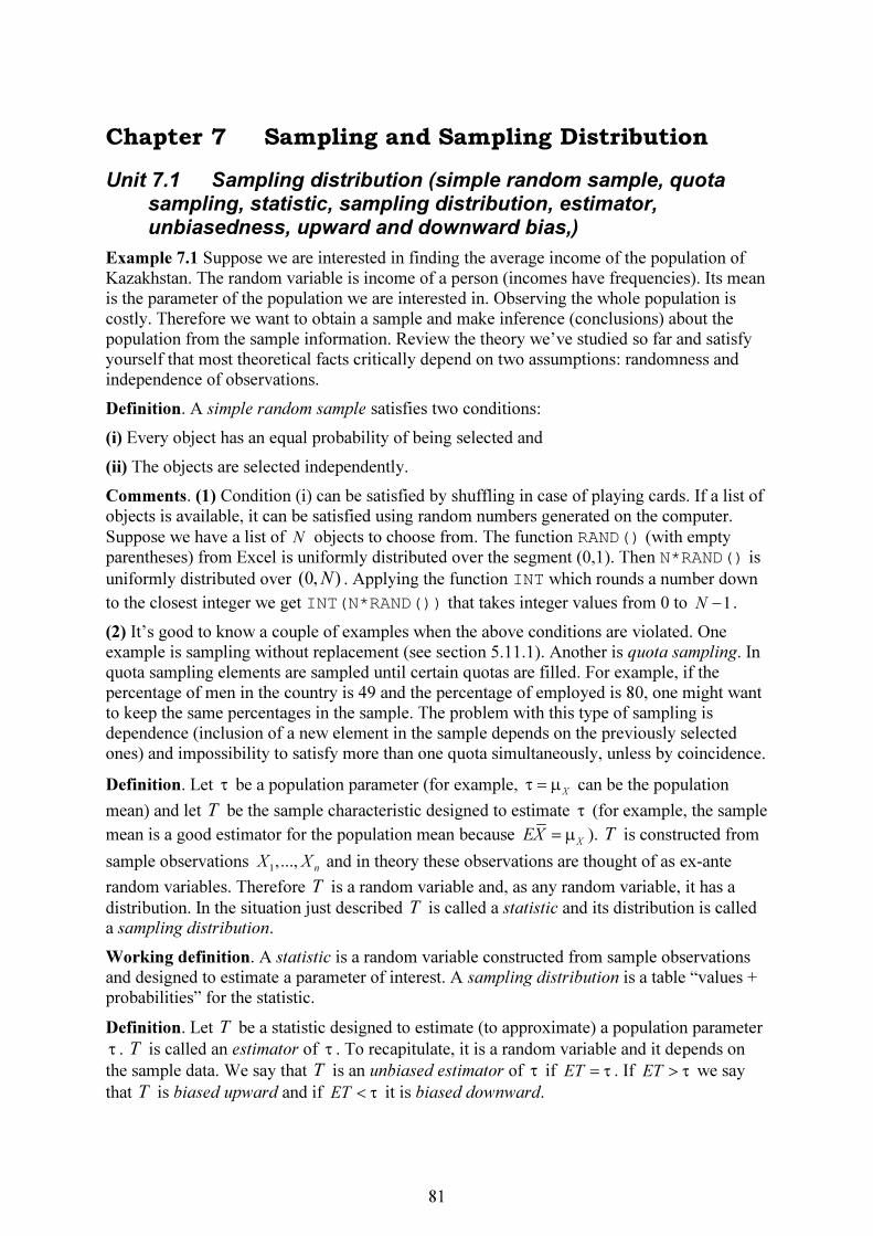
81

Chapter 7 Sampling and Sampling Distribution

Unit 7.1 Sampling distribution (simple random sample, quota sampling, statistic, sampling distribution, estimator, unbiasedness, upward and downward bias,)

Example 7.1 Suppose we are interested in finding the average income of the population of Kazakhstan. The random variable is income of a person (incomes have frequencies). Its mean is the parameter of the population we are interested in. Observing the whole population is costly. Therefore we want to obtain a sample and make inference (conclusions) about the population from the sample information. Review the theory we’ve studied so far and satisfy yourself that most theoretical facts critically depend on two assumptions: randomness and independence of observations.

Definition. A simple random sample satisfies two conditions:

(i) Every object has an equal probability of being selected and

(ii) The objects are selected independently.

Comments. (1) Condition (i) can be satisfied by shuffling in case of playing cards. If a list of objects is available, it can be satisfied using random numbers generated on the computer.

Suppose we have a list of N objects to choose from. The function RAND() (with empty parentheses) from Excel is uniformly distributed over the segment (0,1). Then N*RAND() is uniformly distributed over (0, )N . Applying the function INT which rounds a number down

to the closest integer we get INT(N*RAND()) that takes integer values from 0 to 1N − .

(2) It’s good to know a couple of examples when the above conditions are violated. One example is sampling without replacement (see section 5.11.1). Another is quota sampling. In quota sampling elements are sampled until certain quotas are filled. For example, if the percentage of men in the country is 49 and the percentage of employed is 80, one might want to keep the same percentages in the sample. The problem with this type of sampling is dependence (inclusion of a new element in the sample depends on the previously selected ones) and impossibility to satisfy more than one quota simultaneously, unless by coincidence.

Definition. Let τ be a population parameter (for example, X

τ = µ can be the population

mean) and let T be the sample characteristic designed to estimate τ (for example, the sample

mean is a good estimator for the population mean because X

EX = µ ). T is constructed from

sample observations 1,...,

nX X and in theory these observations are thought of as ex-ante

random variables. Therefore T is a random variable and, as any random variable, it has a

distribution. In the situation just described T is called a statistic and its distribution is called a sampling distribution.

Working definition. A statistic is a random variable constructed from sample observations and designed to estimate a parameter of interest. A sampling distribution is a table “values + probabilities” for the statistic.

Definition. Let T be a statistic designed to estimate (to approximate) a population parameter

τ . T is called an estimator of τ . To recapitulate, it is a random variable and it depends on

the sample data. We say that T is an unbiased estimator of τ if ET = τ . If ET > τ we say

that T is biased upward and if ET < τ it is biased downward.

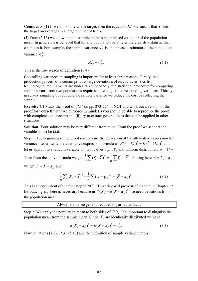
82

Comments. (1) If we think of τ as the target, then the equation ET = τ means that T hits the target on average (in a large number of trials).

(2) From (5.13) we know that the sample mean is an unbiased estimator of the population mean. In general, it is believed that for any population parameter there exists a statistic that

estimates it. For example, the sample variance 2

Xs is an unbiased estimator of the population

variance 2

Xσ :

2 2.

X XEs = σ (7.1)

This is the true reason of definition (3.4).

Controlling variances in sampling is important for at least three reasons. Firstly, in a production process of a certain product large deviations of its characteristics from technological requirements are undesirable. Secondly, the statistical procedure for comparing sample means from two populations requires knowledge of corresponding variances. Thirdly, in survey sampling by reducing the sample variance we reduce the cost of collecting the sample.

Exercise 7.1 Study the proof of (7.1) on pp. 273-274 of NCT and work out a version of the proof for yourself with two purposes in mind: (i) you should be able to reproduce the proof with complete explanations and (ii) try to extract general ideas that can be applied in other situations.

Solution. Your solution may be very different from mine. From the proof we see that the variables must be i.i.d.

Step 1. The beginning of the proof reminds me the derivation of the alternative expression for

variance. Let us write the alternative expression formula as 2 2 2( ) ( )E Y EY EY EY− = − and

let us apply it to a random variable Y with values 1,...,

nY Y and uniform distribution 1/ .

ip n=

Then from the above formula we get 2 2 21 1( )

i iY Y Y Y

n n− = −∑ ∑ . Putting here

i i XY X= −µ

we get X

Y X= −µ and

2 2 21 1( ) ( ) ( ) .

i i X XX X X X

n n− = −µ − −µ∑ ∑ (7.2)

This is an equivalent of the first step in NCT. This trick will prove useful again in Chapter 12.

Introducing Xµ here is necessary because in 2

( ) ( )X

V X E X= −µ we need deviations from

the population mean.

Always try to see general features in particular facts.

Step 2. We apply the population mean to both sides of (7.2). It’s important to distinguish the

population mean from the sample mean. Since i

X are identically distributed we have

2 2 2( ) ( ) .

i X X XE X E X−µ = −µ = σ (7.3)

Now equations (7.2), (7.3), (5.13) and the definition of sample variance imply

83

2 2 2

2 2 2 2

1 1( ) ( )

1 1

1 1.

1 1

X i i

X X X X

nEs E X X E X X

n n n

n n n

n n n n

= − = −− −

− = σ − σ = σ = σ − −

∑ ∑

Exercise 7.2 Prove the sample covariance ,X Y

s is an unbiased estimator of the population

covariance cov( , ).X Y

Unit 7.2 Sampling distributions of sample variances (chi-square distribution, degrees of freedom)

Definition. Let 1,...,

nz z be standard normal independent (we know from Unit 6.8 how to

construct them). Then the variable 2 2

1

n

n i

i

z

=

χ =∑ is called a chi-square distribution with n

degrees of freedom. “Degrees of freedom” is just a formal parameter that determines which entry to look up in a statistical table.

Property 1. 2

nχ is nonnegative, therefore its density

2( )

n

p tχ

vanishes for 0t < .

Property 2. 2

nE nχ = .

Proof. 2 2

1

n

n i

i

E Ez n

=

χ = =∑ by linearity of means and Property 3 of standard normals (section

6.6.2).

Property 3. 2( ) 2

nV nχ = .

Proof. By independence and the alternative expression for variance

2 2 4 2 2

1 1

( ) ( ) [ ( ) ].n n

n i i i

i i

V V z Ez Ez

= =

χ = = −∑ ∑

We accept without proof that

43 for a standard normal.Ez =

Hence, 2

1

( ) (3 1) 2n

n

i

V n

=

χ = − =∑ .

Usually I use the name “Theorem” for complex statements that will not be proved here.

Theorem 7.1 For a random sample of n independent observations from a normal population

with variance 2

Xσ the variable

2

2

1 2

( 1)X

n

X

n s

−

−χ =

σ

is distributed as chi-square with 1n − degrees of freedom.

Exercise 7.3 Find 2( )

XV s .

Solution. By the preceding theorem, homogeneity of variance and Property 3

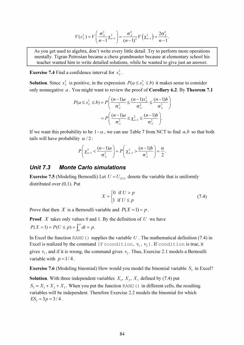
84

( )2 4 4

2 2 2

1 12

2( ) .

1 ( 1) 1

X X X

X n nV s V V

n n n− −

σ σ σ= χ = χ = − − −

As you get used to algebra, don’t write every little detail. Try to perform more operations mentally. Tigran Petrosian became a chess grandmaster because at elementary school his teacher wanted him to write detailed solutions, while he wanted to give just an answer.

Exercise 7.4 Find a confidence interval for 2

Xs .

Solution. Since 2

Xs is positive, in the expression 2

( )X

P a s b≤ ≤ it makes sense to consider

only nonnegative a . You might want to review the proof of Corollary 6.2. By Theorem 7.1

2

2

2 2 2

2

12 2

( 1)( 1) ( 1)( )

( 1) ( 1) .

X

X

X X X

n

X X

n sn a n bP a s b P

n a n bP

−

−− −≤ ≤ = ≤ ≤ σ σ σ

− −= ≤ χ ≤ σ σ

If we want this probability to be 1−α , we can use Table 7 from NCT to find ,a b so that both

tails will have probability / 2α :

2 2

1 12 2

( 1) ( 1).

2n n

X X

n a n bP P

− −

− − αχ < = χ > = σ σ

Unit 7.3 Monte Carlo simulations

Exercise 7.5 (Modeling Bernoulli) Let (0,1)U U= denote the variable that is uniformly

distributed over (0,1). Put

0 if

1 if

U pX

U p

>=

≤ (7.4)

Prove that then X is a Bernoulli variable and ( 1)P X p= = .

Proof. X takes only values 0 and 1. By the definition of U we have

0

( 1) ( ) .p

P X P U p dt p= = ≤ = =∫

In Excel the function RAND() supplies the variable U . The mathematical definition (7.4) in Excel is realized by the command IF(condition,

1v ,

2v ). If condition is true, it

gives 1v , and if it is wrong, the command gives

2v . Thus, Exercise 2.1 models a Bernoulli

variable with 1/ 4p = .

Exercise 7.6 (Modeling binomial) How would you model the binomial variable 3S in Excel?

Solution. With three independent variables 1 2 3, ,X X X defined by (7.4) put

3 1 2 3S X X X= + + . When you put the function RAND() in different cells, the resulting

variables will be independent. Therefore Exercise 2.2 models the binomial for which

33 3 / 4ES p= = .

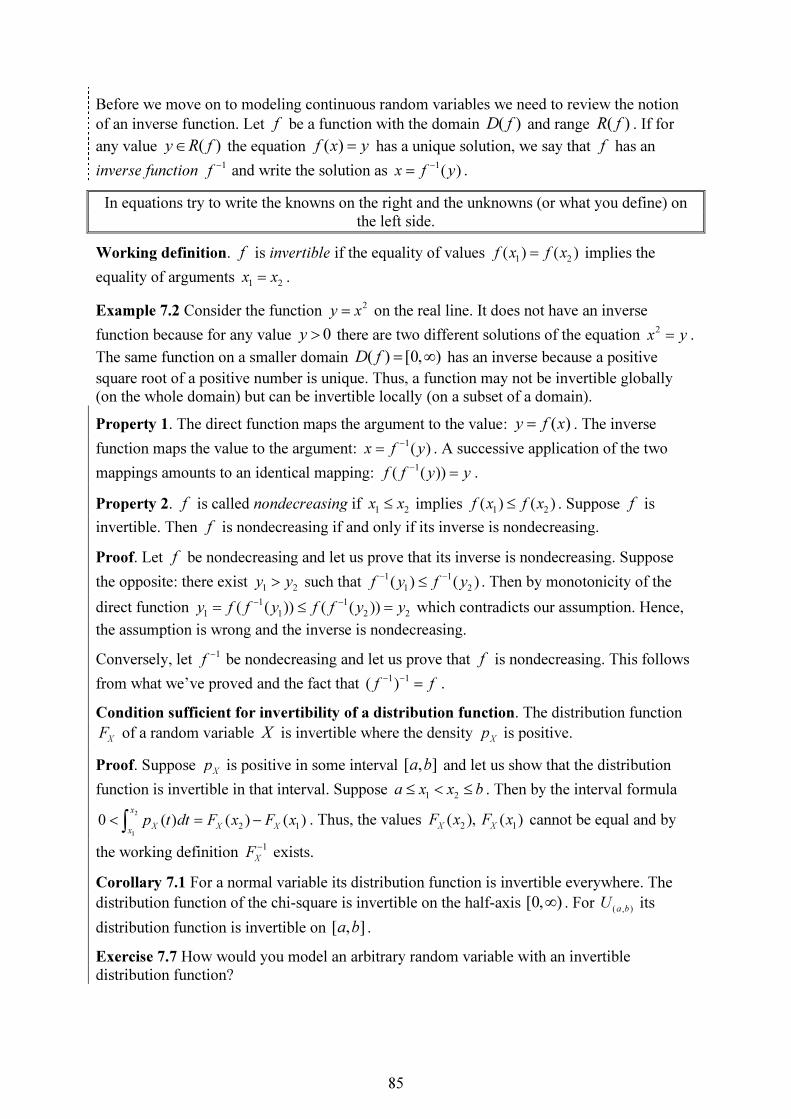
85

Before we move on to modeling continuous random variables we need to review the notion

of an inverse function. Let f be a function with the domain ( )D f and range ( )R f . If for

any value ( )y R f∈ the equation ( )f x y= has a unique solution, we say that f has an

inverse function 1f− and write the solution as 1

( )x f y−

= .

In equations try to write the knowns on the right and the unknowns (or what you define) on the left side.

Working definition. f is invertible if the equality of values 1 2

( ) ( )f x f x= implies the

equality of arguments 1 2x x= .

Example 7.2 Consider the function 2y x= on the real line. It does not have an inverse

function because for any value 0y > there are two different solutions of the equation 2x y= .

The same function on a smaller domain ( ) [0, )D f = ∞ has an inverse because a positive

square root of a positive number is unique. Thus, a function may not be invertible globally (on the whole domain) but can be invertible locally (on a subset of a domain).

Property 1. The direct function maps the argument to the value: ( )y f x= . The inverse

function maps the value to the argument: 1( )x f y

−

= . A successive application of the two

mappings amounts to an identical mapping: 1( ( ))f f y y−

= .

Property 2. f is called nondecreasing if 1 2x x≤ implies

1 2( ) ( )f x f x≤ . Suppose f is

invertible. Then f is nondecreasing if and only if its inverse is nondecreasing.

Proof. Let f be nondecreasing and let us prove that its inverse is nondecreasing. Suppose

the opposite: there exist 1 2y y> such that 1 1

1 2( ) ( )f y f y

− −

≤ . Then by monotonicity of the

direct function 1 1

1 1 2 2( ( )) ( ( ))y f f y f f y y− −

= ≤ = which contradicts our assumption. Hence,

the assumption is wrong and the inverse is nondecreasing.

Conversely, let 1f− be nondecreasing and let us prove that f is nondecreasing. This follows

from what we’ve proved and the fact that 1 1( )f f− −

= .

Condition sufficient for invertibility of a distribution function. The distribution function

XF of a random variable X is invertible where the density

Xp is positive.

Proof. Suppose X

p is positive in some interval [ , ]a b and let us show that the distribution

function is invertible in that interval. Suppose 1 2

a x x b≤ < ≤ . Then by the interval formula

2

1

2 10 ( ) ( ) ( )

x

X X Xx

p t dt F x F x< = −∫ . Thus, the values 2 1

( ), ( )X X

F x F x cannot be equal and by

the working definition 1

XF− exists.

Corollary 7.1 For a normal variable its distribution function is invertible everywhere. The

distribution function of the chi-square is invertible on the half-axis [0, )∞ . For ( , )a bU its

distribution function is invertible on [ , ]a b .

Exercise 7.7 How would you model an arbitrary random variable with an invertible distribution function?

86

Solution. Put 1( )

XY F U

−

= where U is uniformly distributed on (0,1). Since X

F is

nondecreasing, the inequality 1( )

XF U x−

≤ is equivalent to 1( ( )) ( )

X X XU F F U F x

−

= ≤ .

Therefore for any real x ( )

1

0( ) ( ( ) ) ( ( )) ( ).

XF x

Y X X XF x P F U x P U F x dt F x

−

= ≤ = ≤ = =∫ Y is

identically distributed with X .

Despite being short, this proof combines several important ideas. Make sure you understand them.

In Excel the function NORMINV( y ,µ,σ) denotes 1( )

XF y− where X z=σ +µ is normal.

Hence, in Exercise 2.4 we model 8 25X z= + .


1. Fill out the next table:

Table 7.1 Comparison of population and sample formulas

Population formula Sample formula

Mean Discrete and continuous

Variance

Standard deviation

Correlation

2. How would you satisfy the definition of the simple random sampling in case of measuring average income of city residents?

3. Define a sampling distribution and illustrate it with a sampling distribution of a sample proportion.

4. Stating all the necessary assumptions, derive the formulas for the mean and variance of the sample mean.

5. Suppose we sample from a Bernoulli population. How do we figure out the approximate

value of p ? How can we be sure that the approximation is good?

6. Define unbiasedness and prove that the sample variance is an unbiased estimator of the population variance.

7. Find the mean and variance of the chi-square distribution.

8. Find 2( )

XV s and a confidence interval for .

9. Minimum required: 7.9, 7.10, 7.30, 7.40, 7.57, 7.61.

2

Xs

87

Chapter 8 Estimation: Single Population

Unit 8.1 Unbiasedness and efficiency

In NCT this chapter starts with the definition of unbiasedness. In my exposition it was more appropriate to put that definition in Unit 7.1.

Exercise 8.1 If there exists one unbiased estimator of a population parameter, then there exist many unbiased estimators of that parameter.

Proof. Let ET = τ . Take any random variable Y with mean zero and put X T Y= + . Then

EX ET EY= + = τ .

This exercise makes clear that even though unbiasedness is a desirable property, it is not enough to choose from many competing estimators of the same parameter. In statistics we want not only to be able to hit the target on average but also to reduce the spread of estimates around their mean.

Definition. If 1T and

2T are two unbiased estimators of the same parameter τ and

1 2( ) ( )V T V T< , then we say that

1T is more efficient.

Exercise 8.2 If 1T and

2T are two unbiased estimators of the same parameter τ and

1 2( ) ( )V T V T≠ , then, with exception of two cases, there exists an unbiased estimator of the

same parameter which is more efficient than either 1T or

2T .

Proof. Define 1 2

( ) (1 )T a aT a T= + − where a is real. This is a special type of a linear

combination which is convenient to parameterize the points of the segment 1 2

[ , ]T T . With

0 or 1a = we get the left and right endpoints of the segment: 1 2

(1) , (0)T T T T= = . Values

(0,1)a∈ give all other points of the segment. Values [0,1]a∉ give points of the straight line

drawn through 1 2,T T .

( )T a is unbiased: 1 2

( ) (1 )ET a aET a ET= + − = τ . Its variance is

2 2

1 1 2 2( ) ( ) 2 (1 )cov( , ) (1 ) ( )V T a V T a a T T a V T= + − + −

and the first-order condition for its minimization is

1 1 2 22 ( ) (2 4 )cov( , ) 2(1 ) ( ) 0.aV T a T T a V T+ − − − =

Solving this equation for a ,

2 1 2

1

( ) cov( , ).

( )

V T T Ta

V T

−

=

The minimum of ( )V T is at point 0a = if 2 1 2

( ) cov( , )V T T T= and at point 1a = if

1 1 2( ) cov( , )V T T T= . In these two cases it is not possible to reduce variance by forming linear

combinations. In all other cases ( )T a is more efficient than either 1T or

2T .

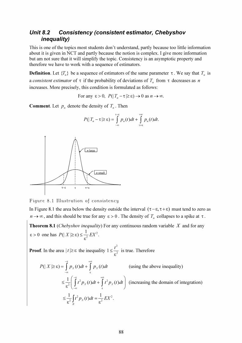
88

Unit 8.2 Consistency (consistent estimator, Chebyshov inequality)

This is one of the topics most students don’t understand, partly because too little information about it is given in NCT and partly because the notion is complex. I give more information but am not sure that it will simplify the topic. Consistency is an asymptotic property and therefore we have to work with a sequence of estimators.

Definition. Let { }nT be a sequence of estimators of the same parameter τ . We say that

nT is

a consistent estimator of τ if the probability of deviations of nT from τ decreases as n

increases. More precisely, this condition is formulated as follows:

For any 0, (| | ) 0 as .n

P T nε > − τ ≥ ε → →∞

Comment. Let n

p denote the density of nT . Then

(| | ) ( ) ( ) .n n n

P T p t dt p t dt

τ−ε +∞

−∞ τ+ε

− τ ≥ ε = +∫ ∫

Figure 8.1 Illustration of consistency

In Figure 8.1 the area below the density outside the interval ( , )τ−ε τ+ε must tend to zero as

n→∞ , and this should be true for any 0ε > . The density of nT collapses to a spike at τ .

Theorem 8.1 (Chebyshov inequality) For any continuous random variable X and for any

0ε > one has 2

2

1(| | ) .P X EX≥ ε ≤

ε

Proof. In the area | |t ≥ ε the inequality 2

21

t≤

ε

is true. Therefore

2 2

2

2

2

(| | ) ( ) ( ) (using the above inequality)

1 ( ) ( ) (increasing the domain of integration)

1 (

X X

X X

X

P X p t dt p t dt

t p t dt t p t dt

t p

−ε +∞

−∞ ε

−ε +∞

−∞ ε

≥ ε = +

≤ + ε

≤ε

∫ ∫

∫ ∫

2

2

1) .

R

t dt EX=ε∫

n small

τ−ε τ τ+ε

n large

89

Consistency of the sample mean. If 1 2, ,...X X are i.i.d., then X is a consistent estimator of

Xµ .

Proof. By the Chebyshov inequality for any 0ε >

2

2 2

2 2 2

1 1(| | ) ( ) ( ) 0, .X

X XP X E X E X EX n

n

σ−µ ≥ ε ≤ −µ = − = → →∞

ε ε ε

Relationship between consistency and unbiasedness

Consistency is an asymptotic property and unbiasedness is a fixed-sample property. If we want to compare them, in both cases we have to assume an infinite sequence of estimators.

Suppose we have a sequence of estimators { }nT of τ . We can ask what is the relationship

between

(i) consistency of nT and

(ii) unbiasedness of nT for every n .

Exercise 8.3 We prove that (i) does not imply (ii). Put 1

nT X

n= + . The sample mean

consistently estimates the population mean and 10

n

→ , therefore nT consistently estimates

the population mean but it is biased.

Exercise 8.4 We prove that (ii) does not imply (i). Suppose 0X

µ = and put

/ ( / )n X

T X n= σ . We have 0n

ET = (unbiasedness). By the central limit theorem nT

converges in distribution to standard normal z and for any 0ε > (| | ) (| | )n

P z P z≥ ε ≈ ≥ ε

which does not tend to zero.

An unbiased estimator sequence may have a large variance. When choosing between such a sequence and a consistent sequence we face a tradeoff: we can allow for a small bias if variance reduces significantly.

Unit 8.3 Confidence interval for the population mean. Case of a

known σ (critical value, margin of error)

Assumptions. A sample of size n is drawn from a normal population. σ is assumed to be

known, µ is unknown and the objective is to obtain a confidence interval for µ .

Step 1. Select the significance level α .

Step 2. Using Table 1 in the Appendix to NCT find a number /2

0zα

> such that

/2 /2( ) 1 .P z z zα α

− < < = −α (8.1)

/2zα is called a critical value of the z statistic corresponding to α (for a two-tail confidence

interval). / 2α is the probability of the left and right tails and the critical value could be

equivalently defined by /2 /2

/ 2 ( ) ( )P z z P z zα α

α = < − = > .

Step 3. Let us standardize the sample mean

90

/

X X

X X

X Xz

n

−µ −µ= =

σ σ

(8.2)

The second equality here uses (5.13). We want to prove that this is really a standard normal.

Theorem 8.2 A sum of independent normal variables is normal.

Exercise 8.5 A linear transformation of a normal variable is normal.

Proof. Suppose X is normal, X z=σ +µ where z is standard normal, and Y is its linear

transformation, Y aX b= + . Then ( ) ( )Y a z b a z a b= σ +µ + = σ + µ+ is normal as a linear

transformation of a standard normal. Here the product aσ may be negative but it doesn’t matter because of the symmetry of z .

From Theorem 8.2 it follows that 1

...

n nS X X= + + is normal. (8.2) is a linear transformation

of nS , so it is normal too. And we know that, being a standardized variable, it has mean zero

and variance 1. Thus, (8.2) is standard normal.

Now we plug (8.2) in (8.1) and use equivalent transformations to get

/2 /2 /2 /2

/2 /2

1/

.

X X X

X

X

X X

X

XP z z P z X z

n n n

P X z X z

n n

α α α α

α α

−µ σ σ −α = − < < = − < −µ < σ

σ σ = − < µ < +

The quantity /2

XME z

nα

σ

= is called a margin of error. We have obtained a confidence

interval for the population mean

( )1 .X

P X ME X ME−α = − < µ < + (8.3)

Note that (8.3) can be written in a different way:

( )1 .X X

P ME X ME−α = µ − < < µ + (8.4)

These two forms reflect different points of view:

(i) In (8.3) the population mean is unknown and estimated from the sample data.

(ii) In (8.4) the population mean is known and the purpose is to obtain ex-ante bounds for the sample mean.

Unit 8.4 Confidence interval for the population mean. Case of an

unknown σ (t-distribution)

Assumptions. A sample of size n is drawn from a normal population. σ is unknown and

estimated by the sample standard deviation, µ is unknown and the objective is to obtain a

confidence interval for µ .

We apply a general statistical idea: when some parameter is unknown, replace it by its estimator. Applied to (8.2) this idea gives

./

X

X

Xt

s n

−µ= (8.5)

91

This takes us to a new class of distributions.

Definition. Let 0 1, ,...,

nz z z be standard normal independent. Then the random variable

0

2

1

nn

ii

zt

z=

=

∑

is called a t -distribution with n degrees of freedom.

Property 1. Like z , nt is symmetric around zero and therefore 0

nEt = .

Property 2. The tails of nt are fatter than those of z . Both have densities that are bell-

shaped, see Figure 8.7 in NCT. If the density of nt is higher than that of z for large

arguments, then for small arguments (around the origin) the opposite should be true because the total density is 1.

Property 3. As n→∞ , nt converges to z . This means that for values 60n > that are not in

Table 8 in the Appendix of NCT one can use values for z from Table 1.

Theorem 8.3 Under independent sampling from a normal population the variables X and 2

Xs

are independent.

Exercise 8.6 Show that (8.5) is distributed as 1n

t−

.

Solution. Using Theorem 7.1 we get

0

2 2 2

1

1.

/ / / / ( 1)

X X

X X X X n

zX X

s n n s n−

−µ −µ= =

σ σ χ −

We have proved in Unit 8.3 that 0

/

X

X

Xz

n

−µ=

σ

is standard normal. By Theorem 8.3 and

definition of the t distribution (8.5) is really 1n

t−

.

Exercise 8.7 (1) Derive the confidence interval for X

µ when X

σ is unknown.

(2) What happens to the critical value 1, /2nt

− α and to the confidence interval when (i) n

increases, (ii) α decreases, (iii) Xs increases?

Unit 8.5 Confidence interval for population proportion

From (5.14) we know that (1 )

ˆ ˆ, ( ) .p p

Ep p V pn

−

= = By the central limit theorem the variable

ˆ

ˆ ˆ ˆ

(1 )p

p Ep p p

p p

n

− −

=

σ −

(8.6)

is approximately normal if n is large enough ( (1 ) 9np p− > ). The problem with (8.6) is that

in the denominator we have an unknown p . Following the general statistical idea, we replace

it by p and obtain

92

ˆ

.ˆ ˆ(1 )

n

p pz

p p

n

−

=

−

(8.7)

Exercise 8.8 Using (8.7) derive the confidence interval for p . What is the expression for

ME ?


1. Show that existence of one unbiased estimator of some parameter implies existence of many unbiased estimators of the same parameter.

2. If you have two unbiased estimators of the same parameter, how do you construct a more efficient one?

3. Define consistency and illustrate geometrically.

4. Derive the confidence interval for the population mean when: (a) σ is unknown and (b) σ is unknown.

5. Prove that (8.5) is distributed as 1n

t−

stating all theoretical facts that you use.

6. Derive the confidence interval for population proportion. Why do you use z statistic in this case?

7. Minimum required: Exercises 8.13, 8.14, 8.25, 8.26, 8.33, 8.34.

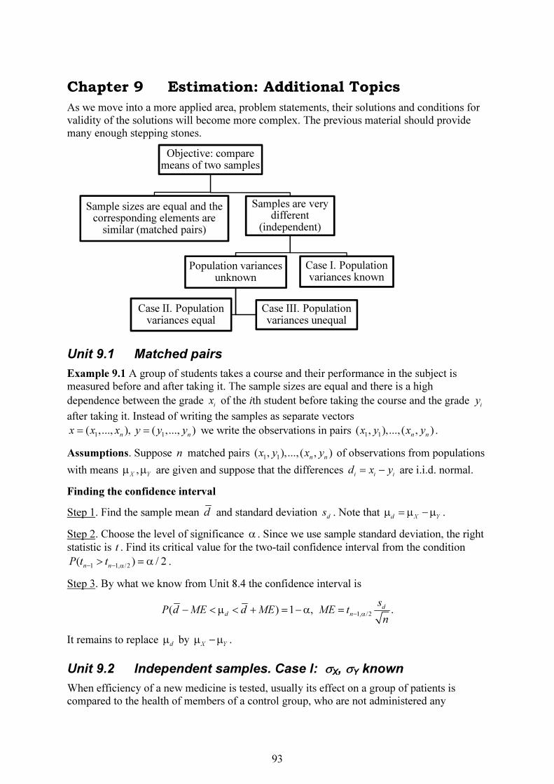
93

Chapter 9 Estimation: Additional Topics

As we move into a more applied area, problem statements, their solutions and conditions for validity of the solutions will become more complex. The previous material should provide many enough stepping stones.

Unit 9.1 Matched pairs

Example 9.1 A group of students takes a course and their performance in the subject is measured before and after taking it. The sample sizes are equal and there is a high

dependence between the grade ix of the ith student before taking the course and the grade

iy

after taking it. Instead of writing the samples as separate vectors

1 1( ,..., ), ( ,..., )

n nx x x y y y= = we write the observations in pairs

1 1( , ),..., ( , )

n nx y x y .

Assumptions. Suppose n matched pairs 1 1

( , ),..., ( , )n n

x y x y of observations from populations

with means ,

X Yµ µ are given and suppose that the differences

i i id x y= − are i.i.d. normal.

Finding the confidence interval

Step 1. Find the sample mean d and standard deviation ds . Note that

d X Yµ = µ −µ .

Step 2. Choose the level of significance α . Since we use sample standard deviation, the right

statistic is t . Find its critical value for the two-tail confidence interval from the condition

1 1, /2( ) / 2

n nP t t

− − α> = α .

Step 3. By what we know from Unit 8.4 the confidence interval is

1, /2( ) 1 , .d

d n

sP d ME d ME ME t

n− α

− < µ < + = −α =

It remains to replace dµ by

X Yµ −µ .

Unit 9.2 Independent samples. Case I: σX, σY known

When efficiency of a new medicine is tested, usually its effect on a group of patients is compared to the health of members of a control group, who are not administered any

Objective: compare means of two samples

Sample sizes are equal and the corresponding elements are similar (matched pairs)

Samples are very different

(independent)

Population variances unknown

Case III. Population variances unequal

Case II. Population variances equal

Case I. Population variances known

94

medication. In this case we have two distinct samples of different sizes ,

X Yn n . They come

independently from two different populations.

Assumptions. The samples 1 1

( ,..., ), ( ,..., )X Y

n nx x x y y y= = are independent normal. The

population means are unknown and the population variances are known.

By properties of means and variances

2 2

( ) , ( ) ( ) ( ) .X Y

X Y

X Y

E X Y EX EY V X Y V X V Yn n

σ σ− = − = µ −µ − = + = + (9.1)


Step 1. Find the sample means.

Step 2. Choose the level of significance α and find the critical value of the z statistic from

1 /2( ) / 2

nP z z

− α> = α .

Step 3. Then the confidence interval for X Y

µ −µ is

2 2

/2( ) 1 , .X Y

X Y

X Y

P X Y ME X Y ME ME zn n

α

σ σ− − < µ −µ < − + = −α = +

Unit 9.3 Independent samples. Case II: σX, σY unknown but equal (pooled estimator)

When 22 2

X Yσ =σ = σ from (9.1) we see that

1 1

( ) .X Y

X Yn n

σ − = σ + (9.2)

The question therefore is how one combines the information contained in two samples to

better estimate σ ? Theorem 7.1 provides the leading idea in this and the next section.

Idea. The population variance 2σ , sample variance

2s and degrees of freedom r should

satisfy the equation

2

2

2r

rs

χ =σ (9.3)

To find the right estimator we use an inductive argument. By Theorem 7.1 we have equations

2 2

2 2

1 12 2

( 1) ( 1), .

X Y

X X Y Y

n n

n s n s

− −

− −χ = χ =

σ σ

Summing them and using the fact that the two chi-square distributions involved are independent we get

2 2

2 2 2

1 1 22 2

( 1) ( 1).

X Y X Y

X X Y Y

n n n n

n s n s

− − + −

− −+ = χ + χ = χ

σ σ (9.4)

From (9.3) and (9.4) we see that the estimator of 2σ should be defined by

95

2 2

2 ( 1) ( 1).

2

X X Y Yp

X Y

n s n s

s

n n

− + −

=

+ −

(9.5)

Definition. (9.5) is called a pooled estimator.

Exercise 9.1 (1) In addition to (9.3), the pooled estimator has the usual unbiasedness property 2 2

pEs = σ .

(2) Besides, it gives more weight to the sample with the larger size.

(3) Obviously, (9.2) is estimated by 1 1

( ) p

X Y

X Y sn n

σ − = + . Following the general

statistical idea, in

0

( ) 1 1

X Y

X Y X Yz

X Y

n n

− −= =

σ −

σ +

replace σ by the pooled estimator to obtain

1 1

p

X Y

X Yt

sn n

−

=

+

Show that this t is distributed as 2

X Yn nt+ −

.


Step 1. Calculate 2 2 2

, , , ,

X Y pX Y s s s .

Step 2. Choose α and find the critical value of the t statistic 2, /2

X Yn nt

+ − α.

Step 3. The confidence interval is ( ) 1 ,X Y

P X Y ME X Y ME− − < µ −µ < − + = −α

where 2, /2

1 1.

X Yn n p

X Y

ME t sn n

+ − α= +

Unit 9.4 Independent samples. Case III: σX, σY unknown and unequal (Satterthwaite’s approximation)

Assumptions. There are two samples of sizes ,

X Yn n , respectively, drawn from normal

populations with unknown population means. Population variances 2 2,

X Yσ σ are unknown and

unequal.

This topic shows how complex and long a preamble can be.

Preamble. Equations (9.1) continue to be true. Denote D X Y= − . Because of (9.1), as

usual, 2

Dσ is estimated by

2 2

2 X Y

D

X Y

s

n n

σ σ= +

and instead of 0

( )D X Y

D D

D X Yz

−µ − − µ −µ= =

σ σ we

use

96

( )

.X Y

D

X Yt

s

− − µ −µ= (9.6)

The idea used in Case II now sounds like this: find the number of degrees of freedom r in such a way that

2

2

2.

D

r

D

rsχ =

σ (9.7)

Suppose (9.7) is true. Taking variance of both sides and using homogeneity we get 2

2 2

22 ( ) ( )

r D

D

rr V V s

= χ = σ

or, rearranging,

4

2

2.

( )

D

D

rV s

σ

=

(9.8)

To find

2( )D

V s we use the result from Exercise 7.3:

4 4

2 2 2

2 2

2 21 1( ) ( ) ( ) .

1 1

X Y

D X Y

X Y X Y

V s V s V sn n n n

σ σ= + = +

− −

Combining this with (9.8) yields

4

2 22 2

.

1 1

1 1

D

X Y

X X Y Y

r

n n n n

σ=

σ σ+

− −

(9.9)

Definition. Replacing in (9.9) population variances by their sample counterparts we obtain Satterthwaite’s approximation for the number of degrees of freedom:

22 2

2 22 2

.

1 1

1 1

X Y

X Y

X Y

X X Y Y

s s

n n

v

s s

n n n n

+

=

+ − −


Step 1. Calculate 2 2, , , ,

X YX Y s s v .

Step 2. Choose α and find the critical value of the t statistic , /2v

tα.

Step 3. The confidence interval is ( ) 1 ,X Y

P X Y ME X Y ME− − < µ −µ < − + = −α

where 2 2

, /2 .

X Y

v

X Y

s sME t

n nα

= +

97

Unit 9.5 Confidence interval for the difference between two population proportions

Exercise 9.2 Suppose that a random sample of X

n observations from a population with

proportion X

p of successes yields a sample proportion ˆX

p and that an independent random

sample of Yn observations from a population with proportion

Yp of successes produces a

sample proportion ˆYp . Which of the Cases I-III would you apply?


1. Assuming that the population variances are known, derive the confidence interval for the difference between two means in case of (a) matched pairs and (b) independent samples.

2. In the context of two independent samples with unknown but equal variances: (a) calculate

( )V X Y− , (b) define the pooled estimator and find its mean and (c) derive the confidence

interval.

3. Give the decision tree for testing the difference between two means showing your choices

when: (a) σ is known/unknown, (b) the samples are similar (matched) or independent, (c) in

case of unknown σ , equal or unequal variances and (d) the parent population is general or

Bernoulli. In all cases give the expression for ME .

4. Minimum required: 9.4, 9.6, 9.11, 9.12, 9.18, 9.27, 9.35.

98

Chapter 10 Hypothesis Testing

Unit 10.1 Concepts of hypothesis testing (null and alternative hypotheses, Type I and Type II errors, Cobb-Douglas production function; increasing, constant and decreasing returns to scale)

In hypothesis testing we assume two possibilities, called hypotheses, about the state of nature. They must be mutually exclusive and collectively exhaustive events, like “the accused is guilty” and “the accused is innocent”. In practice, the true state of nature is never known, and we have to use statistical evidence to make judgment.

One hypothesis is called a null hypothesis and denoted 0

H and the other is called an

alternative hypothesis and denoted aH . Rejecting the null, when it is true, we commit an

error called Type I error. Rejecting the alternative, when it is true, leads to another error, called Type II error.

Table 10.1 States of nature and our decisions

States of nature

0

H is true aH is true

Decision Accept 0

H Right decision Type II error

Reject 0H Type I error Right decision

The choice of the hypotheses is up to us and depends on the circumstances. If we seek a strong evidence in favor of a particular outcome, that outcome should be designated as the alternative hypothesis, because, as comparison of Unit 10.3 and Unit 10.5 shows, it’s easier to control the probability of Type I error.

Example 10.1 In a criminal trial the prosecutor wants to prove that the defendant is guilty, and that would be the alternative. For the defendant’s lawyer the alternative is that the defendant is innocent.

Example 10.2 A Cobb-Douglas production function is defined by ( , )f K L AK Lα β

= where

, ,A α β are constants and ,K L are independent variables (capital and labor). It is

homogeneous of degree α+β : ( , ) ( ) ( ) ( , )b

f tK tL A tK tL t f K Lα β α+

= = . We say that this

function exhibits increasing, constant or decreasing returns to scale if, respectively,

1α+β > , 1α+β = or 1α+β< . In applied research we might want to test

(10.1)

Example 10.3 We believe that usually the supply curve is positively sloping. If we model it

as a straight line, , then to prove that it is really positively sloped we test

(10.2)

Example 10.4 The hypotheses in (10.1) and (10.2) are complementary. In NCT you can see examples of noncomplementary hypotheses, such as

(10.3)

0: 1 against : 1.

aH Hα +β = α +β ≠

p a bq= +

0: 0 against : 0.

aH b H b≤ >

0: 1 against : 1.

aH Hα +β = α +β >

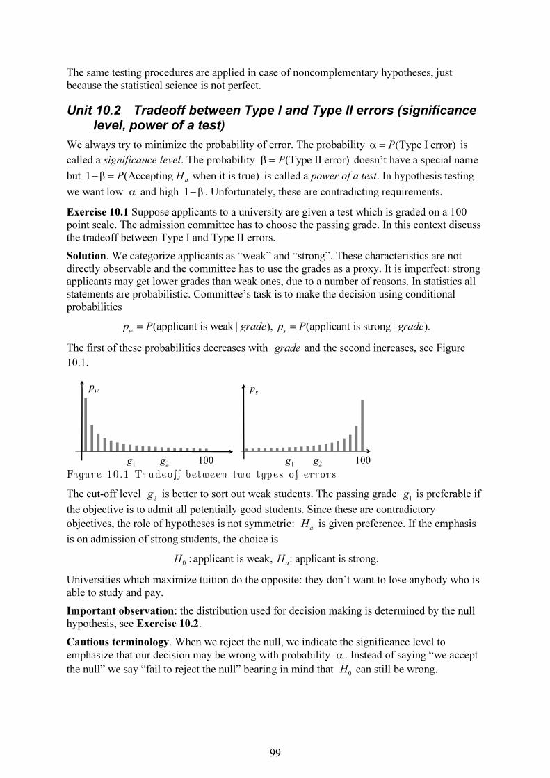
99

The same testing procedures are applied in case of noncomplementary hypotheses, just because the statistical science is not perfect.

Unit 10.2 Tradeoff between Type I and Type II errors (significance level, power of a test)

We always try to minimize the probability of error. The probability is

called a significance level. The probability doesn’t have a special name

but is called a power of a test. In hypothesis testing

we want low and high . Unfortunately, these are contradicting requirements.

Exercise 10.1 Suppose applicants to a university are given a test which is graded on a 100 point scale. The admission committee has to choose the passing grade. In this context discuss the tradeoff between Type I and Type II errors.

Solution. We categorize applicants as “weak” and “strong”. These characteristics are not directly observable and the committee has to use the grades as a proxy. It is imperfect: strong applicants may get lower grades than weak ones, due to a number of reasons. In statistics all statements are probabilistic. Committee’s task is to make the decision using conditional probabilities

The first of these probabilities decreases with and the second increases, see Figure

10.1.

Figure 10.1 Tradeoff between two types of errors

The cut-off level is better to sort out weak students. The passing grade is preferable if

the objective is to admit all potentially good students. Since these are contradictory

objectives, the role of hypotheses is not symmetric: is given preference. If the emphasis

is on admission of strong students, the choice is

Universities which maximize tuition do the opposite: they don’t want to lose anybody who is able to study and pay.

Important observation: the distribution used for decision making is determined by the null hypothesis, see Exercise 10.2.

Cautious terminology. When we reject the null, we indicate the significance level to

emphasize that our decision may be wrong with probability . Instead of saying “we accept

the null” we say “fail to reject the null” bearing in mind that can still be wrong.

(Type I error)Pα =

(Type II error)Pβ =

1 (Accepting when it is true)a

P H−β =

α 1−β

(applicant is weak | ), (applicant is strong | ).w sp P grade p P grade= =

grade

100 100g1

g1

g2

g2

pw p

s

2g

1g

aH

0: applicant is weak, : applicant is strong.

aH H

α

0H

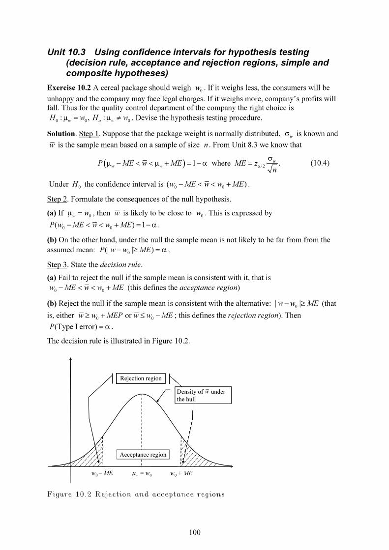
100

Unit 10.3 Using confidence intervals for hypothesis testing (decision rule, acceptance and rejection regions, simple and composite hypotheses)

Exercise 10.2 A cereal package should weigh . If it weighs less, the consumers will be

unhappy and the company may face legal charges. If it weighs more, company’s profits will fall. Thus for the quality control department of the company the right choice is

. Devise the hypothesis testing procedure.

Solution. Step 1. Suppose that the package weight is normally distributed, is known and

is the sample mean based on a sample of size . From Unit 8.3 we know that

(10.4)

Under the confidence interval is .

Step 2. Formulate the consequences of the null hypothesis.

(a) If , then is likely to be close to . This is expressed by

.

(b) On the other hand, under the null the sample mean is not likely to be far from from the

assumed mean: .

Step 3. State the decision rule.

(a) Fail to reject the null if the sample mean is consistent with it, that is

(this defines the acceptance region)

(b) Reject the null if the sample mean is consistent with the alternative: (that

is, either ; this defines the rejection region). Then

.

The decision rule is illustrated in Figure 10.2.

Figure 10.2 Rejection and acceptance regions

0w

0 0 0: , :

w a wH w H wµ = µ ≠

wσ

w n

( ) /21 where .

w

w wP ME w ME ME z

nα

σµ − < < µ + = −α =

0H

0 0( )w ME w w ME− < < +

0wwµ = w

0w

0 0( ) 1P w ME w w ME− < < + = −α

0(| | )P w w ME− ≥ = α

0 0w ME w w ME− < < +

0| |w w ME− ≥

0 0 or w w MEP w w ME≥ + ≤ −

(Type I error)P = α

Density of under

the hull

w0 −ME w

0+ MEµ

w= w

0

Rejection region

Acceptance region

w

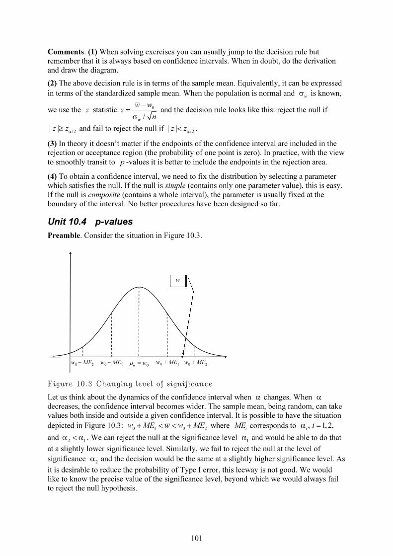
101

Comments. (1) When solving exercises you can usually jump to the decision rule but remember that it is always based on confidence intervals. When in doubt, do the derivation and draw the diagram.

(2) The above decision rule is in terms of the sample mean. Equivalently, it can be expressed

in terms of the standardized sample mean. When the population is normal and is known,

we use the statistic and the decision rule looks like this: reject the null if

and fail to reject the null if .

(3) In theory it doesn’t matter if the endpoints of the confidence interval are included in the rejection or acceptance region (the probability of one point is zero). In practice, with the view

to smoothly transit to -values it is better to include the endpoints in the rejection area.

(4) To obtain a confidence interval, we need to fix the distribution by selecting a parameter which satisfies the null. If the null is simple (contains only one parameter value), this is easy. If the null is composite (contains a whole interval), the parameter is usually fixed at the boundary of the interval. No better procedures have been designed so far.

Unit 10.4 p-values

Preamble. Consider the situation in Figure 10.3.

Figure 10.3 Changing level of significance

Let us think about the dynamics of the confidence interval when changes. When decreases, the confidence interval becomes wider. The sample mean, being random, can take values both inside and outside a given confidence interval. It is possible to have the situation

depicted in Figure 10.3: where corresponds to

and . We can reject the null at the significance level and would be able to do that

at a slightly lower significance level. Similarly, we fail to reject the null at the level of

significance and the decision would be the same at a slightly higher significance level. As

it is desirable to reduce the probability of Type I error, this leeway is not good. We would like to know the precise value of the significance level, beyond which we would always fail to reject the null hypothesis.

wσ

z0

/w

w w

z

n

−

=

σ

/2| |z z

α≥

/2| |z z

α<

p

w0 −ME

1w

0+ ME

1µw

= w0

w0

+ ME2

w0 − ME

2

w

α α

0 1 0 2w ME w w ME+ < < +

iME , 1,2,

iiα =

2 1α < α

1α

2α

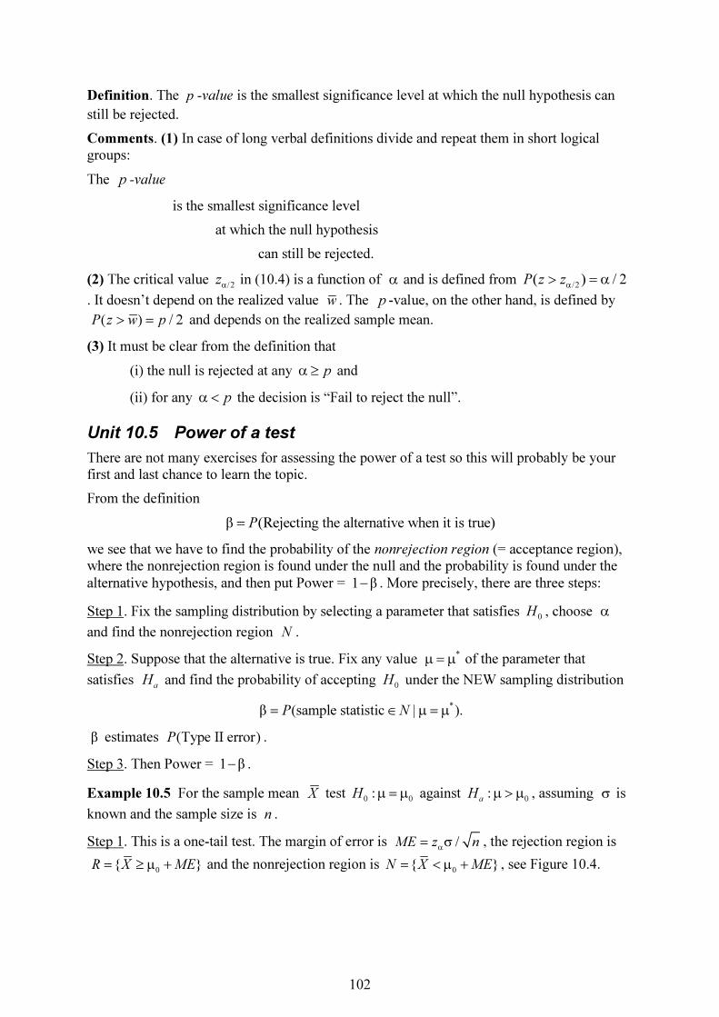
102

Definition. The p -value is the smallest significance level at which the null hypothesis can

still be rejected.

Comments. (1) In case of long verbal definitions divide and repeat them in short logical groups:

The -value

is the smallest significance level

at which the null hypothesis

can still be rejected.

(2) The critical value in (10.4) is a function of and is defined from

. It doesn’t depend on the realized value . The -value, on the other hand, is defined by

and depends on the realized sample mean.

(3) It must be clear from the definition that

(i) the null is rejected at any and

(ii) for any the decision is “Fail to reject the null”.

Unit 10.5 Power of a test

There are not many exercises for assessing the power of a test so this will probably be your first and last chance to learn the topic.

From the definition

we see that we have to find the probability of the nonrejection region (= acceptance region), where the nonrejection region is found under the null and the probability is found under the

alternative hypothesis, and then put Power = . More precisely, there are three steps:

Step 1. Fix the sampling distribution by selecting a parameter that satisfies , choose

and find the nonrejection region .

Step 2. Suppose that the alternative is true. Fix any value of the parameter that

satisfies and find the probability of accepting under the NEW sampling distribution

estimates .

Step 3. Then Power = .

Example 10.5 For the sample mean test against , assuming is

known and the sample size is .

Step 1. This is a one-tail test. The margin of error is , the rejection region is

and the nonrejection region is , see Figure 10.4.

p

/2zα

α/2

( ) / 2P z zα

> = α

w p

( ) / 2P z w p> =

pα ≥

pα <

(Rejecting the alternative when it is true)Pβ =

1−β

0H α

N

*µ = µ

aH

0H

*(sample statistic | ).P Nβ = ∈ µ = µ

β (Type II error)P

1−β

X0 0:H µ = µ

0:aH µ > µ σ

n

/ME z nα

= σ

0{ }R X ME= ≥ µ +

0{ }N X ME= < µ +

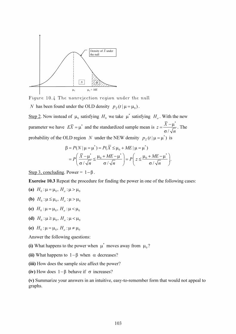
103

Figure 10.4 The nonrejection region under the null

has been found under the OLD density .

Step 2. Now instead of satisfying we take satisfying . With the new

parameter we have and the standardized sample mean is . The

probability of the OLD region under the NEW density is

Step 3, concluding. Power = .

Exercise 10.3 Repeat the procedure for finding the power in one of the following cases:

(a)

(b)

(c)

(d)

(e)

Answer the following questions:

(i) What happens to the power when moves away from ?

(ii) What happens to when decreases?

(iii) How does the sample size affect the power?

(iv) How does behave if increases?

(v) Summarize your answers in an intuitive, easy-to-remember form that would not appeal to graphs.

Density of under

the null

µ0

+ MEµ0

N

X

R

N0

( | )X

p t µ = µ

0µ

0H

*µ

aH

*EX = µ

*

/

Xz

n

−µ=

σ

N*( | )

Xp t µ = µ

* *

0

* **

0 0

( | ) ( | )

./ / /

P N P X ME

ME MEXP P z

n n n

β = µ = µ = ≤ µ + µ = µ

µ + −µ µ + −µ−µ= ≤ = ≤

σ σ σ

1−β

0 0 0: , :

aH Hµ = µ µ > µ

0 0 0: , :

aH Hµ ≤ µ µ > µ

0 0 0: , :

aH Hµ = µ µ < µ

0 0 0: , :

aH Hµ ≥ µ µ < µ

0 0 0: , :

aH Hµ = µ µ ≠ µ

*µ

0µ

1−β α

1−β σ

104


1. In the context of a university admission test discuss the trade-off between Type I and Type II errors.

2. Explain the statistical logic behind the decision rule using the example of a cereal package (the choice of hypotheses and the use of the confidence interval).

3. z statistics versus p -values

(a) Give economic examples of the null and alternative hypotheses which lead to (i) a one-tail test and (ii) a two-tail test.

(b) How are the critical values defined and what are the decision rules in these cases using statistics?

(c) Define values for each of those cases and explain the benefits/drawbacks of

using statistics versus -values.

4. Normal population versus Bernoulli

(a) Select two pairs of hypotheses such that in one case you would apply a two-tail test and in the other – a one-tail test. Assuming that the population is normal and the variance is unknown, illustrate graphically the procedure of testing the mean.

(b) What changes would you make if the population were Bernoulli?

5. Using the example of testing the sample mean describe in full the procedure of assessing the power of a test. Answer the following questions:

(a) What happens to the power when moves away from ?

(b) What happens to when decreases?

(c) How does the sample size affect the power?

(d) How does behave if increases?

6. Give the decision tree for testing the difference between two population means distinguishing between: (a) dependent and independent samples, (b) cases of known and unknown variances, (c) equal and unequal variances when they are unknown and (d) normal and Bernoulli populations.

7. Minimum required: 10.06, 10.13, 10.16, 10.32.

z

p

z p

*µ

0µ

1−β α

1−β σ

105

Chapter 11 Hypothesis Testing II

If you have been following the material, as my students do, this chapter must be easy for you. That’s why the chapter is short.

Unit 11.1 Testing for equality of two sample variances (F-distribution)

Definition. Let and be independent. Then

is called and -distribution with degrees of freedom.

Comments. (1) Equivalently, can be defined by

where are standard normal independent.

(2) From the definitions of and it follows that . This fact is used in simple

regression (a test of significance of a regression coefficient is equivalent to the test of significance).

(3) We know that for independent samples from two normal populations

Hence,

(4) To test the null against the alternative choose , find the

critical values for the two-tail test from

(the notation of critical values follows Table 9 from NCT). Then under the null

1, 1,1 /2 1, 1, /2

2

1, 1,1 /2 1, 1, /22

1 ( )

.

X Y X Y

X Y X Y

n n n n

X

n n n n

Y

P F F F

sP F F

s

− − −α − − α

− − −α − − α

= α = < <

= < <

The null is rejected if either exceeds the upper critical value or is smaller than the

lower critical value.

2

mχ

2

nχ

2

, 2

/

/

m

m n

n

mF

n

χ=χ

F ( , )m n

F

2

1

, 2

1

/

/

m

ii

m n n

m jj

z mF

z n

=

+=

=

∑

∑

1 1,..., , ,...,

m m m nz z z z

+ +

t F2

1,n nt F=

t F

2 2

2 2

1 12 2

( 1) ( 1), .

X Y

X X Y Y

n n

X Y

n s n s

− −

− −= χ = χ

σ σ

22 21

1, 12 2 2

1

/ ( 1)/.

/ / ( 1)

X

X Y

Y

n XX X

n n

Y Y n Y

nsF

s n

−

− −

−

χ −σ= =

σ χ −

2 2

0:

X YH σ = σ

2 2

0:

X YH σ ≠ σ α

1, 1,1 /2 1, 1, /2( ) 1 / 2, ( ) / 2

X Y X Yn n n n

P F F P F F− − −α − − α

> = −α > = α

2 2/

X Ys s

106


1. In one block define and describe properties of chi-square, t and F distributions.

2. Testing for equality of variances

(a) What is the distribution of the ratio of two sample variances from two normal populations?

(b) How would you test for equality of variances from two normal populations?

2. Minimum required: 11.24, 11.28.

107

Chapter 12 Linear Regression

Unlike the previous chapter, this one will be densely populated. It’s because solutions to some exercises from NCT are completely spelled out. This chapter covers the first chapter of a standard econometrics text.

Unit 12.1 Algebra of sample means

For a discrete random variable with and uniform distribution denote

. This is just the sample mean: . Therefore all properties

we’ve established for the mean value operator translate to corresponding properties of sample means. We need:

(a) linearity of means ,

(b) alternative expression for covariance and

(c) variance .

To see usefulness of these abbreviations, compare the last equation to its full form:

The tricky part of the notation just introduced is that can be treated not as real

values of a random variable but as random variables sampled from the same population (this is why they are written using capital X’s). To emphasize the distinction between the

population mean and sample mean, I use the notation for the latter. It give rise to

cov ( , ) ( )( )uX Y X X Y Y= − − and 2

( ) ( )u

V X X X= − .

Unit 12.2 Linear model setup (linear model, error term, explanatory variable, regressor)

We assume that vectors are observed and want to capture dependence of

on . The linear model seeks a linear dependence . Since usually data are

chaotic, exact linear dependence is impossible and it is more realistic to suppose that

differs from a linear function by a random error term . Thus, the main

assumption is

(12.1)

The independent variable is called an explanatory variable or a regressor.

Regarding the random variables for now we assume that their mean is zero. The

regressor is assumed to be deterministic.

An immediate consequence of this is that the dependence of population means of on is

linear: . Out first task is to estimate the intercept and the slope .

X1,...,

nx x

1

1 1...

u nE X x x

n n= + +

uE X X=

( )aX bY aX bY+ = +

( )( )X X Y Y XY XY− − = −

2 2 2( ) ( )X X X X− = −

2

2 2

1 1 1

1 1 1( ) .

n n n

i i i

i i i

X X X Xn n n= = =

− = −

∑ ∑ ∑

1,...,

nX X

X

uE

1 1( , ), ..., ( , )

n nx y x y

iy

ix

1 2i iy x= β +β

iy

1 2 ixβ +β

iu

1 2, 1,..., .

i i iy x u i n= β +β + =

x

1,...,

nu u

iy

ix

1 2i iEy x= β +β

1β

2β

108

Unit 12.3 Ordinary least squares estimation (OLS estimators, normal equations, working formula)

Definition (Gauss). Follow this definition on Figure 12.1. Take an arbitrary straight line

, find the residuals from approximation of the observed values

by the corresponding values along the straight line and accept as OLS estimators of

and those values which minimize the sum of squared residuals

Figure 12.1 Illustration of the OLS procedure

12.3.1 Derivation of OLS estimators

The first order conditions for the minimization of are

Getting rid of −2 and dividing both equations by we get

1 2 1 2

1 1

1 1( ) 0, ( ) 0.

n n

i i i i i

i i

y b b x y b b x xn n= =

− − = − − =∑ ∑ (12.2)

Introducing the vector notation

1 1 1

... , ... , ...

n n n

y x u

y x u

y x u

= = =

(12.3)

we can write (12.2) as Using linearity of sample means

rearrange this:

(12.4)

1 2y b b x= +

1 2( )

i iy b b x− +

iy

1 2 ib b x+

1β

2β

1 2,b b

2

1 2 1 2

1

( , ) ( ) .n

i i

i

f b b y b b x=

= − −∑

xi

yi

b1+b

2xi

y = b1+b

2x

1 2( , )f b b

1 2

1 2

11

1 2

1 2

12

( , )2 ( ) 0,

( , )2 ( ) 0.

n

i i

i

n

i i i

i

f b by b b x

b

f b by b b x x

b

=

=

∂= − − − =

∂

∂= − − − =

∂

∑

∑

n

1 2 1 20, ( ) 0.y b b x y b b x x− − = − − =

2

1 2 1 20, 0.y b b x yx b x b x− − = − − =

109

We have obtained what is called normal equations.

From the first of them we see that we can find

1 2b y b x= − (12.5)

if we know . To find , plug (12.5) into the second normal equation:

This last equation implies

1 1 1 1 1 1

2 2 22 2

2 2

1 1 1 1

1 1 1

( )( ).

1 1

n n n n n n

i i i i i i i i

i i i i i i

n n n n

i i i i

i i i i

x y x y n x y x yn n nyx x y

bx x

x x n x xn n

= = = = = =

= = = =

− − − = = =

− − −

∑ ∑ ∑ ∑ ∑ ∑

∑ ∑ ∑ ∑

(12.6)

(12.5) and (12.6) are called OLS estimators. Applying notation from Unit 12.1 we get an

equivalent expression for the estimator of the slope:

2

cov ( , ).

( )

u

u

x yb

V x= (12.7)

The last part of (12.6) is better for calculations. (12.7) is better for establishing theoretical

properties.

12.3.2 Unbiasedness of OLS estimators

Exercise 12.1 (1) If then the OLS estimators exist.

(2) If, further, and , then the OLS estimators are

unbiased.

Proof. The statement about existence is obvious. Using notation (12.3) let us write the system

of equations (12.1) in a vector form

Using linearity of covariances we rearrange the slope estimator

Covariance of a constant with anything is zero. Covariance of a variable with itself is its

variance. Therefore from the last equation we obtain a working formula for the slope

estimator:

(12.8)

Since, by assumption, is deterministic and the error has mean zero, we get unbiasedness of

the slope estimator

2b

2b

2 2

2 2( )( ) 0.yx x y b x b x− + − =

( ) 0u

V x ≠

0 for all i

Eu i= are deterministicix

1 2.y x u= β +β +

1 2 1 2

2

cov ( , ) cov ( , ) cov ( , ) cov ( , ).

( ) ( )

u u u u

u u

x x u x x x x ub

V x V x

β +β + β +β += =

2 2

cov ( , ).

( )

u

u

x ub

V x= β +

x

2 2 2

cov ( , ).

( )

u

u

x EuEb

V x= β + = β

110

The vector form of the linear model implies

We use the last two equations to prove unbiasedness of the intercept estimator:

Unit 12.4 Variances of OLS estimators (homoscedasticity, autocorrelation, standard errors)

In addition to the assumptions of Exercise 12.1 suppose that

(12.9)

(12.10)

Comments. (1) Homoscedasticity means that variances of the error terms are the same across

observations. It holds when the errors are identically distributed. In economics usually

variances of variables are proportional to their levels (variation in income grows with

income) so the errors are often heteroscedastic.

(2) Absence of autocorrelation holds for independent errors (provided that their means are

null). The condition can be equivalently written as cov( , ) 0,i j

u u i j= ≠ . Time series data are

usually autocorrelated.

Exercise 12.2 Prove that under the above assumptions

(12.11)

Proof. Step 1. Suppose that a random variable is a linear combination of the errors with

constant coefficients:

(12.12)

Then

2 2 2.

u iEZ a= σ ∑

To prove this equation it is useful to visualize the multiplication process. When calculating

each element in the first pair of parentheses is multiplied by each

element in the second pair. Therefore is a sum of the products in the table

Table 12.1 Visualizing a squared sum

…

… … …

…

1 2.y x u= β +β +

2

1 1 2 2 1 2 2 10

( ) ( ) .Eb E x u b x x Eu Eb x= =β

= β +β + − = β +β + − = β

2 2 2

1... (homoscedasticity)

n uEu Eu= = = σ

0 for all (absence of autocorrelation).i j

Eu u i j= ≠

2 1

2 2

2 2 2

2 2

1 1

1, .

( ) ( )

u

b b un n

i i

i i

x

nx x x x

= =

σ σ = σ = σ + − −

∑ ∑

Z

.

i iZ a u=∑

( )( )2

i i j jZ a u a u= ∑ ∑

2Z

1 1 1 1a u a u

1 1 n na u a u

1 1n na u a u

n n n na u a u

111

Separating the diagonal products from off-diagonal and using conditions (12.9)-(12.10) we

get

Step 2. To make use of Step 1, we obtain a representation of type (12.12) for . Rewrite the

working formula (12.8) as

(12.13)

where

The coefficients are deterministic and satisfy

This allows us to simplify (12.13)

Therefore by unbiasedness and Step 1

(12.14)

The sum of squares involved here can be found using properties of means

The last two equations prove the first equation in (12.11).

Step 3. We need to derive a similar representation for

With the notation this becomes In the way similar to (12.14) we

get

2 2 2 2 2

1

.

n

i i i j i j u i

i i j

EZ a Eu a a Eu u a

= ≠

= + = σ∑ ∑ ∑

2b

1

2 2 22

1

2 21 12

1

( )( )cov ( , )

( ) ( )

( )( ) ( )

( )

n

i iu i

n

u ii

n ni

i i ini i

ii

x x u ux ub

V x x x

x xu u a u u

x x

=

=

= =

=

− −= β + = β +

−

−= β + − = β + −

−

∑

∑

∑ ∑∑

2

1

.( )( )

i i

i n

uii

x x x xa

nV xx x=

− −

= =

−∑

ia

1

0.( )

n

i

i u

na na x x

nV x=

= = − =∑

2 2 2 21 1 1 1( ) .

n n n n

i i i i i i ii i i ib a u u a u u a a u

= = = =

= β + − = β + − = β +∑ ∑ ∑ ∑

2

2 2 2 2 2 2

2 2 2 2

1

( ) ( ) ( ) .n

b i i u i

i

E b Eb E b E a x a

=

σ = − = −β = = σ∑ ∑

2 2 2

2 2 2 2

1

( ) 1( ) .

( ) ( ) ( )

n

u

i

i u u i

V xna na x x

n V x nV x x x=

= = − = =

−

∑∑

( )1 1 2 2

1 1

1 1.

i i

i i i i i

b x u a u x

u a xu a x un n

= β +β + − β +

= β + − = β + −

∑

∑ ∑ ∑

1

i ic a x

n

= −1 1

.

i ib c u= β +∑

1

2 2 2 2 2 2

1 1 1 1

1

( ) ( ) ( ) .n

b i i u i

i

E b Eb E b E c x c

=

σ = − = −β = = σ∑ ∑

112

It remains to calculate the sum of squares

The second of the formulas (12.11) follows from the last two equations.

12.4.1 Statistics for testing hypotheses

Definition. Standard errors of OLS estimators are defined by

Theorem 12.1 Let the regressor be deterministic with different from zero. Assume

that the random variables are i.i.d. normal with mean zero and that the true

coefficients are . Then the variables

are distributed as distribution with degrees of freedom.

Unit 12.5 Orthogonality and its consequences (fitted value, residual vector, orthogonality, Pythagorean theorem, Total Sum of Squares, Explained Sum of Squares, Residual Sum of Squares)

After having estimated the coefficients, for prediction purposes we put . This

linear function is called a fitted value. It is defined everywhere, both inside and outside the

sample. It is customary to use the same notation for the vector

where the fitted value is calculated only at the sample points. Hopefully you will see from the

context if the fitted value is a function or a vector. The residual vector is defined as ɵ.e y y= −

Definition. Vectors are called orthogonal if .

Exercise 12.3 (1) Check that the vectors are orthogonal.

(2) The notion of uncorrelated random variables has been borrowed from orthogonality. Let

be arbitrary random variables such that . Put . Prove

that then are uncorrelated. How can you guess a result like this?

First orthogonality relation. .

2

2 2

2

2

2 2

2 2 20

1 1 12

1 1 1 ( )2( )( ) ( ) .

( )i

c ax ax a x

n n n

x

a x a x

n n n n x x=

= − = − +

= − + = +−∑

2 1

2 2

2 2 2

2 2

1 1

1, .

( ) ( )

u

b b un n

i i

i i

s x

s s s

nx x x x

= =

= = + − −

∑ ∑

x ( )u

V x

1,...,

nu u

0 0

1 2,β β

1 2

0 0

1 1 2 2

2 2,

n n

b b

b bt t

s s− −

−β −β= =

t 2n−

1 2y b b x= +

1 2 1 1 2ˆ ( ,..., )

ny b b x b b x= + +

1 1( ,..., ), ( ,..., )

n nx x y y

1 1... 0

n nx y x y+ + =

(0,1) and (1,0)

,X Y ( ) 0V X ≠cov( , )

( )

X YZ Y X

V X= −

,X Z

0e =

113

Comments. (1) This equation is a reflection of the assumption 0Eu = . Notice that in one

case the sample mean is used and in the other the population mean.

(2) Keep in mind that for a model without the intercept the sum of residuals may not

be zero.

(3) This relation also means that the residual is orthogonal to the vector of unities (1,…,1):

.

Proof. By the first normal equation (12.4)

Corollary 12.1 The fitted value has the same sample mean as : .

Proof. By the definition of the residual vector

(12.15)

which implies

(12.16)

Second orthogonality relation. The fitted value and residual are orthogonal: .

Proof. From the second normal equation (12.4)

This equation and the first orthogonality relation give

Theorem 12.2 (Pythagorean theorem) If the vectors are orthogonal, , then

.

Proof.

Definition. If all are the same, they are all equal to and there is no variation in the

dependent variable. Now suppose follows the linear model. The idea is to still measure its

deviation from the sample mean but decompose it into two parts: one which is due to the

linear part and the other which is due to the error. Subtracting the sample mean from

both sides of (12.15) we realize this idea as

(12.17)

This decomposition is accompanied by three definitions:

Total Sum of Squares = measure of magnitude of : ,

Explained Sum of Squares = measure of magnitude of : ,

Residual Sum of Squares = measure of magnitude of the error: .

Exercise 12.4 .

i iy bx=

1 0i ie e ne= ⋅ = =∑ ∑

1 2 1 20.e y b b x y b b x= − − = − − =

y y y=

ˆy y e= +

ˆ ˆ ˆ .y y e y e y= + = + =

ˆ 0i iy e =∑

2 2

1 2 1 2( ) ( ).

i ix e nxe n xy b x b x n xy b x b x= = − − = − −∑

1 2 1 2ˆ ( ) 0.i i i i i i iy e b b x e b e b x e= + = + =∑ ∑ ∑ ∑

,x y 0xy =

2 2 2( )x y x y+ = +

2 2 2 2 2 2 2( ) 2 2 .x y x xy y x xy y x y+ = + + = + + = +

iy y

iy

y

1 2xβ +β

ˆ( ) .y y y y e− = − +

y y−2

1( )

n

iiTSS y y

=

= −∑

ɵy y−

ɵ 2

1( )

n

iiESS y y

=

= −∑

2

1

n

iiRSS e

=

=∑

TSS ESS RSS= +

114

Proof. In the representation (12.17) the two terms on the right are orthogonal by the 1st and

2nd orthogonality relations:

By the Pythagorean theorem then

Unit 12.6 Goodness of fit (coefficient of determination)

Definition. The coefficient of determination is defined by . It is interpreted as the

percentage of total variation of around the sample mean explained by the regression.

Property 1. From Exercise 12.4 it follows that

and that , which justifies its interpretation as percentage.

Property 2. The sample correlation equals .

Proof. By definition and (12.16)

Here by the orthogonality relations

Therefore


1. Explain the setup of simple regression: what is observed, what is the assumed relation

between variables, why we have to include the error, the assumptions about the error and how

we write everything in a vector form.

2. Write down the formal equations from Unit 12.1 and other properties of means, variances

and covariances until you get used to that notation.

3. Define the OLS estimators, derive them and prove unbiasedness. When you do this, do you

have to use assumptions (12.9) and (12.10)?

4. Using t statistics, write down confidence intervals for the coefficients. How do you test

their significance?

ɵ ɵ ɵ( ) ( )( ) 0.y y e ye ye ye y e− = − = − =

ɵ2 2 2( ) ( ) .TSS n y y n y y ne ESS RSS= − = − + = +

2 ESSR

TSS=

y y

2

2 1

2

1

1 1( )

n

ii

n

ii

eRSSR

TSS y y

=

=

= − = −

−

∑

∑2

0 1R< <

ɵ,y yr

2R

ɵ

ɵ

ɵ

ɵ ɵ

ɵ ɵ

ɵ

ɵ,

2 22 2

cov ( , ) ( )( ) ( )( ).

( ) ( ) ( ) ( )( ) ( )

u

y y

y y y y y y y y y yr

V y V y y y y yy y y y

− − − −

= = =

− −− −

ɵ ɵ ɵ ɵ ɵ ɵ2 2

0

( )( ) ( )( ) ( ) ( ) ( ) .y y y y y e y y y y y e y y y y=

− − = + − − = − + − = −

ɵ

ɵ

ɵ

ɵ2 2

2

, 22 2

( ) ( ).

( )( ) ( )y y

y y y yr R

y yy y y y

− −

= = =

−− −

115

5. How do you evaluate goodness of fit using the coefficient of determination, sum of

squared errors and p -values of the estimated coefficients? In other words, if you have two

models for the same dependent variable with different regressors, how can you tell which one

is better?

6. How are the formulas obtained used for prediction?

7. Minimum required: 12.3, 12.20.

Literature

Michaelsen, Larry K., Knight, Arletta Bauman and Fink, L. Dee. Team-based Learning: A

Transformative Use of Small Groups. Greenwood Publishing Group. 2002.

Steven G. Krantz. How to Teach Mathematics. 2nd ed., American Mathematical Society,

Providence.1998.

List of figures Figure 3.1 Numerical characteristics of samples .................................................................................................. 22 Figure 3.2 Five number summary ......................................................................................................................... 24 Figure 4.1 Example of independent events ........................................................................................................... 41 Figure 5.1 Summing vectors using the parallelogram rule ................................................................................... 46 Figure 5.2 Scaling a vector .................................................................................................................................... 47 Figure 5.3 Independent versus uncorrelated pairs of variables ............................................................................ 52 Figure 5.4 Distribution function shape .................................................................................................................. 62 Figure 6.1 Integral as area .................................................................................................................................... 68 Figure 6.2 Approximation of an integral ............................................................................................................... 71 Figure 6.3 Density of standard normal ................................................................................................................. 77 Figure 8.1 Illustration of consistency .................................................................................................................... 88 Figure 10.1 Tradeoff between two types of errors ............................................................................................... 99 Figure 10.2 Rejection and acceptance regions ................................................................................................... 100 Figure 10.3 Changing level of significance .......................................................................................................... 101 Figure 10.4 The nonrejection region under the null ............................................................................................ 103 Figure 12.1 Illustration of the OLS procedure ..................................................................................................... 108

List of tables Table 2.1 Table of absolute and relative frequencies (discrete variable) ............................................................. 16 Table 2.2 Table of absolute and relative frequencies (categorical variable) ........................................................ 16 Table 2.3 Table of absolute and relative frequencies (continuous variable) ........................................................ 17 Table 2.4 Stem-and-leaf display ........................................................................................................................... 19 Table 3.1 Absolute and relative frequencies distribution ..................................................................................... 21 Table 3.2 Exemplary comparison of measures of central tendency ..................................................................... 23 Table 3.3 Summary of results on sample correlation coefficient .......................................................................... 26 Table 4.1 Set operations: definitions, visualization and logic ............................................................................... 29 Table 4.2 Set terminology and probabilistic terminology ..................................................................................... 30 Table 4.3 Probability tables for C (Coin) and D (Die) ............................................................................................ 31 Table 4.4 Probability table in case of a variable with n values ............................................................................. 32 Table 4.5 1-D table of joint events and probabilities ............................................................................................ 37 Table 4.6 Separate probability tables ................................................................................................................... 37 Table 4.7 Joint probability table ........................................................................................................................... 38 Table 4.8 Joint probability table (general case) .................................................................................................... 39 Table 4.9 Leftover joint probabilities .................................................................................................................... 39 Table 5.1 Discrete random variable with n values ................................................................................................ 44 Table 5.2 Table of linear operations with random variables ................................................................................ 46 Table 5.3 Separate probability tables ................................................................................................................... 48 Table 5.4 Joint values and probabilities ................................................................................................................ 48 Table 5.5 General definitions of the sum and product .......................................................................................... 49 Table 5.6 Geometric interpretation of the correlation coefficient ........................................................................ 56

116

Table 5.7 Bernoulli variable definition .................................................................................................................. 57 Table 5.8 Table of possible outcomes and probabilities ....................................................................................... 60 Table 5.9 Distribution of S3 ................................................................................................................................... 61 Table 5.10 Table of probabilities and cumulative probabilities ............................................................................ 63 Table 6.1 Definition of a function of a random variable ....................................................................................... 73 Table 7.1 Comparison of population and sample formulas .................................................................................. 86 Table 10.1 States of nature and our decisions ...................................................................................................... 98 Table 12.1 Visualizing a squared sum ................................................................................................................. 110

Index of terms 110% rule, 13

absolute value, 54

acceptance region, 100

active recalling, 10

addition rule, 35

additivity

of means, 48

of probability, 33

of variance, 54, 73

with respect to the domain of integration, 69

alternative expression

for covariance, 51, 72

for variance, 73

alternative hypothesis, 98

argument, 18

arithmetic square root, 54

assembly formula, 34

autocorrelation, 110

average, 21, 45

axiom, 11

basic outcomes, 31

Bayes theorem, 42

belongs to, 29

Bernoulli variable, 15, 57

binomial variable, 15, 59

Cauchy-Schwarz inequality, 54

central limit theorem, 78

Chebyshov inequality, 88

chi-square distribution, 83

classical probability, 35

Cobb-Douglas production function, 98

coefficient of determination, 114

combinations, 36

commutativity rules, 12

complement, 29

complement rule, 33

completeness axiom, 32, 33

composite hypothesis, 101

condition

equivalent, 52

necessary, 51

sufficient, 51

conditional probability, 40

confidence interval, 78

confidence level, 78

consistent estimator, 88

contingency table, 38

convergence in distribution, 78

coordinate plane, 13

correlation coefficient

population, 55

sample, 26

covariance, 50

sample, 26

covering, 31

cow-and-goat principle, 69

critical value, 89

cross-table, 38

cumulative distribution function, 62

cumulative probabilities, 63

de Morgan’s laws, 30

decile, 24

decision rule, 100

deductive argument, 32

definition, 11

complementary, 14

descriptive, 14

formal, 14

intuitive, 14

simplified, 14

working, 14

degrees of freedom, 83

density, 69

dependent variable, 49

deviation from the mean, 24

difference of sets, 29

discrete random variable, 44

disjoint covering, 31

disjoint sets, 30

distribution

bimodal, 23

symmetric, 23

trimodal, 23

distribution function, 62

distributive law, 30

domain, 18

downward biased, 81

efficient estimator, 87

117

element of, 29

empirical rule, 77

empty set, 30

error

Type I, 98

Type II, 98

error term, 107

estimator, 81

event, 30

elementary, 31

impossible, 31, 34

sure, 34

events

collectively exhaustive, 31

equally likely, 34

mutually exclusive, 31

ex-ante, 58

expected value, 45

expected value of a constant, 72

explanatory variable, 107

ex-post, 58

extended expression (for sum), 38

factorial, 35

F-distribution, 105

fitted value, 112

five-number summary, 24

frequencies

absolute, 16

relative, 16

frequency distribution

absolute, 16

frequency distributions

relative, 16

frequentist approach, 35

function

even, 76

odd, 76

symmetric, 76

function of a variable, 73

going

back, 33

forward, 33

sideways, 33

grouped data formula, 45

histogram, 18

homogeneity of degree 1, 48

homogeneity of degree 2, 53

homogeneity of standard deviation, 54

homoscedasticity, 110

icebreaker principle, 8

identically distributed variables, 58

independent

events, 40

variables, continuous case, 79

variables, discrete case, 49

induction, 33

inductive argument, 32

integral, 68

integration rule, 74

interaction term, 53

interquartile range, 24

intersection, 29

interval

one-tail, 78

two-tail, 78

interval estimate, 78

interval formula, 63

in terms of densities, 70

inverse function, 85

joint


event, 37

probability, 37

leaf, 19

linear combination, 46, 69

linear model, 107

linearity

of covariance, 50, 72

of integrals, 69

of means, 72

lower limit

of integration, 68

of summation, 38

margin of error, 90

marginal


probabilities, 38

mathematical expectation, 45

mean, 21, 45

of a continuous random variable, 72

of the Bernoulli variable, 57

median, 22

mode, 23

monomial, 63

monotonicity, 62

multiplication rule, 40

multiplicativity

of expected values, 72

of means, 49

negative correlation, 26, 56

nondecreasing function, 85

nonnegativity

of probability, 33

of variance, 73

nonoverlapping sets, 30

nonrejection region, 102

118

normal equations, 109

normal variable, 77

alternative definition, 78

null hypothesis, 98

number

even, 11

integer, 12

natural, 12

odd, 11

real, 12

number of successes, 59

occurrence of an event, 31

OLS estimators, 108, 109

order property, 69

orderings, 36

orthogonal vectors, 112

Outcome, 30

outlier, 23

own probabilities, 38

parallelogram rule, 46

parameter, 75

parent population, 58

Pareto diagram, 18

passive repetition, 10

percentile, 24

perfect correlation, 26

negative, 56

positive, 56

point estimate, 78

Poisson approximation to the binomial

distribution, 66

Poisson distribution, 64

pooled estimator, 95

population, 58

portfolio, 47

value, 47

positive correlation, 26, 56

positively skewed, 23

posterior probability, 42

postulate, 11

power of a test, 99

primitive function, 74

prior probability, 42

probability, 33, 34

proportion of successes, 59

p-value, 102

Pythagorean theorem, 113

quadratic equation, 12

quartile, 24

quota sampling, 81

random experiment, 30

random variable, 15

formal definition, 44

intuitive definition, 44

range, 18, 24

of the correlation coefficient, 55

rate of return, 66

real line, 13

regressor, 107

rejection region, 100

representation of data

frequency, 21

ordered, 21

raw, 21

residual vector, 112

returns to scale

constant, 98

decreasing, 98

increasing, 98

sample, 58

mean, 21

size, 15, 58

space, 31

standard deviation, 25

variance, 24

sampling

distribution, 81

with replacement, 58

Satterthwaite’s approximation, 96

scaled variable, 46

scatterplot, 20

set, 29

short expression (for sum), 38

significance level, 78, 99

simple hypothesis, 101

simple random sample, 81

skewness, 23

squared deviation, 24

standard deviation, 54

standard error, 60

OLS estimation, 112

standard normal distribution, 76

standardization, 57, 73

standardized version, 57

statement, 11

existence, 47

universal, 47

statistic, 81

stem, 19

stem-and-leaf display, 19

stochastic variable, 15

subset, 29

sum of random variables, 46

symmetric difference, 29

symmetry of covariance, 52, 73

tail, 23

left, 78

right, 78

119

Taylor decomposition, 63

t-distribution, 91

time series, 19

plot, 19

unbiased estimator, 81

uncorrelated variables, 26, 51, 56

uniformly distributed variable

continuous case, 73

discrete case, 45

union, 29

unit-free property, 56

upper limit

of integration, 68

of summation, 38

upward bias, 81

value, 18

variable of integration, 68

variance

of a constant, 73

of a linear combination, 73

of a sum, 53

of the Bernoulli variable, 57

vector, 46

Venn diagram, 13

weighted mean formula, 45

working formula for the slope estimator, 109

List of exercises

Exercise 2.1, 15

Exercise 2.2, 15

Exercise 2.3, 15

Exercise 2.4, 16

Exercise 2.5, 19

Exercise 2.6, 20

Exercise 3.1, 25

Exercise 3.2, 25

Exercise 3.3, 26

Exercise 3.4, 27

Exercise 4.1, 31

Exercise 4.2, 34

Exercise 4.3, 35

Exercise 4.4, 35

Exercise 4.5, 36

Exercise 4.6, 36

Exercise 4.7, 37

Exercise 4.8, 38

Exercise 4.9, 40

Exercise 5.1, 49

Exercise 5.2, 49

Exercise 5.3, 49

Exercise 5.4, 51

Exercise 5.5, 53

Exercise 5.6, 57

Exercise 5.7, 59

Exercise 5.8, 61

Exercise 5.9, 64

Exercise 5.10, 65

Exercise 6.1, 70

Exercise 6.2, 75

Exercise 6.3, 79

Exercise 6.4, 79

Exercise 7.1, 82

Exercise 7.2, 83

Exercise 7.3, 83

Exercise 7.4, 84

Exercise 7.5, 84

Exercise 7.6, 84

Exercise 7.7, 85

Exercise 8.1, 87

Exercise 8.2, 87

Exercise 8.3, 89

Exercise 8.4, 89

Exercise 8.5, 90

Exercise 8.6, 91

Exercise 8.7, 91

Exercise 8.8, 92

120

Exercise 9.1, 95

Exercise 9.2, 97

Exercise 10.1, 99

Exercise 10.2, 100

Exercise 10.3, 103

Exercise 12.1, 109

Exercise 12.2, 110

Exercise 12.3, 112

Exercise 12.4, 113

List of examples

Example 1.1, 11

Example 1.2, 12

Example 1.3, 12

Example 1.4, 12

Example 4.1, 36

Example 4.2, 36

Example 4.3, 37

Example 4.4, 39

Example 5.1, 44

Example 5.2, 62

Example 6.1, 73

Example 6.2, 73

Example 6.3, 78

Example 7.1, 81

Example 7.2, 85

Example 9.1, 93

Example 10.1, 98

Example 10.2, 98

Example 10.3, 98

Example 10.4, 98

Example 10.5, 102

List of theorems

Theorem 4.1, 42

Theorem 6.1, 78

Theorem 7.1, 83

Theorem 8.1, 88

Theorem 8.2, 90

Theorem 8.3, 91

Theorem 12.1, 112

Theorem 12.2, 113

Companion for “Statistics for Business and Economics” by Paul Newbold, William L. Carlson and...

Documents

Transcript of Companion for “Statistics for Business and Economics” by Paul Newbold, William L. Carlson and...