Communication and correlation among communities

arX

iv:0

902.

0888

v2 [

phys

ics.

soc-

ph]

31

Jul 2

009

Communication and correlation among communities

M. Ostilli1, 2 and J. F. F. Mendes1

1Departamento de Fısica da Universidade de Aveiro, 3810-193 Aveiro, Portugal2Center for Statistical Mechanics and Complexity,

INFM-CNR SMC, Unita di Roma 1, Roma, 00185, Italy.

Given a network and a partition in communities, we consider the issues “how communities in-fluence each other” and “when two given communities do communicate”. Specifically, we addressthese questions in the context of small-world networks, where an arbitrary quenched graph is givenand long range connections are randomly added. We prove that, among the communities, a su-perposition principle applies and gives rise to a natural generalization of the effective field theoryalready presented in [Phys. Rev. E 78, 031102] (n = 1), which here (n > 1) consists in a sort ofeffective TAP (Thouless, Anderson and Palmer) equations in which each community plays the roleof a microscopic spin. The relative susceptibilities derived from these equations calculated at finiteor zero temperature, where the method provides an effective percolation theory, give us the answersto the above issues. Unlike the case n = 1, asymmetries among the communities may lead, viathe TAP-like structure of the equations, to many metastable states whose number, in the case ofnegative short-cuts among the communities, may grow exponentially fast with n. As examples weconsider the n Viana-Bray communities model and the n one-dimensional small-world communitiesmodel. Despite being the simplest ones, the relevance of these models in network theory, as e.g.

in social networks, is crucial and no analytic solution were known until now. Connections betweenpercolation and the fractal dimension of a network are also discussed. Finally, as an inverse prob-lem, we show how, from the relative susceptibilities, a natural and efficient method to detect thecommunity structure of a generic network arises.

For a short presentation of the main result see arXiv:0812.0608.

PACS numbers: 05.50.+q, 64.60.aq, 64.70.-p, 64.70.P-

I. INTRODUCTION

In the last decade we have seen an impressive growthof the network’s science and of its broad range of appli-cations in fields as diverse as physics, biology, economy,sociology, neuroscience, etc... [1, 2, 3, 4, 5]. Many analyt-ical and numerical methods to investigate the statisticalproperties of networks, such as degree distribution, clus-tering coefficient, percolation, and critical phenomena atfinite temperature, as well as dynamical processes, arenowadays available (see [6] and references therein). Inparticular, in recent times, the issue to find the ”opti-mal” community’s structure that should be present in agiven random graph (a network) (L, Γ), L and Γ beingthe set of the vertices and of the bonds, respectively, hasreceived much attention. The general idea behind thecommunity’s structure of a given network comes fromthe observation that in many situations real data showsan intrinsic partition of the vertices of the graph in ngroups, called communities, L = ∪n

l=1L(l), such that be-

tween any two communities there is a number of bondsthat is relatively small if compared with the number ofbonds present in each community. If we indicate by Γ(l,k)

the set ob bonds connecting the l-th and the k-th commu-nities, we can formally express the above idea by usingthe decomposition Γ = ∪n

l≤k=1Γ(l,k), and the inequal-

ity |Γ(l,k)| ≪ |Γ(l)|, |Γ(k)|, for l 6= k. The partition(s)can be used to build a higher-level meta-network wherethe meta-nodes are now the communities (cells, proteins,groups of people, . . .) and play important roles in un-

veiling the functional organization inside the network.In order to detect the community’s structure of a givennetwork, many methods have been proposed and specialprogresses have been made by mapping the problem foridentifying community structures to optimization prob-lems [7, 8, 9, 10, 11, 12, 13], by looking for k−cliquesub-graphs [14], or by looking for clustering desynchro-nization [15] and, very recently, by using random walks[16]. In general there is not a unique criterion to findthe community’s structure [17]. However, once obtainedsome structure, whatsoever the method used, and assum-ing that the found partition (∪n

l=1L(l),∪n

l≤k=1Γ(l,k)) rep-

resents sufficiently well the intrinsic community’s struc-ture of the given network [18], there is still left the fun-damental issue about the true relationships among thesecommunities. Under which conditions, and how muchtwo given communities communicate, how they influenceeach other, positively or negatively, what is the typicalstate of a single community, what is the expected be-havior for n large, etc... are all issues that cannot beaddressed by simply using the above methods to detectthe community structure. In fact, all these methods,with the exception of Refs. [7], [15], and [16], are es-sentially based only on some topological analysis of thenetwork, and in most cases, only local topological prop-erties are taken into account. The way to uncover thereal communication among the communities is to poseover the graph (L, Γ) a minimal model in which the ver-tices assume at least two states, i.e., as the spins in anIsing model. Confining the problem to the equilibriumcase we have hence to use the Gibbs-Boltzmann statisti-

http://arxiv.org/abs/0902.0888v2

http://arxiv.org/abs/0812.0608

2

cal mechanics and find the relative susceptibilities χ(l,k)

among the communities of a suitable Ising model. In thisapproach the temperature T can be seen as a parameterdescribing the freedom of the vertices to assume a stateindependently of the state of the other vertices, while the

coupling J(l,k)i,j between two vertices i and j belonging to

the l-th and k-th community, respectively, as a tendencyof the vertices to be positively or negatively correlated,

according to the amplitude and to the sign of J(l,k)i,j .

We point out that, given a community structure, ourmain aim is to calculate the magnetizations m(l) and therelative susceptibilities χ(l,k) of the communities, whileRefs. [7], [15] and [16], treat the quite different prob-lem of detecting the community structure by looking forthe partition of the graph that, among the communities,minimizes the correlations, the synchronization, or thediffusion, respectively. Although this is a natural and in-teresting way for defining a community structure, and towhich we devote a study in this paper too and find someconnections with [16], in many situations the obtainedpartition does not correspond to the intrinsic partitionof the graph [50].

At least in principle, if a Gibbs-Boltzmann exp(−βH)distribution with some Hamiltonian H has been assumed,

one can obtain βJ(l,k)i,j from the data of the given graph

by isolating the two vertices i, j from all vertices of thegraph other then them, and by measuring the correlationfunction of the obtained isolated dimer 〈σiσj〉

′, where 〈·〉′

stands for the Gibbs-Boltzmann average of the isolateddimer [51]. The general problem is actually more compli-cated due to the presence of two sources of disorder sinceboth the set of the bonds Γ, and the single couplings

{J(l,k)i,j }, may change with time. Assuming that the time

scale over which these changes take place is much largerthan that of the thermal vibrations of the spins, we havethen to facing a disordered Ising model with quencheddisorder.

In this paper we specialize this general problem tothe case of Poissonian disorder of the graph, whilewe leave the disorder of the couplings arbitrary. Weformulate the problem in terms of Ising models ongeneric small-world graphs [19]: given an arbitrary graph(L0, Γ0), the pure graph, and a community’s structure

(∪nl=1L

(l)0 ,∪n

l≤k=1Γ(l,k)0 ), in which each community has

an arbitrary size, we consider a generic Ising Hamilto-nian H0 defined on this non random (quenched) struc-ture, the pure model, characterized by arbitrary couplings

J(l,k)0 , and we add some random connections (short-cuts)

with average connectivities c(l,k), along which a randomcoupling J (l,k) takes place, and study the correspondingrandom Ising model, the random model, having thereforea random Hamiltonian H .

In [20] we established a new general method to ana-lyze critical phenomena on small-world models: we foundan effective field theory that generalizes the Curie-Weiss

mean-field theory via the equation

m(Σ) = m0(βJ(Σ)0 , βJ (Σ)m(Σ)), (1)

and that is able to take into account both the infiniteand finite dimensionality simultaneously present in small-world models. In Eq. (1), m0(βJ0; βh) represents themagnetization of the pure model, i.e., without short-cuts, supposed known as a function of the short-rangecoupling J0 and arbitrary external field h, whereas thesymbol Σ stands for the ferro-like solution, Σ = F , or

the spin glass-like solution, Σ = SG, and J(Σ)0 and J (Σ)

are effective couplings. Here we generalize this result tothe present case of n communities of arbitrary sizes andinteractions; short-range and long-range (or short-cuts)couplings. We show that, among the communities, a nat-ural superposition principle applies and we find that then order parameters, F or SG like, obey a system of equa-tions which, a part from the absence of the Onsager’sreaction term [21], can be seen as an n × n effective sys-tem of TAP (Thouless, Anderson and Palmer) equations[22] in which each community plays the role of a single“microscopic”-spin m(Σ;l), l = 1, . . . , n and, dependingon the sign of the couplings, behave as spins immersedin a ferro or glassy material.

As for one single community, our method is exact in theparamagnetic region (P) (more precisely is exact in theregion where any order parameter is zero) and providesan effective approximation in the other regions, becom-ing exact for unfrustrated disorders even off the P regionin the limits c(l,k) → 0+ and c(l,k) → ∞. In the Ref.[20] (n = 1) we established the general scenario of thecritical behavior coming from these equations, stressingthe differences between the cases J0 ≥ 0 and J0 < 0, theformer being able to give only second-order phase transi-tions with classical critical exponents, whereas the latterbeing able to give rise, for a sufficiently large connectivityc, to multicritical points with also first-order phase tran-sitions. The same scenario essentially takes place also forn ≥ 2 provided that the J0’s and the J ’s be almost thesame for all the communities (and in fact in this case, i.e.,near the homogeneous case, the partition in n communi-ties does not turn out to be very meaningful and takingn = 1 would lead to almost the same result), otherwisemany other situations are possible. In particular, unlikethe case n = 1, relative antiferromagnetism between twocommunities l and k is possible as soon as the J (l,k) havenegative averages, while internal antiferromagnetism in-side a single community, say the l-th one, due to the

presence of negative couplings J(l)0 < 0, is never possible

as soon as disorder is present. Less intuitive and quiteinterestingly, if we try to connect randomly with someadded connectivity c(l,k) the l-th community having in-side only positive couplings (“good”) to the k-th commu-nity having inside only negative couplings (“bad”), notonly the bad community gains a non zero order, but eventhe already good community gets an improved order.

However, with respect to the case n = 1, another pecu-liar feature to take into account is the presence of many

3

metastable states. In fact, this is a general feature ofthe TAP-like structure of the equations: as we considersystems with an increasing number of communities, thenumber of metastable states grows with n and may growexponentially fast in the case of negative short-cuts. Ametastable state can be made virtually stable (or, moreprecisely leading) by forcing the system with appropri-ate initial conditions, by fast cooling, or by means ofsuitable external fields. As a result, with respect to vari-ations of the several parameters of the model (couplings,connectivities, sizes of the communities), the presenceof metastable states may lead itself to first-order phasetransitions even when the J0 are all non negative. Thisgeneral mechanism has been already studied in the sim-plest version of these models, namely the n = 2 Curie-Weiss model (J0 = 0 and c(1,2) = ∞), where a first-orderphase transition was observed to be tuned by the rela-tive sizes of the two communities and by the externalfields [23]; moreover, first-order phase transitions havebeen observed in numerical simulations of a two dimen-sional small-world model with directed shortcuts [24] [52].In particular, in system of many communities, n ≫ 1,a remarkable and natural presence of first-order phasetransitions (tuned by the several parameters) is expectedwhich, if the J ’s or the J0’s are negative, reflects on thefact that the communities, at sufficiently low tempera-ture, behave as spins in an effective glassy state [25, 26].

Finally, we show that the theory can be projected atzero temperature where a natural effective percolationtheory arises. Then, in this limit, a quantity of remark-able importance, the relative susceptibility among thecommunities, is provided and we will show that, by start-ing from the data of the network, it can be efficiently sam-pled via simulated annealing procedures. Such a quantityin fact tells us in a not ambiguous manner whether twogiven communities l and k do communicate or not, andwhat is their characteristic time t(l,k) to exchange a unitof information. It will result clear that, given the puregraph, unlike a local analysis (based therefore only anelementary use of the adjacency matrix) might say, the

presence of some bonds Γ(l,k)0 between the two commu-

nities, does not guarantees that they communicate, i.e.,

that be t(l,k)0 < ∞. More in general, it will become clear

that even a minimal model such as the one we introduce,due to the fact that it incorporates exactly all the corre-lations, short- and long-range like, can give rise to situa-tions which drastically differ from methods in which onlya local analysis of the bonds is taken into account and/orcorrelations (including their signs) are never introduced.

As mentioned before, as a byproduct, we show alsothat, in particular, the percolation theory provides itselfanother natural way to detect community’s structures.More precisely, similarly to what done in [16], we can de-fine a family of generalized modularity functions [8] ableto probe the community structure of the given network,pure or random, at several length scales. We will see thatthe algorithm of this method turns out to be statisticallyefficient in the limit of small and infinite length scales.

In this paper, as first analytical applications of themethod, we consider two important class of models: thegeneralized Viana-Bray (VB) model [27] and its speciallimits of infinite connectivity, i.e., the generalized Curie-Weiss (CW) and the generalized Sherrington-Kirkpatrick(SK) models [28]; and the generalized one-dimensionalsmall-world models for n communities. A complete anal-ysis of these two class of models is beyond the aim ofthis paper since a deeper study, also equipped with somenumerical analysis of the self-consistent equations and,more in general, of the minima of the associated Lan-dau free energy density, would be required. We pointout however that our results are completely novel. No-tice in fact that, without any intention to be exhaustivein citing the large literature on the subject, the state ofthe art of analytical methods for disordered Ising modelsdefined over Poissonian small-world graphs results nowa-days as follows: i) in the case of no short-range cou-plings, J0 = 0, and for one community, n = 1, modulo alarge use of some population dynamics algorithm for lowtemperatures, the replica method and the cavity method[25, 29, 30, 31] have established the base to solve exactlythe model in any region of the phase diagram, even rig-orously in the SK case [32, 33] and in unfrustrated cases[34]; ii) for J0 6= 0 and n = 1 these methods have beensuccessfully applied to the one-dimensional case [35, 36]but a generalization to higher dimensions (except infinitedimensions [37]) seems impossible due to the presence ofloops of any length [53]; on the other hand, even if itis exact only in the P region, the method we have pre-sented in the Ref. [20], modulo solving analytically ornumerically a non random Ising model, can be exactlyapplied in any dimension, and more in general to any un-derlying pure graph (L0, Γ0); iii) for J0 = 0 and n ≥ 2,the problem was solved only in the limit of infinite con-nectivity: exactly in the n = 2 CW case in its generalform, which includes arbitrary sizes of the two commu-nities, but with no coupling disorder [23]; and, withinthe replica-symmetric solution, in the generic n SK case,but only in the presence of a same mutual interactionamong the n communities of same size [38, 39]. Out ofthis range of models, no method was known to face an-alytically the general problem with finite connectivities,in arbitrary dimension d0, and with a general disorder,despite its relevance in network theory, as e.g., in socialnetworks [54].

The paper is organized as follows. In Sec. II we intro-duce the small-world communities network over which wedefine the random Ising models. In Sec. III we presentthe result: in Sec. IIIA we provide the self-consistentequations, the correlation functions, the Landau free en-ergy density and the relative susceptibilities; in Sec. IIIBwe analyze the phase transition scenario; in Sec. IIIC wediscuss the level of accuracy of the method. In Sec. IVwe apply the method to the above mentioned examplecases (CW, SK, VB and one dimensional models). In Sec.V we consider the theory at zero temperature obtain-ing the percolation theory and the characteristic times of

4

communication among communities. In this section, asbyproducts, we show an interesting connection with theconcept of fractal dimension and how to detect a com-munity structure within our framework. Secs. VI anVII are devoted to the proof. Finally in Sec. VIII someconclusions are drawn.

A short presentation of this work can be found inarXiv:0812.0608.

II. RANDOM ISING MODELS ONSMALL-WORLD COMMUNITIES

Let be given n distinct graphs (L(l)0 , Γ

(l)0 ), l = 1, . . . , n,

L(l)0 and Γ

(l)0 being the set of vertices and bonds of the l-

th graph, respectively [55]. Elements of a set of vertices

L(l)0 will be indicated with Latin index i or j, whereas

elements of a set of bonds Γ(l)0 will be indicated as couples

(i, j). Let the size of L(l)0 be

|L(l)0 | = N (l) = α(l)N, (2)

where the α(l)’s are n non negative numbers such that [56]

∑

l

α(l) = 1. (3)

Moreover, let be given other n(n − 1)/2 distinct graphs

(L(l,k)0 , Γ

(l,k)0 ), l < k, with l, k = 1, . . . , n, where

L(l,k)0

def= L

(l)0 ∪ L

(k)0 is the sum-set of the vertices of L

(l)0

and L(k)0 , and Γ

(l,k)0 an arbitrary set of bonds connecting

some vertices of L(l)0 with some vertices of L

(k)0 .

Given, for each community, an Ising model - shortlythe pure model of the community with Hamiltonian

H(l)0

def= −

∑

(i,j)∈Γ(l)0

J(l)0;(i,j)σiσj − h(l)

∑

i∈L(l)0

σi, (4)

let be

H0def=∑

l

H(l)0 −

∑

l<k

∑

(i,j)∈Γ(l,k)0

J(l,k)0;(i,j)σiσj , (5)

where the h(l) are arbitrary external fields and J(l)0;(i,j)’s

and the J(l,k)0;(i,j)’s are arbitrary “short-range” couplings.

From now on, for shortness, we will use for them the

simpler notations J(l)0 ’s and the J

(l,k)0 , respectively, as if

they were uniform couplings. However, it should be keptin mind that there is no limitation in the choices of thesecouplings, as well as in the choice of the graphs (L

(l)0 , Γ

(l)0 )

and (L(l,k)0 , Γ

(l,k)0 ).

Let be given n+n(n−1)/2 independent random graphsc(l,k), l ≤ k = 1, . . . , n. We will indicate by c(l,l) the aver-age connectivity of the graph c(l,l) (average with respectto a measure P (c) we soon prescribe), and by c(l,k) and

c(k,l) the two directed average connectivities of the graphc(l,k) counting how many bonds, in the average, connect

a given vertex of L(l)0 with vertices of L

(k)0 , and vice-versa,

respectively. Due to their definition, for l 6= k, c(l,k) andc(k,l) are not independent, in fact it must hold the fol-lowing balance equation

N (l)c(l,k) = N (k)c(k,l), (6)

or else, by using (2)

α(l)c(l,k) = α(k)c(k,l). (7)

Eq. (7) suggests to define the following symmetric matrixwhich we will soon use:

c(l,k) def= α(l)c(l,k), ∀l, k = 1, . . . , n. (8)

Besides the constrains (7), it is important to recall that,for finite N , the connectivities are bounded as follows

0 ≤ c(l,k) ≤ α(k)N, (9)

or else, by using the symmetric matrix

0 ≤ c(l,k) ≤ α(l)α(k)N. (10)

We will use the symbol c(l,k)i,j to indicate the adja-

cency matrix elements of the graph c(l,k): c(l,k)i,j = 0, 1,

i ∈ L(l)0 , j ∈ L

(k)0 . The symbol c will indicate the graph

obtained as union of all the n + n(n− 1)/2 graphs c(l,k),l ≤, k = 1, . . . , n.

We now define our small-world models. For each lwe super-impose the bonds of the random graph c(l,l)

to connect, through certain short-cuts, some vertices of

L(l)0 , and for each couple (l, k) we super-impose the bonds

of the random graph c(l,k) to connect, through certain

short-cuts, some vertices of L(l)0 with some vertices of

L(l)0 , and define the corresponding small-world model on

the n communities - shortly the random model - as de-scribed by the following Hamiltonian

Hc;Jdef= H0 −

∑

l

∑

i<j, i,j∈L(l)0

c(l,l)ij J

(l,l)ij σiσj

−∑

l<k

∑

i∈L(l)0 ,j∈L

(k)0

c(l,k)ij J

(l,k)ij σiσj , (11)

the free energy F and the averages 〈O〉l, with l = 1, 2,being defined in the usual (quenched) way as

− βFdef=∑

c

P (c)

∫

dP (J) log (Zc;J) , (12)

and

〈O〉ldef=∑

c

P (c)

∫

dP (J) 〈O〉l, l = 1, 2 (13)


5

where Zc;J is the partition function of the quenched sys-tem

Zc;J =∑

{σi}

e−βHc;J({σi}}), (14)

〈O〉c;J the Boltzmann-average of the quenched system(note that 〈O〉c;J depends on the given realization of theJ ’s and of c: 〈O〉 = 〈O〉c;J ; for shortness we will oftenomit to write these dependencies)

〈O〉def=

∑

{σi} Oc;J e−βHc;J({σi})

Zc;J, (15)

and dP (J) and P (c) are two product measures givenin terms of n + n(n − 1)/2 normalized measures,

dµ(l,k)(J(l,k)i,j ) ≥ 0 and other n + n(n − 1)/2 normalized

measures p(l,k)(c(l,k)i,j ) ≥ 0, respectively:

dP (J)def=

∏

l

∏

i<j, i,j∈L(l)0

dµ(l,l)(

J(l,l)i,j

)

,

×∏

l<k

∏

i∈L(l)0 ,j∈L

(k)0

dµ(l,k)(

J(l,k)i,j

)

,

∫

dµ(l,k)(

J(l,k)i,j

)

= 1, (16)

P (c)def=

∏

l

∏

i<j, i,j∈L(l)0

p(l,l)(c(l,l)i,j )

×∏

l<k

∏

i∈L(l)0 ,j∈L

(k)0

p(l,k)(c(l,k)i,j ),

∑

c(l,k)i,j =0,1

p(c(l,k)i,j ) = 1. (17)

The variables c(l,k)i,j ∈ {0, 1} specify whether a “long-

range” bond between the sites i ∈ L(l)0 and j ∈ L

(k)0

is present (c(l,k)i,j = 1) or absent (c

(l,k)i,j = 0), whereas the

J(l,k)i,j ’s are the random couplings of the given bond (i, j).

For l 6= k, the probability p(l,k) to select a bond connect-

ing L(l)0 with L

(k)0 among all the possible N (l)N (k) bonds

is given by p(l,k) = c(l,k)/(Nα(l)α(k)). Therefore the ran-

dom variables c(l,k)i,j ’s obey the following distributions

p(c(l,k)ij ) =

c(l,k)

Nα(l)α(k)δc(l,k)ij

,1

+

(

1 −c(l,k)

Nα(l)α(k)

)

δc(l,k)ij

,0, (18)

which, for l = k reduces to

p(c(l,l)ij ) =

c(l,l)

Nα(l)δc(l,l)ij

,1+

(

1 −c(l,l)

Nα(l)

)

δc(l,l)ij

,0. (19)

Notice that the matrix entering Eq. (18) is the symmetricone and not c(l,k), however, in the thermodynamic limitN → ∞, for each (l, k), the degree random variables

c(l,k)i

def=

∑

j∈L(k)0

c(l,k)i,j , i ∈ L

(l)0 , (20)

will be distributed according to a Poissonian law withthe directed average connectivity c(l,k).

Concerning the measures dµ(l,k), they are completelyarbitrary. When necessary, to be more specific in consid-ering some example, we shall assume one of the followingtypical measures

dµ(l,k)

dJ(l,k)i,j

= δ(

J(l,k)i,j − J (l,k)

)

, (21)

dµ(l,k)

dJ(l,k)i,j

=1

2δ(

J(l,k)i,j − J (l,k)

)

+1

2δ(

J(l,k)i,j + J (l,k)

)

,(22)

dµ(l,k)

dJ(l,k)i,j

=

√

N

2πJ (l,k)exp

−

(

J(l,k)i,j − J(l,k)

N

)2

2J (l,k)N

, (23)

where the parameters J (l,k) (not to be confused with the

random variables J(l,k)i,j ) are arbitrary, and J (l,k) > 0.

III. AN EFFECTIVE FIELD THEORY

A. The self-consistent equations for n communities

Physically, depending on the temperature T , and onthe parameters of the probability distributions {dµ(l,k)}and the connectivities {cl,k}, the random model may sta-bly stay either in the phases P, F, SG, or AF. However, aswe have already showed in the Ref. [20], in our approachfor any choice of T , dµ and c, independently of the signsof the couplings and on the fact that the correspondingorder parameters are zero or not, for the free energy, andthen for any observable, there are always two - and onlytwo - stable solutions that we label as F and SG andthat in the thermodynamic limit only one of the two sur-vives. Therefore, an AF like phase in our approach isnot represented by another solution; an AF like phase, ifany, occurs in the solution with label F. In the Ref. [20]we showed that, for n = 1, for the solution with label Fand SG there are two natural decoupled order parametersthat we have indicated as m(F) and m(SG), respectively.Similarly, now we have n coupled order parameters m(F;l)

for the solution F and n other coupled order parametersm(SG;l) for the solution SG, l = 1, . . . , n. All the resultswe provide are exact up to O(1/N) corrections.

6

1. J(l,k)0 = 0 for l 6= k

Let us consider the interesting case in which there areno short-range interactions between different communi-

ties, i.e., let us assume that J(l,k)0 = 0 for l 6= k. Let

m(l)0 (βJ

(l)0 ; βh(l)) be the stable magnetization of the pure

model with Hamiltonian (4). Then, for both Σ =F andSG, the n order parameters m(Σ;l) satisfy independentlythe following system of n coupled equations

m(Σ;l) = m(l)0

(

βJ(Σ;l)0 ; βH(Σ;l) + βh(l)

)

, (24)

where

βH(Σ;l) def=∑

k

βJ (Σ;l,k)m(Σ;k), (25)

and the effective couplings J (F;l,k), J (SG;l,k), J(F;l)0 and

J(SG;l)0 are given by

βJ (F;l,k) def= c(l,k)

∫

dµ(l,k)(J(l,k)i,j ) tanh(βJ

(l,k)i,j ), (26)

βJ (SG;l,k) def= c(l,k)

∫

dµ(l,k)(J(l,k)i,j ) tanh2(βJ

(l,k)i,j ), (27)

J(F;l)0

def= J

(l)0 , (28)

and

βJ(SG;l)0

def= tanh−1(tanh2(βJ

(l)0 )). (29)

Note that, when α(l) 6= α(k), unlike the random couplings

J(l,k)i,j , the effective couplings J (F;l,k) and J (SG;l,k) are

not symmetric. However, as we shall see soon, the cou-plings entering the free energy are the symmetric ones:

α(l)J (Σ;l,k). Note also that |J(F;l)0 | > J

(SG;l)0 .

For a correlation function C(Σ;l)r of degree r, involving

a set of r vertices belonging only to the same community

L(l)0 we have

C(Σ;l)r = C

(l)0r

(


)

, (30)

whereas for a correlation function C(Σ;l,k)r,s of degree r+s,

involving a set of r vertices belonging to L(l)0 and a set

of s vertices belonging to L(k)0 , with l 6= k, we have

C(Σ;l,k)r,s = C

(l)0

(


)

× C(k)0

(

βJ(Σ;k)0 ; βH(Σ;k) + βh(k)

)

, (31)

where the C(l)0r (βJ

(l)0 ; βh(l))’s are the corresponding cor-

relation functions of degree r of the pure model withHamiltonian (4). For the specific relation between theabove correlation functions and the averages or quadraticaverages of physical observables, we remind the reader toEqs. (24)-(28) of the Ref. [20]. In particular in the Fphase we have

〈σi〉 = m(F;l), i ∈ L(l)0 , (32)

from which, by using (2) and (3), it follows also that theaverage magnetization m(F) is given by [57]

m(F) =∑

l

α(l)m(F;l), (33)

similarly in the SG phase we have

〈σi〉2 = m(SG;l)2, i ∈ L(l)0 , (34)

m(SG)2 =∑

l

α(l)m(SG;l)2. (35)

The free energy density f (Σ) coming from Eq. (12)involves a generalized Landau free energy density L(Σ)

from which it differs only for trivial terms independentfrom the m(Σ)’s. The complete expression for f (Σ) interms of L(Σ) is left to the reader and corresponds to theobvious generalization of Eq. (21) of the Ref. [20]. Theterm L(Σ) reads (βf (Σ) = trivial term +L(Σ)/l(Σ), withl(Σ) = 1, 2 for Σ =F, SG, respectively)

L(Σ)(

m(Σ;1), . . . , m(Σ;n))

=∑

l

α(l)βg(Σ;l), (36)

where

βg(Σ;l) def=

m(Σ;l)

2βH(Σ;l) + βf

(l)0 (βJ

(l)0 ; βH(Σ;l) + βh(l)), (37)

f(l)0 (βJ

(l)0 , βh(l)) being the free energy density in the thermodynamic limit of the pure model with Hamiltonian (4).

7

Eq. (36) can be also expressed in a more symmetric way as

L(Σ)(

m(Σ;1), . . . , m(Σ;n))

=∑

l,k

α(l)βJ (Σ;l,k)m(Σ;l)m(Σ;k)

2+∑

l

α(l)βf(l)0

(

βJ(l)0 ; βH(Σ;l) + βh(l)

)

. (38)

2. ∃(l, k), with l 6= k, such that J(l,k)0 6= 0

Here we consider the most general case in which there are at least two communities that interact also via short-rangecouplings. Now the additivity of the free energy of the pure model with respect to the communities is completely lost

and for any l we need to consider in general m(l)0 ({βJ

(l′,k′)0 }; {βh(l′)}), the stable magnetization of the l-th community

of the pure model with the total Hamiltonian (5) having, in general, n + n(n− 1)/2 short-range couplings {βJ(l′,k′)0 }

and n external fields {βh(l′)} (we use the parenthesis {·} as a short notation to indicate a vector or a matrix with

components l′ = 1, . . . , n or l′, k′ = 1, . . . , n, respectively), where we have also introduced J(l,l)0

def= J

(l)0 . Then, the

order parameters m(Σ;l), for both Σ =F and SG, satisfy the following system of n coupled equations

m(Σ;l) = m(l)0

({

βJ(Σ;l′,k′)0

}

;{

βH(Σ;l′) + βh(l′)})

, (39)

where the effective fields H(Σ;l) and the effective couplings are defined as in Eqs. (25)-(29) (with the obvious gener-

alization for J(Σ;l,k)0 ).

For a correlation function C(Σ;l)r of degree r, involving a set of r vertices belonging to the same l-th community we

have again the obvious generalization of (30), while the obvious generalization of Eq. (31) can hold only between two

groups of communities, say with index l and k, having no short-range couplings: J(l,k)0 = 0. Eqs. (32) and (33) of

course still hold, while the term L(Σ) now becomes

L(Σ)(

m(Σ;1), . . . , m(Σ;n))

=∑

l,k


2+ βf0

({

βJ(l′,k′)0

}

;{

βH(Σ;l′) + βh(l′)})

, (40)

f0

({

βJ(l′,k′)0

}

,{

βh(l′)})

being the free energy density in the thermodynamic limit of the pure model with the total

Hamiltonian (5). When J(l′,k′)0 = 0 for any l 6= k, Eqs. (39) and (40) reduce to Eqs. (24) and (38), respectively.

For given β, among all the possible solutions of the self-consistent system (24)-(25) (or (39)), whose set we indicateby M, in the thermodynamic limit, for both Σ=F and Σ=SG, the true solution

(

m(Σ;1), . . . , m(Σ;n))

, or leading

solution, is the one that minimizes L(Σ):

L(Σ)(

m(Σ;1), . . . , m(Σ;n))

= min(m(Σ;1),...,m(Σ;n))∈M

L(Σ)(

m(Σ;1), . . . , m(Σ;n))

. (41)

For the localization and the reciprocal stability be-tween the F and the SG phases see the discussion in Sec.IIID.

As an immediate consequence of the Eq. (39) weget that the adimensional susceptibility of the ran-

dom model, χ(l,k) def= ∂m(Σ;l)/∂(βh(k)), written in matrix

form is

χ(Σ) =(

1− χ(Σ)0 · βJ(Σ)

)−1

· χ0, (42)

where we have introduced the matrix of the effective long-

range couplings βJ (Σ;l,k), and χ(l,k)0

(

βJ(l)0 ; βh(l)

)

, the

adimensional susceptibility of the l-th pure communitywith respect to the external field h(k) of the k-th com-

munity:

χ(l,k)0

def=

∂m(l)0

({

βJ(Σ;l′,k′)0

}

;{

βh(l′)})

∂βh(k). (43)

Note that in the case J(l,k)0 = 0 for l 6= k, χ

(Σ)0 is a

diagonal matrix whereas χ(Σ) not.

Remark 1. Note that, as it will become clear bylooking at the proof in Sec. VII, unlike the case n = 1,for n ≥ 2 the expression of L(Σ) in Eqs. (36) or (40)has a physical meaning only when calculated at anystable solution of the self-consistent system (24) or (39),respectively. In fact, for n ≥ 2, the free energy term L(Σ)

is different from the original density functional of the

8

model L(Σ) that lives in an enlarged space of the orderparameters; the form of L(Σ) is equal to the form of L(Σ)

only when calculated in a solution of the self-consistentsystem of Eqs. (36) or (40). In this sense, for n ≥ 2, theexpression “Landau free energy density” for L(Σ) wouldbe somehow inappropriate; the true Landau free energydensity is represented by L(Σ) and is given in Sec. VII,but unfortunately its general expression turns out to betoo complicated to be exploited for calculating rigorouslythe stability of a given solution. We shall come backsoon on this point in the next Section. We stress howeverthat Eqs. (36) or (40) cover all the solutions, stable ornot; in other words at any saddle point (see Sec. VII) ofthe original density functional L(Σ) we have L(Σ) = L(Σ).

B. Stability and phase transition’s scenario

Note that, for β sufficiently small (see later) and{

h(l)}

= 0, Eqs. (24) or (39) have always the solution{

m(Σ;l)}

= 0 and, furthermore, if{

m(Σ;l)+

}

is a solution

for{

h(l)}

= 0,{

m(Σ;l)−

}

def= −

{

m(Σ;l)+

}

is a solution as

well. From now on, if not explicitly said, we will referonly to one of the dual solutions. Equations (24) or (39)define a n dimensional map. Under this map a solution{

m(Σ;l)}

of Eq. (24) or (39) is stable (but in general notunique) if

|λl| < 1, l = 1, . . . , n (44)

where {λl} are the eigenvalues of the n × n

matrix χ(Σ)0 · βJ(Σ) calculated at zero field:

m(Σ;l) = 0, l = 1, . . . , n.

Remark 2. Given a solution of the self-consistentsystem (24) or (39), Eq. (44) represents the stabil-ity condition of the solution under iteration as ann-dimensional map. As we have mentioned in Remark1, due to the fact that, for n ≥ 2, the original densityfunctional of the model L(Σ) and the term L(Σ) aredifferent, we cannot calculate the true Hessian ofL(Σ) from the Hessian of L(Σ). Unfortunately, theHessian of L(Σ) has a quite complicated form even whencalculated at a solution of the self-consistent system(24) or (39). The positivity of this Hessian wouldbe important to discriminate rigorously the stabilityof any solution. In this sense, as done for n = 1 inthe Ref. [20], when the transition is of second-order,important information about the critical behavior of thesystem could be obtained by expanding L(Σ) aroundthe solution

{

m(Σ;l)}

= 0 by keeping a sufficientlylarge number of terms involving the even derivatives of

the matrix A(Σ)({

βJ(l,k)0

}

;{

βH(Σ;l) + βh(l)}

)

with

respect to the external fields βh(l) and calculated at{

βH(Σ;l)}

={

βh(l)}

= 0. Such a general study is

beyond the aim of this paper. Note however that, evenif we are not able to discriminate rigorously betweenstable and unstable states, due to the fact that theself-consistent system (24) or (39) give all the possiblesolutions, for any given β we are able to predict exactlywhich is the leading (and then also stable) solutionby looking at the solution that gives the absoluteminimum of L(Σ), even when there are first-order phasetransitions [58].

By setting{

h(l)}

= 0 and expanding Eq. (24) or (39)to the first order, we get the equation for the critical

temperature 1/β(Σ)c of a P-Σ phase transition when it is

of second-order:

maxl=1,...,n

|λl| = 1, (45)

which implies

det(

A(Σ)({

β(Σ)c J

(Σ;l,k)0

}

; {0}))

= 0, (46)

where the n × n matrix A(Σ) is given by

A(Σ) def= 1− χ

(Σ)0 · βJ(Σ)|m(Σ;l)=0, l=1,...,n. (47)

Eqs. (45) or (46) generalize Eq. (44) of the Ref. [20]to which reduce for n = 1. In the Ref. [20] we have

seen that: when J0 ≥ 0 (and then J(Σ)0 ≥ 0), indepen-

dently of the added connectivity c and independently ofthe sign of the shortcuts J ’s (and then independently ofthe sign of J (Σ)), the phase transition, both P-F or P-SG, is second-order and the critical indices are the classic

ones; while, when J0 < 0, we still have J(SG)0 ≥ 0 an then

the P-SG transition is still second-order but, due to the

fact that now J(F)0 < 0, for a sufficiently large c, there

are multicritical points and, moreover, it may appear P-Ffirst-order phase transitions and in such a case the criti-cal temperature in general does not satisfy Eq. (46) andthe critical behavior can belong to the so called ml the-ory of Landau phase transitions, l being an even integergreater or equal to 6. However, when n ≥ 2, the above“simpler” dual scenario for J0 ≥ 0 and J0 < 0 is in gen-eral no more valid. In fact, if for n = 1 in Eq. (44) weset βJ (F) < 0, we see that the solution m(F) = 0 is al-ways stable (recall that the susceptibility is always nonnegative), while, if - for n ≥ 2 - for some couple (l, k)with l 6= k, in Eq. (44) we set βJ (F;l,k) < 0, we see thatin general the solution

{

m(F;l)}

= 0 is no more a stable

solution, even if J(l,l)0 ≥ 0 and J

(l,k)0 = 0 for any l 6= k

(try for example the simplest case: n = 2, J(l,k)0 = 0

and J (Σ;1,1) = J (Σ;2,2) = 0). This effect is of course atthe base of antiferromagnetism and gives a clue on howmuch more complex will be now the scenario of phasetransitions, be P-F or P-SG like.

According to the symmetries of the effective couplings,we distinguish three cases: the homogeneous case, thesymmetric case and the general case.

9

1. The homogeneous case and the absence of internal

antiferromagnetism

Let us consider the uniform case, i.e., the case in whichthe n communities have: equal size, α(l) = 1/n, equalconnectivity, c(l,k) = c, and interact through: arbitrary

short-range couplings, {J(l,k)0 }, but through equally dis-

tributed long-range couplings, dµ(l,k) = dµ also for l = k.

Therefore, these models have only one effective long-range coupling, say βJ (Σ), and only one order param-eter, say m(Σ), and reduce to the small-world models ofone community already studied in the Ref. [20] whoseself-consistent equation, in its most general form to in-clude n arbitrary external fields, was given by (from Eqs.(A7)-(A12) of the Ref. [20])

m(Σ) =1

n

∑

l

m(l)0

({

βJ(Σ;l′,k′)0

}

,{

βJ (Σ)m(Σ)n + βh(k′)})

, (48)

m(Σ;l) = m(l)0

({

βJ(Σ;l′,k′)0

}

,{

βJ (Σ)m(Σ)n + βh(k′)})

, (49)

m(Σ) =1

n

∑

l

m(Σ;l), (50)

where we have used the definitions (26)-(29) and we havetaken into account that the total average connectivity ct

seen by each community is ct = cn. Our general so-lution, Eq. (39), reproduces - of course - this result,but it is interesting to observe that this effect can beseen as due a particular case of the super-position princi-ple that emerges in our self-consistent equations for thegeneral problem. Note that in this special case, despitethe existence of n communities, for each phase F or SG,there is just one order parameter m(Σ). This fact im-plies serious limitations on the possible phases of such amodel. In fact, let us consider for simplicity the case inwhich all the communities have the same internal short-range coupling J

(l,l)0 = J0 and suppose also that there

is no short-range coupling among different communities:

J(l,k)0 = 0 for l 6= k. From Eqs. (48)-(50)we see that for

{h(l)} = {0}, and independently of J0, if J (F) > 0, allthe m(F;l) are parallel (recall that, for h 6= 0, at equi-librium the sign of the thermal average magnetization of

the single l-th community, m(l)0 (βJ0; βh), is equal to the

sign of h). If instead J (F) < 0, at any temperature theonly stable solution of Eq. (48) is m(F) = 0, and sincethe communities do not interact (from the point of viewof our effective field theory), from Eq. (48) it also fol-lows that {m(F;l)} = {0}. More in general, this resultholds essentially also when we allow for the presence of asame short-range coupling among different communities,

say: J(l,k)0 = J

(1,2)0 , for l 6= k. In fact in this case we

have that for {h(l)} = {0}, if J(1,2)0 ≥ 0 and if J (F) > 0,

all the m(F;l) tend to be parallel and equal to the - sin-gle - order parameter m(F); whereas, if J (F) < 0, at anytemperature the only stable solution of Eq. (48) is again

m(F) = 0 which, in turn, implies that, due to Eq. (50),we must have also {m(F;l)} = {0}. A similar argumentfor J (F) < 0 cannot however be repeated if some of the

short-range couplings J(l,k)0 are negative. In such a case

in fact, below the critical temperature TAF ;0 - if any -of a possible antiferromagnetic phase transition of the

pure model, the pure magnetizations m(l)0 ({βJ

(Σ;l,k)0 }; 0)

start to be non zero and to have alternated directionsin some ordered way to give rise to a pure antiferromag-netism so that, from Eqs. (48) and (50), one could havein principle m(F) = 0 but {m(F;l)} 6= {0}. On the otherhand, at sufficiently low temperatures the SG solution(whose effective short- and long-range couplings are allnon negative) will become the leading solution. In fact,as an argument based on frustration suggests, even if weare not able to give here the general proof, we expectthat the pure antiferromagnetism of the pure model (towhich would correspond a zero order parameter m(F))is never able to win against the spin glass solution. Inother words, as soon as c 6= 0 (and then J (F) 6= 0), in

the homogeneous case, for J(1,2)0 ≥ 0 there is no way to

have any kind of antiferromagnetism and, more in gen-

eral, even if J(1,2)0 < 0, antiferromagnetism - if any - is

expected to be very weak and to be dumped by the spinglass phases (note however that for c exactly zero a reg-

ular antiferromagnetism may set in if J(1,2)0 < 0). This

result is quite natural and, for n = 2, in two dimensions,has been numerically confirmed in [40] with the choice

J (1,1) = J (2,2) = J (1,2) = J(1,1)0 = J

(2,2)0 = J

(1,2)0 <

0 [59]. We point out that Eqs. (48)-(50) hold for anychoice of the parameters. In particular, they hold alsofor n = N which amounts formally to a single commu-

10

nity (the result reported in the Appendix of the Ref. [20]referred to this choice).

In conclusion, the homogeneous case does not have an-tiferromagnetism: to have antiferromagnetism in small-world system, it is not enough to have more communitiesbut it is necessary that be present some differentiationamong the distributions of the couplings or some asym-metry, either in the size, in the in- and out-couplings,or in the external fields. Without any differentiation orasymmetry the whole collection of the communities canstay only in the same ferromagnetic or spin glass phasewithout any long-range heterogeneity. For example, atypical minimal condition to have some antiferromag-netism consists in taking, for any l, J (l,l) = 0 and, forany couple (l, k), with l 6= k, all the J (l,k) distributedaccording to a distribution dµ(1,2) having a negative av-erage. We will analyze this case, the symmetric case, indetail in the next paragraph.

2. The symmetric case - mutual antiferromagnetism

The simplest non trivial case to see antiferromagnetismconsists in choosing the parameters in such a way that wehave the same short-range coupling as well as the sameeffective long-range coupling inside any community, andanother same effective long-range coupling between anytwo different communities. This requires that, for any l,

c(l,l) = c(1,1), J(l)0 = J0, dµ(l,l) = dµ(1,1), and, for any

couple (l, k) with l 6= k, c(l,k) = c(1,2), J(l,k)0 = 0, and

dµ(l,k) = dµ(1,2), with dµ(1,2) 6= dµ(1,1) Hence, for Σ =For Σ =SG, we are left with the only three effective cou-

plings: βJ(Σ;l,l)0 = βJ

(Σ)0 , βJ (Σ;l,l) = βJ (Σ;1,1) and, for

l 6= k, βJ (Σ;l,k) = βJ (Σ;1,2) 6= βJ (Σ;1,1). Note that thecondition c(l,k) = c(1,2), for l 6= k, requires the equali-ties of the relative sizes α(l) = 1/n. In this case (thesymmetric case) the matrix A(Σ;l,k) simplifies in

A(Σ;l,k) = bδl,k − x (1 − δl,k) , (51)

where

bdef= 1 − βJ (Σ;1,1)χ0

(

βJ(Σ)0 ; 0

)

, (52)

and

xdef= βJ (Σ;1,2)χ0

(

βJ(Σ)0 ; 0

)

. (53)

Hence, in the symmetric case the determinant can beexplicitly calculated as

detA(Σ) = (b + x)n−1

(b − x (n − 1)) . (54)

From Eq. (54) we see that Eq. (46) for the critical tem-perature of a second-order phase transition has two solu-tions: x = −b and x = b/(n− 1). Therefore, we have thetwo following possible solutions

(

β(Σ)c J (Σ;1,2) − β(Σ)

c J (Σ;1,1))

× χ0

(

β(Σ)c J

(Σ)0 ; 0

)

= −1, (55)

(

(n − 1)β(Σ)c J (Σ;1,2) + β(Σ)

c J (Σ;1,1))

× χ0

(

β(Σ)c J

(Σ)0 ; 0

)

= 1. (56)

For Σ =SG Eq. (56) gives always a solution, whereasfor Σ =F a possible solution will come either fromEq. (55) or from Eq. (56) according to the signs ofthe effective couplings J (F;1,1) and J (F;1,2), which areaverages with respect to the given measures dµ(1,1) anddµ(1,2), respectively. If we are sufficiently far from thehomogeneous case βJ (1,1) = βJ (1,2), antiferromagnetismcan take place at a temperature given by Eq. (55).We can distinguish in turn the symmetric case in twosub-cases.

Only mutual interaction: βJ (F;1,1) = 0. If dµ(1,1) has

zero average and βJ (F;1,2) < 0, the solution for β(F)c

comes only from Eq. (55). In this last case it is easyto see that antiferromagnetism sets in by observing thatfor the self-consistent system (24)-(25) there are for in-stance always solutions of the form

(

m(F;1), . . . , m(F;n))

=(

0, . . . , 0, m(F), 0, . . . , 0,−m(F), 0, . . . , 0)

, (57)

and all its combinations, where m(F) is any solution of

m(F) =

m0

(

βJ(F)0 ; βJ (F;1,2)m0

(

βJ(F)0 ; βJ (F;1,2)m(F)

))

.(58)

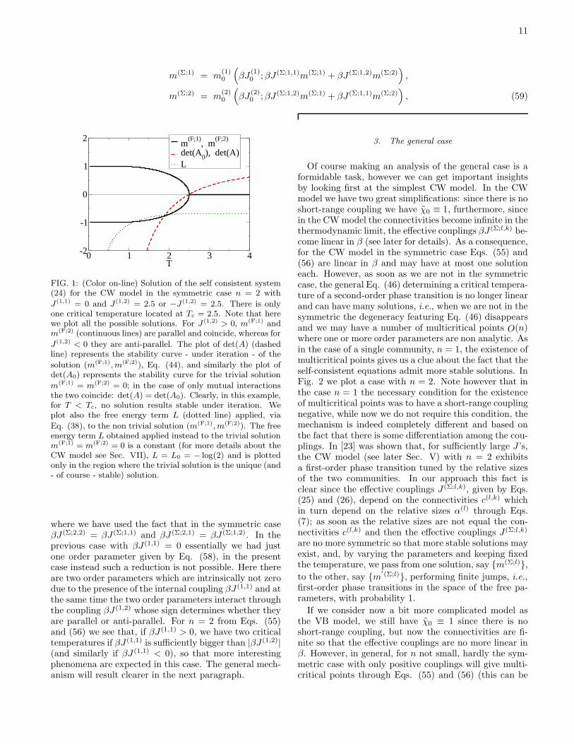
Note that, due to the parity of the function m0 withrespect to its second argument, in Eq. (58) we arefree to substitute J (F;1,2) with |J (F;1,2)|. Solutions asEqs. (57)-(58) are evidently antiferromagnetic and forsufficiently high temperatures are leading against theSG solution. In Fig. 1 we plot a case with J (1,1) = 0and J (1,2) = 1.5. Observe that in this case the solutionm(F) 6= 0 is never stable under iteration. Finally notethat, for J0 < 0 and Σ =F, the two terms appearing inthe lhs of Eqs. (55) and (56) are no more monotonicfunctions of β, so that, for a sufficiently large value of

c(1,2), β(F)c will have multiple solutions. Furthermore, by

observing that all the critical behavior of the system is

encoded in the single susceptibility χ0(βJ(Σ)0 ; 0), we see

that we can use the same analysis performed in the Ref.[20]: when J0 < 0 the non monotonicity reflects also onthe fact that the P-F transition may be of first-order.

Mutual and internal interaction: βJ (1,2), βJ (1,1) 6= 0.Much more interesting is the case in which there are alsointernal long range-couplings. Let us consider for exam-ple the case with two communities. The self-consistentsystem (24) reduces to

11

m(Σ;1) = m(1)0

(

βJ(1)0 ; βJ (Σ;1,1)m(Σ;1) + βJ (Σ;1,2)m(Σ;2)

)

,

m(Σ;2) = m(2)0

(

βJ(2)0 ; βJ (Σ;1,2)m(Σ;1) + βJ (Σ;1,1)m(Σ;2)

)

, (59)

0 1 2 3 4T

-2

-1

0

1

2m

(F;1), m

(F;2)

det(A0), det(A)

L

FIG. 1: (Color on-line) Solution of the self consistent system(24) for the CW model in the symmetric case n = 2 with

J(1,1) = 0 and J(1,2) = 2.5 or −J(1,2) = 2.5. There is onlyone critical temperature located at Tc = 2.5. Note that herewe plot all the possible solutions. For J(1,2) > 0, m(F;1) andm(F;2) (continuous lines) are parallel and coincide, whereas for

J(1,2) < 0 they are anti-parallel. The plot of det(A) (dashedline) represents the stability curve - under iteration - of the

solution (m(F;1), m(F;2)), Eq. (44), and similarly the plot ofdet(A0) represents the stability curve for the trivial solution

m(F;1) = m(F;2) = 0; in the case of only mutual interactionsthe two coincide: det(A) = det(A0). Clearly, in this example,for T < Tc, no solution results stable under iteration. Weplot also the free energy term L (dotted line) applied, via

Eq. (38), to the non trivial solution (m(F;1), m(F;2)). The freeenergy term L obtained applied instead to the trivial solutionm(F;1) = m(F;2) = 0 is a constant (for more details about theCW model see Sec. VII), L = L0 = − log(2) and is plottedonly in the region where the trivial solution is the unique (and- of course - stable) solution.

where we have used the fact that in the symmetric caseβJ (Σ;2,2) = βJ (Σ;1,1) and βJ (Σ;2,1) = βJ (Σ;1,2). In theprevious case with βJ (1,1) = 0 essentially we had justone order parameter given by Eq. (58), in the presentcase instead such a reduction is not possible. Here thereare two order parameters which are intrinsically not zerodue to the presence of the internal coupling βJ (1,1) and atthe same time the two order parameters interact throughthe coupling βJ (1,2) whose sign determines whether theyare parallel or anti-parallel. For n = 2 from Eqs. (55)and (56) we see that, if βJ (1,1) > 0, we have two criticaltemperatures if βJ (1,1) is sufficiently bigger than |βJ (1,2)|(and similarly if βJ (1,1) < 0), so that more interestingphenomena are expected in this case. The general mech-anism will result clearer in the next paragraph.

3. The general case

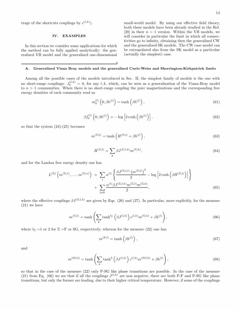
Of course making an analysis of the general case is aformidable task, however we can get important insightsby looking first at the simplest CW model. In the CWmodel we have two great simplifications: since there is noshort-range coupling we have χ0 ≡ 1, furthermore, sincein the CW model the connectivities become infinite in thethermodynamic limit, the effective couplings βJ (Σ;l,k) be-come linear in β (see later for details). As a consequence,for the CW model in the symmetric case Eqs. (55) and(56) are linear in β and may have at most one solutioneach. However, as soon as we are not in the symmetriccase, the general Eq. (46) determining a critical tempera-ture of a second-order phase transition is no longer linearand can have many solutions, i.e., when we are not in thesymmetric the degeneracy featuring Eq. (46) disappearsand we may have a number of multicritical points O(n)where one or more order parameters are non analytic. Asin the case of a single community, n = 1, the existence ofmulticritical points gives us a clue about the fact that theself-consistent equations admit more stable solutions. InFig. 2 we plot a case with n = 2. Note however that inthe case n = 1 the necessary condition for the existenceof multicritical points was to have a short-range couplingnegative, while now we do not require this condition, themechanism is indeed completely different and based onthe fact that there is some differentiation among the cou-plings. In [23] was shown that, for sufficiently large J ’s,the CW model (see later Sec. V) with n = 2 exhibitsa first-order phase transition tuned by the relative sizesof the two communities. In our approach this fact isclear since the effective couplings J (Σ;l,k), given by Eqs.(25) and (26), depend on the connectivities c(l,k) whichin turn depend on the relative sizes α(l) through Eqs.(7); as soon as the relative sizes are not equal the con-nectivities c(l,k) and then the effective couplings J (Σ;l,k)

are no more symmetric so that more stable solutions mayexist, and, by varying the parameters and keeping fixedthe temperature, we pass from one solution, say {m(Σ;l)},

to the other, say {m′(Σ;l)}, performing finite jumps, i.e.,

first-order phase transitions in the space of the free pa-rameters, with probability 1.

If we consider now a bit more complicated model asthe VB model, we still have χ0 ≡ 1 since there is noshort-range coupling, but now the connectivities are fi-nite so that the effective couplings are no more linear inβ. However, in general, for n not small, hardly the sym-metric case with only positive couplings will give multi-critical points through Eqs. (55) and (56) (this can be

12

0 1 2 3 4T

-2

-1

0

1

2m

(F;1), m

(F;2)

det(A0)

det(A)L

FIG. 2: (Color online) Solution of the self consistent sys-tem (24) for the CW model in the symmetric case n = 2

with J(1,1) = 2 and J(1,2) = 2.5, or J(1,2) = −2.5. Notethat here we plot all the possible solutions. For J(1,2) > 0,m(F;1) and m(F;2) (stars) are parallel, whereas for J(1,2) < 0they are anti-parallel. The several branches of det(A) (cir-cles) represent the stability - under iteration - of the several

non trivial solutions (m(F;1), m(F;2)), Eq. (44), and similarlythe plot of det(A0) (dashed line) represents the stability for

the trivial solution m(F;1) = m(F;2) = 0. We plot also theseveral branch’s of the free energy term L (squares) applied,via Eq. (38), to the several solutions. Here Eqs. (55) and(56) give two instability points at the temperatures Tc1 = 2.5and Tc2 = 1.5. In the thermodynamic limit, only Tc1 cor-responds to a true critical temperature, whereas the othercorresponds to a metastable solution. Furthermore we seeanother metastable solution at Tc3 = 1.18 featured as two bro-ken symmetries where (m(F;1), m(F;2)) do not transit around0, but around the values ±0.67.

understood considering large but finite connectivities);to have multicritical points, and, in the space of the pa-rameters, possible first-order phase transitions, it will benecessary to be far from the symmetric case with somedifferentiation among the effective couplings. Finally, weexpect that also in the case of positive short-range cou-plings, this scenario basically holds as well. However,when some of the short-range couplings are negative, thescenario of course changes completely and, as we alreadyknow from the case n = 1, we may have multicriticalpoints and first-order phase transitions also with respectto the temperature and even in the symmetric case, i.e.,without the necessity to have some differentiation amongthe effective couplings.

Recall that, in general, only one solution of the self-consistent equations is leading in the thermodynamiclimit and, furthermore, a phase transition itself may benot leading in this limit, however the stable not leadingsolutions may play an important role when n is high (seenext paragraph).

FIG. 3: (Color online) Solution of the self consistent system(24) for the CW model in the symmetric case n = 3 with

J(1,1) = 3 and J(1,2) = 0.5. Note that here we plot all the pos-sible solutions. We plot also the several branches of the freeenergy term L applied, via Eq. (38), to the several solutions.Here Eqs. (55) and (56) give two instability points at the tem-peratures Tc1 = 4 and Tc2 = 2.5. In the thermodynamic limit,only Tc1 corresponds to a true critical temperature, whereasthe other corresponds to a metastable solution. Furthermorewe see another metastable solution at Tc3 = 1.32 featured astwo broken symmetries where (m(F;1), m(F;2), m(F;3)) do nottransit around 0, but around the values ±0.75.

FIG. 4: (Color online) Solution of the self consistent system(24) for the CW model in the symmetric case n = 3 with

J(1,1) = 3 and J(1,2) = −0.5. Note that here we plot all thepossible solutions. We plot also the several branches of thefree energy term L applied, via Eq. (38), to the several solu-tions. Here Eqs. (55) and (56) give two instability points atthe temperatures Tc1 = 3.5 and Tc2 = 2. In the thermody-namic limit, only Tc1 corresponds to a true critical tempera-ture, whereas the other corresponds to a metastable solution.We see further metastable solutions at Tc3 = 1.6. with mul-tiple broken symmetries where (m(F;1), m(F;2), m(F;3)) do nottransit around 0, but around the values ±0.75 and ±0.80.

4. Behavior for large n

As it was already evident from the previous para-graphs, if there is some differentiation among the com-munities, as n increases the number of solutions of theself-consistent system grows. In Fig. 3 we report a case

13

with n=3. Now, only one of these solutions is leading,nevertheless, the other stable not leading solutions asmetastable states play a more and more important role inthe limit of large n, especially when some of the commu-nities interact through negative couplings. In Fig. 4 wereport a case with n=3 and negative inter-couplings. In-deed, coming back to the symmetric case, from Eqs. (55)and (56) we see that when the number of communitiesis large, n ≫ 1, and the communities are connected, thehighest critical temperature comes only from Eq. (56)and is the solution of the following equation

β(Σ)c J (Σ;1,2)χ0

(

β(Σ)c J

(Σ)0 ; 0

)

≃1

n. (60)

Recalling the definition of J (Σ;1,2) we see that the tran-sition described by Eq. (60) will be either P-F or P-SG.In particular, if J (F;1,2) ≤ 0 the leading transition will beonly P-SG.

In more realistic situations, the system will be far fromthe symmetric case. Typically, different couples of com-munities will be coupled by different couplings of arbi-trary amplitudes and signs, implying therefore frustra-tion. As a consequence, in such a disordered structurethe expected leading transitions will be P-SG. On theother hand such a claim results immediately clear to thereader familiar with spin-glass theory. In fact, if we lookat our self-consistent equations (24)-(25) (or (39)), for ex-ample considering the simplest CW case, apart from thefact that in these equations there is not the Onsager’s re-action term [21], they are formally identical to the TAPequations [22] (recall that βH(Σ;l) is the field seen by l-thcommunity due to the self-magnetization m(Σ;l) and tothe others n − 1 magnetizations). Yet, due to our gen-eral mapping which establishes a strong universality of allthe Poisson small-world models, the general structure ofthese equations roughly speaking is still of the TAP kind- but without the Onsager’s term - even when there areshort-range couplings. Therefore, the typical multi-valleylandscape scenario representing the existence of infinitelymany metastable states (whose number grows exponen-tially with n), possibly also separated by infinitely highfree energy barriers, is expected in the limit of large nwith negative long range couplings [25],[26]. We recallthat at low temperatures, where the glassy scenario hasbeen exactly confirmed in the SK case, the Onsager’sterm disappears [25].

5. Attaching good to bad communities

When in a given community the J ’s are almost absentand the J0’s are negative, or either when the J ’s are neg-ative (at least in average), as we have already learned,there is no way for such a bad community to have anylong-range order, and the only possible state, at low tem-perature, inside this bad community, kept isolated, is theglassy state (provided that its own connectivity be suffi-ciently high). An interesting issue is then to understand

FIG. 5: (Color online) Solutions of the self consistent sys-

tem (24) for the VB model n = 2 with couplings J(1,1) = 1,

J(2,2) = −1 and J(1,2) = −1 or J(1,2) = 1, and connectivitiesc(1,1) = 2, c(2,2) = 2, and c(1,2) = 0 (empty squares for m(F;1)

and continuous line for m(F;2)) or c(1,2) = 1 (stars for m(F;1)

and circles for m(F;2)). We plot also the free energy terms L

(rhombus and filled squares for the two cases).

what happens if we connect the bad community with agood community (i.e., having positive interactions andthen some long-range order) through a certain number(proportional to some added connectivity c(1, 2)) of ran-dom couplings J (1,2). The perhaps surprising answer isthat, not only the bad community gains an order, butalso the already good community improves its order. Wepoint out that this result is not immediately so obvious apriori; the fact that the number of interactions per spinhas been increased by c(1, 2) cannot be used to explainthis effect that takes place for both positive or negativerandom couplings J (1,2). However, a simple argumentbased on the high temperature expansion shows actuallythat this is the case: increasing the average connectivityalways improve the order. In Fig. 5 we report an ex-ample for the VB model and compare the two situationswith and without attaching the two communities.

C. Level of accuracy of the method

As anticipated in the introduction, the level of accu-racy of this effective field theory is the same as that dis-cussed in the Ref. [20]. More precisely, Eqs. (24-40) areexact in the P region, i.e., the region where any of the2n order parameters is zero; whereas in the other regionsprovide an effective approximation whose level of accu-racy depends on the details of the model. In particular,in the absence of frustration the method becomes exactat any temperature in two important limits: in the limitc(l,k) → 0+, l, k = 1, . . . , n, in the case of second-orderphase transitions, due to a simple continuity argument;and in the limit c(l,k) → ∞, l, k = 1, . . . , n, due to thefact that in this case the system becomes a suitable fullyconnected model exactly described by the self-consistentequations (24) (of course, when c(l,k) → ∞, to have afinite critical temperature one has to renormalize the av-

14

erage of the shortcuts couplings by c(l,k)).

IV. EXAMPLES

In this section we consider some applications for whichthe method can be fully applied analytically: the gen-eralized VB model and the generalized one-dimensional

small-world model. By using our effective field theory,both these models have been already studied in the Ref.[20] in their n = 1 version. Within the VB models, wewill consider in particular the limit in which all connec-tivities go to infinity, obtaining then the generalized CWand the generalized SK models. The CW case model canbe extrapolated also from the SK model as a particular(actually the simplest) case.

A. Generalized Viana Bray models and the generalized Curie-Weiss and Sherrington-Kirkpatrick limits

Among all the possible cases of the models introduced in Sec. II, the simplest family of models is the one with

no short-range couplings: J(l,k)0 = 0, for any l, k, which, can be seen as a generalization of the Viana-Bray model

to n > 1 communities. When there is no short-range coupling the pure magnetizations and the corresponding freeenergy densities of each community read as

m(l)0

(

0; βh(l))

= tanh(

βh(l))

, (61)

βf(l)0

(

0; βh(l))

= − log[

2 cosh(

βh(l))]

, (62)

so that the system (24)-(25) becomes

m(Σ;l) = tanh(

H(Σ;l) + βh(l))

, (63)

H(Σ;l) =∑

k

βJ (Σ;l,k)m(Σ;k), (64)

and for the Landau free energy density one has

L(Σ)(

m(Σ;1), . . . , m(Σ;n))

=∑

l

α(l)

{

βJ (Σ;l,l)(

m(Σ;l))2

2− log

[

2 cosh(

βH(Σ;l))]

}

+∑

l 6=k


2, (65)

where the effective couplings βJ (Σ;l,k) are given by Eqs. (26) and (27). In particular, more explicitly, for the measure(21) we have

m(Σ;l) = tanh

(

∑

k

tanhlΣ(

βJ (l,k))

c(l,k)m(Σ;k) + βh(l)

)

, (66)

where lΣ =1 or 2 for Σ =F or SG, respectively; whereas for the measure (22) one has

m(F;l) = tanh(

βh(l))

, (67)

and

m(SG;l) = tanh

(

∑

k

tanh2(

βJ (l,k))

c(l,k)m(SG;k) + βh(l)

)

, (68)

so that in the case of the measure (22) only P-SG like phase transitions are possible. In the case of the measure(21) from Eq. (66) we see that if all the couplings J (l,k) are non negative, there are both P-F and P-SG like phasetransitions, but only the former are leading, due to their higher critical temperature. However, if some of the couplings

15

J (l,k) is negative, in general there can be P-F like phase transitions with competitions between ferromagnetism andantiferromagnetism and, furthermore, for some range of the parameters there can be also a competition with a P-SGlike phase transition that in turn gives rise to n stable spin glass like order parameters m(SG;l).

The inverse critical temperature β(Σ)c of any possible second-order phase transition can be obtained by developing

the self-consistent system (63)-(64) for small m(Σ;l) and h(l) = 0. As we have seen in Sec. IIIB, this amounts to findthe solutions of the equation det(A(Σ;l,k)) = 0 which in the present case becomes

A(Σ;l,k) = δl,k − β(Σ)c J (Σ;l,k), (69)

where we have used χ(l,l)0 (0; βh(l)) = 1−tanh2(βh(l)). The non linear equation detA(Σ) = 0 provides the exact critical

temperature of any second-order phase transition of this generalized Viana-Bray model. For example, for n = 2 thisequation becomes:

(

1 − βJ (Σ;1,1))(

1 − βJ (Σ;2,2))

− βJ (Σ;1,2)βJ (Σ;2,1) = 0, (70)

which, for the measure (21), amounts to

1 −(

c(1,1) tanhlΣ(

βJ (1,1))

+ c(2,2) tanhlΣ(

βJ (2,2)))

+ c(1,1)c(2,2) tanhlΣ(

βJ (1,1))

tanhlΣ(

βJ (2,2))

−α

1 − α

(

c(1,2) tanhlΣ(

βJ (1,2)))2

= 0, (71)

where we have used αdef= α(1), α(2) = 1 − α and Eq. (7). As we have seen in Sec. IIIB, the symmetric case can be

explicitly worked out also for n generic. From Eq. (55) and (56) we have

β(Σ)c J (Σ;1,2) − β(Σ)

c J (Σ;1,1) = −1, (72)

and

(n − 1)β(Σ)c J (Σ;1,2) + β(Σ)

c J (Σ;1,1) = 1. (73)

1. The CW and the SK limits

Let us now consider the Curie-Weiss limit with Σ=F. Given the set of the relative sizes {α(l)}, we can recover theCurie-Weiss limit by choosing the connectivities c(l,k) to be equal to their maximum value which, according to Eq.(9), is given by

c(l,k) = α(k)N. (74)

With this choice the probabilities p(l,k) become

p(c(l,k)ij ) = δ

c(l,k)ij

,1, (75)

so that, by choosing the measure (21) with the J (l,k) renormalized by N

dµ(l,k)

dJ(l,k)i,j

= δ

(

J(l,k)i,j −

J (l,k)

N

)

, (76)

the CW limit is recovered (of course anything can be rephrased in terms of limits by simply substituting the lhsof Eqs. (74)-(76) the equalities with arrows-limits for N → ∞). By using Eqs. (74)-(76) for large N , the system(63)-(64) and the Landau free energy (65), for Σ =F, become

m(F;l) = tanh(

H(F;l) + βh(l))

, (77)

H(F;l) =∑

k

βJ (l,k)α(k)m(F;k), (78)

16

L(F)(

m(Σ;1), . . . , m(Σ;n))

=∑

l

α(l)

{

α(l)βJ (l,l)(

m(Σ;l))2

2− log

[

2 cosh(

βH(F;l))]

}

+∑

l 6=k

α(l)m(Σ;l)βJ (l,k)α(k)m(Σ;k)

2, (79)

which generalizes the result found in [23] for n = 2 to general n. Notice that, as we explain in Sec. IIIC, Eqs. (77)-(79)are exact at any temperature.

Analogously, if we assume again (74) and choose the measure (23), the SK limit is recovered, and for large N thesystem (63)-(64) and the Landau free energy (65), become

m(Σ;l) = tanh(

H(Σ;l) + βh(l))

, (80)

H(Σ;l) =∑

k

βJ (Σ;l,k)m(Σ;k), (81)

L(Σ)(

m(1), . . . , m(n))

=∑

l

α(l)

{

βJ (Σ;l,l)(

m(l))2

2− log

[

2 cosh(

βH(Σ;l))]

}

+∑

l 6=k

α(l)m(l)βJ (Σ;l,k)m(k)

2, (82)

where for large N the effective couplings are given by (according to the measure (23) J (l,k) and J (l,k) are respectivelythe average and the variance of the couplings)

βJ (F;l,k) = α(k)βJ (l,k), (83)

and

βJ (SG;l,k) = α(k)(

βJ (l,k))2

. (84)

Eqs. (80)-(84) generalize the result found in [38] and [39], valid for only a uniform mutual coupling, to general mutualcouplings as well as internal couplings. Notice that, as explained in Sec. IIIC, in unfrustrated systems, i.e., forJ (l,k) ≫ J (l,k), Eqs. (80)-(84) are exact at any temperature.

B. One-dimensional small-world model for n communities

In the Ref. [20] we have studied in detail the one-dimensional small-world model for n = 1 emphasizing the existenceof first-order phase transitions for negative short-range couplings. Here we generalize this result to n communities.

For the free energy, the magnetization and the susceptibility of the pure model of the l-th community we have

− βf(l)0

(

βJ(l)0 , βh(l)

)

= log

{

eβJ(l)0 cosh(βh(l)) +

[

e2βJ(l)0 sinh2(βh(l)) + e−2βJ

(l)0

]12

}

, (85)

m(l)0 (βJ

(l)0 , βh(l)) =

eβJ(l)0 sinh(βh(l))

[


(l)0

]12

, (86)

χ(l)0 (βJ

(l)0 , βh(l)) =

e−βJ(l)0 cosh(βh(l))

[


(l)0

]32

. (87)

17

Therefore, the self-consistent system (24)-(25) for the n communities becomes

m(Σ;l) =eβJ

(Σ;l)0 sinh(βH(Σ;l) + βh(l))

[

e2βJ(Σ;l)0 sinh2(βH(Σ;l) + βh(l)) + e−2βJ

(Σ;l)0

]12

, (88)

H(Σ;l) =∑

k

βJ (Σ;l,k)m(Σ;k). (89)

For the symmetric case, from Eqs. (55) and (56) we obtain that the n communities undergo a second order transitionat a critical temperature given either by

(

β(Σ)c J (Σ;1,2) − β(Σ)

c J (Σ;1,1))

e2β(Σ)c J

(Σ)0 = −1, (90)

or by

(

(n − 1)β(Σ)c J (Σ;1,2) + β(Σ)

c J (Σ;1,1))

e2β(Σ)c J

(Σ)0 = 1, (91)

where we have used, from Eq. (87), χ0(βJ0; 0) = exp(2βJ0).

V. APPLICATION TO PERCOLATION

A. An effective percolation theory

The key point of our approach is a mapping that mapsthe original random model onto a non random one. Inturn this mapping is based on the so called high temper-ature expansion of the free energy which, in a suitableregion of the phase diagram that we call P, converges.The boundary of the P region is established by the criti-cal condition (46). Within a physical picture, in Sec. IIIBwe were mainly concerned with the critical temperature.However, it should be clear that the criticality conditioncan be expressed in terms of any of the parameters enter-ing Eq. (46). In particular, for Σ =F and non negative

couplings βJ (F;l,k) ≥ 0 and J(l,k)0 ≥ 0, it is of remarkable

interest to study the criticality condition in the limit ofzero temperature as well as the behavior of the magne-tizations m(F;l) near this boundary. Recalling the defini-

tion of the set of bonds Γ(l)0 and Γ

(l,k)0 (we find it conve-

nient to define also Γ(l,l)0

def= Γ

(l)0 and Γ0

def= ∪l′,k′ Γ

(l′,k′)0 ),

and exploiting βJ (F;l,k) → c(l,k), for β → ∞, it is easy tosee that in the limit β → ∞ the criticality condition (46)amounts to

det (1− E0 · c) = 0,{

c(l,k) ≥ 0}

(92)

where c is the matrix of the added connectivities c(l,k),and the n × n matrix E0 = E0(Γ0) is given by

E(l,l)0 = lim

β→+∞χ

(l,l)0

(

βJ(l)0 ; 0

)

, (93)

if J(l,k)0 = 0 for any l 6= k, whereas in the general case

E(l,k)0 = lim

β→+∞χ

(l,k)0

({

βJ(l′,k′)0

}

; 0)

. (94)

In the above equations it is understood that we areconsidering only graphs Γ0 such that the pure model hasno finite critical temperature, i.e., it is only βc0 = ∞.In fact, if this is not the case, as occurs for instance ifΓ0 is the d0 dimensional lattice with d0 ≥ 2, the P re-gion is shrunk to the single trivial point c(l,k) ≡ 0 and

we can take effectively E(l,k)0 = +∞ (this issue will be-

come clearer soon, see also Appendix B). More precisely,if βc0 < ∞ or even if βc0 = 0, as occurs in scale free net-works with a power law exponent γ ≤ 3 [41], one shoulduse Eqs. (93) and (94) keeping N finite.

A solution {c(l,k)c } of Eq. (92) represents the exact

critical values (or percolation threshold) of the set of theconnectivities over which a giant connected componentexists. Note that Eq. (92) in general is a non linear equa-tion in the n2 unknown connectivities {c(l, k)}. There-fore, in general, for n ≥ 2, there are infinite solutions as

∞n2

. This degeneracy of Eq. (92) reflects the fact thatgiven n communities, we can realize a connected clus-ter by placing the bonds in many ways, as e.g., eitherover a single community, or between 2 or more commu-nities. However, this high degeneracy can be partiallyremoved, and Eq. (92) simplified, when there are specialsymmetries among the connectivities. In particular, the

symmetric case (J(l,k)0 = 0 for l 6= k, c(l,l) = c(1,1) for any

l and c(l,k) = c(1,2) for any l 6= k) constitutes a simplifiedsituation in which the determinant in Eq. (92) can beexplicitly calculated as in (54). In the symmetric case,

with the further simplification J(l,l)0 = J0, Eq. (92) gives

the following solution splitted into two branches

(

c(1,2)c − c(1,1)

c

)

limβ→+∞

χ0 (βJ0; 0) = −1, (95)

18

and(

(n − 1) c(1,2)c + c(1,1)

c

)

limβ→+∞

χ0 (βJ0; 0) = 1. (96)

Notice that the solution with c(1,2)c = c

(1,1)c = 0 may

occur only for a divergent susceptibility. In particular,when there are no short-range connections, i.e. J0 = 0,we have χ0 (βJ0 = 0; 0) = 1 so that Eqs. (95) and (96)give the surfaces

c(1,2)c = c(1,1)

c − 1, c(1,1)c ≥ 1 (97)

and, for n ≥ 2

c(1,2)c =

1 − c(1,1)c

n − 1, c(1,1)

c < 1, (98)

where we have taken into account that the connectivitiesare defined non negative.

Similarly, one can study the relative size {s(l)} of thegiant connected component by studying, for Σ = F andfor non negative short-range couplings, the self-consistentsystem (24)-(25) in the limit β → +∞, where, again, weexploit βJ (F;l,k) → c(l,k), for β → ∞. In the case of

J(l,k)0 = 0 for l 6= k, we get

s(l) = s(l)0

(

∑

k

c(l,k)s(k)

)

, (99)

where

s(l)0

(

∑

k

c(l,k)s(k)

)

def= m

(l)0

(

limβ→∞

βJ(l)0 ;∑

k

c(l,k)s(k)

)

.(100)

whereas in the general case, from Eq. (39) we get

s(l) = s(l)0

({

∑

k

c(l′,k)s(k)

})

, (101)

where now

s(l)0

({

∑

k

c(l′,k)s(k)

})

def=

m(l)0

(

{

limβ→∞

βJ(l′,k′)0

}

;

{

∑

k

c(l′,k)s(k)

})

.(102)

Note that in the above equations c(l,k)s(k) represents afraction of the connectivity c(l,k), being 0 ≤ s(k) ≤ 1.Note also that, by virtue of some non zero short-range

couplings J(l,k)0 with l 6= k, and J

(l,h)0 with l 6= h and h 6=

k, the relative sizes of the giant connected component

of the two communities l and h, s(l)0 and s

(h)0 (the pure

model), influence each other also if there is no short-cut

among the two communities, J(l,h)0 = 0 .

When we are far from the symmetric case, the self-consistent systems (99) or (101) in general may admitmany stable solutions, i.e., solutions {s(l)} such that thelhs of Eq. (92) is positive. The relative probabilitiesamong these solutions can be calculated as exp(−L) fromthe expressions (36) or (40) for the Landau free energy

density in the limit β → +∞. In the case of J(l,k)0 = 0

for l 6= k, up to a constant term, we get

L(

s(1), . . . , s(n))

=∑

l

α(l)L(l)0

(

∑

k

c(l,k)s(k)

)

+∑

l,k

α(l)c(l,k)s(l)s(k)

2, (103)

where

L(l)0

(

∑

k

c(l,k)s(k)

)

def= lim

β→+∞

βf

(l)0

(

βJ(l)0 ;∑

k

c(l,k)s(k)

)

− limN→∞

1

Nα(l)

∑

(i,j)∈Γ(l)0

log[

cosh(

βJ(l)0;(i,j)

)]

. (104)

Notice that in defining L(l)0 in Eq. (104) we have subtracted the trivial and divergent terms log

[

cosh(

βJ(l)0;(i,j)

)]

which, being constants, do not modify the relative probabilities. Similarly, in the general case we have

L(

s(1), . . . , s(n))

=∑

l,k

α(l)c(l,k)s(l)s(k)

2+ L0

({

∑

k

c(l′,k)s(k)

})

(105)

19

where,

L0

({

∑

k

c(l,k)s(k)

})

def= lim

β→+∞

[

βf0

(

{

βJ(l′)0

}

;

{

∑

k

c(l′,k)s(k)

})

− limN→∞

1

N

∑

(i,j)∈∪l,kΓ(l,k)0

log[

cosh(

βJ(l,k)0;(i,j)

)]

, (106)

Of course, among all the stable solutions of the self-consistent system (99) or (101) the leading solution willbe given by looking at the absolute minimum of L. It isinteresting to observe that the term −L0, as a functionof a generic c, is nothing else than the logarithm of adegenerate partition function. We report its expressionin Appendix A.

The self-consistent systems (99) or (101) are exact inthe P region, that is for all values of the vector {c(l,k)}

below the leading (i.e., minimal) critical surface {c(l,k)c },

however, again, the limits {c(l,k) → 0+} and {c(l,k) → ∞}

will be exact independently of the critical surface {c(l,k)c }.

Under these limitations, our result for percolation con-stitutes a generalization to generic n of the approach de-veloped in [42, 43] which was built for n = 1.

We end this paragraph by giving the meaning of theabove expressions directly in terms of graph theory. Con-

cerning s(l)0 and s(l) they clearly represent the fraction of

the sites belonging to the giant connected component (ifany) in the l-th community. More precisely, in the mostgeneral case we have

s(l)0 ({0}) = lim

N→∞

∑

i∈L(l)0

n(l)i

Nα(l), (107)

where n(l)i = 0, 1 if respectively the vertex i ∈ L

(l)0

belongs or not to a connected cluster with the prop-erty to be giant (if any) and having bonds belonging

to the given initial set of bonds ∪l′,k′Γ(l′,k′)0 . Similarly,

s(l)0

({

c(l′,k′)})

and s(l) have analogous expressions as

Eq. (107) and represent the fraction of sites of the l-thcommunity belonging to a connected component with theproperty to be giant (if any) and having bonds belonging

to the union of the initial set of bonds ∪l′,k′Γ(l′,k′)0 and the

other bonds randomly spread according to the set of the

given added connectivities{

c(l′,k′)}

. Note that, by def-

inition, the only difference between s(l)0

({

c(l′,k′)})

and

s(l) is that in the latter case we have to average over thedifferent realizations of the graph with the distribution(20), while for the former, as for the case of thermody-namics, only the average values of the connectivities aretaken into account. Concerning instead the meaning of

the matrix E(l,k)0 we have (see Appendix B for details)

E(l,l)0 = lim

N→∞

∑

i∈L(l)0

N(l)i

Nα(l), (108)

where N(l)i is defined as the number of vertices belong-

ing to the l-th community (including i itself) which are

reachable from the site i ∈ L(l)0 by at least one path of

connected vertices. We recover hence immediately that,e.g., for the case of no short-range coupling J0 ≡ 0,

we have N(l)i ≡ 1 and then limβ→∞ χ

(l,l)0

(

βJ(l)0 ; 0

)

=

1. Similarly for the case in which (L(l)0 , Γ

(l)0 ) is the

one dimensional chain we have Ni ≡ N and then

limβ→∞ χ(l,l)0

(

βJ(l)0 ; 0

)

= +∞. Finally, for l 6= k, by

defining N(l,k)i , with i belonging to the l-th community,

as the number of vertices belonging to the k-th commu-nity reachable by at least one chain of bonds from thevertex i, we have the following expression analogous toEq. (108)

E(l,k)0 = lim

N→∞

∑

i∈L(l)0

N(l,k)i

Nα(l). (109)

Note that now it can be also N(l,k)i = 0, while, by def-

inition N(l,l)i ≥ 1. Furthermore it holds the following

balance

α(l)E(l,k)0 = α(k)E

(k,l)0 . (110)

By using the obvious generalization of Eqs. (108) and

(109), we can define a quantity similar to E(l,k)0 , E(l,k),

to include the presence of added bonds randomly spreadaccording to the measure (18) with average connectivities{c(l,k)}, and from Eq. (42) in the zero temperature limitwe get (in matrix form):

E = (1− E0 · c)−1 · E0. (111)

Eq. (111) tells us how E changes as we vary the {c(l,k)},being an exact equation as the {c(l,k)} belong to the Pregion.

20

B. Percolation threshold vs fractal dimension

Let us come back, for the moment being, to the casen = 1 and let us consider the simplest model: the VBmodel (see Sec. IV). In this case Eq. (92) gives imme-diately the critical value cc = 1, which is the very longknown value of the percolation threshold for the Pois-sonian graph [44]. On the other hand, if we have a d0-dimensional underlying pure graph (L0, Γ0) and d0 ≥ 1,whatever (L0, Γ0) may be complicated, we always haveE0 = O(N) or, equivalently, in the limit β → +∞ for thesusceptibility of the pure system we have χ0 → +∞, sothat for the critical value we get always the obvious resultcc = 0. To have a critical value cc strictly in the range(0, 1) it is necessary that the underlying graph (L0, Γ0)has a dimension lower than 1: d0 < 1. For exampleone can consider the case in which the graph (L0, Γ0) ismade up of finite units as dimers, triangles, etc.. For in-stance, in the Ref. [20] we have studied the case of dimersfor which we have χ0(βJ0; 0) = (exp(βJ0))/ cosh(βJ0).Therefore in the limit β → +∞ we get χ0 → 2 or, equiv-alently, E0 = 2, which inserted in Eq. (92) gives theresult cc = 1/2. This result is still trivial because in thisexample we have d0 = 0. However, there is no limitationin the choice of the graph (L0, Γ0); all the theory holdsfor any arbitrary graph (L0, Γ0) which in particular canbe some quenched graph obtained by removing randomlya sufficient number of bonds from another initial regulargraph so that the final graph (L0, Γ0) will have a nontrivial value of E0 corresponding to a fractal dimensiond0 ∈ (0, 1) [45]. Similarly, as already stressed in Sec. II

for generic n, for any l and any k, the symbol J(l,k)0 is

actually a short notation to indicate all the short-rangecouplings connecting the l-th and the k-th community:

J(l,k)0 = {J

(l,k)0;(i,j)}, i ∈ L

(l)0 , i ∈ L

(k)0 ; so that the graphs

{(L(l,k)0 , Γ

(l,k)0 )} are completely arbitrary with a non triv-

ial percolation threshold surface coming from Eq. (92).Typically, scale free networks, as the Internet, own frac-tal properties [46], however in this case d0 → ∞ in thethermodynamic limit, so that the percolation thresholdin these networks becomes zero.

C. When two given communities do communicate

The answer to the fundamental question “when andhow much two given communities communicate” is en-

coded in χ(l,k)0 and χ(l,k) which at T = 0 means

E(l,k)0 and E(l,k), respectively. Given the arbitrary pure

graph (L0, Γ0), and some community structure assign-ment which splits the set of bonds Γ0 in n(n− 1)/2 sets,

Γ0 = ∪l,kΓ(l,k)0 , at T = 0, in the pure graph the communi-

ties l and k communicate if and only if E(l,k)0 6= 0. We can

understand the communication process as follows. If sud-denly, at a given initial time, appears an external mag-netic field h(k), which acts uniformly only on the spins

of the k-th community, these spins are forced to changeand, as a consequence, all the spins of the other com-munities will have to suitably change in order to reachthe new equilibrium state. At finite temperature the newequilibrium state will be reached after a relaxation timeτ which grows with the size of the system. However inthe limit T → 0 there is no thermal dissipation and thespin changes take place instantaneously. Therefore, if theexternal field βh(k) changes with time with a constant ve-locity, say v(k), from the relation δm(l) ≃ χ(l,k)δ(βh(k))extrapolated at T = 0, we see that the characteristic time

t(l,k)0 to transmit a unit of information from the commu-

nity k to the community l in the pure model will growas

v(k)t(l,k)0 =

(

E(l,k)0

)−1

. (112)

Similarly, in the random model having a matrix of addedconnectivities c, the communities l and k communicatewith a characteristic time given by

v(k)t(l,k) =(

E(l,k))−1

. (113)

From Eq. (111) we see that in the pure model, if

E(l,k)0 = 0, the two communities l and k cannot commu-

nicate (t(l,k)0 → ∞), but for any arbitrary small c(l,k) > 0

they communicate and the characteristic time decayswith c approximately as (recall that for any l is always

E(l,l)0 ≥ 1)

v(k)t(l,k) ≃(

E(l,k)0 + E

(l,l)0 E

(k,k)0 c(l,k)

)−1

. (114)

Similar relations hold also at finite T provided the ve-locity of the signal, v(k), be sufficiently small so that

τ ≪ t(l,k)0 or τ ≪ t(l,k).

In general if, due to the birth of some giant con-

nected component in the pure model, one has E(l,k)0 → ∞

in the thermodynamic limit, correspondingly we have

t(l,k)0 → 0, and then also t(l,k) → 0; i.e., the communities

communicate instantaneously (they percolate). However,

in the random model, even if E(l,k)0 is finite, provided non

zero, when c approaches the percolation threshold surfacecc, given by Eq. (92), then we have t(l,k) → 0. Of courseintermediate situations will give rise to finite values oft(l,k). In Eq. (111) the matrix E0 represents an inputdata. In general, it can be sampled efficiently by simplesimulated annealing procedures by using Eq. (94), sincethe problem is mapped to an unfrustrated Ising model

(βJ(l,k)0 ≥ 0).

We recall that there is no limitation in the choice of thegraph (L0, Γ0) and that the statistical mechanical frame-work provided through Eqs. (93,94) and Eqs. (107)-(110)is complete and exact. Note in particular that two givencommunities l and k, when immersed in a context of morecommunities, can communicate even if there is no bond

between them, Γ(l,k)0 = {0}, due to the presence of one

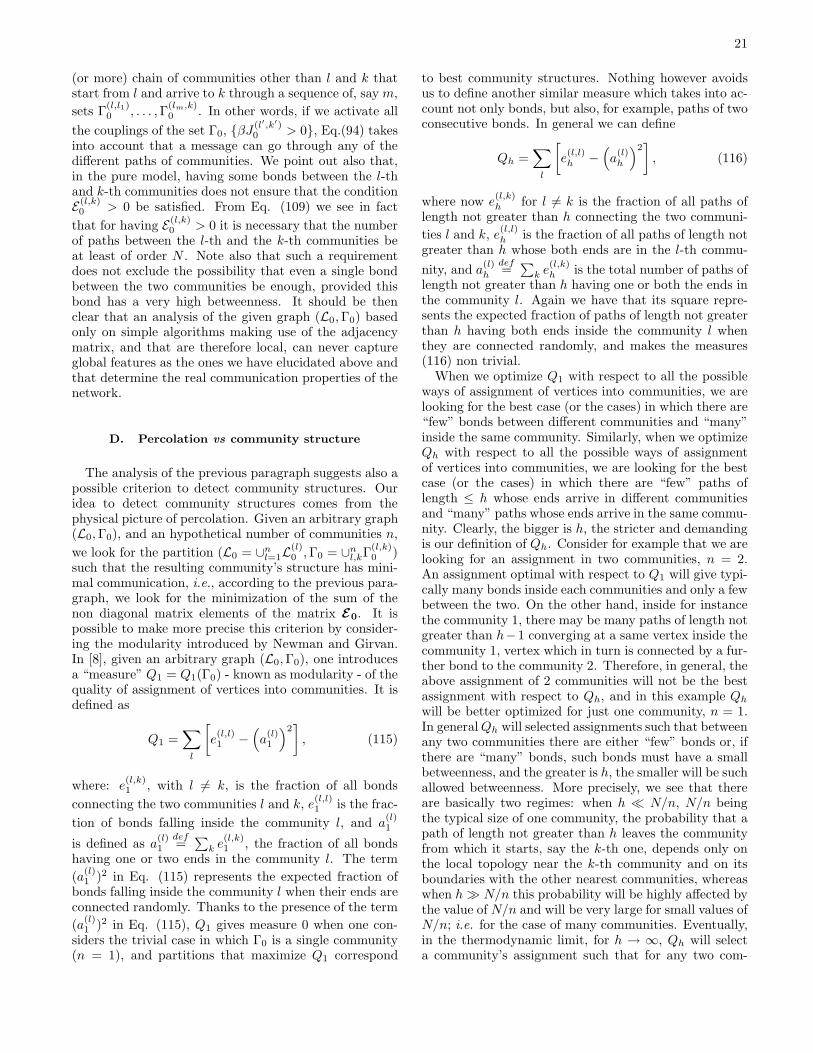
21

(or more) chain of communities other than l and k thatstart from l and arrive to k through a sequence of, say m,

sets Γ(l,l1)0 , . . . , Γ

(lm,k)0 . In other words, if we activate all

the couplings of the set Γ0, {βJ(l′,k′)0 > 0}, Eq.(94) takes

into account that a message can go through any of thedifferent paths of communities. We point out also that,in the pure model, having some bonds between the l-thand k-th communities does not ensure that the conditionE

(l,k)0 > 0 be satisfied. From Eq. (109) we see in fact

that for having E(l,k)0 > 0 it is necessary that the number

of paths between the l-th and the k-th communities beat least of order N . Note also that such a requirementdoes not exclude the possibility that even a single bondbetween the two communities be enough, provided thisbond has a very high betweenness. It should be thenclear that an analysis of the given graph (L0, Γ0) basedonly on simple algorithms making use of the adjacencymatrix, and that are therefore local, can never captureglobal features as the ones we have elucidated above andthat determine the real communication properties of thenetwork.

D. Percolation vs community structure

The analysis of the previous paragraph suggests also apossible criterion to detect community structures. Ouridea to detect community structures comes from thephysical picture of percolation. Given an arbitrary graph(L0, Γ0), and an hypothetical number of communities n,

we look for the partition (L0 = ∪nl=1L

(l)0 , Γ0 = ∪n

l,kΓ(l,k)0 )

such that the resulting community’s structure has mini-mal communication, i.e., according to the previous para-graph, we look for the minimization of the sum of thenon diagonal matrix elements of the matrix E0. It ispossible to make more precise this criterion by consider-ing the modularity introduced by Newman and Girvan.In [8], given an arbitrary graph (L0, Γ0), one introducesa “measure” Q1 = Q1(Γ0) - known as modularity - of thequality of assignment of vertices into communities. It isdefined as

Q1 =∑

l

[

e(l,l)1 −

(

a(l)1

)2]

, (115)

where: e(l,k)1 , with l 6= k, is the fraction of all bonds

connecting the two communities l and k, e(l,l)1 is the frac-

tion of bonds falling inside the community l, and a(l)1

is defined as a(l)1

def=∑

k e(l,k)1 , the fraction of all bonds

having one or two ends in the community l. The term

(a(l)1 )2 in Eq. (115) represents the expected fraction of

bonds falling inside the community l when their ends areconnected randomly. Thanks to the presence of the term

(a(l)1 )2 in Eq. (115), Q1 gives measure 0 when one con-

siders the trivial case in which Γ0 is a single community(n = 1), and partitions that maximize Q1 correspond

to best community structures. Nothing however avoidsus to define another similar measure which takes into ac-count not only bonds, but also, for example, paths of twoconsecutive bonds. In general we can define

Qh =∑

l

[

e(l,l)h −

(

a(l)h

)2]

, (116)

where now e(l,k)h for l 6= k is the fraction of all paths of

length not greater than h connecting the two communi-

ties l and k, e(l,l)h is the fraction of all paths of length not

greater than h whose both ends are in the l-th commu-

nity, and a(l)h

def=∑

k e(l,k)h is the total number of paths of

length not greater than h having one or both the ends inthe community l. Again we have that its square repre-sents the expected fraction of paths of length not greaterthan h having both ends inside the community l whenthey are connected randomly, and makes the measures(116) non trivial.

When we optimize Q1 with respect to all the possibleways of assignment of vertices into communities, we arelooking for the best case (or the cases) in which there are“few” bonds between different communities and “many”inside the same community. Similarly, when we optimizeQh with respect to all the possible ways of assignmentof vertices into communities, we are looking for the bestcase (or the cases) in which there are “few” paths oflength ≤ h whose ends arrive in different communitiesand “many” paths whose ends arrive in the same commu-nity. Clearly, the bigger is h, the stricter and demandingis our definition of Qh. Consider for example that we arelooking for an assignment in two communities, n = 2.An assignment optimal with respect to Q1 will give typi-cally many bonds inside each communities and only a fewbetween the two. On the other hand, inside for instancethe community 1, there may be many paths of length notgreater than h−1 converging at a same vertex inside thecommunity 1, vertex which in turn is connected by a fur-ther bond to the community 2. Therefore, in general, theabove assignment of 2 communities will not be the bestassignment with respect to Qh, and in this example Qh

will be better optimized for just one community, n = 1.In general Qh will selected assignments such that betweenany two communities there are either “few” bonds or, ifthere are “many” bonds, such bonds must have a smallbetweenness, and the greater is h, the smaller will be suchallowed betweenness. More precisely, we see that thereare basically two regimes: when h ≪ N/n, N/n beingthe typical size of one community, the probability that apath of length not greater than h leaves the communityfrom which it starts, say the k-th one, depends only onthe local topology near the k-th community and on itsboundaries with the other nearest communities, whereaswhen h ≫ N/n this probability will be highly affected bythe value of N/n and will be very large for small values ofN/n; i.e. for the case of many communities. Eventually,in the thermodynamic limit, for h → ∞, Qh will selecta community’s assignment such that for any two com-

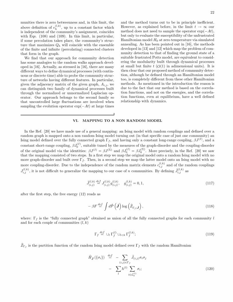
22

munities there is zero betweenness and, in this limit, the

above definition of e(l,k)h , up to a constant factor which

is independent of the community’s assignment, coincideswith Eqs. (108) and (109). In this limit, in particular,if some percolation takes place, the community’s struc-ture that maximizes Qh will coincide with the ensembleof the finite and infinite (percolating) connected clustersthat form in the graph.

We find that our approach for community detectionhas some analogies to the random walks approach devel-oped in [16]. Actually, as stressed in [16], there are manydifferent ways to define dynamical processes (with contin-uous or discrete time) able to probe the community struc-ture of networks having different features. In particular,given the adjacency matrix of the given graph, Ai,j , wecan distinguish two family of dynamical processes builtthrough the normalized or unnormalized Laplacian op-erator. Our approach belongs to the second family sothat uncontrolled large fluctuations are involved whensampling the evolution operator exp(−At) at large times

and the method turns out to be in principle inefficient.However, as explained before, in the limit t → ∞ ourmethod does not need to sample the operator exp(−At),but only to evaluate the susceptibility of the unfrustratedHamiltonian model H0 at zero temperature via simulatedannealing. As has been pointed out in [16], the methodsdeveloped in [13] and [12] which map the problem of com-munity detection to that of finding the ground state of asuitable frustrated Potts model, are equivalent to consid-ering the modularity built through dynamical processesat small but finite t (O(1) in adimensional units). It isthen clear that our proposed method of community detec-tion, although be defined through an Hamiltonian modeltoo, is completely different from these other Hamiltonianmethods. As mentioned in the introduction the reason isdue to the fact that our method is based on the correla-tion functions, and not on the energies, and the correla-tion functions, even at equilibrium, have a well definedrelationship with dynamics.

VI. MAPPING TO A NON RANDOM MODEL

In the Ref. [20] we have made use of a general mapping: an Ising model with random couplings and defined over arandom graph is mapped onto a non random Ising model turning out (in that specific case of just one community) anIsing model defined over the fully connected graph Γf , and having only a constant long-range coupling, βJ (I), and a

constant short-range coupling, βJ(I)0 , suitable tuned by the measures of the graph-disorder and the coupling-disorder

of the original model via the identities: βJ (I) = βJ (Σ) and βJ(I)0 = βJ

(Σ)0 . More precisely, in the Ref. [20] we saw

that the mapping consisted of two steps. In a first step we map the original model onto a random Ising model with nomore graph-disorder and built over Γf . Then, in a second step we map the latter model onto an Ising model with no

more coupling-disorder. Due to the independence of the random matrix elements c(l,k)i,j and of the random couplings

J(l,k)i,j , it is not difficult to generalize the mapping to our case of n communities. By defining J

(l,k)i,j as

J(l,k)(i,j)

def= J

(l,k)(i,j) g

(l,k)(i,j) , g

(l,k)(i,j) = 0, 1, (117)

after the first step, the free energy (12) reads as

− βFdef=

∫

dP(

J)

log(

ZΓf ;J

)

, (118)

where: Γf is the “fully connected graph” obtained as union of all the fully connected graphs for each community land for each couple of communities (l, k)

Γfdef= ∪l Γ

(l)f ∪l<k Γ

(l,k)f ; (119)

ZΓfis the partition function of the random Ising model defined over Γf with the random Hamiltonian

HJ

({σi})def= −

∑

(i,j)∈Γf

J(i,j)σiσj

−∑

l

h(l)∑

i∈L(l)0

σi; (120)

23

and the J ’s are distributed according to the measure dP(

J)

given by

dP(

J)

def=

∏

l

∏

i<j, i,j∈L(l)0

dµ(l,l)(

J(l,l)i,j

)

,

×∏

l<k

∏

i∈L(l)0 ,j∈L

(k)0

dµ(l,k)(

J(l,k)i,j

)

, (121)

with

dµ(l,k)(i,j)

(

J(l,k)(i,j)

)

=

dµ(l,k)0

(

J(l,k)(i,j)

)

, (i, j) ∈ Γ(l,k)0 ,

dµ(l,k)(

J(l,k)(i,j)

)

p(l,k)(

g(l,k)(i,j)

)

, (i, j) ∈ Γ(l,k)f \Γ

(l,k)0 ,

(122)

dµ(l,k)(·) and p(l,k)(·) being the coupling- and bond- (Eq. (18)) measures of the original model introduced in Sec.

II, and dµ(l,k)0 (J0)/dJ0 the delta distribution around the given short-range coupling J

(l,k)0 . For the second step we

have to use the general rule of the mapping to map a random Ising model built over a quenched graph to a nonrandom Ising model (the related Ising model, whose quantities we label with a suffix I) having suitable couplings [39].Depending on whether we are looking for the solution with label F or the solution with label SG, the coupling ormapping substitutions are given by

{

tanh(

βJ(l,k)(i,j)

)}

→

{∫

dµ(

J(l,k)(i,j)

)

tanhlΣ(

βJ(l,k)(i,j)

)

}

, (123)

where lΣ = 1 or 2 for Σ =F or SG, respectively. We recall also that there are no intermediate transformations mixingthe F and the SG solution: there are only two physical transformations, be F or SG, affecting simultaneously all thecouplings. After the second step, the free energy of the original problem reads as

− βF =∑

l

∑

(i,j)∈Γ(l)0

log[

cosh(

βJ(l)0

)]

+∑

l<k

∑

(i,j)∈Γ(l,k)0

log[

cosh(

βJ(l,k)0

)]

+ φ,

+∑

l

∑

(i,j)∈Γ(l)f

∫

dµ(l,k)(i,j)

(

J(l,k)(i,j)

)

log[

cosh(

βJ(l)0

)]

+∑

l<k

∑

(i,j)∈Γ(l,k)f

∫

dµ(l,k)(i,j)

(

J(l,k)(i,j)

)

log[

cosh(

βJ(l,k)0

)]

,(124)

where φ is the non trivial part of the free energy, whose density ϕ, (and similarly any correlation function C) in thethermodynamic limit can be calculated through ϕI (CI), the free energy density (the correlation function) of therelated Ising model having couplings obeying Eq. (123) [60].

VII. DERIVATION OF THE SELF-CONSISTENT EQUATIONS

By using the above result, we are now able to derive Eqs. (24-46). To this aim we have to solve the thermodynamicsof the following related Ising model

HI = −∑

l

J(I;l,l)0

∑

(i,j)∈Γ(l)0

σiσj −∑

l<k

J(I;l,k)0

∑

(i,j)∈Γ(l,k)0

σiσj (125)

−∑

l

J (I;l,l)∑

(i,j)∈Γ(l)f

σiσj −∑

l<k

J (I;l,k)∑

(i,j)∈Γ(l,k)f

σiσj

−∑

l

h(l)∑

i∈L(l)0

σi.

Note that the above couplings (uniform within each appropriate set) J(I;l,k)0 and J (I;l,k) are arbitrary. In fact, the

mapping requires to solve the thermodynamics of the related Ising model with arbitrary adimensional couplings

βJ(I;l,k)0 and βJ (I;l,k) and only after to perform the mapping substitutions (123). Therefore, as done in the Ref.

24

[20], we find it convenient - for physical and conventional reasons - to consider not the Hamiltonian (125) and thetransformations (123), but the following Hamiltonian and transformations

HI = −∑

l

J(I;l,l)0

∑

(i,j)∈Γ(l)0

σiσj −∑

l<k

J(I;l,k)0

∑

(i,j)∈Γ(l,k)0

σiσj (126)

−∑

l

J (I;l,l)

Nα(l)

∑

(i,j)∈Γ(l)f

σiσj −∑

l<k

J (I;l,k)

Nα(l,k)

∑

(i,j)∈Γ(l,k)f

σiσj

−∑

l

h(l)∑

i∈L(l)0

σi,

tanh

βJ

(l,k)(i,j)

N(l,k)(i,j)

→

{∫

dµ(

J(l,k)(i,j)

)

tanhlΣ(

βJ(l,k)(i,j)

)

}

, N(l,k)(i,j)

def=

{

1, (i, j) ∈ Γ(l,k)0

Nα(l,k), (i, j) ∈ Γ(l,k)f \Γ

(l,k)0 ,

(127)

where we have introduced the coefficient α(l,k), giving the total number of possible bonds between the l-th and thek-th community, via N (l,k) = α(l,k)N

α(l,k) def=

{

α(l), l = k,α(l)α(k), l 6= k,

(128)

where α(l) has been introduced in Sec. II and is related to the size N (l) of the l-th community via N (l) = α(l)N .

By using now Eq. (18) in Eqs. (117)-(122), from Eq. (127) applied for large N , we obtain that, after solving thethermodynamics of the related Ising model with Hamiltonian (126), the mapping transformations for any l, k read as

βJ (I;l,k) →α(l,k)

α(k)βJ (Σ;l,k), (129)

βJ(I;l,k)0 → βJ

(Σ;l,k)0 , (130)

where we have made use of Eq. (8) and of the definitions (25)-(28). It is important to observe, from Eq. (129), that,unlike the effective couplings βJ (Σ;l,k), the couplings βJ (I;l,k) of the related Ising model are symmetric.

Let us now solve the related Ising model (126). We have to evaluate the following partition function

ZI =∑

{σi}

e−βHI . (131)

Up to terms O(1) HI can be rewritten as

HI = H0

(

{J(I;l,k)0 }; {h(l)}; {σi}

)

−∑

l

J (I;l,l)

2Nα(l)

∑

i∈L(l)0

σi

2

−∑

l<k

J (I;l,k)

2Nα(l,k)

∑

i∈L(l,k)0

σi

2

−J (I;l,k)

2Nα(l,k)

∑

i∈L(l)0

σi

2

−J (I;l,k)

2Nα(l,k)

∑

i∈L(k)0

σi

2

, (132)

where we have made use of the definition of H0

(

{J(l,k)0 }; {h(l)}; {σi}

)

, the Hamiltonian of the pure model with

couplings {J(l,k)0 } and in the presence of the external fields {h(l)}, and we have introduced

L(l,k)0

def= L

(l)0 ∪ L

(k)0 . (133)

25

Eq. (132) can be rewritten also as

HI = H0

(

{J(I;l,k)0 }; {h(l)}; {σi}

)

−∑

l

J (I;l,l)

2Nα(l)

∑

i∈L(l)0

σi

2

−∑

l<k

J (I;l,k)

2Nα(l,k)

∑

i∈L(l,k)0

σi

2

+∑

l

∑

k, k 6=l

J (I;l,k)

2Nα(l,k)

∑

i∈L(l)0

σi

2

. (134)

We now proceed analogously to the Ref. [20] by using the Gaussian transformation to transform quadratic terms inlinear terms coupled to n + n(n − 1)/2 auxiliary fields that we shall indicate with M (l) and M (l,k). It is convenientto introduce the following definitions

J (I;l,l)

α(l)

def=

J (I;l,l)

α(l)−∑

k,k 6=l

J (I;l,k)

α(l,k), (135)

r(l,k) def=

{

0, if J (I;l,k) ≥ 0,1, if J (I;l,k) < 0,

(136)

and

r(l,l) def=

{

0, if J (I;l,l) ≥ 0,

1, if J (I;l,l) < 0.(137)

By using these definitions and Eq. (134), after the Gaussian transformations, the partition function ZI reads as

ZI =∑

{σi}

∫

∏

l

dM (l)∏

l<k

dM (l,k) exp[

βH0

(

{J(I;l,k)0 }; {0}; {σi}

)]

× exp

[

−∑

l

β|J (I;l,l)|(

M (l))2

N

2α(l)−∑

l<k

β|J (I;l,k)|(

M (l,k))2

N

2α(l,k)

]

× exp

∑

l

(

βJ (I;l,l)ir(l,l)M (l)

α(l)+ βh(l)

)

∑

i∈L(l)0

σi +∑

l<k

βJ (I;l,k)ir(l,k)M (l,k)

α(l,k)

∑

i∈L(l,k)0

σi

, (138)

which, by using the definition of L(l,k)0 and H0

(

{J(l,k)0 }; {h(l)}; {σi}

)

, becomes

ZI =∑

{σi}

∫

∏

l

dM (l)∏

l<k

dM (l,k) exp[

βH0

(

{J(I;l′,k′)0 }; {H(l′)}; {σi}

)]

× exp

[

−∑

l

β|J (I;l,l)|(

M (l))2

N

2α(l)−∑

l<k

β|J (I;l,k)|(

M (l,k))2

N

2α(l,k)

]

, (139)

where we have introduced

H(l) def=

βJ (I;l,l)ir(l,l)M (l)

α(l)+∑

k,k 6=l

βJ (I;l,k)ir(l,k)M (l,k)

α(l,k)+ βh(l). (140)

For finite N we can exchange the sum over the σi’s with the integral and we get

ZI =

∫

∏

l

dM (l)∏

l<k

dM (l,k)e−NLI({M(l)};{M(l,k)}), (141)

26

where

LI

(

{M (l)}; {M (l,k)})

=∑

l

β|J (I;l,l)|(

M (l))2

2α(l)+∑

l<k

β|J (I;l,k)|(

M (l,k))2

2α(l,k)

+∑

l

α(l)βf0

(

{βJ(I;l′,k′)0 }; {βH(l′)}

)

, (142)

f0

(

{βJ(l,k)0 }; {βh(l)}

)

being the free energy density of the pure model with arbitrary couplings {J(l,k)0 } and in the

presence of arbitrary external fields {h(l)}. By performing the saddle point integration and

∂βf0

(

{βJ(I;l′,k′)0 }; {βh(l′)}

)

∂βh(l)= −m

(l)0

(

{βJ(I;l′,k′)0 }; {βh(l′)}

)

(143)

we arrive at the following system of equations for the auxiliary fields

ir(l,l)M (l) = α(l)m(l)0

(

{βJ(I;l′,k′)0 }; {βH(l′)}

)

, (144)

ir(l,k)M (l,k) = α(l)m(l)0

(

{βJ(I;l′,k′)0 }; {βH(l′)}

)

+ α(k)m(k)0

(

{βJ(I;l′,k′)0 }; {βH(l′)}

)

, (145)

where we have used |J (l,k)|ir(l,k)

/J (l,k) = 1/ir(l,k)

and similarly |J (l,l)|ir(l,k)

/J (l,l) = 1/ir(l,k)

. Eqs. (144) and (145) leadimmediately to identify the auxiliary fields with two indices, if solution of the saddle point equations, as

ir(l,k)M (l,k) = ir(l,l)M (l) + ir(k,k)M (k). (146)

If we now use Eqs. (146) and the definitions (135) inside Eqs. (140) we see that the H(l)’s calculated at the saddlepoint simplify in

H(l) =∑

k

βJ (I;l,k)ir(k,k)M (k)

α(l,k)+ βh(l), (147)

so that the system (144) is actually a system of n independent equations in the n unknowns M (l). We can get rid ofthe imaginary unit by changing the set of variables from M (l) to ir(k,k)M (k). Furthermore, if we divide by α(l), thatis if we define

m(l) def=

ir(l,l)M (l)

α(l), (148)

the system (144) becomes

m(l) = m(l)0

(

{βJ(I;l′,k′)0 }; {βH(l′)}

)

, (149)

where the H(l)’s, as a function of the fields m(l), have now the form

H(l) =∑

k

βJ (I;l,k)α(l)m(l)

α(l,k)+ βh(l). (150)

Finally, by performing the mapping transformations (129)-(130), the system of equations (149)-(150) gives the system(24)-(25) or, in its most general form, Eqs. (39). Similarly, given a saddle point solution, by inserting Eqs. (148)-(150)inside Eq. (142) we get the free energy density fI of the related Ising model as

βfI = LI

({

m(l′)})

+ βf0

(

{βJ(I;l′,k′)0 }; {βH(l′)}

)

, (151)

where LI is defined through LI calculated at a given saddle point

LI

({

m(l′)})

= LI

({

M (sp;l)({

m(l′)})}

;{

M (sp;l′,k′)({

m(l′)})})

, (152)

27

where M (sp;l)({

m(l′)})

and M (sp;l,k)({

m(l′)})

are the given solution of the saddle point equations, i.e., modulo the

definitions (148), they satisfy Eqs. (149)-(150). Finally, by using the mapping transformations (129)-(130), Eq. (152)provides the Landau free energy term (38) of the random model, or in its more general form Eq. (40). Of course,as can be checked directly by deriving βfI (βf (Σ), or more simply L(Σ)), with respect to the external field βh(l), the

saddle point {m(l)I } ({m(Σ;l)}), solution of the system (149)-(150) ((39)), are the local magnetizations 〈σi〉 (〈σi〉lΣ), for

i ∈ {L(l)0 }, of the related Ising model (of the random model). The non linear system (39) may admit many solutions.

The unstable solutions which are not local minima of the functional LI , do not have any physical meaning and shouldbe discarded by looking at the Hessian of LI equipped with the transformations (129)-(130) and calculated at thesaddle point. In general we may have more then one stable solution. The saddle point solution that turns out to bealso the absolute minimum of the functional LI equipped with the transformations (129)-(130) corresponds, in thethermodynamic limit, to the leading physical solution, the others being metastable states. Notice that, unlike thecase n = 1, due to the fact that the saddle point solutions live in a n-dimensional section of the original n+n(n−1)/2dimensional space, LI turns out to be quite different from LI and in particular the Hessian of LI has nothing to sharewith the Hessian of LI . Unfortunately the Hessian of LI , which we recall has to be calculated through the secondderivatives of of LI as a function of a generic point {M (l)}, {M (l,k)} of the n + n(n − 1)/2 dimensional space, has aquite complicated form that does not seem to simplify even if calculated at the saddle point. Note however that, givenall the solutions of the self-consistent system (24)-(25) or Eqs. (39), for any value of β, we can always understandwhich one is the leading solution: the leading (and of course stable) solution is the one that minimizes L(Σ).

VIII. CONCLUSIONS

Motivated by the general issue “how two given com-munities influence each other” discussed in the introduc-tion, or in other words, “what are the laws regulating themeta-network”, we have formulated the problem throughthe analysis of a generic disordered Ising model built upover a small-world of communities (the meta-network),where short-range couplings as well as long-range cou-plings are completely arbitrary and the graph disorderis Poissonian. By generalizing the method we presentedin the Ref. [20], we have then solved this random modelin terms of the pure one, where no disorder is present.The resulting self-consistent equations (39) are a sort ofeffective TAP equations in which each community con-tributes as a meta-spin, as if they were microscopic spinsimmersed in a ferro or glassy material.

The consequences of such a general result are then an-alyzed both at finite and zero temperature (in the lattercase only for the unfrustrated case). When the number ofcommunities n is not large, besides ferromagnetism, rel-ative antiferromagnetism among communities may ariseif some of the long-range couplings J ’s have negative av-erages. However, if the number of communities is large,n ≫ 1, the TAP-like structure of the equations leads tomany metastable states, whose number, in the case inwhich the J ’s have negative averages, may grow expo-nentially fast with n, and a glassy scenario among com-munities takes place. In the latter case, the system turnsout to be highly sensitive to small variations of the setof the many free parameters of the model, such as therelative sizes of the communities, α(l), the short-range orthe long range couplings, the averages of the added con-nectivities c(l,k), etc... In other words, the free energylandscape changes fast by changing the free parameters,so that many first-order phase transitions are expectedwhen we vary these parameters. In fact, in a tentative in

modeling societies, between second- and first-order tran-sitions, the latter are expected to be largely prevalent,consistently with the fact that “unpredictable” behaviorof human communities seems to be a largely prevalentrule. Finally, at zero temperature the general formulafor the relative susceptibilities (42) has provided us theanswer to the fundamental issue “when two given com-munities do communicate”. We find that, unlike the puremodel, in the random model two communities l and kdo communicate as soon as c(l,k) > 0. However, theevaluation of the corresponding characteristic time t(l,k)

depends crucially and in a non trivial way on the sus-ceptibilities of the pure model in- and between- the twocommunities via Eqs. (111)-(114). In particular, whenthe matrix of the added connectivities c(l,k) reaches thepercolation threshold c

(l,k)c determined by Eq. (92), the

communities communicate instantaneously (at T = 0).

In conclusion, our analysis at finite or zero tempera-ture shows explicitly that methods aimed to study thecommunication properties and, more in general, the rela-tionships among communities, of a given network, cannotrely on a local analysis in which the adjacency matrix isused only in simple algorithms and/or correlations arenot taken into account. Instead, starting from real-data,it is possible to define in a not ambiguous way a mini-mal model, a disordered Ising model, able to take intoaccount all the correlations, short- and long-range like,present in the given network, and then to capture, viaeffective TAP equations, the exact relationships amongthe communities.

Acknowledgments

This work was supported by the FCT (Portugal) grantsSFRH/BPD/24214/2005, Socialnets, grant 217141, andPTDC/FIS/71551/2006. M. O. thanks L. De Sanctis for

28

useful discussions.

APPENDIX A: PARTITION FUNCTION FOR PERCOLATION

The term −L0, as a function of a generic c, is nothing else than the logarithm of a degenerate partition function ofthe l-th community as follows

L(l)0 (c) = − lim

N→∞

1

Nα(l)log

∑

{σi},i∈L(l)0

ec

P

i∈L(l)0

σi∏

(i,j)∈Γ(l)0

(1 + σiσj)

, (A1)

for the case of J(l,k)0 = 0 for l 6= k, whereas in the general case one has

L0 (c1, . . . , cn) = − limN→∞

1

Nlog

∑

{σi},i∈∪lL(l)0

e

P

lcl

P

i∈L(l)0

σi∏

(i,j)∈∪l,kΓ(l,k)0

(1 + σiσj)

. (A2)

APPENDIX B: DERIVATION OF EQS. (109)-(110)

From the definition of the susceptibility, at any temperature we have

χ(l,l)0

(

βJ(l)0 ; 0

)

= limN→∞

∑

i∈L(l)0

∑

j∈∪lL(l)0

[〈σiσj〉 − 〈σi〉〈σj〉]

Nα(l). (B1)

Now, we have to recall that in our small-world models one has always βc0 < β(F)c , where β

(F)c and βc0 are the inverse

critical temperatures of the model with and without the added short-cuts, respectively (the random model and thepure model). Therefore if the random model is in the P region, also the pure model will be in its P region. We canrepeat the same identical argument for any parameter entering in our models. In particular, given β, if the givenconnectivity are below the critical percolation surface, not only the random model, but also the pure one will be intheir P region, so that in such a region Eq. (B1) becomes

χ(l,l)0

(

βJ(l)0 ; 0

)

= limN→∞

∑

i∈L(l)0

∑

j∈∪lL(l)0

〈σiσj〉

Nα(l). (B2)

Now, due to the fact that in the limit β → ∞ two given spins σi and σj are either infinitely parallel correlated orcompletely uncorrelated if they are respectively connected or not by at least a chain of bonds J0;i,j (supposed hereonly positive if any), from we Eq. (B2) we get

limβ→∞

χ(l,l)0

(

βJ(l)0 ; 0

)

= limN→∞

∑

i∈L(l)0

N(l)i

Nα(l), (B3)

where N(l)i is defined as the number of vertices belonging to the l-th community (including i itself) which are reachable

from the site i ∈ L(l)0 by at least one path of connected vertices. Similarly we arrive at Eq. (110).

[1] S.N. Dorogovtsev, J.F.F. Mendes, Adv. Phys. 51 1079(2002).

[2] S.N. Dorogovtsev, J.F.F. Mendes, Evolution of Networks

29

(University Press: Oxford, 2003).[3] R. Pastor-Satorras, A. Vespignani, Evolution and Struc-

ture of the Internet (University Press: Cambridge)(2004).

[4] M. Newman, A.L. Barabasi, D. J. Watts, The Structure

and Dynamics of Networks (Princeton Studies in Com-plexity, 2006).

[5] G. Caldarelli, Scale-Free Networks (Oxford Finance Se-ries) (2007).

[6] S.N. Dorogovtsev, A.V. Goltsev, J.F.F. Mendes, Rev.Mod. Phys. 80, 1275 (2008).

[7] M. Blatt, S. Wiseman, and E. Domany, Phys. Rev. Lett.76, 3251 (1996).

[8] M. E. J. Newman and M. Girvan, Phys. Rev. E 69,026113 (2004).

[9] M. E. J. Newman, Phys. Rev. E 69, 066133 (2004).[10] A. Clauset, M. E. J. Newman, and C. Moore, Phys. Rev.

E 70, 066111 (2004).[11] A. Capocci, V.D.P. Servedio, G. Caldarelli and F. Co-

laiori, Physica A 352, 669 (2005).[12] J. Reichardt and S. Bornholdt, Phys. Rev. Lett. 93,

218701 (2004).[13] R. Guimera, M. Sales-Pardo, and L.A.N. Amaral, Phys.

Rev. E 70, 025101(R) (2004).[14] I. Derenyi, G. Palla, and T. Vicsek, Phys. Rev. Lett. 94,

160202 (2005).[15] S. Boccaletti, M. Ivanchenko, V. Latora, A. Pluchino,

and A. Rapisarda, Phys. Rev. E 75 045102(R) (2007).[16] R. Lambiotte, J.-C. Delvenne and M. Barahona, “Dy-

namics and Modular Structure in Networks”, arX-ive:0812.1770.

[17] N. Gulbahce, and S. Lehmann, Bioessays 30 (10) , 934 -938 (2008).

[18] B. Karrer, E. Levina, and M. E. J. Newman, Phys. Rev.E 77, 046119 (2008).

[19] D. J. Watts, S. H. Strogatz, Nature, 393, 440 (1998).[20] M. Ostilli and J. F. F. Mendes, Phys. Rev. E 78, 031102

(2008).[21] L. Onsager, J. Am. Chem. Soc., 58, 1486 (1936).[22] D. J. Thouless, P. W. Anderson and R. G. Palmer, Phy-

los. Mag. 35, 593 (1977).[23] P. Contucci, I. Gallo, S. Ghirlanda, To appear in ”Math-

ematics and Society” Ed. Springer. arXiv:0712.1119.[24] A. D. Sanchez, J. M. Lopez, M. A. Rodrıguez, Phys. Rev.

Lett., 88, 048701-1 (2002).[25] M. Mezard, G. Parisi, M.A. Virasoro, Spin Glass Theory

and Beyond (Singapore: World Scientific) (1987).[26] K.H. Fischer and J.A. Hertz, Spin Glasses, Cambridge

University Press (1991).[27] L. Viana, A. J. Bray, J. Phys. C: Solid State Phys. 18,

3037 (1985).[28] D. Sherrington, S. Kirkpatrick, Phys. Rev. Lett. 35, 1792

(1975).[29] M. Mezard, G. Parisi, Eur. Phys. J. B 20, 217-233 (2001).[30] S. Franz, M. Leone, F. Ricci-Tersenghi, and R. Zecchina,

Phys. Rev. Lett. 87, 127209 (2001).[31] M. O. Hase, J. L. R. de Almeida, S. R. Salinas, European

Phys. J. B 47 245 (2005). See also references therein.[32] Guerra F, Comm. Math. Phys. 233 1 (2003).[33] Talagrand M, Ann. Math. 163 221-263 82006).[34] L. De Sanctis, F. Guerra, J. Stat. Phys., 132, 759 (2008).

For exact bounds for the general case see: S. Franz, M.Leone, J. Stat. Phys. 111 535 (2003); L. De Sanctis, J.Stat. Phys. 117, 785 (2004); L. De Sanctis, A. Barra, V.

Folli, J. Phys. A.: Math. Theor. 41 21500 (2008).[35] T. Nikoletopoulos, A. C. C. Coolen, I. Prez Castillo, N.

S. Skantzos, J. P. L. Hatchett and B. Wemmenhove, J.Phys. A: Math. Gen. 37 6455-6475 (2004).

[36] B. Wemmenhove, T. Nikoletopoulos, and J. P. L. Hatch-ett J. Stat. Mech. P11007 (2005).

[37] M. O. Hase, J. F. F. Mendes, J. Phys. A: Math. Theor.41 145002 (2008).

[38] J. L. R. de Almeida, Eur. Phys. J. B, 13, 289 (2000).[39] M. Ostilli, J. Stat. Mech. P10004 (2006).[40] C. P. Herrero, Phys. Rev. E, 77, 041102 (2008).[41] S.N. Dorogovtsev, A.V. Goltsev, J.F.F. Mendes, 2002

Phys. Rev. E 66 016104-1 (2002).[42] C. Moore and M. E. J. Newman, Phys. Rev. E 62, 7059

(2000).[43] M. E. J. Newman, I. Jensen, R. M. Ziff, Phys. Rev. E

65, 021904 (2002).[44] P. Erdos, A. Renyi, Publ. Math. Debrecen 6 290 (1959).[45] B. B. Mandelbrot, “The Fractal Geometry of Nature”

(Freeman, New York) (1983).[46] G. Caldarelli, R. Marchetti, L.Pietronero, Europhys.

Lett. 52, 386-391 (2000).[47] A. Montanari and T. Rizzo, J. Stat. Mech. P10011

(2005).[48] G. Parisi and F. Slanina, J. Stat. Mech. L02003 (2006).[49] M. Chertkov, V. Y Chernyak, J. Stat. Mech. P06009

(2006).[50] Concerning for example [7], where one studies the correla-

tion function of an unfrustrated q-states Potts model, re-quiring that the partition (∪n

l=1L(l),∪n

l≤k=1Γ(l,k)) found

in this way coincides with the intrinsic community struc-ture of the given graph, would imply that the vertices ofthe graph could be truly described as q states variables,while in general, vertices can have much more complexfunctions in the graph, and a description in terms of q

states can be effectively used to represent only some oftheir functions as, e.g., the function of communication.

[51] However, concerning the communication properties, aswill become clear later, if one knows that all the couplingsassociated to Γ are in average strictly positive, at zerotemperature the theory provides a general result whichis completely independent of the couplings.

[52] Even if, for simplicity, we formulate our small-world mod-els only through undirected shortcuts, as we shall show,the effective long-range couplings J ’s entering the self-consistent equations and connecting two different com-munities are directed couplings (that is non symmetric)when the sizes of the two communities differ.

[53] Though perturbative loops expansions around the treelike approximation are possible, see [47, 48, 49].

[54] See comments and references reported in [23].[55] In the Ref. [20] we were mainly interested in the cases in

which (L(l)0 , Γ

(l)0 ) is a regular lattice of dimension d0, we

recall, however, that there is no restriction in the choiceof the graph.

[56] For shortness, from now on, all the sums over the graphindex will be understood to run from 1 to n.

[57] If instead of the normalization (3) we leave the α’s ar-bitrary, the correlation functions must be divided by the

sum of the α’s; as m(F) =P

l α(l)m(F;l)

P

l α(l) .

[58] Of course we make the natural physical assumption thatwhen the saddle point equation admits only one solutionthis be a stable solution.


30

[59] Note that the small-world model considered in [40] isbuilt by rewiring the bonds, rather than by adding a ran-dom connectivity, but for small probabilities p of rewiringor by adding random bonds with small connectivity c, thetwo versions of the models are expected to give nearly

same results by identifying p with c.[60] See the discussion provided in the last part of Sec. IIIA.1

for clarifying how to use the mapping for calculatingphysical correlation functions.

Communication and correlation among communities

Documents

Transcript of Communication and correlation among communities