1

Communicability and Multipartite Structures in Complex Networks at

Negative Absolute Temperatures

Ernesto Estrada1,3*

, Desmond J. Higham

2 and Naomichi Hatano

3

1Institute of Complexity Science, Department of Physics and Department of

Mathematics, University of Strathclyde, Glasgow G1 1XH, UK

2Department of Mathematics, University of Strathclyde, Glasgow G1 1XH, UK

3Institute of Industrial Science, University of Tokyo, Komaba, Meguro, 153-8505,

Japan

* Corresponding author. E-mail: estrada66@yahoo.com

2

Abstract

We here present a method of clearly identifying multi-partite subgraphs in a network.

The method is based on a recently introduced concept of the communicability, which

very clearly identifies communities in a complex network. We here show that, while the

communicability at a positive temperature is useful in identifying communities, the

communicability at a negative temperature is useful in idenfitying multi-partitite

subgraphs; the latter quantity between two nodes is positive when the two nodes belong

to the same subgraph and is negative when not. The method is able to discover `almost'

multi-partite structures, where inter-community connections vastly outweigh intra-

community connections. We illustrate the relevance of this work to real-life food web

and protein-protein interaction networks.

3

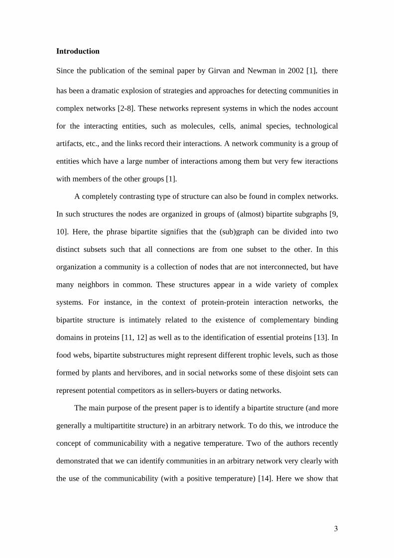
Introduction

Since the publication of the seminal paper by Girvan and Newman in 2002 [1] there

has been a dramatic explosion of strategies and approaches for detecting communities in

complex networks [2-8]. These networks represent systems in which the nodes account

for the interacting entities, such as molecules, cells, animal species, technological

artifacts, etc., and the links record their interactions. A network community is a group of

entities which have a large number of interactions among them but very few iteractions

with members of the other groups [1].

A completely contrasting type of structure can also be found in complex networks.

In such structures the nodes are organized in groups of (almost) bipartite subgraphs [9,

10]. Here, the phrase bipartite signifies that the (sub)graph can be divided into two

distinct subsets such that all connections are from one subset to the other. In this

organization a community is a collection of nodes that are not interconnected, but have

many neighbors in common. These structures appear in a wide variety of complex

systems. For instance, in the context of protein-protein interaction networks, the

bipartite structure is intimately related to the existence of complementary binding

domains in proteins [11, 12] as well as to the identification of essential proteins [13]. In

food webs, bipartite substructures might represent different trophic levels, such as those

formed by plants and hervibores, and in social networks some of these disjoint sets can

represent potential competitors as in sellers-buyers or dating networks.

The main purpose of the present paper is to identify a bipartite structure (and more

generally a multipartitite structure) in an arbitrary network. To do this, we introduce the

concept of communicability with a negative temperature. Two of the authors recently

demonstrated that we can identify communities in an arbitrary network very clearly with

the use of the communicability (with a positive temperature) [14]. Here we show that

4

we can clearly identify a multipartite structure with the use of the communicability with

a negative temperature.

Preliminaries

We represent a complex network by an undirected graph ( )EVG ,= , where V and E

are the sets of nodes and links, respectively. Let G have N nodes. Then the adjacency

matrix of G , ( ) AA =G , is a square, symmetric matrix of order N , whose elements ijA

are ones or zeroes if the corresponding nodes are adjacent or not, respectively. This

matrix has N (not necessarily distinct) real-valued eigenvalues [15], which are denoted

here by N

,,,21… , and assumed to be labelled in a non-increasing manner:

N…

21. Let j

ã be an orthonormal eigenvector corresponding to the

eigenvalue j . Then, ( )ij designates the component of this eigenvector to the ith node

in the network. A graph is said to be bipartite if its nodes can be divided into two

disjoint sets V1 and V2 such that every link connects a vertex in V1 and one in V2, but

there is no edge between two nodes in the same set.

Theoretical Approach

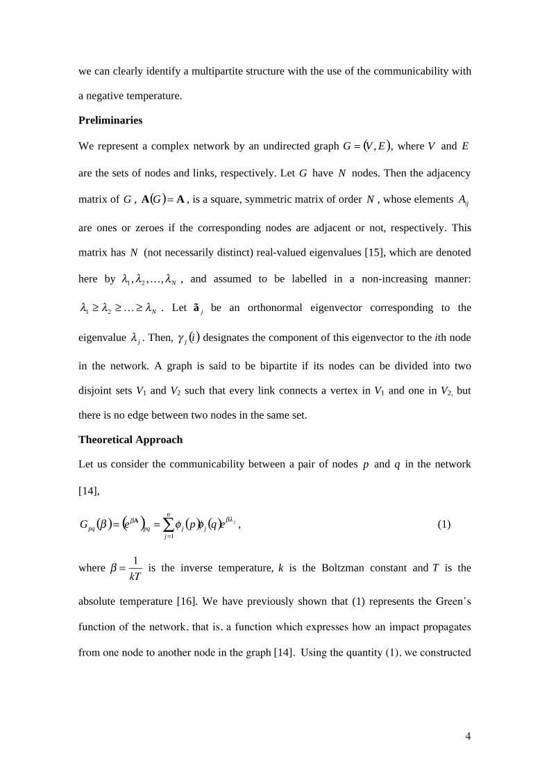
Let us consider the communicability between a pair of nodes p and q in the network

[14],

( ) ( ) ( ) ( ) jeqpeG j

n

j

jpqpq

=

==1

A , (1)

where =1

kT is the inverse temperature, k is the Boltzman constant and T is the

absolute temperature [16]. We have previously shown that (1) represents the Green’s

function of the network, that is, a function which expresses how an impact propagates

from one node to another node in the graph [14]. Using the quantity (1), we constructed

5

the “communicability graph (G) ” from the original graph G . The communicability

graph indicates communities in the graph G very clearly [17].

It is known from spectral clustering techniques that the eigenvectors

corresponding to positive eigenvalues give a partition of the network into clusters of

tightly connected nodes [18, 19]. In contrast, the eigenvectors corresponding to negative

eigenvalues make partitions in which nodes are not close to those which they are linked,

but rather with those with which they are not linked [18, 19]. Such differences have

made possible the classification of complex networks into four universal classes [20].

Let us demonstrate the above statements for a cycle Cn with even number of nodes n .

The adjacency matrix of a cycle is diagonalized by the eigenvectors

j (p) = Reeik j p n{ } , where j (p) denotes the component on the p th node of the

eigenvector with the label j , and kj 2 ( j 1) n . The corresponding eigenvalues are

j = 2coskj . The largest eigenvalue 1 = 2 is given by the eigenvector 1(p) = const.,

which is a partition of the whole network Cn into just one cluster. The second largest

eigenvalue 2 = 2cos 2 n( ) is given by the eigenvector 2 (p) = cos 2 p / n( ) n ,

which is positive for almost half of the nodes and negative for the other half. In short,

the second largest eigenvalue gives a partition of the network Cn into two clusters. On

the other hand, the lowest eigenvalue 1+n /2 = 2 is given by the eigenvector

1+n /2 (p) = ( 1)p n , which gives a partition of the network Cn into two subgraphs;

that is, the eigenvetor is positive for the nodes with even p and negative for the nodes

with odd p .

From the perspective of the communicability function (1) we can say that a

positive (negative) value of increases the contribution of the positive (negative)

6

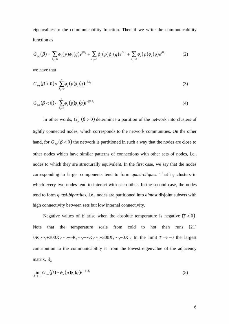
eigenvalues to the communicability function. Then if we write the communicability

function as

Gpq ( ) = j p( ) j q( )e j

j <0

+ j p( ) j q( )e j

j =0

+ j p( ) j q( )e j

j >0

(2)

we have that

( ) ( ) ( )>

>n

jjpq

j

jeqpG0

0 (3)

( ) ( ) ( )<

<n

jjpq

j

jeqpG0

0 (4)

In other words, ( )0>pqG determines a partition of the network into clusters of

tightly connected nodes, which corresponds to the network communities. On the other

hand, for ( )0<pqG the network is partitioned in such a way that the nodes are close to

other nodes which have similar patterns of connections with other sets of nodes, i.e.,

nodes to which they are structurally equivalent. In the first case, we say that the nodes

corresponding to larger components tend to form quasi-cliques. That is, clusters in

which every two nodes tend to interact with each other. In the second case, the nodes

tend to form quasi-bipartites, i.e., nodes are partitioned into almost disjoint subsets with

high connectivity between sets but low internal connectivity.

Negative values of arise when the absolute temperature is negative ( )0<T .

Note that the temperature scale from cold to hot then runs [21]

KKKKKK 0,,300,,,,,,300,,0 ++ . In the limit 0T the largest

contribution to the communicability is from the lowest eigenvalue of the adjacency

matrix, n

( ) ( ) ( ) neqpG nnpqlim (5)

7

which is known to produce a two-coloring of the nodes [22]. In the above-mentioned

example of the cycle Cn , the quantity (5) is positive when p and q have the same

parity (that is, when they belong to the same subgraph) and negative when not. This

implies that the sign of the communicability at a negative temperature indicates whether

two nodes belong to the same subgraph or not. This is the main observation on which

we develop the theoretical approach hereafter.

In order to understand the meaning of the inverse temperature in the context of

complex networks, we may express the communicability in terms of powers of the

adjacency matrix,

( )( )

=

=0 !k

pq

kk

pq

A

k

Ae (11)

Accordingly, represents a weight given to every link of the network. This weight

accounts for the “strength” of the interaction between the corresponding nodes in the

graph. For instance, 0= , which corresponds to the limit T , corresponds to a

graph with no links. This case is similar to a gas formed by monoatomic particles. On

the other hand, very large values of in the limit T +0 represents very large

attractive interactions between pairs of bonded nodes in a similar manner to a solid. The

new cases considered in this work, 0< , correspond to the existence of repulsive

interactions between the pairs of linked nodes, which obligates them to be in separated

clusters forming bipartite structures in the network.

From now on we consider, for the sake of simplicity, the case where 1= . Then,

( ) ( ) ( ) ( ) jeqpeG j

n

j

jpqpq

=

===1

1A . (6)

Now, let us interpret the exponential negative adjacency matrix. First, we expand it in

powers of the adjacency matrix,

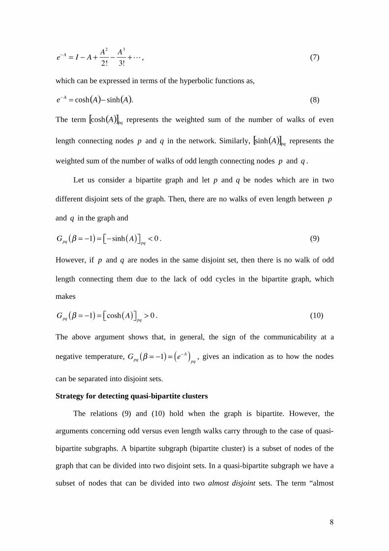
8

e A= I A +

A2

2!

A3

3!+ , (7)

which can be expressed in terms of the hyperbolic functions as,

( ) ( )AAeA

sinhcosh= . (8)

The term ( )[ ]pqAcosh represents the weighted sum of the number of walks of even

length connecting nodes p and q in the network. Similarly, ( )[ ]pqAsinh represents the

weighted sum of the number of walks of odd length connecting nodes p and q .

Let us consider a bipartite graph and let p and q be nodes which are in two

different disjoint sets of the graph. Then, there are no walks of even length between p

and q in the graph and

Gpq = 1( ) = sinh A( )pq< 0 . (9)

However, if p and q are nodes in the same disjoint set, then there is no walk of odd

length connecting them due to the lack of odd cycles in the bipartite graph, which

makes

Gpq = 1( ) = cosh A( )pq> 0 . (10)

The above argument shows that, in general, the sign of the communicability at a

negative temperature, Gpq = 1( ) = e A( )pq

, gives an indication as to how the nodes

can be separated into disjoint sets.

Strategy for detecting quasi-bipartite clusters

The relations (9) and (10) hold when the graph is bipartite. However, the

arguments concerning odd versus even length walks carry through to the case of quasi-

bipartite subgraphs. A bipartite subgraph (bipartite cluster) is a subset of nodes of the

graph that can be divided into two disjoint sets. In a quasi-bipartite subgraph we have a

subset of nodes that can be divided into two almost disjoint sets. The term “almost

9

disjoint” means that most of the links in the subgraph are inter-set links but there are

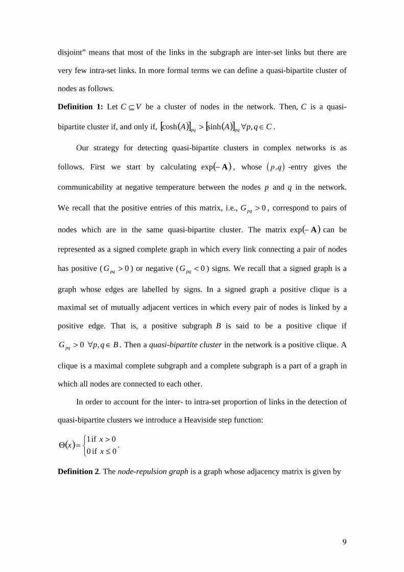
very few intra-set links. In more formal terms we can define a quasi-bipartite cluster of

nodes as follows.

Definition 1: Let VC be a cluster of nodes in the network. Then, C is a quasi-

bipartite cluster if, and only if, ( )[ ] ( )[ ] CqpAA pqpq > ,sinhcosh .

Our strategy for detecting quasi-bipartite clusters in complex networks is as

follows. First we start by calculating ( )Aexp , whose p,q( ) -entry gives the

communicability at negative temperature between the nodes p and q in the network.

We recall that the positive entries of this matrix, i.e., 0>pqG , correspond to pairs of

nodes which are in the same quasi-bipartite cluster. The matrix ( )Aexp can be

represented as a signed complete graph in which every link connecting a pair of nodes

has positive ( 0>pqG ) or negative ( 0<pqG ) signs. We recall that a signed graph is a

graph whose edges are labelled by signs. In a signed graph a positive clique is a

maximal set of mutually adjacent vertices in which every pair of nodes is linked by a

positive edge. That is, a positive subgraph B is said to be a positive clique if

BqpGpq > , 0 . Then a quasi-bipartite cluster in the network is a positive clique. A

clique is a maximal complete subgraph and a complete subgraph is a part of a graph in

which all nodes are connected to each other.

In order to account for the inter- to intra-set proportion of links in the detection of

quasi-bipartite clusters we introduce a Heaviside step function:

( )>

=0 if 0

0 if 1

x

xx .

Definition 2. The node-repulsion graph is a graph whose adjacency matrix is given by

10

( )[ ]Aexp , which results from the elementwise application of the function ( )x to

the matrix ( )Aexp . A pair of nodes p and q in the node-repulsion graph ( )[ ]Aexp

is connected if, and only if, they have 0>pqG .

Now, suppose that there is a link between the nodes p and q and there are also

links between them and a third node r . This means that 0>pqG , 0>prG and 0>qrG .

Consequently, the three nodes form a positive subgraph B . As we want to detect the

largest subset of nodes connected to this triple we have to search for the nodes s for

which BiGis> 0 . Using the node-repulsion graph, this search is reduced to

finding the cliques in a simple graph, ( )[ ]Aexp . These cliques correspond to the

quasi-bipartite clusters of the network.

Finding the cliques in a graph is a classical problem in combinatorial optimization,

which has found applications in diverse areas [23]. Here we use a well-known algorithm

due to Bron and Kerbosch [24], which is a depth-first search for generating all cliques

in a graph. This algorithm consumes a time per clique which is almost independent of

the graph size for random graphs and for the Moon-Moser graphs of n vertices the total

time is proportional to ( ) 3/

14.3n

. The Moon-Moser graphs have the largest number of

maximal cliques possible among all n-vertex graphs regardless of the number of edges

in the graph [25].

Our new algorithm differs from those in [9] and [10] in a number of ways.

Fundamentally, our aim is different. Rather than quantifying the overall bipartivity of

the network, or of individual nodes or edges, we are looking for communities that share

in a bipartite substructure. Moreover, we allow several such substructures to be present.

In contrast to [9], the new algorithm takes account of both odd and even length walks,

avoids the need for a cutoff parameter by considering walks of all possible lengths, and

does not require a complex energy landscape to be searched by a heuristic discrete

11

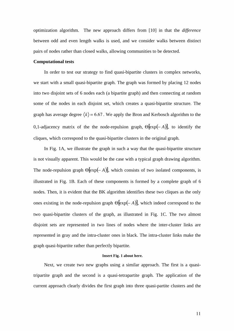
optimization algorithm. The new approach differs from [10] in that the difference

between odd and even length walks is used, and we consider walks between distinct

pairs of nodes rather than closed walks, allowing communities to be detected.

Computational tests

In order to test our strategy to find quasi-bipartite clusters in complex networks,

we start with a small quasi-bipartite graph. The graph was formed by placing 12 nodes

into two disjoint sets of 6 nodes each (a bipartite graph) and then connecting at random

some of the nodes in each disjoint set, which creates a quasi-bipartite structure. The

graph has average degree k = 6.67 . We apply the Bron and Kerbosch algorithm to the

0,1-adjacency matrix of the the node-repulsion graph, ( )[ ]Aexp , to identify the

cliques, which correspond to the quasi-bipartite clusters in the original graph.

In Fig. 1A, we illustrate the graph in such a way that the quasi-bipartite structure

is not visually apparent. This would be the case with a typical graph drawing algorithm.

The node-repulsion graph ( )[ ]Aexp , which consists of two isolated components, is

illustrated in Fig. 1B. Each of these components is formed by a complete graph of 6

nodes. Then, it is evident that the BK algorithm identifies these two cliques as the only

ones existing in the node-repulsion graph ( )[ ]Aexp , which indeed correspond to the

two quasi-bipartite clusters of the graph, as illustrated in Fig. 1C. The two almost

disjoint sets are represented in two lines of nodes where the inter-cluster links are

represented in gray and the intra-cluster ones in black. The intra-cluster links make the

graph quasi-bipartite rather than perfectly bipartite.

Insert Fig. 1 about here.

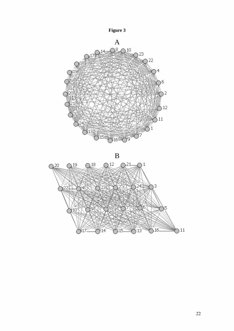
Next, we create two new graphs using a similar approach. The first is a quasi-

tripartite graph and the second is a quasi-tetrapartite graph. The application of the

current approach clearly divides the first graph into three quasi-partite clusters and the

12

second one into four. The graphs and their partitions are illustrated in Figs. 2 and 3,

respectively.

Insert Figs. 2 and 3 about here.

Multipartite Structure in Real-World Networks

As a proof of concept we first select a network which we already know is bipartite.

It is the network of heterosexual contacts obtained empirically at the Cadham Provincial

Laboratory during 6 months between November 1997 and May 1998 [26]. This network,

consisting of 82 nodes and 84 connections, was studied by Lind et al. [27] where

illustrations and details can be found. Our current approach clearly identifies the two

bipartite clusters, one consisting of 47 nodes and the other of 35 (results not shown).

The node-repulsion graph clearly identified the two isolated components.

As a second example, we studied the food web of Canton Creek, which consists

primarily of invertebrates and algae in a tributary, surrounded by pasture, of the Taieri

River in the South Island of New Zealand [28]. This network consists of 108 nodes

(species) and 707 links (trophic relations). Using our current approach, we find that this

network can be divided into two almost-bipartite clusters, one having 66 nodes and the

other 42. Only 20 links connect nodes in the same clusters, 13 of them connect nodes in

the set containing 66 nodes and the other 7 connect nodes in the set of 42 nodes. Thus

97.2% of links are connections between the two almost-bipartite clusters and only 2.8%

links are intracluster connections. In Fig. 4, we illustrate the network and its quasi-

bipartite clusters as found in the current work. Other food webs (see [29] and the

references therein), like that of the pelagic species from the largest of a set of 50 New

York Adirondack lake food webs (Bridge Brook), a marine ecosystem on the northeast

US shelf (Shelf), invertebrates in an English pond (Skipwith) and a food web like

Canton Creek but in native tussock habitat (Stony stream) are also formed by two main

quasi-bipartite clusters with no overlap between them. However, there are other food

webs with a larger number of quasi-bipartite clusters with large overlap among them.

13

One example is the network formed by birds and predators and arthropod prey of Anolis

lizards on the island of St. Martin (see [29] and the references therein), located in the

northern Lesser Antilles (StMartins), which has 116 quasi-partite clusters.

Insert Fig. 4 about here.

The next example corresponds to the protein-protein interaction network (PIN) of

the Kaposi sarcoma-associated herpesvirus (KSHV) [30]. KSHV is a member of the -

herpesvirus subfamily associated with Kaposi sarcoma and B cell lymphomas. Its PIN

was generated by Uetz et al. [30] by testing 12,000 viral protein interactions involving

both full-length proteins and protein fragments. From this pool of interactions, Uetz et

al. [30] identified 123 nonredundant interacting pairs of proteins, 8 of which were self-

interactions. The resulting PIN of KSHV, formed by 50 proteins and 115 interactions, is

illustrated in Fig. 5A. Some of the global topological characteristics of this PIN can be

found in Uetz. et al. [30].

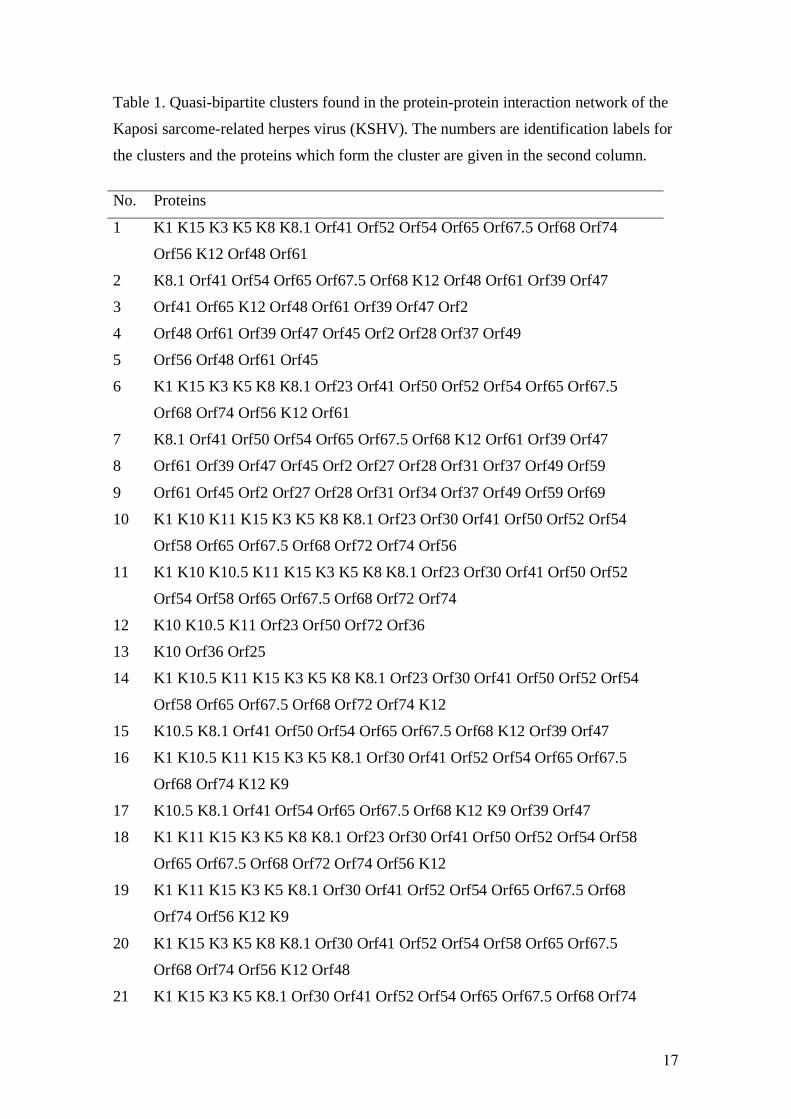
Using our current approach we identify 34 quasi-partite clusters in the PIN of

KSHV. The proteins grouped in every cluster are given in Table 1. The largest clusters

are the number 10, 11, 14 and 18 which have 21 proteins each. However, there is a very

large overlap among them ranging from 66.6% for the clusters 11 and 18 to 95% for the

pairs of clusters (10, 11), (11, 14), (14, 18). There is another group of quasi-bipartite

clusters containing a large number of proteins. They are the clusters 28, 29, 30 and 32.

They also display very large overlapping among them, ranging from 89.5% to 94.7%.

However, these two groups of clusters are completely orthogonal. That is, absolutely no

overlapping exists between any of the clusters of the first group (10, 11, 14 and 18) with

the clusters in the second group (28, 29, 30 and 32). Then we conclude that the PIN of

KSHV can be divided into two disjoint clusters of almost the same size, which contain

78% of the proteins in the PIN. These two clusters are illustrated in the Fig. 5B.

14

On the other side of the coin there are networks displaying a huge number of small

quasi-bipartite clusters. This is the case for those networks lacking a bipartite structure

at all but having a multipartite structure. For instance, the neuronal synaptic network of

the nematode C. Elegans (see [31] and the references therein), which has 280 nodes and

1973 links is formed by 43, 753 quasi-partite clusters. This network has been formerly

shown to have a super-homogeneous structure [32], which explains its lack of

bipartivity.

Conclusions

Given a complex network, the new concept of a node-repulsion graph has intuitive

interpretations in terms of (a) a Green’s function at negative absolute temperature, and

(b) a measure of the discrepancy between the overall number of odd and even walks

between pairs of nodes. Moreover, this concept allows for a natural, well-defined

quantification of quasi-bipartite clusters that can be investigated with a simple,

parameter-free computational algorithm. This new algorithm was able to discover

inherent bipartite communities in real data sets, and hence has the potential to unlock

hidden patterns at the heart of complex networks.

Acknowledgements

EE thanks the support by the Royal Society of Edinburgh and the Edinburgh

Mathematical Society (March 2008) and to the IIS, University of Tokyo for a

fellowship as Research Visitor during April-June, 2008. DJH was supported by

Engineering and Physical Sciences Research Council grant GR/S62383/01

15

References

[1] M. Girvan and M. J. E. Newman, Proc. Natl. Ac. Sci. USA 99, 7821 (2002).

[2] J. Duch and A. Arenas, Nature Phys. Rev. E. 72, 027104 (2005).

[3] G. Palla, I. Derenyi, I. Farkas and T. Vicsek, Nature 435, 814 (2005).

[4] A. Capocci, V. D. P. Servedio, G. Caldarelli and F. Colaiori, Physica A 352, 669

(2005).

[5] R. Guimera and L. A. N. Amaral, Nature 433, 895 (2005).

[6] M. E. J. Newman, Phys. Rev. E. 74, 036104 (2006).

[7] M. E. J. Newman, Eur. Phys. J. B 38, 321 (2004).

[8] L. Danon, J. Duch, A. Diaz-Guilera and A. Arenas, J. Stat. Mech.: Theory Exp.

P09008, (2002).

[9] P. Holme, F. Liljeros, C. R. Edling and B. J. Kim, Phys. Rev. E 68, 056107

(2003).

[10] E. Estrada and J. A. Rodríguez-Velázquez, Phys. Rev. E 72, 046105 (2005).

[11] A. Thomas, R. Cannings, N. A. M. Monk and C. Cannings, Biochem. Soc. Trans.

31, 1491 (2003).

[12] J. L. Morrison, R. Breitling, D. J. Higham and D. R. Gilbert, Bioinformatics 22,

2012 (2006).

[13] E. Estrada, J. Proteome Res. 5, 2177 (2006).

[14] E. Estrada and N. Hatano, Phys. Rev. E 77, 036111 (2008).

[15] N. L. Biggs, Algebraic Graph Theory (Cambridge University Press, Cambridge,

1993).

[16] E. Estrada and N Hatano, Chem. Phys. Lett. 439, 247 (2007).

[17] E. Estrada and N Hatano, submitted 2008.

16

[18] A. J. Seary, W. D. Richards, Jr., in Proceedings of the International Conference

on Social Networks, London, edited by M. G. Everett and K. Rennolds

(Greenwich University Press, London, 1995), Vol. 1, p. 47.

[19] T. Xiao and S. Gong, Pattern Recog. 41, 1012 (2008).

[20] E. Estrada, Phys. Rev. E 75, 016103 (2007).

[21] N. F. Ramsey, Phys. Rev. 103, 20 (1956).

[22] B. Aspvall and J. R. Gilbert, SIAM J. Alg. Disc. Math. 5, 526 (1984).

[23] I. M. Bomze, M. Budinich, P. M. Pardalos and M. Pelillo, in: D.-Z. Du and P. M.

Pardalos (Eds.), Handbook of Combinatorial Optimization, Supplement Vol. A.

Kluwer Academic Publishers, Dordrecht 1999, pp. 1-74.

[24] C. Bron and J. Kerbosch, Comm. ACM 16, 575 (1973).

[25] J. W. Moon and L. Moser, Israel J. Math. 3, 23 (1965).

[26] J. L. Wylie and A. Jolly, Sex Transm. Dis. 28, 14 (2001).

[27] P. G. Lind, M. C. González and H. J. Herrmann, Phys. Rev. E 72, 056127

(2005).

[28] C. Townsend, R. M. Thompson, A. R. McIntosh, C. Kilroy, E. Edwards and M.

R. Scarsbrook, Ecol. Lett. 1, 200 (1998).

[29] J. A. Dunne, R. J. Williams and N. D. Martinez, Proc. Natl. Ac. Sci USA 99,

12917 (2002).

[30] P. Uetz et al., Science 311, 239 (2006).

[31] R. Milo, S. Itzkovitz, N. Kashtan, R. Levitt, S. Shen-Orr, I. Ayzenshtat, M.

Sheffer and U. Alon, Science 303, 1538 (2004).

[32] E. Estrada, Europhys. Lett. 73, 649 (2006).

17

Table 1. Quasi-bipartite clusters found in the protein-protein interaction network of the

Kaposi sarcome-related herpes virus (KSHV). The numbers are identification labels for

the clusters and the proteins which form the cluster are given in the second column.

No. Proteins

1 K1 K15 K3 K5 K8 K8.1 Orf41 Orf52 Orf54 Orf65 Orf67.5 Orf68 Orf74

Orf56 K12 Orf48 Orf61

2 K8.1 Orf41 Orf54 Orf65 Orf67.5 Orf68 K12 Orf48 Orf61 Orf39 Orf47

3 Orf41 Orf65 K12 Orf48 Orf61 Orf39 Orf47 Orf2

4 Orf48 Orf61 Orf39 Orf47 Orf45 Orf2 Orf28 Orf37 Orf49

5 Orf56 Orf48 Orf61 Orf45

6 K1 K15 K3 K5 K8 K8.1 Orf23 Orf41 Orf50 Orf52 Orf54 Orf65 Orf67.5

Orf68 Orf74 Orf56 K12 Orf61

7 K8.1 Orf41 Orf50 Orf54 Orf65 Orf67.5 Orf68 K12 Orf61 Orf39 Orf47

8 Orf61 Orf39 Orf47 Orf45 Orf2 Orf27 Orf28 Orf31 Orf37 Orf49 Orf59

9 Orf61 Orf45 Orf2 Orf27 Orf28 Orf31 Orf34 Orf37 Orf49 Orf59 Orf69

10 K1 K10 K11 K15 K3 K5 K8 K8.1 Orf23 Orf30 Orf41 Orf50 Orf52 Orf54

Orf58 Orf65 Orf67.5 Orf68 Orf72 Orf74 Orf56

11 K1 K10 K10.5 K11 K15 K3 K5 K8 K8.1 Orf23 Orf30 Orf41 Orf50 Orf52

Orf54 Orf58 Orf65 Orf67.5 Orf68 Orf72 Orf74

12 K10 K10.5 K11 Orf23 Orf50 Orf72 Orf36

13 K10 Orf36 Orf25

14 K1 K10.5 K11 K15 K3 K5 K8 K8.1 Orf23 Orf30 Orf41 Orf50 Orf52 Orf54

Orf58 Orf65 Orf67.5 Orf68 Orf72 Orf74 K12

15 K10.5 K8.1 Orf41 Orf50 Orf54 Orf65 Orf67.5 Orf68 K12 Orf39 Orf47

16 K1 K10.5 K11 K15 K3 K5 K8.1 Orf30 Orf41 Orf52 Orf54 Orf65 Orf67.5

Orf68 Orf74 K12 K9

17 K10.5 K8.1 Orf41 Orf54 Orf65 Orf67.5 Orf68 K12 K9 Orf39 Orf47

18 K1 K11 K15 K3 K5 K8 K8.1 Orf23 Orf30 Orf41 Orf50 Orf52 Orf54 Orf58

Orf65 Orf67.5 Orf68 Orf72 Orf74 Orf56 K12

19 K1 K11 K15 K3 K5 K8.1 Orf30 Orf41 Orf52 Orf54 Orf65 Orf67.5 Orf68

Orf74 Orf56 K12 K9

20 K1 K15 K3 K5 K8 K8.1 Orf30 Orf41 Orf52 Orf54 Orf58 Orf65 Orf67.5

Orf68 Orf74 Orf56 K12 Orf48

21 K1 K15 K3 K5 K8.1 Orf30 Orf41 Orf52 Orf54 Orf65 Orf67.5 Orf68 Orf74

18

Orf56 K12 K9 Orf48

22 K8.1 Orf41 Orf54 Orf65 Orf67.5 Orf68 K12 K9 Orf48 Orf39 Orf47

23 Orf41 Orf65 K12 K9 Orf48 Orf39 Orf47 Orf2

24 K9 Orf48 Orf39 Orf47 Orf45 Orf2 Orf37

25 Orf56 K9 Orf48 Orf45

26 K9 Orf45 Orf2 Orf37 Orf57

27 Orf36 Orf25 K7 Orf27 Orf29b Orf31 Orf34 Orf53 Orf57 Orf59 Orf6 Orf60

Orf62 Orf63 Orf69 Orf9

28 Orf25 Orf45 K7 Orf27 Orf28 Orf29b Orf31 Orf34 Orf37 Orf49 Orf53 Orf57

Orf59 Orf6 Orf60 Orf63 Orf69 Orf75 Orf9

29 Orf25 K7 Orf27 Orf28 Orf29b Orf31 Orf34 Orf37 Orf49 Orf53 Orf57 Orf59

Orf6 Orf60 Orf62 Orf63 Orf69 Orf75 Orf9

30 Orf45 K7 Orf2 Orf27 Orf28 Orf29b Orf31 Orf34 Orf37 Orf49 Orf53 Orf57

Orf59 Orf6 Orf60 Orf63 Orf69 Orf75 Orf9

31 Orf39 Orf47 Orf45 K7 Orf2 Orf27 Orf28 Orf31 Orf37 Orf49 Orf53 Orf59

Orf6 Orf60

32 32: K7 Orf2 Orf27 Orf28 Orf29b Orf31 Orf34 Orf37 Orf49 Orf53 Orf57

Orf59 Orf6 Orf60 Orf62 Orf63 Orf69 Orf75 Orf9

33 Orf48 Orf45 Orf2 Orf28 Orf37 Orf49 Orf75

34 Orf56 Orf48 Orf45 Orf75

19

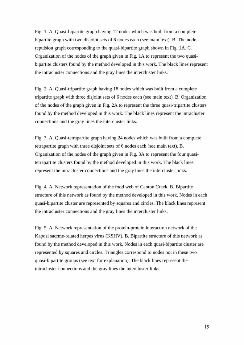
Fig. 1. A. Quasi-bipartite graph having 12 nodes which was built from a complete

bipartite graph with two disjoint sets of 6 nodes each (see main text). B. The node-

repulsion graph corresponding to the quasi-bipartite graph shown in Fig. 1A. C.

Organization of the nodes of the graph given in Fig. 1A to represent the two quasi-

bipartite clusters found by the method developed in this work. The black lines represent

the intracluster connections and the gray lines the intercluster links.

Fig. 2. A. Quasi-tripartite graph having 18 nodes which was built from a complete

tripartite graph with three disjoint sets of 6 nodes each (see main text). B. Organization

of the nodes of the graph given in Fig. 2A to represent the three quasi-tripartite clusters

found by the method developed in this work. The black lines represent the intracluster

connections and the gray lines the intercluster links.

Fig. 3. A. Quasi-tetrapartite graph having 24 nodes which was built from a complete

tetrapartite graph with three disjoint sets of 6 nodes each (see main text). B.

Organization of the nodes of the graph given in Fig. 3A to represent the four quasi-

tetrapartite clusters found by the method developed in this work. The black lines

represent the intracluster connections and the gray lines the intercluster links.

Fig. 4. A. Network representation of the food web of Canton Creek. B. Bipartite

structure of this network as found by the method developed in this work. Nodes in each

quasi-bipartite cluster are represented by squares and circles. The black lines represent

the intracluster connections and the gray lines the intercluster links.

Fig. 5. A. Network representation of the protein-protein interaction network of the

Kaposi sacrme-related herpes virus (KSHV). B. Bipartite structure of this network as

found by the method developed in this work. Nodes in each quasi-bipartite cluster are

represented by squares and circles. Triangles correspond to nodes not in these two

quasi-bipartite groups (see text for explanation). The black lines represent the

intracluster connections and the gray lines the intercluster links

20

Figure 1

A

B

C

21

Figure 2

A

B

22

Figure 3

A

B

23

Figure 4

A

B

24

Figure 5

A

B