Common Knowledge Reference Price and Asymmetric Price Adjustments Evidence from the Retail Gasoline...

Rev Ind Organ (2010) 37:141–159DOI 10.1007/s11151-010-9261-9

Common Knowledge Reference Price and AsymmetricPrice AdjustmentsEvidence from the Retail Gasoline Market in Colombia

Marc Hofstetter · Jorge Tovar

Published online: 22 September 2010© Springer Science+Business Media, LLC. 2010

Abstract There is abundant empirical evidence showing that asymmetric priceadjustments exist in a wide variety of markets. Prices tend to rise faster when costs rise,relative to the rate at which prices drop when costs fall. This paper argues that a com-mon knowledge reference price—a government suggested retail price—eases the exis-tence of asymmetric price adjustments in a scenario where costs are ever-increasing.Our analysis of the Colombian retail gasoline market suggests that when costs rise bymore than the reference price, prices tend to rise more slowly relative to when costsgrow by less than the reference price.

Keywords Asymmetric price adjustments · Gasoline retail markets ·Price transparency · Reference prices

1 Introduction

A recent and abundant empirical literature suggests that asymmetric price adjustmentis common to a wide variety of markets. The pattern found is that prices tend togrow faster when costs rise relative to the rate at which prices drop when costs fall.

A previous version of the paper circulated under the title “Asymmetric price adjustments underever-increasing costs: Evidence from the Retail Gasoline Market in Colombia”.

M. Hofstetter · J. Tovar (B)Department of Economics and CEDE, Universidad de los Andes,Calle 19A No. 1, 37 Este. Edificio W. Of. 825, Bogota, Colombiae-mail: [email protected]: http://economia.uniandes.edu.co/tovar

M. Hofstettere-mail: [email protected]: http://economia.uniandes.edu.co/hofstetter

123

142 M. Hofstetter, J. Tovar

Peltzman (2000), working with 77 consumer goods and 165 producer goods, findsevidence that asymmetric price adjustments do indeed exist in most markets. In arecent paper, Meyer and von Cramon-Taubadel (2004) survey the literature and notethat such findings tend to be robust for the markets for agricultural products, interestrates, and gasoline.

The Colombian gasoline market offers a unique scenario for testing issues relatedto this topic. As explained in detail throughout the paper, the market in Colombia hasa peculiar structure: Every month, the government announces a suggested (thoughnot mandatory) retail price for gasoline. This price is heavily advertised by the localmedia. In local jargon, the price is known as the “reference price for gasoline.”

We take advantage of this market structure to test for asymmetric price adjustmentsof a different sort than those that are commonly explored in the literature. We willnot test whether cost increases trigger a different reaction in prices relative to costdecreases.1 This traditional approach is not possible because the Colombian gaso-line market has the particularity that wholesale gasoline prices—that is, costs—havefollowed an upward trend throughout our sample period.

Instead, this paper explores the hypothesis that when costs rise by less than the risein the common knowledge reference price, retail prices should adjust quickly; con-versely, slower adjustments should occur when costs increase by more than the rise inthe reference price. Why is this? Consider the former case—that is, costs rise by lessthan the rise in the reference price. Under the plausible assumption that consumers donot observe costs, the retailer can quickly pass on the cost increment to retail prices.Consumers would find the retail price increment reasonable based on their expecta-tions (as determined by the reference price); and the quick price adjustment, in thespirit of Lewis’ (2004) story, will not trigger consumers to search. Conversely, if costsincrease more than the reference price, the retailer could choose to delay passing on theincrease, thus avoiding consumers’ search. Hence, the reference price allows retailersto use consumers’ expectations when adjusting prices and asymmetric pricing arises.

We find that when costs grow more than does the reference price, retail prices tendto increase more slowly relative to when costs increase less than the reference price. Inthis sense, reference prices do indeed appear to anchor the expectations of consumers.A rise in costs that is less than the reference price allows retailers to pass the increasequickly through to prices (as consumers find it natural to observe higher prices); alter-natively, a rise in costs above the rise in the reference price forces retailers to delayprice increases. In the latter case—much as represented in Borenstein et al. (1997)and Lewis’ stories—the behavior of retailers prevents consumers from searching forlower prices.

The rest of the paper is organized as follows: Section 2 describes the structure of thegasoline industry in Colombia. Section 3 describes the data used in the paper and takesa first broad look at it. Section 4 tests for price asymmetries, and Section 5 presentsseveral robustness tests. Section 6 concludes.

1 Aside from those authors explicitly mentioned throughout this paper, others, such as Duffy-Deno(1996),Eckert (2002), and Godby et al. (2000) have studied the gasoline market in search of asymmetricprice adjustments. Only the last, using Canadian retail gasoline market data, were unable to find evidenceof asymmetric pricing.

123

Asymmetric Price Adjustments for Gasoline 143

State Controlled Monopoly(Ecopetrol)

GAS STATIONS

REFINERIES

STORAGE CENTERS

WHOLESALERS (Supply Centres) CONSUMERS

Gas stations are owned by wholesalers or by independent owners using one of the wholesaler’sbrands.

IMPORTS

Transport Services

Regulated Prices

Reference Prices

(Major cities only)

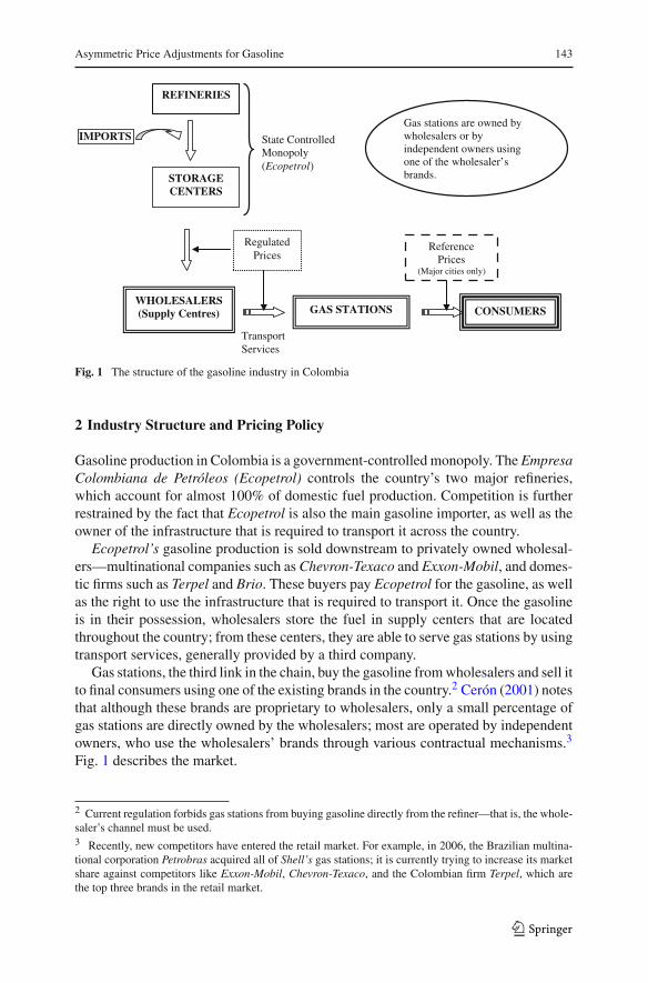
Fig. 1 The structure of the gasoline industry in Colombia

2 Industry Structure and Pricing Policy

Gasoline production in Colombia is a government-controlled monopoly. The EmpresaColombiana de Petróleos (Ecopetrol) controls the country’s two major refineries,which account for almost 100% of domestic fuel production. Competition is furtherrestrained by the fact that Ecopetrol is also the main gasoline importer, as well as theowner of the infrastructure that is required to transport it across the country.

Ecopetrol’s gasoline production is sold downstream to privately owned wholesal-ers—multinational companies such as Chevron-Texaco and Exxon-Mobil, and domes-tic firms such as Terpel and Brio. These buyers pay Ecopetrol for the gasoline, as wellas the right to use the infrastructure that is required to transport it. Once the gasolineis in their possession, wholesalers store the fuel in supply centers that are locatedthroughout the country; from these centers, they are able to serve gas stations by usingtransport services, generally provided by a third company.

Gas stations, the third link in the chain, buy the gasoline from wholesalers and sell itto final consumers using one of the existing brands in the country.2 Cerón (2001) notesthat although these brands are proprietary to wholesalers, only a small percentage ofgas stations are directly owned by the wholesalers; most are operated by independentowners, who use the wholesalers’ brands through various contractual mechanisms.3

Fig. 1 describes the market.

2 Current regulation forbids gas stations from buying gasoline directly from the refiner—that is, the whole-saler’s channel must be used.3 Recently, new competitors have entered the retail market. For example, in 2006, the Brazilian multina-tional corporation Petrobras acquired all of Shell’s gas stations; it is currently trying to increase its marketshare against competitors like Exxon-Mobil, Chevron-Texaco, and the Colombian firm Terpel, which arethe top three brands in the retail market.

123


As inferred from the above discussion, the Colombian gasoline market is highlyregulated over all of the various stages involved. Prior to 1999, when the govern-ment established a new regime for fuel prices in local markets, prices were set on ayearly (or sometimes shorter) basis and remained substantially below internationalprices. According to the 1998–1999 Ministry of Mining and Energy Report to theCongress, this policy implied that Ecopetrol was subsidizing gasoline in Colombia;and consequently the objective of the new formula, was to stop these subsidies.

In 1999, with the objective of inducing competition in both production and dis-tribution, and eliminating the subsidies, a new pricing policy was implemented. Thisnew policy continued to regulate refinery and wholesale prices, but allowed retail gasstations in the major cities to set prices freely.4 This policy, which tried to mirror theconditions faced by a hypothetical importer, determined that the price at the refinery—which is paid by wholesalers to Ecopetrol—should follow the international MexicanGulf Coast price for gasoline, which is adjusted based on import costs.

By 1999, shortly after this new pricing policy came into force, the government real-ized that matching domestic and international prices at the beginning of the productionchain was not sustainable. The policy was implemented during a period when world oilprices were low, but a few months later, international oil and gasoline prices began torise. The effect on domestic prices was immediate, fast, and unexpected by the govern-ment, which decided to control the pace of the adjustment and match the internationalprice only gradually.5 Currently, this gradual adjustment towards international pricesis still under way.

The second stage in Fig. 1, which entails the prices that wholesalers charge gasstations, is also regulated. More specifically, there is a maximum regulated margin,whereby wholesalers are allowed to sell at a price that is equal to or lower than theregulated one. In small cities, the third stage, which entails the price charged by gasstations—is also regulated. Nevertheless, in our paper, we focus on the data frommajor cities, where gas stations are free to set their own price.

In major cities, the only role that the government plays with respect to retail pricesis to establish a suggested (that is, reference) price. Published at the beginning of eachmonth, the reference price—which is city specific—is not mandatory, and retailersmay price above or below it.

For instance, on May 31, 2007, El Tiempo, the main newspaper in Colombia,announced that “starting midnight, the gasoline (reference) price would increase by30.18 pesos”. We will explore the implications of how reference price increments areannounced in Sect. 4. For now, note that the reference price is not a market price, but

4 According to González (2004), major cities account for 60–70% of total gasoline consumption inColombia.5 In addition to this, a new technical modification to the regulation on prices was recently introduced. Asa measure aimed at reducing the contamination produced by CO2 emissions, it is now mandatory to mixregular gasoline with a 10% content of ethanol fuel. Although the mixture of regular and ethanol fuel slightlymodifies the calculations used by the government in establishing the monthly regulated price, the resultingprices have barely changed. During our sample period, which runs through December 2006, this new reg-ulation was applied in only three cities (Bogota, Cali, and Pereira), but is expected to be applied/enactedin more cities in the near future. This new regime became operative in Cali and Pereira in November 2005and in Bogotá in February 2006.

123


rather a suggested price that, according to the government, accounts for all costs inthe production and distribution chain while allowing for retailers to make a reasonableprofit.

There is no explicit formula to determine the reference price, although the govern-ment is aware that by setting both reference and wholesale prices it is explicitly sayingsomething about retailers’ markups. The overall idea is simply to match domestic tointernational prices at a reasonable pace, keeping relatively constant retailers’ mark-ups. The lack of an explicit formula became evident in 2009 when, as petroleum pricesfell, the government decided not to lower either wholesale prices or reference prices,arguing for the need to minimize volatility in gasoline prices.

3 Data: Sources, Description, and Evolution

We use three sets of prices in this paper: retail, wholesale, and reference prices. Theinformation on retail prices is originated in a monthly survey carried out by Unidad dePlaneación Minero Energética (UPME), a government agency that is a subsidiary ofthe Ministry of Mining and Energy. The survey collects retail gasoline prices duringthe first week of each month, directly from gas stations in ten major cities.

In our sample, retail prices are available for 30 months, starting in July 2004 andrunning through December 2006. It consists of an unbalanced panel of prices, ascharged by over 200 gas stations in ten major cities.

Although no regulation prevents gas stations from adjusting prices beyond the firstweek of the month, in practice most (if not all) changes take place on the first dayof each month. Retailers, as predicted by Rotemberg (2005), take advantage of thechange in the reference price to adjust prices simultaneously. Thus, data at a higherfrequency would be of little interest as prices are modified only once per month. Thisis exploited by the UPME survey that, as noted above, collects data during the firstweek of each month.

Data on wholesale prices comes from our own calculations, based on the priceregulations and monthly updates published by the Ministry of Mining and Energy foreach of the 10 cities included in the survey. These prices vary by city, mainly dueto transportation costs.6 Finally, reference prices come from UPME records. Levelsvary by city, but monthly adjustments are similar across cities. For instance, monthlyreference price changes in non-border cities are identical in 71% of the cases. In theborder cities, where price levels are much lower due to the lack of taxes on gasoline,this figure increases to 97%.

Despite the fact that information on regular (81 octane) and premium (87 octane)gasoline is available, we only consider the former, because consumption of the latter isrelatively limited in Colombia. For example, as reported by Ecopetrol, in 2005, regulargasoline sales (in gallons) accounted for 93% of total gasoline sales in the country.

6 Costs may also vary due to certain local taxes, as well as the existence of ethanol fuel in the cases ofBogotá, Cali, and Pereira. In the case of border cities, such as Pasto and Valledupar, the regulation statesthat no tax is to be paid.

123


Bogota

Medellin

Cali

Bucaramanga

Barranquilla

Pasto

Pereira

Valledupar

Santa Marta

Neiva

Monthly Average (All Cities) = 179.93 Total Months = 30

0 10 20 30 40

Average Number of Observations

Fig. 2 The number of retail price observations. Monthly average by city in sample (July 2004–December2006)

The econometric analysis below excludes stations with less than five observations,leaving us with a sample that, on average, consists of 179.9 stations per month overthe 30 month period of analysis. As shown in Fig. 2, in major cities such as Bogota,Cali, and Medellin, a greater number of stations are surveyed relative to smaller citieslike Neiva, Santa Marta, and Valledupar. The ten cities surveyed not only account for32.8% of total gasoline sales in Colombia, but also represent 34.7% of the country’soverall population according to the latest population census.

As mentioned above, not all of the 212 gas stations being sampled register observa-tions every single month.7 Figure 3 shows how the data are distributed in more detail.For example, 154 stations, representing 72.6% of the total, have data for at least 26(out of 30) months.

Figure 4 depicts the evolution and monthly variation of retail, wholesale, andreference prices. Panel A presents the evolution of the three prices over time percity. The retail price is calculated as a simple average across the gas stations withineach city. As argued earlier, the series have an upward trend during the sample period.Both retail average prices and wholesale prices in each of the 10 cities have grownsteadily since July 2004, at monthly average rates slightly greater than 1%.

Prices tend to be lower in border cities, where gasoline pays no taxes. With theexception of Bogota and Neiva, average retail prices are higher than the referenceprice. That retail prices tend to be higher than reference prices suggests that retail-ers have little fear of the government’s re-regulating retail prices. If retailers behaved

7 According to the Colombian Association of Gasoline Retailers (Fendipetróleo), the estimated number ofgas stations in Colombia in 2004 was 2,341; thus, the 212 gas stations used in our sample represent 9.1%of the total stations in the country.

123


4.2%5-9

23.1%10-19

2.8%20-25

69.8%

26-30

Total Number of Gas Stations = 212Total Number of Months = 30

Source: Unidad de Planeación Minero - Energética (UPME)Own Calculations

Fig. 3 Number of stations with valid observations in sample (July 2004–December 2006)

2000

4000

6000

2000

4000

6000

2000

4000

6000

2000

4000

6000

2000

4000

6000

2005

m1

2006

m1

2007

m1

2005

m1

2006

m1

2007

m1

Barranquilla Bogota

Bucaramanga Cali

Medellin Neiva

Pasto Pereira

Santa Marta Valledupar

Reference Retail Wholesale

Col

ombi

an P

esos

A

-200

0

200

400

-200

0

200

400

-200

0

200

400

-200

0

200

400

-200

0

200

400

2005

m1

2006

m1

2007

m1

2005

m1

2006

m1

2007

m1

Barranquilla Bogota

Bucaramanga Cali

Medellin Neiva

Pasto Pereira

Santa Marta Valledupar

Retail Price (Max/Min) Reference Price

Cha

nge

in C

olom

bian

Pes

os

B

*Retail price is a monthly average.

Source:Unidad de Planeación Minero-Energética - UPME, Ministry of Mining and Energy.Own calculations.

Fig. 4 Reference, retail and wholesale gasoline prices. a Reference, retail* and wholesale gasoline prices.b Retail and reference gasoline prices: Prices changes in pesos

123


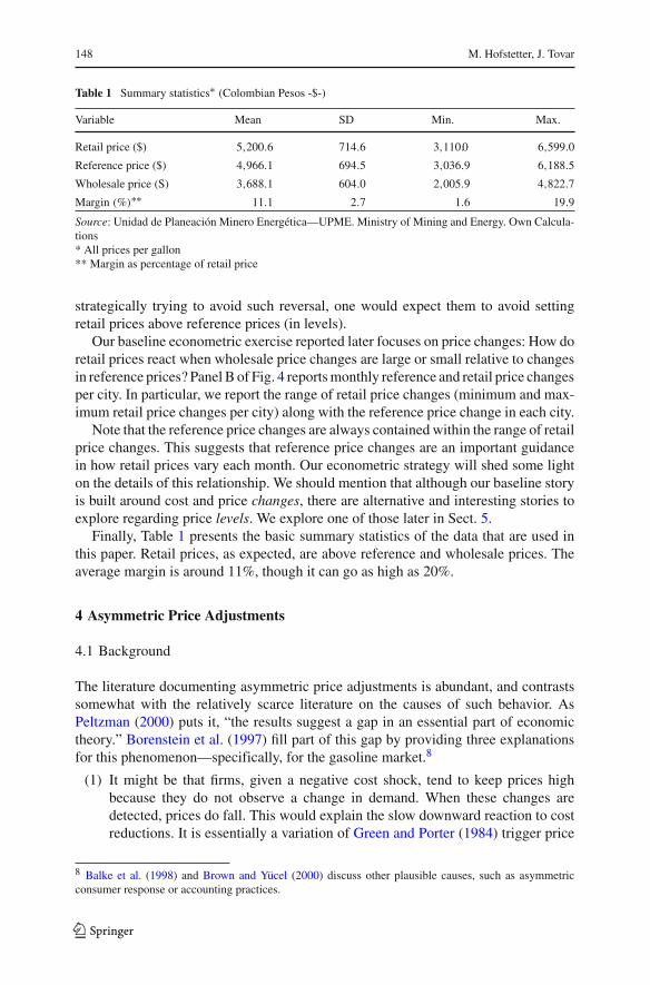
Table 1 Summary statistics∗ (Colombian Pesos -$-)

Variable Mean SD Min. Max.

Retail price ($) 5,200.6 714.6 3,110.0 6,599.0

Reference price ($) 4,966.1 694.5 3,036.9 6,188.5

Wholesale price (S) 3,688.1 604.0 2,005.9 4,822.7

Margin (%)∗∗ 11.1 2.7 1.6 19.9

Source: Unidad de Planeación Minero Energética—UPME. Ministry of Mining and Energy. Own Calcula-tions* All prices per gallon** Margin as percentage of retail price

strategically trying to avoid such reversal, one would expect them to avoid settingretail prices above reference prices (in levels).

Our baseline econometric exercise reported later focuses on price changes: How doretail prices react when wholesale price changes are large or small relative to changesin reference prices? Panel B of Fig. 4 reports monthly reference and retail price changesper city. In particular, we report the range of retail price changes (minimum and max-imum retail price changes per city) along with the reference price change in each city.

Note that the reference price changes are always contained within the range of retailprice changes. This suggests that reference price changes are an important guidancein how retail prices vary each month. Our econometric strategy will shed some lighton the details of this relationship. We should mention that although our baseline storyis built around cost and price changes, there are alternative and interesting stories toexplore regarding price levels. We explore one of those later in Sect. 5.

Finally, Table 1 presents the basic summary statistics of the data that are used inthis paper. Retail prices, as expected, are above reference and wholesale prices. Theaverage margin is around 11%, though it can go as high as 20%.

4 Asymmetric Price Adjustments

4.1 Background

The literature documenting asymmetric price adjustments is abundant, and contrastssomewhat with the relatively scarce literature on the causes of such behavior. AsPeltzman (2000) puts it, “the results suggest a gap in an essential part of economictheory.” Borenstein et al. (1997) fill part of this gap by providing three explanationsfor this phenomenon—specifically, for the gasoline market.8

(1) It might be that firms, given a negative cost shock, tend to keep prices highbecause they do not observe a change in demand. When these changes aredetected, prices do fall. This would explain the slow downward reaction to costreductions. It is essentially a variation of Green and Porter (1984) trigger price

8 Balke et al. (1998) and Brown and Yücel (2000) discuss other plausible causes, such as asymmetricconsumer response or accounting practices.

123


story. In that model, firms, when in equilibrium, restrict output to a level belowthe competitive equilibrium. The price is adjusted—that is, a price war begins—when sales fall below the threshold level.

(2) Given a (sudden and potential) excess of demand, the effect on prices is quicklytransmitted due to the existence of limited inventories and production lags—that is, production is not able to adjust instantly, thus prices increase. On thecontrary, given a (sudden and potential) excess of supply, prices do not fall asquickly due to the existence of production lags and finite inventories—that is,there is an expected though not current excess of available output that can satisfythe market.

(3) Finally, during periods of high volatility, consumers might search less when theyobserve a price change, as they assume it reflects a change in costs rather thana change in margins. This might allow retailers to pass along quickly any costincrease to prices while delaying the transmission of cost decreases.

Eckert (2002) proposes a different explanation. He argues that price asymmetriesmight be explained using Maskin and Tirole (1988) alternating-move price-settingduopoly model. This model predicts a price-cycle equilibrium, with retail prices’being determined by two alternating regimes. The idea is that a price war is estab-lished in the undercutting regime up until the point where it is profitable for a firmto raise prices above the monopoly level. At that point, another undercutting regimestarts.

Rotemberg (2005) state dependent model suggests that firms choose the timing foradjusting prices so that it corresponds with those times when consumers find pricechanges most palatable.

The most common explanation for asymmetric pricing are models based on thesearch hypothesis. Recently, Lewis (2004) developed a theoretical reference pricesearch model, which assumes that consumer’ price expectations are based on observedpast prices.

The idea is that a consumer will not search for alternative retailers if the observedcurrent price is lower than the observed price for previous periods, due to the smallprobability of finding an even lower price. As a result, less consumers search, retailersface a (temporary) inelastic demand, and margins grow. This type of consumer behav-ior implies that when costs rise well above expectations, firms increase prices (thoughnot margins) and consumers will begin searching. On the contrary, when costs fall,firms lower prices, but only enough to prevent consumers from searching. Note thatthe latter implies that when costs fall, margins rise.9

4.2 Results

As mentioned above, the asymmetry we expect to find is conceptually different fromtraditional price asymmetries. We exploit the fact that in Colombia the suggested retailreference price of gasoline is publicly available and heavily advertised every month.Our hypothesis is that consumers’ expectations about the retail price of gasoline are

9 Other recent search related models are discussed in Tappata (2009) and Yang and Ye (2008).

123


Table 2 The number of‘city/months’ with large andsmall cost changes

Source: UPME, own calculations

# Months �SmallC �LargeC �TOTALC

Small/Large 139 140 279

% 49.8 50.2

anchored to the reference price. This generates asymmetric pricing and determines thespeed of retail price adjustments following a cost change.

What kind of an asymmetry would arise? Under the plausible assumption that con-sumers do not observe costs, a rise in costs that is less than the increment of thereference price would allow retailers to quickly transfer the cost increase to prices.In such a situation, consumers would find the retail price increment to be reasonablebased on their expectations. Conversely, if costs increase more than the reference price,retailers will have an incentive to not pass the whole cost increase on to consumers,or at least to delay the increase. Hence, an asymmetry would arise.

When referring to asymmetric price adjustments, then, we have in mind large versussmall increments in the cost relative to the reference price, rather than just positive ornegative cost changes. A large cost change (lc) occurs when wholesale prices increasemore than the reference price. Similarly, a small cost change (sc) refers to smallerincrements in wholesale prices relative to that for the reference price. This is definedon a per month and per city basis.10 Following this definition, Table 2 shows howthe sample is split between large and small changes. The number of observations is279, corresponding to the number of city/month observations that are available. Thisdefinition yields an evenly split sample between large and small cost changes.

Before attempting an econometric estimation of potential price asymmetries, wefirst check a simple corollary of the hypothesis, which is easily testable in our data-set. Our hypothesis states that large cost changes should be accompanied by a slowreaction of prices, while small cost changes should imply a fast price adjustment. As aconsequence, large cost changes should go hand in hand with temporary low margins,while small cost changes should coincide with higher margins.

Table 3 reports simple averages of margins, calculated as the difference betweenretail and wholesale prices, excluding the taxes paid by retailers. This margin is pre-sented as a percentage of the wholesale prices. The results go in the expected direction:Small (large) cost changes are associated with large (small) margins. Moreover, themean margins are statistically different from each other. Nevertheless, the difference isnot economically important. This is not surprising. Margins across retailers and overtime are, potentially, determined by many factors. This exercise is simply describ-ing the data according to a chosen criterion—whether costs change by a large or asmall amount relative to the reference price. The econometric results below expandthe analysis and allow for several relevant controls that this preliminary exerciseignores.

There are several econometric approaches to the problem of estimating asymmetricprice adjustments. Meyer and von Cramon-Taubadel (2004) discuss what they call the

10 Recall that both reference prices and wholesale (regulated) prices are city-specific.

123


Table 3 Mean margin averages for small and large cost changes

Margins (%)∗ �SmallC∗ �LargeC∗ �TOTALC

Mean 10.90% 10.70% 10.80%

N 2,411 2,712 5,123

Source: UPME. Own calculations∗ Relative to (small and large) cost changes between periods t − 1 and t , margins are measured for period t

pre-cointegration approach and the cointegration approach. The basic strategy of theformer is to divide input prices into increasing and decreasing phases, by interactingthem with the appropriate dummy variables. The cointegration approach, on the otherhand, after establishing the long-run relationship between prices and costs, estimateserror correction models for tracking price adjustments to (negative and positive) costshocks. This is the approach followed by Borenstein et al. (1997), and Lewis (2004).

Borenstein et al. (1997) estimate an error correction model wherein, using a one-stage approach, the change in retail prices is explained by the change in costs and alagged error correction term. Bachmeier and Griffin (2003) criticize this approach,arguing that little is known about the finite sample properties of the technique. Lewis(2004) addresses some of these criticisms by using a two-step approach, one thatexplicitly estimates the error correction term in the first stage. In our baseline esti-mation we follow Lewis’ approach. Nevertheless, we check the robustness of ourdecision in Sect. 5, where we show that the results do not differ when using theone-stage approach as proposed by Borenstein et al. (1997).

Equation 1, which corresponds to the first stage of our empirical model, pools thedata by city, and estimates the first step of the error correction model, wherein it istheoretically expected that, over the long run, prices and costs should be related.11 Inparticular, we estimate

Ps,t = φ1Cc,t +212∑

s=1

(ESTs) + φ2t + ηs,t , (1)

where Ps,t stands for the retail price at station s for month t and Cc,t represents thewholesale price in city c during period t . The equation also includes a time trend (t).Station fixed effects (EST) are also included to capture the time-invariant characteris-tics of gas stations, such as location and brand.12 City fixed effects are not includedbecause, recall, wholesale prices are available only at the city level, whereas retail

11 The first stage requires that both retail and wholesale prices be non-stationary, in order to test forcointegration. In the results (not reported here), we find that prices and cost series are non-stationary. Incity-specific cointegration tests between wholesale and average retail prices, we find that there is cointe-gration at a 5% level in about half of the sample. Given the short time span that is covered in our sample(something which makes the identification of cointegration difficult), we interpret the results as indicativeof a long-run relationship between costs and prices, as theory predicts.12 Gas stations might change brands at some point in time. However, in this case, it is an advantage to use asample with a short period of time, as the assumption that brand and other specific gas station characteristicsdo not change is more plausible.

123


Table 4 Estimates of Eq. 1:The price-cost/long-run relation

Source: UPME, own calculations∗∗∗ p < 0.01;∗∗ p < 0.05;∗ p < 0.1

P Coefficient Standarderrors

φ1 C 0.712*** (0.012)

φ2 t 21.608*** (0.425)

N 5,202

Stations 212

R-squared 0.98

prices do vary across stations. The estimates for Eq. 1 generate the error correctionterm (ηs,t−1), which is used during the second stage of the model. The Eq. 1 estimatesare reported in Table 4.

The results in Table 4 show that our estimate of φ1 is 0.71. As in Borenstein et al.(1997), who find a long-run adjustment factor of 0.81, the coefficient is lower thanone. Faced with a similar problem, Lewis (2004), based on a theoretical discussion,decides exogenously to set φ1 equal to one before proceeding to the second stage of theestimation. Following Lewis’ approach we later (in Sect. 5) exogenously set φ1 = 1during the first stage. We find that the main conclusions remain unaltered.

Equation 2 corresponds to the second stage of the error correction model. In par-ticular, we estimate:

�Ps,t =2∑

i=0

(βlc

i �Clcc,t−i + βsc

i �Cscc,t−i

)+

2∑

i=1

(γ lc

i �Plcs,t−i + γ sc

i �Pscs,t−i

)

+ θ lcηs,t−1 + θ scηs,t−1 + εs,t . (2)

The change in prices depends on lagged prices and cost changes, separated accord-ing to the relative size of the cost changes, as discussed above—that is, both thecontemporary and lagged cost changes, as well as the lagged prices are split basedon the large/small cost definition discussed above. Two lags in costs and two lags inprices are included. In the robustness section, we explore whether or not the results aresensitive to the inclusion of additional lags; again we find that the main conclusionsremain unaltered.

The equation also includes the error correction term estimated in Eq. 1. In orderfurther to allow for an asymmetric adjustment, ηs,t−1 is allowed to affect price changesin different ways, depending on whether the costs are large or small (ηlc

s,t−1, ηsc

s,t−1).

This distinction makes the asymmetrical adjustment of prices explicit, and allows fordifferences in the speed at which prices reach their long-run relationship with costs.In results not reported in the paper, we verify the effect of allowing only a single errorcorrection term; our conclusions remain unchanged.

A natural concern when estimating Eq. 2 is the possible endogeneity that arisesfrom retail prices looping back into wholesale prices. Fortunately, this endogeneity isnot present in the Colombian case, inasmuch as wholesale prices are exogenously seton a monthly basis by the government. The main rationale in the strategy for setting

123


Table 5 Estimates of Eq. 2:The large/small cost changes

Source: UPME, own calculations∗∗∗ p<0.01;∗∗ p < 0.05;∗ p < 0.1

�P Coefficient Standarderrors

γlc1 �lcP−1 −0.12701∗∗∗ (0.01957)

γlc2 �lcP−2 0.06319∗∗∗ (0.01942)

γsc1 �scP−1 −0.10343∗∗∗ (0.02274)

γsc2 �scP−2 −0.07242∗∗∗ (0.02222)

βlc0 �lcC 0.87698∗∗∗ (0.01822)

βlc1 �lcC−1 0.25995∗∗∗ (0.02739)

βlc2 �lcC−2 0.06897∗∗∗ (0.02630)

βsc0 �scC 1.26045∗∗∗ (0.05066)

βsc1 �scC−1 0.35496∗∗∗ (0.06444)

βsc2 �scC−2 0.44775∗∗∗ (0.05828)

θlc ηlc−1 −0.20849∗∗∗ (0.01392)

θ sc ηsc−1 −0.22293∗∗∗ (0.01565)

N 4,544

Stations 212

R-squared 0.75904

wholesale prices is to establish a slow convergence towards international oil pricesand, thus, slowly cut oil subsidies. Thus, the wholesale prices are independent of retailprice strategies and internal demand conditions.

The estimated coefficients of Eq. 2, crucial inasmuch as they are the necessaryinputs for obtaining the impulse response functions of prices following cost shocks,are displayed in Table 5.

Following Borenstein et al. (1997), we depict cumulative impulse-response func-tions, tracking the adjustment path of prices given a one-unit change in costs. Themodel allows for different short-run reactions on the part of retail prices, dependingon whether the cost shock was large or small relative to the reference price. Of course,being cumulative, the impulse-response functions converge to the long-run price-costpass-through.13 The complete adjustment process is illustrated in Fig. 5. The plotincludes 95% confidence intervals, calculated using a bootstrap method, to verify thestatistical relevance of the (asymmetric) adjustments.

An asymmetric adjustment of the kind that we hypothesize is recognizable in Fig. 5.The results suggest that if costs rise above the increment in the reference price, retailprices will adjust to a lesser extent than when the opposite is true. If costs rise by 1Colombian peso (COP$), and we assume a reference price increment that is aboveone, retail prices will increase by COP$1.26 a month later. Conversely, if we assumea reference price increment that is smaller than COP$1, a COP$1 increase in costsimplies that, a month later, prices will rise by only COP$0.87.

13 In the long run both functions converge toward the long-run adjustment factor that, as estimated earlier,is 0.71. We test the robustness of this, later in Sect. 5, by forcing the long-run adjustment factor to be one.

123


0

.5

1

1.5

2P

rice

Res

pons

e

0 2 4 6 8 10 12

Months after Initial Cost Change

Large Cost Change Small Cost Change

Cumulative Response of Prices to a $1 Change in Costs (Error Correction Term: LC/SC)Dotted lines are 95% confidence intervalsSource: Unidad de Planeación Minero-Energética - UPME. Ministry of Mining and Energy.Own Calculations

Price lags=2 Cost lags=2

Fig. 5 Impulse response function. Large/small cost changes

Our results suggest that asymmetric pricing is a fact in the Colombian gasolinemarket. In our story, consumers form their expectations based on the reference price.Based on these expectations, consumers decide whether to search or not for better retailprices, and retailers will behave as described in Fig. 5; asymmetric pricing arises.

Cabral and Fishman (2008) argue that, assuming a price increase, consumers willnot search for a better price if they perceive it to be moderate. If, on the contrary,consumers perceive the increase in retail prices to be overly high, they will havean incentive to search. The question is, how can one define empirically what largeand small price increases are? The Colombian market offers us a perfect answer: themonthly and widely publicized reference price. In our case, therefore, we are able tosustain that asymmetric pricing is to a large extent explained by the existence of thisreference price.

An interesting finding is the overshooting of retail prices when cost increases aresmall (relative to changes in the reference price). This result suggests that, very earlyin the process, retail prices increase by more than the expected long-run adjustment.Later on, the price adjusts to the long-run pass-through.

Our empirical strategy, though able to identify the described price asymmetry, isnot designed to uncover the causes of this asymmetry. Nevertheless, as discussedearlier, the literature suggests several explanations for price asymmetries. Some areconsistent with our results and the structure of the gasoline market in Colombia; othersare not.

Green and Porter’s story, as interpreted in this context by Borenstein et al. (1997),does not seem plausible in our case because the trigger price story requires negativedemand shocks and price cycles, which were not observed during our sample period.

Similarly, the inventory argument explaining price asymmetries—that is, that sud-den positive demand shocks quickly raise prices due to limited inventories and pro-duction lags, while sudden positive supply shocks usually imply future but not presentlower prices (again due to production lags and finite inventories)—is based on thepresence of unexpected demand or supply shocks. This is not a plausible argument in

123


this case because: (1) we do not observe sharp changes in demand over the course ofour sample period; and (2) in order for this story to make sense, gas stations wouldhave to regulate inventories, something that is typically not observed.

Eckert (2002) story is not likely to explain our results because in the case studiedin our paper no price cycles were observed, even if defined broadly—that is, relativeto the reference price.

In our view, our results are compatible with at least two theories: First, they areconsistent with Rotemberg (2005) state dependent model. In our case, a large increasein the reference price (relative to costs) is the signal that a change would be palatable,and thus triggers more rapid price adjustments.

Second, our results seem to best fit the search story sketched by Borenstein et al.(1997), and further developed by Lewis (2004), Tappata (2009), Yang and Ye (2008),and Cabral and Fishman (2008). Consumers are potential seekers of better prices, andfirms acknowledge this. The existence of reference prices shape consumers’ expec-tations and determines how quickly cost increases can be passed on to final prices.When costs increase to a greater extent than the reference price, retailers postponethe full adjustment of retail prices to avoid having consumers search out better prices.If no reference price existed, consumers would not necessarily be aware of the rela-tive importance of price increments; hence asymmetric pricing, if present in the data,would require further explanations.

5 Robustness and Extensions

This section tests the robustness of our results and extends the analysis in several direc-tions. In particular, this section reports the results with the following changes relativeto the baseline model: (1) we report the results with four instead of two lags; (2) wereport the impulse response functions following Lewis’ strategy of setting φ1 = 1,

rather than using the estimate from the first stage of the model; (3) we estimate theimpulse response functions using a one-step estimation strategy; and (4) we evaluatewhether retail prices react asymmetrically to cost shocks, with the speed of adjust-ment depending on the relative position of lagged levels of retail prices with respectto reference prices.14

(1) Lag structure: The second stage of our baseline model is estimated using two lagsfor price and cost changes. We check the robustness of our choice by replicatingthe exercise with alternative lag structures. Panel A in Fig. 6 replicates the exer-cise using four lags. We find that the main results remain unaltered. In results thatare not reported, we tried other lag structures and found similar results. Thus,the results are robust for the lag structure used in Eq. 2.

(2) φ1 = 1 : The baseline model follows a two stage approach, wherein the first stageestimates the long-run coefficient linking prices and costs. The value reportedin Table 4 is φ1 = 0.71. Nevertheless, as extensively discussed by Lewis, thetheory suggests that φ1 should be 1. It is conceivable that the coefficient that weobtained is different from the one that is suggested by the theory simply because

14 We thank the editor and one of the referees for suggesting extensions (3) and (4).

123


0

.5

1

1.5P

rice

Res

pons

e

0 2 4 6 8 10 12



Error Correction Term: LC/SC


0

.5

1

1.5

2

Pric

e R

espo

nse

0 2 4 6 8 10 12





0

.5

1

1.5

Pric

e R

espo

nse

0 2 4 6 8 10 12



Single Error Correction Term


0

.5

1

1.5

Pric

e R

espo

nse

0 2 4 6 8 10 12


Retail(t-1)>Reference(t-1) Retail(t-1)<=Reference(t-1)



Cumulative Response of Prices to a $1 Change in CostsDotted lines are 95% confidence intervals

Source: Unidad de Planeación Minero-Energética - UPME. Ministry of Mining and Energy.Own Calculations

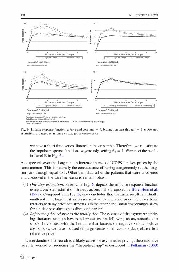
Fig. 6 Impulse response function. a Price and cost lags = 4. b Long-run pass through = 1. c One-stepestimation. d Lagged retail price vs. Lagged reference price

we have a short time-series dimension in our sample. Therefore, we re-estimatethe impulse response function exogenously, setting φ1 = 1. We report the resultsin Panel B in Fig. 6.

As expected, over the long run, an increase in costs of COP$ 1 raises prices by thesame amount. This is naturally the consequence of having exogenously set the long-run pass-through equal to 1. Other than that, all of the patterns that were uncoveredand discussed in the baseline scenario remain robust.

(3) One-step estimation: Panel C in Fig. 6, depicts the impulse response functionusing a one-step estimation strategy as originally proposed by Borenstein et al.(1997). Compared with Fig. 5, one concludes that the main result is virtuallyunaltered, i.e., large cost increases relative to reference price increases forceretailers to delay price adjustments. On the other hand, small cost changes allowfor a quick pass-through as discussed earlier.

(4) Reference price relative to the retail price: The essence of the asymmetric pric-ing literature rests on how retail prices are set following an asymmetric costshock. In contrast with the literature that focuses on negative versus positivecost shocks, we have focused on large versus small cost shocks (relative to areference price).

Understanding that search is a likely cause for asymmetric pricing, theorists haverecently worked on reducing the “theoretical gap” underscored in Peltzman (2000)

123


paper. For instance, Tappata (2009) notes that one plausible explanation, within asearch model framework, is that “prices can vary as a result of a change in consum-ers’ priors. This is an indirect effect that materializes through the variations in searchintensity.”

In this order of ideas, one could think of a potential alternative source of asymmet-ric pricing in the gasoline market in Colombia: the ability of retailers to pass-throughwholesale price increments might depend on whether the retail price in the previousmonth was above or below the reference price. If a retailer was pricing above thereference price in t − 1, the gas station will have less space quickly to pass throughan increase in costs in period t . Similarly, if the retailers’ price in t − 1 was below thereference price, he would be able to pass cost increments faster to consumers.

Panel D reports the impulse response functions based on how retail prices respondto a cost increase depending on where their lagged prices stood relative to the referenceprice. Although the adjustment process is similar to our previous findings, in this casewe do not find any evidence of asymmetric pricing.

Although theoretically reasonable, particularly from a search model point of view,our results suggest that the particular prior that is tested – i.e., lagged retail price rela-tive to the reference price – does not trigger consumers’ search.15 The raw data explainwhy, for Colombia, this is the case. As Fig. 4 notes, retail prices are for the most parthigher than the reference price. In fact, retail prices are higher than the reference pricein 90.3% of the observations. Thus, the fact that consumer priors are not adjusted(i.e., retail prices are always higher) implies that consumers are not motivated tosearch.

6 Concluding Remarks

The objective of this paper was to determine whether the common knowledge of a ref-erence price is associated with asymmetric pricing in a scenario where costs increasethroughout our sample period. In order to test this hypothesis, we used data fromthe Colombian gasoline market where wholesale gasoline prices have consistentlyincreased month by month over the course of our sample period. We exploit the exis-tence of a widely publicized reference price to determine that, even in such a case,asymmetric pricing does exist.

The existence of asymmetric pricing is based on the manner in which consumers’expectations are formed. The reference price—a government suggested (that is, onethat is not mandatory) retail price for gasoline—seems to play a key role in deter-mining whether retailers adjust prices quickly or slowly following a cost increase. Weshow that when the reference price rises more than costs, retailers are able quicklyto pass-through the cost increase to prices. Conversely, if costs rise more than thereference price, retailers delay the pass-through.

15 Note that this robustness exercise only tests within the framework of a search model. However, it doesnot invalidate any other priors embedded in a search model beyond those that are specifically tested – forinstant, the existence of a reference price.

123


The main conclusion is that, under ever-increasing costs, asymmetric pricing doesexist. Our paper suggests that price transparency generates, in a scenario where costsincrease every period, asymmetric price adjustments. This, in turn, suggests thatin certain situations—i.e., when reference price increases by less than costs—thepolicy-maker can affect the impact on prices of a continuous cost increment. Absentthe reference price, retailers would have no incentive to not pass costs changes sys-tematically to prices.

Therefore, a natural extension of our investigation is to test whether in marketswith similar characteristics—for instance, markets with widely publicized “suggestedprices”—price adjustments following cost changes exhibit asymmetries that are sim-ilar to the ones we identified. If so, the existence of asymmetric pricing in a marketwith ever-increasing costs warrants additional theoretical work in order to enhanceour understanding of the causes of such behavior.

Acknowledgments We thank the editor, Lawrence White, and two anonymous referees for helpful com-ments. We also thank Andrés Cardona for his outstanding research assistantship. We are also grateful toUnidad de Planeación Minero Energética (UPME), a Colombian government agency and subsidiary tothe Ministry of Mining and Energy, for providing us with the required data. Finally, participants at theSeminario CEDE and the 2008 Industrial Organization Conference, particularly Matt Lewis, are gratefullyacknowledged. All remaining errors are ours.

References

Bachmeier, L., & Griffin, J. (2003). New evidence of asymmetric gasoline price adjustments. TheReview of Economics and Statistics, 85(3), 772–776.

Balke, N., Brown, S., & Yücel, M. (1998). Crude oil and gasoline prices: An asymmetric relationship.Federal Reserve Bank of Dallas Economic and Financial Policy Review. First Quarter, 2–11.

Brown, S., & Yücel, M. (2000). Gasoline and crude oil: Why the asymmetry? Economic and FinancialReview. Third Quarter, 23–29.

Borenstein, S., Cameron, C., & Gilbert, R. (1997). Do gasoline prices respond asymmetrically to crudeoil price changes?. The Quarterly Journal of Economics, 112, 306–339.

Cabral, L., & Fishman, A. (2008). Business as usual: A consumer search theory of sticky prices andasymmetric price adjustments. Retrieved July 21, 2010 from New York University, Stern Schoolof Business: http://pages.stern.nyu.edu/~lcabral/workingpapers/CabralFishmanAug08.pdf

Cerón, C. (2001). El mercado de distribución de gasolina en Colombia: Un análisis técnico-económicode la estructura de la industria y del comportamiento de los agentes. Mimeo.

Duffy-Deno, K. T. (1996). Retail price asymmetries in local gasoline markets. Energy Economics, 18,81–92.

Eckert, A. (2002). Retail price cycles and response asymmetry. The Canadian Journal of Econom-ics, 35(1), 52–77.

Godby, R., Lintner, A., Stengos, T., & Wandschneider, B. (2000). Testing for asymmetric pricing inthe Canadian retail gasoline market. Energy Economics, 22, 349–369.

González, J. F. (2004). Mercado de combustibles líquidos: Hacia una mayor competencia y transparencia.Asociación Colombiana del Petróleo(ACP), Bogotá, Presentación Foro Expoenergía.

Green, E., & Porter, R. (1984). Non-cooperative collusion under imperfect price information. Econome-trica, LII, 97–100.

Lewis, M. (2004). Asymmetric price adjustment and consumer search: An examination of the retailgasoline market. Dissertation, University of California at Berkeley.

Maskin, E., & Tirole, J. (1988). A theory of dynamic oligopoly II: Price competition, kinked demandcurves and Edgeworth cycles. Econometrica, 56, 571–599.

Meyer, J., & von Cramon-Taubadel, S. (2004). Asymmetric price transmission: A survey. Journal ofAgricultural Economics, 55(3), 581–611.

123

http://pages.stern.nyu.edu/~lcabral/workingpapers/CabralFishmanAug08.pdf


Peltzman, S. (2000). Prices rise faster than they fall. Journal of Political Economy, 108, 466–502.Rotemberg, J. (2005). Customer anger at price increases, changes in the frequency of price adjustment

and monetary policy. Journal of Monetary Economics, LII, 829–852.Tappata, M. (2009). Rockets and feathers. Understanding asymmetric pricing. Rand Journal of Eco-

nomics, 40(4), 673–687.Yang, H., & Ye, L. (2008). Search with learning: understanding asymmetric price adjustments. Rand

Journal of Economics, 39(2), 547–564.

123

Common Knowledge Reference Price and Asymmetric Price Adjustments Evidence from the Retail Gasoline...

Documents

Transcript of Common Knowledge Reference Price and Asymmetric Price Adjustments Evidence from the Retail Gasoline...