Risk Adjustments to the Comparables Range

Reproduced with permission from Tax ManagementTransfer Pricing Report, Vol. 12, No. 05, 07/09/2003.Copyright 2003 by The Bureau of National Affairs, Inc.(800-372-1033) http://www.bna.com

Risk Adjustments to the Comparables Range

BY STEPHEN L. CURTIS

JEAN FRANCOIS RUHASHYANKIKO*

R isk adjustments as conventionally applied mayprovide an acceptable adjustment to the expectedreturns. However, these adjustments may not pro-

vide an appropriate adjustment to the risk itself—thevariance of the expected returns. This article highlightsthat finance theory, supported by empirical findings,may provide a rationale for suitable risk adjustmentsand explains how such adjustments may be performedfor transfer pricing purposes.

The OECD guidelines state: ‘‘In the open market, theassumption of increased risk will also be compensatedby an increase in the expected return.’’1 The guidelinesprovide an example where ‘‘a contract manufacturer orcontract researcher that takes on no meaningful riskwould be entitled to only a limited return.’’2 The U.S.transfer pricing regulations also specify risk adjust-ments in Regs. §1.482-1(d). The regulations provide abrief example of an adjustment for differences in ac-counts payable between the tested party and the com-parables, when each uncontrolled comparable’s operat-ing profit is adjusted downward by the difference in ac-counts payable multiplied by an imputed interest rate

for short-term debt.3 No mention is made regarding theexpected impact on the riskiness of the businesses as aresult of these adjustments to accounts payable and op-erating profits.

At the heart of modern economics lies the assump-tion of risk aversion under which a trader, investor, oragent is willing to bear more risk if there is an appro-priate compensation in terms of expected returns. Theresulting positive risk-return relationship has becomeubiquitous over the years and is embedded in rationalexpectations asset pricing models such as the CapitalAsset Pricing Model, Black-Scholes Option PricingModel, portfolio theories, discounted cash flow analy-ses, and many others.

From an empirical standpoint, Robert Merton firstproposed a linear relationship between the mean andvariance of the market portfolio in 1980.4 While someeconometric studies since have failed to find any mean-ingful predictive relationship between the variance ofreturns and expected risk premia,5 others have, afteraccounting for variables such as consumption-wealthratios, leverage (or asymmetry) effect, and inflation,supported a positive explanatory relationship.6

1 OECD: Transfer Pricing Guidelines for Multinational En-terprises and Tax Administrations, Section 1.23.

2 Ibid., Section 1.25.

3 Regs. §1.482-5(e), Example 5.4 Merton, Robert, ‘‘On Estimating the Expected Return on

the Market: An Exploratory Investigation,’’ Journal of Finan-cial Economics, 8, pp. 323-361.

5 See Campbell, John, ‘‘Stock Returns and the Term Struc-ture,’’ in Journal of Financial Economics, 18 (373-399), andBaille, Richard T., and DeGennaro, Ramon P., ‘‘Stock Returnsand Volatility,’’ Journal of Financial and Quantitative Analy-sis, 25 (June 1990) p. 203-214.

6 See Guo, Hui, Understanding Risk-Return Tradeoff in theStock Market, Federal Reserve Bank of St. Louis, Working Pa-per 2002-001A, and Engle, Robert F., Lilien, David M., andRobins, Russell P., ‘‘Estimating Time Varying Risk Premia in

*Stephen L. Curtis and J.F. Ruhashyankiko,Ph.D., are economists with Ernst & YoungLLP in London.

Copyright � 2003 TAX MANAGEMENT INC., a subsidiary of The Bureau of National Affairs, Inc. ISSN 1063-2069

A TAX MANAGEMENT

TRANSFERPRICING!

This article suggests that the common assumption ofrisk aversion, the widespread use of asset pricing mod-els, and the supporting empirical evidence from equityand industrial markets can be used to perform suitablerisk adjustments to the comparables range, as recom-mended by Section 482 and the OECD guidelines.

Risk-Return Trade-OffThe hypothesized risk-return trade-off is illustrated

in the diagram below. The density function representedby a dashed line represents a higher risk group (per-haps a group of risk-bearing distributors) with an ex-pected return of µ1. As can be seen at the left tail, occa-sionally these distributors earn a loss (point Φ). Thelower risk group (a group of limited risk distributors, or‘LRDs’) has an expected return of µ2. The LRDs havetraded off risk for a lower return. Therefore while theexpected return is lower, it does not vary as much andthey rarely suffer a loss (for illustrative purposes). Asthe diagram illustrates, the business exhibiting thehigher risk also has a higher variation in its expectedreturns (or equivalently a wider range of possible out-comes).

Point Φ could also represent a threshold loss, such asone that would violate loan covenants, or exceed agiven percentage of shareholder equity. Risk is reducedby increasing the number of standard deviations be-tween µ and Φ, made possible by a reduction in the vari-ance of the annual returns (making the business lessvolatile). Given hypothetical values for µ, Φ and σ, wecan see how this occurs: 7

When Φ = 50

µ σ

Coeffi-cient

of Varia-tion

Dis-tance

(µ-Φ)/σ

Prob-abilityof Loss

Φ

Fre-quencyof Loss

Φ

High RiskBusiness

110 50 .46 1.20 11.5% 8.6years

Low RiskBusiness

100 30 .30 1.67 4.75% 21.0years

Table 1a: Example of Adjustment as Advised byU.S. § 482

Assets adjustment: -20

Imputed interest rate: 10%

Implied profit adjustment: -2

Comparablecompany

Sales Assets AdjustedAssets

Profits AdjustedProfits

A 100 100 80 5 3

B 100 100 80 6 4

C 100 100 80 7 5

D 100 100 80 8 6

E 100 100 80 9 7

The following table analyzes the implications on theoperating profit margin and the return on assets (ROA).The advised adjustment reduces the mean operatingprofit margin by 2% from 7% to 5% but leaves the stan-dard deviation (or the inter-quartile range) unchangedat 1.6% and 2% respectively. It is therefore not surpris-ing that no mention is made in Section 482 regardingthe expected impact on riskiness of the business as a re-sult of this adjustment. A closer look, however, suggeststhat an absolute equivalent inter-quartile range arounda lower median actually reflects a greater relative risk.8

To illustrate the point more clearly, the impact on ROAis presented; the advised adjustment reduces the meanROA by 0.7% from 7% to 6.3% but increases the stan-dard deviation by 0.4% from 1.6% to 2% and increasesthe inter-quartile range by 0.5% from 2% to 2.5%.Hence, a smaller expected return is associated withlarger expected variability of return or risk. This resultis counterintuitive.9

Table 1b: Example of Adjustment as Advised by U.S.§482, continued

Comparable company

Operatingprofit

margin

Adjustedoperating

profitmargin

Return onAssets(ROA)

AdjustedROA

A 5.0% 3.0% 5.0% 3.8%

B 6.0% 4.0% 6.0% 5.0%

C 7.0% 5.0% 7.0% 6.3%

D 8.0% 6.0% 8.0% 7.5%

E 9.0% 7.0% 9.0% 8.8%

Mean 7.0% 5.0% 7.0% 6.3%

Standard deviation 1.6% 1.6% 1.6% 2.0%

25th Percentile 6.0% 4.0% 6.0% 5.0%

the Term Structure: The Arch(M) model,’’ in Econometrica, 55(Mar., 1987), pp. 391-407.

7 This approach has been used to study various aspects ofcommercial risk. An excellent example is McCloskey, D.N.,‘‘English Open Fields as Behavior Towards Risk,’’ Research inEconomic History, Vol. 1, (1976), pp. 124-32.

8 Further evidence can be gathered from the coefficient ofvariation (i.e. standard deviation over the mean), which isequal to 0.23 (i.e. 1.6%/7%) before the adjustment and 0.32 (i.e.1.6%/5%) after the adjustment, reflecting a share increase inrelative riskiness.

9 This result is not a mere product of this specific example.It is generated by virtually all common risk adjustments be-cause an equal absolute reduction in operating profit acrosscomparables results in a smaller or larger relative (or propor-tional) impact at the tails. Here, a 0.7% reduction at the mediancomes along with a 1% reduction at the 25th percentile butonly a 0.5% reduction at the 75th percentile. Hence the meanfalls proportionally more than the distance between the bound-aries of the inter-quartile range; this is also valid for any rangeconsidered.

2

7-9-03 Copyright � 2003 TAX MANAGEMENT INC., a subsidiary of The Bureau of National Affairs, Inc. TMTR ISSN 1063-2069

Comparable company

Operatingprofit

margin

Adjustedoperating

profitmargin


AdjustedROA

Median 7.0% 5.0% 7.0% 6.3%

75th Percentile 8.0% 6.0% 8.0% 7.5%

Inter-quartile range 2.0% 2.0% 2.0% 2.5%

The result is counterintuitive because it contradictsthe OECD guidelines, which hold that ‘‘a contractmanufacturer or contract researcher that takes on nomeaningful risk would be entitled to only a limited re-turn.’’ If risk is measured by volatility of the expectedreturns, the adjustment increases risk—contradictingthe general concept of a trade-off between risk and re-turn as discussed above. This is further explained withreference to the Section 482 regulations in Appendix B.

There are two main solutions to solve this counterin-tuitive result: either devise alternative ways of handlingrisk adjustments or complement the advised adjustmentby performing appropriate risk adjustments to the com-parables range. The former approach has been pro-posed in an earlier BNA article;10 this article focuses onthe latter.

The remainder of this article is therefore divided inthree parts. First, it substantiates the counterintuitivenature of the above result by resorting to theoreticaland empirical evidence. Next, it proposes a method toundertake such risk adjustments to the comparablesrange. Finally, it illustrates the mechanics with a nu-merical example.

Equity MarketsA large part of the quantitative evidence for the risk-

return trade-off comes from U.S. equity markets duringthe 20th century. Ibbotson Associates regularly pub-lishes results going back to 1926. These returns areshown below by asset classes for the period 1926-2000.11 The table summarizes the general positive rela-tionship between risks measured by the standard devia-tions and mean returns.12

Table 2: Annual Returns of U.S. Securities 1926-2000

Class Series MeanStandardDeviation

SerialCorrelation

a Micro-Cap Stocks 18.2% 39.3% 0.10

b Ibbotson Small CompanyStocks

16.9% 33.2% 0.07

c Low-Cap Stocks 15.2% 29.9% 0.05

d Mid-Cap Stocks 13.8% 25.1% -0.01

Class Series MeanStandardDeviation

SerialCorrelation

e Large Company Stocks 12.2% 20.5% 0.05

f Long-Term CorporateBonds

6.2% 8.7% 0.08

g Long-Term GovernmentBonds

5.8% 9.4% -0.07

h Intermediate-TermGovernment Bonds

5.6% 5.8% 0.15

i Treasury Bills 3.8% 3.2% 0.91

The density functions of three asset classes (e.g. b, eand f) are shown below and provide a graphical repre-sentation of the empirical relationship between risk andreturn.

It is possible to undertake a more thorough investi-gation of the relationship between risk and return bycomputing the percentage changes in the mean (µ) andthe standard deviation (σ) (as shown in the table below)and running a regression of one against the other. Theregression takes the following form:

The dependent variable is the percentage change inmean returns and the explanatory variable is the per-centage change in standard deviations of returns. Thevariable a β1 represents the multiple of the change inthe expected return investors received between 1926and 2000 for each percentage increase in risk (standarddeviation). The regression was run using the pairs ofdata below, excluding the highest and lowest value of(y/x), which eliminated at least one large outlier.

10 See Urken, P., Barbera, A., and Cole, J., ‘‘Adjusting forDifferences in Risk Levels Between Tested Parties and Compa-rable Firms’’ (12 Transfer Pricing Report 39, 5/14/03),

11 Ibbotson Associates, Stocks, Bonds, Bills and InflationValuation Edition 2003 Yearbook, Chicago: Ibbotson Associ-ates, 2003, Table 2-1, p. 28.

12 The serial correlation indicates the correlation of a vari-able (i.e. equity return) with itself over successive time inter-vals. The observed low serial correlation indicates that the pastprice of equity is a poor predictor of the future price and there-fore indicates a high level of uncertainty, which is correlatedwith the measure of risk adopted in the article (i.e. standarddeviation).

µ µ µ β β σ σ σ ε2 1 2 0 1 2 1 2−( ) = + −( ) +/ /

3

TAX MANAGEMENT TRANSFER PRICING REPORT ISSN 1063-2069 BNA TAX 7-9-03

Table 3: Percentage Changes in Mean and StandardDeviation 13

Mean (x) Standard Deviation (y)

(a-b)/a 0.07 0.16

(b-c)/b 0.10 0.10

(c-d)/c 0.09 0.16

(d-e)/d 0.12 0.18

(e-f)/e 0.49 0.58

(f-g)/f 0.06 -0.08

(g-h)/g 0.03 0.38

(a-c)/a 0.16 0.24

(a-d)/a 0.24 0.36

(a-e)/a 0.33 0.48

(a-f)/a 0.66 0.78

(a-g)/a 0.68 0.76

(a-h)/a 0.69 0.85

(b-d)/b 0.18 0.24

(b-e)/b 0.28 0.38

(b-f)/b 0.63 0.74

(b-g)/b 0.66 0.72

(b-h)/b 0.67 0.83

(c-e)/c 0.20 0.31

(c-f)/c 0.59 0.71

(c-g)/c 0.62 0.69

(c-h)/c 0.63 0.81

(d-f)/d 0.55 0.65

(d-g)/d 0.58 0.63

(d-h)/d 0.59 0.77

(e-g)/e 0.52 0.54

(e-h)/e 0.54 0.72

(f-h)/f 0.10 0.33

The results (with t-statistics in parenthesis) indicatethat each percentage increase in the standard deviationof returns translate into an almost one-to-one percent-age increase in returns. Indeed, the β1 coefficient is sta-tistically non-significantly different from 1 at the 1%level.14

Note that to have confidence that these results werenot arrived at by chance, we would need to subject eachset of results to a test against the others using a hypoth-esis test for the difference between two populationmeans. This test is performed in Appendix A.

It may also be useful to compare correlations be-tween first differences (annual returns) of each class ofsecurities. To the extent that first differences (as well aslevels) are uncorrelated, this would lend support to theidea that a) the markets are not close substitutes, and b)distinct and separate investor classes exist, presumablysegmented by risk (as opposed to transaction costs orcommon influences). A correlation matrix is also pre-sented in Appendix A.15

The overall goodness of fit is given by the coefficientof determination, R2= 0.914. There is a reasonably

strong evidence of a positive linear relationship be-tween risk and return in equity markets. The regressionresults are presented in Appendix C.

Industrial MarketsAs shown above, the hypothesized relationship be-

tween risk and return is generally verified in equitymarkets. The essential question is whether the insightsfrom equity markets can be used to perform risk adjust-ments for transfer pricing purposes. Several examples,corroborated by years of experience in transfer pricing,indicate why these insights are useful under a broad setof circumstances.

The first example draws directly from an earlier BNATax Management article, which considered 20 originalequipment manufacturers (OEM) and seventeen con-tract manufacturers (CM) in the electronics industry: 16

Table 4: Risk Return in Electronic Industry in1994-1996 (using three-year averages)

Gross Profits OEM CMOEM /

CM β1

Mean 36.75 17.66 2.08 1.02

Standard Deviation 15.65 7.68 2.04

OEM CM

Distancefrom

Median:OEM

Distancefrom

Median:CM

25th Percentile 21.81 11.88 16.93 5.18

Median 38.74 17.06 0 0

75th Percentile 49.55 23.03 10.81 5.97

Within this sample the expected return of an OEM istwice as large as the expected return of a CM. The re-sulting a β1 coefficient is very close to the correspond-ing coefficient in the equities markets. The table abovealso shows that the risk may be either measured interms of standard deviation, as is common in financialmarkets, or in terms of range (or distance from me-dian), as is common in transfer pricing, without affect-ing the positive relationship between risk and returns.

A second example of risk-return trade-off is given bythe choice between fixed and adjustable mortgage ratesin property markets. With adjustable rates borrowerscan pay less interest if they are ready to bear some ofthe risk resulting from changes in interest and borrow-

13 Treasury bills were excluded because they exhibited se-rial correlation, resulting in bias in the measurements betweenthe means and standard deviations between asset classes.

14 The intercept is near zero and statistically non-significantly different from zero at the 1% level.

15 See Johnston, J. and DiNardo, J., Econometric Methods,4th ed., New York: McGraw Hill, 1997, pp. 9-12, and Stigler, G.and Sherwin, R., ‘‘The Extent of the Market,’’ Journal of Lawand Economics, vol. 28, (Oct., 1985) pp. 555-585.

16 See Goldzai, E., and Fouts, P., ‘‘Testing Profitability inthe Electronics Industry: Contract Manufacturers VersusOriginal Equipment Manufacturers’’ (8 Transfer Pricing Re-port 3/25/98).

4


ing rates. The lender in turns receives a smaller returnfor bearing less risk.

A third example of risk-return trade-off lies at theheart of corporate finance and the choice between theissuance of debt versus equity. Debt places all liquidityrisk with the borrowing firm, which must incur a cashoutflow to pay interest whether it makes a profit or not.Under an equity option, the firm shares risk with its eq-uity holders. If a loss is incurred, the equity holders ex-perience a reduction in their investment. When profitsarise, however, the equity holders would expect agreater return than the debt holders to compensate fortheir greater risk.

Risk AversionThere are countless other examples of risk-return

trade-offs. The underlying ‘‘truth’’ rests with the as-sumption of risk aversion, which holds that when fac-ing choices with comparable returns, agents tend tohave a preference for certainty, choosing the less-risky(i.e., lower standard deviation) alternative, a construc-tion that economists owe largely to Economics NobelPrize Laureates Milton Friedman and Leonard J. Sav-age.17 The resulting positive risk-return (or mean-standard deviation) relationship underpins most resultsin modern finance.

Another influential Economics Nobel Prize laureate,Paul Samuelson, has recommended an economic treat-ment of the mean-standard deviation issues as one of‘‘probabilistic choice’’.18 Under such treatment a per-son’s risk aversion (or indicator of ordinal preferenceover stochastic prospects) can be modeled as a utilityfunctional indicator. Samuelson showed that risk aver-sion is consistent with utility maximization and thatsuch a relationship could be modeled using the meanand standard deviation under a linear positive relation-ship.

Since such a linear positive relationship between themean and standard deviation is widely used, valid un-der a broad set of circumstances (i.e., risk aversion orutility maximization) and supported by some empiricalevidence in both equity and industrial market, it pro-vides a solid basis for risk adjustments to the compa-rables range, as described below.

Risk Adjustments to the Comparables RangeThe theoretical and empirical evidence supports a

linear positive risk-return relationship. As indicated, thereturn and the risk can be measured by the mean andthe standard deviation, respectively. In transfer pricing,standard deviations are seldom used whereas the use of(inter-quartile) ranges are nearly universal. There isone situation where a close link between standard de-viations and ranges exists: when the distribution ofcomparable returns is normally distributed. Therefore,normal distributions provide the starting point of themethod of risk adjustments to the comparable range.Then, it is possible to check simple conditions to test

whether the distribution of comparable returns is ‘‘closeenough’’ to a normal distribution and risk adjustmentsto the comparables range are meaningful. It follows thatwhile a normal distribution provides a useful reference,it is by no means the only distribution under which suchadjustments can be performed.

Normal distributions are a family of distributionsthat have the same general shape. They are symmetric(i.e., skewness = 0) with values more concentrated inthe middle than in the tails (i.e., kurtosis = 3). Normaldistributions are sometimes described as bell shaped.Examples of normal distributions are shown below:

Notice that while the distributions differ in howspread out they are, the area under each curve is thesame. The height of a normal distribution can be speci-fied mathematically in terms of two parameters: themean (µ) and the standard deviation (σ). The height (or-dinate) of a normal curve is defined as: 19

If the mean and standard deviation of a normal dis-tribution are known, it is easy to figure out the percen-tile rank of a comparable company with a specific re-turn. The conversion between standard deviation andrange is displayed below.

Table 5: Standard Deviation vs. Range

Standarddeviationsfrom mean

Cumulativefrequency

Percentage of observations withinrespective range

2–sigma 4–sigma 6–sigma

-3 0,0013

-2.5 0.0062

-2 0.0227

-1.5 0.0668

-1 0.1587

-0.5 0.3085

0 0.5000 0.6826 0.9545 0.9974

0.5 0.6915

1 0.8413

1.5 0.9332

2 0.9772

17 Friedman, Milton, and Savage, L.J., ‘‘The Utility Analysisof Choices Involving Risk,’’ The Journal of Political Economy,Vol. 56, 4 (Aug., 1948), pp. 279-304.

18 Samuelson, Paul A., Foundations of Economic Analysis,Vol. 80, Cambridge: Harvard University Press, 1983, pp. 503-519.

19 where µ is the mean and σ is the standard deviation, π isthe constant 3.14159, and e is the base of natural logarithmsand is equal to 2.718282. The observation x can, in principle,take on any value from -infinity to +infinity. The value of y isvery close to 0 if x is more than three standard deviations fromthe mean (less than -3 or greater than +3).

y ex

=−

1

2 22

2

2

πσ

µσ

( )

5


Standarddeviationsfrom mean

Cumulativefrequency

Percentage of observations withinrespective range

2–sigma 4–sigma 6–sigma

2.5 0.9938

3 0.9987

The table indicates that, under a normal distribution,about 68% of the observations of comparable returns liewithin two standard deviations (i.e., 2-sigma) from themean, about 95% of the observations of comparable re-turns lie within four standard deviations (i.e., 4-sigma)from the mean and about 99% of the observations ofcomparable returns lie within six standard deviations(i.e., 6-sigma) from the mean. Since an inter-quartilerange covers 50% of the observations around the me-dian, this corresponds to a value between one and twostandard deviations from the mean.

The table below illustrates this fact by revisiting theinitial example that illustrated the adjustment as ad-vised by Section 482.

Table 6: Example under Normal Distribution—AdvisedMean Adjustment

Operatingprofit

margin

Adjustedoperating

profitmargin


AdjustedROA

Mean 7.0% 5.0% 7.0% 6.3%


-1σ 5.4% 3.4% 5.4% 4.3%

-0.63σ (= 25th

Percentile)6.0% 4.0% 6.0% 5.0%

-0.5σ 6.2% 4.2% 6.2% 5.3%

0 (= Median = Mean) 7.0% 5.0% 7.0% 6.3%

+0.5σ 7.8% 5.8% 7.8% 7.3%

+0.63σ (= 75th

Percentile)8.0% 6.0% 8.0% 7.5%

+1σ 8.6% 6.6% 8.6% 8.3%


In the example above, the value of the standard de-viations (as well as the inter-quartile ranges) are thesame as before the adjustment and the counter-intuitiveresult remains. Under a normal distribution the mean isequal to the median and, given the parameters of theexample, the 25th and 75th percentile correspond to±0.63σ or 1.26-sigma.

Under a normal approximation, the frequency distri-bution of the results above would be expected to appearas depicted below. Under such a distribution there are5% of type A companies, 24% of type B, 40% of type C,24% of type D and 5% of type E. These frequencies,which capture the height of a normal distribution, areshown below.

The evidence allowed isolating a key finding whichdescribes the relationship between the mean and thestandard deviation as:20

Since the percentage change in the operating margin(before and after adjustment) is -29% (i.e. (5% - 7%)/

7%), the standard deviation of the operating marginmust be adjusted by -29% from 1.6% to 1.1%. Likewise,the percentage change in the ROA (before and after ad-justment) is -10% (i.e., (6.3% - 7%)/7%), the standard de-viation of the ROA must be adjusted by -10% from 1.6%to 1.4%. The following table highlights the changes.

Table 7: Example of Risk Adjustment under NormalDistribution

Operatingprofit

margin

Adjustedoperating

profitmargin


AdjustedROA

Mean 7.0% 5.0% 7.0% 6.3%


-1σ 5.4% 3.9% 5.4% 4.9%

-0.63σ (= 25th

Percentile)6.0% 4.3% 6.0% 5.4%

-0.5σ 6.2% 4.4% 6.2% 5.6%

0 (= Median = Mean) 7.0% 5.0% 7.0% 6.3%

+0.5σ 7.8% 5.6% 7.8% 7.0%

+0.63σ (= 75th

Percentile)8.0% 5.7% 8.0% 7.2%

+1σ 8.6% 6.1% 8.6% 7.7%


The post-adjustment means are the same as beforebut the standard deviations as well as the (inter-quartile) ranges now reflect the difference in risk.Hence, the counter-intuitive result vanishes. Indeed, acompany that holds fewer inventories is expected toearn a lower return (due to the reduction in assets heldand elimination of related functions) with greater cer-tainty. This reduction in risk is reflected in the reducedstandard deviations and smaller predicted inter-quartileranges (matching the intuition provided earlier, since asmaller σ increases the distance in standard deviationsbetween µ and Φ).

In practice, the comparable returns may not alwaysbe normally distributed. As a matter of fact, when thenumber of comparable companies is small, the compa-rable returns are generally not strictly normally distrib-uted. However, the closer the distribution is to a normaldistribution the greater the confidence in the risk ad-justments to the comparables range. Fortunately, thedistribution tends to converge toward a normal distri-bution as the number of observations increases. In anycase, the practical conditions detailed below seek to de-termine how close the distribution is to a normal distri-bution.

20 This is due to the fact that ß0 and ß1 in the regressionwere found to be statistically non-significantly different fromzero and one, respectively.

µ µ µ σ σ σ2 1 2 2 1 2−( ) ≈ −( )/ /

6


Test 1: Skewness & KurtosisThe first test consists of a visual inspection of the

skewness (which describes the symmetry of a distribu-tion) and kurtosis (which describes the relativepeakedness/flatness of a distribution).21 As a reminder,normal distribution is symmetric (i.e., skewness = 0)with values more concentrated in the middle than in thetails (i.e., kurtosis = 3). These moments are includedinto standard summary statistics that can easily be gen-erated by Excel (or any statistical package).

Table 8: Example Under Normal Distribution

Summary Statistics

Mean 7%

Standard Error 0.8%

Median 7%

Mode 7%

Standard Deviation 1.6%

Sample Variance 0.03%

Kurtosis 2.98

Skewness 0

Range 0.048

Minimum 0.046

Maximum 0.094

Sum 7.2

Count 100

Confidence Level @ 95% 2%

It can be verified that all of the summary statisticsare consistent with the example used so far. The valueof skewness and kurtosis (as well as the equality be-tween mean, median and mode) support the fact thatthe distribution of returns in the above example isclearly normally distributed.

Test 2: Goodness of FitA standard test for normality is the goodness of fit.

The goodness of fit is in fact a formal test of normality,which determines the null hypothesis, based on a χ2

(chi-squared) test for the normal approximation. Thetest compares the distribution of the observed resultswith that of the expected results if the distribution wasnormal. The null hypothesis of a normal distribution isaccepted when the test statistic is less than the criticalvalue.

The test statistic is:22

where O represents the number of actual observa-tions, E represents the number of expected observa-

tions and the index i represents the number of each cat-egory.

The critical value is found by looking up the valuespecified in a chi-squared table with entries (k-1) and α,where k is the number of categories and α represents(1-confidence level). For our purposes we will use k = 6and α = 0.1. Hence, the critical value is χ2

k-1=5, α=0.1 =9.24.

The six categories represent .5σ increments of theNormal distribution. So once the range is known, thecategories can be created based on the mean, standarddeviation, and the normal approximation. Such a tablewould look as follows:

Table 9: Goodness of Fit to Approximate a NormalDistribution

#Standarddeviations

Expectednumber of

observations (E)

Observednumber of

observations (O) (0-E)2/E

a <µ -1.5σ (n/2) - (b) - (c)

b µ -1σ (.95-.68) x (n/2)

c µ.-.5σ .68 x (n/2)

d µ +.5σ .68 x (n/2)

e µ +.1σ (.95-.68) x (n/2)

f >µ +.1.5σ (n/2) - (d) - (e)

_____

χ2

_____

The sum of the last column gives the χ2 test statistic,which should be compared to the critical value. Test 2is not necessary if Test 1 is satisfied but useful other-wise.

Issue: Small Sample Sizes23

The normal approximation to the frequency distribu-tion can typically be used without serious error whenthe sample size is greater than 20, given an acceptablegoodness of fit.24 Given some samples sizes may befewer than 20, the following confidence interval testsshould provide an adequate level of reliability with re-spect to the assumption of normality.

Issue: Chi-Squared TestThe Chi-squared test of the goodness of fit of a nor-

mal distribution will always give a small value of thetest statistic when the sample sizes are sufficientlylarge.25 This results in the problem of accepting an as-sumption of normality, when the underlying distribu-tion may not be normal (and thus the true mean may bedifferent from that observed in the sample). The Chi-squared test is thus a very weak test of normality. Be-cause of the typically small sample sizes observed intransfer pricing situations, a stronger test such as thosedesigned for large samples, would not be appropriate.Therefore this test clearly only tries to set a lowerbound on the ability to apply the adjustment—nothingmore.

The weakness of the Chi-squared test can be over-come by the use of confidence intervals.26 A positiveChi-squared goodness of fit test will be overcome by the

21 In statistical terms, the mean (like the median or mode)is the first moment of the distribution; the variance (or stan-dard deviation) is the second moment; the skewness is thethird moment; and the kurtosis is the fourth moment. A nor-mal distribution is entirely described by its first two momentssince skewness and kurtosis are invariably equal to (or non-significantly different from) zero and three, respectively.

22 Newbold, Paul, Statistics for Business and Economics,New Jersey: Prentice Hall, 1995, p. 407.

23 M.G. Bulmer, Principals of Statistics, New York: DoverPublications, 1979, p. 139.

24 Ibid., p. 134.25 Ibid., pp. 166-167.26 Ibid., p. 167.

χ 22

1=

−( )=∑

O E

Ei i

iik

7


90% CI when the sample size is too small, given thesample variance. Thus an interval estimation test whencompared to the interquartile range, may provide athreshold below which the adjustment cannot be made,given an otherwise positive Chi-squared test.

Test 3: Confidence Interval (CI)Under a normal distribution, the inter-quartile range

sits within 2-sigma (or two standard deviations) fromthe mean (ie ±1σ). The goodness of fit consideredwhether the distribution of comparables could be ap-proximated by a normal distribution by considering arange of 3-sigma (or three standard deviations) fromthe mean (ie ±1.5σ).

This third test considers whether there is a 90% con-fidence that the population mean is in the CI, which de-scribes a range of just under 2x-sigma (or 2x standarddeviations) from the mean where27

As the number of observations increases, the confi-dence interval narrows and the likelihood of obtaininga normal distribution increases. Comparing the result-ing CI with the inter-quartile range determines whetherthere are sufficient comparable companies (i.e., obser-vations) to gain confidence in the risk adjustment to thecomparables inter-quartile range. Failure to pass this fi-nal test would somewhat weaken the confidence in therisk adjustment to the comparables inter-quartile rangeand would require finding additional comparables.

Like skewness and kurtosis, the CI is easily gener-ated by most statistical packages; see bottom line of thesummary statistics table.

Numerical Example

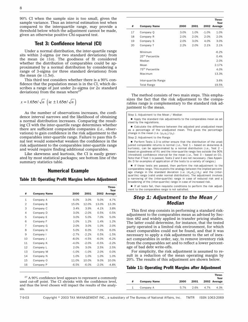
Table 10: Operating Profit Margins before Adjustment

# Company Name 2000 2001 2002

Three-Year

Average

1 Company A 6.0% 3.0% 5.0% 4.7%

2 Company B 15.0% 12.0% 13.0% 13.3%

3 Company C 3.4% 3.9% 4.1% 3.8%

4 Company D 3.0% -2.0% 0.5% 0.5%

5 Company E 3.0% 5.0% 7.0% 5.0%

6 Company F 1.0% 1.2% 1.4% 1.2%

7 Company G 2.0% 3.0% 1.0% 2.0%

8 Company H 5.0% 6.0% 7.0% 6.0%

9 Company I -2.7% -2.2% 0.5% -1.5%

10 Company J -8.0% -4.5% -6.0% -6.2%

11 Company K -4.0% -2.0% -0.5% -2.2%

12 Company L 2.0% 3.0% 2.5% 2.5%

13 Company M -1.0% -1.0% 2.0% 0.0%

14 Company N 1.0% 1.0% 1.0% 1.0%

15 Company O 11.0% 10.0% 9.0% 10.0%

16 Company P -6.5% -6.0% -2.0% -4.8%

# Company Name 2000 2001 2002

Three-Year

Average

17 Company Q 3.0% 1.0% -1.0% 1.0%

18 Company R 2.0% 2.0% 2.0% 2.0%

19 Company S 2.0% 3.0% 4.0% 3.0%

20 Company T 2.2% 2.0% 2.1% 2.1%

Minimum -6.2%

25th Percentile 0.4%

Median 2.0%

Mean 2.17%


Maximum 13.3%

Inter-quartile Range 3.6%

Total Range 19.5%

The method consists of two main steps. This empha-sizes the fact that the risk adjustment to the compa-rables range is complementary to the standard risk ad-justment to the mean.

Step 1: Adjustment to the Mean / Median

s Apply the standard risk adjustments to the comparables mean as ad-vised by the regulations.

s Calculate the difference between the adjusted and unadjusted meanas a percentage of the unadjusted mean. This gives the percentagechange in the mean (i.e. (µ2-µ1)/µ2).

Step 2: Adjustment to the Range

s Perform Tests 1-3 to either ensure that the distribution of the unad-justed comparable returns is normal (i.e., Test 1 – based on skewness &kurtosis), can be approximated by a normal distribution (i.e., Test 2 –based on goodness of fit) and the inter-quartile range lies outside the 90%(threshold) confidence interval for the mean (i.e., Test 3 – based on CI).Note that if Test 1 is passed, Tests 2 and 3 are not necessary. (See Appen-dix D for examples of application of the tests to a variety of ranges.)

s If these tests are passed, then perform the risk-adjustment to thecomparables range. This exploits the analogy between the implied percent-age change in the standard deviation (i.e. (σ2-σ1)/σ2) and the (inter-quartile) range (valid under normal distribution). The adjustment involvesa narrowing of the (inter-quartile) range in case of reduced risk and abroadening of the (inter-quartile) range in case of increased risk.

s If all tests fail, then requisite conditions to perform the risk adjust-ment to the comparables range is not satisfied.

Step 1: Adjustment to the Mean /Median

This first step consists in performing a standard risk-adjustment to the comparables mean as advised by Sec-tion 482 and widely applied in transfer pricing studies.The latter could determine, for instance, that the testedparty operated in a limited risk environment, for whichexact comparables could not be found, and that it wasnecessary to apply a risk adjustment to the set of inex-act comparables in order, say, to remove inventory riskfrom the comparables set and to reflect a lower percent-age of bad debt write-offs.

For simplicity, the risk adjustment is assumed to re-sult in a reduction of the mean operating margin by20%. The results of this adjustment are shown below.

Table 11: Operating Profit Margins after Adjustment

# Company Name 2000 2001 2002

Three-Year

Average

1 Company A 5.7% 2.6% 4.7% 4.3%

27 A 90% confidence level appears to represent a commonlyused cut-off point. The CI shrinks with the confidence level,and thus the level chosen will impact the results of the analy-sis.

x n n= ±( )1 65 1 65. / . /σ σie

8


# Company Name 2000 2001 2002

Three-Year

Average

2 Company B 15.0% 11.9% 12.9% 13.2%

3 Company C 3.0% 3.5% 3.7% 3.4%

4 Company D 2.6% -2.6% 0.0% 0.0%

5 Company E 2.6% 4.7% 6.7% 4.7%

6 Company F 0.5% 0.7% 0.9% 0.7%

7 Company G 1.6% 2.6% 0.5% 1.6%

8 Company H 4.7% 5.7% 6.7% 5.7%

9 Company I -3.3% -2.8% 0.0% -2.0%

10 Company J -8.7% -5.1% -6.7% -6.9%

11 Company K -4.6% -2.6% -1.0% -2.7%

12 Company L 1.6% 2.6% 2.1% 2.1%

13 Company M -1.5% -1.5% 1.6% -0.5%

14 Company N 0.5% 0.5% 0.5% 0.5%

15 Company O 10.8% 9.8% 8.8% 9.8%

16 Company P -7.2% -6.7% -2.6% -5.5%

17 Company Q 2.6% 0.5% -1.5% 0.5%

18 Company R 1.6% 1.6% 1.6% 1.6%

19 Company S 1.6% 2.6% 3.6% 2.6%

20 Company T 1.8% 1.6% 1.7% 1.7%

Minimum -6.9%

25th Percentile -0.1%

Median 1.6%

Mean 1.74%


Maximum 13.2%

Inter-quartile Range 3.8%

Total Range 20.1%

As expected the mean is reduced by 0.43% from2.17% to 1.74%; this corresponds to a reduction of themean operating margin by 20%. Similarly the median isreduced by 0.4% from 2.0% to 1.6%. However, the inter-quartile range increases by 0.2% from 3.6% to 3.8% andthe total range increases by 0.6% from 19.5% to 20.1%.As mentioned earlier, this result is counterintuitive.

This result may also have far-reaching implicationsfor the tested party and the application of the arm’s-length principle. If the tested party operates in a limitedrisk environment, then one would not expect to observelarger yearly swings in operating profit margins thanthose experienced by comparable companies. Therange is therefore expected to be narrower but noteliminated. An arm’s-length limited risk environmentshould therefore be consistent with a narrower range asobtained by the adjustment below.

Step 2: Adjustment to the Range

Test 1: Skewness & KurtosisAs indicated above, this first test can readily be

checked by producing the standard summary statisticsfor the operating profit margins before adjustment.

Table 12: Numerical Example before Adjustment

Summary Statistics

Mean 2.17%

Standard Error 1.0%

Median 2.0%

Summary Statistics

Mode 2.0%

Standard Deviation 4.5%

Sample Variance 0.2%

Kurtosis 1.41

Skewness 0.59

Range 20%

Minimum -6%

Maximum 13%

Sum 43%

Count 20

Confidence Level at 90% 1.73%

Compared to a normal distribution, the distributionof operating margins for comparable companies Athrough T is slightly skewed to the right (i.e., skewness> 0, corroborated by the fact that the mean is greaterthan the median and mode) and is more peaked (i.e.,kurtosis < 3). Although, this distribution is not exactlyNormal it might be ‘‘close enough’’ to perform the riskadjustment to the comparables range. In order to gaingreater confidence on the validity and reliability of themethod, it is worth undertaking the second test.

Test 2: Goodness of FitUnder this test the null hypothesis of a normal distri-

bution is accepted when the test statistic is less than thecritical value. As already computed, the critical value isχ2

k-1=5, α=0.1 = 9.24. As can be seen in the table above,the count is 20, meaning that there are 20 comparablecompanies A through T in the sample; thus n = 20. Thestandard deviation and the ranges to determine the ob-served number of observations refer to the data beforeadjustment.

Table 13: Goodness of Fit before Adjustment

Standarddeviations

Expected number ofobservations (E)

Observed number ofobservations (O) (0-E)2/E

a <µ -1.5σ (n/2) - (b) - (c) =1 From -4.5% to -2.3% :2 1

b µ -1σ (.95-.68) × (n/2) =3 From -2.3% to -0.6% :2 .33

c µ -.5σ .68 × (n/2) =6 From -0.6% to 2.17% :7 .167

d µ -.5σ .68 × (n/2) =6 From 2.17% to 4.41% :4 .67

e µ -.1σ (.95-.68) × (n/2) =3 From 4.41% to 6.65% :3 0

f >µ +.15σ (n/2) - (d) - (e) =1 From 6.65% to 8.88% :2 1

χ2 3.17

Since the test statistic is 3.17 and is less than thecritical value 9.24, the normal distribution cannot be re-jected at 10% level of significance (or 90% level of con-fidence). Although the distribution of operating mar-gins for comparable companies A through T is not ex-actly normal it is found ‘‘close enough’’ to perform therisk adjustment to the comparables range.

Test 3: Confidence Interval (CI)As indicated above, n = 20, therefore the CI is equal

to ±1.65σ/√20 = ±0.37σ or about ±1.73%, as shown in thebottom line of the summary statistics table. Therefore,there is a 90% confidence that the population mean iswithin the following range: µ ± 0.37σ = 2.17% ± 1.73%;that is the CI gives a range from 0.44% to 3.9%.

9


Comparing this CI with the inter-quartile range be-fore adjustment of 0.04% to 4% allows confidence in therisk adjustment to the comparables inter-quartile range.There is a 90% level of confidence that the populationmean is within the inter-quartile range. Hence, thereare sufficient observations to have confidence in therisk adjustment to the comparables range.

The adjustments to the range involve reducing thedistance between the upper quartile and the mean be-fore the adjustment, and the distance between the lowerquartile and the mean before adjustment. These dis-tances are simply multiplied by (1-percentage reductionin the mean) or (1-20%) = .8. The same process is ap-plied to the distance between the endpoints of the rangeand the mean before adjustment.

Table 14: Risk Adjustments

Before anyadjustments

Aftermean

adjustment

%changein themean

Afterrange

adjustmentBefore& After

Minimum -6.2% -6.9% -4.9% 1.2%

25th Percentile 0.4% -0.1% 0.3% -0.1%

Median 2.0% 1.6% -0.4%

Mean 2.17% 1.74% -20% -0.43%

Before anyadjustments

Aftermean

adjustment

%changein themean

Afterrange

adjustmentBefore& After

75th Percentile 4.0% 3.6% 3.2% -0.8%

Maximum 13.3% 13.2% 10.7% -2.7%

Inter-quartileRange

3.6% 3.8% 2.9% -0.7%

Total Range 19.5% 20.1% 15.6% -3.9%

The main premise and insight of the risk adjustmentto the comparables range is to eliminate the counterin-tuitive result whereby a lower mean return is associatedwith a larger risk (i.e., range, which increases from19.5% to 20.1%). After the range adjustment (i.e., fourthcolumn) a lower mean return is associated with a lowerrisk (i.e., range). The ‘‘before and after’’ column con-firms that the ranges are reduced by about 20% (i.e.,-0.7%/3.6% or -3.9%/19.5%)28 in accordance with theevidence presented in this article.

The results are shown graphically below.

28 It is important to keep in mind that the range adjustmentis performed on the initial distribution, before any adjust-ments.

10


11


ConclusionStandard risk adjustments as recommended by the

OECD guidelines and Section 482 regulations defy eco-nomic intuition. This article reviewed the theoreticaland empirical evidence to validate this claim. Underthis process a key finding was uncovered: there appearsto be a positive linear relationship (almost one-to-one)between changes in risk (measured by standard devia-tion) and changes in expected returns.

Because this finding was found to be valid under abroad set of circumstances (i.e., risk aversion or utilitymaximization) and supported by some empirical evi-dence in both equity and industrial markets, it was usedto devise a method to undertake risk adjustments to thecomparables range which was then illustrated througha numerical example. The applicability of the method isfairly general and should provide an essential tool tomap the risk environment under which the tested partyoperates onto an arm’s-length risk-adjusted range.

12


Appendix A

Test For Difference Between Two PopulationMeans

To be able to use the Ibbotson data as a vector ofrelative risk aversion, it is important to be able to con-firm the assumption that each result indeed representsa different investor population, and not different loca-tions within the distribution of a single population. Inother words, it is important to know whether any of theobserved differences could easily have been arrived atby chance. The test used to provide this reliability is thetwo-population hypothesis test, performed on eachpair-wise combination of returns.29

The null hypothesis states that the difference be-tween the sample means is statistically insignificant(e.g., the two samples were actually drawn from thesame population and any differences in the means werearrived at by chance). The alternative hypothesis statesthat the sample means are indeed different (i.e., indi-cate two separate populations with different means) ata specified level of statistical significance. Therefore:

Using a significance level of 95% (α = .05), the teststatistic = zα/2 = z.025 = 1.96 (two-tailed test). The nullhypothesis will be rejected if the test statistic is greaterthan 1.96 or less than -1.96 (indicating the results beingcompared each came from a different population).

The results indicate that except for microcap and Ib-botson small company returns (H0 rejected at the .051

level instead of .05), no two sets of equity returns couldbe considered to have come from the same population.In other words, the data indicates that the risk-returntrade-off is supported empirically, in that the results arenot consistent with chance.

Correlation Matrix: Annual Returns1926-2002

Large Co.Stocks

IbbotsonSmall Co.Stocks

LT Corp.Bonds

LT Govt.Bonds

Ibbotson SmallCo. Stocks

0.785

LT Corp. Bonds 0.193 0.078

LT Govt. Bonds 0.127 -0.011 0.935

IntermediateTerm Govt.Bonds

0.048 -0.064 0.907 0.908

Source: Ibbotson, pp. 30-31.29 Newbold, pp. 352-354.

H DH DThe decision rule is:

Reject H

0

A

0

::µ µµ µ

x y

x y

− = =− /= /=

0

0

00

if ZD

a/20< − −

+

< −x y

n n

Z

x

x

y

y

a

σ σ2 22/

13


14


Appendix B

Note Regarding the U.S. Approach to RiskAdjustments

Regs. §1.482-1(d) discusses comparability differ-ences that involve changes to the expected returns ofthe comparables. It is often the case that exact compa-rables cannot be found with which to benchmark agiven transaction. For instance, the absence of perfectlimited-risk distributor comparables in a given geo-graphic location may require an analysis of risk-bearingdistributors in the same geographic location, with adownward adjustment to comparables profit to reflectthe reduced risk of the tested party. Two of the fivecomparability adjustments mentioned could trigger theproposed range adjustment. These are changes in:

s Risks;

s Economic conditions.

Regs. §1.482-19(d)(iii) discusses comparability dif-ferences between controlled and uncontrolled transac-tions relating to risks that could affect the prices thatwould be charged or paid, or the profit that would beearned, in the transactions being tested. Relevant risksto consider include:

(1) Market risks, including fluctuations in cost,demand, pricing, and inventory levels;

(2) Risks associated with the success or failure ofresearch and development activities;

(3) Financial risks, including fluctuations in for-eign currency exchange and interest rates;

(4) Credit and collection risks;

(5) Product liability risks; and

(6) General business risks related to the owner-ship of property, plant, and equipment.

Regs. §1.482-19(d)(iv) discusses the determination ofthe degree of comparability between controlled and un-controlled transactions. This requires a comparison ofthe significant economic conditions that could affect theprices that would be charged or paid, or the profit thatwould be earned in each of the transactions. These fac-tors include:

(A) The similarity of geographic markets;

(B) The relative size of each market, and the ex-tent of economic development in each;

(C) The level of the market (e.g., wholesale, re-tail, etc.);

(D) The relevant market shares for products,properties, or services transferred;

(E) The location-specific costs of the factors ofproduction and distribution;

(F) The competition in each market with regardto the property or services under review;

(G) The economic condition of the particular in-dustry; and

(H) The alternatives realistically available to thebuyer and seller.

The typical adjustment to reflect acceptance ofgreater risk by the tested party compared to the compa-rables simply adds an additional expected return toeach comparable: [an arm’s-length return] x [theamount of incremental assets being risked]. Most often,this shifts the range to the right asymmetrically. This isbecause adjustments that have a similar impact on theresults in terms of percentage of the profit level indica-tor (PLI) will shift the higher PLIs by a greater absoluteamount than the smaller PLIs. Thus when a group ofcomparables range from –5% to +20%, an adjustmentof +/- 10% to each comparable would shift the rightedge of the range by 2%, and the left edge by only .5%.A symmetric adjustment would only occur when theends of the range are similar in absolute value, or thecomparables with smaller PLIs (the left edge of therange) move a greater absolute distance than the com-parables on the right edge (a highly unlikely result).

This means for example, that a downward adjust-ment to the expected profit of the comparables for a re-duced risk would actually cause comparables to the leftof the mean to exhibit a greater—not reduced—chanceof loss, and possible increase in risk as determined bythe coefficient of variation. This is the counterintuitiveresult that occurs because of the asymmetry describedabove, which typically grows with the movement of themean from zero.

15


Appendix C

Results of Regression

Ordinary Least Squares Estimation

Dependent variable is Change in Mean26 observations used for estimation from 1 to 26

Regressor Coefficient Standard Error T-Ratio[Prob]CONST -.098921 .034535 -2.8644[.009]Change in SD .96228 .058991 16.3124[.000]

R-Squared .91727 R-Bar-Squared .91382S.E. of Regression .069111 F-stat. F( 1, 24) 266.0938[.000]Mean of Dependent Variable .41923 S.D. of Dependent Variable .23542Residual Sum of Squares 11463 Equation Log-likelihood 33.6212Akaike Info. Criterion 31.6212 Schwarz Bayesian Criterion 30.3631

Diagnostic Tests

Diagnostic Tests (I)

Test Statistics LM Version F Version

A: Serial Correlation CHSQ( 1)= 11.0782[.001] F( 1, 23)= 17.0756[.000]

B: Functional Form CHSQ( 1)= .060173[.806] F( 1, 23)= .053353[.819]

C: Normality HSQ( 2)= 30.3429[.000] Not applicable

D: Heteroscedasticity CHSQ( 1)= 1.0209[.312] F( 1, 24)= .98088[.332]

A: Lagrange multiplier test of residual serial correlation

B: Ramsey’s RESET test using the square of the fitted values

C: Based on a test of skewness and kurtosis of residuals

D: Based on the regression of squared residuals on squared fitted values

16


Diagnostic Tests (II)The Ordinary Least Squares (OLS) model is the pre-

ferred method for estimating linear cross-sectional rela-

tionships, unless one of five assumptions is violated.These five assumptions are shown below:30

a Notation: Y=vector of observations on the depen-dent variable; X is the matrix of observations on the in-dependent variables; ε is the vector of disturbances; σ2

is the variance of the disturbances; K is the number ofindependent variables; n is the number of observations,σXiui s is the population covariance between the ex-planatory variable and the disturbance term, I is theidentity matrix.

b Assumptions 2, 3 and 4 are also known as Gauss-Markov conditions. 31

c When the disturbance terms have a mean of zeroand constant variance, it is convenient to assume theyare normally distributed, a result of the central limittheorem (in which the distribution of εare consideredthe composite result of a number of other random vari-ables, in which case their distribution will be normaleven when the distribution of the underlying variablesis not). A requirement for normality is often viewed asunnecessary.32

30Peter Kennedy, A Guide to Econometrics, Malden: Black-well Publishers, Ltd., 1998, pp. 45. Christopher Dougherty, In-troduction to Econometrics, 2nd Ed., New York: Oxford Uni-versity Press, 2002, pp. 78, 250.

31 Dougherty, 77-78.32 William H. Greene, Econometric Analysis, 5th Ed., New

Jersey: Prentice Hall, 2003, p. 17.

17


18


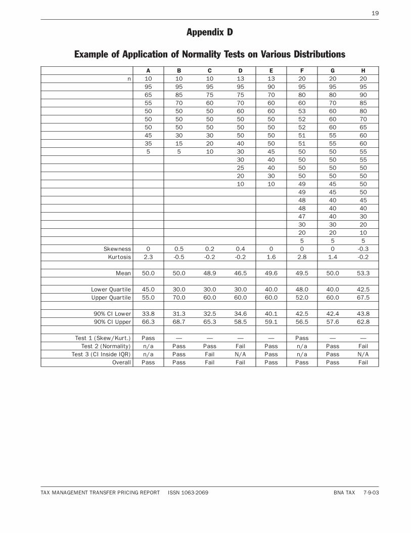
Appendix D

Example of Application of Normality Tests on Various Distributions

A B C D E F G Hn 10 10 10 13 13 20 20 20

95 95 95 95 90 95 95 9565 85 75 75 70 80 80 9055 70 60 70 60 60 70 8550 50 50 60 60 53 60 8050 50 50 50 50 52 60 7050 50 50 50 50 52 60 6545 30 30 50 50 51 55 6035 15 20 40 50 51 55 605 5 10 30 45 50 50 55

30 40 50 50 5525 40 50 50 5020 30 50 50 5010 10 49 45 50

49 45 5048 40 4548 40 4047 40 3030 30 2020 20 105 5 5

Skewness 0 0.5 0.2 0.4 0 0 0 -0.3Kurtosis 2.3 -0.5 -0.2 -0.2 1.6 2.8 1.4 -0.2

Mean 50.0 50.0 48.9 46.5 49.6 49.5 50.0 53.3

Lower Quartile 45.0 30.0 30.0 30.0 40.0 48.0 40.0 42.5Upper Quartile 55.0 70.0 60.0 60.0 60.0 52.0 60.0 67.5

90% CI Lower 33.8 31.3 32.5 34.6 40.1 42.5 42.4 43.890% CI Upper 66.3 68.7 65.3 58.5 59.1 56.5 57.6 62.8

Test 1 (Skew/Kurt.) Pass — — — — Pass — —Test 2 (Normality) n/a Pass Pass Fail Pass n/a Pass Fail

Test 3 (CI Inside IQR) n/a Pass Fail N/A Pass n/a Pass N/AOverall Pass Pass Fail Fail Pass Pass Pass Fail

19


Summary Statistics

A B C D E F G HMean 50.00 50.00 48.89 46.54 49.62 49.50 50.00 53.25Standard Error 7.95 10.07 8.85 6.71 5.32 4.10 4.40 5.49Median 50.00 50.00 50.00 50.00 50.00 50.00 50.00 52.50Mode 50.00 50.00 50.00 50.00 50.00 50.00 50.00 50.00Standard Deviation 23.85 30.21 26.55 24.19 19.20 18.33 19.67 24.56Sample Variance 568.75 912.50 704.86 584.94 368.59 335.95 386.84 603.36Kurtosis 2.30 -0.86 -0.20 -0.24 1.64 2.85 1.39 -0.17Skewness 0.00 0.00 0.24 0.46 0.07 0.02 0.00 -0.26Range 90 90 85 85 80 90 90 90Minimum 5 5 10 10 10 5 5 5Maximum 95 95 95 95 90 95 95 95Count 9 9 9 13 13 20 20 20Confidence Level(90.0%) 14.78 18.72 16.46 11.96 9.49 7.09 7.60 9.50

Chi-Squared TestExpected*

a 0.5 0.5 0.5 0.5 0.5 0.5 0.5b 1.0 1.0 2.0 2.0 2.5 2.5 2.5c 3.0 3.0 4.0 4.0 7.0 7.0 7.0d 3.0 3.0 4.0 4.0 7.0 7.0 7.0e 1.0 1.0 2.0 2.0 2.5 2.5 2.5f 0.5 0.5 0.5 0.5 0.5 0.5 0.5

9.0 9.0 13.0 13.0 20.0 20.0 20.0Observed

a 2 2 2 0 2 3b 0 0 3 1 1 2c 1 1 0 3 5 5d 3 3 3 4 6 5e 1 1 1 2 4 1f 2 2 3 2 2 4

(O - E)2 / Ea 4.50 4.50 4.50 0.50 4.50 12.50b 1.00 1.00 0.50 0.50 0.90 0.10c 1.33 1.33 4.00 0.25 0.57 0.57d 0.00 0.00 0.25 0.00 0.14 0.57e 0.00 0.00 0.50 0.00 0.90 0.90f 4.50 4.50 12.50 4.50 4.50 24.50

Total 11.33 11.33 22.25 5.75 11.51 39.14

Critical Value at 10% Level 9.24 9.24 9.24 9.24 9.24 9.24Critical Value at 5% Level 11.07 11.07 11.07 11.07 11.07 11.07Critical Value at 1% Level 15.09 15.09 15.09 15.09 15.09 15.09Critical Value at 0.5% Level 16.75 16.75 16.75 16.75 16.75 16.75

Pass Yes Yes No Yes Yes NoLevel 5% 1% — 10% 1% —*(The expected values are numbers of observations (not percentages), rounded to the nearest .5)

20


Risk Adjustments to the Comparables Range

Documents

Transcript of Risk Adjustments to the Comparables Range