Electronic copy available at: http://ssrn.com/abstract=1711807

Dipartimento di Scienze Economiche Università degli Studi di Firenze

Working Paper Series

Dipartimento di Scienze Economiche, Università degli Studi di Firenze Via delle Pandette 9, 50127 Firenze, Italia

www.dse.unifi.it The findings, interpretations, and conclusions expressed in the working paper series are those of the authors alone. They do not represent the view of Dipartimento di Scienze Economiche, Università degli Studi di Firenze

Commodity Futures Returns: A Non Linear Markov Regime Switching Model of Hedging and

Speculative Pressures

Giulio Cifarelli and Giovanna Paladino

Working Paper N. 13/2010 November 2010

Electronic copy available at: http://ssrn.com/abstract=1711807

Stampato in proprio in Firenze dal Dipartimento Scienze Economiche (Via delle Pandette 9, 50127 Firenze) nel mese di Novembre 2010,

Esemplare Fuori Commercio Per il Deposito Legale agli effetti della Legge 15 Aprile 2004, N.106

Commodity Futures Returns: A Non Linear Markov Regime

Switching Model of Hedging and Speculative Pressures

Giulio Cifarelli* and Giovanna Paladino°

Abstract

This study introduces a non linear model for commodity futures prices

which accounts for the pressures due to hedging and speculative

activities. The interaction with the corresponding spot market is

considered assuming that a long term equilibrium relationship holds

between futures and spot pricing. Over the 1990-2010 time period, a

dynamic interaction between spot and futures returns in five commodity

markets (copper, cotton, oil, silver, and soybeans) is empirically validated.

An error correction relationship for the cash returns and a non linear

parameterization of the corresponding futures returns are combined with

a bivariate CCC-GARCH representation of the conditional variances.

Hedgers and speculators are contemporaneously at work in the futures

markets, the role of the latter being far from negligible. Finally, in order

to capture the consequences of the growing impact of financial flows on

commodity market pricing, a two-state regime switching model for futures

returns is developed. The empirical findings indicate that hedging and

speculative behavior change significantly across the two regimes, which

we associate with low and high return volatility. High volatility regimes

are, as expected, characterized by a stronger impact of speculation on

futures return dynamics.

Keywords: Commodity spot and futures markets, dynamic hedging,

speculation, non linear GARCH, Markov regime switching.

JEL Classification G13, G15, Q47

The authors are grateful to Filippo Cesarano for extremely useful suggestions. The usual

disclaimer applies.

* University of Florence. Dipartimento di Scienze Economiche, via delle Pandette 9, 50127, Florence Italy; g.cifarelli.76@cantab.net ° LUISS University Economics Department and IntesaSanpaolo, Piazza San Carlo 156, 10156 Torino Italy; gpaladino@luiss.it or giovanna.paladino@intesasanpaolo.com

1

Introduction

A position in a commodity futures market is based on expectations about

the future price behavior and profits (or losses) depend on the accuracy of

the latter. Commodity futures trading does not usually contemplate the

physical delivery upon expiration of the contract. Indeed, offsetting the

position by selling (or buying) back the futures contract is not only doable

but a cheaper strategy.

In this paper we will focus on the two main activities associated with

futures trading: hedging and speculation. They do not have to be

considered as referring to two separate agents. It may well be that typical

hedgers, such as commercial firms, take a view on the market (speculate

on price direction). Alternatively, speculators can find it profitable to

engage in hedging activities (see Stulz, 1996, and Irwin et al., 2009).

Consequently it could be misleading to consider hedgers as pure risk–

averse agents and speculators as risk-seekers. The futures’ demand

functions used in this paper will avoid this simplistic divide.

Futures trading involves an exchange between people with opposite views

of the market (as to the future behavior of prices) and/or a different

degree of risk aversion. It allows to shift the risk from a party that desires

less risk to a party that is willing to accept it in exchange for an expected

profit.1

Why hedging with futures? Futures trading started – historically - when

commodity producers and consumers tried to offset the losses due to

unfavorable price fluctuations. Indeed, the main purpose of hedging is to

reduce the price risk. In the case of an expected price decline, the

hedging strategy of a producer will be to sell a futures contract at time t

and to buy it back at expiration at time t+n. Assuming for simplicity that

tt CF = where tF is the futures price and tC is the corresponding cash

price of a given commodity, the producer will earn the difference

0>− +ntt CF . (The futures price converges to the spot price at the expiry

and ntnt CF ++ ≡ .) In the case of an expected price increase, the hedging

1 Fagan and Gencay (2008) find that hedgers and speculators are often counterparties, since they tend to take opposing positions. Their respective long positions exhibit a strong negative correlation.

2

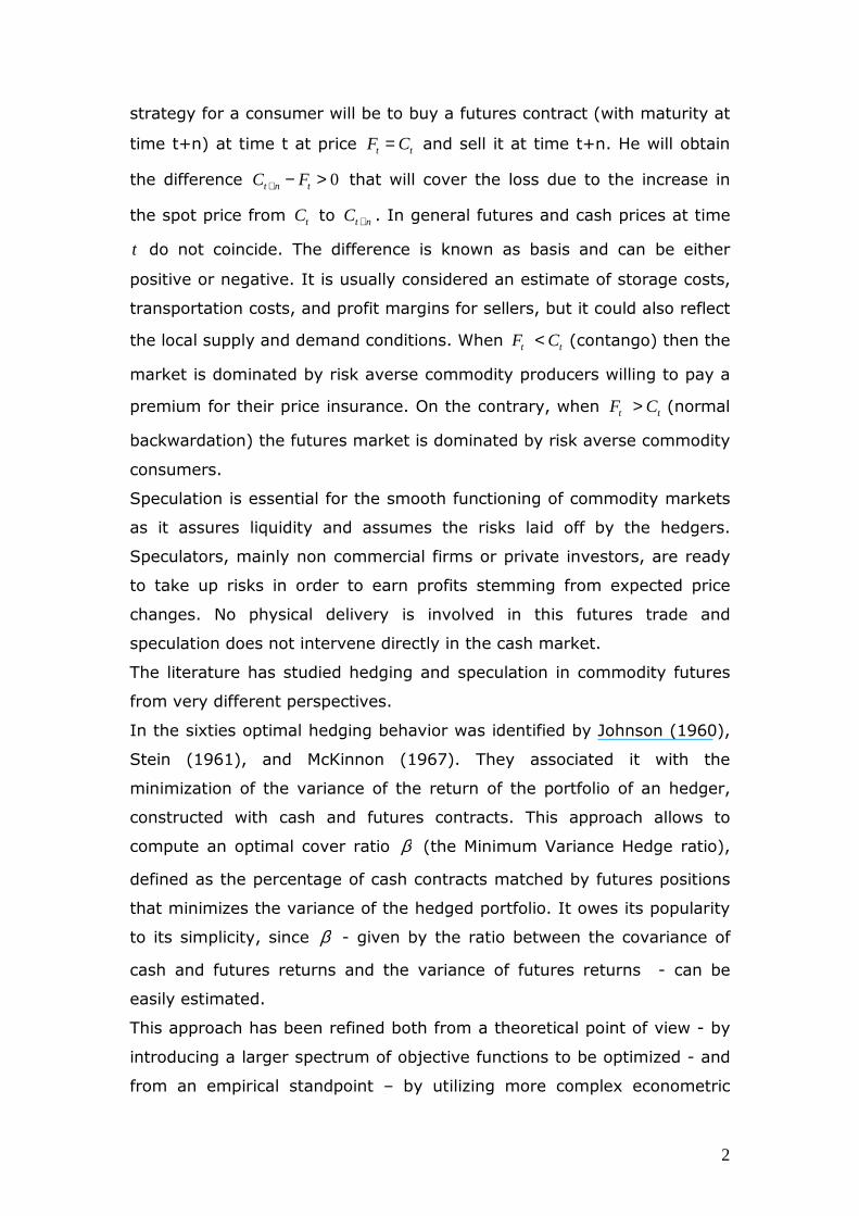
strategy for a consumer will be to buy a futures contract (with maturity at

time t+n) at time t at price tt CF = and sell it at time t+n. He will obtain

the difference 0>−+ tnt FC that will cover the loss due to the increase in

the spot price from tC to ntC + . In general futures and cash prices at time

t do not coincide. The difference is known as basis and can be either

positive or negative. It is usually considered an estimate of storage costs,

transportation costs, and profit margins for sellers, but it could also reflect

the local supply and demand conditions. When tt CF < (contango) then the

market is dominated by risk averse commodity producers willing to pay a

premium for their price insurance. On the contrary, when tt CF > (normal

backwardation) the futures market is dominated by risk averse commodity

consumers.

Speculation is essential for the smooth functioning of commodity markets

as it assures liquidity and assumes the risks laid off by the hedgers.

Speculators, mainly non commercial firms or private investors, are ready

to take up risks in order to earn profits stemming from expected price

changes. No physical delivery is involved in this futures trade and

speculation does not intervene directly in the cash market.

The literature has studied hedging and speculation in commodity futures

from very different perspectives.

In the sixties optimal hedging behavior was identified by Johnson (1960),

Stein (1961), and McKinnon (1967). They associated it with the

minimization of the variance of the return of the portfolio of an hedger,

constructed with cash and futures contracts. This approach allows to

compute an optimal cover ratio β (the Minimum Variance Hedge ratio),

defined as the percentage of cash contracts matched by futures positions

that minimizes the variance of the hedged portfolio. It owes its popularity

to its simplicity, since β - given by the ratio between the covariance of

cash and futures returns and the variance of futures returns - can be

easily estimated.

This approach has been refined both from a theoretical point of view - by

introducing a larger spectrum of objective functions to be optimized - and

from an empirical standpoint – by utilizing more complex econometric

3

methods that allow for time series heteroskedasticity and time variation of

the hedge ratio.

The MVH strategy focuses on the variance of the hedged portfolio and

pays no attention to its expected return. Subsequent improvements

include strategies based on hedged portfolio return mean and variance

expected utility maximization2 (Cecchetti et al., 1988, Lence, 1995),

minimization of the extended mean-Gini coefficient (Kolb and Okunev,

1992), or based on the Generalised Semivariance (GSV) (Lien and Tse,

2000). It has been shown, however, that if futures prices are martingale

processes and if the spot and futures returns are jointly normal then the

optimal hedge ratio will converge to the ratio obtained with the MVH

strategy. As for commodity futures, Chen et al. (2008) find that it is not

possible to reject the pure martingale hypothesis while the joint normality

holds only selectively and over long horizons.

The correlation between spot and futures is not perfect and, given the

stochastic nature of futures and spot prices, the hedge ratio is unlikely to

be constant. Static OLS hedge ratio estimation recognizes that the

correlation between the futures and spot prices is less than perfect

(Ederington, 1979, Figlewski, 1984), but imposes the restriction of a

constant correlation between spot and futures price rates of changes. As

such it could lead to sub-optimal hedging decisions in periods of high basis

volatility and/or to inefficient revisions of the hedge ratio.

Recently, a large body of literature has arisen to cope with the dynamics

of the joint distribution of the returns and with the time-varying nature of

the optimal hedge ratio, using the large family of GARCH models. These

studies suggest that optimal hedge ratios are time dependent and that

dynamic hedging reduces in-sample portfolio variance substantially more

than static hedging.

The out-of-sample advantages of the GARCH hedge ratio are much more

controversial. Some argue that the GARCH hedge ratio enhances the out-

of-sample hedging effectiveness (see, among others, the seminal works of

Baillie and Myers, 1991, and of Kroner and Sultan, 1993, Lee and Yoder,

2 The MVH is not only compatible with a quadratic utility function but, as shown by Benninga et al. (1983), under certain conditions, it is consistent with expected utility maximization, a result that does not depend upon the nature of the utility function.

4

2007, who implement a Markov switching GARCH, and Chan and Young,

2006, who incorporate a jump component in a bivariate GARCH). Others,

however, considering the trade off between the benefits of a dynamic

hedge and both the complexity of the implementation of the GARCH

method and the costs of portfolio rebalancing, conclude that static

hedging is to be preferred (Lence, 1995, Miffre, 2004, and Alexander and

Barbosa, 2007). Recent mixed evidence is set forth by Park and Jei

(2010), while Lien (2009) finds that GARCH modeling raises hedging

effectiveness mostly in small samples, when there are sufficiently large

fluctuations in the conditional variance of the futures returns.

The literature on commodity market speculation has followed two main

strands. A direct approach based on an attempt to micro model

simultaneously speculative and hedging behavior and an indirect

approach, which analyzes the excess co-movement of commodity prices

(with respect to common fundamentals) and ascribes this evidence to

'herding' behavior. In addition some recent studies have tried to exploit

the information, extrapolated from the data provided by the CFTC, on the

commitments of traders.

In an important paper Johnson (1960) suggests that hedging and

speculation in the futures markets are interrelated. Speculation is mainly

attributed to traders’ expectations on future price changes that bring

about an increase/decrease of the optimal hedging ratio in a short

hedging context. Ward and Fletcher (1971) generalize Johnson’s approach

to both long and short hedging and find that speculation is associated with

optimal futures positions (short or long) that are in excess of the 100

percent hedging level.

A different strand of analysis on speculation in the commodity markets

focuses on the presence of excess (with respect to a component explained

by fundamentals) co-movement of returns of unrelated commodities

(Pyndick and Rotemberg, 1990). Subsequent research - see among others

Cashin et al. (1999), Ai et al. (2006), and Lescaroux (2009) - challenged

the excess co-movement hypothesis on both empirical and methodological

grounds. The overall results are mixed and could indeed depend on the

selection of the estimation techniques and/or of the information set (Le

Pen and Sevi, 2010).

5

In recent year the availability of data on the Commitments of Traders

Reports, provided by the Commodity Futures Trading Commission, has

generated a body of papers that try to assess the impact of speculation on

commodity prices measuring speculative positions in terms open interest.

The weekly open interest of each commodity is broken down, according to

the purposes of traders, in long and short reporting commercial hedging,

long and short speculation by reporting non commercial firms, and

positions of non reporting traders. The empirical results, however, are

mixed (Fagan and Gencay, 2008).

This paper contributes to the current debate in different ways.

a. Using a complex non linear CCC-GARCH approach we model

explicitly the reaction of hedgers and speculators to volatility shifts

in the commodity markets. In this way the literature is extended by

adding a dynamic component to the standard two-step optimal

hedge ratio computation.

b. A two-state Markov switching procedure is used to model the

impact of changes in the behavior of commodity markets, changes

due to bullish/bearish reactions to futures price changes and/or to

shifts in risk aversion brought about by return volatility changes.

We identify in this way a financial pattern that seems to play a

growing role in recent commodity market pricing.

c. We model and assess empirically the relative impact of speculative

vs. hedging drivers on futures pricing, and show that periods of

high futures return volatility are usually to be associated with a

more intense speculative activity.

Section 1 The model

Commodity future trading is analyzed in this section, focusing on hedging

and speculative behavior. A hedging transaction is intended to reduce the

risk of unwanted future cash price changes to an acceptable level. Spot

market trades are then associated with trades of the opposite sign in the

corresponding futures market. If the current cash and futures prices are

positively correlated, the financial loss in one market will be compensated

6

by the earnings obtained from holding the opposite position in the other

market.

In more detail, let it

itc Cr log, ∆= and

it

itf Fr log, ∆= , where

itC is the cash

(spot) price of commodity i and i

tF is the price of the corresponding

futures contract. An investor who takes a long (short) position of one unit

in the cash market i will hedge by taking a short (long) position of β units

in the corresponding futures market, which he will buy (sell) back when he

sells (buys) the cash. The hedge ratio β can be seen as the proportion of

the long (short) cash position that is covered by futures sales

(purchases).3

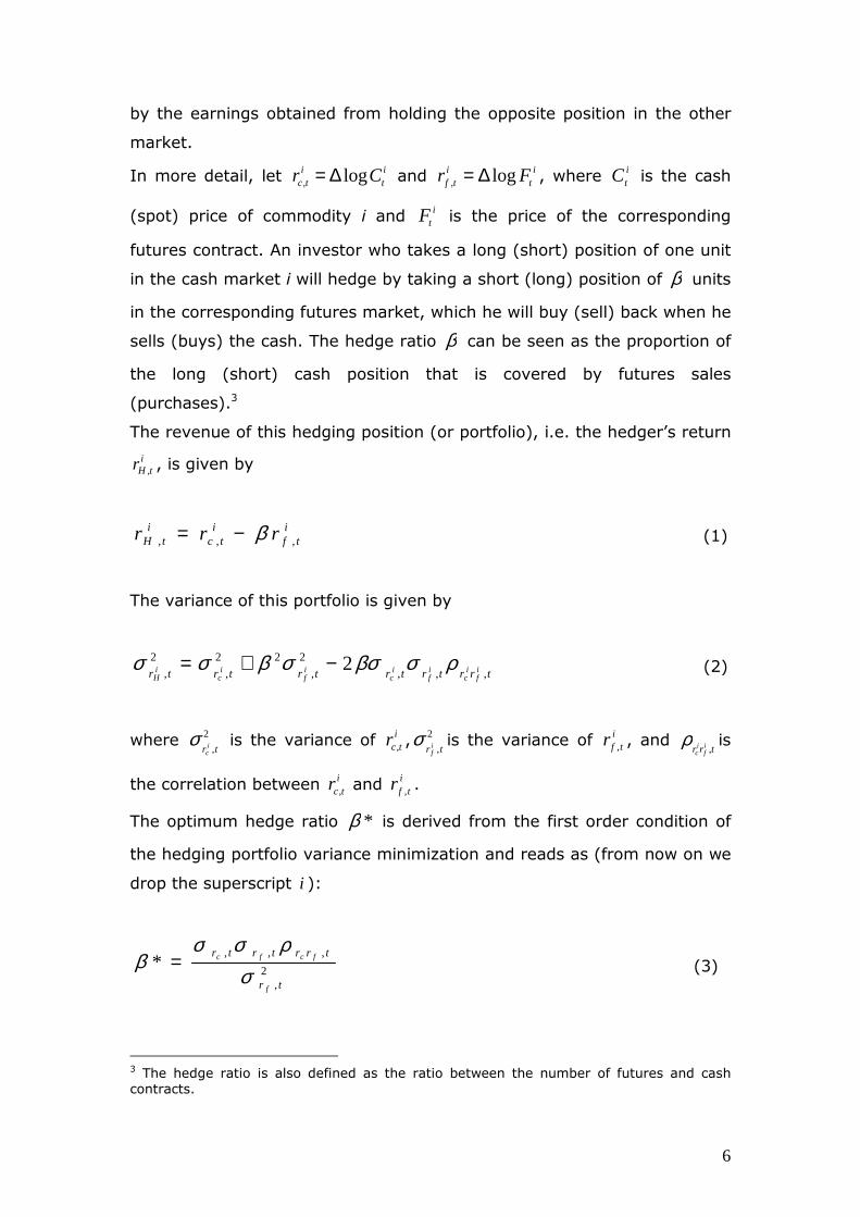
The revenue of this hedging position (or portfolio), i.e. the hedger’s return

itHr , , is given by

itf

itc

itH rrr ,,, β−= (1)

The variance of this portfolio is given by

trrtrtrtrtrtr if

ic

if

ic

if

ic

iH ,,,

2

,

22

,

2

,2 ρσβσσβσσ −+= (2)

where 2

,tr ic

σ is the variance of itcr , ,

2

,tr if

σ is the variance of i

tfr , , and trr if

ic ,

ρ is

the correlation between itcr , and

itfr , .

The optimum hedge ratio *β is derived from the first order condition of

the hedging portfolio variance minimization and reads as (from now on we

drop the superscript i ):

2,

,,,*

tr

trrtrtr

f

fcfc

σρσσ

β = (3)

3 The hedge ratio is also defined as the ratio between the number of futures and cash contracts.

7

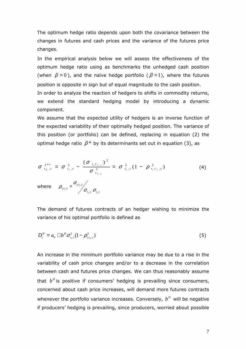
The optimum hedge ratio depends upon both the covariance between the

changes in futures and cash prices and the variance of the futures price

changes.

In the empirical analysis below we will assess the effectiveness of the

optimum hedge ratio using as benchmarks the unhedged cash position

(when 0=β ), and the naïve hedge portfolio ( 1=β ), where the futures

position is opposite in sign but of equal magnitude to the cash position.

In order to analyze the reaction of hedgers to shifts in commodity returns,

we extend the standard hedging model by introducing a dynamic

component.

We assume that the expected utility of hedgers is an inverse function of

the expected variability of their optimally hedged position. The variance of

this position (or portfolio) can be defined, replacing in equation (2) the

optimal hedge ratio *β by its determinants set out in equation (3), as

)1()(

2,

2,2

2

2,

**2,

,

,

trrtrr

rr

trtr fcc

tf

tfc

cHρσ

σσ

σσ −=−= (4)

wheretrtr

trrtrr

cf

fc

fc,,

,, σσ

σρ =

The demand of futures contracts of an hedger wishing to minimize the

variance of his optimal portfolio is defined as

)1( 2,

2,0 trrtr

HHt fcc

baD ρσ −+= (5)

An increase in the minimum portfolio variance may be due to a rise in the

variability of cash price changes and/or to a decrease in the correlation

between cash and futures price changes. We can thus reasonably assume

that Hb is positive if consumers’ hedging is prevailing since consumers,

concerned about cash price increases, will demand more futures contracts

whenever the portfolio variance increases. Conversely, Hb will be negative

if producers’ hedging is prevailing, since producers, worried about possible

8

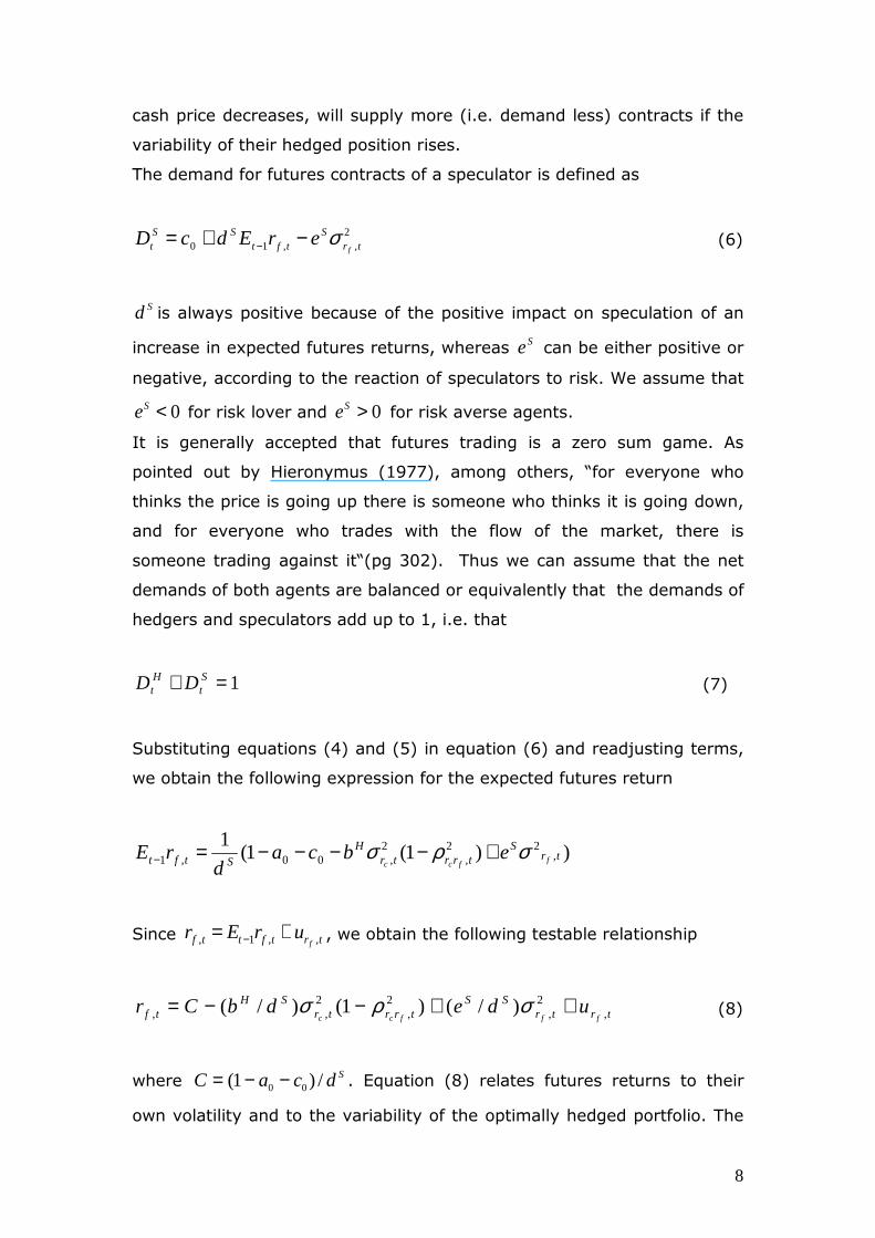
cash price decreases, will supply more (i.e. demand less) contracts if the

variability of their hedged position rises.

The demand for futures contracts of a speculator is defined as

2,,10 tr

Stft

SSt f

erEdcD σ−+= − (6)

Sd is always positive because of the positive impact on speculation of an

increase in expected futures returns, whereas Se can be either positive or

negative, according to the reaction of speculators to risk. We assume that

0<Se for risk lover and 0>Se for risk averse agents.

It is generally accepted that futures trading is a zero sum game. As

pointed out by Hieronymus (1977), among others, “for everyone who

thinks the price is going up there is someone who thinks it is going down,

and for everyone who trades with the flow of the market, there is

someone trading against it“(pg 302). Thus we can assume that the net

demands of both agents are balanced or equivalently that the demands of

hedgers and speculators add up to 1, i.e. that

1=+ St

Ht DD (7)

Substituting equations (4) and (5) in equation (6) and readjusting terms,

we obtain the following expression for the expected futures return

))1(1(1

,22

,2

,00,1 trS

trrtrH

Stft ffccebca

drE σρσ +−−−−=−

Since trtfttf furEr ,,1, += − , we obtain the following testable relationship

trtrSS

trrtrSH

tf fffccudedbCr ,

2,

2,

2,, )/()1()/( ++−−= σρσ (8)

where SdcaC /)1( 00 −−= . Equation (8) relates futures returns to their

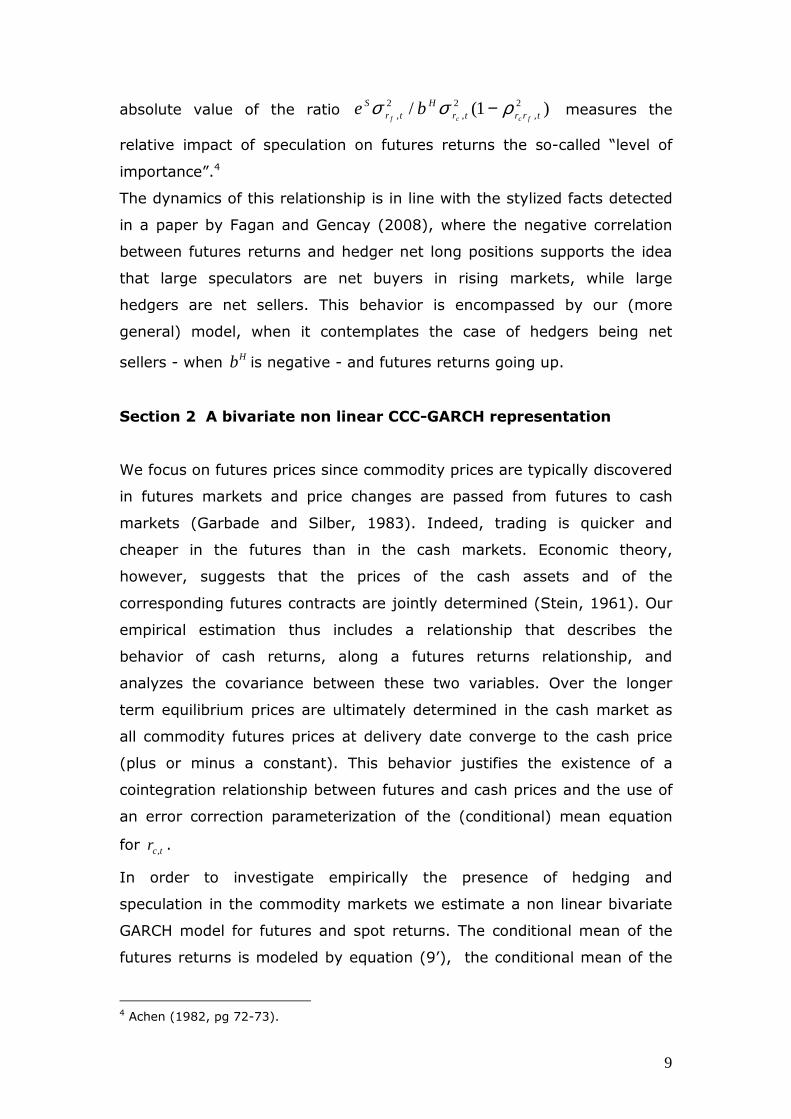
own volatility and to the variability of the optimally hedged portfolio. The

9

absolute value of the ratio )1(/ 2,

2,

2, trrtr

Htr

S

fccfbe ρσσ − measures the

relative impact of speculation on futures returns the so-called “level of

importance”.4

The dynamics of this relationship is in line with the stylized facts detected

in a paper by Fagan and Gencay (2008), where the negative correlation

between futures returns and hedger net long positions supports the idea

that large speculators are net buyers in rising markets, while large

hedgers are net sellers. This behavior is encompassed by our (more

general) model, when it contemplates the case of hedgers being net

sellers - when Hb is negative - and futures returns going up.

Section 2 A bivariate non linear CCC-GARCH representation

We focus on futures prices since commodity prices are typically discovered

in futures markets and price changes are passed from futures to cash

markets (Garbade and Silber, 1983). Indeed, trading is quicker and

cheaper in the futures than in the cash markets. Economic theory,

however, suggests that the prices of the cash assets and of the

corresponding futures contracts are jointly determined (Stein, 1961). Our

empirical estimation thus includes a relationship that describes the

behavior of cash returns, along a futures returns relationship, and

analyzes the covariance between these two variables. Over the longer

term equilibrium prices are ultimately determined in the cash market as

all commodity futures prices at delivery date converge to the cash price

(plus or minus a constant). This behavior justifies the existence of a

cointegration relationship between futures and cash prices and the use of

an error correction parameterization of the (conditional) mean equation

for tcr , .

In order to investigate empirically the presence of hedging and

speculation in the commodity markets we estimate a non linear bivariate

GARCH model for futures and spot returns. The conditional mean of the

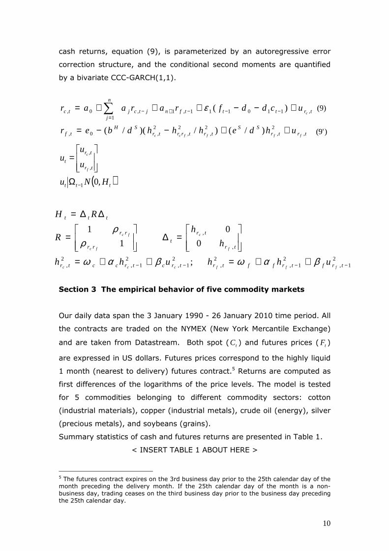
futures returns is modeled by equation (9’), the conditional mean of the

4 Achen (1982, pg 72-73).

10

cash returns, equation (9), is parameterized by an autoregressive error

correction structure, and the conditional second moments are quantified

by a bivariate CCC-GARCH(1,1).

trtrSS

trtrrtrSH

tf

trtttfnjtcj

n

jtc

ffffcc

c

uhdehhhdber

ucddfraraar

,2

,2

,2

,2

,0,

,110111,1,1

0,

)/()/)(/(

)(

++−−=

+−−+++= −−−+−=∑ ε

)'9(

)9(

( ) ,01

,

,

ttt

tr

tr

t

HNu

u

uu

f

c

−Ω

=

Section 3 The empirical behavior of five commodity markets

Our daily data span the 3 January 1990 - 26 January 2010 time period. All

the contracts are traded on the NYMEX (New York Mercantile Exchange)

and are taken from Datastream. Both spot ( tC ) and futures prices ( tF )

are expressed in US dollars. Futures prices correspond to the highly liquid

1 month (nearest to delivery) futures contract.5 Returns are computed as

first differences of the logarithms of the price levels. The model is tested

for 5 commodities belonging to different commodity sectors: cotton

(industrial materials), copper (industrial metals), crude oil (energy), silver

(precious metals), and soybeans (grains).

Summary statistics of cash and futures returns are presented in Table 1.

< INSERT TABLE 1 ABOUT HERE >

5 The futures contract expires on the 3rd business day prior to the 25th calendar day of the month preceding the delivery month. If the 25th calendar day of the month is a non-business day, trading ceases on the third business day prior to the business day preceding the 25th calendar day.

;

0

0

1

1

21,

21,

2,

21,

21,

2,

,

,

−−−− ++=++=

=∆

=

∆∆=

trftrfftrtrctrcctr

tr

tr

trr

rr

ttt

fffccc

f

c

fc

fc

uhhuhh

h

hR

RH

βαϖβαϖ

ρρ

11

Average daily returns are small but not negligible, higher for oil and lower

for soybeans, a pattern that holds also for the daily standard deviations.6

The distributions of both cash and futures returns are always mildly

skewed and significantly leptokurtic, the departure from normality being

confirmed by the size of the corresponding Jarque Bera (JB) test statistics.

Volatility clustering is detected in all cases a finding which supports the

choice of a GARCH parameterization of the conditional second moments.

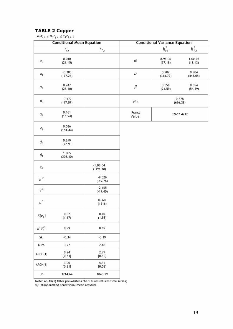
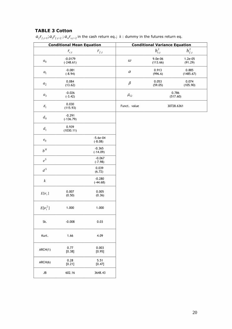
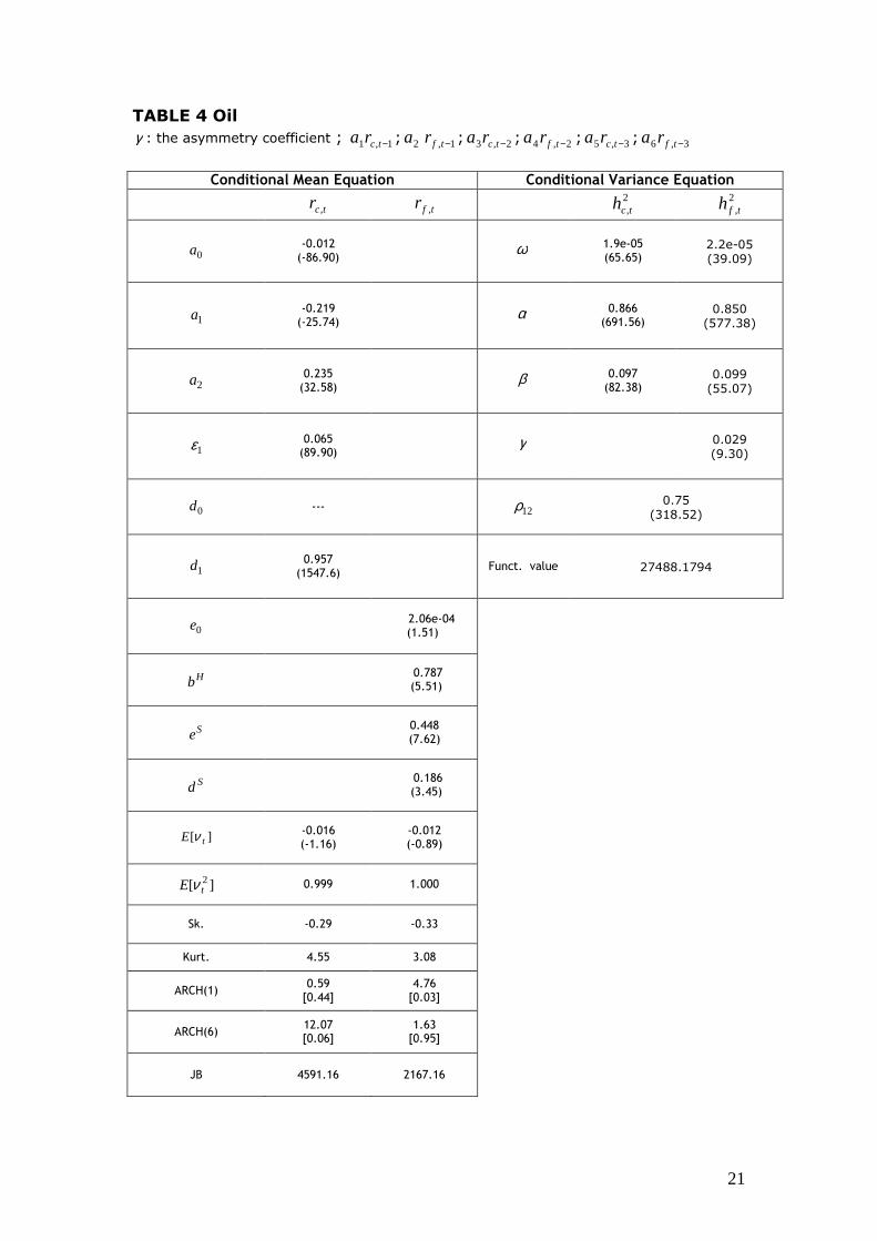
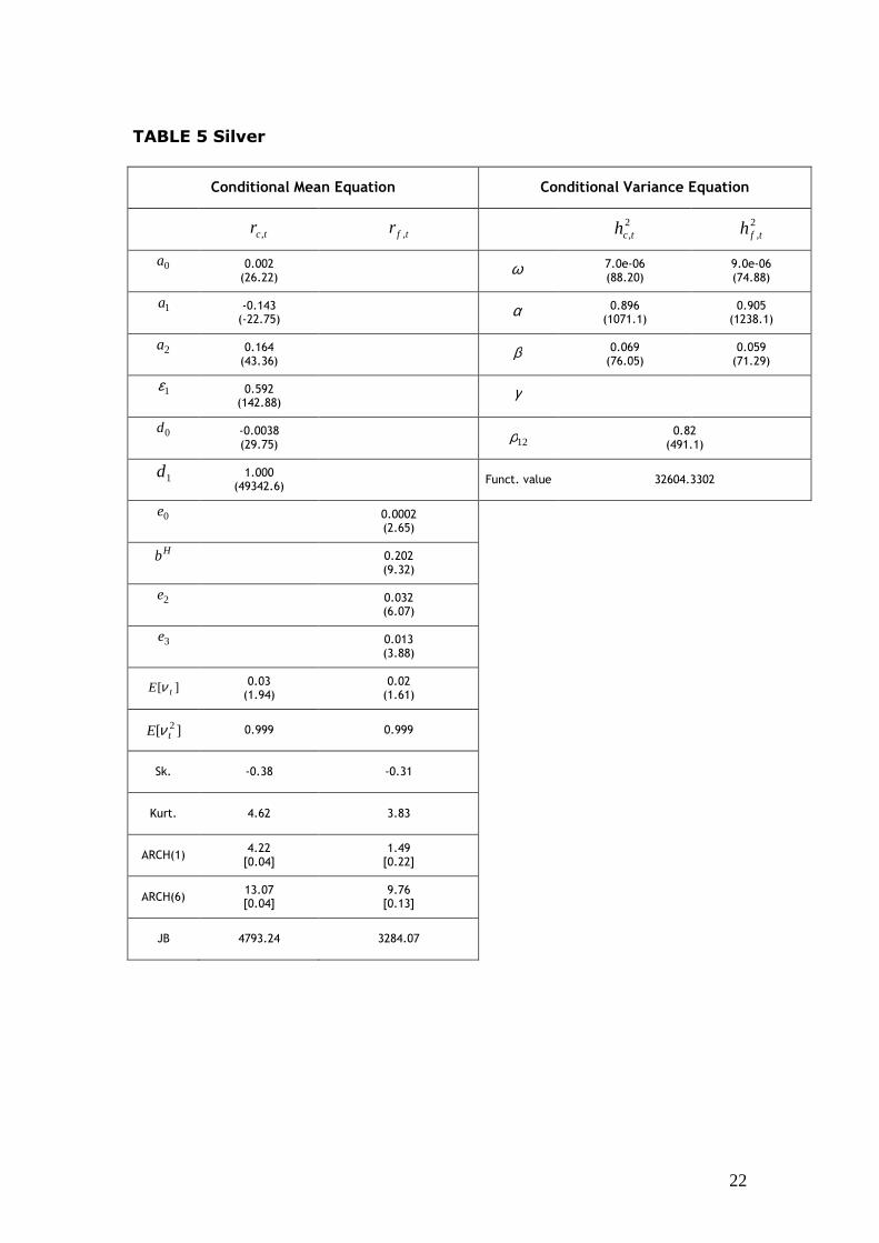
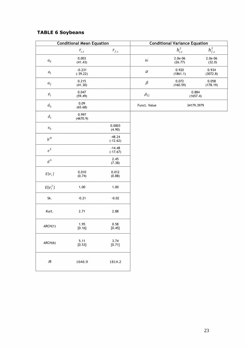
Tables 2 to 6 present parsimonious estimates of the equations of the

bivariate non linear CCC-GARCH(1,1) system set forth in section 2 for 5

commodities. The overall quality of fit is satisfactory. The estimated

parameters are significantly different from zero and the conditional

heteroskedasticity of the residuals has been captured by our GARCH

parameterization.7 The usual misspecification tests suggest that the

standardized residuals tν are always well behaved; for each system

0][ =tE ν , 1][ 2 =tt

E ν , and 2tν is serially uncorrelated.

< INSERT TABLE 2 ABOUT HERE >

< INSERT TABLE 3 ABOUT HERE >

< INSERT TABLE 4 ABOUT HERE >

< INSERT TABLE 5 ABOUT HERE >

< INSERT TABLE 6 ABOUT HERE >

The futures return mean equation (9’) provides the following useful

information on the market drivers. (i) Coefficient Hb estimates are

negative in the case of cotton, copper and soybeans - reflecting the

predominance of producers on the markets - and positive for the

remaining commodities of the sample (oil and silver), because of the

preponderance of consumers. This result is also in line with the effects of

hedging pressure, where futures prices increase when hedgers trade short

and decrease when hedgers are long.8

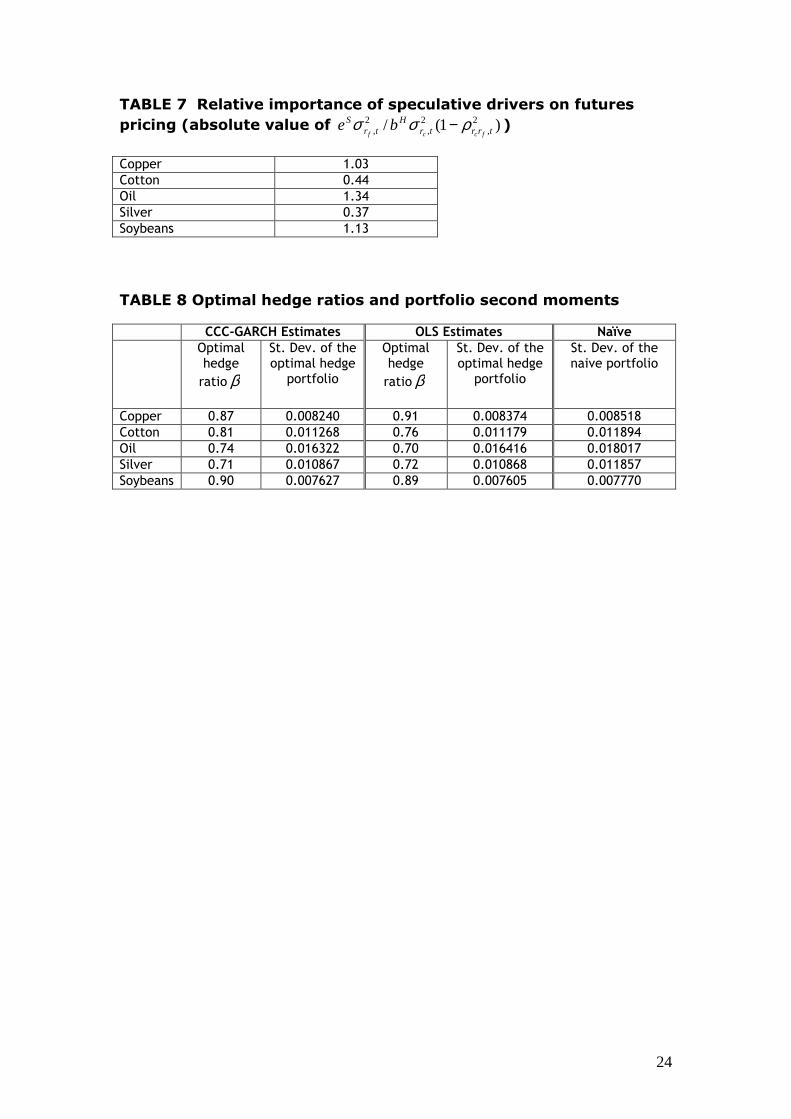
(ii) The absolute value of the ratio between speculative and hedging

factors set forth in Table 7 measures the relative impact of risk on futures

6 The logarithms of the prices of the cash and futures contracts are always I(1) and their first differences I(0). The test statistics are not reported for lack of space. 7 The t-ratios reported in the tables are based on the robust quasi-maximum likelihood estimation procedure of Bollerslev and Wooldridge (1992). 8 See Chang (1985) and Bessembinder (1992).

12

returns. It is higher than 1 for the copper, oil and soybeans markets,

where speculators seem to be more reactive to futures risk than hedgers.

Speculators are risk averse (since the corresponding Se coefficient

estimates are positive) in the oil and silver markets only, a finding that

may be due to the size of the volatility shocks. This issue shall be further

investigated in the next section as is affected by the futures pricing

regime shifts. (iii) The estimates of coefficient sd , which represents the

component of speculators’ demand that is associated with price

expectations, are always positive and significant. They tend to be small,

however, if compared with those of the coefficients of the corresponding

futures returns volatilities.9

< INSERT TABLE 7 ABOUT HERE >

The dynamic specification of our model might introduce distortive effects

in the estimation of the optimal hedge ratio β , that reduce its

effectiveness. We have thus performed the standard comparison of its

hedging performance with the performance of a naïve portfolio hedge ratio

( 1=β ) and of an OLS hedge ratio, obtained as the futures return

coefficient estimate in a regression of cash returns on a constant and on

futures returns. An artificial daily portfolio is introduced where an investor

is assumed to buy (sell) one unit of the cash asset and to sell (buy) β

units of the corresponding futures contract. The unconditional portfolio

return standard deviations are computed over the whole sample and are

set forth in Table 8 for the three hedge ratio estimators. The naïve hedge

portfolios are clearly outperformed by the optimal hedge portfolios, a

finding that differs from the results obtained by Alexander and Barbosa

(2007). Commodity markets, in spite of their growing financiarization,

cannot compare, in terms of efficiency, with the major stock markets and

optimal hedging remains an effective risk reduction technique. Our CCC-

GARCH model provides the minimum risk hedge in three out of five

markets, a finding that corroborates the validity of its parameterization.

9 Equation (9’) imposes coefficient restrictions that are justified by the model. We have estimated a reduced form version of our CCC-GARCH(1,1) model, replacing (bH /dS ) and (eS /dS ) with the corresponding unrestricted coefficients. We were unable to reject the null associated with these restrictions performing standard LR tests. The corresponding tests statistics are available from the authors upon request.

13

Only in the case of cotton and soybeans, among the less volatile markets

of the sample, does the OLS optimal hedge provide the best results.10

< INSERT TABLE 8 ABOUT HERE >

4 Hedging, speculation, and futures pricing regime shifts

Sarno and Valente (2000) and Alizedeh and Nomikos (2004) analyzed the

changes in the relationship between futures and spot stock index returns

using a Markov switching model set out originally by Hamilton (1994). In

our investigation we use this technique in order to analyze the shifts over

two regimes in commodity market hedging and speculative behavior.

Using the full sample estimates of the conditional second moments

obtained in the previous section, equation (9’) is adapted in a second step

to a two-state Markov switching framework in which the drivers of futures

returns are assumed to switch between two different processes, dictated

by the state of the market.

Equation (9’) is thus rewritten as

tsrtrSs

Sstrtrrtr

Ss

Hsstf tffttffccttt

uhdehhhdber ,2

,2

,2

,2

,0, )/()/)(/( ++−−= (10)

where ),0(~ 2, ttf stsr Nu σ , and the unobserved random variable ts indicates

the state in which is the market.

The value of the current regime ts is assumed to depend on the state of

the previous period only, 1−ts , and the transition probability

ijtt pisjsP === − 1 gives the probability that state i will be followed by

state j. In the two state case 11211 =+ pp and 12122 =+ pp , and the

corresponding transition matrix is

10 If we repeat the exercise using weekly returns estimates of our CCC-GARCH(1,1) model and introduce a weekly portfolio rebalancing, the CCC-GARCH beta portfolios consistently outperform both the OLS beta and naïve beta portfolios in all commodity markets.

14

=P

−−

2211

2211

1

1

pp

pp (11)

The joint probability of tfr , and ts is then given by the product

),(),;(),,( 11,1, ψψψ −−− ==== tttttftttf YjsPYjsrfYjsrp 2,1=j (12)

where 1−tY is the information set that includes all past information on the

population parameters and ),,,,( 20 ttttt s

Ss

Ss

Hss edbe σψ = is the vector of

parameters to be estimated. (.)f is the density of tfr , , conditional on the

random variable ts , and (.)P is the conditional probability that ts will take

the value j .

For the two-state case the density distribution of tfr , is, following Hamilton

(1994, Chapter 22)

−

+

−

=− 22

22,

22

21

21,

21

1, 2exp

2

1

2exp

2

1),(

σπσσπσψ trtr

ttfff

uuYrg (13)

wheretsr tf

u ,is the residual of equation (10).

If the unobserved state variable ts is i.i.d. maximum likelihood estimates

of the parameters in ψ are obtained maximizing the following log

likelihood function with respect to the unknown parameters

L ∑=

−=T

tttf Yrg

11, ),(log)( ψψ (14)

where T is the total number of sample observations.

In this paper we base the identification process of the nature of the

regimes, essential for the interpretation of a Markov switching model, on

15

the estimates of equation (10) and on the analysis of the behavior over

time of the state probabilities.

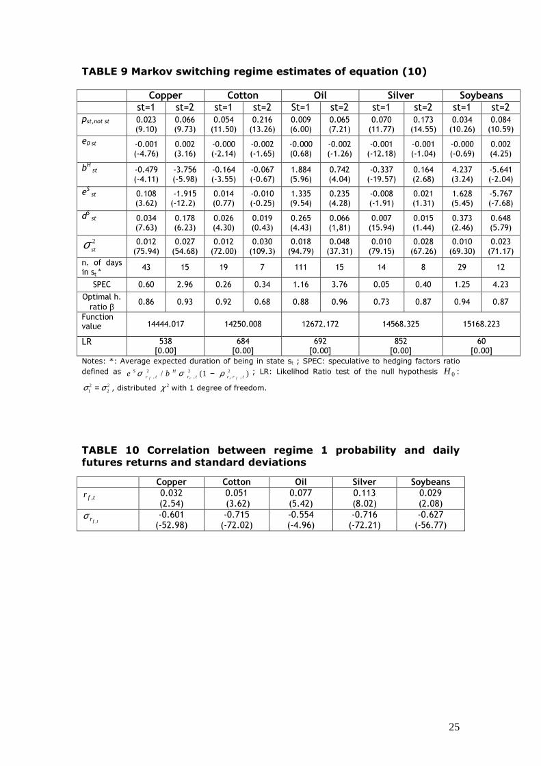
< INSERT TABLE 9 ABOUT HERE >

In Table 9 are set out the estimates of equation (10) for the five

commodity markets. The quality of fit is highly satisfactory since, with the

exception of cotton, the relevant coefficients change across regimes and

are significantly different from zero. The restriction of equal residual

variances is strongly rejected by LR tests performed for each model. The

regime (state) 2 variances are from two to three time larger than those of

regime (state) 1. The probability of switching from a low variance to a

high variance state 12p is lower than the probability of switching from a

high variance to a low variance state 21p . For instance, in the case of oil,

the transition probabilities are %9.012 =p and %5.621 =p ; these findings

indicate that the average expected duration of being in state 1 is close to

111 working days (about 5 months) and the average expected duration of

being in state 2 is of 15 working days.11 The number of days of high

volatility is, on the whole, rather small.

A relevant difference across regimes in hedging and speculative behavior

can be easily detected. The reaction of hedgers is not homogeneous in the

various markets. In the case of copper and soybeans hedgers seem to be

more sensitive to portfolio risk in state 2 while in the remaining markets

the opposite reaction can be detected. The behavior of speculators too

changes with the market. In the case of copper and soybeans a risk

averse behavior in state 1 is reversed with the change of regime;

speculators increase their demand for futures contracts whenever the

volatility rises. In the remaining markets speculators behave in the

opposite way. Their reaction to (a high) futures return volatility decreases

in the case of oil and becomes nil in the case cotton and silver. This

finding is of interest for the interpretation of the main drivers of the

volatility movements for these commodities. It suggests that volatility

changes, in regime 2, may be due more to spillovers from monetary,

11 The average expected duration of being in state 1 is computed according to Hamilton

(1989) as ∑∞

=

−−− =−=−1

1

12

1

1111

1

11 )()1()1(i

i pppip

16

financial, and exchange rate markets than to endogenous market

speculation.

The estimates of the weighted coefficient ratio (SPEC) set forth in Table 9

strongly suggest that in state 2 the impact of speculation on futures price

dynamics is much stronger than in state 1 of the market. Finally, the

optimal hedge ratio β tends to increase during the high volatility period in

the case of oil, silver, and copper (a result due to the significant increase

in correlation between spot and futures returns), while for cotton and

soybeans the reverse holds true.12

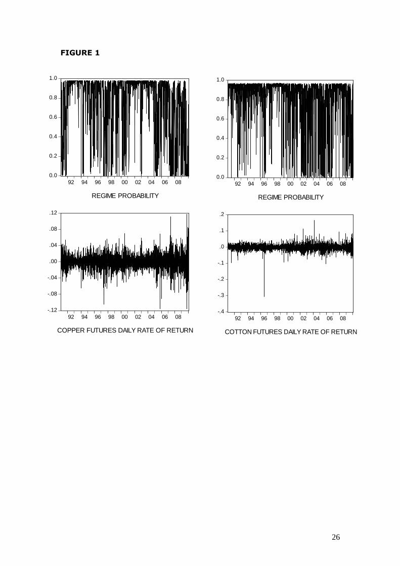
< INSERT FIGURE 1 ABOUT HERE >

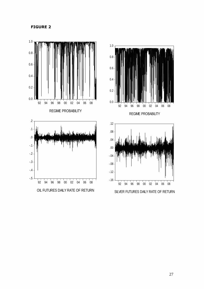
< INSERT FIGURE 2 ABOUT HERE >

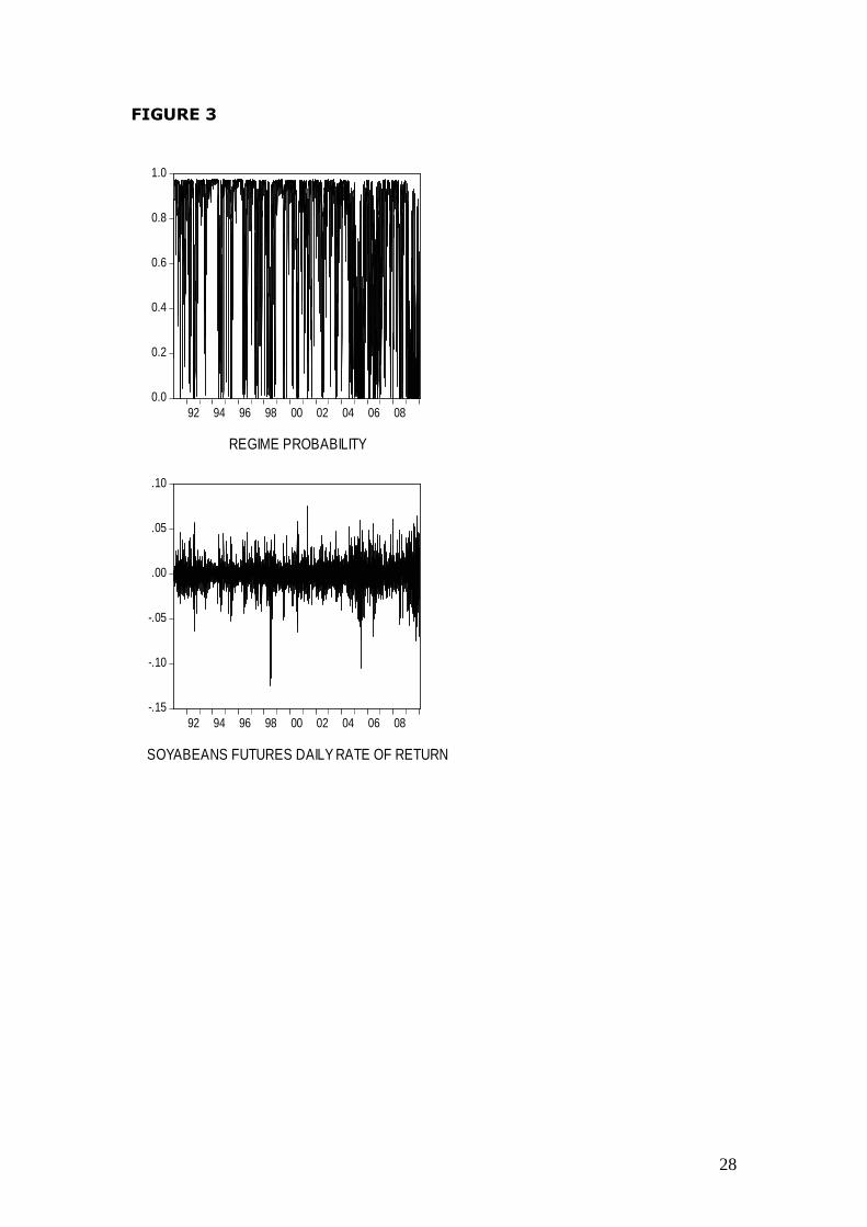
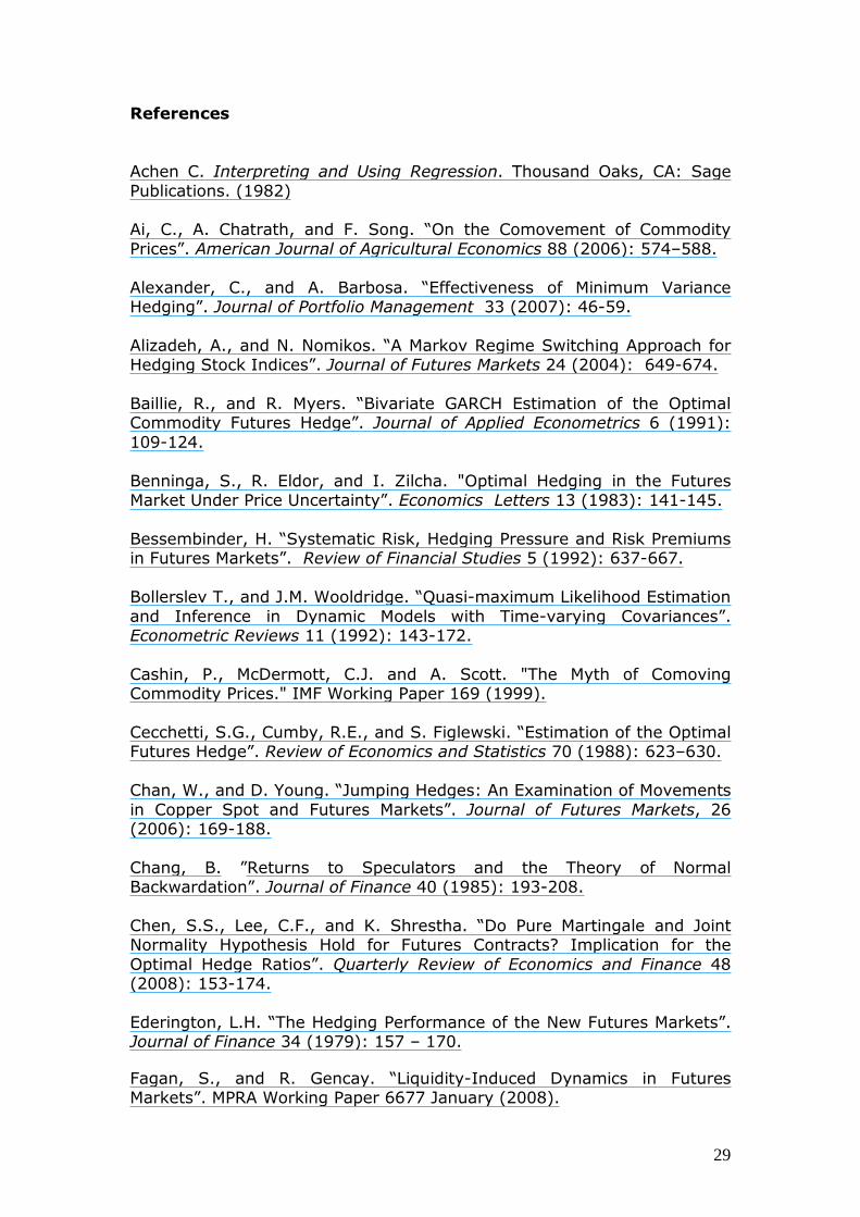
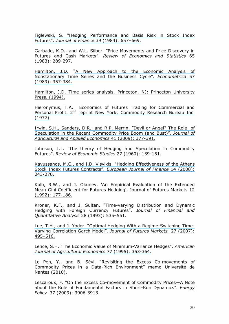
< INSERT FIGURE 3 ABOUT HERE >

Figures 1 to 3 provide useful insights on the dating of the regime shifts. In

the upper graph of each figure is set forth the behavior over the sample of

the time t probability that the market is in regime 1. In the lower graph is

set out the rate of return of the corresponding futures contract. Visual

inspection suggests that regime 1 may be associated with periods in which

return variability is low (and thus regime 2 with periods in which it is

high).13

< INSERT TABLE 10 ABOUT HERE >

In table 10 are finally reported the correlation coefficients between the

probability 1 regime and the daily rate of return and standard deviation of

the corresponding futures contract. As expected, we find a large negative

and significant correlation coefficient between the regime 1 probabilities

and the daily standard deviations. We detect, however, also a significant

positive correlation of these regime probabilities with futures returns. This

result indicates, especially for silver, a more complex identification of the

nature of the state variable ts . Regime 1 is to be associated with both low

futures return variability and, to a lesser extent, with positive futures price

12 The correlation between the spot and futures returns is generally stronger in the high volatility regime. In the case of cotton and soybeans, however, the increase is small (3.75 and 1.16 percent, respectively). This lack of reaction to volatility shifts may explain the portfolio risk minimization results of Table 8, where, for these commodities, the time-varying conditional hedge ratios are outperformed by the constant OLS optimal hedges. 13 For each market, bouts of high variability are clearly identified. They do not coincide in the first half of the sample and tend to be more synchronized in the second half, a symptom of the growing financial integration of the commodity markets.

17

rates of change (i.e. possibly with a bullish market), and regime 2 with

high return variability and negative futures price rates of change (i.e. with

a bearish market).14

5 Conclusions

This paper examines the dynamic behavior of futures returns on five

commodity markets. The interaction between hedgers and speculators is

modelled using a highly non linear parameterization where hedgers react

to deviations from the minimum variance of the hedged portfolio and

speculators respond to standard expected risk returns considerations. The

relationship between expected spot and futures returns and time varying

volatilities is estimated using a non linear in mean CCC-GARCH approach.

The results point to the suitability of this choice because of the quality of

fit and of the sensible meaning of the model’s parameter estimates.

In spite of the growing role of speculation, over the 1990-2010 sample

period, hedgers do play a relevant role since futures returns dynamics is

mostly associated with the variability of the hedged portfolio, especially in

the low volatility regime.

We account for the impact of financial integration of the commodity

markets by allowing the demand of futures to be dependent upon the

“state of the market” via a Markov regime switching approach. Both visual

inspection and correlation analysis suggest that regime 1 be associated

with periods in which return variability is low and regime 2 with periods in

which it is high. Optimal hedging ratios computed in each state are larger

in high volatility regimes for oil, copper and silver, while the reverse holds

true for cotton and soybeans. The differences across regimes in hedging

and speculative behavior are distinctive and not homogeneous across

commodities. The role of speculators appears to be very strong, and

significant, when market volatility is high in the case of copper, soybeans,

and oil. However, the positive correlation of the regime probabilities with

the futures daily rates of returns suggests, especially for silver, a more

complex identification of the nature of the state variable. Thus further

14 According to the standard ADF unit root tests, the time t regime 1 probability time series are always I(0).

18

investigation, e.g. introducing a four regime framework, could provide

additional insights about the nature of the volatility of the futures returns

for some of the commodities of our study.

TABLE 1 Descriptive statistics

Daily sample from 3 January 1990 to 26 January 2010 (5325 observations)

Return Mean St.dev. Sk. Kurt. JB ARCH(1)[pr.] ARCH(5)[pr.]

Copper futures 0.000229 0.0169 -0.22 4.53 4520.46 181.57[0.00] 570.36[0.00]

Copper cash 0.000210 0.0169 -0.21 4.51 4483.09 346.76[0.00] 876.66[0.00]

Cotton futures 0.000112 0.0175 -0.79 22.07 106878.63 14.45[0.00] 91.93[0.00]

Cotton cash 0.000122 0.0174 0.02 2.43 1290.37 177.66[0.00] 843.85[0.00]

Oil futures 0.000270 0.0250 -0.95 17.52 67710.6 73.16[0.00] 365.74[0.00]

Oil cash 0.000240 0.0240 -1.23 24.63 1333762.2 20.55[0.00] 94.68[0.00]

Silver futures 0.000220 0.0165 -0.39 6.89 10498.5 120.53[0.00] 401.85[0.00]

Silver cash 0.000220 0.0177 -0.23 4.40 3521.0 121.88[0.00] 334.44[0.00]

Soybeans futures 0.000095 0.0148 -0.59 5.94 8020.7 29.21[0.00] 206.73[0.00]

Soybeans cash 0.000097 0.0152 -0.75 7.24 11964.7 60.45[0.00] 360.72[0.00] Notes: Sk.: skewness; Kurt.: kurtosis; JB: Jarque Bera test statistic; ARCH(.): Lagrange Multiplier test foth the kth order Arch, probability levels are in square brackets. These notes also apply to the following tables.

19

TABLE 2 Copper 2,41,32,2 ;; −−− tftftc rarara

Conditional Mean Equation Conditional Variance Equation

tcr , tfr , 2,tch

2,tfh

0a 0.010 (21.45)

ϖ 8.9E-06 (37.18)

1.0e-05 (13.43)

1a -0.303 (-27.26)

α 0.907

(314.72) 0.904

(448.05)

2a 0.247 (28.50)

β 0.058 (21.59)

0.054 (54.59)

3a

-0.172 (-17.07)

12ρ 0.878

(696.38)

4a 0.161 (16.94)

Funct Value

32667.4212

1ε 0.036

(151.44)

0d 0.249 (27.93

1d

1.005 (203.40)

0e

-1.0E-04 (-194.48)

Hb

-9.526 (-19.76)

Se -2.165 (-19.40)

Sd 0.370 (1516)

][ tE ν

0.02 (1.67)

0.02 (1.58)

][ 2tE ν 0.99 0.99

Sk. -0.34 -0.19

Kurt.

3.77 2.88

ARCH(1)

0.24 [0.63]

2.74 [0.10]

ARCH(6) 3.00 [0.81]

5.12 [0.53]

JB 3214.64 1840.19

Note: An AR(1) filter pre-whitens the futures returns time series; νt : standardized conditional mean residual.

20

TABLE 3 Cotton

2,31,2 ; −− tftf rara ; 2,4 −tsra in the cash return eq.; k : dummy in the futures return eq.

Conditional Mean Equation Conditional Variance Equation

tcr , tfr , 2,tch

2,tfh

0a -0.0179 (-248.61)

ϖ 9.0e-06 (113.66)

1.2e-05 (91.29)

1a -0.081 (-8.94)

α 0.913 (996.6)

0.885 (1485.67)

2a 0.084 (13.62)

β 0.053 (59.05)

0.074 (105.90)

3a -0.026 (-3.42)

12ρ 0.786

(517.60)

1ε 0.030

(115.93) Funct. value 30728.6361

0d -0.291

(-136.79)

1d

0.939 (1030.11)

0e

-5.6e-04 (-8.08)

Hb

-0.365 (-14.09)

Se -0.067 (-7.98)

Sd 0.039 (6.72)

k -0.280 (-44.68)

][ tE ν

0.007 (0.50)

0.005 (0.36)

][ 2tE ν 1.000 1.000

Sk. -0.008 0.03

Kurt.

1.66 4.09

ARCH(1)

0.77 [0.38]

0.003 [0.95]

ARCH(6) 0.28 [0.21]

5.51 [0.47]

JB 602.16 3648.43

21

TABLE 4 Oil

γ : the asymmetry coefficient ; 1,1 −tcra ; 2a 1, −tfr ; 2,3 −tcra ; 2,4 −tfra ; 3,5 −tcra ; 3,6 −tfra

Conditional Mean Equation Conditional Variance Equation

tcr , tfr , 2,tch

2,tfh

0a -0.012 (-86.90)

ϖ 1.9e-05 (65.65)

2.2e-05 (39.09)

1a -0.219 (-25.74)

α 0.866

(691.56) 0.850 (577.38)

2a 0.235 (32.58)

β 0.097 (82.38)

0.099 (55.07)

1ε 0.065 (89.90)

γ 0.029 (9.30)

0d --- 12ρ 0.75

(318.52)

1d

0.957 (1547.6)

Funct. value 27488.1794

0e

2.06e-04 (1.51)

Hb

0.787 (5.51)

Se 0.448 (7.62)

Sd 0.186 (3.45)

][ tE ν

-0.016 (-1.16)

-0.012 (-0.89)

][ 2tE ν 0.999 1.000

Sk. -0.29 -0.33

Kurt.

4.55 3.08

ARCH(1)

0.59 [0.44]

4.76 [0.03]

ARCH(6) 12.07 [0.06]

1.63 [0.95]

JB 4591.16 2167.16

22

TABLE 5 Silver

Conditional Mean Equation Conditional Variance Equation

tcr , tfr ,

2,tch

2,tfh

0a 0.002 (26.22)

ϖ 7.0e-06 (88.20)

9.0e-06 (74.88)

1a -0.143 (-22.75)

α 0.896

(1071.1) 0.905

(1238.1)

2a 0.164 (43.36)

β 0.069 (76.05)

0.059 (71.29)

1ε 0.592 (142.88)

γ

0d -0.0038 (29.75)

12ρ 0.82

(491.1)

1d

1.000 (49342.6)

Funct. value 32604.3302

0e

0.0002 (2.65)

Hb

0.202 (9.32)

2e

0.032 (6.07)

3e

0.013 (3.88)

][ tE ν

0.03 (1.94)

0.02 (1.61)

][ 2tE ν 0.999 0.999

Sk. -0.38 -0.31

Kurt.

4.62 3.83

ARCH(1)

4.22 [0.04]

1.49 [0.22]

ARCH(6) 13.07 [0.04]

9.76 [0.13]

JB 4793.24 3284.07

23

TABLE 6 Soybeans

Conditional Mean Equation Conditional Variance Equation

tcr , tfr , 2,tch

2,tfh

0a 0.003 (41.43)

ϖ 2.0e-06 (26.77)

2.0e-06 (32.0)

1a -0.231 (-39.22)

α 0.920

(1861.1) 0.934

(3072.8)

2a 0.215 (41.30)

β 0.072

(160.59) 0.058

(178.19)

1ε 0.047 (59.49)

12ρ 0.884

(1657.4)

0d 0.09

(65.68) Funct. Value 34179.3979

1d

0.997 (4670.9)

0e

0.0003 (4.90)

Hb

-48.24 (-12.62)

Se -14.48 (-17.67)

Sd 2.45 (7.38)

][ tE ν

0.010 (0.74)

0.012 (0.88)

][ 2tE ν 1.00 1.00

Sk. -0.21 -0.02

Kurt.

2.71 2.88

ARCH(1)

1.95 [0.16]

0.58 [0.45]

ARCH(6) 5.11 [0.53]

3.74 [0.71]

JB 1646.9 1814.2

24

TABLE 7 Relative importance of speculative drivers on futures

pricing (absolute value of )1(/ 2,

2,

2, trrtr

Htr

S

fccfbe ρσσ − )

Copper 1.03

Cotton 0.44

Oil 1.34

Silver 0.37

Soybeans 1.13

TABLE 8 Optimal hedge ratios and portfolio second moments

CCC-GARCH Estimates OLS Estimates Naïve

Optimal hedge

ratio β

St. Dev. of the optimal hedge

portfolio

Optimal hedge

ratio β

St. Dev. of the optimal hedge

portfolio

St. Dev. of the naive portfolio

Copper 0.87 0.008240 0.91 0.008374 0.008518

Cotton 0.81 0.011268 0.76 0.011179 0.011894

Oil 0.74 0.016322 0.70 0.016416 0.018017

Silver 0.71 0.010867 0.72 0.010868 0.011857

Soybeans 0.90 0.007627 0.89 0.007605 0.007770

25

TABLE 9 Markov switching regime estimates of equation (10) Copper Cotton Oil Silver Soybeans

st=1 st=2 st=1 st=2 St=1 st=2 st=1 st=2 st=1 st=2 pst,not st 0.023

(9.10) 0.066 (9.73)

0.054 (11.50)

0.216 (13.26)

0.009 (6.00)

0.065 (7.21)

0.070 (11.77)

0.173 (14.55)

0.034 (10.26)

0.084 (10.59)

e0 st -0.001 (-4.76)

0.002 (3.16)

-0.000 (-2.14)

-0.002 (-1.65)

-0.000 (0.68)

-0.002 (-1.26)

-0.001 (-12.18)

-0.001 (-1.04)

-0.000 (-0.69)

0.002 (4.25)

bH st -0.479

(-4.11) -3.756 (-5.98)

-0.164 (-3.55)

-0.067 (-0.67)

1.884 (5.96)

0.742 (4.04)

-0.337 (-19.57)

0.164 (2.68)

4.237 (3.24)

-5.641 (-2.04)

eS st 0.108

(3.62) -1.915 (-12.2)

0.014 (0.77)

-0.010 (-0.25)

1.335 (9.54)

0.235 (4.28)

-0.008 (-1.91)

0.021 (1.31)

1.628 (5.45)

-5.767 (-7.68)

dS st 0.034

(7.63) 0.178 (6.23)

0.026 (4.30)

0.019 (0.43)

0.265 (4.43)

0.066 (1,81)

0.007 (15.94)

0.015 (1.44)

0.373 (2.46)

0.648 (5.79)

2stσ

0.012 (75.94)

0.027 (54.68)

0.012 (72.00)

0.030 (109.3)

0.018 (94.79)

0.048 (37.31)

0.010 (79.15)

0.028 (67.26)

0.010 (69.30)

0.023 (71.17)

n. of days in st *

43 15 19 7 111 15 14 8 29 12

SPEC 0.60 2.96 0.26 0.34 1.16 3.76 0.05 0.40 1.25 4.23

Optimal h.

ratio β 0.86 0.93 0.92 0.68 0.88 0.96 0.73 0.87 0.94 0.87

Function value 14444.017 14250.008 12672.172 14568.325 15168.223

LR 538 [0.00]

684 [0.00]

692 [0.00]

852 [0.00]

60 [0.00]

Notes: *: Average expected duration of being in state st ; SPEC: speculative to hedging factors ratio

defined as )1(/ 2,

2,

2, trrtr

Htr

S

fccfbe ρσσ − ; LR: Likelihod Ratio test of the null hypothesis 0H :

22

21 σσ = , distributed 2χ with 1 degree of freedom.

TABLE 10 Correlation between regime 1 probability and daily futures returns and standard deviations

Copper Cotton Oil Silver Soybeans

tfr , 0.032 (2.54)

0.051 (3.62)

0.077 (5.42)

0.113 (8.02)

0.029 (2.08)

tfr ,σ -0.601

(-52.98) -0.715 (-72.02)

-0.554 (-4.96)

-0.716 (-72.21)

-0.627 (-56.77)

26

FIGURE 1

0.0

0.2

0.4

0.6

0.8

1.0

92 94 96 98 00 02 04 06 08

REGIME PROBABILITY

-.4

-.3

-.2

-.1

.0

.1

.2

92 94 96 98 00 02 04 06 08

COTTON FUTURES DAILY RATE OF RETURN

0.0

0.2

0.4

0.6

0.8

1.0

92 94 96 98 00 02 04 06 08

REGIME PROBABILITY

-.12

-.08

-.04

.00

.04

.08

.12

92 94 96 98 00 02 04 06 08

COPPER FUTURES DAILY RATE OF RETURN

27

FIGURE 2

0.0

0.2

0.4

0.6

0.8

1.0

92 94 96 98 00 02 04 06 08

REGIME PROBABILITY

-.16

-.12

-.08

-.04

.00

.04

.08

.12

92 94 96 98 00 02 04 06 08

SILVER FUTURES DAILY RATE OF RETURN

0.0

0.2

0.4

0.6

0.8

1.0

92 94 96 98 00 02 04 06 08

REGIME PROBABILITY

-.5

-.4

-.3

-.2

-.1

.0

.1

.2

92 94 96 98 00 02 04 06 08

OIL FUTURES DAILY RATE OF RETURN

28

FIGURE 3

0.0

0.2

0.4

0.6

0.8

1.0

92 94 96 98 00 02 04 06 08

REGIME PROBABILITY

-.15

-.10

-.05

.00

.05

.10

92 94 96 98 00 02 04 06 08

SOYABEANS FUTURES DAILY RATE OF RETURN

29

References Achen C. Interpreting and Using Regression. Thousand Oaks, CA: Sage Publications. (1982) Ai, C., A. Chatrath, and F. Song. “On the Comovement of Commodity Prices”. American Journal of Agricultural Economics 88 (2006): 574–588. Alexander, C., and A. Barbosa. “Effectiveness of Minimum Variance Hedging”. Journal of Portfolio Management 33 (2007): 46-59. Alizadeh, A., and N. Nomikos. “A Markov Regime Switching Approach for Hedging Stock Indices”. Journal of Futures Markets 24 (2004): 649-674. Baillie, R., and R. Myers. “Bivariate GARCH Estimation of the Optimal Commodity Futures Hedge”. Journal of Applied Econometrics 6 (1991): 109-124. Benninga, S., R. Eldor, and I. Zilcha. "Optimal Hedging in the Futures Market Under Price Uncertainty”. Economics Letters 13 (1983): 141-145. Bessembinder, H. “Systematic Risk, Hedging Pressure and Risk Premiums in Futures Markets”. Review of Financial Studies 5 (1992): 637-667. Bollerslev T., and J.M. Wooldridge. “Quasi-maximum Likelihood Estimation and Inference in Dynamic Models with Time-varying Covariances”. Econometric Reviews 11 (1992): 143-172. Cashin, P., McDermott, C.J. and A. Scott. "The Myth of Comoving Commodity Prices." IMF Working Paper 169 (1999). Cecchetti, S.G., Cumby, R.E., and S. Figlewski. “Estimation of the Optimal Futures Hedge”. Review of Economics and Statistics 70 (1988): 623–630. Chan, W., and D. Young. “Jumping Hedges: An Examination of Movements in Copper Spot and Futures Markets”. Journal of Futures Markets, 26 (2006): 169-188. Chang, B. ”Returns to Speculators and the Theory of Normal Backwardation”. Journal of Finance 40 (1985): 193-208. Chen, S.S., Lee, C.F., and K. Shrestha. “Do Pure Martingale and Joint Normality Hypothesis Hold for Futures Contracts? Implication for the Optimal Hedge Ratios”. Quarterly Review of Economics and Finance 48 (2008): 153-174. Ederington, L.H. “The Hedging Performance of the New Futures Markets”. Journal of Finance 34 (1979): 157 – 170.

Fagan, S., and R. Gencay. “Liquidity-Induced Dynamics in Futures Markets”. MPRA Working Paper 6677 January (2008).

30

Figlewski, S. “Hedging Performance and Basis Risk in Stock Index Futures”. Journal of Finance 39 (1984): 657–669. Garbade, K.D., and W.L. Silber. ”Price Movements and Price Discovery in Futures and Cash Markets”. Review of Economics and Statistics 65 (1983): 289-297. Hamilton, J.D. “A New Approach to the Economic Analysis of Nonstationary Time Series and the Business Cycle”. Econometrica 57 (1989): 357-384. Hamilton, J.D. Time series analysis. Princeton, NJ: Princeton University Press. (1994). Hieronymus, T.A. Economics of Futures Trading for Commercial and Personal Profit. 2nd reprint New York: Commodity Research Bureau Inc. (1977) Irwin, S.H., Sanders, D.R., and R.P. Merrin. ”Devil or Angel? The Role of Speculation in the Recent Commodity Price Boom (and Bust)”. Journal of Agricultural and Applied Economics 41 (2009): 377-391. Johnson, L.L. ”The theory of Hedging and Speculation in Commodity Futures”. Review of Economic Studies 27 (1960): 139-151. Kavussanos, M.C., and I.D. Visvikis. “Hedging Effectiveness of the Athens Stock Index Futures Contracts”. European Journal of Finance 14 (2008): 243-270. Kolb, R.W., and J. Okunev. 'An Empirical Evaluation of the Extended Mean-Gini Coefficient for Futures Hedging', Journal of Futures Markets 12 (1992): 177-186. Kroner, K.F., and J. Sultan. “Time-varying Distribution and Dynamic Hedging with Foreign Currency Futures”. Journal of Financial and

Quantitative Analysis 28 (1993): 535–551. Lee, T.H., and J. Yoder. “Optimal Hedging With a Regime-Switching Time-Varying Correlation Garch Model”. Journal of Futures Markets 27 (2007): 495–516. Lence, S.H. “The Economic Value of Minimum-Variance Hedges”. American Journal of Agricultural Economics 77 (1995): 353-364. Le Pen, Y., and B. Sévi. “Revisiting the Excess Co-movements of Commodity Prices in a Data-Rich Environment” memo Université de Nantes (2010). Lescaroux, F. “On the Excess Co-movement of Commodity Prices—A Note about the Role of Fundamental Factors in Short-Run Dynamics”. Energy Policy 37 (2009): 3906-3913.

31

Lien, D. “A Note on the Hedging Effectiveness of GARCH Models”. International Review of Economics and Finance 18 (2009): 110-112. Lien, D. and Y.K. Tse. “Hedging Downside Risk with Future Contracts”. Applied Financial Economics 10 (2000):163-170. McKinnon, R.L. “Futures Markets, Buffer Stocks and Income Stability for Primary Producers”. Journal of Political Economy 73 (1967): 844-861. Miffre, J.” Conditional OLS Minimum Variance Hedge Ratios”. Journal of Futures Markets 24 (2004): 945-964. Park, S.Y., and S.Y. Jei. “ Estimation and Hedging Effectiveness of Time- Varying Hedge Ratio: Flexible Bivariate Garch Approaches”. Journal of Futures Markets 30 (2010): 71–99. Pyndick, R.S., and J.J. Rotemberg. “The Excess Co-movement of Commodity Prices”. Economic Journal 100 (1990): 1173–1189. Sarno, L., and G. Valente. “The Cost of Carry Model and Regime Shifts in Stock Index Futures Markets: An Empirical Investigation”. Journal of Futures Markets 20 (2000): 603–624. Stein, J.L. “ The Simultaneous Determination of Spot and Futures Prices”. American Economic Review 51(1961): 1012-1025. Stulz, R.M. “Rethinking Risk Management”. Journal of Applied Corporate Finance 9 (1996): 8-24. Ward, R.W., and L.B. Fletcher. “From Hedging to Pure Speculation: a Micro Model of Futures and Cash Market Positions”. American Journal of Agricultural Economics 53 (1971): 71-78.