CMS PAPER CFT-09-002

CMS Paper

2009/11/26

Commissioning and Performance of the CMS Silicon StripTracker with Cosmic Ray Muons

The CMS Collaboration∗

Abstract

During autumn 2008, the Silicon Strip Tracker was operated with the full CMS exper-iment in a comprehensive test, in the presence of the 3.8 T magnetic field producedby the CMS superconducting solenoid. Cosmic ray muons were detected in the muonchambers and used to trigger the readout of all CMS sub-detectors. About 15 millionevents with a muon in the tracker were collected. The efficiency of hit and track recon-struction were measured to be higher than 99% and consistent with expectations fromMonte Carlo simulation. This article details the commissioning and performance ofthe Silicon Strip Tracker with cosmic ray muons.

∗See Appendix A for the list of collaboration members

arX

iv:0

911.

4996

v2 [

phys

ics.

ins-

det]

5 J

an 2

010

1

1 IntroductionThe primary goal of the Compact Muon Solenoid (CMS) experiment [1] is to explore particlephysics at the TeV energy scale exploiting the proton-proton collisions delivered by the LargeHadron Collider (LHC) [2]. The central tracking detector [1] built for the CMS experiment isa unique instrument, in both size and complexity. It comprises two systems based on siliconsensor technology: one employing silicon pixels and another using silicon microstrips. ThePixel Detector surrounds the beampipe and contains 66 million detector channels [3]. The Pixelsystem is, in turn, surrounded by the Silicon Strip Tracker (SST), which is the subject of thispaper.

The SST consists of four main subsystems, shown in Fig. 1: the four-layer Tracker Inner Bar-rel (TIB), the six-layer Tracker Outer Barrel (TOB) and, on each side of the barrel region, thethree-disk Tracker Inner Disks (TID), and the nine-disk Tracker End Caps (TEC). Each TID diskis made of three rings of modules, while TEC disks have seven rings. Overall, the trackercylinder is 5.5 m long and 2.4 m in diameter, with a total active area of 198 m2, consisting of15 148 detector modules and comprising 9.3 million detector channels. Each detector moduleconsists of a carbon or graphite fibre frame, which supports the silicon sensor and the asso-ciated front-end readout electronics. Four barrel layers and three rings in the end cap disksare equipped with double-sided modules, each of which is constructed from two single-sidedmodules mounted back-to-back with a stereo angle of 100 mrad between the strips. The siliconsensors are made up of single-sided p+ strips on n-bulk sensors with two different thicknesses:320 µm and 500 µm in the inner four and outer six layers of the barrel, respectively; 320 µm inthe inner disks; and 320 µm and 500 µm in the inner four and outer three rings of the end capdisks, respectively. There are a total of fifteen different types of sensors in the SST, which varyin terms of strip length and pitch [4] to ensure that the single strip occupancy is low even atfull LHC luminosity.

The first experience of the SST operation and detector performance study was gained in sum-mer 2006, when a small fraction of the SST was inserted into the CMS detector. Cosmic ray

TEC+TEC-

TIB TID

TOB

PIXEL

Figure 1: Schematic cross section of the CMS tracker. Each line represents a detector module.Double lines indicate double-sided modules which deliver stereo hits.

2 2 Commissioning the SST Control and Readout Systems

muon data were recorded in the presence of a solenoidal field up to the maximum design valueof 4 T. The results from this period of data-taking are described elsewhere [5]. Construction ofthe full SST was completed in 2007 and 15% of the full SST was commissioned and operated forseveral months prior to installation in the underground CMS experimental hall. The results ofthis period of stand-alone operation, known as the Slice Test, are also described elsewhere [6, 7].

The installation of the SST within CMS was completed during 2008 and the system underwentits first round of in situ commissioning together with the other CMS sub-detectors during sum-mer 2008. The first operation of the SST in a 3.8 T magnetic field took place during October-November 2008, when the CMS Collaboration conducted a month-long data-taking exerciseknown as the Cosmic Run At Four Tesla (CRAFT) [8]. This exercise provided valuable oper-ational experience, as well as allowing, for the first time, a full study of the SST performanceafter installation. First results from the study are presented here.

This paper is laid out as follows. The procedures used to commission the SST and the resultsfrom the round of in situ commissioning are presented and discussed in Section 2. The finaldata samples from CRAFT and the corresponding Monte Carlo simulations are described inSection 3. The performance results obtained from the CRAFT data samples for hit and trackreconstruction are presented in Sections 4 and 5, respectively.

2 Commissioning the SST Control and Readout SystemsIn order to bring the SST detector into an operational state suitable for data-taking, severalcommissioning procedures are required to checkout, configure, calibrate, and synchronise thevarious hardware components of the control and readout systems. The majority of the com-missioning procedures are performed with the SST operating independently of the rest of theCMS experiment. Only the procedures that concern synchronisation to an external trigger, de-scribed in Section 2.7, require reconstructed particle trajectories from cosmic ray muons or LHCpp collision data. The commissioning of the SST aims to maximise the signal identification ef-ficiency for in-time particles and minimise pileup due to out-of-time particles. The ultimateobjective is to maximise the tracking efficiency while minimising the number of tracks causedby out-of-time signals from adjacent bunch crossings.

Section 2.1 provides an overview of the SST control and readout systems. Section 2.2 sum-marises the checkout procedures used to determine the functional components of these sys-tems. Sections 2.3-2.7 review the various commissioning procedures and their performances.

2.1 The control and readout systems

The major components of the SST readout system [9] are: 15 148 front-end detector modulesthat host 76 000 APV25 [10] readout chips, an analogue optical link system comprising 38 000individual fibres [11], and 440 off-detector analogue receiver boards, known as Front-EndDrivers (FED) [12]. The SST control system [13] is driven by 46 off-detector digital transceiverboards, known as Front-End Controllers (FEC) [14]. The FECs distribute the LHC clock, trig-gers and control signals to the front-end detector modules via Communication and ControlUnits (CCU) [15], which are hosted on 368 control rings.

The APV25 readout chip samples, amplifies, buffers, and processes signals from 128 detectorchannels at a frequency of 40 MHz. Fast pulse shaping is therefore required to provide bunchcrossing identification and minimise pileup. This is difficult to achieve with low noise andpower levels, so the APV25 chip uses pre-amplifier and shaper stages to produce a CR-RCpulse shape with a relatively slow rise-time of 50 ns in an operating mode known as peak. An

2.1 The control and readout systems 3

Time (ns)640 660 680 700 720 740

Hei

ght (

ADC

cou

nts)

100

200

300

400

500

600

700CMS 2008

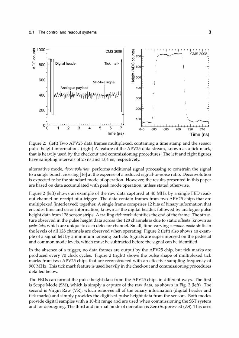
Figure 2: (left) Two APV25 data frames multiplexed, containing a time stamp and the sensorpulse height information. (right) A feature of the APV25 data stream, known as a tick mark,that is heavily used by the checkout and commissioning procedures. The left and right figureshave sampling intervals of 25 ns and 1.04 ns, respectively.

alternative mode, deconvolution, performs additional signal processing to constrain the signalto a single bunch crossing [16] at the expense of a reduced signal-to-noise ratio. Deconvolutionis expected to be the standard mode of operation. However, the results presented in this paperare based on data accumulated with peak mode operation, unless stated otherwise.

Figure 2 (left) shows an example of the raw data captured at 40 MHz by a single FED read-out channel on receipt of a trigger. The data contain frames from two APV25 chips that aremultiplexed (interleaved) together. A single frame comprises 12 bits of binary information thatencodes time and error information, known as the digital header, followed by analogue pulseheight data from 128 sensor strips. A trailing tick mark identifies the end of the frame. The struc-ture observed in the pulse height data across the 128 channels is due to static offsets, known aspedestals, which are unique to each detector channel. Small, time-varying common mode shifts inthe levels of all 128 channels are observed when operating. Figure 2 (left) also shows an exam-ple of a signal left by a minimum ionising particle. Signals are superimposed on the pedestaland common mode levels, which must be subtracted before the signal can be identified.

In the absence of a trigger, no data frames are output by the APV25 chip, but tick marks areproduced every 70 clock cycles. Figure 2 (right) shows the pulse shape of multiplexed tickmarks from two APV25 chips that are reconstructed with an effective sampling frequency of960 MHz. This tick mark feature is used heavily in the checkout and commissioning proceduresdetailed below.

The FEDs can format the pulse height data from the APV25 chips in different ways. The firstis Scope Mode (SM), which is simply a capture of the raw data, as shown in Fig. 2 (left). Thesecond is Virgin Raw (VR), which removes all of the binary information (digital header andtick marks) and simply provides the digitised pulse height data from the sensors. Both modesprovide digital samples with a 10-bit range and are used when commissioning the SST systemand for debugging. The third and normal mode of operation is Zero Suppressed (ZS). This uses

4 2 Commissioning the SST Control and Readout Systems

Field Programmable Gate Array (FPGA) chips to implement algorithms that perform pedestalsubtraction, common mode subtraction, and identification of channels potentially containingsignals above threshold. A threshold of five times the detector channel noise is used for singlechannels, but a threshold of only twice the channel noise is used for signals in contiguouschannels. The zero-suppressed data are output with an 8-bit range.

2.2 Checkout of the detector components and cabling

The checkout procedures are used to identify: responsive and functional devices in the controland readout systems; the cabling of the readout electronics chain, from the front-end detectormodules to the off-detector FED boards; the cabling of the Low Voltage (LV) and High Voltage(HV) buses of the power supply system [17]; and the mapping of the detector modules to theirgeometrical position within the SST superstructure. Automation is possible as each detectormodule hosts a Detector Control Unit (DCU) chip [18], which broadcasts a unique indentifiervia the control system. This identifier is used to tag individual modules.

The cabling of the LV power supply system is established by sequentially powering groupsof detector modules and identifying responsive devices via the control system. Similarly, theHV cabling is determined by applying HV to an individual channel and identifying detectormodules responding with a decreased noise, due to reduced strip capacitance.

Each front-end detector module hosts a Linear Laser Driver (LLD) chip [19], which drives theoptical links that transmit the analogue signals to the off-detector FED boards. The cabling ofthe readout electronics chain is established by configuring individual LLD chips to produceunique patterns in the data stream of the connected FED channels.

The final number of modules used in the CRAFT data-taking period corresponds to 98.0% ofthe total system. The most significant losses were from one control ring in each of the TIB andTOB sub-systems. In the TIB, this was due to a single faulty CCU. The remaining CCUs on thisring have since been recovered using a built-in redundancy feature of the control ring design.The fraction of operational modules was increased to 98.6% after data-taking, once problemsidentified during checkout were investigated more fully.

2.3 Relative synchronisation of the front-end

Relative synchronisation involves adjusting the phase of the LHC clock delivered to the front-end so that the sampling times of all APV25 chips in the system are synchronous. Additionally,the signal sampling time of the FED Analogue/Digital Converters (ADC) is appropriately ad-justed. This procedure accounts for differences in signal propagation time in the control systemdue to differing cable lengths. This synchronisation procedure is important because signal am-plitude is attenuated by as much as 4% per nanosecond mis-synchronisation due to the narrowpulse shape in deconvolution mode.

Using the FED boards in Scope Mode, the tick mark pulse shape is reconstructed with a 1.04 nsstep width by varying the clock phase using a Phase Locked Loop (PLL) chip [20] hosted byeach detector module, as shown in Fig. 2 (right). The ideal sampling point is on the signalplateau, 15 ns after the rising edge of the tick mark. The required delays are thus inferred fromthe arrival times of the tick mark edges at the FED ADCs. The pre-synchronisation timingspread of up to 160 ns is reduced to an RMS of 0.72 ns, with the largest deviation of 4 nscorresponding to a maximum signal attenuation of ∼16% in deconvolution mode.

2.4 Calibration of the readout system gain 5

Time (ns)0 20 40 60 80 100 120 140 160

Am

plit

ude

(a. u

.)

0

200

400

600

800

1000

1200

1400

1600

1800

2000 Before tuning

After tuning

50ns smeared RC-CR fit

CMS 2008

CalibrationEntries 15012

Mean 222.6

RMS 28.91

Signal Amplitude (ADC)

50 100 150 200 250 300 350 400

Num

ber

of A

PV

's

0

20

40

60

80

100

120

140

160

180

200

220Calibration

Entries 15012

Mean 222.6

RMS 28.91

60000 electrons

CMS 2008

Figure 3: (Left) An example of the CR-RC pulse shape of a single APV25 chip, before andafter the pulse shape tuning procedure. (Right) Pulse height measurements using the on-chipcalibration circuitry of APV25 chips in the TEC+.

2.4 Calibration of the readout system gain

One of the largest contributions to gain variation in the readout system is the distribution oflaser output efficiencies caused by the variation of laser-to-fibre alignment from sample to sam-ple during production of the transmitters. In addition some loss may have been introduced atthe three optical patch panels in the fibre system. Changes in the LV power supply or environ-mental temperature can also significantly affect the gain at the level of a FED readout channel.

The calibration procedure aims to optimise the use of the available dynamic range of the FEDADCs and also equalise the gain of the entire readout system. This is achieved by tuning thebias and gain register settings of the LLD chip for individual fibres. Four gain settings arepossible. The amplitude of the tick mark, which is assumed to be roughly constant in time andacross all APV25 chips within the system, is used to measure the gain of each readout channel.The setting that results in a tick mark amplitude closest to 640 ADC counts is chosen, as thisamplitude corresponds to the expected design gain of 0.8. After tuning the system, a spread of±20% is observed, which is expected because of the coarse granularity of the LLD gain settings.

The response of all detector channels can be further equalised during offline reconstruction bycorrecting the signal magnitude by the normalisation factor f = 640 ADC counts /atickmark,where atickmark is the tick mark amplitude in ADC counts. The tick mark amplitude is a goodindicator of the maximum output of the APV25 chip, which corresponds to a charge depositof 175 000 e−. This method provides a calibration factor of 274± 14 e−/ADC count. The esti-mated systematic uncertainty is 5%, attributable to the sensitivity of the tick mark amplitudeto variations in the LV power supply and environmental temperature [6].

2.5 Tuning of the APV25 front-end amplifier pulse shape

The shape of the CR-RC pulse from the APV25 pre-amplifier and shaper stages is dependent onthe input capacitance, which depends on the sensor geometry and evolves with total radiationdose. By default, all APV25 chips are configured with pre-defined settings appropriate to thesensor geometry, based on laboratory measurements [21]. However, non-uniformities in thefabrication process result in a small natural spread in the pulse shape parameters for a giveninput capacitance. This issue is important for performance in deconvolution mode, which issensitive to the CR-RC pulse shape. In order to maximise the signal-to-noise ratio and con-

6 2 Commissioning the SST Control and Readout Systems

���������������������� ��� ���� ���� ���� ���� ���� ���� ���� ���� ����

��������������

�

��

���

��������� ���������

��������� ����������

����� ���������

����� ������������

CMS 2008

Minimal strip noise / Noise median0 0.1 0.2 0.3 0.4 0.5 0.6 0.7 0.8 0.9 1

Num

ber o

f APV

’s

1

10

210

310CMS 2008

Figure 4: (Left) Mean calibrated noise for individual APV25 chips on modules in the TOBsingle side layer 3. (Right) The ratio of minimum noise to median noise per APV25 chip. Thedistinct populations reflect the different noise sources within a module.

fine the signal to a single bunch crossing interval when operating in deconvolution mode, therise time of the CR-RC pulse shape must be tuned to 50 ns and the signal amplitude at 125 nsafter the signal maximum should be 36% of the maximum. This tuning also reduces the tim-ing uncertainties associated with the synchronisation procedures. Figure 3 (left) demonstrateshow the CR-RC pulse shape of an APV25, operating in peak mode, can be improved by theprocedure.

Figure 3 (right) shows the pulse height amplitude (in ADC counts) observed for a charge injec-tion of 60 000 e− using the on-chip calibration circuitry of the APV25 chip. The charge injectionprovided by the calibration circuit is known with a precision of 5% and can be used to calibratethe detector signal amplitude. A mean signal of 223 ADC counts with a RMS of 29 ADC countswas observed, giving a calibration factor of 269 ± 13 e−/ADC counts. This measurement iscompatible with the calibration based on tick mark amplitudes, described in Section 2.4.

2.6 Calibration of the detector channel pedestals and noise

The mean level of the pedestals for the 128 channels of a given APV25 chip, known as the base-line level, can be adjusted to optimise the signal linearity and the use of the available dynamicrange of the APV25. The baseline level for each APV25 chip is adjusted to sit at approximatelyone third of the dynamic range.

Following this baseline adjustment, the pedestal and noise constants for each individual de-tector channel must be measured, as these values are used by the zero-suppression algorithmsimplemented in the FPGA logic of the FEDs. Pedestals and noise are both measured using arandom, low frequency trigger (∼10 Hz) in the absence of signal. Pedestals are first calculatedas the mean of the raw data in each detector channel from a large event sample. They are sub-sequently subtracted from the raw data values for each event. Common mode offsets are eval-uated for each APV25 chip per event by calculating the median of these pedestal-subtracteddata. The median value is then subtracted from each channel. The noise for each detectorchannel is then defined to be the standard deviation of the residual data levels, which can becalibrated using the measurements described in Sections 2.4 and 2.5. Figure 4 (left) shows adistribution of the mean noise measured per APV25 chip, for TOB single side layer 3. The out-liers correspond to APV25 chips from modules with unbiased sensors, due to problems in theHV power supply.

Modules with different sensor geometries are studied separately to account for the different

2.7 Absolute synchronisation to an external trigger 7

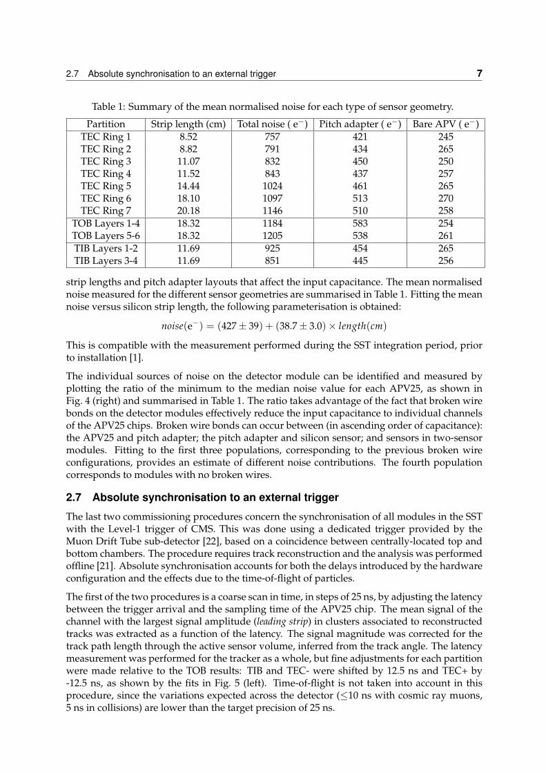
Table 1: Summary of the mean normalised noise for each type of sensor geometry.

Partition Strip length (cm) Total noise ( e−) Pitch adapter ( e−) Bare APV ( e−)TEC Ring 1 8.52 757 421 245TEC Ring 2 8.82 791 434 265TEC Ring 3 11.07 832 450 250TEC Ring 4 11.52 843 437 257TEC Ring 5 14.44 1024 461 265TEC Ring 6 18.10 1097 513 270TEC Ring 7 20.18 1146 510 258

TOB Layers 1-4 18.32 1184 583 254TOB Layers 5-6 18.32 1205 538 261TIB Layers 1-2 11.69 925 454 265TIB Layers 3-4 11.69 851 445 256

strip lengths and pitch adapter layouts that affect the input capacitance. The mean normalisednoise measured for the different sensor geometries are summarised in Table 1. Fitting the meannoise versus silicon strip length, the following parameterisation is obtained:

noise(e−) = (427± 39) + (38.7± 3.0)× length(cm)

This is compatible with the measurement performed during the SST integration period, priorto installation [1].

The individual sources of noise on the detector module can be identified and measured byplotting the ratio of the minimum to the median noise value for each APV25, as shown inFig. 4 (right) and summarised in Table 1. The ratio takes advantage of the fact that broken wirebonds on the detector modules effectively reduce the input capacitance to individual channelsof the APV25 chips. Broken wire bonds can occur between (in ascending order of capacitance):the APV25 and pitch adapter; the pitch adapter and silicon sensor; and sensors in two-sensormodules. Fitting to the first three populations, corresponding to the previous broken wireconfigurations, provides an estimate of different noise contributions. The fourth populationcorresponds to modules with no broken wires.

2.7 Absolute synchronisation to an external trigger

The last two commissioning procedures concern the synchronisation of all modules in the SSTwith the Level-1 trigger of CMS. This was done using a dedicated trigger provided by theMuon Drift Tube sub-detector [22], based on a coincidence between centrally-located top andbottom chambers. The procedure requires track reconstruction and the analysis was performedoffline [21]. Absolute synchronisation accounts for both the delays introduced by the hardwareconfiguration and the effects due to the time-of-flight of particles.

The first of the two procedures is a coarse scan in time, in steps of 25 ns, by adjusting the latencybetween the trigger arrival and the sampling time of the APV25 chip. The mean signal of thechannel with the largest signal amplitude (leading strip) in clusters associated to reconstructedtracks was extracted as a function of the latency. The signal magnitude was corrected for thetrack path length through the active sensor volume, inferred from the track angle. The latencymeasurement was performed for the tracker as a whole, but fine adjustments for each partitionwere made relative to the TOB results: TIB and TEC- were shifted by 12.5 ns and TEC+ by-12.5 ns, as shown by the fits in Fig. 5 (left). Time-of-flight is not taken into account in thisprocedure, since the variations expected across the detector (≤10 ns with cosmic ray muons,5 ns in collisions) are lower than the target precision of 25 ns.

8 3 Data Samples and Monte Carlo Simulations

Latency (ns)-2700 -2600 -2500 -2400 -2300 -2200

Lead

ing

strip

cor

rect

ed a

mpl

itude

(AD

C c

ount

s)

0

10

20

30

40

50

60

70 TIBTOBTEC-TEC+

TIB peak position: -2602.5 ns

TOB peak position: -2590.0 ns

TEC- peak position: -2602.5 ns

TEC+ peak position: -2577.5 ns

CMS 2008

Delay shift (ns)-100 -50 0 50 100

Lead

ing

strip

cor

rect

ed a

mpl

itude

(AD

C c

ount

s)

0

10

20

30

40

50

60

70 CMS 2008

Figure 5: (Left) Mean signal of leading strip in clusters associated to tracks as a function of thelatency (25 ns steps), for each of the four partitions. (Right) Fine delay scan for the TOB layer 3,in deconvolution. The mean position (-14.2 ns) is including the mean time-of-flight of particlesfrom the muon system to the silicon sensors (12 ns).

The last procedure comprises a fine tuning of the synchronisation. It involves skewing theclock delay in steps of 1 ns around the expected optimal value for all modules of a given testlayer, with the configuration of all other modules in the SST unchanged with respect to thevalue obtained from the coarse latency scan. Clusters on the test layer compatible with a re-constructed track are used to reconstruct the pulse shape. Figure 5 (right) shows the resultingpulse shape from clusters found in modules of TOB layer 3, acquired in deconvolution mode.With collision data, the time-of-flight can be adjusted for each individual track, but this is notthe case for cosmic ray muons, for which the jitter from the trigger cannot be subtracted. The14 ns shift observed is consistent with the expected time-of-flight (12 ns) of cosmic ray muonsfrom the Muon Drift Tube chambers to the TOB layer 3.

From analysis of the latency and fine delay scans, correction factors are computed to compen-sate the residual mis-synchronisation of each partition. These corrections range from 1.0 to 1.06with uncertainties of 0.03 and are used to correct the cluster charge in calibration and dE/dxstudies, reported below.

3 Data Samples and Monte Carlo SimulationsIn the following sections, the performance of the tracker will be analysed using the data col-lected during CRAFT. The event reconstruction and selection, data quality monitoring anddata analysis were all performed within the CMS software framework, known as CMSSW [23].The data quality was monitored during both the online and offline reconstruction [24]. Thedata were categorised and the results of this categorisation procedure propagated to the CMSDataset Bookkeeping System [25]. Unless otherwise stated, only runs for which the quality wascertified as good, i.e., no problems were known to affect the Trigger and Tracker performance,were used for the analyses presented in this paper.

The data-taking period can be split into three distinct intervals in time, based on magnetic fieldconditions and tracker performance. Each period has approximately uniform conditions. In

9

the first period, period A, part of the SST was not correctly synchronised with the rest of theCMS detector. This problem was fixed for data taken in subsequent periods. The magnet wasat its nominal field value of 3.8 T during periods A and B, while period C corresponds to datataken with the magnet switched off. Unless stated otherwise, the following results are basedonly on events from period B.

For the studies presented in this paper, the events selected by the Global Muon Trigger [26]were used. This data sample was additionally filtered to include only events that contain atleast one reconstructed track in the tracker or that have a track reconstructed in the muonchambers whose trajectory points back into the SST barrel volume.

Several analyses use a simulated sample of 21 million cosmic ray muons to derive correctionfactors and compare results. The sample was generated using the CMSCGEN package [27, 28].The detector was simulated using the standard program of CMSSW. Modules known to beexcluded from the read-out were masked in the simulation. Besides this, the simulation wasnot optimised to the conditions of CRAFT. Nevertheless, the agreement with the data wassufficient for the purpose of the studies presented.

4 Performance of the Local ReconstructionIn this section, the reconstruction at the level of the single detector module, is presented. Thecosmic ray muon rate is small and events with more than one track are rare. So with zero-suppression only a tiny fraction of the SST channels are read out in any one event. Thesechannels which pass zero-suppression and therefore have non-zero ADC counts are known asdigi. Despite the zero suppression, digis may still only consist of noise.

Clusters are formed from digs by means of a three threshold algorithm [23]. Clusters are seededby digis which have a charge that is at least three times greater than the corresponding channelnoise. For each seed, neighbouring strips are added if the strip charge is more than twice thestrip noise. A cluster is kept if its total charge is more than five times the cluster noise, defined

as σcluster =√

∑i σ2i , where σi is the noise from strip i, and the sum runs over all strips in the

cluster.

In the following, the properties of both digis and clusters are studied and the performance ofeach SST subsystem is assessed.

4.1 Occupancy

The average number of digis per event and the occupancy are shown for each SST subsystemin Table 2. The strip occupancy is computed after removing the masked modules (2.0 %). Theaverage occupancy in the SST is 4× 10−4, as expected from simulation and from the propertiesof the zero suppression algorithm. The digi occupancy is dominated by noise, but the clus-ter algorithm reconstructs less than ten hits per event when there is no track within the SSTacceptance.

4.2 Signal-to-noise ratio

The signal-to-noise ratio is a benchmark for the performance of the SST. It is particularly usefulfor studying the stability over time. In the signal-to-noise ratio, the cluster noise is divided by√

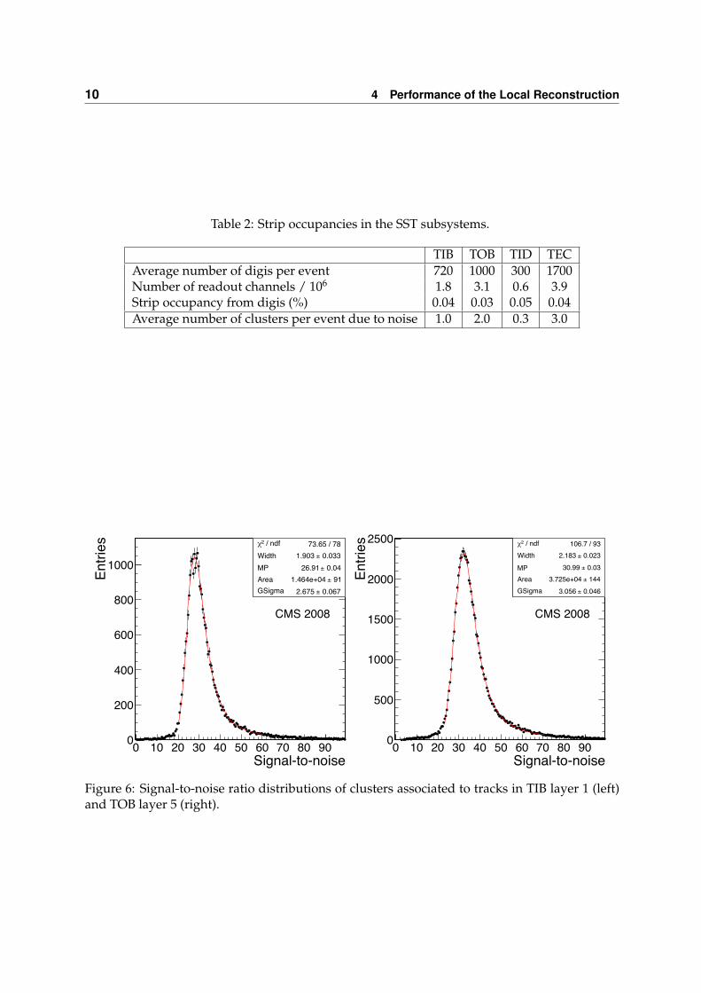
Nstrips, so that the resulting noise value is approximately equal to the strip noise, indepen-dently of the size of the cluster. The path-length corrected signal-to-noise ratio distributionsare presented in Fig. 6 for TIB layer 1 and TOB layer 5. The distributions have been fitted with

10 4 Performance of the Local Reconstruction

Table 2: Strip occupancies in the SST subsystems.

TIB TOB TID TECAverage number of digis per event 720 1000 300 1700Number of readout channels / 106 1.8 3.1 0.6 3.9Strip occupancy from digis (%) 0.04 0.03 0.05 0.04Average number of clusters per event due to noise 1.0 2.0 0.3 3.0

/ ndf 2χ 73.65 / 78Width 0.033± 1.903 MP 0.04± 26.91 Area 91± 1.464e+04 GSigma 0.067± 2.675

Signal-to-noise0 10 20 30 40 50 60 70 80 90

Entri

es

0

200

400

600

800

1000

/ ndf 2χ 73.65 / 78Width 0.033± 1.903 MP 0.04± 26.91 Area 91± 1.464e+04 GSigma 0.067± 2.675

CMS 2008

/ ndf 2χ 106.7 / 93Width 0.023± 2.183 MP 0.03± 30.99 Area 144± 3.725e+04 GSigma 0.046± 3.056

Signal-to-noise0 10 20 30 40 50 60 70 80 90

Entri

es

0

500

1000

1500

2000

2500 / ndf 2χ 106.7 / 93Width 0.023± 2.183 MP 0.03± 30.99 Area 144± 3.725e+04 GSigma 0.046± 3.056

CMS 2008

Figure 6: Signal-to-noise ratio distributions of clusters associated to tracks in TIB layer 1 (left)and TOB layer 5 (right).

4.3 Gain calibration 11

a Landau function convoluted with a Gaussian function to determine the most probable valuefor the signal-to-noise ratio. The result is in the range 25-30 for thin modules and 31-36 for thickones, and within 5% from the expected values. Thick sensors collect about a factor of 5/3 morecharge than the thin sensors, but this does not simply scale up the signal-to-noise ratio, as thenoise is also larger for thick sensors, because of the longer strips of these modules.

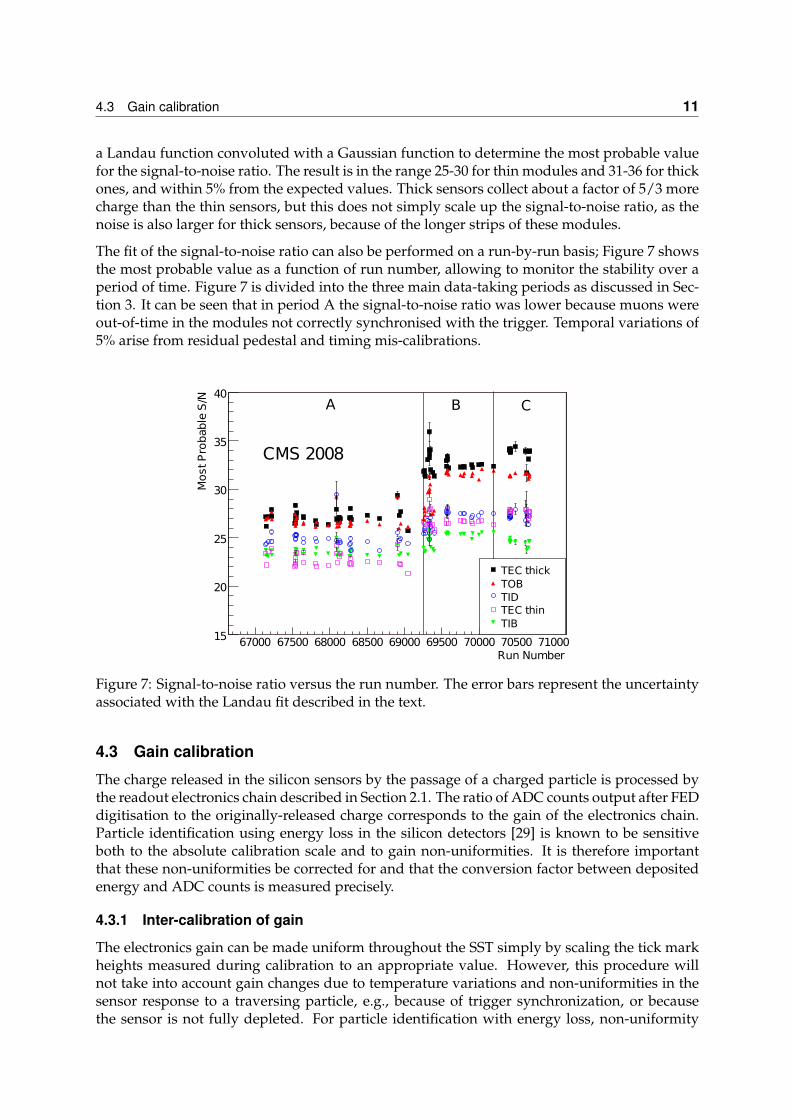
The fit of the signal-to-noise ratio can also be performed on a run-by-run basis; Figure 7 showsthe most probable value as a function of run number, allowing to monitor the stability over aperiod of time. Figure 7 is divided into the three main data-taking periods as discussed in Sec-tion 3. It can be seen that in period A the signal-to-noise ratio was lower because muons wereout-of-time in the modules not correctly synchronised with the trigger. Temporal variations of5% arise from residual pedestal and timing mis-calibrations.

Run Number67000 67500 68000 68500 69000 69500 70000 70500 71000

MostProbableS/N

15

20

25

30

35

40

TOB

TIB

TIDTEC thin

TEC thick

A B C

CMS 2008

Figure 7: Signal-to-noise ratio versus the run number. The error bars represent the uncertaintyassociated with the Landau fit described in the text.

4.3 Gain calibration

The charge released in the silicon sensors by the passage of a charged particle is processed bythe readout electronics chain described in Section 2.1. The ratio of ADC counts output after FEDdigitisation to the originally-released charge corresponds to the gain of the electronics chain.Particle identification using energy loss in the silicon detectors [29] is known to be sensitiveboth to the absolute calibration scale and to gain non-uniformities. It is therefore importantthat these non-uniformities be corrected for and that the conversion factor between depositedenergy and ADC counts is measured precisely.

4.3.1 Inter-calibration of gain

The electronics gain can be made uniform throughout the SST simply by scaling the tick markheights measured during calibration to an appropriate value. However, this procedure willnot take into account gain changes due to temperature variations and non-uniformities in thesensor response to a traversing particle, e.g., because of trigger synchronization, or becausethe sensor is not fully depleted. For particle identification with energy loss, non-uniformity

12 4 Performance of the Local Reconstruction

MPV (ADC counts/mm)0 100 200 300 400 500

Num

ber o

f APV

s

0

200

400

600

800

1000CMS 2008mµ320

mµ500 mµ320 + 500

Figure 8: Most probable value of the cluster charge for different thicknesses before gain cali-bration.

must not exceed 2% [29]. This level of inter-calibration can be achieved only using the signalsproduced by particles. The path length corrected charge of those clusters associated with trackswas fitted with a separate Landau curve for each APV25 chip. Figure 8 shows the distributionof most probable values for APVs with at least 50 clusters, subdivided by sensor thickness. Thespread of these distributions is around 10%.

The most probable value of each distribution is then used to compute the inter-calibration con-stants by normalising the signal to 300 ADC counts/mm – the value expected for a minimumionising particle with a calibration of 270 e−/ADC count (Section 2.5). The inter-calibrationconstants determined in this manner were used in the final reprocessing of the CRAFT data,resulting in a uniform response.

4.3.2 Absolute calibration using energy deposit information

In addition to the inter-calibration constants, for particle identification using energy loss, the ra-tio of deposited charge to ADC counts must be measured. The energy loss by particles travers-ing thin layers of silicon is described by the Landau-Vavilov-Bichsel theory [30]. The mostprobable energy deposition per unit of length, ∆p/x, is described by the Bichsel function anddepends on both the silicon thickness and the particle momentum. For muons, the function hasa minimum at 0.5 GeV/c and then rises to reach a plateau for momenta greater than 10 GeV/c.The absolute gain calibration can be determined by fitting the Bichsel function predictions tothe measured ∆p/x values from the CRAFT data sample.

The quantity ∆p/x is measured using the charge of clusters associated to tracks as a functionof track momentum. The resulting charge distributions are fitted with a Landau convolutedwith a Gaussian. Only tracks with at least six hits and χ2/ndf less than 10 are considered. Inaddition, only clusters with fewer than four strips are taken into account. This last requirementis imposed in order to avoid mis-reconstructed clusters.

Before the absolute calibration factor can be extracted from the cluster charge data, two cor-rections must be applied. Firstly, a correction is needed to take into account any charge lossin the zero-suppression process and during clustering. This is determined using Monte Carlosimulations for each subsystem and for both thin and thick sensors in the end caps. Secondly, acorrection is needed to handle the imperfect synchronisation between the different subsystems.

4.4 Lorentz angle measurement 13

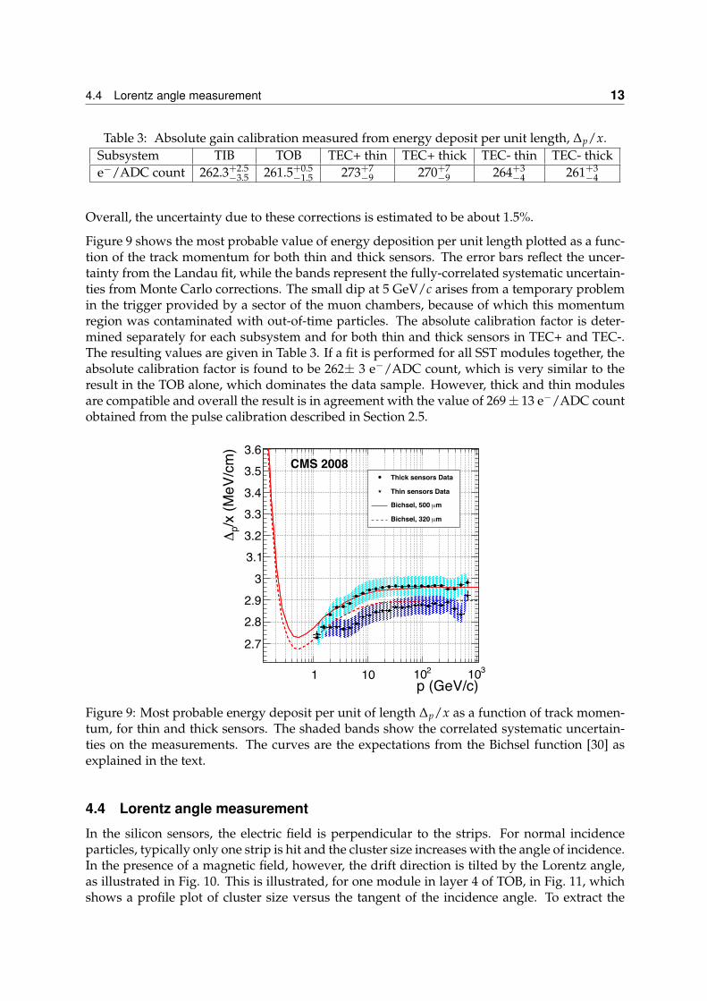
Table 3: Absolute gain calibration measured from energy deposit per unit length, ∆p/x.Subsystem TIB TOB TEC+ thin TEC+ thick TEC- thin TEC- thicke−/ADC count 262.3+2.5

−3.5 261.5+0.5−1.5 273+7

−9 270+7−9 264+3

−4 261+3−4

Overall, the uncertainty due to these corrections is estimated to be about 1.5%.

Figure 9 shows the most probable value of energy deposition per unit length plotted as a func-tion of the track momentum for both thin and thick sensors. The error bars reflect the uncer-tainty from the Landau fit, while the bands represent the fully-correlated systematic uncertain-ties from Monte Carlo corrections. The small dip at 5 GeV/c arises from a temporary problemin the trigger provided by a sector of the muon chambers, because of which this momentumregion was contaminated with out-of-time particles. The absolute calibration factor is deter-mined separately for each subsystem and for both thin and thick sensors in TEC+ and TEC-.The resulting values are given in Table 3. If a fit is performed for all SST modules together, theabsolute calibration factor is found to be 262± 3 e−/ADC count, which is very similar to theresult in the TOB alone, which dominates the data sample. However, thick and thin modulesare compatible and overall the result is in agreement with the value of 269± 13 e−/ADC countobtained from the pulse calibration described in Section 2.5.

p (GeV/c)1 10 210 310

/x (M

eV/c

m)

p!

2.7

2.82.9

33.13.23.33.43.53.6

Thick sensors Data

Thin sensors Data

mµBichsel, 500

mµBichsel, 320

CMS 2008

Figure 9: Most probable energy deposit per unit of length ∆p/x as a function of track momen-tum, for thin and thick sensors. The shaded bands show the correlated systematic uncertain-ties on the measurements. The curves are the expectations from the Bichsel function [30] asexplained in the text.

4.4 Lorentz angle measurement

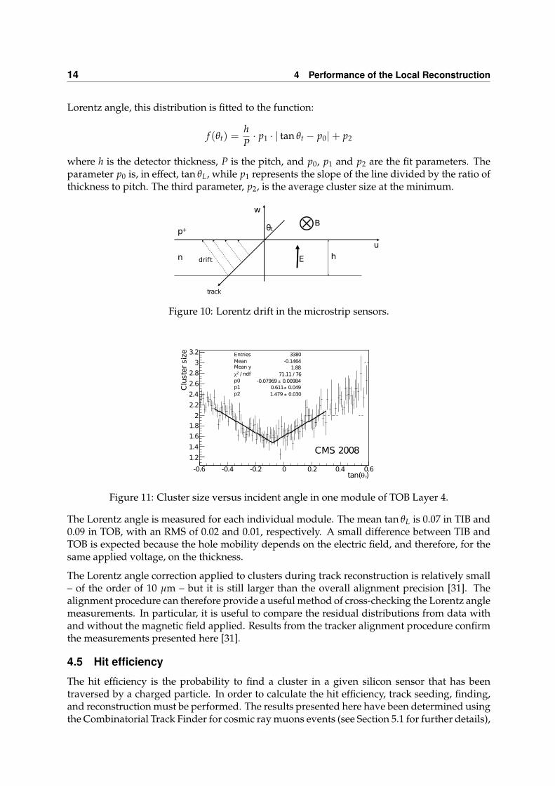
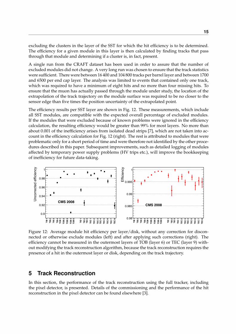
In the silicon sensors, the electric field is perpendicular to the strips. For normal incidenceparticles, typically only one strip is hit and the cluster size increases with the angle of incidence.In the presence of a magnetic field, however, the drift direction is tilted by the Lorentz angle,as illustrated in Fig. 10. This is illustrated, for one module in layer 4 of TOB, in Fig. 11, whichshows a profile plot of cluster size versus the tangent of the incidence angle. To extract the

14 4 Performance of the Local Reconstruction

Lorentz angle, this distribution is fitted to the function:

f (θt) =hP· p1 · | tan θt − p0|+ p2

where h is the detector thickness, P is the pitch, and p0, p1 and p2 are the fit parameters. Theparameter p0 is, in effect, tan θL, while p1 represents the slope of the line divided by the ratio ofthickness to pitch. The third parameter, p2, is the average cluster size at the minimum.

p+

n

w

track

B

E h

θt

u

drift

Figure 10: Lorentz drift in the microstrip sensors.

Entries 3380Mean -0.1464Mean y 1.88

/ ndf 71.11 / 76p0 0.00984�2

0.611 p2 0.030

-0.07969 p1 0.049

1.479 ��

�

)t�tan(-0.6 -0.4 -0.2 0 0.2 0.4 0.6

Clu

ster

siz

e

1.2

1.4

1.6

1.8

2

2.2

2.4

2.6

2.8

3

3.2

CMS 2008

Figure 11: Cluster size versus incident angle in one module of TOB Layer 4.

The Lorentz angle is measured for each individual module. The mean tan θL is 0.07 in TIB and0.09 in TOB, with an RMS of 0.02 and 0.01, respectively. A small difference between TIB andTOB is expected because the hole mobility depends on the electric field, and therefore, for thesame applied voltage, on the thickness.

The Lorentz angle correction applied to clusters during track reconstruction is relatively small– of the order of 10 µm – but it is still larger than the overall alignment precision [31]. Thealignment procedure can therefore provide a useful method of cross-checking the Lorentz anglemeasurements. In particular, it is useful to compare the residual distributions from data withand without the magnetic field applied. Results from the tracker alignment procedure confirmthe measurements presented here [31].

4.5 Hit efficiency

The hit efficiency is the probability to find a cluster in a given silicon sensor that has beentraversed by a charged particle. In order to calculate the hit efficiency, track seeding, finding,and reconstruction must be performed. The results presented here have been determined usingthe Combinatorial Track Finder for cosmic ray muons events (see Section 5.1 for further details),

15

excluding the clusters in the layer of the SST for which the hit efficiency is to be determined.The efficiency for a given module in this layer is then calculated by finding tracks that passthrough that module and determining if a cluster is, in fact, present.

A single run from the CRAFT dataset has been used in order to assure that the number ofexcluded modules did not change. A very long run was chosen to ensure that the track statisticswere sufficient. There were between 16 400 and 104 800 tracks per barrel layer and between 1700and 6500 per end cap layer. The analysis was limited to events that contained only one track,which was required to have a minimum of eight hits and no more than four missing hits. Toensure that the muon has actually passed through the module under study, the location of theextrapolation of the track trajectory on the module surface was required to be no closer to thesensor edge than five times the position uncertainty of the extrapolated point.

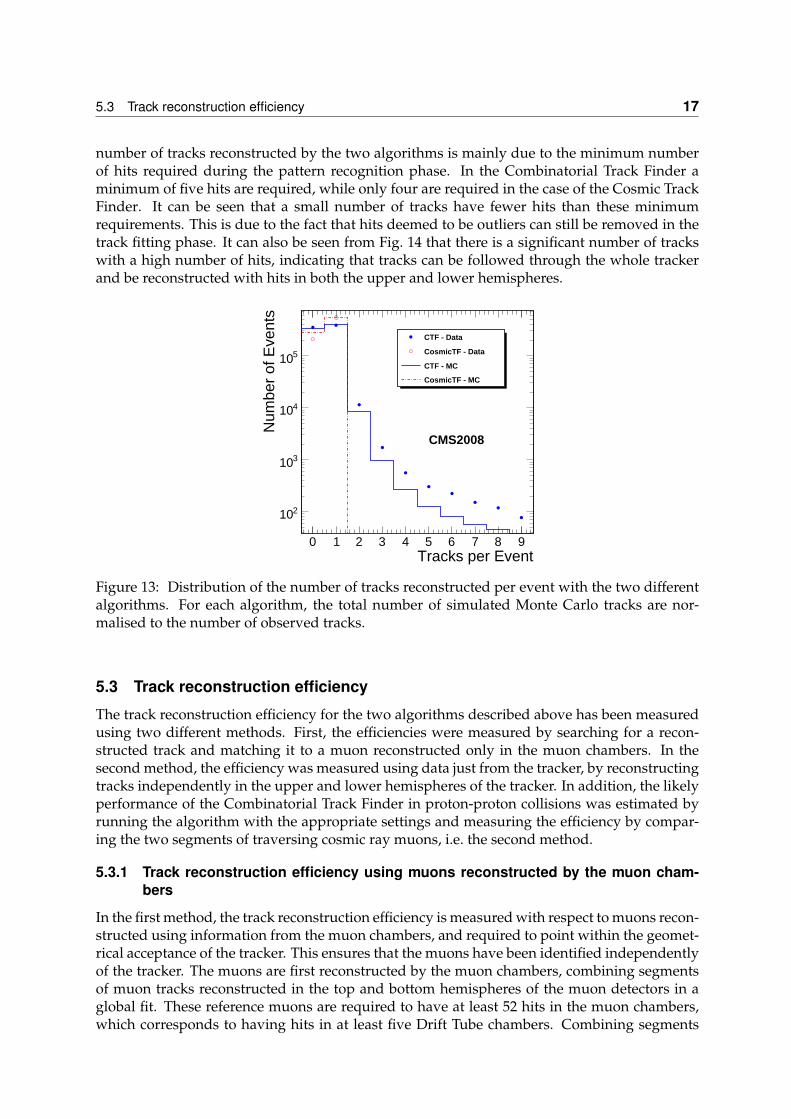
The efficiency results per SST layer are shown in Fig. 12. These measurements, which includeall SST modules, are compatible with the expected overall percentage of excluded modules.If the modules that were excluded because of known problems were ignored in the efficiencycalculation, the resulting efficiency would be greater than 99% for most layers. No more thanabout 0.001 of the inefficiency arises from isolated dead strips [7], which are not taken into ac-count in the efficiency calculation for Fig. 12 (right). The rest is attributed to modules that wereproblematic only for a short period of time and were therefore not identified by the other proce-dures described in this paper. Subsequent improvements, such as detailed logging of modulesaffected by temporary power supply problems (HV trips etc.), will improve the bookkeepingof inefficiency for future data-taking.

TIB

1TI

B 2

TIB

3

TIB

4TO

B 1

TOB

2

TOB

3

TOB

4TO

B 5

TID

1

TID

2TI

D 3

TEC

1

TEC

2

TEC

3TE

C 4

TEC

5

TEC

6

TEC

7TE

C 8

TIB

1TI

B 2

TIB

3

TIB

4TO

B 1

TOB

2

TOB

3

TOB

4TO

B 5

TID

1

TID

2TI

D 3

TEC

1

TEC

2

TEC

3TE

C 4

TEC

5

TEC

6

TEC

7TE

C 8

Unco

rrect

ed e

fficie

ncy

0.9

0.92

0.94

0.96

0.98

1

CMS 2008

TIB

1TI

B 2

TIB

3

TIB

4TO

B 1

TOB

2

TOB

3

TOB

4TO

B 5

TID

1

TID

2TI

D 3

TEC

1

TEC

2

TEC

3TE

C 4

TEC

5

TEC

6

TEC

7TE

C 8

TIB

1TI

B 2

TIB

3

TIB

4TO

B 1

TOB

2

TOB

3

TOB

4TO

B 5

TID

1

TID

2TI

D 3

TEC

1

TEC

2

TEC

3TE

C 4

TEC

5

TEC

6

TEC

7TE

C 8

Effic

ienc

y

0.98

0.985

0.99

0.995

1

CMS 2008

Figure 12: Average module hit efficiency per layer/disk, without any correction for discon-nected or otherwise exclude modules (left) and after applying such corrections (right). Theefficiency cannot be measured in the outermost layers of TOB (layer 6) or TEC (layer 9) with-out modifying the track reconstruction algorithm, because the track reconstruction requires thepresence of a hit in the outermost layer or disk, depending on the track trajectory.

5 Track ReconstructionIn this section, the performance of the track reconstruction using the full tracker, includingthe pixel detector, is presented. Details of the commissioning and the performance of the hitreconstruction in the pixel detector can be found elsewhere [3].

16 5 Track Reconstruction

5.1 Track reconstruction algorithms

The two main algorithms used to reconstruct tracks from cosmic ray muons in CRAFT dataare the Combinatorial Track Finder (CTF) and the Cosmic Track Finder (CosmicTF). The Com-binatorial Track Finder is the standard track reconstruction algorithm intended for use withproton-proton collisions and the main focus of the present study; for these runs, it has beenspecially re-configured to handle the different topology of cosmic muon events. The second al-gorithm was devised specifically for the reconstruction of single track cosmic ray muon events.Since it is meant as a cross-check of the Combinatorial Track Finder, it has not been tuned to thesame level of performance. A full description of these algorithms can be found elsewhere [7].

There have been two significant changes in the Combinatorial Track Finder since its first usein the Slice Test, both relating to the seed finding phase. The Slice Test was performed withoutthe presence of a magnetic field and with only limited angular coverage. Now that the fulltracker is available, seed finding in the barrel uses TOB layers only and both hit triplets andpairs are generated. In the end caps, hits in adjacent disks are used to form hit pairs. Thepresence of the 3.8 T magnetic field means that for hit-triplet seeds, the curvature of the helixyields an initial estimate of the momentum. For hit pairs seeds, an initial estimate of 2 GeV/cis used, which corresponds to the most probable value. The detector has been aligned with themethods described in Reference [31].

5.2 Track reconstruction results

The number of tracks reconstructed by the two algorithms in the data from Period B, withoutapplying any additional track quality criteria, except those applied during the track reconstruc-tion itself, are 2.2 million using the Combinatorial Track Finder and 2.7 million by the CosmicTrack Finder.

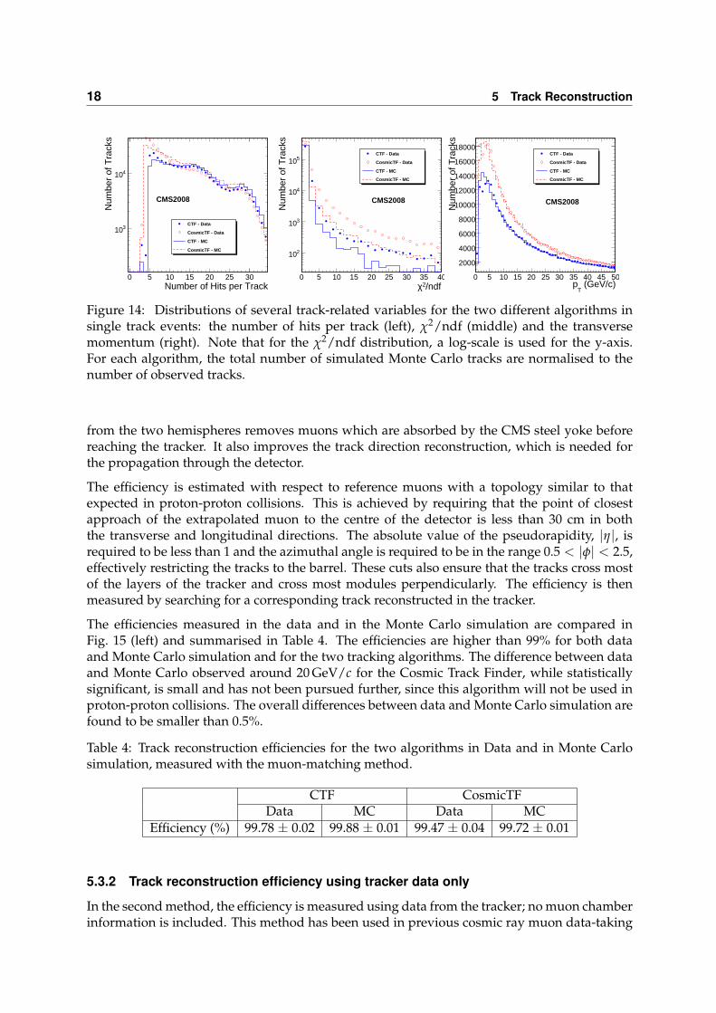
The number of reconstructed tracks per event is shown in Fig. 13, and Fig. 14 shows the dis-tributions of a number of track-related quantities compared between a subset of the data andMonte Carlo simulation. The large number of events without reconstructed tracks is mainlydue to muons outside of the fiducial volume for which fewer than five hits are reconstructed inthe tracker.

It can be seen that reasonable agreement is found between the data and the Monte Carlo sim-ulation, although there are some discrepancies that require further investigation. These arethought to be due to the reconstruction of showers by the track reconstruction algorithms. TheCombinatorial Track Finder is capable of reconstructing more than one track per event, but asit has not been optimised to reconstruct showers, multi-track events tend to contain a numberof fake or badly reconstructed tracks. These are mostly low momentum tracks with a smallnumber of hits and large χ2 values, and the fake rate is estimated to be around 1%. For thisreason, only single track events are used in the rest of the results presented in this paper, andthe distributions shown in Fig. 14 are only for single track events. Small discrepancies remainfor tracks with fewer hits and low momentum. These could be due to detector noise and lim-itations in the simulation in describing the low momentum range of cosmic ray muons, suchas the position of the concrete plug covering the shaft. The simulation assumed that the CMSaccess shaft was always closed by a thick concrete plug, while, during the data-taking period, itwas also opened or half-opened. The absence of the concrete plug causes more low momentummuons to reach the tracker [32]. The noise is responsible for fake hits added to genuine tracksand, occasionally, fake tracks, which contribute to the discrepancies in the χ2 distribution.

By design the Cosmic Track Finder reconstructs only one track. The difference between the

5.3 Track reconstruction efficiency 17

number of tracks reconstructed by the two algorithms is mainly due to the minimum numberof hits required during the pattern recognition phase. In the Combinatorial Track Finder aminimum of five hits are required, while only four are required in the case of the Cosmic TrackFinder. It can be seen that a small number of tracks have fewer hits than these minimumrequirements. This is due to the fact that hits deemed to be outliers can still be removed in thetrack fitting phase. It can also be seen from Fig. 14 that there is a significant number of trackswith a high number of hits, indicating that tracks can be followed through the whole trackerand be reconstructed with hits in both the upper and lower hemispheres.

Tracks per Event0 1 2 3 4 5 6 7 8 9

Num

ber

of E

vent

s

210

310

410

510

CMS2008

CTF - Data

CosmicTF - Data

CTF - MC

CosmicTF - MC

Figure 13: Distribution of the number of tracks reconstructed per event with the two differentalgorithms. For each algorithm, the total number of simulated Monte Carlo tracks are nor-malised to the number of observed tracks.

5.3 Track reconstruction efficiency

The track reconstruction efficiency for the two algorithms described above has been measuredusing two different methods. First, the efficiencies were measured by searching for a recon-structed track and matching it to a muon reconstructed only in the muon chambers. In thesecond method, the efficiency was measured using data just from the tracker, by reconstructingtracks independently in the upper and lower hemispheres of the tracker. In addition, the likelyperformance of the Combinatorial Track Finder in proton-proton collisions was estimated byrunning the algorithm with the appropriate settings and measuring the efficiency by compar-ing the two segments of traversing cosmic ray muons, i.e. the second method.

5.3.1 Track reconstruction efficiency using muons reconstructed by the muon cham-bers

In the first method, the track reconstruction efficiency is measured with respect to muons recon-structed using information from the muon chambers, and required to point within the geomet-rical acceptance of the tracker. This ensures that the muons have been identified independentlyof the tracker. The muons are first reconstructed by the muon chambers, combining segmentsof muon tracks reconstructed in the top and bottom hemispheres of the muon detectors in aglobal fit. These reference muons are required to have at least 52 hits in the muon chambers,which corresponds to having hits in at least five Drift Tube chambers. Combining segments

18 5 Track Reconstruction

Number of Hits per Track0 5 10 15 20 25 30

Num

ber

of T

rack

s

310

410

CMS2008

CTF - Data

CosmicTF - Data

CTF - MC

CosmicTF - MC

/ndf2χ0 5 10 15 20 25 30 35 40

Num

ber

of T

rack

s

210

310

410

510

CMS2008

CTF - Data

CosmicTF - Data

CTF - MC

CosmicTF - MC

(GeV/c)T

p0 5 10 15 20 25 30 35 40 45 50

Num

ber

of T

rack

s

2000

4000

6000

8000

10000

12000

14000

16000

18000

CMS2008

CTF - Data

CosmicTF - Data

CTF - MC

CosmicTF - MC

Figure 14: Distributions of several track-related variables for the two different algorithms insingle track events: the number of hits per track (left), χ2/ndf (middle) and the transversemomentum (right). Note that for the χ2/ndf distribution, a log-scale is used for the y-axis.For each algorithm, the total number of simulated Monte Carlo tracks are normalised to thenumber of observed tracks.

from the two hemispheres removes muons which are absorbed by the CMS steel yoke beforereaching the tracker. It also improves the track direction reconstruction, which is needed forthe propagation through the detector.

The efficiency is estimated with respect to reference muons with a topology similar to thatexpected in proton-proton collisions. This is achieved by requiring that the point of closestapproach of the extrapolated muon to the centre of the detector is less than 30 cm in boththe transverse and longitudinal directions. The absolute value of the pseudorapidity, |η|, isrequired to be less than 1 and the azimuthal angle is required to be in the range 0.5 < |φ| < 2.5,effectively restricting the tracks to the barrel. These cuts also ensure that the tracks cross mostof the layers of the tracker and cross most modules perpendicularly. The efficiency is thenmeasured by searching for a corresponding track reconstructed in the tracker.

The efficiencies measured in the data and in the Monte Carlo simulation are compared inFig. 15 (left) and summarised in Table 4. The efficiencies are higher than 99% for both dataand Monte Carlo simulation and for the two tracking algorithms. The difference between dataand Monte Carlo observed around 20 GeV/c for the Cosmic Track Finder, while statisticallysignificant, is small and has not been pursued further, since this algorithm will not be used inproton-proton collisions. The overall differences between data and Monte Carlo simulation arefound to be smaller than 0.5%.

Table 4: Track reconstruction efficiencies for the two algorithms in Data and in Monte Carlosimulation, measured with the muon-matching method.

CTF CosmicTFData MC Data MC

Efficiency (%) 99.78 ± 0.02 99.88 ± 0.01 99.47 ± 0.04 99.72 ± 0.01

5.3.2 Track reconstruction efficiency using tracker data only

In the second method, the efficiency is measured using data from the tracker; no muon chamberinformation is included. This method has been used in previous cosmic ray muon data-taking

5.3 Track reconstruction efficiency 19

(GeV/c)T

p0 20 40 60 80 100

Effi

cien

cy

0.96

0.965

0.97

0.975

0.98

0.985

0.99

0.995

1

1.005

CTF - Data

CTF - MC

CosmicTF - Data

CosmicTF - MC

CMS 2008

(GeV/c)T

p0 20 40 60 80 100

Effi

cien

cy(B

|T)

0.650.7

0.750.8

0.850.9

0.951

CMS 2008

(GeV/c)T

p0 20 40 60 80 100

Effi

cien

cy(T

|B)

0.650.7

0.750.8

0.850.9

0.951

CTF - Data

CTF - MC

CosmicTF - Data

CosmicTF - MC

Figure 15: Track reconstruction efficiency as a function of the measured transverse momen-tum of the reference track, as measured with the track-muon matching method (left) and theTop/Bottom comparison method (right).

exercises, when the efficiency was evaluated using track segments reconstructed separately inthe TIB and TOB [7]. As cosmic ray muons pass through the tracker from top to bottom, thetracker was divided into two hemispheres along the y = 0 horizontal plane for this study. Thetracks were reconstructed independently in the two hemispheres. Tracks reconstructed in theupper hemisphere are referred to as top tracks and those reconstructed in the lower hemisphereas bottom tracks. Tracks in one hemisphere are used as references to measure the efficiency inthe other hemisphere. Two such measurements are performed: ε(T|B), where, given a bottomtrack, a matching top track is sought and vice versa (ε(B|T)). The matching is performed byrequiring that the two opposite-half tracks have pseudorapidities that satisfy |∆η| < 0.5.

Only events containing a single track with a topology similar to that expected in proton-protoncollisions are analysed and the same track requirements that were applied in Section 5.3.1 areused. To reconstruct the two track legs independently, only seeds with hits in the top or bottomhemisphere are selected and, before the final track fit, the hits in the other hemisphere areremoved from the track. After track segment reconstruction, a track is only retained for furtheranalysis if it contains at least 7 hits and satisfies the requirement χ2/ndf > 10. Furthermore, toensure that a matching track can be reconstructed, the extrapolation of the reference track intothe other hemisphere is required to cross at least five layers.

The efficiencies measured using this method are shown in Fig. 15 (right) and Table 5. Thedifference seen for low momentum tracks for the Cosmic Track Finder is small, and has notbeen pursued further. The lower efficiency for top tracks is primarily caused by a large inactivearea in the upper half of TOB layer 4, which would otherwise be used to build track seeds. Thiswill not be an issue for the track reconstruction that will be used in proton-proton collisions asin this case, tracks are seeded principally in the pixel detector with the tracking then proceedingtowards the outer layers of the SST. The efficiencies measured in the Monte Carlo simulationare consistent with those measured in the data to within 1%.

20 5 Track Reconstruction

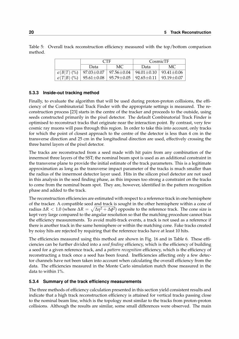
Table 5: Overall track reconstruction efficiency measured with the top/bottom comparisonmethod.

CTF CosmicTFData MC Data MC

ε(B|T) (%) 97.03±0.07 97.56±0.04 94.01±0.10 93.41±0.06ε(T|B) (%) 95.61±0.08 95.79±0.05 92.65±0.11 93.19±0.07

5.3.3 Inside-out tracking method

Finally, to evaluate the algorithm that will be used during proton-proton collisions, the effi-ciency of the Combinatorial Track Finder with the appropriate settings is measured. The re-construction process [23] starts in the centre of the tracker and proceeds to the outside, usingseeds constructed primarily in the pixel detector. The default Combinatorial Track Finder isoptimised to reconstruct tracks that originate near the interaction point. By contrast, very fewcosmic ray muons will pass through this region. In order to take this into account, only tracksfor which the point of closest approach to the centre of the detector is less than 4 cm in thetransverse direction and 25 cm in the longitudinal direction are used, effectively crossing thethree barrel layers of the pixel detector.

The tracks are reconstructed from a seed made with hit pairs from any combination of theinnermost three layers of the SST; the nominal beam spot is used as an additional constraint inthe transverse plane to provide the initial estimate of the track parameters. This is a legitimateapproximation as long as the transverse impact parameter of the tracks is much smaller thanthe radius of the innermost detector layer used. Hits in the silicon pixel detector are not usedin this analysis in the seed finding phase, as this imposes too strong a constraint on the tracksto come from the nominal beam spot. They are, however, identified in the pattern recognitionphase and added to the track.

The reconstruction efficiencies are estimated with respect to a reference track in one hemisphereof the tracker. A compatible seed and track is sought in the other hemisphere within a cone ofradius ∆R < 1.0 (where ∆R =

√∆η2 + ∆φ2) opposite to the reference track. The cone size is

kept very large compared to the angular resolution so that the matching procedure cannot biasthe efficiency measurements. To avoid multi-track events, a track is not used as a reference ifthere is another track in the same hemisphere or within the matching cone. Fake tracks createdby noisy hits are rejected by requiring that the reference tracks have at least 10 hits.

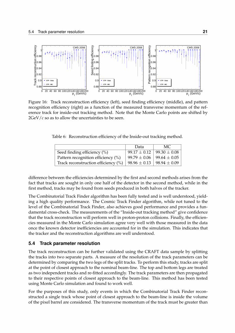
The efficiencies measured using this method are shown in Fig. 16 and in Table 6. These effi-ciencies can be further divided into a seed finding efficiency, which is the efficiency of buildinga seed for a given reference track, and a pattern recognition efficiency, which is the efficiency ofreconstructing a track once a seed has been found. Inefficiencies affecting only a few detec-tor channels have not been taken into account when calculating the overall efficiency from thedata. The efficiencies measured in the Monte Carlo simulation match those measured in thedata to within 1%.

5.3.4 Summary of the track efficiency measurements

The three methods of efficiency calculation presented in this section yield consistent results andindicate that a high track reconstruction efficiency is attained for vertical tracks passing closeto the nominal beam line, which is the topology most similar to the tracks from proton-protoncollisions. Although the results are similar, some small differences were observed. The main

5.4 Track parameter resolution 21

(GeV/c)T

p0 20 40 60 80 100120140160180200

Tra

ck r

econ

stru

ctio

n ef

ficie

ncy

0.88

0.9

0.92

0.94

0.96

0.98

1CMS 2008

CTF - Data

CTF - MC

(GeV/c)T

p0 20 40 60 80 100120140160180200

See

d fin

ding

effi

cien

cy

0.88

0.9

0.92

0.94

0.96

0.98

1CMS 2008

CTF - Data

CTF - MC

(GeV/c)T

p0 20 40 60 80 100120140160180200

Pat

tern

rec

ogni

tion

effic

ienc

y

0.88

0.9

0.92

0.94

0.96

0.98

1CMS 2008

CTF - Data

CTF - MC

Figure 16: Track reconstruction efficiency (left), seed finding efficiency (middle), and patternrecognition efficiency (right) as a function of the measured transverse momentum of the ref-erence track for inside-out tracking method. Note that the Monte Carlo points are shifted by2GeV/c so as to allow the uncertainties to be seen.

Table 6: Reconstruction efficiency of the Inside-out tracking method.

Data MCSeed finding efficiency (%) 99.17 ± 0.12 99.30 ± 0.08Pattern recognition efficiency (%) 99.79 ± 0.06 99.64 ± 0.05Track reconstruction efficiency (%) 98.96 ± 0.13 98.94 ± 0.09

difference between the efficiencies determined by the first and second methods arises from thefact that tracks are sought in only one half of the detector in the second method, while in thefirst method, tracks may be found from seeds produced in both halves of the tracker.

The Combinatorial Track Finder algorithm has been fully tested and is well understood, yield-ing a high quality performance. The Cosmic Track Finder algorithm, while not tuned to thelevel of the Combinatorial Track Finder, also achieves good performance and provides a fun-damental cross-check. The measurements of the “Inside-out tracking method” give confidencethat the track reconstruction will perform well in proton-proton collisions. Finally, the efficien-cies measured in the Monte Carlo simulation agree very well with those measured in the dataonce the known detector inefficiencies are accounted for in the simulation. This indicates thatthe tracker and the reconstruction algorithms are well understood.

5.4 Track parameter resolution

The track reconstruction can be further validated using the CRAFT data sample by splittingthe tracks into two separate parts. A measure of the resolution of the track parameters can bedetermined by comparing the two legs of the split tracks. To perform this study, tracks are splitat the point of closest approach to the nominal beam-line. The top and bottom legs are treatedas two independent tracks and re-fitted accordingly. The track parameters are then propagatedto their respective points of closest approach to the beam-line. This method has been testedusing Monte Carlo simulation and found to work well.

For the purposes of this study, only events in which the Combinatorial Track Finder recon-structed a single track whose point of closest approach to the beam-line is inside the volumeof the pixel barrel are considered. The transverse momentum of the track must be greater than

22 5 Track Reconstruction

Table 7: Standard deviation, mean, and 95% coverage of the residual and pull distributions ofthe track parameters. The units indicated pertain only to the residual distributions.

Track parameter Residual distributions Pull distributionsStd. Dev. Mean 95% Cov. Std. Dev. Mean 95% Cov.

pT (GeV/c) 0.083 0.000 1.92 0.99 0.01 2.1Inverse pT ( GeV−1c) 0.00035 0.00003 0.00213 0.99 -0.01 2.1φ (mrad) 0.19 0.001 0.87 1.08 -0.02 2.4θ (mrad) 0.40 0.003 1.11 0.93 -0.01 2.1dxy (µm) 22 0.30 61 1.22 0.00 2.9dz (µm) 39 0.28 94 0.94 -0.01 2.1

4 GeV/c and its χ2 must satisfy the requirement χ2/ndf < 100. In addition, the track mustcontain a minimum of 10 hits, with at least two hits being on double-sided strip modules.There must also be six hits in the pixel barrel subsystem. After splitting, each track segment isrequired to have at least six hits, three of which must be in the pixel barrel.

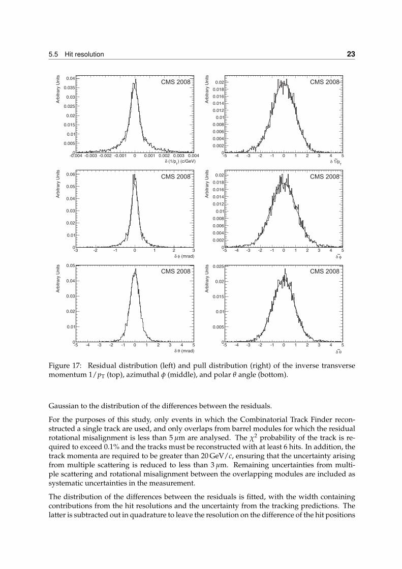
The results of this analysis are summarised in Table 7, while the distributions of the residualsand pulls of the inverse transverse momentum and the azimuthal (φ) and polar (θ) angles areshown in Fig. 17. The corresponding distributions for the transverse (dxy) and longitudinal(dz) impact parameters can be found elsewhere [3]. For each track parameter, the residualsare defined as δx = (x1 − x2)/

√2. The factor of

√2 is needed to account for the fact that

the two legs are statistically independent. The standardised residuals (or pulls) are defined by

δx = (x1 − x2)/√

σ2x1 + σ2

x2. In Table 7 the mean and standard deviation (referred to as theresolution) of a Gaussian fitted to the peak of the distributions are given. In order to get anestimate of the tails of the distributions, the half-widths of the symmetric intervals covering95% of the distribution (also known as the 95% coverage), which, in the case of a Gaussiandistribution, correspond to twice the standard deviation, are also given in Table 7.

The same quantities are used to characterise the pull distributions. In this case, the standarddeviations of the fitted Gaussians are taken as the pull values. It can be seen that the resolutionof the angles and the impact parameters are well described by a Gaussian. The resolution as afunction of the momentum has been presented elsewhere [31].

5.5 Hit resolution

The hit resolution has been studied by measuring the track residuals, which are defined asthe difference between the hit position and the track position. The track is deliberately recon-structed excluding the hit under study in order to avoid bias. The uncertainty relating to thetrack position is much larger than the inherent hit resolution, so a single track residual is notsensitive to the resolution. However, the track position difference between two nearby mod-ules can be measured with much greater precision. A technique using tracks passing throughoverlapping modules from the same tracker layer is employed to compare the difference inresidual values for the two measurements in the overlapping modules [7]. The difference in hitpositions, ∆xhit, is compared to the difference in the predicted positions, ∆xpred, and the widthof the resulting distribution arises from the hit resolution and the uncertainty from the track-ing predictions. The hit resolution can therefore be determined by subtracting the uncertaintyfrom the tracking prediction. This overlap technique also serves to reduce the uncertaintyarising from multiple scattering, by limiting the track extrapolation to short distances. Anyuncertainty from translational misalignment between the modules is also avoided by fitting a

5.5 Hit resolution 23

) (c/GeV)T

(1/pδ-0.004 -0.003 -0.002 -0.001 0 0.001 0.002 0.003 0.004

Arb

itrar

y U

nits

0

0.005

0.01

0.015

0.02

0.025

0.03

0.035

0.04CMS 2008

T 1/pδ~-5 -4 -3 -2 -1 0 1 2 3 4 5

Arb

itrar

y U

nits

00.0020.0040.0060.008

0.010.0120.0140.0160.018

0.02 CMS 2008

(mrad)φδ-3 -2 -1 0 1 2 3

Arb

itrar

y U

nits

0

0.01

0.02

0.03

0.04

0.05

0.06 CMS 2008

φδ~

-5 -4 -3 -2 -1 0 1 2 3 4 5

Arb

itrar

y U

nits

00.0020.0040.0060.008

0.010.0120.0140.0160.018

0.02 CMS 2008

(mrad)θδ-5 -4 -3 -2 -1 0 1 2 3 4 5

Arb

itrar

y U

nits

0

0.01

0.02

0.03

0.04

0.05CMS 2008

θδ~

-5 -4 -3 -2 -1 0 1 2 3 4 5

Arb

itrar

y U

nits

0

0.005

0.01

0.015

0.02

0.025CMS 2008

Figure 17: Residual distribution (left) and pull distribution (right) of the inverse transversemomentum 1/pT (top), azimuthal φ (middle), and polar θ angle (bottom).

Gaussian to the distribution of the differences between the residuals.

For the purposes of this study, only events in which the Combinatorial Track Finder recon-structed a single track are used, and only overlaps from barrel modules for which the residualrotational misalignment is less than 5 µm are analysed. The χ2 probability of the track is re-quired to exceed 0.1% and the tracks must be reconstructed with at least 6 hits. In addition, thetrack momenta are required to be greater than 20 GeV/c, ensuring that the uncertainty arisingfrom multiple scattering is reduced to less than 3 µm. Remaining uncertainties from multi-ple scattering and rotational misalignment between the overlapping modules are included assystematic uncertainties in the measurement.

The distribution of the differences between the residuals is fitted, with the width containingcontributions from the hit resolutions and the uncertainty from the tracking predictions. Thelatter is subtracted out in quadrature to leave the resolution on the difference of the hit positions

24 6 Summary

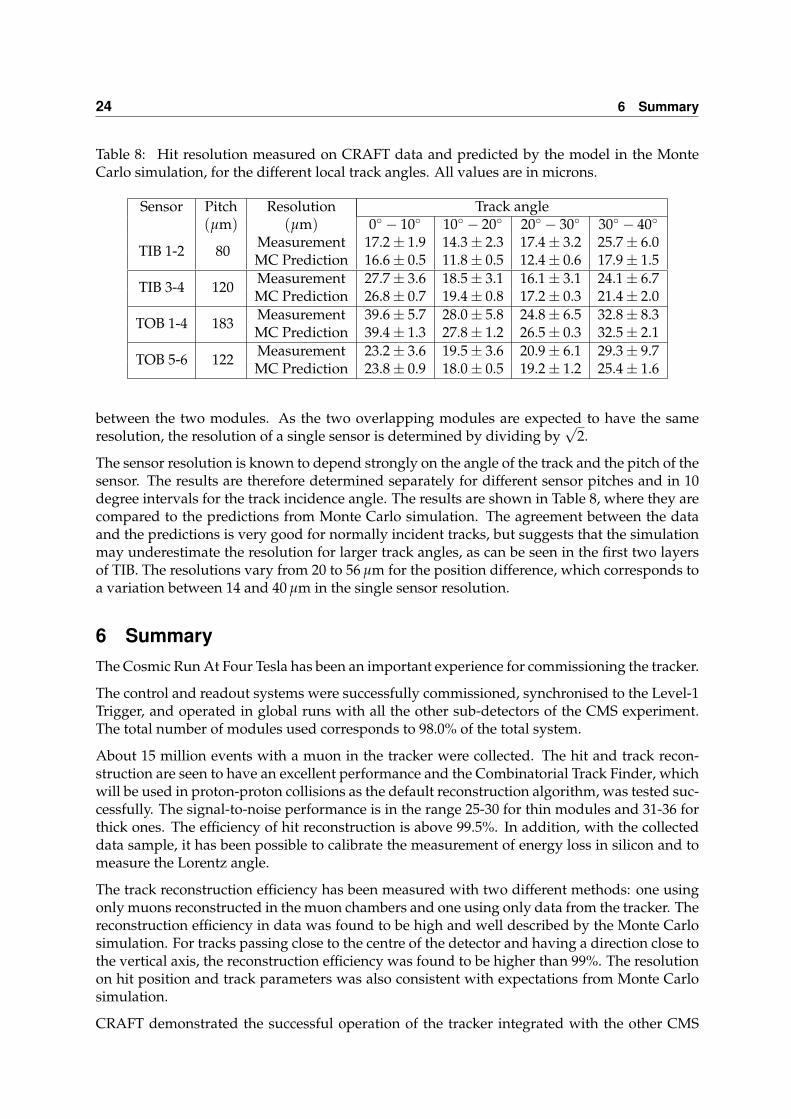
Table 8: Hit resolution measured on CRAFT data and predicted by the model in the MonteCarlo simulation, for the different local track angles. All values are in microns.

Sensor Pitch Resolution Track angle(µm) (µm) 0◦ − 10◦ 10◦ − 20◦ 20◦ − 30◦ 30◦ − 40◦

TIB 1-2 80Measurement 17.2± 1.9 14.3± 2.3 17.4± 3.2 25.7± 6.0MC Prediction 16.6± 0.5 11.8± 0.5 12.4± 0.6 17.9± 1.5

TIB 3-4 120Measurement 27.7± 3.6 18.5± 3.1 16.1± 3.1 24.1± 6.7MC Prediction 26.8± 0.7 19.4± 0.8 17.2± 0.3 21.4± 2.0

TOB 1-4 183Measurement 39.6± 5.7 28.0± 5.8 24.8± 6.5 32.8± 8.3MC Prediction 39.4± 1.3 27.8± 1.2 26.5± 0.3 32.5± 2.1

TOB 5-6 122Measurement 23.2± 3.6 19.5± 3.6 20.9± 6.1 29.3± 9.7MC Prediction 23.8± 0.9 18.0± 0.5 19.2± 1.2 25.4± 1.6

between the two modules. As the two overlapping modules are expected to have the sameresolution, the resolution of a single sensor is determined by dividing by

√2.

The sensor resolution is known to depend strongly on the angle of the track and the pitch of thesensor. The results are therefore determined separately for different sensor pitches and in 10degree intervals for the track incidence angle. The results are shown in Table 8, where they arecompared to the predictions from Monte Carlo simulation. The agreement between the dataand the predictions is very good for normally incident tracks, but suggests that the simulationmay underestimate the resolution for larger track angles, as can be seen in the first two layersof TIB. The resolutions vary from 20 to 56 µm for the position difference, which corresponds toa variation between 14 and 40 µm in the single sensor resolution.

6 SummaryThe Cosmic Run At Four Tesla has been an important experience for commissioning the tracker.

The control and readout systems were successfully commissioned, synchronised to the Level-1Trigger, and operated in global runs with all the other sub-detectors of the CMS experiment.The total number of modules used corresponds to 98.0% of the total system.

About 15 million events with a muon in the tracker were collected. The hit and track recon-struction are seen to have an excellent performance and the Combinatorial Track Finder, whichwill be used in proton-proton collisions as the default reconstruction algorithm, was tested suc-cessfully. The signal-to-noise performance is in the range 25-30 for thin modules and 31-36 forthick ones. The efficiency of hit reconstruction is above 99.5%. In addition, with the collecteddata sample, it has been possible to calibrate the measurement of energy loss in silicon and tomeasure the Lorentz angle.

The track reconstruction efficiency has been measured with two different methods: one usingonly muons reconstructed in the muon chambers and one using only data from the tracker. Thereconstruction efficiency in data was found to be high and well described by the Monte Carlosimulation. For tracks passing close to the centre of the detector and having a direction close tothe vertical axis, the reconstruction efficiency was found to be higher than 99%. The resolutionon hit position and track parameters was also consistent with expectations from Monte Carlosimulation.

CRAFT demonstrated the successful operation of the tracker integrated with the other CMS

25

subsystems. It was an important milestone towards final commissioning with colliding beamdata.

AcknowledgmentsWe thank the technical and administrative staff at CERN and other CMS Institutes, and ac-knowledge support from: FMSR (Austria); FNRS and FWO (Belgium); CNPq, CAPES, FAPERJ,and FAPESP (Brazil); MES (Bulgaria); CERN; CAS, MoST, and NSFC (China); COLCIEN-CIAS (Colombia); MSES (Croatia); RPF (Cyprus); Academy of Sciences and NICPB (Estonia);Academy of Finland, ME, and HIP (Finland); CEA and CNRS/IN2P3 (France); BMBF, DFG,and HGF (Germany); GSRT (Greece); OTKA and NKTH (Hungary); DAE and DST (India);IPM (Iran); SFI (Ireland); INFN (Italy); NRF (Korea); LAS (Lithuania); CINVESTAV, CONA-CYT, SEP, and UASLP-FAI (Mexico); PAEC (Pakistan); SCSR (Poland); FCT (Portugal); JINR(Armenia, Belarus, Georgia, Ukraine, Uzbekistan); MST and MAE (Russia); MSTDS (Serbia);MICINN and CPAN (Spain); Swiss Funding Agencies (Switzerland); NSC (Taipei); TUBITAKand TAEK (Turkey); STFC (United Kingdom); DOE and NSF (USA). Individuals have receivedsupport from the Marie-Curie IEF program (European Union); the Leventis Foundation; the A.P. Sloan Foundation; and the Alexander von Humboldt Foundation.

References[1] CMS Collaboration, “The CMS experiment at the CERN LHC”, JINST 3 (2008) S08004.

doi:10.1088/1748-0221/3/08/S08004.

[2] L. Evans, (ed. ) and P. Bryant, (ed. ), “LHC Machine”, JINST 3 (2008) S08001.doi:10.1088/1748-0221/3/08/S08001.

[3] CMS Collaboration, “The CMS Pixel Detector Operation and Performance at the CosmicRun at Four Tesla”, CMS-CFT-09-001. To be submitted to JINST.

[4] L. Borrello et al., “Sensor Design for the CMS Silicon Strip Tracker”, CMS Note 2003/020(2003).

[5] W. Adam et al., “The CMS tracker operation and performance at the Magnet Test andCosmic Challenge”, JINST 3 (2008) P07006. doi:10.1088/1748-0221/3/07/P07006.

[6] W. Adam et al., “Performance studies of the CMS Strip Tracker before installation”, JINST4 (2009) P06009. doi:10.1088/1748-0221/4/06/P06009.

[7] W. Adam et al., “Stand-alone Cosmic Muon Reconstruction Before Installation of theCMS Silicon Strip Tracker”, JINST 4 (2009) P05004.doi:10.1088/1748-0221/4/05/P05004.

[8] CMS Collaboration, “The CMS Cosmic Run at Four Tesla”, CMS-CFT-09-008. To besubmitted to JINST.

[9] CMS Collaboration, “The Tracker Project: Technical design report”, CERN-LHCC1998-006 (1998).

[10] M. Raymond et al., “The CMS Tracker APV25 0.25 µm CMOS Readout Chip”, Proceedingsof the 6th workshop on electronics for LHC experiments, Krakow (2000) 130.

26 6 Summary

[11] J. Troska et al., “Optical readout and control systems for the CMS tracker”, IEEE Trans.Nucl. Sci. 50 (2003) 1067–1072. doi:10.1109/TNS.2003.815124.

[12] C. Foudas et al., “The CMS tracker readout front end driver”, IEEE Trans. Nucl. Sci. 52(2005) 2836–2840, arXiv:physics/0510229. doi:10.1109/TNS.2005.860173.

[13] F. Drouhin et al., “The CERN CMS tracker control system ”, Nuclear Science SymposiumConference Record, IEEE 2 (2004) 1196.

[14] K. Kloukinas et al., “FEC-CCS: A common front-end controller card for the CMS detectorelectronics”, Proceedings of the 12th Workshop on Electronics for LHC and Future Experiments(LECC 2006), Valencia (2006) 179.

[15] C. Paillard, C. Ljuslin, and A. Marchioro, “The CCU25: A network orientedcommunication and control unit integrated circuit in a 0.25-mu-m CMOS technology”,Proceedings of the 8th Workshop on Electronics for LHC Experiments, Colmar (2002) 174.

[16] S. Gadomski et al., “The Deconvolution method of fast pulse shaping at hadroncolliders”, Nucl. Instrum. Meth. A320 (1992) 217–227.doi:10.1016/0168-9002(92)90779-4.

[17] S. Paoletti, “The implementation of the power supply system of the CMS silicon striptracker”, in 10th Workshop on Electronics for LHC and future experiments (2004)CERN-2004-010, CERN-LHCC-2004-030.

[18] G. Magazzu, A. Marchioro, and P. Moreira, “The detector control unit: An ASIC for themonitoring of the CMS silicon tracker”, IEEE Trans. Nucl. Sci. 51 (2004) 1333–1336.doi:10.1109/TNS.2004.832925.

[19] G. Cervelli, A. Marchioro, P. Moreira et al., “A radiation tolerant laser driver array foroptical transmission in the LHC experiments”, Proceedings of the 7th Workshop onElectronics for LHC Experiments, Stockholm (2001).

[20] P. Placidi, A. Marchioro, P. Moreira et al., “A 40-MHz clock and trigger recovery circuitfor the CMS tracker fabricated in a 0.25-mu-m CMOS technology and using a selfcalibration technique”, Proceedings of the 5th Workshop on Electronics for the LHCExperiments, Snowmass, Colorado (1999) 469.

[21] C. Delaere et al., “Procedure for the fine delay adjustment of the CMS tracker,”, CMS Note2008/007 (2008).

[22] CMS Collaboration, “Performance of the CMS Drift-Tube Local Trigger with CosmicRays”, CFT-09-022. To be submitted to JINST.

[23] CMS Collaboration, “CMS physics: Technical design report”, CERN-LHCC 2006-001(2006).

[24] CMS Collaboration, “CMS Data Processing Workflows During an Extended Cosmic RayRun”, CMS-CFT-09-007. To be submitted to JINST.

[25] A. Afaq et al., “The CMS dataset bookkeeping service”, J. Phys. Conf. Ser. 119 (2008)072001. doi:10.1088/1742-6596/119/7/072001.

[26] CMS Collaboration, “Performance of the CMS Level-1 Trigger during Commissioningwith Cosmic Rays”, CMS-CFT-09-013. To be submitted to JINST.

27

[27] P. Biallass, T. Hebbeker, and K. Hopfner, “Simulation of Cosmic Muons and Comparisonwith Data from Cosmic Challenge using Drift Tube Chambers”, CMS Note 2007/024(2007).

[28] P. Biallass and T. Hebbeker, “Parameterisation of the Cosmic Muon Flux for theGenerator CMSCGEN”, arXiv:0907.5514.

[29] A. Giammanco, “Particle Identification with Energy Loss in the CMS Silicon StripTracker”, CMS Note 2008/005 (2008).

[30] H. Bichsel, “Straggling in thin silicon detectors”, Rev. Mod. Phys. 60 (1988) 663–699.doi:10.1103/RevModPhys.60.663.

[31] CMS Collaboration, “Alignment of the CMS inner tracking system with cosmic rayparticles”, CMS-CFT-09-003. To be submitted to JINST.

[32] CMS Collaboration, “Performance of CMS Muon Reconstruction in Cosmic-Ray Events”,CFT-09-014. To be submitted to JINST.

28 6 Summary

29

A The CMS CollaborationYerevan Physics Institute, Yerevan, ArmeniaS. Chatrchyan, V. Khachatryan, A.M. Sirunyan

Institut fur Hochenergiephysik der OeAW, Wien, AustriaW. Adam, B. Arnold, H. Bergauer, T. Bergauer, M. Dragicevic, M. Eichberger, J. Ero, M. Friedl,R. Fruhwirth, V.M. Ghete, J. Hammer1, S. Hansel, M. Hoch, N. Hormann, J. Hrubec, M. Jeitler,G. Kasieczka, K. Kastner, M. Krammer, D. Liko, I. Magrans de Abril, I. Mikulec, F. Mittermayr,B. Neuherz, M. Oberegger, M. Padrta, M. Pernicka, H. Rohringer, S. Schmid, R. Schofbeck,T. Schreiner, R. Stark, H. Steininger, J. Strauss, A. Taurok, F. Teischinger, T. Themel, D. Uhl,P. Wagner, W. Waltenberger, G. Walzel, E. Widl, C.-E. Wulz

National Centre for Particle and High Energy Physics, Minsk, BelarusV. Chekhovsky, O. Dvornikov, I. Emeliantchik, A. Litomin, V. Makarenko, I. Marfin,V. Mossolov, N. Shumeiko, A. Solin, R. Stefanovitch, J. Suarez Gonzalez, A. Tikhonov

Research Institute for Nuclear Problems, Minsk, BelarusA. Fedorov, A. Karneyeu, M. Korzhik, V. Panov, R. Zuyeuski

Research Institute of Applied Physical Problems, Minsk, BelarusP. Kuchinsky

Universiteit Antwerpen, Antwerpen, BelgiumW. Beaumont, L. Benucci, M. Cardaci, E.A. De Wolf, E. Delmeire, D. Druzhkin, M. Hashemi,X. Janssen, T. Maes, L. Mucibello, S. Ochesanu, R. Rougny, M. Selvaggi, H. Van Haevermaet,P. Van Mechelen, N. Van Remortel

Vrije Universiteit Brussel, Brussel, BelgiumV. Adler, S. Beauceron, S. Blyweert, J. D’Hondt, S. De Weirdt, O. Devroede, J. Heyninck, A. Ka-logeropoulos, J. Maes, M. Maes, M.U. Mozer, S. Tavernier, W. Van Doninck1, P. Van Mulders,I. Villella

Universite Libre de Bruxelles, Bruxelles, BelgiumO. Bouhali, E.C. Chabert, O. Charaf, B. Clerbaux, G. De Lentdecker, V. Dero, S. Elgammal,A.P.R. Gay, G.H. Hammad, P.E. Marage, S. Rugovac, C. Vander Velde, P. Vanlaer, J. Wickens

Ghent University, Ghent, BelgiumM. Grunewald, B. Klein, A. Marinov, D. Ryckbosch, F. Thyssen, M. Tytgat, L. Vanelderen,P. Verwilligen

Universite Catholique de Louvain, Louvain-la-Neuve, BelgiumS. Basegmez, G. Bruno, J. Caudron, C. Delaere, P. Demin, D. Favart, A. Giammanco,G. Gregoire, V. Lemaitre, O. Militaru, S. Ovyn, K. Piotrzkowski1, L. Quertenmont, N. Schul

Universite de Mons, Mons, BelgiumN. Beliy, E. Daubie

Centro Brasileiro de Pesquisas Fisicas, Rio de Janeiro, BrazilG.A. Alves, M.E. Pol, M.H.G. Souza

Universidade do Estado do Rio de Janeiro, Rio de Janeiro, BrazilW. Carvalho, D. De Jesus Damiao, C. De Oliveira Martins, S. Fonseca De Souza, L. Mundim,V. Oguri, A. Santoro, S.M. Silva Do Amaral, A. Sznajder

Instituto de Fisica Teorica, Universidade Estadual Paulista, Sao Paulo, Brazil

30 A The CMS Collaboration

T.R. Fernandez Perez Tomei, M.A. Ferreira Dias, E. M. Gregores2, S.F. Novaes

Institute for Nuclear Research and Nuclear Energy, Sofia, BulgariaK. Abadjiev1, T. Anguelov, J. Damgov, N. Darmenov1, L. Dimitrov, V. Genchev1, P. Iaydjiev,S. Piperov, S. Stoykova, G. Sultanov, R. Trayanov, I. Vankov

University of Sofia, Sofia, BulgariaA. Dimitrov, M. Dyulendarova, V. Kozhuharov, L. Litov, E. Marinova, M. Mateev, B. Pavlov,P. Petkov, Z. Toteva1

Institute of High Energy Physics, Beijing, ChinaG.M. Chen, H.S. Chen, W. Guan, C.H. Jiang, D. Liang, B. Liu, X. Meng, J. Tao, J. Wang, Z. Wang,Z. Xue, Z. Zhang

State Key Lab. of Nucl. Phys. and Tech., Peking University, Beijing, ChinaY. Ban, J. Cai, Y. Ge, S. Guo, Z. Hu, Y. Mao, S.J. Qian, H. Teng, B. Zhu

Universidad de Los Andes, Bogota, ColombiaC. Avila, M. Baquero Ruiz, C.A. Carrillo Montoya, A. Gomez, B. Gomez Moreno, A.A. OcampoRios, A.F. Osorio Oliveros, D. Reyes Romero, J.C. Sanabria

Technical University of Split, Split, CroatiaN. Godinovic, K. Lelas, R. Plestina, D. Polic, I. Puljak

University of Split, Split, CroatiaZ. Antunovic, M. Dzelalija

Institute Rudjer Boskovic, Zagreb, CroatiaV. Brigljevic, S. Duric, K. Kadija, S. Morovic

University of Cyprus, Nicosia, CyprusR. Fereos, M. Galanti, J. Mousa, A. Papadakis, F. Ptochos, P.A. Razis, D. Tsiakkouri, Z. Zinonos

National Institute of Chemical Physics and Biophysics, Tallinn, EstoniaA. Hektor, M. Kadastik, K. Kannike, M. Muntel, M. Raidal, L. Rebane

Helsinki Institute of Physics, Helsinki, FinlandE. Anttila, S. Czellar, J. Harkonen, A. Heikkinen, V. Karimaki, R. Kinnunen, J. Klem, M.J. Ko-rtelainen, T. Lampen, K. Lassila-Perini, S. Lehti, T. Linden, P. Luukka, T. Maenpaa, J. Nysten,E. Tuominen, J. Tuominiemi, D. Ungaro, L. Wendland

Lappeenranta University of Technology, Lappeenranta, FinlandK. Banzuzi, A. Korpela, T. Tuuva

Laboratoire d’Annecy-le-Vieux de Physique des Particules, IN2P3-CNRS, Annecy-le-Vieux,FranceP. Nedelec, D. Sillou

DSM/IRFU, CEA/Saclay, Gif-sur-Yvette, FranceM. Besancon, R. Chipaux, M. Dejardin, D. Denegri, J. Descamps, B. Fabbro, J.L. Faure, F. Ferri,S. Ganjour, F.X. Gentit, A. Givernaud, P. Gras, G. Hamel de Monchenault, P. Jarry, M.C. Lemaire,E. Locci, J. Malcles, M. Marionneau, L. Millischer, J. Rander, A. Rosowsky, D. Rousseau,M. Titov, P. Verrecchia

Laboratoire Leprince-Ringuet, Ecole Polytechnique, IN2P3-CNRS, Palaiseau, FranceS. Baffioni, L. Bianchini, M. Bluj3, P. Busson, C. Charlot, L. Dobrzynski, R. Granier de Cas-sagnac, M. Haguenauer, P. Mine, P. Paganini, Y. Sirois, C. Thiebaux, A. Zabi

31

Institut Pluridisciplinaire Hubert Curien, Universite de Strasbourg, Universite de HauteAlsace Mulhouse, CNRS/IN2P3, Strasbourg, FranceJ.-L. Agram4, A. Besson, D. Bloch, D. Bodin, J.-M. Brom, E. Conte4, F. Drouhin4, J.-C. Fontaine4,D. Gele, U. Goerlach, L. Gross, P. Juillot, A.-C. Le Bihan, Y. Patois, J. Speck, P. Van Hove

Universite de Lyon, Universite Claude Bernard Lyon 1, CNRS-IN2P3, Institut de PhysiqueNucleaire de Lyon, Villeurbanne, FranceC. Baty, M. Bedjidian, J. Blaha, G. Boudoul, H. Brun, N. Chanon, R. Chierici, D. Contardo,P. Depasse, T. Dupasquier, H. El Mamouni, F. Fassi5, J. Fay, S. Gascon, B. Ille, T. Kurca, T. LeGrand, M. Lethuillier, N. Lumb, L. Mirabito, S. Perries, M. Vander Donckt, P. Verdier

E. Andronikashvili Institute of Physics, Academy of Science, Tbilisi, GeorgiaN. Djaoshvili, N. Roinishvili, V. Roinishvili

Institute of High Energy Physics and Informatization, Tbilisi State University, Tbilisi,GeorgiaN. Amaglobeli

RWTH Aachen University, I. Physikalisches Institut, Aachen, GermanyR. Adolphi, G. Anagnostou, R. Brauer, W. Braunschweig, M. Edelhoff, H. Esser, L. Feld,W. Karpinski, A. Khomich, K. Klein, N. Mohr, A. Ostaptchouk, D. Pandoulas, G. Pierschel,F. Raupach, S. Schael, A. Schultz von Dratzig, G. Schwering, D. Sprenger, M. Thomas, M. Weber,B. Wittmer, M. Wlochal

RWTH Aachen University, III. Physikalisches Institut A, Aachen, GermanyO. Actis, G. Altenhofer, W. Bender, P. Biallass, M. Erdmann, G. Fetchenhauer1, J. Frangenheim,T. Hebbeker, G. Hilgers, A. Hinzmann, K. Hoepfner, C. Hof, M. Kirsch, T. Klimkovich,P. Kreuzer1, D. Lanske†, M. Merschmeyer, A. Meyer, B. Philipps, H. Pieta, H. Reithler,S.A. Schmitz, L. Sonnenschein, M. Sowa, J. Steggemann, H. Szczesny, D. Teyssier, C. Zeidler

RWTH Aachen University, III. Physikalisches Institut B, Aachen, GermanyM. Bontenackels, M. Davids, M. Duda, G. Flugge, H. Geenen, M. Giffels, W. Haj Ahmad, T. Her-manns, D. Heydhausen, S. Kalinin, T. Kress, A. Linn, A. Nowack, L. Perchalla, M. Poettgens,O. Pooth, P. Sauerland, A. Stahl, D. Tornier, M.H. Zoeller

Deutsches Elektronen-Synchrotron, Hamburg, GermanyM. Aldaya Martin, U. Behrens, K. Borras, A. Campbell, E. Castro, D. Dammann, G. Eckerlin,A. Flossdorf, G. Flucke, A. Geiser, D. Hatton, J. Hauk, H. Jung, M. Kasemann, I. Katkov,C. Kleinwort, H. Kluge, A. Knutsson, E. Kuznetsova, W. Lange, W. Lohmann, R. Mankel1,M. Marienfeld, A.B. Meyer, S. Miglioranzi, J. Mnich, M. Ohlerich, J. Olzem, A. Parenti,C. Rosemann, R. Schmidt, T. Schoerner-Sadenius, D. Volyanskyy, C. Wissing, W.D. Zeuner1

University of Hamburg, Hamburg, GermanyC. Autermann, F. Bechtel, J. Draeger, D. Eckstein, U. Gebbert, K. Kaschube, G. Kaussen,R. Klanner, B. Mura, S. Naumann-Emme, F. Nowak, U. Pein, C. Sander, P. Schleper, T. Schum,H. Stadie, G. Steinbruck, J. Thomsen, R. Wolf

Institut fur Experimentelle Kernphysik, Karlsruhe, GermanyJ. Bauer, P. Blum, V. Buege, A. Cakir, T. Chwalek, W. De Boer, A. Dierlamm, G. Dirkes,M. Feindt, U. Felzmann, M. Frey, A. Furgeri, J. Gruschke, C. Hackstein, F. Hartmann1,S. Heier, M. Heinrich, H. Held, D. Hirschbuehl, K.H. Hoffmann, S. Honc, C. Jung, T. Kuhr,T. Liamsuwan, D. Martschei, S. Mueller, Th. Muller, M.B. Neuland, M. Niegel, O. Oberst,A. Oehler, J. Ott, T. Peiffer, D. Piparo, G. Quast, K. Rabbertz, F. Ratnikov, N. Ratnikova, M. Renz,C. Saout1, G. Sartisohn, A. Scheurer, P. Schieferdecker, F.-P. Schilling, G. Schott, H.J. Simonis,

32 A The CMS Collaboration

F.M. Stober, P. Sturm, D. Troendle, A. Trunov, W. Wagner, J. Wagner-Kuhr, M. Zeise, V. Zhukov6,E.B. Ziebarth

Institute of Nuclear Physics ”Demokritos”, Aghia Paraskevi, GreeceG. Daskalakis, T. Geralis, K. Karafasoulis, A. Kyriakis, D. Loukas, A. Markou, C. Markou,C. Mavrommatis, E. Petrakou, A. Zachariadou

University of Athens, Athens, GreeceL. Gouskos, P. Katsas, A. Panagiotou1

University of Ioannina, Ioannina, GreeceI. Evangelou, P. Kokkas, N. Manthos, I. Papadopoulos, V. Patras, F.A. Triantis

KFKI Research Institute for Particle and Nuclear Physics, Budapest, HungaryG. Bencze1, L. Boldizsar, G. Debreczeni, C. Hajdu1, S. Hernath, P. Hidas, D. Horvath7, K. Kra-jczar, A. Laszlo, G. Patay, F. Sikler, N. Toth, G. Vesztergombi

Institute of Nuclear Research ATOMKI, Debrecen, HungaryN. Beni, G. Christian, J. Imrek, J. Molnar, D. Novak, J. Palinkas, G. Szekely, Z. Szillasi1,K. Tokesi, V. Veszpremi

University of Debrecen, Debrecen, HungaryA. Kapusi, G. Marian, P. Raics, Z. Szabo, Z.L. Trocsanyi, B. Ujvari, G. Zilizi

Panjab University, Chandigarh, IndiaS. Bansal, H.S. Bawa, S.B. Beri, V. Bhatnagar, M. Jindal, M. Kaur, R. Kaur, J.M. Kohli,M.Z. Mehta, N. Nishu, L.K. Saini, A. Sharma, A. Singh, J.B. Singh, S.P. Singh

University of Delhi, Delhi, IndiaS. Ahuja, S. Arora, S. Bhattacharya8, S. Chauhan, B.C. Choudhary, P. Gupta, S. Jain, S. Jain,M. Jha, A. Kumar, K. Ranjan, R.K. Shivpuri, A.K. Srivastava

Bhabha Atomic Research Centre, Mumbai, IndiaR.K. Choudhury, D. Dutta, S. Kailas, S.K. Kataria, A.K. Mohanty, L.M. Pant, P. Shukla, A. Top-kar

Tata Institute of Fundamental Research - EHEP, Mumbai, IndiaT. Aziz, M. Guchait9, A. Gurtu, M. Maity10, D. Majumder, G. Majumder, K. Mazumdar,A. Nayak, A. Saha, K. Sudhakar

Tata Institute of Fundamental Research - HECR, Mumbai, IndiaS. Banerjee, S. Dugad, N.K. Mondal

Institute for Studies in Theoretical Physics & Mathematics (IPM), Tehran, IranH. Arfaei, H. Bakhshiansohi, A. Fahim, A. Jafari, M. Mohammadi Najafabadi, A. Moshaii,S. Paktinat Mehdiabadi, S. Rouhani, B. Safarzadeh, M. Zeinali

University College Dublin, Dublin, IrelandM. Felcini

INFN Sezione di Bari a, Universita di Bari b, Politecnico di Bari c, Bari, ItalyM. Abbresciaa ,b, L. Barbonea, F. Chiumaruloa, A. Clementea, A. Colaleoa, D. Creanzaa,c,G. Cuscelaa, N. De Filippisa, M. De Palmaa,b, G. De Robertisa, G. Donvitoa, F. Fedelea, L. Fiorea,M. Francoa, G. Iasellia,c, N. Lacalamitaa, F. Loddoa, L. Lusitoa,b, G. Maggia,c, M. Maggia,N. Mannaa,b, B. Marangellia ,b, S. Mya ,c, S. Natalia ,b, S. Nuzzoa,b, G. Papagnia, S. Piccolomoa,G.A. Pierroa, C. Pintoa, A. Pompilia ,b, G. Pugliesea ,c, R. Rajana, A. Ranieria, F. Romanoa,c,

33

G. Rosellia,b, G. Selvaggia ,b, Y. Shindea, L. Silvestrisa, S. Tupputia ,b, G. Zitoa

INFN Sezione di Bologna a, Universita di Bologna b, Bologna, ItalyG. Abbiendia, W. Bacchia ,b, A.C. Benvenutia, M. Boldinia, D. Bonacorsia, S. Braibant-Giacomellia,b, V.D. Cafaroa, S.S. Caiazzaa, P. Capiluppia,b, A. Castroa ,b, F.R. Cavalloa,G. Codispotia,b, M. Cuffiania,b, I. D’Antonea, G.M. Dallavallea,1, F. Fabbria, A. Fanfania ,b,D. Fasanellaa, P. Giacomellia, V. Giordanoa, M. Giuntaa ,1, C. Grandia, M. Guerzonia,S. Marcellinia, G. Masettia,b, A. Montanaria, F.L. Navarriaa,b, F. Odoricia, G. Pellegrinia,A. Perrottaa, A.M. Rossia,b, T. Rovellia ,b, G. Sirolia ,b, G. Torromeoa, R. Travaglinia ,b

INFN Sezione di Catania a, Universita di Catania b, Catania, ItalyS. Albergoa,b, S. Costaa,b, R. Potenzaa,b, A. Tricomia,b, C. Tuvea

INFN Sezione di Firenze a, Universita di Firenze b, Firenze, ItalyG. Barbaglia, G. Broccoloa,b, V. Ciullia ,b, C. Civininia, R. D’Alessandroa ,b, E. Focardia ,b,S. Frosalia,b, E. Galloa, C. Gentaa,b, G. Landia ,b, P. Lenzia,b ,1, M. Meschinia, S. Paolettia,G. Sguazzonia, A. Tropianoa

INFN Laboratori Nazionali di Frascati, Frascati, ItalyL. Benussi, M. Bertani, S. Bianco, S. Colafranceschi11, D. Colonna11, F. Fabbri, M. Giardoni,L. Passamonti, D. Piccolo, D. Pierluigi, B. Ponzio, A. Russo

INFN Sezione di Genova, Genova, ItalyP. Fabbricatore, R. Musenich

INFN Sezione di Milano-Biccoca a, Universita di Milano-Bicocca b, Milano, ItalyA. Benagliaa, M. Callonia, G.B. Ceratia ,b ,1, P. D’Angeloa, F. De Guioa, F.M. Farinaa, A. Ghezzia,P. Govonia,b, M. Malbertia,b ,1, S. Malvezzia, A. Martellia, D. Menascea, V. Miccioa,b, L. Moronia,P. Negria,b, M. Paganonia ,b, D. Pedrinia, A. Pulliaa ,b, S. Ragazzia ,b, N. Redaellia, S. Salaa,R. Salernoa,b, T. Tabarelli de Fatisa ,b, V. Tancinia,b, S. Taronia ,b

INFN Sezione di Napoli a, Universita di Napoli ”Federico II” b, Napoli, ItalyS. Buontempoa, N. Cavalloa, A. Cimminoa ,b ,1, M. De Gruttolaa,b ,1, F. Fabozzia,12, A.O.M. Iorioa,L. Listaa, D. Lomidzea, P. Nolia ,b, P. Paoluccia, C. Sciaccaa,b

INFN Sezione di Padova a, Universita di Padova b, Padova, ItalyP. Azzia,1, N. Bacchettaa, L. Barcellana, P. Bellana ,b ,1, M. Bellatoa, M. Benettonia, M. Biasottoa ,13,D. Biselloa,b, E. Borsatoa ,b, A. Brancaa, R. Carlina ,b, L. Castellania, P. Checchiaa, E. Contia,F. Dal Corsoa, M. De Mattiaa,b, T. Dorigoa, U. Dossellia, F. Fanzagoa, F. Gasparinia ,b,U. Gasparinia,b, P. Giubilatoa,b, F. Gonellaa, A. Greselea,14, M. Gulminia ,13, A. Kaminskiya ,b,S. Lacapraraa ,13, I. Lazzizzeraa ,14, M. Margonia ,b, G. Marona ,13, S. Mattiazzoa,b, M. Mazzucatoa,M. Meneghellia, A.T. Meneguzzoa,b, M. Michelottoa, F. Montecassianoa, M. Nespoloa,M. Passaseoa, M. Pegoraroa, L. Perrozzia, N. Pozzobona ,b, P. Ronchesea,b, F. Simonettoa,b,N. Tonioloa, E. Torassaa, M. Tosia ,b, A. Triossia, S. Vaninia ,b, S. Venturaa, P. Zottoa,b,G. Zumerlea,b

INFN Sezione di Pavia a, Universita di Pavia b, Pavia, ItalyP. Baessoa,b, U. Berzanoa, S. Bricolaa, M.M. Necchia ,b, D. Paganoa,b, S.P. Rattia,b, C. Riccardia,b,P. Torrea ,b, A. Vicinia, P. Vituloa,b, C. Viviania,b

INFN Sezione di Perugia a, Universita di Perugia b, Perugia, ItalyD. Aisaa, S. Aisaa, E. Babuccia, M. Biasinia,b, G.M. Bileia, B. Caponeria,b, B. Checcuccia, N. Dinua,L. Fanoa, L. Farnesinia, P. Laricciaa,b, A. Lucaronia,b, G. Mantovania ,b, A. Nappia,b, A. Pilusoa,V. Postolachea, A. Santocchiaa,b, L. Servolia, D. Tonoiua, A. Vedaeea, R. Volpea ,b

34 A The CMS Collaboration

INFN Sezione di Pisa a, Universita di Pisa b, Scuola Normale Superiore di Pisa c, Pisa, ItalyP. Azzurria ,c, G. Bagliesia, J. Bernardinia,b, L. Berrettaa, T. Boccalia, A. Boccia ,c, L. Borrelloa,c,F. Bosia, F. Calzolaria, R. Castaldia, R. Dell’Orsoa, F. Fioria,b, L. Foaa ,c, S. Gennaia,c, A. Giassia,A. Kraana, F. Ligabuea ,c, T. Lomtadzea, F. Mariania, L. Martinia, M. Massaa, A. Messineoa ,b,A. Moggia, F. Pallaa, F. Palmonaria, G. Petragnania, G. Petrucciania ,c, F. Raffaellia, S. Sarkara,G. Segneria, A.T. Serbana, P. Spagnoloa ,1, R. Tenchinia ,1, S. Tolainia, G. Tonellia,b ,1, A. Venturia,P.G. Verdinia

INFN Sezione di Roma a, Universita di Roma ”La Sapienza” b, Roma, ItalyS. Baccaroa ,15, L. Baronea,b, A. Bartolonia, F. Cavallaria ,1, I. Dafineia, D. Del Rea ,b, E. DiMarcoa ,b, M. Diemoza, D. Francia,b, E. Longoa,b, G. Organtinia ,b, A. Palmaa ,b, F. Pandolfia ,b,R. Paramattia,1, F. Pellegrinoa, S. Rahatloua ,b, C. Rovellia

INFN Sezione di Torino a, Universita di Torino b, Universita del Piemonte Orientale (No-vara) c, Torino, ItalyG. Alampia, N. Amapanea ,b, R. Arcidiaconoa,b, S. Argiroa,b, M. Arneodoa ,c, C. Biinoa,M.A. Borgiaa,b, C. Bottaa,b, N. Cartigliaa, R. Castelloa ,b, G. Cerminaraa,b, M. Costaa ,b,D. Dattolaa, G. Dellacasaa, N. Demariaa, G. Dugheraa, F. Dumitrachea, A. Grazianoa ,b,C. Mariottia, M. Maronea,b, S. Masellia, E. Migliorea,b, G. Milaa ,b, V. Monacoa ,b, M. Musicha ,b,M. Nervoa ,b, M.M. Obertinoa ,c, S. Oggeroa,b, R. Paneroa, N. Pastronea, M. Pelliccionia ,b,A. Romeroa,b, M. Ruspaa,c, R. Sacchia,b, A. Solanoa,b, A. Staianoa, P.P. Trapania ,b ,1, D. Trocinoa ,b,A. Vilela Pereiraa,b, L. Viscaa,b, A. Zampieria

INFN Sezione di Trieste a, Universita di Trieste b, Trieste, ItalyF. Ambroglinia ,b, S. Belfortea, F. Cossuttia, G. Della Riccaa,b, B. Gobboa, A. Penzoa

Kyungpook National University, Daegu, KoreaS. Chang, J. Chung, D.H. Kim, G.N. Kim, D.J. Kong, H. Park, D.C. Son

Wonkwang University, Iksan, KoreaS.Y. Bahk

Chonnam National University, Kwangju, KoreaS. Song

Konkuk University, Seoul, KoreaS.Y. Jung

Korea University, Seoul, KoreaB. Hong, H. Kim, J.H. Kim, K.S. Lee, D.H. Moon, S.K. Park, H.B. Rhee, K.S. Sim

Seoul National University, Seoul, KoreaJ. Kim

University of Seoul, Seoul, KoreaM. Choi, G. Hahn, I.C. Park

Sungkyunkwan University, Suwon, KoreaS. Choi, Y. Choi, J. Goh, H. Jeong, T.J. Kim, J. Lee, S. Lee

Vilnius University, Vilnius, LithuaniaM. Janulis, D. Martisiute, P. Petrov, T. Sabonis

Centro de Investigacion y de Estudios Avanzados del IPN, Mexico City, MexicoH. Castilla Valdez1, A. Sanchez Hernandez

35

Universidad Iberoamericana, Mexico City, MexicoS. Carrillo Moreno

Universidad Autonoma de San Luis Potosı, San Luis Potosı, MexicoA. Morelos Pineda

University of Auckland, Auckland, New ZealandP. Allfrey, R.N.C. Gray, D. Krofcheck

University of Canterbury, Christchurch, New ZealandN. Bernardino Rodrigues, P.H. Butler, T. Signal, J.C. Williams

National Centre for Physics, Quaid-I-Azam University, Islamabad, PakistanM. Ahmad, I. Ahmed, W. Ahmed, M.I. Asghar, M.I.M. Awan, H.R. Hoorani, I. Hussain,W.A. Khan, T. Khurshid, S. Muhammad, S. Qazi, H. Shahzad

Institute of Experimental Physics, Warsaw, PolandM. Cwiok, R. Dabrowski, W. Dominik, K. Doroba, M. Konecki, J. Krolikowski, K. Pozniak16,R. Romaniuk, W. Zabolotny16, P. Zych

Soltan Institute for Nuclear Studies, Warsaw, PolandT. Frueboes, R. Gokieli, L. Goscilo, M. Gorski, M. Kazana, K. Nawrocki, M. Szleper, G. Wrochna,P. Zalewski

Laboratorio de Instrumentacao e Fısica Experimental de Partıculas, Lisboa, PortugalN. Almeida, L. Antunes Pedro, P. Bargassa, A. David, P. Faccioli, P.G. Ferreira Parracho,M. Freitas Ferreira, M. Gallinaro, M. Guerra Jordao, P. Martins, G. Mini, P. Musella, J. Pela,L. Raposo, P.Q. Ribeiro, S. Sampaio, J. Seixas, J. Silva, P. Silva, D. Soares, M. Sousa, J. Varela,H.K. Wohri

Joint Institute for Nuclear Research, Dubna, RussiaI. Altsybeev, I. Belotelov, P. Bunin, Y. Ershov, I. Filozova, M. Finger, M. Finger Jr., A. Golunov,I. Golutvin, N. Gorbounov, V. Kalagin, A. Kamenev, V. Karjavin, V. Konoplyanikov, V. Ko-renkov, G. Kozlov, A. Kurenkov, A. Lanev, A. Makankin, V.V. Mitsyn, P. Moisenz, E. Nikonov,D. Oleynik, V. Palichik, V. Perelygin, A. Petrosyan, R. Semenov, S. Shmatov, V. Smirnov,D. Smolin, E. Tikhonenko, S. Vasil’ev, A. Vishnevskiy, A. Volodko, A. Zarubin, V. Zhiltsov

Petersburg Nuclear Physics Institute, Gatchina (St Petersburg), RussiaN. Bondar, L. Chtchipounov, A. Denisov, Y. Gavrikov, G. Gavrilov, V. Golovtsov, Y. Ivanov,V. Kim, V. Kozlov, P. Levchenko, G. Obrant, E. Orishchin, A. Petrunin, Y. Shcheglov, A. Shchet-kovskiy, V. Sknar, I. Smirnov, V. Sulimov, V. Tarakanov, L. Uvarov, S. Vavilov, G. Velichko,S. Volkov, A. Vorobyev

Institute for Nuclear Research, Moscow, RussiaYu. Andreev, A. Anisimov, P. Antipov, A. Dermenev, S. Gninenko, N. Golubev, M. Kirsanov,N. Krasnikov, V. Matveev, A. Pashenkov, V.E. Postoev, A. Solovey, A. Solovey, A. Toropin,S. Troitsky

Institute for Theoretical and Experimental Physics, Moscow, RussiaA. Baud, V. Epshteyn, V. Gavrilov, N. Ilina, V. Kaftanov†, V. Kolosov, M. Kossov1, A. Krokhotin,S. Kuleshov, A. Oulianov, G. Safronov, S. Semenov, I. Shreyber, V. Stolin, E. Vlasov, A. Zhokin

Moscow State University, Moscow, RussiaE. Boos, M. Dubinin17, L. Dudko, A. Ershov, A. Gribushin, V. Klyukhin, O. Kodolova, I. Lokhtin,S. Petrushanko, L. Sarycheva, V. Savrin, A. Snigirev, I. Vardanyan

36 A The CMS Collaboration

P.N. Lebedev Physical Institute, Moscow, RussiaI. Dremin, M. Kirakosyan, N. Konovalova, S.V. Rusakov, A. Vinogradov

State Research Center of Russian Federation, Institute for High Energy Physics, Protvino,RussiaS. Akimenko, A. Artamonov, I. Azhgirey, S. Bitioukov, V. Burtovoy, V. Grishin1, V. Kachanov,D. Konstantinov, V. Krychkine, A. Levine, I. Lobov, V. Lukanin, Y. Mel’nik, V. Petrov, R. Ryutin,S. Slabospitsky, A. Sobol, A. Sytine, L. Tourtchanovitch, S. Troshin, N. Tyurin, A. Uzunian,A. Volkov

Vinca Institute of Nuclear Sciences, Belgrade, SerbiaP. Adzic, M. Djordjevic, D. Jovanovic18, D. Krpic18, D. Maletic, J. Puzovic18, N. Smiljkovic

Centro de Investigaciones Energeticas Medioambientales y Tecnologicas (CIEMAT),Madrid, SpainM. Aguilar-Benitez, J. Alberdi, J. Alcaraz Maestre, P. Arce, J.M. Barcala, C. Battilana, C. BurgosLazaro, J. Caballero Bejar, E. Calvo, M. Cardenas Montes, M. Cepeda, M. Cerrada, M. ChamizoLlatas, F. Clemente, N. Colino, M. Daniel, B. De La Cruz, A. Delgado Peris, C. Diez Pardos,C. Fernandez Bedoya, J.P. Fernandez Ramos, A. Ferrando, J. Flix, M.C. Fouz, P. Garcia-Abia,A.C. Garcia-Bonilla, O. Gonzalez Lopez, S. Goy Lopez, J.M. Hernandez, M.I. Josa, J. Marin,G. Merino, J. Molina, A. Molinero, J.J. Navarrete, J.C. Oller, J. Puerta Pelayo, L. Romero,J. Santaolalla, C. Villanueva Munoz, C. Willmott, C. Yuste

Universidad Autonoma de Madrid, Madrid, SpainC. Albajar, M. Blanco Otano, J.F. de Troconiz, A. Garcia Raboso, J.O. Lopez Berengueres

Universidad de Oviedo, Oviedo, SpainJ. Cuevas, J. Fernandez Menendez, I. Gonzalez Caballero, L. Lloret Iglesias, H. Naves Sordo,J.M. Vizan Garcia

Instituto de Fısica de Cantabria (IFCA), CSIC-Universidad de Cantabria, Santander, SpainI.J. Cabrillo, A. Calderon, S.H. Chuang, I. Diaz Merino, C. Diez Gonzalez, J. Duarte Campder-ros, M. Fernandez, G. Gomez, J. Gonzalez Sanchez, R. Gonzalez Suarez, C. Jorda, P. LobellePardo, A. Lopez Virto, J. Marco, R. Marco, C. Martinez Rivero, P. Martinez Ruiz del Arbol,F. Matorras, T. Rodrigo, A. Ruiz Jimeno, L. Scodellaro, M. Sobron Sanudo, I. Vila, R. VilarCortabitarte

CERN, European Organization for Nuclear Research, Geneva, SwitzerlandD. Abbaneo, E. Albert, M. Alidra, S. Ashby, E. Auffray, J. Baechler, P. Baillon, A.H. Ball,S.L. Bally, D. Barney, F. Beaudette19, R. Bellan, D. Benedetti, G. Benelli, C. Bernet, P. Bloch,S. Bolognesi, M. Bona, J. Bos, N. Bourgeois, T. Bourrel, H. Breuker, K. Bunkowski, D. Campi,T. Camporesi, E. Cano, A. Cattai, J.P. Chatelain, M. Chauvey, T. Christiansen, J.A. CoarasaPerez, A. Conde Garcia, R. Covarelli, B. Cure, A. De Roeck, V. Delachenal, D. Deyrail, S. DiVincenzo20, S. Dos Santos, T. Dupont, L.M. Edera, A. Elliott-Peisert, M. Eppard, M. Favre,N. Frank, W. Funk, A. Gaddi, M. Gastal, M. Gateau, H. Gerwig, D. Gigi, K. Gill, D. Giordano,J.P. Girod, F. Glege, R. Gomez-Reino Garrido, R. Goudard, S. Gowdy, R. Guida, L. Guiducci,J. Gutleber, M. Hansen, C. Hartl, J. Harvey, B. Hegner, H.F. Hoffmann, A. Holzner, A. Honma,M. Huhtinen, V. Innocente, P. Janot, G. Le Godec, P. Lecoq, C. Leonidopoulos, R. Loos,C. Lourenco, A. Lyonnet, A. Macpherson, N. Magini, J.D. Maillefaud, G. Maire, T. Maki,L. Malgeri, M. Mannelli, L. Masetti, F. Meijers, P. Meridiani, S. Mersi, E. Meschi, A. MeynetCordonnier, R. Moser, M. Mulders, J. Mulon, M. Noy, A. Oh, G. Olesen, A. Onnela, T. Orimoto,L. Orsini, E. Perez, G. Perinic, J.F. Pernot, P. Petagna, P. Petiot, A. Petrilli, A. Pfeiffer, M. Pierini,M. Pimia, R. Pintus, B. Pirollet, H. Postema, A. Racz, S. Ravat, S.B. Rew, J. Rodrigues Antunes,

37

G. Rolandi21, M. Rovere, V. Ryjov, H. Sakulin, D. Samyn, H. Sauce, C. Schafer, W.D. Schlatter,M. Schroder, C. Schwick, A. Sciaba, I. Segoni, A. Sharma, N. Siegrist, P. Siegrist, N. Sinanis,T. Sobrier, P. Sphicas22, D. Spiga, M. Spiropulu17, F. Stockli, P. Traczyk, P. Tropea, J. Troska,A. Tsirou, L. Veillet, G.I. Veres, M. Voutilainen, P. Wertelaers, M. Zanetti

Paul Scherrer Institut, Villigen, SwitzerlandW. Bertl, K. Deiters, W. Erdmann, K. Gabathuler, R. Horisberger, Q. Ingram, H.C. Kaestli,S. Konig, D. Kotlinski, U. Langenegger, F. Meier, D. Renker, T. Rohe, J. Sibille23,A. Starodumov24

Institute for Particle Physics, ETH Zurich, Zurich, SwitzerlandB. Betev, L. Caminada25, Z. Chen, S. Cittolin, D.R. Da Silva Di Calafiori, S. Dambach25,G. Dissertori, M. Dittmar, C. Eggel25, J. Eugster, G. Faber, K. Freudenreich, C. Grab, A. Herve,W. Hintz, P. Lecomte, P.D. Luckey, W. Lustermann, C. Marchica25, P. Milenovic26, F. Moort-gat, A. Nardulli, F. Nessi-Tedaldi, L. Pape, F. Pauss, T. Punz, A. Rizzi, F.J. Ronga, L. Sala,A.K. Sanchez, M.-C. Sawley, V. Sordini, B. Stieger, L. Tauscher†, A. Thea, K. Theofilatos,D. Treille, P. Trub25, M. Weber, L. Wehrli, J. Weng, S. Zelepoukine27

Universitat Zurich, Zurich, SwitzerlandC. Amsler, V. Chiochia, S. De Visscher, C. Regenfus, P. Robmann, T. Rommerskirchen,A. Schmidt, D. Tsirigkas, L. Wilke

National Central University, Chung-Li, TaiwanY.H. Chang, E.A. Chen, W.T. Chen, A. Go, C.M. Kuo, S.W. Li, W. Lin

National Taiwan University (NTU), Taipei, TaiwanP. Bartalini, P. Chang, Y. Chao, K.F. Chen, W.-S. Hou, Y. Hsiung, Y.J. Lei, S.W. Lin, R.-S. Lu,J. Schumann, J.G. Shiu, Y.M. Tzeng, K. Ueno, Y. Velikzhanin, C.C. Wang, M. Wang

Cukurova University, Adana, TurkeyA. Adiguzel, A. Ayhan, A. Azman Gokce, M.N. Bakirci, S. Cerci, I. Dumanoglu, E. Eskut,S. Girgis, E. Gurpinar, I. Hos, T. Karaman, T. Karaman, A. Kayis Topaksu, P. Kurt, G. Onengut,G. Onengut Gokbulut, K. Ozdemir, S. Ozturk, A. Polatoz, K. Sogut28, B. Tali, H. Topakli,D. Uzun, L.N. Vergili, M. Vergili

Middle East Technical University, Physics Department, Ankara, TurkeyI.V. Akin, T. Aliev, S. Bilmis, M. Deniz, H. Gamsizkan, A.M. Guler, K. Ocalan, M. Serin, R. Sever,U.E. Surat, M. Zeyrek

Bogazici University, Department of Physics, Istanbul, TurkeyM. Deliomeroglu, D. Demir29, E. Gulmez, A. Halu, B. Isildak, M. Kaya30, O. Kaya30, S. Ozkoru-cuklu31, N. Sonmez32

National Scientific Center, Kharkov Institute of Physics and Technology, Kharkov, UkraineL. Levchuk, S. Lukyanenko, D. Soroka, S. Zub

University of Bristol, Bristol, United KingdomF. Bostock, J.J. Brooke, T.L. Cheng, D. Cussans, R. Frazier, J. Goldstein, N. Grant,M. Hansen, G.P. Heath, H.F. Heath, C. Hill, B. Huckvale, J. Jackson, C.K. Mackay, S. Metson,D.M. Newbold33, K. Nirunpong, V.J. Smith, J. Velthuis, R. Walton

Rutherford Appleton Laboratory, Didcot, United KingdomK.W. Bell, C. Brew, R.M. Brown, B. Camanzi, D.J.A. Cockerill, J.A. Coughlan, N.I. Geddes,K. Harder, S. Harper, B.W. Kennedy, P. Murray, C.H. Shepherd-Themistocleous, I.R. Tomalin,J.H. Williams†, W.J. Womersley, S.D. Worm

38 A The CMS Collaboration

Imperial College, University of London, London, United KingdomR. Bainbridge, G. Ball, J. Ballin, R. Beuselinck, O. Buchmuller, D. Colling, N. Cripps, G. Davies,M. Della Negra, C. Foudas, J. Fulcher, D. Futyan, G. Hall, J. Hays, G. Iles, G. Karapos-toli, B.C. MacEvoy, A.-M. Magnan, J. Marrouche, J. Nash, A. Nikitenko24, A. Papageorgiou,M. Pesaresi, K. Petridis, M. Pioppi34, D.M. Raymond, N. Rompotis, A. Rose, M.J. Ryan,C. Seez, P. Sharp, G. Sidiropoulos1, M. Stettler, M. Stoye, M. Takahashi, A. Tapper, C. Timlin,S. Tourneur, M. Vazquez Acosta, T. Virdee1, S. Wakefield, D. Wardrope, T. Whyntie, M. Wing-ham

Brunel University, Uxbridge, United KingdomJ.E. Cole, I. Goitom, P.R. Hobson, A. Khan, P. Kyberd, D. Leslie, C. Munro, I.D. Reid,C. Siamitros, R. Taylor, L. Teodorescu, I. Yaselli

Boston University, Boston, USAT. Bose, M. Carleton, E. Hazen, A.H. Heering, A. Heister, J. St. John, P. Lawson, D. Lazic,D. Osborne, J. Rohlf, L. Sulak, S. Wu

Brown University, Providence, USAJ. Andrea, A. Avetisyan, S. Bhattacharya, J.P. Chou, D. Cutts, S. Esen, G. Kukartsev, G. Lands-berg, M. Narain, D. Nguyen, T. Speer, K.V. Tsang

University of California, Davis, Davis, USAR. Breedon, M. Calderon De La Barca Sanchez, M. Case, D. Cebra, M. Chertok, J. Conway,P.T. Cox, J. Dolen, R. Erbacher, E. Friis, W. Ko, A. Kopecky, R. Lander, A. Lister, H. Liu,S. Maruyama, T. Miceli, M. Nikolic, D. Pellett, J. Robles, M. Searle, J. Smith, M. Squires, J. Stilley,M. Tripathi, R. Vasquez Sierra, C. Veelken

University of California, Los Angeles, Los Angeles, USAV. Andreev, K. Arisaka, D. Cline, R. Cousins, S. Erhan1, J. Hauser, M. Ignatenko, C. Jarvis,J. Mumford, C. Plager, G. Rakness, P. Schlein†, J. Tucker, V. Valuev, R. Wallny, X. Yang

University of California, Riverside, Riverside, USAJ. Babb, M. Bose, A. Chandra, R. Clare, J.A. Ellison, J.W. Gary, G. Hanson, G.Y. Jeng, S.C. Kao,F. Liu, H. Liu, A. Luthra, H. Nguyen, G. Pasztor35, A. Satpathy, B.C. Shen†, R. Stringer, J. Sturdy,V. Sytnik, R. Wilken, S. Wimpenny

University of California, San Diego, La Jolla, USAJ.G. Branson, E. Dusinberre, D. Evans, F. Golf, R. Kelley, M. Lebourgeois, J. Letts, E. Lipeles,B. Mangano, J. Muelmenstaedt, M. Norman, S. Padhi, A. Petrucci, H. Pi, M. Pieri, R. Ranieri,M. Sani, V. Sharma, S. Simon, F. Wurthwein, A. Yagil

University of California, Santa Barbara, Santa Barbara, USAC. Campagnari, M. D’Alfonso, T. Danielson, J. Garberson, J. Incandela, C. Justus, P. Kalavase,S.A. Koay, D. Kovalskyi, V. Krutelyov, J. Lamb, S. Lowette, V. Pavlunin, F. Rebassoo, J. Ribnik,J. Richman, R. Rossin, D. Stuart, W. To, J.R. Vlimant, M. Witherell

California Institute of Technology, Pasadena, USAA. Apresyan, A. Bornheim, J. Bunn, M. Chiorboli, M. Gataullin, D. Kcira, V. Litvine, Y. Ma,H.B. Newman, C. Rogan, V. Timciuc, J. Veverka, R. Wilkinson, Y. Yang, L. Zhang, K. Zhu,R.Y. Zhu

Carnegie Mellon University, Pittsburgh, USAB. Akgun, R. Carroll, T. Ferguson, D.W. Jang, S.Y. Jun, M. Paulini, J. Russ, N. Terentyev,H. Vogel, I. Vorobiev

39

University of Colorado at Boulder, Boulder, USAJ.P. Cumalat, M.E. Dinardo, B.R. Drell, W.T. Ford, B. Heyburn, E. Luiggi Lopez, U. Nauenberg,K. Stenson, K. Ulmer, S.R. Wagner, S.L. Zang

Cornell University, Ithaca, USAL. Agostino, J. Alexander, F. Blekman, D. Cassel, A. Chatterjee, S. Das, L.K. Gibbons, B. Heltsley,W. Hopkins, A. Khukhunaishvili, B. Kreis, V. Kuznetsov, J.R. Patterson, D. Puigh, A. Ryd, X. Shi,S. Stroiney, W. Sun, W.D. Teo, J. Thom, J. Vaughan, Y. Weng, P. Wittich

Fairfield University, Fairfield, USAC.P. Beetz, G. Cirino, C. Sanzeni, D. Winn

Fermi National Accelerator Laboratory, Batavia, USAS. Abdullin, M.A. Afaq1, M. Albrow, B. Ananthan, G. Apollinari, M. Atac, W. Badgett, L. Bagby,J.A. Bakken, B. Baldin, S. Banerjee, K. Banicz, L.A.T. Bauerdick, A. Beretvas, J. Berryhill,P.C. Bhat, K. Biery, M. Binkley, I. Bloch, F. Borcherding, A.M. Brett, K. Burkett, J.N. Butler,V. Chetluru, H.W.K. Cheung, F. Chlebana, I. Churin, S. Cihangir, M. Crawford, W. Dagenhart,M. Demarteau, G. Derylo, D. Dykstra, D.P. Eartly, J.E. Elias, V.D. Elvira, D. Evans, L. Feng,M. Fischler, I. Fisk, S. Foulkes, J. Freeman, P. Gartung, E. Gottschalk, T. Grassi, D. Green,Y. Guo, O. Gutsche, A. Hahn, J. Hanlon, R.M. Harris, B. Holzman, J. Howell, D. Hufnagel,E. James, H. Jensen, M. Johnson, C.D. Jones, U. Joshi, E. Juska, J. Kaiser, B. Klima, S. Kossiakov,K. Kousouris, S. Kwan, C.M. Lei, P. Limon, J.A. Lopez Perez, S. Los, L. Lueking, G. Lukhanin,S. Lusin1, J. Lykken, K. Maeshima, J.M. Marraffino, D. Mason, P. McBride, T. Miao, K. Mishra,S. Moccia, R. Mommsen, S. Mrenna, A.S. Muhammad, C. Newman-Holmes, C. Noeding,V. O’Dell, O. Prokofyev, R. Rivera, C.H. Rivetta, A. Ronzhin, P. Rossman, S. Ryu, V. Sekhri,E. Sexton-Kennedy, I. Sfiligoi, S. Sharma, T.M. Shaw, D. Shpakov, E. Skup, R.P. Smith†, A. Soha,W.J. Spalding, L. Spiegel, I. Suzuki, P. Tan, W. Tanenbaum, S. Tkaczyk1, R. Trentadue1, L. Up-legger, E.W. Vaandering, R. Vidal, J. Whitmore, E. Wicklund, W. Wu, J. Yarba, F. Yumiceva,J.C. Yun

University of Florida, Gainesville, USAD. Acosta, P. Avery, V. Barashko, D. Bourilkov, M. Chen, G.P. Di Giovanni, D. Dobur,A. Drozdetskiy, R.D. Field, Y. Fu, I.K. Furic, J. Gartner, D. Holmes, B. Kim, S. Klimenko,J. Konigsberg, A. Korytov, K. Kotov, A. Kropivnitskaya, T. Kypreos, A. Madorsky, K. Matchev,G. Mitselmakher, Y. Pakhotin, J. Piedra Gomez, C. Prescott, V. Rapsevicius, R. Remington,M. Schmitt, B. Scurlock, D. Wang, J. Yelton

Florida International University, Miami, USAC. Ceron, V. Gaultney, L. Kramer, L.M. Lebolo, S. Linn, P. Markowitz, G. Martinez, J.L. Ro-driguez

Florida State University, Tallahassee, USAT. Adams, A. Askew, H. Baer, M. Bertoldi, J. Chen, W.G.D. Dharmaratna, S.V. Gleyzer, J. Haas,S. Hagopian, V. Hagopian, M. Jenkins, K.F. Johnson, E. Prettner, H. Prosper, S. Sekmen

Florida Institute of Technology, Melbourne, USAM.M. Baarmand, S. Guragain, M. Hohlmann, H. Kalakhety, H. Mermerkaya, R. Ralich, I. Vo-dopiyanov

University of Illinois at Chicago (UIC), Chicago, USAB. Abelev, M.R. Adams, I.M. Anghel, L. Apanasevich, V.E. Bazterra, R.R. Betts, J. Callner,M.A. Castro, R. Cavanaugh, C. Dragoiu, E.J. Garcia-Solis, C.E. Gerber, D.J. Hofman, S. Kha-latian, C. Mironov, E. Shabalina, A. Smoron, N. Varelas

40 A The CMS Collaboration

The University of Iowa, Iowa City, USAU. Akgun, E.A. Albayrak, A.S. Ayan, B. Bilki, R. Briggs, K. Cankocak36, K. Chung, W. Clarida,P. Debbins, F. Duru, F.D. Ingram, C.K. Lae, E. McCliment, J.-P. Merlo, A. Mestvirishvili,M.J. Miller, A. Moeller, J. Nachtman, C.R. Newsom, E. Norbeck, J. Olson, Y. Onel, F. Ozok,J. Parsons, I. Schmidt, S. Sen, J. Wetzel, T. Yetkin, K. Yi

Johns Hopkins University, Baltimore, USAB.A. Barnett, B. Blumenfeld, A. Bonato, C.Y. Chien, D. Fehling, G. Giurgiu, A.V. Gritsan,Z.J. Guo, P. Maksimovic, S. Rappoccio, M. Swartz, N.V. Tran, Y. Zhang

The University of Kansas, Lawrence, USAP. Baringer, A. Bean, O. Grachov, M. Murray, V. Radicci, S. Sanders, J.S. Wood, V. Zhukova

Kansas State University, Manhattan, USAD. Bandurin, T. Bolton, K. Kaadze, A. Liu, Y. Maravin, D. Onoprienko, I. Svintradze, Z. Wan

Lawrence Livermore National Laboratory, Livermore, USAJ. Gronberg, J. Hollar, D. Lange, D. Wright

University of Maryland, College Park, USAD. Baden, R. Bard, M. Boutemeur, S.C. Eno, D. Ferencek, N.J. Hadley, R.G. Kellogg, M. Kirn,S. Kunori, K. Rossato, P. Rumerio, F. Santanastasio, A. Skuja, J. Temple, M.B. Tonjes, S.C. Ton-war, T. Toole, E. Twedt

Massachusetts Institute of Technology, Cambridge, USAB. Alver, G. Bauer, J. Bendavid, W. Busza, E. Butz, I.A. Cali, M. Chan, D. D’Enterria, P. Everaerts,G. Gomez Ceballos, K.A. Hahn, P. Harris, S. Jaditz, Y. Kim, M. Klute, Y.-J. Lee, W. Li, C. Loizides,T. Ma, M. Miller, S. Nahn, C. Paus, C. Roland, G. Roland, M. Rudolph, G. Stephans, K. Sumorok,K. Sung, S. Vaurynovich, E.A. Wenger, B. Wyslouch, S. Xie, Y. Yilmaz, A.S. Yoon

University of Minnesota, Minneapolis, USAD. Bailleux, S.I. Cooper, P. Cushman, B. Dahmes, A. De Benedetti, A. Dolgopolov, P.R. Dudero,R. Egeland, G. Franzoni, J. Haupt, A. Inyakin37, K. Klapoetke, Y. Kubota, J. Mans, N. Mirman,D. Petyt, V. Rekovic, R. Rusack, M. Schroeder, A. Singovsky, J. Zhang

University of Mississippi, University, USAL.M. Cremaldi, R. Godang, R. Kroeger, L. Perera, R. Rahmat, D.A. Sanders, P. Sonnek, D. Sum-mers

University of Nebraska-Lincoln, Lincoln, USAK. Bloom, B. Bockelman, S. Bose, J. Butt, D.R. Claes, A. Dominguez, M. Eads, J. Keller, T. Kelly,I. Kravchenko, J. Lazo-Flores, C. Lundstedt, H. Malbouisson, S. Malik, G.R. Snow

State University of New York at Buffalo, Buffalo, USAU. Baur, I. Iashvili, A. Kharchilava, A. Kumar, K. Smith, M. Strang

Northeastern University, Boston, USAG. Alverson, E. Barberis, O. Boeriu, G. Eulisse, G. Govi, T. McCauley, Y. Musienko38, S. Muzaf-far, I. Osborne, T. Paul, S. Reucroft, J. Swain, L. Taylor, L. Tuura

Northwestern University, Evanston, USAA. Anastassov, B. Gobbi, A. Kubik, R.A. Ofierzynski, A. Pozdnyakov, M. Schmitt, S. Stoynev,M. Velasco, S. Won

University of Notre Dame, Notre Dame, USAL. Antonelli, D. Berry, M. Hildreth, C. Jessop, D.J. Karmgard, T. Kolberg, K. Lannon, S. Lynch,

41

N. Marinelli, D.M. Morse, R. Ruchti, J. Slaunwhite, J. Warchol, M. Wayne

The Ohio State University, Columbus, USAB. Bylsma, L.S. Durkin, J. Gilmore39, J. Gu, P. Killewald, T.Y. Ling, G. Williams

Princeton University, Princeton, USAN. Adam, E. Berry, P. Elmer, A. Garmash, D. Gerbaudo, V. Halyo, A. Hunt, J. Jones, E. Laird,D. Marlow, T. Medvedeva, M. Mooney, J. Olsen, P. Piroue, D. Stickland, C. Tully, J.S. Werner,T. Wildish, Z. Xie, A. Zuranski

University of Puerto Rico, Mayaguez, USAJ.G. Acosta, M. Bonnett Del Alamo, X.T. Huang, A. Lopez, H. Mendez, S. Oliveros, J.E. RamirezVargas, N. Santacruz, A. Zatzerklyany

Purdue University, West Lafayette, USAE. Alagoz, E. Antillon, V.E. Barnes, G. Bolla, D. Bortoletto, A. Everett, A.F. Garfinkel, Z. Gecse,L. Gutay, N. Ippolito, M. Jones, O. Koybasi, A.T. Laasanen, N. Leonardo, C. Liu, V. Maroussov,P. Merkel, D.H. Miller, N. Neumeister, A. Sedov, I. Shipsey, H.D. Yoo, Y. Zheng

Purdue University Calumet, Hammond, USAP. Jindal, N. Parashar

Rice University, Houston, USAV. Cuplov, K.M. Ecklund, F.J.M. Geurts, J.H. Liu, D. Maronde, M. Matveev, B.P. Padley,R. Redjimi, J. Roberts, L. Sabbatini, A. Tumanov

University of Rochester, Rochester, USAB. Betchart, A. Bodek, H. Budd, Y.S. Chung, P. de Barbaro, R. Demina, H. Flacher, Y. Gotra,A. Harel, S. Korjenevski, D.C. Miner, D. Orbaker, G. Petrillo, D. Vishnevskiy, M. Zielinski

The Rockefeller University, New York, USAA. Bhatti, L. Demortier, K. Goulianos, K. Hatakeyama, G. Lungu, C. Mesropian, M. Yan

Rutgers, the State University of New Jersey, Piscataway, USAO. Atramentov, E. Bartz, Y. Gershtein, E. Halkiadakis, D. Hits, A. Lath, K. Rose, S. Schnetzer,S. Somalwar, R. Stone, S. Thomas, T.L. Watts

University of Tennessee, Knoxville, USAG. Cerizza, M. Hollingsworth, S. Spanier, Z.C. Yang, A. York

Texas A&M University, College Station, USAJ. Asaadi, A. Aurisano, R. Eusebi, A. Golyash, A. Gurrola, T. Kamon, C.N. Nguyen, J. Pivarski,A. Safonov, S. Sengupta, D. Toback, M. Weinberger

Texas Tech University, Lubbock, USAN. Akchurin, L. Berntzon, K. Gumus, C. Jeong, H. Kim, S.W. Lee, S. Popescu, Y. Roh, A. Sill,I. Volobouev, E. Washington, R. Wigmans, E. Yazgan

Vanderbilt University, Nashville, USAD. Engh, C. Florez, W. Johns, S. Pathak, P. Sheldon

University of Virginia, Charlottesville, USAD. Andelin, M.W. Arenton, M. Balazs, S. Boutle, M. Buehler, S. Conetti, B. Cox, R. Hirosky,A. Ledovskoy, C. Neu, D. Phillips II, M. Ronquest, R. Yohay

Wayne State University, Detroit, USAS. Gollapinni, K. Gunthoti, R. Harr, P.E. Karchin, M. Mattson, A. Sakharov

42 A The CMS Collaboration

University of Wisconsin, Madison, USAM. Anderson, M. Bachtis, J.N. Bellinger, D. Carlsmith, I. Crotty1, S. Dasu, S. Dutta, J. Efron,F. Feyzi, K. Flood, L. Gray, K.S. Grogg, M. Grothe, R. Hall-Wilton1, M. Jaworski, P. Klabbers,J. Klukas, A. Lanaro, C. Lazaridis, J. Leonard, R. Loveless, M. Magrans de Abril, A. Mohapatra,G. Ott, G. Polese, D. Reeder, A. Savin, W.H. Smith, A. Sourkov40, J. Swanson, M. Weinberg,D. Wenman, M. Wensveen, A. White

†: Deceased1: Also at CERN, European Organization for Nuclear Research, Geneva, Switzerland2: Also at Universidade Federal do ABC, Santo Andre, Brazil3: Also at Soltan Institute for Nuclear Studies, Warsaw, Poland4: Also at Universite de Haute-Alsace, Mulhouse, France5: Also at Centre de Calcul de l’Institut National de Physique Nucleaire et de Physique desParticules (IN2P3), Villeurbanne, France6: Also at Moscow State University, Moscow, Russia7: Also at Institute of Nuclear Research ATOMKI, Debrecen, Hungary8: Also at University of California, San Diego, La Jolla, USA9: Also at Tata Institute of Fundamental Research - HECR, Mumbai, India10: Also at University of Visva-Bharati, Santiniketan, India11: Also at Facolta’ Ingegneria Universita’ di Roma ”La Sapienza”, Roma, Italy12: Also at Universita della Basilicata, Potenza, Italy13: Also at Laboratori Nazionali di Legnaro dell’ INFN, Legnaro, Italy14: Also at Universita di Trento, Trento, Italy15: Also at ENEA - Casaccia Research Center, S. Maria di Galeria, Italy16: Also at Warsaw University of Technology, Institute of Electronic Systems, Warsaw, Poland17: Also at California Institute of Technology, Pasadena, USA18: Also at Faculty of Physics of University of Belgrade, Belgrade, Serbia19: Also at Laboratoire Leprince-Ringuet, Ecole Polytechnique, IN2P3-CNRS, Palaiseau, France20: Also at Alstom Contracting, Geneve, Switzerland21: Also at Scuola Normale e Sezione dell’ INFN, Pisa, Italy22: Also at University of Athens, Athens, Greece23: Also at The University of Kansas, Lawrence, USA24: Also at Institute for Theoretical and Experimental Physics, Moscow, Russia25: Also at Paul Scherrer Institut, Villigen, Switzerland26: Also at Vinca Institute of Nuclear Sciences, Belgrade, Serbia27: Also at University of Wisconsin, Madison, USA28: Also at Mersin University, Mersin, Turkey29: Also at Izmir Institute of Technology, Izmir, Turkey30: Also at Kafkas University, Kars, Turkey31: Also at Suleyman Demirel University, Isparta, Turkey32: Also at Ege University, Izmir, Turkey33: Also at Rutherford Appleton Laboratory, Didcot, United Kingdom34: Also at INFN Sezione di Perugia; Universita di Perugia, Perugia, Italy35: Also at KFKI Research Institute for Particle and Nuclear Physics, Budapest, Hungary36: Also at Istanbul Technical University, Istanbul, Turkey37: Also at University of Minnesota, Minneapolis, USA38: Also at Institute for Nuclear Research, Moscow, Russia39: Also at Texas A&M University, College Station, USA40: Also at State Research Center of Russian Federation, Institute for High Energy Physics,Protvino, Russia

43