1

Comments by reviewer #1 are reproduced in the sans-serif font below. Our responses follow each comment in a blue, italicized, serif font. Text additions to the manuscript appear in the manuscript in red color. Deletions from the manuscript are described in the responses below.

In addition to the changes triggered by reviewer comments, other changes were made to improve readability. The significant additional additions or changes also show up in red color in the manuscript.

------------------------------------------------------------------------------------------------------------------------------------------

Pg 2, line 21: Please give a brief description of each stove type so that the reasons behind the differences in emissions are clearer.

The text was amended to clarify what the stoves are generally used for and the primary combustion type. Additions to the text are highlighted in red. The authors agree that these additions will assist the readers in making sense of the different emissions from the stoves that are described later.

“This time, we measured emissions in field conditions from two traditional, locally-made cookstoves, the chulha and the angithi. The former is a primarily flaming stove with generally higher modified combustion efficiencies or concentration ratios of carbon dioxide to the sum of carbon dioxide and carbon monoxide (average dung-chulha 0.865), used to cook village meals. The angithi is largely smoldering with lower modified combustion efficiencies (average dung-angithi 0.819) and is primarily used for cooking animal fodder and simmering milk.”

Additional text was added on page 3.

Pg 3, line 1: Was the dung:brushwood ratio known for each mixed fire to accurately estimate fuel C content?

Yes it was. The following sentence was added to clarify this point.

“When mixtures of dung and brushwood were used, both were individually weighed to accurately determine the carbon mass burned.”

Pg 4, line 12: “The background filter mass was adjusted to match the flow rate of the sample filter by assuming the flow rate is proportional to the filter mass.” This sentence is confusing. How would mass “match” a flow rate? Are the authors saying the sampled volume of the background filter was not always the same as that of the PM sample and therefore the background mass was scaled up or down according to the ratio of the sample volumes? Also, in Figure 1, the flow rate of the background filter is nominally the same as the PM filter, so were these marginal adjustments? Please rephrase this sentence.

We agree this was confusing as written. We clarified that Teflon A (sample) and Teflon C (background) of Figure 1 were reserved for gravimetric analysis, whereas Teflon B was not used in this paper. With this it becomes clear that the background mass needs to be adjusted for flow rate, which is now described as matching sampling volumes in the text. We also explicitly state our assumption that the amount of PM collected on the filter is proportional to the sampling flow rate through the filter.

Pg 7, line 12: In the comparison of EFs between this work and Stockwell et al., some consideration should be given to MCE. MCE could account for some of the EF differences for brushwood given the higher MCE of this study compared to Stockwell, although it is unlikely to explain the differences for

2

dung. Is there sufficient information in Stockwell et al. (2016) to calculate EFs in g/kg C that could be overlaid on Figure 3 (or use g/kg in figure 3)?

Thank you for making this suggestion. We plotted their raw EF data in the supplemental information (Figure S2.2). There is more agreement in our datasets than it first appeared. This spurred a conversation with the authors of Stockwell et al., 2016 during which we learned that much of the discrepancy could come from adjusting their laboratory EFs to better match field observations. We also added text to explain this in the paper (page 7-8).

Section 3.2: The overall discussion section would likely flow better if the MCE section is moved earlier, as most of the preceding discussion requires consideration of MCE.

We believe that the emission factors are the most impactful contribution of this manuscript. Therefore, we decided to show first the emission factors in the chemical composition section. The statement that emissions generally have an inverse relationship with MCE is common knowledge, and does not warrant extensive discussion at the beginning of the paper. Rather, we focus on compounds/compound classes that have interesting relationships with MCE.

Pg 7, line 28: In Figure 3b, the EFs from the chulha stove appear to follow a clear linear trend with MCE regardless of fuel type. In contrast, emissions from the angithi stove show no apparent trend with MCE. The benzene case is also similar. Could these “complicated” MCE relationships be due to differences between the two stoves? The authors should discuss the different MCE trends observed between the different stove types.

We agree with this interpretation, and convey that the fuel-stove combination is important for determining emissions (not just MCE) in the second paragraph of the MCE section 3.2. A sentence was added to emphasize this point.

“Knowledge of the cook fire MCE alone is not sufficient to determine the EF of ethane. Combustion specific to the fuel-stove combination is a significant factor in cook fire emissions.”

Pg 7, line 30: Alkyne emissions from the chulha stove clearly show increasing EF with decreasing MCE (negative slope). This contradicts the discussion on pg 6, line 34 that alkynes are predominantly emitted from flaming combustion, which would show a positive EF vs. MCE slope. Please reconcile those two points.

At lower MCEs there is a positive slope, this is largely encompassed by the dung-burning stoves. As there is more flaming combustion, we do in fact measure higher emissions of alkynes. However, it is well known that overall emissions are lower at higher MCEs. If one compares emission factors from ethane, alkenes, and alkynes in Figure 3, alkynes are highest at MCEs>0.95.

Pg 8, line 36: “aromatics make up on average roughly 95% of SOA precursors for all cook fires.” This is not at all surprising considering that nearly all of the other compounds measured are either too light to contribute significantly to SOA production or don’t have a reported SOAP value (Table S3). A simple disclaimer is warranted stating as such and that the contribution of aromatic hydrocarbons to SOAP here is likely an upper limit depending on the composition of the unmeasured fraction of VOCs in cookstove emissions. The authors may additionally want to compare to Stockwell et al. 2015 (Atmos. Chem. Phys., 15, 845-865), who measured laboratory cooking fires using PTR-TOFMS and observed many other compounds that could act as SOA precursors.

While Stockwell et al. 2015 did measure EFs from laboratory cook fires using PTR-TOF-MS, we chose to focus on Stockwell et al. 2016 because they use similar fuels and some of these measurements are in the

3

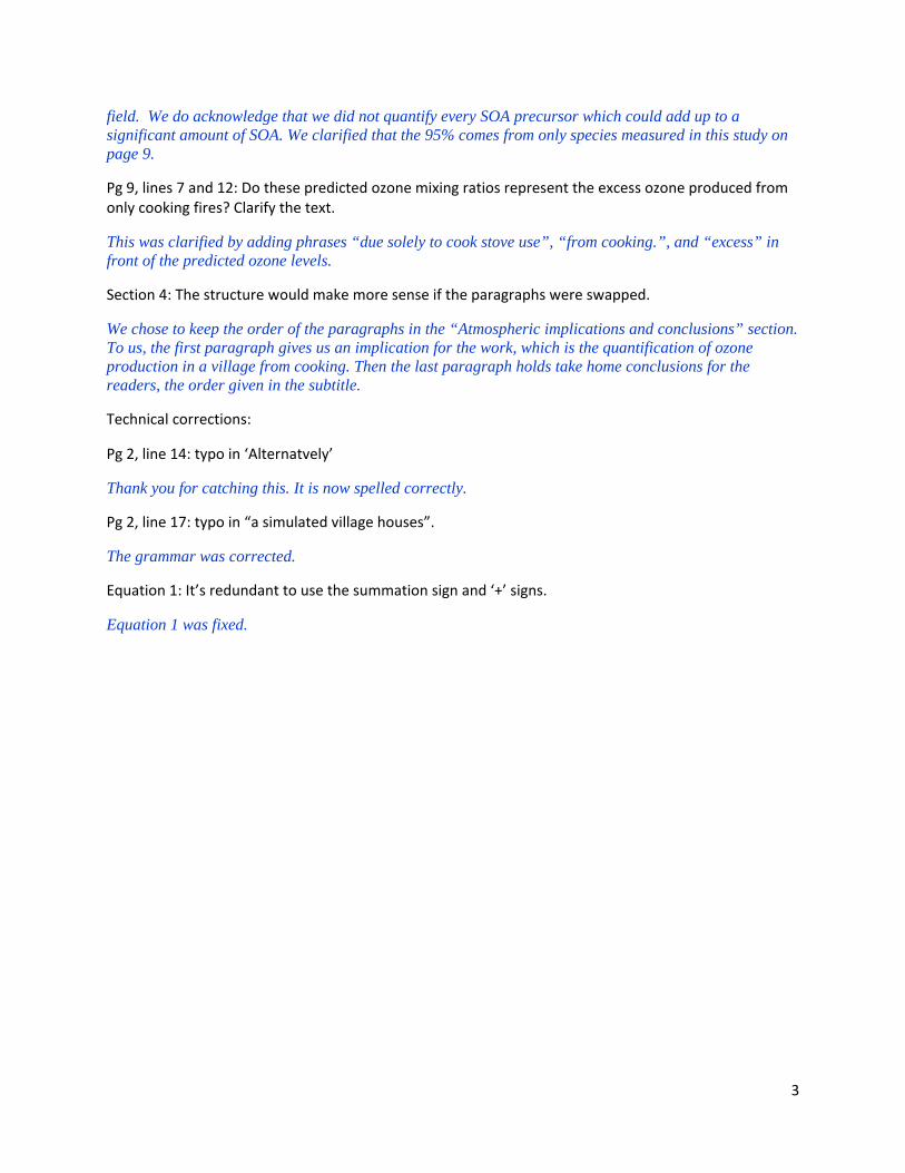
field. We do acknowledge that we did not quantify every SOA precursor which could add up to a significant amount of SOA. We clarified that the 95% comes from only species measured in this study on page 9.

Pg 9, lines 7 and 12: Do these predicted ozone mixing ratios represent the excess ozone produced from only cooking fires? Clarify the text.

This was clarified by adding phrases “due solely to cook stove use”, “from cooking.”, and “excess” in front of the predicted ozone levels.

Section 4: The structure would make more sense if the paragraphs were swapped.

We chose to keep the order of the paragraphs in the “Atmospheric implications and conclusions” section. To us, the first paragraph gives us an implication for the work, which is the quantification of ozone production in a village from cooking. Then the last paragraph holds take home conclusions for the readers, the order given in the subtitle.

Technical corrections:

Pg 2, line 14: typo in ‘Alternatvely’

Thank you for catching this. It is now spelled correctly.

Pg 2, line 17: typo in “a simulated village houses”.

The grammar was corrected.

Equation 1: It’s redundant to use the summation sign and ‘+’ signs.

Equation 1 was fixed.

Comments by reviewer #2 are reproduced in the sans-serif font below. Our responses follow each comment in a blue, italicized, serif font. Text additions to the manuscript appear in the manuscript in red color. Deletions from the manuscript are described in the responses below.

------------------------------------------------------------------------------------------------------------------------------------------

1. There is a wide diversity of stove and fuel types globally and the stove and fuel types explored here are but a small fraction of those used in real world. So while the gas-phase speciation offers a detailed view of the emissions from these stove-fuel sources, how are the stove-fuel sources in this work representative of the stove-fuel combinations in India and globally? More specifically, what fraction of the gas-phase emissions from cookstoves come from the stove-fuels described in this work? And depending on the answers to the previous question, how can this speciation, if at all, be used to inform the gas-phase emissions speciation in large-scale atmospheric models?

The objectives of the current paper are not to produce representative values for global emissions. Stockwell et al., 2016 and this work are the most comprehensive measurements to date in producing speciated gas phase emission factors. The stoves and fuels measured in the current study are predominant in the Indo-Gangetic plains. As a part of this collaborative project, the Seinfeld group at Caltech is modeling secondary organic aerosol formation using CMAQ to describe rural North India.

2. Since multiple tests were done with each stove-fuel combination, were other important variables recorded and/or controlled during the test? For example, fuel moisture content, environmental conditions (e.g., temperature, relative humidity), fuel size and burn rate, cooking pots, meals cooked. According to the authors, are any of these variables important in explaining the variability? Citing relevant literature on the factors affecting cookstove emissions variability would be helpful.

Moisture content of the fuels did not correlate with emission factors; in all cases the r2<0.3. In one case, we did see a negative relationship between emission and moisture content (Benzene, dung-angithi, r2=0.718). We did plot the emission factors as a function of fuel moisture content for a fraction of compounds as examples shown below. We found that meal cooked is not a significant variable (p>0.05). We added the recorded data for each cook fire to the supplemental information, including variable information and emission factors so the dataset is publically accessible. The following statements were added to make this clear to the reader.

“Fuel moisture content, fuel mass burned, and meals cooked were noted for each cook fire, and can be found in the supporting information.” (Page 3)

“There are many factors that may lead to variability in biomass burning emissions including pyrolysis temperature (Chen and Bond, 2010), fuel moisture content (Tihay-Felicelli et al., 2017), and the wind speed/direction (Surawski et al., 2015), among others. Relationships between emissions and fuel moisture content (Figure S1) or meal cooked were not found to be significant for any compounds (p< 0.05). This paper focuses on the relationships between emissions and fuel-stove combination.” (Page 6)

3. Some more detail on the fuels and stoves for the less informed reader would be helpful. What animals was the dung from? Presumably cow? What is an Angithi stove? What is a chulha? How are these different? What is brushwood? Is the brushwood from a particular plant? The use of pictures could help.

The following was added to the introduction, to explain the hypothesis that these stove will lead to different emissions.

“The former is a primarily flaming stove with generally higher modified combustion efficiencies or concentration ratios of carbon dioxide to the sum of carbon dioxide and carbon monoxide (average dung-chulha 0.865), used to cook village meals. The angithi is largely smoldering with lower modified combustion efficiencies (average dung-angithi 0.819) and is primarily used for cooking animal fodder and simmering milk.”

The pictures of stoves and the kitchen are already published in Fleming et al., 2018, but the reader is referred to this publication for more extensive information about the materials used in the cook fires. The following sentences were added to the experimental methods section.

“Animal fodder simmers upon smoldering dung in a clay bowl, referred to as an angithi. Chulha stoves are made from bricks and a covering of clay, and the availability of oxygen from the packing of biomass fuels results in primarily flaming combustion. The chulha is used to cook most meals for the family in this village. Buffalo and cow dung patties and brushwood, in the form of branches and twigs, were used in chulha stoves, and for the 13 mixed fuel cooking events dung and brushwood were combined in a ratio determined by the cook’s preference.”

4. In equations 1-3, how are mT and mT,c estimated/calculated?

The language in red was added to clearly show how mT and mT,C are obtained.

“Fuels were weighed before they were burned, and the dry mass was calculated based on moisture content measurements. The ash was weighed after the cooking event and subtracted from the dry mass of the fuel giving the net dry fuel burned for the cooking event, mT. When mixtures of dung and brushwood were used, both were individually weighed to more accurately determine the carbon mass burned. The fraction of carbon in the fuel used to yield mT,C was taken to be 0.33 for buffalo dung and 0.45 for brushwood fuels based on Smith et al. 2000.”

5. Page 4, line 11: What is the limit of detection and limit of quantification for the filter measurement? The 0.75 µg blank seems quite low.

We determined the method detection limit to be 9.3 micrograms based off the standard deviation of the field blanks multiplied by 3. All masses for the sample and background filters are above this limit of detection.

6. Page 5, line 1: I am not sure what the point is of normalizing the SOA production from a species to that of toluene? Why not report the SOA production in absolute values of g/kg-fuel when the presentation of results in Figure 2(c) is done in relative format anyways?

The SOAP value for a particular VOC, as described by Derwent et al., 2010, is the change in SOA mass concentration when this VOC is introduced into the photochemical transport model, divided by the change in SOA mass concentration for when toluene is introduced. We use these SOAP values published in Derwent et al., 2010 to determine SOA forming potential for each quantified VOC. We are simply inheriting these data from the literature to estimate the relative magnitude of the effects, with the hope that more detailed modeling work would follow. The dataset is publicly available, so if one wished to generate absolute g SOA mass/ kg fuel burned by estimating the SOA yield for toluene in the plume, this is possible.

7. Why was the maximum incremental reactivity approach used to determine the ozone potential? If an alternative method was used (e.g., MOIR, EBIR), do the findings change?

Maximum incremental reactivity was chosen because a VOC limited regime gives us the highest sensitivity in ozone generation to cooking emissions. Carter 1994 concludes that the MIR scenario, since it is based on integrated ozone production rather than maximizing peak ozone levels (MOR scenario,) is generally less dependent on exact NOx inputs. This high-NOx scenario might be more realistic as well since we are focusing on smoke plumes. A sentence was added to the experimental section 2.7 summarizing this explanation for the use of the MIR scenario.

8. Can more details about the SOA formation be added? Were the SOA yields for low or high NOx conditions? What OA mass concentration as the absorbing mass was used to determine the SOA yield? Were they corrected for vapor wall losses? NOx and vapor wall loss corrections are species dependent (see Zhang et al., 2014) and may change the apportionment shown in Figure 2(c).

The photochemical trajectory model is outfitted with the Master Chemical Mechanism (MCM 3.1), which dictates gas-phase reactions and SOA formation. NO was initialized at 2 ppb, and NO2 to 6 ppb. This is now described in section 2.5.

9. Page 7, lines 3-21: Are the brushwood results in this study comparable to the hardwood results from Stockwell et al. (2016)? If yes, why? It is unclear what the point of the comparison to the Stockwell study is since the manuscript only has a few sentences on this comparison. Is it just to show that the emissions in this study were lower than those in Stockwell et al. (2016). The explanations offered for the lower emissions was not satisfactory. Did the authors try to compare the emissions on a normalized basis with each other? Do they correlate?

Stockwell et al. 2016 and this paper are the most comprehensive gas-phase inventories to date in terms of cook fire emissions. It made sense to the authors to cross-compare the results. “Hardwood” and “brushwood” emissions appear to be more similar to each other than emissions from dung-based fuels. There are some real differences in emissions from cook fires between the studies, and we do our best to explain in the text these differences for the reader to compare. In S2.1 we plot the EFs in Stockwell et al. 2016 against those reported in our paper. In the review process, we’ve learned more about how the laboratory EFs were adjusted to field observations in Stockwell et al., 2016, and we believe these adjustments may have contributed to the discrepancy in the reported EFs. We’ve added Figure S2.2 where we plot the unadjusted emission factors in both studies, and there is an encouraging degree of agreement in the actually measured (unadjusted) values.

10. Section 3.3 for SOA: Was there an estimate for emissions of total non-methane organic gases (NMOG)? What fraction did the speciated compounds account for of the total NMOG? Were any intermediate volatility and semi-volatile organic compounds targeted? What fraction of the NMOG was unspeciated? What implications does this unspeciated fraction that may include lower-volatility vapors have for SOA formation?

We agree that there are semi and intermediate volatility compounds that were not measured in this study. Many of these will contribute to SOA and ozone formation. We did not attempt to quantify NMOG. This was not possible using our carbon balance method and an unknown dilution factor. We have added a “disclaimer” to the manuscript in the “SOA formation potential” section, printed below.

“We would like to emphasize that the SOAP-weighted emissions are reflective of only the measured VOCs, and there are likely semi-volatile and intermediate volatility compounds that are not measured but also contribute to SOA formation.”

11. Section 4: Could atmospheric implications for SOA formation also be determined for this village similar to those for O3? How would the SOA formation compare to the primary PM2.5 emissions? Unfortunately the SOA forming potentials generated using Derwent et al. 2010 only give relative amounts of SOA formation. From this analysis we concluded that a dung-chulha cook fire would produce almost 3 times more SOA than a brushwood-chulha cook fire. However, with this methodology we cannot compare the absolute magnitudes of primary and secondary emissions. Further work on addressing this exact question is in progress with the Seinfeld group at Caltech to model SOA formation in a simulated village.

1

Emissions from village cookstoves in Haryana, India and their potential impacts on air quality Lauren T. Fleming,1 Robert Weltman,2 Ankit Yadav,3 Rufus D. Edwards,2 Narendra K. Arora,3Ajay Pillarisetti,4 Simone Meinardi,1 Kirk R. Smith,4 Donald R. Blake,1 and Sergey A. Nizkorodov1,* 1Department of Chemistry, University of California, Irvine, CA 92697, USA 5 2Department of Epidemiology, University of California, Irvine, CA 92697, USA 3The Inclen Trust, Okhla Industrial Area, Phase-I, New Delhi-110020, India 4School of Public Health, University of California, Berkeley, CA 94720, USA Correspondence to: Sergey Nizkorodov (nizkorod@uci.edu) 10 Abstract. Air quality in rural India is impacted by residential cooking and heating with biomass fuels. In this study, emissions of

CO, CO2, and 76 volatile organic compounds (VOCs) and fine particulate matter (PM2.5) were quantified to better understand the

relationship between cook fire emissions and ambient ozone and secondary organic aerosol (SOA) formation. Cooking was

carried out by a local cook and traditional dishes were prepared on locally built chulha or angithi cookstoves using brushwood or 15 dung fuels. Cook fire emissions were collected throughout the cooking event in a Kynar bag (VOCs) and on PTFE filters

(PM2.5). Gas samples were transferred from a Kynar bag to previously evacuated stainless steel canisters and analyzed using gas

chromatography coupled to flame ionization, electron capture, and mass spectrometry detectors. VOC emission factors were

calculated from the measured mixing ratios using the carbon-balance method, which assumes that all carbon in the fuel is

converted to CO2, CO, VOCs, and PM2.5 when the fuel is burned. Filter samples were weighed to calculate PM2.5 emission 20 factors. Dung fuels and angithi cookstoves resulted in significantly higher emissions of most VOCs (p< 0.05). Utilizing dung-

angithi cook fires resulted in twice as much of the measured VOCs compared to dung-chulha, and four times as much as

brushwood-chulha with 84.0, 43.2, and 17.2 g measured VOC/ kg fuel carbon, respectively. This matches expectations, as the

use of dung fuels and angithi cookstoves results in lower modified combustion efficiencies compared to brushwood fuels and

chulha cookstoves. Alkynes and benzene were exceptions and had significantly higher emissions when cooking using a chulha 25 as opposed to an angithi with dung fuel (for example, benzene emission factors were 3.18 g/ kg fuel carbon for dung-chulha and

2.38 g/ kg fuel carbon for dung-angithi). This study estimated that three times as much SOA and ozone in the Maximum

Incremental Reactivity (MIR) regime may be produced from dung-chulha as opposed to brushwood-chulha cook fires. Aromatic

compounds dominated as SOA precursors from all types of cook fires, but benzene was responsible for the majority of SOA

formation potential from all chulha cook fire VOCs, while substituted aromatics were more important for dung-angithi. Future 30 studies should investigate benzene exposures from different stove and fuel combinations and model SOA formation from cook

fire VOCs to verify public health and air quality impacts from cook fires.

1 Introduction

Parts of rural India are comprised of densely populated villages with ambient ozone and PM2.5 levels that affect air quality for 35 inhabitants (Bisht et al., 2015; Ojha et al., 2012; Reddy, 2012). For example, in the rural area of Anantapur in Southern India,

monthly mean ozone levels varied between 29 ppbv (parts per billion by volume) in August during the monsoon season and 56

ppbv in April (Reddy, 2012). In Pantnagar, a semi-urban city, the maximum observed ozone concentration was 105 ppbv for one

2

day in May, with the lowest average monthly maximum of 50 ppbv being in January (Ojha et al., 2012). In terms of PM2.5 levels,

Bisht et al. (2015) observed an average of 50 µg m-3 of PM2.5 over July-November 2011 in rural Mahabubnagar. While

measurements of O3 and PM2.5 in rural India are relatively scarce, it has become clear that household combustion is a major

contributor to ambient levels of these pollutants. For example Balakrishnan et al. (2013) measured PM2.5 concentrations in

households and observed 24-hour concentrations of 163 to 609 µg m-3. Over the last half-decade, several researchers have, 5 through independent studies, come to the conclusion that a significant fraction (22-52%) of ambient PM2.5 is directly emitted

from residential cooking and heating (Butt et al., 2016; Chafe et al., 2014; Conibear et al., 2018; GBD MAPS Working Group,

2018; Guttikunda et al., 2016; Klimont et al., 2017; Lelieveld et al., 2015; Silva et al., 2016).

Residences in India were estimated to consume 220, 86.5, and 93.0 Tg per year of dry matter of wood fuel, agricultural residues,

and dung, respectively in the year 1985 (Yevich and Logan, 2003). While the fraction of Indians using biomass cook fuels is 10 decreasing, the total population is increasing such that biomass fuels are still being utilized at approximately the same overall

level (Pandey et al., 2014). Emissions of primary PM2.5 from residential cooking in India were estimated to be 2.6 Tg per year

based on a compiled emissions inventory (Pandey et al., 2014). Additionally, Pandey et al. (2014) estimated that 4.9 Tg of non-

methane volatile organic compounds (NMVOCs) are produced annually in India from residential cooking. This suggests that

additional PM2.5 mass may be formed via secondary pathways from the oxidation of NMVOCs and either nucleation of new 15 particles or condensation onto existing PM2.5. Alternatively, these non-methane VOCs could contribute to photochemical ozone

production in the presence of NOx (Finlayson-Pitts and Pitts, 2000).

In this study, we quantified emissions of CO, CO2, and 76 different VOCs from 55 cook fires carried out by a local cook in a

village home cooking typical meals. It is thus a substantially updated version of the work done in simulated village houses in

India and China in the 1990s, where 58 fuel-stove combinations were measured in semi-controlled conditions using water boiling 20 tests including a number of non-biomass stoves although a similar set of pollutants were measured (Smith et al., 2000b, 2000a;

Tsai et al., 2003; Zhang et al., 2000). This time, we measured emissions in field conditions from two traditional, locally-made

cookstoves, the chulha and the angithi. The former is a primarily flaming stove with generally higher modified combustion

efficiencies or concentration ratios of carbon dioxide to the sum of carbon dioxide and carbon monoxide (average dung-chulha

0.865), used to cook village meals. The angithi is largely smoldering with lower modified combustion efficiencies (average 25 dung-angithi 0.819) and is primarily used for cooking animal fodder and simmering milk. We measured emissions from

cookstoves with two kinds of biomass; the most popular biomass type brushwood (Census of India, 2011) and dung cakes. Our

first objective is to characterize emissions of select VOCs and PM2.5 from these fuel-stove combinations. Subsequently, with the

aid of secondary organic aerosol (SOA) potential values from Derwent et al. (2010), incremental reactivity first described in

Carter, (1994), and second-order rate coefficients with OH combined with our emission factors, we estimate SOA forming 30 potentials, ozone formed in a VOC-limited regime, and OH reactivity, respectively. Given their widespread use in India,

emissions from these biomass-burning stoves are estimated to impact regional air quality due to both primary and secondary

organic aerosol and ozone formation.

2 Experimental Methods

2.1 Field site and sample collection 35

3

The field office was located at the SOMAARTH Demographic, Development, and Environmental Surveillance Site in Palwal

District, Haryana, India run by the International Clinical Epidemiological Network (INCLEN). The site consists of 51 villages in

the area with roughly 200,000 inhabitants (Balakrishnan et al., 2015; Mukhopadhyay et al., 2012; Pillarisetti et al., 2014).

Samples were collected from cookstove emissions between August 5 and September 3, 2015. Cooking events occurred at a

village kitchen in Khatela, Palwal District. A local cook was hired to prepare meals for human consumption consisting of either 5 chapatti or rice with vegetables using a chulha stove, as well as animal food using an angithi stove.

Animal fodder simmers in a pot set upon smoldering dung in a clay bowl, referred to as an angithi. Chulha stoves are made from

bricks and a covering of clay, and the availability of oxygen from the packing of biomass fuels results in primarily flaming

combustion. The chulha is used to cook most meals for families in this village. Buffalo and cow dung patties and brushwood, in

the form of branches and twigs, were used in chulha stoves, and for the 13 mixed fuel cooking events dung and brushwood were 10 combined in a ratio determined by the cook’s preference. Stoves and food ingredients were produced and fuels procured by the

household or village. Fuel moisture content, fuel mass burned, and meals cooked were noted for each cook fire, and can be found

in the supporting information. Additional information regarding the cooking events and set-up can be found in Fleming et al.,

2018.

The sampling scheme is illustrated in Figure 1. Air sampling pumps (PCXR-8, SKC Inc.) created a flow of emissions through the 15 sampling apparatus. Emissions were captured with three-pronged probes that were fixed 60 cm above the cookstove. PM2.5

emissions and gases were sampled through cyclones (2.5 µm, URG Corporation). The resulting flow of particles was captured on

either quartz or PTFE filters, while gases were collected in an 80 L Kynar bag throughout the entire cooking event. Flows were

measured both before and after sampling to ensure they did not change by more than 10% using a mass flowmeter (TSI 4140).

After the cooking event, pumps were turned off and a whole air sampler, consisting of a stainless steel canister (2L) welded to a 20 Bellows-sealed valve (Swagelok), was filled to ambient pressure from the Kynar bag. Whole air samplers were thoroughly

flushed and evacuated in the Rowland-Blake laboratory before being shipped to India. At the end of the measurement campaign,

whole air samplers were shipped back to the laboratory and analyzed within two months of the end of the field measurements. A

“grab” whole air sample was collected before cooking commenced each day. This served as a background for all cooking events

sampled on that day. 25

2.2 Gas chromatography analysis

Colman et al., 2001 described the VOC analysis protocol in detail. Briefly, a known amount of the whole air sample (WAS)

flowed over glass beads inside a U-shaped trap cooled by liquid nitrogen. The flow was regulated by a mass flow controller and

resulted in a 600 Torr drop in the pressure in the whole air sampler. High volatility gases such as O2 and N2 passed over the

beads, while lower volatility gases adsorbed onto the beads. Compounds were re-volatilized by immersing the trap in hot water 30 and were injected into a He carrier gas stream where the flow was split equally to 5 columns housed in 3 gas chromatographs

(HP-6890). The compounds were separated by gas chromatography and subsequently detected by two electron capture, two

flame ionization, and one quadrupole mass spectrometer detectors. Peaks corresponding to compounds of interest were

integrated manually. CO/CO2 and CH4 were analyzed using separate GC systems equipped with thermal conductivity and flame

ionization detectors as described in Simpson et al., 2014. The CO/CO2 GC-FID system is equipped with a Ni catalyst that 35 converts CO into detectable CH4.

2.3 Gas and PM2.5 Emission factor calculations

4

Emission factors (EFs) were calculated using the carbon-balance method, which assumes that all carbon in the fuel is converted

to CO2, CO, VOCs, and PM when the fuel is burned. The total gas-phase carbon emissions were approximated with the

concentrations of CO2, CO, as well as 76 detected VOCs measured using WAS. This is a good approximation since most emitted

carbon resides in CO2 and CO (> 95 %), so the error associated with VOCs that are not detected is relatively small (Roden and

Bond, 2006; Smith et al., 1993; Wathore et al., 2017; Zhang et al., 2000). The mass of carbon in species i (mi,C) was calculated 5 using equation (1).

m𝑖,C (g) = C𝑖,C(g/m3)CCO2,C+CCO,C+CCH4,C+⋯+CC6H6,C (g/m3)

⋅ mT,C (kg) ⋅ 1000 g1 kg

(1)

Where Ci,C represents the mass concentration of carbon for species i, and mT,C refers to the carbon mass of the fuel, adjusted for

ash and char carbon. Fuels were weighed before they were burned, and the dry mass was calculated based on moisture content

measurements. The ash was weighed after the cooking event and subtracted from the dry mass of the fuel giving the net dry fuel 10 burned for the cooking event, mT. When mixtures of dung and brushwood were used, both were individually weighed to more

accurately determine the carbon mass burned. The fraction of carbon in the fuel used to yield mT,C was taken to be 0.33 for

buffalo and cow dung and 0.45 for brushwood fuels based on Smith et al. 2000. Carbon in ash was estimated as 2.9% and 80.9%

of the measured char mass for dry dung and dry brushwood, respectively (Smith et al., 2000b). For each species with nc,i carbon

atoms in the formula and molecular weight MWi, the emissions factor (EFi) was calculated using equation (2). 15

(2)

In addition to the emission factor normalized by the total fuel mass, emission factors were normalized to the total carbon mass in

the fuel, calculated via equation (3).

(3)

PM2.5 mass was determined gravimetrically using Teflon filters (PTFE, SKC Inc., 47 mm) weighed on a Cahn-28 electrobalance 20 with a repeatability of ±1.0 µg after equilibrating for a minimum of 24 hours in a humidity and temperature-controlled

environment both before and after sample collection (average temperature 19.5± 0.5 ºC; average relative humidity 49 ±5%).

Another gravimetric filter was collected in the background during the cooking event and was equilibrated and weighed in the

same way (Figure 1, Teflon C). Four field blanks filters were prepared by opening filters and then immediately closing and

sealing the filters the same way as all samples; these filters had negligible mass loading (average: -0.75 µg) relative to samples 25 (average: 1.57 mg). The background filter mass (Figure 1, Teflon C) was adjusted by matching the sampling volume to that of

the sample gravimetric Teflon filter (Figure 1, Teflon A). This assumes that the mass of PM2.5 collected on the filter is directly

proportional to the flow rate through the filter. The background mass was then subtracted from the sample mass to obtain the

mass of PM (mPM) in equation (4) below.

EFPMEFCO

=mPM

Vair�mCO

Vair� (4) 30

EF𝑖 �g VOC𝑖kg fuel

� =m𝑖,C(g) ⋅ MW𝑖 (g/mol)

nc,𝑖 × 12.00 (g/mol)mT(kg)

EF𝑖 �g VOC𝑖

kg fuel C� = EF𝑖 �

g VOC𝑖kg fuel

� ⋅mT(kg)

mT,C(kg)

5

2.4 Modified Combustion Efficiency (MCE)

Modified combustion efficiency (MCE) is defined as follows:

MCE = ∆CO2∆CO+∆CO2

(5)

where ΔCO and ΔCO2 are background-subtracted mixing ratios of CO and CO2 for the time-integrated whole air sample. The

total carbon mixing ratio is approximated by the sum of carbon monoxide and carbon dioxide in this definition. 5

2.5 SOA Forming potential

Relative SOA forming potential from measured VOCs was estimated using secondary organic aerosol potential (SOAP) values

from Derwent et al., 2010, who used a photochemical transport model to simulate the SOA mass increase from the instantaneous

emission of a particular VOC in a single parcel of air travelling across Europe. The model was outfitted with the Master

Chemical Mechanism (MCM v.3.1) and the UK National Atmospheric Emission Inventory. The model was initialized with 2 10 ppbv NO and 6 ppbv NO2 (Derwent et al., 1998). SOA mass was estimated assuming equilibrium partitioning of oxidation

products. Partitioning coefficients were calculated using absorptive partitioning theory of Pankow, 1994. In the SOAP approach,

all SOA mass increases from a particular VOC (i) are normalized to that of toluene as shown in equation (6).

SOAPi = Increment in SOA mass concentration with species 𝑖Increment in SOA mass concentration with toluene

× 100 (6)

SOA forming potential was calculated from the published SOAP values using equation (7). 15

SOA potential = ∑ SOAP𝑖 × EF𝑖 �g VOC𝑖kg fuel C

�𝑛𝑖=0 (7)

Table S1 lists the SOAP values used to calculate SOA forming potential in this study. We emphasize that the SOA forming

potential presented here is a relative value, and does not represent an absolute SOA yield.

2.6 OH reactivity

Total OH reactivity normalized by the mixing ratio of CO was calculated using equation (8). 20

OH reactivity � 1s∙ppbv CO

� = ∑ 𝑘𝑂𝑂,𝑖 � cm3

molec∙s � × ER𝑖 �

pptv VOC𝑖 ppbv CO

� × 2.46 × 107 � moleccm3∙pptv

�𝑛𝑖=0 (8)

Second-order rate constants (kOH) at 25°C were taken from the NIST chemical kinetics database (Manion et al., 2015). Table S1

reproduces the kOH constants used in the study. ERi is the emission ratio for compound i in pptv of VOC per ppbv of CO. The

last term serves as a conversion factor from VOC mixing ratio to concentration at standard ambient temperature and pressure

(25°C, 1 atm). By using the emission ratio to CO, we can track OH reactivity from VOCs depending on the extent of dilution 25 from the plume. From here forward, the OH reactivity (s-1) reported is the average at the location of the sampling probes, or

roughly 60 cm above the cookstove.

2.7 Ozone-forming potential (OFP)

The ozone-forming potential was estimated from the incremental reactivity of VOCs tabulated in Carter, 2010. Incremental

reactivities were calculated by comparing ozone formation before and after a VOC was introduced in a box model simulation. 30

6

The Maximum Incremental Reactivity (MIR) scenario sets high NOx concentrations, optimized to yield the largest incremental

ozone production. In other words, ozone production was VOC limited. Because of this, the OFPs given here represent a scenario

where VOC emissions from cooking have the largest impact on ozone production. This high-NOX scenario was chosen for high

sensitivity in ozone production from cooking emission VOCs. In addition, it is expected to be more realistic for a smoke plume

in which NOx is co-emitted with VOCs. OFPs were calculated using equation (9). 5

OFP � g O3kg fuel C

� = ∑ MIR � g O3g VOC𝑖

� × EFi �g VOC𝑖kg fuel C

�𝑛𝑖=0 (9)

OFPs used in this study are listed next to the corresponding compound in Table S1.

2.8 Statistical analysis

One-way analysis of variance (ANOVA) with Tukey Post-Hoc testing was utilized to determine if there were significant

differences (p<0.05) in emissions of specific VOCs among categorical variables, i.e., stove and fuel types. All analyses were 10 performed in R version 3.4.0 and RStudio version 1.0.143 (RStudio Inc, 2016).

3 Results and discussion

3.1 Chemical composition

Average VOC and PM2.5 EFs (g/ kg dry fuel) as well as MCE are given in Table 1. The compounds are grouped by fuel-stove

combination, with major species (CO2, CO, CH4, and PM2.5) listed first, followed by sulfur-containing compounds, halogen-15 containing compounds, organonitrates, alkanes, alkenes, alkynes, aromatics, terpenes, and oxygenated compounds. The sample

size (n) used for calculating the average values and standard deviations was n=18 for dung-chulha, n=14 for brushwood-chulha,

n=13 for mixed-chulha, and n=10 for dung-angithi. For the majority of the compounds, the standard deviations are smaller than

or comparable to the average values, indicating fair reproducibility. There are many factors that may lead to variability in

biomass burning emissions including pyrolysis temperature (Chen and Bond, 2010), fuel moisture content (Tihay-Felicelli et al., 20 2017), and the wind speed/direction (Surawski et al., 2015), among others. Relationships between emissions and fuel moisture

content (Figure S1) or meal cooked were not found to be significant for any compounds (all p< 0.05). This paper therefore

focuses on the relationships between emissions and fuel-stove combination.

Figure 2a visually shows the mass fraction attributed to each compound class for the measured gas-phase emissions. The total

EFs given below the pie charts are normalized by fuel carbon in Figure 2a in order to compare between cook fires generated with 25 dung, wood, and wood-dung mixtures which have different carbon contents. The total measured VOC emissions from dung-

angithi were roughly twice that of dung-chulha in terms of gram per kilogram fuel carbon. Further, dung-chulha emitted more

than twice that of brushwood-chulha. The most prominent difference is non-furan oxygenates, making up almost half of all

brushwood-chulha emissions and a smaller fraction for other fuel-stove combinations. While oxygenates make up a higher

fraction of brushwood-chulha emissions, the absolute EFs for oxygenates from dung-burning and angithi cook fires are higher as 30 discussed later in more detail.

Table 2 shows EFs (g/ kg fuel C) for select VOCs. The differences in mean EFs for each fuel-stove combination are also

included in Table 2. Mean differences in EFs reported for chulha and angithi stoves were calculated for cook fires utilizing only

dung fuels. Likewise, mean EFs for wood and dung cook fires only represent cooking events using the chulha. This was done to

isolate a single variable—either fuel or stove type. For all alkanes and most alkenes, we measured higher emissions for dung-35

7

angithi cook fires (Table 2). Also, from the mean differences in EFs, we found that stove specific combustion conditions impacts

emissions more than the selection of fuel type. The difference is so dramatic for alkanes and most alkenes that the mean

difference in EFs for cookstoves burning dung is always larger than the mean EF of that compound. For comparison, the mean

difference in EFs for chulha cookstoves is always lower than the overall mean EF. Ethene was an exception; there was no

relationship between ethene emissions and stove type. On the other hand, the mean EF of ethene by dung cook fires was very 5 large compared to mean EFs from brushwood cook fires with a mean difference in EFs of 4.05 g/ kg fuel C. Some alkenes with

two double bonds were also exceptions. For 1,3-butadiene (p= 0.06) and 1,2-butadiene (p= 0.089), stove and EF may or may not

have a significant relationship. 1,2-Propadiene emissions from chulha cookstoves are higher (p< 0.01). All three compounds still

show a significant relationship to fuel type with EFs being higher for dung cook fires.

Similar to alkanes and alkenes, aromatics, oxygenates, halogen-, and sulfur-containing compounds all had higher emissions per 10 kilogram of fuel carbon when dung fuels and angithi stoves were utilized compared to brushwood fuels and chulha stoves,

respectively. We focus on the behavior of the most interesting groups of compounds in the discussion below.

The chlorine-containing organic compounds are generally expected to come from cook fires in large quantities. However, we

observed an interesting practice in which the cook often used plastic bags to start the fire, which could be a source of chlorine-

containing compounds if composed of polyvinyl chloride. Carbonyl sulfide (OCS) is largely responsible for the yellow sulfur-15 containing fraction in Figure 2a and biomass burning is a well-known source of OCS in the atmosphere (Crutzen et al., 1979).

Similar to other VOCs, OCS was significantly emitted in higher quantities when anigithi stoves and dung fuels were utilized.

Benzene had higher emissions from chulha stoves, which had higher MCEs when cooking with dung fuels compared to angithi

stoves (dung-chulha 3.18 g/ kg fuel C and dung-angithi 2.38 g/ kg fuel C). As the simplest aromatic compound, benzene also had

the largest average difference in fuel type EFs compared to other aromatics (2.18 g/ kg fuel C, dung-wood). This information is 20 relevant for exposure assessment, as benzene is a known human carcinogen. Higher benzene emissions from chulha cook fires

could lead to higher benzene exposures which is a potential public health concern. However, it should be noted that the cook

usually cannot control the stove used, as the angithi and chulha are used to prepare different types of meals, and exposure to

benzene is not straightforward from its emission factors.

Higher emissions of alkynes were observed from dung fuels and chulha cookstoves. The latter observation is consistent with the 25 literature showing flaming combustion generates more alkynes (Barrefors and Petersson, 1995; Lee et al., 2005). Chulha cook

fires always had higher MCE than angithi cook fires (Table 1) which rely on smoldering combustion. Approximately the same

difference in alkyne emissions results from comparing the chulha to the angithi using dung, in relation to using wood versus

dung in combination with the chulha. There were two exceptions in stove type for 1-butane (p= 0.055) and 2-butane (p>> 0.05).

The former may or may not have a relationship with stove type, while the latter does not. Emissions of some compounds did not 30 show a relationship with either fuel or stove type, and are listed in Table S2.

VOC emissions from Stockwell et al. (2016) are also provided in Table 1 for comparison of VOC EFs. Samples in Stockwell et

al. (2016) were collected in April 2015 in and around Kathmandu and the Tarai plains, which border India. While both are EFs

from cookstoves using similar fuels, there are differences in the studies that should be noted. Stockwell et al. (2016) collected

measurements of simulated cooking in a laboratory and from cooking fires in households; it was not noted in the latter case what 35 meals were cooked. EFs were calculated from similar WAS measurements, but as grab samples in an area of the kitchen away

from the fire (as opposed to the time-integrated approach used here). Emissions were assumed to be well-mixed in the kitchen

8

prior to sampling. Stockwell et al. (2016) also used a range of stoves, including the traditional single-pot mud stove, open three-

stone fire, bhuse chulo, rocket, chimney, and forced draft stoves. “Dung” cook fires sometimes used a combination of fuels, such

as wood. Finally, our study also has a larger sample size than Stockwell et al. (2016) with n=49 versus n≈10.

The emission factors for most compounds determined in this study were lower compared to those reported in Table 4 of the

Stockwell et al. (2016) paper. Figure S2.1 visually shows that the EFs were generally lower in the present study. In some cases, 5 EFs in this study were an order of magnitude lower, most notably n-pentane and n-hexane. We also found that our emission

factors were always higher for dung-chulha compared to brushwood-chulha, which was not always the case in Stockwell et al.

(2016). The EFs in Stockwell et al. (2016) could be biased high due to calculations rather than real differences in emissions. For

example, ignoring ash and char carbon and using the same carbon content inflates the EFs reported in our paper by 7% for dung

and 24% for brushwood emissions. However, this is a small percentage compared to the observed differences between EFs 10 between the two measurements. By examining the EFs reported in the supporting information section of the Stockwell et al.

(2016), we found that the disagreement resulted from the way the final recommended EFs were obtained from the measurements.

Because Stockwell et al. (2016) measured both laboratory and field cook fires, they elected to adjust the laboratory EFs to

account for the lower MCEs observed in the field. It has been shown by Roden et al. (2009) and Johnson et al. (2008) that

cooking activities can strongly influence emissions, for example due to the cook tending to the cook fire differently, thus 15 affecting combustion conditions. However, such adjustments should be done with caution because EF and MCE do not always

follow a linear trend, as explained in the next section. Figure S2.2 plots the unadjusted laboratory and field emission factors as a

function of MCE for all the measurements in Stockwell et al. (2016), as well as this study. Plotting the unadjusted EFs resolves

most of the differences in observed EFs between the two studies. The data show an encouraging level agreement despite the

differences in the experimental design between the two studies. 20

3.2 Modified combustion efficiency

The use of dung and angithi, rather than brushwood and chulha, respectively, results in lower modified combustion efficiencies

as shown in Figure 3. In general, at lower MCEs we measured higher emissions of gas-phase compounds as discussed in Section

3.1. For example, emissions of ethane (Figure 3a) and other alkanes increase with decreasing MCE. However the dependence of

ethane EF on MCE is not linear as observed in previous studies (Liu et al., 2017; Selimovic et al., 2018). For other VOCs, the 25 dependence of the EF on MCE deviates from the linear trend even more, with the maximum EF observed at intermediate MCE

values. For example, the ethene EF (Figure 3b) increases with decreasing MCE at MCEs > 0.85, but it has the opposite trend at

MCEs < 0.85. Previously, we discussed that there is no relationship between ethene EF and stove type and we see this more

clearly in Figure 3b. Alkynes have the same relationship to MCE as ethene, but it is even more pronounced (Figure 3c). Benzene

(Figure 3e) stands apart from other aromatics with a relationship with MCE similar to ethene, while other aromatics have an EF 30 versus MCE curve similar to alkanes and most other VOCs. In Figure 3e, we see again that emissions from brushwood-chulha

and dung-angithi cook fires result in lower emissions of benzene compared to dung-chulha. Alkenes with two double bonds

generally have a negative correlation between emissions and MCE, such as 1,3-butadiene in Figure 3f. The 1,3-butadiene EF

versus MCE plot is not necessarily representative of all analogous plots for alkenes with two double bonds, as they have different

shapes. 1,3-butadiene was chosen as its emission is high compared to other compounds in its subcategory and it also has health 35 implications. It also happens to have a more linear relationship with MCE, albeit noisy.

It is of interest to compare EFs obtained from different fuel-stove combinations but with the same MCE. In the case of ethane,

different cook fire types yield vastly different EFs at the same MCE. For example, at MCE≈ 0.87, mixed-chulha has an EF of

9

roughly 1.5 g/ kg fuel C, dung-chulha is 2.5 g/ kg fuel C, and dung-angithi is 5.5 g/ kg fuel C. Knowledge of the cook fire MCE

alone is not sufficient to determine the EF of ethane. Combustion conditions specific to the fuel-stove combination is a

significant factor in determining cook fire emissions. A similar conclusion can be reached for most of the measured gases,

including non-ethene alkenes in Figure 3d.

3.3 Secondary pollutant formation and reactivity 5

OH reactivity and ozone forming potential

Total OH reactivity (s-1) based on the measured VOCs in Figure 2b is given per ppbv of CO. Predicted OH reactivities in the

village due to a single cooking event are 10.2, 6.73, 4.93, and 4.83 s-1 for emissions from dung-angithi, dung-chulha, mixed-

chulha, and brushwood-chulha cook fires, respectively. This assumes a CO mixing ratio of 338 ppbv, which we measured as the

average background mixing ratio over the whole campaign. The relative total OH reactivity is over twice as high for dung-10 angithi cook fires as it is for brushwood-chulha cook fires.

The classes of compounds that act as the most important OH radical sinks in descending order are alkenes, oxygenates, furans,

terpenes, and aromatics. Alkenes make up more than 50% of OH reactivity for all cook fire types. Ethene (by fuel type) and

propene (by fuel and stove combination) are mostly responsible for the differences in fuel-stove combination results for alkenes.

For oxygenates, methanol (p< 0.01) and acrolein (p< 0.05) have significantly higher OH reactivity with wood fuel, while 15 acetaldehyde has significantly higher OH reactivity with the angithi stove (p< 0.001). Differences in OH reactivity due to furans

were observed for stove type but not fuel type. All three of the measured furans significantly contribute (p<0.001) to a 6%

increase in the fraction of OH reactivity due to furans for dung-angithi (12%) as opposed to dung-chulha (6%). The percentage

of OH reactivity due to aromatics is constant at ~4% for the fuel-stove combinations. However, different aromatic compounds

are responsible for this ~4% contribution depending on the cook fire type. Benzene dominates OH reactivity due to aromatics for 20 chulha cook fires. For angithi cook fires aromatics other than benzene, in particular toluene, dictate the OH reactivity for

aromatics. Isoprene is solely responsible for the differences in OH reactivity due to terpenes.

Figure 2d shows the total ozone forming potential (g/ O3 kg fuel) in the MIR scenario, as well as contributions to OFP by

compound class. A critical step in photochemical ozone production is VOC reacting with OH. Therefore, the ozone forming

potential contributions by compound class are similar to those for OH reactivity (Figure 2c). Total OFP is nearly a factor of 3 25 higher for dung-chulha compared to brushwood-chulha, while it’s twice as high for dung-angithi as compared to dung-chulha.

SOA formation potential

SOAP-weighted emissions relate SOA production from the different cook fire types in a qualitative manner. The contribution of

each compound class to the total SOA formation potential is shown in Figure 2c. We emphasize that the SOAP-weighted

emissions are reflective of only the measured VOCs, and there are likely semi-volatile and intermediate volatility compounds 30 that are not measured but also contribute to SOA formation. The sum of the contributions by each compound class, or the total

SOA forming potential, is also shown below the pie charts. Dung fuels and angithi stoves yield larger amounts of SOA.

However, fuel type is more important than stove type in terms of SOA formation. SOAP-weighted emissions are a factor of three

higher for dung-chulha compared to brushwood-chulha. We discussed previously that benzene emissions are significantly higher

from chulha cook fires compared to angithi cook fires. These higher benzene emissions directly impact public health and also 35 dictate SOA formation for chulha emissions. Benzene emissions are responsible for at least half of the SOA formation from the

10

chulha cook fire VOCs we measured. Beyond benzene, aromatics make up on average roughly 95% of SOA precursors

measured in this study for all cook fires. While benzene is prominent for chulha cook fires, C8-C9 aromatics, toluene, and

benzene contribute in approximately equal proportions to SOA formation in dung-angithi smoke plumes.

4 Atmospheric implications and conclusions

The extent of ozone formation hinges on the villages’ overall NOx levels as well as VOC emissions. However, in a VOC-limited 5 regime, with each household in this village cooking three meals a day using the chulha and mixed fuels (brushwood + dung), 3.3

x 105 g ozone per day is expected to be produced due solely to cookstove use. This was estimated based off the Census of India

2011 data for the village of Khatela and assuming the same fuel consumption as that used in this study. Over the lunch hour,

when solar radiation is most intense, 30 ppbv of excess ozone is predicted. For this calculation we assumed a calm wind speed of

0.5 m/s, and confined our analysis to the village of Khatela with a boundary layer height of 1 km and village length of 1 km. In a 10 similar way we calculated the amount of ozone that could be generated from cooking animal fodder. We assumed that every

household prepares animal fodder every three days in addition to the assumptions already discussed, resulting in an additional

7.9 x 104 grams of O3 produced per day from cooking. If we assume every household in the village prepares animal fodder in the

same hour, excess ozone levels of 7 ppbv are predicted, using the same assumptions described earlier for the lunch hour. We

should note that these estimations are approximate and a regional air quality model with detailed household level inputs should 15 be used to more precisely predict the impact of cook fire emissions on ozone levels.

Using dung patties as opposed to brushwood has a large impact on local PM2.5 and ozone levels. Measured PM2.5 concentrations

were more than a factor of two higher for dung-chulha compared to brushwood-chulha in grams emitted per kilogram of fuel

carbon burned. In addition to this, the total SOA forming potential is three times higher for dung-chulha than that of brushwood-

chulha. We also estimated that dung-chulha cook fires produce roughly 3 times more ozone in the MIR regime than brushwood-20 chulha cook fires (163 g O3 kg fuel C versus 56.9 g O3 kg fuel C). However, compounds such as benzene are emitted in higher

quantities from the chulha (1.03 g kg-1 dry fuel) versus angithi (0.373 g kg-1 dry fuel), and this public health concern should be

investigated in more detail.

Acknowledgements

We thank the village of Khatela and our cook for welcoming us and for participating in the study. We also want to acknowledge 25 Sneha Gautam’s role in supporting the field work. This research was supported by EPA STAR grant R835425 Impacts of

household sources on outdoor pollution at village and regional scales in India. The contents are solely the responsibility of the

authors and do not necessarily represent the official views of the US EPA. The US EPA does not endorse the purchase of any

commercial products or services mentioned in the publication.

References 30

Balakrishnan, K., Ghosh, S., Ganguli, B., Sambandam, S., Bruce, N., Barnes, D. F. and Smith, K. R.: State and national

household concentrations of PM2.5 from solid cookfuel use: Results from measurements and modeling in India for estimation of

the global burden of disease, Environ. Heal., 12(1), 77, doi:10.1186/1476-069X-12-77, 2013.

Balakrishnan, K., Sambandam, S., Ghosh, S., Mukhopadhyay, K., Vaswani, M., Arora, N. K., Jack, D., Pillariseti, A., Bates, M.

N. and Smith, K. R.: Household Air Pollution Exposures of Pregnant Women Receiving Advanced Combustion Cookstoves in 35 India: Implications for Intervention, Ann. Glob. Heal., 81(3), 375–385, doi:10.1016/j.aogh.2015.08.009, 2015.

11

Barrefors, G. and Petersson, G.: Volatile hydrocarbons from domestic wood burning, Chemosphere, 30(8), 1551–1556,

doi:10.1016/0045-6535(95)00048-D, 1995.

Bisht, D. S., Srivastava, A. K., Pipal, A. S., Srivastava, M. K., Pandey, A. K., Tiwari, S. and Pandithurai, G.: Aerosol

characteristics at a rural station in southern peninsular India during CAIPEEX-IGOC: physical and chemical properties, Environ.

Sci. Pollut. Res., 22(7), 5293–5304, doi:10.1007/s11356-014-3836-1, 2015. 5

Butt, E. W., Rap, A., Schmidt, A., Scott, C. E., Pringle, K. J., Reddington, C. L., Richards, N. A. D., Woodhouse, M. T.,

Ramirez-Villegas, J., Yang, H., Vakkari, V., Stone, E. A., Rupakheti, M., S. Praveen, P., G. van Zyl, P., P. Beukes, J., Josipovic,

M., Mitchell, E. J. S., Sallu, S. M., Forster, P. M. and Spracklen, D. V.: The impact of residential combustion emissions on

atmospheric aerosol, human health, and climate, Atmos. Chem. Phys., 16(2), 873–905, doi:10.5194/acp-16-873-2016, 2016.

Carter, W. P. L.: Development of Ozone Reactivity Scales for Volatile Organic Compounds, Air Waste, 44(7), 881–899, 10 doi:10.1080/1073161X.1994.10467290, 1994.

Carter, W. P. L.: Development of the SAPRC-07 chemical mechanism, Atmos. Environ., 44(40), 5324–5335,

doi:10.1016/J.ATMOSENV.2010.01.026, 2010.

Census of India: Households by Availability of Separate Kitchen and Type of Fuel Used for Cooking, [online] Available from:

http://www.censusindia.gov.in/2011census/Hlo-series/HH10.html (Accessed 8 August 2017), 2011. 15

Chafe, Z. A., Brauer, M., Klimont, Z., Van Dingenen, R., Mehta, S., Rao, S., Riahi, K., Dentener, F. and Smith, K. R.:

Household Cooking with Solid Fuels Contributes to Ambient PM2.5 Air Pollution and the Burden of Disease, Environ. Health

Perspect., 122(12), 1314–1320, doi:10.1289/ehp.1206340, 2014.

Chen, Y. and Bond, T. C.: Light absorption by organic carbon from wood combustion, Atmos. Chem. Phys., 10(4), 1773–1787,

doi:10.5194/acp-10-1773-2010, 2010. 20

Colman, J. J., Swanson, A. L., Meinardi, S., Sive, B. C., Blake, D. R. and Rowland, F. S.: Description of the analysis of a wide

range of volatile organic compounds in whole air samples collected during PEM-Tropics A and B, Anal. Chem., 73(15), 3723–

3731, doi:10.1021/ac010027g, 2001.

Conibear, L., Butt, E. W., Knote, C., Arnold, S. R. and Spracklen, D. V.: Residential energy use emissions dominate health

impacts from exposure to ambient particulate matter in India, Nat. Commun., 9(1), 617, doi:10.1038/s41467-018-02986-7, 2018. 25

Crutzen, P. J., Heidt, L. E., Krasnec, J. P., Pollock, W. H. and Seiler, W.: Biomass burning as a source of atmospheric gases CO,

H2, N2O, NO, CH3Cl and COS, Nature, 282(5736), 253–256, doi:10.1038/282253a0, 1979.

Derwent, R. G., Jenkin, M. E., Saunders, S. M. and Pilling, M. J.: Photochemical ozone creation potentials for organic

compounds in northwest Europe calculated with a master chemical mechanism, Atmos. Environ., 32(14–15), 2429–2441,

doi:10.1016/S1352-2310(98)00053-3, 1998. 30

Derwent, R. G., Jenkin, M. E., Utembe, S. R., Shallcross, D. E., Murrells, T. P. and Passant, N. R.: Secondary organic aerosol

formation from a large number of reactive man-made organic compounds, Sci. Total Environ., 408(16), 3374–3381,

doi:10.1016/j.scitotenv.2010.04.013, 2010.

12

Finlayson-Pitts, B. J. and Pitts, J. N.: Chemistry of the Upper and Lower Atmosphere: Theory, Experiments, and Applications,

Academic Press, San Diego, CA., 2000.

Fleming, L. T., Lin, P., Laskin, A., Laskin, J., Weltman, R., Edwards, R. D., Arora, N. K., Yadav, A., Meinardi, S., Blake, D. R.,

Pillarisetti, A., Smith, K. R. and Nizkorodov, S. A.: Molecular composition of particulate matter emissions from dung and

brushwood burning household cookstoves in Haryana, India, Atmos. Chem. Phys., 18(4), 2461–2480, doi:10.5194/acp-18-2461-5 2018, 2018.

GBD MAPS Working Group: Summary for Policy Makers., in Burden of Disease Attributable to Major Air Pollution Sources in

India., Health Effects Institute, Boston, MA., 2018.

Guttikunda, S., Jawahar, P., Gota, S. and KA, N.: UrbanEmissions.info, [online] Available from:

http://www.urbanemissions.info/ (Accessed 10 August 2017), 2016. 10

Johnson, M., Edwards, R., Alatorre Frenk, C. and Masera, O.: In-field greenhouse gas emissions from cookstoves in rural

Mexican households, Atmos. Environ., 42(6), 1206–1222, doi:10.1016/j.atmosenv.2007.10.034, 2008.

Klimont, Z., Kupiainen, K., Heyes, C., Purohit, P., Cofala, J., Rafaj, P., Borken-Kleefeld, J. and Schöpp, W.: Global

anthropogenic emissions of particulate matter including black carbon, Atmos. Chem. Phys., 17(14), 8681–8723,

doi:10.5194/acp-17-8681-2017, 2017. 15

Lee, S., Baumann, K., Schauer, J. J., Sheesley, R. J., Naeher, L. P., Meinardi, S., Blake, D. R., Edgerton, E. S., Russell, A. G.

and Clements, M.: Gaseous and particulate emissions from prescribed burning in Georgia, Environ. Sci. Technol., 39(23), 9049–

9056, doi:10.1021/es051583l, 2005.

Lelieveld, J., Evans, J. S., Fnais, M., Giannadaki, D. and Pozzer, A.: The contribution of outdoor air pollution sources to

premature mortality on a global scale, Nature, 525(7569), 367–371, doi:10.1038/nature15371, 2015. 20

Liu, X., Huey, L. G., Yokelson, R. J., Selimovic, V., Simpson, I. J., Müller, M., Jimenez, J. L., Campuzano-Jost, P., Beyersdorf,

A. J., Blake, D. R., Butterfield, Z., Choi, Y., Crounse, J. D., Day, D. A., Diskin, G. S., Dubey, M. K., Fortner, E., Hanisco, T. F.,

Hu, W., King, L. E., Kleinman, L., Meinardi, S., Mikoviny, T., Onasch, T. B., Palm, B. B., Peischl, J., Pollack, I. B., Ryerson, T.

B., Sachse, G. W., Sedlacek, A. J., Shilling, J. E., Springston, S., St. Clair, J. M., Tanner, D. J., Teng, A. P., Wennberg, P. O.,

Wisthaler, A. and Wolfe, G. M.: Airborne measurements of western U.S. wildfire emissions: Comparison with prescribed 25 burning and air quality implications, J. Geophys. Res. Atmos., 122(11), 6108–6129, doi:10.1002/2016JD026315, 2017.

Manion, J. A., Huie, R. E., Levin, R. D., Burgess Jr., D. R., Orkin, V. L., Tsang, W., McGivern, W. S., Hudgens, J. W.,

Knyazev, V. D., Atkinson, D. B., Chai, E., Tereza, A. M., Lin, C. Y., Allison, T. C., Mallard, W. G., Westley, F., Herron, J. T.,

Hampson, R. F. and Frizzell, D. H.: NIST Chemical Kinetics Database, in NIST Standard Reference Database 17, National

Institute of Standards and Technology, Gaithersburg, Maryland, 20899-8320., 2015. 30

Mukhopadhyay, R., Sambandam, S., Pillarisetti, A., Jack, D., Mukhopadhyay, K., Balakrishnan, K., Vaswani, M., Bates, M. N.,

Kinney, P. L., Arora, N. and Smith, K. R.: Cooking practices, air quality, and the acceptability of advanced cookstoves in

Haryana, India: an exploratory study to inform large-scale interventions., Glob. Health Action, 5, 1–13,

doi:10.3402/gha.v5i0.19016, 2012.

13

Ojha, N., Naja, M., Singh, K. P., Sarangi, T., Kumar, R., Lal, S., Lawrence, M. G., Butler, T. M. and Chandola, H. C.:

Variabilities in ozone at a semi-urban site in the Indo-Gangetic Plain region: Association with the meteorology and regional

processes, J. Geophys. Res. Atmos., 117(D20), doi:10.1029/2012JD017716, 2012.

Pandey, A., Sadavarte, P., Rao, A. and Venkataraman, C.: Trends in multi-pollutant emissions from a technology-linked

inventory for India: II. Residential, agricultural and informal industry sectors, Atmos. Environ., 99, 341–352, 5 doi:10.1016/J.ATMOSENV.2014.09.080, 2014.

Pankow, J. F.: An absorption model of the gas/aerosol partitioning involved in the formation of secondary organic aerosol,

Atmos. Environ., 28(2), 189–193, doi:10.1016/1352-2310(94)90094-9, 1994.

Pillarisetti, A., Vaswani, M., Jack, D., Balakrishnan, K., Bates, M. N., Arora, N. K. and Smith, K. R.: Patterns of Stove Usage

after Introduction of an Advanced Cookstove: The Long-Term Application of Household Sensors, Environ. Sci. Technol., 10 48(24), 14525–14533, doi:10.1021/es504624c, 2014.

Reddy, B. S. K.: Analysis of Diurnal and Seasonal Behavior of Surface Ozone and Its Precursors (NOx) at a Semi-Arid Rural

Site in Southern India, Aerosol Air Qual. Res., doi:10.4209/aaqr.2012.03.0055, 2012.

Roden, C. A. and Bond, T. C.: Emission Factors and Real-Time Optical Properties of Particles Emitted from Traditional Wood

Burning Cookstoves, Environ. Sci. Technol., 40(21), 6750–6757, doi:10.1021/ES052080I, 2006. 15

Roden, C. A., Bond, T. C., Conway, S., Osorto Pinel, A. B., MacCarty, N. and Still, D.: Laboratory and field investigations of

particulate and carbon monoxide emissions from traditional and improved cookstoves, Atmos. Environ., 43(6), 1170–1181,

doi:10.1016/j.atmosenv.2008.05.041, 2009.

RStudio Inc: RStudio: Integrated Development Environment for R, 2016.

Selimovic, V., Yokelson, R. J., Warneke, C., Roberts, J. M., de Gouw, J., Reardon, J. and Griffith, D. W. T.: Aerosol optical 20 properties and trace gas emissions by PAX and OP-FTIR for laboratory-simulated western US wildfires during FIREX, Atmos.

Chem. Phys., 18(4), 2929–2948, doi:10.5194/acp-18-2929-2018, 2018.

Silva, R. A., Adelman, Z., Fry, M. M. and West, J. J.: The Impact of Individual Anthropogenic Emissions Sectors on the Global

Burden of Human Mortality due to Ambient Air Pollution, Environ. Health Perspect., 124(11), 1776–1784,

doi:10.1289/EHP177, 2016. 25

Simpson, I. J., Aburizaiza, O. S., Siddique, A., Barletta, B., Blake, N. J., Gartner, A., Khwaja, H., Meinardi, S., Zeb, J. and

Blake, D. R.: Air Quality in Mecca and Surrounding Holy Places in Saudi Arabia During Hajj: Initial Survey, Environ. Sci.

Technol., 48(15), 8529–8537, doi:10.1021/es5017476, 2014.

Smith, K. R., Khalil, M. A. K., Rasmussen, R. A., Thorneloe, S. A., Manegdeg, F. and Apte, M.: Greenhouse gases from

biomass and fossil fuel stoves in developing countries: A Manila pilot study, Chemosphere, 26(1–4), 479–505, 30 doi:10.1016/0045-6535(93)90440-G, 1993.

Smith, K. R., Uma, R., Kishore, V., Lata, K., Joshi, V., Zhang, J., Rasmussen, R. and Khalil, M.: Greenhouse gases from small-

scale combustion devices in developing countries, phase IIA. Household stoves in India (EPA/600/R-00/052), U.S.

14

Environmental Protection Agency, Washington D.C., 2000a.

Smith, K. R., Uma, R., Kishore, V. V. N., Zhang, J., Joshi, V. and Khalil, M. A. K.: Greenhouse Implications of Household

Stoves: An Analysis for India, Annu. Rev. Energy Env., 25, 741–63, 2000b.

Stockwell, C. E., Christian, T. J., Goetz, J. D., Jayarathne, T., Bhave, P. V., Praveen, P. S., Adhikari, S., Maharjan, R., DeCarlo,

P. F., Stone, E. A., Saikawa, E., Blake, D. R., Simpson, I. J., Yokelson, R. J. and Panday, A. K.: Nepal Ambient Monitoring and 5 Source Testing Experiment (NAMaSTE): emissions of trace gases and light-absorbing carbon from wood and dung cooking

fires, garbage and crop residue burning, brick kilns, and other sources, Atmos. Chem. Phys., 16(17), 11043–11081,

doi:10.5194/acp-16-11043-2016, 2016.

Surawski, N. C., Sullivan, A. L., Meyer, C. P., Roxburgh, S. H. and Polglase, P. J.: Greenhouse gas emissions from laboratory-

scale fires in wildland fuels depend on fire spread mode and phase of combustion, Atmos. Chem. Phys., 15(9), 5259–5273, 10 doi:10.5194/acp-15-5259-2015, 2015.

Tihay-Felicelli, V., Santoni, P. A., Gerandi, G. and Barboni, T.: Smoke emissions due to burning of green waste in the

Mediterranean area: Influence of fuel moisture content and fuel mass, Atmos. Environ., 159, 92–106,

doi:10.1016/J.ATMOSENV.2017.04.002, 2017.

Tsai, S. M., Zhang, J. (Jim), Smith, K. R., Ma, Y., Rasmussen, R. A. and Khalil, M. A. K.: Characterization of Non-methane 15 Hydrocarbons Emitted from Various Cookstoves Used in China, Environ. Sci. Technol., 37(13), 2869–2877,

doi:10.1021/es026232a, 2003.

Wathore, R., Mortimer, K. and Grieshop, A. P.: In-Use Emissions and Estimated Impacts of Traditional, Natural- and Forced-

Draft Cookstoves in Rural Malawi, Environ. Sci. Technol., 51(3), 1929–1938, doi:10.1021/acs.est.6b05557, 2017.

Yevich, R. and Logan, J. A.: An assessment of biofuel use and burning of agricultural waste in the developing world, Global 20 Biogeochem. Cycles, 17(4), n/a-n/a, doi:10.1029/2002GB001952, 2003.

Zhang, J., Smith, K. ., Ma, Y., Ye, S., Jiang, F., Qi, W., Liu, P., Khalil, M. A. ., Rasmussen, R. . and Thorneloe, S. .: Greenhouse

gases and other airborne pollutants from household stoves in China: a database for emission factors, Atmos. Environ., 34(26),

4537–4549, doi:10.1016/S1352-2310(99)00450-1, 2000.

25

15

Figure 1. Sampling train for collecting cookstove emissions. PCXR8 (blue) are sampling pumps, WAS or whole air samples (green) are the air samplers, and orange boxes are Teflon or quartz filters used to collect PM2.5.

16

Figure 2. Pie charts showing the contribution of each species class to gas-phase composition (a), OH reactivity (b), SOAP-weighted emissions (c), and ozone-forming potential (d). For (b) and (d), total aromatics are shown rather than the breakdown of aromatics shown in (a) and (c). Sums of all components are shown below the pie chart.

a1-Buten-3-yne is grouped in with alkynes

17

Figure 3. Emission factors as a function of modified combustion efficiency (MCE) for select species. Open circles indicate cooking events conducted with angithi stoves, whereas filled squares indicate chulha stoves. Color indicates fuel, either brushwood (blue), dung (red), or mixed (purple).

a1-Buten-3-yne is grouped in with alkynes

18

Table 1. Averaged emission factors and standard deviation of PM2.5 and gas-phase species (g kg-1 dry fuel) for dung-chulha, brushwood-chulha, mixed-chulha, and dung-angithi cook fires. Previously published emission factors (g kg-1 dry fuel) from dung and hardwood cook fires are shown for comparison (Stockwell et al. 2016). Sample sizes for the current study (n) were n=18 for dung-chulha, n=14 for brushwood-chulha, n=13 for mixed-chulha, and n=10 for dung-angithi.

Compound (formula)

Dung-chulha Average (SD)

Brushwood-chulha Average (SD)

Mixed-chulha Average (SD)

Dung-angithi Average (SD)

Stockwell et al. (2016) Dung Average (SD)

Stockwell et al. (2016) Hardwood Average (SD)

Modified Combustion Efficiency

0.865 (0.014) 0.937 (0.035) 0.892 (0.021) 0.819 (0.031) 0.898 0.923

PM2.5 19.2 (7.1) 7.42 (5.67) 11.0 (2.0) 33.2 (7.6) 14.73 (0.33)* 7.97 (3.80)* Carbon dioxide

(CO2) 984 (23) 1242 (61) 969 (31) 888 (48) 1129 (80) 1462 (16)

Carbon monoxide (CO) 97.7 (9.5) 53.0 (30.1) 74.8 (16.0) 125 (20) 80.9 (13.8) 77.2 (13.5)

Methane (CH4) 6.92 (1.23) 4.80 (2.09) 4.84 (0.89) 15.1 (2.6) 6.65 (0.46) 5.16 (1.39) Sulfur-containing

Carbonyl sulfide (OCS) 0.124 (0.040) 1.44 (0.54) x 10-2 8.50 (2.42) x 10-2 0.352 (0.217) 0.148 (0.123) 1.87 (1.15) x 10-2

DMS (C2H6S) 9.69 (4.54) x 10-3 1.39 (1.34) x 10-3 4.81 (2.26) x 10-3 4.34 (3.11) x 10-2 2.37 (0.08) x 10-2 0.255 (0.359) Halogen-containing Dichloromethane

(CH2Cl2) 4.46 (3.94) x 10-4 2.18 (3.13) x 10-4 4.04 (6.44) x 10-4 4.56 (2.73) x 10-4 nm nm

Chloromethane (CH3Cl) 1.78 (0.70) 0.280 (0.157) 1.02 (0.42) 4.58 (1.89) 1.60 (1.53) 2.36 (1.62) x 10-2

Bromomethane (CH3Br) 6.57 (2.78) x 10-3 7.92 (2.13) x 10-4 4.35 (1.81) x 10-3 1.43 (0.57) x 10-2 5.34 (3.02) x 10-3 5.61 (3.01) x 10-4

Iodomethane (CH3I)

6.10 (4.78) x 10-4 9.62 (2.31) x 10-5 2.41 (0.66) x 10-4 8.83 (1.62) x 10-4 4.39 (1.78) x 10-4 1.23 (1.11) x 10-4

Ethyl chloride (C2H5Cl) 2.54 (1.17) x 10-3 4.22 (3.72) x 10-4 1.59 (0.67) x 10-3 9.11 (3.50) x 10-3 nm nm

Dichloroethane (C2H4Cl2)

8.80 (2.98) x 10-4 2.55 (2.17) x 10-4 1.21 (2.32) x 10-3 1.47 (0.91) x 10-3 4.97 x 10-3 (-) 1.24 (0.30) x 10-4

Nitrates Methyl nitrate (CH3ONO2)

1.83 (5.18) x 10-3 5.34 (14.4) x 10-3 6.60 (11.7) x 10-3 0.170 (0.339) 1.46 (1.94) x 10-2 6.96 (5.73) x 10-3

Ethyl nitrate (CH3ONO2)

2.37 (3.86) x 10-4 5.54 (10.2) x 10-4 2.27 (6.40) x 10-3 4.53 (11.6) x 10-2 nm nm

i-Propylnitrate (C3H7ONO2)

1.90 (1.61) x 10-4 2.40 (4.92) x 10-4 4.10 (8.38) x 10-4 5.90 (12.1) x 10-3 nm nm

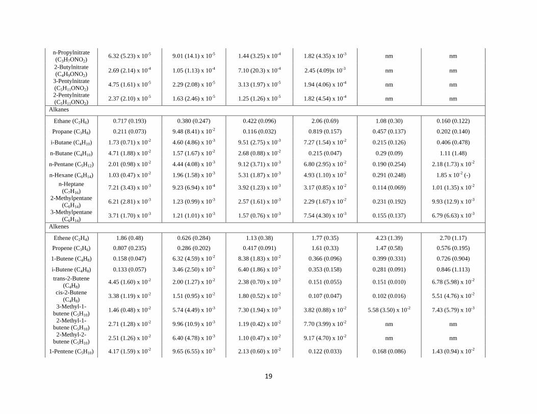
19

n-Propylnitrate (C3H7ONO2)

6.32 (5.23) x 10-5 9.01 (14.1) x 10-5 1.44 (3.25) x 10-4 1.82 (4.35) x 10-3 nm nm

2-Butylnitrate (C4H9ONO2)

2.69 (2.14) x 10-4 1.05 (1.13) x 10-4 7.10 (20.3) x 10-4 2.45 (4.09)x 10-3 nm nm

3-Pentylnitrate (C5H11ONO2)

4.75 (1.61) x 10-5 2.29 (2.08) x 10-5 3.13 (1.97) x 10-5 1.94 (4.06) x 10-4 nm nm

2-Pentylnitrate (C5H11ONO2)

2.37 (2.10) x 10-5 1.63 (2.46) x 10-5 1.25 (1.26) x 10-5 1.82 (4.54) x 10-4 nm nm

Alkanes

Ethane (C2H6) 0.717 (0.193) 0.380 (0.247) 0.422 (0.096) 2.06 (0.69) 1.08 (0.30) 0.160 (0.122)

Propane (C3H8) 0.211 (0.073) 9.48 (8.41) x 10-2 0.116 (0.032) 0.819 (0.157) 0.457 (0.137) 0.202 (0.140)

i-Butane (C4H10) 1.73 (0.71) x 10-2 4.60 (4.86) x 10-3 9.51 (2.75) x 10-3 7.27 (1.54) x 10-2 0.215 (0.126) 0.406 (0.478)

n-Butane (C4H10) 4.71 (1.88) x 10-2 1.57 (1.67) x 10-2 2.68 (0.88) x 10-2 0.215 (0.047) 0.29 (0.09) 1.11 (1.48)

n-Pentane (C5H12) 2.01 (0.98) x 10-2 4.44 (4.08) x 10-3 9.12 (3.71) x 10-3 6.80 (2.95) x 10-2 0.190 (0.254) 2.18 (1.73) x 10-2

n-Hexane (C6H14) 1.03 (0.47) x 10-2 1.96 (1.58) x 10-3 5.31 (1.87) x 10-3 4.93 (1.10) x 10-2 0.291 (0.248) 1.85 x 10-2 (-) n-Heptane

(C7H16) 7.21 (3.43) x 10-3 9.23 (6.94) x 10-4 3.92 (1.23) x 10-3 3.17 (0.85) x 10-2 0.114 (0.069) 1.01 (1.35) x 10-2

2-Methylpentane (C6H14)

6.21 (2.81) x 10-3 1.23 (0.99) x 10-3 2.57 (1.61) x 10-3 2.29 (1.67) x 10-2 0.231 (0.192) 9.93 (12.9) x 10-3

3-Methylpentane (C6H14)

3.71 (1.70) x 10-3 1.21 (1.01) x 10-3 1.57 (0.76) x 10-3 7.54 (4.30) x 10-3 0.155 (0.137) 6.79 (6.63) x 10-3

Alkenes

Ethene (C2H4) 1.86 (0.48) 0.626 (0.284) 1.13 (0.38) 1.77 (0.35) 4.23 (1.39) 2.70 (1.17)

Propene (C3H6) 0.807 (0.235) 0.286 (0.202) 0.417 (0.091) 1.61 (0.33) 1.47 (0.58) 0.576 (0.195)

1-Butene (C4H8) 0.158 (0.047) 6.32 (4.59) x 10-2 8.38 (1.83) x 10-2 0.366 (0.096) 0.399 (0.331) 0.726 (0.904)

i-Butene (C4H8) 0.133 (0.057) 3.46 (2.50) x 10-2 6.40 (1.86) x 10-2 0.353 (0.158) 0.281 (0.091) 0.846 (1.113) trans-2-Butene

(C4H8) 4.45 (1.60) x 10-2 2.00 (1.27) x 10-2 2.38 (0.70) x 10-2 0.151 (0.055) 0.151 (0.010) 6.78 (5.98) x 10-2

cis-2-Butene (C4H8)

3.38 (1.19) x 10-2 1.51 (0.95) x 10-2 1.80 (0.52) x 10-2 0.107 (0.047) 0.102 (0.016) 5.51 (4.76) x 10-2

3-Methyl-1-butene (C5H10)

1.46 (0.48) x 10-2 5.74 (4.49) x 10-3 7.30 (1.94) x 10-3 3.82 (0.88) x 10-2 5.58 (3.50) x 10-2 7.43 (5.79) x 10-3

2-Methyl-1-butene (C5H10)

2.71 (1.28) x 10-2 9.96 (10.9) x 10-3 1.19 (0.42) x 10-2 7.70 (3.99) x 10-2 nm nm

2-Methyl-2-butene (C5H10)

2.51 (1.26) x 10-2 6.40 (4.78) x 10-3 1.10 (0.47) x 10-2 9.17 (4.70) x 10-2 nm nm

1-Pentene (C5H10) 4.17 (1.59) x 10-2 9.65 (6.55) x 10-3 2.13 (0.60) x 10-2 0.122 (0.033) 0.168 (0.086) 1.43 (0.94) x 10-2

20

trans-2-Pentene (C5H10)

1.74 (0.65) x 10-2 8.89 (5.77) x 10-3 8.69 (2.22) x 10-3 5.14 (2.70) x 10-2 0.115 (0.035) 1.05 (0.83) x 10-2

cis-2-Pentene (C5H10)

1.00 (0.36) x 10-2 5.55 (3.62) x 10-3 4.98 (1.26) x 10-3 2.50 (1.28) x 10-2 5.14 (0.76) x 10-2 8.69 x 10-3 (-)

1-Hexene (C6H12) 6.10 (2.46) x 10-2 1.26 (0.73) x 10-2 3.09 (0.91) x 10-2 0.167 (0.050) nm nm 1,2-Propadiene

(C3H4) 3.76 (1.69) x 10-2 1.31 (0.62) x 10-2 2.32 (0.86) x 10-2 1.80 (0.923) x 10-2 7.15 (6.76) x 10-2 2.33 (1.07) x 10-2

1,2-Butadiene (C4H6)

5.54 (1.68) x 10-3 2.82 (1.81) x 10-3 3.10 (1.06) x 10-3 4.33 (1.59) x 10-3 nm nm

1,3-Butadiene (C4H6)

0.203 (0.071) 7.44 (3.99) x 10-2 0.108 (0.061) 0.263 (0.082) 0.409 (0.306) 0.204 (0.144)

Isoprene (C5H8) 8.94 (5.80) x 10-2 1.98 (1.48) x 10-2 3.03 (2.39) x 10-2 0.188 (0.143) 0.325 (0.443) 4.16 (2.23) x 10-2 1,3-Pentadiene

(C5H8) 1.96 (1.05) x 10-2 9.17 (4.79) x 10-3 9.39 (6.43) x 10-3 5.66 (2.94) x 10-2 nm nm

Alkynes

Ethyne 1.13 (0.42) 0.467 (0.160) 0.890 (0.323) 0.325 (0.238) 0.593 (0.443) 0.764 (0.363) 1-Propyne 9.42 (3.46) x 10-2 3.82 (1.76) x 10-2 5.99 (2.22) x 10-2 5.20 (2.83) x 10-2 nm nm

1-Buten-3-yne (C4H4)

5.04 (1.72) x 10-2 1.86 (0.90) x 10-2 3.46 (1.53) x 10-2 1.74 (1.26) x 10-2 nm nm

1-Butyne (C4H6) 7.72 (2.29) x 10-3 4.07 (2.24) x 10-3 4.48 (1.41) x 10-3 5.97 (1.93) x 10-3 2.29 (1.38) x 10-2 1.28 (0.47) x 10-2

2-Butyne (C4H6) 4.31 (1.15) x 10-3 2.55 (1.44) x 10-3 2.47 (0.70) x 10-3 4.52 (1.40) x 10-3 1.86 (0.91) x 10-2 1.02 (0.66) x 10-2 1,3-Butadyne

(C4H2) 6.07 (2.66) x 10-3 2.71 (1.21) x 10-3 5.43 (2.01) x 10-3 1.53 (1.31) x 10-3 nm nm

Aromatics

Benzene (C6H6) 1.03 (0.33) 0.373 (0.149) 0.723 (0.218) 0.769 (0.175) 1.96 (0.45) 1.05 (0.19)

Toluene (C7H8) 0.483 (0.273) 0.221 (0.085) 0.297 (0.077) 0.860 (0.167) 1.26 (0.05) 0.241 (0.160) Ethylbenzene

(C8H10) 3.41 (0.791) x 10-2 1.25 (1.20) x 10-2 1.97 (0.40) x 10-2 9.78 (1.66) x 10-2 0.366 (0.085) 4.19 (4.25) x 10-2

m/p-Xylene (C8H10)

6.36 (1.26) x 10-2 2.78 (1.56) x 10-2 4.03 (0.98) x 10-2 0.148 (0.030) 0.601 (0.294) 9.57 (7.99) x 10-2

o-Xylene (C8H10) 2.38 (0.76) x 10-2 8.37 (5.78) x 10-3 1.44 (0.41) x 10-2 7.96 (1.91) x 10-2 0.228 (0.083) 3.93 (4.31) x 10-2

Styrene (C8H8) 5.88 (1.58) x 10-2 2.28 (1.50) x 10-2 3.40 (1.90) x 10-2 8.63 (5.96) x 10-2 0.255 (0.091) 8.71 (6.69) x 10-2 i-Propylbenzene

(C9H12) 2.91 (0.77) x 10-3 1.20 (1.11) x 10-3 1.69 (0.45) x 10-3 9.30 (4.90) x 10-3 1.87 (1.40) x 10-2 1.70 (1.67) x 10-2

n-Propylbenzene (C9H12)

6.48 (2.59) x 10-3 1.84 (1.65) x 10-3 4.02 (1.59) x 10-3 3.95 (2.69) x 10-2 3.10 (1.45) x 10-2 1.78 (1.58) x 10-2

3-Ethyltoluene (C9H12)

1.44 (0.48)x 10-2 5.46 (4.40) x 10-3 8.59 (3.26) x 10-3 7.14 (4.13) x 10-2 5.61 (2.38) x 10-2 2.62 (0.54) x 10-2

21

4-Ethyltoluene (C9H12)

6.35 (2.36) x 10-3 2.54 (1.81) x 10-3 4.18 (1.96) x 10-3 3.71 (2.30) x 10-2 3.57 (1.74) x 10-2 2.07 (1.19) x 10-2

2-Ethyltoluene (C9H12)

6.89 (2.50) x 10-3 2.70 (1.68) x 10-3 4.63 (2.07) x 10-3 3.76 (2.69) x 10-2 3.39 (1.34) x 10-2 2.10 (1.16) x 10-2

1,3,5-Trimethylbenzene

(C9H12) 3.87 (1.71) x 10-3 1.63 (1.22) x 10-3 2.65 (1.43) x 10-3 2.23 (1.60) x 10-2 1.79 (0.83) x 10-2 2.14 x 10-2 (-)

1,2,4-Trimethylbenzene

(C9H12) 1.04 (0.46) x 10-2 4.25 (2.69) x 10-3 7.52 (4.28) x 10-3 6.23 (5.18) x 10-2 3.91 (1.65) x 10-2 1.74 (2.35) x 10-2

1,2,3-Trimethylbenzene

(C9H12) 4.76 (2.59) x 10-3 1.16 (0.81) x 10-3 3.84 (2.69) x 10-3 3.01 (3.16) x 10-2 2.34 (0.43) x 10-2 2.16 x 10-2 (-)

Terpenes alpha-Pinene

(C10H16) 8.30 (5.40) x 10-4 5.38 (6.94) x 10-4 7.82 (6.32) x 10-4 2.26 (2.53) x 10-3 0.35 (0.49) 2.02 (2.33) x 10-2

beta-Pinene (C10H16)

2.27 (1.49) x 10-3 1.37 (0.91) x 10-3 2.76 (3.15) x 10-3 2.89 (3.56) x 10-3 0.471 (-) 4.67 x 10-2 (-)

Oxygenates Acetaldehyde

(C2H4O) 0.805 (0.279) 0.334 (0.199) 0.447 (0.119) 1.70 (0.75) 1.88 (1.63) 0.541 (0.362)

Butanal (C4H8O) 4.28 (1.50) x 10-2 1.90 (1.29) x 10-2 2.68 (1.05) x 10-2 0.108 (0.047) 5.40 (2.19) x 10-2 8.28 (6.27) x 10-3

Acetone (C3H6O) 0.705 (0.219) 0.365 (0.226) 0.416 (0.108) 2.05 (0.52) 1.63 (0.38) 0.524 (0.256) 2-Butanone

(C4H8O) 0.172 (0.057) 8.00 (6.18) x 10-2 0.103 (0.038) 0.498 (0.151) 0.262 (0.109) 0.232 (0.286)

2-Propenal (C3H4O) 0.186 (0.060) 0.127 (0.069) 0.127 (0.059) 0.295 (0.245) nm nm

MVK (C4H6O) 0.129 (0.040) 6.59 (4.56) x 10-2 6.31 (2.76) x 10-2 0.280 (0.147) nm nm

Furan (C4H4O) 0.109 (0.041) 5.98 (3.37) x 10-2 6.81 (2.19) x 10-2 0.379 (0.093) 0.534 (0.209) 0.241 (0.024) 2-Methylfuran

(C5H6O) 0.117 (0.051) 5.92 (4.77) x 10-2 6.92 (2.83) x 10-2 0.488 (0.227) nm nm

Furfural (C5H4O2) 8.55 (6.05) x 10-2 4.28 (5.51) x 10-2 8.22 (5.09) x 10-2 0.316 (0.133) nm nm Methanol (CH3OH) 2.09 (1.14) 2.03 (2.01) 1.18 (0.40) 4.23 (3.40) 2.38 (0.90) 1.92 (0.61)

Ethanol (CH5OH) 4.08 (5.93) x 10-2 2.18 (2.00) x 10-2 5.63 (6.69) x 10-2 7.62 (9.08) x 10-2 0.563 (0.589) 0.128 (0.017) *From Jayarathne et al. (2017), but part of same NAMaSTE study nm indicates the species was not measured (-) from Stockwell et al. (2016) indicates that the measurement was not above background.

22

Table 2. Emission factors (g VOC/ kg fuel C) for select compounds. The mean differences between dung/angithi and dung/chulha are shown and similarly for dung/chulha and brushwood/chulha. The significance between fuel or stove and EF is indicated with asterisks. Accompanying the mean differences is the average emission factor (g VOC/ kg fuel C) for dung cook fires and chulha cook fires, as well as the overall average for all performed cook fires. Compound Average EF

for all cook fires (g/ kg fuel C)

Angithi-chulha average EF difference (g/ kg fuel C)

Average EF for dung fires (g/ kg fuel C)

Dung-brushwood average EF difference (g/ kg fuel C)

Average EF for chulha cook fires (g/ kg fuel C)

Ethane 2.47 (2.16) 4.18*** 3.70 (2.43) 1.19*** 1.60 (0.744) Propane 0.827 (0.866) 1.88*** 1.32 (0.976) 0.397*** 0.448 (0.256) n-Butane 0.200 (0.236) 0.52*** 0.331 (0.271) 0.0568*** 0.097 (0.063)

Ethene 4.17 (2.02) N/A 5.64 (1.32) 4.05*** 3.88 (2.07)

Propene 2.24 (1.61) 2.50*** 3.38 (1.48) 1.72*** 1.63 (0.93)

1-Butene 0.473 (0.373) 0.644*** 0.718 (0.377) 0.213*** 0.327 (0.180)

Ethyne 2.32 (1.41) -2.46*** 2.58 (1.63) 2.21*** 2.61 (1.37)

1-Propye 0.196 (0.108) -0.129** 0.244 (0.116) 0.187*** 0.204 (0.112)

1-Butyne 1.74 x 10-2 (7.74 x 10-3)

-0.101*** 0.219 (0.007) 0.105*** 0.017 (0.008)

* denotes p<0.05, ** p<0.01, *** p<0.001

1

Supporting Information Emissions from village cookstoves in Haryana, India and their potential impacts on air quality Lauren T. Fleming,1 Robert Weltman,2 Ankit Yadav,3 Rufus D. Edwards,2 Narendra K. Arora,3Ajay Pillarisetti,4 Simone Meinardi,1 Kirk R. Smith,4 Donald R. Blake,1 and Sergey A. Nizkorodov1,* 1Department of Chemistry, University of California, Irvine, CA 92697, USA 2Department of Epidemiology, University of California, Irvine, CA 92697, USA 3The Inclen Trust, Okhla Industrial Area, Phase-I, New Delhi-110020, India 4School of Public Health, University of California, Berkeley, CA 94720, USA

Correspondence to: Sergey Nizkorodov (nizkorod@uci.edu)

2

Table S1. Average emission factors and standard deviation of PM2.5 and gas-phase species (g kg-1 dry fuel carbon) for dung-chulha, brushwood-chulha, mixed-chulha, and dung-angithi cook fires. Sample size (n) was n=12 for dung-chulha, n=14 for brushwood-chulha, n=13 for mixed-chulha, n=10 for dung-angithi. SOAP values, kOH, and MIR values used to calculate predicted SOAP-weighted potentials, OH reactivity, and ozone-forming potential are included for the quantified species. SOAP values were taken from Derwent et al. (2010), kOH were found in the NIST Chemical Kinetics Database, and MIR values are found in Carter et al. 1994.

Compound Dung-chulha Average (SD)

Brushwood-chulha Average (SD)

Mixed-chulha Average (SD)

Dung-angithi Average (SD)

SOAP kOH (x 1012) (cm3 molec -1 s-1)

MIR (g O3/ g VOC)

Carbon dioxide (CO2) 3028 (80) 3365 (148) 3171 (83) 2745 (144) 0a 0 0

Carbon monoxide (CO) 301 (33) 143 (78) 243 (47) 385 (61) 0a 0.15 0.056

Methane (CH4) 21.3 (4.0) 12.9 (5.4) 15.8 (2.7) 46.7 (8.2) 0a 0.006 0.0144

Sulfur-containing

Carbonyl sulfide (OCS) 0.382 (0.135) 3.89 (1.36) x 10-2 0.279 (0.083) 1.09 (0.67) 0a 0.002 0

DMS (C2H6S) 2.98 (1.55) x 10-2 3.68 (3.36) x 10-3 1.57 (0.74) x 10-2 0.134 (0.096) 0a 5.4 0

Halogen-containing Dichloromethane (CH2Cl2)

1.37 (1.48) x10-3 5.79 (8.21) x 10-4 1.35 (2.20) x 10-3 1.41 (0.85) x 10-3 0a 0.123 0.041

Chloromethane (CH3Cl) 5.48 (2.41) 0.751 (0.393) 3.34 (1.37) 14.2 (5.8) 0a 0.369 0.038

Bromomethane (CH3Br) 2.02 (0.96) x 10-2 2.14 (0.57) x 10-3 1.42 (0.59) x 10-2 4.42 (1.75) x 10-2 0a 0.0288 0.0187

Iodomethane (CH3I) 1.88 (0.40) x 10-3 2.61 (0.61) x 10-4 7.87 (2.08) x 10-4 2.73 (0.51) x 10-3 0a 0.0723 -0.56

Ethyl chloride (C2H5Cl) 7.83 (3.93) x 10-3 1.13 (0.95) x 10-3 5.23 (2.25) x 10-3 2.82 (1.08) x 10-2 0a 0.423 0.29 Dichloroethane (C2H4Cl2)

2.71 (1.00) x 10-3 6.86 (5.78) x 10-4 4.04 (7.92) x 10-3 4.55 (2.82) x 10-3 0a 0.023 0.21

Nitrates Methyl nitrate (CH3ONO2)

5.62 (19.5) x 10-3 1.47 (4.00) x 10-2 2.19 (3.95) x 10-2 0.527 (1.048) 0a 0.023 0

Ethyl nitrate (CH3ONO2)

7.27 (14.5) x 10-4 1.50 (2.80) x 10-3 7.63 (21.77) x 10-3 0.140 (0.357) 0a 0.178 0

i-Propylnitrate (C3H7ONO2)

5.85 (5.66) x 10-4 6.57 (13.64) x 10-4 1.37 (2.86) x 10-3 1.83 (3.75) x 10-2 0a 0.287 0

n-Propylnitrate (C3H7ONO2)

1.94 (1.82) x 10-4 2.43 (3.83) x 10-4 4.81 (11.05) x 10-4 5.63 (13.44) x 10-3 0a 0.731 0

2-Butylnitrate (C4H9ONO2)

8.27 (7.41) x 10-4 2.82 (3.07) x 10-4 2.39 (6.92) x 10-3 7.57 (15.15) x 10-3 0a 0.93 0

3-Pentylnitrate (C5H11ONO2)

1.46 (0.49) x 10-4 6.15 (5.54) x 10-5 1.02 (0.62) x 10-4 6.01 (12.55) x 10-4 0a 1 0

2-Pentylnitrate (C5H11ONO2)

7.27 (4.52) x 10-5 4.41 (6.71) x 10-5 4.05 (4.04) x 10-5 5.61 (14.00) x 10-4 0a 1 0

Alkanes

Ethane (C2H6) 2.21 (0.60) 1.02 (0.64) 1.38 (0.30) 6.38 (2.14) 0.1 0.244 0.28

3

Propane (C3H8) 0.650 (0.219) 0.253 (0.211) 0.378 (0.106) 2.53 (0.49) 0 1.1 0.49

i-Butane (C4H10) 5.31 (2.14) x 10-2 1.23 (1.22) x 10-2 3.12 (0.92) x 10-2 0.225 (0.048) 0 2.12 1.23

n-Butane (C4H10) 0.145 (0.058) 4.20 (4.22) x 10-2 8.83 (3.06) x 10-2 0.665 (0.148) 0.3 2.4 1.15

n-Pentane (C5H12) 6.18 (2.46) x 10-2 1.19 (1.03) x 10-2 2.99 (1.24) x 10-2 0.210 (0.091) 0.3 3.8 1.31

n-Hexane (C6H14) 3.16 (1.30) x 10-2 5.25 (4.05) x 10-3 1.74 (0.63) x 10-2 0.153 (0.034) 0.1 5.2 1.24

n-Heptane (C7H16) 2.22 (1.02) x 10-2 2.49 (1.86) x 10-3 1.29 (0.41) x 10-2 9.79 (2.63) x 10-2 0.1 6.8 1.07 2-Methylpentane (C6H14)

1.91 (0.75) x 10-2 3.28 (2.51) x 10-3 8.44 (5.36) x 10-3 7.07 (5.18) x 10-2 0 5.2 1.5

3-Methylpentane (C6H14)

1.14 (0.53) x 10-2 3.23 (2.64) x 10-3 5.12 (2.44) x 10-3 2.33 (1.33) x 10-2 0.2 5.2 1.8

Alkenes

Ethene (C2H4) 5.73 (1.36) 1.68 (0.73) 3.68 (1.15) 5.47 (1.09) 1.3 8.51 9

Propene (C3H6) 2.48 (0.60) 0.765 (0.506) 1.36 (0.28) 4.98 (1.04) 1.6 30.1 11.66

1-Butene (C4H8) 0.488 (0.140) 0.169 (0.115) 0.274 (0.058) 1.13 (0.30) 1.2 31 9.73

i-Butene (C4H8) 0.411 (0.125) 9.25 (6.25) x 10-2 0.209 (0.060) 1.09 (0.49) 0.6 51 1.23

trans-2-Butene (C4H8) 0.137 (0.047) 5.36 (3.30) x 10-2 7.79 (2.22) x 10-2 0.466 (0.170) 4.0 64 15.16

cis-2-Butene (C4H8) 0.104 (0.037) 4.04 (2.45) x 10-2 5.88 (1.69) x 10-2 0.331 (0.145) 3.6 56 14.24 3-Methyl-1-butene (C5H10)

4.50 (1.44) x 10-2 1.53 (1.13) x 10-2 2.39 (0.62) x 10-2 0.118 (0.027) 0.6 32 6.99

2-Methyl-1-butene (C5H10)

8.33 (2.97) x 10-2 2.65 (2.72) x 10-2 3.92 (1.38) x 10-2 0.238 (0.124) 0.9 61 6.4

2-Methyl-2-butene (C5H10)

7.72 (3.14) x 10-2 1.71 (1.24) x 10-2 3.61 (1.53) x 10-2 0.284 (0.146) 1.9 87 14.08

1-Pentene (C5H10) 0.128 (0.048) 2.58 (1.64) x 10-2 6.99 (1.98) x 10-2 0.378 (0.102) 0 27.4 7.21

trans-2-Pentene (C5H10) 5.34 (1.68) x 10-2 2.38 (1.49) x 10-2 7.79 (2.22) x 10-2 0.159 (0.064) 3.1 67 10.56

cis-2-Pentene (C5H10) 3.08 (0.90) x 10-2 1.49 (0.94) x 10-2 5.88 (1.69) x 10-2 7.72 (3.98) x 10-2 3.1 65 10.38

1-Hexene (C6H12) 0.188 (0.072) 3.38 (1.83) x 10-2 0.101 (0.030) 0.517 (0.157) 0 37 5.49

1,2-Propadiene (C3H4) 0.116 (0.033) 3.51 (1.57) x 10-2 7.55 (2.72) x 10-2 5.56 (2.84) x 10-2 1.8b 0.45 8.45

1,2-Butadiene (C4H6) 1.70 (0.48) x 10-2 7.54 (4.69) x 10-3 1.01 (0.33) x 10-2 1.34 (0.49) x 10-2 1.8b 27 9.35

1,3-Butadiene (C4H6) 0.626 (0.221) 0.201 (0.105) 0.352 (0.195) 0.813 (0.254) 1.8 67 12.61

Isoprene (C5H8) 0.275 (0.151) 5.31 (3.88) x 10-2 9.89 (7.79) x 10-2 0.582 (0.444) 1.9 100 10.61

1,3-Pentadiene (C5H8) 6.02 (3.37) x 10-2 2.47 (1.26) x 10-2 3.08 (2.11) x 10-2 0.175 (0.091) 1.8c 117 12.5

Alkynes

Ethyne (C2H2) 3.46 (1.21) 1.25 (0.39) 2.89 (1.00) 1.01 (0.74) 0.1 0.9 0.95

1-Propyne (C3H4) 0.290 (0.084) 0.103 (0.045) 0.195 (0.070) 0.161 (0.087) 0a 3.1 6.72

4

1-Buten-3-yne (C4H4) 0.155 (0.048) 5.01 (2.27) x 10-2 0.113 (0.048) 5.37 (3.87) x 10-2 0a 20 10.48

1-Butyne (C4H6) 2.37 (0.69) x 10-2 1.09 (0.57) x 10-2 1.46 (0.44) x 10-2 1.85 (0.60) x 10-2 0a 8 6.11

2-Butyne (C4H6) 1.33 (0.48) x 10-2 6.84 (3.70) x 10-3 8.06 (2.13) x 10-3 1.40 (0.44) x 10-2 0a 8 16.32

1,3-Butadyne (C4H2) 1.87 (0.75) x 10-2 7.27 (3.00) x 10-3 1.77 (0.62) x 10-2 4.74 (4.07) x 10-3 0a 16 5.76

Aromatics

Benzene (C6H6) 3.18 (1.09) 1.00 (0.37) 2.36 (0.68) 2.38 (0.55) 92.9 1.2 0.72

Toluene (C7H8) 1.49 (1.03) 0.597 (0.218) 0.972 (0.250) 2.66 (0.52) 100.0 6.2 4

Ethylbenzene (C8H10) 0.105 (0.027) 3.34 (3.03) x 10-2 6.43 (1.20) x 10-2 0.303 (0.052) 111.6 7.5 3.04

m/p-Xylene (C8H10) 0.196 (0.044) 7.45 (3.89) x 10-2 0.131 (0.030) 0.458 (0.093) 75.8 19 2.51

o-Xylene (C8H10) 7.31 (2.44) x 10-2 2.24 (1.46) x 10-2 4.68 (1.21) x 10-2 0.246 (0.060) 95.5 14 2.51

Styrene (C8H8) 5.88 (1.81) x 10-2 2.28 (1.50) x 10-2 3.40 (1.90) x 10-2 8.64 (5.96) x 10-2 212.3 43 1.53

i-Propylbenzene (C9H12) 8.97 (2.73) x 10-3 3.21 (2.78) x 10-3 5.51 (1.31) x 10-3 2.88 (1.51) x 10-2 95.5 6.6 6.23 n-Propylbenzene (C9H12)

2.00 (0.87) x 10-2 4.90 (4.14) x 10-3 1.30 (0.47) x 10-2 0.122 (0.083) 109.7 5.7 6.23

3-Ethyltoluene (C9H12) 4.44 (1.67) x 10-2 1.46 (1.14) x 10-2 2.79 (0.98) x 10-2 0.221 (0.128) 94.8 22.4 7.39

4-Ethyltoluene (C9H12) 1.96 (0.79) x 10-2 6.78 (4.65) x 10-3 1.35 (0.59) x 10-2 0.115 (0.071) 69.7 13.6 4.44

2-Ethyltoluene (C9H12) 2.12 (0.87) x 10-2 7.22 (4.33) x 10-3 1.50 (0.62) x 10-2 0.116 (0.083) 94.8 13.2 5.59 1,3,5-Trimethylbenzene (C9H12)

1.19 (0.55) x 10-2 4.37 (3.18) x 10-3 8.59 (4.28) x 10-3 6.89 (4.93) x 10-2 13.5 60 11.76

1,2,4-Trimethylbenzene (C9H12)

3.22 (1.59) x 10-2 1.14 (0.70) x 10-2 2.43 (1.28) x 10-2 0.193 (0.160) 20.6 32 8.87

1,2,3-Trimethylbenzene (C9H12)

1.47 (0.78) x 10-2 3.11 (2.08) x 10-3 1.24 (0.82) x 10-2 9.30 (9.75) x 10-2 43.9 29 11.97

Terpenes

alpha-Pinene (C10H16) 2.55 (1.92) x 10-3 1.44 (1.81) x 10-3 2.54 (2.08) x 10-3 6.97 (7.78) x 10-3 17.4 52 4.51

beta-Pinene (C10H16) 6.98 (5.20) x 10-3 3.69 (2.46) x 10-3 8.98 (10.14) x 10-3 8.93 (10.96) x 10-3 18.1 74 3.52

Oxygenates

Acetaldehyde (C2H4O) 2.48 (0.92) 0.897 (0.520) 1.46 (0.38) 5.26 (2.34) 0.6 16 6.54

Butanal (C4H8O) 0.132 (0.047) 5.09 (3.32) x 10-2 8.77 (3.50) x 10-2 0.334 (0.145) 0 24 5.97

Acetone (C3H6O) 2.17 (0.69) 0.977 (0.584) 1.36 (0.35) 6.34 (1.63) 0.3 0.19 0.36

2-Butanone (C4H8O) 0.530 (0.183) 0.214 (0.161) 0.338 (0.130) 1.54 (0.47) 0.6 1.2 1.48

2-Propenal (C3H4O) 0.573 (0.202) 0.342 (0.177) 0.414 (0.192) 0.914 (0.761) 1.0a 20 7.45

MVK (C4H6O) 0.396 (0.121) 0.176 (0.117) 0.205 (0.087) 0.865 (0.458) 1.0a 19 9.65

Furan (C4H4O) 0.336 (0.141) 0.160 (0.086) 0.223 (0.072) 1.17 (0.29) 1.0a 40 9.15

5

2-Methylfuran (C5H6O) 0.360 (0.177) 0.158 (0.123) 0.226 (0.093) 1.51 (0.70) 1.0a 62 8.3

Furfural (C5H4O2) 0.263 (0.218) 0.113 (0.143) 0.265 (0.161) 0.981 (0.414) 1.0a 35 10

Methanol (CH3OH) 6.43 (3.77) 5.38 (5.20) 3.84 (1.26) 13.1 (10.6) 0.3 0.9 0.67

Ethanol (CH5OH) 0.126 (0.220) 5.80 (5.19) x 10-2 0.184 (0.220) 0.236 (0.281) 0.6 3.4 1.53 agiven values of either 0 or 1, SOAP values not reported bvalues based on 1,3-butadiene cvalue based on (E)-1,3-Pentadiene

6

Table S2. Summary of aromatic compounds, oxygenates, halogen- and sulfur- containing compounds that do not have higher emissions when using angithi stove and/or dung fuel. Significant relationships between emissions and either stove or fuel are indicated by marking the type that gives the larger emissions. N/A indicates no relationship was found. P values are listed in addition to the fuel or stove type if the relationship is not clear.

Compound Stove Fuel Benzene Chulha Dung Styrene Angithi

(p=0.0723) Dung

Acrolein Angithi (p=0.0787)

Dung

Methanol Angithi N/A Ethanol N/A N/A Furfural Angithi Dung (p=

0.03) Dichloromethane N/A N/A 1,2-dichloroethane Angithi N/A Iodomethane Angithi

(p=0.0891) Dung

7

Figure S1. Emission factors (g VOC/ kg fuel C) versus moisture content of the fuel. Red markers indicate dung fuel was used, while blue markers indicate brushwood fuel. Filled square markers indicate chulha stoves, while open circles indicate angithi stoves were used. If a significant correlation was observed (r2> 0.70) for a particular fuel-stove combination, the linear regression trendline is shown.

8

Figure S2.1 Comparison of EFs (g/ kg dry fuel) in the present study to those of Stockwell et al., 2016. The blue line indicates 1:1 agreement of the emission factors, with points above the blue line indicating higher EFs reported in Stockwell et al., 2016. Likewise, points below represent compounds that have a higher EF in the present study.

9

Figure S2.2 Emission factors (g/ kg fuel C) plotted as a function of modified combustion efficiency for select species. Open circles indicate cooking events conducted with angithi stoves, whereas filled squares indicate chulha stoves. Color indicates fuel, either brushwood (blue), dung (red), or mixed (purple). Crosses indicate measurements from Stockwell et al. 2016.