Please see below a response to the reviewer and editor comments on our paper, followed by a

“track-changes” version compared with that originally submitted. We thank both reviewers and

the editor for their constructive comments, which have improved the paper.

Reviewer 1:

An important contribution and the most novel part of this work, is the simulations in which both a NH meltwater source and changes in the

WAIS are simulated. Currently this topic is only introduced in the very last line of the introduction and the simulations are not even

mentioned in the conclusions. I think this part of the manuscript should be discussed more comprehensively in the introduction, including

previous work (e.g. Goelzer et al, 2016, Steig et al., 2015) and indications that such a WAIS collapse has occurred during or previous to the

LIG. In the conclusions question could be addressed such as ’What did the WAIS simulations tell us?’, or ’How should future simulations on

this topic be improved in order to better address the issues discussed in the manuscript’? References: Goelzer et al., 2016: doi:10.5194/cp-

2015-175, 2016

Added to the conclusions: “Conversely, removing the WAIS in the simulations does not improve the

model-data comparison in East Antarctica or the Southern Ocean. However, the lack of data

coverage does not allow us to draw conclusions regarding the configuration of the LIG WAIS. ”.

Added to the Abstract: “. Further simulations in which the West Antarctic ice sheet is also removed

lead to warming in East Antarctica and the Southern Ocean but do not appreciably improve the

model-data comparison”. Note that the WAIS simulations are not the main focus of the paper, but

we do think it is important to report them, to guide future workers in this field, even though we can

draw no strong conclusions from them. In introduction: “We further perform an idealized

simulation with the WAIS removed to test whether this has any additional influence on regional

warming in our model framework, as recent work has indicated that some of the warmth seen in

Antarctic ice core records during the LIG could partly be explained by a reduced West Antarctic ice

sheet (Steig et al, 2015)”. Also in results: “Indeed, a recent study has suggested that the water

isotopic data from the Mount Moulton ice core drilled in West Antarctica compared with water

isotopic profiles from East Antarctic ice cores, is consistent with a collapse of the WAIS during the

LIG (Steig et al., 2015). This potential melting of the WAIS during the early LIG could explain or

partially explain the mismatch between the model simulations and Southern Ocean/East Antarctic

data timeslices at 130 ka”

Page 1 line 17: As discussed in the manuscript, a number of previous studies used a model-data approach to investigate the impact of

Northern Hemisphere freshwater forcing on the early LIG climate, so perhaps ’for the first time’ is a little too strong, although this study is

certainly more thorough and presents, as is mentioned, a more ’integrated model-data approach’.

We have modified the text to: “This integrated model-data approach, the most thorough to date,

provides evidence that Northern Hemisphere freshwater forcing is an important player in the

evolution of early Last Interglacial climate.”

Page 1 line 22: If the LIG is from 129-116ka, can one still consider 130ka as early LIG? Perhaps a technical detail, but on the other hand a

good illustration of the broader issue that defining deglacial and interglacial periods is not trivial and perhaps not even desirable.

Yes, 130 ka can be considered as early LIG since, as pointed out by the reviewer, it is not trivial to define interglacials. The interval “129-116 ka” we provided in the submitted manuscript at the beginning of our text is based on eustatic sea level variations using the 0 m sea level value as used in the last IPCC assessment report (Masson-Delmotte et al. 2013). However, if we were to define the LIG considering an alternative way such as the one considering the ice core dD 403‰ threshold value, it would give a date of about ~132 ka (based on the AICC2012 chronology, Bazin et al. 2012). In their recent paper, Govin et al. (2015) clearly illustrate how the timing of the beginning of the LIG varies widely depending on the climatic archives and tracers that are considered. A thorough discussion on this topic is also provided in the Past Interglacials Working Group of PAGES, 2016). Still, we think it is necessary to give at the start of the paper an indication of the age interval for the LIG, and as such write in the revised manuscript: “Peak high latitude temperatures were several

degrees warmer during the Last Interglacial (LIG, approximately 129-116 thousand years ago, ka, based on eustatic sea level variations, Masson-Delmotte et al. 2013) (Clark and Huybers, 2009; Masson-Delmotte et al., 2011; Otto-Bliesner et al., 2006; Sime et al., 2009; Turney and Jones, 2010).” We also add at the beginning of Section 2: “The LIG starts at 129 ka when using a definition based on the eustatic sea level (Masson-Delmotte et al. 2013); however, considering dating uncertainties associated with paleoclimatic records during this time interval (see Govin et al. 2015 for a review), and the fact that defining the boundaries of interglacial periods is not trivial (see discussion in the PIGS Working Group of PAGES, 2016), we consider our 130 ka simulations as representative of the “early LIG”.

Page 2 line 14: What is meant with ’partially account for changes in seasonality of precipitation’? Do the uncertainty estimates account for

this or can part of the ice core oxygen isotope changes be accounted for by changes in the seasonality of precipitation?

We apologize if the sentence in the original manuscript was unclear. Precipitation intermittency, changes in moisture origin as well as site elevation and ice origin changes (e.g. Jouzel et al., 2003; Stenni et al., 2010) probably affect the quantified temperature changes reconstructed based on ice core water isotopic records. Here, the Antarctic temperature reconstructions provided in the 130 ka data based time slice and which are the ones published in Masson-Delmotte et al. (2011) are based on the present day spatial relationship between the ice isotopic composition of the snow and surface temperature (“isotopic thermometer”) after correction for sea water isotopic composition and moisture source correction taking into account deuterium excess data. An uncertainty of about 1°C can be associated to these reconstructions. However, these reconstructions are considered as annual means while in principle they reflect precipitation-weighted temperatures. Bias due to possible changes in the seasonality of precipitation cannot be quantified in ice core data but in order to account at least partially for them, we consider an overall uncertainty of 1.5°C for the Antarctic temperature reconstructions included in the 130 ka data time slice. We have now slightly reorganized the paragraph and we have rephrased the sentence in the revised manuscript, we hope this is clearer now: “(see Capron et al. (2014) for methodological details and 2σ uncertainty estimates for individual records). Note that Antarctic annual surface air temperature reconstructions are estimated based on the water isotopic records after correction for sea water isotopic composition and moisture source correction using deuterium excess data (Masson-Delmotte et al. 2011). Capron et al. 2014 consider an error of 1.5°C associated with these reconstructions. It accounts for the uncertainty associated with this method and also partially accounts for the uncertainty associated with possible impacts of changes in seasonality of precipitation on the reconstructions, which remains difficult to quantify in ice core data (Masson-Delmotte et al. 2011).”

Page 3 lines 7-9: It is mentioned that Loutre et al. (2014) already performed a model-data comparison including NH freshwater fluxes for

the early LIG, but that their work still showed model-data mismatches. Doesn’t the present work still show these? Perhaps they became

smaller? Or we have a better understanding of why these mismatches occur?

We agree that the present work does show the mismatches highlighted in Loutre et al. (2014). It is

difficult to determine if these mismatches are smaller overall or not as Loutre et al (2014) only

compared with a set of surface temperature timeseries from only 12 locations while we are looking

at a time slice averaged over 2ka and centred on 130 ka .

Page 3 lines 16-19: Both Bakker et al. (2013) and Loutre et al. (2014) included a model-data comparison, be it small and less rigorous than

the one presented here. Another such model-data comparison for this time interval was performed by SanchezGoni et al. (2012).

Bakker et al. (2013) only included a model inter-comparison. No comparisons were made with data.

Loutre et al. (2014) do not shown a comparison with the data sets in the Southern Hemisphere given

in Capron et al. (2014). Sanchez-Goni et al (2012) only compare with one record from the North

Atlantic. We have, however, included the Sanchez-Goni (2012) record and modified the text for

clarity: “Although previous modeling studies (e.g. Bakker et al., 2013; Holden et al., 2010; Loutre et

al., 2014; Sanchez-Goni et al., 2012) have looked at the impact of freshwater forcing on early LIG

climate they did not link the response with the data reconstructions in the high latitude regions of

the Northern and Southern Hemispheres…”

Introduction: The recent work by Goelzer et al. (2016) should be discussed as well since it is closely related to the questions that are

addressed in this manuscript.

See response to Editor’s comment.

Experimental design: Discuss some aspects of the experimental design in a little more detail: Are 200 year simulations are sufficiently long

to investigate a bi-polar seesaw response? Hosing a large region between 50-70N seems highly idealized. What do we know about the

distribution of meltwater during that period and what difference could it make to include a more realistic meltwater scheme? Meltwater

from the WAIS is neglected. Why and how could this impact the results?

Added “To test the robustness of the results to the 200-yer simulation length, we extended the 130

ka simulation with 0.2 Sv of freshwater forcing for a further 200 model years (400 years in total). In

the Southern Ocean the rate of change of summer-SST with time is very small, and the difference

between the 50-yr climate mean JFM anomaly after 200 years compared with the 50-yr climate

mean after 400 years is trivial (not shown); the difference ranges between -0.5 and 0.5˚C for the

majority of the region, which is well within the uncertainty of the data synthesis from Capron et al.

(2014) of 2.6˚C on average”. Added “Given the uncertainty around the actual location of the

freshwater flux, we prescribe an idealized hosing region”. Added “Given the uncertainty in the

location and rate of freshwater forcing associated with the WAIS removal, we do not prescribe

additional freshwater fluxes from the WAIS. ”

Page 4 lines 28-30: What about model uncertainties or inter-model differences in simulated temperature anomalies, can those explain the

model-data mismatch?

The point we are making here is that in our model, the model-data discrepancy is much too large to

be explained by uncertainties associated with the surface temperature reconstructions from the

marine and ice records (2σ of 2.6°C on average). Later in the paper we discuss the inter-model

differences.

Page 6 lines 4-16: It does not really become apparent from this paragraph that another important reason to perform simulation in which

the WAIS is removed is because this could explain the persisting SH model-data mismatch.

We agree with the reviewer and have added the following sentence: “This potential melting of the

WAIS during the early LIG could explain or partially explain the mismatch between the model

simulations and Southern Ocean/East Antarctic data timeslices at 130 ka.”

Page 6 line 18: From table 2 it appears to me that the number are identical so why is the model-data match slightly improved?

The reviewer is correct that the numbers are identical to 1 d.p. As a result we have reworded the

text.

Page 6 line 24: Why would you replace it with shrubs? Is there any indications that those would grow there during the LIG? And related to

that, why is such a big impact found between replacing it with bare ground or shrubs, I would expect that that region is covered with snow

year round?

Added “There is some uncertainty as to the extent or type of vegetation which may or may not have

grown on an unglaciated West Antarctica during the LIG, and the vegetation type replacing a

previously glaciated surface can have significant effect on the magnitude of warming (Stone and

Lunt, 2013).”. Also in Methods, added “, to test the response to uncertainty in the land-cover type

which would replace the ice sheet”

From the last paragraph of the results section and figures 4 and 6 it is not fully clear to me how SH temperatures evolved during the LIG and

how this relates to the limited NH freshwater forcing after 127ka. This scenario would suggest that after the early LIG, when the NH

freshwater returned to a low baseline, the bi-polar seesaw seized, potentially leading to cooling in the SH. Is that seen in the 125ka time-

slice of Capron et al. (2014)? If not, how could this be explained? Please discuss this very interesting topic in more detail in this paragraph

and perhaps include suggestions for future research on this topic.

The Capron et al (2014) data shows that at 125 ka, the temperatures around Antarctica are still

relatively warm, whereas the North Atlantic is no longer cold, relative to 130 ka. This is not very

surprising when looking at Figure 4, because the freshwater has a much larger cooling effect in the

Northern Hemisphere than it has warming effect in the Southern Hemisphere. Added “However, in

order to fully explore the temporal variations in temperature through the LIG, fully transient

simulations with time-evolving forcings would be required.

Table 2: The improvement of the SH and EAIS model-data match when included the NH 0.2Sv meltwater forcing is surprisingly small. What

are we missing?

This is simply related to the fact that the freshwater has a large cooling effect in the north Atlantic,

but a relatively minor warming over Antarctica itself and the Southern Ocean.

Table 2: The lowest two lines (125ka) are they also compared with the 125ka time-slice of Capron et al. (2014)? Please explain in the caption.

Yes the 125 ka experiments are also compared with Capron et al. (2014). We have added the

following text to the figure caption: “The model output is compared with the 130 ka and 125 ka time

slices from Capron et al. (2014).”

Table 2: Mention in the caption which simulations were previously published and which are newly performed for this study.

We have added the following text for clarity: “Note that the simulations without freshwater forcing

includeed were previous described in Lunt et al. (2013) and references therein.”

Figure 1: Consider including a proxy records showing the AMOC evolution during this period. For instance one of the d13C records shown

by Sanchez-Goni et al. (2012) and Govin et al. (2012).

We have added the δ13C record from the North Atlantic core CH69-K09 from Govin et al. (2012)

Figure 1: An additional vertical axis showing the rate of sea level change in Sv would be easier to compare with for instance figure 9.

Done.

Figure 1: the ’early SH warmth’ is not very clear in EDC temperatures. Please clarify.

Done. We also now state in the caption of the revised manuscript the following: “Note that Govin et al. 2015 reports in the Table 5 of their paper that the Antarctic reconstructed surface temperature (based on EDC dD) starts increasing at 135.6 ±2.5 ka based on the use of the RAMPFIT software.”

Figure 1: please include in the caption a description of the grey band shown in the figure.

Added to caption: The grey band highlights the 129-131 ka time interval that has been considered for the construction of the 130 ka data based time slice for surface temperature (see Capron et al. 2014 for details on the methodology).

Figure 3: This could perhaps also be shown in another figure that shows a map of the North Atlantic region.

We think that the region is most clearly represented in this way – adding it to the other Figures

would make them somewhat cluttered.

Figure 6: Why is the model response so different over Antarctica while it is so similar over the Southern Ocean? Is seems unrelated to the

changes in the North Atlantic. Is this difference also there at 130ka?

Note that left and right panels are two different models in Figure 6. They have different oceans and

different land surface and seaice schemes. As such, it is not particularly surprising that they exhibit

different responses over the ocean compared to over land.

Figure 8: Why does the North Atlantic show a warming in figure c?

This warming is relatively weak – as such we do not think it is a particularly robust signal, and likely

to be model-dependent. We consider it beyond the scope of this paper to explore this small signal

in detail.

Page 1 lines 13-17. Line is very long and difficult to read. Please rewrite.

We have re-worded this section accordingly: “Using a full complexity General Circulation Model we

perform climate model simulations representative of 130 ka conditions which include a magnitude

of freshwater forcing derived from data at this time. We show that this meltwater from the remnant

Northern Hemisphere ice-sheets during the glacial-interglacial transition accounts for the observed

colder than present temperatures in the North Atlantic at 130 ka and also results in warmer than

present temperatures in the Southern Ocean via the bipolar seesaw mechanism.”

Page 1 line 22 and 27: At multiple locations double brackets are used, either like (...(..)) or like (...)(..). Consider adjusting.

We have edited this to avoid )( and (…(..))

Page 2 line 2: consider removing ’build’.

We have changed this to: “However, such a unique time slice representative of LIG maximum

warmth…”

Page 2 line 5: consider rewording to ’evidence of hemishperic surface temperature asynchrony’.

Done.

Page 2 line 7: above 40S can be interpreted erroneously.

We agree and have reworded accordingly: “(latitudes northward of 40°N and southward of 40°S)”

Page 2 line 15: is there a difference between non-synchronous and asynchronous or are they equivalent?

These are equivalent but we have changed this to asynchronous for consistency.

Page 2 line 16: ice core records are not ’summer’, correct?

The reviewer is correct and this is not clear in the text. We have now added annual in brackets after

Antarctic.

Page 2 line 22: Not all models used by Bakker et al. (2013) are of intermediate complexity.

We have reworded this sentence to reflect this: “An ensemble of LIG transient simulations with

climate models of intermediate complexity or GCMs with low resolution/accelerated forcing,…”

Page 2 line 27: ’neglected to take into account’, consider rewording.

We have changed the text to: “For example, previous GCM simulations did not consider freshwater

forcing…”

Page 2 lines 28-30: not sure what the purpose is of this sentence at this place.

This sentence is included to illustrate that this missing process of freshwater forcing from melting

ice sheets has also been shown to account for a mismatch between data and model to back-up why

this should be explored for the early LIG. We have inserted the word “Accordingly” at the beginning

of the sentence to improve the linkage.

Page 2 line 29: mostly ’mismatch’ is used instead of miss-match, consider rewording.

We have changed this to mismatch.

Page 3 line 17: at several places there is an underscore between the bracket after a reference and the next word “)00,perhapsalatexissue.

This has now been rectified.

Page 3 line 21: what is meant here with ’delay’? Would we expect the two hemispheres to show synchronous maximum warmth?

We have changed this to “difference” in peak warmth rather than delay. The astronomical forcing

at 130ka would suggest that you would expect to see warming in the Northern Hemisphere earlier

than shown in the data.

Page 4 line 27 and 31: year is missing after Capron et al.

The years have been inserted.

Page 5 line 2: are the model values from single grid cells?

Yes the model values are taken from a single grid-cell. We have clarified this in the text.

Page 5 line 7: what is the basis of the chosen grouping?

Added “(chosen based on geographical proximity)”.

Page 6 line 20: Perhaps replace 1C by 1.5C in accordance with table 2.

We prefer to keep 1˚C as the value in Table 2 refers to the RMSE.

Page 6 line 21: Where was this 1Sv of freshwater added, in the North Atlantic or in the Southern Ocean? Please clarify.

We have clarified this by stating in the “North Atlantic”

Page 6 line 34: Is that an average over the whole North Atlantic or only over the locations for which Capron et al. (2014) provide proxy-

records?

Yes, the average is only over the locations for which Capron et al. (2014) provide records in the

North Atlantic. We have modified the text accordingly: “Figure 9 shows the model summer North

Atlantic temperature response (averaged over the locations for which Capron et al. (2014) provide

temperature records) for freshwater input varying from 0 to 1 Sv compared with the average NH

temperature anomaly from the Capron et al. (2014) dataset (horizontal dashed line)”

Page 7 line 11: From Figure 1 an age of 127ka seems more appropriate.

We prefer to keep 128 ka, which seems reasonable from Figure 1.

Figure 4 line 7: Space missing between ’The’ and 130ka.

Done.

Figure 8 line 4: (a) should not be bold I think.

Done.

Reviewer 2

Fresh water fluxes: Freshwater fluxes (FW) are commonly applied to suppress deep water production and AMOC strength in climate models. In this case the size of the perturbation, 0.2 Sv, is supported by data. The 0.2 Sv FW flux is plausible, but I think the authors should be a little more cautious in their conclusion (e.g. in the abstract) that FW release is what ‘accounts for’ the observed temperature anomalies. Recent work on the timing of IRD layers, AMOC changes and temperature anomalies provide a good lesson on why such caution is advised. Barker et al., (2015) and Alvares Solas et al., (2013) have shown that the Heinrich Event 1 freshwater release into the North Atlantic and marginal seas comes *too late* to have caused the AMOC shutdown seen in proxies during the early part of the last deglaciation. Furthermore, recent papers have presented alternative triggers for AMOC changes, such as salt oscillator in the North Atlantic (Peltier and Vettoretti, 2014) or changes in Laurentide ice sheet height affecting windstress over the sub-polar gyre (Zhang et al., 2014). Climate changes at northern high latitudes due to shifts in modes of atmospheric circulation also remains a possibility (Kleppin et al., 2015), as appears to be the case in the NorESM simu- lation cited in the text (p5l21). All this is to say that while FW forcing reduces the data model discrepancy it does not rule out alternative mechanisms for triggering millennial-scale cooling of the NH; the authors need to acknowledge this in the revised version. Some discussion of alternative mechanisms would strengthen the paper.

In the Abstract, changed “accounts for” to “produces a modelled climate response similar to”. Added to introduction: “It is worth noting that mechanisms other than freshwater fluxes have been invoked which could cause millennial-scale variations in climate through changes in AMOC behavior. These include a salt oscillator in the North Atlantic (Peltier and Vettoretti, 2014), and wind stresses over the sub-polar gyre caused by changes in the Laurentide ice sheet geometry (Zhang et al., 2014). Furthermore, high latitude climates are influenced by changes in the mode of atmospheric circulation (e.g. Kleppin et al., 2015). However, our main focus here is on characterising the role of freshwater fluxes in contributing to the LIG model-data mismatches.” The HadCM3 simulations are run for 200 years. I doubt that this is long enough to see the final result of changes in ocean heat transport on Antarctic temperature. The recent work by the WAIS Divide Project Members (2015) shows that during MIS3 the *onset* of the bipolar

seesaw signal in the WAIS ice core systematically lags Greenland transitions by ca 200 years (i.e. they report not seeing any signal for the first 200 years). The Antarctic warming in response to FW discharge in the North Atlantic appears to be arriving sooner than this in the HadCM3 simulations - which begs the question: how is the signal propagated so quickly to the southern high latitudes? I don’t think the answer to this question is needed in the current manuscript, but the authors should at least acknowledge that Antarctic and Sth Ocn temperatures have probably not completed their adjustment to the change in ocean heat transport.

See response to similar comment from Reviewer 1: Added “To test the robustness of the results to

the 200-year simulation length, we extended the 130 ka simulation with 0.2 Sv of freshwater forcing

for a further 200 model years (400 years in total). In the Southern Ocean the rate of change of

summer-SST with time is very small, and the difference between the 50-yr climate mean JFM

anomaly after 200 years compared with the 50-yr climate mean after 400 years is trivial (not shown);

the difference ranges between -0.5 and 0.5˚C for the majority of the region, which is well within the

uncertainty of the data synthesis from Capron et al. (2014) of 2.6˚C on average.

p5l18: Stocker’s (1998) perspective covers several possible mechanisms for out of phase climate changes in Antarctica and Greenland. The authors do not spell out which of these mechanism they are referring to. Is it the concept, mostly attributed to Crowley (1992), of a change in northward heat transport in the Atlantic? Or is it Broecker’s (1998) idea of competition between NADW and AABW production? Some more discussion is needed here and some additional references.

Yes, correct – the mechanism is most similar to that proposed by Crowley. Changed to “The addition of freshwater into the North Atlantic results in a bipolar seesaw response (Stocker, 1998) with a redistribution of heat between the hemispheres resulting from decreased northward heat transport through the Atlantic (Crowley, 1992)”

Figure 4 and p4l18: It’s counterproductive to begin the results section by comparing the 130k time slice with the Turney and Jones (2010) data. Three reasons: (1) TJ2010 is not the new result here so why put it first. (2) As is pointed out, the TJ2010 assumptions of synchronous temperature changes across the Eemian and of annual mean temperature estimates are flawed. (3) In any case, it It doesn’t make sense to compare their 116-130ka slice to your 129-131ka mode time slice (as you say, any similarities are misleading!). I suggest to cover TJ2010 in the introduction and perhaps later in the discussion, but remove from Figure 4 and remove from the start of the results section.

We think that it is important to show our results in the context of previous work. Figure 4 is specifically designed to show the transition (from left to right) of (a to b) improving the interpretation of the data and the seasonality of the models, and (b to c) adding freshwater to the models. We think that this transition is best represented by showing the Turney et al data, even if we do argue that its interpretation is flawed. In all figures the temperature anomalies that are not significant according to a t test need to be masked out.

In this case we only discuss anomalies in the text which are substantial, and therefore not likely to be an artefact of the interannual variability. In addition, showing the entire signal rather than masking out can be informative as to the spatial structure and extent of the anomlies. Furthermore, the t-test is not appropriate unless the underlying data is normally distributed, which it rarely is in terms of climatic data. As such, we prefer not to mask out regions as suggested. p2 l17: ..early *onset of* warming..

Done. p4 l32-p5l11: The flow of the results section is interrupted by the digression to talk about two methods of calculating RMSE. I would help the reader to focus on the results if the RMSE methods were moved to a subsection of the methods.

Done. It appears that the RMSE is being calculated without including the uncertainty in the observations. Since observational uncertainties are provided by Capron et al there is no excuse not to make full use of them here. The observational uncertainty should be listed each time an RMSE is given for the data vs model comparison (or the equivalent data should be tabulated). Better still would be to give the data vs model RMSE in the form of a 95/

Added “Note that the Capron et al (2014) dataset cites uncertainties in the data of 2.6oC on average

for the data, and the RMSE values should be viewed in this context.” RMS statistics do not account

for the uncertainty in the observations. To do so would probably require some sort of Bayesian

calculation which is beyond the scope of this work.

Figure 4 and 6: Please state in the caption how the anomalies are calculated. Compared to present day control HADCM3 run?

Added “Anomalies calculated relative to the preindustrial for the model and relative to modern for

the data.”

p4l2: Simulations are mentioned with FW varying from 0 to 1 Sv ‘to determine the sensitivity of the model to FW forcing under the LIG climate regime (Fig 3)’. But Fig 3 just shows where the FW was applied. Reading on I see that the results of the sensitivity study come up near the end of the Discussion. The choice to focus on the 0.2Sv forcing is an essential part of the experimental design and so should be justified early on. I would suggest to move these details on the model’s AMOC sensitivity to the methods section and also to include a reference to the current Fig 9 in the methods section.

Moved the reference to Figure 3 earlier to clarify that it relates only to the location of the freshwater flux. Referenced Figure 9 in the Methods. We justify the reason for focussing on 0.2 Sv in the methods: “According to the highly-resolved millennial-scale global sea level reconstruction based on Red Sea records (Grant et al., 2012) the rate of sea level rise was 21.8 m/kyr at 130 ka during the glacial-interglacial transition (Fig. 1f, g). This is equivalent to a flux of approximately 0.2 Sv, an estimate in agreement with the 0.19 Sv calculated by Carlson (2008) based on coral records. As a consequence we choose a NH freshwater input (assuming no contribution from the melting of the Antarctic ice-sheet at this time) of 0.2 Sv (HadCM3_BRIS_130ka_0.2Sv) as our best-estimate scenario with which to compare our model temperature output and the high latitude data synthesis at 130 ka.” p5l12: You should mention here the 12Sv reduction in the AMOC.

Done. p5l14: Is 3.3C still a significant discrepancy considering the observational uncertainty?

See similar comment from Reviewer 1. Added to Methods: “Note that the Capron et al (2014)

dataset cites uncertainties in the data of 2.6oC on average for the data, and the RMSE values should

be viewed in this context.”

p5l30: I can not find where Lunt et al (2008) discuss the influence of AMOC changes on Sth Ocn SSTs and I can not find where Vellinga and Wood (2002) discuss changes in advective heat transport to Antarctica. Please expand or revise. Pedro et al., (2016), goes into some detail on how AMOC variations may affect Antarctic and Sth Ocn temperatures and should be cited here; they emphasise the importance of sea ice changes.

Agreed – replaced with “Recent work has suggested that the climatic signals arising from changes in the northward heat transport in the Atlantic, such as we have here, can be communicated to Antarctica by feedbacks associated with sea ice (Pedro et al, 2016). ” p6l6:’only modest’. Rephrase, since the upper estimate of 4.3m is equivalent to a rather immodest 70% of the 6 m estimate.

Rephrased to: “The contribution of the Greenland ice-sheet to global LIG sea level rise has recently been quantified (Born and Nisancioglu, 2012; Colville et al., 2011; Helsen et al., 2013; NEEM community members, 2013; Quiquet et al., 2013; Stone et al., 2013), with the IPCC Fifth Assessment Report stating a range very likely between 1.4 and 4.3 m of equivalent sea level height (Masson-Delmotte et al., 2013). ” p6l16: Some more discussion of the results compared with Steig (2015) would be useful. For example, do Steig’s results lend support to a collapse of WAIS already by 130ka?.

In response to comments by Reviewer 1, we now set up the paper by expanding on the findings by Steig. However, their results cannot be used to argue strongly for the exact timing of the WAIS collapse.

p6l24: The decision to replace WAIS with shrubs comes with no reference or argument about why shrubs are an appropriate land cover compared for example to bare ground (as in the Dry Valleys today). Please either justify this choice or revise, also consider whether Figure 8c is really necessary.

We do think this is important. There is uncertainty as to what vegetation (if any) was present on LIG West Antarctica. Previous studies have explored this in the context of the Greenland ice sheet (e.g. Stone and Lunt, 2013). We make it clearer that this is a sensitivity study: “There is some uncertainty as to the extent or type of vegetation which may or may not have grown on an unglaciated West Antarctica during the LIG, and the vegetation type replacing a previously glaciated surface can have significant effect on the magnitude of warming (Stone and Lunt, 2013)”. Also in Methods, added “, to test the response to uncertainty in the land-cover type which would replace the ice sheet”

p7l6: Now it becomes more clear that changes in northward heat transport within the AMOC are what you propose explains the North Atlantic cooling. Hence the Crowley (1992) mechanism should be cited earlier.

Agreed – see reply to previous comment, we now cite Crowley (1992) as suggested.

Editor

The work by Goelzer et al., 2015 appears to be most important for your paper and it is published in CPD and therefore citable (it has a doi

and will continue to be available on the web). Please include it in your revised version.

Done – the Goelzer paper is now ‘in press’. Added “Goelzer et al (in press) showed that freshwater

fluxes from the decaying Laurentide ice sheet during Termination II resulted in a decreased AMOC

and associated increases in Southern Ocean temperatures, whereas freshwater from the Antarctic

ice sheet led to surface cooling in the same region.”

reviewer #2 makes an important point on alternative processes that could lead to millennial-scale cooling of the northern hemisphere.

Please elaborate shortly on those in your introduction.

Added “It is worth noting that mechanisms other than freshwater fluxes have been invoked which

could cause millennial-scale variations in climate through changes in AMOC behavior. These

include a salt oscillator in the North Atlantic (Peltier and Vettoretti, 2014), and wind stresses over

the sub-polar gyre caused by changes in the Laurentide ice sheet geometry (Zhang et al., 2014).

Furthermore, high latitude climates are influenced by changes in the mode of atmospheric

circulation (e.g. Kleppin et al., 2015). However, our main focus here is on characterising the role of

freshwater fluxes in contributing to the LIG model-data mismatches.”

please state in your text that the data uncertainties have not been included in your RSME (see also annotated pdf attached to this editor's

reply)

As suggested, added: “which we do not propagate into the RMSE values.”

you may want to cite Goelzer et al. (CPD 2015) and DeConto and Pollard (Nature, 2016) on the issue of WAIS collapse in models

Done.

a few minor language issues have been annotated in the file attached.

Done.

References

Bakker, P. et al. (2013). Last interglacial temperature evolution - a model inter-comparison, Clim Past, 9, 605-619.

Bazin et al. (2012). The Antarctic ice core chronology (AICC2012): an optimized multi-parameter and multi-site dating approach for the last

120 thousand years doi:10.5194/cp-9-1733- 2013.

Capron et al. (2014). Temporal and spatial structure of multi-millennial temperature changes at high latitudes during the Last Interglacial,

Quaternary Science Reviews, 103, 116-133.

Crowley, T.J. (1992). North Atlantic deep water cools the Southern Hemisphere, Paleoceanography 7, 489.

Goelzer et al. (2016). Last Interglacial climate and sea-level evolution from a coupled ice sheet-climate model, doi:10.5194/cp-2015- 175.

Govin et al. (2012). Persistent influence of ice sheet melting on high northern latitude climate during the early Last Interglacial, Clim Past, 8,

483-507.

Govin et al. (2015). Sequence of events from the onset to the demise of the Last Interglacial: Evaluating strengths and limitations of

chronologies used in climatic archives, Quaternary Science Reviews, 129, 1-36.

Kleppin, H., M. Jochum, B. Otto-Bliesner, C. A. Shields, and S. Yeager (2015), Stochastic atmospheric forcing as a cause of Greenland climate transitions, J. Clim., 28, 7741–7763.

Loutre et al. (2014). Factors controlling the last interglacial climate as simulated by LOVECLIM1.3, Clim Past, 10, 1541-1565.

Masson-Delmotte et al. (2011). A comparison of the present and last interglacial periods in six Antarctic ice cores, Clim Past, 7, 397-423.

Masson-Delmotte et al. (2013) Information from Paleoclimate Archives. In: Climate Change 2013: The Physical Science Basis. Contribution

of Working Group I to the Fifth Assessment Report of the Intergovernmental Panel on Climate Change Stocker, T. F., Qin, D., Plattner, G.- K.,

Tignor, M., Allen, S. K., Boschung, J., Nauels, A., Xia, Y., Bex, V., and Midgley, P. M. (Eds.), Cambridge University Press.

Past Interglacials Working Group of PAGES (2016): Interglacials of the last 800,000 years. Reviews of Geophysics,

doi:10.1002/2015RG000482.

Peltier, W. R., and G. Vettoretti (2014), Dansgaard-Oeschger oscillations predicted in a comprehensive model of glacial climate: A “kicked” salt oscillator in the Atlantic, Geophys. Res. Lett., 41, 7306–7313.

Sanchez-Goni et al. (2012). European climate optimum and enhanced Greenland melt during the Last Interglacial, Geology, 40, 627-630.

Steig et al. (2015) Influence of West Antarctic Ice Sheet collapse on Antarctic surface climate, GRL, doi: 10.1002/2015GL063861.

Stone, E. J. and Lunt, D. J. (2013) The role of vegetation feedbacks on Greenland glaciation. Climate Dynamics, 40(11), 2671-

2686,doi:10.1007/s00382-012- 1390-4.

Zhang, X., M. Prange, U. Merkel, and M. Schulz (2014), Instability of the Atlantic overturning circulation during Marine Isotope Stage 3,

Geophys. Res. Lett., 41, 4285–4293.

1

Impact of melt water on high latitude early Last Interglacial climate

Emma J. Stone1, Emilie Capron2, 3, Daniel J. Lunt1, Antony J. Payne1, Joy S. Singarayer4, Paul J. Valdes1

and Eric W.Wolff5

1 BRIDGE, School of Geographical Sciences, University of Bristol, Bristol, UK 2 British Antarctic Survey, Cambridge, UK 5 3 Centre for ice and Climate, Niels Bohr Institute, University of Copenhagen, Copenhagen, Denmark 4 Department of Meteorology, University of Reading, Reading, UK 5 Department of Earth Sciences, University of Cambridge, Cambridge, UK

Correspondence to: E. J. Stone (emma.j.stone@bristol.ac.uk)

Abstract. Recent data compilations of the early Last Interglacial period have indicated a bipolar temperature response at 130 10

ka, with colder-than-present temperatures in the North Atlantic and warmer-than-present temperatures in the Southern Ocean

and over Antarctica. However, climate model simulations of this period have been unable to reproduce this response, when

only orbital and greenhouse gas forcings are considered in a climate model framework. Here we show usingUsing a full

complexity General Circulation Model we perform climate model simulations at representative of 130 ka with theconditions

which include a magnitude of freshwater forcing derived from data, at this time. We show that this meltwater from the 15

remnant Northern Hemisphere ice-sheets during the glacial-interglacial transition accounts forproduces a modelled climate

response similar to the observed colder -than -present temperatures in the North Atlantic at 130 ka, and also results in warmer

-than -present temperatures in the Southern Ocean via the bipolar seesaw mechanism. Further simulations in which the West

Antarctic ice sheet is also removed lead to warming in East Antarctica and the Southern Ocean but do not appreciably improve

the model-data comparison. This integrated model-data approach, for the first time, provides evidence that Northern 20

Hemisphere freshwater forcing is an important player in the evolution of early Last Interglacial climate.

1 Introduction

Understanding the climate feedback processes that occur in the high latitude regions is essential because they are particularly

sensitive to changes in radiative forcing and act as amplifiers of climate change (Vaughan et al., 2013). Peak high latitude

temperatures were several degrees warmer during the Last Interglacial (LIG, approximately 129-116 thousand years ago, ka) 25

, based on eustatic sea level variations, Masson-Delmotte et al. 2013) ((Clark and Huybers, 2009; Masson-Delmotte et al.,

2011; Otto-Bliesner et al., 2006; Sime et al., 2009; Turney and Jones, 2010) and maximum global sea level was 6 to 9 m higher

than today (Dutton et al., 2015; Dutton and Lambeck, 2012; Kopp et al., 2009). Thus, the LIG represents an ideal case study

to understand and test the climate mechanisms that operate under warm climates. The LIG, however, should not be considered

ana direct analogue for future climate due to the difference in primary forcing mechanisms (of seasonal astronomical changes 30

versus greenhouse gas (GHG) changes) to explain the observed warmth.

Formatted: English (United Kingdom)

Formatted: English (United Kingdom)

2

Until recently, climate model simulations of the LIG were typically compared with a data synthesis for surface temperature

consisting of one single snapshot representing the warmest temperature anomalies for the whole LIG (Lunt et al., 2013; McKay

et al., 2011; Otto-Bliesner et al., 2013). In particular, the annual surface temperature data synthesis from Turney and Jones

(2010) illustrates the large-scale spatial pattern in peak LIG warmth but does not provide a global temporal climatic evolution

due to the difficulty in obtaining robust and coherent LIG chronologies (Govin et al., 2015). However, suchSuch a unique time 5

slice built forcompilation of LIG maximum warmth, as wasin the approach of Turney and Jones, neglects any potential

asynchronous temperature changes between regions while previous studies (Bauch et al., 2011; CLIMAP Project Members,

1984; Govin et al., 2012; Ruddiman et al., 1980; Van Nieuwenhove et al., 2011; Winsor et al., 2012), though limited to only a

few records, have provided evidence of hemispheric surface temperature hemispheric asynchrony during the early LIG.

A new LIG compilation (Capron et al., 2014) of surface temperature changes has been produced for the high latitude oceans 10

(above latitudes northward of 40°N and southward of 40°S) and polar ice-sheets. In contrast to previous LIG datasets, this new

data synthesis benefits from a coherent temporal framework between marine and ice core records. It thus provides the first

spatio-temporal description of the climate between 135 and 110 ka. In particular, surface temperature anomalies have been

calculated for four time windows: 114-116, 119-121, 124-126 and 129-131 ka, referred to as the data-based 115, 120, 125 and

130 ka time slices. These four time slices are associated with quantitative estimates of temperature errors, including the error 15

in the reconstructed sea surface temperature (SST) and the propagation of dating uncertainties: the 2σ uncertainty on SST

anomalies is 2.6ºC on average and 1.5ºC for Antarctic surface temperatures (see Capron et al. (2014) for methodological details

and 2σ uncertainty estimates for individual records; note that estimates from ice cores partially account for changes in

seasonality of precipitation). ). Note that Antarctic annual surface air temperature reconstructions are estimated based on the

water isotopic records after correction for sea water isotopic composition and moisture source correction using deuterium 20

excess data (Masson-Delmotte et al. 2011). Capron et al. (2014) consider an error of 1.5°C associated with these

reconstructions. It accounts for the uncertainty associated with this method and also partially accounts for the uncertainty

associated with possible impacts of changes in seasonality of precipitation on the reconstructions, which remains difficult to

quantify in ice core data (Masson-Delmotte et al. 2011).

The data-based 130 ka time slice indicates robust new insights into the early LIG climate with non-synchronousasynchronous 25

maximum summer temperature changes relative to present day between the two hemispheres where the Southern Ocean and

Antarctic (annual) records show early onset of warming compared with the North Atlantic records (Fig. 1c, d, e).

Comparison with snapshot climate model simulations selected as part of an ‘ensemble of opportunity’ (Lunt et al., 2013) and

presented in the most recent IPCC report (Masson-Delmotte et al., 2013) shows that the majority of models predict warmer

than present conditions earlier than documented in the North Atlantic records (Fig. 2), while the magnitude of the reconstructed 30

early Southern Ocean and Antarctic warming is not captured (Fig. 2). An ensemble of LIG transient simulations with climate

models of intermediate complexity or General Circulation Models (GCMs) with low resolution/accelerated forcing, also shows

that only including orbital and GHG forcing results in peak Northern Hemisphere (NH) warming occurring earlier than that

shown in the marine data records (Bakker et al., 2013). These results highlight not only the importance of producing defined

Formatted: Font: +Body (Times New Roman), English(United Kingdom)

3

time slices rather than a unique snapshot representative of the whole LIG but also that important missing processes in the

models are likely required to account for this temporal mismatch between data and model temperature anomalies (Capron et

al., 2014). For example, previous General Circulation Model (GCM) simulations neglected to take into accountdid not consider

freshwater forcing from melting of the NH ice-sheets prior and during the onset of the transition from glacial to interglacial

conditions at 130 ka (Lunt et al., 2013). OtherAccordingly, other work has invoked freshwater forcing from melting ice-sheets 5

to account for a miss-matchmismatch between model and data records in the geological past (Smith and Gregory, 2009).

Enhanced insolation forcing in the NH during the penultimate deglaciation resulted in rapid ice-sheet retreat and an increase

in freshwater input to the North Atlantic and a suppression of the Atlantic Meridional Overturning Circulation (AMOC) near

the end of the deglaciation (Carlson, 2008). In addition, marine sediment core evidence shows North Atlantic Deep Water

(NADW) production was reduced compared with present day but recovered to present day values by 125 ka (Böhm et al., 10

2015; Lototskaya and Ganssen, 1999; Oppo et al., 1997).

A 130 ka climate model simulation (Holden et al., 2010), including freshwater forcing, shows warming over Antarctica with

a freshwater input of 1 Sv into the North Atlantic between 50 and 70˚N, but still underestimates the temperature anomaly

interpreted from East Antarctic ice cores. This mismatch between model and data is reconciled if the West Antarctic Ice-Sheet

(WAIS) is removed in their simulation. However, a freshwater flux of 1 Sv is unrealistic for this time period when compared 15

with rates of change in sea level (Grant et al., 2012, Figure 1h). Previous modeling studies (Loutre et al., 2014; Ritz et al.,

2011, Goelzer et al, in press) using climate models of intermediate complexity show a reduction in the strength of the AMOC

as a result of freshwater input into the North Atlantic. Although Loutre et al. (2014) were able to model the delay in NH

warmth in the early LIG when freshwater forcing was included, there is still a mismatch in timing and/or magnitude between

their model temperature response and the temperature reconstructions. Govin et al. (2012) considered the melting of the 20

Greenland ice-sheet and its influence on surface temperatures and NADW formation at 126 ka and showed a slow-down of

the AMOC along with reduced SSTs in the North Atlantic but the timing of the cooling from the new data synthesis of Capron

et al. (2014) pre-dates conditions at 126 ka. Similar work by Bakker et al. (2012) and Otto-Bliesner et al. (2006) showed

melting of the Greenland ice-sheet resulted in a reduction in the AMOC strength and cooling in the vicinity of the Labrador

Sea. Goelzer et al (in press) showed that freshwater fluxes from the decaying Laurentide ice sheet during Termination II 25

resulted in a decreased AMOC and associated increases in Southern Ocean temperatures, whereas freshwater from the

Antarctic ice sheet led to surface cooling in the same region. It is worth noting that mechanisms other than freshwater fluxes

have been invoked which could cause millennial-scale variations in climate through changes in AMOC behavior. These

include a salt oscillator in the North Atlantic (Peltier and Vettoretti, 2014), and wind stresses over the sub-polar gyre caused

by changes in the Laurentide ice sheet geometry (Zhang et al., 2014). Furthermore, high latitude climates are influenced by 30

changes in the mode of atmospheric circulation (e.g. Kleppin et al., 2015). However, our main focus here is on characterising

the role of freshwater fluxes in contributing to the LIG model-data mismatches.

The recent studies (Capron et al., 2014; Govin et al., 2012; Marino et al., 2015) based on proxy reconstructions of temperature

and sea level speculated that the input of freshwater into the North Atlantic could explain the reconstructed NH versus Southern

Formatted: No underline

4

Hemisphere (SH) early LIG temperature pattern, via a bipolar response. Although previous modeling studies (e.g. Bakker et

al., 2013; Holden et al., 2010; Loutre et al., 2014; Sanchez-Goni et al., 2012) have looked at the impact of freshwater forcing

on early LIG climate they did not link the response with the data reconstructions in the high latitude regions of the Northern

and Southern Hemispheres and did not attribute this to a bipolar seesaw mechanism. As such, we perform the first rigorous

model-data comparison approach to examine the impact and sensitivity of freshwater forcing on the high latitude climate of 5

the early LIG to test whether the hypothesis of a bipolar mechanism is feasible in the framework of a comprehensive fully

coupled climate model to explain the delaydifference in peak warmth conditions between hemispheres at 130 ka. We further

perform an idealized simulation with the WAIS removed to test whether this has any additional influence on regional warming

in our model framework., as recent work has indicated that some of the warmth seen in Antarctic ice core records during the

LIG could partly be explained by a reduced West Antarctic ice sheet (Steig et al, 2015). 10

2 Experimental Design

In order to reconcile the high latitude mismatch between the data and model output at the beginning of the LIG for both

hemispheres, we perform snapshot climate model simulations, representative of 130 ka conditions. The LIG starts at 129 ka

when using a definition based on the eustatic sea level (Masson-Delmotte et al. 2013); however, considering dating

uncertainties associated with paleoclimatic records during this time interval (see Govin et al. 2015 for a review), and the fact 15

that defining the boundaries of interglacial periods is not trivial (see discussion in the Past Interglacials Working Group of

PAGES, 2016), we consider our 130 ka simulations as representative of the “early LIG”. We use the UK Met Office fully

coupled GCM, HadCM3 with an atmospheric horizontal grid spacing of 2.5˚ (latitude) by 3.75˚ (longitude) and an ocean

horizontal grid spacing of 1.25˚ by 1.25˚ (Gordon et al., 2000), which includes the MOSES 2.1 land surface scheme where

water and energy fluxes are calculated. For comparison with data we take advantage of the 130 ka data-based time slice 20

produced by Capron et al. (2014). Compared with the pre-industrial period (see Table 1), the astronomical forcing, resulted

in greater seasonality, leading to pronounced high northern latitude summer insolation during the early part of the LIG (Fig.

1a). GHG concentrations were similar to pre-industrial values based on records obtained from ice cores (Loulergue et al.,

2008; Lüthi et al., 2008; Schilt et al., 2010) (Fig. 1b). In addition to prescribing these forcings we further vary the amounts of

freshwater input between 0 and 1 Sv (Table 1, Figure 9) injected uniformly between 50 and 70˚N in the North Atlantic Ocean 25

(Fig. 3) in order to determine the sensitivity of the model to freshwater forcing under an early LIG climate regime (Fig. 3)..

Given the uncertainty around the actual location of the freshwater flux, we prescribe an idealised hosing region. The climate

simulations are run for 200 model years with fixed pre-industrial vegetation and ice-sheet distributions. According to the

highly-resolved millennial-scale global sea level reconstruction based on Red Sea records (Grant et al., 2012) the rate of sea

level rise was 21.8about 15.2 m/kyr at 130 ka during the glacial-interglacial transition (Fig. 1f, g1g,h). This is equivalent to a 30

flux of approximately 0.217 Sv, an estimate in agreement with the 0.19 Sv calculated by Carlson (2008) based on coral records.

As a consequence we choose a NH freshwater input (assuming no contribution from the melting of the Antarctic ice-sheet at

Formatted: No underline

5

this time) of 0.2 Sv (HadCM3_BRIS_130ka_0.2Sv) as our best-estimate scenario with which to compare our model

temperature output and the high latitude data synthesis at 130 ka. We also perform a 130 ka simulation forced with a freshwater

forcing of 0.2 Sv and the WAIS removed and its bedrock after removal defined to be 200 m above sea level

(HadCM3_BRIS_130ka_0.2Sv_NOWAIS) and replaced with a bare soil surface, more akin to what is observed in the Dry

Valleys today. A land surface type was chosen instead of ocean, due to instabilities in the ocean numerics in HadCM3 close 5

to the poleSouth Pole. However, Holden et al. (2010) show with the GENIE climate model that replacing the WAIS with ocean

rather than land results in only a slight increase in the surface air temperatures over Antarctica. We perform analysis on the

last 50 model years of each simulationGiven the uncertainty in the location and rate of freshwater forcing associated with the

WAIS removal, we do not prescribe additional freshwater fluxes from the WAIS. Finally, we also perform a 130 ka simulation

forced with a freshwater forcing of 0.2 Sv and the WAIS removed, but with WAIS replaced with shrubs instead of bare soil, 10

to test the response to uncertainty in the land-cover type which would replace the ice sheet. We perform analysis on the last

50 model years of each simulation. To test the robustness of the results to the 200-year simulation length, we extended the

130 ka simulation with 0.2 Sv of freshwater forcing for a further 200 model years (400 years in total). In the Southern Ocean

the rate of change of summer-SST with time is very small, and the difference between the 50-yr climate mean JFM anomaly

after 200 years compared with the 50-yr climate mean after 400 years is very small (not shown); the difference ranges between 15

-0.5 and 0.5˚C for the majority of the region, which is well within the uncertainty of the data synthesis from Capron et al.

(2014) of 2.6˚C on average.

For the model-data comparison, two methods have been used to calculate the Root Mean Square Error (RMSE) to determine

the influence of clustering of the data points on the RMSE calculation. Method 1 is based on comparing each observation (xi)

at 130 ka with its coincident grid cell model value (yi) according to Eq. (1): 20

𝑅𝑀𝑆𝐸1 = √∑ (𝑥𝑖−𝑦𝑖)

2𝑁𝑖=1

𝑁, (1)

where N is the total number of observations. Method 2 takes into account the effect of clustering of the observations when

compared with model values. The RMSE is calculated according to Eq. (2):

𝑅𝑀𝑆𝐸2 =√∑

(∑ |𝑥𝑖𝑗−𝑦𝑖𝑗|𝑛𝑖𝑗=1

𝑛𝑖⁄ )2

𝐺

𝐺𝑖=1 , (2)

where G is the total number of groups of clustered data points, ni is the number of observations in each group, xi is the 25

observation and yi is the model value. Each group (chosen based on geographical proximity) is shown in Fig. 5 according to a

different color for the data compilation at 130 ka and 125 ka for the three geographical regions considered. The absolute error

is calculated between each observation and its coincident model value then averaged over the group

Formatted: English (United Kingdom)

6

3 Results and Discussion

Figure 4a shows results from the 130 ka climate simulation with no additional freshwater input compared with the Turney and

Jones (2010) time slice, the latter assuming synchronous temperature changes across the globe during the LIG. Figure 4b

shows a comparison with the high-latitude 130 ka time slice from the Capron et al. (2014) synthesis. Note that Turney and

Jones (2010) interpret the records as annual temperature means while Capron et al. (2014) interpret the marine records as 5

summer temperature means, as proposed by the authors of the original papers, and the ice core records as annual means. In the

North Atlantic, any similarity between the model and the Turney and Jones data is misleading as the LIG temperature

maximum recorded by their study generally occurred later than 130 ka; a similar compilation restricted to data from 130 ka

would be much colder than the data shown in Fig. 4a. This behavior is seen in the Capron et al. (2014) 130 ka data synthesis,

now interpreted as seasonal, showing a cooling in the North Atlantic. The model simulation with only orbital and GHG forcing 10

(Fig. 4b) matches poorly to the 130 ka compilation of Capron et al., with too high temperature anomalies in the NH (Root

Mean Square Error, RMSE 5.9˚C) and too low temperature anomalies in the SH (RMSE 2.4˚C).4b) matches poorly to the 130

ka compilation of Capron et al. (2014), with too high temperature anomalies in the NH (RMSE1 = 5.9˚C) and too low

temperature anomalies in the SH (RMSE1 = 2.4˚C). The mismatches in temperature between data and model are much too

large to be resolved even taking into account the uncertainties on the marine temperature reconstructions. Regarding 15

temperatures over Antarctica, near-surface annual air temperature anomalies are several degrees cooler in the model compared

with the Capron et al. synthesis, even considering the uncertainty in the temperature reconstructions (RMSE 1.7˚C).

Furthermore, two methods have been used to calculate the RMSE to determine the influence of clustering of the data points

on the RMSE calculation. Method 1 is based on comparing each observation (xi) at 130 ka with its coincident model value (yi)

according to Eq. (1):Capron et al. (2014) synthesis, even considering the uncertainty in the temperature reconstructions (RMSE1 20

= 1.7˚C). Furthermore, Table 2 shows that the RMSE result for each region is similar for both RMSE1 and RMSE2. Note that

the Capron et al (2014) dataset cites uncertainties in the data of 2.6oC on average for the data, which we do not propagate into

the RMSE values.

𝑅𝑀𝑆𝐸 = √∑ (𝑥𝑖−𝑦𝑖)

2𝑁𝑖=1

𝑁, (1)

where N is the total number of observations. Method 2 takes into account the effect of clustering of the observations when 25

compared with model values. The RMSE is calculated according to Eq. (2):

𝑅𝑀𝑆𝐸 = √∑(∑ |𝑥𝑖𝑗−𝑦𝑖𝑗|

𝑛𝑖𝑗=1

𝑛𝑖⁄ )2

𝐺

𝐺𝑖=1 , (2)

where G is the total number of groups of clustered data points, ni is the number of observations in each group, xi is the

observation and yi is the model value. Each group is shown in Fig. 5 according to a different color for the data compilation at

130 ka and 125 ka for the three geographical regions considered. The absolute error is calculated between each observation 30

7

and its coincident model value then averaged over the group. Table 2 shows that the RMSE result for each region is similar

for both methods.

Inclusion of a constant freshwater forcing of 0.2 Sv in the North Atlantic in the model results in a decrease in the strength of

the AMOC of more than 10 Sv, and an associated change from warming in the North Atlantic to a cooling compared with

present day (Fig. 4c). This leads to a considerable improvement in the RMSERMSE1 from 5.9˚C to 3.3˚C for the North Atlantic 5

compared with Capron et al. (2014). A warming compared with present is observed in the climate model during the summer

months for the Southern Ocean, similar to when no freshwater forcing is included, but is more extensive in the vicinity of the

WAIS with SSTs up to 2˚C warmer than present. However, there is a lack of temperature records from ocean sediment cores

to further validate the model simulation in this region. The addition of freshwater into the North Atlantic results in a bipolar

seesaw response (Stocker, 1998) with a redistribution of heat between the hemispheres resulting from decreased northward 10

heat transport through the Atlantic (Crowley, 1992), although the response in the NH is stronger compared with that simulated

in the Southern Ocean. Here we use a snapshot approach and, therefore, do not consider the timing of phasing between the

hemispheres with relation to the bipolar seesaw.

Other mechanisms have been suggested to explain the colder than present North Atlantic at 130 ka. A study using the NorESM

climate model (Langebroek and Nisancioglu, 2014) (see Fig. 2 and Table 2) shows cooling in the North Atlantic without the 15

need to invoke freshwater input. They attribute this to an expansion of the southeastern part of the subpolar gyre and an

eastward shift in the North Atlantic Current combined with a stronger AMOC. However, marine sediment core evidence

suggests that the AMOC was temporarily weaker at this time (e.g. Böhm et al., 2015). Furthermore, this cooling persists at

125 ka when the data shows an overall warming compared with present day (see Fig. 6 and Table 2 for details).

The Southern Ocean warming is coherent with the warmer-than-present conditions suggested in ice core records from East 20

Antarctica. There is a small improvement in the RMSE over East Antarctica (RMSE1 = 1.5˚C) when freshwater forcing is

included compared to without (RMSE1 = 1.7˚C), although the model is still too cold by up to 2˚C, similar to Holden et al.

(2010). Indeed, this behavior has been observed in previous studies (Lunt et al., 2008; Vellinga and Wood, 2002) where

oceanographic changes in SSTs in the Southern Ocean due to AMOC changes also lead to similar temperature changes over

Antarctica, via advection transfer of heat in the atmosphere.Recent work has suggested that the southern hemisphere cooling 25

arising from changes in the northward heat transport in the Atlantic, such as we have here, can be communicated to Antarctica

by feedbacks associated with sea ice expansion; in particular, the expanded seaice reduces the winter warming effect of the

Southern Ocean (Pedro et al, 2016).

Although the new LIG data synthesis of Capron et al. (2014) does not extend to continental records and to latitudes lower than

45°N, note that forcing the model at 130 ka with a 0.2 Sv freshwater flux leads to simulated surface air temperatures over 30

Europe that are consistent with existing datasets (e.g. Sanchez-Goni et al., 2012; see Fig. 7).

The contribution of the Greenland ice-sheet to global LIG sea level rise has recently been found to contribute only modest

amountsquantified (Born and Nisancioglu, 2012; Colville et al., 2011; Helsen et al., 2013; NEEM community members, 2013;

Quiquet et al., 2013; Stone et al., 2013) to the global sea level rise during the LIG, with the IPCC Fifth Assessment Report

8

stating a range very likely between 1.4 and 4.3 m of equivalent sea level height (Masson-Delmotte et al., 2013). Taking

contributions from thermal expansion and mountain glaciers into account and that global sea level was at least 6 m higher than

today (Dutton et al., 2015) this implies that a contribution is likely also required from the WAIS (noted specifically by Colville

et al. (2011)), and/or other parts of the Antarctic Ice-Sheet. Although studies have suggested the possibility of an East Antarctic

contribution (Bradley et al., 2012; Fogwill et al., 2014; Pingree et al., 2011) this has yet to be quantitatively supported by 5

observational or modeling evidence. Future research using ice-sheet models could investigate whether the warming of the

Southern Ocean via the bipolar seesaw mechanism leads to enhanced basal melting of the WAIS and retreat of the grounding

line (Joughin et al., 2012; Timmermann and Hellmer, 2013, Goelzer et al, in review, DeConto and Pollard, 2016) at the

beginning of the LIG. Indeed, a recent study has suggested that the water isotopic data from the Mount Moulton ice core drilled

in West Antarctica compared with water isotopic profiles from East Antarctic ice cores, is consistent with a collapse of the 10

WAIS during the LIG (Steig et al., 2015). This potential melting of the WAIS during the early LIG could explain or partially

explain the mismatch between the model simulations and Southern Ocean/East Antarctic data timeslices at 130 ka.

InHowever, in the additional simulation (Fig. 8a) where we remove the WAIS and include the freshwater forcing input of 0.2

Sv (HadCM3_BRIS_130ka_0.2Sv_NOWAIS), the model-data match is slightlynot improved (see Table 2) over East

Antarctica with and still underestimates the temperature response by at least 1˚C (Fig. 8a), although there is an increase in 15

overall warming compared with the case when only freshwater forcing is considered (Fig. 8b) but still underestimates the

temperature response by at least 1˚C (Fig. 8a).8b). This result supports, to ansome extent, the findings of Holden et al. (2010)

where the WAIS was removed and 1 Sv of freshwater was added in the North Atlantic leading to enhanced warming over East

Antarctica but, in our case, a more realistic amount of freshwater forcing based on data is implemented.

There is some uncertainty as to the extent or type of vegetation which may or may not have grown on an unglaciated West 20

Antarctica during the LIG, and the vegetation type replacing a previously glaciated surface can have a significant effect on the

magnitude of warming (Stone and Lunt, 2013). Figure 8c further shows that warming over Antarctica is sensitive to the land

surface type chosen to replace the WAIS with an increase in annual temperature by up to 2˚C over Antarctica when covered

with a shrub surface type compared withinstead of bare soil. Another study using the CCSM3 model (Otto-Bliesner et al.,

2013), but without additional NH freshwater forcing, found very limited improvement in the model response when the WAIS 25

was removed and replaced with ocean. It is possible that our simulations with WAIS replaced by a land type is overestimating

the warming.

Threshold behavior of modeled AMOC strength in response to varying amounts of freshwater forcing has been previously

investigated with models showing a range from 0.1 to 0.5 Sv at which NADW formation can no longer be sustained (Rahmstorf

et al., 2005). As a result of this range in response of AMOC collapse to freshwater input, we perform an analysis of the response 30

of the high latitude regions to varying amounts of freshwater forcing in the North Atlantic to test the sensitivity of the model

under 130 ka forcing conditions. This is similar to the study of Bakker et al. (2012) which looked at the sensitivity of the

AMOC to Greenland ice-sheet melt during the LIG using a climate model of intermediate complexity. Figure 9 shows the

average summer North Atlantic temperature responseFigure 9 shows the model summer North Atlantic temperature response

9

(averaged over the locations for which Capron et al. (2014) provide temperature records) for freshwater input varying from 0

to 1 Sv compared with the average NH temperature anomaly from the Capron et al. (2014) dataset (horizontal dashed line). In

addition the strength of the AMOC at 30˚N for the varying amounts of freshwater forcing is included. It is clear that HadCM3

shows a distinct threshold at around 0.2 Sv under LIG boundary conditions where freshwater input amounts greater or equal

to this lead to sufficient freshening in areas of NADW formation and a reduction in the mixed layer depth in these regions. 5

This freshening results in reducing the overturning strength of the AMOC considerably by more than 10 Sv. As a result the

average temperature response observed in the North Atlantic becomes cooler than present due to a reduction in northward

ocean heat transport. The weakening of the overturning circulation occurs within 50 model years.

The implication of these simulations and the NH forcings depicted in Fig. 1 is that the freshwater forcing from the melting of

the remnant ice-sheets provides a mechanism to warm the Antarctic and Southern Ocean during the early LIG for a limited 10

amount of time. From about 128 ka onwards, NH surface temperature records and modeling studies (Capron et al., 2014) show

surface warming relative to today also occurred in the NH. At 125 ka, when the meltwater flux (Fig. 1) had likely returned to

a low baseline, the match between HadCM3 (orbital and GHG forcing only) and a similar compilation of data (targeted at 125

ka, Fig. 6) is reasonable (Capron et al., 2014), strengthening the case that a bipolar seesaw signal is required to reconcile the

evolution of temperature between 130 and 125 ka. This inter-hemispheric bipolar seesaw pattern in temperature response 15

during the penultimate deglaciation first suggested by CLIMAP Project Members (1984) was also highlighted in recent studies

by Masson-Delmotte et al. (2010) and Marino et al. (2015) while such a pattern has also been shown during Termination 1

(Shakun et al., 2012). Thus, this hemispheric asynchrony represents an important feature of at least the last two glacial

terminations. However, in order to fully explore the temporal variations in temperature through the LIG, fully transient

simulations with time-evolving forcings would be required. 20

4 Conclusions

Using new 130 ka snapshot GCM simulations and benefiting from the advent of a new time-varying data-based representation

of the climate evolution across the LIG, we provide valuable modeling insights to explain the inter-hemispheric asynchrony

in temperature response during the early part of the LIG. We show that inclusion of freshwater input (determined from data

records) into the North Atlantic due to the melting of the remnant NH ice-sheets from the penultimate glaciation can explain 25

the cold summer temperature anomalies observed in the NH paleorecords and an extensive early warming of the SH at 130 ka.

Conversely, removing the WAIS in the simulations does not improve the model-data comparison in East Antarctica or the

Southern Ocean. However, the lack of data coverage does not allow us to draw conclusions regarding the configuration of the

LIG WAIS. Our new results highlight the need for additional paleoclimatic records (e.g. marine sediment records in the

vicinity of the WAIS) in order to better characterize both the spatial and temporal high latitude climatic patterns during the 30

LIG. Possible future work should include analyzing ice-sheet model simulations of the WAIS to test whether the ocean

warming in these simulations is substantial enough to increase basal melting of the ice-sheet and grounding line retreat, and to

Formatted: Font: Not Bold

10

account for the warming observed from ice core records in East Antarctica at 130 ka. This study shows the importance of

studying the LIG not in isolation but also in the context of the preceding glaciation. It further emphasizes the importance of

considering other forcings in addition to changes in orbital and GHG forcings (which can lead to abrupt changes in the climate)

in future model simulations to improve the evaluation of their impact on climate change, particularly in the high latitude

regions. 5

References

Bakker, P., Stone, E. J., Charbit, S., Groger, M., Krebs-Kanzow, U., Ritz, S. P., Varma, V., Khon, V., Lunt, D. J., Mikolajewicz,

U., Prange, M., Renssen, H., Schneider, B., and Schulz, M.: Last interglacial temperature evolution - a model inter-comparison,

Clim Past, 9, 605-619, 2013.

Bakker, P., van Meerbeeck, C. J., and Renssen, H.: Sensitivity of the North Atlantic climate to Greenland Ice Sheet melting 10

during the Last Interglacial, Clim Past, 8, 995-1009, 2012.

Bauch, H. A., Kandiano, E. S., Helmke, J., Andersen, N., Rosell-Mele, A., and Erlenkeuser, H.: Climatic bisection of the last

interglacial warm period in the Polar North Atlantic, Quaternary Science Reviews, 30, 1813-1818, 2011.

Bazin, L., Landais, A., Lemieux-Dudon, B., Kele, H. T. M., Veres, D., Parrenin, F., Martinerie, P., Ritz, C., Capron, E.,

Lipenkov, V., Loutre, M. F., Raynaud, D., Vinther, B., Svensson, A., Rasmussen, S. O., Severi, M., Blunier, T., Leuenberger, 15

M., Fischer, H., Masson-Delmotte, V., Chappellaz, J., and Wolff, E.: An optimized multi-proxy, multi-site Antarctic ice and

gas orbital chronology (AICC2012): 120-800 ka, Clim Past, 9, 1715-1731, 2013.

Böhm, E., Lippold, J., Gutjahr, M., Frank, M., Blaser, P., Antz, B., Fohlmeister, J., Frank, N., Andersen, M. B., and Deininger,

M.: Strong and deep Atlantic meridional overturning circulation during the last glacial cycle, Nature, 517, 73-76, 2015.

Born, A. and Nisancioglu, K. H.: Melting of Northern Greenland during the last interglaciation, Cryosphere, 6, 1239-1250, 20

2012.

Bradley, S. L., Siddall, M., Milne, G. A., Masson-Delmotte, V., and Wolff, E.: Where might we find evidence of a Last

Interglacial West Antarctic Ice Sheet collapse in Antarctic ice core records?, Global and Planetary Change, 88-89, 64-75, 2012.

Capron, E., Govin, A., Stone, E. J., Masson-Delmotte, V., Mulitza, S., Otto-Bliesner, B., Rasmussen, T. L., Sime, L. C.,

Waelbroeck, C., and Wolff, E.: Temporal and spatial structure of multi-millennial temperature changes at high latitudes during 25

the Last Interglacial, Quaternary Science Reviews, 103, 116-133, 2014.

Carlson, A. E.: Why there was not a Younger Dryas-like event during the Penultimate Deglaciation, Quaternary Science

Reviews, 27, 882-887, 2008.

Clark, P. U. and Huybers, P.: GLOBAL CHANGEGlobal Change: Interglacial and future sea level, Nature, 462, 856-857,

2009. 30

CLIMAP Project Members: The Last Interglacial Ocean, Quaternary Research, 21, 123-224, 1984.

Colville, E. J., Carlson, A. E., Beard, B. L., Hatfield, R. G., Stoner, J. S., Reyes, A. V., and Ullman, D. J.: Sr-Nd-Pb Isotope

Evidence for Ice-Sheet Presence on Southern Greenland During the Last Interglacial, Science, 333, 620-623, 2011.

Crowley, T.J. (1992), North Atlantic deep water cools the Southern Hemisphere, Paleoceanography 7, 489.

1. DeConto, R.M. and Pollard, D. Contribution of Antarctica to past and future sea-level rise. Nature, 2016; 531 (7596): 591 35

DOI:10.1038/nature17145

Dutton, A., Carlson, A. E., Long, A. J., Milne, G. A., Clark, P. U., DeConto, R., Horton, B. P., Rahmstorf, S., and Raymo, M.

E.: Sea-level rise due to polar ice-sheet mass loss during past warm periods, Science, 349, 2015.

Dutton, A. and Lambeck, K.: Ice Volume and Sea Level During the Last Interglacial, Science, 337, 216-219, 2012.

Fogwill, C. J., Turney, C. S. M., Meissner, K. J., Golledge, N. R., Spence, P., Roberts, J. L., England, M. H., Jones, R. T., and 40

Carter, L.: Testing the sensitivity of the East Antarctic Ice Sheet to Southern Ocean dynamics: past changes and future

implications Journal of Quaternary Science, 29, 508-508, 2014.

Goelzer, H., Huybrechts, P., Loutre, M.-F., and Fichefet, T.: Impact of ice sheet meltwater fluxes on the climate evolution at

the onset of the Last Interglacial, in press, Clim. Past.

Formatted: Font: +Body (Times New Roman)

Formatted: Font: +Body (Times New Roman)

Formatted: Font: +Body (Times New Roman), Font color:Text 1

11

Goelzer, H., Huybrechts, P., Loutre, M.-F., and Fichefet, T.: Last Interglacial climate and sea-level evolution from a coupled

ice sheet-climate model, Clim. Past Discuss., doi:10.5194/cp-2015-175, in review, 2016.

Gordon, C., Cooper, C., Senior, C. A., Banks, H., Gregory, J. M., Johns, T. C., Mitchell, J. F. B., and Wood, R. A.: The

simulation of SST, sea ice extents and ocean heat transports in a version of the Hadley Centre coupled model without flux

adjustments, Climate Dynamics, 16, 147-168, 2000. 5

Govin, A., Braconnot, P., Capron, E., Cortijo, E., Duplessy, J. C., Jansen, E., Labeyrie, L., Landais, A., Marti, O., Michel, E.,

Mosquet, E., Risebrobakken, B., Swingedouw, D., and Waelbroeck, C.: Persistent influence of ice sheet melting on high

northern latitude climate during the early Last Interglacial, Clim Past, 8, 483-507, 2012.

Govin, A., Capron, E., Tzedakis, P. C., Verheyden, S., Ghaleb, B., Hillaire-Marcel, C., St-Onge, G., Stoner, J. S., Bassinot, F.,

Bazin, L., Blunier, T., Combourieu-Nebout, N., El Ouahabi, A., Genty, D., Gersonde, R., Jimenez-Amat, P., Landais, A., 10

Martrat, B., Masson-Delmotte, V., Parrenin, F., Seidenkrantz, M.-S., Veres, D., Waelbroeck, C., and Zahn, R.: Sequence of

events from the onset to the demise of the Last Interglacial: Evaluating strengths and limitations of chronologies used in

climatic archives, Quaternary Science Reviews, 129, 1-36, 2015.

Grant, K. M., Rohling, E. J., Bar-Matthews, M., Ayalon, A., Medina-Elizalde, M., Ramsey, C. B., Satow, C., and Roberts, A.

P.: Rapid coupling between ice volume and polar temperature over the past 150,000 years, Nature, 491, 744-747, 2012. 15

Helsen, M. M., van de Berg, W. J., van de Wal, R. S. W., van den Broeke, M. R., and Oerlemans, J.: Coupled regional climate-

ice-sheet simulation shows limited Greenland ice loss during the Eemian, Clim Past, 9, 1773-1788, 2013.

Holden, P. B., Edwards, N. R., Wolff, E. W., Lang, N. J., Singarayer, J. S., Valdes, P. J., and Stocker, T. F.: Interhemispheric

coupling, the West Antarctic Ice Sheet and warm Antarctic interglacials, Clim Past, 6, 431-443, 2010.

Joughin, I., Alley, R. B., and Holland, D. M.: Ice-Sheet Response to Oceanic Forcing, Science, 338, 1172-1176, 2012. 20

Kleppin, H., M. Jochum, B. Otto-Bliesner, C. A. Shields, and S. Yeager (2015), Stochastic atmospheric forcing as a cause of

Greenland climate transitions, J. Clim., 28, 7741–7763.

Kopp, R. E., Simons, F. J., Mitrovica, J. X., Maloof, A. C., and Oppenheimer, M.: Probabilistic assessment of sea level during

the last interglacial stage, Nature, 462, 863-868, 2009.

Langebroek, P. M. and Nisancioglu, K. H.: Simulating last interglacial climate with NorESM: role of insolation and greenhouse 25

gases in the timing of peak warmth, Clim Past, 10, 1305-1318, 2014.

Laskar, J., Robutel, P., Joutel, F., Gastineau, M., Correia, A. C. M., and Levrard, B.: A long-term numerical solution for the

insolation quantities of the Earth, Astronomy & Astrophysics, 428, 261-285, 2004.

Lototskaya, A. and Ganssen, G. M.: The structure of Termination II (penultimate deglaciation and Eemian) in the North

Atlantic, Quaternary Science Reviews, 18, 1641-1654, 1999. 30

Loulergue, L., Schilt, A., Spahni, R., Masson-Delmotte, V., Blunier, T., Lemieux, B., Barnola, J. M., Raynaud, D., Stocker,

T. F., and Chappellaz, J.: Orbital and millennial-scale features of atmospheric CH4 over the past 800,000 years, Nature, 453,

383-386, 2008.

Loutre, M. F., Fichefet, T., Goosse, H., Huybrechts, P., Goelzer, H., and Capron, E.: Factors controlling the last interglacial

climate as simulated by LOVECLIM1.3, Clim Past, 10, 1541-1565, 2014. 35

Lunt, D. J., Abe-Ouchi, A., Bakker, P., Berger, A., Braconnot, P., Charbit, S., Fischer, N., Herold, N., Jungclaus, J. H., Khon,

V. C., Krebs-Kanzow, U., Langebroek, P. M., Lohmann, G., Nisancioglu, K. H., Otto-Bliesner, B. L., Park, W., Pfeiffer, M.,

Phipps, S. J., Prange, M., Rachmayani, R., Renssen, H., Rosenbloom, N., Schneider, B., Stone, E. J., Takahashi, K., Wei, W.,

Yin, Q., and Zhang, Z. S.: A multi-model assessment of last interglacial temperatures, Clim Past, 9, 699-717, 2013.

Lunt, D. J., Valdes, P. J., Haywood, A., and Rutt, I. C.: Closure of the Panama Seaway during the Pliocene: implications for 40

climate and Northern Hemisphere glaciation, Climate Dynamics, 30, 1-18, 2008.

Lüthi, D., Le Floch, M., Bereiter, B., Blunier, T., Barnola, J. M., Siegenthaler, U., Raynaud, D., Jouzel, J., Fischer, H.,

Kawamura, K., and Stocker, T. F.: High-resolution carbon dioxide concentration record 650,000-800,000 years before present,

Nature, 453, 379-382, 2008.

Marino, G., Rohling, E. J., Rodríguez-Sanz, L., Grant, K. M., Heslop, D., Roberts, A. P., Stanford, J. D., and Yu, J.: A minimum 45

thermodynamic model for the bipolar seesaw, Nature, 522, 197-201, 2015.

Masson-Delmotte, V., Buiron, D., Ekaykin, A., Frezzotti, M., Gallee, H., Jouzel, J., Krinner, G., Landais, A., Motoyama, H.,

Oerter, H., Pol, K., Pollard, D., Ritz, C., Schlosser, E., Sime, L. C., Sodemann, H., Stenni, B., Uemura, R., and Vimeux, F.: A

comparison of the present and last interglacial periods in six Antarctic ice cores, Clim Past, 7, 397-423, 2011.

Formatted: Font: +Body (Times New Roman), Font color:Text 1

12

Masson-Delmotte, V., Schulz, M., Abe-Ouchi, A., Beer, J., Ganopolski, A., González Rouco, J. F., Jansen, E., Lambeck, K.,

Luterbacher, J., Naish, T., Osborn, T., Otto-Bliesner, B., Quinn, T., Ramesh, R., Rojas, M., Shao, X., and Timmermann, A.:

Information from Paleoclimate Archives. In: Climate Change 2013: The Physical Science Basis. Contribution of Working

Group I to the Fifth Assessment Report of the Intergovernmental Panel on Climate Change Stocker, T. F., Qin, D., Plattner,

G.-K., Tignor, M., Allen, S. K., Boschung, J., Nauels, A., Xia, Y., Bex, V., and Midgley, P. M. (Eds.), Cambridge University 5

Press, 2013.

Masson-Delmotte, V., Stenni, B., Blunier, T., Cattani, O., Chappellaz, J., Cheng, H., Dreyfus, G., Edwards, R. L., Falourd, S.,

Govin, A., Kawamura, K., Johnsen, S. J., Jouzel, J., Landais, A., Lemieux-Dudon, B., Lourantou, A., Marshall, G., Minster,

B., Mudelsee, M., Pol, K., Rothlisberger, R., Selmo, E., and Waelbroeck, C.: Abrupt change of Antarctic moisture origin at

the end of Termination II, P Natl Acad Sci USA, 107, 12091-12094, 2010. 10

McKay, N. P., Overpeck, J. T., and Otto-Bliesner, B. L.: The role of ocean thermal expansion in Last Interglacial sea level

rise, Geophysical Research Letters, 38, 2011.

NEEM community members: Eemian interglacial reconstructed from a Greenland folded ice core, Nature, 493, 489-494, 2013.

Oppo, D. W., Horowitz, M., and Lehman, S. J.: Marine core evidence for reduced deep water production during Termination

II followed by a relatively stable substage 5e (Eemian), Paleoceanography, 12, 51-63, 1997. 15

Oppo, D. W., McManus, J. F., and Cullen, J. L.: Evolution and demise of the Last Interglacial warmth in the subpolar North

Atlantic, Quaternary Science Reviews, 25, 3268-3277, 2006.

Otto-Bliesner, B. L., Marsha, S. J., Overpeck, J. T., Miller, G. H., Hu, A. X., and CAPE Last Interglacial Members: Simulating

Arctic Climate Warmth and Icefield Retreat in the Last Interglaciation, Science, 311, 1751-1753, 2006.

Otto-Bliesner, B. L., Rosenbloom, N., Stone, E. J., McKay, N. P., Lunt, D. J., Brady, E. C., and Overpeck, J. T.: How warm 20

was the last interglacial? New model-data comparisons, Philosophical Transactions of the Royal Society a-Mathematical

Physical and Engineering Sciences, 371, 2013.

Past Interglacials Working Group of PAGES: Interglacials of the last 800,000 years, Reviews of Geophysics, 54, 162-219,

doi: 1002/2015RG000482, 2016.

Pedro, J. B., et al. (2016), The spatial extent and dynamics of the Antarctic Cold Reversal, Nat. Geosci., 9, 51–55. 25

Peltier, W. R., and G. Vettoretti (2014), Dansgaard-Oeschger oscillations predicted in a comprehensive model of glacial

climate: A “kicked” salt oscillator in the Atlantic, Geophys. Res. Lett., 41, 7306–7313.

Pingree, K., Lurie, M., and Hughes, T.: Is the East Antarctic ice sheet stable?, Quaternary Research, 75, 417-429, 2011.

Quiquet, A., Ritz, C., Punge, H. J., and Melia, D. S. Y.: Greenland ice sheet contribution to sea level rise during the last

interglacial period: a modelling study driven and constrained by ice core data, Clim Past, 9, 353-366, 2013. 30

Rahmstorf, S., Crucifix, M., Ganopolski, A., Goosse, H., Kamenkovich, I., Knutti, R., Lohmann, G., Marsh, R., Mysak, L. A.,

Wang, Z. M., and Weaver, A. J.: Thermohaline circulation hysteresis: A model intercomparison, Geophysical Research Letters,

32, 2005.

Ritz, S. P., Stocker, T. F., and Joos, F.: A Coupled Dynamical Ocean-Energy Balance Atmosphere Model for Paleoclimate

Studies, Journal of Climate, 24, 349-375, 2011. 35

Ruddiman, W. F., Molfino, B., Esmay, A., and Pokras, E.: Evidence Bearing on the Mechanism of Rapid Deglaciation,

Climatic Change, 3, 65-87, 1980.

Sanchez-Goni, M. F., Bakker, P., Desprat, S., Carlson, A. E., Van Meerbeeck, C. J., Peyron, O., Naughton, F., Fletcher, W. J.,

Eynaud, F., Rossignol, L., and Renssen, H.: European climate optimum and enhanced Greenland melt during the Last

Interglacial, Geology, 40, 627-630, 2012. 40

Schilt, A., Baumgartner, M., Schwander, J., Buiron, D., Capron, E., Chappellaz, J., Loulergue, L., Schupbach, S., Spahni, R.,

Fischer, H., and Stocker, T. F.: Atmospheric nitrous oxide during the last 140,000 years, Earth and Planetary Science Letters,

300, 33-43, 2010.

Schneider, R., Schmitt, J., Kohler, P., Joos, F., and Fischer, H.: A reconstruction of atmospheric carbon dioxide and its stable

carbon isotopic composition from the penultimate glacial maximum to the last glacial inception, Clim Past, 9, 2507-2523, 45

2013.

Shakun, J. D., Clark, P. U., He, F., Marcott, S. A., Mix, A. C., Liu, Z. Y., Otto-Bliesner, B., Schmittner, A., and Bard, E.:

Global warming preceded by increasing carbon dioxide concentrations during the last deglaciation, Nature, 484, 49-54, 2012.

Sime, L. C., Wolff, E. W., Oliver, K. I. C., and Tindall, J. C.: Evidence for warmer interglacials in East Antarctic ice cores,

Nature, 462, 342-345, 2009. 50

13

Smith, R. S. and Gregory, J. M.: A study of the sensitivity of ocean overturning circulation and climate to freshwater input in

different regions of the North Atlantic, Geophysical Research Letters, 36, 2009.

Steig, E. J., Huybers, K., Singh, H. A., Steiger, N. J., Ding, Q. H., Frierson, D. M. W., Popp, T., and White, J. W. C.: Influence

of West Antarctic Ice Sheet collapse on Antarctic surface climate, Geophysical Research Letters, 42, 4862-4868, 2015.

Stocker, T. F.: Climate change - The seesaw effect, Science, 282, 61-62, 1998. 5

Stone, E. J., Lunt, D. J., Annan, J. D., and Hargreaves, J. C.: Quantification of the Greenland ice sheet contribution to Last

Interglacial sea level rise, Clim Past, 9, 621-639, 2013.

Stone, E.J. and Lunt D.J., The role of vegetation feedbacks on Greenland glaciation, Climate Dynamics, 40, 2671-2686,

2013. [doi:10.1007/s00382-012-1390-4].

Timmermann, R. and Hellmer, H. H.: Southern Ocean warming and increased ice shelf basal melting in the twenty-first and 10

twenty-second centuries based on coupled ice-ocean finite-element modelling, Ocean Dynam, 63, 1011-1026, 2013.

Turney, C. S. M. and Jones, R. T.: Does the Agulhas Current amplify global temperatures during super-interglacials?, Journal

of Quaternary Science, 25, 839-843, 2010.

Van Nieuwenhove, N., Bauch, H. A., Eynaud, F., Kandiano, E., Cortijo, E., and Turon, J. L.: Evidence for delayed poleward

expansion of North Atlantic surface waters during the last interglacial (MIS 5e), Quaternary Science Reviews, 30, 934-946, 15

2011.

Vaughan, D. G., Comiso, J. C., Allison, I., Carrasco, J., Kaser, G., Kwok, R., Mote, P., Murray, T., Paul, F., Ren, J., Rignot,

E., Solomina, O., Steffen, K., and Zhang, T.: Observations: Cryosphere. In: Climate Change 2013: The Physical Science Basis.

Contribution of Working Group I to the Fifth Assessment Report of the Intergovernmental Panel on Climate Change, Stocker,

T. F., Qin, D., Plattner, G.-K., Tignor, M., Allen, S. K., Boschung, J., Nauels, A., Xia, Y., Bex, V., and Midgley, P. M. (Eds.), 20

Cambridge University Press, Cambridge, United Kingdom and New York, NY, USA, 2013.

Vellinga, M. and Wood, R. A.: Global climatic impacts of a collapse of the Atlantic thermohaline circulation, Climatic Change,

54, 251-267, 2002.

Veres, D., Bazin, L., Landais, A., Kele, H. T. M., Lemieux-Dudon, B., Parrenin, F., Martinerie, P., Blayo, E., Blunier, T.,

Capron, E., Chappellaz, J., Rasmussen, S. O., Severi, M., Svensson, A., Vinther, B., and Wolff, E. W.: The Antarctic ice core 25

chronology (AICC2012): an optimized multi-parameter and multi-site dating approach for the last 120 thousand years, Clim

Past, 9, 1733-1748, 2013.

Winsor, K., Carlson, A. E., Klinkhammer, G. P., Stoner, J. S., and Hatfield, R. G.: Evolution of the northeast Labrador Sea

during the last interglaciation, Geochemistry Geophysics Geosystems, 13, 2012.

Zhang, X., M. Prange, U. Merkel, and M. Schulz (2014), Instability of the Atlantic overturning circulation during Marine 30

Isotope Stage 3, Geophys. Res. Lett., 41, 4285–4293.

Acknowledgements

The model data for this paper is available on request from the following website:

http://www.bridge.bris.ac.uk/resources/simulations. The data synthesis can be accessed from the online Supplementary

Material from Capron et al. (2014). This work was carried with funding from the UK-NERC consortium iGlass (NE/I009906/1) 35

and is also a contribution to the European Union's Seventh Framework programme (FP7/2007–2013) under grant agreement

243908, “Past4Future. Climate change – Learning from the past climate”. This is Past4Future contribution no 85. The climate

model simulations were carried out using the computational facilities of the Advanced Computing Research Centre, University

of Bristol - http://www.bris.ac.uk/acrc/http://www.bris.ac.uk/acrc/. We thank the reviewers whose constructive comments

improved the paper. 40

14

5

10

15

20

Greenhouse Gas concentration Orbital parameters

CO2

(ppm)

CH4

(ppb)

N2O

(ppb) Obliquity (˚) Eccentricity

Perihelion

(day of year)

257 512 239 24.25 0.0401 121.8

Freshwater forcing

(Sv) 0.0 0.1 0.2 0.3 0.4 0.5 1.0

WAIS; GrIS state M; M M; M 1. M; M

2. N; M M; M M; M M; M M; M

Table 1. Greenhouse gas concentrations, orbital and freshwater forcing, state of the ice sheets (GrIS-Greenland Ice-Sheet; M

= modern day ice sheet; N=No ice-sheet and orography flattened) for the GCM simulations at 130 ka.

25

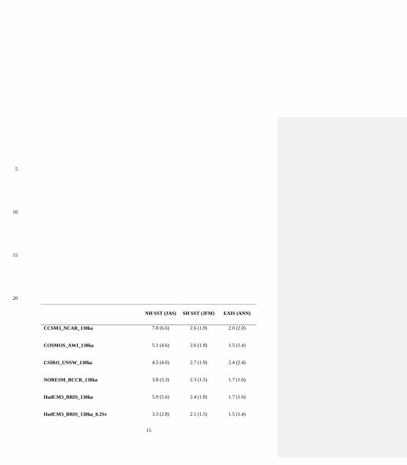
15

5

10

15

20

NH SST (JAS) SH SST (JFM) EAIS (ANN)

CCSM3_NCAR_130ka

7.8 (6.6) 2.6 (1.9) 2.0 (2.0)

COSMOS_AWI_130ka

5.1 (4.6) 2.6 (1.8) 1.5 (1.4)

CSIRO_UNSW_130ka

4.5 (4.0) 2.7 (1.9) 2.4 (2.4)

NORESM_BCCR_130ka

3.8 (3.3) 2.3 (1.5) 1.7 (1.6)

HadCM3_BRIS_130ka

5.9 (5.6) 2.4 (1.8) 1.7 (1.6)

HadCM3_BRIS_130ka_0.2Sv 3.3 (2.8) 2.1 (1.5) 1.5 (1.4)

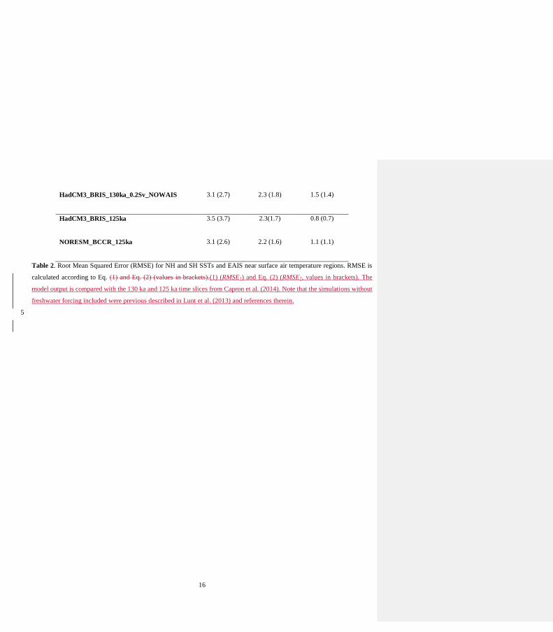
16

HadCM3_BRIS_130ka_0.2Sv_NOWAIS

3.1 (2.7) 2.3 (1.8) 1.5 (1.4)

HadCM3_BRIS_125ka

3.5 (3.7) 2.3(1.7) 0.8 (0.7)

NORESM_BCCR_125ka

3.1 (2.6) 2.2 (1.6) 1.1 (1.1)

Table 2. Root Mean Squared Error (RMSE) for NH and SH SSTs and EAIS near surface air temperature regions. RMSE is

calculated according to Eq. (1) and Eq. (2) (values in brackets).(1) (RMSE1) and Eq. (2) (RMSE2, values in brackets). The

model output is compared with the 130 ka and 125 ka time slices from Capron et al. (2014). Note that the simulations without

freshwater forcing included were previous described in Lunt et al. (2013) and references therein.

5

17

18

Figure 1. (a) 65°N (black) and 65˚S (grey) summer insolation (Laskar et al., 2004). (b) EDC ice core CO2 concentration

(Schneider et al., 2013) (black). (c) North Atlantic core ODP-980 summer-SST reconstruction (Oppo et al., 2006) (green) and

associated 2σ uncertainty envelope (Capron et al., 2014) (light green). (d (d) North Atlantic core CH69-K09 δ13C record 5

(Govin et al. 2012 and 2σ uncertainty envelope (this study, see details on the methodology in Capron et al., 2014). (e) Southern

Ocean core MD02-2488 summer-SST reconstruction (Govin et al., 2012) (pink) and 2σ uncertainty envelope (Capron et al.,

2014) (light pink). (ef) EDC surface temperature reconstruction (dark blue) and associated 1.5˚C uncertainty envelope

(Masson-Delmotte et al., 2011) (light blue). Ice and marine sediment records (a-d) are presented on the AICC2012 ice core

chronology (Bazin et al., 2013; Capron et al., 2014; Veres et al., 2013). (fNote that Govin et al. (2015) reports in the Table 5 10

of their paper that the Antarctic reconstructed surface temperature (based on EDC dD) starts increasing at 135.6 ±2.5 ka based

on the use of the RAMPFIT software. (g) Red Sea relative sea level (RSL) data (probability maximum, red) with 95%

confidence interval (Grant et al., 2012) (orange). (gh) Red Sea rate of RSL change (probability maximum for the first-order

time derivative, in meters/kyrSv, black) with 95% confidence interval (Grant et al., 2012) (grey). Note that ice and marine

records from (a) to (ef) are shown on the AICC2012 ice core chronology (Bazin et al., 2013; Capron et al., 2014; Veres et al., 15

2013) while the Red Sea records (f, g, h) are displayed on their original age scale which is independent from the AICC2012

ice core chronology (see Grant et al., 2012 for details) The grey vertical line marks 130 ka. The grey band highlights the 129-

Formatted: Line spacing: single, Don't adjust space betweenLatin and Asian text, Don't adjust space between Asian textand numbers

19

131 ka time interval that has been considered for the construction of the 130 ka data based time slice for surface temperature

(see Capron et al. 2014 for details on the methodology).

5

Figure 2. Simulated summer (NH-July, August, September; SH-January, February March) (left and middle panels) SST and

annual (right panel) surface air temperature change relative to present daypreindustrial, for GCM model results previously

Formatted: English (United Kingdom)

Formatted: Font: Times New Roman, Not Bold, English(United States)

20

published (Lunt et al., 2013) and their ensemble mean. The simulations are compared with the new data-based 130 ka time

slice (Capron et al., 2014).

5

Figure 3. The North Atlantic region for freshwater input denoted by the red box (50-70˚N). Note that the freshwater amount

is evenly distributed within this region.

21

Figure 4. Simulated 130 ka SSTs and near surface air temperature anomalies compared with data for the high latitude regions.

The top two rows are SSTs (annual or summer as labelled) and the bottom row is annual mean near surface air temperature.

Left panel (a) LIG peak warmth data synthesis of Turney and Jones (2010) (dots) compared with 130 ka annual temperature

anomalies (GHG and orbital forcing only). Middle panel (b) The 130 ka data-based time slice (dots) compared with simulated 5

summer-SST anomalies for the NH (July, August, and September) and SH (January, February, and March) (GHG and orbital

forcing only). Right panel (c) The130The 130 ka data-based time slice (dots) compared with summer-SST anomalies for the

NH and SH (GHG, orbital forcing and a constant freshwater input of 0.2 Sv into the North Atlantic). Note the non-linear

temperature scale. Anomalies calculated relative to the preindustrial for the model and relative to modern for the data.

22

Figure 5. Locations of 130 ka and 125 ka data-based time slice data from Capron et al. (2014). The colors denote the groups

of data used in Method 2 (Eq. (2)) to calculate the RMSE for each region. 5

10

23

Figure 6. Simulated summer (NH-July, August, September; SH-January, February March) SST and annual (bottom panel)

surface air temperature changeanomalies at 125 ka compared with the Capron et al. (2014) 125 ka data-based time slice. Left

panel: HadCM3, right panel: NorESM. Table 2 shows a similar agreement with data for NorESM and HadCM3 (which has no

cooling in the North Atlantic) in the NH when compared with the 125 ka data-based time slice from Capron et al. [2014]. 5

However, NorESM shows poor agreement with the data synthesis over Antarctica. Anomalies calculated relative to the

preindustrial for the model and relative to xxx for the data.

24

Figure 7. Simulated summer (July, August and September) near surface air temperature anomaly compared with preindustrial 5

at 130 ka over southern Europe and the North Atlantic region. The simulation is forced with 0.2 Sv of freshwater flux as well

as changes to the GHGs and orbital forcing (HadCM3_BRIS_130ka_0.2Sv).

25

Figure 8. (a) Simulated 130 ka SST and near surface air temperature anomalies, with the WAIS removed and replaced with

bare soil and a North Atlantic freshwater input forcing of 0.2 Sv, compared with the Capron et al. (2014) 130 ka time slice.

(b) Difference in SST and near surface air temperature between (a) and the 130 ka simulation with 0.2 Sv freshwater forcing

only (Fig. 4c). (c) Difference in SST and near surface air temperature when the WAIS is replaced with shrub compared with 5

bare soil (Fig. 8a). Left: summer-SST anomalies for the NH (July, August, and September); middle: summer-SST anomalies

in the SH (January, February, and March); right: annual near surface air temperature anomalies over Antarctica. It has been

shown that this warming over East Antarctica is attributed to climatic effects rather than isostatic effects arising from a

reduction in the WAIS (Bradley et al., 2012).

Formatted: Font: Not Bold

26

Figure 9. Response of the North Atlantic summer-SSTs and strength of the overturning circulation to varying amounts of

freshwater input injected between 50 and 70˚N (0 Sv, 0.1 Sv, 0.2 Sv, 0.3 Sv, 0.4 Sv, 0.5 Sv, 1 Sv). Left axis: Average 50-year

model temperature anomaly relative to present day. The temperature is averaged over all model grid-boxes where data points 5

are located. Right axis: 50-year average maximum Atlantic Meridional Overturning Circulation strength at 30˚N. The dashed

horizontal line corresponds to the average summer (July, August, September) temperature anomaly for all marine data located

at >40˚N for the 130 ka time slice (Capron et al., 2014).

10

15