Commands in destra v11 - Q-DAS
89
Commands in destra v11 destra v11 (2015-07-24 / 11.0.3.2)
-
Upload
khangminh22 -
Category
Documents
-
view
0 -
download
0
Transcript of Commands in destra v11 - Q-DAS

Commands in destra v11
destra v11 (2015-07-24 / 11.0.3.2)

Commands in destra v11 2/89
Version: 2.0 © 2015 Q-DAS GmbH, 69469 Weinheim Doku-Nr.: QDOC-572-67
Contents 1. Overview of specific commands in destra v11 ................................................................ 5
2. Start tab ......................................................................................................................... 6
2.1 “Create“ group in the Start tab ................................................................................. 6
2.1.1 New option in the “Create“ group of the Start tab .............................................................................. 7
2.1.2 Measurement System Analysis option in the “Create“ group of the Start tab .................................... 7
How to create a data source for measurement system analysis, type-1 study ........................................... 8
How to create a data source for measurement system analysis, type-2 study ........................................... 8
How to create a data source for measurement system analysis, type-3 study ........................................... 9
How to create a data source for measurement system analysis, stability .................................................. 9
How to create a data source for measurement system analysis, linearity ................................................ 10
How to create a data source for measurement system analysis, signal detection ................................... 10
How to create a data source for measurement system analysis, kappa coefficient ................................. 11
How to create a data source for measurement system analysis, type-1 study (2nd true position) ............ 13
2.1.3 Process Capability Analysis option in the “Create“ group of the Start tab ....................................... 14
How to create a data source for machine capability analysis ................................................................... 14
How to create a data source for process capability analysis .................................................................... 15
How to create a data source for a 1-part report ........................................................................................ 15
How to create a data source for a 5-part report ........................................................................................ 16
How to create a data source for discrete data .......................................................................................... 16
How to create a data source for an error log sheet .................................................................................. 17
How to create a data source for a machine capability analysis including positional tolerances ............... 17
2.1.4 Model f(x) | Correlation option in the “Create“ group of the Start tab ............................................... 18
How to create a data source for Pearson’s correlation coefficient ............................................................ 18
2.1.5 Model f(x) | Regression option in the “Create“ group of the Start tab .............................................. 19
How to create a data source for simple regression .................................................................................. 19
How to create a data source for multiple regression ................................................................................ 20
How to create a data source for multivariate regression .......................................................................... 20
How to create a data source for logistic regression .................................................................................. 21
2.1.6 Model f (x) | Analysis of Variance option in the “Create” group of the Start tab ............................... 22
How to create a data source for an analysis of variance (ANOVA) for single or multiple factors ............. 22
How to create a data source for an analysis of covariance (ANCOVA) .................................................... 23
How to create a data source for a multivariate analysis of variance (MANOVA) ...................................... 24
How to create a data source for a repeated measures ANOVA ............................................................... 25
2.1.7 Design option in the “Create“ group of the Start tab ........................................................................ 25
How to create a new design ..................................................................................................................... 26
Commands in destra v11 3/89
Version: 2.0 © 2015 Q-DAS GmbH, 69469 Weinheim Doku-Nr.: QDOC-572-67
How to create a new design based on the data of an existing one .......................................................... 27
How to augment an available design ........................................................................................................ 28
2.1.8 Test procedures option in the “Create“ group of the Start tab ......................................................... 29
How to create a data source for a 1-sample t-test .................................................................................... 29
How to create a data source for a 1-sample χ²-test .................................................................................. 29
How to create a data source for a Wilcoxon test ...................................................................................... 29
How to create a data source for a 2-sample t-test (independent samples) .............................................. 30
How to create a data source for a 2-sample t-test (paired samples) ........................................................ 30
How to create a data source for a Mann-Whitnex test .............................................................................. 30
How to create a data source for a F-test .................................................................................................. 30
How to create a data source for a rank test for dispersions ..................................................................... 31
How to create a data source for a simple analysis of variance (test) ....................................................... 31
How to create a data source for a Bartlett test ......................................................................................... 31
How to create a data source for the Kruskal-Wallis H-test ....................................................................... 31
How to create a data source for a Levene test ......................................................................................... 31
How to create a data source for a 1-sample µ-test .................................................................................. 33
How to create a data source for a 1-sample p-test ................................................................................... 33
How to create a data source for a 2-sample µ-test .................................................................................. 33
How to create a data source for a 2-sample p-test (BD) .......................................................................... 34
How to create a data source for a k-sample chi-squared test (PD) .......................................................... 34
How to create a data source for a test of homogeneity (PD) .................................................................... 34
How to create a k-sample chi-squared test (BD) ...................................................................................... 34
2.1.9 Reliability Analysis option of the “Create“ group in the Start tab ...................................................... 35
How to create a data source for reliability analysis................................................................................... 35
2.2 “Evaluation“ group in the Start tab ..........................................................................36
2.2.1 Evaluation strategy option in the “Evaluation“ group of the Start tab ............................................... 36
2.2.2 Standard procedure option in the “Evaluation“ group of the Start tab .............................................. 36
2.2.3 Distributions option in the “Evaluation“ group of the Start tab .......................................................... 37
2.2.4 Model f(x) | Correlation option in the “Evaluation“ group of the Start tab ......................................... 38
Evaluation based on Pearson’s correlation .............................................................................................. 38
2.2.5 Model f(x) | Regression option in the “Evaluation“ group of the Start tab ........................................ 40
How to evaluate simple regression ........................................................................................................... 40
How to evaluate multiple regression ......................................................................................................... 42
How to evaluate multivariate regression ................................................................................................... 44
How to evaluate logistic regression .......................................................................................................... 45
2.2.6 Model f(x) | Analysis of Variance option in the “Evaluation“ group of the Start tab .......................... 47

Commands in destra v11 4/89
Version: 2.0 © 2015 Q-DAS GmbH, 69469 Weinheim Doku-Nr.: QDOC-572-67
How to evaluate simple or multiple analysis of variance (ANOVA) .......................................................... 47
How to evaluate an analysis of covariance (ANCOVA) ............................................................................ 49
How to evaluate a multivariate analysis of variance (MANOVA) .............................................................. 50
How to evaluate repeated measures ANOVA .......................................................................................... 52
2.2.7 Design option in the “Evaluation“ group of the Start tab .................................................................. 54
2.2.8 Test procedures option in the “Evaluation“ group of the Start tab ................................................... 54
Test procedures for continuous characteristic values............................................................................... 54
How to evaluate a 1-sample t-test (normal distribution: parameter µ) ...................................................... 55
How to evaluate a 1-sample chi-squared test (normal distribution: parameter sigma) ............................. 57
How to evaluate the Wilcoxon test (median) ............................................................................................ 59
How to evaluate the 2-sample t-test (normal distribution: parameter µ, independent samples) ............... 61
How to evaluate a 2-sample F-test (normal distribution: sigma) ............................................................... 63
How to evaluate a 2-sample Mann-Whitnex U-test (median) ................................................................... 65
How to evaluate a 2-sample rank test for dispersions (dispersion) .......................................................... 67
How to evaluate a simple analysis of variance (normal distribution: parameter µ) .................................. 69
How to evaluate a k-sample Bartlett test (normal distribution: parameter σ) ............................................ 71
Howe to evaluate a k-sample Kruskal-Wallis test (location: median) ....................................................... 72
How to evaluate a k-sample Levene test (variance) ................................................................................. 74
Test procedures for discrete values ......................................................................................................... 76
How to evaluate a 1-sample µ-test (Poisson distribution: parameter µ) .................................................. 76
How to evaluate a 1-sample p-test (binomial distribution: parameter p) ................................................... 78
How to evaluate a 2-sample µ-test (Poisson distribution: parameter µ) .................................................. 79
How to evaluate a 2-sample p-test (binomial distribution: parameter p) ................................................... 81
How to evaluate a k-sample chi-squared test (Poisson distribution: parameter µ) .................................. 82
How to evaluate a k-sample χ²-test (Poisson distribution: parameter µ) .................................................. 84
How to evaluate a k-sample χ²-test (binomial distribution: parameter p) .................................................. 85
3. Index .............................................................................................................................88

Commands in destra v11 5/89
Version: 2.0 © 2015 Q-DAS GmbH, 69469 Weinheim Doku-Nr.: QDOC-572-67
1. Overview of specific commands in destra v11 This reference manual focuses on the Start tab including the “Create” and “Evaluation” groups of
commands. The included commands or options are very important in destra since each data
set you create and evaluate in the Project Explorer either creates a data source node or a session
node. You thus have to consider some special aspects and differences compared to the
application of our software products solara.MP and qs-STAT. These differences are
explained in the following.
This reference manual helps you understand the principle behind the new Project Explorer
and explains how to find a certain analysis function.
We will be pleased about any feedback and any suggestions for improvement of this
reference manual.

Commands in destra v11 6/89
Version: 2.0 © 2015 Q-DAS GmbH, 69469 Weinheim Doku-Nr.: QDOC-572-67
2. Start tab
Figure 2-1: Start tab including the “Create“, “Evaluation“ and “Reports“ groups of commands
Two groups of the Start tab are of particular importance.
Create
Evaluation
Use the options of the Create group to create new data sources. You either transfer data to
these sources or enter them. Now you can evaluate these data sources by using the options of
the Evaluation group.
The single options are explained in the following.
2.1 “Create“ group in the Start tab
Figure 2-2: “Create“ group in the Start tab
Almost all of these options create a new data source in the Project Explorer (the only
exception is the New option). However, this does not always mean that you actually create
nothing but a new data source in the Project Explorer by selecting one of these options. The
number and type of new structural elements the program creates in the Project Explorer
always depend on the node you selected in the Project Explorer when you click the
respective button. You will observe that the program often creates further nodes in the
Project Explorer in addition to the respective data source.
The reason is the specified strict hierarchy of the Project Explorer‘s structural
elements.
A project phase always represents the next level below the project node.
A work space always represents the next level below a project phase.
A data source always represents the next level below a work space.

Commands in destra v11 7/89
Version: 2.0 © 2015 Q-DAS GmbH, 69469 Weinheim Doku-Nr.: QDOC-572-67
The following table gives an overview of the structural elements the program creates
automatically in the Project Explorer as soon as you select any option from the ”Create”
group.
Selected node Automatically generated structural elements in the Project Explorer
Project Project phase – work space – data source
Project phase Work space – data source
Work space Data source
Data source Data source Table 2-1: Overview of possible automatically generated structural elements when applying an option in the “Create“ group of the Start tab
2.1.1 New option in the “Create“ group of the Start tab
Figure 2-3: New option
New | Project phase: This option creates a new project phase node in the Project Explorer.
New | Work space: This option creates a new work space in the Project Explorer.
2.1.2 Measurement System Analysis option in the “Create“ group of the Start tab
Figure 2-4: Measurement System Analysis option

Commands in destra v11 8/89
Version: 2.0 © 2015 Q-DAS GmbH, 69469 Weinheim Doku-Nr.: QDOC-572-67
How to create a data source for measurement system analysis, type-1 study
Start | Create | Measurement System Analysis | Type 1 Study 1: This option creates a data source
for type-1 study in the Measurement System Analysis module. The Measurement System
Analysis – Type-1 Study dialog box opens. It includes an input mask for the following information.
Name: Enter the characteristic description.
Characteristic type: deactivated
Unit: Enter the unit of the measured quantity.
Nominal size: Enter the nominal dimension of the characteristic.
LSL: Enter the lower specification limit.
USL: Enter the upper specification limit.
RE: Enter the resolution of the measurement system.
XRef: Enter the reference value of the measurement standard as given in the
corresponding calibration certificate.
Figure 2-5: Upper part of the Measurement System Analysis – Type-1 Study dialog box
Confirm your input to open the values mask. You enter the measurement results there. Now
you start an evaluation by selecting the respective data source in the Project Explorer and
clicking Start | Evaluation | Standard procedure.
How to create a data source for measurement system analysis, type-2 study
Start | Create | Measurement System Analysis | Type 2 study: This option creates a data source for
type-2 study in the Measurement System Analysis module. The Measurement System
Analysis – Type-2 Study dialog box opens. It includes an input mask for the following information.
Name: Enter the characteristic description.
Characteristic type: deactivated
Unit: Enter the unit of the measured quantity.
Nominal size: Enter the nominal dimension of the characteristic.
LSL: Enter the lower specification limit.
USL: Enter the upper specification limit.
k: Enter the number of operators.
r: Enter the number of repeated measurements.
n: Enter the number of parts applied in this study.
Figure 2-6: Upper part of the Measurement System Analysis – Type-2 Study dialog box

Commands in destra v11 9/89
Version: 2.0 © 2015 Q-DAS GmbH, 69469 Weinheim Doku-Nr.: QDOC-572-67
Confirm your input to open the values mask. You enter the measurement results there. Now
you start an evaluation by selecting the respective data source in the Project Explorer and
clicking Start | Evaluation | Standard procedure.
How to create a data source for measurement system analysis, type-3 study
Start | Create | Measurement System Analysis | Type 3 study: This option creates a data source for
type-3 study in the Measurement System Analysis module. The Measurement System
Analysis – Type-3 Study dialog box opens. It includes an input mask for the following information.
Name: Enter the characteristic description.
Characteristic type: deactivated
Unit: Enter the unit of the measured quantity.
Nominal size: Enter the nominal dimension of the characteristic.
LSL: Enter the lower specification limit.
USL: Enter the upper specification limit.
r: Enter the number of repeated measurements.
n: Enter the number of applied parts.
Figure 2-7: Upper part of the Measurement System Analysis – Type-3 Study dialog box
Confirm your input to open the values mask. You enter the measurement results there. Now
you start an evaluation by selecting the respective data source in the Project Explorer and
clicking Start | Evaluation | Standard procedure.
How to create a data source for measurement system analysis, stability
Start | Create | Measurement System Analysis | Type 5 study (stability): This option creates a data
source for stability analysis (bias and repeatability) in the Measurement System Analysis
module. The Measurement System Analysis – Stability dialog box opens. It includes an input mask
for the following information.
Name: Enter the characteristic description.
Characteristic type: deactivated
Unit: Enter the unit of the measured quantity.
r: Enter the number of repeated measurements.
XRef: Enter the reference value of the measurement standard as given in the
corresponding calibration certificate.

Commands in destra v11 10/89
Version: 2.0 © 2015 Q-DAS GmbH, 69469 Weinheim Doku-Nr.: QDOC-572-67
Figure 2-8: Upper part of the Measurement System Analysis – Stability dialog box
Confirm your input to open the values mask. You enter the measurement results there. Now
you start an evaluation by selecting the respective data source in the Project Explorer and
clicking Start | Evaluation | Standard procedure.
How to create a data source for measurement system analysis, linearity
Start | Create | Measurement System Analysis | Type 4 study (linearity): This option creates a data
source for testing bias by using several measurement standards in the Measurement
System Analysis module. The Measurement System Analysis – Linearity dialog box opens. It
includes an input mask for the following information.
Name: Enter the characteristic description.
Characteristic type: deactivated
Unit: Enter the unit of the measured quantity.
Nominal size: Enter the nominal dimension of the characteristic.
LSL: Enter the lower specification limit.
USL: Enter the upper specification limit.
r: Enter the number of repeated measurements.
n: Enter the number of applied measurement standards/reference parts.
m: Enter the number of repeated measurements per measurement
standard/reference part.
Figure 2-9: Upper part of the Measurement System Analysis – Linearity dialog box
Confirm your input to open the values mask. You enter the measurement results there. Now
you start an evaluation by selecting the respective data source in the Project Explorer and
clicking Start | Evaluation | Standard procedure.
How to create a data source for measurement system analysis, signal detection
Start | Create | Measurement System Analysis | Signal detection: This option creates a data source
for the method of signal detection in the Measurement System Analysis module. The
Measurement System Analysis – Signal Detection dialog box opens. It includes an input mask for
the following information.
Name: Enter the characteristic description.
Characteristic type: deactivated
Unit: Enter the unit of the measured quantity.

Commands in destra v11 11/89
Version: 2.0 © 2015 Q-DAS GmbH, 69469 Weinheim Doku-Nr.: QDOC-572-67
Nominal size: Enter the nominal dimension of the characteristic.
LSL: Enter the lower specification limit.
USL: Enter the upper specification limit.
k: Enter the number of operators.
r: Enter the number of repeated measurements per part.
n: Enter the number of applied parts.
m: Enter the number of reference values per part (“normally” m = 1).
Figure 2-10: Upper part of the Measurement System Analysis – Signal detection dialog box
Confirm your input to open the values mask. You enter the numerical reference
measurement results in the first column.
Note: The values for USL and LSL relate to these reference measurements!
You use numerical values (numbers) to indicate the test decisions of the respective operator.
0 indicates Part is not o.k.
1 indicates Part is o.k.
Now you start an evaluation by selecting the respective data source in the Project Explorer
and clicking Start | Evaluation | Standard procedure.
How to create a data source for measurement system analysis, kappa coefficient
Start | Create | Measurement System Analysis | Kappa coefficient: This option creates a data source
for Fleiss’ or Cohen’s kappa in the Measurement System Analysis module. The
Measurement System Analysis – Kappa coefficient dialog box opens. It includes an input mask for
the following information.
Name: Enter the characteristic description.
Characteristic type: deactivated
Catalogue: Select the catalogue you want to apply.
k: Enter the number of operators.
r: Enter the number of repeated measurements.
n: Enter the number of applied parts.
m: Enter the number of reference values per part.

Commands in destra v11 12/89
Version: 2.0 © 2015 Q-DAS GmbH, 69469 Weinheim Doku-Nr.: QDOC-572-67
Figure 2-11: Measurement System Analysis – Kappa coefficient dialog box
Values indicating the decision of operators have to be available in a catalogue. In other
words: You first have to create the content of such a catalogue, such as Part o.k. or Part
n.o.k. The lower part of the dialog box shows to options specifying the selection of the
catalogue to be applied.
1. Catalogue is part of data source
2. Catalogue is read from config DB
Figure 2-12: Lower part of the Measurement System Analysis – Kappa coefficient dialog including two radio buttons for the selection of catalogues to be applied
The Catalogue is part of data source radio button is enabled by default. By using this option,
you have to enter possible values for test decisions manually in the Level values list (framed
in red in Figure 2-11). The program saves these level values to the project.
Select the Catalogue is read from config DB radio button and the program only applies
values from the ordinal classes catalogue of the database adjusted in the program
configuration (File | Configuration | Catalogues).
Note: In case you activate the second radio button – catalogue from database – you have to consider that the contents of the ordinal classes catalogue is identical in both database when you want to exchange the project file between users working at different sites or between customer and supplier. Otherwise, you will notice a considerable difference between the evaluation results of the two users…
Note: In order to learn how to handle the database, we recommend you to attend the
respective seminar of our affiliated company TEQ.

Commands in destra v11 13/89
Version: 2.0 © 2015 Q-DAS GmbH, 69469 Weinheim Doku-Nr.: QDOC-572-67
Click on the button in the Catalogue column of the Measurement System Analysis – Kappa coefficient
dialog box to open the Characteristic catalogue: … dialog box.
Figure 2-13: Characteristic catalogue: … dialog box
Select the Create new catalogue radio button to create a new catalogue with an individual
catalogue name.
In case the data source already includes a catalogue that you want to apply, you activate the
Selection of available catalogues option. After you selected the respective catalogue, you may
select the included level values for the characteristic.
Note: Create a new catalogue with an individual name before specifying level values in the automatically generated default catalogue. Since we do not change the name of the default catalogue but create a new catalogue, the new catalogue does not take over the entries of the default catalogue. It is thus empty!
Confirm your input to open the values mask. You enter the characteristic values. Now you
start an evaluation by selecting the respective data source in the Project Explorer and
clicking Start | Evaluation | Standard procedure.
How to create a data source for measurement system analysis, type-1 study (2nd true position)
Start | Create | Measurement System Analysis | Type-1 study (2nd true position: This option creates a
characteristic group for two-dimensional and three-dimensional evaluations of type-1 studies
in the Measurement System Analysis module. The Measurement System Analysis – true
position MSA type 1 study dialog box opens. You only adjust the dimension here – 2D or 3D. Do
not enter any further information; otherwise you might have to delete erroneous values later
on…
Figure 2-14: Upper part of the Measurement System Analysis – true position MSA type 1 study dialog box
Confirm your input to open the values mask. You enter the measurement results for the
subordinate characteristics. Values of superordinate characteristics are not relevant to this

Commands in destra v11 14/89
Version: 2.0 © 2015 Q-DAS GmbH, 69469 Weinheim Doku-Nr.: QDOC-572-67
type of evaluation. However, you have to enter the information about the single
characteristics now.
Tip: Open the Edit tab and select Characteristics mask to open the characteristics mask. Here you edit the data of each single characteristic.
Now you start an evaluation by selecting the respective data source in the Project Explorer
and clicking Start | Evaluation | Standard procedure.
2.1.3 Process Capability Analysis option in the “Create“ group of the Start tab
Figure 2-15: Process Capability Analysis option
How to create a data source for machine capability analysis
Start | Create | Process Capability Analysis | Short-term capability of 1 sample (Cm, Cmk): The program
generates a data source including a continuous (variable) characteristic for machine
capability analysis in the Sample Analysis module.
Figure 2-16: Upper part of the Process Capability Analysis – Machine Capability dialog box
The Process Capability Analysis – Machine Capability dialog box opens. It includes an input mask
for the following information.
Name: Enter the characteristic description.
Characteristic type: deactivated
Unit: Enter the unit of the measured quantity.
Nominal size: Enter the nominal dimension of the characteristic.
LSL: Enter the lower specification limit of the characteristic.

Commands in destra v11 15/89
Version: 2.0 © 2015 Q-DAS GmbH, 69469 Weinheim Doku-Nr.: QDOC-572-67
USL: Enter the upper specification limit of the characteristic.
Confirm your input to open the values mask. You enter the characteristic values here. Now
you start an evaluation by selecting the respective data source in the Project Explorer and
clicking Start | Evaluation | Standard procedure.
How to create a data source for process capability analysis
Start | Create | Process Capability Analysis | Process capability of k sample (Pp, Ppk, Cp, Cpk): The
program generates a data source including a continuous (variable) characteristic for process
capability analysis in the Process Capability Analysis module.
Figure 2-17: Upper part of the Process Capability Analysis – Process Capability dialog box
The Process Capability Analysis – Process Capability dialog box opens. It includes an input mask
for the following information.
Name: Enter the characteristic description.
Characteristic type: deactivated
Unit: Enter the unit of the measured quantity.
Nominal size: Enter the nominal dimension of the characteristic.
LSL: Enter the lower specification limit.
USL: Enter the upper specification limit.
Confirm your input to open the values mask. You enter the characteristic values here. Now
you start an evaluation by selecting the respective data source in the Project Explorer and
clicking Start | Evaluation | Standard procedure.
How to create a data source for a 1-part report
Start | Create | Process Capability Analysis | 1 Part Report: The program generates a data source
including a continuous (variable) characteristic for a 1-part report in the Sample Analysis
module.
Figure 2-18: Upper part of the Process Capability Analysis – 1 Part Report dialog box
The Process Capability Analysis – 1 Part Report dialog box opens. It includes an input mask for the
following information.
Commands in destra v11 16/89
Version: 2.0 © 2015 Q-DAS GmbH, 69469 Weinheim Doku-Nr.: QDOC-572-67
Name: Enter the characteristic description.
Characteristic type: deactivated
Unit: Enter the unit of the measured quantity.
Nominal size: Enter the nominal dimension of the characteristic.
LSL: Enter the lower specification limit.
USL: Enter the upper specification limit.
Confirm your input to open the values mask. You enter the characteristic values here. Now
you start an evaluation by selecting the respective data source in the Project Explorer and
clicking Start | Evaluation | Standard procedure.
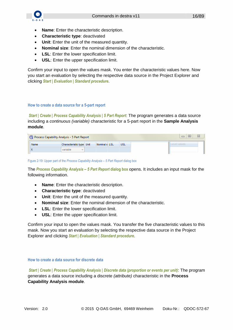
How to create a data source for a 5-part report
Start | Create | Process Capability Analysis | 5 Part Report: The program generates a data source
including a continuous (variable) characteristic for a 5-part report in the Sample Analysis
module.
Figure 2-19: Upper part of the Process Capability Analysis – 5 Part Report dialog box
The Process Capability Analysis – 5 Part Report dialog box opens. It includes an input mask for the
following information.
Name: Enter the characteristic description.
Characteristic type: deactivated
Unit: Enter the unit of the measured quantity.
Nominal size: Enter the nominal dimension of the characteristic.
LSL: Enter the lower specification limit.
USL: Enter the upper specification limit.
Confirm your input to open the values mask. You transfer the five characteristic values to this
mask. Now you start an evaluation by selecting the respective data source in the Project
Explorer and clicking Start | Evaluation | Standard procedure.
How to create a data source for discrete data
Start | Create | Process Capability Analysis | Discrete data (proportion or events per unit): The program
generates a data source including a discrete (attribute) characteristic in the Process
Capability Analysis module.

Commands in destra v11 17/89
Version: 2.0 © 2015 Q-DAS GmbH, 69469 Weinheim Doku-Nr.: QDOC-572-67
Figure 2-20: Upper part of the Process Capability Analysis – Attribute analysis dialog box
The Process Capability Analysis – Attribute Analysis dialog box opens. You enter the name of the
characteristic and the subgroup size n.
Note: The content of the Characteristic type attribute field is fixed by default. In case you need a variable subgroup size n, select Characteristics mask from the Edit tab. Now you change the attribute entry in the ”Characteristic type” field of the characteristics mask and select variable from the drop-down menu.
Confirm your input to open the values mask. You enter or transfer the values. Now you start
an evaluation by selecting the respective data source in the Project Explorer and clicking Start
| Evaluation | Standard procedure.
How to create a data source for an error log sheet
Start | Create | Process Capability Analysis | Error log sheet (events per unit): The program generates
a data source including a group of discrete (attribute) characteristics for evaluating an error
log sheet in the Process Capability Analysis module.
Figure 2-21: Upper part of the Process Capability Analysis – Error log sheet dialog box
The Process Capability Analysis – Error log sheet dialog box opens. You enter the name of the
error log sheet, the number of error types NDC available in the error log sheet and the
subgroup size n. The sampling scheme is either adjusted to the value fixed (= invariable and
thus constant) or variable.
Confirm your input to open the values mask. You enter or transfer the values. Now you start
an evaluation by selecting the respective data source in the Project Explorer and clicking Start
| Evaluation | Standard procedure.
How to create a data source for a machine capability analysis including positional tolerances
Start | Create | Process Capability Analysis | Short-term capability of 2D / 3D characteristics (Pm, Pmk):
The program generates a data source including a group of continuous (variable)

Commands in destra v11 18/89
Version: 2.0 © 2015 Q-DAS GmbH, 69469 Weinheim Doku-Nr.: QDOC-572-67
characteristics for evaluating capability of 2D or 3D positional tolerances in the Sample
Analysis module.
2.1.4 Model f(x) | Correlation option in the “Create“ group of the Start tab
Figure 2-22: Model f(x) option
How to create a data source for Pearson’s correlation coefficient
Start | Create | Model f(x) | Correlation | Pearson: The program generates a data source for
correlation analysis in the Analysis of Regression / Variance module.
Figure 2-23: Upper part of the Process Improvement – Pearson correlation dialog box
The Process Improvement – Pearson correlation dialog box opens. It includes an input mask for the
following information.
Name: Enter the description of the characteristics.
Characteristic type: Select the characteristic type.
Catalogue: remains empty
Unit: Enter the unit of the characteristic.
Edit the characteristics and confirm your input to open the values mask. You enter or transfer
the characteristic data.
Note: Please always consider that each line refers to a specific characteristic. In case the number of cells of the different columns differs, it is quite likely that an error slipped in.
Now you start an evaluation by selecting the respective data source in the Project Explorer
and clicking Start | Evaluation | Model f(x) | Correlation | Pearson.

Commands in destra v11 19/89
Version: 2.0 © 2015 Q-DAS GmbH, 69469 Weinheim Doku-Nr.: QDOC-572-67
Note: You may apply the Model f(x) | Correlation | Spearman or Model f(x) | Correlation | Kendall functions in the same way as described above.
2.1.5 Model f(x) | Regression option in the “Create“ group of the Start tab
How to create a data source for simple regression
Start | Create | Model f(x) | Regression | Simple: The program generates a data source for simple
regression in the Analysis of Regression / Variance module.
Figure 2-24: Upper part of the Process Improvement – Simple regression dialog box
The Process Improvement – Simple regression dialog box opens. It includes an input mask for the
following information.
Name: Enter the description of the characteristics.
Characteristic type: Select the characteristic type.
Catalogue: remains empty
Unit: Enter the unit of the characteristic.
X: Select the characteristic you want to use as a factor.
Y: Select the characteristic you want to use as a response.
The dialog box includes two continuous (variable) characteristics by default – a factor (or
independent variable) referred to as X and the response (or dependent variable) referred to
as Y.
Edit the characteristics and confirm your input to open the values mask. You enter or transfer
the characteristic values.
Note: Please always consider that each line refers to a specific characteristic. In case the number of cells of the different columns differs, it is quite likely that an error slipped in.
Now you start an evaluation by selecting the respective data source in the Project Explorer
and clicking Start | Evaluation | Model f(x) | Regression | Simple.

Commands in destra v11 20/89
Version: 2.0 © 2015 Q-DAS GmbH, 69469 Weinheim Doku-Nr.: QDOC-572-67
How to create a data source for multiple regression
Start | Create | Model f(x) | Regression | Multiple: The program generates a data source for
multiple regression in the Analysis of Regression / Variance module.
Figure 2-25: Upper part of the Process Improvement – Multiple regression dialog box
The Process Improvement – Multiple regression dialog box opens. The dialog box includes three
continuous (variable) characteristics by default – two factors (or independent variable)
referred to as X1 and X2 and the response (or dependent variable) referred to as Y.
Edit the characteristics and confirm your input to open the values mask. You enter or transfer
the characteristic values.
Note: Please always consider that each line refers to a specific characteristic. In case the number of cells of the different columns differs, it is quite likely that an error slipped in.
Now you start an evaluation by selecting the respective data source in the Project Explorer
and clicking Start | Evaluation | Model f(x) | Regression | Multiple.
How to create a data source for multivariate regression
Start | Create | Model f(x) | Regression | Multivariate: The program generates a data source for
multivariate regression in the Analysis of Regression / Variance module.
The Process Improvement – Multivariate regression dialog box opens. It includes an input mask for
the following information.
Name: Enter the description of the characteristics.
Characteristic type: remains unchanged
Catalogue: remains empty
Unit: Enter the unit of the characteristics.
X: Select characteristics you want to use as a factor.
Y: Select characteristics you want to use as a response.
Commands in destra v11 21/89
Version: 2.0 © 2015 Q-DAS GmbH, 69469 Weinheim Doku-Nr.: QDOC-572-67
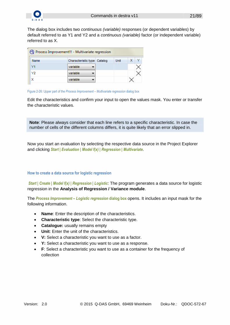
The dialog box includes two continuous (variable) responses (or dependent variables) by
default referred to as Y1 and Y2 and a continuous (variable) factor (or independent variable)
referred to as X.
Figure 2-26: Upper part of the Process Improvement – Multivariate regression dialog box
Edit the characteristics and confirm your input to open the values mask. You enter or transfer
the characteristic values.
Note: Please always consider that each line refers to a specific characteristic. In case the number of cells of the different columns differs, it is quite likely that an error slipped in.
Now you start an evaluation by selecting the respective data source in the Project Explorer
and clicking Start | Evaluation | Model f(x) | Regression | Multivariate.
How to create a data source for logistic regression
Start | Create | Model f(x) | Regression | Logistic: The program generates a data source for logistic
regression in the Analysis of Regression / Variance module.
The Process Improvement – Logistic regression dialog box opens. It includes an input mask for the
following information.
Name: Enter the description of the characteristics.
Characteristic type: Select the characteristic type.
Catalogue: usually remains empty
Unit: Enter the unit of the characteristics.
V: Select a characteristic you want to use as a factor.
Y: Select a characteristic you want to use as a response.
F: Select a characteristic you want to use as a container for the frequency of
collection

Commands in destra v11 22/89
Version: 2.0 © 2015 Q-DAS GmbH, 69469 Weinheim Doku-Nr.: QDOC-572-67
The dialog box includes an ordinal response (or dependent variables) by default referred to
as Y and two factors (or independent variables) referred to as X1 and X2. In addition, there is
a column for frequencies.
Figure 2-27: Upper part of the Process Improvement – Logistic regression dialog box
Note: Even if you only want to include single measurements in the data source, you must not delete the frequency column! You just have to enter a “1” into the cells of this column in the values mask.
Enter possible values of the ordinal or nominal response into the Level values column on the
right-hand side of the dialog box. Edit the characteristics and confirm your input to open the
values mask. You enter or transfer the characteristic values. Now you start an evaluation by
selecting the respective data source in the Project Explorer and clicking Start | Evaluation |
Model f(x) | Regression | Logistic.
2.1.6 Model f (x) | Analysis of Variance option in the “Create” group of the Start tab
How to create a data source for an analysis of variance (ANOVA) for single or multiple factors
Start | Create | Model f(x) | Analysis of variance | ANOVA: The program generates a data source for
an analysis of variance in the Analysis of Regression / Variance module.
The Process Improvement – Analysis of variance dialog box opens. It includes an input mask for
the following information.
Name: Enter the description of the characteristics.
Characteristic type: Select the characteristic type.
Catalogue: You either create a new catalogue or select an existing one.
Unit: Enter the unit of each characteristic.
X: Select a characteristic you want to use as a factor with fixed level values.
Z: Select a characteristic you want to use as a factor with random level values.
Y: Select a characteristic you want to use as a response.

Commands in destra v11 23/89
Version: 2.0 © 2015 Q-DAS GmbH, 69469 Weinheim Doku-Nr.: QDOC-572-67
The dialog box includes a continuous (variable) response by default referred to as Y and two
ordinal factors (or influence quantities) referred to as A and B. Enter possible values of each
factor into the Level values column on the right-hand side of the dialog box.
Note: In case you forget to enter level values here and you enter level values in the values mask later on, the program will show a message informing you that the entered value in unknown.
Note: In case you forget to enter level values here and you transfer data from the Windows
clipboard to the values mask later on, the program will show a number of error messages
and will NOT transfer the level values.
Tip: In case you face data including factors whose level values are not entirely known, you cannot enter the list of level values here. Save the data as a CSV file – e.g. in Microsoft Excel – instead. Now you import this CSV file by selecting File | File… | Import. The program transfers the factors as nominal values and creates the ordinal classes catalogue automatically for level values.
Figure 2-28: Upper part of the Process Improvement – Analysis of Variance dialog box
Edit the characteristics and confirm your input to open the values mask. You transfer the
characteristic values. Now you start an evaluation by selecting the respective data source in
the Project Explorer and clicking Start | Evaluation | Model f(x) | Analysis of Variance | ANOVA.
How to create a data source for an analysis of covariance (ANCOVA)
Start | Create | Model f(x) | Analysis of variance | ANCOVA: The program generates a data source
for an analysis of covariance in the Analysis of Regression / Variance module.
The Process Improvement – ANCOVA dialog box opens. It includes an input mask for the following
information.
Name: Enter the description of the characteristics.
Characteristic type: Select the characteristic type.
Catalogue: You either create a new catalogue or select an existing one.
Unit: Enter the unit of each characteristic.
X: Select a characteristic you want to use as a factor with fixed level values.
V: Select a characteristic you want to use as a covariable (continuous values).

Commands in destra v11 24/89
Version: 2.0 © 2015 Q-DAS GmbH, 69469 Weinheim Doku-Nr.: QDOC-572-67
Y: Select a characteristic you want to use as a response.
Figure 2-29: Upper part of the Process Improvement – ANCOVA dialog box
The dialog box includes a continuous (variable) response by default referred to as Y, an
ordinal factor referred to as A and a continuous (variable) covariable called X. Enter possible
values of the ordinal factor into the Level values column on the right-hand side of the dialog
box.
Edit the characteristics and confirm your input to open the values mask. You transfer the
characteristic values. Now you start an evaluation by selecting the respective data source in
the Project Explorer and clicking Start | Evaluation | Model f(x) | Analysis of Variance | ANCOVA.
How to create a data source for a multivariate analysis of variance (MANOVA)
Start | Create | Model f(x) | Analysis of variance | MANOVA: The program generates a data source
for a multivariate analysis of variance in the Analysis of Regression / Variance module.
The Process Improvement – Multivariate analysis of variance dialog box opens. It includes an input
mask for the following information.
Name: Enter the description of the characteristics.
Characteristic type: Select the characteristic type.
Catalogue: You either select an existing catalogue for factors or create a new one by
entering values in the Level values column.
Unit: Enter the unit of each characteristic.
X: Select a characteristic you want to use as a factor with fixed level values.
V: Select a characteristic you want to use as a factor with continuous level values.
Y: Select a characteristic you want to use as a response (continuous values).
The dialog box includes two continuous (variable) responses by default referred to as Y1 and
Y2 and an ordinal factor referred to as A.
Figure 2-30: Upper part of the Process Improvement – Multivariate analysis of variance dialog box
Edit the characteristics and confirm your input to open the values mask. You transfer the
characteristic values. Now you start an evaluation by selecting the respective data source in
the Project Explorer and clicking Start | Evaluation | Model f(x) | Analysis of Variance | MANOVA.

Commands in destra v11 25/89
Version: 2.0 © 2015 Q-DAS GmbH, 69469 Weinheim Doku-Nr.: QDOC-572-67
How to create a data source for a repeated measures ANOVA
Start | Create | Model f(x) | Analysis of variance | Repeated measures: The program generates a data
source for a multivariate repeated measures ANOVA in the Analysis of Regression /
Variance module.
The Process Improvement – Multivariate repeated measures ANOVA dialog box opens. It includes an
input mask for the following information.
Name: Enter the description of the characteristics.
Characteristic type: Select the characteristic type.
Catalogue: You either select a factor level catalogue for ordinal characteristics or
enter possible factor levels in the Level values column.
Unit: Enter the unit of each characteristic.
X: Select a characteristic you want to use as a factor with fixed level values.
R: Select a characteristic you want to use as a repeated measure container.
Y: Select a characteristic you want to use as a response.
Figure 2-31: Upper part of the Process Improvement – Multivariate repeated measures ANOVA dialog box
The dialog box includes a responses Y, a repeated measures container RM and a factor A
with fixed level values by default.
Edit the characteristics and confirm your input to open the values mask. You transfer the
characteristic values. Now you start an evaluation by selecting the respective data source in
the Project Explorer and clicking Start | Evaluation | Model f(x) | Analysis of Variance | Repeated
measures.
2.1.7 Design option in the “Create“ group of the Start tab
Figure 2-32: Design option

Commands in destra v11 26/89
Version: 2.0 © 2015 Q-DAS GmbH, 69469 Weinheim Doku-Nr.: QDOC-572-67
How to create a new design
Start | Create | Design | Create design: The program generates a data source based on the
selected design in the Analysis of Regression / Variance module. The Design of experiments
window opens. Select the respective design in the Selection tab.
Figure 2-33: Upper part of the Design of experiments window
Available designs in the Design of experiments window
1st level 2nd level 3rd level
Screening designs Plackett-Burman designs Not available
Factorial designs 2-level designs
D-optimal designs
Multi-level designs
Response surface designs Central composite designs Not available
Box-Behnken designs Not available
D-optimal designs Not available
Mixture designs Simplex lattice designs Not available
Simplex centroid designs Not available
D-optimal designs (mixture) Not available Table 2-2: Overview of designs available in the Design of experiments window
Note: When you select a 2-level design, the Selection of factorial designs with 2 factor levels dialog box opens. Select the respective design by click.
Figure 2-34: Selection of factorial designs with 2 factor levels dialog box

Commands in destra v11 27/89
Version: 2.0 © 2015 Q-DAS GmbH, 69469 Weinheim Doku-Nr.: QDOC-572-67
Let’s go back to the Design of experiments window. Depending on the selected type of
design, it offers up to five different tabs.
Figure 2-35: Upper part of the Design of experiments window including several tabs
In general, you enter the required information into the tabs from left to right.
The following table provides a brief overview of the contents available in the single tabs.
Tab Contents
Selection Tree structure including all available designs
Definition (Contents of this tab depend on the selected design.)
Definition of
responses
factors
level values of factors
number of replicates
number of centre points
number of blocks
randomization option
…
Settings D-opt design (Only available after selection of D-optimal design)
Only available after selection of D-optimal design. Select the type of model, number of blocks and define number of additional runs.
Design Evaluation (Contents of this tab depend on the selected design.)
Gives an overview specific to the selected design. It includes statistics helping you evaluate the properties of the created design.
Design (Contents of this tab depend on the selected design.)
Shows all lines of the created design completely. You may still adjust the sorting of single or several factor columns.
Table 2-3: Overview of tabs available in the Design of experiments tab
How to create a new design based on the data of an existing one
Start | Create | Design | Reuse design: In order to use this function, you have to select an
available data source in the Project Explorer that already includes a design. The
program opens the Design of experiments window. Select the respective type of design in the
Selection tab. The new design applies all factors and level values but you may still adapt them,

Commands in destra v11 28/89
Version: 2.0 © 2015 Q-DAS GmbH, 69469 Weinheim Doku-Nr.: QDOC-572-67
if required. destra creates the new design as a new data source in the Analysis of
Regression / Variance module.
How to augment an available design
Start | Create | Design | Augment design: In order to use this function, you have to select an
available data source in the Project Explorer that already includes a factorial design
with 2 factor levels. This option augments (= changes!) the existing design in the data
source. You may either add centre points to a factorial design with 2 factor levels that does
not include any centre point so far or add further centre and axial points to a factorial design
with 2 factor levels. Caution: You cannot undo these steps!
Figure 2-36: Add centre points dialog box
Figure 2-37: Add axial points dialog box

Commands in destra v11 29/89
Version: 2.0 © 2015 Q-DAS GmbH, 69469 Weinheim Doku-Nr.: QDOC-572-67
2.1.8 Test procedures option in the “Create“ group of the Start tab
Figure 2-38: Test procedures | Continuous values option
How to create a data source for a 1-sample t-test
Start | Create | Test procedures | Continuous values | 1-sample t-test (location: µ): The program
generates a data source in the Analysis of Regression / Variance module including a
continuous characteristic for comparing the location parameter µ of a population (normally
distributed population assumed) to a default value. Start the evaluation by activating the
respective data source in the Project Explorer and selecting Start | Evaluation | Test procedures |
Continuous values | 1-sample t-test (location: µ).
How to create a data source for a 1-sample χ²-test
Start | Create | Test procedures | Continuous values | 1-sample ²-test (variance): The program
generates a data source in the Analysis of Regression / Variance module including a
continuous characteristic for comparing the standard deviation of a population (normally
distributed random variable assumed) to a default value. Start the evaluation by activating
the respective data source in the Project Explorer and selecting Start | Evaluation | Test
procedures | Continuous values | 1-sample ²-test (variance).
How to create a data source for a Wilcoxon test
Start | Create | Test procedures | Continuous values | 1-sample Wilcoxon test (location: median): The
program generates a data source in the Analysis of Regression / Variance module
including a continuous characteristic for comparing the median of a unimodal population to a
default value. Start the evaluation by activating the respective data source in the Project
Explorer and selecting Start | Evaluation | Test procedures | Continuous values | 1-sample Wilcoxon
test (location: median).

Commands in destra v11 30/89
Version: 2.0 © 2015 Q-DAS GmbH, 69469 Weinheim Doku-Nr.: QDOC-572-67
How to create a data source for a 2-sample t-test (independent samples)
Start | Create | Test procedures | Continuous values | 2-sample t-test (location: µ): The program
generates a data source in the Analysis of Regression / Variance module including two
continuous characteristics for comparing the location parameter µ of two populations
(normally distributed random variables assumed). Start the evaluation by activating the
respective data source in the Project Explorer and selecting Start | Evaluation | Test procedures |
Continuous values | 2-sample t-test (location: µ).
How to create a data source for a 2-sample t-test (paired samples)
Start | Create | Test procedures | Continuous values | 2-sample t-test (paired: µ): The program
generates a data source in the Analysis of Regression / Variance module including two
paired continuous characteristics from two populations (normally distributed random
variables assumed). Start the evaluation by activating the respective data source in the
Project Explorer and selecting Start | Evaluation | Test procedures | Continuous values | 2-sample t-
test (paired: µ).
How to create a data source for a Mann-Whitnex test
Start | Create | Test procedures | Continuous values | 2-sample Mann-Whitnex U-test (location: median):
The program generates a data source in the Analysis of Regression / Variance module
including two continuous characteristics for a test comparing the medians of both
populations. Start the evaluation by activating the respective data source in the Project
Explorer and selecting Start | Evaluation | Test procedures | Continuous values | 2-sample Mann-
Whitnex U-test (location: median).
How to create a data source for a F-test
Start | Create | Test procedures | Continuous values | 2-sample F-test (variance: ): The program
generates a data source in the Analysis of Regression / Variance module including two
continuous characteristics for comparing the variance of two populations (normally
distributed random variables assumed). Start the evaluation by activating the respective data
source in the Project Explorer and selecting Start | Evaluation | Test procedures | Continuous
values | 2-sample F-test (variance: ).

Commands in destra v11 31/89
Version: 2.0 © 2015 Q-DAS GmbH, 69469 Weinheim Doku-Nr.: QDOC-572-67
How to create a data source for a rank test for dispersions
Start | Create | Test procedures | Continuous values | 2-sample rank test for dispersions (dispersion):
The program generates a data source in the Analysis of Regression / Variance module
including two continuous characteristics for comparing the variance of two populations. Start
the evaluation by activating the respective data source in the Project Explorer and selecting
Start | Evaluation | Test procedures | Continuous values | 2-sample rank test for dispersions (dispersion).
How to create a data source for a simple analysis of variance (test)
Start | Create | Test procedures | Continuous values | k-sample analysis of variance (location: µ): The
program generates a data source in the Analysis of Regression / Variance module
including k = 3 continuous characteristics for comparing the location parameter µ (normally
distributed random variables assumed) of k populations. Start the evaluation by activating the
respective data source in the Project Explorer and selecting Start | Evaluation | Test procedures |
Continuous values | k-sample analysis of variance (location: µ).
How to create a data source for a Bartlett test
Start | Create | Test procedures | Continuous values | k-sample Bartlett test (variance: ): The program
generates a data source in the Analysis of Regression / Variance module including k = 3
continuous characteristics for comparing the variance of k populations (normally distributed
random variables assumed). Start the evaluation by activating the respective data source in
the Project Explorer and selecting Start | Evaluation | Test procedures | Continuous values | k-sample
Bartlett test (variance: ).
How to create a data source for the Kruskal-Wallis H-test
Start | Create | Test procedures | Continuous values | k-sample Kruskal-Wallis test (location: median):
The program generates a data source in the Analysis of Regression / Variance module
including k = 3 continuous characteristics for comparing the location of k populations. Start
the evaluation by activating the respective data source in the Project Explorer and selecting
Start | Evaluation | Test procedures | Continuous values | k-sample Kruskal-Wallis test (location: median).
How to create a data source for a Levene test
Start | Create | Test procedures | Continuous values | k-sample Levene test (variance): The program
generates a data source in the Analysis of Regression / Variance module including k = 3
continuous characteristics for comparing the variance of k populations. Start the evaluation

Commands in destra v11 32/89
Version: 2.0 © 2015 Q-DAS GmbH, 69469 Weinheim Doku-Nr.: QDOC-572-67
by activating the respective data source in the Project Explorer and selecting Start | Evaluation
| Test procedures | Continuous values | k-sample Levene test (variance).

Commands in destra v11 33/89
Version: 2.0 © 2015 Q-DAS GmbH, 69469 Weinheim Doku-Nr.: QDOC-572-67
Figure 2-39: Test procedures | Discrete values option
How to create a data source for a 1-sample µ-test
Start | Create | Test procedures | Discrete values | 1-sample test – events per unit (PD): The program
generates a data source in the Analysis of Regression / Variance module including a
discrete (attribute) characteristic for comparing the parameter µ of a population to a default
value (random variable of Poisson distribution assumed). Start the evaluation by activating
the respective data source in the Project Explorer and selecting Start | Evaluation | Test
procedures | Discrete values | 1- sample test – events per unit (PD).
How to create a data source for a 1-sample p-test
Start | Create | Test procedures | Discrete values | 1-sample test – proportion (BD): The program
generates a data source in the Analysis of Regression / Variance module including a
discrete (attribute) characteristic for comparing the parameter p of a population to a default
value (random variable of binomial distribution assumed). Start the evaluation by activating
the respective data source in the Project Explorer and selecting Start | Evaluation | Test
procedures | Discrete values | 1- sample test – proportion (BD).
How to create a data source for a 2-sample µ-test
Start | Create | Test procedures | Discrete values | 2-sample test – events per unit (PD): The program
generates a data source in the Analysis of Regression / Variance module including two
discrete (attribute) characteristics for comparing the parameter µ of two populations (random
variable of Poisson distribution assumed). Start the evaluation by activating the respective
data source in the Project Explorer and selecting Start | Evaluation | Test procedures | Discrete
values | 2- sample test – events per unit (PD).

Commands in destra v11 34/89
Version: 2.0 © 2015 Q-DAS GmbH, 69469 Weinheim Doku-Nr.: QDOC-572-67
How to create a data source for a 2-sample p-test (BD)
Start | Create | Test procedures | Discrete values | 2-sample test – proportions (BD): The program
generates a data source in the Analysis of Regression / Variance module including two
discrete (attribute) characteristics for comparing the parameter p of two populations (random
variable of binomial distribution assumed). Start the evaluation by activating the respective
data source in the Project Explorer and selecting Start | Evaluation | Test procedures | Discrete
values | 2-sample test – proportions (BD).
How to create a data source for a k-sample chi-squared test (PD)
Start | Create | Test procedures | Discrete values | k-sample χ²-test – events per unit (PD): The program
generates a data source in the Analysis of Regression / Variance module including k=3
discrete (attribute) characteristics for comparing the parameter µ (random variable of Poisson
distribution assumed) of k populations. Start the evaluation by activating the respective data
source in the Project Explorer and selecting Start | Evaluation | Test procedures | Discrete values |
k-sample χ²-test – events per unit (PD).
How to create a data source for a test of homogeneity (PD)
Start | Create | Test procedures | Discrete values | k-sample χ²-test of homogeneity: The program
generates a data source in the Analysis of Regression / Variance module including k=3
discrete (attribute) characteristics for comparing homogeneity of k populations. Start the
evaluation by activating the respective data source in the Project Explorer and selecting Start
| Evaluation | Test procedures | Discrete values | k-sample χ²-test of homogeneity.
How to create a k-sample chi-squared test (BD)
Start | Create | Test procedures | Discrete values | k-sample χ²-test - proportions: The program
generates a data source in the Analysis of Regression / Variance module including k=3
discrete (attribute) characteristics for comparing the parameter p (random variable of
binomial distribution assumed) of k populations. Start the evaluation by activating the
respective data source in the Project Explorer and selecting Start | Evaluation | Test procedures |
Discrete values | k-sample χ²-test –proportions (BD).
Commands in destra v11 35/89
Version: 2.0 © 2015 Q-DAS GmbH, 69469 Weinheim Doku-Nr.: QDOC-572-67
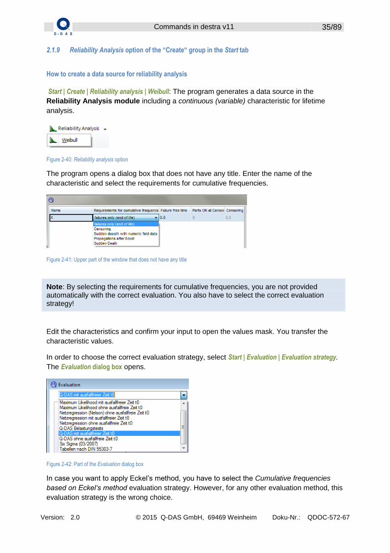
2.1.9 Reliability Analysis option of the “Create“ group in the Start tab
How to create a data source for reliability analysis
Start | Create | Reliability analysis | Weibull: The program generates a data source in the
Reliability Analysis module including a continuous (variable) characteristic for lifetime
analysis.
Figure 2-40: Reliability analysis option
The program opens a dialog box that does not have any title. Enter the name of the
characteristic and select the requirements for cumulative frequencies.
Figure 2-41: Upper part of the window that does not have any title
Note: By selecting the requirements for cumulative frequencies, you are not provided automatically with the correct evaluation. You also have to select the correct evaluation strategy!
Edit the characteristics and confirm your input to open the values mask. You transfer the
characteristic values.
In order to choose the correct evaluation strategy, select Start | Evaluation | Evaluation strategy.
The Evaluation dialog box opens.
Figure 2-42: Part of the Evaluation dialog box
In case you want to apply Eckel’s method, you have to select the Cumulative frequencies
based on Eckel‘s method evaluation strategy. However, for any other evaluation method, this
evaluation strategy is the wrong choice.

Commands in destra v11 36/89
Version: 2.0 © 2015 Q-DAS GmbH, 69469 Weinheim Doku-Nr.: QDOC-572-67
With or without failure-free time: In case the name of the evaluation strategy contains
“without failure-free time“, the respective evaluation strategy always applies a Weibull
distribution including two parameters – a scale and a shape parameter. All evaluation
strategies including “with failure-free time“ in their name always apply a Weibull distribution
with three parameters – a scale, a shape and an offset parameter.
Regression analysis or maximum likelihood: The term included in the name of the evaluation
strategy often refers to the estimation procedure estimating Weibull parameters. In case it
includes the word “regression“, it applies the method of least squares according to
Legendre/Gauss. Evaluation strategies containing “maximum likelihood“ apply the respective
estimation procedure developed by Sir R. A. Fisher.
Start the evaluation by activating the respective data source in the Project Explorer and
selecting Start | Evaluation | Test procedures.
2.2 “Evaluation“ group in the Start tab
Figure 2-43: “Evaluation“ group in the Start tab
2.2.1 Evaluation strategy option in the “Evaluation“ group of the Start tab
Start | Evaluation | Evaluation strategy: The Evaluation window opens. The contents of this
window depend on the currently active evaluation module and on the settings of the
respective evaluation strategy. Only users with administrator rights are able to change
an evaluation strategy or create a new one. Any other user just sees the settings but
cannot adjust them.
2.2.2 Standard procedure option in the “Evaluation“ group of the Start tab
Start | Evaluation | Standard procedure: This option evaluates all data sources of the following
modules.
Measurement System Analysis
o Type-1 to type-3 study, linearity, stability, kappa methods, signal detection
Sample Analysis
o 1-part and 5-part reports, machine capability analyses

Commands in destra v11 37/89
Version: 2.0 © 2015 Q-DAS GmbH, 69469 Weinheim Doku-Nr.: QDOC-572-67
Process Capability Analysis
o Process capability analyses, error log sheets, discrete characteristics
Reliability analysis
First you select the data source in the Project Explorer. Look at the title line of the program to see
the evaluation module of the data source. In case it is one of the modules listed above, select
Start | Evaluation | Standard procedure.
The program now appends a session node to the selected data source. It includes the initial
evaluation result.
Note: In case the data source already has a session node, you do not select the Standard procedure option again. Just click the session node to show the available window of results. If required, select the respective options from the Graphics and Results tabs to show further graphics and tables of results.
2.2.3 Distributions option in the “Evaluation“ group of the Start tab
Start | Evaluation | Distributions: This option opens the Distributions window showing the result of
the distributions the program selected automatically. The selection of distributions is normally
based on the set evaluation strategy and the program searches for the suitable distribution of
each characteristic automatically.
Note: When you open the window, the program does not show the distribution selected automatically based on the evaluation strategy since it shows Distributions (without offset) by default even though the Calculate best possible offset option might be activated in the evaluation strategy… We recommend you to close the Distributions window by clicking the Cancel button in order to avoid unintended changes of selected distributions.
Figure 2-44: Upper part of the Distributions window
The meaning of the single columns is explained in the following.
Commands in destra v11 38/89
Version: 2.0 © 2015 Q-DAS GmbH, 69469 Weinheim Doku-Nr.: QDOC-572-67
cal.: The distributions given in evaluation strategy are already activated (boxes are checked).
If required, you may activate further evaluation strategies manually; however, this only
affects the software temporarily.
curr.: The radio button of the distribution model selected automatically based on the
evaluation strategy is selected by default. You may select a different model – but only
temporarily.
Offset: In case there is an offset parameter available for the respective distribution, this
column shows its (estimated) value.
r100%: The “100% regression coefficient“ is a measure of goodness-of-fit between an
empirical distribution function (= “cumulative line“ of all characteristic values) and the
theoretical distribution function (mathematical distribution model). The closer the r-value to 1,
the better fits the theoretical distribution model with the characteristic values.
r25%: The “25% regression coefficient“ is a measure of conformance between the distribution
model and the first (0 to 25%) quartile or the fourth quartile (75% to 100%) of characteristic
values. Based on the Cpk calculation, the program decides which of the two quartiles will be
applied in each individual case. The software always selects the quartile lying next to the
critical specification limit.
²: This column indicates the chi-square test statistic of the chi-square goodness-of-fit test.
The smaller the test statistic, the better fits the model with the data – this is adequate
evidence for a good fit (theoretically expected and observed class frequencies match quite
well in case of small chi-square values). Attention: The test depends on the selected
classification model – if you select a different classification, you will have a different test
result…
Note: In case the Regression coefficient option is activated for the selection of distributions in the evaluation strategy, the program searches automatically for the best-suitable distribution model with the highest cumulative value = r100% + r25%.
2.2.4 Model f(x) | Correlation option in the “Evaluation“ group of the Start tab
Evaluation based on Pearson’s correlation
Start | Evaluation | Correlation | Pearson: This option starts a correlation analysis according to
Pearson to evaluate an existing data source.
Note: This option only evaluates data sources of the following modules.
Sample Analysis
Process Capability Analysis

Commands in destra v11 39/89
Version: 2.0 © 2015 Q-DAS GmbH, 69469 Weinheim Doku-Nr.: QDOC-572-67
Analysis of Regression / Variance
Select the data source you want to evaluate by click in the Project Explorer. The data source
has to contain at least two continuous (variable) characteristics with paired values.
Note: In case the number of values of the characteristics to be correlated differs, it is quite
likely that these characteristics do not include paired values.
In general, it is not reasonable to start a correlation analysis with characteristics whose
values are not paired. In such a case, you maybe should use a part ID or time stamp to filter
out characteristic values that can be paired.
The Selection of correlation variables dialog box opens.
Figure 2-45: Selection of correlation variables dialog box
Select the characteristics you want to correlate and confirm your choice. The Pearson dialog
box opens.
Figure 2-46: Pearson dialog box; the background colour of the results text depends on the actual value of the correlation coefficient r.

Commands in destra v11 40/89
Version: 2.0 © 2015 Q-DAS GmbH, 69469 Weinheim Doku-Nr.: QDOC-572-67
The Pearson dialog box contains a matrix of different graphics. The diagonal from the upper
left-hand corner to the lower right-hand corner shows the value plot of each characteristic.
The upper right-hand corner shows the scatter plot of all combinations of paired
characteristic values and the field in the lower left-hand corner displays the results. These
results include the following information.
r = Pearson’s correlation coefficient
a = Axis intercept of the best-fit line adapted to the pairs of values
b = Gradient of the best-fit line adapted to the pairs of values
Note: You may apply the options Correlation | Kendall and Correlation | Spearman in the same way as described above. Kendall’s and Spearman’s correlation calculate with ranks (ordinally scaled characteristic values); this is the reason why both types of analyses are often referred to as “distribution-free methods“. Compared to these methods, Pearson’s correlation coefficient, however, requires characteristics considered to be normally distributed random variables.
2.2.5 Model f(x) | Regression option in the “Evaluation“ group of the Start tab
Note: You cannot apply the content of additional data fields as factors in an analysis of
variance or as input quantities in a regression analysis.
How to evaluate simple regression
Start | Evaluation | Regression | Simple: This option starts a simple regression analysis to
evaluate a data source of the Analysis of Regression / Variance module containing at
least two continuous (variable) characteristics.
Select the data source you want to evaluate in the Project Explorer. Now select Start |
Evaluation | Model f(x) | Regression | Simple. The SelectGrid dialog box opens and shows the
Characteristics selection tab.
Figure 2-47: SelectGrid dialog box – Characteristics selection tab
This tab includes a table consisting of several columns.

Commands in destra v11 41/89
Version: 2.0 © 2015 Q-DAS GmbH, 69469 Weinheim Doku-Nr.: QDOC-572-67
Characteristic: Name of the characteristic
Characteristic type: Only shows variable characteristics of the data source.
N: Shows the number of values each characteristic contains.
Levels: Shows the number of numerically different characteristic values.
X: Select the characteristic you want to use as an input quantity.
Y: Select the characteristic you want to use as a response.
Activate column X to use a characteristic as an input quantity X and highlight column Y to
define a characteristic as a response Y.
Open the Model tab to select a model.
Figure 2-48: SelectGrid dialog box – Model tab
Factor | characteristic: Lists the characteristic you defined as an input quantity
before.
Model: Shows the description of all calculated models
Regression function: Shows the functional equations of all calculated models
Regression plot: Shows a preview of each calculated model
R²: Shows the coefficient of determination of each calculated model
R²adj: Shows the corrected coefficient of determination of each calculated model
Select the desired model by click, e.g. the model with the highest corrected coefficient of
determination. Confirm your choice by clicking OK. The program creates a new session node
below the selected data source. You append a result node to this session node; it includes
the result of the regression analysis. The software shows the evaluation of the model based
on the analysis of variance by default.
Tip: You may show further graphics or tables of results for the regression analysis by selecting the result node and opening e.g.
Graphics | Linear model | Model graphics | Regression plot
Graphics | Linear model | Parameter tables | Coefficients
Graphics | Linear model | Diagnostics | Residuals
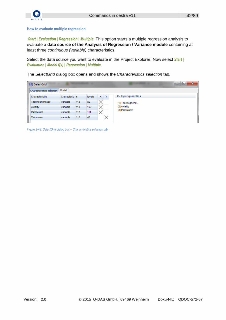
Commands in destra v11 42/89
Version: 2.0 © 2015 Q-DAS GmbH, 69469 Weinheim Doku-Nr.: QDOC-572-67
How to evaluate multiple regression
Start | Evaluation | Regression | Multiple: This option starts a multiple regression analysis to
evaluate a data source of the Analysis of Regression / Variance module containing at
least three continuous (variable) characteristics.
Select the data source you want to evaluate in the Project Explorer. Now select Start |
Evaluation | Model f(x) | Regression | Multiple.
The SelectGrid dialog box opens and shows the Characteristics selection tab.
Figure 2-49: SelectGrid dialog box – Characteristics selection tab

Commands in destra v11 43/89
Version: 2.0 © 2015 Q-DAS GmbH, 69469 Weinheim Doku-Nr.: QDOC-572-67
This tab includes a table consisting of several columns.
Characteristic: Name of the characteristic
Characteristic type: Only shows variable characteristics of the data source.
n: Shows the number of values each characteristic contains.
Levels: Shows the number of numerically different characteristic values.
X: Select the characteristic you want to use as an input quantity.
Y: Select the characteristic you want to use as a response.
Activate at least two characteristics in column X as influence quantities and one or several
characteristics as a response in column Y. Now you open the Model tab of this dialog box.
Note: After you selected two or more responses, the program calculates an own model for each response. Each model includes the same influence quantities X. The selected model you are going to adjust in the Model tab is initially the same for each response. If you want to select different model for the single responses, you can only do this after completing the current evaluation. You select Edit | Model selection.
After you opened the Model tab in the SelectGrid window, the program shows several buttons to
select a model.
Figure 2-50: SelectGrid dialog box – Model tab
Click on a button to select the corresponding model. Confirm your choice by clicking OK.
The program creates a new session node below the selected data source. You append a
result node for each response to this session node. The software shows the evaluation of the
model based on the analysis of variance by default.
Tip: You may show further graphics or tables of results for the regression analysis by selecting the result node and opening e.g.
Graphics | Linear model | Model graphics | Regression plot
Graphics | Linear model | Parameter tables | Coefficients
Graphics | Linear model | Diagnostics | Residuals

Commands in destra v11 44/89
Version: 2.0 © 2015 Q-DAS GmbH, 69469 Weinheim Doku-Nr.: QDOC-572-67
How to evaluate multivariate regression
Start | Evaluation | Regression | Multivariate: This option starts a multivariate regression analysis
to evaluate a data source of the Analysis of Regression / Variance module containing at
least three continuous (variable) characteristics.
Note: The characteristic values in a single line need to be paired values.
Select the data source you want to evaluate in the Project Explorer. Now select Start |
Evaluation | Model f(x) | Regression | Multivariate. The SelectGrid dialog box opens and shows the
Characteristics selection tab.
Figure 2-51: SelectGrid dialog box – Characteristics selection tab
This tab includes a table consisting of several columns.
Characteristic: Name of the characteristic
Characteristic type: Measuring scale of characteristics
n: Shows the number of values each characteristic contains.
Levels: Shows the number of different characteristic values.
X: Select the characteristic you want to use as an influence quantity.
Y: Select the characteristic you want to use as a response.
Activate two or more characteristics in column Y as a response and at least one characteristic
as a factor in column X. Now you open the Model tab of this dialog box.
Figure 2-52: SelectGrid dialog box – Model tab

Commands in destra v11 45/89
Version: 2.0 © 2015 Q-DAS GmbH, 69469 Weinheim Doku-Nr.: QDOC-572-67
Click on a button under “Standard models” to select the corresponding model. Confirm your
choice by clicking OK.
The program creates a new session node below the selected data source. This node is
called Reg by default. You may append several result nodes to this session node.
The Multivariate evaluation result node includes the Type III SS window showing the results of
the multivariate model evaluation. In addition, each response has an own result node
containing the results of simple or multiple regression analyses.
Figure 2-53: Type III SS window including the results of multivariate model evaluation
How to evaluate logistic regression
Start | Evaluation | Regression | Logistic: This option starts a logistic regression analysis to
evaluate a data source of the Analysis of Regression / Variance module. The data
source has to include at least
an ordinally scaled characteristic containing response values
a continuous (variable) characteristic containing factor values
a continuous characteristic containing frequencies.
Note: The characteristic values in a single line need to be paired values.
Select the data source you want to evaluate in the Project Explorer. Now select Start |
Evaluation | Model f(x) | Regression | Logistic. The SelectGrid dialog box opens and shows the
Characteristics selection tab.

Commands in destra v11 46/89
Version: 2.0 © 2015 Q-DAS GmbH, 69469 Weinheim Doku-Nr.: QDOC-572-67
Figure 2-54: SelectGrid dialog box – Characteristics selection tab
This tab includes a table consisting of several columns.
Characteristic: Name of the characteristic
Characteristic type: Measuring scale of characteristics
n: Shows the number of values each characteristic contains.
Levels: Shows the number of different characteristic values.
X: Select the characteristic you want to use as an influence quantity with fixed level
values (discrete, ordinally scaled factor).
V: Select the characteristic you want to use as a continuous (variable) influence
quantity.
Y: Select the characteristic you want to use as an ordinal response.
F: Select the characteristic you want to use to count frequencies.
Activate the respective characteristics in columns X to F and open the Model tab.
Click on a button under “Standard models” to select the corresponding model.
Figure 2-55: SelectGrid dialog box – Model tab
Open the Options tab.
Figure 2-56: SelectGrid dialog box –Options tab

Commands in destra v11 47/89
Version: 2.0 © 2015 Q-DAS GmbH, 69469 Weinheim Doku-Nr.: QDOC-572-67
Select the value of response Y you want to consider as an event. Confirm your choice by
clicking OK.
The program creates a session node. It is called LOG by default. A result node is appended
to the node. It has the name of the response. Click on the new result node and the
Summary/input window opens by default (even though you will not assume it from its name,
it really contains results).
Tip: You may show further graphics or tables of results for the logistic regression analysis by selecting the result node and opening e.g.
Graphics | Linear model | Parameter tables | Model information
Graphics | Linear model | Model graphics | Predicted probability
Graphics | Linear model | Model graphics | Odds ratios
Graphics | Linear model | Model graphics | ROC
2.2.6 Model f(x) | Analysis of Variance option in the “Evaluation“ group of the Start tab
Note: You cannot apply the content of additional data fields as factors in an analysis of variance or as input quantities in a regression analysis. The manual import of only few additional data fields is currently a poor function; it is not worth showing. Moreover, the manual import is rather annoying. Who wants to import additional data for 20 characteristics in the age of Big Data? We will seek a new user-friendly solution in the future.
How to evaluate simple or multiple analysis of variance (ANOVA)
Start | Evaluation | Model f(x) | Analysis of variance | ANOVA: This option starts a simple analysis
of variance including a data source from the Analysis of Regression / Variance module.
The data source has to contain at least a continuous (variable) characteristic and a discrete
(ordinal) characteristic. Please always consider that each line refers to the values of a
specific characteristic.
Select the respective data source in the Project Explorer and click Start | Evaluation | Model f(x) |
Analysis of variance | ANOVA.
The SelectGrid dialog box opens and shows the Characteristics selection tab. This tab includes a
table consisting of several columns.
Characteristic: Name of the characteristic

Commands in destra v11 48/89
Version: 2.0 © 2015 Q-DAS GmbH, 69469 Weinheim Doku-Nr.: QDOC-572-67
Characteristic type: Measuring scale of characteristics
n: Shows the number of values each characteristic contains.
Levels: Shows the number of numerically different characteristic values.
X: Select the characteristic you want to use as a factor with a fixed level value.
Z: Select the characteristic you want to use as a factor with random level values
Y: Select the characteristic you want to use as a response.
You clicked on column X of characteristic X to use this characteristic as a factor with fixed
level values in the following example. In addition, you clicked on column Y of characteristic Y
to use this characteristic as a response.
Figure 2-57: SelectGrid dialog box – Characteristics selection tab
Open the Model tab to select a model. Choose the respective model by click and confirm your
choice by clicking OK.
Figure 2-58: SelectGrid dialog box – Model tab
After you confirmed your choice, the program appends a session node called GLM to the
evaluated data source. In addition, this session node includes a result node with the name of
the evaluated response. Select this node to see the evaluation result of the analysis of
variance.
Tip: You may show further graphics or tables of results for the current analysis of variance by selecting the result node and opening e.g.
Graphics | Linear model | Parameter tables | Model evaluation
Graphics | Linear model | Parameter tables | LS-Means
Graphics | Linear model | Parameter tables | Pairwise differences
Graphics | Linear model | Parameter tables | Expected mean squares

Commands in destra v11 49/89
Version: 2.0 © 2015 Q-DAS GmbH, 69469 Weinheim Doku-Nr.: QDOC-572-67
Graphics | Linear model | Model graphics | Main effect plots
Graphics | Linear model | Diagnostics | Residuals
How to evaluate an analysis of covariance (ANCOVA)
Start | Evaluation | Model f(x) | Analysis of variance | ANCOVA: This option starts an analysis of
covariance including a data source from the Analysis of Regression / Variance module.
The data source has to contain at least two continuous (variable) characteristics and a
discrete (ordinal) characteristic. Please always consider that each line refers to the values of
a specific characteristic.
Select the respective data source in the Project Explorer and click Start | Evaluation | Model f(x) |
Analysis of variance | ANCOVA.
The SelectGrid dialog box opens and shows the Characteristics selection tab. This tab includes a
table consisting of several columns.
Characteristic: Name of the characteristic
Characteristic type: Measuring scale of characteristics
n: Shows the number of values each characteristic contains.
Levels: Shows the number of numerically different characteristic values.
X: Select the characteristic you want to use as a factor with a fixed level value.
V: Select a continuous (variable) characteristic you want to use as a covariable.
Y: Select a continuous (variable) characteristic you want to use as a response.
The following figure shows an example of model selection. The ordinal characteristic A was
selected as a factor with fixed levels. The continuous (variable) characteristic B serves as a
covariable and the continuous (variable) characteristic Y is the response. Now you open the
Model tab.
Figure 2-59: SelectGrid dialog box – Characteristics selection tab
The Model tab in the SelectGrid dialog box includes several buttons for model selection. Select
the respective standard model and confirm your choice.

Commands in destra v11 50/89
Version: 2.0 © 2015 Q-DAS GmbH, 69469 Weinheim Doku-Nr.: QDOC-572-67
Figure 2-60: SelectGrid dialog box – Model tab
After you confirmed the respective model, the Type III (adj.) dialog box opens showing the
model’s evaluation results of the analysis of variance.
The program appends a session node called GLM to the evaluated data source in the Project
Explorer. In addition, this session node includes a result node with the name of the evaluated
response. Select this node to see the evaluation result of the analysis of variance.
Tip: You may show further graphics or tables of results for the current analysis of variance by selecting the result node and opening e.g.
Graphics | Linear model | Parameter tables | Model evaluation
Graphics | Linear model | Parameter tables | LS-Means
Graphics | Linear model | Parameter tables | Pairwise differences
Graphics | Linear model | Parameter tables | Expected mean squares
Graphics | Linear model | Model graphics | Main effect plots
Graphics | Linear model | Diagnostics | Residuals
How to evaluate a multivariate analysis of variance (MANOVA)
Start | Evaluation | Model f(x) | Analysis of variance | MANOVA: This option starts a multivariate
analysis of variance including a data source from the Analysis of Regression /
Variance module. The data source has to contain at least two continuous (variable)
characteristics and a discrete (ordinal) characteristic.
Note: Please always consider that each line refers to the values of a specific characteristic.

Commands in destra v11 51/89
Version: 2.0 © 2015 Q-DAS GmbH, 69469 Weinheim Doku-Nr.: QDOC-572-67
Select the respective data source in the Project Explorer and click Start | Evaluation | Model f(x) |
Analysis of variance | MANOVA.
The SelectGrid dialog box opens and shows the Characteristics selection tab. This tab includes a
table consisting of several columns.
Characteristic: Name of the characteristic
Characteristic type: Measuring scale of characteristics
n: Shows the number of values each characteristic contains.
Levels: Shows the number of numerically different characteristic values.
X: Select the characteristic you want to use as a factor with a fixed level value.
V: Select a characteristic you want to use as a continuous (variable) covariable.
Y: Select a characteristic you want to use as a response.
Figure 2-61: SelectGrid dialog box – Characteristics selection tab
Select the respective characteristics as response or factor and open the Model tab to select
a model.
Figure 2-62: SelectGrid dialog box – Model tab
The Model tab in the SelectGrid dialog box includes several buttons for model selection. Select
the respective standard model and confirm your choice.
Tip: Activate the Extended radio button under “Input“ to display the input field under “Advanced model input“. Use this field to modify the formula of the model you selected before.
Symbol Meaning Example
+ Additive main effects A + B
* Multiplicative interaction A + B + A * B

Commands in destra v11 52/89
Version: 2.0 © 2015 Q-DAS GmbH, 69469 Weinheim Doku-Nr.: QDOC-572-67
() Nested factors A + B(A)
[] Crossed factors A + B + [A*B](C) Table 2-4: Symbols used in the advanced model input
The program appends a session node called GLM to the evaluated data source in the Project
Explorer. In addition, this session node includes a result node with the name of the evaluated
response.
Tip: You may show further graphics or tables of results for the current analysis of variance by selecting the result node and opening e.g.
Graphics | Linear model | Parameter tables | Model evaluation
Graphics | Linear model | Parameter tables | LS-Means
Graphics | Linear model | Parameter tables | Pairwise differences
Graphics | Linear model | Parameter tables | Expected mean squares
Graphics | Linear model | Model graphics | Main effect plots
Graphics | Linear model | Diagnostics | Residuals
How to evaluate repeated measures ANOVA
Start | Evaluation | Model f(x) | Analysis of variance | Repeated measures: This option starts a
repeated measures ANOVA including a data source from the Analysis of Regression /
Variance module.
Note: Please always consider that each line refers to the values of a specific characteristic.
Select the respective data source in the Project Explorer and click Start | Evaluation | Model f(x) |
Analysis of variance | Repeated measures.
The SelectGrid dialog box opens and shows the Characteristics selection tab. This tab includes a
table consisting of several columns.
Characteristic: Name of the characteristic
Characteristic type: Measuring scale of characteristics
n: Shows the number of values each characteristic contains.
Levels: Shows the number of numerically different characteristic values.
X: Select the characteristic you want to use as a factor with fixed level values.
V: Select a characteristic you want to use as a covariable.
R: Select a characteristic you want to use as a repeated measure variable.
Y: Select a characteristic you want to use as a response.

Commands in destra v11 53/89
Version: 2.0 © 2015 Q-DAS GmbH, 69469 Weinheim Doku-Nr.: QDOC-572-67
The following figure shows an exemplary selection of characteristics in the SelectGrid dialog
box.
Figure 2-63: SelectGrid dialog box – Characteristics selection tab; here you select the characteristics for factors and responses in column X (factor with fixed level values), V (covariable), R (repeated measure) and Y (response)
After you defined factors and responses, you open the Model tab.
Figure 2-64: SelectGrid dialog box –Model tab; click the respective button to select a model
The Model tab opens. It includes several buttons for model selection under “Standard models“.
Select the respective standard model and confirm your choice. The program appends a
session node called GLM to the evaluated data source in the Project Explorer. In addition,
this session node includes a result node with the name of the evaluated response.
Select the result node to show the evaluation results of repeated measures ANOVA.
Tip: You may show further graphics or tables of results for the current analysis of variance by selecting the result node and opening e.g.
Graphics | Linear model | Parameter tables | Mauchlys tests
Graphics | Linear model | Parameter tables | Type I SS

Commands in destra v11 54/89
Version: 2.0 © 2015 Q-DAS GmbH, 69469 Weinheim Doku-Nr.: QDOC-572-67
2.2.7 Design option in the “Evaluation“ group of the Start tab
Start | Evaluation | Design: This option evaluates the available design of experiments. First you
select a data source including an experimental design (including response values!) in the
Project Explorer.
Note: The design of experiments has to be created in destra. You cannot import an experimental design from any other software product.
This option generates a new session node called DOE in the Project Explorer. In addition,
the program appends an own result node to the session node for each response available in
the design of experiments. The descriptions of the result nodes refer to the names of the
responses.
Tip: The program provides the Table of effects and Model selection options in the “Model” group of the Edit tab. They specifically apply to regression and design models. Use these options to delete significant model terms from the regression model or to adapt models to user-specific requirements.
2.2.8 Test procedures option in the “Evaluation“ group of the Start tab
Test procedures for continuous characteristic values
Figure 2-65: Test procedures | Continuous values
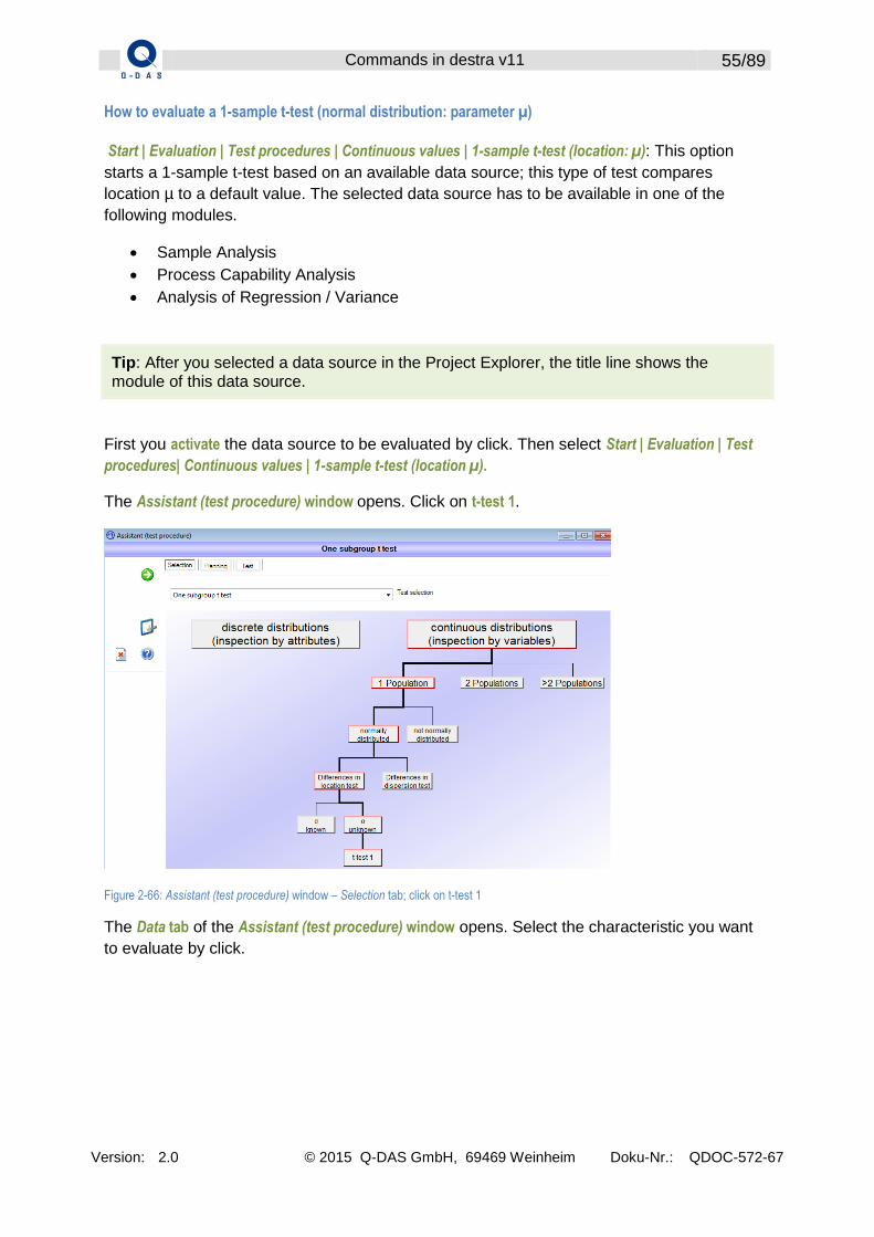
Commands in destra v11 55/89
Version: 2.0 © 2015 Q-DAS GmbH, 69469 Weinheim Doku-Nr.: QDOC-572-67
How to evaluate a 1-sample t-test (normal distribution: parameter µ)
Start | Evaluation | Test procedures | Continuous values | 1-sample t-test (location: µ): This option
starts a 1-sample t-test based on an available data source; this type of test compares
location µ to a default value. The selected data source has to be available in one of the
following modules.
Sample Analysis
Process Capability Analysis
Analysis of Regression / Variance
Tip: After you selected a data source in the Project Explorer, the title line shows the module of this data source.
First you activate the data source to be evaluated by click. Then select Start | Evaluation | Test
procedures| Continuous values | 1-sample t-test (location µ).
The Assistant (test procedure) window opens. Click on t-test 1.
Figure 2-66: Assistant (test procedure) window – Selection tab; click on t-test 1
The Data tab of the Assistant (test procedure) window opens. Select the characteristic you want
to evaluate by click.

Commands in destra v11 56/89
Version: 2.0 © 2015 Q-DAS GmbH, 69469 Weinheim Doku-Nr.: QDOC-572-67
Figure 2-67: Assistant (test procedure) window – Data tab; select the continuous (variable) characteristic you want to evaluate by clicking on the active column in the respective line
Click the Next button (green circle with the arrow pointing to the right).
Figure 2-68: Assistant (test procedure) window – Planning tab; take the next step by clicking the Next button (green circle with arrow to the right)
Take the next step by clicking the Next button. The Test tab opens.

Commands in destra v11 57/89
Version: 2.0 © 2015 Q-DAS GmbH, 69469 Weinheim Doku-Nr.: QDOC-572-67
Figure 2-69: Assistant (test procedure) window – Test tab; enter a target value for the average µ0, activate the hypothesis to be tested and click the „calculator“ icon to calculate results
First you enter the specified value µ0 and select the hypothesis to be tested. Now you click the
“calculator“ icon on the left-hand side of the window (not in the ribbon!).
The window shows the test result. You can find the Assistant (test procedures) window by
default in the Test Stat session node of the Project Explorer. The program appended the
session node automatically to the evaluated data source.
How to evaluate a 1-sample chi-squared test (normal distribution: parameter sigma)
Start | Evaluation | Test procedures | Continuous values | 1-sample χ²-test (variance): This option starts
a chi-squared test based on an available data source; this type of test compares variance
sigma to a default value. The selected data source has to be available in one of the following
modules.
Sample Analysis
Process Capability Analysis
Analysis of Regression / Variance
Tip: After you selected a data source in the Project Explorer, the title line shows the module of this data source.
First you activate the data source to be evaluated by click. Then select Start | Evaluation | Test
procedures| Continuous values | 1-sample χ²-test (variance).

Commands in destra v11 58/89
Version: 2.0 © 2015 Q-DAS GmbH, 69469 Weinheim Doku-Nr.: QDOC-572-67
The Assistant (test procedure) window opens. Click on χ²-test.
Figure 2-70: Assistant (test procedure) window – Selection tab; click on χ²-test
The Data tab of the Assistant (test procedure) window opens. Select the characteristic you want
to evaluate by click.
Figure 2-71: Assistant (test procedure) window – Data tab; select the characteristic you want to evaluate by clicking on the active column in the respective line
Click the Next button (green circle with the arrow pointing to the right) twice since you do not
have to make any adjustments in the Planning tab. The Test tab opens. First you enter the
specified value (target value) serving as a default value for the standard deviation 0 and select
the hypothesis to be tested. Now you click the “calculator“ icon on the left-hand side of the
window (not in the ribbon!).

Commands in destra v11 59/89
Version: 2.0 © 2015 Q-DAS GmbH, 69469 Weinheim Doku-Nr.: QDOC-572-67
Figure 2-72: Assistant (test procedure) window – Test tab; enter a target value for the standard deviation, activate the hypothesis to be tested and click the „calculator“ icon
The program created a session node automatically in the Project Explorer. This node is referred
to as Test Stat by default. The program always appends the session node to the evaluated
data source.
How to evaluate the Wilcoxon test (median)
Start | Evaluation | Test procedures | Continuous values | 1-sample Wilcoxon test (location: median):
This option starts a 1-sample Wilcoxon test based on an available data source; this type of
test compares the median of a population to a default value. The selected data source has to
be available in one of the following modules.
Sample Analysis
Process Capability Analysis
Analysis of Regression / Variance
First you activate the data source to be evaluated by click. Then select Start | Evaluation | Test
procedures| Continuous values | 1-sample Wilcoxon test (location: median).
The Assistant (test procedure) window opens. Click on 1-sample Wilcoxon signed-rank test.

Commands in destra v11 60/89
Version: 2.0 © 2015 Q-DAS GmbH, 69469 Weinheim Doku-Nr.: QDOC-572-67
Figure 2-73: Assistant (test procedure) window – Selection tab; click on 1-sample Wilcoxon signed-rank test
The Data tab of the Assistant (test procedure) window opens. Select the characteristic you want
to evaluate by click.
Figure 2-74: Assistant (test procedure) window – Data tab; select the characteristic you want to evaluate by clicking on the active column in the respective line
Click the Next button (green circle with the arrow pointing to the right). The Test tab opens. First
you enter the target value of the median and select the hypothesis to be tested. Now you click
the “calculator“ icon on the left-hand side of the window (not in the ribbon!).

Commands in destra v11 61/89
Version: 2.0 © 2015 Q-DAS GmbH, 69469 Weinheim Doku-Nr.: QDOC-572-67
Figure 2-75: Assistant (test procedure) window – Test tab; enter a target value for the median, activate the hypothesis to be tested and click the ”calculator“ icon to calculate results
The program created a session node automatically in the Project Explorer. This node is referred
to as Test Stat by default. The program always appends the session node to the evaluated
data source.
How to evaluate the 2-sample t-test (normal distribution: parameter µ, independent samples)
Start | Evaluation | Test procedures | Continuous values | 2-sample t-test (location: µ): This option
starts a 2-sample t-test based on an available data source; this type of test compares the
locations µ of two populations. The selected data source has to be available in one of the
following modules.
Sample Analysis
Process Capability Analysis
Analysis of Regression / Variance
First you activate the data source to be evaluated by click. Then select Start | Evaluation | Test
procedures| Continuous values | 2-sample t-test (location: µ).
The Assistant (test procedure) window opens. Click on t-test 2 in the Selection tab.

Commands in destra v11 62/89
Version: 2.0 © 2015 Q-DAS GmbH, 69469 Weinheim Doku-Nr.: QDOC-572-67
Figure 2-76: Assistant (test procedure) window – Selection tab; click on t-test 2
The Data tab of the Assistant (test procedure) window opens. Select the characteristics you want
to compare by click on the active column. The following figure shows an example.
Figure 2-77: Assistant (test procedure) window – Data tab; select the characteristics you want to compare by clicking on the active column in the respective two lines
Click the Next button (green circle with the arrow pointing to the right). The Planning tab opens
but you do not have to make any adjustments here. Click the Next button once again to open
the Test tab. First you select the hypothesis to be tested. Now you click the “calculator“ icon on
the left-hand side of the window (not in the ribbon!).

Commands in destra v11 63/89
Version: 2.0 © 2015 Q-DAS GmbH, 69469 Weinheim Doku-Nr.: QDOC-572-67
Figure 2-78: Assistant (test procedure) window – Test tab; activate the hypothesis to be tested and click the “calculator“ icon to calculate results
The program created a session node automatically in the Project Explorer. This node is referred
to as Test Stat by default. The program always appends the session node to the evaluated
data source.
How to evaluate a 2-sample F-test (normal distribution: sigma)
Start | Evaluation | Test procedures | Continuous values | 2-sample F-test: This option starts a 2-
sample F-test; it tests the equality of variances σ of two populations. The selected data
source has to be available in one of the following modules.
Sample Analysis
Process Capability Analysis
Analysis of Regression / Variance
First you activate the data source to be evaluated by click. Then select Start | Evaluation | Test
procedures| Continuous values | 2-sample F-test.
The Assistant (test procedure) window opens. Click on F-test in the Selection tab.

Commands in destra v11 64/89
Version: 2.0 © 2015 Q-DAS GmbH, 69469 Weinheim Doku-Nr.: QDOC-572-67
Figure 2-79: Assistant (test procedure) window – Selection tab; click on F-test
The Data tab of the Assistant (test procedure) window opens. Select the characteristics you want
to compare by click on the active column.
Figure 2-80: Assistant (test procedure) window – Data tab; select the characteristics you want to compare by clicking on the active column in the respective two lines
Click the Next button (green circle with the arrow pointing to the right). The Planning tab opens
but you do not have to make any adjustments here. Click the Next button once again to open
the Test tab. First you select the hypothesis to be tested. Now you click the “calculator“ icon on
the left-hand side of the window (not in the ribbon!).

Commands in destra v11 65/89
Version: 2.0 © 2015 Q-DAS GmbH, 69469 Weinheim Doku-Nr.: QDOC-572-67
Figure 2-81: Assistant (test procedure) window – Test tab; activate the hypothesis to be tested and click the ”calculator“ icon to calculate results
The program created a session node automatically in the Project Explorer. This node is referred
to as Test Stat by default. The program always appends the session node to the evaluated
data source. The window shown above is the content of this session node.
How to evaluate a 2-sample Mann-Whitnex U-test (median)
Start | Evaluation | Test procedures | Continuous values | 2-sample Mann-Whitnex test (location:
median): This option starts a 2-sample Mann-Whitnex U-test; it tests the equality of medians
of two populations. The selected data source has to be available in one of the following
modules.
Sample Analysis
Process Capability Analysis
Analysis of Regression / Variance
First you activate the data source to be evaluated by click. Then select Start | Evaluation | Test
procedures| Continuous values | 2-sample Mann-Whitnex test (location: median).
The Assistant (test procedure) window opens. Click on U-test in the Selection tab.

Commands in destra v11 66/89
Version: 2.0 © 2015 Q-DAS GmbH, 69469 Weinheim Doku-Nr.: QDOC-572-67
Figure 2-82: Assistant (test procedure) window – Selection tab; click on U-test
The Data tab of the Assistant (test procedure) window opens. Select the characteristics you want
to compare by click on the active column.
Figure 2-83: Assistant (test procedure) window – Data tab; select the characteristics you want to compare by clicking on the active column in the respective two lines
Click the Next button (green circle with the arrow pointing to the right). The Test tab opens. First
you select the hypothesis to be tested. Now you click the “calculator“ icon on the left-hand side
of the window (not in the ribbon!).

Commands in destra v11 67/89
Version: 2.0 © 2015 Q-DAS GmbH, 69469 Weinheim Doku-Nr.: QDOC-572-67
Figure 2-84: Assistant (test procedure) window – Test tab; activate the hypothesis to be tested and click the ”calculator“ icon to calculate results
The program created a session node automatically in the Project Explorer. This node is referred
to as Test Stat by default. The program always appends the session node to the evaluated
data source.
How to evaluate a 2-sample rank test for dispersions (dispersion)
Start | Evaluation | Test procedures | Continuous values | 2-sample rank test for dispersions
(dispersion): This option starts a 2-sample rank test for dispersions based on an available data
source; it tests the equality of medians of two populations. The selected data source has to
be available in one of the following modules.
Sample Analysis
Process Capability Analysis
Analysis of Regression / Variance
First you activate the data source to be evaluated by click. Then select Start | Evaluation | Test
procedures| Continuous values | 2-sample rank test for dispersions (dispersion).
The Assistant (test procedure) window opens. Click on Siegel Turkey test in the Selection tab.
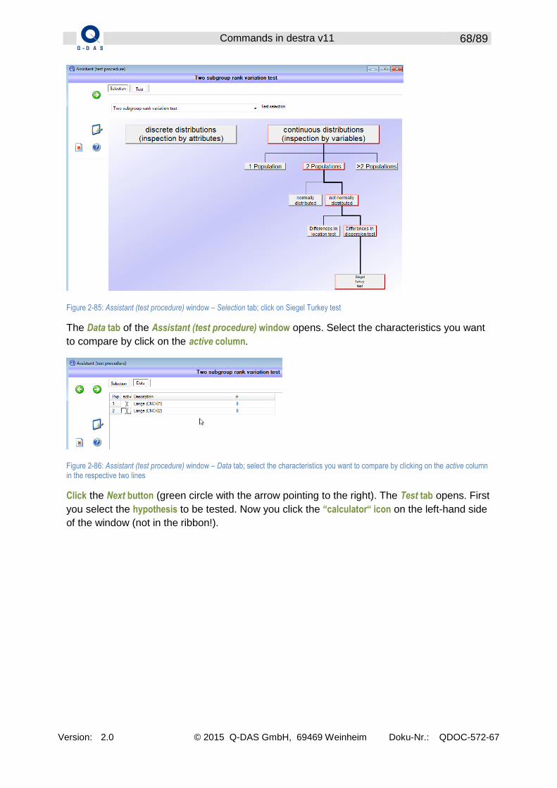
Commands in destra v11 68/89
Version: 2.0 © 2015 Q-DAS GmbH, 69469 Weinheim Doku-Nr.: QDOC-572-67
Figure 2-85: Assistant (test procedure) window – Selection tab; click on Siegel Turkey test
The Data tab of the Assistant (test procedure) window opens. Select the characteristics you want
to compare by click on the active column.
Figure 2-86: Assistant (test procedure) window – Data tab; select the characteristics you want to compare by clicking on the active column in the respective two lines
Click the Next button (green circle with the arrow pointing to the right). The Test tab opens. First
you select the hypothesis to be tested. Now you click the “calculator“ icon on the left-hand side
of the window (not in the ribbon!).

Commands in destra v11 69/89
Version: 2.0 © 2015 Q-DAS GmbH, 69469 Weinheim Doku-Nr.: QDOC-572-67
Figure 2-87: Assistant (test procedure) window – Test tab; activate the hypothesis to be tested and click the ”calculator“ icon to calculate results
The program created a session node automatically in the Project Explorer. This node is referred
to as Test Stat by default. The program always appends the session node to the evaluated
data source.
How to evaluate a simple analysis of variance (normal distribution: parameter µ)
Start | Evaluation | Test procedures | Continuous values | k-sample analysis of variance (location: µ):
This option starts a simple analysis of variance based on an available data source; it tests
the homogeneity of locations of k populations. The selected data source has to be available
in one of the following modules.
Sample Analysis
Process Capability Analysis
Analysis of Regression / Variance
First you activate the data source to be evaluated by click. Then select Start | Evaluation | Test
procedures| Continuous values | k-sample analysis of variance (location: µ).
The Assistant (test procedure) window opens. Click on One-way ANOVA in the Selection tab.
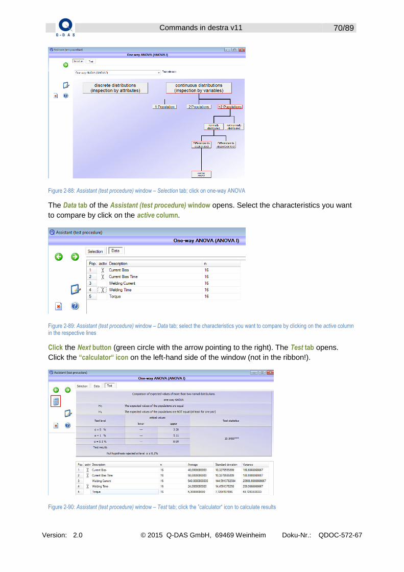
Commands in destra v11 70/89
Version: 2.0 © 2015 Q-DAS GmbH, 69469 Weinheim Doku-Nr.: QDOC-572-67
Figure 2-88: Assistant (test procedure) window – Selection tab; click on one-way ANOVA
The Data tab of the Assistant (test procedure) window opens. Select the characteristics you want
to compare by click on the active column.
Figure 2-89: Assistant (test procedure) window – Data tab; select the characteristics you want to compare by clicking on the active column in the respective lines
Click the Next button (green circle with the arrow pointing to the right). The Test tab opens.
Click the “calculator“ icon on the left-hand side of the window (not in the ribbon!).
Figure 2-90: Assistant (test procedure) window – Test tab; click the ”calculator“ icon to calculate results
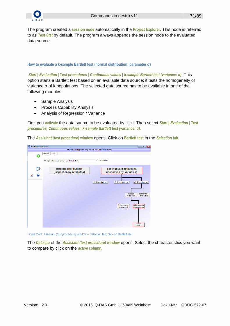
Commands in destra v11 71/89
Version: 2.0 © 2015 Q-DAS GmbH, 69469 Weinheim Doku-Nr.: QDOC-572-67
The program created a session node automatically in the Project Explorer. This node is referred
to as Test Stat by default. The program always appends the session node to the evaluated
data source.
How to evaluate a k-sample Bartlett test (normal distribution: parameter σ)
Start | Evaluation | Test procedures | Continuous values | k-sample Bartlett test (variance: σ): This
option starts a Bartlett test based on an available data source; it tests the homogeneity of
variance σ of k populations. The selected data source has to be available in one of the
following modules.
Sample Analysis
Process Capability Analysis
Analysis of Regression / Variance
First you activate the data source to be evaluated by click. Then select Start | Evaluation | Test
procedures| Continuous values | k-sample Bartlett test (variance: σ).
The Assistant (test procedure) window opens. Click on Bartlett test in the Selection tab.
Figure 2-91: Assistant (test procedure) window – Selection tab; click on Bartlett test
The Data tab of the Assistant (test procedure) window opens. Select the characteristics you want
to compare by click on the active column.

Commands in destra v11 72/89
Version: 2.0 © 2015 Q-DAS GmbH, 69469 Weinheim Doku-Nr.: QDOC-572-67
Figure 2-92: Assistant (test procedure) window – Data tab; select the characteristics you want to compare by clicking on the active column in the respective lines
Click the Next button (green circle with the arrow pointing to the right). The Test tab opens.
Click the “calculator“ icon on the left-hand side of the window (not in the ribbon!).
Figure 2-93: Assistant (test procedure) window – Test tab; click the ”calculator“ icon to calculate results
The program created a session node automatically in the Project Explorer. This node is referred
to as Test Stat by default. The program always appends the session node to the evaluated
data source.
Howe to evaluate a k-sample Kruskal-Wallis test (location: median)
Start | Evaluation | Test procedures | Continuous values | k-sample Kruskal-Wallis test (location:
median): This option starts a Kruskal-Wallis test based on an available data source; it tests
the homogeneity of location of k populations. The selected data source has to be available in
one of the following modules.
Sample Analysis
Process Capability Analysis
Analysis of Regression / Variance
First you activate the data source to be evaluated by click. Then select Start | Evaluation | Test
procedures| Continuous values | k-sample Kruskal-Wallis test (location: median).
The Assistant (test procedure) window opens. Click on H-test Kruskal-Wallis in the Selection tab.

Commands in destra v11 73/89
Version: 2.0 © 2015 Q-DAS GmbH, 69469 Weinheim Doku-Nr.: QDOC-572-67
Figure 2-94: Assistant (test procedure) window – Selection tab; click on H-test Kruskal-Wallis
The Data tab of the Assistant (test procedure) window opens. Select the characteristics you want
to compare by click on the active column.
Figure 2-95: Assistant (test procedure) window – Data tab; select the characteristics you want to compare by clicking on the active column in the respective lines
Click the Next button (green circle with the arrow pointing to the right). The Test tab opens.
Click the “calculator“ icon on the left-hand side of the window (not in the ribbon!).
Figure 2-96: Assistant (test procedure) window – Test tab; click the ”calculator“ icon to calculate results

Commands in destra v11 74/89
Version: 2.0 © 2015 Q-DAS GmbH, 69469 Weinheim Doku-Nr.: QDOC-572-67
The program created a session node automatically in the Project Explorer. This node is referred
to as Test Stat by default. The program always appends the session node to the evaluated
data source.
How to evaluate a k-sample Levene test (variance)
Start | Evaluation | Test procedures | Continuous values | k-sample Levene test (variance): This option
starts a Levene test based on an available data source; it tests the homogeneity of variance
of k populations. The selected data source has to be available in one of the following
modules.
Sample Analysis
Process Capability Analysis
Analysis of Regression / Variance
First you activate the data source to be evaluated by click. Then select Start | Evaluation | Test
procedures| Continuous values | k-sample Levene test (variance).
The Assistant (test procedure) window opens. Click on Levene test in the Selection tab.
Figure 2-97: Assistant (test procedure) window – Selection tab; click on Levene test
The Data tab of the Assistant (test procedure) window opens. Select the characteristics you want
to compare by click on the active column.

Commands in destra v11 75/89
Version: 2.0 © 2015 Q-DAS GmbH, 69469 Weinheim Doku-Nr.: QDOC-572-67
Figure 2-98: Assistant (test procedure) window – Data tab; select the characteristics you want to compare by clicking on the active column in the respective lines
Click the Next button (green circle with the arrow pointing to the right). The Test tab opens.
Click the “calculator“ icon on the left-hand side of the window (not in the ribbon!).
The program created a session node automatically in the Project Explorer. This node is referred
to as Test Stat by default. The program always appends the session node to the evaluated
data source.

Commands in destra v11 76/89
Version: 2.0 © 2015 Q-DAS GmbH, 69469 Weinheim Doku-Nr.: QDOC-572-67
Test procedures for discrete values
Figure 2-99: Test procedures | Discrete values
How to evaluate a 1-sample µ-test (Poisson distribution: parameter µ)
Start | Evaluation | Test procedures | Discrete values | 1-sample test – events per unit (PD): This option
starts a one-sample test based on an available data source; it compares parameter µ of a
population based on a Poisson distribution to a default value. The selected data source has
to be available in one of the following modules.
Process Capability Analysis
Analysis of Regression / Variance
First you activate the data source to be evaluated by click. Then select Start | Evaluation | Test
procedures| Discrete values | 1-sample test – events per unit (PD).
The Assistant (test procedure) window opens. Click on p-test (PD) 1 in the Selection tab.
Figure 2-100: Assistant (test procedure) window – Selection tab; click on Levene test

Commands in destra v11 77/89
Version: 2.0 © 2015 Q-DAS GmbH, 69469 Weinheim Doku-Nr.: QDOC-572-67
The Data tab of the Assistant (test procedure) window opens. Select the characteristic you want
to check by click on the active column.
Figure 2-101: Assistant (test procedure) window – Data tab; select the characteristic you want to check by clicking on the active column in the respective line
Click the Next button (green circle with the arrow pointing to the right). The Planning tab opens
but you do not have to make any adjustments here. Click the Next button once again to open
the Test tab. First you enter the target value for parameter µ0 of the population based on a
Poisson distribution. Then you select the hypothesis to be tested and click the “calculator“ icon
on the left-hand side of the window (not in the ribbon!) to gain the test results.
Figure 2-102: Assistant (test procedure) window – Test tab; enter a default value for parameter µ0, activate the hypothesis to be tested and click the ”calculator“ icon to calculate results
The program created a session node automatically in the Project Explorer. This node is referred
to as Test Stat by default. The program always appends the session node to the evaluated
data source.

Commands in destra v11 78/89
Version: 2.0 © 2015 Q-DAS GmbH, 69469 Weinheim Doku-Nr.: QDOC-572-67
How to evaluate a 1-sample p-test (binomial distribution: parameter p)
Start | Evaluation | Test procedures | Discrete values | 1-sample test – proportion (BD): This option
starts a one-sample p-test based on an available data source; it compares parameter p of a
binomially distributed population to a default value p0. The selected data source has to be
available in one of the following modules.
Process Capability Analysis
Analysis of Regression / Variance
First you activate the data source to be evaluated by click. Then select Start | Evaluation | Test
procedures| Discrete values | 1-sample test – proportion (BD).
The Assistant (test procedure) window opens. Click on p-test (BD) 1 in the Selection tab.
Figure 2-103: Assistant (test procedure) window – Selection tab; click on p-test (BD) 1
The Data tab of the Assistant (test procedure) window opens. Select the characteristic you want
to check by click on the active column.
Figure 2-104: Assistant (test procedure) window – Data tab; select the characteristic you want to check by clicking on the active column in the respective line
Click the Next button (green circle with the arrow pointing to the right). The Planning tab opens
but you do not have to make any adjustments here. Click the Next button once again to open
the Test tab. First you enter the default value p0 of the population. Then you select the
hypothesis to be tested and click the “calculator“ icon on the left-hand side of the window (not
in the ribbon!) to start the evaluation.

Commands in destra v11 79/89
Version: 2.0 © 2015 Q-DAS GmbH, 69469 Weinheim Doku-Nr.: QDOC-572-67
Figure 2-105: Assistant (test procedure) window – Test tab; enter a default value p0, activate the hypothesis to be tested and click the ”calculator“ icon to calculate results
The program created a session node automatically in the Project Explorer. This node is referred
to as Test Stat by default. The program always appends the session node to the evaluated
data source.
How to evaluate a 2-sample µ-test (Poisson distribution: parameter µ)
Start | Evaluation | Test procedures | Discrete values | 2-sample test – events per unit (PD): This option
starts a 2-sample test based on an available data source; it test the homogeneity of µ of two
populations. The selected data source has to be available in one of the following modules.
Process Capability Analysis
Analysis of Regression / Variance
First you activate the data source to be evaluated by click. Then select Start | Evaluation | Test
procedures| Discrete values | 2-sample test – events per unit (PD).
The Assistant (test procedure) window opens. Click on p-test (PD) 2 in the Selection tab.

Commands in destra v11 80/89
Version: 2.0 © 2015 Q-DAS GmbH, 69469 Weinheim Doku-Nr.: QDOC-572-67
Figure 2-106: Assistant (test procedure) window – Selection tab; click on p-test (PD) 2
The Data tab of the Assistant (test procedure) window opens. Select the characteristics you want
to compare by click on the respective active columns.
Figure 2-107: Assistant (test procedure) window – Data tab; select the characteristics you want to compare by clicking on the active column in the respective lines
Click the Next button (green circle with the arrow pointing to the right). The test tab opens. First
you select the hypothesis to be tested and click the “calculator“ icon on the left-hand side of the
window (not in the ribbon!).
Figure 2-108: Assistant (test procedure) window – Test tab; activate the hypothesis to be tested and click the ”calculator“ icon to calculate results

Commands in destra v11 81/89
Version: 2.0 © 2015 Q-DAS GmbH, 69469 Weinheim Doku-Nr.: QDOC-572-67
The program created a session node automatically in the Project Explorer. This node is referred
to as Test Stat by default. The program always appends the session node to the evaluated
data source.
How to evaluate a 2-sample p-test (binomial distribution: parameter p)
Start | Evaluation | Test procedures | Discrete values | 2-sample test – proportions (BD): This option
starts a 2-sample test based on an available data source; it test the homogeneity of the
populations’ proportions. The selected data source has to be available in one of the following
modules.
Process Capability Analysis
Analysis of Regression / Variance
First you activate the data source to be evaluated by click. Then select Start | Evaluation | Test
procedures| Discrete values | 2-sample test – proportions (BD).
The Assistant (test procedure) window opens. Click on p-test (BD) 2 in the Selection tab.
Figure 2-109: Assistant (test procedure) window – Selection tab; click on p-test (BD) 2
The Data tab of the Assistant (test procedure) window opens. Select the characteristics you want
to compare by click on the respective active column.
Figure 2-110: Assistant (test procedure) window – Data tab; select the characteristics you want to compare by clicking on the active column in the respective lines

Commands in destra v11 82/89
Version: 2.0 © 2015 Q-DAS GmbH, 69469 Weinheim Doku-Nr.: QDOC-572-67
Click the Next button (green circle with the arrow pointing to the right). The test tab opens. First
you select the hypothesis to be tested and click the “calculator“ icon on the left-hand side of the
window (not in the ribbon!).
Figure 2-111: Assistant (test procedure) window – Test tab; activate the hypothesis to be tested and click the ”calculator“ icon to calculate results
The program created a session node automatically in the Project Explorer. This node is referred
to as Test Stat by default. The program always appends the session node to the evaluated
data source.
How to evaluate a k-sample chi-squared test (Poisson distribution: parameter µ)
Start | Evaluation | Test procedures | Discrete values | k-sample χ²-test – events per unit (PD): This
option starts a chi-squared test based on an available data source; it test the homogeneity of
the k populations’ parameter µ. The selected data source has to be available in one of the
following modules.
Process Capability Analysis
Analysis of Regression / Variance
First you activate the data source to be evaluated by click. Then select Start | Evaluation | Test
procedures| Discrete values | k-sample χ²-test – events per unit (PD).
The Assistant (test procedure) window opens. Click on χ²-test in the Selection tab.

Commands in destra v11 83/89
Version: 2.0 © 2015 Q-DAS GmbH, 69469 Weinheim Doku-Nr.: QDOC-572-67
Figure 2-112: Assistant (test procedure) window – Selection tab; click on χ²-test
The Data tab of the Assistant (test procedure) window opens. Select the characteristics you want
to compare by click on the respective active column.
Figure 2-113: Assistant (test procedure) window – Data tab; select the characteristics you want to compare by clicking on the active column in the respective lines
Click the Next button (green circle with the arrow pointing to the right). The test tab opens. You
click the “calculator“ icon on the left-hand side of the window (not in the ribbon!).
Figure 2-114: Assistant (test procedure) window – Test tab; click the ”calculator“ icon to calculate results

Commands in destra v11 84/89
Version: 2.0 © 2015 Q-DAS GmbH, 69469 Weinheim Doku-Nr.: QDOC-572-67
The program created a session node automatically in the Project Explorer. This node is referred
to as Test Stat by default. The program always appends the session node to the evaluated
data source.
How to evaluate a k-sample χ²-test (Poisson distribution: parameter µ)
Start | Evaluation | Test procedures | Discrete values | k-sample χ²-test of homogeneity: This option
starts a test of homogeneity developed by Sir. R. A. Fisher; it tests the homogeneity of the k
populations’ parameter µ. The selected data source has to be available in one of the
following modules.
Process Capability Analysis
Analysis of Regression / Variance
First you activate the data source to be evaluated by click. Then select Start | Evaluation | Test
procedures| Discrete values | k-sample χ²-test of homogeneity.
The Assistant (test procedure) window opens. Click on χ² homogeneity test in the Selection tab.
Figure 2-115: Assistant (test procedure) window – Selection tab; click on χ² homogeneity test
The Data tab of the Assistant (test procedure) window opens. Select the characteristics you want
to compare by click on the respective active column.
Figure 2-116: Assistant (test procedure) window – Data tab; select the characteristics you want to compare by clicking on the active column in the respective lines

Commands in destra v11 85/89
Version: 2.0 © 2015 Q-DAS GmbH, 69469 Weinheim Doku-Nr.: QDOC-572-67
Click the Next button (green circle with the arrow pointing to the right). The test tab opens. You
click the “calculator“ icon on the left-hand side of the window (not in the ribbon!) to calculate
the result.
Figure 2-117: Assistant (test procedure) window – Test tab; click the ”calculator“ icon to calculate results
The program created a session node automatically in the Project Explorer. This node is referred
to as Test Stat by default. The program always appends the session node to the evaluated
data source.
How to evaluate a k-sample χ²-test (binomial distribution: parameter p)
Start | Evaluation | Test procedures | Discrete values | k-sample χ²-test – proportions (BD): This option
starts a k-sample χ²-test; it tests the homogeneity of the k populations’ parameter p. The
selected data source has to be available in one of the following modules.
Process Capability Analysis
Analysis of Regression / Variance
First you activate the data source to be evaluated by click. Then select Start | Evaluation | Test
procedures| Discrete values | k-sample χ²-test – proportions (BD).
The Assistant (test procedure) window opens. Click on χ²-test in the Selection tab.

Commands in destra v11 86/89
Version: 2.0 © 2015 Q-DAS GmbH, 69469 Weinheim Doku-Nr.: QDOC-572-67
Figure 2-118: Assistant (test procedure) window – Selection tab; click on χ²-test
The Data tab of the Assistant (test procedure) window opens. Select the characteristics you want
to compare by click on the respective active column.
Figure 2-119: Assistant (test procedure) window – Data tab; select the characteristics you want to compare by clicking on the active column in the respective lines
Click the Next button (green circle with the arrow pointing to the right). The test tab opens. You
click the “calculator“ icon on the left-hand side of the window (not in the ribbon!) to calculate
the result.
Figure 2-120: Assistant (test procedure) window – Test tab; click the ”calculator“ icon to calculate results

Commands in destra v11 87/89
Version: 2.0 © 2015 Q-DAS GmbH, 69469 Weinheim Doku-Nr.: QDOC-572-67
The program created a session node automatically in the Project Explorer. This node is referred
to as Test Stat by default. The program always appends the session node to the evaluated
data source.
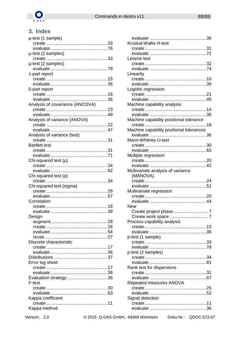
Commands in destra v11 88/89
Version: 2.0 © 2015 Q-DAS GmbH, 69469 Weinheim Doku-Nr.: QDOC-572-67
3. Index µ-test (1 sample)
create ................................................ 33 evaluate ............................................. 76
µ-test (2 samples) create ................................................ 33
µ-test (2 samples) evaluate ............................................. 79
1-part report create ................................................ 15 evaluate ............................................. 36
5-part report create ................................................ 16 evaluate ............................................. 36
Analysis of covariance (ANCOVA) create ................................................ 23 evaluate ............................................. 49
Analysis of variance (ANOVA) create ................................................ 22 evaluate ............................................. 47
Analysis of variance (test) create ................................................ 31
Bartlett test create ................................................ 31 evaluate ............................................. 71
Chi-squared test (µ) create ................................................ 34 evaluate ............................................. 82
Chi-squared test (p) create ................................................ 34
Chi-squared test (sigma) create ................................................ 29 evaluate ............................................. 57
Correlation create ................................................ 18 evaluate ............................................. 39
Design augment ............................................. 28 create ................................................ 26 evaluate ............................................. 54 reuse ................................................. 27
Discrete characteristic create ................................................ 17 evaluate ............................................. 36
Distributions .......................................... 37 Error log sheet
create ................................................ 17 evaluate ............................................. 36
Evaluation strategy ................................ 36 F-test
create ................................................ 30 evaluate ............................................. 63
Kappa coefficient create ................................................ 11
Kappa method
evaluate .............................................36 Kruskal-Wallis H-test
create .................................................31 evaluate .............................................72
Levene test create .................................................32 evaluate .............................................74
Linearity create .................................................10 evaluate .............................................36
Logistic regression create .................................................21 evaluate .............................................45
Machine capability analysis create .................................................14 evaluate .............................................36
Machine capability positional tolerance create .................................................18
Machine capability positional tolerances evaluate .............................................36
Mann-Whitney U-test create .................................................30 evaluate .............................................65
Multiple regression create .................................................20 evaluate .............................................42
Multivariate analysis of variance (MANOVA) create .................................................24 evaluate .............................................51
Multivariate regression create .................................................20 evaluate .............................................44
New Create project phase ........................... 7 Create work space .............................. 7
Process capability analysis create .................................................15 evaluate .............................................36
p-test (1 sample) create .................................................33 evaluate .............................................78
p-test (2 samples) create .................................................34 evaluate .............................................81
Rank test for dispersions create .................................................31 evaluate .............................................67
Repeated measures ANOVA create .................................................25 evaluate .............................................52
Signal detection create .................................................11 evaluate .............................................36

Commands in destra v11 89/89
Version: 2.0 © 2015 Q-DAS GmbH, 69469 Weinheim Doku-Nr.: QDOC-572-67
Simple analysis of variance evaluate ............................................. 69
Simple regression create ................................................ 19 evaluate ............................................. 41
Stability create .................................................. 9 evaluate ............................................. 36
Test of homogeneity create ................................................ 34 evaluate ............................................. 84
t-test (1 independent samples) create ................................................ 30
t-test (1 paired samples) create ................................................ 30
t-test (1 sample) create ................................................ 29 evaluate ............................................. 55
t-test (2 independent samples) evaluate ............................................. 61
Type-1 study
create .................................................. 8 evaluate .............................................36
Type-1 study 2nd true position create .................................................13
Type-1 study positional tolerance evaluate .............................................36
Type-2 study create .................................................. 8 evaluate .............................................36
Type-3 study create .................................................. 9 evaluate .............................................36
Weibull analysis create .................................................35 evaluate .............................................36
Wilcoxon test create .................................................29 evaluate .............................................59
χ²-test (p) evaluate .............................................85