INTERNATIONAL JOURNAL FOR NUMERICAL METHODS IN FLUIDSInt. J. Numer. Meth. Fluids 2008; 57:329–354Published online 6 November 2007 in Wiley InterScience (www.interscience.wiley.com). DOI: 10.1002/fld.1637

Combined interface boundary condition method for coupledthermal simulations

B. Roe1, R. Jaiman1, A. Haselbacher2 and P. H. Geubelle1,∗,†

1University of Illinois at Urbana-Champaign, Urbana, IL 61801, U.S.A.2University of Florida, Gainesville, FL 32611, U.S.A.

SUMMARY

A new procedure for modeling the conjugate heat-transfer process between fluid and structure subdomainsis presented. The procedure relies on higher-order combined interface boundary conditions (CIBC) forimproved accuracy and stability. Traditionally, continuity of temperature and heat flux along interfaces issatisfied through algebraic jump conditions in a staggered fashion. More specifically, Dirichlet temperatureconditions are usually imposed on the fluid side and Neumann heat-flux conditions are imposed on thesolid side for the stability of conventional sequential staggered procedure. In this type of treatment,the interface introduces additional stability constraints to the coupled thermal simulations. By utilizing theCIBC technique on the Dirichlet boundary conditions, a staggered procedure can be constructed with thesame order of accuracy and stability as those of standalone computations. Using the Godunov–Ryabenkiinormal-mode analysis, a range of values of the coupling parameter is found that yields a stable and accurateinterface discretization. The effectiveness of the method is investigated by presenting and discussingperformance evaluation data using a 1D finite-difference formulation for each subdomain. Copyright q2007 John Wiley & Sons, Ltd.

Received 12 December 2006; Revised 30 August 2007; Accepted 6 September 2007

KEY WORDS: conjugate heat transfer; staggered procedure; combined interface boundary conditions;stability

1. INTRODUCTION

The thermal interaction between fluid and solid subdomains plays an important role in a widerange of multiphysics problems, such as heating of space vehicles in hypersonic flow [1], heating

∗Correspondence to: P. H. Geubelle, Department of Aerospace Engineering, University of Illinois, 306 Talbot Lab,104 S. Wright St., Urbana, IL 61801, U.S.A.

†E-mail: geubelle@uiuc.edu

Contract/grant sponsor: Center for Simulation of Advanced Rockets at the University of Illinois at Urbana-Champaign/Department of Energy through the University of California; contract/grant number: B523819

Copyright q 2007 John Wiley & Sons, Ltd.

330 B. ROE ET AL.

and cooling of turbine blades in jet engines [2], and thermoelastic deformation of a structure dueto aerodynamic heating [3]. One way of modeling the above phenomena is to use a monolithic(i.e. tightly coupled) discretization for both solid and fluid subdomains with the interface boundaryconditions [4, 5]. However, one generally solves different equations in the solid and fluid subdo-mains: Typically, the unsteady thermal diffusion equation is computed in the solid subdomain,and the Navier–Stokes equations supplemented by appropriate turbulence models are solved in thefluids subdomain. In addition, the discretization approaches are often different: Commonly, thefinite-element method is used in the solid subdomain, whereas the finite-volume method is adoptedin the fluid subdomain. These differences can lead to difficulties in developing a computationallyefficient monolithic scheme.

A natural way of avoiding such difficulties is to solve the coupled thermal equations in apartitioned manner. In a partitioned solution procedure, the fluid and solid subdomains are solvedsequentially on decomposed non-overlapping subdomains. A key component of a partitionedprocedure is the formulation and implementation of the interface conditions characterizing thefluid–structure coupling. The fluid and structure equations are alternately integrated in time byseparate solvers with the aid of Dirichlet and Neumann boundary conditions along the interface.This technique for solving coupled mechanical system was introduced by Felippa and Park [6],which is often referred to the conventional sequential staggered (CSS) procedure.

For conjugate heat-transfer problems without deformation, Giles [7] demonstrated that the fluidsubdomain should be given a Dirichlet condition for temperature continuity, while the solid subdo-main should be subjected to a Neumann condition for heat-flux continuity to maximize stabilitywhen both subdomains are discretized with finite-difference methods. As shown in [7, 8], thestability restriction of the CSS procedure is more restrictive than those of the individual subdo-mains. The stability analyses were conducted using the Godunov and Ryabenkii [9] method and theanalytical results were verified numerically. In [8], special emphasis was placed on the effect of theinterface motion on the stability limit for both finite-difference and finite-volume/finite-elementdiscretizations of the fluid and solid subdomains. The results indicated that the stability propertiesof the explicit CSS procedure are strongly dependent on the interface characteristics, e.g. interfacevelocity, relative physical (e.g. mass density, heat capacities), and geometric properties (e.g. meshsize) along the interface. Additionally, the CSS scheme suffers from a time lag between the inte-gration of the coupled thermal equations. This time lag leads to an artificial energy production,which may cause numerical instability in the coupled thermal simulations. A similar phenomenonhas been observed in 1D model piston problem for fluid–structure interaction (FSI) in [10].A special treatment is thus required to counteract energy production in the staggered scheme.

In this study, we present a new coupling scheme that reduces and eliminates stability constraintsassociated with the interface treatment, while preserving the explicit ‘loosely coupled’ nature ofthe solution procedure. The new coupling scheme, referred to as the combined interface boundarycondition (CIBC) scheme, consists of partitioning the coupled subdomain and imposing interfaceconditions that relax the temperature continuity (Dirichlet) condition. Instead, higher-order correc-tions that are applied to obtain new interface values with appropriate compensation may counteractwith the artificial energy production caused by the staggering process. A similar approach has beenused in [11, 12] to show stability of linearized FSI using matching and non-matching meshes. Tothe best of our knowledge, this method has not been considered in any previous studies of transientconjugate heat-transfer problems. Our emphasis hereafter is to study the numerical stability andaccuracy of the CIBC scheme with the aid of explicit 1D loosely coupled thermal system. A variantof the CIBC scheme has been developed and implemented for nonlinear FSI using unstructured

Copyright q 2007 John Wiley & Sons, Ltd. Int. J. Numer. Meth. Fluids 2008; 57:329–354DOI: 10.1002/fld

COMBINED THERMAL BOUNDARY CONDITIONS 331

finite-volume formulation in the fluid subdomain and finite-element discretization in the structuralsubdomain [13].

Of interest in this work is the 1D thermal diffusion problem with a moving interfacedescribed by

�C�T�t

+�Cv0�T�x

=−�q�x

with q=−��T�x

(1)

where T (x, t) represents the temperature field, q(x, t) is the heat flux, � is the density, C isthe relevant specific heat, v0 is the interface velocity, and � is the thermal conductivity. Themodel equation (1) can be used to represent each subdomain, although the material parametersare discontinuous across the interface. Throughout this article, �, C , v0, and � are assumed to beconstant in each subdomain. Each subdomain can represent either fluid or solid media.

Following the convention adopted by Giles [7], the subdomain that passed the Dirichlet conditionis represented by + subscripts, while the subdomain that passed the Neumann condition is repre-sented by − subscripts. Based on the results of [7, 8], the + and − subdomains should representthe fluid and solid, respectively, for maximum stability. Hence, the terms ‘fluid subdomain’ and ‘+subdomain’ are used interchangeably, and similarly for ‘solid subdomain’ and ‘− subdomain’. Forthe fluid subdomain �+, C is the specific heat at constant volume CV . For the solid subdomain �−,C is equal to the specific heat CP . The boundary conditions as x→±∞ are that the temperaturefield asymptotes to constant values T±∞, and hence the heat flux tends to zero. At the interface�, the Dirichlet and Neumann continuity conditions are given by

T+ =T− and q+ =q− (2)

We discretize both subdomains with the finite-difference technique. As discussed in [7], a stabilityanalysis for this 1D coupled thermal model problem allows us to generate a necessary stabilitycondition for more complex 2D and 3D computations.

The remainder of this article is organized as follows. Section 2 summarizes the CSS scheme,and the formulation and implementation of the CIBC method are described in Section 3. InSection 4, the stability of the CIBC scheme is analyzed using the Godunov–Ryabenkii theory. Thestability analysis is verified numerically in Section 5, where results of an accuracy study are alsoreported.

2. CSS SCHEME

In partitioned staggered procedures, the fluid and solid thermal fields are commonly discretized inspace by different schemes and integrated in time by a staggered numerical scheme (see Figure 1).A simple and popular partitioned procedure for solving conjugate heat-transfer problems is theCSS scheme [6] whose generic cycle is described in Algorithm 1. For simplicity, we first considerthe particular case of a stationary interface for the 1D coupled thermal system, for which (1) takesthe form

c�T�t

=−�q�x

with q=−��T�x

(3)

where c=�C . Most of the derivations and results summarized in this paper pertain to the stationaryinterface case, while the more complex moving interface problem is discussed in Section 5.2.

Copyright q 2007 John Wiley & Sons, Ltd. Int. J. Numer. Meth. Fluids 2008; 57:329–354DOI: 10.1002/fld

332 B. ROE ET AL.

Algorithm 1. Explicit CSS scheme for the coupled thermal problem

1. Start from initial temperature fields prescribed in both subdomains2. Update temperature solution as follows:(a) Advance heat equation for solid (−) subdomain using known interface heat flux qn0−

c−�T−�t

∣∣∣∣n =− �q−�x

∣∣∣∣n in �−

(b) Impose Dirichlet condition on the interface boundary of fluid (+)

T n0+ =(1−�)T n

0− +�T n+10− on � where �∈[0,1]

(c) Advance heat equation for fluid (+) subdomain using known interface temperature T n0+

c+�T+�t

∣∣∣∣n =− �q+�x

∣∣∣∣n in �+

(d) Extract interface heat flux qn+10+ and impose Neumann condition on the interface boundary

of solid (−) subdomain

qn+10− =(1−�)qn0+ +�qn+1

0+ on � where �∈[0,1]

In Algorithm 1, |n denotes the current time level for the derivatives, and � and � are weightingparameters to interpolate the interface solutions between the time levels n and n+1. In the case of�=0 and �=0, the solutions at time level n+1 is ignored and the previous solution at time step nis transferred to the respective subdomains. This method is referred to a parallel conventionalstaggered method [6], since the fluid and structural subdomains can start their computations at thesame time level and perform their inner subdomain integrations in a parallel way. When �=1 and�=1, the CSS method described above is obtained. Selecting values between zero and one for �and � may result in an under-relaxed staggered scheme that usually introduces spurious dissipationto the coupled system.

For non-overlapping interfaces, the governing equation is not applied along the interface. Instead,the continuity conditions given by (2) are enforced sequentially. This time-stepping approach maysuffer significantly from destabilizing effects introduced by the interface conditions. Instabilityassociated with the interface may depend on relative physical and discretization parameters of theneighboring subdomains, e.g. heat capacity, density, mesh resolutions, and time steps. Moreover,due to obvious time lag between the �+ and �− computations, sequential staggered solutiontechniques can be only formally first-order accurate in time when no extrapolations are used,although the individual subdomains may be higher-order accurate.

For these reasons, it is often attempted to correct these deficiencies in partitioned looselycoupled framework by performing inner- or pseudo-iterations between each pair of consecutive

Copyright q 2007 John Wiley & Sons, Ltd. Int. J. Numer. Meth. Fluids 2008; 57:329–354DOI: 10.1002/fld

COMBINED THERMAL BOUNDARY CONDITIONS 333

Figure 1. Schematic of conventional sequential staggered (CSS) scheme for �=1 and�=1. Step labels 2(a)–(d) refer to Algorithm 1.

time stations. Sometimes such staggered procedures are referred to as strong coupling methods[14] in the literature of aeroelasticity. However, these pseudo-iterations increase the complexityof the implementation of conjugate heat-transfer analyses as well as the computational cost ofeach time step. These drawbacks of staggered methods motivate us to construct a new couplingprocedure for improving information exchange across the interface, as described in the followingsection.

3. COMBINED INTERFACE BOUNDARY CONDITIONS METHOD

3.1. Overview

Owing to inherent flexibility in the partitioned loosely coupled method, it is relatively easy toconstruct various iterative coupling procedures at both the conceptual and algorithmic levels.However, it may be a challenging task to design a partitioned method that provides temporalaccuracy and numerical stability. The CIBC approach achieves improved stability and precision by

Copyright q 2007 John Wiley & Sons, Ltd. Int. J. Numer. Meth. Fluids 2008; 57:329–354DOI: 10.1002/fld

334 B. ROE ET AL.

solving additional partial differential equations (PDEs) for the interface quantities based on theirspace and time derivatives.

The CIBC scheme shares features with the iterative interface relaxation procedure [15, 16],which involves a relaxation parameter and iterates the interface procedure at each pseudo-time step.In [15, 16], some guidelines are also given on the optimal choice of the relaxation parameter. Asin interface relaxation procedures, the CIBC scheme involves a coupling parameter for combiningthe error in heat-flux rate (i.e. history effects) with the net heat-flux gradient with the goal ofcorrecting the Dirichlet condition. The derivations presented in this section assume a non-movinginterface, i.e. v0=0. The more general case for which v0 �=0 is discussed in Section 5.2.

3.2. Formulation and algorithm

In the conventional staggered scheme, the governing equation of each subdomain has no influencealong the interface. Instead, the continuity of heat flux (Neumann condition) and temperaturecontinuity (Dirichlet condition) given by (2) are enforced. By contrast, in the CIBC methodformulation, the interface solution is influenced explicitly by the neighboring subdomains. For thecoupled thermal problem, specific residual operators for the Dirichlet condition RD and Neumanncondition RN are given by

RD(

�T0−�t

,�q0−�t

,�q0+�n

,�q0+�t

)=0, RN(q0+,q0−)=0 (4)

where (�q0+/�n) denotes the derivative of the fluid heat-flux q0+ with respect to the outwardnormal n along the interface �. Based on the current solutions on both sides of the interface,these operators calculate successive corrections to the solution on the interface �. Although thecoupling scheme described in [12] calls for corrections of both the Dirichlet and Neumann boundaryconditions, the treatment described hereafter deals with the modification of the Dirichlet conditiononly. This approach is used because preliminary numerical tests demonstrated no additional stabilityenhancement if the Neumann boundary conditions were also modified. In fact, tests have shown thata CIBC approach that corrects both boundary conditions may exhibit worse stability characteristicsthan the one that corrects the Dirichlet condition or the Neumann condition separately at each timestep. The reasons for this behavior are still under investigation.

The derivation of the residual RD for the CIBC scheme starts with the Dirichlet condition (2)for the fluid subdomain �+, which can be differentiated with respect to time as

�T0+�t

= �T0−�t

(5)

Expressing (3) for the interface gives

c+�T0+�t

=−�q0+�x

(6)

where c± =�±C±. Substituting (5) into (6) yields

c+�T0−�t

=−�q0+�x

(7)

Copyright q 2007 John Wiley & Sons, Ltd. Int. J. Numer. Meth. Fluids 2008; 57:329–354DOI: 10.1002/fld

COMBINED THERMAL BOUNDARY CONDITIONS 335

Differentiating the Neumann condition for the solid subdomain �− with respect to time, we obtain

�q0−�t

= �q0+�t

(8)

By multiplying (8) with a dimensional coupling parameter � with the units of time/length andadding the resulting equation to (7), we can write an expression for RD as

c+�T0−�t

+ �q0+�x

+�

(�q0+�t

− �q0−�t

)=0 (9)

While (8) is satisfied at the continuum level, it is not necessarily satisfied for the discrete coupledsystem based on the partitioned staggered procedure.

Relationship (9) provides an estimate for the temperature correction between the two successivetime levels n and n+1. Instead of applying T n+1

0− to the fluid subdomain as in the conventionalstaggered scheme, we apply a corrected temperature value

T n0∗ =T n

0− +�T n0− (10)

where the temperature correction �T n0− is obtained by discretizing (9) as

�T n0− = �t

c+

[−�qn0+

�x+�

(�qn0−�t

− �qn0+�t

)](11)

In (11), �/�x and �/�t can be simply computed using first-order accurate difference approximations.Owing to the lack of local energy conservation in the staggered partitioned scheme compared withthe monolithic scheme, there is a non-zero value of the temperature correction �T n

0− at the discretetime level n. A detailed analysis is presented in Appendix A.

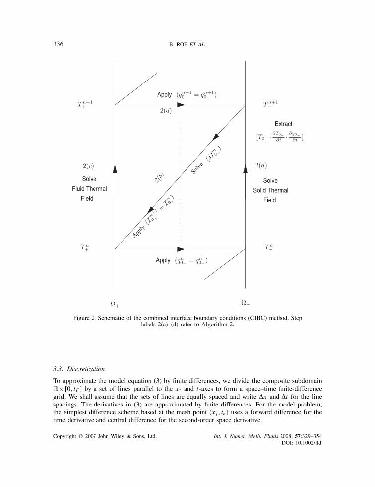
Since the standard Dirichlet condition has been used to derive this result, temperature continuityis still satisfied indirectly. Using (3) also ensures that the interface temperature solution satisfiesthe governing differential equation, which tends to improve both the accuracy and the stability ofthe interface discretization. Figure 2 illustrates the CIBC coupling algorithm for a coupled thermalsimulation. This algorithm differs from the conventional staggered scheme only in the treatmentof the Dirichlet boundary condition (10).

It is worth pointing out that since the CIBC method decomposes and combines interfaceboundary conditions at the continuum level, the convergence analysis for this coupling methodcan be carried out at the continuum level (i.e. in terms of PDEs) and therefore is a mathe-matical and not a numerical analysis problem. Such a stability analysis is carried out at thedifferential level using energy arguments in [12] for linearized FSI. There are several challengingquestions, however, concerning practical applications of such methods, such as finding suitablevalues of the coupling parameter �. In the following section, the stability of the CIBC methodis analyzed using the Godunov–Ryabenkii method and suitable values of the coupling parameterare determined.

Copyright q 2007 John Wiley & Sons, Ltd. Int. J. Numer. Meth. Fluids 2008; 57:329–354DOI: 10.1002/fld

336 B. ROE ET AL.

Figure 2. Schematic of the combined interface boundary conditions (CIBC) method. Steplabels 2(a)–(d) refer to Algorithm 2.

3.3. Discretization

To approximate the model equation (3) by finite differences, we divide the composite subdomainR̄×[0, tF ] by a set of lines parallel to the x- and t-axes to form a space–time finite-differencegrid. We shall assume that the sets of lines are equally spaced and write �x and �t for the linespacings. The derivatives in (3) are approximated by finite differences. For the model problem,the simplest difference scheme based at the mesh point (x j , tn) uses a forward difference for thetime derivative and central difference for the second-order space derivative.

Copyright q 2007 John Wiley & Sons, Ltd. Int. J. Numer. Meth. Fluids 2008; 57:329–354DOI: 10.1002/fld

COMBINED THERMAL BOUNDARY CONDITIONS 337

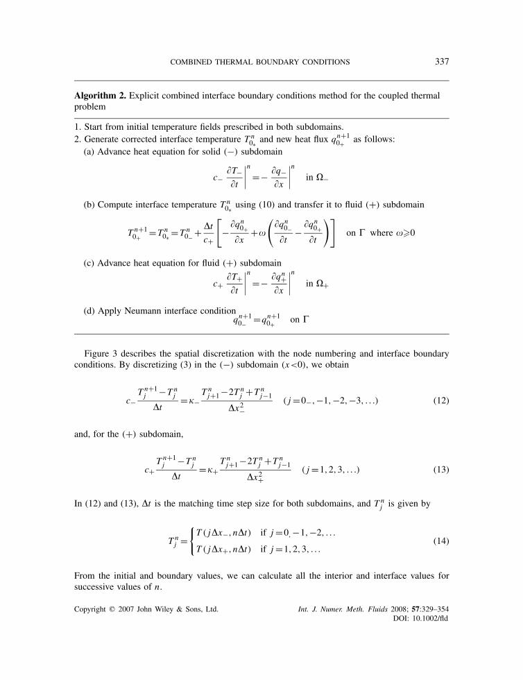
Algorithm 2. Explicit combined interface boundary conditions method for the coupled thermalproblem

1. Start from initial temperature fields prescribed in both subdomains.2. Generate corrected interface temperature T n

0∗ and new heat flux qn+10+ as follows:

(a) Advance heat equation for solid (−) subdomain

c−�T−�t

∣∣∣∣n =− �q−�x

∣∣∣∣n in �−

(b) Compute interface temperature T n0∗ using (10) and transfer it to fluid (+) subdomain

T n+10+ =T n

0∗ =T n0− + �t

c+

[−�qn0+

�x+�

(�qn0−�t

− �qn0+�t

)]on � where ��0

(c) Advance heat equation for fluid (+) subdomain

c+�T+�t

∣∣∣∣n =− �qn+�x

∣∣∣∣n in �+

(d) Apply Neumann interface conditionqn+10− =qn+1

0+ on �

Figure 3 describes the spatial discretization with the node numbering and interface boundaryconditions. By discretizing (3) in the (−) subdomain (x<0), we obtain

c−T n+1j −T n

j

�t=�−

T nj+1−2T n

j +T nj−1

�x2−( j =0−,−1,−2,−3, . . .) (12)

and, for the (+) subdomain,

c+T n+1j −T n

j

�t=�+

T nj+1−2T n

j +T nj−1

�x2+( j =1,2,3, . . .) (13)

In (12) and (13), �t is the matching time step size for both subdomains, and T nj is given by

T nj =

{T ( j�x−,n�t) if j =0,−1,−2, . . .

T ( j�x+,n�t) if j =1,2,3, . . .(14)

From the initial and boundary values, we can calculate all the interior and interface values forsuccessive values of n.

Copyright q 2007 John Wiley & Sons, Ltd. Int. J. Numer. Meth. Fluids 2008; 57:329–354DOI: 10.1002/fld

338 B. ROE ET AL.

Figure 3. Schematic of discretized subdomain and node numbering.

For the interface boundary conditions, we apply the Neumann condition on the (−) subdomainand the Dirichlet condition on the (+) subdomain, as indicated in Figure 3. By discretizing (3)along the interface, we obtain

c−T n+10− −T n

0−�t

=(

−q+−�−T n0− −T n

−1

�x−

)2

�x−(15)

where the heat flux q+ is computed by a first-order approximation of the temperature gradient onthe interface

q+ =−�+

(T n1 −T n

0∗�x+

)(16)

and it is transferred to the (−) subdomain as the Neumann boundary condition with the aid of thecorrected temperature value T ∗

0 .The fully discretized version of (10) is thus

T n0∗ = T n

0− + �t

c+

(�+�x2+

(T n−12 −2T n−1

1 +T n−10+ )

+�

{�+

�x+�t[(T n−1

1 −T n−10+ )−(T n−2

1 −T n−20+ )]

− �−�x−�t

[(T n0− −T n

−1)−(T n−10− −T n−1

−1 )]})

(17)

Using the explicit update, the Dirichlet boundary condition to the fluid domain is set by thecorrected interface temperature field T n

0∗

T n+10+ =T n

0∗ (18)

Copyright q 2007 John Wiley & Sons, Ltd. Int. J. Numer. Meth. Fluids 2008; 57:329–354DOI: 10.1002/fld

COMBINED THERMAL BOUNDARY CONDITIONS 339

where T0+ lags by T0∗ one iteration. Furthermore, combining (15)–(17) yields

T n+10+ = T n

0− + 2�t

c−�x−

{�+�x+

(T n1 −T n

0− − �t

c+

[�+�x2+

(T n−12 −2T n−1

1 +T n−10+ )

+�

{�+

�x+�t[(T n−1

1 −T n−10+ )−(T n−2

1 −T n−20+ )]

− �−�x−�t

[(T n0− −T n

−1)−(T n−10− −T n−1

−1 )]}])

− �−�x−

[T n0− −T n

−1]}

(19)

The more general case involving interface motion is analyzed in Appendix B.

4. GODUNOV–RYABENKII STABILITY ANALYSIS

The stability analysis relies on the normal-mode representation, which generalizes further thematrix method by replacing it with local modes as a power series of quasi-eigenvectors [9]. Thisconstitutes a property for local analysis of the influence of boundary conditions as opposed to thevon Neumann analysis, which requires periodic conditions. In addition, it allows us to derive exactsolutions of the difference schemes and permits the analysis of the error propagation through thespace mesh.

As in [7, 8], we now apply the stability theory of Godunov–Ryabenkii [9, 17] to examine theexistence of separable normal modes of the form at node point i and time step n:

T nj =

⎧⎨⎩znk j

− if j�0

znk j+ if j>0

(20)

for the difference equations (12), (13), and (19), where z is the time-amplification factor and k isthe space-amplification factor. When introduced into a numerical scheme formed by the interiorscheme and the interface conditions, we obtain a set of characteristic equations that couples thetime-amplification factor z with the space-amplification factor k.

The theory states that the interior scheme needs to be von Neumann stable in a domain and amode k j with |k|>1 will lead to an unbounded solution in space, which means that k j will increasewithout bound when j goes to infinity. Therefore, |k| should be less than one, and the necessarycondition states that all the modes with |k|�1 produced by the interface boundary conditionsshould correspond to |z|<1.

Let us now define the following non-dimensional parameters:

r ≡ c+�x+c−�x−

(21)

d± ≡ �±�t

c±�x2±(22)

Copyright q 2007 John Wiley & Sons, Ltd. Int. J. Numer. Meth. Fluids 2008; 57:329–354DOI: 10.1002/fld

340 B. ROE ET AL.

and

�± ≡ �±�

c±�x±(23)

The parameters defined by (21) and (22) are equal to those used in [7, 8]. The parameters definedby (23), which contain the coupling parameter �, arise due to the CIBC treatment of the interfacecoupling.

Solving (12) for T n+1j and applying the dimensionless parameter d−, we obtain

T n+1j =T n

j +d−(T nj+1−2T n

j +T nj−1) (24)

Substituting (20) into (24), the characteristic equation becomes

z=1+d−(k−−2+k−1− ) (25)

in the (−) subdomain. Similarly, for the (+) subdomain, we obtain the characteristic equation

z=1+d+(k+−2+k−1+ ) (26)

The discretized interface relation (19) can be rewritten as

T n+10+ = T n

0− +2rd+[T n1 −T n

0+ −�+(T n−11 −T n−1

0+ −T n−21 +T n−2

0+ )

+ d−�+d+r

(T n0− −T n

−1−T n−10− +T n−1

−1 )−d+(T n−12 −2T n−1

1 +T n−10− )

]−2d−(T n

0− −T n−1) (27)

by substituting the non-dimensional parameters d+, d−, �+, and r . Applying (20) to (27) yieldsthe characteristic relation

z = 1+2rd+[(k+−1)−�+(k+−1)(z−1−z−2)

−z−1d+(k2+−2k++1)]+2d−(1−k−1− )[�+(1−z−1)−1] (28)

The interface stability relation is then obtained by solving (25) and (26) for k− and k+, respectively,and substituting the results into (28). k− is given by

k−1− =1− 1−z

2d−

(1∓

√1− 4d−

1−z

)(29)

Similarly, the solution for k+ is

k+ =1− 1−z

2d+

(1∓

√1− 4d+

1−z

)(30)

Copyright q 2007 John Wiley & Sons, Ltd. Int. J. Numer. Meth. Fluids 2008; 57:329–354DOI: 10.1002/fld

COMBINED THERMAL BOUNDARY CONDITIONS 341

As stated earlier, to ensure stability as j→±∞, |k+|<1 and |k−|>1. These requirements arefulfilled by taking the negative signs in (29) and (30). Hence, we obtain

z = 1−2rd+

[1−z

2d+

(1−

√1− 4d+

1−z

)]

×{1−�+

(1

z− 1

z2

)+z−1d+

[1−z

2d+

(1−

√1− 4d+

1−z

)]}

+2d−

[1−z

2d−

(1−

√1− 4d−

1−z

)][�+(1− 1

z

)−1

](31)

which can be solved for r as

r =z−1−2d−

[1−z

2d−

(1−√1− 4d−

1−z

)][�+(1−z−1)−1]

−2d+

[1−z

2d+

(1−√1− 4d+

1−z

)]{1−�+(z−1−z−2)+z−1d+

[1−z

2d+

(1−√1− 4d+

1−z

)]} (32)

The requirement for stability is |z|<1. The solution z=1 yields trivial solution in (32). Bysetting z=−1 in (32), we arrive at the following analytical stability criterion for the CIBC scheme:

r<

√1−2d−(1−2�+)+2�+

(1−√1−2d+)(2�++√

1−2d+)(33)

Note that setting �+ =0 does not cause (33) to revert to the stability criterion of the CSS schemegiven by [7]. This can be simply explained from (10), where setting �=0 leads to

T n0∗ =T n+1

0− + �t

c+�qn+�x

(34)

There are two points to be made about (33). Firstly, the terms multiplied by � represent informationfrom the interface history, while the heat-flux gradient term appearing in (33) is essentially ahigher-order spatial term that remains even when �=0. Secondly, if we set d+ =d− =0.5, whichcorresponds to the maximum time step size allowed by the Courant–Friedrichs–Lewy (CFL)condition in the fluid and solid subdomains, the stability criterion reduces to r<1 and is completelyindependent of d+, d−, and �.

5. NUMERICAL RESULTS AND DISCUSSION

To assess the stability and precision of the CIBC coupling scheme and the accuracy of theanalytical stability criterion derived in the previous section, we present results of a 1D numericalstudy performed with a coupled finite-difference thermal solver. The finite-difference equationsare consistent with the formulation used for deriving (33).

Copyright q 2007 John Wiley & Sons, Ltd. Int. J. Numer. Meth. Fluids 2008; 57:329–354DOI: 10.1002/fld

342 B. ROE ET AL.

The model test problem specifies a uniform temperature in each domain, 1K in the fluidsubdomain and 0 K in the solid subdomain. At time t=0, the fluid subdomain is updated with T0−from the solid subdomain, producing the heat flux, q+. After the first time step, T0∗ , defined by (10),is computed and used for updating the fluid subdomain (see Algorithm 2). The numerical resultsobtained with the CIBC coupling scheme are compared with those obtained with the traditionalstaggered scheme presented in Algorithm 1 with �=1 and �=1.

Each subdomain is 1m in length (l+ = l− =1), and we use 200 equally distributed gridpoints to discretize both the subdomains. In addition, all the computations use the followingparameters:

• specific heat capacities (J/m3K), c+ =1000, c− =2000;• thermal conductivities (W/mK), �+ =0.1, �− =0.2;• non-dimensional final time t∗F =(tF�+/c+l2+)=(tF�−/c−l2−)=0.1.

5.1. Non-moving interface

5.1.1. Stability assessment. Figure 4(a) shows the maximum value of d+ for which a stable solutioncan be maintained as the coupling parameter � changes. Here, r is chosen as 1 and d− varies from0.35 to 0.5. In the figure, analytical stability limits obtained from (33) are denoted by the thickercurves, the numerical results are given by symbols, and the analytical stability limits correspondingto the conventional staggered scheme [8] are indicated by the thinner horizontal curves.

Four comments can be made about these results. First, the analytical and numerical stabilitylimits match very well for all cases shown here. Second, in all cases, the stability limits imposedby the CIBC scheme are less restrictive than those corresponding to the conventional staggeredcoupling method. Third, when the non-dimensional coupling parameter �+ is less than roughly0.5, the simulation remains stable even when d+ =0.5, which is in fact the CFL limit of the fluid(+) subdomain. For �+>0.5, the maximum d+ allowed decreases, yet remains significantly largerthan that allowed when using the traditional coupling algorithm (thinner horizontal lines). Finally,the figure shows that, as d− increases from 0.35 to 0.5, the rate at which the critical value of d+decreases from 0.5 is reduced. It seems counterintuitive that increasing d− should correspondinglyincrease the critical value of d+, but this occurs due to the problem approaching the scenario inwhich d+ =d− =0.5, where, as stated in Section 4, the stability criterion reduces to r<1.

Similar conclusions can be reached from the results shown in Figure 4(b). However, �+ has theopposite effect on the critical value of d− as it did on d+. That is, d− =0.5 gives a stable solutionwhen �+ is equal to or larger than about 0.3, and decreases when �+ falls below this value. Againwe see that, when d+ =0.5, the critical value of d− is also 0.5. Unlike in the case of Figure 4(a),however, there is not an obvious pattern in the effect of decreasing d+ from 0.5 where �+<0.3. Inall cases, the stability criterion still accurately predicts the critical value of d−. Again, the curvecorresponding to the conventional staggered scheme shows that d−crit is smaller than that observedwith the CIBC scheme. For clarity, only the conventional staggered scheme curve that representsthe maximum value of d−crit is shown.

Figures 4(c) and (d) are similar to Figures 4(a) and (b), respectively, except that r =0.75. Thetwo figures are qualitatively identical to their r =1 counterparts, although here the numerical valuesof d+crit and d−crit have increased and the point at which �+ is able to maintain stability at 0.5has shifted from 0.5 and 0.3 to 0.9 and 0.15, respectively. As before, the results produced by theCIBC method are more stable than those of the conventional staggered method for the range ofcoupling parameter �+ shown.

Copyright q 2007 John Wiley & Sons, Ltd. Int. J. Numer. Meth. Fluids 2008; 57:329–354DOI: 10.1002/fld

COMBINED THERMAL BOUNDARY CONDITIONS 343

(c) (d)

(a) (b)

Figure 4. Effect of the non-dimensional coupling parameter �+ on the stability of thecoupled scheme, i.e. on the critical values of d+ and d− beyond which instability occurs.(a) and (b): r =1; (c) and (d): r =0.75. The curves and symbols, respectively, denote theanalytical and numerical solutions of the CIBC scheme, while the thinner horizontal lines

correspond to the stability limit of the conventional staggered scheme.

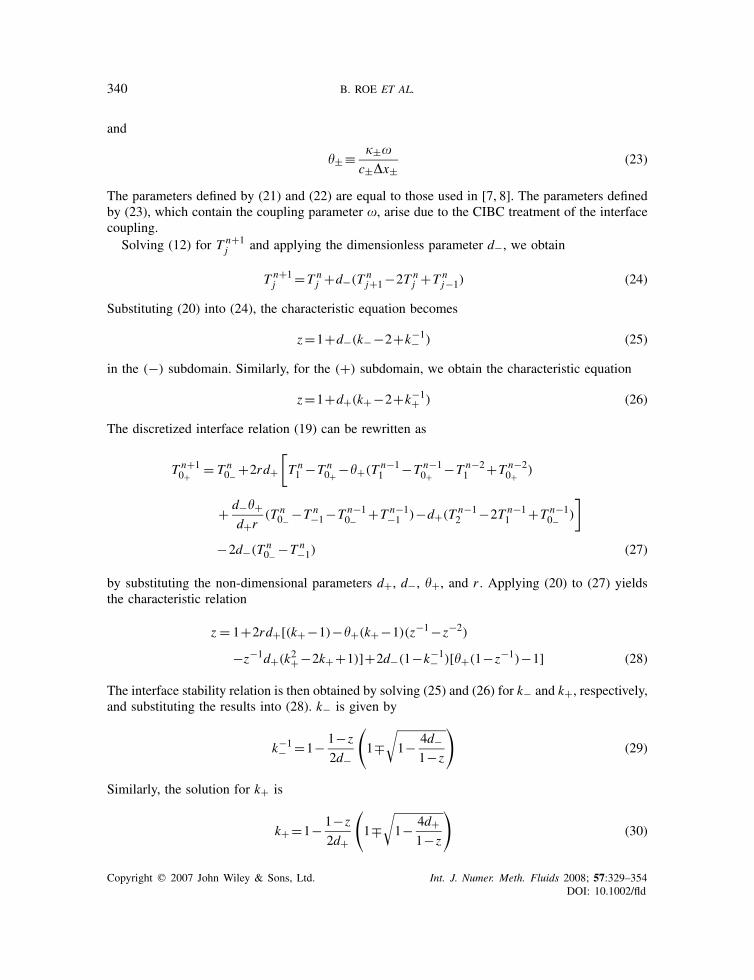
It was stated previously that, when d+ =d− =0.5, the stability criterion becomes r<1. Indeed,as shown in Figure 5(a), a simulation in which d+ =d− =0.5 and r =1 seem to be neutrally stable.When r<1, the simulation becomes stable, as shown in Figure 5(b), for which r =0.99. It shouldbe pointed out that r =1 is not a stringent stability limit since previous studies [7, 8] have shownthat the coupling algorithm should always be arranged such that the fluid subdomain is given aDirichlet condition and the solid subdomain a Neumann condition. In this case, for similar meshspacings, r is always less than unity.

Figure 6(a) shows the region of stability for various values of r for the conventional staggeredscheme. These results are compared with the results of the CIBC scheme shown in Figure 6(b).While the stability zone of the conventional staggered algorithm only fills the entire region of

Copyright q 2007 John Wiley & Sons, Ltd. Int. J. Numer. Meth. Fluids 2008; 57:329–354DOI: 10.1002/fld

344 B. ROE ET AL.

0 200 400 600 800 10000

0.1

0.2

0.3

0.4

0.5

0.6

0.7

0.8

0.9

1

Time Step

Inte

rfac

e T

empe

ratu

re (

K)

0 200 400 600 800 10000

0.1

0.2

0.3

0.4

0.5

0.6

0.7

0.8

0.9

1

Time Step

Inte

rfac

e T

empe

ratu

re (

K)

(a) (b)

Figure 5. Interface temperature evolution where d+ =d− =0.5 and �+ =0.5: (a) r =1 and (b) r =0.99.

0 0.1 0.2 0.3 0.4 0.50

0.05

0.1

0.15

0.2

0.25

0.3

0.35

0.4

0.45

0.5

d− d−

d + d +

r = 0.25r = 0.5r = 0.75r = 1r = 1.25r = 1.5r = 1.75

0 0.1 0.2 0.3 0.4 0.50

0.05

0.1

0.15

0.2

0.25

0.3

0.35

0.4

0.45

0.5

r ≤ 1r = 1.25r = 1.5r = 1.75

(a) (b)

Figure 6. Effect of r on the predicted stability zones, with the stability regions lying below the curves:(a) conventional staggered scheme and (b) CIBC with �+ =0.5.

potential stability as r →∞, Figure 6(b) shows that the CIBC scheme requires only that r<1 toreach that scenario. As r increases from 1, the size of the stability zone shrinks for the CIBCscheme, as it does for the conventional staggered scheme. Further, the figure illustrates that, forthe range of r considered and �+ =0.5, the CIBC scheme is more stable than the CSS scheme.

The results presented above lead to the following conclusions: Firstly, the CIBC scheme allowsthe thermal FSI simulation to operate under conditions beyond the stability limit of the conventionalstaggered scheme. Secondly, if r<1, the problem is stable when d+ =d− =0.5, regardless of thechoice of �+. When this is not the case, not all choices of �+ are equally suitable. Thirdly, if r =1,optimal values of �+ from the point of view of stability seem to lie between 0.3 and 0.5.

Copyright q 2007 John Wiley & Sons, Ltd. Int. J. Numer. Meth. Fluids 2008; 57:329–354DOI: 10.1002/fld

COMBINED THERMAL BOUNDARY CONDITIONS 345

5.1.2. Accuracy assessment. We now turn our attention to the issue of accuracy of the new couplingscheme, and, in particular, on the effect of the coupling parameter on the precision of the numericalsolution.

To quantify the accuracy of the coupling algorithm, we compare the numerical solution withthe exact temperature field for two semi-infinite subdomains given by [18]

T+(x, t)= �+�−1/2D+ Ti+

�+�−1/2D+ +�−�−1/2

D−

⎡⎣1+ �−�−1/2

D−

�+�−1/2D+

erf

(x

2√

�D+ t

)⎤⎦ (35)

and

T−(x, t)= �+�−1/2D+ Ti+

�+�−1/2D+ +�−�−1/2

D−erfc

( |x |2√

�D− t

)(36)

where �D± =�±/c± and Ti+ is the initial temperature of the (+) subdomain, which, for our testproblem, is chosen as 1K. The exact interface temperature is thus given by

T ex0 = �+�−1/2

D+ Ti+

�+�−1/2D+ +�−�−1/2

D−(37)

To quantify the error incurred in simulations with the CSS and CIBC schemes, we take theL2-norm of the computed interface temperature with respect to its analytical value,

�T0(t∗F )=

√√√√√∑n(t∗F )

k=1 (T k0num

−T k0ex

)2∑n(t∗F )

k=1 (T k0ex

)2(38)

where n(t∗F ) is the number of time steps between t=0 and t= t∗F , and T num0k

and T ex0k

refer to thenumerical and exact interface temperatures at time step k.

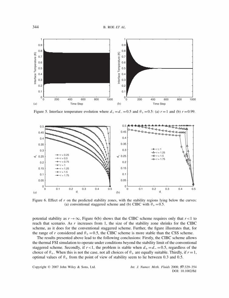
Figure 7 shows the effect of �+ on the interface error. In all cases, the error appears to beincreasing with �+�0.5 and, correspondingly, decreasing with d+ and d−, which is expected.However, each value of d± has an optimal value of �+ to minimize interface discretization error.In general, the optimal range of �+ is 0.1<�+<0.5.

In Figure 8(a), �T0 is given for both the CIBC and conventional staggered schemes. For theCIBC scheme, we set �+ =0.5 and results are shown for d+ =d− =0.25, 0.4, and 0.5. On theother hand, for the conventional staggered scheme only the results for the d+ =d− =0.25 caseare shown, as it is unstable for the other two values. Considering first the d+ =d− =0.25 case,for which a direct comparison can be made, we note that the CIBC scheme produces slightlymore accurate results for most values of r . When r is greater than roughly 0.8, the conventionalstaggered algorithm is slightly more accurate. Again, increasing d+ and d− produces an expectedincrease in error, which for both cases is larger than either algorithm operating at d+ =d− =0.25.Further, Figure 8(b) shows significant improvements in the interface accuracy, up to almost a factorof 2 for some values of r , for �+ =0.25.

Another aspect of the CIBC algorithm and that requires study is the order of temporal conver-gence. To that effect, we analyze the computation of �T0 at the interface for various time stepsizes by varying d±. Since material properties and grid spacings are held fixed for all cases,

Copyright q 2007 John Wiley & Sons, Ltd. Int. J. Numer. Meth. Fluids 2008; 57:329–354DOI: 10.1002/fld

346 B. ROE ET AL.

Figure 7. Effect of coupling parameter �+ on the interface error for d+ =d− =0.25,0.4, and 0.5, r =1 and n=500.

(b)(a)

Figure 8. Comparison of error produced from the simulations using the CIBC (symbols) and the conven-tional staggered scheme (solid curve) as r is varied and n=500: (a) �+ =0.5 and (b) �+ =0.25.

changes in the error are a direct result of varying the time step. Figures 9(a) and (b) show theresults of a temporal convergence study for r =0.5 and 1.0, respectively. For the CIBC scheme,the measured slope of �T0 is consistently higher than 2 for the three values of �+ considered, i.e.�+ ={0.5,0.25,0.125}. The lowest value of �+ =0.125 shows an order of accuracy greater than4, which suggests that the temporal convergence rate can be controlled by varying the couplingparameter. However, it is important to keep in mind that a lower limit is placed on �+ by thestability requirements presented in Figures 4(b) and (d).

Copyright q 2007 John Wiley & Sons, Ltd. Int. J. Numer. Meth. Fluids 2008; 57:329–354DOI: 10.1002/fld

COMBINED THERMAL BOUNDARY CONDITIONS 347

(b)(a)

Figure 9. Dependence of the L2-norm of the interface error at t∗F for time steprefinement at n=500: (a) r =0.5 and (b) r =1.0.

Indeed, the convergence rate of the CIBC scheme is substantially higher than that providedby the CSS scheme and individual subdomains. For this particular case, the CSS scheme has theorder of accuracy of 0.55 for r =0.5 and 1.35 for r =1.0. The temporal convergence rate for anindividual subdomain is about 1.0, which is expected for the forward Euler integration scheme.Furthermore, the two figures together show that there is a significant effect of the parameter ron the local temporal convergence rate, which implies that the local energy conservation error isdependent on the ratio of physical and geometric properties across the interface.

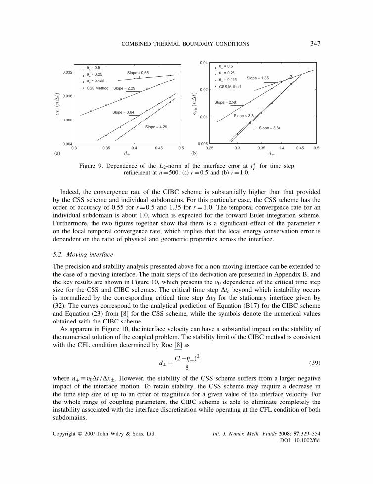
5.2. Moving interface

The precision and stability analysis presented above for a non-moving interface can be extended tothe case of a moving interface. The main steps of the derivation are presented in Appendix B, andthe key results are shown in Figure 10, which presents the v0 dependence of the critical time stepsize for the CSS and CIBC schemes. The critical time step �tc beyond which instability occursis normalized by the corresponding critical time step �t0 for the stationary interface given by(32). The curves correspond to the analytical prediction of Equation (B17) for the CIBC schemeand Equation (23) from [8] for the CSS scheme, while the symbols denote the numerical valuesobtained with the CIBC scheme.

As apparent in Figure 10, the interface velocity can have a substantial impact on the stability ofthe numerical solution of the coupled problem. The stability limit of the CIBC method is consistentwith the CFL condition determined by Roe [8] as

d± = (2−±)2

8(39)

where ± ≡v0�t/�x±. However, the stability of the CSS scheme suffers from a larger negativeimpact of the interface motion. To retain stability, the CSS scheme may require a decrease inthe time step size of up to an order of magnitude for a given value of the interface velocity. Forthe whole range of coupling parameters, the CIBC scheme is able to eliminate completely theinstability associated with the interface discretization while operating at the CFL condition of bothsubdomains.

Copyright q 2007 John Wiley & Sons, Ltd. Int. J. Numer. Meth. Fluids 2008; 57:329–354DOI: 10.1002/fld

348 B. ROE ET AL.

ll

Figure 10. Effect of the interface velocity v0 on the critical time step size. �t0 denotes the critical valueof the time step for a non-moving interface as described by (32), with r =1 and �+ =0.5.

Although the analyses were performed here for the 1D model diffusion equation, the results areexpected to be applicable to more complex situations in which the 2D and 3D diffusion equationis used to model the heat flux in the structure and the 2D/3D Navier–Stokes equations are usedto model the behavior of the fluid.

6. CONCLUSION

Typical solution methods for conjugate heat-transfer problems update the temperature field in eachsubdomain by passing the fluid subdomain a temperature (Dirichlet) condition and the solid subdo-main a heat-flux (Neumann) condition. This explicit coupling scheme is simple to implement andcan be effective. However, it suffers from the important disadvantage that the coupling introducesa stability limit that is more restrictive than that of the two subdomains. In this paper, a newcoupling scheme for the conjugate heat-transfer problem was introduced that reduces or eliminatesthis additional stability limit. The new coupling scheme consists of solving an additional PDEon the interface. This additional equation is derived from the Dirichlet and Neumann conditionsat the interface and the governing equations in one of the subdomains and is therefore termedthe combined interface boundary condition (CIBC) method. The additional equation contains acoupling parameter � and is solved for a correction to the predicted interface temperature.

The Godunov–Ryabenkii method was used to analyze the stability properties of the CIBCmethod. The results of the stability analysis were verified using numerical tests. These tests showedthat by careful selection of � the stability zone of the coupled problem can be expanded such thatonly the CFL condition of each subdomain limits the stability of the problem. The optimal valueof the non-dimensional coupling parameter, �+, seems to be approximately 0.1–0.5.

In addition to stability, the issue of accuracy of the coupled thermal algorithm was addressed. Bycomparing with an analytical solution, we verified that, in many cases, the CIBC scheme is not onlymore stable but also more accurate than the CSS method. Furthermore, convergence studies showed

Copyright q 2007 John Wiley & Sons, Ltd. Int. J. Numer. Meth. Fluids 2008; 57:329–354DOI: 10.1002/fld

COMBINED THERMAL BOUNDARY CONDITIONS 349

that the CIBC method results in an interface temperature that has a temporal convergence rategreater than 2, in contrast to the CSS schemes, which tend to achieve only first-order convergence.

APPENDIX A: MONOLITHIC VS PARTITIONED SCHEMES

To derive the comparison of the interface treatments between the monolithic and partitionedstaggered schemes, we examine initial-value coupled thermal problem (3) using the finite-differencetechnique. In the monolithic discretization, using forward Euler time differencing and conservativespatial differencing based on the integral form of the unsteady thermal equation on the intervalx j−1/2�x�x j+1/2 gives

C j (Tn+1j −T n

j )=−(qnj+1/2−qnj−1/2) (A1)

where qnj+1/2=−K j+1/2(T nj+1−T n

j ) with

K j+1/2={

�−/�x−, j+ 12<0

�+/�x+, j+ 12>0

and

C j =

⎧⎪⎪⎨⎪⎪⎩c−�x−/�t, j<0

12 (c−�x−/�t+c+�x+/�t), j =0

c+�x+/�t, j>0

The interface continuity conditions are embedded implicitly in the governing equations with thetwo-sided approximations for the heat flux. This discretization is unconditionally stable from theviewpoint of interface treatment, i.e. the interface does not introduce any stability constraints [7].

In the partitioned staggered scheme, each part of the domain is solved independently with theinformation from the other subdomain. Thus, for given solutions at time level n in both subdomains,the explicit numerical algorithm for determining T n+1

j is with the heat-flux data for the (−) domainand the temperature data for the (+) domain

c−T n+1j −T n

j

�t= �−

T nj+1−2T n

j +T nj−1

�x2−, j<0

c+T n+1j −T n

j

�t= �+

T nj+1−2T n

j +T nj−1

�x2+, j>0

(A2)

At the interface point ‘0’, the discretized heat-flux continuity relation takes the form

c−�x−2

(T n+10 −T n

0

�t

)=�+

T n1 −T n

0

�x+︸ ︷︷ ︸−qI

−�−T n0 −T n

−1

�x−(A3)

Copyright q 2007 John Wiley & Sons, Ltd. Int. J. Numer. Meth. Fluids 2008; 57:329–354DOI: 10.1002/fld

350 B. ROE ET AL.

while the temperature continuity condition reads

T n0 =TI (A4)

where the Neumann quantity qI is computed from the one-sided approximation with the first-order accuracy at the interface of the (+) domain and the Dirichlet quantity TI is directly appliedfrom the (−) domain. From (A1) and (A3), it is clear that the partitioned scheme ignores thequantity c+�x+/2�t due to the one-sided biasing in the interface computation. If (c+�x+/2�t)(c−�x−/2�t), this leads to a large partitioning error in the form of interface residual thermalenergy. Consequently, the partitioned staggered scheme is conditionally stable and the stabilitydepends on the relative physical and discretization parameters. The Godunov–Ryabenkii’s stabilitytheory quantifies the propagation of instability modes associated with the partitioning error betweenthe two consecutive time steps for a range of r .

This analysis clearly indicates that appropriate compensation to the partitioning error is required.The CIBC method achieves that compensation by constructing an interface differential operatorwith the aid of the dimensional coupling parameter �.

APPENDIX B: ANALYTICAL STABILITY LIMIT OF THERMAL MOVING INTERFACE

As mentioned previously, the subdomains are discretized with a finite-difference scheme: forwarddifference in time, a backward difference for the first spatial derivative, and a centered differencefor the second spatial derivative.

In the (−) subdomain (x<v0t), the discretized version of (1) is

c−T n+1j −T n

j

�t+c−v0

T nj −T n

j−1

�x−=�−

T nj+1−2T n

j +T nj−1

�x2−( j =0−,−1,−2,−3, . . .) (B1)

and the (+) subdomain (x>v0t), (1) takes the similar form

c+T n+1j −T n

j

�t+c+v0

T nj −T n

j−1

�x+=�+

T nj+1−2T n

j +T nj−1

�x2+( j =1,2,3, . . .) (B2)

The flux q is computed at the left edge of the (+) subdomain to be passed to the (−) subdomainas a boundary condition. The discrete form of the heat-flux continuity condition at the interface(x=v0t) is thus

c−T n+10 −T n

0

�t+c−v0

T n0 −T n

−1

�x−=(

−q+−�−T n0 −T n

−1

�x−

)2

�x−(B3)

The flux is computed from (+) values in a first-order accurate manner as

q+ =−�+(T n1 −T ∗

0

�x+

)(B4)

Copyright q 2007 John Wiley & Sons, Ltd. Int. J. Numer. Meth. Fluids 2008; 57:329–354DOI: 10.1002/fld

COMBINED THERMAL BOUNDARY CONDITIONS 351

and is transferred as the imposed interface heat flux to the (−) subdomain

T n0∗ = T n

0− + �t

c+

(�+�x2+

[T n−12 −2T n−1

1 +T n−10+ ]− c+v0

�x+(T n−1

1 −T n−10+ )

+�

{�+

�x+�t[(T n−1

1 −T n−10+ )−(T n−2

1 −T n−20+ )]

− �−�x−�t

[(T n0− −T n

−1)−(T n−10− −T n−1

−1 )]})

(B5)

Combining (B3)–(B5) yields

c−T n+10− −T n

0−�t

= 2

�x−

{�+�x+

[T n1 −T n

0− − �t

c+

(�+�x2+

[T n−12 −2T n−1

1 +T n−10+ ]

−c+v0

�x+(T n−1

1 −T n−10+ )+�

{�+

�x+�t[(T n−1

1 −T n−10+ )−(T n−2

1 −T n−20+ )]

− �−�x−�t

[(T n0− −T n

−1)−(T n−10− −T n−1

−1 )]})]

− �−�x−

[T n0− −T n

−1]}

−c−v0

�x−(T n

0− −T n−1) (B6)

In addition to the non-dimensional parameters (21)–(23), we must define

± ≡v0�t

�x±(B7)

which corresponds to the interface motion. Focusing our attention on the (−) subdomain, we solve(B1) for T n+1

j and use the dimensionless parameters d− and − to obtain

T n+1j =T n

j +d−(T nj+1−2T n

j +T nj−1)−−(T n

j −T nj−1) (B8)

Substituting (20) into (B8) yields

z=1+d−(k−−2+k−1− )−−(1−k−1− ) (B9)

Applying the same steps to the (+) subdomain leads to

z=1+d+(k+−2+k−1+ )−+(1−k−1+ ) (B10)

Copyright q 2007 John Wiley & Sons, Ltd. Int. J. Numer. Meth. Fluids 2008; 57:329–354DOI: 10.1002/fld

352 B. ROE ET AL.

Turning our attention to the discretized interface equation (B6), we solve for T n+10 to obtain

T n+10− = T n

0− + 2�t

c−�x−

{�+�x+

[T n1 −T n

0− − �t

c+

(�+�x2+

[T n−12 −2T n−1

1 +T n−10+ ]

− c+v0

�x+(T n−1

1 −T n−10+ )+�

{�+

�x+�t[(T n−1

1 −T n−10+ )−(T n−2

1 −T n−20+ )]

− �−�x−�t

[(T n0− −T n

−1)−(T n−10− −T n−1

−1 )]})]

− �−�x−

[T n0− −T n

−1]}

− v0�t

�x−(T n

0− −T n−1) (B11)

or, in terms of the non-dimensional parameters d , , and r ,

T n+10− = T n

0− +2rd+[T n1 −T n

0− −�+(T n−11 −T n−1

0+ −T n−21 +T n−2

0+ )

+ d−�+d+r

(T n0− −T n

−1−T n−10− +T n−1

−1 )−d+(T n−12 −2T n−1

1 +T n−10+ )

++(T n−11 −T n−1

0+ )]−2d−(T n0− −T n

−1)−−(T n0− −T n

−1) (B12)

Substituting (20) into (B12) gives

z = 1+2rd+[(k+−1)−�+(k+−1)(z−1−z−2)−z−1d+(k2+−2k++1)+z−1+(k+−1)]+(1−k−1− )[2d−�+(1−z−1)−(2d−+−)] (B13)

Expressions (B9), (B10), and (B13) provide the three equations for the three unknowns: k−,k+, and z. To obtain an interface stability criterion, we solve (B9) and (B10) for k− and k+,respectively, and substitute the resulting expressions into (B13). Solving (B9) for k− gives

k−1− =1− −d−+−

− (1−z−−)

2(d−+−)

[1∓

√1− 4d−(1−z)

(1−z−−)2

](B14)

while (B10) yields

k+ =1− 1−z−+2d+

[1∓

√1− 4d+(1−z)

(1−z−+)2

](B15)

From (20), we can see that the conditions |k+|<1 and |k−|>1 ensure that the tempera-ture remains finite for j →±∞. These requirements are fulfilled by taking the negative signs

Copyright q 2007 John Wiley & Sons, Ltd. Int. J. Numer. Meth. Fluids 2008; 57:329–354DOI: 10.1002/fld

COMBINED THERMAL BOUNDARY CONDITIONS 353

in (B14) and (B15). Hence, we obtain

z = 1−2rd+

(1−z−+

2d+

[1−

√1− 4d+(1−z)

(1−z−+)2

])[1−�+

(1

z− 1

z2

)

+ z−1d+

(1−z−+

2d+

[1−

√1− 4d+(1−z)

(1−z−+)2

])+z−1+

]

+(

−d−+−

+ 1−z−−2(d−+−)

[1−

√1− 4d−(1−z)

(1−z−−)2

])

×[2d−�+(1−z−1)−(2d−+−)] (B16)

For stability, it is required that |z|<1. Note that z=1 produces the trivial solution, r <∞.Therefore, the stability criterion is found by inserting z=−1 into (B16), yielding the followinginequality for stability of the CIBC coupling scheme for the moving interface case:

r<

2+[

−d−+−

+ 2−−2(d−+−)

(1−

√1− 8d−

(2−−)2

)][4d−�+−(2d−+−)]

(2−+)

(1−

√1− 8d+

(2−+)2

)[1+2�+−+− 2−+

2

(1−

√1− 8d+

(2−+)2

)] (B17)

The above inequality reduces to (33) if + =0. Based on the analytical stability limit given by(B17), it is possible to determine the influence of interface motion in the stability of the CIBCmethod.

REFERENCES

1. Johnson HB, Seipp TG, Candler GV. Numerical study of hypersonic reacting boundary layer transition on cones.Physics of Fluids 1998; 10(10):2676–2685.

2. Sondak SL, Dorney DJ. Simulation of coupled unsteady flow and heat conduction in turbine stage. AIAA Journalof Propulsion and Power 2000; 16(6):1141–1148.

3. Lee I, Roh JH, Oh IK. Aerothermoelastic phenomena of aerospace and composite structures. Journal of ThermalStresses 2003; 26(6):525–546.

4. Armero F, Simo JC. A new unconditionally stable fractional step method for nonlinear thermomechanicalproblems. International Journal for Numerical Methods in Engineering 1992; 35:737–756.

5. Zohdi TI. An adaptive recursive staggering strategy for simulating multi-field coupled processes in micro-heterogenous solids. International Journal for Numerical Methods in Engineering 2002; 53:1511–1532.

6. Felippa CA, Park KC. Staggered transient analysis procedures for coupled mechanical systems: formulation.Computer Methods in Applied Mechanics and Engineering 1980; 24:61–111.

7. Giles MB. Stability analysis of numerical interface conditions in fluid–structure thermal analysis. InternationalJournal for Numerical Methods in Fluids 1997; 25:421–436.

8. Roe B, Haselbacher A, Geubelle PH. Stability of fluid–structure thermal simulations on moving grids. InternationalJournal for Numerical Methods in Fluids 2007; 54:1097–1117.

9. Godunov SK, Ryabenkii VS. The Theory of Difference Schemes—An Introduction. North-Holland: Amsterdam,1964.

Copyright q 2007 John Wiley & Sons, Ltd. Int. J. Numer. Meth. Fluids 2008; 57:329–354DOI: 10.1002/fld

354 B. ROE ET AL.

10. Blom FJ. A monolithical fluid–structure interaction algorithm applied to the piston problem. Computer Methodsin Applied Mechanics and Engineering 1998; 167:369–391.

11. Feng X. Analysis of finite element methods and domain decomposition algorithms for a fluid–solid interactionproblem. SIAM Journal on Numerical Analysis 2000; 38:1312–1336.

12. Jaiman RK, Jiao X, Geubelle PH, Loth E. Conservative load transfer along curved fluid–solid interface withnonmatching meshes. Journal of Computational Physics 2006; 218:372–397.

13. Jaiman RK, Geubelle PH, Loth E, Jiao X. Stable and accurate loosely-coupled scheme for unsteady fluid–structureinteraction. AIAA Paper, 2007–334.

14. Strganac TW, Mook DT. Numerical model of unsteady subsonic aeroelastic behavior. AIAA Journal 1990; 28:903–909.

15. Funaro D, Quarteroni A, Zanolli P. An iterative procedure with interface relaxation for domain decompositionmethods. SIAM Journal on Numerical Analysis 1998; 25(6):1213–1236.

16. Rice JR, Tsompanopoulou P, Vavalis E. Interface relaxation methods for elliptic differential equations. AppliedNumerical Mathematics 2000; 32:219–245.

17. Richtmyer RD, Morton KW. Difference Methods for Initial-value Problems (2nd edn). Wiley-Interscience: NewYork, 1967.

18. Carslaw HS, Jaeger JC. Conduction of Heat in Solids. Clarendon Press: Oxford, 1959.

Copyright q 2007 John Wiley & Sons, Ltd. Int. J. Numer. Meth. Fluids 2008; 57:329–354DOI: 10.1002/fld