Preprint -- Preprint -- Preprint -- Preprint -- Preprint -- Preprint --

An exact approach for maximizing the lifetime of sensor networks with

adjustable sensing ranges

Andre Rossi∗ Alok Singh

Marc Sevaux

Lab-STICC, Universite de Bretagne Sud – F-56321 Lorient, France

Department of Computer and Information Sciences, University of Hyderabad

Hyderabad 500 046, Andhra Pradesh, India

April 23, 2014

Abstract

This paper addresses the problem of target coverage for wireless sensor networks, where the sensing rangeof sensors can vary, thereby saving energy when only close targets need to be monitored. Two versions ofthis problem are addressed. In the first version, sensing ranges are supposed to be continuously adjustable(up to the maximum sensing range). In the second version, sensing ranges have to be chosen among a set ofpredefined values common to all sensors. An exact approach based on a column generation algorithm is proposedfor solving these problems. The use of a genetic algorithm within the column generation scheme significantlydecreases computation time, which results in an efficient exact approach.

keywords: Wireless Sensor Networks; Network lifetime; Column Generation; Genetic algorithm.

1 Introduction

Advances in signal processing and embedded systems are at the origin of the growing popularity of Wireless SensorNetworks (WSN) in a wide range of applications [1]. While they were initially used in remote or hostile environments(for battlefield surveillance, or tsunami monitoring), WSN are also increasingly used for health care [12]. Althoughthese applications rely on very different types of sensors, most of them share the following characteristics: sensorsoperate on a battery that cannot be recharged, and a large number of sensors is deployed for improving faulttolerance and lifetime. This paper is concerned with lifetime maximization, that is achieved by making the bestpossible use of sensors redundancy. Moreover, the sensors are supposed to have adjustable sensing ranges. Sucha feature saves energy in the situation where a sensor needs to cover close targets only, as power requirement is anon-decreasing function of the distance between the sensor and the farthest target it covers.

More formally, suppose n sensors are randomly deployed in order to cover a set of m targets {τ1, . . . , τk, . . . , τm}.Each sensor si has an initial energy bi. Sensors can either be active or inactive. An inactive sensor does not coverany target, and its power consumption is negligible. When a sensor is active, its power consumption depends onits sensing range. All the sensors have the same maximum sensing range, denoted by Rmax: a sensor can covera target if its distance is less than or equal to Rmax. Lifetime maximization is reached by gathering sensors intonon-disjoint subsets called covers (each cover being such that each target can be covered by at least one sensor inthat cover), and by scheduling these covers, i.e., by determining the amount of time during which each cover isused. The sensors that are not part of the cover that is currently being used are not active. Moreover, covers arenot necessarily disjoint, as this allows for reaching longer lifetimes [15]. The schedule must be such that the totalamount of energy consumed by sensor si is at most equal to its initial energy bi. The network lifetime is the sumof these durations: when it is exceeded, the coverage of all targets is no longer possible.

This paper addresses two close versions of the lifetime maximization problem:

• Lifetime Maximization with Ad-hoc Sensing Ranges (LM-ASR). Each sensor can adjust its sensing range soas to cover targets with the minimum amount of necessary power (for all targets which distance to the sensor

∗Corresponding author, andre.rossi@univ-ubs.fr

1

Preprint -- Preprint -- Preprint -- Preprint -- Preprint -- Preprint --

is less than Rmax). In this model, continuous variations of the sensing range are allowed, this problem versionis addressed in [6],

• Lifetime Maximization with Predefined Sensing Ranges (LM-PSR). Sensors have MPSR nonzero and distinctpredefined sensing ranges, so all the targets that are under such a predefined range are covered at a predefinedpower level. In this model, MPSR predefined sensing ranges are supposed to be given, this problem version isaddressed in [3].

A mathematical formulation based on integer or linear programming is proposed in [3] and [6], but is neverused for solving the problem, as both formulations rely on an exponential number of variables. In [17, 18, 16, 11],heuristic methods are proposed for finding the best possible cover for LM-PSR. More precisely, [11] uses a NSGA-IIapproach, where a trade off is sought between the coverage rate of the sensors in the cover (breach is allowed), thefinancial cost of the cover (which is proportional to the number of sensors in the cover) and the total power of thesensors used in the cover. These approaches, however, are concerned with the generation of a single cover, and theproblem of maximizing lifetime is not addressed.

The present paper generalizes both problems, and provides exact approaches hybridized with metaheuristicsfor both of them. These approaches are based on column generation, which has been successfully used to addresslifetime maximization problems in the literature [2, 8, 9, 14].

The remainder of this paper is organized as follows. Section 2 describes in detail the terminology and notationsused in this paper and illustrates them, wherever appropriate, with suitable examples. Section 3 describes theproblem models and their resolution approaches. Computational results along with their analysis are presented inSection 4. Finally, Section 5 outlines some concluding remarks and ideas for future works.

2 Definitions and notations

All the notations introduced in this section can be found in Table 1.

2.1 Power consumption and sensor coverage

Dealing with adjustable sensing ranges requires to extend the notion of covers as follows. A cover Sj is a n-columnvector of nonnegative reals where Si,j > 0 if and only if sensor si is part of the cover. Si,j is the power (i.e., theenergy consumption rate) of sensor si in the cover. If sensor si is not part of Sj , then Si,j = 0 as this sensor doesnot consume energy when Sj is used. The amount of energy consumed by active cover Sj is proportional to tj ,where tj is the amount of time during which cover Sj is used.

The battery of sensor si has initial energy bi and the power consumption of si is denoted by pi(t), as it can varyover time if the sensing range of si does. Consequently, the constraint on the limited amount of energy availablefor sensor si can be stated as

∫ +∞

0

pi(t)dt ≤ bi ∀i ∈ {1, . . . , n} (1)

It is assumed that pi(t) is a function of the sensing range r(t): pi(t) = f (r(t)). As in [3] and [6], two powerconsumption models are considered. The first one is referred to as the linear model, the second one is the quadraticmodel.

flin(r) = pmax( r

Rmax

)

0 ≤ r ≤ Rmax

fqua(r) = pmax( r

Rmax

)2

0 ≤ r ≤ Rmax

In both cases, pi(t) is equal to pmax when the sensing range is equal to Rmax (its maximum value). Since themodels proposed in this paper do not depend on the form of the power consumption function, it is denoted by f(r),and is either flin(r) or fqua(r).

In both LM-ASR and LM-PSR, r(t) can only assume a finite set of numerical values. This is obvious for LM-PSR, and in LM-ASR, r(t) assumes at most as many different values as there are targets under a sensor range.Thus, it can be deduced that pi(t) is a step function of time. Indeed, the step values are either set by the distanceto neighboring targets in LM-ASR, or are taken in a predefined collection of values in LM-PSR. Equation (1) canthen be written as

2

Preprint -- Preprint -- Preprint -- Preprint -- Preprint -- Preprint --

c∑

j=1

Si,jtj ≤ bi ∀i ∈ {1, . . . , n} (2)

Where c is the number of covers, and Si,j is the power consumption of sensor si associated with the sensingrange selected for that cover.

Every sensor si is associated with an ordered set Di containing the targets that it can cover, sorted by increasingpower requirement. In an ideal environment, the targets in Di are those with distance to sensor si less than or equalto Rmax. We assume such an environment, even though this hypothesis is not necessary for the solution approachesproposed in this paper to be valid. The presence of obstacles in the environment, for example, may cause the sensorspower consumption not to be a function of r(t) alone as in f . Such a situation can be handled with no inconvenienceusing one of the two following approaches. If a more realistic function for computing power requirement is available,then it is used instead of flin of fqua. Otherwise, the network can go through an initialization phase during whichthe sensing range increases progressively (in LM-ASR), or takes its predefined values sequentially (in LM-PSR),and the targets discovered during that phase are stored along with the corresponding power they require. Howeverin that case, the problem name should refer to adjustable power levels, rather than adjustable sensing ranges.

Whatever the method for computing or measuring power consumption, the targets in Di are sorted by increasingpower requirement, i.e., Di(1) is the target that can be covered by sensor si with minimum power consumption,whereas Di(|Di|) is the target that can be covered by sensor si with maximum power consumption. pi,r is definedas the minimum power consumption of sensor si required for covering targets Di(r), for all r in {1, . . . , |Di|}. Moreformally, pi,r−1 ≤ pi,r for all i in {1, . . . , n}, and for all r in {2, . . . , |Di|}. The maximum number of different powerconsumption values that a sensor can have is denoted by M . In LM-ASR, M = maxi∈{1,...,n} |Di|. In LM-PSR,M = MPSR. In the case of LM-PSR, R is the set of the predefined sensing ranges sorted by increasing order, withRMPSR

= Rmax and |R| = MPSR.For all k ∈ {1, . . . ,m}, Ck,i is defined as the power consumption minimum rank at which sensor si can cover

target τk, if the distance between si and τk is less than or equal to Rmax. If the distance is greater than Rmax, thenCk,i is set to M + 1. For example, Ck,i = z with z ∈ {1, . . . ,M} means that target τk can be covered by sensor si,provided that its power is at least pi,z. If z = M + 1, then target τk is out of range of si.

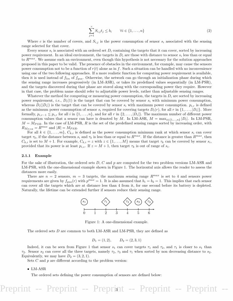
2.1.1 Example

For the sake of illustration, the ordered sets D, C and p are computed for the two problem versions LM-ASR andLM-PSR, with the one-dimensional example shown in Figure 1. The horizontal axis allows the reader to assess thedistances more easily.

There are n = 2 sensors, m = 3 targets, the maximum sensing range Rmax is set to 4 and sensors powerrequirements are given by fqua(r) with pmax = 1. It is also assumed that b1 = b2 = 1. This implies that each sensorcan cover all the targets which are at distance less than 4 from it, for one second before its battery is depleted.Naturally, the lifetime can be extended further if sensors reduce their sensing range.

0 1 2 3 4 5 6

s1 s2τ1 τ2 τ3

Figure 1: A one-dimensional example.

The ordered sets D are common to both LM-ASR and LM-PSR, they are defined as

D1 = (1, 2), D2 = (2, 3, 1)

Indeed, it can be seen from Figure 1 that sensor s1 can cover targets τ1 and τ2, and τ1 is closer to s1 thanτ2. Sensor s2 can cover all the three targets, namely τ2, τ3 and τ1 when sorted by non decreasing distance to s2.Equivalently, we may have D2 = (3, 2, 1).

Sets C and p are different according to the problem version:

• LM-ASR

The ordered sets defining the power consumption of sensors are defined below:

3

Preprint -- Preprint -- Preprint -- Preprint -- Preprint -- Preprint --

p1 =

(

1

4, 1

)

, p2 =

(

1

16,1

16,9

16

)

Sensor s1 is at distance 2 from the closest target it covers, hence p1,1 =(

2Rmax

)2=0.25. The second target in

D1 is at distance Rmax from s1, hence p1,2 reaches its maximum value (i.e., 1).

Sensor s2 is at distance 1 from the closest target it covers, hence p2,1 =(

1Rmax

)2= 1

16 . The second target inD2 is also at distance 1 from s2, hence p2,2 = 1

16 , and target τ1 is at distance 3 so p2,3 = 916 .

The maximum cardinality of Di over i in {1, . . . , n} defines the maximum number of different sensing rangesthat a sensor can have. Here, s1 has two sensing ranges, and s2 has three, so M = 3.

The ordered sets Ck that indicate the rank in power consumption of the sensors that cover target τk are:

C1 = (1, 3), C2 = (2, 1), C3 = (4, 2)

Target τ1 is covered by s1, which can cover it using its first (lower) sensing range. τ1 is also covered by s2,but it requires its third sensing range to reach that target.

Target τ2 is covered by s1, which can cover it using its second (highest) sensing range; it is also covered by s2but only requires its lower sensing range to reach it.

Finally, target τ3 is not covered by s1, hence C3,1 is set to M + 1 = 4. Target τ3 is covered by sensor s2, andrequires its second sensing range (or its first sensing range, as they are equal).

• LM-PSR

It is supposed that MPSR = 2, and the two predefined sensing ranges are R = {2, 4}. By definition of fqua(r),the corresponding power consumption levels are 1

4 and 1 respectively.

The ordered sets defining the power consumption of sensors are

p1 =

(

1

4, 1

)

, p2 =

(

1

4,1

4, 1

)

Sensor s1 is at distance 2 from the closest target it covers, hence the first predefined sensing range is needed

so p1,1 =(

24

)2= 0.25. The second target in D1 is at distance Rmax from s1, hence p1,2 reaches its maximum

value (i.e., 1).

Sensor s2 is at distance 1 from the closest target it covers, so p2,1 = 14 . The second target in D2 is at distance

2 from s2, hence p2,2 = 14 : both targets require the first predefined sensing range to be used. Target τ1 is at

distance 3 so the second predefined sensing range is used, leading to p2,3 = 1.

The maximum number of different sensing ranges is equal to the number of predefined sensing ranges soM = 2.

The ordered sets Ck that indicate the rank in power consumption of the sensors that cover target τk are:

C1 = (1, 2), C2 = (2, 1), C3 = (3, 1)

Target τ1 is covered by s1, which can cover it using the first predefined sensing range. τ1 is also covered bys2, but it requires the second predefined sensing range to reach that target.

Target τ2 is covered by s1, which can cover it using the second sensing range; it is also covered by s2 whichcan cover it using the first sensing range to reach it.

Finally, target τ3 is not covered by s1, hence C3,1 is set to M + 1 = 3. Target τ3 is covered by sensor s2, andrequires the first predefined sensing range.

2.2 Cover dominance properties

This section introduces two equivalent ways of representing covers. Those two different encodings are necessary asthey are both used in the column generation approach. Then, theoretical properties are provided for characterizingnon-dominated covers, that are useful for maximizing lifetime.

4

Preprint -- Preprint -- Preprint -- Preprint -- Preprint -- Preprint --

2.2.1 Cover encodings

Real vector encoding

Cover Sj can be defined as a n-column real vector where Si,j is the power consumption of sensor si, i.e., for alli ∈ {1, . . . , n}, Si,j belongs to the discrete set {0, pi,1, pi,2, . . . , pi,|Di|} for LM-ASR, and Si,j belongs to the discreteset {0, pi,1, pi,2, . . . , pi,MPSR

} for LM-PSR. For both problems, Si,j = 0 if and only if si is not part of cover Sj .

Binary encoding

Equivalently, Sj can be represented as a set of n ordered lists of |Di| binary numbers for LM-ASR, and MPSR

binary numbers for LM-PSR. More precisely, xi,r,j is set to one if sensor si is part of the cover and is used with powerpi,r, for all i ∈ {1, . . . , n}, it is zero otherwise. In addition, at most one variable xi,r,j should be set to one for alli ∈ {1, . . . , n} as each sensor has at most one power consumption level (and no level at all if it is not part of the cover).

Changing encoding

The following equation is used for transforming a cover from the binary encoding to the real vector encoding inLM-ASR.

Si,j =

|Di|∑

r=1

xi,r,jpi,r ∀i ∈ {1, . . . , n}, ∀j ∈ {1, . . . , c} (3)

For LM-PSR, |Di| and pi,r must be replaced with MPSR and f(Rr), respectively.The reciprocal transformation is given in Algorithm 1 for LM-ASR.

for i = 1 to n do

for r = 1 to |Di| doif Si,j = pi,r then

xi,r,j ← 1;else

xi,r,j ← 0;

Algorithm 1: From the real vector encoding to the binary encoding.

Algorithm 1 can be used for LM-PSR, by replacing |Di| and pi,r with MPSR and f(Rr), respectively.

2.2.2 Non-dominated covers

All the approaches that use column generation for addressing lifetime maximization in wireless sensor networks relyon the notion of cover [2, 9, 14]. In all these column generation approaches, the main issue is to find a cover thatis likely to increase further the lifetime of the current solution. To the best of our knowledge, this article providesthe first theoretical study on how to reduce the search space of such attractive covers. As a result, it is shown thatthe search space can be reduced to non-dominated covers. This provides a significant advantage over performing asearch in the much larger set of valid covers.

A cover is said to be valid if the power level of its sensors is such that all the targets are covered by at least onesensor. A valid cover Sj is said to be dominated if there exists another valid cover Sj′ containing a subset of sensorsof Sj that are used at a lower power level, and at least one sensor is used in Sj′ at a strictly lower power than in Sj .More formally, Sj is dominated if there exists another valid cover Sj′ such that Si,j′ ≤ Si,j for all i ∈ {1, . . . , n},and there exists at least one integer i0 in {1, . . . , n} such that Si0,j′ < Si0,j .

Therefore, in any non-dominated cover, decreasing the power level of any sensor compromises coverage. Conse-quently, a non-dominated cover can be built from any valid cover by decreasing the power of sensors as long as itis possible to do so without compromising targets coverage. This process is referred to as cover refinement and isimplemented in Algorithm 2.

Lemma 1. There exists an optimal solution to LM-ASR (or LM-PSR) in which non-dominated covers only areused a non-zero amount of time.

5

Preprint -- Preprint -- Preprint -- Preprint -- Preprint -- Preprint --

Proof. Lemma 1 is proved by contradiction. Suppose that all optimal solutions to LM-ASR (or LM-PSR) are suchthat there exists a dominated cover Sj used for a nonzero amount of time. Then a non-dominated cover Sj′ can bebuilt from Sj , and be used instead of Sj in the optimal solution. Doing so preserves target coverage by definition ofnon-dominated covers. Repeating this process for all dominated covers used a nonzero amount of time leads to anoptimal solution to LM-ASR (or LM-PSR) where non-dominated covers only are used a non-zero amount of time.Contradiction.

As a consequence of Lemma 1, the search for an optimal solution to LM-ASR (or LM-PSR) can be restricted tonon-dominated covers only. Enforcing this restriction is efficient when designing a solution approach to LM-ASRor LM-PSR, as non-dominated covers are generally a small fraction of valid covers.

Lemma 2. The number of sensors in a non-dominated cover is at most m.

Proof. Each target has to be covered by at least one sensor, so at most m sensors are required for covering all thetargets. If a valid cover has more than m sensors, then one of them can be removed, so it is dominated.

Lemma 2 can be seen as a necessary (but not sufficient) condition for a cover to be non-dominated. It is usedin the column generation algorithm for building candidate non-dominated covers in Section 3.3.

Table 1: Notations

Notation Meaning

n Number of sensorsm Number of targetssi A sensor, for all i ∈ {1, . . . , n}τk A target, for all k ∈ {1, . . . ,m}bi Initial energy of sensor si for all i ∈ {1, . . . , n}

pi(t) Power consumption of sensor si over timeDi Targets covered by sensor si, sorted by increasing power requirementpi,r Minimum power consumption of sensor si required for covering target Di(r), for all r ∈ {1, . . . , |Di|}Rmax Sensors’ maximum sensing rangeM Maximum number of different power consumption values that a sensor can haveR Set of the predefined sensing ranges sorted by increasing order (for LM-PSR only)Ck,i Power consumption minimum rank at which sensor si can cover target τkSj jth cover (i.e., set of sensors). Si,j is the power of sensor si in the cover, ∀j ∈ {1, . . . , c}tj Amount of time during which cover Sj is used

xi,r,j Binary decision variable that is set to one iff sensor si is part of cover Sj and is used with power pi,r

2.2.3 Example

The Example introduced in Section 2.1.1 is used again for illustrating both cover encodings, valid covers, dominatedand non-dominated covers, for LM-ASR and LM-PSR.

• LM-ASR

There exist 5 valid covers, represented under the real vector encoding:

SASR1 =

[

14116

]

, SASR2 =

[

0916

]

, SASR3 =

[

1116

]

, SASR4 =

[

1916

]

, SASR5 =

[

14916

]

Covers SASR3 , SASR

4 and SASR5 are dominated because of cover SASR

1 . Hence, SASR1 and SASR

2 are non-dominated.

The binary encoding of covers SASR1 and SASR

2 are XASR1 and XASR

2 respectively:

XASR1 =

[

1 0 −1 0 0

]

, XASR2 =

[

0 0 −0 0 1

]

6

Preprint -- Preprint -- Preprint -- Preprint -- Preprint -- Preprint --

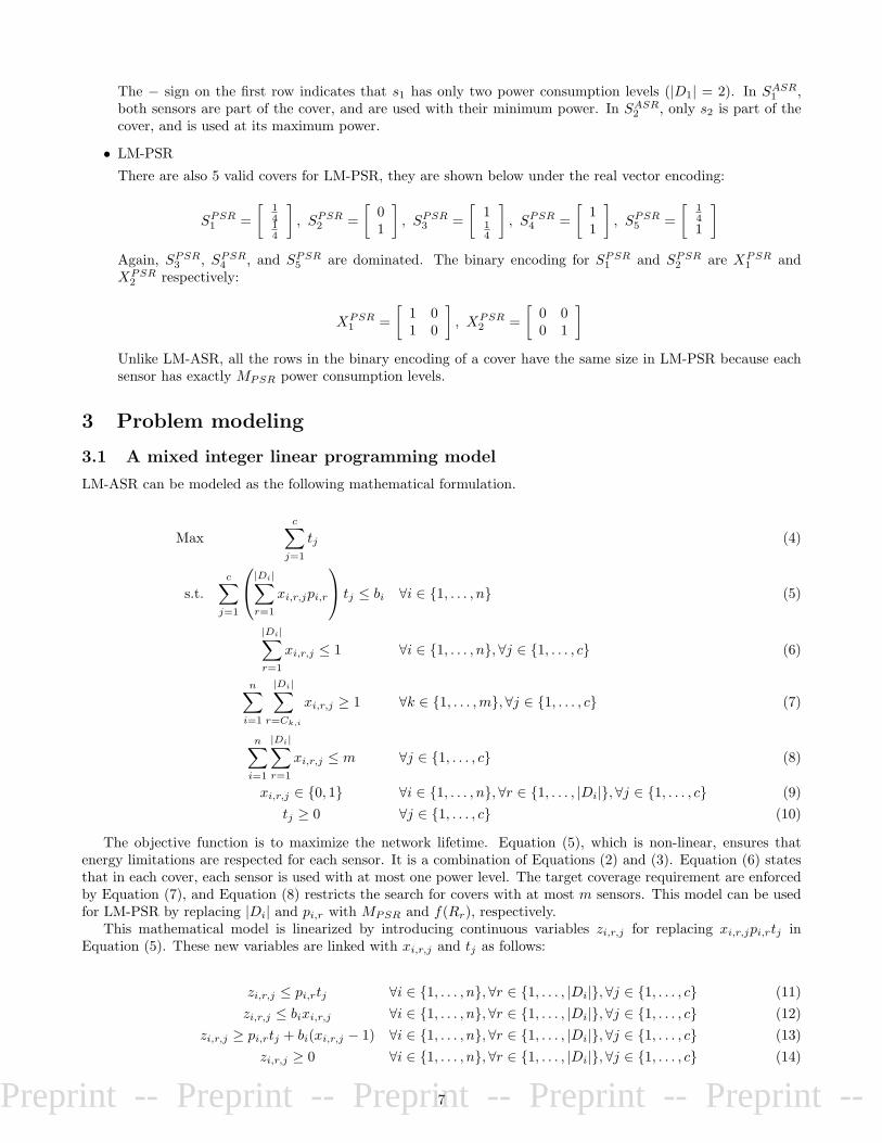
The − sign on the first row indicates that s1 has only two power consumption levels (|D1| = 2). In SASR1 ,

both sensors are part of the cover, and are used with their minimum power. In SASR2 , only s2 is part of the

cover, and is used at its maximum power.

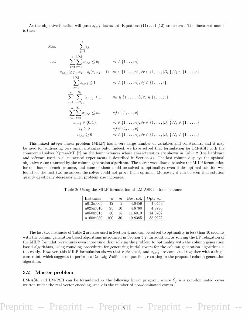
• LM-PSR

There are also 5 valid covers for LM-PSR, they are shown below under the real vector encoding:

SPSR1 =

[

1414

]

, SPSR2 =

[

01

]

, SPSR3 =

[

114

]

, SPSR4 =

[

11

]

, SPSR5 =

[

141

]

Again, SPSR3 , SPSR

4 , and SPSR5 are dominated. The binary encoding for SPSR

1 and SPSR2 are XPSR

1 andXPSR

2 respectively:

XPSR1 =

[

1 01 0

]

, XPSR2 =

[

0 00 1

]

Unlike LM-ASR, all the rows in the binary encoding of a cover have the same size in LM-PSR because eachsensor has exactly MPSR power consumption levels.

3 Problem modeling

3.1 A mixed integer linear programming model

LM-ASR can be modeled as the following mathematical formulation.

Max

c∑

j=1

tj (4)

s.t.

c∑

j=1

|Di|∑

r=1

xi,r,jpi,r

tj ≤ bi ∀i ∈ {1, . . . , n} (5)

|Di|∑

r=1

xi,r,j ≤ 1 ∀i ∈ {1, . . . , n}, ∀j ∈ {1, . . . , c} (6)

n∑

i=1

|Di|∑

r=Ck,i

xi,r,j ≥ 1 ∀k ∈ {1, . . . ,m}, ∀j ∈ {1, . . . , c} (7)

n∑

i=1

|Di|∑

r=1

xi,r,j ≤ m ∀j ∈ {1, . . . , c} (8)

xi,r,j ∈ {0, 1} ∀i ∈ {1, . . . , n}, ∀r ∈ {1, . . . , |Di|}, ∀j ∈ {1, . . . , c} (9)

tj ≥ 0 ∀j ∈ {1, . . . , c} (10)

The objective function is to maximize the network lifetime. Equation (5), which is non-linear, ensures thatenergy limitations are respected for each sensor. It is a combination of Equations (2) and (3). Equation (6) statesthat in each cover, each sensor is used with at most one power level. The target coverage requirement are enforcedby Equation (7), and Equation (8) restricts the search for covers with at most m sensors. This model can be usedfor LM-PSR by replacing |Di| and pi,r with MPSR and f(Rr), respectively.

This mathematical model is linearized by introducing continuous variables zi,r,j for replacing xi,r,jpi,rtj inEquation (5). These new variables are linked with xi,r,j and tj as follows:

zi,r,j ≤ pi,rtj ∀i ∈ {1, . . . , n}, ∀r ∈ {1, . . . , |Di|}, ∀j ∈ {1, . . . , c} (11)

zi,r,j ≤ bixi,r,j ∀i ∈ {1, . . . , n}, ∀r ∈ {1, . . . , |Di|}, ∀j ∈ {1, . . . , c} (12)

zi,r,j ≥ pi,rtj + bi(xi,r,j − 1) ∀i ∈ {1, . . . , n}, ∀r ∈ {1, . . . , |Di|}, ∀j ∈ {1, . . . , c} (13)

zi,r,j ≥ 0 ∀i ∈ {1, . . . , n}, ∀r ∈ {1, . . . , |Di|}, ∀j ∈ {1, . . . , c} (14)

7

Preprint -- Preprint -- Preprint -- Preprint -- Preprint -- Preprint --

As the objective function will push zi,r,j downward, Equations (11) and (12) are useless. The linearized modelis then

Max

c∑

j=1

tj

s.t.

c∑

j=1

|Di|∑

r=1

zi,r,j ≤ bi ∀i ∈ {1, . . . , n}

zi,r,j ≥ pi,rtj + bi(xi,r,j − 1) ∀i ∈ {1, . . . , n}, ∀r ∈ {1, . . . , |Di|}, ∀j ∈ {1, . . . , c}

|Di|∑

r=1

xi,r,j ≤ 1 ∀i ∈ {1, . . . , n}, ∀j ∈ {1, . . . , c}

n∑

i=1

|Di|∑

r=Ck,i

xi,r,j ≥ 1 ∀k ∈ {1, . . . ,m}, ∀j ∈ {1, . . . , c}

n∑

i=1

|Di|∑

r=1

xi,r,j ≤ m ∀j ∈ {1, . . . , c}

xi,r,j ∈ {0, 1} ∀i ∈ {1, . . . , n}, ∀r ∈ {1, . . . , |Di|}, ∀j ∈ {1, . . . , c}

tj ≥ 0 ∀j ∈ {1, . . . , c}

zi,r,j ≥ 0 ∀i ∈ {1, . . . , n}, ∀r ∈ {1, . . . , |Di|}, ∀j ∈ {1, . . . , c}

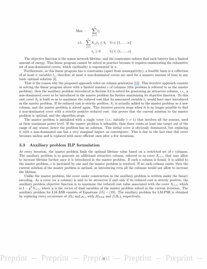
This mixed integer linear problem (MILP) has a very large number of variables and constraints, and it maybe used for addressing very small instances only. Indeed, we have solved that formulation for LM-ASR with thecommercial solver Xpress-MP [7] on the four instances whose characteristics are shown in Table 2 (the hardwareand software used in all numerical experiments is described in Section 4). The last column displays the optimalobjective value returned by the column generation algorithm. The solver was allowed to solve the MILP formulationfor one hour on each instance, and none of them could be solved to optimality: even if the optimal solution wasfound for the first two instances, the solver could not prove them optimal. Moreover, it can be seen that solutionquality drastically decreases when problem size increases.

Table 2: Using the MILP formulation of LM-ASR on four instances

Instances n m Best sol. Opt. sol.n012m005 12 5 4.0459 4.0459n025m010 25 10 4.8780 4.8780n050m015 50 15 11.6013 14.0702n100m030 100 30 19.8385 38.9922

The last two instances of Table 2 are also used in Section 4, and can be solved to optimality in less than 10 secondswith the column generation based algorithms introduced in Section 3.2. In addition, as solving the LP relaxation ofthe MILP formulation requires even more time than solving the problem to optimality with the column generationbased algorithms, using rounding procedures for generating initial covers for the column generation algorithms istoo costly. However, this MILP formulation shows that variables tj and xi,r,j are connected together with a singleconstraint, which suggests to perform a Dantzig-Wolfe decomposition, resulting in the proposed column generationalgorithm.

3.2 Master problem

LM-ASR and LM-PSR can be formulated as the following linear program, where Sj is a non-dominated coverwritten under the real vector encoding, and c is the number of non-dominated covers.

8

Preprint -- Preprint -- Preprint -- Preprint -- Preprint -- Preprint --

Max

c∑

j=1

tj

s.t.

c∑

j=1

Si,jtj ≤ bi ∀i ∈ {1, . . . , n}

tj ≥ 0 ∀j ∈ {1, . . . , c}

The objective function is the sensor network lifetime, and the constraints enforce that each battery has a limitedamount of energy. This linear program cannot be solved in practice because it requires enumerating the exhaustiveset of non-dominated covers, which cardinality is exponential in n.

Furthermore, as this linear program has n constraints (apart from nonnegativity), a feasible basis is a collectionof at most n variables tj , therefore at most n non-dominated covers are used for a nonzero amount of time in anybasic optimal solution [4].

That is the reason why the proposed approach relies on column generation [13]. This iterative approach consistsin solving the linear program above with a limited number c of columns (this problem is referred to as the masterproblem), then the auxiliary problem introduced in Section 3.3 is solved for generating an attractive column, i.e., anon-dominated cover to be introduced in the master problem for further maximizing its objective function. To thisend, cover Sj is built so as to maximize the reduced cost that its associated variable tj would have once introducedin the master problem. If its reduced cost is strictly positive, Sj is actually added to the master problem as a newcolumn, and the master problem is solved again. This iterative process stops when it is no longer possible to finda non-dominated cover with a strictly positive reduced cost: this proves that the current solution to the masterproblem is optimal, and the algorithm stops.

The master problem is initialized with a single cover (i.e., initially c = 1) that involves all the sensors, usedat their maximum power level. If the master problem is infeasible, then there exists at least one target out of therange of any sensor, hence the problem has no solution. This initial cover is obviously dominated, but replacingit with a non-dominated one has a very marginal impact on convergence. This is due to the fact that this coverbecomes useless and is replaced with more efficient ones after a few iterations.

3.3 Auxiliary problem ILP formulation

At every iteration, the master problem finds the optimal lifetime value based on a restricted set of c columns.The auxiliary problem is to generate an additional attractive column, referred to as cover Sc+1, that may allowto increase lifetime further once it is introduced in the master problem. If such a column is found, it is added tothe master problem, c is increased by one and the master problem is resolved. If no such column exists, then thecurrent solution of the master problem is optimal, as introducing even all the columns would not allow to increasethe lifetime.

Unlike the master problem, the cover under construction in the auxiliary problem is written under the binaryencoding. As a cover (or a column) is said to be attractive if and only if its reduced cost is strictly positive, theauxiliary problem objective function is to maximize the reduced cost value associated with the cover Sc+1, whichis 1 − yTSc+1, where y is the vector of dual variables of the master problem solved in the current iteration. Theauxiliary problem for LM-ASR consists of Equations (15) − (19). The auxiliary problem for LM-PSR is obtainedby replacing every occurrence of |Di| and pi,r with MPSR and f(Rr), respectively.

9

Preprint -- Preprint -- Preprint -- Preprint -- Preprint -- Preprint --

Max 1−

n∑

i=1

|Di|∑

r=1

xi,r,c+1pi,r

yi (15)

s.t.

|Di|∑

r=1

xi,r,c+1 ≤ 1 ∀i ∈ {1, . . . , n} (16)

n∑

i=1

|Di|∑

r=Ck,i

xi,r,c+1 ≥ 1 ∀k ∈ {1, . . . ,m} (17)

n∑

i=1

|Di|∑

r=1

xi,r,c+1 ≤ m (18)

xi,r,c+1 ∈ {0, 1} ∀i ∈ {1, . . . , n}∀r ∈ {1, . . . , |Di|} (19)

The decision variables are xi,r,c+1, whereas yi, pi,r, Ck and Di are given data. The objective function is thereduced cost of the new cover, where Si,c+1 have been substituted using Equation (3). Constraint (16) ensures thateach sensor is associated to a single power level (or no power level at all if it is not part of the cover). Constraint(17) states that the cover must be valid, i.e., all targets must be covered by at least one sensor. Note that if sensorsi does not cover target τk, then r = M + 1 and so no term involving xi,r,c+1 is part of the sum. Constraint (18)is the necessary condition stated in Lemma 2 for the cover to be non-dominated. Finally, constraint (19) enforcebinary requirements.

The auxiliary problem returns Sc+1 if its objective value is strictly positive, otherwise the algorithm stops asa zero objective value implies that there does not exists any attractive cover, hence the master problem currentsolution is optimal.

3.3.1 Relationship between LM-ASR and LM-PSR

The auxiliary problem can be strengthened in the case of LM-PSR. If a sensor is such that there is no target locatedat distance d ∈]Rr, Rr+1] with r ∈ {1, . . . ,MPSR − 1}, then the corresponding power level (namely f(Rr)) is neverused by this sensor. Consequently, variable xi,r,c+1 can be set to zero. Thus, Equation (20) is added to the auxiliaryproblem.

xi,r,c+1 = 0 ∀(i, r) ∈ {1, . . . , n} × {1, . . . ,MPSR}, f(Rr) /∈ pi (20)

Such a situation never happens with LM-ASR, as power levels are defined for each sensor for exactly fitting itsneighboring targets with minimum power requirement. Equation (20) is then specific to LM-PSR.

Despite constraint (18), the cover returned after solving the auxiliary problem may not always be non-dominated.Algorithm 2 is a post-optimization procedure that aims at refining Sc+1 (under binary encoding) so as to make itnon-dominated.

10

Preprint -- Preprint -- Preprint -- Preprint -- Preprint -- Preprint --

for i = 1 to n do

for r = |Di| to 1 do

if xi,r,c+1 = 1 then

xi,r,c+1 ← 0;if r > 1 then

xi,r−1,c+1 ← 1;

breach← false;k ← 1;while breach =false and k ≤ m do

if

n∑

i′=1

|Di′ |∑

r′=Ck,i′

xi′,r′,c+1 = 0 then

breach← true;

k ← k + 1;

if breach = true then

xi,r,c+1 ← 1;if r > 1 then

xi,r−1,c+1 ← 0;

Algorithm 2: Refining Sc+1 (under binary encoding) into a non-dominated cover.

Algorithm 2 attempts to reduce the power of all sensors in Sc+1 to its closest lower level. If the consideredsensor is already using its minimum power, it is tested for removal. Then, the coverage constraints (Equation (17))are checked. If one of them does not hold, the Boolean variable breach is set to true, and the sensor is set backto its original power level. Otherwise, further power reductions and removals are attempted. When this algorithmterminates, the resulting cover is non-dominated as reducing the power or removing any sensor compromises targetcoverage.

Lemma 3. Whatever MPSR and the values for the predefined sensing ranges, the objective function value reachedby LM-ASR is always larger than or equal to the objective function value reached by LM-PSR.

Proof. Let SPSR be an optimal solution to LM-PSR consisting of c covers denoted by SPSRj , each of them being

used a nonzero amount of time tj . A feasible solution to LM-ASR consisting in c covers used the same amount oftime and denoted by {SASR

1 , . . . , SASRc } is built from SPSR by transforming the cover SPSR

j for all j in {1, . . . , c}as follows.

For all i in {1, . . . , n}, SASRi,j is set to pi,r where r is the maximum integer such that pi,r ≤ SPSR

i,j . Thus, sensor

si covers the same targets in SPSRj and SASR

j because by definition of pi,r the targets covered by si are the same

for any power value in [pi,r, pi,r+1[. Consequently, SASRj ≤ SPSR

j for all j ∈ {1, . . . , c} so SASRj can be used for tj

units of time, leading to the same lifetime duration as SPSR.

Lemma 4. LM-PSR and LM-ASR have the same optimal objective value if

⋃

i∈{1,...,n}r∈{1,...,|Di|}

pi,r ⊆⋃

r∈{1,...,MPSR}

f(Rr) (21)

Where pi,r refer to power levels in LM-ASR, f(Rr) being the power levels in LM-PSR, associated with predefinedsensing ranges.

Proof. If Equation (21) holds, then any non-dominated cover for LM-ASR is also non-dominated for LM-PSR. Then,LM-PSR is identical to LM-ASR: for each sensor, all useless power levels are associated a zero decision variablein the auxiliary problem by Equation (20). Once zero decision variables are removed, the auxiliary problems forLM-ASR and LM-PSR are identical.

The example in Figure 2 shows that Equation (21) is not a necessary condition for LM-PSR and LM-ASR tohave identical optimal objective values. Indeed, all power levels in LM-ASR may not be used in an optimal solution.More specifically, s1 has to maintain its sensing range to Rmax = 4 for covering target τ2, hence its sensing range

11

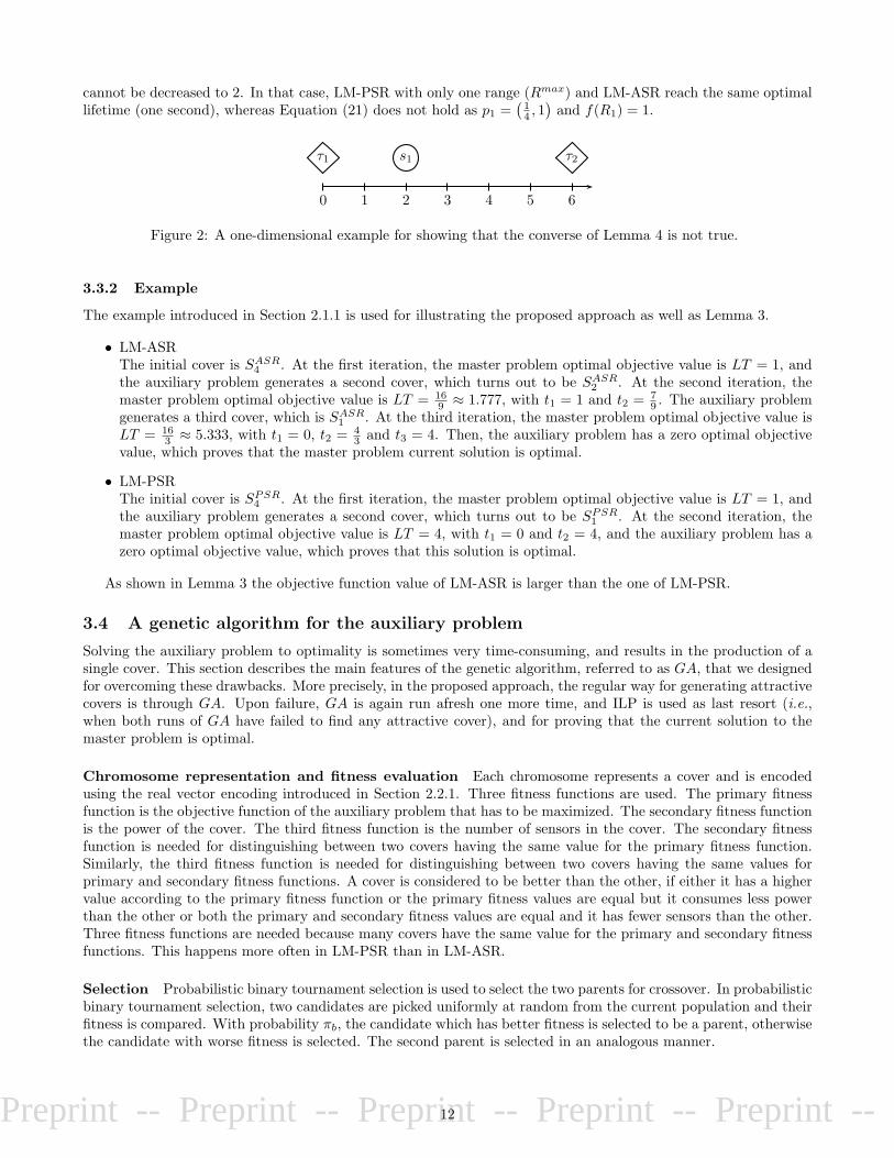
Preprint -- Preprint -- Preprint -- Preprint -- Preprint -- Preprint --

cannot be decreased to 2. In that case, LM-PSR with only one range (Rmax) and LM-ASR reach the same optimallifetime (one second), whereas Equation (21) does not hold as p1 =

(

14 , 1

)

and f(R1) = 1.

0 1 2 3 4 5 6

s1τ1 τ2

Figure 2: A one-dimensional example for showing that the converse of Lemma 4 is not true.

3.3.2 Example

The example introduced in Section 2.1.1 is used for illustrating the proposed approach as well as Lemma 3.

• LM-ASRThe initial cover is SASR

4 . At the first iteration, the master problem optimal objective value is LT = 1, andthe auxiliary problem generates a second cover, which turns out to be SASR

2 . At the second iteration, themaster problem optimal objective value is LT = 16

9 ≈ 1.777, with t1 = 1 and t2 = 79 . The auxiliary problem

generates a third cover, which is SASR1 . At the third iteration, the master problem optimal objective value is

LT = 163 ≈ 5.333, with t1 = 0, t2 = 4

3 and t3 = 4. Then, the auxiliary problem has a zero optimal objectivevalue, which proves that the master problem current solution is optimal.

• LM-PSRThe initial cover is SPSR

4 . At the first iteration, the master problem optimal objective value is LT = 1, andthe auxiliary problem generates a second cover, which turns out to be SPSR

1 . At the second iteration, themaster problem optimal objective value is LT = 4, with t1 = 0 and t2 = 4, and the auxiliary problem has azero optimal objective value, which proves that this solution is optimal.

As shown in Lemma 3 the objective function value of LM-ASR is larger than the one of LM-PSR.

3.4 A genetic algorithm for the auxiliary problem

Solving the auxiliary problem to optimality is sometimes very time-consuming, and results in the production of asingle cover. This section describes the main features of the genetic algorithm, referred to as GA, that we designedfor overcoming these drawbacks. More precisely, in the proposed approach, the regular way for generating attractivecovers is through GA. Upon failure, GA is again run afresh one more time, and ILP is used as last resort (i.e.,when both runs of GA have failed to find any attractive cover), and for proving that the current solution to themaster problem is optimal.

Chromosome representation and fitness evaluation Each chromosome represents a cover and is encodedusing the real vector encoding introduced in Section 2.2.1. Three fitness functions are used. The primary fitnessfunction is the objective function of the auxiliary problem that has to be maximized. The secondary fitness functionis the power of the cover. The third fitness function is the number of sensors in the cover. The secondary fitnessfunction is needed for distinguishing between two covers having the same value for the primary fitness function.Similarly, the third fitness function is needed for distinguishing between two covers having the same values forprimary and secondary fitness functions. A cover is considered to be better than the other, if either it has a highervalue according to the primary fitness function or the primary fitness values are equal but it consumes less powerthan the other or both the primary and secondary fitness values are equal and it has fewer sensors than the other.Three fitness functions are needed because many covers have the same value for the primary and secondary fitnessfunctions. This happens more often in LM-PSR than in LM-ASR.

Selection Probabilistic binary tournament selection is used to select the two parents for crossover. In probabilisticbinary tournament selection, two candidates are picked uniformly at random from the current population and theirfitness is compared. With probability πb, the candidate which has better fitness is selected to be a parent, otherwisethe candidate with worse fitness is selected. The second parent is selected in an analogous manner.

12

Preprint -- Preprint -- Preprint -- Preprint -- Preprint -- Preprint --

Crossover We have used the two crossover operators. The first crossover operator that is used simply transferseach sensor present in either of the two parents to the child chromosome. However, if a sensor is present in both theparents and have different power levels then for such a sensor the child will have the higher of the two power levelswith probability πh, otherwise it will have the lower of the two power levels. The second crossover that is used isthe uniform crossover. The first crossover is used with probability πf , otherwise the second crossover is used. Thetwo crossovers are needed to maintain a balance between exploitation and exploration.

Mutation Mutation is applied to the child obtained through crossover. The mutation operator considers eachsensor one-by-one, and, if it is present in the child, it deletes it with probability πm. If a sensor is not present thenmutation operator inserts it at a random power level with probability πm.

Repair operator The child chromosome obtained after the application of genetic operators may not be feasible.Therefore, a repair operator is designed, which not only converts the child into a feasible cover, but also into agood non-dominated cover. It consist of three stages. The first stage transforms the child into a feasible cover. Thesecond stage tries to improve the value of the auxiliary problem’s objective function (hereafter, refers to as objectivefunction in the remainder of this section) by removing some sensors. The third stage tries to further improve thevalue of the objective function by reducing the range of some sensors.

The first stage considers each target one-by-one and if the target under consideration is not covered by anysensor then it either adds a new sensor to the cover or increases the power level of an existing sensor in a way thatcovers the target in question and that leads to minimum reduction in the value of the objective function. Coverageinformation of all targets are updated before considering the next target.

The second stage deletes those sensors from the cover all of whose covered targets are covered by other sensorsalso. It follows an iterative process. During each iteration it begins by computing the set Sred of those sensors inthe cover, all of whose targets are redundantly covered. Then from this set it removes the sensor si correspondingto the maximum yi × pi,r value from the cover, where pi,r is the current power level of sensor si. This process isrepeated, until the iteration, where Sred is found to be empty. Note that deleting sensor with maximum yi × pi,rvalue leads to maximum increase in the value of the objective function.

The third stage ensures that remaining sensors are used only at their respective minimum power levels necessaryfor covering all targets. It follows an iterative process where during each iteration it decreases the power of a sensorfrom its current level to its next (strictly) lower level if doing so does not result into a coverage breach. If there aremore than one candidate sensors, then the power level of sensor with maximum yi × (pi,r − pi,q) value is reducedfrom its current value pi,r to its next (strictly) lower level pi,q. Note that for LM-PSR, (r − q) = 1, whereas forLM-ASR as many power levels can be equal so (r − q) ≥ 1 . This process is repeated until it is not possible toreduce the power level of any sensor.

Replacement policy Our genetic algorithm uses steady-state population replacement method [5]. In this methodgenetic algorithm repeatedly selects two parents, performs crossover and mutation to generate a single child thatreplaces a less fit member of the population. This is different from generational method where the entire parentpopulation is replaced with an equal number of newly created children every generation. In comparison to thegenerational method, the steady-state population replacement method generally finds better solutions faster. Thisis due to keeping the best solutions in the population permanently and the immediate availability of the generatedchild for selection and reproduction. Another advantage of the steady-state population replacement method is theease with which duplicate copies of the same individuals are avoided in the population. In the generational method,duplicate copies of the highly fit individuals may exist in the population. Within few generations, these highlyfit individuals can dominate the whole population. When this happens, the crossover becomes totally ineffectiveand the mutation becomes the only possible way to improve solution quality. When this happens, improvement,if any, in solution quality is quite slow. Such a situation is known as the premature convergence. In the steady-state method, we can easily prevent this situation by simply comparing each newly generated child with currentpopulation members and discarding the child, if it is identical to any current member.

Initial population generation Each member of the initial population is generated randomly by following athree stage procedure. With probability πa, the first stage includes as many sensors as possible with yi = 0 at theirmaximum power level. Actually, these sensors do not contribute to the objective function irrespective of their powerlevels. These sensors are added to the solution one-by-one in some random order and the coverage information of allthe target are updated whenever a sensor is added to the solution. The remaining uncovered targets are covered byfollowing an iterative approach. During each iteration an uncovered target is selected randomly and then a sensor

13

Preprint -- Preprint -- Preprint -- Preprint -- Preprint -- Preprint --

that can cover this target is also selected randomly. This sensor can be a new sensor or a sensor already presentin the cover but with a power level lower than required for covering the target under consideration. The powerlevel of this sensor is set to the minimum power level necessary for covering the target in question. The coverageinformation of all the targets are updated. This process is repeated until no target is left uncovered. The secondand third stages are exactly similar to the second and third stages of repair operator except during each iterationa candidate is selected randomly. This is done to increase the diversity of initial population.

Each newly generated chromosome is checked for uniqueness against the population members generated so far,and, if it is unique, then it is included in the initial population, otherwise it is discarded.

Other features If our genetic algorithms found an attractive cover then up to MAXCOV ER best attractivecovers are returned at each iteration which accelerates convergence. If the genetic algorithm fails to find an attractivecover, it is applied afresh one more time before using the ILP. The stopping criterion that is used for our geneticalgorithm is the maximum number of consecutive iterations itmax without improvement in best solution quality.However, the value of itmax varies over the set OPTION = {50, 100, 250, 500, 1000, 2000} from one run to theother. If in the previous run genetic algorithm returned less than MAXCOV ER attractive covers then itmax isset to next higher value, if possible, in the OPTION , otherwise itmax is set to next lower value, if possible, in theOPTION . itmax is set to 50 in the very first run of the genetic algorithm.

In case of LM-ASR, as many power levels are equal, therefore, whenever a sensor is set to a new power level acheck is made to ensure that all targets that can be covered with that much power, are indeed covered.

4 Computational results

4.1 Instances and experimental setup

The instances that we have used in our computational experiments have been generated as follows. n sensors and mtargets are generated at random in a 500× 500 area. The maximum sensing range of sensors is set to Rmax = 150.The instance name format is nXXXmYYY, where XXX ∈ {50, 100, 150, 200, 300, 600} is the number of sensors, and YYY

∈ {15, 30, 45, 60, 90, 120, 180, 360} is the number of targets. Five instances of the same size have been generated,leading to a grand total of 60 different instances.

In addition to LM-ASR, LM-PSR is addressed for 3 different numbers of sensing ranges. In PSR1, sensors areeither sensing up to their maximum range Rmax, or not used at all; this corresponds to the problem where sensingranges are not adjustable. In PSR3, the three sensing ranges are {50, 100, 150} and in PSR6, the six consideredsensing ranges are {25, 50, 75, 100, 125, 150}. Thus, the number of sensing ranges considered in this paper is as largeas in [3]. The quadratic model fqua defined in Section 2.1 has been used for the sensors’ power consumption.

All the approaches presented in this paper are implemented in c, a function is used for removing the covers useda zero amount of time when the number of covers exceeds 10(n +m + 1) in the master problem (this is expectedto keep the master program fast when GA returns up to MAXCOV ER covers per iteration). Algorithm 2 is alsorun at every iteration for transforming the cover found by the auxiliary problem into a non-dominated cover.

For the genetic algorithm, we have used a population of min(n, 100) individuals, MAXCOV ER = 10, πa = 0.25,πf = 0.8, πh = 0.9, πm = 0.05. We have used two different values of πb. The first parent is selected with πb = 0.9,whereas the second parent is selected with πb = 0.8. All these parameter values are chosen empirically after largenumber of trials.

All the computations have been performed on an Intel Xeon Processor system at 2.66 GHz, with 8 GB RAMunder Microsoft Windows 7. The LP and ILP solver is GLPK [10].

4.2 Results

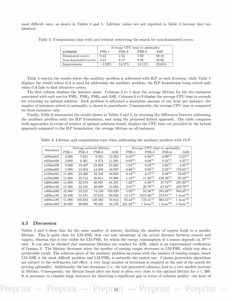
As a preliminary result, the benefit of using non-dominated covers is assessed on the 5 instances with n = 150sensors and m = 45 targets, for LM-ASR and LM-PSR. The first row of Table 3 displays the CPU time in secondsof the column generation algorithm for which the cover refinement procedure (see Algorithm 2) is never used, andwhere Equation (18) is not present in the auxiliary problem. The second row of the table shows the results wherethe cover refinement procedure is called after each iteration of the auxiliary problem, and where Equation (18) ispresent in the auxiliary problem formulation. In both cases, ILP only is used for addressing the auxiliary problem.The last row displays the CPU time improvement (in percent) when using non-dominated covers.

It can be seen that the benefit of restricting the search for attractive covers to non-dominated ones is morevisible for LM-ASR, and for LM-PSR with a high number of predefined sensing ranges. These problems are the

14

Preprint -- Preprint -- Preprint -- Preprint -- Preprint -- Preprint --

most difficult ones, as shown in Tables 4 and 5. Lifetime values are not reported in Table 3 because they areidentical.

Table 3: Computation time with and without restricting the search for non-dominated covers.

Average CPU time to optimalityn150m045 PSR-1 PSR-3 PSR-6 ASRDominated covers 0.43 2.54 7.93 69.18Non-dominated covers 0.44 2.17 6.89 52.82Improvement −2.33% 14.57% 13.11% 23.65%

Table 4 reports the results where the auxiliary problem is addressed with ILP at each iteration, while Table 5displays the results where GA is used for addressing the auxiliary problem, the ILP formulation being solved onlywhen GA fails to find attractive covers.

The first column displays the instance name. Columns 2 to 5 show the average lifetime for the five instancesassociated with each row for PSR1, PSR3, PSR6 and ASR. Columns 6 to 9 display the average CPU time in secondsfor returning an optimal solution. Each problem is allocated a maximum amount of one hour per instance; thenumber of instances solved to optimality is shown in parenthesis. Consequently, the average CPU time is computedon these instances only.

Finally, Table 6 summarizes the results shown in Tables 4 and 5, by stressing the differences between addressingthe auxiliary problem with the ILP formulation, and using the proposed hybrid approach. The table comparesboth approaches in terms of number of optimal solutions found, displays the CPU time cut provided by the hybridapproach compared to the ILP formulation, the average lifetime on all instances.

Table 4: Lifetime and computation time when addressing the auxiliary problem with ILP .

InstancesAverage network lifetime Average CPU time to optimality

PSR-1 PSR-3 PSR-6 ASR PSR-1 PSR-3 PSR-6 ASR

n050m015 4.000 7.621 9.561 12.262 0.03(5) 0.06(5) 0.09(5) 0.22(5)

n050m030 3.600 6.361 8.474 11.291 0.03(5) 0.08(5) 0.16(5) 0.37(5)

n100m030 9.000 19.487 24.089 31.665 1.04(5) 0.83(5) 2.66(5) 4.61(5)

n100m060 7.000 12.004 14.088 18.937 0.96(5) 0.96(5) 2.23(5) 178.66(5)

n150m045 11.800 24.360 32.502 44.934 0.44(5) 2.17(5) 6.89(5) 52.82(5)

n150m090 11.600 23.744 29.814 41.993 1.18(5) 11.26(5) 126.39(5) 95.29(2)

n200m060 14.600 32.378 46.867 64.455 1.02(5) 6.36(5) 47.73(5) 235.30(4)

n200m120 14.400 32.105 39.699 55.003 2.81(5) 20.70(5) 67.83(5) 270.79(2)

n300m090 25.000 55.525 74.139 103.320 5.38(5) 82.36(4) 285.88(3) 984.85(1)

n300m180 23.400 54.581 67.643 93.930 14.14(5) 1015.86(5) 373.81(1) 1 hour(0)

n600m180 51.000 105.683 138.292 58.844 82.34(5) 722.41(3) 963.55(1) 1 hour(0)

n600m360 48.600 96.000 90.625 16.176 221.22(5) 1 hour(0) 1 hour(0) 1 hour(0)

4.3 Discussion

Tables 4 and 5 show that for the same number of sensors, doubling the number of targets leads to a smallerlifetime. This is quite clear for LM-ASR, that can take advantage of the actual distance between sensors andtargets, whereas this is less visible for LM-PSR1 for which the energy consumption of a sensor depends on Rmax

only. It can also be checked that maximum lifetimes are reached for ASR, which is an experimental verificationof Lemma 3. The lifetime decreases when the number of sensing ranges decreases in LM-PSR, which was also apredictable result. The solution space of the auxiliary problem increases with the number of sensing ranges, henceLM-ASR is the most difficult problem and LM-PSR1 is naturally the easiest one. Column generation algorithmsare subject to the well-known tail effect: a very large number of iterations is required at the end of the search forproving optimality. Additionally, the last iterations (i.e., the last generated columns) lead to a very modest increasein lifetime. Consequently, the lifetime found after one hour is often very close to the optimal lifetime for n ≤ 300.It is necessary to consider large instances for observing a significant gap in terms of solution quality: one hour of

15

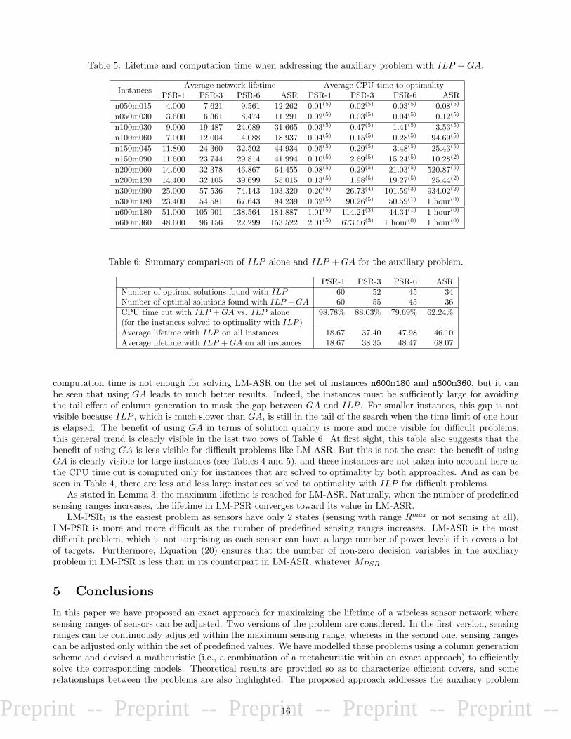
Preprint -- Preprint -- Preprint -- Preprint -- Preprint -- Preprint --

Table 5: Lifetime and computation time when addressing the auxiliary problem with ILP +GA.

InstancesAverage network lifetime Average CPU time to optimality

PSR-1 PSR-3 PSR-6 ASR PSR-1 PSR-3 PSR-6 ASR

n050m015 4.000 7.621 9.561 12.262 0.01(5) 0.02(5) 0.03(5) 0.08(5)

n050m030 3.600 6.361 8.474 11.291 0.02(5) 0.03(5) 0.04(5) 0.12(5)

n100m030 9.000 19.487 24.089 31.665 0.03(5) 0.47(5) 1.41(5) 3.53(5)

n100m060 7.000 12.004 14.088 18.937 0.04(5) 0.15(5) 0.28(5) 94.69(5)

n150m045 11.800 24.360 32.502 44.934 0.05(5) 0.29(5) 3.48(5) 25.43(5)

n150m090 11.600 23.744 29.814 41.994 0.10(5) 2.69(5) 15.24(5) 10.28(2)

n200m060 14.600 32.378 46.867 64.455 0.08(5) 0.29(5) 21.03(5) 520.87(5)

n200m120 14.400 32.105 39.699 55.015 0.13(5) 1.98(5) 19.27(5) 25.44(2)

n300m090 25.000 57.536 74.143 103.320 0.20(5) 26.73(4) 101.59(3) 934.02(2)

n300m180 23.400 54.581 67.643 94.239 0.32(5) 90.26(5) 50.59(1) 1 hour(0)

n600m180 51.000 105.901 138.564 184.887 1.01(5) 114.24(3) 44.34(1) 1 hour(0)

n600m360 48.600 96.156 122.299 153.522 2.01(5) 673.56(3) 1 hour(0) 1 hour(0)

Table 6: Summary comparison of ILP alone and ILP +GA for the auxiliary problem.

PSR-1 PSR-3 PSR-6 ASRNumber of optimal solutions found with ILP 60 52 45 34Number of optimal solutions found with ILP +GA 60 55 45 36CPU time cut with ILP +GA vs. ILP alone(for the instances solved to optimality with ILP )

98.78% 88.03% 79.69% 62.24%

Average lifetime with ILP on all instances 18.67 37.40 47.98 46.10Average lifetime with ILP +GA on all instances 18.67 38.35 48.47 68.07

computation time is not enough for solving LM-ASR on the set of instances n600m180 and n600m360, but it canbe seen that using GA leads to much better results. Indeed, the instances must be sufficiently large for avoidingthe tail effect of column generation to mask the gap between GA and ILP . For smaller instances, this gap is notvisible because ILP , which is much slower than GA, is still in the tail of the search when the time limit of one houris elapsed. The benefit of using GA in terms of solution quality is more and more visible for difficult problems;this general trend is clearly visible in the last two rows of Table 6. At first sight, this table also suggests that thebenefit of using GA is less visible for difficult problems like LM-ASR. But this is not the case: the benefit of usingGA is clearly visible for large instances (see Tables 4 and 5), and these instances are not taken into account here asthe CPU time cut is computed only for instances that are solved to optimality by both approaches. And as can beseen in Table 4, there are less and less large instances solved to optimality with ILP for difficult problems.

As stated in Lemma 3, the maximum lifetime is reached for LM-ASR. Naturally, when the number of predefinedsensing ranges increases, the lifetime in LM-PSR converges toward its value in LM-ASR.

LM-PSR1 is the easiest problem as sensors have only 2 states (sensing with range Rmax or not sensing at all),LM-PSR is more and more difficult as the number of predefined sensing ranges increases. LM-ASR is the mostdifficult problem, which is not surprising as each sensor can have a large number of power levels if it covers a lotof targets. Furthermore, Equation (20) ensures that the number of non-zero decision variables in the auxiliaryproblem in LM-PSR is less than in its counterpart in LM-ASR, whatever MPSR.

5 Conclusions

In this paper we have proposed an exact approach for maximizing the lifetime of a wireless sensor network wheresensing ranges of sensors can be adjusted. Two versions of the problem are considered. In the first version, sensingranges can be continuously adjusted within the maximum sensing range, whereas in the second one, sensing rangescan be adjusted only within the set of predefined values. We have modelled these problems using a column generationscheme and devised a matheuristic (i.e., a combination of a metaheuristic within an exact approach) to efficientlysolve the corresponding models. Theoretical results are provided so as to characterize efficient covers, and somerelationships between the problems are also highlighted. The proposed approach addresses the auxiliary problem

16

Preprint -- Preprint -- Preprint -- Preprint -- Preprint -- Preprint --

with an efficient genetic algorithm. Computational results demonstrate that for both versions, the use of geneticalgorithm within the column generation scheme significantly reduces the computation time, without compromisingoptimality.

Our results suggest that the use of non-dominated covers could be efficiently adapted to different versions ofthe lifetime maximization problems. Similar approaches can be designed for other scheduling problems in wirelesssensor networks. As a future work, we intend to experiment with other population based metaheuristics within thecolumn generation scheme to assess their suitability for such use.

References

[1] I. Akyildiz, W. Su, Y. Sankarasubramaniam, and E. Cayirci. Wireless sensor networks: a survey. ComputerNetworks, 38(4):393–422, 2002.

[2] A. Alfieri, A. Bianco, P. Brandimarte, and C.F. Chiasserini. Maximizing system lifetime in wireless sensornetworks. Eur J Oper Res, 181:390–402, 2007.

[3] M. Cardei, J. Wu, M. Lu, and M. Pervaiz. Maximum network lifetime in wireless sensor networks withadjustable sensing ranges. In IEEE International Conference on Wireless And Mobile Computing, NetworkingAnd Communications (WiMob’2005), pages 438–445, 2005.

[4] V. Chvatal. Linear Programming. W. H. Freeman and Company, New York, 1980.

[5] L. Davis. Handbook of Genetic Algorithms. Van Nostrand Reinhold, New York, 1991.

[6] A. Dhawan, C. Vu, A. Zelikovsky, Y. Li, and S. Prasad. Maximum lifetime of sensor networks with adjustablesensing range. In Seventh ACIS International Conference on Software Engineering, Artificial Intelligence,Networking and Parallel/Distributed Computing, pages 285–289, 2006.

[7] FICO. Xpress-MP. http://www.dashoptimization.com/, 2009.

[8] M. Gentili, and A. Raiconi α-Coverage to extend network lifetime on wireless sensor networks. OptimizationLetters, Available online, 1–16, 2012.

[9] Y. Gu, Y. Ji, J. Li, and B. Zhao. Theoretical treatment of target coverage problem in wireless sensor networks.Journal of Computer Science and Technology, 26:117–129, 2011.

[10] GLPK (GNU Linear Programming Kit). http://www.gnu.org/software/glpk/, February 2012.

[11] J. Jia, J. Chen, G. Chang, Y. Wen, and J. Song. Multi-objective optimization for coverage control in wirelesssensor network with adjustable sensing radius. Computers & Mathematics with Applications, 57:1767–1775,2009.

[12] B. Latre, B. Braem, I. Moerman, C. Blondia, and P. Demeester. A survey on wireless body area networks.Wireless Networks, 17:1–18, 2011.

[13] M.E. Lubbecke and J. Desrosiers. Selected topics in column generation. Operations Research, 53:1007–1023,2005.

[14] A. Rossi, A. Singh, and M. Sevaux. A column generation algorithm for sensor coverage scheduling underbandwidth constraints. Networks, To appear.

[15] C. Wang, M. T. Thai, Y. Li, F. Wang, and W. Wu. Optimization scheme for sensor coverage scheduling withbandwidth constraints. Optimization letters, 3(1):63–75, 2009.

[16] J. Wang and S. Medidi. Energy efficient coverage with variable sensing radii in wireless sensor networks. InThird IEEE International Conference on Wireless and Mobile Computing, Networking and Communications(WiMob 2007), White Plains, New York, USA, 2007.

[17] J. Wu and S. Yang. Coverage issue in sensor networks with adjustable ranges. In Proceedings of the InternationalConference on Parallel Processing Workshop, ICPP 2004, pages 61–68, 2004.

[18] Z. Zhou, S. Das, and H. Gupta. Variable radii connected sensor cover in sensor networks. ACM Transactionson Sensor Networks (TOSN), 5(1):8:1–8:36, 2009.

17