Collective coordinate approximation to the scattering of solitons

in modified NLS and sine-Gordon models.

H. E. Baron ?

and

W. J. Zakrzewski ?

(?) Department of Mathematical Sciences,

Durham University, Durham DH1 3LE, U.K.

h.e.baron@durham.ac.uk,

w.j.zakrzewski@durham.ac.uk

Abstract

We use a collective coordinate approximation to model the scattering of two solitons

in modified nonlinear Schrodinger and sine-Gordon systems. We find that the anoma-

lies of the conservation laws of the charges as calculated using the collective coordinate

approximation demonstrate the same dependence on the symmetry of the field configu-

ration as that previously found analytically and using a full numerical simulation. This

suggests that the collective coordinate approximation is a suitable method to investigate

quasi-integrability in perturbed integrable models. We also discuss the general accuracy

of this approximation by comparing our results with those of the full numerical simula-

tions and find that the approximation is often remarkably accurate though less so when

the models are a long way from the integrable case.

arX

iv:1

411.

3620

v1 [

hep-

th]

13

Nov

201

4

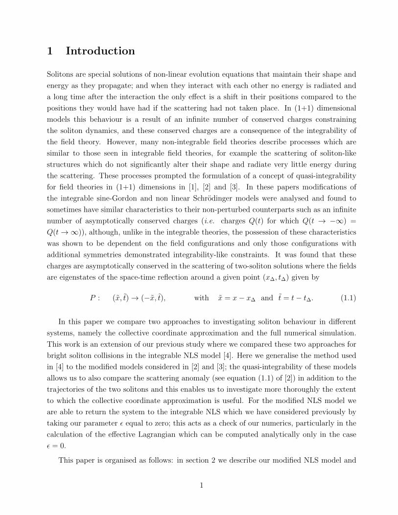
1 Introduction

Solitons are special solutions of non-linear evolution equations that maintain their shape and

energy as they propagate; and when they interact with each other no energy is radiated and

a long time after the interaction the only effect is a shift in their positions compared to the

positions they would have had if the scattering had not taken place. In (1+1) dimensional

models this behaviour is a result of an infinite number of conserved charges constraining

the soliton dynamics, and these conserved charges are a consequence of the integrability of

the field theory. However, many non-integrable field theories describe processes which are

similar to those seen in integrable field theories, for example the scattering of soliton-like

structures which do not significantly alter their shape and radiate very little energy during

the scattering. These processes prompted the formulation of a concept of quasi-integrability

for field theories in (1+1) dimensions in [1], [2] and [3]. In these papers modifications of

the integrable sine-Gordon and non linear Schrodinger models were analysed and found to

sometimes have similar characteristics to their non-perturbed counterparts such as an infinite

number of asymptotically conserved charges (i.e. charges Q(t) for which Q(t → −∞) =

Q(t→∞)), although, unlike in the integrable theories, the possession of these characteristics

was shown to be dependent on the field configurations and only those configurations with

additional symmetries demonstrated integrability-like constraints. It was found that these

charges are asymptotically conserved in the scattering of two-soliton solutions where the fields

are eigenstates of the space-time reflection around a given point (x∆, t∆) given by

P : (x, t)→ (−x, t), with x = x− x∆ and t = t− t∆. (1.1)

In this paper we compare two approaches to investigating soliton behaviour in different

systems, namely the collective coordinate approximation and the full numerical simulation.

This work is an extension of our previous study where we compared these two approaches for

bright soliton collisions in the integrable NLS model [4]. Here we generalise the method used

in [4] to the modified models considered in [2] and [3]; the quasi-integrability of these models

allows us to also compare the scattering anomaly (see equation (1.1) of [2]) in addition to the

trajectories of the two solitons and this enables us to investigate more thoroughly the extent

to which the collective coordinate approximation is useful. For the modified NLS model we

are able to return the system to the integrable NLS which we have considered previously by

taking our parameter ε equal to zero; this acts as a check of our numerics, particularly in the

calculation of the effective Lagrangian which can be computed analytically only in the case

ε = 0.

This paper is organised as follows: in section 2 we describe our modified NLS model and

1

construct an approximation ansatz for a two-soliton solution in this model. We then compare

the results of the two approaches in this system starting with the ε = 0 case where the model

returns to the integrable NLS before discussing the more general ε 6= 0 case. In section 3 we

describe our modified sine-Gordon model and construct a two-soliton approximation ansatz

in this model; we then compare the two approaches in this system. Finally we present our

conclusions in section 4.

2 The modified NLS model

We consider the Lagrangian for a non-relativistic complex scalar field in (1+1) dimensions

L =

∫dx

i

2(ψ∗∂tψ − ψ∂tψ∗)− ∂xψ∗∂xψ − V

(|ψ|2

). (2.1)

The equations of motion are

i∂tψ = −∂2xψ +

δV

δ|ψ|2ψ, (2.2)

together with its complex conjugate.

The equation (2.2) admits an anomalous zero curvature representation and from this,

after some mathematical manipulation, an infinite number of anomalous conservation laws

were derived in [2] to be given by:

dQ(n)

dt= βn; with Q(n) =

∫ ∞−∞

dx a(3,−n)x ; where βn =

∫ ∞−∞

dxX α(3,−n) (2.3)

for n = 0, 1, 2, ..., where

X ≡ −i ∂x(δV

δ|ψ|2− 2 η |ψ|2

)(2.4)

and explicit expressions for the first few a(3,−n)x and α(3,−n) are given in appendix A in [2].

It is clear that when the potential corresponds to the NLS potential, i.e. VNLS = η |ψ|4, the

anomaly X given in (2.4) vanishes and so do βn. The theory becomes integrable as it has an

infinite number of conserved charges Q(n).

We use the potential as in [2]

V =2

2 + εη(|ψ|2

)2+ε(2.5)

so that it returns to the unperturbed NLS potential in the case ε = 0.

2

As shown in [2], for η < 0, this model has a one-soliton solution given by

ψ =

(√2 + ε

2 |η|b

cosh [(1 + ε) b (x− vt− x0)]

) 11+ε

ei[(b2− v

2

4

)t+ v

2x], (2.6)

where b, v and x0 are real parameters of the solution.

When the field configuration ψ transforms under the parity defined in (1.1) as

P (ψ) = (−1)nψ∗ (2.7)

then the system has an infinite number of asymptotically conserved charges, i.e.

Q(n)(t = +∞) = Q(n)(t = −∞). (2.8)

2.1 The two-soliton configuration for modified NLS

Here we construct a set of collective coordinates for the study of the scattering of two such

solitons with η = −1. We use a natural extension of our approximation ansatz in [4] and so

we take our approximation ansatz for two solitons in the modified NLS system to be given by

ψ = ψ1 + ψ2 = ϕ1eiθ1 + ϕ2e

iθ2 (2.9)

where

ϕ1 =

(√2 + ε

2

a1(t)

cosh [(1 + ε) a1(t) (x+ ξ1(t))]

) 11+ε

, θ1 = −µ1(t)

(x+

ξ1(t)

2

)+a2

1(t) t+λ1(t),

ϕ2 =

(√2 + ε

2

a2(t)

cosh [(1 + ε) a2(t) (x+ ξ2(t))]

) 11+ε

, θ2 = −µ2(t)

(x+

ξ2(t)

2

)+a2

2(t) t+λ2(t),

and a1,2(t), ξ1,2(t), µ1,2(t) and λ1,2(t) are our collective coordinates. This approximation

ansatz models two lumps with heights a1,2(t), positions ξ1,2(t), velocities µ1,2(t) and phases

λ1,2(t). When the two lumps are far apart they resemble two one-soliton solutions akin to (2.6).

In the case ε = 0 this ansatz is similar to the one we used in [4] with the additional features of

a time dependence in the width of the solitons, and the independence of the height, position,

velocity and phase of each soliton. These changes have been made based on our observations

in [4] and we later show that this improved approximation ansatz gives more accurate results

for NLS solitons compared with our previous results.

3

This approximation ansatz transforms as in (2.7), and so the system with this field con-

figuration has an infinite number of asymptotically conserved charges, if the solitons have

relative phase δ ≡ λ1 − λ2 = nπ for n ∈ Z.

Using this approximation ansatz we then follow the same procedure as before except that,

with the addition of the parameter ε, we are no longer able to analytically integrate the

relevant expressions to get the effective Lagrangian so the required integrals are calculated

numerically. As before, we use the 4th order Runge-Kutta method to numerically solve our

equations of motion.

2.2 Results for NLS

We start by analysing the scattering of our two-solitons with small values of initial velocity

as the collective coordinate approximation is expected to be a good approximation for slowly

moving solitons. To test our procedure we first consider the cases where ε = 0 which corre-

sponds to the non-perturbed, integrable NLS. This also allows us to test the our numerical

integration and, by comparison with the same integrals computed analytically, we have be-

come satisfied with the accuracy of the numerical integration. For the ε = 0 case, as seen

in our previous work [4], the solitons’ scattering is highly dependent on the relative phase

between them, i.e. δ ≡ λ1− λ2, so first of all, we compare the solitons’ dynamics between the

collective coordinate approximation and full numerical simulation for a range of δ. In all our

studies we used η = −1.

Figure 1 compares the trajectories given by the collective coordinate approximation and

those given by the full numerical simulation for solitons with initial position ξ1 = −5, ξ2 = 5;

initial velocity µ1 = 0.005, µ2 = −0.005; and initial phase difference δ = 0, π4, π

2, 3π

4, π (the

results are symmetric around π and periodic in 2π). We plot the position of the soliton on the

left and the negative position of the soliton on the right (for the approximation this corresponds

to ξ1(t) and −ξ2(t)) to aid comparison between the two interacting solitons. This figure shows

that the collective coordinate approximation is remarkably accurate for most values of δ, with

both approaches producing almost identical trajectories (making it difficult to distinguish all

the lines) including separate trajectories for the left and right solitons whenever δ 6= nπ.

However, in the case δ = 0 the solitons in the collective coordinate approximation begin to

repel much earlier than in the full simulation. We also observed that the behaviour of the

solitons in the full simulation has a subtle dependence on δ and, correspondingly, on how

close the solitons come together during the scattering and the collective coordinate does not

capture this complicated behaviour exactly. We think this is probably because in the full

simulation the solitons deform one another away from the form given by (2.9) when they are

4

in close proximity and the collective coordinate approximation does not allow this.

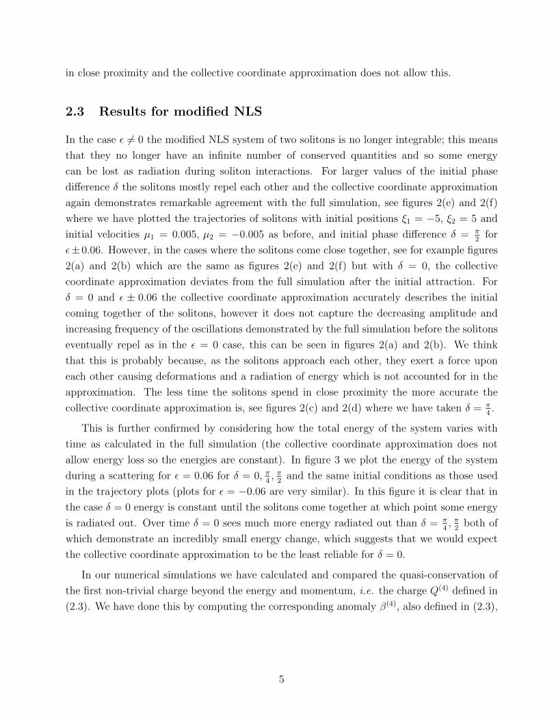
2.3 Results for modified NLS

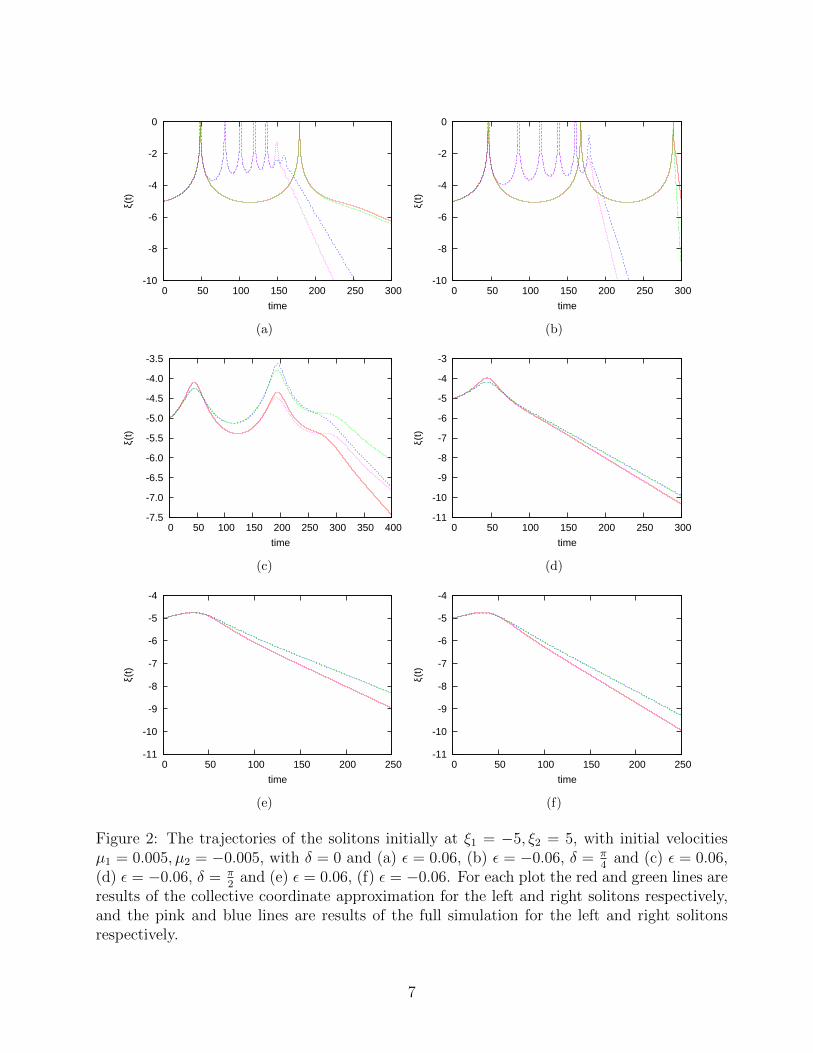
In the case ε 6= 0 the modified NLS system of two solitons is no longer integrable; this means

that they no longer have an infinite number of conserved quantities and so some energy

can be lost as radiation during soliton interactions. For larger values of the initial phase

difference δ the solitons mostly repel each other and the collective coordinate approximation

again demonstrates remarkable agreement with the full simulation, see figures 2(e) and 2(f)

where we have plotted the trajectories of solitons with initial positions ξ1 = −5, ξ2 = 5 and

initial velocities µ1 = 0.005, µ2 = −0.005 as before, and initial phase difference δ = π2

for

ε± 0.06. However, in the cases where the solitons come close together, see for example figures

2(a) and 2(b) which are the same as figures 2(e) and 2(f) but with δ = 0, the collective

coordinate approximation deviates from the full simulation after the initial attraction. For

δ = 0 and ε ± 0.06 the collective coordinate approximation accurately describes the initial

coming together of the solitons, however it does not capture the decreasing amplitude and

increasing frequency of the oscillations demonstrated by the full simulation before the solitons

eventually repel as in the ε = 0 case, this can be seen in figures 2(a) and 2(b). We think

that this is probably because, as the solitons approach each other, they exert a force upon

each other causing deformations and a radiation of energy which is not accounted for in the

approximation. The less time the solitons spend in close proximity the more accurate the

collective coordinate approximation is, see figures 2(c) and 2(d) where we have taken δ = π4.

This is further confirmed by considering how the total energy of the system varies with

time as calculated in the full simulation (the collective coordinate approximation does not

allow energy loss so the energies are constant). In figure 3 we plot the energy of the system

during a scattering for ε = 0.06 for δ = 0, π4, π

2and the same initial conditions as those used

in the trajectory plots (plots for ε = −0.06 are very similar). In this figure it is clear that in

the case δ = 0 energy is constant until the solitons come together at which point some energy

is radiated out. Over time δ = 0 sees much more energy radiated out than δ = π4, π

2both of

which demonstrate an incredibly small energy change, which suggests that we would expect

the collective coordinate approximation to be the least reliable for δ = 0.

In our numerical simulations we have calculated and compared the quasi-conservation of

the first non-trivial charge beyond the energy and momentum, i.e. the charge Q(4) defined in

(2.3). We have done this by computing the corresponding anomaly β(4), also defined in (2.3),

5

-10

-8

-6

-4

-2

0

0 200 400 600 800 1000 1200 1400

ξ(t)

time

(a)

-11

-10

-9

-8

-7

-6

-5

-4

0 50 100 150 200 250

ξ(t)

time

(b)

-11

-10

-9

-8

-7

-6

-5

-4

0 50 100 150 200 250

ξ(t)

time

(c)

-11

-10

-9

-8

-7

-6

-5

-4

0 50 100 150 200 250

ξ(t)

time

(d)

-11

-10

-9

-8

-7

-6

-5

-4

0 50 100 150 200 250

ξ(t)

time

(e)

Figure 1: The trajectories of the solitons initially at ξ1 = −5, ξ2 = 5, with initial velocitiesµ1 = 0.005, µ2 = −0.005 for initial phase differences: (a) δ = 0, (b) δ = π

4, (c) δ = π

2, (d)

δ = 3π4

,(e) δ = π. For each plot the red and green lines are results of the collective coordinateapproximation for the left and right solitons respectively, and the pink and blue lines areresults of the full simulation for the left and right solitons respectively. Note that the red andpink lines, and the green and blue lines are often coincident.

6

-10

-8

-6

-4

-2

0

0 50 100 150 200 250 300

ξ(t)

time

(a)

-10

-8

-6

-4

-2

0

0 50 100 150 200 250 300

ξ(t)

time

(b)

-7.5

-7.0

-6.5

-6.0

-5.5

-5.0

-4.5

-4.0

-3.5

0 50 100 150 200 250 300 350 400

ξ(t)

time

(c)

-11

-10

-9

-8

-7

-6

-5

-4

-3

0 50 100 150 200 250 300

ξ(t)

time

(d)

-11

-10

-9

-8

-7

-6

-5

-4

0 50 100 150 200 250

ξ(t)

time

(e)

-11

-10

-9

-8

-7

-6

-5

-4

0 50 100 150 200 250

ξ(t)

time

(f)

Figure 2: The trajectories of the solitons initially at ξ1 = −5, ξ2 = 5, with initial velocitiesµ1 = 0.005, µ2 = −0.005, with δ = 0 and (a) ε = 0.06, (b) ε = −0.06, δ = π

4and (c) ε = 0.06,

(d) ε = −0.06, δ = π2

and (e) ε = 0.06, (f) ε = −0.06. For each plot the red and green lines areresults of the collective coordinate approximation for the left and right solitons respectively,and the pink and blue lines are results of the full simulation for the left and right solitonsrespectively.

7

-1.270

-1.265

-1.260

-1.255

-1.250

-1.245

-1.240

-1.235

0 50 100 150 200 250 300 350en

ergy

time

Figure 3: The energy of the solitons for ε = 0.06 placed initially at ξ1 = −5, ξ2 = 5, andwith initial velocities µ1 = 0.005, µ2 = −0.005. δ = 0 corresponds to the solid line, δ = π

4the

dotted line and δ = π2

the dashed line.

and by integrating it over time to get the integrated anomaly:

χ(4)(t) ≡∫ t

−∞dt′ β4 =

∫ t

−∞dt′∫ ∞−∞

dxXα(3,−4) (2.10)

= −2i

∫ t

−∞dt′∫ ∞−∞

dx ((ε+ 1)Rε − 1) ∂xR

[−6R2 +

3

2(∂xϕ)2R− 2 ∂2

xR +3

2

(∂xR)2

R

]

this is computed in terms of the fields R and ϕ which are defined by writing the soliton

solution ψ in the form ψ ≡√Rei

ϕ2 .

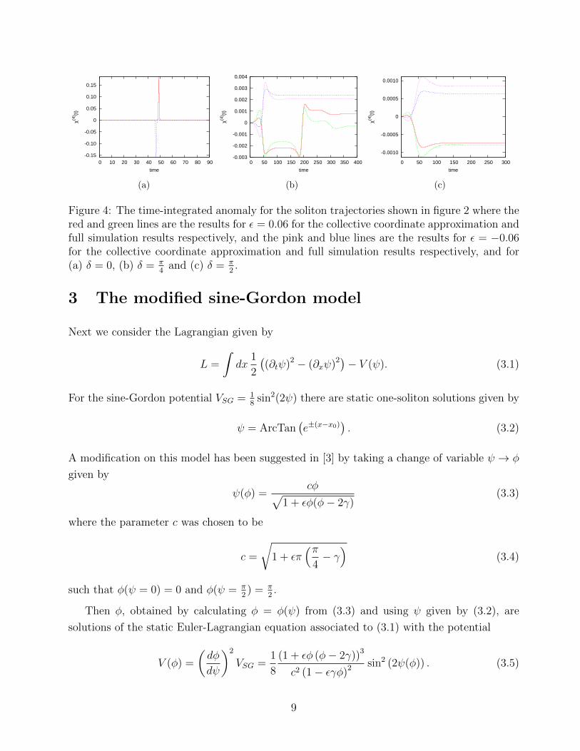
In figure 4 we plot the time-integrated anomaly for each of the trajectories shown in

figure 2, and we can see that the results are very similar although not as exact as some of

the trajectories. The time integrated anomalies are most different in the case δ = 0 as the

collective coordinate approximation shows a distinct peak when the solitons come together

compared to the results from the full simulation which display only a minute deviation from

zero at these points (of the order 10−7). However, when the solitons are far apart the time-

integrated anomaly does return to zero as predicted in [2] when δ is an integer value of π, as

this corresponds to the case when the parity symmetry described in (2.7) is present. When δ is

not an integer multiple of π this symmetry is not present and the integrated anomalies do not

return to zero, and the collective coordinate method shows similar time-integrated anomalies

to those found in the full simulation.

8

-0.15

-0.10

-0.05

0

0.05

0.10

0.15

0 10 20 30 40 50 60 70 80 90

χ(4) (t

)

time

(a)

-0.003

-0.002

-0.001

0

0.001

0.002

0.003

0.004

0 50 100 150 200 250 300 350 400

χ(4) (t

)

time

(b)

-0.0010

-0.0005

0

0.0005

0.0010

0 50 100 150 200 250 300

χ(4) (t

)

time

(c)

Figure 4: The time-integrated anomaly for the soliton trajectories shown in figure 2 where thered and green lines are the results for ε = 0.06 for the collective coordinate approximation andfull simulation results respectively, and the pink and blue lines are the results for ε = −0.06for the collective coordinate approximation and full simulation results respectively, and for(a) δ = 0, (b) δ = π

4and (c) δ = π

2.

3 The modified sine-Gordon model

Next we consider the Lagrangian given by

L =

∫dx

1

2

((∂tψ)2 − (∂xψ)2)− V (ψ). (3.1)

For the sine-Gordon potential VSG = 18

sin2(2ψ) there are static one-soliton solutions given by

ψ = ArcTan(e±(x−x0)

). (3.2)

A modification on this model has been suggested in [3] by taking a change of variable ψ → φ

given by

ψ(φ) =cφ√

1 + εφ(φ− 2γ)(3.3)

where the parameter c was chosen to be

c =

√1 + επ

(π4− γ)

(3.4)

such that φ(ψ = 0) = 0 and φ(ψ = π2) = π

2.

Then φ, obtained by calculating φ = φ(ψ) from (3.3) and using ψ given by (3.2), are

solutions of the static Euler-Lagrangian equation associated to (3.1) with the potential

V (φ) =

(dφ

dψ

)2

VSG =1

8

(1 + εφ (φ− 2γ))3

c2 (1− εγφ)2 sin2 (2ψ(φ)) . (3.5)

9

0

0.1

0.2

0.3

0.4

0.5

0.6

0.7

-3.95838 -π/2 0 π/2 3.95838

V(φ

)

φ

(a)

0

0.5

1.0

1.5

2.0

2.5

-5.73026 -1.86352 0 π/2 3.64283

V(φ

)

φ

(b)

Figure 5: The modified potential V (φ) against φ for ε = 0.05 and (a) γ = 0, (b) γ = 1.

In the case ε = 0 the parameter γ becomes irrelevant and the potential (3.5) returns to the

unperturbed sine-Gordon potential and φ = ψ. For ε 6= 0 and γ = 0 the model has the

symmetry φ = −φ, and for ε, γ 6= 0 there is no symmetry. This can be seen in figure 5 where

we have plotted the potential as a function of φ for various values of ε and γ. By varying the

parameters ε and γ the effects of this symmetry on the theory can be seen.

In a similar manner to the NLS case the sine-Gordon has a set of anomalous conservation

laws derived in [3] and given by:

dQ(2n+1)

dt= β2n+1; with Q(2n+1) =

∫ ∞−∞

dx a(2n+1)x ; where β(2n+1) =

∫ ∞−∞

dx X α(2n+1)

(3.6)

for n = 0, 1, 2, 3, ... and

X =iw

2∂−φ

[d2V

dφ2+ w2V −m

](3.7)

which vanishes for the sine-Gordon potential when the parameters m,w are chosen to be

m = 1, w = 4.

If the field configuration transforms under the parity defined in (1.1) as

P (φ) = −φ+ const. (3.8)

and if the potential evaluated on such a solution is even under the parity, i.e.

P (V ) = V (3.9)

10

then we have an infinite set of conserved quantities which are conserved asymptotically, i.e.

Q(2n+1)(t = +∞) = Q(2n+1)(t = −∞). (3.10)

In this model the field configuration and potential transform as in (3.8) and (3.9), and so we

have an infinite number of aymptotically conserved charges, when γ = 0.

3.1 The two-soliton configuration for sine-Gordon

Here we construct a two-soliton ansatz for the modified sine-Gordon in the collective coordi-

nate approximation starting with:

ψ = ψ1 + ψ2 = ArcTan(2 Sinh(x) e−a(t)

)(3.11)

which models two kinks, one placed at −a(t) whose field varies between(−π

2, 0)

and one placed

at a(t) which varies between(0, π

2

). When a(t) is large (3.11) represents two well separated

kinks, and for energetic reasons it must be that a(t) > 0 for all times. This ansatz was used

in [5] to test the collective coordinate approximation for the scattering of sine-Gordon kinks

and was found to work remarkably well.

To construct the ansatz for the modified sine-Gordon we now perform the change of vari-

ables (3.3) for ψ given by (3.11) to get

φ =ψ2εγ +

√ψ2c2 + ψ4ε (−1 + γ2ε)

ψ2ε− c2for x < 0 (3.12)

φ =ψ2εγ −

√ψ2c2 + ψ4ε (−1 + γ2ε)

ψ2ε− c2for x > 0

and this is our two soliton ansatz field configuration to the Euler-Lagrange equation associated

to (3.1) with the potential given by (3.5). This ansatz returns to the ansatz for the unmodified

sine-Gordon in the case ε = 0. For ε 6= 0, γ = 0 the kinks are altered but still retain the

symmetry φ = −φ, whereas for ε 6= 0, γ 6= 0 this symmetry is lost due to the shift in the vacua

which can be seen in figure 5(b).

We then use this ansatz to find an effective Lagrangian from which we derive the equation

of motion for our collective coordinate a(t), calculating any necessary integrals numerically.

We use the 4th order Runge-Kutta method to evolve our two soliton ansatz field configuration.

11

2.02.53.03.54.04.55.05.56.06.57.07.5

0 5 10 15 20 25 30

a(t)

time

(a)

2.0

2.5

3.0

3.5

4.0

4.5

5.0

5.5

6.0

6.5

0 5 10 15 20 25 30

a(t)

time

(b)

Figure 6: The trajectories of the solitons with initial velocity v = 0.3, with (a) γ = 0and, top to bottom, ε = −0.2,−0.1, 0, 0.1, 0.2 and in (b) ε = 0.1 and, top to bottom, γ =−0.4,−0.2, 0, 0.2, 0.4.

3.2 Results for modified sine-Gordon

We analyse the scattering of our two kinks and consider the effects of changing the parameters

ε and γ on the trajectories of moving solitons. For each of the plots we take a small velocity,

v = 0.3, as the collective coordinate approximation is a good approximation for slowly moving

solitons and we start the solitons at ±6.

In figure 6(a) we present a plot of trajectories for γ = 0 and a range of ε, and in the ε = 0

case we compare our trajectory to that in [5]. They are clearly in excellent agreement. For

increasing ε we see the solitons come closer together before repelling and for decreasing ε we

see the reverse. In figure 6(b) we explore various values of γ for ε = 0.1; from this we see that

γ effects the trajectory in a similar way to ε but to a lesser extent.

We consider the quasi-conservation of the first non-trivial charge beyond the energy itself

Q(4)(t) defined in (3.6) by calculating both the anomaly β(3) and, as in the NLS case, the time

integrated anomaly which is given by:

χ(3) = −1

2

∫ t

t0

dt′ β(3) = 4

∫ t

t0

dt′∫ ∞−∞

dx ∂−φ ∂2−φ

[d2 V

dφ2+ 16V − 1

](3.13)

where ∂− = ∂t − ∂x and t0 is the initial time of the simulation which is usually taken to be

zero.

In figure 7 we plot the time-integrated anomaly with time for solitons placed at ±20 with

initial velocity v = 0.05, with ε = 0.000001 and various values of γ. Notice that in the full

simulation the time-integrated anomaly is always slowly increasing prior to the scattering of

12

-5.0e-09

0

5.0e-09

1.0e-08

1.5e-08

2.0e-08

2.5e-08

3.0e-08

0 100 200 300 400 500 600

χ~ (3)

time

(a)

-4e-08

-3e-08

-2e-08

-1e-08

0

1e-08

2e-08

0 100 200 300 400 500 600

χ~ (3)

time

(b)

-8e-08

-7e-08

-6e-08

-5e-08

-4e-08

-3e-08

-2e-08

-1e-08

0

1e-08

0 100 200 300 400 500 600

χ~ (3)

time

(c)

-2.0e-06-1.8e-06-1.6e-06-1.4e-06-1.2e-06-1.0e-06-8.0e-07-6.0e-07-4.0e-07-2.0e-07

02.0e-07

0 100 200 300 400 500 600

χ~ (3)

time

(d)

-1e-08

0

1e-08

2e-08

3e-08

4e-08

5e-08

6e-08

0 100 200 300 400 500 600

χ~ (3)

time

(e)

Figure 7: The time-integrated anomaly for solitons initially at a(t) = 20 with velocity v =−0.05 and ε = 0.000001. The red and green lines are the results for the collective coordinateapproximation and full simulation results respectively, and γ is chosen to be (a) γ = 0.00001,(b) γ = 0.002, (c) γ = 0.004 and (d) γ = 0.1 .

the solitons and slowly decreasing after the scattering, this is due to slight fluctuations away

from zero in the anomaly which themselves are probably a result of numerical errors rather

than any physical effect. When γ is small the collective coordinate approximation and the

full simulation demonstrate excellent agreement, and far away from the scattering the time-

integrated anomaly is close to zero which is expected when γ is small and the model is close to

the symmetry described in (3.8) and (3.9). As γ is taken further from zero we transfer from a

model with approximate symmetry to a model where this symmetry is broken. We see in figure

7 that the further γ is from zero the further the time-integrated anomaly is from zero after the

scattering of the solitons, and in figures 7(b) and 7(e) we see that the symmetry can be broken

in either direction depending on the sign of γ. The collective coordinate approximation still

gives a good approximation to the behaviour of the time-integrated anomaly as we move away

from the symmetric case though the values are modified. These observations are consistent

for various values of ε.

13

4 Conclusions

In this paper we have performed further studies of quasi-integrability using the collective co-

ordinate approximation. We have considered a modified NLS and a modified sine-Gordon

system where the anomaly was found (in [2] and [3]) to vanish for field configurations pos-

sessing particular parity symmetries and we have confirmed that, when using the collective

coordinate approximation, the anomaly also vanishes in those cases. We have also investi-

gated the suitability of the collective coordinate approximation in these systems by comparing

the trajectories and anomalies of scattering solitons calculated using the collective coordinate

approximation and the full numerical simulation. We have found that, with an appropriate

choice of ansatz, the collective coordinate approximation is remarkably accurate in both sys-

tems. However, in the modified NLS the approximation has been found to be less reliable the

more time the solitons spend in close proximity to each other. We think that this is probably

because the collective coordinate approximation does not allow for the deformation of the

solitons away from their original form or the radiation of energy which is likely to occur when

the solitons are close. We also found that in the modified sine-Gordon case the approximation

is very accurate when the field configuration possess the parity symmetry necessary for the

anomaly to vanish and, when the field configuration moves away from that symmetry, the col-

lective coordinate approximation still accurately captures the behaviour of the time-integrated

anomaly but the values are modified. These observations suggest that the collective coordi-

nate approximation is a suitable method to further investigate quasi-integrability in other

perturbations of integrable models.

5 Acknowledgements

HB is supported by an STFC studentship.

References

[1] L. A. Ferreira and W. J. Zakrzewski, JHEP 1105, 130 (2011).

[2] L. A. Ferreira, G. Luchini and W. J. Zakrzewski, JHEP 1209, 103 (2012).

[3] L. A. Ferreira and W. J. Zakrzewski, JHEP 01, 058 (2014).

[4] H. E. Baron, G. Luchini and W. J. Zakrzewski, J. Phys. A 47, 265201 (2014).

[5] P. M. Sutcliffe, Nucl. Phys. B 393, 211 (1993).

14