UNIVERSITY OF CALIFORNIA SANTA CRUZ

Coherent structures and larval transport in the California Current system

A dissertation submitted in partial satisfaction of the requirements for the degree of

DOCTOR OF PHILOSOPHY

in EARTH SCIENCES

by Cheryl S. Harrison

December 2012

The Dissertation of Cheryl S. Harrison is approved: Professor Eli A. Silver, Chair Professor David A. Siegel Research Scientist Adina Payton Professor Pete Raimondi

Tyrus Miller Vice Provost and Dean of Graduate Studies

Copyright © by Cheryl S. Harrison

2012

iii

Contents

List of Figures.............................................................................................................. v

Abstract....................................................................................................................... vi

Acknowledgements .................................................................................................... ix

Chapter 1 Introduction .............................................................................................. 1 Bibliography.......................................................................................................................10

Chapter 2 LCS in the CCS—sensitivities and limitations..................................... 14

Chapter 3 The role of filamentation and eddy-eddy interactions in marine larval accumulation and transport..................................................................................... 37

Abstract ..............................................................................................................................37 3.1 Introduction .............................................................................................................38 3.2 Lagrangian Coherent Structures (LCS)................................................................43 3.3 Models.......................................................................................................................47 3.4 Results.......................................................................................................................50

3.4.1 LCS, filamentation and larval density patterns ..................................................50 3.4.2 Filaments and fronts ...........................................................................................54 3.4.3 Eddy-eddy interactions, source regions and larval age distributions .................57

3.5 Discussion .................................................................................................................66 3.5.1 Application of LCS.............................................................................................66 3.5.2 Comparisons with observations and prior studies ..............................................68 3.5.3 Potential Roles of Larval Behavior ....................................................................72

3.6 Summary ..................................................................................................................73 3.7 Acknowledgements ..................................................................................................74 3.8 Bibliography.............................................................................................................75

Chapter 4 The tattered curtain hypothesis revisited: coastal jets control larval settlement patterns.................................................................................................... 83

Abstract ..............................................................................................................................83 4.1 Introduction .............................................................................................................84 4.2 Background theory ..................................................................................................89

4.2.1 Eulerian dynamics: upwelling jets and offshore transport .................................89 4.2.2 Lagrangian dynamics: a kinematic model of the upwelling jet..........................92

4.3 Biophysical Model....................................................................................................94 4.4 Modeling Results......................................................................................................96

4.4.1 Modeled patterns of coastal retention and settlement ........................................96

iv

4.4.2 Statistical Correlation Between Wind and Settlement .....................................101 4.5 Conclusions.............................................................................................................104 4.6 Discussion ...............................................................................................................104 4.7 Bibliography...........................................................................................................108

Chapter 5 Conclusions and directions for future research................................. 124 5.1 Conclusions.............................................................................................................124 5.2 Directions for future research ..............................................................................126

5.2.1 Quantifying biological patchiness. ...................................................................126 5.2.2 LCS and predators in the CCS..........................................................................129

5.3 Bibliography...........................................................................................................132

Appendix: Glossary ................................................................................................ 134

List of Supplemental Movies.................................................................................. 135 Movie 2.1 Daily LCS visualization for Fall 2005. .....................................................135 Movie 2.2 Comparison of Eulerian and Lagrangian metrics for 2002...................135 Movie 3.1 What happens to particles near LCS?.....................................................135 Movie 3.2 Larval density field....................................................................................135 Movie 4.1 Particles in the CCS-in-a-box model........................................................136 Movie 5.1 LCS and sea lion tracks ............................................................................136

v

List of Figures

Figure 1.1 Satellite observations of the California Current system (CCS)................... 1 Figure 1.2 Stagnation points and their manifolds ......................................................... 4 Figure 1.3 FTLE fields and LCS in the CCS................................................................ 5 Figure 3.1 Schematics of fluid/particle behavior near Lagrangian coherent structures (LCS)........................................................................................................................... 44 Figure 3.2 Comparison of Eulerian and Lagrangian surface fields. ........................... 48 Figure 3.3 North transect. ........................................................................................... 51 Figure 3.4 South transect. ........................................................................................... 53 Figure 3.5 Filament and frontal statistics.................................................................... 55 Figure 3.6 Packet formation........................................................................................ 57 Figure 3.7 Packet age class and source region distribution. ....................................... 60 Figure 3.8 Density distributions by age class on model day 177................................ 61 Figure 3.9 Source and age distributions...................................................................... 64 Figure 3.10 Particle density and packet statistics. ...................................................... 65 Figure 3.11 Effect of swimming on density patterns.................................................. 67 Figure 4.1 Features of upwelling dynamics in Eastern Boundary Currents (EBCs). 113 Figure 4.2 Gaussian jet. ............................................................................................ 114 Figure 4.3 Alongshore jet surface fields. .................................................................. 115 Figure 4.4 Coastal jet transects. ................................................................................ 116 Figure 4.5 Settlement patterns and wind for Run 111. ............................................. 117 Figure 4.6 Jet retention patterns................................................................................ 118 Figure 4.7 Settlement patterns and wind for Run 141. ............................................. 119 Figure 4.8 Settlement patterns and wind for Run 113. ............................................. 120 Figure 4.9 Statistics of wind-settlement correlation for Run 111............................. 121 Figure 4.10 Ensemble wind-settlement correlation statistics. .................................. 122 Figure 4.11 Scatterplot of integrated wind product W20 vs. number of settling particles. .................................................................................................................... 123

vi

Abstract

Coherent structures and larval transport in the California Current system

Cheryl S. Harrison

In the California Current system (CCS), coherent structures such as jets and eddies

strongly control the biological response to coastal upwelling. One of the outstanding

problems in marine ecology is to understand the mechanisms of larval transport.

Details of transport dynamics from nearshore to offshore, and subsequent delivery of

coastally spawned propagules back to favorable settlement areas, strongly control

marine population dynamics. Recent developments in applied dynamical systems

allow the identification of coherent structure boundaries by numerical calculation of

Lagrangian coherent structures (LCS), finite-time analogs of stable and unstable

manifolds of hyperbolic fixed points. These material lines divide the flow into regions

of disparate transport fate and illuminate the skeleton of filamentation and mixing.

Using altimetric observations of the CCS, we show that LCS are less sensitive to

noise and under-resolution than Eulerian metrics, and can map events undetectable by

analysis of the frozen-time velocity field. However, small-scale dynamics such as

lobes are not well resolved by altimetric observations. In an ocean circulation model

of an idealized CCS, LCS are used to track filamentation and eddy-eddy interactions,

important larval transport pathways from the shelf offshore. Filaments and packets

caused by eddy-eddy interaction are stable to horizontal swimming perturbations, as

predicted by the structural stability of hyperbolic manifolds. Retention in the

vii

upwelling jet is high and strongly patterns larval settlement. Settlement events are

best correlated with integrated upwelling intensity and not upwelling relaxation

events as commonly assumed. These studies demonstrate that coherent structures play

a large role in coastal ecosystems, and that techniques and theorems from dynamical

systems can provide insight into dominant transport pathways controlling coastal

ecosystems.

viii

Dedicated to Ralph

And all the other midwives of scientific revolution

Chase a deer and end up everywhere

-Rumi

ix

Acknowledgements

This work, and my subsequent academic trajectory, would have been in no way

possible without the academic assistance, logistical support and general sensei-like

qualities of Prof. David A. Siegel. He has been an example of how to forge your own

path and not just get away with it, but be wildly successful and have fun in the

process. His commitment and respect towards my academic vision, general academic

jedi training, and especially his ability to perturb trajectories toward more favorable

outcomes have been invaluable, to put it mildly.

I would like to thank the senior faculty of the UCSC Earth and Planetary Science

Dept, especially Eli Silver, for personifying that really the most fun you could ever

have is to do and teach science. This and the familial, supportive environment they

created enabled me to see that there may be a place for me in academia. I would also

like to thank the members of my committee, especially Adina Paytan, without whose

support and encouragement I would not be here. Gary Glatzmaier advised the first

chapter of this work, and his example of high integrity in both scientific practice and

in all academic endeavors has been immensely valuable.

The majority of acknowledgement for this work belongs to my family. For my entire

life, I have been nurtured with the crazy idea that I could do anything I wanted to.

Believing this and thus supported, so I now stand

1

Chapter 1 Introduction

Transport in the California Current system (CCS) is inherently chaotic (Fig. 1.1).

Instabilities generated in the upwelling jet (Brink 1987, Barth 1989, Durski and Allen

2005) coalesce into filaments and eddies that remain semi-coherent for weeks,

penetrating 100’s of kilometers offshore (Brink and Cowles 1991, Marchesiello et al.

2003, Capet et al. 2008, Ch. 3, Ch. 4). Large eddies (up 100-200 km in diameter)

form off instabilities in the main branch of the CCS as it migrates offshore at the end

of the upwelling season (Chelton et al. 2007, Ch 2), and are constrained by the beta

effect to propagate westward for months to years, transporting biologically important

materials far into the quiescent ocean interior, and forming important foraging habitat

for birds and marine predators (Capet et al. 2008, Ainly et al. 2009). Continuously

forced by ever-changing coastal winds (Burk and Thompson 1996), poleward

propagating coastally trapped waves (Brink 1991) and the ubiquitous interseasonal

variability of ENSO and PDO (Checkley and Barth 2009), the resulting quasi-

turbulent equilibrium state of the CCS is not quite turbulent enough to render

statistical methods applicable (Lekien and Coulliette 2003, Pasquero et al. 2007).

Figure 1.1 Satellite observations of the California Current system (CCS) (left) NOAA AVHRR satellite image of sea surface temperature on 10/9/92. (right) Ocean color (chlorophyll) near Monterey Bay.

2

3

There is a great amount of dynamical systems formalism for dealing with chaotic

systems; indeed this is one of the great mathematical achievements of the last century

(Abraham and Marsden 1978, Abraham and Shaw 1992, Wiggins 1992,

Guckenheimer and Holmes 1997). Dynamical systems focuses on the trajectories, i.e.

solutions of differential equations, instead of focusing on the forces, the terms in the

differential equations, or on the velocity field itself. The paradigm here is that much

of the behavior of the solutions is universal; there are a limited number of structures

that are combined to generate many different transport patterns—kind of a periodic

table of solution patterns with well-defined evolutions (i.e. bifurcations; Okubo

1970). There is a natural application of these methods to ocean transport (Wiggins

2005, Samelson and Wiggins 2006), which is governed by the non-linear Navier-

Stokes (NS) equations (e.g., McWilliams 2006). These equations are inherently

analytically intractable, and looking at the NS equations tells one very little about the

emergent behavior of the system.

This point is highlighted by the large number of new ocean dynamics discovered

since the advent of remote sensing by satellite (Ch 2 and references therein), and the

application of regional eddy-resolving ocean models (Marchesiello et al. 2004; Ch 3

& 4). How we think about the CCS and eastern boundary currents (EBCs) in general

has changed immensely in a very short time, with one of the great realizations being

that these systems are much more dynamic and unpredictable than we previously

4

thought (Hickey 1998, Hill et al. 1998, Marchesiello 2004). Here the endeavor is to

add to this knowledge base by applying recent results from dynamical systems.

Figure 1.2 Stagnation points and their manifolds Centers or elliptical (E) and saddle or hyperbolic (H) stagnation points organize transport in oceanic flows. Trajectories orbit elliptical points (dashed line). Near saddle points trajectories move on hyperbolic trajectories (black lines). Special trajectories form the inset or stable manifold (red) and outset or unstable manifold (blue) of the hyperbolic fixed point. These separatrices act as transport barriers and divide the flow into regions experiencing distinct transport fates in both forward and backward time.

Structures governing chaotic transport are organized around fixed or stagnation points

in the flow and their associated manifolds (Fig. 1.2). For time invariant systems there

is no motion at fixed points, i.e. the velocity vanishes, and fixed points can be found

by zeros of the velocity field and classified by eigenvalues of the Jacobian matrix

(Okubo 1970). In 2D incompressible ocean dynamics there are two types of fixed

5

points: centers and saddles. Near centers or elliptical stagnation points trajectories

move on closed elliptical orbits; these commonly occur in the centers of eddies. Near

saddles trajectories are hyperbolic in shape (Fig. 1.2). Saddles are stable in one

direction, with flow moving in toward the fixed point (red lines in Fig. 1.2) and

unstable in another direction, with flow moving away from the fixed point (blue

lines). These special trajectories are called the stable and unstable manifolds, or the

inset and outset of the hyperbolic fixed point (Abraham and Shaw 1992). Nearby

trajectories move asymptotically toward unstable manifolds, and we call these

attractors; likewise trajectories move asymptotically away from stable manifolds, i.e.

they are repelling.

The insets and outsets of saddle points extend out into the flow, often forming a

complex tangle of intersections as they wrap around eddies and other more exotic

structures (Fig. 1.2 & 1.3). Because they are trajectories, solutions to the NS

equations, existence and uniqueness of such solutions insures that they are also

transport boundaries, i.e. material cannot cross over them (see Shadden et al. 2005 for

exceptions). In time varying systems, these manifolds move with the fluid

Figure 1.3 FTLE fields and LCS in the CCS Shown are backward (left) and forward (middle) finite-time Lyapunov exponent (FTLE, days-1) maps computed from observations of sea surface height in the California Current system (CCS). (right) Lagrangian coherent structures (LCS) are identified by maxima or ridges of the forward FTLE (red) and backward FTLE (blue) and combined to make a map of coherent structure boundaries. Axes are degrees N (vertical) and degrees E (horizontal).

6

7

(supplemental movies 2.1, 2.2, 3.1), acting as a skeleton around which turbulent

transport is organized (Samelson and Wiggins 2006, Shadden et al. 2005, Mathur et

al. 2007).

Over the last decade, arguably the greatest advance to come out of applied dynamical

systems is the development of techniques to detect and track hyperbolic manifolds in

realistic velocity data (Haller 2002, Shadden et al. 2005). This innovation has resulted

in a large number of applications, from flow dynamics in the heart to the break up of

the atmospheric polar vortex associated with the ozone hole (reviewed in Shadden

2012 and Samelson 2013). Traditionally, hyperbolic manifolds were tediously

determined by identifying hyperbolic fixed points in the flow and seeding a dense

cloud of particles that would then stretch out and trace the unstable manifold of the

fixed point (e.g., supplemental movie 3.1). But this is a laborious process, involving

tracking of fixed points through time, which is quite difficult due to the complexity of

interactions (supplemental movie 3.1). These problems are compounded further by

the fact that zeros of the frozen time velocity field do not necessarily correspond to

fixed points in the time varying dynamics (Shadden et al. 2005, Mancho et al. 2006).

In order automate the detection of coherent structures, methods were pioneered using

various metrics on dense particle grids or groups of particles (Boffetta et al 2001,

Haller 2002, d’Ovidio et al. 2004), enabled by the exponential increase in computing

power. This culminated in the seminal work of Shadden et al. (2005), which defines

finite-time analogs of stable and unstable hyperbolic manifolds as Lagrangian

8

coherent structures (LCS), the ridges of the finite-time Lyapunov exponent (FTLE)

scalar field (Fig. 1.3). Details of this methodology are summarized in Ch. 2.

A central problem in marine ecology is the transport and dispersal of marine

propagules (larvae, eggs, spores), an inherently Lagrangian problem. Many species,

both pelagic (open ocean) and benthic (sea floor dwelling) spawn their young in the

productive coastal oceans of Eastern Boundary Currents (EBCs) such as the CCS

(e.g., Parrish et al. 1981, Rodríguez et al. 1999). These propagules are released into

the water column at some depth and must grow and often feed in the plankton,

drifting and swimming in the ocean currents until reaching maturity. In the case of

benthic species, residence time in the pelagic stage, called pelagic larval duration

(PLD), allow larvae to gain competency to recruit to suitable habitat and thus begin

the next stage of their lives, a strategy going back to the Cambrian (Valentine 2002).

PLD varies greatly between species, from a few days (abalone) up to many months

(some rockfish species). Likewise, swimming and other locomotive ability also varies

for benthic larvae, with a number of diverse strategies employed (e.g., Shanks 1985,

Morse 1991). But to leading order larvae are often considered passive or buoyant

floaters (Metaxas 2011), making the dispersal of these planktonic organisms a natural

application problem for chaotic Lagrangian transport techniques.

The main questions of this work is then, are dynamical systems techniques that detect

the separatrices bounding jets and eddies useful for determining Lagrangian (and thus

9

biological) transport patterns in the fecund and relentlessly productive CCS? Can the

wealth of mathematical formalism, intuition and theorems from the dynamical

systems study of coherent structures, lobe transport and other theorems tell us

anything useful about how transport works in the coastal ocean that can enable us to

better detect, model and manage our coastal ecosystems? This is the task at hand, and

is by no means complete.

This has been a challenging project. The inherent interdisciplinary nature of the

problem and the lack of existing literature and tradition have required forging my

own path, an inherently risky undertaking, but one with many rewards. The central

joy of science is the process of discovery: of finding new ideas and phenomena that

make sense of existing observations and expand our conceptual understanding of

important problems. The intersection between oceanography, dynamical systems and

marine ecology is an especially rich emerging field, and I am very happy to be on its

forefront.

This dissertation is organized as follows. Chapter 2 is a reproduction of a manuscript

published in GAFD (Harrison and Glatzmaier 2012) that applies LCS to

observational data in the CCS (geostrophic velocity fields calculated from satellite

observations of sea surface height) and empirically assesses the sensitivity to noise

and resolution, testing the structural stability of these features. Chapter 3 is a

manuscript currently in review on LCS and eddy interactions controlling nearshore to

10

offshore larval transport and packet formation in an idealized ocean model of the

Central California coast (Mitarai et al. 2008, Siegel et al. 2008). Chapter 4 is a

manuscript revisiting and revising a famous hypothesis on coherent structures

controlling settlement patterns in the same model (Roughgarden et al. 1991); here we

find that retention in the upwelling jet largely controls settlement patterns, and

similarity to other studies suggests this is a widespread phenomenon. Finally, Chapter

5 offers overall conclusions and outlines directions for future work, including

presentation of some work in progress.

Bibliography

R. H. Abraham and J. E. Marsden. Foundations of Mechanics. AMS Chelsea Publishing, 1978.

R. Abraham and C. D. Shaw. Dynamics–the geometry of behavior. Addison Wesley Publishing Company, 1992.

D. Ainley, K. Dugger, R. Ford, S. Pierce, D. Reese, R. Brodeur, C. Tynan, and J. Barth. Association of predators and prey at frontal features in the California Current: competition, facilitation, and co-occurrence. Marine Ecology Progress Series, 389:271–294, 2009.

J. A. Barth. Stability of a coastal upwelling front 2. Model results and comparison with observations. Journal of Geophysical Research, 94(C8):10857–10, 1989.

K. H. Brink. Upwelling fronts: implications and unknowns. South African Journal of Marine Science, 5(1):3–9, 1987.

K. Brink. Coastal-trapped waves and wind-driven currents over the continental shelf. Annual review of fluid mechanics, 23(1):389–412, 1991.

K. H. Brink and T. J. Cowles. The coastal transition zone program. Journal of Geophysical Research, 96(C8):14637–14, 1991.

11

G. Boffetta, G. Lacorata, G. Redaelli, and A. Vulpiani. Detecting barriers to transport: a review of different techniques. Physica D: Nonlinear Phenomena, 159(1-2):58 – 70, 2001.

S. D. Burk and W. T. Thompson. The summertime low-level jet and marine boundary layer structure along the California coast. Monthly Weather Review, 124(4):668–686, 2012/01/24 1996.

X. Capet, F. Colas, J. C. McWilliams, P. Penven, and P. Marchesiello. Eddies in eastern boundary subtropical upwelling systems, Vol. 177, pages 131–147. AGU, Washington, DC, 2008.

D. M. Checkley Jr and J. A. Barth. Patterns and processes in the California Current System. Progress in Oceanography, 83(1-4):49–64, 2009.

D. B. Chelton, M. G. Schlax, R. M. Samelson, and R. A. de Szoeke. Global observations of large oceanic eddies. Geophys. Res. Lett, 34(15):L15606, 2007.

F. d’Ovidio, V. Fernandez, E. Hernandez-Garcia, and C. Lopez. Mixing structures in the Mediterranean Sea from finite-size Lyapunov exponents. Geophysical Research Letters, 31(17), 2004.

S. M. Durski and J. S. Allen. Finite-amplitude evolution of instabilities associated with the coastal upwelling front. Journal of physical oceanography, 35(9):1606–1628, 2005.

J. Guckenheimer and P. Holmes. Nonlinear oscillations, dynamical systems, and bifurcations of vector fields. Springer-Verlag, 1997.

G. Haller. Lagrangian coherent structures from approximate velocity data. Physics of Fluids, 14(6):1851– 1861, 2002.

C. S. Harrison and G. A. Glatzmaier. Lagrangian coherent structures in the California Current system – sensitivities and limitations. Geophysical & Astrophysical Fluid Dynamics, 106(1):22–44, 2012.

B. M. Hickey. Coastal oceanography of western North America from the tip of Baja California to Vancouver Island. In A. Robinson and K. Brink, editors, The Sea—The Global Coastal Ocean, Regional Studies and Synthesis, volume 11, pages 345–393. John Wiley and Sons, Inc., New York, 1998.

A. E. Hill, B. M. Hickey, F. A. Shillington, P. T. Strub, K. H. Brink, E. D. Barton, and A. C. Thomas. Eastern ocean boundaries coastal segment. In A. Robinson and K. Brink, editors, The Sea—The Global Coastal Ocean, Regional Studies and Synthesis, volume 11, pages 29–67. John Wiley & Sons Inc, New York, 1998.

12

F. Lekien and C. Coulliette. Chaotic stirring in quasi-turbulent flows. Philosophical Transactions of the Royal Society a-Mathematical Physical and Engineering Sciences, 365(1861):3061–3084, 2007.

A. Mancho, D. Small, and S. Wiggins. A tutorial on dynamical systems concepts applied to Lagrangian transport in oceanic flows defined as finite-time data sets: Theoretical and computational issues. Physics Reports, 437(3-4):55–124, 2006.

P. Marchesiello, J. C. McWilliams, and A. Shchepetkin. Equilibrium structure and dynamics of the California current system. Journal of Physical Oceanography, 33(4):753–783, 2003.

M. Mathur, G. Haller, T. Peacock, J. Ruppert-Felsot, and H. Swinney. Uncovering the Lagrangian skeleton of turbulence. Physical review letters, 98(14):144502, 2007.

J. McWilliams. Fundamentals of geophysical fluid dynamics. Cambridge Univ Pr, 2006.

A. Metaxas. Behaviour in flow: perspectives on the distribution and dispersion of meroplanktonic larvae in the water column. Canadian Journal of Fisheries and Aquatic Sciences, 58(1):86–98, 2001.

S. Mitarai, D. Siegel, and K. Winters. A numerical study of stochastic larval settlement in the California Current system. Journal of Marine Systems, 69(3-4):295–309, 2008.

A. N. C. Morse. How do planktonic larvae know where to settle? American Scientist, 79(2):pp. 154–167, 1991.

A. Okubo. Horizontal dispersion of floatable particles in the vicinity of velocity singularities such as convergences. Deep-Sea Research, 17:445–454, 1970.

R. Parrish, C. Nelson, and A. Bakun. Transport mechanisms and reproductive success of fishes in the California Current. Biol. Oceanogr, 1(2):175–203, 1981.

C. Pasquero, A. Bracco, A. Provenzale, and J. B. Weiss. Particle motion in a sea of eddies. In A. Griffa, A. Kirwan, A. Mariano, T. Ozgokmen, and T. Rossby, editors, Lagrangian analysis and prediction of coastal and ocean dynamics, page 89. Cambridge University Press, Cambridge ; New York, NY, 2007.

J. Rodríguez, S. Hernández-Léon, and E. Barton. Mesoscale distribution of fish larvae in relation to an upwelling filament off Northwest Africa. Deep Sea Research Part I: Oceanographic Research Papers, 46(11):1969–1984, 1999.

13

J. Roughgarden, J. Pennington, D. Stoner, S. Alexander, and K. Miller. Collisions of upwelling fronts with the intertidal zone: the cause of recruitment pulses in barnacle populations of Central California. Acta Oecologica, 12(1):35–51, 1991.

R. M. Samelson and S. Wiggins. Lagrangian transport in geophysical jets and waves: the dynamical systems approach. Springer, New York, N.Y., 2006.

R. M. Samelson. Lagrangian motion, coherent structures, and lines of persistent material strain. Annual Review of Marine Science, 5(1), 2013.

A. Shanks. Behavioral basis of internal-wave-induced shoreward transport of megalopae of the crab Pachygrapsus crassipes. Marine Ecology Progress Series, 24:289–295, 1985.

S. C. Shadden, F. Lekien, and J. E. Marsden. Definition and properties of Lagrangian coherent structures from finite-time Lyapunov exponents in two-dimensional aperiodic flows. Physica D, 212(3-4):271–304, 2005.

S. C. Shadden. Lagrangian coherent structures. In R. Grigoriev and H. G. Schuster, editors, Transport and Mixing in Laminar Flows: From Microfluidics to Oceanic Currents, Annual Reviews of Nonlinear Dynamics and Complexity, Chapter 3. Wiley, 2012.

D. A. Siegel, S. Mitarai, C. J. Costello, S. D. Gaines, B. E. Kendall, R. R. Warner, and K. B. Winters. The stochastic nature of larval connectivity among nearshore marine populations. Proceedings of the National Academy of Sciences, 105(26):8974, 2008.

J. W. Valentine. Prelude to the Cambrian explosion. Annual Review of Earth and Planetary Sciences, 30(1):285–306, 2002.

S. Wiggins. Chaotic transport in dynamical systems. Springer-Verlag, 1992.

S. Wiggins. The dynamical systems approach to lagrangian transport in oceanic flows. Annual Review of Fluid Mechanics, 37:295–328, 2005.

14

Chapter 2 LCS in the CCS—sensitivities and limitations

Geophysical and Astrophysical Fluid DynamicsVol. 106, No. 1, February 2012, 22–44

Lagrangian coherent structures in the California CurrentSystem – sensitivities and limitations

CHERYL S. HARRISON* and GARY A. GLATZMAIER

Earth and Planetary Sciences Department, University of California,1156 High Street, Santa Cruz, CA 95064, USA

(Received 28 May 2010; in final form 27 August 2010; first published online 13 December 2010)

We report on numerical experiments to test the sensitivity of Lagrangian coherent structures(LCSs), found by identifying ridges of the finite-time Lyapunov exponent (FTLE), to errors intwo systems representing the California Current System (CCS). First, we consider a syntheticmesoscale eddy field generated from Fourier filtering satellite altimetry observations of theCCS. Second, we consider the full observational satellite altimetry field in the same region.LCS are found to be relatively insensitive to both sparse spatial and temporal resolution and tothe velocity field interpolation method. Strongly attracting and repelling LCS are robust toperturbations of the velocity field of over 20% of the maximum regional velocity. Contours ofthe Okubo–Weiss (OW) parameter are found to be consistent with LCS in large mature eddiesin the unperturbed systems. The OW parameter is unable to identify eddies at the uncertaintylevel expected for altimetry observations of the CCS. At this expected error level, the FTLEmethod is reliable for locating boundaries of large eddies and strong jets. Small LCS featuressuch as lobes are not well resolved even at low error levels, suggesting that reliabledetermination of lobe dynamics from altimetry will be problematic.

Keywords: Lagrangian coherent structures; Lyapunov exponents; mesoscale eddies; oceantransport; California Current

1. Introduction

Transport at the ocean surface has important implications for biological processes atmany trophic levels and is governed by coherent structures of varying scale (cf. Martin2003, Wiggins 2005). Many regions of the coastal and open ocean transport aredominated by meandering jets, mesoscale ocean eddies and eddy dipoles (Simpson andLynn 1990, Beron-Vera et al. 2008). Theoretical studies, numerical models and in situmeasurements show these eddies have often isolated water masses in their interiors forlong periods of time, indicating transport barriers exist on their edges. Eddies can carrythis isolated interior water with them as they travel, leading to such phenomenaas nutrient transport into depleted oligotrophic waters which triggers biologicalproductivity, retention of planktonic organisms in eddy interiors and transport of

*Corresponding author. Email: harrison@pmc.ucsc.edu

Geophysical and Astrophysical Fluid DynamicsISSN 0309-1929 print/ISSN 1029-0419 online ! 2012 Taylor & Francis

http://dx.doi.org/10.1080/03091929.2010.532793

Dow

nloa

ded

by [C

hery

l Har

rison

] at 1

3:39

01

Sept

embe

r 201

2

15

coastal waters over long distances out to the open sea (e.g. Bracco et al. 2000, Pasqueroet al. 2007, Rovegno et al. 2009).

In contrast, eddy edges are regions of rapid transport and mixing where tracergradients are intensified (Tang and Boozer 1996, Abraham and Bowen 2002, d’Ovidioet al. 2009). These boundaries have been associated with vertical transport (Capet et al.2008, Calil and Richards 2010), chlorophyll concentration (Lehahn et al. 2007) and seabird foraging (Kai et al. 2009). Globally, predators are observed to preferentially swimand forage along sea surface temperature gradients associated with coherent structureedges (e.g. Worm et al. 2005). On a larger scale, there is interest in parameterizingstatistics of mixing excited by ocean eddies for inclusion in global ocean circulationmodels (e.g. Ponte et al. 2007, Waugh and Abraham 2008).

Though of great interest, identification of eddy boundaries in both model andobservational fields is not trivial. Often a snapshot of the velocity field is analyzedusing classical dynamical system techniques as in the Okubo–Weiss (OW) partition(Okubo 1970, Weiss 1991). When 3D model fields are analyzed, the vertical componentof the vorticity is often employed for coherent structure identification (e.g. Calil andRichards 2010, Koszalka et al. 2010). But what is of primary interest – the transport ofwater parcels in and out of an eddy or across a coherent structure – is fundamentally aLagrangian problem. This requires consideration of the full time-varying dynamics andintegration of particle trajectories to adequately capture a feat that is only now tractablewith increased computational resources.

Recent dynamical system techniques (e.g. Haller and Yuan 2000, d’Ovidio et al. 2004,Mancho et al. 2004, Shadden et al. 2005, Lekien et al. 2007, Rypina et al. 2007) haveprovided tools for mapping the wealth of information that the Lagrangian approachprovides, including the identification of transport barriers, transport mechanisms, andregions of rapid dispersion (cf. Wiggins 2003). These tools have been applied togeophysical systems as diverse as the Earth’s mantle (Farnetani and Samuel 2003), theozone hole (Rypina et al. 2007), and harmful algal blooms in the coastal ocean(Olascoaga et al. 2008). Here we focus on identification of coherent structures in theCalifornia Current System (CCS) using the Lagrangian coherent structure (LCS)technique, which uses maxima of the finite-time Lyapunov exponent (FTLE) field(Shadden et al. 2005). We calculate LCS in systems derived from satellite altimetryobservations. Currently, there is much interest in both the oceanography and marineecology communities to fully explore the application of LCS. The need for a study ofthe limitations of this approach is the motivation of this work.

Finite Lyapunov exponents have not been previously studied in the CCS except onvery regional scales (Coulliette et al. 2007, Ramp et al. 2009, Shadden et al. 2009), wherethey have been used to study transport associated with the Monterey Bay eddy, and onvery large scales (Beron-Vera et al. 2008, Waugh and Abraham 2008, Rossi et al. 2009),where they have been applied to studies of global mixing and eddy visualization. Sinceeddies and other coherent structures are similar throughout all Eastern Boundaryupwelling systems and other regions in the global ocean (Chelton et al. 2007), we believethe results here will be widely applicable.

To assess the efficacy of the dynamical systems approach in studying the generaltransport characteristics of the CCS we ask the question, how well does the FLTEmethod work given the available data and its inherent uncertainty? There is sometheoretical (Haller 2002) and experimental (Shadden et al. 2009) evidence that LCSderived from approximate, discrete (i.e. real-world) data are robust to errors in the

LCS in the CCS 23

Dow

nloa

ded

by [C

hery

l Har

rison

] at 1

3:39

01

Sept

embe

r 201

2

16

velocity field. Our goal is to experimentally test the extent of this stability for LCSderived from satellite altimetry observations, which are known to have high levels ofuncertainty, especially in regions of low variability such as the CCS (e.g. Pascual et al.2009). To this end, we first construct a synthetic model that captures the dynamics ofthe largest eddies in the CCS but can represent them with finer spatial and temporalresolution than the observations. In contrast to other studies (Olcay et al. 2010,Poje et al. 2010), we are not asking how small perturbations affect LCS location, sincewe know there are always errors in the observations and thus the LCS are inherentlyapproximate, but how large the errors have to be before the overall topological structureof the system is obscured. That is, we are testing when LCS break down and howreliable they are in observational oceanography. We do this with the motivation that wewould like to apply the LCS method of identifying ocean transport processes inobservational data in future studies.

The remainder of this article is organized as follows. In section 2 we provide somebackground on LCSs and the FTLE. In section 3 we present the data, models andmethods employed in this study. This includes explanation of how the synthetic field isconstructed. Section 4 contains results of this study. First we compare the LCS and OWmethods, then report results of testing the effects of noise and resolution in both the fullobservational and synthetic models, and finally show that the maximum FTLE dependson the initial spacing of the Lagrangian particles. We conclude with a summary anddiscussion of the implications of these results in section 5.

2. Lagrangian coherent structures

2.1. Background

In time-invariant systems distinct dynamical regions can be divided up by findingseparatrices, trajectories that divide one flow structure from another. For theapplication to mesoscale ocean dynamics, a well-studied example is the boundarybetween an eddy and a jet (e.g. Samelson 1992). This system can be visualized byexamining the structure of an analytical kinematic model representing cold and warmcore eddies straddling a western boundary current (such as the Gulf Stream) after itseparates from the coast. These kinematics can be described by the streamfunction(Samelson and Wiggins 2006)

! "by# A sin$x" !t% sin$ y%, $1%

where x and y are the along-jet and across-jet horizontal coordinates, respectively.From (1) the velocity field can be extracted by taking the partial derivatives

_x ! u ! " @ @y

! b" A sin$x" !t% cos$ y%, $2%

_y ! v ! @

@x! A cos$x" !t% sin$ y%, $3%

where the dot represents a derivative in time.Consider initially the stationary system (!! 0), i.e. no phase velocity. From

inspection of the velocity field (figure 1) we can see that there are two recirculation

24 C. S. Harrison and G. A. Glatzmaier

Dow

nloa

ded

by [C

hery

l Har

rison

] at 1

3:39

01

Sept

embe

r 201

2

17

regions (eddies) separated by a meandering jet. Near the centers of the eddies fluidrecirculates in elliptical orbits around the fixed point where the velocity vanishes, whilefluid near the center of the jet is transported downstream. Two questions emerge:(1) what divides these two regions and (2) how do we find this separatrix? This is themotivation for the identification of hyperbolic material curves, also called LCSs,which divide the dynamics into distinct regions and provide a framework, or skeleton(Mathur et al. 2007), for understanding transport.

In addition to the elliptical fixed points in the center of the eddies there are hyperbolicfixed points, or saddle points, on the boundary between the jet and the eddy. Near thesehyperbolic points, some particles that begin close together separate at an initiallyexponential rate; whereas other particles that are initially far apart move closer to eachother at an exponential rate, causing water parcels to be stretched along the eddy-jetboundary (figure 1). Between these trajectories, there exists a trajectory on whichparticles arrive at (depart from) the hyperbolic fixed point in the limit of infinite-time.This is called the stable (unstable) manifold, hyperbolic material curve or repelling(attracting) LCS of that fixed point. Nearby trajectories diverge away from(converge to) it as they near the saddle point. (Note the unfortunate definition ofrepelling LCS as stable; this is historical.)

In the time-invariant case, LCS correspond to streamlines. For time-varying(non-autonomous) systems fixed points and hyperbolic material curves may stillexist but cannot be found by classifying the fixed points in a snapshot of the flow(Shadden et al. 2005, Wiggins 2005, Samelson and Wiggins 2006). The time-varyingtopology can be close to the frozen-time topology if the system is evolving slowlyenough, as is often found to be the case in oceanographic systems (Haller and Poje1998). Still, in the extension to time-varying systems instantaneous streamlines do notcorrespond to transport barriers, necessitating the use of other methods in theirdetermination (Boffetta et al. 2001, Haller 2001, Abraham and Bowen 2002,

Figure 1. Meandering jet kinematic model (1) with b! 0.25m/s, A! 0.5m/s and !! 0.04m/s plotted fort! 11 days. Domain size is 2!" 100 km by !" 100 km. With these parameters the eddies are moving to theright. Here we plot the coincidence of particles (white dots) moving with the flow forward in time, and theattracting LCS, the ridge of the FTLE field (gray field), calculated from backwards integration of particletrajectories. Particles visualized by white dots were initialized in a horizontal line near the bottom boundary att! 0, and have been swept up and concentrated along the edge of the eddy.

LCS in the CCS 25

Dow

nloa

ded

by [C

hery

l Har

rison

] at 1

3:39

01

Sept

embe

r 201

2

18

d’Ovidio et al. 2004, Mancho et al. 2004, Shadden et al. 2005). LCS in time-varyingsystems can be visualized using maxima of the direct or FTLE field, though othermethods (notably the finite size Lyapunov exponent) exist and have been widely applied(cf. d’Ovidio et al. 2009).

2.2. Definition of the FTLE

The velocity field

dx

dt! v"x, t# "4#

can be integrated to generate Lagrangian particle trajectories x(x0, t). If we wish tofollow the evolution of the difference between some initially close particles, we can trackthe relative dispersion !x(t)! x(a, t)$ x(b, t) as the particle positions evolve in time.The evolution of !x is governed to first order by

!x"t2# ! D!x"t1#, "5#

where !x(t1) is the initial separation between the particles at time t1 and D is thedeformation gradient tensor (cf. Ottino 1989) and Dij! (@xi(t2)/@xj(t1)).Particles straddling a repelling LCS separate at an exponential rate as they approacha saddle point. This allows one to define the LCS as maximal curves of the localmaximum rate of average exponential particle separation (Haller 2001, Shadden et al.2005), i.e.

! ! 1

jt2 $ t1jln""max#1=2, "6#

where ! is the FTLE and "max is the maximum eigenvalue of (DTD). Note that ! is ascalar field and depends on space, the initial time t1 and the integration time jt2$ t1j.Forward integration is used to determine repelling LCS, and backward integration isused to determine attracting LCS.

Practically, D is calculated by finite differencing. Given velocities on a regular 2Dgrid at a sequence of discrete times, we interpolate (4) in space and time to advect tracerparticles. For every snapshot of the FTLE field we start (at time t1) a new set ofuniformly distributed tracer particles that are advected to time t2 to numericallycompute a deformation tensor D at time t1, defined on the cartesian grid (x, y) as

D"x, y, t1, t2# !

@x2@x1

@x2@y1

@y2@x1

@y2@y1

0

BBB@

1

CCCA: "7#

The partial derivatives in (7) are computed as ratios of the separation betweentwo neighboring tracer particles at time t2 over their separation at time t1. Forexample, consider a given grid location (x1, y1) on the ocean surface and its

26 C. S. Harrison and G. A. Glatzmaier

Dow

nloa

ded

by [C

hery

l Har

rison

] at 1

3:39

01

Sept

embe

r 201

2

19

four nearest neighbors at time t1 (figure 2). We make the followingapproximation:

D!x, y, t1, t2" #

xE2 $ xW2xE1 $ xW1

xN2 $ xS2yN1 $ yS1

yE2 $ yW2xE1 $ xW1

yN2 $ yS2yN1 $ yS1

0

BBBB@

1

CCCCA: !8"

3. Data, models and methods

3.1. Data and construction of the synthetic field

The time averaged structure of the CCS is characterized by an equatorward jet thatintensifies seasonally in response to alongshore wind stress at the ocean surface (Hickey1998) (figure 3(a)). The variability of the CCS is often conceptualized as a mesoscaleeddy field superimposed on this average structure, with maximum eddy kinetic energyin the late summer and early fall (e.g. Marchesiello et al. 2003, Veneziani et al. 2009).Examination of the altimetry standard deviation (figure 3(b)) reveals the scope of theeddy field, which extends from NW to SE (parallel to the coastline) from roughly 32% to43%N and 229% to 238%E. The peak in this standard deviation (9 cm) is almost half ofthe time-averaged rise in the sea surface height (&20 cm) across the intense part ofthe mesoscale eddy region. Thus, rather than being a small perturbation on theclimatological mean, the mesoscale eddy field dominates the dynamics (and ofparticular interest to this study, the transport dynamics) in the CCS.

To capture the dynamics of this eddy field in a synthetic model in which the temporaland spatial resolution of the velocities can be varied, we Fourier filter remotely sensedaltimetric sea surface height data. By retaining only the larger dominant modes in theresulting empirical dispersion relation, we construct a synthetic time-dependent eddyfield of horizontal flows that has the same spatial structure, eddy propagation speedsand decorrelation timescale as the available mesoscale observations of the CCS.

(x2W , y2

W )

(x2N ,y2

N )

(x1W ,y1

W )

(x2,y2)

(x1N ,y1

N )

(x1S , y1

S )

(x1E ,y1

E )

(x2E ,y2

E )

(x2S ,y2

S )(x1 ,y1 )

Figure 2. Schematic representation of particle grid evolution from model time t1 to t2.

LCS in the CCS 27

Dow

nloa

ded

by [C

hery

l Har

rison

] at 1

3:39

01

Sept

embe

r 201

2

20

Satellite altimetry is taken from the Archiving, Validation and Interpretation ofSatellite Oceanographic Data (AVISO) updated absolute dynamic topography (ADT)product, which represents sea surface height relative to a reference geoid. This productis the most accurate data currently available from remotely sensed altimetric sea surfaceheight off the US West Coast, merging signals from multiple satellites duringpost-processing to increase accuracy (Dibarboure et al. 2009, Pascual et al. 2009). WeFourier analyze the AVISO data within an offshore region extending from 32–47.5!Nand 225–235!E (boxes in figure 3) to minimize inclusion of inaccurate data near thecoastline. This region covers a large extent of the mesoscale eddy field off the CentralCalifornia coast. ADT weekly output is analyzed from 1992–2008, the total time theupdated product was available from AVISO at the time of this study.

The discrete Fourier transform (DFT) of the altimetric data is calculated over theocean surface in latitude, longitude, and through time. The synthetic model isconstructed by examination of the dispersion relation (figure 4), and restriction of theinverse transform to the nine most dominant modes in the mesoscale range,corresponding to wavelengths ranging from 260 to 419 km and with periods rangingfrom 7 to 10 months. These modes account for only about 30% of the power in thisrange but when inverted to physical space result in a synthetic sea surface height fieldthat exhibits the same size ("2!) and westward phase propagation velocity ("2 cm/s) ofthe larger eddies seen in the full observational field. The decorrelation time scale,calculated as the first zero crossing of temporal autocorrelation of the synthetic seasurface height, is "10 days over the entire spatial domain, compared to spatiallyvarying 10–15 day decorrelation time scale for the observational field. Note that,

5

7.5

10

10

12.5

12.5

12.5

12.5

15

15

15

1517.5

17.5

17.5

20

20

20

22.5

22.5

25

25

27.5

27.5

30

30

32.5

32.5

35

3537.5

40

40

Mean ADT (cm)1992 2008

Longitude

Latit

ude

226 228 230 232 234 236 238 240 242

32

34

36

38

40

42

44

46

48

50

4

45

55

5

5

5

5

5

5

5 5

5

55

66

6

6

6

6

6

6

6

6

6

6

6 6

6

6

7

7

7

7

7

7

8

8

8

8

9

ADT Standard Deviation (cm)1992 2008

Longitude226 228 230 232 234 236 238 240 242

32

34

36

38

40

42

44

46

48

50

(a) (b)

Figure 3. The 16-year average (a) and standard deviation (b) of ADT, a proxy for sea surface height, takenfrom AVISO satellite altimetry data, with the Fourier analyzed region denoted by the box. The CCS iscommonly characterized by an eddy field (b) superimposed on an equatorward jet (a). The strength and extentof this eddy field can be visualized by examination of areas of maximal standard deviation. Note that thechange in ADT across the intense part of the eddy field is only "20 cm, whereas the standard deviation has amaximum of 9 cm and so represents a significant departure from the mean.

28 C. S. Harrison and G. A. Glatzmaier

Dow

nloa

ded

by [C

hery

l Har

rison

] at 1

3:39

01

Sept

embe

r 201

2

21

however, a more practical time scale for the LCS is the average time for the phase ofthese eddies to propagate a distance equal to their size, which is roughly 70 days.

For both the reduced synthetic model and the full observational altimetry field,geostrophic velocities are calculated in the usual manner:

u ! " g

fRe

@h

@!, v ! g

fRe cos!

@h

@", #9$

where u and v are the zonal and meridional velocities, respectively, g is the gravitationalacceleration, f is the Coriolis parameter, " is longitude, ! is latitude, Re is the Earth’sradius, and h is the sea surface height. That is, because of the geostrophicapproximation, velocities at the ocean surface are simply defined as being directedperpendicular to the local gradient of the sea surface height, with amplitudesproportional to the amplitude of this gradient. Since the maxima of the sea surfaceheight are smaller for the synthetic field (owing to the reduction in power spectrum), wescale the synthetic velocity field to have the same maximal value as the full AVISOobservational field. This ensures that the timescales of the particle dynamics and FTLEevolution are consistent across the two models.

3.2. LCS calculation

We use the FTLE method (section 2.2) for this study because it has been shown bothanalytically and experimentally that if the ridges of the FTLE field are sharp and wellbehaved then the flux across them is negligible (Shadden et al. 2005). Further, it hasbeen shown that hyperbolic material curves found by any method are robust to errors inobservational or model velocity fields if they are strongly attracting or repelling or existfor a sufficient amount of time. In such a case, errors in the velocity field can even be

1 1.2 1.4 1.6 1.8 20.012

0.014

0.016

0.018

0.02

0.022

0.024

0.026

0.028

(oscillations year–1)

K (

rad

km–1

)

log

10P

ower

1.45

1.4

1.35

1.3

1.25

1.2

1.15

Figure 4. Dominant frequencies (#) and wavenumbers (K) in the dispersion relation for the observationalfield, here restricted to the mesoscale range. The nine modes from the Fourier analysis with the most energy(squares) are retained and inverted to create a synthetic field capturing the dynamics of eddies in the CCS.Here K ! #k2x % k2y$

1=2. Color figures are available in the electronic version.

LCS in the CCS 29

Dow

nloa

ded

by [C

hery

l Har

rison

] at 1

3:39

01

Sept

embe

r 201

2

22

large if they are short lived (Haller 2002). This is due to the fact that though the particletrajectories will in general diverge exponentially from the true trajectories near arepelling hyperbolic material curve (i.e. sensitive dependence on initial conditions), theLCS are not expected to be perturbed to the same degree, because errors in the particletrajectories spread along the LCS. This is explored experimentally in section 4.3.

In this study, each temporal realization of the FTLE (initialized at time t1) isdetermined by initializing particles on a regular, dense grid and integrating theirtrajectories forward to time t2 using a fourth-order Runge–Kutta integration algorithm.Initial particle separations of 0.01!–0.10! resolution in both latitude and longitude wereexplored to visualize the LCS (figure 5), with 0.05 degrees chosen for most of oursimulations as a balance between computational speed and clarity of visualization.

Whereas the maximum value of the FTLE depends on the initial separation of theseeded particles used to calculate the trajectories (section 4.4), there is little effect on thelocations of the LCS. We interpolate velocities in space and time by both cubic andlinear methods to test the dependence of the sensitivity of the LCS on interpolationscheme. The FTLE is calculated every 1–7 days, since it was found for the systemsstudied here that the LCS change very little in this amount of time.

For each temporal snapshot of the forward or backward FTLE, particle trajectoriesare integrated for 24 days or longer. The ridges of the FTLE field lengthen and attainsharp maxima in more regions when using longer integration times, revealing morestructure in the LCS (figure 5) and identifying chaotic regions by eventually ‘‘filling’’them with LCS. We found that after 24–36 days the LCS capture the majority of theeddy boundaries for high activity regions and cover the study region enough to test theirsensitivity. To visualize the LCS at a given t1, maxima of forward and backward FTLEmaps (figure 11 in section 4.3) are combined (figure 6).

One difficulty in calculating the FTLE (or any Lagrangian measurement) in a finitedomain is what to do for particles that leave the model boundary during the integrationtime (Tang et al. 2010). Here we follow the method of Shadden et al. (2009), andcalculate the FTLE field for particles exiting the model boundary, and their neighbors,at the time the particles leave instead of at t2. This fix is very inaccurate for quickly

Figure 5. Forward FTLE for (a) 0.1! and (b) 0.025! initial particle separation and 24 day trajectoryintegration time for the synthetic model (section 3.1), and (c) 0.025! particle separation and 48 dayintegration. Finer FTLE resolution affects the width of the LCS and the maximum FTLE value (notevariation in gray scale limits). Longer integration time ‘‘grows’’ the LCS.

30 C. S. Harrison and G. A. Glatzmaier

Dow

nloa

ded

by [C

hery

l Har

rison

] at 1

3:39

01

Sept

embe

r 201

2

23

exiting particles, where the FTLE does not have time to converge and develop the sharpmaxima needed to identify the LCS. Therefore, for this study we only calculate the LCSwell inside the model boundary (1–2! in all directions) to minimize the number ofparticles exiting during each integration. Because the maximum FTLE amplitudedecreases with time (section 4.4) care must be taken when identifying the ridges if theFTLE are calculated this way.

4. Results

4.1. LCSs and OW contours

Here we test the use of LCSs as a diagnostic tool for measuring how well the interiors ofeddies are isolated from their surroundings. We also compare the use of LCS with themore commonly and historically used Eulerian time-invariant diagnostics, such as theOW parameter (Okubo 1970, Weiss 1991).

The OW parameter measures the relative strengths of vorticity and shear and isdefined as

OW " s2 # !2,

Figure 6. Lagrangian vs. Eulerian determination of coherent structures in the observational field forOctober 19, 2005. Attracting (blue) and repelling (red) LCS are shown on the left. Short black lines on the leftfigure are trajectories for $1 day, with a black circle indicating the final particle position. In the right figurecontours of sea surface height (SSH), geostrophic velocity vectors, and the OW parameter (color field, unitsare %10#10 s#2) are plotted for the same day. The SSH contour interval is 3 cm, the maximum fluid velocity is35 cm/s. Dark blue regions indicate elliptical trajectories (high vorticity), yellow and orange regions indicateregions of high shear near instantaneous saddle points. The zero contour of the OW parameter is indicated bya white line. See text for interpretation. Color figures are available in the electronic version.

LCS in the CCS 31

Dow

nloa

ded

by [C

hery

l Har

rison

] at 1

3:39

01

Sept

embe

r 201

2

24

where

s2 ! "@u=@x# @v=@y$2 % "@u=@y% @v=@x$2

is the sum of the squares of the normal and shearing deformation (Okubo 1970), and

!2 ! "@v=@x# @u=@y$2

is the square of the vertical vorticity. OW can be used to ‘‘roughly’’ divide theinstantaneous velocity field into regions dominated by vorticity (OW5 0), such as theinteriors of eddies, and regions dominated by shear (OW4 0). This is equivalent toclassifying the eigenvalues of the Jacobian of the velocity field, a technique used toclassify fixed points of steady systems as elliptical (centers) or hyperbolic (saddles) intime-invariant systems (Okubo 1970).

It has recently been shown that for a persistent standing eddy in the WesternMediterranean there is a strong correlation between LCS and contours of the zerolevel of the OW parameter (d’Ovidio et al. 2009), whereas previous work inturbulence simulations has found that the OW zero contours generally plot inside theeddy boundaries defined by the LCS (Haller and Yuan 2000). Because eddies in theCCS represent a unique dynamical system relative to these two studies, we seek tovalidate the common use of the OW parameter in determination of eddy boundaries(e.g. Isern-Fontanet et al. 2003, Chelton et al. 2007, Rovegno et al. 2009, Nencioliet al. 2010).

In the CCS, eddy phase propagation velocities (&2 cm/s) are an order of magnitudesmaller than fluid velocities along eddy boundaries (&10–50 cm/s), especially for largeeddies. This velocity scale separation arguably holds for most large eddies in theglobal ocean (Chelton et al. 2007), indicating that the instantaneous velocity fieldcould represent the Lagrangian dynamics well. Some dynamical systems studies testthe limit of fast eddy propagation speeds using a kinematic model and suggest thatthis order of magnitude difference is small enough that the Eulerian and Lagrangiantopologies remain consistent (e.g. Haller and Poje 1998). In contrast, a more recentstudy using observational data has suggested that the OW parameter is not adequatefor eddy identification (Beron-Vera et al. 2008). So how correlated are LCS and OWcontours in the CCS? Here we begin to explore this question by assuming (for now)that geostrophic velocities taken from altimetry exactly represent the dynamics ofthe CCS.

Figure 6 compares Eulerian and Lagrangian diagnostics for a large anti-cycloniceddy (37'N, 231.5'E) soon after it detaches from a large meander in the main branch ofthe California current and begins its 20 plus week journey westward to our domainboundary. By inspection of both the velocity field and the LCS ‘‘map’’, we can see thatthe large eddy is accompanied to the south by a smaller cyclonic eddy and by a smallcyclonic/anti-cyclonic eddy pair to the northwest. This coupling of eddies in the form ofeddy dipoles is common and widely studied in physical and biological oceanography(e.g. Simpson and Lynn 1990, Beron-Vera et al. 2008).

By inspection of the LCS map, we see that there is extensive entrainment of thesurrounding ocean into the larger eddy, with a direct transport pathway or ‘‘mixingchannel’’ from the equatorward jet (visible in the north east of the figure), consistentwith previous kinematic studies of eddy–jet interaction (Haller and Poje 1998). There isalso a smaller eddy, centered at 39'N and 232'E, in the process of being absorbed into

32 C. S. Harrison and G. A. Glatzmaier

Dow

nloa

ded

by [C

hery

l Har

rison

] at 1

3:39

01

Sept

embe

r 201

2

25

the large eddy (movie 1).y The attracting LCS in the center of this large eddy representregions of exponential particle separation in backward time and thus particles straddlingthem were recently widely separated and outside of the eddy. This pathway ofentrainment crosses the zero contour of the OW parameter, indicating it is not a robustbarrier in this instance.

Later in its evolution the mixing channel is broken and there are no longer LCS in thelarge eddy’s interior (movie 1), indicating that entrainment largely stops after formationand the large eddy is perhaps immune to perturbation by smaller scale features. Thisobservation is consistent with the theory that high potential vorticity gradients at eddyedges make them impermeable to the surrounding fluid except during formation,dissolution and when the eddies are highly perturbed (cf. Pasquero et al. 2007).Contrary to Beron-Vera et al. (2008), we find that for these large, mature eddies the OWpartition and the LCS are consistent, validating the use of the OW parameter in thiscase. This agreement between the OW partition and LCS is seen for large well-formededdies in other years as well (movie 2)y.

Due to the filtering technique, eddies in the synthetic model are not generated bypinching off from a jet-like structure, but always appear well-developed. These largeeddies also do not interact strongly, but instead propagate westward at similar speeds.Thus the dynamics of the synthetic model can be thought of as ‘‘all large eddies all thetime’’. Similar to what is found for the large, well-developed eddies in the observationalsystem, the OW partition for the synthetic model is consistent with the eddy boundariesdetermined by the LCS (figure 7a) and is discussed further in section 4.2.1.

4.2. Noise sensitivity

Though the ability of satellite altimetry to accurately represent ocean dynamics hasvastly improved over the last decade (cf. Le Traon et al. 2009), there is still significantuncertainty resulting from poor satellite coverage in space and time. This uncertainty,often called the mapping error, can dominate the signal in regions of low variability,such as the central North Pacific, leading to large errors in altimetry derived velocityfields (cf. Pascual et al. 2007). Such velocity fields are often used without considerationof the large errors involved. Recently, Pascual et al. (2009) compared global altimetry-derived surface velocities with in-situ drifter velocities and found average differences of!10 cm/s in the CCS region. West and North of the main jet in the region, theCalifornia Current (where velocities are upwards of 50 cm/s), lies a low variabilityregion where average velocities are often less than 10 cm/s (figure 7). In this region theuncertainty is often as large as the recorded observations, necessitating carefulconsideration of error effects.

In this section we examine the effects of errors in the altimetry field and show thatLCS identification of transport barriers is less sensitive than the more commonly usedOW parameter (section 4.1). Our error field is constructed using normally distributedrandom noise added to both the synthetic model and observational sea surface heightfields, with a unique random noise distribution added each week. Four different testswere conducted with the RMS sea surface height noise being 1, 2, 3, and 4 cm,respectively. Each centimeter of added noise corresponds to an additional perturbation

ySee supplemental material in electronic version.

LCS in the CCS 33

Dow

nloa

ded

by [C

hery

l Har

rison

] at 1

3:39

01

Sept

embe

r 201

2

26

in the derived velocity of about !5 cm/s, resulting in velocity perturbations ranging onaverage from 5 to 20 cm/s.

Satellite mapping errors in the CCS can be larger than 3 cm (Pascual et al. 2006), butbecause they are spatially correlated velocity, errors will not be as large as those in ourtest simulations for the same SSH perturbation. Our approach to represent these errorsresults in artificially large SSH gradients which lead to velocity errors could beunrealistic. For this reason, we choose to emphasize the average velocity error in orderto compare our results with the observed velocity errors reported in the literature.

4.2.1. Noise in the synthetic field. The synthetic CCS model is homogeneous enoughto determine a threshold for LCS identification, but also contains enough variability to

Figure 7. Effect of noise on the synthetic field. Model week 600 velocities are shown in (c), where the color-field represents the magnitude of the velocity field and the arrows indicate velocity direction and magnitude.Attracting (blue) and repelling (red) LCS are plotted for the unperturbed field (a) and four levels of noise(b–f). The dashed lines in a, b and d are the OW contours, plotted at "20% of the first standard deviation forthat week. See section 4.2.1. Color figures are available in the electronic version.

34 C. S. Harrison and G. A. Glatzmaier

Dow

nloa

ded

by [C

hery

l Har

rison

] at 1

3:39

01

Sept

embe

r 201

2

27

examine the effects of noise on regions of differing signal strength. Figure 7 depicts thevelocity field and LCS for week 600 of the synthetic model. During this time the eddyfield exhibits a weaker circulation in the north, with maximum velocities less than15 cm/s, and a stronger region to the south, with maximum velocities of 35 cm/s. Highermaximum velocities correspond to faster relative dispersion, consequently LCS in thesouthern portion of the domain are more intense, develop in shorter integration timeand are theoretically more resistant to perturbation (section 3.2).

For the unperturbed synthetic field (figure 7(a)) we see that the OW parameter iseffective at finding the intense eddy cores corresponding to low mixing. Eddy cores arethe regions where there are no strong LCS and thus where particles do not disperse ineither forward or backward time for an appreciable period. Here we have plotted theOW contour at 20% of the first standard deviation in the negative direction orOWc!"0.2!, where sigma is the standard deviation taken over the entire field for alltime, as is commonly done in application of the OW parameter in automated eddyidentification routines (e.g. Rovegno et al. 2009, Nencioli et al. 2010). We note that thechoice of contour level for the OW parameter is somewhat arbitrary since there is strongspatial and temporal variation in the eddy field. Though the LCS and the OW partitionare consistent, the LCS cross the OW contours in many locations, indicating thatthough the OW contours are effective at eddy identification, they cannot be consideredrobust transport barriers since flow is in general tangental to LCS curves.

At the 1 cm rms SSH (5 cm/s velocity) noise level, both the OW and LCS methods areeffective in eddy identification in the high velocity region, whereas in the weak eddyregion the signal is dominated by noise and both methods fail to identify any coherentstructures (figure 7(b)). At the 2 cm rms (10 cm/s) noise level the OW contours are notable to identify eddies even in the strongest regions, whereas the LCS method isvery effective at identifying regions of low dispersion for the stronger eddy cores(figure 7(d)). Note that this noise level corresponds to roughly 30% of the maximumvelocity and so represents a large perturbation on the field. OW contours are omitted atthe higher noise levels in figure 7 as they become even more noise dominated.

Regions of low mixing, such as the large eddy center at (40#N, 230#E), are stillevident even at the 4 cm rms (20 cm/s) noise level (figure 7(f)), a perturbation that is onaverage greater than 50% of the maximum velocity. From these observations it is clearthat, if the motivation of eddy identification is to determine regions of coherent andisolated water parcels free of entrainment from the surrounding fluid, the LCS methodis more effective than the OW parameter. It is also clear that the LCS method is robustto uncertainties of 20% or more of the maximum regional velocity.

4.2.2. Noise in the observational field. In this section we report that strong LCS in theobservational velocity field are also able to withstand a 20–30% perturbation. Figure 8shows the perturbed LCS for October 19th, 2005, as in figure 6. There are two eddydipole pairs evident at this time. The largest, centered at 37#N and 231.5#E, hasmaximum velocities of 35 cm/s between the two eddies. To the northwest, centered at40#N and 230#E, is a smaller and weaker eddy pair with maximum velocities of less than25 cm/s. The LCS structures for the weaker eddy pair are still clearly evident at the 1 cm(5 cm/s) noise level (figure 8(d)), which represents a perturbation of over 25% of themaximum velocity for this dipole. At the 2 cm (10 cm/s) noise level (figure 8(e)), thesmall eddy pair is no longer identifiable, whereas the largest eddy is clearly evident. This

LCS in the CCS 35

Dow

nloa

ded

by [C

hery

l Har

rison

] at 1

3:39

01

Sept

embe

r 201

2

28

noise level represents an approximately 30% perturbation on the large eddy pair. TheLCS mapping also shows the major jet of the CCS, the California Current, in theeastern portion of figure 8. This jet (figure 8(c)) has maximum velocities upwards of40 cm/s, and is still evident in the LCS plots at the 3 cm (15 cm/s) noise level,representing an uncertainty of well over 30% (figure 8(d)).

Notably, the OW contours are not able to identify the jet structure of the CCS, one ofthe main features in the dynamics in this system. The LCS method allows visualizationof these jet structures and continuity of eddies over time, including their formationand dissolution, eddy-eddy interaction and entrainment pathways (movies 1 and 2).As found for the synthetic model, OW contours are somewhat effective at the 1 cmnoise level but ineffective at eddy identification at higher levels of perturbation

Figure 8. Noise in the observational field. OW contours for two noise levels (a), (b) for the same day andscaling as in figure 6, geostrophic velocities (c), and attracting (blue) and repelling (red) LCS for three noiselevels (d)–(f) for altimetry observations of the CCS on October 19, 2005. See section 4.2.2. Color figures areavailable in the electronic version.

36 C. S. Harrison and G. A. Glatzmaier

Dow

nloa

ded

by [C

hery

l Har

rison

] at 1

3:39

01

Sept

embe

r 201

2

29

(figures 8(a) and (b)). Since average velocity errors for altimetric observations of theCCS have been found to be on the order of 10 cm/s (Pascual et al. 2009), consistent withthe 2 cm perturbation level used in this study, this raises the question of how reliable theOW contours are for eddy identification using altimetric observations in the CCSwithout smoothing of the velocity field (Chelton et al. 2007). It should be noted thateven with the noisy fields, we found that the FTLE maxima are insensitive to theinterpolation scheme (cubic or linear), which we explore more in the next section.

4.3. Resolution sensitivity

To test the effects of resolution on LCS identification for CCS-sized eddies, weconstruct a high-resolution synthetic model. To this end, an inverse DFT isused to obtain a sea surface height field with three times better resolution than theAVISO data, or !0.1" (10 km) in both the latitudinal and longitudinal directions.From this higher resolution field, velocities are calculated using (9) and the FTLE fieldscomputed.

The velocities of the triple-resolution synthetic model are sub-sampled at increasinglypoorer spatial resolution and the LCS recalculated. We compare two synthetic cases,the triple resolution model described above to one with 2.3 times worse resolution thanthe best AVISO observations, i.e. !0.7" (70 km). Even at this coarse resolution the LCSare remarkably unperturbed, regardless of the interpolation scheme used. Thisinsensitivity is illustrated in figure 9, which depicts a typical temporal snapshot of theforward FTLE for the synthetic field with both the highest resolution, interpolated witha cubic scheme, and the lowest resolution, interpolated with the less accurate linearscheme. Here we see that, although the LCS are less smooth in some regions for thepoorer spatial resolution, they still retain their continuity. Remarkably, within a smallfraction of a degree, the LCS are in the same location in both realizations.

Figure 9. Typical snapshot of the forward finite-time Lyapunov (FFTLE) field for the synthetic model fieldsampled at 0.1" (a) and 0.7" (b) velocity resolution. The absolute difference between the final particle positions(after 24-day integration) is shown in (c) for the two realizations of the FTLE shown in (a) and (b). Althoughthe maximum difference in the particle positions is !500 km or !5", the LCS are relatively similar (less than0.5" different) between the two realizations.

LCS in the CCS 37

Dow

nloa

ded

by [C

hery

l Har

rison

] at 1

3:39

01

Sept

embe

r 201

2

30

This insensitivity is more robust for the strongest LCS (those with the highest FTLEvalues), in accordance with theoretical results (Haller 2001).

Comparing the difference in particle positions at the final integration time for the twovelocity fields (figure 9(c)), we note that the error is greatest along the LCS. This is notsurprising since the forward-time LCS depicted here are repelling; thus along these theparticle trajectories exhibit sensitive dependence on initial conditions and relativedispersion is maximized. Whereas the maximum difference in the final particle positionsis !500 km (which is roughly 5" along a great circle), the error in the LCS is an order ofmagnitude less, around 0.5".

To give a clear picture of the sharpness of the FTLE maxima and their insensitivity toresolution, figure 10 illustrates a typical cross section of the FTLE fields describedabove. The locations of the velocity grid for both velocity resolutions are plotted (at thebottom) in order to compare them with the separation size between the sharp peaks ofthe FTLE field representing the LCS. With the exception of a tail of the poorlydeveloped LCS located at 37"N, all FTLE peaks produced with the 0.7" resolution areonly slightly perturbed in their locations relative to the 0.1" resolution. Also shown infigure 10 are the effects of the interpolation scheme. Although linear interpolation andcubic interpolation differ greatly for small values of the FTLE, at the maxima thedifference is relatively small.

Since LCS in the synthetic field are insensitive to resolutions worse than the bestavailable for the observational data, we now turn to analyzing the AVISO ADT field(section 3.1). Geostrophic velocities are calculated using the highest ADT resolutionavailable, 1/3", then sub-sampled to produce a 2/3" (!70 km) velocity field. Figure 11shows a detail of a representative section of the forward and backward LCS for bothresolutions. Whereas there is some effect on the LCS, the strongest structures (indicatedin black) are surprisingly robust to under-resolution. Notably, there is only a smallperturbation to both the attracting and repelling LCS for the small southern eddy,which has a diameter comparable to the grid spacing in the coarser resolution.

34 N 35 N 36 N 37 N 38 N 39 N 40 N 41 N 42 N 43 N 44 N 45 N

0

0.05

0.1

0.15

0.2

Latitude

FF

TLE

(da

ys1 )

0.1° FFTLE0.7° linear0.7° cubic0.7° grid0.1° grid

Figure 10. Transect of the forward finite-time Lyapunov exponent (FFTLE) fields shown in figure 9 along230"E. Also shown here is the effect of the interpolation scheme for the 0.7" velocity resolution synthetic fieldand the spacing of the velocity grid for the two resolutions (dots). Though the error between realizations isrelatively large in regions of lower FTLE, differences in the locations of FTLE maxima (the LCS) are minimalat poor resolution for both the cubic and linear interpolation algorithms.

38 C. S. Harrison and G. A. Glatzmaier

Dow

nloa

ded

by [C

hery

l Har

rison

] at 1

3:39

01

Sept

embe

r 201

2

31

In contrast, the smallest eddy centered at 39!N has completely vanished at the coarseresolution. Tests of the sensitivity of the LCS to interpolation scheme were repeated onthe observational field with the same results as in the synthetic field. Even in the 2/3!

field, the sharpest peaks of the FTLE fields indicating well-developed LCS were notsensitive to the interpolation scheme used.

Similar to the findings for spatial resolution, LCS were found to be insensitive tocoarse temporal resolution in both the observational and synthetic fields. Littledifference was found for large-scale structures at 14 day and finer temporal resolutionfor both the observational and synthetic fields (not shown), with the synthetic fieldinsensitive to even coarser sub-sampling than 14 days. This is surprising since thedecorrelation timescale of the SSH is "10 days for both fields. We do note that the eddyturnover time ("10 days for a particle to circle a 200 km eddy) is much less than the timefor the same eddy to propagate one eddy diameter ("70 days), i.e. the field is notchanging rapidly, at least for larger eddies. Therefore coarser temporal resolution thanthe decorrelation and eddy turnover times imply is needed to ‘‘break’’ the LCS.

Figure 11. Detail of backward FTLE (BFTLE) and FFTLE fields for 1/3! and 2/3! observation-basedvelocity fields. Surprisingly, most LCS are visible at the 2/3! velocity resolution, even the small eddy (centeredat 36.5!N) which is less than 1! in diameter. Note that the smallest eddy visible in the BFTLE field, centeredat 39!N, is not resolved at the coarser resolution.

LCS in the CCS 39

Dow

nloa

ded

by [C

hery

l Har

rison

] at 1

3:39

01

Sept

embe

r 201

2

32

4.4. Statistics of the FTLE

It is known that Lyapunov exponents change with particle integration time(cf. Abraham and Bowen 2002, Bracco et al. 2004). In the classical definition of theLyapunov exponent, a positive value in the limit t!1 is an indication that a system(or a region of a system) is chaotic. This convergence can be clearly seen in the temporalevolution of the pdf of the forward FTLE fields through narrowing of the pdf over time(figure 12). We report here that the pdf is also dependent on the initial particle densityused to compute the FTLE. Whereas the temporal evolution of the spatially averagedFTLE is not dependent on the initial particle density, the maximum FTLE is (figure 13).Here we have calculated these statistics using the synthetic model described in section3.1 in the domain shown in figure 5, but we note that these results hold for all threesystems described in this article, including the kinematic model presented in section 2.

5. Summary and discussion

Assuming perfect observational data, the LCS method resolves many features of theCCS, such as the main jet of the California Current and eddy–eddy interactions, thatthe OW parameter does not. Given ideal observations, we do find for large well-developed westward propagating eddies in the CCS the OW parameter is capable ofeddy identification and is fairly congruent with transport barriers defined by the LCS.

Figure 12. Probability density function (pdf) of the FFTLE field for the domain shown in figure 5 using fourdifferent integration times t! jt2" t1j. The dashed line is the pdf for a lower initial particle density,corresponding to a particle separation of 0.05#, the solid for a higher initial particle density with a separationof 0.025#. The pdf narrows over time as the finite Lyapunov exponent converges to the classical Lyapunovexponent. The maximum value of the FTLE is reduced for larger initial particle separation for all integrationtimes.

40 C. S. Harrison and G. A. Glatzmaier

Dow

nloa

ded

by [C

hery

l Har

rison

] at 1

3:39

01

Sept

embe

r 201

2

33

This similarity breaks down when eddies are forming, are small, or interact stronglywith other features. We have also found that maximum FTLE values are affected by theinitial particle density.

We find that LCS are robust to fairly sparse spatial resolution, and to perturbationsto the model velocity field up to 20–30% or more of the maximum fluid velocity of thecoherent feature to be resolved. Owing to the level of errors in the best satellite altimetryproducts currently available, we conclude that the LCS method is robust only for verylarge and strong features in the CCS, and should be used with caution in regions of lowSSH variability and for small scale features. This suggests that altimetry observationsare not fine enough in space and time to resolve lobe dynamics (e.g. Samelson andWiggins 2006, Mendoza et al. 2010), at least in the CCS. In addition, we have foundthat the OW method of eddy identification is much more sensitive to noisy data thanthe FTLE method, and is unable to identify coherent features at uncertainty levelsexpected for altimetric observations of the CCS. Thus, this research highlights the needfor more adequate altimetry observations in low SSH variability regions in order toidentify mesoscale structures using any method.

Our finding that minima of the FTLE field are sensitive to velocity errors hasimportant implications for use of the recently proposed method of finding KAM-liketori (another type of coherent structure, e.g. Rypina et al. (2009)) in non-analyticalsystems. In this method coincident minima of both the forward and backwardFTLE are identified as jets or closed trajectories (Beron-Vera et al. 2010). Since theFTLE field is more sensitive at minima than maxima, the determination of theseminima may not be well constrained for noisy and/or poorly resolved velocity fields,and may be especially vulnerable for models using satellite data where the errors arerelatively large.

Figure 13. The spatially averaged, hFFTLEi (lower lines), and the maximum forward FTLE (upper lines)for the domain shown in figure 5, shown for both 0.025! and 0.05! initial grid spacings. The horizontal axis isthe integration time t" jt2# t1j for one realization of the FTLE field. Note the coincidence of the averageFTLE for both grid spacings.

LCS in the CCS 41

Dow

nloa

ded

by [C

hery

l Har

rison

] at 1

3:39

01

Sept

embe

r 201

2

34

We have not considered the additional limitations of assuming geostrophy and 2Ddynamics for systems derived from altimetry, though these simplifications likely add tothe uncertainties. We also do not explore the limit of how fast flow patterns definedinstantaneously as eddies can propagate before transport boundaries are conceptuallyincongruent relative to those those found in steady state dynamics. We do, however,note that eddy phase velocities are in general observed to be an order of magnitude lessthan the fluid velocities in the global ocean (Chelton et al. 2007); therefore these resultsshould be applicable to many ocean regions.

Finally, because of the limits in the accuracy of altimetry measurements near thecoastline, we have excluded this dynamically and ecologically important region from ourdomain. Current efforts exist to improve remote observations of coastal waters boththrough advancements in altimetric processing and the construction and real-timeoperation of HF radar arrays. These new products will enable application of dynamicalsystem techniques to coastal regions using high-quality observations of surface dynamics.

Acknowledgements

We would like to thank C.A. Edwards and M. Mangel for their support. We would alsolike to thank A. Pascual for discussion of her results. This work was partially supportedby the Center for Stock Assessment Research (CSTAR) a partnership between NOAAFisheries Santa Cruz Laboratory and UCSC. Satellite altimetry products wereproduced by SSALTO/DUACS and distributed by AVISO, with support from CNES(http://www.aviso.oceanobs.com/duacs/).

References

Abraham, E.R. and Bowen, M.M., Chaotic stirring by a mesoscale surface-ocean flow. Chaos 2002, 12,373–381.

Beron-Vera, F.J., Olascoaga, M.J., Brown, M.G., Kocak, H. and Rypina, I.I., Invariant-tori-like Lagrangiancoherent structures in geophysical flows. Chaos 2010, 20, 017514.

Beron-Vera, F.J., Olascoaga, M.J. and Goni, G.J., Oceanic mesoscale eddies as revealed by Lagrangiancoherent structures. Geophys. Res. Lett. 2008, 35, 7.

Boffetta, G., Lacorata, G., Radaelli, G. and Vulpiani, A., Detecting barriers to transport: a review ofdifferent techniques. Physica D 2001, 159, 58–70.

Bracco, A., Provenzale, A. and Scheuring, I., Mesoscale vortices and the paradox of the plankton. P. Roy.Soc. B – Biol. Sci. 2000, 267, 1795–1800.

Bracco, A., von Hardenberg, J., Provenzale, A., Weiss, J. and McWilliams, J.C., Dispersion and mixing inquasigeostrophic turbulence. Phys. Rev. Lett. 2004, 92, 4.

Calil, P.H.R. and Richards, K.J., Transient upwelling hot spots in the oligotrophic North Pacific.J. Geo-phys. Res. 2010, 115, C02003.

Capet, X., McWilliams, J., Molemaker, M. and Shchepetkin, A., Mesoscale to submesoscale transition in theCalifornia Current system. Part II: frontal processes. J. Phys. Oceanogr. 2008, 38, 44–64.

Chelton, D.B., Schlax, M.G., Samelson, R.M. and de Szoeke, R.A., Global observations of large oceaniceddies. Geophys. Res. Lett. 2007, 34, L15606.

Coulliette, C., Lekien, F., Paduan, J.D., Haller, G. and Marsden, J.E., Optimal pollution mitigation inMonterey Bay based on coastal radar data and nonlinear dynamics. Environ. Sci. Technol. 2007, 41,6562–6572.

Dibarboure, G., Lauret, O., Mertz, F., Rosmorduc, V. and Maheu, C., SSALTO/DUACS User Handbook:(M)SLA and (M)ADT Near-Real Time and Delayed Time Products 2009. (Ramonville St Agne, France:AVISO).

42 C. S. Harrison and G. A. Glatzmaier

Dow

nloa

ded

by [C

hery

l Har

rison

] at 1

3:39

01

Sept

embe

r 201

2

35

d’Ovidio, F., Fernandez, V., Hernandez-Garcia, E. and Lopez, C., Mixing structures in the MediterraneanSea from finite-size Lyapunov exponents. Geophys. Res. Lett. 2004, 31, 1L17203.

d’Ovidio, F., Isern-Fontanet, J., Lopez, C., Hernandez-Garcia, E. and Garcia-Ladon, E., Comparisonbetween Eulerian diagnostics and finite-size Lyapunov exponents computed from altimetry in theAlgerian basin. Deep-Sea Res. Pt. I 2009, 56, 15–31.

Farnetani, C.G. and Samuel, H., Lagrangian structures and stirring in the Earth’s mantle. Earth Planet. Sci.Lett. 2003, 206, 335–348.

Haller, G., Distinguished material surfaces and coherent structures in three-dimensional fluid flows. PhysicaD 2001, 149, 248–277.

Haller, G., Lagrangian coherent structures from approximate velocity data. Phys. Fluids 2002, 14, 1851–1861.Haller, G. and Poje, A.C., Finite time transport in aperiodic flows. Physica D 1998, 119, 352–380.Haller, G. and Yuan, G., Lagrangian coherent structures and mixing in two-dimensional turbulence.

Physica D 2000, 147, 352–370.Hickey, B.M., Coastal oceanography of western north America from the tip of Baja California to Vancouver

Island. In The Sea – The Global Coastal Ocean, Regional Studies and Synthesis, edited by A. Robinsonand K. Brink, Vol. 11, chap. 12, pp. 345–393, 1998. (John Wiley and Sons, Inc.: New York).

Isern-Fontanet, J., Garcıa-Ladona, E. and Font, J., Identification of marine eddies from altimetric maps.J. Atmos. Ocean Technol. 2003, 20, 772–778.

Kai, E.T., Rossi, V., Sudre, J., Weimerskirch, H., Lopez, C., Hernandez-Garcia, E., Marsac, F. andGarcon, V., Top marine predators track Lagrangian coherent structures. Proc. Natl. Acad. Sci. USA2009, 106, 8245–8250.

Koszalka, I., Ceballos, L. and Bracco, A., Vertical mixing and coherent anticyclones in the ocean: the role ofstratification. Nonlinear Proc. Geoph. 2010, 17, 37–47.

Le Traon, P.Y., Larnicol, G., Guinehut, S., Pouliquen, S., Bentamy, A., Roemmich, D., Donlon, C.,Roquet, H., Jacobs, G., Griffin, D., Bonjean, F., Hoepffner, N. and Breivik, L.A., Data assembly andprocessing for operational oceanography: 10 years of achievements. Oceanography 2009, 22, 56.

Lehahn, Y., d’Ovidio, F., Levy, M. and Heifetz, E., Stirring of the northeast Atlantic spring bloom: aLagrangian analysis based on multisatellite data. J. Geophys. Res. 2007, 112, 15.

Lekien, F., Shadden, S.C. and Marsden, J.E., Lagrangian coherent structures in n-dimensional systems.J. Math. Phys. 2007, 48, 19.

Mancho, A.M., Small, D. and Wiggins, S., Computation of hyperbolic trajectories and their stable andunstable manifolds for oceanographic flows represented as data sets. Nonlinear Proc. Geoph. 2004, 11,17–33.

Marchesiello, P., McWilliams, J.C. and Shchepetkin, A., Equilibrium structure and dynamics of theCalifornia Current System. J. Phys. Oceanogr. 2003, 33, 753–783.

Martin, A., Phytoplankton patchiness: the role of lateral stirring and mixing. Prog. Oceanogr. 2003, 57,125–174.

Mathur, M., Haller, G., Peacock, T., Ruppert-Felsot, J.E. and Swinney, H.L., Uncovering the Lagrangianskeleton of turbulence. Phys. Rev. Lett. 2007, 98, 144502.

Mendoza, C., Mancho, A. and Rio, M., The turnstile mechanism across the Kuroshio current: analysis ofdynamics in altimeter velocity fields. Nonlinear Proc. Geoph. 2010, 17, 103–111.

Nencioli, F., Dong, C., Dickey, T., Washburn, L. and McWilliams, J.C., A vector geometry based eddydetection algorithm and its application to a high-resolution numerical model product and high-frequency radar surface velocities in the Southern California Bight. J. Atmos. Ocean Tech. 2010, 27,564–574.

Okubo, A., Horizontal dispersion of oatable particles in the vicinity of velocity singularities such asconvergences. Deep-Sea Res. 1970, 17, 445–454.

Olascoaga, M.J., Beron-Vera, F.J., Brand, L.E. and Kocak, H., Tracing the early development of harmfulalgal blooms on the West Florida Shelf with the aid of Lagrangian coherent structures. J. Geophys. Res.2008, 113, c12014.

Olcay, A.B., Pottebaum, T.S. and Krueger, P.S., Sensitivity of Lagrangian coherent structure identification toflow field resolution and random errors. Chaos 2010, 20, 017506.

Ottino, J.M., The Kinematics of Mixing: Stretching, Chaos, and Transport, 1989. (Cambridge; New York:Cambridge University Press).

Pascual, A., Boone, C., Larnicol, G. and Traon, P.Y.L., On the quality of real-time altimeter gridded fields:comparison with in situ data. J. Atmos. Ocean Tech. 2009, 26, 556–569.

Pascual, A., Faugere, Y., Larnicol, G. and Le Traon, P.Y., Improved description of the ocean mesoscalevariability by combining four satellite altimeters. Geophys. Res. Lett. 2006, 33, 611.

Pascual, A., Pujol, M.I., Larnicol, G., Le Traon, P.Y. and Rio, M.H., Mesoscale mapping capabilities ofmultisatellite altimeter missions: first results with real data in the Mediterranean Sea. J. Marine Syst.2007, 65, 190–211.

Pasquero, C., Bracco, A., Provenzale, A. and Weiss, J.B., Particle motion in a sea of eddies. In LagrangianAnalysis and Prediction of Coastal and Ocean Dynamics, edited by A. Griffa, A.D. Kirwan, A.J. Mariano,T. Ozgokmen and T. Rossby, p. 89, 2007. (Cambridge University Press: Cambridge; New York).

LCS in the CCS 43

Dow

nloa

ded

by [C

hery

l Har

rison

] at 1

3:39

01

Sept

embe

r 201

2

36

Poje, A.C., Haza, A.C., Ozgokmen, T.M., Magaldi, M.G. and Garraffo, Z.D., Resolution dependent relativedispersion statistics in a hierarchy of ocean models. Ocean Model. 2010, 31, 36–50.

Ponte, R.M., Wunsch, C. and Stammer, D., Spatial mapping of time-variable errors in Jason-1 and TOPEX/Poseidon sea surface height measurements. J. Atmos. Ocean Technol. 2007, 24, 1078–1085.

Ramp, S.R., Davis, R.E., Leonard, N.E., Shulman, I., Chao, Y., Robinson, A.R., Marsden, J.,Lermusiaux, P.F.J., Fratantoni, D.M., Paduan, J.D., Chavez, F.P., Bahr, F.L., Liang, S., Leslie, W.and Li, Z., Preparing to predict: the second Autonomous Ocean Sampling Network (AOSN-II)experiment in the Monterey Bay. Deep-Sea Res. Pt. II 2009, 56, 68–86.

Rossi, V., Lopez, C., Hernandez-Garcia, E., Sudre, J., Garcon, V. and Morel, Y., Surface mixing andbiological activity in the four eastern boundary upwelling systems. Nonlinear Proc. Geoph. 2009, 16,557–568.

Rovegno, P.S., Edwards, C.A. and Bruland, K.W., Observations of a Kenai Eddy and a Sitka Eddy in theNorthern Gulf of Alaska. J. Geophys. Res. 2009, 114, C11012.

Rypina, I.I., Brown, M.G., Beron-Vera, F.J., Kocak, H., Olascoaga, M.J. and Udovydchenkov, I.A., On theLagrangian dynamics of atmospheric zonal jets and the permeability of the stratospheric polar vortex.J. Atmos. Sci. 2007, 64, 3595.

Rypina, I.I., Brown, M.G. and Kocak, H., Transport in an idealized three-gyre system with application to theadriatic sea. J. Phys. Oceanogr. 2009, 39, 675–690.

Samelson, R.M., Fluid exchange across a meandering jet. J. Phys. Oceanogr. 1992, 22, 431–440.Samelson, R.M. and Wiggins, S., Lagrangian Transport in Geophysical Jets and Waves: The Dynamical

Systems Approach, 2006. (New York: Springer).Shadden, S.C., Lekien, F. and Marsden, J.E., Definition and properties of Lagrangian coherent structures

from finite-time Lyapunov exponents in two-dimensional aperiodic flows. Physica D 2005, 212, 271–304.Shadden, S.C., Lekien, F., Paduan, J.D., Chavez, F.P. and Marsden, J.E., The correlation between surface

drifters and coherent structures based on high-frequency radar data in Monterey Bay. Deep-Sea Res.Pt. II 2009, 56, 161–172.

Simpson, J.J. and Lynn, R.J., A mesoscale eddy dipole in the offshore California Current. J. Geophys. Res.1990, 95, 13009.

Tang, W., Chan, P. and Haller, G., Accurate extraction of Lagrangian coherent structures over finite domainswith application to flight data analysis over Hong Kong International Airport. Chaos 2010, 20, 017502.

Tang, X.Z. and Boozer, A.H., Finite time Lyapunov exponent and advection–diffusion equation. Physica D1996, 95, 283–305.

Veneziani, M., Edwards, C.A., Doyle, J.D. and Foley, D., A central California coastal ocean modeling study:1. Forward model and the inuence of realistic versus climatological forcing. J. Geophys. Res. 2009, 114,16.

Waugh, D.W. and Abraham, E.R., Stirring in the global surface ocean. Geophys Res. Lett. 2008, 35, 5.Weiss, J.B., The dynamics of enstrophy transfer in two-dimensional hydrodynamics. Physica D 1991, 48,

273–294.Wiggins, S., Introduction to Applied Nonlinear Dynamical Systems and Chaos, 2003. (New York: Springer).Wiggins, S., The dynamical systems approach to Lagrangian transport in oceanic flows. Annu. Rev. Fluid

Mech. 2005, 37, 295–328.Worm, B., Sandow, M., Oschlies, A., Lotze, H. and Myers, R., Global patterns of predator diversity in the

open oceans. Science 2005, 309, 1365.

44 C. S. Harrison and G. A. Glatzmaier

Dow

nloa

ded

by [C

hery

l Har

rison

] at 1

3:39

01

Sept

embe

r 201

2

37

Chapter 3 The role of filamentation and eddy-eddy interactions in marine larval accumulation and transport

Cheryl S. Harrison1*, David A. Siegel2 and Satoshi Mitarai3

1Earth and Planetary Sciences Department, University of California, Santa Cruz, CA 95064, USA chsharrison@gmail.com 2Earth Research Institute and Department of Geography, University of California, Santa Barbara, California, 93106 USA 3Marine Biophysics Unit, Okinawa Institute of Science and Technology, Okinawa 904-0495, Japan

Publication status: in review in MEPS

Abstract

A coupled particle-tracking/ocean circulation model of an idealized eastern boundary

upwelling current is used to explore the mesoscale pathways of larval transport. We

find that simulated larvae are often organized into filaments found between mesoscale

eddies that correspond to attracting Lagrangian coherent structures (LCS). LCS are

material curves that map filamentation and transport boundaries, often corresponding

to the locations of sea surface temperature fronts. Filamentation and eddy-eddy

interactions aggregate larvae from many source regions and release times into small,

highly dense packets that can be transported back to the shelf. Larval densities in

these packets can be up to two orders of magnitude greater than initial release

densities near the coast and are robust to strong levels of random “swimming”

38

perturbations. This study suggests that coherent flow structures play an important role

in pelagic transport of marine larvae.

3.1 Introduction

Eastern boundary currents (EBCs) such as the California Current System (CCS)

contain many of the most productive fisheries in the world (e.g., Ryther 1969,

Chassot et al. 2010), and coastal waters in EBCs are important habitats and spawning

grounds for many species of fishes and invertebrates (Parrish et al. 1981, Love et al.

2002). The elevated rate of productivity in EBCs is due to coastal upwelling, where

equatorward coastal winds drive ocean surface transport offshore, bringing nutrient-

rich water to the surface, thus driving primary productivity. Coastal upwelling also

generates mesoscale coherent structures, notably upwelling filaments, jets and eddies

(Flament et al. 1985, Brink and Cowles 1991, Haynes et al. 1993). These structures

organize the transport of upwelled waters containing biologically important material

such as nutrients, plankton and marine propagules (e.g., larvae, eggs, spores; Parrish

et al. 1981, Larson et al. 1994, Rodriguez et al. 1999).

Ocean transport of propagules connects populations of many coastal marine species

(Levin 2006, Cowen and Sponaugle 2009). Consequently, understanding marine

propagule transport is important for a wide range of scientific and management

problems, from assessment of recruitment dynamics and population genetics to

fisheries management and marine conservation planning (e.g., Warner and Cowen

39

2002, Palumbi 2003, Botsford et al. 2009, Costello et al. 2010). Marine propagules

themselves are typically small (a few mm’s to a few cm’s) and require days to months

in the plankton to develop competency for their next life stage (Strathmann 1985,

Metaxis and Saunders 2009). While larvae of many species are capable of a variety

of behaviors that can alter their dispersal patterns (Shanks 1985, Sponaugle et al.

2002), they are also strongly affected by prevailing currents, where they are dispersed

over spatial scales from 100’s of m to 100’s of km (e.g., Jackson and Strathmann

1981, Kinlan and Gaines 2003, Siegel et al. 2003, Shanks 2009). Current variability

in EBCs is typically much stronger than the mean flow (Marchecello et al. 2003,

Harrison and Glatzmaier 2012) and depends on topographic, remote and seasonal

forcing (Haynes et al 1993, Hill et al. 1998, Marchecello et. al 2003, Marchecello and

Estrade 2009), making the effect of eddies on dispersal both important and highly

variable in space and time (Largier 2003, Mitarai et al. 2008, Siegel et al. 2008).

Larval transport has been commonly modeled as a diffusive process (e.g., Okubo

1980, Jackson and Strathmann 1981, Largier 2003), sometimes with the addition of a

simplistic mean flow advection (Roberts 1997, Gaylord and Gaines 2000, Siegel et al.

2003, Shanks 2009). This led to the idea of a Gaussian dispersion kernel to quantify

larval transport (e.g., Largier 2003, Siegel et al. 2003), a concept that has been used

extensively to inform ecosystem management practices (see Botsford et al. 2009 for a

review). However, observations of larval settlement across many oceanographic

regimes show that large, local, intermittent settlement events are common, and that

40

single events can dominate local recruitment for a year or more (Ebert and Russell

1998, Warner et al. 2000). This suggests the Gaussian kernel approach does not

satisfactorily represent larval transport processes on timescales relevant to marine

populations (Mitarai et al. 2008, Siegel et al. 2008), and that resolving recruitment

events driven by ocean variability is crucial to advancing understanding of dispersal

and connectivity (Warner et al. 2000, Largier 2003, Botsford 2009, Mitarai et al.

2009).

Recent approaches have utilized ocean circulation model flow fields, remote sensing

observations, as well as a growing number of in situ observations to characterize

larval transport and recruitment patterns more realistically than ever before (e.g.,

Bjorksted et al. 2002, Cowen et al. 2006, Aiken et al. 2007, Broitman et al. 2008,

Mitarai et al. 2009, Watson et al. 2010, Aiken et al. 2011, Drake et al. 2011, Kim and

Barth 2011, Woodson et al. 2012). These observations and models illustrate the large

role that coherent flow structures (such as filaments and eddies) play in the transport

of plankton, larvae, and other propagules. In particular, several recent studies have

highlighted the delivery of discrete “packets” of larvae back to the nearshore as an

important settlement process (e.g., Mitarai et al. 2008, Siegel et al. 2008), consistent

with observations of episodic recruitment (Warner et al. 2000). The temporally

intermittent and spatially heterogeneous patterns of larval settlement and connectivity

seen in these studies are thought to have important consequences for metapopulation

dynamics, species coexistence and optimal fisheries management (e.g., Berkley et al.

41

2010, Costello et al. 2010, Aiken and Navarette 2011, Bode et al. 2011, Watson et al.

2011a, 2011b, 2012). It has been hypothesized that the complex eddying dynamics of

the coastal ocean are driving packet formation and subsequent transport (Siegel et al.

2008); however, the physical details remain largely unclear.

The goal of this study is to explore the processes that control the generation and

movement of filaments and larval packets. One of the hallmarks of ocean turbulence

is eddy-eddy interaction and merger (McWilliams 1984, Bracco et al. 2004), moving

energy from small to large scales and resulting in eddies up to 200 kilometers in

diameter that can persist for weeks to years (Marchecello et al. 2003, Marchecello

and Estrade 2009, Harrison and Glatzmaier 2012). During eddy merger smaller

eddies are entrained and filamented along the edges of larger eddies (McWilliams

1984, Harrison and Glatzmaier 2012). Here we find eddy interaction results in

creation of dense, often long filamental packets of larvae that can bring together

larvae of many ages and source regions into a small area.

Our modeling system was created to replicate mesoscale dynamics off the Central

California coast (Mitarai et al. 2008, Siegel et al. 2008), but it captures much of the

dynamics common to all eastern boundary upwelling currents. The modeling

framework consists of a three-dimensional ocean model, a particle-tracking model to

keep track of simulated larvae, and an analytical tool from dynamical systems theory:

Lagrangian coherent structures (LCS). LCS are used as a metric to map the attractors

42

of the filamentation process, to visualize transport boundaries and eddy interactions,

and provide a framework for understanding the kinematics of ocean transport

(d’Ovidio et al. 2004, Wiggins 2005, Samelson and Wiggins 2006, Beron-Vera et al.

2008, Shadden 2012). Our hypothesis is that attracting LCS (ALCS) will mark the

dominant transport pathways of marine propagules. That is, larvae will be

preferentially concentrated in “larval superhighways” mapped by ALCS, as opposed

to within eddy interiors (where there are generally few LCS), or more regularly in

some sort of average, diffusive regime. To the best of our knowledge, the utility of

LCS have yet to be explored in the context of marine propagule transport, although

LCS have been the focus of many recent studies of pollutant and biological transport

in marine systems (e.g., Lehahn et al. 2007, 2011; Olascoaga et al. 2008; Shadden et

al. 2009; Rossi et al. 2009; Tew Kai et al. 2009; d’Ovidio et al. 2010; Calil and

Richards 2010, Katija et al. 2011, Huhn et al. 2012).

The paper is organized as follows. Section 3.2 introduces LCS and highlights

concepts relevant to the findings here. Section 3.3 outlines the ocean and particle

tracking model used in this study. Section 3.4.1 reports our findings on the connection

between filamentation and LCS, 3.4.2 explores the relationship between filaments,

LCS and fronts, and 3.4.3 contains results on how the filamentation and eddying

processes affect age class and source region accumulation, highlighting the role of

eddy-eddy interactions in concentrating larvae. Section 3.5 is a discussion of our

findings, including material demonstrating robustness of filaments and packets to

43

swimming, and outlines directions for future study and application. The paper is

summarized in Sec. 3.6.

3.2 Lagrangian Coherent Structures (LCS)

Our goal in this section is to provide a brief conceptual introduction to LCS and to

make a few specific points relevant to the methods and results presented here. We

refer the interested reader to the excellent reviews by Wiggins (2005) and Shadden

(2012), the textbook by Samelson and Wiggins (2006) and an online tutorial

(Shadden 2005) for more detailed information and examples.

Lagrangian coherent structures (LCS) can be thought of as material lines on the ocean

surface that act as transport barriers and map regions of active filamentation,

effectively allowing us to visualize the skeleton of turbulent transport (e.g., Haller

2002; d’Ovidio et al. 2004; Shadden et al. 2005, 2012; Mathur 2007; Beron-Vera et

al. 2008). Broadly, particles on a surface will move toward and along an attracting

LCS (ALCS) and away from and along a repelling LCS (RLCS). LCS are also ideally

particle trajectories, so a particle will remain on an LCS once it encounters it

(supplemental movie 3.1).

Trajectories of water parcels near attracting and repelling LCS associated with a

saddle (or stagnation) point are illustrated in Fig. 3.1a. Arrows indicate the

instantaneous direction of movement of water parcel trajectories within in the fluid.

44

Figure 3.1 Schematics of fluid/particle behavior near Lagrangian coherent structures (LCS). Attracting (blue) and repelling (red) LCS often intersect at saddle points. Fluid initially surrounding the saddle point at t1 (gray circle, left) stretches out along the attracting LCS, forming a long, thin filament by time t3. Nearby fluid parcels (black) move along hyperbolic trajectories (solid black lines), remaining relatively unstretched through time. Attracting and repelling LCS surrounding an eddy (right) are commonly nearly coincident, often forming a complex tangle of intersections (see also Fig. 3.2a and supplemental movie 3.1). The blue lines represent ALCS, trajectories separating fluid parcels (on either side),

that at this moment are close to each other but in the recent past were much farther

apart. That is, there is confluence of fluid particle trajectories near the ALCS (which

is not necessarily a horizontal convergence or downwelling). The red lines in Fig.

3.1a represent RLCS, trajectories separating fluid parcels that will soon separate, that

is experience diffluence (and not necessarily divergence or upwelling). Near

Lagrangian saddle points—the intersection of repelling and attracting LCS—fluid

stretches out in time along the ALCS into a long, thin filament (Fig. 3.1a, gray, see

also supplemental movie 3.1). In this way the gradient of a passive tracer field can be

!"#"

$$%&'()*+(

,-./01&'()*+(

23(24(25(

45

intensified by the filamentation process without any horizontal convergence or

associated downwelling. For buoyant particles (as used here) or similarly any

planktonic material that maintains its position in the water column, any horizontal

convergence (i.e., downwelling) will intensify the process of filamentation and lead to

stronger gradients in tracer fields (e.g., Genin et al. 2005, Bakun 2010).

How are LCS calculated? Fluid parcels nearby but not on a LCS (Fig. 3.1a, black

ovals, also see supplemental movie 3.1) move along and asymptotically toward the

ALCS and away from the RLCS on hyperbolic trajectories (black lines). Along these

trajectories neighboring fluid parcels are strained differing amounts by the flow field.

These differences in stretching rates allow the detection of LCS by calculating

Lyapunov exponents, which quantify the rate that neighboring particles separate.

Here we use the finite-time Lyapunov exponent (FTLE) (Haller 2002, Shadden et al.

2005), although other methods have been developed (d’Ovidio et al. 2004, Mancho et

al, 2006). In essence, the FTLE is a scalar field that measures the time-averaged local

exponential rate of particle separation. The FTLE is calculated by seeding the fluid

with a dense grid of passive tracer particles, integrating their trajectories, and tracking

the separation of initially nearby particles through time (the relative dispersion).

Particles on either side of an LCS will diverge at an exponential rate as they approach

the saddle point, i.e.,

Δx(x,T) = Δx(t0) exp(λT),

46

where Δx(x,T) is the spatial separation between initially nearby particles at time T, T

= t-t0 is the particle trajectory integration time, and Δx(t0) the initial separation. The

local finite-time Lyapunov exponent is found by solving for the exponent λ, which is

a function of the initial particle location x(t0), T, and the starting time t0,

λ(x(t0),T,t0) = 1/|T| ln(||Δx(x,T)/Δx(t0)||),

where the norm of the deformation gradient ||Δx(x,T)/Δx(t0)|| is found by identifying

the square root of the maximal singular value (i.e., the maximum stretching factor) at

each initial particle location (Haller 2002, Shadden et al. 2005). LCS are identified

from FTLE scalar fields as high values or ridges. Repelling LCS are found by

evolving particle trajectories forward in time (T > 0) while attracting LCS by

evolving particle trajectories backward in time (T < 0). Longer integration times

effectively grow the LCS away from the saddle points, heightening and thinning the

LCS (e.g., Fig. 2.5). Here we use an initial particle separation of 500 m and an

integration time of 24 days, more than long enough to grow the LCS so that the

relevant flow features are visualized.

The implication of LCS being material curves is that fluid moving along an LCS will

stay on this curve and not pass across it (supplemental movie 3.1). Thus, ideally LCS

act as transport barriers for passive particles and tracers advected by the large-scale

flow (Shadden et al. 2005). LCS can map long-lived fronts separating ocean water

masses with different characteristics (e.g., temperature, salinity, oxygen). While

47

temperature or density fronts imply a transport barrier is present, the converse is not

necessarily true, and LCS may map transport barriers that are not associated with

fronts. However for ocean flows in near-geostrophic balance, LCS and fronts will

likely coincide.

Repelling LCS are often found nearly coincident with attracting LCS, especially

around eddies (Figs. 3.1b, 3.2a). This coincidence should be expected. For time-

invariant systems, attracting LCS associated with one saddle point often form the

repelling LCS of another saddle point (heteroclinic trajectories), or even circle back

and attach to same saddle point (homoclinic trajectories). Thus an LCS can be both

attracting and repelling at the same time, with respect to different source material

(Samelson and Wiggins 2006). However, this connectivity breaks up with

perturbation (Wiggins 2005, Samelson and Wiggins 2006). In general we expect

attracting and repelling LCS on the ocean surface should in many cases be close to

each other, but not coincide exactly (Fig. 3.1b, 3.2a). This will become important in

the statistical analysis to follow.

3.3 Models

The CCS-in-a-box model, implemented in the Regional Ocean Modeling System

(ROMS) (Shchepetkin and McWilliams 2005), was designed to replicate the

mesoscale eddy dynamics of central California coastal circulation in a simplified

48

Figure 3.2 Comparison of Eulerian and Lagrangian surface fields. Here we show (a) Lagrangian coherent structures (LCS), (b) larval density (larvae/km2), (c) sea surface temperature (SST, color) with sea surface height (SSH, contours), and (d) surface horizontal velocity (arrows) and near-surface (color, second model level ~5 m depth, positive upwelling) vertical velocity for day 37 in model run 111. In (a) blue lines represent attracting LCS, red lines repelling LCS. Larval density (b) is binned to 1 km squares and shown in a log scale as larvae are highly concentrated in narrow regions; simulated larvae were released inshore of the dashed line. The SSH interval is 1 cm. Larvae are primarily located in filaments that correspond to attracting LCS, SST fronts and enhanced vertical velocities on either side of the filament. Transects along bold black lines are shown in Fig. 3.3 (north transect) and Fig. 3.4 (south transect).

49

domain (Mitarai et al. 2008, Siegel et al. 2008). The three-dimensional model domain

features a north/south periodic (wrap-around) boundary, an open western boundary,

and a narrow shelf (~10km) along a straight eastern boundary coastline. A constant

alongshore pressure gradient is imposed within the model which creates a poleward

undercurrent. The model is forced by a variable wind stress that replicates the

temporal wind variability off Central California during summer upwelling (a typical

July). A total of 28 runs with different wind stress time courses (with identical wind

stress statistics) were created to represent interannual variability in upwelling forcing.

Implementation details for the CCS-in-a-box model can be found in Mitarai et al.

(2008) and Siegel et al. (2008).

Marine propagules are modeled as quasi-Lagrangian tracer ocean particles originating

from the shelf region but are constrained to remain on the top ocean model layer.

These modeled propagules are meant to represent larvae that prefer to stay near the

surface, a common strategy (e.g. Love et al. 2002). This simplifies the transport

dynamics into a horizontal, two-dimensional, time-dependent problem. For both the

larval transport and LCS calculations, tracer particle positions are integrated in time

using a fourth-order Runge-Kutta scheme with the ROMS-simulated surface

velocities (saved every 6 hrs) interpolated to the particle locations each integration

time step. Larvae (i.e., tracer particles) are released daily from day 1 to day 170

within the shelf zone (<10 km offshore) on a regular 2 km-grid and tracked from the

time of release until the end of each 180-day run; effectively we are assuming all

50

shelf areas are larval source regions and that larvae are continuously released.

Because larval mortality is not modeled, the number of larvae (and the range of ages

since release of those larvae) increases with time. Each tracer particle is considered to

potentially represent a large number of actual larvae because individuals of many

species release thousands to millions of larvae at one time (e.g., Love et al. 2002;

Mitarai et al. 2008, 2009). Here we will use larva, particle and propagule

interchangeably with the understanding that we mean modeled, surface-following

particle for each of these terms.

3.4 Results

3.4.1 LCS, filamentation and larval density patterns

Flow features produced in the model (Fig. 3.2) broadly resemble those observed, both

off California (Flament et al. 1985, Brink and Cowles 1991) and in other eastern

boundary currents (Haynes et al. 1993, Hill et al. 1998). Instabilities in the upwelling

jet produce eddies and upwelling filaments, which are fast, relatively narrow (on the

order of 10’s of km wide) features with coherent flow reaching up to ~100 meters

deep into the water column that can quickly move material offshore (Flament et al.

1985). As these upwelling filaments and other flow features interact with the eddy

field offshore, they are stirred and filamented further, resulting in a patchy

distribution of larvae.

51

Figure 3.3 North transect. Transects of model surface fields across a filament spiraling into an eddy (upper bold line in Fig. 3.2b). Larval abundance (a) is high in narrow regions corresponding to attracting Lagrangian coherent structures (LCS, light gray vertical bars). LCS are found by identifying maxima of the finite-time Lyapunov exponent (FTLE, c). The sea surface temperature (SST) gradient (dashed line in b) is high where LCS separate cold and warm water. Vertical velocities (d) from the second model level (∼5m depth) are strongest on either side of the strongest temperature fronts (here at 180 km alongshore) with positive vertical velocity (upwelling) on the warmer side of the front as the ageostrophic circulation attempts to stratify the front.

Similarly patchy density distributions are seen throughout this model run

(supplemental movie 3.2) as well as all other runs. Regions of high larval density are

observed to correspond with attracting LCS, but only sometimes with repelling LCS

(Fig. 3.2a & 3.2b). Coincidence of filaments, LCS and surface variables is illustrated

in Figs. 3.3 & 3.4, where transects are taken across two regions (bold vertical lines in

Fig. 3.2b). Fig. 3.3 transects a filament in three places as it spirals into a cyclonic

52

eddy. Fig. 3.4 transects two filaments, one filament is crossed twice as it is swept

shoreward around an elongated eddy. Transects of the forward and backward FTLE

fields are plotted in Figs. 3.3c and 3.4c; attracting LCS are marked with light gray

bars and plotted on other panels. Regions of high density are found on or near ALCS

(Figs. 3.3a & 3.4a). Conversely not all ALCS correspond to regions of high larval

abundance, as they are not connected to a region where particles were released (cf.

Figs. 3.4a & 3.4c). Regions of high larval concentration only sometimes coincide

with RLCS, high values of the forward FTLE field (red in Fig. 3.2a, short-dashed

lines in Figs. 3.3c & 3.4c), with coincidence mainly occurring when the RLCS are

close to ALCS (e.g., Fig. 3.4c at 50 km).

To assess the statistical relationship between LCS and filaments, statistics of the

forward (FFTLE) and backward (BFTLE) FTLE fields throughout the model domain

were compared to the values of these fields interpolated to particle positions. We

asked the following: 1) How often are larvae on an LCS? and 2) Which type of LCS

do they end up on? Complementary cumulative distribution functions for backward

and forward FTLE values are shown in Fig. 3.5a for a single day (day 37, also shown

in Fig. 3.2) and in Fig. 3.5b for a 100-day ensemble. Cumulative distribution

functions for the FTLE values are calculated for the entire domain (gray lines in Figs.

3.5a & b) and for where particles are located (black lines). Pairwise comparisons of

cumulative distribution functions (BFTLE vs. BFTLE at particle positions, FFTLE

vs. FFTLE at particle positions, and BFTLE at particle positions vs. FFTLE at

53

Figure 3.4 South transect. Transects of model surface fields across two filaments (lower bold line in Fig. 3.2b). Model fields are as in Fig. 3.3. Note that not every attracting LCS (gray bars) corresponds to a filament containing coastal material (a), and that some regions of larval filamentation do not correspond with temperature fronts but are still marked by LCS (here at 50 km alongshore).

particle positions) were done using a Kolmogorov–Smirnov test. All pairs of

distributions were significantly different (p < 0.001), as expected given the large

number of data points (N > 104 for all distributions).

Particles were determined to be on or sufficiently near an LCS when the FTLE values

at their positions were above 0.2 day−1 (shown in Fig. 3.3c and Fig. 3.4c as a

horizontal dashed line). This threshold is determined experimentally and depends on

the ocean dynamics and the FTLE integration time. FTLE field statistics at the

54

particle positions were compared to FTLE statistics for the entire domain. Larvae

were more likely on an LCS (40-60%) than if they were randomly distributed (~25%

of all larvae expected for day 37; Fig. 3.5a). Furthermore for day 37, larvae were

much more likely to be on attracting LCS (~60% of all larvae) than on repelling LCS

(~40% of all larvae) consistent with the arguments presented in Sec. 3.2. Extending

the analysis to a 100-day ensemble (Fig. 3.5b), larvae were more likely on LCS (25-

40%) than if they were randomly distributed (~20%), and again more likely on

attracting LCS (~40% of all larvae), than on repelling LCS (~25% of all larvae). This

suggests filamentation mapped by LCS plays an important role in transport of

material originating over the shelf in EBCs.

3.4.2 Filaments and fronts

In the CCS-in-a-box model, larval filaments marked by LCS are often found between

cyclonic (cold-core) and anti-cyclonic (warm-core) eddies (Figs. 3.2-3.4). Hence

larval filaments are also associated with high sea surface temperature (SST) gradients,

consistent with larval surveys in the CCS (e.g., Larson et al. 1994). However, the

transects in Fig. 3.4 show some cases where LCS and high particle densities are not

coincident with a SST front (e.g., at 50 km alongshore in Fig. 3.4). To test the

relationship of LCS and SST fronts we asked: If a particle is on an LCS, how much

more likely is it to be on a front? Fig. 3.5c compares the complementary cumulative

distribution of the horizontal (surface) SST gradient magnitude |∇hSST| with the

distribution at all particle positions and for particles near LCS (FTLE > 0.2 day−1)

55

over the 100-day ensemble. Particles were more likely to be on higher values of

|∇hSST| than if randomly distributed (e.g. 40% above 0.1oC/km, ~25% expected), and

particles on or near LCS were even more likely to be on high values (50-60% above

0.1oC/km, twice as many as expected; p < 0.001 for all comparisons). This suggests

larvae originating over the shelf and those on LCS in particular are more likely to be

on fronts.

Regions of high SST gradients are observed to be associated with locally enhanced

vertical velocities on the second model layer (∼5 m) on either side of the front (and

thus LCS, Figs 3.2d, 3.3d, 3.4d), consistent with a secondary ageostrophic circulation

attempting to stratify the front (e.g., Capet et al. 2008; Klein and Lapeyre, 2009).

Frontal vertical velocities are difficult to correlate statistically with SST fronts (and

by extension LCS and filaments) since they are maximal at either side of the front and

not along it (Capet et al. 2008). Possible implications are discussed in Sec. 3.5.2.

Figure 3.5 Filament and frontal statistics. Comparison of backward (BFTLE) and forward (FFTLE) finite-time Lyapunov exponent statistics for (a) the day shown in previous figures, and (b) a 100-day ensemble. Also shown are the SST gradient statistics (hSST, in oC/km) for the 100-day ensemble (c). Cumulative distribution functions have been summed from the highest to lowest values. LCS are here defined by values of the FTLE fields greater than 0.2 days-1 (vertical lines). In general particles are more often on LCS than if they are randomly distributed (gray lines), and especially more likely to be on attracting LCS (black solid lines) than repelling LCS (black dashed lines). Likewise particles are more likely to be on temperature fronts (high hSST) than if they were randomly distributed (c), and even more likely when they are on attracting LCS (ALCS) or repelling LCS (RLCS).

56

57

3.4.3 Eddy-eddy interactions, source regions and larval age distributions

The ages of larvae along filaments are generally older the farther out to sea they are

from their initial release location, as has been observed in situ (Rodriguez et al.

1999). In Fig. 3.3 each of the three filament crossings are at a different oceanographic

(or integrated path) distance from the shelf. Larvae are shown in two age classes, 0-20

days old and 20 days and older (Fig. 3.3a). Along the filament, a higher abundance of

older larvae is found in regions that have a greater oceanographic distance from

shore. This age pattern is also seen in the southern transect (Fig. 3.4a), where both

filaments are farther in a path sense from the source region than in the eddy transect.

Here larvae are older, with the age gradient of larvae along the twice-crossed filament

increasing with oceanographic distance from shore.

In contrast to these simple examples, the interaction of larval filaments and eddies can

result in complex density and age structure patterns. As an example of this process, a

time series of eddy interaction, merging, and larval particle packet formation is shown

in Fig. 3.6. Here a 25 km diameter cyclonic eddy is formed initially near the shelf

Figure 3.6 Packet formation. The interaction of anticylonic eddies over model days 91-103 leads to the formation of a dense accumulation of larvae in a narrow filamental packet. Top row: density of all age classes (particles/km2, shown in log scale). Middle row: attracting (blue) and repelling (red) LCS. Bottom row: sea surface height (SSH) with 0.5 cm contour interval. Note this is a subregion of the model domain shown in other figures. Numbers in the lower left panel refer to eddies mentioned in the text. A transect of larval density is shown in Fig. 3.7 along the black line in the upper right panel.

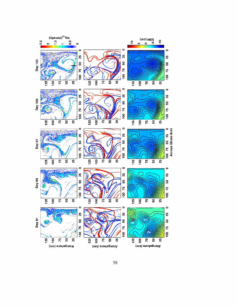
58

59

with a mass of simulated larvae spiraling into its center (day 91, eddy 1). This small

eddy interacts with a similarly sized eddy (eddy 2), and a larger cyclonic eddy (eddy

3) over a ten-day period (days 94-103), which can be visualized by the particle

density field, the LCS locations and the sea surface height (SSH; Fig. 3.6). During the

interaction, both particle density and LCS distributions show that the contents of eddy

1 are compressed and filamented around the periphery of the larger eddy, resulting in

a thin, dense packet of material that was formerly the core of eddy 1 being transported

back towards the coast along the larger eddy’s exterior. In contrast, the SSH

signatures of the two small eddies appear to merge during the interaction (Fig. 3.6,

day 97), illustrating that what is observed in the Eulerian frame (SSH) does not

necessarily determine the transport fate of larval particles (the time-integrated

Lagrangian flow), as has often been noted in the dynamical systems literature (i.e.,

Shadden et al. 2005). The packet has a maximal density of over 90 particles/km2,

roughly two orders of magnitude greater than the initial particle release density (<1

larvae/km2). Note that many LCS are swept together and combined as the packet is

formed, and the resulting large number of collinear attracting LCS are coincident with

striations of dense material (Fig. 3.6, day 103).

Packets formed by eddy interactions can result in a wide range of larval age classes

from many source locations being concentrated in a very small spatial area. The dense

packet shown in Fig. 3.6 (black line on day 103) contains larvae ranging from less

than 20 to more than 60 days old (Fig. 3.7a). The material in the densest portion of

60

Figure 3.7 Packet age class and source region distribution. Transect of larval density (a) from 56 km offshore on model day 103 (along the vertical black line in the upper right panel in Fig. 3.6) with age class makeup (in days, grayscale). Ages range from less to 20 days to more than 60 days within a narrow spatial region. Larvae in the densest part of the larval packet (22-23 km alongshore, 92 particles) come from a wide range of source locations (b), where source regions have been unwrapped to account for transport across the periodic boundary in the ocean circulation model. Bin size for this histogram in (b) is 10 km; the vertical axis is the number of particles from each source region.

61

the packet (22-23 km alongshore in Fig. 3.7a), representing one square km bin in Fig.

3.6, came from sources up to 50 km south and 220 km north of the packet location on

day 103 (Fig. 3.7b), where the source regions have been unwrapped to account for the

periodic boundary in the ocean circulation model. Notably some of this material came

from south of its current location, having traveled against the average southward

alongshore flow.

Filamentation can lead to a quick trip offshore, decreasing transit time away from the

shelf. For example, on day 177 particles ranging from 7-29 days old are found over

150 km offshore concentrated in a filament that wraps around the periodic model

boundary (Fig. 3.8a, denoted by X’s). Conversely, filaments often bend back toward

the coast or get folded into a persistent retention zone (i.e., an eddy), resulting in

older larvae being transported back towards the shelf. Inshore of the filament

described above are many regions of older larvae (30-120+ days old, Fig. 3.8b-e); we

will focus on two of these areas, marked in boxes in Fig. 3.8f. Histograms of source

Figure 3.8 Density distributions by age class on model day 177. Shown are ages 7-29 days (a), 30-59 days (b), 60-89 days (c), 90-119 days (d), 120 days and over (e), and all age classes (e). Larval density (particles/km2) is shown on log scale to facilitate visualization. Note the feature centered at 100 km offshore and 175 km alongshore (dashed box in f) has integrated particles from many different age classes (b-e), and that some particles are near the coast (<50 km) even after 120 days (e, solid box in f). In contrast young larvae (a) have reached upwards of 150 km offshore in a fast moving filament (denoted by X’s) that wraps around the periodic model boundary. See supplemental movie 3.2 for visualization of density through the model run. Age and source distributions for the boxed regions are shown in Fig. 3.9.

62

63

locations and age distributions for the two boxed regions are shown in Fig. 3.9.

For the coherent structure on day 177 (dashed box in Fig. 3.8f), again a large number

of larvae with a diverse range of ages have been concentrated into a small region (see

supplemental movie 3.2 for animation). There are over 15,000 particles in this

structure, 16% of the total number of particles in the entire domain at this time.

Within the coherent structure particles range from 40 to 170 days old and are from

source regions spanning 150 to over 800 km alongshore (Fig. 3.9a-b). Note that in

Fig. 3.9a the tails of the distribution are not completely shown and some larvae

originate from source locations more than 1200 km alongshore. These particles with

distant sources have crossed the periodic domain four times, representing distant

poleward sources. Some larvae older than 120 days are within 50 km of the coast

(solid box in Fig. 3.8f). This packet contains particles ranging from 20 to 170 days

old and from -10 to 500 km alongshore (Fig. 3.9c-d). Thus eddy interaction may

result in transport of material back to the shelf (and for some larvae back to their

source locations) long after release.

In general, while the filamentation and eddy merging process is complex and takes

variable forms, dense packets resulting from eddy-eddy interaction and filamentation

are found throughout this model run (see supplemental movies), and all other model

runs. To assess the average statistics of packet formation and their associated larval

age and source distributions, we define packets as 1 km square regions. Note this is

64

Figure 3.9 Source and age distributions. Histograms of source locations (a,c) and age distributions (b,d) for the two boxed regions in Fig. 3.8f. Here in both examples larvae from a wide range of sources and release times are found in the same region. The coherent structure (a-b, dashed box in 3.8f) has integrated larvae originating from 150 to over 800 km alongshore (a), and contains particles ranging from 40 to 170 days old. A coastal packet (c-d, solid box in 3.8f) has particles that came from -10 to 600 km alongshore, and are less than 30 to over 175 days old. Source locations have been unwrapped as in Fig. 3.7, with a bin size of 50 km. Age bins are 10 days wide. N is the total number of particles in the histogram. Note the difference in vertical scales for each plot.

much smaller than the features described above. Figure 3.10 shows the

complementary cumulative distribution for density in these 1 km bins interpolated to

particle positions for all of model run 111. In most cases particles are in packets many

times denser than their release densities (<1 km-2; i.e. P = 0.54 for density greater

than 5 km-2). Average age and source histograms were determined for very dense

65

packets (density >50 km-2, P = 0.06, gray shading in Fig. 3.10, N = 8140 packets) by

Figure 3.10 Particle density and packet statistics. Complementary cumulative distribution of density at particle locations shows that over the model run 6% (P = 0.059) of particles are found in packets (shaded gray, defined by density > 50 in a 1 km2 bin). Combined histograms (with source and age averages removed for each packet) show a wide range of source regions (inset top) and ages (inset bottom) for larvae in packets. Horizontal axes on histograms show a portion of the long tails for each distribution.

subtracting out the averages for each packet and combining (Fig. 3.10 inset, N =

7x105 particles in total). Standard deviations are 73 km for source regions and 14

days for ages in packets, with long tails for both histograms as seen in previous

examples. As in Fig. 3.8, larger packets are made of many of these smaller dense

packets, which could result in a wider range of age and source regions for larger

66

features (as in Fig. 3.9). These results suggest that on average dense regions of larvae

will contain larvae from a wide range of source locations and release times. Since

eddy interaction processes are similar throughout the global ocean (McWilliams

1984, Bracco et al. 2004), similar packets are expected be found across a wide range

of marine ecosystems.

3.5 Discussion

3.5.1 Application of LCS

It may be possible to use LCS operationally for tracking regions of dense planktonic

accumulation. Given availability of high-quality ocean surface velocity fields (i.e. HF

radar, operational data assimilative coastal ocean models), attracting LCS can be

assessed for connection to spawning regions and tracked through time (i.e. Shadden et

al. 2009). However, instead of just a diagnostic metric it may prove more powerful to

use LCS as a conceptual tool to understand the kinematic framework that larval

transport dynamics rests in, as LCS make the connection between filamentation,

transport boundaries and frontal processes. Perhaps more importantly, theorems from

dynamical systems can help predict the sensitivity of ecological processes associated

with LCS.

For example, while the effects of swimming are difficult to model, involving species-

specific assumptions about cues, swimming duration, speed and direction (Metaxas

67

Figure 3.11 Effect of swimming on density patterns. Density distributions are shown as in Fig. 3.8f with addition of random-walk type swimming at two levels: (a) 1 cm/s and (b) 10 cm/s standard deviation. As expected given the structural stability of LCS, dense packets

and Saunders 2009), we can predict that LCS will still delineate important transport

pathways for slow swimmers. Since LCS are structurally stable (Haller 2002,

Harrison and Glatzmaier 2012), i.e. largely insensitive to perturbations, it follows that

up to a certain swimming speed in any direction, or for short, strong bursts of

swimming, larvae will effectively remain on LCS. To provide a rough demonstration

of this stability, Fig. 3.11 shows the effect of normally distributed, random-walk

horizontal “swimming” on the density patterns shown in Fig. 3.8f. The random-walk

perturbations were added with a standard deviation σ of 1 cm/s and 10 cm/s. For both

cases the horizontal swimming direction and magnitude was randomized at each

particle time step. For a perturbation of σ = 1 cm/s density patterns remain close to

their original distributions (compare Figs. 3.8f & 3.11a). At a perturbation level of σ

68

= 10 cm/s (much higher than the expected swimming speeds of most early stage

larvae; e.g., Love et al. 2002) packets and filaments are still in evidence; maximum

concentrations have been reduced, but are still an order of magnitude higher than the

release density (Fig. 3.11b). Thus we expect filaments and eddies are robust

aggregators of planktonic and nektonic organisms under a wide range of behavioral

strategies.

3.5.2 Comparisons with observations and prior studies

The present analyses linking processes of filamentation and larval distributions

should be widely applicable as upwelling dynamics are similar across all EBCs (e.g.,

Haynes et al. 1993, Hill et al. 1998). For example, neritic larvae and coastal

planktonic species are persistently found in upwelling filaments and their associated

eddies in the Canary EBC (Rodriguez et al. 1999, Bécognée et al. 2009), and this is

thought to be an important larval transport pathway from the mainland to offshore

islands. In the CCS, the transport of propagules in filaments is consistent with the

observed higher abundance of larvae at fronts (Larson et al. 1994, Bjorkstedt et al.

2002), though to our knowledge these two phenomena have not been previously

connected. Packet formation by eddy-eddy interaction, filamentation and transport

back to the shelf may explain the delivery of discrete settlement pulses of larvae that

contain a wide range of age classes and species, and also contribute to shorter than

expected dispersal distances (Warner et al. 2000, Warner and Cowen 2002, Shanks

69

2009). These observations may be explained to leading order by ocean transport

alone, without invoking complex larval behavior or life histories.

Larval concentration in filaments may explain regions of predictably higher

settlement downstream from headlands (Ebert and Russell 1988), as well as

preferential spawning areas observed at submerged promontories (Karnauskas et al.

2011). Instead of adding more variability, a complex coastline will often organize the

flow into more regular and predictable patterns. When an alongshore current reaches

a coastal headland it is directed offshore, often forming a filament or eddy (e.g.,

Haynes et al. 1993), and so can regularly generate high larval concentration, making

these areas advantageous spawning grounds (Karnauskas et al. 2011). If this

concentrated material were directed back to shore it would result in a large, perhaps

quick settlement pulse over a narrow coastal area, as seen in modeling studies

downstream from promontories (Kim and Barth 2011). Such settlement pulses are

expected to be correlated with frontal arrival, as has been observed in the CCS

(Woodson et al. 2012).

Recent modeling studies suggest packet delivery back to the shore is a common

phenomenon. Packet delivery will manifest in connectivity diagrams (Cowen et al.

2006, Siegel et al. 2008) as a linear feature, indicating a wide range of source regions

were deposited at one arrival location (as in Fig. 3.7). This pattern is prominent in

many connectivity studies (Aiken et al. 2011, Drake et al. 2011, Kim and Barth

70

2011). However, it is unclear from these studies if linear connectivity patterns are due

to single events or accrue over longer timescales. Since packet formation appears to

be a consequence of the eddy-eddy interaction and filamentation processes, we expect

it will occur across all ocean regions and likely generates the patterns seen in these

studies.

Biophysical and trophic interactions along coastal upwelling filaments and fronts

could influence larval survivability. Primary production is observed to be higher in

upwelling filaments, as nutrient-rich water is carried offshore (Brink and Cowles

1991, Hill et al. 1998), and also along fronts, where both planktonic and fish biomass

can be enhanced (e.g., Landry et al. 2012). In addition, frontal vertical velocities due

to submesoscale instabilities have been shown in coupled physical-ecosystem models

to induce nutrient injection and increase productivity, but also induce export materials

from the euphotic zone (see Lévy 2008 and Klein and Lapeyre 2009 for reviews).

Further seabirds, fish and other marine animals are known to use fronts for foraging

and efficient transport (e.g., Fiedler and Bernard 1987, Tew Kai et al. 2009, Munk et

al. 2010), indicating increased predation susceptibility for larvae at fronts. Thus larval

survivability on filaments will be controlled by a combination of enhanced fitness due

to food availability, higher mortality due to vertical export, or locally enhanced

predation.

71

Many EBCs have wider shelves than the California coastline, such as those off Africa

and the Iberian Peninsula. For these systems, upwelling can be centered at the shelf

break creating a kinematic boundary between a poleward shelf flow and the

equatorward upwelling jet (Peliz et al. 2002). This on-shelf/shelf break flow

partitioning appears to depend on the details of both the pycnocline and wind forcing

(Estrade et al. 2008), and has been observed to act as a retention mechanism for river

outflow and very nearshore species (Santos et al. 2004). Similarly, observations (Hill

et al. 1998) and more realistic models of the CCS often exhibit poleward flow close to

the coast (e.g., Drake and Edwards 2011). We speculate that retention within this

poleward flow, similar to the studies off the Iberian Peninsula, may limit the offshore

extent of many intertidal and very nearshore spawners (Shanks and Sherman 2009),

and perhaps contribute to the shorter than expected dispersal distances observed for

some species (Shanks 2009). To our knowledge it remains unclear what the temporal

dynamics, response to wind variation, and three-dimensional kinematics are for this

type of retention mechanism. However the dynamical systems approach to identifying

and classifying kinematic boundaries should be useful for diagnosing larval retention

in these systems.

The breakdown of fronts by small eddies and meanders is readily seen in satellite

observations (Flament et al. 1985); in ROMS these frontal instabilities are known to

intensify with increasing model resolution (Capet et al. 2008). Such instabilities

would likely lead to more mixing along filaments (Badin et al. 2011), but to our

72

knowledge has yet to be studied in the context of marine ecology. However, in situ

measurements suggest that frontal accumulation of planktonic organisms in filaments

is robust in the extension from model to reality (Larson et al. 1994, Rodriguez et al.

1999).

3.5.3 Potential Roles of Larval Behavior

Many species’ larvae and eggs are found preferentially near the ocean surface (e.g.,

Shanks 1985, Rodriguez et al. 1999, Bjorkstedt et al. 2002, Love et al. 2002, Metaxas

and Saunders 2009). Our particle model formulation assumes propagules swim or

float to overcome than the modest model vertical velocities (<5 m/d; Figs. 3.2-3.4),

i.e. prefer to be in the productive euphotic zone. If particles were free to move

vertically this could result in a lesser degree of density enhancement; instead of

aggregating at the surface, non-buoyant particles will be pushed down by surface

convergence and downwelling (e.g., Bakun 2010). Though modeled vertical

velocities here are instantaneously small, the accumulated effect over time can be

large and will increase density patchiness (Zhong et al. 2011). Our analysis of

transport boundaries and particle filimentation also applies to any floating material

originating over the shelf (pollutants, macrophytes, etc.), and aggregations of these

materials can form pelagic habitats for a variety of marine organisms (Shanks 1985,

Dempster and Taquet 2004), indicating a possible secondary effect on larval

distribtutions.

73

Previous results show ontogenetic vertical migration does not have strong effects on

the larval settlement statistics in the CCS-in-a-box model (Mitarai et al. 2008, Siegel

et al. 2008). Upwelling filaments are generally coherent up to ~100 m depth (e.g.,

Brink and Cowles 1991), so it follows that with even a moderate change in vertical

position larvae will remain within these flow structures. In contrast, regions with

generally high vertical velocity shear, for example estuaries (North et al. 2008) or

systems with bifurcations in major currents, such as off the north coast of Norway

(Fiksen et al. 2007), will be more sensitive to larval behavior. A common feature of

EBCs is vertical shear between the coastal equatorward upwelling jet and the

poleward undercurrent (Hill et al 1998), and larval transport in this region is known to

be affected by diurnal vertical migration (Aiken and Navarette 2011). It still remains

largely unclear where, when and to what extent vertical swimming will be important

given realistic flow fields.

3.6 Summary

Larvae released above the shelf in an idealized EBC are often transported in filaments

that coincide with LCS. Larvae are more likely to be found on an attracting LCS

(~40% over a 100-day ensemble) than on repelling LCS (~25%), and more likely on

LCS than if they were randomly distributed (~20% expected). Larvae on LCS are also

more likely to be on SST fronts, although this is not always the case. Eddy-eddy

interaction and filamentation processes result in the creation of dense packets, which

74

bring larvae of many age classes and source regions together into a small spatial

region. Results are consistent with observations of larval distributions and settlement

patterns in EBCs and other systems. Packet formation as a manifestation of eddy

interaction and filamentation processes should occur globally. These packets

sometimes get transported back to the coast, and the associated pattern of

connectivity is seen in other studies. LCS are insensitive to a moderate degree of

perturbation (e.g., swimming) and so are expected to be robust in mapping transport

pathways under a variety of larval behavioral strategies.

3.7 Acknowledgements

Input from G. Glatzmaier and P. Raimondi were helpful in focusing this project, as

well as overall support and writing assistance from R. Warner, K. Brink, A. Payton

and E. Silver. Four anonymous reviewers supplied thoughtful critiques that greatly

improved the manuscript. This project was supported in part by NSF grant OCE-

030844 as part of the Flow, Fish and Fishing Biocomplexity in the Environment

project, by NSF grant OCE-1155813, by the Center for Stock Assessment Research

(CSTAR), a partnership between NOAA Fisheries Santa Cruz Laboratory and UCSC,

and by IGPP Santa Cruz.

75

3.8 Bibliography

Aiken CM, Navarrete CM, Castillo M, Castilla JC (2007) Along-shore larval dispersal kernels in a numerical ocean model of the central Chilean coast. Mar Ecol Prog Ser 339:13

Aiken CM, Navarrete SA (2011) Environmental fluctuations and asymmetrical dispersal: generalized stability theory for studying metapopulation persistence and marine protected areas. Mar Ecol Prog Ser 428:77– 88

Aiken CA, Navarrete SA, and Pelegrí JL (2011) Potential changes in larval dispersal and alongshore connectivity on the central Chilean coast due to an altered wind climate. J Geophys Res 116(G4):G04026

Badin G, Tandon A, Mahadevan A (2011) Lateral mixing in the pycnocline by baroclinic mixed layer eddies. J Phys Oceanogr 41(11):2080–2101

Bakun A (2010) Linking climate to population variability in marine ecosystems characterized by non-simple dynamics: conceptual templates and schematic constructs. J Mar Syst 79:361–373

Bécognée P, Moyano M, Almeida C, Rodríguez J, Fraile-Nuez E, Hernández-Guerra A, Hernández-León S (2009) Mesoscale distribution of clupeoid larvae in an upwelling filament trapped by a quasi-permanent cyclonic eddy off Northwest Africa. Deep-Sea Res Part I 56(3):330–343

Berkley HA, Kendall BE, Mitarai S, Siegel DA (2010) Turbulent dispersal promotes species coexistence. Ecol Lett 13(3):360–371

Beron-Vera FJ, Olascoaga MJ, Goni GJ (2008) Oceanic mesoscale eddies as revealed by Lagrangian coherent structures. Geophys Res Lett 35(12):7

Bjorkstedt EP, Rosenfeld LK, Grantham BA, Shkedy Y, Roughgarden J (2002) Distributions of larval rockfishes Sebastes spp. across nearshore fronts in a coastal upwelling region. Mar Ecol Prog Ser 242:215–228

Bode M, Bode L, Armsworth PR (2011) Different dispersal abilities allow reef fish to coexist. Proc Nat Acad Sci 108(39):16317–16321,

Botsford LW, Brumbaugh DR, Grimes C, Kellner JB, Largier J, O’Farrell MR, Ralston S, Soulanille E, Wespestad V (2009) Connectivity, sustainability, and yield: bridging the gap between conventional fisheries management and marine protected areas. Rev Fish Biol Fish 19(1):69–95

76

Bracco A, von Hardenberg J, Provenzale A, Weiss JB, McWilliams JC (2004) Dispersion and mixing in quasigeostrophic turbulence. Phys Rev Lett 92(8):4

Brink KH, Cowles TJ (1991) The coastal transition zone program. J Geophys Res 96(C8):14637–14647

Broitman BR, Blanchette CA, Menge BA, Lubchenco J, Krenz C, Foley M, Raimondi PT, Lohse D, Gaines SD (2008) Spatial and temporal patterns of invertebrate recruitment along the west coast of the United States. Ecol Monogr 78(3):403–421

Calil PHR, Richards KJ (2010) Transient upwelling hot spots in the oligotrophic North Pacific. J Geophys Res 115(C2):C02003

Capet X, McWilliams JC, Molemaker MJ, Shchepetkin AF (2008) Mesoscale to submesoscale transition in the California Current system. Part II: Frontal processes. J Phys Oceanogr 38(1):44–64

Chassot E, Bonhommeau S, Dulvy NK, Mélin F, Watson R, Gascuel D, Le Pape O (2010) Global marine primary production constrains fisheries catches. Ecol Lett 13(4):495–505

Costello C, Rassweiler A, Siegel DA, De Leo G, Micheli F, Rosenberg A (2010) The value of spatial information in MPA network design. PNAS 107(43):18294–18299

Cowen RK, Paris CB, Srinivasan A (2006) Scaling of connectivity in marine populations. Science 311(5760):522–527

Cowen RK, Sponaugle S (2009) Larval dispersal and marine population connectivity. Annu Rev Mar Sci 1:443–466

Dempster T, Taquet M (2004) Fish aggregation device (FAD) research: gaps in current knowledge and future directions for ecological studies. Rev Fish Bio Fish 14(1):21–42

d’Ovidio F, De Monte S, Alvain S, Dandonneau Y, Lévy M (2010) Fluid dynamical niches of phytoplankton types. PNAS 107(43):18366

d’Ovidio F, Fernández V, Hernández-García E, López C (2004) Mixing structures in the Mediterranean Sea from finite-size Lyapunov exponents. Geophys Res Lett 31(17)

Drake PT, Edwards CA, Barth JA (2011) Dispersion and connectivity estimates along the U.S. west coast from a realistic numerical model. J Mar Res, 69(1):1–37

77

Ebert TA, Russell MP (1988) Latitudinal variation in size structure of the west coast purple sea urchin: a correlation with headlands. Limnol Oceanogr 33(2):286–294

Estrade P, Marchesiello P, Verdiere D, Colin A, Roy C (2008) Cross-shelf structure of coastal upwelling: A two dimensional extension of Ekman’s theory and a mechanism for inner shelf upwelling shut down. J Mar Res 66(5):589–616

Fiedler PC, Bernard HJ (1987) Tuna aggregation and feeding near fronts observed in satellite imagery. Cont Shelf Res 7(8):871–881

Fiksen Ø, Jørgensen C, Kristiansen T, Vikebø F, Huse G (2007) Linking behavioural ecology and oceanography: larval behaviour determines growth, mortality and dispersal. Mar Ecol Prog Ser 347:195–205

Flament P, Armi L, Washburn L (1985) The evolving structure of an upwelling filament. J Geophys Res 90(11):765–11

Gaylord B, Gaines SD (2000) Temperature or transport? range limits in marine species mediated solely by flow. Am Nat 155(6):769

Genin A, Jaffe J, Reef R, Richter C, Franks P (2005) Swimming against the flow: a mechanism of zooplankton aggregation. Science 308(5723):860

Haller G (2002) Lagrangian coherent structures from approximate velocity data. Phys Fluids 14(6):1851–1861

Harrison CS, Glatzmaier GA (2012) Lagrangian coherent structures in the California Current System–sensitivities and limitations. Geophys Astrophys Fluid Dyn 106(1):22–44

Haynes R, Barton E, Pilling I (1993) Development, persistence, and variability of upwelling filaments off the Atlantic Coast of the Iberian Peninsula. J Geophys Res 98(C12):22681–22692

Hedgecock D (1994) Does variance in reproductive success limit effective population sizes of marine organisms? In: Beaumont AR (ed) Genetics and evolution of aquatic organisms. Chapman and Hall, London, UK

Hill AE, Hickey BM, Shillington FA, Strub PT, Brink KH, Barton ED, Thomas AC. (1998) Eastern ocean boundaries coastal segment. In: Robinson AR, Brink, KH (eds). The Sea, Vol. 11. John Wiley & Sons Inc, London

Huhn F, von Kameke A, Pérez-Muñuzuri V, Olascoaga MJ, and Beron-Vera FJ (2012) The impact of advective transport by the South Indian Ocean Countercurrent on the Madagascar plankton bloom. Geophys Res Lett 39(L06602).

78

Jackson GA, Strathmann RR (1981) Larval mortality from offshore mixing as a link between precompetent and competent periods of development. Am Nat 118(1):16-26

Karnauskas M, Chérubin LM, Paris CB (2011) Adaptive significance of the formation of multi-species fish spawning aggregations near submerged capes. PLoS ONE 6(7):e22067

Katija K, Beaulieu WT, Regula C, Colin SP, Costello JH, Dabiri JO (2011) Quantification of flows generated by the hydromedusa Aequorea victoria: a Lagrangian coherent structure analysis. Mar Ecol Prog Ser, 435:111–123

Kim S, Barth JA (2011) Connectivity and larval dispersal along the Oregon coast estimated by numerical simulations. J Geophys Res 116(C6)

Kinlan B, Gaines S (2003) Propagule dispersal in marine and terrestrial environments: a community perspective. Ecology 84(8):2007–2020

Klein P, Lapeyre G (2009) The oceanic vertical pump induced by mesoscale and submesoscale turbulence. Annu Rev Mar Sci 1:351–375

Landry MR, Ohman MD, Goericke R, Stukel MR, Barbeau KA, Bundy R, Kahru M (2012). Pelagic community responses to a deep-water front in the California Current Ecosystem: overview of the A-Front study. J Plank Res, in press.

Largier JL (2003) Considerations in estimating larval dispersal distances from oceanographic data. Ecol App 13(sp1):71–89

Larson RJ, Lenarz WH, Ralston S (1994) The distribution of pelagic juvenile rockfish of the genus Sebastes in the upwelling region off central California. Calif Coop Ocean Fish Invest Rep 35:175– 221

Lehahn Y, d’Ovidio F, Lévy M, Heifetz E (2007) Stirring of the northeast Atlantic spring bloom: A Lagrangian analysis based on multisatellite data. J Geophys Res 112(C8):C08005

Lehahn Y, d’Ovidio F, Lévy M, Amitai Y, Heifetz E (2011) Long range transport of a quasi isolated chlorophyll patch by an Agulhas ring. Geophys Res Lett 38(16):L16610

Levin L (2006) Recent progress in understanding larval dispersal: new directions and digressions. Inta Comp Bio 46(3):282

Lévy M (2008) The modulation of biological production by oceanic mesoscale turbulence. In: Weiss JB, Provenzale A (eds). Transport and Mixing in Geophysical Flows, Springer

79

Love M, Yoklavich M, Thorsteinson L (2002) The rockfishes of the northeast Pacific. Univ of Cal Press

Mancho A, Small D, Wiggins S (2006) A tutorial on dynamical systems concepts applied to Lagrangian transport in oceanic flows defined as finite-time data sets: Theoretical and computational issues. Phys Rep, 437(3-4):55–124

Marchesiello P, McWilliams JC, Shchepetkin AF (2003) Equilibrium structure and dynamics of the California Current System. J Phys Ocean, 33(4):753–783

Marchesiello P, Estrade P (2009) Eddy activity and mixing in upwelling systems: a comparative study of Northwest Africa and California regions. Int J Earth Sci 98(2):299–308

Mathur M, Haller G, Peacock T, Ruppert-Felsot J, Swinney H (2007) Uncovering the Lagrangian skeleton of turbulence. Phys Rev Lett 98(14):144502

McWilliams JC (1984) Emergence of isolated coherent vortices in turbulent flow. J Fluid Mech 146:21–43

Metaxas A, Saunders M (2009) Quantifying the “bio-” components in biophysical models of larval transport in marine benthic invertebrates: advances and pitfalls. Biol Bull 216(3):257

Mitarai S, Siegel DA, Winters KB (2008) A numerical study of stochastic larval settlement in the California Current system. J Mar Syst 69:295–309

Mitarai S, Siegel DA, Watson JR, Dong C, McWilliams JC (2009) Quantifying connectivity in the coastal ocean with application to the Southern California Bight. J Geophys Res 114

Morgan SG, Fisher JL, Miller SH, McAfee ST, and Largier JL (2009) Nearshore larval retention in a region of strong upwelling and recruitment limitation. Ecology, 90(12):3489–3502

Munk P, Hansen MM, Maes GE, Nielsen TG, Castonguay M, Riemann L, Sparholt H, Als TD, Aarestrup K, Andersen NG, et al. (2010) Oceanic fronts in the Sargasso Sea control the early life and drift of Atlantic eels. Proc R Soc B 227(1700):3593–3599

North EW, Schlag Z, Hood RR, Li M, Zhong L, Gross T, Kennedy VS (2008) Vertical swimming behavior influences the dispersal of simulated oyster larvae in a coupled particle-tracking and hydrodynamic model of Chesapeake Bay. Mar Ecol Prog Ser 359(99):115

80

Okubo A (1980) Diffusion and ecological problems: mathematical models. Springer-Verlag, Berlin

Olascoaga MJ, Beron-Vera FJ, Brand LE, Koçak H (2008) Tracing the early development of harmful algal blooms on the West Florida Shelf with the aid of Lagrangian coherent structures. J Geophys Res 113(c12):c12014

Palumbi S (2003) Population genetics, demographic connectivity, and the design of marine reserves. Ecol App 13(sp1):146–158

Parrish RH, Nelson CS, Bakun A (1981) Transport mechanisms and reproductive success of fishes in the California Current. Biol Oceanogr 1(2):175–203

Peliz Á, Rosa T, Santos A, Pissarra J (2002) Fronts, jets, and counter-flows in the Western Iberian upwelling system. J Mar Sys 35(1-2):61–77

Roberts C (1997) Connectivity and management of Caribbean coral reefs. Science, 278(5342):1454–1457

Rodriguez JM, Hernández-León S, Barton ED (1999) Mesoscale distribution of fish larvae in relation to an upwelling filament off Northwest Africa. Deep-Sea Res Part I 46(11):1969–1984

Rossi V, López C, Hernández-García E, Sudre J, Garçon V, Morel Y (2009) Surface mixing and biological activity in the four Eastern Boundary Upwelling Systems. Nonl Proc Geophys 16(4):557–568

Ryther JH (1969) Photosynthesis and fish production in the sea. Science 166(3901):72

Samelson RM, Wiggins S (2006) Lagrangian transport in geophysical jets and waves: the dynamical systems approach. Springer, New York, N.Y.

Santos AMP, Peliz A, Dubert J, Oliveira PB, Angélico M, Ré P (2004) Impact of a winter upwelling event on the distribution and transport of sardine (Sardina pilchardus) eggs and larvae off Western Iberia: a retention mechanism. Cont Shelf Res 24(2):149–165

Shadden SC (2005) LCS tutorial. Accessed 22-Mar-2012. http://mmae.iit.edu/shadden/LCS-tutorial/

Shadden SC (2012) Lagrangian coherent structures. In: Grigoriev R, Schuster HG (eds). Transport and Mixing in Laminar Flows: From Microfluidics to Oceanic Currents, Wiley

81

Shadden SC, Lekien F, Marsden JE (2005) Definition and properties of Lagrangian coherent structures from finite-time Lyapunov exponents in two-dimensional aperiodic flows. Phys D 212(3- 4):271–304

Shadden SC, Lekien F, Paduan JD, Chavez FP, Marsden JE (2009) The correlation between surface drifters and coherent structures based on high-frequency radar data in Monterey Bay. Deep-Sea Res Part II 56(3-5):161–172

Shanks AL (1985) Behavioral basis of internal-wave-induced shoreward transport of megalopae of the crab Pachygrapsus crassipes. Mar Ecol Prog Ser, 24:289–295

Shanks AL (2009) Pelagic larval duration and dispersal distance revisited. The Bio Bull 216(3):373

Shanks AL, Shearman RK (2009) Paradigm lost? Cross-shelf distributions of intertidal invertebrate larvae are unaffected by upwelling or downwelling. Mar Ecol Prog Ser 385:189–204

Shchepetkin AF, McWilliams JC (2005) The regional oceanic modeling system (ROMS): a split-explicit, free-surface, topography-following-coordinate oceanic model. Ocean Model 9(4):347–404

Siegel DA, Kinlan BP, Gaylord B, Gaines SD (2003) Lagrangian descriptions of marine larval dispersion. Mar Ecol Prog Ser 260:83–96

Siegel DA, Mitarai S, Costello CJ, Gaines SD, Kendall BE, Warner RR, Winters KB (2008) The stochastic nature of larval connectivity among nearshore marine populations. PNAS 105(26):8974

Sponaugle S, Cowen R, Shanks A, Morgan W, Leis J, Pineda J, Boehlert G, Kingsford M, Lindeman K, Grimes C, et al. (2002) Predicting self-recruitment in marine populations: biophysical correlates and mechanisms. Bull Mar Sci, 70(Sup 1):341–375

Strathmann R (1985) Feeding and nonfeeding larval development and life-history evolution in marine invertebrates. Ann Rev Ecol Sys 16:339–361

Tew Kai E, Rossi V, Sudre J, Weimerskirch H, López C, Hernández-García E, Marsac F, Garçon V (2009) Top marine predators track Lagrangian coherent structures. PNAS 106(20):8245–8250

Warner R, Cowen R (2002) Local retention of production in marine populations: evidence, mechanisms, and consequences. Bull Mar Sci 70(1):245–249

82

Warner R, Swearer S, Caselle J (2000) Larval accumulation and retention: implications for the design of marine reserves and essential habitat. Bull Mar Sci 66(3):821–830

Watson J, Mitarai S, Siegel DA, Caselle JE, Dong C, and McWilliams JC (2010) Realized and potential larval connectivity in the Southern California Bight. Mar Ecol Prog Ser, 401:31–48

Watson J, Hayes CG, Raimondi PT, Mitarai S, Dong C, McWilliams JC, Blanchette CA, Caselle JE, Siegel DA (2011a) Currents connecting communities: Nearshore community similarity and ocean circulation. Ecology, 92, 1193–1200

Watson J, Siegel DA, Kendall BE, Mitarai S, Rassweiler A, Gaines SD, (2011b) Identifying critical regions in small-world marine metapopulations, Proc Nat Acad Sci USA, 108:E907-E913.

Watson J, Kendall BE, Siegel DA, Mitarai S (2012) Changing seascapes, stochastic connectivity and marine metapopulation dynamics. Amer Nat 180:99-112

Wiggins S (2005) The dynamical systems approach to Lagrangian transport in oceanic flows. Annu Rev Fluid Mech 37:295–328

Woodson CB, McManus MA, Tyburczy JA, Barth J, Washburn L, Caselle JE, Carr MH, Malone DP, Raimondi PT, Menge BA, Palumbi SR (2012) Coastal fronts set recruitment and connectivity patterns across multiple taxa. Lim Ocean, 57(2):582–596

Y. Zhong, A. Bracco, and T. A. Villareal. Pattern formation at the ocean surface: Sargassum distribution and the role of the eddy field. Lim Ocean: Fluid Enviro, 2:12–27, 2012.

83

Chapter 4 The tattered curtain hypothesis revisited: coastal jets control larval settlement patterns

Cheryl S. Harrison1 and David A. Siegel2

1 Earth and Planetary Sciences Department, University of California, Santa Cruz, CA

95064, USA chsharrison@gmail.com

2 Earth Research Institute and Department of Geography, University of California,

Santa Barbara, California, 93106 USA

Target journal: ASLO Fluids and Environments

Abstract

The details of upwelling dynamics and retention of coastal waters is important for

understanding dispersal of coastally originating material and thus dynamics of marine

ecosystems. Motivated by observations of larval recruitment patterns, a hypothesis

was put forward in the 1980’s describing the upwelling front as a “tattered curtain,”

retaining coastally released larvae, but broken up by filaments and eddies. This

transport barrier was expected to respond to local wind forcing by moving offshore in

complex meanders, moving back to the coast under upwelling relaxation. Here we

revisit and revise this hypothesis using an idealized ocean model of an eastern

boundary upwelling current driven by realistically temporally varying winds. In the

84

model, coastal retention patterns are strongly controlled by the upwelling jet,

resulting in significant along-shore coherence in settlement patterns when the jet is

near the coast. Modeled particle density is highest near the core of the jet, bounded by

high velocity shear lines on either side, consistent with dynamical systems theory of

jet cores as retentive barriers. Using an ensemble of model runs, we show empirically

that potential settlement is highest after periods of extended moderate upwelling.

Extended strong upwelling “tatters” the upwelling jet, driving material far offshore in

complex patterns. Settlement is best explained by 20-day integrated alongshore wind

(r = 0.62). Settlement is only marginally explained by upwelling wind relaxation

events (r = 0.33). Retention in coastal jets should be a widespread phenomenon as

indicated by numerous studies consistent with the results here.

4.1 Introduction

One of the central problems in marine ecology is the temporal and spatial dynamics

affecting transport of coastally spawned species. Coastal upwelling ecosystems,

though representing only a small extent of the ocean surface, contain a

disproportionate number of the ocean’s fisheries (Ryther 1969). Along the coast,

recently upwelled water brings nutrients to the surface where they can be utilized by

phytoplankton, providing energy to coastal ecosystems. Many coastal species are

benthic – remaining near the sea floor or in intertidal areas for their adult lives. Many

benthic species have a pelagic (open ocean) larval or juvenile stage. A common

85

reproductive strategy is to spawn thousands to millions of larvae that drift or swim

with the currents, feeding in the plankton for days to months until gaining

competency to recruit back to suitable habitat, forming the next generation. This

spawning strategy is utilized across diverse species, from tiny barnacles up to large

groundfish: animals inhabiting the kelp beds, rocky substrate, and intertidal habitats

all along the coastal shelf and slope. Many commercially exploited benthic species

renew their populations very slowly, and so are overfished to the point of being

threatened or endangered. Understanding the lifecycle dynamics of these fisheries,

especially the poorly understood pelagic stage, is important for appropriate

management. Retention over the shelf during the larval competency window insures

that spawn is not swept far offshore away from suitable habitat, and a growing

number of observations suggest that this limited dispersal due to retention is much

more common than previously thought (Warner and Cowen 2002, Shanks and

Sherman 2009). However, the degree to which oceanography determines settlement

patterns remains poorly understood.

For benthic species, distribution of spawn near suitable habitat after some residence

time in the plankton, often called pelagic larval duration (PLD), determines the

success of animals recruiting to the adult stage, and thus the strength of the

population for that spawning season. To explain the observed pulses of recruitment of

barnacle larvae along the coast, a hypothesis was put forward in the 1980’s that

linked dynamics of the upwelling front to settlement pulses (Roughgarden et al. 1988,

86

1991). In this paradigm, the front between recently upwelled water near the coast and

warmer water offshore was considered a convergence zone where planktonic

organisms were aggregated. The distance of this upwelling front from the shore was

thought to be determined largely by the strength of the upwelling winds, carrying

larvae far from shore when upwelling was strong and back towards shore during

relaxation, resulting in a large settlement pulse when the upwelling front collides with

the coast. This hypothesis was thought to be especially relevant for intertidal species

along the Central California coast: in this region the shelf is narrow, the upwelling

front close to shore and many species spawn during the spring to fall upwelling

season. The details of this hypothesis are best appreciated in the original text

(Roughgarden et al. 1991):

“We imagine, somewhat simplistically, the upwelling front as a ‘tattered

curtain’ hanging before an open window. It is tattered because it is punctured

by offshore squirts such as those typical of Point Arena, Point Reyes, and

Point Sur. It does not move as rigid iron curtain in response to the upwelling

strength, but instead is pushed and pulled locally, billowing in toward shore in

some spots while remaining far from shore at others. Thus, during a short

period of relaxation, small parts of the upwelling front may touch the coast

leading to local recruitment. But during an extended relaxation, long sections

of the front collide with the shore leading to nearly synchronous recruitment

across long stretches of the coast. Moreover, the correlation (of say, 1 day lag)

87

between upwelling-causing winds and recruitment is fussed by the distance of

the front from shore: if the front is far from shore, as in the spring, and

extended relaxation is needed to produce a recruitment pulse, but if the front

has gradually moved closer to shore, as in the summer, a short relaxation may

effect a recruitment pulse. Furthermore, when eddies and meanders disrupt a

simple linear geometry for the front, mixed signals result. Because of annual

variability in the strength of the California Current, in the abruptness of the

relaxation events during Summer, and in the prominence of eddies and

meanders in the California Current, the temporal patterns of larval recruitment

in consecutive years are not exact replicates. We term this overall hypothesis

the ‘tattered curtain’ hypothesis.”

In the decades since the tattered curtain hypothesis was first put forward scores of

studies have demonstrated a relationship between upwelling winds, larval distribution

and settlement events for a wide range of coastal species and in regions far beyond

the California coast (cf. Shanks and Sherman 2009). Subsequently, this hypothesis

has become generally accepted as the prevailing wisdom. However, recently the

upwelling relaxation implies settlement paradigm as well as “supply side” ecology in

general (the idea that ocean transport determines larval delivery) has come under

strong scrutiny. Limited dispersal is much more common than previously assumed

(Spongule et al. 2002, Swearer et al. 2002, Warner and Cowen. 2002), and

observations along the California coast in particular demonstrate that many species

88

recruit under strong upwelling conditions (Morgan et al. 2009, Shanks and Sherman

2009). A hypothesis often invoked to explain these observations, especially along the

California coast, is that larval behavior keeps spawn close to the coast, limiting

offshore transport (e.g., Batchelder et al. 2002). However, testing of this alternate

hypothesis requires confidence in the null hypothesis that without larval behavior

upwelling winds imply offshore transport and that upwelling relaxation, with a few

days lag, indeed should result in settlement pulses. Systematic testing of this

upwelling relaxation paradigm has yet to be done from an ocean modeling

perspective and is the goal of this study.

This paper is organized as follows. Section 4.2 outlines background theory on both

the Eulerian and Lagrangian dynamics of upwelling jets. Section 4.3 describes the

biophysical model used. Section 4.4 contains modeling results on patterns of coastal

retention and settlement as well as the statistical correlation between upwelling winds

and settlement patterns. Section 4.5 summarizes our conclusions. Finally, section 4.6

contains discussion of the results, including evidence from other studies that the

mechanisms seen here set settlement patterns in a number of regions.

89

4.2 Background theory

4.2.1 Eulerian dynamics: upwelling jets and offshore transport

In the coastal ocean, jets are a common occurrence, with the most dominant jets along

western boundary currents (e.g., Gulf Stream, Kuroshio). Eastern boundary currents

(EBCs), such as the California Current system (CCS), feature upwelling jets (Fig.

4.1), a geostrophic response to the upwelling of the pycnocline associated with the

“peeling back” of the surface ocean by offshore Ekman transport (Brink 1983, Hill et

al. 1998). Here there is a change in density moving offshore from colder, denser,

recently upwelled water near the coast to warmer, lighter water offshore, i.e. the

upwelling front. This density gradient results in a change in sea surface height and

thus a pressure force towards the coast. When the flow is in geostrophic balance the

Coriolis force balances this pressure gradient, and flow is along lines of constant sea

surface height moving towards the equator, resulting in an equatorward upwelling jet.

In theory the strength of this jet is directly proportional to the density gradient across

the upwelling front, and so in highly stratified regions the jet is fast and relatively

narrow.

In a tattered curtain, a breeze will preferentially flow through rips in the curtain,

unimpeded by the curtain’s weight. Similarly, swift offshore transport in coastal

upwelling systems will preferentially occur in regions where the upwelling jet is

already weakened by instabilities, the openings in the jet. In the case of the tattered

90

curtain, resistance is applied by the weight of the curtain: the heavier the curtain the

more resistance to the wind. In the case of coastal upwelling, resistance is applied by

coastal velocity shear, with more resistance for stronger shear, i.e. a faster alongshore

jet. To see this relationship, consider idealized Ekman mass transport in an upwelling

system. Ekman transport is calculated from the alongshore momentum balance by

assuming that horizontal velocity can be decomposed into a geostrophic and Ekman

component, i.e. u = uG + uE, and that all (non-linear) advection terms are negligible

(e.g., Gill 1982, Brink 1983). In upwelling systems this results in the alongshore

momentum balance

fuE = Τy/ρ,

where f is the Coriolis parameter, uE offshore (upwelling) velocity integrated over the

depth in which the winds act, Τy the wind stress at the ocean surface in the alongshore

direction, and ρ density. In the presence of a steady upwelling jet, offshore advection

of alongshore velocity becomes important and the momentum balance must be

modified to include nonlinear coupling between the Ekman and background

(geostrophic) modes, i.e.

uE δvG/δx + fuE = Τy/ρ,

where δvG/δx is the depth integrated cross-shelf shear of the alongshore velocity. This

results in a reduced upwelling velocity

uE = Τy/ρ(f + δvG/δx).

91

When δvG/δx is positive (an on the inshore flank of the upwelling jet), the strength of

the offshore transport is reduced by the magnitude of the velocity shear (Brink 1987,

Woodson in revision).

Weak points in the upwelling jet (where δvG/δx is small and thus uE stronger) can

occur through spontaneous instability, meanders instigated by local topography or

remotely forced by coastally trapped waves, or by interactions with the energetic

offshore eddy field generated by previous instabilities (Strub et al. 1991, Barth 1994,

Durski and Allen 2005). Most of these generation mechanisms are inherently

complex and involve nonlinear interactions (with the important exception of

interactions with coastal topography) and so exhibit a large degree of variability and

unpredictability (e.g., Durski and Allen 2005). Instabilities commonly result in eddies

and meanders in the coastal jet, as well as upwelling filaments, which often terminate

in eddies (Fig. 4.1), and squirts, which are wider offshore excursions of the upwelling

jet featuring fast cross-shelf velocities (Strub et al. 1991, Haynes et al. 1993,

Marchesiello et al. 2003, Durski and Allen 2005, Bécongée et al. 2009). All of these

features have strong effects on larval distribution patterns (Harrison et al. in review)

Despite the complexity of coastal circulation, simplified analytical results suggest the

distance of the upwelling front from shore is linearly proportional to the integrated

upwelling wind intensity, and this result has been somewhat borne out in observations

(Austin and Barth 2002), as well as in observed and modeled larval distributions and

settlement patterns (Roughgarden et al. 1988, 1991; Kim and Barth 2011). These

92

studies suggest a “settlement index” analogous to an upwelling index may be

tractable. Here we use a model of an idealized upwelling system to examine the

feasibility of finding such an index.

4.2.2 Lagrangian dynamics: a kinematic model of the upwelling jet

To understand how jets impact coastal Lagrangian transport, consider the idealized jet

(e.g., Kundu 1990):

where y is along the jet, x across the jet, A is the maximum jet velocity centered at

x=0 and the width of the jet is a function of the constant L (Fig. 4.2). This system

represents an idealized stationary Gaussian jet which is not accelerating in time in the

along jet-direction. Note the maximum across-jet velocity gradient (dv/dx)max occurs

at

€

x = ± 22 L (marked as vertical lines in Fig. 4.2), corresponding to the highest

velocity shear. This system can be integrated directly to provide the trajectories given

an initial position (x0,y0):

Here particles in the jet move linearly in time with a speed that is a function of their

initial position across the jet x0. It should be clear that particles within the center of

the jet move faster than those near the edge of the jet, in accordance with the shear of

the velocity field adjacent to the jet core. Effectively these lines of maximum shear

!

dx /dt = u = 0dy /dt = v = Aexp("x 2 /L2)

!

x(t) = x0y(t) = y0 + At exp("x0

2 /L2)

93

are a momentum or kinetic energy barrier. To move across the maximal shear zones

material must acquire or lose a large amount of kinetic energy, analogous to stepping

on the accelerator when changing from a slow lane to a fast lane on a busy freeway.

The amount of relative dispersion, i.e. separation between neighboring particle

trajectories, can be calculated as

,

which is maximized in the same location as the velocity shear, at

€

x0 = ± 22 L . Thus

blobs of material deposited at the shear zones will stretch out over time as material

closer to the jet center is transported faster than material towards the flanks of the jet.

The relative dispersion has a minimum at x0 = 0, and so material near the jet center

will remain coherent, staying together as it moves along within the jet core.

In studies motivated by dynamical systems results concerning the stability of

invariant tori, trajectories near jet cores have been shown to be remarkably stable to

perturbations in analytical (e.g., Samelson 1992, Rypina et al. 2007), experimental

(e.g., Beron-Vera et al. 2010), and observational studies (Rypina et al. 2011). These

jet cores, where the flow is shearless, remain a significant transport barrier when

regions on either side of the jet become more turbulent due to wave breaking or other

disturbances. Thus jets in general are expected to be very robust transport barriers

both because of the change in momentum needed to move in and out of them and also

their stability under perturbation.

!

dy /dx0 = "(2Ax0t L2)exp("x0

2 /L2)

94

4.3 Biophysical Model

The ocean model used in this study was formulated in the Regional Ocean Modeling

System (ROMS), a finite-difference, hydrostatic primitive equation community ocean

model that uses sigma coordinates in the vertical direction and a split-explicit time

stepping routine to represent the barotropic and baroclinic modes (Shchepetkin and

McWilliams 2005). The three-dimensional model setup was designed to simulate

mesoscale processes affecting Lagrangian transport along the central California Coast

(see Mitarai et al. 2008 and Siegel et al. 2008 for more details). Bathymetry and

forcing were adapted from observations at CalCOFI line 70 (California Oceanic

Cooperative Fisheries Investigations; e.g., Chelton 1984; Lynn and Simpson, 1987)

off the coast of Big Sur, CA during a typical July, the height of the upwelling season

for this region (Spring – Fall). The model features a straight eastern coast with a free-

slip boundary condition. Minimum depth is set to 10 m and maximum depth to 500

m, with a narrow shelf (~ 10 km) as typical for this region. There is no alongshore

variation in bathymetry. Horizontal resolution is 2 km and 20 sigma levels are used in

the vertical, with increased vertical resolution near the top and bottom of the domain

and near the coast. The north-south boundary is periodic necessitating use of an f-

plane for the Coriolis parameter.

The model is initialized using CalCOFI climatological data and nudged at the open

western boundary toward the climatology, which creates a realistic average vertical

95

temperature profile after the two year spin-up (Fig. 1 in Mitarai et al. 2008). A

climatological alongshore pressure gradient is estimated using mean dynamic height

differences between CalCOFI hydrographic sections off Point Arena and Point

Conception (lines 60 and 80; Lynn and Simpson 1987) and imposed within the model

as a body force that decreases with depth. Surface wind stress is modeled as a

statistically stationary Gaussian random process with magnitudes and decorrelation

timescales taken from buoy wind data (National Data Buoy Center stations 46028,

46012, and 46042) and spatial wind observations for the region. The wind field is

assumed to vary on spatial scales much larger than the model domain while

magnitude decreases toward the shore (i.e. positive wind stress curl), consistent with

observations along the California coast (Picket and Paduan 2003, Capet et al 2008).

This resulting wind product allows an ensemble of runs forced by time varying wind

fields that capture the statistics and temporal patterns driving upwelling dynamics

along the Central California coast (Mitarai et al. 2008).

Each of the 28 model ensemble runs lasts 180 days. Particles are released on a regular

2-km grid over the shelf each day for 170 days, constrained to the surface, and

tracked with a second order Runga-Kutta integration algorithm using ROMS model

surface velocities saved every 6 hrs (much shorter than the Eulerian decorrelation

timescale). For the analysis we focus on particles with 20-40 day residence time, or

pelagic larval duration (PLD), a common PLD for temperate fishes. When these 20-

40 PLD particles are found over the shelf, i.e. less than 10 km from shore, we

96

determine that they have “settled,” by which we mean potential settlement, as we are

not modeling spatial fecundity, life histories or mortality in the plankton. While the

total number of particles increases with time, the number of 20-40 PLD particles is

constant after day 40, as particles age in and out of this age class at constant rates.

4.4 Modeling Results

4.4.1 Modeled patterns of coastal retention and settlement

Inspection of model fields over the ensemble of runs shows that material released

over the shelf is often retained in the core of the upwelling jet. To illustrate this

retention pattern, we first present detailed results from a single model run (Run 111).

Fig. 4.3 shows surface fields of sea surface temperature (SST) and sea surface height

(SSH); surface velocity magnitude and direction, including a close up of the coastal

jet; density of particles of all ages (binned to a 1km2 grid and shown in log scale); and

density of 20-40 day pelagic larval duration (PLD) particles. The upwelling jet is

linear for a significant alongshore extent (over 100 km), but breaks up in a fast

offshore squirt and recirculation region towards the north of the domain (at ~225 km

along shore). Note this squirt occurs even under wind forcing that is coherent

alongshore and is not generated by coastal topography (Strub et al. 1991). Velocity

across the upwelling jet is roughly Gaussian as in the kinematic model (Fig. 4.3c).

Modeled density distributions are high within the core of the jet for larvae of all ages

(Fig. 4.3d). The upwelling jet retains 20-40 PLD larvae over the shelf, within the

97

settlement zone (dashed line in Fig. 4.3e), so that settlement is coherent for a wide

alongshore region.

To further illustrate the spatial relationship between modeled velocity, temperature

and particle density fields, Fig. 4.4 transects the model surface fields shown in Fig.

4.3, including the velocity field, velocity gradient, surface temperature gradient and

particle densities. The core of the jet is marked by the zero crossing of the velocity

gradient (Fig. 4.4b), and corresponds to the maximum SST gradient as predicted by

geostrophic balance (Fig. 4.4c). This jet core is also coincident with the region of

locally highest retention, and maximal velocity shear lines bound this high density

region as predicted by the kinematic model (Fig. 4.4d). This pattern of retention and

correlation in model variables is seen across the ensemble of 28 runs.

Visualization of settlement patterns through time for Run 111 is shown in a

Hovmöller plot (Fig. 4.5a). Here the number of 20-40 PLD particles is summed

between 0-10 km offshore for every 1 km along shore each day and visualized with

time increasing to the right. Settlement is strongly coherent along the coast, with

moderate levels tending to occur simultaneously (blue), with more sparse high

magnitude events interspersed (green to red). Settlement often ceases coherently all

across the domain (e.g., at day 140) often coincident with very strong upwelling

events (Fig. 4.5b). Coherent settlement patterns are broken up by regions of low or no

settlement propagating poleward through time (yellow arrows), while dense packets

98

move equatorward (black arrows). For example, the emerging jet instability at ~200

km alongshore on day 125 (Fig. 4.3d-e) appears in the settlement diagram as a region

of no settlement propagating poleward from day 110 to day 135. Here a meander

becomes unstable, eventually joining with the large squirt to the north. During this

same period a dense packet moves south within the jet during a time of overall high

settlement.

To visualize the flow features causing these patterns, Fig. 4.6 plots particle

distributions along with model SST and SSH surface fields for three days of the

model run shown in previous figures. Particles are colored blue for all particle ages,

black for 20-40 PLD and green for settling particles, i.e. for 20-40 PLD within 10 km

of the coast. On day 80 (Fig. 4.6a,d) there is retention in the coastal jet interrupted by

meanders around smaller eddies (~10 km diameter), and broken by a wide squirt

centered at 125 km alongshore. From day 80 to day 85 (Fig. 4.6b,e) eddies and their

associated breaks in retention have moved northward, while the squirt has narrowed.

The effects of these structures are visible in Fig. 4.5 as poleward propagating regions

of no settlement (yellow arrows). This poleward propagation of eddies is seen

throughout the ensemble of runs, and is consistent with coastally trapped wave theory

and observations (Brink 1991). A range of propagation speeds are seen over the

ensemble, likely due to the wide spectrum of wind forcing frequencies exciting these

features.

99

After extended strong upwelling, patterns of coastal retention move offshore (Fig.

4.6c), coincident with cooler temperatures along the coast (Fig. 4.6f). After the jet has

moved far offshore and broken up (supplemental movie 4.1), it takes a period of

weaker upwelling before the jet reforms and settlement resumes. By day 125 the same

pattern of a coastal jet broken up by a large squirt (Fig. 4.3) seen earlier in the run

(Fig. 4.6), emerges and continues for some time. These patterns of semi-coherence in

settlement are similar throughout all model runs (cf. Fig. 4.7), and are consistent with

the tattered curtain hypothesis, with the exception that retention is caused by stability

of the jet core and not by accumulation at the upwelling front due to downwelling.

Does upwelling relaxation imply delivery of material back to the coast? We have seen

that settlement often stops abruptly after strong upwelling events, but the relationship

of downwelling events and settlement is more complicated. The three largest

settlement events in model Run 111 occur during various wind conditions (Fig. 4.5b).

The first, centered around day 40, peaks after an upwelling relaxation event on day 42

but is significantly strong before this event and continues after relaxation ends. The

second and largest event, centered at day 87, occurs immediately after a large wind

relaxation, with a four-day lag between the peak relaxation and peak settlement times,

in the manner of upwelling-relaxation-implies-settlement paradigm. The next

settlement event (days 110-140) is broad in time and occurs during a time of

intermittent upwelling favorable winds. Notably there is only a small pulse of

settlement after the two wind relaxation events between day 100 and 110. Note that

100

settlement is lowest after prolonged strong upwelling winds, i.e. from days 86-103,

with a few days lag between the initiation of strong upwelling and decrease in

settlement. These model observations suggest an integrated effect of strong upwelling

in breaking patterns of coastal retention, i.e. complete tattering of the curtain.

Another example of settlement patterns is shown in Fig. 4.7 (Run 141). As in Fig. 4.6,

the spatial coherence of settlement is evident, again broken up by poleward

propagating features and dense packets traveling equatorward within the jet. There

are two large settlement events; the first occurs about 5 days after downwelling winds

relax (day 40), the second during a period of persistent moderate upwelling. Again

settlement ceases after strong upwelling events. Upwelling relaxation around day 130

consists of two nearby periods of downwelling favorable winds without any large

settlement events afterward. This relaxation event occurs after a long period of

upwelling favorable winds, when extended upwelling has transported most 20-40

PLD particles far offshore, so that when winds reverse they are not available to be

moved back to shore (supplemental movie 4.1).

As an endmember case, Run 113 exhibits the highest level of coastal retention of the

28 model runs (Fig. 4.8). Here settlement is high for a 40-day period peaking after a

period of moderate upwelling (Fig. 4.8b), and the settlement pattern is coherent along

a significant stretch of the coast (Fig. 4.8a). Inspection of the particle distribution

demonstrates that in this case the upwelling jet, though complex in shape, remains

101

close to the coast for an extended period of time. Again, upwelling relaxation events

have only a moderate correlation with settlement intensity. Wind relaxation on day

80, after a 20 day period of high intensity upwelling, results in only a small amount of

settlement. A subsequent relaxation event at day 100, after another 20-day period of

strong upwelling, has no associated settlement. A third, more pronounced relaxation

event occurs after day 160 and at this time settlement patterns follow the wind pattern

with a 2-5 day lag as seen in other runs, but this is much smaller settlement event than

when the jet is in place.

4.4.2 Statistical Correlation Between Wind and Settlement

The above results suggest that periods of moderate upwelling will be accompanied by

high settlement events, and that extended strong upwelling will completely tatter the

jet, moving particles of 20-40 PLD far offshore, decreasing settlement even if the

winds relax. But how much upwelling is needed to tatter the curtain, and can we

make any predictions about settlement of 20-40 PLD particles based on wind

patterns?

First, let us consider the statistical relationship between alongshore wind and

settlement for the test case Run 111 shown in Figs 3-6. The cross correlation peaks at

r = 0.44 for a 3-day lag (Fig. 4.9a), consistent with the large pulse of settlement after

the upwelling relaxation around day 84. However, there is also a larger broad window

of correlation for over 20 days lag time, consistent with the hypothesis that upwelling

102

intensity over some period of time is important in determining retention (or lack of

retention). To test this hypothesis we take the integrated alongshore wind, integrating

from the day in question backwards in time, and correlate this integrated wind

product with the settlement timeseries. In other words, we construct the wind product

, where v is the alongshore wind speed (far from the coastal

boundary layer), t the model day and T the integration window size. This results in a

peak correlation of r = 0.77 for T = 20 days (Fig. 4.9b), much higher than the lagged

wind result. As in the case of the lagged correlation there is a wide range of averaging

times with significant correlation.

To demonstrate the correlation dependence on the averaging window, Fig. 4.9 shows

the effect of different values of T on the integrated wind product. Here both the wind

product and the settlement timeseries have been normalized for the correlation

calculation. For the shorter averaging time (T = 5 days, Fig. 4.9c) the integrated wind

product predicts the short settlement pulse following the relaxation event and some of

the variability in the second settlement event, but generally does not do well in

predicting times of low or no settlement, for example from day 40 to 80 and from day

140 onward. However, the 20 day averaged wind product (W20), corresponding to the

maximum correlation (Fig. 4.9b), does very well in predicting these periods of low

settlement, as well as the broader, lower settlement window from days 116 -140 (Fig.

4.9d). The result that W20 correlates with settlement patterns is consistent with the

!

WT (t) = v(t)dtt"T

t#

103

observations in the previous section: that retention is low after long periods of strong

upwelling, and retention high during times of moderate sustained upwelling (as

opposed to just during relaxation events).

The combined statistical correlation of the lagged wind and retention is similar for the

ensemble of 28 runs (Fig. 4.10), again with a low correlation in the lagged result (r =

0.33 for a 2 day lag) and a peak correlation for a 20-day integration window. Here the

max correlation coefficient is r = 0.62, less than the single test run case, but with a

similar shape of correlation as a function of T. Note that the peak in the ensemble

case is sharper (compare Fig. 4.10b and 4.9b). If we examine a scatter plot of the

number of settlers and the integrated wind product W20 (Fig. 4.11), we see that for all

runs, very high levels of upwelling (W20 << 0) result in low settlement, and also that

there is always settlement under low integrated upwelling (W20 > -50).

Because of the significant correlation level for a wide range of integrated wind

conditions, as well as the high variability in the amount of settlement for the most

significantly correlated wind product W20 (Fig. 4.11), we determine that settlement is

only partially predictable by an upwelling wind product. However, we can predict the

endmember behavior for this simplified EBC: 1) during low integrated upwelling

winds some amount of potential settlement (with a high degree of variability) is

expected, 2) during extended heavy upwelling settlement will be low, 3) it is not

upwelling relaxation that results in settlement but moderate, sustained upwelling that

104

results in a highly retentive jet that entrains coastal material and acts as a significant

barrier to cross-shelf transport.

4.5 Conclusions

Larval settlement patterns in an ocean model of the central California coast are

largely controlled by retention in the upwelling jet. This jet remains close to the coast

over wide stretches, broken up by large squirts accommodating fast offshore

transport. Retention within the core of the jet is predicted by dynamical systems

theory, and regions of high retention are bounded by high velocity shear at the flanks

of the jet. Squirts, filaments and meanders caused by coastally trapped eddies

propagate poleward, modulating settlement patterns, while dense packets move

equatorward within the jet. High settlement events only weakly correlate with

upwelling wind relaxation (r = 0.33) and are better explained by a 20-day integrated

wind product (r = 0.62). Settlement is low after strong extended upwelling completely

tatters the jet, moving particles of settling age far offshore in complex patterns, and it

takes some time for the jet to reform and affect settlement patterns. For moderate

extended upwelling, coastal retention is high but highly variable in magnitude. This

follows from the inherent nonlinearity of upwelling jet dynamics.

4.6 Discussion

Here modeled retention indeed possesses an inherent stochasticistity due to nonlinear

dynamics of the upwelling jet and its interaction with offshore features, as well as the

105

prevalence of packets of dense material that appear to be folded into the jet

intermittently (Siegel et al. 2008, Harrison et al., in review). This indicates that

determining detailed settlement patterns in similarly turbulent systems (e.g., Mitarai

et al 2009) will require a “weather prediction” approach involving regional data

assimilative modeling (e.g., Roughan et al. 2011), or a significantly sized dataset of

coastal remote sensing observations that can be used to perform Lagrangian tracking

experiments and estimate local settlement events.

Some systems may be more predictable. The winds used to force our model feature

regular strong upwelling, much higher the other regions of the CCS (Picket and

Paduan 2003). Upwelling regions with consistent, weaker upwelling winds exhibit

more linear, predictable coastal jets (such as on well-studied Oregon shelf; Austin and

Barth 2002, Kim and Barth 2011). Our finding that moderate upwelling is associated

with high retention suggests settlement would be strongly modulated by the

upwelling jet in these regions, and may be more deterministic than stochastic for

these more regular flows (Kim and Barth 2011). A long-term study of barnacle and

mussel recruitment along the US West Coast (Broitman et al. 2008) is consistent with

this idea. In that study larval recruitment is largely synchronous along the central

Oregon coast, where the upwelling jet is a semi-permanent feature, and stochastic in

more energetic regions. Modeling results for the region (Kim and Barth, 2011) show

similar results to those here: that upwelling relaxation is poorly correlated with

settlement events and that an integrated wind product better explains settlement

106

events. Kim and Barth (2011) found a peak correlation for an 8-day integrated wind

product and settlement of 15-35 PLD particles (for a single model run), indicating

that optimally correlated wind products will need to be tuned to the region and

pelagic larval duration of interest.

Similar to Oregon, the Peru-Chile upwelling system features a straight N/S coastline

and a series of nearshore coastal jets, both equatorward at the surface and poleward

below. Here upwelling winds are persistently strong in some regions for most of the

year. A modeling study of this system (Aiken et al., 2011) showed that increased

upwelling winds associated with global warming decreased retention for neutrally

buoyant larvae, consistent with the results here. Aiken et al. (2011) also found an

increase in settlement for vertically migrating larvae, which were retained in the

global-warming-intensified poleward undercurrent until settling age. Thus even under

persistently strong upwelling conditions larval behavior coupled with retention in

coastal jets (in this case the undercurrent) may increase larval settlement (Morgan et

al. 2009, Shanks and Sherman 2009).

In upwelling systems with wider shelves, as in the Iberian, Canary and Beneguela

regions, upwelling can be centered far offshore at the shelf break (Estrade et al.

2008). This creates a series of geostropicly balanced alongshore jets, poleward

onshore of the upwelling center and equatorward offshore. Hence where larvae are

retained may depend on their release location: larvae released very close to shore

107

could get caught in the poleward jet (along with river output), while larvae spawned

on the outer shelf or slope could be retained in the more offshore equatorward jet.

This could lead to very strong retention for very nearshore spawning species in the

poleward coastal jet, as has been seen in the Iberian upwelling system in both

observational and modeling studies (Santos et al. 2004, Domingues et al. 2012).

These very nearshore jets are strongly coherent along the coast, reverse with

variability of the large-scale wind forcing, and again exhibit a high degree of

predictably (Domingues et al. 2012). Similarly but for different dynamical reasons,

the CCS also features coastal poleward flows during upwelling relaxation and low

upwelling times of year (Roughan et al. 2006, Drake and Edwards 2011), and flow

reversals of this very nearshore jet have been observed to affect intertidal settlement

(Dudas et al. 2009). These studies suggest highly retentive very nearshore jets will

exert an important hydrodynamic control on the settlement of very nearshore

spawning species.

High shear areas on the flanks of the upwelling jet were found to sometimes coincide

with collinear attracting and repelling Lagrangian coherent structures (LCS; Beron-

Vera et al. 2010). This follows from the high relative dispersion in both backward and

forward time for high velocity shear areas; such features are found farther offshore

along the main jet of the CCS (Harrison and Glatzmaier 2012) and so were expected

for this region. However, here collinear LCS were not found to be reliable markers of

the high density region boundaries, perhaps due to the short timescales that the jet

108

edges are stable. Instantaneous high velocity shear was a better marker for the jet

boundary, and much easier to calculate. Likewise, tori identified by low values of the

finite-time Lyapunov exponents, indicating minima of relative dispersion (Beron-

Vera et al. 2010, Rypina et al. 2011) were sometimes clear at the jet core and

sometimes not; this may be a function of the Lagrangian particle integration time

(Beron-Vera et al. 2010), or the sensitivity of this method (Harrison and Glatzmaier

2012). Another possible explanation is that because the jet is highly interactive with

coastal eddies (Fig. 4.6, Durski and Allen 2005), there is a significant amount of

exchange in and out of the jet (Samelson 1992). Lobe exchange here is highly

“messy,” most likely due to the broad spectrum of frequencies forcing this system.

Further investigation is needed to determine how useful these dynamical system

techniques will be given realistic flows.

4.7 Bibliography

C. M. Aiken, S. A. Navarrete, and J. L. Pelegrí. Potential changes in larval dispersal and alongshore connectivity on the central Chilean coast due to an altered wind climate. Journal of Geophysical Research, 116(G4):G04026, 2011.

J. A. Austin and J. A. Barth. Variation in the position of the upwelling front on the Oregon shelf. J. Geophys. Res, 107:3180, 2002.

J. A. Barth. Short-wave length instabilities on coastal jets and fronts. J. Geophys. Res, 99:16095–16115, 1994.

H. Batchelder, C. Edwards, and T. Powell. Individual-based models of copepod populations in coastal upwelling regions. Progress in Oceanography, 53(2-4):307–334, 2002.

109

P. Bécognée, M. Moyano, C. Almeida, J. M. Rodríguez, E. Fraile-Nuez, A. Hernández-Guerra, and S. Hernández-León. Mesoscale distribution of clupeoid larvae in an upwelling filament trapped by a quasi-permanent cyclonic eddy off Northwest Africa. Deep Sea Research Part I: Oceanographic Research Papers, 56(3):330–343, 2009.

F. J. Beron-Vera, M. J. Olascoaga, M. G. Brown, H. Koçak, and I. I. Rypina. Invariant-tori-like Lagrangian coherent structures in geophysical flows. Chaos, 20(1):017514–017514, 2010.

K. H. Brink. The near-surface dynamics of coastal upwelling. Progress In Oceanography, 12(3):223 – 257, 1983.

K. H. Brink. Upwelling fronts: implications and unknowns. South African Journal of Marine Science, 5(1):3–9, 1987.

K. H. Brink. Coastal-trapped waves and wind-driven currents over the continental shelf. Annual review of fluid mechanics, 23(1):389–412, 1991.

B. R. Broitman, C. A. Blanchette, B. A. Menge, J. Lubchenco, C. Krenz, M. Foley, P. T. Raimondi, D. Lohse, and S. D. Gaines. Spatial and temporal patterns of invertebrate recruitment along the west coast of the United States. Ecological Monographs, 78(3):403–421, 2008.

X. J. Capet, P. Marchesiello, and J. C. McWilliams. Upwelling response to coastal wind profiles. Geophysical research letters, 31(13):L13311, 2004.

D. B. Chelton. Seasonal variability of alongshore geostrophic velocity off central California. Journal of Geophysical Research, 1984.

C. P. Domingues, R. Nolasco, J. Dubert, and H. Queiroga. Model-derived dispersal pathways from multiple source populations explain variability of invertebrate larval supply. PLoS ONE, 7(4):e35794, 04 2012.

P. T. Drake, C. A. Edwards, and J. A. Barth. Dispersion and connectivity estimates along the U.S. West Coast from a realistic numerical model. Journal of Marine Research, 69(1):1–37, 2011.

S. E. Dudas, B. A. Grantham, A. R. Kirincich, B. A. Menge, J. Lubchenco, and J. A. Barth. Current reversals as determinants of intertidal recruitment on the central Oregon coast. ICES Journal of Marine Science, 66(2):396, 2009.

S. M. Durski and J. S. Allen. Finite-amplitude evolution of instabilities associated with the coastal upwelling front. Journal of physical oceanography, 35(9):1606–1628, 2005.

110

P. Estrade, P. Marchesiello, D. Verdiere, A. C. Colin, and C. Roy. Cross-shelf structure of coastal upwelling: A two dimensional extension of Ekman’s theory and a mechanism for inner shelf upwelling shut down. Journal of Marine Research, 66(5):589–616, 2008.

A. E. Gill. Atmosphere-Ocean dynamics. Academic Press, 1982.

C. S. Harrison, D. A. Siegel and S. Mitarai. The role of filamentation and eddy-eddy interactions in marine larval accumulation and transport. MEPS, in review.

R. Haynes, E. D. Barton, and I. Pilling. Development, persistence, and variability of upwelling filaments off the Atlantic coast of the Iberian Peninsula. J Geophys Res, 98(C12):22681–22692, 1993.

A. E. Hill, B. M. Hickey, F. A. Shillington, P. T. Strub, K. H. Brink, E. D. Barton, and A. C. Thomas. Eastern ocean boundaries coastal segment, Vol. 11 of The Sea, pages 29–67. John Wiley & Sons Inc, London, 1998.

S. Kim and J. A. Barth. Connectivity and larval dispersal along the Oregon coast estimated by numerical simulations. J. Geophys. Res., 116(C6), 06 2011.

P. K. Kundu. Fluid Mechanics. Academic Press, 1990.

R. J. Lynn and J. J. Simpson. The California Current system: The seasonal variability of its physical characteristics. J. Geophys. Res, 92(12):947–12, 1987.

P. Marchesiello, J. C. McWilliams, and A. Shchepetkin. Equilibrium structure and dynamics of the California Current system. Journal of Physical Oceanography, 33(4):753–783, 2003.

S. Mitarai, D. A. Siegel, and K. B. Winters. A numerical study of stochastic larval settlement in the California Current system. J. Marine Syst., 69(3-4):295–309, 2008.

S. Mitarai, D. A. Siegel, J. R. Watson, C. Dong, and J. C. McWilliams. Quantifying connectivity in the coastal ocean with application to the Southern California Bight. J. Geophys. Res, 114, 2009.

S. Morgan, J. Fisher, S. Miller, S. McAfee, and J. Largier. Nearshore larval retention in a region of strong upwelling and recruitment limitation. Ecology, 90(12):3489–3502, 2009.

M. Pickett and J. Paduan. Ekman transport and pumping in the California Current based on the U.S. Navy’s high-resolution atmospheric model (COAMPS). Journal of Geophysical Research (Oceans), 108:25–1, 2003.

111

M. Roughan, N. Garfield, J. Largier, E. Dever, C. Dorman, D. Peterson, and J. Dorman. Transport and retention in an upwelling region: The role of across-shelf structure. Deep Sea Research Part II: Topical Studies in Oceanography, 53(25-26):2931–2955, 2006.

M. Roughan, H. Macdonald, M. Baird, and T. Glasby. Modelling coastal connectivity in a western boundary current: Seasonal and inter-annual variability. Deep Sea Research Part II: Topical Studies in Oceanography, 58(5):628–644, 2011.

J. Roughgarden, S. Gaines, and H. Possingham. Recruitment dynamics in complex life cycles. Science, 241(4872):1460–1466, 1988.

J. Roughgarden, J. Pennington, D. Stoner, S. Alexander, and K. Miller. Collisions of upwelling fronts with the intertidal zone: the cause of recruitment pulses in barnacle populations of central California. Acta Oecologica, 12(1):35–51, 1991.

I. I. Rypina, M. G. Brown, F. J. Beron-Vera, H. Koçak, M. J. Olascoaga, and I. Udovydchenkov. On the Lagrangian dynamics of atmospheric zonal jets and the permeability of the stratospheric polar vortex. Journal of Atmospheric Sciences, 64:3595, 2007.

I. I. Rypina, L. J. Pratt, and M. S. Lozier. Near-surface transport pathways in the North Atlantic Ocean: Looking for throughput from the subtropical to the subpolar gyre. Journal of Physical Oceanography, 41(5):911–925, 2011.

J. Ryther. Photosynthesis and fish production in the sea. Science, 166(3901):72, 1969.

R. M. Samelson. Fluid exchange across a meandering jet. Journal of Physical Oceanography, 22(4):431– 444, 2012/05/03 1992.

A. Santos, A. Peliz, J. Dubert, P. Oliveira, M. Angélico, and P. Ré. Impact of a winter upwelling event on the distribution and transport of sardine (Sardina pilchardus) eggs and larvae off western Iberia: a retention mechanism. Continental Shelf Research, 24(2):149–165, 2004.

A. Shanks and R. Shearman. Paradigm lost? Cross-shelf distributions of intertidal invertebrate larvae are unaffected by upwelling or downwelling. Marine Ecology Progress Series, 385:189–204, 2009.

A. Shchepetkin and J. McWilliams. The regional oceanic modeling system (ROMS): a split-explicit, free-surface, topography-following-coordinate oceanic model. Ocean Modelling, 9(4):347–404, 2005.

D. A. Siegel, S. Mitarai, C. J. Costello, S. D. Gaines, B. E. Kendall, R. R. Warner, and K. B. Winters. The stochastic nature of larval connectivity among nearshore

112

marine populations. Proceedings of the National Academy of Sciences, 105(26):8974, 2008.

S. Sponaugle, R. Cowen, A. Shanks, S. Morgan, J. Leis, J. Pineda, G. Boehlert, M. Kingsford, K. Lindeman, C. Grimes, et al. Predicting self-recruitment in marine populations: biophysical correlates and mechanisms. Bulletin of Marine Science, 70(Supplement 1):341–375, 2002.

P. Strub, P. Kosro, A. Huyer, and CTZ Collaborators. The nature of the cold filaments in the California Current System. Journal of Geophysical Research, 96(C8):14743–14, 1991.

S. Swearer, J. Shima, M. Hellberg, S. Thorrold, G. Jones, D. Robertson, S. Morgan, K. Selkoe, G. Ruiz, and R. Warner. Evidence of self-recruitment in demersal marine populations. Bulletin of Marine Science, 70(Supplement 1):251–271, 2002.

R. Warner and R. Cowen. Local retention of production in marine populations: evidence, mechanisms, and consequences. Bulletin of Marine Science, 70(1):245–249, 2002.

Woodson, C.B. Spatio-temporal variability in cross-shelf exchange across Monterey Bay, CA. J Phys Oceanogr, in revision.

113

Figure 4.1 Features of upwelling dynamics in Eastern Boundary Currents (EBCs). Driven by persistent equatorward winds, EBCs often feature a surface equatorward upwelling jet modulated by instabilities such as filaments. A poleward undercurrent commonly lies beneath the surface jet, and this undercurrent can move from the shelf slope towards the surface during winter or upwelling relaxation events. (From Hill et al. 1998)

!"#$%&'#"()*+(,-.#%%&/0(1&21,%$34/((&/5(*2&/6(7889:(;<#(=#$(>?(77(

;<#(;$@#2#"(+,2A$&/(BC-4A<#D&D(

!/((A<#((789EFD(($((-$2$"&0G((#G#20#"((A4((#H-%$&/((A<#((4ID#2>#"((%$2>$%("&DA2&I,34/(($/"((D#@%#G#/A((-$@#2/D((4J((A<#((+$%&K42/&$((14$DA(LM4,0<0$2A#/(7899(=1&#/1#:(7887(NO)P?(!/(A<&D(D1#/$2&4(A<#(,-.#%%&/0(K24/A(%&G&AD(4JD<42#(A2$/D-42A(4K(/#2&31(LD<#%KP(D-#1&#D($/"(%$2>$#?(N%%()$DA#2/(*4,/"$2C(+,22#/AD(L)*+DP(D<$2#(D&G&%$2(1<$2$1A#2&D31D5(• (N(D,2K$1#(14$DA$%(#Q,$A42.$2"(,-.#%%&/0(R#A(• (S&A<($/($DD41&$A#"(,-.#%%&/0(K24/A(• (*246#/(,-(IC(DQ,&2AD($/"(T%$G#/AD(• (U2&>#/(IC(3G#V>$2C&/0(.&/"D(• (BC-4A<#D&D5(.&/"D(G4>#(K24/A(4/W4JD<42#:(14/A24%%&/0(D#@%#G#/A(

X#>#2(A#DA#"(&/($(41#$/(G4"#%(

114

Figure 4.2 Gaussian jet. Velocity profile for an idealized Gaussian jet. High velocity shear lines are marked in blue.

!"#$%&'()*+&#$,+-(.'&/")$

%0"$)1)#"2$

0')$#0"$)+3-4+($

'(.$#0"$2'5/2-2$6"3+7/#1$8&'./"(#$.69.5$+77-&)$'#$5$:$;<=>9>?$%0")"$'&"$"@"746"31$2+2"(#-2$A'&&/"&)B$C0"&"$#0"$70'(8"$/($2+2"(#-2$("".".$#+$2+6"$/($+&$+-#$+D$#0"$E"#$/)$8&"'#")#?$F+#"$#0")"$A'&&/"&)$'&"$+($"/#0"&$)/."$+D$#0"$-*C"33/(8$D&+(#$G5$:$HIB$(+#$'3+(8$/#?$$$

!

˙ x = u = 0˙ y = v = Aexp(" x 2 L2)

# $ %

!

x(t) = x0y(t) = y0 + Atexp(" x 2 L2)

# $ %

%0"$&"3'46"$./)*"&)/+(B$$$$$$$ $ $$$$$$$$$$$$$$$$$$$$$$$$$$$$$ $$$$$$$$$$$$$$$$B$/)$'3)+$2'5/2/J".$'#$5$:$;<=>9>B$'(.$."*"(.)$"5*+("(4'331$+($#0"$/(/4'3$7+(./4+($5H?$%0"$K%<L$2"#&/7$C/33$*/7M$-*$#0/)$)0"'&N#1*"$<OP$A+-(.'&1$')$'$2'5/2'3$7-&6"$/($A+#0$D+&C'&.$'(.$A'7MC'&.$42"?$

!

"y "x0 = (#2Ax0t L2)exp(#x0

2 /L2)

Q7"'(/7$E"#)$#"(.$#+$A"$R'-))/'($/($G"?8?$S-(.-I?$T($#0"$7')"$+D$'$7+')#'3$-*C"33/(8$E"#B$8"+)#&+*0/7$A'3'(7"$*&"./7#)$#0"$2'5/2-2$6"3+7/#1$C/33$7+/(7/."$C/#0$#0"$2'5/2-2$PP%$G'(.$#0-)$PPUI$8&'./"(#B$'3+(8$#0"$-*C"33/(8$D&+(#?$,-#$C0"&"$'&"$#0"$#&'()*+&#$A+-(.'&/")V$

R'-))/'($!"#$C/#0$W$:$<$:$X?$

115

Figure 4.3 Alongshore jet surface fields. Model surface fields for Run 111 day 125. Material released on the shelf is retained in the coastal upwelling jet. The model coast is on the right, poleward is up. (a) Sea surface temperature (SST) in color and sea surface height (SSH) contours, shown with 0.5 cm interval. (b) Surface velocity magnitude and direction. (c) Close-up of the upwelling jet velocity field. (d) Particle density for all residence time, binned to 1km2 and shown in log scale. (e) Particle density for 20-40 day residence time. Particles were released inshore of the vertical dashed line in d & e, <10 km from the model coast. A transect along the horizontal line at 50 km along shore is shown in Fig. 4.4.

116

Figure 4.4 Coastal jet transects. Transects across the upwelling jet for model day 125 of Run 111 (Fig. 4.3), where the jet is found running parallel to the coast. Panels are alongshore velocity v (a), cross-shore gradient of alongshore velocity dv/dx (b), across-shore sea surface temperature (SST) gradient (c) and particle density (d). Grey solid lines identify maximum cross-shore velocity shear. Maximum jet velocity (the jet core) is denoted by a dashed grey line (identified by zero crossing of dv/dx). Dense material is found between the high shear regions and is higher towards the center of the jet.

30 20 1010

5

0

5

x (km)

v (c

m/s

)

30 20 100

2

4

6

8

10

x (km)

dens

ity (N

/km

2 )

20 40 PDAll

30 20 101.5

1

0.5

0

0.5

x (km)

dv/d

x (c

m/s

/km

)

Day 125 y = 50 km

30 20 100.1

0.05

0

0.05

0.1

x (km)

dsst

/dx

(o C/k

m)

!" #"

$" %"

117

Figure 4.5 Settlement patterns and wind for Run 111. (a) Hovmöller plot of settlement density, defined as particles with 20-40 day residence time summed over the shelf (< 10 km), through the model run (horizontal axis). (b) Alongshore wind (dashed line) and number of particles retained (solid line) through the model run. Negative (equatorward) wind is upwelling favorable. Black arrows indicate packets of dense material moving within the jet, yellow arrows breaks in settlement patterns caused by poleward propagating coherent structures that break up and modulate the jet (Fig. 4.6).

a!

b!

118

Figure 4.6 Jet retention patterns. Particles and SST/SSH are shown for days 80 (a,d), 85 (b,e) and 100 (c,f) in model Run 111. Particles are colored by residence time and position: blue particles are all releases; black are 20-40 day olds; green are 20-40 day olds and within 10 km of the coast, i.e. settling particles. SSH contour interval is 0.5 cm (black lines in d-f). Material within the coastal jet moves equatorward (black arrow in panel a), while meanders in the coastal jet propagate poleward (yellow arrow in panel a). During a period of moderate upwelling (a,d), offshore transport occurs mainly in an offshore squirt while nearby the jet remains close to the coast. After a long period of heavy upwelling, retention patterns have moved offshore (c,f). See supplemental movie 4.1 for particle visualization through time.

119

Figure 4.7 Settlement patterns and wind for Run 141. Model fields shown as in Fig. 4.5. See text for interpretation.

120

Figure 4.8 Settlement patterns and wind for Run 113. Model fields shown as in Figs 4.5 & 4.7. Note change in scale for number of retained particles from previous figures (b; max is over 4000 on day 141). See text for interpretation

121

Figure 4.9 Statistics of wind-settlement correlation for Run 111. (a) Cross-correlation between number of settlers and alongshore wind peaks at r = 0.44 for a 3-day lag. (b) Correlation is higher for an integrated wind product, peaking at r = 0.77 for a 20 day integration window, with a wide range of similarly correlated window sizes. Some settlement events are better predicted by a short integration time (c), while long periods of low settlement are better predicted by longer wind integration (d).

122

Figure 4.10 Ensemble wind-settlement correlation statistics. (a) Cross correlation between wind and settlement peaks at r = 0.33 for a 3-day lag. (b) Correlation between settlement and integrated alongshore wind WT, where T is the integration window size, peaks at r = 0.62 for T = 20 days, within a wide range of similarly correlated T values.

123

Figure 4.11 Scatterplot of integrated wind product W20 vs. number of settling particles. Settlement is predictably low under extended strong upwelling conditions (W20 << 0) Under moderate levels of integrated upwelling (W20 > -50) settlement is always present but highly variable in magnitude. The outlier case Run 113 is plotted in red.

124

Chapter 5 Conclusions and directions for future research

5.1 Conclusions

It is now clear that coherent structures are ubiquitous in the California Current system

and exert strong controls on larval dispersal and settlement patterns. Methods and

theorems from dynamical systems can lead to important conceptual insights in how

these systems work and their stability under perturbation.

Chapter 2 shows that Lagrangian and Eulerian metrics agree for large, well developed

eddies in the CCS, with Lagrangian metrics less sensitive to model resolution and

noise. Coherent structure interactions (such as eddy-eddy merging) can be illuminated

by LCS maps. Small coherent features, such as lobes, are not well resolved by

altimetry due to spatial and temporal limitations. This, and the lack of adequate

coastal coverage, makes altimetric measurements somewhat limited for studying

ecosystem processes, except those associated with large coherent structures. (Sec.

5.2.2)

Chapter 3 shows filamentation, mapped by attracting LCS, is a major transport

pathway from the shelf offshore. Filaments also correspond to fronts and localized

upwelling and downwelling, indicating that details of frontal submesoscale processes

will be important in patterning ecosystem response in upwelling systems. Eddy-eddy

125

interaction and merging drives formation of dense packets that remain coherent for

long periods. These packets sweep together larvae of many source regions and release

times, and delivery back to the shore can generate quick pulses of high connectivity.

These findings are consistent with both larval surveys and other modeling studies.

Chapter 4 revisits Roughgarden’s tattered curtain hypothesis, which predicts that

during upwelling relaxation collisions of the upwelling front with the coast cause

pulses of larval settlement. Here we find that stability of the jet core causes retention,

and integrated upwelling favorable winds and not upwelling relaxation events are best

correlated with settlement patterns. Low integrated upwelling results in a persistent

upwelling jet, while high integrated upwelling tatters this curtain completely,

destroying retention and limiting settlement. The prevalence of coastal jets and

evidence of their effects on settlement patterns is widespread, indicating this is an

important process in many systems.

What are some of the questions remaining? First, it is important to quantify how

coherent structures impede mixing and pattern coastal ecosystem processes. While

this seems to be a very simple question, the answer is a bit illusive. What metrics do

we use? How do we define ecosystem patchiness and what are the important

processes generating this patchiness? What are the implications of patchiness for

patterning ecosystems? The next section outlines some preliminary studies related to

these problems.

126

5.2 Directions for future research

5.2.1 Quantifying biological patchiness.

We have seen in Chapters 3 and 4 that retention in the upwelling jet, eddy-eddy

interaction, and filamentation can lead to the formation of dense packets of material.

The questions we seek to answer here are: 1) How do we define how patchy the

resulting density distribution is? 2) How is this patchiness affected by particle/larval

behavior?

Mixing or patchiness metrics have a long tradition in fisheries ecology (cf. Bez 2000),

biological oceanography (Abraham 1998), engineering fluids (Dankiwerts 1952), and

dynamical systems studies (Grassberger and Procaccia 1983), with a concomitant

array of applications. Metrics range from simple concentration variance based metrics

(Bez 2000, Stremler 2008), to Fourier based (Abraham 1998, Mahadevan and

Campbell 2002, Mathew et al. 2005, Shaw et al. 2004) and fractal metrics

(Pierrehumbert 1991). The adage here is that a mixing measure “should be selected

according to the specific application and it is futile to devise a single measure to

cover all contingencies” (Ottino 1989). In some systems, the various metrics may be

related (Phelps and Tucker 2006), and at least in the engineering fluids studies some

effort has been made to define a standard of how homogeneity of a mixture should be

defined quantitatively (Boss 1986).

127

Figure 5.1 Various mixing measures for Run 111 (a) The concentration variance based mixing efficiency Φ is a single number measuring the variability of the larval density distribution from a well mixed (Φ = 1) to an unmixed (Φ = 0) state. Here Φ(t) is shown for all ages (black) and 20-40 day olds (gray). (b) The spatial density diagram (SDD) shows the percentage of area covered by the percentage of larvae for the least mixed (day 117) and best mixed (day 179) days as determined by Φ for 20-40 day olds. In all cases, larvae cover less than 30% of the ocean surface, and coverage is less for 20-40 day olds on the least mixed day (grey solid line) than on the best mixed day (grey dashed line). (c) The fractal dimension measures the dimensionality of the density distribution from linear (slope = 1) to 2D (slope = 2). At small scales, fractal dimension is low due to filamental (linear) features (Fig. 5.2d). (d) Fractal dimension D changes in time and appears similar to the variance based mixing metric Φ(t) for 20-40 day old larvae (a).

128

Figure 5.2 Larval density patterns on well mixed and poorly mixed days. Plots of concentration density (particles/km2) binned to one square kilometer for larvae of all age classes (a,c) and at settling age (b,d) assuming a 20-40 day pelagic larval duration. Density is shown for both the most well-mixed day (day 117: a,b) and least mixed day (day 179: c,d) determined by the mixing efficiency Φ for 20-40 day olds (Fig. 5.1a). The least mixed day (d) features a dense packet of larvae ~150km offshore along a long filament.

In larval ecology there is an old meme of the well-mixed-larval-pool, a scenario

where larvae released from the coast are transported offshore and homogenized until

being transported back to shore by downwelling or some other process (e.g., Pineda

2000). Given the insights on packet formation and retention gained in Chapters 3 and

129

4 it is natural to ask: how well mixed is the larval pool, and how do we quantify this?

In this way we can compare the mixing ability of systems across space, time and for

various larval behaviors.

Figure 5.1 shows the application of mixing measures to the same run shown in

Chapters 3 and 4 (Run 111). Here we assess the degree of mixing through time for all

releases and 20-40 day old larvae. Time series of variance based (Fig. 5.1a) and

fractal metrics (Fig. 5.1c-d) show surprising agreement. On poorly mixed days

variance is high, mixing low, and dimensionality more 1D than 2D, which follows

from the linearity of filaments caused by aggregation processes (Fig. 5.2). At no time

do larvae cover more than a small fraction of the total area (Fig. 5.1b), with 20-40 day

olds coving less than 5% of the coastal area on the most poorly mixed day in the

model run. These metrics can be applied to model experiments with larval swimming

(Fig. 3.11) to quantify the effect of swimming on patchiness (not shown).

5.2.2 LCS and predators in the CCS

Recent studies have highlighted the correlation of LCS and predator foraging tracks,

beginning with the work of Tew Kai et al. (2009), which showed that frigate birds

track both attracting and repelling LCS in the Mozambique Channel. Here I show

Figure 5.3 LCS and sea lion tracks Two foraging excursions (green squares) for one individual California sea lion (circles) are located at LCS (left) on the edge of an eddy and (right) on the edge of jet-like coherent structure. See supplemental movie 5.1 for animation.

130

131

some preliminary results on predator tracks in the CCS and discuss some possible

mechanisms of biological enhancement at LCS.

Maps of California sea lion tracks and LCS off the California coast are shown in Fig.

5.3. Here one individual makes two offshore trips over a period of a few weeks (green

squares; see supplemental movie 5.1 for animation). Each trip coincides with foraging

behavior near a coherent structure boundary: the first trip at the edge of an eddy and

coincident with a repelling LCS (red, Fig. 5.3 left panel), the second trip at a jet

boundary coincident with collinear repelling and attracting LCS (red and blue lines,

Fig. 5.3. right panel). Similar results are seen for other individual sea lions

(supplemental movie 5.1), as well as for albatross populations nesting in both in the

southern CCS and near Hawaii (not shown).

What is going on at LCS that makes them desirable foraging areas? The foraging

locations in Fig. 5.3 are far enough offshore (~200 km) that there is may be little

connection to enhancement and filamentation from upwelling sources. This suggests

enhancement of forage species either because of local primary production

enhancement (Capet et al. 2008, Calil and Richards 2010, Ch 3) and an energetic

cascade up to higher trophic levels, patchiness production from eddy-eddy interaction

(Ch 3), or some combination of both. Further study is needed to determine the details.

132

5.3 Bibliography

E. R. Abraham. The generation of plankton patchiness by turbulent stirring. Nature, 391(6667):577–580, 1998.

J. Boss. Evolution of the homogeneity degree of a mixture. Bulk Solids Handling, 6(6):1207–1215, 1986.

P. Calil and K. Richards. Transient upwelling hot spots in the oligotrophic North Pacific. Journal of Geophysical Research, 115(C2):C02003, 2010.

X. Capet, J. McWilliams, M. Molemaker, and A. Shchepetkin. Mesoscale to submesoscale transition in the California Current system. Part II: Frontal processes. Journal of Physical Oceanography, 38(1):44–64, 2008.

P. Danckwerts. The definition and measurement of some characteristics of mixtures. Applied Scientific Research, 3(4):279–296, 1952.

P. Grassberger and I. Procaccia. Measuring the strangeness of strange attractors. Physica D: Nonlinear Phenomena, 9(1-2):189 – 208, 1983.

A. Mahadevan and J. Campbell. Biogeochemical patchiness at the sea surface. Geophys. Res. Lett, 29(19):1926, 2002.

G. Mathew, I. Mezic, and L. Petzold. A multiscale measure for mixing. Physica D: Nonlinear Phenomena, 211(1-2):23–46, 2005.

J. M. Ottino. The kinematics of mixing: stretching, chaos, and transport. Cambridge University Press, Cambridge ; New York, NY, 1989.

J.H. Phelps and C.L. Tucker III. Lagrangian particle calculations of distributive mixing: limitations and applications. Chemical engineering science, 61(20):6826–6836, 2006.

R. Pierrehumbert. Large-scale horizontal mixing in planetary atmospheres. Physics of Fluids A: Fluid Dynamics, 3:1250, 1991.

J. Pineda. Linking larval settlement to larval transport: assumptions, potentials, and pitfalls. Oceanography of the Eastern Pacific, 1:84–105, 2000.

133

T. Shaw, J. Thiffeault, and C. Doering. Stirring up trouble: Multi-scale mixing measures for steady scalar sources. Physica D: Nonlinear Phenomena, 231(2):143–164, 2007.

M. Stremler. Mixing Measures. In: Encyclopedia of microfluidics and nanofluidics Springer Verlag, 2008.

E. Tew Kai, V. Rossi, J. Sudre, H. Weimerskirch, C. Lopez, E. Hernandez-Garcia, F. Marsac, and V. Garcon. Top marine predators track Lagrangian coherent structures. PNAS, 106(20):8245–8250, 2009.

134

Appendix: Glossary

FTLE = finite-time Lyapunov exponent

FFTLE = forward FTLE

BFTLE = backward FTLE

LCS = Lagrangian coherent structure

ALCS = attracting LCS

RLCS = repelling LCS

CCS = California Current system

EBC = eastern boundary current

135

List of Supplemental Movies

Movie 2.1 Daily LCS visualization for Fall 2005. Red curves are repelling (forward-time) LCS, and blue curves are attracting (backward-time) LCS. The 0.2 sigma contour of the Okubo-Weiss parameter is superimposed on the last frame (black). Rapid entrainment in the large eddy stops after it detaches from the main jet, here indicated by the disappearance of the spiraling attracting (blue) LCS in the eddy interior. For the mature eddy the LCS and the OW contours are consistent. See sections 2.4.1 & 2.4.2.

Movie 2.2 Comparison of Eulerian and Lagrangian metrics for 2002. The left frame contains contours of ADT (sea surface height from reference geoid) and the geostrophic velocity field. The right frame shows attracting (blue) and repelling (red) LCS and a contour of the Okubo-Weiss parameter (black). Here we use the 0.5 sigma Okubo-Weiss contour to aid in LCS visualization. See sections 2.4.1 & 2.4.2.

Movie 3.1 What happens to particles near LCS? Attracting and repelling Lagrangian coherent structures (LCS) are mapped by identifying regions in the fluid where particles initially close to one another are maximally stretched out in both backward and forward time. To motivate this conceptually, here we show the evolution of particle trajectories on and near attracting (blue) and repelling (red) LCS for the model run shown in other figures. On model day 33 blue particles are initialized in a dense 100 by 100 grid (this appears as a single dot) on four saddle points and integrated forward in time. The blue particles stretch out in forward time along the attracting LCS, also shown in blue in the background field. Similarly, red particles are initialized at the end of the movie (day 46) and integrated backward in time, where they stretch out along the repelling LCS (red curves); viewed in forward time these red particles converge onto the saddle points where they were initialized. Particles on both the forward and backward LCS stay on LCS as they move with the fluid. Particles in green are initialized nearby the LCS at the same initial densities as the groups of red and blue particles; these move along and towards the blue attracting LCS, but do not stretch out to the same degree as the red and blue particle sets.

Movie 3.2 Larval density field Time series of larval density (all age classes) for the model run shown in figures. Particle density is binned to 1 km2 and shown in a log scale to facilitate visualization of the wide range of densities.

136

Movie 4.1 Particles in the CCS-in-a-box model Particles are colored based on age: blue for all ages, black for 20-40 days old (i.e. potential settlers) and green for settlers (20-40 day olds that are within 10 km of the coast).

Movie 5.1 LCS and sea lion tracks Lagrangian coherent structures (LCS) calculated from altimetric (AVISO) data are plotted with California sea lion tracks for the beginning of 2006. LCS are shown daily with sea lion positions (black and green circles) for the entire day.