Adult demography and larval processes in coastal benthic populations intertidal barnacles in...

Adult Demography and Larval Processes in Coastal BenthicPopulations: Intertidal Barnacles in Southern California

and Baja California

by

Fabian J. TapiaB.S., University of Concepci6n, Chile, 1994

Submitted in partial fulfillment of the requirements for the degree of

Doctor of Philosophy

at the

MASSACHUSETTS INSTITUTE OF TECHNOLOGY

and the

WOODS HOLE OCEANOGRAPHIC INSTITUTION

September 2005

© 2005 Fabin J. TapiaAll rights reserved.

The author hereby grants to MIT and WHOI permission to reproducaper and electronic copies of thisthesis in whole or in part and ist it publicly

Signature of Author

Certified by

Accepted by

Joint Prografiin Ocetography7AUJied Ocean Science and EngineeringMassachusetts Institute of Technology

and Woods Hole Oceanographic Institution, ,(f) ~ September 2005

/I / - v/ tow_ rJesfis Pineda

Thesis Supervisor-1- &\ I

/'

- ' /John WaterburyChair, Joint Commteqfor Biological Oceanography

Woo sJole Oceanographic Institution

ARCHIVES OF TECHNOLOGY

OT 4 RARIE005

LIBRARIES--. nU

_ _

To my parents Olga and Luis Alberto.Their believing in me taught me how to believe in myself.

3

Adult Demography and Larval Processes in Coastal Benthic Populations:Intertidal Barnacles in Southern California and Baja California

by

Fabiin J. Tapia

Joint Program in Oceanography/Applied Ocean Science and EngineeringMassachusetts Institute of Technology and Woods Hole Oceanographic Institution

September 2005

ABSTRACT

The geographic distribution and dynamics of coastal benthic populations are shaped by physical -biological interactions affecting larval dispersal and the demography of juvenile and adultindividuals. This thesis focused on nearshore patterns of larval distribution and regional patternsin demography of intertidal barnacles in Southern and Baja California. Horizontal and verticaldistributions, and the mortality rates of larvae, were assessed from short term (i.e. days) small-scale observations (0.1-1 km) in nearshore waters. Observations on spatial variability of adultbarnacle demography were gathered over 1.5 years at scales of hundreds of kilometers.

Stage-specific horizontal distributions and nearshore current measurements suggested that larvaeof Balanus g-landula and Chthamalus spp. may experience limited dispersal. High mortality ratescould further limit travel distances and the exchange of individuals among disjunct populations.Data on vertical distributions indicated that nauplii and cyprids of Balanus nubilus and Pollicipespolymerus occur at different depths. Nauplii remained near the surface at all times, whereascyprids occurred in the bottom half of the water column. Such distributions, combined withvertical variability in horizontal flows, might cause the observed horizontal segregation of naupliiand cyprids.

Differences in survival, growth rate, size structure, and per capita fertility of adult Balanusglandula were observed between Dana Point (Southern California) and Punta Baja (BajaCalifornia), a site located near the species' southern limit of distribution. Effects of spatialdifferences in demography on population persistence were assessed with a stage-structured matrixmodel. Model analyses indicated that the Punta Baja population is more susceptible toenvironmental stochasticity and more prone to local extinction than populations located furthernorth.

This thesis emphasizes the importance of characterizing factors that affect the dynamics ofbenthic populations at multiple spatial-temporal scales, and the usefulness of small scale high-frequency observations of nearshore phenomena, especially in relation with the dispersal oflarvae.

Thesis Supervisor: Jesfis Pineda, Associate ScientistBiology DepartmentWoods Hole Oceanographic Institution

4

ACKNOWLEDGEMENTS

I would like to thank many people who made these years of graduate school possible, andmany others who enriched the experience of being here on all levels.

First, it would have been impossible to get here without funding, so I must thank theChilean MIDEPLAN (Ministerio de Planificaci6n y Cooperaci6n), which provided fundsfor the first three years of my doctoral studies through a Presidential Fellowship (BecaPresidente de la Repfiblica). Tuition, stipend, and research funds for the rest of my timeas a Joint Program student came from National Science Foundation grants OCE-0083976and OCE-9986627 to my thesis supervisor (Jesfis Pineda), and through the WHOIAcademic Programs Office.

Julia, Marsha, and Stacey at the WHOI Academic Programs Office provided all thesupport I needed through the years. John Farrington and Judy McDowell were alwaysthere to listen and to help.

I was lucky to land on a lab where, depending on the lunar phase, time of year, and whoknows what other environmental variables, I would find a thesis supervisor, an advisor, afellow fisherman, or sometimes just a friend to go have a beer with. Jesfis was all of that.I learned a lot from him, and I am very grateful for it. Vicke Starczak was many things aswell. She was always there, willing to listen to my yapping about the latest plot I hadmade, to my sometimes untimely statistical questions, and to pretty much any thoughtthat was crossing my mind when I happened to walk into the lab. Claudio DiBacco cameto the lab as a post doc and became both a highly regarded colleague and a dear friend,whose feedback on scientific and non-scientific matters was always appreciated. LynneDavies, Hazel Richmond and Todd Stueckle were important members of this family aswell. I am especially grateful to Lynne for her always positive and cheerful attitudetowards helping me out with the plankton sorting.

Almost two years of my time as a Woods Hole student were spent in Southern California,where I was lucky to have Jim Leichter host me as a visiting scholar in his lab at theScripps Institution of Oceanography. Jim provided invaluable logistical and scientificsupport, and became the advisor away from home and a good friend. Mike Murray, EdParnell, Kristin Riser, Catherine Johnson, Luis Vilchis, Carlos Neira, and Falk Feddersenwere among the people who made me feel at home at SIO and in the city of San Diego.My work in Baja California would not have been possible without the logistical andmoral support provided by Lydia Ladah and Manuel Lopez at CICESE (Ensenada). Theyhad much to do on my getting the work done in a beautiful but sometimes tricky tonavigate part of the world.

5

My dear friends Oscar Pizarro, Sarah Webster, Chris Roman, and Tim Prestero, plusmany others I won't even attempt to list here, made me feel part of a community, andthoroughly enjoy every day, season, and year in this town.

Bea deserves a separate paragraph. Her encouragement, boundless generosity,unconditional support, and wonderful company always helped me put things inperspective during this last year of grad school. Contrary to what some people say the lastmonths of a Ph.D. should be like, I really enjoyed the process of finishing my thesis, andBea had a lot to do with it.

I want to thank my family for their loving support and encouragement. My parents Olgaand Luis Alberto have always been my biggest fans. My siblings Margarita, Julio andLuis gave me all the love, attention, and hard times a little brother can handle. GrandpaRosamel and grandma Margarita watch me get started in this world, and left manywonderful images in my memory. I have been blessed with the environment I grew up in,for it taught me how to enjoy simple things.

Thank you all.

6

TABLE OF CONTENTS

ABSTRACT. ........................................ 4

ACKNOWLEDGEMENTS ........................................... 5

TABLE OF CONTENTS ............................................ 7

LIST OF FIG URES ............................................ 8

LIST O F TA BLES ........................................................................................................................................ 9

CH A PTER 1 ........................................... 10

1.1. BACKGROUND AND MOTIVATION OF THIS STUDY ........................................... 101.2. SYNOPSIS ........................................... 131.3. REFERENCES ............................................ 15

2. CHAPTER 2 ........................................... 19

2.1. A BSTRAC T ............................... ................................................................................................... 192.2. I NTRODUCTION .......................... ................................................................................................. 202.3. MATERIALS AND METHODS ......................................... 222.4. RESULTS ......................................... 292.5. D ISCUSSION ......................................... 332.6. ACKNOW LEDGEM ENTS ............................................................................................................... 392.7. REFERENCES ......................................... 402.8. TABLES ......................................... 44

2.9. FI[GURES ......................................... 47

3. CHAPTER 3 ........................................ 56

3.1. ABSTRACT ................................ .................................................................................................. 563.2. I NTRODUCTION .......................... ................................................................................................. 573.3. MATERIALS AND METHODS ......................................... 593.4. RESULTS ......................................... 623.5. D ISCUSSION ......................................... 643.6. ACKNOWLEDGEMENTS ......................................... 693.7. REFERENCES ......................................... 693.8. TABLES ......................................... 743.9. FIGURES ......................................... 76

4. CH A PTER 4 ...................................................................................................................................... 83

4.1. A BSTRAC T ............................... ................................................................................................... 834.2. IN TRODUCTION ........................... ................................................................................................ 844.3. M ATERIALS AND METHODS ......................................... 864.4. RESULTS ......................................... 984.5. D ISCUSSION ........................................ 1034.6. ACKNOWLEDGEMENTS ........................................ 1084.7. RiF .ERENCES ........................................ 1094.8. TABLES ........................................ 1134.9. FIGURES ........................................ 120

5. CHAPT'ER 5 ....................................... 134

6. APPENDIX A .................................................................................................................................. 138

7

LIST OF FIGURES

Figure 2.1 ........................................... 48

Figure 2.2 ...................................................................................................................................... 49

Figure 2.3 ...................................................................................................................................... 50

Figure 2.4 .................................... 51

Figure 2.5 ....................................................................................................................................... 52

Figure 2.6 ....................................................................................................................................... 53

Figure 2.7 ...................................................................................................................................... 54

Figure 2.8 ....................................................................................................................................... 55

Figure 3.1 ....................................................................................................................................... 77

Figure 3.2 ....................................................................................................................................... 78

Figure 3.3 ....................................................................................................................................... 79

Figure 3.4..................................................................................................................................... 80

Figure 3.5 ...................................................................................................................................... 81

Figure 3.6 ...................................................................................................................................... 82

Figure 4.1 .................................................................................................................................... 121

Figure 4.2 ..................................... 122

Figure 4.3 ..................................... 123

Figure 4.4 ..................................... 124

Figure 4.5 ..................................... 125

Figure 4.6 ..................................... 126

Figure 4.7 ..................... ...... ......... ......................................................................................... 127

Figure 4.8 .................................... 128

Figure 4.9 ..................................... 129

Figure 4.10 .................................... 130

Figure 4.11 .................................... 131

Figure 4.12 .................................... 132

Figure 4.13 .................................... 133

8

LIST OF TABLES

Table 2.1 ....................................................................................................................................... 45

Table 2.2 ....................................................................................................................................... 46

Table 3.1 ........................................................................................................................................ 75

Table 4.1 ........................................ 114

Table 4.2 ...................................... 115

Table 4.3 ................................. . . . . 116

Table 4.4 ...................................... 117

Table 4.5 ...................................... 118

Table 4.6 ....................................... 119

9

CHAPTER 1

GENERAL INTRODUCTION

1.1. BACKGROUND AND MOTIVATION OF THIS STUDY

Coastal ecosystems have been modified by human activities over the past

centuries (Vitousek et al. 1997; Jackson et al. 2001). A large fraction of the world

population is concentrated around coastal areas, which are heavily exploited for food,

recreation, and waste disposal. Marine biological communities have been directly

affected by these uses, especially by overfishing and habitat degradation (Botsford et al.

1997; Jackson et al. 2001), and will likely be impacted by future changes in global

climate (Sagarin et al. 1999). Such changes may affect the distribution and abundance of

species, altering the composition of coastal communities and making some species more

prone to local extinction, while facilitating the colonization of others. Many species have

disappeared from coastal habitats due to natural and human-induced changes in the

physical and biological environment (Jackson et al. 2001; Lotze and Milewski 2004), and

reports of invasive or exotic species in coastal habitats have recently increased (Ruiz et al.

2000; Orensanz et al. 2002; Castilla et al. 2005). Marine reserves have been established

over the last decade as a means to protect habitats and biodiversity, as well as to manage

marine resources under exploitation (Dayton et al. 2000; Lubchenco et al. 2003).

Underlying the concept of a marine reserve is the principle that an area can be defined

such that it encompasses the spatial scale at which population renewal takes place. The

size of this "home range" is given by the scale of dispersal of its individuals, which in

turn is a function of a species' life cycle and the scale of dominant physical processes

(Shanks et al. 2003).

Many species of coastal invertebrates and fish produce larvae that spend minutes

to months in the plankton (Levin and Bridges 1995), where they undergo morphological,

10

behavioral and physiological changes before reaching a stage that is competent to

metamorphose into a juvenile individual. During their time in the plankton, larvae may be

transported by currents and disperse over long distances (Scheltema 1968, 1986), joining

the adult population at localities that are often far from their parental sites. Thus, the

supply and settlement of larvae onto a given population may be decoupled from its

reproductive output. To assess the extent to which population renewal is decoupled from

local reproductive output, and to estimate the spatial scales at which disjunct populations

exchange individuals (i.e. scales of connectivity), it is necessary to characterize the

interaction between larval biology and hydrodynamic processes affecting their dispersal.

For instance, increases in the rate of larval mortality with respect to residual current

velocities may greatly reduce dispersal distances (Ellien et al. 2004). On the other hand,

differences in vertical distribution and swimming behavior may result in distinct patterns

of dispersal for different stages of larval development under similar advective regimes

(e.g. Bousfield 1955; Rothlisberg and Miller 1983).

Invertebrate larvae vary in size and morphology (Levin and Bridges 1995). Size

ranges from tens to thousands of microns, whereas morphology and body architecture

include a variety of swimming appendages, calcareous shells, chitinous carapaces, spines,

as well as structures that increase buoyancy, facilitate locomotion, or might protect

against predators (Morgan 1995). A similarly wide range of variability is found for

swimming speeds, which may range from less than 1 cm s-1 in ciliated larvae to 2-8 cm s-

in some crustacean larvae (Chia et al. 1984). Horizontal current velocities in coastal

waters are typically greater than these swimming speeds (Largier 2003, p. S75 and

references therein), hence most invertebrate larvae are unable to determine their position

by horizontal swimming. However, vertical shear in horizontal currents may determine

specific patterns of circulation and generate differences in the dispersal patterns of larvae

occurring at different depths in the water column (Hannah et al. 1997; Hill 1998). For

instance, it has been suggested that a number of coastal and estuarine larvae may take

advantage of vertical shear and control their horizontal displacements by moving up and

down the water column at various times of the tidal or diurnal cycle (e.g. Bousfield 1955;

11

Forward 1988; DiBacco et al. 2001; Poulin et al. 2002). Neustonic larvae may be

transported by onshore-moving warm fronts (Pineda 1994), whereas the larvae of other

taxa may be transported by responding to transient hydrodynamic features such as

internal bores (Pineda 1999; Helfrich and Pineda 2003). Thus, there are many cases

where larvae do not behave as passive particles, and dispersal cannot be predicted simply

from mean flows without information on the behavior and vertical distribution of larvae.

It has been suggested that variability in mortality rates may greatly constrain the

dispersal distances of invertebrate larvae (e.g. Ellien et al. 2004). However, despite its

importance for dispersal and connectivity, available estimates of larval mortality remain

scarce and highly uncertain (Rumrill 1990; Morgan 1995). Larval mortality can be

estimated directly when larval aggregations are tracked over time, using the observed

change in larval abundance to compute a mortality rate averaged over that period.

Although such tracking may be feasible in closed or semi-enclosed environments (e.g.

Lamare and Barker 1999; Arnold et al. 2005), in open coastal waters it requires

observations at spatial and temporal scales that are seldom achieved (e.g. Natunewicz et

al. 2001). Thus, laboratory (Johnson and Brink 1998) and indirect field methods are

usually employed to estimate mortality from ratios of local larval production to

recruitment (e.g. Thorson 1950; Connell 1970) or from information on the stage

composition of larvae over a given area (Aksnes et al. 1997).

While the physical and biological processes that affect larval dispersal and

mortality may define the potential limits of a species geographic range, the factors that

ultimately determine its persistence and demography at a given site are those affecting

post-settlement survival (see Gosselin and Qian 1997) and the subsequent recruitment of

settlers into reproductive adults. Regional differences in these factors must affect the

spatial variability of a population's structure and vital rates and, by extension, its

geographic distribution.

12

1.2. SYNOPSIS

The motivation of this thesis is to understand the processes that affect the

nearshore distribution of larval invertebrates and their potential effect on distribution,

connectivity, and persistence of coastal benthic populations. Intertidal barnacles were

chosen as model species because of their abundance, accessibility and wide distribution

in coastal environments, and the extensive body of knowledge on their morphology,

reproductive biology, larval development and population dynamics accumulated in the

literature for over 100 years (e.g. Darwin 1854; Hatton 1938; Barnes and Barnes 1956;

Crisp 1962; Hines 1979; Crisp and Bourget 1985; Barnes 1989; Crisp et al. 1991; Barnes

1999; Wethey 2002). Results presented in following chapters focus on the larvae and

adults of the acorn barnacle Balanus glandula Darwin, 1854, and on the larvae of

Chthamalus fissus Darwin 1854, Pollicipes polymerus Sowerby, 1833, and Balanus

nubilus Darwin, 1854. The first three species are numerically dominant on intertidal

habitats in Southern California and Baja California. Balanus glandula occurs in the high

to middle intertidal zone along the west coast of North America from the Aleutian Islands

to San Quintin, Baja California (Newman and Abbott 1980). Chthamalusfissus is found

in the high and upper middle intertidal zone between San Francisco and Baja California

(Newman and Abbott 1980). Its distribution occasionally overlaps with that of

Chthamalus dalli Pilsbry 1916, a northern species found from Alaska to a southern limit

that fluctuates between Point Conception (Wares 2001) and San Diego (Newman and

Abbott 1980). Pollicipes polymerus is found in the middle intertidal zone of wave-swept

rocky shores from British Columbia to Punta Abreojos, Baja California (Newman and

Abbott 1980), whereas Balanus nubilus occurs from the lower intertidal to 90 m depths,

and from La Jolla, Southern California, to Alaska (Newman and Abbott 1980).

Observations on the adults and larvae of these species were gathered at regional

(10-100 kmin) and local scales (0.1-1 km), and aimed at addressing questions regarding the

effect of nearshore physical processes on larval distribution, dispersal and mortality, as

well as the geographic distribution and persistence of adults.

13

In Chapter 2, I attempt to characterize the small-scale distribution and mortality of

larval barnacles in nearshore waters. Stage-specific spatial distributions of Balanus

glandula and Chthamalus spp. larvae were observed daily over seven days. The results

are used to discuss the potential for dispersal of larvae in nearshore waters. Chapter 3

presents observations on the vertical distribution of larvae in nearshore waters over a 48

hour period, showing that different stages of development occur at different depths in the

water column. These patterns do not change between day and night and, combined with

vertical variability in horizontal flows, may explain the horizontal segregation of nauplii

and cyprids observed in Chapter 2. The role of onshore winds as a physical mechanism

forcing the nearshore distribution of surface material, and possibly of neustonic larvae, is

discussed in the publication included as Appendix A.

Chapter 4 focuses on a regional analysis of the population structure and

demography of Balanus glandula in Southern California and Baja California. Field

observations on size structure, growth rates, survival and per capita fertility were

combined with a stage-structured matrix population model to assess the effect that spatial

changes in demography and environmental variability may have on population

persistence and geographic distribution.

Finally, general conclusions from the results of this thesis and recommendations

for future research are presented on Chapter 5.

14

1.3. REFERENCES

Aksnes DL, Miller CB, Ohman MD, Wood SN (1997) Estimation techniques used in studies ofcopepod population dynamics - A review of underlying assumptions. Sarsia 82: 279-296

Arnold WS, Hitchcock GL, Frischer ME, Wanninkhof R, Sheng YP (2005) Dispersal of anintroduced larval cohort in a coastal lagoon. Limnology and Oceanography 50: 587-597

Barnes H, Barnes M (1956) The general biology of Balanus glandula Darwin. Pacific Science 10:415-422

Barnes M (1989) Egg production in cirripedes. Oceanography and Marine Biology AnnualReview 27: 91-166

Barnes M (1999) The mortality of intertidal cirripedes. Oceanography and Marine BiologyAnnual Review 37: 153-244

Botsford LW, Castilla JC, Peterson CH (1997) The management of fisheries and marineecosystems. Science 277: 509-515

Bousfield EL (1955) Ecological control of the occurrence of barnacles in the Miramichi Estuary.Bulletin of the National Museum of Canada Biological Series 137: 1-65

Castilla JC, Uribe M, Bahamonde N, Clarke M, Desqueyroux-Faundez R, Kong I, Moyano H,Rozbaczylo N, Santelices B, Valdovinos C, Zavala P (2005) Down under thesoutheastern Pacific: marine non-indigenous species in Chile. Biological Invasions 7:213-232

Chia F-S, Buckland-Nicks J, Young CM (1984) Locomotion of marine invertebrate larvae: areview. Canadian Journal of Zoology 62: 1205-1222

Connell JH (1970) A predator-prey system in the marine intertidal region. I. Balanus glandulaand several predatory species of Thais. Ecological Monographs 40: 49-78

Crisp DJ (1962) The planktonic stages of the cirripedia Balanus balanoides (L.) and Balanusbalanus (L.) from North temperate waters. Crustaceana 3: 207-221

Crisp DJ, Bourget E (1985) Growth in barnacles. Advances in Marine Biology 22: 199-244

Crisp DJ, Hill EM, Holland DL (1991) A review of the hatching process in barnacles CrustaceanEgg Production, pp 57-68

Darwin C (1854) A monograph on the Subclass Cirripedia, with figures of all the species. TheBalanidae, the Verrucidae, etc. Ray Society, London

Dayton PK, Sala E, Tegner MJ, Thrush S (2000) Marine reserves: parks, baselines, and fisheryenhancement. Bulletin of Marine Science 66: 617-634

15

DiBacco C, Sutton D, McConnico L (2001) Vertical migration behavior and horizontaldistribution of brachyuran larvae in a low-inflow estuary: implications for bay-oceanexchange. Marine Ecology Progress Series 217: 191-206

Ellien C, Thiebaut E, Dumas F, Salomon J-C, Nival P (2004) A modelling study of the respectiverole of hydrodynamic processes and larval mortality on larval dispersal and recruitmentof benthic invertebrates: example of Pectinaria koreni (Annelida: Polychaeta) in the Bayof Seine (English Channel). Journal of Plankton Research 26: 117-132

Forward R13J (1988) Diel vertical migration: zooplankton photobiology and behaviour.Oceanography and Marine Biology Annual Review 26: 361-393

Gosselin LA, Qian P-Y (1997) Juvenile mortality in benthic marine invertebrates. MarineEcology Progress Series 146: 265-282

Hannah CG., Naimie CE, Loder JW, Werner FE (1997) Upper-ocean transport mechanisms fromthe Gulf of Maine to Georges Bank, with implications for Calanus supply. ContinentalShelfResearch 17: 1887-1911

Hatton H (1938) Essais de bionomie explicative sur quelques especes intercotidales d'algues etd'animaux. Annls Inst Ocdanogr Monaco 17: 241-348

Helfrich KR, Pineda J (2003) Accumulation of particles in propagating fronts. Limnology andOce;Lnography 48: 1509-1520

Hill AE (1998) Diel vertical migration in stratified tidal flows: Implications for plankton dispersal.Journal of Marine Research 56: 1069-1096

Hines AH (1.979) The comparative reproduction ecology of three species of intertidal barnacles.In: Stancyk SE (ed) Reproductive Ecology of Marine Invertebrates. University of SouthCarolina Press, Columbia, pp 213-234

Jackson JBC, Kirby MX, Berger WH, Bjorndal KA, Botsford LW, Bourque BJ, Bradbury RH,Cooke R, Erlandson J, Estes JA, Hughes TP, Kidwell S, Lange CB, Lenihan HS, PandolfiJM, Peterson CH, Steneck RS, Tegner MJ, Warner RR (2001) Historical overfishing andthe recent collapse of coastal ecosystems. Science 293: 629-638

Johnson KB, Brink LA (1998) Predation on bivalve veligers by polychaete larvae. BiologicalBulletin 194: 297-303

Lamare MD, Barker MF (1999) In situ estimates of larval development and mortality in the NewZealand sea urchin Evechinus chloroticus (Echonodermata: Echinoidea). Marine EcologyProgress Series 180: 197-211

Largier JL (2003) Considerations in estimating larval dispersal distances from oceanographic data.Ecological Applications 13: S71-S89

16

Levin LA, Bridges TS (1995) Pattern and diversity in reproduction and development. In:McEdward L (ed) Ecology of Marine Invertebrate Larvae. CRC Press, Boca Raton, pp 1-48

Lotze HK, Milewski I (2004) Two centuries of multiple human impacts and successive changesin a North Atlantic food web. Ecological Applications 14: 1428-1447

Lubchenco J, Palumbi SR, Gaines SD, Andelman S (2003) Plugging a hole in the ocean: theemerging science of marine reserves. Ecological Applications 13: S3-S7

Morgan SG (1995) Life and death in the plankton: larval mortality and adaptation. In: McEdwardL (ed) Ecology of Marine Invertebrate Larvae. CRC Press, Boca Raton, FL, pp 279-321

Natunewicz CC, Epifanio CE, Garvine RW (2001) Transport of crab larval patches in the coastalocean. Marine Ecology Progress Series 222: 143-154

Newman WA, Abbott DP (1980) Cirripedia: the barnacles. In: Morris RH, Abbott DP, HaderlieEG (eds) Intertidal Invertebrates of California. Stanford University Press, Stanford, pp502..535

Orensanz J'[, Schwindt E, Pastorino G, Bortolus A, Casas G, Darrigran G, Elias R, Lopez GappaJJ, Obenat S, Pascual M, Penchaszadeh P, Piriz ML, Scarabino F, Spivak ED, VallarinoEA (2002) No longer the pristine confines of the world ocean: A survey of exotic marinespecies in the Southwestern Atlantic. Biological Invasions 4: 115-143

Pineda J (1994) Internal tidal bores in the nearshore: warm-water fronts, seaward gravity currentsand the onshore transport of neustonic larvae. Journal of Marine Research 52: 427-458

Pineda J (1999) Circulation and larval distribution in internal tidal bore warm fronts. Limnologyand Oceanography 44: 1400-1414

Poulin E, Palma AT, Leiva G, Narvaez D, Pacheco R, Navarrete SA, Castilla JC (2002) Avoidingoffshore transport of competent larvae during upwelling events: The case of thegastropod Concholepas concholepas in Central Chile. Limnology and Oceanography 47:1248-1255

Rothlisberg PC, Miller CB (1983) Factors affecting the distribution, abundance, and survival ofPandalus jordani (Decapoda, Pandalidae) larvae off the Oregon coast. Fishery Bulletin81: 455-472

Ruiz GM, Fofonoff PW, Carlton JT, Wonham MJ, Hines AH (2000) Invasion of coastal marinecommunities in North America: Apparent patterns, processes, and biases. Annual Reviewof Ecology and Systematics 31: 481-531

Rumrill SS (1990) Natural mortality of marine invertebrate larvae. Ophelia 32: 163-198

Sagarin RD, Barry JP, Gilman SE, Baxter CH (1999) Climate-related change in an intertidalcommunity over short and long time scales. Ecological Monographs 69: 465-490

17

Scheltema RS (1968) Dispersal of larvae by Equatorial ocean currents and its importance to thezoogeography of shoal-water tropical species. Nature 217: 1159-1162

Scheltema RS (1986) On dispersal and planktonic larvae of benthic invertebrates: An eclecticoverview and summary of problems. Bulletin of Marine Science 39: 290-322

Shanks AL, Grantham BA, Carr MH (2003) Propagule dispersal distance and the size and spacingof marine reserves. Ecological Applications 13: S159-S169

Thorson G (1950) Reproductive and larval ecology of marine bottom invertebrates. BiologicalReviews 25: 1-45

Vitousek PM, Mooney HA, Lubchenco J, Melillo JM (1997) Human domination of earth'secosystems. Science 277: 494-499

Wares JP (2001) Patterns of speciation inferred from mitochondrial DNA in North AmericanChtthamalus (Cirripedia: Blanomorpha: Chthamaloidea). Molecular Phylogenetics andEvolution 18: 104-116

Wethey DS (2002) Biogeography, competition, and microclimate: The barnacle Chthamalusfragilis in New England. Integrative and Comparative Biology 42: 872-880

18

2. CHAPTER 2

LIMITED DISPERSAL AND HIGH MORTALITY OF BARNACLE

LARVAE IN THE NEARSHORE

2.1. ABSTRACT

The stage-specific spatial distribution and mortality of Balanus glandula and

Chthamalus spp. larvae were assessed from a series of daily vertical plankton tows

collected off La Jolla, Southern California, on 6-12 March 2003. Sampling stations were

located within 1.1 km of the shoreline, at depths of 10 - 45 meters. Vertical distributions

of temperature and current velocities were recorded at an average depth of 16 m. For both

species, a spatial segregation of naupliar stages and cyprids was observed, although the

differences were statistically significant for Chthamalus spp. only. Earlier naupliar stages

(NII-NIII) were more abundant at the inshore stations, whereas later stages (NIV-NVI)

were more abundant at the offshore. Cyprid concentrations were higher at the inshore

stations. These structured spatial distributions suggest limited dispersal of intertidal

barnacle larvae in the nearshore. Trajectories computed from current measurements, and

a set of assumptions regarding the vertical distribution of larvae, predicted short dispersal

distances (2-8 km) over a 7-day period. Vertical life tables were used to estimate naupliar

mortality from daily stage distributions. Average estimates for the instantaneous rate of

larval mortality in B. glandula and Chthamalus spp. were 0.329 d' (SD=0.045 d-') and

0.232 d-' (SD=0.033 d-l), respectively. These mortality estimates are substantially higher

than previously assumed for these species. I discuss the limitations of these data, as well

as the implications of limited dispersal and high larval mortality for the connectivity

among populations of intertidal barnacles and other coastal species with a similar life

cycle.

19

2.2. INTRODUCTION

Many coastal benthic invertebrates have complex life cycles. Sedentary adults

release larvae into the pelagic environment, where development is completed within days

to months (Levin and Bridges 1995). Larvae may be transported over long distances

during their development (Scheltema 1968, 1986), which often results in recruitment

being decoupled from adult abundance at any given site. Coastal populations are thus

considered open in terms of their reproductive output and local demography. To assess

how much of the local recruitment is determined by local reproductive output, the rates of

dispersal and mortality of early larval stages must be known. The speed, trajectory and

vertical variability of horizontal currents play an important role on larval dispersal,

especially for species whose vertical distribution changes over the course of development

(e.g. Bousfield 1955).

Intertidal barnacles are conspicuous members of coastal communities around the

world. Their high abundance, wide geographical distribution, and sessile adult stage

make them good model species for the study of interactions between larval dispersal and

the openness of a population. Past studies have focused on mesoscale patterns of adult

and larval distribution (i.e. tens to hundreds of km), as well as their dependence on

physical variability at similar scales. Mathematical models that couple benthic and

oceanic processes have been used in a series of influential studies (Roughgarden et al.

1988; Possingham and Roughgarden 1990; Alexander and Roughgarden 1996; Connolly

and Roughgarden 1998; Gaylord and Gaines 2000) to assess the effect of biological and

physical variables on mesoscale patterns of barnacle distribution. Central to all of these

studies is the idea that larvae are swept away from their parental, intertidal populations by

along-shore and cross-shore advection, determined by mesoscale coastal circulation and

Ekman transport, respectively (Roughgarden et al. 1988). In this framework, the

openness and connectivity of intertidal barnacle populations are determined by the

20

survival of' larvae in the plankton, the intensity of onshore transport, and substrate

availability.

Extensive research has been done on the influence of substrate type and

availability on larval settlement and recruitment (e.g. Raimondi 1988; Pineda 1994b;

Pineda and Caswell 1997), as well as the physical mechanisms that mediate the onshore

transport of larvae. Patterns of larval settlement have been linked to the occurrence of

internal waves (Shanks 1983), internal tidal bores (Pineda 1991, 1994a), persistent

onshore winds (Bertness et al. 1996), and the cross-shore displacement of surface waters

during relaxation of wind-induced upwelling (Farrel et al. 1991; Wing et al. 1995).

Contrastingly, the survival and dispersal of early larval stages in the nearshore have not

been investigated extensively (but see Natunewicz et al. 2001), although retention and

self-recruitment might be more prevalent than previously thought (Cowen et al. 2000;

Sponaugle et al. 2002; Warner and Cowen 2002). Assessing the scales of dispersal and

the mortality of larvae in the nearshore is thus necessary for understanding the

interactions between nearshore hydrodynamics and the openness of coastal populations.

In this contribution I examine the small-scale (-1 km from shore) horizontal

distribution and estimate the mortality rate of larval Balanus glandula and Chthamalus

spp., the two most abundant species of intertidal barnacles on the US West Coast.

Persistent patterns of spatial distribution were observed, with a horizontal segregation of

late naupliar stages and cyprids. These observations and a series of particle trajectories

predicted fiom nearshore current velocities suggest a limited larval dispersal larvae.

Larval mortality estimates for both species were substantially higher than the rates

previously assumed (see Gaylord and Gaines 2000, p. 774). I discuss the limitations of

these results in relation to local physical variability and larval behavior, as well as the

assumptions underlying the estimation of larval mortality rates.

21

2.3. MATERIALS AND METHODS

2.3.1. Study site and species

The survey was conducted in nearshore waters off the Scripps Institution of

Oceanography (SIO) pier in La Jolla, Southern California, between 6-13 March 2003

(hereafter I)ays 1-8 of the survey). Intertidal barnacles on which this study was based are

two of the most abundant species found on the US West Coast. The acorn barnacle

Balanus glandula Darwin, 1854 occurs in the high to middle intertidal zone along the

west coast of North America from the Aleutian Islands to San Quintin, Baja California

(Newman and Abbott 1980). Chthamalusfissus is found between San Francisco and Baja

California (Newman and Abbott 1980), and dominates the high to upper middle intertidal

in La Jolla. Its distribution, however, occasionally overlaps with that of C. dalli, a

northern species found from Alaska to a southern limit that fluctuates between Point

Conception (Wares 2001) and San Diego (Newman and Abbott 1980). Although adult C.

fissus and C. dalli can be identified by dissection and microscopic examination (Newman

and Abbott 1980), their larvae are morphologically identical (Miller et al. 1989). Thus,

chthamalid larvae will be referred to as Chthamalus spp., as larval identification was

based solely on morphological criteria (see below).

Timing of the survey was based on the known reproductive cycle of B. glandula

and C. fissus, and aimed at finding their larvae in nearshore waters. Chthamalus settlers

can be found year round at a wide range of tidal heights in Central and Southern

California (Hines 1979; Pineda 1994b and unpublished observations). Individuals reach

sexual maturity ca. 2 months after settlement, after which up to 16 small broods are

continuously produced each year (Hines 1976). Adult B. glandula, in contrast, produce 2

to 6 broods over a reproductive season that extends from early winter to late spring

(Barnes and Barnes 1956; Hines 1979; Newman and Abbott 1980). Settlement takes

place between late winter and early summer (Hines 1979 and author's unpublished

observations).

22

2.3.2. Sampling procedure

Plankton samples were collected daily over 7 days from 3 stations located within

0.3, 0.6 and .1 km of the shoreline, at depths of 10 - 40 m (Fig. 2.1). Plankton was

collected by vertically towing a 110 [pm mesh net (0.75 m diameter, 2.75 m length) from

bottom to surface. The water volume sampled at each station was estimated using a

mechanical flowmeter (General Oceanics 2030). Samples were taken into the laboratory

and preserved in 95% ethanol.

Concurrently with the plankton survey, I monitored settlement of B. glandula and

Chthamalus spp. larvae on collectors deployed within the vertical range of adult

distribution at a nearby intertidal site (Dike Rock, Fig. 2.1). Collectors were made out of

11-cm long pieces of white PVC pipe (2.54 cm diameter), which were cut in half

lengthwise and grooved in three areas. A hole was drilled in the center, so that the

collectors could be attached to the substrate using stainless steel screws that were

cemented into holes drilled in the rock. Settlement collectors were first deployed on Day

1 and recovered/replaced daily during the daytime low tide until Day 8. Tidal height and

wave action precluded the recovery of collectors on Day 4. Barnacles on recovered

collectors were identified and enumerated using a dissecting microscope. Only larvae that

settled within ca. 0.16 mm of the intersection between the groove bottom and wall were

counted, since settlement rarely occurs outside this area. Hence, the area of substrate per

collector was -1.9 cm2 (Pineda 1994b). Settlement rates were computed as number of

settlers per day of deployment.

2.3.3. Identification of larvae and analysis of spatialpatterns

The classification of larvae by species and stage was based on morphological

descriptions for Balanus glandula (Branscomb and Vedder 1982; Brown and

Roughgarden 1985) and Chthamalus spp. larvae (Miller et al. 1989), as well as for other

23

species that occur in the study area (Lewis 1975; Miller and Roughgarden 1994).

Abundances of naupliar stages NII through NVI are reported only, as NI larvae molt into

NII within hours of hatching at the temperatures recorded in the survey area (Brown and

Roughgarden 1985; Miller et al. 1989).

Spatial patterns in the distribution of different larval stages were analyzed using a

two-way Analysis of Variance (ANOVA) without replicates, in which sampling stations

and days were used as factors. To achieve homogeneity of variances prior to the analysis,

concentrations of nauplii and cyprids were transformed as log(x+l) and -1/(x+l),

respectively.

2.3.4. Environmental variables

From Day 1, temperature in the water column was recorded at 1 minute intervals

with Onset Stowaway XTI loggers (response time < 15 sec), located at the surface and at

1, 2, 4, 6, 8, 10, 12 and 14 meters above the bottom (mab). The string of loggers was

deployed at a depth of ca. 18 m (Fig. 2.1). Horizontal and vertical currents were

measured with a bottom-mounted 1,200 kHz Acoustic Doppler Current Profiler (ADCP,

RD Instruments, USA), deployed on Day 1 near Station 2 at a depth of ca. 16 m (Fig. 2.1).

Measurements were recorded in 1 meter bins at 1-min intervals (60 pings per ensemble).

Due to the temporal variability in water depth introduced by tidal fluctuations, surface

wave action, and side lobbing, data collected from the surface bins had to be discarded.

The uppermost bin with reliable data was at 14 mab, which was on average 2 m below

the surface.

Data on hourly wind velocity and direction were obtained from the SIO Coastal

Data Information Program website (http://cdip.ucsd.edu). The wind gauge (Qualimetrics

Skyvane anemometer) was located at 20.2 m above Mean Lower Low Water (MLLW),

on the west end of the SIO Pier. Wind data were rotated and aligned to the average

shoreline orientation (21° with respect to true north) and then decomposed into along-

24

shore and cross-shore components. ADCP data were aligned to the main axis of

variability for horizontal currents (24.7° with respect to true north), which roughly

paralleled the shoreline orientation. The orientation of this axis was given by the major

eigenvector of a covariance matrix computed for depth-averaged east and north velocities.

2.3.5. Assessment ofpotential dispersal - Progressive Vector Diagrams

Hypotheses regarding the nearshore distribution of barnacle larvae were

formulated using Progressive Vector Diagrams (PVD). The construction of these

diagrams is based on the strong assumption that horizontal currents measured at a single

point are representative of a larger area. PVDs were used as a first-order approach to

project the trajectory of particles found in nearshore waters at the study area. The goal of

this analysis was to assess how likely it is for a particle to remain in nearshore waters

within the time scale of this study (7 days). Near-surface current velocities from moored

current meters might fail to predict the trajectory of particles found in the uppermost

layer of the water column (Tapia et al. 2004, Appendix A). However, it was assumed that

the depth range for which reliable current meter data were available (2-14 mab) was

representative of the vertical range of larval distribution.

PVDs were computed as predicted (x, y) positions at time t:

n n

x(t) = Atu(ti) y(t) = AtEv(ti) (2.1)i=1 i=1

where u(t) and v(t) are the east and north current speeds measured by the current meter at

a given depth at time t, and At is the sampling interval (Emery and Thomson 1998, p.

165). PVDs were computed for the duration of the study, and for six different patterns of

25

larval vertical distribution. First, it was assumed that larvae are uniformly distributed in

the water column, and their trajectory was predicted using depth-averaged current

velocities. For the second through fourth alternative patterns, it was assumed that larvae

remain at mid depths (7-9 mab), near the bottom (2-4 mab), and near the surface (12-14

mab) at all times. In the last two cases, larvae were assigned behavior in the form of

diurnal vertical migrations (DVM), so that they occur near the bottom during the day

(defined as 6:00-18:00 PST) and near the surface at night. In one case (Two-layer DVM )

larvae were assumed to move between the upper and lower half of the water column,

whereas in the final example (Extreme DVM) larvae moved between a 3-m thick layer

near the surface (12-14 mab) and a layer of similar thickness near the bottom (2-4 mab).

2.3.6. Estimation of larval mortality

Vertical life tables (Aksnes and Ohman 1996) were used to estimate the mortality

of nauplius larvae. The method yields estimates of mortality at the transitions between

contiguous larval stages, and is recommended for cases where advection is expected to

affect the horizontal distribution of larvae (Aksnes et al. 1997). Mortality is estimated

from instantaneous stage distributions (i.e. obtained at one point in time), hence it is not

necessary to track a particular larval aggregation. Instead, the stage distribution must be

representative of the population under study, and spatial coverage and resolution should

be large enough to compensate for the effect of small-scale patchiness.

Derivations of the method presented by Aksnes and Ohman (1996, p. 1462) are

summarized below. Three main assumptions are made : (1) daily recruitment (pi) to a

given stage i is constant over the duration of that stage, (2) the duration of a stage (ai) is

constant and equal for all individuals in the same stage, and (3) the mortality over that

period (i) is constant. Thus, the number of nauplii in stage i at time t = x can be

expressed as:

26

x

ni = Pi exp[-i(x-t)]dt= ~ [1-exp(-9iai)] (2.2)x-a

which is equal to the number of larvae that recruited during the last ai days and survived

(Aksnes and Ohman 1996). If it is also assumed that the mortality rate is constant for a

period equal to the duration of two consecutive stages i and i+1, then the number of

nauplius larvae in stage i+1 at day x is:

ni+, = i+, exp[- O(x - t)] dt = P [ - exp(- Oa,1 )] (2.3)x-aj+l

The number of cyprid larvae, for which the stage duration ac is assumed infinite

by the analysis, can be expressed as:

X

nc = Pc exp[-0c(x-t)]dt = Pc (2.4)

Finally, the rate of recruitment to a stage i+1 is the product of recruitment to the

previous stage i and the stage-specific survival :

Pi+, = Pi exp(- Oiai) (2.5)

An equation that relates the relative abundance of two consecutive stages with

their duration and mortality rate can be obtained by combining Eqs. 2.2, 2.3, and 2.5, and

by setting 0,, = 0:

ni - exp(Oa i )-1 (2.6)

ni+, 1- exp(- Ocri+, )

Similarly, an equation that relates the number of nauplius VI and cyprid larvae

can be obtained by combining Eqs. 2.2, 2.4, and 2.5.

27

0= Iv In·lv( + 1 (2.7)

Equation 2.6 was solved iteratively to obtain estimates of the mortality rate at the

transition between naupliar stages NII-NV. The estimated mortality of NVI larvae was

obtained directly from Equation 2.7. Estimates of the number of individuals per stage for

each day with plankton observations (Days 1-7) were obtained by pooling larval counts

recorded at the three stations. An average stage duration of 3 days was used for

Chthamalus spp. (Miller et al. 1989), whereas durations of 1, 2, 2, 3, and 3 days were

used for B. glandula NII, NIII, NIV, NV, and NVI, respectively (Brown and

Roughgarden 1985).

28

2.4. RESULTS

2.4.1. Spatial-temporal distribution of larval stages

Patterns of spatial distribution for different larval stages were consistent for both

species. In general, earlier naupliar stages (NII and NIII) were more abundant at the

inshore stations, whereas later stages (NV-NVI) increased in abundance towards the

offshore station (Fig. 2.2, 2.3). The statistical analysis of stage-specific distributions

indicated no significant between-station differences for all but one larval stage in Balanus

glandula (NII, Table 2.1). Conversely, the analysis of Chthamalus spp. distributions

indicated significant spatial differences in all but one case (NII, Table 2.1). The

concentration of B. glandula NII larvae at the offshore station was significantly lower

than at the inshore stations (Table 2.1). On the other hand, concentrations of Chthamalus

spp. NIV, NV, and NVI larvae were significantly higher at the offshore station. Although

not statistically significant for B. glandula, cyprid concentrations were higher at the

inshore stations (Fig. 2.2f, 2.3f) and resembled the distributions of NII rather than, for

instance, NVI.

High concentrations of cyprids relative to NVI larvae at the inshore station suggest

that cyprids were advected from an adjacent source, or that their distribution was dictated

by a different set of physical and behavioral factors. These high concentrations of cyprids

at the inshore station could also be the result of accumulation over an undetermined

number of days. Patchiness in larval distribution appeared to be species specific. For

example, on Day 1 the concentration of B. glandula NII decreased steadily from 14.5 to

1.5 indiv m '3 between the inshore and offshore station (Fig. 2.2a), whereas Chthamalus

spp. NII peaked at Station 2 with 108 indiv m3. This concentration was two orders of

magnitude higher than observed at the other two stations (Fig. 2.3a).

29

2.4.2. Temporal variability in stage distribution

Daily stage distributions for B. glandula and Chthamalus spp. (Fig. 2.4a-g, 2.4h-n)

were obtained by pooling larval counts from the three sampling stations. All stages of

larval development in B. glandula were observed on all but one day of the survey (Fig.

2.4f). Stage distributions of B. glandula were dominated by NII and NIV during the first

three days of the survey (Fig. 2.4a-c). The distributions observed on subsequent days

were dominated by NII (Fig. 2.4d-g), suggesting a constant input of newly hatched larvae,

either released by local adults of advected into the study area from adjacent populations.

Stage distributions of Chthamalus spp. larvae were dominated by NII on five out of seven

days of observations (Fig. 2.4h-n), but most notably on days 5-7 (Fig. 2.4k-n). This

suggests a continuous input of larvae released locally or at a site from which they can be

advected within the time it takes for the NII-NIII transition to occur (-3 days, Miller et al.

1989). A high abundance of cyprid larvae on days 3-5 and 7, relative to the abundance of

NVI larvae (Fig. 2.4j-l,n), suggests that cyprids are either transported into the study area

from an external source or accumulated over time.

2.4.3. Settlement at Dike Rock

Larvae of both species settled at Dike Rock throughout the survey (Fig. 2.5),

suggesting that cyprids found in the plankton samples were competent to settle. In

general, and consistent with their higher abundance in the plankton (Fig. 2.3f),

Chthamalus spp. cyprids settled at higher rates than those of B. glandula (Fig. 2.5a).

While the timing of settlement in B. glandula was not correlated with changes in cyprid

abundance in the nearshore (Fig. 2.5b), daily changes in the rate of settlement of

Chthamalus spp. larvae were positively correlated with daily changes in their

concentration at the inshore station (Fig. 2.5c).

30

2.4.4. Environmental variables

Wind data for March 2003 indicated that the survey was conducted during a

relatively calm period (Fig. 2.6a, inset). Cross-shore wind speeds ranged from -2.5 to 3.2

m s -1 (positive is onshore, 111° east of true north), whereas along-shore speeds ranged

between -2.0 and 2.8 m s 1 (positive is 21° east of true north). Fluctuations in cross-shore

wind velocities, up to 3 m s in amplitude (Fig. 2.6a), followed a diurnal cycle that was

consistent with the daily sea breeze.

Horizontal currents measured during the survey were dominated by along-shore

flows (Fig.. 2.6b). Along-shore currents were more energetic (up to 17 cm s ') and

uniformly distributed through the water column than cross-shore currents (< 10 cm s),

where most of the energy was concentrated near the surface (Fig. 2.6c). Variability in the

along-shore flow was dominated by the barotropic tide, with semidiurnal changes in

current direction throughout the water column (Fig. 2.6b). The vertical structure of cross-

shore flows, on the other hand, was consistent with the structure of mode one internal

motions, often showing two layers of variable thickness that were flowing in opposite

directions (Fig. 2.6c).

Temperature measurements showed a stratified water column, with differences

between the surface and the bottom that reached ca. 5C on Day 7 (Fig. 2.6d).

Semidiurnal fluctuations in temperature distribution, associated with the tidal cycle,

occurred throughout the survey. A propagating internal tidal bore warm front was

observed in the afternoon of Day 3 (Fig. 2.6d). The occurrence of this bore coincided

with an increase in the velocity of onshore currents throughout the water column,

especially near the bottom (Fig. 2.6c), as well as a change in the vertical structure of

along-shore velocities (Fig. 2.6b). Although a high tide made it impossible to record

settlement immediately after such feature occurred (Day 4), maximum Chthamalus spp.

settlement was observed on the following day (Fig. 2.5a).

31

2.4.5. Progressive Vector Diagrams

In no instance did the PVD produce trajectories that suggest an offshore dispersal

of larvae (Fig. 2.7). According to the predicted trajectories, larvae would remain within

ca. 2 km of their release point in all but one case. Only when larvae were assumed to

occur near the bottom at all times did the PVD predict a longer, northward trajectory that

intersected with the shoreline -8 km north of the starting point (Fig. 2.7b). Trajectories

predicted when PVD computations were started at different phases of the tidal cycle

(symbols in Fig. 2.7) suggested that the tidal phase during which particles are released

should not affect the expected range of dispersal distances.

2.4.6. Mortality estimates

Highly variable daily stage distributions (Fig. 2.4) precluded the estimation of

mortality for all transitions between naupliar stages. Larval counts were pooled for the

contiguous stages NII-NIII and NIV-NV, so that reported mortality estimates correspond

to the transitions NII+NIII NIV+NV, NIV+NV - NVI, and NVI C (Table 2.2).

Average mortality estimates ranged between 0.298 d-' and 0.396 d'1 for B. glandula, and

between 0.176 d and 0.309 d- 1 for Chthamalus spp.. There was no trend in the average

values or in the variability of mortality estimates with stage transitions (Fig. 2.8).

Average mortality rates computed across stage transitions and days were 0.329 d-'

(SE=0.045 d-') for B. glandula larvae, and 0.232 d-1 (SE=0.033 d-1) for Chthamalus spp.

32

2.5. DIscuSSION

I have shown stage-specific patterns of spatial distribution that point to a limited

dispersal of intertidal barnacle larvae in the nearshore, and estimated mortality rates that

are substantially higher than previously assumed. However, large daily fluctuations in the

observed stage distributions suggest that the spatial coverage and resolution of the survey

were insufficient to compensate for nearshore advection and small-scale patchiness. Thus,

the basic assumption of the mortality estimation method may have not been met. Despite

the apparent effect of advection on the observed stage structures, spatial distributions of

late larval stages suggested that larvae may complete their development within a short

distance from shore. The generality of these results should be tested at sites with different

coastal configuration and bathymetry, as two submarine canyons flanking the study area

may have played a role in the nearshore retention of larvae. Horizontal flows and their

variability at scales of kilometers, together with stage-specific patterns of vertical

distribution, must be better described before any conclusions can be drawn as to dispersal

distances expected for these larvae.

2.5.1. Spatial distribution and settlement of larvae

Observed temporal changes in stage distributions suggested a continuous input of

early nauplii (NII) into nearshore waters, especially after Day 4 (Fig. 2.4). Consistently

higher concentrations of NII larvae at Stations 1 and 2 could indicate a continuous

production of larvae at the study area, superimposed with continuous input of larvae

produced at neighboring populations. Food availability and water temperature affect the

rate of development in barnacle larvae (Barnes and Barnes 1958; Scheltema and Williams

1982). Assuming that food concentration is sufficiently high, it should take 2-3 days for

NII larvae to molt into NIII at the average temperature of ca. 15°C recorded during this

study (Brown and Roughgarden 1985; Miller et al. 1989). During such time, a passive

33

particle in the area could have been transported 2.4 - 3.6 km northward, based on a depth-

averaged mean velocity of 1.4 cm s-1 computed from alongshore current measurements.

Thus, intertidal populations located within a few kilometers of each other could be

connected through the dispersal of early larval stages, assuming that their behavior

resembles that of a passive particle more closely than that of later stages.

Cyprid concentrations at the inshore station were higher than those of NVI larvae,

suggesting that some of the observed cyprids did not settle immediately after molting

from a NVI larva and were accumulated over an undetermined number of days. Nauplii

and cyprids are likely to exhibit different behaviors, especially in terms of their response

to transient, hydrodynamic features that could transport them onshore (Pineda 1999;

Helfrich and Pineda 2003). Cyprids collected at the inshore station may have also been

transported from an adjacent population, or from an offshore source located beyond

Station 3. Current velocities recorded during this study, and the change in relative

importance of advective versus diffusive forces as a function of distance to shore (see

Largier 2003), suggest that advection by currents is more likely to affect the along-shore

distribution of larvae. Thus, higher concentrations of cyprid larvae at the inshore station

are probably the result of an interaction between stage-specific behavior, duration of the

cyprid stage, and the variability of cross-shore flows. Vertical distributions of cyprids and

their responses to transient hydrodynamic features must be assessed in order to further

investigate this question.

Cross-shore flows of opposite directions, dominated by the internal tide, were

often observed in the current meter data, whereas along-shore flows were predominately

uniform throughout the water column. Under such conditions, vertically migrating larvae

may be able to control their distance to shore, but unable to control their position on the

along-shore axis, which would be strongly affected by the energetic flows associated with

the barotropic tide. Net alongshore transport may be restricted due to the oscillatory

nature of tidal flows, although it has been shown that oscillating along-shore flows can

generate complex spatial-temporal patterns of larval distribution (Richards et al. 1995).

34

An increase in the abundance of later stages at the offshore station towards the end of the

survey could be ascribed to an accumulation of larvae produced at a number of

neighboring populations, rather than to the retention of larvae released only at the study

area. No conclusion can be reached, however, without knowledge on the ontogenetic

patterns in vertical distribution and migration behavior of these larvae.

Another factor that could contribute to the observed patterns of cross-shore larval

distribution is the effect of wind forcing on the transport of surface materials. As

previously observed at a similar site in the region (Tapia et al. 2004), cross-shore winds

blew onshore during the day and slightly reversed their direction at night. Although at

this point it is not known whether late larval stages occur close enough to the surface to

be affected by onshore winds, larval settlement observed at the appropriate frequencies

could provide a means to test for this potential association. The frequency of settlement

observations in this study did not allow us to test for a correlation with diurnal changes in

wind forcing. Had settlement been monitored at a semi-diurnal frequency (e.g. at dawn

and dusk), significantly higher numbers of settlers should have been observed at dusk if

cross-shore winds have any effect on the distribution of competent larvae.

2.5.2. Assessing larval dispersal in nearshore waters

As larvae develop in the plankton, they acquire behaviors that could either

increase dispersal or facilitate retention. For example, crustacean larvae use diurnal

vertical migrations or other vertical swimming behaviors to exploit vertical shear in

horizontal currents to move in and out of estuaries (Forward 1988) or bays (DiBacco et

al. 2001), or to remain close to shore (Sponaugle et al. 2002, p. 349). Mortality and

dilution, on the other hand, cause a decrease in the abundance of larvae in nearshore

waters to an extent that is currently unknown for most species (but see Ellien et al. 2004).

Estimating these rates in the field requires tracking aggregations of larvae with a spatial

35

and temporal resolution that is rarely achieved (e.g. Natunewicz et al. 2001; Arnold et al.

2005).

Tagging larvae to estimate mortality and dispersal through a mark-recapture

approach has numerous disadvantages and logistical limitations (see Levin 1990),

especially for larvae that are as small and abundant as the larvae of intertidal barnacles.

Natural or environmentally-induced tags have provided a means to assess larval dispersal

over temporal scales of days to months (e.g. Swearer et al. 1999; DiBacco and Levin

2000; Becker et al. 2005). However, the applicability of this approach to tracking

barnacle larvae is very limited, given the duration of their planktonic life and the loss of

hard structures during ecdysis. Nauplius I larvae, for instance, molt into NII within hours

of hatching (Brown and Roughgarden 1985; Miller et al. 1989). Therefore, in order to

assess the dispersal of barnacle larvae over temporal scales of days to weeks we must

resort to a high-frequency characterization of nearshore circulation patterns and plankton

distribution.

Although more spatial coverage is required to characterize horizontal flows and

their variability in the study area, it was assumed that horizontal current velocities

measured at the study site were representative of nearshore conditions. This assumption

is critical when interpreting results of the PVD analysis, which pointed to a limited

dispersal (11-10 km) of larval barnacles in nearshore waters off Southern California.

Before these results can be extrapolated to other sites in the region, the spatial variability

of nearshore flows must be assessed. It is also necessary to investigate the role of two

submarine canyons flanking the sampling area (Fig. 2.1) on the retention and/or

aggregation of larvae. Furthermore, hypotheses regarding vertical migration behavior,

ontogenetic changes in the range of vertical distribution, and swimming responses to

transient hydrodynamic features, remain to be tested.

36

2.5.3. Mortality estimates

Using vertical life tables to estimate mortality at every transition between larval

stages yielded a large number of estimates that were negative, zero, or greater than one

(results not shown). Such values are clearly outside the range of values expected for a

closed system, or for a stage distribution that is representative of the larval population.

Although it would not be correct to use these values, for instance, to parameterize a

population model, it is possible to use them to infer how open the area was in terms of

larval dispersal over the duration of our study.

On four out of seven days, mortality estimates for the NII-NIII transition in

Balanus glandula were greater than one, suggesting that an input of NII and/or a loss of

NIII larvae had occurred. Estimates for the NIII-NIV transition in B. glandula were either

negative or zero on four out of seven days, suggesting a loss of NIII, or an input of NIV

larvae. Negative or zero estimates for the transitions NII-NIII (2 out of 7) and NIII-NIV

(5 out of 7) in Chthamalus spp. also suggested a loss of NIII, and probably of NII, during

the first two days. This is probably related to ontogenetic differences in swimming

abilities and vertical distribution. Perhaps NII-NIII larvae are less able to determine their

position within the water column, becoming easily entrained in along-shore flows.

The estimated rates of larval mortality presented here were clearly affected by

insufficient spatial coverage and resolution of our sampling. Although the vertical life

table method does not require tracking an individual larval aggregation, instantaneous

stage structures utilized in the estimation of mortality are assumed to represent the

population's stage composition (Aksnes and Ohman 1996). Daily stage distributions

observed in this study were highly variable, and suggested that the plankton survey

lacked the spatial coverage needed to compensate for small-scale patchiness and

advection of early naupliar stages. Furthermore, the assumption of constant and equal

development time for all larvae in a given stage (Aksnes and Ohman 1996) could be

unrealistic for the larvae of B. glandula and Chthamalus spp., which have shown an

37

increase in the variability of stage duration between early and late naupliar stages (Brown

and Roughgarden 1985; Miller et al. 1989).

The results suggest that average mortality rates of barnacle nauplii in nearshore

waters fluctuate around 20-40% per day (Fig. 2.8). These values are substantially higher

than previously assumed for B. glandula and Chthamalus spp. (Connolly and

Roughgarden 1998, p. 323), but within the range of mortality estimates found in the

literature for other benthic invertebrate larvae (Rumrill 1990; Morgan 1995; Lamare and

Barker 1999). A nominal mortality rate of 0.05 d- 1 has been used repeatedly in modeling

studies that describe the distribution and population dynamics of B. glandula and

Chthamalus spp. from Northern California and Oregon (see Gaylord and Gaines 2000, p.

774). This estimate was reportedly obtained from stage-specific counts of Semibalanus

balanoides larvae, collected on 3 occasions over a period of 20 days from a pier in

Millport, Scotland (Pyefinch 1949). The characteristics of my sampling design and target

species make the data presented in this contribution more likely to provide a realistic

estimate for the mortality of B. glandula and Chthamalus spp. larvae in nearshore waters.

However, similar surveys must be conducted at other sites in the region to contrast and

validate these estimates.

A four- to six-fold increase in mortality rates would have a substantial effect on

the number of larvae completing their planktonic development. When constant mortality

rates of 20 - 40% d-1 are used together with a simple exponential decay function to

project the numbers of larvae in a closed system after 2.5 weeks (average development

time for barnacle larvae at -15 C), the numbers of larvae expected to complete their

development are 15 - 450 times smaller than the number expected with a 5% d-

mortality. Depending on larval duration, such increases in mortality rates could change

the relevant larval transport mechanisms, shorten the mean expected travel distances (e.g.

Ellien et al. 2004), and ultimately affect the scales of connectivity among populations.

Results presented in this paper have implications for the current view on

population openness and connectivity in coastal marine invertebrates. If the high

38

mortality rates and potential for limited larval dispersal inferred from these data are

characteristic of intertidal populations in the region, the distances at which populations

are connected by larval exchange could be no longer than 1-10 km. If populations with a

similar life cycle are indeed disconnected at such scales, future efforts to model the

relationship between local population dynamics and hydrodynamics must shift from an

emphasis on mesoscale processes to a better description of nearshore processes and

spatial changes in dispersal and self-recruitment.

2.6. ACKNOWLEDGEMENTS

I am indebted to J. Leichter (Scripps Institution of Oceanography) for his invaluable

scientific and logistical support during my time at SIO. Field work was greatly facilitated

by M. Murray and E. Parnell (SIO). Bathymetric data for La Jolla used in Fig. 2.1 were

provided by S. Elgar (WHOI). Comments by V. Starczak, J. Jarrett, and B. Mourifio

substantially improved an earlier version of this manuscript. This research was supported

by a National Science Foundation grant to Jesis Pineda (WHOI).

39

2.7. REFERENCES

Aksnes DL, Miller CB, Ohman MD, Wood SN (1997) Estimation techniques used in studies ofcopepod population dynamics - A review of underlying assumptions. Sarsia 82: 279-296

Aksnes DL, Ohman MD (1996) A vertical life table approach to zooplankton mortality estimation.Limnology and Oceanography 41: 1461-1469

Alexander SE, Roughgarden J (1996) Larval transport and population dynamics of intertidalbarnacles: a coupled benthic/oceanic model. Ecological Monographs 66: 259-275

Arnold WS,, Hitchcock GL, Frischer ME, Wanninkhof R, Sheng YP (2005) Dispersal of anintroduced larval cohort in a coastal lagoon. Limnology and Oceanography 50: 587-597


Barnes H, IBarnes M (1958) The rate of development of Balanus balanoides (L.) larvae.Limnology and Oceanography 3: 29-32

Becker BJ, Fodrie FJ, McMillan PA, Levin LA (2005) Spatial and temporal variation in traceelemental fingerprints of mytilid mussel shells: A precursor to invertebrate larval tracking.Limnology and Oceanography 50: 48-61

Bertness MD:, Gaines SD, Wahle RA (1996) Wind-driven settlement patterns in the acornbarnacle Semibalanus balanoides. Marine Ecology Progress Series 137: 103-110

Bousfield EL, (1955) Ecological control of the occurrence of barnacles in the Miramichi Estuary.Bulletin of the National Museum of Canada Biological Series 137: 1-65

Branscomb ES, Vedder K (1982) A description of the naupliar stages of the barnacles Balanusglandula Darwin, Balanus cariosus Pallas, and Balanus crenatus Bruguiere (Cirripedia,Thoracica). Crustaceana 42: 83-95

Brown SK, Roughgarden J (1985) Growth, morphology, and laboratory culture of larvae ofBalanus glandula (Cirripedia: Thoracica). Journal of Crustacean Biology 5: 574-590

Connolly SR, Roughgarden J (1998) A latitudinal gradient in northeast Pacific intertidalcommunity structure: evidence for an oceanographically based synthesis of marinecommunity theory. American Naturalist 151: 311-326

Cowen RK, Lwiza KMM, Sponaugle S, Paris CB, Olson DB (2000) Connectivity of marinepopulations: open or closed? Science 287: 857-859

DiBacco C, Levin LA (2000) Development and application of elemental fingerprinting to trackthe dispersal of marine invertebrate larvae. Limnology and Oceanography 45: 871 -880

40



Emery WJ, Thomson RE (1998) Data Analysis Methods in Physical Oceanography. PergamonPress, New York

Farrel TM, Bracher D, Roughgarden J (1991) Cross-shelf transport causes recruitment tointertidal populations in central California. Limnology and Oceanography 36: 279-288

Forward RBJ (1988) Diel vertical migration: zooplankton photobiology and behaviour.Oceanography and Marine Biology Annual Review 26: 361-393

Gaylord B, Gaines SD (2000) Temperature or transport? Range limits in marine species mediatedsolely by flow. American Naturalist 155: 769-789

Helfrich KR, Pineda J (2003) Accumulation of particles in propagating fronts. Limnology andOceanography 48: 1509-1520

Hines AH (1976) Comparative reproductive ecology of three species of intertidal barnacles. Ph.D.Zoology Department, Berkeley

Hines AH (1979) The comparative reproduction ecology of three species of intertidal barnacles.In: Stancyk SE (ed) Reproductive Ecology of Marine Invertebrates. University of SouthCarolina Press, Columbia, pp 213-234



Levin LA (1990) A review of methods for labeling and tracking marine invertebrate larvae.Ophelia 32: 115-144


Lewis CA (1975) Development of the gooseneck barnacle Pollicipes polymerus (Cirripedia:Lepodomorpha): fertilization through settlement. Marine Biology 32: 141-153

41

Miller KM, Blower SM, Hedgecock D, Roughgarden J (1989) Comparison of larval and adultstages of Chthamalus dalli and Chthamalus fissus (Cirripedia: Thoracica). Journal ofCrustacean Biology 9: 242-256

Miller KM, Roughgarden J (1994) Descriptions of the larvae of Tetraclita rubescens andMegabalanus californicus with a comparison of the common barnacle larvae of thecentral California coast. Journal of Crustacean Biology 14: 579-600


Natunewicz CC, Epifanio CE, Garvine RW (2001) Transport of crab larval patches in the coastalocean. Marine Ecology Progress Series 222: 143-154

Newman WA, Abbott DP (1980) Cirripedia: the barnacles. In: Morris RH, Abbott DP, HaderlieEG (eds) Intertidal Invertebrates of California. Stanford University Press, Stanford, pp502-535

Pineda J (1991) Predictable upwelling and the shoreward transport of planktonic larvae byinternal tidal bores. Science 253: 548-551

Pineda J (1994a) Internal tidal bores in the nearshore: warm-water fronts, seaward gravitycurrents and the onshore transport of neustonic larvae. Journal of Marine Research 52:427-458

Pineda J (1 994b) Spatial and temporal patterns in barnacle settlement rate along a southernCalifornia rocky shore. Marine Ecology Progress Series 107: 125-138

Pineda J (1999) Circulation and larval distribution in internal tidal bore warm fronts. Limnologyand O(ceanography 44: 1400-1414

Pineda J, Caswell H (1997) Dependence of settlement rate on suitable substrate area. MarineBiology 129: 541-548

Possingham H, Roughgarden J (1990) Spatial population dynamics of a marine organism with acomplex life cycle. Ecology 71: 973-985

Raimondi P (1988) Rock type affects settlement, recruitment, and zonation of the barnacleChthamalus anisopoma Pilsbury. Journal of Experimental Marine Biology and Ecology123: 253-267

Richards SA, Possingham HP, Noye BJ (1995) Larval dispersion along a straight coast with tidalcurrents: complex distribution patterns from a simple model. Marine Ecology ProgressSeries 122: 59-71

Roughgarden J, Gaines SD, Possingham H (1988) Recruitment dynamics in complex life cycles.Science 241: 1460-1466


42



Scheltema RS, Williams IP (1982) Significance of temperature to larval survival and length ofdevelopment in Balanus eburneus (Crustacea: Cirripedia). Marine Ecology ProgressSeries 9: 43-49

Shanks AL (1983) Surface slicks associated with tidally forced internal waves may transportpelagic larvae of benthic invertebrates and fishes shoreward. Marine Ecology ProgressSeries 13: 311-315

Sponaugle S, Cowen RK, Shanks A, Morgan SG, Leis JM, Pineda J, Boehlert GW, Kingsford MJ,Lindeman KC, Grimes C, Munro JL (2002) Predicting self-recruitment in marinepopulations: biophysical correlates and mechanisms. Bulletin of Marine Science 70: 341-375

Swearer SE, Caselle JE, Lea DW, Warner RR (1999) Larval retention and recruitment in anisland population of a coral-reef fish. Nature 402: 799-802

Tapia FJ, Pineda J, Ocampo-Torres FJ, Fuchs HL, Parnell PE, Montero P, Ramos S (2004) High-frequency observations of wind-forced onshore transport at a coastal site in BajaCalifornia. Continental Shelf Research 24: 1573-1585

Wares JP (2001) Patterns of speciation inferred from mitochondrial DNA in North AmericanChthamalus (Cirripedia: Blanomorpha: Chthamaloidea). Molecular Phylogenetics andEvolution 18: 104-116

Warner RR, Cowen RK (2002) Local retention of production in marine populations: evidence,mechanisms, and consequences. Bulletin of Marine Science 70: 245-249

Wing SR, Botsford LW, Largier JL, Morgan LE (1995) Spatial structure of relaxation events andcrab settlement in the northern California upwelling system. Marine Ecology ProgressSeries 128: 199-211

43

2.8. TABLES

44

Table 2.1

Results of wo-way ANOVAs used to test for spatial (between-station) differences in theconcentration of each larval stage. Different days of the study were treated as repeatobservations (df = 2,6 for all tests). Significant between-station differences are indicatedin bold. The results of Tukey pair-wise comparisons, performed for each test with asignificant between-station effect, are shown on the third column for each species (*P<0.05; **: P<0.01).

Stage Balanus glandula Chthamalus spp.-F 2,6 p Pairwise differences F2,6 P Pairwise differences

NII 10.973 0.002 Stl > St3*, St2 > St3** 3.120 0.089

NIII 3.168 0.082 6.508 0.015 St2 > St 1*

NIV 1.254 0.323 25.373 0.000 St3 > St 1*, St2 > St 1'*

NV 1.872 0.200 32.301 0.000 St3 > St 1, St2 > St 1**

NVI 3.533 0.065 28.256 0.000 St3 > St 1', St2 > St 1**

Cyprids 2.451 0.132 10.326 0.004 St 1 > St 3**

45

Table 2.2

Estimates of mortality obtained for each day and stage transition. Empty cells correspondto days/transitions for which the estimated mortality rate was zero or negative.

Stage MORTALITY ESTIMATES (d-1)Transition Day 1 Day 2 Day 3 Day 4 Day 5 Day 6 Day 7

Balanus glandula

II+III - IV+V 0.279 0.043 0.128 0.421 0.288 0.322 0.603

IV+V -- VI 0.393 0.282 0.366 0.036 0.311 0.108

VI - C 0.123 0.629 0.558 0.210 0.462 - 0.693

Chthamalus spp.

11+111 IV+V 0.239 - - 0.083 0.119 0.243 0.320

IV+V -> VI 0.441 0.224 0.300 0.475 0.315 0.149 0.262

VI - C 0.082 0.501 0.135 0.015 0.086 0.327 0.089

46

2.9. FIGURES

47

500m

Figure 2.1

Study area in La Jolla, Southern California. The numbered crosses indicate thesampling stations. The letters A and T show the location of the Doppler currentmeter (32°51.833'N, 117°15.786'W) and temperature mooring (32°51.827'N,117°15.894'W). Contour lines indicate depth in meters.

48

C21Q) ~Q)o ~ o ~0 0

co..c co..c.UJ .UJ00 00- -t'lE t?Eo~ o~

C'?0

0 .., CO ..,. N 0 ..,. N ..... 0 ro.... CeW J9d geNe? eW J9d 9BNe? ~

~~s::~~"':l~s::~

c:::3Cl:l

C21 Q) "lQ) (.;...

o ~ o ~ 00 0 Vl

co..c cD..c c::.UJ .UJ 0°0 °0 "Z- - ::l

t'lEP?E ..0

"i:o~ o~ -Vl

:.a

CO N ClO ..,. 0 ..,. C'? N ..... 0 ~-.... .-eW J9d 8eNe? ro

eW J9d geNB?0.VluC'(3(1)0.VlI

(1)~ro-Vl(1)

..c::

C21Q) ~Q)-

o ~ o~ "::0 0 >-.CI)..c «/5 .t::

.UJ00 00 :E- - ro

t'lEt?E "i:

o~ o~ roN ::>

N ~"""Q,j 0

~ II) 0 II) 01 0 CD cD .". N 01 .. 0.- - - = E~eW J9d geNB? eW J9d geNe7 .- (1)~ r-

49

C'lQ) C'lQ)o ~ o ~0 0

GO.c GO.&:.(/) .(/)

°0 °0- -P?E

t'lEo~ o~

0 tD GO .",. tv 0 1:1 .",. tv 0 V.- l\l

eW.lad aeNe? eW.lad SeNe?C

~ci0-fJJ

~;:::-':lf::':l~-G

qQ) qQ) t..-o ~ o ~ 0

0 0 fJJ

GO.c rqfi c::.V) 0

00 00 'Z- - ::sP?E t'lE .0O~ O~ .t:....

fJJ:.acP N tD .". 0 .". ", tv .... 0

e;.... ... 'Z

eW.lad aeAle?l\l

eW.lad aeNe? 0-fJJ

Ur.;::'u

QJ0-fJJI

QJOl)l\l....fJJ

QJ..cC21Q) C21Q) ....o ~ o ~ .5

0 0(D.c fIlfi .f'.V)00 00 :c- -

C"lEC"lE l\l

.t:o~ o~ l\l

~ >M e;

'-

~8 R 0 0 0 CD CD .". N 0 ~ 0.... .- ;.. 0-........ = EeW.lad aeNe? 0()

eW.lad aeNe? ~QJ

E-

50

A

nI -1

B

FnnFiIr-

Day 1N=358

i I

Day 2N=297

C Day3N=219

D Day 4

Day 4N=137

I---- 1 -- ---E Day5

N=225

F Day6N=108

G Day7N=88

F--- 1 l , *

Day 1N=683

Day 2N=379

J

lK

Day 3N=93

Day 4N=399

___L Day 5

N=162

-_-___Day 6N=114

Day 7N=236

___ -_ 11 III IV V VI C 11 III IV V VI C

Larval stage

Figure 2.4

Stage distributions of Balanus glandula (A-G) and Chthamalus spp. (H-N) larvaefor each day of the survey (Day 1 = 6 March 2003). Relative stage frequencieswere computed from total counts of larvae (N) at the three sampling stations.

51

0.75

0.50

0.25

0.75

0.50

0.25

0.75

0.50

0.25

0.75

0.50

0.25

0.75

0.50

0.25

0(D

0)

a)

a)

0.75

0.50

0.25

0.75

0.50

0.25

_ _- . .. .. .. .. .

H

_I

L....

D

_.. k

M

Day 1 Day 2 Day 3 Day 4 Day 5 Day 6 Day 7 Day 8

_ Ie

_3;~~ ~ 12 C 08

0 4~~O O 0~~~~ ~ 0

O -4 0

-8 Pearson's r = 0.955-12 P= 0.011

_ . , . , . . , tD~~~~~~.1-1.5 -1.0 -0.5 0.0 0.5 1.0 1.5 2.0 -8 -6 -4 -2 0 2 4 6

D Cyprid abundance (# m -3 ) D Cyprid abundance (# m - 3)

Figure 2.5

Larval settlement at Dike Rock (A), and the correlation between daily changes insettlement and daily changes in nearshore cyprid concentration for B. glandula (B)and Chthamalus spp. (C).

52

20

t1

coa)

15

10

5

0

4

E

2

'C

a)Ea)

a)

cn

-2.0 8

A __

12

»10 g-

eeen~oa

o

13

-20

18

o10 ~

IIIen~o 0;c;-

-10 3~

20

-20

20

-10 3~

17

.16 ';;}3

15 ~

14 ~

I I

U) I I- Cross.~hore IE

I Along.s~ore'tJ I IQ) I IQ) I IC-

O 1l/)

'tJc -2~

14E0 12--0 10.cE 80...-~ 6Q)- 4Q)

~14

E0 12::0 10.cE 80...-l/) 6...S 4Q)

~

E 15

0--0.c 10E0...-l/)... 5Q)-Q)

::E

Day 1 Day 2 Day 3 Day 4 Day 5 Day6 Day7 DayS

Figure 2.6

Time series of environmental variables measured at the study area. Along-shore andcross-shore winds (A) were computed from hourly measurements gathered at the ScrippsInstitution of Oceanography pier for the month of March 2003 (inset). Box in insetcorresponds to A. The series of along-shore and cross-shore horizontal currents (8 and C,both in cm S-I), and temperature distribution (D), were plotted using low-pass filteredseries of ]O-point (i.e. 10 min) running means.

53

-- Mid depth-- Uniform

Figure 2.7

Progressive Vector Diagrams (PVD) computed from current meter data collectedduring this study. Results are presented in three panels for clarity. All trajectories(lines) started from Station 1 (square), and were computed for six cases of larvalvertical distribution (see Materials and Methods). Numbers at the end of eachtrajectory correspond to the approximate time (in hours) after which a particlewould have collided with the shore. SYmbols along the shore correspond to theendpoints of PVDs computed at different times during a tidal cycle. Circles anddiamonds correspond to the thin and thick lines, respectively. The ScrippsInstitution of Oceanography pier is indicated by P.

54

0.6

0.5

0.4

0.3

0.2

0.1

0.0

E Balanus glandula

o Balanus glandula* Chthamalus spp.

'r I I

11+111 - IV+V IV+V- VI VI- C

Stage transition

Figure 2.8

Average estimates of larval mortality rate ( SE=SD/In) for three stagetransitions in Balanus glandula and Chthamalus spp. Negative and zerovalues (see Table 2.2) were not included in the computations.

55

->,.U

0

3. CHAPTER 3

STAGE-SPECIFIC VERTICAL DISTRIBUTIONS OF BARNACLE

LARVAE IN THE NEARSHORE

3.1. ABSTRACT

The vertical distribution of barnacle larvae was monitored at a nearshore station

off Southern California over a 48-hour period in June 2003. Counts of nauplii and cyprids

were tested for the existence of between-stage differences, as well as diurnal changes in

the vertical distribution of these stages. Plankton samples were collected every 2 hours

from 3 depth intervals (0.5-9, 11-19, and 21-29 m). Environmental information was

collected from CTD casts conducted immediately after each plankton station. Collected

larvae were enumerated and identified to species and stage of development. Nauplii of

the intertidal barnacle Chthamalus spp. were numerically dominant (81.7%) and present

at all stages of larval development, yet cyprids of this species were absent from our

samples. Most collected cyprids (84.2%) were identified as the subtidal barnacle Balanus

nubilus, which only accounted for 5.6% of total nauplii. Distinct patterns of distribution

were found when species-specific distributions of nauplii and cyprids were compared.

Naupliar stages of all species occurred near the surface, whereas cyprids were

concentrated within the bottom half of the water column at all times. These vertical

patterns, which did not change between day and night or across species, are considered in

relation to previously observed differences in the horizontal distribution of nauplii and

cyprids. I review the factors that are likely to explain this vertical separation and their

implications for the dispersal of larval stages in the nearshore.

56

3.2. INTRODUCTION

The life cycle of many benthic invertebrates includes a dispersive larval stage

(Thorson 1950). Sedentary adults produce larvae that spend from hours to months in the

plankton before they become competent to settle on adult habitats (Levin and Bridges

1995). During that time they can disperse over potentially long distances (Scheltema

1968, 1986), and larvae that survive to settle often do so in habitats that are far from their

parental populations. Larval dispersal is thus the mechanism by which many disjunct

populations of benthic invertebrates are demographically and genetically connected. The

spatial scale of such exchange of individuals is relevant for understanding recruitment

variability (Sponaugle et al. 2002) and for the design of marine reserves (Gaines et al.

2003). Dispersal of planktonic larvae also allows sedentary species to re-colonize and

invade coastal habitats. Therefore, the characterization of factors that control the

horizontal distribution and dispersal of larvae is key to understanding species geographic

ranges and rates of invasion in coastal environments.

Swimming abilities of most invertebrate larvae are limited relative to the

horizontal velocities of coastal currents. Swimming speeds range from less than 1 cm s l

in ciliated larvae to a maximum of 2-8 cm s in the larvae of some crustaceans (Chia et

al. 1984), whereas typical velocities of alongshore currents may fluctuate between 10 and

30 cm s (argier 2003 and references therein). However, the majority of larvae do not

behave as passive particles, and dispersal cannot be predicted simply from mean flows

without information on their behavior and vertical distribution. Vertical shear in

horizontal currents can generate large differences in the dispersal patterns of larvae

occurring at different depths in the water column (Rothlisberg et al. 1995; Hannah et al.

1997; Hill 1998). For instance, it has been suggested that a number of coastal and

estuarine larvae can control their horizontal displacements by moving up and down the

water column at various times of the tidal or diurnal cycle (e.g. Bousfield 1955; DiBacco

57

et al. 2001). Consequently, knowledge of the vertical distribution of invertebrate larvae is

essential to understand patterns of dispersal and horizontal distribution.

Intertidal and subtidal barnacles are conspicuous members of coastal communities

around the world. Their high abundance, wide geographic distribution, and accessibility

make them ideal organisms to study the interaction between nearshore physical processes

and larval dispersal. Extensive information is available on the reproductive cycle,

ecology and larval development of a number of intertidal species (e.g. Barnes and Barnes

1956; Crisp 1962; Hines 1979; Crisp and Bourget 1985; Barnes 1989; Crisp et al. 1991;

Barnes 1999; Wethey 2002). Most adult barnacles are cross-fertilizing hermaphrodites

that maintain fertilized eggs in the mantle cavity for several weeks and release up to tens

of thousands of nauplius larvae into the plankton (e.g. Hines 1976). Most nauplii must

feed on microalgae and undergo six molts before attaining a cyprid stage, which is the

non-feeding larva that eventually settles onto hard substrata and metamorphoses into a

juvenile barnacle.

Recent observations in Southern California show substantial differences in the

horizontal distribution of cyprids and the naupliar stages that precede them (see Chapter

2), suggesting that nauplii and cyprids are affected by different sets of advective forces in

the nearshore. Differences in the vertical distribution of nauplii and cyprids may have

contributed to the observed horizontal segregation of barnacle larval stages. Here I

document temporal patterns in the vertical distribution of barnacle larvae observed in

nearshore waters off Southern California over a 48-hour period. The objective of this

study was to test for the existence of (1) between-stage differences in vertical distribution

and (2) diurnal changes in the vertical distribution of these stages. The results indicate

that nauplii and cyprids of the subtidal Balanus nubilus and the intertidal gooseneck

barnacle Pollicipes polymerus occur at different depths, and that their vertical

distributions do not change between day and night.

58


Sampling was conducted in June 2003 onboard the R/V Robert Gordon Sproul of

the Scripps Institution of Oceanography (SIO). The ship was anchored for 48 hours,

starting on 8 June at 23:00 Pacific Daylight Time (PDT), at a coastal station located at a

depth of 30 m and approximately 2 km off Del Mar (32055.91'N, 117°16.79'W) in

Southern California, USA (Fig. 3.1). Plankton samples were collected every 2 hours from

3 depth intervals (0.5-9, 11-19, and 21-29 meters) using a semi-vortex AC pump (Ebara

DVS, Ebara Corp.). To insure an even sampling of water, the pump was hauled up and

down within each depth interval at ca. 1 m s for approximately 20 min, until 6 m3 of

water were filtered through a 110 m mesh net. Volume of water filtered was measured

with a digital flow meter attached to the pump hose. Plankton samples were preserved

onboard using buffered 4% formaldehyde, and sorted under a dissecting microscope in

the laboratory.

A C(TD-Rosette (Seabird SBE9) equipped with a fluorometer (Seatech) was

lowered down to 29 m immediately after a plankton station was completed. Additional

environmental data was obtained from the SIO Coastal Data Information Program

website (http://cdip.ucsd.edu). Hourly data recorded at the SIO pier (32°52.00'N,

117015.42'W, ca. 8 km SE of the ship's position) were used to compute alongshore and

cross-shore components of wind. Winds were rotated in order to align them with the

shoreline orientation in the area (3500 relative to true North). Data on wave significant

height and direction recorded every 30 min at a nearby buoy (32057.72'N, 117°16.38'W,

Fig. 3.1) were obtained from the same database.

All barnacle larvae in the samples were enumerated. Nauplii and cyprids were

identified to the lowest possible taxonomic level. The species identification and staging

of nauplius larvae were based on morphological criteria given by Lewis (1975), Standing

(1980), Brown and Roughgarden (1985), Miller et al. (1989), and Miller and

Roughgarden (1994). Chthamalid larvae encountered in our samples were probably those

59

of Chthamalus fissus, a species that occurs between San Francisco and Baja California

(Newman and Abbott 1980) and that numerically dominates the high to upper middle

intertidal in La Jolla. However, I refer to the larvae in our samples as Chthamalus spp.

because the geographic distribution of C. fissus occasionally overlaps with that of C. dalli,

a northern species with a southern limit that fluctuates between Point Conception and San

Diego (Newman and Abbott 1980; Wares 2001). Adult C. fissus and C. dalli can be

identified upon dissection and microscopic examination, but their larvae are

morphologically identical (Miller et al. 1989).

Counts of nauplii and cyprids for each species were used to test for between-stage

differences in vertical distribution, as well as day/night differences within stages. I used a

statistical test that allows for comparisons of vertical plankton distributions in the

presence of patchiness and when multiple replicates are available (Beet et al. 2003).

Samples taken at different times were pooled into two sets of observations, daytime and

nighttime, and considered as replicates. Three plankton profiles collected at transition

times (i.e. dawn or dusk) were not used in the analysis.

I tested the null hypothesis that means of larval abundance at each depth under

one condition (i.e. daytime) are the same as the means under another condition (i.e.

nighttime), using the test statistic

2 i=+l (3.1)

where [i is the average count of n replicates for condition i and depthj, and ,i and are

maximum likelihood estimates of the mean (uy) and dispersion coefficient (ca) of a

negative binomial distribution, which is recommended to describe count data with a

variance to mean ratio greater than one (Hayek and Buzas 1997). The log-likelihood

function and details on the procedure used to obtain the maximum likelihood estimates

are given by Beet et al. (2003).

60

To correct for potential effects of serial autocorrelation within groups (i.e. day and

night), statistical comparisons of vertical distributions were performed using subsets of

plankton profiles selected at random from the pooled datasets. This procedure was

repeated ten times for each comparison, and ranges of values obtained for the test statistic

B and its corresponding probability under the null hypothesis (i.e. p-values) are reported

below. The same sub-sampling scheme was used when the vertical distributions of

nauplii and cyprids were compared.

Finally, temporal changes in the vertical distribution of nauplii and cyprids were

compared with those observed for temperature and chlorophyll-a in the water column

using the Mean Depth of Distribution (MDD) of each larval group. MDDs were

calculated for each plankton profilej as the weighted average

DD = Z nji (3.2)I Nj i=1

where zi is the mean depth of interval i, nji is the number of nauplii or cyprids collected

within that interval, and Nj is the total number of nauplii or cyprids found at timej.

61

3.4. RESULTS

Total larval counts showed large and persistent differences in the abundance of

nauplii and cyprids throughout the sampling period (Fig. 3.2). Nauplii were more

abundant near the surface (Fig. 3.2a), with 89% of total nauplii collected between 0.5-9 m.

In contrast, most cyprids were found away from the surface (Fig. 3.2b), with 34% and

59% of the total counts collected within the mid-depth and near-bottom intervals,

respectively.

Chthamalus spp. represented 78% of the total nauplii found at any given depth

interval (Fig. 3.3). Nauplii of the intertidal gooseneck barnacle Pollicipes polymerus and

the subtidal species Balanus nubilus occurred with lower abundance and were mostly

found near the surface (Fig. 3.3). A contrasting species composition was observed in

cyprids, with a numerical dominance of B. nubilus (84.2% of total cyprids) and the

absence of Chthamalus spp. (Fig. 3.3). All naupliar stages of Chthamalus spp. were

observed at the near-surface depth interval, with a shift in stage composition over the 48

hours of sampling (Fig. 3.4). The stage structures of P. polymerus and B. nubilus nauplii,

on the other hand, were dominated by early stages (i.e. NII-NIV) throughout the

observation period (Fig. 3.4).

Mean fractions of nauplii and cyprids computed from species-specific counts

showed no day/night differences within each group, but suggested a consistent difference

in the distributions of nauplii and cyprids (Fig. 3.5). This was confirmed by the statistical

comparisons of vertical profiles, which showed that the distributions of nauplii or cyprids

do not significantly change between day and night, but are significantly different from

each other at all times (Table 3.1). This vertical separation between nauplii and cyprids

was also apparent when total counts were used to compute mean depths of distribution

(MDD). At all times during the observation period, the majority of cyprids were found at

a greater depth than nauplii (Fig. 3.6). There was no obvious correspondence between the

observed temporal changes in MDD of nauplii or cyprids and fluctuations in cross-shore

62

or alongshore winds (Fig. 3.6c), wave action or tidal height (data not shown).

Temperature and chlorophyll contours from CTD measurements showed that the majority

of cyprids remained below the surface mixed layer at all times (Fig. 3.6a), and that the

MDD of naupliar stages did not overlap with depths at which maximum chlorophyll

concentrations were detected (Fig. 3.6b).

63

3.5. DISCUSSION

Significant differences were found in the vertical distributions of nauplii and

cyprids of Balanus nubilus and Pollicipes polymerus. No day/night differences were

observed in the distribution of sampled larval stages for B. nubilus, Chthamalus spp., and

P. polymerus. A majority of the collected cyprids (84.2%) were those of Balanus nubilus,

a subtidal barnacle that occurs from the low intertidal to depths of 90 m (Newman and

Abbott 1980). This species accounted for only 5.6% of total nauplii. In contrast, nauplii

of the intertidal barnacle Chthamalus spp. were numerically dominant (81.7%) and

present at all stages of development, yet cyprids of this species were not found in the

samples. This absence of Chthamalus spp. cyprids, despite the abundance of their nauplii,

is an intriguing result that I discuss below.

3.5.1. Larval distribution in relation to environmental variables

Mean Depths of Distribution (MDD) computed for total nauplii did not appear to

track the vertical distribution of chlorophyll concentration. Although the observed

chlorophyll values were rather low for coastal waters (e.g. Barnett and Jahn 1987;

Phillips 2005), nauplii were expected to occur at depths with the highest pigment

concentration if their constant vertical distribution is to be interpreted as an adaptation for

feeding. Transient increases in near-surface and mid-depth chlorophyll fluorescence

associated with high-frequency (> 2 cycles h-1) internal waves have been observed during

spring and summer in this area (Lennert-Cody and Franks 2002). Given the sampling

frequency and short duration of this study, such features cannot be ruled out as a potential

source of food for nauplii in near-surface depths.

Forcing of surface layers by wind may have a potential effect on the horizontal

distribution of larvae (e.g. Bertness et al. 1996; Garland et al. 2002). The cross-shore

component of wind at our study site was either positive or just below zero, and a signal

64

corresponding to the onshore sea breeze could be detected during the daytime hours (Fig.

3.6c). This persistent onshore breeze could have an influence on the horizontal

distribution of near-surface material (Tapia et al. 2004). However, its effect on the

position of larvae with respect to shore can only be speculated at this point.

3.5.2. Stage-specific differences in distribution

Differences in the vertical distributions of barnacle nauplii and cyprids appeared

consistent with observations previously reported for coastal and estuarine waters. Over 4

years of sampling at a site ca. 50 km north of our sampling station, Barnett and Jahn

(1987) found that total cyprids (species not identified) were consistently more abundant

near the bottom and within 4 km from shore. Pineda (1991) found unidentified cyprids

that were more abundant near the bottom than at the surface in shallow waters (4-16 m)

off La Jolla, Southern California. Bousfield (1955) observed that early nauplii of Balanus

improvisus and Balanus crenatus in the Miramichi Estuary occurred closer to the surface,

whereas nauplius VI and cyprids were concentrated near the bottom. At a shallow bay in

New Brunswick, Canada, cyprids of Semibalanus balanoides were most abundant within

the bottom half of the water column and showed no apparent day/night difference in their

vertical distribution (Miron et al. 1999, Fig. 3). A contrasting distribution was found for

cyprids of the intertidal barnacle Verruca stroemia at tens of kilometers off the west coast

of Brittany (Le Fevre and Bourget 1991). Cyprids occurred predominantly in the upper

meter of the water column, whereas nauplii had a more uniform distribution. This

suggests that differences in the vertical distribution of nauplii and cyprids are probably

species specific, and that vertical differences observed in this study for B. nubilus and P.

polymerus cannot be extrapolated to Chthamalus spp. until both nauplii and cyprids are

observed over similar temporal scales.

The absence of Chthamalus spp. cyprids, despite high concentrations of nauplii,

could be due to differences in the behavior and swimming abilities of these stages. In

65

March 2003, Tapia and Pineda (submitted, see Chapter 2) observed consistently higher

concentrations (up to 22 per m3) of Chthamalus spp. cyprids within 300 m of shore, at ca.

10 m depth, over a 7-day period in La Jolla, approximately 10 km SE of our sampling

station. Concentrations declined to almost zero at a station located 1.1 km offshore (ca.

40 m depth). Thus, it is possible that Chthamalus spp. cyprids were not found in this

study because at a station located ca. 2 km offshore their concentrations were too low to

be detected. Differences in behavior and perhaps swimming abilities between

Chthamalus spp. cyprids and nauplii might explain these low concentrations, as cyprids

could be better able to move shorewards and to aggregate near adult habitats. Cyprids

might accomplish this by responding to cross-shore moving hydrodynamic features

(Pineda 1999; Helfrich and Pineda 2003).

The above argument must be qualified by the fact that different sampling gear

was utilized in the present study and that conducted by Tapia and Pineda (see Chapter 2).

Plankton samples taken by Tapia and Pineda corresponded to vertical tows of a 75 cm

diameter net with 110 pm mesh size. Average volumes of water filtered ranged from 8.25

m3 at the nearshore station to 18.15 m3 at the station located 1.1 km from shore. Samples

taken for the present study were collected by filtering 6 m3 of water with a pump that was

lowered to a maximum depth of 29 m, at a site with an average depth of 30 m. It could be

argued that Chthamalus spp. cyprids were not collected because they occurred within the

space between maximum pumping depth and the bottom. However, Pineda (1999)

collected cyprids of Chthamalus spp. and Pollicipes polymerus using the same type of

pump to filter 4 m3 of water at maximum depths of 4 m below the surface, at least 2 m

above the bottom. Thus, it is unlikely that the absence of Chthamalus spp. cyprids was

due to low sampling efficiency. Still, confirming their absence from our sampling station

does not prove that their horizontal distribution resembled that observed by Tapia and

Pineda in La Jolla (see Chapter 2), and a future study that includes spatial replication is

needed to verify these patterns.

66

3.5.3. Implications for larval horizontal distribution

The occurrence, forcing factors, and ecological implications of vertical

movements in the plankton have been the subject of extensive research for the past 70

years (e.g. Hardy 1936; Forward 1988). Diurnal vertical migrations, in which planktonic

organisms move between near-bottom and near-surface waters at dawn and dusk, have

been interpreted as a predator avoidance behavior (e.g. Zaret and Suffern 1976; Ohman

and Cohen 1983), as well as a mechanism by which many planktonic taxa control their

position with respect to shore (e.g. Shanks 1986; Rothlisberg et al. 1995; Poulin et al.

2002). Numerous examples are available in the literature where the vertical motions of

certain taxa, mostly coastal, are such that vertical differences in horizontal flows allow

them to remain in, or to move out of a given area (e.g. Bousfield 1955; Pineda 1999;

DiBacco et al. 2001). Ontogenetic changes in vertical distribution could result from

changes in swimming and feeding behavior. It has been suggested that earlier stages may

spend more time in near-surface waters due to a phototactic response enhanced by

starvation (e.g. Singarajah et al. 1967), whereas later stages may spend more time in

deeper waters to avoid visual predators (e.g. Hays 1995). Transient shifts in the vertical

distribution of barnacle cyprids can result from a behavioral response to transient

hydrodynamic features (Pineda 1999). It has been shown for copepods that individual

variability in energy reserves, measured as lipid storage, can explain intra-specific

differences in the amplitude of vertical migrations (Hays et al. 2001).

Why do cyprids remain close to the bottom, whereas nauplii occur in the upper

half of the water column? The studies cited above suggest that energetic advantages and

behavioral differences between cyprids and nauplii could be invoked to answer this

question. First, cyprids are non-feeding larvae, hence feeding cannot be considered as a

mechanism forcing their vertical distribution. Second, lower temperatures in bottom

waters might reduce the consumption rate of lipid reserves, thus allowing cyprids to

remain competent for longer periods of time. Laboratory and field observations indicate

that low temperatures, or even freezing, can lengthen the competency period for some

67

species (Pechenik et al. 1993; Pineda et al. 2005). Near-bottom waters at the sampling

station were ca. 7C colder than surface waters throughout the 48-h survey, and similar

vertical differences have been recorded at La Jolla through the spring and summer (e.g.

Pineda and L6pez 2002, Fig. 4). A near-bottom habitat could thus increase the

competency time of cyprids, and therefore increase their chance to find suitable substrate

and settle. Also, bottom waters may provide cyprids with better conditions to remain in

the nearshore. Wind-driven cross-shelf transport of bottom waters (Garland et al. 2002)

and onshore moving features such as internal tidal bores (Pineda 1999) could aid these

larvae in reaching a suitable substrate to settle. Observations presented here on the

vertical distribution of cyprids, and their apparent concentration in nearshore waters

(Chapter 2) raise the question of whether cyprids of intertidal barnacles found tens of

kilometers offshore (e.g. Roughgarden et al. 1988; Le Fvre and Bourget 1991) are likely

to return to adult habitats and settle successfully during their competency period. Perhaps

larvae found at such distances from shore have been lost from the pool of potential

settlers, and should not be considered as viable propagules in models that integrate

mesoscale physical processes and the dynamics of benthic populations (e.g. Alexander

and Roughgarden 1996).

In summary, I have presented distinct patterns of vertical distribution for different

stages of barnacle larvae in nearshore waters. Nauplii occur near the surface, whereas the

non-feeding cyprids are concentrated in the bottom half of the water column. These

vertical patterns, which did not appear to change between day and night or across species,

suggest that previously observed differences in the horizontal distribution of larvae may

be caused by ontogenetic changes in vertical distribution, and probably behavior, that

allow cyprids to respond to transient hydrodynamic features and to move shorewards

more effectively than nauplii.

68


I gratefully acknowledge the help of many people who made this work possible. The

captain and crew of the R/V Sproul (SIO) provided all the assistance and expertise we

could possibly need. T. Stueckle, S. Dean, J. Hernandez-Leon, R. Bermudez, J. Acosta, N.

Olivares, and F. Miranda assisted with the collection of samples. L. Davies was of great

help with the sorting and enumeration of larvae. A. Beet and A. Solow (WHOI) provided

valuable advice on the data analysis. This work was funded by NSF grants to Jesis

Pineda (WHOI).

3.7. REFERENCES

Alexander SE, Roughgarden J (1996) Larval transport and population dynamics of intertidalbarnacles: a coupled benthic/oceanic model. Ecological Monographs 66: 259-275


Barnes M (1989) Egg production in cirripedes. Oceanography and Marine Biology AnnualReview 27: 91-166

Barnes M (1999) The mortality of intertidal cirripedes. Oceanography and Marine BiologyAnnual Review 37: 153-244

Barnett AM, Jahn AE (1987) Pattern and persistence of a nearshore planktonic ecosystem offSouthern California. Continental Shelf Research 7: 1-25

Beet A, Solow AR, Bollens SM (2003) Comparing vertical plankton profiles with replication.Marine Ecology Progress Series 262: 285-287

Bertness MI), Gaines SD, Wahle RA (1996) Wind-driven settlement patterns in the acornbarnacle Semibalanus balanoides. Marine Ecology Progress Series 137: 103-110

Bousfield EL, (1955) Ecological control of the occurrence of barnacles in the Miramichi Estuary.Bulletin of the National Museum of Canada Biological Series 137: 1-65


69

Chia F-S, Buckland-Nicks J, Young CM (1984) Locomotion of marine invertebrate larvae: areview. Canadian Journal of Zoology 62: 1205-1222

Crisp DJ (1962) The planktonic stages of the cirripedia Balanus balanoides (L.) and Balanusbalanus (L.) from North temperate waters. Crustaceana 3: 207-221

Crisp DJ, Bourget E (1985) Growth in barnacles. Advances in Marine Biology 22: 199-244

Crisp DJ, Hill EM, Holland DL (1991) A review of the hatching process in barnacles CrustaceanEgg Production, pp 57-68


Forward RBJ (1988) Diel vertical migration: zooplankton photobiology and behaviour.Oceanography and Marine Biology Annual Review 26: 361-393

Gaines SD, Gaylord B, Largier JL (2003) Avoiding current oversights in marine reserve design.Ecological Applications 13: S32-S46

Garland ED., Zimmer CA, Lentz SJ (2002) Larval distributions in inner-shelf waters: The roles ofwind-driven cross-shelf currents and diel vertical migrations. Limnology andOceanography 47: 803-817

Hannah CG., Naimie CE, Loder JW, Werner FE (1997) Upper-ocean transport mechanisms fromthe Gulf of Maine to Georges Bank, with implications for Calanus supply. ContinentalShelf Research 17: 1887-1911

Hardy AC (1:936) Plankton ecology and the hypothesis of animal exclusion. Proceedings of theLinnean Society 148: 64-70

Hayek LA, Buzas MA (1997) Surveying natural populations. Columbia University Press, NewYork

Hays GC (1995) Ontogenetic and seasonal variation in the diel vertical migration of the copepodsMetridia lucens and Metridia longa. Limnology and Oceanography 40: 1461-1465

Hays GC, Kennedy H, Frost BW (2001) Individual variability in diel vertical migration of amarine copepod: Why some individuals remain at depth while others migrate. Limnologyand Oceanography 46: 2050-2054

Helfrich KR, Pineda J (2003) Accumulation of particles in propagating fronts. Limnology andOceanography 48: 1509-1520

Hill AE (1998) Diel vertical migration in stratified tidal flows: Implications for plankton dispersal.Journal of Marine Research 56: 1069-1096

70


Hines AH (].979) The comparative reproduction ecology of three species of intertidal barnacles.In: Stancyk SE (ed) Reproductive Ecology of Marine Invertebrates. University of SouthCarolina Press, Columbia, pp 213-234


Le Fvre J, Bourget E (1991) Neustonic niche for cirripede larvae as a possible adaptation tolong-range dispersal. Marine Ecology Progress Series 74: 185-194

Lennert-Cody CE, Franks PJS (2002) Fluorescence patches in high-frequency internal waves.Marine Ecology Progress Series 235: 29-42


Lewis CA (1975) Development of the gooseneck barnacle Pollicipes polymerus (Cirripedia:Lepodomorpha): fertilization through settlement. Marine Biology 32: 141-153

Miller KM, Blower SM, Hedgecock D, Roughgarden J (1989) Comparison of larval and adultstages of Chthamalus dalli and Chthamalus fissus (Cirripedia: Thoracica). Journal ofCrustacean Biology 9: 242-256

Miller KM, Roughgarden J (1994) Descriptions of the larvae of Tetraclita rubescens andMegabalanus californicus with a comparison of the common barnacle larvae of thecentral California coast. Journal of Crustacean Biology 14: 579-600

Miron G, Boudreau B, Bourget E (1999) Intertidal barnacle distribution: a case study usingmultiple working hypotheses. Marine Ecology Progress Series 189: 205-219


Ohman MD, Cohen EB (1983) Reverse diel vertical migration: An escape from invertebratepredators. Science 220: 1404-1407

Pechenik JA, Rittschof D, Schmidt AR (1993) Influence of delayed metamorphosis on survivaland growth of juvenile barnacles Balanus amphitrite. Marine Biology 115: 287-294

Phillips NE (2005) Growth of filter-feeding benthic invertebrates from a region with variableupwelling intensity. Marine Ecology Progress Series 295: 79-89

Pineda J (1991) Predictable upwelling and the shoreward transport of planktonic larvae byinternal tidal bores. Science 253: 548-551

71


Pineda J, DiBacco C, Starczack V (2005) Barnacle larvae in ice: Survival, reproduction, and timeto postsettlement metamorphosis. Limnology and Oceanography In Press

Pineda J, L6pez M (2002) Temperature, stratification and barnacle larval settlement in twoCalifornian sites. Continental Shelf Research 22: 1183-1198

Poulin E, Palma AT, Leiva G, Narvaez D, Pacheco R, Navarrete SA, Castilla JC (2002) Avoidingoffshore transport of competent larvae during upwelling events: The case of thegastropod Concholepas concholepas in Central Chile. Limnology and Oceanography 47:1248-1255

Rothlisberg PC, Church JA, Fandry CB (1995) A mechanism for near-shore concentration andestuarine recruitment of post-larval Penaeus plebejus Hess (Decapoda, Penaeidae).Estuarine, Coastal and Shelf Science 40: 115-138




Shanks AL (1986) Vertical migration and cross-shelf dispersal of larval Cancer spp. andRandallia ornata (Crustacea: Brachyura) off the coast of southern California. MarineBiology 92: 189-199

Singarajah KV, Moyse J, Knight-Jones EW (1967) The effect of feeding upon the phototacticbehaviour of cirripede nauplii. Journal of Experimental Marine Biology and Ecology 1:144-153

Sponaugle S, Cowen RK, Shanks A, Morgan SG, Leis JM, Pineda J, Boehlert GW, Kingsford MJ,Lindeman KC, Grimes C, Munro JL (2002) Predicting self-recruitment in marinepopulations: biophysical correlates and mechanisms. Bulletin of Marine Science 70: 341-375

Standing JD (1980) Common inshore barnacle cyprids of the Oregonian faunal province(Crustacea: Cirripedia). Proceedings of the Biological Society of Washington 93: 1184-1203

Tapia FJ, Pineda J, Ocampo-Torres FJ, Fuchs HL, Parnell PE, Montero P, Ramos S (2004) High-frequency observations of wind-forced onshore transport at a coastal site in BajaCalifornia. Continental Shelf Research 24: 1573-1585

72


Wares JP (2001) Patterns of speciation inferred from mitochondrial DNA in North AmericanChthamalus (Cirripedia: Blanomorpha: Chthamaloidea). Molecular Phylogenetics andEvolution 18: 104-116


Zaret TM, Suffern JS (1976) Vertical migration in zooplankton as a predator avoidancemechanism. Limnology and Oceanography 21: 804-813

73

3.8. TABLES

74

Table 3.1

Comparisons of vertical distributions for species-specific and total counts ofbarnacle larvae. The test statistic B (Beet et al. 2003) and its corresponding p-valuewere computed ten times for each comparison. The range of observed values isreported. Asterisks indicate comparisons were significant differences were found(c=0.05).

Comparison B p

Balanus nubilus

Nauplii day vs Nauplii night

Cyprids day vs Cyprids night

Nauplii day vs Cyprids day *

Nauplii night vs Cyprids night *

Pollicipes polymerus


Nauplii day vs Cyprids day *

Chthamalus spp.


Total counts


Cyprids day vs Cyprids night

0.0000 - 2.9288

0.0976- 1.6367

9.6415- 15.666

15.589 - 21.426

0.4864 - 2.4200

14.630- 19.584

0.3087 - 3.1196

0.8009 - 4.3161

0.0002- 1.2561

0.2312- 1.0000

0.4412 - 0.9524

0.0004 - 0.0081

0.0000 - 0.0004

0.2982 - 0.7841

0.0000- 0.0007

0.2102 - 0.8570

0.1156 - 0.6700

0.5336 - 0.9999

75

3.9. FIGURES

76

I~

RV Sproul*.Buoy101

Figure 3.1

Location of our sampling area in Southern California (left, rectangle) and detailedview (right) of the ship's position with respect to shore (star), and to the ScrippsInstitution of Oceanography (SID) pier. Wave data were recorded at the positionmarked Buoy 101.

77

80L..

-0-- 0.5-9 m(])....(]) --- 11 -19 mE 60 -.- 21 -29 mCJ:c:JCJL.. 40(])a.--Ja. 20::>«z

00 10 20 30 40 50

2.5L..(]) -0-- 0.5-9 m....(]) 2.0 --- 11 -19 mECJ -.- 21 -29 m:c:J 1.5CJL..(])a. 1.0(j)00:: 0.5a.>-t)

0.00 10 20 30 40 50

Time (hours)

Figure 3.2

Temporal variability in the concentration of barnacle nauplii (A) and cyprids (B)sampled from three depth intervals at a coastal station in Southern California(32°55.91 'N, 117°16.79'W). Concentrations were computed from total counts oflarvae found in each sample. Shading indicates nighttime samples. Vertical dashedlines correspond to sunrise and sunset times. The series was started at 23 :00 (PDT)on 8 June, 2003.

78

NAUPLII CYPRIDS

oc.nCD

3

o 6 12 18 24 30 36 42 48

0.5

0.5

1.0

o 6 12 18 24 30 36 42 48

1.0 r-- 1.0 I

~i ~

0.5 0.5 ~CD

3

0.5

0.5

+'"C:JoU

CO+'"o+'"-oco

:+:iUCO 1.0~

LL

Time (hours) Time (hours)

~ Megabalanus californicusI"""'''''''',' Balanus nubilusc::::::::J Pollicipes polymerus- Chthamalus spp.

Figure 3.3

Species composition of total counts for nauplii (left panels) and cyprids (rightpanels) at three depth intervals. The four most abundant species are shown.

79

o00

>I

Z

I>I

Zo~zI

""j"

zI

I

Z

I

Q)

Et=

o

<0C") ..-

en....:Jo£----

oC")

o

oC")

<0C") W....

:Jo..,. £C\l ----

Q)~ Et=

C\l....

C\l....

co....l~

It)

o

It)

o

E(j)NI

T"""

N

1

E(j)T"""I

T"""T"""

It)

o

It)

o

It)

o

I

I

4ldap pue sapads Jad!!Idneu lelOllo UOlpeJ:l

It)

o

E(j)I

It)

o

It)

o

It)

o

(J)

2Q)

~-oQ.(J)Q)

.9-(,)'-:::::::oQ

All larvae Chthamalus spp. B. nubilus

5

15

25

P. polymerus

0.

5

15

25

0.5 1.0 0.5

Cyprids Cyprids Cyprids Cyprids! 9 S0

0.0 0.5 1.0 0.0 0.5 1.0 0.0 0.5 1.0 0.0 0.5 1.0

Mean fraction of total count

Figure 3.5

Mean vertical distributions of barnacle nauplii and cyprids during the day (whitebars) and night (black bars) at a coastal station in Southern California (32°55.91'N,117°16.79'W). Fractions of total counts were computed separately for nauplii andcyprids in each plankton profile, and averaged for each depth interval acrossdaytime and nighttime samples. Error bars are standard errors.

81

NaupliiE.5r

a-a)0

Nauplii - Nauplii Nauplii

0.0 1.0 0.0 0.5 1.0 0.0 0.5 1.0

5

10

15

- 20L-eu..c 25~0)L-::Jen 5en0)L-a.. 10

15

20

25

>. 6+-'.u40-

0)";'"2> en

"C E 0c'-""

~ -20 6 12 18 24 30 36 42 48

Time (hours)

Figure 3.6

Mean Depths of Distribution (MDD) of barnacle larvae and environmentalvariability. MDDs are superimposed on temperature (A) and chlorophyll (B)contours from CTD data collected after each plankton station. Hourly winds (C)were measured at a site ca. 8 kIn SE of the sampling station. Horizontal black andwhite bars indicate nighttime and daytime. Dashed vertical lines correspond tosunrise and sunset time.

82

4. CHAPTER 4

SPATIAL PATTERNS IN LIFE HISTORY TRAITS OF INTERTIDAL

BARNACLES: IMPLICATIONS FOR GEOGRAPHIC RANGES

4.1. ABSTRACT

Regional changes in demography of the intertidal barnacle Balanus glandula were

studied over 400 km of shoreline in Southern California and Baja California. Significant

spatial differences were found in the size distribution, growth, and survival rates of adult

individuals along the study region. Size-specific fertility did not significantly change over

the same geographic range. Field observations were used to parameterize a stage-

structured matrix population model for sites at the extremes and at the middle of the

region. Estimates of growth rate and net reproductive rate were greater than one

throughout the region, although values calculated for the southernmost site, Punta Baja,

were substantially smaller and closer to a demographic threshold that separates

persistence from local extinction. Sensitivity calculations indicated that larval survival

had the largest effect on population growth and net reproductive rate. Robustness of the

three local models to environmental stochasticity was assessed by simulating different

regimes of interannual variability in the survival of larvae and juveniles. Simulation

results showed large between-site differences, with the model parameterized for Punta

Baja being the least robust to environmental stochasticity and more prone to local

extinction. I conclude that a spatial gradient in vital rates and temporal variability in the

environment would be sufficient conditions to generate a range endpoint for Balanus

glandula near Punta Baja.

83

4.2. INTRODUCTION

Biogeography is concerned with the geographic distribution of species and the

factors that determine their range endpoints over long periods of time. The endpoints of a

species' range often correlate with physical and biological factors that prevent or limit

dispersal of individuals (for a review see Gaston 2003, Chapter 2). Mountains, lakes, or

an ocean can be effective barriers for the dispersal of terrestrial species. In the marine

environment, barriers for dispersal are more difficult to characterize. In the absence of

physical, topographic barriers, the exchange of individuals between two areas is

constrained by hydrodynamic features and discontinuities in physical-chemical

conditions that often change in their intensity and spatial extent. Thus, the geographic

limits of distribution for marine species are intrinsically more flexible than those of

terrestrial species.

Many coastal species, particularly benthic invertebrates, have complex life cycles

(Thorson 1950). Sedentary adults produce planktonic larvae that can disperse over

potentially long distances during their development (Scheltema 1986). Surviving larvae

settle as adults on habitats that are often far from their parental populations. Larval stages

are thus the "vector" by which many benthic species can colonize new habitats, and the

potential limits of a species range are determined by physical and biological processes

that affect the horizontal distribution of larvae. The factors that ultimately determine the

geographic range of a species, however, are those that affect post-settlement survival and

the subsequent recruitment of settlers into reproductive adults (see Gosselin and Qian

1997). Regional differences in these factors must affect the spatial variability of a

population's demography (i.e. its structure and vital rates) and, by extension, the position

and variability of its range endpoints.

Range endpoints have been traditionally attributed to discontinuities in the

environment and to physiological limitations of a species (e.g. Hutchins 1947; Cox and

Moore 2000(; Gaston 2003). Regional differences in survival, growth, and fertility of

84

benthic invertebrates have been correlated with changes in environmental factors such as

the availability of food and temperature (e.g. Sanford and Menge 2001; Phillips 2005),

availability of substrate (e.g. Wethey 1984), physiological stress and inter-specific

competition (Wethey 2002), as well as regional differences in larval supply (e.g.

Connolly and Roughgarden 1998). Recent analyses of metapopulation models, however,

have shown that range endpoints could arise from smooth spatial gradients in

demographic rates, in the absence of environmental discontinuities (Lennon et al. 1997;

Holt and Keitt 2000). Other modeling studies have suggested that dynamic physical

boundaries such as coastal currents could set and maintain limits in the distribution of

coastal species (Gaylord and Gaines 2000) in the absence of demographic gradients or

physiological limitations.

In this paper I combine field observations and a stage-structured matrix

population model to submit that the southern range endpoint of Balanus glandula, an

intertidal barnacle from the west coast of North America, could be explained by spatial

changes in demographic rates that make local populations less robust to environmental

stochasticity. Matrix models have been extensively applied to terrestrial and marine

populations (Caswell et al. 1997). Age-structured and size-structured models have been

previously formulated for sedentary benthic species with complex life cycles

(Roughgarden et al. 1985; Pascual and Caswell 1991; Hyder et al. 2001; Svensson et al.

2004). I use a simple two-stage model to explore the effects of environmental

stochasticity and spatial changes in vital rates on the persistence of local populations.

Parameters for this model were estimated from field observations on size structure,

growth, survival, and reproductive activity of adult B. glandula over 1.5 years in a 400-

kilometer region of Southern California and Baja California. I conclude that a spatial

gradient in vital rates and temporal variability in the environment would be sufficient

conditions l;o generate a range endpoint for B. glandula near the southern limit of our

study region.

85


4.3.1. Species, study sites and sampling procedure

The acorn barnacle Balanus glandula Darwin, 1854 is a widespread and abundant

intertidal species that occurs in the middle to high intertidal zone along the west coast of

North America, from the Aleutian Islands to Punta Baja, Baja California (Newman and

Abbott 1980 and author's personal observations). Recent reports indicate its occurrence

as an invasive species of intertidal habitats in Japanese (Kado 2003) and Argentinean

shores (Orensanz et al. 2002). The reproduction of B. glandula is seasonal in Southern

California and Baja California. Larvae are released by adults from early winter to late

spring (Barnes and Barnes 1956; Hines 1979; Newman and Abbott 1980), and settlement

takes place between late winter and early summer (Hines 1979; Pineda and L6pez 2002).

The study region encompassed -400 kilometers of shoreline, from Dana Point

(33°27.78'N, 117°42.92'W) in Southern California, USA, to Punta Baja (29°57.25'N,

115°48.64'W) in Baja California, Mexico (Fig. 4.1). Seven sites were visited

approximately monthly over 16-month period (Table 4.1). On each visit, ca. 100 adult

Balanus glandula were collected haphazardly from an area that spanned - 100 m of

coastline and the entire vertical range of distribution. Individuals were preserved in 95%

ethanol for :lirther analysis in the laboratory.

Pictures of four 5 x 5 cm quadrats were taken on each visit using a 4 megapixel

digital camera (Nikon Coolpix 4500, Nikon Inc.). Low magnification pictures of whole

quadrats were taken, as well as high-magnification shots of smaller portions that resolved

the smallest settlers (-300 tm). Thermistors (Tidbit loggers, Onset Computer) that

recorded temperature at hourly intervals were deployed in the lower intertidal at each site.

86

4.3.2. Measurements and data analysis

Up to 100 individuals from each site and sampling month were measured and

inspected for reproductive status. They were classified into three different stages:

immature (no apparent egg masses or gonad development), mature with no egg masses

(yolk accumulation, no distinct egg mass), and mature with egg masses (egg masses

distinct, with individual eggs clearly visible). Egg masses that appeared intact were

removed from gravid individuals and preserved in 95% ethanol for subsequent fertility

analysis (see below).

The following measurements were taken to the nearest 0.01 mm from each

individual: basal length (longest axis of base), basal width (perpendicular to longest axis),

opercular length, opercular width (perpendicular to opercular length), and height. We

investigated the existence of spatial trends in morphometry with a Principal Component

Analysis (PCA) of measurements collected at all sites and sampling times (N = 6,957

individuals). In a PCA, new variables (i.e. components) are computed as linear

combinations of the variables originally measured (Morrison 1976). The sets of

coefficients that defined those linear combinations in our case corresponded to the

eigenvectors of the correlation matrix for all five sets of measurements. We used the

principal component that explained the largest percentage of total variance (i.e.

eigenvector corresponding to the largest eigenvalue) to summarize size information along

the study region, and to conduct between-site comparisons of mean size for each season.

Mean sizes within each season were compared with a one-way Analysis of Variance

(ANOVA) that used sites as treatments. Homogeneity of variances was tested prior to this

analysis using the Hartley test of largest to smallest variance ratio (Sokal and Rohlf 1995).

4.3.3. Estimation of growth and survival rates

Photographs collected over 16 months were used to estimate a growth function for

B. glandula at the extremes of the study region, Dana Point and Punta Baja. Individuals

87

that had been photographed repeatedly at those sites for 1-14 months were tracked and

measured. Lack of individuals that survived for sufficiently long periods after settlement

precluded the estimation of growth parameters at other sites. Assignments of age to

recently settled individuals were based on a set of daily measurements of settlers in La

Jolla, Southern California. Individuals with opercular lengths of 440 - 530 pm were

assigned age 0 months with an error assumed to be no greater than a few days.

Size-at-age data were used to estimate the parameters of a von Bertalanffy growth

function:

L t =L (1-e k(t-to)) (4.1)

where t is time, Loo is the asymptotic maximum size, k is a parameter proportional to the

rate at which Lt approaches L, and to corresponds to the age expected for an individual

of size zero. Estimates of L, k and to were obtained for each site with a non-linear

ordinary least squares regression. The two sets of parameters were compared using a

randomization algorithm devised by Weinberg and Helser (1996), which is briefly

outlined below.

Under the null hypothesis of no difference in growth parameters between sites,

age-size pairs are all drawn from the same population. If that is the case, a growth curve

fitted to the combined dataset of size Nc = N1 + N2, where 1 and 2 are site indices, should

not differ from curves fitted separately for each site using N1 and N2 observations. Thus,

the sum of squared residuals obtained from a curved fitted to the combined dataset (SSRc)

should not be greater than the sums of squared residuals obtained from fitting two

separate curves (SSRI+SSR2), hence the test statistic

DO = SSRE - (SSR1 + SSR2 ) (4.2)

88

should be small. A large value of Do indicates that one curve fitted to the combined

dataset cannot explain part of the variability that two separate site-specific fits do explain,

hence there is a small chance that the null hypothesis is true.

Prior to the calculation of Do, a von Bertalanffy growth curve was fitted to the

combined set of size-age observations gathered from Dana Point (N1=28) and Punta Baja

(N2=57). The significance of Do was evaluated by comparing it with a probability

distribution obtained from the repeated computation of

Dx = SSRE -(SSR,' +SSR2*), (4.3)

where the asterisks indicate sums of squared residuals from growth curves fitted to

groups of N. and N2 observations that are randomly allocated to each group from the

pooled data-set. This random allocation of data pairs and computation of Dx was repeated

NT= 10,000 times, and a p-value was computed as P(DX > Do) = (x+ 1)(N-+ 1), where x is

the number of iterations in which Dx > Do (Edgington 1986).

Survival probabilities were estimated separately for adults and juveniles from

frequency distributions of minimum longevity, which was measured as the number of

months an individual was photographed alive. Lack of sufficient data precluded the

estimation of survival rates at all sites. Only Dana Point and Punta Baja, together with

pooled observations from La Jolla and San Antonio (hereby referred to as LJ-SA),

provided sufficient data to estimate survival rates of adults and juveniles. The assignment

of juvenile or adult status to each individual in the photographs was done by comparing

their size with the average minimum opercular length of gravid individuals found in the

field samples (2.03 mm, SD = 0.33 mm). Because photographs were taken monthly,

many juveniles were only photographed once. Minimum ages for these specimens were

estimated from their opercular length and the above mentioned growth curves.

The probability of surviving until time t was computed as

89

P( < t)= -- ni, (4.4)N i=1

where ni is the number of individuals with longevity i and N is the total number of

individuals tracked in the photographs. Temporal changes in survival probability were

modeled for t = 1-12 months using a negative exponential function, which was fitted to

probabilities computed as in Eq. 4.4 by least-squares regression.

4.3.4. Fertility analysis

A subset of gravid individuals collected during the 2002-2003 winter was used to

conduct an analysis of fertility at size, i.e. number of eggs per brood as a function of

individual size. Individuals spanning the range of sizes found at each site were chosen

among those with intact egg masses. A volumetric method was used to estimate the total

number of eggs per brood. The egg masses extracted from an individual barnacle were

suspended in water and separated mechanically using a combination of vortexing and

manual brushing, after which they were placed in a suspension of 80 ml of water. Ten 1-

ml aliquots were examined under the microscope, and the numbers of eggs were recorded,

averaged, and used to estimate total number of eggs. Aliquots were taken with an

automatic pipette in sets of five at a time, so as to minimize the effect of sampling

without replacement. Extra sets of aliquots were taken whenever the coefficient of

variation of egg counts was greater than 20%. Comparisons of volumetric estimates and

the total number of eggs counted in a subset of individuals indicated that the method was

accurate within 6-15%.

A Principal Component Analysis (PCA) was performed on the morphometric data

of individuals used for egg counting, in order to find the best predictor variable for the

analysis of fertility at size, as well as to compare the size structure of gravid individuals

between sites. The first principal component (PC1) was used as predictor variable in a

90

reduced major axis regression of log-transformed fertility versus size data. This type of

model II regression is recommended for cases in which both the predictor and response

variable are observed with error (Rayner 1985). Prior to the analysis, an upper cutoff was

chosen for the predictor variable, so that comparisons would be made among regression

lines fitted within similar size ranges. A threshold of 20 mm was chosen for PC , which

resulted in a total of 11 observations removed from the original dataset (2, 1, 1, and 7

from DP, L.U, SA and ST, respectively).

4.3.5. Stage-structured matrixpopulation model

Observations were modeled with a seasonal two-stage matrix model for the

population of Balanus glandula (Fig. 4.2). The model relates the abundance of juvenile

and adult individuals with transition probabilities at two different times of the year: a

settlement season centered on March, and a reproductive season centered on December.

The choice of these periods was based on the available literature (e.g. Hines 1979) as

well as on the author's field observations. The separation of a yearly cycle into two

different transition matrices with different projection intervals is warranted by the

difference in time scales at which such transitions take place (Caswell 2001). On average,

the transition between settlement and reproduction takes place over a period of nine

months, whereas the transition between larval production and settlement as juveniles

occurs within 3 months (Fig. 4.2). For the first transition, the number of adults (n2) that

will be alive to reproduce in December is a function of the survival probabilities for

individuals that were juveniles (a) and adults (b) in March:

n2 =(a b) nI (4.5)

In the second transition (December to March), the numbers of juvenile and adult

individuals are given by

91

rl 2 h d) (4.6)

where d is the probability of adult survival from December to March, and the

reproductive termfs (Fig. 4.2) is a product of the per capita fertility of adults () and the

survival of larvae in the plankton (s).

Both transitions can be combined to obtain one matrix equation that projects the

number of individuals from one yearly census to the next. However, different equations

are obtained depending on the time of year for which projections are made. For example,

if a census is conducted every December, there will be no juveniles in the population, and

the abundance of adults will be given by the juveniles that survived after settlement plus

adults that survived from the previous year. The equation that projects the population

from year to year is found by substituting Eq. (4.6) into Eq. (4.5):

n2 (t + 1) = (afs + bd) n2 (t) (4.7)

where afs 4- bd = X is the population growth rate (i.e. rate at which the population will

increase from year to year).

For a March-March projection interval, both juveniles and adults are encountered

on each census, and a projection matrix is found by substituting Eq. (4.5) into Eq. (4.6):

n : :afs bfs (4.8)

j2 2ad bd

where afs amounts to a recruitment probability (i.e. production and survival of larvae

times post-settlement survival), ad is the probability of surviving the first year of benthic

life, bfs is the reproductive output of surviving adults, and bd is the year-round

probability of adult survival (Fig. 4.2).

92

If the projection matrix in Eq. (4.8) is separated into a transition matrix (T) and a

reproduction matrix (F),

T + 0 l afs bfs (4.9)Lad bd 0 o' (49)

formulas to compute life expectancies and net reproductive rates can be obtained from

the fundamental matrix (N)

N = (I - T) ad bd ](4.10)I-l bd l bd

where I is the identity matrix. Life expectancies (i.e. number of years an individual is

expected to live) for juveniles and adults in the population were calculated as the sum of

the first and second column of this matrix, respectively. Finally, the largest eigenvalue of

the matrix that results from pre-multiplying the fundamental matrix (Eq. 4.10) by the

reproductive matrix (F in Eq. 4.9) corresponds to the Net Reproductive Rate (Ro)

afsR as, (4.11)

which is the mean number of individuals a juvenile will produce by the end of its life,

hence the rate by which the population will increase from one generation to the next

(Caswell 2001).

I studied the asymptotic and transient behavior of the model when parameterized

for three different localities along the study region: Punta Baja, La Jolla - San Antonio,

and Dana Point. The original goal was to estimate model parameters for at least three

sites, at the extremes and middle of the study region. Insufficient data precluded the

satisfactory parameterization of the model for any single locality other than Punta Baja

and Dana Point. Observations taken at La Jolla and San Antonio were pooled in order to

obtain a third case study. For each site, population growth rate (X=afs+bd) and net

93

reproductive rate (Eq. 4.11) were computed, as well as their sensitivity to changes in the

model parameters. Sensitivities were calculated as partial derivatives of the respective

rate with respect to each parameter. Life expectancies were calculated for juveniles and

adults at each site.

To analyze the effect that interactions between parameters could have on

population persistence, I first defined persistence as a population state where the growth

rate X > 1. A condition for persistence in terms of the model parameters can be found by

substituting the definition of X (Eq. 4.7) into this inequality and solving for the

reproductive termfs:

1-bdfs> -bd (4.12)a

where the ratio on the right hand side is proportional to mortality in the benthic part of

the life cycle. Thus, the population will persist if the reproductive termfs - which would

be proportional to larval supply - balances the combined effect of juvenile and adult

mortality. Dividing both sides of Eq. 4.12 by (1-bd)/a, the left hand side of the inequality

is equivalent to the Net Reproductive Rate (Eq. 4.11) and the condition for persistence is

reduced to Ro > 1. Thus, Ro could also be interpreted as the ratio by which larval supply

exceeds mortality in a population, or as how far a population is from crossing the line

between persistence and local extinction. Assuming that per capita fertility () is constant

at any given site - owing to a characteristic size distribution of reproductive individuals

and a space invariant fertility function - I calculated the minimum per capita fertility

required to attain persistence given a combination of survival probabilities.

To explore the effects of environmental stochasticity on the persistence of each

population, I simulated random interannual fluctuations in the parameters to which

growth and net reproductive rates were most sensitive. Two scenarios were used. In one

of them, larval survival varied from year to year while all other parameters were kept

constant. In the second scenario, the stochastic parameter was juvenile survival. Values

94

for larval survival (s) and juvenile survival (a) were drawn at random from uniform

probability distributions. Parameters for these distributions were chosen such that the

range of possible values would encompass, and go beyond, those estimated from our field

observations. For example, ranges used for the lower and upper limits of the larval

survival distribution were smin = .00005 - .0025 and Smax = .0025 - .01, which assuming a

constant mortality rate and a 21-day larval period would correspond to instantaneous

mortality rates of ca. 0.5 - 0.3 and ca. 0.3 - 0.2 d, respectively. Recent estimates of

instantaneous mortality rates for B. glandula larvae ranged from 0.2 to 0.4 d-1 (see

Chapter 2).

For each site and simulation, the transition matrix and initial conditions n1=l

juveniles and n2=1 adults were used to project population size over T=40,000 time steps.

On each time step, a value for the respective stochastic survival parameter was taken at

random from its probability distribution. The log of the mean stochastic growth rate (Xs)

was estimated as

log2I = l ogIN , (4.13)Tt0 t N )

where Nt is the total number of individuals in the population at time t. Population size N(t)

is lognormally distributed when the population is projected over a sufficiently long period,

so that log 2 is normally distributed with mean t log A, and variance tog (Caswell 2001).

Survival values in the simulations were independent and identically distributed, hence it

was possible to estimate o2 (i.e. rate of increase of the variance of log N) as

-2 = 2(log p - log 2 ) (4.14)

where log 1i is the growth rate of mean population size, computed as the log of the

dominant eigenvalue of the average projection matrix. This estimate was used to compute

the probability of quasi-extinction, defined as the probability that population size declines

below a fraction 9 of the initial population size, and calculated as

95

1 if log2s < 0

Pq () = (4.15)

exp 2 log A log 0) if logAs > 0

4.3.6. Estimation of model parameters

Mean per capita fertility f) was estimated from the mean size of gravid

individuals at each site and the corresponding fertility regression. Confidence limits forf

were obtained from bootstrap distributions, which were computed by resampling with

replacement from the size and fertility data available for each site (see Manly 1997). A

reduced major axis regression of fertility (see above) was performed on each of Nit=

10,000 iterations per site, using bootstrap datasets sampled from the original sets of

fertility-at-size observations. The same number of size datasets was generated by

bootstrapping from size observations at each site, and used to compute the mean size of

gravid individuals. Size and fertility observations for La Jolla and San Antonio were

pooled prior to this procedure.

The mean estimate for larval survival (s) was based on recent estimates of the

instantaneous mortality rate of larval B. glandula in nearshore waters off La Jolla,

Southern California (see Chapter 2). I assumed that the number of surviving larvae

decayed exponentially at a constant rate of 0.2 d-' over a 21-day period. The choice of 21

days for larval duration was based on published observations of development time

(Brown and Roughgarden 1985) at temperatures similar to those recorded at the intertidal

sites during the reproductive season. Mean estimates for the survival probabilities of

juveniles and adults (a, b and d) were obtained from negative exponential curves fitted to

survival data from each site (see above). All of these mean estimates (s, a, b, d) had

96

associated sampling errors that I attempted to include in the calculations of population

growth rate, net reproductive rate, and life expectancies with a Monte Carlo procedure.

Rather than using only one parameter value on each rate calculation, vectors of values

were generated by random sampling from their respective probability distributions.

Values of larval survival (s) were obtained from a uniform distribution with limits

defined by the fraction of larvae that would survive after 14 - 28 days with a constant

mortality rate of 0.2 d ' (Smi, = 0.0037, smax = 0.061). Juvenile survival (a) was sampled

from a uniform distribution that ranged between the minimum and maximum estimates

obtained from field measurements. Adult survival after 3 and 9 months (d and b) was

calculated using the exponential curves fitted to survival data from each site: y = e,

where y is survival, x is time (in months) and the parameter r is a normally distributed

random variable with mean and standard deviation given by its least-squares estimator

and standard error. On each iteration of the Monte Carlo procedure, a different vector of

parameter values was used to compute growth rate, net reproductive rate, and juvenile

and adult life expectancies. I used 10,000 repetitions to obtain probability distributions

from which 95% confidence limits were obtained using the bias-corrected percentile

method (Manly 1997).

97

4.4. RESULrTS

4.4.1. Size structure and timing of reproductive activity

A Principal Component Analysis of morphometric data for all sites and measured

individuals (Table 4.2) produced a first principal component that explained 75.4% of the

total variability in size structure. A new variable (PC1) was produced with this set of

weights, and is used for the remainder of this paper to describe the size structure of

Balanus glandula. The weights used to compute PCi from five originally measured

variables were very similar in magnitude relative to PC2 and PC3 (Table 4.2), hence the

new variable approximately corresponds to the summation of all five measurements, and

could be visualized as the outer line or external perimeter of each individual.

The frequency distributions of PC1 (Fig. 4.3) were similar in shape for some pairs

of neighboring sites (e.g. San Quintin and Punta Baja in winter 2003-2004 and summer

2003), with a weak trend of decreasing mean size from Dana Point to Punta Baja.

Significant between-site differences were found when means were compared for each

season using a one-factor ANOVA (F6,3005= 62.03 for winter 2002-03, F6,2004 = 91.68 for

summer 2003, F6,1927 = 40.85 for winter 2003-04, F6, 1161 = 41.60 for gravid individuals;

all P<0.001). Bonferroni-adjusted pairwise comparisons showed consistent spatial

patterns (Table 4.3). For example, differences in mean sizes recorded at the extremes of

the study region were always significant (e.g. DP-LJ versus SQ-PB). San Quintin and

Punta Baja were significantly different from the rest, but not from each other, on two out

of three seasons and when gravid individuals were compared. Finally, differences in

mean size were always significant between La Jolla and sites located south of it (Table

4.3). In addition to spatial differences in their means, size distributions recorded at the

extremes of the study region differed significantly in their shapes. A comparison of

standardized residuals from a two-way contingency table analysis of PC1 distributions

showed that large individuals were more abundant, and smaller ones more scarce, than

expected at Dana Point and La Jolla under the hypothesis of independence (Fig. 4.4). The

98

opposite was true for San Quintin and Punta Baja: small and large individuals were more

and less numerous, respectively, than expected under the hypothesis of independence

between site and size frequency (Fig. 4.4).

Temporal changes in the proportion of brooding individuals occurred

synchronously across the study region at the monthly sampling interval (Fig. 4.5). A

small and narrow peak in brooding activity, centered on March 2003, was observed

during the first winter. Brooding increased earlier in the reproductive season and

remained high for a longer time during the second winter (Fig. 4.5), with maximum

percentages observed between January and March 2004. It is possible that the small peak

recorded during the first winter of our study corresponded to a late-season pulse of

reproduction. High percentages of brooding individuals were found at San Quintin and

Santo Toms in September 2002 (author's personal observations), suggesting that

reproduction started earlier on that season. The synchronous increase in brooding activity

observed between November 2003 and January 2004 coincided with a downward trend in

intertidal temperatures (Fig. 4.5). Differences in temperature of up to 7 °C between Dana

Point and Punta Baja were observed from spring to late summer.

4.4.2. Growth and survival rates

Growth parameters estimated from size-at-age observations at each site were

significantly different (Do = 3.872, P = 0.0001) and indicated that individuals at Punta

Baja grew more slowly than at Dana Point (kpB=0.11 < kDp=0.20, Fig. 4.6). Estimated

asymptotic maximum sizes (LOO) suggest that barnacles at Punta Baja could grow to larger

sizes than those at Dana Point (LopB=4.20 > LDp=4.05, Fig. 4.6). However, the

comparatively low estimate of adult survival obtained for Punta Baja (Fig. 4.7) suggests

that these individuals are unlikely to survive the time necessary to attain larger sizes. This

is consistent with observed differences in size distributions at the extremes of the region

(Fig. 4.4). A rapid decline in the survival of juveniles was observed at all sites during the

99

first four months after settlement (Fig. 4.7). This decrease was less pronounced at Punta

Baja, where the probability of a juvenile to survive for nine months after settlement was

greater than at LJ-SA and Dana Point (Fig. 4.7).

4.4.3. Fertility at size and mean per capita fertility

A PCA of morphometric data for gravid barnacles utilized in the fertility analysis

produced a first principal component that explained 81.7% of the total variability in size

structure (Table 2). As with the PCA performed on the full dataset, these weights were

very similar in magnitude, so the interpretation of the variable PCi as body perimeter

remained valid. The second principal component explained an additional 7.8% of the

total variability (Table 2). Scores computed with these two components for all individuals

used in the fertility analysis showed no apparent separation between sites when plotted on

a PCi-PC2 plane (results not shown), suggesting that differences in morphometry could

be ruled out as the cause of any between-site differences in size specific fertility.

With the exception of Santo Tomis, fertility regressions yielded similar

relationships between number of eggs and individual size throughout the study region

(Fig. 4.8). The slope of the fertility function at Santo Tomis was larger than those

estimated for neighboring sites. However, there was partial overlap among bootstrap

confidence intervals when a correction was made to allow for pairwise comparisons with

a group significance of a = 0.05 (Table 4.4). Similar estimates of mean per capita fertility

were obtained for Dana Point and LJ-SA (ca. 6,000 eggs), whereas an average individual

at Punta Baja was expected to produce less than half as many eggs (Table 4.5). Bootstrap

distributions of per capita fertility were symmetrical around mean estimates for each site

(Fig. 4.9) and very similar for Dana Point and LJ-SA, with ca. 70% overlap in their 95%

confidence intervals (Table 4.5). There was no overlap between these two distributions

and that obtained for Punta Baja (Fig. 4.9, Table 4.5).

100

4.4.4. Matrix population model

Results from the analyses detailed in previous sections were used to parameterize

the projection matrix in Eq. (4.8) for Dana Point, LJ-SA, and Punta Baja. Median

estimates of population growth rate (X) were greater than one at all three sites (Table 4.5),

with values obtained for the northern sites being three times higher than at Punta Baja

(Table 4.5). Probability distributions of X were very similar in shape and width at Dana

Point and LJ-SA, with wide confidence intervals that almost completely overlapped

(Table 4.5'). Greater differences were found in the probability distributions of Net

Reproductive Rate (Ro). Median estimates were all greater than one, but increased by a

factor of two from Dana Point to LJ-SA, and decreased by a factor of thirteen between

LJ-SA and Punta Baja (Table 4.5). In terms of the condition for persistence previously

defined (Eq. 4.12), Punta Baja was thirteen times closer than LJ-SA to crossing the line

between persistence and local extinction. A very narrow and positively skewed

distribution at Punta Baja (Fig. 4. Ob) yielded a 2% probability of finding values of Ro <

1. The difference in R between Dana Point and LJ-SA was due to differences in

estimated adult survival (e.g. Table 4.5), which also generated substantial differences in

the probability distributions of juvenile and adult life expectancies at these sites (Fig.

4. 10c,d). Juveniles and adults at LJ-SA were expected to live 0.23 and 2.53 years longer

than at Dana Point. Distributions of juvenile and adult expectancies at Punta Baja were

extremely narrow and close to one (Fig. 4.10c,d and Table 4.5), indicating that barnacles

at this site are not likely to be in the population for much longer than one yearly census.

Sensitivity calculations indicated that growth rates and net reproductive rates were

disproportionately more sensitive to changes in the survival of early stages of the life

cycle. Larval survival (s) had the largest effect at all three sites, although the importance

of juvenile survival (a) appeared to increase at LJ-SA (Table 4.6). Based on these

findings and the assumption that per capita fertility () is constant for a given site, I used

the inequality in Eq. 4.12 to compute minimum fertilities required to attain persistence

under different combinations of larval survival and 'benthic mortality ratios', i.e. (1-bd)la.

101

The results showed that northern sites, given their per capita fertility, could persist with

larval survival an order of magnitude lower than values that would drive Punta Baja to

local extinction (Fig. 4.11). The horizontal arrows on Figure 4.11 point to survival values

of 0.0029, 0.0006 and 0.0005 for Punta Baja, LJ-SA and Dana Point, respectively.

Assuming an exponential decay in the number of surviving larvae and an average

development time of 21 days, these values would correspond to instantaneous mortality

rates of 0.28 d-l, 0.35 d-, and 0.36 d-. Mortality rates that are comparable to these values

have been recently estimated for the larvae of Balanus glandula in nearshore waters off

La Jolla (see Chapter 2).

Sensitivity calculations suggested that the persistence of a local population could be

greatly affected by temporal fluctuations in the survival probabilities of larvae (s) and

juveniles (a). The sensitivity of Ro to these parameters was a function of per capita

fertility and adult survival (Table 4.6), which showed the largest differences between

Punta Baja and the two northern sites (Table 4.5). The effects that interannual variability

in these parameters would have on population persistence are summarized in Figures 4.12

and 4.13. Each panel in these figures shows the results of 900 simulations, corresponding

to 900 different probability distributions from which survival values were drawn at

random. Contours on Figure 4.12 correspond to the stochastic growth rate (log A,), which

was always positive for Dana Point and LJ-SA, and negative on ca. 30% of the

simulations for Punta Baja (Fig. 4.12). A similar pattern was observed for quasi-

extinction probabilities (Fig. 4.13). Dana Point and LJ-SA had a zero probability of

quasi-extinction throughout the parameter space used in the simulations. Quasi-extinction

had a probability of one in 30% of the simulations conducted for Punta Baja (Fig. 4.13).

Consistent with Figure 4.11, persistence was not possible at Punta Baja when larval

survival ranged between values smaller than 0.0029 (Fig. 4.13). Persistence at Punta Baja

was possible only when years with low survival (of either larvae or juveniles) were as

likely to occur as years with high survival (Fig. 4.13). In other words, this population

could withstand very low recruitment years only if years with very high recruitment were

equally likely.

102

4.5. DISCUSSION

I have found spatial differences in the size distribution, growth, and survival rates

of Balanus glandula within a 400-km range in Southern and Baja California. The results

suggest that a range endpoint for this species could result from spatial changes in

demography in a temporally variable environment. Previous studies based on spatially

explicit models have suggested that range endpoints in coastal populations could result

from the interaction between larval advection and substrate availability (Roughgarden et

al. 1988), or from advective transport only (Gaylord and Gaines 2000). On the other hand,

a recent field-based experimental study shows that interactions between physiological

stress and inter-specific competition could limit the distribution of intertidal species

(Wethey 2002). Here I used field observations and a stage-structured matrix model to

show that a spatial gradient in vital rates and environmental stochasticity are sufficient

conditions to generate a range endpoint for Balanus glandula near Punta Baja.

4.5.1. Population structure and vital rates

There were consistent spatial patterns in the size structure of Balanus glandula.

Both the mean and shape of size distributions changed significantly from Dana Point to

Punta Baja in all three seasons. Mean sizes were significantly smaller at Punta Baja

because small and large individuals were, respectively, more and less abundant than

expected under the hypothesis of spatial homogeneity in size distributions. Such

differences may be caused by differences in the growth rate and survival of adults at

Punta Baja and Dana Point.

Spatial changes in the growth rate of adult Balanus glandula have been ascribed

to differences in temperature (Phillips 2005), food availability (Duggins et al. 1989), or

both (Sanford and Menge 2001). In general, warmer temperatures and higher food

availability should increase growth rates, although temperature appears to be a more

103

important factor. Differences in B. glandula growth rates recently found around Point

Conception (Phillips 2005) occurred in the absence of patterns in chlorophyll-a

concentration (used as a proxy for food availability), and attributed to spatial differences

in temperature. These results are consistent with the differences in growth found between

Punta Baja and Dana Point. Growth at Punta Baja was significantly slower than at Dana

Point, where intertidal water temperatures were up to 7C warmer during the summer and

early autunm. Although in situ chlorophyll concentrations were not measured, shipboard

measurements conducted in the spring of 2002, 2003 and 2004 off Punta Baja and La

Jolla (Pineda et al., unpublished results) showed higher chlorophyll-a concentrations and

colder temperatures in nearshore waters off Punta Baja. Satellite-derived chlorophyll

maps for the region (Espinosa-Carreon et al. 2004) suggest that such spatial differences in

pigment concentration are consistent over inter-annual scales. Thus, differences in growth

rate between the extremes of the sampling region could be caused by spatial differences

in temperature rather than food availability. Differences in adult survival, on the other

hand, could be linked to spatial changes in a number of physical and biological factors,

including predation pressure, substrate availability and substrate quality. Given the low

sampling frequency used in this study, at this point I could only speculate as to the role of

these factors in determining survival. Experimental work at local scales and higher

sampling frequencies is needed to gather a more complete picture of the interaction

between physical and biological factors that determine the observed differences in vital

rates.

Although size distributions were significantly different between the extremes of

the study region, no spatial differences in morphometry (i.e. relative magnitudes of

different body dimensions) were detected. This finding supported the use of one global

variable (PC 1) to describe and compare the size structure of B. glandula along the study

region. Furthermore, it allowed the direct comparison of fertility regressions from

different sites. With the exception of Santo Toms, between-site differences in the slope

of fertility regressions were small, and suggested that changes in reproductive output over

regional scales are determined primarily by changes in the size structure and density of

104

reproductive adults. Results from other comparisons of crustacean fertility conducted at

similar latitudes and spatial scales are consistent with these results. For instance, Dugan

et al. (1991) found no significant differences in the slopes of their fertility regressions for

sand crabs Emerita analoga from six sites along 400 kilometers of the Southern

California coast.

4.5.2. Stage structured matrix model

The analysis of a stage-structured matrix model indicated that an imbalance

between the reproductive termfs and the mortality of adults and juveniles (Eq. 4.12) is a

necessary condition for population persistence. Field observations verified that such

condition holds at all three sites for which the model was parameterized. However, the

factor by which population renewal was larger than the benthic mortality ratio -

equivalent to the net reproductive rate (Table 4.5) - decreased more than ten times

between La Jolla - San Antonio and Punta Baja, a site that is near the southern limit of

distribution of Balanus glandula. This latitudinal change in net reproductive rate suggests

that, as barnacle populations get closer to Punta Baja, they get closer to crossing a

threshold between persistence and local extinction.

Sensitivity calculations showed that larval survival and juvenile survival had the

largest proportional effects on growth rate (X) and net reproductive rate (Ro), and by

extension on population persistence. The simulations confirmed these results and

suggested that inter-annual fluctuations in the survival of larvae and juveniles could

generate between-site differences in susceptibility to quasi-extinction, defined here as the

event of population size falling below a fraction 0. I1 of the initial population size. Dana

Point and L.J-SA, the two northern sites, appeared robust to large changes in the survival

of larvae and juveniles. These sites yielded positive estimates of the log mean stochastic

growth rate., and zero probability of quasi-extinction, for the entire range of parameter

values used in the simulations. Results were dramatically different for Punta Baja, which

105

was susceptible to quasi-extinction under ca. 30% of the simulated regimes of

stochasticity in larval survival and juvenile survival.

The stage-structured matrix model was formulated in a non-spatial context, where

larval numbers decrease due to natural mortality (e.g. predation and starvation) as well as

by advection and diffusion. Thus, stochasticity in the larval survival parameter (s) must

reflect the combined variability of biological and physical processes that affect mortality

and advection-diffusion of larvae in the nearshore. It follows that spatial differences in

physical forcing should generate spatial differences in larval supply. In the context of the

model, this amounts to saying that different local populations may experience degrees of

stochasticity found at different regions of the parameter space shown on Figures 4.12 and

4.13 (left pmanels), which could increase between-site differences in susceptibility to local

extinction.

Physical observations conducted in recent years show more intense advective

forcing at Punta Baja than at La Jolla. Coastal upwelling is more prevalent at Punta Baja,

and can be detected as net offshore flows down to depths of ca. 40 m (L6pez and Pineda

2004). Such conditions might increase the offshore transport of larvae (e.g. Roughgarden

et al. 1988; but see Garland and Zimmer 2002) and the interannual variability in larval

supply at Punta Baja. Low per capita fertilities at San Quintin and Punta Baja could

further contribute to a reduction of larval abundance in the nearshore.

4.5.3. Caveats and limitations of this study

The spatial coverage that allowed to show geographic patterns in the demography

of Balanus glandula was attained at the expense of sampling frequency. Therefore, it was

not possible to simultaneously investigate processes that could generate some of these

patterns. Settlement rate, i.e. number of larvae settling per unit time per unit area of

available substrate, has been traditionally used as a proxy for larval supply (e.g. Gaines et

al. 1985; Miron et al. 1995), although small scale hydrodynamics, behavioral factors and

106

space availability may decouple these two processes (Pineda 2000). Information on

settlement rates at the sampling sites could have provided valuable insight on inter-site

differences in larval supply and susceptibility to extinction. Sampling intervals, however,

would have had to be much shorter (e.g. 1 day), as inter-site differences due to larval

supply can be obscured by differences due to post-settlement mortality.

Another limitation imposed by a low sampling frequency was the lack of temporal

resolution in the observation of reproductive timing. Although spatial differences in the

timing or duration of the brooding season were not apparent in the data, the frequency of

field observations was probably insufficient to resolve differences of days to weeks in the

timing of reproduction across the study region. Laboratory and field observations indicate

that warm water may shorten the brooding season of Balanus glandula and that, to some

extent, cold water would have the opposite effect (Hines 1976, 1979). Temperature

differences between Dana Point and Punta Baja fluctuated around 7°C in spring-summer

and approached zero in late fall to early winter. The effect of such spatial differences in

temperature regime on the timing and duration of a brooding season, and potentially on

the number of broods produced per individual, remains to be investigated. Spatial

differences in the number of broods produced per individual in one season could change

the latitudinal gradient observed in mean per capita fertility and perhaps affect the

model's predictions.

Finally, the simplicity of this matrix model made it possible to obtain simple

linear expressions for growth rate (X) and net reproductive rate (Ro), which made it

possible to calculate sensitivities of these rates to individual parameters. However,

leaving density-dependent effects out of the model might have been an over

simplification that could potentially affect this work's conclusions. It has been shown that

sharp boundaries in spatial distribution could be generated by smooth gradients in intra-

specific interactions (Wilson et al. 1996), many of which could be attributed to density

dependence. For example, survival rates of juveniles and adults are likely to depend on

local density (Svensson et al. 2004). Per capita fertility could decrease at low densities

107

due to an Allee effect (Wethey 1984), as adult barnacles must be within a minimum

distance of their neighbors in order for fertilization to take place (Barnes and Crisp 1956).

Settlement, whether gregarious (Knight-Jones and Stevenson 1950; Kent et al. 2003) or

proportional to free space (Gaines and Roughgarden 1985; Hyder et al. 2001, but see

Pineda and Caswell 1997), could also be a function of local adult density.

Thus, the possibility that a range endpoint for Balanus glandula at Punta Baja is

the manifestation of one or more density dependent effects on local demography cannot

be ruled out. I can only argue that, in the framework of these field observations and

model results, spatial differences in adult survival and mean per capita fertility alone can

largely affect the susceptibility of a population to local extinction, and possibly the

geographic limits of a species' distribution.


This work was supported by a National Science Foundation grant to Jesfis Pineda

(WHOI). I thank J. Leichter (SIO) and L. Ladah (CICESE) for their support while

conducting field work in Southern California and Baja California. The matrix model

analysis greatly benefited from comments provided by H. Caswell. Statistical advice

from V. Starczak was fundamental. This manuscript is part of FT's doctoral dissertation

at the MIT/WHOI Joint Program in Biological Oceanography.

108

4.7. REFERENCES


Barnes H, Crisp DJ (1956) Evidence of self-fertilization in certain species of barnacles. Journal ofthe Marine Biological Association of the United Kingdom 35: 63 1-639


Caswell H (2001) Matrix Population Models: Construction, Analysis, and Interpretation. Sinauer,Sunderland, MA

Caswell H, Nisbet RM, de Roos AM, Tuljapurkar S (1997) Structured-population models: Manymethods, a few basic concepts. In: Tuljapurkar S, Caswell H (eds) Structured-populationModels in Marine, Terrestrial and Freshwater Systems. Chapman and Hall, New York, pp3-17


Cox CB, Moore PD (2000) Biogeography. An ecological and evolutionary approach. BlackwellScience, Malden, MA

Dugan JE, Wenner AM, Hubbard DM (1991) Geographic variation in the reproductive biology ofthe sand crab Emerita analoga (Stimpson) on the California coast. Journal ofExperimental Marine Biology and Ecology 150: 63-81

Duggins DO, Simenstad CA, Estes JA (1989) Magnification of secondary production by kelpdetritus in coastal marine ecosystems. Science 245: 170-173

Edgington ES (1986) Randomization tests. In: Kotz S, Johnson N (eds) Encyclopedia ofStatistical Sciences. Wiley, New York, pp 530-583

Espinosa-Carreon TL, Strub PT, Beier E, Ocampo-Torres F, Gaxiola-Castro G (2004) Seasonaland interannual variability of satellite-derived chlorophyll pigment, surface height, andtemperature off Baja California. Journal of Geophysical Research 109:doi: 10.1 029/2003JC002105

Gaines S, Brown S, Roughgarden J (1985) Spatial variation in larval concentrations as a cause ofspatial variation in settlement for the barnacle, Balanus glandula. Oecologia 67: 267-272

Gaines S, Roughgarden J (1985) Larval settlement rate: a leading determinant of structure in anecological community of the marine intertidal zone. Proceedings of the NationalAcademy of Sciences USA 82: 3707-3711

109

Garland ED, Zimmer CA (2002) Hourly variations in planktonic larval concentrations on theinner shelf: emerging patterns and processes. Journal of Marine Research 60: 311-325

Gaston KJ (2003) The Structure and Dynamics of Geographic Ranges. Oxford University Press,Oxford

Gaylord B, Gaines SD (2000) Temperature or transport? Range limits in marine species mediatedsolely by flow. American Naturalist 155: 769-789

Gosselin LA, Qian P-Y (1997) Juvenile mortality in benthic marine invertebrates. MarineEcology Progress Series 146: 265-282


Hines AH (1979) The comparative reproduction ecology of three species of intertidal barnacles.In: Stancyk SE (ed) Reproductive Ecology of Marine Invertebrates. University of SouthCarolina Press, Columbia, pp 213-234

Holt RD, Keitt TH (2000) Alternative causes for range limits: a metapopulation perspective.Ecology Letters 3: 41-47

Hutchins LW (1947) The bases for temperature zonation in geographical distribution. EcologicalMonographs 17: 325-335

Hyder K, Aberg P, Johnson MP, Hawkins SJ (2001) Models of open populations with space-limited recruitment: extension of theory and application to the barnacle Chthamalusmontagui. Journal of Animal Ecology 70: 853-863

Kado R (200.3) Invasion of Japanese shores by the NE Pacific barnacle Balanus glandula and itsecological and biogeographical impact. Marine Ecology Progress Series 149: 199-206

Kent A, Hawkins SJ, Doncaster CP (2003) Population consequences of mutual attraction betweensettling and adult barnacles. Journal of Animal Ecology 72: 941-952

Knight-Jones EW, Stevenson JP (1950) Gregariousness during settlement in the barnacleElminius modestus (Darwin). Journal of the Marine Biological Association of the UnitedKingdom 29: 281-297

Lennon JJ, Turner JRG, Connell D (1997) A metapopulation model of species boundaries. Oikos78: 486-502

L6pez M, Pineda J (2004) Coastal winds and pressure signals along the Baja California andSouthern California coasts Ocean Sciences Meeting. EOS Transactions 84, Portland, OR

Manly BF (1997) Randomization, Bootstrap and Monte Carlo Methods in Biology. Chapman &Hall /' CRC, New York

110

Miron G, Boudreau B, Bourget E (1995) Use of larval supply in benthic ecology - Testingcorrelations between larval supply and larval settlement. Marine Ecology Progress Series124: 301-305

Morrison DF (1976) Multivariate Statistical Methods. McGraw-Hill, New York


Orensanz JM, Schwindt E, Pastorino G, Bortolus A, Casas G, Darrigran G, Elias R, Lopez GappaJJ, Obenat S, Pascual M, Penchaszadeh P, Piriz ML, Scarabino F, Spivak ED, VallarinoEA (2002) No longer the pristine confines of the world ocean: A survey of exotic marinespecies in the Southwestern Atlantic. Biological Invasions 4: 115-143

Pascual M, Caswell H (1991) The dynamics of a size-classified benthic population withreproductive subsidy. Theoretical Population Biology 39: 129-147

Phillips NE (2005) Growth of filter-feeding benthic invertebrates from a region with variableupwelling intensity. Marine Ecology Progress Series 295: 79-89

Pineda J (2000) Linking larval settlement to larval transport: assumptions, potentials, and pitfalls.In: Fdarber-Lorda J (ed) Oceanography of the Eastern Pacific. CICESE, Ensenada, pp 84-105

Pineda J, Caswell H (1997) Dependence of settlement rate on suitable substrate area. MarineBiology 129: 541-548

Pineda J, L6pez M (2002) Temperature, stratification and barnacle larval settlement in twoCalifornian sites. Continental Shelf Research 22: 1183-1198

Rayner JMV (1985) Linear relations in biomechanics: the statistics of scaling functions. Journalof Zoology 206: 415-439


Roughgarden J, Iwasa Y, Baxter C (1985) Demographic theory for an open marine populationwith space-limited recruitment. Ecology 66: 54-67

Sanford E, Menge BA (2001) Spatial and temporal variation in barnacle growth in a coastalupwelling system. Marine Ecology Progress Series 209: 143-157

Scheltema R (1986) On dispersal and planktonic larvae of benthic invertebrates: An eclecticoverview and summary of problems. Bulletin of Marine Science 39: 290-322

Sokal RR, Rohlf FJ (1995) Biometry: The principles and practice of statistics in biologicalresearch. W.H. Freeman & Co., New York

111

Svensson CJ, Jenkins SR, Hawkins SJ, Myers AA, Range P, Paula J, O'Riordan RM, Aberg P(2004) Models of open populations with space-limited recruitment in stochasticenvironments: relative importance of recruitment and survival in populations ofSemibalanus balanoides. Marine Ecology Progress Series 275: 185-197


Weinberg JR, Helser TE (1996) Growth of the Atlantic surfclam, Spisula solidissima, fromGeorges Bank to the Delmarva Peninsula, USA. Marine Biology 126: 663-674

Wethey DS (1984) Effects of crowding on fecundity in barnacles: Semibalanus (Balanus)balanoides, Balanus glandula, and Chthamalus dalli. Canadian Journal of Zoology 62:1788-1795


Wilson WG, Nisbet RM, Ross AH, Robles C, Desharnais RA (1996) Abrupt population changesalong smooth environmental gradients. Bulletin of Mathematical Biology 58: 907-922

112

4.8. TABLES

113

Table 4.1

Sampling effort for each site and month, showing the numbers ofindividuals sampled, measured and inspected for reproductive condition.Sampling sites from north to south (see Fig. 1), are Dana Point (DP), LaJolla (LJ), San Antonio (SA), Santo Tomis (ST), Erendira (ER), SanQuintin (SQ), and Punta Baja (PB).

SamplingDate SIT E

DP LJ SA ST ER SQ PB

Winter 2002 - 2003

November 2002 117 102 96 93 94 100 92

December 2002 100 97 100 - 94 100 68

January 2003 99 98 100 96 93 100February 2003 85 54 97 53 95 101 40

March 2003 100 98 91 105 75 92 87

Summer 2003April 2003 98 79 75 43 57 37 40May 2003 92 65 99 - - 89 100

July 2003 62 86 60 76 72 47 64September 2003 100 96 99 99 94 94 88

Winter 2003 - 2004November 03 100 69 96 73 96 100 60December 03 99 95 95 99 96 100 44

January 04 69 56 - 69 - - 66March 04 78 64 - 79 59 64 108

Total 1199 1059 1008 885 925 1024 857

114

Table 4.2

Principal Component Analysis performed on morphometric data collected forBalanus glandula at all localities. Columns show the weights assigned tooriginally measured variables. Weights were computed as eigenvectorscorresponding to the three largest eigenvalues of the correlation matrix for eachdataset. Only the components that explained more than 5% of the total varianceare reported.

Global data Fertility subsetVariable (N = 6,957) (N = 202 gravid indiv.)

PC1 PC2 PC3 PC1 PC2 PC3

Basal length 0.459 0.020 -0.491 0.456 0.279 -0.363

Basal width 0.452 0.011 -0.588 0.448 0.247 -0.576

Opercular length 0.458 -0.426 0.377 0.460 -0.448 0.114

Opercular width 0.466 -0.332 0.376 0.447 -0.596 0.159

Height 0.398 0.841 0.359 0.425 0.552 0.706

% Total var. 75.408 9.816 8.357 81.732 7.786 5.718

115

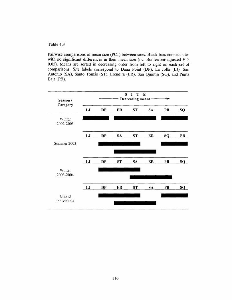
Table 4.3

Pairwise comparisons of mean size (PC1) between sites. Black bars connect siteswith no significant differences in their mean size (i.e. Bonferroni-adjusted P >0.05). Means are sorted in decreasing order from left to right on each set ofcomparisons. Site labels correspond to Dana Point (DP), La Jolla (LJ), SanAntonio (SA), Santo Tomas (ST), Erendira (ER), San Quintin (SQ), and PuntaBaja (PB).

S I T E

Season / Decreasing means -Category

LJ DP ER ST SA PB SQ

Winter2002-2003

LJ DP SA ST ER SQ PB

Summer 2003

LJ DP ST SA ER PB SQ

Winter2003-2004

LJ DP ER ST SA PB SQ

Gravidindividuals

116

Table 4.4

Mean. slope estimates from the reduced major axis regression of fertility atsize. Confidence intervals were obtained by bootstrapping. The 99.6%confidence limits (a = 0.004) were used for pairwise comparisons with agroup significance of a = 0.05.

95% Conf.

Lower

2.404

2.855

2.223

3.857

2.729

2.621

Limits

Upper

3.549

3.788

3.299

4.962

5.261

3.552

99.6% Conf. Limits

Lower Upper

2.159 3.888

2.529 4.115

1.910 3.623

3.548 5.398

1.618 7.159

2.368 3.801

117

Site

Dana Point

La Jolla

San Antonio

Santo Tom/rs

San Quintin

Punta Baja

Meanestimate

2.949

3.327

2.833

4.388

3.640

3.095

��

Table 4.5

Parameterization and asymptotic analysis of projection matrices for Punta Baja (PB), LaJolla - San Antonio (LJ-SA) and Dana Point (DP). Numbers in brackets correspond to95% confidence limits computed from bootstrap (#) and Monte Carlo (+) distributions(see Materials and Methods).

SITE

Parameter Symbol/Formula PB LJ-SA DP

Per capita fertility

Larval survival

Juvenile survival

Mar-Dec Adult survival

Dec-Mar Adult survival

Growth rate

(X)

f

a

b

d

afs + bd

2436

[2032 - 2998]#

0.015

0.135

0.154

0.535

6.5

[1.1 - 17.1]+

6625

[5844 - 7530]#

0.015

0.044

0.860

0.951

18.1

[3.5 - 46.5]+

6232

[5513 - 7025]#

0.015

0.110

0.736

0.903

17.2

[3.2 - 44.2] +

Net Reproductive Rate

(Ro)

afsl(1-bd) 7.0

[1.1 - 18.6] +

95.2

[14.8 - 255.1] +

49.0

[7.7- 130.6]+

Juvenile life expectancy

(JLE)

l+[ad/(1-bd)]

Adult life expectancy

(ALE)

1/(1-bd) 1.09

[1.06- 1.13]+

5.50

[4.93 - 6.28] +

2.97

[2.69 - 3.35]+

* : Based on a 21-day larval duration and a constant mortality rate of 0.2 d-

118

1.05

[1.03 - 1.08]+

1.47

[1.24- 1.72] +

1.24

[1.12- 1.37]+

Table 4.6

Sensitivity (S) of the population growth rate (X) and net reproductive rate (Ro) toeach of the model parameters. Parameter estimates obtained for each site (Table5) were used in the computations.

Punta Baja La Jolla Dana PointModel Sensitivity San Antonio

parameter formula S % S % S %

Population growth rate (X)f as 0.002 0.00 0.001 0.00 0.002 0.00s af 328.86 89.83 291.50 74.23 685.52 87.82a fs 36.54 9.98 99.38 25.31 93.48 11.97b d 0.54 0.15 0.95 0.24 0.90 0.12d b 0.15 0.04 0.86 0.22 0.74 0.09

Net reproductive rate (R0)f asl(l-bd) 0.002 0.00 0.004 0.00 0.005 0.00s afl(1-bd) 358.39 89.10 1600.42 67.11 2043.94 82.67a jfs(1-bd) 39.82 9.90 545.60 22.88 278.72 11.27b afsdl(1-bd)2 3.13 0.78 125.34 5.26 82.55 3.34

d afsbl(1-bd) 2 0.90 0.22 113.35 4.75 67.28 2.72

119

4.9. FIGURES

120

I.

3

I I I I I 1

118 ° 1170 1160 1150

Figure 4.1

Map of the Southern California and Baja California region where thisstudy was conducted. Labels correspond to intertidal sampling sites.

121

330

320

31

30°

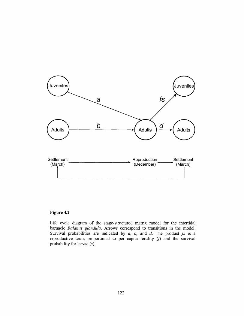
a fs

b

Settlement(March)

I

Reproduction Settlement(December) * (March)

Figure 4.2

Life cycle diagram of the stage-structured matrix model for the intertidalbarnacle Balanus glandula. Arrows correspond to transitions in the model.Survival probabilities are indicated by a, b, and d. The product fs is areproductive term, proportional to per capita fertility () and the survivalprobability for larvae (s).

122

__

L·

10

Summer Winter GravidApr 03 - Sep 03 Nov 03 - Mar 04 individuals

[lJCIJ[IJ[IjITj[lj5 10 15 20 25 5 10 15 20 25 5 10 15 20 25

m[IJ[lJ5 10 15 20 25 5 10 15 20 25 5 10 15 20 25

[IJQ;:J[lJ20 25 5 10 15 20 25 5 10 15 20 25

N=223 [IJ[]::J20 25 5N = 451

20 25N=484

20 25

N = 347

0.4

WinterNov 02 - Mar 03

0.6rnDP ........•.•.........N. =. 501

0.4 .

0.2

0.6 5 10 15 20 25LJ : N =449

III

0.2

0.6 5 10

SA0.4

0.2>.uc 5 10Q) 0.6::J ST0" 0.4Q)'-'+- 0.2Q)>

:.;::;co 5 10CD 0.6 ER0::: 0.4

0.2

5 10 15 20 25 5 10 15 20 25 5 10 15 20 25

[[J[I:J~5 10 15 20 25 5 10 15 20 25 5 10 15 20 25

[IJ[1:J[I]0.2

::~~::i°=~:15 10 15 20 25

0.6 IPB I N = 287

0.4 II

5 10 15 20 25 5 10 15 20 25 5 10 15 20 25 5 10 15 20 25

Principal Component 1 (mm)

Figure 4.3

Size distribution of Balanus glandula per season, site and reproductive state inSouthern and Baja California. Size is the first principal component of a PCAperformed on the global set of size measurements (Table 2). Vertical solid anddashed lines are the mean and median size for each distribution. Black barscorrespond to gravid individuals. Two-letter codes for site names (see Figure 1)correspond to Dana Point (DP), La Jolla (LJ), San Antonio (SA), Santo Tomas(ST), Erendira (ER), San Quintin (SQ), and Punta Baja (PB).

123

CJ DP [E[E) sa10 ~LJ -PB

o

-10Nov 2002 - Mar 2003

<6 8 10 12 14 16 18 20 22 >24

10

en 0ro::::l

~ -10~ Apr 2003 - Sep 2003

"'CQ).~"'CL-

ro"'C 10cro

+'"

C/) 0

-10

10

o

-10

<6 8 10 12 14 16 18 20 22 >24

Nov 2003 - Mar 2004

<6 8 10 12 14 16 18 20 22 >24

Gravid individuals

<8 10 12 14 16 18 20 >22

Figure 4.4

Size interval [PC1 (mm)]

Distribution of residuals from a two-way contingency table analysis of sizefrequency distributions at the extremes of the sampling region. Standardizedresiduals were computed as (Oij-Eij)/...JEij, where Oij corresponds to the frequencyof size interval j observed at site i, and Eij is the frequency expected for that siteand size interval under the hypothesis of independence.

124

WinterNov 02 - Mar 03

0.75

0.50

0.25

0.00

0.75

0.50

0.25

0.00

0):

00~0

-000

CU-U-LL

0.75

0.50

0.25

0.00

0.75

0.50

0.25

0.00

0.75

0.50

0.25

0.00

0.75

0.50

0.25

0.00

0.75

0.50

0.25

nnn

Summer WinterApr 03 - Sep 03 Nov 03 - Mar 04

Dana Point n I

i I'I ,*.'\' ,%,t-"

11-02 1-03 3-03 5-03 7-03 9-03 11-03 1-04 3-04

11-02 1-03 3-03 5-03 7-03 9-03 11-03 1-04 3-04

San Antonio

V, al S f

11-02 1-03 3-03 5-03 7-03 9-03 11-03 1-04 3-04

11-02 1-03 3-03 5-03 7-03 9-03 11-03 1-04 3-04

San Quintin

11-0 2 1-03 3-03 5-03 7-03 9 -03 11-03 1-04 3-04

11-02 1-03 3-03 5-03 7-03 9-03 11-03 1-04 3-04

25

20

15

10

25

20

15

10

25

20

15

10 O25

20

15 La)

10 EE

25 ()

20

15

10

25

20

15

10

25

20

15

11-02 1-03 3-03 5-03 7-03 9-03 11-03 1-04 3-04

Sampling date (Month-Year)

Figure 4.5

Time series of the proportion of gravid individuals at each site and sampling date.Gray lines correspond to water temperatures measured in the lower intertidal ateach site. Data for La Jolla were obtained from the Network of EnvironmentalObservations of the Coastal Ocean database (http://www.es.ucsc.edu/-neoco/).Dashed vertical lines separate the seasons used in the analysis of size data.

125

I

IV X

11-02 1-03 3-03 5-03 7-03 9-03 11-03 1-04 3-04

Erendira

A~~~~~~~"

Punta Baja I Azh ~Vt\ \,, f\> .A

V\P e. e A.

I

I,II

I . I

.i

v.vv

- V,- -,"j

r- I "lI -,Ilw ._ _i tv, _ _ _ _

5

4

3

-

1C1a)

0a

O

2

1

0 2 4 6 8 10 12 145

4

3

2

I

0 2 4 6 8 10 12 14

Age (t = months)

Figure 4.6

Growth parameters for Balanus glandula at Dana Point and Punta Baja. Linesare von Bertalanffy growth curves fitted to age-size observations. Equationswith the corresponding estimates of von Bertalanffy parameters are shown onthe lower right corner of each panel.

126

1.0

0.8~

~..cco 0.6..c ~ DPAduit0 ~ LJ-SA AdultL..C. ---*- PB AdultCO -0- DP Juvenile> 0.4 -Cl- LJ-SA Juvenile.2: -A- PB Juvenile::len

0.2

a

Figure 4.7

2 468Time (months)

10 12

Survival curves estimated for juveniles (gray lines and symbols) and adults(black lines and symbols) from Dana Point (circles), La Jolla - San Antonio(squares), and Punta Baja (triangles).

127

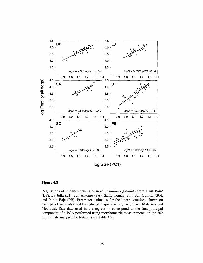
DP

o

logN = 2.95*1ogPC + 0.39

0.9 1.0 1.1 1.2 1.3 1.,

SA 0

%o

IogN = 2.83*ogPC + 0.49

0.9 1.0 1.1 1.2 1.3 1.'

SQ

0

logN = 3.64*ogPC - 0.330. 1. 1. 1.L . .

4.5

4.0

3.5

3.0

2.5

4.5

4.0

3.5

3.0

2.5

4.5

4.0

3.5

3.0

2.5

0.9 1.0 1.1 1.2 1.3 1.4

LJ o

logN = 3.33*ogPC - 0.04

0.9 1.0 1.1 1.2 1.3 1.4

ST

0 0 0

o

IogN = 4.39*/ogPC - 1.41

0.9 1.0 1.1 1.2 1.3 1.4

PBo

e o oA00o

-" e ~ p/be B

logN = 3.09*logPC + 0.07

0.9 1.0 1.1 1.2 1.3 1.4

log Size (PC1)

Figure 4.8

Regressions of fertility versus size in adult Balanus glandula from Dana Point(DP), La Jolla (), San Antonio (SA), Santo Tomas (ST), San Quintin (SQ),and Punta Baja (PB). Parameter estimates for the linear equations shown oneach panel were obtained by reduced major axis regression (see Materials andMethods). Size data used in the regression correspond to the first principalcomponent of a PCA performed using morphometric measurements on the 202individuals analyzed for fertility (see Table 4.2).

128

4.5

4.0

:3.5

:3.0

2. 5

4.5

4.0

3.5

3.0

2.5

0)0)a,

.- ,

a,U-

0)04.5

4.0

3.5

3.0

2.5

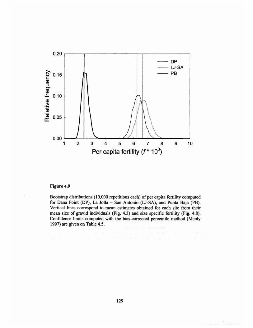
-- DP-- LJ-SA-PB

0.20

~u 0.15cQ)::JC"Q)

J= 0.10Q)>~CO

~ 0.05

0.001

Figure 4.9

2 3 4 5 6 7 8

Per capita fertility (f * 103)9 10

Bootstrap distributions (10,000 repetitions each) of per capita fertility computedfor Dana Point (DP), La Jolla - San Antonio (LJ-SA), and Punta Baja (PB).Vertical lines correspond to mean estimates obtained for each site from theirmean size of gravid individuals (Fig. 4.3) and size specific fertility (Fig. 4.8).Confidence limits' computed with the bias-corrected percentile method (Manly1997) are given on Table 4.5.

129

0.025>.g 0.020Q)5- -- DP~ 0.015 '__m""_ LJ-SA-Q) 0.010 -- PB~ bl :1.J' '~lil ,ij

-m 0.005 (" 'lr, .• , I. t!\~1~j"tO::.i 11V\~~/4. .,~

I ~t~~w0.000 .•o 10 20 30 40 50

Population growth rate (A.)

A

150

Net Reproductive Rate (Ro)

B

200

! CII

/

I!

Ir ......~ I

- ~ ..,~~-..,.""",-

0.12>. 0.10()cQ)

0.08::JC"'Q)L- 0.06-Q)> 0.04+:ico

Q) 0.020::

0.001.0 1.2 1.4 1.6 1.8 2 3 4 5 6

D

7Juvenile lifeexpectancy (years)

Figure 4.10

Adult lifeexpectancy (years)

Probability distributions of population growth rate (A), net reproductive rate (B), andjuvenile and adult lifeexpectancies (C, D) computed for Dana Point (DP), La Jolla-San Antonio (LJ-SA), and Punta Baja (PB). Vertical lines correspond to the medianof each distribution. The probability of finding a net reproductive rate smaller thanone (B) were calculated as the number of cases with Ro< 1 divided by the total numberof repetitions. Confidence limits computed with the bias-corrected percentile method(Manly 1997) are given on Table 4.5.

130

I v

2 3 4 5 6 7 8

Benthic Mortality ratio

[(1 -bd)la]

Figure 4.11

Fertility thresholds for Balanus glandula at Dana Point (DP), La Jolla - SanAntonio (LJ-SA), and Punta Baja (PB). Contours correspond to theminimum per capita fertility required to attain population persistence giventhe benthic mortality ratio and larval survival shown on the x and y axes.Gray arrows originate from the x-axis value computed for each site (seeTable 4.5), intersect their corresponding contour of mean per capita fertility,and point to the minimum larval survival (y-axis) that would allow them topersist ( > 1).

131

10-2

co

-

2 10-3V)

-J

1 n-4

0.01DP

0.1DP

0.008 0.08

0.0

-1.0

-0.5

1.$

1.5

0.02

0.02

LJ-SA

1

1

0.01

0.01

0.01 0.02

Lower limit (a)

0.1

0.1

0.04

0.06

0.08

0.06

0.04

0.04

0.06

L-a>a.a.~ 0.08

-co---co>.~:Jen

~ca>>:J......

'+-o

1

0.5

0.002

0.002

LJ-SA

0.001

0.001

0.001 0.002

Lower limit (5)

0.01

0.01

0.008

0.006

0.004

0.004

0.006

0.008

0.004

0.006

EL-a>a.a.

~

'+-o

-en---

Figure 4.12

Stochastic growth rate log As computed for Dana Point (DP), La Jolla - SanAntonio (LJ-SA) and Punta Baja (PB) under different regImes ofenvironmental stochasticity. Axes correspond to lower and upper limits of theuniform probability distributions used to simulate interannual fluctuations inlarval survival (left panels) and juvenile survival (right panels). The thickcontour indicates combinations of parameters for which log As = O.

132

0.01 T 0.1 I

DP DP0.008 0.08

0.006 0.06

0.004 ..- 0.04..- roen , -'-'

ro 0.001 0.002 ro 0.01 0.020.01 > 0.1> .~ T

.~ LJ-SA LJ-SA~~ 0.008 en 0.08en0>

ro c:~ 0.006 0> 0.06ro >'+-

~0 0.004 '+- 0.04:t: 0E , . :t:

0.001 0.002 E 0.01 0.02t-O> 0.01 t- 0.1 1.0c.. 0>c.. c..

::::> 0.008 c.. 0.08 0.8::::>

0.6

0.0060.4

0.004 0.04 0.2

0.00.001 0.002 0.01 0.02

Lower limit (5) Lower limit (a)

Figure 4.13

Quasi-extinction probabilities Pq( 8=0.1) computed for Dana Point (DP), LaJolla - San Antonio (LJ-SA) and Punta Baja (PB) under different regimes ofenvironmental stochasticity. Axes correspond to lower and upper limits of theuniform probability distributions used to simulate interannual fluctuations inlarval survival (left panels) and juvenile survival (right panels). Regions of theparameter space for which P q(8)= 1 are shown in black.

133

5. CHAPTER 5

GENERAL CONCLUSIONS

The results of this dissertation emphasize the importance of a small-scale, high-

frequency approach to study nearshore phenomena, especially in relation with the

dispersal of invertebrate larvae. The importance of choosing right temporal and spatial

scales cannot be overstated. In recent years it has become clear that often there is not a

unique right scale of observation, and that small-scale physical and biological processes

in the nearshore may be modulated by large-scale phenomena (e.g. Pineda and L6pez

2002). The question of whether a population functions as an open or closed system is also

dependent on the spatial and temporal scales of observation. For example, populations

separated by 100 kilometers may not exchange individuals at demographically relevant

temporal scales (i.e. years), but still be genetically connected by larval dispersal

occurring at scales of decades to thousands of years.

Observed patterns of nearshore larval distribution (Chapter 2) agree with recent

suggestions that long distance dispersal of larvae in the nearshore may not be as

pervasive as traditionally thought (e.g. Jones et al. 1999; Swearer et al. 1999). Consistent

small-scale (0.1-1 km) patterns in the stage-specific horizontal distribution of Balanus

glandula and Chthamalus spp. larvae suggest that larvae may be retained within short

distances to shore over the duration of their planktonic life. Horizontal segregation of

nauplii and cyprids in both species, with the latter being substantially more abundant at

the inshore station, suggests that ontogenetic changes in behavior may impact the

expected horizontal distribution and dispersal distances for the larvae of coastal

invertebrates.

The mortality estimates obtained for barnacle nauplii in nearshore waters

fluctuated around 20-40% per day (Chapter 2). These are substantially higher than a 5%

d-' previously assumed for B. glandula and Chthamalus spp. (Connolly and Roughgarden

1998, p. 323), but within the range of mortality estimates found in the literature for other

134

benthic invertebrate larvae (Rumrill 1990; Morgan 1995; Lamare and Barker 1999).

Although more studies are needed to verify these estimates, a four- to six-fold increase in

mortality should reduce the number of larvae that complete their planktonic development

and, by extension, shorten mean travel distances and scales of connectivity among

populations. The shape of a dispersal kernel - the distribution of dispersal distances from

a point source - depends on larval duration relative to local hydrodynamics (e.g. Siegel et

al. 2003). For example, dispersal kernels with long tails may be observed when strong

residual currents disperse larvae with a short development time. Increasing larval

mortality could truncate the tails of such distributions and cause a reduction in the mean

distance of dispersal. A recent modeling study (Ellien et al. 2004) has shown that losses

due to mortality can be more important than those due to hydrodynamics when larval

duration is short relative to the intensity of residual currents. Increasing mortality rates

from 5% to 9% d greatly reduced effective dispersal distances for larvae of the

polychaete Pectinaria koreni. Thus, depending on the species and local hydrodynamics,

changes in larval mortality rates may shift our view as to whether a population is open or

closed.

Results presented in Chapter 2 suggest that coastal invertebrate populations

separated by distances as short as tens of kilometers might be demographically

disconnected. Such disconnection would reduce the spatial scales of coherence in

population dynamics, affect the robustness of local populations to environmental

perturbations, and ultimately impact the persistence of a species within its geographic

limits of distribution.

The observation of distinct and consistent patterns of vertical distribution in the

nauplii and cyprids of two barnacle species at a nearshore site (Chapter 3) suggested that

horizontal segregation of larval stages might result from the interaction of ontogenetic

changes in behavior and vertical shear of horizontal currents in the nearshore. The

absence of Chthamalus spp. cyprids from the sampling station, located ca. 2 km offshore

and approximately 10 km NW of La Jolla - where high concentrations of Chthamalus

135

spp. cyprids have been observed (Pineda 1999 and Chapter 2) - is intriguing because

Chthamalus spp. nauplii were numerically dominant and present at all stages of

development. This absence did not allow testing whether Chthamalus spp. nauplii and

cyprids occur at different depths. Thus, a connection between the horizontal segregation

observed between nauplii and cyprids of Chthamalus spp. at La Jolla and differences in

the vertical distribution of these stages must be tested. More field observations are needed

in a future attempt to verify the biological-physical mechanisms that generate the

observed patterns of larval distribution. Future efforts to model the relationship between

local population dynamics and hydrodynamics must shift from an emphasis on mesoscale

processes to a better description of nearshore processes and spatial changes in dispersal

and self-recruitment. Also, the variability in nearshore hydrodynamics must be better

resolved, perhaps with high-frequency observations of horizontal flows collected

simultaneously at several points over a larger area. Estimates of dispersal trajectories and

distances would benefit from an assessment of the spatial variability in mean horizontal

flows in the nearshore.

Finally, the analysis of adult demography over scales of hundreds of kilometers

yielded valuable insights on the interaction between spatial changes in vital rates,

robustness to environmental stochasticity, susceptibility to local extinction, and

geographic ranges of distribution. The combination of extensive field observations on

population structure, growth, and reproductive rates with a simple mathematical model

proved to be a fruitful approach to the assessment of factors that might determine the

geographic distribution of coastal benthic populations. Future studies should include the

actual geographic limit of distribution of this species, and monitor the regional variability

in recruitment and larval supply, as well as the variability in physical-chemical factors

that are likely to affect rates of growth and reproduction and ultimately generate spatial

patterns in population demography.

136

REFERENCES




Jones GP, Milicich MJ, Emslie MJ, Lunow C (1999) Self-recruitment in a coral reef fishpopulation. Nature 402: 802-804



Pineda J, Lpez M (2002) Temperature, stratification and barnacle larval settlement in twoCalifornian sites. Continental Shelf Research 22: 1183-1198


Siegel DA, Kinlan BP, Gaylord B, Gaines SD (2003) Lagrangian descriptions of marine larvaldispersion. Marine Ecology Progress Series 260: 83-96

Swearer SE, Caselle JE, Lea DW, Warner RR (1999) Larval retention and recruitment in anisland population of a coral-reef fish. Nature 402: 799-802

137

6. APPENDIX A

High-frequency observations of wind-forced onshore transportat a coastal site in Baja California.

Tapia FJ, Pineda J, Ocampo-Torres FJ, Fuchs HL, Parnell PE, Montero P, Ramos S

Continental Shelf Research 24: 1573-1585. 2004.

Reprinted with permission of Elsevier Ltd.

138

Available online at www.sciencedirect.com

SCIENCE CdDIRECT CONTINENTAL SHELFRESEARCH

ELSEVIER Continental Shelf Research 24 (2004) 1573-1585www.elsevier.com/locate/csr

High-frequency observations of wind-forced onshore transportat a coastal site in Baja California

Fabian J. Tapiaa '*, Jesis Pinedaa, Francisco J. Ocampo-Torresb, Heidi L. Fuchsa,P. Edward Parnellc , Paulina Monterod, Sergio Ramosb

aBiology Department MS-34, Woods Hole Oceanographic Institution, Woods Hole, MA 02543, USAb Departamento de Oceanografia Fisica, Centro de Investigaci6n Cientifica y de Educaci6n Superior de Ensenada, Km 107 Carretera

Tijuana-Ensenada, Ensenada, BC 22860, MexicoCScripps Institution of Oceanography, Integrative Oceanography Division, 9500 Gilman Drive 0227, La Jolla, CA 92093-0227, USA

d Centro de Ciencias y Ecologia Aplicada, Universidad del Mar, Carmen 446 - Cerro Placeres, Valparaiso, Chile

Received 26 August 2003; received in revised form 27 February 2004; accepted 26 March 2004

Available online 20 July 2004

Abstract

We investigated the effect of the daily sea breeze on the surface flow at Bahia Salsipuedes, Baja California, Mexico.DIrifter-tracking experiments were conducted over a 2-week period in July, 1999. Surface drifters were deployed dailyand their trajectories tracked from a small boat for 3-7 h. Wind speed and direction, as well as the vertical distributionof temperature and current velocities were measured throughout the observation period. Our results indicate that strongwinds associated with the daily sea breeze at the study area can produce onshore surface currents with velocities of up to10 cm s-' (net transport of up to 2 km in a diurnal cycle). There was a hyperbolic relationship between onshore windstress and net onshore transport of the drifters. A decrease in stratification and more consistent pattern of onshoretransport were associated with sustained winds > 6 m s - towards the end of the study. Progressive vector diagramscomputed from near-surface currents failed to predict the trajectory of drifters, especially on days where wind forcingwas more consistent in terms of direction and magnitude. We discuss the implications of these results regarding thecollection of settlement data and their interpretation in terms of larval supply to coastal populations.i{~ 2004 Elsevier Ltd. All rights reserved.

Keywords: Sea breeze; Onshore transport; Drifters; Neuston; Baja California

1. Introduction

The dynamics of coastal populations is highlydependent on the mechanisms and processesaffecting the spatial distribution and the fate of

*Corresponding author.E-mail address. [email protected] (F.J. Tapia).

larvae prior to settlement. Research efforts duringthe past decades have been focused on the physicalprocesses that are likely to affect the distributionof larvae relative to adult populations (e.g.Johnson, 1939; Scheltema, 1968; Butman, 1987;Pineda, 1994b; Epifanio and Garvine, 2001), andon the importance of substrate availability (e.g.Bertness et al., 1992; Pineda, 1994a). Such a

0278-4343/$- see front matter © 2004 Elsevier Ltd. All rights reserved.doi: 10. 1016/j.csr.2004.0.3.013

139

F.J. Tapia et al. / Continental Shelf Research 24 (2004) 1573-1585

'supply side' approach (see Underwood and Fair-weather, 1989) has yielded valuable insights on therelevance of physical processes as predictors of thelocal and regional dynamics of adult populations.I[n order to characterize the variability of larvalsupply to coastal populations, however, it isnecessary to assess patterns of larval distributionat spatial and temporal scales that are relevant to aspecies' life cycle and ecology. Plankton patchinessand logistic constraints preclude the use of suchsampling strategy in most cases, thus forcing theuse of proxies for larval supply that are morefeasible to monitor over extended periods of time(e.g. settlement-see Pineda, 2000).

Settlement has been the proxy of choice in anumber of studies focused on the supply of larvaeto adult populations of coastal invertebrates, suchas crabs (Wing et al., 1995b; Reyns and Sponaugle,]999), sea urchins (Ebert et al., 1994; Wing et al.,1995a), and barnacles (Gaines et al., 1985; Pineda,1994a). Artificial and/or natural surfaces areprovided for the larvae to settle on, and monitoredat intervals of days to weeks. Settlement time seriesdata are then analyzed in conjunction withenvironmental data series to identify temporalcorrelations between larval supply and physicalvariability (e.g. Farrel et al., 1991; Wing et al.,1995a; Pineda and L6pez, 2002). A number ofpublished studies have documented correlationsbetween larval settlement and physical processesoccurring at a range of temporal scales: from intra-seasonal changes in wind forcing (Bertness et al.,1996), upwelling intensity (Wing et al., 1995a), andthe stratification of the water column (Pineda andL6pez, 2002), to interannual changes in riverdischarge (Gaines and Bertness, 1992). The im-portance of higher-frequency physical variabilityfor settlement, however, has not been extensivelystudied and cannot be resolved at the samplingfrequencies typically used in settlement surveys.Therefore, inferences made so far about larvaltransport are probably biased towards lower-fi-equency mechanisms if based only on settlementdata (Pineda, 2000).

Few high-frequency mechanisms with a poten-tial effect on the onshore transport of larvae havebeen documented so far. Internal tidal bores, aseasonal and somewhat predictable phenomenon

that occurs in coastal environments at scales ofhours to days, are an example of high-frequencyforcing likely to affect the onshore transport ofboth planktonic and neustonic larvae (Pineda,1994b, 1999).

The diurnal sea breeze, which is also seasonaland locally predictable in its occurrence, representsanother highly episodic phenomenon that couldpotentially affect larval settlement (Kaplan et al.,2003; but see Epifanio and Garvine, 2001, p. 54).The sea breeze is characterized by a daily regime ofvariability, generated by oscillations in the land-sea temperature gradient, which in some regionscan explain fluctuations of up to 7ms - inonshore wind speed (Simpson, 1994). Such dailysurges in onshore winds may affect the cross-shoredistribution of material suspended in the uppercentimeters of the water column (i.e. neuston),including the larvae of a number of coastalinvertebrates. Thus, by modulating the onshoreflow of surface waters, the sea breeze could havean effect on the timing and variability of recruit-ment in coastal populations with neustonic larvae.

In this contribution we investigate the effect ofthe sea breeze on cross-shore surface currents bymeans of drifter-tracking experiments, which wereconducted over a period of 2 weeks at BahiaSalsipuedes in northern Baja California. Ourresults demonstrate the potential for the diurnalsea breeze to substantially affect onshore transportof neustonic material. We discuss the implicationsof these results regarding the collection of settle-ment data and their interpretation in terms oflarval supply to coastal populations.

2. Materials and methods

The experiments were conducted on 13-22 July,1999 (Table 1), at Bahia Salsipuedes (31° 56' N,116° 46' W) in northern Baja California (Fig. 1).Every morning at about 7:30-9:30 AM (PDT), wedeployed a set of 5-6 drifters, which were circularpieces of soft and flexible, Scootguard TM non-slipsurface (30 cm in diameter, 1 mm thickness) withsix small lead "split-shot" lead weights (2.5 g each)attached to the edges (Fig. 2). When deployed, thedrifters remained at the air-sea interface, with less

140

1574

F.J. Tapia et al. Continental Shelf Research 24 (2004) 1573-1585

- ' 0 o= ( CO-vo666o

o oo o , 0 _. _ 00 N '.--- ClO~l--

n - o n - i 0

00 o' ON ON n-GVl 00-

v o o o oe o oON - '. -ON ON -

O N o 0-0 0 0 ON 00

Cl 0 0 In 0 -

_ o ci _oo

-o000 0-0

_oo oo _ o _-

N 00 ON N _ …Cl__ _

Lf° 00 /m 00moo o ~ 0 - 'd .. -

0 0 o

n- 0 / (

0 0 o )

O O ON ON ON ON

-~; 2~ 73 - - -

m '.<0 ON 0__ _ I IIM n \Q Iraq 1

-,ClCl~

33°00'

32040'

32020'

32°00'

O n

.

a ,v

)000

t;,0'

.a

>

O

C~ n0L -

_00

C);

C,Co O;Y

- 3: -o

o 2-00000

Oo3

c o O

a e c O,0~

._ o b o

cc o 02- O x

31 °40'

117020'

11 7o00'

116040'

Fig. 1. Geographic location of Bahia Salsipuedes. The starindicates the study site.

than 50% of their surface area exposed to directwind forcing (Fig. 2). Drifters were deployed at theonset of the sea breeze events (i.e. a suddenincrease in onshore winds that occurred at 8:00-12:00 each day), at approximately the samelocation every day (31° 56.31' N; 116° 46.72' W),and tracked from a small motor boat for 3-7h,depending on the weather conditions and on theboat's proximity to the surf zone. The location ofeach drifter was recorded about every 20 min usinga differential GPS.

We assumed that the drifters were tracking themotion of the uppermost layers of the watercolumn, rather than their own response to windforcing. Our assumption was based on the drifterdesign (Fig. 2), and on the statistical similaritybetween the drifter paths and those followedby pieces of kelp that were found at the air-seainterface, collected in situ, and deployed

141

1575

,'&

0',

0'

in

0n

0

-o

00p0

0

-o00

n0

S_

zv

o_

E

rb_

9EtZ

a

E

E

V:

EZ

0

0n.0

E0

-0

-0

0

00.

7;0

03.5

O0

0at-Z,

.qn

.e

th0U

,.an

-

vl

n.a

0

0

g

o .0'00

o'300000

'00

>

Si00C

.-,

_

0'00.0

03

0

0

0.0

0u

0

0

s0S0n0,

0d

1576 Fl. Tapia et al. / Continental Shelf Research 24 (2004) 1573-1585

Fig. 2. Side view picture (A). and top and side view schematics (B and C) of the drifters used in this study. The arrows (and blackcircles in Band C) indicate the position of the six small lead weights attached to the drifters edge. The edge areas (dark shading in Band C) correspond to the fraction of the drifter's surface that remained underwater. The central area (light shade in B and C)corresponds to the portion that was exposed to the wind during a deployment.

concurrently with the drifters (Solow, WHOI,• pers. comm.).

Throughout the observation period we moni-tored the thermal structure of the water columnusing a string of Onset StowAway XTI loggers(response time < 15s), programmed with a sam-pling interval of 40 s and located at 2, 5, 8, and 11meters above the bottom (mab), plus one logger atthe surface. We also monitored the verticalstructure of nearshore currents with a bottom-mounted, upward looking 1200kHz Dopplercurrent meter (RD Instruments, San Diego, CA),which measured at intervals of 40s (100 pings perensemble) and in bins of 0.4 m within a depthrange of 0.95-14.55mab. Both the temperaturemooring and the current meter were located at adepth of 16m (31° 56.28' N; 116° 45.68' W).Average wind velocity and direction were recordedover 5min intervals using a CMB3280 Aanderaa

142

Coastal Monitoring Buoy, anchored at a nearbylocation (31° 55.28' N; 116° 45.39' W, ca. 2kmsouth of the current meter mooring). Prior to theanalysis, wind directions were rotated and alignedto the average shoreline orientation (355°), andthen decomposed into alongshore and cross-shorecomponents.

We studied the effect of wind forcing on thewater column using two different approaches.First, on a time-domain approach, we studied theeffect of wind forcing on stratification by comput-ing wind stress at the surface as

I'toI = pu.2, (1)

where p is air density and u. is the frictionvelocity, which was computed from wind SPeeddata as in Large et al. (1995, Eq. 8). We calculatedstratification as the square of the Brunt-ViisiIifrequency (}12) for each one of the four pairs of

FJ. Tapia et al. / Continental Shelf Research 24 (2004) 1573-1585

temperature series (i.e. 2-5mab, 5-8mab,11 mab, and 11 mab -surface) as

_N2 _ g apPo oz'

where g is gravity (9.8ms-2), po is the meandensity of the water column, and z is depth. Wethen obtained depth-averaged values for N 2 byvertically averaging the four series mentionedabove. The temperature and wind time series werelow-pass filtered prior to the computations (cutofffrequency of 6 cycles h-1), and a constant salinityvalue of 34psu was assumed. Second, on afrequency-domain approach, we performedspectral analyses on the time series for wind(-- 5,000 observations) and temperature(- 42,000 observations) collected at the study sitebetween 7-23 July and 4-23 July, respectively.Raw data were linearly detrended prior to thecomputation of an average Welch periodogram.The wind and temperature series were divided intonon-overlapping segments of 210 (3.6d) and 213points (3.8 d), respectively.

To understand the contribution of wind toonshore transport:, we analyzed the effect of windstress on the motion and trajectory of the drifters.We computed net onshore displacements for eachdrifter/day, and then performed a nonlinearregression of net onshore displacement versus theonshore wind stress integrated over the duration ofeach deployment. We also analyzed changes in thecorrelation between drifter trajectories and winddirection as a function of wind speed for eachdeployment. For n average drifter positionsrecorded during a deployment, we computed n-1velocity vectors. Velocity vectors were decom-posed into cross-shore and alongshore compo-nents of the drifter trajectories, which were linearlyregressed against the respective components ofwind forcing. We chose a 10 min lag between windmeasurements and the drifter observationsto which they were paired (i.e. midpoint betweendrifter observations). We tested whetherdrifter trajectories can be predicted from current-meter data by comparing the observed trajectorieswith progressive vector diagrams (PVDs) fromour measurements of horizontal velocities near thesurface. The predicted (x,y) positions were

8- computed as

n n

(2) = t (ti),y(t = At v (ti),(2) i=1 i=1

(3)

where u(t) and v(t) are the east and north currentspeeds measured by the current meter at time t,and At is the sampling interval (Emery andThomson, 1998, p. 165). Due to large errorsintroduced by tidal fluctuations in water depth,surface wave action, and side lobbing, datacollected from the surface bins by the Dopplercurrent meter had to be discarded. Thus, ouruppermost bin with reliable data was located at13 mab, on average 2 m below the surface.

Finally, we observed settlement of invertebratelarvae on the drifters. Although these observationswere not quantitative, we use the taxonomiccomposition of the settlers and the time scalesover which settlement was observed to conjectureon the potential effects of sea breeze events on thedistribution and onshore transport of neustoniclarvae.

3. Results

We completed 7 days of drifter observationsduring which a total of 36 drifters were deployedand tracked for an average of 5 h (Table 1). Windspeeds measured during the study were highlyvariable, with most of the variability explained bychanges in the cross-shore component (Figs. 3aand 4a). Onshore winds dominated during thesecond half of the study, with daily oscillations ofup to 8 m s - which extended for about 8 h (Fig.3a). The dominance of a diurnal frequency in thevariability of cross-shore winds was confirmed bythe computed power spectra (Fig. 4a). Coincidentwith these daily surges in onshore winds, weobserved short-term increases in the temperatureof surface waters (Fig. 3b). Towards the end of theobservation period, these rapid increases in tem-perature could be detected throughout the watercolumn (Fig. 3b), which is consistent with theobserved decrease in the depth-averaged stratifica-tion (Fig. 3c). A diurnal frequency dominated thevariability of temperature between the surface and

143

1577

1578 F.I. Tapia et al.I Continental Shelf Research 24 (2004) 1573-1585

8 (A) - cross-shore wind-'":'111 - alongshore wind

5 4

I~ 0c~

-413 ]4 IS 16 17 18 19 20 21 22

22

G 20~~ 18

!168-

~ 14

14 15 16 17 18 19 20 21 22

2.0 3

2 e-r 1.5 "-'III i~.e 1.0 0 ]~

Ma;

;Z 0.5 ~i=

14 IS 16 17 18 19 20 21 22

Date (JuJy ] 999)

Fig. 3. Wind speed (A), water temperature (B) and mean stratificationof the water column (C)during the drifterdeployments at BahiaSalsipuedes in July 1999. Tidal heights predicted for the port of Ensenada, Baja California, are also shown in C (gray line).

11 mab (Fig. 4b-c), and could be detected at depthto 2 mab (Fig. 4f). A second peak in the powerspectra was found at the semi-diurnal frequency(Le. about 2 cycles day-I, Fig. 4c-f), which domi-nated the variability of temperature near thebottom, but nonetheless could be detected up to11 mab (Fig. 4c-f). Large fluctuations in stratifica-tion observed at the beginning of our study (Fig.,3c) appeared to be driven by the semi-diurnalinternal tides rather than wind forcing.

Persistent wind forcing towards the end of thestudy caused a net onshore transport of thedrifters (Fig. 5a), which increased as a functionof wind stress integrated over the duration of thedeployments (Fig. 5b). Drifters were transportedonshore at speeds of up to 10 em s- I. The intensity

of wind forcing during the experiments determinedthe degree of correlation between drifterpaths andwind direction (Fig. 6). A better alignment ofdrifterpaths and wind on the cross-shore directionisconsistent with the higher wind speeds recordedalong this axis (Fig. 3a). The response of surfacewaters (and therefore drifter paths) to the tempor-al variability in wind forcing can be clearly seen inFig. 7, in which the wind vectors have beensuperimposed on the drifter trajectoriesfor July 20and July 22 ..

The temporal variability in the horizontalvelocities of near-surface currents (Fig. 8b) wasconsistent with the timing and intensity of windforcing (Fig. 8a). Near-surface currents showed atendency to be decoupled from currents measured

144


deeper in the water column (Fig. 8b). PVDscomputed from horizontal velocities measured at13mab (Fig. 9) showed a poor performance aspredictors of drifter trajectories. The observedtrajectories seemed to be the result of an interac-tion between wind and tidal forcing, whichexplained most of the variability in the PVDs(Fig. 9). The discrepancy between predicted andobserved drifter displacement varied as a functionof the magnitude and variability of wind forcingduring the deployments. The largest discrepancieswere observed on days with strong and persistentwinds, whereas smaller values tended to occur ondays with more variable wind forcing, both interms of speed and direction (Table 1). A closerinspection of Fig. 9 and the wind data series (Fig.3a) suggests that not only the magnitude andvariability of wind forcing, but also its timingrelative to the tidal cycle (Fig. 3c) ultimatelydetermined drifter trajectories.

We incidentally observed settlement of neus-tonic zooplankton on the drifters. The mostabundant taxa corresponded to flatworms (0.5-52.8 indivh- 1), brachyuran and anomuran mega-lopae (0.4-3.0 indiv h-), isopods (0.2-2.0 in-divh-1), amphipods (0.2-1.7indivh-'), andlepadid barnacle larvae (0.4-1.0indiv h 1). Thehighest settlement rates for these taxa wereobserved during the last four days of the study(19-22 July), which exhibited the strongest on-shore winds (Fig. 3a).

4. Discussion

102

10"

0 2 4 6 8 10 12

Frequency (cycles per day)

Fig. 4. Power spectra computed for the wind (A) andtemperature time series (B-F) recorded at Bahia Salsipuedesin July 1999. Bars on the right-hand side of each panelcorrespond to 95% confidence intervals. The dashed linesindicate diurnal variability; mab: meters above the bottom.

Our results indicate that neustonic material hasthe potential to be transported onshore by thedaily sea breeze at Bahia Salsipuedes (Fig. 5). Acausal relationship is supported by the observeddrifter trajectories (Figs. 5 and 6) and theirresponse to short-term fluctuations in wind direc-tion (Fig. 7), as well as by the discrepanciesbetween actual drifter trajectories and thosepredicted by progressive vector diagrams (PVDs)computed from the horizontal velocities of near-surface currents (Fig. 9). These results are relevantbecause currents in the coastal ocean are generallymore energetic on the alongshore axis (Winant,

145

I CP

E(St-

C;

102

10'

10"

1Y0-

1 '1 O210z

1 O"

10 20

UC

I )2

10''

1579


31 57'

31 56'

(A) I 11647' 1 16°46'

2.0

0Ezin.4'I

1.5

1.0

0.5

0.0

-0.5

(B) Total onshore wind stress (N m' 2)

Fig. 5. (A) Average paths followed by drifters on different days; the numbers are the July date corresponding to each trajectory,whereas the arrow indicates the point of deployment. (B) Net onshore displacement of drifters as a function of onshore wind stressintegrated over the duration of each deployment. The large open circle in (A) indicates the position of the Doppler current meter andtemperature moorings.

0.2

. 0 Of 1

(A)

2

-o'UU

I-W

-C(B)

(B)

EU-oU

5,r

U

3 4

Average wind speed (m s' l)

30

20

10

0

-10

30

20

10

0

-10

-4 -2 0 2 4 6

(C) Wind speed (m s'1)

Fig. 6. (A) Changes in the correlation between average drifter and wind direction as a function of the average wind speed during eachdeployment. Linear regression analyses were performed separately for alongshore (closed symbols) and cross-shore (open symbols)components of wind and drifter direction, and for each day with drifter deployments (July 13, 15, 16, 19, 20, 21, 22). (B and C)Example of how the values indicated with squares (in A) were obtained for July 21; W is average wind speed for the deployment.

1980), with few mechanisms acting on the cross-shore dimension with sufficient energy to generateonshore transport at the temporal and spatialscales observed here (e.g. internal tidal bores-seePineda, 1994b).

The surface drifters used in this study are aneffective means to investigate the short-term

response of the surface layer (i.e. first fewcentimeters) to local wind forcing. Water move-ment at this biologically relevant layer-where asuite of particles including neustonic plankton canbe accumulated (see LeFevre, 1986)-is leftunresolved by most instruments, including acous-tic current meters and other drifter designs that

146

1.o R = 0.653W= 2.92 m s' _. ..~

0.8

0.6

0.4

0-1

'RI*0

U

* cross-shoreo alongshore

0

~o~~ ~0

00 0

W = 0.91 m s'

a 00

1580

5 �Er:�

A A

F.l. Tapia et al. / Continental Shelf Research 24 (2004) 1573-1585 1581

lo.5km

31"57'

S m 1('-116"46'

Fig. 7. Example of drifter trajectories in relation to thetemporal variability of wind forcing on July 20 and July 22,1999. Open circles correspond to drifter positions, whereas thethin lines are a vectorial representation of the average windspeed and direction measured during the interval prior to eachdrifter observation. Closed circles indicate the point of drifterdeployment.

can go deeper into the water column and/or bedirectly affected by wind forcing. One disadvan-tage of our approach, however, is the need tovisually and continuously track the drifters from aboat. Currently available technology should makeit feasible to address such problem by attaching asmall positioning/tracking device to each surfacedrifter, so that their position can be recordedwithout compromising their ability to track thesurface layer.

The discrepancies we observed between actualdrifter paths and those predicted by PVDs shouldbe taken into account before any conclusionsabout larval transport are drawn from Euleriancurrent data. Our data suggest that the observeddiscrepancies between the PVDs and driftertrajectories may be due to an interaction betweenthe magnitude and variability of wind forcing andtidal currents. However, one source of error thatcould explain part of the discrepancy is the varyingdistance between our top bin with reliable currentmeter data (13mab) and the surface of the watercolumn. Given that our main objective was tostudy the effect of the daily sea breeze on theonshore transport of surface currents, the experi-

147

ments were conducted at roughly the same time ofthe day. This means that on some days theobservations took place at high tide (July 13, 15),at low tide (July 20, 21), or during the transitionfrom low to high (July 16, 19). Unfortunately, apressure sensor was not available and therefore welack accurate data on the sea level at our study siteduring drifter deployments. Tidal predictions forEnsenada (ca. 20 km south of Bahia Salsipuedes),indicate sea-level fluctuations of up to 2.4m duringthe course of the deployments, which would haveincreased the distance from the top ADCP bin tothe surface from 2 to 4.4 m. Such a change couldcertainly increase the discrepancy between thetrajectories predicted from a PVD and thoseactually followed by the drifters, especially on ahighly stratified water column (Figs. 8 and 9).

Our observations were focused on drifter pathsand on the physical variables associated with thewater column's response to wind forcing, and didnot include an assessment of the spatial distribu-tion and/or settlement of neustonic larvae in thearea. Therefore, a connection between this trans-port mechanism and the recruitment of coastalspecies with neustonic larvae is yet to be demon-strated. If there is a connection, however, andlarvae of coastal invertebrates are in fact trans-ported onshore by the sea breeze, it would bepossible to predict the spatial-temporal distribu-tion of larval settlement in some populations basedon local wind patterns and shore orientation. Anassessment of the effect of sea breeze events on thespatial distribution and timing of settlement is thuswarranted.

A follow up of our study should include asurvey of neustonic meroplankton in the area withconcurrent drifter deployments and settlementobservations. Given the diurnal frequency of seabreeze events, any attempt to link such events tolocal settlement patterns will have to considerobservations taken at shorter intervals than it iscustomary (Le. at least semi-diurnally). Lack oftemporal resolution could result in a misinterpre-tation of the mechanisms that determine thetiming and intensity of settlement in populationswith neustonic larvae.

Wind-driven onshore transport of neustonicinvertebrates has been suggested as a cause of

1582 F.J. Tapia et al. I Continental Shelf Research 24 (2004) 1573-1585

1Vl

"'0C

~(A)

, ... i i

g 13 ...':dl....t-'/$.II/"""""--~/t1m~!/I't/l\i\"\\IlWil\~\~III UhllJ~ ... ,(..i/lIlUJ$/lt1~".~~'.,-/\""i"I"T~\W!"("~ 8 -"7' ""Wf\\II11III1I/!lh, 'tn1f./AlniII Iitlll/li,~ ...."'1'-4l/mhilJJt_"'/IJ \IV~ ;; I ;' I I~ ; ._......:--~\ll\l\llIl*\\\\\,J1I""\\l~\I~"l-"'\I~\lII,,~~bl> '!' 1 !' I I ;

"OJ . I i I ; I , Ii:::r: 2 " •.... ,,'~,~:.~,,~\\IAII~~\II.\I"+~.J~,~"~,-+-,,/....L..~

I~ i 'j i: I! :

(8) o 2 4 6 8 to 12 14 16 18 20 22 24

(C)

o 2 4 6 8 10 12 14

Time (h)16 18 20 22 24

Fig. 8. Example of the effect of wind forcing (A) on the circulation (B) and thermal structure (C) of the water column in BahiaSalsipuedes on July 19, 1999. The shaded area in A corresponds to the duration of the drifter deployment. The stickplots in B show thevariability in direction and magnitude (see scale bar at lower left comer) of horizontal currents at the same depths at which temperaturewas recorded. The vectors indicate the direction currents are flowing towards (up is north).

the spatial patterns observed in barnacle settle-ment (Kendall et aI., 1982; Bertness et aI., 1996),and in the spatial distribution of neustonic isopods(Locke and Corey, 1989), post-larval crabs

148

(Shanks, 1986; Eggleston et aI., 1998) and lobstermegalopae (Hudon and Fradette, 1993). If suchwind events are persistent and consistent enoughover demographically relevant time scales, they

F.J. Tapia et al. I Continental Shelf Research 24 (2004) 1573-1585 1583

2.45 ms'l

125.4~

3.13ms"92.6"

Fig. 9. Comparison of observed versus predicted trajectories ofdrifters at Bahia Salsipuedes, Baja California, in July 1999.Open circles indicate the observed drifter trajectories. Predictedtrajectories (closed circles) correspond to a PVD, computedfrom horizontal current velocity data collected at 13mab. Thegray line is a PVD computed using only those frequencies of thecurrent data that correspond to the barotropic tide. The insetsshow average wind speed and direction (0° = N) over theduration of each deployment. The scale bar at the lower leftcorner of each panel corresponds to a distance of 1km.

could have an impact on the connectivity and/ordemographic isolation among adjacent coastalpopulations. At sea level, the sea breeze is highlyasymmetrical, with a marked predominance ofonshore over offshore winds (Fig. 3a). Hence, thesea breeze can have a cumulative effect (i.e. overmore than one diurnal cycle) on the cross-shoredistribution of neustonic larvae. A persistent seabreeze-mediated onshore transport could allowneustonic larvae to either remain close to the

149

shoreline throughout their development, or torepeatedly reach it, hence increasing their prob-ability of being close to adult habitats whencompetent to settle. Thus, the sea breeze couldconstitute an effective transport and/or retentionmechanism in areas with a configuration ofshoreline and wind forcing such as that observedat Bahia Salsipuedes.

The effect of wind forcing on larval retentionand demographic isolation could be intensified iflarval behavior is invoked, such as the reversevertical migration hypothesized by Poulin et aI.(2002) for neustonic larvae of the subtidal gastro-pod Concholepas concholepas. Even under condi-tions of strong upwelling (i.e. strong offshoreEkman transport), the larvae of C. concholepas areconsistently found between the shoreline and theupwelling front. Such observation, along with dataon the temporal variability of larval distribution,suggests that a reverse vertical migration behaviormight be allowing these larvae to stay close tosubtidal habitats (see Fig. 6 in Poulin et aI., 2002).The interaction between physical processes like thesea breeze and behavioral mechanisms such asvertical migrations could increase the local reten-tion of neustonic larvae and the demographicisolation of adjacent populations.

Finally, these results might also be relevant forunderstanding the onshore transport of pollutants,often discharged a few kilometers from shore nearcoastal cities (e.g. Boehm et aI., 2002). Suchdischarges are likely to contain buoyant particlesthan can reach surface waters. Our observationssuggest that such particles could be rapidlytransported onshore by the sea breeze.

Acknowledgements

Supported by US NSF grant to JP and MexicanCONACYT grant DAJ J002/750/00 C-834/00 toFJO-T. FT was supported by the Chilean MID-EPLAN, and PM by WHOI and CIPO-IAI. M.Hendershott (SIO) first suggested to one of us (JP)the use of low profile, flexible floating objects formeasuring surface circulation. We thank J. Leich-ter (SIO), M. Lopez (CICESE), and two anon-ymous reviewers for their comments on an earlier

FJ. Tapia et al. I Continental Shelf Research 24 (2004) 1573-1585

version of this manuscript, and S. Ortegon and A.Bravo for their assistance in the field. This isWHOI contribution number 11,098.

References

Bertness, M.D., Gaines, S.D., Stephens, E.G., Yund, P.O.,1992. Components of recruitment in populations of theacorn barnacle Sernibalanus balanoides (Linnaeus). Journalof Experimental Marine Biology and Ecology 156, 199-215.

Bertness, M.D., Gaines, S.D., Wahle, R.A., 1996. Wind-drivensettlement patterns in the acorn barnacle Semibalanusbalanoides. Marine: Ecology Progress Series 137, 103-110.

Boehm, A.B., Sanders, B.F., Winant, C.D., 2002. Cross-shelftransport at Huntington Beach. Implications for the fate ofsewage discharged through an offshore ocean outfall.Environmental Science and Technology 36, 1899-1906.

Butman, C.A., 1987. Larval settlement of soft-sedimentinvertebrates: The spatial scales of pattern explained byactive habitat selection and the emerging role of hydro-dynamical processes. Oceanography and Marine BiologyAnnual Review 25, 113-165.

Ebert, T.A., Schroeter, S.C., Dixon, J.D., Kalvass, P., 1994.Settlement patterns of red and purple sea urchins (Strongy-locentrotus franciscanus and S. purpuratus) in California,USA. Marine Ecology Progress Series, 111, 41-52.

Eggleston, D.B., Armstrong, D.A., Elis, W.E., Patton, W.S.,1998. Estuarine fonts as conduits for larval transport:Hydrodynamics and spatial distribution of Dungeness crabpostlarvae. Marine Ecology Progress Series 164, 73-82.

Emery, W.J., Thomson, R.E., 1998. Data Analysis Methods inPhysical Oceanography. Pergamon Press, New York.

Epifanio, C.E., Garvine, R.W., 2001. Larval transport on theAtlantic continental shelf of North America: A review.Estuarine Coastal and Shelf Science 52, 51-77.

Farrel, T.M., Bracher, D., Roughgarden, J., 1991. Cross-shelftransport causes recruitment to intertidal populations incentral California. Limnology and Oceanography 36, 279-288.

Gaines, S., Brown, S., Roughgarden, J., 1985. Spatial variationin larval concentrations as a cause of spatial variation insettlement for the barnacle, Balanus glandula. Oecologia 67,267-272.

Gaines, S.D., Bertness, M.D., 1992. Dispersal of juveniles andvariable recruitment in sessile marine species. Nature 360,579-580.

I-[udon, C., Fradette, P., 1993. Wind-induced advection oflarval decapods into Baie de Plaisance (Iles de la Madeleine,Quebec). Canadian Journal of Fisheries and AquaticSciences 50, 1422-1434.

Johnson, M.W., 1939. The correlation of water movements anddispersal of pelagic larval stages of certain littoral animals,especially the sand crab Emerita. Journal of MarineResearch 2, 236-245.

Kaplan, D.M., Largier, J.L., Navarrete, S., Guiiiez, R.,Castilla, J.C., 2003. Large diurnal temperature fluctuationsin the nearshore water column. Estuarine Coastal and ShelfScience 57, 385-398.

Kendall, M.A., Bowman, R.S., Williamson, P., Lewis, J.R.,1982. Settlement patterns, density and stability in thebarnacle Balanus balanoides. Netherlands Journal of SeaResearch 16, 119-126.

Large, W.G., Morzel, J., Crawford, G.B., 1995. Accounting forsurface wave distortion of the marine wind profile in low-level ocean storms wind measurements. Journal of PhysicalOceanography 25, 2959-2971.

LeFevre, J., 1986. Aspects of the biology of frontal systems.Advances in Marine Biology 23, 163-299.

Locke, A., Corey, S., 1989. Amphipods, isopods andsurface currents: A case for passive dispersal in theBay of Fundy, Canada. Journal of Plankton Research 11,419-430.

Pineda, J., 1994a. Spatial and temporal patterns in barnaclesettlement rate along a southern California rocky shore.Marine Ecology Progress Series 107, 125-138.

Pineda, J., 1994b. Internal tidal bores in the nearshore: Warm-water fronts, seaward gravity currents and the onshoretransport of neustonic larvae. Journal of Marine Research52, 427-458.

Pineda, J., 1999. Circulation and larval distribution in internaltidal bore warm fronts. Limnology and Oceanography 44,1400-1414.

Pineda, J., 2000. Linking larval settlement to larval transport:assumptions, potentials, and pitfalls. In: Frber-Lorda, J.(Ed.), Oceanography of the Eastern Pacific, Vol. 1.CICESE, Ensenada, pp. 84-105.

Pineda, J., L6pez, M., 2002. Temperature, stratification andbarnacle larval settlement in two Californian sites. Con-tinental Shelf Research 22, 1183-1198.

Poulin, E., Palma, A.T., Leiva, G., Narvaez, D., Pacheco, R.,Navarrete, S.A., Castilla, J.C., 2002. Avoiding offshoretransport of competent larvae during upwelling events: Thecase of the gastropod Concholepas concholepas in CentralChile. Limnology and Oceanography 47, 1248-1255.

Reyns, N., Sponaugle, S., 1999. Patterns and processes ofbrachyuran crab settlement to Caribbean coral reefs.Marine Ecology Progress Series 185, 155-170.

Scheltema, R.S., 1968. Dispersal of larvae by Equatorial oceancurrents and its importance to the zoogeography of shoal-water tropical species. Nature 217, 1159-1162.

Shanks, A.L., 1986. Vertical migration and cross-shelf dispersalof larval Cancer spp. and Randallia ornata (Crustacea:Brachyura) off the coast of southern california. MarineBiology 92, 189-199.

Simpson, J.E., 1994. Sea Breeze and Local Winds. CambridgeUniversity Press, Cambridge.

Underwood, A.J., Fairweather, P.G., 1989. Supply side ecologyand benthic marine ecology. Trends in Ecology andEvolution 4, 16-20.

Winant, C.D., 1980. Coastal circulation and wind-inducedcurrents. Annual Review of Fluid Mechanics 12, 271-301.

150

1584


Wing, S.E., Largier, I.L., Botsford, L.W., Quinn, J.F., 1995a.Settlement and transport of benthic invertebrates in anintermittent upwelling region. Limnology and Oceanogra-phy 40, 316-329.

Wing, S.R., Botsford, L.W., Largier, J.L., Morgan, L.E.,1995b. Spatial structure of relaxation events and crabsettlement in the northern California upwelling system.Marine Ecology Progress Series 128, 199-211.

151

1585

Adult demography and larval processes in coastal benthic populations intertidal barnacles in...

Documents

Transcript of Adult demography and larval processes in coastal benthic populations intertidal barnacles in...