COBALT, MOLYBDENUM, AND NICKEL COMPLEXES ...

Michigan Technological University Michigan Technological University

Digital Commons @ Michigan Tech Digital Commons @ Michigan Tech

Dissertations, Master's Theses and Master's Reports

2021

COBALT, MOLYBDENUM, AND NICKEL COMPLEXES, NATURAL COBALT, MOLYBDENUM, AND NICKEL COMPLEXES, NATURAL

ZEOLITES, EPOXIDATION, AND FREE RADICAL REACTIONS ZEOLITES, EPOXIDATION, AND FREE RADICAL REACTIONS

Nicholas K. Newberry Michigan Technological University, [email protected]

Copyright 2021 Nicholas K. Newberry

Recommended Citation Recommended Citation Newberry, Nicholas K., "COBALT, MOLYBDENUM, AND NICKEL COMPLEXES, NATURAL ZEOLITES, EPOXIDATION, AND FREE RADICAL REACTIONS", Open Access Dissertation, Michigan Technological University, 2021. https://doi.org/10.37099/mtu.dc.etdr/1336

Follow this and additional works at: https://digitalcommons.mtu.edu/etdr

Part of the Analytical Chemistry Commons, Environmental Chemistry Commons, Inorganic Chemistry Commons, Materials Chemistry Commons, Organic Chemistry Commons, and the Physical Chemistry Commons

http://www.mtu.edu/

http://www.mtu.edu/

https://digitalcommons.mtu.edu/

https://digitalcommons.mtu.edu/etdr

https://doi.org/10.37099/mtu.dc.etdr/1336

https://digitalcommons.mtu.edu/etdr?utm_source=digitalcommons.mtu.edu%2Fetdr%2F1336&utm_medium=PDF&utm_campaign=PDFCoverPages

http://network.bepress.com/hgg/discipline/132?utm_source=digitalcommons.mtu.edu%2Fetdr%2F1336&utm_medium=PDF&utm_campaign=PDFCoverPages







COBALT, MOLYBDENUM, AND NICKEL COMPLEXES, NATURAL ZEOLITES,

EPOXIDATION, AND FREE RADICAL REACTIONS

By

Nicholas K. Newberry

A DISSERTATION

Submitted in partial fulfillment of the requirements for the degree of

DOCTOR OF PHILOSOPHY

In Chemistry

MICHIGAN TECHNOLOGICAL UNIVERSITY

2021

© 2021 Nicholas K. Newberry

This dissertation has been approved in partial fulfillment of the requirements for the

Degree of DOCTOR OF PHILOSOPHY in Chemistry.

Department of Chemistry

Dissertation Advisor: Rudy Luck

Committee Member: Tarun K. Dam

Committee Member: Loredana Valenzano-Slough

Committee Member: John Jaszczak

Department Chair Sarah Green

iii

Contents

Chapter 1 Background ................................................................................................... 1

1.1 Catalysis ..................................................................................................... 1

1.2 Fluorescence ............................................................................................... 2

1.3 Macrocyclic Ligands/Template Synthesis ................................................. 3

1.4 Lignin ......................................................................................................... 4

1.5 Zeolites ....................................................................................................... 5

1.6 Modification of Zeolites ............................................................................. 6

1.7 Epoxidation of Olefins ............................................................................... 6

Chapter 2 Syntheses, X-ray structure, emission, and vibrational spectroscopies, DFT and thermogravimetric studies of two complexes containing the bidentate ligand ((5-phenyl-1H-pyrazol-3-yl)methyl) phosphine oxide ........................................................ 9

2.1 Abstract ...................................................................................................... 9

2.2 Introduction .............................................................................................. 10

2.3 Experimental ............................................................................................ 11 2.3.1 Materials………………………………………………………………………………...11

2.3.2 Synthesis of [Co((C6H5)2POCH2(C3N2H2)(C6H5))2(C4H8O)2][ClO4]2 (2) ......... 12

2.3.3 Synthesis of Mo2O4Cl2((C6H5)2POCH2(C3N2H2)(C6H5))(THF) (3) ….12

3.3.4 X-ray crystallography ................................................................. 13

2.3.5 DFT calculations ........................................................................ 15

2.4 Results and Discussion ............................................................................. 18

2.5 Conclusion ................................................................................................ 25

2.6 Supplementary Materials ......................................................................... 26

Chapter 3 Syntheses, theoretical studies, and crystal structures of [Ni(II)SSRRL](PF6)2 and [Ni(II)SRSRL](Cl)(PF6) that contains anagostic interactions .................................. 57

3.1 Abstract .................................................................................................... 57

3.2 Introduction .............................................................................................. 58

3.3 Experimental ............................................................................................ 62 3.3.1 Materials ..................................................................................... 62

iv

3.3.2 Synthesis of 5,5,7,12,12,14-hexamethyl-1(S),4(S),8(R),11(R)-tetraazacyclotetradecane-nickel(II)[PF6]2, [Ni(II)SSRRL](PF6)2, and 5,5,7,12,12,14-hexamethyl-1(S),4(R),8(S),11(R)-tetraazacyclotetradecane-nickel(II)[Cl][PF6], [Ni(II)SRSRL](Cl)(PF6), at pH 3 .................................................................................... 63

3.3.3 Syntheses of complexes [Ni(II)SSRRL](PF6)2 and [Ni(II)SRSRL](Cl)(PF6) at pH 1 ..................................................................................... 65

3.3.4 X-ray crystallography ................................................................. 67

3.4 Results and Discussion ............................................................................. 69

3.6 Conclusions .............................................................................................. 84

3.7 Supplementary Data ................................................................................. 84

Chapter 4 Double-Shell Lignin Nanocapsules Are a Stable Vehicle for Fungicide Encapsulation and Release ........................................................................................ 109

4.1 Abstract .................................................................................................. 109

4.2 Introduction ............................................................................................ 110

4.3 Experimental .......................................................................................... 112 4.3.1 Materials ................................................................................... 112

4.3.2 Nanocapsule Synthesis .............................................................. 112

4.3.3 Nanocapsule Characterization ................................................. 113

4.3.4 Fungicide Encapsulation and Release ...................................... 114

4.4 Results and Discussion ........................................................................... 115 4.4.1 Kraft Lignin .............................................................................. 115

4.4.2 Double-Shell Nanocapsule. ...................................................... 116

4.4.3 Synthetic Methodology .............................................................. 117

4.4.4 Nanocapsule Stability Properties ............................................. 120

4.4.5 Mechanisms of Formation ........................................................ 120

4.4.6 Fungicide Encapsulation .......................................................... 121

4.4.7 Mechanisms of Fungicide Encapsulation ................................. 124

4.5 Conclusions ............................................................................................ 125

4.6 Supporting Information .......................................................................... 125 4.6.1 Supporting Experimental .......................................................... 125

v

Supporting Results and Discussion .......................................... 127

4.6.2 127

Chapter 5 Hydrochloric Acid Modification and Lead Removal Studies on Naturally Occurring Zeolites from Nevada, New Mexico, and Arizona ................................... 130

5.1 Abstract .................................................................................................. 130

5.2 Introduction ............................................................................................ 131

5.3 Materials and Methods ........................................................................... 133 5.3.1 Materials ................................................................................... 133

5.3.2 Methods ..................................................................................... 134

5.4 Results and Discussion ........................................................................... 137 5.4.1 X-ray Diffraction ...................................................................... 137

5.4.2 Surface Area Analysis ............................................................... 142

5.4.3 X-ray Fluorescence/EDS .......................................................... 144

5.4.4 27Al NMR ................................................................................... 145

5.4.5 29Si MAS NMR .......................................................................... 148

5.4.6 SEM ........................................................................................... 151

5.4.7 ATR-FTIR ................................................................................. 152

5.4.8 Lead Removal Study ................................................................. 154

5.5 Conclusions ............................................................................................ 155

Chapter 6 Free radical catalyzed reactions with cyclohexene and cyclooctene with peroxides as initiators. ............................................................................................... 158

6.1 Abstract .................................................................................................. 159

6.2 Introduction ............................................................................................ 160

6.3 EXPERIMENTAL ................................................................................. 161 6.3.1 Materials 161

6.3.2 Equipment 161

6.3.3 General reaction conditions ..................................................... 161

7.3.3 Reactions conducted under an Air Atmosphere or Nitrogen and Oxygen Atmospheres with Mercury Bubbler Backpressure ...................................... 162

vi

7.3.4 Reactions in a Teflon container ................................................ 162

7.3.5 Reaction in a sealed glass container with 115 mL volume. ...... 162

7.3.6 Quantification of Reactions ...................................................... 163

7.3.7 Theoretical calculations ........................................................... 163

6.4 Results .................................................................................................... 164

6.5 Discussion .............................................................................................. 174

6.6 Conclusions ............................................................................................ 182

6.7 Supplementary Data for Chapter 6 ......................................................... 183

7 Dissertation Summary ...................................................................................... 218

8 Future Work ...................................................................................................... 220

10 Reference List ................................................................................................... 221

9 Copyright Documentation ................................................................................ 251

11.1 Copyright Documentation for Chapter 3 Journal of Coordination Chemistry (Taylor and Francis) ......................................................................................... 251

11.2 Copyright Documentation for Chapter 4 Can. J. Chem. (NRC Research Press) 252

11.3 Copyright Documentation for Chapter 5 ACS Sustainable Chem. Eng. 256

11.4 Copyright Documentation for Chapter 6 MDPI Processes .................... 257

11.5 Copyright Documentation for Chapter 7 ................................................ 257

Appendix .................................................................................................................... 258

A1 Fourier Transform Infrared (FTIR) ........................................................... 258 A1.1 Theory 258

A1.2 Sampling 258

A2 Nuclear Magnetic Resonance (NMR) ........................................................ 260 A2.1 Theory 260

A2.2 Samples 261

A3 Magnetic Susceptibility .............................................................................. 261 A3.1 Theory 261

vii

A5 Thermogravimetric Analysis (TGA) .......................................................... 262 A5.1 Theory 262

A6 Ultraviolet-Visible Absorbance Spectroscopy (UV-vis) ............................ 263 A6.1 Theory 263

A6.2 Samples 264

A7 Fluorescence Spectroscopy ......................................................................... 265 A7.1 Theory 265

A8 X-Ray Diffraction (Single Crystal) ............................................................ 266 A8.1 Theory 266

A9 Cyclic Voltammetry.................................................................................... 267 A9.1 Theory 267

A10 Scanning Transmission Electron Microscope (STEM) ............................ 268 A10.1 Theory 268

A11 Brunauer-Emmett-Teller Surface Area (BET) ......................................... 269 A11.1 Theory 269

A12 Confocal Fluorescence Microscopy ......................................................... 270 A12.1 Theory 270

A13 X-Ray Diffraction (Powder) ..................................................................... 271 A13.1 Theory 271

A14 Energy Dispersive Spectroscopy/ X-Ray Fluorescence (EDS/ERF) ........ 272 A14.1 Theory 272

A15 Atomic Absorption (AA) .......................................................................... 273 A15.1 Theory 273

A16 Scanning Electron Microscopy (SEM) ..................................................... 274 A16.1 Theory 274

A17 Theory of gas chromatography .............................................................. 275 A17.1 Flame ionization Detector ............................................................................... 276

A17.2 Mass Spectrometry Detector ........................................................................... 276

viii

List of Figures

Figure 1.1 contains the catalytic cycle for the hydrogenation of terminal alkenes using Wilkinson’s catalyst.2 ............................................................................... 2

Figure 1.2 shows the scheme for synthesizing a macrocyclic ligand where the water ligands on the nickel (II) tetrafluoroborate hexahydrate are replaced with ethylene diamine. Then a condensation reaction between acetone and ethylene diamine forms the macrocyclic ligand while one ethylene diamine from the nickel (II) tetrafluoroborate tris-ethylenediamine is released into the solution.5 ........................................................................................................................... 4

Figure 1.3 contains the structures of coniferyl, sinapyl, and p-coumaryl alcohols. ..... 5

Figure 1.4 contains ethylene oxide (left), cyclohexene oxide (middle), and cyclooctene oxide (right). Of which cyclohexene oxide and cyclooctene oxide are the epoxides of interest in Chapter 7. .......................................................... 7

Figure 1.5 shows the synthesis of ethylene oxide from ethylene using oxygen as the oxidizer and silver oxide as the catalyst.15 ......................................................... 7

Figure 2.1 Platon30 rendered with PovRay31 representation of 2 with atoms represented by spheres of arbitrary sizes. The disordered orientation of the THF ligand is drawn with dashes, and only one perchlorate anion is illustrated. Symmetry code: (#1) -x+2, -y, -z+1. ............................................................... 16

Figure 2.2 Unit cell packing37 of 2 viewed down the b axis. Atoms are represented by spheres of arbitrary sizes using the default Mercury color scheme, and H-atoms are not illustrated. .................................................................................. 17

Figure 2.3 Platon30 rendered with PovRay31 representation of the asymmetric unit for 3 with atoms represented by spheres of arbitrary sizes. The dashed bonds represent the H-bonded interactions between N2 to O7 (N2-H2A=0.82(2)Å, N2-07=2.797(2)Å) and N4 to O8 (N4-H4A=0.89(2), N4-O8=2.738(2)Å). Atoms for the THF molecule inclusive of O7 were generated with symmetry code 1-x, 1-y, 1-z. ............................................................................................ 22

Figure 2.4 Mercury37 prepared overlay of the two molecules constituting the asymmetric unit in 3. Atoms belonging to the molecule defined by Mo(1) are in red, and those for Mo(2) are in blue. ........................................................... 22

Figure 2.5 Unit cell packing37a of 3 viewed down the a axis. Atoms are represented by spheres of arbitrary sizes using the default Mercury color scheme. ........... 23

Figure 3.1. ORTEP76 drawing (with POV-Ray31 rendering) of the cation in ............. 65

ix

Figure 3.2. Mercury37 drawing of the packing arrangement in [Ni(II)SSRRL](PF6)2. [Colour online.] ................................................................................................ 66

Figure 3.3. ORTEP76 drawing (with POV-Ray31 rendering) of the major ................. 73

Figure 3.4. Mercury37 drawing of the packing arrangement in .................................. 76

Figure 3.5. Cyclic voltammetry of complexes 1, 2, [Ni(II)SSRRL](PF6)2, and ........... 77

Figure 3.6. Ring critical points (large red spheres) indicated numerically for [Ni(II)SSRRL](PF6)2 (left) and [Ni(II)SRSRL](Cl)(PF6) (right). Listed values are for ∇2ρ(r) in au. Bond critical points (small yellow spheres) are indicated along bond paths, with weak ones indicated by dashed lines. ......................... 83

Figure S3.1 Neat FTIR spectrum of complex 3-SRSR. .............................................. 88

Figure S3.2 Neat FTIR spectrum of complex 3-SSRR. .............................................. 89

Figure S3.3 Visible spectrum of complex 3-SSRR in acetone, acetonitrile, and DMSO. ............................................................................................................. 90

Figure S3.4 Visible spectrum of complex 3-SRSR in DMSO, acetonitrile, and water. ......................................................................................................................... 90

Figure S3.5 1H NMR spectrum of 3-SSRR in acetone-d6. ......................................... 91

Figure S3.6 1H NMR spectrum of 3-SRSR in D2O. ................................................... 92

Figure S3.7 1H NMR spectrum of 3-SSRR in CD3CN. .............................................. 93

Figure S3.8 1H NMR spectrum of 3-SRSR in CD3CN. ............................................. 94

Figure S3.9. GaussView representation of 3-SSRR. ................................................. 97

Figure S3.10. Calculated IR spectrum for 3-SSRR. ................................................... 98

Figure S3.11. Calculated UV-Vis spectrum for 3-SSRR. .......................................... 98

Figure S3.12. Drawings of selected molecular orbitals listed in Table S3.5. ........... 100

Figure S3.13. GaussView representation of 3-SRSR. ............................................. 102

Figure S3.14. Calculated IR spectrum for 3-SRSR. ................................................. 104

Figure S3.15. Calculated UV-Vis spectrum for 3-SRSR. ........................................ 104

Figure S3.16. Expansion of the vertical scale for the Calculated UV-Vis spectrum for 3-SRSR. ......................................................................................................... 105

Figure S3.17. Drawings of selected molecular orbitals listed in Table S3.8. ........... 107

x

Figure 4.1 (A) Single-shell encapsulating SDS. (B) Single-shell encapsulating CTAB. (C) Enlarged image of single-shell encapsulating CTAB. (D) Close-up of the surfactant-core single shell. (E) Surfactant-free single shell. (F) Lateral view of a surfactant-free single shell. (G) Cross-linked single shell. (H) Double-shell nanocapsule. (I) White/black under focus−overfocus revealing the two shells at different heights. (J) Interior of the hollow structure of the double-shell nanocapsule. The copper grid is the mesh-like structure in the background. The red arrows point at the two shells. ..................................... 118

Figure 4.2 (A) Hydrodynamic size of the double-shell nanocapsule as a function of pH of the solvent (water). (B) ζ-potential of the double-shell nanocapsules as a function of the pH of the solvent (water). (C) Size distribution of the double-shell nanocapsules at a solvent (water) pH of 7. (D) Hydrodynamic size of the double-shell nanocapsule as a function of time in water at pH 7 for a period of 8 months. (E) ζ-potential of the double-shell nanocapsules as a function of time in water at pH 7 for a period of 8 months. The letters represent the results from Tukey’s simultaneous tests for the difference of means on the hydrodynamic size as a function of pH. Analysis performed in Minitab. Averages that do not share a letter are statistically significantly different. ... 119

Figure 4.3 UV spectra of kraft lignin and the double-shell nanocapsule. Image edited with BioRender.com. ..................................................................................... 121

Figure 4.4 (A) Confocal fluorescence microscopic image of double-shell encapsulating propiconazole, taken six days postincubation. (B) Release profile of propiconazole from the double shell. (C) Pore thickness distribution in the single shell and double shell. ............................................................... 123

Figure 4.5 UV spectra of double-shell encapsulating propiconazole. ...................... 124

Figure S4.1. A) HAADF spectra and corresponding B) EDS plot of the single-shell. The units represent milli Counts (mCounts) and kilo Counts (kCounts). The black dashed lines show transitions from one nanoparticle domain to another. C) Elemental distribution on the surface of the single shell. D) Elemental distribution on the surface of the double-shell. ............................................. 128

Figure S4.2. FTIR spectra of kraft lignin, non-crosslinked single shell, cross-linked single shell, and cross-linked double-shell nanocapsules. The spectra have been stacked vertically for clarity. ................................................................. 129

Figure 5.1 The XRD pattern of calcined AZLB-Ca. ................................................ 138

Figure 5.2 The XRD pattern of calcined AZLB-Na. ................................................ 139

Figure 5.3 (A, above) The XRD pattern of calcined NV-Na. (B, below) An expanded drawing of the XRD pattern for calcined NV-Na illustrated using QualX2184.

xi

Solid vertical lines represent card [00-900-1391] clinoptilolite-Na at an FoM of 0.75. Raw data converted with PowDLL185. ............................................. 139

Figure 5.4 The XRD pattern of calcined NM-Ca. The AZLB-Na and AZLB-Ca zeolites lost all crystallinity when boiled in HCl acid for 30 min, which is demonstrated by the loss of all sharp reflections and the spectra appearing as broad bumps (Figures 5.5 and 5.6) as a result of random scattering due to an amorphous material. In contrast, the NV-Na and NM-Ca zeolites did not lose all crystallinity during the boiling process in HCl acid (Figures 5.7 and 5.8, respectively). This is conclusive evidence of the instability of these chabazites subjected to HCl modification and the inherent stability of the clinoptilolites as evident in the 30 min HCl NV-Na, Figure 5.7, card [00-900- 1393] clinoptilolite-Na at an FoM of 0.66, and 30 min HCl NM-Ca, Figure 5.8, card [00-901- 4410] boggsite192 of formula Ca3.4O70.76Si24 at an FoM of 0.77, both determined using QualX2184. In particular, NM-Ca registered the least change possible because it is mostly composed of alpha quartz, Figure 5.8. ............ 140

Figure 5.5 The XRD patterns of calcined AZLB-Ca and 30 min HCl AZLB-Ca. ... 140

Figure 5.6 The XRD patterns of calcined AZLB-Na and 30 min HCl AZLB-Na. .. 141

Figure 5.7 The XRD patterns of calcined NV-Na and the 30 min HCl NV-Na. ...... 141

Figure 5.8 The XRD patterns of calcined NM-Ca and 30 min HCl NM-Ca. ........... 142

Figure 5.9 The 27Al NMR of calcined NV-Na externally referenced to 1M Al(NO3)3 at 0.0 ppm. ..................................................................................................... 147

Figure 5.10 The 27Al NMR of 30 min HCl NV-Na externally referenced to 1 M Al(NO3)3 at 0.0 ppm. ..................................................................................... 148

Figure 5.11 The 29Si NMR spectrum of calcined NV-Na referenced externally to a sample of talc at −98.1 ppm relative to tetramethylsilane (TMS) at 0 ppm. The shaded inset depicts the obtained resonances on top and the deconvoluted components of the fit below. ......................................................................... 150

Figure 5.12 The 29Si NMR spectrum of 30 min HCl NV-Na referenced externally to a sample of talc at −98.1 ppm relative to TMS at 0 ppm. The resonances on top are from the sample, and the deconvoluted components of the fit are below. ....................................................................................................................... 151

Figure 5.13 The SEM images of calcined NV-Na at a 100µm scale (a), a 10µm scale (b), and a 5µm scale (c), and that of 30 min HCl NV-Na at a 50µm scale (d), a 10µm scale (e), and a 5µm scale (f). ............................................................. 152

Figure 5.14 The ATR-FTIR spectra of Calcined NV-Na, 30 min HCl NV-Na, Calcined NM-Ca, and 30 min HCl NM-Ca. .................................................. 153

xii

Figure 6.1. Drawings of the LCAOs for the HOMOs for the oxo- (left) and peroxo-bridged (right) species depicted in Scheme 6.1. ............................................ 172


Figure A1 shows a simplified version of a typical FTIR instrument. ....................... 258

Figure A.2 shows a simplified version of an FTIR/ATR instrument. ...................... 259

Figure A3 shows a simplified diagram of how NMR works based on a simple 1H nucleus. .......................................................................................................... 260

Figure A4 contains the diagram showing how a Guoy balance works to determine the magnetic susceptibility of a sample. .............................................................. 262

Figure A5 shows a simplified version of how a TGA machine works. .................... 263

Figure A6 shows a simplified view of a UV-Vis machine ....................................... 264

Figure A7 shows a simplified example of a fluorescence spectroscopy machine. ... 265

Figure A8 shows a typical example of single-crystal x-ray diffraction. The black rectangle on the right shows a typical example of a diffraction pattern that is made by the crystal diffracting the X-ray beam. ........................................... 267

Figure A9 shows the typical setup for cyclic voltammetry. ..................................... 268

Figure A10 Shows an example of how a TEM machine works. To make a STEM image, the beam is scanned over an area of the sample, and the images are compiled together. ......................................................................................... 269

Figure A11 shows a simplified diagram to explain how BET surface area is measured. ....................................................................................................... 270

Figure A12 shows a diagram of a confocal fluorescence microscope. ..................... 271

Figure A13 shows a typical setup for X-ray diffraction when using a powder sample. Only the crystals that are oriented in the proper orientation are responsible for producing the signal for the diffracted X-ray beam. The green cubes represent the crystals in the sample that are in the correct orientation for diffraction, and the blue cubes represent crystals that are not oriented correctly for diffraction. ....................................................................................................................... 272

Figure A14 shows a diagram of how an X-ray can be generated by bombarding a sample with higher-energy X-rays. ................................................................ 273

Figure A15 shows a diagram of the typical configuration of an EDS/XRF machine. ....................................................................................................................... 273

Figure A16 shows a diagram of an Atomic Absorption Spectrometer. .................... 274

xiii

Figure A17 is a diagram of a SEM machine. ............................................................ 275

Figure A18 shows a representative setup of a gas chromatography machine. ......... 276

List of Schemes

Scheme 2.1 Synthesis of 2 and 3 ................................................................................. 19

Scheme 3.1. Synthesis of 5,5,7,12,12,14-hexamethyl-1,4,8,11- tetraazacyclotetradecane-nickel(II )・(PF6)2, 3, and stereoviews of the cations in [Ni(II)SSRRL](PF6)2 and [Ni(II)SRSRL](Cl)(PF6). [Colour online.] ............ 59

Scheme 6.1. Proposed mechanism for the free radical transformation of cyclohexene into the products observed. A potential energy plot for each transformation was calculated and the supplementary figure numbers, the activation energy and ΔHr in kcal/mol are indicated in that order. ............................................ 170

Scheme 6.2. Proposed mechanism for the free radical transformation of cyclooctene into the products observed. A potential energy plot for each transformation was calculated and the supplementary figure numbers, the activation energy and ΔHr in kcal/mol are indicated in that order. ............................................ 174

List of tables

Table 2.1 and Table 2.2 Crystal data and refinement details of 2 and 3, and Selected bond distances (Å) and angles (°) for 2 from X-ray and theory.a .................... 14

Table 2.3 Selected bond distances and angles for 3 from X-ray and theory. .............. 16

Table S3.1. Atomic coordinates for 2. ........................................................................ 29

Table S3.2. Excitation energies and oscillator strength for complex 2 ....................... 34

Table S3.3. Atomic coordinates for 3-THF. ............................................................... 37

Table S3.4. Excitation Energies and Oscillator Strengths for 3-THF. ...................... 39

Table S3.5. Atomic coordinates for 3. ........................................................................ 45

Table S3.6. Excitation Energies and Oscillator Strengths for 3. ................................ 50

Table 3.1 Crystal data and structure refinement for [Ni(II)SSRRL](PF6)2 and [Ni(II)SRSRL](Cl)(PF6). ................................................................................... 70

Table 3.2 Selected bond distances and angles [Colour online] ................................... 74

xiv

Table 4.3 Chemical Properties Measured for the Kraft Lignin Utilized in This Study.............................................................................................................. 115

Table 4.4 Properties and Characteristics of Kraft Lignin, Single-Shell Nanocapsules, and Double-Shell Nanocapsules .................................................................... 123

Table S4.1. Evidence of removal of surfactant using elemental concentrations of sulfur and sodium determined by EDS. ......................................................... 127

Table S4.2. Concentration changes of the elemental composition of nanocapsules at different stages of formation. Increased nitrogen concentration correlates to increased propiconazole encapsulation. ......................................................... 127

Table S4.3. Tukey pairwise comparisons of the hydrodynamic size of the nanocapsule as a function of pH. Analysis performed in Minitab. ............... 128

Table 5.1 The surface area analysis measurements for calcined and HCl etched zeolites. .......................................................................................................... 143

Table 5.2 The average mesopore and micropore diameter. ...................................... 144

Table 5.3 The XRF data for zeolites in mole %. ....................................................... 145

Table 5.4 The weight percentages from our calculated data and that of the manufacturer. ................................................................................................. 145

Table 5.5 The Pb2+ removal by the zeolites at a time of 5 days at 35 °C. ................ 154

Table 5.6 The Pb2+ removal by the K+ charged zeolites at a time of 5 days at 35 °C. ....................................................................................................................... 155



Table 6.1. Products from the oxidation of cyclohexene under various environments after 72 hrs.a ................................................................................................... 164

Table 6.2. Oxidation of cyclohexene using tBuOOH or H2O2 after 72 hrs.a ............ 164

Table 6.3. The ratio of products in the oxidation of cyclohexene at 24, 48 and 72 hrs.a ....................................................................................................................... 165

Table 6.4. Products from the oxidation of cyclohexene in a glass apparatus vs a Teflon apparatus.a .......................................................................................... 165

Table 6.5. The reaction of 2-cyclohexen-1-ol with and without tBuOOH and under air or nitrogen.a ................................................................................................... 166

xv

Table 6.6. The reaction of cyclohexene oxide with and without tBuOOH.a ............. 166

Table 6.7. Reactions with various alkenes.a .............................................................. 167

Table 6.8. Oxidation of cyclooctene at various temperatures and in various solvents.a ....................................................................................................................... 167

Table 6.9. Oxidation of cyclooctene under different atmospheres.a ......................... 168

Table 6.10. Reactions of cyclooctene with various oxidizers.a ................................. 169

Table 6.11. The yields of products from the oxidation of cyclohexene using O2, tBuOOH or H2O2 as the oxidizer. See references for other conditions of the reactions. A dash indicates that the yield for that product if present was not reported. ......................................................................................................... 178

Table 6.12. The yields of products from the oxidation of cyclooctene using O2, tBuOOH (TBO) or H2O2 as the oxidant. See references for other conditions of the reactions. A dash indicates that the yield for that product was not reported. ....................................................................................................................... 181

Table S6.1 contains the details of reactions from literature and this work of cyclohexene using t-butyl hydroperoxide as the oxidizer. Entries are listed in increasing order based on the yield of the 2-cyclohexen-1-one denoted as KET. ............................................................................................................... 198

Table S6.2 contains the details of reactions from literature and this work of cyclohexene using hydrogen peroxide as the oxidizer. Entries are listed in increasing order based on the yield of the 2-cyclohexen-1-one denoted as KET. Following is the list based on the yield of cyclohexene oxide denoted as EPO. ............................................................................................................... 200

Table S6.3 contains the details of reactions from literature and this work of cyclohexene using oxygen as the oxidizer. Entries are listed in increasing order based on the yield of the 2-cyclohexen-1-one denoted as KET. Following is the list based on the yield of cyclohexene oxide denoted as EPO. ....................................................................................................................... 204

Table S6.4 contains the details of reactions from literature and this work of cyclooctene using t-butyl hydroperoxide as the oxidizer. Entries are listed in increasing order based on the yield of the cyclooctene oxide denoted as EPO. ....................................................................................................................... 212

Table S6.5 contains the details of reactions from literature and this work of cyclooctene using hydrogen peroxide as the oxidizer. Entries are listed in increasing order based on the yield of the cyclooctene oxide denoted as EPO. ....................................................................................................................... 214

xvi

Table S6.6 contains the details of reactions from literature and this work of cyclooctene using oxygen as the oxidizer. Entries are listed in increasing order based on the yield of the cyclooctene oxide denoted as EPO. ....................... 217

xvii

List of Charts

Chart 2.1 Illustration of related molecules compound A19, compound B21, and Compound C-E22. ............................................................................................ 11

Chart 3.1. Representations of the stereochemistry for the nickel cations from the 79 structural results.61 ........................................................................................... 61

Chart 3.1. Selected LCAOs for [Ni(II)SSRRL](PF6)2 and [Ni(II)SRSRL](Cl)(PF6) from different functionals. [Colour online.] ............................................................. 81

xviii

Preface

The conceptualization of the projects in Chapters 2, 3, 5, and 6 in this

dissertation was from Dr. Rudy L. Luck. Conceptualization of the project in Chapter 4

was from Dr. Rebecca G. Ong.

In Chapter 2, the methodology used to conduct the experiments was made by

Rudy L. Luck, John S. Maass, and Nick K. Newberry. A formal analysis of the data

was performed by John S. Maass, Nick K. Newberry, and Rudy L. Luck. The

investigation was performed by John S. Maass and Nick K. Newberry. Resources

provided by Rudy L. Luck. Data Curation was performed by John S. Maass, Mathias

Zeller, and Nick K. Newberry. Preparation of original draft by John S. Maass, Nick K.

Newberry, and Rudy L. Luck. Review and editing were performed by John S. Maass,

Mathias Zeller, Nick K. Newberry, and Rudy L. Luck. Visualization was performed

by John S. Maass, Nick K. Newberry, and Rudy L. Luck. Supervision was performed

by Rudy L. Luck. Project Administration was performed by Rudy L. Luck. John S.

Maass, and Nick K. Newberry.


Rudy L. Luck and Nick K. Newberry. A formal analysis of the data was performed by

Nick K. Newberry and Rudy L. Luck. The investigation was performed by Peyton C.

Bainbridge and Nick K. Newberry. Resources provided by Rudy L. Luck. Data

Curation was performed by Nick K. Newberry. Preparation of original draft by Peyton

C. Bainbridge, Nick K. Newberry, and Rudy L. Luck. Review and editing were

performed by Peyton C. Bainbridge, Nick K. Newberry, and Rudy L. Luck.

Visualization was performed by Nick K. Newberry and Rudy L. Luck. Supervision

was performed by Rudy L. Luck. Project Administration was performed by Rudy L.

Luck and Nick K. Newberry.

In Chapter 4, Raisa C. A. Ela, Patricia A. Heiden, and Rebecca G. Ong

performed the development and writing of the original draft. Raisa C. A. Ela was

responsible for the design and execution of experiments, Momoko Tajiri took the UV

xix

measurements, and Nick K. Newberry completed the surface area and porosity

analysis and calculations. Raisa C. A. Ela, Patricia A. Heiden, Momoko Tajiri, Nick

K. Newberry, and Rebecca G. Ong were responsible for the revision and editing of

the manuscript.



Nick K. Newberry and Rudy L. Luck. The investigation was performed by Garven

M. Huntley and Nick K. Newberry. Resources provided by Rudy L. Luck. Data

Curation was performed by Garven M. Huntley and Nick K. Newberry. Preparation of

original draft by Nick K. Newberry and Rudy L. Luck. Review and editing were

performed by Garven M. Huntley, Nick K. Newberry, Michael E. Mullins, and Rudy

L. Luck. Visualization was performed by Nick K. Newberry and Rudy L. Luck.

Supervision was performed by Rudy L. Luck. Project Administration was performed

by Rudy L. Luck and Nick K. Newberry.



Nick K. Newberry and Rudy L. Luck. The investigation was performed by Nick K.

Newberry. Resources provided by Rudy L. Luck. Data Curation was performed by

Nick K. Newberry. Preparation of original draft by Nick K. Newberry and Rudy L.

Luck. Review and editing were performed by Nick K. Newberry and Rudy L. Luck.

Visualization was performed by Nick K. Newberry and Rudy L. Luck. Supervision

was performed by Rudy L. Luck. Project Administration was performed by Rudy L.

Luck and Nick K. Newberry.

xx

Acknowledgments

Thank you, Dr. Rudy Luck, for your teachings and guidance through this Ph.D. Also,

thank you to the Chemistry Department at Michigan Technological University for

supporting me as a Graduate Teaching Assistant. I would like to thank my committee

for their time and guidance Dr. Loredana Valenzano-Slough, Dr. John Jaszczak, Dr.

Tarun K. Dam, and Dr. Rudy Luck.

xxi

Definitions

AZLB-Na = Natural Zeolite from Arizona Land Basin with the dominant cation being

Na+

AZLB-Ca = Natural Zeolite from Arizona Land Basin with the dominant cation being

Ca2+

NV-Na = Natural Zeolite from Nevada with the dominant cation of Na+

NM-Ca = Natural Zeolite from New Mexico with dominant cation being Ca2+

xxii

List of abbreviations

XRF X-Ray Fluorescence

XRD X-Ray Diffraction

DFT Density Functional Theory

EDS Energy Dispersive Spectroscopy

NMR Nuclear Magnetic Resonance

AZLB Arizona Land Basin

NM New Mexico

NV Nevada

Py pyridine

Pyr pyrimidine

FTIR Fourier Transform Infrared

TGA Thermogravimetric Analysis

UV-Vis Ultraviolet-Visible

TEM Transmission Electron Microscopy

STEM Scanning Transmission Electron Microscopy

SEM Scanning Electron Microscopy

BET Brunauer Emmett Teller

AA Atomic Absorption

GC Gas Chromatography

FID Flame Ionization Detector

xxiii

MS Mass Spectrometry

THF Tetrahydrofuran

MSB Magnetic Susceptibility Balance

DMSO Dimethyl Sulfoxide

CSD Cambridge Structural Database

ORTEP Oak Ridge Thermal Ellipsoid Plot

PCM Polarizable Continuum Model

CTAB Cetrimonium Bromide

SDS Sodium Dodecyl Sulfate

HAADF High-Angle Annular Dark Field

HCl Hydrochloric Acid

MAS Magic Angle Spinning

APD Tetrahedral Aluminophosphate in a Zeolite Framework

CLI Clinoptilolite

CHA Chabazite

ERI Erionite

HOMO Highest Occupied Molecular Orbital

LUMO Lowest Unoccupied Molecular Orbital

EPO Epoxide

OH Alcohol

KET Ketone

xxiv

ACN Acetonitrile

DCE 1,2-dichloroethane

DCM dichloromethane

DMSO dimethylsulfoxide

TbuOOH tert-butyl hydroperoxide

SiC silicon carbide

BHT butylated hydroxy toluene

NMP n-methylpyrrolidinone

xxv

Abstract

Chapter 2 is based on the synthesis and study of the compounds of the bidentate

ligand ((5-phenyl-1H-pyrazol-3-yl)methyl)phosphine oxide with molybdenum and

cobalt as the transition metal. The complexes were analyzed via FTIR, NMR, UV-

Vis, Fluorescence Spectroscopy, TGA, DFT, and XRD. Chapter 3 resulted in the

synthesis of the complexes [Ni(II)SSRRL](PF6)2 and [Ni(II)SRSRL](Cl)(PF6) of which

[Ni(II)SRSRL](Cl)(PF6) had not been previously analyzed. Both products were

analyzed via FTIR, NMR, UV-Vis, CV, DFT, and XRD. Chapter 5 contains the

results of the characterization and modification of 4 natural zeolites (AZLB-Na,

AZLB-Ca, NM-CA, NV-Na) from the United States in an attempt to increase the

surface area of the zeolites to make them more efficient at the adsorption/absorption

of lead from a simulated contaminated water source. AZLB-Na and AZLB-Ca turned

into amorphous material, while NV-Na and NM-Ca retained crystallinity when treated

with concentrated hydrochloric acid. NV-Na and NM-Ca untreated had surface areas

of 19.0(4)m2/g and 20.0(1)m2/g, respectively. After 30 minutes of reflux in

concentrated hydrochloric acid, the surface area increased to 158(7)m2/g and

111(4)m2/g, respectively. The study based on the uptake of lead showed NV-Na and

NM-Ca removing 1.50(17)meq/g Pb2+ and 0.27(14)meq/g Pb2+ and with the treated

zeolites 30 min HCl NV-Na and 30 min HCl NM-Ca resulting in 0.41(23)meq/g Pb2+

and 0.09(9)meq/g Pb2+. Chapter 6 relates to the epoxidation of olefins. In the case of

cyclohexene with 5 mole percent t-butyl hydroperoxide, a yield of 2(1)% cyclohexene

oxide, 8.0(3)% 2-cyclohexen-1-ol, and 23.66(1)% 2-cyclohexen-1-one was achieved

with no catalysts, and in the epoxidation of cyclooctene using 5 mole percent t-butyl

hydroperoxide, a yield of 40(2)% cyclooctene oxide, 1.18(2)% 2-cycloocten-1-one,

and 0.35(1)% 2-cyclooctene-1-ol was achieved with no catalysts.

1

Chapter 1 Background

1.1 Catalysis

Catalysts are commonly used in chemical industries to increase the yield,

efficiency, and even quality of the products of chemical reactions. This equates to a

considerable saving of resources such as starting materials, energy used, and chemical

waste. Catalysts work by promoting the chemical reaction by lowering the energy

required to perform the reaction. An essential characteristic of a catalyst is that it is

not used up in a chemical reaction.1 Catalysts are usually classified into two groups,

homogenous and heterogeneous catalysts.

Homogenous catalysts are present in the same phase as the reactants, which

typically means that the catalyst dissolves. Homogeneous catalysts usually have high

selectivity towards a single product which can eliminate the issues of separation of

unwanted byproducts in the reactions. However, one drawback of homogeneous

catalysts is that since they dissolve in the reaction mixture, it is difficult to recover

and reuse the catalyst.2

Heterogeneous catalysts are catalysts that are not in the same phase as the

reaction. Usually, heterogeneous catalysts are solids, while the reactants are liquids

or gasses. Heterogeneous catalysts have a couple of advantages, they are easily

recovered and reused due to the ease of being able to filter the solid from the reaction,

and they are usually more heat stable and can be used for higher temperature and

pressure reactions.2 Figure 1.1 below contains the catalytic cycle for the

hydrogenation of terminal alkenes using Wilkinson’s catalyst. The importance of

figure 1.1. is that the catalyst is regenerated after one cycle.

2

Rh

PPh3Ph3P

Cl PPh3

H H

Rh

HPh3P

Cl PPh3PPh3

H

Rh

HPh3P

Cl PPh3

H

Rh

HPh3P

Cl PPh3

H

R

Rh

Ph3P

Cl PPh3

H

H RMe

Rh

Ph3P

Cl PPh3

Ph3P

H RMe

PPh3

R

PPh3

R

H

Figure 1.1 contains the catalytic cycle for the hydrogenation of terminal alkenes

using Wilkinson’s catalyst.2

1.2 Fluorescence

Ultraviolet radiation is an abundant source of energy that is naturally generated

by the sun and is also easy to generate synthetically using electric lights.3 Rather than

heating a reaction that could be sensitive to heat, causing many problems such as

product degradation, evaporation, or polymerization, the use of ultraviolet light could

3

be used to avoid these problems and also promote the desired reaction. When a

molecule absorbs ultraviolet radiation, an electron gets promoted to a higher energy

level which is known as an excited state. At this point, a few things could happen. If

the electron quickly comes back down to the ground state, the energy emitted is in the

form of molecular vibrations or movement, and no fluorescence is observed. If the

electron loses a small amount of energy through vibration and then slowly comes

back down to the ground state, then the energy that is emitted will be in the form of

visible light at lower energy than the initial energy used to excite the molecule, which

will cause the molecule to fluoresce.

1.3 Macrocyclic Ligands/Template Synthesis

Typically, when a metal-organic complex is synthesized, the ligand is first

synthesized and then connected to the metal. Macrocycles are rings with 12 or more

atoms4. When a macrocycle contains heteroatoms capable of binding to metal, the

macrocycle is referred to as a macrocyclic ligand.

Ni

OH2

H2O OH2

OH2

OH2H2O NH2

H2N3+ Ni

H2N

H2N NH2

H2N

NH2NH2

+

O

Ni

NH

N HN

N

(BF4)2

(BF4)2

(BF4)2

4

4

Figure 1.2 shows the scheme for synthesizing a macrocyclic ligand where the water

ligands on the nickel (II) tetrafluoroborate hexahydrate are replaced with ethylene

diamine. Then a condensation reaction between acetone and ethylene diamine forms

the macrocyclic ligand while one ethylene diamine from the nickel (II)

tetrafluoroborate tris-ethylenediamine is released into the solution.5

Template reactions are when the metal coordination sphere formed by the

orbitals interacts with the pieces that will form the ligands and brings them near so

they can react.6 This produces a high selectivity towards the desired reaction rather

than the reaction proceeding randomly.

1.4 Lignin

Lignin is the second most abundant organic material on earth, with cellulose

being the most abundant. Lignin is responsible for the structural integrity of plants

along with the responsibility of protecting the plant from foreign invaders such as

fungi and also to aid in the healing of wounds to the structure of the plant.7 Lignin

also protects the plant from damage that can be caused by ultraviolet radiation.8

Lignin is a polymer comprised of 3 different groups named coniferyl, sinapyl, and p-

coumaryl alcohol.9 These three structures are shown below in Figure 1.3.

5

OH

HO

OH

HO

OH

HO

O O O

p-coumaryl sinapyl coniferyl

Figure 1.3 contains the structures of coniferyl, sinapyl, and p-coumaryl alcohols.

In 2010, 50 million tons of lignin were produced by the paper manufacturing industry,

and only 2% was used for processes other than burning the lignin for its fuel value.10

1.5 Zeolites

Natural zeolites are a mineral formed by the alteration of volcanic glass under a

wide variety of conditions such as varying temperatures and pressures in nature.

Zeolites are aluminosilicate materials with a rigid framework of anionic nature that

contain channels and pores. Inside these pores can be cations that can participate in

ion exchanges. These pores are also known to adsorb molecules.11 The pores of

zeolites can also act as a reaction site. Zeolites are commonly used in the cracking

and reforming process in the petroleum industry and as adsorbents/absorbents of

cations. Another common use of zeolites is as molecular sieves. Zeolites have many

pores, which are usually uniform in size and can be used to selectively absorb

molecules based on their size. Molecular sieves with a pore size of 3Å are commonly

used to remove water from organic solvents because the water molecule can fit into

the pore of the zeolite, but the organic solvent is too large to fit into the pore. Zeolites

6

are crystalline materials which means they are uniform in structure and have a regular

repeating pattern. However, the biggest problem is that natural zeolites are not as

efficient as synthetic zeolites. This is due to the lower surface area meaning that there

are not as many pores in natural zeolites as there are in synthetic zeolites.

While synthetic zeolites have proven to be very useful in a wide variety of

chemical reactions, their price is quite high, and their syntheses also produces a large

amount of waste.12 Synthetic zeolites are typically made by crystallizing a gel made

from silica and alumina around another molecule known as a template. The template

is then removed by heating the material to a high temperature in the presence of

oxygen which causes the template to burn/oxidize.

1.6 Modification of Zeolites

An option to increase the activity and the surface area of the natural zeolites is

to chemically etch more pores into the zeolites or make the current pores and channels

larger by removing part of the framework that is present, making more channels and

pores. Two common ways to etch the surfaces of aluminosilicates are to use either a

strong base or a strong acid. A strong base such as sodium hydroxide is typically used

to dissolve silicon and aluminum from the framework, and a strong acid such as nitric

acid or hydrochloric acid is used to selectively dissolve the aluminum while

hydrofluoric acid is used to dissolve both silicon and aluminum.13, 14 While the goal

is to increase the surface area of the zeolite by etching the surface and creating new

pores, we do not want to destroy the crystalline structure which would collapse the

zeolite into an amorphous material which is randomly ordered and would be less

useful at ion exchange due to there being no more ion exchange sites in the material.

1.7 Epoxidation of Olefins

Epoxides are cyclic ethers forming a three-membered ring. Ethylene oxide is the

most commonly used epoxide which is used as a fumigant and in the production

7

of ethylene glycol, which is mainly used as antifreeze. More complex epoxides

are used to make epoxy resins or glues and they are also used in organic

syntheses.

Figure 1.4 contains ethylene oxide (left), cyclohexene oxide (middle), and

cyclooctene oxide (right). Of which cyclohexene oxide and cyclooctene oxide are the

epoxides of interest in Chapter 7.

Epoxides are typically formed using catalysts and oxidizers or using a peroxy

acid. Figure 1.5 below shows the synthesis of ethylene oxide using oxygen and silver

oxide as a catalyst along with heat. Figure 1.6 below shows the synthesis of an

epoxide from an olefin using the peroxy acid MCPBA.

O2, HeatAg2O

O

Figure 1.5 shows the synthesis of ethylene oxide from ethylene using oxygen as the

oxidizer and silver oxide as the catalyst.15

8

H3C

CH3

ClOOH

OMCPBA

CH2Cl2 Solvent

H

O

CH3

HH3C

H

H

Figure 1.6 shows the synthesis of trans-2,3-dimethyloxacyclopropane from trans-2-

butene using MCPBA as the peroxy acid and dichloromethane as the solvent.16

9

Chapter 2 Syntheses, X-ray structure, emission, and

vibrational spectroscopies, DFT and thermogravimetric

studies of two complexes containing the bidentate ligand ((5-

phenyl-1H-pyrazol-3-yl)methyl) phosphine oxide

Rudy L. Lucka*, John S. Massa, Nick K. Newberrya, and Matthias Zellerb

aDepartment of Chemistry, Michigan Technological University, Houghton, MI, USA; bDepartment of Chemistry, Purdue University, West Lafayette, IN, USA

2.1 Abstract

The coordination chemistry of (diphenyl((5-phenyl-1H-pyrazol-3-yl)methyl)

phosphine oxide), 1, was explored. Reacting appropriate equivalents of this ligand and

either cobalt perchlorate or MoO2Cl2 results in formation of

[Co((C6H5)2POCH2(C3N2H2)(C6H5))2(C4H8O)2] [ClO4]2, 2, and MoO2

Cl2((C6H5)2POCH2(C3N2H2)(C6H5))(THF), 3. Complexes were characterized by

FTIR, NMR, TGA, and elemental analyses. Single crystal X-ray spectroscopy reveals

octahedral geometries for both compounds. Complex 2 consists of two trans THF

ligands in axial positions and two (diphenyl((5-phenyl-1H-pyrazol-3-yl)methyl)

phosphine oxide) ligands occupying equatorial positions resulting in an overall

octahedral geometry. Two perchlorate counter-anions complete the structure. The Co

ion resides on an inversion point. THF contains disorder with the four carbon atoms

and the major orientation refined to occupancy of 86.1(9) %. Complex 3 consists of

the cis-dioxo MoO2 unit bonded with axial trans-chloride ligands and 1 in the

equatorial plane completing the disordered octahedral geometry. A THF ligand is

hydrogen-bonded to the H atom on the nitrogen of the pyrazole moiety in ligand 1.

DFT calculations based on geometries obtained crystallographically were useful in

assigning FTIR peaks and the UV-vis spectra.

10

2.2 Introduction We are interested in studying the coordination properties of (diphenyl((5-phenyl-1H-

pyrazol-3-yl)methyl) phosphine oxide) for its ability to capture and transfer light to a

central atom, see Chart 2.1. Our prior work demonstrated the ability of this ligand to

absorb UV radiation and transfer energy to Sm, Eu, and Tb, as judged by the emission

spectra17. The structures of the compounds were reported and consisted of two ligands

coordinated in a bidentate manner in a cisoid configuration in the equatorial plane

with three chloride ligands attached in a mer-configuration. A recent general search

consisting of a phosphine oxide attached to pyrazole, i.e., ((1 H-pyrazol-3-

yl)methyl)dimethylphosphine oxide, in the Cambridge Data Base18 did not result in

any additional hits except for the three aforementioned complexes. However, related

ligands have been examined. Among these are studies on the coordination chemistry

of diethyl 2-pyridylmethylphosphonate (2-pmpe) (A in Chart 2.1) with high spin

cobalt(II)19 and copper(II)20 and various derivatives of a phosphinic amide ligand N-

(4-methylpyrimidin-2-yl)-P,P-diphenylphosphinic amide, (B in Chart 3.1) forming a

monomeric complex with Zn2þ and a linear Co(II) trimer21 and trans-Cu(C)2(ClO4)2,

trans-[Co(C)2(CH3OH)2](ClO4)2, trans-[Co(D)2(H2O)2](ClO4)2, cis-

[Co(D)2(NO3)](NO3) and polymeric [Ag(E)(NO3)(CH3CN)]22.

Based on these reports, we decided to investigate the coordination chemistry

of 1 with cobalt for comparison and also to examine the bonding with molybdenum to

assess the ability of the ligand to absorb and transmit light to effect oxidation

reactions. This would allow for a direct comparison with related Mo complexes

11

containing phosphine oxide ligands which were previously demonstrated to be

effective oxidation catalysts23-26. The two complexes synthesized were characterized

by FTIR and NMR spectroscopy, and structures were determined by single-crystal X-

ray crystallography. Thermal decomposition was assessed gravimetrically, and DFT

calculations afforded some insight into the electronic structures.

2.3 Experimental

2.3.1 Materials

Chemicals were purchased from Sigma-Aldrich Chemicals, and solvents were

purified

as needed. MoO2Cl2 27 and the (diphenyl((5-phenyl-1H-pyrazol-3-yl)methyl) phos-

Chart 2.1 Illustration of related molecules compound A19, compound B21, and

Compound C-E22.

phine oxide), 117, were synthesized as previously described. Elemental analyses were

conducted by Galbraith Laboratories, Knoxville, TN. IR spectra (neat) were recorded

on a Perkin Elmer Spectrum One spectrometer. 1H and 31P NMR data were recorded

on a Varian XL-400 spectrometer referenced to (CD3)2SO (i.e., the protonated

impurity) and 85% H3PO4, respectively. Magnetic measurements were conducted on a

Johnson Matthey Auto MSB instrument. The TGA analyses were conducted on a

Shimadzu

12

TGA-50 analyzer under either oxygen or nitrogen gas flow of 10 ml/minute to 800°C

at a rate of 10°C per minute. Absorbance spectra were obtained using quartz cells in

a Perkin Elmer Lambda 35 UV/Vis Spectrometer. Fluorescence spectra were obtained

using quartz cells (solution) and glass capillaries (solid) on a Horiba (Jobin Yvon)

Fluoromax-4 Spectrofluorometer.

2.3.2 Synthesis of [Co((C6H5)2POCH2(C3N2H2)(C6H5))2(C4H8O)2][ClO4]2 (2)

Co(ClO4)2*6H2O (0.101 g (0.276mmol)) was dissolved in 10ml of THF in a 50ml

Erlenmeyer flask and 0.188 g (0.525mmol) of 1 was added to the solution which was

stirred for 6 h. Hexanes were then added until a pink oil separated. The oil was left to

sit overnight and crystallized, resulting in X-ray quality pink crystals of

[Co((C6H5)2POCH2(C3N2H2) (C6H5))2(C4H8O)2][ClO4]2, 2, 0.251 g (0.2318mmol),

yield 84.0%. Elemental analysis: calcd. For C52H54Cl2CoN4O12P2: C 55.83, H 4.86%;

found: C 55.85, H 5.12%.

2.3.3 Synthesis of Mo2O4Cl2((C6H5)2POCH2(C3N2H2)(C6H5))(THF) (3)

MoO2Cl2 (0.101 g (0.275mmol)) and 0.0936 g (0.2749mmol) of 1 were mixed

together in 15ml of methylene chloride. The solution went from cloudy to light

yellow. After six hours, hexanes were added until the solution turned cloudy, and this

was allowed to sit undisturbed overnight. Subsequent filtration yielded 0.101 g

(0.1873mmol) of Mo2O4Cl2((C6H5)2POCH2(C3N2H2)(C6H5)), yield 68.1%. Crystals

suitable for X-ray crystallography were grown by layering tetrahydrofuran solutions

of this compound with hexanes which resulted in the formation of

Mo2O4Cl2((C6H5)2POCH2(C3N2H2)(C6H5))(THF), 3. Elemental analysis: calcd. For

C22H19Cl2N2O3PMo*C4H8O: C 49.62, H 4.32%; found: C 49.12, H 4.32%. 31P NMR

(161.9MHz, (CD3)2SO): δ=27.75. 1H NMR (400MHz, (CD3)2SO): δ=3.89 (d, 2JHP ¼

12 Hz, 2 H, CH2), δ=6.20 (s, 1H, CHpz), δ=7.02-7.90 (m, 16H, NH and (C6H5)3), see

Figure S2.1 (supplementary material).

13

3.3.4 X-ray crystallography

X-ray quality crystals for 2 and 3 were obtained by diffusion of hexanes into THF

solutions of the compounds. Diffraction data for all compounds were collected using a

Bruker AXS SMART APEX CCD diffractometer using monochromatic Mo Ka

radiation with the omega scan technique. Single crystals of the compounds were

mounted on Mitegen micromesh supports using viscous oil flash-cooled to 100 K.

Data were collected, unit cells determined, and the data integrated and corrected for

absorption and other systematic errors using the Apex2 suite of programs28. The

structures were solved by direct methods and refined by full-matrix least-squares

against F2 with all reflections using SHELXL29. Crystals of 2 contained a slight

disorder with four carbons in the THF ligand and this

14

Table 2.1 and Table 2.2 Crystal data and refinement details of 2 and 3, and Selected

bond distances (Å) and angles (°) for 2 from X-ray and theory.a

refined to 87.3(8)% occupancies. One of these carbon atoms C24A was poorly

behaved and modeled with isotropic parameters. Hydrogens were refined mixed with

the ones attached to the pyrazole moiety discovered in difference maps and refined

15

freely and the rest at calculated positions. Final figures of merit for the two structures

are listed in Table 2.1, and selected bond distances and angles for 2 and 3 are in

Tables 2.2 and 2.3, respectively. Ball and stick representations of the molecules are

given in Figures 2.1 (for 2) and 2.3 (for 3).

2.3.5 DFT calculations

Superior, a high-performance computing infrastructure at Michigan Technological

University, was used for the theoretical calculations presented in this publication. All

16

Table 2.3 Selected bond distances and angles for 3 from X-ray and theory.

Figure 2.1 Platon30 rendered with PovRay31 representation of 2 with atoms

represented by spheres of arbitrary sizes. The disordered orientation of the THF

ligand is drawn with dashes, and only one perchlorate anion is illustrated. Symmetry

code: (#1) -x+2, -y, -z+1.

17

calculations were carried out using Gaussian 16, A0332. An initial geometry for 1 was

obtained using the UFF option in Avogadro33, and those for 2 and 3 were obtained

from the crystal structure results. Functionals B3LYP34, 35, and APFD36 combined

Figure 2.2 Unit cell packing37 of 2 viewed down the b axis. Atoms are represented by

spheres of arbitrary sizes using the default Mercury color scheme, and H-atoms are

not illustrated.

18

with basis sets 6-311þG(d,p)38, 39 for 1, and the LanL2DZ40 basis set for the Mo and

Co in 2 and 3, respectively, were utilized as noted. Frequency calculations were

conducted for all structures, and imaginary peaks were not obtained. The program

GaussSum41 was utilized in checking the progression of the various refinements.

2.4 Results and Discussion

The complexes were synthesized as shown in Scheme 2.1. Both were air-stable solids,

and 2 was pink while 3 was light yellow. The results of FTIR spectroscopy (Figures

S2.7 and S2.12, supplementary material) confirmed the presence of the ligand in both

cases. In 2 and 3, bending and stretching absorptions for the P=O bond were observed

at 1081, 1026 cm-1 and 1123, 1087 cm-1, respectively, compared to 1170 cm-1 for the

free ligand17. These assignments were based on results from the theoretical

calculations described below. A large absorption at 695 and 689 cm-1 for 2 and 3,

respectively, could be assigned to a bending mode involving the P=O bond. For 2, an

absorption at 3417 cm-1 was ascribed to a ν(NH) stretch, but a band in this area was not

observed for 3, possibly due to the formation of a hydrogen bond between the H-atom

and an O-atom from the THF solvate (as determined by single-crystal X-ray

determination).

Decomposition upon thermal analysis of 2 and 3 was carried out using TGA,

and the traces are given in the Supplementary Information (Figures S2.2–S2.5,

supplementary material). The figures contain speculative molecular fragments which

may have been produced with the weights of these indicated for comparison. Under a

mostly

19

Scheme 2.1 Synthesis of 2 and 3

nitrogen atmosphere, 2 may have lost THF at 266°C, and then the organic matter is

consumed by the perchlorate anions from 360°C to 538°C resulting in a black powder

that was not identified (Figure S2.2, supplementary material). Interestingly, a

completely different decomposition pathway is obtained if the heating is conducted

under oxygen, as evident in Figure S2.3. Here an abrupt decomposition occurs at

269°C with a 72% mass loss, eventually resulting in CoO.Co2O3. The decomposition

of Co(ClO4)2·6H2O was assessed under mostly nitrogen for comparison (Figure S2.4,

supplementary material), and this appears to lose three water molecules at 140°C and

then collapse to CoO.Co2O3 over the temperature range of 227–260°C is based on the

final weight produced. This mixed oxidation state species was also suggested to be

produced in the TGA analysis of a cobalt-containing polymer42; suggesting that this

mixed oxide species may also be produced in the decomposition of 2 when conducted

under an oxygen atmosphere. Our apparatus is not completely sealed and is not

capable of preventing some oxygen from getting into the reaction chamber. In a TGA

measurement on lanthanide triflates and perchlorates with N,N,N,N’-

20

tetramethylsuccinamide, no weight loss was observed up to 220°C, but at higher

temperatures, ejection of sample from the reaction pan was observed, which resulted

in variable and unreliable results43. The TGA for 3 was conducted under mostly

nitrogen and demonstrated the loss of the H-bonded THF molecule at 150°C and then

a slow decomposition from 280 to 580°C ending up in the form of a dark grey brittle

substance, possibly MoO2Cl2, based on the weight at the end (Figure S2.5,

supplementary material).

Ball and stick representations of 2 and 3 are given in Figures 2.1 and 2.3,

respectively. Comparisons of selected bond angles and distances are given in Tables

2.2 and 2.3 for 2 and 3 and their respective theoretically calculated structures.

Complex 2 features the Co ion situated on an inversion point with the two ligands

arranged trans on the equatorial plane with two THF molecules (disordered) bonded

axially, resulting in an octahedral geometry. The fact that the cobalt to ligand atom

distances are not that different (i.e., the largest difference is 0.08 Å, Table 2.2) would

suggest a high spin d7 configuration on the Co. This was confirmed by a mass

susceptibility measurement on 2, which resulted in a somewhat high value of 5.350

BM (usually 4.7 to 5.2 BM44), suggesting that orbital coupling pertains as is normally

the case with the d7 configuration of Co(II). A trans-arrangement of the ligand was

also reported for similar octahedral cobalt complexes featuring ligands A-E in Chart

2.1. One interesting aspect of the coordination is the fact that the Co-N distance for 2

at 2.0902(15) Å is significantly shorter than those reported for [Co(A)2(H2O)2](ClO4)2

at 2.1947(16) and 2.2104(16) Å19, that involved the center atom in a trimer structure

with B, 2.192(3) Å21, trans- [Co(C)2(CH3OH)2](ClO4)2 at 2.241(2) Å, and trans-

[Co(D)2(H2O)2](ClO4)2 at 2.170(2) and 2.189(2) Å22. This would suggest that the

substituted pyrazole (pz) N atom in 1 is a better r-donor of electron density than that

of the substituted pyridine (py) and pyrimidine (pyr) ligands in the aforementioned

complexes. One ranking of the basicity of these nitrogen heterocycles would be the

pKa values for their protonated states which is for pyH, 5.17>pzH, 2.61>pyrH, 1.345.

On this basis, pz would appear to be a better donor of electron density than pyr, but py

21

would rank higher than both, and this is ascribed to the inductive withdrawing effect

of the second nitrogen atom. However, it should be noted that 2 has two hydrogen

bonds between adjacent ligands involving H atoms on the pz moiety and O atoms

attached to P (distance of 2.33(2) Å), and this may result in a stronger interaction

between Co and N. It was also discovered in a series of [MeHgL](NO3) complexes

and as assessed by the magnitude of the 2J(1H-199Hg) coupling constants, that N-

substituted imidazole and pyrazole ligands were better r-donors than pyridines46. The

metal to ligand bond distances calculated (DFT) for 2 are all slightly longer than those

measured by diffraction, but the bond angles are in good agreement (Table 2.2).

The unit cell packing of 2 is illustrated in Figure 3.2 and features alternating

planes of cobalt complex cations and perchlorate anions as illustrated looking down

the b axis. One set of adjacent phenyl groups, each attached to different cobalt

complex cations, are in a planar arrangement to each other but skewed so that only the

outer edges of the rings approach a distance of 3.462 Å. The close approach of the H

atoms bonded to the disordered THF ligand to the perchlorate anions of 2.452 Å

would suggest that this proximity may be responsible for the disordered arrangement.

Complex 3, as depicted in Figure 2.3, consists of two distorted octahedral

molecules (i.e., labeled as Mo1 and Mo2) in the asymmetric unit. The two oxo ligands

have similar O-Mo-O angles of 103.79(6) for O(2)-Mo(1)-O(3) and 103.91(6)° for

O(5)-Mo(2)-O(6), Table 2.3. There is a very small but significant difference in the

bidentate coordination angles for 1, comparing the O(1)-Mo(1)-N(1) angle of

79.30(4)° to O(4)-Mo(2)-N(3) of 79.04(4)° that together with the two oxo ligands

constitute the equatorial plane for the molecules. The two chlorides occupy axial

positions and contain significantly different Cl-Mo-Cl angles of 159.509(16)° for

Cl(2)-Mo(1)-Cl(1) and 161.553(16)° for Cl(4)- Mo(2)-Cl(3) and these ligands are

bent away from the multiply bonded oxo groups

22

Figure 2.3 Platon30 rendered with PovRay31 representation of the asymmetric unit for

3 with atoms represented by spheres of arbitrary sizes. The dashed bonds represent

the H-bonded interactions between N2 to O7 (N2-H2A=0.82(2)Å, N2-07=2.797(2)Å)

and N4 to O8 (N4-H4A=0.89(2), N4-O8=2.738(2)Å). Atoms for the THF molecule

inclusive of O7 were generated with symmetry code 1-x, 1-y, 1-z.

Figure 2.4 Mercury37 prepared overlay of the two molecules constituting the

asymmetric unit in 3. Atoms belonging to the molecule defined by Mo(1) are in red,

and those for Mo(2) are in blue.

towards 1. THF molecules are H-bonded to the H atom on the pyrazole moiety in both

molecules, as shown in Figure 2.3. The four short Mo-Ooxo distances ranging from

1.6879(12) to 1.7021(13) Å are indicative of multiple bonds, whereas the equatorial

23

Mo-O of 2.1799(11) Å for Mo(1)-O(1) and 2.1675(11) for Mo(2)-O(4) would suggest

a single bond. The Mo-N atom bond distances of 2.3510(14) Å for Mo(1)-N(1) and

2.3467(14) Å for Mo(2)-N(3) would suggest a very long bond between these atoms in

the two compounds. This appears because the H atoms attached to N(2) and N(4) are

H-bonded to a THF molecule (Figure 2.2), and the resulting steric crowding may

affect the ability of N(1) and N(2) to more effectively bond with Mo. The two H-

bonded distances are significantly different, with O(7)-H(2A) at 1.98(2) Å and O(8)-

H(4A) at 1.85(2) Å. An overlay of the two complexes reveals that the major

difference in the conformers is in one of the phenyl rings attached to P, as seen on the

right side of the illustration in Figure 2.4. The THF ligands dissociate readily in

DMSO, as evident in the 1H NMR spectrum of 3 (Figure S2.1). The chemical shift of

the THF H-atoms at 1.76 and 3.60 are identical to those reported for THF in DMSO47,

suggesting that these THF molecules are

Figure 2.5 Unit cell packing37a of 3 viewed down the a axis. Atoms are represented

by spheres of arbitrary sizes using the default Mercury color scheme.

24

no longer H-bonded to 3. For the DFT calculation of 3, models with and without THF

were utilized. The bond distances listed in Table 2.3 are slightly longer than those

obtained crystallographically. The data do show an increase in the Mo(1)-N(1) bond

distance of 2.455 to 2.478 (without and with THF, respectively), perhaps as a result of

an increased steric hindrance as noted above. There is reasonable agreement between

most of the bond angles, but some do differ substantially (Table 2.3).

The unit cell packing for 3 is illustrated in Figure 2.5. Molecules are held

together by weak H-bonds between the H atoms on the attached THF ligand on one

molecule and the terminal Cl on an adjacent molecule with the shortest interaction at

2.876 Å. The packing arrangement also allows for contacts between Cl on adjacent

molecules of 4.1958(5) Å, but as distances of 4 Å were assessed as contributing only

2 kcals of stability48, these contacts within 3 are probably not that significant and most

likely result in a serendipitous consequence of crystal packing.

The light absorption properties of 1 were previously described and consist of

an absorption at 253nm and emissions at 309 and 611nm17. The emission at a higher

wavelength was ascribed to Rayleigh second-order scattering49. As this ligand was

capable of absorbing light and then transmitting this to lanthanide elements Sm, Eu

and Tb17 based on emission spectra measurements, it was of interest to measure the

electronic properties of 2 and 3. Solutions of 2 and 3 in CH2Cl2 absorb at 256 and

255nm as evidenced in Figures S2.9 and S2.18 (supplementary material),

respectively. The TD-DFT50 calculated values are 355 and 340nm for 2 (Figure S2.8,

supplementary material) and 3 (Figure S2.17, supplementary material), respectively,

but 300nm for 3 without the H-bonded THF ligand (Figure S2.14, supplementary

material), in reasonable agreement with the experimentally obtained results51. The

emission spectra (Figure S2.10 for 2 and Figure S2.19 for 3, supplementary material)

indicate substantially weakened fluorescence from the bonded ligand, much reduced

in comparison to the free ligand, and no fluorescence from either metal center. In the

emission spectra peaks

25

the large bumps at 365 and 607 emanated either from the CH2Cl2 solvent (including

the large narrow band at 500 nm), Figure S2.20 (supplementary material), or from

some other intractable impurity as evidenced in Figure S2.20 (supplementary

material) which features the emission spectrum of the CH2Cl2 utilized. Attempts to

increase the emission intensity by increasing the concentration of 2 was not successful

as the intensity of the emission decreased. Excited-state results from the TD-DFT

calculations are listed in tables S2.2 and S2.6, and all of these transitions contained

very low f values. A difference density diagram featuring the highest f value (i.e., the

oscillator strength where a value of 0 indicates a forbidden transition) for 2, Figure

S2.11 (supplementary material, excited-state 9 with f=0.0658), reveals that this

transition arose from the p-orbitals on 1 and was not transferred to the metal center

but distributed among ligand orbitals. For 3, calculations at the indicated level of

sophistication were able to identify the HOMO to be based primarily on the phenyl

pyrazole part of 1, but, as the difference density diagram in Figure S2.21

(supplementary material) for excited state 1 shows, the transfer ends up on an LCAO

involving the metal-based orbitals. This is with an f value of 0.0150, suggesting a

transition that would be very weak. All of the 20 excited states calculated for 3 listed

in Table S2.4 contained very low f values, and none had a LUMO, which had

contribution from π* orbitals on 1. In conclusion, the experimentally obtained

absorption and emission data suggest that, in contrast to the report with

lanthanide elements where transfer of electron density occurred from the ligand to

the metal, no such transfer takes place in 2 and 3.

2.5 Conclusion

The binding ability of 1 formed coordination complexes with cobalt, i.e., 2 and

molybdenum, i.e., 3. The complexes were characterized by FTIR, 1H NMR for 3,

TGA, UV-vis, and single-crystal X-ray diffraction. Electronic transitions were

determined experimentally to be primarily ligand-based. DFT calculation with basis

sets 6-311þG(d,p) for 1 and the LanL2DZ basis set for Mo and Co were conducted,

and these generated fairly reasonable bond distances and angles for the geometries

26

compared to the data obtained crystallographically and allowed for the assignment of

the FTIR data.

2.6 Supplementary Materials

Figure S2.1 1H NMR spectrum of complex 3 in (CD3)2SO.

27

Figure S2.2. TGA for Complex 2 under nitrogen.

Figure S2.3. TGA for complex 2 under oxygen.

28

Figure S2.4. TGA for Co(ClO4)2*6H2O under nitrogen.

Figure S2.5. TGA for Complex 3 under nitrogen.

3.35773.0125

1.154

0

0.5

1

1.5

2

2.5

3

3.5

4

0

100

200

300

400

500

600

700

800

900

0 500 1000 1500 2000 2500 3000 3500 4000 4500 5000

Wei

ght,

mg

Tem

pera

ture

, o C

Time, secs

Complex 3Temp C TGA mg

MoO2Cl2((C6H5)2POCH2(C3N2H2)(C6H5))(THF)

MoO2Cl2((C6H5)2POCH2(C3N2H2)(C6H5)) 2.9729

MoO2Cl2 1.061Mo2O3 0.639

29

Theoretical Calculations.

Figure S2.6. Drawing of compound 2 with atoms represented as spheres of arbitrary

size (H-white, C-grey, N-blue, and O-red) using the GaussView52 program.

Table S2.1. Atomic coordinates for 2.

Row Symbol X Y Z

1 Co -0.01866 -0.00152 -0.01933

2 P 2.381864 2.171229 0.512861

3 O 1.986164 0.717375 0.2047

4 O 0.011928 -0.66317 2.057006

5 N -2.1621 2.054374 0.533009

6 H -2.74216 1.309899 0.163748

7 N -0.84452 1.806112 0.659961

8 C 3.935363 2.218087 1.450366

9 C 4.621876 3.425973 1.636572

10 H 4.260932 4.342892 1.184861

11 C 5.787088 3.450705 2.396672

12 H 6.316373 4.38533 2.537954

13 C 6.276182 2.275248 2.966651

14 H 7.186542 2.297669 3.554063

15 C 5.599555 1.071947 2.777926

16 H 5.981672 0.157333 3.215399

17 C 4.428693 1.040827 2.023916

18 H 3.905391 0.105355 1.873887

19 C 2.628094 3.190312 -0.97049

30

20 C 1.775218 4.250399 -1.30051

21 H 0.930355 4.50056 -0.67163

22 C 2.009165 5.000372 -2.45164

23 H 1.349096 5.823128 -2.69873

24 C 3.08853 4.695417 -3.27759

25 H 3.270578 5.283023 -4.16965

26 C 3.93879 3.636766 -2.95593

27 H 4.780779 3.400946 -3.59552

28 C 3.71326 2.886848 -1.80672

29 H 4.387823 2.075585 -1.55707

30 C 1.134653 2.982646 1.599922

31 H 1.259548 2.477734 2.564059

32 H 1.43478 4.020441 1.756076

33 C -0.30621 2.915235 1.182171

34 C -1.30187 3.886736 1.372098

35 H -1.17929 4.867952 1.799388

36 C -2.49444 3.299084 0.951205

37 C -3.86892 3.811051 0.934979

38 C -4.09979 5.187253 0.794401

39 H -3.26232 5.864772 0.678505

40 C -5.39853 5.684903 0.782175

41 H -5.56337 6.749999 0.670057

42 C -6.48395 4.818225 0.906261

43 H -7.49496 5.207955 0.895522

44 C -6.26382 3.448942 1.048234

45 H -7.10259 2.771342 1.155668

46 C -4.96637 2.946853 1.066578

47 H -4.81063 1.883914 1.21187

48 C -0.97879 -0.28059 3.057246

49 H -1.96228 -0.36587 2.599071

50 H -0.79935 0.760532 3.339207

51 C -0.7488 -1.22888 4.226916

52 H -1.29235 -2.16361 4.072885

53 H -1.07107 -0.79389 5.173798

54 C 0.766053 -1.46902 4.15899

55 H 1.306859 -0.63206 4.608596

56 H 1.078089 -2.386 4.660063

57 C 1.022505 -1.52586 2.656175

58 H 2.000308 -1.14526 2.365876

59 H 0.88877 -2.53342 2.255457

60 P -2.39702 -2.20216 -0.49823

61 O -2.01673 -0.73334 -0.24694

62 O -0.03362 0.681489 -2.08609

63 N 2.139024 -2.02907 -0.59196

64 H 2.70917 -1.26722 -0.24051

65 N 0.814193 -1.80802 -0.69511

66 C -3.96584 -2.30522 -1.40587

67 C -4.63511 -3.52966 -1.54019

68 H -4.25128 -4.42558 -1.06582

69 C -5.81258 -3.5983 -2.27836

70 H -6.32833 -4.54561 -2.37956

71 C -6.33093 -2.45048 -2.87807

72 H -7.25078 -2.5072 -3.44815

73 C -5.67094 -1.23104 -2.7417

74 H -6.07518 -0.33787 -3.20299

75 C -4.48807 -1.1563 -2.00967

76 H -3.97662 -0.20894 -1.90095

77 C -2.60381 -3.17531 1.022278

78 C -1.73651 -4.21922 1.366302

79 H -0.90043 -4.48088 0.730406

80 C -1.94574 -4.9412 2.539913

81 H -1.27473 -5.75196 2.796988

82 C -3.01441 -4.62431 3.375096

83 H -3.17743 -5.1906 4.284469

84 C -3.87867 -3.58138 3.039879

85 H -4.71284 -3.33623 3.686203

86 C -3.67824 -2.85987 1.867982

87 H -4.36639 -2.06341 1.608374

88 C -1.16064 -3.03636 -1.58037

89 H -1.31387 -2.57161 -2.56043

90 H -1.44865 -4.08384 -1.68992

91 C 0.287647 -2.9323 -1.19675

92 C 1.298495 -3.88532 -1.39838

93 H 1.186895 -4.87287 -1.81395

94 C 2.487134 -3.2709 -1.00553

95 C 3.870371 -3.75901 -1.00941

96 C 4.126232 -5.13085 -0.86878

97 H 3.302014 -5.82193 -0.73861

98 C 5.43304 -5.60702 -0.87445

99 H 5.617035 -6.66893 -0.76199

31

100 C 6.502057 -4.72292 -1.01678

101 H 7.519446 -5.09585 -1.01987

102 C 6.257114 -3.3579 -1.15901

103 H 7.082841 -2.66677 -1.28047

104 C 4.95139 -2.87735 -1.15944

105 H 4.776167 -1.81762 -1.30486

106 C 0.999495 0.341431 -3.05852

107 H 1.96453 0.457088 -2.56918

108 H 0.864684 -0.70255 -3.35339

109 C 0.771569 1.291491 -4.22685

110 H 1.27414 2.244561 -4.04697

111 H 1.140611 0.878474 -5.16646

112 C -0.75291 1.472411 -4.20624

113 H -1.24534 0.618712 -4.67945

114 H -1.08457 2.380728 -4.71046

115 C -1.06003 1.506144 -2.71191

116 H -2.03081 1.08394 -2.45645

117 H -0.98204 2.515643 -2.30107

Figure S2.7. Uncorrected calculated FTIR (top) and experimental (neat) spectrum of

compound 2.

32

Figure S2.8. Calculated UV-Vis spectrum for 2.

Figure S2.9. UV-vis absorption spectrum of 2 in CH2Cl2.

256

0

0.1

0.2

0.3

0.4

0.5

0.6

0.7

0.8

0.9

230 330 430 530 630 730

Abs

orba

nce

Wavelength (nm)

Complex 2 Absorption

33

Figure S2.10. Emission spectrum of 2 in CH2Cl2.

304

365

607

0

10000

20000

30000

40000

50000

60000

260 360 460 560 660 760

Inte

nsity

(CPS

)

Wavelength (nm)

Complex 2 Emission

34

Figure S2.11. Difference density illustrations as iso-surfaces of complex 2 featuring

excited state 9. Red areas indicate values for the different densities of -4.575e-5, and

blue are for 4.575e+5; see the scale on top of the illustration.

Table S2.2. Excitation energies and oscillator strength for complex 2

Of the 10 Excited States calculated, numbers 1-6 all had f=0 and are not listed.

Excited State 7: 3.2699 eV 379.17 nm f=0.0120 <S**2>=5.360

235A -> 249A 0.12356

236A -> 239A 0.32756

236A -> 241A 0.16219

35

237A -> 238A 0.38446

232B -> 249B -0.12313

233B -> 235B 0.51914

233B -> 240B -0.32932

234B -> 237B 0.39114

Excited-state symmetry could not be determined.


234A -> 248A -0.12997

235A -> 249A -0.10160

236A -> 238A -0.40323

237A -> 239A -0.35297

237A -> 241A -0.17487

231B -> 248B 0.12869

231B -> 249B -0.10172

232B -> 249B 0.10051

233B -> 237B 0.40190

234B -> 235B 0.42470

234B -> 240B -0.35126



236A -> 239A -0.20267

236A -> 241A -0.10347

237A -> 238A -0.23598

216B -> 235B 0.13146

233B -> 235B 0.82444

233B -> 240B 0.24223

234B -> 237B -0.20855

36



236A -> 238A 0.19182

237A -> 239A 0.16812

215B -> 235B -0.17587

218B -> 235B -0.18954

222B -> 235B 0.11160

224B -> 235B -0.13338

233B -> 237B -0.18662

234B -> 235B 0.79749

234B -> 240B 0.20793

Figure S2.12. Drawing of complex 3-THF with atoms represented as spheres of

arbitrary size (H-white, C-grey, N-blue, and O-red) using the GaussView52 program.

37

Table S2.3. Atomic coordinates for 3-THF.

Row Symbol X Y Z

1 Mo 0.086855 -2.30858 0.749534

2 Cl -0.77129 -1.06986 2.660818

3 Cl 0.971937 -2.65984 -1.48426

4 O 1.476902 -0.57469 0.69014

5 O -1.36859 -3.19089 0.536603

6 P 1.781997 0.63781 -0.1834

7 O 1.130298 -3.37055 1.578721

8 N -1.15585 -0.55977 -0.4446

9 N -2.4906 -0.54362 -0.31526

10 C 3.426765 0.493876 -0.93756

11 C 4.338673 -0.37616 -0.32931

12 H 4.033419 -0.95171 0.536218

13 C 5.620017 -0.51439 -0.85613

14 H 6.321668 -1.19413 -0.38702

15 C 5.993871 0.206246 -1.98897

16 H 6.990652 0.091935 -2.39944

17 C 5.083847 1.065308 -2.60355

18 H 5.368842 1.615338 -3.49295

19 C 3.800717 1.209403 -2.08193

20 H 3.099119 1.868075 -2.58196

21 C 1.711533 2.153055 0.818682

22 C 2.291672 3.353573 0.387931

23 H 2.842074 3.399855 -0.54497

24 C 2.185316 4.49725 1.17351

25 H 2.640074 5.423406 0.841189

26 C 1.506905 4.446295 2.391865

27 H 1.430113 5.337354 3.004791

28 C 0.937251 3.25125 2.824644

29 H 0.41661 3.207104 3.774244

30 C 1.036863 2.100867 2.043656

31 H 0.601837 1.167419 2.380784

32 C 0.568747 0.803422 -1.56353

33 H 0.652718 1.802773 -1.99488

34 H 0.871544 0.067799 -2.31414

35 C -0.84245 0.540717 -1.13383

36 C -2.00426 1.278845 -1.42361

37 H -2.07454 2.192261 -1.99057

38 C -3.05887 0.54873 -0.88138

39 C -4.50553 0.786606 -0.87866

40 C -5.41462 -0.28136 -0.85299

41 H -5.05418 -1.30405 -0.86649

42 C -6.78535 -0.04144 -0.84558

43 H -7.47513 -0.87728 -0.82832

44 C -7.26955 1.265251 -0.87302

45 H -8.33746 1.450271 -0.86976

46 C -6.37328 2.333077 -0.90622

47 H -6.74268 3.35207 -0.92253

48 C -5.00246 2.097529 -0.90515

49 H -4.31124 2.932288 -0.9047

50 H -2.92089 -1.27791 0.23152

38

Figure S2.13. Uncorrected calculated FTIR (top) and experimental (neat) spectrum

of compound 3-THF.

39

Figure S2.14. Calculated UV-Vis spectrum for 3-THF.

Table S2.4. Excitation Energies and Oscillator Strengths for 3-THF.

Excited State 1: Singlet-A 3.2471 eV 381.84 nm f=0.0050 <S**2>=0.000

123 ->127 0.12167

124 ->127 -0.16728

125 ->127 0.16951

126 ->127 0.63847

This state is for optimization and/or second-order correction.

Total Energy, E(TD-HF/TD-DFT) = -2513.41919938

Copying the excited state density for this state as the 1-particle RhoCI density.


125 ->127 0.64720

125 ->128 -0.12494

126 ->127 -0.17906


115 ->127 -0.32597

40

117 ->127 0.28114

118 ->127 -0.12711

120 ->127 0.12828

122 ->127 0.24040

123 ->127 0.32876

124 ->127 0.30449


115 ->127 0.13256

121 ->127 -0.17799

123 ->127 -0.33523

124 ->127 0.49530

126 ->127 0.19683


115 ->128 0.10084

120 ->127 0.12487

124 ->127 0.10330

126 ->128 0.63474


115 ->127 0.24921

120 ->127 0.41889

121 ->127 0.37316

125 ->128 0.11490

126 ->128 -0.14380


115 ->127 0.43593

41

115 ->128 0.25707

117 ->128 -0.15314

122 ->127 0.13802

122 ->128 -0.11521

123 ->127 0.27149

123 ->128 -0.17953

124 ->128 -0.11762


115 ->127 -0.17057

115 ->128 0.18463

123 ->127 -0.10403

123 ->128 -0.20541

125 ->128 0.57423


115 ->127 -0.19034

115 ->128 0.36534

117 ->128 -0.17443

120 ->127 0.18451

121 ->127 0.16534

123 ->127 -0.15981

123 ->128 -0.13077

124 ->128 -0.11009

125 ->128 -0.29745

126 ->128 -0.11307


116 ->127 -0.19279

42

117 ->127 0.41534

119 ->127 0.20407

120 ->127 0.27589

121 ->127 -0.18972

123 ->127 -0.17126

124 ->127 -0.25896


114 ->127 -0.10820

119 ->128 -0.12282

120 ->128 0.43022

121 ->128 0.27652

123 ->128 -0.23999

124 ->128 0.27854


114 ->127 -0.21378

116 ->127 0.11526

120 ->128 -0.18988

121 ->128 -0.35946

123 ->128 -0.16387

124 ->128 0.40779

126 ->128 0.11369


123 ->129 0.13524

124 ->129 -0.14728

125 ->129 0.10231

126 ->129 0.64243

43


114 ->127 0.11022

115 ->128 0.38021

116 ->127 -0.10648

121 ->127 -0.17473

122 ->128 0.19209

123 ->128 0.29609

124 ->128 0.23612

125 ->129 -0.23803


114 ->127 -0.12438

116 ->127 0.11857

119 ->127 0.58812

121 ->127 0.18587

123 ->128 0.10847


117 ->127 -0.26979

118 ->127 0.14080

119 ->127 0.16146

120 ->127 0.27534

121 ->127 -0.34060

123 ->127 0.19035

125 ->129 0.34391


119 ->127 -0.10206

44

120 ->127 -0.22383

122 ->127 0.46846

123 ->127 -0.22261

125 ->129 0.34356


115 ->128 -0.13048

117 ->127 -0.24402

118 ->127 0.17097

122 ->127 0.39881

123 ->128 -0.17797

125 ->129 -0.36097


113 ->127 -0.11385

114 ->127 0.27748

116 ->127 -0.31403

118 ->127 0.32745

119 ->127 0.21072

120 ->127 -0.13321

121 ->127 0.19691

123 ->127 0.10987

123 ->128 -0.10029

124 ->128 0.12495


114 ->127 -0.21094

116 ->127 0.24946

117 ->127 0.24978

45

118 ->127 0.53318

Figure S2.15. Drawing of complex 3 with atoms represented as spheres of arbitrary

size (H-white, C-grey, N-blue, and O-red) using the GaussView52 program.

Table S2.5. Atomic coordinates for 3.

Row Symbol X Y Z

1 Mo 0.103201 -2.11335 0.260193

2 Cl -0.43066 -1.00032 2.349646

3 Cl 0.902324 -2.36761 -2.03236

4 O 1.944797 -0.88518 0.442124

5 O -1.50865 -2.58572 -0.08158

6 P 2.534305 0.412901 -0.10215

7 O 0.821416 -3.51643 0.906753

8 N -0.60145 0.088514 -0.63169

9 N -1.87649 0.510649 -0.5193

10 H -2.59628 -0.12392 -0.14073

11 C 4.221174 0.125515 -0.71609

12 C 5.271273 1.024325 -0.49616

13 H 5.111051 1.926499 0.081444

14 C 6.539307 0.74925 -1.00411

15 H 7.351608 1.444835 -0.82721

16 C 6.764044 -0.42156 -1.72557

17 H 7.752778 -0.63529 -2.11569

18 C 5.721796 -1.32381 -1.93662

19 H 5.897458 -2.24082 -2.48698

20 C 4.45169 -1.0575 -1.43353

21 H 3.645726 -1.76694 -1.58396

22 C 2.567005 1.709308 1.167332

23 C 2.740337 3.0634 0.850313

24 H 2.84718 3.383698 -0.18034

25 C 2.770062 4.017047 1.863842

46

26 H 2.900253 5.064101 1.615613

27 C 2.624316 3.624272 3.19442

28 H 2.643155 4.369007 3.982094

29 C 2.443068 2.279777 3.510954

30 H 2.313993 1.975275 4.54295

31 C 2.41317 1.319373 2.50226

32 H 2.243047 0.276727 2.73901

33 C 1.529979 1.003049 -1.52123

34 H 1.910685 1.966097 -1.86646

35 H 1.698218 0.268547 -2.31448

36 C 0.071574 1.101046 -1.1942

37 C -0.78696 2.18226 -1.43409

38 H -0.52719 3.139664 -1.85385

39 C -2.04189 1.771091 -0.99092

40 C -3.31817 2.497826 -0.99322

41 C -3.51317 3.546954 -1.90531

42 H -2.738 3.783661 -2.62469

43 C -4.69937 4.272815 -1.91131

44 H -4.83288 5.077263 -2.62578

45 C -5.71661 3.960674 -1.01002

46 H -6.64221 4.524934 -1.01508

47 C -5.53559 2.916159 -0.10533

48 H -6.32076 2.665855 0.599162

49 C -4.34794 2.190066 -0.09229

50 H -4.2271 1.378563 0.613091

51 O -4.09726 -1.04951 0.382264

52 C -4.65038 -1.85642 -0.6859

53 H -3.82642 -2.21206 -1.31165

54 H -5.31145 -1.22132 -1.28004

55 C -5.36827 -3.01779 0.000846

56 H -5.41181 -3.90606 -0.63204

57 H -6.39237 -2.73526 0.264321

58 C -4.51869 -3.21804 1.265388

59 H -5.05774 -3.72262 2.069632

60 H -3.61982 -3.79186 1.032319

61 C -4.14039 -1.78407 1.634348

62 H -4.89874 -1.31727 2.274187

63 H -3.16484 -1.69923 2.113033

47

Figure S2.16. Uncorrected calculated FTIR (top) and experimental (neat) spectrum

of compound 3.

48

Figure S2.17. Calculated UV-Vis spectrum for 3.

Figure S2.18. UV-vis absorption spectrum of 3 in CH2Cl2.

255

0

0.2

0.4

0.6

0.8

1

1.2

1.4

230 330 430 530 630 730

Abs

orba

nce

Wavelength (nm)

Complex 3 Absorption

49

Figure S2.19. Emission spectrum of 3 in CH2Cl2.

Figure S2.20. Emission spectrum of solvent CH2Cl2.

301

367

603

0

50000

100000

150000

200000

250000

260 360 460 560 660 760

Inte

nsity

(CPS

)

Wavelength (nm)

Complex 3 Emission

368, 3.67E+05

0.00E+002.00E+054.00E+056.00E+058.00E+051.00E+061.20E+061.40E+061.60E+061.80E+062.00E+06

260 360 460 560 660 760

Inte

nsity

wavelength (nm)

Emission Spectra for DCM

50

Figure S2.21. Difference density illustrations as iso-surfaces of complex 3 featuring

excited state 1. Red areas indicate values for the different densities of -1.630e-4, and

blue are for 1.630e+4; see the scale on top of the illustration.

Table S2.6. Excitation Energies and Oscillator Strengths for 3.


146 ->147 0.69782

This state is for optimization and/or second-order correction.

Total Energy, E(TD-HF/TD-DFT) = -2745.81946723

Copying the excited state density for this state as the 1-particle RhoCI density.

51


146 ->148 0.69826


144 ->147 0.10857

145 ->147 0.68291


139 ->147 0.10870

143 ->147 0.57198

144 ->147 0.36299


138 ->147 0.43782

138 ->148 0.10518

139 ->147 -0.11074

140 ->147 0.10225

141 ->147 0.24170

142 ->147 0.18035

145 ->148 -0.39444


138 ->147 0.28953

141 ->147 0.17741

142 ->147 0.11876

145 ->147 0.14031

145 ->148 0.54863


52

143 ->147 -0.12292

144 ->147 0.20200

146 ->149 0.65613


143 ->147 -0.31811

144 ->147 0.54582

146 ->149 -0.23116


134 ->147 -0.25364

137 ->147 0.35126

138 ->147 -0.18130

139 ->147 0.16234

142 ->147 0.47008


130 ->147 -0.11303

131 ->147 0.25360

132 ->147 -0.25513

133 ->147 -0.18508

134 ->147 0.18465

135 ->147 0.35829

136 ->147 0.27870

139 ->147 0.12867

143 ->147 -0.13991


134 ->147 -0.15779

53

137 ->147 0.27830

141 ->147 0.43667

142 ->147 -0.41895


135 ->148 0.10235

136 ->147 -0.12966

137 ->147 0.11875

138 ->148 0.11659

140 ->147 -0.11182

143 ->148 0.52579

144 ->148 0.33012


135 ->147 -0.17235

136 ->147 0.26236

137 ->147 -0.21965

138 ->147 -0.30606

139 ->147 -0.10450

140 ->147 0.30958

141 ->147 0.25667

143 ->147 0.11266

143 ->148 0.14856

144 ->148 0.10547


137 ->147 0.19953

138 ->147 0.12748

140 ->147 0.52823

54

141 ->147 -0.33481

142 ->147 -0.14809


131 ->147 -0.20081

132 ->147 0.23213

133 ->147 0.11226

134 ->147 -0.12937

136 ->147 0.52577

138 ->147 0.12342

140 ->147 -0.14386


132 ->147 0.10794

137 ->147 -0.21114

139 ->147 0.60557

140 ->147 0.12864


134 ->148 -0.12562

137 ->148 0.18299

138 ->148 0.41386

140 ->148 0.12445

141 ->148 0.30993

142 ->148 0.27591

144 ->148 -0.11529

145 ->148 0.11033


55

131 ->148 0.20817

132 ->147 0.12888

132 ->148 -0.20030

133 ->148 -0.13580

134 ->148 0.14031

135 ->147 0.36139

135 ->148 0.19463

136 ->148 0.13848

139 ->147 -0.13754

140 ->147 0.17768

144 ->148 -0.18004


131 ->147 -0.17530

131 ->148 -0.20522

132 ->147 0.11042

132 ->148 0.14978

133 ->148 0.11496

134 ->148 -0.10728

135 ->147 0.33580

135 ->148 -0.15446

136 ->147 -0.13084

143 ->148 -0.13205

144 ->148 0.33881


131 ->147 0.10568

131 ->148 0.15468

132 ->148 -0.13121

56

133 ->148 -0.10736

135 ->147 -0.15277

142 ->148 0.13066

143 ->148 -0.35212

144 ->148 0.44168

57

Chapter 3 Syntheses, theoretical studies, and crystal

structures of [Ni(II)SSRRL](PF6)2 and [Ni(II)SRSRL](Cl)(PF6)

that contains anagostic interactions

Peyton C. Bainbridge, Rudy L. Luck, and Nick K. Newberry

3.1 Abstract

The syntheses of two square-planar nickel complexes containing the condensation and

subsequently reduced products obtained by reacting [Ni(en)3](BF4)2 and acetone are

reported. The complexes5,5,7,12,12,14-hexamethyl 1(S),4(S),8(R),11(R)-

tetraazacyclotetradecane-nickel(II)[PF6]2 and 5,5,7,12,12,14-hexamethyl-

1(S),4(R),8(S),11(R)-tetraazacyclotetradecane-nickel(II)[Cl][PF6] labelled as

[Ni(II)SSRRL](PF6)2 and [Ni(II)SRSRL](Cl)(PF6), respectively, were found to have

slightly different solubilities that allowed for their purification. The complexes were

characterized by FTIR, 1H NMR, and UV–vis spectra. Redox potentials, determined

by cyclic voltammetry, established that [Ni(II)SSRRL](PF6)2 exhibits a reversible

oxidation (E1/2(ox) = 0.85 V) and reduction (E1/2(red) = −1.59 V), whereas

[Ni(II)SRSRL](Cl)(PF6) displays an irreversible oxidation (Epa(ox) = 1.37 V) and

reversible reduction (E1/2(red) = −1.62 V) relative to the ferrocene couple at 0.0 V.

Single-crystal X-ray determinations established that one of the compounds,

[Ni(II)SSRRL](PF6)2, contained two PF6-anions, whereas the other compound,

[Ni(II)SRSRL](Cl)(PF6), contained one Cl− and one PF6-anion. In the solid-state,

compound [Ni(II)SSRRL](PF6)2 was held together by H-bonds between H atoms on

the Ni containing dictation and F atoms in the PF6- anion. Compound

Ni(II)SRSRL](Cl)(PF6) crystallized in the form of dimers held together by interactions

between H atoms attached to N atoms on adjacent cations binding to two Cl− anions in

the middle with these dimers held together by further H-bonding to interstitial PF6-

anions. Complex [Ni(II)SRSRL](Cl)(PF6) was found to contain anagostic interactions

58

on the bases of NMR (downfield shift in C–H protons) and structural data (2.3 < d(H-

Ni) < 2.9 Å), as well as theoretical calculations.

3.2 Introduction

The syntheses and structures of macrocyclic Schiff base–amine complexes of

nickel(II)53 were comprehensively described and characterized by Curtis5, 54-56 and

consisted of a novel template approach, as shown in Scheme 3.1. Following a seminal

structural publication57, at least 43 crystal structure reports58 featuring the nickel

cationic complex in 2 have been reported.59 The cation in 3, produced by sodium

borohydride reduction60 of 2, has also been examined crystallographically as

evidenced by at least 79 structural reports61 (based on a non-selective search for all

isomeric forms of the Ni–ligand complex, Supplementary Table S3.1) in the

Cambridge Structural Database (CSD);59 however, none with the

59

Scheme 3.1. Synthesis of 5,5,7,12,12,14-hexamethyl-1,4,8,11-

tetraazacyclotetradecane-nickel(II )・(PF6)2, 3, and stereoviews of the cations in

[Ni(II)SSRRL](PF6)2 and [Ni(II)SRSRL](Cl)(PF6). [Colour online.]

60

PF6- counterion have been reported. The various conformational forms of this ligand

have been previously described;60, 62, the totals for each of the forms for which crystal

structures have been reported are listed in Chart 3.1. The four N atoms and the two

pseudotertiary C atoms in the six-membered rings are all chiral. Additionally, the two

ethyl moieties can each exist in δ or λ conformations, and these arrangements are

commonly found in crystal structure analyses in the form of disorder. The six-

membered ring inclusive of the Ni, two N atoms, and a –C(CH3)CH2C(CH3)2– section

occurs most commonly in a chair conformation, though in some cases twisted

conformations are observed. Interestingly, forms A and B, which feature SSRR(SR)δλ

and SSRR(SR)δλ-R2S9 conformations, respectively (considering the bottom left N

atom in each illustrated arrangement in Chart 3.1 as number 1 and going

anticlockwise around the ring for the N atoms, the conformation of the pseudo-tertiary

C atoms in the six-membered rings in brackets, followed by the conformations of the

ethylene group and, in some cases, methyl groups attached to the ethylenic moiety),

are found in 56 structures. Form C contains disorder between the propane-1,2-

diamine ligand (also chiral) and opposite ethylenediamine

moiety, but all forms exhibit the SRSS(RS)λδ-R2

61

Chart 3.1. Representations of the stereochemistry for the nickel cations from the 79

structural results.61

conformation. The six structures representing form D have a different arrangement of

the N–H groups and feature the RRRR(SS)λλ conformation. One structure each was

62

reported for forms E63 and F64 featuring SRSR(SS)λλ-R2S9 and RSSS(SS)δδ-S2R9

conformations, respectively. Forms G–J have all the H atoms bonded to the N atoms

pointing in the same direction from the nickel coordination equatorial plane but

feature different chiral representations due to the presence of the additional methyl

groups in forms G and H. All forms of G (RRSR(RR)__-S2) either contain disorder

with the methyl group on the propane-1,2-diamine fragment as mentioned above or

contain mixtures of molecules containing this ligand and those containing only the

ethylenediamine moiety.62 An example of form H (SSSS(SS)δδ-R2R9) was earlier

published as the perchlorate salt, then as three polymorphs,63, 65, and then with the

counteranion [ZnCl4]2−63. The final two forms, I and J, differ in the arrangement of

the ethylene sections. Form I (RSRS(SS)λδ) was observed if the synthesis was

conducted under acidic conditions, which hinders inversion at the N atoms.60 A

structure of form I, co-crystallized with a large vanadium cluster, was more recently

reported.66 Form J, SRSR(RR)__, was reported as a perchlorate salt67 and then with a

mixture of anions consisting of perchlorate, chromate, and water molecules in the

crystal with one form of the cation exhibiting disorder.68 Structures that crystallized in

centrosymmetric space groups contain the mirror images of the structural forms

displayed in Chart 3.1, but some were chiral.60, 64, 69-72 Herein, we report slightly

revised syntheses for forms A, I, and J and show how they could be differentiated

based on their 1H NMR spectra (i.e., A from I and J). The structures of these

complexes were also determined crystallographically, and the electronic properties

were assessed via theoretical calculations and redox potentials. The results confirm

the existence of anagostic interactions73, 74 in the complexes exhibiting forms I and J.

3.3 Experimental

3.3.1 Materials

Chemicals were purchased from Fisher Scientific ([Ni(H2O)6][BF4]2, Strem

Chemicals, Inc. (NH4PF6), and Sigma-Aldrich Chemicals (solvents). Solvents were

reagent grade and used as received. Complex 2 was synthesized as previously

63

described for the borohydride salt.75 The elemental analysis was conducted by

Galbraith Laboratories, Knoxville, TN. IR spectra were recorded on a PerkinElmer

Spectrum One (neat) spectrometer with a Perkin Elmer Universal

ATR Sampling Accessory. 1H NMR data were recorded on a Varian XL-400

spectrometer referenced to D2O or acetone-d6. Magnetic measurements were

conducted on a Johnson Matthey Auto MSB instrument. Absorbance spectra were

obtained using quartz cells in a Perkin Elmer Lambda 35 UV/Vis Spectrometer.

Cyclic voltammograms were recorded in a 0.2 mol/L (nBu)4NPF6 acetonitrile solution

under nitrogen using a CH Instruments Electrochemical Analyzer. The working

electrode used was glassy carbon, the counter electrode was platinum wire, and the

reference electrode consisted of a silver wire in 10 mmol/L silver nitrate dissolved in

acetonitrile sealed with a vycor plug. Ferrocene was added as an internal reference,

and spectra are normalized to the Fc/Fc+ couple set to 0.00 V.

3.3.2 Synthesis of 5,5,7,12,12,14-hexamethyl-1(S),4(S),8(R),11(R)-

tetraazacyclotetradecane-nickel(II)[PF6]2, [Ni(II)SSRRL](PF6)2, and

5,5,7,12,12,14-hexamethyl-1(S),4(R),8(S),11(R)-tetraazacyclotetradecane-

nickel(II)[Cl][PF6], [Ni(II)SRSRL](Cl)(PF6), at pH 3 Complex 2 (194 mg) was added to 5 mL of water and heated to 80 °C. Sodium

borohydride (126 mg) was added slowly with rapid stirring. The yellow solution

turned dark brown-black, and purple foam was observed above the solution. The

mixture was heated for an additional 30 min and then allowed to cool for 10 min

before adjusting to pH 3 using 6M hydrochloric acid. Ammonium

hexafluorophosphate (207 mg) was dissolved in 1mL of water and then

added to the reaction mixture. An orange precipitate formed immediately and was

filtered off and washed with cold ethanol and diethyl ether; this orange precipitate is a

mixture of the two forms. The filtrate was allowed to evaporate slowly for 1 week,

which resulted in a mixture of orange powder, red crystals, and white crystals. Any

remaining liquid was removed via vacuum filtration, and acetone was added to the

64

mixture. The solution was filtered, resulting in the separation of the red and white

crystals from the orange crystals, which remained in solution. The red crystals were

separated from the white crystals by dissolving them into methanol and collecting the

filtrate. The methanol solution consisted mostly of the form [Ni(II)SRSRL](Cl)(PF6)

with a small amount of [Ni(II)SSRRL](PF6)2, whereas the acetone solution consisted

mostly of the form [Ni(II)SSRRL](PF6)2 with a small amount of

[Ni(II)SRSRL](Cl)(PF6). Both solutions were allowed to evaporate to dryness. To

separate [Ni(II)SSRRL](PF6)2 from [Ni(II)SRSRL](Cl)(PF6), the solids obtained were

stirred in a small amount of water. The water fraction contains product

[Ni(II)SRSRL](Cl)(PF6), and the insoluble fraction includes product

[Ni(II)SSRRL](PF6)2. Complex [Ni(II)SRSRL](Cl)(PF6) was recrystallized by

dissolving in hot ethanol and then slowly adding diethyl ether until cloudiness barely

persisted, and then the solution was cooled. The product was collected by filtration

and washed with cold ethanol and diethyl ether. Complex [Ni(II)SSRRL](PF6)2 was

recrystallized by dissolving the solid in hot water and then allowed to cool to effect

crystallization. The product was obtained via filtration and washed with cold ethanol

and diethyl ether. The yield of product [Ni(II)SSRRL](PF6)2 was 223 mg (93.3%), and

the yield of product [Ni(II)SRSRL](Cl)(PF6) was 11 mg (5.5%).

65

Figure 3.1. ORTEP76 drawing (with POV-Ray31 rendering) of the cation in

[Ni(II)SSRRL](PF6)2. Thermal ellipsoids are drawn at the 50% probability level, and H

atoms are represented by spheres of arbitrary radii. [Colour online.]

3.3.3 Syntheses of complexes [Ni(II)SSRRL](PF6)2 and [Ni(II)SRSRL](Cl)(PF6) at

pH 1 Complex 2 (201 mg) was dissolved in 5mL of water and heated to 80 °C. Sodium

borohydride (130 mg) was added slowly for 20 min. The solution darkened, and a

purple foam was observed. The mixture was then heated for an additional 30 min,

allowed to cool for 10 min, and the solution was adjusted to pH 1 using 6M

hydrochloric acid. Ammonium hexafluorophosphate (206 mg) was dissolved in 1mL

of water and added to the solution. An orange precipitate formed immediately. This

was filtered off and washed with cold ethanol and diethyl ether. The solution was

allowed to evaporate slowly over 1 week, resulting in a mixture of orange powder and

red and white crystals (possibly a hexafluorophosphate salt). One of these red crystals

was suitable for single crystal diffractometry. Any remaining liquid was removed via

vacuum filtration, and the precipitate was washed with acetone, which dissolves and

separates the orange powder from the mixture. The red crystals were separated from

66

the white crystals by washings with methanol and subsequent filtration. The methanol

solution consisted mostly of the form [Ni(II)SRSRL](Cl)(PF6) with a small amount of

[Ni(II)SSRRL](PF6)2, whereas the acetone solution consisted mostly of the form

[Ni(II)SSRRL](PF6)2 with a small amount of [Ni(II)SRSRL](Cl)(PF6). Both the

methanol and acetone fractions were allowed to evaporate to dryness. The compounds

were separated using the procedures described above. The yield of the orange powder

(product [Ni(II)SSRRL](PF6)2) was 102 mg (41.1%), and the yield of product

[Ni(II)SRSRL](Cl)(PF6) was 46 mg (22.4%). Crystals of complex [Ni(II)SSRRL](PF6)2

were grown by diffusion of solutions consisting of 102 mg of ammonium

hexafluorophosphate in 0.5 mL of water on the bottom, pure water, and a top layer of

30 mg of complex [Ni(II)SSRRL](PF6)2 in 2 mL of acetone. This was capped and left

to stand for about 1-week, forming crystals at the interface of the layers. Crystals of

[Ni(II)SRSRL](Cl)(PF6) were obtained accidentally during a preparation where the

reaction mixture was left undisturbed for 1 week. In retrospect, given the stability of

these cations, ion exchange chromatography may also be capable of effecting a

separation, but this was not investigated. Elemental analysis on the bulk product

corresponded to a 1.7(PF6-) + 0.3(Cl−) counter ion formation: calcd. For

C16H36Cl0.3F10.2N4NiP1.7: C 32.00%, H 6.04%; found: C 32.46%, H 6.00%. 1H NMR

for [Ni(II)SRSRL](Cl)(PF6) (400 MHz, (CD3)2CO), with the subscripts to the right of

the C atom identifying which C atoms the H atoms are bonded to, see Figure 3.1: _ =

1.205 (d,3JHH = 4 Hz, 6H, C1H3), δ= 1.250 (s, 6H, C6H3), δ= 1.380 (dd,2JHH = 16

Hz,3JHH =12 Hz, 2H, C4Htrans to H on C3),δ= 1.757 (d,2JHH = 16, 2H,

C4Hperpendicular to H on C3), δ= 1.895 (s, 6H, C2H3), δ= 2.530 (s, 4H, C7Heq, C8Heq),

δ= 2.92 (br, 2H, C3H), δ= 3.085 (s, 4H, C7Hax, C8Hax),

Figure 3.2. Mercury37 drawing of the packing arrangement in [Ni(II)SSRRL](PF6)2.

[Colour online.]

67

δ= 3.175 (s, 2H, N2H), and δ= 3.550 (s, 2H, N1H); see Supplementary Figure S4.5.

The singlet at δ= 2.998 may be due to H2O but the other singlet, at δ= 2.965, is

unknown. 1H NMR for [Ni(II)SSRRL](PF6)2 (400 MHz, D2O), the subscripts to the

right of the C atom identifies which C atoms the H atoms are bonded to, see Figure

4.2: δ= 0.96 (d,3JHH = 8 Hz, 6H, C6H3, C14H3), δ= 1.07 (s, 6H, C3H3, C10H3), δ= 1.12

(m, 2H, C4Htrans to H on C5, C12Htrans to H on C13), δ= 1.72 (m,2JHH = 16, 2H,

C4Hperpendicular to H on C5, C12Hperpendicular to H on C13), δ = 2.10 (s, 6H, C2H3,

C11H3), δ= 2.39, 2.49, 2.58 (m, 8H, C7H2, C8H2, C15H2, C16H2), δ= 3.37 (br, 2H, C5H,

C13H), δ= 3.54 (br, 2H, N1H, N3H), and δ= 3.87 (br, 2H, N2H, N4H); see

Supplementary Figure S3.6.

3.3.4 X-ray crystallography

In both cases, suitable crystals were cut to an appropriate size and fixed onto the head

of thin glass fibers with epoxy resin, which were anchored in goniometer mounting

68

pins. The pin-mounted crystal was then inserted into the goniometer head of the Enraf

Nonius Turbo CAD-4 diffractometer and centered in the beam path. Standard CAD4

centering, indexing, and data collection programs were utilized.77 Data were reduced,

corrected for decay, and then for absorption using psi-scans,78 and then solved using

the program SIR2018,79, which afforded nearly complete solutions for the non-H

atoms in all cases. These programs were utilized using the WinGX interface.80 The

models were then refined using SHELXL-2018/329 first with isotropic and then

anisotropic thermal parameters to convergence. For complex [Ni(II)SRSRL](Cl)(PF6),

it was apparent that one of the ethylene moieties and the anion were disordered. The

ethylene disorder was modeled by refining the occupancies of the disordered atoms

with their sum constrained to unity and resulted in a 61(2):39(2)% ratio for the

occupancies. The six fluorine atoms in the anion were modeled in three orientations

and restrained with SAME/SADI options resulting in 71(1):16(1):13(1)%

occupancies. The fluorine atoms in the anion in complex [Ni(II)SSRRL](PF6)2 was

accounted for in two orientations resulting in 60(3):40(3)% occupancies. In both

cases, H atoms attached to C atoms were accounted for with thermal parameters

constrained to ride on the C atom on which they were bonded and set to 1.5 times the

isotropic equivalent of the atoms they were attached to. The H atoms attached to the N

atoms were located in difference maps and freely refined. Crystal and data collection

parameters are summarized in Table 3.1.

3.3.5 DFT calculations

All calculations were carried out using Gaussian 16, A03.81 Atomic positions from the

single-crystal determinations provided the starting coordinates. The APFD36

functional combined with basis sets 6-311+G(d)40 for the non-metal atoms and the

LanL2DZ40 basis set for the Ni atoms were utilized. Frequency calculations were

conducted for all structures, and imaginary peaks were not obtained. Calculations

were also conducted using the mPW1PW91/genecp functionality, Ni with the

effective core potential SDD82, 83 basis set, and with the H and C atoms involved in

69

the close interaction defined with 6-311++G(2d,2p) basis sets and the rest at the 6-

31G(d) level. Ten excited states were assessed using TD-DFT optimizations84 in a

polarizable continuum model (PCM) in acetone. Coordinates of all optimized

structures, calculated IR and UV–vis spectra, listings of the 10 calculated excited

states, and drawings of selected molecular orbitals are presented in the Supplementary

data.


The various isomeric forms of complex 3 have their origins in the fact that compound

2 in Scheme 3.1 has two chiral N atoms, which result in two non-enantiomeric

configurations, SR and SS. Subsequent reduction of these species with preservation of

initial configurations results in the cations present in complexes [Ni(II)SSRRL](PF6)2

and [Ni(II)SRSRL](Cl)(PF6). Maintaining configuration at the N atoms (i.e., reducing

inversion) and formation of metastable structures was noted previously to be possible

under acidic conditions.60 The complexes can be separated and isolated due to their

differing solubilities with complex [Ni(II)SRSRL](Cl)(PF6) being more soluble in

room temperature water and methanol, whereas complex [Ni(II)SSRRL](PF6)2 is more

soluble in acetone and hot water. Complex [Ni(II)SRSRL](Cl)(PF6) melted in the

range 302–316 °C with the orange powder transforming into a dark red liquid, which

quickly decomposed to brown. In contrast, complex [Ni(II)SSRRL](PF6)2 melted in the

range 187–200 °C with a gas evolving at 235 °C and the liquid turning dark brown at

251 °C. The complexes display very different IR spectra due to the different

conformations of the ligand and also the fact that [Ni(II)SRSRL](Cl)(PF6)

(Supplementary Figure S3.2) has Cl− and PF6- as counterions. Thus, a reduced

intensity band is present for the PF6- anion in [Ni(II)SRSRL](Cl)(PF6) (Supplementary

Figure S3.2) in comparison with [Ni(II)SSRRL](PF6)2 (Supplementary Figure S3.1) at

838 cm−1. Additionally, a broad absorption from 1170–925 cm−1 due to C−C, C−H,

and C−N bending modes is present in [Ni(II)SRSRL](Cl)(PF6) in contrast to more

sharply defined medium intensity absorptions at 1190, 1173, 1147, 1100, and 1022

cm−1 for [Ni(II)SSRRL](PF6)2 as a result of a more symmetrical geometry. There are

70

also absorption bands centered around 2975 cm−1 due to C−H stretching and bands at

3221 and 3216 cm−1 due to N−H stretching for [Ni(II)SSRRL](PF6)2 and

[Ni(II)SRSRL](Cl)(PF6), respectively. In addition, a small absorption at 3095 cm−1 is

present in the spectrum for [Ni(II)SRSRL](Cl)(PF6), which may be due to the N–H to

Cl interactions (see structural results below). The visible spectra for the complexes

consist of a broad transition that only changes slightly in different solvents. Complex

[Ni(II)SSRRL](PF6)2 displays a small broad absorption centered at 462 nm (acetone),

456 (acetonitrile), and 466 nm (DMSO) (Supplementary Figure S3.3), whereas

complex [Ni(II)SRSRL](Cl)(PF6) absorbs at 451 nm (DMSO), 456 nm (acetonitrile),

and 453 nm (water) (Supplementary Figure S3.4). These complexes also display

interesting 1H NMR spectra, as shown in Supplementary Figure. S3.5–S3.8. Due to

their differing solubilities, the 1H NMR spectra were initially obtained in different

solvents, acetone-d6 for [Ni(II)SSRRL](PF6)2 (Supplementary Figure S3.5) and D2O

for [Ni(II)SRSRL](Cl)(PF6) (Supplementary Figure S3.6). Previous assignments of the 1H NMR spectra illustrated the formation of different isomeric forms of complex 2 in

Scheme 3.1,85, and thus, if mixtures were initially prepared, these would add to the

complexities present in the spectra reported here. The resonances from the methyl

groups for [Ni(II)SSRRL](PF6)2 consist of a doublet at δ 1.205 (J = 4 Hz) and two

singlets that are at δ 1.250 and 1.895 for

Table 3.1 Crystal data and structure refinement for [Ni(II)SSRRL](PF6)2 and

[Ni(II)SRSRL](Cl)(PF6).

71

the H atoms attached to C1, C6, and C2, respectively (Figure 3.1; Supplementary

Figure S3.5). This downfield shift for the signal for the H atoms bonded to C2 as

opposed to C6 is probably due to the closer proximity to the tetragonal axis on the

nickel atom, as noted previously.60 9 The two H atoms on C4 appear to resonate at

δ1.380 (dd) and 1.757 (d), an assignment also confirmed based on integration. Here,

we employ the Karplus observation86 to differentiate between these two protons on C4

based on the dihedral angle between the H atoms on the vicinal C3 and C4 atoms

(Figure 3.1) and the expected coupling. The H atom that has a 179.8° dihedral angle

to the H atom on C3 appears as the doublet of doublets, whereas the other H atom on

C4 at 64.3° appears as the doublet. Interestingly the H atom on C3 is assigned as

coming downfield at δ 2.92. Based on intensities, the ethylenic H atoms may be

differentiated based on axial and equatorial arrangements. Thus, the broad resonance

72

at δ 2.530 may be due to the equatorial H atoms, and that at δ 3.085 may be due to the

axially located resonances on the C7 and C8 atoms. The proximity to the Ni atom was

used for possible identification of the H atoms bonded to the N atoms, with closer

proximity resulting in a downfield shift. Thus, H atoms on N2 (H12–Ni = 2.326 Å)

resonate at δ 3.175, and those on N1 (H11–Ni = 2.217 A) resonate at δ3.550. The 1H

NMR spectrum of [Ni(II)SRSRL](Cl)(PF6) contains a similar pattern for the methyl

resonances, except that those H atoms on C2 and C11 are shifted further downfield,

appearing at δ 2.10 compared with the δ 1.895 obtained for the equivalent groups in

[Ni(II)SSRRL](PF6)2 (Figure 3.3; Supplementary Figure S3.6). This downfield shift is

one of the main aspects of an anagostic interaction

73

Figure 3.3. ORTEP76 drawing (with POV-Ray31 rendering) of the major orientation

of the cation in [Ni(II)SRSRL](Cl)(PF6). Thermal ellipsoids are drawn at the 50%

probability level, and H atoms are represented by spheres of arbitrary radii. [Colour

online.]

(i.e., largely electrostatic) as opposed to an agostic one (i.e., a 3-center, 2-electron

bond) where upfield shifts are observed.73 The ethylenic H atoms resonate in the form

of a 2:1:1 pattern at δ 2.39, 2.49, and 2.58, based on intensities. However, as the

crystal struc-

74

Table 3.2 Selected bond distances and angles [Colour online]

ture (see below) contained disorder in the ethylene moieties, definitive assignments

are not possible. The H atoms on the N atoms are identified as broad singlets at δ 3.54

(for those on N1 and N3) and 3.87 (for those on N2 and N4) based on closer

proximity to the Ni center resulting in a downfield shift. The remaining three H atoms

in the six-membered ring are harder to discern due to complexities in the respective

regions (based on comparison with the spectrum for [Ni(II)SSRRL](PF6)2) but

tentatively assigned as indicated in the Experimental section. It is noteworthy that the

equivalent H atoms bonded to C5 and C13 in [Ni(II)SRSRL](Cl)(PF6) resonate further

downfield (δ 3.37) compared with those bonded to C3 in [Ni(II)SSRRL](PF6)2 (δ 2.92).

This is also evidence of anagostic interactions. Compound [Ni(II)SSRRL](PF6)2 either

75

forms a square pyramidal complex with one apically bound CD3CN or an octahedral

arrangement with two axial CD3CN ligands as the spectrum in CD3CN consisted of

very broad resonances indicating paramagnetism at δ 0.5, 5.25, and 7.25

(Supplementary Figure S3.7). In contrast, the spectrum of [Ni(II)SRSRL](Cl)(PF6) in

CD3CN (Supplementary Figure S3.8) was similar to that obtained when

[Ni(II)SRSRL](Cl)(PF6) was dissolved in D2O (Supplementary Figure S3.6),

suggesting that a square planar geometry is maintained with presumably steric

hindrance blocking coordination of acetonitrile. ORTEP representations of

[Ni(II)SSRRL](PF6)2 and [Ni(II)SRSRL](Cl)(PF6) are displayed in Figures. 3.1 and 3.3,

respectively, stereoviews of the cations are in Scheme 3.1, and selected bond

distances are given in Table 3.2. With [Ni(II)SSRRL](PF6)2, the Ni atom is situated on

an inversion point, and the conformation of this arrangement is SSRR(SR)δλ (point

group Ci), which corresponds to structure A in Chart 3.1, i.e., the most common

arrangement. The coordination sphere of the asymmetric unit consists of the Ni and

two N atoms with similar distances for Ni–N1 and Ni–N2 at 1.955(3) and 1.954(3) A,

respectively (Table 3.2). In both structures, H atoms attached to N atoms were refined

freely, whereas those attached to C atoms were inserted at calculated positions and

refined with thermal parameters constrained to the riding atom. The coordination

sphere in [Ni(II)SSRRL](PF6)2 is thus square planar with adjacent angles close to 90°

with N1–Ni–N2’ = 93.38(12)° and N1–Ni–N2 = 86.62(12)°. The overall geometry

consists of two five-membered rings arising from the coordination of ethylenediamine

and two six-membered ones from the condensation of four acetone molecules. The

five-membered rings are in a δλ configuration, and the two six-membered rings are in

almost flattened chair conformations caused by the H atoms attached to the N-atoms

in each ring being on opposite sides of the equatorial plane (Figure 3.1). The structure

is held together by a series of H-bonded arrangements with two PF6- anions bridging

two cations forming extended chains, which are also held together by H-bonds

(involving F atoms and H atoms bonded to the N1, N2, C4, C6, and C8 atoms;

76

Supplementary Table S4.2) between the anions and adjacent cations as depicted in

Figure 3.2.

Figure 3.4. Mercury37 drawing of the packing arrangement in [Ni(II)SRSRL](Cl)(PF6).

[Colour online.]

77

Figure 3.5. Cyclic voltammetry of complexes 1, 2, [Ni(II)SSRRL](PF6)2, and

[Ni(II)SRSRL](Cl)(PF6) referenced to ferrocene at 0.0 V. [Colour online.]

In contrast, the asymmetric unit of [Ni(II)SRSRL](Cl)(PF6) consists of the cation, one

Cl− anion, and one PF6- anion. There is a 61(2):39(2)% disorder in one of the ethylene

groups, and this structure corresponds to a similar ratio of forms J and I, respectively,

in Chart 4.1. The coordination sphere around the Ni atom is distorted square planar

with distances Ni–N1 = 1.931(3), Ni–N2 = 1.921(3), Ni–N3 = 1.921(3), and Ni–N4 =

1.913(3) A and trans angles deviate significantly from linearity at Ni–Ni–N3 =

174.25(14)° and N2–Ni–N4 = 166.26(16)°. As shown in Figure 4.3, the ethylene

chains are in λλ configurations with a puckered-up arrangement in the two six-

membered rings resulting in close contacts between the Ni atom and H atoms at

distances of Ni–H2B = 2.893 and Ni–H11B = 2.729 Å. These distances are shorter

than the equivalent one, i.e., NiH2B =2.948 Å in [Ni(II)SSRRL](PF6)2 (Table 4.2), and

this puckered-up arrangement results in the four H atoms bonded to N atoms being on

the same side of the coordination equatorial plane (point group C2). Overall, the

78

structure is held together by H-bonds to the Cl− and PF6- anions. Two cations are

bonded together by H-bonds to two Cl− anions that are each situated in the middle and

slightly about a plane described by H atoms attached to the N atoms from two adjacent

cations. These dimers of cations and Cl− anions are then situated in a staggered

adjacent arrangement (i.e., with respect to the Cl− anions) held together with H-bonds

to the F atoms on the PF6- anions (Figure 3.4; Supplementary Table S3.3).

Table 3.3. Potentials (V) for complexes 1, 2, [Ni(II)SSRRL](PF6)2, and

[Ni(II)SRSRL](Cl)(PF6).

Cyclic voltammograms and listing of potentials of complexes 1, 2,

[Ni(II)SSRRL](PF6)2, and [Ni(II)SRSRL](Cl)(PF6) are displayed in Figure 3.5 and

Table 3.3, respectively. Complex 1 displays two irreversible oxidations at 0.89 V

(NiII/III) and 1.54 V (NiIII/IV) but does not display a reduction. In contrast,

complexes 2, [Ni(II)SSRRL](PF6)2, and [Ni(II)SRSRL](Cl)(PF6) display reversible one

electron (NiII/I) reductions at −1.59, −1.59, and −1.62 V, respectively. Only complex

[Ni(II)SSRRL](PF6)2 displays a reversible (NiII/III) oxidation at 0.85 V. If the

voltammogram trace for complex [Ni(II)SSRRL](PF6)2 is allowed to reverse at 2.2 V,

then only two irreversible oxidations at 0.93 and 1.58 V are observed (Figure 3.5).

Presumably, not enough of [Ni(II)SSRRL](PF6)2+ is present to be reduced on the return

trace. Interestingly, complex [Ni(II)SRSRL](Cl)(PF6) does not show a reversible

oxidation, and only an irreversible oxidation at 1.37 V is observed. Given the unique

arrangement of the nitrogen bonded H-atoms, it is likely that reductive elimination of

dihydrogen occurs with Ni(III), resulting in an irreversible oxidation, as recently

79

noted for a thiolate-bound Ni(III) hydride complex.87 The magnitudes of the oxidation

and reduction potentials obtained are comparable with those obtained for a series of

square pyramidal Ni complexes containing a tetraazacyclotetradecane ring in the

equatorial plane with derivatized acetylides at the apex, except, in that case, only

irreversible oxidation and reduction potentials were obtained.88 Theoretical

calculations on the cations in [Ni(II)SSRRL](PF6)2, [Ni(II)SRSRL](Cl)(PF6)(λλ), and

[Ni(II)SRSRL](Cl)(PF6)(λδ) were conducted to verify various aspects of the

complexes pertaining to thermodynamic stabilities, electronic transitions, and

assessment of anagostic interactions. Surprisingly, for calculations conducted with the

APFD/6-311+G(d)- LanL2DZ functional/basis set combination (Supplementary Table

S3.4), complex [Ni(II)SSRRL](PF6)2 with a total electronic energy of −1019.0631 Ha

is only very slightly more stable than [Ni(II)SRSRL](Cl)(PF6)(λλ) (−1019.0619 Ha)

and equivalent to [Ni(II)SRSRL](Cl)(PF6)(λδ) (−1019.0638 Ha). [Ni(II)SSRRL](PF6)2

was assessed a dipole moment of 0 D in contrast to [Ni(II)SRSRL](Cl)(PF6)(λλ) and

[Ni(II)SRSRL](Cl)(PF6)(λδ) at 4.531 and 4.666 D, respectively. This correlates with

the differences in solubility noted for [Ni(II)SRSRL](Cl)(PF6) in methanol as opposed

to acetone for [Ni(II)SSRRL](PF6)2 in the Experimental section. Interestingly,

conformation [Ni(II)SRSRL](Cl)(PF6)(λδ) is more stable than that of

[Ni(II)SRSRL](Cl)(PF6)(λλ). Ten excited states were calculated for the cations in

[Ni(II)SSRRL] (PF6)2 (Supplementary Table S3.6), and [Ni(II)SRSRL](Cl)(PF6)(λλ)

(Supplementary Table S3.9), with selected LCAOs for the orbitals depicted in

Supplementary Figures S3.12 and S3.17, respectively. For [Ni(II)SSRRL](PF6)2, only

the transitions in the UV range, i.e., Supplementary Table S3.6, excited states 5 and 6,

which correspond to ligand to metal charge transfer, have nonzero oscillator strengths.

The experimentally observed transition at 462 nm in acetone (Supplementary Figure

S3.3), which may correspond to excited states 2 and (or) 3, has an oscillator strength

of 0, most likely due to this transition being forbidden (mostly dd).84 In contrast,

with [Ni(II)SRSRL](Cl)(PF6), we observed an absorption band with a very weak

oscillator strength of 0.0022 for excited state 2 centered at 506.25 nm (Supplementary

80

Table S3.9 and Figure S3.16), which may arise from vibronic coupling corresponding

to that observed experimentally at 451 nm in DMSO and possibly from the

asymmetry in this conformation.

81

Chart 3.1. Selected LCAOs for [Ni(II)SSRRL](PF6)2 and [Ni(II)SRSRL](Cl)(PF6) from

different functionals. [Colour online.]

Interestingly, in a study of M・・・H–C d8 square planar complexes,89 calculations

with the mPW1PW91/SDD82 method were found to give the best-optimized structures

out of other “effective core potential basis sets (LanL2DZ, CEP31G, CEP-121G, and

82

SDD)”.90 On that basis, we also conducted calculations using the APFD/6-311+G(d)-

LanL2DZ and the mPW1PW91/SDD34 methods and drawings of selected orbitals are

displayed in Chart 3.2. Suitable coordinates for the cations were obtained from the

crystal structure results, and these were then optimized to produce the comparable

distances and angles listed in Table 3.2. Additionally, the LCAOs depicted in Chart

3.2 calculated with the two functionals are quite similar. In both cases, the HOMO

and the LUMO appeared to be mostly comprised of the dz2 and dx2-y2 orbitals,

respectively, for [Ni(II)SSRRL](PF6)2 and [Ni(II)SRSRL](Cl)(PF6) (Chart 3.2). There is

no evidence of a direct bonding interaction in the LCAOs between the Ni atom and

the closest H atom bonded to atom C2 (Chart 3.2; Supplementary Figure S3.12) for

[Ni(II)SSRRL](PF6)2 with either functional. However, for the H atoms on C2 and C11

(Figure 3.3), there is evidence of positive overlap between a Ni dxz/yz orbital and the

C–H * orbital (based on phase similarity) as seen for [Ni(II)SRSRL](Cl)(PF6)-85 (i.e.,

HOMO-3 in Chart 3.2). A similar interaction involving a HOMO-3 molecular orbital

was noted for Pt square planar complexes,89, and this was deemed preagostic (i.e.,

anagostic). Additionally, various non-bonded interactions were

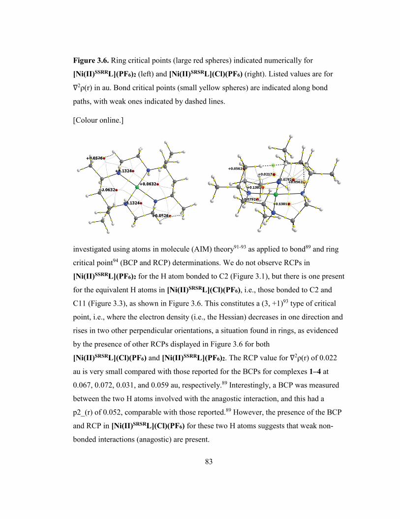
83

Figure 3.6. Ring critical points (large red spheres) indicated numerically for

[Ni(II)SSRRL](PF6)2 (left) and [Ni(II)SRSRL](Cl)(PF6) (right). Listed values are for

∇2ρ(r) in au. Bond critical points (small yellow spheres) are indicated along bond

paths, with weak ones indicated by dashed lines.

[Colour online.]

investigated using atoms in molecule (AIM) theory91-93 as applied to bond89 and ring

critical point94 (BCP and RCP) determinations. We do not observe RCPs in

[Ni(II)SSRRL](PF6)2 for the H atom bonded to C2 (Figure 3.1), but there is one present

for the equivalent H atoms in [Ni(II)SRSRL](Cl)(PF6), i.e., those bonded to C2 and

C11 (Figure 3.3), as shown in Figure 3.6. This constitutes a (3, +1)93 type of critical

point, i.e., where the electron density (i.e., the Hessian) decreases in one direction and

rises in two other perpendicular orientations, a situation found in rings, as evidenced

by the presence of other RCPs displayed in Figure 3.6 for both

[Ni(II)SRSRL](Cl)(PF6) and [Ni(II)SSRRL](PF6)2. The RCP value for ∇2ρ(r) of 0.022

au is very small compared with those reported for the BCPs for complexes 1–4 at

0.067, 0.072, 0.031, and 0.059 au, respectively.89 Interestingly, a BCP was measured

between the two H atoms involved with the anagostic interaction, and this had a

p2_(r) of 0.052, comparable with those reported.89 However, the presence of the BCP

and RCP in [Ni(II)SRSRL](Cl)(PF6) for these two H atoms suggests that weak non-

bonded interactions (anagostic) are present.

84

3.6 Conclusions

We have reported modifications to existing synthetic pathways to produce and isolate

compounds [Ni(II)SSRRL](PF6)2 and [Ni(II)SRSRL](Cl)(PF6) in reasonable yields.

Complex [Ni(II)SSRRL](PF6)2 is described as having an overall configuration of

SSRR(SR)δλ, whereas complex [Ni(II)SRSRL](Cl)(PF6) is composed of a mixture of

61(2)% SRSR(RR)λλ and 39(2)% RSRS(SS)λδ. On the basis of stated criteria for

anagostic interactions and in comparison with

the NMR, structural, and theoretical properties obtained for [Ni(II)SSRRL](PF6)2,

complex [Ni(II)SRSRL](Cl)(PF6) was assessed as having anagostic interactions

between the H atoms on two methyl groups and the Ni atom.

3.7 Supplementary Data

Table S3.1. Listing of conformational forms and corresponding REFL codes in the

CSD.59

JIVBAU

AJITOE

AJITOE01

BADSAA(Et)

BADSAA10(Et)

BADSEE(Et)

85

BIYZIT

BUSBIC

BUSBIC01

CAPVUL

FIBHED

IDIKOY

IVUYON

KOHSUX

MAZNIA

MEAZNI

MEAZNI01

MEAZNI02

MONKUW

MUVYIL

NIGTET

NIGTET01

OBOPEC

OCAREP

PIMHAU

QQQFMG

QQQFMJ

QUBCAS

RAJLOE

UDUPOY

UQOREY

WACKUJ

WACLAQ

WUFQOF

XEHKEB

YOWNON

NOLHAA (phenylethylene)

Table S3.1 (contd.). Listing of conformational forms and corresponding REFL codes

in the CSD.59

ANEMUD BURZUL (first two packing NIATET

86

disorder)

ANEMUD01 BUSBOI NIATET01

ANENAK BUSBUO (ordered) NIATET02

ANENAK01

NIATET03

ANENEO

RABWIC

ANENEO01

RABWOI

ANENIS

ANENIS01

CERVIF (disorder with a (N-

Me))

EBAJOJ01

EBAKUQ

EBAKUQ01

OCMENH

OCMENH01

OCMENH02

OCMENH03

OCMENH04

QAFVIF

XALQUZ

87

Table S3.1 (contd.). Listing of conformational forms and corresponding REFL codes

in the CSD.59

EBAJOJ

AJITUK (partial Me dis Co-

Crystal with en)

AJIVAS (partial Me dis Co-

Crystal with en)

AJIVEW (Me disorder)

ECUREA

88

OCMENI LIFYEG (massive counterion)

QADSIA NIBTET

QADSIA01 QADSIA02

QADSOG

RAPXOW

VURRAC

Figure S3.1 Neat FTIR spectrum of complex 3-SRSR.

0

20

40

60

80

100

120

65011501650215026503150

%Tr

ansm

ittan

ce

Wavenumber (cm-1)

IR of Complex 3-SRSR

N HC-H

P-F

89

Figure S3.2 Neat FTIR spectrum of complex 3-SSRR.

50

60

70

80

90

100

110

65011501650215026503150

% T

rans

mitt

ance

Wavenumber (cm-1)

IR of Complex 3-SSRR

N-H C-H Stretching

P-F

0

0.2

0.4

0.6

0.8

1

1.2

350 400 450 500 550 600 650 700 750 800

Abso

rban

ce

Wavelenth (nm)

Complex 3-SSRR in various solvents462 nm

456 nmAcetone

Acetonitrile

DMSO

90

Figure S3.3 Visible spectrum of complex 3-SSRR in acetone, acetonitrile, and

DMSO.

Figure S3.4 Visible spectrum of complex 3-SRSR in DMSO, acetonitrile, and water.

0

0.2

0.4

0.6

0.8

1

1.2

1.4

1.6

350 400 450 500 550 600 650 700 750 800

Abso

rban

ce

Wavelength (nm)

Complex 3-SRSR in various solvents451 nm

456 nm

453

Water

Acetonitrile

DMSO

91

Figure S3.5 1H NMR spectrum of 3-SSRR in acetone-d6.

92

Figure S3.6 1H NMR spectrum of 3-SRSR in D2O.

93

Figure S3.7 1H NMR spectrum of 3-SSRR in CD3CN.

94

Figure S3.8 1H NMR spectrum of 3-SRSR in CD3CN.

Table S3.2. Listing of hydrogen bonds in 3-SSRR.

D-H d(D-H) d(H..A) <DHA d(D..A) A

N1-H11 0.772 2.392 167.31 3.151 F4â [ x-1/2, -y+1/2, z+1/2 ]

N1-H11 0.772 2.536 138.36 3.155 F11^b [ x-1/2, -y+1/2, z+1/2 ]

N1-H11 0.772 2.406 168.06 3.166 F14^b [ x-1/2, -y+1/2, z+1/2 ]

N2-H12 0.907 2.343 138.97 3.085 F2â [ x-1/2, -y+3/2, z+1/2 ]

N2-H12 0.907 2.561 132.98 3.248 F11^b [ -x+1/2, y+1/2, -z+1/2 ]

N2-H12 0.907 2.285 144.66 3.069 F12^b [ x-1/2, -y+3/2, z+1/2 ]

C4-H4A 0.970 2.375 153.95 3.275 F5â [ x-1/2, -y+1/2, z+1/2 ]

C4-H4A 0.970 2.635 161.40 3.567 F15^b [ x-1/2, -y+1/2, z+1/2 ]

95

C6-H6A 0.960 2.614 130.63 3.320 F15^b [ -x+1, -y+1, -z+1 ]

C8-H8A 0.970 2.565 134.08 3.314 F6â [ -x, -y+1, -z+1 ]

C8-H8A 0.970 2.558 137.93 3.341 F16^b [ -x, -y+1, -z+1 ]

Table S3.3.Listing of hydrogen bonds in 3-SRSR.

D-H d(D-H) d(H..A) <DHA d(D..A) A

C2-H2C 0.960 2.577 155.90 3.476 F2â

C3-H3A 0.960 2.436 127.40 3.114 F4A^b [ x, y-1, z ]

C4-H4A 0.970 2.975 134.94 3.724 Cl1

C6-H6A 0.960 2.617 127.62 3.292 F1B^c [ -x+1, -y+2, -z+1 ]

C7â-H7Bâ 0.970 2.544 129.14 3.245 F1â [ x-1, y-1, z ]

C8â-H8Bâ 0.970 2.498 125.84 3.165 F3â [ -x+1, -y+2, -z+1 ]

C11-H11C 0.960 2.532 167.88 3.476 F3A^b [ -x+1, -y+2, -z+1 ]

C11-H11C 0.960 2.469 160.11 3.387 F5B^c [ -x+1, -y+2, -z+1 ]

C13-H13 0.980 2.430 145.98 3.289 F2A^b

C13-H13 0.980 2.545 134.95 3.310 F4B^c

C15-H15A 0.970 2.539 117.29 3.106 F6B^c [ -x+1, -y+2, -z ]

C15-H15B 0.970 2.611 120.99 3.219 F4â [ -x+1, -y+2, -z ]

C16-H16A 0.970 2.502 172.76 3.467 F2â

N1-H101 0.852 2.433 158.60 3.242 Cl1

N2-H102 0.807 2.624 155.56 3.375 Cl1

N3-H103 0.961 2.352 160.47 3.273 Cl1 [ -x, -y+1, -z ]

96

N4-H104 0.806 2.535 165.48 3.322 Cl1 [ -x, -y+1, -z ]

Theoretical Calculations

Table S3.4. Comparison of selected thermodynamic data for the cations in 3-SSRR,

3-SRSR(λλ), and 3-SRSR(λδ) computed under identical conditions.

Factor 3-SSRR 3-SRSR(λλ) 3-SRSR(λδ)

E (RAPFD) (Hartrees) -1019.0631 -1019.0619 -1019.0638 ∆ (kJ/mol) compared to 3- SSRR 0 3.1506 -1.8378

Dipole moment (Debye) 0 4.5308 4.6659899 EE = Zero=point Energy (Hartrees) -1018.5241 -1018.5221 -1018.5252

∆ (kJ/mol) compared to 3- SSRR 0 -5.251 8.13905

EE + Thermal Energy Correction (Hartrees) -1018.5025 -1018.5007 -1018.5034


EE + Thermal Enthalpy Correction (Hartrees) -1018.5016 -1018.4997 -1018.5025


EE + Thermal Free Energy Correction (Hartrees)

-1018.571 -1018.5686 -1018.5716


E (thermal) (kcal/mol 351.774 352.171 351.644 Results for 3-SSRR based on AFPD/GENECP with Ni at LanL2DZ and H, C, N at 6-

311+G(d) basis sets.

97

Figure S3.9. GaussView representation of 3-SSRR.

Table S3.5. Calculated atomic coordinates for 3-SSRR.

Ro

Symb

X Y Z 1 Ni -9E-07 -1.4E-

4.1E-06 2 N 1.301236 -

-0.15669 3 H 1.148505 -

-1.13128 4 N -1.3268 -

0.51735

5 H -1.46484 -

1.51087

6 C 3.5711 2.3156

-0.12671 7 H 3.189436 3.2565

0.27320

8 H 4.540862 2.1390

0.34276

9 H 3.737227 2.4359

-1.20156 10 C 2.395589 1.0120

1.66645

11 H 2.047118 1.9540

2.09443 12 H 1.644683 0.2492

1.89377

13 H 3.320305 0.7461

2.18323 14 C 2.646321 1.1321

0.16780

15 C 3.298262 -

-0.41503 16 H 3.261615 -

-1.51193 17 H 4.361551 -

-0.16077 18 C 2.758107 -

0.07337

19 H 2.892397 -

1.15699

Ro

Symb

X Y Z 20 C 3.510344 -

-0.57884 21 H 4.576647 -

-0.35539 22 H 3.174086 -

-0.21936 23 H 3.396374 -

-1.66731 24 C 0.699922 -

0.71576

25 H 0.851429 -

1.74982

26 H 1.179357 -3.5583 0.59086

27 C -0.75638 -

0.38313

28 H -0.88739 -

-0.64848 29 H -1.27542 -

1.02985

30 N -1.30124 1.5652

0.15669

31 H -1.14851 1.8255

1.13129

32 N 1.326792 1.3044

-0.51735 33 H 1.464828 1.1245

-1.51087 34 C -3.57111 -

0.12667

35 H -3.18946 -

-0.27327 36 H -4.54087 -2.139 -0.34279 37 H -3.73723 -

1.20151

38 C -2.39556 -

-1.66646

98

Ro

Symb

X Y Z 39 H -2.04713 -

-2.09445 40 H -1.64462 -

-1.89375 41 H -3.32026 -

-2.18324 42 C -2.64632 -

-0.16781 43 C -3.29826 0.1196

0.41502

44 H -3.26162 0.0735

1.51192

45 H -4.36155 0.0974

0.16075

46 C -2.75811 1.4450

-0.07337 47 H -2.89239 1.4996

-1.157 48 C -3.51035 2.5998

0.57884

Ro

Symb

X Y Z 49 H -4.57665 2.5217

0.35537

50 H -3.1741 3.5740

0.21936

51 H -3.39639 2.5756

1.66730

52 C -0.69992 2.5840

-0.71574 53 H -0.85143 2.2646

-1.7498 54 H -1.17935 3.5583

-0.59084 55 C 0.756376 2.6586

-0.38312 56 H 0.887392 2.9882

0.64850

57 H 1.275422 3.3682

-1.02983

Figure S3.10. Calculated IR spectrum for 3-SSRR.

Figure S3.11. Calculated UV-Vis spectrum for 3-SSRR.

99

Table S3.6. Excitation energies and oscillator strengths listing for 3-SSRR.

Excited Nature E (eV) λ (nm) f Orbital Normalized State transitions coefficient 1: A 1.6615 746.21 0.0000 88 -> 89 0.71252

88 <- 89 -0.15346 2: A 2.1112 587.28 0.0000 87 -> 89 0.70829

87 <- 89 -0.10627 3: A 2.2018 563.11 0.0000 86 -> 89 0.70614 4: A 2.5628 483.77 0.0000 78 -> 89 -0.18200

80 -> 89 0.23756 82 -> 89 0.61428 83 -> 89 -0.11924

5: A 5.1041 242.91 0.3607 85 -> 89 0.69764 6: A 5.5083 225.09 0.3231 84 -> 89 0.69567 7: A 5.8095 213.42 0.0000 78 -> 89 -0.17908

80 -> 89 0.22258 83 -> 89 0.61590

8: A 5.9872 207.08 0.0000 77 -> 89 0.18672

78 -> 89 -0.20454 80 -> 89 0.50672 82 -> 89 -0.31175 83 -> 89 -0.23220

9: A 6.0726 204.17 0.0195 81 -> 89 0.69738 10: A 6.1938 200.18 0.0056 79 -> 89 0.69881

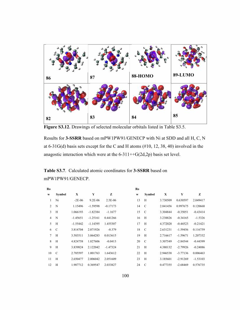
100

86

87

88-HOMO

89-LUMO

82

83

84

85

Figure S3.12. Drawings of selected molecular orbitals listed in Table S3.5.

Results for 3-SSRR based on mPW1PW91/GENECP with Ni at SDD and all H, C, N

at 6-31G(d) basis sets except for the C and H atoms (#10, 12, 38, 40) involved in the

anagostic interaction which were at the 6-311++G(2d,2p) basis set level.

Table S3.7. Calculated atomic coordinates for 3-SSRR based on

mPW1PW91/GENECP.

Ro

w Symbol X Y Z

1 Ni -2E-06 9.2E-06 2.5E-06

2 N 1.15496 -1.59598 -0.17173

3 H 1.066193 -1.82384 -1.1677

4 N -1.45651 -1.25161 0.441266

5 H -1.55442 -1.14395 1.455307

6 C 3.814704 2.071926 -0.379

7 H 3.583511 3.064283 0.013615

8 H 4.824758 1.827606 -0.0413

9 H 3.839824 2.122042 -1.47324

10 C 2.785597 1.001763 1.643612

11 H 2.650477 2.006042 2.051609

12 H 1.987712 0.369547 2.033827

Ro

w Symbol X Y Z

13 H 3.730509 0.630597 2.049417

14 C 2.841456 0.997675 0.120668

15 C 3.304844 -0.35051 -0.43414

16 H 3.238826 -0.34165 -1.5326

17 H 4.372028 -0.44523 -0.21421

18 C 2.631231 -1.59456 0.116759

19 H 2.716617 -1.59671 1.207332

20 C 3.307549 -2.84544 -0.44399

21 H 4.380132 -2.79926 -0.24086

22 H 2.946538 -3.77136 0.006463

23 H 3.185601 -2.91269 -1.53103

24 C 0.477355 -2.68469 0.576735

101

Ro

w Symbol X Y Z

25 H 0.637305 -2.50318 1.644213

26 H 0.901657 -3.66163 0.336778

27 C -0.98077 -2.64092 0.224884

28 H -1.12957 -2.89691 -0.82651

29 H -1.54836 -3.35313 0.827364

30 N -1.15497 1.595996 0.171721

31 H -1.06622 1.823856 1.167697

32 N 1.456509 1.25163 -0.44125

33 H 1.554415 1.143969 -1.45529

34 C -3.81465 -2.07196 0.379037

35 H -3.58333 -3.06434 -0.01344

36 H -4.8247 -1.82776 0.041226

37 H -3.83986 -2.12196 1.473287

38 C -2.78557 -1.00182 -1.6436

39 H -2.65037 -2.00611 -2.05155

40 H -1.98773 -0.36956 -2.03383

41 H -3.73051 -0.63074 -2.04943

Ro

w Symbol X Y Z

42 C -2.84145 -0.99768 -0.12066

43 C -3.30486 0.350513 0.43412

44 H -3.23885 0.341672 1.53258

45 H -4.37204 0.44523 0.214175

46 C -2.63124 1.594564 -0.11678

47 H -2.71661 1.596698 -1.20736

48 C -3.30757 2.845448 0.443937

49 H -4.38015 2.799263 0.240799

50 H -2.94656 3.771367 -0.00652

51 H -3.18564 2.912709 1.530987

52 C -0.47737 2.684705 -0.57674

53 H -0.63731 2.503186 -1.64421

54 H -0.90168 3.661639 -0.33678

55 C 0.980757 2.640936 -0.22488

56 H 1.129543 2.896935 0.826521

57 H 1.548336 3.353157 -0.82736

Results for 3-SRSR based on AFPD/GENECP with Ni at LanL2DZ and H, C, N at 6-

311+G(d) basis sets.

102

Figure S3.13. GaussView representation of 3-SRSR.

103

Table S3.8. Calculated atomic coordinates for 3-SRSR.

Row Symbol X Y Z

1 C 0.601671 -2.69523 -0.28284

2 H 1.230412 -3.54844 -0.54812

3 H 0.312581 -2.80161 0.763496

4 C -0.61615 -2.62265 -1.16732

5 H -1.24649 -3.5067 -1.06185

6 H -0.32013 -2.56052 -2.21927

7 C -2.40016 -1.44475 0.236132

8 H -1.87122 -1.56915 1.186058

9 C -3.36798 -2.60903 0.041126

10 H -2.89465 -3.58452 0.167544

11 H -4.15891 -2.55007 0.792706

12 H -3.84679 -2.57646 -0.94349

13 C -3.16654 -0.12149 0.225699

14 H -3.64399 0.002455 -0.75894

15 H -3.99666 -0.21847 0.930762

16 C -2.42288 1.170107 0.599041

17 C -1.80681 1.058532 1.987691

18 H -2.57065 0.73387 2.698967

19 H -0.99702 0.331548 2.026963

20 H -1.42752 2.013038 2.358786

21 C -3.42805 2.325597 0.556595

22 H -4.25367 2.119997 1.24246

23 H -2.98339 3.272636 0.870774

24 H -3.85781 2.453923 -0.44304

25 C -0.60168 2.695236 -0.28275

26 H -0.31254 2.801595 0.763569

27 H -1.23044 3.548451 -0.54799

28 C 0.616091 2.622673 -1.16729

29 H 1.246438 3.506722 -1.06184

Row Symbol X Y Z

30 H 0.320031 2.560564 -2.21923

31 C 2.400178 1.444746 0.236044

32 H 1.871282 1.569129 1.185999

33 C 3.367991 2.609031 0.041009

34 H 4.158959 2.550048 0.792549

35 H 3.846746 2.576472 -0.94363

36 H 2.894664 3.58452 0.167466

37 C 3.166547 0.121482 0.225553

38 H 3.643952 -0.00244 -0.75911

39 H 3.996704 0.218452 0.93058

40 C 2.422905 -1.17012 0.598907

41 C 1.8069 -1.05857 1.987585

42 H 2.57077 -0.73392 2.698834

43 H 0.997108 -0.33158 2.026906

44 H 1.427615 -2.01308 2.358679

45 C 3.428072 -2.32561 0.556396

46 H 4.253724 -2.12002 1.242229

47 H 2.983428 -3.27265 0.870579

48 H 3.857783 -2.45392 -0.44326

49 N 1.336843 -1.40854 -0.43859

50 N -1.35525 -1.37032 -0.84167

51 N -1.33686 1.408551 -0.4385

52 N 1.355212 1.370341 -0.84171

53 Ni -1.3E-05 5.5E-06 -0.58939

54 H -1.82474 1.466397 -1.33652

55 H 1.866096 1.110427 -1.68811

56 H 1.82468 -1.46637 -1.33663

57 H -1.86618 -1.11039 -1.68805

104

Figure S3.14. Calculated IR spectrum for 3-SRSR.

Figure S3.15. Calculated UV-Vis spectrum for 3-SRSR.

105

Figure S3.16. Expansion of the vertical scale for the Calculated UV-Vis spectrum for

3-SRSR.

106

Table S3.9. Excitation energies and oscillator strengths listing for 3-SRSR.

Excited Nature E (eV) λ (nm) f Orbital Normalized State transitions coefficient 1: A 2.1195 584.98 0.0005 88 -> 89 0.70628

88 <- 89 -0.11994 2: A 2.4491 506.25 0.0022 84 -> 89 0.16437

85 -> 89 0.20628 86 -> 89 -0.11605 87 -> 89 0.64293

3: A 2.5634 483.67 0.0003 84 -> 89 0.12272

86 -> 89 0.67965 87 -> 89 0.12258

4: A 2.9146 425.39 0.0000 77 -> 89 0.13056

80 -> 89 -0.18904 82 -> 89 0.45944 83 -> 89 0.47112

5: A 5.4465 227.64 0.2635 84 -> 89 0.10399

85 -> 89 0.64660 86 -> 89 0.11288 87 -> 89 -0.21999

6: A 5.9555 208.18 0.2575 84 -> 89 0.65665

85 -> 89 -0.14290 86 -> 89 -0.11501 87 -> 89 -0.15107

7: A 6.2220 199.27 0.0022 82 -> 89 0.44321

83 -> 89 -0.42446 88 -> 90 -0.32626

8: A 6.3101 196.49 0.0022 77 -> 89 -0.27174

80 -> 89 0.59667 82 -> 89 0.13105 83 -> 89 0.18197

9: A 6.4155 193.26 0.0050 78 -> 89 0.14387

82 -> 89 0.23447 83 -> 89 -0.19341 88 -> 90 0.59529

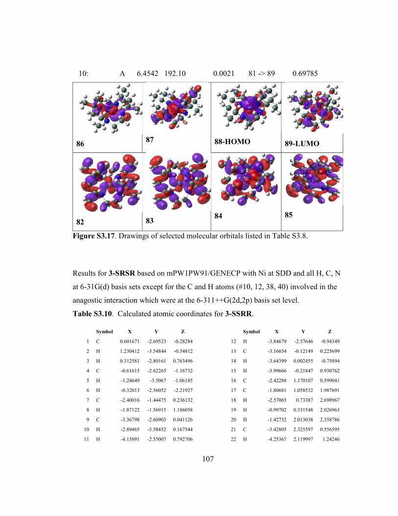
107

10: A 6.4542 192.10 0.0021 81 -> 89 0.69785

86

87

88-HOMO

89-LUMO

82

83

84

85

Figure S3.17. Drawings of selected molecular orbitals listed in Table S3.8.

Results for 3-SRSR based on mPW1PW91/GENECP with Ni at SDD and all H, C, N

at 6-31G(d) basis sets except for the C and H atoms (#10, 12, 38, 40) involved in the

anagostic interaction which were at the 6-311++G(2d,2p) basis set level.

Table S3.10. Calculated atomic coordinates for 3-SSRR.

Symbol X Y Z

1 C 0.601671 -2.69523 -0.28284

2 H 1.230412 -3.54844 -0.54812

3 H 0.312581 -2.80161 0.763496

4 C -0.61615 -2.62265 -1.16732

5 H -1.24649 -3.5067 -1.06185

6 H -0.32013 -2.56052 -2.21927

7 C -2.40016 -1.44475 0.236132

8 H -1.87122 -1.56915 1.186058

9 C -3.36798 -2.60903 0.041126

10 H -2.89465 -3.58452 0.167544

11 H -4.15891 -2.55007 0.792706

Symbol X Y Z

12 H -3.84679 -2.57646 -0.94349

13 C -3.16654 -0.12149 0.225699

14 H -3.64399 0.002455 -0.75894

15 H -3.99666 -0.21847 0.930762

16 C -2.42288 1.170107 0.599041

17 C -1.80681 1.058532 1.987691

18 H -2.57065 0.73387 2.698967

19 H -0.99702 0.331548 2.026963

20 H -1.42752 2.013038 2.358786

21 C -3.42805 2.325597 0.556595

22 H -4.25367 2.119997 1.24246

108

Symbol X Y Z

23 H -2.98339 3.272636 0.870774

24 H -3.85781 2.453923 -0.44304

25 C -0.60168 2.695236 -0.28275

26 H -0.31254 2.801595 0.763569

27 H -1.23044 3.548451 -0.54799

28 C 0.616091 2.622673 -1.16729

29 H 1.246438 3.506722 -1.06184

30 H 0.320031 2.560564 -2.21923

31 C 2.400178 1.444746 0.236044

32 H 1.871282 1.569129 1.185999

33 C 3.367991 2.609031 0.041009

34 H 4.158959 2.550048 0.792549

35 H 3.846746 2.576472 -0.94363

36 H 2.894664 3.58452 0.167466

37 C 3.166547 0.121482 0.225553

38 H 3.643952 -0.00244 -0.75911

39 H 3.996704 0.218452 0.93058

40 C 2.422905 -1.17012 0.598907

Symbol X Y Z

41 C 1.8069 -1.05857 1.987585

42 H 2.57077 -0.73392 2.698834

43 H 0.997108 -0.33158 2.026906

44 H 1.427615 -2.01308 2.358679

45 C 3.428072 -2.32561 0.556396

46 H 4.253724 -2.12002 1.242229

47 H 2.983428 -3.27265 0.870579

48 H 3.857783 -2.45392 -0.44326

49 N 1.336843 -1.40854 -0.43859

50 N -1.35525 -1.37032 -0.84167

51 N -1.33686 1.408551 -0.4385

52 N 1.355212 1.370341 -0.84171

53 Ni -1.3E-05 5.5E-06 -0.58939

54 H -1.82474 1.466397 -1.33652

55 H 1.866096 1.110427 -1.68811

56 H 1.82468 -1.46637 -1.33663

57 H -1.86618 -1.11039 -1.68805

109

Chapter 4 Double-Shell Lignin Nanocapsules Are a Stable

Vehicle for Fungicide Encapsulation and Release

Raisa Carmen Andeme Ela,* Momoko Tajiri, Nick K. Newberry, Patricia A. Heiden,

and Rebecca G. Ong

4.1 Abstract

Industry is increasingly turning to biobased and environmentally benign

materials for use in high-value applications. Kraft lignin’s low cost and inherent

properties, such as its easily tunable amphiphilic nature, adsorption capacity, and

natural

cross-linking tendency, make it suitable for use as a raw material for high-value

nanomaterials. To support that need, this paper describes the synthesis of innovative,

double-shelled lignin nanocapsules from hardwood kraft lignin, their performance

towards encapsulating a fungicide, and effectiveness at controlling its release. The

recovered lignin was dissolved without further modification in tetrahydrofuran and

inserted dropwise into a water/ethanol solution containing sacrificial surfactant

templates. Monodispersed, hollow, double-shell nanocapsules were produced via a

two-step self-assembly. The water/ethanol solution acted as a nonsolvent while

simultaneously providing strategic sites for controlled-size production. The shells of

the

nanocapsules were cross-linked with biodegradable maleic anhydride to bolster the

structural stability. The average hydrodynamic diameter of the particles was 241.8 ±

33.3 nm, and these structures were stable in water for eight months. The specific

surface area of kraft lignin increased by 4-fold in the double-shell nanocapsule form.

The nanocapsules were loaded with propiconazole at an entrapment efficiency of

56.1%. This system could represent an effective method to enable the biologically

activated, controlled release of fungicides.

KEYWORDS: Kraft lignin, Nanocapsule, Double shell, Drug vehicle, Release studies

110

4.2 Introduction

Sustainable and biologically, and environmentally friendly materials are essential

components to achieving ecological balance.95 Lignin is the second most abundant

biopolymer in the biosphere, representing 30% of nonfossil carbon. It is comprised of

polymerized coniferyl, sinapyl, and p-coumaryl monomers that are largely linked

together by β-O-4 ether bonds.96 In the cell walls of vascular plants, lignin provides

antioxidant and antimicrobial properties and resistance to ultraviolet light,97 and there

are many potential applications for lignin that could benefit from these inherent

characteristics. The main industrial source of lignin is the kraft pulping process, and

kraft lignin is an attractive renewable precursor with high valorization potential.96 The

kraft process produces approximately 53 million metric tons of lignin per year, and of

this, only ∼2% is utilized in advanced applications, with the remainder being

combusted for energy and chemical recovery.98 Various high-value products have been

proposed for lignin, of which the major advances have been focused on carbon fiber

technology,99 hydrogels,100, and nanoparticles.101-103 Lignin nanoparticles have

applications in biomedical, environmental, electronic, and personal care products and

thermoplastics.101-104 However, one property of lignin that has hindered its use

industrially is its inherent hydrophobicity, which causes it to sediment in aqueous

systems. Lignin nanoparticles are able to overcome this challenge by forming

nanoparticles in water that are stabilized by electrostatic repulsions between the ionized

surface hydroxyl groups.105, 106 However, the physical and chemical properties of the

final particle depend on the type of lignin precursor, synthesis route, and post-synthesis

modifications. Hollow lignin spheres have been produced from unmodified kraft lignin

through a solvent exchange process.107 This is a significant advancement, as most

methods have relied on copolymerization and unsustainable approaches to chemically

modify the lignin precursor prior to nanoparticle synthesis.105, 106 The production of

hollow particles from unmodified kraft lignin was achieved by dissolving lignin in

tetrahydrofuran and slowly inserting water into the system. The particles ranged in

size, 200−600 nm, and they were reported to be stable for 45 days.107 Nonetheless, the

111

specific mechanism responsible for the formation of the hollow structure was not

described sufficiently, as solid spheres have also been produced from kraft lignin using

the same approach.101, 105 All papers have attributed the nanoparticle formation

mechanism primarily to π−π stacking between the aromatic rings. Thus, a deeper

understanding of the phenomenon that promotes cavity formation is needed. Li et al.

reported perforated kraft lignin nanocapsules108 that were obtained by adding water to a

lignin in ethanol solution. This method produced fine particles. The core of some

particles fused together upon ethanol removal, and the particles were reported to flatten

upon drying. Various studies have studied the suitability of lignin nanoparticles for

drug delivery;109; however, only Zhou et al.110 investigated the mechanisms driving

encapsulation and release, in this case of a hydrophilic drug, from lignin nanoparticles.

As such, there is significant room for additional research. Producing uniform and stable

hollow structures from unmodified kraft lignin could pave the way toward its

commercial utilization in drug-delivery applications. One way to achieve a high yield

of regular structures is by employing surfactant templates.111 Li et al.112 prepared an

alkali lignin−anionic surfactant nanoparticle complex and reported it to be effective for

the encapsulation of a hydrophobic compound, but released it at a fast rate. Yiamawas

et al.113 used a nonionic surfactant to envelope a kraft lignin-based nanoparticle

encapsulating a UV-active cargo. Both methods modified the lignin precursor to

promote the molecular assembly. In this work, an inventive mesoporous, uniform,

doubleshelled, hollow particle was produced from unmodified kraft lignin. The

mechanisms inducing particle morphology and stability in water were studied. For this

study, we encapsulated the common foliar fungicide, propiconazole, which has modest

solubility in water into the mesoporous double-shell nanocapsule, with the expectation

that the amphiphilic nature of lignin would enhance the uptake and retention of the

propiconazole within the nanocapsules. The drug encapsulation and retention

mechanisms for this system were also investigated.

112

4.3 Experimental

4.3.1 Materials

The kraft lignin utilized in this study was precipitated from a mixed-hardwood black

liquor obtained from Verso (Quinnesec, MI) through the LignoBoost process to a final

pH of 4.2 at 70 °C. The lignin was vacuum freeze-dried (FreeZone 4.5L, 77500/77510,

Labconco) for 18 h at a temperature of −40 °C.114 The characterization methodology

can be found in the supplemental document. All reagents were utilized as purchased.

The ethanol (EtOH) utilized was 95% concentration, and the water ultrapure.

4.3.2 Nanocapsule Synthesis

Kraft lignin was dissolved in tetrahydrofuran (THF) (1.2 g: 35 mL) under continuous

stirring for 2 h at room temperature. A total of ∼0.15 g remained undissolved and was

separated from the liquid by decanting. A water/EtOH solution (2:1, v/v) was prepared,

and 200 mL of this solution was stirred at medium-low speed and heated to 67 ± 3 °C.

To this solution, 0.8 g of either the cationic surfactant cetrimonium bromide (CTAB) or

anionic surfactant sodium dodecyl sulfate (SDS) was added. The surfactant was

allowed to disperse for 20 min, and then 20 mL of the lignin/THF solution was added

dropwise with a 1 mL pipet within an interval of 20 min. The self-assembly was

allowed to proceed under stirring for 30 min; then, the dispersion was centrifuged

(5810R, Eppendorf) for 1 h at 5 °C and 1200 rpm. The supernatant was discarded, and

the pellet was sonicated in a warm bath at 69 °C (M1800H, Branson) for 30 min with a

5% (v/v) EtOH water solution containing 1% (v/v) sulfuric acid at pH 6 to remove the

surfactant.111 This washing step was repeated twice. The nanocapsules were

subsequently cross-linked in a dilute aqueous mixture containing 20 mg of maleic

anhydride and 200 μL of dibutyl tin dilaurate as a catalyst. The esterification was

allowed to proceed for 15 min at room temperature. Then, the nanocapsules were

washed once with EtOH and twice with water to remove all traces of the reagents

utilizing centrifugation and resuspension through sonication. To create the second

113

shell, the process was repeated on the single-shell particles with a 15 mL lignin/THF

solution. The nanocapsules were kept suspended in distilled water at a pH of 7.

4.3.3 Nanocapsule Characterization

The morphologies of the nanostructures were studied using transmission electron

microscopy (FEI 200 kV Titan Themis) operating at 60 kV. The sample preparation

was done by dripping 10 μL of the aqueous nanocapsule suspension onto a copper grid,

and the drop was allowed to disperse out for 2 min; the excess water was removed by

absorbing it from the sides of the grid using filter paper, and the grids were left to dry

in a desiccator for 4 days. The particles were not stained. Images collected and shown

are representative after observing different areas throughout the grid. The mean

hydrodynamic particle size and zeta (ζ)-potential of the nanocapsules were measured at

25 °C by a zetasizer (Malvern Nano- ZS) at a refractive index of 1.61.115 The spatial

distribution and relative proportions of the elements were studied by energy dispersive

X-ray spectrometry (EDS) and high angle annular dark-field (HAADF) imaging

techniques (STEM, FEI 200 kV Titan Themis). The samples (precipitated kraft lignin

and the nanocapsules) were oven-dried at 105 °C for 3.5 h prior to surface area

measurement. These were utilized to determine the specific surface area and the

porosity of each. The dried samples were degassed (at 100 °C, 1 mm mercury (Hg) for

4 h), and the measurements were performed by nitrogen (N2) and helium (He)

sorption, respectively, through the 5- point Brunauer−Emmett−Teller (BET) method

(ASAP 2020, Micrometrics). The functional groups of the oven-dried recovered kraft

lignin, the empty single shell before cross-linking, the cross-linked single shell, and the

final double-shell nanocapsules were evaluated using Fourier transform infrared

spectroscopy with 65 scans on a MIRacle A Diamond prizm-ZnSe support element

(SHIMADZU, IRTracer-100).

114

The average number of molecules assembled per particle (Nass) was computed from eq

1,

𝑁𝑁𝑎𝑎𝑎𝑎𝑎𝑎 =𝑀𝑀𝑤𝑤𝑝𝑝

𝑀𝑀𝑤𝑤𝑚𝑚 (1)

𝜌𝜌 =𝑀𝑀𝑛𝑛𝑝𝑝

𝑁𝑁𝐴𝐴4𝜋𝜋 �𝑅𝑅ℎ3

3 � (2)

(2) where Mwp represents the molecular weight of the particle estimated from the shell

hydrodynamic radius, Mwm represents the molecular weight of KL, and the particle

density (ρ) is from eq 2,108 where NA represents Avogadro’s number and Rh the

hydrodynamic radius of the shell.

4.3.4 Fungicide Encapsulation and Release

The nanocapsules were loaded according to a published method with some

modifications.110, 116 Briefly, the lignin nanocapsules were incubated in a parafilm-

sealed 500 mL glass beaker with a 0.01% (v/v) propiconazole solution in water, at a

ratio of 10:1 (w/w) nanocapsules to propiconazole on a mass basis. The tube was kept

in the dark for 20 h on an orbital shaker at ambient conditions. The mixture was

centrifuged and the loaded nanocapsule pellet was washed once and redispersed in

water at a concentration of 20 mg/mL. The percentage of the mass attributed to the

drug per nanocapsule could be determined by eq 3, and eq 4 permitted the total

entrapment efficiency of propiconazole in the total nanocapsule mass. The maximum

absorbance for propiconazole was taken at a wavelength of 223 nm. Measurements

were conducted through UV spectrophotometry using a 1 cm quartz cuvette, and the

calculation was performed by a calibration curve (UV−vis−NIR spectrophotometer,

Shimadzu UV-3600 Plus).

115

𝐷𝐷𝐷𝐷𝐷𝐷𝐷𝐷 𝐿𝐿𝐿𝐿𝐿𝐿𝐿𝐿𝐿𝐿𝐿𝐿𝐷𝐷 (%) =𝑤𝑤𝑤𝑤𝐿𝐿𝐷𝐷ℎ𝑡𝑡 𝐿𝐿𝑜𝑜 𝐿𝐿𝐷𝐷𝐷𝐷𝐷𝐷 𝐿𝐿𝐿𝐿 𝐿𝐿𝐿𝐿𝐿𝐿𝐿𝐿𝑛𝑛𝐿𝐿𝑛𝑛𝑛𝑛𝐷𝐷𝑛𝑛𝑤𝑤𝑛𝑛

𝑤𝑤𝑤𝑤𝐿𝐿𝐷𝐷ℎ𝑡𝑡 𝐿𝐿𝑜𝑜 𝐿𝐿𝐿𝐿𝐿𝐿𝐿𝐿𝑛𝑛𝐿𝐿𝑛𝑛𝑛𝑛𝐷𝐷𝑛𝑛𝑤𝑤𝑛𝑛× 100 (3)

𝐸𝐸𝐿𝐿𝑡𝑡𝐷𝐷𝐿𝐿𝑛𝑛𝐸𝐸𝑤𝑤𝐿𝐿𝑡𝑡 𝐸𝐸𝑜𝑜𝑜𝑜𝐿𝐿𝑛𝑛𝐿𝐿𝑤𝑤𝐿𝐿𝑛𝑛𝐸𝐸 (%) =𝑤𝑤𝑤𝑤𝐿𝐿𝐷𝐷ℎ𝑡𝑡 𝐿𝐿𝑜𝑜 𝐿𝐿𝐷𝐷𝐷𝐷𝐷𝐷 𝐿𝐿𝐿𝐿 𝐿𝐿𝐿𝐿𝐿𝐿𝐿𝐿𝑛𝑛𝐿𝐿𝑛𝑛𝑛𝑛𝐷𝐷𝑛𝑛𝑤𝑤𝑛𝑛𝑤𝑤𝑤𝑤𝐿𝐿𝐷𝐷ℎ𝑡𝑡 𝐿𝐿𝑜𝑜 𝐿𝐿𝐷𝐷𝐷𝐷𝐷𝐷 𝑜𝑜𝑤𝑤𝐿𝐿 𝐿𝐿𝐿𝐿𝐿𝐿𝑡𝑡𝐿𝐿𝐿𝐿𝑛𝑛𝑛𝑛𝐸𝐸

× 100 (4)

The drug release studies were performed by placing the loaded drug dispersion in a

6−8 kDa dialysis tube and placing it in a parafilm-sealed 500 mL glass beaker

containing 150 mL of water rotating on an orbital shaker at ambient conditions. A red-

fluorescence label (Cy5) was added to propiconazole via a click reaction. The details

are given in the supplemental document. The specific location of Cy5-labeled

propiconazole within the nanocapsule was visualized by confocal fluorescence

microscopy at an excitation of 488 nm for lignin and 635 nm for propiconazole at a

single confocal point. The objective lens numerical aperture was 0.9, and the

magnification was 40× (Olympus FluoView, FV1000). The sample preparation was

done by simply dripping the loaded nanocapsule solution on a microscope dish.


4.4.1 Kraft Lignin

The first objective of this work was to make sure that the key properties of the kraft

lignin isolated and used here were comparable to those reported in the literature. The

number-averaged molecular weight (Mw) of the kraft lignin is relatively high (Table

4.1); as such, the chains are not expected

Table 4.3 Chemical Properties Measured for the Kraft Lignin Utilized in This

Study

property value

Mw (kDa) 2.47 ± 0.06

polydispersity (Đ) 4.63 ± 0.13

aliphatic OH (mmol/g lignin) 3.61 ± 0.11

116

sinapyl OH (mmol/g lignin) 1.91 ± 0.77

coniferyl OH (mmol/g lignin) 1.03 ± 0.06

p-comaryl OH (mmol/g lignin) 0.25 ± 0.03

carboxyl OH (mmol/g lignin) 0.56 ± 0.16

ash (%) 4.72 ± 0.34

C:O (%) 2.90 ± 0.07

Na (g/kg) 52.5 ± 3.13

hemicelluloses (%) 1.68 ± 0.16

xylose 1.34 ± 0.05

glucose 0.082 ± 0.002

galactose 0.048 ± 0.004

mannose 0.13 ± 0.01

to solubilize in ethanol, which would act as an antisolvent.108, 117 Moreover, the

presence of hydroxyl groups in the lignin precursor will induce a charge on the surface

of the nanocapsule (Figure 4.2B), thus stabilizing the structures through electrostatic

repulsions.105, 106 Similarly, the significant presence of the sodium ion (Na+) (Table

4.1) could contribute to the particle stability by promoting ion−π interactions.118 The

aliphatic and phenolic hydroxyl content agrees with what has been previously reported

for kraft lignin (1.65−3.28 mmol/g and 1.58−3.58 mmol/g, respectively).103, 119, 120

Similarly, the ratio of carbon to oxygen atoms (C:O) coincides with previous reports

(2.4−3.1).121, 122 The physical and chemical properties tested support that the methods

used to isolate the lignin did not alter it so its performance should not differ from that

of the other kraft lignins.

4.4.2 Double-Shell Nanocapsule.

The nanocapsule synthesis method reported herein yielded monodispersed, double-

shelled particles, which were stable in water in the pH range 4−7 (Figure 4.1, Figure

4.2A, B). These particles are considered fine particles with an average hydrodynamic

size of 242 ± 33 nm at pH 7 (Figure 4.2). The self-assembly of the kraft lignin

molecules occurred in a solvent evaporation process. It was hypothesized that at 65 °C,

the THF would evaporate from the system. It is well-known that ethanol and water are

117

mutually soluble; nonetheless, previous work on kraft lignin nanoparticles proved that,

in a water−ethanol system, a considerable portion of ethanol was entrapped in the

hydrophobic core of the nanocapsules.108, 123, 124 Moreover, ethanol has been reported to

enhance the homogeneity of the resultant nanoparticles.123 This leads us to a hypothesis

that, in a water−ethanol system, the ethanol provides specific sites for hydrophobic

segregation, thus producing globules of uniform size and shape at an optimum

precursor concentration. Amphiphilic molecules adopt the conformation (self-

assembly) that costs them less energy with respect to the system conditions,125 in this

system, both the surfactant and kraft lignin assembled into a spherical shape (Figure

4.1A−D).

4.4.3 Synthetic Methodology

The sacrificial surfactant sodium dodecyl sulfate (SDS) produced nanocapsules of a

wide size range (Figure 4.1A), which could be due to the negative head of the

surfactant electrostatically repulsing the negatively ionized lignin molecules. The sulfur

content in the nanocapsules produced by SDS was monitored through energy

dispersive spectroscopy (EDS), and this was utilized to assess the effectiveness of the

surfactant removal method (Table S4.1). On the other hand, the cetrimonium bromide

(CTAB) surfactant, which has a positively charged headgroup, yielded monodispersed

nanocapsules (Figure 4.1B−C). It was observed that when the lignin precursor

concentration was increased from 0.03 g/mL to 0.05 g/mL, under the same

experimental conditions, the average hydrodynamic diameter of the double-shelled

nanocapsule increased as well, from 242 ± 33 nm to 489 ± 25 nm. This occurs as a

result of the enhanced nucleation−growth mechanism of the particles due to excess

lignin molecules.105 After successful removal of the surfactant (Table S4.1), the

particles were cross-linked (Figure 4.1G) with maleic anhydride, which forms ester

cross-links between aliphatic hydroxyl groups.126 Cross-linking with maleic anhydride

preserves the antiradical and antioxidative properties of lignin, which stem primarily

from the phenolic hydroxyl groups,127 and enhances cargo retention for drug-delivery

118

applications.128 Moreover, making the particles less hydrophilic while remaining

dispersed in water. Cross-linking typically results in some volume reduction due to loss

of chain ends, and this could partially contribute to the shrinking of the particles after

acetylation and addition of the second shell (Figure 4.1G, H). The shrinking could also

occur as a result of adding additional weight to a coreless shell; as such, the second

shell may also contribute to the observed shrinkage. The shrinking phenomenon as a

result of acetylation was also observed by Chen et al.129 Cross-linking enhances the

structural integrity and assists in generating a second shell by modestly increasing the

hydrophobicity of the first shell. This is observed from a slight reduction in the ζ-

potential after cross-linking (Figure 4.1F, G). The increased hydrophobicity

Figure 4.1 (A) Single-shell encapsulating SDS. (B) Single-shell encapsulating CTAB.

(C) Enlarged image of single-shell encapsulating CTAB. (D) Close-up of the

surfactant-core single shell. (E) Surfactant-free single shell. (F) Lateral view of a

surfactant-free single shell. (G) Cross-linked single shell. (H) Double-shell

nanocapsule. (I) White/black under focus−overfocus revealing the two shells at

different heights. (J) Interior of the hollow structure of the double-shell nanocapsule.

The copper grid is the mesh-like structure in the background. The red arrows point at

the two shells.

119

Figure 4.2 (A) Hydrodynamic size of the double-shell nanocapsule as a function of pH

of the solvent (water). (B) ζ-potential of the double-shell nanocapsules as a function of

the pH of the solvent (water). (C) Size distribution of the double-shell nanocapsules at

a solvent (water) pH of 7. (D) Hydrodynamic size of the double-shell nanocapsule as a

function of time in water at pH 7 for a period of 8 months. (E) ζ-potential of the

double-shell nanocapsules as a function of time in water at pH 7 for a period of 8

months. The letters represent the results from Tukey’s simultaneous tests for the

difference of means on the hydrodynamic size as a function of pH. Analysis performed

in Minitab. Averages that do not share a letter are statistically significantly different.

would promote surfactant attachment to the existing shell and facilitate the generation

of a second hollow shell.129, 130 The two shells were successfully produced (Figure

4.1H−J), and the white-black under-focus/overfocus microscope technique revealed

that the two detected shells are at different heights (Figure 4.1I). Moreover, Figure

4.1H suggests that both the first (lower) shell and the second shell have a thickness of

∼ 7 nm.

120

4.4.4 Nanocapsule Stability Properties

For ζ-potentials between −10 mV and 10 mV, particles are considered neutral.131 The

double-shell nanocapsules become neutrally charged below pH 4, and they aggregate

as a result of hydrophobic interactions (Figure 4.2A, B). Above pH 7, the molecules

become significantly ionized, and the nanocapsules start expanding (Figure 4.2A, B).

Furthermore, at elevated pH, ester bonds can undergo hydrolysis, and this could also

contribute to the nanocapsule expansion. The nanocapsules have a unimodal size

distribution, with a minute peak of 0.2% intensity between 0.5 and 0.8 μm (Figure

4.2C). The sizes reported by TEM are lower than the hydrodynamic sizes. This

discrepancy results as the hydrodynamic size includes the water molecules that interact

at the electric double layer. The particles were observed to be stable in water at pH 7

for a period of eight months (Figure 4.2D, E). Nonetheless, the ζ-potential trend reveals

the particles become slightly protonated over time. This could be because even though

the nanocapsules are well-dispersed, they may experience flocculation at high

concentrations.132

4.4.5 Mechanisms of Formation

To study the nanocapsule formation mechanisms, the spatial distribution of the

elements on the surface of the particles and their mutual orientations were analyzed by

EDS and HAADF. Changes in the functional groups and their conformations were

evaluated by FTIR and UV spectra. The results showed that the ratio of carbon to

oxygen (C:O) is higher at the periphery of the hollow space across the surface of the

first shell (Figure S4.1A, B). This suggests a more hydrophobic core for the first shell.

The potassium ion (K+), Na+, and sulfur (S2−) appear to be randomly distributed.

Moreover, the presence of Na+ in the surface of the second shell (Figure S4.1D) could

contribute to ion−π interactions. The ultraviolet spectrum of kraft lignin and the

double-shell nanocapsules revealed a bathochromic (red) shift in the nanocapsule curve

(Figure 4.3). This shift is typical of a J-

121

Figure 4.3 UV spectra of kraft lignin and the double-shell nanocapsule. Image edited

with BioRender.com.

aggregation, and it has been interpreted as revealing π−π interactions between benzene

rings.107 J-aggregation is a head to- tail orientation between interacting rings. The

hyperchromic shift and the adsorption peak at 232 nm in the double-shell spectrum

could be attributed to the increased presence of carboxyl groups from the esterification,

thus increasing the absorptivity.133, 134

4.4.6 Fungicide Encapsulation

Lignin nanostructures can be employed in applications that exploit the inherent

properties of lignin, such as UV protection.97, 135 In this work, the inherent ability of

lignin to act as a radical scavenger is being exploited.136 This property is enhanced in

nanomaterials compared to the raw molecule.137 In this work, this property is used for

the purpose of creating a dual-action antifungal system. Nanomaterials possess the

quality of high surface area to volume ratio,111 an interesting trait for optimum cargo

loading. The surface area provides available space that cargo may occupy. The specific

surface area (SAp) of kraft lignin increased by 2.5 times in the single-shell and 4.2

times in the double-shell (Table 4.2). Similarly, the average pore dimensions also

increased from the raw molecule to the double-shelled nanocapsule; however, the

average pore volume (Vp) of the single-shell is 16.9% higher than that of the double-

shell, and the average pore width (Wp) was 12.95 nm larger in the single-shell. There

122

is a reported trade-off between SAp and Vp; moreover, a wider pore distribution in the

second shell, as well as cross-linking, may have aided in the reduction of Wp. The

surface area is the primary factor aiding cargo loading; as such, the entrapment

efficiency of the fungicide propiconazole in the double-shell is 21.4% higher than in

the single-shell, and the drug loading of the double-shell was calculated to be 5.6%.

Moreover, the larger pore width (Wp) in the single shell may have deterred cargo

entrapment by encouraging cargo diffusion into the storage medium.129 Moreover, the

double-shell possesses a double barrier which would reduce diffusion. Propiconazole

has modest solubility in water. This nature would permit for a preference to settle in

the less hydrophilic core of the nanocapsule in an aqueous medium. The density (ρ) of

the double-shelled nanocapsule is less than that of water; as such, the particles are

expected to float in the storage media. The number of molecules (Nass) forming the

double-shelled nanocapsule is ∼2.6× larger than the number of molecules forming the

single-shelled nanocapsule. This could also contribute to the elongation of the double-

shell (Figure 4.1H). According to the FTIR spectra, the hydroxyl peak is broader in

nanocapsule conformations (Figure S4.2). This could be due to the stacking of the

molecules in the nanocapsule form promoting inter and intramolecular hydrogen

bonding.138 All the nanocapsule spectra show the presence of intermolecular hydrogen

bonding, which is inferred from the broad hydroxyl stretch in the region 3350−3200

cm−1, and this could contribute to particle stability in water. The FTIR spectra reveal

that cross-linking increases the concentration of carbonyl hydroxyl, carbonyl (C=O),

alkene (C=C), and ester (C−O) groups, indicating that the esterification has taken

place. THF absorption peaks are seen at 3125−3165 cm−1, none of our spectra have

additional peaks in this region, so this confirms the absence of THF in the particles.106

Based on confocal imaging, UV spectroscopy, and the increased nanocapsule nitrogen

content, the double-shell nanocapsules successfully encapsulated propiconazole (Figure

4.4A, Table 4.2, Table S4.2); as a result, the hydrodynamic radius

123

Table 4.4 Properties and Characteristics of Kraft Lignin, Single-Shell Nanocapsules,

and Double-Shell Nanocapsules

specific

surface

area [SAp]

(cm2/g)

average

pore

volume

[Vp]

(mm3/g)

average

pore

width

[Wp]

(nm)

entrapment

efficiency

(%)

average number of

lignin molecules

assembled [Nass]

nanocapsule

density [ρ]

(g/cm3)

hydrodynamic

radius [Rh]

(nm)

kraft

lignin

650 0.1 7.1 - - - -

single

shell

1590 1.0 26.2 34.7 ± 0.9 54.5

×

103

0.8 41.9 ± 0.9

double

shell

2700 0.9 13.2 56.1 ± 2.1 14.4

×

104

0.8 58.1 ± 7.9

Figure 4.4 (A) Confocal fluorescence microscopic image of double-shell encapsulating

propiconazole, taken six days postincubation. (B) Release profile of propiconazole

from the double shell. (C) Pore thickness distribution in the single shell and double

shell.

(Rh) of the double-shell increased from 120.9 ± 16.65 nm to 212.3 ± 8.5 nm (both

values include hollow region), but the ζ- potential decreased slightly from −38.65 ±

0.64 mV to −27.1 ± 1.5 mV. The double-shell nanocapsules displayed a slow release of

propiconazole (Figure 4.4B), retaining 15.7% of the initially loaded drug by the end of

the second week. This sustained release of active cargo could prolong the active effect

124

of the fungicide. Furthermore, the size and polydispersity of a particle contribute to the

stability of the cargo release, and the double-shell particles are considered

monodispersed (polydispersity less than 0.7),139 and fall within the nanoparticle−fine

particle range. The single-shell and double-shell nanocapsules possessed similar pore

thicknesses (0.35 to ∼0.5 nm), while the double-shell had an extra pore thickness

dimension at 0.61 nm, which could be attributed to the thickness of the second shell

(Figure 4.4C).

4.4.7 Mechanisms of Fungicide Encapsulation

The mechanisms of propiconazole encapsulation into the double-shell nanocapsules

were investigated by UV spectroscopy (Figure 4.5).

Figure 4.5 UV spectra of double-shell encapsulating propiconazole.

It is expected that the propiconazole molecules settling in the pores of the nanocapsule

will sterically hinder intermolecular hydrogen bonding.140 This would result in a slight

decrease in electrostatic stability (Figure 4.4A). The UV spectra reveal a hypochromic

shift from the empty to the loaded double-shell nanocapsule. This could be due to

molecular stacking between propiconazole and the double-shell or due to submerged

hydroxyl groups in the double shell, and thus, a slight decrease in absorptivity. This

phenomenon could also be responsible for the decreased electrostatic stability of

125

double-shell nanocapsules upon loading propiconazole. As such, it can be concluded

that diffusion and hydrophobic interactions drive the encapsulation process.

4.5 Conclusions

We have synthesized unprecedented double-compartment nanocapsules from

unmodified kraft lignin. These structures are monodispersed and stable for periods of

up to 8 months in water at neutral pH, as indicated by stable hydrodynamic size.

Similarly, the ζ-potential remained strongly negative for the same duration. The

increased carbon to oxygen ratio at the periphery of the central hollow cavity reveals

the hydrophobic nature of the hollow cores. The mechanisms driving the nanocapsule

formation have been determined to be hydrophobic interactions, nucleation−growth,

π−π stackings of benzene rings, plausibly ion−π stackings, and intermolecular and

intramolecular hydrogen bonding. Upon successful encapsulation of propiconazole into

the double-shell nanocapsule by diffusion and hydrophobic interactions, the

nanocapsules displayed slow release kinetics preserving ∼16% of the initially loaded

drug at the end of 2 weeks. This novel synthetic methodology will support designing

diverse lignin nanoparticles for different uses.

4.6 Supporting Information

4.6.1 Supporting Experimental

4.6.1.1 Kraft Lignin Characterization

Oven-dried kraft lignin was acetylated by reacting a 100 mg sample with 5 mL of a

pyridine/acetic anhydride solution (1:1, v/v) for 18 hours. The reaction was quenched

with a 50% aqueous methanol solution, and the pellet washed sequentially with 99.5%

methanol, distilled water, and 95% ethanol.141 The relative molecular weight of the

acetylated kraft lignin was determined from size exclusion chromatography (Malvern

OMNISEC), with tetrahydrofuran as the mobile phase, and the analysis was performed

126

by polystyrene standards with an exclusion limit of 400 kDa. The hydroxyl content was

analyzed via 31P-NMR (Unity Inova, Varian, 400 MHz) at 25 °C. The sample was

prepared by dissolving ~ 40 mg of oven-dried lignin in 500 μl of an anhydrous

pyridine/deuterated chloroform solution (1.6:1, v/v). To this, 100 μl of cyclohexanol,

50 μl of chromium (III) acetylacetone, and 100 μl of 2-chloro-4,4,5,5-tetramethyl-

1,3,2-dioxaphospholane were added. The reaction proceeded for 25 minutes, and 600

μl of the mixture was transferred to an NMR tube for analysis with a relaxation delay

of 5 s and through 512 scans. Cyclohexanol was taken as the internal standard, and the

different hydroxyl group contents were calculated based on the ratio of the integrated

area peaks. The following spectral regions were considered: aliphatic hydroxyls (149.1-

145.4 ppm), cyclohexanol (145.3-144.9 ppm), syringyl phenolic hydroxyls (143.3-

142.0 ppm), guaiacyl phenolic hydroxyls (140.5-138.6 ppm), p-hydroxyphenyl

hydroxyls (138.5-137.3 ppm), and carboxyl hydroxyls (135.9-134 ppm).142 The atomic

concentration of carbon and oxygen was analyzed by X-ray photoelectron spectrometer

(PHI 5800) using a magnesium (Mg) beam. Analysis was performed using the XPS

Casa software. Sodium content was measured by X-ray fluorescence spectrometer

(Xenemetrix EX-6600 EDS) and analyzed from calibration standards. The residual

sugars in kraft lignin were hydrolyzed143, and the hydrolysate was analyzed by high-

performance liquid chromatography (HPLC) (1100 series, RID, and DAD, Agilent

Technologies) in a HPX-87 P-Column (300 x 7.8 mm) with ultra-filtered water as the

mobile phase. The analysis was performed by calibration standards for the sugar

moieties, glucose, xylose, mannose, arabinose, and galactose.

4.6.1.2 Red fluorescence label addition to propiconazole

In a typical experiment, 10 mg of propiconazole was dissolved in 100 mL ultra-filtered

water. To it, 5 mg of ammonium tetrachlorocuprate (II) dihydrate, 1 mg of 95% Cy5-

alkyne, and 0.1 mL of a sodium acetylide suspension in xylene were added. The

reaction was conducted at ambient conditions. The reaction pathway was developed

based on an idea obtained from Lumiprobe life sciences solutions’ website.144

127

4.6.2 Supporting Results and Discussion

Table S4.1. Evidence of removal of surfactant using elemental concentrations of sulfur

and sodium determined by EDS.

Atomic fraction (%)

S Na

Kraft lignin 0.5 ± 0.2 1.8 ± 0.7

Single shell + SDS 1.1 ± 0.4 0.2 ± 0.1

Single shell 0.2 ± 0.1 0.2 ± 0.1

Double shell + SDS 1.3 ± 0.5 0.8 ± 0.3

Double shell 0.5 ± 0.1 0.1 ± 0.0

Table S4.2. Concentration changes of the elemental composition of nanocapsules at

different stages of formation. Increased nitrogen concentration correlates to increased

propiconazole encapsulation.

Atomic fraction (%)

C O N S Na

Kraft lignin 93.1 ± 2.2 4.1 ± 1.4 0 0.5 ± 0.2 1.8 ± 0.7

Single shell 94.1 ± 2.0 4.5 ± 0.1 0 0.2 ± 0.1 0.4 ± 0.2

Double shell 93.3 ± 0.4 5.5 ± 1.1 0.7 ± 0.2 0.5 ± 0.1 0.1 ± 0.0

Double shell

+

propiconazole

91.2 ± 2.7 5.6 ± 1.1 2.5 ± 0.5 0.3 ± 0.1 0.4 ± 0.1

128

Table S4.3. Tukey pairwise comparisons of the hydrodynamic size of the nanocapsule

as a function of pH. Analysis performed in Minitab.

Solution pH Average

hydrodynamic

size (nm)

Standard

deviation (nm)

GroupingS

2 1139.5 12.0 A

4 468.5 74.1 B

7 241.8 33.3 B

8 1711.0 140.0 C

10 2401.5 132.2 D

12 2725.2 78.9 D S Samples that do not share a letter are statistically different.

Figure S4.1. A) HAADF spectra and corresponding B) EDS plot of the single-shell.

The units represent milli Counts (mCounts) and kilo Counts (kCounts). The black

dashed lines show transitions from one nanoparticle domain to another. C) Elemental

129

distribution on the surface of the single shell. D) Elemental distribution on the surface

of the double-shell.

Figure S4.2. FTIR spectra of kraft lignin, non-crosslinked single shell, cross-linked

single shell, and cross-linked double-shell nanocapsules. The spectra have been stacked

vertically for clarity.

130

Chapter 5 Hydrochloric Acid Modification and Lead

Removal Studies on Naturally Occurring Zeolites from

Nevada, New Mexico, and Arizona

Garven M. Huntley 1, Rudy L. Luck 1, *, Michael E. Mullins 2 and Nick K. Newberry 1

1 Department of Chemistry, Michigan Technological University, 1400 Townsend

Drive, Houghton, MI 49931, USA; [email protected] (G.M.H.);

[email protected](N.K.N.)

2 Department of Chemical Engineering, Michigan Technological University, 1400

Townsend Drive, Houghton, MI 49931, USA; [email protected]

* Correspondence: [email protected]; Tel.: +1-906-487-7137; Fax: +1-906-487-2061

5.1 Abstract

Four naturally occurring zeolites were examined to verify their assignments as

chabazites AZLB-Ca and AZLB-Na (Bowie, Arizona) and clinoptilolites NM-Ca

(Winston, New Mexico) and NV-Na (Ash Meadows, Nevada). Based on powder X-ray

diffraction, NM-Ca was discovered to be mostly quartz with some clinoptilolite

residues. Treatment with concentrated HCl (12.1 M) acid resulted in AZLB-Ca and

AZLB-Na, the chabazite-like species, becoming amorphous, as confirmed by powder

X-ray diffraction. In contrast, NM-Ca and NV-Na, which are clinoptilolite-like species,

withstood boiling in concentrated HCl acid. This treatment removes calcium,

magnesium, sodium, potassium, aluminum, and iron atoms or ions from the framework

while leaving the silicon framework intact as confirmed via X-ray fluorescence and

diffraction. SEM images on calcined and HCl treated NV-Na were obtained. BET

surface area analysis confirmed an increase in surface area for the two zeolites after

treatment, NM-Ca 20.0(1) to 111(4) m2 /g and NV-Na 19.0(4) to 158(7) m2 /g. 29Si and 27Al MAS NMR were performed on the natural and treated NV-Na zeolite, and the data

mailto:[email protected]

131

for the natural NV-Na zeolite suggested a Si: Al ratio of 4.33 similar to that determined

by X-Ray fluorescence of 4.55. Removal of lead ions from solution decreased from the

native NM-Ca, 0.27(14), NV-Na, 1.50(17) meq/g compared to the modified zeolites,

30 min HCl treated NM-Ca 0.06(9) and NV-Na, 0.41(23) meq/g, and also decreased

upon K+ ion pretreatment in the HCl modified zeolites.

Keywords: clinoptilolites; acid modification; heavy metals; toxic substances;

purification; lead removal.

5.2 Introduction

Natural zeolites, which are composed of hydrated aluminosilicates containing group I

and II metals145, are an abundant resource146, with desirable chemical properties for

many different applications, such as in construction147, slow release of fertilizer148-154,

cosmetics155, reduction of lactate or ammonia in mammalian blood156, removal of Fe

and Mn from water157, catalysis and ion exchange158, and in environmental

protection159. Zeolites have a crystalline structure with small voids, commonly called

pores, that act as a site for the zeolite to capture or stabilize different cations or

molecules. These compounds have been utilized to remove salinity/sodicity160,

copper161, Cr6+162, Mn2+163, heavy metals164, ammonia165, phosphorus166, purify

urine167, zinc168 from wastewater, and also anions such as Cl− and CO32−169. Zeolites

contain cations to stabilize the negative charge in their structure, with Na+, K+, Ca2+,

and Mg2+ being the four most common with others possible170. While it is possible to

synthesize a single phase of clinoptilolite171, as much as 4.75 mg Fe/g of Mexican

natural zeolite consisting of clinoptilolite, mordenite, and feldspar phases was

reported172. During the ion exchange process, zeolites adsorb toxic metal ions dissolved

in solutions into their pores while releasing the other cations present in the structure

into the solutions. Thus, water contaminated with Pb2+ ions, which are toxic to humans,

could be made safe by stirring with a zeolite to remove the Pb2+ ions from the solution.

The Pb2+ ions would be contained inside the zeolite and could be easily filtered off, and

the Na+ ion that was previously in the zeolite would now be dissolved in the water,

132

rendering it safer for human consumption173. In this report, four naturally occurring

zeolites that were reported to be of the chabazite and clinoptilolite (based on Si: Al ≥

4.0 174) varieties were examined175. The chabazite form has been explored for its

unusually high-sodium composition176 and chemical upgrading177, and the clinoptilolite

zeolite has been studied for various membrane applications178-180. Additionally, both

chabazite and clinoptilolite were previously subjected to treatment with base and

applied for Pb2+ and Cd2+ removal181. It was of some interest to determine if

modifications under acidic conditions while maintaining structural integrity were

possible and what impact this would have on their properties and potential use in

remediation, an idea prompted by a publication on chemical etching on a glass surface

using HCl182. A report dealing with the treatment of naturally occurring clinoptilolites

in Cuba using 0.6 M HCl discovered that milder forms of acid treatment were required

as higher concentrations led to the decomposition of the zeolites. Another report found

that the basic clinoptilolite structure remained after acid leaching and heating to 600

°C. In the present study, the integrity of the samples, i.e., their purity and classification

as chabazite and clinoptilolite, was assessed as evident by powder X-ray diffraction.

Additionally, treatment with concentrated HCl removes metal ions from the pores

leaving the silicon framework intact with the clinoptilolite variety, whereas the

chabazite ones became amorphous. A variety of analytical techniques were employed

to assess the nature and composition of the natural and acid-modified zeolites,

including solid-state 29Si and 27Al NMR, BET measurements183, SEM images, and

powder X-ray fluorescence and diffraction. Lead removal studies on the clinoptilolite

samples suggested differing capacities between the two samples after calcination and

deterioration of Pb2+ storage capacity upon modification.

The following abbreviations are used. APD—AlPO4-D, a tetrahedrally coordinated

aluminophosphate zeolite framework ATR—FTIR-Attenuated Total Reflectance-

Fourier Transformed Infrared spectroscopy BET—Brunauer Emmett Teller CHA—

chabazite CLI—clinoptilolite EDS/XRF—energy dispersive X-ray spectroscopy/X-ray

133

fluorescence ERI—erionite HCl—hydrochloric acid MAS—magic angle spinning

NMR—nuclear magnetic resonance SEM—scanning electron microscope.

5.3 Materials and Methods

5.3.1 Materials

The zeolites were generously donated from the St. Cloud Mining Company and

consisted of St. Cloud Mining Bowie chabazite (AZLB-Na, −325 mesh), St. Cloud

Mining Bowie chabazite (AZLB-Ca, −325 mesh), St. Cloud Winston clinoptilolite

(NM-Ca, −325 mesh), and St. Cloud Mining Ash Meadows clinoptilolite (NV-Na,

−325 mesh), where AZLB = Arizona Land Basin, NM = New Mexico, NV = Nevada,

Na is the dominant cation, and Ca is the dominant cation. HCl (12.1 M) and HNO3

(15.6 M) acids were obtained from Fisher. Lead nitrate was obtained from

Mallinckrodt Chemical Works.

5.3.1.1 Zeolite Modifications

5.3.1.1.1 Calcined Zeolites

The calcined zeolite samples were obtained by heating the zeolites at 550 °C for 5 h

under air. After cooling the zeolite, the samples were stored in a desiccator to prevent

the absorption of water.

5.3.1.1.2 Hydrochloric Acid Treated Zeolites

The HCl acid-treated samples were prepared by heating at 85 °C a solution of the acid

and zeolite at a ratio of 10 mL of concentrated HCl (12.1 M) per gram of zeolite. This

was based on a procedural modification from the literature182, and the samples were

placed in an oil bath for 10, 20, 30, or 40 min and, upon removal, allowed to cool for

20 min. The zeolite was quickly filtered off after cooling and washed with water three

times at a ratio of 5 mL per gram of zeolite initially used. The final rinse was clear as

134

assessed with pH paper, and when added to solutions of AgNO3, did not result in a

white (i.e., AgCl) precipitate. The zeolite was dried overnight in an oven at 70 ᴼC and

then calcined at 550 ᴼC in a flow of air for 5 h. After cooling, the zeolite was stored in

a desiccator to prevent the absorption of water.

5.3.2 Methods

5.3.2.1 X-ray Diffraction

X-ray diffraction spectra of the zeolites were collected using a Scintag XDS 2000

Diffractometer (Scintag Inc., Division of Thermo, Dearborn, MI, US) using a copper

target to generate X-rays and a graphite monochromator with a scan range of 5–60°2θ,

a step size of 0.020°, a count time of 0.600 s, and a step scan rate of 2.0 deg/min. The

samples were packed into an aluminum sample plate of dimensions of 30 mm wide by

90 mm long by 8 mm depth. The data were analyzed using the program DMSNT v

1.37 (1994–1998) Scintag Inc. (Division of Thermo, Dearborn, MI, US). The spectra

were background-subtracted using a manual spline curve fit. Sample phase

identification was conducted using QualX2184 after the raw data was transformed using

PowDLL185.

5.3.2.2 Surface Area Analysis

Surface area analysis was performed using an ASAP 2020 machine made by

Micrometrics (Norcross, GA, USA). The program used for the analysis was the “5-

point BET Analysis” program supplied by the manufacturer. Some modifications were

required and consisted of adding parameters from the standard micropore analysis

program (from the manufacturer) to the 5 Point BET Program. The samples were

degassed at 350 °C at 1 mm Hg for 4 h and backfilled with nitrogen gas. The BET

analysis was performed using nitrogen gas, and the micropore analysis was performed

using helium gas. Calibration of the machine was checked by running a standard

supplied by Micrometrics.

135

5.3.2.3 Energy Dispersive Specroscopy/X-ray Fluorescence EDS/XRF

Energy Dispersive Spectroscopy EDS/XRF was performed to obtain an elemental

composition of the zeolites using a Xenemetrix EX-6600 EDS machine (Migdal

HaEmek, Israel) with a rhodium target to generate the X-rays. Samples were prepared

by mixing the zeolite with corn starch at a ratio of 4:1 weight zeolite: corn starch. The

mixture was added to an aluminum cup with a diameter of 3 cm and a depth of 0.75

cm. Once packed by hand pressure, the cup was loaded into a hydraulic press and

pressure applied for 1 min up to 700 psi; once reached, the sample was held for 1 min

at 700 psi, and then for 1 min, the pressure was released.

5.3.2.4 NMR Study of Zeolite

27Al MAS and 29Si MAS NMR analyses of calcined NV-Na and 30 min HCl NV-Na

were performed at ambient temperature on a Varian Infinity-Plus NMR spectrometer

equipped with a 6 mm MAS broadband probe operating at 79.41 MHz for 29Si, 104.2

MHz for 27Al, and 399.75 MHz for 1H. Samples were spun at the magic angle at 4

kHz. A standard one-pulse was used for all experiments. The 29Si pulse width was 4

µs, the pulse delay was 120 s, the acquisition length was 20.5 ms, and between 650 and

700 scans were collected. Exponential multiplication of 100 Hz was used before the

Fourier transform. Chemical shifts were referenced against an external sample of talc at

−98.1 ppm relative to TMS (tetramethylsilane) at 0 ppm. The 27Al pulse width was 1

µs, the pulse delay was 0.2 s, the acquisition length was 2.1 ms, and between 8000 and

10,000 scans were collected. Exponential multiplication of 100 Hz was used prior to

the Fourier transform. Chemical shifts were referenced against an external sample of

1M Al(NO3)3 at 0.0 ppm.

5.3.2.5 Scanning Electron Microscopy

SEMs were performed on uncoated samples (loaded onto double-sided carbon tape

followed by air removal of unstuck material) using a Hitachi S4700 scanning electron

microscope at a voltage of 15–20 kV and 10–20 µA.

136

5.3.2.6 ATR-FTIR

ATR-FTIR spectroscopy was performed on pure material using calcined and modified

pulverized samples on a PerkinElmer Spectrum one with a Perkin Elmer universal

ATR sampling attachment.

5.3.2.7 Lead Removal Studies

An analysis of the amount of lead absorbed or adsorbed by the zeolite was performed

using a Buck Scientific Model 200 A atomic absorption spectrometer. A Fisher hollow

cathode tube for lead analysis was used at an operating current of 10 mA. The detector

was set to a wavelength of 283.3 nm with a slit width of 0.7 nm. A 335 mg/L

concentrated lead nitrate solution was made using water with a pH of 4.5, which was

adjusted using HNO3 acid. A total of 0.250 g of previously dried zeolite was added to

150 mL of the 335 ppm lead nitrate solution and stirred for 5 days at room temperature

as detailed previously186. After 5 days, the solution was centrifuged, the sample was

diluted, and analysis was performed on the AAS.

137

5.3.2.8 Flow Chart of Techniques

The techniques utilized in this paper are illustrated in Scheme 1.

Scheme 5.1 Flow chart summarizing results and listing utilized analytical techniques.


5.4.1 X-ray Diffraction

Initial Phase Assignment The spectra obtained for AZLB-Ca, Figure 5.1, and AZLB-

Na, Figure 5.2, suggests the presence of chabazite if one compares the patterns to that

obtained from simulations187 of single-crystal X-ray data165. In particular, present were

intense reflections for Miller indices (1 0 0) and (3 1 1) at 2θ of 9.40 and 30.40°,

respectively, which are ascribed to chabazite187. These suggest that the samples were

dominantly chabazite; however, differing ratios of erionite and AlPO4-D were also

evident in the samples187, 188. Interestingly, no phases indicative of clinoptilolite,

heulandite, or alpha quartz were observed in either sample AZLB-Ca or AZLB-Na,

Figures 5.1 and 5.2, respectively. The X-ray powder spectra for the clinoptilolite

samples, NV-Na Figure 5.3 and NM-Ca Figure 5.4, also contained large differences.

138

Evidence for clinoptilolites is in the presence of reflections at 9.88, 11.19, and 22.49°

in 2θ ascribable to the (0 2 0), (2 0 0), and (3 3 0) Miller indices respectively187, 189, 190.

In the case of the calcined NV-Na sample (Figure 5.3a), signals for these peaks are

quite intense, and the sample appears to be quite pure. There was a match for

clinoptilolite-Na (card [00-900-1391]) at an FoM of 0.75 determined using QualX2

(Figure 5.3b). Raw data from the diffractometer were converted with PowDLL185 for

use with the QualX2184 program. In the case of NM-Ca (Figure 5.4), the most intense

peak is located at about a 2θ of 26.6°, and the program QualX2 could not find a match

to clinoptilolite. This is probably because this calcined NM-Ca sample is mostly alpha

quartz, which has its most intense reflection at a 2θ of 26.65° due to the (1 0 1) Miller

phase191. There is some evidence of clinoptilolite in the sample judging by small peaks

at the 2θ angles mentioned above, but it is clearly not the dominant constituent. No

chabazite or erionite species were observed in either sample NV-Na or NM-Ca.

Figure 5.1 The XRD pattern of calcined AZLB-Ca.

139

Figure 5.2 The XRD pattern of calcined AZLB-Na.

Figure 5.3 (A, above) The XRD pattern of calcined NV-Na. (B, below) An expanded

drawing of the XRD pattern for calcined NV-Na illustrated using QualX2184. Solid

vertical lines represent card [00-900-1391] clinoptilolite-Na at an FoM of 0.75. Raw

data converted with PowDLL185.

140

Figure 5.4 The XRD pattern of calcined NM-Ca. The AZLB-Na and AZLB-Ca

zeolites lost all crystallinity when boiled in HCl acid for 30 min, which is demonstrated

by the loss of all sharp reflections and the spectra appearing as broad bumps (Figures

5.5 and 5.6) as a result of random scattering due to an amorphous material. In contrast,

the NV-Na and NM-Ca zeolites did not lose all crystallinity during the boiling process

in HCl acid (Figures 5.7 and 5.8, respectively). This is conclusive evidence of the

instability of these chabazites subjected to HCl modification and the inherent stability

of the clinoptilolites as evident in the 30 min HCl NV-Na, Figure 5.7, card [00-900-

1393] clinoptilolite-Na at an FoM of 0.66, and 30 min HCl NM-Ca, Figure 5.8, card

[00-901- 4410] boggsite192 of formula Ca3.4O70.76Si24 at an FoM of 0.77, both

determined using QualX2184. In particular, NM-Ca registered the least change possible

because it is mostly composed of alpha quartz, Figure 5.8.

Figure 5.5 The XRD patterns of calcined AZLB-Ca and 30 min HCl AZLB-Ca.

141

Figure 5.6 The XRD patterns of calcined AZLB-Na and 30 min HCl AZLB-Na.

Figure 5.7 The XRD patterns of calcined NV-Na and the 30 min HCl NV-Na.

142

Figure 5.8 The XRD patterns of calcined NM-Ca and 30 min HCl NM-Ca.

5.4.2 Surface Area Analysis

Based on the fact that the chabazite samples lost crystallinity upon treatment with conc.

HCl, only surface area analyses on the clinoptilolite samples were conducted. Thus

NM-Ca and NV-Na were both subjected to boiling concentrated HCl acid for a varying

amount of time from 10 to 40 min, as listed with the surface area analysis results

(Table 5.1). This indicated that 30 min etching of the zeolite produced the highest

surface area, with 40 min etching resulting in a decrease in the surface area, which is

likely due to the acid collapsing some of the crystalline structures. Therefore, in this

case, the optimum time for boiling the clinoptilolite zeolite in HCl acid is 30 min. In

the case of NV-Na, the surface area increased from 19 to 158 m2 /g, and the pore

volume increased from 0.04 to 0.12 cm3 /g. The NM-Ca increased in surface area from

20 to 111 m2 /g, and the pore volume increased from 0.04 to 0.10 cm3 /g. The values

for the micropore, mesopore, and external surface areas provide valuable insight into

what is happening during the etching process, Tables 5.1 and 5.2. There is a dramatic

increase in micropore area of the HCl acid-etched zeolites, 4.800 to 94.99 m2/g for

calcined NV-Na to 30 min HCl NV-Na, and 2.730 to 55.15 m2 /g for calcined NM-Ca

to 30 min HCL NM-Ca, suggesting that either new micropores are forming and/or the

143

existing micropores are being deepened, increasing their surface area. In the case of the

calcined NM-Ca sample versus the 10 min HCl NM-Ca sample, Table 5.2, the 10 min

HCl NM-Ca sample has a smaller average micropore diameter going from 4.584 to

4.388 Å, and this likely represents new micropores being formed, thus lowering the

average value for the micropore diameter. The 30 min HCl NM-Ca sample seems to

reach a maximum average micropore diameter of 4.597 Å before declining in the 40

min HCl NM-Ca sample to 4.588 Å, which is probably due to the crystallinity of the

zeolite collapsing based on the loss of surface area of the sample, see Table 5.1. In

contrast, NV-Na appears less stable to HCl treatment, and the average micropore

diameter increases from 4.586 to 4.600 Å for calcined NV-Na to 30 min HCl NV-Na,

respectively. In the case of mesopores, calcined NV-Na has a value of 91.00 Å, which

decreases to 31.06 Å in the 10 min HCl NV-Na sample. This is attributable to the

formation of new mesopores, thus lowering the average diameter of mesopores. The

same trend is observed with the calcined NM-Ca sample, which has an initial average

mesopore diameter of 93.71 Å (calcined NM-Ca), and changes to 40.31 Å (10 min HCl

NM-Ca sample). In the case of the NM-Ca zeolite, the average mesopore diameter

continues to become lower with longer treatment in HCl acid. However, the NV-Na

zeolite reaches equilibrium around a 32 Å average mesopore diameter (Table 5.2).

Table 5.1 The surface area analysis measurements for calcined and HCl etched

zeolites.

144

Table 5.2 The average mesopore and micropore diameter.

5.4.3 X-ray Fluorescence/EDS

The NM-Ca zeolite has a much greater mole percentage concentration of Ca (6.31%)

compared to that for NV-Na (1.14%) while containing less Na (0.10 to 0.25,

respectively), clearly justifying the label, Table 5.3. There is also more Fe in NM-Ca

compared to NV-Na (2.67 to 0.79%, respectively) and correspondingly less Si (76.26

to 84.36%, respectively). The X-ray fluorescence data results in Table 5.3 show, by

way of the reduction in molar percentage concentrations, that etching the zeolites in

concentrated HCl acid effectively removes sodium, calcium, potassium, magnesium,

iron, and aluminum, while the silicon concentration increases proportionally. Table 5.4

lists the weight percentage data supplied by the manufacturer175 and that obtained by

converting the molar percentages in Table 5.3 to weight percentages. This requires the

assumption that only the ions listed in Table 5.3 were present and are also present in

the zeolite in the oxide form indicated in the table. Additionally, XRF is not good at

determining very low concentrations. However, there are large differences in the

weight percentages between our determinations and those determined by the

manufacturer. This may well be due to natural variation in the samples used in the

studies. Our determinations of the concentrations of Al2O3 would appear to be much

lower, whereas those for SiO2 are higher compared to those listed by the manufacturer.

145

However, this does correlate with the X-ray powder diffraction pattern where quartz

was found in NM-Ca, Figure 5.8. On this basis, NV-Na is composed mostly of K2O,

Al2O3, and SiO2, in contrast to NM-Ca, where CaO, K2O, Fe2O3, Al2O3, and SiO2 are

the major contributors. This calculation allows for a stoichiometric formula for NV-Na

of [Na2O]0.01[CaO]0.11[K2O]0.27[MgO]0.02[Fe2O3]0.11[P2O5]0.05[Al2O3]0.80[SiO2]8.63 and

NM-Ca of [CaO]0.60[K2O]0.34[MgO]0.04[Fe2O3]0.36[Al2O3]0.83[SiO2]7.79.

Table 5.3 The XRF data for zeolites in mole %.

Table 5.4 The weight percentages from our calculated data and that of the

manufacturer.

a Reference 175

5.4.4 27Al NMR

Aluminum NMR is very sensitive to the geometry with 6-coordinate species resonating

around 4–11 ppm and 4-coordinate downfield in the range 55–66 ppm depending on

the nature of the aluminosilicate species193. Only one signal at 55 ppm belonging to

146

tetrahedral aluminum species was evident in the 27Al spectrum of a clinoptilolite found

in Cuba194. As is evident in Figure 5.9, which displays the 27Al NMR of the calcined

NV-Na sample, the Al in that sample is composed mainly of 4-coordinate Al species,

as the spectrum consists mainly of a single large resonance at 54.49 ppm. A much

smaller quantity is in the octahedral conformation that corresponds to the peak at 2.60

ppm. Applying a framework equation193, which equates the position of the 27Al

isotropic chemical shift to the angles on the Al (i.e., δAl = 132 − (0.5 • ∠Al-O-Si)),

would suggest a mean ∠Al-O-Si of 155°. However, this derivation is not valid for

zeolites with a high percentage of Si, as other factors also pertain195. Subjecting the

zeolite to HCl resulted in changes in the 27Al NMR spectrum, as evident in Figure 5.10.

The peak for the 4-coordinate species in calcined NV-Na shifts from 54.99 to a broad

peak with peaks at 53.96 and 59.64 ppm for the 30 min HCl NV-Na. Additionally,

there is a slight shift in the octahedral resonance from 2.60 to 2.03 ppm. This indicates

that the ratio of tetrahedral to octahedral aluminum has changed; however, it is

unknown whether this is due to conversion or the dissolution of one of the forms

following HCl treatment176.

147

Figure 5.9 The 27Al NMR of calcined NV-Na externally referenced to 1M Al(NO3)3 at

0.0 ppm.

148

Figure 5.10 The 27Al NMR of 30 min HCl NV-Na externally referenced to 1 M

Al(NO3)3 at 0.0 ppm.

5.4.5 29Si MAS NMR

5.4.5.1 Calcined NV-Na

The 29Si NMR spectrum of clinoptilolite has been reported to consist of peaks at -

112.8, −106.9, and −100.6 ppm, with the peak at −106.9 ppm having the highest

intensity196. The spectrum for calcined NV-Na contains many signals, as listed in

Figure 6.11, but the one with the most area occurs at −106.02 ppm (27.12%). Peaks at

−112.14 (13.46%) and −100.1 (23.43%) ppm are also obtained, and these are probably

from the clinoptilolite regions within calcined NV-Na. Peaks at -95.99 (19.56%),

−101.11 (2.48%), and −108.58 (13.90%) ppm are also evident in the deconvoluted

149

analysis, Figure 5.10. The peak at −95.99 ppm may be either due to SiOH and Si(OH)2

groups, as Si resonances for these groups lie in this range196, or related to the presence

of Fe3+ complexes rather than Al3+194. Studies on a natural clinoptilolite from Cuba

reported peaks and area percentages of −94.90 (5.7%), −97.8 (2.3%), −100.90 (34%),

−106.90 (45.3%), and −112.70 (13.7%)194. These peaks are very close in position and

area to that ascribed to a heulandite zeolite that has the following peaks and areas, -

93.44 (4.25%), −98.44 (31.26%), −104.63 (56.11%), and −111.41 (8.37%)197.

However, in our NV-Na sample, the peaks at -101.11 (2.48%) and −108.58 (13.90%)

are probably due to impurities, with the one at −108.58 ppm possibly due to regions of

pure (SiO2)n198. The Si: Al ratio was calculated from the 29Si MAS NMR data using

Equation (1)196.

𝑆𝑆𝐿𝐿𝐴𝐴𝑛𝑛

=∑04𝐼𝐼𝑆𝑆𝑆𝑆(𝑛𝑛𝐴𝐴𝑛𝑛)

∑040.25 ∗ 𝐿𝐿𝐼𝐼𝑆𝑆𝑆𝑆(𝑛𝑛𝐴𝐴𝑛𝑛)

(1)

In this equation, n represents the number of aluminum atoms connected to silicon

through an oxygen bridge, and a value of 4.34 for the Si: Al ratio pertains to justify a

mostly clinoptilolite designation.

150

Figure 5.11 The 29Si NMR spectrum of calcined NV-Na referenced externally to a

sample of talc at −98.1 ppm relative to tetramethylsilane (TMS) at 0 ppm. The shaded

inset depicts the obtained resonances on top and the deconvoluted components of the

fit below.

5.4.5.2 30 min HCl NV-Na

There are dramatic changes to the 29Si NMR spectrum of the 30 min HCl NV-Na,

Figure 5.12, compared to NV-Na, Figure 5.11. A peak (ppm) and area percentage

profile of −91.13 (1.83%), −94.01 (1.97%), −97.51 (9.25%), −102.81 (22.40%),

−108.37 (39.36%) and −112.33 (25.19%) is obtained. The intense clinoptilolite peak at

−106.02 present in NV-Na is no longer present, and an increase in the peak at −108.37,

which was ascribed above to (SiO2)n entities, is observed. The peaks at −91.13 and

−94.01 ppm may be due to SiOH and Si(OH)2 groups, and the peaks at −97.51 and

−102.81 ppm correspond to silicon being connected to either one or two aluminum

151

atoms via oxygen atom bridges196. As the nature of this modified zeolite is not known

precisely, the Si: Al ratio cannot be assessed.

Figure 5.12 The 29Si NMR spectrum of 30 min HCl NV-Na referenced externally to a

sample of talc at −98.1 ppm relative to TMS at 0 ppm. The resonances on top are from

the sample, and the deconvoluted components of the fit are below.

5.4.6 SEM

Scanning electron micrographs of calcined NV-Na and 30 min HCl NV-Na were

obtained as presented in Figure 5.13. The overall morphology of calcined NV-Na looks

smoother than those published at an equal magnification (i.e., 10 µm) and somewhat

larger, approx. 20 µm compared to 5 µm199. HCl treatment results in a much less

“smooth” surface comparing the images in Figure 5.13b for calcined NV-Na and (e) for

30 min HCL NV-Na, and there appear to be many more voids, which correlates

152

positively with the increase in surface area measurements from the BET calculations.

The 5 µm images for the samples consist of smooth surfaces, albeit with smaller

particle sizes for the 30 min HCl NV-Na.

Figure 5.13 The SEM images of calcined NV-Na at a 100µm scale (a), a 10µm scale

(b), and a 5µm scale (c), and that of 30 min HCl NV-Na at a 50µm scale (d), a 10µm

scale (e), and a 5µm scale (f).

5.4.7 ATR-FTIR

The ATR-FTIR spectra for the calcined and HCl-modified clinoptilolites are displayed

in Figure 5.14. All contain a small absorption around 1650 cm−1, which has been

ascribed to a deformation vibration of residual water bound up inside of the zeolite200.

The very large broad absorption is due to stretches of the Si-O or Al-O bonds of a

tetrahedral nature in the zeolite. It is noteworthy that the center of this absorption shifts

from 1024 to 1071 cm−1 for the calcined NV-Na to 30 min HCl NV-Na. Quartz is

known to have a large absorption around 1088 cm−1201, and the fact that this peak for

the 30 min HCl NV-Na occurs at 1071 cm−1 would suggest that most of the non-Si

elements were removed in the HCl treatment, leaving behind essentially porous quartz.

The peaks around 795 cm−1 are due to the symmetric stretch of Si-O or Al-O bonds of

153

a tetrahedral nature of the zeolite202. Finally, the peak that appears in calcined NV-Na

at 672 cm−1 is indicative of an octahedral species, most likely aluminum or iron200.

Figure 5.14 The ATR-FTIR spectra of Calcined NV-Na, 30 min HCl NV-Na, Calcined

NM-Ca, and 30 min HCl NM-Ca.

154

5.4.8 Lead Removal Study

It was of interest to compare the lead absorption and/or adsorption capacities between

the calcined material and the 30 min HCl modified clinoptilolites, which had more

micropores and a larger surface area. First, AZLB-Na and AZLB-Ca removed 2.05(27)

and 2.00(11) meq/g of Pb2+, and this was slightly more than the removal with the

clinoptilolites, as evident in Table 5.5. This difference, i.e., better removal with

chabazites than clinoptilolites, was previously noted181. Two other natural

clinoptilolites report an ion exchange of 0.730 meq/g Pb2+203 and 0.433 meq/g Pb2+204.

NV-Na calcined is significantly better at the ion exchange of Pb2+ than these natural

clinoptilolites at 1.50(17) meq/g, Table 5.5. NM-Ca, 30 min HCl NV-Na, and 30 min

HCl NM-Ca are not as efficient for ion exchange of Pb2+ with values of 0.27(14),

0.41(23), and 0.06(9) meq/g, respectively, Table 5.5. The results of this lead removal

study prove that treating the zeolite in HCl acid decreases the ability of the zeolite to

remove lead ions from the solution. Theoretically, if the removal of lead was based on

ion exchange, the Pb2+ ion would likely exchange with K+ due to the radius of Pb2+

being 133 pm versus K+ having a radius of 137 pm205. However, if lead ions are

exchanged solely with K+ ions, NM-Ca should have a higher rate of removal than NV-

Na. The increase in uptake by NV-Na may be attributed to the fact that it contains less

quartz than NM-Ca. Thus a more clinoptilolite structure, as was evident in the X-ray

powder diffraction spectra, Figures 5.3 and 5.4.

Table 5.5 The Pb2+ removal by the zeolites at a time of 5 days at 35 °C.

In order to increase the lead ion uptake, the zeolites (natural and modified NV-Na and

NM-Ca) were stirred in a 1 M KCl solution at 25 °C for 5 days, Table 5.6. The

155

solutions were then filtered and washed with water until the filtrate was clear of

chloride ions, which were monitored by tests with silver nitrate solution206. After

drying and calcining at 550 °C for 5 h, these treated zeolites were tested similarly for

their ability to remove lead ions from polluted water.

Table 5.6 The Pb2+ removal by the K+ charged zeolites at a time of 5 days at 35 °C.

The results listed in Table 5.6 show that charging NV-Na with KCl decreased its ability

to remove lead, as there was a significant decrease in the quantities removed, 1.50(17)

for NV-Na calcined to 0.84(5) meq/g for the K+ charged sample. There were no

significant differences with the other zeolites, as this method did not have high enough

precision, as is evident in the data in Tables 5.5 and 5.6. However, charging these

zeolites with potassium ions by stirring in a potassium chloride solution was ineffective

at increasing the zeolite’s ability to remove Pb2+ ions from the solution. It is also

possible, given the high percentage concentration of Si in the two zeolites, removal of

the Fe3+ and Al3+ ions results in a more electrically neutral species, thus reducing the

capacity for ion exchange.

5.5 Conclusions

The assignment of four natural zeolites, labeled AZLB-Ca, AZLB-Na, NV-Na, and

NM-Ca, as containing chabazite and clinoptilolite forms were examined by X-ray

powder diffraction. One of these, NM-Ca, turned out to be mostly quartz, namely NM-

Ca. The two chabazites (AZLB-Na and AZLB-Ca) lost structural integrity after boiling

in concentrated HCl acid, as is evident by the amorphous pattern generated in the

powder X-ray diffraction patterns. Zeolites NV-Na and NM-Ca, which are

clinoptilolites, withstood boiling in concentrated HCl acid, as can be seen by the

156

remaining sharp peaks in their powder X-ray diffraction spectra. Results from X-ray

fluorescence measurements confirmed that concentrated HCl acid was effective at

removing aluminum, calcium, magnesium, sodium, potassium, and iron from the

framework. These two results suggested that NM-Ca had a higher concentration of

quartz impurities than NV-Na. The increase in pore size/or increase in the number of

pores by removing atoms from the structure was confirmed via BET surface area

analysis with NM-Ca 20.0(1) to 111(4) m2 /g and NV-Na 19.0(4) to 158(7) m2 /g. 29Si

and 27Al MAS NMR were performed on the natural and treated NV-Na zeolite, and the

data for the natural NV-Na zeolite suggested a Si: Al ratio of 4.33 similar to that

determined by X-Ray fluorescence of 4.55. A lead removal study performed to

determine whether the increase in pore size/or increase in the number of pores after the

acid treatment would result in increased capturing of lead ions found that the acid

treatment decreased the ability of the zeolite to remove lead ions from the solution.

Unmodified NM-Ca removed 0.27(14), NV-Na, 1.50(17) meq/g compared to the

modified zeolites, 30 min HCl treated NM-Ca 0.06(9) and NV-Na, 0.41(23) meq/g, and

also decreased upon K+ ion pretreatment in the HCl modified zeolites. Thus, increasing

the surface area of the natural zeolites with concentrated HCL acid treatment was not

useful at increasing cation removal or ion exchange capabilities. However, it is also

possible that the removal of acid in the acid-treated zeolites was not thorough, and

thus, lead removal was compromised with the acid-treated samples species. These

results suggest that clinoptilolites modified with this 12.1 M HCl concentrated

treatment, which results in substantially larger pore sizes, may be better suited for

removing neutral contaminants from solution or as 3-dimensional hollow structures to

allow for slow release of fertilizers in soil treatment.

All authors have read and agreed to the published version of the manuscript. Funding:

This research received no external funding. Institutional Review Board Statement: Not

applicable. Informed Consent Statement: Not applicable. Acknowledgments: Special

thanks to Jared Edwards for obtaining the SEM images, Edward Laitila for assistance

with the XRF measurements, and Daniel Holmes of the Max T. Rogers NMR Facility

157

at Michigan State University for the solid-state NMR spectra. The zeolites were

generously donated by the St. Cloud Mining Company. Michigan Technological

University is acknowledged for its support. Insightful comments from reviewers are

acknowledged. Conflicts of Interest: The authors declare no conflict of interest.

158

Chapter 6 Free radical catalyzed reactions with

cyclohexene and cyclooctene with peroxides as initiators.

Rudy L. Luck* and Nick K. Newberry

Department of Chemistry, Michigan Technological University, 1400 Townsend Drive, Houghton, MI USA 49931.

Correspondence: [email protected]; Tel.: +1-906-487-7137; Fax: +1-906-487-2061

159

6.1 Abstract

The free radical oxidation reaction of cyclohexene is accomplished at 80 °C in a 10:1

1,2-dichloroethane:acetonitrile mixture under an air atmosphere using 0.05 molar

equivalents of either tBuOOH or H2O2 and results in a 33.7% conversion yielding

23.7% 2-cyclohexen-1-one, 8.0% 2-cyclohexen-1-ol and 2.0% cyclohexene oxide. In

contrast, with cyclooctene under similar conditions, a 42.3% conversion is obtained,

40.3% epoxide, 0.35% of 1,2-cyclooctanediol, and 1.18% of 2-cycloocten-1-one. The

reaction is not catalyzed by a glass reaction flask, works best at 80 °C, has the highest

yield of products in a 10:1 DCE:ACN solvent mixture, and the overall yield and

composition of the products in the case of cyclooctene is dependent on the

concentration of reactants in solution. The reaction is dependent on oxygen as reduced

yields are obtain under a nitrogen atmosphere, is initiated best with H2O2 and tBuOOH

and does not work with ammonium persulfate as a radical initiator. This free radical

reaction was not useful for three other alkenes tested as under similar reaction

conditions, many products formed with styrene, 2-indanone (7(2)% conversion rate)

with indene and there was no reaction with pentene. Transition states and activation

energies were calculated using Gaussian for possible reaction pathways involving

radicals produced from the homolysis of the peroxide O–O bond which abstract an

alkyl H atom adjacent to the double bond forming a cyclic alkene radical. This can

react rapidly with oxygen forming a cyclic-alkene peroxide radical. This intermediate

may result in ketone products via a unimolecular pathway whereas the formation of

epoxides requires a bimolecular route. A comparison of oxidation reactions on

cyclohexene and cyclooctene from the literature reveals yields of products similar to

those reported here suggesting that these reactions may have occurred via a similar free

radical mechanism and not via catalysis.

160

6.2 Introduction

It was noted some decades ago207 that if a wide range of oxidized products are

produced in reactions involving the epoxidation of an alkene, then autoxidation

processes may be operative. More recently, there have been many reports recently

which assert the utility of various metal complexes and supports as catalysts in which

oxidation of cyclohexene occurs and where a wide variety of products are obtained.208

For example, with cyclohexene, a range of products were obtained using as the catalyst

Cu deposited onto a zeolite and H2O2 affording the products shown below.209

In fact, differing quantities of products are obtained in experiments involving

the oxidation of either cyclohexene or cyclooctene. Tables S6.1-S6.6 list the results of

oxidation reactions obtained with different oxidant concentrations employing either tBuOOH, H2O2 or O2, and catalysts. Herein, the extent of free radical oxidation with

cyclohexene and cyclooctene using a relative concentration of 5% of tBuOOH or H2O2

as radical initiators is determined. We find that reactions with cyclohexene result in a

33.7% conversion producing 23.7% 2-cyclohexen-1-one, 8.0% 2-cyclohexen-1-ol and

2.0% cyclohexene oxide. In contrast, with cyclooctene under similar conditions, 42.3%

conversion is obtained, 40.3% epoxide, 0.35% of 1,2-cyclooctanediol, and 1.18% of 2-

cycloocten-1-one. These experiments were conducted under a variety of experimental

conditions and theory is utilized to suggest mechanisms by which these different

products are obtained.210 The results suggest that free radical chemistry may be

contributing to some reports of catalysis (Tables S6.1-S6.6) in the oxidation of

cyclohexene and cyclooctene.

161

6.3 EXPERIMENTAL

6.3.1 Materials

Z-cyclooctene 95%, cyclooctene oxide 99%, cyclooctane diol 99%,

cyclohexene 99%, 2-cyclohexen-1-one 95%, cyclohexene oxide 98%, 2-cyclohexen-1-

ol 95%, 2-indanone 98%, 1,2-dichloroethane (DCE) 99%, and styrene 99% were all

purchased from Sigma Aldrich and used as received. Tert-butyl hydroperoxide 70% in

water was purchased from Acros Organics and was titrated using KI and sodium

thiosulfate confirming an oxidizer concentration of about 69%. 1-hexene 98% was

obtained from Fluka. Hydrogen peroxide 30% in water was obtained from Macron and

was titrated using KI and sodium thiosulfate resulting in an oxidizer concentration of

about 31%. Acetonitrile (ACN) was obtained from J.T. Baker and was distilled over

calcium hydride before use. Dichloromethane, 1,1,1-trichloroethane, and chloroform

were obtained from Fisher and used as received. Dimethyl sulfoxide was obtained from

Fisher and was dried with molecular sieves before use. Chlorobenzene 99% was from

Mallincrockdt. Decane 99% was used as the internal standard.

6.3.2 Equipment

Reactions were analyzed using a Shimadzu 2010 Gas chromatograph with a

flame ionization detector. The GC was equipped with a DB-5 column made by J&W

Scientific L=30, ID=0.25, Film=0.25 microns.

6.3.3 General reaction conditions

Reactions were typically done as follows, 4.6 mmol of alkene, 5mL of solvent,

0.5 mL of co-solvent (5.5 mL of solvent when cosolvent not used), 5 mol% of oxidizer

(i.e., 0.23 mmol), 0.300 mL of decane as the internal standard. In some cases, the

amounts of oxidizers, type of solvent, temperature, and type of atmospheres varied and

will be indicated as such. Samples were taken from the reaction at 72 hrs.

162

7.3.3 Reactions conducted under an Air Atmosphere or Nitrogen and Oxygen Atmospheres with Mercury Bubbler Backpressure

Reactions under air were conducted in a 2 neck round bottom glass flask with a

stir bar and a condenser attached. The other neck of the flask was plugged with a

stopper and served as a place to easily sample the reaction. The top of the condenser

was open to the atmosphere. The flask was lowered into an oil bath that was set at the

reaction temperature of 80 °C. In the experiments conducted under N2 or O2, the top of

the condenser had a gas inlet adapter attached which was connected to a mercury

bubbler to provide back pressure through a Schlenk line. The reaction system was

evacuated and then backfilled with the respective gas for the reaction. The flask was

lowered into an oil bath that was set at the reaction temperature.

7.3.4 Reactions in a Teflon container

Reactions in a Teflon container was conducted by placing reactants inside a

sealed Teflon autoclave with a volume of about 120 mL. The autoclave was heated in

an oven at 80°C. The autoclave was removed and allowed to cool and opened to

refresh the air in the autoclave every 24 hrs.

7.3.5 Reaction in a sealed glass container with 115 mL volume.

The reaction was conducted in a 2 neck round bottom flask (100 mL) with a stir

bar and a condenser attached. The total volume of the condenser was 15 mL resulting

in 115 mL of volume for the whole apparatus. The top of the condenser was fitted with

a gas adapter and attached to a mercury bubbler to provide back pressure through a

Schlenk line. The reaction was heated to 80°C and then the gas adapter was closed to

approximate conditions in the Teflon container. The flask was also opened every 24

hours to refresh the air in the reaction similar to the conditions used with the Teflon

apparatus.

163

7.3.6 Quantification of Reactions

Quantification graphs were made by making 4 samples of varying

concentrations of the products with the internal standard and running the samples on

the GCFID machine. The concentration was graphed vs the ratio of area of product

divided by the area of decane. The graphs were checked with a calibration sample

before running each reaction sample to ensure the machine was working correctly by

analyzing a sample with a known amount of product.

7.3.7 Theoretical calculations

Models for the different compounds were generated using previously published

procedures.211 Energy was minimized using the MM2 functionality in Chem3D,212

then force field (UFF) calculations in Avogadro33 were utilized. Density functional

theory (DFT), using the APFD functional36 and electron basis sets initially at the 6-

31g(d) level led to convergence of the atomic positions in Gaussian 16, Revision

A.03.213 The results from this level were refined in a Polarizable Continuum Model

(PCM)214 of 1,2-dichloroethane with 6-311g+(d) basis sets and frequency calculations

conducted. One imaginary frequency was observed for the transition state species

obtained via QST2 or QST3 calculations. Results for all data and figures were

interpreted using either GaussView 6215 or GoodVibes 216and some presented as

Supporting Information.

164

6.4 Results The total conversion of cyclohexene to oxidized products does not vary much

whether the atmosphere is pure air or oxygen at 33.7 and 31.1 % respectively, see

Table 6.1. However, there is some difference in selectivity for when the environment is

pure oxygen, selectivity towards the epoxide is slightly increased 6(1)% under oxygen

compared to 2(1)% under air.

Table 6.1. Products from the oxidation of cyclohexene under various environments after 72 hrs.a

Atmosphere cyclohexene oxide (%)

2-cyclohexen-1-ol (%)

2-cyclohexen-1-one (%)

Total Conversion

(%) Air 2(1) 8.0(3) 23.66(1) 33.7

Oxygen 6(1) 8.1(1) 17.0(1) 31.1 aConditions: 4.6 mmol cyclohexene, 10:1 DCE:ACN, 0.3 mL decane (internal standard), 5 mole % 70% tBuOOH, 80°C.

The results in Table 6.2 show that using hydrogen peroxide or tert-butyl

hydroperoxide as the initiator of the free radical reaction does not result in significant

differences either in total conversion or selectivity of products.

Table 6.2. Oxidation of cyclohexene using tBuOOH or H2O2 after 72 hrs.a

Oxidizer cyclohexene oxide (%)



Total Conversion

(%) 0.05 eq 70%

tBuOOH 2(1) 8.0(3) 23.66(1) 33.68

0.05eq 30% H2O2

2(1) 9.4(2) 23.5(1) 35.16

aConditions: 4.6 mmol cyclohexene, 10:1 DCE:ACN, 0.3 mL decane (internal standard), 5 mole % oxidizer, 80°C, air atmosphere.

The composition of the products changes with length of reaction time as the

amount of the alcohol and ketone increase compared to yield of epoxide, Table 6.3.

165

Table 6.3. The ratio of products in the oxidation of cyclohexene at 24, 48 and 72 hrs.a

Substrate Ratio Epoxide:Alcohol:Ke

tone at 24 hrs

Ratio Epoxide:Alcohol:Ke

tone at 48 hrs

Ratio Epoxide:Alcohol:Ke

tone at 72 hrs Cyclohexe

ne 1 : 1.93 : 9.86 1 : 1.68 : 8.40 1 : 3.99 : 11.77

aConditions: 4.6 mmol cyclohexene, 10:1 DCE:ACN, 0.3 mL decane (internal standard), 5 mole % 70% tBuOOH, 80°C, air atmosphere.

The difference in the reaction of the oxidation of cyclohexene when using a

glass apparatus versus using a Teflon apparatus was also evaluated, Table 6.4.

Reactions conducted in glass under an air atmosphere resulted in 33.66% total

conversion compared with that conducted in the sealed Teflon container with a 22.15%

total conversion. However, when the experiment was conducted in glass under sealed

conditions with approximately the same volume of air, a closer value of 25.7% was

obtained. Therefore, the large difference in yield between the two reactions with the

reaction under air versus the sealed Teflon container is due to the supply of air to the

reactions and there does not appear to be catalysis from the surface of the glass

container.

Table 6.4. Products from the oxidation of cyclohexene in a glass apparatus vs a Teflon apparatus.a

Reaction container

cyclohexene oxide (%)



Total Conversion

(%) Glass (under

air) 2(1) 8.0(3) 23.66(1) 33.66

Teflon Autoclave

2(1) 9.9(3) 10.25(1) 22.15

Glass (sealed) 2(1) 12(1) 11.7(2) 25.7 aConditions: 4.6 mmol cyclohexene, 10:1 DCE:ACN, 0.3 mL decane (internal Standard), 5 mole % 70% tBuOOH, 80°C, 72 hrs, air atmosphere.

Experiments to probe the reactivity of 2-cyclohexen-1-ol were also conducted

and the results are listed in Table 6.5. The results indicate that under air and without

the presence of a peroxide, 2-cyclohexen-1-ol does not transform into 2-cyclohexen-1-

one in the solvent mixture 10:1 DCE:ACN at 80 °C. However, with added tBuOOH

166

and under an air atmosphere, a transformation resulting in a 38.93(8)% yield (based on

a 100% conversion of the alcohol) of the ketone is observed. Under nitrogen with

similar reactant conditions, some decomposition of the 2-cyclohexen-1-ol is observed

but there is not the same extent of conversion to 2-cyclohexen-1-one suggesting that

oxygen is required for this transformation.

Table 6.5. The reaction of 2-cyclohexen-1-ol with and without tBuOOH and under air or nitrogen.a

Oxidizer Atmosphere 2-cyclohexen-1-ol 2-cyclohexen-1-one

Noneb Air 100(3) 4.3(2)

0.030 mL tBuOOH Air 48.3(5) 38.93(8)

0.030 mL tBuOOH Nitrogen 86.4(3) 5.8(2) aConditions: 451 µL 2-cyclohexen-1-ol, 10:1 DCE:ACN, 0.3 mL decane (internal Standard), 80°C, 72 hrs. bThe bottle of 2-cyclohexen-1-ol was tested for purity via GCFID and consisted of 94(1)% alcohol and 3.1(1)% ketone.

Cyclohexene oxide was demonstrated to be stable under the conditions of the

experiment as the data in Table 6.6 shows as there appears to be no significant changes

in the concentration of the oxide and the alcohol that were in the original solution

obtained.

Table 6.6. The reaction of cyclohexene oxide with and without tBuOOH.a

Oxidizer cyclohexene oxide 2-cyclohexen-1-ol 2-cyclohexen-1-one

Noneb 93(1) 0.38(6) 0

0.030 mL tBuOOH 96(2) 0.28(8) 0 aConditions: 465 µL cyclohexene oxide, 10:1 DCE:CAN 5.5 mL, 0.3 mL decane (internal Standard), 80°C, 72 hrs. bThe bottle of cyclohexene oxide was tested for purity via GCFID and consisted of 95(2)% oxide and 0.26(8)% of the alcohol.

Under similar reaction conditions and in contrast to reactions with cyclohexene

and cyclooctene, oxidized products were not obtained with 1-pentene, indene had a 7%

yield of 2-indanone and styrene resulted in many different products, Table 6.7.

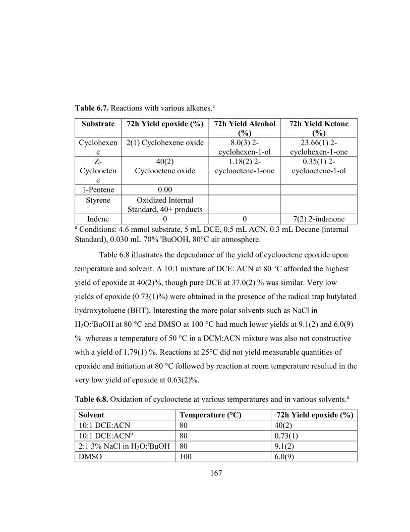
167

Table 6.7. Reactions with various alkenes.a

Substrate 72h Yield epoxide (%) 72h Yield Alcohol (%)

72h Yield Ketone (%)

Cyclohexene

2(1) Cyclohexene oxide 8.0(3) 2-cyclohexen-1-ol

23.66(1) 2-cyclohexen-1-one

Z-Cycloocten

e

40(2) Cyclooctene oxide

1.18(2) 2-cyclooctene-1-one

0.35(1) 2-cyclooctene-1-ol

1-Pentene 0.00

Styrene Oxidized Internal Standard, 40+ products

Indene 0 0 7(2) 2-indanone a Conditions: 4.6 mmol substrate, 5 mL DCE, 0.5 mL ACN, 0.3 mL Decane (internal Standard), 0.030 mL 70% tBuOOH, 80°C air atmosphere.

Table 6.8 illustrates the dependance of the yield of cyclooctene epoxide upon

temperature and solvent. A 10:1 mixture of DCE: ACN at 80 °C afforded the highest

yield of epoxide at 40(2)%, though pure DCE at 37.0(2) % was similar. Very low

yields of epoxide (0.73(1)%) were obtained in the presence of the radical trap butylated

hydroxytoluene (BHT). Interesting the more polar solvents such as NaCl in

H2O:tBuOH at 80 °C and DMSO at 100 °C had much lower yields at 9.1(2) and 6.0(9)

% whereas a temperature of 50 °C in a DCM:ACN mixture was also not constructive

with a yield of 1.79(1) %. Reactions at 25°C did not yield measurable quantities of

epoxide and initiation at 80 °C followed by reaction at room temperature resulted in the

very low yield of epoxide at 0.63(2)%.

Table 6.8. Oxidation of cyclooctene at various temperatures and in various solvents.a

Solvent Temperature (°C) 72h Yield epoxide (%) 10:1 DCE:ACN 80 40(2) 10:1 DCE:ACNb 80 0.73(1) 2:1 3% NaCl in H2O:tBuOH 80 9.1(2) DMSO 100 6.0(9)

168

10:1 DCM: ACN 50 1.79(1) 10:1 Chlorobenzene:ACN 80 15.0(2) 10:1 1,1,1-trichloroethane:ACN

80 17.5(2)

ACN 80 28.9(5) DCE 80 37.0(2) 10:1 DCE: ACN 25 0.00 10:1 DCE: ACN Heat at 80 for 30 minutes

then cool to room temp 0.63(2)

10:1 DCE: ACN (11 mL) 80 9.22(9)c

aConditions: 4.6 mmol Z-cyclooctene, 5.5 mL solvent total, varying temp (50-100°C) see above, 0.030 mL 70% tBuOOH, 72 hrs, air atmosphere. bReaction contained 551 mg of BHT. cAlso produced 0.42(2)% ketone and 0.315(4)% diol.

Experiments were also conducted under different atmospheres where the

concentration of oxygen varied from 0 to 100%, Table 6.9. Reactions under 100%

oxygen afforded the highest yield of epoxide, 49.1(7)% compared to under air at

40(2)%, whereas those under nitrogen or in a sealed glass tube where the oxygen

supply was restricted, had very low yields of epoxide probably resulting from the direct

reaction of the added tBuOOH and cyclooctene. An experiment with one equivalent of tBuOOH per cyclooctene conducted under nitrogen resulted in 14.1(1)% of the

epoxide, 5.3(2)% of 2-cycloocten-1-one and 5.1(4)% 1,2-cyclooctanediol.

Table 6.9. Oxidation of cyclooctene under different atmospheres.a

Atmosphere 72h Yield epoxide (%) Air 40(2) Oxygen Oil Bubbler Backpressure 49.1(7) Nitrogen Oil Bubbler Backpressure 1.76(2) Sealed Glass Tube 2.7(1) Nitrogen with 100% equiv tBuOOH 14.1(1)b

aConditions: 4.6 mmol Z-cyclooctene, 5 mL DCE, 0.5 mL ACN, 0.3 mL Decane (internal Standard), 0.030 mL 70% tBuOOH, 80°C, 72 hrs. b 502 mg Z-Cyclooctene, 0.610 mL 70% tBuOOH, also produces 5.3(2)% 2-cycloocten-1-one and 5.1(4)% 1,2-cyclooctanediol.

169

Table 6.10 shows the reactions of cyclooctene with various oxidizers. The

amount of 0.05 eq 70% tBuOOH produced the highest yield of epoxide at 40.2(2) equal

to that when one equivalent was used.

Table 6.10. Reactions of cyclooctene with various oxidizers.a

Oxidizer 72h Yield epoxide (%) 0.05eq 70% tBuOOH 40(2) None 0 0.05eq 70% tBuOOH added at start then 24h and 48h

41(2)

0.05eq 30%H2O2 31(2) 0.05eq Cyclooctene oxide 3.9(1) 0.9eq Ammonium persulfate 0 1eq 70% tBuOOH 40(2)

aConditions: 4.6 mmol Z-cyclooctene, 5 mL DCE, 0.5 mL ACN, 0.3 mL Decane (internal Standard), Varying oxidizers, 80°C Air atmosphere

Mechanistic and theoretical calculations

The direct reaction between tBuOOH and either cyclohexene or cyclooctene is

accomplished with an activation energy calculated to be 33.15 or 30.05 kcal/mol,

respectively, and is exothermic with ΔHreact = -49.87 and -52.94 kcal/mol respectively,

see Figs. S1 and S2. This activation energy is comparable to that required to break the

peroxide O–O bond which was calculated to be 33.12 kcal/mol, Fig. S3, but the

binuclear reaction also requires a collision to occur whereas the bond rupture is

unimolecular and presumably occurs at 80 °C. This value of 33.12 kcal/mol is similar

to that from other low level calculations (around 34 kcal/mol) though higher level

calculations in the case of tBuOOH puts the O–O bond homolysis at 41 kcal/mol.217

Proposed mechanisms for the formation of the products observed from the

reactions between tBuOOH and cyclohexene or cyclooctene are displayed in Schemes

6.1 and 6.2 respectively. It is necessary to invoke a free radical mechanism as the yield

of products far

170

O +

OH OH

+ HOH

O2

OO

+

OOHOH

OH

OOO

O

O

OHO OH

O OH H2O

S3, 33.12, 30.55

S6, 14.46, 1.57

S6, 7.11, -30.41

S5, 1.36, -12.76S5, 37.59, 0.04

S5, 0, -50.26

S7, 15.28, -0.54

S9, 49.04, -73.18

23.7%

8.01%

2.01%

S4, 4.28, -19.81

S6, 7.11, -30.41

OHO

S8, 30.73, 27.67

S10, 5.55, -13.21

S11, 36.87, 1.54

Scheme 6.1. Proposed mechanism for the free radical transformation of cyclohexene into the products observed. A potential energy plot for each transformation was calculated and the supplementary figure numbers, the activation energy and ΔHr in kcal/mol are indicated in that order.

exceeds the quantity of peroxide (i.e., 5% molar equivalents of peroxide to alkene)

added to the reaction mixture. As can be seen on the top left in Scheme 6.1, the

generation of a cyclohexene radical is accomplished at an activation energy of 4.28

kcal/mol and the subsequent reaction with oxygen would then be almost instantaneous

with an activation energy of 1.36 kcal/mol. Both reactions are exothermic at -19.81 and

-12.76 kcal/mol respectively. These low values in the activation energies for the

generation of the cyclohexene peroxy radical would suggest that the concentration of

the cyclohexene peroxy radical is much greater than the concentration of the

cyclohexene radical and subsequent reactions which have higher activation energy

barriers would proceed at a slower rate.218It is likely that cyclohex-2-en-1-ol is

produced from the direct reaction of cyclohexene radical with an hydroxy radical as

171

shown in the top center of Scheme 6.1 and, notably, this compound is obtained in 8.01

% yield.

The formation of 2-cyclohexen-1-one can proceed via two pathways. One of

these, a unimolecular mechanism, involves a hydrogen atom 1-3 migration on the

cyclohexene peroxy radical with subsequent rapid O–O bond cleavage resulting in 2-

cyclohexen-1-one and a hydroxy radical with an activation energy of 37.59 kcal/mol as

shown on the top right of Scheme 6.1 and Fig. S6.5. The other pathway involves a

bimolecular reaction between the cyclohexene peroxy radical and cyclohexene

resulting in hydrogen abstraction to form 1-hydroperoxycyclohex-2-ene and a

cyclohexene radical with the subsequent generation of 2-cyclohexen-1-one and water at

activation energies of 15.28 and 49.04 kcal/mol respectively. The 3-

hydroperoxycyclohex-1-ene molecule can also undergo homolytic O–O bond fissure

resulting in 1-oxo-cyclohex-2-ene and hydroxy radicals as shown on the bottom right

of Scheme 6.1.

The formation of cyclohexene epoxide (7-oxabicyclo[4.1.0]heptane) can be

envisaged via two pathways as depicted in the center and bottom left of Scheme 6.1.

The direct reaction between a cyclohexene peroxy radical and cyclohexene leads to a

peroxide bridged radical species at an activation energy of 14.46 kcal/mol, Fig. S6.6,

with subsequent rearrangement to form the epoxide and the 1-oxo-cyclohex-2-ene

radical. This radical which is also produced as a result of homolytic fission of the O–O

bond in 1-hydroperoxycyclohex-2-ene can also react with cyclohexene to form a oxo-

bridged radical which can decompose into the epoxide and cyclohexene radical at

activation energies of 5.55 and 36.87 kcal/mol respectively. Pictures of the LCAOs for

the HOMOs in the oxo- and peroxo-bridged radicals, Fig. 1, indicate that the odd

electron is mostly localized on the carbon atom indicated in Scheme 6.1.

172

Figure 6.1. Drawings of the LCAOs for the HOMOs for the oxo- (left) and peroxo-bridged (right) species depicted in Scheme 6.1.

The yields of the compounds obtained, namely the 8.01% of alcohol, the 23.7%

of the alkene ketone and the 2.01% of the epoxide would suggest that a unimolecular

free radical pathway is favored as this would generate sufficient hydroxy radicals to

yield the 8.01% of alcohol and the 23.7% of the ketone.

An examination of the heat of reaction as listed in Scheme 6.1 shows that

breaking the O–O bond in the peroxide structures is endothermic at 30.55 kcal/mol for tBuOOH and 27.67 kcal/mol for 3-hydroperoxycyclohex-1-ene. The most

thermodynamically favored product is 2-cyclohexen-1-one which most likely results

from the pathway on the top right of Scheme 6.1.

With cyclooctene, similar activation energies are obtained for some of the

proposed reactions, Scheme 6.2. The activation energies for the formation of

cyclooctene radical and subsequent reaction with oxygen are calculated to be 2.22 and

0.80 kcal/mol respectively. Subsequent activation energies are much higher which

would lead to an increased concentration of the cyclooctene peroxy radical depicted on

the top of Scheme 6.2. The calculated activation energies for subsequent reactions for

the bimolecular pathway (which lead to formation of epoxide) are much lower than that

for the unimolecular step (depicted on the top of Scheme 6.2) and it is possible that this

peroxy radical is more stable than that of cyclohexene and this allows the bimolecular

pathway to proceed leading to the yield of cyclooctene epoxide (9-

oxabicyclo[6.1.0]nonane, 40.3%) obtained. It is noteworthy that the calculated

173

activation energy for the biscyclooctene peroxide bridged dimer at 5.73 kcal/mol is

much lower than that for the equivalent step in the cyclohexene pathway at 7.11

kcal/mol and this may also be contributing to the increase yield of epoxide product

with cyclooctene. The reaction of the 1-oxo-cyclooct-2ene radical with cyclooctene to

form an ether radical as shown on the bottom of Scheme 6.2 is calculated to have an

activation energy of 23.77 kcal/mol which is much higher than that for the equivalent

reaction with cyclohexene at 5.55 kcal/mol. Subsequent decomposition of the ether

radical affords the epoxide and more cyclooctene radical at an activation energy of

29.96 kcal/mol which is lower than the equivalent reaction in the case of cyclohexene

at 36.87 kcal/mol. It is interesting that this pathway with the formation of the ether

radical yields the cyclooctene radical and as a substantial quantity of the cyclooctene

radical must be produced to have a 40.3% yield of the epoxide, this pathway must be

operative. We do not see any (Z)-cyclooct-2-en-1-ol under the conditions of the

experiment so the 1-oxo-cyclooct-2-ene radical is not abstracting a hydrogen atom

from cyclooctene and the ether radical is produced.

OOH O +

OH OH

+ HOH

O2

OO

O

OHO

OH

OH

O

O

OH1.2%

40.3%

H2O

O2.8 %

H2O

OO

+

S3, 33.12, 30.55

S12, 2.22, -21.26

S13, 0.80, -17.69

S20, 5.73, -31.69

S21, 29.96, -2.27 S20, 5.73, -31.69

S19, 23.77, -6.76

S18, 33.16, 29.40

S17, 44.21, -71.94S15, 14.15, 1.40 S16, 14.72, 0.66

OHO

S14, 33.32, -2.45OH

174

Scheme 6.2. Proposed mechanism for the free radical transformation of cyclooctene into the products observed. A potential energy plot for each transformation was calculated and the supplementary figure numbers, the activation energy and ΔHr in kcal/mol are indicated in that order.

Drawings of the LCAOs for the HOMOs in the oxo- and peroxy-bridged dimeric radicals, Fig. 6.2, situate the radical on the carbon atom depicted in Scheme 6.2.

Figure 6.2. Drawings of the LCAOs for the HOMOs for the oxo- (left) and peroxo-bridged (right) species depicted in Scheme 6.2.

As was the case with cyclohexene, the most thermodynamic favored product appears to

be (Z)-cyclooct-2-en-1-one, Scheme 6.2. Experimentally this compound is only

obtained with a yield of 2.8% in contrast to the less thermodynamically favored

epoxide product at 40.3%.

6.5 Discussion In most cases the reaction was allowed to go for 72 h and involved 5% of

peroxide to cycloalkene substrate. A wide range of experiments were conducted to

determine if oxygen was required.for the reaction. The data in Table 6.1 show that

slightly more of the epoxide product is obtained under pure oxygen with less of the 2-

cyclohexe-1-one compound with similar conversion rates of around 32%. For

cyclooctene, more epoxide is produced under pure oxygen (49.1(7)% compared to

40(2) % under air, Table 6.9. The results under nitrogen gas or in a sealed glass tube

with a small quantity of oxygen were also similar at 1.76(2)5 and 2.7(1) %

respectively, suggesting that a direct reaction between the added peroxide agent at 5%

175

molar equivalents was capable of producing some epoxide at a very lower yield. Under

nitrogen and with 100% equivalent peroxide added, we find only 14.1(1) % yield of the

epoxide with some cyclooct-2-en-1-one, 5.3(2)%, and 1,2-cyclooctanediol, 5.1(4)%,

also being produced. The reaction appears not to involve catalysis by the surface of the

glass container. Experiments done using a Teflon container with a similar volume of

trapped oxygen from the air above the mixture did not result in significant differences

in yields as the data in Table 6.4 illustrate. Under these experimental conditions, many

products were observed with styrene as substrate, none for 1-pentene and indene

afforded 7(2)% of indanone, Table 6.7. The reaction is based on free radicals as

experiments conducted in the presence of the free radical trap BHT only resulted in

very low yields of epoxide, i.e., 0.73(1) % in the case of cyclooctene, Table 6.8.

The nature of the oxidizing agent was also examined. The data in Table 6.10

show that an oxidizer is required with ammonium persulfate not affording any epoxide

and cyclooctene oxide remaining unchanged. Five percent equivalents of H2O2 to

substrate produced less epoxide at 31(2)% compared to 5% and 100% equivalent tBuOOH where an identical yield was obtained at 40(2)%.

The reaction can be initiated with either tBuOOH or H2O2 in the case of

cyclohexene, Table 6.2, and similar conversions are obtained at 33.68 and 35.16%

respectively. We had previously reported results for cyclooctene but at that time did not

contemplate a free radical mechanism but had used catalysts such as

MCl2(O)2(OPMePh2)2, M = Mo or W, where yields of the desired epoxide were 100%

and 61% respectively after 24 h.219The fact that reactions without the catalysts

involving just tBuOOH and cycooctene resulted in significant quantities of epoxide at

26% at 90 oC and 6 h was also noted but this was with stoichiometric equivalence.

Given the nature of the products obtained in the oxidation of cyclohexene,

measurements of the reaction mixture were determined after 24, 48 and 72 h and these

demonstrated that the quantities of alcohol and ketone increased with time, Table 6.3.

However it is not clear from this experiment if the epoxide was initially produced and

176

then transformed into the other products. Results of experiments to probe the stability

of the products under reaction conditions in the case of cyclohexene are listed in Tables

6.5 and 6.6 for 2-cyclohexen-1-ol and cyclohexene oxide respectively. Both of these

compounds are stable in the absence of 5% equivalents of peroxide but 2-cyclohexen-

1-ol does result in 38.93(8)% yield of 2-cyclohexen-1-one after 72 hours under air but

only 5.8(2) % under nitrogen which is slightly larger than the stock solution which had

3.1(1)%. In contrast there are no significant changes in the concentration of

cyclohexene oxide and 2-cyclohexen-1-ol when subjected to 5% peroxide or heated in

its absence, Table 6.6. Increasing the reaction temperature to 100 oC in DMSO only

resulted in 6.0(9)% yield of epoxide. Interestingly, increasing the volume of solvent

used from 5.5 to 11 mL resulted in a 9.22(9)% yield of epoxide, much reduced from

that obtained with 5.5 mL at 40(2)%.

These experimental results are in keeping with the proposed mechanisms

shown in Schemes 6.1 and 6.2. The reaction temperature of 80 oC is required for the

homolysis of the peroxide O–O bond with subsequent generation of the alkene

peroxide radical. This can then essentially react with free cycloalkene to produce a

peroxide bridged radical which can decompose to form the epoxide and an oxoradical

which is the dominant reaction in the case of cyclooctene. The oxoradical can also

react with cycloalkene to produce a bridging oxide radical which can decompose to

produce an epoxide and a cycloalkene radical which can then react with oxygen

initiating another cycle. This step is important in generating free cycloalkene radicals

to obtain the experimental yields. Running the reaction under more dilute conditions

resulted in a much lower yield of the epoxide in the case of cyclooctene providing

experimental evidence of this bimolecular pathway. It is not obvious why under these

conditions, the oxidation of cyclohexene results mostly in the ketone 2-cyclohexen-1-

one. The pathway suggested for the formation of this compound is via a unimolecular

pathway, Scheme 6.1, and the transition state activation energy for this pathway is

higher than that for the bimolecular pathway a circumstance which pertains for both

cyclohexene and cyclooctene. While it is established that the lower transition state

177

pathway may not be the one utilized in a unimolecular reaction,220, 221 the fact that

under more dilute conditions less of the epoxide was formed with cyclooctene, Table

6.8, suggests that it is not useful to comparing transition states between unimolecular

and bimolecular pathways as the route with the lower activation energy may not be the

one chosen. For cyclooctene, the bimolecular pathway appears to function with more

concentrated solutions but with cyclohexene, the unimolecular one may be operative.

Tables 6.11 and 6.12 lists a subsection of literature results using tBuOOH, H2O2

and O2 as the oxygen source (more comprehensive listings including reaction details

are available as supplementary information, Table S6.1-S6.6) where, in some cases, a

range of products are obtained for cyclohexene and cyclooctene respectively. This

listing is compromised as different reaction conditions of temperature, solvent, ratio of

peroxide to substrate are involved and these complicate direct comparison to the results

reported here. However, it is likely that those listings in Table 6.11 closest to the

products obtained herein or with mixtures of products are functioning not under

catalytic conditions but via free radical mechanisms such as those depicted in Scheme

6.1. The yields of the products were calculated from the conversions listed together

with the percentages of products obtained. One immediate conclusion from an

examination of these listings is that with cyclohexene, Table 6.11, the major product in

most cases is the alkene oxide, whereas with cyclooctene, Table 6.12, the epoxide is

the major product.

It is important to note that nearly all the reactions listed were conducted with

greater than 100% equivalence of peroxide to substrate as the idea was to directly

transfer the O atom. This reason, together with the temperature at which the reaction

was conducted, may account for some variation in the products obtained. For

cyclohexene, Table 6.11, the composition of the product changes from 100% epoxide

to 100% cycloalkene ketone with a very rough correlation from homogeneous to

heterogeneous catalysts as an examination of the column for catalyst in the table would

reveal. This would suggest that the catalysts are forming peroxides which are more

effective at transferring a more activated oxygen atom to the cycloalkene resulting in

178

the epoxide whereas with a heterogeneous catalyst (or perhaps nanoparticles), it is

more difficult for such a transfer to take place and the cycloalkene ketone results,

perhaps from a unimolecular pathway. In all the listed cases for cyclohexene, the use of

group 6 transition metal catalysts showed some of the highest yields for epoxide with

the trend of Mo>W>>Cr with Cr resulting in 2-cyclohexen-1-one. Other transition

metal catalysts such as Fe, Au, Ag, Cu, Rh, Mn, Co, Zn, Ti, Ru, and V were used and

produced a wide variety of products. Comparing Mn porphyrin cage (93% epoxide)

and Mn(Oac)2·4H2O (85% ketone) demonstrates that the transition metal may not be

the determining factor as one produces mainly cyclohexene epoxide (presumably

homogeneous) and the other produces 2-cyclohexen-1-one (perhaps nanoparticles). Of

note is the reaction employing 0.05 eq of tBuOOH with the catalyst Au/CNTs-

IM222where yields of 43.6% cyclohexene oxide, 7.48% 2-cyclohexen-1-ol and 6.38%

2-cyclohexen-1-one are obtained in contrast to that reported here at 2.01, 8.01 and

23.7% respectively. This may well be related to the fact that Au does not form multiple

bonds with oxygen atoms223 and hence a more facile transfer of Au bonded O atom to

the double bond resulting in cyclohexene oxide is possible. It is curious that many of

the listed reactions involved greater than 100% molar equivalents of peroxide to

cycloalkene and this presumably compensates for catalytic decomposition of the

peroxide on the metal surface.

Table 6.11. The yields of products from the oxidation of cyclohexene using O2, tBuOOH or H2O2 as the oxidizer. See references for other conditions of the reactions. A dash indicates that the yield for that product if present was not reported.

Catalyst Oxidant Yield O

Yield HO

Yield O

Yield HO OH

Others Ref.

[MoO2Cl2(H2O)2]· (H2dipy-pra)Cl2, NaHCO3

4 eq H2O2 99 - - - - 224

H3PW12O40 2 eq H2O2 78.2 - - - - 225 [MoO(O2)2 4,4-bipy]n 2.5 eq H2O2 95 - - - - 226

(4-ddp)1.5Na5.5[PTi2W10O40]·5

H2O

2 eq H2O2 9.02 - - 1.65 - 227

179

(VOTPPCl8) 2 eq H2O2 99 - - - - 228 Co-salen-SBA15 2 eq H2O2 60 - - - - 229

Mn porphyrin cage 1 atm O2 93 - - - - 230 NHPI, Co(OAc)2, and

Mo(CO)6, 4Å MS 1 atm O2 59.2 - - - - 231

Fe3O4/tart/Mn(TCPP)Cl 1 atm O2 86 12 - - - 232 Cu-MOF 1 atm O2 0.16 0.22 0.47 - 6.14OOH

a

233

TBA5Na3[(Cp∗)Rh·P2W15Nb3O62]

1 atm O2 - 0.10 0.8 - - 234

No Catalyst 2 eq TBO - - 1.12 - - 235 [LMn(OAc)2] 2 eq H2O2 61.4 3.6 2.2 - - 236

VO(acac)2 1 atm O2 6.5 2.6 2.34 - 14.6EPOHa

237

[Cu-Imace-H-H][BF4] 1 atm O2 50.4 1.8 5.4 - - 238 Mo(VI)Cl2O2Bipy/TiO2SC-150 fresh (photocatalysis)

1 atm O2 45.4 3.82 5.47 - - 239

Au/CNTs-IM 0.05eq TBO 43.6 7.48 6.38 - - 222 TBA16[Co4(P2W15O56)2] 9 eq H2O2 3.23 5.7 10.1 - - 240 TBA₅Na₃[(COD)Ir·P₂W

Nb₃O₆₂] 1 atm O2 2 10 12 - - 234

Cu(H2btec)(bipy) MOF 1 eq TBO 47.15 - 12.38

- 4.97 ANONEa

241

[LFe(OAc)2] 0.5 eq H2O2 3.1 9.8 13.4 - - 236 TBA16[Ni4(P2W15O56)2] 9 eq H2O2 3.24 8.1 15.7 - - 240 [NSP]@MWNTs Nickel

salophen nanotubes 1 atm O2 - 49.8 19.5 - - 242

TBA16[Mn4(P2W15O56)2] 9 eq H2O2 10.0 7.03 20.0 - - 240 None 0.05 eq

H2O2 2.14 9.44 23.6 - - TW

b

None 0.05 eq TBO

2.01 8.01 23.7 - - TWb

CFO‐Ce0.3 1.5 eq H2O2 1.47 15.7 26.4 - - 243 TBA₄.₅Na₂.₅[(be·

nzene)Ru·P₂W₁₅Nb₃O₆₂] 1 atm O2 8 20 28 - - 234

(nBu4N)4W10O32/SiO2/ Fe(TDCPP)Cl+hν+Dark 3

hrs

1 atm O2 1.4 20 29 - 1.6ETHa

48OOHa

244

TBA8[(CO)3Re·P2W15Nb3O62]

1 atm O2 7 20 30 - - 234

LFe(NO3) 1 eq H2O2 10.5 29.5 35.3 11.1 - 245 Cr-MCM-41 2 eq TBO - - 39.0 - - 235 Co-g-C3N4 39.5 atm O2 - 12.9 40.1 1.06 - 246

TBA12[Fe4(P2W15O56)2] 9 eq H2O2 23.6 9.88 42.6 - - 240 TBA16[Zn4(P2W15O56)2] 9 eq H2O2 33.9 8.7 44.4 - - 240

BNO2-Cu-TDCPP 3.95 atm O2 - 13.8 45.5 - 6.60OTHERS

247

LRuCl 1 eq H2O2 13.0 30.8 47.1 5.17 - 245 Cr‐MCM‐41 2 eq H2O2 - - 47.3 - - 248 Fe(TPP)Cl 1 atm O2 - - 52 - - 249

Calcined CuO catalyst 3.95 atm O2 4.41 31.1 54.4 - - 250

180

Cr‐MCM‐48 2 eq TBO - - 55.6 - - 235 Diacetoxyiodobenzene

K2CO3 4 eq TBO - - 56 - - 251

AgNP-MCM-41 0.05 eq TBO

0.69 18.0 59.4 - - 252

Rh2(cap)4 5 eq TBO - - 60 - - 253 MgCl2/NHPI 3 atm O2 - - 60.3 - - 254

Cr‐mZrP 2 eq H2O2 - - 63 - - 255 CoCl2 1 atm O2 - 4 71 - - 256

g-C3N4/NHPI 1 atm O2 - - 71.6 - - 257 Cu(II) salqu complex 3 eq TBO - - 74 - - 258

CoCr‐HTSi2 1 eq H2O2 - 26 74 - - 259 [Cu(Pht)(Im)2]·1.5H2On 9 eq H2O2 11.3 11.5 75.2 - - 260 [Mn(C6H5COO)(H2O)-(phen)2](ClO4)(CH3OH)

8 eq TBO 4.6 2.5 76 11.2 - 261

[C10mim] [Co(F6-acac)3] 1 atm O2 -- - 81 - - 262 Mn(Oac)2·4H2O 2 eq TBO - - 85 - - 263

Ag‐VPO 3 eq TBO - - 86.3 - - 264 Fe3O4 MNPs 3 eq TBO - - 87 - - 265

[(TAML)Fe(III)] − 1 atm O2 11 - 89 - - 266 Au-Silica 8-13 atm O2 - 2.76 89.2 - - 267 CoEPS3 6 eq TBO - - 90 - - 268

asee Fig. S22. bThis work.

We find that for cyclooctene, 5 mole% tBuOOH resulted in 40.3% epoxide,

0.35% of 1,2-cyclooctanediol, and 1.18% of 2-cycloocten-1-one suggesting that

oxygen and free radicals must be involved in this reaction, Table 6.12. The use of

group 6 transition metal catalysts also showed some of the highest yields for producing

the epoxide with the trend of Mo > W. This may be due to differences in M–O bond

strength as tungsten is reported to form very strong bonds with oxygen.269 Other

transition metal catalysts such as Fe, Au, Ag, Cu, Rh, Mn, Co, Zn, Ti, Re, and V were

also employed but produced a variety of products. Interestingly large tungsten oxide

clusters, e.g., TBA16[Ni4(P2W15O56)2], TBA12[Fe4(P2W15O56)2],

TBA16[Zn4(P2W15O56)2],[32] resulted in significant quantities of the ketone, 2-

cycloocten-1-one and 1,2-cyclooctanediol at 19.1, 47.8 and 43% yield

respectively.236Due to the different conditions used (lower temperatures and 200 to 900

mole % equivalents of peroxide) it is not reasonable to compare this work with the

others listed in Table 6.12, but in these reactions, some decomposition of the peroxide

may be occurring rending the possibility of free radical reactions. It was also found that

the amount of ketone produced increased as the quantity of peroxide used in the

181

reaction increased.270 It is possible that reactions affording less than 40% of epoxide

product are occurring via free radical mechanisms but those greater than 50% may well

involve metal atom catalyst.

Table 6.12. The yields of products from the oxidation of cyclooctene using O2, tBuOOH (TBO) or H2O2 as the oxidant. See references for other conditions of the reactions. A dash indicates that the yield for that product was not reported.

Catalyst Oxidant Yield O

Yield OHHO

Yield O

Yield OH

Yield

OHO

Ref.

Nonea 2 eq H2O2 - - - - - 240 (nBu4N)4W10O32+hν 1 atm O2 1.9 - - - 5.8 244

VO(acac)2 1 atm O2 2.97 - - - - 237 TBA16[Co4(P2W15O56)2] 9 eq H2O2 4.51 - 4.4 2.09 - 240 TBA16[Ni4(P2W15O56)2] 9 eq H2O2 6.93 - 19.1 6.93 - 240

Au on SiC 1.5 eq TBO 8.07 - - - - 271 TBA16[Mn4(P2W15O56)2] 2 eq H2O2 10.7 - 12.2 3.12 - 240

[LFe(Oac)2] 0.5 eq H2O2 19.5 - - - - 236 Au/CNTs-IM 0.05 eq

TBO 24.0 - 4.59 4.26 - 222

TBA12[Fe4(P2W15O56)2] 9 eq H2O2 30 - 47.8 3.24 - 240 TBA16[Zn4(P2W15O56)2] 9 eq H2O2 31 - 43 12 - 240

None 0.05 eq H2O2

31.0 - - - - TWb

MoCl2(O)2(OPMePh2)2 1.5 eq H2O2 35 - - - - 219 None 0.05 eq

TBO 40.3 0.35 1.18 - - TWb

[MoO(O2)2 4,4-bipy]n 2.5 eq H2O2 41 - - - - 226 WCl2(O)2(OPMePh2)2 1.5 eq TBO 61 - - - - 219

(LMnCl2) 2 eq H2O2 64 - - - - 236 Fe3O4 MNPs 3 eq TBO 70 - - - - 265

(4-ddp)1.5Na5.5[PTi2W10O40]·5

H2O

2 eq H2O2 70 - - - - 227

Gold Clusters 1 atm O2 70 - - - - 272 WCl2(O)2(OPMePh2)2 1.5 eq H2O2 70 - - - - 219

AgNP-MCM-41 0.05 eq TBO

72.4 - 2.02 0.22 - 252

NHPI, Co(OAc)2, and Mo(CO)6, 4Å MS

1 atm O2 73.9 - - - 0.1 231

γ-SiW10Fe3+(OH2)2O386− 1 atm O2 80.4 - - - - 273

Mn porphyrin cage 1 atm O2 89 - - - - 230 H3PW12O40 2 eq H2O2 89.3 - - - - 225

182

Fe3O4/tart/Mn(TCPP)Cl 1 atm O2 96 - - - - 232 [MoO₂Cl₂(H₂O)₂]· (H₂dipy-

pra)Cl₂, 4 eq H2O2 99 - - - - 224

[CH₃ReO₃] 2 eq H2O2 100 - - - - 274 MoCl2(O)2(OPMePh2)2 1.5 eq TBO 100 - - - - 219

aReaction conducted at 50 oC. bTW = this work.

Of particular note are those reactions catalyzed in the presence of just oxygen.

The catalyst labelled as Mn porphyrin cage (representing a supramolecular manganese

porphyrin complex) requires an aldehyde reductant (i.e., 10 equivalents of

isobutyraldehyde) and results in remarkable yields of epoxide in the case of

cyclohexene (93%, Table 6.11) and cyclooctene (89%, Table 6.12).230This reaction

does not proceed in the presence of BHT suggesting that free radical species are

involved.230 In contrast to the mechanisms suggested in Schemes 6.1 and 6.2, the

proposed mechanism in this case involves the formation of an acyl radical from

isobutyraldehyde with subsequent formation of a peroxide by reaction with oxygen

which results in the formation of a manganese oxide that transfers the O atom to the

alkene resulting in the epoxide. This shows that very complex mechanisms pertain to

the systems listed in Tables 6.11 and 6.12.

6.6 Conclusions

A variety of experimental conditions including using a Teflon container to

conduct the reaction, changing reaction concentration and temperature, using the free

radical trap BHT, using different solvents and oxygen or nitrogen atmospheres

permitted the conclusion that the oxidation of cyclohexene and cyclooctene in the

presence of 0.05 equivalents of either H2O2 or tBuOOH under oxygen occurs via the

formation of free radicals. Under the stated reaction conditions 23.7% 2-cyclohexen-1-

one, 8.0% 2-cyclohexen-1-ol and 2.0% cyclohexene oxide were obtained for

cyclohexene and 40.3% epoxide, 0.35% of 1,2-cyclooctanediol, and 1.18% of 2-

cycloocten-1-one for cyclooctene. Two Schemes were proposed which suggested that

the formation of ketones required higher activation energies based on Gaussian

calculations and occurred via a unimolecular pathway and that the formation of

183

epoxide required lowed activation energies was bimolecular. The data suggests that

some results in the literature may well be the result of free radical reactions.

6.7 Supplementary Data for Chapter 6

Figure S6.1. PE plot for the reaction between cyclohexene and tBuOOH.

184

Figure S6.2. PE plot for the reaction between cyclooctene and tBuOOH.

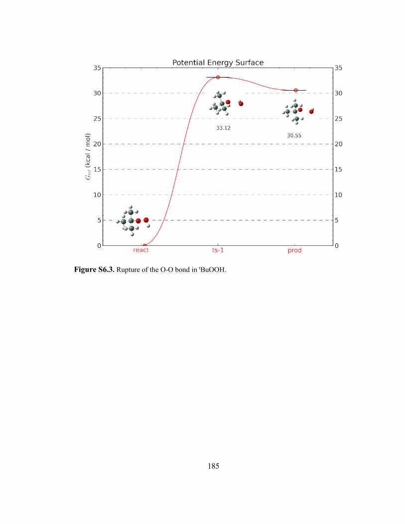
185

Figure S6.3. Rupture of the O-O bond in tBuOOH.

186

Figure S6.4. Abstracting a proton from cyclohexene by the tBuO• radical

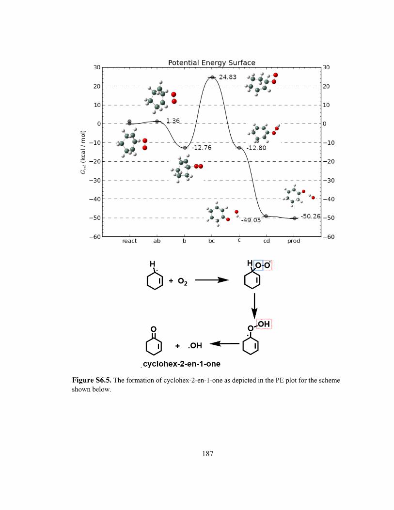
187

.

Figure S6.5. The formation of cyclohex-2-en-1-one as depicted in the PE plot for the scheme shown below.

188

Figure S6.6. The formation of cyclohexene oxide as depicted in the PE plot for the scheme shown below.

189

Figure S6.7. The formation of 3-hydroperoxycyclohex-1-ene as depicted in the PE plot for the scheme shown below the plot.

190

Figure S6.8. Rupture of the O–O bond in 3-hydroperoxycyclohex-1-ene to form 1-oxo-cyclohex-2-ene and hydroxide radicals.

191

Figure S6.9. The formation of cyclohex-2-en-1-one as depicted in the PE plot for the scheme shown below the plot.

192

Figure S6.10. The reaction of the 1-oxo-cyclohex-2-ene radical with cyclohexene to form a dicyclohexene ether radical.

Figure S6.11. Dissociation of the dicyclohexene ether radical into cyclohexene epoxide and cyclohexene radical.

193

Figure S6.12. Abstraction of a proton from cyclooctene by the tBuO• radical.

Figure S6.13. Reaction of O2 with the cyclooctene radical.

194

Figure S6.14. Hydrogen atom shift in the cyclooctene peroxy radical.

Figure S6.15. Reaction between cyclooctene and the cyclooctene peroxy radical to produce the peroxo-bridged radical dimer.

195

Figure S6.16. Formation of cyclooctene radical and (Z)-3-hydroperoxycyclooct-1-ene from the reaction between (Z)-1-peroxycyclooct-2-ene radical and cyclooctene.

Figure S6.17. The formation of (Z)-cyclooct-2-en-1-one from (Z)-1-hydroperoxycyclooct-2-ene.

196

Figure S6.18. Homolytic rupture of the peroxide bond in (Z)-3-hydroperoxycyclooct-1-ene.

Figure S6.19. Formation of the oxo bridged radical from the 1-oxocyclooct-2-ene radical and and cyclooctene.

197

Figure S6.20. Formation of 9-oxabicyclo[6.1.0]nonane and an alkene oxo radical from the fragmentation of the (Z)-9-(cyclooct-2-en-1-yloxy)-93-oxabicyclo[6.1.0]nonane radical.

Figure S6.21. Formation of 9-oxabicyclo[6.1.0]nonane and cyclooctene radical from the decomposition of the biscyclooctene ether radical.

198

O O OH OOH

O

EPO KET OH OOH ANONEO

OH

ETH

OHOH

DIOL

Figure S6.22. shows the structures that relate to the shorthand code for the molecules in Table S6.1, S6.2, and S6.3 below.

Table S6.1 contains the details of reactions from literature and this work of cyclohexene using t-butyl hydroperoxide as the oxidizer. Entries are listed in increasing order based on the yield of the 2-cyclohexen-1-one denoted as KET.

Catalyst Temp (°C)

Oxidizer Solvent Time (Hours)

Yields Ref.

No Catalyst 120 2eq TbuOOH

chlorobenzene 12 1.12%KET 235, 275

MCM-41 120 2eq TBuOOH

chlorobenzene 12 1.46%KET 235

MCM-48 120 2eq TBuOOH

chlorobenzene 12 1.89%KET 235, 276

Cu(H2btec)(bipy) MOF

30 1eq TBuOOH

DCE 24 18.44%EPO 4.60%ANONE 4.32% KET

241

Au/CNTs-IM 85 0.05eq TbuOOH

ACN 6 43.6%EPO 7.48%OH 6.38%KET

277


50 1eq TbuOOH

DCE 24 38.75%EPO 4.85%ANONE 9.97%KET

241


75 1eq TbuOOH

DCE 24 47.15%EPO 4.97%ANONE 12.38%KET

241

None 80 0.05eq TBuOOH

DCE/ACN 72 2.01%EPO 8.01%OH

This Work

199

23.7%KET Cr-MCM-41 120 2eq

TbuOOH chlorobenzene 12 39.0%KET 235

Cr‐MCM‐48 120 2eq TbuOOH

chlorobenzene 12 55.6%KET 235

Diacetoxyiodobenzene K2CO3

-20 4 eq TbuOOH

nPrCO2nBu 12 56%KET 251

AgNP-MCM-41 80 0.05eq TBuOOH

DCE/ACN 72 0.69%EPO 18.0%OH 59.4%KET

252

Rh2(cap)4 40 5eq TbuOOH

DCE 1 60% KET 253

Cu(II) salqu complex

70 3eq TBuOOH

ACN 1 74%KET 258

[Mn2(μ-C6H5COO)2(bipy)4]⋅2(ClO4)

70 8eq TBuOOH

ACN 1 3.8%EPO 2.8%OH 75.1%KET 11.8%DIOL

261

[Mn(C6H5COO)(H2

O)(phen)2](ClO4)(CH3OH)

70 8eq TBuOOH

ACN 1.5 4.6%EPO 2.5%OH 76%KET 11.2%DIOL

261

Mn(Oac)2·4H2O 0 2eq TbuOOH

DCM 0.33 85%KET 263

Ag‐VPO 82 3eq TbuOOH

ACN 6 86.3%KET 264

Fe3O4 MNPs 120 3eq TBuOOH

None 6 87%KET 265

Co ESP3 70 6eq TbuOOH

Benzene 16 90%KET 268

Co EPS3 50 6eq TbuOOH

ACN 24 90%KET 268

200

Table S6.2 contains the details of reactions from literature and this work of cyclohexene using hydrogen peroxide as the oxidizer. Entries are listed in increasing order based on the yield of the 2-cyclohexen-1-one denoted as KET. Following is the list based on the yield of cyclohexene oxide denoted as EPO.

Catalyst Temp (°C)


Yields Ref.

(LMnCl2) 25 2eq H2O2 ACN 6 53.3%EPO 21.%OH 1.7%KET

236

[LMn(OAc)2] 25 2eq H2O2 ACN 6 61.4%EPO 3.6%OH 2.2%KET

236

TBA16[Co4(P2W15O56)2]

50 2eq H2O2 ACN 6 4.4%EPO 2.2%OH 4.4%KET

240

TBA10[Co4(PW9O34)2

] 50 2eq H2O2 ACN 6 7.5%EPO

2.7%OH 4.8%KET

240

Fe Zeolite Y 80 1eq H2O2 ACN 18 7.3%EPO 5.0%KET

245

Ru Zeolite Y 80 1eq H2O2 ACN 18 6.1%EPO 5.7%KET

245

TBA10[Mn4(PW9O34)2

] 50 2eq H2O2 ACN 6 19.6%EP

O 2.24%OH 6.16%KET

240

TBA16[Mn4(P2W15O56

)2] 50 2eq H2O2 ACN 6 14.4%EP

O 2.64%OH 6.96%KET

240

LFeCl2 25 0.5eq H2O2 ACN 24 2.66%EPO 7.96%OH 8.87%KET

236

TBA16[Co4(P2W15O56)2]


240

201

TBA10[Co4(PW9O34)2

] 50 9eq H2O2 ACN 6 5.04%EP

O 5.67%OH 10.3%KET

240

None 70 1eq H2O2 Methanol 12 8.84%EPO/DIOL 6.76%OH 10.4%KET

259

TBA16[Ni4(P2W15O56)2]


240

TBA10[Zn (PW9O34)2] 50 2eq H2O2 ACN 6 70.4%EPO 4.4%OH 13.2%KET

240

[LFe(OAc)2] 25 0.5eq H2O2 ACN 24 3.1%EPO 9.8%OH 13.4%KET

236

TBA10[Ni4(PW9O34)2] 50 2eq H2O2 ACN 6 11.2%EPO 6.4%OH 14.4%KET

240

TBA16[Zn4(P2W15O56)2]

50 2eq H2O2 ACN 6 49%EPO 6.3%OH 14.7%KET

240

TBA10[Mn4(PW9O34)2

] 50 9eq H2O2 ACN 6 12.6%EP

O 6.12%OH 15.2%KET

240

TBA16[Ni4(P2W15O56)2]


240

TBA12[Fe4(P2W15O56)2]

50 2eq H2O2 ACN 6 42.9%EPO 4.62%OH

240

202

18.5%KET

TBA6[Fe4(PW9O34)2] 50 2eq H2O2 ACN 6 53.9%EPO 3.85%OH 19.3%KET

240

TBA16[Mn4(P2W15O56

)2] 50 9eq H2O2 ACN 6 10.0%EP

O 7.03%OH 20.0%KET

240

None 80 0.05eq H2O2 DCE/ACN

72 2.14%EPO 9.44%OH 23.6%KET

This work

CFO‐Ce0.3 90 1.5eq H2O2 1,4-dioxane

9 1.47%EPO 15.7%OH 26.4%KET

243


240

LFe(NO3) 80 1eq H2O2 ACN 18 11.1%DIOL 10.5%EPO 29.5%OH 35.3%KET

245


240

[Co(Pht)(Im)2]n 22 9eq H2O2 Acetone 1 1.94%EPO 18.7%OH 40.6%KET

260

TBA12[Fe4(P2W15O56)2]

50 9eq H2O2 ACN 6 23.6%EPO 9.88%OH

240

203

42.6%KET

[Cu(Pht)(Im)2]·1.5H2

On

22 4.5eq H2O2 Acetone 48 4.67%EPO 11.4%OH 43.4%KET

260

TBA16[Zn4(P2W15O56)2]


240

TBA10[Zn4(PW9O34)2] 50 9eq H2O2 ACN 6 44.6%EPO 9.9%OH 44.6%KET

240

(LRuCl) 80 1eq H2O2 ACN 18 5.17%DIOL 13.0%EPO 30.8%OH 47.1%KET

245

Cr‐MCM‐41 80 2eq H2O2 Methanol 12 47.3%KET

248

Cr‐mZrP 80 2eq H2O2 None 12 63%KET 255 CoCr‐HTSi2 70 1eq H2O2 Methanol 12 26%OH

74%KET 259


On

22 9eq H2O2 Acetone half

1 11.3%EPO 11.5%OH 75.2%KET

260


On

22 9eq H2O2 Acetone 48 1.49%EPO 6.78%OH 85.6%KET

260


On

22 9eq H2O2 Acetone 1 8.39%EPO 3.06%OH 87.7%KET

260


On

22 12 eq H2O2 Acetone 48 0.49%EPO 5.32%OH

260

204

Table S6.3 contains the details of reactions from literature and this work of cyclohexene using oxygen as the oxidizer. Entries are listed in increasing order based on the yield of the 2-cyclohexen-1-one denoted as KET. Following is the list based on the yield of cyclohexene oxide denoted as EPO.

93.4%KET

(4-ddp)1.5Na5.5[PTi2W10

O40]·5H2O

50 2eq H2O2 ACN/DCE

10 9.02%EPO 1.65%DIOL

227

H3PW11VO40 65 2eq H2O2 DCE 7 37.5%EPO

225

H3PW9Mo3O40 65 2eq H2O2 DCE 7 49.3%EPO

225

Co-salen-SBA15 90 2eq H2O2 None 0.033 60%EPO 229 H3PW12O40 65 2eq H2O2 DCE 7 78.2%EP

O 225

[MoO(O2)2 4,4-bipy]n 25 2.5eq H2O2 DCE 6 95%EPO 226 POSS–OIM8–PW 70 1.2eq H2O2 ACN 2 99%EPO 278 [MoO₂Cl₂(H₂O)₂]· (H₂dipy-pra)Cl₂

25 4eq H2O2 ACN 1.5 99%EPO 224

[MoO2Cl2(H2O)2]· (H2dipy-pra)Cl2, NaHCO3

25 4eq H2O2 ACN 1 99%EPO 224

(VOTPPCl8) 60 2eq H2O2 ACN/Water

0.5 99%EPO 228

Catalyst Temp (°C)


Yields Ref.

VO(acac)2 60 1 atm O2 None - None 237 VO(acac)2 60 1 atm O2 ACN 40 None 237 VO(acac)2 60 1 atm O2 t-butanol 40 None 237 VO(acac)2 60 1 atm O2 Aniline 40 None 237 VO(acac)2 60 1 atm O2 n-hexane 40 None 237 None 45 Oxygen

balloon None 15 None 233

Cu(BF4)2H2O 45 Oxygen balloon

None 15 None 233

Cu(BF4)2H2O+ppy 45 Oxygen Balloon

None 15 None 233

Cu-MOF 25 Oxygen balloon

None 15 None 233

205

TBA9P2W15Nb3O62

(control reaction) 38 1atm O2 DCM 24 None 234

(n-Bu₄N)₅Na₃[(1,5-COD)Ir·P₂W₁₅Nb₃O₆₂]

38 1atm O2 DMSO 24 None 234

Halloysite nanotubes supported PANI (PANI@HA/1 M/2.04-HCl)

70 2eq H2O2 None 24 97.7%DIOL 0.44%OH 0.05%KET

279

Cu-MOF 35 Oxygen Balloon

None 15 0.22%OOH 0.02%OH 0.06%KET

233

Cu-MOF 45 Oxygen Balloon

None 15 4.29%OOH 0.10%EPO 0.14%OH 0.28%KET

233

Cu-MOF 50 Oxygen balloon

None 15 6.14%OOH 0.16%EPO, 0.22%OH, 0.47%KET

233

TBA5Na3[(Cp∗)Rh·P2

W15Nb3O62] 38 1atm O2 DCM 24 0.10%OH

0.8%KET 234

HA 75 O2 bubbling 10 mins

None 18 0.09%DIOL 0.57%OH 0.97%KET

279


38 1atm O2 DMF 24 1%EPO 2%OH 1%KET

234


38 1atm O2 Acetone 24 1%OH 1%KET

234

None 75 O2 bubbled 10 mins

None 18 0.42%EPO, 2.42%OH, 1.19KET

279

206

CpV(CO)4 60 1 atm O2 None 1.5 3.96%EPOH 3.63%EPO 1.87%OH 1.54%KET

237

V2O5 60 1 atm O2 None 7.5 3.28%EPOH 1.92%EPO 0.96%OH 1.84%KET

237


38 1atm O2 Methanol 24 1%OH 2%KET

234


38 1atm O2 Ethanol 24 1%OH 2%KET

234

VO(acac)2 60 1 atm O2 Benzene 22 8.28%EPOH 5.76%EPO 1.8%OH 2.16%KET

237

VO(acac)2 60 1 atm O2 DCE 15 14.6%EPOH 6.5%EPO 2.6%OH 2.34%KET

237

VO(acac)2 60 1 atm O2 1,4-dioxane

26 9.03%EPOH 6.72%EPO 2.73%OH 2.52%KET

237

None 90 4MPa O2 Water 5 1.20%DIOL 1.00%OH 2.83%KET

246

VO(acac)2+AIBN 60 1 atm O2 None 2.5 7.79%EPOH 5.32%EPO 2.85%OH

237

207

3.04%KET


38 1atm O2 1-C2H4Cl2 24 1%EPO 2%OH 4%KET

234

HA/Co2+-2 : 1 75 O2 bubbling 10 mins

None 18 1.03%DIOL 4.16%OH 4.39%KET

279

[Cu-Imace-H-H][BF4] 60 O2 bubbling ACN 3 50.4%EPO 1.8%OH 5.4%KET

238

Mo(VI)Cl2O2Bipy/TiO2

SC-150 fresh (photocatalysis)

19 O2 ACN 56 45.4%EPO 3.82%OH 5.47%KET

239

HA/HCl-18 h 75 O2 bubbling 10 mins

None 18 0.14%EPO 3.66%OH 5.50%KET

279


38 1atm O2 ACN 24 1%EPO 1%EPO 6%KET

234

(nBu4N)4W10O32/SiO2+hν

22 760 torr O2 ACN 2 1.5%ETH 89%OOH 1.2%EPO 1.9%OH 6.4%KET

244

CpV(CO)4 60 1 atm O2 None 0.4 0.96%EPOH 2.72%EPO 5.92%OH 6.40%KET

237

VO(acac)2 60 1 atm O2 Ethanol 4.5 3.36%EPO 3.78%OH 6.86%KET

237

HA/HCl-6 h/Co2+-2 : 1 75 O2 bubbling 10 mins

None 18 0.53%DIOL 2.71%OH

279

208

7.24%KET

(nBu4N)4W10O32+hν 22 760 torr O2 ACN 2 1%ETH 89%OOH 0.7%EPO, 1.8%OH, 7.5%KET

244

Co(NO3)2·6H2O 75 O2 bubbling 10 mins

None 18 0.68%EPO 0.48%DIOL 4.10%OH 8.27%KET

279

Co(NO₃)₂·6H₂O 75 O2 bubbled 10 mins

None 18 0.73%EPO, 4.10%OH, 8.27%KET

279

HA/HCl-7.5 h/Co2+-2 : 1

75 O2 bubbling 10 mins

None 18 1.51%DIOL 6.33%OH 8.98%KET

279

TBA₅Na₃[(COD)Rh·P₂W₁₅Nb₃O₆₂]

38 1atm O2 DCM 24 0%EPO, 3%OH, 9%KET

234

HA/NaOH-18 h/Co2+-1 : 1



279

HA/HCl-18 h/Co2+-0.5 : 1



279



234

209

Co-C 90 4MPa O2 Water 5 1.27%DIOL 4.18%OH 10.7%KET

246


38 1atm O2 1,1,2,2-C2H2Cl4

24 2%EPO 1%OH 11%KET

234

TBA₅Na₃[(COD)Ir·P₂W Nb₃O₆₂]


234

VO(acac)2 60 1 atm O2 DMF 2.5 4.32%EPO 6.72%OH 12.9%KET

237

Co-SiO2 90 4MPa O2 Water 5 1.03%DIOL 5.09%OH 12.9%KET

246

HA/HCl-18 h/Co2+-1 : 1



279

HA/NaOH-18 h/Co2+-4 : 1



279

HA/HCl-11 h/Co2+-2 : 1



279

HA/NaOH-18 h/Co2+-2 : 1


None 18 0.60%EPO 5.22%DIOL 7.49%OH

279

210

15.8%KET

(nBu4N)4W10O32/SiO2/ Fe(TDCPP)Cl+hν

22 760 torr O2 ACN 2 1.2%ETH 73%OOH 0.8%EPO 9.0%OH 16%KET

244

Co-TiO2 90 4MPa O2 Water 5 1.28%DIOL 4.58%OH 16.6%KET

246

Co(II)-containing metal–organic frameworks

80 Oxygen Balloon

None 20 0.98%EPO 12.9%OH 16.8%KET

279

Co(II)-containing metal–organic frameworks

80 Oxygen Balloon

None 24 1.00%EPO, 12.90%OH, 16.81%KET

279

PVA stabilized CuNP 100 4 bar O2 None 6 2.18%EPO 14.2%OH 17.3%KET

250

HA/HCl-18 h/Co2+-4 : 1



279

[NSP]@MWNTs Nickel salophen nanotubes

70 1 atm O2 None 10 49.8%OH 19.5%KET

242

TBA₄.₅Na₂.₅[(be· nzene)Ru·P₂W₁₅Nb₃O₆₂]


234

(nBu4N)4W10O32/SiO2/ Fe(TDCPP)Cl+hν+dark 3 hours

22 760 torr O2 ACN 2 1.1%ETH 59%OOH 1.4%EPO 20%OH 29%KET

244

211

(nBu4N)4W10O32/SiO2/ Fe(TDCPP)Cl+hν+Dark 3 hours

22 760 torr O2 ACN 2 1.6%ETH 48%OOH 1.4%EPO 20%OH 29%KET

244

TBA8[(CO)3Re·P2W15Nb3O62]


234

HA/HCl-18 h/Co2+-2 : 1



279

Au-Bentonite 80 8-13 bar O2 None 18 18.0%OH 33.4%KET 1.59%OTH

267

Co-g-C3N4 90 4MPa O2 Water 5 1.06%DIOL 12.9%OH 40.1%KET

246

BNO2-Cu-TDCPP 100 400KPa O2 None 4 13.8%OH 45.5%KET 6.60%OTHERS

247

Fe(TPP)Cl 25 1 atm O2 ACN 24 52%KET 249 Calcined CuO catalyst 100 4 bar O2 None 6 4.41%EP

O 31.1%OH 54.4%KET

250

MgCl2/NHPI 80 0.3 MPa O2 ACN 4 60.3%KET

254

CoCl2 45 1 atm O2 NMP 19 4%OH 71%KET

256

g-C3N4/NHPI 60 1 atm O2 ACN 8 71.6%KET

257

[C10mim] [Co(F6-acac)3]

60 1 atm O2 None 6 81%KET 262

[(TAML)Fe(III)] − 25 Bubbling O2 ACN 4 11%EPO 89%KET

266

Au-Silica 80 8-13 bar O2 None 18 2.76%OH 267

212

O OHO

OHO HO

EPO DIOL KET OOH

OH

OH

Figure S6.23. contains the structures that are associated with the shorthand codes that relate to the codes in tables S6.4, S6.5, and S6.6.

Table S6.4 contains the details of reactions from literature and this work of cyclooctene using t-butyl hydroperoxide as the oxidizer. Entries are listed in increasing order based on the yield of the cyclooctene oxide denoted as EPO.

89.2%KET

None 23 Oxygen Balloon

DCM 4 15%EPO 230


60 1 atm O2 None 14 59.2%EPO

231

Fe3O4/tart/Mn(TCPP)Cl 25 Oxygen balloon

ACN 8 86%EPO 12%OH

232

Mn(TPP)Cl 23 Oxygen Balloon

DCE 4 91%EPO 230

Mn porphyrin cage 0.5 mol%

23 Oxygen Balloon

DCE 4 92%EPO 230

Mn porphyrin cage 23 Oxygen Balloon

DCM 4 93%EPO 230

Catalyst Temp (°C)

Oxidizer Solvent

Time (hours)

Yields Ref.

HAuCl₄·3H₂O 85 0.05eq TBuOOH

ACN 6 2.25%EPO 0.49%OH 0.37%KET

277

213

Al2O3 80 1.5eq TbuOOH

None 24 3.14%EPO

271

None 80 1.5eq TbuOOH

None 24 3.31%EPO

271

1% Au on Al2O3 80 1.5eq TbuOOH

None 24 4.57%EPO

271

SiC 80 1.5eq TbuOOH

None 24 5.25%EPO

271

1% Au on SiC 80 1.5eq TbuOOH

None 24 8.07%EPO

271

Au/GA-IM

85 0.05eq TBuOOH

ACN 6 10.1%EPO 3.36%OH 2.50%KET

277

Au/TiO2-IM

85 0.05eq TBuOOH

ACN 6 11.5%EPO 2.93%OH 1.26%KET

277

Au/AC-IM

85 0.05eq TBuOOH

ACN 6 12.4%EPO 1.07%OH 1.43%KET

277

Au/SiO2-IM

85 0.05eq TBuOOH

ACN 6 17.7%EPO 3.35%OH 1.32%KET

277

Au/Al2O3-IM

85 0.05eq TBuOOH

ACN 6 18.9%EPO 3.68%OH 3.52%KET

277

Au/CNTs-IM 85 0.05eq TBuOOH

ACN 6 24.0%EPO

277

214

Table S6.5 contains the details of reactions from literature and this work of cyclooctene using hydrogen peroxide as the oxidizer. Entries are listed in increasing order based on the yield of the cyclooctene oxide denoted as EPO.

4.26%OH 4.59%KET

None 80 0.05eq TBuOOH

DCE/ACN

72 40.3%EPO 0.35%OH 1.18%KET

This Work

Fe3O4 MNPs 120 3eq TBuOOH None 4 70%EPO 265

AgNP-MCM-41 80 0.05eq TBuOOH

DCE/ACN

72 72.4%EPO 0.22%OH 2.02%KET

252

Catalyst Temp (°C)


Yields Ref.

None 50 2eq H2O2 ACN 6 None 240 None 50 9eq H2O2 ACN 6 None 240 TBA16[Co4(P2W15O56)2] 50 9eq H2O2 ACN 6 4.51%EPO

2.09%OH 4.4%KET

240

TBA16[Co4(P2W15O56)2] 50 2eq H2O2 ACN 6 4.62%EPO 0.7%OH 1.68%KET

240

TBA16[Ni4(P2W15O56)2] 50 9eq H2O2 ACN 6 6.93%EPO 6.93%OH 19.1%KET

240

TBA10[Co4(PW9O34)2] 50 2eq H2O2 ACN 6 7%EPO 1%OH 2%KET

240

TBA10[Co4(PW9O34)2] 50 9eq H2O2 ACN 6 7.2%EPO 2.56%OH 6.24%KET

240

215

H3[PW12O40]·6H2O +cetylpyridinium chloride

50 2eq H2O2 ACN/DCE

10 9%EPO 227

TBA16[Mn4(P2W15O56)2] 50 9eq H2O2 ACN 6 10.7%EPO 3.12%OH 12.2%KET

240

TBA16[Ni4(P2W15O56)2] 50 2eq H2O2 ACN 6 10.8%EPO 3.6%OH 8%KET

240

[NBu4]3[PW12O40] 50 2eq H2O2 ACN/DCE

10 11%EPO 227

4-dea3[PW12O40] 50 2eq H2O2 ACN/DCE

10 11%EPO 227

TBA10[Ni4(PW9O34)2] 50 9eq H2O2 ACN 6 11%EPO 9.24%OH 23.8%KET

240

H3[PW12O40]·6H2O 50 2eq H2O2 ACN/DCE

10 12%EPO 227

4-ddp3[PW12O40] 50 2eq H2O2 ACN/DCE

10 14%EPO 227

TBA16[Mn4(P2W15O56)2] 50 2eq H2O2 ACN 6 16.2%EPO 0.36%OH 1.44%KET

240

(LFeCl2) 25 0.5eq H2O2

ACN 24 16.5%EPO 236


240

TBA10[Mn4(PW9O34)2] 50 9eq H2O2 ACN 6 18.8%EPO 3.63%OH 10.6%KET

240

[LFe(Oac)2] 25 0.5eq H2O2

ACN 24 19.5%EPO 236

(4-dea)4.5Li0.5[PTiW11O40]·4H2O

50 2eq H2O2 ACN/DCE

10 21%EPO 227

TBA10[Mn4(PW9O34)2] 50 2eq H2O2 ACN 6 23.5%EPO 0.25%OH 1.25%KET

240

(4-ddp)4.5Li0.5[PTiW11O40]·14H2

O

50 2eq H2O2 ACN/DCE

10 26%EPO 227

TBA12[Fe4(P2W15O56)2] 50 9eq H2O2 ACN 6 30%EPO 3.24%OH 47.8%KET

240

TBA16[Zn4(P2W15O56)2] 50 9eq H2O2 ACN 6 31%EPO 12%OH 43%KET

240

216

None 80 0.05eq H2O2

DCE/ACN

72 31.02%EPO

This Work

(4-dea)3Na4[PTi2W10O40]·9H2O

69 2eq H2O2 ACN 10 38%EPO 227

[MoO(O2)2 4,4-bipy]n 25 2.5eq H2O2

DCE 6 41%EPO 226

(4-dea)3Na4[PTi2W10O40]·9H2O

64 2eq H2O2 ACN/Benzene

10 46%EPO 227


240

(4-ddp)1.5Na5.5[PTi2W10O40]·5H2

O

64 2eq H2O2 ACN/Benzene

10 48%EPO 227

TBA12[Fe4(P2W15O56)2] 50 2eq H2O2 ACN 6 54%EPO 0.6%OH 5.4%KET

240

[LMn(OAc)2] 25 2eq H2O2 ACN 6 54%EPO 236 [NBu4]5[PTiW11O40]·H2O 50 2eq H2O2 ACN/DC

E 10 54%EPO 227

(4-ddp)1.5Na5.5[PTi2W10O40]·5H2

O

50 2eq H2O2 ACN/DCE

10 55%EPO 227

[NBu4]5K2[PTi2W10O40]·6H2

O 50 2eq H2O2 ACN/DC

E 10 56%EPO 227

(4-dea)3Na4[PTi2W10O40] 9H2O

50 2eq H2O2 ACN/DCE

10 58%EPO 227

TBA16[Zn4(P2W15O56)2] 50 2eq H2O2 ACN 6 59.2%EPO 0.65%OH 5.2%KET

240

TBA10[Zn4(PW9O34)2] 50 9eq H2O2 ACN 6 61.4%EPO 5.94%OH 31.7%KET

240


240

(LMnCl2) 25 2eq H2O2 ACN 6 64%EPO 236 (4-ddp)1.5Na5.5[PTi2W10O40]·5H2

O

69 2eq H2O2 ACN 10 70%EPO 227

TBA10[Zn4(PW9O34)2] 50 2eq H2O2 ACN 6 84.2%EPO 0.85%KET

240

H3PW12O40 65 2eq H2O2 DCE 0.15 89.3%EPO 225 [MoO₂Cl₂(H₂O)₂]· (H₂dipy-pra)Cl₂,

25 4eq H2O2 ACN 1 99%EPO 224

[CH₃ReO₃] 0 2eq H2O2 C3H2F6O 3 100%EPO 274

217

Table S6.6 contains the details of reactions from literature and this work of cyclooctene using oxygen as the oxidizer. Entries are listed in increasing order based on the yield of the cyclooctene oxide denoted as EPO.

Abbreviations: EPO=Epoxide, OH=Alcohol, KET=Ketone, ACN=Acetonitrile, DCE=1,2-

dichloroethane, DCM=dichloromethane, DMSO=dimethylsulfoxide, TbuOOH=tert-butyl

hydroperoxide, SiC=silicon carbide, BHT=butylated hydroxy toluene, NMP=n-

methylpyrrolidinone

Catalyst Temp (°C)


Yields Ref.

(nBu4N)4W10O32+hν 22 760 torr O2 ACN 2 5.8%OOH 1.9% EPO

244

(nBu4N)4W10O32/SiO2+hν

22 760 torr O2 ACN 2 1%OOH 2.3%EPO

244

VO(acac)2 60 1 atm O2 None 8 2.97%EPO 237 (nBu4N)4W10O32/SiO2/ Fe(TDCPP)Cl+hν

22 760 torr O2 ACN 2 0.1%OOH 4.0%EPO

244

(nBu4N)4W10O32/SiO2/ Fe(TDCPP)Cl+hν+Dark 3 hours

22 760 torr O2 ACN 2 4.2%EPO 244

(nBu4N)4W10O32/ Fe(TDCPP)Cl+hν

22 760 torr O2 ACN 2 3.0%OOH 4.9% EPO

244

(nBu4N)4W10O32/ Fe(TDCPP)Cl+hν+Dark 3 hours

22 760 torr O2 ACN 2 1.0%OOH 8.1% EPO

244

Mn porphyrin cage 23 Oxygen balloon

DCE 24 48%EPO 230

Gold clusters 100 Oxygen Bubbling

None 14 70%EPO 272


60 1 atm O2 None 14 0.1%OOH 73.9%EPO

231

γ-SiW10Fe3+(OH2)2O38

6− 83 1 atm O2 DCE/AC

N 385 80.4%EPO

273

Mn porphyrin cage 23 Oxygen balloon

DCE 8 89%EPO 230

Fe3O4/tart/Mn(TCPP)Cl

25 Oxygen Balloon

ACN 8 96%EPO 232

218

7 Dissertation Summary In Chapter 2, a bidentate ligand containing phosphorus and nitrogen that was

previously synthesized was reacted with molybdenum and cobalt to create two new

metal complexes, [Co((C6H5)2POCH2(C3N2H2)(C6H5))2(C4H8O)2][ClO4]2, and

Mo2O4Cl2((C6H5)2POCH2(C3N2H2)(C6H5))(THF). These complexes were analyzed

via magnetic susceptibility, X-ray crystallography, FTIR, 1HNMR, UV-Vis, TGA,

DFT, and Fluorescence spectroscopy. The ligand showed properties of

fluorescence by itself, and a previous study showed that the terbium complex using

the ligand was highly fluorescent. But in the case of this study, it appeared that

there was no new fluorescence when attached to molybdenum or cobalt.

In Chapter 3, a mistake in a routine inorganic chemistry teaching laboratory on

the synthesis of macrocyclic nickel complexes led to the discovery of a new

complex with a unique stereochemistry. While trying to synthesize

[Ni(II)SSRRL](PF6)2, the pH was adjusted to a pH of 1 rather than 3, and

[Ni(II)SRSRL](Cl)(PF6) was the dominant product. The complex was characterized

via X-ray crystallography, FTIR, 1HNMR, Cyclic Voltammetry, and DFT.

In Chapter 4, double-shell lignin nanocapsules were synthesized to transport

antifungal medications with the goal of protecting them from the harsh

environment of the body. This would enable the controlled release of the

medication and could prevent the medicine from being destroyed by the harsh

environment of the body. The double-shell lignin nanocapsules were analyzed

using FTIR, UV-Vis, Confocal Microscopy, BET, and TEM. The double-shell

lignin nanocapsules had the stability of 8 months in water at room temperature.

The average hydrodynamic size of the double-shell lignin nanocapsules was

241.8(33.3) nm, and entrapment efficiency of 56.1% for propiconazole.

In Chapter 5, four natural zeolites from the United States were studied for their

ability to adsorb/absorb lead ions from a simulated contaminated water source.

Then the zeolites were modified using hydrochloric acid in an attempt to increase

219

the surface area and porosity in an attempt to increase lead adsorption/absorption.

The zeolites were also charged with potassium ions in an attempt to make the

zeolite better at the ion exchange with lead ions, with no success in increasing the

adsorption of lead. However, the increase in surface area of the natural zeolites was

successful, which may be helpful for other purposes. The zeolites were analyzed

using FTIR, 29Si MAS NMR, 27Al MAS NMR, BET, SEM, XRF, XRD, and the

lead adsorption was studied using AA.

In Chapter 6, the reaction of cyclohexene using 5 mole% oxidizer resulted in

23.7% 2-cyclohexen-1-one, 8.0% 2-cyclohexen-1-ol and 2.0%. The reaction of

cyclooctene with 5 mole% oxidizer resulted in 40.3% epoxide, 0.35% of 1,2-

cyclooctanediol, and 1.18% of 2-cycloocten-1-one for cyclooctene. Since the yield

is higher than 5%, this indicates that oxygen from the atmosphere is heavily

involved. The distribution of products suggests a free radical mechanism. A

mechanism was proposed for the epoxidation of cyclohexene and cyclooctene. In

the case of cyclooctene, the epoxide is the major product, and in the case of

cyclohexene, 2-cyclohexen-1-one is the major product. Gaussian calculations

suggest that cyclohexene proceeds through a unimolecular pathway and

cyclooctene proceeds through a bimolecular pathway based on the lowest energy

for the pathways. This is theorized to be the reason for the difference in products

between cyclohexene and cyclooctene. Reactions were quantified using GCFID.

220

8 Future Work

In Chapter 2, future work would include using the molybdenum and cobalt

complexes as catalysts to double-check that they will not do any ultraviolet-induced

catalysis as is the prediction based on the results from Fluorescence spectroscopy. Then

a ligand re-design may be the proper way to approach this project.

For Chapter 3, future work would include using the complex as a catalyst to

determine what reactions could be improved using the catalyst. Also, what would be

helpful is the stereochemistry directing ability of the complexes due to their unique

stereochemistry in the complexes themselves.

For Chapter 4, future work would include using the lignin nanocapsules containing

the antifungal medications in vitro and then in vivo.

For Chapter 5, Future work would include using the modified zeolites as catalysts.

Many zeolites are used in the cracking and reforming of hydrocarbons in the petroleum

industry. The increased surface area zeolites would likely be more useful for this

application rather than the adsorption/absorption of lead ions. Also, the natural zeolites

could be used as a support for nanoparticles in nanoparticle catalysis; that way, the

nanoparticles can be easily collected with the support and re-used in another reaction.

For Chapter 6, Future work would include trying to do more computational

chemistry in an attempt to understand better the mechanism through which the reaction

progresses. An understanding of why cyclooctene makes cyclooctene oxide and why

cyclohexene makes 2-cyclohexen-1-one could provide very valuable insight into free

radical chemistry and epoxidation reactions. The formation of aziridines from alkynes

and nitric oxide could also provide some insight into free radical chemistry related to

alkenes and alkynes.

221

10 Reference List

1. Michael T. Madigan, J. M. M., Kelly S. Bender, Daniel H. Buckley, David A.

Stahl, Brock Biology of Microorganisms. . 14th ed.; Pearson: 2015.

2. Shriver, D. F. W. M. T. O. T. R. J. A. F. A., Inorganic chemistry. 2014.

3. Directorate., S. M. Ultraviolet Waves.

https://science.nasa.gov/ems/10_ultravioletwaves (accessed 09/23/).

4. Driggers, E. M.; Hale, S. P.; Lee, J.; Terrett, N. K., The exploration of

macrocycles for drug discovery — an underexploited structural class. Nature Reviews

Drug Discovery 2008, 7 (7), 608-624.

5. Curtis, N. F., Macrocyclic coordination compounds formed by condensation of

metal-amine complexes with aliphatic carbonyl compounds. Coordination Chemistry

Reviews 1968, 3 (1), 3-47.

6. Woollins, J. D., Inorganic experiments. John Wiley & Sons: 2010.

7. Britannica Lignin. https://www.britannica.com/science/lignin (accessed

9/28/21).

8. Zhang, Y.; Naebe, M., Lignin: A Review on Structure, Properties, and

Applications as a Light-Colored UV Absorber. ACS Sustainable Chemistry &

Engineering 2021, 9 (4), 1427-1442.

9. Freudenberg, K.; Neish, A. C., Constitution and biosynthesis of lignin.

Constitution and biosynthesis of lignin. 1968.

10. Smolarski, N., High-value opportunities for lignin: unlocking its potential.

Frost & Sullivan 2012, 1, 1-15.

11. Ramesh, K.; Reddy, D. D., Chapter Four - Zeolites and Their Potential Uses in

Agriculture. In Advances in Agronomy, Sparks, D. L., Ed. Academic Press: 2011; Vol.

113, pp 219-241.

12. Sherman, J. D., Synthetic zeolites and other microporous oxide molecular

sieves. Proceedings of the National Academy of Sciences 1999, 96 (7), 3471-3478.

13. Valtchev, V.; Mintova, S., Hierarchical zeolites. MRS Bulletin 2016, 41 (9),

689-693.

https://science.nasa.gov/ems/10_ultravioletwaves

https://www.britannica.com/science/lignin

222

14. Yu, W.; Yuan, P.; Liu, D.; Deng, L.; Yuan, W.; Tao, B.; Cheng, H.; Chen,

F., Facile preparation of hierarchically porous diatomite/MFI-type zeolite composites

and their performance of benzene adsorption: The effects of NaOH etching

pretreatment. Journal of Hazardous Materials 2015, 285, 173-181.

15. Synthesis of Epoxides.

16. 11.3.6 Epoxidation of Alkenes.

17. J.S. Maass, R. K. W., R.L. Luck, M. Zeller., Inorg. Chim. Acta 2018, 471, 481.

18. Allen, F., The Cambridge Structural Database: a quarter of a million crystal

structures and rising. Acta Crystallographica Section B 2002, 58 (3 Part 1), 380-388.

19. B. Z_ urowska, J. M. s., Z. Ciunik, J. Ochocki., J. Mol. Struct. 2006, 791, 98.

20. B. Zurowska, A. B. n., J. Ochocki., Mater. Sci. 2009, 27, 987.

21. Yeh, C.-W.; Chen, J.-D., Role of ligand conformation in the structural diversity

of divalent complexes containing phosphinic amide ligand. Inorganic Chemistry

Communications 2011, 14 (8), 1212-1216.

22. C.-W. Yeh, K.-H. C., C.-Y. Hu, W. Hsu, J.-D. Chen., Polyhedron 2012, 31,

657.

23. Feng, L.; Maass, J. S.; Luck, R. L., Synthesis and characterization of four

cubical molybdenum(V) tetramers and their catalytic properties for the epoxidation of

cis-cyclooctene using H2O2. Inorganica Chimica Acta 2011, 373 (1), 85-92.

24. L. Feng, E. U., R.L. Luck. , J. Organomet. Chem. 2008, 693, 1564.

25. Yi, L.; Ge, W.; L., L. R.; Mu, Y.; Xiao, H., Oxidation of Alcohols with

Hydrogen Peroxide Catalyzed by Molybdenum(VI)–Peroxo Complex under Solvent-

free Conditions. Chemistry Letters 2007, 36 (10), 1236-1237.

26. Jimtaisong, A.; Luck, R. L., Synthesis and catalytic epoxidation activity with

TBHP and H2O2 of dioxo-, oxoperoxo-, and oxodiperoxo molybdenum(VI) and

tungsten(VI) compounds containing monodentate or bidentate phosphine oxide

ligands: crystal structures of WCl2(O)2(OPMePh2)2, WCl2(O)(O2)(OPMePh2)2,

MoCl2(O)2dppmO2.C4H10O, WCl2(O)2dppmO2, Mo(O)(O2)2dppmO2, and

W(O)(O2)2dppmO2. Inorg Chem 2006, 45 (25), 10391-402.

223

27. Fronczek, F. R.; Luck, R. L.; Wang, G., Packing and compositional disorder

with MoO2Cl2(OPMePh2)2, MoOCl3(OPMePh2)2 and MoCl4(OPMePh2)2 as

assessed by single crystal X-ray diffraction. Inorganica Chimica Acta 2003, 342, 247-

254.

28. Bruker, Apex2 v2.1-4. Madison, WI, USA 2007.

29. Sheldrick, G., SHELXT - Integrated space-group and crystal-structure

determination. Acta Crystallographica Section A 2015, 71 (1), 3-8.

30. Spek., A. L., Acta Crystallogr. D Biol. Crystallogr. 2009, D65, 148.

31. Persistence of Vision Pty. Ltd., 3.7,. http://www.povray.org/download/.

32. Frisch, M. J.; Trucks, G. W.; Schlegel, H. B.; Scuseria, G. E.; Robb, M. A.;

Cheeseman, J. R.; Scalmani, G.; Barone, V.; Petersson, G. A.; Nakatsuji, H.; Li, X.;

Caricato, M.; Marenich, A. V.; Bloino, J.; Janesko, B. G.; Gomperts, R.; Mennucci,

B.; Hratchian, H. P.; Ortiz, J. V.; Izmaylov, A. F.; Sonnenberg, J. L.; Williams;

Ding, F.; Lipparini, F.; Egidi, F.; Goings, J.; Peng, B.; Petrone, A.; Henderson, T.;

Ranasinghe, D.; Zakrzewski, V. G.; Gao, J.; Rega, N.; Zheng, G.; Liang, W.; Hada,

M.; Ehara, M.; Toyota, K.; Fukuda, R.; Hasegawa, J.; Ishida, M.; Nakajima, T.;

Honda, Y.; Kitao, O.; Nakai, H.; Vreven, T.; Throssell, K.; Montgomery Jr., J. A.;

Peralta, J. E.; Ogliaro, F.; Bearpark, M. J.; Heyd, J. J.; Brothers, E. N.; Kudin, K.

N.; Staroverov, V. N.; Keith, T. A.; Kobayashi, R.; Normand, J.; Raghavachari, K.;

Rendell, A. P.; Burant, J. C.; Iyengar, S. S.; Tomasi, J.; Cossi, M.; Millam, J. M.;

Klene, M.; Adamo, C.; Cammi, R.; Ochterski, J. W.; Martin, R. L.; Morokuma, K.;

Farkas, O.; Foresman, J. B.; Fox, D. J. Gaussian 16 Rev. C.01, Wallingford, CT, 2016.

33. Hanwell, M. D.; Curtis, D. E.; Lonie, D. C.; Vandermeersch, T.; Zurek, E.;

Hutchison, G. R., Avogadro: an advanced semantic chemical editor, visualization, and

analysis platform. Journal of Cheminformatics 2012, 4 (1), 17.

34. Becke., A. D., J. Chem. Phys. 1993, 98, 5648.

35. Lee, C.; Yang, W.; Parr, R. G., Development of the Colle-Salvetti correlation-

energy formula into a functional of the electron density. Physical Review B 1988, 37

(2), 785-789.

http://www.povray.org/download/

224

36. Austin, A.; Petersson, G. A.; Frisch, M. J.; Dobek, F. J.; Scalmani, G.;

Throssell, K., A Density Functional with Spherical Atom Dispersion Terms. Journal of

Chemical Theory and Computation 2012, 8 (12), 4989-5007.

37. Macrae, C. F.; Bruno, I. J.; Chisholm, J. A.; Edgington, P. R.; McCabe, P.;

Pidcock, E.; Rodriguez-Monge, L.; Taylor, R.; van de Streek, J.; Wood, P. A.,

Mercury CSD 2.0 - new features for the visualization and investigation of crystal

structures. Journal of Applied Crystallography 2008, 41 (2), 466-470.

38. Raghavachari, K.; Trucks, G. W., Highly correlated systems. Excitation

energies of first row transition metals Sc–Cu. The Journal of Chemical Physics 1989,

91 (2), 1062-1065.

39. Binning Jr., R. C.; Curtiss, L. A., Compact contracted basis sets for third-row

atoms: Ga–Kr. Journal of Computational Chemistry 1990, 11 (10), 1206-1216.

40. Hay, P. J.; Wadt, W. R., Ab initio effective core potentials for molecular

calculations. Potentials for K to Au including the outermost core orbitals. The Journal

of Chemical Physics 1985, 82 (1), 299-310.

41. O'Boyle, N. M.; Tenderholt, A. L.; Langner, K. M., cclib: a library for

package-independent computational chemistry algorithms. J Comput Chem 2008, 29

(5), 839-45.

42. Jin, L.-N.; Liu, Q.; Sun, W.-Y., Shape-controlled synthesis of Co 3 O 4

nanostructures derived from coordination polymer precursors and their application to

the thermal decomposition of ammonium perchlorate. CrystEngComm 2012, 14 (22),

7721-7726.

43. Rapko, B. M.; McNamara, B. K.; Rogers, R. D.; Broker, G. A.; Lumetta, G.

J.; Hay, B. P., Coordination of Lanthanide Triflates and Perchlorates with N, N, N ‘, N

‘-Tetramethylsuccinamide. Inorganic chemistry 2000, 39 (21), 4858-4867.

44. F.A. Cotton, G. W., M. Bochmann, C. Murillo., Advanced Inorganic

Chemistry,. 6th ed.; 821, Wiley, United States of America (1998). 1998.

45. Dean, J. A., Lange's handbook of chemistry. Material and manufacturing

process 1990, 5 (4), 687-688.

225

46. Canty, A. J.; Lee, C. V., Interaction of methylmercury (II) with N-substituted

pyrazoles.. sigma.-Donor ability of pyridines, imidazoles, and pyrazoles.

Organometallics 1982, 1 (8), 1063-1066.

47. Fulmer, G. R.; Miller, A. J.; Sherden, N. H.; Gottlieb, H. E.; Nudelman, A.;

Stoltz, B. M.; Bercaw, J. E.; Goldberg, K. I., NMR chemical shifts of trace impurities:

common laboratory solvents, organics, and gases in deuterated solvents relevant to the

organometallic chemist. Organometallics 2010, 29 (9), 2176-2179.

48. Vener, M. V.; Shishkina, A. V.; Rykounov, A. A.; Tsirelson, V. G., Cl··· Cl

interactions in molecular crystals: Insights from the theoretical charge density analysis.

The Journal of Physical Chemistry A 2013, 117 (35), 8459-8467.

49. Liu, J. F.; Li, N. B.; Luo, H. Q., Resonance Rayleigh scattering, second-order

scattering and frequency doubling scattering spectra for studying the interaction of

erythrosine with Fe (phen) 32+ and its analytical application. Spectrochimica Acta Part

A: Molecular and Biomolecular Spectroscopy 2011, 79 (3), 631-637.

50. Jacquemin, D.; Wathelet, V.; Perpete, E. A.; Adamo, C., Extensive TD-DFT

benchmark: singlet-excited states of organic molecules. Journal of Chemical Theory

and Computation 2009, 5 (9), 2420-2435.

51. Adamo, C.; Jacquemin, D., The calculations of excited-state properties with

Time-Dependent Density Functional Theory. Chemical Society Reviews 2013, 42 (3),

845-856.

52. R. Dennington, T. A. K., J.M. Millam GaussView, V. 6.; Semichem Inc:

Shawnee

Mission, KS, 2016.

53. Curtis, N. F., 855. Transition-metal complexes with aliphatic Schiff bases. Part

I. Nickel(II) complexes with N-isopropylidene-ethylenediamine schiff bases. Journal

of the Chemical Society (Resumed) 1960, (0), 4409-4413.

54. Curtis, N. F., Chem. N.Z. 2002, 2 (66), 41.

226

55. Curtis, N. F., Configurational isomerism of 2,5,5,7,9,12,12,14-octamethyl-

1,4,8,11-tetraazacyclotetradecane and its compounds. Coordination Chemistry Reviews

2012, 256 (9), 878-895.

56. Curtis, N. F., Syntheses and structures of compounds with acyclic imine ligands

formed by reactions of coordinated amines with carbonyl compounds. Inorganica

Chimica Acta 2019, 498, 118843.

57. Curtis, N. F. H., D. A., Chem. Ind. 1961, (1708).

58. 43 CSD REFCODES: AJITAQ, A., AQIXEE01, AVAROG, AVOJIE,

CEQRUO, CEQRUO01, CEQSEZ, CEQSID, CIXQUW, CIXRAD, DARPAN,

DEHTIT, FOTSUD, GOJRAA, HIMWAB, HMACNI, ITEKIB, KINNOK, KUGNEF,

KUGNEF01, KUGNEF02, KUGNEF03, KUGNEF04, MAZTNI02, MAZTNI10,

MAZTNI11, MELFUE, MUCBIW, OMACNI10, QAHMAP, RIGYAK, RUVSAD,

SIBCIQ, SUVZAL, UWUDUM, VUYKUW, VUYKUW01, XAZLEQ, XONPEX,

XONPIB, YENLIM, NOLGUT.

59. Groom, C. R.; Bruno, I. J.; Lightfoot, M. P.; Ward, S. C., The Cambridge

Structural Database. Acta Crystallographica Section B 2016, 72 (2), 171-179.

60. Curtis, N. F.; Swann, D. A.; Waters, T. N., Structural studies on co-ordinated

macrocyclic ligands. Part III. Preparations and crystal structure analyses of salts of the

nickel(II) complex C-rac-5,5,7,12,12,14-hexamethyl-1,4,8,11-tetra-

azacyclotetradecane, [Ni(tetb)]2+, in the α-, β-, and γ-configurations. Journal of the

Chemical Society, Dalton Transactions 1973, (19), 1963-1974.

61. 79 CSD REFCODES: JIVBAU, A., AJITOE01, AJITUK, AJIVAS, AJIVEW,

ANEMUD, ANEMUD01, ANENAK, ANENAK01, ANENEO, ANENEO01,

ANENIS, ANENIS01, BADSAA, BADSAA10, BADSEE, BIYZIT, BURZUL,

BUSBIC, BUSBIC01, BUSBOI, BUSBUO, CAPVUL, CERVIF, EBAJOJ,

EBAJOJ01, EBAKUQ, EBAKUQ01, ECUREA, FIBHED, IDIKOY, IVUYON,

KOHSUX, LIFYEG, MAZNIA, MEAZNI, MEAZNI01, MEAZNI02, MONKUW,

MUVYIL, NIATET, NIATET01, NIATET02, NIATET03, NIBTET, NIGTET,

NIGTET01, OBOPEC, OCAREP, OCMENH, OCMENH01, OCMENH02,

227

OCMENH03, OCMENH04, OCMENI, PIMHAU, QADSIA, QADSIA01,

QADSIA02, QADSOG, QAFVIF, QQQFMG, QQQFMJ, QUBCAS, RABWIC,

RABWOI, RAJLOE, RAPXOW, UDUPOY, UQOREY, VURRAC, WACKUJ,

WACLAQ, WUFQOF, XALQUZ, XEHKEB, YOWNON, NOLHAA.

62. Curtis, N. F. W., J.; Butcher, R., Inorg. Chim. Acta. 2015, (436), 103.

63. Curtis, N. F.; Coles, M. P.; Wikaira, J., Preparations and structures of nickel(II)

compounds of 2,9-rac-2,5,5,7,9,12,12,14-octamethyl-1,4,8,11-tetraazacyclotetradecane.

Polyhedron 2016, 110, 282-290.

64. Lin, Y.-C.; Misra, T. K.; Lu, T.-H.; Joseph, M. S.; Chung, C.-S.,

Reassignment, Isolation, Spectral and X-ray Characterization of Diastereoisomers of

the Macrocyclic Ligand 3,10-meso-3,5,7,7,10,12,14,14-Octamethyl-1,4,8,11-

tetraazacyclotetradecane and their NiII and CuII Complexes. European Journal of

Inorganic Chemistry 2006, 2006 (5), 994-1005.

65. Curtis, N. F. W., J.; Robinson, W. T., CCDC 773392. CSD Communication

2010.

66. Ou, G.-C. Y., X.-Y.; Li, Z.-Z., Jiegou Huaxue (Chin.) (Chin. J. Struct. Chem.)

2013, 32, 375.

67. Jiang, L.; Feng, X.-L.; Lu, T.-B., Supramolecular Architectures of Macrocyclic

Nickel(II) Complexes with Defined Structures of Cis and Trans Configurations.

Crystal Growth & Design 2005, 5 (4), 1469-1475.

68. Ou, G.; Jiang, L.; Feng, X.; Lu, T., Synthesis and structures of two

supramolecular complexes constructed via hydrogen bond linking. Science in China

Series B: Chemistry 2009, 52 (4), 465-470.

69. Ito, T. I., H.; Toriumi, K., Acta Crystallogr., Sect. B: Struct. Crystallogr. Cryst.

Chem. Geol. 1981, 37, 1412.

70. Curtis, N. F.; Butcher, R. J.; Coles, M. P.; Wikaira, J., Preparation and

structures of nickel(II) compounds of 2,9-meso-7,14-rac-2,5,5,7,9,12,12,14-

octamethyl-1,4,8,11-tetraazacyclotetradecane. Polyhedron 2017, 132, 130-143.

228

71. Thuéry, P.; Atoini, Y.; Harrowfield, J., Chiral Discrete and Polymeric Uranyl

Ion Complexes with (1R,3S)-(+)-Camphorate Ligands: Counterion-Dependent

Formation of a Hexanuclear Cage. Inorganic Chemistry 2019, 58 (1), 870-880.

72. Ou, G.-C.; Wang, Z.-Z.; Yang, L.-Z.; Zhao, C.-Y.; Lu, T.-B., Chiral

resolution of a racemic macrocyclic complex by recognition of one enantiomer over the

other: structures and DFT calculations. Dalton Transactions 2010, 39 (18), 4274-4279.

73. Brookhart, M.; Green, M. L. H.; Parkin, G., Agostic interactions in transition

metal compounds. Proceedings of the National Academy of Sciences 2007, 104 (17),

6908-6914.

74. Huynh, H. V.; Wong, L. R.; Ng, P. S., Anagostic Interactions and Catalytic

Activities of Sterically Bulky Benzannulated N-Heterocyclic Carbene Complexes of

Nickel(II). Organometallics 2008, 27 (10), 2231-2237.

75. Curtis, N. F., 169. Borohydride derivatives of some complex nickel(II) amine

cations. Journal of the Chemical Society (Resumed) 1965, (0), 924-931.

76. Farrugia, L., WinGX and ORTEP for Windows: an update. Journal of Applied

Crystallography 2012, 45 (4), 849-854.

77. Enraf–Nonius., CAD-4 EXPRESS. The Netherlands, , 1994.

78. North, A. C. T.; Phillips, D. C.; Mathews, F. S., A semi-empirical method of

absorption correction. Acta Crystallographica Section A 1968, 24 (3), 351-359.

79. Burla, M. C.; Caliandro, R.; Carrozzini, B.; Cascarano, G. L.; Cuocci, C.;

Giacovazzo, C.; Mallamo, M.; Mazzone, A.; Polidori, G., Crystal structure

determination and refinement via SIR2014. Journal of Applied Crystallography 2015,

48 (1), 306-309.

80. Farrugia, L., WinGX suite for small-molecule single-crystal crystallography.

Journal of Applied Crystallography 1999, 32 (4), 837-838.

81. Frisch, M. J. T., G. W.; Schlegel, H. B.; Scuseria, G. E.; Robb, M. A.;

Cheeseman, J. R.; Scalmani, G.; Barone, V.; Petersson, G. A.; Nakatsuji, H., et al.,

Gaussian 16, Revision A.03. Wallingford, CT, 2016.

229

82. Leininger, T.; Nicklass, A.; Stoll, H.; Dolg, M.; Schwerdtfeger, P., The

accuracy of the pseudopotential approximation. II. A comparison of various core sizes

for indium pseudopotentials in calculations for spectroscopic constants of InH, InF, and

InCl. The Journal of Chemical Physics 1996, 105 (3), 1052-1059.

83. Adamo, C.; Barone, V., Exchange functionals with improved long-range

behavior and adiabatic connection methods without adjustable parameters: The mPW

and mPW1PW models. The Journal of Chemical Physics 1998, 108 (2), 664-675.

84. Escudero, D. L., A. D.; Jacquemin, D. Time-dependent density functional

theory: a tool to explore excited states. In: Leszczynski, J.; Kaczmarek-Kedziera, A.;

Puzyn, T.; G. Papadopoulos, M.; Reis, H.; K. Shukla, M., Editors., Handbook of

Computational Chemistry. Springer International Publishing: 2017.

85. Warner, L. G.; Rose, N. J.; Busch, D. H., Proton magnetic resonance study of

the stereochemistry of a macrocyclic Schiff base-amine complex of nickel(II). Journal

of the American Chemical Society 1968, 90 (25), 6938-6946.

86. Karplus, M., Vicinal Proton Coupling in Nuclear Magnetic Resonance. Journal

of the American Chemical Society 1963, 85 (18), 2870-2871.

87. Gu, N. X.; Oyala, P. H.; Peters, J. C., H2 Evolution from a Thiolate-Bound

Ni(III) Hydride. Journal of the American Chemical Society 2020, 142 (17), 7827-7835.

88. Tyler, S. F.; Natoli, S. N.; Vlaisavljevich, B.; Fanwick, P. E.; Ren, T.,

Turning a New Leaf on Metal-TMC Chemistry: NiII(TMC) Acetylides. Inorganic

Chemistry 2015, 54 (20), 10058-10064.

89. Zhang, Y.; Lewis, J. C.; Bergman, R. G.; Ellman, J. A.; Oldfield, E., NMR

Shifts, Orbitals, and M···H−X Bonding in d8 Square Planar Metal Complexes.

Organometallics 2006, 25 (14), 3515-3519.

90. Zhang, Y.; Guo, Z.; You, X.-Z., Hydrolysis Theory for Cisplatin and Its

Analogues Based on Density Functional Studies. Journal of the American Chemical

Society 2001, 123 (38), 9378-9387.

91. Keith, T. A., AIMAll (Version 19.10.12). . Overland Park KS, USA, 2019.

230

92. Bader, R. F. W., A Bond Path: A Universal Indicator of Bonded Interactions.

The Journal of Physical Chemistry A 1998, 102 (37), 7314-7323.

93. Bader, R. F. W., Atoms in molecules—a quantum theory. Oxford University

Press: Oxford,, 1990.

94. Palusiak, M.; Grabowski, S. J., Characteristics of ring critical point as

descriptors of H-bond strength. Journal of Chemical Research 2004, 2004 (7), 492-

493.

95. Richter, A. P.; Bharti, B.; Armstrong, H. B.; Brown, J. S.; Plemmons, D.;

Paunov, V. N.; Stoyanov, S. D.; Velev, O. D., Synthesis and Characterization of

Biodegradable Lignin Nanoparticles with Tunable Surface Properties. Langmuir 2016,

32 (25), 6468-6477.

96. Wallmo, H.; Theliander, H.; Richards, T. In Lignin precipitation from kraft

black liquors : kinetics and carbon dioxide absorption, 2007.

97. Zhang, H.; Liu, X.; Fu, S.; Chen, Y., High-value utilization of kraft lignin:

Color reduction and evaluation as sunscreen ingredient. International Journal of

Biological Macromolecules 2019, 133, 86-92.

98. Mahmood, N.; Yuan, Z.; Schmidt, J.; Xu, C., Depolymerization of lignins and

their applications for the preparation of polyols and rigid polyurethane foams: A

review. Renewable and Sustainable Energy Reviews 2016, 60, 317-329.

99. Liu, H.; Dai, Z.; Cao, Q.; Shi, X.; Wang, X.; Li, H.; Han, Y.; Li, Y.; Zhou,

J., Lignin/Polyacrylonitrile Carbon Fibers: The Effect of Fractionation and Purification

on Properties of Derived Carbon Fibers. ACS Sustainable Chemistry & Engineering

2018, 6 (7), 8554-8562.

100. Gan, D.; Xing, W.; Jiang, L.; Fang, J.; Zhao, C.; Ren, F.; Fang, L.; Wang,

K.; Lu, X., Plant-inspired adhesive and tough hydrogel based on Ag-Lignin

nanoparticles-triggered dynamic redox catechol chemistry. Nature Communications

2019, 10 (1), 1487.

231

101. Dai, L.; Liu, R.; Hu, L.-Q.; Zou, Z.-F.; Si, C.-L., Lignin Nanoparticle as a

Novel Green Carrier for the Efficient Delivery of Resveratrol. ACS Sustainable

Chemistry & Engineering 2017, 5 (9), 8241-8249.

102. Zhang, H.; Fu, S.; Chen, Y., Basic understanding of the color distinction of

lignin and the proper selection of lignin in color-depended utilizations. International

Journal of Biological Macromolecules 2020, 147, 607-615.

103. Chen, L.; Zhou, X.; Shi, Y.; Gao, B.; Wu, J.; Kirk, T. B.; Xu, J.; Xue, W.,

Green synthesis of lignin nanoparticle in aqueous hydrotropic solution toward

broadening the window for its processing and application. Chemical Engineering

Journal 2018, 346, 217-225.

104. Garcia Gonzalez, M. N.; Levi, M.; Turri, S.; Griffini, G., Lignin nanoparticles

by ultrasonication and their incorporation in waterborne polymer nanocomposites.

Journal of Applied Polymer Science 2017, 134 (38), 45318.

105. Lievonen, M.; Valle-Delgado, J. J.; Mattinen, M.-L.; Hult, E.-L.; Lintinen,

K.; Kostiainen, M. A.; Paananen, A.; Szilvay, G. R.; Setälä, H.; Österberg, M., A

simple process for lignin nanoparticle preparation. Green Chemistry 2016, 18 (5),

1416-1422.

106. Qian, Y.; Deng, Y.; Qiu, X.; Li, H.; Yang, D., Formation of uniform colloidal

spheres from lignin, a renewable resource recovered from pulping spent liquor. Green

Chemistry 2014, 16 (4), 2156-2163.

107. Li, H.; Deng, Y.; Liang, J.; Dai, Y.; Li, B.; Ren, Y.; Qiu, X.; Li, C., Direct

Preparation of Hollow Nanospheres with Kraft Lignin: A Facile Strategy for Effective

Utilization of Biomass Waste. Bioresources 2016, 11, 3073-3083.

108. Li, H.; Deng, Y.; Liu, B.; Ren, Y.; Liang, J.; Qian, Y.; Qiu, X.; Li, C.;

Zheng, D., Preparation of Nanocapsules via the Self-Assembly of Kraft Lignin: A

Totally Green Process with Renewable Resources. ACS Sustainable Chemistry &

Engineering 2016, 4 (4), 1946-1953.

109. Chauhan, P. S., Lignin nanoparticles: Eco-friendly and versatile tool for new

era. Bioresource Technology Reports 2020, 9, 100374.

232

110. Zhou, Y.; Han, Y.; Li, G.; Chu, F., Effects of Lignin-Based Hollow

Nanoparticle Structure on the Loading and Release Behavior of Doxorubicin.

Materials 2019, 12 (10), 1694.

111. LaBauve, A. E.; Rinker, T. E.; Noureddine, A.; Serda, R. E.; Howe, J. Y.;

Sherman, M. B.; Rasley, A.; Brinker, C. J.; Sasaki, D. Y.; Negrete, O. A., Lipid-

Coated Mesoporous Silica Nanoparticles for the Delivery of the ML336 Antiviral to

Inhibit Encephalitic Alphavirus Infection. Sci Rep 2018, 8 (1), 13990.

112. Li, Y.; Yang, D.; Lu, S.; Lao, S.; Qiu, X., Modified Lignin with Anionic

Surfactant and Its Application in Controlled Release of Avermectin. Journal of

Agricultural and Food Chemistry 2018, 66 (13), 3457-3464.

113. Yiamsawas, D.; Beckers, S. J.; Lu, H.; Landfester, K.; Wurm, F. R.,

Morphology-Controlled Synthesis of Lignin Nanocarriers for Drug Delivery and

Carbon Materials. ACS Biomaterials Science & Engineering 2017, 3 (10), 2375-2383.

114. Andeme Ela, R. C.; Spahn, L.; Safaie, N.; Ferrier, R. C.; Ong, R. G.,

Understanding the Effect of Precipitation Process Variables on Hardwood Lignin

Characteristics and Recovery from Black Liquor. ACS Sustainable Chemistry &

Engineering 2020, 8 (37), 13997-14005.

115. Li, Y.; Fu, Q.; Yu, S.; Yan, M.; Berglund, L., Optically Transparent Wood

from a Nanoporous Cellulosic Template: Combining Functional and Structural

Performance. Biomacromolecules 2016, 17 (4), 1358-1364.

116. Zhou, Y.; Han, Y.; Li, G.; Yang, S.; Xiong, F.; Chu, F., Preparation of

Targeted Lignin–Based Hollow Nanoparticles for the Delivery of Doxorubicin.

Nanomaterials 2019, 9 (2), 188.

117. Rao, X.; Liu, Y.; Zhang, Q.; Chen, W.; Liu, Y.; Yu, H., Assembly of

Organosolv Lignin Residues into Submicron Spheres: The Effects of Granulating in

Ethanol/Water Mixtures and Homogenization. ACS Omega 2017, 2 (6), 2858-2865.

118. Mishra, P. K.; Ekielski, A., The Self-Assembly of Lignin and Its Application in

Nanoparticle Synthesis: A Short Review. Nanomaterials 2019, 9 (2), 243.

233

119. Cui, C.; Sun, R.; Argyropoulos, D. S., Fractional Precipitation of Softwood

Kraft Lignin: Isolation of Narrow Fractions Common to a Variety of Lignins. ACS

Sustainable Chemistry & Engineering 2014, 2 (4), 959-968.

120. Nair, S. S.; Sharma, S.; Pu, Y.; Sun, Q.; Pan, S.; Zhu, J. Y.; Deng, Y.;

Ragauskas, A. J., High shear homogenization of lignin to nanolignin and thermal

stability of nanolignin-polyvinyl alcohol blends. ChemSusChem 2014, 7 (12), 3513-20.

121. Ház, A.; Jablonský, M.; Šurina, I.; Kačík, F.; Bubeníková, T.; Ďurkovič, J.,

Chemical Composition and Thermal Behavior of Kraft Lignins. Forests 2019, 10 (6),

483.

122. Hu, J.; Xiao, R.; Shen, D.; Zhang, H., Structural analysis of lignin residue

from black liquor and its thermal performance in thermogravimetric-Fourier transform

infrared spectroscopy. Bioresour Technol 2013, 128, 633-9.

123. Matsakas, L.; Karnaouri, A.; Cwirzen, A.; Rova, U.; Christakopoulos, P.,

Formation of Lignin Nanoparticles by Combining Organosolv Pretreatment of Birch

Biomass and Homogenization Processes. Molecules 2018, 23 (7), 1822.

124. Wang, J.; Qian, Y.; Li, L.; Qiu, X., Atomic Force Microscopy and Molecular

Dynamics Simulations for Study of Lignin Solution Self-Assembly Mechanisms in

Organic–Aqueous Solvent Mixtures. ChemSusChem 2020, 13 (17), 4420-4427.

125. Brinker, C. J.; Lu, Y.; Sellinger, A.; Fan, H., Evaporation-Induced Self-

Assembly: Nanostructures Made Easy. Advanced Materials 1999, 11 (7), 579-585.

126. Wang, H.; Chen, W.; Zhang, X.; Wei, Y.; Zhang, A.; Liu, S.; Wang, X.;

Liu, C., Structural Changes of Bagasse dusring the Homogeneous Esterification with

Maleic Anhydride in Ionic Liquid 1-Allyl-3-methylimidazolium Chloride. Polymers

2018, 10 (4), 433.

127. Li, Z.; Ge, Y., Antioxidant activities of lignin extracted from sugarcane bagasse

via different chemical procedures. International Journal of Biological Macromolecules

2012, 51 (5), 1116-1120.

128. Zhang, Y.; Mustapha, A. N.; Zhang, X.; Baiocco, D.; Wellio, G.; Davies, T.;

Zhang, Z.; Li, Y., Improved volatile cargo retention and mechanical properties of

234

capsules via sediment-free in situ polymerization with cross-linked poly(vinyl alcohol)

as an emulsifier. Journal of Colloid and Interface Science 2020, 568, 155-164.

129. Chen, N.; Dempere, L. A.; Tong, Z., Synthesis of pH-Responsive Lignin-

Based Nanocapsules for Controlled Release of Hydrophobic Molecules. ACS

Sustainable Chemistry & Engineering 2016, 4 (10), 5204-5211.

130. Li, Y.; Wu, M.; Wang, B.; Wu, Y.; Ma, M.; Zhang, X., Synthesis of

Magnetic Lignin-Based Hollow Microspheres: A Highly Adsorptive and Reusable

Adsorbent Derived from Renewable Resources. ACS Sustainable Chemistry &

Engineering 2016, 4 (10), 5523-5532.

131. Clogston, J. D. P., A. K. , Zeta potential measurement. Methods Mol. Biol.

2011, 697, 63-70.

132. Hasan, A.; Fatehi, P., Flocculation of kaolin particles with cationic lignin

polymers. Scientific Reports 2019, 9 (1), 2672.

133. Ammar, M. M., N.; Slimi, H.; Elaloui, E. , Isolation and purification of alfa

grass kraft lignin from industrial waste. Curr. Trends Biomedical Eng. & Biosci. 2017,

6 (2), 31-35.

134. Luo, S. P. C., J. Z.; McDonald, A. G. , Cross-linking of technical lignin via

esterification and thermally initiated free radical reaction. . Ind. Crops Prod. 2018, 121,

169-179.

135. Xing, Q.; Buono, P.; Ruch, D.; Dubois, P.; Wu, L.; Wang, W.-J.,

Biodegradable UV-Blocking Films through Core–Shell Lignin–Melanin Nanoparticles

in Poly(butylene adipate-co-terephthalate). ACS Sustainable Chemistry & Engineering

2019, 7 (4), 4147-4157.

136. Espinoza-Acosta, J. L. T.-C., P. I.; Ramirez-Wong, B.; Lopez-Saiz, C. M.;

Montaño-Leyva, B. , Antioxidant, antimicrobial, and antimutagenic properties of

technical lignins and their applications. BioResources 2016, 11 (2), 5452-5481.

137. Qi, G.; Yang, W.; Puglia, D.; Wang, H.; Xu, P.; Dong, W.; Zheng, T.; Ma,

P., Hydrophobic, UV resistant and dielectric polyurethane-nanolignin composites with

good reprocessability. Materials & Design 2020, 196, 109150.

235

138. Gilca, I. A.; Popa, V. I.; Crestini, C., Obtaining lignin nanoparticles by

sonication. Ultrason Sonochem 2015, 23, 369-75.

139. Danaei, M.; Dehghankhold, M.; Ataei, S.; Hasanzadeh Davarani, F.;

Javanmard, R.; Dokhani, A.; Khorasani, S.; Mozafari, M. R., Impact of Particle Size

and Polydispersity Index on the Clinical Applications of Lipidic Nanocarrier Systems.

Pharmaceutics 2018, 10 (2), 57.

140. Chemistry, D. o. Introduction to IR Spectra. https://webspectra.chem.ucla.

(accessed 08/20/2020).

141. Zoia, L. S., A.; Frigerio, P.; Orlandi, M., Exploring allylation and claisen

rearrangement as a novel chemical modification of lignin. Bioresources 2014, 9 (4),

6540-6561.

142. Argyropoulos, D. S., Quantitative Phosphorus-31 NMR Analysis of Lignins, a

New Tool for the Lignin Chemist. Journal of Wood Chemistry and Technology 1994,

14 (1), 45-63.

143. Sluiter, A. H. B. R., R.; Scarlata, C.; Sluiter, J.; Templeton, D.; Crocker, D.,

Determination of structural carbohydrate and lignin in biomass. 2019.

144. https://www.lumiprobe.com/p/cy5-

alkyne?gclid=EAlalQobChMI8dX7tYDT6wIVRr7ACh251gpFEAAYASAAEgL7LvD

_BwE

145. Virta, R. L., United States Government, Department of the Interior. U.S.

Geological Survey Minerals Yearbook 2001, 1-5.

146. J.V., S., Origin and structure of zeolites. ACS Monogr. 1976, 171, 3-79.

147. Funada, S. O., T.; Nakamura, K.; Sasagawa, S.; Tanaka, M.; Igarashi, K.; Abe,

T.; Obata, K.; Sasaki, S. Fired Zeolites Useful for Construction Materials, Direct-Heat

Cooking Utensils, and Warm Rock Bathtubs. 2007.

148. Yorukogullari, E. A Novel Ecological and Biological Organomineral Fertilizer.

2019.

149. Song, H. G., W.; Liu, J. Compound Fertilizer and Its Preparation Method.

CN108083950, 2018.

https://webspectra.chem.ucla/

https://www.lumiprobe.com/p/cy5-alkyne?gclid=EAlalQobChMI8dX7tYDT6wIVRr7ACh251gpFEAAYASAAEgL7LvD_BwE



236

150. Zhu, J. Z., X. Functional Soil Conditioning Agent and Preparation Method

Thereof. 2017.

151. Meng, F. Y., L. Fertilizer Containing Seaweed Extract and Preparation Method

Thereof. 2017.

152. Jin, Z. Z., Y.; Xu, W.; Lai, N. Special Slow Release Water-Soluble Fertilizer

Used for Grape. 2017.

153. Chen, Q. Z., J. Controlled-Release Phosphorus Fertilizer Using ph Sensitive

Material and Preparation Method Thereof. 2015.

154. Jin, W. M., X. Zeolite Sustained-Release Fertilizer and Its Manufacturing

Method. 2013.

155. Merchant, R. J. C., P.L.S.; Ashenden, P.J. Improvements in or relating to

cleaning or cosmetic compositions comprising natural zeolites. 2010.

156. Herzog, C. H., J.; Lelas, A. Use of zeolites for reducing the proportion of

lactates and ammonium in human and animal organisms. 2003.

157. Barloková, D.; Ilavsky, J., Natural Zeolites with a Surface MnO2 Layer in

Water Treatment. Chemicke Listy 2014, 108, 1153-1157.

158. Mumpton, F. A., Uses of natural zeolites in agriculture and industry.

Proceedings of the National Academy of Sciences 1999, 96 (7), 3463.

159. Szerement, J.; Szatanik-Kloc, A.; Jarosz, R.; Bajda, T.; Mierzwa-Hersztek,

M., Contemporary applications of natural and synthetic zeolites from fly ash in

agriculture and environmental protection. Journal of Cleaner Production 2021, 311,

127461.

160. Wen, J. D., H.; Zeng, G. , Application of zeolite in removing salinity/sodicity

from wastewater: A review of mechanisms, challenges and opportunities. J. Clean.

Prod. 2018, 197, 1435–1446.

161. Krstj , V.; Urpaevj , T.; Pfaovski, B. D., A review on adsorbents for treatment

of water and wastewaters containing copper ions. Chemical Engineering Science 2018,

192, 273-287.

237

162. Chojnacka, M. S., P.; Petrus, R.; Warchol, Cr(vi) sorption on surface-modified

natural zeolites. J. Przem. Chem. 2017, 96, 332–337.

163. Ates, A.; Akgül, G., Modification of natural zeolite with NaOH for removal of

manganese in drinking water. Powder Technology 2016, 287, 285-291.

164. Yuna, Z., Review of the Natural, Modified, and Synthetic Zeolites for Heavy

Metals Removal from Wastewater. Environmental Engineering Science 2016, 33 (7),

443-454.

165. Wang, K., Method and regeneration of sodium modified zeolites for treatment

of ammonia-nitrogen wastewater. Shuichuli Jishu 2016, 42, 118-120.

166. Shi, H. W., L.; Yan, C.; Li, X. , Research progress of phosphorus removal by

zeolite in wastewater. Guangdong Huagong 2014, 41, 165, 169.

167. Regmi, U. B., T.H. , Ammonium and potassium removal from undiluted and

diluted hydrolyzed urine using natural zeolites. Chemosphere 2021, 268, 128849.

168. Zwain, H. M.; Vakili, M.; Dahlan, I., Waste Material Adsorbents for Zinc

Removal from Wastewater: A Comprehensive Review. International Journal of

Chemical Engineering 2014, 2014, 347912.

169. Suhartana; Sukmasari, E.; Azmiyawati, C., Modification of Natural Zeolite

with Fe(III) and Its Application as Adsorbent Chloride and Carbonate ions. IOP

Conference Series: Materials Science and Engineering 2018, 349, 012075.

170. Armbruster, T.; Gunter, M. E., Crystal Structures of Natural Zeolites. Reviews

in Mineralogy and Geochemistry 2001, 45 (1), 1-67.

171. Ambrozova, P.; Kynicky, J.; Urubek, T.; Nguyen, V. D., Synthesis and

Modification of Clinoptilolite. Molecules 2017, 22 (7), 1107.

172. Ruíz-Baltazar, A.; Esparza, R.; Gonzalez, M.; Rosas, G.; Pérez, R.,

Preparation and Characterization of Natural Zeolite Modified with Iron Nanoparticles.

Journal of Nanomaterials 2015, 2015, 364763.

173. Wani, A. L.; Ara, A.; Usmani, J. A., Lead toxicity: a review. Interdiscip

Toxicol 2015, 8 (2), 55-64.

238

174. Coombs, D. S. A., A.; Armbruster, T.; Artioli, G.; Colella, C.; Galli, E.; Grice,

J.D.; Liebau, F.; Mandarino, J.A.; Minato, H.; et al. , Recommended nomenclature for

zeolite minerals: Report of the subcommittee on zeolites of the international

mineralogical association, commission on new minerals and mineral names. . Can.

Miner. 1997, 35, 1571–1606.

175. Company, S. C. M. https://www.stcloudmining.com/sales/data-sheets-

applications/.

176. Thrush, K. A.; Kuznicki, S. M., Characterization of chabazite and chabazite-

like zeolites of unusual composition. Journal of the Chemical Society, Faraday

Transactions 1991, 87 (7), 1031-1035.

177. Kuznicki, S. M.; Lin, C. C. H.; Bian, J.; Anson, A., Chemical upgrading of

sedimentary Na-chabazite from Bowie, Arizona. Clays and Clay Minerals 2007, 55

(3), 235-238.

178. Yazdanbakhsh, F. A., M.; Sawada, J.A.; Kuznicki, S.M. , A clinoptilolite-pdms

mixed-matrix membrane for high temperature water softening. Water Sci. Technol.

2016, 73, 1409-1417.

179. An, W.; Zhou, X.; Liu, X.; Chai, P. W.; Kuznicki, T.; Kuznicki, S. M.,

Natural zeolite clinoptilolite-phosphate composite Membranes for water desalination

by pervaporation. Journal of Membrane Science 2014, 470, 431-438.

180. Adamaref, S. A., W.; Jarligo, M.O.; Kuznicki, T.; Kuznicki, S.M. , Natural

clinoptilolite composite membranes on tubular stainless steel supports for water

softening. Water Sci. Technol. 2014, 70, 1412–1418.

181. Kesraoui-Ouki, S.; Cheeseman, C.; Perry, R., Effects of conditioning and

treatment of chabazite and clinoptilolite prior to lead and cadmium removal.

Environmental Science & Technology 1993, 27 (6), 1108-1116.

182. Jang, H. K.; Chung, Y.-D.; Whangbo, S. W.; Lyo, I. W.; Whang, C. N.; Lee,

S. J.; Lee, S., Effects of chemical etching with hydrochloric acid on a glass surface.

Journal of Vacuum Science & Technology A: Vacuum, Surfaces, and Films 2000, 18,

2563-2567.

https://www.stcloudmining.com/sales/data-sheets-applications/

https://www.stcloudmining.com/sales/data-sheets-applications/

239

183. Brunauer, S.; Emmett, P. H.; Teller, E., Adsorption of Gases in Multimolecular

Layers. Journal of the American Chemical Society 1938, 60 (2), 309-319.

184. Altomare, A.; Corriero, N.; Cuocci, C.; Falcicchio, A.; Moliterni, A.; Rizzi,

R., QUALX2.0: a qualitative phase analysis software using the freely available

database POW_COD. Journal of Applied Crystallography 2015, 48 (2), 598-603.

185. O'Neill, L., ICDD Annual Spring Meetings. Powder Diffraction 2013, 28 (2),

137-148.

186. Ali, A. A.-H.; El-Bishtawi, R., Removal of Lead and Nickel Ions Using Zeolite

Tuff. Journal of Chemical Technology & Biotechnology 1997, 69 (1), 27-34.

187. Higgins, M. M. J. T. a. J. B., Collection of Simulated Xrd Powder Patterns for

Zeolites. Amsterdam,The Netherlands, 2001.

188. Keller, E. B.; Meier, W. M.; Kirchner, R. M., Synthesis, structures of AlPO4-C

and AlPO4-D, and their topotactic transformation. Solid State Ionics 1990, 43, 93-102.

189. Galli, E.; Gottardi, G.; Mayer, H.; Preisinger, A.; Passaglia, E., The structure

of potassium-exchanged heulandite at 293, 373 and 593 K. Acta Crystallographica

Section B 1983, 39 (2), 189-197.

190. Koyama, K. T., Y. , Clinoptilolite: The distribution of potassium atoms and its

role in thermal stability. Z. Kristallogr. Cryst. Mater. 1977, 145, 216-239.

191. Levien, L. P., C.T.; Weidner, D.J., Structure and elastic properties of quartz at

pressure. Am. Miner. 1980, 65, 920-930.

192. Arletti, R.; Quartieri, S.; Vezzalini, G., Elastic behavior of zeolite boggsite in

silicon oil and aqueous medium: A case of high-pressure-induced over-hydration.

American Mineralogist 2010, 95, 1247-1256.

193. Lippmaa, E.; Samoson, A.; Magi, M., High-resolution aluminum-27 NMR of

aluminosilicates. Journal of the American Chemical Society 1986, 108 (8), 1730-1735.

194. Garcia-Basabe, Y. R.-I., I.; de Menorval, L.-C.; Llewellyn, P.; Maurin, G.;

Lewis, D.W.; Binions, R.; Autie, M.; Ruiz-Salvador, A.R. , Step-wise dealumination of

natural clinoptilolite: Structural and physicochemical characterization. . Microporous

Mesoporous Mater. 2010, 135, 187–196.

240

195. Holzinger, J.; Nielsen, M.; Beato, P.; Brogaard, R. Y.; Buono, C.; Dyballa,

M.; Falsig, H.; Skibsted, J.; Svelle, S., Identification of Distinct Framework

Aluminum Sites in Zeolite ZSM-23: A Combined Computational and Experimental

27Al NMR Study. The Journal of Physical Chemistry C 2019, 123 (13), 7831-7844.

196. Lippmaa, E.; Maegi, M.; Samoson, A.; Tarmak, M.; Engelhardt, G.,

Investigation of the structure of zeolites by solid-state high-resolution silicon-29 NMR

spectroscopy. Journal of the American Chemical Society 1981, 103 (17), 4992-4996.

197. Khodabandeh, S.; Davis, M. E., Synthesis of a heulandite-type zeolite by

hydrothermal conversion of zeolite P1. Chemical Communications 1996, (10), 1205-

1206.

198. Malfait, W. J. H., W.E.; Verel, R., 29si nmr spectroscopy of silica glass: T1

relaxation and constraints on the si–o–si bond angle

distribution. Chem. Geol. 2008, 256, 269–277.

199. Minceva, M.; Fajgar, R.; Markovska, L.; Meshko, V., Comparative Study of

Zn2+, Cd2+, and Pb2+ Removal From Water Solution Using Natural Clinoptilolitic

Zeolite and Commercial Granulated Activated Carbon. Equilibrium of Adsorption.

Separation Science and Technology 2008, 43 (8), 2117-2143.

200. Zendelska, A.; Golomeova, M.; Jakupi, Š.; Lisichkov, K.; Kuvendziev, S.;

Marinkovski, M., CHARACTERIZATION AND APPLICATION OF

CLINOPTILOLITE FOR REMOVAL OF HEAVY METAL IONS FROM WATER

RESOURCES. 2018, 32.

201. Shahack-Gross, R.; Bar-Yosef, O.; Weiner, S., Black-Coloured Bones in

Hayonim Cave, Israel: Differentiating Between Burning and Oxide Staining. Journal

of Archaeological Science 1997, 24 (5), 439-446.

202. Akdeniz, Y.; Ülkü, S., Thermal stability of Ag-exchanged clinoptilolite rich

mineral. Journal of Thermal Analysis and Calorimetry 2008, 94 (3), 703-710.

203. Oter, O.; Akcay, H., Use of natural clinoptilolite to improve water quality:

sorption and selectivity studies of lead(II), copper(II), zinc(II), and nickel(II). Water

Environ Res 2007, 79 (3), 329-35.

241

204. Inglezakis, V. J.; Loizidou, M. D.; Grigoropoulou, H. P., Equilibrium and

kinetic ion exchange studies of Pb2+, Cr3+, Fe3+ and Cu2+ on natural clinoptilolite.

Water Res 2002, 36 (11), 2784-92.

205. Shannon, R., Revised effective ionic radii and systematic studies of interatomic

distances in halides and chalcogenides. Acta Crystallographica Section A 1976, 32 (5),

751-767.

206. Santiago, O.; Walsh, K.; Kele, B.; Gardner, E.; Chapman, J., Novel pre-

treatment of zeolite materials for the removal of sodium ions: potential materials for

coal seam gas co-produced wastewater. SpringerPlus 2016, 5 (1), 571.

207. Hamilton, D. E.; Drago, R. S.; Zombeck, A., Mechanistic studies on the

cobalt(II) Schiff base catalyzed oxidation of olefins by O2. Journal of the American

Chemical Society 1987, 109 (2), 374-379.

208. Cao, H.; Zhu, B.; Yang, Y.; Xu, L.; Yu, L.; Xu, Q., Recent advances on

controllable and selective catalytic oxidation of cyclohexene. Chinese Journal of

Catalysis 2018, 39 (5), 899-907.

209. Cánepa, A. L.; Chanquía, C. M.; Eimer, G. A.; Casuscelli, S. G., Oxidation of

olefins employing mesoporous molecular sieves modified with copper. Appl. Catal., A

2013, 462-463, 8-14.

210. Hoffmann, R.; Minkin, V. I.; Carpenter, B. K., Ockham's Razor and chemistry.

HYLE 1998, 3.

211. Bainbridge, P. C.; Luck, R. L.; Newberry, N. K., Syntheses, theoretical studies,

and crystal structures of [Ni(II)SSRRL](PF6)2 and [Ni(II)SRSRL](Cl)(PF6) that

contains anagostic interactions. Can. J. Chem. 2020, Ahead of Print.

212. ChemBio3D ChemBio3D http://www.cambridgesoft.com/software/chembio3d,

2012.

213. Frisch, M. J.; Trucks, G. W.; Schlegel, H. B.; Scuseria, G. E.; Robb, M. A.;

Cheeseman, J. R.; Scalmani, G.; Barone, V.; Petersson, G. A.; Nakatsuji, H.; Li, X.;

Caricato, M.; Marenich, A. V.; Bloino, J.; Janesko, B. G.; Gomperts, R.; Mennucci,

B.; Hratchian, H. P.; Ortiz, J. V.; Izmaylov, A. F.; Sonnenberg, J. L.; Williams-

http://www.cambridgesoft.com/software/chembio3d

242

Young, D.; Ding, F.; Lipparini, F.; Egidi, F.; Goings, J.; Peng, B.; Petrone, A.;

Henderson, T.; Ranasinghe, D.; Zakrzewski, V. G.; Gao, J.; Rega, N.; Zheng, G.;

Liang, W.; Hada, M.; Ehara, M.; Toyota, K.; Fukuda, R.; Hasegawa, J.; Ishida, M.;

Nakajima, T.; Honda, Y.; Kitao, O.; Nakai, H.; Vreven, T.; Throssell, K.;

Montgomery, J. A., Jr; Peralta, J. E.; Ogliaro, F.; Bearpark, M. J.; Heyd, J. J.;

Brothers, E. N.; Kudin, K. N.; Staroverov, V. N.; Keith, T. A.; Kobayashi, R.;

Normand, J.; Raghavachari, K.; Rendell, A. P.; Burant, J. C.; Iyengar, S. S.;

Tomasi, J.; Cossi, M.; Millam, J. M.; Klene, M.; Adamo, C.; Cammi, R.; Ochterski,

J. W.; Martin, R. L.; Morokuma, K.; Farkas, O.; Foresman, J. B.; Fox, D. J.

Gaussian 16, Revision A.03, Gaussian, Inc.: Wallingford CT, 2016.

214. Scalmani, G.; Frisch, M. J., Continuous surface charge polarizable continuum

models of solvation. I. General formalism. The Journal of Chemical Physics 2010, 132

(11), 114110.

215. Dennington, R.; Keith, T. A.; Millam, J. M. GaussView, Version 6.0.16,

6.0.16; GaussView, Version 6.0.16. Semichem Inc.: Shawnee Mission, KS.,

GaussView, Version 6.0.16. Semichem Inc. 2016.

216. Luchini, G.; Alegre-Requena, J.; Funes-Ardoiz, I.; Paton, R., GoodVibes:

automated thermochemistry for heterogeneous computational chemistry data [version

1; peer review: 2 approved with reservations]. F1000Research 2020, 9 (291).

217. Bach, R. D.; Ayala, P. Y.; Schlegel, H. B., A Reassessment of the Bond

Dissociation Energies of Peroxides. An ab Initio Study. Journal of the American

Chemical Society 1996, 118 (50), 12758-12765.

218. Ingold, K. U.; Pratt, D. A., Advances in Radical-Trapping Antioxidant

Chemistry in the 21st Century: A Kinetics and Mechanisms Perspective. Chem Rev

2014, 114 (18), 9022-9046.

219. Jimtaisong, A.; Luck, R. L., Synthesis and Catalytic Epoxidation Activity with

TBHP and H2O2 of Dioxo-, Oxoperoxo-, and Oxodiperoxo Molybdenum(VI) and

Tungsten(VI) Compounds Containing Monodentate or Bidentate Phosphine Oxide

Ligands: Crystal Structures of WCl2(O)2(OPMePh2)2, WCl2(O)(O2)(OPMePh2)2,

243

MoCl2(O)2dppmO2·C4H10O, WCl2(O)2dppmO2, Mo(O)(O2)2dppmO2, and

W(O)(O2)2dppmO2. Inorg. Chem. 2006, 45 (25), 10391-10402.

220. Carpenter, B. K., Taking the high road and getting there before you. Science

(Washington, DC, U. S.) 2011, 332 (6035), 1269-1270.

221. Schreiner, P. R.; Reisenauer, H. P.; Ley, D.; Gerbig, D.; Wu, C.-H.; Allen,

W. D., Methylhydroxycarbene: Tunneling Control of a Chemical Reaction. Science

2011, 332 (6035), 1300-1303.

222. Li, B.; He, P.; Yi, G.; Lin, H.; Yuan, Y., Performance of Gold Nanoparticles

Supported on Carbon Nanotubes for Selective Oxidation of Cyclooctene with Use of

O2 and TBHP. Catal. Lett. 2009, 133 (1), 33.

223. O'Halloran, K. P.; Zhao, C.; Ando, N. S.; Schultz, A. J.; Koetzle, T. F.;

Piccoli, P. M. B.; Hedman, B.; Hodgson, K. O.; Bobyr, E.; Kirk, M. L.; Knottenbelt,

S.; Depperman, E. C.; Stein, B.; Anderson, T. M.; Cao, R.; Geletii, Y. V.;

Hardcastle, K. I.; Musaev, D. G.; Neiwert, W. A.; Fang, X.; Morokuma, K.; Wu, S.;

Kögerler, P.; Hill, C. L., Revisiting the polyoxometalate-based late-transition-metal-

oxo complexes: the "oxo wall" stands. Inorganic chemistry 2012, 51 (13), 7025-7031.

224. Luan, Y.; Wang, G.; Luck, R. L.; Yang, M., A Two‐Dimensional, Hydrogen‐

Bond‐Cross‐Linked Molybdenum (VI) Network Polymer with Catalytic Activity.

Wiley Online Library: 2007.

225. Timofeeva, M.; Pai, Z.; Tolstikov, A.; Kustova, G.; Selivanova, N.;

Berdnikova, P.; Brylyakov, K.; Shangina, A.; Utkin, V., Epoxidation of cycloolefins

with hydrogen peroxide in the presence of heteropoly acids combined with phase

transfer catalyst. Russian chemical bulletin 2003, 52 (2), 480-486.

226. Afsharpour, M.; Mahjoub, A.; Amini, M., Synthesis, characterization and

catalytic activity of a new peroxomolybdenum (VI) complex-based coordination

polymer. Applied Catalysis A: General 2007, 327 (2), 205-210.

227. Yamase, T.; Ishikawa, E.; Asai, Y.; Kanai, S., Alkene epoxidation by

hydrogen peroxide in the presence of titanium-substituted Keggin-type

polyoxotungstates [PTixW12− xO40](3+ 2x)− and [PTixW12− xO40− x (O2) x](3+

244

2x)−(x= 1 and 2). Journal of Molecular Catalysis A: Chemical 1996, 114 (1-3), 237-

245.

228. Kumar, R.; Chaudhary, N.; Sankar, M.; Maurya, M. R., Electron deficient

nonplanar β-octachlorovanadylporphyrin as a highly efficient and selective epoxidation

catalyst for olefins. Dalton Transactions 2015, 44 (40), 17720-17729.

229. Luque, R.; Badamali, S. K.; Clark, J. H.; Fleming, M.; Macquarrie, D. J.,

Controlling selectivity in catalysis: Selective greener oxidation of cyclohexene under

microwave conditions. Applied Catalysis A: General 2008, 341 (1-2), 154-159.

230. Bernar, I.; Rutjes, F. P.; Elemans, J. A.; Nolte, R. J., Aerobic epoxidation of

low-molecular-weight and polymeric olefins by a supramolecular manganese porphyrin

catalyst. Catalysts 2019, 9 (2), 195.

231. Iwahama, T.; Hatta, G.; Sakaguchi, S.; Ishii, Y., Epoxidation of alkenes using

alkyl hydroperoxides generated in situ by catalytic autoxidation of hydrocarbons with

dioxygen. Chemical Communications 2000, (2), 163-164.

232. Farokhi, A.; Hosseini-Monfared, H., A recyclable Mn–porphyrin catalyst for

enantioselective epoxidation of unfunctionalized olefins using molecular dioxygen.

New Journal of Chemistry 2016, 40 (6), 5032-5043.

233. Jiang, D.; Mallat, T.; Meier, D. M.; Urakawa, A.; Baiker, A., Copper metal–

organic framework: Structure and activity in the allylic oxidation of cyclohexene with

molecular oxygen. Journal of Catalysis 2010, 270 (1), 26-33.

234. Weiner, H.; Trovarelli, A.; Finke, R. G., Expanded product, plus kinetic and

mechanistic, studies of polyoxoanion-based cyclohexene oxidation catalysis: the

detection of∼ 70 products at higher conversion leading to a simple, product-based test

for the presence of olefin autoxidation. Journal of Molecular Catalysis A: Chemical

2003, 191 (2), 217-252.

235. Dapurkar, S. E.; Sakthivel, A.; Selvam, P., Novel mesoporous (Cr)MCM-48

molecular sieves: Promising heterogeneous catalysts for selective oxidation reactions.

New Journal of Chemistry 2003, 27 (8), 1184-1190.

245

236. Papastergiou, M.; Stathi, P.; Milaeva, E.; Deligiannakis, Y.; Louloudi, M.,

Comparative study of the catalytic thermodynamic barriers for two homologous Mn-

and Fe-non-heme oxidation catalysts. Journal of Catalysis 2016, 341, 104-115.

237. Kaneda, K.; Jitsukawa, K.; Itoh, T.; Teranishi, S., Direct epoxy alcohol

synthesis from cyclic olefins using molecular oxygen and VO (acac) 2-AIBN catalyst

system. The Journal of Organic Chemistry 1980, 45 (15), 3004-3009.

238. Yang, G.; Du, H.; Liu, J.; Zhou, Z.; Hu, X.; Zhang, Z., Oxidation of olefins

using molecular oxygen catalyzed by a part per million level of recyclable copper

catalyst under mild conditions. Green Chemistry 2017, 19 (3), 675-681.

239. Martínez, H.; Cáceres, M. F.; Martínez, F.; Páez-Mozo, E. A.; Valange, S.;

Castellanos, N. J.; Molina, D.; Barrault, J.; Arzoumanian, H., Photo-epoxidation of

cyclohexene, cyclooctene and 1-octene with molecular oxygen catalyzed by dichloro

dioxo-(4, 4′-dicarboxylato-2, 2′-bipyridine) molybdenum (VI) grafted on mesoporous

TiO2. Journal of Molecular Catalysis A: Chemical 2016, 423, 248-255.

240. Riahi Farsani, M.; Jalilian, F.; Yadollahi, B.; Amiri Rudbari, H., Comparison

between various Keggin and Wells–Dawson sandwich‐type polyoxometalates in

catalytic oxidation of cyclooctene and cyclohexene with hydrogen peroxide. Applied

Organometallic Chemistry 2015, 29 (1), 7-11.

241. Brown, K.; Zolezzi, S.; Aguirre, P.; Venegas-Yazigi, D.; Paredes-García, V.;

Baggio, R.; Novak, M. A.; Spodine, E., [Cu(H2btec)(bipy)]∞: a novel metal organic

framework (MOF) as heterogeneous catalyst for the oxidation of olefins. Dalton

Transactions 2009, (8), 1422-1427.

242. Bazarganipour, M.; Salavati-Niasari, M., Synthesis, characterization and

chemical binding of a Ni (II) Schiff base complex on functionalized MWNTs;

Catalytic oxidation of cyclohexene with molecular oxygen. Chemical Engineering

Journal 2016, 286, 259-265.

243. Tong, J.; Li, W.; Bo, L.; Wang, H.; Hu, Y.; Zhang, Z.; Mahboob, A.,

Selective oxidation of styrene catalyzed by cerium-doped cobalt ferrite nanocrystals

with greatly enhanced catalytic performance. Journal of Catalysis 2016, 344, 474-481.

246

244. Molinari, A.; Amadelli, R.; Carassiti, V.; Maldotti, A., Photocatalyzed

Oxidation of Cyclohexene and Cyclooctene with (nBu4N) 4W10O32 and (nBu4N)

4W10O32/FeIII [meso‐Tetrakis (2, 6‐dichlorophenyl) porphyrin] in Homogeneous and

Heterogeneous Systems. European Journal of Inorganic Chemistry 2000, 2000 (1), 91-

96.

245. Godhani, D. R.; Nakum, H. D.; Parmar, D. K.; Mehta, J. P.; Desai, N. C.,

Zeolite Y encaged Ru (III) and Fe (III) complexes for oxidation of styrene,

cyclohexene, limonene, and α-pinene: An eye-catching impact of H2SO4 on product

selectivity. Journal of Molecular Catalysis A: Chemical 2017, 426, 223-237.

246. Yang, D.; Jiang, T.; Wu, T.; Zhang, P.; Han, H.; Han, B., Highly selective

oxidation of cyclohexene to 2-cyclohexene-1-one in water using molecular oxygen

over Fe–Co–gC 3 N 4. Catalysis Science & Technology 2016, 6 (1), 193-200.

247. Henriques, C. A.; Fernandes, A.; Rossi, L. M.; Ribeiro, M. F.; Calvete, M. J.;

Pereira, M. M., Biologically inspired and magnetically recoverable copper porphyrinic

catalysts: A greener approach for oxidation of hydrocarbons with molecular oxygen.

Advanced Functional Materials 2016, 26 (19), 3359-3368.

248. Mohapatra, S.; Selvam, P., A highly selective, heterogeneous route to enones

from allylic and benzylic compounds over mesoporous CrMCM-41 molecular sieves.

Journal of Catalysis 2007, 249 (2), 394-396.

249. Li, S.-J.; Wang, Y.-G., A novel and selective catalytic oxidation of

hydrocarbons to ketones using chloramine-T/O2/Fe (TPP) Cl system. Tetrahedron

letters 2005, 46 (46), 8013-8015.

250. da Silva, F. P.; Gonçalves, R. V.; Rossi, L. M., Magnetically recoverable

copper oxide catalysts for aerobic allylic oxidation of cyclohexene. Journal of

Molecular Catalysis A: Chemical 2017, 426, 534-541.

251. Zhao, Y.; Yeung, Y.-Y., An Unprecedented Method for the Generation of tert-

Butylperoxy Radical Using DIB/TBHP Protocol: Solvent Effect and Application on

Allylic Oxidation. Organic Letters 2010, 12 (9), 2128-2131.

247

252. Chen, Z.; Luck, R. L., Oxidation of olefins using atmospheric oxygen atoms

initiated by tert-butylhydroperoxide or hydrogen peroxide with silver nanoparticles

deposited on MCM-41 as catalysts. Green Chemistry 2016, 18 (11), 3354-3359.

253. Catino, A. J.; Forslund, R. E.; Doyle, M. P., Dirhodium (II) caprolactamate: An

exceptional catalyst for allylic oxidation. Journal of the American Chemical Society

2004, 126 (42), 13622-13623.

254. Yang, X.; Zhou, L.; Chen, Y.; Chen, C.; Su, Y.; Miao, H.; Xu, J., A

promotion effect of alkaline-earth chloride on N-hydroxyphthalimide-catalyzed aerobic

oxidation of hydrocarbons. Catalysis Communications 2009, 11 (3), 171-174.

255. Sinhamahapatra, A.; Sutradhar, N.; Pahari, S. K.; Pal, P.; Bajaj, H. C.;

Jayachandran, M.; Panda, A. B., Allylic and Benzylic Oxidation over CrIII‐

Incorporated Mesoporous Zirconium Phosphate with 100% Selectivity. ChemCatChem

2011, 3 (9), 1447-1450.

256. Alper, H.; Harustiak, M., Allylic oxidation of olefins catalyzed by cobalt

chloride. The beneficial effect of N-methylpyrrolidinone. Journal of molecular

catalysis 1993, 84 (1), 87-92.

257. Zhang, P.; Wang, Y.; Yao, J.; Wang, C.; Yan, C.; Antonietti, M.; Li, H.,

Visible‐light‐induced metal‐free allylic oxidation utilizing a coupled photocatalytic

system of g‐C3N4 and N‐hydroxy compounds. Advanced Synthesis & Catalysis 2011,

353 (9), 1447-1451.

258. Li, Y.; Lee, T. B.; Wang, T.; Gamble, A. V.; Gorden, A. E., Allylic C–H

Activations Using Cu (II) 2-Quinoxalinol Salen and tert-Butyl Hydroperoxide. The

Journal of organic chemistry 2012, 77 (10), 4628-4633.

259. Thangaraj, B.; Jayaraj, C.; Ganesh, V.; Ayyamperumal, S., Silicate

intercalated cobalt chromium–hydrotalcite (CoCr–HTSi): An environment-friendly

recyclable catalyst for organic transformations. Catalysis Communications 2016, 74,

85-90.

260. Baca, S. G.; Reetz, M. T.; Goddard, R.; Filippova, I. G.; Simonov, Y. A.;

Gdaniec, M.; Gerbeleu, N., Coordination polymers constructed from o-phthalic acid

248

and diamines: syntheses and crystal structures of the phthalate-imidazole complexes

{[Cu (Pht)(Im) 2]· 1.5 H2O} n and [Co (Pht)(Im) 2] n and their application in

oxidation catalysis. Polyhedron 2006, 25 (5), 1215-1222.

261. Kani, I.; Bolat, S., Effective catalytic oxidation of alcohols and alkenes with

monomeric versus dimeric manganese (II) catalysts and t‐BuOOH. Applied

Organometallic Chemistry 2016, 30 (8), 713-721.

262. Zhang, P.; Gong, Y.; Lv, Y.; Guo, Y.; Wang, Y.; Wang, C.; Li, H., Ionic

liquids with metal chelate anions. Chemical Communications 2012, 48 (17), 2334-

2336.

263. Pan, J.-F.; Chen, K., A facile catalytic oxidation of activated hydrocarbons to

the carbonyl functionality mediated by Mn (II) complexes. Journal of Molecular

Catalysis A: Chemical 2001, 176 (1-2), 19-22.

264. Liu, J.; Wang, F.; Ma, Z.; Lin, J.; Gu, Z., Vanadium phosphorus oxide

modified by silver doping: A highly effective catalyst for allylic oxidation of

cycloolefins. Catalysis Communications 2011, 15 (1), 103-107.

265. Zarghani, M.; Akhlaghinia, B., Fe 3 O 4 magnetic nanoparticles (MNPs) as an

efficient catalyst for selective oxidation of benzylic and allylic C–H bonds to carbonyl

compounds with tert-butyl hydroperoxide. RSC advances 2016, 6 (45), 38592-38601.

266. Sankaralingam, M.; Lee, Y.-M.; Nam, W.; Fukuzumi, S., Selective

oxygenation of cyclohexene by dioxygen via an iron (V)-oxo complex-autocatalyzed

reaction. Inorganic chemistry 2017, 56 (9), 5096-5104.

267. Ghasemi, G.; Martínez-Huerta, M.; Ghiaci, M., Synthesis and characterization

of Au nanocatalyst on modifed bentonite and silica and their applications for solvent

free oxidation of cyclohexene with molecular oxygen. Journal of Molecular Catalysis

A: Chemical 2015, 406, 118-126.

268. Jurado-Gonzalez, M.; Sullivan, A. C.; Wilson, J. R., Allylic and benzylic

oxidation using cobalt (II) alkyl phosphonate modified silica. Tetrahedron letters 2003,

44 (22), 4283-4286.

249

269. Crevier, T. J.; Mayer, J. M., C−O Bond Homolysis in a Tungsten Alkoxide:

The Mechanism of Alcohol Deoxygenation by WCl2(PMe3)4 and WH2Cl2(PMe3)4.

Journal of the American Chemical Society 1997, 119 (36), 8485-8491.

270. Farsani, M. R.; Jalilian, F.; Yadollahi, B.; Rudbari, H. A., A comparative

study on Keggin and Wells-Dawson sandwich type polyoxometallates in the oxidation

of alcohols with 30% hydrogen peroxide. Polyhedron 2014, 76, 102-107.

271. Bawaked, S.; Dummer, N. F.; Bethell, D.; Knight, D. W.; Hutchings, G. J.,

Solvent-free selective epoxidation of cyclooctene using supported gold catalysts: an

investigation of catalyst re-use. Green Chemistry 2011, 13 (1), 127-134.

272. Qian, L.; Wang, Z.; Beletskiy, E. V.; Liu, J.; Dos Santos, H. J.; Li, T.;

Rangel, M. d. C.; Kung, M. C.; Kung, H. H., Stable and solubilized active Au atom

clusters for selective epoxidation of cis-cyclooctene with molecular oxygen. Nature

communications 2017, 8 (1), 1-9.

273. Nishiyama, Y.; Nakagawa, Y.; Mizuno, N., High turnover numbers for the

catalytic selective epoxidation of alkenes with 1 atm of molecular oxygen. Angewandte

Chemie 2001, 113 (19), 3751-3753.

274. Altmann, P.; Cokoja, M.; Kühn, F. E., Fluorinated Solvents in

Methyltrioxorhenium-Catalyzed Olefin Epoxidations. European Journal of Inorganic

Chemistry 2012, 2012 (19), 3235-3239.

275. Jin, F.; Chang, C.-C.; Yang, C.-W.; Lee, J.-F.; Jang, L.-Y.; Cheng, S., New

mesoporous titanosilicate MCM-36 material synthesized by pillaring layered ERB-1

precursor. Journal of Materials Chemistry A 2015, 3 (16), 8715-8724.

276. Jin, F.; Huang, S.; Cheng, S.; Wu, Y.; Chang, C.-C.; Huang, Y.-W., The

influences of Al species and Ti species on the catalytic epoxidation over Si/Ti-pillared

MCM-36 synthesized from MCM-22. Catalysis Science & Technology 2015, 5 (5),

3007-3016.

277. Li, B.; He, P.; Yi, G.; Lin, H.; Yuan, Y., Performance of gold nanoparticles

supported on carbon nanotubes for selective oxidation of cyclooctene with use of O 2

and TBHP. Catalysis letters 2009, 133 (1), 33-40.

250

278. Zhao, J.; Leng, Y.; Jiang, P.; Wang, J.; Zhang, C., POSS-derived mesoporous

ionic copolymer–polyoxometalate catalysts with a surfactant function for epoxidation

reactions. New Journal of Chemistry 2016, 40 (2), 1022-1028.

279. Li, C.; Zhao, Y.; Zhu, T.; Ruan, J.; Li, G., Effective solvent-free oxidation of

cyclohexene to allylic products with oxygen by mesoporous etched halloysite nanotube

supported Co 2+. RSC advances 2018, 8 (27), 14870-14878.

251

9 Copyright Documentation

11.1 Copyright Documentation for Chapter 3 Journal of Coordination

Chemistry (Taylor and Francis)

Copied from https://authorservices.taylorandfrancis.com/publishing-your-

research/moving-through-production/copyright-for-journal-authors/

After assigning copyright, you will still retain the right to:

• Be credited as the author of the article.

• Make printed copies of your article to use for a lecture or class that you are

leading on a non-commercial basis.

• Share your article using your free eprints with friends, colleagues and

influential people you would like to read your work.

• Include your article Author’s Original Manuscript (AOM) or Accepted

Manuscript(AM), depending on the embargo period in your thesis or

dissertation. The Version of Record cannot be used. For more information

about manuscript versions and how you can use them, please see our guide to

sharing your work.

• Present your article at a meeting or conference and distribute printed copies of

the article on a non-commercial basis.

• Post the AOM/AM on a departmental, personal website or institutional

repositories depending on embargo period. To find the embargo period for any

Taylor & Francis journal, please use the Open Access Options Finder.

https://authorservices.taylorandfrancis.com/publishing-your-research/moving-through-production/copyright-for-journal-authors/

https://authorservices.taylorandfrancis.com/publishing-your-research/moving-through-production/copyright-for-journal-authors/

https://authorservices.taylorandfrancis.com/research-impact/sharing-versions-of-journal-articles/#eprints

https://authorservices.taylorandfrancis.com/research-impact/sharing-versions-of-journal-articles/






https://authorservices.taylorandfrancis.com/publishing-open-access/oa-options-finder/

252

11.2 Copyright Documentation for Chapter 4 Can. J. Chem. (NRC

Research Press)

256

11.3 Copyright Documentation for Chapter 5 ACS Sustainable

Chem. Eng.

Reprinted with permission from [Andeme Ela, R. C., et al. (2020). "Double-Shell

Lignin Nanocapsules Are a Stable Vehicle for Fungicide Encapsulation and Release."

ACS Sustainable Chemistry & Engineering 8(46): 17299-17306]. Copyright [2020]

American Chemical Society.

Copied from: https://pubs.acs.org/pb-assets/acspubs/Migrated/dissertation.pdf

American Chemical Society’s Policy on Theses and Dissertations This policy

addresses permission to include your article(s) or portions of text from your article(s)

in your thesis. Reuse/Republication of the Entire Work in Theses or Collections:

Authors may reuse all or part of the Submitted, Accepted or Published Work in a thesis

or dissertation that the author writes and is required to submit to satisfy the criteria of

degree-granting institutions. Such reuse is permitted subject to the ACS’ “Ethical

Guidelines to Publication of Chemical Research”. Appropriate citation of the Published

Work must be made as follows "Reprinted with permission from [COMPLETE

REFERENCE CITATION]. Copyright [YEAR] American Chemical Society." Insert

the appropriate wording in place of the capitalized words. Citation information may be

found after the “Cite this:” heading below the title of the online version and at the

bottom of the first page of the pdf or print version of your ACS journal article. If the

thesis or dissertation to be published is in electronic format, a direct link to the

Published Work must also be included using the ACS Articles on Request author-

directed link. If your university requires written permission and your manuscript has

not yet received a DOI (published ASAP), send a request to [email protected] that

includes the manuscript number, the name of the ACS journal, and the date that you

need to receive our reply. If your university requires you to obtain permission for

manuscripts in ASAP status or final published articles, you must use the RightsLink

permission system. See RightsLink instructions at

http://pubs.acs.org/page/copyright/permissions.html and make requests at the “Rights

https://pubs.acs.org/pb-assets/acspubs/Migrated/dissertation.pdf

257

& Permissions” link under the title of the online version of the article. Submission to a

Dissertation Distributor: If you plan to submit your thesis to UMI or to another

dissertation distributor, you should not include the unpublished ACS paper in your

thesis if the thesis will be disseminated electronically, until ACS has published your

paper. After publication of the paper by ACS, you may release the entire thesis (not the

individual ACS article by itself) for electronic dissemination through the distributor;

ACS’s copyright credit line should be printed on the first page of the ACS paper.

11.4 Copyright Documentation for Chapter 6 MDPI Processes

Copied from

https://www.mdpi.com/authors/rights#:~:text=For%20all%20articles%20publish

ed%20in,read%20the%20paper%20for%20free.

For all articles published in MDPI journals, copyright is retained by the

authors. Articles are licensed under an open access Creative Commons CC BY 4.0

license, meaning that anyone may download and read the paper for free. In addition,

the article may be reused and quoted provided that the original published version is

cited. These conditions allow for maximum use and exposure of the work, while

ensuring that the authors receive proper credit.

In exceptional circumstances articles may be licensed differently. If you have specific

condition (such as one linked to funding) that does not allow this license, please

mention this to the editorial office of the journal at submission. Exceptions will be

granted at the discretion of the publisher.

11.5 Copyright Documentation for Chapter 7

Not yet published.

https://www.mdpi.com/authors/rights#:%7E:text=For%20all%20articles%20published%20in,read%20the%20paper%20for%20free

https://www.mdpi.com/authors/rights#:%7E:text=For%20all%20articles%20published%20in,read%20the%20paper%20for%20free

258

A Appendix A1 Fourier Transform Infrared (FTIR) A1.1 Theory

Fourier Transform Infrared, used in Chapters 2, 3, 4, and 6, works by emitting

infrared radiation from a source. This radiation is passed through a sample, and some

of the radiation is absorbed. Some of the radiation that passes through the sample loses

some of its energy in the excitation of the material due to the vibrations and stretches

of the bonds in the molecule. The radiation that makes it through is measured by the

detector, and a percent transmittance is given for each wavelength or energy. This

spectrum is converted mathematically using the Fourier Transform of intensity as a

function of the radiation’s energy. The spectrum produced shows a signature of the

molecule based on the specific wavelength of energy that was absorbed that can be

deciphered to determine the functional groups contained in the material.

.

Figure A1 shows a simplified version of a typical FTIR instrument.

When looking at an FTIR spectrum, a peak at a specific wavenumber (energy),

each peak can be designated to a symmetric stretch, asymmetric stretch, or vibration of

certain functional groups of the molecule. These signature peaks at these wavelengths

can be used to determine the functional groups contained in the molecule and the

characteristics of the bonds of the substance.

A1.2 Sampling No matter the sample, the air inside the machine can interact with the radiation

and absorb energy. Thus, a background spectrum needs to be obtained. This adjusts for

the composition of the air in the room, assuming all of the air is made of the same

259

mixture of compounds such as CO2, CO, N2, O2, H2O, etc. Samples for FTIR can be

gas, liquid, or solid phase.

For the analysis of gas-phase samples, a sample chamber is used to contain

them and placed into the beam. For liquid samples, a common technique is to put a

drop of the liquid on a salt plate made of NaCl and sandwich the drop with another

plate; however, the sample cannot contain water as it would dissolve the NaCl salt

plate. For solid, a pellet can be made by mixing the sample with KBr and compressing

it into a pellet where the KBr acts to dilute the solid so it does not completely absorb

the radiation resulting in no detection of the signal. Another technique for solids is

making a nujol mull. This is done by finely grinding the powder with a few drops of

mineral oil in a mortar and pestle or between two ground glass joints. The drawback of

a nujol mull is that the peaks pertaining to mineral oil will also be present in the

spectra.

A more common technique is called attenuated total reflectance (ATR); this

works by a slightly different method. Instead of passing the beam of radiation through

the sample, it is reflected off the sample at an angle. This can eliminate the need to

make a “mull” or dissolve the product and can also be used with aqueous samples,

unlike the NaCl and KBr plates that would be dissolved by the water in the sample.

This technique is preferred due to the low amount of sample prep that needs to be done

and the non-destructive nature of the analysis of the sample.

Figure A.2 shows a simplified version of an FTIR/ATR instrument.

260

A2 Nuclear Magnetic Resonance (NMR) A2.1 Theory

NMR used in Chapters 2, 3, and 6 is performed by inserting a sample into a

very strong magnetic field. When an atom with a spin state is inserted into an

external magnetic field, it aligns its magnetic field with the external magnetic

field. The sample is then irradiated with radio waves of a certain energy. This

energy causes the atom to go from a low spin state to a high spin state, thus

reversing the direction of its magnetic field to be opposite of the external

magnetic field. When the atom returns from the high spin state to the lower

spin state, the energy is emitted as a radio wave. This energy is going to be

very specific to the atom and its environment, which through interpretation, can

be used to help determine the structure of the molecules in the sample.

Figure A3 shows a simplified diagram of how NMR works based on a simple 1H nucleus.

261

A2.2 Samples Typical nuclei analyzed via NMR spectroscopy are 1H, 13C, 19F, 31P, and less

common 27Al, and 29Si. Samples can be solid or liquid, with liquid being the

most common.

A3 Magnetic Susceptibility A3.1 Theory

Magnetic susceptibility used in Chapter 2 is used to measure the magnetic

moment of substances. When all electrons in a substance are paired, the

substance is diamagnetic, or it repels a magnet. When there are unpaired

electrons, then the substance is paramagnetic, or it is attracted to a magnet. To

measure magnetic susceptibility, the sample is weighed and packed into a tube.

The volume of the tube is taken, and then the sample is weighed on a balance

with an applied magnetic field. The measurement can then be used to determine

the number of unpaired electrons for a substance. This technique is typically

used for metal complexes to determine whether the complex is high spin or low

spin and can also help with the determination of the oxidation state of the metal.

262

Figure A4 contains the diagram showing how a Guoy balance works to determine the magnetic susceptibility of a sample.

A5 Thermogravimetric Analysis (TGA) A5.1 Theory

Thermogravimetric Analysis (TGA) used in Chapter 2 works by measuring the

mass of a sample while heating the sample under a flow of nitrogen. As the

sample is heated and decomposes, the mass loss can be analyzed, and the path

of decomposition can be found. TGA can be very useful to determine the

lability of ligands and the stability of metal-organic complexes.

263

Figure A5 shows a simplified version of how a TGA machine works.

A6 Ultraviolet-Visible Absorbance Spectroscopy (UV-vis) A6.1 Theory

Ultraviolet-visible spectroscopy (UV-Vis Spectroscopy) used in Chapter 2

works by using a source to generate radiation in the energy corresponding to ultraviolet

or visible wavelength energy. This radiation is then passed through a sample, and then

the energy that passes through the sample is detected. If all of the light passes through,

then the sample did not absorb any energy, also referred toknown as the sample has no

absorbance, but if not all of the light passes through, then the sample absorbed the

radiation.

Molecules can absorb radiation in the form of energy by going from a low spin

state to a higher spin state. This energy is then released when the high spin state relaxes

to a lower spin state as vibration. The wavelength that a chemical absorbs the radiation

264

energy at is specific to the amount of energy that it takes to promote an electron in the

molecule from a low spin state to a high spin state.

When using a simple UV-Vis spectrometer, a single wavelength is selected and

used on the samples. This single wavelength technique is typically used for

quantification work when the absorbance wavelength of a substance is known.

When using a more complex UV-Vis spectrometer, a scan of wavelength is

typically used first. This determines the absorbance over a specified range of the

ultraviolet-visible spectrum. This multiple wavelength scan is typically used when

trying to determine the absorbance of new compounds or studying the shift in

absorbance of compounds. The more complex UV-Vis spectrometer can also be set to

a specific wavelength to use in the same way as the simple UV-Vis spectrometer.

Figure A6 shows a simplified view of a UV-Vis machine

A6.2 Samples Samples for UV-Vis are typically a liquid as solids are too dense for the ultraviolet-

visible radiation to pass through; thus, they absorb all of the radiation. Samples are

usually placed in a glass or quartz cuvette. When analyzing a sample via UV-vis

spectroscopy, glass cuvettes can be used for a wavelength above 300 nm, but a quartz

cuvette must be used for a wavelength less than 300 nm because glass absorbs

radiation less than 300 nm in energy. Quartz cuvettes can be used for all samples but

aren’t typically used unless the desired wavelength is less than 300 nm due to the high

price of quartz cuvettes.

265

A7 Fluorescence Spectroscopy A7.1 Theory

Fluorescence spectroscopy used in Chapter 2 works by emitting energy at a

sample at a specified wavelength termed the excitation energy. A detector is positioned

at a right angle to the incident beam; that way, any radiation made by the incident beam

is not hitting the detector. When this energy hits the sample, the result is that it

promotes an electron from a lower energy level to a higher energy level. If that

promoted electron comes back to the previous level very quickly, then the energy of

that electron moving to the lower level is emitted in the form of vibrational energy, and

no fluorescence is observed. However, if the promoted electron loses a small amount of

energy and slowly returns to the lower energy level, then the energy is emitted in the

form of visible light and fluorescence is observed.

Figure A7 shows a simplified example of a fluorescence spectroscopy machine.

266

A8 X-Ray Diffraction (Single Crystal)

A8.1 Theory X-ray diffraction (Single Crystal) used in Chapters 2 and 3 works by generating

an X-ray beam, and this beam is passed through a crystal. The crystal is a

uniform structure that diffracts the X-ray beam, which makes it scatter at a

unique angle, producing an X-ray diffraction pattern. Only X-rays that are

diffracted at an angle in accordance with Bragg’s law (nλ=2dsinθ) will produce

signals that have constructive interference meaning the signals do not cancel

each other. When Bragg’s law is not obeyed, a phenomenon known as

destructive interference can happen, which cancels out the signal of the

diffracted beam resulting in no signal at the detector, which results in no

diffraction pattern. Since the crystal is uniform, the scattering of the beams by

the electrons is uniform by rotating the crystal and changing the angle between

the detector and the X-ray source; the collection of the diffracted beams that

obey Bragg’s law for different values of θ is completed. Once the diffraction

patterns are collected at all of the different crystal planes or d spacings, a

Fourier transform can be performed to give the coordinates of the density of

electrons within the crystal. A model can be built using computer software

based on the number of electrons at each location in the model.

267

Figure A8 shows a typical example of single-crystal x-ray diffraction. The black rectangle on the right shows a typical example of a diffraction pattern that is made by the crystal diffracting the X-ray beam.

A9 Cyclic Voltammetry A9.1 Theory

Cyclic voltammetry used in Chapter 3 works by applying a voltage or potential

to a solution containing the sample along with an electrolyte. This potential

causes the oxidation of the material, which is seen as a change in the potential

between the reference and the working electrode. The sample can also go

through a reduction which can be seen as a change in the potential between the

reference and the working electrode. This technique is most commonly used to

determine the oxidation/reduction potential for metal complexes to estimate

their likelihood of being a good oxidation/reduction catalyst.

268

Figure A9 shows the typical setup for cyclic voltammetry.

A10 Scanning Transmission Electron Microscope (STEM) A10.1 Theory

Scanning Transmission Electron Microscopy used in Chapter 4 works by

shooting a beam of electrons at a sample, and an image is made by collecting

the electrons that pass through the sample. It is typically known as

Transmission Electron Microscopy (TEM), and Scanning just means that it

collects an average picture of the area by moving the beam to different areas of

the material.

269

Figure A101 Shows an example of how a TEM machine works. To make a STEM image, the beam is scanned over an area of the sample, and the images are compiled together.

A11 Brunauer-Emmett-Teller Surface Area (BET) A11.1 Theory

BET used in Chapters 4 and 6 is used to measure the surface area of very small

materials. BET works by dosing a chamber with a certain volume of nitrogen

gas. This chamber is dipped into liquid nitrogen, which then causes the nitrogen

gas to condense in a single layer onto the surface of the material. This change in

pressure due to the nitrogen condensing can then be calculated as how many

molecules of N2 condensed on the surface, and this can be calculated as the

surface area. The volume of the pores can also be measured by increasing the

pressure in the sample chamber which will force the nitrogen into the pores

when it condenses on the surface of the material. The difference in amount of

270

nitrogen absorbed/adsorbed vs how much was simply adsorbed is the volume of

the pores.

Figure A11 shows a simplified diagram to explain how BET surface area is measured.

A12 Confocal Fluorescence Microscopy A12.1 Theory

Confocal Microscopy used in Chapter 4 is a technique that uses the

combination of fluorescence and microscopy. It works by shining a laser at the

sample to supply the energy needed to make the sample fluoresce. Then it uses

a camera under high magnification to take a picture of the sample. This is

commonly used for the imaging of cells and other biological structures.

271

Figure A12 shows a diagram of a confocal fluorescence microscope.

A13 X-Ray Diffraction (Powder) A13.1 Theory

X-ray diffraction (powder) used in Chapter 6 is the same technique as X-Ray

Diffraction (Crystal), but the difference is the sample that is being X-rayed.

When using a crystal, the crystal is oriented in the beam to collect the desired

data. In the case of a powder, the sample is still crystalline, but each crystal is

not ordered in the same direction. Instead, the crystals are ordered in random

directions, but naturally, a portion of the crystals are ordered in the proper

orientation to be analyzed with the X-ray beam. Crystals that are oriented

properly will diffract the X-ray beam at a specific angle that can be detected.

All other X-rays that are diffracted by crystals that are not in the correct

orientation miss the detector. Only X-rays that are diffracted at an angle in

accordance with Bragg’s law (nλ=2dsinθ) will produce signals that have

constructive interference meaning the signals do not cancel each other. When

Bragg’s law is not obeyed, a phenomenon known as destructive interference

can happen, which cancels out the signal of the diffracted beam resulting in no

signal at the detector. When using XRD (powder), the angle between the

272

incident beam and the detector is changed, and the data is collected as a graph

of intensity vs. angle. The position of the signal based on θ can then be used to

calculate the d spacing for the crystal planes. These spacings are very specific

in minerals and can be compared to databases to determine the phases present

in the sample and possibly the identity of the sample. The determination of

unknown crystal structures is not typically done using XRD (powder) Due to

the difficulty involved with structure determination.

Figure A13 shows a typical setup for X-ray diffraction when using a powder sample. Only the crystals that are oriented in the proper orientation are responsible for producing the signal for the diffracted X-ray beam. The green cubes represent the crystals in the sample that are in the correct orientation for diffraction, and the blue cubes represent crystals that are not oriented correctly for diffraction.

A14 Energy Dispersive Spectroscopy/ X-Ray Fluorescence (EDS/ERF) A14.1 Theory

EDS/XRF used in Chapter 6 works by bombarding the sample with an X-ray.

This causes an electron from an inner shell to be ejected. Once this electron is

ejected, then an electron from an outer shell moves to fill the space of the

electron that was ejected. This process of the electron moving from the outer

shell to the inner shell emits energy in the form of an X-ray. The energy

associated with this X-ray is specific to the element from which it comes from,

273

thus when the energy is measured, the value can be compared with standard

values to determine the elemental composition of the sample.

Figure A14 shows a diagram of how an X-ray can be generated by bombarding a sample with higher-energy X-rays.

Figure A15 shows a diagram of the typical configuration of an EDS/XRF machine.

A15 Atomic Absorption (AA) A15.1 Theory

Atomic absorption used in Chapter 6 works by using a source bulb that has a

filament made from the element of interest, which is aimed at a detector that

collects only a specific selected wavelength. Between the source and the

274

detector is a flame that uses an aspirator to distribute the sample into the flame,

where it is energized. When the sample is excited, it causes the absorption of

some of the incident light coming from the source bulb, which is read by the

detector as an absorption of the incident light. Using this value for absorption,

the quantification is possible if a quantification graph made from standards of

known concentration is made.

Figure A16 shows a diagram of an Atomic Absorption Spectrometer.

A16 Scanning Electron Microscopy (SEM) A16.1 Theory

SEM used in Chapter 6 works by shooting a beam of electrons at a sample.

When this beam hits the sample, some of the electrons are absorbed, and others

bounce off the sample. The ones that bounce off the sample are collected by a

detector that is positioned on the peripheral of the machine. The machine

collects a number of electrons over a certain area of the material by scanning

across the material, which results in an image of the surface.

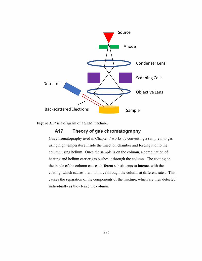
275

Figure A17 is a diagram of a SEM machine.

A17 Theory of gas chromatography Gas chromatography used in Chapter 7 works by converting a sample into gas

using high temperature inside the injection chamber and forcing it onto the

column using helium. Once the sample is on the column, a combination of

heating and helium carrier gas pushes it through the column. The coating on

the inside of the column causes different substituents to interact with the

coating, which causes them to move through the column at different rates. This

causes the separation of the components of the mixture, which are then detected

individually as they leave the column.

276

Figure A18 shows a representative setup of a gas chromatography machine.

A17.1 Flame ionization Detector A flame ionization detector works by passing the substances that come out of

the column into a flame. This causes ionization, and this is detected as a

voltage from the detector. This detected signal forms a peak. The area of this

peak can be used to determine how much of the substance was detected, but the

amount is relative and needs to be used in conjunction with a quantification

graph made using the same parameters and machine.

A17.2 Mass Spectrometry Detector A mass spectrometry detector works by ionizing the materials that come out of

the column. This causes the material to become charged. This can then be

measured using a potential applied inside the machine based on the mass to

charge ratio.

COBALT, MOLYBDENUM, AND NICKEL COMPLEXES ...

Documents

Transcript of COBALT, MOLYBDENUM, AND NICKEL COMPLEXES ...