Coastal Squeeze Evidence and Monitoring Requirement ...
188
www.naturalresourceswales.gov.uk Coastal Squeeze Evidence and Monitoring Requirement Review Oaten, J., Brooks, A. and Frost, N. ABPmer NRW Evidence Report No. 307 Date
-
Upload
khangminh22 -
Category
Documents
-
view
0 -
download
0
Transcript of Coastal Squeeze Evidence and Monitoring Requirement ...
www.naturalresourceswales.gov.uk www.naturalresourceswales.gov.uk
Coastal Squeeze Evidence and Monitoring Requirement Review
Oaten, J., Brooks, A. and Frost, N. ABPmer
NRW Evidence Report No. 307
Date
Page 1 www.naturalresourceswales.gov.uk www.naturalresourceswales.gov.uk
About Natural Resources Wales
Natural Resources Wales’ purpose is to pursue sustainable management of natural resources. This means looking after air, land, water, wildlife, plants and soil to improve Wales’ well-being, and provide a better future for everyone.
Evidence at Natural Resources Wales
Natural Resources Wales is an evidence based organisation. We seek to ensure that our strategy, decisions, operations and advice to Welsh Government and others are underpinned by sound and quality-assured evidence. We recognise that it is critically important to have a good understanding of our changing environment.
We will realise this vision by: Maintaining and developing the technical specialist skills of our staff; Securing our data and information; Having a well resourced proactive programme of evidence work; Continuing to review and add to our evidence to ensure it is fit for the challenges
facing us; and Communicating our evidence in an open and transparent way.
This Evidence Report series serves as a record of work carried out or commissioned by Natural Resources Wales. It also helps us to share and promote use of our evidence by others and develop future collaborations. However, the views and recommendations presented in this report are not necessarily those of NRW and should, therefore, not be attributed to NRW.

Page 2 www.naturalresourceswales.gov.uk www.naturalresourceswales.gov.uk
Report series: NRW Evidence Report Report number: 307 Publication date: November 2018 Contract number: WAO000E/000A/1174A - CE0529 Contractor: ABPmerContract Manager: Park, R. Title: Coastal Squeeze Evidence and Monitoring
Requirement Review Author(s): Oaten, J., Brooks, A. Frost, N. Peer Reviewer(s) Hull, S. (ABPmer), Park, R. (NRW), Rimington, N. (NRW) Approved By: Park, R., Rimington, N. Restrictions: None
Distribution List (core) NRW Library, Bangor (One Electronic) 3 National Library of Wales (Electronic Only) 1 British Library (Electronic Only) 1 Welsh Government Library (Electronic Only) 1 Scottish Natural Heritage Library (Electronic Only) 1 Natural England Library (Electronic Only) 1
Recommended citation for this volume: Oaten, J., Brooks, A. and Frost, N. 2018. Coastal Squeeze Evidence and Monitoring Requirement Review. NRW Report No: 307, 188pp, Natural Resources Wales, Cardiff.

Page 3 www.naturalresourceswales.gov.uk www.naturalresourceswales.gov.uk
Contents Crynodeb Gweithredol .............................................................................................................. 8
Executive Summary ............................................................................................................... 18
1. Introduction ..................................................................................................................... 27
1.1. Overview ........................................................................................................................... 27
1.2. Report structure ................................................................................................................ 29
2. Project Background ........................................................................................................ 30
2.1. Shoreline Management Plans ........................................................................................... 30
2.2. Defining coastal squeeze .................................................................................................. 33
2.3. Sea level rise .................................................................................................................... 35
2.4. Predicted habitat losses in Wales ..................................................................................... 40
2.4.1. National Habitat Creation Programme ........................................................................... 42
3. Calculating coastal squeeze ........................................................................................... 46
3.1. Causes of change to intertidal areas ................................................................................ 46
3.2. Establishing a baseline ..................................................................................................... 50
3.3. Calculating losses ............................................................................................................. 52
4. Review of Possible Monitoring Techniques .................................................................... 54
4.1. Introduction ....................................................................................................................... 54
4.2. Sea level ........................................................................................................................... 56
4.2.1. Overview of monitoring techniques ................................................................................ 56
4.2.2. Processing and analysis of data ..................................................................................... 60
4.2.3. Technical review ............................................................................................................. 61
4.3. Topography/bathymetry .................................................................................................... 64
4.3.1. Overview of monitoring techniques ................................................................................ 64
4.3.2. Processing and analysis of data ..................................................................................... 66
4.3.3. Technical review ............................................................................................................. 67
4.4. Habitat types, boundaries and condition ........................................................................... 71
4.4.1. Overview of techniques .................................................................................................. 71
4.4.2. Processing and analysis of data ..................................................................................... 72
4.4.3. Technical review ............................................................................................................. 74
4.5. Summary ........................................................................................................................... 78
5. Current Monitoring and Other Relevant Data ................................................................. 80
5.1. Overview ........................................................................................................................... 80
5.2. Sea level monitoring ......................................................................................................... 81
5.2.1. Tide gauges .................................................................................................................... 81
5.2.2. Satellite altimetry ............................................................................................................ 81
5.3. Water Framework Directive monitoring ............................................................................ 82
5.4. Marine Protected Area monitoring .................................................................................... 82
5.4.1. Marine Regulation 35 Habitat Features .......................................................................... 83
5.4.2. Marine Article 17 Reporting Habitat Features ................................................................ 83
5.5. Other monitoring ............................................................................................................... 84

Page 4 www.naturalresourceswales.gov.uk www.naturalresourceswales.gov.uk
5.5.1. Light Detection and Ranging (LiDAR) ............................................................................ 84
5.5.2. Multispectral imagery ...................................................................................................... 84
5.5.3. Hydrographic monitoring ................................................................................................ 85
5.6. Hydrodynamic modelling data .......................................................................................... 86
5.7. Wales Coastal Monitoring Centre ..................................................................................... 86
5.8. Summary ........................................................................................................................... 87
6. Uncertainty ..................................................................................................................... 93
6.1. Overview ........................................................................................................................... 93
6.2. Instrument measurement uncertainty ............................................................................... 93
6.3. Thematic uncertainty ......................................................................................................... 95
6.4. Causes of change and effects to intertidal habitat ............................................................ 96
6.5. Upscaling observed records of change from a local to regional scale ............................. 96
6.6. Using records of observed change to estimate future habitat losses ............................... 97
6.7. Statistical evaluation of overall uncertainty ....................................................................... 97
7. Options Appraisal Assessment ....................................................................................... 99
7.1. Reducing uncertainty ........................................................................................................ 99
7.1.1. Control sites as means of isolating change attributable to coastal squeeze .................. 99
7.1.2. Expert geomorphological assessment .........................................................................100
7.2. Overview of options ........................................................................................................101
7.2.1. Sub-options ...................................................................................................................102
7.2.2. Monitoring frequency ....................................................................................................104
7.3. Appraisal method ............................................................................................................104
7.3.1. Key assumptions ..........................................................................................................104
7.3.2. Critical success factors .................................................................................................105
7.4. Option 1 – Use sea level rise monitoring and existing data (Business as usual) ...........107
7.4.1. Description of approach ................................................................................................107
7.5. Option 2 – Bespoke intertidal habitat monitoring for representative flood risk management projects and assets (Do minimum) ...........................................................109
7.5.1. Description of approach ................................................................................................109
7.5.2. Option 2a ......................................................................................................................111
7.5.3. Option 2b ......................................................................................................................113
7.6. Option 3 – Bespoke intertidal habitat monitoring for all planned flood risk management projects and assets (Do medium) ...................................................................................115
7.6.1. Description of approach ................................................................................................115
7.6.2. Option 3a ......................................................................................................................116
7.6.3. Option 3b ......................................................................................................................117
7.7. Option 4 – Bespoke intertidal habitat monitoring in all HTL policy locations (Do maximum) ........................................................................................................................................119
7.7.1. Description of approach ................................................................................................119
7.7.2. Option 4a ......................................................................................................................119
7.7.3. Option 4b ......................................................................................................................120
7.8. Summary .........................................................................................................................122
8. Discussion and conclusion ........................................................................................... 127

Page 5 www.naturalresourceswales.gov.uk www.naturalresourceswales.gov.uk
8.1. Uncertainty ......................................................................................................................127
8.2. Monitoring options ...........................................................................................................127
8.2.1. Wider considerations ....................................................................................................129
8.3. Recommendations ..........................................................................................................129
8.3.1. Implications of recommendations .................................................................................131
9. References ................................................................................................................... 132
10. Abbreviations/Acronyms ............................................................................................... 143
11. Appendix A. NRW and Local Authority Flood Risk Management Assets and Projects 145
12. Appendix B. Case Study Review .................................................................................. 149
12.1. Introduction .....................................................................................................................149
12.2. Coastal squeeze determination studies ..........................................................................149
12.2.1. Introduction ...................................................................................................................149
12.2.2. England .........................................................................................................................149
12.2.3. Elsewhere .....................................................................................................................160
12.3. Intertidal habitat change monitoring studies ...................................................................165
12.3.1. Introduction ...................................................................................................................165
12.3.2. UK case studies ............................................................................................................165
12.3.3. Case studies from elsewhere .......................................................................................172
12.4. References ......................................................................................................................173
13. Appendix C. Monitoring Datasets Review .................................................................... 177
Data Archive Appendix ......................................................................................................... 186

Page 6 www.naturalresourceswales.gov.uk
List of Figures Figure 1 Schematic of project structure ............................................................................ 28
Figure 2 SMP2 policies for each epoch ............................................................................ 31
Figure 3 Diagrammatic illustration of coastal squeeze under rising sea level (Source Pontee, 2017) ......................................................................................................................... 33
Figure 4 Vertical land movement (mm/yr) for the UK, based on the GIA modelling of Bradley et al. (2009) ............................................................................................................... 37
Figure 5 Projections of relative sea level rise for selected locations around Wales, based on outputs from UKCP09 ....................................................................................................... 38
Figure 6 Principal components involved in coastal and estuarine morphodynamics (adapted from Pye and Blott, 2008) ....................................................................................... 47
Figure 7 Standard deviation from de-trended annual mean sea level time series from 30 tide gauge sites around the North Sea (after Wahl et al. 2013) ............................................. 57
Figure 8 (Left) Example tide gauge record. Yellow squares indicate representative sampling interval from satellite altimeter. (Right) UK Coastline with Envisat 35 day repeat tracks in yellow, and the locations of the 34 gauges of the UK tide gauge network indicated in red (from Cotton et al. 2016). ................................................................................................. 58
Figure 9 Maps of gridded Envisat altimeter sea level data (2002-2010): (Left) Long term trend in mm/yr; (Right) amplitude of the annual cycle (mm) ................................................... 59
Figure 10 Correlation (a) and root-mean-square difference (RMSD) (b) between de-seasoned and de-trended sea level from altimetry and tide gauge observations. Empty circles in a denote non-significant correlation. (From Cipollini et al., 2017) ........................... 60
Figure 11 Bathymetric survey data for Welsh waters available through the UKHO INSPIRE portal ....................................................................................................................... 85
Figure 12 Monitoring data and programmes collected in the Severn Estuary .................. 88
Figure 13 Monitoring data and programmes collected in south Wales ............................. 89
Figure 14 Monitoring data and programmes collected in south west Wales ..................... 90
Figure 15 Monitoring data and programmes collected in north west Wales ..................... 91
Figure 16 Monitoring data and programmes collected in north Wales .............................. 92
Figure 17 The effect of slope and vertical (a) and horizontal (b) accuracy on calculated area .......................................................................................................................................94 Figure 18 Steepening mode classification scheme based on changes in position of High Water Mark (HMW) and Low Water Mark (LWM). From Taylor et al., 2004. ....................... 100
Figure 19 Selected flood and coastal defence projects in Natura 2000 sites in Wales .. 110
Figure 20 Flood and coastal defence projects in Natura 2000 sites in Wales ................ 115
Figure 21 Summary of monitoring options ...................................................................... 128
Figure 22 Comparison of predicted equilibrium widths with observed widths in Hamford Water (Source: Royal Haskoning, 2018) .............................................................................. 160
Figure 23 Flow process of saltmarsh extent mapping (Source: Hambridge and Phelan, 2014) .................................................................................................................................. 166
Figure 24 Changing saltmarsh extent in Langstone Harbour (Source: CCO, 2008) ....... 169

Page 7 www.naturalresourceswales.gov.uk
List of Tables Table 1 Previous definitions of coastal squeeze used by various organisations (From Pontee, 2013) ......................................................................................................................... 34
Table 2 Predicted intertidal habitat losses in Welsh Natura 2000 sites as reported by NRW.
Table 3
.......................................................................................................41
Revised estimates (high-level indicative only) of intertidal habitat losses in Welsh Natura 2000 sites ................................................................................................................... 42
Table 4 Indicative balance sheet template for NHCP (the top row for each designated site is completed with habitat loss estimates provided by NRW) ........................................... 43
Table 5 Potential causes of beach erosion and intertidal habitat width reduction (adapted from Pontee, 2013). ................................................................................................................ 46
Table 6 Criteria and RAG rating to be reviewed for each monitoring technique .............. 55
Table 7 Technical review for sea level monitoring options. ............................................. 63
Table 8 Technical review for topographic/bathymetric monitoring options ...................... 68
Table 9 Technical review for habitat monitoring options .................................................. 76
Table 10 Error (m²) in calculated area related to vertical accuracy slope,per m of coastline95 Table 11 Error (m²) in calculated area related to horizontal accuracy slope,per m of coastline ............................................................................................................................95
Table 12 Categories of uncertainty .................................................................................... 98
Table 13 Look-up table for monitoring costs .................................................................... 106
Table 14 Indicative costs for Option 1.............................................................................. 109
Table 15 Semi-quantitative assessment of uncertainty associated with Option 1 ........... 109
Table 16 Indicative costs for Option 2a............................................................................ 112
Table 17 Semi-quantitative assessment of uncertainty associated with Option 2a ......... 113
Table 18 Indicative costs for Option 2b............................................................................ 113
Table 19 Semi-quantitative assessment of uncertainty associated with Option 2b ......... 114
Table 20 Indicative costs for Option 3a............................................................................ 116
Table 21 Semi-quantitative assessment of uncertainty associated with Option 3a ......... 117
Table 22 Indicative costs for Option 3b............................................................................ 118
Table 23 Semi-quantitative assessment of uncertainty associated with Option 3b ......... 118
Table 24 Indicative costs for Option 4a............................................................................ 119
Table 25 Semi-quantitative assessment of uncertainty associated with Option 4a ......... 120
Table 26 Indicative costs for Option 4b............................................................................ 121
Table 27 Semi-quantitative assessment of uncertainty associated with Option 4b ......... 121
Table 28 Summary of costs and uncertainty associated with each monitoring option ..... 124
Table 29 Benefits and disadvantages of semi-automated versus manual digitisation ..... 167
Table 30 Previous saltmarsh studies undertaken in England and the Anglian region (from ABPmer, 2016) ..................................................................................................................... 171
Page 8 www.naturalresourceswales.gov.uk
Crynodeb Gweithredol Cefndir y gofyniad ar gyfer opsiynau monitro tystiolaeth Mae Cyfoeth Naturiol Cymru yn cyflenwi'r Rhaglen Genedlaethol Creu Cynefinoedd ar ran Llywodraeth Cymru. Diben y rhaglen yw nodi cyfleoedd ar gyfer creu cynefinoedd a chyflenwi gwrthbwyso amgylcheddol amserol i hwyluso gweithredu cynlluniau rheoli traethlin a diogelu rhwydwaith Natura 2000 yng Nghymru. Mae Rhaglen Genedlaethol Creu Cynefinoedd yn ymwneud yn bennaf ag effeithiau o ardaloedd arfordirol gyda pholisi 'cadw'r llinell' ac yn cyflenwi cynefin cydadferol ar gyfer awdurdodau rheoli perygl llifogydd, ond gall hefyd fod yn fecanwaith cyflenwi iawndal ar gyfer cynlluniau trydydd parti sy'n ddarostyngedig i gytundebau partneriaeth mewn amgylchiadau eithriadol. Mae'r Rhaglen Genedlaethol Creu Cynefinoedd yn gyfrifol am gyflenwi cynefin cydadferol priodol o faint ac ansawdd digonol i wrthbwyso effeithiau ‘gwasgfa arfordirol’1 ar gyfanrwydd y gyfres o safleoedd Natura 2000. Felly mae cyflenwi'r Rhaglen Genedlaethol Creu Cynefinoedd yn cael ei lywio gan y colledion a ragwelir o'r cynlluniau rheoli traethlin (a strategaethau rheoli perygl llifogydd ar gyfer aberoedd Afon Dyfrdwy ac Afon Hafren) a'r Asesiadau Rheoliadau Cynefinoedd. Er mwyn dangos i Lywodraeth Cymru fod y Rhaglen Genedlaethol Creu Cynefinoedd yn rheoli'r cydbwysedd o golledion ac enillion cynefin, y perygl toriad ac unrhyw berygl o or-ddyrannu adnoddau, mae'n bwysig cadarnhau bod mesurau creu o raddfa ac ansawdd angenrheidiol a bod targedau diwygiedig y Rhaglen Genedlaethol Creu Cynefinoedd yn sicrhau bod y graddau a’r cyfanswm a grëwyd yn cydymffurfio â'r gofynion rheoleiddiol yn ymwneud â'r cynefin a gollwyd yn sgil gwasgfa arfordirol. Mae hyn yn gofyn am y canlynol: 1. Diffinio targedau a'u cynnal 2. Monitro colledion/enillion cynefin. Gellir cyflawni hyn drwy wneud y canlynol:
a. Yn anuniongyrchol, drwy olrhain cyfraddau cyflawnedig cynnydd yn lefel y môr a defnyddio'r wybodaeth hon fel procsi er mwyn dangos digonolrwydd mesurau cydadferol a llywio targedau gwrthbwyso a adnewyddwyd
b. Yn uniongyrchol, drwy fonitro maint cynefin o fewn rhwydwaith Natura 2000 i ddangos cyfraddau colled gwirioneddol (o'u cymharu â'r hyn a ragwelwyd)
Nodau ac amcanion Prif nod y prosiect hwn yw datblygu amrediad o opsiynau monitro posibl i lywio dealltwriaeth o golledion gwasgfa arfordirol yng Nghymru sy'n codi o weithredu polisïau 'cadw'r llinell' y cynlluniau rheoli traethlin. Er mwyn cyflawni'r nod hwn, mae cyfres o dasgau cydgysylltiedig wedi cael eu cwblhau. Mae’r rhain yn cynnwys:
1 Bu cryn drafodaeth (ac mae'n parhau) o ran yr union ddiffiniad o wasgfa arfordirol. Fodd bynnag, yn seiliedig ar adolygiad o'r diffiniadau amrywiol a ddefnyddir o fewn y deunyddiau darllen ac o'r gymuned reoli arfordirol yn y DU, defnyddir y diffiniad canlynol: 'Mae gwasgfa arfordirol yn un math o golli cynefin arfordirol, lle y bo cynefin rhynglanwol yn cael ei golli drwy'r marc llanw uchel yn cael ei osod gan amddiffyniad neu strwythur (h.y. mae’r marc llanw uchel yn erbyn strwythur caled fel morglawdd) a thrwy’r marc llanw isel yn symud tuag at y tir wrth ymateb i gynnydd yn lefel y môr.' [Pontee, 2011]

Page 9 www.naturalresourceswales.gov.uk
Adolygu a chofnodi dealltwriaeth gyfredol o golledion cynefinoedd a ragwelir sy'n
gysylltiedig â gwasgfa arfordirol, gan gydnabod y cyfyngiadau sy'n gysylltiedig â phenderfynu ar achos ac effaith, a dosbarthiad a statws cynefinoedd Atodiad 1 yng Nghymru sy'n agored i niwed yn sgil gwasgfa arfordirol
Adolygiad o ddeunyddiau darllen yn ymwneud â monitro gwasgfa arfordirol, gan gynnwys: - Adolygu technegau i fesur cynnydd yn lefel y môr - Adolygu technegau i fonitro maint a chyflwr cynefinoedd rhynglanwol - Adolygu'r hyn mae pobl eraill yn ei wneud yn y DU ac yn rhyngwladol i fonitro
gwasgfa arfordirol Adolygu'r gwaith monitro presennol sy'n cael ei wneud yn nyfroedd Cymru y gellid
ei addasu i fodloni gofynion monitro gwasgfa arfordirol Ansicrwydd Mae ansicrwydd yn fater ac yn gyfyngiad allweddol o ran monitro effeithiau gwasgfa arfordirol yn effeithiol ac wrth benderfynu ar dargedau gwrthbwyso cynefinoedd ar gyfer mesurau cydadferol o fewn y Rhaglen Genedlaethol Creu Cynefinoedd i fodloni gofynion y Gyfarwyddeb Cynefinoedd. Mae angen cydnabod yr ansicrwydd hwn drwy gydol unrhyw broses gwneud penderfyniadau yn ymwneud â graddfa'r monitro i'w gweithredu ar gyfer asesu gwasgfa arfordirol ac effeithlonrwydd opsiynau sydd ar gael i adolygu targedau'r Rhaglen Genedlaethol Creu Cynefinoedd yn ddigonol. Er ei fod yn bosibl monitro cynnydd o ran lefel y môr yn gywir (dros gyfnodau amser hir), yn ogystal â newid ffisegol a biolegol yn y parth rhynglanwol, mae penderfynu ar yr elfen o newid a allai gael ei phriodoli’n benodol i ddylanwad gwasgfa arfordirol yn broblematig. Mae hyn oherwydd er bod gan bresenoldeb amddiffynfeydd arfordirol sefydlog a chynnydd o ran lefel y môr y potensial i arwain at golli/dirywiad pellach i gynefin rhynglanwol, gallai newidiadau hefyd ddigwydd mewn ymateb i ffactorau eraill nad ydynt yn gysylltiedig o gwbl â lefel y môr a gwasgfa arfordirol. Mae'r ffactorau eraill hyn yn niferus ac yn aml yn rhyng-gysylltiedig, sy'n gwneud ynysu eu dylanwad yn anodd iawn. Er enghraifft, mae nifer o astudiaethau wedi dangos nad yw'r cynnydd o ran lefel y môr hyd yn hyn wedi bod yr achos pwysicaf o ran colli morfa heli a gwastadeddau rhynglanwol, o'i gymharu â mecanweithiau achosol eraill megis dylanwadau metereolegol. Mae'r achosion posibl hyn o golled cynefinoedd yn cynnwys newidiadau o ran: Ceryntau llanw Amodau tonnau Cyflenwad gwaddodion Morffoleg sianeli Trothwyon erydu gwaddodion Hinsawdd (gan gynnwys tymheredd a mewnbwn dŵr croyw) Yn benodol, gall dylanwad cylchoedd naturiol ar forffoleg rhynglanwol fod yn sylweddol iawn. Efallai o bwysigrwydd mwyaf yma yw dylanwad stormusrwydd (a allai arwain at fwy o egni tonnau yn ogystal â newidiadau tymor byr o ran lefel y môr) a'r cylch nodol sy'n perthyn i'r lleuad (sy'n achosi amrywiad o ran amrediad llanwol dros gyfnod o 18.6 mlynedd).

Page 10 www.naturalresourceswales.gov.uk
Er gwaethaf yr anawsterau cynhenid o ran monitro/penderfynu ar newid sy'n benodol gysylltiedig â gwasgfa arfordirol, mae'r adroddiad yn ystyried sut fyddai orau i ddiffinio/adolygu targedau ar gyfer y Rhaglen Genedlaethol Creu Cynefinoedd. Y ddau brif ddull gweithredu a nodwyd yw'r isod: Olrhain cyfraddau cyflawnedig cynnydd o ran lefel y môr Monitro colledion cynefinoedd sy'n gysylltiedig â gwasgfa arfordirol Mae'r prif ganfyddiadau ac argymhellion ar gyfer pob dull gweithredu wedi cael eu hamlinellu isod. Olrhain cyfraddau cyflawnedig cynnydd o ran lefel y môr Mae'r holl amcangyfrifon o golledion cynefin yn y dyfodol sy'n codi o wasgfa arfordirol yn gynhenid sensitif i'r rhagamcanion o lefel y môr a ddefnyddir i lywio'r dadansoddiad. Mae hyn yn bennaf yn sgil y ffaith fod ardaloedd rhynglanwol fel arfer yn cael eu nodweddu gan raddiannau bas iawn ac, mewn canlyniad, gallai hyd yn oed newidiadau eithaf bach o ran codi arwyneb y môr arwain at raddau mawr o gynefin yn cael eu heffeithio gan y newid hwnnw. Dros amser, mae amcangyfrifon o gynnydd o ran lefel y môr yn y dyfodol wedi cael eu mireinio, wrth i’n gwybodaeth am fecanweithiau gyrru newid wella a chofnodion lloeren manylach/hirach o gynnydd yn lefel y môr ddod ar gael. Mae canfyddiadau allweddol o ran mesur a rhagamcaniad cynnydd o ran lefel y môr yng nghyd-destun colli cynefin yn y dyfodol fel a ganlyn: Gallai data mesur y llanw a (pheth) data lloeren gael eu defnyddio mewn dull
gweithredu 'hypsometrig'2 ar gyfer dilysu amcangyfrifon gwasgfa arfordirol. Mae gan y ddwy ffynhonnell ddata'r potensial i gyflenwi lefelau uchel o gywirdeb a thra-chywiredd o ran tueddiadau yn lefelau cymedrig y môr, er bod angen ystyriaeth ofalus wrth ddefnyddio naill set ddata neu'r llall o'r cyfnod amser y gellir penderfynu ar dueddiadau ystyrlon ac (yn achos data lloeren) gwybodaeth ehangach am batrymau rhanbarthol addasiad rhew isostatig.
O ran llywio dadansoddiad hypsometrig o wasgfa arfordirol yng Nghymru, mae'n debygol mai'r defnydd o ddata mesur llanwol yw'r datrysiad mwyaf priodol a chost-effeithiol ar hyn o bryd: er nad yw'n cael yr un ymdriniaeth ofodol â data lloeren, mae'r mesuryddion llanwol yn cofnodi newid cymharol o ran lefel y môr (yn hytrach na newid o ran uchder arwyneb y môr), sef y paramedr mwyaf perthnasol er mwyn llywio mesuriadau o wasgfa arfordirol. Hefyd, tra bo data lloeren yn cael ei gasglu'n barhaus o ddyfroedd Cymru, deellir nad yw'n cael ei brosesu'n rheolaidd er mwyn galluogi penderfynu ar dueddiadau cymedrig o ran lefel y môr ar raddfa leol. I'r gwrthwyneb, mae'r elfen brosesu hon eisoes yn cael ei chyflawni gan Ganolfan Data Eigioneg Prydain (BODC) ar gyfer mesuryddion llanwol, gyda data yn cael ei wneud ar gael yn rhwydd bob blwyddyn. Fodd bynnag, yn y dyfodol
2 Dull gweithredu asesu a ddefnyddir i gyfrifo gwasgfa arfordirol sy'n seiliedig ar dybiaethau cyffredinol ynglŷn â lle y gellir dod o hyd i fathau cynefin rhynglanwol mewn perthynas â lefelau llanwol. Gallai'r wybodaeth hon gael ei chyfuno wedyn â data topograffeg (fel arfer mewn system gwybodaeth ddaearyddol) i gyfrifo colli cynefin posibl o dan lefelau'r môr sy'n codi.

Page 11 www.naturalresourceswales.gov.uk
(pan fydd problemau methodolegol hysbys wedi cael eu datrys), mae'n debygol y bydd arsylwadau lloerennau ar newid o ran lefel y môr o werth mawr o ran ategu a dilysu'r cofnodion mesuryddion llanwol arfordirol.
Bydd rhagamcanion cynnydd o ran lefel y môr yn cael eu darparu yn UKCP18 ac mae rhagamcanion yn debygol o fod tua 20–30% yn fwy na'r gwerthoedd cyfatebol a gyflwynwyd yn UKCP09 ar gyfer y senario allyriadau uchaf. Mae hyn yn golygu ei fod yn bosibl fod rhagamcanion presennol o golledion gwasgfa arfordirol yng Nghymru wedi cael eu hamcangyfrif yn rhy isel yn sgil diffyg ceidwadaeth mewn rhagamcanion cynharach o ran cynnydd yn lefel y môr. Fodd bynnag, gallai'r diffyg ceidwadaeth hwn gael ei wrthbwyso gan natur geidwadol iawn y rhagdybiaethau a ddefnyddiwyd mewn mannau eraill yn y broses asesu, yn arbennig y rheini sy'n gysylltiedig â gallu (neu fel arall) cyfraddau gwaddodi i fod ar yr un raddfa â'r cynnydd o ran lefel y môr.
Monitro colledion cynefinoedd sy'n gysylltiedig â gwasgfa arfordirol Mae amrywiaeth o dechnegau monitro ar gael sydd wedi cael eu hadolygu a'u hasesu ar gyfer eu gallu i fesur graddau, cyflwr a'r math o gynefin. Mae costau dangosol sy'n gysylltiedig â phob techneg monitro hefyd wedi cael eu penderfynu. Mae'r technegau a adolygwyd wedi cael eu crynhoi fel a ganlyn: Topograffeg/bathymetreg:
- Datgelu a mesur golau (LiDAR) - Radar - Stereo-ffotogrametreg gan ddefnyddio delweddau amlsbectral - Arolygon bathymetreg - Sganwyr laser daearol - System Lloeren Mordwyaeth Fyd-eang Ginetig Amser Real (RTK GNSS)
Mathau, ffiniau a chyflwr cynefinoedd: - Delweddaeth amlsbectrol (gan gynnwys ffotograffiaeth o'r awyr) - Delweddaeth hypersbectrol - Arolygon maes o gynefin (e.e. arolwg cynefin Cam I)
Problem allweddol a nodwyd wrth fonitro newid yw'r anhawster o ran dal cynefinoedd yn eu graddau llanwol isaf gan ei bod hi'n brin i'r rhain gael eu datguddio am gyfnodau sylweddol o amser. At hynny, nid oes gan gynefinoedd rhynglanwol ffiniau sefydlog, sy'n gwneud cymariaethau amserol yn anodd. Mae'r gallu i unrhyw dechneg monitro gael ei hailadrodd wedi'i gyfyngu'n sylweddol gan y ffaith hon. Fodd bynnag, os bydd colledion cynefinoedd i'w cyfrifo gydag unrhyw sicrwydd, mae'n hanfodol i'w harolygu ar yr un graddau llanwol (isaf). Yn ychwanegol at yr adolygiad uchod o dechnegau monitro, cynhaliwyd hefyd adolygiad ar wahân o ddata monitro arfordirol sy'n cael ei gasglu ar hyn o bryd ar draws dyfroedd Cymru, a fydd o bosibl yn ddefnyddiol ar gyfer mesur colledion gwasgfa arfordirol yn y dyfodol. Y setiau data allweddol a nodwyd sydd â'r potensial i gyfrannu at ddosbarthiad cynefinoedd, eu graddau ac asesiad o’u cyflwr yw'r rhaglenni monitro cyflwr a gynhelir fel rhan o gyfrifoldebau Cyfoeth Naturiol Cymru / Llywodraeth Cymru o dan y Gyfarwyddeb Fframwaith Dŵr a'r Gyfarwyddeb Cynefinoedd. Yn benodol, mae gan raddau'r morfa heli a aseswyd o dan y Gyfarwyddeb Fframwaith Dŵr y potensial i nodi newidiadau yn uniongyrchol o ran

Page 12 www.naturalresourceswales.gov.uk
graddau cynefinoedd (ond maent yn esgeuluso cynefinoedd fflatiau llaid a fflatiau tywod). Gallai data ad hoc arall fod ar gael, megis LiDAR, delweddaeth amlsbectrol a data hydrograffeg, a allai lywio newid. Mae hefyd corff sylweddol o ddata hanesyddol ar gael i Cyfoeth Naturiol Cymru, sy'n disgrifio cynefinoedd a rhywogaethau sy'n agored i niwed oherwydd gwasgfa arfordirol. Gallai hwn fod yn adnodd pwysig i benderfynu ar yr amodau gwaelodlin y gellir cymharu newid yn eu herbyn. Fodd bynnag, er bod graddau rhesymol o orgyffwrdd rhwng y data cynefin hwn a'r unedau polisi lle y bo'r polisïau 'cadw'r llinell' wedi cael eu haseinio, mae'r graddau y mae'r data yn cydberthyn i'r prosiectau llifogydd ac amddiffyn arfordirol a gynlluniwyd yn fwy cyfyngedig. Dylid nodi hefyd fod cymhwysedd rhaglenni monitro cyfredol i lywio gwasgfa arfordirol yn ddarostyngedig i nifer o gyfyngiadau pellach. O'r pwysigrwydd mwyaf yw'r ffaith nad yw'r rhaglenni monitro hyn wedi cael eu dylunio i asesu effeithiau gwasgfa arfordirol, dim ond newidiadau o ran cyflwr, dosbarthiad/graddau a statws cyffredinol cynefinoedd. At hynny, mae nifer o setiau data ond yn cael eu casglu mewn lleoliadau samplu arwahanol, heb asesu graddau rhynglanwol llawn y cynefin sy'n cael ei arolygu. Fodd bynnag, gallai'r data hwn barhau i fod yn ddefnyddiol ar gyfer llywio asesiad o gyflwr y cynefin. Opsiynau monitro a nodwyd Ar ôl adolygu (i) potensial y technegau monitro y gellir eu defnyddio i lywio amcangyfrifon o golledion gwasgfa arfordirol a (ii) rhaglenni monitro arfordirol presennol yng Nghymru, sefydlwyd pedwar opsiwn cyffredinol i lywio'r ddealltwriaeth o golledion gwasgfa arfordirol yng Nghymru. Gwnaed dadansoddiad o fudd a chost pob opsiwn, gan ystyried yr amrediad o baramedrau roedd pob opsiwn yn ei gwmpasu, yn ogystal ag ansicrwydd cyffredinol amcangyfrifedig gyda phob dull gweithredu. Mae Opsiwn 1 yn cynnwys monitro'r cynnydd o ran lefel y môr (yn seiliedig ar ddata mesur llanwol presennol) a chan ddefnyddio data monitro (biolegol a ffisegol) sydd eisoes yn cael ei gasglu yng Nghymru er mwyn llywio newid i ategu targedau gwrthbwyso cynefinoedd. Ystyrir bod hwn yn ddull gweithredu 'busnes fel arfer' er bod costau ychwanegol sylweddol ymhlyg yn yr opsiwn hwn sy'n gysylltiedig â phrosesu a dehongli data. Mae Opsiynau 2, 3 a 4 yn ychwanegol at Opsiwn 1 ac mae pob un yn cynnwys rhaglen fonitro bwrpasol i gasglu data ar newidiadau o ran ardaloedd a chynefinoedd rhynglanwol, gyda data'n cael ei gasglu bob chwe blynedd. Mae Opsiwn 2 yn defnyddio'r dull gweithredu hwn ar ddetholiad o safleoedd lle y bo cynlluniau amddiffyn arfordirol ar y gweill i'w hadeiladu, ac ystyrir ei fod yn ddull gweithredu 'gwneud y lleiaf'. Mae Opsiwn 3 yn debyg i Opsiwn 2 ond mae'n monitro newid ymhob safle lle y bo cynlluniau amddiffyn arfordirol ar y gweill i gael eu hadeiladu, ac ystyrir ei fod yn ddull gweithredu 'canolig'. Mae Opsiwn 4 yn monitro newid ymhob ardal polisi 'cadw'r llinell' o arfordir Cymru, ac ystyrir ei fod yn ddull gweithredu 'gwneud y mwyaf'.

Page 13 www.naturalresourceswales.gov.uk
Mae Opsiwn 2, 3 a 4 yn cynnwys is-opsiynau a) a b). Mae is-opsiwn a) yn cynnwys monitro newidiadau yn y graddau rhynglanwol sydd angen data ar dopograffi/bathymetreg a lefel y môr (o fesuryddion llanwol / altimetreg lloeren). Mae is-opsiwn b) yn cynnwys monitro newidiadau o ran graddau rhynglanwol (fel opsiwn a), yn ogystal â monitro newidiadau o ran mathau, ardal a chyflwr cynefinoedd o fewn y graddau rhynglanwol. Mae'r holl opsiynau yn cynnwys asesiadau geomorffolegol arbenigol i gysylltu unrhyw newidiadau cyflawnedig mewn ardaloedd rhynglanwol â gwasgfa arfordirol yn y ffordd orau. Mae costau dangosol ar gyfer pob un o'r pedwar opsiwn monitro a nodwyd yn cael eu crynhoi yn y tabl isod, ar gyfer y cyfnod hyd at 2105. Mae'r rhain yn amrywio'n sylweddol rhwng opsiynau. Er hynny, ymhob achos gwelir eu bod yn sylweddol pan fônt yn cael eu hystyried yn gyffredinol ar gyfer pob un o'r tri chyfnod cynllun rheoli traethlin.
Trosolwg o gostau ar gyfer pob opsiwn monitro ar gyfer y cyfnod hyd at 2105
Opsiwn Is-opsiwn Costau (£k)
Cyfnod 1 (hyd at 2025)
Cyfnod 2 (hyd at 2055)
Cyfnod 3 (hyd at 2105)
1* Amherthnasol 5 138 964
2 a 6 – 19 236 – 357 1,652 – 2,501 b 12 – 41 382 – 659 2,672 – 4,618
3 a 7 – 46 243 – 625 1,703 – 4,380
b 27 – 70 520 – 944 3,645 – 6,612
4 a 11 – 192 283 – 2,053 1,979 – 14,384
b 105 – 306 1,282 – 3,248 8,978 – 22,757 * Er nad yw'r opsiwn hwn, sy’n cynnwys casglu data monitro presennol, yn gofyn am unrhyw wariant ar gasglu data maes newydd, nid yw'n 'rhydd rhag cost' oherwydd y bydd angen arbenigwyr technegol i nodi, trefnu a dadansoddi'r data. Fodd bynnag, nodir ei fod yn debygol y bydd gan Cyfoeth Naturiol Cymru yr arbenigedd hwn yn fewnol.
Gyda'r holl opsiynau monitro, mae lefelau uchel o ansicrwydd yn gysylltiedig â'r anallu i benderfynu ar achos newid cynefin rhynglanwol. Mae dulliau o leihau ansicrwydd wedi cael eu hystyried yn yr adroddiad hwn: mae'r rhain yn cynnwys defnyddio gwaith monitro mewn safleoedd rheoli er mwyn cymharu arfordiroedd sydd wedi eu diogelu â’r rhai sydd heb eu diogelu. Fodd bynnag, canfuwyd bod cyfyngiadau mawr i ddulliau o'r fath, oherwydd y bydd hyd yn oed mân wahaniaethau o ran mecanweithiau gorfodi a nodweddion proffil yn peryglu’r gallu i wneud cymhariaeth ystyrlon rhwng safleoedd penodol ac o ganlyniad ni fyddent yn lleihau neu'n lliniaru'r cyfyngiadau yn sgil ansicrwydd uchel yn fawr. Yn unol â hynny, nid ydynt wedi cael eu cynnwys yn yr opsiynau monitro a amlinellir uchod. Felly, mae lefel annerbyniol o ansicrwydd yn parhau, sydd â goblygiadau ar gyfer monitro costau buddsoddiad ac iawndal. Ystyriaethau ehangach Dros y degawd diwethaf, bu datblygiadau sylweddol iawn o ran gweithredu technegau synhwyro o bell ar gyfer monitro'r amgylchedd morol. Hefyd, bu datblygiadau sylweddol ym maes cyfrifiadura a chynnydd o ran soffistigeiddrwydd modelau rhifyddol sy'n gallu efelychu prosesau arfordirol ac aberol. Mae pob
Page 14 www.naturalresourceswales.gov.uk
rheswm dros gredu y bydd y datblygiadau hyn yn parhau yn y dyfodol. Yn unol â hynny, mae'n bwysig fod adolygiad rheolaidd o opsiynau monitro posibl oherwydd y disgwyl y bydd technegau newydd (ac o bosib rhai mwy cost-effeithiol) yn dod i'r amlwg. Gallai'r data newydd hwn, wedi'i gyplysu â modelau mwy soffistigedig, leihau ansicrwydd ynglŷn ag achos ac effaith yn y dyfodol. At hynny, mae'n bwysig fod cysylltiadau â phrosiectau ymchwil parhaus yn cael eu cynnal.3 Mae'n hanfodol cydnabod bod llawer o'r data monitro a ddefnyddir i lywio dealltwriaeth o golli cynefin yn sgil gwasgfa arfordirol hefyd yn berthnasol o ran llywio agweddau eraill ar newid amgylcheddol, a goblygiadau amgylcheddol Llywodraeth Cymru (e.e. gofynion o dan y Gyfarwyddeb Cynefinoedd a'r Gyfarwyddeb Fframwaith Dŵr). Yn unol â hynny, mae'n bwysig fod mater monitro gwasgfa arfordirol yn cael ei ystyried yn gyfannol, ochr yn ochr â rhaglenni a mentrau monitro morol eraill, megis y Rhaglen Monitro a Modelu'r Amgylchedd a Materion Gwledig. Gallai hyn olygu y gall rhai o'r costau sy'n gysylltiedig â monitro i lywio targedau gwrthbwyso cynefin gael eu rhannu ar draws llifau gwaith lluosog. Casgliadau ac argymhellion Yng ngoleuni diffyg pŵer o ran unrhyw opsiwn monitro i ynysu newid a wnaed gan wasgfa arfordirol o'r holl ffactorau grym eraill, ni ystyrir ei fod yn gost-effeithiol i fuddsoddi mewn casglu data monitro newydd gyda'r diben penodol o benderfynu ar golled yn sgil gwasgfa arfordirol. Mae synnwyr clir o enillion gostyngol wrth ystyried gwariant yn erbyn lleihau ansicrwydd. At hynny, mae llawer o'r casglu, prosesu a dadansoddi data yn gofyn am offer, meddalwedd, sgiliau ac adnoddau nad ydynt ar gael o fewn Cyfoeth Naturiol Cymru ar hyn o bryd ac felly byddai angen gwariant ychwanegol. Er gwaethaf yr uchod, mae monitro Opsiwn 1 yn dal i ddarparu dull gweithredu monitro integredig, gan nodi newidiadau yn y statws cadwraethol ffafriol (y Gyfarwyddeb Cynefinoedd) a Statws Ansawdd Ecolegol (y Gyfarwyddeb Fframwaith Dŵr) a allai fod yn sgil cyfuniad o ffactorau gorfodi, gan gynnwys gwasgfa arfordirol. Mewn theori, gallai casglu tystiolaeth fonitro ffisegol a biolegol yn y dyfodol helpu i nodi'r ardaloedd hynny lle y mae cyfraddau gwaddodi wedi cadw ar yr un lefel â chynnydd yn lefel y môr ac felly lle nad oes gwasgfa arfordirol wedi digwydd. Yn debyg, ar raddfa leol, gallai data monitro o’r math hwn hefyd gael ei ddefnyddio i ddiystyru gwasgfa arfordirol fel prif achos newid. Er enghraifft, un enghraifft o hyn allai fod lle mae sianel wedi mudo, gan beri i ardaloedd rhynglanwol cyfagos gael eu herydu. Fodd bynnag, yn y rhan fwyaf o leoliadau lle mae peth colledion net hirdymor wedi cael eu nodi, byddai'n anodd iawn penderfynu yn union faint o'r golled hon sydd i'w phriodoli yn uniongyrchol i wasgfa arfordirol mewn cymhariaeth â ffactorau eraill. Er mwyn hyd yn oed ceisio hyn, byddai angen symiau sylweddol o ddata i gael eu casglu dros ardaloedd eang iawn, ac mewn cyfnodau amser rheolaidd, a byddai angen adolygiad geomorffolegol arbenigol sylweddol o’r holl ddata hefyd. Byddai hyn yn hollol anymarferol ar raddfa genedlaethol ac, mewn nifer o achosion, efallai na fydd yn arwain at leihad ystyrlon o ran ansicrwydd.
3 Mae prosiect sy’n cael ei gyflawni gan Asiantaeth yr Amgylchedd, mewn partneriaeth â Natural England, DEFRA, Cyfoeth Naturiol Cymru a Llywodraeth Cymru (o dan y teitl 'Beth yw gwasgfa arfordirol?'), yn anelu at ddatblygu dealltwriaeth a rennir o wasgfa arfordirol.

Page 15 www.naturalresourceswales.gov.uk
Hyd yn oed yn y lleoliadau hynny lle roedd y dystiolaeth fonitro yn nodi dim newid, ni fyddai'r tueddiadau yr arsylwyd arnynt o reidrwydd yn darparu sail gadarn ar gyfer sefydlu/mireinio amcangyfrifon o golled a ddisgwylir i ddigwydd yn y dyfodol yn sgil gwasgfa arfordirol. Mae hyn oherwydd bod y rhyngchwarae rhwng gyrwyr proses sydd wedi arwain at y newid a arsylwyd yn annhebygol o aros yr un peth yn y dyfodol, yn arbennig yng ngoleuni’r cyfraddau aflinol (disgwyliedig) o ran cynnydd yn lefel y môr. Mae penderfynu ar union lefelau ansicrwydd sy'n cyd-fynd ag amcangyfrifon o wasgfa arfordirol yn y dyfodol yn seiliedig ar y data monitro yn anodd ei bennu a byddent yn amrywio yn ofodol. Fodd bynnag, mae'n rhesymol tybio, hyd yn oed gyda data monitro da ar waith, mewn nifer o enghreifftiau byddai amcangyfrifon o golli cynefin yn sgil gwasgfa arfordirol yn agos at ±100%. Golyga hyn, ar gyfer aber enwol lle y bo'r amcangyfrif colli cynefin yn sgil gwasgfa arfordirol yn 100 hectar, gallai'r gwerth gwirioneddol fod yn yr amrediad o tua 0 i 200 hectar. Mae’r prif argymhellion o'r adroddiad hwn fel a ganlyn: 1. O'r opsiynau monitro a nodwyd, mae dull gweithredu 'busnes fel arfer' yn
cael ei ystyried i fod y dull gweithredu mwyaf priodol ('Opsiwn 1'). Mae hyn yn cynnwys ategu amcangyfrifon o golledion cynefin yn seiliedig ar yr ail gyfres o gynlluniau rheoli traethlin gyda data ar gynnydd cyflawnedig o ran lefel gymedrig y môr. Mae data cynnydd o ran lefel y môr ar ei ben ei hun ond yn brocsi ar gyfer gwasgfa arfordirol ac nid yw'n darparu gwybodaeth am golled cynefin yn y 'byd go-iawn'. Yn hytrach, mae'n cynrychioli mwy o ddull proffwydol o ddiweddaru amcangyfrifon o golled cynefin. Yn unol â hynny, mae hefyd yn bwysig gwneud y defnydd gorau o'r holl ddata a gwybodaeth sydd ar gael ac sydd eisoes yn cael ei gasglu yng Nghymru, gan gynnwys data y Gyfarwyddeb Fframwaith Dŵr, delweddau o'r awyr a LiDAR (a gesglir ar sail ad hoc). Ni fydd y data hwn o gydraniad gofodol ac amserol digonol i wella’n fawr dealltwriaeth o'r gyrwyr proses sydd y tu ôl i'r newid yr arsylwyd arno. Fodd bynnag, gallai gael ei ddefnyddio fel gwiriad synnwyr ar amcangyfrifon o golled gwasgfa arfordirol yn seiliedig yn uniongyrchol ar ddata am gynnydd o ran lefel y môr, gan ddarparu eglurder ar y cyfeiriad a threfn maint newid cynefin. Ar y cyfan, mae'r argymhelliad hwn yn cynnwys dull gweithredu monitro integredig defnyddiol ond nid yw o hyd yn cynnwys mecanwaith dibynadwy i ddiweddaru targedau gwrthbwyso cynefin.
Mae'r opsiwn hwn yn ei wneud yn ofynnol i Cyfoeth Naturiol Cymru wneud y canlynol:
Adolygu gwybodaeth am gynnydd yn lefel gymedrig y môr a adroddir gan Ganolfan Data Eigioneg Prydain (BODC) ar gyfer gorsafoedd mesur llanw Cymru yn erbyn rhagamcanion cyfatebol a ddefnyddir i lywio cynlluniau rheoli traethlin (yn y dyfodol, gallai gwybodaeth lloeren gael ei defnyddio at y diben hwn er, ar hyn o bryd, ystyrir ei fod yn annigonol o ran cywirdeb)
Casglu'r holl ddata perthnasol arall sydd ar gael (e.e. delweddaeth o'r awyr, LiDAR ac ati) i mewn i system gwybodaeth ddaearyddol er mwyn ei gymharu

Page 16 www.naturalresourceswales.gov.uk
Prosesu a dadansoddi data, gydag asesiad geomorffolegol arbenigol i fireinio amcangyfrifon o golli cynefin ymhellach y gellir ei briodoli i wasgfa arfordirol (lle y bo'n bosibl)
2. Mae'r amlder y mae colli gwasgfa arfordirol / rhagamcaniadau o golled yn y dyfodol yn cael eu diweddaru yn cael ei ddylanwadu gan nifer o ffactorau. Mae'r rhain yn cynnwys argaeledd cyllideb/adnoddau ac amrywioldeb naturiol yn ogystal ag amlder rhaglenni monitro parhaus. Gan ystyried hyn i gyd, argymhellir cynnal dadansoddiad bob tua 18 mlynedd, gan alinio â'r cylch nodol sy'n perthyn i'r lleuad o 18.6 mlynedd a ddisgwylir i fod yn ddylanwad allweddol ar newid morffolegol i ardaloedd rhynglanwol. Fodd bynnag, dylai data monitro gael ei gasglu o hyd yn fwy rheolaidd er mwyn galluogi sefydlu llun o'r newid. Deellir bod gwaith monitro presennol y Gyfarwyddeb Fframwaith Dŵr yn ogystal ag adrodd am Sefyllfa Adnoddau Naturiol yn cael ei gynnal oddeutu bob chwe blynedd. Yn unol â hynny, awgrymir bod y data yn cael ei gasglu ar amserlenni tebyg.
3. Bydd rhagamcanion cynnydd o ran lefel y môr wedi'u diweddaru yn cael eu darparu yn UKCP18 ac yn debygol o fod tua 20–30% yn fwy na'r gwerthoedd cyfatebol a gyflwynwyd yn UKCP09 ar gyfer y senario allyriadau uchaf. Mae'n debygol y bydd diweddariadau pellach yn cael eu gwneud dros y degawdau nesaf, wrth i fwy o ddealltwriaeth ynglŷn â chyflymu posibl mewn cyfraddau cynnydd o ran lefel y môr ddod i'r amlwg. Wrth iddynt ddod ar gael, argymhellir y dylai'r rhagamcanion diwygiedig hyn gael eu cymharu yn ôl cyfraddau cynnydd blaenorol o ran lefel y môr (a ddefnyddiwyd i lywio'r ail gyfres o gynlluniau rheoli traethlin) i fireinio amcangyfrifon gwreiddiol Asesiadau Rheoliadau Cynefin yr ail gyfres o gynlluniau rheoli traethlin (neu eu diwygiadau dilynol) o golledion yn y dyfodol yn sgil gwasgfa arfordirol.
4. Dylai'r fantolen colli cynefin hefyd gael ei diweddaru o gynllun i gynllun,
wrth i brosiectau amddiffyn arfordirol newydd gael eu gweithredu. Disgwylir y bydd gwybodaeth safle fanwl yn cael ei chasglu i lywio pob prosiect (gan gynnwys codiad rhynglanwol, graddau morfa heli) a bod hwn yn gyfle i wella Opsiwn 1, a gallai gael ei defnyddio i ddatblygu gwaelodlin y gallai newid yn y dyfodol gael ei fesur yn ei erbyn. Fodd bynnag, cydnabyddir y bydd y data yn benodol i safle a bod angen iddo gael ei osod yng nghyd-destun newid morffolegol ehangach, a’i fod yn gyfyngedig o hyd gan ansicrwydd achos ac effaith.
Goblygiadau'r argymhellion Mae'r dull gweithredu monitro integredig a argymhellir yn caniatáu ffordd i Cyfoeth Naturiol Cymru o alinio goblygiadau monitro eraill ac mae'n galluogi cynnal cyfanrwydd y gyfres o safleoedd Natura 2000 a effeithir gan amrediad o ffactorau grym sy'n cynnwys gwasgfa arfordirol. Mae hyn yn bodloni Erthygl 6 y Gyfarwyddeb Cynefinoedd, sy'n ymwneud â sicrhau bod cyflwr cynefinoedd yn ffafriol. Fodd bynnag, ar hyn o bryd mae'n annichonadwy ynysu newid a achosir gan wasgfa arfordirol gyda lefelau derbyniol o ansicrwydd, ac felly nid yw'n fuddiol o safbwynt cost i fonitro newid o'r fath i ddiweddaru targedau gwrthbwyso cynefin. Felly, nid yw'r opsiwn monitro hwn (ac yn wir unrhyw fonitro a adolygir yma) yn cynnig dull

Page 17 www.naturalresourceswales.gov.uk
gweithredu er mwyn rheoli achosion o dorri rheolau Erthygl 6 y Gyfarwyddeb Cynefinoedd sy'n ymwneud â mesurau cydadferol. Gellir dadlau mai dull mwy effeithlon ac ymarferol yw rheoli risg torri rheolau drwy fuddsoddi mewn creu cynefin newydd.

Page 18 www.naturalresourceswales.gov.uk
Executive Summary Background on Requirement for Evidence Monitoring Options Natural Resources Wales (NRW) is delivering the National Habitat Creation Programme (NHCP) on behalf of Welsh Government. The purpose of the programme is to identify opportunities for habitat creation and deliver timely environmental offset to facilitate the implementation of the Shoreline Management Plans (SMPs) and protect the Natura 2000 network in Wales. NHCP relates primarily to the impacts from coastal areas with a “hold-the-line” (HTL) policy and delivers compensatory habitat for flood risk management authorities, but can also be a delivery mechanism of compensation for third party schemes subject to partnership agreements in exceptional circumstances. The NHCP is responsible for delivering appropriate compensatory habitat of sufficient extent and quality to offset ‘coastal squeeze4’ effects on the integrity of the Natura 2000 series. NHCP delivery is therefore informed by the predicted losses arising from the SMPs’ (and Flood Risk Management Strategies for the Dee & Severn Estuaries) Habitats Regulations Assessments. To demonstrate to Welsh Government that the NHCP is managing the balance of habitat losses and gains, the infraction risk and any risk of over-allocating resources, it is important to substantiate that creation measures are of a necessary extent and quality and that revised NHCP targets ensure that the rates and total amount created comply with the regulatory requirements regarding the habitat lost from coastal squeeze. This requires: 1. Definition of targets and maintaining them; and 2. Monitoring of habitat loss/ gain. This may be achieved:
a. Indirectly, by tracking realised rates of sea-level rise and using this information as a proxy to demonstrate the sufficiency of compensatory measures and inform refreshed offset targets; and
b. Directly, by monitoring of habitat extent within the Natura 2000 network to demonstrate actual rates of loss (compared with predicted).
Aims and Objectives The main aim of this project is to develop a range of potential monitoring options to inform understanding of coastal squeeze losses in Wales arising from implementation of SMP HTL policies. To achieve this aim, a series of inter-related tasks have been completed. These include:
4 There has (and continues to be) some debate with regards to the exact definition of coastal squeeze. However, based on a review of the various definitions used in the literature and within the coastal management community in the UK, the following definition is used: ‘Coastal squeeze is one form of coastal habitat loss, where intertidal habitat is lost due to the high-water mark being fixed by a defence or structure (i.e. the high-water mark residing against a hard structure such as a seawall) and the low water mark migrating landwards in response to sea level rise.’ [Pontee, 2011]

Page 19 www.naturalresourceswales.gov.uk
Review and documentation of current understanding of predicted habitat losses associated with coastal squeeze, recognising the limitations associated with determining cause and effect, and the distribution and status of Annex 1 habitats in Wales vulnerable to coastal squeeze;
A literature review relating to coastal squeeze monitoring, including: - Review of techniques to measure sea level rise; - Review of techniques to monitor the extent and condition of intertidal habitats; - Review of what others are doing in the UK and worldwide to monitor coastal
squeeze; Review of existing monitoring that is undertaken in Welsh waters that could be
adapted to fulfil coastal squeeze monitoring requirements. Uncertainty Uncertainty is a key issue and limitation in effectively monitoring coastal squeeze impacts and in determining habitat offset targets for compensatory measures within the NHCP to meet Habitats Directive obligations. This uncertainty needs to be recognised throughout any decision-making process regarding the scale of monitoring to be applied to assessing coastal squeeze and the efficacy of options available to adequately revise NHCP targets. While it is possible to accurately measure sea level rise (over long-time frames), as well as physical and biological change in the intertidal zone, determination of the component of change which may be specifically attributable to the influence of coastal squeeze is problematic. This is because while the presence of fixed coastal defences and sea level rise has the potential to result in a loss of/ deterioration to intertidal habitat, such changes may also occur in response to other factors which are entirely un-related to sea level rise and coastal squeeze. These other factors are numerous and often inter-related which makes isolating their influence very difficult. A number of studies, for example, have shown that sea level rise to date has not been the most important cause of saltmarsh and intertidal flat loss, in comparison to other causal mechanisms such as meteorological influences. These various potential causes of habitat loss include changes in: Tidal currents; Wave conditions; Sediment supply; Channel morphology; Sediment erosion thresholds; and Climate (including temperature and freshwater input). In particular, the influence of natural cycles on intertidal morphology may be very significant. Perhaps of greatest importance here is the influence of storminess (which may result in greater wave energy as well as short term changes in sea level) and the lunar nodal cycle (which causes variation in tidal range over an 18.6-year period). Notwithstanding the inherent difficulties in monitoring/ determining change specifically associated with coastal squeeze, the report considers how best to define/ revise targets for the NHCP. The two main approaches identified are:
Page 20 www.naturalresourceswales.gov.uk
Tracking realised rates of sea level rise; and/or Monitoring of habitat losses associated with coastal squeeze. Key findings and recommendations for each approach are set out below. Tracking Realised Rates of Sea Level Rise All estimates of future habitat loss arising from coastal squeeze are inherently sensitive to the projections of sea level used to inform the analysis. This is primarily due to the fact that intertidal areas are typically characterised by very shallow gradients hence even quite small changes in the elevation of sea surface may translate into large extents of habitat being affected by that change. Over time, estimates of future sea level rise have been refined, as our knowledge of the driving mechanisms of change has improved and more detailed/longer satellite based records of actual sea level rise have become available. Key findings regarding the measurement and projection of sea level rise in the context of future habitat loss are as follows: Both tide gauge and (some) satellite data may be used in a ‘hypsometric’5
approach for the validation of coastal squeeze estimates. Both data sources have the potential to deliver high levels of accuracy and precision with regard to trends in mean sea level although the utilisation of either dataset requires careful consideration of the time period over which meaningful trends can be determined and (in the case of satellite data) wider knowledge about regional patterns of glacio isostatic adjustment.
In terms of informing hypsometric analysis of coastal squeeze in Wales, it is probable that the use of tide gauge data is currently the most appropriate and cost-effective solution: whilst not achieving the same spatial coverage as satellite data, the tide gauges record relative sea level change (rather than change in sea-surface height), which is the most relevant parameter for informing coastal squeeze. Moreover, while satellite data is continually collected from Welsh waters, it is understood that it is not routinely processed to enable the determination of local-scale mean sea level trends. Conversely, this processing element is already carried out by the British Oceanographic Data Centre (BODC) for tide gauges, with data made freely available on an annual basis. However, in future (and once known methodological issues have been resolved), satellite derived observations of sea level change are likely to be of great value in complementing and validating the coastal tide gauge records.
Updated sea level rise projections will be provided in UKCP18 and projections are likely to be around 20-30% larger than the equivalent values presented in UKCP09 for the highest emissions scenario. This means that it is possible existing estimates of coastal squeeze losses in Wales are underestimated due to a lack of conservatism in earlier sea level rise projections. However, this lack of conservatism may be offset by the highly conservative nature of the assumptions
5 An assessment approach used to calculate coastal squeeze which is based on broad assumptions as to where intertidal habitat types can be found in relation to tidal levels. This information may subsequently be combined with topographic data (typically in a GIS) to calculate potential habitat loss under rising sea levels.

Page 21 www.naturalresourceswales.gov.uk
used elsewhere in the assessment process, especially those associated with the ability (or otherwise) of sedimentation rates to keep pace with sea level rise.
Monitoring Habitat Losses Associated with Coastal Squeeze A range of available monitoring techniques have been reviewed and assessed for their ability to measure extent, condition and habitat type. Indicative costs associated with each monitoring technique have also been determined. The techniques reviewed are summarised as follows: Topography/bathymetry:
- Light Detection and Ranging (LiDAR); - Radar; - Stereo-photogrammetry using multispectral images; - Bathymetric surveys; - Terrestrial laser scanners; and - Real Time Kinetic Global Navigation Satellite System (RTK GNSS).
Habitat types, boundaries and condition: - Multispectral imagery (including aerial photography); - Hyperspectral imagery; and - Field habitat surveys (e.g. Phase I habitat survey).
A key issue identified in monitoring change is the difficulty in capturing habitats at the lowest tidal extent as these are rarely exposed for significant periods of time. Furthermore, intertidal habitats do not have fixed boundaries which make temporal comparisons difficult. The ability for any monitoring technique to be repeatable is severely limited by this fact, however, if habitat losses are to be calculated with any certainty it is crucial to survey at the same (lowest) tidal states. In addition to the above review of monitoring techniques, a separate review of coastal monitoring data currently being collected across Welsh waters which is potentially useful for measuring future coastal squeeze losses was also undertaken. The key datasets that have been identified as having the potential to contribute to habitat distribution, extent and condition assessment are condition monitoring programmes undertaken as part of NRW/Welsh Government responsibilities under the Water Framework Directive and the Habitats Directive. In particular, saltmarsh extents assessed under the WFD have the potential to directly indicate changes in habitat extent (but neglects mudflat and sandflat habitats). Other ad-hoc data may be available such as LiDAR, multispectral imagery, and hydrographic data which may inform change. There is also a significant body of historic data available to NRW which describes habitats and species vulnerable to coastal squeeze. This may be an important resource to determine baseline conditions against which change can be compared. However, while there is a reasonable degree of overlap between this habitat data and policy units where HTL policies have been assigned, the extent to which the data correlate with planned flood and coastal defence projects is more limited.

Page 22 www.naturalresourceswales.gov.uk
It should also be noted, that the applicability of current monitoring programmes to inform coastal squeeze is subject to a number of further limitations. Of most importance is the fact that these monitoring programmes are not designed to assess coastal squeeze impacts, only changes in habitat condition, distribution/extent and status in general. Furthermore, a number of the datasets are only collected in discrete sample locations, without assessing the full intertidal extent of the habitat being surveyed. This data may, however, remain useful for informing an assessment of habitat condition. Identified Monitoring Options Having reviewed (i) potential monitoring techniques which could be used to inform estimates of coastal squeeze loss; and (ii) existing Welsh coastal monitoring programs, four broad options to inform understanding of coastal squeeze losses in Wales were established. A cost benefit analysis of each option was carried out, taking into consideration both the range of parameters that each option covered, as well as estimated overall uncertainty with each approach. Option 1 includes monitoring sea level rise (based on existing tide gauge data), and using (biological and physical) monitoring data that is already collected in Wales to inform change, to augment habitat offset targets. This is considered a ‘business as usual’ approach although implicit to this option are significant additional costs associated with data processing and interpretation. Options 2, 3 and 4 are additional to Option 1 and each involve a bespoke monitoring programme to collect data on changes in intertidal areas and habitat, with data collected approximately every 6 years. Option 2 employs this approach on a selection of sites where coastal defence schemes are due to be constructed, and is considered a ‘do minimum’ approach. Option 3 is similar to Option 2 but monitors change at all sites where coastal defence schemes are due to be constructed, and is considered a ‘do medium’ approach. Option 4 monitors change at all HTL policy areas of the Welsh coastline, and is considered a ‘do maximum’ approach. Options 2, 3 and 4 include sub-options a) and b). Sub-option a consists of monitoring changes in intertidal extent which requires data on topography/bathymetry and sea level (from tide gauges/satellite altimetry). Sub-option b) consists of monitoring changes in intertidal extent (as with sub-option a), as well as monitoring changes in habitat types, area, and condition within the intertidal extent. All options involve expert geomorphological assessment to best relate any realised changes in intertidal areas to coastal squeeze. Indicative costs for each of the four identified monitoring options are summarised in the table below, for the period up to 2105. These vary considerably between options although in all cases, are found to be substantial when considered as a whole for all three SMP epochs.

Page 23 www.naturalresourceswales.gov.uk
Overview of Costs for Each Monitoring Option for the Period up to 2105
Option Sub-option Costs (£k)
Epoch 1 (up to 2025)
Epoch 2 (up to 2055)
Epoch 3 (up to 2105)
1* N/A 5 138 964
2 a 6 - 19 236 - 357 1,652 – 2,501 b 12 - 41 382 - 659 2,672 - 4,618
3 a 7 - 46 243 - 625 1,703 - 4,380
b 27 - 70 520 - 944 3,645 - 6,612
4 a 11 - 192 283 - 2,053 1,979 - 14,384
b 105 - 306 1,282 - 3,248 8,978 - 22,757 * Although this option involving the collation of existing monitoring data does not require any expenditure on the collection of new field data, it is not ‘cost free’ as technical experts will be required to identify, organise and analyse the data. However, it is noted that NRW are likely to have this expertise in house.
With all monitoring options, there are high levels of uncertainty associated with the inability to determine the cause of intertidal habitat change. Methods to reduce uncertainty have been considered in this report: these include the use of monitoring at control sites to compare defended and un-defended coastlines. However, such methods were found to have major limitations, since even subtle differences in forcing mechanisms and profile characteristics will compromise meaningful site-specific comparison between locations and subsequently would not greatly reduce or mitigate the limitations due to high uncertainty. Accordingly, they have not been included in the monitoring options set out above. Therefore, an unacceptable level of uncertainty remains, which has ramifications for monitoring investment and compensation costs. Wider considerations Over the past decade or so, there have been very significant advances in the application of remote sensing techniques for monitoring of the marine environment. In addition, there have also been considerable advances in computing and increases in the sophistication of numerical models capable of simulating coastal and estuarine processes. There is every reason to believe that these advances will continue in the future. Accordingly, it is important that there is a periodic review of potential monitoring options as new (potentially more cost-effective) techniques are expected to emerge. This new data, coupled with more sophisticated models may help reduce uncertainty on cause and effect in future. Furthermore, it is important that linkages with ongoing research projects are maintained6. It is essential to recognise that much of the monitoring data used to inform understanding of habitat loss to coastal squeeze may also be of relevance in informing other aspects of environmental change, and Welsh Government’s 6 A project being delivered by The Environment Agency, in partnership with Natural England, Defra, NRW, and Welsh Government (entitled ‘What is Coastal Squeeze?’) aims to develop a shared understanding of coastal squeeze.
Page 24 www.naturalresourceswales.gov.uk
environmental obligations (e.g. requirements under the Habitats Directive and WFD). Accordingly, it is important that the issue of coastal squeeze monitoring is considered holistically, alongside other marine monitoring programmes and initiatives, such as the Environmental and Rural Affairs Monitoring and Modelling Programme (ERAMMP). This may well mean that some of the costs associated with monitoring to inform habitat offset targets can be shared across multiple work streams. Conclusions and Recommendations In light of the lack of power in any monitoring option to isolate coastal squeeze induced change from all other forcing factors, it is not considered cost-effective to invest in the collection of new monitoring data with the specific purpose of determining coastal squeeze loss. There is a clear case of diminishing returns when considering expenditure versus reducing uncertainty. Furthermore, much of the data acquisition, processing, and analysis requires equipment, software, skills and resources that are not currently available within NRW and therefore would require additional expenditure. Notwithstanding the above, monitoring Option 1 does still provide an integrated monitoring approach, identifying changes in the Favourable Conservation Status (Habitats Directive) and Ecological Quality Status (WFD) which may be due to a combination of forcing factors including coastal squeeze. In theory, the future collection of physical and biological monitoring evidence could help identify those areas where sedimentation rates have kept pace with sea level rise and therefore where coastal squeeze has not occurred. Similarly, at a local scale such monitoring data could also be used to rule out coastal squeeze as a major cause of change. An example of this may be (for instance) where a channel has migrated, causing erosion of adjacent intertidal areas. However, in the vast majority of locations where some long-term net loss is identified, it would be very difficult to ascertain exactly how much of this loss is directly attributable to coastal squeeze in comparison to other factors. To even attempt this would require considerable amounts of data to be collected over very wide areas and at frequent time intervals, with all data also requiring substantial expert geomorphological review. This would be completely impractical at a national scale and in many instances, may not result in meaningful reductions in uncertainty. Even in those locations where monitoring evidence identified no change, the observed trends would not necessarily provide a sound basis for establishing/ refining estimates of loss expected to occur in future due to coastal squeeze. This is because the inter-play of process drivers which has given rise to the observed change is unlikely to remain the same going forward, especially in light of (anticipated) non-linear rates of sea level rise. Determination of the precise levels of uncertainty accompanying estimates of future coastal squeeze based on monitoring data are difficult to determine and would vary spatially. However, it is reasonable to assume that even with good monitoring data in place, in many instances estimates of habitat loss due to coastal squeeze would be close to ±100%. This means that for a nominal estuary in which the coastal squeeze habitat loss estimate is 100 ha, the actual value may be in the range circa 0 to 200 ha.
Page 25 www.naturalresourceswales.gov.uk
The main recommendations from this report are as follows: 1. Of the identified monitoring options, a ‘business as usual’ approach is
considered to be most suitable (‘Option 1’). This involves augmenting SMP2-based habitat loss estimates with data on realised mean sea level rise. Sea level rise data alone is only a proxy for coastal squeeze and does not provide information on ‘real-world’ habitat loss. Instead, it represents more of a predictive means of updating habitat loss estimates. Accordingly, it is also important to make best use of all available data and information that is already being collected in Wales, including WFD monitoring data, aerial imagery and LiDAR (collected on an ad hoc basis). This data will not be of sufficient spatial and temporal resolution to greatly enhance understanding of the process drivers behind observed change. However, it may be used as a sense check on estimates of coastal squeeze loss based directly on sea level rise data, providing clarity on the direction of travel and order of magnitude of habitat change. Overall, this recommendation comprises a useful integrated monitoring approach though still does not offer a reliable mechanism to update habitat offset targets.
This Option requires NRW to undertake the following:
Review mean sea level rise information reported by the British Oceanographic Data Centre (BODC) for Welsh tide gauge stations against equivalent projections used to inform SMPs. (In future, satellite information may be used for this purpose although presently it is considered to be of insufficient accuracy);
Collate all other relevant available data (e.g. aerial imagery, LiDAR etc) into a GIS for comparison; and
Process and analyse data, with expert geomorphological assessment to further refine estimates of habitat loss attributable to coastal squeeze (where possible).
2. The frequency with which coastal squeeze loss/ future loss projections should be updated is influenced by a number of factors. These include budget/resource availability, natural variability as well as the frequency of ongoing monitoring programmes. Taking all of this into account, it is recommended that analysis is carried out every 18 years or so, aligning with the 18.6-year lunar nodal cycle that is expected to be a key influence on morphological change to intertidal areas. However, available monitoring data should still be collated on a more frequent basis to enable a picture of change to be built up. It is understood that existing WFD monitoring as well as State of Natural Resources reporting (SoNaRR) is undertaken every 6 years or so. Accordingly, it is suggested that data is assembled at similar timescales.
3. Updated sea level rise projections will be provided in UKCP18 and projections are likely to be around 20-30% larger than the equivalent values presented in UKCP09 for the highest emissions scenario. It is probable that further updates will be made over the coming decades, as greater understanding about possible acceleration in rates of sea level rise emerges. As they become available, it is recommended that these revised projections should be compared against previous sea level rise rates (used to inform the SMP2s) to refine original

Page 26 www.naturalresourceswales.gov.uk
SMP2 Habitat Regulation Assessment (or subsequently revised) estimates of future coastal squeeze loss.
4. The habitat loss balance sheet should also be updated on a scheme by
scheme basis, as and when new coastal defence projects are implemented. It is expected that detailed site information will be collected to inform each project (including intertidal elevation, saltmarsh extent) and this is an opportunity to enhance Option 1, and may be used to develop a baseline from which future change can be measured. However, it is recognised that data will be site specific and needs to be set in the context of wider morphological change, and is still limited by the uncertainties of cause and effect.
Implications of recommendations The recommended integrated monitoring approach allows NRW a means of aligning other monitoring obligations and enables maintenance of the integrity of the Natura 2000 affected by a range of forcing factors that include coastal squeeze. This satisfies Article 6 of the Habitats Directive which relate to ensuring the condition of habitats is favourable. However, it is currently infeasible to isolate change caused by coastal squeeze with acceptable levels of uncertainty, and therefore not cost-beneficial to monitor such change to update habitat offset targets. Therefore, this monitoring option (and indeed any monitoring reviewed here) does not offer an approach to manage infraction of Article 6(4) of the Habitats Directive relating to compensatory measures. An arguably more efficient and practical approach is to manage infraction risk through investment in creating new habitat.

Page 27 www.naturalresourceswales.gov.uk
1. Introduction
1.1. Overview Shoreline Management Plans (SMPs) are non-statutory, high level policy documents for coastal flood and erosion risk management planning, covering the whole of the Welsh and English coast. They have been developed to identify the most sustainable approach to managing flood and coastal erosion risks over the next 100 years. The implementation of these plans has the potential to result in losses of internationally protected habitats through a mechanism known as coastal squeeze. Such damage would be contrary to the requirements of the Habitats Directive which is transposed in Wales through the Conservation and Habitats and Species Regulations 2017. Potential habitat losses arising from coastal squeeze have therefore been determined and the SMPs have been subject to a Habitats Regulations Assessment (HRA). These assessments concluded that adverse effects could not be ruled out for any of the SMP2s relating to Wales and as such compensatory measures would be required. Measures have therefore been put in place to avoid the loss of or damage to protected habitats and as such the risk of non-compliance with international and national obligations. This includes the establishment of the National Habitat Creation Programme (NHCP) which is being delivered by Natural Resources Wales (NRW) on behalf of Welsh Government. Key to the success of the NHCP is a programme of ongoing review to determine any actual loss due to coastal squeeze, detriment or accretion (gain) of protected habitat, and adjustment of compensatory habitat targets accordingly. It is therefore important that any monitoring and supporting analyses that are undertaken to inform the NHCP is underpinned by a sound appreciation of the current situation in Wales as well as mechanisms to measure and understand ongoing and future change. This project has consequently identified a series of options for monitoring changes in intertidal and habitat extent (and condition) that can be attributed to the future implementation of plans or projects in line with SMP2 policies. An outline of this process is provided in Figure 1 with further background detail provided in Section 2. It is important to emphasise that the NHCP is only concerned with losses attributed to coastal squeeze in front of new and maintained coastal defences; the difficulties in separating coastal squeeze from other factors that affect habitat change are explored throughout this report. The overall aims of this project are therefore to review the best available techniques for: Tracking realised rates of sea-level rise to demonstrate the sufficiency of
compensatory measures and inform refreshed offset targets; and Development of options to monitor coastal squeeze losses within the
Natura 2000 network (focussing on saltmarsh and mudflat/sandflat) to demonstrate actual rates of loss (compared with predicted) and to inform re-evaluation of habitat-offset targets.

Page 28 www.naturalresourceswales.gov.uk
To achieve these objectives a series of inter-related tasks have been completed. These are outlined below, and include: Review and documentation of current understanding of predicted habitat
losses associated with coastal squeeze, recognising the limitations associated with determining cause and effect, and the distribution and status of Annex 1 habitats in Wales vulnerable to coastal squeeze;
A literature review relating to coastal squeeze monitoring, including: - Review techniques to measure SLR; - Review techniques to monitor the extent and condition of intertidal
habitats; - Review what others are doing in the UK and worldwide to monitor
coastal squeeze; Review of existing monitoring that is undertaken in Welsh waters that could
be adapted to fulfil NHCP monitoring requirements; and Development of a range of potential monitoring options to inform
understanding of coastal squeeze losses in Wales arising from implementation of SMP Hold the Line (HTL) policies.
Figure 1 Schematic of project structure

Page 29 www.naturalresourceswales.gov.uk
1.2. Report structure
The outputs of these tasks have been documented within this report which is structured according to: Section 1 – Introduction, which provides an overview to the project as a
whole; Section 2 – Provides further background to the project and sets the context
and definitions on which this work has been based; Section 3 – Discusses the causes of change to intertidal areas and the
implications this has for calculating coastal squeeze; Section 4 – Provides a review of techniques that are available to monitor
parameters that feed in to coastal squeeze assessments including consideration of resolution, accuracy, sources of error, spatial coverage, repeatability, ease of implementation, costs and wider benefits;
Sections 5 – Details monitoring data that is currently collected across Welsh waters which is potentially useful for measuring future coastal squeeze losses;
Section 6 – Includes a summary of the key elements of uncertainty when determining coastal squeeze losses and making future projections;
Section 7– Outlines a series of options to inform an understanding of coastal squeeze losses in Wales arising from implementation of SMP2 policies, including a cost benefit analysis of each option; and
Section 8 – Contains the overarching conclusions arising from this project, including recommendations for future monitoring options and associated limitations.

Page 30 www.naturalresourceswales.gov.uk
2. Project Background There are a number of definitions that are central to the understanding of the outputs of this project. This section therefore provides a summary of the context and definitions on which this work has been based including in relation to SMPs, coastal squeeze and sea level rise. Key considerations for calculating coastal squeeze estimates based on a review of previous case studies have also been provided within this section.
2.1. Shoreline Management Plans SMPs in Wales have been developed jointly by local authorities and NRW in order to describe how a stretch of shoreline is most likely to be managed to address future coastal flood and/or erosion risk. The first round of SMPs were completed in early 2000s. A second round of plans (SMP2) followed with a baseline date of 2005 and were agreed by the Welsh Government Minister for Natural Resources in 2014. The Welsh coastline has been split into four areas (North Wales7; West Wales8, South Wales9 and Severn Estuary10) for the purposes of the SMP2s (Figure 2). Each area is further divided into management units, and again into policy units for which different management policies are defined for future management of the coastline over three epochs: 20 years; 50 years and 100 years. The four management policy terms used in the SMP2s are defined as follows: No Active intervention (NAI) – There is no planned investment in defending
against flooding or erosion, whether or not an artificial defence has existed previously;
Hold the (existing defence) Line (HTL) – An aspiration to build or maintain artificial defences so that the position of the shoreline remains. Sometimes, the type or method of defence may change to achieve this result;
Managed realignment (MR) – Allowing the shoreline to move naturally, but managing the process to direct it in certain areas. This is usually done in low-lying areas, but may occasionally apply to cliffs; and
Advance the Line (ATL) – New defences are built on the seaward side. The SMP2 policies are mapped in Figure 2 for the first (20 years), second (50 years) and third epochs (100 years) respectively. Where a HTL policy is implemented this has the potential to impact on the extent (and condition) of internationally designated habitats through a mechanism known as coastal squeeze.
7 The North West England and North Wales SMP http://www.mycoastline.org.uk 8 The West of Wales SMP http://www.westofwalessmp.org/ 9 The South Wales SMP http://www.southwalescoast.co.uk/ 10 The Severn Estuary SMP http://www.severnestuary.net/secg/smpr.html

Page 31 www.naturalresourceswales.gov.uk
Figure 2 SMP2 policies for each epoch

Page 32 www.naturalresourceswales.gov.uk
Further explanation of the concept of coastal squeeze is presented below (see Section 2.2). The same would also apply for an ATL policy, however, there are currently no SMPs with ATL policies in Wales. Losses that can be attributed to HTL policies are the main focus of the NHCP (see Section 2.4.1). It should also be noted, however, that habitat losses/degradation may also result under the following scenarios: Natural losses against rising ground; Losses in NAI units where there is currently a defence in place but it will be
allowed to degrade over time (i.e. coastal squeeze may occur while that structure continues to exist);
Losses in MR units where MR hasn’t been implemented, and the policy is effectively NAI as per the scenario above; and
Losses in any policy unit (and could be any policy) where defences are maintained but that maintenance work falls outside the regulatory regime.
Under Article 6(3) of the EC Directive on the Conservation of Natural Habitats and of Wild Fauna & Fauna (the Habitats Directive), an Appropriate Assessment (AA) is required where a plan or project is likely to have a significant effect upon a Natura 2000 site (also known as a ‘European Site’) either individually or in-combination with other plans or projects. HRA is a recognised step by step process which helps determine if there is a likely significant effect and identify if there is an ‘adverse effect on the integrity’ of a European/Ramsar site. Article 6(4) of the EC Habitats Directive (92/43/EC) establish strict procedures for the approval of plans or projects that have the potential to affect designated features associated with European/Ramsar sites. When evaluating the effects of a proposed development on these designated sites as part of the HRA process, if the competent authority cannot conclude that the plan or project will not have an Adverse Effect On Integrity (AEOI) of a European/Ramsar site (either alone or in combination with other plans or projects), the plan or project can only be adopted if it has been ascertained that there are no alternative solutions and it is necessary for Imperative Reasons of Overriding Public Interest (IROPI), including those of a social or economic nature. In these circumstances, before such a plan can proceed, compensatory measures must be secured to ensure that the overall coherence of the network of Natura 2000 sites is maintained. The SMP2s were subject to Appropriate Assessments which concluded that adverse effects could not be ruled out for any of the SMP2s relating to Wales, due to the anticipated effects of coastal squeeze in HTL policy areas. An IROPI case was submitted to the European Commission which outlined the needs and alternatives case for the implementation of the SMP2 policies, potential habitat losses as identified in the SMP2s (see Section 2.4) and a strategic approach to securing compensatory measures. It should be noted, however, that each individual plan/project that is brought forward will also be subject to the full range of applicable environmental assessments (including Appropriate Assessment).

Page 33 www.naturalresourceswales.gov.uk
In this context, the Coastal Risk Management Programme (CRMP) will provide this funding to support local authority coastal protection schemes delivered between 2018-19 and 2020-21. There have been a number of business case submissions from local authorities to Welsh Government to apply for funding through CRMP, most of which are anticipating marine licence screening for coastal squeeze. Furthermore, NRW have a list of planned projects to manage flood risk. A list of these projects is provided in Appendix A. These assessments will further inform the national compensatory habitat requirements. The compensatory measures necessary to offset these losses will then be delivered as part of a strategic approach to address the adverse effects of implementing SMP2 policies through the NHCP (see Section 2.4.1).
2.2. Defining coastal squeeze The term ‘coastal squeeze’ is commonly used to describe the loss of coastal habitats in front of sea defences (Figure 3). The origin of the term was documented by Doody (2004) who cited it as having arisen from observations of the loss of saltmarsh and mudflat in the Wash, due to reclamation; and the loss of seaward portions of saltmarshes in Essex, due to erosion (Pontee, 2017). However, the term coastal squeeze has not been used consistently: sometimes it has been taken to refer to intertidal habitats whilst sometimes it has been taken to refer to the entire coastal zone. In some instances, the term has been taken to refer to habitat losses due to anthropogenic effects alone, whilst in other instances it is used to describe both natural and anthropogenic effects (Pontee, 2013). A summary of the range of definitions of coastal squeeze used by various organisations is set out in Table 1.
Figure 3 Diagrammatic illustration of coastal squeeze under rising sea level (Source Pontee, 2017)

Page 34 www.naturalresourceswales.gov.uk
Table 1 Previous definitions of coastal squeeze used by various organisations (From Pontee, 2013)
Source Definition Main Cause Defra (2003)
‘The process by which coastal habitats and natural features are progressively lost or drowned, caught between coastal defences and rising sea levels’.
SLR Anthropogenic defences
Defra (2005)
no specific definition Anthropogenic defences
English Nature et al. (2003)
‘Flood defence can play a beneficial or detrimental role in the maintenance of designated features by preventing flooding of freshwater habitats or by causing coastal squeeze. This creates dilemmas for organisations advising on and implementing flood defence.’ ‘… in the face of relative sea level rise and shoreline change, these defences will lead to a continued ‘squeeze’ on designated intertidal habitats from sea level rise….’
SLR Anthropogenic defences
‘The process by which coastal habitats are progressively reduced in area and lose functionality when caught between rising sea level and fixed sea defences or high ground.’
SLR Anthropogenic defences High ground
English Nature (2006)
‘In many coastal and estuarine environments, flood and coastal defences constrain the ability of intertidal habitats (notably saltmarsh) to naturally move landward in response to sea-level rise. This effect results in intertidal habitat loss, and is commonly termed ‘coastal squeeze’.
SLR • anthropogenic defences
Black and Veatch (2006)
If sea levels rise without flood defences in place, the intertidal area is able to gradually move inland over time and there is no net loss of habitat. With defences or other constraints present, the movement inland of the high water line is impeded but the low water line moves shoreward, which leads to a loss of the intertidal area.’
SLR Anthropogenic defences
Page 35 www.naturalresourceswales.gov.uk
Based on a review of the various definitions used in the literature and within the coastal management community in the UK, Pontee (2011) proposed the following definition: ‘Coastal squeeze is one form of coastal habitat loss, where intertidal habitat is lost due to the high-water mark being fixed by a defence or structure (i.e. the high-water mark residing against a hard structure such as a seawall) and the low water mark migrating landwards in response to sea level rise.’ It is this definition which is used throughout the remainder of this report. It should be noted, however, that the definition of coastal squeeze remains under review. A project being delivered by The Environment Agency, in partnership with Natural England, Defra, NRW, and Welsh Government (entitled ‘What is Coastal Squeeze?’) aims to develop a shared understanding of coastal squeeze. This project which is due to be delivered in mid-2019 has been commissioned to establish a single agreed definition of coastal squeeze and a consistent methodology to determine the extent of predicted habitat losses. It is intended that the outputs will allow the Environment Agency, Natural England, NRW and local authorities to determine the correct amounts of compensatory habitat needed in coastal and estuary settings under a range of coastal management scenarios. The final outputs of that collaborative project will not be available in time to inform this current project but may provide further insights should there be any subsequent updates to the key deliverables.
2.3. Sea level rise All estimates of future habitat loss arising from coastal squeeze are inherently sensitive to the projections of sea level used to inform the analysis. This is primary due to the fact that intertidal areas are typically characterised by very shallow gradients hence even quite small changes in the elevation of sea surface may translate into large areas of habitat being affected by that change. Over time, estimates of future sea level rise have been refined, as our knowledge of the driving mechanisms of change has improved and more detailed/longer satellite based records of actual sea level rise have become available. This section provides a summary of how these estimates have evolved and includes discussion of the latest projections of future sea level rise from the Intergovernmental Panel on Climate Change (IPCC). These projections are subsequently considered alongside earlier projections of sea level rise used to inform the SMP HRAs, with accompanying discussion provided on the implication for the estimates of coastal squeeze habitat loss. Sea level has risen globally by around 0.2 m from 1901 to 2010, at an average rate of 1.7 mm per year (IPCC 2013). This is consistent with a best estimate trend of 1.4 ± 0.2 mm/yr for sea level rise based on UK tide gauge records, once corrected for land movement (Woodworth et al., 2009). However, an apparent change in rate to ~3 mm/yr has been observed during the past 30 years, as determined from a number of studies looking at satellite records of global mean sea level (e.g. Cazenave and Nerem, 2004; Church and White,

Page 36 www.naturalresourceswales.gov.uk
2006) tide gauges worldwide (e.g. Menendez and Woodworth, 2010) as well as combined analysis of sea level, hydrosphere and cryosphere data (Chambers et al., 2017). Global sea level is expected to continue rising, but projections vary widely. The most recent assessments of the IPCC stated with “medium confidence” that global mean sea levels will increase by 0.44 to 0.74 m by 2100 (IPCC, 2013), an increase on the 0.18 to 0.59 m previously projected by IPCC (2007). Some projections suggest sea levels may rise by up to 1.5– 2.5 m (Church et al., 2013; DeConto and Pollard, 2016), mostly due to much larger contributions from the Antarctic ice sheet. There is much lower confidence in these estimates although more recent studies suggest this trend is increasingly more likely (e.g. Knight et al., 2015). Because of this wide range in future projections (and the possibility of very large increases in mean sea level by 2100), there is considerable interest in recently observed records of sea level rise and whether they reveal acceleration in the rate of change. The recent study of Nerem et al. (2018) finds that sea level is accelerating at rates which are consistent with the processed-based model projections of sea level for representative greenhouse concentration emission pathway 8.5 – (the pathway with the highest greenhouse gas emissions in the (latest) IPCC Fifth Assessment Report (IPCC, 2013)). (This equates to 0.654 ± 0.119 m of sea-level rise by 2100 relative to 2005). This projection of future sea-level rise is based only on the satellite-observed changes over the last 25 years, assuming that sea level changes similarly in the future: if sea level begins changing more rapidly, for example due to rapid changes in ice sheet dynamics, then this simple extrapolation will likely represent a conservative lower bound on future sea-level change. While climate change will bring about a steady rise in the mean water level around the Welsh coastline, there are important natural variations that occur year-to-year and on longer timescales. Local factors, such as ocean circulation and land uplift, modify regional sea level rise around the global mean, making it more or less severe in different areas (Pugh and Woodworth 2014). In the UK, a key influence on vertical land movements (and regional variation in sea level change) is glacio-isostatic adjustment (GIA) associated with the melting of former ice sheets. In brief, those locations closest to the former centre of ice loading (which was over northern Britain) still experience crustal rebound today which partially offsets eustatic sea level rise. Conversely, in those locations more distant from the centre of ice loading (i.e. southern Britain), the crust is subsiding and this will exacerbate rates of sea level rise in these locations. When considering coastal squeeze, it is this position of mean sea-level ‘relative’ to the land surface which is of greatest importance since vertical movements of both the elevation of the sea surface and land can contribute to coastal squeeze. These regional patterns of crustal movement are important as they will contribute to spatial gradients in rates of future sea level in Wales, contributing to spatial variability in rates of coastal squeeze. GIA may be considered using

Page 37 www.naturalresourceswales.gov.uk
a geophysical model which includes details of the Earth's physical structure (e.g. upper and lower mantle viscosity and thickness) to allow response to the loading associated with ice-sheet formation and loss. Bradley et al. (2009) used the GIA model of Milne et al. and the ice loading of Shennan et al. (2006) to produce a map which infers the spatial patterns of vertical velocity over the whole of the UK (Figure 4). This model is constrained by GPS time-series measurements and shows that in north Wales, net vertical land movements are close to zero whilst in southern areas, rates of subsidence are around 0.5 mm/yr. On this basis (and all other factors being equal), locations in the south of Wales are slightly more at risk from the combined effects of land sinking and sea levels rising than those in north of Wales.
Figure 4 Vertical land movement (mm/yr) for the UK, based on the GIA modelling of Bradley et al. (2009)

Page 38 www.naturalresourceswales.gov.uk
At the time of writing, the most robust projections of future sea level for Wales are provided by UKCP09 (Lowe et al., 2009). These projections are based upon global climate models used to inform Inter Governmental Panel on Climate Change (IPCC) 4th Assessment Report (AR4) (IPCC, 2007) and provide yearly estimates of sea level rise (until 2100) at 25 km grid cell resolution, under ‘high’, ‘medium’ and ‘low’ future greenhouse gas emission scenarios. Selected outputs for a number of locations covering Welsh Natura 2000 sites are shown in Figure 5. This clearly shows that, despite some regional scale variation in projected rates of change, under a medium emissions scenario (95%ile) all areas are expected to see sea level rise somewhere in the range 0.65 to 0.75 m by 2100 and there is high confidence in this occurring (see Haigh & Nicholls, 2017 and Robins et al. 2016 for further discussion).
Figure 5 Projections of relative sea level rise for selected locations around Wales, based on outputs from UKCP09
Since the publication of UKCP09 (in 2009) there have been several scientific advancements in the field of climate science, meaning that these projections now require updating. The reasons for this have been set out by the Met Office (Met Office, 2016) and are summarised below: Global Climate models have become more sophisticated. They now
include a wider range of Earth System processes and are better able to reproduce observed climatic changes (Flato et al., 2013).
As already stated, climate change scenarios used to underpin the work of the IPCC has evolved. The AR4 (IPCC, 2007) models used the Special Report on Emissions Scenarios but more flexible Representative Concentration Pathways are now used as the basis of climate change projections in the latest IPCC 5th Assessment Report (AR5) (IPCC, 2013).
Page 39 www.naturalresourceswales.gov.uk
There have been advances in our physical understanding of climate change and better agreement between process-based models and available observations. In particular, there is: - Greater confidence in projections of global mean sea level owing to
improved understanding of the components of sea level, - Better agreement between processed-based models and observations,
and - Ice-sheet dynamical changes have been included in process-based
projections of global and regional sea level change. The above developments are all being captured in the UKCP18 project which will update UKCP09 projections of sea level rise, utilising the climate model outputs and methods used in the latest IPCC Fifth Assessment Report (IPCC, 2013). UKCP18 project outputs will be available in November 2018. Preliminary work at the Met Office Hadley Centre suggests that the central estimates of regional sea level change over the 21st Century for UKCP18 will be around 20-30% larger than the equivalent values presented in UKCP09 for the highest emissions scenario (Met Office, 2016). This is principally due to the greater contribution to sea level rise from ice sheets, with evidence showing mass losses from the Greenland and West Antarctic ice sheets are now accelerating. (It is for this reason that the Environment Agency now requests the use of the UKCP09 relative sea level rise medium emission 95% projection for projects or strategies seeking Government Flood Defence Grant Aid (Environment Agency, 2016)). It is our understanding that the estimates of coastal squeeze loss presented in Section 2.4 for Welsh Natura 2000 sites are based on the sea level rise projections recommended in the PAG3 (Flood and Coastal Defence Project Appraisal Guidance Economic Appraisal) guidance (MAFF, 1999). For the southwest and Wales, an allowance of 5 mm/year is given and this equates to a rise of 0.575 m for the period 1990 to 2105. Based on the above discussion, this rate is expected to be slightly lower than that forecast in UKCP18. On this basis, existing estimates of future habitat loss presented in the SMP HRAs may be an underestimation. However, it is noted here that these future estimates of habitat loss arising from coastal squeeze often tend to be inherently conservative as they typically do not take into account sedimentation, which may at least partially offset any loss. This is discussed further in Section 3.1 and 6. In summary, the key messages regarding estimates of sea level rise and future habitat loss are as follows: Estimates of future sea level rise vary due to the uncertainty surrounding
future greenhouse gas emissions and consequent climate change; - Recently observed records of sea level rise suggests sea levels are
rising at a rate consistent with a higher emissions scenario (and may accelerate in the future, for example, due to rapid changes in ice sheet dynamics);

Page 40 www.naturalresourceswales.gov.uk
Local factors further modify regional sea level rise around the global mean, making it more or less severe in different areas; - This includes factors such as ocean circulation and vertical land
movement; Based on vertical land movement following the glacial period, south Wales
is undergoing subsidence and is therefore expected to experience slightly more relative sea level rise than north Wales;
Updated sea level rise projections will be provided in UKCP18; - Projections are likely to be around 20-30% larger than the equivalent
values presented in UKCP09 for the highest emissions scenario; On the basis of the above, it is possible existing estimates of coastal
squeeze losses in Wales are underestimated due to a lack of conservatism in sea level rise projections (which were based on the broadly medium PAG3 scenario); - However, this lack of conservatism may be offset by the highly
conservative nature of the assumptions used elsewhere in the assessment process, especially those associated with the ability (or otherwise) of sedimentation rates to keep pace with sea level rise.
2.4. Predicted habitat losses in Wales
The nature of coastal squeeze is such that the habitats affected are those that front a fixed defence or structure. In the context of Wales, predictions of habitat loss that have been made to date largely focus on overall intertidal extent (using a definition of MLWS to MHWS and it is this definition that is being applied within this project). In some instances, however, a distinction has been made between intertidal mudflat/sandflat and saltmarsh habitats (e.g. West Wales SMP2 HRA). For the purposes of this project which is considering potential changes in habitat extent (and condition) at a national scale, these two habitat types have been prioritised. In practice, more discrete habitats/species that could be impacted by coastal squeeze would be considered in the more detailed assessments at the scale of individual projects. For Wales, the most comprehensive view of predicted habitat losses has primarily been derived from the analysis undertaken to inform the SMP2s and associated HRAs. These assessments were developed incorporating changes due to areas of future shoreline management as defined in the SMP2s and in some cases changes in habitat extent due to natural variation. The figures produced are based on modelling estimates using sea level rise predictions11 against currently implemented and proposed coastal defence schemes. The figures developed within the HRAs have been reviewed and where required, updated by NRW to develop a predictive requirement for habitat creation. The most recent predicted figures that have been used to identify potential habitat creation requirements in Wales are presented in Table 2
11 The assessments in the SMP2s are understood to have used PAG3 sea level rise predictions, which are equivalent to UKPC09 predictions until 2055 and marginally pessimistic in comparison between 2055 and 2105.

Page 41 www.naturalresourceswales.gov.uk
below. These are expressed in terms of overall change in extent of the intertidal zone.
Table 2 Predicted intertidal habitat losses in Welsh Natura 2000 sites as reported by NRW.
Designated site name Coastal Squeeze Intertidal Losses (ha) - Wales By 2025 By 2055 By 2105 Total
Severn Estuary SAC/SPA (in Wales*) 226 463 1223 1912 Burry Inlet/Carmarthen Bay SAC/SPA 59 163 411 633 Pembrokeshire Marine SAC 2 4 5 11 Lleyn Peninsula and the Sarnau SAC 40 150 111 440** Anglesey Coast Saltmarsh SAC 1 4 11 16 Menai Strait and Conwy Bay SAC 3 12 1 12*** Dee Estuary SPA 0 140 454 594 Total 331 936 2216 3618 * Predictions for Severn Estuary losses in both England and Wales are approximately three times these areas (679 ha by 2025, 1388 ha by 2055, and 3670 ha by 2105, totalling 5737 ha). ** Total figure understood to be updated to from 300 ha following review by JBA consulting (Rick Park, personal communication, 28/06/2018). *** Total figure understood to be updated from 16 ha following review by JBA consulting (Rick Park, personal communication, 28/06/2018).
It should be noted, however, that the Welsh Government does not consider Article 6(3) of the Habitats Directive to apply to any coastal squeeze attributed to the existence of a historic flood defence (as included in the estimates in Table 2). On this basis, the figures presented in Table 2 can be refined, using the available information on planned schemes set out in Appendix A. It is understood that all of these schemes are to be built in the first SMP2 epoch (i.e. before 2025). Further refinements can also be made by using the latest sea level rise estimates from UKCP09, which are considered to be more robust than those provided in PAG3 (and which were used to inform SMP2 habitat loss estimates). Table 3 sets out these revised estimates through application of the following methodology: Step 1: The total length of HTL coastline in each Natura 2000 site was
calculated (in GIS); Step 2: The total length of new schemes in each Natura 2000 was
calculated. (Given that scheme details are unavailable, all of the schemes identified from Appendix A as significant coastal projects in HTL policy areas are assumed to be 1 km in length);
Step 3: Existing estimates of habitat loss presented in Table 2 were scaled, according to the ratio of new defence length to total length of HTL coastline in individual Natura 2000 sites;
Step 4: The new estimates calculated in Step 3 were then scaled further, according to the ratio of UKCP09 sea level rise estimates (per epoch) to those presented in PAG3.

Page 42 www.naturalresourceswales.gov.uk
These are considered high-level, indicative revised estimates only and any new targets would require more robust scrutiny and agreement before implementation. However, the outputs of this assessment provide a simplistic demonstration of what actual losses could be, based on assumptions consistent with Welsh Government’s policy. This highlights the importance of defining targets at the outset, and maintaining a balance sheet of predicted and realised habitat losses (see Section 2.4.1 and Table 4), based on the best available data and knowledge of schemes/projects to be progressed. This will largely be informed through the impact assessment process during planning and consenting.
Table 3 Revised estimates (high-level indicative only) of intertidal habitat losses in Welsh Natura 2000 sites
Designated site name
Defences Revised Coastal Squeeze Intertidal Losses (ha) - Wales
Total length HTL (km)
Approx. Total scheme length (km) ^
By 2025
By 2055
By 2105
Existing Loss Total (ha)
Revised Loss Total (ha)
Severn Estuary SAC/SPA (in Wales)
102 11 4 31 39 1912 281
Burry Inlet/Carmarthen Bay SAC/SPA
58 5 1 8 10 633 91
Pembrokeshire Marine SAC
15 1 0 0 0 11 1
Lleyn Peninsula and the Sarnau SAC
145 14 (unable to calculate without revised JBA estimates)
440 29
Anglesey Coast Saltmarsh SAC
3 1 0 0 0 16 7
Menai Strait and Conwy Bay SAC
53 8 (unable to calculate without revised JBA estimates)
12 2
Dee Estuary SPA
41 3 0 0 0 594 64
Total 417 43 3618 475 ^Assumes 1 km average length for each proposed coastal defence scheme
2.4.1. National Habitat Creation Programme
The NHCP was set up by the Welsh Government to scope for and provide any necessary coastal habitat compensation as a result of the plans or projects funded through its flood and coastal erosion risk management programme(s) related to SMP policies. The NHCP is being delivered by NRW on behalf of Welsh Government. NHCP primarily delivers compensatory habitat for flood risk management authorities, but can also be a delivery mechanism of compensation for third party schemes subject to partnership agreements.

Page 43 www.naturalresourceswales.gov.uk
It is very much the intention of the NHCP to keep habitat creation requirement estimates under continual review. The maintenance of a balance sheet of predicted habitat losses against realised habitat losses would achieve this. An example of a proposed balance sheet template is provided in Table 4. This includes a re-evaluation of requirements when individual plan/project level assessments are undertaken as well as wider updates in the context of increased understanding. Such understanding could come through the collection and analysis of monitoring data, more detailed assessments as well as periodic re-evaluation of predicted habitat loss based on updated rates of sea level rise (or other underlying key assumptions). This is consistent with the SMP2 IROPI ‘monitor and review’ approach and will allow NRW to demonstrate to Welsh Government that the NHCP is managing both the infraction risk and any risk of over-allocating resources. Further information on how this can be achieved in practice is presented throughout the rest of the report.
Table 4 Indicative balance sheet template for NHCP (the top row for each designated site is completed with habitat loss estimates provided by NRW)
Designated site name By 2025 By 2055 By 2105 Total
Severn Estuary SAC/SPA (in Wales) PREDICTED LOSS 226 463 1223 1912 REALISED LOSS HABITAT OFFSET TARGETS COMPENSATED HABITAT GAIN CUMULATIVE BALANCE (realised loss vs. compensatory gain)
Burry Inlet/Carmarthen Bay SAC/SPA PREDICTED LOSS 59 163 411 633 REALISED LOSS HABITAT OFFSET TARGETS COMPENSATED HABITAT GAIN CUMULATIVE BALANCE (realised loss vs. compensatory gain)
Pembrokeshire Marine SAC PREDICTED LOSS 2 4 5 11 REALISED LOSS HABITAT OFFSET TARGETS COMPENSATED HABITAT GAIN CUMULATIVE BALANCE (realised loss vs. compensatory gain)
Lleyn Peninsula and the Sarnau SAC PREDICTED LOSS 40 150 111 440 REALISED LOSS HABITAT OFFSET TARGETS COMPENSATED HABITAT GAIN CUMULATIVE BALANCE (realised loss vs. compensatory gain)
Anglesey Coast Saltmarsh SAC

Page 44 www.naturalresourceswales.gov.uk
Designated site name By 2025 By 2055 By 2105 Total
PREDICTED LOSS 1 4 11 16 REALISED LOSS HABITAT OFFSET TARGETS COMPENSATED HABITAT GAIN CUMULATIVE BALANCE (realised loss vs. compensatory gain)
Menai Strait and Conwy Bay SAC PREDICTED LOSS 3 12 1 12 REALISED LOSS HABITAT OFFSET TARGETS COMPENSATED HABITAT GAIN CUMULATIVE BALANCE (realised loss vs. compensatory gain)
Dee Estuary SPA PREDICTED LOSS 0 140 454 594 REALISED LOSS HABITAT OFFSET TARGETS COMPENSATED HABITAT GAIN CUMULATIVE BALANCE (realised loss vs. compensatory gain)
It is important to substantiate that creation measures are of a necessary extent and quality and that rates and total amount created comply with the regulatory requirements regarding the habitat lost from coastal squeeze. This is necessary to inform Welsh Government decision making in accordance with the Conservation of Species and Habitat Regulations (2017) Regulation 64 (5) and (6) on the allocation of compensatory resources and ensuring that NHCP is ‘in credit’. In this context, it should be noted that the Welsh Government does not consider Article 6(3) of the Habitats Directive to apply to any coastal squeeze attributed to the existence of a historic flood defence. The main focus of the NHCP is therefore on the potential coastal squeeze effects arising from the implementation of the SMP2 HTL policies. This does not negate the need, however, to consider the wider requirements of Article 6(2) of the Habitats Directive which requires Member States to avoid deterioration of natural habitats and the habitats of species for which Special Areas of Conservation (SAC) have been designated. Furthermore NRW (on behalf of Welsh Government) has wider functions with respect to maintaining and enhancing biodiversity in Wales. Any work undertaken as part of the NHCP should therefore been mindful of these wider obligations, which include, for example: The Environment (Wales) Act 2016 puts in place the legislation needed to
plan and manage Wales’ natural resources in a more proactive, sustainable and joined-up way;

Page 45 www.naturalresourceswales.gov.uk
The Well-being of Future Generations (Wales) Act also became law in April 2015 and is concerned with improving the social, economic, environmental and cultural well-being of Wales;
The Marine and Coastal Access Act 2009 provides the legal mechanism to help ensure clean, healthy, safe, productive and biologically diverse oceans and seas by putting in place a new system for improved management and protection of the marine and coastal environment;
The Marine Strategy Framework Directive (MSFD) outlines a transparent, legislative framework for an ecosystem-based approach to the management of human activities which supports the sustainable use of marine goods and services. The overarching goal of the Directive is to achieve ‘Good Environmental Status’ (GES) by 2020 across Europe’s marine environment;
The purpose of the Water Framework Directive (WFD) is to establish a framework for the protection of inland surface waters (rivers and lakes), transitional waters (estuaries), coastal waters and groundwater; and
Ongoing initiatives such as the Environmental and Rural Affairs Monitoring and Modelling Programme (ERAMMP).
It is therefore important that the wider benefits of each of the options identified in Section 7 are fully considered in any decision-making process.

Page 46 www.naturalresourceswales.gov.uk
3. Calculating coastal squeeze
3.1. Causes of change to intertidal areas Whilst the presence of fixed coastal defences and sea level rise has the potential to result in the loss/ deterioration in intertidal habitat, it is important to recognise that such changes may also occur in response to other factors which are entirely un-related to sea level rise and coastal squeeze. Therefore, habitat change in front of a coastal defence does not necessarily mean that that change is related to coastal squeeze. This is a key issue in monitoring coastal squeeze impacts and determining habitat offset targets for compensatory measures within the NHCP to meet Habitats Directive obligations. A number of studies have shown that sea level rise to date has not been the most important cause of saltmarsh and intertidal flat loss, in comparison to other causal mechanisms such as meteorological influences (e.g. Pye, 2000; van der Wal and Pye, 2004). These various potential causes of habitat loss have previously been discussed by Pontee (2011, 2013) and are summarised in Table 5 and Figure 6, below.
Table 5 Potential causes of beach erosion and intertidal habitat width reduction (adapted from Pontee, 2013).
Category Explanation
Sea defences Loss due to intertidal not being able to move landwards
Changes in tidal currents
Changes in flood/ebb tidal dominance in estuaries leading to changes in the import/export of sediment in estuaries Increases in currents due to constructions caused by reclamations or structures Increases in currents caused by increases in tidal prism in estuaries due to SLR Increases in currents caused by changing positions of channels and banks
Changes in wave conditions
Increased wave attack upon coast due to SLR Increases in wave attack due to changes in nearshore water depths due to changing positions of channels and banks Increased wave attack on shoreline due to more frequent, longer lasting or more severe storms arising from climate change Increased wave attack due to a shift in direction in the wind/wave climate Intensification of wave attack due to beach lowering on an adjacent shore Increased loss of sediment due to changes in the angle of approach of dominant waves Construction of sea walls causing reflection of storm waves and consequent beach lowering
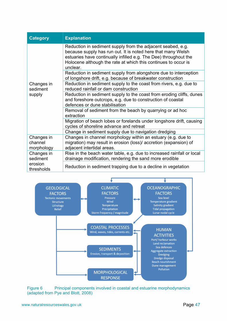
Page 47 www.naturalresourceswales.gov.uk
Category Explanation
Changes in sediment supply
Reduction in sediment supply from the adjacent seabed, e.g. because supply has run out. It is noted here that many Welsh estuaries have continually infilled e.g. The Dee) throughout the Holocene although the rate at which this continues to occur is unclear. Reduction in sediment supply from alongshore due to interception of longshore drift, e.g. because of breakwater construction Reduction in sediment supply to the coast from rivers, e.g. due to reduced rainfall or dam construction Reduction in sediment supply to the coast from eroding cliffs, dunes and foreshore outcrops, e.g. due to construction of coastal defences or dune stabilisation Removal of sediment from the beach by quarrying or ad hoc extraction Migration of beach lobes or forelands under longshore drift, causing cycles of shoreline advance and retreat Change in sediment supply due to navigation dredging
Changes in channel morphology
Changes in channel morphology within an estuary (e.g. due to migration) may result in erosion (loss)/ accretion (expansion) of adjacent intertidal areas.
Changes in sediment erosion thresholds
Rise in the beach water table, e.g. due to increased rainfall or local drainage modification, rendering the sand more erodible
Reduction in sediment trapping due to a decline in vegetation
Figure 6 Principal components involved in coastal and estuarine morphodynamics (adapted from Pye and Blott, 2008)
Page 48 www.naturalresourceswales.gov.uk
The above concept is well illustrated through the work of Pontee (2011), which looked at change along 74 coastal profiles in northwest England. Of the 74 profiles that were analysed, 44 (59%) had some form of defence or other structure present, whilst 30 profiles (41%) had no defences or structures present. Overall, 21 profiles (28%) show coastal narrowing; 11 (of the 44 defended) profiles (25%) and 10 (of the 30 undefended) profiles (33%). These findings are consistent with there being a number of other factors responsible for changes in the width of the coastal zone in addition to the presence of defences and sea level rise. Other contributing factors for observed change in northwest England suggested by Pontee (2011) include shifting positions of offshore banks and channels as well as changes in the wind wave climate. The influence of natural cycles on intertidal morphology has also been considered in a number of studies. Of particular importance is the influence of storminess (which may result in greater wave energy as well as short term changes in sea level) and the lunar nodal cycle (which causes variation in tidal range over an 18.6-year period). These are discussed further in Box 1 and 2. Similarly, sediment supply and variation in rates of sedimentation are also greatly important in determining changes to intertidal morphology, as discussed in Box 3. Box 1 The influence of storminess on intertidal morphology The impact of storminess on change to intertidal morphology/ habitat has recently been demonstrated for the Severn Estuary (The Crown Estate, 2016). This study analysed recent (2006 to 2014) LiDAR measurements of the intertidal evolution of the Outer Severn Estuary and compared the results of this analysis against evidence from 19th and 20th century surveys, geomorphological features, archaeology, geomorphological theory and other contemporary measurements of intertidal change. The short-term LiDAR evidence indicates overall accretion and stability; while the long-term evidence indicates a clear signal of continued erosion since before Roman times, related (at least in part) to sea level rise. However, these two apparently contradictory trends can be explained through consideration of trends in wind/wave action in the Severn estuary: the recent period of LiDAR measurements were shown to have been collected during a relatively benign period of wind-wave activity in comparison to preceding decades. These cycles of storminess are related to the North Atlantic Oscillation (NAO), a weather phenomenon in the North Atlantic Ocean of fluctuations in the difference of atmospheric pressure at sea level between the Icelandic low and the Azores high.

Page 49 www.naturalresourceswales.gov.uk
Box 2 The influence of the 18.6-year lunar nodal cycle The 18.6-year lunar nodal cycle results in a circa 3.7% fluctuation in tidal range over this period (Pugh, 2004). This means that for a macro-tidal setting such as Conwy Bay (tidal range 7 m), the variation in the elevation of spring high tide will be around 0.13 m. The nodal cycle modulates tidal amplitudes and currents, and consequently sedimentation in tide-influenced sedimentary environments. With increased water depth wave heights will increase and similarly their velocity and erosion capability will also increase. A number of studies have considered the influence of the lunar nodal cycle on coastal and estuarine morphology, both through direct field evidence and monitoring. Oost et al. (1993) present data which show that the effects of the lunar nodal cycle are obvious along the coast of the Dutch barrier islands and in the sedimentary fill of abandoned channels. Long term records of bathymetric change in the Humber Estuary (UK) and Westerschelde Estuary (Netherlands) also clearly demonstrate the influence of the lunar nodal cycle on estuary volume, resulting in phases of enhanced estuarine sedimentation (e.g. Jeuken et al., 2003; ABP Research, 1999). The above field observations have also been supported by modelling studies. French (2006) used modelling to demonstrate significant variability in marsh sedimentation associated with 18.6-year tidal modulation whilst Townend et al. (2007) used ESTMORF to demonstrate the influence of the lunar nodal cycle (as well as forcing due to sea-level rise and longer-term changes in tidal range) on the morphological evolution of the Humber Estuary. These studies demonstrate that observed change may simply be part of a cycle, rather than a trend, with this variability complicating the interpretation of sedimentation or elevation change data obtained from monitoring programmes of short duration. Later work by Wang and Townend (2012) also involving ESTMORF shows that the response of an estuary to the nodal tidal variation is not uniform along the length of the estuary: the response is strongest at the mouth and head of the estuary, decreasing exponentially in upstream and downstream directions from these respective limits.
Box 3 The influence of sediment supply and rates of sedimentation Marsh vertical and horizontal growth is strongly dependent on sediment supply, which, if diminished, can switch marshes from accreting to eroding and preclude their keeping pace with sea-level rise (Bouma et al., 2014). Emergent evidence for the past 70 years shows that many marshes on the west coast of England and Wales have undergone dynamic changes in areal extent, but the collective area has expanded, particularly since the 1960s (Robins et al., 2015). However, it is noted here that in some places schemes (such as peatland management) have recently been implemented to reduce silt input to estuaries and these potentially have the capacity to reverse this trend of marsh expansion.

Page 50 www.naturalresourceswales.gov.uk
Given that sediment availability is such a key determinant in the morphological response of intertidal areas to sea level rise, sediment budget analysis is likely to have an important role to play in estimates of habitat loss due to coastal squeeze. The principles of sediment budget analysis are set out in Defra (2018): the approach may be used to help determine if a system has an overall surplus (accretion) or deficit (erosion) of material and therefore whether parts of a system are in balance/equilibrium. Over longer timescales, climate change impacts (unrelated to sea level rise) may also influence intertidal habitat extent. These have previously been considered in detail by Robins et al. (2015) and results are summarised below. A moderate rise in the annual average temperature has the potential to boost vegetation productivity and favour marsh expansion, although a greater frequency of dry summer spells could depress plant growth through desiccation and evaporation-driven increases in sediment salinity (Gedan and Bertness, 2010). Increased frequency of high rainfall events is likely to boost riverine sediments supply to marshes, which is a key stimulant of marsh vertical growth (Fagherazzi et al., 2013). Conversely, future increased storminess could accelerate erosion of marshes located in wide estuaries, where the fetch, and thus potential wave energy, is higher. Finally, natural dynamism within an estuary - such as the Dwyryd which is extremely morphologically active with the channel shifting dramatically in quite short periods – means that change in intertidal extent may occur either side of the channel in response to it migrating. The implication of this is that a focus on one part of the estuary in terms of analysis of extent of intertidal habitats could be flawed as a result, with high uncertainty in extrapolating these changes for the purpose of revising NHCP targets. All of the above discussion serves as a reminder that coastal habitat change occurs on a wide range of temporal and spatial scales (Kraus et al., 1991; Cowell and Thom, 1994). It is important to recognise these dynamics in order to distinguish between short term variability and longer-term trends for deterioration which may adversely affect conservation status (Pontee, 2013). This appreciation of the drivers of change is important in determining appropriate time-scales for monitoring (Section 7.2.2).
3.2. Establishing a baseline Notwithstanding the difficulties in differentiating change in intertidal habitats attributed to coastal squeeze (discussed above) a range of approaches have been applied to calculate the effects (and future projections) of the changes that may be attributed to coastal squeeze. A more detailed review of what has been done elsewhere is provided in Appendix B. From the outset, it is noted that in order to attempt to quantify coastal squeeze loss an accurate baseline must be in place from which any change can be determined. However, it is important to realise that this will only provide a ‘snapshot’ of the situation at any particular time; there will be short-term

Page 51 www.naturalresourceswales.gov.uk
variation as a result of the various forcing factors outlined in Section 3.1. Notwithstanding this, establishing a baseline requires the topography of the intertidal to be determined, as well as the demarcation of the tidal limits: The topography of the intertidal is best established through a combination
of different survey techniques since no one survey type can accurately capture both the top and bottom end of the intertidal (see Section 4); and
Tidal range varies geographically, contributing to large spatial variations in the width of the intertidal zone. Accurate determination of the geographic extent of the intertidal in any given location requires continuous information on the elevation of both MWHS and MLWS (or HAT and LAT depending on the definition being applied) and this is most readily obtained through hydrodynamic modelling. (Over time, it is possible that the sea level rise may contribute to some change in tidal wave propagation, resulting in modification of the tidal range. However, any such changes in tidal range are anticipated to be small for central estimates of 21st century mean sea level rise (Lane and Prandle, 2007).
The topography of the intertidal is best replicated through the creation of a Digital Elevation Model (DEM). To date DEMs have typically been established in a GIS environment using a variety of available data sources, and interpolation in a GIS or a modelling environment (e.g. CCO, 2008; CH2M, 2015). Experience in other countries, notably England, has shown that establishing a consistent and comprehensive baseline DEM can be difficult for the intertidal zone as a whole, but also for saltmarshes, which are typically easier to map than mudflat. Mudflat mapping is frequently not available, patchy or comes with uncertainties relating to the boundary along the transition into the subtidal zone. These difficulties are associated with the available survey techniques (see Section 4) as well as data processing methods including interpolation which can lead to errors. To estimate the extents of individual habitat types this has typically been based on broad assumptions as to where intertidal habitat types can be found in relation to tidal levels (based on Nottage and Robertson, 2005, amongst others): Mudflat between the levels of Mean Low Water Springs (MLWS) and Mean
High Water Neaps (MHWN); Saltmarsh between MHWN and Mean High Water Springs (MHWS); Upper saltmarsh between MHWS and Highest Astronomical Tide (HAT); Transitional grassland between HAT and one metre above HAT (HAT+1);
and Grassland and other terrestrial habitats at elevations over one metre above
HAT. These relationships have been applied to DEMs and respective water levels to provide an approximation of habitat extents. This is known as a hypsometric approach. It is recognised that this ‘habitat prediction’ process involves an inherent simplification of the likely presence of intertidal habitats, particularly saltmarshes, as the formation of vegetation will be dependent on a number of site specific influences (including exposure, substrate and drainage patterns). Many habitat mapping and prediction exercises have thus developed system

Page 52 www.naturalresourceswales.gov.uk
specific equations to determine where certain saltmarsh zones are located in a given estuary or along a given coastline stretch. For example, for its Blackwater saltmarsh change project, ABPmer (2016) divided the estuary into five zones, and developed simple equations for saltmarsh zonation based on aerial imagery interpretation. With regard to saltmarsh in particular, attempts have also been made to establish a more comprehensive baseline, and also gain an understanding of historic trends. The lower mudflat extent has typically been related to the level of MLWS, interpolated from existing records where data was not available. Rarely have dedicated mudflat surveys been undertaken for determining coastal squeeze estimates.
3.3. Calculating losses In order to estimate coastal squeeze losses, past studies have generally followed two main approaches: Predictive forecasting based on past trends, conceptual understanding and
analysis within a GIS framework; or Predictive forecasting based on past trends, conceptual understanding and
analysis within a GIS framework supported by specific numerical modelling tools.
Once a baseline DEM had been established, many of the early coastal squeeze studies in England (mostly in connection with CHaMPs) used modelling, predominantly regime modelling, to project losses into the future. A regime model predicts how an estuary/system model might respond to changes in either the estuary form (reclamation, engineering works, etc.) or the forcing conditions (sea level, tidal range, etc.) in order to return to a regime condition. This would typically be accompanied by a detailed literature review and geomorphological assessment to gain a thorough conceptual understanding of the system being investigated. In addition, further modelling studies were also conducted to verify/sensitivity test results. For example, for the Thames and Severn FRMS strategies, ASMITA (Aggregated Scale Morphological Interaction between a Tidal basin the Adjacent coast) was also employed; ASMITA can take account of estuarine landward movement/rollover (estuary transgression). These models were run for various sea level rise scenarios based on relevant government guidance of the time. General intertidal and individual habitat extents were again predicted based on an updated DEM and projected water levels at the respective time steps (using the same methods as used to define the baseline (see Section 3.2)). In some early studies, and several more recent projects (e.g. the Poole and Exe FRMSs in England), coastal squeeze estimates have been determined using GIS exercises only (without the use of detailed modelling). In these instances, future predictions of habitat extent have been determined through the adjustment of the baseline based on extrapolation of sea level rise estimates for each epoch. Accretion has not typically been taken into account in past studies, though some (such as the Solent Dynamic Coast Project (CCC, 2008)) applied various annual accretion scenarios as sensitivity tests.

Page 53 www.naturalresourceswales.gov.uk
Previous studies have also assumed that all predicted changes in habitat extent are attributable to coastal squeeze, which would not be the case in reality (see Section 3.1). Current means of calculating habitat loss attributed to coastal squeeze do not have a robust method to decipher these from other forcing factors. This results in very high uncertainties in habitat loss estimates. Uncertainty in defining coastal squeeze losses has typically been acknowledged in only qualitative terms, and/or adopting what are perceived to be conservative values, or expressed by presenting range values for losses.
Page 54 www.naturalresourceswales.gov.uk
4. Review of Possible Monitoring Techniques
4.1. Introduction As described in the previous section, there is an inherent difficulty in monitoring/ determining change specifically associated with coastal squeeze. Notwithstanding this, any attempt to monitor coastal squeeze needs to firstly understand changes in sea levels, as well as the extent, condition and habitat types of the intertidal zone. This requires a combination of physical and biological monitoring with adequate spatial and temporal resolution. Intertidal extent requires an accurate assessment of the location of MHWS and MLWS using data on topography or bathymetry, tidal heights (e.g. from tide gauges) and a modelled output of this information (see Section 3.2). An assessment of habitat extent and condition of habitats within the intertidal zone requires data on habitat types, habitat boundaries and their location, and the ecological quality of communities of species within them. In order to identify the most appropriate options for monitoring coastal squeeze in Wales, it is pertinent to explore a range of available monitoring techniques applied to monitoring coastal habitats. In this section, these have been grouped by the parameters that are required to be measured to assess extent, condition and habitat types (described above). These are summarised as follows, with the corresponding monitoring techniques which are reviewed in this section: Sea level:
- Tide gauges; and - Satellite altimetry.
Topography/bathymetry: - LiDAR; - Radar; - Stereo-photogrammetry using multispectral images; - Bathymetric surveys; - Terrestrial laser scanners; and - Real Time Kinetic Global Navigation Satellite System (RTK GNSS).
Habitat types, boundaries and condition: - Multispectral imagery (including aerial photography); - Hyperspectral imagery; and - Field habitat surveys (e.g. Phase I habitat survey).
This section provides an overview of what each technique can measure and how it measures it, and the processing of data required to monitor changes in coastal habitats. A technical review of each technique is provided (at the end of each sub-section), as well as a summary of key considerations. The technical review is based on the following criteria, and Table 6 provides a qualitative scoring system (RAG rating) for each: Spatial resolution (number of data measurements spatially); Accuracy (horizontal and vertical accuracy of measurements OR accuracy
of habitat classification (thematic accuracy));

Page 55 www.naturalresourceswales.gov.uk
Sources of error (e.g. subjectivity, weather and ground conditions etc.); Spatial coverage; Repeatability (repeatability in capturing data and ability to compare data); Ease of implementation (effort/time required for data collection); Costs (costs associated with data collection and processing – not including
assessment/analysis of data); and Wider benefits (usefulness of data to contribute to a wider integrated
approach to environmental monitoring (e.g. ERAMMP).
Table 6 Criteria and RAG rating to be reviewed for each monitoring technique
Criteria Technique Scoring range
Spatial resolution All ≥10 m 1 to 10 m ≤1 m
Accuracy
Horizontal All ≥1 m 0.1 to 1 m ≤ 0.1 m
Vertical Topographic / bathymetric / sea level
≥1 m 0.1 to 1 m ≤ 0.1 m
Thematic Multispectral, hyperspectral, field survey
<50% habitat classification accuracy 50 to 75% habitat classification accuracy >75% habitat classification accuracy
Sources of error All High vulnerability to error Medium vulnerability to error Low vulnerability to error
Spatial coverage All Local Regional National
Repeatability All
Data is incomparable on temporal scales Repeatability limited by timings of data capture Data capture timed with favourable conditions
Ease of implementation
All
Data collection/processing is labour intensive and complex Data collection/processing requires some planning Minimal planning required for data collection/processing
Costs All ≥£200 per km² £100 to £199 per km² ≤£99 per km²
Wider benefits All
No other applications Indirectly applicable to other environmental monitoring Directly applicable to other environmental monitoring

Page 56 www.naturalresourceswales.gov.uk
4.2. Sea level
Accurate information on sea level rise is of fundamental importance for both estimating the scale/rate of coastal squeeze at a project level and for determining the rate of change in area, extent and (potentially) condition of the intertidal features affected by rising sea levels in HTL policy locations. Tracking observed rates of sea level rise is also of relevance in the re-evaluation of NHCP targets based on original estimates of coastal squeeze, derived from sea level rise projections (these estimates were made for the whole Wales Natura 2000 network relating to the SMPs at the HRA and IROPI stage (signed off in 2014/15) and are made at the Project level as Marine Licenses are evaluated).
4.2.1. Overview of monitoring techniques Tide gauges and satellite altimetry are the two main techniques used to measure the present rates of change in sea level and form the basis for estimates of global mean sea level change (e.g. Menendez and Woodworth, 2010). However, from the outset it is important to note that tide gauges measure sea level relative to the ocean floor whereas the reference for satellite altimetry is the earth's centre. Accordingly, tide gauges provide information on ‘relative’ sea level change (i.e. isostatic and eustatic components) whereas satellite altimetry data provides information on ‘absolute’ change in the level of the sea surface (i.e. eustatic component). Making the direct connection between the sea level measured by a tide gauge and that measured by a satellite altimeter is not a trivial exercise, as the two measurements will be separated in time and space and it is therefore necessary to understand how all the components contributing to the total sea level vary in the locale of the tide gauge. It is also important to ensure consistent corrections are applied to both sets of data (Cotton et al., 2016). Importantly, (and as previously stated in Section 2.3), when considering coastal squeeze, it is the position of mean sea-level ‘relative’ to the land surface which is of greatest importance since vertical movements of both the elevation of the sea surface and land can contribute to coastal squeeze. A key consideration when using observed records of mean sea level rise (either tide gauge or satellite) to validate existing coastal squeeze estimates is the time-scale over which the mean should be determined. Indeed, mean sea level may exhibit significant inter-annual variation, driven by meteorological influences such as mean sea level pressure, local winds, precipitation or river run-off. These trends may be linked to variations in ocean circulation such as the Atlantic Meridional Overturning Circulation (AMOC) and for Wales - the related Gulf Stream. This concept has been demonstrated for locations in the North Sea by Wahl et al. (2013) (Figure 7).
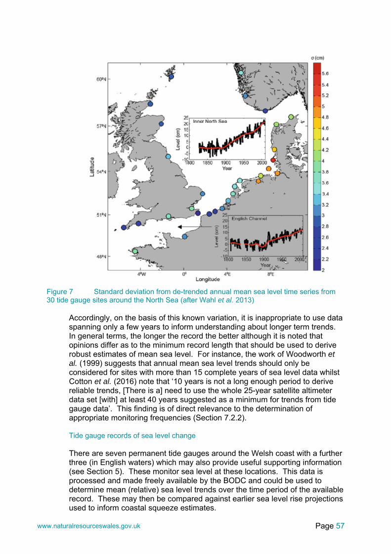
Page 57 www.naturalresourceswales.gov.uk
Figure 7 Standard deviation from de-trended annual mean sea level time series from 30 tide gauge sites around the North Sea (after Wahl et al. 2013)
Accordingly, on the basis of this known variation, it is inappropriate to use data spanning only a few years to inform understanding about longer term trends. In general terms, the longer the record the better although it is noted that opinions differ as to the minimum record length that should be used to derive robust estimates of mean sea level. For instance, the work of Woodworth et al. (1999) suggests that annual mean sea level trends should only be considered for sites with more than 15 complete years of sea level data whilst Cotton et al. (2016) note that ‘10 years is not a long enough period to derive reliable trends, [There is a] need to use the whole 25-year satellite altimeter data set [with] at least 40 years suggested as a minimum for trends from tide gauge data’. This finding is of direct relevance to the determination of appropriate monitoring frequencies (Section 7.2.2). Tide gauge records of sea level change There are seven permanent tide gauges around the Welsh coast with a further three (in English waters) which may also provide useful supporting information (see Section 5). These monitor sea level at these locations. This data is processed and made freely available by the BODC and could be used to determine mean (relative) sea level trends over the time period of the available record. These may then be compared against earlier sea level rise projections used to inform coastal squeeze estimates.
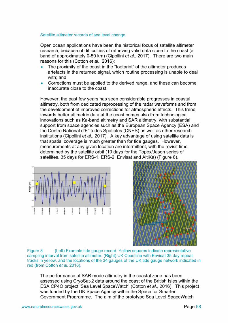
Page 58 www.naturalresourceswales.gov.uk
Satellite altimeter records of sea level change Open ocean applications have been the historical focus of satellite altimeter research, because of difficulties of retrieving valid data close to the coast (a band of approximately 0-50 km) (Cipollini et al., 2017). There are two main reasons for this (Cotton et al., 2016): The proximity of the coast in the “footprint” of the altimeter produces
artefacts in the returned signal, which routine processing is unable to deal with; and
Corrections must be applied to the derived range, and these can become inaccurate close to the coast.
However, the past few years has seen considerable progresses in coastal altimetry, both from dedicated reprocessing of the radar waveforms and from the development of improved corrections for atmospheric effects. This trend towards better altimetric data at the coast comes also from technological innovations such as Ka-band altimetry and SAR altimetry, with substantial support from space agencies such as the European Space Agency (ESA) and the Centre National d’E´ tudes Spatiales (CNES) as well as other research institutions (Cipollini et al., 2017). A key advantage of using satellite data is that spatial coverage is much greater than for tide gauges. However, measurements at any given location are intermittent, with the revisit time determined by the satellite orbit (10 days for the Topex/Jason series of satellites, 35 days for ERS-1, ERS-2, Envisat and AltiKa) (Figure 8).
Figure 8 (Left) Example tide gauge record. Yellow squares indicate representative sampling interval from satellite altimeter. (Right) UK Coastline with Envisat 35 day repeat tracks in yellow, and the locations of the 34 gauges of the UK tide gauge network indicated in red (from Cotton et al. 2016).
The performance of SAR mode altimetry in the coastal zone has been assessed using CryoSat-2 data around the coast of the British Isles within the ESA CP4O project ‘Sea Level SpaceWatch’ (Cotton et al., 2016). This project was funded by the UK Space Agency within the Space for Smarter Government Programme. The aim of the prototype Sea Level SpaceWatch

Page 59 www.naturalresourceswales.gov.uk
service was to provide information on observed sea level around the UK by processing space-borne altimeter data, and to provide that information alongside equivalently processed tide gauge data. This would then allow planners to verify the regional variability of sea level at multiple time scales and observe the presence of any significant inter-annual changes (Cotton et al., 2016). Example gridded altimeter outputs produced as part of the SpaceWatch program are shown in Figure 9, with sea level trend data (mm/yr) provided at 3.5 km intervals along each track. Key conclusions from the project are set out below (Cotton et al., 2016): Altimetry has the potential to provide sea level information (trends,
variability, seasonal signals) in the coastal region; Altimeter data provide a fine spatial sampling along satellite tracks that
nicely complements the virtually continuous temporal sampling by tide gauges; and
A longer period of altimeter data (i.e. greater than the period analysed which was from 2002-2010) is required to support reliable trend estimates.
Figure 9 Maps of gridded Envisat altimeter sea level data (2002-2010): (Left) Long term trend in mm/yr; (Right) amplitude of the annual cycle (mm)
A follow-up study by Cippolli et al. (2017) presented a comparison between the UK altimetry and tide gauge observations on inter-annual timescales. This research demonstrated a very good agreement between coastal altimetry and tide gauge observations (Figure 10). However, in some locations (notably Portbury and Severn Bridge), poor correlations were observed. It is understood that this relates to the estuarine location of these sites. This is an important point of note, given that most saltmarsh, sandflat and mudflat habitats are themselves, located in estuarine environments in transitional waters. The recommendation stemming from the work of Cipollini et al. (2017) is that further efforts are still needed to study sea level trends in the coastal zone from past and present satellite missions. (Based on costs presented in Cotton et al. (2016), it is understood that this work may be in the range £70-100k.) Further improvements are expected from more refined processing and screening of altimetric data, but in particular from the constant improvements in

Page 60 www.naturalresourceswales.gov.uk
the geophysical corrections applied to them, owing to the noisier nature of the data when coming near shore.
Figure 10 Correlation (a) and root-mean-square difference (RMSD) (b) between de-seasoned and de-trended sea level from altimetry and tide gauge observations. Empty circles in a denote non-significant correlation. (From Cipollini et al., 2017) 4.2.2. Processing and analysis of data
On the basis of Figure 12 to Figure 16, it is apparent that there is a good geographical spread of tide gauges around Wales: this is important, particularly given the known spatial variation in glacio-isostatic adjustment (Figure 4). It may therefore be a reasonable assumption to make that the mean sea level signature observed at the nearest tide gauge(s) to any given Natura 2000 site of interest would be broadly representative for the Natura 2000 site as a whole. Although meteorological factors could potentially influence longer term mean sea level trends at the local scale, it is considered that any error introduced by this uncertainty would be very small in comparison to that associated with other factors contributing to overall uncertainty, most notably incomplete knowledge of sedimentation rates. The latter is a critical complicating factor when using a hypsometric approach to determining coastal squeeze loss and this is discussed further in Section 4.2.3. As already noted in this section, satellite data only provides information on the elevation of the sea surface, and not on trends in mean relative sea level. Accordingly, even if satellite altimeter data were to be used in future (once known methodological processing errors have been resolved) the data would still need to be corrected for isostatic change. It should be possible to achieve this in the first instance through use of GPS measurements of crustal motion alongside modelling patterns of GIA (see Figure 4) (Bradley et al., 2009).

Page 61 www.naturalresourceswales.gov.uk
4.2.3. Technical review This section demonstrates that both tide gauge and (some) satellite data may be used in a hypsometric approach for the validation of coastal squeeze estimates. Both data sources have the potential to deliver high levels of accuracy and precision with regards to trends in mean sea level although the utilisation of either dataset requires careful consideration of the time period over which meaningful trends can be determined and (in the case of satellite data) wider knowledge about regional patterns of GIA. In terms of informing hypsometric analysis of coastal squeeze in Wales, it is probable that the use of tide gauge data is currently the most appropriate and cost-effective solution: whilst not achieving the same spatial coverage as satellite data, the tide gauges record relative sea level change (rather than change in sea-surface height), which is the most relevant parameter for informing coastal squeeze. Moreover, whilst satellite data is continually collected from Welsh waters, it is understood that it is not routinely processed to enable the determination of local-scale mean sea level trends. Conversely, this processing element is already carried out by the BODC for tide gauges, with data made freely available on an annual basis. However, in future (and once known methodological issues have been resolved), satellite derived observations of sea level change are likely to be of great value in complementing and validating the coastal tide gauge records. Whilst hypsometric analysis of coastal squeeze may potentially be undertaken relatively quickly and efficiently, there is considerable uncertainty with the approach due to the role of sedimentation, as well as other factors (see Section 3.1 and 6.4). Marshes respond to relative sea level rise in part by building soil elevation thereby (at least partially) offsetting loss to coastal squeeze. Indeed, depending on the availability of sediment, the saltmarsh extent may therefore be maintained even under rising sea levels. Vertical sediment accretion data are available for many marshes in North America and Europe (Horton et al., 2018) and these could (at least) theoretically be used to help inform understanding of potential sedimentation rates. However, any attempt to apply a sedimentation correction factor to estimates of coastal squeeze would be extremely difficult and associated with high levels of uncertainty: sedimentation rates will vary spatially (alongshore and across shore) with rates of accretion across low lying mud flat areas likely to be far lower than for vegetated marsh areas higher up the intertidal. Sedimentation rates will also vary temporally and comparing current accretion rates to future rates of relative sea level rise may be problematic for a number of reasons. In particular, accretion rates tend to increase with flooding duration so that marshes may accrete faster under accelerated relative sea level rise (e.g. Kirwan et al., 2016; Friedrichs and Perry (2001)). Finally, it is noted that any uncertainty introduced through unknown sedimentation rates will be considerably reduced in rocky intertidal areas fronting defended stretches of coast. However, the occurrence of such settings is limited in Wales.

Page 62 www.naturalresourceswales.gov.uk
Using sea level rise projections to update future loss estimates As discussed in Section 2.3, projections of sea level rise are available for Wales (on a 25 km grid), from UKCP09 for the period between 1990 and 2100. These projections are soon (November 2018) to be updated by UKCP18 sea level rise projections and it is probable that further updates will be made over the coming decades, as greater understanding about possible acceleration in rates of sea level rise emerges. As they become available, these revised projections should be compared against previous sea level rise rates to refine estimates of future coastal squeeze loss. In effect, this would involve re-calculating the loss estimates following the same hypsometric approach summarised in Section 3.2 and Section 4.3.2. A technical review of techniques to monitor sea levels is provided in Table 7.

Page 63
Table 7 Technical review for sea level monitoring options.
Criteria Resolution Vertical accuracy
Sources of error
Spatial coverage
Repeatability Ease of implementation (time)
Costs (data collection)
Wider benefits
Sea level data (to inform hypso-metric analysis)
Tide gauge
High temporal resolution of records, enabling mean sea level to be determined at centimetric scale.
Potential for highly accurate records of relative sea level change at instrument location.
Significant uncertainties arise with projections of morphological change, owing to uncertainty around sedimentation rates (and other factors surrounding cause and effect – see Section 3.1).
Good geographic spread of records around Welsh coast.
Standardised methodologies available for determining mean sea level from long term records.
Data is easily obtainable; some desk based GIS processing required to determine intertidal change.
Sea level data already collected and processed by the NTSLF².
Data extremely helpful in informing wider coastal monitoring, including flood risk management.
Sat. Known difficulties in deriving mean sea level trends from up-estuary locations¹.
Good coverage of all areas.
Repeatability may be complicated through use of differing processing algorithms.
Satellite data requires a lot of post-processing; some desk based GIS processing required to determine intertidal change.
Satellite data already collected but significant work required to process.
¹ (Cippolli et al., 2017) ² https://www.bodc.ac.uk/

Page 64 www.naturalresourceswales.gov.uk
4.3. Topography/bathymetry Most habitat maps are created using optical imagery and field observations, as reviewed in Section 4.4. This allows habitat boundaries to be deciphered and are inherently useful (Kendall et al., 2001; Battista et al., 2007). However, they do not provide topographic information12, which is important as this influences the spatial distribution of marine organisms and is imperative for monitoring implications of sea level rise on coastal squeeze (Pittman et al., 2007; Wilson et al., 2007; Wedding et al., 2008; Costa et al., 2009). The product of topographic/bathymetric data are digital elevation models (DEMs); three-dimensional representations of a ground surface. This collective term can be separated into two types, the definitions of which are somewhat interchangeable. It is generally agreed that digital surface models (DSMs) represent the height of earth’s surface and the objects on it (i.e. trees, vegetation, houses) whereas digital terrain models (DTMs) represent the height of bare earth surface.
4.3.1. Overview of monitoring techniques
LiDAR
Light detection and ranging (LiDAR) uses lasers to obtain information on the location and height of features on the ground, by recording the return of pulses from the ground usually from aircraft. Essentially LiDAR produces a DEM which shows the elevation of land. This has applications to monitoring coastal squeeze, both to complement happing mapping data and for predicted habitat modelling. The latter involves assessing potential intertidal extents based on tidal levels and can be used to predict how this may change with sea level rise (see Section 4.3.2). LiDAR can also measure bathymetry, however, issues such as surface roughness and water clarity (which is prevalent around the Welsh coastline) is problematic for accurate bathymetric measurements using LiDAR. The topography of intertidal mud and sandflats may be difficult to measure using LiDAR due to the reflectivity of these surfaces when wet, causing the laser signal to be reflected away from the direction of the sensor (and not scattered back in many directions), known as specular reflection (Schmidt et al., 2013; Wiehle et al., 2015). This decreases the vertical accuracy of measuring flat waterlogged areas (Choril et al., 2018).
Radar
Topographic data can be obtained in a similar way to LiDAR but with the use of radio detection and ranging (radar) using radio waves (Souza-Filho and Paradella, 2003; Ryu et al., 2008; Di Paolo et al., 2017). It is now more commonly applied from satellites for coastal monitoring, though land and aircraft-based sensors are available.
12 Orthorectified imagery combines imagery with digital elevation models (i.e. LiDAR/RADR data) to remove image distortion and create a geometrically and planimetrically correct image.
Page 65 www.naturalresourceswales.gov.uk
Radar can provide information on topography and create DEMs similarly to LiDAR. Improved capabilities of radar for monitoring coastal habitats are realised with Synthetic Aperture Radar (SAR) whereby resolution is increased using the motion of the radar antenna over the target region, and is now commonly used. For example, with the launch of TerraSAR-X in 2007 (and other satellites following this), resolutions on the scale of metres are available for radar which have previously been limited by poor resolutions (Adolph et al., 2018). Radar is also affected by specular reflection; however, it can also detect waterlines, and use this to create a DEM, effectively using the sea as an altimeter (Mason et al., 2000). This is especially applicable to the intertidal zone. It works by using radar imagery to detect the water’s edge at various states of the tide. Heights relative to mean sea level, predicted using hydrodynamic tide-surge models and tide gauges, are then superimposed on geo-coded waterlines (Mason et al., 2000; Mason et al., 2010). From multiple images over a range of tidal states, a set of heighted waterlines can be assembled, and interpolated to form a DEM (Mason et al., 2010). The waterline method can also be achieved with other imagery (e.g. multispectral) but a satellite SAR image is most commonly used (Mason et al., 2000). From this information, the extent and topography of the intertidal zone can be mapped. The variation of habitats within it are not decipherable. Stereo-photogrammetry using multispectral images It is possible to obtain topographic information from multispectral imagery (satellite, aircraft or UAV derived) which is reviewed separately in Section 4.4.1, by comparing stereo-pairs (Mason et al., 2000). Two overlapping images are required to calculate heights of features on the ground (Mason et al., 2000). This is slightly less accurate than LiDAR, and previously only changes on the scale of 0.1 m vertically and above were detectable by this technique (Environment Agency, 2007). But this is still relatively seldom applied to coastal monitoring and recent testing from UAVs is producing accuracies comparable with LiDAR (CCO, pers. comms.). Therefore, use of this technique may increase in the future, particularly considering the potential cost savings compared to LiDAR if collected from satellite imagery or UAVs. Bathymetric survey Single beam and multibeam echosounders may be used to determine bathymetry via vessel based survey. Both techniques involve measurement of the timing of returning sound pulses from the seabed, and measure the depth below the vessel which is corrected to tide levels with the use of differential GPS (CCO, 2018a). The main benefit of multibeam survey is that it enables a far higher resolution survey to be obtained than for single beam, with far greater seabed coverage per survey transect. However, instrument costs are higher and data processing requirements are greater.

Page 66 www.naturalresourceswales.gov.uk
This technique is applicable for measuring bathymetry at the lowest extents of the intertidal zone, which is a major drawback of most terrestrial and remote sensing monitoring techniques. Real time kinetic global navigation satellite system Traditionally, topographical surveys in the field were undertaken using levelling equipment and total station theodolite. These are optical techniques that involved taking elevation readings from a measuring staff relative to a fixed datum, with the latter being capable of obtaining XYZ coordinate data. Topographic information is now more commonly obtained by GPS measurements, the most accurate of which that can be applied to topographical surveys is Real Time Kinetic (RTK) Global Navigation Satellite System (GNSS). This makes use of a base station and rover station carried by a surveyor. The base station is able to correct for errors in satellite signals, and multiple rover stations can be used to collect highly accurate topographic and positional data; this is the most accurate form of topographic surveying technique. Furthermore, marsh sediment levels can be obtained from this technique, rather than just vegetation height, which is not possible from others (i.e. DTMs rather than DSMs). This is because LiDAR and other techniques cannot penetrate saltmarsh vegetation as it is too dense and therefore cannot distinguish between marsh height and vegetation height (Fernandez-Nunez et al., 2017). Obtaining information on marsh levels may somewhat discern cause and effect of intertidal changes. Terrestrial laser scanners Terrestrial laser scanners can also be used to map local topography. They work in a similar way to LiDAR, but collect information from an instrument on the ground. It is a more accurate and higher resolution means to gain topographic information, but is commonly only applied at local scales. It becomes less accurate on flatter, wetter surfaces, and is more appropriate for mapping cliff lines. Terrestrial laser scanners can either be static or mobile types. The latter can be fitted to an all-terrain vehicle (ATV); it has improved spatial coverage getting its position from GNSS and is corrected for by an inertial motion unit.
4.3.2. Processing and analysis of data Processing Processing of topographic data mainly involves merging mosaics into a single dataset, geo-referencing, and interpolation of gaps in values (e.g. using nearest neighbours according to Euclidean distance) (Chirol et al., 2018). LiDAR is affected by atmospheric scattering and cloud cover and needs to be avoided or corrected, however lighting is not an issue and LiDAR can be flown at night. Radar techniques are unaffected by atmospheric scattering and are

Page 67 www.naturalresourceswales.gov.uk
advantageous to LiDAR in that regard. Bathymetric data needs to be corrected for sound velocity profiles which can be affected by things like currents. Analysis As mentioned in Section 3.2 and 4.2 a hypsometric approach to the analysis of coastal squeeze can be used, combining information on: Sea level change; Intertidal topography/bathymetry (DEMs); Modelling to provide information on tidal range, interpolated from tide
gauge data; and Criteria determining the vertical zonation of intertidal areas, based on
known relationships between the distribution of intertidal habitats and reference tidal water levels (see Section 3.2).
It is a relatively simple GIS task to determine intertidal extent comparing sea level and available DEM. The majority of the work involves the use of a pre-processed, mosaicked DEM and the development of a number of rule bases, where segmentation and classification of the major habitat classes is carried out. This may equate to around a day of time for a competent person (after processing). The amount of data (or area it is applied to) should also not increase the analysis time significantly.
4.3.3. Technical review LiDAR is likely to be an expensive option as it is generally flown from aircraft, however it is the most commonly used technique to obtain topographic data in terrestrial environments. Furthermore, data is collected on a national scale at fairly regular intervals (see Section 5.5), so it may be possible to coordinate data collections for multiple purposes. Radar obtained from satellite data may be a cheaper option, but its accuracies tend to be less than LiDAR. A major limitation with these techniques (as with most remote sensing techniques) is capturing lower intertidal zones. Bathymetric surveys will provide data at the lowest intertidal zone, but is very expensive. Stereo-photogrammetric techniques have not been applied in earnest, though early applications to monitoring the coastal zone suggest promise with at least comparable accuracies to LiDAR (CCO, pers. comms.). Similarly, to field habitat surveys, RTK GNSS may not be a practical monitoring option on a national scale, but offers the best accuracies at local scales. It is important to note that, aside from field surveys using RTK GNSS, current accuracy margins of remotely sensed topographic and bathymetric surveys (approximately 0.1-1 m) either overlap or exceed global projections of sea level rise over the next century (approximately 0.44-0.74 m). This suggests most monitoring and assessment of intertidal changes may be inadequate in the context of coastal squeeze and rising sea levels (Fernandez-Nunez et al., 2017). A technical review of techniques to monitor sea levels is provided in Table 8.

Page 68
Table 8 Technical review for topographic/bathymetric monitoring options
Criteria Resolution Horizontal / vertical accuracy
Sources of error
Spatial coverage
Repeatability Ease of implement-ation (time)
Costs (data collection)
Wider benefits
LiDAR Aerial Spatial resolution between 25 cm and 2 m¹.
Vertical accuracy ±5 to 15 cm².
Acquisition at suitable tidal states due to water reflectivity³.
High and rapid spatial coverage up to 50 km² per hour⁴.
As with most remote sensing techniques, issues are capturing lowest tidal extents and weather conditions. Bathymetric LiDAR is limited by water clarity in Wales⁵.
Aerial surveyors need to be commissioned and flights programmed to align with favourable weather and tides.
Costs approximately £265 per km² for data acquisition and processing⁶.
Topographic information can be applied to other applications such as flood modelling and coastal protection.
Radar Sat. Courser resolution than LiDAR due to longer wavelengths, but have recently improved to resolutions of 1.5 to 3.5 m (TerraSAR-X)⁷.
Up to ±1 m vertical accuracy⁸. Waterline method up to 40 cm but can vary⁹.
Acquisition at suitable tidal states due to water reflectivity.
Good spatial coverage.
Allows all weather, day and night capture¹⁰. Can capture lowest tidal extents using waterline method.
Data is easily obtainable soon after image capture.
Taking TerraSAR-X as an example, costs range from £19 to £38 per km² for a resolution of 1 to 2 m (SpotLight mode) ¹¹. Converted from Euros to Pound sterling (23/08).
Topographic information can be applied to other applications such as flood modelling and coastal protection.
Multi-spectral (stereo-pairs)
Sat. See multispectral imagery in Table 9.
Vertical accuracy approximately ±1 to 15 m¹².
See multispectral imagery in Table 9.
See multispectral imagery in Table 9.
See multispectral imagery in Table 9.
See multispectral imagery in Table 9.
See multispectral imagery in Table 9.
See multispectral imagery in Table 9.

Page 69
Criteria Resolution Horizontal / vertical accuracy
Sources of error
Spatial coverage
Repeatability Ease of implement-ation (time)
Costs (data collection)
Wider benefits
Aerial See multispectral imagery in Table 9.
Vertical accuracy approximately ±0.5 m¹³.
See multispectral imagery in Table 9.
See multispectral imagery in Table 9.
See multispectral imagery in Table 9.
See multispectral imagery in Table 9.
See multispectral imagery in Table 9.
See multispectral imagery in Table 9.
UAV See multispectral imagery in Table 9.
Vertical accuracy up to ±5 cm⁶.
See multispectral imagery in Table 9.
See multispectral imagery in Table 9.
See multispectral imagery in Table 9.
See multispectral imagery in Table 9.
See multispectral imagery in Table 9.
See multispectral imagery in Table 9.
Bathy-metric surveys
Single beam¹⁴
Spaced survey lines required due to single beam – assumed 25 m. Approximately 0.5 m resolution along-track.
Horizontal accuracy up to ±0.1 m. Vertical accuracy of ±0.2 m.
Variations in sea state, currents and seabed sediments may contribute to error. Tidal levels need to be corrected for¹⁵.
Limited by water depth (tide) and vessel speed. Single beam, and need for transects, limits coverage to approximately 2 to 3 km per survey day.
Can be timed with high tides and favourable weather.
Difficult to implement on wide scale at high resolutions.
Estimated to be £330 to £660 per km.
Bathymetric information can be applied to other applications such as flood modelling, coastal protection, and hydrographic surveys.
Multi-beam¹⁴
Approximately 0.5 m.
Horizontal accuracy up to ±0.1 m. Vertical accuracy of ±0.1 m.
Limited by water depth (tide) and vessel speed. Approximately 7.5 to 15 km per survey day could be surveyed at high tides.
Estimated to be £200 to £400 per km.

Page 70
Criteria Resolution Horizontal / vertical accuracy
Sources of error
Spatial coverage
Repeatability Ease of implement-ation (time)
Costs (data collection)
Wider benefits
RTK GNSS User defined. Horizontal accuracy ±1 cm¹⁶. Vertical accuracy ±2 cm¹⁶.
Very small error achieved through corrections with base station.
Localised scale limited to accessible areas.
Can be timed with low tides though will be difficult to capture lowest tidal extents.
Labour intensive, and difficult to implement on wide scale at high resolutions.
Expensive due to time required to undertake surveys. Estimated to be £200 per km² of coastline.
Topographic information can be applied to other applications such as flood modelling and coastal protection.
Terrestrial laser scanners
Very high resolution on millimetric scale¹⁶.
Accuracies of up to ±3 mm can be achieved¹⁷.
Error incurred on wet surfaces due to reflectivity¹⁸.
Points can be gathered over 150 m radius of laser¹⁸.
Can be timed with low tides though will be difficult to capture lowest tidal extents.
Labour intensive, and difficult to implement on wide scale at high resolutions.
Estimated to be £200 per km² based on personnel time.
Topographic information can be applied to other applications such as flood modelling and coastal protection.
¹ (NRW, 2018) ² (PCO, 2010; Klemas, 2011; Geomatics Group and Natural England, 2011) ³ (Schmidt et al., 2013; Wiehle et al., 2015) ⁴ (Royal Haskoning, 2015) ⁵ (Klemas, 2013) ⁶ (CCO, pers. comms.) ⁷ (Fritz et al., 2018; Adolph et al., 2018) ⁸ http://www.infoterra.es/asset/cms/file/tsx_international_pricelist_en_issue_03.pdf ⁹ (Mason et al., 2010) ¹⁰ (Mason et al., 2010; Bartlett and Celliers, 2016) ¹¹ Adolph et al. (2018); Purdy et al., (2017) ¹² (Guan et al., 2018) ¹³ (Pulighe and Fava, 2013) ¹⁴ (ABPmer, pers. comms.) ¹⁵ (CCO, 2018a) ¹⁶ (USGS, 2017) ¹⁷ (Digital Surveys Ltd, 2018) ¹⁸ (CCO, 2018b)

Page 71 www.naturalresourceswales.gov.uk
4.4. Habitat types, boundaries and condition In order to monitor the extent and condition of intertidal habitats, and impacts attributed to coastal squeeze, information on the types of habitats that are present, their location, and condition is required. Condition is comprised of a number of things, including physical structure and morphology (which can be inferred from topographic surveys). It is also comprised of species composition, ecological functioning, and habitat extent and distribution. Conservation objectives of designated features aim for favourable status of these parameters. This can be provided by the following monitoring techniques.
4.4.1. Overview of techniques Multispectral imagery Multispectral imagery measures multiple spectrums of light that are reflected from the earth. It is a remote sensing technique that can be undertaken from satellite, aircraft or UAV based platforms. Aerial photography (photographs taken of the earth from above, generally from aircraft) is a form of multispectral imagery that measures visible wavelengths of light (red, green and blue bands). Light within the near-infrared (NIR) bands can also be captured, as well as other distinct bands within the electromagnetic spectrum. This imagery is most commonly captured by digital cameras, known as passive sensors as they measure natural emissions produced by earth’s surface (i.e. reflected sunlight) (Purkis and Klemas, 2011). Digital cameras are able to capture photographs with photogrammetric positional accuracy coupled with GPS (Klemas, 2013). Different spectrums of light can be selected by digital cameras using filters. Multispectral images of coastlines are most commonly used to provide information on the location, distribution and extent of coastal habitats. It is possible to differentiate land surfaces when measuring visible spectrum of light (i.e. aerial photography) with visual interpretation. Furthermore, vegetation can be classified using NIR spectrums of light, exploiting the fact visible light is absorbed and NIR light is reflected by photosynthetic vegetation (Weier and Herring, 2000). Therefore, multispectral imagery tends to be applied more regularly to the measurement of saltmarsh extent, as it is relatively easy to distinguish this habitat from surrounding land cover, however mudflats and sandflats can also be measured (Environment Systems, 2015). To a certain extent, analysing the reflectance value of ground surfaces in multispectral images can also aid differentiation of ground surfaces. Hyperspectral imagery Hyperspectral imagery is a remote sensing technique which can be undertaken from both satellite and aircraft; few applications with UAVs have been undertaken. The technique measures narrower and more spectral bands than multispectral imagery. It captures wavelengths within the visible and infrared and also within thermal portions of the electromagnetic spectrum

Page 72 www.naturalresourceswales.gov.uk
(Jensen et al., 2007). The method involved in hyperspectral imaging includes the analysis of specific characteristics of spectral signatures of the earth’s surface. From this, pixels within the image can be assigned to a habitat or surface. Hyperspectral imagers offer more information than multispectral imagers as they gather data across a wider spectrum of wavelengths reflected from earth. This enables a discrimination of the reflectance values of the earth’s surface which can be used to classify habitat or surfaces in more detail. For example, species communities and habitat zonation (e.g. pioneer marsh, mid-marsh, upper marsh) within habitats, and even their productivity, can be measured (Klemas, 2013). Analysis of species communities may offer information on habitat structure which can inform the condition of habitats, as well as extent and distribution as with multispectral imagery. Field habitat surveys Field habitat surveying involves collecting information on habitats on the ground, by hand. Field data can be collected by walking habitat extents using GPS, recording species (e.g. presence/absence and abundance/coverage with the use of quadrats), organism sampling (e.g. collection for laboratory analysis), analysing community zonation, and recording other physical data of note (e.g. substrate, micro-topography, human impacts/disturbance etc.). To map habitat extent in the field a handheld GPS device can used to record points along a habitat boundary, which is walked by a surveyor. However, RTK GNSS is a more accurate way to map boundaries and topography in the field to centimetre accuracy (see Section 4.3). Quadrat samples, organism sampling, and transects can also be taken to contribute to condition assessment. Field habitat surveying offers the most accurate and detailed amount of information on coastal habitats. It allows the diversity of habitats to be determined by the presence and abundance of species, as well as the extent, distribution, and location of habitats with the use of GPS, as with other remote sensing techniques. Therefore, this facilitates a full assessment of condition of habitats. It also assists in imagery interpretation of coastal habitats obtained from remote sensing techniques via ground truthing (UK-TAG, 2014). Evidence of erosion and accretion can also be ascertained in the field by visual observations of shoreline profile (JNCC, 2004).
4.4.2. Processing and analysis of data Processing Before multispectral or hyperspectral images are used to monitor coastal squeeze they first have to be processed to provide meaningful data. This primarily comprises corrections for weather conditions and atmospheric scattering (i.e. clouds, haze etc.) which are known as radiometric corrections, and for geographical positioning and orientation (i.e. correcting for earth’s
Page 73 www.naturalresourceswales.gov.uk
rotation and attitude of satellite) known as geometric corrections (Klemas, 2011). This makes use of ground control points and accurate maps such as Ordnance Survey (OS) Mastermap (Van Beijma, 2015). Images also have to be corrected for optical distortions caused by ground terrain and sensor view angle (a process known as orthorectification). This involves the use of an accurate DTM/DEM (usually obtained from LiDAR) (Harder, 2016). Before this is applied imagery cannot be used to determine accurate habitat extent. Further image processing may include pan sharpening and image fusion or mosaicking to improve the quality of the image (Cawkwell et al., 2007). The accuracy of hyperspectral data is improved by gathering ground radiometry data. It assists with waveband selection and to gather spectral data on intertidal cover types to build a spectral library; however, ground radiometry is not generally used in final applications/classifications (Thomson et al., 2003; Garono et al., 2004). It also allows for the calculation of atmosphere-corrected remote sensing reflectance, and to derive coefficients to convert radiance to reflectance (Costa et al., 2007). Ground radiometry data needs to be collected simultaneously with the sensor-overflight and positioned accurately using differential GPS (Godet et al., 2009). Once a spectral library is built, automated methods can be used to classify pixels. Post treatment analysis is highly complex and requires specialised software and individuals (Godet et al., 2009). Ground-based field surveys are used to support the analysis of most remote sensing data via ground-truthing by providing information on the intertidal biotopes that are present, as well as their general location and extent. Thomson et al. (2003) also used this for cross comparisons between sampling points and remotely sensed class maps in a partial validation exercise. Relatively little processing is required before field survey data can be used to monitor coastal squeeze. However, GPS points, field notes and other data need to be uploaded into a GIS environment, which can take time (Godet et al., 2009). Analysis Essentially, calculating changes in habitat extent involves mapping boundaries and calculating the area of habitats. This is then compared on temporal scales. Interpretation of multispectral and hyperspectral imagery is an important step in calculating habitat loss, and there is a variety of methods. Habitat mapping can be achieved through either manual tracing/digitisation (e.g. CCO, 2008; Gardiner et al., 2007), or incorporate various degrees of automation using software to identify and help map habitat (normally verified against ground surveys) (e.g. EA, 2011; WFD monitoring). Topographic data (particularly LiDAR) can also be used to help zone large systems, based on a local understanding and interpretation of tidal elevations and topography (e.g. ABPmer, 2016) (see Section 4.3).

Page 74 www.naturalresourceswales.gov.uk
The manual process simply involves tracing along the edge of a habitat boundary in a GIS environment, based on the best judgement of the interpreter. The automated approach uses a number of methods. One method is to use image segmentation software, such as eCognition, to form ‘objects’ with similar pixels and shape which can then be assigned a habitat (Environment Systems, 2015). This is known as object-orientated classification. This is applicable to hyperspectral imagery and depends on good acquisition of ground radiometric data. The same premise can also be applied be applied to multispectral imagery, though the levels of habitat classification may be a higher level (i.e. vegetation (saltmarsh), bare sand etc.) due to the lesser amount of detail in spectral signatures. Other methods use fuzzy classifications where boundaries are less fixed as pixels are allowed partial membership of habitats (Cawkwell et al., 2007). The accuracy to which habitats can be classified by these techniques (thematic accuracy – see Section 6) is dependent on data quality, ground truthing and threshold employed. Habitat mapping using field data is undertaken in a GIS environment, with base mapping consisting of aerial photography or OS maps. GPS data can be downloaded into a GIS platform, and digitised habitat polygons have to be drawn manually on to aerial photography or maps. This is usually undertaken, or at least overseen, by field surveyors. The expense associated with analysis for manual digitisation of habitats in a GIS environment is assumed to be around £1000/km². This is based on time stated by Godet et al. (2009). For a semi-automated approach using software, this is assumed to be approximately twice as fast, therefore costing around £500/km².
4.4.3. Technical review In terms of monitoring saltmarsh and vegetation extent, multispectral imagery is widely used particularly due to added advantage of NIR imagery and photosynthetic vegetation discrimination. It is also capable of identifying intertidal mudflats and sandflats. Hyperspectral imagery, although useful in further classifying habitat and with the ability to operate automatic classifications, the software and data storage requirements and the expense of processing time may render this technique unfeasible. Ground truthing and some amount of field habitat surveys is a necessity for all techniques to improve the degree of confidence with habitat monitoring. It’s application as a national monitoring technique may be impractical. Means of data collection Most habitat monitoring techniques can be applied from a variety of platforms (both remote sensing and on the ground), and much of the criteria assessed, such as resolution, spatial coverage, and costs is somewhat governed by this.

Page 75 www.naturalresourceswales.gov.uk
Satellite data provides a wider spatial coverage for a smaller cost but at lower resolutions and accuracy, compared to aerial imagery and UAVs. Satellite imagery can either be obtained by examining archived imagery, or by tasking satellites to acquire data on certain areas. It is important to realise that not all images obtained by satellites are useable due to coverage, cloud cover (for optical based sensors), and timing of orbital flyovers with low tide. However, it is likely useful archived images are obtainable over longer time frames. Newer technology is emerging such as CubeSat, where smaller and numerous satellites are launched which offer near daily measurements. This is applied to the Living Wales13 project, and this type of data may be applicable to monitoring coastal squeeze going forward (see Section 5.5.2). With advancing technology, the accuracy, resolution and availability of data for coastal monitoring are increasing. Indeed, advances in technology and the capability of monitoring techniques will continue to improve throughout the SMP2 epochs. Use of UAVs for remote sensing is becoming more established, with advances in technology aiding more wide scale applications. Due to lower flying heights, higher resolutions are available as well as lower costs for observation over small areas. Furthermore, data collection may be more reactive in areas of high temporal change and easily timed to favourable weather and low tides. Imagery collected using UAVs is being undertaken by the Vale of Glamorgan14. However, UAV technology does not currently offer wide scale monitoring of coastal areas. Field habitat surveying on large scales at high resolutions becomes impractical, as well as costly, and does not offer a pragmatic solution to monitoring coastal squeeze alone. This is because it is highly time consuming due to personnel time in the field, and post-survey analysis (e.g. taxonomic laboratory work, sediment analysis), and requires experienced biologists/ecologists (Godet et al., 2009). It is, however, an important ground-truthing tool to improve the certainty of remotely sensed data. A technical review of techniques to monitor sea levels is provided in Table 9.
13 http://jncc.defra.gov.uk/pdf/EO_Welsh%20EOG.pdf 14 http://www.valeofglamorgan.gov.uk/Documents/_Committee%20Reports/Scrutiny-ER/2018/18-02-15/Coastal-Monitoring-Update-Presentation.pdf

Page 76 www.naturalresourceswales.gov.uk
Table 9 Technical review for habitat monitoring options
Criteria Resolution Horizontal/ thematic accuracy
Sources of error Spatial coverage Repeatability Ease of implement-ation (time)
Costs (data collection)
Wider benefits
Multi-spectral imagery
Sat. Medium resolution between 20 and 30 m¹. High resolution 0.3 m².
Approximately 70% habitat classification accuracy achievable (even with lower resolutions of 10 to 20 m)³.
Ecotones, interpreter subjectivity, and data quality issues (e.g. lighting, cloud etc.) cause difficulty in defining habitat boundaries and classifications.
Wide spatial coverage due to high altitude.
Repeatability may be limited by timing of overflights with low tides, weather, and interpretation of imagery.
Data is easily obtainable soon after image capture.
Some medium resolution data freely available. Depending on resolution and number of bands, higher resolution (<1 m) costs for archived data are approximately £8 to £18 per km², and for tasked data approximately £11 to £26 per km² ⁴. Note image processing costs are custom specifications. Converted from US Dollars to Pound sterling (23/08).
Other useful applications include general land cover mapping.
Aerial Between 10 and 25 cm suitable for monitoring saltmarsh⁵.
83% and 87% mapping accuracy achievable for sandflat and saltmarsh, respectively (between 0.1 m and 1 m resolution)⁶.
Smaller spatial coverage, though still relatively large, due to lower altitude than satellite.
Can be timed for good weather conditions and low tides though will be difficult to capture lowest tidal extents. Interpretation of imagery can affect repeatability.
Aerial surveyors need to be commissioned and flights programmed to align with favourable weather and tides.
Approximately £123 per km² ⁷.
UAV Excellent resolution due to low altitude flights, ca. <1 cm⁸.
Likely more accurate than techniques at higher altitudes.
Limited spatial coverage due to low altitude flights.
Equipment needs to be purchased, operators trained, though a single person can undertake surveys and offers high temporal resolutions. Can be reactive to good weather and tides.
Survey grade UAV approximately £60,000 as purchased by New Forest District Council for the Channel Coastal Observatory Programme⁹. Cost effective over time, estimated £100/km² personnel time.
Hyper-spectral imagery
Sat. Medium resolutions available, for example, Hyperion system obtain resolution of 30 m¹⁰.
Few examples applied to monitoring coastal habitats.
Interpreter subjectivity is reduced through use of spectral signatures. Robust and representative spectral data is required to decrease error with habitat classification.
Wide spatial coverage due to high altitude.
Repeatability may be limited by timing of overflights with low tides, weather, and interpretation of imagery.
Complex image processing with large amount of data requiring specialised software, large data storage, and extensive processing time¹¹.
Similar to other satellite remote sensing techniques, though large data amounts and software may increase costs.
May inform condition of habitats in terms of habitat structure.
Aerial Resolution decreases with number of bandwidths analysed. Approximately 1.5 m to 5 m¹².
Approximately 70% to 90% accuracy in habitat mapping.
Smaller spatial coverage, though still relatively large, due to lower altitude than satellite.
Can be timed for good weather conditions and low tides though will be difficult to capture lowest tidal extents. Interpretation of imagery can affect repeatability.
Similar to other aerial remote sensing techniques, though large data amounts and software may increase costs. Approximately £170 per km² ¹³.
UAV Few examples applied to monitoring coastal habitats.
Few examples applied to monitoring coastal habitats.
Few examples applied to monitoring coastal habitats.
Few examples applied to monitoring coastal habitats.
Few examples applied to monitoring coastal habitats.
Few examples applied to monitoring coastal habitats.
Few examples applied to monitoring coastal habitats.
Few examples applied to monitoring coastal habitats.

Page 77 www.naturalresourceswales.gov.uk
Criteria Resolution Horizontal/ thematic accuracy
Sources of error Spatial coverage Repeatability Ease of implement-ation (time)
Costs (data collection)
Wider benefits
Field habitat survey User defined. Horizontal accuracy for handheld GPS unit usually between 3 and 10 m, differential grade GPS (i.e. RTK GNSS) 1 cm accuracy¹⁴.
Human error identifying habitat boundaries and species, though should be reduced with sufficient expertise.
Poor coverage, limited further by access restrictions.
Some interpretation in the field is subjective, though comparisons and repeatability can be improved following standards and specialised training.
Labour intensive, and difficult to implement on wide scale at high resolutions.
Expensive due to time required to undertake surveys. Estimated to be £500 per km of coastline.
Detailed character-isation of habitat, with direct measurements of condition and species abundance/ diversity. Applicable to other national level requirements (e.g. WFD/MPA).
¹ (Thompson et al., 2003) ² (Purdy et al., 2017) ³ (Cawkwell et al., 2007) ⁴ (Purdy et al., 2017) ⁵ (UK-TAG, 2014) ⁶ (Environment Systems, 2015) ⁷ (CCO, pers. comms.) ⁸ (Casella et al., 2017) ⁹ https://procontract.due-north.com/ContractsRegister/Index?resetFilter=True ¹⁰ (Klemas, 2013) ¹¹ (Jensen et al., 1996; Hirano et al., 2003; Klemas, 2013) ¹² (Garono et al., 2004; Costa et al., 2007; Thomson et al., 2003) ¹³ (Mumby et al., 1999) ¹⁴ (USGS, 2017)
Page 78 www.naturalresourceswales.gov.uk
4.5. Summary A range of techniques are available which may be used to determine change in intertidal habitat extent. However, even with this data the determination of cause and effect remains problematic and this means isolating the amount of change attributable to coastal squeeze is extremely difficult to achieve with any certainty. Notwithstanding this, expert judgement may be applied to help refine coastal squeeze estimates and this concept is explored further in Section 7.1. A key issue in monitoring change is the difficulty in capturing habitats at the lowest tidal extent as these are rarely exposed for significant periods of time. Furthermore, intertidal habitats do not have fixed boundaries which make temporal comparisons difficult (Geomatics Group and Natural England, 2011). The ability for any monitoring technique to be repeatable is severely limited by this fact, however, if habitat losses are to be calculated with any certainty it is crucial to survey at the same (lowest) tidal states. Nevertheless, each monitoring technique reviewed in this section has useful applications and can be used to inform estimates of change to habitat extent, distribution and condition. In reality, a single technique is rarely used in isolation, and a combination of approaches is typically applied (see Section 7). For example, topographic information, whilst useful for calculating intertidal extent, would not be used as a primary data source for habitat extent or community mapping (Hambridge and Phelan, 2014). This is because it is unable to provide information on habitat types or extent. However, it often contributes useful information to complement data on habitat types/extent, or be used to inform the vulnerability of habitat to sea level rise. Chust et al. (2010) showed that LiDAR topographic values alone only provided habitat classification of saltmarsh and rocky shores in the Oka estuary, Spain, with an accuracy between 52.4% to 65.4%. When combined with multispectral imagery overall classification accuracies were between 84.5% and 92.1%. Indeed, imagery is often combined with topographic data such as LiDAR to correct for geographic and orientation based discrepancies. Adolph et al. (2018) also promoted the use of satellite based SAR imagery with the fusion of multispectral data to expand the interpretation of advanced satellite-borne remote sensing techniques. This concept is summarised by the Crick Framework (JNCC, 2018). It recognises that due to the nature of intertidal habitats, with varying transitions between habitat zones and seasonal and tidal variations, there is uncertainty in its classification (this is discussed further in Section 6). As such intertidal habitats are unlikely to be measured accurately with one remote sensing technique alone, but ancillary data (such as topographic information or field survey data) is required to more confidently assign habitat types to remotely sensed imagery. It recommends that multispectral and LiDAR data is needed to map saltmarsh, mudflats and sandflats using remote sensing.

Page 79 www.naturalresourceswales.gov.uk
Information on change to mean sea level may also be used as a proxy for coastal squeeze, with loss estimates based on hypsometric analysis. Tide gauge (and potentially satellite) data may be used to inform this analysis. However, it is of fundamental importance that robust mean sea level trends are established which reflect long term change beyond the range of natural variability caused by atmospheric and tidal cycles.
Page 80 www.naturalresourceswales.gov.uk
5. Current Monitoring and Other Relevant Data
5.1. Overview It is important that any ongoing review of habitat compensation requirements, arising from coastal squeeze losses, is based on the best available data. A comprehensive review of existing monitoring campaigns within Welsh waters has therefore been undertaken. The main focus has been on datasets that are likely to be collected going forwards as they have the greatest potential to inform ongoing habitat change. This does not, however, detract from the importance of historic data to inform an understanding of changes that are observed across a range of spatial scales. In this context, such historic datasets will be of particular use in understanding baseline conditions as part of individual project assessments. A search has been undertaken to identify data currently held by NRW, along with other publicly available data, which has the potential to inform either the baseline or continuing monitoring of intertidal habitats. Initially a review of the NRW data library (Lle15) was undertaken to identify data sets that could potentially be used to inform an assessment of intertidal habitat condition and extent. Wider consideration was also given to data that could be available from impact assessment and post consent monitoring. In reviewing potentially suitable datasets consideration has been given to: The relevance of the data to understand change in extent (and condition)
of intertidal habitat (focussing on intertidal mudflat/sandflat and saltmarsh16) as well as the causes of such change;
Age of the data; and Likelihood of a repeat survey as part of ongoing monitoring commitments. Where the databases have been identified as potentially useful they have been mapped against the current distribution of Annex I habitats and areas of HTL policy in Figure 12 to Figure 16 (these are presented at the end of Section 5). It is important to understand where monitoring programmes are undertaken relative to the SMP policies, in order that their potential value in informing coastal squeeze estimates can be evaluated. This has been used to support the appraisal of the most suitable monitoring strategies going forwards. The following sections consider data collected as part of sea level monitoring programmes, WFD monitoring requirements, MPA condition monitoring, as well as data collected by local authorities or coastal groups. These datasets are discussed below. A more detailed summary of the potentially useful datasets is provided in Appendix C which includes information on:
15 http://lle.gov.wales/home 16 Additional datasets that could also be useful for site specific assessments for other SAC features have also been listed in Appendix C where identified.

Page 81 www.naturalresourceswales.gov.uk
Data Title/Evidence Source - describes the monitoring programme for the dataset;
Data collection dates - the dates between which surveys have been undertaken;
Frequency - the periodicity of data collection, where surveys are repeated; Features considered - the key habitat features within the dataset; Attributes measured - the characteristics of the feature captured within the
dataset; MPA applicability – highlights overlap with MPAs in Wales; and Hyperlink to where the data is held - or reference to dataset location where
accessible online.
5.2. Sea level monitoring
5.2.1. Tide gauges Sea level changes in Wales (and around the British Isles) are monitored by a UK national network of 43 strategically important tide gauges. The UK National Tide Gauge Network of sea level gauges was established after violent storms in the North Sea in 1953 resulted in serious flooding in the Thames Estuary. The network is owned and operated by the Environment Agency, with seven tide gauge stations in Wales (included in Figure 12 to Figure 16): Llandudno, Holyhead, Barmouth, Fishguard, Milford Haven, Mumbles and Newport. There are also a number of other tide gauges nearby to Welsh Waters (including Illfracombe, Avonmouth and Liverpool) which may also be of relevance in helping to determine regional trends in mean sea level. The data collected at these tide gauges is analysed by The National Tidal and Sea Level Facility (NTSLF), the UK centre of excellence for sea level monitoring, coastal flood forecasting and the analysis of sea level extremes. Quality checked tide gauge data are subsequently made available for download (for free) via the British Oceanographic Data Centre (BODC website). The data includes 15-minute data values for January 1993 onwards and hourly values prior to 1993. Monthly and yearly mean sea levels are also available for some or all of this period.
5.2.2. Satellite altimetry Whilst satellite data is being continually collected from Welsh waters, this data is not presently being systematically analysed for regional trends in mean sea level. The Sea Level SpaceWatch, a project, funded by the UK Space Agency under the Space for Smarter Government Programme (SSGP) carried out an analysis of data from January to March 2015 but this was not part of a longer-term monitoring strategy and therefore is not included here. Instead, due consideration to the findings from the Spacewatch project has been given in Section 4.2.
Page 82 www.naturalresourceswales.gov.uk
5.3. Water Framework Directive monitoring Monitoring to fulfil the requirements of the WFD is undertaken by NRW in six yearly cycles. The next review of WFD waterbody status is due to be undertaken in 2021. A number of standards and tools have been designed to monitor and classify habitats under the WFD. This includes the Saltmarsh Tool developed by UK Technical Advisory Group (UK-TAG), and a standardised method for mapping developed by the North Atlantic Marine Biological Analytical Quality Control Scheme (NMBAQCS) in conjunction with the Environment Agency. As part of the WFD monitoring aerial imagery supported by ground truthing surveys is assessed using the saltmarsh mapping standard (Hambridge and Phelan, 2014) to identify areas of saltmarsh. The data is then fed through the Saltmarsh Tool (UK-TAG, 2014), to determine the saltmarsh extents and zonation17 and subsequently used to provide an assessment of the condition of the saltmarsh habitat. The WFD saltmarsh monitoring data (data points mapped onto Figure 12 to Figure 16, Appendix C) covers all saltmarsh areas around the Welsh coastline and is updated periodically as a rolling programme. A comparison of the reported extents between years can therefore theoretically be used to review changes in saltmarsh extent around the Welsh coastline. However, this data in isolation would not allow detection of coastal squeeze impacts. This is because the methodology is not tailored towards determining causes of change. This would require additional information on patterns of saltmarsh accretion, erosion and dissection as well as a wider understanding of the physical processes in operation. The data that is collected on intertidal mudflats and sandflats for WFD is typically based on discrete sampling points in the field as opposed to mapping of overall habitat extent or condition, and therefore is of limited use for these habitat features.
5.4. Marine Protected Area monitoring There are a number of requirements to understand and report on the condition of habitats that are protected through international and UK legislation. Two composite data layers (which are essentially comprised of the same datasets) have therefore been developed by NRW: Marine Regulation 35 Habitat Features and Marine Article 17 Reporting Habitat Features. On their own, these data only lend themselves to monitoring change in intertidal habitats. Change attributable to coastal squeeze impact is unable to be determined without expensive augmentation and alteration to update habitat compensation targets.
17 The saltmarsh area is generally split into five zones: Pioneer Salicornia and pioneer species; Spartina dominant marsh; Mid-Low marsh mix (Atriplex, Puccinellia); High marsh (Festuca rubra, Elytrygia dominant marsh, Bulboshoenus, Juncus dominant marsh); and Brackish water reedbeds (Phragmites).
Page 83 www.naturalresourceswales.gov.uk
5.4.1. Marine Regulation 35 Habitat Features The “Marine Regulation 35 Habitat Features” data layers are made up of a series of datasets showing the extent of features for which marine Special Areas of Conservation (SACs) are designated and forms part of the advice packages NRW prepares for marine SACs under Regulation 35 (formerly Regulation 33) of the Conservation of Habitats and Species Regulations. They show the presence of features within marine SACs at the time of site designation against which statutory advice can be given. They also act as a baseline for feature extent against which changes can be measured during reporting under Article 17 of the Habitats Directive; a process that is undertaken every six years. The layers are created by collating records from numerous surveys, monitoring programmes, expert knowledge, and third-party providers and then combining them using GIS to produce layers containing points, polygons or lines. The original datasets surveys and monitoring events from which the records have been extracted vary widely in dates, going back many decades in some cases. However, surveys were undertaken between the dates of 1899 - 2015. The layers are updated when new evidence to inform feature extent becomes available. It is important to note that some surveys on which the Marine Regulation 35 Habitat Features data layers are based, for example the Phase 1 intertidal Surveys, may not be an accurate representation of the full extent of the intertidal zone (intertidal habitats were not mapped to MLWS (or LAT) in many locations).
5.4.2. Marine Article 17 Reporting Habitat Features The “Marine Article 17 Reporting Habitat Features” data layers effectively present the same information as Marine Regulation 35 Habitat Features but structured according to 18 dataset layers covering Annex 1 marine features. Habitats Directive Article 17 reporting maps (used to show extents of Annex I habitats in Figure 12 to Figure 16) are a snapshot of the most up to date spatial data for features listed on the various Annexes of the Directive at the time of reporting. They represent the current best-known extent/location and status of features both inside and outside of SACs. Article 17 maps are reviewed and updated every six years as part of the Habitats Directive reporting process (with possible interim updates occurring in line with JNCC’s Article 17 mapping programme). This does not necessarily mean that data is collected every six years. The parameters monitored include saltmarsh, mudflats and sandflats, bedrock reef, Sabellaria reef, rockpools, tide-swept reef, under boulders, Zostera beds and nationally rare or scarce species. The temporal frequency of the monitoring varies between sites; stations are visited at least every six years, but many sites where there are particular pressures are visited annually (NRW, 2017). Sites surveyed under this programme are mapped under the NRW Intertidal Monitoring Dataset in Figure 12 to Figure 16.

Page 84 www.naturalresourceswales.gov.uk
The data collected to inform obligations under the Habitats Directive can be directly utilised to indicate the condition of a habitat, or the success of a particular species at a point in time within the MPA network. For a number of the datasets the spatial extent of the sampling is limited, and therefore the potential to apply the datasets to determine habitat extent is reduced. However, there are some datasets which include assessment of habitat extent, specifically those related to the Article 17/Regulation 35 reporting. Temporally the sampling dates and frequency of sampling within datasets vary. As an overarching dataset NRW Intertidal Monitoring Surveys at various sites are repeated with varying frequencies, and are therefore potentially applicable to the monitoring of changes in habitat extent or condition. The likelihood and frequency of any ongoing monitoring is unknown which limits the understanding of the potential usefulness in determining future coastal squeeze projections particularly when recommending time intervals at which this could be best undertaken.
5.5. Other monitoring In addition to the data collected to inform national reporting programmes described above, a series of datasets are available having been collected for specific projects or as part of smaller scale environmental monitoring. These datasets have been grouped according to their collection methodology and are discussed below, and captured in Appendix C.
5.5.1. Light Detection and Ranging (LiDAR) As part of various monitoring schemes, a wide-ranging coverage of LiDAR data has been collected for Welsh territory, including around the coastline. The newest dataset for the Welsh territory was collected in 2015. It is understood that going forwards there is a programme by NRW in conjunction with Welsh Government to undertake a National LiDAR capture programme for Wales. LIDAR data, when collected periodically, can be used to assess changes in coastline elevation and morphology, and therefore, when used in conjunction with other datasets, can be appropriately processed to give an indication of changes in the intertidal area. The potential application of LiDAR to coastal squeeze data collection has been discussed in Section 4.3.
5.5.2. Multispectral imagery As part of the Living Wales project Welsh Government, in conjunction with Aberystwyth University, have carried out a review of available aerial imagery. In addition to area specific aerial imagery used for WFD assessments (discussed above in Section 5.3) a number of historic national aerial imagery data sets are held (mix of 25-40 cm resolution) dating from 1940 through to 2013. Through the Living Wales project Welsh Government has access to high resolution (near daily) satellite imagery from CubeSat/RapidEye satellites,
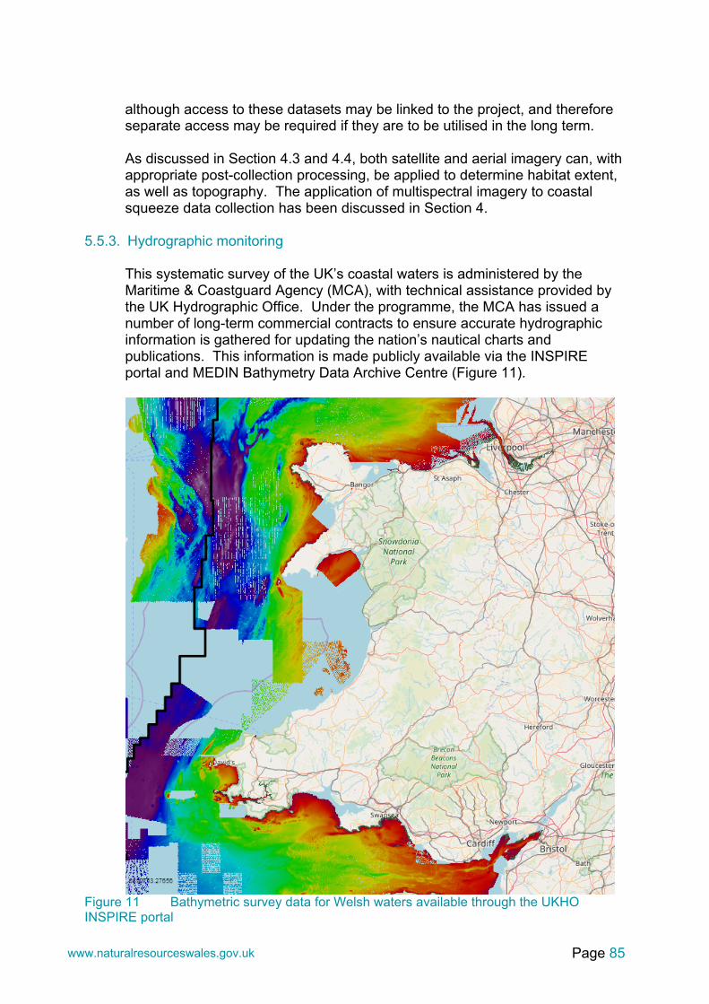
Page 85 www.naturalresourceswales.gov.uk
although access to these datasets may be linked to the project, and therefore separate access may be required if they are to be utilised in the long term. As discussed in Section 4.3 and 4.4, both satellite and aerial imagery can, with appropriate post-collection processing, be applied to determine habitat extent, as well as topography. The application of multispectral imagery to coastal squeeze data collection has been discussed in Section 4.
5.5.3. Hydrographic monitoring This systematic survey of the UK’s coastal waters is administered by the Maritime & Coastguard Agency (MCA), with technical assistance provided by the UK Hydrographic Office. Under the programme, the MCA has issued a number of long-term commercial contracts to ensure accurate hydrographic information is gathered for updating the nation’s nautical charts and publications. This information is made publicly available via the INSPIRE portal and MEDIN Bathymetry Data Archive Centre (Figure 11).
Figure 11 Bathymetric survey data for Welsh waters available through the UKHO INSPIRE portal

Page 86 www.naturalresourceswales.gov.uk
However, surveys are of varying resolution (e.g. single beam versus multibeam) and coverage is spatially uneven, with focus on areas used for navigation. As a consequence of the latter, coverage of intertidal areas is typically limited. The frequency with which repeat surveys are undertaken also varies, with annual surveys largely restricted to dynamic areas experiencing regular morphological change. Hydrographic surveys are also regularly undertaken by port authorities (such as Associated British Ports and the Bristol Port Company in the Severn Estuary/ Bristol Channel). However, as for those surveys administered by the MCA, the focus is largely on subtidal (navigable) areas.
5.6. Hydrodynamic modelling data As previously stated in Section 3.2, accurate determination of the geographic extent of the intertidal in any given location requires spatially continuous information on the elevation of the upper and lower boundaries of the intertidal, relative to a fixed data (e.g. ODN, CD etc.). This is most readily achieved through numerical modelling, to extrapolate information available from observational records available from (single point) tide gauge. Importantly, the long term observational records should span a period of 18.6 years or more, in order to fully capture variation in tidal range introduced via lunar cycles. A number of regional scale hydrodynamic models are available from which water level information could be obtained. These include the Proudman Oceanographic Laboratory POLCOMS model, the ABPmer SEASTATES model as well as the Technical University of Denmark (DTI) DTU10 model. However, arguably the most efficient means by which to obtain the necessary tidal water level information for Welsh waters is through the use of Vertical Offshore Reference Frame (VORF) surfaces. These are freely available high resolution digital models of reference surfaces such as mean sea level (MSL), lowest astronomical tide (LAT) and Chart Datum (CD) all modelled with respect to the terrestrial reference frame used for GPS/GNSS positioning: ETRF89 (or ITRF). These surfaces can also be used to infer levels of HAT, MHWS and MLWS which can be further used to inform potential habitat extents. Outputs are available at 0.003 degree intervals – (this is spatially variable but in Welsh waters, equates to approximately 550 m x 900 m spacing) – and can also be quickly converted to ODN via straightforward GIS processing. The latter is likely to be helpful, since LiDAR data is one of the most widely use ways of mapping larger areas of intertidal and this elevation data is typically expressed relative to ODN.
5.7. Wales Coastal Monitoring Centre In determining potentially useful data sources to inform ongoing and future coastal squeeze assessments it is worth noting that the Wales Coastal Monitoring Centre (WCMC) is due to become re-established. The WCMC was originally established in 2010 with the purpose of improving the co-ordination of coastal monitoring data collection, storage and analysis. The Centre was hosted by Gwynedd Council; however, the centre has been inactive during recent years due to a gap in funding.

Page 87 www.naturalresourceswales.gov.uk
Funding has now been agreed to re-establish the WCMC, which will provide a focal point for the collection and collation of coastal monitoring data in Wales. In the absence of the WCMC some local councils have undertaken limited surveys using a variety of techniques, predominantly with the purpose of monitoring coastal erosion to discharge their responsibilities with regards to coastal protection. It is expected that in future the data associated with these surveys will be collated and managed by the WCMC.
5.8. Summary
Data collected as part of a repeating monitoring programme has the potential to be used as a way of identifying changes to habitat extent through integrated monitoring of change that may be in response to a range of forcing factors including coastal squeeze. The key datasets that have been identified as having the potential to contribute to habitat distribution, extent and condition assessment are condition monitoring programmes undertaken as part of NRW/Welsh Government responsibilities under the WFD and the Habitats Directive. In particular, saltmarsh extents assessed under the WFD have the potential to directly indicate changes in habitat extent (but neglects mudflat and sandflat habitats). Other ad-hoc data may be available such as LiDAR, multispectral imagery, and hydrographic data which may inform change. There is also a significant body of historic data available to NRW which describes habitats and species vulnerable to coastal squeeze. This may be an important resource to determine baseline conditions against which change can be compared. However, whilst there is a reasonable degree of overlap between this habitat data and policy units where HTL policies have been assigned, the extent to which the data correlate with planned flood and coastal defence project is more limited (see Figure 12 to Figure 16).
The approach of using best available evidence and knowledge, as would be proposed if current monitoring data were to be used to inform coastal squeeze habitat loss estimates, is undertaken in the State of Natural Resources Report (SoNaRR)18. The report aims to provide the evidence to which Welsh Ministers must have regard when preparing or revising priorities for action at a national level, and is required under the Environment (Wales) Act 2016. SoNaRR will be published on five yearly cycle19.
It should also be noted, that the applicability of current monitoring programmes to inform coastal squeeze is subject to a number of further limitations. Of most importance is the fact that these monitoring programmes are not designed to assess coastal squeeze impacts, just changes in habitat condition, distribution/extent and status in general. Furthermore, a number of the collected datasets are only collected in discrete sample locations at frequencies of 3-6 years, without assessing the full intertidal extent of the habitat being surveyed. This data may, however, remain useful for informing an assessment of habitat condition. Some of the data has also not been updated recently and may have limited value in understanding changes in dynamic environments unless it is collected with sufficient regularity.
18 http://www.naturalresources.wales/sonarr?lang=en 19 http://senedd.assembly.wales/mgIssueHistoryHome.aspx?IId=16107
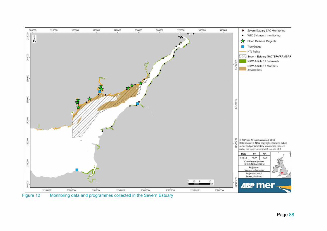
Page 88
Figure 12 Monitoring data and programmes collected in the Severn Estuary

Page 89
Figure 13 Monitoring data and programmes collected in south Wales

Page 90 www.naturalresourceswales.gov.uk
Figure 14 Monitoring data and programmes collected in south west Wales

Page 91 www.naturalresourceswales.gov.uk
Figure 15 Monitoring data and programmes collected in north west Wales

Page 92
Figure 16 Monitoring data and programmes collected in north Wales

Page 93 www.naturalresourceswales.gov.uk
6. Uncertainty
6.1. Overview Any attempt to quantitatively determine habitat loss via coastal squeeze (both in terms of determining change that has already occurred and in terms of estimating future loss) will necessarily be associated with uncertainty. This uncertainty may arise in a number of ways (e.g. ICES, 2012; Strong, 2015) and may differ between monitoring techniques. Causes of uncertainty include: Spatial uncertainty related to instrument measurement accuracy; Thematic uncertainty associated with habitat class/boundary classification; Uncertainty arising from the determination of cause and effect, in particular
the contribution from coastal squeeze to overall observed change; and Uncertainty introduced through the process of upscaling estimates of future
loss established from indicator location(s) to the scale of an SAC/SPA (or wider).
Additional uncertainty to that described above may also be introduced when using records of observed change to estimate future habitat losses, to be presented in a balance sheet of predicted habitat losses against realised habitat losses. This is because such an approach also relies upon knowledge of both the past magnitude/ rate of sea level change associated with the observed habitat loss coupled with estimates of future sea level rise. Both past measurements of sea level change as well as future projections of SLR are associated with uncertainty. The potential sources of error outlined above are considered below. This information has been used to inform a semi-quantitative appraisal of uncertainty for each of the monitoring options set out in Section 7.
6.2. Instrument measurement uncertainty Spatial uncertainty is the product of (but not limited to) instrument error or capabilities, particularly resolution and accuracy, as well as the positioning system used to geo-reference data. These sources of uncertainty have already been explored for each of the monitoring techniques discussed in Section 4. Resolution influences the size of features that can be detected, and therefore, poorer resolutions will have higher uncertainty associated with the output (Strong, 2015). This is because smaller features will be missed if the resolution is greater (i.e. poorer) than its size. As such, the effects of resolution can vary depending on the size of features that are present. Horizontal and vertical accuracy of the data, which can be governed by conditions (e.g. weather, water reflectance), corrections and pre-processing applied to the data, will also affect its accuracy to represent ground conditions, contributing to uncertainty. It is very important to note that the slope of the intertidal area can have a large influence on the magnitude of error and uncertainty attributed to vertical instrument accuracy (applicable to topographic data e.g. LiDAR). On gently sloping intertidal areas, even modest vertical inaccuracies may have a

Page 94 www.naturalresourceswales.gov.uk
disproportionately large influence on the error associated with calculated areas, whereas, the same error in accuracy on a steeply sloping intertidal area, will have less effect on calculated areas (Figure 17a). Horizontal inaccuracies are proportionally related to inaccuracies in calculated habitat areas regardless of slope (Figure 17b).
Figure 17 The effect of slope and vertical (a) and horizontal (b) accuracy on calculated area
The error attributed to instrument accuracies can theoretically be quantitatively determined through consideration of equipment specifications to arrive at a statistical measure of accuracy with regards to differences between mapped habitat extents, and real-world habitat extents. This is achieved by using trigonometric equations. Table 10 shows the influence of vertical accuracy, as well as slope, has on calculated areas of habitat. It is demonstrated that vertical inaccuracies on shallow angled shorelines have a more pronounced impact on uncertainty in calculated area. Slope angle does not affect the impact horizontal accuracy has on calculated areas (Table 11).
a) b)
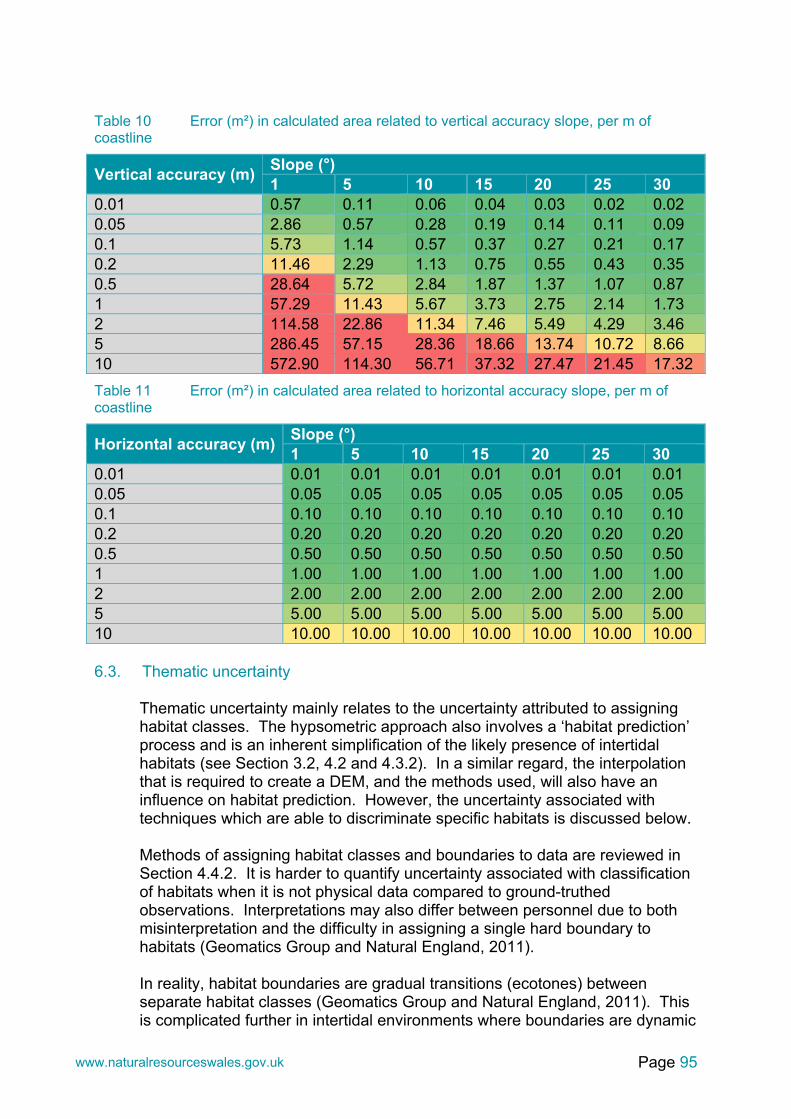
Page 95 www.naturalresourceswales.gov.uk
Table 10 Error (m²) in calculated area related to vertical accuracy slope, per m of coastline
Vertical accuracy (m) Slope (°) 1 5 10 15 20 25 30
0.01 0.57 0.11 0.06 0.04 0.03 0.02 0.02 0.05 2.86 0.57 0.28 0.19 0.14 0.11 0.09 0.1 5.73 1.14 0.57 0.37 0.27 0.21 0.17 0.2 11.46 2.29 1.13 0.75 0.55 0.43 0.35 0.5 28.64 5.72 2.84 1.87 1.37 1.07 0.87 1 57.29 11.43 5.67 3.73 2.75 2.14 1.73 2 114.58 22.86 11.34 7.46 5.49 4.29 3.46 5 286.45 57.15 28.36 18.66 13.74 10.72 8.66 10 572.90 114.30 56.71 37.32 27.47 21.45 17.32
Table 11 Error (m²) in calculated area related to horizontal accuracy slope, per m of coastline
Horizontal accuracy (m) Slope (°) 1 5 10 15 20 25 30
0.01 0.01 0.01 0.01 0.01 0.01 0.01 0.01 0.05 0.05 0.05 0.05 0.05 0.05 0.05 0.05 0.1 0.10 0.10 0.10 0.10 0.10 0.10 0.10 0.2 0.20 0.20 0.20 0.20 0.20 0.20 0.20 0.5 0.50 0.50 0.50 0.50 0.50 0.50 0.50 1 1.00 1.00 1.00 1.00 1.00 1.00 1.00 2 2.00 2.00 2.00 2.00 2.00 2.00 2.00 5 5.00 5.00 5.00 5.00 5.00 5.00 5.00 10 10.00 10.00 10.00 10.00 10.00 10.00 10.00
6.3. Thematic uncertainty
Thematic uncertainty mainly relates to the uncertainty attributed to assigning habitat classes. The hypsometric approach also involves a ‘habitat prediction’ process and is an inherent simplification of the likely presence of intertidal habitats (see Section 3.2, 4.2 and 4.3.2). In a similar regard, the interpolation that is required to create a DEM, and the methods used, will also have an influence on habitat prediction. However, the uncertainty associated with techniques which are able to discriminate specific habitats is discussed below. Methods of assigning habitat classes and boundaries to data are reviewed in Section 4.4.2. It is harder to quantify uncertainty associated with classification of habitats when it is not physical data compared to ground-truthed observations. Interpretations may also differ between personnel due to both misinterpretation and the difficulty in assigning a single hard boundary to habitats (Geomatics Group and Natural England, 2011). In reality, habitat boundaries are gradual transitions (ecotones) between separate habitat classes (Geomatics Group and Natural England, 2011). This is complicated further in intertidal environments where boundaries are dynamic

Page 96 www.naturalresourceswales.gov.uk
and often not stationary over time. Therefore, determining habitat boundaries is subjective and hard to achieve both in the field as well as via remotely sensed data. Further, thresholds (i.e. reflectance values, or species composition) between habitats need to be assigned to data which has associated uncertainties (Strong, 2015). Inappropriate or incorrect threshold values may be attributed to poor data quality caused by errors in processing, conditions during collections (e.g. cloud cover), or misidentification of species in the field. These various sources of uncertainty also affect the repeatability and comparability of data collected by each monitoring technique.
6.4. Causes of change and effects to intertidal habitat There are multiple causes of change to intertidal areas (both extent and condition) and it is an inherently difficult task to determine exactly what process is driving observed change in any given location (see Section 3.1). Therefore, a very high degree of uncertainty is created when trying to attribute what proportion of change to habitat is caused by coastal squeeze. This uncertainty associated with determination of cause and effect is considered to be the single greatest contributor to overall uncertainty and greatly complicates any attempt to revise targets for habitat compensation in a robust manner. It is extremely difficult to overcome this issue, but ways of reducing this uncertainty are considered in Section 7.1.
6.5. Upscaling observed records of change from a local to regional scale Given the costs/ time involved with some of the potential monitoring options discussed in Section 7, it may be appropriate to monitor change at target locations within Natura 2000 sites, upscaling results to derive estimates of loss at the scale of the SAC/ SPA as a whole (or wider depending on data availability). (The suitability of this approach is appraised separately, in Section 7.5 and 7.6). However, this approach has the potential to introduce additional levels of uncertainty, through selective bias. For instance, most of the Natura 2000 sites around Wales are characterised by a range of differing environments, both in terms of their physical setting (e.g. open coast versus estuarine; coarse grained versus fine grained etc.) and chemical (e.g. saline versus brackish etc.) setting. Target locations which only represent a sub set of the range of environmental settings within any given Natura 2000 site may be a poor analogue for change across the site as a whole. An example of this could be the (over) reliance on target locations in the outer Severn Estuary which are exposed to wave influence to determine net change across the entire Severn Estuary SAC, much of which is reasonably sheltered from wave influence. In order to reduce the uncertainty introduced by the upscaling process, it is necessary to give careful consideration to the number and geographical distribution of target monitoring within each Natura 2000 site. As well as focussing on proposed coastal defence locations, these also need to broadly reflect the range of environmental settings of all HTL units within each Natura 2000 site.

Page 97 www.naturalresourceswales.gov.uk
6.6. Using records of observed change to estimate future habitat losses In order to use records of observed habitat change to refine existing estimates of future loss presented in the SMPs it is necessary to have a detailed understanding of both: (i) The change in relative sea level which occurred over the period of
observed habitat change; (ii) The change in relative sea level which is expected to occur in future; and (iii) All other factors, aside from sea level rise, affecting causes of intertidal
habitat change. The former can be used in conjunction with measured change in habitat extent to determine a loss: sea level rise ratio. This can then be scaled up to determine a future trajectory of loss against predicted sea level rise. However, the margin of error associated with future estimates of habitat loss are potentially very large. Indeed, because of the range variables which contribute to these predictions, it is probable that uncertainty could be in the order of 100% or more. This is consistent with determinations of uncertainty presented in the Severn Estuary Coastal Habitat Management Plan (CHaMP) which has subsequently used to help inform the SMP. More generally, it is noted here that incomplete understanding of the relationship between sea level rise, as well as other factors discussed in Section 3.1 and 6.4, and habitat loss probably introduces as much uncertainty to future estimates of habitat loss as the range of plausible sea level rise scenarios set out in UKCP09, based on high, medium and low emissions scenarios (Section 2.3).
6.7. Statistical evaluation of overall uncertainty To determine which of the possible monitoring options set out in Section 7 provides the most robust and cost-effective solution for monitoring of coastal squeeze, it is necessary to be able to compare levels of uncertainty between different options. In order to achieve this, all of the sources of uncertainty set out in this section need to be aggregated and, where possible, quantified enabling an overall statistical evaluation of power to be determined. However, from the outset it should be emphasised that this is an extremely difficult undertaking: some categories of uncertainty are almost impossible to quantify with any precision, whilst the magnitude of uncertainty is likely to vary on a site-by-site basis (for example differences between micro-tidal and macro-tidal environments) as well as between monitoring techniques. This is particularly the case when considering cause and effect of observed habitat loss. Accordingly, a semi-quantitative method for the determination of overall uncertainty has been established and is described below. Step 1: For each monitoring option, expert judgement has been used to determine how much four sources of uncertainty identified in this section (and repeated below) could cause the calculated value of change to habitat area to alter by in percentage terms:
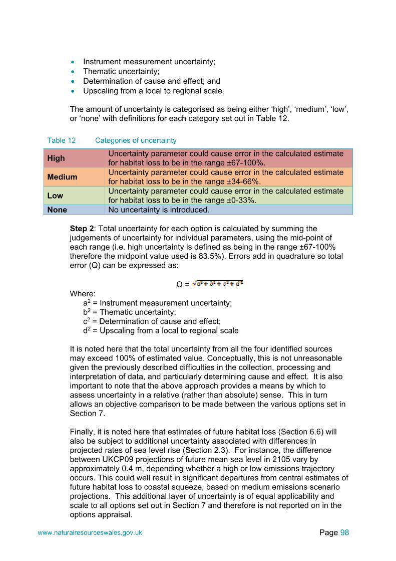
Page 98 www.naturalresourceswales.gov.uk
Instrument measurement uncertainty; Thematic uncertainty; Determination of cause and effect; and Upscaling from a local to regional scale. The amount of uncertainty is categorised as being either ‘high’, ‘medium’, ‘low’, or ‘none’ with definitions for each category set out in Table 12.
Table 12 Categories of uncertainty
High Uncertainty parameter could cause error in the calculated estimate for habitat loss to be in the range ±67-100%.
Medium Uncertainty parameter could cause error in the calculated estimate for habitat loss to be in the range ±34-66%.
Low Uncertainty parameter could cause error in the calculated estimate for habitat loss to be in the range ±0-33%.
None No uncertainty is introduced. Step 2: Total uncertainty for each option is calculated by summing the judgements of uncertainty for individual parameters, using the mid-point of each range (i.e. high uncertainty is defined as being in the range ±67-100% therefore the midpoint value used is 83.5%). Errors add in quadrature so total error (Q) can be expressed as:
Q = Where:
a2 = Instrument measurement uncertainty; b2 = Thematic uncertainty; c2 = Determination of cause and effect; d2 = Upscaling from a local to regional scale
It is noted here that the total uncertainty from all the four identified sources may exceed 100% of estimated value. Conceptually, this is not unreasonable given the previously described difficulties in the collection, processing and interpretation of data, and particularly determining cause and effect. It is also important to note that the above approach provides a means by which to assess uncertainty in a relative (rather than absolute) sense. This in turn allows an objective comparison to be made between the various options set in Section 7. Finally, it is noted here that estimates of future habitat loss (Section 6.6) will also be subject to additional uncertainty associated with differences in projected rates of sea level rise (Section 2.3). For instance, the difference between UKCP09 projections of future mean sea level in 2105 vary by approximately 0.4 m, depending whether a high or low emissions trajectory occurs. This could well result in significant departures from central estimates of future habitat loss to coastal squeeze, based on medium emissions scenario projections. This additional layer of uncertainty is of equal applicability and scale to all options set out in Section 7 and therefore is not reported on in the options appraisal.
Page 99 www.naturalresourceswales.gov.uk
7. Options Appraisal Assessment This section appraises a number of proposed options for monitoring coastal squeeze losses within the Natura 2000 network to demonstrate actual rates of loss attributed to the implementation of SMP2 policies in Wales (compared with predicted). The ultimate aim of this is to maintain a balance sheet of habitat losses, and ensure the NHCP is ‘in credit’ (see Section 2.4.1). In this section, methods of reducing uncertainty associated with cause and effect are reviewed. An overview is then provided on the proposed list of options. This outlines the justification in selected monitoring techniques, and the assumptions within each option to facilitate the appraisal. It also includes a description of the suggested monitoring frequency for all monitoring options. Before analysing each proposed monitoring option individually, the appraisal criteria (critical success factors) and the methodology by which options are assessed is presented.
7.1. Reducing uncertainty Highlighted throughout this report is the inherent uncertainty attributed to measuring coastal squeeze. Section 6 discusses sources of uncertainty and a semi-quantitative method of evaluating uncertainty. To some extent, uncertainty can be reduced by using more sophisticated techniques to accurately monitor change, and increasing the spatial resolution of measurements. However, uncertainty is dominated by the difficulties associated with determining cause and effect, and this is problematic since the NHCP requires monitoring of only coastal squeeze impacts to update habitat offset targets. Therefore, before monitoring options are proposed, this section discusses means to reduce uncertainty attributed to cause and effect.
7.1.1. Control sites as means of isolating change attributable to coastal squeeze In theory, the component of change attributable to coastal squeeze at a specific location could be isolated and quantified through the use of ‘control sites’. These control sites would have to be located very nearby and subject to the same forcing mechanisms, foreshore profile, material type and habitat composition as the location of interest with defences in place. Both sites could then be monitored and observed differences in intertidal extent/ habitat condition between the sites over time could be interpreted as change caused by coastal squeeze. However, in practice such an approach is likely to be unworkable. It would be extremely difficult to identify two locations subject to identical forcing mechanisms and profile characteristics with the only difference being the presence of coastal defence infrastructure. Even very subtle differences (for instance adjacent sub-tidal bathymetry/coastal aspect etc.) could have greater influence on morphological change across the intertidal than that caused by any rise in sea level over the analysis period. The implications of this are that

Page 100 www.naturalresourceswales.gov.uk
any estimates of coastal squeeze loss derived in this way would themselves be subject to large uncertainty. In addition, there is added uncertainty caused by the need to upscale results from these control sites to scales of a Natura 2000 site or nationally, and it would require a significant amount of time and money to implement such a programme of monitoring. This, together with the limited confidence from the outset that the datasets would isolate the effects of sea level rise on intertidal morphology/habitats, renders the use of control sites inappropriate.
7.1.2. Expert geomorphological assessment Given the lack of means to confidently decipher coastal squeeze induced change, the best option is considered to be that any monitoring is accompanied by geomorphological assessment of the data to help determine (in a semi-quantitative manner) cause and effect. This information should in turn, be used to refine estimates of loss attributable to coastal squeeze. A key element of any geomorphological review would be an appraisal of the nature of observed change in intertidal profile (see Figure 18, noting S4 type profile responses may constitute coastal squeeze) since this may help separate out those changes resulting from coastal squeeze and those from other causes. This expert review could also consider data on a range of key driving mechanisms of change such as storminess, using hindcast metocean data.
Figure 18 Steepening mode classification scheme based on changes in position of High Water Mark (HMW) and Low Water Mark (LWM). From Taylor et al., 2004.

Page 101 www.naturalresourceswales.gov.uk
7.2. Overview of options Following a review of available monitoring techniques (Section 4) and current monitoring data in Wales (Section 5), a short-list of possible monitoring options have been identified for monitoring coastal squeeze in Wales. These include: Option 1 – Use sea level rise monitoring and existing data (Business as
usual) Option 2 – Bespoke intertidal habitat monitoring for representative flood
risk management projects and assets (Do minimum) - Option 2a – Focus on monitoring intertidal extent and estimate habitat
loss - Option 2b – Focus on monitoring habitat types and condition within
intertidal extent Option 3 – Bespoke intertidal habitat monitoring for all planned flood risk
management projects and assets (Do medium) - Option 3a – Focus on monitoring intertidal extent and estimate habitat
loss - Option 3b – Focus on monitoring habitat types and condition within
intertidal extent Option 4 – Bespoke intertidal habitat monitoring in all HTL policy locations
(Do maximum) - Option 4a – Focus on monitoring intertidal extent and estimate habitat
loss - Option 4b – Focus on monitoring habitat types and condition within
intertidal extent Option 1 focuses on tracking sea level rise via tide gauges around Wales, which is already being processed by the National Tidal and Sea Level Facility (see Section 5). This data can then be used to adjust habitat offset targets estimated from the SMP2 HRAs/IROPI, as well any estimates of habitat loss from project level assessments for marine licences. This option also includes making best use of wider monitoring datasets that are collected in Wales, as discussed in Section 5. Given these are limited in their application to coastal squeeze monitoring, further analysis of this data, such as extent mapping, interpretation, and analysis, would be required to inform coastal squeeze. (Use of this existing data is primarily suggested to help refine habitat loss estimates where possible). Furthermore, upscaling would be required to predict rates of change along all HTL policy areas. Up-scaling is proposed to involve measuring percentage habitat loss and comparing that to the observed sea level rise over the same period. This scaled relationship would then be applied to other HTL policy areas taking into account various analogues relating to environmental setting. It is important to note that current repeat monitoring programmes may not continue indefinitely throughout each epoch. However, for the purposes of this project, it is assumed some form of similar monitoring will continue and the potential for this to be used to inform coastal squeeze will continue. This option is described further in Section 7.4. All other options involve a bespoke intertidal habitat monitoring programme to inform new estimates for coastal squeeze habitat loss.

Page 102 www.naturalresourceswales.gov.uk
Option 2 involves selecting representative local authority and NRW flood risk management projects (Section 2.1 and Appendix A) which are significant coastal schemes in HTL policy areas within Natura 2000 sites, due to be implemented in the first epoch. Monitoring will then be applied to these sites only, and changes will be scaled up to predict rates of change along all HTL policy areas by the same method as proposed for Option 1. Representative projects have been selected based upon isostatic rebound rates latitudinally across Wales to best represent differences in sea level rise expected across Wales (i.e. representative locations are spread across north, mid and south Wales). Selected projects are also distributed between open coast and estuarine environments. This option also includes work proposed under Option 1. This option is described further in Section 7.5. Option 3 involves monitoring areas fronting all local authority and NRW flood risk management projects which are due to be implemented. Habitat changes will then be scaled up to predict rates of change along all HTL policy areas by the same method as proposed for Option 1. This option also includes work proposed under Option 1. This option is described further in Section 7.6. Option 4 involves monitoring areas fronting all assets in HTL policy areas. This option also includes work proposed under Option 1. This option is described further in Section 7.7.
7.2.1. Sub-options Parameters to be monitored Within Option 2, 3 and 4 are two sub-options which cover the various parameters for monitoring coastal squeeze. Sub-option a) consists of monitoring changes in intertidal extent which requires data on topography/bathymetry and sea level (from tide gauges/satellite altimetry). This follows methods and techniques described in Section 3.2, 4.2 and 4.3. Sub-option b) consists of monitoring changes in intertidal extent (as with sub-option a), as well as monitoring changes in habitat types, area, and condition within the intertidal extent summarised in Section 4.4. Effectively, sub-option b is an additional monitoring step on top of sub-option a. Therefore, sub-option b is appraised in combination with sub-option a. High and low-cost ranges for each sub-option are presented. Monitoring techniques and data acquisition A range of techniques have been identified as potentially able to monitor these parameters (Section 4). This section details the justification in selecting specific monitoring techniques and methods within each Option and sub-option, and outlines the assumptions made for the purpose of the options appraisal. In reality, there are a number of combinations and permutations of monitoring techniques that could be used to monitor both intertidal extent (sub-option a) and habitat extent and condition (sub-option b). For the purposes of this options appraisal, a low-cost and high-cost range is presented for each
Page 103 www.naturalresourceswales.gov.uk
sub-option. Which techniques these comprise is clarified in Sections 7.5 to 7.7. Most topographic and bathymetric survey techniques identified in Section 4.3 are appraised for sub-option a). This is with the exception of single-beam bathymetry surveys and stereo-photogrammetry. For the former, it is more cost effective to use multibeam bathymetry surveys, due to the quicker collection of data and coverage possible per survey. For the latter, applications of this technique are currently seldom applied to DEM production in the coastal zone, though technological developments may increase its use (however, collection of multispectral data is appraised under sub-option b). Furthermore, for each option it may not be appropriate to employ some techniques due to their costs and potential spatial coverage. For example, it is not cost-effective to employ LiDAR (from aircraft) on a scheme-by-scheme basis since the individual schemes will only have a small footprint, and as such, it is not included within Option 2. However, for Options 3 and 4, LiDAR is included as a potential monitoring technique. This is also the case for topographic surveying using RTK GNSS and terrestrial laser scanners, being included for only Option 2. In terms of monitoring habitat type and extent, multispectral imagery seems the most applicable monitoring technique and offers distinct advantages, particularly with the added advantage of NIR imagery and photosynthetic vegetation discrimination. It is also capable of identifying intertidal mudflats and sandflats. Hyperspectral imagery, although useful in further classifying habitat and with the ability to operate automatic classifications, the software and data storage requirements and the expense of processing time may render this technique unfeasible. Therefore, it has not been included as a monitoring technique in the options. Where monitoring techniques can be performed from a range of remote sensing techniques (i.e. satellite, aircraft, UAVs) a range has been appraised. This is mainly applicable to multispectral imagery within sub-option b). However, the collection of multispectral imagery by aircraft would not be cost effective on a scheme-by-scheme basis. Therefore, aerial multispectral imagery has not been included as a monitoring technique for Option 2. Equally, collection of multispectral imagery by UAV has not been included as a monitoring option in Option 3 and 4, as it is not practical to cover such large areas by UAV. For sub-option b) habitat field surveying involves two personnel per survey, equipped with differential GPS (e.g. RTK GNSS). GPS points will be mapped on the best available aerial imagery (the acquisition of which is assumed to be subsumed within other data collections). Standard information to inform habitat condition will be collected. Field habitat surveying has only been included as a monitoring technique in Option 2 as inclusion in Option 3 and 4 would be impractical (aside from ground-truthing). It is important to note that the proposed monitoring techniques are rapidly improving, and it is possible that the capabilities and costs stated in this report
Page 104 www.naturalresourceswales.gov.uk
will need to be reviewed before implementation, and at intervals thereafter. Ultimately this could influence the ‘option’ taken forward at any point in time. Mapping techniques (image classification/segmentation) for sub-option b For sub-option b) all image analysis and habitat mapping for each option will be undertaken using a semi-automated approach with object-orientated classification/spectral classifiers using software such as eCognition (Environment Systems, 2015). Both topographic information (under sub-option b) and ground truthing will improve the classification of habitats.
7.2.2. Monitoring frequency As previously discussed in Section 3.1, intertidal morphology and extent varies in response to a range of forcing mechanisms which operate over short, medium and longer-term timescales. Because of this, it is important to determine the most appropriate frequency with which monitoring is undertaken to reduce the number of variables which may be contributing to any observed change (Section 3.1). One of the most significant causes of change is likely to be variation in tidal range caused by the 18.6 yr lunar nodal cycle. On this basis, it would ideally make sense to align monitoring programmes/habitat-offset target revisions to this time frame. WFD monitoring is currently undertaken every six years: as well as aligning with the 18-year cycle, much of the collected data is also of value in informing understanding of coastal squeeze loss (Section 5.3). The six-year monitoring frequency will not capture the peaks and troughs of the lunar nodal cycle, meaning some consideration will need to be given as to how to adjust for its influence. However, collection of data at this frequency will help to build up a picture of change over time. Observational evidence of sea level change is obviously of critical importance in helping to determine coastal squeeze impacts. As set out in Section 4.2.1, at least 15 years of data is required – preferably more – to determine reliable trends in mean sea level. Accordingly, it would not make sense to report at more frequent timescales than this. On the basis of the above, it is suggested that analysis to update habitat offset targets is carried out every 18 years or so, with monitoring data (and other relevant information) collated on a more frequent basis (every six years). The latter aligns with timescales already in place for WFD monitoring and will help to enable a picture of change to be determined.
7.3. Appraisal method
7.3.1. Key assumptions The following assumptions have been made for the purposes of the options appraisal:
Page 105 www.naturalresourceswales.gov.uk
Options 1, 2 and 3 are scaled up to cover all HTL policy areas, in order for options to be comparable.
Local and NRW flood risk management projects (Appendix A) come online midway through epoch 1 (2021.5) with monitoring required thereafter;
All HTL policies in epoch 1 will need to be monitored throughout all epochs, even if changed to NAI or MR (as the defence is likely to remain in place, and habitat change (possibly gain) is likely to occur);
Monitoring frequency of six years for monitoring of change (to align with WFD monitoring) with expert geomorphological assessment every 18 years;
Archived satellite imagery is assumed to be satisfactory for coastal squeeze monitoring purposes due to the amount of data captured and frequency of monitoring required;
Field surveying equipment (e.g. GPS/RTK GNSS, quadrats, cameras etc.) does not need to be purchased as it is readily available to NRW and local authorities for a variety of purposes;
Personnel time is considered the only cost associated with field surveying and does not include travelling time;
All habitat monitoring is undertaken in summer months to coincide with favourable weather (i.e. no weather downtime) and peak growing seasons;
For each km of coastline, it assumed 0.4 km² of fronting intertidal is present for the purposes of calculating costs. This is based on a total of approximately 327 km² of intertidal area in SACs20 in Wales, along approximately 920 km of coastline in SACs;
Costs for personnel time are based on an assumed rate of £500/day; An inflation rate of 3% has been used to calculate future costs, informed by
HM Treasury Forecasts for the UK Economy as well as economic and fiscal outlook information from the Office for Budget Responsibility; and
All costs presented are approximate and have been rounded to the nearest £1,000.
7.3.2. Critical success factors
Each option has been assessed against two critical success factors: Cost; and Uncertainty. Cost A low-cost and high-cost estimate has been provided for each option, in the first, second and third epochs. This takes account of expected rates of inflation. A look up table for costs is presented in Table 13 for each monitoring technique proposed within each sub-option and has been informed by the review in Section 4. In some cases, best-guess estimates have been provided due to a lack information on the costs of these techniques.
20 https://naturalresources.wales/media/676202/life-n2k-facts-and-figures-report.pdf
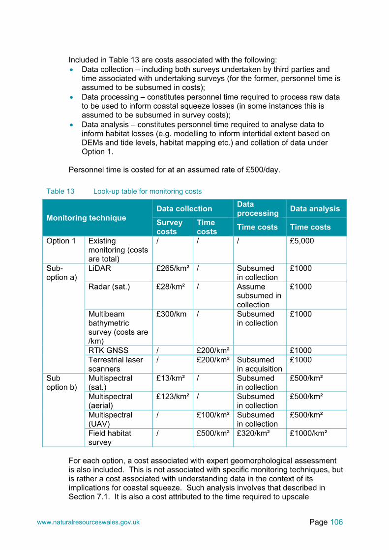
Page 106 www.naturalresourceswales.gov.uk
Included in Table 13 are costs associated with the following: Data collection – including both surveys undertaken by third parties and
time associated with undertaking surveys (for the former, personnel time is assumed to be subsumed in costs);
Data processing – constitutes personnel time required to process raw data to be used to inform coastal squeeze losses (in some instances this is assumed to be subsumed in survey costs);
Data analysis – constitutes personnel time required to analyse data to inform habitat losses (e.g. modelling to inform intertidal extent based on DEMs and tide levels, habitat mapping etc.) and collation of data under Option 1.
Personnel time is costed for at an assumed rate of £500/day.
Table 13 Look-up table for monitoring costs
Monitoring technique Data collection
Data processing
Data analysis
Survey costs
Time costs
Time costs Time costs
Option 1 Existing monitoring (costs are total)
/ / / £5,000
Sub-option a)
LiDAR £265/km² / Subsumed in collection
£1000
Radar (sat.) £28/km²
/ Assume subsumed in collection
£1000
Multibeam bathymetric survey (costs are /km)
£300/km / Subsumed in collection
£1000
RTK GNSS / £200/km² £1000 Terrestrial laser scanners
/ £200/km²
Subsumed in acquisition
£1000
Sub option b)
Multispectral (sat.)
£13/km²
/ Subsumed in collection
£500/km²
Multispectral (aerial)
£123/km² / Subsumed in collection
£500/km²
Multispectral (UAV)
/ £100/km²
Subsumed in collection
£500/km²
Field habitat survey
/ £500/km² £320/km² £1000/km²
For each option, a cost associated with expert geomorphological assessment is also included. This is not associated with specific monitoring techniques, but is rather a cost associated with understanding data in the context of its implications for coastal squeeze. Such analysis involves that described in Section 7.1. It is also a cost attributed to the time required to upscale

Page 107 www.naturalresourceswales.gov.uk
measured losses to all HTL policies in the Natura 2000 network (for Option 1, 2, and 3 only). This is assumed to be £20,000 for all options. All estimated costs for each option are reported to the nearest £100. However, it is important to reiterate that a number of high level assumptions have been made to derive cost estimates for each option, and they should be considered as indicative only. Uncertainty Means of assessing uncertainty is described in Section 6.7, and is undertaken for each option. The following aspects of uncertainty have been assessed: Instrument measurement uncertainty; Thematic uncertainty; Determination of cause and effect; and Upscaling from a local to regional scale or adjusting NHCP targets. These have been added together in quadrature, to give an overall percentage of uncertainty. This semi-quantitative approach enables an uncertainty ‘score’ to be associated with each option; this approach is considered a relative (rather than absolute) measure to aid comparison (see Section 6.7), and allows an appraisal to be made between the cost of each option against the confidence in its outcomes. It is also important to note, as mentioned in Section 6.7, that uncertainty associated with differences in projected rates of sea level rise (Section 2.3) and consequent estimates of future habitat loss (Section 6.6) is not included in any of the options as it is equal for all of them. Uncertainty is assessed for low-cost and high-cost ranges (and for sub-option b, their combinations with sub-option a low-cost and high-cost ranges) for each option.
7.4. Option 1 – Use sea level rise monitoring and existing data (Business as usual)
7.4.1. Description of approach This option involves making use of tide gauge data from the National Tidal and Sea Level Facility to track realised rates of sea level rise, and augmenting previous analysis undertaken within the HRAs of the SMP2s. As the HRA assessments were informed by modelling estimates using sea level predictions, and sediment modelling against currently implemented defences and SMP2 polices, a simple revaluation of habitat losses based on realised rates of sea level would refine coastal squeeze habitat losses. This option will build on the conceptual understanding of processes at each location. Existing monitoring (see Section 5) applicable to monitoring sea level, intertidal extent, habitat types and/or condition, as well as coastal processes and morphological change are also proposed to be used within this option, particularly:
Page 108 www.naturalresourceswales.gov.uk
Satellite altimetry; WFD monitoring; MPA condition monitoring; LiDAR; Aerial imagery (multispectral); and Hydrographic monitoring and modelling. This monitoring data is currently collected in large parts of Wales, some within the Natura 2000 network, and intersecting with HTL policies (see Section 5). However, it is unlikely data will be wholly available for specific sites where coastal defence projects may cause coastal squeeze, or all areas of HTL policies in the Natura 2000 network. Therefore, some form of upscaling to cover all HTL policy areas would be required. Furthermore, it is unlikely that existing data alone will provide complete information on distribution, extent and condition of habitats at the scale/accuracy necessary to inform change or coastal squeeze. Therefore, use of this existing monitoring data is suggested to help refine existing habitat loss estimates where possible following further analysis (e.g. extent mapping, interpretation), if data is sufficient. It is envisaged this will provide a sense check and inform the direction of travel and order of magnitude of loss estimates. In order to apply this data to determining coastal squeeze in Natura 2000 sites in Wales, analysis would likely entail: Examining intertidal extent by comparing DEMs with sea levels, and
collating information from hydrographic monitoring data; Examining habitat type and extent (and possibly condition) through habitat
mapping from aerial imagery (multispectral); and Deriving habitat condition from data collected in the field. Cost In terms of data collection and processing, this option entails no costs since it takes advantage of data already collected. However, the collation of existing monitoring is not ‘cost free’ as technical experts will be required to identify, organise and analyse the data, though it is noted that NRW are likely to have this expertise in house. Consequently, a total estimated present-day cost of £5,000 is assumed for each monitoring round. This is equivalent to around 10 days of analysis. Table 14 shows the costs associated with Option 1. Including expert geomorphological assessment (£20,000) every 18 years, this amounts to a total cost of £5k up to the end of epoch 1 (with 1 monitoring round), £138k from present to the end of epoch 2 (with 6 monitoring rounds and 2 expert geomorphological assessments), and £964k from present up to the end of epoch 3 (with 15 monitoring rounds and 5 expert geomorphological assessments), accounting for inflation at 3%.
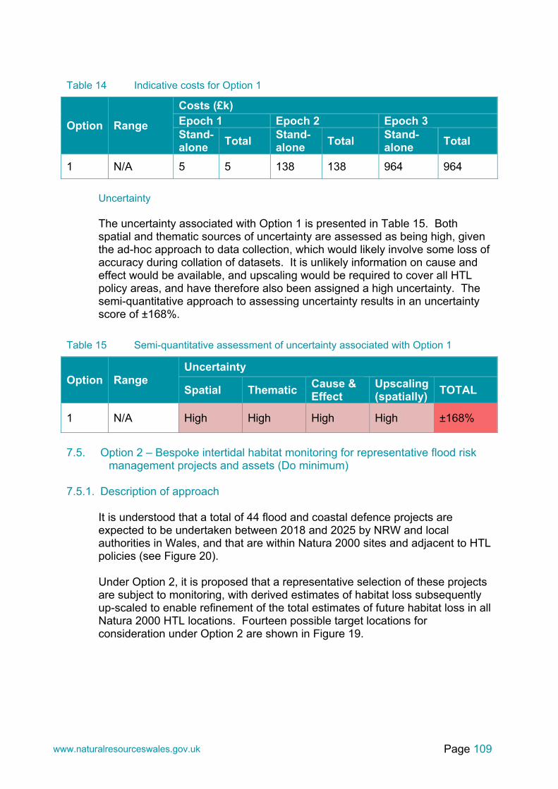
Page 109 www.naturalresourceswales.gov.uk
Table 14 Indicative costs for Option 1
Option Range
Costs (£k) Epoch 1 Epoch 2 Epoch 3 Stand-alone
Total Stand-alone
Total Stand-alone
Total
1 N/A 5 5 138 138 964 964
Uncertainty The uncertainty associated with Option 1 is presented in Table 15. Both spatial and thematic sources of uncertainty are assessed as being high, given the ad-hoc approach to data collection, which would likely involve some loss of accuracy during collation of datasets. It is unlikely information on cause and effect would be available, and upscaling would be required to cover all HTL policy areas, and have therefore also been assigned a high uncertainty. The semi-quantitative approach to assessing uncertainty results in an uncertainty score of ±168%.
Table 15 Semi-quantitative assessment of uncertainty associated with Option 1
Option Range Uncertainty
Spatial Thematic Cause & Effect
Upscaling (spatially)
TOTAL
1 N/A High High High High ±168%
7.5. Option 2 – Bespoke intertidal habitat monitoring for representative flood risk
management projects and assets (Do minimum)
7.5.1. Description of approach It is understood that a total of 44 flood and coastal defence projects are expected to be undertaken between 2018 and 2025 by NRW and local authorities in Wales, and that are within Natura 2000 sites and adjacent to HTL policies (see Figure 20). Under Option 2, it is proposed that a representative selection of these projects are subject to monitoring, with derived estimates of habitat loss subsequently up-scaled to enable refinement of the total estimates of future habitat loss in all Natura 2000 HTL locations. Fourteen possible target locations for consideration under Option 2 are shown in Figure 19.

Page 110 www.naturalresourceswales.gov.uk
Figure 19 Selected flood and coastal defence projects in Natura 2000 sites in Wales

Page 111 www.naturalresourceswales.gov.uk
These have been chosen on the basis of the following: Over 50% of total projected future loss in Welsh Natura 2000 habitat area
is expected to occur in the Severn Estuary SAC, with 18% occurring in Carmarthen Bay and Estuaries SAC and less in other designated sites (Table 2). The distribution of possible target locations in Figure 19 is therefore biased towards these locations which are expected to experience greatest loss.
The rate at which coastal change occurs may be expected to vary according to environmental setting with open coast sedimentary environments (which typically are characterised by the presence of sandy sediments) potentially responding differently to more sheltered estuarine settings (which are generally characterised by the presence of saltmarsh, mud and/or sandy sediments),
Future sea level rise in Wales will vary geographically in response to GIA (Section 2.3). This will contribute to spatial variation in rates of habitat loss to coastal squeeze. The greatest variation in GIA is encountered along a north-south (rather than east-west) gradient and therefore a spread of sites from both north and south have been selected.
No chosen locations are characterised by the presence of rocky substrates as the response of these settings to sea level rise is considerably more straight forward to predict than for sedimentary environments.
The majority of the chosen target locations are expected to have a HTL management policy for all three epochs (i.e. to 2105). However, even where the policy is expected to change from HTL to NAI or MR, monitoring is still expected to be necessary since the defence can be expected to remain in place or habitat change to occur, therefore contributing to habitat loss.
For the purposes of the options appraisal, it is assumed that each scheme is 1 km long, and that 2 km of coastline should be monitored.
7.5.2. Option 2a As with Option 1, existing monitoring data is utilised for Option 2a. In addition, specific data is to be collected on topography/bathymetry in order to create a DEM which can be compared to sea levels and intertidal extent estimated. Relatively simple data analysis in a GIS environment is required to do this. The following monitoring techniques are suggested to obtain topographic/bathymetric information: Radar (sat.); Multibeam bathymetric survey; RTK GNSS; and Terrestrial laser scanners. In reality, one, or a combination of these techniques would be used; it would not be cost-effective or pragmatic to use all techniques. Radar (sat.), RTK GNSS, and terrestrial laser scanners could be used to gather elevation data above the water level (i.e. upper intertidal) and elevations towards the lower
Page 112 www.naturalresourceswales.gov.uk
intertidal zone could be interpolated. Otherwise, bathymetric surveys could provide missing data at the MLWS level. Therefore, the range of costs and uncertainty have been stated for this option, with the upper range including bathymetry surveys. Cost Table 16 shows the costs associated with Option 2a including inflation at 3%. For this option, the lowest costed range comprises data obtained from radar (sat.) with interpolation to MLWS. The highest costed range comprises data obtained by RTK GNSS and multibeam bathymetric surveys. Both include expert geomorphological assessment (£20,000) every 18 years. Option 2a is an additional cost to Option 1, and therefore stand-alone and total costs are shown in Table 16.
Table 16 Indicative costs for Option 2a
Option Range
Costs (£k)
Epoch 1 Epoch 2 Epoch 3 Stand-alone
Total Stand-alone
Total Stand-alone Total
2a
Low cost (Radar (sat.) + interpolation)
1 6 98 236 688 1,652
High cost (RTK GNSS + multibeam bathymetry)
14 19 219 357 1,537 2,501
Uncertainty The uncertainty associated with Option 2a is presented in Table 17. A medium spatial uncertainty has been attributed to the low-costed range comprising elevation data from radar measurements from satellites and interpolation to MLWS, given the relatively low resolution and accuracy and interpolation required. Low spatial uncertainty has been attributed to the high-costed range comprising topographic information obtained by RTK GNSS and bathymetric surveys given the full spatial coverage and relative accuracy of measurements. Thematic uncertainty has been given a medium ranking due to the assumptions required to be made with habitat location and extent based on tidal heights. Similarly, to Option 1, uncertainty associated with cause and effect and upscaling is deemed to be high. The semi-quantitative approach to assessing uncertainty results in an uncertainty score of ±139% and ±130% for the low and high costed range, respectively.

Page 113 www.naturalresourceswales.gov.uk
Table 17 Semi-quantitative assessment of uncertainty associated with Option 2a
Option Range Uncertainty
Spatial Thematic Cause & Effect
Upscaling (spatially) TOTAL
2a
Low cost (radar (sat.) + interpolation)
Medium Medium High High ±139%
High cost (RTK GNSS + multibeam bathymetry)
Low Medium High High ±130%
7.5.3. Option 2b
Option 2b consists of obtaining data under Option 1, and Option 2a (above). Further data is collected to provide information on habitats types, extent and condition by the following range of monitoring techniques: Multispectral (sat.); Multispectral (UAV); and Field habitat survey. A range of costs and uncertainty have been stated for this option. Furthermore, this option is treated as an ‘add-on’ option to Option 2a, to be employed if it is deemed appropriate. Therefore, combinations of low-cost and high-cost ranges are presented for the costs and uncertainty appraisal. Cost Table 18 shows the costs associated with Option 2b including inflation at 3%. For this option, the lowest costed range comprises multispectral data (sat.).
Table 18 Indicative costs for Option 2b
Option Range
Costs (£k)
Epoch 1 Epoch 2 Epoch 3 Stand-alone
Total Stand-alone
Total Stand-alone Total
2b
Low cost + 2a low cost (multispectral (sat.))
6 12 146 382 1,020 2,672
Low cost + 2a high cost (multispectral (sat.))
6 25 146 503 1,020 3,521
High cost + 2a low cost (field habitat survey)
22 28 302 538 2,117 3,769

Page 114 www.naturalresourceswales.gov.uk
Option Range
Costs (£k)
Epoch 1 Epoch 2 Epoch 3 Stand-alone
Total Stand-alone
Total Stand-alone Total
High cost + 2a high cost (field habitat survey)
22 41 302 659 2,117 4,618
The highest costed range comprises data obtained by field habitat surveys. Both include expert geomorphological assessment (£20,000). Option 2b is an additional cost to Option 1 and 2a, and therefore stand-alone and total costs are shown in Table 18. Uncertainty The uncertainty associated with Option 2b is presented in Table 19. The spatial uncertainty mirrors that assessed under Option 2a. The thematic uncertainty for this option is deemed to be low, given that information will be obtained on habitat types and extent. Both cause and effect and upscaling uncertainty is judged to be high. Therefore, Option 2b reduces the uncertainty score of by 9% compared with Option 2a.
Table 19 Semi-quantitative assessment of uncertainty associated with Option 2b
Option Range Uncertainty
Spatial Thematic Cause & Effect
Upscaling (spatially)
TOTAL
2b
Low cost + 2a low cost (multispectral (sat.))
Medium Low High High ±130%
Low cost + 2a high cost (multispectral (sat.))
Low Low High High ±121%
High cost + 2a low cost (field habitat survey)
Medium Low High High ±130%
High cost + 2a high cost (field habitat survey)
Low Low High High ±121%

Page 115 www.naturalresourceswales.gov.uk
7.6. Option 3 – Bespoke intertidal habitat monitoring for all planned flood risk management projects and assets (Do medium)
7.6.1. Description of approach
For Option 3, intertidal areas fronting all flood and coastal defence projects identified in Figure 20 will be monitored. As with Option 2, derived estimates of habitat loss will be subsequently up-scaled to enable refinement of the total estimates of future habitat loss in all Natura 2000 HTL locations.
Figure 20 Flood and coastal defence projects in Natura 2000 sites in Wales

Page 116 www.naturalresourceswales.gov.uk
7.6.2. Option 3a Option 3a generally mirrors Option 2a. However, due to the differing spatial scale at which it is applied, RTK GNSS and terrestrial laser scanners are replaced by the use of aircraft-borne LiDAR, the following monitoring techniques are suggested to obtain topographic/bathymetric information: LiDAR; Radar (sat.); and Multibeam bathymetric survey. A range of costs and uncertainty have been stated for this option that incorporate the above. Cost Table 20 shows the associated costs for Option 3a including inflation at 3%. For this option, the lowest costed range comprises data obtained from radar (sat.) with interpolation to MLWS. The highest costed range comprises data obtained by LiDAR and multibeam bathymetric surveys. Both include expert geomorphological assessment (£20,000) every 18 years. Option 3a is an additional cost to Option 1, and therefore stand-alone and total costs are shown in Table 20.
Table 20 Indicative costs for Option 3a
Option Range
Costs (£k) Epoch 1 Epoch 2 Epoch 3 Stand-alone
Total Stand-alone
Total Stand-alone
Total
3a
Low cost (radar (sat.) + interpolation)
2 7 105 243 739 1,703
High cost (LiDAR + multibeam bathymetry)
41 46 487 625 3,416 4,380
Uncertainty The uncertainty associated with Option 3a is presented in Table 21. A medium spatial uncertainty has been attributed to the low-costed range comprising elevation data from radar measurements from satellites, given the relatively low resolution and accuracy and interpolation required to MLWS. Low spatial uncertainty has been attributed to the high costed range comprising topographic information obtained by LiDAR and bathymetric surveys given the full spatial coverage. Thematic uncertainty has been given a medium ranking due to the assumptions required to be made with habitat location and extent

Page 117 www.naturalresourceswales.gov.uk
based on tidal heights. Similarly, to Options 1 and 2, uncertainty associated with cause and effect to be high. However, as the amount of upscaling required for this option is slightly less than required for Options 1 and 2, it has been given a medium ranking of uncertainty. The semi-quantitative approach to assessing uncertainty results in an uncertainty score of ±121% and ±111% for the low and high costed range, respectively.
Table 21 Semi-quantitative assessment of uncertainty associated with Option 3a
Option Range Uncertainty
Spatial Thematic Cause & Effect
Upscaling (spatially)
TOTAL
3a
Low cost (radar (sat.) + interpolation)
Medium Medium High Medium ±121%
High cost (LiDAR + multibeam bathymetry)
Low Medium High Medium ±111%
7.6.3. Option 3b
Option 3b consists of obtaining data under Option 1, and Option 3a (above). Due to the differing spatial scale at which it is applied, field habitat surveys and the use of UAVs are not deemed applicable (as with Option 2b), and further data to provide information on habitats types, extent and condition by the following range of monitoring techniques is suggested: Multispectral (sat.); and Multispectral (aerial). A range of costs and uncertainty have been stated for this option that incorporate the above. Furthermore, this option is treated as an ‘add-on’ option to Option 3a, to be employed if it is deemed appropriate. Therefore, combinations of low-cost and high-cost ranges are presented for the uncertainty appraisal. Cost Table 22 shows the costs associated with Option 3b including inflation at 3%. For this option, the lowest costed range comprises multispectral data (sat.). The highest costed range comprises multispectral data (aerial). Both include expert geomorphological assessment (£20,000) every 18 years. Option 3b is an additional cost to Option 1 and Option 3a, and therefore stand-alone and total costs are shown in Table 22.

Page 118 www.naturalresourceswales.gov.uk
Table 22 Indicative costs for Option 3b
Option Range
Costs (£k)
Epoch 1 Epoch 2 Epoch 3 Stand-alone
Total Stand-alone
Total Stand-alone
Total
3b
Low cost + 3a low cost (multispectral (sat.))
20 27 277 520 1,942 3,645
Low cost + 3a high cost (multispectral (sat.))
20 66 277 902 1,942 6,322
High cost + 3a low cost (multispectral (aerial))
24 31 319 562 2,232 3,935
High cost + 3a high cost (multispectral (aerial))
24 70 319 944 2,232 6,612
Uncertainty The uncertainty associated with Option 3b is presented in Table 23.
Table 23 Semi-quantitative assessment of uncertainty associated with Option 3b
Option Range Uncertainty
Spatial Thematic Cause & Effect
Upscaling (spatially)
TOTAL
3b
Low cost + 3a low cost (multispectral (sat.))
Medium Low High Medium ±111%
Low cost + 3a high cost (multispectral (sat.))
Low Low High Medium ±101%
High cost + 3a low cost (multispectral (aerial))
Medium Low High Medium ±111%
High cost + 3a high cost (multispectral (aerial))
Low Low High Medium ±101%

Page 119 www.naturalresourceswales.gov.uk
The spatial uncertainty mirrors that assessed under Option 3a. The thematic uncertainty for this option is deemed to be low, given that information will be obtained on habitat types and extent. As with all options, uncertainty associated with cause and effect remains high. Like Option 3a, upscaling uncertainty is judged to be medium. Therefore, Option 3b reduces the uncertainty score by 10% compared with Option 3a.
7.7. Option 4 – Bespoke intertidal habitat monitoring in all HTL policy locations (Do maximum)
7.7.1. Description of approach
For Option 4, all HTL policy areas in epoch 1, as shown in Figure 2 will be monitored. Consequently, derived estimates of habitat loss do not need to be up-scaled; this approach is deemed the most comprehensive monitoring option.
7.7.2. Option 4a Option 4a is essentially the same as Option 3a, due to the relatively similar spatial scales. Therefore, the following monitoring techniques are suggested to obtain topographic/bathymetric information: LiDAR; Radar (sat.); and Multibeam bathymetric survey. A range of costs and uncertainty has been stated for this option that incorporate the above. Cost Table 24 shows the costs associated with Option 4a including inflation at 3%. For this option, the lowest costed estimate comprises data obtained from radar (sat.) with interpolation to MLWS. The highest costed estimate comprises data obtained by LiDAR and multibeam bathymetric surveys. Both include expert geomorphological assessment (£20,000) every 18 years.
Table 24 Indicative costs for Option 4a
Option Range
Costs (£k) Epoch 1 Epoch 2 Epoch 3 Stand-alone
Total Stand-alone
Total Stand-alone
Total
4a
Low cost (radar (sat.) + interpolation)
6 11 145 283 1,015 1,979
High cost (LiDAR + multibeam bathymetry)
187 192 1,915 2,053 13,420 14,384

Page 120 www.naturalresourceswales.gov.uk
Option 4a is an additional cost to Option 1, and therefore stand-alone and total costs are shown in Table 24. Uncertainty The uncertainty associated with Option 4a is presented in Table 25. The same spatial uncertainty is judged for this option, as for Option 3a as the same techniques are proposed. Similarly, thematic uncertainty has been given a medium ranking. As with all options, uncertainty associated with cause and effect is high. However, as no upscaling is required for this option, there is no associated uncertainty. The semi-quantitative approach to assessing uncertainty results in an uncertainty score of ±110% and ±99% for the low and high-costed ranges, respectively.
Table 25 Semi-quantitative assessment of uncertainty associated with Option 4a
Option Range Uncertainty
Spatial Thematic Cause & Effect
Upscaling (spatially)
TOTAL
4a
Low cost (radar (sat.) + interpolation)
Medium Medium High None ±110%
High cost (LiDAR + multibeam bathymetry)
Low Medium High None ±99%
7.7.3. Option 4b
Option 4b consists of obtaining data under Option 1, and Option 4a (above). Similarly to Option 3b, further data to provide information on habitats types, extent and condition by the following range of monitoring techniques is suggested: Multispectral (sat.); and Multispectral (aerial). A range of costs and uncertainty have been stated for this option that incorporate the above. Furthermore, this option is treated as an ‘add-on’ option to Option 4a, to be employed if it is deemed appropriate. Therefore, combinations of low-cost and high-cost ranges are presented for the cost and uncertainty appraisal. Cost Table 26 shows the costs associated with Option 4b including inflation at 3%. For this option, the lowest costed estimate comprises multispectral data (sat.). The highest cost estimate comprises multispectral data (aerial). Both include expert geomorphological assessment (£20,000) every 18 years.

Page 121 www.naturalresourceswales.gov.uk
Option 4b is an additional cost to Option 1 and Option 4a, and therefore stand-alone and total costs are shown in Table 26.
Table 26 Indicative costs for Option 4b
Option Range
Costs (£k)
Epoch 1 Epoch 2 Epoch 3 Stand-alone
Total Stand-alone
Total Stand-alone
Total
4b
Low cost + 4a low cost (multispectral (sat.))
94 105 999 1,282 6,999 8,978
Low cost + 4a high cost (multispectral (sat.))
94 286 999 3,052 6,999 21,383
High cost + 4a low cost (multispectral (aerial))
114 125 1,195 1,478 8,373 10,352
High cost + 4a high cost (multispectral (aerial))
114 306 1,195 3,248 8,373 22,757
Uncertainty
The uncertainty associated with Option 4b is presented in Table 27.
Table 27 Semi-quantitative assessment of uncertainty associated with Option 4b
Option Range Uncertainty
Spatial Thematic Cause & Effect
Upscaling (spatially)
TOTAL
4b
Low cost + 4a low cost (multispectral (sat.))
Medium Low High None ±99%
Low cost + 4a high cost (multispectral (sat.))
Low Low High None ±87%
High cost + 4a low cost (multispectral (aerial))
Medium Low High None ±99%
High cost + 4a high cost (multispectral (aerial))
Low Low High None ±87%
Page 122 www.naturalresourceswales.gov.uk
The spatial uncertainty mirrors that assessed under Option 4a. The thematic uncertainty for this option is deemed to be low, as with Options 2b and 3b. As with all options, uncertainty associated with cause and effect remains high. Like Option 4a, as no upscaling is required, there is no associated uncertainty for this option. Therefore, Option 4b reduces the uncertainty score by 11% compared with Option 4a.
7.8. Summary Table 28 provides a summary of the costs and uncertainty associated with each of the considered options. It is important to reiterate that costs are indicative only, and are derived from a number of high level assumptions. A brief summary of each of the options is also provided below. Option 1 has the lowest total estimated cost of £964k to 2105. It also has the highest uncertainty score of ±168% of any of the options, as it is unable to provide information on the spatial extent or type of habitats, has upscaling uncertainties, and uncertainties with cause and effect. However, this option represents a ‘business as usual’ approach and constitutes comparatively less costs compared with other monitoring Options. There is also value in adopting this monitoring approach, making best use of data collected under other monitoring requirements, and integrating change monitoring with wider NRW obligations (i.e. WFD and Habitats Directive). Option 2 entails estimated costs ranging between £1,652k and £4,618k to 2105, depending on various monitoring techniques and whether sub-option a) (where only extent can be determined) or sub-option b) (where habitat type can be deduced) is employed. Uncertainty scores range from ±139% to ±121% respectively, due to lower spatial uncertainty associated with more accurate (and costlier) instrumentation and, for sup-option b), lower thematic uncertainty since habitat types can be ascertained. However, uncertainties are still high due to cause and effect of coastal squeeze and upscaling from targeted locations to all HTL policy areas. Option 3 is estimated to cost between £1,703k and £6,612k by 2105 and uncertainty scores range from ±121% to ±101% (depending on sub-options and monitoring techniques). Since all planned flood and coastal defence projects are monitored in this option, costs are higher, and uncertainty associated with upscaling to all HTL policy areas is reduced. Nevertheless, cause and effect uncertainties remain high. Spatial and thematic uncertainties are similar to Option 2. Option 4 is the most expensive option with cost estimates ranging between £1,979k to £22,757k, and has the least associated uncertainty with scores ranging from 110% to 87% (depending on sub-options and monitoring techniques). Both high costs and lower uncertainty are products of monitoring being undertaken over all HTL policy areas, reducing upscaling uncertainty to zero. However, as with all options, uncertainty of cause and effect remains high.

Page 123 www.naturalresourceswales.gov.uk
In summary, as would be expected, uncertainty associated with each monitoring option is decreased as the cost of monitoring increases. However, a large margin of error is still likely for all best estimates of habitat loss derived from any monitoring option. This is attributed mainly to the uncertainty in relating the scale of changes specifically to coastal squeeze even with the proposed expert geomorphological assessment. There is also additional uncertainty that would be introduced when projecting future habitat loss, which is not captured within the total uncertainty score. This limits the applicability of monitoring to manage the habitat compensatory requirements under the NHCP (see Box 4). However, monitoring options at least provide an assessment of wider obligations of habitat change monitoring. Box 4 Context of uncertainty Given the inherent high degree of uncertainty associated with any monitoring option, it is important to set the context in which monitoring output may be used for habitat compensation. Semi-quantitative relative uncertainty scores have been provided in this report for each option; determination of the precise levels of uncertainty accompanying estimates of coastal squeeze based on monitoring data are difficult to determine and would vary spatially. Based on this review, it is reasonable to assume that even with good monitoring data in place, in many instances estimates of habitat loss attributable to coastal squeeze could be around ±100%. This means that for a nominal estuary in which the habitat loss estimate associated with coastal squeeze is 100 ha, the actual value may be in the range circa 0 to 200 ha. Cost implications for habitat creation, based on habitat creation costs up to £100k/ha, could be the difference between £0 and £20 million.

Page 124
Table 28 Summary of costs and uncertainty associated with each monitoring option
Option Range
Costs (£k) Uncertainty Epoch 1 Epoch 2 Epoch 3
Spatial ThematicCause & Effect
Upscaling (spatially)
TOTAL Stand-alone
Total Stand-alone
Total Stand-alone
Total
1 N/A 5 5 138 138 964 964 High High High High ±168%
2a
Low cost (radar (sat.) + interpolation)
1 6 98 236 688 1,652 Medium Medium High High ±139%
High cost (RTK GNSS + multibeam bathymetry)
14 19 219 357 1,537 2,501 Low Medium High High ±130%
2b
Low cost + 2a low cost (multispectral (sat.))
6 12 146 382 1,020 2,672 Medium Low High High ±130%
Low cost + 2a high cost (multispectral (sat.))
6 25 146 503 1,020 3,521 Low Low High High ±121%
High cost + 2a low cost (field habitat survey)
22 28 302 538 2,117 3,769 Medium Low High High ±130%
High cost + 2a high cost (field habitat survey)
22 41 302 659 2,117 4,618 Low Low High High ±121%

Page 125
Option Range
Costs (£k) Uncertainty Epoch 1 Epoch 2 Epoch 3
Spatial ThematicCause & Effect
Upscaling (spatially)
TOTAL Stand-alone
Total Stand-alone
Total Stand-alone
Total
3a
Low cost (radar (sat.) + interpolation)
2 7 105 243 739 1,703 Medium Medium High Medium ±121%
High cost (LiDAR + multibeam bathymetry)
41 46 487 625 3,416 4,380 Low Medium High Medium ±111%
3b
Low cost + 3a low cost (multispectral (sat.))
20 27 277 520 1,942 3,645 Medium Low High Medium ±111%
Low cost + 3a high cost (multispectral (sat.))
20 66 277 902 1,942 6,322 Low Low High Medium ±101%
High cost + 3a low cost (multispectral (aerial))
24 31 319 562 2,232 3,935 Medium Low High Medium ±111%
High cost + 3a high cost (multispectral (aerial))
24 70 319 944 2,232 6,612 Low Low High Medium ±101%
4a
Low cost (radar (sat.) + interpolation)
6 11 145 283 1,015 1,979 Medium Medium High None ±110%
High cost (LiDAR + multibeam bathymetry)
187 192 1,915 2,053 13,420 14,384 Low Medium High None ±99%
Page 126
Option Range
Costs (£k) Uncertainty Epoch 1 Epoch 2 Epoch 3
Spatial ThematicCause & Effect
Upscaling (spatially)
TOTAL Stand-alone
Total Stand-alone
Total Stand-alone
Total
4b
Low cost + 4a low cost (multispectral (sat.))
94 105 999 1,282 6,999 8,978 Medium Low High None ±99%
Low cost + 4a high cost (multispectral (sat.))
94 286 999 3,052 6,999 21,383 Low Low High None ±87%
High cost + 4a low cost (multispectral (aerial))
114 125 1,195 1,478 8,373 10,352 Medium Low High None ±99%
High cost + 4a high cost (multispectral (aerial))
114 306 1,195 3,248 8,373 22,757 Low Low High None ±87%

Page 127 www.naturalresourceswales.gov.uk
8. Discussion and conclusion
The aim of this project was to develop and appraise options to monitor coastal squeeze losses within the Welsh Natura 2000 network, focussing on the two habitat features most affected by coastal squeeze: saltmarsh and mudflat/sandflat. The evidence monitoring programme would demonstrate the scale and rate of loss (compared with predicted) and inform re-evaluation of NHCP habitat-offset targets. These targets would be at the scale of SACs.
8.1. Uncertainty Determination of the component of habitat change which is specifically attributable to the influence of coastal squeeze is extremely problematic and open to uncertainty. This is because of the large number of factors that contribute to change as well as the inter-relationships between them. This uncertainty needs to be recognised throughout any decision-making process regarding the efficacy of monitoring programmes under consideration (especially the ability of a monitoring option to provide evidence at the required level of accuracy and precision for the purpose of revising wider NHCP targets). Furthermore, the level of investment needed to achieve adequate confidence is likely to be very large, so any programme must be able to resolve the impact of coastal squeeze on the affected features and be fairly certain that changes are not due to other environmental or ecological forcing factors. Methods to reduce this uncertainty have been considered: these include the use of control sites to compare defended and un-defended coastlines or monitoring over wider coastal systems. However, such methods were found to have major limitations, since even subtle differences in forcing mechanisms and profile characteristics will compromise meaningful comparison between locations. Their use as a means to identify uncertainty thereby improving the efficacy of any coastal squeeze monitoring programme is limited and therefore not recommended.
8.2. Monitoring options Four broad options are presented in Section 7 of this review. Option 1 includes monitoring sea level rise (based on existing tide gauge data), and using monitoring data that is already collected in Wales to inform change, to augment habitat offset targets. This is considered a ‘business as usual’ approach although it is highlighted that additional costs are anticipated to assimilate and further interpret data. Options 2, 3 and 4 are additional to Option 1 and each involve a bespoke monitoring programme to collect data on changes in intertidal extent (sub-option a) and habitat type, extent and condition (sub-option b). Option 2 employs this approach on a selection of sites where coastal defence schemes are due to be constructed, and is considered a ‘do minimum’ approach. Option 3 is similar to Option 2 but monitors change at all sites where coastal defence schemes are due to be constructed, and is considered a ‘do medium’ approach. Option 4 monitors change at all HTL policy areas of the Welsh coastline, and is considered a ‘do

Page 128 www.naturalresourceswales.gov.uk
maximum’ approach. All options involve expert geomorphological assessment to best relate any realised changes in intertidal areas to coastal squeeze. In light of the lack of power in any monitoring option to isolate coastal squeeze induced change from all other forcing factors and reduce uncertainty it is not considered to be cost-effective to invest in any bespoke monitoring programme specifically considering coastal squeeze. Therefore, Options 2, 3 and 4 are not recommended: even with the proposed expert geomorphological assessment to help determine cause and effect, considerable uncertainty remains. In other words, there is a clear case of diminishing returns when considering expenditure versus reducing uncertainty (Figure 21). Furthermore, much of the data acquisition, processing, and analysis requires equipment, software, skills and resources that are not currently available within NRW and therefore would require additional expenditure.
Calculate actual habitat losses
Use existing monitoring to track sea levels
Augment estimates of habitat loss
Use bespoke monitoring to determine change
High uncertainty on cause and effect
Option 1 (£) Option 2, 3 & 4 (£££)
Coastal squeeze estimate with high
uncertainty
High uncertainty on cause and effect
High uncertainty on actual habitat loss
Use other monitoring data
Figure 21 Summary of monitoring options In theory, the future collection of physical and biological monitoring evidence could help identify those areas where sedimentation rates have kept pace with sea level rise and therefore where coastal squeeze has not occurred. Similarly, at a local scale such monitoring data could also be used to rule out coastal squeeze as a major cause of change. An example of this may be (for instance) where a channel has migrated, causing erosion of adjacent intertidal areas. However, in the vast majority of locations where some long-term net loss is identified, it would be very difficult to ascertain exactly how much of this loss is directly attributable to coastal squeeze in comparison to other factors. To even attempt this would require considerable amounts of data to be collected over very wide areas and at frequent time intervals, with all data also requiring substantial expert geomorphological review. This would be completely impractical at a national scale and in many instances, may not result in meaningful reductions in uncertainty.
Page 129 www.naturalresourceswales.gov.uk
Even in those locations where monitoring evidence identified no change, the observed trends would not necessarily provide a sound basis for establishing/ refining estimates of loss expected to occur in future due to coastal squeeze. This is because the inter-play of process drivers which has given rise to the observed change is unlikely to remain the same going forward, especially in light of (anticipated) non-linear rates of sea level rise.
8.2.1. Wider considerations Over the past decade or so, there have been very significant advances in the application of remote sensing techniques for monitoring of the marine environment. In addition, there have also been considerable advances in computing and increases in the sophistication of numerical models capable of simulating coastal and estuarine processes. There is every reason to believe that these advances will continue in the future. Accordingly, it is important that there is a periodic review of potential monitoring options as new (potentially more cost-effective) techniques are expected to emerge. This new data, coupled with more sophisticated models may help reduce uncertainty regarding cause and effect in future. Furthermore, it is important that linkages with ongoing research projects are maintained. It is essential to recognise that much of the monitoring data used to inform understanding of habit loss to coastal squeeze may also be of relevance in informing other aspects of environmental change, and Welsh Government’s environmental obligations (e.g. requirements under the Habitats Directive and WFD). Accordingly, it is important that the issue of coastal squeeze monitoring is considered holistically, alongside other marine monitoring programmes. This may well mean that some of the costs associated with monitoring to inform habitat offset targets can be shared across multiple work streams.
8.3. Recommendations For the purposes of maintaining an up to date balance sheet on habitat loss for all Welsh Natura 2000 sites, a ‘business as usual’ monitoring approach in line with Option 1 is considered most suitable. This involves augmenting current habitat loss estimates with data on realised sea level rise. Of course, sea level rise data alone is only a proxy for coastal squeeze and does not provide information on ‘real-world’ habitat loss. Instead, it represents more of a predictive means of updating habitat offset targets. Accordingly, it is also important to make best use of all available data and information that is already being collected in Wales. Neglecting to use this data when considering coastal squeeze losses potentially passes on the opportunity to further understand how intertidal areas are responding to forcing factors. This information may possibly allow habitat offset targets to be further refined if coastal processes can be better understood from this data although it is noted that this option will still not provide a full account on observed intertidal habitat change. It is envisaged these data will provide a sense check on estimates of coastal squeeze loss based directly on sea level rise data, providing clarity on the direction of travel and order of magnitude of habitat change. Overall, this recommendation comprises a useful integrated monitoring approach though

Page 130 www.naturalresourceswales.gov.uk
still does not offer a reliable mechanism to update habitat offset targets (see Box 5).
Box 5 Efficacy of an integrated monitoring approach A ‘business as usual’ monitoring approach in line with Option 1 offers an integrated monitoring approach. Opportunities to link monitoring and analysis of sea level rise between the UKCP programme and NHCP is beneficial for both purposes. This approach also focusses on monitoring of change that addresses a combination of drivers including WFD (Ecological Quality Status) and the Habitats Directives (Favourable Conservation Status). Articles 6(1), 6(2) and 6(3) of the Habitats Directive relate to maintaining and restoring the Natura 2000 at a favourable condition, avoiding damaging activities, and undertaking Appropriate Assessment to determine significant effects from plans or projects. The proposed approach would allow habitat offset targets to be refined in order to maintain the integrity of the Natura 2000 affected by a range of forcing factors that include coastal squeeze. However, it does not monitor the separate effects of Article 6(4) associated with the compensatory requirements for plans and projects that cause coastal squeeze. Therefore, this integrated monitoring approach (and indeed other monitoring options reviewed) does not provide a robust means, with acceptable levels of uncertainty, of monitoring coastal squeeze induced habitat loss and updating habitat offset targets under the NHCP.
The frequency with which coastal squeeze loss/ future loss projections should be calculated is influenced by a number of factors. These include budget/resource availability, natural variability as well as the frequency of ongoing monitoring programmes. Taking all of this into account, it is suggested that analysis and expert geomorphological assessment to update habitat offset targets is carried out every 18 years or so, aligning with the 18.6-year lunar nodal cycle that is expected to be a key influence on morphological change to intertidal areas. However, monitoring data should still be collated on a more frequent basis to enable a picture of change to be built up. WFD monitoring data is potentially of value in informing understanding of coastal squeeze loss and this monitoring is currently undertaken every six years. Accordingly, it is suggested that data is assembled over similar timescales. This would also align with the amalgamation of data and information to inform SoNaRR. Determination of the most suitable monitoring option has also been influenced by Welsh Government’s policy on only compensating for coastal squeeze-induced habitat loss caused by new coastal defences. This tends to favour adoption of a ’business as usual’ approach where assessment and data collection is undertaken as coastal defence schemes undergo planning and consenting. This can be used to further refine habitat offset targets. However, it is recognised that data will be site specific and needs to be set in the context of wider morphological change, and is still limited by the uncertainties of cause and effect.

Page 131 www.naturalresourceswales.gov.uk
8.3.1. Implications of recommendations The recommended integrated monitoring approach allows NRW a means of aligning other monitoring obligations and enables maintenance of the integrity of the Natura 2000 affected by a range of forcing factors that include coastal squeeze. This satisfies Article 6 of the Habitats Directive which relate to ensuring the condition of habitats is favourable. However, it is currently infeasible to isolate change caused by coastal squeeze with acceptable levels of uncertainty, and therefore not cost-beneficial to monitor such change to update habitat offset targets. Therefore, this monitoring option (and indeed any monitoring reviewed here) does not offer an approach to manage infraction of Article 6(4) of the Habitats Directive relating to compensatory measures. An arguably more efficient and practical approach is to manage infraction risk through investment in creating new habitat.

Page 132 www.naturalresourceswales.gov.uk
9. References ABP Research (1999). Historic analysis of Humber morphology. Humber Estuary geomorphology studies—stage 2. Report 839 for the Environment Agency. Southampton: ABP Research, 1999. (28 pp, 49 figs). ABPmer SEASTATES: http://www.seastates.net/ Adolph, W., Farke, H., Lehner, S. and Ehlers, M. (2018). Remote sensing intertidal flats with TerraSAR-X. A SAR perspective of the structural elements of a tidal basin for monitoring in the Wadden Sea. Remote Sensing, 10, 1085. Bartlett, D. and Celliers, L. (2016). Geoinformatics for Marine and Coastal Management. Battista, T. A., Costa, B. M., & Anderson, S. M. (2007). Shallow-water benthic habitats of the main eight Hawaiian Islands. NOAA Technical Memorandum NOS NCCOS 61 (Online). Black and Veatch (2006). Coastal squeeze study, Issue 2. Report produced for the Environment Agency, 30pp + appendices. August 2006. BODC (2016). 2015 Annual Report for the UK National Tide Gauge Network. https://tinyurl.com/y8tetzuj. Accessed on 17/07/18 Bradley, S. L., Milne, G. A., Teferle, F. N., Bingley, R. M., Orliac, E. J. (2009). Glacial isostatic adjustment of the British Isles: new constraints from GPS measurements of crustal motions. Geophysical Journal International, 178, 14-22. Brando, V. E. and Decker, A. G. (2003). Satellite hyperspectral remote sensing for estimating estuarine and coastal water quality. IEEE Transactions on Geoscience and Remote Sensing, 41, 1378–1387. Casella, E., Collin, A., Harris, D., Ferse, S., Bejarano, S., Parravicini, V. and Hench, J. (2017). Mapping coral reefs using consumer-grade drones and structure from motion photogrammetry techniques. Coral Reefs, 36: 269-275. https://doi.org/10.1007/s00338-016-1522-0 Cawkwell, F., Dwyer, N., Bartlett, D., Ameztoy, I., O’Connor, B., O’Dea, L., Hills, J., Brown, A., Cross, N., O’Donnell, M. and Thomas, I. (2007). Saltmarsh habitat classification from satellite imagery. 3rd EARSeL Workshop Remote Sensing of the Coastal Zone. 7-9 June 2007, Bolzano, Italy. Cazenave, A., Nerem, R. S. (2004). Present-day sea level change, Observations and causes, Reviews of Geophysics, 42, RG3001. CCO (2008). Solent Dynamic Coast Project Main Report (A tool for SMP2).

Page 133 www.naturalresourceswales.gov.uk
CCO. (2018a). Bathymetric Survey Techniques [Online] Available at: http://www.channelcoast.org/southwest/survey_techniques/bathymetric/?link=bathymetric_survey_techniques.html (Accessed 5th August 2018). CCO. (2018b). Topographic Surveys [Online] Available at: https://www.channelcoast.org/survey_techniques/ (Accessed 5th August 2018). CH2M (2015) Humber Estuary: Coastal Squeeze Analysis Project. Draft report for the Environment Agency. CH2M, Swindon, 67p. Chambers, D. P., Cazenave, A., Champollion, N., Dieng, H. B., Llovel, W., Forsberg, R., von Schuckmann, K., and Wada, Y. (2017). Evaluation of the Global Mean Sea Level Budget between 1993 and 2014, Surveys in Geophysics, 38, 309–327. Chirol, C., Haigh, I. D., Pontee, N., Thompson, C. E. and Gallop S. L. (2018). Parametrizing tidal creek morphology in mature saltmarshes using semi-automated extraction from lidar. Remote Sensing of Environment, 209, 291-311. Chivers, M. (n.d.). Differential GPS Explained – Esri ArcUser Online. {Online] Available at: http://www.esri.com/news/arcuser/0103/differential1of2.html (accessed 6 June 2018). Christian, B. and Krishnayya, N. S. R. (2009). Classification of tropical trees growing in a sanctuary using Hyperion (EO-1) and SAM algorithm. Current Science, 96, 1601–1607. Church, J. A., and White, N. J. (2006). A 20th century acceleration in global sea-level rise. Geophysical Research Letters, 33, L01602, doi:10.1029/2005GL024826. Church, J. A., Clark, P.U., Cazenave, A., Gregory, J. M., Jevrejeva, S., Levermann, A., Merrifield, M. A., Milne, G. A., Nerem, R. S., Nunn, P. D., Payne, A. J., Pfeffer, W. T., Stammer, D. and Unnikrishnan, A. S. (2013). Sea Level Change. In: Climate Change 2013: The Physical Science Basis. Contribution of Working Group I to the Fifth Assessment Report of the Intergovernmental Panel on Climate Change [Stocker, T.F., D. Qin, G.-K. Plattner, M. Tignor, S.K. Allen, J. Boschung, A. Nauels, Y. Xia, V. Bex and P.M. Midgley (eds.)]. Cambridge University Press, Cambridge, United Kingdom and New York, NY, USA. Chust, G., Grande, M., Galparsoro, I., Uriarte, A. and Borja, A. (2010). Capabilities of the bathymetric Hawk Eye LiDAR for coastal habitat mapping: A case study within a Basque estuary. Estuarine, Coastal and Shelf Science, 89(3), 200-213.

Page 134 www.naturalresourceswales.gov.uk
Cipollini, P., Calafat, F. M., Jevrejeva, S. et al. (2017). Monitoring Sea Level in the Coastal Zone with Satellite Altimetry and Tide Gauges. Surveys in Geophysics, 38, 33. Costa, B., Battista, T. A. and Pittman, S. J. (2009). Comparative evaluation of airborne LiDAR and ship-based multibeam Sonar bathymetry and intensity for mapping coral reef ecosystems. Remote Sensing of Environment, 113(5), 1082-1100. Costa, M., Loos, E. A., Shaw, A., Steckler, C. and Hill, P. (2007). Hyperspectral imagery for mapping intertidal vegetation at Robert Bank tidal flats, British Columbia, Canada. Canadian Journal of Remote Sensing, 33(2), 130-141. Cotton, P. D., Cipollini, P., Calafat, F. M., Hibbert, A. and Williams, S. (2016). Sea level space watch: a service for monitoring UK sea level, wales coastal practitioners conference, Llandudno, April 2016. DeConto, R. M. and Pollard D. (2016). Contribution of Antarctica to past and future sea-level rise. Nature, 531. Defra (2003). Guidance Note on Managed Realignment: Land Purchase, Compensation and Payment for Alternative Beneficial Land Use. Defra (2005). Coastal Squeeze Implications for Flood Management the Guidance. [Online} https://assets.publishing.service.gov.uk/government/uploads/system/uploads/attachment_data/file/181444/coastalsqueeze.pdf (Accessed 19th July 2018). Defra (2018). Sediment budget analysis: practitioner guide. Report: SC150011 Digital Surveys Ltd (2018). 3D Laser Scanning Services [Online] Available at: www.digitalsurveys.co.uk/services/3d-laser-scanning/terrestrial (Accessed 3rd August 2018). Di Paola, G., Alberico, I., Aucelli, P. P. C., Matano, F., Rizzo, A. and Vilardo, G. (2017). Coastal subsidence detected by Synthetic Aperture Radar interferometry and its effects coupled with future sea‐level rise: the case of the Sele Plain (Southern Italy). Journal of Flood Risk Management, 11(2), 191-206. Dodd, M. (2011). Where are my quadrats? Positional accuracy in fieldwork. Methods in Ecology and Evolution, 2, 576–584. Doody, J. P. (2004). Coastal squeeze – an historical perspective. Journal of Coastal Conservation, 10, 129‐138. DroneApps (2015). Price wars: counting the cost of drones, planes and satellites. [Online] Available at: https://droneapps.co/category/case-studies/ (accessed 13 June 2018).

Page 135 www.naturalresourceswales.gov.uk
Ellis, J. M. and Dodd, H. S. (2000). Applications and Lessons Learned with Airborne Multispectral Imaging. Fourteenth International Conference on Applied Geologic Remote Sensing (Las Vegas, Nevada), November 8, 2000. English Nature (2006). Coastal Squeeze, saltmarsh loss and Special Protection Areas. English Nature Research Report No. 710. Report produced by Royal Haskoning for English Nature, Peterborough, 55pp. English Nature, Environment Agency, Defra, Natural Environment Research Council (2003). Conservation of dynamic coasts - A framework for managing Natura 2000. Living with the Sea LIFE Project, English Nature, Peterborough, ISBN number: 1 85716 743 0, 39pp. Environment Agency (2016). Adapting to Climate Change: Advice for Flood and Coastal Erosion Risk Management Authorities. Environment Agency (2007). Saltmarsh management manual. R&D Technical Report SC030220. Environment Agency (2011). The extent of saltmarsh in England and Wales: 2006–2009. Environment Systems (2015). Lot 7 Ecological Mapping Framework Priority Habitats and Supporting Habitats and Phase 1 Habitats – North West England. Sefton Council. Fernandez-Nunez, M., Burningham, H. and Ojeda Zujar, J. (2017). Improving the accuracy of LiDAR-derived digital terrain models for saltmarsh management. Journal of Coastal Conservation, 21, 209-222. Flato, G., Marotzke, J., Abiodun, B., Braconnot, P., Chou, S. C., Collins, W., Cox, P., Driouech, F., Emori, S., Eyring, V., Forest, C., Gleckler, P., Guilyardi, E., Jakob, C., Kattsov, V., Reason, C. and Rummukainen, M. (2013). Evaluation of Climate Models. In: Climate Change 2013: The Physical Science Basis. Contribution of Working Group I to the Fifth Assessment Report of the Intergovernmental Panel on Climate Change [Stocker, T.F., D. Qin, G.-K. Plattner, M. Tignor, S.K. Allen, J. Boschung, A. Nauels, Y. Xia, V. Bex and P.M. Midgley (eds.)]. Cambridge University Press, Cambridge, United Kingdom and New York, NY, USA. Friedrichs, C. T. and Perry, J. E. (2001). Tidal salt marsh morphodynamics: a synthesis. Journal of Coastal Research, 27, 7–37. Fritz, T., Eineder, M. (2008). TerraSAR-X Ground Segment Basic Product Specification Document. Available at: http://sss.terrasar-x.dlr.de/docs/TX-GS-DD-3302.pdf (accessed on 27 April 2018)

Page 136 www.naturalresourceswales.gov.uk
Garono, R. J., Simenstad, C. A., Robinson, R. and Ripley, H. (2004). Using high spatial resolution hyperspectral imagery to map intertidal habitat structure in Hood Canal, Washington, U.S.A. Canadian Journal of Remote Sensing, 30(1), 54-63. Geomatics Group and Natural England (2011). Natural England/Environment Agency Collaboration: Operational use of Remote Sensing for Environmental Monitoring. [Online] Available at: http://publications.naturalengland.org.uk/file/205029 (accessed 7 May June). Gilmore, M. S., Civco, D. L., Wilson, E. H., Barrett, N., Prisloe, S., Hurd, J. D. and Chadwick, C. (2010). Remote sensing and in situ measurements for delineation and assessment of coastal marshes and their constituent species. In: Wang, J. (ed.), Remote Sensing of Coastal Environments. Boca Raton, Florida: CRC, pp. 261–280. Godet, L., Fournier, J., Toupoint, N. and Oliver, F. (2009). Mapping and monitoring intertidal benthic habitats: a review of techniques and a proposal for a new visual methodology for the European coasts. Progress in Physical Geography, 33, 378-402. Guan, Z., Jiang, Y., Zhang, G. (2018). Vertical accuracy simulation of stereo mapping using a small matrix charge-coupled device. Remote Sensing, 10, 29. Haigh, I. and Nicholls, R. (2017). Marine Climate Change Impacts Partnership: Science Review – Coastal Flooding. Hambidge, C. and Phelan, N. (2014). Saltmarsh mapping standardisation for the Water Framework Directive. [Online] Available at http://www.nmbaqcs.org/scheme-components/under-development/reports/saltmarsh-mapping-standardisation-for-the-water-framework-directive/ (accessed 2 July 2018). Haynes, T. A., Angus, S., Seanlan, C. and Bhatti, N. (2017). Developing a saltmarsh monitoring methodology to meet multiple policy and management objectives in Scotland. Journal of Coastal Conservation, 21, 445-452. Hirano, A., Madden, M., and Welch, R. (2003). Hyperspectral image data for mapping wetland vegetation. Wetlands, 23, 436-448. IPCC, 2007: Climate Change 2007: The Physical Science Basis. Contribution of Working Group I to the Fourth Assessment Report of the Intergovernmental Panel on Climate Change [Solomon, S., D. Qin, M. Manning, Z. Chen, M. Marquis, K.B. Averyt, M. Tignor and H.L. Miller (eds.)]. Cambridge University Press, Cambridge, United Kingdom and New York, NY, USA, 996 pp. IPCC, 2013: Climate Change 2013: The Physical Science Basis. Contribution of Working Group I to the Fifth Assessment Report of the Intergovernmental Panel on Climate Change [Stocker, T.F., D. Qin, G.-K. Plattner, M. Tignor, S.K. Allen, J. Boschung, A. Nauels, Y. Xia, V. Bex and P.M. Midgley (eds.)].

Page 137 www.naturalresourceswales.gov.uk
Cambridge University Press, Cambridge, United Kingdom and New York, NY, USA, 1535 pp Jensen, J. R. (1996). Introductory Digital Image Processing: A Remote Sensing Perspective, 2nd edition. Upper Saddle River, New Jersey: Prentice Hall. Jensen, J. R., (2007). Remote Sensing of the Environment: An Earth Resource Perspective. Upper Saddle River, New Jersey: Prentice Hall. Jeuken, M. C. J. L., Wang, Z. B., Keiller, D., Townend, I. H. and Liek G. A. (2003). Morphological response of estuaries to nodal tide variation. In Int. Conf. Estuaries & Coasts (ICEC-2003), pp. 167–173. ABP Research (1999). Historic analysis of Humber morphology, Humber Estuary Geomorphology Studies—Stage 2, Binnie, Black & Veatch for the Environment Agency, ABP Research, Southampton, Report No: R.839, K28C49 figs. JNCC (2010). Handbook for Phase 1 habitat survey – a technique for environmental audit. JNCC (2004). Common Standards Monitoring Guidance for Saltmarsh Habitats. [Online] Available at: http://jncc.defra.gov.uk/pdf/CSM_coastal_saltmarsh.pdf (Accessed 21 May 2018). Kendall, M. S., Monaco, M. E., Buja, K. R., Christensen, J. D., Kruer, C. R., Finkbeiner, M. and Warner, R. A. (2001). Methods used to map the benthic habitats of Puerto Rico and the U.S. Virgin Islands. NOAA Technical Report (Online). Kirwan, M. L. and Megonigal, J. P. (2013). Tidal wetland stability in the face of human impacts and sea-level rise. Nature 504, 53–60. Klemas, V. (2011). Remote sensing of wetlands: case studies comparing practical techniques. Journal of Coastal Research, 27, 418–427. Klemas, V. (2013). Airborne remote sensing of coastal features and processes: An overview. Journal of Coastal Research, 29(2), 239-255. Lane, A. and Prandle, D. (2007). Changing flood risks in estuaries due to global climate change: forecasts from observations, theory and models. International Journal of Applied Mathematics and Engineering Sciences, 1 (1). 69-88. Lowe, J., Howard, T., Pardaens, A., Tinker, J., Holt, J., Wakelin, S., Milne, G., Leake, J., Wolf, J., Horsburgh, K., Reeder, T., Jenkins, G., Ridley, J., Dye, S. and Bradley, S. (2009). UK Climate Projections Science Report: Marine and coastal projections. Met Office Hadley Centre: Exeter.

Page 138 www.naturalresourceswales.gov.uk
Lucas, R., Medcalf, K., Brown, A., Bunting, P., Breyer, J., Clewley, D., Keyworth, S., Blackmore, P. (2011). Updating the Phase 1 habitat map of Wales, UK, using satellite sensor data. ISPRS Journal of Photogrammetry and Remote Sensing, 66(1), 81-102. Lunetta, R. S. and Balogh, M. E. (1999). Application of multi-temporal Landsat 5 TM imagery for wetland identification. Photogrammetric Engineering and Remote Sensing, 65, 1303–1310. MAFF (1999): FCDPAG3 Flood and coastal defence project appraisal guidance – economic appraisal, London: MAFF (now Defra). Mason, D. C., Scott, T. R. and Dance, S. L. (2010). Remote sensing of intertidal morphological change in Morecambe Bay, U.K., between 1991 and 2007. Estuarine, Coastal and Shelf Science, 87(3). pp. 487-496. Menéndez, M., and P. L. Woodworth (2010), Changes in extreme high water levels based on a quasi‐global tide‐gauge data set, J. Geophys. Res., 115. Matese, A., Toscano, P., Di Gennaro, S. F., Genesio, L., Vaccari, F. P., Primicerio, J., Belli, C., Zaldei, A., Bianconi, R. and Gioli, B. (2015). Intercomparison of UAV, aircraft and satellite remote sensing platforms for precision viticulture. Remote Sensing, 7, 2971-2990. McCarthy, M. J. and Halls, J. N. (2014). Habitat mapping and change assessment of coastal environments: an examination of WorldView-2, QuickBird, and IKONOS Satellite Imagery and Airborne LiDAR for mapping barrier island habitats. ISPRS International Journal of Geo-Information, 3, 297-325. McCorry, M. (2007). Saltmarsh Monitoring Project 2006 – Summary Report. An unpublished report for the National Parks & Wildlife Service, Department of Environment, Heritage and Local Government, Dublin. McCorry, M. and Ryle, T. (2009). Saltmarsh Monitoring Project 2007-2008 – Final Report. A Report for Research Branch, National Parks and Wildlife Service, Department of Environment, Heritage and Local Government, Dublin. [Online] Available at: https://www.npws.ie/sites/default/files/publications/pdf/McCorry_%26_Ryle_2009_Saltmarsh_survey_V1.pdf (Accessed 8 May 2018). Menéndez, M., and Woodworth, P. L. (2010). Changes in extreme high water levels based on a quasi-global tide-gauge dataset. Journal of Geophysical Research 115, C10011. Met Office (2016). Is UKCP09 still an appropriate tool for adaptation planning? [Online] Available at: https://tinyurl.com/y98f5r5e . (Accessed 17 July 2018).

Page 139 www.naturalresourceswales.gov.uk
Ministry of Agriculture, Fisheries and Food (1999). Flood and Coastal Defence Project Appraisal Guidance Economic Appraisal (FCDPAG3). Mumby, P. J., Green, E. P., Edwards, A. J. and Clark, C. D. (1999). The cost-effectiveness of remote sensing for tropical coastal resources assessment and management. Journal of Environmental Management, 55, 157-166. Natural England (2015). The status of Habitats Directive Annex I saltmarsh habitats, transition zones and Spartina species in England. Natural England Commissioned Report NECR185. Nottage, A. S. and Robertson, P. A. (2005). The Saltmarsh Creation Handbook: A Project Manager's Guide to the Creation of Saltmarsh and Intertidal Mudflat (RSPB Management Guides). RSPB, Sandy, 128p. NRW (2017). NRW Intertidal Monitoring Surveys, UKDMOS [Online] Available at http://www.ukdmos.org/ukdmos/details.php?mlb=1&tpd=10247&tpc=programme (Accessed 20 July 2018) NRW (2018). LiDAR Composite Dataset – Lle. [Online] Available at: http://lle.gov.wales/Catalogue/Item/LidarCompositeDataset/?lang=en (accessed 24 May 2018). NRW data library http://lle.gov.wales/home Oost, A., Haas, H., Ijnsen, F., van den Boogert, J. F. and de Boer, P. L. (1993). The 18.6 yr nodal cycle and its impact on tidal sedimentation. Sedimentary Geology, 87(1–2); 1-11. Papes, M., Tupayachi, R., Martinez, P., Peterson, A. T. and Powell, G. V. N. (2010). Using hyperspectral satellite imagery for regional inventories: a test with tropical emergent trees in the Amazon Basin. Journal of Vegetation Science, 21, 342–354. PCO (2010). Surveys Techniques – Southwest Regional Coastal Monitoring Programme. [Online] Available at: http://www.channelcoast.org/southwest/survey_techniques/ (accessed 24 May 2018). Pittman, S., Christenson, J., Caldow, C., Menza, C., and Monaco, M. (2007). Predictive mapping of fish species richness across shallow-water seascapes in the Caribbean. Ecological Modelling, 204, 9−21. Pontee, N. (2013). Defining coastal squeeze: a discussion. Ocean and Coastal Management, 84, 204-207. Pontee, N. (2017). Dispelling the Myths Surrounding Coastal Squeeze. Flood and Coast 2017 conference, Telford International Centre, 28-30 March 2017.

Page 140 www.naturalresourceswales.gov.uk
Pontee, N. (2011). Reappraising coastal squeeze: A case study from the NW England. Proceedings of the Institution of Civil Engineers, Maritime Engineering Journal. Volume 164, Issue 3, September 2011, pp. 127–138. Pulighe, G. and Fava, F. (2013) DEM extraction from archive aerial photos: accuracy assessment in areas of complex topography. European Journal of Remote Sensing, 46, 1, 363-378. DOI: 10.5721/EuJRS20134621 Purdy, R., Harris, R., Carver, J. and Slater, D. (2017). Remote sensing – Phase 1 (Research) Final Report. Smarter Regulation of Waste in Europe (LIFE13 ENV-UK-000549) LIFE SMART Waste Project. [Online] Available at: https://www.sepa.org.uk/media/311269/lsw-b8-phase-1-final-report-v10.pdf (accessed 13 June 2018). Purkis, S. J. and Klemas, V. (2011). Remote Sensing and Global Environmental Change. Oxford, United Kingdom: Wiley-Blackwell. Pye, K. and Blott, S.J. (2009a). Coastal Change in Suffolk on Decadal to Centennial Timescales. Internal Research Report IR638, Kenneth Pye Associates Ltd, Crowthorne. Robins, P. E., Skov, M. W., Lewis, M. J., Gimenez, L., Davies, A. G., Malham, S. K., ... Jago, C. F. (2015). Impact of climate change on UK estuaries: A review of past trends and potential projections. Estuarine, Coastal and Shelf Science, 169, 119-135. DOI: 10.1016/j.ecss.2015.12.016 Royal Haskoning (2015). Morphological Characterisation of the Severn Estuary and Solway Firth. [Online] Available at: http://publications.naturalengland.org.uk/file/4784847277522944 (accessed 24 May 2018). Pye, K. (2000). Saltmarsh erosion in southeast England: mechanisms, causes and implications. British Saltmarshes (eds B.R. Sherwood, B.G. Gardiner & T. Harris), pp. 360– 396. The Linnean Society of London, London, UK. Ryu, J. H., Kim, C. H., Lee, Y. K., Won, J. S., Chun, S. S. and Lee, S. (2008). Detecting the intertidal morphologic change using satellite data. Estuarine, Coastal and Shelf Science, 78, 623-632. Schmidt, A., Rottensteiner, F. and Soergel, U. (2013). Monitoring concepts for coastal areas using lidar data. International Archives of the Photogrammetry, Remote Sensing and Spatial Information Sciences, Volume XL-1/W1, ISPRS Hannover Workshop 2013, 21 – 24 May 2013, Hannover, Germany. Shennan, I. et al. 2006. Relative sea-level changes, glacial isostatic modelling and ice-sheet reconstructions from the British Isles since the Last Glacial Maximum. Journal of Quaternary Science, 21: 585–599.

Page 141 www.naturalresourceswales.gov.uk
Souza-Filho, P. W. M. and Paradella, W. R. (2003). Use of synthetic aperture radar for recognition of coastal geomorphological features, land-use assessment and shoreline changes in Bragança coast, Pará, Northern Brazil. Annals of the Brazilian Academy of Sciences, 75(3), 341-356. Taylor, J., Murdock, A. P., and Pontee, N. I. (2004) A macro review of coastal steepening around England and Wales. Journal of Geography, 2004, 170, 3, 179-188 Thomson, A. G., Fuller, R. M., Yates, M. G., Brown, S. L., Cox, R. and Wadsworth, R. A. (2003). The use of airborne remote sensing for extensive mapping of intertidal sediments and saltmarshes in eastern England. International Journal of Remote Sensing, 24(13), 2717-2737. Townend, I. H., Wang, Z. B., Rees J. G. (2007). Millennial to annual volume changes in the Humber Estuary, Proceedings of the Royal Society of London A, 463, 837-854. UK. (2013). Third Report by the United Kingdom under Article 17 on the implementation of the Directive from January 2007 to December 2012, Conservation status assessment for H1140 - Mudflats and sandflats not covered by seawater at low tide. UK-TAG (2014). UK-TAG Transitional and Coastal Water Assessment Method. Angiosperms. Saltmarsh Tool. ISBN 978-1-906934-40-8. [Online] Available at: https://www.wfduk.org/sites/default/files/Media/Characterisation%20of%20the%20water%20environment/Biological%20Method%20Statements/TraC%20Saltmarsh%20Tool%20UKTAG%20Method%20Statement.PDF (Accessed 21 May 2018). USGS. (2017). Global Positioning Application and Practice. [Online] Available at: https://water.usgs.gov/osw/gps/ (Accessed 31 July 2018). Van Beijma, S. (2015). Remote sensing-based mapping and modelling of salt marsh habitats based on optical, LiDAR and SAR data. PhD Thesis, University of Leicester. Van der Wal, D & Pye, K 2004, 'Patterns, rates and possible causes of saltmarsh erosion in the Greater Thames area (UK)' Geomorphology, vol. 61, no. 3-4, pp. Wahl, T., Haigh, I., Albrecht, F., Dillingh, D., Jensen, J., Nicholls, R., Weisse, R., Woodworth, P. L. and Wöppelmann, G. (2013). Observed mean sea level changes around the North Sea coastline from 1800 to present. Earth Science Reviews, 124, 51–67. Wang, Z. B., Towend, I. (2012). Influence of the nodal tide on the morphological response of estuaries. Marine Geology 291-294: 73–82
Page 142 www.naturalresourceswales.gov.uk
Wedding, L., Friedlander, A., McGranaghan, M., Yost, R. and Monaco, M. (2008). Using bathymetric LiDAR to define nearshore benthic habitat complexity: implications for management of reef fish assemblages in Hawaii. Remote Sensing of Environment, 112, 59−4165. Weier, J. and Herring, D. (2000). Measuring vegetation (NDVI & EVI) – NASA Earth Observatory [Online] Available at: https://earthobservatory.nasa.gov/Features/MeasuringVegetation/measuring_vegetation_1.php (accessed 25 June 2018). Wiehle, S., Lehner, S. and Pleskachevsky, A. (2015). Waterline detection and monitoring in the German Wadden Sea using high resolution satellite-based radar measurements. The International Archives of the Photogrammetry, Remote Sensing and Spatial Information Sciences, Volume XL-7/W3, 36th International Symposium on Remote Sensing of the Environment, 11-15 May 2015, Berlin, Germany. Wilson, M. F. J., O'Connell, B., Brown, C., Guinan, J. C. and Grehan, A. J. (2007). Multiscale terrain analysis of multibeam bathymetry data for habitat mapping on the continental slope. Marine Geodesy, 30, 3−35. Websites Astrium GEO-Information Services TerraSAR-X Services International Price List - http://www.infoterra.es/asset/cms/file/tsx_international_pricelist_en_issue_03.pdf Contracts register - https://procontract.due-north.com/ContractsRegister/Index?resetFilter=True

Page 143 www.naturalresourceswales.gov.uk
10. Abbreviations/Acronyms AEOI Adverse Effect On Integrity AR Assessment Report AR4 4th Assessment Report AR5 5th Assessment Report ASMITA Aggregated Scale Morphological Interaction between a Tidal
basin the Adjacent coast ATL Advance the Line BODC British Oceanographic Data Centre CCO Channel Coastal Observatory CD Chart Datum CHaMPs Coastal Habitat Management Plans CNES Centre National d’E´ tudes Spatiales CRMP Coastal Risk Management Programme DEM Digital Elevation Model DSM Digital Surface Model DTI Technical University of Denmark DTM digital terrain models DTM Digital Terrain Model ECMAS Estuarine and Coastal Monitoring and Assessment Service
(English Environment Agency) ERAMMP Environmental and Rural Affairs Monitoring and Modelling
Programme ESA European Space Agency FCRM Flood and Coastal Risk Management FRMS Flood Risk Management Strategy GES Good Environmental Status’ GIA Glacio-isostatic adjustment GIS Geographic Information System GNSS Global Navigation Satellite System GPS Global Positioning System HAT Highest Astronomical Tide HRA Habitats Regulations Assessment HTL Hold the Line HWM High Water Mark IPCC Intergovernmental Panel on Climate Change IROPI Imperative Reasons of Overriding Public Interest JNCC Joint Nature ConservatioN Committee LAT Lowest Astronomical Tide LiDAR Light Detection And Ranging Lle Geo-Portal (Welsh Government/Natural Resources Wales) LWM Low Water Mark MAT Maximum Annual Tide MCA Maritime & Coastguard Agency MEDIN Marine Environmental Data and Information Network MELUR-SH Ministerium für Energiewende, Landwirtschaft, Umwelt, Natur
und Digitalisierung Schleswig Holstein (Ministry responsible for coastal defence (amongst others) in the German federal state of Schleswig Holstein)

Page 144 www.naturalresourceswales.gov.uk
MHWN Mean High Water Neaps MLWS Mean Low Water Springs MPA Marine Protected Area MR Managed realignment MSFD Marine Strategy Framework Directive MSL Mean Sea Level MWHS Mean High Water Springs NAI No Active intervention NAO North Atlantic Oscillation NHCP National Habitat Creation Programme NIR Near-infrared NMBAQCS North Atlantic Marine Biological Analytical Quality Control
Scheme NOAA National Oceanic and Atmospheric Administration NRW Natural Resources Wales NTSLF National Tidal and Sea Level Facility ODN Ordnance Datum Newlyn OS Ordnance Survey PAG Project Appraisal Guidance RHCP Regional Habitat Creation Programme RMSD root-mean-square difference RSPB Royal Society for the Protection of Birds RTK Real Time Kinetic RTK GNSS Real-time Kinetic Global Navigation Satellite System SAC Special Areas of Conservation SAR Synthetic Aperature Radar SDCP Solent Dynamic Coast Project SLR Sea Level Rise SMP Shoreline Management Plans SMPs Shoreline Management Plans SPA Special Protection Area SSGP Space for Smarter Government Programme UAV Unmanned Aerial Vehicles UK United Kingdom UKCP UK Climate Projections UKCP09 UK Climate Projections 2009 UKCP18 UK Climate Projections 2018 UK-TAG UK Technical Advisory Group US United States USGS US Geological Survey VORF Vertical Offshore Reference Frame WARMER Wetland Accretion Rate Model of Ecosystem Resilience WCMC Wales Coastal Monitoring Centre WFD Water Framework Directive
Cardinal points/directions are used unless otherwise stated. SI units are used unless otherwise stated.

Page 145 www.naturalresourceswales.gov.uk
11. Appendix A. NRW and Local Authority Flood Risk Management Assets and Projects
Marine Licensing and Specialist Advice Framework
NRW FRMW Capital Investment Programme (OFFICIAL SENSITIVE)
Blaenau Gwent - Blaenau Gwent
Cwm IA
Abertillery IA
Abertillery & Six Bells - Structural Assessment
Abertillery - Gabion Repairs
Aberbeeg Woodland Wall Replacement
Aberbeeg Flow Monitoring Station
Bridgend - Pen-yr-Bont ar Ogwr
Aberkenfig FAS
Ogmore Vale Initial Assessment
Maesteg Initial Assessment
Coychurch Wall
Pencoed Initial Assesment
Ogmore Culvert Shoal Management
Upper Garw Wetland Creation
Coychurch Natural Flood Management Techniques Trial
River Ogmore Access Ladders
Coytrahen Station Refurbishment
Caerphilly - Caerffili
Llanbradach IA
Machen Initial Assessment
Dyffryn Meadows Ind Est IA
Bridge St, Newbridge - New FAS
Caerphilly Tributaries IA
New Tredegar Deshoal
Coedypia, Ystrad Mynach - Structural Assessment
Ystrad Mynach Deshoal
Bedwas Walls - Structural Assessment
Risca Flood Risk Management
Bedwas Access Improvements
Cardiff - Caerdydd
Cardiff FAS - Scheme Review
Roath and Rhymney Flood Risk Management
Leckwith Bridge Industrial Estate
Llanrumney - Retreat of Defences
Ball Road, Llanrumney

Page 146 www.naturalresourceswales.gov.uk
NRW FRMW Capital Investment Programme (OFFICIAL SENSITIVE)
Melingriffith - Bank Repairs
Began Farm Blockstone Repairs
Cardiff Remedial Wall Repairs (Ops Delivery)
Cardiff Embankment Repairs (Ops Delivery)
Cardiff Bay Siltation Monitoring
Carmarthenshire - Sir Gaerfyrddin
Machynys Flood Defence Maintenance
Laugharne Mill Leat De Silt
Morfa Berwig Watervole Habitat
Ceredigion - Sir Ceredigion
Cardigan Tidal Defences
Clarach Coastal
Aberaeron
Conwy - Conwy
Tanlan Embankment Viablity Study
Gele Sluice
Afon Conwy Stone Frontage Repair
Afon Conwy Tan Lan Breach Repair
Morfa Madryn Compensation Habitat Creation
Denbighshire - Sir Ddinbych
Tidal Clwyd FRMS Review 2017
Glanfyddion Sluice
Pont Robin Tidal Outfall Refurbishment
Rhyl Sluice
Flintshire - Sir y Fflint
Work arising from the Dee strategy
Greenfield Embankment Improvements
Point of Ayr
Gwynedd - Gwynedd
Ty Gwyn Tidal Door Modelling
Ffriog Cliffs Sea Defence Repairs
Porthmadog Tidal Structures
Dysynni Low Level Outfall Tidal Doors Replacement
Glaslyn Tidal Doors - Emergency Works
Fairbourne Flood Risk Management Scheme
Draenogau Tidal Doors
Llandanwg Breakwater
Fairbourne & Barmouth - Tidal Flood Risk Modelling
Abererch Dunes Sheet Piling Refurbishment
Aberech Bank Reprofile
Garndolbenmaen Gauging Station
Porthmadog Fluvial Options Appraisal
Ty Gwyn Tidal doors and penstock renewal
Vale of Ffestiniog Compensation Habitat Creation
Morfa Madryn Coastal Realignment

Page 147 www.naturalresourceswales.gov.uk
NRW FRMW Capital Investment Programme (OFFICIAL SENSITIVE)
Isle of Anglesey - Sir Ynys Mon
Malltraeth Tidal Doors Replacement
Monmouthshire - Sir Fynwy
Sudbrook/Chepstow - Sea Defence Improvements
Julians Reen Access Improvements and Wing Wall Repair
Selwyns Door - Culvert Replacement
Portland Grounds Sea Defence Improvement
West Pill Outfall Improvments
St Regis Sea Defence Repair
Neath Port Talbot - Castell-nedd Port Talbot
Neath Abbey IA
Newport - Casnewydd
Crindau Pill Flood Risk Management Improvements
Liswerry Pill - New FAS
Tabbs Gout Sea Defence Improvements
Riverside Newport - 90s Wall [Structural Assessment]
Pembrokeshire - Sir Benfro
Haverfordwest Defences
Ritec Culvert Improvements
Little Haven
Swansea - Abertawe
Crofty River Channel Improvements
Loughor Flood Bank Repairs
Cwm Ivy Marsh Managed Realignment
Penclawdd Flood Risk Management
The Vale of Glamorgan - Bro Morgannwg
Cadoxton Sea Door Improvements

Page 148 www.naturalresourceswales.gov.uk
Local Authority FRM assets considered for Coastal Risk Management Programme or CRMP - (anticipating marine licence screening for coastal squeeze) Project/Location Local Authority
Red Wharf Bay Anglesey
Porthcawl Eastern Prom (Phase 1) Bridgend
Pendine Carmarthen
Porthdinllaen Gwynedd
Y Felinheli Gwynedd
Aberavon Neath Port Talbot
Brunel Dock Neath Port Talbot
Rover Way Cardiff
Aberaeron All Phases Ceredigion
East Rhyl Denbighshire
Aberdyfi Gwynedd
Stephenson St Newport
Mumbles Swansea
Colwyn Bay Rhos Conwy
Llandudno Conwy
Kinmel / Llandulas Conwy
Llanfairfechan Conwy
Rhyl Harbour Denbighshire
Llanfaes Anglesey
Brynsiencyn Anglesey
Penrhyn Bay Conwy
Aberystwyth Ceredigion
Borth Ynys Las Ceredigion
Llangrannog Ceredigion
Barmouth North Gwynedd
Borth y Gest Gwynedd
Pwllheli Gwynedd
Barmouth Viaduct Gardens Gwynedd
Rhyl to Talacre Flintshire
Parrog Pembs
Newgale Pembs
Holyhead Anglesey
Old Colwyn Conwy
Menai Bridge Anglesey
Newton Bridgend
Pillmawr Newport
Pillgwenlly Newport
Hirael Bay Gwynedd

Page 149 www.naturalresourceswales.gov.uk
12. Appendix B. Case Study Review 12.1. Introduction This appendix presents case studies for coastal squeeze determination studies (Section 12.2) and studies undertaken to measure historical intertidal habitat change (Section 12.3). 12.2. Coastal squeeze determination studies 12.2.1. Introduction In this section, English case studies are first presented (Section 12.2.2), before some studies from elsewhere are discussed (including the United States) (Section 12.2.3). 12.2.2. England Introduction In England, likely designated habitat losses due to coastal squeeze have been investigated under a number of frameworks, notably Coastal Habitat Management Plans (CHaMPs), Shoreline Management Plans (SMPs) and Flood Risk Management Strategies (FRMSs). In the early 2000s, English Nature (now Natural England) oversaw the production of CHaMPs, which investigated potential coastal squeeze losses in designated sites; initially in seven pilot areas / coastal ‘cells’ in England (along the South, South-East and Anglian coasts). Subsequently, CHaMPs were undertaken in various other cells and estuaries, including the Severn and the Humber. Various approaches to determining coastal squeeze losses to saltmarshes / intertidal areas were used. These methods included the use of linear extrapolation of historic trends, specialist numerical modelling tools (e.g. regime modelling, ASMITA), and expert geomorphological assessments. In 2003, Defra issued interim guidance on coastal squeeze in relation to flood management plans and projects in designated coastal areas. In 2005, a revised guidance was published (Defra, 2005). This advised that such plans or projects should be assessed and, should there be a negative assessment (and no alternative solutions), compensatory measures would likely have to be secured by the operating authority. Wherever possible, SMPs and FRMSs should be used to help anticipate both habitat creation requirements and opportunities. Operating authorities were encouraged to develop habitat creation programmes (such as then already existing Environment Agency’s Anglian Regional Habitat Creation Programme (RHCP)) to plan and manage the delivery of compensatory habitat creation. Consequently, coastal squeeze assessments have been undertaken for most major estuaries and coastlines in England. The following sections provide examples of how coastal squeeze has been assessed for a selection of English regions / estuaries, namely:
Page 150 www.naturalresourceswales.gov.uk
The Humber; The Solent; Poole Harbour (and the Exe); The Severn; and The Thames. The ‘Healthy Estuaries’ project is also briefly summarised. Humber studies International Designations The Humber is designated under various international and national designations; internationally, it is designated as a Special Area of Conservation (SAC) and a Special Protection Area (SPA) under the Habitats Regulations and also considered an internationally important wetland under the Ramsar Convention. Together these designations form a European Marine Site (EMS). Potential coastal squeeze losses to these sites due to flood risk management activities have been investigated several times, as outlined below. CHaMP investigations For the Humber CHaMP (Environment Agency / Black and Veatch, 2005), the predictions of future changes (2000-2050) to designated intertidal habitats in the Humber Estuary, three different types of model were run to predict the long-term evolution of the estuary (a regime model, a hybrid model and a form model). The models all provided predictions of how the intertidal area of the whole Humber might respond to rises in mean sea level if the existing flood defences around the estuary are maintained on their current alignment. Two sea level rise (SLR) scenarios were run, (at the time) current SLR of 1.8 mm/year and a higher constant rate of 6 mm/year (based on Defra guidance at the time). The range of model predictions for the loss of Humber intertidal area over the next 50 years with a 1.8 mm/year SLR was from 125 to 167 ha. The estimate of each model was within 15 % of the average loss of 146 ha calculated from all three models. With a SLR rate of 6mm/year, the range of estimates for the loss of Humber intertidal area during the next 50 years was from 325 to 557 ha. The average from the three models was 446 ha, and the range of estimates was found to be within 30% of this average. Based on the range of estimates, a consortium of experts then recommended that the following allowances for the loss of intertidal area due to coastal squeeze in the Humber over a period of 50 years should be adopted: 200 ha if the rise in mean sea level is 1.8 mm/year; and 600 ha if the rise in mean sea level is 6 mm/year. These were considered to be upper-bound figures, based on the average prediction from the models with a precautionary allowance for uncertainty (taken as one third of the average value) and assumed that, for a given rate of SLR, the same area would be lost each year.

Page 151 www.naturalresourceswales.gov.uk
The consortium recommended that the actual SLR rates and habitat losses should be reviewed and the predictions re-assessed every 20 years from the baseline date (the year 2000). The modelling and expert judgement were supported by historical analysis of bathymetric and saltmarsh changes. Specifically, aerial surveys flown in 1976 and 1995 were used to identify change in saltmarsh area in the estuary between these periods. Previous surveys were also reviewed and saltmarsh losses between 1950 and 2000 tabulated for the different stretches of the estuary. An earlier historical analysis of the Humber bathymetric charts was revisited, and the long-term trends in sea levels and tides, and the sediment budget of the Humber reviewed. The historic tides and bathymetry since 1936 were also modelled, the principal sections of the inner, middle and outer estuaries, and sub-divisions of these sections being used as a basis for this analysis. Furthermore, the estimates were supported by a study whereby the habitat types on the Humber Estuary were predicted for 2050 (when compared to 2000), by ABPmer (2003). This involved calculating the extent of the individual intertidal habitats in a GIS format, based on a series of rules relating habitat type to the elevation at the site. Flood Risk Management Strategy studies The CHaMP figures were subsequently used to inform the 2008 Humber FRMS (‘Planning for the Rising Tides’) (Environment Agency, 2008). Following on from the CHaMP, other studies have sought to update the understanding of coastal squeeze losses in the estuary, commissioned by the Environment Agency to support the FRMS. For example, in 2009/10, ABPmer (ABPmer, 2010b), on behalf of the Environment Agency, undertook 2D modelling to understand changes to intertidal areas, based on developing digital elevation models (DEMs) from bathymetric and LiDAR data for available years between 2000 and 2007. The results of this study indicated a predicted reduction of 26 ha (19%) in 2007, relative to 2000. In 2015, CH2M undertook analysis of recent changes to the Humber Estuary intertidal by creating detailed DEMs constructed from LiDAR and bathymetric data. Changes in intertidal area were derived between two epochs, 2000-03 and 2009-15. These actual changes were then compared with those predicted by the CHaMP, using linear extrapolation to determine predicted loss figures for 2015 (e.g. 120 ha for a 6 mm/year rise in mean sea level). The study concluded that there had been an overall net loss of intertidal area above Lowest Astronomical Tide (LAT) (excluding managed realignment) of 319 ha. However, it was theorised that these changes in intertidal extent were not the result of coastal squeeze, as there had been ‘a net increase in shore-attached intertidal area above MSL, which would be expected to show losses if coastal squeeze were occurring against defences’. This study also highlighted that previous estimates of intertidal habitat extent in the Humber Estuary were subject to potential errors and uncertainties arising from the basic limitations of the bathymetric DEMs used in conjunction with hydrodynamic models to predict tidal contours along the estuary (including: temporally varying data quality issues, differing

Page 152 www.naturalresourceswales.gov.uk
data processing procedures, poor coverage of the lower intertidal zone around MLWS and LAT by both LiDAR and bathymetry surveys). Furthermore, the study critiqued that: ‘previous assessments of coastal squeeze made during the development of the Humber Estuary FRMS considered the general losses of coastal habitats under a scenario of sea level rise and the maintenance of defences. Such an approach includes changes due to shifts in channels, wave energy, sediment supply, vegetation growth etc. as well as any changes that might be caused by defences. No attempt was made to isolate those changes that might be due to the defences per se. It is therefore likely that previous estimates of coastal squeeze were overly conservative, and that the actual losses have been smaller.’ It should be noted that a comprehensive review of the FRMS is currently underway; this is expected to include an update to the coastal squeeze loss figures. The methodology to this is not known. Solent studies International Designations Several large protected areas are located in the Solent, including: the Solent and Southampton Water SPA/Ramsar; Portsmouth Harbour SPA/Ramsar; Chichester and Langstone Harbour SPA/Ramsar; Solent and Dorset Coast pSPA; Solent Maritime SAC and the Solent and Isle of Wight Lagoons SAC. CHaMP investigations The Solent CHaMP was one of the seven pilot studies, and assessed likely coastal squeeze losses using ‘an approach involving reasoned extrapolation of historical trends and expert judgement’ (Royal Haskoning, 2003). This involved collating existing information to obtain approximate baselines of existing habitats. The CHaMP area was divided into seven functional Habitat Units (HUs), and losses estimated for each, and four intertidal habitat groups (saltmarsh, intertidal mud and sand flats, saline lagoon, vegetated shingle). In total, by 2100, it was estimated that between 9 and 10 % of the intertidal would be lost (up to 825 ha). SMP investigations The Solent Dynamic Coast Project (SDCP) (CCO, 2008) was conducted on behalf of several regional operating authorities in order to inform the second round of SMPs in the region. It aimed to quantify likely future coastal squeeze losses and identify and rank possible compensatory sites. Across the north Solent, flood defence related coastal squeeze losses over 100 years were estimated to be as follows: up to 5 ha for mudflat, and 495 to 595 ha of saltmarsh. This was based on a ‘robust methodology of historical aerial photography interpretation and analysis of topographic and tidal elevation data’ (in a GIS environment) (CCO, 2008). Specifically, the North Solent was divided into 12 geographical units (the Isle of Wight was not included). For each unit, the rates of historical saltmarsh change were calculated for various past periods, and then extrapolated in a linear fashion for three future epochs (2025, 2055 and 2105), based on the best, worst and most recent bi-decadal past periods. This ‘provided measured historical and projected future rates, accounting for all local factors operating at each site, such as Spartina dieback, wave attack, sea level rise, dredging, reclamation, development and pollution’ (p.16).

Page 153 www.naturalresourceswales.gov.uk
Please note that mudflat was not analysed, due to the historical photography rarely extending to its lower limit, interpreted as MLWS for the SDCP. The saltmarsh loss extrapolation was supported by a GIS exercise, whereby a DEM based on 2005 LiDAR data and best available bathymetry data (to determine lower extent of mudflat) was “flooded” to various levels to predict and visually demonstrate probable future mudflat and saltmarsh evolution for 2025, 2055 and 2105. Sensitivity tests applying varying scenarios of vertical sediment accretion were undertaken; by applying three accretion scenarios (none, 3 mm and 6 mm per annum) on top of one rate of SLR (6 mm, following the Defra (2006) guidance). It is unclear how the SDCP then arrived at the above-quoted predicted losses, as the report merely specifies that ‘predictions were based on interpretation of tidal elevations and topography’, indicating that the GIS exercise described in the above paragraph mainly informed the quoted figures. However, the report does not specify why a range is quoted for saltmarsh, and how uncertainty has been accounted for. How the historic extrapolation featured into the final coastal squeeze calculations is also not explained in CCO (2018). Following completion of the second round of SMP2s for this region21, coastal squeeze compensation targets were identified and these informed the initial phases of the Environment Agency’s Regional Habitat Creation Programme (RHCP). These RHCP targets resulted in the implementation of habitat creation projects at Lymington and at Medmerry (where 183 ha of intertidal was created) which addressed historical (prior to the SMP) and Epoch 1 (2005 to 2025) habitat losses. These Solent and South Downs SMP2 targets were revisited recently by the Eastern Solent Coastal Partnership on behalf of the Environment Agency (Environment Agency, 201822), in order to underpin what is now referred to as the Regional Habitat Compensation Programme (RHCP). During this process, it was recognised that the SMPs had not calculated net habitat changes but had instead relied on evaluating cumulative losses only. This was despite the fact that mudflat habitat in estuaries/harbours was increasing as the marshes were retreating. Once these areas of mudflat gains were offset against the losses in other systems (but all within the Solent CHaMP area), the predicted losses of mudflat habitat were dramatically altered to become a net gain over all three epochs of the SMP2. The focus for habitat creation in the Solent is therefore now on delivering saltmarsh and grazing marsh by Epoch 3 (i.e. between 2056 and 2105). It is understood that this re-visitation involved using the SDCP figures and balancing these in a different manner, rather than a new analysis of coastal squeeze. The SSD RHCP Strategic Update report has recently been approved by the Environment Agency and Natural England. The SSD SMP2 habitat changes and associated RHCP compensation requirements are divided into five habitat type categories as follows:
21 In particular, the North Solent SMP which covered 386 km of coastline between Hurst Spit and
Selsey Point and was produced in 2010 by the New Forest District Council in conjunction with the North Solent Client Steering Group.
22 See also ESCP presentation to the Solent Forum ESCP http://www.solentforum.org/networking/meeting/RHCP.pdf

Page 154 www.naturalresourceswales.gov.uk
Intertidal Mudflats (including all intertidal sediments): anticipated gain of 43 ha by the end of Epoch 3;
Intertidal Saltmarsh: anticipated loss of 435 ha by the end of Epoch 3; Coastal Grazing Marsh: anticipated loss of 76 ha by the end of Epoch 3; Freshwater Habitat: anticipated loss of 4 ha by the end of Epoch 3; and Saline Lagoons: no anticipated change over Epochs 1 to 3. In the Solent the evidence for these iterative analyses, and then by the ESCP is underpinned by a comprehensive CCO and Environment Agency monitoring programme which includes regular or continuous surveys of tidal elevation, wave conditions, in-situ topographic survey, bathymetric mapping and remote sensing (including LiDAR and aerial photography) topography. This evidence has underpinned the SDCP and then the SMP2 particularly. Over time this evidence may also be used to underpin any measure to revisit and check the habitat compensation targets. At this time, there are no formal plans for further target review work following the sequence of studies that have already been completed over the last 15 years (as described above). However, this ongoing evidence collection work is expected to be used to contribute to other related regional initiatives, including for example: Reviews of the performance of habitats restoration work at Medmerry that have
been carried out by the Environment Agency (2017); and Investigations into the condition of marshes across the Solent which have been
jointly undertaken by Natural England and Environment Agency by comparing CASI imaging and LiDAR data from 2008 to 2016 to identify where marshes within the Solent are accreting, eroding marsh and/or showing signs of that marsh vegetation fragmentation.
Poole Harbour studies International Designations The entire intertidal and subtidal area of Poole Harbour is SPA, Ramsar and SSSI designated (also incorporating some of the coastal grassland areas). SMP investigations No dedicated CHaMP appears to have been undertaken for Poole Harbour. The first time coastal squeeze losses were calculated for the Harbour was in connection with the first SMP (Halcrow, 1999). For this, habitat change under each SMP management scenario was predicted using a topographical model (Harvey et al., 2008). Adopting the then estimated SLR of 5mm/year, it was estimated that SLR of 250 mm over fifty years would lead to the loss of a further 150 ha of saltmarsh directly from coastal squeeze in the Harbour. A baseline and historical trends were derived from aerial imagery interpretation. Flood Risk Management Strategy studies These coastal squeeze estimates were updated for the Environment Agency’s Poole and Wareham Flood and Coastal Risk Management (FCRM) Strategy (published in 2014). A dedicated study was undertaken on ‘Habitat Predictions and Cause Allocation’ (Atkins and Halcrow, 2012). This aimed to quantify the different causes attributable to habitat change, assessing any potential differentiation in cause

Page 155 www.naturalresourceswales.gov.uk
between what was termed ‘structural change’ (which occurs naturally in response to SLR due to the morphology of the harbour) and FCRM caused change (which occurs due to FCRM or other man-made assets and activities). The study avoided the use of the term 'coastal squeeze' throughout (though the overall Strategy documents later adopted the term). The 2012 study highlighted that 'the most frequently documented form of FCRM caused change is often referred to as coastal squeeze, and pointed out that Pontee (2011) ‘highlighted that there are a number of factors that combine to cause variations in retreat rates and habitat zones at individual locations’, including ‘morphological, hydrodynamic and biological changes’. However, it was considered beyond the scope of the 2012 study to appraise all of the potential contributory factors for habitat changes, but it was noted that ‘interpretation of the quantified findings of this study should be carried out with the awareness of the potential for further influencing factors’. A GIS based approach was used to assess coastal squeeze losses. A DEM was created using the latest LiDAR data, and an intertidal habitat baseline derived using astronomic zoning of intertidal habitats via LiDAR data (verified against available habitat maps). Future SLR predictions (Environment Agency, 2011) were used to determine the predicted change in habitat extent over the following 100 years, by raising the level of the astronomic tide levels used to zone habitats. This was specifically carried out for the low 50 percentile, medium 95 percentile and upper end climate change scenarios. The habitat change findings of this study were represented as a range based on these SLR scenarios. The habitats / features of the Harbour were split according to the level of influence FCRM / man made assets may have on them, specifically: Habitat with strong spatial or process connection to natural coastline. These are
features that are mobile, could respond to SLR, but are unlikely to be influenced by FCRM/man-made assets or activities.
Habitat with uncertain spatial or process connection to FCRM/man-made assets or activities. These are features that are mobile, could respond to SLR, and are likely to be less influenced by FCRM/man-made assets or activities.
Habitat with significant spatial or process connection to FCRM/man-made assets or activities. These are features that are mobile, could respond to SLR, and are influenced by FCRM/man-made assets or activities.
The GIS analysis was supported by an expert geomorphological assessment, assessment of LiDAR data (to gauge likely rates and tends for accretion and erosion of the habitats of the harbour), as well as an ‘accommodation space analysis’ (Halcrow 2004) (which revealed the amount of sediment required annually in the Harbour to keep pace with SLR). Historic habitat loss figures were consulted where available (no new imagery analysis as part of the strategy), and an average annual loss calculated for the Harbour. Total man-made change since 2010 was calculated for three epochs (2030, 2060, 2110) and the following habitat categories: Subtidal; Intertidal (rock, boulders, mud and sandflats); Saltmarsh, transitional saltmarsh and reedbed; Grazing marsh, heath, fen and acid grass; and

Page 156 www.naturalresourceswales.gov.uk
Scrub and broadleaved woodland, Molinia meadow and non-classified. For example, saltmarsh (and reedbed) losses of between 37 and 234 ha were predicted for 2110. It is unclear exactly how these losses were calculated, as the report (Atkins and Halcrow, 2012) does not go into this level of detail. It is implied that the GIS based estimates were reviewed against the other investigations, including assumed accretion rates. The summary notes that ‘within the results, there is a clear predicted trend for the sub-tidal to increase in extent in the harbour, due to the estimated harbour accretion being less than the predicted SLR’. Exe FRMS This methodology would have also been applied for the Exe FCRM Strategy, which was undertaken concurrently to the Poole Harbour Strategy, by the same consultant team. Severn Estuary studies International Designations The Severn Estuary’s intertidal and subtidal is highly designated, with an SAC covering all of the sub and intertidal areas up to just beyond the islands of Flat and Steep Holme. SPA and Ramsar sites furthermore protect all intertidal and some shallow subtidal areas. CHaMP investigations In order to achieve the morphological predictions for the Severn CHaMP, a range of assessment tools were applied: Regime23; ASMITA24; Wave Energetics; Historical Trends Analysis (bathymetry analysis and literature review for saltmarsh
change (reviewing earlier studies which had utilised aerial photography analysis)); Tidal Asymmetry; Tidal Delta; and Sediment Budget Analysis. These studies were then synthesised in an ‘Expert Geomorphological Assessment’ (ABPmer, 2007), which also presented the predictions under future epochs. The main assessment tool was the (morphological) regime modelling, as the outputs were considered to ‘provide the best available spatial predictions of the morphological form of the estuary under future scenarios’. Therefore, the results formed the basis on which the habitat predictions were made.
23 A regime model predicts how the estuary might respond to changes in either the estuary form
(reclamation, engineering works, etc.) or the forcing conditions (sea level, tidal range, etc) in order to return to a regime/equilibrium condition.
24 ‘Aggregated Scale Morphological Interaction between a Tidal basin the Adjacent coast’; such a model can take account of estuarine landward movement / rollover (estuary transgression.

Page 157 www.naturalresourceswales.gov.uk
The Regime model developed by ABPmer utilised cross sections with a maximum spacing of 500 m, and used model runs to describe water level, discharge, velocity, cross section area and width. It also included the lunar nodal cycle. It was based on a DEM created from the latest bathymetry and LiDAR data. The regime model was designed to predict how the estuary would respond to changes in morphology as a result of reclamation, engineering works, etc., or a change in the forcing conditions (sea level, tidal range, etc.) in order to return to a regime condition. Using a 6 mm sea level increase per year (as per Defra guidance at the time), the model demonstrated a decrease in intertidal areas (MHWS-MLWS) progressing through the next century. The predicted change was approximately 7% loss over the next 50 years and over 9% loss in 100 years. The losses were also presented for each habitat group and ‘habitat behaviour unit’ (the estuary was split into six of these). The regime model was verified against an earlier (2004) modelling exercise by Royal Haskoning, as well as a third model developed by ABPmer as part of the CHaMP investigations. The latter was an ASMITA model. Flood Risk Management Strategy studies The CHaMP figures were updated in 2009 for the Severn Flood Risk Management Strategy (ABPmer, 2009), using revised SLR predictions based on the 2006 Defra guidance (whereby different annual rates would be applied depending on period, e.g. 2085-2115, 14.5 mm/yr were applied). The study area was also extended, and an updated/advanced ‘hybrid’ regime model used. Six scenarios were run, applying different SLR variations, with or without the lunar nodal cycle (with one restricted to the CHaMP study area for comparison). A scenario which did not take account of the lunar nodal cycle was considered to provide the central prediction of intertidal change over the 100-year prediction period, and the losses for the individual Habitat Behaviour Units were extracted from the mode based on this scenario. Overall, for the whole of the Severn Estuary FRMS area, a loss of 11 % intertidal was predicted by 2105. Habitat predictions were also made for each unit, based on the modelling results, by applying various assumptions in a GIS environment. Predictive rules were applied to the baseline conditions for verification prior to use in the prediction of future extents. From these rules, and the use of the detailed baseline description as derived from biotope maps of the estuary, it was possible to distinguish between: Intertidal substratum (between MLWS and the lower limit of saltmarsh). This
definition includes: - Shingle and rocky shore (including shingle beaches); and - Intertidal sandflat and mudflat.
Saltmarsh (lower and upper limits). As the rules are largely based on elevation and water levels this will also include areas of upper shingle and rock.
Transitional grassland (upper limit of saltmarsh to the closest geological constraint).
Subtidal substratum (below MLWS). The habitat predictions were based on an interpretation of the physical modelling outputs, as well as an understanding of the functioning of the system.
Page 158 www.naturalresourceswales.gov.uk
Following on from the Strategy, in 2010, ABPmer were furthermore commissioned to provide a high-level estimate of how much of the predicted habitat changes can be attributed to natural coastal ‘defence structures’ (such as naturally raised ground etc.) or man-made structures (such as rock revetments, armour protection units, etc.) (ABPmer, 2010b). This study was undertaken in a GIS environment, using the same assumptions as applied during the 2009 study. It was concluded that just under 3 % of the intertidal losses can be attributed to ‘natural’ defence structures. Thames Estuary studies International Designations In the Thames, the intertidal areas in the outer margins, east of Gravesend, and also the Marshes of the Medway, are SPA and Ramsar designated (as are significant swathes of coastal grassland); a marine SPA also covers the subtidal in the Greater Outer Thames area, from the Isle of Sheppey eastwards. CHaMP investigations The Greater Thames CHaMP followed a similar approach to that of the Severn and Humber CHaMPs. Again, a range of techniques were applied to provide the morphological predictions of future conditions within the study area and the component Habitat Behaviour Units (ABPmer, 2008). The tools used included: Regime Modelling Tidal Asymmetry; Historical Trends Analysis; Sediment Budget; Shoreline Evolution; and Expert Geomorphological Assessment. The predicted morphological form of the Greater Thames CHaMP study area at 20, 50 and 100 years, was derived from the modelling work and the results of this analysis used to provide an indication of the predicted extent of the intertidal area at each time period. The project utilised the 2006 Defra guidance to define the future rate of SLR. Similar to the Severn Estuary CHaMP, results were presented for different ‘habitat behaviour units’ as well as individual intertidal habitat groups. A habitat baseline was derived from the Environment Agency Digital Habitat Inventory and saltmarsh polygon dataset. Future habitats were mapped in a GIS environment, based on model-predicted water levels in 2026, 2056 and 2106 (and ‘a series of rules relating habitat type to environmental variables at the site’). Uncertainty was highlighted in a brief section, relating to limitations of modelling and understanding of the system, but this was not reflected in a sensitivity range for the habitat predictions. Flood Risk Management Strategy For the Thames Estuary’s FRMS (TE2100), the predicted habitat losses within the estuary arising from coastal squeeze in the presence of the existing flood defences were calculated using the same methodology as that used for the Greater Thames CHaMP. The analysis was re-done as the study areas did not align.

Page 159 www.naturalresourceswales.gov.uk
Healthy Estuaries The ‘healthy estuaries’ project, an ongoing project commissioned by Natural England, seeks to evaluate the morphological ‘health’ of a selection of English designated estuaries and thus inform measures needed to restore and then sustain this position. This work is based on the assumption that the morphology of an estuary is related to the amount of intertidal habitat that can be sustained. It is used to support Natural England’s advice to the Environment Agency on intertidal habitat creation that will be needed by 2020 to restore estuaries affected by coastal squeeze to favourable condition. Specifically, it indicates where intertidal habitat creation ideally should be focussed in order to help move an estuary system closer to morphological equilibrium (and achieve favourable condition). An evidence-based methodology using GIS and Excel tools was developed to determine the morphological condition of an estuary. In order to do this, a method was developed to define the equilibrium form of an estuary using Regime Theory. This form is then compared to the existing (observed) form of the estuary to determine if it is able to support additional intertidal habitat of appropriate quality in appropriate locations. The results are supposed to indicate where intertidal habitat creation would promote estuary equilibrium defined by the method. The initial report (Royal Haskoning, 2016) focused on applying the methodology to two case studies, namely: Chichester and Langstone Harbours; and The Humber Estuary. Best available bathymetry and LiDAR data was used to determine current state form / create a DEM. The authors noted difficulties in creating these DEMs, amongst others due to incomplete bathymetry coverage, issues relating to interpolation and meshing the bathymetry with the LiDAR. Data was collected either to the foot of flood embankments or MHWS if no defences were present. The following tidal datums were defined along each system: MHWS, MHWN and MLWS (using linear interpolation between admiralty datums. The regime relationship for each estuary was considered to be between spring tidal prism (the volume of water that enters and leaves the estuary during a spring tide) and the cross-sectional area at MHWN tide at the mouth. Given this relationship, all the observed estuary morphological parameters were calculated using the bathymetric data set relative to the elevation of MHWN tide, whereas the observed tidal prism was calculated using a combination of the MHWS tide datum, MLWS tide datum, and the bathymetry. Cross-sections of the estuaries were then extracted from the DEMs and interrogated to determine whether the respective section was in equilibrium or not (by comparing actual with regime-predicted width). Several regime equations were applied to test sensitivity. A comparison of the results determined that the ‘constant evolution’ relationship was ‘currently the best available’. General conclusions were then drawn for the estuary case studies. For example, in Chichester Harbour, the ‘constant evolution’ relationship suggested a predominantly over-sized system. Pressure points were also highlighted, i.e. sections where the systems appear to be
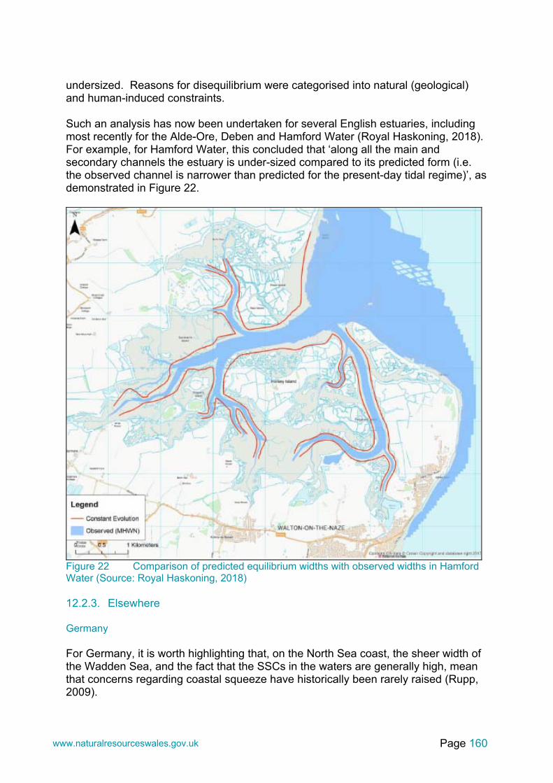
Page 160 www.naturalresourceswales.gov.uk
undersized. Reasons for disequilibrium were categorised into natural (geological) and human-induced constraints. Such an analysis has now been undertaken for several English estuaries, including most recently for the Alde-Ore, Deben and Hamford Water (Royal Haskoning, 2018). For example, for Hamford Water, this concluded that ‘along all the main and secondary channels the estuary is under-sized compared to its predicted form (i.e. the observed channel is narrower than predicted for the present-day tidal regime)’, as demonstrated in Figure 22.
Figure 22 Comparison of predicted equilibrium widths with observed widths in Hamford Water (Source: Royal Haskoning, 2018) 12.2.3. Elsewhere Germany For Germany, it is worth highlighting that, on the North Sea coast, the sheer width of the Wadden Sea, and the fact that the SSCs in the waters are generally high, mean that concerns regarding coastal squeeze have historically been rarely raised (Rupp, 2009).

Page 161 www.naturalresourceswales.gov.uk
For example, in 2015, the coastal defence ministry of the federal state of Schleswig Holstein (the most northerly federal state in Germany), produced a document outlining its strategy for the Wadden Sea up to 2100 (MELUR-SH, 2015). This presented general conclusions on the potential impacts of two SLR scenarios based on expert judgment, drawing on known overall trends regarding the movement of the Wadden Sea barrier islands and SSCs, as well as one detailed (Delft 3D modelling) study of a German North Sea embayment. The two SLR related scenarios were based on IPCC predictions. For the ‘moderate’ scenario, a SLR of 4 mm/yr was assumed to 2050 and 6 mm/yr to 2100. For the ‘increased’ scenario, 6 mm and 10 mm/yr were assumed respectively. An increase in average tidal range was also expected for each scenario, and increased tidal flows predicted. Assumptions regarding accretion were made based on available literature. Saltmarshes were expected to keep pace with all rates of SLR used, whereas sand and mudflats were anticipated to lag slightly behind. On this basis, sand/mudflat losses of 15 to 75 % were estimated by between 2050 and 2100, with the highest loss assumed for the ‘increased’ scenario and the 2100 epoch. Due to these losses not being immediate, and a general Wadden-Sea wide policy of non-intervention (if safe and practicable), no targets for habitat creation were determined on the basis of this study. US Maine In 2013, Torio and Chumura reported on an academic study, whereby fuzzy logic was applied in a GIS environment to assess coastal squeeze of tidal wetlands. This addressed limits to wetland migration inland with rising sea level, and did not calculate changes in marsh area from submergence of existing marsh surfaces or retreat of its seaward edge. In order to establish a baseline, DEMs were created using LiDAR and satellite imagery. Information from previous research studies was utilised to determine tidal elevation ranges of saltmarshes for each of the estuaries (e.g. at Falmouth, Maine, saltmarsh was found to range from 0.02m below mean sea level (MSL) to 1.95 m above MSL). This was also verified against aerial imagery. A ‘‘Coastal Squeeze Index’’ was developed, which could be used to assess the potential of coastal squeeze along the borders of a single wetland and to rank the threats faced by multiple wetlands. The index was based on interpretation of surrounding topography and ‘impervious surfaces’ derived from LiDAR and advanced space-borne thermal emission and reflection radiometry imagery, respectively. Using this index, the authors compared the present and future threat of coastal squeeze to marshes in Wells and Portland, Maine, in the United States and Kouchibouguac National Park in New Brunswick, Canada. The method examined current and future tidal floodplains and applied ‘incremental’ (but linear) increases in sea level in a GIS environment. These were assigned to parameters representing slope and anthropogenic barriers. In order to assess the

Page 162 www.naturalresourceswales.gov.uk
relative threats of coastal squeeze, the authors used fuzzy membership functions to weight the degree to which slope and imperviousness (the study’s proxy for anthropogenic barriers) contribute to coastal squeeze. The results were combined into the index to determine the portions of current and future marsh areas threatened by squeeze (along the upper shore). Specifically, this identified shoreline stretches where upper marshes would not be able to / would struggle to migrate. No loss figures per se were presented. Gulf of Mexico Borchert et al. (2018) undertook a study to compare the capacity of the estuaries along the northern Gulf of Mexico coast to accommodate landward migration. The study area included 39 estuaries in the following five US states: Texas, Louisiana, Mississippi, Alabama and Florida. For elevation data, the study utilised DEMs created from LiDAR, whereby the NOAA’s ‘VDatum’ software tool was used to transform the vertical (terrestrial) datum to a tidal datum. A ‘current tidal saline wetland’ baseline surface was created using the best available data from the U.S. Fish and Wildlife Service’s National Wetlands Inventory. Urban areas were identified through two data sources, namely a so-called SLEUTH (Slope, Land use, Excluded, Urban, Transportation and Hillshade) layer and the ‘developed land cover classes’ (i.e. developed high intensity, developed medium intensity, developed low intensity and developed open space) contained within a U.S. Geological Survey (USGS) database. In order to determine ‘the elevation threshold for the tidal saline wetland boundary’, elevation data relative to MHW for the most recent tidal epoch was determined using the VDatum tool. This was verified with available habitat data to ‘reduce some of the issues related to elevation uncertainty, particularly in comparison with efforts that use an elevation threshold based solely on a tidal datum (i.e. without the use of habitat data)’. Three linear SLR scenarios were applied to gauge future trends, 0.5 m, 1 m, and 1.5 m by 2100. The study reported ‘area available for wetland migration’, as well as ‘area with urban barriers to wetland migration’; actual losses due to coastal squeeze were not apparently presented. Estuaries which have a large amount of urban land that is expected to impede wetland migration were highlighted; this was concluded to affect six estuaries in particular. Pacific coast Over the course of around five years, Thorne et al. (2018) undertook a comprehensive comparison of 14 estuaries along the Pacific coast of the continental United States, and identified those estuaries where future wetland losses are expected to be large (not using the term ‘coastal squeeze’).

Page 163 www.naturalresourceswales.gov.uk
In summary, the authors empirically modelled vulnerability of the estuaries’ wetlands by integrating data on their site-specific topography, tidal inundation, historic accretion rates, vegetation composition, and underlying sediment properties. More detail on the methodology is now presented below. Baseline A wetland baseline was obtained using long-term water level data and detailed surveys of wetland surface elevation. A combination of National Oceanic and Atmospheric Administration (NOAA) tidal data and water level monitoring at the sites themselves were used to obtain local tidal datums. Specifically, water level loggers in tidal channels adjacent to the study sites were deployed in order to estimate local mean high water (MHW) and MHWS following the tidal computation methods of NOAA (2003); GPS measurements were also taken at the loggers on a monthly basis to verify readings; readings were also corrected for barometric pressure. Mean tide level for each site was also estimated by using the NOAA VDATUM model (http://vdatum.noaa.gov/). Inundation frequency related to tidal elevation was estimated using the tide data; marsh zones were delineated on the basis of this data. For example, low marsh was defined as the elevation range between the lowest vegetation plot and the elevation reached by 50% of all recorded high tides (with low marsh flooded at least once daily, on average). Mudflat was defined as occurring between local mean lower low water (i.e. MLWS) and the lowest extent of emergent tidal marsh vegetation. In this fashion, marsh habitat zones were calculated for each estuary. Modelling Empirical modelling was then employed to examine coastal squeeze / the effects of SLR on the marshes. This model was called ‘WARMER’ [Wetland Accretion Rate Model of Ecosystem Resilience]. WARMER is a 1D model of wetland elevation change based on sediment cohorts, where cohort volume was calculated annually as a function of mineral deposition, compaction, organic matter accumulation, and decomposition rates. The formulae employed in the model are presented in Thorne et al. (2018). To parameterise WARMER, wetland accretion rates were obtained from either new carbon-dated sediment cores, or from the literature. In the model, the annual mineral accretion rate is a function of inundation frequency and the mineral accumulation rates measured from the carbon dating. Compaction and decomposition functions were also taken account of following Callaway et al. (1996) and Swanson et al. (2013), and using insights from the cores. ‘Unimodal’ functional relationships were used to quantify variability in organic matter deposition along the tidal elevation gradient at each site, based on the qualitative relationship observed for Spartina alterniflora in the literature. This was supported by aerial imagery interpretation, whereby a ‘normalized difference vegetation index’ was used to identify productive vegetated areas. A differentiation between above and below ground organic matter contributions was made based on a constant ‘root-to-shoot ratio’ for organic matter production, drawing on available studies.
Page 164 www.naturalresourceswales.gov.uk
WARMER was then used to assess the potential in situ average vertical accretion response (mineral and organic) and the horizontal migration potential into adjacent low-lying areas for each marsh, against various non-linear SLR projections for the Pacific coast of North America (based on 2012 guidance; high, moderate and low scenarios were run). It should be noted that in those simulations, a similar sediment supply as measured in the cores / past was assumed, thus no account was taken of such a supply potentially changing in the future. Results were summarised at 10 year intervals. Results interpretation and presentation GIS interpretation (based on LiDAR DEMs) was then used to assess opportunities and limitations to marsh migration / wetland transgression. This was done by deriving an upper elevation band corresponding with the high SLR scenario (e.g. 1.66 m above the current high marsh boundary at California sites). The potential for marsh migration was considered to be limited if human infrastructure (for example, roads and cities) and other large natural features (for example, rivers) would prevent it. A wetland migration potential index was then calculated by dividing the current marsh area of a given estuary by the area of suitable upland migration area. In terms of result presentation, habitat areas were calculated for each estuary, divided into mudflat, low, middle and high marsh. Future development / percentage change was calculated for 2050 and 2110. For example, by 2110, there was predicted to be a general loss of middle and high marsh habitats across the study are, and submergence of tidal marsh, with a conversion to intertidal mudflat and open water at 36 % of the study sites. Uncertainty With regard to uncertainty, it was noted that ‘validation of tidal marsh model projections is difficult because there are typically no historic high-precision elevation data available for hindcast comparisons’. However, the authors examined metrics that served as a form of model validation; for example, they calculated the equilibrium elevation after 2,000 years at the historic SLR rate and found that marsh equilibrium generally occurred between MHW and MAT (maximum annual tide), which are elevations typical of mature marsh development (with the exception of four sites, where accretion rates were too low to maintain a constant marsh surface at the historic rate of SLR). Modelling certainty was also discussed by the authors; highlighting that some simplifying assumptions had to be made, based on the evidence base at the time, particularly regarding coastal wetland ecosystems function in relation to water inundation. As WARMER is a model of vegetated marsh soil; it was acknowledged that model behaviour at un-vegetated mudflat and subtidal elevations would not be well represented in the modelling outputs. Also, lateral or vertical erosion was not included, neither were processes such as wind-driven wave erosion and scarp formation. Large uncertainty with regard to future inter-annual variations of SLR was also acknowledged, for example related to the El Niño Southern Oscillation. Furthermore, sensitivity of the model to mineral accumulation rates was highlighted, as was sensitivity of organic accumulation in relation to salinity changes. It was considered that ‘despite these simplifications, the sites specific calibration of

Page 165 www.naturalresourceswales.gov.uk
WARMER that was used facilitates comparison of relative SLR risk to tidal wetland across the U.S. Pacific coast in a robust methodology’. 12.3. Intertidal habitat change monitoring studies 12.3.1. Introduction In order to inform coastal squeeze assessment studies, historical trend analysis is generally undertaken, notably for saltmarshes. Case studies for monitoring studies are now presented; in Section 12.3.2, UK case studies are first presented, before some studies from elsewhere are discussed (Section 12.3.3). 12.3.2. UK case studies England WFD saltmarsh monitoring Extent mapping In England, WFD saltmarsh monitoring is based on aerial imagery interpretation. This follows the methodology developed by NMBAQCS (Hambridge and Phelan, 2014) and the WFD-UK TAG. The former documents states that aerial photographic image capture should be: Between June and September (or as early as May in some cases) to capture
growing season; Free from cloud and cloud cover (i.e. stable lighting conditions); When the sun angle is greater than 20 degrees (i.e. in full daylight); and When the saltmarsh and creek system is fully exposed by the tide (i.e. low water
spring tides). Aerial survey data to be collected for WFD assessment using the WFD UK-TAG saltmarsh tool specifies the need for red green blue (RGB), and near Infrared (NIR) if available. The validity of these outputs for photographic interpretation is dependent upon image quality, time of growing season, and time of day imagery was acquired. The actual extent mapping is done through a combination of semi-automated and manual digitization processes, by the Environment Agency’s Geomatics team (pers. comm., Estuarine and Coastal Monitoring and Assessment Service (ECMAS), Environment Agency). The semi-automated mapping approach is considered to balance efficiency and accuracy. It requires knowledge of spectral classification and a handling of large raster and vector datasets. In simple terms, it utilises NIR channels of the 4-band photography and produces a greyscale vegetation index image. This measurement is known as the normalised difference vegetation index (NDVI). Pixels of a certain value are assigned one of two classes; high values are vegetation, and low values are non-vegetation. The threshold is determined by eye which best represents the vegetation within the imagery; this sometimes varies for different parts of the imagery (often dependent on lighting qualities/imbalances). Digital pixel based classification is filtered to remove clumps of vegetation smaller than 5 m² and internal areas of non-saltmarsh smaller than 150 m² (this is also specified by Environment Agency (2011)). A vector format image is then created, and visually inspected to remove

Page 166 www.naturalresourceswales.gov.uk
non-saltmarsh vegetation (e.g. macro-algae) or re-add saltmarsh that may have been missed in the original classification. Creek width standardisation processing to dissolve any creeks less than 2 m in width is finally undertaken (also specified in Environment Agency, 2011). The manual digitizing method basically comprises image data displayed in an GIS environment, at a standard scale to ensure consistency in mapping output. The boundary of saltmarsh is then digitized, applying creek width, external and internal fragment mapping as set out by Environment Agency criteria. For first time mapping, this can produce smoother output because it is not based on pixel classifications. However, it is often time consuming, especially in areas of high fragmentation. Figure 23 shows a flow process of saltmarsh extent mapping.
Figure 23 Flow process of saltmarsh extent mapping (Source: Hambridge and Phelan, 2014)
Aerial flights
Generate Vegetation Index using Near Infrared and Red
channels
Desktop
Photointerpretation
Semi-automated processing using Vegetation Index
Extent map
Historic saltmarsh data
1. Prior ground truthing information
Flightplanning
Available aerial imagery
Processing(Ortho-correction,
Mosaicing and colour balancing)
2. Ground truthing/
3. Validation assessment
Previous extent map

Page 167 www.naturalresourceswales.gov.uk
Benefits and disadvantages of semi-automated and manual digitization, as detailed by Hambridge and Phelan (2014) are set out in Table 29.
Table 29 Benefits and disadvantages of semi-automated versus manual digitisation
Benefits Disadvantages Semi-automated extent mapping
Cost effective NIR data required (though should not result in significantly more cost)
Repeatable Relies on photosynthetic vegetation to work (manual intervention required otherwise)
Simple, standardised methodology Potential for inconsistency in outputs from different interpreters
Most processing can be done in standard GIS environment (e.g. ArcGIS)
Potential for noise when comparing multiple outputs
20 cm photography adequate Manual extent mapping Smooth outlines Time consuming
QA process may be incorporated into digitising
More potential for inconsistency in outputs between different interpreters than semi-automated approach
NIR data not necessary Fragmented marsh may take a long time to map
Personal communication with members of the Environment Agency’s ECMAS (July 2018), reveals that change is measured by comparing a baseline dataset with a later dataset. In the early years, data was collected relatively frequently (approximately every three to four years), but this has now been reduced to every six years (due to the data not showing much change during the shorter intervals). In terms of aerial imagery capture, the ECMAS ‘piggy back’ onto other flight programmes, so we they do not have complete control of when the data is captured. For the baseline, ECMAS largely utilised the national data derived from an extensive aerial imagery mapping study undertaken between 2006 and 09 (and reported on in Environment Agency, 2011; this followed a semi-automated methodology). Where errors in the latter data are spotted, the baseline is edited if necessary. ECMAS was not able to share costs for these tasks. Saltmarsh community mapping In order to map saltmarsh communities / zones, a point classification approach has been adopted by the Environment Agency to map saltmarsh zonation for WFD purposes, as summarised by Hambridge and Phelan (2014) on behalf of NMBAQCS. Ground data is integral to classifying the plant community and assisting photointerpretation. This may be in the form of quadrat data, saltmarsh transition data, or basic community confirmation. The point classification system involves creating a rectangular grid of points spaced 10 m apart (or 5 m for smaller waterbodies less than 30 ha). Each point would then be assigned a saltmarsh zone according to the vegetation they lie on top of. This

Page 168 www.naturalresourceswales.gov.uk
was deemed a more efficient and robust way to map saltmarsh zones compared to vector mapping, where the complexity of drawing shapefiles around zones was too time consuming and risked file corruptions. The later also required more decisions to be made i.e. where is the boundary, is the block of vegetation worth mapping, and what class does the vegetation belong to? For the point classification system, only the latter needs to be decided. Habitat mapping guidance Saltmarsh habitat mapping in England is undertaken with reference to the ‘Common Standards Monitoring Guidance for Saltmarsh habitats’ (JNCC, 2004). This suggests that sampling is possible over a period of several months, with a recommendation of May to October. This is because most saltmarsh plants are perennial, however, areas suffering from coastal squeeze may primarily consist of lower marsh plants which comprise relatively higher abundances of annuals. Therefore, a survey period of April to August is recommended. JNCC (2004) propose field surveys to be undertaken in structured walks (W shape) with at least 10 monitoring stops in each management unit. These should be planned on maps/aerial photographs prior to the survey to avoid subjectivity. At each stop, appropriate attributes (percentage cover, species composition) should be assessed and photographs taken throughout, recording features using GPS. According to JNCC (2004), transects are recommended to assess saltmarsh zonation, and can detect long-term negative trends. The widths of saltmarsh habitat measured from the strandline to the lowest continuous marsh are endorsed for measurement. Five locations should be pre-selected based on maps or aerial photography to avoid subjectivity in selection, and locations fixed by GPS in the field. The measured width of zones should be compared across surveys, in order to indicate changes in habitat extent. To assess condition for habitat extent, and collect evidence of habitat loss/gain in the field, JNCC (2004) has produced a dichotomous stepped key within their guidance; this is as follows:
1) Extent of the feature based on the most recent aerial photography Appears to be increasing or no apparent change = go to 2 Increase in some places, decrease in others or appears to be net decrease
over the entire area = got to 3 2) Evidence of accretion at the marsh edge (accretional ramp with pioneer
species) = favourable condition for extent 3) Evidence of erosion in some areas (mud mounds, cliff edge topping) but
accretion in other areas (accretional ramp with pioneer species); including a net balance or gain within system = favourable condition for extent Or Evidence of erosion over most of the marsh edge surface areas (mud mounds, cliff edge toppling etc.) combined with loss of horizontal extent of saltmarsh area = go to 4
4) Need to consider the long-term future of the saltmarsh feature Is the saltmarsh constrained by natural topographical features (e.g. high
ground, cliff) = favourable condition for extent Do anthropogenic constraints prevent the feature from reaching
morphological equilibrium = unfavourable condition for extent
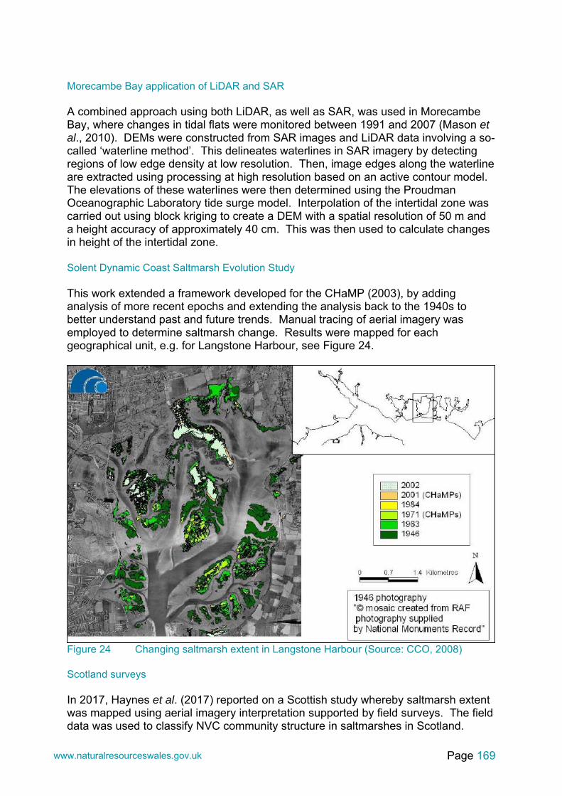
Page 169 www.naturalresourceswales.gov.uk
Morecambe Bay application of LiDAR and SAR A combined approach using both LiDAR, as well as SAR, was used in Morecambe Bay, where changes in tidal flats were monitored between 1991 and 2007 (Mason et al., 2010). DEMs were constructed from SAR images and LiDAR data involving a so-called ‘waterline method’. This delineates waterlines in SAR imagery by detecting regions of low edge density at low resolution. Then, image edges along the waterline are extracted using processing at high resolution based on an active contour model. The elevations of these waterlines were then determined using the Proudman Oceanographic Laboratory tide surge model. Interpolation of the intertidal zone was carried out using block kriging to create a DEM with a spatial resolution of 50 m and a height accuracy of approximately 40 cm. This was then used to calculate changes in height of the intertidal zone. Solent Dynamic Coast Saltmarsh Evolution Study This work extended a framework developed for the CHaMP (2003), by adding analysis of more recent epochs and extending the analysis back to the 1940s to better understand past and future trends. Manual tracing of aerial imagery was employed to determine saltmarsh change. Results were mapped for each geographical unit, e.g. for Langstone Harbour, see Figure 24.
Figure 24 Changing saltmarsh extent in Langstone Harbour (Source: CCO, 2008) Scotland surveys In 2017, Haynes et al. (2017) reported on a Scottish study whereby saltmarsh extent was mapped using aerial imagery interpretation supported by field surveys. The field data was used to classify NVC community structure in saltmarshes in Scotland.

Page 170 www.naturalresourceswales.gov.uk
Vegetation sampling following NVC methodology was undertaken, with at least one quadrat sample of each saltmarsh sub-community per site. This included samples of transitional vegetation types with halophytes present on a selective basis. Condition monitoring was undertaken for Salicornia and annuals colonising mud and sand (Pioneer saltmarsh – H1310) and Atlantic salt meadows (Glauco-Puccinellietalia maritimae) (Atlantic saltmarsh – H1330) as per JNCC guidance (see section on England WFD saltmarsh monitoring). Habitat mapping was undertaken using GIS and aerial photography by Haynes et al. (2017). Digitised habitat polygons were drawn manually on to aerial photography at a scale of 1:4000. This was undertaken, or at least overseen, by field surveyors. Vegetation patterning in the field could then be cross-referenced with historic aerial photography; differences were noted on habitat maps including changes to the seaward extent of the marsh. Habitats maps were completed to sub-community level for saltmarsh and to community levels for associated habitats. An attribute table was created for all of the saltmarsh polygons with information including site name, area, and the NVC communities present. Blackwater saltmarsh change study In 2016, the RSPB (Royal Society for the Protection of Birds) commissioned ABPmer to undertake a study of Blackwater saltmarshes by reviewing remote sensing data from 2008/09 to 2015 and comparing results against previous studies. The RSPB commissioned the study to prove or disprove anecdotal observations of continued losses of these marshes. LiDAR data was used as the primary data for this analysis. The alternative approach of manually digitising/tracing the saltmarsh boundaries based on aerial imagery was discounted due to the resource intensity involved in this process. It was also felt that, due to the ‘cliffed’ nature of the saltmarsh edges in the Blackwater Estuary, determining the edges of the saltmarshes should be relatively easy, when compared to saltmarshes in other estuaries which exhibit a more gradual transition from mudflat to saltmarsh. Also, given that most of the Blackwater Estuary is backed by defence embankments, determining a landward extent of saltmarshes was considered to be relatively straightforward. DEMs were created from available LiDAR surveys, clipped to the bottoms of the embankments. The seaward extent of the saltmarshes was mapped by determining the tidal elevation of the lower saltmarsh boundary through aerial imagery interpretation. The estuary was split into zones where different tidal elevations were applied. For example in the more exposed outer estuary, saltmarsh was found to extent to From this analysis objective measurements of marsh loss were derived encompassing the areas of the estuary that were covered by both the 2008/9 and the 2015 LiDAR surveys and verified against the aerial imagery. This determined that saltmarshes losses had occurred over the seven-year study period, averaging around 1.7 ha per year

Page 171 www.naturalresourceswales.gov.uk
Separate analyses were also made of the alignment/retreat of the exposed marsh edges and of wider changes to the overall extent of saltmarsh habitat. This analysis led to the conclusion that noticeable saltmarsh edge erosion had occurred along around 45 % of the shoreline during the seven-year study period. As part of this data review, the methodologies and limitations / caveats of previous national and regional investigations were also summarised; this summary table is reproduced below (Table 30).
Table 30 Previous saltmarsh studies undertaken in England and the Anglian region (from ABPmer, 2016)
Author & Year Methodology and Extent Limitations/Caveats Institute of Terrestrial Ecology (ITE) (1973)1
Saltmarsh tracing/digitisation onto OS basemaps using aerial photographs flown at a 1:10,560 scale (Essex, Suffolk and Kent).
No orthorectification applied.
Burd (1992)2
Interpretation of (1973) ITE maps. Tracing/digitisation of saltmarshes using aerial photographs flown at a 1:5,000 scale in 1988 (Essex and north Kent). Supported by extensive field surveys.
Unrectified maps; comparison of maps with different scales, produced using different approaches (e.g. re sizes of creeks, exclusion of degraded saltmarsh/bare patches).
Cooper et al. (2000)1
Interpretation of ITE (1973) and Burd (1992) mapping. Tracing/digitisation of saltmarshes using 1998 aerial images (scale: 1:5,000) (Essex).
Areas of algae and eelgrass excluded from the survey, but reedbed included.
Natural England (2006)1
Saltmarsh change in selected Essex SPAs; review of previous studies, no new digitisation.
No new digitisation/tracing (except for Crouch/Roach).
Environment Agency (2011)3
National study. Tracing/digitisation of saltmarshes using 2007/08 aerial images, to 10 cm resolution. Tracing rules: map: (1) areas >5 m2; (2) internal parts >150 m2; (3) creeks up to ca. 1.5 m width; (4) discrete saltmarsh formations only. Imagery processing software used to aid process (shape patterns/spectral signatures). Some ground-truthing.
Blackwater observations: Inconsistent mapping of saltmarsh creeks; extensive areas of algae on mud mapped as saltmarsh. Included some, but not all managed realignment areas. Included one reclaimed area & one backbarrier swamp area (Ramsay Marsh).
IECS (2011)4
Saltmarsh change in Essex SSSIs only. Review of previous studies/literature. Tracing/ digitisation using aerial imagery (scale: 10,000, resolution: 25cm; 1997, 2000 and 2008).
Excluded non-SSSI areas. Included some, but not all managed realignment areas in Blackwater. Some creeks possibly mapped inconsistently between years.

Page 172 www.naturalresourceswales.gov.uk
Author & Year Methodology and Extent Limitations/Caveats Tracing rules: map: (1) areas >5 m2; (2) creeks >3 m at mouth; (3) large creek pans/barren areas; (4) fragmented marsh as appropriate. No imagery processing software used. Some ground-truthing.
Many internal creeks and pans generally not mapped in Blackwater, especially in larger complexes.
Limitations identified by: 1) IECS (2011); 2) IECS (2011) and Natural England (2006); 3) ABPmer during this study; 4) IECS (2011) and ABPmer during this study. Please note that the exact scope of the contract, and resources involved, are not known to ABPmer, and might have affected the effort expended on truthing the data.
12.3.3. Case studies from elsewhere Ireland Based on the above-mentioned JNCC guidance, McCorry and Ryle (2009) undertook a saltmarsh change study which for at several sites around the coast of Ireland, similar to several above-listed case studies, adopted a combination of aerial imagery interpretation and field surveys. Field surveys were generally conducted in pairs and habitats were covered by zig-zagging from the seaward to landward boundaries, noting habitat boundaries and classifications. Monitoring stops, where detailed information to inform habitat structure was recorded, were stratified so that internal habitat variation could be included (i.e. located in lower, middle and upper shore). An integrated GPS-handheld computer (GeoExplorer – Trimble GeoXT) was used to facilitate the collection of data using pre-programmed drop-down menus and text fields. Furthermore, descriptions of plant communities, saltmarsh zonation, physical structure (creeks and pans), micro-topography, and habitat transitions were recorded and written in to pro-forma. Photographs were taken to aid habitat descriptions and record impact activities; the location and aspect was taken using GPS and compass respectively. GIS software was then used interpret the field data and compare the measured extents to previous extents. With regard to field data, McCorry and Ryle (2009) collected data on habitat points/boundaries, notable species, quadrat results, negative impacts, features, photographs and points of interest and stored using proprietary Terrasync software (Trimble). This was then downloaded and imported into GIS software to allow digital mapping. Current extents were compared to previous sets of OSI digital aerial photos (from 2003 and 2004), 6 inch OSI maps and older NPWS habitat maps to see if habitat area had changed significantly due to erosion or accretion, and if trends correlated with observations in the field. This method was considered unsuitable to record small changes (approximately 5-10 m loss/gain) due to the relative accuracy of the ortho-rectified aerial photos. Other details may also be difficult to constrain such as natural transitions to other habitats (e.g. saltmarsh covered by sand-dunes). Limitations were also noted with regard to the GPS receiver, which can be affected by atmospheric noise, so corrections need to be applied to data
Page 173 www.naturalresourceswales.gov.uk
Similar methods were adopted by Natural England (2015) to assess the status of Annex I saltmarsh habitats. Denmark In Denmark, automated classification of saltmarshes is used utilising aerial photography interpretation combined with elevation models and reference transects (Aarhus University, 2015). In Denmark, there has been a ‘tradition for nationwide aerial orthophoto image acquisition since the beginning of the 1990s’, and these have been undertaken every two years since 2002 the data acquisitions have been repeated on a biennial basis. The imagery data is generally acquired post-spring. 12.4. References Aarhus University (2015). Remote sensing based classification of structural elements of coastal habitats. Aarhus University, Aarhus, 46p. ABPmer (2003). The Prediction of Habitat Types on the Humber Estuary. Report R1016, ABPmer, Southampton, 26p. ABPmer (2007). Severn Estuary CHaMP Morphological Assessments; Part H: Expert Geomorphological Assessment. Report R1260h, ABPmer, Southampton, 42p. ABPmer (2008). Greater Thames CHaMP Summary Document. Report R1448, ABPmer, Southampton, 86p. ABPmer (2009). Predicted Morphological Form of the Severn Estuary. Report R1512, ABPmer, Southampton, 25p. ABPmer (2010a). Humber CHaMP Monitoring Study. Report R1467, ABPmer, Southampton, 131p. ABPmer (2010b). Predicted Habitat Change in the Severn Estuary. Report R1692TN, ABPmer, Southampton, 10p. ABPmer (2016). Evaluation of Saltmarsh Change in the Blackwater Estuary, Essex, Review of remote sensing data from 2008 to 2015. Report No 2562. A report produced by ABPmer for RSPB. 48p. Borchert, S. M., Osland, M. J., Enwright, N. M., Griffith, K. T. (2018). Coastal wetland adaptation to sea level rise: Quantifying potential for landward migration and coastal squeeze. J Appl Ecol. 2018, p.1–12. Burd, F. (1992). Erosion and vegetation change on the saltmarshes of Essex and north Kent between 1973 and 1988. Research and Survey in Nature Conservation No. 42. English Nature, Peterborough, 108p. Callaway, J. C., Nyman, J. A., DeLaune, R. D. (2009). Sediment accretion in coastal wetlands: A review and a simulation model of processes. Curr. Top. Wetland Biogeochem. 2, 2–23 (1996).

Page 174 www.naturalresourceswales.gov.uk
CH2M (2015). Humber Estuary: Coastal Squeeze Analysis Project. Draft report for the Environment Agency. CH2M, Swindon, 67p. Channel Coastal Observatory (2008). Solent Dynamic Coast Project Main Report (A tool for SMP2) Cooper, N. J., Skrzypczak, T., and Burd, F. (2000). Erosion of the saltmarshes of Essex between 1988 and 1998. Report to the Environment Agency (Anglian Region). In: IECS, 2011 Defra (2005). Coastal Squeeze Implications for Flood Management - The Requirements of The European Birds and Habitats Directives Defra Policy Guidance. Defra, London, 7p. English Nature (2006). Coastal squeeze, saltmarsh loss and Special Protection Areas. English Nature, Peterborough, 58p. Environment Agency (2008). Planning for the rising tides - The Humber Flood Risk Management Strategy. Environment Agency, Leeds, 32p. Environment Agency (2011). The extent of saltmarsh in England and Wales: 2006–2009. Environment Agency, Bristol, 48p. Environment Agency (2017). Medmerry Management Realignment Monitoring Update Summer 2017 ESCP (2017). Solent and South Downs Regional Habitat Compensation Programme Halcrow (1999). Poole and Christchurch Bays Shoreline Management Plan. 4 volumes available at: http://www.twobays.net/smp1.htm [last accessed July 2018] Hambridge, C. and Phelan, N. (2014). Saltmarsh mapping standardisation for the Water Framework Directive – NMBAQCS. [Online] Available at: http://www.nmbaqcs.org/media/1088/saltmarsh-mapping-standard_140814_final.docx (accessed 1 June 2018). Harvey, R., Born, K., Young, J., Miller, I., Watts, B., Tinch, R. and Provins, A. (2008). Planning for rising tides at Wareham, Poole Harbour. Proceedings of 43rd Defra/Environment Agency Flood and Coastal Management Conference, Manchester, 2008. P.X.3.1-x.3.12. Haynes, T. A., Angus, S., Seanlan, C. and Bhatti, N. (2017). Developing a saltmarsh monitoring methodology to meet multiple policy and management objectives in Scotland. Journal of Coastal Conservation, 21, 445-452. Institute of Estuarine and Coastal Studies (IECS) (2011). Essex Coastal SSSIs: Assessment of Changes in Extent of Saltmarsh Over the Period 1997 to 2008. IECS, Hull, 86p.

Page 175 www.naturalresourceswales.gov.uk
Institute of Terrestrial Ecology (ITE) (1974). Aspects of the ecology of the coastal area in the outer Thames Estuary and the impact of the proposed Maplin Airport. In: Burd, 1992. JNCC (2004). Common Standards Monitoring Guidance for Saltmarsh Habitats. [Online] Available at: http://jncc.defra.gov.uk/pdf/CSM_coastal_saltmarsh.pdf (Accessed 21 May 2018). Mason, D. C., Scott, T. R. and Dance, S. L. (2010). Remote sensing of intertidal morphological change in Morecambe Bay, U.K., between 1991 and 2007. Estuarine, Coastal and Shelf Science, 87(3). pp. 487-496. McCorry, M. and Ryle, T. (2009). Saltmarsh Monitoring Project 2007-2008 – Final Report. A Report for Research Branch, National Parks and Wildlife Service, Department of Environment, Heritage and Local Government, Dublin. [Online] Available at: https://www.npws.ie/sites/default/files/publications/pdf/McCorry_%26_Ryle_2009_Saltmarsh_survey_V1.pdf (Accessed 8 May 2018). MELUR-SH (2015). Strategie für das Wattenmeer 2100. Ministerium für Energiewende, Landwirtschaft, Umwelt und ländliche Räume des Landes Schleswig-Holstein, Kiel, Germany, 88p. National Oceanic and Atmospheric Administration (NOAA) (2003). Computational Techniques for Tidal Datums Handbook (National Oceanic and Atmospheric Administration, Special Publication NOS CO-OPS 2, 2003), 98p. NFDC (2010). North Solent Shoreline Management Plan. NSSMP CPW1839. Final 16 December 2010 Nottage, A. S. and Robertson, P. A. (2005). The Saltmarsh Creation Handbook: A Project Manager's Guide to the Creation of Saltmarsh and Intertidal Mudflat (RSPB Management Guides). RSPB, Sandy, 128p. Pontee, N. (2011). Reappraising coastal squeeze: A case study from North-West England. Proceedings of the Institution of Civil Engineers: Maritime Engineering. 164. 10.1680/maen.2011.164.3.127. Royal Haskoning (2003). Solent Coastal Habitat Management Plan, Volume 1. Key authors: Malcolm Royal Haskoning (2004). North Wessex proto Coastal Habitat Management Plan (CHaMP). Produced for the Environment Agency and English Nature. Royal Haskoning (2016). Healthy Estuaries 2020: Towards Addressing Coastal Squeeze in Estuaries. Royal Haskoning, Peterborough, 73p. Royal Haskoning (2018). Healthy Estuaries 2020: An Assessment of Estuary Morphological Equilibrium – Alde-Ore, Deben and Hamford Water. Royal Haskoning, Peterborough, 101p.

Page 176 www.naturalresourceswales.gov.uk
Rupp (2009). The Future of Managed Realignment of Coastal Flood Plains in Northern Europe - a Comparative Study. PhD thesis, University of Southampton, School of Civil Engineering and the Environment. Swanson, K. M., Drexler, J. Z., Schoellhamer, D. H., Thorne, K. M., Casazza, M. L., Overton, C. T., Callaway, J. C., and Takekawa, J. Y. (2013). Wetland Accretion Rate Model of Ecosystem Resilience (WARMER) and its application to habitat sustainability for endangered species in the San Francisco Estuary. Estuaries and Coast 37, 476–492. Thorne, K., MacDonald, G., Guntenspergen, G., Ambrose, R., Buffington, K., Dugger, B., Takekawa, J. (2018). U.S. Pacific coastal wetland resilience and vulnerability to sea-level rise. Science Advances, 4, eaao3270. Torio, D. D. and Chmura, G. L. (2013). Assessing coastal squeeze of tidal wetlands. Journal of Coastal Research, 29(5), 1049-1061. UK-TAG (2014). UK-TAG Transitional and Coastal Water Assessment Method. Angiosperms. Saltmarsh Tool. [Online] Available at: https://www.wfduk.org/sites/default/files/Media/Characterisation%20of%20the%20water%20environment/Biological%20Method%20Statements/TraC%20Saltmarsh%20Tool%20UKTAG%20Method%20Statement.PDF (Accessed 21 May 2018).

Page 177
13. Appendix C. Monitoring Datasets Review
Serial Data/Evidence Source
Dates Frequency Features Attribute MPA Location
1 Flood Defences 2015 -11-03 Quarterly (updates)
Potential to cover all SAC features
Structure and Function of Habitat
All Welsh SAC's https://data.gov.uk/dataset/spatial-flood-defences-including-standardised-attributes
2 Historic Aerial Imagery to Monitor Temporal Change in Intertidal Habitats
1969-01-01/ 201312-31
N/A Potential to cover all SAC features
Range of Habitat All Welsh SAC's https://libcat.naturalresources.wales/webview/?infile=details.glu&loid=115512&rs=606386&hitno=36
3 Intertidal Mapping Project (Updating Marine Intertidal Phase 1 Biotope Mapping Survey)
2007-08-31/ 201010-08
As needed Potential to cover all SAC features
Range of Habitat All Welsh SAC's https://libcat.naturalresources.wales/webview/?infile=details.glu&loid=114453&rs=606413&hitno=113
4 Intertidal Monitoring of Saltmarsh Extent in Carmarthen Bay and Estuaries Special Areas of Conservation (SAC) 2009
2009-09-21/ 200909-22
Not planned Salicornia and other annuals colonising mud and sand
Range of Habitat Carmarthen Bay and Estuaries / Bae Caerfyrddin ac Aberoedd SAC
https://libcat.naturalresources.wales/webview/?infile=details.glu&loid=114945&rs=606413&hitno=88
5 Intertidal Monitoring of the Mawddach Estuary Sediments in Pen Llyn ar Sarnau Special Area of Conservation (SAC) 2012
2012-07-23/ 201207-24
Annual Potential to cover all SAC features
Structure and Function of Habitat
Pen Llyn a'r Sarnau / Lleyn Peninsula and the Sarnau SAC
https://libcat.naturalresources.wales/webview/?infile=details.glu&loid=115333&rs=606465&hitno=454
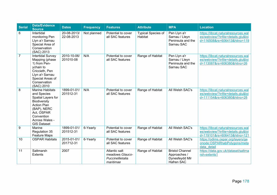
Page 178
Serial Data/Evidence Source
Dates Frequency Features Attribute MPA Location
6 Intertidal monitoring Pen Llyn a’r Sarnau Special Area of Conservation (SAC) 2013
20-08-2013/ 22-08-2013
Not planned Potential to cover all SAC features
Typical Species of Habitat
Pen Llyn a'r Sarnau / Lleyn Peninsula and the Sarnau SAC
https://libcat.naturalresources.wales/webview/?infile=details.glu&loid=116508&rs=606413&hitno=119
7 Intertidal Survey Mapping (phase 1) from Pen-ychain to Criccieth, Pen Llyn a'r Sarnau Special Areas of Conservation (SAC) 2010
2010-10-06/ 201010-08
N/A Potential to cover all SAC features
Range of Habitat Pen Llyn a'r Sarnau / Lleyn Peninsula and the Sarnau SAC
https://libcat.naturalresources.wales/webview/?infile=details.glu&loid=113087&rs=606380&hitno=26
8 Marine Habitats and Species Spatial Layers for Biodiversity Action Plan (BAP), NERC Act, OSPAR Convention Across Wales - GIS Dataset
1899-01-01/ 201512-31
N/A Potential to cover all SAC features
Range of Habitat All Welsh SAC's https://libcat.naturalresources.wales/webview/?infile=details.glu&loid=111154&rs=606380&hitno=28
9 Marine Regulation 35 Feature Maps
1899-01-01/ 201512-31
6-Yearly Potential to cover all SAC features
Range of Habitat All Welsh SAC's https://libcat.naturalresources.wales/webview/?infile=details.glu&loid=119101&rs=606413&hitno=121
10 OSPAR Habitats 2015-01-01/ 201712-31
6-Yearly Potential to cover all SAC features
Range of Habitat All Welsh SAC's https://odims.ospar.org/layers/geonode:OSPARhabPolygons/metadata_detail
11 Saltmarsh Extents
2007 Atlantic salt meadows Glauco- Puccinellietalia maritimae
Range of Habitat Bristol Channel Approaches / Dynesfeydd Mlr Hafren SAC
https://data.gov.uk/dataset/saltmarsh-extents1

Page 179
Serial Data/Evidence Source
Dates Frequency Features Attribute MPA Location
12 Saltmarsh Extents
2009-01-01/ 201605-01
Atlantic salt meadows Glauco- Puccinellietalia maritimae
Range of Habitat All Welsh SAC's http://lle.gov.wales/catalogue/item/SaltmarshExtents/?lang=en
13 Severn Estuary SAC Monitoring
2016-09-30/ 201610-03
Potential to cover all SAC features
Typical Species of Habitat
Severn Estuary (England) SAC
https://data.gov.uk/dataset/2011-natural-england-severn-estuary-benthic-grab-survey
14 UK Article 17 Habitats
1899-01-01/ 201512-31
Six yearly Potential to cover all SAC features
Range of Habitat All Welsh SAC's http://lle.gov.wales/catalogue/item/MarineArt17Features
15 WFD Coastal Waterbodies Cycle 2
2013-04-01/ 201512-31
Potential to cover all SAC features
Range of Habitat All Welsh SAC's https://libcat.naturalresources.wales/webview/?infile=details.glu&loid=116271&rs=665935&hitno=1
16 WFD Transitional Waterbodies Cycle 2
2013-04-01/ 201512-31
Potential to cover all SAC features
Typical Species of Habitat
All Welsh SAC's https://libcat.naturalresources.wales/webview/?infile=details.glu&loid=116272&rs=665977&hitno=1
17 Menai Strait and Conwy Bay Special Area of Conservation (SAC) muddy gravel survey (2013)
2013-06-24/ 201306-28
Not planned Mudflats and sandflats not covered by seawater at low tide
Range of Habitat Y Fenai a Bae Conwy / Menai Strait and Conwy Bay SAC
https://libcat.naturalresources.wales/webview/?infile=details.glu&loid=115886&rs=606413&hitno=138
18 National Tide and Sea Level Facility
1915 -01-01 /Present
900 seconds Potential to cover all listed intertidal SAC features
Range of Habitat All Welsh SAC's http://www.ukdmos.org/search-directory
19 NRW Intertidal Monitoring Surveys
2004-07-05/ 201702-23
Rolling Programme
Potential to cover all listed intertidal SAC features
Range of Habitat All Welsh SAC's http://www.ukdmos.org/ukdmos/details.php?mlb=1&tpd=10247&tpc=programme
20 Severn Estuary Special Area of Conservation (SAC) and Special Protection Area (SPA): Intertidal Mudflats and
2012-10-13/ 201211-14
Not planned Mudflats and sandflats not covered by seawater at low tide
Typical Species of Habitat
Severn Estuary (England) SAC
https://libcat.naturalresources.wales/webview/?infile=details.glu&loid=115547&rs=606465&hitno=426

Page 180
Serial Data/Evidence Source
Dates Frequency Features Attribute MPA Location
Sandflats Condition Assessment 2012
21 WFD Saltmarsh monitoring
2007-01-01/ 201703-18
Rolling Programme
Atlantic salt meadows Glauco- Puccinellietalia maritimae
Typical Species of Habitat
All Welsh SAC's http://www.ukdmos.org/ukdmos/details.php?mlb=1&tpd=11225&tpc=programme
22 WFD TraC saltmarsh
2007-01-01/present
Rolling Programme
Atlantic salt meadows Glauco- Puccinellietalia maritimae
Typical Species of Habitat
All Welsh SAC's http://ukdmos.org/ukdmos/details.php?mlb=1&tpd=11225&tpc=programme
23 LIDAR terrain and surfaces models Wales
2015-01-01 /2015-12-31
Rolling Programme
N/A N/A All Welsh SAC's https://libcat.naturalresources.wales/webview/?tiarray=full&oid=116814
Additional Monitoring of SAC features not applicable to Coastal Squeeze but included for information purposes and may be useful on a site specific level:
24 Extent and Distribution of Saline Lagoons in Wales (2009)
2009-01-01/ 200912-31
Not planned Coastal Lagoon Range of Habitat Bae Cemlyn / Cemlyn Bay SAC Pembrokeshire Marine / Sir Benfro Forol SAC Pen Lleyn Peninsula and the Sarnau SAC
https://libcat.naturalresources.wales/webview/?infile=details.glu&loid=109756&rs=606413&hitno=85
25 Intertidal Monitoring of Boulders Habitat in the Menai Strait and Colwyn Bay Special Area of Conservation (SAC) 2009
2009-06-22/ 200906-25
Not planned Reefs / Underboulder
Typical Species of Habitat
Y Fenai a Bae Conwy / Menai Strait and Conwy Bay SAC
https://libcat.naturalresources.wales/webview/?infile=details.glu&loid=115074&rs=606413&hitno=176
26 Intertidal Monitoring of Rocky Reefs in
2007-01-01/ 201512-31
N/A Potential to cover all SAC features
Typical Species of Habitat
Pembrokeshire Marine / Sir Benfro Forol SAC
https://libcat.naturalresources.wales/webview/?infile=details.glu&loid=115409&rs=606413&hitno=60

Page 181
Serial Data/Evidence Source
Dates Frequency Features Attribute MPA Location
Pembrokeshire Marine Special Area of Conservation (SAC) 2007- 2010
27 Intertidal Monitoring of Sabellaria alveolata Reefs in Pen Llyn a'r Sarnau Special Area of Conservation (SAC) 2012
2012-07-24/ 201207-24
Annual Reefs / Sabellaria alveolata
Range of Habitat Pen Llyn a'r Sarnau / Lleyn Peninsula and the Sarnau SAC
https://libcat.naturalresources.wales/webview/?infile=details.glu&loid=115332&rs=606465&hitno=475
28 Intertidal Monitoring of Sabellaria alveolata Reefs in Pen Llyn a'r Sarnau Special Areas of Conservation (SACs) 2010
2010-07-11/ 201007-16
Not planned Reefs / Sabellaria alveolata
Typical Species of Habitat
Pen Llyn a'r Sarnau / Lleyn Peninsula and the Sarnau SAC
https://libcat.naturalresources.wales/webview/?infile=details.glu&loid=114458&rs=606413&hitno=116
29 Intertidal Monitoring of Sabellaria Reef in Cardigan Bay Special Area of Conservation (SAC) 2008
2008-05-05/ 200805-08
Not planned Reefs / Sabellaria alveolata
Range of Habitat Cardigan Bay / Bae Ceredigion SAC
https://libcat.naturalresources.wales/webview/?infile=details.glu&loid=115072&rs=606413&hitno=133
30 Intertidal Monitoring of Sabellaria reef in Pen Llyn a'r Sarnau Special Areas of
2009-07-08/ 200907-10
N/A Reefs Typical Species of Habitat
Pen Llyn a'r Sarnau / Lleyn Peninsula and the Sarnau SAC
https://libcat.naturalresources.wales/webview/?infile=details.glu&loid=114388&rs=606413&hitno=61

Page 182
Serial Data/Evidence Source
Dates Frequency Features Attribute MPA Location
Conservation (SACs) 2009
31 Intertidal Monitoring of the Biotope SLR.FserX.T in the Menai Strait and Colwyn Bay Special Areas of Conservation (SAC) 2009
2009-06-26/ 200906-26
Not planned Mudflats and sandflats not covered by seawater at low tide
Range of Habitat Y Fenai a Bae Conwy / Menai Strait and Conwy Bay SAC
https://libcat.naturalresources.wales/webview/?infile=details.glu&loid=115081&rs=606413&hitno=242
32 Intertidal Monitoring of the Biotope SLR.FserX.T in the Menai Strait and Colwyn Bay Special Areas of Conservation (SACs) 2010
2010-07-15/ 201007-15
Not planned Reefs Range of Habitat Y Fenai a Bae Conwy / Menai Strait and Conwy Bay SAC
https://libcat.naturalresources.wales/webview/?infile=details.glu&loid=114949&rs=606413&hitno=134
33 Priority Marine Habitats of Wales: Blue Mussel Beds (Mytilus edulis)
1982-04-10/ 200910-01
N/A Estuaries / Blue Mussel Beds (Mytilus edulis)
Range of Habitat Cardigan Bay / Bae Ceredigion SAC Carmarthen Bay and Estuaries / Bae Caerfyrddin ac Aberoedd SAC Pembrokeshire Marine / Sir Benfro Forol SAC Pen Llyn a'r Sarnau / Lleyn Peninsula and the Sarnau SAC Y Fenai a Bae Conwy / Menai
https://libcat.naturalresources.wales/webview/?infile=details.glu&loid=114723&rs=606413&hitno=65

Page 183
Serial Data/Evidence Source
Dates Frequency Features Attribute MPA Location
Strait and Conwy Bay SAC
34 Priority Marine Habitats of Wales: Estuarine Rock
1978-07-08/ 201108-21
N/A Estuaries Range of Habitat Carmarthen Bay and Estuaries / Bae Caerfyrddin ac Aberoedd SAC Dee Estuary / Aber Dyfrdwy (England) SAC Glannau Mon: Cors heli / Anglesey Coast: Saltmarsh SAC Pembrokeshire Marine / Sir Benfro Forol SAC Pen Llyn a'r Sarnau / Lleyn Peninsula and the Sarnau SAC Severn Estuary (England) SAC
https://libcat.naturalresources.wales/webview/?infile=details.glu&loid=114727&rs=606413&hitno=67
35 Priority Marine Habitats of Wales: Seagrass Beds
1935-01-01/ 200910-01
N/A Estuaries / Mudflats and sandflats not covered by seawater at low tide / Seagrass
Range of Habitat Carmarthen Bay and Estuaries / Bae Caerfyrddin ac Aberoedd SAC Pembrokeshire Marine / Sir Benfro Forol SAC Pen Llyn a'r Sarnau / Lleyn Peninsula and the Sarnau SAC Severn Estuary (Wales) SAC Y Fenai a Bae
https://libcat.naturalresources.wales/webview/?infile=details.glu&loid=114739&rs=606413&hitno=74

Page 184
Serial Data/Evidence Source
Dates Frequency Features Attribute MPA Location
Conwy / Menai Strait and Conwy Bay SAC
36 Volunteer Diver Seagrass Zostera marina Surveys Porth Dinllaen (2009)
2009-06-14/ 200907-05
Annual Mudflats and sandflats not covered by seawater at low tide / Seagrass
Range of Habitat Pen Llyn a'r Sarnau / Lleyn Peninsula and the Sarnau SAC
https://libcat.naturalresources.wales/webview/?infile=details.glu&loid=111487&rs=606465&hitno=555
37 WFD TraC fucoid extent
2015 -12- 2/ Rolling Programme
Potential to cover all SAC features
Typical Species of Habitat
All Welsh SAC's https://data.gov.uk/dataset/wfd-cycle-2-trac-macroalgae-classification
38 WFD TraC rocky shore
2007-01-01/ 201509-30
Unknown Potential to cover all SAC features
Typical Species of Habitat
All Welsh SAC's https://data.gov.uk/dataset/wfd-rocky-shore-macroalgal-species1
39 Cemlyn Lagoon Soft Sediment Infauna Survey (2006 - 2012)
2006-03-01/ 201212-31
Annual Coastal Lagoon Typical Species of Habitat
Bae Cemlyn / Cemlyn Bay SAC
https://libcat.naturalresources.wales/webview/?infile=details.glu&loid=110464&rs=606465&hitno=458
40 Intertidal Monitoring of Eelgrass (Zostera marina) Beds in Pen Llyn a'r Sarnau Special Areas of Conservation (SACs) 2010
2010-07-11/ 201007-16
Not planned Mudflats and sandflats not covered by seawater at low tide / Seagrass
Range of Habitat Pen Llyn a'r Sarnau / Lleyn Peninsula and the Sarnau SAC
https://libcat.naturalresources.wales/webview/?infile=details.glu&loid=114459&rs=606413&hitno=177
41 Intertidal Monitoring of Eelgrass (Zostera) Beds in Carmarthen Bay and Estuaries Special Areas of Conservation (SACs) 2009
2009-09-25/ 200909-24
Not planned Estuaries / Seagrass
Typical Species of Habitat
Carmarthen Bay and Estuaries / Bae Caerfyrddin ac Aberoedd SAC
https://libcat.naturalresources.wales/webview/?infile=details.glu&loid=114943&rs=606413&hitno=178
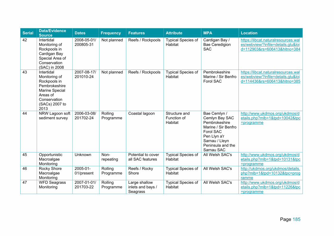
Page 185
Serial Data/Evidence Source
Dates Frequency Features Attribute MPA Location
42 Intertidal Monitoring of Rockpools in Cardigan Bay Special Area of Conservation (SAC) in 2008
2008-05-01/ 200805-31
Not planned Reefs / Rockpools Typical Species of Habitat
Cardigan Bay / Bae Ceredigion SAC
https://libcat.naturalresources.wales/webview/?infile=details.glu&loid=112903&rs=606413&hitno=384
43 Intertidal Monitoring of Rockpools in Pembrokeshire Marine Special Areas of Conservation (SACs) 2007 to 2013
2007-08-17/ 201010-24
Not planned Reefs / Rockpools Typical Species of Habitat
Pembrokeshire Marine / Sir Benfro Forol SAC
https://libcat.naturalresources.wales/webview/?infile=details.glu&loid=114436&rs=606413&hitno=385
44 NRW Lagoon soft sediment survey
2006-03-08/ 201702-24
Rolling Programme
Coastal lagoon Structure and Function of Habitat
Bae Cemlyn / Cemlyn Bay SAC Pembrokeshire Marine / Sir Benfro Forol SAC Pen Llyn a'r Sarnau / Lleyn Peninsula and the Sarnau SAC
http://www.ukdmos.org/ukdmos/details.php?mlb=1&tpd=10042&tpc=programme
45 Opportunistic Macroalgae Monitoring
Unknown Non-repeating
Potential to cover all SAC features
Typical Species of Habitat
All Welsh SAC's http://www.ukdmos.org/ukdmos/details.php?mlb=1&tpd=10131&tpc=programme
46 Rocky Shore Macroalgae Monitoring
2005-01-01/present
Rolling Programme
Reefs / Rocky Shore
Typical Species of Habitat
All Welsh SAC's http://ukdmos.org/ukdmos/details.php?mlb=1&tpd=10132&tpc=programme
47 WFD Seagrass Monitoring
2007-01-01/ 201703-22
Rolling Programme
Large shallow inlets and bays / Seagrass
Typical Species of Habitat
All Welsh SAC's http://www.ukdmos.org/ukdmos/details.php?mlb=1&tpd=11226&tpc=programme

Page 186 www.naturalresourceswales.gov.uk
Data Archive Appendix No data outputs were produced as part of this project.

Published by: Natural Resources Wales Cambria House29 Newport RoadCardiffCF24 0TP
0300 065 3000 (Mon-Fri, 8am - 6pm)
enquiries@naturalresourceswales.gov.ukwww.naturalresourceswales.gov.uk
All rights reserved. This document may be reproduced with prior permission of Natural Resources Wales
Further copies of this report are available from:
Email: [email protected]
© Natural Resources Wales