Coastal Perturbations of Marine-Layer Winds, Wind Stress, and Wind Stress Curl along California and...

1152 VOLUME 34J O U R N A L O F P H Y S I C A L O C E A N O G R A P H Y

q 2004 American Meteorological Society

Coastal Perturbations of Marine-Layer Winds, Wind Stress, and Wind Stress Curlalong California and Baja California in June 1999

DARKO KORACIN

Desert Research Institute, Reno, Nevada

CLIVE E. DORMAN

Scripps Institution of Oceanography, La Jolla, and San Diego State University, San Diego, California

EDWARD P. DEVER

Scripps Institution of Oceanography, La Jolla, California

(Manuscript received 29 April 2003, in final form 9 October 2003)

ABSTRACT

Month-long simulations using the fifth-generation Pennsylvania State University–National Center for Atmo-spheric Research Mesoscale Model (MM5) with a horizontal resolution of 9 km have been used to investigateperturbations of topographically forced wind stress and wind stress curl during upwelling-favorable winds alongthe California and Baja California coasts during June 1999. The dominant spatial inhomogeneity of the windstress and wind stress curl is near the coast. Wind and wind stress maxima are found in the lees of major capesnear the coastline. Positive wind stress curl occurs in a narrow band near the coast, while the region fartheroffshore is characterized by a broad band of weak negative curl. Curvature of the coastline, such as along theSouthern California Bight, forces the northerly flow toward the east and generates positive wind stress curl evenif the magnitude of the stress is constant. The largest wind stress curl is simulated in the lees of Point Conceptionand the Santa Barbara Channel. The Baja California wind stress is upwelling favorable. Although the windsand wind stress exhibit great spatial variability in response to synoptic forcing, the wind stress curl has relativelysmall variation. The narrow band of positive wind stress curl along the coast adds about 5% to the coastalupwelling generated by adjustment to the coastal boundary condition. The larger area of positive wind stresscurl in the lee of Point Conception may be of first-order importance to circulation in the Santa Barbara Channeland the Southern California Bight.

1. Introduction

The importance of winds, wind stress, and wind stresscurl in driving ocean dynamics is well known; however,the accuracy of estimates of spatial and temporal char-acteristics is significantly limited by a lack of obser-vations over the ocean. In the late 1970s the problemof accurate estimates of wind stress in coastal regionswas recognized and elaborated on by Nelson (1977).Significant advances in understanding the structure ofwind stress and wind stress curl came from direct mea-surements of near-surface winds and wind stress usinginstrumented aircraft (Caldwell et al. 1986; Beardsleyet al. 1987; Enriques and Friehe 1995, 1997; Rogers etal. 1998; Dorman et al. 1999). By the late 1990s, satellitemicrowave instruments generated surface wind esti-mates with a horizontal resolution of about 0.258, but

Corresponding author address: Dr. Darko Koracin, Desert Re-search Institute, 2215 Raggio Pkwy., Reno, NV 89512.E-mail: [email protected]

measurement errors require heavy filtering to obtain re-liable estimates of wind stress and wind stress curl. Thisfiltering does not generally affect estimates on largescales, but it effectively eliminates the possibility ofinvestigating the relationship between wind stress andwind stress curl and the ocean response on smaller spa-tial scales. Initially, the two pixels nearest to the coast(a distance of approximately 50 km) are contaminated,preventing coverage of perhaps the most important zoneto wind-driven upwelling. Because of the absence ofmeasurements over the ocean and simplistic estimatesof wind stress, detailed maps of coastal wind stress andwind stress curl, arguably the most important forcingfactors to the coastal ocean, are still not available (ex-cluding a few limited aircraft measurements). Advancesin satellite retrieval techniques, atmospheric modeling,and computational technology, however, allow for newmethods of investigating wind stress and its evolutionand spatial distribution over the ocean.

We focus on wind stress and wind stress curl for the

MAY 2004 1153K O R A C I N E T A L .

FIG. 1. Map of the MM5 domain and topography with buoy locations and key geographicalpoints. The N–S coastline orientation changes to SE at Cape Mendocino, initiating a California-scale expansion fan with high wind speed and wind stress. The coastline change to E at PointConception is responsible for the largest positive wind stress curl in the area.

major wind-driven coastal upwelling zone off the coastof California and northern Baja California. The meansummer sea level pressure field is set up by the NorthPacific anticyclone off the U.S. West Coast and a ther-mal low over the southwestern United States. This pres-sure gradient drives winds to the south along the coastfrom southern Oregon to central Baja California, as con-firmed by ship measurements (Nelson 1977), nearshorebuoys and coastal stations (Halliwell and Allen 1987;Dorman and Winant 1995; Dorman et al. 2000), andregional/mesoscale numerical modeling (Dorman et al.2000; Koracin and Dorman 2001).

A unique element of the California atmospheric ma-rine layer during summer is that it has hydraulic prop-erties with expansion fans in the lees (faster flow andshallower marine layer) and compression bulges on theupwind sides of the capes (slower flow and deeper ma-

rine layer), as reviewed in Koracin and Dorman (2001).In addition to cape-scale expansion fans, there is a Cal-ifornia-scale expansion fan due to the eastward bend ofthe California coast (Edwards 2000).

In order to investigate the spatial and temporal struc-ture of wind stress and wind stress curl along the Cal-ifornia and northern Baja California coast, we conducteda numerical experiment using the fifth-generation Penn-sylvania State University–National Center for Atmo-spheric Research (NCAR) Mesoscale Model (MM5;Grell et al. 1995). Simulations with 9-km horizontalresolution were performed for all of June 1999 for theregion indicated in Fig. 1. We evaluated the model usingbuoy and satellite data, and the simulated wind fieldswere used to compute the hourly wind stress by twocommon algorithms. The simulated wind stress field wasused to compute wind stress curl along the California


and Baja California coasts. Our main objective was toinvestigate spatial and temporal variability of the winds,wind stress, and wind stress curl in response to coastaltopographic forcing of the marine airflow. We discussthe mechanisms for generating wind stress and windstress curl and their effects on coastal upwelling.

2. Model setup

MM5 is a community model that has been developedjointly by NCAR and The Pennsylvania State University(Dudhia 1993; Grell et al. 1995) and has been usedworldwide in a variety of research and application stud-ies. Specifically, MM5 has been employed in studies ofatmospheric dynamics along the California coast (Ko-racin and Dorman 2001) and as a driver for an oceanmodel (Powers and Stoelinga 2000; Beg Paklar et al.2001). For the purpose of this study, MM5 was run ina nonhydrostatic mode with 9-km horizontal resolutionand an integration step of 27 s for all of June 1999. Themonth of June was selected because significant up-welling along the U.S. West Coast occurs during thelate spring and early summer months. The model do-main consisted of 149 3 191 grid points in the hori-zontal and 35 sigma levels in the vertical direction. Themodel domain was represented as a Lambert conformalmap projection and was centered at 35.158N, 120.658W.Topography was read from the 300-resolution global ter-rain and land use files. First-guess synoptic fields forevery 12 h were obtained from the National Centers forEnvironmental Prediction (NCEP) Global Data Assim-ilation System archive. Synoptic information includesvirtual temperature, geopotential height, U and V windcomponents, and relative humidity on a global grid witha horizontal resolution of 2.58 in both latitudinal andlongitudinal extensions. This synoptic information washorizontally interpolated onto the model grid by a two-dimensional, 16-point overlapping parabolic fit. Assim-ilation of all available upper-air and surface station datainto the synoptic fields was performed by objective anal-ysis using a model grid extended horizontally by 180km on all sides. Twelve-hour lateral boundary condi-tions (from NCEP reanalysis fields) were used to runMM5 for the entire period. Model options include mixedphase microphysics, parameterization of shortwave andlongwave radiation including cloud–radiation effects,and the Grell cumulus parameterization (Grell et al.1995). Surface heat and moisture fluxes were computed,and the surface temperature was predicted using a sur-face energy balance algorithm and a five-layer soil mod-el. The Gayno–Seaman turbulence parameterization(Shafran et al. 2000) was chosen, which provides theturbulence kinetic energy as a prognostic variable basedon level-2.5 turbulence closure (Mellor and Yamada1974). Figure 1 shows the model grid setup with to-pography and geographical locations that will be ref-erenced in the text.

3. Model evaluation

MM5 has been evaluated for many applications (seeinformation online at http://www.mmm.ucar.edu/mm5)and appears to be a reliable modeling tool in atmo-spheric studies. It is still important, however, to evaluatethe model results in predicting complex coastal dynam-ics. Koracin and Dorman (2001) used MM5 to simulatewind and wind divergence fields along the Californiacoast for all of June 1996 and evaluated the modeledwinds using data from the National Data Buoy Center(NDBC) and coastal wind profilers with more than18 000 comparison points. Koracin and Dorman (2001)also used satellite visual cloud image and infrared datato indirectly evaluate the wind divergence field near thecoast and offshore. Their study shows that MM5 is asufficiently accurate tool to predict the main character-istics of the marine-layer dynamics along the U.S. WestCoast.

In this paper, we examine the accuracy of MM5 inpredicting the marine atmospheric boundary layer dy-namics for all of June 1999 using NDBC buoys as areference. The accuracy of buoy-measured winds hasbeen established for northern California NDBC buoysduring summer (Friehe et al. 1984) and winter (Beards-ley et al. 1997) by aircraft flying at about 30-m altitudeover the buoy. Adjustment to a common height wasaccomplished with the Large and Pond (1981) bulk pa-rameterization. Agreement was good, with an aircraftminus buoy wind speed average difference and standarddeviation of 0.6 6 0.8 m s21. It should be noted thatthe scatter has been linked to unresolved variables char-acterizing the ocean wave field, difference between thewind and wave field vectors, and other factors (reviewedin Jones and Toba 2001).

We selected seven buoys representing the northern,central, and southern areas of the California coast andcompared data from these sources with model results atcorresponding points. Buoy locations are shown in Fig.1. The main statistics of the comparison are shown inTable 1. The model was able to correctly reproduce themagnitude of the observed wind speed, and modeledresults compared to measurements achieved high cor-relation coefficients ranging from 0.61 to 0.82. In par-ticular, there were four buoys for which the model yield-ed correlation coefficients greater than 0.8. The weakestcorrelation of modeled versus observed wind speed wasfor buoys 46025 and 46030. One possible reason is thatsimulations of low wind speeds include model uncer-tainty due to weak forcing of the dynamics (buoy46025). Generally, model results can smooth extremesas compared to local point measurements (decreasinghigh and increasing low values). This is mainly due tothe influence of neighboring points on a numerical so-lution for a given point in the presence of significantspatial gradients. Buoy 46030 is located in a complexposition near Cape Mendocino, and the present model

MAY 2004 1155K O R A C I N E T A L .

TABLE 1. Basic statistics of the MM5 evaluation for wind speed (m s21) using the buoy data for all of June 1999; N: number of observations,ME: mean error-bias, MAE: mean absolute error, rmse: population root-mean-square error, and rmsve: root-mean-square vector error.

Buoy

Location

(8N) (8W) NMean MM5

(m s21)Mean obs

(m s21)

Std devMM5

(m s21)

Std devobs

(m s21)Correla-tion coef

ME(m s21)

MAE(m s21)

Rmse(m s21)

Rmsve(m s21)

460134601446025460284603046047

38.2039.2033.7035.7440.4232.43

123.30124.00119.10121.89124.53119.53

671671671671672671

8.877.964.107.387.306.41

9.107.963.258.916.937.85

2.552.922.292.262.392.31

3.913.672.013.931.872.57

0.820.710.670.810.630.82

0.230.000.85

21.530.371.44

1.821.941.532.531.591.76

2.342.551.972.921.932.06

2.973.261.973.398.672.26

resolution is not sufficient to resolve details of coastaltopographic effects at that location.

As an illustration of the model evaluation, compari-sons between simulations and measurements at a highwind regime location (buoy 46013) and a low windregime location (buoy 46025) are shown in Fig. 2. Atime series of wind speed and wind direction shows thatMM5 was able to correctly reproduce wind speed pat-terns with three periods of increased winds, three short-term wind minima, and persistent wind directionthroughout the entire month (buoy 46013; Fig. 2a).Some of the differences between the model simulationsand measurements can be attributed to differences insampling—buoy data is an 8-min average at every hour,while model results represent grid- and time-averagedvalues. The model correctly reproduced the range oflow wind speeds as well as significant wind speed anddirection variations at buoy 46025 (Fig. 2b). Table 1also shows that the bias between modeled and observedwind speed is significantly smaller than the standarddeviations of both the modeled and observed time seriesof wind speed.

An additional method of evaluating model results isto perform spectral analysis of a wind speed time series.Power spectra for model simulations and measurementresults at the location of buoy 46013 are shown in Fig.3. In both cases, the model simulations showed similarspectral behavior to measurements but overestimated theinfluence of diurnal oscillations as compared with os-cillations for shorter periods. Model simulations andmeasurements both showed significant diurnal peaks atboth locations, increased spectra in the inertial oscil-lation range, and semidiurnal peaks.

Since the number of operational meteorological buoysis few, they provide limited information on the spatialstructure of winds over the ocean. In recent years, sat-ellite-based, microwave observations are emerging asan excellent source of information on surface winds overthe open ocean. The satellite-borne Special Sensor Mi-crowave Imager (SSM/I) was the most advanced systemavailable in June 1999; it provided wind speed but notdirection. Wentz (1997) used NDBC and other meteo-rological buoys to find that for wind speeds, the sys-tematic error for SSM/I is 0.3 m s21 and the rms erroris 0.9 m s21. In the coastal ocean, SSM/I satellite windsare contaminated and unusable if closer than two pixels

to land, which includes most of the NDBC buoys alongcoastal California and Oregon. Away from land, thereremains active discussion about satellite-based accuracybecause of the lack of an appropriate measurement sys-tem. The only long-term ground truth measurements areprovided by buoys, single point measurements that arenot related in a simple way to satellite measurementsover an area with a 25-km footprint (Larsen et al. 2001).Special care should be exercised when comparing buoysalong the western coast of the United States with sat-ellite data since most of the buoys are located 15–25km from the coast. Taking the nearest offshore pixel isunrepresentative of an inshore buoy (we will show laterthat this is the most intense field of wind, wind stress,and wind stress curl). The reactivated NDBC buoy46047, however, is sufficiently far offshore to be com-pared with uncontaminated satellite wind measure-ments. This allows intercomparison of buoy, satellite,and model simulations for June 1999. During this time,there were twice-a-day passes near 0800 and 2000 LST,but track gaps reduced these to 37 satellite measure-ments for the month. The wind speed mean and standarddeviation for the buoy 46047 data, MM5 results, andthe satellite measurements are shown in Table 2. Cor-relation coefficients among buoy data, model grid-av-eraged results, and satellite area-averaged data are veryhigh and are similar, ranging from 0.73 to 0.82. BothMM5 and the satellite underestimate buoy measure-ments; however, the bias for model versus buoy andsatellite versus buoy data is small in comparison withany of the standard deviations (buoy, model, and sat-ellite). A time series (Fig. 4) of all three results confirmsthat they track each other fairly well except for an oc-casional deviation. Both the satellite and MM5 resultsreproduced the major strong-wind events during 3–4,7–16, 19–22, and 25–27 June as well as minima around5, 18, 23–24, and 28–29 June.

In order to evaluate simulated winds over the ocean,we compared SSM/I satellite-derived and simulated sur-face wind speed averaged for all of June 1999 (Fig. 5).The simulated wind speed field agrees reasonably wellwith satellite-derived winds, although there are signif-icant differences in sampling and averaging procedures,spatial resolution (0.258 for satellite and 9 km for themodel), and height representativeness, and there are lim-itations of satellite detection near the coast. Both the


FIG. 2. Time series of hourly surface wind speed and direction as measured (dots) and simulated (plussigns) at (a) buoy 46013 and (b) buoy 46025 for all of Jun 1999.

MAY 2004 1157K O R A C I N E T A L .

FIG. 3. Normalized power spectra computed from buoy 46013 data(dashed line) and MM5 results (solid line) for all of Jun 1999. Modeland buoy show similar diurnal oscillations. Arrows point to diurnalpeaks.

TABLE 2. Comparisons among MM5 simulation, satellite SSM/I,and NDBC buoy 46047 wind for the 33 time intervals common toall three during Jun 1999.

Mean(m s21)

Median(m s21)

Std dev(m s21)

Correlation coef

With buoyWith

satellite

ModelSatelliteBuoy

6.506.797.76

6.746.608.40

2.482.582.71

0.730.82

0.76

0.82

FIG. 4. Time series of wind speed for buoy 46047 data (solid line),MM5 results (dotted line), and SSM/I satellite data (dashed line withstars) for all of Jun 1999.

SSM/I measurements and simulations clearly agree ona broad high-speed wind zone along northern and centralCalifornia with maxima centered in the lee of PointArena. The satellite-derived field also confirms that ma-jor capes (e.g., Cape Mendocino, Point Arena) inducepersistent flow disturbances in terms of significant windspeed maxima in their lees. The modeled large area oflow wind speed on the eastern side of the CaliforniaBight and farther southward also can be seen in thesatellite data.

4. Marine-layer winds

Figure 6 shows surface wind vectors simulated withMM5 and averaged for all of June 1999. The modelresults show adjustment of northerly offshore flows intodominantly northwesterly flows near the coast with windspeed generally increasing toward the coast. The av-erage flow structure for June 1999 appears to be similarto the average flow for June 1996 (Koracin and Dorman2001). A noticeable sequence of expansion fans anddeceleration areas is present with the simulated monthlymean average wind speed up to 8.8 m s21 in the leesof major capes. In most of the lees, the wind maximumis confined in a laterally narrow offshore band with awidth of about 100 km or less. Near Point Conception,the area of maximum wind is elongated about 200 kmin the offshore direction due to the sharp turn of thecoastline and the effects of islands on the flow. Con-sidering a broader view, Figs. 5 and 6 suggest that thenorthern and central California coasts represent a re-gional (California)-scale lee, an interpretation supportedby a numerical model study (Edwards 2000) and anobservational study (Edwards et al. 2001). Here, theCalifornia-scale expansion fan is marked by the en-hanced wind speed area bordered by the 6.5 m s21 wind

speed isotach (Fig. 6). This appears to be a significant,persistent feature found in ship observations (Nelson1977), buoy and coastal stations (Dorman and Winant1995; Dorman et al. 2000), and MM5 simulations forall of June 1996 (Koracin and Dorman 2001). The south-eastern portion of the Southern California Bight is aweak wind zone with a substantial cross-shore, non-upwelling-favorable wind direction. The upwelling-con-sistent, shore-parallel flow along southern California isreestablished near 338N and continues along northernBaja California. Wind speed variability during June1999 is represented by its standard deviation (Fig. 7).Most of the flow variability appears to be in the narrowzone near the coast. The 2 m s21 isoline roughly marksthe area of the California regional-scale lee, while the2.5 m s21 and greater isolines indicate coastal mesoscaleflow forcing by topographic features. One of the twoareas with the greatest standard deviation is in the leeof Cape Mendocino, which may be due to this area beingon a fluctuating edge of the northern end of the Cali-fornia-scale high wind speed region (Dorman et al.2000; Haack et al. 2001). The lee of Point Arena doesnot have a peak variation as it is more solidly in thecenter of the persistent high speed winds. The otherextreme variability area is in the immediate lee of PointConception with its right angle coastal bend, the island


FIG. 5. Surface wind speed (m s21) averaged for all of Jun 1999 as (left) derived from SSM/I satellite data and (right)simulated with MM5.

lees, and weak winds in the eastern portion of the South-ern California Bight. Secondary maxima are in the Mon-terey and Point Sur regions. The figure also shows thatthe islands in the Southern California Bight and off theBaja California coast significantly modify the flow cre-ating narrow lees many times longer than the islandsthemselves.

5. Wind stress

The temporal and spatial structure of wind stress iscrucial to understanding the forcing of the ocean currentand coastal upwelling. We investigate the stress by com-paring two algorithms for estimating bulk wind stressover the ocean, namely, those according to Large andPond (1981) and Deacon and Webb (1962). These twoalgorithms, hereinafter denoted as LP and DW, are usedto examine whether different formulations will inducesignificant differences in the pattern of the wind stressand wind stress curl. A number of algorithms for windstress computation, starting with the early work by Ross-by and Montgomery (1935), are discussed by Toba etal. (2001). According to Toba et al. (2001), the Largeand Pond (1981) algorithm is based on one of the largestmeasurement datasets. Beardsley et al. (1997) showedthat some more recent algorithms, such as the TropicalOcean and Global Atmosphere Coupled Ocean–Atmo-sphere Research Experiment (TOGA COARE; Fairall

et al. 1996), produce essentially the same results as theLarge and Pond algorithm. The Large and Pond algo-rithm has been commonly used in atmospheric and oce-anic studies (e.g., Dorman and Winant 1995; Wentz1997; Dorman et al. 2000; Samelson 2002). The Deaconand Webb algorithm was chosen in our study as one ofthe possible upper limits of estimated stress because ithas one of the greatest intercept parameters (1.0) and asignificant coefficient (0.07) in the relationship betweendrag coefficient and wind velocity [see below and alsoToba et al. (2001)]. In the first step of our analysis, weused simple expressions empirically determined fornear-neutral stability conditions. The assumption ofnear-neutral conditions in June for the simulated area issupported by ship observations, which show that themajority of the bulk Richardson stability index offsetfrom the neutral induces a change in wind stress in therange of 24% to 11% (Nelson 1977). According to theLP algorithm, bulk stress tLP is calculated as follows:

2 2t 5 Ï(t ) 1 (t ) , t 5 rC VU,LP x,LP y,LP x,LP d,LP

2 2t 5 rC VV, V 5 ÏU 1 V , andy,LP d,LP

23 211.2 3 10 for 4 # V , 11 m s23C 5 (0.49 1 0.065V) 3 10 (1)d,LP

21for 11 # V # 25 m s ,

where U and V are wind components in the X and Y

MAY 2004 1159K O R A C I N E T A L .

FIG. 6. Simulated wind vectors and contours of surface wind speed(m s21) averaged for all of Jun 1999. Contour interval is 0.5 m s21.Expansion fans form high-speed areas on the California scale (en-closed by 6.5 m s21) and in the lees of every major cape.

FIG. 7. Standard deviation of the simulated surface wind speed (ms21) as determined from MM5 simulations for all of Jun 1999. Con-tour interval is 0.25 m s21. Maxima are in the lees of major capes.The 2.25 m s21 isoline is coincident with the California-scale ex-pansion fan.

directions, respectively; r is the air density; Cd is thedrag coefficient for neutral conditions; is the resultantVwind speed; and the subscript LP refers to the Largeand Pond algorithm.

According to the DW algorithm, bulk stress tDW iscalculated as follows:

2 2t 5 Ï(t ) 1 (t ) , t 5 rc VU,DW x,DW y,DW x,DW d,DW

2 2t 5 rc VV, V 5 ÏU 1 V , andy,DW d,DW

23C 5 (1 1 0.07V) 3 10 , (2)d,DW

where the notation is the same as above except that thesubscript DW refers to the Deacon and Webb algorithm.Both algorithms are developed for wind speed at 10 mand near-neutral atmospheric stability conditions in thesurface atmospheric boundary layer.

Figure 8 shows simulated wind stress averaged forall of June 1999 using algorithms by LP and DW. Thegeneral patterns of the simulated wind stress are similarfor both schemes. The greatest stress is coincident withthe strongest winds, which are offshore of Cape Men-docino and Point Arena with secondary maxima south-west of Point Conception, off Point Sur, and off thenorthern Baja California coast. A large area of low windstress extends from the eastern side of the SouthernCalifornia Bight southward through San Diego coastalwaters. Significantly low values are simulated in the lees

of islands in the Southern California Bight and off thesouthern California coast. The area of the Californiaregional-scale lee that was seen in the simulated windsis also seen in the wind stress and is bordered by the0.07–0.08-Pa wind stress isoline (LP algorithm). Whenusing these algorithms, we found that wind stress isgreater when using the DW scheme compared to usingthe LP algorithm; however, the main features are sim-ilarly captured by both schemes. Maximum wind stressfrom all hourly simulations in June 1999 up to 0.37 Pa(LP) and 0.52 Pa (DW) is confined to the nearshorezone of about 50 km where maximum winds are pre-dicted. Similar to the locations of the highest monthlyaveraged values, the main maxima are in the lees ofCape Mendocino, Point Arena, Point Sur, and near PointConception. A plot of the standard deviation of windstress (not shown) confirms that the greatest monthlystress variability is in the California regional-scale lee.The strength of this expansion fan is significantly de-pendent on the alignment of the synoptic flow with re-spect to the coastline and coastal topography.

We compared wind stress estimates for the LP andDW algorithms using buoy data and model results atcorresponding buoy locations. Since the simulatedwinds showed high correlation with measurements butgenerally underpredicted some of the high wind mea-


FIG. 8. Averaged wind stress (Pa) for all of Jun 1999 calculated using the (left) Large and Pond and (right) Deacon andWebb algorithms. Largest stress is found near the coast, and extreme values are found in expansion fans in the lees of capes.The patterns and extreme-value center locations are independent of the wind stress algorithm.

FIG. 9. Time series of wind stress (Pa) as estimated from MM5 (solid line) and buoys (dotted line) at two buoy locations, (left) 46013and (right) 46025, using the Large and Pond algorithm. Buoy locations are shown in Fig. 1.

surements (Table 1), the wind stress calculated from themodel results in these cases also underpredicted thebuoy-estimated wind stress. Although the simulatedwind stress underestimates most of the higher peaks ofthe stress computed from buoy data, it is of the sameorder of magnitude, closely follows the time evolutionof the observed stress, and correlates well with the stressestimated from the buoy data (Fig. 9). It should be men-tioned that the model, because of its spatial and temporal

averaging, cannot reproduce the sharp wind peaks mea-sured by the buoy as an 8-min average every hour. Buoy46030 is located at the edge of the upwind side of CapeMendocino, and consequently both measurements andmodel results show relatively small to medium windstress in comparison with that calculated for other lo-cations. Moving downcost, buoys 46014 and 46013(Fig. 9) are located in the lees of Cape Mendocino andPoint Arena and show intense wind stress throughout

MAY 2004 1161K O R A C I N E T A L .

the entire month. Buoy 46028 is located in the narrowexpansion fan in the lee of Point Sur and also exhibitssignificant wind stress. According to the measurements,the largest wind stress is estimated at the buoy 46054location in the immediate lee of Point Conception. Theeastern side of the Southern California Bight wherebuoy 46025 is located is characterized by significantwind minima (Figs. 5 and 6) and wind stress minima(Fig. 9). Consequently, the estimated stress from bothmeasurements and model results in this area is signif-icantly small. Buoy 46047 is located at the downwindedge of the Point Conception expansion fan, and theestimated wind stress is significantly greater than atbuoy 46025 but still correspondingly smaller comparedto the maximum wind stress at buoy 46054. Since mod-eled wind stress bias is relatively similar for all buoysand wind direction is captured well by the model (Fig.2), modeled wind stress can be used to estimate windstress curl, which cannot be estimated from the sparseand inadequate buoy network.

As a comparison, the ship-based, long-term mean forthe June maximum value off northern California (Nel-son 1977) is similar to the MM5 June 1999 simulation(about 0.1–0.15 Pa). Ship-based stress is much smootherand broader, however, with areas greater than 0.1 Paextending farther offshore (400 km) and along the coast(328–418N). The MM5 stress value greater than 0.1 Paextends from 378 to 418N with the peak value at thecoast. It is possible that the inshore minimum of theship-based stress along northern and central Californiais due to the avoidance of high wind speed areas thatwere confirmed by aircraft and buoy measurements citedearlier. It should be mentioned that ship-based stresswas computed from available ship observations insquares of 18 on the side.

6. Wind stress curl

The temporal and spatial structures of wind stress curlmay play a significant role in oceanic upwelling. Fur-thermore, the role of wind stress curl in coastal up-welling is poorly understood because of a lack of suit-able measurements and computational difficulties. Tobetter understand this role, we used the wind stress re-sults discussed in the previous section to compute thewind stress curl.

Wind stress curl (C) was calculated as

Dt Dty xC 5 2 , (3)Dx Dy

where Dx and Dy are the model grid resolutions in theX and Y directions. Because of the horizontal resolutionof 9 km, we are neglecting the earth’s curvature effectsin the computation of wind stress curl. The average windstress curl calculated using the LP and DW algorithmsfor all of June 1999 is shown in Fig. 10a. According tothe simulations, a significantly large positive wind stresscurl is confined to a narrow band at the coastline while

the remainder of the area is dominated by weakly neg-ative wind stress curl.

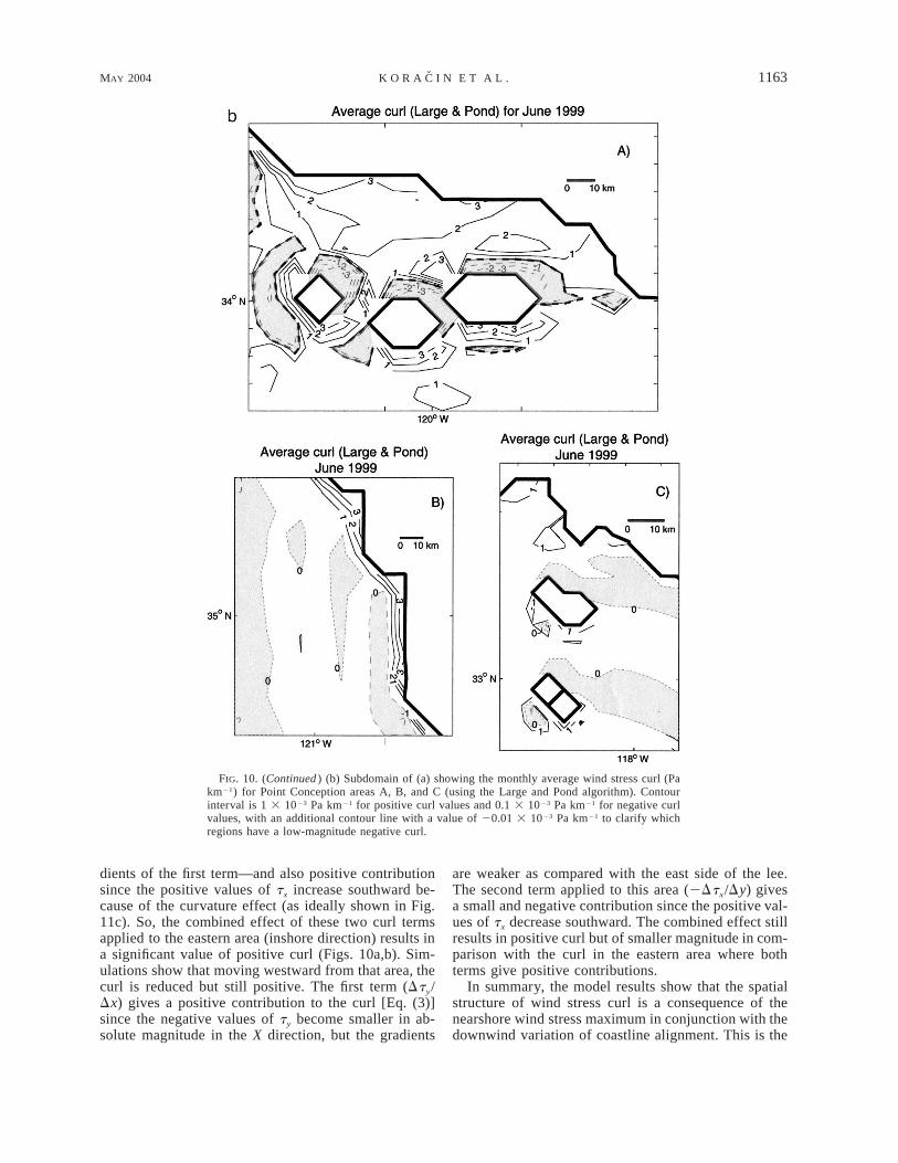
As the greatest values and gradients of wind stresscurl are near the coastline, the subdomain areas of Fig.10a are shown in Figs. 10b and 10c for easier viewing.The Point Conception and vicinity areas are shown inFig. 10b. Large positive values of wind stress curl arein the Santa Barbara Channel and island lees, whilenegative values are found on the north sides of the is-lands (panel A). On the upwind side of Point Concep-tion, strong positive curl is confined to a narrow coastalband, while the rest of the offshore area is characterizedby weak near-zero and negative wind stress curl (panelB). Islands in the eastern part of the Southern CaliforniaBight induce long downwind banners of weak positivewind stress curl (panel C). Although the dimensions ofthe islands are small as compared with the model res-olution, they appear to be sufficiently resolved (see Fig.10b) and induce significant modification of the windstructure and consequent wind stress and wind stresscurl. In a subsequent study, we will focus on the PointConception area using higher horizontal model reso-lution. Details of wind stress curl in the Cape Mendo-cino area are shown in Fig. 10c.

In order to understand the spatial structure of the windstress curl, we considered the basic aspects of the windstress structure near the coast. Figure 11a shows ide-alized conditions of the lateral shear of the wind speedthat can be expected near coast in the case of weakforcing of the flow by coastal topography when thecoastline is parallel to the flow. In this conventionalview, wind speed decreases with the decrease in lateraldistance toward the coast. Assuming that wind stress iscollinear with wind, this would create a positive windstress curl in that region. In contrast to this conventionalpicture, present simulations show quite a different flowstructure (depicted in Fig. 11b). Wind stress in the ex-pansion fans increases laterally in the direction towardthe coastline. Only at the closest distance does the windstress drop off. This creates a very narrow band of pos-itive wind stress curl in the vicinity of the coastline anda much broader region of negative wind stress curl onthe western side of expansion fans. The effect of thenearshore wind maximum (Fig. 11b) resembles the caseof wind, wind stress, and curl of wind stress in the leeof Cape Mendocino (see Figs. 5, 8, and 10a,c).

Gradients of the components of wind stress can beused to understand the resultant structure of the windstress curl (Fig. 12). Let us consider the areas east andwest of the maximum stress location near the coast inthe lee of Cape Mendocino. In the eastern area (inshoredirection), the first term (Dty/Dx) gives a positive con-tribution to the curl [Eq. (3)] since the negative valuesof ty are become smaller in absolute magnitude in theX direction. The second term applied to this area (2Dtx/Dy) gives a smaller contribution—weaker gradients ascompared with the gradients of the first term—but is,as a whole, a negative contribution since the positive


FIG. 10. (a) Average wind stress curl (Pa km21) for all of Jun 1999 calculated from hourly wind stress curl values estimatedwith the (left) Large and Pond and (right) Deacon and Webb algorithms. The offshore region is dominated by a weak, positivewind stress curl that is independent of the algorithm. Positive wind stress curl is restricted to the NW portion of the SouthernCalifornia Bight and close to the coast and islands. Details of the wind stress curl in areas A, B, C, and D are shown in (b)and (c).

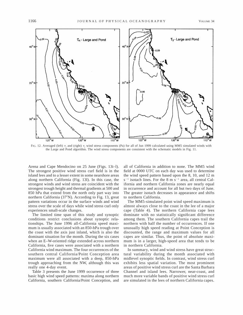
values of tx are decreasing southward. So, the combinedeffect of these two curl terms applied to the eastern area(inshore direction) results in a narrow band of positivecurl (Figs. 10a,c). In the western area (offshore direc-tion), the first term (Dty/Dx) gives a negative contri-bution to the curl [Eq. (3)] since the negative values ofty become greater in absolute magnitude in the X di-rection. The second term applied to this area (2Dtx/Dy) gives small negative or near-zero values since thepositive values of tx are decreasing southward. So, thecombined effect of these two curl terms applied to thewestern area (offshore direction) is a broad band ofnegative curl (Figs. 10a,c). The same reasoning can beapplied to the Point Arena lee where the positive curlis simulated in a narrow band near the coastline whilenegative and near-zero curl prevail in the offshore di-rection. A major turn in the flow occurred downwindof Point Arena where the coastline turns roughly from3608 to 3208 alignment. As anticipated by the idealizedreasoning (Fig. 11c), the tx component increases down-wind. As discussed above, this increase induces negativevalues of the second term in the curl equation and re-duces the dominant positive value of the first term inthe near-shore zone. Farther downwind, the curvatureeffect weakens and the gradient of tx downwind (secondterm) becomes negligible. The first term dominates and

consequently the curl becomes positive in the offshoredirection in a relatively broad band of the San FranciscoBay and Monterey Bay areas.

The two idealized conditions shown in Figs. 11a and11b considered only variations of the y component ofstress in the X direction [see Eq. (3)]. When the coastlinebends to the east (Point Arena and Point Conception),there is an additional effect on wind stress curl due tochange (downwind increase) in the x component of thestress in the Y direction (Fig. 11c). This results in asignificant increase in positive wind stress curl centeredto the east of the initial flow band. It should be notedthat this effect is due to curving of the flow even whenthe magnitude of the stress is constant along the flowtrajectory. This is further clarified by analyzing the spa-tial distribution of the surface wind stress components(Fig. 12).

Now, let us consider the reasons for the large positivecurl in the lee of Point Conception and the Santa BarbaraChannel islands. The largest curl on the eastern side ofthe lee (Fig. 10b) can be explained as follows. The firstterm (Dty/Dx) gives a large positive contribution to thecurl [Eq. (3)] since the negative values of ty becomesmaller in absolute magnitude in the X direction. Thesecond term applied to this area (2Dtx/Dy) gives asmaller—weaker gradients as compared with the gra-

MAY 2004 1163K O R A C I N E T A L .

FIG. 10. (Continued ) (b) Subdomain of (a) showing the monthly average wind stress curl (Pakm21) for Point Conception areas A, B, and C (using the Large and Pond algorithm). Contourinterval is 1 3 1023 Pa km21 for positive curl values and 0.1 3 1023 Pa km21 for negative curlvalues, with an additional contour line with a value of 20.01 3 1023 Pa km21 to clarify whichregions have a low-magnitude negative curl.

dients of the first term—and also positive contributionsince the positive values of tx increase southward be-cause of the curvature effect (as ideally shown in Fig.11c). So, the combined effect of these two curl termsapplied to the eastern area (inshore direction) results ina significant value of positive curl (Figs. 10a,b). Sim-ulations show that moving westward from that area, thecurl is reduced but still positive. The first term (Dty/Dx) gives a positive contribution to the curl [Eq. (3)]since the negative values of ty become smaller in ab-solute magnitude in the X direction, but the gradients

are weaker as compared with the east side of the lee.The second term applied to this area (2Dtx/Dy) givesa small and negative contribution since the positive val-ues of tx decrease southward. The combined effect stillresults in positive curl but of smaller magnitude in com-parison with the curl in the eastern area where bothterms give positive contributions.

In summary, the model results show that the spatialstructure of wind stress curl is a consequence of thenearshore wind stress maximum in conjunction with thedownwind variation of coastline alignment. This is the


FIG. 10 (Continued ) (c) Subdomain of (a) showing the monthlyaverage wind stress curl (Pa km 21 ) for the Cape Mendocino areaD in (a) (using the Large and Pond algorithm). Contour intervalis 1 3 10 23 Pa km 21 for positive curl values and 0.1 3 10 23 Pakm 21 for negative curl values, with an additional contour line witha value of 20.01 3 10 23 Pa km 21 to clarify which regions havelow-magnitude negative curl.

reason for the band of positive wind stress curl that isnarrow and near the shore along northern California andbroad in the Southern California Bight.

Estimation of possible error in computation of windstress curl

Since there are no available, spatially dense obser-vations over the ocean, it is not possible to determinemodel error at points where there are no measurements.For example, we assume that modeled stress has a bias

with respect to the stress calculated from buoy data. Inthis case, that bias is then added to the modeled stressat the neighboring points around the buoy location andthe stress calculation will be altered; however, the curlwill be the same as before, adding the bias due to thesubtraction of the same bias in the Y and X directions.As an illustration, we consider data for buoy 46013(Table 1). Applying the average simulated V wind com-ponent and average wind speed at the buoy location,one can obtain a baseline ty. Adding model bias to theaverage wind speed and the component of the bias inthe Y direction to the simulated V, one can obtain ty

with bias. In this case, the difference between baselinety and ty with bias is 5%. In the other case, if we add1 m s21 to the wind speed and the appropriate fractionof that value to the V wind component [the possiblebuoy measurement error is up to 61 m s21; Gilhousen(1987)], the difference between this baseline ty and thealtered ty is 25%. So, in this case (and similarly for sixout of eight buoys; Table 1), a possible measurementerror can induce a greater discrepancy in calculatedstress than model bias. Table 1 also shows that all biasesare smaller than the standard deviation of the measure-ments. Error in the computed curl cannot be easily de-termined; however, using certain assumptions, we canroughly estimate it. Since we do not know the spatialdistribution of the bias, we linearly interpolate the biasbetween two neighboring buoys (46013 and 46014). Thechange in the wind speed bias is 0.0172 m s21 per eachgridpoint separation (9 km). Consider the monthly av-eraged wind components at the four model pointsaround the buoy 46013 location that are used to calculatewind stress and wind stress curl. First, we compute thewind stress components and wind stress curl (baselinecurl). Then we keep the same wind components for thesouthern and western points, while we add the changein the wind speed bias per two grid separations to thenorthern and eastern points. Next, we calculate the windstress components and curl (curl with bias). The dif-ference between baseline curl and curl with bias is 22%.To summarize, bias and error in the wind speed cansignificantly influence wind stress; however, the com-puted curl could be altered to a lesser extent. Note alsothat spatial change of the bias, and not the actual value,is important to determining possible curl error.

7. Synoptic variations of wind, wind stress, andwind stress curl

The purpose of this section is to discuss temporal andspatial variation of sea level winds, wind stress, andwind stress curl in response to midlevel synoptic forc-ing. Monthly means shown in the foregoing text areaverages of individual events that have greatly differentwind and wind stress patterns. Edwards (2000) usedbuoy data and satellite-measured winds to show that theCalifornia-scale expansion fan structure and maximumwind speed are related to the synoptic-scale pressure

MAY 2004 1165K O R A C I N E T A L .

FIG. 11. Schematic of the idealized lateral shear of the surface wind stress in the cases of wind stress maximum (a) faroffshore and (b) near shore, and (c) the effect of coastline curvature on the spatial variation of the wind stress and wind stresscomponents. Aircraft, SSM/I satellite, and MM5 simulations corroborate the dominance of the nearshore wind stress maximumfor northern and central California. The coastline curvature case applies to the immediate lee of Point Conception.

gradient. Taking a different approach, Cui et al. (1998)applied a numerical model to an idealized Californiacoast and found that the sea level wind field structureis related to the direction of background airflow. Here,we focus on the wind speed and wind stress maximastructure and position along the coast, which providethe strongest signals and are of high interest. Three casesof wind maxima occurring between Cape Mendocinoand Point Conception, near Point Conception, and alongnorthern California during June 1999 are shown that aretypical of the range of synoptic events.

The first event is a broad, sea level wind speed andwind stress maximum extending from Cape Mendocinoto the south of Point Conception on 7 June (Figs. 13a–d). Weak winds and wind stress cover most of the South-ern California Bight, with even weaker structure in theisland lees. Positive wind stress curl appears along al-most the entire California coast in nearshore, narrowbands with peak values in the lees of capes and islands(Fig. 13d). The broad area of high-speed winds is causedby increased pressure gradients associated with a stron-ger summer 500-hPa trough with a N–S oriented axiscrossing the central California coast as reflected in the500-hPa height (Fig. 14a, bottom row) and temperature

(Fig. 14b, bottom row). At sea level, the isobars overthe northern and central California coast are nearly me-ridional with comparatively dense, uniform spacing.The coldest 850-hPa temperatures occur with this event.

The second event has a sea level wind and wind stressmaximum around Point Conception extending south-ward in a narrow band on 15 June (Figs. 13e–h). Weakwinds are simulated in the eastern part of the SouthernCalifornia Bight, Baja California, and the lee of Gua-dalupe Island as well as around Cape Mendocino. Thestrongest positive wind stress curl field is in the SantaBarbara Channel and island wakes, while in northernCalifornia the nearshore positive curl is weak (Fig. 13h).In this case, there is a WNW–ESE-oriented trough at500 and 850 hPa west of California extending to 338N(Figs. 14a,b). The shortest distance to the coast fromthe trough is at Point Conception, coincident with thesea level wind and wind stress maximum. Thermal gra-dients are weak at 850 and 500 hPa, causing the stron-gest sea level pressure gradients to be near central Cal-ifornia and Point Conception.

The third event is characterized by a high wind speedand wind stress band that is narrower in comparisonwith previous events with maxima in the lees of Point


FIG. 12. Averaged (left) tx and (right) ty wind stress components (Pa) for all of Jun 1999 calculated using MM5 simulated winds withthe Large and Pond algorithm. The wind stress components are consistent with the schematic models in Fig. 11.

Arena and Cape Mendocino on 25 June (Figs. 13i–l).The strongest positive wind stress curl field is in theisland lees and to a lesser extent in some nearshore areasalong northern California (Fig. 13l). In this case, thestrongest winds and wind stress are coincident with thestrongest trough height and thermal gradients at 500 and850 hPa that extend from the north only part way intonorthern California (378N). According to Fig. 13, greatpattern variations occur in the surface winds and windstress over the scale of days while wind stress curl onlyexperiences small-scale changes.

The limited time span of this study and synopticconditions restrict conclusions about synoptic rela-tionships. The June 1996 all-California speed maxi-mum is usually associated with an 850-hPa trough overthe coast with the axis just inland, which is also thedominant situation for the month. During the six caseswhen an E–W-oriented ridge extended across northernCalifornia, five cases were associated with a northernCalifornia wind maximum. The four occurrences of thesouthern central California/Point Conception areamaximum were all associated with a deep, 850-hPatrough approaching from the NW, although this wasreally one 4-day event.

Table 3 presents the June 1999 occurrence of threebasic high wind speed patterns: maxima along northernCalifornia, southern California/Point Conception, and

all of California in addition to none. The MM5 windfield at 0000 UTC on each day was used to determinethe wind speed pattern based upon the 8, 10, and 12 ms21 isotach lines. For the 8 m s21 area, all central Cal-ifornia and northern California zones are nearly equalin occurrence and account for all but two days of June.The greater isotach decreases in appearance and shiftsto northern California.

The MM5-simulated point wind speed maximum isalmost always close to the coast in the lee of a majorcape (Table 4). The northern California cape leesdominate with no statistically significant differenceamong them. The southern California capes trail thenorthern with half the number of occurrences. If oneunusually high speed reading at Point Conception isdiscounted, the range and maximum values for allcapes are similar. Thus, the point of absolute maxi-mum is in a larger, high-speed area that tends to bein northern California.

In summary, wind and wind stress have great struc-tural variability during the month associated withmidlevel synoptic fields. In contrast, wind stress curlexhibits less spatial variation. The most prominentareas of positive wind stress curl are the Santa BarbaraChannel and island lees. Narrower, near-coast, andmuch more variable bands of positive wind stress curlare simulated in the lees of northern California capes.

MAY 2004 1167K O R A C I N E T A L .

FIG. 13. (top) SSM/I satellite-derived surface wind speed (m s21) and simulated (2d row) surfacewind (m s21), (3d row) wind stress (Pa), and (bottom) wind stress curl (Pa km21) for (left) 7, (center)15, and (right) 25 Jun. All valid near 0000 UTC except for the 15 Jun satellite data, which are near1600 UTC.


FIG. 14. (a) Analysis of (top) sea level pressure (hPa) and (middle) 850- and (bottom) 500-hPa geopotententialheight (gpm), valid at the same times and orientation as in Fig. 13. Synoptic analysis is modified from NOAA–Cooperative Institute for Research in Environmental Sciences Climate Diagnostics Center analyses. Large-scale, surfacepattern changes are related to midlevel, synoptic changes.

8. Effects of wind stress variability and windstress curl on ocean dynamics

The model results show three significant features. Thestrongest upwelling-favorable winds are found between

Cape Mendocino and Point Reyes (Figs. 5, 6, and 8).The model also generates two persistent wind stress curlpatterns from expansion fans associated with the capes(Fig. 10). There is a narrow band of positive wind stresscurl confined to within approximately 20 km of the coast

MAY 2004 1169K O R A C I N E T A L .

FIG. 14. (Continued ) (b) (top) SSM/I satellite-derived surface wind speed (m s21), and analyses of air temperature at(middle) 850 and (bottom) 500 hPa (K).

TABLE 3. Characterization of daily wind speed maximum patternalong California for Jun 1999 at 0000 UTC.

MM5contour

NorthernCalifornia

South-centralCalifornia,

Point ConceptionAll

California None

8 m s21

10 m s21

12 m s21

1172

410

1340

21828

(Fig. 10a) and a much larger area of positive wind stresscurl in the lee of Point Conception (Fig. 10b). Whateffects could these patterns have on wind-driven up-welling and is there any evidence for these types ofeffects?

Like in the smaller expansion fans found at many ofthe capes along the California and Oregon coasts, thelarge-scale increase in wind speed between Cape Men-


TABLE 4. MM5 maximum wind location for Jun 1999 at 0000 UTC, which almost always occurs in the lee of a cape and close to thecoast. A single event is counted twice if two maxima are within 0.5 m s21.

Cape Mendocino Point Arena Point Sur Point Conception Other

No. of casesMean (m s21)Range (m s21)

1312.5

9.9–14.2

1311.7

8.6–13.4

712.5

11.1–13.6

613.4

11.3–17.5

1——

docino and Point Reyes (Fig. 6) may result from anexpansion fan associated with the large-scale change inthe coastline orientation (Edwards et al. 2002). Thisalong-coast variation in wind stress strength is likely tocontribute to increased coastal upwelling between CapeMendocino and Point Reyes. Satellite sea surface tem-perature (SST) estimates and surface buoys provide ev-idence of increased upwelling and decreased near-sur-face temperatures. Kelly (1985) examined the spatialand temporal structure of SST images and buoy windmeasurements for the northern California coast betweenApril and July 1981. The SST temporal mean showeda temperature minimum between Cape Mendocino andPoint Reyes. Sea surface temperature variability wasanalyzed using empirical orthogonal functions (EOFs).Of the three SST EOFs discussed, the first was asso-ciated with seasonal warming, while the second corre-sponded to increased temperature variability betweenCape Mendocino and Point Reyes. The second was sig-nificantly correlated with wind stress variability in a wayconsistent with increased winds and coastal upwellingin this area. Buoy temperatures analyzed by Dormanand Winant (1995) also show evidence of increased up-welling between Cape Mendocino and Point Reyes. Av-erage summer buoy temperatures in this region were108–118C as compared with temperatures near 148Csouth of Point Reyes and north of Cape Blanco, Oregon.

In addition to the large-scale increase in wind stressbetween Cape Mendocino and Point Reyes, there is anarrow coastal band (Figs. 10a–c) of positive wind stresscurl all along the coast. This band would tend to rein-force coastal upwelling caused by adjustment of thecross-shelf Ekman transport to the presence of the coast.To compare curl-driven upwelling to coastal upwellingit is instructive to form a crude estimate of the scale ofthe coastal upwelling vertical velocity. For a spatiallyuniform wind stress (and two-dimensional coastline andbathymetry), coastal upwelling is confined to the regionbetween the inner shelf and midshelf. Over the innershelf, there is top-to-bottom momentum transfer im-parted by the wind stress. This reduces the wind-driven,cross-shelf transport from the theoretical Ekman trans-port. Over the midshelf, surface and bottom boundarylayers are distinct, and surface transport approaches theEkman transport. Between the inner shelf and midshelf,the divergence in cross-shelf, wind-driven surface trans-port provides the traditional mechanism for upwelling.The transition between the inner shelf and midshelf isnot at a fixed location or depth but rather depends onstratification and bottom slope. Over the northern Cal-

ifornia shelf, evidence suggests the transition generallyoccurs somewhere between the 30-m isobath, which iswell within the inner shelf (Lentz 1994), and the 90-misobath where the surface and bottom boundary layersare almost always distinct (e.g., Dever 1997). Theseisobaths are generally within 20 km of the coast. Thishorizontal scale and the Ekman transport forced bycoastal wind stress provide an estimate of upwellingcaused by an adjustment of cross-shelf transport to thecoastal boundary.

For two-dimensional volume balance,

du dw5 2 , (4)

dx dz

where u is cross-shelf velocity, x is cross-shelf direction,w is vertical velocity, and z is vertical direction. Integratingfrom the base of the mixed layer, 2h to 0, yields

dU5 2w(2h) (5)

dx

since vertical velocity at the surface is 0. Here U is thesurface cross-shelf transport, U at the midshelf is theEkman transport, and U at the inner shelf is 0. Crudely,Dx is the distance over which adjustment from the innershelf to the midshelf occurs and is about 10 km:

Dt1 y2 5 w(2h), (6)

r f Dx

where ty is along-shelf wind stress, r is ocean density,f is the Coriolis acceleration, Dx is the scale over whichthe surface transport goes from zero to the full Ekmantransport, and w is the vertical velocity at the base ofthe surface boundary layer, 2h. For ty 5 20.1 Pa, r5 1.025 kg m23, f 5 9 3 1025 s21, and Dx 5 104 m,w 5 1024 m s21 or 10 m day21.

Surface divergence (upwelling) caused by the coastalband of positive wind stress curl occurs over the samescales (roughly within 20 km of the coast) as upwellingcaused by adjustment of the wind-driven, cross-shelftransport to the presence of the coast. Its magnitude isgiven by the wind stress curl shown in Fig. 10a. Theupwelling velocity caused by wind stress curl, C, in thenearshore positive wind stress is mainly caused by thesurface Ekman transport divergence associated with they component of wind stress. Upwelling velocity at thebase of the mixed layer is given by C(r f )21. For therange of curl C 5 1–5 (31023 Pa km21), with r and fas above, the upwelling velocity w is in the range of 1–5 (31026 m s21) or 0.1–0.5 m day21. Thus, on monthly

MAY 2004 1171K O R A C I N E T A L .

averaged time scales, this model results imply that thecoastal wind stress curl effect is secondary but not in-significant.

On event time scales, both wind stress and wind stresscurl deviate significantly from the monthly average. Therelative importance of coastal boundary upwelling andcurl-driven upwelling tends to be similar to that notedabove, however. This is because, as the wind stress ina given region increases, the curl near the coast alsoincreases. For example, on 7 June (Fig. 13), both bulkstress and curl along the coast are about double theirmonthly averages. This cannot be confirmed, however,as direct observations of surface Ekman transport di-vergence are lacking for the short (20 km) scales ofcoastal wind stress curl suggested by the June 1999averages.

Some support for the importance of wind stress curlin forcing ocean dynamics is found in recent modelresults. Off Oregon, Oke et al. (2002) found evidenceof the importance of wind stress variability by consid-ering a numerical model that included data assimilationof observed surface currents. The model was forced bytime-varying, spatially uniform winds but incorporateda correction term through data assimilation. The spatialstructure of the correction term and its correlation withwind forcing led Oke et al. (2002) to conclude that thecorrection term was associated with unresolved spatialvariability in the wind stress. The cross-shelf structureof the correction term was remarkably consistent withthe spatial structure of the wind field predicted by ahigh-resolution numerical model (Samelson et al. 2002).

Aircraft measurements also indicate that coastal windstress curl could be important, perhaps more importantthan suggested by this model. Enriquez and Friehe(1995) considered a simple ocean model forced by windstress curl consistent with aircraft observations over thenorthern California shelf. To isolate the effects of windstress curl variability from bathymetry, they used a 1.5-layer model with an active surface layer and a quiescentbottom layer. For the wind stress curl values considered,they found that wind stress curl could more than doublethe upwelling over the uniform wind stress case. It isimportant to note that the wind stress curl values theyused were based on aircraft measurements and were upto 10 times the monthly average curl values generatedby this model. Besides the difference in the time periods,one significant reason for this difference may be themodel’s comparatively large grid spacing (9 km) in com-parison with the aircraft’s effective horizontal-scale res-olution (on the order of 100 m). This limited the scalesover which the wind stress curl could be calculated.

In addition to the narrow band of positive wind stresscurl, there is a larger area of positive wind stress curlassociated with the change in coastline orientation atPoint Conception (Figs. 10a,b and 11c). Over the SantaBarbara Channel, positive wind stress curl has been ob-served in aircraft measurements. Over the Southern Cal-ifornia Bight, positive wind stress curl is observed in

satellite wind measurements (Fig. 13) and in seasonalaverages of shipboard measurements. The effects of thispositive wind stress curl have been considered in theSanta Barbara Channel and in the greater Southern Cal-ifornia Bight. Munchow (2000) averaged aircraft-de-rived estimates of the wind stress curl in the Santa Bar-bara Channel and concluded that the wind stress curlcould drive Ekman pumping velocities of 4 m day21.He also concluded that this Ekman pumping may havea role in setting up a cyclonic circulation cell in thewestern Santa Barbara Channel. As with the work ofEnriquez and Friehe (1995), the curl values calculatedby Munchow (2000) included scales smaller than thescales we used. In the Santa Barbara Channel, Dever(2004) objectively mapped current and wind fields frommoored time series. There was some qualitative agree-ment between a region of positive wind stress curl southof Point Conception and a collocated upwelling area,but uncertainty estimates precluded more testing to es-tablish quantitative agreement. Recently, Oey (2002)compared model results in the Santa Barbara Channelforced by coarse-scale winds with those forced by high-er-resolution winds and concluded the more realisticwinds were critical to model performance. On the South-ern California Bight scale, Bray et al. (1999) consideredthe effects of a seasonally averaged wind stress curl(Winant and Dorman 1997) on circulation. Bray et al.(1999) found some evidence that the seasonal regionalwind stress curl could drive the seasonal circulation inthe Southern California Bight, either through Ekmanpumping caused by positive wind stress curl or by theSverdup balance. They concluded, however, that the ob-servations were an inadequate test of these mechanismsand that a model capable of including unsteady forcingwould be a better tool.

9. Summary and conclusions

This study shows that winds, wind stress, and windstress curl are significantly perturbed along Californiaand Baja California in the upwelling season. The nu-merical simulations show dominant spatial inhomoge-neity and temporal variation of wind and wind stressnear the coast with maxima in the lees of major capesnear the coastline. This variation results from the influ-ence of coastal topography, geometry of the coastline,and synoptic conditions. While winds and wind stressexhibit significant structure on both the regional scaleand mesoscale, positive upwelling-favorable wind stresscurl appears to be significant on smaller scales and isconfined generally to a narrow band near the coastlineand in the island lees. Oceanic surface cross-shelf trans-port responds to wind forcing on time scales from daysto more than one month (e.g., Dever 1997). Our modelresults demonstrate the wind stress and wind stress curlvariability over similar time scales. Hence, wind vari-ability has a strong likelihood of affecting cross-shelftransport and upwelling.


The comparison among buoy 46047 data, SSM/I mea-surements, and MM5 simulations indicates that modelresults and satellite measurements show similar windspeeds while both underestimate buoy-measured winds.Differences between observations and model results arecaused by many factors but particularly model resolu-tion and the nature of grid-averaged numerical solutions,model assumptions, simplifications, inaccuracies inphysical parameterizations, and satellite minimum de-tection area (footprint) versus buoy spot measurement.

Both satellite-derived and modeled monthly averagedwind speeds show an intense wind maxima along thenorthern California coast and a broad area of high windsdownwind to the Point Conception area. This area ofincreased wind marks the California regional-scale lee.Both model and satellite show weak winds in the south-eastern California Bight and secondary wind maximain northern Baja California. The region of increasedwind stress maps the area of increased wind with max-imum stress in the lees of major capes. In both the areasof Cape Mendocino/Point Arena and the Santa BarbaraChannel, the maximum hourly wind stress computedfrom simulations is in excess of 0.32 Pa. In the offshoreregion of the modeling domain, the maximum windstress is generally around 0.15 Pa. This large-scale var-iability likely drives increased coastal upwelling andaccounts for the along-shelf minima in sea surface tem-peratures historically observed between Cape Mendo-cino and San Francisco.

In the areas where the coastline extends north–southand the prevailing wind and wind stress are southward,wind stress curl is weakly negative westward (in theoffshore direction) and strongly positive eastward (to-ward the coastline) of the location of the maximum windand wind stress. As a consequence, most of the Cali-fornia coastal waters appear to be under the influenceof weak negative wind stress curl.

In the areas where the coastline turns eastward andthe dominant northerly flow is channeled, the interplayof spatial variations of wind and wind stress componentsin the X and Y directions generate positive wind stresscurl. The area with the most intense positive wind stresscurl is simulated for the western side of the CaliforniaBight where the coastline alignment changes by 908.This curvature effect causes both of the gradient termsin the wind stress curl calculation to be positive andcontributes to the high positive value.

Day-by-day analysis of simulations and observationsshows that winds and wind stress significantly vary bothspatially and temporally; however, the upwelling-fa-vorable positive wind stress curl is persistently confinedto a narrow coastal band within about 20 km of thenorthern California shore and to a broad patch extendingmore than 100 km offshore in the Southern CaliforniaBight.

The coastal positive wind stress curl band occurs inthe same area as the active upwelling forced by ad-justment to the coastal boundary condition. The wind

stress generated by these model simulations indicatesthat curl-driven upwelling is secondary to boundary-driven upwelling but is not negligible, with curl-drivenupwelling being about 5% of the boundary-driven up-welling for the monthly averaged wind stress curl. Thisestimate of curl-driven upwelling is likely to be a lowerbound given the limitations in model resolution (9 km)and curl values computed from aircraft measurementson an event basis and limited area. The larger-scalepositive wind stress curl in the lee of Point Conceptionis qualitatively similar to the curl patterns derived fromsatellite data and ship observations. There is strong ev-idence to suggest that this positive curl affects circu-lation in the Santa Barbara Channel and the SouthernCalifornia Bight.

Acknowledgments. The study has been supported byDOI-MMS Cooperative Agreement 14-35-0001-30571,and NSF COOP Project Grant OCE-9907884. One ofthe authors (DK) also acknowledges partial supportfrom DOD–DEPSCoR–ONR Grant N00014-00-1-0524.Mr. Travis McCord and Mr. Domagoj Podnar providedgreat help in the technical preparation of the manuscript.Mister Roger Kreidberg is acknowledged for editorialassistance.

REFERENCES

Beardsley, R. C., C. E. Dorman, C. A. Friehe, L. K. Rosenfeld, andC. D. Winant, 1987: Local atmospheric forcing during the coastalocean dynamics experiment. I. A description of the marineboundary layer and atmospheric conditions over a northern Cal-ifornia upwelling region. J. Geophys. Res., 92, 1467–1488.

——, A. G. Enriquez, C. A. Friehe, and C. A. Alessi, 1997: Inter-comparison of aircraft and buoy measurements of wind and windstress during SMILE. J. Atmos. Oceanic Technol., 14, 969–977.

Beg Paklar, G., V. Isakov, D. Koracin, V. Kourafalou, and M. Orlic,2001: A case study of bora-driven flow and density changes onthe Adriatic shelf (January 1987). Cont. Shelf Res., 21, 1751–1783.

Bray, N. A., A. Keyes, and W. M. L Morawitz, 1999: The Californiacurrent system in the Southern California Bight and the SantaBarbara Channel. J. Geophys. Res., 104, 7695–7714.

Caldwell, P. C., D. W. Stuart, and K. H. Brink, 1986: Mesoscale windvariability near Point Conception, California, during spring1983. J. Climate Appl. Meteor., 25, 1241–1254.

Cui, Z., M. Tjernstrom, and B. Grisogono, 1998: Idealized simula-tions of atmospheric coastal flow along the central coast of Cal-ifornia. J. Appl. Meteor., 37, 1332–1363.

Deacon, E. L., and E. K. Webb, 1962: Interchange of propertiesbetween sea and air. The Sea, M. N. Hill, Ed., Ideas and Ob-servations on Progress in the Study of the Seas, Vol. 1, JohnWiley and Sons, 43–87.

Dever, E. P., 1997: Wind-forced cross-shelf circulation on the northernCalifornia shelf. J. Phys. Oceanogr., 27, 1566–1580.

——, 2004: Objective maps of near-surface flow states near PointConception, California. J. Phys. Oceanogr., 34, 444–461.

Dorman, C. E., and C. D. Winant, 1995: Buoy observations of theatmosphere along the west coast of the United States, 1981–1990. J. Geophys. Res., 100, 16 029–16 044.

——, D. P. Rogers, W. Nuss, and W. T. Thompson, 1999: Adjustmentof the summer marine boundary layer around Pt. Sur, California.Mon. Wea. Rev., 127, 2143–2159.

——, T. Holt, D. P. Rogers, and K. Edwards, 2000: Large-scale struc-

MAY 2004 1173K O R A C I N E T A L .

ture of the June–July 1996 marine boundary layer along Cali-fornia and Oregon. Mon. Wea. Rev., 128, 1632–1652.

Dudhia, J., 1993: A nonhydrostatic version of the Penn State/NCARmesoscale model: Validation tests and simulations of an Atlanticcyclone and cold front. Mon. Wea. Rev., 121, 1493–1513.

Edwards, K. A., 2000: The marine atmospheric boundary layer duringCoastal Waves 96. Ph.D. thesis, University of California, SanDiego, 132 pp.

——, A. M. Rogerson, C. D. Winant, and D. P. Rogers, 2001: Ad-justment of the marine atmospheric boundary layer to a coastalcape. J. Atmos. Sci., 58, 1511–1528.

——, D. P. Rogers, and C. E. Dorman, 2002: Adjustment of the marineatmospheric boundary layer to the large-scale bend in the Cal-ifornia coast. J. Geophys. Res., 107, 3213, doi:10.1029/2001JC000807.

Enriquez, A. G., and C. A. Friehe, 1995: Effects of wind stress andwind stress curl variability on coastal upwelling. J. Phys. Ocean-ogr., 25, 1651–1671.

——, and ——, 1997: Bulk parameterization of momentum, heat,and moisture fluxes over a coastal upwelling area. J. Geophys.Res., 102, 5781–5798.

Fairall, C. W., E. F. Bradley, D. P. Rogers, J. B. Edson, and G. S.Young, 1996: Bulk parameterization of air–sea fluxes for Trop-ical Ocean Global Atmosphere Coupled Ocean–Atmosphere Re-sponse Experiment. J. Geophys. Res., 101, 3747–3764.

Friehe, C. A., R. C. Beardsley, C. D. Winant, and J. P. Dean, 1984:Intercomparison of aircraft and surface buoy meteorological dataduring CODE 1. J. Atmos. Oceanic Technol., 1, 79–86.

Haack, T., S. Burk, C. E. Dorman, and D. P. Rogers, 2001: Super-critical flow interaction within the Cape Blanco–Cape Mendo-cino complex. Mon. Wea. Rev., 129, 688–708.

Halliwell, G. R., and J. S. Allen, 1987: The large-scale coastal windfield along the west coast of North America, 1981–1982. J. Geo-phys. Res., 92, 1861–1884.

Gilhousen, D. B., 1987: A field evaluation of NDBC moored buoywinds. J. Atmos. Oceanic Technol., 4, 94–104.

Grell, G. A., J. Dudhia, and D. R. Stauffer, 1995: A description ofthe fifth-generation Penn State/NCAR Mesoscale Model (MM5).National Center for Atmospheric Research Tech. Note TN-398,122 pp.

Jones, I. S. F., and Y. Toba, 2001: Wind Stress over the Ocean. Cam-bridge University Press, 307 pp.

Kelly, K. A., 1985: The influence of winds and topography on thesea surface temperature over the northern California slope. J.Geophys. Res., 90, 11 783–11 798.

Koracin, D., and C. E. Dorman, 2001: Marine atmospheric boundary

layer divergence and clouds along California in June 1996. Mon.Wea. Rev., 129, 2040–2056.

Large, W. G., and S. Pond, 1981: Open ocean momentum flux mea-surements in moderate to strong winds. J. Phys. Oceanogr., 11,324–481.

Larsen, S. E., M. Yelland, P. Taylor, I. S. F. Jones, L. Hasse, and R.A. Brown, 2001: The measurement of surface stress. Wind Stressover the Ocean, I. S. F. Jones and Y. Toba, Eds., CambridgeUniversity Press, 155–180.

Lentz, S. J., 1994: Current dynamics over the northern Californiainner shelf. J. Phys. Oceanogr., 24, 2461–2478.

Mellor, G. L., and T. Yamada, 1974: A hierarchy of turbulence closuremodels for planetary boundary layers. J. Atmos. Sci., 31, 1791–1806.

Munchow, A., 2000: Wind stress curl forcing of the coastal oceannear Point Conception, California. J. Phys. Oceanogr., 30, 1265–1280.

Nelson, C. S., 1977: Wind stress curl over the California current.NOAA Tech. Rep. NMFS SSRF-714, 87 pp. [NTIS PB-272310.]

Oey, L.-Y., 2002: A data-assimilated model of the near-surface cir-culation of the Santa Barbara Channel: Comparison of obser-vations and dynamical predictions. Eos, Trans. Amer. Geophys.Union, 83 (Fall Meeting Suppl.), Abstract OS71F-06.

Oke, P. R., J. S. Allen, R. N. Miller, G. D. Egbert, and P. M. Kosro,2002: Assimilation of surface velocity data into a primitive equa-tion coastal ocean model. J. Geophys. Res., 107, 3122, doi:10.1029/2000JC000511.

Powers, J. G., and M. T. Stoelinga, 2000: A coupled air–sea mesoscalemodel: Experiments in atmospheric sensitivity to marine rough-ness. Mon. Wea. Rev., 128, 208–228.

Rogers, D. P., and Coauthors, 1998: Highlights of Coastal Waves,1996. Bull. Amer. Meteor. Soc., 79, 1307–1326.

Rossby, C. G., and R. Montgomery, 1935: The layer of frictionalinfluence in wind and ocean currents. Papers in Physical Ocean-ography and Meteorology, No. 3, MIT and WHOI, 101 pp.

Samelson, R. M., and Coauthors, 2002: Wind stress forcing of theOregon coastal ocean during the 1999 upwelling season. J. Geo-phys. Res., 107, 3034, doi:10.1029/2001JC000900.

Shafran, P. C., N. L. Seaman, and G. A. Gayno, 2000: Evaluation ofnumerical predictions of boundary layer structure during theLake Michigan Ozone Study. J. Appl. Meteor., 39, 412–426.

Toba, Y., S. D. Smith, and N. Ebuchi, 2001: Historical drag expres-sions. Wind Stress over the Ocean, I. S. F. Jones and Y. Toba,Eds., Cambridge University Press, 35–53.

Wentz, F. J., 1997: A well-calibrated ocean algorithm for SpecialSensor Microwave/Imager. J. Geophys. Res., 102, 8703–8718.

Winant, C. D., and C. E. Dorman, 1997: Seasonal patterns of surfacewind stress and heat flux over the Southern California Bight. J.Geophys. Res., 102, 5641–5653.

Coastal Perturbations of Marine-Layer Winds, Wind Stress, and Wind Stress Curl along California and...

Documents

Transcript of Coastal Perturbations of Marine-Layer Winds, Wind Stress, and Wind Stress Curl along California and...