High stress drop events in the Victoria, Baja California earthquake swarm of 1978 March

Geophys. J. R. astr. SOC. (1984) 76,725-152

High stress drop events in the Victoria, Baja California earthquake swarm of 1978 March

Luis Munguia* and James N. Brune Institute of Geophysics and Planetary Physics (AO25), Scripps Institution of Oceanography, University o f California at San Diego, La Jolla, Culifornia 92093, USA

Received 1983 August 4; in original form 1983 April 14

Summary. The Victoria earthquake swarm of 1978 March with magnitudes up to ML = 4.8 occurred near the northern end of the Cerro Prieto fault in northern Baja California, Mexico. Accurate epicentre locations of a number of earthquakes in the swarm reveal that the activity concentrated in a zone of about 6 km radius (projected on the horizontal), with earthquakes occur- ing mostly at depths of around 12 km. A composite fault plane solution prepared with data from the larger earthquakes of the swarm indicates right- lateral strike-slip motion along a vertical plane extending parallel to the Cerro Prieto fault.

Seismic moment, source radius and stress drop are calculated from strong motion records and digital seismograph records obtained at short epicentral distances, in most cases less than 10 km. From calculated displacement spectra and Brune’s model, stress drops between 1 bar and - 1 kbar were estimated for earthquakes with seismic moments in the range 1.4 x l O I 9 - 2.9 x loz3 dyne cm. Eighteen events (of 44 studied here) had stress drops higher than 90 bar, a result in striking contrast to lower stress drop results from previous distant-station studies of earthquakes in the region. Results of com- paring near-source and large distance spectral shapes for two earthquakes in the Victoria swarm region indicate that scattering and attenuation are a likely cause of the severe reduction of high-frequency energy (clearly shown by the larger distance spectra), and thus of the resulting lower stress-drop determinations at large distances. If these events are characteristic of other large events in the region then the low stress-drop determinations of Thatcher, and Thatcher & Hanks for this region may be in doubt.

Very high peak horizontal ground accelerations (up to 0.6 g) were measured from the near-source records which were characterized by short-duration bursts of high-frequency energy. It is suggested here that these high peak accelerations resulted from a combined effect of high stress drop and sediment amplification. Using a crustal model derived from McMechan & Mooney,

*Present address: Centro de Investigacidn Cientifica y , de Educacidn Superior de Ensenada, Division Ciencias de la Tierra, PO Box 4843, San Ysidro, California 92073, USA.

by guest on October 18, 2016

http://gji.oxfordjournals.org/D

ownloaded from

http://gji.oxfordjournals.org/

726 L. Munguta and J. N. Brune a sedimentary amplification factor of 3.4 is estimated and used as a correction in calculation of the earthquake source parameters. Four other high stress drop (up to - 2.5 kbar) earthquakes in this area were also analysed. The high stress-drop values obtained from seismic spectra are corroborated by using the rms (root mean square) acceleration formulation introduced by Hanks.

Introduction

Recent deployment of strong motion instruments and high gain seismographs near active faults in the northern Baja California region provides more accurate epicentre locations and source mechanism studies for improved understanding of the earthquake strong motion and the physics of earthquake sources. Seismological studies of the northern Baja California- Sonora region were conducted by Lomnitz et al. (1970), Reyes et al. (1975), Johnson, Madrid & Koczynski (1976), Thatcher '(1972), Thatcher & Hanks (1973), Albores et al. (1978), Reyes (1979), Brune et al. (1980), and Nava & Brune (1983) among others. The more active faults of the region are the Imperial and Cerro Prieto faults, two right-lateral transform faults which run through the Salton Trough and are offset by a short spreading centre just east of the Cerro Prieto volcano (30 km SE of Mexicali, BC, Mexico). The seismicity associated with this system of faults consists in large part of swarms of earthquakes of small magnitude (ML G 5), although two moderately large earthquakes have occurred recently (1979 October 15 ML = 6.6, and 1980 June 9 ML = 6.1). The 1979 October 15 earthquake produced the most complete set of strong motion records ever recorded for an event of this size, with recorded vertical accelerations of over 1 g and horizontal accelerations of up to 0.82g. The 1980 June earthquake also recorded high accelerations, over 1 g vertical and 0.95g horizontal.

In this paper, we report results of a study of an earthquake swarm which occurred in the neighbourhood of Victoria, a small village near the north-western end of the Cerro Prieto fault. The swarm activity began on 1978 March 10 with earthquakes of magnitude ML of about 3, and continued for about 15 days, with some earthquakes reaching magnitudes as high as 4.8. The larger earthquakes of this swarm were felt at Mexicali, Imperial Valley and Yuma (Earthquake Data Report). The stronger events of the series occurred within the first two days of activityand were recorded by two strong motion stations operating permanently in the zone of the epicentres. Many other events with magnitudes ML of up to 4.1 were recorded by an array of four threecomponent digital recorders deployed in the epicentral region beginning March 15. Strong motion data for two earthquakes which occurred one year before the 1978 Victoria earthquake swarm, as well as two aftershocks of the 1980 June Victoria earthquake, are also analysed to complement the Victoria swarm study. In the following sections of this paper we describe studies of epicentre locations, fault plane solution, wave form characteristics and source parameter determinations.

Data

The local data used in this study were of three types: (a) data from an array of high sensi- tivity smoked paper recorders (operated by the Centro de Investigacidn Cientifica y Edu- cacidn Superior de Ensenada, CICESE), (b) data from four threecomponent digital seismic event recorders installed in the epicentral region within four days of the swarm initiation, and (c) data from two permanent SMA-1 accelerographs triggered by the larger events during the first days of the swarm. In addition to data from local instruments, long-period WWSSN records from US and Canadian stations were also used to estimate seismic moments and M,, mb magnitudes.



ownloaded from


High stress drop events in northern Baja California 727

Instrumentation

DIGITAL S E I S M I C E V E N T R E C O R D E R S

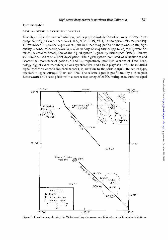
Four days after the swarm initiation, we began the installation of an array of four threecomponent digital event recorders (OLA, VEN, SON, VCT) in the epicentral area (see Fig. 1). We missed the earlier larger events, but in a recording period of about one month, high- quality records of earthquakes in a wide variety of magnitudes (up to ML = 4.1) were obtained. A detailed description of the digital system is given by Brune etal. (1980). Here we shall limit ourselves to a brief description. The digital system consisted of Kinemetrics and Geotech seismometers of periods 5 and 1 s, respectively, modified versions of Terra Tech- nology digital event recorders, a clock synchronizer, and a field playback unit. The modified digital recorders encode (on each record), in addition to the seismic signal, the sensor type, orientation, @in settings, filters and time. The seismic signal is pre-filtered by a three-pole Butterworth anti-aliasing filter with a corner frequency of 25 Hz, multiplexed with the signal

3 2 " 4 :

32O30

1

3 0 ' 115O15' 1 15°00' 32045'

A T L X

km 1 I 3 0 ' 115O15' 11

32O30'

$2'15'

7 0 '

Figure 1. Location map showing the Victoria earthquake swarm area (dashed contour) and seismic stations.



ownloaded from


728

of the other two channels, digitized by a 12-bit analogue to digital converter at a rate of 100 samples s -', delayed 1.6 s in a serial pre-event memory, and recorded on magnetic tape. The internal time standard has a crystal controlled oscillator which is accurate to 1 part in lo6 .

L. Munguia and J. N. Brune

S T R O N G M O T I O N I N S T R U M E N T S

A set of acceleration records was obtained from two accelerometers triggered by the larger earthquakes occurring during the initial stage of the Victoria swarm. The acceleration recording instruments are part of the permanent strong motion network which operates in the northern region of Baja California and Sonora (Prince et al. 1977; Brune et el. 1983) and are located at stations Victoria (VIC) and Delta (DEL), indicated by solid squares on the map of Fig. 1. The stations consisted of three-component SMA-1 accelerographs located slightly off the Cerro Prieto fault and oriented in such a way that the horizontal sensors recorded motion approximately parallel and perpendicular to the fault trace. In most cases, the instruments were triggered by the P-wave, allowing use of the S-minus trigger time in the hypocentre locations. The VIC and DEL analogue film records were enlarged three times and then hand-digitized and corrected for instrument response. The true ground acceleration was then integrated to obtain velocity and displacement records.

S M O K E D P A P E R I N S T R U M E N T S

The smoked paper instrument network (Fig. 1) began operating about seven months before the Victoria swarm (maintained by personnel from CICESE). The recording instrumentation consisted of Ranger SS1 1 s period seismometers with a Sprengnether MEQ-800 smoked paper recording system. Minute marks were recorded each 120mm and WWVB radio time was recorded at the beginning and end of the records. This allowed measurements of sharp P-wave arrival times with an absolute error of approximately k0.05 s.

Seismicity pattern, epicentre location and fault plane solution

The activity in the Victoria swarm began on March 10 with earthquakes of magnitude ML of about 3. The larger events of the swarm (ML =4.5, 4.8, 4.8) occurred in the first two days, and relatively high seismicity continued for about 15 days.

The earthquakes and recording stations were all located in the same geological region, which has a structure consisting mainly of silts, sands and alluvial sediments of Tertiary and Quaternary age, overlying the basement at 5 4 km depth (Biehler, Kovach & Allen 1964; Puente & de la Pena 1978). A velocity model composed of flat homogeneous layers was used in programs H Y P O ~ I (Lee & Lahr 1975) and MICRO (Buland 1976, modified to use layered structures) to compute the hypocentral locations for these events. S-P and S-minus- trigger times observed on most of the VIC strong motion records were consistently between 2.0 and 2.2 s. Strong motion records from DEL indicated S-minus-trigger times between 3.6 and 3.8 s. Based on the trigger specifications of the SMA-1 instruments and the characteristics of the P-wave signals, we estimate that the difference between the P time and the trigger time is less than about 0.1 s, and thus S-minus-trigger times were used in combination with smoked paper data in the hypocentre location for the larger events. Fig. 2 shows the distribution of the located epicentres. Some of these epicentres were taken from a study of the seismicity of the Cerro Prieto geothermal field by Reyes (1979), and the rest were obtained by us. The epicentres plotted spread within a circular area of about 6 km radius



ownloaded from


High stress drop events in northern Baja California ' i " ' I " " I " " I " "

7 29

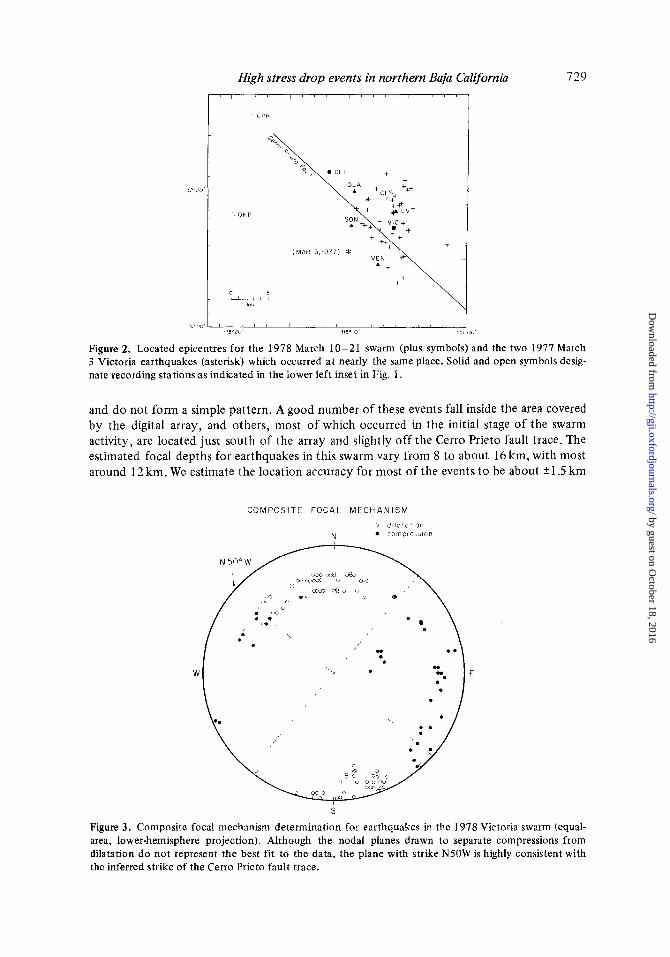
I ', CPR

Figure 2. Located epicentres for the 1978 March 10-21 swarm (plus symbols) and 3 Victoria earthquakes (asterisk) which occurred at nearly the same place. Solid and nate recording stations as indicated in the lower left inset in Fig. 1 .

the two 1977 March open symbols desig-

and do not form a simple pattern. A good number of these events fall inside the area covered by the digital array, and others, most of which occurred in the initial stage of the swarm activity, are located just south of the array and slightly off the Cerro Prieto fault trace. The estimated focal depths for earthquakes in this swarm vary from 8 to about 16 km, with most around 12 km. We estimate the location accuracy for most of the events to be about + I .5 km

C O M P O S I T E F O C A L M E C H A N I S M

0 d l l o l o t l o n co rnp re i i i un N

S

Figure 3. Composite focal mechanism determination for earthquakes in the 1978 Victoria swarm (equal- area, lower-hemisphere projection). Although the nodal planes drawn to separate compressions from dilatation do not represent the best fit to the data, the plane with strike N50W is highly consistent with the inferred strike of the Cerro Prieto fault trace.



ownloaded from


730

in both epicentre and focal depth. This error arises in part because not all the stations of the array recorded continuously, resulting in poor location control, and also, in part, because the true geological structure beneath the recording stations is not known exactly and may vary laterally (Puente & de la Pena 1978).

Evidence of tightly packed clusters of epicentres comes from the examination of ?he waveforms produced by these earthquakes. Subsets of events recorded either by strong motion instruments or by digital recorder systems produced similar records (see Figs 4 and 1 1, for example) suggesting tight clusters.

To investigate the mechanism of earthquakes in this swarm, P-wave first motion data for 14 of the larger events recorded at the more distant smoked paper stations and at stations of the US Geological Survey - California Institute of Technology (USGS-CALTECH) southern California array were combined to prepare a composite fault-plane solution. The data were plotted on an equal-area loyer-hemisphere projection, and nodal planes were drawn to separate, as best as possible, the compressions from the dilatations (see Fig. 3). Although near the nodal planes a few data points still remain in the wrong quadrant, the composite focal mechanism suggests predominantly right-lateral strike-slip motion. The nodal plane with strike N50"W has been chosen as the plane of motion, since it agrees very well with the inferred strike of the Cerro Prieto fault trace.


Seismogram characteristics

S T R O N G M O T I O N R E C O R D S

The strong motion stations (VIC and DEL) recorded only the larger earthquakes which occurred within the first four days of the swarm activity. Since the digital array deployment began at the end of this period little overlap exists between recordings from these two kinds of instruments.

The strong motion stations yielded acceleration records for 20 events with magnitudes ML between 3.0 and 4.8. Six events of this data set were recorded by both stations, but after recording the event of March 11, 23 : 57 GMT ML = 4.8 the station DEL ran out of film and the rest of the earthquakes in the set were recorded only at VIC. Epicentral distances to the strong motion stations VIC and DEL are less than about 10 and 15 km respectively. (In the rest of this paper events will be identified by the hour and minute of origin time and, when necessary, the second.) Some of the larger acceleration records obtained from these stations are shown in Figs 4, 5 and 6 together with velocity and displacement records. A summary of the results obtained from analyses of the acceleration data is given in Table 1 . As shown in this table, the maximum acceleration (0.57g) was observed at VIC for the March 12, 18:42 GMT, ML = 4.8 event (Fig. 5), at DEL, and the largest peak horizontal acceleration (0.3 1 g) was produced by the March 11, 23 :57 GMT, ML = 4.8 event (Fig. 6). The vertical acceleration was only slightly less (0.29g). Peak accelerations produced by this event at VIC were 0.46 g . These two events were the largest of the series and for both, the duration of horizontal accelerations in excess of 0.1 g was about 3.5 s at VIC. High horizontal peak acceleration was also produced at VIC by the March 12, 00 :30 GMT, ML = 4.5 event (Fig. 5 ) , for which the recorded horizontal accelerations were 0.42g and 0.45g.

Records from both strong motion stations show a considerable amount of energy at high frequencies, indicating that attenuation did not greatly reduce the high-frequency energy, even though the waves passed through a very thick low-velocity sedimentary section.

As can be seen on the records of Figs 4-6, the VIC displacement waveforms are for the most part relatively simple and a certain degree of similarity among records from different



ownloaded from


High stress drop events in northern Baja California Table 1. Acceleration data.

Date

Mar 11

Mar 12

Mar 13 Mar 16 Mar 18

Time

05 17 05 1 8

05 18

05 40

21 52

23 57

23 58 23 58 23 59 23 59 00 01 00 30 18 42

20 05 22 01 23 10 09 11 01 51 04 40

-

Station

DEL DEL VIC DEL VIC DEL v IC DEL VIC DEL VIC VIC VIC V 1C DEL v IC V IC VIC v IC VIC v IC VIC VIC VIC VIC

S-tr igger Peak accel. lg)

3.60 0.016 3.80 0.040 1.50 0.140 3.80 0.008 2.10 0.085 3.65 0.045 2.1 0 0.1 20 3.75 0.017 2.1 0 0.052 3.50 0.135 1.70 0.467 2.1 5 0.06 5 2.1 5 0.043 2.00 0.048 3.75 0.010 2.1 5 0.071 2.1 0 0.420 2.26 0.570 2.00 0.050 2.1 0 0.1 28 2.1 5 0.03 3 1.95 0.1 50 2.1 6 0.266 2.20 0.115 1.85 0.054

Z

0.016 0.030 0.030 0.035 0.019 0.04 8 0.053 0.027 0.014 0.290 0.330 0.022 0.01 2 0.012 0.048 0.083 0.086 0.240 0.01 0 0.019 0.035 0.053 0.059 0.079

SE

0.01 7 0.021 0.130 0.026 0.112 0.050 0.1 30 0.026 0.051 0.310 0.475 0.068 0.069 0.06 1 0.009 0.110 0.4 50 0.336 0.059 0.1 09 0.035 0.1 84 0.243 0.147 0.065

Distance (km)

13.1 18.6 7.5

17.4 6.9

15.0 4.2

20.7 9.7

15.0 5.5

3.5 7.5

2.1 3.2 3 .O 5.7 4.3

73 I

ML

3.3 3 -3

3.4

3.7

3 .O

4.8

4.5 4.8

3.2 3 -2 3.7 3.6 4.1 3.7

earthquakes can be seen (see the records for events 0540,091 1 , and 0030 o n Figs 4 and 5). Even though the resemblance among the strong motion records is not as spectacular as in the case of some of the digital recordings (discussed later), probably due t o larger and more complex sources,it does suggest that these larger events occurred in nearly the same location.

On the DEL records, vertical and horizontal peak accelerations are comparable in amplitude, and in some cases the maximum peak acceleration was recorded on the vertical component. One o f the more remarkable features on the DEL horizontal records is the clear long-period phase arriving a t about 5.6-6.0 s behind the direct S-wave (see records of Fig. 6). This phase has been interpreted as the first multiple of the S-wave reflecting in the sedimentary section.

D I G I T A L R E C O R D S

Earthquakes with magnitudes ML of up to 4.1 were recorded at from one t o three of the digital stations indicated o n the map o f Fig. 1. Typical sets of three component recordings produced a t each station are displayed on Figs 7-10. In some cases the instruments were triggered by the S-wave and we show only the two horizontal components o n those figures. The SON records, with about equal amplitude on the three components, have the more complicated appearance. This could be a result of a combination of particular properties a t the recording site and of radiation pattern effects. Records from the other stations are in some cases simple and in others complicated but , as in the case of the SON records, all of them are rich in high frequencies which persist throughout most of the record.



ownloaded from


732 L. Munguia and J. N. Brune

E V E N T 0 5 4 0 V I C S45W E V E N T 0911 V I C S45W PERK 261 3 L V i E C 2

PERK 3 7 C W S F C PERK 7 3 C W S E C -,-- .A

V I C S45E V I C S45E PFRK -127 4 CpI/SFC2

PFRK -3 I CWSFC

PERK a i cn

0 5

SECONDS

Figure 4. Horizontal components of ground acceleration, velocity and displacement for the earthquakes 0540 (ML = 3.7) and 091 1 (ML = 3.6) recorded at station VIC.

E V E N T 0030 V I C S45W

PERK 17 3CWSEC J W >

J PERK -I 2 C M a 0 t: --

V I C z J W 0 -

u a

PERK 2 J C W S E L J W >

V I C S45E J

!$ P E W 15.2CM/SEC i w - >

J PER< -1 L C t l a : :- c)

E V E N T 1842 V I C S45W

PERK- 26.8CWSEC y.

V I C z PERK 216.5 CWSECZ

_x_

PERY 5 ICM/SEC zul\nvz

SECONDS

Figure 5. Ground acceleration, velocity, and displacement for earthquakes 0030 (ML = 4.5) and 1842 (ML = 4.8) recorded at station VIC.



ownloaded from



1140

P E T a j c n $

- -4

9 1

SECONOS

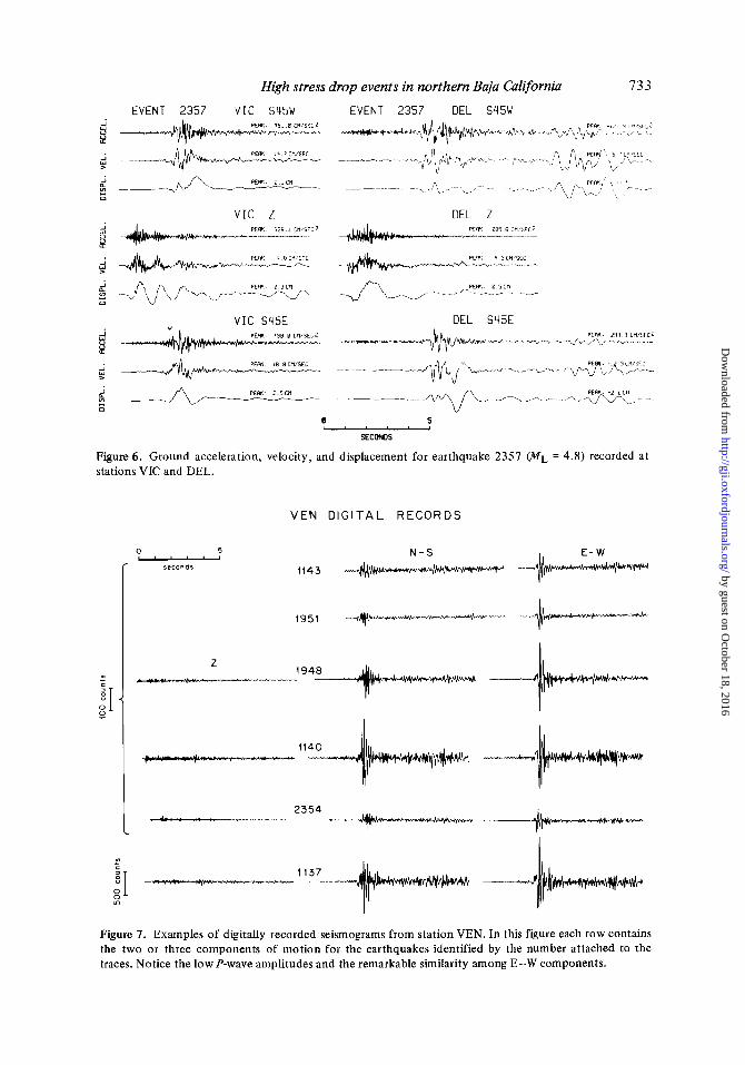
Figure 6. Ground acceleration, velocity, and displacement for earthquake 2357 (ML = 4.8) recorded at stations VIC and DEL.

L

0 ZI P

VEN D I G I T A L RECORDS

0 5 I ~ ~ ~ ’ 1

seconds

N - S 1143

1951 “ut.---.--.----.----



ownloaded from


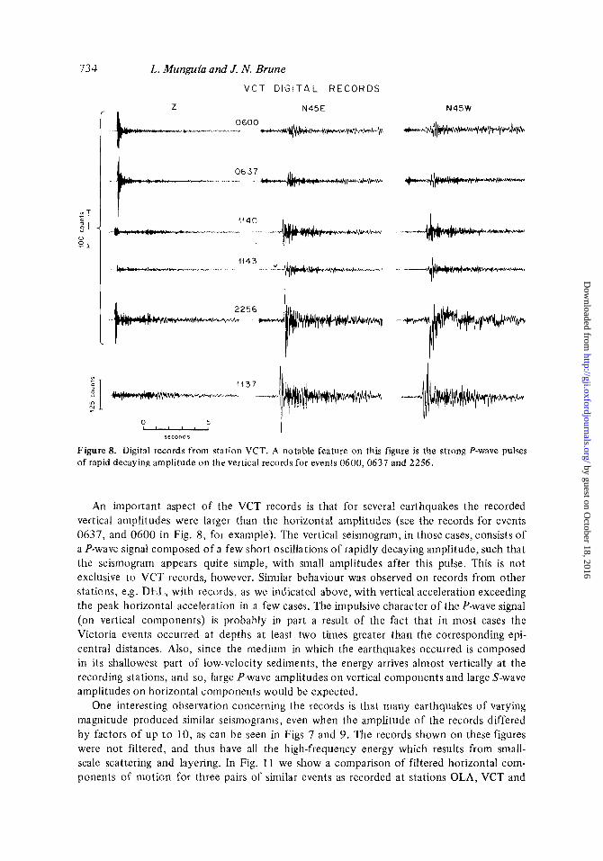
734 L. Munguta and J. N. Brune V C T D I G I T A L R E C O R D S

Z N45E N45W

seconds

Figure 8. Digital records from station VCT. A notable feature on this figure is the strong P-wave pulses of rapid decaying amplitude on the vertical records for events 0600,0637 and 2256 .

An important aspect of the VCT records is that for several earthquakes the recorded vertical amplitudes were larger than the horizontal amplitudes (see the records for events 0637, and 0600 in Fig. 8, for example). The vertical seismogram, in those cases, consists of a P-wave signal composed of a few short oscillations of rapidly decaying amplitude, such that the seismogram appears quite simple, with small amplitudes after this pulse. This is not exclusive to VCT records, however. Similar behaviour was observed on records from other stations, e.g. DEL, with records, as we indicated above, with vertical acceleration exceeding the peak horizontal acceleration in a few cases. The impulsive character of the P-wave signal (on vertical components) is probably in part a result of the fact that in most cases the Victoria events occurred at depths at least two times greater than the corresponding epicentral distances. Also, since the medium in which the earthquakes occurred is composed in its shallowest part of low-velocity sediments, the energy arrives almost vertically at the recording stations, and so, large P-wave amplitudes on vertical components and large S-wave amplitudes on horizontal components would be expected.

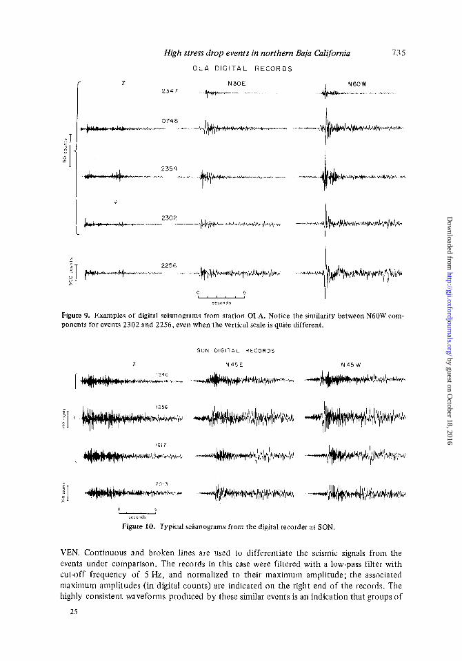
One interesting observation concerning the records is that many earthquakes of varying magnitude produced similar seismograms, even when the amplitude of the records differed by factors of up to 10, as can be seen in Figs 7 and 9. The records shown on these figures were not filtered, and thus have all the high-frequency energy which results from small- scale scattering and layering. In Fig. 11 we show a comparison of filtered horizontal components of motion for three pairs of similar events as recorded at stations OLA, VCT and



ownloaded from


High stress drop events in northern Baja California

O L A D I G I T A L R E C O R D S

73 5

c

0

Z 2347

N 3 0 E

0 5

seconds I

Figure 9. Examples of digital seismograms from station OLA. Notice the similarity between N60W components for events 2302 and 2256, even when the vertical scale is quite different.

0 5

seconds

Figure 10. Typical seismograms from the digital recorder at SON.

VEN. Continuous and broken lines are used to differentiate the seismic signals from the events under comparison. The records in this case were filtered with a low-pass filter with cut-off frequency of 5 Hz, and normalized to their maximum amplitude; the associated maximum amplitudes (in digital counts) are indicated on the right end of the records. The highly consistent waveforms produced by these similar events is an indication that groups of

25



ownloaded from


736 L. Munguia and J. N. Brune

S I M I L A R E V E N T S

0 5 I 1 1 I I I

Seconds

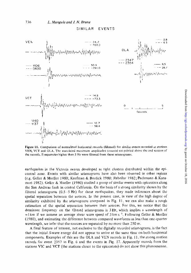
Figure 11. Comparison of normalized horizontal records (filtered) for similar events recorded at stations VEN, VCT and OLA. The associated maximum amplitudes (counts) are printed above the end section of the records. Frequencies higher than 5 Hz were filtered from these seismograms.

earthquakes in the Victoria swarm developed as tight clusters distributed within the epicentral zone. Events with similar seismograms have also been observed in other regions (e.g. Geller & Mueller 1980; Kaufman & Burdick 1980; Rebollar 1982; Pechmann & Kana- mori 1982). Geller & Mueller (1980) studied a group of similar events with epicentres along the San Andreas fault in central California. On the basis of a strong similarity shown by the filtered seismograms (0.5-5 Hz) for those earthquakes, they made inferences about the spatial separation between the sources. In the present case, in view of the high degree of similarity exhibited by the seismograms compared in Fig. 11, we can also make a rough estimation of the spatial separation between their sources. For this, we notice that the dominant frequency on the filtered seismograms is 3Hz, which implies a wavelength of 2 1 km if we assume an average shear wave speed of 3 km s-'. Following Geller & Mueller (1980), and estimating the difference between compared waveforms as less than one-quarter wavelength, we infer that the sources are separated by no more than 250 m.

A final feature of interest, not exclusive to the digitally recorded seismograms, is the fact that the initial S-wave energy did not appear to arrive at the same time on both horizontal components. Examples of this are the OLA and VEN records in Fig. 1 1, the strong motion records for event 2357 in Fig. 6 and the events in Fig. 17. Apparently records from the stations VIC and VCT (the stations closer to the epicentres) do not show this phenomenon.



ownloaded from



Whether this phenomenon is due to local anisotropy, multipathing effects, or another mechanism is not known at present.

Source parameters

Near-source data recorded by the digital event recorders and strong motion instruments are analysed here in terms of spectral parameters. The process of unpacking, editing and compu- tation of spectra for the digital data are described by Brune etal. (1980). All well-recorded events for which the signal to noise ratio was high were analysed. Different sample lengths were considered for Fourier analysis. We first used 5 s of the horizontal records, beginning with the S-wave. The resulting spectra were corrected for anelastic attenuation and instrument response. Then whole record (i.e. P-wave plus 5’-wave) spectra of the horizontal records were also compujted and corrected in the same way. No significant difference was found, as was expected, since the P-wave amplitude on the horizontal records is very low. Also, as more of the S-wave coda was added, very little effect on the spectrum shape was noted. For comparison with results of Hartzell & Brune (1977), we assumed a Q value of 150 for the attenuation correction. Other values of Q (from 100 to 350) were also tried, only those spectra corresponding to the smaller events (for which the signal to noise is low) showed significant shifts of the estimated corner frequency for assumed values of Q lower than 150. Sin& et al. (1982), using data from aftershocks of the Imperial Valley earthquake (1979 October 15, ML = 6.6), studied the spectral attenuation of SH-waves along the Imperial fault. They found that for sources below 4 km, Q is a function of frequency that increases from about 60 at 3 Hz to 500 at 25 Hz. Their proposed model of Q for the Imperial Valley structure is approximately consistent with the Q value we have used here, since at the close distances involved the results are not very sensitive to the Q value assumed.

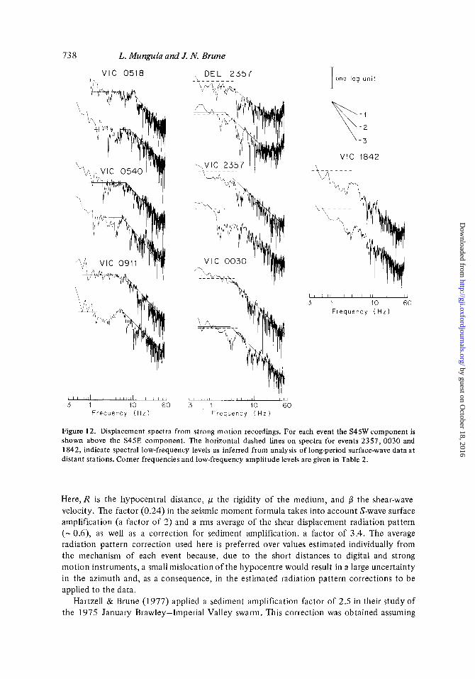
In Figs 12 and 13 we show examples of displacement spectra calculated from strong motion data and from digitally recorded data, respectively. It can be seen on these two figures that in some cases the spectrum has a simple shape with relatively well-defined low- and high-frequency asymptotes, with the intersection defining the corner frequency fo ; in other cases the spectra cannot be interpreted this simply. For the larger events the low- frequency spectral level can be constrained by surface waves, discussed later, and give spectral levels indicated by the dashed lines.

A noticeable feature on the strong motion spectra is the fact that for periods longer than 2-3 s, the amplitudes increase considerably. This might be a result of the combined effects of long-period noise and long-period digitization errors. Spectra for some of the smaller events (ML s 3 ) recorded in digital form also show a similar rise of the lower-frequency portion of the spectrum, a result of low signal to noise ratio and division by a small number for the instrumental correction. In general the spectra also show a rise at the higher-frequency end, a result of noise and the attenuation correction. With these features of the spectrum in mind, we estimated the low-frequency level, no, and the corner frequency so, for use with Brune’s (1970, 1971) equations to estimate source parameters. Seismic moment M o , radius of a semicircular fault r , and stress drop CJ were calculated using the expressions

7 Mo C J = - - 16 r3 (3 1



ownloaded from


73 N. Brune

_ _

Y V I C 2357

one log u n i t I

V I C 1842

I 1 1 / 1 1 1 1 I I l l l l 1 1 l 1 I t I I

3 1 10 60 F r e q u e n c y ( H z )

1 1 1 l I l 1 1 . , 1 l l l l 1 1 I 1 , I / 1 , , 1 , 1 . / 1 1 I , , ,

3 1 10 60 3 1 10 60 F r e q u e n c y ( H z ) F r e q u e n c y ( H z )

Figure 12. Displacement spectra from strong motion recordings. For each event the S45W component is shown above the S45E component. The horizontal dashed lines on spectra for events 2357, 0030 and 1842, indicate spectral low-frequency levels as inferred from analysis of long-period surface-wave data at distant stations. Corner frequencies and low-frequency amplitude levels are given in Table 2.

Here, R is the hypocentral distance, ~ . l the rigidity of the medium, and 0 the shear-wave velocity. The factor (0.24) in the seismic moment formula takes into account S-wave surface amplification (a factor of 2) and a rms average of the shear displacement radiation pattern (-0.6), as well as a correction for sediment amplification, a factor of 3.4. The average radiation pattern correction used here is preferred over values estimated individually from the mechanism of each event because, due to the short distances to digital and strong motion instruments, a small mislocation of the hypocentre would result in a large uncertainty in the azimuth and, as a consequence, in the estimated radiation pattern corrections to be applied to the data.

Hartzell & Brune (1977) applied a sediment amplification factor of 2.5 in their study of the 1975 January Brawley-Imperial Valley swarm. This correction was obtained assuming



ownloaded from



V E N 1948 O L A 2 2 5 6

3.5

3.0

z

k-

V U J

I

9 2 .5 -

a - - a 2.0

a

1.5

1.0

V C T 1228

V E N 1143

-

~

~

-

\ V C T 1606

1 1 1 1 1 1 l l I I l l l l J , I I 1 1 1 1 1 1 1 1 1 1 1 I 1 1 1 1 1 1 1 3 1 10 40 3 I 10 40

F r e q u e n c y ( H z )

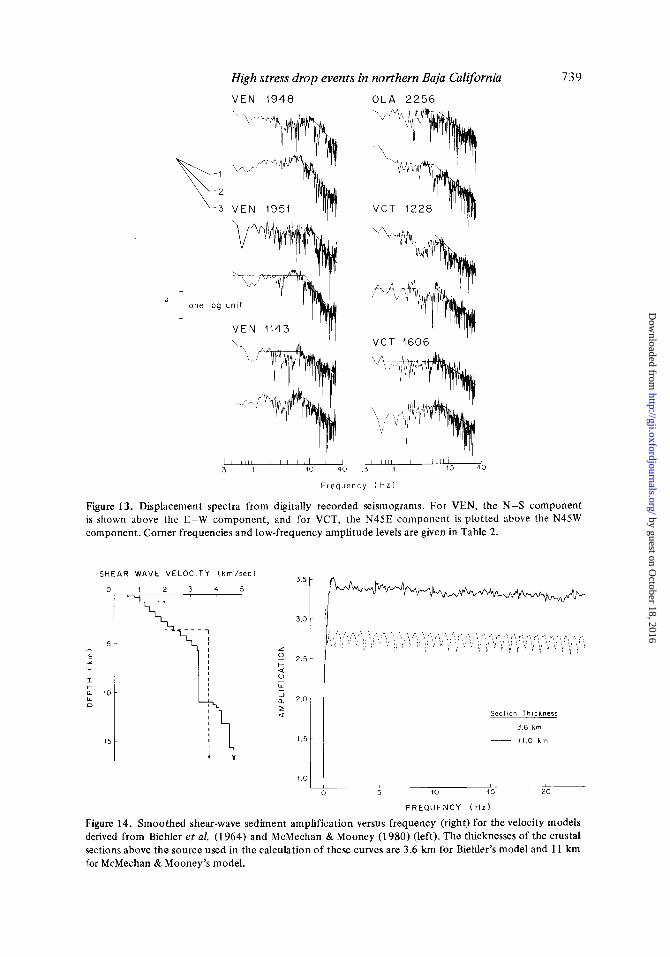
Figure 13. Displacement spectra from digitally recorded seismograms. For VEN, the N-S component is shown above the E-W component, and for VCT, the N45E component is plotted above the N45W component. Corner frequencies and low-frequency amplitude levels are given in Table 2.

SHEAR W A V E V E L O C I T Y ( k m / s e c )

4 7

1 I

I I I I

5 -

I r a 10 - W D

15 -

Sec t ion T h i c k n e s s ~~

3.6 km

__ 11 0 h m

0 5 10 45 20

F R E Q U E N C Y ( H Z )

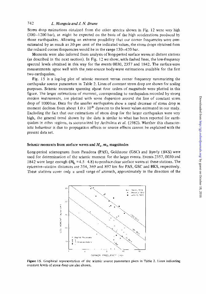
Figure 14. Smoothed shear-wave sediment amplification versus frequency (right) for the velocity models derived from Biehler et al. (1 964) and McMechan & Mooney (1 980) (left). The thicknesses of the crustal sections above the source used in the calculation of these curves are 3.6 km for Biehler’s model and 1 1 km for McMechan & Mooney’s model.



ownloaded from


740 L. Mungufa and J. N. Brune

Table 2. Epicentre and source parameter data. - -

D A T I T I M 5 MAG EPIC. COORD. STN. R DEPTH L O G n . f. M r L I M r v Y H I> H M S M L LAT N LON W IKn! I K m ! ( C D - S ! (Hz! lDyns-crnI (a! I B i o r r ) ( D y n e - c m ! l m l ( B a r s !

7 8 3 I I 5 I 8 6 . 4 3.3 3 2 . 2 7 1 1 5 . 0 3 V l C 7 .5 1 4 . 4 -1.96 7 . 2 4 8 . 2 8 5 8 22 1 3 4 5 2 2 . 1 B . 3 8 5 E 22 I40 6 1 6 . 7 - 2 . 8 0 6.61 0 . 2 6 0 E 22 I 4 7 3 6 1 . 2

7 8 3 I 1 5 10 3 0 . 4 3 .7 3 2 . 2 5 1 1 5 . 0 9 DEL 15.0 1 4 . 9 -1.00 2 . 4 8 8 . 3 3 9 E 2 3 4 0 4 2 2 5 . 2 0 . 2 5 8 E 2 3 388 3 7 5 . 9 - 1 . 1 4 2 . 4 5 8 . 2 4 5 E 23 3 9 4 1 7 4 . 8 - 1 . 7 0 4 . 2 7 0 . 4 9 4 E 2 2 2 2 7 1 8 4 . 9 - 1 . 5 2 3 . 4 7 0 . 7 4 8 E 2 2 2 7 9 158.3

V l t 4 . 1

- 8 . 5 2 3 . 1 6 0 . 8 9 6 E 2 3 3 0 6 1365.0 0 . 1 B 9 E 2 4 3 4 1 1 2 8 1 . 6 - 0 . 7 6 2 . 5 1 0 .64BE 2 3 3 8 5 4 9 5 . 3

78 3 I I 2 3 5 7 4 5 . 5 4.8 3 2 . 2 4 1 1 5 . 1 1 V I C 5 . 4 DEL 1 5 . 1

- 2 . 3 5 10.00 B . 9 2 4 E 2 1 9 7 - 2 . 3 5 1 0 . 9 6 0 . 9 2 4 E 2 1 8 8

7 8 3 11 0 I VIC

7 8 3 12 0 3 0 1 7 . 2 4 . 5 3 2 3 2 1 1 5 . 0 9 VIC 3.5 12.5 - 0 . 4 8 2 . 3 4 8.6881 2 3 4 1 3 -8.50 2 . 8 2 0 . 6 5 7 ~ 2 3 3 4 4

- 1 . 8 2 5 . 5 8 8 . 3 7 3 E 2 2 1 7 6 -1.98 6 . 3 1 0.3lBL 2 2 I53

7 8 3 1 2 2 0 s 3 . 2 V l t

7 8 3 I 3 9 I I 3 7 . 2 3 . 6 3 2 . 3 1 1 1 5 . 1 0 V I C 3 . 0 1 3 . 2 - 1 . 4 8 5 . 6 2 0 . 7 1 7 E 2 2 1 7 2 -1.40 5 . 3 7 8 . 8 6 2 E 2 2 I80

- 4 . 2 7 - 4 . 2 5 78 3 1 5 I ? 4 6 2 . 0 SON

- 3 . 7 0 3 . 7 2 0 . 2 1 9 E 2 0 2 6 1 -3.60 2 . 8 2 0 . 2 7 6 E 2 0 3 4 4

-4.04 1 1 . 7 5 0 .243E Z B 8 2

0.1 iE 2 0 0 . I 4 4 E 2 8

7 8 3 15 1 2 56 2 3 . a 2 . 5 3 2 . 3 3 1 1 5 . 1 5 50N 4 . 1

J

- 4 . 8 3 1 1 . 2 2 0 . 2 4 8 ~ 2 0 86 7 8 3 1 5 I 2 57 SON

7 8 3 1 5 1 6 1 7 15.9 2 . 7 3 2 . 3 2 l l 5 . l l SON 5 . 7 - 3 . 2 4 3.55 0 . l 2 9 E 2 1 2 7 3 -3.08 3 . 2 4 0 . I B 6 E 2 1 2 9 9

4 4 5 . 4 0 . 1 3 1 E 2 2 9 2 7 2 5 . 5 5 8 7 . 2

4 2 7 . 4 B . 9 5 2 E 2 3 3 7 5 7 8 8 . 8 7 0 9 . 3

2 9 8 . 2 0 . 4 8 3 E 2 2 I64 4 r 8 . 6 3 7 5 . 1

6 1 4 . 3 B . I l 2 E 2 3 1 7 6 8 9 3 . 5 643.3

8 . 1 9 9 E 2 8

8 .5 8 . 3 5 0 E 2 0 2 9 6 8 . 3

0 . 6

2 5 . 3

4 . 2

10.3

5 . 9

216.5

367 0

1 6 . 1

8 . 4

5 6

2 5 5

9 0 . 6

6 0

1 . 9

3 7

2 3 . 2

10.4

5 7 . 0

1 2 . 5

2 9 . 4

1 1 . 8

2 . 3

56.0

1 0 . 8

5 9 9

19.0 B . 3 4 7 E 2 8 8 4 1 6 . 9

2 . 8 8 . 2 2 2 1 2 1 2 8 5 3.0

7 8 I 1 5 19 4 8 SON

VEN

- 4 . 2 3 1 0 . 4 7 0 . 1 3 3 E 2 0 9 2 - 4 . 2 0 10.00 8 . 1 4 3 E 20 9 7 - 4 . 8 4 9 . 5 5 8 . l 8 0 E 20 101 - 3 . 8 6 7 . 5 9 0 . 2 7 2 E 2 8 1 2 8

7 . 4 8 . 2 5 7 E ZB 183 6 . 9 7 .5 5 . 7

78 3 1 5 1 9 5 1

7 8 3 15 2 0 1 3 1 7 . 6 3 . 2 3 2 . 3 4

- 4 . 3 2 9 . 3 3 0 . l 0 4 E 2 0 I04 -4 .16 8 . 3 2 8 . 1 5 0 E 2 0 I 1 6

VEN 4 . 1 8 . l 7 9 E 2 0 I10 4 . 2

9 1 . 8 0 . 8 5 7 E 2 1 I 2 0 44.0

1 5 . 0 9 SON 8 . 7 9 . 3 - 2 . 9 7 9.55 8 . 2 1 9 E 2 1 101 - 2 . 8 7 6 . 9 2 8 . 2 7 5 ~ 2 1 148 - 2 . 0 5 0 . 1 4 2 E 2 2 - 2 . 7 4 8 . 7 1 0 . 4 2 0 E 2 1 1 1 1 - 2 . 5 2 7 . 0 8 0 . 6 9 7 E 2 1 1 3 7

1 5 . 0 8 VEN 11.0 10.5 - 2 . 2 4 6 . 6 1 8 . 1 4 0 E 2 2 I 4 7 - 2 . 2 4 6 . 6 1 8 . l 4 0 E 2 2 1 4 7 - 1 . 4 5 4.68 0 . 6 2 9 E 2 2 2 8 7 - 1 . 7 2 4 . 1 7 0 . 3 9 4 E 2 2 2 3 2 -1.90 6 . 3 1 8 . 2 4 I E 2 2 153 - 1 . 7 6 5 . 8 1 8 . 3 3 3 E 22 193

VCT 3 . 4 VEN 11.0

VCT 3 . 5 OLA 7 . 5 V I C 5 . 7

1 3 3 . 8 1 1 9 . 2

I8 3 16 I 5 1 9.8 4 . 1 3 2 . 3 4 1 9 4 . 8 0 . 4 d 2 E 2 2 1 7 4 1 9 4 . 8 3 1 0 . 1 1 3 7 . 6 2 9 1 . 6 2 0 1 . 7

78 3 15 7 1 8

7 8 3 I 7 2 d 2 I Z . 3 2 . 5 3 2 31

OLA - 3 . 8 2 0 . 3 5 8 E 2 0 - 3 . 5 8 7 . 5 9 0 . 7 4 8 ~ 2 0 1 2 8

0 . 7 8 2 E 2 0 1 2 8 1 5 . 7

1 5 . 1 2 V C T 2.0 14.8 - 3 . 5 8 0 . 7 1 5 s 2 0 - 3 . 4 4 5 . 7 5 8 . 9 0 9 1 2 0 I68 - 3 . 2 8 1 . 2 7 0 . 1 3 1 E 2 1 2 2 7

3 2 3 2 1 1 5 . 1 1 VCT I 5 11.8 - 3 . 8 0 - ? 6 0

VEN 7 . 0

0 . 3 0 2 E 2 0 LI 1 7 r 7 1

7 " 3 1 7 5 5 2 6 . 0

0 . 1 3 9 E 2 1 193 8 . 3 1 . 9

0 . 4 9 6 E 2 0

78 3 ~7 b 37 35 a 2 . 4 I: 3 3 1 1 5 . 1 0 V C T 2 . 8 1 1 . 4 - 4 . 1 6 B . 1 2 8 1 2 0 - 4 . 0 0 7 . 4 1 0 . 2 3 5 E 2 0 I 3 1 - 4 . 0 0 0 . 2 3 6 E 2 0

VEN 9 . 4 0 . 2 8 3 1 2 0 1 3 1

1.6

18.9 0 . 5 1 3 E 2 0 96 38 6 16.8

6 . 4 5 . 7

78 3 1 7 2 7 54 5 3 0.0 3 - 2 8 1 1 5 . 0 8 OLA 9 . 0 1 3 . 0 - 3 . 7 2 9 . 3 3 0 . 6 8 3 1 2 0 104 - 3 5 0 10.00 B . 8 0 I E 2 0 9 7 - 3 . 8 5 1 0 . 4 7 0 .303E 20 9 2 - 4 . 3 6 1 0 . 9 6 0.l00E 2 0 88 - 4 . 2 6 9 . 7 7 0 . I 2 6 E 2 0 99

18 : l e 1 4 0 2 8 5 3 . 7 3 2 . 3 3 I l 5 . 0 8 OLA 7 . 0 1 0 . 2 - 1 . 7 2 2 . 1 9 0 . 3 7 7 E 2 2 443 - 1 . 4 2 2 . 4 0 0 . 7 5 3 E 2 2 404 - 1 9 4 3 5 3 8 . 1 9 6 1 22 2 6 7 - 2 . 0 0 5 . 0 1 0 . l 7 l E 2 2 193 - 2 . 0 8 3.89 8 . 1 9 7 E 22 2 4 9 - 1 . 8 6 3 . 3 1 0 . 3 2 7 E 2 2 2 9 2

VCT 3 . 2 YEN 6.0

VCT 3.1

" E N 1 0 . 7

1 9 . 0 0 . 4 7 6 E 2 2 2 8 4 50.1 d 5 2

183 5 5 5 . 9 5 7 . 2

- 4 . 1 5 8 . 9 1 8 . 1 7 4 1 2 0 109 - 3 98 5 . 8 9 0 . 2 5 8 E 2 0 1 6 &

- 4 . 4 4 - 4 . 4 0 6.61 0 . l 0 2 E 2 0 1 4 7

- 4 . 0 0 7 . 0 8 0 . 1 5 1 E 2 0 1 3 7 -3.84 6 . 1 7 0.2!91 2 0 1 5 7

78 3 I H " A Y YEN

78 3 1 8 1 5 1 VEN

7 P 3 1 8 5 l i 53.' 2 . 2 3 2 . 2 8 1 1 5 . 1 4 VLN 4 . 6

0 . 9 3 0 E 1 9

5 . 9 0 . 3 0 6 s 2 0 131 2 5

0 . 1 3 8 E 2 0 1 4 7 1 . 4

2 6 0 . 2 6 2 E 2 0 I d 6 2 5

78 3 i 8 b B :.u 7.7 ? 2 29 1 1 5 . 1 2 VEN 4 .6 1 2 . 5 - 3 . 1 2 6 . 3 1 0 . 1 5 2 E 2 1 1 5 3 - 3 . 0 4 6.31 8.1951 2 1 1 5 3 - 3 . 5 7 7 . 0 8 0 . 5 5 7 E 2 0 1 3 7 - 3 37 7 . 5 9 0 .883E 2 0 1 2 8

YCT 3 . 3

1 9 6 0 . 1 5 2 E 2 1 I 4 2 23 6

9 . 5 I8 6

0 . 2 I 7 E 2 0 0 . 2 9 2 E 2 0

I 8 7 I 8 I I 6 3 9 'i 2 . 1 3C 3 0 1 1 5 . l 2 V I N 5 . 8 1 2 . 0 -3.18 - 3 . 8 5

78 3 I 8 I 1 3 0 16 ? 2 . 1 3 2 3 1 1 1 5 . l 6 VEN 8 0 1 1 . 6 - 4 . 1 6 1 1 . 2 2 0 . 1 5 6 E '0 86 - d . 0 7 7 . 9 4 0 . 1 9 2 E 2 0 1 2 2

0 . 3 6 0 E 2B

1 0 . 6 0 . 2 4 6 1 2 0 1 0 1 4 6

7 8 3 I8 I ! 37 4 4 . 1 2 . 9 3 2 27 1 1 5 . 1 1 V E N 3 . 1 1 2 . 5 - 3 . 0 6 8.13 0 . l 8 0 E 21 1 1 9 - 2 . 9 6 7 . 7 6 0 . 2 2 6 E 2 1 I 2 5 -2.82 5 . 2 5 0 . 3 2 2 E 2 1 1 8 4 - 1 . 7 2 5 . 5 0 0 . 4 0 5 E 2 1 1 7 6

VCT 4 . 5

4 6 5 0 . 1 0 1 E 2 1 1 4 5

5 1 . 0 2 2 . 4 3 2 . 4

V E N

VCT

- 2 . 5 0 2 . 5 1 8 . 8 7 2 t 21 3 8 5 - 2 . 1 0 2 . 5 1 0 .219E 22 385 - 2 . 2 5 2 . 5 1 0.1051 22 3 8 5 - 2 . 3 6 2 . 2 9 8 . 8 1 7 E 2 1 4 2 3

6 . 7 0 . l 7 4 E 2 2 3 9 4 1 6 . 7

8 . 0 4 . 7

7 8 3 1 1 I ' 4 0 i t ~ ' . 0 3 2 - 7 5 1 1 5 . 0 9 VEN 3 . 6 1 0 . 3 - 3 . 7 0 9 . 1 2 0 . 3 4 9 E 2 0 1 0 6 - 3 . 5 9 7 . 7 6 0 . 1 4 9 E 2 0 1 2 5 - 3 . 4 6 1 8 . 7 2 0 .672E 2 0 9 0 - 3 . 4 5 9 . 5 5 8 . 6 8 8 E 20 I01

V C T 6 . 4

1 2 . 7 0 . 7 6 3 1 2 0 104 !0. I 39 9 2 8 . 9

VE N

VC T

-4.04 7 . 0 8 0 . 2 1 3 1 2 0 137 -3 98 7.94 0 . 2 1 9 E 2 0 1 2 2 - 3 . 6 0 7 . 2 4 0 . 4 9 5 E 20 1 3 4 - 3 . 4 1 7 . 2 4 0 . 1 1 6 E 2 0 !31

4 I 0 . 5 1 2 E 2 0 > P I 6 7 9 . 1

1 3 . 1

- 2 . 3 0 1 . 3 2 8 . 8 8 9 1 2 1 7 3 4 - 2 . 2 0 I 6 6 0 . I I 2 E 22 583

7 8 I I 0 2; 'In l l A 2.9 3 2 . 2 8 1 1 6 . 1 1 VCT 3 . 4 11.0 - 2 . 5 7 5 . 8 9 0 . 4 9 8 1 2 1 I 6 4 - 2 . 9 8 6 . 3 1 0 . 2 2 2 E 21 153 - 2 . 6 0 5 . 2 5 0 . 5 3 2 E 2 1 1 8 4

7 8 3 1 9 2 7 2 28 2 2 . 2 2 2 . 2 8 115.10 OLA 7 . 7 1 0 . 8 - 3 8 0 6 . 3 1 8 . 3 3 7 E 2 0 1 5 3 - 3 . 3 4 6 . 1 7 0 . 9 7 2 E 2 0 1 5 7

- 3 . 5 0 I0 4 7 0 . 7 4 8 E 2 0 9 2 - 3 . 4 8 0 . 7 8 3 E 2 0

8 8 3 1 9 4 53 7 . I VCT

O L A 7 . 3

7R 3 2 Y 1 2* VCT

7 P 3 2 0 1P 3 1 2 1 I' 2.6 3 2 3 0 115.10 VCT 0 . 7 1 1 . 1 - 2 . 7 8 5 . 5 0 8 . 2 9 3 1 2 1 1 7 6

1 . 0 0 . I I 2 E 22 2 . 8

49.0 0 . 5 9 0 E 2 1 2 6 9 3 7 . I

1 1 . 0

4 1 4 0 , l B B E 2 1

4 . 1 0 . 9 2 6 E 2 0

6 5 0

I 6 6

1 5 5

9 2

2 3 4 0 . 4 1 4 E 2 1 1 7 6 3 3 1



ownloaded from


High stress drop events in northern Baja California 74 1

Table 2 - continued - - I

DATE T I M E HAG E P I C . COORO. STN. R DEPTH LOCO. fo H r u PI r u Y n D H H s n L L A T N L m w I K m l I K m l l c m - 5 ) ( H z l ( D y n e - c a J 1 m J ( B a r s 1 I D y n a - c m l l n l ( B a r 3 1

- 2 . 2 0 5 . 6 2 0 . 1 3 1 E 2 2 1 7 2 1 1 1 . 9 8 . 1 5 1 E 2 2 I 7 6 1 2 0 . 5 - 2 . 4 0 5 . 3 7 0 . 8 2 1 E 2 1 1 8 0 6 1 . 5

- 2 . 8 0 6 . 9 2 0 . 3 2 8 E 2 1 I45 5 2 . 3 0 . 5 1 l E 2 1 1 3 3 9 3 . 9 - 2 . 7 2 7 . 5 9 5 . 3 9 4 E 2 1 I 2 8 0 2 . 9

- 2 . 6 4 7 . 2 4 0 . 6 5 5 E 2 1 134 1 1 9 . 9 5 . 7 1 7 E 2 1 1 2 9 1 4 6 . 0 - 2 . 9 0 7 . 7 6 0 . 3 6 0 E 2 1 1 2 5 0 1 . 1

- 1 . 1 2 3 . 4 7 0 . 2 8 4 E 2 3 2 7 9 5 7 0 6 0 . 3 2 8 E 2 3 2 2 2 1 3 0 6 . 3 - 1 . 3 2 5 . 2 5 5 . l 7 9 E 2 3 I84 1 2 4 8 . 3

- 1 . 2 8 4 . 5 7 0 . 2 3 6 E 2 3 2 1 2 1 0 8 7 . 3 0 3 6 8 E 2 3 2 1 2 1 6 9 3 . 1

' 6 ? 2 0 I ? 2 8 V C T

- + 3 :a 1 6 6 v c r

'i i 2 1 1 3 1 0 2 . 8 VEN

7 7 3 ? I : 16 15.5 3 . 7 DE t

- 1 . 1 2 4 . 5 7 0 . 2 8 4 ~ 2 3 2 1 2 1 3 0 7 . 2 77 3 ? i i 56 3:.a 3 . 8 DEL

R 7 ' 5 3 30 i 5 .D V I C

- 3 6 9 3 3 0 20.N V I C

- 1 . 8 4 0 . 7 1 0 . 2 9 9 E 2 2 111 9 5 2 . 3 0 . 4 5 4 E 22 116 1 2 6 3 . 8 - 1 . 7 0 7 . 9 6 0 . 3 4 3 E 2 2 1 2 2 8 2 9 . 4

- 1 . 3 2 6 . 9 2 8 . I l E E 2 3 I 4 0 1 8 8 1 . 4 8 . 1 9 9 E 2 3 148 2 5 4 1 . 1 - 1 . 2 2 6 . 1 7 0 . 1 4 9 E 2 3 I 5 7 1 6 7 6 . 9

the Biehler-Wgstmoreland structure (Biehler et al. 1964), with the thickness of the section above the source amplifying the SH motion being 3.6 km. On the left side of Fig. 14 we have plotted this averaged model (dashed line), as well as a more refined velocity crustal model of the Imperial Valley (solid line) derived from the work of McMechan & Mooney (1980). Using this latter model we obtained the shear-wave energy amplification (smoothed) which is displayed as a function of frequency on the right side of Fig. 14 (for vertically travelling plane waves). Since earthquakes in the Victoria area occur at greater depths than in the Brawley-Imperial area, we used a section 11 .O km thick to calculate this amplification curve. A smoothed amplification curve calculated with the velocity model used by Hartzell & Brune (1977) is also shown in Fig. 14 for comparison. An amplitude amplification factor of 3.4, deduced from this figure, was used as a correction for the source parameter calcu- lations. We also checked this sediment amplification factor using computed Green's functions and obtained a value within 25 per cent of that calculated using plane waves.

Table 2 gives a summary of earthquake epicentres and source parameters for the earthquakes studied. Events on this table have magnitudes, ML, between 2.0 and 4.8, and were recorded at epicentral distances from almost zero up to about 15 km. The last six columns in Table 2 give information about the estimated source parameters; of those six columns, the first three show individual estimations, and the next three show averages. To obtain these averages, the low-frequency spectral amplitudes for the horizontal seismograms at each station were combined vectorially, and the result was used in equation (1) to estimate the seismic moments. In cases for which only one horizontal component was available, an equal low-frequency spectral amplitude was assumed for the other component and the moment was estimated accordingly. The final value of the seismic moment is the average of the estimated moments at each recording station. To estimate the source radius we used, with equation (2), the average of the corner frequencies obtained from all available stations. As has been pointed out in other studies (Tucker & Brune 1977; Hartzell & Brune 1977), uncertainty in the measurement of this parameter causes serious uncertainty in the source radius and hence in the stress drop. However, many of the spectra analysed here had well- defined corner frequencies and thus the error associated with the corner frequency picking is relatively small.

Displacement spectra for some of the larger events are not easy to interpret with confi- dence. For example, the VIC spectra for the event 2357, shown in Fig. 12, are similar to each other in their high-frequency portion, but differ markedly at frequencies lower than about 4 Hz. The S45E component (lower), in this case, shows an amplitude gap that masks the corner frequency of the spectrum. Also difficult to interpret are the spectra for the event 1842, in which case no clear corner frequencies are shown by the spectra. Because of this a reliable inference of the stress drop associated to this earthquake cannot be made.



ownloaded from


742 L. Munguia and J. N. Brune Stress drop estimations obtained from the other spectra shown in Fig. 12 were very high (300-1200 bar), as might be expected on the basis of the high accelerations produced b j those earthquakes. Allowing an extreme possibility that our corner frequencies were over- estimated by as much as 3 0 per cent of the indicated values, the stress drops obtained from the reduced corner frequencies would be in the range 1 3 0 4 2 0 bar.

Moments were also inferred from analysis of long-period surface waves at distant stations (as described in the next section). In Fig. 12 we show, with dashed lines, the low-frequency spectral levels obtained in this way for the events 0030, 2357 and 1842. The surface-wave measurements agree well with the near-source body-wave estimations available for the first two earthquakes.

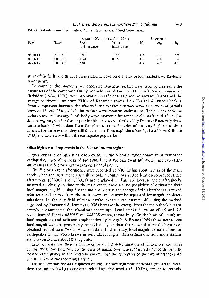
Fig. 15 is a log-log plot of seismic moment versus corner frequency summarizing the earthquake source parameters in Table 2. Lines of constant stress drop are shown for scaling purposes. Seismic moments spanning about four orders of magnitude were plotted in this figure. The larger estimations of moment, corresponding to earthquakes recorded by strong motion instruments, are plotted with some dispersion around the line of constant stress drop of l000bar. Data for the smaller earthquakes show a rapid decrease of stress drop as moment declines from about 1.0 x loz1 dyne cm to the lower values estimated in our study. Excluding the fact that our estimations of stress drop for the larger earthquakes were very high, the general trend shown by the data is similar to what has been reported for earthquakes in other regions, as summarized by Archuleta et al. (1982). Whether this characteristic behaviour is due to propagation effects or source effects cannot be explained with the present data set.

Seismic moments from surface waves and M,, mb magnitudes

Long-period seismograms from Pasadena (PAS), Goldstone (GSC) and Byerly (BKS) were used for determination of the seismic moment for the larger events. Events 2357,0030 and 1842 were large enough (ML =4.5-4.8) to produce clear surface waves at these stations. The epicentre-station distances are 354, 369 and 897 km for PAS, GSC and BKS, respectively. These stations cover only a small range of azimuth, approximately in the direction of the

2 3

7 2

- E

21 - r z Y

I 0 2

0 2 0

..c M a r c h , 1978 6 March 3, (977 \.. June 9 . 1980

I 2 5 10 20

C O R N E R F R E O U E N C Y ( H i 1

Figure 15. Graphical representation of the seismic source parameters given in Table 2. Lines indicating constant levels of stress drop are also shown.



ownloaded from


High stress drop events in northern Baja California 743 Table 3. Seismic moment estimations from surface waves and local body waves.

Moment Mo (dyne cm) (X 1 023)

surface waves body waves

March 1 1 23 : 57 1.93 1.09 4.8 4.7 3.9 March 12 00 : 30 0.58 0.95 4.5 4.4 3.4 March 12 1 8 : 4 2 2.86 4.8 4.1 4.1

Magnitude Date Time From From ML mb Ms

strike ofthe fault, and thus, at these stations, Love-wave energy predominated over Rayleigh- wave energy.

To computJe the moments, we generated synthetic surface-wave seismograms using the parameters of the composite fault plane solution of Fig. 3 and the surface-wave program of Harkrider (1964, 1970), with attenuation coefficients as given by Alewine (1974) and the average continental structure KHC2 of Kanamori (taken from Hartzell & Brune 1977). A direct comparison between the observed and synthetic surface-wave amplitudes at periods between 16 and 25 s yielded the surface-wave moment estimations. Table 3 has both the surface-wave and average local body-wave moments for events 2357, 0030 and 1842. The M, and mb magnitudes that appear in this table were calculated by Dr Peter Basham (private communication) with data from Canadian stations. In spite of the very high stress drop inferred for these events, they still discriminate from explosions (see fig. 16 of Nava & Brune 1983) and lie clearly within the earthquake population.

Other high stressdrop events in the Victoria swarm region

Further evidence of high stress-drop events in the Victoria region comes from four other earthquakes: two aftershocks of the 1980 June 9 Victoria event (ML =ti.]), and two earthquakes near the Victoria swarm area on 1977 March 3.

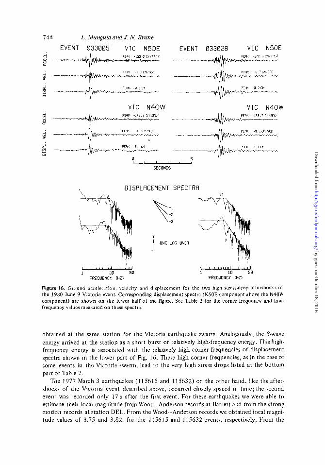
The Victoria event aftershocks were recorded at VIC within about 2 min of the main shock, when the instrument was still recording continuously. Acceleration records for these aftershocks (033005 and 033028) are displayed in Fig. 16. Because these aftershocks occurred so closely in time to the main event, there was no possibility of estimating their local magnitude, ML, using distant stations because the energy of the aftershocks is mixed with scattered energy from the main event and cannot be separated for magnitude determinations. In the near-field of these earthquakes we can estimate M t using the method suggested by Kanamori & Jennings (1978) because the energy from the main shock has not severely contaminated the aftershock recordings. Local amplitude values of 4.9 and 5.3 were obtained for the 033055 and 033028 events, respectively. On the basis of a study on local magnitude and sediment amplification by Munguia & Brune (1984) these near-source local magnitudes are presumably somewhat higher than the values that would have been obtained from distant Wood-Anderson data. In that study, local magnitude estimations for earthquakes in the Victoria swarm were always higher than estimations from more distant stations (on average about 0.5 log units).

Lack of data for these aftershocks prevented determination of epicentres and focal depths. We know, however, on the basis of similar S-P times measured on records for well- located earthquakes in the Victoria swarm, that the epicentres of the two aftershocks are within 10 km of the recording stations.

The acceleration records displayed on Fig. 16 show high peak horizontal ground accelerations (of up to 0.41 g) associated with high frequencies (5-lOHz), similar to records.



ownloaded from


744 L . Mungufa and J. N. Brune

E V E N T 033005 V I C N50E E V E N T 033028 V I C N50E PEAK -130 0 CWSECZ J

W u u a

PEAK fi 7 C W S E C J w w

V I C N 4 0 W V I C N 4 0 W PERK 385 7 C W S F L ~ J w u u U

PFRK 3 7 CWSFC J w >

J a Cn 0

PFQK a C i l PERK 0 3 C M w

0 5

SECONDS * a * > . ,

D I S P L A C E M E N T SPECTRA

- I -2 -3

T I ONE LOG U N I T - 1 10 50

FREOUENCY (HZ1

Figure 16. Ground acceleration, velocity and displacement for the two high stress-drop aftershocks of the 1980 June 9 Victoria event. Corresponding displacement spectra (N50E component above the N40W component) are shown on the lower half of the figure. See Table 2 for the corner frequency and low- frequency values measured o n these spectra.

obtained at the same station for the Victoria earthquake swarm. Analogously, the S-wave energy arrived at the station as a short burst of relatively high-frequency energy. This high- frequency energy is associated with the relatively high corner frequencies of displacement spectra shown in the lower part of Fig. 16. These high corner frequencies, as in the case of some events in the Victoria swarm, lead to the very high stress drops listed at the bottom part of Table 2.

The 1977 March 3 earthquakes (115615 and 115632) on the other hand, like the aftershocks of the Victoria event described above, occurred closely spaced in time; the second event was recorded only 17 s after the first event. For these earthquakes we were able to estimate their local magnitude from Wood-Anderson records at Barrett and from the strong motion records at station DEL. From the Wood-Anderson records we obtained local magnitude values of 3.75 and 3.82, for the 11 561 5 and 11 5632 events, respectively. From the



ownloaded from



EVENT 115615 DEL S45W EVENT 115632 DEL S45W PERK: 155.3 CWSEC2

PERK: -3.0CM/SEC PERK: q.BCN/SEC

PERK - 0 . l C M +- DEL S45E DEL S45E

PERK. -25Y.fi CWSEC2

PERK: -q.8CM/SEC PERK. -6.2 CM/SEC

PERK. 0 . 2 C M PERK. 5 . 3 C l i

0 5

SECONDS & 1

Figure 17. Ground acceleration, velocity and displacement records for the 1977 March 3 Victoria events (ML = 3.7, 3.8). Notice the strong similarity that exists between corresponding components of motion, as well as a delay of the S-wave packet from one horizontal component to the other.

strong motion data the estimated magnitudes are larger, 4.93 and 5.11 for the first and second events, respectively, almost the same as for the Victoria event aftershocks described above.

A combination of DEL strong motion data and P-wave readings and polarities from southern California stations allowed estimation of a preliminary epicentre and fault plane solution for these earthquakes. The calculated epicentre has been represented in Fig. 2 by an asterisk; the lower-hemisphere equal-area projection prepared with available P-wave first motion data, although not very well constrained by data, was very similar to the mechanism determined for earthquakes in the Victoria swarm and is not shown here.

The analogue acceleration records available for the study of these earthquakes were pro- cessed in the same way as for the Victoria swarm events. Fig. 17 shows the two horizontal components of corrected ground motion for each earthquake. The first feature to be noticed from these records is the strong similarity that exists between corresponding components of motion. This is evidence that both earthquakes occurred at nearly the same place and with approximately the same source mechanism. The second notable feature is that the S-wave energy packets appear to be delayed on one horizontal component relative to the other by about 0.5 s. This is a feature that we first observed on OLA and DEL records for earthquakes in the Victoria swarm. Finally, we notice that on the 1977 March strong motion records the strong surface-reflected S-phase observed on DEL records for the 1978 March earthquakes is not present, possibly because the depth and/or epicentral distance was different.

Source parameters for these earthquakes were calculated as before, and once again the calculated stress drops were of the order of a kilobar (bottom part of Table 2 and Fig. 15). Thus with respect to frequency content, pulse shape, and inferred stress drop, these earthquakes, like the Victoria event aftershocks, are quite similar to the Victoria swarm events.



ownloaded from


746

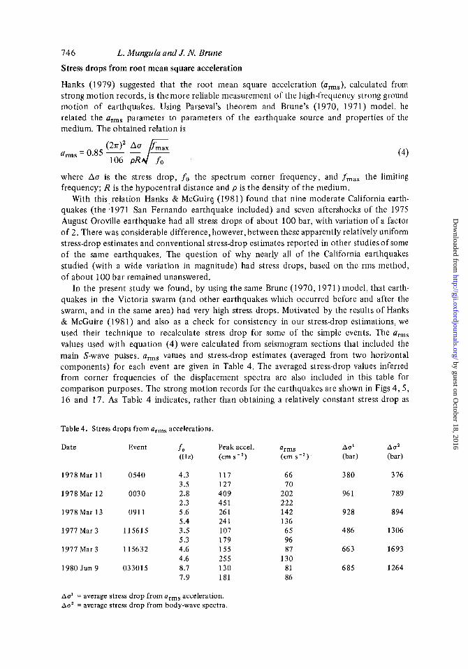
Stress drops from root mean square acceleration

Hanks (1 979) suggested that the root mean square acceleration (ams), calculated from strong motion records, is the more reliable measurement of the high-frequency strong ground motion of earthquakes. Using Parseval’s theorem and Brune’s (1970, 1971) model, he related the ams parameter to parameters of the earthquake source and properties of the medium. The obtained relation is

L. Munguta and J. N. Brune

(4)

where Aa is the stress drop, fo the spectrum corner frequency, and f,, the limiting frequency; R is the hypocentral distance and p is the density of the medium.

With this relation Hanks & McGuirS (1981) found that nine moderate California earthquakes (the 1971 San Fernando earthquake included) and seven aftershocks of the 1975 August Oroville earthquake had all stress drops of about 100 bar, with variation of a factor of 2. There was considerable difference, however, between these apparently relatively uniform stress-drop estimates and conventional stress-drop estimates reported in other studies of some of the same earthquakes. The question of why nearly all of the California earthquakes studied (with a wide variation in magnitude) had stress drops, based on the rms method, of about 100 bar remained unanswered.

In the present study we found, by using the same Brune (1970,1971) model, that earthquakes in the Victoria swarm (and other earthquakes which occurred before and after the swarm, and in the same area) had very high stress drops. Motivated by the results of Hanks & McGuire (1981) and also as a check for consistency in our stress-drop estimations, we used their technique to recalculate stress drop for some of the simple events. The urns values used with equation (4) were calculated from seismogram sections that included the main S-wave pulses. arms values and stress-drop estimates (averaged from two horizontal components) for each event are given in Table 4. The averaged stress-drop values inferred from corner frequencies of the displacement spectra are also included in this table for comparison purposes. The strong motion records for the earthquakes are shown in Figs 4 ,5 , 16 and 17. As Table 4 indicates, rather than obtaining a relatively constant stress drop as

Table 4. Stress drops from arms accelerations.

Date Event fo Peak accel. arms A d A d (H 2) (cm s - * ) (cm s- ’ ) (bar) (bar)

1978Mar 11 0540 4.3 3.5

1978Mar 12 003 0 2.8 2.3

1978Mar 13 091 1 5.6 5.4

1977 Mar 3 115615 3.5 5.3

1977 Mar 3 115632 4.6 4.6

1980 Jun 9 033015 8.7 7.9

117 127 409 451 26 1 24 1 107 179 155 255 130 181

66 380 3 76 70

202 96 1 7 89 222 142 928 894 136 65 4 86 1306 96 87 663 1693

130 81 685 1264 86

A d = average stress drop from arms acceleration. A d = average stress drop from body-wave spectra.



ownloaded from



found by Hanks & McGuire, we obtained values which vary considerably from one event to the other, consistent with the observed large variations in the recorded ground accelerations. These arms stress-drop values agree better with stress-drop values from body-wave spectra than with hypothetical constant 100 bar stress-drop value. This seems reasonable, given that Brune’s (1970) model plays a major role in both estimation methods. In stress-drop determinations using the Brune (1970, 1971) model, the two parameters usually used are the moment and corner frequency, whereas in Hanks’ proposed use of the model, the rms acceleration over a time period close to the reciprocal of the corner frequency is used. Thus in the first application of the model, the results are predominantly controlled by energy at frequencies near and lower than the corner frequency, whereas in Hanks’ rms application of the model the results are predominantly controlled by energy at frequencies higher than the corner frequency. If the spectra have a shape like the simple shape of the model, both for frequencies below and above the corner frequency, both applications should give similar results. This appears to be approximately the case for the events we have used for comparison here.

Stress drops from distant station data

In preceding sections of this paper we have shown that the larger earthquakes in the 1978 Victoria swarm, as well as the two aftershocks of the 1980 Victoria earthquake and the 1977 Victoria events, were events of very high stress drops. This is important in view of the fact that previous results obtained from analyses of distant station data (A > 100 km) indicated very low stress drops for earthquakes of similar and larger sizes in the northern Baja California and Gulf of California regions (Thatcher 1972; Thatcher &Hanks 1973;also low apparent stresses found by Wyss & Brune 1971). In these previous investigations stress drops of less than 10 bar were reported for events in the Gulf of California region while values of up to around lOObar were determined for earthquakes in northern Baja California. The earthquakes studied here are located in the region where, based on previous results, we would have expected low stress drops, since they occurred in a region considered the land- ward continuation of the Gulf of California to the north - the Mexicali Valley. It is there- fore important to understand why our near-source estimations differ so drastically from previous estimations for earthquakes of the same region, especially since both the near- and large-distance estimates of stress drop under discussion were obtained by interpreting the seismic spectrum in terms of the same model (Brune 1970, 1971). As an attempt to understand this, we studied the spectral shape for two earthquakes in the Victoria swarm region at distances comparable to the distances used in previous studies. One of the earthquakes considered is the event 2357 (ML = 4.8) in the Victoria earthquake swarm, for which strong motion records and corresponding displacement spectra are given in Figs 6 and 12, respectively. Wood-Anderson seismograms with signals of good quality for digitization purposes were recorded for this event at station PAS, at a distance of 354 kni from the source.

Digitized horizontal components of motion from PAS are shown in the left half of Fig. 18, along with displacement spectra calculated from the record windows indicated by the bar between the records. These spectra were corrected for instrument response and attenuation (Q = 250). For comparison purposes the spectra calculated from the strong motion records for this earthquake at stations DEL and VIC are also shown in this figure. The VIC and PAS spectra were reduced to the distance to station DEL.

In using the PAS spectra to calculate the source parameters for this event, we adopted the formulation and material propertiesused by Thatcher & Hanks (1973) and obtained a seismic moment of 2.35 x dyne cm (average of the two components), a value which is in good agreement with the moment obtained from surface-wave analysis, and within a factor of



ownloaded from


748 2

- 1 U W

5 0 - W

U 3 - 1 * - - a E Q - 2

- 1

L. Munguia and J. A! Brune

\ - 3

1 - l

0s 10 10

F r e q u e n c y ( H z I J

E V E N T 2 3 5 7

W - A R E C O R D S A T P A S ( 3 5 4 k m )

I

~ P A S D E L

01 1.0 10

F r e q u e n c y ( H z )

1 1

i U 0 ' 03 , /I'

T i m e ( s e c )

Figure 18. Comparison of spectra from near-source and distant station data for the 1978 March 11 (23 : 57 GMT, M L = 4.8) Victoria swarm earthquake (left) and the 1980 June 9 (23 : 33 GMT,ML = 4.3) Victoria aftershock (right). These 1978 and 1980 spectra were normalized to distances of 19 and 13 km, respectively (distances to station DEL). The horizontal dashed line drawn with the 1978 spectra indicates the low-frequency level inferred from analyses of surface-wave data. Wood-Anderson records at Pasadena (PAS) for the 1978 earthquake are also shown.

about 2 of the value inferred from the Victoria strong motion records (Table 3). However, the corner frequencies inferred from the Pasadena records are considerably lower than the ones observed on the near-source spectra and, as a result, the stress drop inferred from these records (- 8 bar) is about two orders of magnitude lower than the value obtained from the strong motion data (1200 bar). It is important to notice that the inferred stress drop from the Pasadena records falls within the range of values reported by Thatcher &Hanks (1973) for this region.

A similar discrepancy between near-source and distant spectral corner frequencies is shown on the right part of Fig. 18. In this case the compared data were recorded at stations DEL and PAS for an aftershock (at 23:33, June 9 , ML =4.3) of the 1980 Victoria earthquake.



ownloaded from


High stress drop events in northern Baja California 749 Distances to DEL and PAS, from a preliminary epicentre, were 1.25 and 340 km, respectively. As in the case of the Victoria swarm event, there is a marked difference between the corner frequencies on near-source and large-distance spectra. Such pronounced differences, if characteristic of other earthquakes of the region, cast doubt on the low stress drop determinations of Thatcher & Hanks for this region and suggest that scattering and attenuation (or some other mechanism) have severely distorted the spectra at Pasadena to give the low results. In the case of the two earthquakes considered here the paths (Victoria-Pasadena) have traversed the boundary between two radically different geological regions, the Salton Trough-Mexicali Valley and the granitic Peninsular Ranges. Thus it might be expected that high-frequency energy would be attenuated and scattered along this path with consequent severe distortion of the spectral shape. The effect of this would produce unreliable estimates of stress drop. It is important, however, to bear in mind that in the case of low stress-drop events in th,e region (i.e. low near-source corner frequencies), the effect of high-frequency attenuation at PAS would not have an effect as drastic on the inferred stress drop as for the two events shown here (which have very high near-source corner frequency) and thus, estimations of stress drop from Wood-Anderson records at PAS (for lower corner frequency earthquakes) would be less in error.

A serious limitation of the analysis presented in this section, however, has been the in- sufficient number of well-recorded events at both close-in and large-distance stations. No doubt when more records for earthquakes in the region studied at present become available, a more detailed study aimed at understanding the near-source and distant station spectral corner frequency discrepancy observed here would be of considerable interest.

Discussion and conclusions

The Victoria swarm earthquakes occurred at depths of between 8 and 16km with most events having their sources at depth of around 12 km as determined from good quality near- source data. These focal depths are rather large, when compared to estimation of depths for earthquakes in the Imperial Valley (4-9 km, Johnson & Hadley 1976; Boore & Fletcher 1983), but are similar t o focal depths estimated for some recent earthquakes located farther from the spreading centres (e.g. the 1979 Imperial Valley event, H = 10 km, Chavez et al. 1982; the 1980 Victoria event,H= 12 km, Frez 1982; the 1976 Mesa de Andrade events,H= 10 km, Nava & Brune 1983). Focal depth determinations for other swarms and background seismicity, indicate that within the Cerro Prieto spreading centre region, small earthquakes may occur as shallow as 2 km (Reyes 1979; Majer et al. 1978). From aftershock studies, it has also been found that the earthquake depth limit increases with distance from the ends of the transform faults (Wong & Frez 1982, for example). On this basis, it appears that the seismogenic zone near the middle sections of both the Cerro Prieto and Imperial faults extends deeper than it does near the ends of either fault (i.e. near the spreading centre), probably a result of cooler temperatures prevailing away from the crustal spreading zones. This might also be the reason that the larger earthquakes in the region apparently occur mainly along the middle sections of these transform faults (since the vertical dimension available for rupture is greater there). The change in the stress field produced by the larger earthquakes apparently causes triggering of smaller earthquakes in the adjacent higher tem- perature and highly fractured zones of crustal extension, e.g. the 1980 Victoria event and the 1979 Imperial Valley events in which the aftershock activity concentrated toward the ends of the Cerro Prieto and Imperial faults respectively.

Perhaps the most important result of our study is the observation that high irequencies and high accelerations are commonly observed on strong motion records for relatively small



ownloaded from


750

events ( M < 5). These seismogram characteristics are rather surprising in view of the thick sedimentary structure that overlays the basement in which the earthquakes occurred. The high-frequency content and high accelerations imply that attenuation of the medium did not play a major role in reducing the high-frequency energy radiated at the source. Sedimentary amplification was a major factor contributing to the large recorded peak accelerations (a factor of - 3). A theoretical amplification factor of about 3.4 was estimated on the basis of an l l k m thick section derived from the crustal velocity model of the Imperial Valley proposed by McMechan & Mooney (1980). It might be inferred, then, that if these earthquakes had occurred in a region with hard rock extending to the surface the ground motion would have been considerably smaller.

We obtained displacement spectra with relatively high corner frequencies, which when interpreted in terms of Brune’s (1970, 1971) model, resulted in very high estimations of stress drop (of the order of kilobars for some events). Although there is no known reason why such anomalously high stress-drop e;ents should occur in this region, the understanding of such events is crucial to understanding earthquake hazard, strong motion and source mechanism. As a check on these high estimates of stress drop, we used the rms acceleration formulation introduced by Hanks (1979) to recalculate this source parameter for a few of the simplest events. The stress-drop values calculated using this rms acceleration method were in good agreement with the high values obtained using the displacement spectra and corner frequency method.

Evidence of similar high stress-drop events in other regions is becoming increasingly common as more near-source earthquake data sets accumulate (e.g. House & Boatwright 1980; Fletcher, Brady & Hanks 1980; Hartzell & Brune 1977, and McGarr 1981 among others). The stress drops estimated here for the larger earthquakes considered were much higher (over 2 orders of magnitude) than results obtained earlier for earthquakes of the region by Thatcher (1 972) and Thatcher & Hanks (1973) using more distant Wood-Anderson records. A plausible explanation for this apparent discrepancy is that attenuation and scattering have severely distorted the distant station Wood-Anderson spectra making them unreliable for the determination of source parameters. For the events we compared, displacement spectra calculated from stations at these larger distances showed corner frequencies significantly lower than those measured on near-source displacement spectra for the same earthquakes. Although we compared spectra for only two earthquakes, the discrepancy in the corner frequency was observed consistently on all components of motion analysed. Thus we conclude that distant station recordings ( A > 100km) such as some used by Thatcher (1972) and Thatcher & Hanks (1973) are unreliable for estimating stress drops and peak accelerations in this region.

The Victoria swarm earthquakes, as well as the other four earthquakes studied here are important because they contribute to increasing evidence that, under certain circumstances, factors like high stress drop, low attenuation, scattering, and anomalous sediment amplification of motion, can combine to produce very high ground accelerations in the near-field of small earthquakes. This is a fundamentally important observation for strong motion seismology, independent of any interpretation in terms of a source model.


Acknowledgments

We would like to acknowledge the assistance and cooperation during the field work of Frank Vernon, Alejandro Nava, Alfonso Re yes, Javier Gonzalez and several students at CICESE. We wish to express our thanks to Jorge Prince and Enrique Mena from the Institute of Engineering, UNAM for providing us with the digitized acceleration data, and to Alfonso



ownloaded from



Reyes for providing us with the smoked paper data and some preliminary epicentre data for earthquakes in the Cerro Prieto-Imperial faults. We also thank P. W. Basham, who sent us the magnitudes for some of the Victoria swarm events. Special thanks are due to Rich Simons for his valuable contribution in the preparation of the digital data, and to Shelley Marquez for typing the manuscript and Ruth Zdvorak for drafting some of the figures.

This research was supported by the National Council of Science and Technology of Mexico (CONACYT) and the National Science Foundation Grant CEE 81 -200096.

References

Albores, A.. Reyes, A., Brune, J. N., Gonzalez, J., Garcilazo, L. & Saurez, F., 1978. Seismicity studies of the Cerro Prieto Geothermal Field, Proc. 1st Symp. Cerro Prieto Geothermal Field.

Alewine, R. W., J 974. Application of linear inversion theory toward the estimation of seismic source parameters, PhD thesis, California Institute of Technology, Pasadena.

Archuleta, R. J., Cranswick, E., Mueller, C. H. & Spudich, P., 1982. Source parameters of the 1980 Mammoth Lakes, California, earthquake sequence,J. geophys. Res., 87,4595-4607.

Biehler, S., Kovach, R. L. & Allen, C. R., 1964. Geophysical framework of northern end of Gulf of Cali- fornia structural province, Mem. Am. Ass. Petrol. Geol., 3 , 126-143.

Boore, D. M. & Fletcher, J. B., 1983. A preliminary study of selected aftershocks of the 1979 Imperial Valley earthquake from digital acceleration and velocity recordings, in The Imperial Valley, Cali- fornia, Earthquake of October 15, 1979, Prof Pap. U S . geol. Surv. 109-118, United States Geological Survey, Menlo Park, California.

Brune, J. N., 1970. Tectonic stress and the spectra of seismic shear waves from earthquakes, J. geophys. Res., 75,4997-5009.

Brune, J. N., 1971. Correction, J. geophys. Res., 76, 5002. Brune, J. N., Prince, J . , Vernon, F., Mena, E. & Simons, R., 1983. Strong motion data recorded in Mexico

during the October 15 main shock, in The Imperial Valley, California, Earthquake of October 15, 1979, Pro5 Pap. 1254, U.S. geol. Sum., United States Geological Survey, Menlo Park, California.

Brune, J. N., Simons, R. A,, Vernon, F., Canales, L. & Reyes, A., 1980. Digital seismic event recorders: description and examples from the San Jacinto fault, the Imperial fault, the Cerro Prieto fault, and the Oaxaca, Mexico subduction fault, Bull, seism. SOC. Am., 70, 1395-1408.

Buland, R., 1976. The mechanics of locating earthquakes, Bull. seism. SOC. Am., 66, 173-1 87. Chavez, D., Gonzalez, J . , Reyes, A., Medina, M., Duarte, C., Brune, J. N., Vernon, F., Simons, R., Hutton,

L. K., German, P. T. & Johnson, C. E., 1982. Main-shock location and magnitude determination using combined US . and Mexican data, in The Imperial Valley, California, Earthquake of October IS, 1979, Prof. Pap, 1254, US. geol. Surv. 51-54, United States Geological Survey, Menlo Park, California.

Fletcher, J. B., Brady, A. G . & Hanks, T. C., 1980. Strong motion accelerograms of the Oroville, Calif- fornia aftershock: data processing and the aftershocks of 0350 August 6, 1975, Bull. seism. SOC. Am., 70,243-267.

Frez, J . , 1982. Main shock location and fault mechanism, in The Mexicali Valley Earthquake of9 June 1980, eds Anderson, J. G. & Simons, R. S . , Earthq. Engrg. Res. Inst. Newsl. 16,74-76.

Geller, R. J. & Mueller, C. S., 1980. Four similar earthquakes in Central California, Geophys. Res. Lett., 7,821-824.

Hanks, T. C., 1979. b values and w-Y seismic source models: implications for tectonic stress variations along active crustal fault zones and the estimation of high-frequency strong ground motion, J. geophys. Res., 84,2235-2242.

Hanks, T. C. & McGuire, R. K., 1981. The character of high-frequency strong ground motion, Bull. seism. SOC. Am., 71,2071-2095.

Harkrider, D. G., 1964. Surface waves in multilayered elastic media. Part I. Rayleigh and Love waves from buried sources in a multilayered elastic halfspace, Bull. seism. SOC. Am., 54, 627-679.

Harkrider, D. G., 1970. Surface waves in multilayered elastic media. Part 11. Higher mode spectra and spectral ratios from point sources in plain layered earth models,BuZZ. seism. Soc. Am., 60, 1937- 1987.

Hartzell, S. H. & Brune, J . N., 1977. Source parameters for the January 1975 Brawley-Imperial Valley earthquake swarm, Pageoph., 115,333-355.



ownloaded from


752

House, L. & Boatwright, J., 1980. Investigation of two high stress drop earthquakes in the Shumagin seismic gap, Alaska, J. geophys. Rex, 85, 7151-7165.

Johnson, D. E. & Hadley, D. M., 1976. Tectonic implications of the Brawley earthquake swarm, Imperial Valley, California, January 1975, Bull. seism. SOC. Am., 66, 1133-1 144.

Johnson, T. L., Madrid, J. & Koczynski, T., 1976. A study of microseismicity in northern Baja California, Mexico, Bull. seism. SOC. Am., 66, 1921-1929.

Kanamori, H. & Jennings, P. C., 1978. Determination of local magnitude, M L , from strong motion accelerograms, Bull. seism. SOC. Am., 68, 47 1-485.

Kaufman, K. & Burdick, L. J., 1980. The reproducing earthquakes of the Galapagos Islands, Bull. seisrn. SOC. Am., 70,1759-1 770.

Lee, W. H. & Lahr, J. C., 1975. HYPO? I : a computer program for determining hypocentre, magnitude and first motion pattern of local earthquakes, Open-File Rep. U S . geol, Surv., 75 -3 11, 113 pp.

Lomnitz, C., Mooser, F., Allen, C., Brune, J. N. & Thatcher, W., 1970. Seismicity and tectonics of the northern Gulf of California region, Mexico, preliminary results, Geofis. int. LO, 3 1-48.

Majer, E. L., McEvilly, T. V., Albores, A. & Diaz, S., 1978. Seismological studies at Cerro Prieto, Proc. First Symp. Cerro Prieto Geothermal Field, September 20-22, San Diego, California, pp. 239- 245.

McCarr, A., 1981. Analysis of peak ground motion in terms of a model of inhomogenous faulting, J. geophys. Res., 86,3901-3912.

McMechan, G. A. & Mooney, W. D., 1980. Asymptotic ray theory and synthetic seismograms for laterally varying structures: theory and application to the Imperial Valley, California, Bull. seism. SOC. Am., 70,2021-2035.

Munguia, L. & Brune, J. N., 1984. Local magnitude and sediment amplification observations from earthquakes in the northern Baja California-southern California region, Bull. seism. SOC. Am. , 74, 107-119.

Nava, F. A. & Brune, J. N., 1983. Source mechanism and surface wave excitation for two earthquakes in northern Baja California, Mexico, Geophys. J. R . astr. Soc., 13, 739-763.

Pechmann, J. C. & Kanamori, H., 1982. Waveforms and spectra of preshocks and aftershocks of the 1979 Imperial Valley, California earthquake: evidence for fault heterogeneity?, J. geophys. Res., 87, 10 579-10 597.

Prince, J., Brune, J. N., Reyes, A. & Nava, A., 1977. Strong motion instrumentation of northern Baja California, 72nd Annual Meeting Seismological Society of America, Sacramento, California, April 5-7.

Puente, I. & de la Pena, A., 1978. Geologia del Campo Geotdrmico de Cerro Prieto, Proc. 1st Symp. Cerro Prieto Geothermal Field, pp. 17-40, Baja California, Mexico.

Rebollar, C. J . , 1982. Earthquake source parameter estimates using limited digital seismic data, PhD thesis, University of Alberta, Edmonton, Canada.

Reyes, A., 1979. Estudio de microsismicidad del sistema de fallas transformadas Imperial-Cerro Prieto, Znforme T&cnico GEO79-01, Centro de Investigacidn Cientffica y Educacidn Superior de Ensenada, Baja California, Mexico.

Reyes, A. J., Brune, T., Barkcr, L., Canalcs, J., Madrid, J., Rebllar, C. J . & Munguia, L., 1Y75. A micro- earthquake survey of the San Miguel fault zone, Baja California, Mexico, Geophys. Res. Lett., 2, 56-59.

Singh, S. K., Apsel, R. J., Fried, J. & Brune, J. N., 1982. Spectral attenuation of SH-waves along the Imperial fault, Bull. seism. Soc. Am., 72, 2003-2016.

Thatcher, W., 1972. Regional variation of seismic source parameters in the northern Baja California area, J. geophys. Res., 77, 1549-1565.

Thatcher, W. & Hanks, T. C., 1973. Source parameters of southern California earthquakes, J. geophys. Res., 78, 8547-8576.

Tucker, B. E. & Brune, J. N., 1977. Source mechanism and mb-Ms analysis of aftershocks of the San Fernando earthquake, Geophys. J. R . astr. Soc., 49,371-426.

Wong, V. & Frez, J . , 1982. Aftershock locations and fault mechanisms, in The Mexicali Earthquake of June 1980, eds Anderson, J . G . & Simons, R. S., Earthq. Engrg. Res. Znst. Newsl., 16, 76-79.

Wyss, M. & Brune, J . N., 1971. Regional variations of source properties in southern California estimated from the ratio of short-to-long-period amplitudes, Bull. seism. SOC. Am., 61, 11 53-1 167.

L. Munguiu and J. N. Brune



ownloaded from


High stress drop events in the Victoria, Baja California earthquake swarm of 1978 March

Documents

Transcript of High stress drop events in the Victoria, Baja California earthquake swarm of 1978 March