Co-Movements of Oil, Gold, the US Dollar, and Stocks

Modern Economy, 2012, 3, 111-117 doi:10.4236/me.2012.31015 Published Online January 2012 (http://www.SciRP.org/journal/me)

111

Co-Movements of Oil, Gold, the US Dollar, and Stocks*

Subarna K. Samanta1, Ali H. M. Zadeh2 1School of Business, The College of New Jersey, Ewing, USA

2Department of Management, Susquehanna University, Selinsgrove, USA Email: [email protected], [email protected]

Received October 26, 2011; revised November 28, 2011; accepted December 19, 2011

ABSTRACT

This paper examines the co-movements of several macro-variables in the world economy over a period of more than twenty years. Long-term co movements are examined by tracking the cointegration, common trend factor and the spill- er index over these variables (gold price, stock price, real exchange rate for dollar and the oil price of crude oil). Pre- minary examination suggests the possibility of cointegration among these variables indicating co-movements, although the spillover indices are found to be very small. Keywords: Stationarity; VARMA; Common Trends; Co-Integration; Granger Causality; Volatility; Spillover Index

1. Introduction

The financial markets are getting more integrated and co- ovements in financial markets (i.e., interdependence of equity markets of several countries), as well as financial indexes (i.e., interdependence of asset returns and return volatilities in different markets) have become of im- mense interest to financial analysts and portfolio mana- gers. For example, high volatility of oil prices and their exorbitant increase in prices sometimes have serious impact on other macroeconomic economic variables and policy makers and business in oil consuming countries express serious concerns about it. Several researchers (for example, Johnson and Soenen (2002) [1], King et al. (1994) [2], Ewing et al. (1997) [3], and Forbes and Ri- gobon (2002) [4], Engsted and Tanggaard (2007) [5], and Anderson et al. (2007) [6], and others such as Salman (2008) [7], Sester (2008) [8], Vergeler (2008) [9] & Yue- Jun (2008) [10]) have analyzed different aspects of this interdependence among the macroeconomic variables over the recent years. Most of the studies have used co- integration and error correction modeling techniques to isolate and identify the long-run equilibrium relationships among these variables. These studies are an important addition to our understanding of the co-movements of these variables and allow us to make appropriate prediction about the future co-movements.

Recently, Diebold and Yilmaz (2009) [11] have used a simple but different technique to capture the so-called spil-

lover effects or the interdependence among the economic variables using the forecast error variance decomposition methodology. They have noted that spillover effects are time varying and the nature of the spillover indices de- pend on the measurement standards used. Understanding these relationships is important for the portfolio investors who want to diversify their investment opportunities and policy makers pursuing stabilization of the economy.

In this paper, we will use these techniques of esti- mating the spillover mechanism developed by Diebold and Yilmaz to analyze the interdependence of returns and volatilities of four important macro-variables: These are gold prices, exchange rates for dollar as dollar is the international reserve currency, price of oil, and the stock prices as measured by Dow Jones Industrial Average. We intend to examine to what extent these variables are interrelated, and whether returns/volatilities of one index can predict movements in other indexes. We intend to examine the behavior of both returns and return volatilities of the aforementioned indexes using measures of return spillovers and volatility spillovers. We also want to examine the recently observed inverse relationship (re- verse causality) between the US dollar and oil prices. While previous studies show that after 1973 oil prices and the value of the US dollar have moved in the same direction (i.e., increase in oil prices have led to the US dollar appreciation), the examination of the recently observed inverse relationship is certainly of interest.

In addition, we also want to explore the statistical properties of these variables using vector autoregressive moving average procedure or models. This procedure can be used to analyze the contemporaneous correlations as well as correlations to each other’s past values.

*Initial draft of this paper was presented at the annual meeting of the 71st

International Atlantic Economic Conference, Athens, Greece, 16-19 Mar-ch 2011. Authors acknowledge the important comments by the discus-sants of the session and the chair of the session at the conference, and the comments received from the referees of this journal. However, all re-maining errors and omissions are authors’ responsibility.

Copyright © 2012 SciRes. ME

S. K. SAMANTA ET AL. 112

We plan to use daily data for several years and employ the appropriate econometric techniques to identify and extricate new information regarding the relationship among these variables. Data was collected on the daily price of NYMEX crude oil futures, and the US Dollar Index (DXY), price of gold and DJ index (see references # [12- 14]). The data was obtained from a Bloomberg terminal using daily closing prices from January 1989 through September 2009 with more than 5200 observations. It is quite apparent that appropriate inferences from this statistical study will enhance our understanding about the co- movement of such important economic variables.

2. Model

This study analyzes the relationships or the co-movements among return and return volatilities of four major indexes (i.e., gold prices, real exchange rates for dollar, price of oil, and the stock prices as measured by Dow Jones Industrial Average) and examines the behavior of these indices using the vector auto-regression method and by spillover index discussed by Diebold and Yilmaz (2009) [11]. This is a brief summary of the modeling process.

Let yt = (y1t, y2t, , ykt)’ where t = 1, 2, 3, , denote a k dimensional time series vector of random variable of interest denoted by y. The p-th order VAR (or the VARMA model) can be written as

t 1 t 1 p t pY y y t (1)

where εt is a vector of white noise process with εt = (ε1t, ε2t, , εkt)’ with properties: E(εt) = 0, E(εt, εt’) = ∑ a non negative matrix, and E(εt, εs’) = 0 for t ≠ s, α = (α1, , αk)’ is a constant, and φi is a k × k matrix of parameters. It is well known that a finite autoregressive process can be represented by an infinite moving average process as follows,

t 0 t 1 t 1 2 t 2Y , (2)

where β is a vector of constant and νt is a transformation of εt, and θi is a matrix of constants. It should be pointed out that VARMA models may not be uniquely defined or identified, which requires structural specifications. How- ever, analyzing and modeling the series jointly by the VARMA models enables us to understand the dynamic relationships among the series over time, and it also allows us to make improvements on the forecasting of these variables. Typical analysis based on VARMA procedure provides us with various tests of the long-run effects and adjustments of coefficients among the variables included in the model. We will consider the traditional tests such as the Dicky-Fuller test for stationarity, Johansen co-integration test, and the Stock-Watson common trend test for the possibility of co-integration among nonstationary vector processes among others. Stock-Watson (1988) [15] proposed a method for testing the common trend among k dimensional time series. The null hypothesis is that the

vector time series Yt has m common trends where m ≤ k and the alternative is that it has s common trend where s < m. The test procedure and the test statistics is com- puted from first order serial correlation matrix of Yt.

Next we will examine the spillover index developed by Diebold and Yilmaz (2009) [11]. They have shown that the one step ahead forecast error vector can be written as

t 1,t t 1 t 1,t 0 t 1,e y y A u (3)

where A0 is a matrix of parameters, and the covariance matrix for the forecast error can be written as A0A0’. They have analyzed the forecast error variance decomposition to compute the spillover index, since the forecast error variance decomposition reveals the proportion of the movements of a variable due to its own shocks versus shocks due to other variables. Diebold and Yilmaz estimated the spillover effect and calculating the spillover ratio (index) by combining the cross variances relative to total forecast error variations. In particular, total spillover effect is defined as the sum of cross covariances, while the total forecast error variation is represented by the trace of the matrix A0A0’. For a 2 by 2 matrix A0A0’ the Spillover Index can written as {(a0,12

2 + a0,212)/trace(A0A0’)} × 100.

This can be generalized for higher order A0A0’ matrix re- flecting more than one step-ahead forecast.

3. Data

Data for this empirical investigation was collected on the daily price of NYMEX crude oil futures and the US Dol- lar Index (USDX). To further the study data was also collected on the price of gold and Dow-Jones Industrial Ave- rage. The data was obtained from a Bloomberg terminal using daily closing prices from January 1989 through September 2009. It has more than 5200 observations. Ty- pically, an index shows a change in an economy or secu- rities market through statistical analysis. A futures contract is an agreement made on the floor of a futures exchange to buy or sell a commodity or financial instru- ment at a predetermined price. When you purchase a futures contract you are agreeing to pay the pre-determined price for future delivery. When you purchase the contract, the item for future delivery has not yet been produced.

The US dollar Index: The US dollar index is a calculation of six currencies that have been averaged against the US dollar (it was created by the US Federal Reserve following the Bretton Woods agreement1). The US Dollar

1The US Dollar Index, as explained by ICE futures, was created as a way to provide external bilateral trade weighted average of the US dollar as it freely floated against global currencies. The formula for the calculation of the US dollar Index is 50.14348112 multiplied by the product of all com-ponents raised to an exponent equal to the % weighting ((EURUSD^ –0.576) × (JPY^ –0.136) × (GBP^ –0.119) × (CAN^ –0.091) × (SEK^ –0.042) × (CHF^ –0.036)). All currencies are expressed in units of currency per U.S. dollar (ICE, 2009), and currency weights are Euro (57.6%), Canadian dollar (9.1%), Japanese yen (13.6%), Swedish krona (4.2%), British pound (11.9%), and Swiss franc (3.6%).


S. K. SAMANTA ET AL.


113

Index contains six component currencies: the French fr- ank, Japanese yen, British pound, Canadian dollar, Swe- dish krona and Swiss franc. It was listed on November 20th 1985 as futures contract.

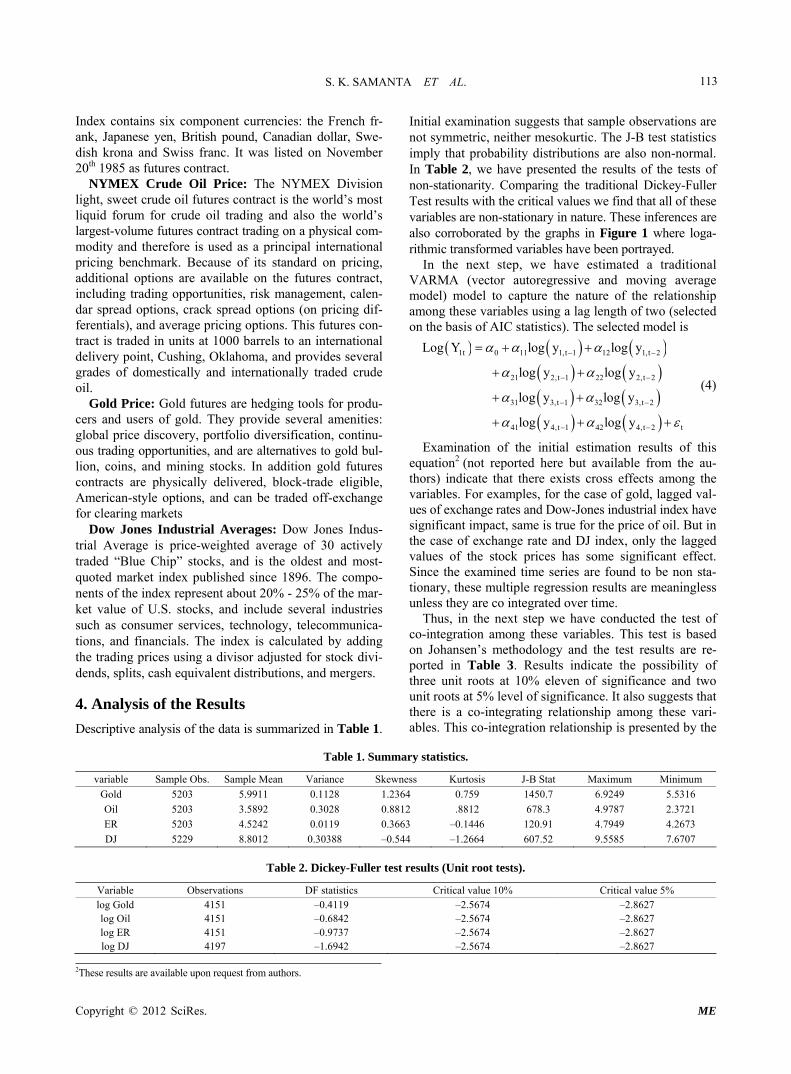
Initial examination suggests that sample observations are not symmetric, neither mesokurtic. The J-B test statistics imply that probability distributions are also non-normal. In Table 2, we have presented the results of the tests of non-stationarity. Comparing the traditional Dickey-Fuller Test results with the critical values we find that all of these variables are non-stationary in nature. These inferences are also corroborated by the graphs in Figure 1 where logarithmic transformed variables have been portrayed.

NYMEX Crude Oil Price: The NYMEX Division light, sweet crude oil futures contract is the world’s most liquid forum for crude oil trading and also the world’s largest-volume futures contract trading on a physical commodity and therefore is used as a principal international pricing benchmark. Because of its standard on pricing, additional options are available on the futures contract, including trading opportunities, risk management, calen- dar spread options, crack spread options (on pricing dif- ferentials), and average pricing options. This futures contract is traded in units at 1000 barrels to an international delivery point, Cushing, Oklahoma, and provides several grades of domestically and internationally traded crude oil.

In the next step, we have estimated a traditional VARMA (vector autoregressive and moving average model) model to capture the nature of the relationship among these variables using a lag length of two (selected on the basis of AIC statistics). The selected model is

1t 0 11 1,t 1 12 1,t 2

21 2,t 1 22 2,t 2

31 3,t 1 32 3,t 2

41 4,t 1 42 4,t 2 t

Log Y log y log y

log y log y

log y log y

log y log y

(4) Gold Price: Gold futures are hedging tools for produ-

cers and users of gold. They provide several amenities: global price discovery, portfolio diversification, continu- ous trading opportunities, and are alternatives to gold bul- lion, coins, and mining stocks. In addition gold futures contracts are physically delivered, block-trade eligible, American-style options, and can be traded off-exchange for clearing markets

Examination of the initial estimation results of this equation2 (not reported here but available from the authors) indicate that there exists cross effects among the variables. For examples, for the case of gold, lagged values of exchange rates and Dow-Jones industrial index have significant impact, same is true for the price of oil. But in the case of exchange rate and DJ index, only the lagged values of the stock prices has some significant effect. Since the examined time series are found to be non stationary, these multiple regression results are meaningless unless they are co integrated over time.

Dow Jones Industrial Averages: Dow Jones Indus- trial Average is price-weighted average of 30 actively traded “Blue Chip” stocks, and is the oldest and most- quoted market index published since 1896. The compo- nents of the index represent about 20% - 25% of the market value of U.S. stocks, and include several industries such as consumer services, technology, telecommunica- tions, and financials. The index is calculated by adding the trading prices using a divisor adjusted for stock divi- dends, splits, cash equivalent distributions, and mergers.

Thus, in the next step we have conducted the test of co-integration among these variables. This test is based on Johansen’s methodology and the test results are reported in Table 3. Results indicate the possibility of three unit roots at 10% eleven of significance and two unit roots at 5% level of significance. It also suggests that there is a co-integrating relationship among these variables. This co-integration relationship is presented by the

4. Analysis of the Results

Descriptive analysis of the data is summarized in Table 1.

Table 1. Summary statistics.

variable Sample Obs. Sample Mean Variance Skewness Kurtosis J-B Stat Maximum Minimum

Gold 5203 5.9911 0.1128 1.2364 0.759 1450.7 6.9249 5.5316

Oil 5203 3.5892 0.3028 0.8812 .8812 678.3 4.9787 2.3721

ER 5203 4.5242 0.0119 0.3663 –0.1446 120.91 4.7949 4.2673

DJ 5229 8.8012 0.30388 –0.544 –1.2664 607.52 9.5585 7.6707

Table 2. Dickey-Fuller test results (Unit root tests).

Variable Observations DF statistics Critical value 10% Critical value 5% log Gold 4151 –0.4119 –2.5674 –2.8627 log Oil 4151 –0.6842 –2.5674 –2.8627 log ER 4151 –0.9737 –2.5674 –2.8627 log DJ 4197 –1.6942 –2.5674 –2.8627

2These results are available upon request from authors.


log of gold prices

1989 1991 1993 1995 1997 1999 2001 2003 2005 2007 20095.50

5.75

6.00

6.25

6.50

6.75

7.00

log of exchange rates

1989 1991 1993 1995 1997 1999 2001 2003 2005 2007 20094.2

4.3

4.4

4.5

4.6

4.7

4.8

log of DJ index

1989 1991 1993 1995 1997 1999 2001 2003 2005 2007 20097.50

8.00

8.50

9.00

9.50

log of oil prices

1989 1991 1993 1995 1997 1999 2001 2003 2005 2007 20092.0

2.5

3.0

3.5

4.0

4.5

5.0

Figure 1. Logarithmic transformed variables

Table 3. Test for Co-integration: l (1)-ANALYSIS (using CATS).

p-r r Eig. Value Trace Trace* Frac95 p-Value p-Value*

4 0 0.224 48.779 45.745 40.095 0.003 0.001

3 1 0.196 31.780 30.975 34.214 0.0723 0.088

2 2 0.082 14.940 12.401 18.81 0.155 0.26

1 3 0.006 8.298 7.262 11.28 0.816 8.890

*(possibility of three unit roots of 10% level and two unit roots at 5% level). traditional error correction models and statistical results are reported in Tables 4 to 7. But the error correction re-sults are mixed. We notice that error correction terms are significant in the case of variables exchange rates and DJ

industrial index. Error correction terms are not statistically significant for gold price and oil price. Thus, there is some ambiguity regarding these error correction results. But, this co-integration is further corroborated by the Stock-



Table 4. VAR/System—Estimation by co-integrated least square.

Variable Coeff Std Error t-Stat Significance

1. D log Gold (t – 1) –0.037825 0.015577 –2.42824 0.01521 2. D log Gold (t – 2) –0.030153 0.015572 –1.93640 0.05287 3. D log Oil (t – 1) 0.005655 0.005959 0.94903 0.34266 4. D log Oil (t – 2) 0.003938 0.006083 0.64735 0.51744 5. D log ER (t – 1) –0.091889 0.028425 –3.23262 0.00124 6. D log ER (t – 2) 0.022052 0.028442 –0.77532 0.43819 7. D log DJ (t – 1) –0.031623 0.046651 –0.67781 0.49793 8. D log DJ (t – 2) 0.007852 0.046345 0.16942 0.86547 9. EC1 (t – 1) –0.000117 0.000146 –0.80296 0.42204

Dependent variable: log Gold; Durbin-Watson statistic 1.9726.

Table 5. Dependent variable log Oil.

Variable Coeff Std Error T-Stat Significance

1. D log Gold (t – 1) –0.008301 0.039109 –0.21225 0.83192 2. D log Gold (t – 2) 0.019459 0.039096 0.49774 0.61868 3. D log Oil (t – 1) –0.010667 0.014961 –0.71299 0.47588 4. D log Oil (t – 2) –0.037673 0.015273 –2.46664 0.01367 5. D log ER (t – 1) 0.108702 0.071366 1.52317 0.12778 6. D log ER (t – 2) 0.021502 0.071409 0.30111 0.76335 7. D log DJ (t – 1) –0.231436 0.117135 –1.97581 0.04824 8. D log DJ (t – 2) 0.083188 0.116355 0.71495 0.47468 9. EC1 (t – 1) 0.000479 0.000366 1.30880 0.19067

Durbin-Watson statistic 2.0168.

Table 6. Dependent variable log ER.


1. D log Gold (t – 1) –0.007115 0.008432 –0.84385 0.398797 2. D log Gold (t – 2) –0.011392 0.008429 –1.35157 0.176579 3. D log Oil (t – 1) –0.004221 0.003225 –1.30857 0.190746 4. D log Oil (t – 2) 0.002005 0.003293 0.60898 0.542569 5. D log ER (t – 1) –0.006237 0.015386 –0.40540 0.685198 6. D log ER (t – 2) 0.001706 0.015395 0.11080 0.911783 7. D log DJ (t – 1) –0.019836 0.025253 –0.78551 0.432195 8. D log DJ (t – 2) 0.023086 0.025085 0.92032 0.357451 9. EC1 (t-1) .0000155 0.000079 1.96779 0.049152


Table 7. Dependent variable log DJ.


1. D log Gold (t – 1) –0.021493 0.017485 –1.22928 0.219031 2. D log Gold (t – 2) –0.002457 0.017479 –0.14062 0.888176 3. D log Oil (t – 1) –0.011120 0.006688 –1.66253 0.096474 4. D log Oil (t – 2) –0.001885 0.006828 –0.27607 0.782506 5. D log ER (t – 1) 0.012159 0.031906 0.38109 0.703156 6. D log ER (t – 2) –0.003422 0.031925 –0.10718 0.914648 7. D log DJ (t – 1) 0.013559 0.052368 0.25893 0.795700 8. D log DJ (t – 2) –0.043411 0.052019 –0.83453 0.404027 9. EC1 (t – 1) 0.000351 0.000163 2.14517 0.031991


Watson’s common trend test given in Table 8 where sin- gle common trend appears to exist. The estimate of the

long-run relationship is given below (with t-stat in the pa- rentheses):

l og GOLD 11.5144 0.3783log Oil 1.3845log ER 0.007602log DJ (105.69) (61.39) (–54.89) (–11.22) (5)



Table 9. Granger-Causality wald test. It unambiguously indicates the existence of co integra-

tion among the variables and consequent volatility spillover.

Next, we have also used the Granger causality tests to analyze the nature of relationship among these variables. The causality test results are reported in Table 9. These statistical results imply the existence of causality from stock price and gold price to other variables (oil price and exchange rates) while they are not influenced by them. Thus, Gold price and Stock prices are influenced by themselves only. On the other hand Oil prices and Ex- change rates are caused by other variables as well. This obviously implies the existence of causality among the variables and existence of volatility transmission or spillover between financial markets and stock markets but with asymmetric relationships.

Table 8. Testing for Stock-Watson’s common trends using differencing filter.

Ho: Rank = m

H1: Rank = s

Eigen value Filter 5% Critical

value Lag

1 0 1.000460 2.40 –14.10 2

2 0 1

1.000405 0.997896

2.11 –24.95

–8.80 –23.00

Test DF Chi-Square Pr > Chi-Sq

1 3 3.97 0.2646

2 3 10.84 0.0126 3 3 9.53 0.0230

4 3 4.22 0.2383

Test 1: log Gold causes the other variables (log OIL, log ER, log DJ); but the other variables do not cause log Gold, i.e. log Gold is influenced by itself; Test 2: log Oil is caused by the other variables (log Gold, log ER, log DJ); but the other variables are not caused by the log Oil; Test 3: log ER is casued by the other variables (log GOLD, log OIL, log DJ); but the other variables are not caused by the log ER; Test 4: log DJ causes the other variables (log Gold, log OIL, log ER, log DJ); but the other variables do not cause log DJ, i.e. log DJ is influenced by itself.

In the next two Tables, (Tables 10 and 11) we have

presented the specific spillover index following Diebold and Yilmaz methodology. In Table 10, we have presented the spillover index based on one-step ahead forecast and in Table 11; the two-step ahead forecast results are reported. Apparently for one-step ahead forecast, spillover index is very little, even less than one percent. How- ever, for the two-step ahead forecast it is about 6%, im- plying the possibility of larger spillover for longer forecasting horizon. It should be pointed out that we have analyzed the data taking logarithmic transformation only. We have not considered the rate of change of the variables; in that case we may obtain different results.

Table 10. Spillover table (one-step forecast).

To Gold Oil ER DJ From others

Gold 99.996 0.00 0.001 0.003 0.004

Oil 0.014 98.53 1.45 0.00 1.46

ER 0.005 0.001 99.42 0.0 0.006

DJ 0.00 0.001 0.001 99.998 0.002

Contribution to Others 0.019 0.002 1.452 0.003 Spillover index

Contribution Including own 100.1 99.538 100.87 100.001 0.737%

Table 11. Spillover table (two-step forecast).

To Gold Oil ER DJ From others

Gold 99.89 0.01 0.05 0.035 .095 Oil 3.75 96.16 0.02 0.025 3.795 ER 8.86 0.061 90.82 0.24 9.161 DJ 0.601 0.032 0.059 99.35 0.692

Contribution to Others 13.211 0.103 0.129 0.3 Spillover index Contribution Including own 113.101 96.263 90.94 99.65 6.86%

5. Conclusion

This paper conducts an investigation about the co-movements of several economic variables over a period of time. These variables are: World Gold price, World Oil price, US Stock price (measured by Dow-Jones Industrial Index) and real exchange rate for US dollar. Using daily data for over twenty years (considering logarithmic trans-

formation only), it examines the existence of co-integration, common trend, Granger causality and volatility spillover for these macro variables. Initial statistical results indicate the possible existence of co-movements among them however, not all of them are moving simul- taneously. It seems likely that stock price and gold price are more likely to move on their own while oil price and exchange rates likely to be influenced by other variables.



REFERENCES [1] R. A. Amano and S. Van Norden, “Oil Prices and the

Rise and Fall of the U.S. Real Exchange Rate,” Journal of International Money and Finance, Vol. 17, No. 2, 1998, pp. 299-316. doi:10.1016/S0261-5606(98)00004-7

[2] A. Bénassy-Quéré, V. Mignon and A. Penot, “China and the Relationship between the Oil Price and the Dollar,” Energy Policy, Vol. 35, No. 11, 2007, pp. 5785-5905.

[3] M. Chinn and L. Johnston, “Real Exchange Rate Levels, Productivity and Demand Shocks: Evidence from a Panel of 14 Countries,” IMF Working Paper, Washington DC, 1997.

[4] A. Coull, “Trading Oil Price Chart—USD,” Master the Markets, Oil. http://www.trading-oil.org/oil-price-chart-usd/

[5] P. H. Gray, “Dollar Depreciation and the Price of Gaso- line,” International Trade, Vol. 12, No. 1 1998, pp. 119- 128. doi:10.1080/08853909808523900

[6] K. Lien, “Is the US Dollar Driving Oil…or Vice Versa?” Home Trading Commodities, Futures, & Forex Article. 20 May 2009. http://www.moneyshow.com

[7] R. Salman, “The US Dollar and Oil Pricing Revisited,” 2004.http://www.mees.com/postedarticles/oped/a47n01d02.htm.

[8] B. W. Setser, “Understanding the Correlation between Oil

Prices and the Falling Dollar,” Council on Foreign Rela- tions, 18 June 2008. http://www.cfr.org

[9] P. K. Verleger Jr., “The Oil-Dollar Link,” International Economy, Vol. 22, No. 2, 2008, pp. 46-50.

[10] Y.-J. Zhang, et al., “Spillover Effect of US Dollar Ex- change Rate on Oil Prices,” Journal of Policy Modeling Vol. 30, No. 6, 2008, pp. 973-991. doi:10.1016/j.jpolmod.2008.02.002

[11] Light Sweet Crude Oil, 2008. http://www.nymex.com/lsco_fut_descri.aspx

[12] US Commodity Fututes Trading Commision. Rep. Inter- agency Task Force on Commodity Markets, July 2008. http://www.cftc.gov/ucm/groups/public/@newsroom/documents/file/itfinterimreportoncrudeoil0708

[13] U.S. Dollar Index Futures, ICE Futures US. ICE, Jan. 2009. https://www.theice.com/publicdocs/nybot/ICE_Dollar_Index_FAQ.pdf>.

[14] Science Direct. 14 Feb. 2008. http://www.sciencedirect.com/science?_ob=ArticleURL&_udi=B6V82-4RV17FD

[15] Roach, Stephen, “US Dollar—Oil Correlation Unveiled,” 2008. http://www.dailyfx.com/story/other/free_third_party_research/US_Dollar___Oil_Correlation_1219674072277.html


http://dx.doi.org/10.1016/S0261-5606(98)00004-7

http://dx.doi.org/10.1080/08853909808523900

http://dx.doi.org/10.1016/j.jpolmod.2008.02.002

Copyright of Modern Economy is the property of Scientific Research Publishing and its content may not be

copied or emailed to multiple sites or posted to a listserv without the copyright holder's express written

permission. However, users may print, download, or email articles for individual use.

Co-Movements of Oil, Gold, the US Dollar, and Stocks

Documents

Transcript of Co-Movements of Oil, Gold, the US Dollar, and Stocks