CLOUD COMPUTING 2016 Proceedings - ThinkMind

CLOUD COMPUTING 2016

The Seventh International Conference on Cloud Computing, GRIDs, and

Virtualization

ISBN: 978-1-61208-460-2

March 20 - 24, 2016

Rome, Italy

CLOUD COMPUTING 2016 Editors

Carlos Becker Westphall, Federal University of Santa Catarina, Brazil

Yong Woo Lee, University of Seoul, Korea

Stefan Rass, Universitaet Klagenfurt, Institute of Applied Informatics, Austria

1 / 157


Forward

The Seventh International Conference on Cloud Computing, GRIDs, and Virtualization (CLOUDCOMPUTING 2016), held between March 20-24, 2016 in Rome, Italy, continued a series ofevents targeted to prospect the applications supported by the new paradigm and validate thetechniques and the mechanisms. A complementary target was to identify the open issues andthe challenges to fix them, especially on security, privacy, and inter- and intra-clouds protocols.

Cloud computing is a normal evolution of distributed computing combined with Service-oriented architecture, leveraging most of the GRID features and Virtualization merits. Thetechnology foundations for cloud computing led to a new approach of reusing what wasachieved in GRID computing with support from virtualization.

The conference had the following tracks:

Cloud computing

Computing in virtualization-based environments

Platforms, infrastructures and applications

Challenging features

Similar to the previous edition, this event attracted excellent contributions and activeparticipation from all over the world. We were very pleased to receive top qualitycontributions.

We take here the opportunity to warmly thank all the members of the CLOUD COMPUTING2016 technical program committee, as well as the numerous reviewers. The creation of such ahigh quality conference program would not have been possible without their involvement. Wealso kindly thank all the authors that dedicated much of their time and effort to contribute toCLOUD COMPUTING 2016. We truly believe that, thanks to all these efforts, the finalconference program consisted of top quality contributions.

Also, this event could not have been a reality without the support of many individuals,organizations and sponsors. We also gratefully thank the members of the CLOUD COMPUTING2016 organizing committee for their help in handling the logistics and for their work that madethis professional meeting a success.

We hope that CLOUD COMPUTING 2016 was a successful international forum for the exchangeof ideas and results between academia and industry and to promote further progress in thearea of cloud computing, GRIDs and virtualization. We also hope that Rome provided a pleasant

2 / 157

environment during the conference and everyone saved some time for exploring this beautifulcity.

CLOUD COMPUTING 2016 Chairs

CLOUD COMPUTING 2016 Advisory Chairs

Jaime Lloret Mauri, Polytechnic University of Valencia, SpainWolf Zimmermann, Martin-Luther University Halle-Wittenberg, GermanyYong Woo Lee, University of Seoul, KoreaAlain April, École de Technologie Supérieure - Montreal, CanadaChristoph Reich, Furtwangen University, Germany

CLOUD COMPUTING 2016 Industry/Research Chairs

Wolfgang Gentzsch, The UberCloud, GermanyTony Shan, Keane Inc., USAAnna Schwanengel, Siemens AG, GermanyAtsuji Sekiguchi, Fujitsu Laboratories Ltd., Japan

COULD COMPUTING 2016 Special Area Chairs

SecurityChih-Cheng Hung, Southern Polytechnic State University - Marietta, USA

GRIDJorge Ejarque, Barcelona Supercomputing Center, SpainJavier Diaz-Montes, Rutgers University, USANam Beng Tan, Nanyang Polytechnic, Singapore

Autonomic computingIvan Rodero, Rutgers the State University of New Jersey/NSF Center for Autonomic Computing,USAHong Zhu, Oxford Brookes University, UK

Service-orientedQi Yu, Rochester Institute of Technology, USA

PlatformsArden Agopyan, ClouadArena, Turkey

3 / 157


Committee

CLOUD COMPUTING Advisory Committee

Jaime Lloret Mauri, Polytechnic University of Valencia, SpainWolf Zimmermann, Martin-Luther University Halle-Wittenberg, GermanyYong Woo Lee, University of Seoul, KoreaAlain April, École de Technologie Supérieure - Montreal, CanadaChristoph Reich, Furtwangen University, Germany

CLOUD COMPUTING 2016 Industry/Research Chairs

Wolfgang Gentzsch, The UberCloud, GermanyTony Shan, Keane Inc., USAAnna Schwanengel, Siemens AG, GermanyAtsuji Sekiguchi, Fujitsu Laboratories Ltd., Japan

COULD COMPUTING 2016 Special Area Chairs

SecurityChih-Cheng Hung, Southern Polytechnic State University - Marietta, USA

GRIDJorge Ejarque, Barcelona Supercomputing Center, SpainJavier Diaz-Montes, Rutgers University, USANam Beng Tan, Nanyang Polytechnic, Singapore

Autonomic computingIvan Rodero, Rutgers the State University of New Jersey/NSF Center for Autonomic Computing, USAHong Zhu, Oxford Brookes University, UK

Service-orientedQi Yu, Rochester Institute of Technology, USA

PlatformsArden Agopyan, ClouadArena, Turkey

CLOUD COMPUTING 2016 Technical Program Committee

Jemal Abawajy, Deakin University - Victoria, AustraliaImad Abbadi, University of Oxford, UKTaher M. Ali, Gulf University for Science & Technology, Kuwait

4 / 157

Abdulelah Alwabel, University of Southampton, UKAlain April, École de Technologie Supérieure - Montreal, CanadaAlvaro E. Arenas, Instituto de Empresa Business School, SpainJosé Enrique Armendáriz-Iñigo, Public University of Navarre, SpainIrina Astrova, Tallinn University of Technology, EstoniaBenjamin Aziz, University of Portsmouth, UKXiaoying Bai, Tsinghua University, ChinaPanagiotis Bamidis, Aristotle University of Thessaloniki, GreeceAli Kashif Bashir, Osaka University, JapanLuis Eduardo Bautista Villalpando, Autonomous University of Aguascalientes, MexicoCarlos Becker Westphall, Federal University of Santa Catarina, BrazilAli Beklen, CloudArena, TurkeyElhadj Benkhelifa, Staffordshire University, UKAndreas Berl, Deggendorf Institute of Technology, GermanySimona Bernardi, Centro Universitario de la Defensa / Academia General Militar - Zaragoza, SpainNik Bessis, University of Derby, UKPeter Charles Bloodsworth, National University of Sciences and Technology (NUST), PakistanAlexander Bolotov, University of Westminster, UKSara Bouchenak, University of Grenoble I, FranceWilliam Buchanan, Edinburgh Napier University, UKAli R. Butt, Virginia Tech, USAJames Byrne, Dublin City University, IrelandMassimo Cafaro, University of Salento, ItalyMustafa Canim, IBM Thomas J. Watson Research Center, USAMassimo Canonico, University of Piemonte Orientale, ItalyPaolo Campegiani, University of Rome Tor Vergata, ItalyJuan-Vicente Capella-Hernández, Universitat Politècnica de València, SpainCarmen Carrión Espinosa, Universidad de Castilla-La Mancha, SpainSimon Caton, Karlsruhe Institute of Technology, GermanyK. Chandrasekaran, National Institute of Technology Karnataka, IndiaHsi-Ya Chang, National Center for High-Performance Computing (NCHC), TaiwanRong N Chang, IBM T.J. Watson Research Center, USARuay-Shiung Chang, National Taipei University of Business, TaiwanKyle Chard, University of Chicago and Argonne National Laboratory, USAAntonin Chazalet, IT&Labs, FranceShiping Chen, CSIRO ICT Centre, AustraliaYe Chen, Microsoft Corp., USAYixin Chen, Washington University in St. Louis, USAZhixiong Chen, Mercy College - NY, USA

William Cheng-Chung Chu(朱正忠), Tunghai University, TaiwanYeh-Ching Chung, National Tsing Hua University, TaiwanMarcello Coppola, ST Microelectronics, FranceAntonio Corradi, Università di Bologna, ItalyMarcelo Corrales, University of Hanover, GermanyFabio M. Costa, Universidade Federal de Goias (UFG), BrazilSérgio A. A. de Freitas, Univerty of Brasilia, BrazilAnderson Santana de Oliveira, SAP Labs, FranceNoel De Palma, University Joseph Fourier, France

5 / 157

César A. F. De Rose, Catholic University of Rio Grande Sul (PUCRS), BrazilEliezer Dekel, IBM Research - Haifa, IsraelYuri Demchenko, University of Amsterdam, The NetherlandsNirmit Desai, IBM T J Watson Research Center, USAEdna Dias Canedo, Universidade de Brasília - UnB Gama, BrazilJavier Diaz-Montes, Rutgers University, USAZhihui Du, Tsinghua University, ChinaQiang Duan, Pennsylvania State University, USARobert Anderson Duncan, University of Aberdeen, UKJorge Ejarque Artigas , Barcelona Supercomputing Center, SpainKaoutar El Maghraoui, IBM T. J. Watson Research Center, USAAtilla Elçi, Suleyman Demirel University - Isparta, TurkeyKhalil El-Khatib, University of Ontario Institute of Technology - Oshawa, CanadaMohamed Eltoweissy, Virginia Military Institute and Virginia Tech, USAJavier Fabra, University of Zaragoza, SpainFairouz Fakhfakh, University of Sfax , TunisiaHamid Mohammadi Fard, University of Innsbuck, AustriaReza Farivar, University of Illinois at Urbana-Champaign, USAUmar Farooq, Amazon.com - Seattle, USAMaria Beatriz Felgar de Toledo, University of Campinas, BrazilLuca Ferretti, University of Modena and Reggio Emilia, ItalyLuca Foschini, Università degli Studi di Bologna, ItalySören Frey, Daimler TSS GmbH, GermanySong Fu, University of North Texas - Denton, USAMartin Gaedke, Technische Universität Chemnitz, GermanyWolfgang Gentzsch, The UberCloud, GermanyMichael Gerhards, FH-AACHEN - University of Applied Sciences, GermanyLee Gillam, University of Surrey, UKKatja Gilly, Miguel Hernandez University, SpainSpyridon V. Gogouvitis, Siemens AG, GermanyAbraham Gomez, École de technologie supérieure (ÉTS), Montreal, CanadaAndres Gomez, Applications and Projects Department Manager Fundación CESGA, SpainAndrzej M. Goscinski, Deakin University, AustraliaNils Grushka, NEC Laboratories Europe - Heidelberg, GermanyJordi Guitart, Universitat Politècnica de Catalunya - Barcelona Supercomputing Center, SpainMarjan Gusev, “Ss. Cyril and Methodius” University of Skopje, MacedoniaYi-Ke Guo, Imperial College London, UKMarjan Gushev, Univ. Sts Cyril and Methodius, MacedoniaThomas J. Hacker, Purdue University, USARui Han, Institute of Computing Technology - Chinese Academy of Sciences, ChinaWeili Han, Fudan University, ChinaHaiwu He, INRIA, FranceSergio Hernández, University of Zaragoza, SpainNeil Chue Hong, University of Edinburgh, UKPao-Ann Hsiung, National Chung Cheng University, TaiwanLei Huang, Prairie View A&M University, USAChih-Cheng Hung, Southern Polytechnic State University - Marietta, USARichard Hill, University of Derby, UK

6 / 157

Uwe Hohenstein, Siemens AG, GermanyLuigi Lo Iacono, Cologne University of Applied Sciences, GermanyShadi Ibrahim, INRIA Rennes - Bretagne Atlantique Research Center, FranceYoshiro Imai, Kagawa University, JapanAnca Daniela Ionita, University "Politehnica" of Bucharest, RomaniaXuxian Jiang, North Carolina State University, USAEugene John, The University of Texas at San Antonio, USACarlos Juiz, Universitat de les Illes Balears, SpainVerena Kantere, University of Geneva, SwitzerlandBill Karakostas, VLTN gcv, Antwerp, BelgiumSokratis K. Katsikas, University of Piraeus, GreeceTakis Katsoulakos, INLECOM Systems, UKZaheer Khan, University of the West of England, UKPrashant Khanna, JK Lakshmipat University, Jaipur, IndiaShinji Kikuchi, Fujitsu Laboratories Ltd., JapanPeter Kilpatrick, Queen's University Belfast, UKTan Kok Kiong, National University of Singapore, SingaporeWilliam Knottenbelt, Imperial College London - South Kensington Campus, UKSinan Kockara, University of Central Arkansas, USAJoanna Kolodziej, University of Bielsko-Biala, PolandKenji Kono, Keio University, JapanDimitri Konstantas, University of Geneva, SwitzerlandArne Koschel, Hochschule Hannover, GermanyGeorge Kousiouris, National Technical University of Athens, GreeceSotiris Koussouris, National Technical University of Athens, GreeceKenichi Kourai, Kyushu Institute of Technology, JapanNane Kratzke, Lübeck University of Applied Sciences, GermanyHeinz Kredel, Universität Mannheim, GermanyHans Günther Kruse, Universität Mannheim, GermanyYu Kuang, University of Nevada Las Vegas, USAAlex Kuo, University of Victoria, CanadaTobias Kurze, Karlsruher Institut für Technologie (KIT), GermanyDharmender Singh Kushwaha, Motilal Nehru National Institute of Technology - Allahabad, IndiaDimosthenis Kyriazis, University of Piraeus, GreeceGiuseppe La Torre, University of Catania, ItalyRomain Laborde, University Paul Sabatier, FrancePetros Lampsas, Central Greece University of Applied Sciences, GreeceErwin Laure, KTH, SwedenAlexander Lazovik, University of Groningen, The NetherlandsCraig Lee, The Aerospace Corporation, USAYong Woo Lee, University of Seoul. KoreaGrace Lewis, CMU Software Engineering Institute - Pittsburgh, USAJianxin Li, Beihang University, ChinaKuan-Ching Li, Providence University, TaiwanMaozhen Li, Brunel University - Uxbridge, UKDan Lin, Missouri University of Science and Technology, USAWei-Ming Lin, University of Texas at San Antonio, USAPanos Linos, Butler University, USA

7 / 157

Xiaoqing (Frank) Liu, Missouri University of Science and Technology, USAXiaodong Liu, Edinburgh Napier University, UKXumin Liu, Rochester Institute of Technology, USAThomas Loruenser, AIT Austrian Institute of Technology GmbH, AustriaH. Karen Lu, CISSP/Gemalto, Inc., USAGlenn R Luecke, Iowa State University, USAMon-Yen Luo, National Kaohsiung University of Applied Sciences, TaiwanIlias Maglogiannis, University of Central Greece - Lamia, GreeceRabi N. Mahapatra, Texas A&M University, USAShikharesh Majumdar, Carleton University, CanadaOlivier Markowitch, Universite Libre de Bruxelles, BelgiumMing Mao, University of Virginia, USAAttila Csaba Marosi, MTA SZTAKI Computer and Automation Research Institute/Hungarian Academy ofSciences - Budapest, HungaryKeith Martin, University of London Egham Hill, UKGregorio Martinez, University of Murcia, SpainGoran Martinovic, J.J. Strossmayer University of Osijek, CroatiaPhilippe Massonet, CETIC, BelgiumMichael Maurer, Vienna University of Technology, AustriaPer Håkon Meland, SINTEF ICT, NorwayJean-Marc Menaud, Mines Nantes, FranceAndreas Menychtas, National Technical University of Athens, GreeceJose Merseguer, Universidad de Zaragoza, SpainShigeru Miyake, Hitachi Ltd., JapanMohamed Mohamed, IBM US Almaden, USAOwen Molloy, National University of Ireland – Galway, IrelandPatrice Moreaux, LISTIC/Polytech Annecy-Chambéry, Université Savoie Mont Blanc, FrancePaolo Mori, Istituto di Informatica e Telematica (IIT) - Consiglio Nazionale delle Ricerche (CNR), ItalyClaude Moulin, Technology University of Compiègne, FranceFrancesc D. Muñoz-Escoí, Universitat Politècnica de València, SpainMasayuki Murata, Osaka University, JapanHidemoto Nakada, National Institute of Advanced Industrial Science and Technology (AIST), JapanRich Neill, Cablevision Systems, USASurya Nepal, CSIRO ICT Centre, AustraliaRodrigo Neves Calheiros, University of Melbourne, AustraliaToan Nguyen, INRIA, FranceBogdan Nicolae, IBM Research, IrelandAida Omerovic, SINTEF, NorwayAmmar Oulamara, University of Lorraine, FranceAlexander Paar, TWT GmbH Science and Innovation, GermanyClaus Pahl, Dublin City University, IrelandBrajendra Panda, University of Arkansas, USAMassimo Paolucci, DOCOMO Labs, ItalyAlexander Papaspyrou, Technische Universität Dortmund, GermanyValerio Pascucci, University of Utah, USADavid Paul, University of New England, AustraliaAl-Sakib Khan Pathan, International Islamic University Malaysia (IIUM), MalaysiaSiani Pearson, Hewlett-Packard Laboratories, USA

8 / 157

Antonio J. Peña, Barcelona Supercomputing Center, SpainGiovanna Petrone, University of Torino, ItalySabri Pllana, University of Vienna, AustriaAgostino Poggi, Università degli Studi di Parma, ItalyJari Porras, Lappeenranta University of Technology, FinlandThomas E. Potok, Oak Ridge National Laboratory, USAFrancesco Quaglia, Sapienza Univesita' di Roma, ItalyXinyu Que, IBM T.J. Watson Researcher Center, USAManuel Ramos Cabrer, University of Vigo, SpainRajendra K. Raj, Rochester Institute of Technology, USADanda B. Rawat, Georgia Southern University, USAChristoph Reich, Hochschule Furtwangen University, GermanyDolores Rexachs, University Autonoma of Barcelona (UAB), SpainSebastian Rieger, University of Applied Sciences Fulda, GermanySashko Ristov, “Ss. Cyril and Methodius” University of Skopje, MacedoniaNorbert Ritter, University of Hamburg, GermanyIvan Rodero, Rutgers University, USADaniel A. Rodríguez Silva, Galician Research and Development Center in Advanced Telecomunications"(GRADIANT), SpainPaolo Romano, Instituto Superior Técnico/INESC-ID Lisbon, PortugalThomas Rübsamen, Furtwangen University, GermanyHadi Salimi, Iran University of Science and Technology - Tehran, IranAltino Sampaio, Instituto Politécnico do Porto, PortugalIñigo San Aniceto Orbegozo, Universidad Complutense de Madrid, SpainElena Sanchez Nielsen, Universidad de La Laguna, SpainVolker Sander, FH Aachen University of Applied Sciences, GermanyGregor Schiele, Digital Enterprise Research Institute (DERI) at the National University of Ireland, Galway(NUIG), IrelandMichael Schumacher-Debril, Institut Informatique de Gestion - HES-SO, SwitzerlandWael Sellami, Faculty of Economic Sciences and Management of Sfax, TunisiaHermes Senger, Federal University of Sao Carlos, BrazilLarry Weidong Shi, University of Houston, USAAlan Sill, Texas Tech University, USAFernando Silva Parreiras, FUMEC University, BrazilLuca Silvestri, University of Rome "Tor Vergata", ItalyAlex Sim, Lawrence Berkeley National Laboratory, USALuca Spalazzi, Università Politecnica delle Marche - Ancona, ItalyGeorge Spanoudakis, City University London, UKRizou Stamatia, Singular Logic S.A., GreeceMarco Aurelio Stelmar Netto, IBM Research, BrazilHung-Min Sun, National Tsing Hua University, TaiwanYasuyuki Tahara, University of Electro-Communications, JapanDomenico Talia, DIMES - Unical, ItalyJie Tao, Steinbuch Centre for Computing/Karlsruhe Institute of Technology (KIT), GermanyJoe M. Tekli, Lebanese American University, LebanonOrazio Tomarchio, University of Catania, ItalyStefano Travelli, Entaksi Solutions Srl, ItalyParimala Thulasiraman, University of Manitoba, Canada

9 / 157

Ruppa Thulasiram, University of Manitoba, CanadaRaul Valin, Swansea University, UKCarlo Vallati, University of Pisa, ItalyGeoffroy R. Vallee, Oak Ridge National Laboratory, USALuis Miguel Vaquero-Gonzalez, Hewlett-Packard Labs Bristol, UKMichael Vassilakopoulos, University of Thessaly, GreeceJose Luis Vazquez-Poletti, Universidad Complutense de Madrid, SpainLuís Veiga, Instituto Superior Técnico - ULisboa / INESC-ID Lisboa, PortugalSalvatore Venticinque, Second University of Naples - Aversa, ItalyMario Jose Villamizar Cano, Universidad de loa Andes - Bogotá, ColombiaSalvatore Vitabile, University of Palermo, ItalyBruno Volckaert, Ghent University - iMinds, BelgiumsLizhe Wang, Center for Earth Observation & Digital Earth - Chinese Academy of Sciences, ChinaZhi Wang, Florida State University, USAMandy Weißbach, University of Halle, GermanyPhilipp Wieder, Gesellschaft fuer wissenschaftliche Datenverarbeitung mbH - Goettingen (GWDG),GermanyJohn Williams, Massachusetts Institute of Technology, USAPeter Wong, SDL Fredhopper, NetherlandsChristos Xenakis, University of Piraeus, GreeceHiroshi Yamada, Tokyo University of Agriculture and Technology, JapanChao-Tung Yang, Tunghai University, Taiwan R.O.C.Hongji Yang, De Montfort University (DMU) - Leicester, UKYanjiang Yang, Institute for Infocomm Research, SingaporeUstun Yildiz, University of California, USAQi Yu, Rochester Institute of Technology, USAJong P. Yoon, Mercy College - Dobbs Ferry, USAJie Yu, National University of Defense Technology (NUDT), ChinaZe Yu, University of Florida, USAMassimo Villari, University of Messina, ItalyVadim Zaliva, Tristero Consulting / Carnegie Mellon University (CMU), USAJosé Luis Zechinelli Martini, Fundación Universidad de las Américas, Puebla (UDLAP), MexicoBaokang Zhao, National University of Defence Technology, ChinaXinghui Zhao, Washington State University Vancouver, CanadaZibin Zheng, Sun Yat-sen University, ChinaJingyu Zhou, Shanghai Jiao Tong University, ChinaHong Zhu, Oxford Brookes University, UKWolf Zimmermann, University of Halle, Germany

10 / 157

Copyright Information

For your reference, this is the text governing the copyright release for material published by IARIA.

The copyright release is a transfer of publication rights, which allows IARIA and its partners to drive the

dissemination of the published material. This allows IARIA to give articles increased visibility via

distribution, inclusion in libraries, and arrangements for submission to indexes.

I, the undersigned, declare that the article is original, and that I represent the authors of this article in

the copyright release matters. If this work has been done as work-for-hire, I have obtained all necessary

clearances to execute a copyright release. I hereby irrevocably transfer exclusive copyright for this

material to IARIA. I give IARIA permission or reproduce the work in any media format such as, but not

limited to, print, digital, or electronic. I give IARIA permission to distribute the materials without

restriction to any institutions or individuals. I give IARIA permission to submit the work for inclusion in

article repositories as IARIA sees fit.

I, the undersigned, declare that to the best of my knowledge, the article is does not contain libelous or

otherwise unlawful contents or invading the right of privacy or infringing on a proprietary right.

Following the copyright release, any circulated version of the article must bear the copyright notice and

any header and footer information that IARIA applies to the published article.

IARIA grants royalty-free permission to the authors to disseminate the work, under the above

provisions, for any academic, commercial, or industrial use. IARIA grants royalty-free permission to any

individuals or institutions to make the article available electronically, online, or in print.

IARIA acknowledges that rights to any algorithm, process, procedure, apparatus, or articles of

manufacture remain with the authors and their employers.

I, the undersigned, understand that IARIA will not be liable, in contract, tort (including, without

limitation, negligence), pre-contract or other representations (other than fraudulent

misrepresentations) or otherwise in connection with the publication of my work.

Exception to the above is made for work-for-hire performed while employed by the government. In that

case, copyright to the material remains with the said government. The rightful owners (authors and

government entity) grant unlimited and unrestricted permission to IARIA, IARIA's contractors, and

IARIA's partners to further distribute the work.

11 / 157

Table of Contents

Impact of Cloud Computing on Enhancing the Use of Renewable EnergyKwa-Sur Tam

1

Towards Using Homomorphic Encryption for Cryptographic Access Control in Outsourced Data ProcessingStefan Rass and Peter Schartner

7

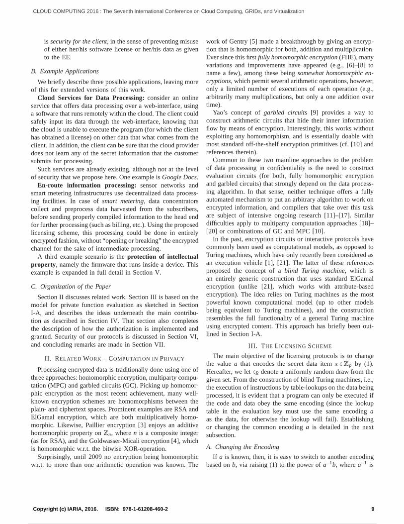
Data Center Network Structure Using Hybrid Optoelectronic RoutersYuichi Ohsita and Masayuki Murata

14

The Impact of Public Cloud Price Schemes on Multi-TenancyUwe Hohenstein and Stefan Appel

22

A Novel Framework for Simulating Computing Infrastructure and Network Data Flows Targeted on CloudComputingPeter Krauss, Tobias Kurze, Achim Streit, and Bernhard Neumair

30

Overcome Vendor Lock-In by Integrating Already Available Container Technologies - Towards Transferability inCloud Computing for SMEsPeter-Christian Quint and Nane Kratzke

38

Cloud Data Denormalization of Anonymous TransactionsAspen Olmsted and Gayathri Santhanakrishnan

42

Modeling Non-Functional Requirements in Cloud Hosted Application Software EngineeringSantoshi Devata and Aspen Olmsted

47

Enabling Resource Scheduling in Cloud Distributed Videoconferencing SystemsAlvaro Alonso, Pedro Rodriguez, Ignacio Aguado, and Joaquin Salvachua

51

Energy Saving in Data Center Servers Using Optimal Scheduling to Ensure QoSConor McBay, Gerard Parr, and Sally McClean

57

Model Driven Framework for the Configuration and the Deployment of Applications in the CloudHiba Alili, Rim Drira, and Henda Hajjami ben ghezala

61

Modeling Workflow of Tasks and Task Interaction Graphs to Schedule on the CloudMahmoud Naghibzadeh

69

Instruments for Cloud Suppliers to Accelerate their BusinessesFred Kessler, Stella Gatziu Grivas, and Claudio Giovanoli

76

1 / 2 12 / 157

How to Synchronize Large-Scale Ultra-Fine-Grained Processors in Optimum-TimeHiroshi Umeo

81

Dynamic Power Simulator Utilizing Computational Fluid Dynamics and Machine Learning for Proposing TaskAllocation in a Data CenterKazumasa Kitada, Yutaka Nakamura, Kazuhiro Matsuda, and Morito Matsuoka

87

Analysis of Virtual Networking Options for Securing Virtual MachinesRamaswamy Chandramouli

95

Profiling and Predicting Task Execution Time Variation of Consolidated Virtual MachinesMaruf Ahmed and Albert Y. Zomaya

103

Data Locality via Coordinated Caching for Distributed ProcessingMax Fischer and Eileen Kuehn

113

Enhancing Cloud Security and Privacy: The Cloud Audit ProblemBob Duncan and Mark Whittington

119

Enhancing Cloud Security and Privacy: The Power and the Weakness of the Audit TrailBob Duncan and Mark Whittington

125

Online Traffic Classification Based on Swarm IntelligenceTakumi Sue, Yuichi Ohsita, and Masayuki Murata

131

Comparing Replication Strategies for Financial Data on Openstack based Private CloudDeepak Bajpai and Ruppa K. Thulasiram

139

Powered by TCPDF (www.tcpdf.org)

2 / 2 13 / 157

Impact of Cloud Computing on Enhancing the Use of Renewable Energy

Kwa-Sur Tam

Department of Electrical & Computer Engineering

Virginia Tech

Blacksburg, Virginia, U.S.A.

Email: [email protected]

Abstract — Renewable energy has been identified as one of the

disruptive technologies that have the potential for massive

impact on the society for the coming years. A major concern

for using renewable energy such as solar photovoltaics and

wind is its variable nature. The importance of this concern is

increasing in recent years as the penetration levels of

renewable energy have been increasing rapidly in the electric

power grids worldwide. Forecasting is a major tool that can be

used to address the variable nature of renewable energy.

Cloud Computing provides the enabling technology to handle

the complexity of renewable energy forecasting and can

enhance more widespread and more effective utilization of

renewable energy. This paper presents the new applications of

using Cloud Computing to enhance the use of renewable

energy through the achievement of two goals. The first goal is

to present a Cloud Computing-enabled renewable energy

forecasting system--the FaaS (Forecast-as-a-Service)

framework--to demonstrate the technical feasibility. Based on

the service-oriented architecture (SOA), the FaaS has been

successful in generating user-specified solar or wind forecast

on demand and at reasonable costs. Using the FaaS as the

starting point, the second goal of this paper is to present from a

broader perspective the potential impact of Cloud Computing

on the use of renewable energy. Cloud Computing, coupled

with other technology trends, supports the development of new

applications and business models that could flourish the

renewable energy industry.

Keywords – Cloud Computing; services; service-oriented

architecture; forecasting; renewable energy; cyberinfrastructure.

I. INTRODUCTION

Providing almost unlimited computing resources on a pay-per-use basis, Cloud Computing provides new options for data-intensive and computation-intensive applications. Cloud computing not only makes possible the completion of complex computational tasks within shorter time frames but also enables such capabilities to be available at affordable costs. This paper describes the impact of Cloud Computing on the use of renewable energy.

Renewable energy has been identified as one of the disruptive technologies that have the potential for massive impact on the society for the coming years [1]. A major concern for using renewable energy such as solar photovoltaics and wind is its variable nature. The importance of this concern is increasing in recent years as the penetration levels of renewable energy have been increasing

rapidly in the electric power grids worldwide. Forecasting is a major tool that can be used to address the variable nature of renewable energy. Based on the forecast information, variability can be accommodated on the power supply side by implementing measures such as generation scheduling and storage backup, and on the power consumption side by implementing demand-side management and demand response programs. Accurate forecasting of renewable energy will provide important contribution to the realization of smart grid and enable more widespread and efficient utilization of renewable energy. Cloud Computing provides the enabling technology to handle the complexity of renewable energy forecasting.

This paper presents the new applications of using Cloud

Computing to enhance the use of renewable energy through

the achievement of two goals. The first goal is to present a

Cloud Computing-enabled renewable energy forecasting

system--the FaaS (Forecast-as-a-Service) framework--to

demonstrate the technical feasibility. Based on the service-

oriented architecture (SOA), the FaaS has been successful in

generating user-specified solar or wind forecast on demand

and at reasonable costs. The FaaS framework can be used

as a software-as-a-service (SaaS) to provide prospecting or

operational forecast for solar or wind power systems. It can

also be used as a platform-as-a-service (PaaS) to develop

more capabilities or more customized functionalities.

Using the FaaS as the starting point, the second goal of

this paper is to present from a broader perspective the

potential impact of Cloud Computing on the use of

renewable energy. Cloud Computing, coupled with other

technology trends, supports the development of new

applications and business models that could flourish the

renewable energy industry.

This paper offers contributions that are different from

those reported in existing literature. Although both the FaaS

and the CloudCast [2] are concerned with forecasting, FaaS

is different from CloudCast not only in terms of the services

provided but also in terms of the underlying design. Efforts

to bring together service-oriented architecture and Cloud

Computing have been reported in the literature [3][4]. FaaS

is different from these efforts in that FaaS also addresses

service pricing issues. There are patterns for object-oriented

software design [5] and patterns for SOA service design [6].

The FaaS Framework may be viewed as the preliminary

version of a Cloud Computing pattern for on-demand

1Copyright (c) IARIA, 2016. ISBN: 978-1-61208-460-2

CLOUD COMPUTING 2016 : The Seventh International Conference on Cloud Computing, GRIDs, and Virtualization

14 / 157

quantitative forecasting processes. By improving the

flexibility and economics of renewable energy forecasting

services, FaaS also achieves the goal of Services Computing

[7].

Section II presents the concepts and implementation of

the FaaS framework and the forecasting results generated.

Broader impact of Cloud Computing on the use of

renewable energy is discussed in Section III. Conclusions

are contained in Section IV.

II. CLOUD-ENABLED FORECASTING SYSTEM

As shown on the top of Figure 1, a quantitative

forecasting process may be grouped into four major steps:

problem definition; data collection; analysis and model

formulation; and forecast generation. . Using the principles

of service-oriented architecture (SOA), each of these major

steps can be performed by a composite service. Figure 1

shows the layered organization of a SOA framework used in

the FaaS framework for the forecasting of renewable

energy. Services in the Service Layer consist of the

fundamental and agnostic services that are not coupled to

any specific application. They perform tasks such as data

transfer over the Internet (Transfer Tools services),

statistical analysis (Statistical Tools services), forecasting

(Forecast Tools services), etc. Many of these basic services

are used in both the wind and the solar power forecasting

processes.

On top of the Service Layer are the Composite Service

and Workflow Layer. The External Data Collection

Framework (EDCF) is responsible for gathering relevant

data from different sources over the Internet. These data are

available from a variety of sources: federal agencies,

national databases and archives, private organizations,

universities, data vendors and equipment vendors. From

these sources, different types of data are rendered in

different formats: satellite images, sensor measurement data,

computer model data, vendor product data, etc.

The Internal Data Retrieval Framework (IDRF)

processes and analyses the externally collected data and

stores the results as internal data for future uses. The

Forecast Generation Framework (FGF) generates the

pertinent forecast of either wind or solar power at the

location specified by the user. The FaaS controller serves to

organize the entire forecast process and orchestrates

different services to implement the workflow.

Each of the major steps shown on top of Figure 1 is

performed by a composite service: the EDCF for data

collection; the IDRF for the support of analysis and model

formulation; the FGF for forecasting and the FaaS controller

for problem definition and overall coordination.

The EDCF, IDRF, FGF and the FaaS controller are all

composite services designed by applying SOA principles

[6][8]. They are implemented by using the Windows

Communication Foundation (WCF) [9], Microsoft Azure

and .NET technologies [10].

EDCFIDRF

FGF

.NET

Services

Data Collection Analysis and Model Formulation Forecasting

Problem Definition

· · ·

Internal

Data

Sources

External

Data

Sources

Foundation

Tools

Transfer

Tools

Forecast

Tools

FaaS Controller

Service Layer

Statistical

Tools

Composite Service Layer

Figure 1. A SOA-based framework for the forecasting process

Figure 2. Implementation of the FaaS framework using Windows Azure

Figure 2 shows the implementation of the FaaS system

using the Windows Azure Cloud Computing platform. To

initiate a forecast process, a user through a web page

specifies the renewable energy source (solar or wind), the

location (latitude and longitude), the kind of forecasting



15 / 157

services (prospecting or operational), uncertainty

quantification (with or without), and whether characteristics

of energy conversion equipment (such as a particular model

of a solar panel or a wind turbine from a list of

manufacturers) should be included in the computation to

make the forecast more realistic. Based on the customer-

specified forecast request, the FaaS controller formulates a

workflow consisting of all the tasks that need to be

performed.

If relevant data are not available in the internal database

(bottom layer in Figure 1), the FaaS controller informs the

EDCF to obtain the needed data from external sources over

the Internet and store the collected data in the Azure Blob

storage. The FaaS system keeps a database of external data

sources in a Meta Data Repository (MDR). MDR stores

information about what kind of data a data source provides,

the web address, the protocol for data access and the data

format. Based on the metadata from the MDR, the EDCF

initiates a data collection process to gather data for the

location (or the nearest location) requested by the user from

the pertinent data source. The EDCF utilizes the Transfer

Tools services (shown in Figure 1) and other basic services

to accomplish the external data collection process.

The IDRF takes the raw data from the Azure Blob

storage, performs data analysis and stores the results in the

Azure Table storage in the standardized formats for which

the forecasting models are designed. As a composite

service, the IDRF utilizes the appropriate services based on

the metadata for the raw data. For example, the Statistical

Tools service is used to generate statistics for long term

historical data analysis. The Discrete Fourier Transform

service is used to generate frequency domain components.

Using data prepared by the IDRF and stored in the Azure

Table storage, the FGF generates the forecast based on the

user’s request. Different forecasting methods are

implemented as services and used by the FGF. The forecast

results are emailed to the user.

Because of the variety of information involved in the

FaaS framework, it is important to have a well-organized

Meta Data Repository (MDR) and an effective Meta Data

Repository Management System (MDRMS) [11]. EDCF,

IDRF, FGF and the FaaS controller all interact with the

MDR through the MDRMS.

Figure 3 shows an example of the results provided by the

FaaS system in response to a request for solar power

forecast for operational planning purpose. The forecast is

performed at the user-specified location in terms of latitude

and longitude. If data is not available internally or

externally for the requested location, data for the nearest

location with data will be used to generate the forecast and

the user will be notified of this distance. For example,

Figure 3 shows that the distance between the requested and

actual location for the forecast is 2.52 km. A number of

basic services have been developed for tasks such as the

computation of distances based on longitude and latitude

coordinates, calculation of sky clearness index (KD in

Figure3), statistical analysis of data, etc. Figure 3 shows

that the day ahead solar energy forecast is 6.036 kWh/m2.

Figure 3. An example of forecast results in response to a request

Due to the complexity of SOA, the costs of SOA-based

projects are difficult to estimate although there have been

attempts to do so [12][13]. This project attempts to develop

a method to price services so that a customer has the option

to decide whether to proceed with the forecast request after

viewing the estimated cost. The approach taken by the FaaS

adopts the divide-and-conquer concept and product pricing

concepts [14].

The price of each service is computed by using a 3-step

process.

Step 1: Calculate the total cost by combining the cost of

manpower for software development, the cost of resources

utilized, etc., and imposing an overhead rate and indirect

costs.

Step 2: Estimate the expected number of usage of this

service over a time horizon before the next major update.

Step 3: Divide the total cost computed in step 1 by the

expected number of usages in step 2 to obtain the service

price per usage.

When services are combined to form composite services,

the prices of constituent services are included in the cost of

resources utilized. All the costs and prices are updated

periodically after more usage information becomes

available.

You requested operational forecast data. Time of Report Delivery 3/24/2013 7:04:47 PM GMT Time of Request 3/24/2013 7:04:44 PM GMT Cost 16.68 dollars Location: Name Blacksburg, Virginia

Latitude 37.217 Latitude you entered 37.2

Longitude 80.417 W Longitude you entered 80.4 W State Code VA Source of Renewable Energy Solar Solar Panel: Vendor Sun Power Model SPR-200-WHT-U Efficiency 16.08 % Distance between requested and actual location: 2.52 km Day-ahead Forecasted Energy Production: 6.036 kWh/m^2 KD : 0.705



16 / 157

To implement this pricing method, each service is

equipped with two endpoints – one endpoint is used for

technical functionalities and the second endpoint is used for

pricing purposes. When a service is consumed because of

its technical functionalities, the pricing endpoint of the same

service will also be incorporated into the overall pricing

workflow. When a certain mission is accomplished by a

sequence (or workflow) of services, not only the technical

requirement is met but the associated price of accomplishing

the mission is also calculated.

Using the economic endpoints of all services involved,

the FaaS controller estimates the cost for the request and

send the cost estimate to the requester. If the requester

accepts the estimated cost, the requester will provide the

email address to which the forecast results will be sent. The

FaaS system will then perform the required tasks in the

cloud and deliver the forecast results over the Internet after

the work is complete.

Figure 3 shows that the estimated cost for that particular

forecast request is US$ 16.68. Table I shows an example of

the overall solar forecasting cost and the costs of the

composite services for project prospecting and operational

planning, respectively. The prices for prospecting forecasts

are usually higher than those of the operational forecasts

because they involve data over longer time horizons and

utilize more computational resources. Results of this project

indicate that the costs of prospecting forecasts are in the

range of US$ 60-80 per request while the costs for

operational forecasts are in the range of US$ 10-20 per

request. Additional services, such as uncertainty

quantification, can be requested for additional prices in the

order of a few dollars. These costs are much lower than the

monthly or annual subscription fees charged by current

renewable energy forecast service vendors.

Figure 4 shows the application of the FaaS system to

solar power forecasting. A similar diagram can be drawn to

show the application of the FaaS system to wind power

forecasting. As shown in the upper half of Figure 4, a large

volume of data is needed for solar power forecasting. These

data are available from a variety of sources that provide data

of different types and in different formats. The EDCF is

designed to obtain data of different types from various

sources over the Internet and store them in the Azure Blob

storage. The IDRF processes the raw data into a unified

format useful for the different forecasting methods

implemented as services. This two-step process is the

approach adopted by the FaaS system to handle big data.

FaaS demonstrates that automated collection and processing

of large amount of data in various formats and from

different sources is a unique capability provided by Cloud

Computing.

As shown in the lower half of Figure 4, this framework

delivers different types of forecasts to different types of

users. There are potential users who want forecasts of

future solar power production to support the making of

investment decisions. Current users of solar power need to

know the short-term forecasts to make arrangement for

operation. Electric utilities need to know the solar power

forecast with quantified uncertainty to properly plan for

their operation. The FaaS system delivers a variety of user-

specified forecast results over the Internet to meet forecast

needs at reasonable costs. On-demand delivery of user-

specified services at different levels of details for various

kinds of applications is another unique capability provided

by Cloud Computing.

TABLE I. AN EXAMPLE OF THE COSTS OF FORECASTING SERVICES

Power

Companies

Solar

Photovoltaics

Power

Producers

Forecast Generator Framework

(FGF)

External Data Collection Framework

(EDCF)

Azure

Platform

Potential

Solar

Photovoltaics

Users/Producers

Sources of

Weather

Information

Sources of

Measurement

Data

Solar

Photovoltaics

Power

Users

FaaS

Controller

Sources of

Historic

Data

Sources of

Photovoltaic

System

Information

Internal

Data

Retrieval

Framework

(IDRF)

Internal

Data

Sources

Figure 4. Application of FaaS to solar energy forecasting

III. IMPACT OF CLOUD COMPUTING

Renewable energy forecasting is data-intensive and

computation-intensive. Providing almost unlimited

computing resources on demand, Cloud Computing

provides new options for the computation and delivery of

different kinds of services, and opens up new opportunities

for entrepreneurs to establish new business models.

Creativity and innovativeness of entrepreneurship will add

Forecast

Type

Service Cost

(US $)

Overall Cost

(US $)

Project

Prospecting

EDCF 10.55

62.89 IDRF 32.02

FGF 20.32

FGF

(with UQ)

22.87

65.44

Operational

Planning

EDCF 3.84

13.92 IDRF 3.06

FGF 7.02



17 / 157

new impetus to enable more widespread utilization of

renewable energy and will hasten the fulfillment of its

potential to meet the energy needs of human society.

Depending on what responsibilities are shifted to the

cloud, current and potential users of renewable energy can

choose a service model and a deployment model most

appropriate for their respective situations. SaaS provides

flexibility and cost effectiveness. An organization only

needs to connect to the forecast application software

through a Web browser and use it, without the hassle and

expense of developing, implementing, or supporting it.

FaaS is an example of such an application.

The FaaS framework enables different users to specify

and pay for only the forecast services they need on demand.

Cloud-based systems, such as the FaaS, are especially

meaningful to individuals and small companies that would

like to consider using renewable energy but lacks the

resources to obtain forecast information that fits their

particular needs. Cloud-based systems, such as the FaaS

framework, can provide a broad impact by removing some

barriers for more widespread use of renewable energy.

Although some government agencies and large research labs

that have substantial computing resources have the

capability to perform similar computational tasks as those

described in this paper, these organizations do not provide

on-demand forecasting services at affordable prices to the

general public, especially for customized services at

customer-specified locations. A few commercial vendors

provide forecasting services but they usually demand higher

prices and long-term commitment. Since a Cloud-based

system, such as the FaaS system, can provide customized

forecast services on an on-demand pay-only-what-you-need

basis, it plays an important role in making renewable energy

forecasting widely accessible and affordable for current and

potential renewable energy users.

The use of PaaS is appropriate when new capabilities

need to be developed for a particular application. Generic

services delivered with the PaaS can increase the speed of

development and reduce costs. FaaS can function as a PaaS

and provide these benefits by making its underlying services

(developed as SOA services) available to developers to

build new composite services and application-specific

services as well as workflows. Users that want to use FaaS

as PaaS have access to the service libraries to develop new

capabilities by using/modifying/adding SOA services.

Forecasting renewable energy availability is even more

important for isolated power systems because the forecasts

enable the system operators to better prepare and manage

the balance between the load demand and the power

generation. Convenient and cost-effective access to

accurate renewable energy forecasting can encourage the

use of renewable energy especially in rural areas where it is

expensive to build electric power transmission and

distribution infrastructures. Efforts by the U.S. Department

of Agriculture to develop wireless broadband access in

small and medium-sized communities would enable the

availability of Cloud-based forecast systems, such as the

FaaS system, to many new renewable energy users.

Internet access is essential for the benefits of Cloud

Computing to materialize. Mobile Internet technology,

consisting largely of smartphones and tablets, has been

undergoing fast growth in recent years not only in

developed countries but even more remarkably in

developing countries. Because of the prohibitive cost of

building conventional wired infrastructure in developing

countries, wireless Internet is expected to grow very rapidly

in the coming years [15]. In parallel to this development,

Cloud-based forecasting services delivered over mobile

Internet are especially useful for the development of

distributed renewable energy systems in developing

countries where electric power grids have not been

extensively developed, especially in rural areas.

Due to the advance in technologies such as miniature

sensors and wireless networks, Internet of Things (IoT) will

be widely adopted especially in health care, infrastructure

and public-sector services in the coming years [16]. By

using sensors to gather information which is then

transmitted using wireless networks, IoT is bringing

significant improvement to remote monitoring. With more

information gathered by using IoT on a continual basis, the

number of information sources shown in the upper portion

of Figure 4 will increase significantly. Because of the

amount of data generated, Cloud Computing technologies

have been suggested to merge with IoT to form the Cloud of

Things (CoT) [17]. CoT combines two of the twelve

disruptive technologies that will transform life, business,

and the global economy in the coming years [1]. Renewable

energy forecasting and effective utilization of renewable

energy can benefit greatly from the information collected by

using IoT and processed/analyzed by using CoT. The FaaS

system presented in this paper may be viewed as an early

version of a more comprehensive CoT system along this

trend.

Urbanization is an important factor to be included in the

planning for sustainability. Currently more than half of the

world population lives in the cities. Urban areas of the

world are expected to absorb almost all the future

population growth while at the same time drawing in some

of the rural population. To handle the issues caused by

growing urbanization, cities need to be transformed into

“smart cities” that manage their resources (including

renewable energy sources) efficiently. Internet of Things

and Cloud Computing are enabling technologies that can

increase the “smartness” by increasing the cities’ awareness

of its environment and situations. Along this direction, the

ClouT project has been initiated as a collaborative project

jointly funded by the 7th

Framework Programme of the

European Commission and by the National Institute of

Information and Communications Technology of Japan.

Cloud-based data collection and analytic systems, such as

the FaaS system, will play an important role in smart cities

in the future.



18 / 157

In the future, the FaaS framework may be expanded

into an even more powerful Cyber-Infrastructure For

Renewable Energy (CIFRE) as shown in Figure 5. CIFRE

will serve as a focal point for obtaining and sharing data and

information, upgrading models by using new and shared

data, sharing different kinds of SOA services to build new

applications, combining forecasts obtained from using

different approaches and from different forecasters,

collaboration and cooperation between different

combinations of stakeholders, education and training, etc.

Cloud Computing will be instrumental in the development

and deployment of CIFRE.

Cyber Infrastructure For Renewable Energy

(CIFRE)

DATA

SERVICES

Researchers

ForecastersEducators

Electric Car Owners

Renewable Energy

Users

Microgrid Operators

Entrepreneurs

Farmers

Others

Utilities

Figure 5. CIFRE (Cyber infrastructure for renewable energy) in the cloud

IV. CONCLUSIONS

This paper presents a Cloud Computing-enabled

renewable energy forecasting system--the FaaS (Forecast-

as-a-Service) framework. Based on the service-oriented

architecture, the FaaS has been successful in generating

user-defined solar or wind forecast on demand at reasonable

costs. FaaS demonstrates that Cloud Computing offers two

unique capabilities in the forecasting of renewable energy.

The first one is automated collection and processing of large

amount of data in various formats and from different

sources. The second one is on-demand delivery of user-

specified services at different levels of details for various

kinds of applications.

A service pricing method that equips each service with a

technical endpoint and an economic endpoint has been

developed for the FaaS framework. When a mission is

accomplished by a workflow, not only the technical

requirement is met but the associated price is also calculated

by using this method.

The broader impact of Cloud Computing on the use of

renewable energy is presented. Coupled with mobile

internet and Internet of things, Cloud Computing supports

the development of new applications such as Cloud of

things, smart cities, CIFRE and more widespread utilization

of renewable energy in the rural areas.

ACKNOWLEDGMENT

This work is partially supported by the U.S. National Science Foundation under Grant 1048079. Contribution from Rakesh Sehgal is acknowledged.

REFERENCES

[1] J. Manyika, et al., Disruptive Technologies: Advances That

Will Transform Life, Business, And The Global Economy,

McKinsey Global Institute, 2013.

[2] D. Krishnappa, D. Irwin, E. Lyons and M. Zink, “CloudCast:

Cloud Computing for short-term weather forecasts”,

Computing in Science & Engineering, pp. 30-37, 2013.

[3] Y. Wei, K. Sukumar, C. Vecchiola, D. Karunamoorthy and R.

Buyya1, “Aneka cloud application platform and its integration

with Windows Azure”, Chapter 27, Cloud Computing:

Methodology, Systems, and Applications, CRC Press, 2011.

[4] W. Tsai, X. Sun and J. Balasooriya, “Service-Oriented Cloud

Computing Architecture”, Seventh International Conference

on Information Technology, pp. 684-689, 2010.

[5] E. Gamma, R. Helm, R. Johnson, J. Vlissides, Design Patterns

Elements of Reusable Object-Oriented Software, Addison-

Wesley, 1995.

[6] T. Erl, SOA Design Patterns, Prentice Hall, 2009.

[7] J. Zhao, M. Tanniru, L. Zhang, “Services computing as the

foundation of enterprise agility: Overview of recent advances

and introduction to the special issue”, Information System

Front, Vol. 9, pp. 1–8, 2007.

[8] T. Erl, SOA Principles of Service Design, Prentice Hall, 2008.

[9] J. Lowy, Programming WCF Services, Third Edition,

O’REILLY 2010.

[10] D. Chou, et al., SOA with .NET & Windows Azure, Prentice

Hall, 2010.

[11] D. Marco and M. Jennings, Universal Meta Data Models,

Wiley Publishing Inc., 2004.

[12] L. Yusuf, et al., “A Framework for Costing Service-Oriented

Architecture (SOA) Projects Using Work Breakdown

Structure (WBS) Approach”, Global Journal of Computer

Science and Technology, Vol. 11, Issue 15, pp. 35-47, 2011.

[13] Z. Li and J. Keung, “Software Cost Estimation Framework for

Service-Oriented Architecture Systems using Divide-and-

Conquer Approach”, Proc. Fifth IEEE International

Symposium on Service Oriented System Engineering, pp. 47-

54, 2010.

[14] H. Snyder and E. Davenport, Costing and Pricing in the

Digital Age, Library Association Publishing, 1997.

[15] Wireless Internet Institute, The Wireless Internet Opportunity

for Devel oping Countries, World Times Inc, 2003.

[16] P. Parwekar, ”From Internet of Things towards Cloud of

Things”, Proceedings, 2nd International Conference on

Computer and Communication Technology (ICCCT-2011),

pp. 329 – 333, 2011.

[17] M. Aazam, et al., “Cloud of Things: Integrating Internet of

Things and Cloud Computing and the issues involved”,

Proceedings 11th International Bhurban Conference on

Applied Sciences & Technology (IBCAST), Islamabad,

Pakistan, pp. 414-419, 2014.



19 / 157

Towards Using Homomorphic Encryption forCryptographic Access Control in Outsourced Data

ProcessingStefan Rass, Peter Schartner

Universitat Klagenfurt, Department of Applied Informaticsemail: {stefan.rass, peter.schartner}@aau.at

Abstract—We report on a computational model for data pro-cessing in privacy. As a core design goal here, we will focus onhow the data owner can authorize another party to process dataon his behalf. In that scenario, the algorithm or software forthe processing can even be provided by a third party. The goalis here to protect the intellectual property rights of all threeplayers (data owner, execution environment and software vendor),while retaining an efficient system that allows data processing indistrusted environments, such as clouds. We first sketch a simplemethod for private function evaluation. On this basis, we describehow code and data can be bound together, to implement anintrinsic access control, so that the user remains the exclusiveowner of the data, and a software vendor can prevent any use ofcode unless it is licensed. Since there is no access control logic, wegain a particularly strong protection against code manipulations(such as “cracking” of software).

Keywords—private function evaluation; cloud computing; licens-ing; security; cryptography.

I. I NTRODUCTION

Cloud computing is an evolving technology, offering newservices like external storage and scalable data processingpower. Up to now, most cases of data processing, such asstatistical computations on medical data, are subject to moststringent privacy requirements, making it impossible to havethird parties process such person-related information.

A classical technique to prevent unauthorized parties fromreading confidential information is by use of encryption. Un-fortunately, this essentially also prevents any form of process-ing. This work concerns a generic extension [1] to standardElGamal encryption, towards enabling permitted parties toprocess encrypted information without ever gaining accesstothe underlying data.

The core of this paper is a mechanism to endow the data andsoftware owner with the capability of allowing or preventingdesignated parties from using either the data or the softwarefor any data processing application. This is to let users retainfull control over their data and software. The licensing schemedescribed herein is thus a method of providing or revokingthe explicit consent to data processing in privacy. Moreover,unlike classical access control techniques, our scheme is cryp-tographic and as such cannot be circumvented nor deactivatedby standard hacking techniques.

provide data /retrieve results

client

data

dataobtain/grantlicense

data confidential?(encrypted?)

cloud provider

platform softwarevendor

buy/distributesoftware

software (intellectual property)protected?

access/usage controlover code and data?

software

software

Figure 1. Example Scenario – Cloud Computing.

The most general scenario to which our licensing scheme(and computing model) applies involves three entities: first,there is theclient (CL), who owns data that needs processing.The second player is thesoftware vendor(SV), who ownsthe code for data processing. The third party is theexecutionenvironment(EE), which is the place where the actual dataprocessing takes place (e.g., a cloud provider with sufficienthardware resources, or similar).

Figure 1 illustrates an example scenario, in which a clienthands over its data to a cloud provider who runs third-party software for data processing services. Security issues areprinted in italics.

Especially the client and software vendor have differentinterests, which may include (but are not limited to) thefollowing:● The client wants to keep its data confidential and wants

to keep control over how and where it is processed● The software vendor wants to prevent theft of its computer

programs (software piracy), or other misuse of its softwareby unauthorized parties

The execution environment can be seen as theattacker in oursetting: it is the only party that has access to both, the data



20 / 157

and the algorithms to process it. So, its main interest wouldbegaining access to the data, or run the program on data of itsown supply. We emphasize that the described protection doesnot automatically extend to the algorithm itself. However,it isa simple yet unexplored possibility to apply code obfuscationin the computational model that we sketch in Section I-A.

Based on the above division, we can distinguish the follow-ing four scenarios:

1) All three entities separated: in this setting, the EE runsan externally provided software from the SV on dataprovided by the CL.

2) SV= EE: an example instantiation of this setting would becloud SaaS, such as GoogleDocs. Here, the client obtainsa licence to use a particular software, but seeks to protecthis data from the eyes of the (cloud) provider.

3) CL = SV: here, the client is the one to provide the code fordata analysis, yet seeks to outsource the (perhaps costly)computation to an external entity, e.g., a cloud provider.

4) CL = EE: the client obtains the software from the SV andruns the code on its own data within its own premises.Here, actually no particular licensing beyond standardmeasures is required (not even encrypted code execution),so we leave this scenario out of further investigations.

A. The Basic Idea – Outline of the Main Contributions

Briefly sketching what comes up, we will describe howalgorithms can be executed on encrypted data, using a ablindTuring machine(BTM) [1]. Leaving the details of BTMsaside here (for space reasons), the central insight upon whichthis work is based is the fact that BTMs require a secretencoding of the data, which establishes compatibility betweenthe data and the program that processes it. More specifically,BTMs, in the way used in this paper, allow the execution ofarbitrary assembly instructions on encrypted data. Briefly(yetincompletely) summarizing the idea posed in [1], we encryptadata itemx into a pair(Epk1(x),Epk2(g

x)), wherepk1, pk2 aretwo distinct public keys,gx is a cryptographic commitmentto x, and E is any public key encryption. The crux of thisconstruction is the possibility of comparing two encryptedvaluesx1

?= x2, without revealing either value, based only ondecryptions of the commitmentsx1 = x2 ⇐⇒ gx1 = gx2. Herein,neither commitment revealsx1 or x2, if computing discretelogarithm computations are intractable in the underlying groupof E (the trick is similar yet with a different goal as forcommitment consistent encryption; cf. [2]). Hereafter, wewilluse a subgroup of prime orderq within the setZp, when p isa large safe prime.

Executing arithmetic assembly instructions likeadd A,B, C, whereA←B+C andB,C are encrypted values, comput-ing the sum (or any other operation like multiplications, logicalconnectives, etc.) can be done by a humble table-lookup, basedon the equality checking of encrypted inputs. Equally obviousis that the necessary lookup tables have to be small, i.e., wehave only a small number of inputs{x1, . . . ,xn}. Practically,n

is limited to small values ofn, to keep the lookup tables (ofsizeO(n2) feasibly small). Indeed, this is still an advantage ofmany fully homomorphic encryption schemes, which work onthe bit-level (where we would haven= 2 for x1 = 0 andx2 = 1in our setting).

The smallness of the plaintext space, together with theequality checking of the (so-modified) encryption scheme, alsoenables attacks by brute-force trial encryptions (ofx1, . . . ,xn)and equality checks of the candidate plaintext to decipherany register content. Thwarting this attack is simple, if theencryption additionally uses a secret random representative ato encode the input before encrypting it (thus taking away theadversary’s ability to brute-force try all possible plaintexts).That is, the encryption ofx is actually one ofa ⋅ x. To easenotation in the following, we writeEpk(ga⋅x) as a shorthand ofthe secret messagex being encoded with the random valuea,where the encoding is

x↦ gax. (1)

As a technical condition, we require gcd(a, p−1) = 1.Our description of the computational model is admittedly

somewhat incomplete, as we do not discuss how memoryaccess or control flow can be handled in the blind Turing ma-chine model (when applied to assembly instruction executions).We leave this route for further exploration along follow upresearch, and confine ourselves to the observation that code(involving encrypted constants like offsets for memory access,etc.) and data can be made compatible or incompatible, basedon whether the secret encoding used for the code (a valuea)and the data (another valueb) is equal or not.

The rest of the paper will be devoted to changing the secretvalue a – the encoding– or negotiating it between two orthree parties (CL, SV, EE). The respective protocols formthe announcedlicensingscheme, which are nothing else thanthe authorizationto use the encryption’s plaintext comparisonfacility. Practically, knowledge ofa and the comparison keys(the secret decryption keysk2 belonging topk2, to decrypt thecommitments) enable (or in absence disable) the ability to runan arbitrary algorithm on encrypted data.

The authorization is thus bound to knowledge of anevalua-tion key, which is composed from the comparison token (secretkey sk2), plus the lookup tables (for all assembly instructions).The encodinga is excludedfrom the evaluation key, so that itcan be given to the EE without enabling it to process data ofits own interest.

Blind Turing machines provide a technical possibility to dothe following upon a combination with the licensing schemeas described in Section III:

1) Encrypt a software in a way so that only licensed copiesof it can be run on input data. This issecurity for thesoftware vendor, in the sense of preventing software usewithout license, e.g., by the EE.

2) Encrypt data in a way to bind its use to a single li-censed copy of a software (so that data processing byunauthorized parties is cryptographically prevented). This



21 / 157

is security for the client, in the sense of preventing misuseof either her/his software license or her/his data as givento the EE.

B. Example Applications

We briefly describe three possible applications, leaving moreof this for extended versions of this work.

Cloud Services for Data Processing:consider an onlineservice that offers data processing over a web-interface, usinga software that runs remotely within the cloud. The client couldsafely input its data through the web-interface, knowing thatthe cloud is unable to execute the program (for which the clienthas obtained a license) on other data that what comes from theclient. In addition, the client can be sure that the cloud providerdoes not learn any of the secret information that the customersubmits for processing.

Such services are already existing, although not at the levelof security that we propose here. One example isGoogle Docs.

En-route information processing: sensor networks andsmart metering infrastructures use decentralized data process-ing facilities. In case ofsmart metering, data concentratorscollect and preprocess data harvested from the subscribers,before sending properly compiled information to the head endfor further processing (such as billing, etc.). Using the proposedlicensing scheme, this processing could be done in entirelyencrypted fashion, without “opening or breaking” the encryptedchannel for the sake of intermediate processing.

A third example scenario is theprotection of intellectualproperty , namely the firmware that runs inside a device. Thisexample is expanded in full detail in Section V.

C. Organization of the Paper

Section II discusses related work. Section III is based on themodel for private function evaluation as sketched in SectionI-A, and describes the ideas underneath the main contribu-tion as described in Section IV. That section also completesthe description of how the authorization is implemented andgranted. Security of our protocols is discussed in Section VI,and concluding remarks are made in Section VII.

II. RELATED WORK – COMPUTATION IN PRIVACY

Processing encrypted data is traditionally done using one ofthree approaches: homomorphic encryption, multiparty compu-tation (MPC) and garbled circuits (GC). Picking up homomor-phic encryption as the most recent achievement, many well-known encryption schemes are homomorphisms between theplain- and ciphertext spaces. Prominent examples are RSA andElGamal encryption, which are both multiplicatively homo-morphic. Likewise, Paillier encryption [3] enjoys an additivehomomorphic property onZn, wheren is a composite integer(as for RSA), and the Goldwasser-Micali encryption [4], whichis homomorphic w.r.t. the bitwise XOR-operation.

Surprisingly, until 2009 no encryption being homomorphicw.r.t. to more than one arithmetic operation was known. The

work of Gentry [5] made a breakthrough by giving an encryp-tion that is homomorphic for both, addition and multiplication.Ever since this firstfully homomorphic encryption(FHE), manyvariations and improvements have appeared (e.g., [6]–[8] toname a few), among these beingsomewhat homomorphic en-cryptions, which permit several arithmetic operations, however,only a limited number of executions of each operation (e.g.,arbitrarily many multiplications, but only a one addition overtime).

Yao’s concept ofgarbled circuits [9] provides a way toconstruct arithmetic circuits that hide their inner informationflow by means of encryption. Interestingly, this works withoutexploiting any homomorphism, and is essentially doable withmost standard off-the-shelf encryption primitives (cf. [10] andreferences therein).

Common to these two mainline approaches to the problemof data processing in confidentiality is the need to constructevaluation circuits (for both, fully homomorphic encryptionand garbled circuits) that strongly depend on the data process-ing algorithm. In that sense, neither technique offers a fullyautomated mechanism to put an arbitrary algorithm to work onencrypted information, and compilers that take over this taskare subject of intensive ongoing research [11]–[17]. Similardifficulties apply to multiparty computation approaches [18]–[20] or combinations of GC and MPC [10].

In the past, encryption circuits or interactive protocols havecommonly been used as computational models, as opposed toTuring machines, which have only recently been considered asan execution vehicle [1], [21]. The latter of these referencesproposed the concept of ablind Turing machine, which isan entirely generic construction that uses standard ElGamalencryption (unlike [21], which works with attribute-basedencryption). The idea relies on Turing machines as the mostpowerful known computational model (up to other modelsbeing equivalent to Turing machines), and the constructionresembles the full functionality of a general Turing machineusing encrypted content. This approach has briefly been out-lined in Section I-A.

III. T HE L ICENSING SCHEME

The main objective of the licensing protocols is to changethe valuea that encodes the secret data itemx ∈ Zp by (1).Hereafter, we let∈R denote a uniformly random draw from thegiven set. From the construction of blind Turing machines, i.e.,the execution of instructions by table-lookups on the data beingprocessed, it is evident that a program can only be executed ifthe code and data obey the same encoding (since the lookuptable in the evaluation key must use the same encodingaas the data, for otherwise the lookup will fail). Establishingor changing the common encodinga is detailed in the nextsubsection.

A. Changing the Encoding

If a is known, then, it is easy to switch to another encodingbased onb, via raising (1) to the power ofa−1b, wherea−1 is



22 / 157

computed modulop−1 (this inverse exists, as we assumedarelatively prime top−1; see Section III). This gives

(gax)a−1b ≡ gaxa−1b ≡ gbx (mod p). (2)

B. Negotiating an Encoding

If a given encoding of one entity (e.g., the SV) shall bechanged to a chosen encoding of another entity (e.g., the CL),then the following interactive scheme can be used to switchfrom encodinga to encodingb, while revealing neither valueto the other party. The protocol is as follows, where entityAsecretly knows the encodinga, which shall be changed into theencodingb that entityB secretly chose. Common knowledgeof both parties are all system parameters, in particular thegeneratorg and primep are known to both partiesA andB.

1) A→B: an encoded itemgax.2) B→A: raise gax to b, and return the value(gax)b ≡ gabx

(mod p).3) A: strip a from the exponent via(gaxb)a

−1≡ gbx (mod p).

A can continue to work with the new encodingb, whichis in turn unknown toA.

Notice that the knowledge ofA is x,a,gx,gax andgabx, fromwhich b cannot be extracted efficiently.

IV. PUTTING IT TO WORK

With the encoding taking the form (1) and the encryptionEbeing multiplicatively homomorphic(e.g., ElGamal), we canapply Diffie-Hellman like protocols to change the values inthe exponentga⋅x even within an encryption. In the following,it is important to stress that any communication between theentities in the upcoming scenarios is encrypted, in order toprevent external eavesdroppers from trivial disclosure ofsecretinformation (an evident possibility in the protocols).

1) Licensing Scenario 1: Three Separated Parties:Supposethat a programP written by the SV resides within the EEunder an encodinga (unknown to the EE). We assume that theprogramP is encrypted under the SV’s public keypkSV forreasons of intellectual property protection and to effectivelyprevent an execution without explicit permission by the SV.

To obtain a license (permission) and execute the program,the following steps are taken (Figure 2 illustrates the processin alignment to Figure 1).

1) The CL initiates the protocol by asking SV for a license.2) The SV chooses a secret valueb ∈ Zp and sends the

quantity a−1b mod(p−1) to the EE, which it can useto “personalize” the programP by re-encoding it as

EpkSV(gax)a

−1b =EpkSV((gax)a

−1b) =EpkSV(gbx), (3)

by virtue of the multiplicative homomorphy ofEpkSV.3) The CL prepares the evaluation key, i.e., the respective

lookup-tables underhis ownpublic keypkCL. This impliesthat all results obtained from the lookup table can onlybe decrypted by CL after the computation has finished. Inparticular, it assures that all internal intermediate results

ask forlicense

b ∈RZp

a−1b

encoded dataEpkCL(gby)

CLpkCL datay

EE

EpkSV(gax)↦ EpkSV

(gbx)

SV

a ∈Zp

prepareevaluation key3

1

1

22

4

Figure 2. Licensing scenario involving three separated parties.

obtained over the execution ofP will be encrypted underthe CL’s public key, so that they remain inaccessible forthe EE or the SV.

4) Usingb the CL can encode and submit its data to the EEfor processing. The results are encrypted underpkCL andhence only accessible to the CL afterwards.

It is obvious that the scheme becomes insecure if two outof three of these entities collaborate in a hostile fashion.Ineither case, the secret encoding and also the secret data couldbe disclosed.

2) Licensing Scenario 2: SV= EE: Here, the EE/SV knowsthe encodinga but the client can interactively change it intohis own chosen encodingb to obtain a license. Referring toSection III-B for the details, the remaining steps comprisetheexecution of the programP, which is then compatible withthe secret encodingb under which the data has been prepared.For personalization, the SV/EE decrypts and submits all codeitems EpkSV(g

ax) to the client for re-encoding. Note that theCL cannotrun the program, as it lacks the code itself (the CLgets only the constants found in the code). Figure 3 illustratesthe details.

3) Licensing Scenario 3: CL= SV: This case is even moretrivial, as the CL, being the SV at the same time, simplychooses the encodinga and submits its code and data to theEE for processing. No change or interactive negotiation ofencoding is required here.

4) Involving a Different End-User:In some cases, the CLmay be the source but not the final end-user of the data (e.g., ina smart meter network, where the CL is a user’s smart meter,the EE is a data aggregator/data concentrator, and the end-useris the energy provider’s head end system). In such cases, itis straightforward to prepare the evaluation key for a (fourth)party EU (end user). The change is simply by preparing theevaluation key under the EU’s public keypkEU instead ofpkCL.With this modification, all of the above scenarios work exactlyas described.

V. EXAMPLE APPLICATION SCENARIO

Another potentially very important application of our licens-ing scheme concerns theprotection of firmware (intellectualproperty). Suppose a manufacturer – here being the client CL –obtains the device’s firmware from an external software vendor



23 / 157

ask forlicense

EpkSV(gax) EpkSV

(gabx)encoded dataEpkCL

(gby)

CL

pkCL b ∈RZp, datay

EE = SV

EpkSV(gabx)↦ EpkSV

(gbx)

1 2 3 4

Figure 3. Licensing scenario when the data processing and software remainswith the SV.

(SV). Furthermore, assume the device is equipped with aninternal unique identity, such as a physically uncloneablefunc-tion (PUF) or other hardwired unchangeable and uncloneableidentity. We call this identityID.

As before, let the firmware be code with encrypted fragmentsof the formEpkSV(g

ax), under a secret encodinga∈Zp used bythe SV, which is unknown to CL. After uploading the firmware,the device manufacturer obtains a license by

1) choosing a secret valueβ and submitting the blindedidentity β ⋅ ID MOD p to SV, and

2) retrieving the license L′ = (gb⋅ID⋅β ,a−1⋅ b ⋅ (ID2) ⋅

β 2MOD p) from the firmware manufacturer, whereb ∈ Zp is a secret random value chosen by the SV.The device manufacturer then strips the factorsβ , resp.β 2, from the contents ofL′ to obtain the final licenseL = (ℓ1,ℓ2) = (gb⋅ID ,a−1

⋅b ⋅(ID2)MOD p).We note that blindingβ is only required to avoid attackerslistening on the channel in an attempt to clone an identity andhence a device, runnable with the same license as for the honestmanufacturer. Usingβ , the licenseL cannot be obtained fromL′ unless by the device manufacturer (or the device itself),knowing β .

Using the licenseL, the CL can personalize the code via

(EpkSV(gax))

ℓ2 = (EpkSV(gax))

a−1bID2

=EpkSV(gb⋅ID2⋅x), (4)

and can encode input datay accordingly by computing

ℓy⋅ID1 ≡ (gb⋅ID)y⋅ID ≡ gb⋅ID2⋅y (mod p). (5)

We stress that an extracted firmware (e.g., software piracy)will not run on a structurally identical hardware, as the otherdevice works with a differentID′ ≠ ID, even if the same licenseL = (ℓ1,ℓ2) is brought into the device!

To see this, observe that the encoding is actuallyb ⋅ ID2,yet the encoding information for the data is onlygb⋅ID , whichenforces an exponentiation with the internally supplied identity(e.g., PUF-value)ID. Hence, the encoding by (5) will fail toreproduceID2 in the exponent, asID cannot be replaced in

the second device (as coming from a PUF for example). Theexponent, in that case, will take the formgb⋅ID⋅ID′ ⋅y, which isincompatible with the program encoded viagb⋅ID2

.

VI. SECURITY

By construction and the discussion in Section I-A, ourscheme becomes insecure under any of the following twocircumstances:

1) collaboration of at least two entities in any of the de-scribed licensing scenarios

2) a party succeeds in extracting the constanta that definesthe secret encoding of symbols as defined in (1).

Obviously, we cannot mathematically rule out hostile cooper-ations among any of the entities in our context, but we canprove that the second of the above attack scenarios will failunder usual computational intractability hypotheses.

More concretely, we prove security of our licensing schemeby showing that the extraction of a license is at least ashard as computing discrete logarithms in the underlying group(see Definition VI.1). To this end, we distinguish differentpotential attackers and licensing scenarios according to ourpreceding discussion. Throughout this section, we assumepassive adversaries and authenticated parties (thus, we donotdiscuss person-in-the-middle scenarios here).

Definition VI.1 (Discrete Logarithm Problem). Given: aprime p, a generator g ofZ∗p and a value y∈Z∗p.

Sought: an integer x∈N, such that y= gxMOD p. We writex= dlogg(y) and call this thebase-g-logarithm ofy.

We call this problemintractable, if there is no efficientalgorithm able to compute the base-g-logarithm of y.

Under the intractability of discrete logarithms, securityofour scheme is easy to prove in every scenario. Observe thatthe encryption wrapped around the values considered in thefollowing can be neglected in cases where the attacker is an“insider”, i.e., the client CL, the execution environment EE, oran external person-in-the-middle intruder.

A. Licensing Scenario 1: Three Separated Parties

Precluding collaborations between parties, the attacker caneither be the client, the execution environment or an externaleavesdropper. Consequently, we need to analyze security ineach case separately.

This case is essentially trivial, as the client CL gets only hispersonal licenseb, but cannot access the encrypted quantitya−1b that is sent directly to the execution environment. Asbis chosen stochastically independent ofa, it does not provideany information abouta.

Under a slight modification by sendinggb instead ofb in thisscenario, we can even allow an attacker to mount a person-in-the-middle attack, in the course of which he getsa−1b andgb

in plain text. The following result asserts security even underthis modified stronger setting.



24 / 157

Proposition VI.2 (Security against external adversaries). Leta ∈Zp be the secret license used by the software vendor, andlet I = (a−1b,gb) be the attacker’s information. Computing afrom I is at least as hard as computing discrete logarithms.

Proof. Let A be an algorithm that extractsa from I =(a−1b,gb).We construct another algorithmA′ that computes discretelogarithms and takes only negligibly more time for this thanAneeds. Given a valuey, algorithmA′ simply submits the pair(z,y) to A, wherez is a uniformly random number. Asb isuniquely determined byy= gx, there is another unique numberz′ that satisfiesz= z′ ⋅x, wherez′ is stochastically independentof x. Hence, the pair(z,y) has the proper distribution to act asinput toA, andA returnsz′ so that the sought discrete logarithmof y returned byA′ is x= z′ ⋅z.

By symmetry, security against a malicious execution envi-ronment EE holds by the same line of arguments, and underboth, the modified and original licensing scenario. The problemfor a malicious EE is to compute the client’s licenseb fromits informationI = (a−1b,gby), which is even harder as before,as there is another stochastically independent quantityy thatblindsb in that case. We hence get the following result, whoseproof is obvious from the preceding discussion:

Proposition VI.3 (Security against malicious EE). Let b∈Zp

be the secret license of the CL, and let I= (a−1b,gyb) be theattacker’s information. Computing b from I is at least as hardas computing discrete logarithms.

B. Licensing Scenario 2: SV= EE

Here, the problem is to extractb from (gax,gabx,gby).Given that the software vendor is identical to the executionenvironment, we can assume the attacker to know the valuesx and a, so that the actual problem is to computeb fromI = (gb,gby).

Proposition VI.4 (Security in case of malicious SV=EE). Letp,q be primes so that p= 2q+ 1 and let g generate a q-order subgroup ofZp. Computing the client’s secret b fromI =(gb,gby) is at least as hard as computing discrete logarithmsin the subgroup⟨g⟩ ⊊Zp.

Proof. The argument is again a reduction: letA be an algorithmthat correctly returnsb upon inputI = (gb,gby). We constructan algorithmA′ that computes discrete logarithms as follows:given a valuey, we submit the input(y,z) to A, wherez isa random value. Asy= gx uniquely defines a valuex, it alsouniquely defines a valuez′ so thatz= gxz′ . To see this, observethat the solvability of the equationgby = z, by taking discretelogarithms on both sides, is equivalent to the solvability ofcongruenceby≡dloggz (mod q), which is trivial. Hence,(y,z)has the proper input-distribution forA, which then correctlyreturns the discrete logarithmx of y= gx.

We stress that working in subgroups is not explicitly as-sumed in the previous security proofs, yet is a standard

requirement in secure instantiations of ElGamal encryptions,such as over elliptic curves. Hence, the additional hypothesisof proposition VI.4 is mild and will always be satisfied inpractical scenarios.

C. Licensing Scenario 3: CL= SV

Here, the problem is for the EE to extract informationfrom the data submitted by the client. This is equivalent toeither breaking the cipher or computing discrete logarithms,and hence covered by known security proofs concerning theunderlying cryptographic concepts.

VII. C ONCLUSION AND OUTLOOK

This work is compilation of concepts that enable secure andauthorized processing of encrypted information. In essence,it is a deployment scheme for private function evaluationbased on blind Turing machines, where the involved partiescan secure their interests (prevention of software piracy andprevention of personal data misuse) by running interactiveprotocols.

Along experiments with implementations of the ideassketched here, we identified various security issues and pos-sible attacks, some of which were sketched in the previoussections. Future work is on implementing the described ideasand studies of security implications on a real prototype imple-menting a full computing platform. To this end, the concept ofoblivious lookup tables [22] has been devised as a substitutethat does lookups without comparing encrypted plaintexts.

Unfortunately, chosen instruction attacks are not entirelydisabled in that case, since branching instructions and memoryaccess can be turned into a plaintext comparison facility (e.g.,by submitting conditional branches and observe the controlflow, or by asking for two ciphertexts to address the samememory cell, using the fact that the physical addressing is mostlikely deterministic). A working prevention against such misusecalls for additional code obfuscation (particularly on thebranchinstructions) and secure memory access techniques (such asoblivious RAM or private information retrieval). Interestingly,this renders the proof of security of blind Turing machinesagainst active adversaries (see [1]) practically void, as theassumptions of the proof are violated in side-channel scenarios.

As an overall conclusion, however, the following points canbe made:

● Processing encrypted informationappears possibleusingstandard encryption, although this induces new vulner-abilities like side-channel information leakage. Whetherultimate security can be achieved in this generic con-struction (as incompletely sketched in Section I-A) is aninteresting open issue; we hope that this article stipulatesfuture research in this direction.

● Authorized processing of data can be achieved in varioussettings by agreeing on secret encodings and/or chang-ing them interactively by exploiting the homomorphy ofencryption, as described in Section III.



25 / 157

● The efficiency of our licensing scheme depends on howlarge the code is that we “personalize”, since everyinstruction of a program and every data item has to be(re-)encoded. The main practical bottleneck will, however,be the underlying data processing system; in case of blindTuring machines, this amounts to roughly 1 multiplicationand 1 exponentiation per instruction (processing up to 4bits). See [23] for a detailed analysis and comparison tocompeting approaches.

It is important to note that any of the described schemescan be implemented in general groups; there is no need tostrictly rely on modulo-arithmetic (this particular instantiationserves only illustrative purposes). Hence, for a practicalimple-mentation, we recommend elliptic curve groups (elliptic curvecryptography) or similar as a substitute for the structureZp.

Most importantly, the scheme works mostly using off-the-shelf cryptographic primitives that have been known fordecades, are well understood and enjoy good hardware supportalready.

REFERENCES

[1] S. Rass, “Blind turing-machines: Arbitrary private computations fromgroup homomorphic encryption,” International J. of Advanced ComputerScience and Applications, vol. 4, no. 11, pp. 47–56, 2013.

[2] E. Cuvelier, O. Pereira, and T. Peters, “Election verifiability or ballotprivacy: Do we need to choose?” Cryptology ePrint Archive, Report2013/216, 2013, http://eprint.iacr.org/.

[3] P. Paillier, “Public-key cryptosystems based on composite degree resid-uosity classes,” in Proc. of EUROCRYPT’99, ser. LNCS, vol. 1592.Springer, 1999, pp. 223–238.

[4] S. Goldwasser and S. Micali, “Probabilistic encryption,” Special issue ofJ. of Computer and Systems Sciences, vol. 28, no. 2, pp. 270–299, April1984.

[5] C. Gentry, “Fully homomorphic encryption using ideal lattices,” inProc. of STOC’09. New York, NY, USA: ACM, 2009, pp. 169–178.[Online]. Available: http://doi.acm.org/10.1145/1536414.1536440

[6] C. A. Melchor, P. Gaborit, and J. Herranz, “Additively HomomorphicEncryption with d-Operand Multiplications,” in CRYPTO, ser. LNCS,vol. 6223. Springer, 2010, pp. 138–154.

[7] A. Lewko, T. Okamoto, A. Sahai, K. Takashima, and B. Waters,“Fully secure functional encryption: attribute-based encryption and(hierarchical) inner product encryption,” in Prof. of EUROCRYPT’10.Berlin, Heidelberg: Springer, 2010, pp. 62–91. [Online]. Available:http://dx.doi.org/10.1007/978-3-642-13190-54

[8] D. Boneh, E. Goh, and K. Nissim, “Evaluating 2-DNF formulas onciphertexts,” in Proc. of TCC’05, LNCS 3378, 2005, pp. 325–341.

[9] A. C.-C. Yao, “How to Generate and Exchange Secrets (ExtendedAbstract),” in FOCS. IEEE, 1986, pp. 162–167.

[10] Y. Huang, D. Evans, J. Katz, and L. Malka, “Faster securetwo-partycomputation using garbled circuits,” in 20th USENIX Security Symp.USENIX Assoc., 2011.

[11] N. Tsoutsos and M. Maniatakos, “HEROIC: homomorphically encryptedone instruction computer,” in Proc. of (IEEE DATE’14), March 2014, pp.1–6.

[12] S. Carpov, P. Dubrulle, and R. Sirdey, “Armadillo: a compilation chainfor privacy preserving applications,” Cryptology ePrint Archive, Report2014/988, 2014, http://eprint.iacr.org/.

[13] C. Aguilar-Melchor, S. Fau, C. Fontaine, G. Gogniat, and R. Sirdey,“Recent advances in homomorphic encryption: A possible future forsignal processing in the encrypted domain,” Signal Processing Magazine,IEEE, vol. 30, no. 2, pp. 108–117, March 2013.

[14] M. Brenner, J. Wiebelitz, G. von Voigt, and M. Smith, “Secret programexecution in the cloud applying homomorphic encryption,” in Proc. ofIEEE DEST, May 2011, pp. 114–119.

[15] V. Kolesnikov and T. Schneider, “A practical universalcircuitconstruction and secure evaluation of private functions,”in Prof. ofFC, G. Tsudik, Ed. Springer, 2008, pp. 83–97. [Online]. Available:http://dx.doi.org/10.1007/978-3-540-85230-87

[16] W. Melicher, S. Zahur, and D. Evans, “An intermediate language forgarbled circuits,” in Poster at IEEE Symp. on Security and Privacy, 2012.

[17] S. Goldwasser, Y. Kalai, R. A. Popa, V. Vaikuntanathan,andN. Zeldovich, “Reusable garbled circuits and succinct functionalencryption,” in Proc. of STOC’13. New York, NY, USA: ACM, 2013,pp. 555–564. [Online]. Available: http://doi.acm.org/10.1145/2488608.2488678

[18] Z. Beerliova-Trubıniova and M. Hirt, “Perfectly-secure MPC withlinear communication complexity,” in Proc. of TCC’08. Berlin,Heidelberg: Springer, 2008, pp. 213–230. [Online]. Available: http://dl.acm.org/citation.cfm?id=1802614.1802632

[19] W. Henecka, S. Kogl, A.-R. Sadeghi, T. Schneider, and I. Wehrenberg,“TASTY: Tool for Automating Secure Two-Party Computations,” in CCS.ACM, 2010, pp. 451–462.

[20] Y. Lindell, B. Pinkas, and N. P. Smart, “Implementing two-partycomputation efficiently with security against malicious adversaries,”in Proc. of SCN’08. Springer, 2008, pp. 2–20. [Online]. Available:http://dx.doi.org/10.1007/978-3-540-85855-32

[21] S. Goldwasser, Y. Kalai, R. A. Popa, V. Vaikuntanathan,and N. Zel-dovich, “How to run turing machines on encrypted data,” CryptologyePrint Archive, Report 2013/229, 2013, http://eprint.iacr.org/.

[22] S. Rass, P. Schartner, and M. Wamser, “Oblivious lookuptables,”2015, accepted at the 15th Central European Conference on Cryptology(CECC), http://arxiv.org/abs/1505.00605.

[23] S. Rass, P. Schartner, and M. Brodbeck, “Private function evaluationby local two-party computation,” EURASIP Journal on InformationSecurity, vol. 2015, no. 1, 2015. [Online]. Available: http://dx.doi.org/10.1186/s13635-015-0025-9



26 / 157

Data Center Network Structure using Hybrid Optoelectronic Routers

Yuichi Ohsita, and Masayuki MurataGraduate School of Information Science and Technology, Osaka University

Osaka, Japan{y-ohsita, murata}@ist.osaka-u.ac.jp

Abstract—Large data centers hosting hundreds of thousandsof servers have been built to handle huge amounts of data. Ina large data center, servers cooperate with each other, and thusthe data center network must accommodate a large amount oftraffic between servers. However, the energy consumption of largedata center networks is a major problem because several large-capacity switches or many conventional switches are required tohandle the traffic. A low-energy hybrid optoelectronic router hasbeen proposed to provide high bandwidth between data centerservers. The hybrid optoelectronic router has an optical packetswitching functionality and packet buffering in the electronicdomain. The optical packet switching provides large bandwidthcommunication between the optical ports. In addition, the routercan be directly connected to server racks by its electronic port.The packets from the server racks are stored in an electronicbuffer in the router. Then, the packets are converted into opticalpackets and sent to another router. Finally, when the packetsarrive at the router connected to the destination server rack,they are stored in the buffer, converted to electronic packets,and sent to the destination server rack. In this paper, wediscuss a data center network structure that contains hybridoptoelectronic routers. We propose a method for constructinga data center network that uses hybrid optoelectronic routersefficiently. Furthermore, we discuss the effect of the networkstructure on the number of routers required to accommodate alarge amount of traffic in a mega data center.

Keywords—Data Center Network; Topology; Optical PacketSwitch

I. INTRODUCTION

Large data centers with tens and even hundreds of thousandsof servers have been built to handle the vast amount of datagenerated by various online applications. Data center serverscommunicate with each other to handle the data. A lack ofbandwidth or large delay prevents communication betweenservers and increases the time taken to retrieve data. Thisdegrades the performance of the data center.

The energy consumption of data centers, which increaseswith the data center size, is another major problem, and theenergy consumption of the network is a substantial proportionof total energy usage [1]. Therefore, data center networks withhigh energy efficiency and high communication performanceare required [2].

Optical networking is a promising approach to constructingnetworks with high energy efficiency [3]. Optical networkdevices provide low latency communication with low energyconsumption because they relay optical signals without con-version to electrical signals. Optical networking also provideshigh bandwidth via technologies such as wavelength divisionmultiplexing (WDM).

An optical packet switch architecture called the hybridoptoelectronic router was proposed for data centers byIbrahim et al. [4]. The hybrid optoelectronic router has opticalpacket switching functionality and packet buffering in theelectronic domain. The optical packet switching functionalityprovides large bandwidth communication between the opticalports by relaying the optical packets without conversion toelectronic signals unless packet collision occurs. Even if acollision occurs, the router can retransfer the packets afterstoring them in the electronic buffer.

In addition, the hybrid optoelectronic router can be con-nected directly to server racks via its electronic port. Thepackets from the server racks are stored in an electronic bufferin the router, and then converted into optical packets and sentto another router. Finally, if the packets arrive at the routerconnected to the destination server rack, the packets are storedin the buffer, converted to electronic packets, and sent to thedestination server rack.

The network structure is important for constructing a largedata center that uses hybrid optoelectronic routers and shoulduse the large bandwidth of the hybrid optoelectronic routersefficiently. However, if each server rack can be connectedto multiple routers, the connection from the server racksmay have a large effect on the network performance. Wehave proposed a network structure that uses optical packetswitches and multiple connections from the server racks [5].However, our previous work used multiple connections fromthe server racks only to provide connectivity when opticalpacket switches fail, and did not discuss the effect of usingmultiple connections from the server racks on the performanceof the data center network.

In this paper, we propose a method to construct a datacenter network structure that accommodates a large amount oftraffic by using the hybrid optoelectronic routers and multipleconnections from the server racks efficiently. We evaluateour network structure and demonstrate that our method canaccommodate more traffic than a torus network. In addition,we discuss the importance of using multiple links from theserver racks, and show that multiple links are necessary toconstruct a large data center with sufficient bandwidth betweenserver rack pairs.

The rest of this paper is organized as follows. Section IIexplains related work about data center networks using opticalnetwork technologies. Section III provides an overview ofhybrid optoelectronic routers and the data center networkthat uses hybrid optoelectronic routers. Section IV proposesa method to construct data center network structures using



27 / 157

hybrid optoelectronic routers. Section V discusses building adata center network that can accommodate more servers with-out decreasing bandwidth based on our method of constructingdata center network structures. Finally, we conclude this paperin Section VI.

II. RELATED WORK

Farrington et al. proposed a data center network architecturethat uses optical path switches [6]. In this network, the opticalpath switches are placed at the core of the data center networkand are configured to connect the server rack pairs that aregenerating a large amount of traffic. Similar architecture usingoptical circuit switches was proposed by Wang [7]. However,the configuration of the optical path switches takes time, andthis architecture cannot handle frequent traffic changes thatoften occur in a data center [8].

Another approach is to use optical packet switches [4],[9]–[13]. Optical packet switches contain arrayed waveguidegrating routers (AWGRs) and wavelength converters. Becausethe output port of the input signal depends on the wavelengthof the input signal in AWGRs, the destination port is changedby changing the wavelength. Optical packet switches relayoptical packets based on the optical labels attached to thepackets. Because optical packet switches do not require theestablishment of paths, a network constructed of optical packetswitches can handle frequent changes in traffic.

Optical packet switches with a large number of ports havealso been constructed by connecting optical packet switcheswith a small number of ports. Xi et al. constructed an opticalpacket switch with a large number of ports by connect-ing the optical switches in a Clos topology [12]. Liboiron-Ladouceur et al. built a large data center by connectingthe optical switches in a Tree topology [14]. However, theyconsidered only the connections between optical switches. Ina data center, servers may have electronic ports instead ofoptical ports. Therefore, we need to consider the connectionfrom the servers or server racks that have electronic ports.

An optical packet switch architecture proposed byIbrahim et al. [4], called a hybrid optoelectronic router, haselectronic ports that can be connected directly to the servers.By using the connections between optical switches, and con-nections between optical switches and server racks, the datacenter network can accommodate a large amount of trafficbetween a large number of servers. However, a data centernetwork that efficiently uses the both of these connectionshas not been reported. Therefore, we discuss a data centernetwork structure that accommodates a large amount of trafficby efficiently using hybrid optoelectronic routers.

III. DATA CENTER NETWORKS WITH HYBRID

OPTOELECTRONIC ROUTERS

In this section, we introduce the hybrid optoelectronicrouter, and the data center network constructed of them.

OpticalSwitch

CMOSmemory

Convertor

ConvertorConvertorConvertor

Convertor

ConvertorConvertorConvertor

Label ProcessorLabel ProcessorLabel ProcessorLabel Processor

from anotherHybrid Optoelectronic Router

from anotherHybrid Optoelectronic Router

to/from server racks

Figure 1. Hybrid optoelectronic router.

Server racks

ToR switches

Core network constructed of hybrid optoelectronic routers

Figure 2. Network with hybrid optoelectronic routers in a data center.

A. Hybrid optoelectronic routers

Figure 1 shows a hybrid optoelectronic router. Each hybridoptoelectronic router has ports connected to other hybridoptoelectronic routers (hereafter called optical ports), andports connected to the server rack (hereafter called electronicports).

When an optical packet arrives through the optical port,the label processors identify its label and destination, and thecontroller controls the switching fabric to relay the packetto the destination. If the destination port is busy, the packetis stored in the electronic buffer after the optical packet isconverted to an electronic packet. The packet is re-sent afterit is converted into an optical packet.

Electronic packets from a server rack arrive through theelectronic port. The electronic packet is buffered and convertedinto an optical packet. The converted packet is relayed in thesame way as optical packets from the other optical packetswitches. Optical packets sent to a server rack are also bufferedand converted to electronic packets that are relayed to theserver rack.

B. Data center network using hybrid optoelectronic routers

Optical networks containing hybrid optoelectronic routersprovide large bandwidth communication. Therefore, we placean optical network containing hybrid optoelectronic routers atthe core of the data center network. Each server rack has anToR switch and is connected to the core network by connectingits electronic ToR switch to multiple hybrid optoelectronicrouters. Figure 2 shows an example of a data center networkcontaining hybrid optoelectronic routers.

In this network structures, the connections between thehybrid optoelectronic routers, and between the server racksand the hybrid optoelectronic routers must be set, which isdiscussed in Section IV.



28 / 157

C. Routing in the data center network by using hybrid opto-electronic routers

In the data center, the traffic changes frequently. If the routesare controlled by a central controller, the central controllerhas to collect the traffic information about the whole networkfrequently, which requires a large overhead.

Therefore, we use routing that balances the load amongthe shortest paths by using only the local information. Eachhybrid optoelectronic router has a routing table, which includesmultiple next hybrid optoelectronic routers on the shortestpaths to each destination hybrid optoelectronic router. Whena hybrid optoelectronic router receives a packet, the hybridoptoelectronic router selects the next router with the smallestload from the routing table.

When a ToR switch sends a packet to the core hybridoptoelectronic router network, the ToR switch encapsulatesthe packet by attaching the destination hybrid optoelectronicrouter. The packet is sent to one of the hybrid optoelectronicrouters connected to the ToR switch. The first and destinationrouter pair is selected from candidate pairs with the smallestnumber of hops for the first router connected to the sourceserver rack and the destination hybrid router connected to thedestination server. If there are multiple candidate pairs, thepair is selected randomly to balance the loads.

IV. CONSTRUCTION OF THE NETWORK STRUCTURE

In this section, we propose a method for constructing thedata center network structure by using hybrid optoelectronicrouters. The server racks are grouped, and the racks in eachgroup are connected to the same hybrid optoelectronic routers.Each server rack is connected to R hybrid optoelectronicrouters, and each hybrid optoelectronic router is connected toS groups of server racks. We construct a network containingSR groups of server racks and RSR−1 hybrid optoelectronicrouters.

First, we connect the server racks to hybrid optoelectronicrouters, and then set the connections between the routers.

A. Connection from server racks

We aim to maximize the amount of traffic that can beaccommodated. A large number of hops between server racksdecreases the amount of traffic that can be handled becausehops consume bandwidths for a large number of links.

We connect server racks to hybrid optoelectronic routers tomaximize the number of server racks that can communicatethrough only one hybrid optoelectronic router. We use anetwork architecture similar to the BCube [15].

We separate hybrid optoelectronic routers into R layers, andeach server rack is connected to one hybrid optoelectronicrouter in each layer. To determine the connections betweenserver racks and hybrid optoelectronic routers, we set the IDto the server rack group. Similarly, we set the ID to the hybridoptoelectronic routers in each layer.

We connect the ith hybrid optoelectronic router at the rthlayer to the jth server rack when � i

Sr−1 � = � jSr � and i mod

Sr−1 = j mod Sr−1 are satisfied. By doing so, the server

rack groups sharing hybrid optoelectronic routers are differentfor the different layers.

B. Connections between hybrid optoelectronic routers

After connecting the hybrid optoelectronic routers, we con-struct the connections between hybrid optoelectronic routers.To search for the best connections, we generate and selectcandidate connections.

1) Candidate connections: The number of availableconnections between hybrid optoelectronic routers is

(RSR−1)2CPRSR−1 , where P is the number of optical portsof each hybrid optoelectronic router. The number of availableconnections is too large, and it takes a long time to select thebest one from all available connections. Therefore, we focuson candidates for which the number of hops between serverracks is small, because networks where the number of hopsis large cannot accommodate a large number of hops becausethe hops waste the bandwidth of many links. In addition, wefocus on candidates where all hybrid optoelectronic routersplay the same role, because if there are hybrid optoelectronicrouters that play a special role, such as the root node of thetree topology, the loads on the special routers becomes large.

We construct the candidates through the following steps.

1) Set the network structure, where all server racks are con-nected to the hybrid optoelectronic routers but no linksbetween hybrid optoelectronic router are constructed, asa candidate.

2) Add one link per hybrid optoelectronic router for eachcandidate if the candidate has an empty optical port. Ifno candidate has an empty optical port, end the process.

3) Select N candidates based on the number of hopsbetween server racks.

4) Go to step 2.

In Step 2, we add links to each hybrid optoelectronic routerso that all hybrid optoelectronic routers play the same role.After adding one link from the first hybrid optoelectronicrouter, we add links that have the same properties as the firstlink. In this paper, we regard the links satisfying the followingconstraints as links with the same properties.

• The source router for the link is included in the samelayer.

• The destination router for the link is included in the samelayer.

• The number of hops from the source router to thedestination router on the network before adding the linksis the same.

In Step 3, we select N candidates based on the numberof hops between server racks. In this paper, we select thecandidates with the largest number of hops between the serverracks. If multiple candidates have the same largest number ofhops. we compare the average number of hops between allserver rack pairs.

Algorithm 1 shows the pseudo code for generating Ncandidates. In this pseudo code, R is the set of the hybridoptoelectronic routers, cinit is the initial candidate network



29 / 157

topology where all server racks are connected to the hybridoptoelectronic routers, but no links between hybrid optoelec-tronic routers are constructed. In each iteration from Line 3to 35, we update the list of the candidates C by adding oneoptical link per hybrid optoelectronic router. To add one linkper hybrid optoelectronic router, we first decide the router pairwhere the new link is added at Line 10. Then, for each router,we find target routers that have the same properties as the linkadded at Line 10, and add links between found route pairsfrom Line 12 to 23. At the end of each iteration, we save onlyN candidates from Line 33 to 34.

In these steps, we continue the iteration from Line 3 to35 P times. In each iteration, we generate and evaluate atmost N(RSR−1)2 where RSR−1 is the number of hybridoptoelectronic routers. That is, to generate the candidates, weevaluate at most PN(RSR−1)2 candidates. The number ofgenerated and evaluated candidates becomes large as the num-ber of hybrid optoelectronic routers becomes large. However,the number of hybrid optoelectronic routers is much smallerthan the number of server racks. In addition, the candidates canbe evaluated in parallel. Moreover, the candidate topologiesare generated only once before constructing a data center.Therefore, we believe that the calculation time for generatingthe candidate topologies should not be a major problem.

2) Selection of the best candidate: Finally, we select thebest candidate from the generated candidates. We simulate therouting in the data center when traffic is generated betweenall server rack pairs. Next, we select the candidate with thesmallest link utilization to construct the network structurethat can accommodate the largest amount of traffic. Whenconstructing the data center network, the traffic within a datacenter is unknown. Thus. we set the traffic between all serverrack pairs so that traffic between all server rack pairs equal.

C. Incremental construction

Constructing a data center network with a large numberof server racks simultaneously is difficult. The data centershould be incrementally constructed by adding server racksand routers. We propose a method to construct the data centernetwork structure incrementally. We first calculate a suitablenetwork structure including the maximum number of serverracks and hybrid optoelectronic routers. Hereafter, we callthis calculated network structure the largest network structure.Next, we construct the subset of the largest network structurethat can connect the currently required number of server racks.When it is necessary to add more servers to the currentnetwork, we find the best network structure that includes thecurrent routers and server racks and is a subset of the largestnetwork structure. In the rest of this subsection, we explainthe steps to finding the best network structure in detail.

1) Construction of the network structure when the numberof the required server rack groups is given: We construct anetwork structure that can connect the number of the requiredserver rack groups. The suitable network structure is calculatedby generating candidates for the network structure that is a

Algorithm 1 Generation of N candidates for connectionsbetween hybrid optoelectronic routers.

1: Clear the list of candidates, C.2: Add cinit to C.3: while True do4: Clear the list of newly generated candidates, C′

5: for c ∈ C do6: Select the router, r1 ∈ R, with the largest number of

remaining ports.7: for r2 ∈ R do8: if r2 has remaining ports in c then9: Clear the list of temporal candidate Ctmp

10: Construct a new candidate, cnew, by adding linkbetween r1 and r2 to c.

11: All cnew to Ctmp

12: for r3 ∈ R do13: Clear the list of temporal candidate C

′tmp

14: for ctmp ∈ Ctmp do15: for r4 ∈ R do16: if r4 has the remaining ports in the

network, ctmp then17: if link r3, r4 has the same property as

link r1, r2 then18: Construct a new candidate, c

′new,by adding a link between r3 and r4to ctmp.

19: Add c′new to C

′tmp

20: end if21: end if22: end for23: end for24: Ctmp ← C

′tmp

25: end for26: Add all candidates ctmp ∈ Ctmp to C ′

27: end if28: end for29: end for30: if C ′ is empty then31: return C32: end if33: Constructing the list of candidates C′′ by selecting N

candidates from C ′

34: C ← C ′′

35: end while

subset of the largest network structure, and selecting one ofthem. The candidates are generated by the following steps.

1) Construct the initial network. If there is a current work-ing network, the current network is set as the initialnetwork. Otherwise, select the server rack group with thesmallest ID, and construct the initial network includingthe selected server rack group and all hybrid optoelec-tronic routers to which the groups are connected.

2) Add the constructed initial network to the list of incom-



30 / 157

plete candidates.3) For each network in the list of incomplete candidates,

generate the new networks by adding one hybrid op-toelectronic router that is not included in the network,but has a link to one router included in the networkin the largest network structure, and by adding linksbetween hybrid optoelectronic routers included in thenew network. Then, save the new network in the list ofnewly constructed candidates.

4) For each network in the list of newly constructed candi-dates, count the number of server rack groups connectedto the hybrid optoelectronic router. If the number ofserver racks is more than the number of required serverrack groups, add the network to the list of candidates.

5) If the list of candidates includes more than one can-didate, end the process. Otherwise, replace the list ofincomplete candidates with the list of newly constructedcandidates, and go back to step 3.

In Step 1. we select the server rack group with the smallestID, because all server rack groups play the same role in thelargest network structure.

In these steps, we look for a network structure that canconnect the required number of server rack groups by addingone hybrid optoelectronic router during each iteration. Weend the process if at least one candidate is found. As aresult, we can find candidates that can connect the requirednumber of server racks with the smallest number of hybridoptoelectronic routers. The pseudo code for these steps isshown in Algorithm 2.

Next, we select the candidate that can accommodate thelargest amount traffic through simulating the routing, similarto Section IV-B2.

Finally, we add optical links between hybrid optoelectronicrouters or electronic links between server rack groups andhybrid optoelectronic routers if there are unused ports. Byadding links, we can accommodate more traffic. In this paper,we generate all patterns of added links and select the bestpattern to accommodate the largest amount of traffic throughthe routing simulation.

2) Construction of the network structure when the numberof the required server racks is given: The network structureshould be constructed to accommodate any possible traf-fic rate. To guarantee this, we use valiant load balancing(VLB) [16]. In VLB, we select the intermediate nodes ran-domly regardless of the destination to avoid concentratingtraffic on certain links, even when traffic volume of certainnode pairs is large. In the data center network, the intermediatenode is selected from the server racks. The packet is encapsu-lated by attaching a header whose destination is the selectedintermediate server rack. When the intermediate server rackreceives the packet, it relays the packet to the final destinationafter removing the header.

By applying VLB, the traffic rate between server rack Tsatisfies the following inequality.

T ≤ 2B

N

Algorithm 2 Construction of candidate subnetworks of thelargest network structure.

1: Clear C incomplete.2: Add the initial candidate, cinit, to C incomplete.3: while True do4: Clear C

′incomplete

5: for c ∈ C incomplete do6: for r ∈ R do7: if r is not included in c but has a link to a router

included in c then8: Generate new candidate cnew by adding the

router, r, and the server racks connected to rto c.

9: Add cnew to C′incomplete

10: end if11: end for12: end for13: Clear Ccomplete

14: for c ∈ C′incomplete do

15: if c include more than the required number of serverrack groups then

16: Add c to Ccomplete

17: end if18: end for19: if Ccomplete is not empty then20: return Ccomplete

21: end if22: C incomplete ← C

′incomplete

23: end while

Here, B is the bandwidth from a server rack and N is thenumber of server racks. That is, we construct a networkstructure that can accommodate the flow of data with 2B

Sbetween all server rack pairs.

Based on this, when the number of required server racks,N , is given, we construct the data center network that canaccommodate N server racks by the following steps.

1) Set the number of server rack groups S to the number ofthe server rack groups included in the current network.If the data center network is newly constructed, set S to1.

2) Set the number of server racks in each server rack groupto N

S .3) Construct a network that can accommodate S server rack

groups by the steps in IV-C1.4) Check whether the constructed network can accommo-

date the traffic 2BN between all server rack pairs. If yes,

designate the current network as a suitable network.Otherwise, go back to step 2 after incrementing S.

D. Properties of the constructed data center network

1) Constructed network structure: First, we show the net-work structure constructed by our method. Figure 3 showsthe network constructed from 10 hybrid optoelectronic routerswith four optical ports and 25 server rack groups that have two



31 / 157

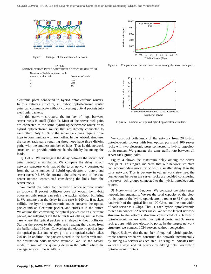
Hybrid optoelectronic router

Server rack group

Figure 3. Example of the constructed network.

TABLE INUMBER OF HOPS IN THE CONSTRUCTED NETWORK STRUCTURE.

Number of hybrid optoelectronicrouters on the path Number of paths1 1922 2883 96

electronic ports connected to hybrid optoelectronic routers.In this network structure, all hybrid optoelectronic routerpairs can communicate without converting optical packets intoelectronic packets.

In this network structure, the number of hops betweenserver racks is small (Table I). Most of the server rack pairsare connected to the same hybrid optoelectronic router or tohybrid optoelectronic routers that are directly connected toeach other. Only 16 % of the server rack pairs require threehops to communicate with each other. In the network structure,the server rack pairs requiring three hops have three disjointpaths with the smallest number of hops. That is, this networkstructure can provide sufficient bandwidth by balancing theloads.

2) Delay: We investigate the delay between the server rackpairs through a simulation. We compare the delay in ournetwork structure with that of the torus network constructedfrom the same number of hybrid optoelectronic routers andserver racks [4]. We demonstrate the effectiveness of the datacenter network constructed considering the links from theserver racks.

We model the delay for the hybrid optoelectronic routeras follows. If packet collision does not occur, the hybridoptoelectronic router can relay the packet without bufferingit. We assume that the delay in this case is 240 ns. If packetscollide, the hybrid optoelectronic router converts the opticalpacket into an electronic packet, and stores it in the buffer.We assume that converting the optical packet into an electronicpacket, and relaying it via the buffer takes 240 ns, similar to thecase where the optical packets are relayed without collision.Storing the packet to the buffer and reading the packet fromthe buffer takes 180 ns. Converting the electronic packet intothe optical packet and relaying it to the optical switch takes240 ns. In addition, the packets stored in the buffer wait untilthe destination ports become available. We use the M/M/1model to simulate the queuing delay in the buffer, where theaverage service time is 240 ns.

0

2000

4000

6000

8000

10000

0 0.5 1 1.5 2 2.5 3 3.5 4

Max

imum

del

ay [n

s]

Total traffic rate [Tbps]

Our NetworkTorus

Figure 4. Comparison of the maximum delay among the server rack pairs.

0

5

10

15

20

25

30

35

0 100 200 300 400 500 600 700 800 900 1000 1100

Num

ber

of r

equi

red

rout

ers

Number of servers

Figure 5. Number of required hybrid optoelectronic routers.

We construct both kinds of the network from 20 hybridoptoelectronic routers with four optical ports and 100 serverracks with two electronic ports connected to hybrid optoelec-tronic routers. We generate the same traffic rate between allserver rack group pairs.

Figure 4 shows the maximum delay among the serverrack pairs. This figure indicates that our network structurecan accommodate more traffic with a smaller delay than thetorus network. This is because in our network structure, theconnections between the server racks are decided consideringthe server rack groups connected to the hybrid optoelectronicrouters.

3) Incremental construction: We construct the data centernetwork incrementally. We set the total capacity of the elec-tronic ports of the hybrid optoelectronic router to 32 Gbps, thebandwidth of the optical link to 100 Gbps, and the bandwidthof each server to 1 Gbps. That is, each hybrid optoelectronicrouter can connect 32 server racks. We set the largest networkstructure to the network structure constructed of 256 hybridoptoelectronic routers with four optical ports, and 32 serverrack groups with two electronic ports. In the largest networkstructure, we connect 1024 servers without congestion.

Figure 5 shows that the number of required hybrid optoelec-tronic routers when we construct the network incrementallyby adding 64 servers at each step. This figure indicates thatwe can always add 64 servers by adding only two hybridoptoelectronic routers.



32 / 157

0

1000

2000

3000

4000

5000

6000

7000

0 20 40 60 80 100 120 140 160 180 200

Num

ber

of s

erve

rs

Number of hybrid optoelectronic routers

Number of Electronic Port=2Number of Electronic Port=3

Figure 6. Number of hybrid optoelectronic routers vs number of accommo-dated servers (four optical ports).

V. DISCUSSION

In this section, we discuss the network structure that is suit-able for a large data center based on our construction method.We investigate the relationship between the number of hybridoptoelectronic routers and the number of servers that can beaccommodated without congestion for any traffic pattern byusing VLB. In this investigation, we set the total capacity ofthe electronic ports of the hybrid optoelectronic router to asufficiently large value, to focus on the bandwidth provided bythe core network constructed of hybrid optoelectronic routers.We set the bandwidth of the optical link to 100 Gbps, and thebandwidth of the link from a server to 1 Gbps.

Figure 6 shows the relationship between the number of ac-commodated servers and the number of hybrid optoelectronicrouters when each hybrid optoelectronic router has four opticalports. The figure shows network structures that include serverracks with two or three electronic ports. As the number ofhybrid optoelectronic routers increases, the number of opticallinks increases, which increases the capacity of the networkand the number of accommodated servers. However, as thenumber of hybrid optoelectronic routers increases, the numberof hops between hybrid optoelectronic routers increases. As aresult, when the number of hybrid optoelectronic routers be-comes sufficiently large, adding hybrid optoelectronic routerscannot greatly increase the number of servers that can beaccommodated. In particular, when the number of electronicports for each server rack is two, adding hybrid optoelectronicrouters decreases the number of servers that can be accom-modated. In contrast, the server racks with three electronicports can accommodate more server racks. This is because theincrease in the number of links from the server rack decreasesthe number of hops between server racks.

We also investigate the case where each hybrid opto-electronic router has 12 optical ports. Figure 7 shows therelationship between the number of accommodated servers andthe number of hybrid optoelectronic routers when each hybridoptoelectronic router has 12 optical ports. Compared with

0

5000

10000

15000

20000

25000

0 20 40 60 80 100 120 140 160 180 200

Num

ber

of s

erve

rs

Number of hybrid optoelectronic routers

Number of Electronic Port=2Number of Electronic Port=3Number of Electronic Port=5

Figure 7. Number of hybrid optoelectronic routers vs number of accommo-dated servers (12 optical ports).

Figure 6, the network constructed of hybrid optoelectronicrouters with 12 optical ports can accommodate more serversbecause this network can provide more bandwidth owing tothe larger number of optical links. In addition, the increase inthe optical links decreases the number of hops between opticalhybrid optoelectronic routers.

This figure also indicates that even if we use the hybridoptoelectronic router with 12 optical ports, we cannot accom-modate more than 20,000 servers for server racks with twoor three electronic ports. However, by connecting each serverrack to four hybrid optoelectronic routers, we can connect25,000 servers by using 80 hybrid optoelectronic routers. Thatis, to construct a large data center, multiple links from serverracks are necessary.

VI. CONCLUSION

In this paper, we discussed a data center network structureusing hybrid optoelectronic routers. We proposed a method toconstruct a data center network that uses hybrid optoelectronicrouters efficiently. We investigated the effect of the networkstructure on the number of routers required to accommodatea large amount of traffic in a mega data center. The resultsindicate that multiple links from server racks are necessaryto construct a large data center, even if hybrid optoelectronicrouters are used.

ACKNOWLEDGMENTS

This work was funded by the National Institute of Informa-tion and Communications Technology (NICT) R&D program,“Basic technologies for high-performance optoelectronic hy-brid packet router”.

REFERENCES

[1] A. Greenberg, J. Hamilton, D. A. Maltz, and P. Patel, “The cost of acloud: research problems in data center networks,” ACM SIGCOMMComputer Communication Review, vol. 39, Jan. 2009, pp. 68–73.

[2] D. Abts, M. Marty, P. Wells, P. Klausler, and H. Liu, “Energy pro-portional datacenter networks,” in Proceedings of the 37th annualinternational symposium on computer architecture (ISCA 2010), June2010, pp. 338–347.



33 / 157

[3] S. J. B. Yoo, “Optical packet and burst switching technologies for thefuture photonic internet,” Journal of Lightwave Technology, vol. 24,Dec. 2006, pp. 4468–4492.

[4] S. A. lbrahim et al., “100-Gb/s optical packet switching technologies fordata center networks,” in Proceedings of Photonics in Switching, July2014, pp. 1–2.

[5] Y. Ohsita and M. Murata, “Data center network topologies using opticalpacket switches,” in Proceedings of DCPerf, June 2012, pp. 57–64.

[6] N. Farrington et al., “Helios: a hybrid electrical/optical switch ar-chitecture for modular data centers,” ACM SIGCOMM ComputerCommunication Review, vol. 40, Oct. 2010, pp. 339–350.

[7] G. Wang et al., “c-through: Part-time optics in data centers,” in Pro-ceedings of ACM SIGCOMM, Oct. 2010, pp. 327–338.

[8] T. Benson, A. Anand, A. Akella, and M. Zhang, “MicroTE: FineGrained Traffic Engineering for Data Centers,” in Proceedings of ACMCoNEXT, Dec. 2011, pp. 1–12.

[9] C. Guillemot et al., “Transparent optical packet switching: The europeanACTS KEOPS project approach,” Journal of Lightwave Technology,vol. 16, Dec. 1998, pp. 2117–2134.

[10] Z. Zhu et al., “Rf photonics signal processing in subcarrier multiplexedoptical-label switching communication systems,” Journal of LightwaveTechnology, vol. 21, Dec. 2003, pp. 3155–3166.

[11] Z. Pan, H. Yang, Z. Zhu, and S. J. B. Yoo, “Demonstration of an optical-label switching router with multicast and contention resolution at mixeddata rates,” IEEE Photonics Technology Letters, vol. 18, Jan. 2006,pp. 307–309.

[12] K. Xi, Y. H. Kao, M. Yang, and H. J. Chao, “Petabit optical switch fordata center networks.” Technical Report, Polytechnic Institute of NewYork University, http://eeweb.poly.edu/∼chao/publications/petasw.pdf.

[13] X. Ye et al., “DOS: a scalable optical switch for datacenters,” inProceedings of ANCS, Oct. 2010, pp. 1–12.

[14] O. Liboiron-Ladouceur, I. Cerutti, P. G. Raponi, N. Andriolli, andP. Castoldi, “Energy-efficient design of a scalable optical multiplaneinterconnection architecture,” IEEE Journal of Selected Topics inQuantum Electronics, vol. 17, Mar. 2011, pp. 377–383.

[15] C. Guo et al., “BCube: A high performance, server-centric networkarchitecture for modular data centers,” ACM SIGCOMM ComputerCommunication Review, vol. 39, Aug. 2009, pp. 63–74.

[16] M. Kodialam, T. V. Lakshman, and S. Sengupta, “Efficient and robustrouting of highly variable traffic,” in Proceedings of HotNets, Nov.2004, pp. 1–6.



34 / 157

The Impact of Public Cloud Price Schemes on Multi-Tenancy

Uwe Hohenstein, Stefan Appel

Corporate Technology

Siemens AG, Corporate Technology, Otto-Hahn-Ring 6

D-81730 Muenchen, Germany

Email: {Uwe.Hohenstein,Stefan.Appel}@siemens.com

Abstract—Multi-tenancy is one key element to make Software-

as-a-Service profitable. Multi-tenancy refers to an architecture

model where one software instance serves a set of multiple

clients of different organizations, i.e., tenants. This reduces the

number of application instances and consequently saves

operational costs. This paper focuses on using relational

databases in multi-tenant architectures, thereby stressing the

cost aspect in public cloud environments. Investigating the

various price schemes of cloud providers, it illustrates the

difficulties to achieve cost-efficient multi-tenancy. As a result,

the broad variety of price factors and schemes lead to certain,

very different strategies and require adapting multi-tenant

architectures to fit the respective cloud providers’ specifics.

Keywords-multi-tenancy; databases; cost; SaaS.

I. INTRODUCTION

Software is more and more becoming an on-demand service drawn from the Internet, known as Software-as-a-Service (SaaS). SaaS is a delivery model that enables customers, the so-called tenants, to lease services without local installations and license costs. Tenants benefit from a "happy-go-lucky package": The SaaS vendor takes care of hardware and software installation, administration, and maintenance. Moreover, a tenant can use a service immediately due to a fast and automated provisioning [1].

Multi-tenancy is a software architecture principle allowing SaaS to make full use of the economy of scale: A shared infrastructure for several tenants saves operational cost due to an increased utilization of hardware resources and improved ease of maintenance [4]. Multi-tenancy is often considered as the key to SaaS.

Several authors, e.g., [23], discuss architectures according to what is shared by the tenants: the topmost web frontend, middle tier application server, and underlying database. Concerning the database, [5] describes a number of patterns, which support the implementation of multi-tenancy. We here distinguish between a 1-DB-per-tenant and a 1-global-DB strategy. The first one provides a database (DB) of its own for each tenant, thus achieving high data isolation, while several tenants share a common database without physical data isolation in the second variant. Further variants as discussed by [5] are irrelevant in this work.

In this paper, we report on industrial experiences when deploying SaaS in public clouds. Particularly, we focus on cost aspects of multi-tenancy for SaaS using a database because we feel economical aspects not appropriately tackled so far in research. Indeed, economic concerns are important

as SaaS providers need to operate with high profit to remain competitive. We here elaborate on the huge differences of price schemes for relational database systems of public cloud providers and the impact on multi-tenancy. Even if various software engineering techniques propose NoSQL databases, relational systems are still often used in industrial applications, especially if being migrated to the Cloud.

Section II presents some related work and motivates why further investigations about cost aspects are necessary. We investigate the price models of various well-known public cloud providers in Section III: Amazon Web Services (AWS), HP Cloud, Microsoft Azure, and Oracle. The price information can be found at their homepages. We discuss in detail the impact of the price models on multi-tenancy strategies and the difficulties to optimize costs. In particular, we quantify the respective costs for implementing multi-tenancy by comparing a 1-DB-per-tenant strategy with a 1-global-DB. Finally, conclusions are drawn in Section IV.

II. RELATED WORK

The work in [4] considers performance isolation of tenants, scalability issues for tenants from different continents, security and data protection, configurability, and data isolation as the main challenges of multi-tenancy. These topics are well investigated. For instance, [17] investigates configurability of multi-tenant applications in case studies.

The possible variants of multi-tenancy have been described, among others, by [5]. Based on the number of tenants, the number of users per tenant, and the amount of data per tenant, [25] makes recommendations on the best multi-tenant variant to use.

Armbrust et al. [1] identify short-term billing as one of the novel features of cloud computing and [8] consider cost as one important research challenge for cloud computing. However, most works on economic issues around cloud computing focus on cost comparisons between cloud and on-premises and lease-or-buy decisions [22]. For example, [9] provides a framework that can be used to compare the costs of using a cloud with an in-house IT infrastructure, and [15] presents a formal mathematical model for the total cost of ownership (TCO) identifying various cost factors. Other authors such as [2][10], focus on deploying scientific applications on Amazon, thereby pointing at major cost drivers. [11] performs the TPC-W benchmark for a Web application with a backend database and compares the costs for operating the web application on several major cloud providers. A comparison of various equivalent architectural



35 / 157

solutions, however, using different components, such as queue and table storage, has been performed by [7]. The results show that the type of architecture can dramatically affect the operational cost.

Cost aspects in the context of multi-tenancy are tackled by [18][19]. They consider approaches to reduce resource consumption as a general cost driver, looking at the infrastructure, middleware and application tier, and what can be shared among tenants.

Another approach, discussed by [24], reduces costs by putting values of utilization and performance models in genetic algorithms.

The authors of [13] develop a method for selecting the best database in which a new tenant should be placed, while keeping the remaining database space as flexible as possible for placing further tenants. Their method reduces overall resource consumptions in multi-tenant environments. Cost factors taken into account are related to on-premises installations: hardware, power, lighting, air conditioning, etc.

Based on existing single-tenant applications, [3] stresses on another cost aspect for multi-tenant applications: maintenance efforts. The recurrence of maintenance tasks (e.g., patches or updates) raises operating cost.

The work in [6] recognizes a viable charging model being crucial for the profitability and sustainability for SaaS providers. Moreover, the costs for redesigning or developing software must not be ignored in SaaS pricing. Accordingly, [18] discusses a cost model for reengineering measures.

The challenges of calculating the costs each tenant ge-nerates for a SaaS application in a public cloud are discussed in [21]. This is indispensable to establish a profitable billing model for a SaaS application. The paper shows that only rudimentary support is available by cloud providers.

To sum up, the profitable aspects of multi-tenancy for SaaS providers are researched insufficiently. All the mentioned work is quite general and does mostly not take into account common public cloud platforms and their price schemes. Even best practices of cloud providers, for instance [16] and [19], do not support SaaS providers to reduce cost. As the next section illustrates, there is a strong need to investigate cost aspects for those platforms.

III. COST CONSIDERATIONS

Deploying multi-tenant applications in a public cloud causes expenses for the consumed resources, i.e., the pricing scheme of cloud providers comes into play. Unfortunately, the price schemes for cloud providers differ a lot and are based upon different factors such as the data volume, data transfer, etc. That is why we investigate the price schemes for databases of some major public cloud providers. The goal is to discuss variances in price schemes and how these affect multi-tenancy strategies for SaaS applications. We assume that each tenant demands a certain amount of database storage. We then compare storage that is provided using a dedicated database per tenant with a global database for all tenants to guide a decision.

Please note it is not our intention to compare different cloud providers with regard to costs or features. That is the reason why we keep the providers anonymous. There is also

no common tool offered by all providers. Furthermore, the price schemes of cloud providers are quite diverging and incorporate different factors. We rather illustrate the variety of price schemes and service offerings leading to different architectures. This also means that the discussion of each offering has a different structure. Moreover, the prices are changing frequently, while the scheme usually remains stable. We here refer to the state as of September 2015.

We only consider resources that are available on-demand to fully benefit from the cloud. This excludes, e.g., reserved instances since those require long-term binding and thus impose a financial risk.

TABLE I. PRICE SCHEME FOR OFFERING 1.

Consumption Price Additional GB

0 to 100 MB $4.995 (fix price)

100 MB to 1 GB $9.99 (fix price)

1 to 10 GB $9.99 for 1st 1 GB $3.996

10 to 50 GB $45.96 for 1st 10 GB $1.996

50 to 150 GB $125.88 for 1st 50 GB $0.999

A. Offering 1

Offering 1 is a database server available as Platform-as-a-Service (PaaS) in a public cloud. PaaS include licenses and seems to be reasonable for multi-tenancy. Without PaaS, there is no elasticity since licenses must be ordered in time.

Table I presents the recent prices for a Microsoft SQL Server in the US East region. In addition, outgoing data is charged for each database individually with a decreasing rate. The first 5 GB are for free, each additional GB is charged with 8.7ct/GB and 8.3ct/GB above 10 TB, decreasing to 5ct/GB for more than 350TB. However, the cost reduction is insignificant unless there is extremely high outgoing transfer. The storage consumption is the main cost driver. Each database is paid for the amount of stored data. There is no cost difference between using one or several database servers for hosting the databases due to virtuali-zation. We even could not detect any performance difference between placing databases on one virtual server or several ones. One has to pay for the consumed storage in every database – the number of databases and servers is irrelevant. At a first glance, the price scheme suggests the same costs for 1-DB-per-tenant and 1-global-DB (keeping all tenants). There seems to be no cost benefit for sharing one database between several tenants, since SaaS providers are charged for the total amount of used storage. However, there are indeed higher costs for individual tenant databases since

sizes larger than 1 GB are rounded up to full GBs;

smaller databases are more expensive per GB than larger ones due to a progressive reduction.

Since pricing occurs in increments of 1 GB, hundred tenants with each a 1.1 GB database are charged with 100*2 GB, i.e., 100 * $13.986 = $1398.60 a month. In contrast, one database with 100 * 1.1GB = 110 GB is charged with $185.82, i.e., a total difference of $1212.78 or a difference of $12.13 for each tenant (per-tenant difference).

Figure 1 compares the costs of both strategies for various numbers of tenants (10,25,...,400). The x-axis represents the database size, the y-axis the per-tenant difference in US$,



36 / 157

i.e., the additional amount of money a SaaS provider has to pay for each tenant compared to a 1-global-DB strategy (note that the prices in Figure 1 must be multiplied by the number of tenants for total costs). The difference stays below $10 for tenant sizes up to 3 GB. The number of tenants is mostly irrelevant. This is why the lines are superposing; only the “10 tenants” line is noticeable. In the worst case, we have to pay $50 more for each tenant with a 1-DB-per-tenant strategy. A linear price drop occurs after 50 GB because even 1-DB-per-tenant uses larger and cheaper databases. Anyway, a 1-DB-per-tenant strategy can become quite expensive compared to a 1-global-DB strategy.

Please note the amount of used storage is charged. That is, an empty database is theoretically for free. However, even an empty database stores some administrative data so that the costs are effectively $4.995 per month (for < 100MB). Anyway, these are small starting costs for both a 1-DB-per-tenant and a 1-global-DB strategy.

There is no difference between provisioning a 10 GB and a 150 GB database from a cost point of view as the stored data counts. A 1-global-DB strategy, having the problem not to know how many tenants to serve, can start with 150 GB, thus avoiding the problem of later upgrading databases and possibly risking a downtime while having low upfront cost. Even for a 1-DB- per-tenant strategy, larger databases can be provisioned in order to be able to handle larger tenants without risk.

However, there is a limitation of 150 GB per database, which hinders putting a high amount of tenants with larger storage consumption in a single database. Reaching the limit requires splitting the database into two.

Along with this comes the challenge to determine a cost-efficient placement strategy. Assume an existing 90 GB database and that we need 40 and 30 GB more space for two further tenants: Putting 60 GB into the existing 90 GB data-base and 10 GB into a new one is the cheapest option with $225.75 + $45.96 = $271.71, more than $70 cheaper than using a new 40 GB and a new 30 GB database: $165.84 + $105.84 + $85.88 = $357.56. Even using a new 70 GB is more expensive with $311.70. An appropriate tenant placement strategy is to fill databases up to the 150 GB threshold, maybe minus some possible space for tenants’ expansions, e.g., $286.58 = $205.80 (90+40 GB) + $85.88 (30 GB).

Figure 1. Price difference per tenant for Offering 1.

TABLE II. PRICE SCHEME FOR OFFERING 2.

Level Price/month DB size Session limit Transaction rate / hour

B ~$5 2 300 16,600

S0 ~$15 250 600 31,260

S1 ~$30 250 900 56,040

S2 ~$75 250 1,200 154,200

S3 $150 250 306,000

P1 ~$465 500 2,400 378.000

P2 ~$930 500 4,800 820,800

P3 ~$3,720 500 19,200 2,646,000

B. Offering 2

This candidate offers three tiers (Basic, Standard, Pre-mium). Table II shows the Microsoft SQL Server prices in the US East region for various performance levels inside.

Again, each individual database is paid according to the price scheme. But in contrast to Offering 1, the provisioning of the tier is relevant, not the effective storage consumption.

Figure 2 compares per-tenant costs for the 1-DB-per-tenant and 1-global-DB strategies in the same way as in Figure 1. 1-global-DB uses S0 databases, while 1-DB-per-tenant uses B (<= 2 GB) and S0 (> 2 GB) depending on the required size.

One of the worst cases that could happen for 1-DB-per-tenant is to have 100 tenants with 2.2 GB (S0) each, resulting in $1500 per month since each tenant cannot be satisfied with the B tier. In contrast, 1 * 220 GB (S0) for 1-global-DB costs $15. That is a per tenant difference of $14.85. However, it is unclear here whether an S0 level is sufficient for handling 100 tenants from a performance point of view.

A 1-DB-per-tenant strategy is about $5 more expensive if the size is lower than 2GB, and about $15 otherwise. The difference is never higher than $14.77, and drops to $12 for 50 GB and to $9 for 100 GB.

For each database, we have to pay at least $5 a month for at most 2 GB and $15 for up to 250 GB. The costs occur even for an empty database. These baseline costs have to be paid for a 1-gobal-DB, too, starting with the first tenant.

Especially for a 1-global-DB approach, a new challenge arises: Each service level determines not only an upper limit for the database size but also for the number of allowed parallel sessions and the number of (internal) worker threads. Furthermore, there is an impact on the transaction rate (cf. Table II). We have to stay below these limits. Upgrading the category in case of reaching the limit happens online, i.e., without any downtime – in theory: if the database size limit is reached, no further insertions are possible until the upgrade has finished. According to the documentation, such a migration can take several minutes up to hours depending on the database size. If the allowed number of sessions is reached, no further clients can connect unless sessions are released by other users. And if the transaction rate is insufficient, the performance will degrade. Hence, a prediction of tenants’ data and usage behavior is required. The number of sessions might become the restrictive factor for a 1-global-DB strategy. In the following, we discuss the impact of the number of users and required sessions on costs by means of sample calculations.



37 / 157

TABLE III. COMPARISON OF CONFIGURATIONS.

Configuration

1 vs. 2

# sessions for

1 vs. 2

Transaction rate

1000/h (1 vs. 2)

a 5*S0 1*S2 3000 1200 156 154

b 2*S0 1*S1 1200 900 62 56

c 2*P1 1*P2 4800 4800 756 820

d 4*P2 1*P3 19200 19200 3283 2646

e 31*S0 1*P1 18600 2400 969 378

Keeping 100 tenants in 1*S0 offers 600 sessions, i.e., 6 sessions per tenant (which might be too small); the monthly costs are $15. We can scale-up to 1*P3 with 19,200 sessions, i.e., 192 per tenant, for a high price of $3720. To achieve the same number of sessions, we can also scale-out to 32*S0 for $480 or use 64*B for $360 if each database is smaller than 2 GB. In contrast, a pure 1-DB-per-tenant strategy for 100 tenants costs $500 for B: This seems to be affordable, especially because of 30,000 sessions. For the price of one P3, we also get 248*S0 databases with 148,000 sessions (6 times more than 1*P3) and a 3 times higher transaction rate of 7,752,480.

For serving 100 tenants with 20 parallel users each, we need 2000 sessions in total. We can achieve this by either 7*B (for $35), 4*S0 ($60), 3*S1 ($90), 1*P1 ($465), or 2*S2 ($500) with very different prices. A pure 1-DB-per-tenant for B is with $500 in the price area of the last two options, but supporting 300 sessions per tenant instead of 20.

Figure 3 illustrates the costs in US$ to achieve x sessions for 100 tenants. B1 represents a pure 1-DB-per-tenant strategy using B-level instances. The P levels are most expensive, even S2 is quite expensive. An obvious question is what the benefit of higher levels in the context of multi-tenancy is. Table III compares several configurations with same prices. There is no consistent behavior. However, several smaller machines seem to be superior to same priced larger ones with a few exceptions. One exception is row (c) where 1*P2 is a little better than 2*P1. More sessions can usually be achieved if n smaller tiers are used instead of one larger one for the same price.

Considering Table II again, we also notice that the session and transaction rates increase from tier to tier less proportional than the prices. Exceptions for transaction rates are S1->S2 and P1->P2. It seems to be reasonable to scale-out instead of scaling-up to obtain more sessions and tran-sactions.

Figure 2. 1-DB-per-tenant vs. 1-global-DB for Offering 2.

TABLE IV. PRICE SCHEME FOR OFFERING 3.

Instance Type RAM Storage Price/month

XS 1 GB 15 GB $73

S 2 GB 30 GB $146

M 4 GB 60 GB $292

L 8 GB 120 GB $584

XL 16 GB 240 GB $1,168

XXL 32 GB 480 GB $2,336

Another advantage is that baseline costs can be saved. A 1-global-DB strategy requires a high-level database with a high price already for the first tenant independent of the number of eventually stored tenants.

Indeed, it is difficult to derive a strategy for identifying a suitable configuration. Important questions arise:

Is an upgrade possible in short time, without outage? This would allow for 1-global-DB to start small for few tenants and upgrade if performance suffers or the number of sessions increases. For 1-DB-per-tenant, we could start with B and upgrade to S0.

Are only the session and transaction rates of a level relevant, or are there any other (invisible) performance metrics to consider? The doc-umentation mentions only that the predictability, i.e., the consistency of response times, is increasing from B to Px, however being the same within a tier.

C. Offering 3

Offering 3 provides a MySQL database as PaaS. The regular prices are for virtualized databases on an hourly basis. The payment is based upon the following factors:

The instance type, which limits the maximal data-base size and determines the RAM (cf. Table IV).

The outgoing data transfer: the first GB is for free, we then pay 12ct/GB up to 10 TB, further GBs for 9ct up to 40 TB, etc.

In contrast to Offering 1, the provisioned storage is paid. The prices and the features increase with the instance type linearly, i.e., each next higher instance type doubles the RAM and maximal database size for a doubled price.

Comparing the strategies, we notice that 5 tenant databases à 15 GB (XS) are charged with $365. One global database à 75 GB is more expensive (!) with $584 since we are forced to provision a 120GB (L) database. The difference per tenant is $43.80. However, using 15GB (XS) increments for 1-global-DB, we can achieve the cheaper price.

Figure 3. Costs to achieve x sessions per tenant for Offering 2.



38 / 157

TABLE V. PRICE SCHEME FOR OFFERING 4.

Type Max database size Data Transfer Price/month

5GB 5 GB 30 GB $175

20GB 20 GB 120 GB $900

50GB 50 GB 300 GB $2,000

Hence, we should use XS partitions in order not to pay for unused storage. Thus, an appropriate cost strategy for 1-global-DB is to fill XS databases one by one with tenants. However, this has architectural implications in order to connect each tenant to the right database instances. A 1-DB-per-tenant approach could also benefit that way. There is no need to use larger instances unless we do not want to spread tenant data across databases due to implementation effort.

A worst case scenario is storing 15 tenants with 100MB each. 1-DB-per-tenant is charged with $1095 = (15*XS), while one global XS database costs $73 for 1.5 GB. That is a difference per tenant of $68.13.

Figure 4 illustrates that 1-DB-per-tenant, compared to 1-global-DB based upon XS databases, is more expensive for sizes much smaller than the storage threshold. Reaching the threshold, the difference diminishes. Hence, it is reasonable to use one database for each tenant if the storage size is near a threshold. In summary, we observe larger per-tenant differences depending on database sizes. The range where the difference stays below $20 is very small. Moreover, the variances for different numbers of tenants are small.

An incremental acquisition of XS databases even saves baseline costs. However, it is an open issue to be investigated whether larger instances provide a better performance. The time for upgrading from one instance type to another is not important here.

D. Offering 4

Three database types are available, each limiting the maximal amount of storage. Table V shows that each type also limits the allowed data transfer.

A comparison of the types gives some first insights: 20GB is 5 times more expensive than 5GB, but offers only 4 times more data transfer and storage. 50GB is 2.2 times more expensive than 20GB, but offers 2.5 times more data transfer and storage. And 50GB is 11 times more expensive than 5GB, but offers only 10 times more resources. Hence, 20GB has the worst price ratio, 5GB the best one. Obviously, using 5GB databases seems to be reasonable for either strategy un-less we do not want to spread tenant data across databases.

Figure 4. Price diff. of 1-DB-per-tenant vs. 1-global-DB for Offering 3.

TABLE VI. COMPARISON OF SAMPLE CONFIGURATIONS

Config #tenants database

size

Costs Data

transfer

Per-tenant

costs

100*5GB 100 1 GB 17,500 3000 175

2*50GB 4,000 600 40

5*20GB 4,500 600 45

20*5GB 3,500 600 35

200*5GB 200 4 GB 35,000 6000 175

16*50GB 32,000 4800 160

40*20GB 36,000 4800 180

100*5GB 100 5 GB 17,500 3000 175

10*50GB 20,000 3000 200

25*20GB 22,500 3000 225

Table VI compares a 1-DB-per-tenant configuration (the first lines) with others. For 200 tenants à 4GB, using 20GB databases is more expensive than 1-DB-per-tenant; the same holds for 100 tenants à 5GB.

Figure 5 summarizes the price-per-tenant differences if 5GB increments are used. A 1-DB-per-tenant strategy is only reasonable if the database size is near a multiple of 5 GB, or if the required data transfer is high. The larger the distance is, the higher will be the per-tenant costs compared to a 1-global-DB. This saw tooth behavior is repeating. The number of tenants has again no impact.

Since the data transfer is limited by the instance type, a challenge arises for the 1-global-DB strategy: this can stop several or all tenants from accessing the database. Additional data transfer cannot be acquired even for extra charges.

A possible strategy for 1-global-DB is to start with 5GB and to add further ones later; this means less upfront costs. Moreover, 5GB is the cheapest category wrt. gains. Please note that downsizing is not possible. This causes further costs in case a tenant stops using the SaaS service.

E. Offering 5

Offering 5 provides a virtual machine (VM) with a Microsoft SQL Server for various operating systems. The price model is quite complex covering several factors.

At first, a VM has to be chosen for hosting the database server. Table VII summarizes the prices for a Windows OS in the East US region. Each tier has a different number of virtual cores (vCores), RAM, and temporary disk space. A0-A7 covers the standard tier; A0-A4 are also available in a basic tier with little lower prices ($13-$440) than the standard tier.

Figure 5. Price diff. of 1-DB-per-tenant vs. 1-global-DB for Offering 5.



39 / 157

TABLE VII. PRICE SCHEME FOR OFFERING 5

Tier vCores RAM TempDisk price/month #disks

A0 1 768 MB 20 GB $15 1

A1 1 1.75 GB 70 GB $67 2

A2 2 3.5 GB 135 GB $134 4

A3 4 7 GB 285 GB $268 8

A4 8 14 GB 605 GB $536 16

A5 2 14 GB 135 GB $246 4

A6 4 28 GB 285 GB $492 8

A7 8 56 GB 605 GB $983 16

A8 8 56 GB 382 GB $1,823 16

A9 16 112 GB 382 GB $3,646 16

D1 1 3.5 GB 50 GB $127 1

D2 2 7 GB 100 GB $254 2

D3 4 14 GB 200 GB $509 4

D4 8 28 GB 400 GB $1,018 8

D11 2 14 GB 100 GB $600 2

D12 4 28 GB 200 GB $1,080 4

D13 8 56 GB 400 GB $1,943 8

D14 16 112 GB 800 GB $2,611 15

A8 and A9 are network-optimized instances adding an InfiniBand network with remote direct memory access (RDMA) technology. The D-tier is compute-optimized with 60% faster CPUs, more memory, and a local SSD. An OS disk space of 127 GB is available and must be paid with ignorable 2.4ct per GB/month.

Furthermore, the server is charged per minute. The prices depend on the number of cores of the used VM: $298 for 1-4 core machines, $595 for 8 cores, and $1190 for 16 cores for a SQL Server Standard Edition in a month. The Enterprise Edition is more expensive, e.g., $4464 for a 16-core VM.

Additional costs occur for attached storage. There is a maximum of number of 1TB data disks (#disks in Table VII). The costs can be neglected with 5ct/GB-month for the first 1000 TB of consumed storage in a page blob. The costs are thus dominated by other factors than disk space.

As a major difference to previous price schemes, a database server is provisioned and paid instead of a single database. The database server offers full control like operated on-premises. Several databases can be managed in that server. This directly implies that a 1-DB-per-tenant strategy is feasible, i.e., each tenant can obtain a database of its own with individual credentials. A strong isolation is thus given without any extra charge. As a consequence, a strategy could be to use one database server and set up one database for each tenant until performance decreases.

Instead of comparing 1-DB-per-tenant and 1-global-DB, we have to consider how many database servers (hosting several databases) of what tier we have to apply for the expected number of tenants and users. One strategy could be to start with a small VM and increase the instance type with the number of tenants. This implies that such an upgrade is possible within short time.

If an upgrade could cause a downtime, we have to decide whether to use several small VMs or few larger ones from a cost perspective. There are high minimal costs of at least $311 per month for each database server ($13 for the smallest Windows VM A0 Basic plus the database server). A high number of tenants/databases will obviously require larger VMs, leading to higher baseline costs.

TABLE VIII. CONFIGURATIONS TO ACHIEVE 112 GB RAM.

configuration # vCores Price (decreasing)

8*D11 16 $4,800

8*A4 64 $4,288

8*D3 32 $4,072

2*D13 16 $3,886

A9 16 $3,646

2*A8 16 $3,646

D14 16 $2,611

8*A5 16 $1,968

2*A7 16 $1,966

The question is what configuration is sufficient for a given number of tenants and amounts of data. Unfortunately, no performance hints are provided to ease the decision. It might be better to provision a larger VM since it can be used for other purposes as well if being idle. A brief evaluation of an SQL Server Standard Edition shows the following:

a) 1*A9 costs $4836 ($3646 for the VM, $1190 for the

SQL Server), offering 16 vCores and 112 GB RAM.

b) For the same price we get 8.5*A3 with ~34 vCores

and ~60 GB RAM in total.

c) Alternatively, we can also purchase 3*A7 with 24

vCores and 168 GB RAM.

d) 13*A1 comes for $4745 with ~23 GB RAM and 13

vCores. (d) offers the least equipment for the price because of the

high number of database servers, each for $298. Options (b) and (c) favor either vCores or RAM. In general it looks reasonable to avoid high-class VMs and to use several middle-class VMs.

An incremental provisioning can also help to reduce upfront baseline costs, which occur already with the first tenant. However, a deeper empirical performance evaluation is necessary due to further open questions:

What VM should be chosen? Table VIII shows several options to achieve 112 GB RAM with very different prices and numbers of vCores.

Similarly, there are many variants for 14 or 28 GB RAM, each yielding different vCores with prices ranging from $246 to $600 for 14GB RAM, and from $492 to $1089 for 28 GB RAM.

Finally, when pursuing the approach with one or few small servers, it is indispensable to know how long it last to upgrade the category of a VM.

F. Offering 6

Similar to Offering 5, this option again offers a VM running a database server, however, with several differences regarding pricing. Several database systems such as MySQL, Oracle, PostgreSQL, and SQL Server are supported in various database instance classes of three categories: Micro, Standard, and Memory-optimized.

The prices depend on the chosen instance type, the type of database server, and the region. The prices for a MySQL database in the US East region are presented in Table IX. The underlying VM and the MySQL license are already included in the price. The instance class determines the number of virtual CPUs (vCPU) and the main memory.



40 / 157

TABLE IX. PRICE SCHEME FOR OFFERING 6.

Category Instance type Price / month vCPU RAM

Micro XS $12.41 1 1

S $24.82 1 2

M $49.64 2 4

Standard M $65.70 1 3.75

L $135.05 2 7.5

XL $260.10 4 15

XXL $520.20 8 30

Memory-optimized

(MemOpt)

L $175.20 2 15

XL $346.75 4 30.5

XXL $689.85 8 61

4XL $1379.70 16 122

8XL $2759.40 32 244

An additional cost factor is the outgoing data transfer to the Internet of 9ct/GB: prices decrease with the amount, 1 GB-month is for free. The price decrease for larger volumes is insignificant.

Furthermore, the amount of data is charged according to two alternative classes of database storage:

a) General purpose for 11.5ct per GB-month with a

range from 5 GB to 3 TB; 3 IOPS per GB are included.

b) Provisioned IOPS for 12.5ct per GB-month and

additional $0.10 per requested IOPS/month, with a range

from 100 GB to 3 TB and 1,000 IOPS to 30,000 IOPS. IOPS (IO per second) determines an upper limit for IO.

IO itself is not charged. Again, we have to decide how many servers are

reasonable. The baseline costs for each database server are determined by the minimal settings: The smallest installation in terms of cost for MySQL is Micro XS with $12.41/month. Provisioned IOPS storage is available at a minimum of 100 GB and 1000 IOPS, i.e., $12.50 (100*12.5ct) plus $100 (1000 IOPS à 10ct) ending up with costs of at least $112.50 per server. Using alternate general purpose storage, we have to provision at least 5 GB for 57.5ct (5*11.5ct); but then only 15 IOPS are available (see (a) above). Hence, setting up a minimal MySQL server, e.g., for each tenant, comes with at least $13 using general purpose storage, while provisioned storage is much more expensive with $125.

A calculation and comparison of using one or several database servers is difficult since several factors are unclear. A high-end server might be more appropriate since the high provisioning cost for storage occur only once. According to the documentation, the network performance also increases with a higher instance class. However, many smaller servers avoid higher, tenant-independent upfront investments for a larger instance and required IOPS.

Table X shows some configurations with similar monthly costs. The provided equipment differs a lot. Obviously, (a) is better equipped than (b). But each of (a) and (d) has an advantage for vCPUs or RAM, respectively.

It is important to note that the provisioned numbers are relevant, not the effective usage. This means, the required storage for each tenant has to be estimated in order not to overpay for unused resources. The same holds for the IOPS rate. These costs occur already for the first tenant independently of consumed resources.

TABLE X. COMPARISON OF CONFIGURATIONS.

Configuration vCPUs RAM Costs

a 1* 8XL (mem-opt) 32 244 $2759

b 2 * 4XL (standard) 16 244 $2759

c 20 * L (standard) 40 150 $2704

d 42 * M (standard) 42 157 $2759

One strategy could be to start with small servers and increase the instance type and configuration if necessary. This implies that such an upgrade is possible within short time and without downtime in the meantime. Otherwise, a larger machine with larger storage and IOPS can be provisioned from the beginning, however, causing high starting costs already for some few tenants.

Another strategy is to use one smaller server for each tenant, e.g., for $13. Then, the expenses increase tenant by tenant. This also gives more flexibility for provisioning IOPS according to tenants’ requirements.

An important question is what IOPS rate is sufficient since the IOPS rate is a limiting factor: Throttling of users can occur if the limit is reached. Obviously, keeping several tenants in one server requires higher IOPS rates. It is unclear what the advantage of provisioned storage is compared to general purpose storage. From a pure cost perspective, 6000 IOPS are charged with $600 for provisioned storage. To achieve 6000 IOPS with general purpose storage, we have to use 2TB (remind the factor in (a)), i.e., being much cheaper with $230 and already including storage. Since there is an upper database limit of 3 TB in any case, general purpose IOPS ends with 9,000 IOPS; provisioned storage can handle up to 30,000 IOPS.

IV. CONCLUSIONS

This paper took a deeper look into the price schemes of popular cloud database providers and investigated their cost impact on multi-tenancy. We thereby focused on storing tenants’ data in relational databases. We showed that a cost-efficient database deployment for multi-tenancy heavily depends on providers due to very different price schemes. Several differences become apparent.

Offering 2-6 charge for provisioned storage, i.e., upfront costs occur even if small data is stored. In contrast, Offering 1 charge for storage consumption which avoids starting costs instead.

Sometimes, databases are paid (cf. Offerings 1-4); sometimes whole DB servers are provisioned (cf. Offering 5 and 6) so that several isolated databases can be managed with specific credentials.

Offerings 2 and 4 define certain limits on transaction rates, data transfer, or number of sessions. Reaching such a limit could stop a SaaS application for serving tenants.

For Offerings 3, 5, and 6, equipment such as RAM increases with each level, while this is not controllable and visible in Offerings 1, 2, and 4.

There are direct cost factors such as storage, IOPS, sessions, cores, or data transfer, i.e., they are directly part of the price scheme. We detected indirect cost factors, too. For example, it might be necessary to use and pay a larger virtual



41 / 157

machine (VM) in order to achieve a certain transaction rate, e.g., Offering 2.

The broad spectrum of price schemes makes it difficult to find an appropriate provider-independent cost-optimized configuration for multi-tenant applications. However, we could present some analyses comparing the cost of a 1-DB-per-tenant and a 1-global-DB strategy and displaying the characteristics for different tenant sizes. The results also have a strong impact on the cloud provider selection. For example, if a strong isolation is requested, a provider with too high prices for a 1 DB-per-tenant strategy might not be qualified for a selection.

As a consequence, it is difficult to select the best provider from the cost perspective. But we think that our analysis helps architects of multi-tenant software to decide upon a cloud offering for the anticipated requirements. Besides architects, cloud providers can benefit from our analysis when it comes to adjust their service offerings.

This all affects portability of SaaS applications, too. It is not easy to define an economic provider-independent strategy for multi-tenancy. Furthermore, architectures must take into account several aspects. For example, monitoring consumption becomes necessary because of thresholds such as a database upper limit of parallel sessions, IO limits, or any other type of throttling. This is indispensable to react in time if a threshold is reached because a service is in danger of being stopped.

Future work will tackle open questions, including practi-cal investigations. One important question is about the pro-visioning time. This point is relevant in any strategy since additional databases have to be acquired. Similarly, upgrad-ing a database level is important for saving upfront costs.

Finally, we intend to collect further challenges from an industrial perspective.

REFERENCES

[1] M. Armbrust et al., “A View of Cloud Computing,” Communications of the ACM, 53(4), April 2010, pp. 50-58.

[2] B. Berriman, G. Juve, E. Deelman, M. Regelson, and P. Plavchan, “The Application of Cloud Computing to Astronomy: A Study of Cost and Performance,” Proc. of 6th IEEE Int. Conf. on e-Science, 2010, pp. 1-7.

[3] C. Bezemer, A. Zaidman, B. Platzbeecke, T. Hurkmans, and A. Hart, “Enabling Multitenancy: An Industrial Experience Report,” in: Technical Report of Delft Uni. of Technology, TUD-SERG-2010-030, 2010.

[4] C. Bezemer and A. Zaidman, “Challenges of Reengineering into Multitenant SaaS Applications,“ in: Technical Report of Delft Uni. of Technology, TUD-SERG-2010-012, 2010.

[5] F. Chong, G. Carraro, and R, Wolter, “Multi-Tenant Data Architecture,“ June 2006, http://msdn.microsoft.com/en-us /library/aa479086.aspx [retrieved: February 2016]

[6] T. Dillon, C. Wu, and E. Chang, “Cloud Computing: Issues and Challenges,“ in Proc. 24th Int. Conf. on Advanced Information Networking and Applications, 2010, pp. 27-33.

[7] U. Hohenstein, R. Krummenacher, L. Mittermeier, and S. Dippl, “Choosing the Right Cloud Architecture - A Cost Perspective,“ in Proc. on Cloud Computing and Services Science (CLOSER), 2012, pp. 334-344.

[8] A. Khajeh-Hosseini, I. Sommerville, and I. Sriram, “Research Challenges for Enterprise Cloud Computing,“ in Proc. 1st

ACM Symposium on Cloud Computing, SOCC 2010, Indianapolis, pp. 450-457.

[9] M. Klems, J. Nimis, and S. Tai, “Do Clouds Compute? A Framework for Estimating the Value of Cloud Computing,” in Designing E-Business Systems. Markets, Services, and Networks, Lecture Notes in Business Information Processing, Vol. 22, 2008, pp.110-123.

[10] D. Kondo, B. Javadi, P. Malecot, F. Cappello, and D. Anderson, “Cost-Benefit Analysis of Cloud Computing versus Desktop Grids,“ in Proc. of the 2009 IEEE Int. Symp. on Parallel&Distributed Processing, May 2009, pp 1-12.

[11] D. Kossmann, T. Kraska, and S. Loesing, “An Evaluation of Alternative Architectures for Transaction in Processing in the Cloud,” ACM SIGMOD 2010, pp. 579-590.

[12] R. Krebs, C. Momm, and S. Kounev, “Architectural Concerns in Multi-Tenant SaaS Applications,“ in CLOSER 2012, pp. 426-431.

[13] T. Kwok and A. Mohindra, “Resource Calculations With Constraints, and Placement of Tenants and Instances for Multi-Tenant SaaS Application,“ in Proc. Int. Conf. on Service-Oriented Computing, (ICSOC) 2008. LNCS, vol. 5364, pp. 633-648.

[14] M. Lindner, F. Galán, and C. Chapman, “The Cloud Supply Chain: A Framework for Information, Monitoring, Accounting and Billing,“ in Proc. on ICST Cloud Computing, 2010, pp. 1-22.

[15] B. Martens, M., Walterbusch, and F. Teuteberg, “Evaluating Cloud Computing Services from a Total Cost of Ownership Perspective,“ 45th Hawaii International Conference on System Sciences (HICSS-45), 2012, pp. 1564-1572.

[16] Microsoft, “Developing Multitenant Applications on Windows Azure“. http://msdn.microsoft.com/en-us/library /ff966499.aspx [retrieved: January 2016]

[17] R. Mietzner, F. Leymann, and M. Papazoglou, “Defining Composite Configurable SaaS Application Packages Using SCA, Variability Descriptors and Multi-Tenancy Patterns,“ in 3rd Int. Conf. on Internet and Web Applications and Services (ICIW), 2008, pp. 156-161

[18] C. Momm and R. Krebs, “A Qualitative Discussion of Different Approaches for Implementing Multi-Tenant SaaS Offerings,“ in Proc. Software Engineering 2011, pp. 139-150.

[19] C. Osipov, G. Goldszmidt, M. Taylor, and I. Poddar, “Develop and Deploy Multi-Tenant Web-Delivered Solutions Using IBM Middleware: Part 2: Approaches for Enabling Multi-Tenancy,” in: IBM’s technical library, 2009.

[20] A. Schwanengel, U. Hohenstein, and M. Jaeger, “Automated Load Adaptation for Cloud Environments in Regard of Cost Models,“ in Proc. on CLOSER, 2012, pp. 562-567.

[21] A. Schwanengel and U. Hohenstein, “Challenges with Tenant-Specific Cost Determination in Multi-Tenant Applications,“ in 4th Int. Conf. on Cloud Computing, Grids and Virtualization, Valencia (2013), pp. 36-42.

[22] E. Walker, “The Real Cost of a CPU Hour,“ Computer 2009, Vol. 42(4), pp. 35-41.

[23] S. Walraven, E. Truyen, and W. Joosen, “A Middleware Layer for Flexible and Cost-Efficient Multi-Tenant Applications,“ in Proc. on Middleware, 2011 (LNCS 7049), pp. 370-389.

[24] D. Westermann and C. Momm, “Using Software Performance Curves for Dependable and Cost-Efficient Service Hosting,“ in Proc. on Quality of Service-Oriented Software Systems (QUASOSS), 2010, pp. 1-6.

[25] Z. Wang et al, “A Study and Performance Evaluation of the Multi-Tenant Data Tier Design Pattern for Service Oriented Computing,” in IEEE Int. Conf. On eBusiness Engineering, (ICEBE) 2008, 94-101



42 / 157

A Novel Framework for SimulatingComputing Infrastructure and Network Data Flows

Targeted on Cloud Computing

Peter KraußKarlsruhe Institute of TechnologySteinbuch Centre for Computing

76128 KarlsruheEmail: [email protected]

Achim StreitKarlsruhe Institute of TechnologySteinbuch Centre for Computing


Tobias KurzeKarlsruhe Institute of Technology

Library76131 Karlsruhe


Bernhard NeumairKarlsruhe Institute of TechnologySteinbuch Centre for Computing


Abstract— Understanding how computing infrastructure deci-sions influence overall performance and cost can be very difficult.Simulation techniques are an important tool to help analyse andevaluate different infrastructure configurations and deploymentscenarios. As diversity of cloud computing resources is growing,the space of possible infrastructure configurations becomes largerand finding the best solution becomes harder. In our previouspaper, we presented a framework to benchmark cloud resourcesto obtain objective and comparable results. Based on those results,our simulation framework allows to model applications and toestimate their performance. Compared to other infrastructure orcloud simulation tools our framework excels when it comes tothe simulation of network data flows.

Keywords–Broad band networks, quality of service, infrastruc-ture, cloud, simulation, framework

I. INTRODUCTION

Due to the rise of cloud computing during the last fewyears - for a widely accepted definition of the term see [1][2] -and its further growing adoption in commercial, industrial andresearch endeavors [3][4], there are more and more differentinfrastructure offerings and possible applications. Differenttypes of applications have different requirements on the under-lying (virtual) hardware and are structured differently. Findingdeployment policies that deliver good performance and arecost-efficient under varying conditions is challenging becauseof multiple reasons.

First, the number of possible deployments for a givenapplication respectively for workload executing systems, growsrapidly with the number of components of an application aswell as with the number of available resources to choose from.Secondly, clouds do not always deliver the same performanceand are subject to varying demand. Further, as cloud resourcesare delivered via public broadband networks, it is hard or evenimpossible to reproduce identical test conditions. As it is nei-ther practical to try out each and every possible deployment nor

feasible to reproduce an identical test environment, simulatingthe respective scenarios is the better approach. Therefore, wedeveloped an infrastructure simulation framework that focuseson cloud environments, but in principle it can be used for anykind of infrastructure. The framework allows the simulation oflarge-scale applications that may be deployed across differentcloud providers.

Our framework provides informations about the completebehavior of a configured workload running on a user definedinfrastructure. During the simulation, a user can access all thestatus information he might need, this includes load on disk,CPU, memory as well as network interfaces. This allows a userto attach e.g., cost models or simulate bad or malfunctioninghardware. Our approach is unique in the way it modelsnetworks and is very lightweight compared to other tools.

The paper is structured as follows:A short overview of cloud respectively infrastructure sim-ulation tools is given in Section II. Next, we present ourinfrastructure model and introduce resource providers and ournetwork simulation model. Then, we give a description of howworkloads are specified, followed by the section dedicated tothe implementation of the simulator. Next, in addition to thetheoretical model, we describe how calibration of the simulatoris done and show the validity of the framework. Lastly a shortsummary including a discussion of the validation’s results isgiven.

II. RELATED WORK

In the field of cloud simulation, a lot of research withvarying focus has already been done. Lim et al. developedMDCSim [5], a simulation platform for multi-tier data centersthat allows performance and power consumption analysis.The simulator is event based and designed as a three-layerarchitecture – user layer, kernel layer, communication layer.It is able to capture details such as kernel level scheduling



43 / 157

strategies. For communication, the simulator supports IBAand Ethernet over TCP/IP. By changing the timing parametersother protocols can be incorporated. For kernel requests, thesimulator considers multiple CPUs as a single resource and ismodeled according to the Linux scheduler 2.6.9.

Another well known toolkit for modeling and simulatingcloud environments is CloudSim [6][7]. It is event-based andallows to model data centers, virtual machines and resourceprovisioning policies. Furthermore it is possible to modelfederation of clouds resp. inter-networked clouds. Allocationof virtual machines to hosts is done based on a First-Come-First-Serve basis. CloudSim implements time-shared as wellas space-shared policies at host and at VM level to assignresources. Besides aforementioned aspects, CloudSim modelsthe cloud market based on a multi-layered design, whereby thefirst layer represents costs per unit related to the IaaS modeland the second layer comprises costs related to the SaaS model.Network behavior is modeled using a latency matrix and amessage will be forwarded by the event management engineafter a delay specified by the according entry in the latencymatrix.

NetworkCloudSim [8] has been developed by Garg andBuyya and is an extension for CloudSim providing a networkand generalized application model, allowing a more preciseevaluation of scheduling and provisioning policies. Network-CloudSim adds three main entities: Switch, NetworkDatacenterand NetworkDatacenterBroker. Also new classes to modelnetworks have been added to the original classes of CloudSim.This allows a better modelling of applications that rely onspecific means of communication such as MPI for example.

DartCSim+ [9] is another enhancement of CloudSim. Theauthors claim to have overcome limitations of CloudSim inregard to three aspects: – simultaneous support of powerand network model is not possible – simulation of networkcomponents is not power-aware – migration does not take intoaccount network overheads To overcame aforementioned lim-itations, the authors developed a range of entities as extensionfor CloudSim.

Wickremasinghe et al. propose another CloudSim relatedtool named CloudAnalyst [10], that helps studying the be-haviour of large-scale cloud applications. CloudAnalyst takesinto account the geographic dıstribution of an application andof its users. CloudAnalyst provides a graphical user interfacethat allows users to model their experimental setups.

Nunez et al. developed another cloud simulator callediCanCloud [11][12] with focus on lage experiment setups.iCanCloud features a global hypervisor that can integrate anybrokering policy and is configurable through a graphical userinterface. It also provides a POSIX-based API and supportsconfigurations for different storage systems such as remotefile systems like NFS or parallel files systems and RAIDconfigurations.

In our own previous work [13] we created a performancemeasuring tool. The publication contains a description of theused architecture to monitor a large amount of cloud resourcesover time. We were able to show that the perfromance ofvirtualized infrastructure resources does vary over time, eventhough it should be constant, as well as the performance

of network interconnects between virtual machines. This as-pect is not covered by common simulation frameworks. Theframework presented in this paper is capable of taking thefactors shown in [13] into account. We use the measuredperformance values from [13] to calibrate our simulationframework presented in this publication.

III. INFRASTRUCTURE MODEL

Our model describes an infrastructure cloud environmentas a hierarchy of entities. The entities on the lowest levelprovide resources, which are in our model calculation powerin units called cpu cycles, ephemeral memory in units calledmbytes, persistent storage space in multiples of mbytes andfinally network traffic which is described by transfers betweennetwork enabling entities characterized by a bandwidth inunits of mbytes per time step. The entities that provide thoseresources are called vCPU, vMemory, vStorage and vNet whichcreates instances of vTransfer objects.

On the next level, the model introduces another entitycalled vMachine. This entity can be associated with anycombination and any amount of entities of the level belowand is a loose equvivalent to a virtual machine in a real cloud.Further a vMachine can be associated with so called vWorkloadobjects. Those objects contain a description of a workload andare described in the course of this paper (see Section IV).

The next layer contains vDatacenter objects that in turncontain vMachine objects. A vDatacenter in addition is asso-ciated with two coordinates that express a location in a 2D-space and can be used to position different datacenters relativeto each other. The distance between datacenters is factored inwhen data transfers happen, since previous works showed thatthis can affect transfers [13].

Beside those layers, the model is based on a global envi-ronment object containing all entities related to the simulatedinfrastructure. This environment provides a global, steadilyincreasing counter to represent the simulation time in logicalseconds. With each step the timer advances by one and thesimulation progresses. The environment makes sure that allobjects associated with it are notified at least once per timestep about the new simulation time so they will update andpossibly advance their state.

In the following subsections, major parts of this model willbe explained in deeper detail.

A. Resource Providers

As mentioned before the model is based on four resourcesthat are provided by four resource providers. These entities arealways associated with a maximum capacity and a provisioningspeed. The first describes how many units of a certain resourceare provided whereas the latter expresses at what speed thisresource can be delivered. In addition, each resource can eitherbe ephemeral or static. Ephemeral resources reset their capacityat the beginning of each new time step while static resourcesdo not. In our model the following four resource providers aredefined:

vCPU As mentioned, this object provides calculation powerin units of cpu cycles. The resource is ephemeral andresets to its predefined maximum capacity with every



44 / 157

simulation step and the resource can be consumed atinstant speed.

vMemory To represent a machine’s internal memory, weintroduced a vMemory resource provider. In contrast tophysical RAM, this resource does reset its capacity withevery time step due to how workloads are designedin our model: A vWorkload does not allocate and freememory but it provides an absolute value representinghow much memory is required at a certain point intime. All operations on a vMemory object are performedinstantly.

vStorage A vStorage object represents a comparably slow andlimited storage device for example a hard disk or solidstate drive. The provider’s operational speed is capped ata predefined rate (throughput) which in addition is sharedamong all entities currently using the resource.

vNet This object represents a network device which cantransfer a given amount of data per time step. The object’sbandwidth is shared among all currently active transfersand each transfer’s speed further depends on the receiver’sbandwidth. Since proper network simulation is a majorpart of our framework this will be discussed in detailin a following section (see Section III-B). We assume aphysical network card to operate in duplex mode, sendingand receiving speeds are not correlated in any way andare thus modeled as two independent vNet instances thatmay be configured with different bandwidths.

vTransfer vTransfer objects contain all information that de-scribe the state of ongoing data transfer, such as currenttransmission speed and associated vNet instances (ori-gin/destination). In contrast to the previously presentedobjects, vCPU, vMemory, vStorage and vNet, a vTransferdoes not have a representation in real hardware and is acompletly virtual construct.

Since access to the ‘fast’ resources calculation power andephemeral memory is considered to be performed instantly,no sophisticated scheduling is needed: In case those resourcesare requested by one or more workloads, the resource providersimply evenly divides the available resources among the re-questers. In our current implementation, the scheduler followsa round-robin manner to divide the resources. In case a requestcannot be fulfilled, an appropriate notification is sent to thevWorkload for it to react according to its configuration. Forexample, a common workload will request as many CPUcycles as possible and a certain amount of memory. As longas the first request does not lead to a critical error, a typicalworkload can still execute even if there’s only a few cyclesassigned to it. On the other hand, a workload will most likelycrash if a memory requirement cannot be met.

In contrast, access to the ‘slow’ resources, storage andnetwork, has to be scheduled. We model two operationson storage devices: write and read. Both operations areperformed equally but in the first case, the capacity of theresource provider is decreased by the amount of transferreddata whereas in the latter case, the capacity remains constant.When an operation on such a storage resource is initiated, theresource provider will register the operation and evenly dividethe available bandwidth among the contenders and processthem in parallel. An operation is considered as failed, if therequested amount of data cannot be written or read.

D

CA

BL1 L2 L3

1,000InterfaceBandwidth

Transfer

1,000

1,000 100Figure 1. A simple example of a network graph.

B. Network Simulation

One of the major concerns of the simulator describedin this paper is the network simulation model. As indicatedabove a proper calculation of per-transfer speeds can bedifficult due to the dependency on the sender’s as well asthe receiver’s bandwidth. The complexity increases with thenumber of transfers, which, in addition, might or might notshare the same destination. A simple example is depicted inFigure 1. The example shows four vNet objects named A,B, C and D associated with the bandwidths bwA = 1,000,bwB = 1,000, bwC = 100 and bwD = 1,000 and threetransfers between those (L1 = B → A, L2 = B → Cand L3 = C → D). The data transfers are represented asinstances of vTransfer. It is obvious that the bandwidth ofB has to be shared among two transfers L1 and L2 whilebeing capped by the available bandwidth of C after taking L3

into account. The arising challenge is to balance the transferspeeds in a realistic manner in real-time while considering thatthe network configuration might significantly change betweentime steps due to added or removed nodes or transfers. Dueto those constraints known algorithms like those based onthe max-flow/min-cut-theorem [14] are not suitable for ourenvironment. Instead we developed an agent-based algorithmthat determines the available bandwidth per active transfer atthe current simulation time solely based on the informationprovided by the receivers of the transfered data.

The algorithm we propose uses an iterative approach thatconverges to a solution where an optimal data flow between allvNet objects is achieved. This algorithm is further based ona graph whose vertexes M = {M1, . . . ,Mn} are represent-ing data sending or data receiving network interfaces (vNetobjects) and whose set of edges L = {L1, . . . , Ln} are repre-senting network transfers (vTransfer objects). Each vertex Mi

is associated with a limited transfer rate bw(Mi) = bwi > 0expressing the bandwidth of the vNet. The set of vTransfersNi contains all vTransfers originating from Mi and is a subsetof L.

To calculate the current transfer speed st at time t of avTransfer object Lk = Li→j = LMi→Mj

with Li→j ∈ Ni

originating from o(Lk) = Mi and targeted to d(Lk) = Mj , thealgorithm works in an iterative manner realistically saturatingthe interfaces.

In a first step (t = 0), for each vNet instance all avail-able bandwidth is divided proportionally among the activevTransfers based on the theoretically possible transfer speedsto the corresponding remote partners which is assumed to bedefined by the speed of the slowest involved vNet. This can



45 / 157

TABLE I. A SAMPLE CALCULATION FOR THENETWORK GRAPH SHOWN IN FIGURE 1.

L1 L2 L3

1st Iteration

A 1000 – –B 909 91 –C – 50 50D – – 1000

min() 909 50 50

2nd Iteration

A 1000 – –B 948 52 –C – 50 50D – – 1000

min() 948 50 50

3rd Iteration

A 1000 – –B 950 50 –C – 50 50D – – 1000

min() 950 50 50

be expressed in the following equation:

s′0(Li→j) = s′t=0(Li→j) =bwj∑

n∈Ni

bw(d(n))× bwi (1)

In most cases, this assumption is just a rough approximationand not exact, but it is a starting point for the algorithm towork with. With further iterations the value will be graduallycorrected.

The result of calculation (1) represents the bandwidth asending vNet entity Mi could provide for a transfer Li→j toa target Mj at maximum at time t = 0. The same value thenhas to be calculated for the receiving vNet object. The speedused for the transfer is then determined by the smaller of bothvalues:

s0(Li→j) = min(s′0(Li→j), s′0(Lj→i)) (2)

For the next steps (t > 0) the speed of a vTransfer instancewill no longer be based on the predefined bandwidth of theinvolved vNets but on the previously calculated transfer speeds.The equations to determine the speed s of a transfer Li→j atany time t > 0 are adjusted to:

s′t(Li→j) =st−1(Li→j)∑

n∈Ni

st−1(n))︸︷︷︸A

×bwi (3)

st(Li→j) = min(s′t(Li→j), s′t(Lj→i)) (4)

With the factor A always being less or equal than 1.0 themaximum bandwidth of source network interface is neverexceeded. Further A can only be equal to 1.0 in the case of asingle active transfer, which results in that transfer using themaximum available capacity.

Using this algorithm we are able to determine the speed ofa transfer at any time simply by factoring in either previouslycalculated transfer speeds in case of t > 0 or the neighboringmachines theoretically possible transfer speeds in case of t =0. A sample calculation for the example discussed above isshown in Table I. The first fours rows of the tables contain thevalues for s′t for the transfer corresponding transfer expressedby the columns. The last row of each table contains the valueof st. One can see that over time, the speeds of the transfers

TABLE II. PROPERTIES OF A WORKLOAD OBJECT.

Resource type data type descriptionvCPU integer Value expressing the total amount of

calculation power the workload willuse expressed in cpu cycles.

vMemory f(cpu cycles) Function returning the amount of usedvMemory when a given amount of cpucycles has be processed or is remain-ing.

vStorage, vNetwork list List of triplets expressing the amountof cpu cycles to be remaining or pro-cessed for a defined operation to beexecuted and a flag allowing parallelexecution.

converge to a final value that overall saturates the vNets A toD.

Finally, when using the model above, the calculated trans-mission speeds will always be based upon ideal networkconnections transmitted over ideal network cables withoutany kind of noise. Thus, we want to point out, that in ourimplementation we add in a factor called ‘scatter’ to expresssome randomness in latency and bandwidth and represent acombination of all kind of complex signal fluctuations. Ourtest show, that a variation of a few percent in transfer speeds isrealistic due to physical connections not performing perfectlyat all times.

IV. WORKLOAD DESCRIPTION

In our model, each workload is associated with a certainamount of load related to the resources described in Subsec-tion III-A. We do not consider workloads not associated withany resource consumption, so the minimal defined workloadwill be a workload only consuming a single cycle of calcu-lation power. This enables the use of calculation power as areference for other resource usages: Instead of modeling usageof vMemory based on the time passed since the launch ofthe workload we model memory conumption as a functionof consumed calculation power. In general, the definition ofmemory as a function over cpu cycles instead of processingtime is a more realistic approach: a started but not advancing(i.e., due to missing resources) workload will not change itsstate and thus not change its consumption of memory.

Since the usage of storage and network are time-consumingprocesses due to the non-instant character of the underlyingresource providers we cannot transfer this mechanism par forpar. As a solution we designed storage and network usage astriggers likewise based on the amount of cpu cycles. Thosetriggers are simple integers and are executed as soon as thenumber of consumed or remaining cpu cycles has reachedthe configured value. Upon execution the trigger can theninstantiate new network transfers or storage operation whichare then processed. In addition the user can specify if thoseoperations should be processed in parallel or if the workloadshould pause meanwhile.

Beside the described resource-related properties which aresummarized in Table II each workload may execute user-defined subroutines upon reaching certain states to control theflow of workloads. Predefined states are init which gets exe-cuted when the workload is launched on a vMachine instance,finish which is associated with the workload terminating and



46 / 157

error, the state that a workload changes to upon failing. Inaddition a user can add other trigger and subroutines.

To start the simulation of a workload on a given infrastruc-ture, the workload object has to be registered at a vMachineinstance. The vMachine then enables access to its resourcesby reading the workload definition at the current simulationtime and passing appropriate requests to the resource providerswhich then schedule the incoming requests.

V. IMPLEMENTATION

We realized the described model using Python 2.7 basedon the concepts of the object-oriented programming paradigm.The most important components to mention are the differentresource providers vNet, vMemory, vStorage and vNetworkalong with vTransfer, the higher level entities vMachine andvDatacentre and finally the global environment object calledenv. Whereas most of the implementation can be consideredstraight forward, we want to highlight some aspects we con-sider implementation specific.

First, we implemented the resource provider’s schedulingin case of more than one workload accessing the resource ata time is done in a round-robin manner. Hereby, the resourceprovider allocates an equal amount of the available resourceto each consumer. In the future, we plan to implement otherscheduling mechanisms.

Python natively does not offer an event handling concept,so we based our simulator on generators. A generator functionallows to define a function that behaves like a iterator. Thedetails of this concept are described in [15] (PEP0289 andPEP0342). This enables the implementation of time-dependentactions, like network transfers and storage operations as loops.An action requiring more than one time step to be performed isexpressed as a set of smaller parts that are one time step longand yield at the end of their execution. We believe that usinggenerators leads to less error-prone code due to the simplicityand the linear, synchronous layout.

Finally, due to the simulator not running in parallel but call-ing subtasks subsequently one at a time, one has to make surethat one task doesn’t change the simulation state prematurely.We solved this by deep-copying the simulator’s state beforethe execution of the subtask begins. Then, all subtasks referto the copy when reading values while making the changes tothe original state.

VI. CALIBRATION AND VALIDATION

To use the simulation framework, users must specify theavailable infrastructure by defining resource providers as ex-plained in Section III-A. The model can be calibrated based oneither of two correlated degrees of freedom: either the resourceprovider’s performance or the workload’s resource usage canbe tuned. As soon as one dimension is set, the other has to bepicked accordingly to get consistent results.

With the model being a simplification of reality it is up tothe user to configure the infrastructure in a suitable way forone’s use-case. Any calibration settings are workload specific,since for example a workload might or might not benefitfrom certain CPU features (i.e., Streaming SIMD Extensions

TABLE III. AVERAGE PERFORMANCE OF COMMON CPUS REGARDINGPSEUDO-RANDOM NUMBER GENERATION.

CPU name clock frequency Performance [MB/s]Intel i3-2100 3.1 GHz 16.3 ± 0.9%

Intel i5-4288u 2.6 GHz 13.5 ± 1.4%Intel Xeon E5520 2.27 GHz 7.2 ± 1.8%

Intel Xeon E5-2650 2.0 GHz 3.6 ± 8.5%

(SSE) [16]) or network related characteristics (e.g., delays dueto encryption settings).

In addition to this systematic calibration, performancevariations on all sorts of resources might occur due to non-perfect behavior of hardware. Those variations are comparablysmall and are covered by the aforementioned scatter factors weadded to the model in our implementation. Those aspects areusually only known to system or software engineers or can beobtained by benchmarking.

We provide consistent calibration values based on thefollowing assumptions for an Amazon EC2 environment:

• A workload that is modeled for a resource provider thatsupports a certain CPU feature may need less CPU cyclesand is modeled accordingly.

• The same application that is modeled for a resourceprovider that does not support a certain CPU feature mayneed more CPU cycles and is modeled accordingly.

• The simulated execution of the same application usingresource providers that are n-times more powerful than theoriginal resource providers for which the application hadbeen tuned in the beginning should take in the order of an-th of the time when compared to the initial simulation.

• The simulated execution of an application should yieldapproximately the same results when compared to realrun-time, respectively should be faster or slower in thesame order of magnitude relative to the application themodel’s parameters were derived from.

To derive calibration values, we ran a high number (approx.560,000) of tests on different machine configurations usinga distributed benchmark suite. A detailed description of thetests can be found in [13]. To obtain the calibration values, wecorrelated the resources of the simulation environment withthe performance of the corresponding real hardware.

A. Calibration

In a first step, we calibrated calculation power basedon data of a synthetic CPU benchmark. In our case thisis the single-threaded calculation of pseudo-random numbersfor checksumming purposes on virtual machines of the EC2instance type “t2.small” in the region “us-east-1”. For ourcalibration, we set 2,000 cpu cycles = 2,000MHz, which isthe average clock frequency a virtual CPU on the used EC2instances provides as stated by Amazon. The benchmarksshowed an average random number generation rate of 3.6 ±8.5% megabytes per second per core using an Intel Xeon E5-2650 running at 2GHz. Table III shows the results of the samebenchmark on other CPUs for reference. Using this data, wecan state that a real-world workload using the same amount ofcomputing power as required for the generation of 3,600,000pseudo-random numbers would run one second. As mentionedabove, this value might seem to be abstract compared to e.g.,



47 / 157

TABLE IV. AVERAGE PERFORMANCE OF COMMON CPUS REGARDINGPSEUDO-RANDOM NUMBER GENERATION.

Evaluated transfer distance std. deviationus-east-1 ↔ us-west-1 3,600 km 13.4%us-west-1 ↔ eu-west-1 8,000 km 14.5%

ap-southeast-1 ↔ eu-west-1 11,300 km 17.3%ap-southeast-1 ↔ us-west-1 13,900 km 19.7%

GFLOPS, but since a user might not necessarily know theamount of FLOPS his specific workload conducts as well ashe might not know what CPU features are beneficial to hisprogram, the description based on the benchmark results ofhis actual workload is more usable.

In contrast to the calibration of calculation power, storageand memory are less complex. The only free parameter asso-ciated with a vStorage instance is the bandwidth per time step.Nearly 50,000 performance tests on the aforementioned Ama-zon EC2 instances resulted in an average of 40 ± 2.5%MB/s.For vMemory, the only free parameter is the capacity, whichis expressed as an integer. Other parameters, like e.g., accesslatency are not covered by the model.

The last parameters to be calibrated are those related tothe network simulation. The bandwidth of a network device isprimarily defined by its specifications and can usually be setstraight forward. However, due to our calibration environmentbeing virtualized, we had to measure the actual network capa-bilities which resulted in a bandwidth of 350Mbit/sec±18%.Secondarily, the model considers the distance between senderand receiver as an influencing factor. A network transferwill be slower proportionally to the distance between twocommunicating machines. This factor can be significant andresults in variations of transfer speeds of up to 13% (fortransfers between us-east-1 situated in North Virginia, USAand us-west-1 in California, USA) to 20% (for transfersbetween us-west-1 and ap-southeast-1 in Singapore). A moredetailed listing of the influence of distance between transferendpoints on the fluctuation range of transfer speeds canbe found in Table IV. We assume a fluctuation of 2% perkilometer on the first 4,000 km and 1% per kilometer above.This is in good accordance with the measured results and,in rough approximation, expresses that connections on thefirst 4,000 km are most likely connections on mainland withdelays caused by e.g., routing devices. Longer distances canbe assumed to be oversea connections that are mostly free ofinterference. The final parameter the model includes factorsin the quality of the involved hardware components. Networktransfers between the same machines on the same cable stillfluctuate in a non-negligible, statistical manner following agaussian curve. In our data we measured a standard deviationof 5%.

With the values deduced from our benchmarks and pre-sented in this section, we want to validate the simulation en-vironment’s functionality by predicting the behavior of a real-world scenario using the simulator and compare the results.

B. Validation

The validation of the system’s behavior regarding pureCPU load was done by simulating the calculation of 1,000MBof pseudo-random numbers as explained in the calibrationsection. Based on the observations above, the expected runtime

A D

CT2

T3

B

T4

T1

350 350

350 100

InterfaceBandwidth

Transfer

Figure 2. The graph representing the network validation environment.

0.4 0.5 0.6 0.7 0.8 0.9 1.0 1.1 1.2

Bandwidth (normalized)

0

1

2

3

4

5

6

7

8

Occ

uran

ce(n

orm

aliz

ed)

Gaussian µ = 1.0 σ = 0.05

measured data

Figure 3. Normalized histogram of the measured bandwidths.

per job is 288 s. This expectation is covered by the simulationhowever, the observed values on real machines showed strongfluctuations of up to 31% and a standard deviation of 7.9%.A detailed description can be found in [13].

Next, we validated the behavior of the vStorage imple-mentation. Since the system is based on a slow resourceprovider equal to the one implemented to represent networkdevices the validation of vStorage is shortened. The simulatedworkload is a single threaded application writing 10,000MBto disk. According to the calibration, this process should take250 s. We were able to reproduce this value in our simulationenvironment with a average deviation equal to the calibrated2.5%. This result was then compared to the performancevalues measured by bonnie++. We were able to show goodaccordance between the test cases although the aforementionedeffect of varying performance biased the results. In numbers,the deviation between simulated and observed results for theduration of the benchmark was averaging at 5.3% with peaksof 13.1%.

Exemplary we choose a network setup similar to the onedescribed in Section III-B and depicted in Figure 1 for vali-dation of the network model. However, we slightly modifiedthe scenario to match the environment we used for calibration(Amazon EC2, region us-east-1, “t2.small” instances). To bemore conclusive, in addition to a static network layout, weassume another transfer between machine A and D to appearafter five seconds. The new scenario is depicted in Figure 2and reads as follows:

At time t = 0, machine A initiates the transferof 500MB of data to machine B (T1). Meanwhilemachine C sends 500MB of data to B (T2) and500MB of data to D (T3). A, B, D hold 350Mbit/snetwork devices, C is associated with a 100Mbit/sdevice. At t = 5, A initiates an additional transferof 500MB of data to D (T4).

We executed the scenario 100 times in reality and using



48 / 157

0

10

20

30

40

50

T1 simulatedT1 measured

0

2

4

6

8

10

band

wid

th[M

B/s]


0 5 10 15 20 25 30

simulation time [s]

−10

0

10

20

30

40

50


Figure 4. Comparison of measured and simulated bandwidths over time.

the simulator. In our first configuration, all machines aresituated within the same data center and thus the geographicalcorrection factor is zero and we only expect fluctuations of fivepercent due to our calibration. After dropping obvious outliers,the results confirm the assumption of a gaussian distributedmicro-scattering as visualized in Figure 3.

The plot depicted in Figure 4 shows the transfer speedsfor each transfer at a given time averaged over all performedbenchmarks. Altogether we observed accurate accordance be-tween simulation and reality as shown by the convergence ofthe transfer speeds to the expected values. However, in the firstseconds, a large discrepancy can be seen. Since the values arefar above the specifications of the network device, we assumethe filling of caches or buffers being the cause. The transfersT2 and T3 evidently converge to 6.25MB/s, the theoreticalmaximum of the sending network card. T1 stays slightly belowthe theoretical maximum sending speed of A. This is expectedsince the overall bandwidth has to be shared with T4 as soonas t ≥ 5.

In a second series of tests, we moved machine C to eu-west-1, 3,600 km away from the other machines. This leads tothe geographical correction factor being relevant and thus to befactored in during calculation. Again, the whole scenario wasdone 100 times. This time we observed a bigger discrepancyand larger fluctuations. As mentioned in [13], factors like timeof day respectively day of week do affect the performance ofthe virtual environments and their attached network devices.Since the deviation of the simulated results from those mea-sured in reality is not larger than 7% at any time ttransfer > 3sduring our tests, we consider the simplification as acceptable.

VII. DISCUSSION, CONCLUSION AND OUTLOOK

As the tests show, our simulation framework provides goodresults after calibration has been done. The avarage deviationof the simulation results compared to real-world findings islower than 7.9 percent for CPU simulation, lower than 5.3percent for storage simulation and lower than 7 percent fornetwork simulation.

The network simulation converges almost to the same meantransfer speed, only during the first few seconds the simulationunderestimates the transfer speed that can be achived in the

real-world. Our simulation never yields results for transferspeeds that are above the actual link speed - in contrast tothe real world due to cache effects in the first few seconds.After around three seconds the simulated transfer rate is closeto the real-world transfer rate. As the focus of our simulationframework is not to deliver a precise estimation of transferspeeds at all times, but to provide good overall results, thementioned deviations are negligible in our case.

Our CPU simulations yielded very similar average resultswhen compared to real-word tests. However, there are somedeviations that can be explained by varying performance ofthe cloud infrastructure. As we found in [13], the performanceof cloud infrastructure is not constant over time. Neglectingthose variations, our results were quite good.

Our simulation framework allows to model infrastructureand workloads in a flexible way. There are two degres offreedom that allow to set one of them conviniently whilechoosing the other accordingly. The simulation frameworkyields consistent results and converges quickly. As it is writtenin Python, it is very lightweight and extensible with littleeffort. However, during testing we noted that some facts thatare particularly important when simulating cloud infrastructurecannot yet be captured by our framework. Most importantly:cloud resources do not always yield the same performance.Without knowing the exact reasons, we strongly suspect thatvarying load of the providers’ infrastructure as well as varyingload of the inter-connecting networks.

Therefore, the next iteration of our simulation frameworkmust support resource providers that yield a time-dependentamount of resources instead of a fixed number of, e.g., CPUcycles. Also, multi core support as well as the ability to captureCPU features are points to adress in future releases. Furtherwe plan to expand the framework in the future to supporta user when developing higher level functionalities such asscheduling mechanisms for distributed systems or simulationsof platform services. Another aspect that is not yet covered byour framework and that should be tackled in future releases isa price model for infrastructure resources - something that isof particular interest in cloud computing.

REFERENCES

[1] P. Mell and T. Grance, “The nist definition of cloud computing,”National Institute of Standards and Technology, vol. 53, no. 6, 2009,p. 50.

[2] S. NIST, “800-145,“,” A NIST definition of cloud computing”,[online]http://csrc. nist. gov/publications/nistpubs/800-145/SP800-145. pdf,2011, [accessed 1-February-2016].

[3] Bundesverband Informationswirtschaft, Telekommunikation und neueMedien e.V., “Cloud Computing – Ein ganzheitlicher Blick uber dieTechnik hinaus,” 2010.

[4] BITKOM Research, “Cloud monitor 2014,” 2014.

[5] S. hwan Lim, B. Sharma, G. Nam, E. K. Kim, and C. R. Das, “Mdcsim:A multi-tier data center simulation, platform,” in in Cluster Computingand Workshops, 2009. CLUSTER ’09. IEEE International Conferenceon, 2009.

[6] R. N. Calheiros, R. Ranjan, A. Beloglazov, C. A. F. De Rose, andR. Buyya, “Cloudsim: a toolkit for modeling and simulation of cloudcomputing environments and evaluation of resource provisioning algo-rithms,” Software: Practice and Experience, vol. 41, no. 1, 2011, pp.23–50.



49 / 157

[7] R. Buyya, R. Ranjan, and R. N. Calheiros, “Modeling and simulationof scalable cloud computing environments and the CloudSim toolkit:Challenges and opportunities,” Jul. 2009, [accessed 1-February-2016].

[8] S. Garg and R. Buyya, “Networkcloudsim: Modelling parallel appli-cations in cloud simulations,” in Utility and Cloud Computing (UCC),2011 Fourth IEEE International Conference on, Dec 2011, pp. 105–113.

[9] X. Li, X. Jiang, K. Ye, and P. Huang, “Dartcsim+: Enhanced cloudsimwith the power and network models integrated,” in Cloud Computing(CLOUD), 2013 IEEE Sixth International Conference on, June 2013,pp. 644–651.

[10] B. Wickremasinghe, R. Calheiros, and R. Buyya, “Cloudanalyst: Acloudsim-based visual modeller for analysing cloud computing envi-ronments and applications,” in Advanced Information Networking andApplications (AINA), 2010 24th IEEE International Conference on,April 2010, pp. 446–452.

[11] A. Nunez and et al., “icancloud: A flexible and scalable cloud infras-tructure simulator,” J. Grid Comput., vol. 10, no. 1, Mar. 2012, pp.185–209.

[12] G. Castane, A. Nunez, and J. Carretero, “icancloud: A brief architectureoverview,” in Parallel and Distributed Processing with Applications(ISPA), 2012 IEEE 10th International Symposium on, July 2012, pp.853–854.

[13] P. Krauss, T. Kurze, and A. Streit, “Cloudbench – A Frameworkfor Distributed, Self-organizing, Continuous and Topology-aware IaaSCloud Benchmarking with Super-peer Networks,” in e-Science (e-Science), 2015 IEEE 11th International Conference on, Aug 2015, pp.273–278.

[14] Wikipedia, “Max-Flow-Min-Cut-Theorem — Wikipedia, the freeencyclopedia,” 2015, [accessed 1-February-2016]. [Online]. Available:https://de.wikipedia.org/wiki/Max-Flow-Min-Cut-Theorem

[15] D. Goodger and B. Warsaw, “Index of Python EnhancementProposals,” 2016, [accessed 1-February-2016]. [Online]. Available:https://www.python.org/dev/peps/

[16] R. Ramanathan, R. Curry, S. Chennupaty, R. L. Cross, S. Kuo, and M. J.Buxton, “Extending the World’s Most Popular Processor Architecture,”Intel Corporation, White Paper, 2006.



50 / 157

Overcome Vendor Lock-In by Integrating Already Available Container TechnologiesTowards Transferability in Cloud Computing for SMEs

Peter-Christian Quint, Nane KratzkeLubeck University of Applied Sciences, Center of Excellence CoSA

Lubeck, Germanyemail: {peter-christian.quint, nane.kratzke}@fh-luebeck.de

Abstract—Container clusters have an inherent complexity. Adistributed container application in the cloud can be complexat planning, installation and configuration, maintenance andsearch for failures. Small and medium enterprises (SMEs) aremostly limited by their personnel and financial restrictions.Using advanced cloud technologies like a container cluster oftenrequires high personnel expenses or the use of an external systembuilder. In addition to economical, security- and governanceissues there is also the concern of technical vendor lock-ins.This paper introduces C4S, an open source system for SMEsto deploy and operate their container application with featureslike elasticity, auto-scaling and load balancing. The system alsosupports transferability features for migrating container betweendifferent Infrastructure as a Service (IaaS) platforms. This paperpresents a solution for SMEs to use the benefits of cloudcomputing without the disadvantages of vendor lock-in.

Keywords–Microservice; Container; Docker; Container Cluster;Software Defined Network; Cloud Computing; SME

I. INTRODUCTIONInfrastructure as a service (IaaS) enables companies to

get resources like computational power, storage and networkconnectivity on demand. IaaS can be obtained on public orprivate clouds. Public clouds are provided by third parties forgeneral public use. Type representatives are Amazon’s ElasticCompute Cloud (EC2) and Google Compute Engine (GCE).Private Cloud are intended for the exclusive use by a singleorganization [1]. They are mostly installed on the respectivecompanies own infrastructure. OpenStack is a cloud platformfor providing (not exclusively) private clouds. One big benefitusing cloud computing is the elastic scaling. Elasticity meansthe possibility to match available resources with the currentdemands as closely as possible [2]. Scalability is the ability ofthe system to accommodate larger loads by adding resourcesor accommodate weakening loads by removing resources [3].With autoscaling, resources can be added automatically whenthey are needed and removed when they are not in use [4].The resources are allocated on demand and the customer onlyhas to pay for resources he really used. The system describedin this paper will support several, public and private, cloudenvironments. Features like elastic scaling and transferabilitywill also be available. The authors define transferability as thepossibility to migrate some or all containers between differentcloud platforms. This is needed to avoid vendor lock-in bythe cloud providers, which is a major obstacle for small andmedium enterprises (SMEs) in cloud computing [5]. Only afew research projects deal with the specific needs of SMEs incloud computing [6].

In the last few years, container technologies like Dockergot more and more common. Docker is an open source andlightweight virtualization solution to provide an application

deployment without having the overhead of virtual machines[7]. With Docker, applications can be easily deployed onseveral machine types. This makes it possible to launch con-tainers from the same application (image), e.g., on a personalcomputer or a datacenter server.

Container clusters like Kubernetes (arose from GoogleBorg [8]) and Mesos [9] can deploy a huge number ofcontainers on private and public clouds. A big benefit of clustertechnologies is the horizontal scalability of the containers, thefast development and the contained software defined network,which is often necessary for distributed container applications.Container and container cluster software are mostly opensource and free to use.

SMEs are mostly financially and personnel-wise restricted(see the European definition of SME [10]). Since the man-agement of container cluster applications with features liketransferability and elasticity is complex, it can be very difficultto achieve for a small (maybe only one person size) ITdepartment. Getting started using services like Infrastructureas a Service (IaaS) might be very simple. But the use ofadvanced cloud technologies like clusters, containers and cloudbenefits like auto-scaling and load balancing can quickly growinto complex technical solutions. The cloud provider suppliedservices (i.e., auto-scaling) might pose another issue due tooften having non-standardized service APIs. This is oftenresulting in inherent vendor lock-in [11]. However, there areproducts and services to manage these technologies like theT-Systems Cloud Broker and Amazon EC2 Container Service(ECS). These management solutions also have disadvantages.For example, the Cloud Broker is a commercial product, whichis inherently designed for very big companies. This kind ofcloud broker services move the dependencies from the cloudprovider to the system/service provider like T-Systems. ECSworks only with Amazon EC2-instances, which means there isstill a vendor lock-in. Both solutions just shift vendor lock-into another company. Creating an open source system for easydeployment and managing of cloud applications in a containercluster would support SMEs using these technologies withoutworries about vendor lock-in.

The software presented in this paper is called C4S. Thename is an acronym for Container Cluster in Cloud ComputingSystem. C4S is designed to (automatically) deploy an operatingcontainer cluster application without vendor lock-in. Moreover,the system will be able to monitor the cloud platform, thecontainer cluster and the containers themselves. Beside barereporting, the system will offer methods to keep the applicationrunning in most failure states. Altogether, the C4S can makecontainer cluster cloud computing technologies usable forSMEs without large and highly specialized IT departments.



51 / 157

C4S is not exclusively designed for SMEs. The user groupof C4S is not limited to specific company types, so (e.g.,big international) companies with small and specific in-house-departments can use it, too.

Section II describes the features and the requirements ofthe C4S system. An overview about the C4S architectureis given in Section III. The intended validation of concept,which is performed at the final phase, is presented in SectionIV. Related work, several business services and products aredescribed in Section V. Finally, the conclusion is presented inSectionVI.

II. GENERAL REQUIREMENTS OF C4SC4S is designed to handle the high complexity of a

container cluster with benefits like elasticity, auto-scaling andtransferability. Feature requirements and the technical speci-fications are explained below. By designing and developing ageneric cloud service description language, a solution to definesecure, transferable and elastic services of typical complexitywill be provided. Thus, they are deployable to any IaaS cloudinfrastructure. This work promotes the implementation of easy-to-handle, elastic and transferable cloud applications.

A. Deploying and Controlling Applications

The basic feature of C4S is to deploy a distributed containerapplication on cloud environments. Therefore, the user caneasily configure the needed containers, the interfaces and thecloud environments. According to the user set configuration,the system will automatically deploy the application on thecontainer cluster and the cloud platforms. Overall, there arethree controlling levels the management solution C4S has tosupport:

The Container Application can be configured, launched,controlled, changed and stopped. Application parts (e.g., con-tainer types) must be replaceable (e.g., changing of containerimages to keep the application up to date). Details like thestatus and the configuration of every single container and anoverview of all running containers should also be visible forthe customers.

The Container Cluster is used for automatic deploymentof the container on the available virtual machines (runningon IaaS platforms). Therefore, the cluster solution can create,terminate and transfer containers. The user is able to set valueslike the deployment limitations and restrictions in the containerhost selection.

Virtual Machines on IaaS platforms form the host systemof the container cluster with the containers. The system shouldsupport a management solution for monitoring the status aswell as creating and terminating virtual machines on severalcloud platforms. The user is able to set values like thevirtual machine limitations and the favored platform for eachcontainer type.

A view with all used machines, their type, running time,and other data is also necessary to observe, e.g., economicinformation like actual costs. The system has to be ableto monitor on all controlling levels. In case of failure, themonitoring system should trigger reports and automatic actionsto keep the application running.

B. Usage of Cloud FeaturesAs described in Section I, cloud computing enables features

like elasticity, scalability and load balancing. C4S enables theuser to handle the inherent complexity of these features in aneasy way. Auto-Scaling containers on the cluster and virtualmachines on IaaS platforms is also featured.

C. Prevent DependenciesTo avoid vendor lock-in by the cloud provider, the

system can install a multi-cloud container cluster with transfer-ability features. On demand, some or all containers can migratefrom one cloud provider to another. Accordingly, the user hasfull control over where the containers are running.

To prevent dependencies by used software and ser-vices, the C4S will be published under MIT license. It isrecommended that all third-party parts like the cluster softwareare also open source. Thus, the consuming companies avoiddependencies to the C4S system and adapt the source codeto their special needs. The system has to be designed genericfor several cloud platforms. A modular architecture enablesextensions for other platforms. Beside the cloud platforms, theusers should not be limited by the choice of the containercluster. The modular architecture enables later extensions formissing cluster connectivity.

III. C4S ARCHITECTUREThe architecture is divided into four layers. The core of

C4S is the deployment and the monitoring engine. The usercan manage the deployment and get the monitoring events overtwo interfaces. The other two parts are the container clusterand the IaaS environments.

GraphicalUserInterface

...

ContainerCluster

CommandLineInterface

IaaSPla:orm

s

DeploymentEngine

MonitoringEngine

Deploymentlanguage

1

2

3

4

VirtualMachinesVirtual

Machines VirtualMachines Virtual

Machines

DataStorageEngine

Figure 1. C4S architecture overview

A. Interfaces À

The management system will provide a web-based graph-ical user interface (GUI) and a command line interface (CLI),see Figure 1, À. Here the user can set the the account dataand limits of the IaaS platforms, the configuration for scalingand also set transfer orders (e.g., moving containers to another



52 / 157

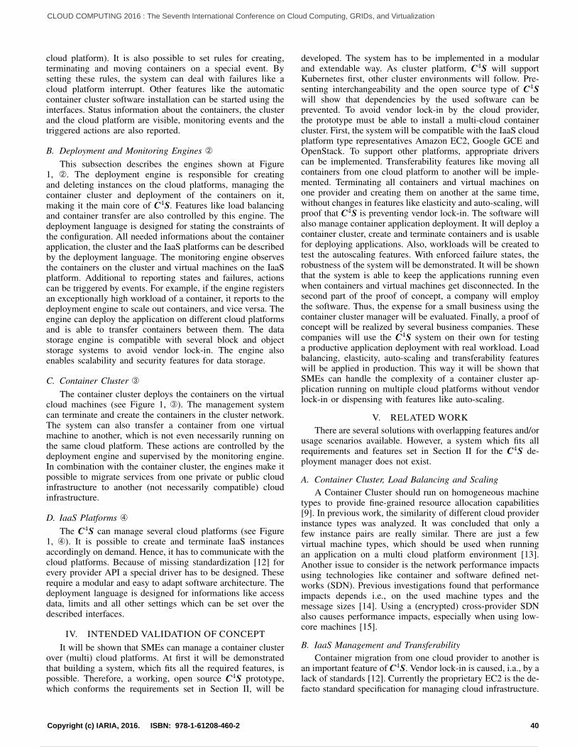
cloud platform). It is also possible to set rules for creating,terminating and moving containers on a special event. Bysetting these rules, the system can deal with failures like acloud platform interrupt. Other features like the automaticcontainer cluster software installation can be started using theinterfaces. Status information about the containers, the clusterand the cloud platform are visible, monitoring events and thetriggered actions are also reported.

B. Deployment and Monitoring Engines Á

This subsection describes the engines shown at Figure1, Á. The deployment engine is responsible for creatingand deleting instances on the cloud platforms, managing thecontainer cluster and deployment of the containers on it,making it the main core of C4S. Features like load balancingand container transfer are also controlled by this engine. Thedeployment language is designed for stating the constraints ofthe configuration. All needed informations about the containerapplication, the cluster and the IaaS platforms can be describedby the deployment language. The monitoring engine observesthe containers on the cluster and virtual machines on the IaaSplatform. Additional to reporting states and failures, actionscan be triggered by events. For example, if the engine registersan exceptionally high workload of a container, it reports to thedeployment engine to scale out containers, and vice versa. Theengine can deploy the application on different cloud platformsand is able to transfer containers between them. The datastorage engine is compatible with several block and objectstorage systems to avoid vendor lock-in. The engine alsoenables scalability and security features for data storage.

C. Container Cluster Â

The container cluster deploys the containers on the virtualcloud machines (see Figure 1, Â). The management systemcan terminate and create the containers in the cluster network.The system can also transfer a container from one virtualmachine to another, which is not even necessarily running onthe same cloud platform. These actions are controlled by thedeployment engine and supervised by the monitoring engine.In combination with the container cluster, the engines make itpossible to migrate services from one private or public cloudinfrastructure to another (not necessarily compatible) cloudinfrastructure.

D. IaaS Platforms Ã

The C4S can manage several cloud platforms (see Figure1, Ã). It is possible to create and terminate IaaS instancesaccordingly on demand. Hence, it has to communicate with thecloud platforms. Because of missing standardization [12] forevery provider API a special driver has to be designed. Theserequire a modular and easy to adapt software architecture. Thedeployment language is designed for informations like accessdata, limits and all other settings which can be set over thedescribed interfaces.

IV. INTENDED VALIDATION OF CONCEPTIt will be shown that SMEs can manage a container cluster

over (multi) cloud platforms. At first it will be demonstratedthat building a system, which fits all the required features, ispossible. Therefore, a working, open source C4S prototype,which conforms the requirements set in Section II, will be

developed. The system has to be implemented in a modularand extendable way. As cluster platform, C4S will supportKubernetes first, other cluster environments will follow. Pre-senting interchangeability and the open source type of C4Swill show that dependencies by the used software can beprevented. To avoid vendor lock-in by the cloud provider,the prototype must be able to install a multi-cloud containercluster. First, the system will be compatible with the IaaS cloudplatform type representatives Amazon EC2, Google GCE andOpenStack. To support other platforms, appropriate driverscan be implemented. Transferability features like moving allcontainers from one cloud platform to another will be imple-mented. Terminating all containers and virtual machines onone provider and creating them on another at the same time,without changes in features like elasticity and auto-scaling, willproof that C4S is preventing vendor lock-in. The software willalso manage container application deployment. It will deploy acontainer cluster, create and terminate containers and is usablefor deploying applications. Also, workloads will be created totest the autoscaling features. With enforced failure states, therobustness of the system will be demonstrated. It will be shownthat the system is able to keep the applications running evenwhen containers and virtual machines get disconnected. In thesecond part of the proof of concept, a company will employthe software. Thus, the expense for a small business using thecontainer cluster manager will be evaluated. Finally, a proof ofconcept will be realized by several business companies. Thesecompanies will use the C4S system on their own for testinga productive application deployment with real workload. Loadbalancing, elasticity, auto-scaling and transferability featureswill be applied in production. This way it will be shown thatSMEs can handle the complexity of a container cluster ap-plication running on multiple cloud platforms without vendorlock-in or dispensing with features like auto-scaling.

V. RELATED WORKThere are several solutions with overlapping features and/or

usage scenarios available. However, a system which fits allrequirements and features set in Section II for the C4S de-ployment manager does not exist.

A. Container Cluster, Load Balancing and ScalingA Container Cluster should run on homogeneous machine

types to provide fine-grained resource allocation capabilities[9]. In previous work, the similarity of different cloud providerinstance types was analyzed. It was concluded that only afew instance pairs are really similar. There are just a fewvirtual machine types, which should be used when runningan application on a multi cloud platform environment [13].Another issue to consider is the network performance impactsusing technologies like container and software defined net-works (SDN). Previous investigations found that performanceimpacts depends i.e., on the used machine types and themessage sizes [14]. Using a (encrypted) cross-provider SDNalso causes performance impacts, especially when using low-core machines [15].

B. IaaS Management and TransferabilityContainer migration from one cloud provider to another is

an important feature of C4S. Vendor lock-in is caused, i.a., by alack of standards [12]. Currently the proprietary EC2 is the de-facto standard specification for managing cloud infrastructure.



53 / 157

However, open standards like OCCI and CIMI are important toreduce vendor lock-in situations [16]. C4S includes a specialIaaS driver for each supported cloud provider. Other researchapproaches in cloud migration can be reviewed under [17].There are several solutions like Apache Libcloud, KOALA[18], Scalr, Apache jclouds and deltacloud and T-SystemsCloud Broker for managing and deploying virtual machines onIaaS platforms. Except for the T-Systems Cloud Broker, thesolutions are open source but have mostly payable services,reduced functionality or limited virtual machine quantities.These systems support features like creating, stopping andscaling virtual machines on IaaS cloud platforms. Some ofthem like the T-Systems Cloud Broker, Scalr and Apachejclouds are designed for cross-platform IaaS deployment. Incontrast to the C4S requirements, the presented cloud managersare limited to IaaS managing and do not offer containerdeploying services. Some of them do not prevent vendor lock-in by cloud providers or create new dependencies by itself(e.g., T-System Cloud Broker, KOALA is limited to AmazonAWS API compatible services).

C. Application DeploymentPeinl et al. [19] has defined requirements for a container

application deploying system. These coincide strongly with therequirements for the C4S system, which have been discussedin Section II-A. He also gives an overview about containercluster managing. For easy deployment a container applicationwith monitoring, scaling and controlling benefits, there existseveral commercial solutions like the Amazon EC2 ContainerService (ECS), Microsoft Azure Container Service and GiantSwarm. Limited to the providers own IaaS infrastructure,these solutions are not designed for multi-cloud platformusages, especially between public clouds (a requirement ofC4S). Open source cluster managers are Apache Mesos andKubernetes. These systems are designed to run workloadsacross tens of thousands of machines. The benefits and issuesusing cluster technologies are very high reliability, availabilityand scalability [9] [8]. However, they are not designed tocreate and terminate virtual machines (like AWS instances),but to deploy applications on given resources. So, they cannotprevent cloud provider dependencies on their own, but provideessential ingredients to do so. Another cluster managementtool for increasing the efficiency of datacenter servers iscalled Quasar, which is developed by the Stanford Universityand designed for maximizing resource utilization. The systemperforms coordinated resource allocation. Several techniquesanalyze performance interferences, scaling (up and out) andresource heterogeneity [20].

VI. CONCLUSIONThe C4S is in the planning state, although some parts are

already implemented, like the cloud platform driver for fastdeploying IaaS instances. The next step is the creation ofa deployment language for dedicated containers to run on aKubernetes container cluster, finding solutions for containercluster scaling problems and handling stateful tasks like filestorage. The system will be implemented in a modular andgeneric way to allow an easy adaptation for different cloudplatforms and container cluster software. With C4S SMEs willbe able to deploy and operate their container applications onan elastic, auto-scaling and load balancing multi-cloud clusterwith transferability features to prevent vendor lock-in.

ACKNOWLEDGMENT

This research is funded by German Federal Min-istry of Education and Research (Project Cloud TRANSIT,03FH021PX4). The author thank the University of Lubeck(Institute of Telematics) and fat IT solution GmbH (Kiel) fortheir support of Cloud TRANSIT.

REFERENCES[1] P. Mell and T. Grance, “The nist definition of cloud computing,” 2011.[2] M. Armbrust et al., “A view of cloud computing,” Communications of

the ACM, vol. 53, no. 4, 2010, pp. 50–58.[3] L. M. Vaquero, L. Rodero-Merino, and R. Buyya, “Dynamically scaling

applications in the cloud,” ACM SIGCOMM Computer CommunicationReview, vol. 41, no. 1, 2011, pp. 45–52.

[4] M. Mao and M. Humphrey, “Auto-scaling to minimize cost and meetapplication deadlines in cloud workflows,” in Proceedings of 2011 In-ternational Conference for High Performance Computing, Networking,Storage and Analysis. ACM, 2011, p. 49.

[5] N. Kratzke, “Lightweight virtualization cluster - howto overcome cloudvendor lock-in,” Journal of Computer and Communication (JCC), vol. 2,no. 12, oct 2014.

[6] R. Sahandi, A. Alkhalil, and J. Opara-Martins, “Cloud computing fromsmes perspective: A survey-based investigation,” Journal of InformationTechnology Management, vol. 24, no. 1, 2013, pp. 1–12.

[7] J. Turnbull, The Docker Book: Containerization is the new virtualiza-tion. James Turnbull, 2014.

[8] A. Verma, L. Pedrosa, M. Korupolu, D. Oppenheimer, E. Tune, andJ. Wilkes, “Large-scale cluster management at google with borg,” inProceedings of the Tenth European Conference on Computer Systems.ACM, 2015, p. 18.

[9] B. Hindman et al., “Mesos: A platform for fine-grained resource sharingin the data center.” in NSDI, vol. 11, 2011, pp. 22–22.

[10] Definition recommendation of micro, small and medium-sizedenterprises by the european communities. Last access 12th Nov.2015. [Online]. Available: http://eur-lex.europa.eu/legal-content/EN/TXT/?uri=uriserv:OJ.L .2003.124.01.0036.01.ENG

[11] N. Kratzke, “A lightweight virtualization cluster reference architecturederived from open source paas platforms,” Open J. Mob. Comput. CloudComput, vol. 1, 2014, pp. 17–30.

[12] J. Opara-Martins, R. Sahandi, and F. Tian, “Critical review of vendorlock-in and its impact on adoption of cloud computing,” in InformationSociety (i-Society), 2014 International Conference on. IEEE, 2014,pp. 92–97.

[13] N. Kratzke and P.-C. Quint, “How to operate container clusters moreefficiently? some insights concerning containers, software-defined-networks, and their sometimes counterintuitive impact on networkperformance,” International Journal on Advances in Networks andServices, vol. 8, no. 3&4, 2015, (in press).

[14] N. Kratzke and P.-C. Quint, “About automatic benchmarking of iaascloud service providers for a world of container clusters,” Journal ofCloud Computing Research, vol. 1, no. 1, 2015, pp. 16–34.

[15] N. Kratzke, “About microservices, containers and their underestimatedimpact on network performance,” CLOUD COMPUTING 2015, 2015,p. 180.

[16] C. Pahl, L. Zhang, and F. Fowley, “Interoperability standards for cloudarchitecture,” in 3rd International Conference on Cloud Computing andServices Science, CLOSER. Dublin City University, 2013, pp. 8–10.

[17] P. Jamshidi, A. Ahmad, and C. Pahl, “Cloud migration research: asystematic review,” Cloud Computing, IEEE Transactions on, vol. 1,no. 2, 2013, pp. 142–157.

[18] C. Baun, M. Kunze, and V. Mauch, “The koala cloud manager: Cloudservice management the easy way,” in Cloud Computing (CLOUD),2011 IEEE International Conference on. IEEE, 2011, pp. 744–745.

[19] R. Peinl and F. Holzschuher, “The docker ecosystem needs consolida-tion.” in CLOSER, 2015, pp. 535–542.

[20] C. Delimitrou and C. Kozyrakis, “Quasar: Resource-efficient and qos-aware cluster management,” ACM SIGPLAN Notices, vol. 49, no. 4,2014, pp. 127–144.



54 / 157

Cloud Data Denormalization of Anonymous Transactions

Aspen Olmsted, Gayathri Santhanakrishnan

Department of Computer Science

College of Charleston, Charleston, SC 29401

e-mail: [email protected], [email protected]

Abstract— In this paper, we investigate the problem of

representing transaction data in PAAS cloud-based systems.

We compare traditional database normalization techniques

with our denormalized approach. In this research, we

specifically focus on transactional data that is not attached to a

specific customer. The absence of the relationship in the

customer object allows for the vertical merging of tuples. to be

stored in aggregate form. The journaling features of the data

store, allow full audits of transactions while not requiring

anonymous data to be materialized in fine-grained levels. The

horizontal merging of objects is also deployed to remove detail

lookup data instance records and replace them with business

rule objects.

Keywords-web services; distributed database; modeling

I. INTRODUCTION

In this work, we investigate the problem of representing transactional data in a platform as a service (PAAS) cloud-based system. In traditional client-server architectures, database normalization is used to ensure that redundant data is not stored in the system. Redundant data can lead to update anomalies if the developer is not careful to update every instance of a fact when modifying data. Normalization is also performed to ensure unrelated facts are not stored in the same tuples resulting in deleting anomalies.

Data representation in the cloud has many of the same challenges as data representation in client/server architectures. One challenge data representation in the cloud has that is not shared with client/server is the minimization of data because costs of cloud data storage are significantly higher than local storage. We are thinking of simple costs for disk storage, not true costs. Organizations budget only the costs of disk drives for local storage which are in the tens of dollars per gigabyte but cloud storage can be in the hundreds of dollars per gigabyte per month [1]. Often this storage is expressed as the number of tuples in the data store instead of the number of bytes on the disk drive holding the data. For example, force.com [2] charges for blocks of data measured in megabytes but they calculate usage as a flat 2KB per tuple. Zoho Corporation also tracks data storage by the tuple for serval of their cloud products including Creator [3] and CRM [4]. The tuple count method is used as it is easier to calculate in a multi-tenant system where the physical disk drives are shared by many clients.

In this paper, we present an algorithm that will minimize the number of tuples used to store the facts for a software system. We use a motivating example from a cloud software system developed by students in our lab. The algorithm performs three main operations:

The horizontal merging of objects – several distinct relations are combined into one.

The vertical merging of objects – several distinct instances of the same type of facts is combined into one.

Business rule adoption – instead of storing tuples to represent availability of lookup data, we replace the tables with pattern based business rules

We apply our algorithm to a system in the humanities application domain and show an approximately 500% reduction in tuple storage.

Date [5] invests a good deal of his text on the definition

of denormalization. He argues that denormalization is when

the number of relational variables is reduced, and functional

dependencies are introduced where the left hand of the

functional dependency no longer is a super key. In our

work, we perform many optimizations. When we

horizontally merge relations, then we are performing a true

denormalization. Other optimizations such as vertical

merging do not fit Date’s definition of denormalization. We

choose to stay with the term denormalization algorithm as it

is a set of steps taken after the normalization process.

The organization of the paper is as follows. Section 2

describes the related work and the limitations of current

methods. In Section 3 we give a motivating example where

our algorithm is useful and describe our denormalization

algorithm. Section 4 describes additional enhancements

through the design of business rule objects. Section 5

explores reporting from the denormalized objects utilizing

the object version history stored in the journal. Section 6

contains our comparison of the proposed method and the

traditional database normalization method. We conclude and

discuss future work in Section 7. .

II. RELATED WORK

Sanders and Shin [6] investigate the process to be

followed when denormalization is done on relational data

management systems (RDBMS) to gain better query

performance. Their work was done before the cloud

database offerings became prevalent. In the cloud, database

performance is less of an issue to storage requirements

because the systems are designed to distribute queries across

many systems.

Conley and Whitehurst [7] patented the idea of

denormalizing databases for performance but hiding the

denormalization for the end user. Their work focuses on

merging two relations into one relationship to eliminate the

processing required to join the records back together. Their

work uses horizontal denormalization to gain performance.



55 / 157

Our work uses both horizontal and vertical denormalization

to minimize storage space and increase usability.

Most denormalization research work was done in the

late 1990s and was focused on improvement in query

performance over the correctness and usability of the data.

Recently, folks like Andrey Balmin have looked at

denormalization as a technique to improve the performance

of querying XML data. Like the previously mentioned

research, this work differs from our work in the desired end

goal of minimized data storage and end user usage.

In Bisdas’ [8] blog, he demonstrates ways that end users

can improve data visualization by vertically merging

hierarchical data in the Salesforce, data model. He takes

advantage of the trigger architecture to create redundant

data in the hierarchy. Taber [9] also recommends

denormalization to improve data visualization. The problem

with both solutions is that data storage requirements are

increased while correctness is jeopardized by the redundant

data.

In our previous work [10], we study UML models from

the perspective of integrating heterogeneous software

systems. In the work, we create an algorithm to sort cyclical

UML class data diagrams to enable transaction reformation

in the integration. In the process, discoveries were made on

the freshness of data at different layers in the UML graph.

The knowledge is useful in this study when considering

anomalies that can happen in response to data updates.

Additional semantics for models can be added by the

integration of the matching UML Activity and Class

diagrams. UML provides an extensibility mechanism that

allows a designer to add new semantics to a model. A

stereotype is one of three types of extensibility mechanisms

in the UML that allows a designer to extend the vocabulary

of UML to represent new model elements [11].

Traditionally these semantics were consumed by the

software developer manually and translated into the

program code in a hard coded fashion. Developers have implemented business rules in software

systems since the first software package was developed. Most research has been around developing expert systems to process large business rule trees efficiently. Charles Forgy [12] developed the Rete Algorithm, which has become the standard algorithm used in business rule engines. Forgy has published several variations on the Rete Algorithm over the past few decades.

III. DENORMALIZATION

We demonstrate our work using a Tour Reservation

System (TRS). TRS uses web services to provide a variety

of functionalities to the patrons who are visiting a museum

or historical organization. We use the UML specification

to represent the meta-data. Figure 1 shows a UML class

diagram for an implementation of this functionality. The

Unified Modeling Language includes a set of graphic

notation techniques to create visual models of object-

oriented software systems [13]. In this study, we use data

collected by the Gettysburg Foundation on visitors to their

national battlefield. The system is modeled and

implemented on the force.com [2] cloud platform.

Figure 1 shows a normalized UML class model of

reservation transactions of visitors to the Gettysburg

National Battlefield. In the model the central object ticket

represents a pass for an entry that is valid for a specific date

and time and a specific activity. Activities are itinerary

items the visitor can be involved in while visiting the

battlefield. In the normalized model, each ticket is linked to

a specific activity schedule entry that will designate the date

and time the pass is valid for entry. Each activity schedule

is linked to an activity object that designates the name and

location of the activity.

Each ticket is linked to a user in the Gettysburg

organization who was responsible for the transaction. Each

ticket can be linked to a patron object. In the case of

advanced reservations, there will be a valid patron object

linked to the ticket. Advanced reservations are transactions

that take place through the organization's website or over

the phone to a reservation agent. In the case of walk-up

transactions, there will not be a linked patron. A walk-up

transaction is a transaction that takes place when a visitor

arrives on the site without a prior reservation and pays for

the ticket at the front desk.

In Figure 1, the multiplicity of the association between

the patron and the ticket is a zero or one to many. A

multiplicity that can be zero represents anonymous data.

Anonymous data is data that does not need to be specified in

order for the transaction to be valid. In the example

transaction, the patron can remain anonymous but still visit

the battlefield and partake in the activities. In the case of

the sample Gettysburg data, 60 percent of ticketing

transactions were anonymous.

In the case of the force.com [2] PAAS, data storage is

charged by the tuple. With an enterprise license to the

platform, the organization is granted access to one gigabyte

of data storage. The storage is measured by treating every

tuple as two kilobytes. This form of measurement allows

Figure 1. Normalized Transaction Model



56 / 157

the organization 500,000 tuples in the enterprise data

storage option. The data collected for the normalized data

model would allow the Gettysburg organization to store

around nine months’ worth of data. With the anonymous

transaction, the ticket and the payment data is only

important on the original transaction level for auditing. For

example, the accounting department may want to see the

details behind a specific ticket agent’s cash total for the day.

Another example would be the marketing department wants

to see the ticket price patterns within an hour of the day.

The force.com [2] platform uses an Oracle relational

database to deliver the data storage services but adds a

journal feature so history can be stored on all changes to an

object over time. This journal can be used at no additional

data storage cost. The field level changes stored in the

journal would allow aggregate data to be stored for

anonymous transactions and still have the detail to perform

the audits mentioned earlier.

If an object is used between two other objects where the

middle object is the “many” side of the one-to-many

relationship and the one side of the other relationship, then

the same data can be represented by moving the attributes to

the object on the composition side of the relationship. The

middle object is then able to be removed, reducing the

number of tuples representing the same amount of data. In

Figure 1, the “Activity Schedule” object fits this profile and

can be horizontally merged with the “Ticket” object. In our

previous work [10], we study UML data model freshness

requirements and document the relationship between data

changes and location in the UML graph. In our findings, we

see that middle object nodes are less predisposed to changes

than leaf nodes. The lower amount of data changes reduces

the change of update anomalies.

In Figure 1, we also designate objects that are updated in

transactions differently than objects that are navigated for

transactional lookup values. Two stereotypes are added to

the diagram:

Transactional – The classes designated with the

orange color and the <<Transactional>> tag are

updated during transactional activities.

Lookup – The classes designated with the green

color and the <<Lookup>> tag are not updated

during transactional activities. The data in these

classes are created by administrative activities.

During transactions, the data is searched for the

proper values.

The Denormalization Algorithm, Algorithm 1,

transforms a normalized model stored in a UML class

diagram into a denormalized model represented as an entity-

relationship diagram. The algorithm assumes input and

output of the models in the XMI [14] format. XMI is a

standard exchange format used to represent structural

models in a non-proprietary way.

The algorithm first loops through each object in the

normalized model and adds the object and attributes as

entities in the denormalized entity-relationship diagram. If

the object has the transactional stereotype, then the

attributes are marked unique. Surrogate identifier fields are

added to each object’s definition to be used as an auto-

incrementing primary key.

The next pass of the algorithm is to find objects that can

be eliminated from the middle relationship of two “one-to-

many” relationships. The original model, in Figure 1, had

an activity schedule object that consumed a lot of data space

by storing a lot of tuples to represent the occurrences an

activity can take place. We use a stereotype of “PK”

applied to attributes in the original model to designate the

primary identifier for instances of an object. This

designation allows us to shift the attribute down the

association and swap the positioning of the objects. In this

iteration over the objects, we also look for date-time data

Figure 2 Denormalized Transaction Model

Algorithm 1. Denormalization Algorithm

INPUT: normalizedObjects (XMI representation of

UML class diagram)

OUTPUT: denormalizedEntities (XMI representation

of denormalized entities)

foreach object in normalizedObjects

add entity to denormalizedEntities

foreach attribute in object

add attribute to entity

if object is transactional

mark attribute as unique

add id attribute as primary key

mark id as autoincrement

foreach entity in denormalizedEntities

if entity is both a many side and a one side of two

relationships

and a lookup object

foreach attribute in object

if attribute is PK

add attributes to many side entity

if attribute is a datetime type expand date pattern

swap graph location entity of the one sides

foreach association in normalizedObjects

if association is one-to-may and many side is transactional

add foreign key to many side entity

add quantity field to entity on many side



57 / 157

types that are part of the primary key. When we locate an

occurrence, we replace the attribute with a date-time

specification occurrence. The date-time specification

includes a starting date, ending date, starting time, ending

time and day of the week pattern.

The final pass of the algorithm adds foreign keys and

aggregation counters. The aggregation significantly reduces

the count of tuples stored. An example of this is shown in

Figure 1. Instead of having an instance of each ticket, we

add the quantity field to store the aggregate count for the

unique attributes.

Figure 2 shows an entity-relationship diagram of a

transformed model of Figure 1. Unique attributes have been

applied where aggregations should be performed. The

activity schedule entity has been shifted out in the graph,

and the quantity fields have been added to the aggregated

transactional objects.

IV. BUSINESS RULES

Business rule engines have sprung up to allow the

separation of business rules from the core application code.

The systems are designed to allow the end users to change

the business rules freely without changing the original

application code. In 2007, International Data Corporation

implemented a survey where they asked 'How often do you

want to customize the business rules in your software?’.

Ninety percent of the respondents reported that they

changed their business rules annually or more frequently.

Thirty-four percent of the respondents reported that they

changed their business rules monthly [15].

Figure 2 shows two tables that implement business rules:

Activity Schedule – This table implements the

date-time pattern mentioned earlier to store the

business rules for when a particular activity is

valid.

Price Schedule – This table implements the

date-time pattern mentioned earlier to store the

business rules for when a particular price is

available.

In each case objects in Figure 1, that inserted instances to

represent availability, are replaced with rule instances to

represent the availability. So instead of having a tuple per

availability instance, a single tuple can represent the pattern.

In the case of activity schedules, the example year had over

26,000 instances of availability that were replaced with 30

instances of the business rule.

V. OBJECT HISTORY ANALYSIS

One of the main reasons enterprises develop or purchase

software solutions to allow the organization to increase their

knowledge of their operations through the analysis of the

data collected in the software solution. The denormalization

solution presented earlier may limit the data available from

the denormalization process. The data is presented to the

users through dashboards, reports or exports. A dashboard

is presented as a graphical chart to measure where the

organization stands compared to a goal. Examples of these

would be sales to date compared to same period last year. A

report has a set of input parameters that control the data

displayed. The data displayed in the report tends to include

tables with aggregated values. Exports allow for the

exporting of data into a two-dimensional table saved as a

comma separated value (CSV) format. In this format,

attributes represent the columns of the data. Columns are

escaped with double quotes and separated by commas. For

our purposes, we will refer to all three categories generically

as reports.

Current state and historical comparison are the two

categories of reports a user may want to pull in their

analysis. In current state reports only the latest version of

the object is needed. In historical comparison reports, all

versions of an object may be needed depending on the level

of aggregation. An example of a historical comparison

report would be a report that compares sales for the month

compared to sales last year in the same month.

In our work, we developed Algorithm 2 to create an in-

memory copy of all historical versions of a specific object.

We use code to generate the data and then generate the

report output. If the organization wanted to allow end users

to report on historical versions, they could modify

Algorithm 2 to write records as temporary tuples and then

call the reporting tool.

VI. EMPIRICAL RESULTS

The empirical results demonstrate the success of

representing the example transaction data with significantly

lower cloud storage costs. TABLE 1 shows the tuple counts

for the original data model and the denormalized data

model. Both data models represent the complete 2014

calendar year of visitor transactions for the Gettysburg

National Battlefield. The denormalized model creates a 78%

reduction in the number of tuples. In the specific case of the

Algorithm 2. History Creation Algorithm

INPUT: object

OUTPUT: collection of object’s version history

Set thisObject = newest version of object Set objectVersions = empty list

Set fieldVersions = distinct saveDates values from object journal

Sort fieldVersions by saveDate descending Set lastDate = maximum(saveDate)

Foreach version in fieldVersions

If lastDate = version.saveDate objectVersions.add(thisObject)

Set thisObject.[version/attribute] = version.value

Set lastDate = version.saveDate Return objectVersions



58 / 157

force.com [2] platform, the reduction in number of tuples

allows the organization to store nearly three years of

transaction data in the data storage provided without

additional subscriptions costs. In the minimal data storage

provided to an enterprise customer of force.com [2], the

organization receives 500,000 tuples. Additional data

storage is available to the organization for a monthly

subscription price of 2,000 tuples per dollar. Using the

normalized data model, the organization would not be able

to store a complete year of data without needing to purchase

more data storage.

VII. CONCLUSION

In this paper, we propose an algorithm for object

denormalization when transforming an application domain

object model to a data model used in a cloud PAAS data

store. Our solution is based on navigating the relationships

in a UML class diagram and horizontally compressing

classes between multiple one-to-many relationships,

aggregating relationships on anonymous relationships and

using temporal offering patterns.

In this research, we studied a specific application

domain related to humanities organizations. The algorithms

can be applied to similar application domains that contain

entity objects representing transactions and customers.

Future work needs to test our algorithms in other application

domains to ensure the work applies across different

application domains.

REFERENCES

[1] brainsell blog, "Salesforce, SugarCRM and SalesLogix —

Data Storage Costs Compared," 2016. [Online]. Available:

https://www.zoho.com/creator/pricing-comparison.html.

[Accessed 03 02 2016].

[2] Salesforce.com, inc, "Run your business better with Force.,"

2006. [Online]. Available:

http://www.salesforce.com/platform/products/force/?d=701

30000000f27V&internal=true. [Accessed 03 02 2016].

[3] Zoho Corporation, "Creator Pricing Comparison," 2016.

[Online]. Available: https://www.zoho.com/creator/pricing-

comparison.html. [Accessed 03 02 2016].

[4] Zoho Corporation, "Compare Zoho CRM editions," 2016.

[Online]. Available:

https://www.zoho.com/crm/comparison.html. [Accessed 03

02 2016].

[5] C. J. Date, "Denormalization," in Database Design and

Relational Theory, O'Reilly Media, 2012.

[6] G. L. Sanders and S. Shin, "Denormalization Effects on

Performance of RDBMS," in Proceedings of the 34th

Hawaii International Conference on Systems Sciences,

2001.

[7] J. D. Conley and R. P. Whitehurst, "Automatic and

transparent denormalization support, wherein

denormalization is achieved through appending of fields to

base relations of a normalized database". USA Patent

US5369761 A, 29 November 1994.

[8] A. Bisda , "Salesforce Denormalization Delivers New

Power for Nurtures," DemandGen, 29 07 2014. [Online].

Available: http://www.demandgen.com/salesforce-

denormalization-delivers-new-power-nurtures/. [Accessed

09 11 2015].

[9] D. Taber, Salesforce.com Secrets of Success: Best Practices

for Growth and Profitability, Prentice Hall, 2013.

[10] A. Olmsted, "Fresh, Atomic, Consistent and Durable

(FACD) Data Integration Guarantees," in Software

Engineering and Data Engineering, 2015 International

Conference for, San Diego, CA, 2015.

[11] Object Management Group, "Unified Modeling Language:

Supersturcture," 05 02 2007. [Online]. Available:

http://www.omg.org/spec/UML/2.1.1/. [Accessed 08 01

2013].

[12] C. L. Forgy, "Rete: A fast algorithm for the many

pattern/many object pattern match problem," Artificial

Intelligence, vol. 19, no. 1, p. 17–37, 1982.

[13] Object Management Group, "Unified Modeling Language:

Supersturcture," 05 02 2007. [Online]. Available:

http://www.omg.org/spec/UML/2.1.1/. [Accessed 08 01

2013].

[14] Object Management Group, "OMG Formal Versions of

XMI," 06 2015. [Online]. Available:

http://www.omg.org/spec/XMI/. [Accessed 11 11 2015].

[15] Ceiton Technologies, "Introducing Workflow," [Online].

Available:

http://ceiton.com/CMS/EN/workflow/introduction.html#Cus

tomization. [Accessed 15 09 2014].

TABLE 1. EMPIRICAL RESULTS

Table Normalized

Tuples

Denormalized

Tuples

user 31 31

patron 17,610 17,610

ticket 738,981 157,780

activity

schedule

26,697 30

price schedule 220 24

activity 17 17

Total 783,556 175,492



59 / 157

Modeling Non-Functional Requirements in Cloud Hosted Application

Software Engineering

Santoshi Devata, Aspen Olmsted

Department of Computer Science College of Charleston, Charleston, SC 29401

e-mail: [email protected], [email protected]

Abstract- Functional Requirements are the primary focus

of software development projects for both end users and

developers. The Non-Functional Requirements (NFR) are

treated as a secondary class requirement, ignored until the

end of the development cycle. They are often hidden,

overshadowed and therefore, frequently neglected or

forgotten. NFRs are sometimes difficult to deal with and

are the most expensive in certain cases. NFRs become even

more important with cloud architectures because the

concurrent load and response latency are more vulnerable

using public networks than they were on private networks.

More wok is needed on mapping NFR models into software

code. Developing a cloud based system with functional

requirements only is not enough to build a good and useful

software. NFRs should become an integral part of software

development. In this paper, we focus on the modeling of

NFRs and the transformations from UML models into the

source code. Specifically, we choose three NFRS: response

time, concurrency, user response time for a Theater

Booking system.

Keywords - Non-Functional Requirements; NFRs;

Response time; Concurrency

I. INTRODUCTION

The software engineering process is intended to

produce software with specific functionality that is

delivered on time, within budget and satisfying

customer’s need. Bruegge and Dutoit [1] dedicate the

first chapter of their text book to these outcomes and

budget constraints. These demands mean that the

software development is focused and driven by the

functional requirements. The software market is

changing every day increasing its demands for providing

best quality software that not only implements all the

desired functionality but also satisfies the NFRs.

Including NFRs in the model, leads to a complete

software capable of handling not just the requirements

associated with the product but also provides the

usability according to the current standards. NFRs

(sometimes also referred to as software qualities)

indicate how the system behaves and includes

requirements dealing with system performance,

operation, required resources and costs, verification,

documentation, security, portability, and reliability.

Thus, satisfying NFRs is critical to building good

software systems and expedites the time-to-the-market

process, since errors due to not properly dealing with

NFR, which is usually time-consuming and complex,

can be avoided. However, software engineers need to

know whether the performance cost of the algorithms

that deal with the various NFRs will violate the basic

performance requirements or conflict among

themselves.

Failing to address NFRs in the design phase can lead

to a software product that may meet all the functional

requirements but fail to be useful because it cannot be

used. In the United State, the federal government

contracted a 3rd party vendor to develop an application

for individuals to register for health care coverage. The

designers failed to specify the NFRs for concurrency,

and the application could not be used because of the

mistake. [2]

NFRs are sometimes not intuitive to the developers,

so implementing and including them in the development

cycles is challenging. There are different approaches to

handling the NFRs, but the best way is to model them

and implement for each case. Rahman and Ripon [3]

describe a use case and the challenge of integrating the

NFRs into the design models.

The organization of the paper is as follows: Section

2 describes the related work and the limitations of

current methods. In Section 3 we give a motivating

example and explain our proposal, present our

algorithms and show how they are used in our research.

We conclude and discuss future work in Section 4.

II. RELATED WORK

Functional requirements are defined and represented

in many ways. These functional requirements are the

basis of software development, but NFRs are the ones

that supply the rules when implementing the code. Many

authors have looked at NFRs and the problems of their

inclusion in the design process. Pavlovski and Zou [4]

define NFRs as specific behaviors and operational

constraints, such as performance expectations and policy

constraints. Though there are many discussions about the

NFRs, they are not taken as seriously as they should be.

Glinz [5] suggest the notion of splitting both functional

and NFRs into a set of categories and make groups of



60 / 157

them so that they are inherently considered while

developing the applications. Alexander [6] suggests

looking at the language used to describe the

requirements. Words ending in ‘-ility’ are often the

NFRs. Examples of these words are reliability and

verifiability. All of their work focuses on identification

of the NFRs. Our work builds on theirs by applying

domain specific models using extensibility mechanisms

built into standard modeling notations.

Ranabahu and Sheth [7] explore four different

modeling semantics required when representing cloud

application requirements. These include data, functional,

non-functional and system. Their work focuses on

functional and system requirements. There is a small

overlap with our work, but only with nonfunctional

requirements from the system perspective. They build

on work done by Stuart [8] in his workshops where he

defined semantic modeling languages to model cloud

computing requirements in the three phases of the cloud

application life cycle. The three phases are development,

deployment, and management. Our work adds to the

missing semantic category of NFRs.

In Ranabahu and Sheth [7] work they use Unified

Markup Language (UML) [9] to model the functional

requirements only. UML is a standardized notation for

representing interactions, structure and process flow of

software systems. UML consists of many different

diagram types. Individual diagrams can be linked

together to model different perspectives of the same part

of a software system. We utilize UML to express the

NFRs also.

Additional semantics for models can be added by the

integration of the matching UML Activity and Class

diagrams. UML provides an extensibility mechanism

that allows a designer to add new semantics to a model.

A stereotype is one of three types of extensibility

mechanisms in the UML that allows a designer to extend

the vocabulary of UML to represent new model elements

[10]. Traditionally the semantics were consumed by the

software developer and manually translated into the

program code in a hard coded fashion.

Object Constraint Language (OCL) [11] is part of the

official Object Management Group (OMG) standard for

UML. An OCL constraint formulates restrictions for the

semantics of the UML specification. An OCL constraint

is always true if the data is consistent. Each OCL

constraint is a declarative expression in the design model

that states correctness. Expression of the constraint

happens on the level of the class, and enforcement

happens on the level of the object. OCL has operations

to observe the system state but does not contain any

operations to change the system state.

Our contribution in the domain of cloud computing

software modeling is in the use of modeling standards

such as UML and OCL with their extensibility

mechanism of stereotypes to model the NFRs. We

demonstrate these models can be transformed into

application source code through the application of three

application domain constraints.

III. RESEARCH PROPOSAL

Our contribution in this work is to look at application

domain specific NFRs that are useful for cloud based

application architectures. We model the NFRs using the

extensibility mechanisms built into the standard

modeling notations of UML and OCL to specify those

NFRs. We then auto-generate code for NFRS using

Java. We demonstrate the NFRs using a theater booking

system example. A theater booking system is an online

application used by theatres to sell their entrance tickets.

Figure 1 shows an activity diagram for a theatre booking

system where the NFRs are represented using UML

stereotypes. We chose to focus on three NFRs for this

study: response time, concurrency, and pick seat time to

implement the theater booking system. For each NFR,

we model in UML and OCL utilizing stereotypes to

apply the additional required semantics. We then

generate code from the model to enforce the NFRS. The

code is generated for these NFRs for use in a cloud

application that uses the threads on the server side for

each client.

Request response time is one of the key performance

measures in a theater booking system. It is an NFR that

is represented as a ‘Response time’ stereotype in the

UML activity diagram (Figure 1). This stereotype is

related to every interaction between the client and the

server. In general terms, response time can be defined as

the amount of time system takes to process a request after

it has received one. A control flow in an activity diagram

can be assigned the stereotype. In the algorithm that is

used to enforce for this stereotype, the time is noted right

before the request is sent to the server and the difference

is measured once the response is received. The

difference between the send and receive time gives the

response time for the request. Specific stereotypes are

used to represent different latency requirements.

Examples are “low latency: and “high latency”. Runtime

configuration can define the allowable time for each

stereotype. Response time for each request from the

users is measured, and the average response is calculated

for the overall system. This is particularly useful to

measure the overall system performance and compare it

over time. If the average response time increases, we can

further get the average response of each module/type of

requests and find the bottlenecks. Algorithm 1 shows the

algorithm implemented to guarantee this NFR. In the

algorithm, the client notifies the server when the timeout

occurs to enable the server to rollback any partial work

completed.



61 / 157

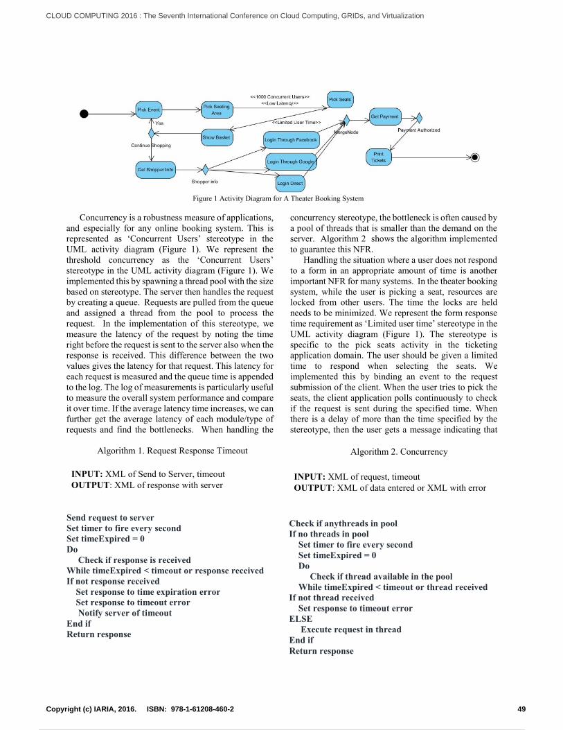
Concurrency is a robustness measure of applications,

and especially for any online booking system. This is

represented as ‘Concurrent Users’ stereotype in the

UML activity diagram (Figure 1). We represent the

threshold concurrency as the ‘Concurrent Users’

stereotype in the UML activity diagram (Figure 1). We

implemented this by spawning a thread pool with the size

based on stereotype. The server then handles the request

by creating a queue. Requests are pulled from the queue

and assigned a thread from the pool to process the

request. In the implementation of this stereotype, we

measure the latency of the request by noting the time

right before the request is sent to the server also when the

response is received. This difference between the two

values gives the latency for that request. This latency for

each request is measured and the queue time is appended

to the log. The log of measurements is particularly useful

to measure the overall system performance and compare

it over time. If the average latency time increases, we can

further get the average latency of each module/type of

requests and find the bottlenecks. When handling the

concurrency stereotype, the bottleneck is often caused by

a pool of threads that is smaller than the demand on the

server. Algorithm 2 shows the algorithm implemented

to guarantee this NFR.

Handling the situation where a user does not respond

to a form in an appropriate amount of time is another

important NFR for many systems. In the theater booking

system, while the user is picking a seat, resources are

locked from other users. The time the locks are held

needs to be minimized. We represent the form response

time requirement as ‘Limited user time’ stereotype in the

UML activity diagram (Figure 1). The stereotype is

specific to the pick seats activity in the ticketing

application domain. The user should be given a limited

time to respond when selecting the seats. We

implemented this by binding an event to the request

submission of the client. When the user tries to pick the

seats, the client application polls continuously to check

if the request is sent during the specified time. When

there is a delay of more than the time specified by the

stereotype, then the user gets a message indicating that

Algorithm 1. Request Response Timeout

INPUT: XML of Send to Server, timeout

OUTPUT: XML of response with server

Send request to server

Set timer to fire every second

Set timeExpired = 0

Do

Check if response is received

While timeExpired < timeout or response received

If not response received

Set response to time expiration error

Set response to timeout error

Notify server of timeout

End if

Return response

Figure 1 Activity Diagram for A Theater Booking System

Algorithm 2. Concurrency

INPUT: XML of request, timeout

OUTPUT: XML of data entered or XML with error

Check if anythreads in pool

If no threads in pool


Set timeExpired = 0

Do

Check if thread available in the pool

While timeExpired < timeout or thread received

If not thread received


ELSE

Execute request in thread

End if

Return response



62 / 157

there locks have been released. If the request is sent

before the specified time, then the user will proceed to

next activity. Algorithm 3 shows the algorithm

implemented to guarantee this NFR.

IV. CONCLUSION/FURTHER RESEARCH

In this work, we show that it is possible to model

many cloud based software NFRs using UML

stereotypes. UML diagrams have been used for years to

model the functional requirements of the application.

We extended the modeling of functional requirements by

using UML stereotypes to model the NFRs in the same

design model. The UML stereotype is transformed to

application code that guarantees the NFR will be

enforced. Future work will enhance our work to include

OCL constraints to broaden the type of NFRs that can be

modeled and transformed into cloud application code.

REFERENCES

[1] B. Bruegge and A. Dutoit, Object-Oriented

Software Engineering, Prentice Hall, Inc, 2010.

[2] T. Mullaney, "Obama adviser: Demand

overwhelmed HealthCare.gov," USA Today, 06

10 2013. [Online]. Available:

http://www.usatoday.com/story/news/nation/201

3/10/05/health-care-website-repairs/2927597/.

[Accessed 24 02 2016].

[3] M. M. Rahman and S. Ripon, "Elicitation and

Modeling Non-Functional Requirements – A POS

Case Study," International Journal of Future

Computer and Communication, vol. 2, no. 5, pp.

485-489, 2013.

[4] C. J. Pavlovski and J. Zou, "Non-functional

requirements in business process modeling,"

Proceedings of the Fifth on Asia-Pacific

Conference on Conceptual Modelling, vol. 79,

2008.

[5] M. Glinz, "Rethinking the Notion of Non-

Functional Requirements," Third World Congress

for Software Quality, Munich, Germany, 2005.

[6] Alexander, I, "Misuse Cases Help to Elicit Non-

Functional Requirements," Computing & Control

Engineering Journal, 14, 40-45, 2003.

[7] R. Ajith and A. Sheth, "Semantic Modeling for

Cloud Computing, Part I," Computing, vol.

May/June, pp. 81-83, 2010.

[8] S. Charlton, Model Driven Design and operations

for the Cloud, Towards Best Practices in Cloud

Computing Workshop, 2009.

[9] Object Management Group, "OMG Formal

Versions of UML," 06 2015. [Online]. Available:

http://www.omg.org/spec/UML/. [Accessed 11

09 2015].

[10] Object Management Group, "Unified Modeling

Language: Supersturcture," 05 02 2007. [Online].

Available:

http://www.omg.org/spec/UML/2.1.1/. [Accessed

08 01 2013].

[11] Object Management Group, "OMG Formally

Released Versions of OCL," 02 2014. [Online].

Available: http://www.omg.org/spec/OCL/.

[Accessed 09 11 2015].

Algorithm 3. User Response Timeout

INPUT: XML of form to display, timeout

OUTPUT: XML of data entered or XML with error

Show form to user


Set timeExpired = 0

Do

Check if response is received

While timeExpired < timeout or response received

If not response received

Notify user of time expiration


End if

Return response



63 / 157

Enabling Resource Scheduling in Cloud Distributed Videoconferencing Systems

Alvaro Alonso, Pedro Rodrıguez, Ignacio Aguado, Joaquın SalvachuaDepartamento de Ingenierıa de Sistemas Telematicos

Universidad Politecnica de MadridMadrid, Spain

email:{aalonsog, prodriguez, iaguado, jsalvachua}@dit.upm.es

Abstract—When deploying videoconferencing systems inCloud based infrastructures, one of the most complex challengesis to distribute Multipoint Control Units (MCUs) among dif-ferent servers. By addressing this challenge, we can improvethe flexibility and the performance of this type of systems.However, to actually take advantage of the Cloud possibilitieswe have also to introduce mechanisms to dynamically schedulethe distribution of the MCUs across the available resources.In this paper, we propose a resource scheduling model forvideoconferencing systems and, starting from an existing MCUdistribution architecture, we design a solution to enable theresource scheduling basing on custom criteria. These criteria canbe based on the characteristics of each server or in their status inreal time. We validate the extended model by setting up a typicalvideoconferencing deployment among a set of Cloud providersand testing a decision algorithm. We conclude that the proposedmodel enables the use of a wide range of algorithms that can beadapted to the needs of different Cloud deployments.

Keywords—cloud computing; videoconferencing; distributedMCU; scheduling

I. INTRODUCTION

Nowadays, a very important part of the applications andservices we consume over Internet are provided in Cloud [1]infrastructures. The main advantage of using this technologyis that one can adapt the amount of provisioned resources fora service based on the demand. In traditional deployments,one has to forecast the demand before obtaining the hardwareand this involves a lack of flexibility that can result in awaste of resources. However, using Cloud based deploymentsone can dynamically scale a service in almost real time byadding or removing computing capacity. In other words, CloudComputing provides the illusion of infinite computationalpower on a pay-per-use basis.

In addition to this advantage, this flexibility enables easierand more efficient ways to distribute the services among dif-ferent servers. Thus, one can balance the system load, replicateinstances or geographically distribute them. These operationsare done almost instantaneously with a click or by calling anAPI. Even some public Cloud providers offer components thatautomatically distribute the load between servers. However,these mechanisms are usually designed to be used by request-response services such as RESTful or web services.

In videoconferencing systems, the communication betweenparticipants is usually performed via a central server calledMultipoint Control Unit (MCU). MCUs are used to addressthe signalling and to interchange the media streams betweenpeers. Furthermore, in advanced configurations they are usedto record sessions or to transcode video and audio flows.

Today, thanks to technologies such as Adobe Flash [2] andHTML5 [3] with its real-time communications standard Web

Real Time Communications (WebRTC) [4], videoconferencingsystems are accessible from web applications and mobiledevices and its use is open to a higher number of users thanever before. On the other hand, the demand of these servicescan vary dynamically in short periods of time. The fluctuationin the number of users and the managed sessions results insubstantial changes in the computing capacity consumed bythe MCUs. Hence, and this is strengthened in [5], deployingMCUs in Cloud infrastructures offers several advantages. Oneof them is the already mentioned idea of distributing a serviceamong several servers. But, as anticipated, the standard solu-tions for resource scheduling do not apply to the specific caseof MCU distribution.

In traditional web services based on HTTP, it is usuallyenough with a distribution of the users requests using loadbalancers. These components are adapted to the requirementsof complex web services. However, we argue no generalsolution for distributed videoconferencing systems is available.Here, the resource use in each of the distributed nodes maydepend on several parameters besides the number of users.This can be understood with a very easy example. Suppose anscenario with an MCU distributed in two servers and managingsix users each. In the first MCU the six users are connected tothe same videoconferencing room and in the second one eachuser is connected alone to a different room. Obviously, thefirst MCU is consuming more resources because it is receivingpackets from each user and broadcasting them to all of therest while the second one is only receiving packets from theusers without any processing to do. Furthermore, to address thescheduling challenge in this scope we first need to understandwhich type of criteria we need to take into account and thenwe must enable a way to schedule the load distribution takingthose criteria into account.

In the next Section, we analyse the existing solutionsregarding resource scheduling in the Cloud and why they donot cover the videoconferencing scenario. Then, in Section IIIwe describe our scheduling model and extend an existent dis-tributed architecture to cover the needed requirements. Then, inSection IV we validate the solution with a real implementationand a typical use case. Finally, in Section V we enumeratethe main conclusions obtained and we analyse the differentresearch lines we open to continue the work.

II. RELATED WORK

Scheduling Cloud Computing resources has always beena subject under study. Being able to dynamically adapt andchange the available resources depending on the demand ofthe users is a key point in services deployed in the Cloud.Many strategies have been designed in order to solve this



64 / 157

problem, using techniques like the Genetic Algorithm [6],Particle Swarm Optimization (PSO) [7], Ant Colony Optimiza-tion (ACO) [8] or Load Balancing Ant Colony Optimization(LBACO) [9]. All of them try to find an optimal resourceallocation for workload in a generic Cloud architecture.

In spite of all of this work, there is not any solutionspecifically designed for a videoconferencing service. How-ever, there exists a model which, if properly developed, couldbe useful. The model described in [10] could be the firststep of Scheduling a videoconference service in the Cloud.There, the authors propose an architecture that allows to easilydivide an MCU in atomic parts called One To Many (OTMs).An OTM is a software component that basically broadcastsa video/audio stream to many participants. And these OTMscan be distributed among different servers without introducingextra latency in the communications.

It is important to define a valid and efficient algorithm forthis kind of services to obtain better performance and moreflexibility. However, in order to achieve this goal it is essentialto propose a mechanism that allows us to implement it in themodel described above. No other solutions have been definedfor this new layer of functionality in a videoconference service,but this work defines, implements and tests one.

We extend the OTM model by adding the layer that allowsus to decide how to schedule the resources among the dis-tributed OTMs (dOTMs). These decisions are customisable andcan be based on the characteristics or the status of the serverswhere the OTMs are deployed. As an example case we alsoprovide a basic algorithm. With this mechanism, specificallydesigned for a videoconferencing service architecture, it ispossible to define new algorithms, grouping different criteria.

III. VIDEOCONFERENCING RESOURCE SCHEDULING

We have concluded that the first thing we need to startworking for an efficient videoconferencing services distribu-tion is to design a model that allows us to introduce customdecisions to schedule the resources. In this section, we describethe model we propose by analysing the main characteristics ithas to cover. We also design an architecture that extends theexisting MCU distribution model dOTMs to comply with thoserequirements.

A. Model descriptionAs introduced above, distributed MCU servers differ from

common web services in many aspects. Videoconferencing isnot a request-response service and the amount of resourcesneeded per user depends on the size of the videoconferencingsessions. According to this, we cannot distribute the usershomogeneously among distributed MCUs. When connectinga new user, we need to know certain information about thecurrent status of each of the available servers to decide whichto use. Once the decision is taken, we need to be able to assignthe connection to the selected MCU. Thus, the model we areproposing needs to cover three main aspects:

1) Decision layer: Having a distributed MCU, we needa central component in charge of deciding where to allocateeach connection. This component has to be configurable withcustom decision algorithms that take as input the list ofavailable MCUs and their information and return the selectedone. Once the decision is taken this component has to be ableto communicate directly with the selected MCU to allocate the

resources there. Moreover, the algorithms can be automaticallymodified in real-time taking into account the feedback receivedfrom the MCUs.

2) MCU registration: To be able to communicate with aspecific MCU, the decision layer must have a list with allthe available ones. So, an MCU has to be registered in thecentral component when it is added to the pool of availableMCUs. In the registration, the MCU can specify a set of fixedcharacteristics of itself that can be used by the algorithms atdecision time.

3) MCU report: The fixed information set at registrationtime is not enough. In the decision layer we also need real-timeinformation about the status of the MCUs. Thus, the algorithmscan decide also basing on parameters such us the CPU orMemory use of each MCU. Therefore, we also need a returningchannel between the decision layer and each MCU.

B. Architecture designTo put these three requirements in a real MCU distribution

model we have designed an architecture that extends the onedescribed in [10]. The key of this architecture is the design ofa mechanism to split a traditional software MCU into smallercomponents called OneToManys (OTMs). A OTM receivespackets from a source and forwards it to many destinations,usually participants in a videoconferencing session. If all theparticipants of a session are sharing their media with the others,the MCU receives the media packets from each participantand forwards them to the rest. Thus, with the dOTMs model,we can manage a session using a OTM for each participant.Running each OTM in a single process we can distribute thesame session among different servers. To achieve this it isnecessary to isolate the media layer of the MCU.

The dOTMs model proposes the division of a traditionalMCU into three layers: signalling, control and media. There-fore, as detailed in [11], this separation results in an architec-ture with three main components:

• OTM: the software unit in charge of receiving mediapackets from a participant and broadcast it to many.

• Agent: the component in charge of managing OTMs.We have an Agent per each machine in which we wantto host OTMs.

• Controller: manages videoconference rooms and inter-changes the signalling messages between clients andOTMs. It also communicates with Agents to start andstop OTMs.

To perform the signalling, these components communicatebetween them using a Message Bus. When a new participantjoins a videoconferencing session and wants to publish media,the Controller asks an Agent to create a new OTM and estab-lishes the signalling between the client and the created OTM.When they are connected the media communication takesplace directly between them. When other participant wantsto subscribe to the published media, the Controller searchesthe corresponding OTM and establishes the connection in thesame way.

If we start Agents in different servers we can distribute eventhe same videoconferencing session in different infrastructurestaking advantage of the Cloud benefits exposed before. How-ever, the dOTMs model does not specify how to schedule theresources between the available Agents. We have to adapt themodel to the requirements explained above modifying the way



65 / 157

in which the Controller and the Agents communicate betweenthem.

Reviewing the three requirements explained in the modeldescription and analysing the current dOTMs architecture wecan observe the following:

1) Agent decision: When a new OTM is required in asession, the Controller selects the Agent in round-robin modesending the creation request to one of the available Agentseach time. We need to support the creation of OTMs inspecific Agents basing on custom algorithms. In order toenable that, we have to introduce a way to allow the Controllerto communicate directly with a specific Agent.

2) Agent registration: The Controller does not really haveawareness about the existing Agents. To communicate withthem sends a message to a message bus and the bus is theone that redirects it to one of the subscribed Agents. We needto add a mechanism to provide the Controller a list of theavailable Agents in every moment. In other words, every Agenthas to be registered in the Controller.

3) Agent report: To take the decision of which Agentselect to create a new OTM, the Controller needs informationof the available Agents. It is specially interesting to haveinformation of the status of each Agent in real time. In thecurrent configuration, once an OTM is created the Controllersends messages directly to it and does not need to communicatewith the Agent anymore. To support a real time report from theAgents we need to enable a persistent communication channelbetween each Agent and the Controller.

Figure 1 illustrates the extensions we propose in this paper.We introduce a new message queue for each of the Agents(Agent id). These queues are configured in a direct unicastmode and used by the Controller to communicate directly withan Agent. When a new Agent is added to the environment itcreates a new queue to be able to receive messages. All theAgents are still subscribed to the common queue (Agent) butnow that queue is able to send broadcast messages to all theAgents. This queue is used by the Controller to send a periodicmessage that will be answered by the existing Agents. In theresponse of these messages each Agent includes three types ofinformation:

• Contact information: the needed information to con-tact the Agent. It basically includes the id of the queuecreated by the Agent.

• Fixed information: constant information that is con-figured when creating the Agent.

• Realtime information: information about the state ofthe Agent in each moment.

With this information sent periodically, the Controller hasan updated list of the available Agents. Furthermore, when anew OTM is needed it can use the information (both fixed andreal-time) of the Agents to decide to which of them delegatethe creation. Once decided it sends the creation message usingthe specific queue. The broadcast queue is still configured to beable to send messages in round robin mode. Thus, if one doesnot want to specify which Agent to use and wants to evenlydistribute the connections between all of them, the system canbe used as before. Finally, the periodic broadcast messagesare also used as a heartbeat to ensure that an Agent is stillavailable and reachable. The Controller stores a count of thenot responded messages to determine when an Agent is notusable anymore.

Machine 1

Message Bus

Controller

Agent 1

agent_1 agent_2 agent

Machine 2

Agent 2

Figure 1: Message Bus configuration

TABLE I: MESSAGES FROM THE CONTROLLER TO THE AGENTS

createOTM

Requests a new OTM to an Agent. The Agent is selected in roundrobin mode.

Queue Agent

Type unicast

Parameters -

Returns OTM id

createOTM

Requests a new OTM to a specific Agent.

Queue Agent id

Type unicast

Parameters -

Returns OTM id

deleteOTM

Forces the destruction of an OTM. The message is sent to all theAgents and only the Agent that owns the OTM deletes it.

Queue Agent

Type broadcast

Parameters OTM id

Returns Result code

getAgents

Requests information to all the Agents available in the system.

Queue Agent

Type broadcast

Parameters -

Returns Stats object

In Table I, we can see the detailed specification of themessages we need to enable the proposed mechanism. Thetwo original messages (createOTM and deleteOTM) are thesame, but we need a new createOTM message to create in aspecific Agent (sent to the unicast queue of the Agent) andthe getAgents broadcast message to obtain the status of eachAgent.



66 / 157

IV. VALIDATION

We have proposed a mechanism that, having a videocon-ferencing system distributed between several nodes, allows usto dynamically decide how to schedule the load among them.In this section, we validate the mechanism testing a workingimplementation of the model in a real videoconferencingdeployment.

A. ImplementationTo validate the solution we use an open source project

named Licode [12]. Licode is developed by the authors of thispaper and provides a WebRTC compatible videoconferencingsystem with three main parts.

The first one is an MCU built on top of the WebRTCstandard that implements a signalling protocol based on SDPexchange. For the establishment of the media connection itimplements the Interactive Connectivity Establishment (ICE)[13] standard and for the encryption of all the media data Se-cure Real-time Transport Protocol (SRTP) [14] and DatagramTransport Layer Security (DTLS) [15] protocols. The secondpart is a JavaScript client API that wraps the WebRTC APIfacilitating the development of videoconferencing applicationsand adding the necessary modules to communicate with theMCU. Finally, to ensure the security in the signalling betweenclients and MCU, Licode includes an authorisation modulebased on Nuve [16]. This module is also in charge of themanagement of rooms and it is able to start entire MCUs indifferent machines in order to scale the system.

The current Licode version implements the mechanismexposed in this work using the Advanced Message QueuingProtocol (AMQP) [17] protocol for the message bus, morespecifically the RabbitMQ implementation. To send the unicastmessages we have implemented an Remote Procedure Call(RPC) mechanism using direct exchanges and for the broadcastmessages we use topic exchanges.

When the Controller sends the getAgents broadcast mes-sage to get the information about the existing Agents, theyrespond with the following information:

• Agent id: a unique identifier of the Agent.• rpc id: the identifier of the AMQP queue to which

the Agent is subscribed.• Metadata object: a JSON object used to store fixed

information when starting the Agent.• Stats object: a JSON object with realtime information

about the state of the Agent. It includes CPU andmemory usage.

• Keep Alive counter: a counter used to ensure thatthe Agent is still responding to the requests. Whenthe counter reaches an established limit, the Agent isunregistered in the Controller.

To take the decision of which Agent choose to createa new OTM, the Controller uses the round robin mode asdefault. Custom policies can be configured by introducingprogrammatic scripts. A custom script receives as a parameteran object with the Agents information, performs the decisionbased on it and returns the selected Agent.

B. Experiment descriptionUsing Licode project and its implementation of the model

proposed, we have performed an experiment to prove thatthe solution works in a real use case. We propose a very

Message Bus

Controller

AWS EC2 VM

Agent 3

Web Application

Authorization Server

Google Cloud VM

Agent 2

Openstack VM

Agent 1

Figure 2: Deployment configuration

TABLE II: INSTANCES USED FOR THE AGENTS

Cloud Platform Instance Type CPU Memory

Openstack m1.small 1 vCPU 2 GB

Google Cloud f1-micro 1 vCPU (Shared GCPU) 0.60 GB

Amazon EC2 t2.micro 1 vCPU (Variable ECU) 1 GB

common scenario in which we (as supposed videoconferenceas a service provider) need to provide videoconferencing roomson demand to a variable number of users.

To host the needed resources we own a set of physicalcomputers in which, to facilitate the deployment, we have setup a private cloud environment to deploy virtual machines.If we eventually need more resources we have the possibilityof hosting them in two different public cloud providers. Thecomponent that we will deploy in the public cloud providersis the Agent in charge of creating new OTMs. In this casethe Agent is the bottleneck when it comes to resources use.As seen in [10], dOTMs are limited by CPU, bandwidthor memory are not a limiting factor in public clouds’ lowprocessing power instances. Thus, for the purpose of thisexperiment we will replicate the conditions and simplify loadmetrics to only take into account CPU measurements.

The deployment of resources in those public Clouds im-plies an economic cost so the criteria is to prioritise the useof the private Cloud and only when we do not have computecapabilities there, we use the public ones. However, in this casewe always want to reserve a part of the computing power ofthe private Cloud to host private meetings so we will configurea use threshold below the maximum computational level.

Once the set up is ready, we start connecting clients tovideoconferencing rooms. First clients will be handled in theprivate cloud and when the configured threshold is reached, wewill start handling the new ones in the public Clouds. To decidewhich of the two available public Clouds we will select, wewill follow load criteria, using in each moment the one thatis consuming less resources. We also define a weight factorbetween both public clouds that can be used to set a prioritytaking into account different criteria.

C. Deployment set upTo deploy the needed component for the experiment we

have chosen Openstack Compute [18] as the private cloud andAmazon Web Services EC2 [19] and Google Compute Engine[20] as the public ones. In Figure 2 we can see a diagram ofthe configuration.



67 / 157

0

10

20

30

40

50

60

70

80

0 35

70

105

140

175

210

245

280

315

350

385

420

455

490

525

560

595

630

665

700

735

770

805

840

875

910

945

980

1015

10

50

1085

11

20

1155

11

90

1225

12

60

1295

13

30

1365

14

00

1435

14

70

1505

15

40

1575

16

10

1645

16

80

CPU

Usa

ge (%

)

Time (sec)

Google OS EC2

Figure 3: Cloud Providers CPU Usage

Algorithm 1 Agent decisionRequire: cpuThreshold , weightFactor , osAgent ,

googleAgent , ec2Agent1: osCPU getCurrentCPU (osAgent)2: if osCPU < cpuThreshold then3: return osAgent

4: else5: googleCPU getCurrentCPU (googleAgent)6: ec2CPU getCurrentCPU (ec2Agent)7: if googleCPU ⇤ weightFactor < ec2CPU then8: return googleAgent

9: else10: return ec2Agent

11: end if12: end if

We have deployed the Controller in a separate virtualmachine. In other virtual machine we have deployed theAuthorisation Server (Nuve), the Web Application server andthe RabbitMQ server. The infrastructure in which these com-ponents have been deployed is not relevant for this experiment.Nor the capabilities of the virtual machines. On the otherhand we have deployed an Agent in a virtual machine of eachof the mentioned cloud providers, Openstack, Google Cloudand Amazon EC2. The characteristics of the selected virtualmachines are described in Table II. The operating system usedis Ubuntu 14.04 LTS for all of them.

The small size and computing power of the selected virtualmachines is not a problem in the scope of the scenarios wedesigned. It is very convenient to have a low enough processingpower that we can saturate easily to test the ability to allocateOTMs. Regarding the amount of bandwidth available for thistype of instance, we have tested it is enough to handle theamount of users we are going to connect.

To host the clients we have used the same instance type asthe Amazon EC2 Agent. They connect using Chromium [21]browser (the open-source project behind the Google Chrome)version 45.

Algorithm 1 shows the decision policy we have configuredin the Controller. The algorithm is executed everytime we needa new OTM. In the Metadata object of each Agent, we canfind the cloud provider where it is running. This way we obtainthe values of osAgent , googleAgent and ec2Agent . We set thisparameter in each Agent at boot time. On the other hand, theStats object allows as to get the current CPU consumption ofeach Agent (getCurrentCPU () method). In this experimentwe have configured the following constants:

• cpuThreshold : 60 %• weightFactor : 1With this threshold value we ensure that a 40% of the

private cloud computing capability is reserved for specialrooms that we need to host internally. In this experimentwe have set a neutral weight factor. This means that thereis no priority between the public cloud providers. When thepublic part is needed, we always create the Agent in theinfrastructure that is consuming less CPU. However, usingthis factor we could design algorithms that establish prioritiestaking into account advanced criteria such us the pricing, thegeographical location, etc. Furthermore, we can use algorithmswith feedback that modify the value of that factor taking intoaccount real-time aspects, such as the fluctuation of the pricing.

D. ResultsWe have created six videoconferencing rooms and con-

nected clients to a random one every 35 seconds, starting insecond number 110. This dynamic is only changed in secondnumber 1320, when five clients disconnect from their rooms.The results of the experiment are showed in Figure 3.

As it can be observed, on one hand the CPU usage inthe Openstack vitual machine keeps growing as new clientsconnect to the service. On the other hand, the activity in theGoogle Cloud and Amazon EC2 ones is almost null. Thefirst key point can be found at second number 875, wherethe threshold of 60% is first exceeded. From that momentthe CPU Usage in Google Cloud and Amazon EC2 virtualmachines starts growing, while the Openstack one suffersminor variations but remains almost constant. The growth of



68 / 157

Google Cloud and Amazon EC2 stops at second 1330 as aconsequence of the disconnection of five clients explainedbefore. From that moment, the CPU usage of the Openstackvirtual machine stops exceeding the threshold, so new clientsstart connecting again to it instead of connecting to GoogleCloud or Amazon EC2 ones. Finally, in second number 1410the threshold is exceeded again, so the Openstack CPU usageremains constant and the Google Cloud and Amazon EC2starts growing again until the end of the measures in second1680.

V. CONCLUSIONS AND FUTURE WORK

Cloud Computing provides numerous benefits to scalableand distributed services. There are several studies regardinghow to efficiently distribute web services or databases takingadvantage of the Cloud. But in relation with videoconferencingsystems and MCU servers the literature is not so extensive.This type of systems has particular characteristics that makethe traditional load balancers not optimal.

In this paper, we have defined a model for schedulingresources in videoconferencing Cloud deployments and de-signed an architecture that enables this scheduling basingon the realtime status of the MCUs that are managing thesessions. Thanks to this new model, we can design cloud-based scenarios in which we distribute the load accordingto advanced decision algorithms. To validate that the modelactually covers the requirements of videoconferencing scalablesystems, we have set up a real deployment using a set of wellknown Cloud providers and illustrating a very common usecase. For this we have used a complete implementation of themodel configuring it with an algorithm prototype that simulatesthe requirements of a videoconferencing as a service provider.

The main conclusion after the experiment is that the pro-posed model actually works and offers a customisable way todistribute a videoconferencing service according to the specificrequirements of each deployment. Once we have the tools toenable this custom decisions, the main challenge is to studyalgorithms that could standardise the requirements of typicalvideoconferencing scenarios. Thus, multiple lines of researchare opened from this point. The immediate one is to test otherkind of algorithms that take into account different criteria thanthe load of the virtual machines. For instance, a scheme basedon the pricing of each Cloud provider should be explored.

If we geographically distribute the Agents, we can also takeinto account latency constraints to improve the quality of thecommunications connecting each client to the closer Agent.Furthermore, if the Agents can be connected between themusing trees we can improve the latencies even more. As wecan see in [22] using hybrid clouds also offers cost saves inmany cases.

Other interesting line is the design of algorithms withfeedback that are modified in real-time taking into accountthe status of the Agents. Finally and putting all of these thingstogether, it is interesting the study of common characteristicsof videoconferencing deployments that allow us to generalisethe requirements and design a global procedure to schedulethe resources.

REFERENCES

[1] P. Mell and T. Grance, “The NIST Definition of Cloud Comput-ing,” http://csrc.nist.gov/publications/nistpubs/800-145/SP800-145.pdf[retrieved: March, 2013], 2009.

[2] Adobe Flash Player. [Online]. Available:http://get.adobe.com/en/flashplayer/ (retrieved: January, 2016)

[3] HTML5 W3C. [Online]. Available: http://dev.w3.org/html5/spec/(retrieved: January, 2016)

[4] A. Bergkvist, D. C. Burnett, C. Jennings, and A. Narayanan, “Webrtc1.0: Real-time communication between browsers,” August 2012.

[5] A. Alonso, P. Rodriguez, J. Salvachua, and J. Cervino, “Deploying amultipoint control unit in the cloud: Opportunities and challenges,” inCLOUD COMPUTING 2013, The Fourth International Conference onCloud Computing, GRIDs, and Virtualization, 2013, pp. 173–178.

[6] C. Zhao, S. Zhang, Q. Liu, J. Xie, and J. Hu, “Independent tasksscheduling based on genetic algorithm in cloud computing,” in WirelessCommunications, Networking and Mobile Computing, 2009. WiCom’09. 5th International Conference on, Sept 2009, pp. 1–4.

[7] S. Pandey, L. Wu, S. Guru, and R. Buyya, “A particle swarmoptimization-based heuristic for scheduling workflow applications incloud computing environments,” in Advanced Information Networkingand Applications (AINA), 2010 24th IEEE International Conference on,April 2010, pp. 400–407.

[8] X. Lu and Z. Gu, “A load-adapative cloud resource scheduling modelbased on ant colony algorithm,” in Cloud Computing and IntelligenceSystems (CCIS), 2011 IEEE International Conference on, Sept 2011,pp. 296–300.

[9] K. Li, G. Xu, G. Zhao, Y. Dong, and D. Wang, “Cloud task schedulingbased on load balancing ant colony optimization,” in Chinagrid Con-ference (ChinaGrid), 2011 Sixth Annual, Aug 2011, pp. 3–9.

[10] P. Rodriguez, A. Alonso, J. Salvachua, and J. Cervino, “dOTM: Amechanism for distributing centralized multi-party video conferencingin the cloud,” in The 2nd International Conference on Future Internetof Things and Cloud (FiCloud-2014). IEEE, 2014, pp. 61–67.

[11] P. Rodrıguez, A. Alonso, J. Salvachua, and J. Cervino, “Materialisinga new architecture for a distributed mcu in the cloud,”Computer Standards & Interfaces, pp. –, 2015. [Online]. Available:http://www.sciencedirect.com/science/article/pii/S0920548915001014(retrieved: January, 2016)

[12] Licode. [Online]. Available: http://lynckia.com/licode (retrieved:January, 2016)

[13] J. Rosenberg, “Interactive Connectivity Establishment (ICE): A Protocolfor Network Address Translator (NAT) Traversal for Offer/AnswerProtocols,” Internet Requests for Comments, RFC Editor, RFC5245, April 2010. [Online]. Available: http://tools.ietf.org/html/rfc5245(retrieved: January, 2016)

[14] M. Baugher, “The Secure Real-time Transport Protocol (SRTP),”Internet Requests for Comments, RFC Editor, RFC 3711, March2004. [Online]. Available: http://tools.ietf.org/html/rfc3711 (retrieved:January, 2016)

[15] E. Rescorla, “Datagram Transport Layer Security,” Internet Requestsfor Comments, RFC Editor, RFC 4347, April 2006. [Online]. Available:http://tools.ietf.org/html/rfc4347 (retrieved: January, 2016)

[16] P. Rodrıguez, D. Gallego, J. Cervino, F. Escribano, J. Quemada, et al.,“Vaas: Videoconference as a service,” in Collaborative Computing:Networking, Applications and Worksharing, 2009. CollaborateCom2009. 5th International Conference on. IEEE, 2009, pp. 1–11.

[17] “OASIS Advanced Message Queuing Protocol (AMQP) Version 1.0,”OASIS Standard, Tech. Rep., October 2012.

[18] Openstack. [Online]. Available:http://www.openstack.org/software/openstack-compute/ (retrieved:January, 2016)

[19] Amazon EC2. [Online]. Available: http://aws.amazon.com/ec2(retrieved: January, 2016)

[20] Google Compute Engine. [Online]. Available:http://cloud.google.com/compute (retrieved: January, 2016)

[21] Chromium. [Online]. Available: http://www.chromium.org/ (retrieved:January, 2016)

[22] J. Cervino, P. Rodriguez, I. Trajkovska, F. Escribano, and J. Salvachua,“A cost-effective methodology applied to videoconference services overhybrid clouds,” Mobile Networks and Applications, vol. 18, no. 1, pp.103–109, 2013. [Online]. Available: http://dx.doi.org/10.1007/s11036-

012-0380-4 (retrieved: January, 2016)



69 / 157

Energy Saving in Data Center Servers Using Optimal Scheduling to Ensure QoS

Conor McBay, Gerard Parr and Sally McClean

School of Computing and Information Engineering

Ulster University

Northern Ireland, United Kingdom

Email: [email protected], {gp.parr, si.mcclean}@ulster.ac.uk

Abstract— With the rise in popularity of cloud computing the

amount of energy consumed by the cloud computing data centres

has increased dramatically. Cloud service providers are aiming

to reduce their carbon footprint by reducing the energy their

data centres produce, while maintain an expected Quality-of-

Service adhering to set Service Level Agreements. In this paper,

we present our suggested approach for using previously

researched energy efficiency techniques, particularly Dynamic

Voltage/Frequency Scaling and sleep states, more efficiently

through the aid of an SLA-based priority scheduling algorithm,

and the results we expect from our research.

Keywords—cloud computing; energy; DVFS; sleep mode;

scheduling; quality-of-service.

I. INTRODUCTION

As the use of ICT continues to become an essential aspect of modern life its increased usage has caused the high production of greenhouse gases, contributing 2-3% of global emissions, and is rising each year [1]. The recent popularisation of cloud computing is a contributing factor to this heightened usage. Cloud service providers aim to maintain an expected Quality-of-Service (QoS) and meet set Service Level Agreements (SLAs) while attempting to be cost effective. One of the biggest costs to providers is energy consumption in cloud data centers. Servers, essential for operations within the data center, consume vast amounts of energy. At times large amounts of energy is being wasted on servers that are not operating at their full capacity and may in fact be in an idle state, doing nothing.

The problem faced by cloud service providers is how to reduce the energy consumption within their data centers, while also maintaining the expected QoS and SLA requirements. There has been a lot of research into ways of dealing with the relationship between energy consumption and expected performance, but there are few incentives for providers to use the methods suggested. Reasons for this are that most have not been tested on real world applications and the providers fear that such approaches may lead to breaches in SLAs with corresponding loss of customers [2].

Our proposed solution to this problem is to create a cloud data center infrastructure taking advantage of existing energy saving techniques. Our solution will feature servers that have had these techniques applied to them, while there will be a small number of servers operating as standard as an incentive for providers, by allowing high priority jobs to be completed quickly and by acting as a buffer in case of losing operating servers. An algorithm will be created to allocate incoming tasks

to either the standard or energy efficient servers dynamically based on priority scheme.

The rest of this paper is structured as follows. In Section II, we discuss the existing literature and research in this area. In Section III, we expand on our planned architecture and explain our proposed approach. In section IV, we discuss our simulation setup. In Section V, we display the results we have found thus far and what results we expect from our final version. Finally, in Section VI, we present our conclusions found at this point and outline our planned future work.

II. LITERATURE REVIEW

Various studies have been carried out into improving the energy efficiency of cloud computing [1, 3-4], some of which mentioned in Table I. Among the most frequently suggested methods are sleep modes, dynamic speed scaling, DVFS, virtualization, resource allocation, virtual machine migration, green routing, and workload optimization [3]. Our research focuses on a combination of sleep modes and DVFS, as well as introducing a scheduling algorithm to help optimize the process.

Sleep modes, wherein servers can be put into low power states, are one of the most common approaches in order to reduce energy consumption. The basis for this approach is saving energy by powering down servers when they are not needed. By turning off idle servers within a data centre, energy consumption is reduced. However, continually switching servers on and off can cause a time delay and energy penalties. Testa et al. propose a controller in addition to IEEE 802.az Energy Efficient Ethernet to manage transitions between low powered and standard powered states [5]. Using traffic forecasting to manage sleep modes has been suggest by Morosi et al. [6]. Their forecasting based algorithm, forecasting based sleep mode algorithm (FBSMA), allows for daily calculations of approximate traffic. Another common suggested method of improving energy efficiency is DVFS. This technique allows for the frequency of the CPU to be reduced in times when the CPU load is low, meaning less voltage of power can be consumed [7]. Meisner et al. propose the PowerNap system using DVFS in conjunction with dynamic power management [8]. The Power Aware List-based Scheduling and the Power Aware Task Clustering algorithms suggested by Wang et al use DVFS to propose that non-critical jobs can be run slowly over time to allow the CPUs’ frequencies to be reduced [9].

There are various scheduling schemes suggested in research aiming to improve energy efficiency in data center servers. Dong et al. propose a scheduler that will select the most energy



70 / 157

TABLE I. TABLE OF ENERGY EFFICIENCY METHODS IN LITERATURE

Method Uses

Ref Sleep Mode DVFS Scheduling

IEEE 802.az Energy Efficient Ethernet Yes No No [5]

Forecasting Based Sleep Mode Algorithm Yes No No [6]

Dynamic Voltage/Frequency Scaling No Yes No [7]

PowerNap Yes Yes No [8]

PALS & PATC Algorithms Yes Yes No [9]

Most Energy Efficient Server First No No Yes [10]

Vacation Queueing Model Yes No Yes [11]

Separate Scheduling Algorithms No No Yes [12]

Intelligent scheduling with DVFS Yes Yes Yes [13]

efficient server first [10]. This method allocates tasks based on server energy profiles, and is shown to outperform random scheduling and least-allocated-server-first scheduling. Cheng et al. suggest a method that uses a vacation queueing model to model task schedule, then analyse task sojourn time and energy consumption of computation nodes to create algorithms [11]. Reddy and Chandan’s method of using three processors to each run a different scheduling algorithm (earliest-deadline-first, earliest-deadline-late, and first-come-first-served) found energy savings when compared to existing stand-by sparing for periodic tasks, but their savings do not show in all their experiments [12]. Calheiros and Buyya propose a method that combines intelligent scheduling with DVFS for minimum frequency and power consumption, and for completion before user-defined deadline [13]. This approach focuses on urgent, CPU intensive tasks, and their results show between a 2% and 29% improvement on the baseline energy consumption [14].

III. PLANNED ARCHITECTURE

As mentioned previously, our proposed solution is to create a cloud data center infrastructure taking advantage of existing energy saving techniques. Within our infrastructure, we plan to have a combination of servers using energy efficiency techniques, along with servers that operate as normal as fall back to incentivize cloud service providers. Using the literature, we have decided to tackle the issue using a combination of sleep modes, DVFS, and energy efficient scheduling, however unlike the intelligent scheduling with DVFS method, our solution will be applied to all tasks as opposed to CPU intensive tasks only.

Our planned architecture will be made up of two sets of servers: standard servers, that is servers running as normal with no energy efficiency methods applied, and ‘green’ servers, that will be running using sleep modes and DVFS in order to reduce their energy consumption. A simple outline can be seen in Fig 2. Sleep modes will activate if the incoming traffic to the data center is light and a smaller number of servers can be utilized to handle the workload. DVFS will be used in much the same way, where the traffic allows for the frequency of the processers to be reduced, thereby lowering the energy consumption of the servers. In addition, the green servers will be running with lower processing speeds as we also believe that this will lead to reduced energy consumption.

Currently, we plan on having 90% of the servers within the data center operate using our green model. The final 10% will be running as normal. We believe that with most of the servers using our reduced energy method the energy savings should be sizeable. The remaining 10% will help to ensure that the QoS does not suffer. These values are just a starting point, from which we plan to experiment with different ratios to find the most beneficial setup.

In addition to the energy efficiency techniques applied to the servers, we plan to implement a scheduling algorithm that will direct tasks to the appropriate servers based on a priority scheme within the task’s SLA requirements and maintain expected QoS rates for users. Outlined in Fig. 1, at a basic level we envision that tasks will have at least one of the following requirements:

• High priority requirement, meaning the task is of the highest urgency and to be completed as soon as possible with no regards to energy consumption.

• Time requirement, meaning the task can either be on a quick time limit or that it can be run slowly over time on a ‘slow burn’.

• Energy requirement, meaning the task is to be as energy efficient as possible while meeting all its other SLA requirements.

The scheduling algorithm will use these requirements to decide which server the task should be assigned to as follows. As each task arrives on the network, information on whether it is a priority task, has a time limit, or has an energy limit will be found. If the task is a priority task then it is immediately assigned to the next available server in order to meet its priority requirements. If the task has a time limit, or can be run at a lower processing rate over a longer time period, then first the target completion time will be found. For each server currently on the network, its 95 percentile completion time will be found. The first server to return a completion time that is within range of the target completion time will be assigned the task. Finally, if the task has a preferred energy limit then the energy target will be found first. Following that, the 95 percentile energy consumption per task will be found, however unlike for the time limit, only low energy servers will be used. The task will be assigned to the first low energy server to return an energy consumption per task within range of the target consumption.



71 / 157

Figure 1. Flow chart of proposed algorithm functionality

IV. SIMULATION SETUP

After testing out a range of simulation software, including CloudSim, DCSim, and iCanCloud [14], for our experiments we decided to use the Greencloud simulator [15]. Greencloud is a packet-level simulator for energy-aware cloud computing in data centers and an extension of the ns-2 simulation software.

Figure 2. Outline of planned architecture.

We decided to use Greencloud as it is a simulator designed specifically for measuring the energy efficiency of cloud computing data centers. Greencloud uses a three-tier data

center design, seen in Fig. 3, consisting of a core layer, an aggregation layer, and an access layer.

Currently our simulation setup consists of 144 servers, all of the same specification, with 1 core switch, 2 aggregation switches, and 3 access switches. The servers’ specification contain commodity processors with 4 cores, 8GB of memory, and 500GB of disk storage, giving the data center a total of 576057600MIPS (Millions of Instructions Per Second) of processing power.

To examine QoS in our simulation, we are using round-trip time. We have self-imposed a limit of 2 seconds on single tasks. Tasks exceeding the 2 second limit are in breach of QoS, however we have also decided on a 5% trade-off, allowing for 5% of tasks within the experiments to exceed this limit without being in breach of SLAs.

V. RESULTS

Using the simulator, we have tested the energy consumption of the data center when servers are run as normal and when DVFS and sleep modes have been applied. For this experiment, we used a random assignment scheduler and aimed or a data center workload of around 30%. This created 32689 tasks for the data center to process.

We found that using DVFS and sleep modes in a data center can reduce the energy consumption. As seen, the data center consumes 495.3 W*h using standard servers, with the servers consuming 332 W*h of that. In comparison, when DVFS and sleep modes are applied, the data center consumes 472.1 W*h, with the servers consuming 308.8 W*h. That is a percentage difference of 7.24% without any optimisation applied.

VI. CONCLUSIONS AND FUTURE WORK

In this paper, we presented our idea to introduce a cloud data center infrastructure taking advantage of existing energy saving techniques combined with a priority scheme based scheduling algorithm in order to optimise the process and maintain QoS. We have suggested an approach wherein a major number of servers within the data center are run using



72 / 157

energy efficiency methods, such as DVFS and sleep modes, and a small minority are left to run as standard as an incentive to cloud service providers. We outlined the structure for our scheduling algorithm based upon SLA requirements and how we think it can improve the energy efficiency of cloud data centers.

Figure 3. Example of a simple three-tier data centre architecture in Greencloud.

The results from our experiments thus far have shown that by using DVFS and sleep modes in cloud data centers the energy consumption of the servers can be reduced, and that there is still room for improvement, and we aim for our scheduling algorithm to help do this.

In the future, we aim to accomplish several key issues. Firstly, we will expand our simulation model to create our two distinct types of servers. Using our original 144 servers, approximately 10% will be left to run using the initial specifications with no energy efficiency methods applied. The remaining 90% will be run with slower processing speeds, as well as DVFS and sleep modes to allow for the servers to be placed into a lower power state then the incoming traffic is low.

The next step in our planned work is to amend our simulated tasks with our new SLA priority scheme. Tasks will be assigned at least one of the three priority requirements discussed previously. Once the priority scheme is in place we will work to implement our scheduling algorithm that will assign incoming tasks to the relevant servers based upon the priority scheme. Using this algorithm we hope to find that the energy efficiency methods enacted can be optimised to achieve the best energy reduction results possible while maintaining the QoS through measuring task completion time, failed tasks, and dropped packets.

Finally, as another incentive for cloud service providers, we are aiming to create realistic simulated workloads based on Google cluster data that was released in 2011 [16]. This data has been collected over a period of three months in one of Google’s cloud data centers and offers real world information

that can be adapted for our simulations. We hope that the inclusion of this data in our workload generation will show how our optimised approach would react if placed in a real world situation. This would act as another incentive for cloud service providers, along with the standard powered servers, to implement more ‘green’ energy applications.

REFERENCES

[1] A. Hameed et al., “A Survey and Taxonomy on Energy Efficient Resource Allocation Techniques for Cloud Computing Systems,” in Computing, 2014, pp. 1–24.

[2] Y. Georgiou, D. Glesser, K. Rzadca, and D. Trystram, “A Scheduler-Level Incentive Mechanism for Energy Efficiency in HPC,” in 2015 15th IEEE/ACM International Symposium on Cluster, Cloud and Grid Computing, 2015, pp. 617–626.

[3] A. Kulseitova and A. T. Fong, “A Survey of Energy-Efficient Techniques in Cloud Data Centers,” in 2013 International Conference on ICT for Smart Society (ICISS), 2013, pp. 1–5.

[4] G. L. Valentini et al., “An overview of energy efficiency techniques in cluster computing systems”, Cluster Computing, vol. 16, no. 1, pp 3-15, 2013.

[5] P. Testa, A. Germoni, and M. Listanti, “QoS-aware sleep mode controller in ‘Energy Efficient Ethernet,’” in 2012 IEEE Global Communications Conference (GLOBECOM), 2012, pp. 3455–3459.

[6] S. Morosi, P. Piunti, and E. Del Re, “Sleep mode management in cellular networks: a traffic based technique enabling energy saving,” Trans. Emerg. Telecommun. Technol., vol. 24, no. 3, pp. 331–341, 2013.

[7] A. Hammadi and L. Mhamdi, “A survey on architectures and energy efficiency in Data Center Networks,” Comput. Commun., vol. 40, no. 1, pp. 1–21, Dec. 2013.

[8] D. Meisner, B. T. Gold, and T. F. Wenisch, “The PowerNap Server Architecture,” ACM Trans. Comput. Syst., vol. 29, no. 1, pp. 1–24, Feb. 2011.

[9] L. Wang et al. , “Energy-aware parallel task scheduling in a cluster,” Futur. Gener. Comput. Syst., vol. 29, no. 7, pp. 1661–1670, Sep. 2013.

[10] Z. Dong, N. Liu, and R. Rojas-Cessa, “Greedy scheduling of tasks with time constraints for energy-efficient cloud-computing data centers,” J. Cloud Comput., vol. 4, no. 1, pp. 1-14, 2015.

[11] C. Cheng, J. Li, and Y. Wang, “An energy-saving task scheduling strategy based on vacation queuing theory in cloud computing,” Tsinghua Sci. Technol., vol. 20, no. 1, pp. 28–39, 2015.

[12] H. K. S. Reddy and S. P. Chandan, “Energy aware scheduling of real-time and non real-time tasks on cloud processors (Green Cloud Computing),” in 2014 International Conference on Information Communication and Embedded Systems (ICICES), 2014, no. 978, pp. 1–5.

[13] R. N. Calheiros and R. Buyya, “Energy-Efficient Scheduling of Urgent Bag-of-Tasks Applications in Clouds through DVFS,” in 2014 IEEE 6th International Conference on Cloud Computing Technology and Science, 2014, pp. 342–349.

[14] W. Zhao, Y. Peng, F. Xie, and Z. Dai, “Modeling and simulation of cloud computing: A review,” in Proceedings - 2012 IEEE Asia Pacific Cloud Computing Congress, APCloudCC 2012, 2012, pp. 20–24.

[15] D. Kliazovich, P. Bouvry, and S. U. Khan, “GreenCloud: A packet-level simulator of energy-aware cloud computing data centers,” J. Supercomput., vol. 62, pp. 1263–1283, 2012.

[16] C. Reiss, J. Wilkes, and J. J. L. Hellerstein, “Google cluster-usage traces: format+ schema,” 2011.



73 / 157

Model Driven Framework for the Configuration and the Deploymentof Applications in the Cloud

Hiba Alili, Rim Drira and Henda Hajjami Ben GhezalaRIADI Laboratory, National School of Computer Sciences,

University of Manouba, 2010 la Manouba, TunisiaE-mail: {alilihiba,drirarim,hhbg.hhbg}@gmail.com

Abstract—Cloud computing offers a distributed computing envi-ronment where applications can be deployed and managed. Manycompanies are seeing substantial interest to extend their technicalinfrastructure by adopting cloud infrastructures. Although thechoice of such an environment may seem advantageous, users arefaced with many challenges, especially with regard to deploymentand migration of applications in the Cloud. To address some ofthese challenges, we propose a new approach based on model-driven engineering techniques (MDE), called MoDAC-Deploy,for the assistance to the configuration and the deployment ofapplications in the Cloud. This paper focuses on the design andthe implementation of our approach. In fact, we developed amodel-driven Framework with generative mechanisms to simplifyand to automate cloud services deployment process, to overcomeAPIs heterogeneity, to minimize the vendor lock-in and to enableapplication portability among different cloud infrastructures byreusing configurations/deployments ”Model a configuration onceand deploy it anywhere”. We conducted also a case studyin order to validate our proposed approach. Our empiricalresults demonstrate the effectiveness of our MDE Frameworkto seamlessly deploy services in the cloud and to migrate easilybetween different Cloud Service Providers (CSPs) without anyprogramming efforts.

Keywords-Deployment; Cloud Computing; Model Driven Engi-neering.

I. INTRODUCTION

Cloud Computing is a paradigm shift that involves dynamicprovisioning of shared computing resources on demand. It is apay-as-you-use billing model that offers computing resourcesas a service in an attempt to reduce IT capital and operatingexpenditures [1].Particularly, Infrastructure as a Service (IaaS)allows users to allocate computational, storage and networkingresources from Cloud Service Providers (CSPs). It offers tousers the ability to customize the environment to suit theirapplications and even it supports the deployment of legacyapplications without any modification in their source code. Inorder to make efficient use of such an environment, tools areneeded to automatically deploy, configure and run services ina repeatable way. In this context, we focus in this paper onthe deployment of applications in IaaS environment.

Deploying applications in cloud infrastructures is not atrivial task, as it relies on handcrafted scripts and it requiresincreased complexity and additional effort. Doing so is timeconsuming and error prone, especially for deployments with alarge number of nodes. Moreover, the growing trend towardsmigrating applications and services to the cloud has led tothe emergence of different CSPs, in turn leading to differentspecifications of provided resources and to heterogeneousAPIs. These challenges make it hard for cloud customers toseamlessly transition their services to the cloud or migrate

between different CSPs. These challenges can be classifiedinto three main categories:

• Deployment Complexity: the deployment in the cloudis a very complex process given the large numberof operations required to finish with a successfuldeployment (e.g., the restructuring of each applicationlayer for the cloud, the auto-scaling of services, themonitoring and the optimization of the applicationservices to take advantage of the cloud benefits) [2].In fact, to successfully deploy an application in thecloud, a good preparation of the target environment isessential to be compatible with its architecture.

• Programming and Deployment Heterogeneity: CSPssuch as Amazon Web Services [3], Google CloudPlatform [4], Rackspace, and Microsoft Azure [5] pro-vide different APIs to their customers to manage theirresources on the cloud, which is often carried out pro-grammatically using this APIs. This API heterogeneityimposes a steep learning curve for cloud customers[6]. To overcome this concern, CSPs often provide aweb-based management console. Unfortunately, theseuser interfaces are very specific to the CSP and hencedo not resolve the original problem.

• Vendor lock-in and Portability: The fear of vendorlock-in is often cited as a major impediment to cloudservice adoption. In fact, the proprietary APIs pro-vided by each CSP are incompatible with those ofother CSPs and as a result it limits the ability ofcloud customers to seamlessly migrate their servicesbetween different CSPs. For that reason, many cus-tomers stay with a provider that doesnt meet theirneeds, just to avoid the cumbersome process.

Addressing these challenges requires a framework thatholistically focuses on the core set of the deployment prob-lems. In parallel, MDE has emerged as a software engineeringparadigm for dealing with the problem of system interoperabil-ity and portability across different execution platforms. ModelDriven Architecture (MDA) does this separating business andtechnical concerns and proposing techniques to integrate them.In addition, MDA techniques allow generating automaticallycode from models. Thus, we believe that MDE techniques arepromising to address the challenges outlined above (automat-ing the deployment process and ensuring the portability acrossdifferent cloud infrastructures).

In this context, we propose in this paper an intuitiveabstraction, based on MDE standards, to cloud customers tomodel software deployment in the cloud and to enable variousCSP-agnostic. This abstraction is realized as a modeling toolbased on a domain specific modeling language (DSML) with



74 / 157

generative capabilities. Our proposal, which we call MoDAC-Deploy (Model Driven Framework for the Assistance to CloudDeployment), includes three key artifacts: (1) IaaSEditor, amodeling tool which provides an intuitive user interface thatallows cloud customers to define the deployment model oftheir applications in the cloud. It presents an abstraction layerisolating applications from the underlying cloud provider andhiding APIs. This tool is based on (2) IaaSMetaModel, a meta-model that captures all the concepts needed to specify anaccurate cloud deployment. And finally (3) ScriptGenerator,a generative tool that concludes automatically the deploymentscript from the deployment model created within IaaSEditor.Our framework shields cloud users from having to manuallywrite scripts using low-level APIs and enables applicaionportability among different CSPs.

This paper is organized as follows: Section 2 brieflydiscusses scientific works closely related to ours. In Section 3 ,we introduce the MDE basis, especially we describe the MDAprocess. Section 4 describes our model driven framework forthe configuration and the deployment of applications in thecloud. In Section 5, we illustrate a case study to evaluate andto demonstrate the effectiveness of our deployment frameworkand finally, Section 6 provides concluding remarks and outlinesfuture works.

II. RELATED WORKS

Our work has taken shape in the context of a rich literaturefocused on simplifying the deployment of applications inthe cloud. In fact, several works have shown an interestto automate the deployment process and to deal with APIheterogeneity. We propose in this section to analyze the stateof the art about software deployment and identifying the goodpractices to be reused in our own solution.

Juve and al. [7] have developed a system called Wrangler toprovision, configure and manage virtual machine deploymentsin the cloud. Wrangler allows users to specify the layout oftheir application declaratively using an eXtensible Mark-upLangage (XML) format and then to send this deploymentdescription to a web service that manages the provisioningof virtual machines, the installation and the configurationof software and services. This system is able to interfacewith different resource providers,as it currently supports onlyAmazon EC2 [8], Eucalyptus [9] and OpenNebula [10]. Butauthors haven’t talk about the possibility to extend this systemin order to support other CSPs. While our solution is designedspecifically to support multiple CSPs and to easily add newcloud artifacts. Our approach intends also to completely shieldsoftware designers from any programming efforts contrary toWrangler that requires the preparation of an XML descriptionof the deployment model.

Caglar and al. [11] have proposed a solution based onMDE, including a domain-specific modeling language (DSML)for automating deployment of applications in the cloud andgenerative technologies. The meta-model of the deploymentmodel in this DSML was designed in order to overcomethe challenges resulting from heterogeneity in CSP APIsand deployment policies. It consists of Print, Sleep, Up-load, Download, RunApp, Terminate, CreaeInstance, Waitfor-Startup, Connect, Entity, and Keyfile model components,which are used during the deployment process. Connectionsbetween components are also defined in the meta-model.

The interpretation of the created deployment model generatesthe appropriate deployment script in Python, which containsand execute the deployment steps. Just like Wrangler [11],this work is limited to VM management, while our worksupports also storage and network connectivity management.In addition, it allows users to specify resources into groups(availability group, security group and auto-scaling group).

In [12], the authors describe their automatic deploymentplatform that they developed for the Microsoft Azure cloud,driven by the need of a chemistry application performingQuantitative Structure-Activity Relationship (QSAR) analysis.The main goal was to enable the execution of existing non-.Netsoftware in the Azure infrastructure which was designed onlyfor applications based on the .Net framework, and which sup-ports a specific, queue-based software architecture. By usingthe proposed deployment framework, the QSAR applicationwas successfully running in the Azure infrastructure. However,this solution is dedicated only to the Azure cloud and it needsto be generalized.

Shekhar and al. [13] have proposed a framework for con-ducting price/performance tradeoffs in executing MapReducejobs at various CSPs, selecting the best option and deployingand executing the job on the selected CSP infrastructure. All ofthese capabilities are driven by an MDE framework. However,the MDE abstractions are being developed and the realizationas a web-hosted service is still under development. While thisefforts is promising, they need to be tested and evaluated.

Other recent efforts like Deltacloud [14], Libcloud [15] andjclouds [16] have been developed to deal with API hetero-geneity. These libraries hide away differences among multiplecloud provider APIs and allow users to manage different cloudresources through a unified common API. This has solvedthe multi-cloud problem in a very detailed manner, but thecomplexity is therefore even larger (i.e., users need to learnhow to program using these APIs).

A model-driven approach for automating cloud deploymentis also presented in [17]. Hamdaqa et al. have proposed a(5+1) architectural view model, where each view correspondsto a different perspective on cloud application deployment.This view model enables cloud stakeholders (e.g., providers,developers, administrators and financial managers) to leveragecloud platform capabilities. The (5+1) view model has beenrealized as a layered, domain specific modeling language(DSML), called StartusML, and the capabilities of this lan-guage have been illustrated using a representative domainexample. The model was derived by investigating the processof architecting cloud applications, and then providing a setof meta-models to describe cloud applications within theirecosystem: an availability meta-model, an adaptation meta-model, a performance meta-model, a service meta-model, aworkflow meta-model and finally a provider meta-model. Eachmeta-model in the (5+1) view model is dedicated a layer inStratusML. Our work has synergies with this work in thecontext of providing a user interface in order to facilitate theconfiguration and the description of the deployment model ofapplications in the cloud. Our deployment framework presentsa fairly comprehensive DSML that allows the users to describetheir applications deployment architecture in terms of servicesand interactions. It clarifies the cloud service model and itsrequirements in terms most cloud customers would understand.We developed also generative technologies to automate the de-



75 / 157

ployment process and to resolve the problem of the repetitionof tedious tasks.

In the reminder of this paper, we will focus on present-ing and evaluating our proposed contribution with respect torelated work.

III. DEFINITIONSThis section gives a short overview of Model-Driven En-

gineering and its related concepts.

A. Model Driven EngineeringMDE is becoming an emergent software engineering

paradigm to specify, develop and maintain software systems.In MDE, models are the primary artifact of the engineeringprocess and are used, for instance, to (semi)automaticallygenerate the implementation of the final software system.

According to the Object Management Group [6] MDEis a specific approach to software engineering that definesa theoretical framework for generating a code from modelsusing successive model transformations [18]. The main goalof this approach is to separate the business side of a systemfrom its implementation. The business model of a system cantherefore drive its implementations on different platforms. Inthis way, we can expect to obtain better coherence betweenimplementation and interoperability.

In brief, MDE aims to raise the level of abstraction inprogram specification and increase automation in programdevelopment. The best-known MDE initiative is the MDAproposed by the OMG [19].

B. Model Driven ArchitectureMDA states that it models the environment and the require-

ments for a system in a Computational Independent Model(CIM). A CIM does not show the details of system structure.Thus, a CIM can be used to build a Platform IndependentModel (PIM). A PIM focuses on the operation of the systemwhile hiding details related to the use of a particular platform.PIM maintains platform independence in order to be suitablefor use with different platforms. The transformation of aPIM into a Platform Specific Model (PSM) is based on theassociated Platform Model (PM). A PSM is a system modelfor a specific platform. It combines PIM specifications with thedetails that specify how that system uses a particular platform.Figure 1 shows the main concepts used in MDA.

C. MDE for the Cloud deploymentConsiderable attention has been focused recently on MDE

as an alternative solution to overcome some of the deploymentconcerns in the cloud. In fact, the MDE approach holdspromise in:

1) Simplifying and (semi)automating the process ofdeployment of applications in the cloud, by cre-ating specific modeling languages/ tools that hidedevelopment complexity while also significantly re-ducing the learning curve involved in moving to acloud platform. They allow accurate descriptions witha semantic precision.

2) Ensuring portability and interoperability of sys-tems across different platforms, by developing

Figure 1. Main concepts of the MDA approach

generic and extensible cloud artifacts. This shieldsthe users from the variabilities in CSPs.

In the literature, a number of recent papers have alreadyexplored this possibility as StartusML [17] and works donein [11][12][13]. Nevertheless, all of these works have focusedonly on resolving the heterogeneity problem. Our currentresearch focuses on resolving all of the challenges mentionedabove in Section 1 and on providing a complete solution foran automated deployment in the cloud.

IV. MODAC-DEPLOY: A MODEL DRIVENFRAMEWORK FOR THE ASSISTANCE TO CLOUD

DEPLOYMENTOur goal is to provide a complete solution that assists

software designers to configure and to deploy successfully theirapplications in the Cloud. In this section, we present moredetails about the MoDAC-Deploy architecture, giving the mainsteps required for deploying an application in the cloud andits capabilities.

A. Overview

The key idea of the MoDAC-Deploy framework is tosimplify as much as possible the deployment process in thecloud by proposing an abstraction layer isolating applicationsfrom the underlying environment and hiding API details. Infact, shielding users from having to manually write scriptsusing low-level APIs hides the deployment complexity anddramatically reduces manual efforts and the time required toconfigure cloud resources. In addition, our framework hasbeen designed specifically to support multiple CSPs in orderto enable application portability among different CSPs. Soapplications can be easily moved from one cloud infrastructureto another which would satisfy more their needs withoutany additional efforts: ”model the software deployment onceand deploy it anywhere”. In fact, users have only to changethe selected provider from the available list presented in ourframework and then reuse the same deployment model to



76 / 157

deploy their applications in the new chosen cloud infrastruc-ture. Figure 2 shows our framework architecture. It includesthree main modeling tools: IaaSEditor, IaaSMetaModel andScriptGenerator. We have used Eclipse Modeling Frameworkto develop the DSML and the generative capabilities withinour framework.

Figure 2. Overview of the MoDAC-Deploy approach

Both IaaSEditor and ScriptGenerator use the deploymentmeta-model IaaSMetaModel in order to guarantee the creationof a valid model and the generation of an executable deploy-ment script.

B. Deployment processFollowing MDA practices, an application deployment is

achieved in three-step process:First, users specify and define the hosting architecture of

their applications through creating a new deployment modelunder IaaSEditor. The deployment model is saved as anXMI description consisting of several nodes (components).Each node may correspond to a virtual machine or to astorage medium, then it would be associated to a namedgroup, namely a SecurityGroup, an AutoScaling-Group or anAvailibilityGroup. This deployment model is defined using themeta-model IaaSMetaModel. A simple validation should bedone at this level to guarantee a valid deployment model andthen an executable deployment script.

Second, a model transformation engine with specific rulesis used to transform the preceding model into a CSP-specificmodel.

Finally, ScriptGenerator ensures the generation of thedeployment script script.sh from the XMI document generatedwithin IaaSEditor. The generated script presents an executablebash script which should be token later and executed onthe command line interface of the underlying provider. Usershave access to the generated script and they can identifypossible values as wanted. Figure 3 illustrates the process thatthe MoDAC-Deploy framework goes through to facilitate andsemi-automate the deployment into cloud infrastructures.

C. IaaSMetaModelIaaSMetaModel is depicted in Figure 4. This meta-model

captures all the concepts that are needed to specify a cloud

Figure 3. Deployment Process

deployment. It comprises multiple extensible and customiz-able classes, all of these classes are generic cloud artifacts,describing the functioning and the dependence of the differentcomponents and application services to be deployed on thecloud. The meta-model components and their responsibilitiesare as follows:

• Hosting Architecture: is the main class of our de-ployment meta-model. It presents the hosting ar-chitecture of the application to be deployed in thecloud. Through this class, users can specify the cloudprovider and their authentication credentials requiredby the provider. A good design of the hosting archi-tecture is essential to have a successful deployment.

• Application: presents the name of the application tobe deployed, its version, the URL designated by thedeveloper to access to this application. It contains alsoentities named File such as text file, executable file, orany other library files to be uploaded onto the VMsthat it is connected to. The application’s set up andlog files are copied from a local directory to anotherdirectory on a VM in the cloud.

• VirtualMachine: is used to define requested VMs fromclients and to specify their characteristics such asthe image ID, the VM size, the availability zoneand the number of instances required to execute theapplication in the cloud. Through this class, we canalso enable the monitoring of our instances VM.

• StorageMedium: we classify the storage mediumsinto three categories: DataBaseStorage, SimpleStorageand VolumeStorage. DataBaseStorage offers both rela-tional and NoSQL database infrastructure. SimpleStor-age provides a persistent storage of large amountsof distributed object, highly scalable, sustainable andavailable while VolumeStorage provides disk support,we can associate multiple disks to a virtual machine.

• Group: designates a collection of virtual machinesor storage mediums with common characteristics, wedistinguish between three group categories: Availi-bilityGroup, AutoScalingGroup and SecurityGroup. ASecurityGroup consists of a set of access controlrules that describe traffic filters to our VMs. It isanalogous to an inbound network firewall, for whichwe specify the protocols, ports, and source IPs rangesthat are allowed to reach the VM instances. AnAutoScalingGroup presents scaling factors to applyon a set of virtual machines. The number of runningVM instances can be dynamically scaled out and in,according to certain conditions in order to handlechanges in traffic: it is possible to increase the sizeof a group of instances to meet a load peak or to



77 / 157

Figure 4. IaaSMetaModel

reduce the executing park in the case of the decrease oftraffic. Finally, an AvailibilityGroup nests componentswhich need to be hosted in the same location. It is asuperclass for the three geolocation groups (i.e., ZoneRegion and Datacenter).

• EndPoint: handles incoming network traffic to cloudcomponents. An endpoint is a URL that is the entrypoint for a web service. For each endpoint, we as-sociate a range of IP addresses and the port throughwhich a cloud component/ task can connect to others.An endpoint uses a specific protocol that determinethe syntax and semantics of the messages that areexchanged between the two communication parties.An endpoint can be external if it is publicly visibleor internal if it is only accessible within the cloudapplication. Also, each endpoint has a public portand a private port: the public port is used to listenfor incoming traffic to the virtual machine from theInternet while the private port is used to listen forincoming traffic, typically destined to an applicationor service running on the virtual machine.

This meta-model was developed after inspecting manuallythree cloud infrastructures, namely Amazon Web Services,Windows Azure and Google Cloud Platform. Furthermore,adding additional provider concepts is designed to be relativelysimple.

D. IaaSEditorAs described above, IaaSEditor provides an intuitive user

interface that allows cloud customers to define their applicationservices and to configure the target environment through asimple graphical modeling, shielding them from programmingefforts. Once users have created the deployment model of theirapplications, they can choose any CSP supported by our frame-work and the created deployment model can then be reusedto move the application into another Cloud infrastructure bychanging only the selected CSP under IaaSEditor and someCSP-specific properties such as the VM image ID.

Figure 5 presents the editor IaaSEditor. it is composed ofthree layouts:

• Design workspace : Here users can design andvalidate their deployment models, and ask for thegeneration of the script deployment.

• Palette : it contains the different components to usein creating the deployment model, grouped togetherin different categories (Resources, Groups, Relations)according to their role.

• Configuration Tabs : Each tab opens a view thatdisplays the properties of the selected element in thedesign workspace. These properties can be edited tochange or set the parameters related to a particularcomponent.

E. ScriptGeneratorWe have used Acceleo, a code generation tool under the

framework Eclipse, to implement our ScriptGenerator.

Figure 5. Generation of the deployment script



78 / 157

Figure 6. IaaSEditor

Users launch the generation of the deployment script witha simple click as shown in Figure 5.

Through a set of model transformation templates, Script-Generator synthesizes the deployment script from the de-ployment model created within the editor IaaSEditor for theunderlying CSP (cf. Figure 6). In fact, templates convert datafrom the input model into the deployment script to configurecloud environment and to deploy the application.

In this Section, we described how the modeling capabilitiesare used to implement our framework and how the developedmodeling tools can help to facilitate the deployment of servicesinto cloud infrastructures. In the next Section, we will illustratea case study in order to evaluate our deployment frameworkand to demonstrate its effectiveness.

V. CASE STUDYWe consider here a stock management application, suffi-

cient to demonstrate the effectiveness of our deployment solu-tion. we deployed this application across two different cloudinfrastructures: Amazon Web Services (AWS) and GoogleCloud Platform in order to underline the deployment porta-bility among different CSPs.

To provision and to configure all necessary infrastructure,we need first to design the application architecture in orderto ensure that it meets our requirements. This application isstructured into logical tiers. The first tier is the web browser,which is responsible for presenting the user interface. Themiddle tier is an application server, which is responsible for theapplication’s functionality. The third tier is a database server,which is responsible for data storage.

To this end, we defined two virtual machines and thenumber of instances to create from each one, one instance for

MySQL (the database server) and 3 instances for Apache/PHP(application servers). In fact, we decided to deploy the MySQLdatabase on an independent machine to properly manage thescalability of the application. Then we created a security groupfor each virtual machine to control and to filter the trafficallowed to reach the instances and we specified rules to eachsecurity group. In our case, we enabled inbound HTTP accessfrom anywhere and inbound SSH traffic from our computer’spublic IP address so that we can connect to our instances.MySQL port was only opened for the Apache/PHP instances.In addition, an AutoScalingGroup is associated to PHP Serversin order to launch or terminate instances as demand on theapplication increases or decreases. So we configured auto-scaling to launch an additional Apache/PHP instance wheneverCPU usage exceeds 60 percent for ten minutes and to terminatean instance whenever CPU usage under 30 percent. Every newadded instance connect to the same MySQL database. Onceour system was setup and configured, we installed neededrepositories such as Apache 2 and PHP and we deployed ourcode to the application servers (PHP servers) and finally weassociated a domain name with our web application. The finaldeployment model is presented in Figure 6.

Thanks to MoDAC-Deploy, all these steps are simplyconducted by drag and drop operations and by filling propertiesin the tab ”Configuration Tabs”.

Figure 7 depicts the deployment script of the underlyingapplication in AWS. The captured lines of code creates aMySQL instance and defines the characteristics of the virtualmachine to be provisioned. We chose a linux image-32 bitsfor the MySQL server. It creates also a Key Pair, whichpresents the credentials we used to SSH into the box. Then,we opened the SSH port (22) and the HTTP port (80) for the



79 / 157

MySQL server. And finally, we imported the database backupfile ”stockProduits.sql” and we started the MySQL instance.

Figure 7. The deployment script in Amazon Web Services

We reused the same deployment model to move the man-agement stock application into the Google Cloud Platform. Allwhat we did is to change the CSP as illustrated in Figure 8.

Figure 8. Cloud Services Provider Selection

We modified also the VM imageID from ”ami-0c87ad78”in AWS to ”https://www.googleapis.com/compute/v1/projects/ubuntu-os-cloud/global/images/ubuntu-1404-trusty-v20150316” in Google Cloud Platform.

Figure 9. The deployment script in Google Cloud Platform

The generated deployment script is depicted in Figure 9.

VI. CONCLUSION AND FUTURE WORKThis paper presented the results of investigations on the

main challenges of the deployment of applications in the cloudand on the modeling capabilities that can help to implementour proposed solution.

So, we have developed a model-driven framework forcloud deployment, which facilitates and semi-automates thedeployment of services to cloud infrastructures. This reducesthe deployment complexity and errors that can occur duringmanual configurations as well as costs. It helps also to shieldusers from complex programming efforts, the low- level API

details and from the heterogeneity in cloud providers. Inaddition, our solution enables application portability betweendifferent clouds and allows to minimize the vendor lock-in.Generated script can be executed only on unix machine, we arecurrently working on generating deployment scripts running onwindows.

As a minority of providers that offer autoscaling capabil-ities to automatically add or remove virtual machines froman instance group based on increases or decreases in loadas Amazon Windows Azure (within an Auto Scaling group),Google Cloud Platform (i.e., define the autoscaling policy andthe autoscaler performs automatic scaling) and Windows Azure(through configuring the autoscale status), our next researchthread will definitely revolve around this feature, we plan todevelop algorithms and techniques for dynamically scalingdeployments in response to application demand in other IaaSand for re-configuring deployments. Cloud computing comeswith a cost where the accounting is based on a utility model.Making decisions on how many cloud resources to use to hosta service, and when and how much to autoscale is a significantchallenge for the cloud customers. Understanding what will theimpact of these decisions be on both the expected performancedelivered to the service and cost incurred by the customeris even harder. In that context, developing mechanisms forestimating deployment performance and cost and selecting theproper cloud deployment is an issue to be addressed in ongoingwork.

Besides, the current capabilities presented by this frame-work can be extended further to handle complex architecturessuch as network applications by adding new cloud artifactsand why not make it able to deploy multi-cloud architectures(i.e., deploying applications across multiple cloud providers,e.g., deploy a single workload on one provider, with a backupon another). We plan also to move in the direction of makingthe deployment DSML as mature and complete by coveringnew CSPs as well as private IaaS.

REFERENCES

[1] M. Hamdaqa, T. Livogiannis, and L. Tahvildari, “A reference model fordeveloping cloud applications,” in CLOSER, 2011, pp. 98–103.

[2] R. Gadhgadhi, M. Cheriet, A. Kanso, and S. Khazri, “Openicra: Towardsa generic model for automatic deployment and hosting of applicationsin the cloud,” in IJ-CLOSER, 2013, pp. 249–275.

[3] Amazon Web Services, http://aws.amazon.com, [Accessed 09 Novem-ber 2015].

[4] Google Cloud Platform, http://cloud.google.com, [Accessed 24 October2015].

[5] Windows Azure, http://azure.microsoft.com, [Accessed 04 November2015].

[6] OMG, Object Management Group, http://www.omg.org.[7] G. Juve and E. Deelman, “Automating application deployment in

infrastructure clouds,” in CLOUDCOM ’11, pp. 658–665.[8] Amazon, Elastic Compute Cloud (EC2), http://aws.amazon.com/ec2,

[Accessed 09 November 2015].[9] D. Nurmi et al., “The eucalyptus open-source cloud-computing system,”

in CCGRID ’09, 2009, pp. 124–131.[10] OpenNebula, http://www.opennebula.org, [Accessed 27 October 2015].[11] F. Caglar, K. An, S. Shekhar, and A. Gokhale, “Model-driven perfor-

mance estimation, deployment, and resource management for cloud-hosted services,” in DSM ’13, 2013, pp. 21–26.

[12] J. Cala and P. Watson, “Automatic software deployment in the azurecloud,” in Distributed Applications and Interoperable Systems, 2010,vol. 6115, pp. 155–168.



80 / 157

[13] S. Shekhar et al., “A model-driven approach for price/performancetradeoffs in cloud-based mapreduce application deployment,” in MOD-ELS, 2013, pp. 37–42.

[14] Deltacloud, https://deltacloud.apache.org/, [Accessed 18 September2015].

[15] Libcloud, http://libcloud.apache.org/, [Accessed 22 September 2015].[16] jclouds, http://jclouds.apache.org/, [Accessed 28 September 2015].[17] M. Hamdaqa and L. Tahvildari, “The (5+1) architectural view model

for cloud applications,” in 24th CSSE, 2014, pp. 46–60.[18] J. Bezivin, “Model driven engineering: An emerging technical space,” in

Generative and Transformational Techniques in Software Engineering,2006, pp. 36–64.

[19] MDA, Model Driven Architecture, http://www.omg.org/mda, [Accessed27 November 2015].



81 / 157


Copyright (c) IARIA, 2016. ISBN: 978-1-61208-460-2 69

Modeling Workflow of Tasks and Task Interaction Graphs to Schedule on theCloud

Mahmoud NaghibzadehDepartment of Computer Engineering

Ferdowsi University of MashhadMashhad, Iran


Abstract-Many composite computational activities aremodeled as directed acyclic graphs called workflows in whicheach vertex is a task and each directed edge represents bothprecedence and possible communication from its originatingvertex to its ending vertex. When the execution of a task iscompleted, the communication with its successor(s) starts andanticipated data are transferred. Only after all parents of atask are completed and their results (if any) are received bythe task its execution can start. These constraints restrict amore general case in which some tasks could communicateduring their executions. In this paper, a task-model composedof both interaction and precedence of tasks is introduced. It isshown that this kind of graph can be transformed into anextended directed acyclic graphs, called hybrid directedacyclic graph, composed of tasks and super-tasks. Super-tasks need not be recognized manually and the proposedmethod automatically finds them. This can simplify the designof complex workflows. Validity conditions of hybrid directedacyclic graphs are investigated and a verification algorithm isdeveloped. Also, scheduling aspects of hybrid workflows onthe cloud is highlighted and some results are reported. Thisinventive idea can open a whole new area of research andpractice in the field of workflow modeling and scheduling.

Keywords-Task interaction-precedence graph; hybrid DAG;hybrid workflow; Cloud computing.

I. INTRODUCTION

Activities of many composite processes such aslikelihood propagation using Bayesian network, family trees(actually graphs) in genealogy, and scientific and industrialworkflows, are modeled as Directed Acyclic Graphs(DAGs) in which many vertices are connected via directededges [1]. As the name suggests, an important property ofsuch graphs is that there is no cycle in a DAG. This model isapplicable where there is control and data dependencies anda partial precedence relation between tasks and if a task hasto transfer data to one (or more) of its successors it can doso at the end of its execution, i.e., in the middle of executionit is not possible for two or more tasks to interact. Thisresembles an assembly line in which one station has tocomplete its job and then pass the object to the next station.In any case, a DAG represents a partial ordering of tasksthat must be obeyed for their executions. Figure 1 shows aDAG composed of 11 vertices and 15 edges. The numbernext to a vertex shows its required execution time averagedon all applicable resource types. The real resource type forthe execution of each task will be determined during theactual scheduling of the workflow, before the execution ofthe workflow starts. Consequently, the exact execution timeof each task will be computed using the average execution

time given on the workflow and the relative processingpower of the resource to be used to the average processingpower of the resource types. Likewise, the number on anedge shows the average data transfer time from theoriginating vertex of the edge to the ending vertex of theedge. The exact transfer time will be computed during thescheduling time when the actual resources for source anddestination tasks are determined, hence, the communicationlink and its baud rate is known. The transfer takes place atthe end of the execution of the originating task of the edge.

Figure 1. A DAG of precedence-communicating tasks

On the other hand, a Task Interaction Graph (TIG) isused to show which tasks of an application interact duringtheir executions [2]. All tasks of a TIG can startsimultaneously and each task can continue its execution sofar as it does not need to synchronize or communicate withany other task. Only two directly connected tasks, i.e.,neighbors, could interact and it is possible that they may notdo so depending on the logic of the corresponding programsand the current values of data objects. Also, even theinteraction may be one sided, in some circumstances. Thenature of interaction depends on the parallel problem beingsolved; it may be an actual information transfer or anindirect communication to use a shared data object. Forexample, suppose a parallel program is designed to multiplya sparse Matrix M with m rows and n columns by vector Vwith n rows. Suppose Task i’s responsibility is pairwisemultiplication of elements of Row i, i=1,2,…m of Matrix Mand corresponding elements of Vector V and computingtheir sum, Formula (1),

ݏ : ܯ [ , ] ∗ [ ]ଵஸஸ, ெ [,]ஷ

(1)

T9

24

T2 T3 T8

36

T1

25

T4 T11

158 12

4

5

16

15

T6

16 31

T5 T10T7

10147

9 6

1230 48

28

13

24

8

18

82 / 157



Here, Task k, k=1,2,..n and Task l, l=1,2,…n, lkconflict on elements of Vector V for which both M[k,j] andM[l,j] are nonzero [3]. These two tasks cannotsimultaneously access the same memory location. Thenature of task interaction in this example is indirect. In thecontext of scheduling DAGs and TIGs, and now the TaskInteraction-Precedence Graph, a task is a piece of work thatis completely assigned to one processor to do.

The cloud, provides wide varieties of resources andsoftware in the forms of Infrastructure as a Service (IaaS),Platform as a Service (PaaS), and Software as a Service(SaaS) for public use [4]. Users can lease these services forthe needed periods of time and pay as they are used. This isa great opportunity for many users who are short of requiredresources to run their computational jobs. Schedulingscientific workflows on the cloud is an ongoing researchactivity with continuous improvements on their quality ofservices such as make-span, price to be paid, energyefficiency, and fairness. Fairness is related to workloads ofworkflows belonging to one enterprise where it wants to benondiscriminatory in assigning resources to differentworkflows [5]. A workflow, if modeled as a DAG, isunable to handle task interactions that can happen any timeduring their executions. In this paper, a new task modelingapproach called Task Interaction-Precedence Graph(TIPG) is introduced in which all types of task precedence,dependency, and interaction is possible, subject to passingvalidity tests. Difficulties involved in the scheduling ofapplications which can be modeled using TIPG is studied.Some scheduling results are presented which shows thesuccess rate of scheduling is improved. However, theoriginality of this work is on the introduction of a new taskmodel which allows tasks of a workflow to directly orindirectly interact during their execution.

The remainder of the paper is organized as follows.Section 2 reviews related work. Section 3 formulates theproblem being studied. Section 4 discusses the validityverification of a given TIPG and its scheduling on thecloud, including the designed algorithms for bothverification and scheduling. Section 5 concludes.

II. RELATED WORK

In scheduling workflows on the cloud, we are facedwith different quality of services needed by users. Optimalscheduling of a workflow represented by a general DAG isan NP-hard problem [6]. Therefore, different approachessuch as integer linear programming [7], genetic algorithms[8], and heuristic algorithms [9], are proposed to produceclose to optimal solutions. The objective is often meeting auser-defined deadline, minimizing the computational costof the workflow, minimizing the make-span, and/ormaximizing the success rate of the proposed algorithm. Ofcourse, some algorithms are multi-objective which meansthat they are designed to optimize more than one objective,such as minimizing timespan and cost at the same time[10]. Here, make-span is defined to be the time length fromwhen the workflow is submitted to the cloud to the timewhen its execution is completed. Success rate is the ratio ofthe number of workflows successfully scheduled to the

total number of workflows examined. There are many otheraspects to scheduling workflows such as data andcomputation privacy [11] and simultaneous scheduling ofmany workflows belonging to one organization [12].

Scheduling TIGs is another field which makes thefoundation of this paper’s scheduling extended workflows.In a connected TIG, it is not possible to complete one (ormany but not all) task at a time but the whole TIG mustcomplete at one time. For example, the whole sparse matrixand vector multiplication is one super-task and computingeach element of the resulting vector can be organized asone task. Tasks of such a super-task can simultaneously runon different hardware resources of the cloud. However, it ispossible to assign more than one task to one processor to beexecuted in some specified order. Figure 2 shows a TIGgraph for accomplishment of the parallel multiplication of asmall-size sparse matrix and a vector. A TIG may representa complete independent application or it may be part of alarger application. For example, it can be matrixmultiplication using matrix-vector product to reduce thenumber of operations as part of solving a system of linearequations. The latter is widely used in many applications.

Figure 2. The TIG of matrix-vector multiplication

TIGs are traditionally scheduled on multiprocessors andcomputer clusters. Nowadays, distributed systems and theclouds provide favorable platforms for solving parallelapplications [13]. A TIPG is neither a simple DAG nor aTIG but a new graph model in which both interaction andprecedence is allowed. The closest model to this could be aDAG (or workflow) of simple (sequential) tasks andparallel tasks. Nevertheless, there are many differencesbetween the two. (1) Before the production of a DAG oftasks and parallel tasks (which will be called TPDAG forshort) parallel tasks of the application being modeled haveto be recognized and to be considered as indivisible units,similar to simple tasks within the model. However, a TIPGmodel starts with (simple) tasks only and there is nocomposite task in the beginning. Two different types ofrelations are allowed between each pair of tasks, interactionand communication. Interaction resembles concurrency oftasks and information exchange during execution, whilecommunication resembles precedence and data transferfrom one task to the other at the end of execution of theformer. The recognition of super-tasks in the TIPG isautomatic and without the interference of users. Thisincreases ease of workflow design and at the same time thepossibility to recognize parallel tasks in their smallestpossible size. (2) Parallel tasks of a TPDAG are co-scheduled to run in parallel, i.e., all subtasks of a paralleltask start simultaneously and the whole parallel task

8534769617

12 2510 8

4 5 97 422 11

T1 T2

T5

T3T4

83 / 157



completes at one time. This means, a child of a parallel taskcannot start until the whole parallel task is completed andits data (if any) is received [8]. On the other hand, tasks ofa super-task within a TIPG can run concurrently, i.e., theycan start at different times and complete at different timesas long as interactions are possible. Besides, any child of asuper-task can start its execution as soon as its parent tasks(not the whole super-task) are completed. This can have agreat impact on the time span of the TIPG and as a resulton the price to be paid for running the TIPG on the Cloud.(3) Inputs to a parallel task are receive by the parallel taskitself and outputs are also sent by the parallel task. For asuper-task of a TIPG, any input from external tasks of asuper-task is independently received by the receiving taskwithin the super-task and any output from a task within thesuper-task is sent directly by the sending task within thesuper-task. As a result, parallel communication from/totasks of a super-task is the norm. This is another flexibility,which can have a great impact on the quality of schedulingservices. Our work could be considered as an extension ofworkflows of tasks and parallel tasks which have been usedby many applications. A well-known such application isProteomics workflow [14]. Many workflow managementsoftware such as Pegasus have the capability to handleparallel tasks.

III. PROBLEM FORMULATION

A directed acyclic graph, when used to modelworkflows, prohibits tasks to directly or indirectly interactduring their executions. We propose an extended modelcalled TIPG which allows interaction, communication, andprecedence capabilities, simultaneously.

A TIPG, G(V, U, D), consists of a set of vertices, V, aset of undirected edges, U, and a set of directed edges, D.Each edge, directed or undirected, connects one vertex toanother and there could be at the most one edge betweenany pair of vertices. Note that, the transfer of informationbetween two interacting tasks could occur any time duringtheir executions or even, at the end of the execution of onetask it could send information to another task (which is notcompleted yet) for the last chance. Because we want TIPGsto be extensions of DAGs, considering directed edges only,a TIPG must be acyclic, i.e., it should not be possible tostart from some vertex and follow a sequence of directededges and reach back to the same vertex. For undirectededges only, cycles are not forbidden. For a TIPG graph tobe valid it must be acyclic with respect to directed edgesand also conflict-free.

Definition 1: A TIPG is conflict-free if there is no directedpath between any pairs of vertices of any connectedcomponent of the TIPG where only undirected edges areconsidered to obtain these connected components.Definition 2: In the rest of this paper, wherever we talkabout connected components of a TIPG graph G(V, U, D)we mean, a sub-graph G(V, U) G(V, U, D), V V,and UU, i.e., U is composed of only undirected edges ofthe TIPG.

Definition 2 complies with the classical definition ofconnected components for undirected graphs when alldirected edges of the TIPG are ignored. Recall that, incomputer science, for a directed graph, the concept ofstrongly connected components is used rather thanconnected components.

If there is any conflict in a TIPG graph it means thatthere is at least one pair of vertices that one vertex precedesthe other and at the same time they can interact during theirexecutions. This is definitely impossible because paralleland precedence constraints may not intermix, hence thedesign of such a system is incorrect and it should be fixedbefore going about running it. Therefore, conflict detection,which will be discussed later, could be thought of one typeof design verification.

For example, sparse matrix and vector multiplication isseldom a complete application and it can be part of solvinga greater problem such as matrix multiplication usingmatrix-vector product to reduce the number of operationsand solving a system of linear equations. Although, in someworkflows, cycles composed of two or more tasks arepossible, whenever the control flow reaches one of thesetasks it should start executing from the beginning. This isnot the case for a TIG which is part of a workflow. If anundirected edge connects two vertices vi and vj it isrepresented by either (vi, vj) or (vj, vi), with no distinction.However, if a directed edge connects two vertices vk and vl

it is represented by <vk, vl>, where vk is the starting vertexand vl is the ending vertex of the edge. A directed edgebetween a pair of tasks, <vk, vl>, means that the executionof task vk must precede the execution of task vl and that vk

can transfer information to vl once at the end of vk’sexecution.

Suppose for the DAG of Figure 1, tasks T3 and T4, T4

and T5, and T9 and T10 have to interact during theirexecutions. The resulting TIPG is shown in Figure 3. In thisfigure, all execution and communication times are removedonly to increase clarity of the graphical representation ofthe TIPG, but they are implicitly in place.

Figure 3. A sample task interaction-precedence graph

Later it will be shown that this TIPG is conflict-free,which means it could be a valid model for tasks of a realapplication. Such an application cannot be modeled byneither a DAG nor a TIG graph and nor a workflow oftasks and parallel tasks. To represent a TIPG graph an NNmatrix, M, where N is the number of vertices, is used. Inthis matrix, which is usually very sparse, if there is no edgebetween vi and vj, i, j =1,2,3,…N then M[i,j] =Null; if there

T9

T2 T3 T8

T1 T4 T11T6

T5 T10T7

84 / 157



is an undirected edge from vertex vi to vertex vj then M[i,j]=0; otherwise M[i, j] is set to the average data transfertime from vi to vj, i.e.,

ܯ [ , ] = ቐ

,ݑ ݓݐ

0, ݑ ݎ ݐ ݓݐ

ݐ ݎݐ ݏ ݐݎ ݎ ݐ , ℎݐ ݓݎ ݏ

IV. VALIDITY VERIFICATION ANDSCHEDULING

In the context of this research a TIPG must pass threetest to become a valid Hybrid Directed Acyclic Graph(HDAG), i.e., A DAG of tasks and super-tasks. (1) Theoriginal TIPG must be acyclic with respect to directededges, i.e., ignoring all undirected edges. (2) The TIPGmust be conflict-free. (3) Considering each connectedcomponent as being an indivisible super-task with oneentry and one exit, such a graph must be acyclic. Condition2 is an absolute must satisfy statement, otherwise the modelis not valid. Condition 1 is the restriction of our researchmeaning that, this research aims at eventually schedulingworkflows which can be modeled as DAGs and no othermodels of workflows such as iteration structure. Condition3 is a complementary to Condition 1.

An algorithm has to be designed to systematicallyperform these tests. After the first test is successful, it hasto find all connected components of the graph consideringonly undirected edges. A connected component shouldinclude at least two vertices. For every pair of vertices ofevery connected component we have to make sure there isno directed path from one to the other, i.e., consideringonly directed edges of the TIPG in this stage. This is calledconflict-freeness of the TIPG. Using notations of Definition2, if for any two vertices (vi, vj)U there is at least onepath, PU, from vi to vj the TIPG is not conflict-free andhence the model is not valid. Then the whole TIPG isrestructured in the form of a directed graph by consideringeach whole connected component as one indivisible super-task. For this phase, communications to all tasks of a super-task are received by the super-task itself and allcommunications from the tasks of a super-task are from thesuper-task itself. The final check is to make sure that thenew directed graph of tasks and super-tasks is acyclic. It isworth mentioning that restructuring action is only for thepurpose of making sure that there is no cycle in the model.After this checking action is completed, thecommunications to/from a task within a super-task woulddirectly go to/from the task itself. Algorithm 1 shows thesteps to be taken for transformation of a TIPG to a directedgraph and verifying its validity as a hybrid DAG. At thestart of the algorithm, Matrix M is the representation of theTIPG as it is explained earlier. This matrix will beaugmented with new rows and columns corresponding tothe connected components found. The number of elementsin vector V is equal to the number of vertices on theoriginal TIPG. At the end, Vector V represents whichvertex belongs to which component, i.e.,

= ൜0, ݒ ݐݎ ݔ ݐݏ ݕ ݐ ݐ ݐ ℎݐ,ݐ ݓݎ ݏ

Since algorithms for finding cycles (if any) in a directedgraph (Test 1) is not a new topic, we will assume that thegiven TIPG graph is already acyclic. Algorithm 1 firstproduces all connected components and then proceeds withthe validity tests. See Figure 4.

-------------------------------------------------------------------------1:Boolean procedure HDAG_Production&Validity(M, V)2: while (exists new connected component, C)3: Update vector V to represent this component4: end while /*from here on components are connected*/5: for every (pair of vertices (vi,vj) of every component) do6: if (exists a directed path from vi to vj or vj to vi)7: return false8: end if9: end for10: for every (component, C) do11: add a new row and column to M and

fill its entries using Rules 2 to 512: end for13: for every (vertex v of every component) do14: replace all positive values of row v by null15: replace all positive values of column v by null16: end for17: if (cycle (M, V)) return false18: else return true19: end procedure-------------------------------------------------------------------------

Figure 4. Algorithm 1- producing a potential Hybrid DAG (HDAG) froma TIPG and checking its validity

In Lines 2 to 4 all connected components of the givenTIPG are found, one by one. From Line 4 on any referenceto component means connected component. Vector V is setto represent which tasks of the original TIPG are parts ofwhich component, if any. The conflict-freeness of eachconnected component is then checked in Lines 5 to 9 and ifthere is at least one conflict in any connected componentthere is a design error and the original TIPG must beredesigned. Conflict-freeness of all connected componentsimplies conflict-freeness of the whole TIPG. Eachcomponent is called a super-task, in its entirety, is now anew object in the model. To represent connections of eachof these new objects with other objects, for everycomponent a new row and a new column is amended to theMatrix M, i.e., super-tasks are represented in the samestructure where tasks are represented. The values ofelements of these rows and columns are filled with respectto communication times between tasks and super-tasks tothis super-task (and vice versa) using Rules 2 to 5 that arediscussed later. Lines 10 to 12 of the algorithm have thisresponsibility. There should not be any edge from a task ora super-task outside a given super-task to a task inside thissuper-task and vice versa. Such edges have to be changedto/from the super-task itself. Lines 13 to 16 are intended toserve this purpose. What remains is that we have to makesure the resulting graph of tasks and super-tasks, whereeach super-task, as a whole, is considered an indivisibleunit of work in this stage, is acyclic. Line 17 will take careof this job and if a violation is diagnosed the graph is notacyclic. Otherwise, the hybrid DAG is valid. In the body ofAlgorithm 1 the following rules are used.

Rule 1: All vertices and undirected edges of everyconnected component are separately grouped andencapsulated as a super-task, before going about checkingthe correctness of the model.

85 / 157



Rule 2: Any data sent from an external task or super-task toa task within a super-task is sent to the super-task itself.Rule 3: Any data to be sent from a task within a super-taskto an external task or super-task is sent by the super-task.Rule 4: If an external task or super-task wants to send datato more than one task within a super-task the average of thedata volumes over all receiving tasks is sent to the super-task. It is assumed that there are independentcommunication links between each pair of resources. Thisassumption enables us to consider average of data insteadof sum of data. There are two points to be cleared withrespect to sending data to more than one task within asuper-task: (1) message processing time is negligiblecompared to message transfer time, hence the sender canhandle parallel sends simultaneously, and (2) each receivertask can immediately start its execution after the expecteddata from its parent(s) is received. These two points justifyusing the average data volume instead of the sum of datavolume on a link which connects an external task or super-task to many tasks within a super-task.Rule 5: If more than one task within a super-task want tosend data to an external task or super-task the average ofthe data volume is sent by the super-task. The justificationfor using the average of data volume, instead of the sum ofdata volume, is similar to the reasoning used for Rule 4.

A. Time complexity of Algorithm 1

The number of operations needed for lines 2 to 4 ofAlgorithm 1 is proportional to (N+E), i.e., C1(N+E), whereC1, N, and E, are a constant, the number of vertices, and thenumber of edges in the original TIPG, respectively. Thenumber of operations for Lines 5 to 9 is proportional to thenumber of pairs of vertices times NlogN+E, i.e.,C2N

2(NlogN+E). The number of operations for line 17 isC3(N+E). Therefore, the time complexity of the algorithm isdominated by the time complexity of Lines 5 to 9.Consequently, the time complexity of the algorithm isO(N2(NlogN+E)). For the TIPG of Figure 3, Vector V willbe filled as in Formula (2).

VT=(0,0,0,1,1,1,0,0,0,2,2,0)

T(2)

There are two connected components, (1) the TIG oftasks T3, T4, and T5, and (2) the TIG of tasks T9 and T10.There are no directed paths from T3 to T4, T4 to T5, T3 toT5, T4 to T3, T5 to T4, T5 to T3, T9 to T10, or T10 to T9.Therefore, the TIPG of Figure 3 is conflict-free. Thealgorithm checks and makes sure that there is no cycle inthe whole new graph of tasks and super-tasks when eachsuper-task is considered indivisible. The new graph is avalid hybrid workflow. The resulting hybrid DAG is shownin Figure 5.

Figure 5. Hybrid DAG obtained from TIPG of Figure 3

An actual implementation of Algorithm 1 could includea preliminary stage of finding the reachability matrix of thegraph by considering only directed edges. This can be doneusing the Floyed-Warshall algorithm [15]. The matrix canbe accessed in Line 6 of the algorithm many times. Thecomplexity of the preliminary stage of the algorithm isO(N3), where N is the number of vertices. This is a lowertime complexity than the time complexity of the algorithmwhich we produced earlier, hence the time complexity ofthe algorithm is still O(N2(NlogN+E)).

B. Scheduling hybrid workflows

Conventionally, workflow schedulers assume that tasksare non-preemptable hence, each processing resource runsthe current task in a single-programming fashion. With theextension of workflows to include super-tasks called TIGsmultiprogramming becomes more attractive and beneficialto the cloud users. Tasks of a TIG may have quite differentexecution times, on the one hand and, they should be co-scheduled to be able to interact during execution. We arefaced with three options, (1) allocation of as manyprocessing resources as there are tasks and assigning eachtask to one resource, (2) assigning all tasks of each TIG toone fast enough processing resource and running then in amultiprogramming fashion, and (3) clustering tasks andallocation of as many processing resources as there areclusters and assigning each cluster to one resource thenrunning each cluster in a multiprogramming fashion.

By selecting Option 1 we are aware that all tasks shouldstart simultaneously in order to be able to interact duringexecution since otherwise resources’ time could be wasteddue to tasks wanting to interact with others which are notavailable. It is not always the case that whenever we wantto schedule a TIG in the midst of scheduling a workflow itwould be beneficial to lease new resources from the cloud.Furthermore, at the time of assigning a TIG, the finish timeof already leased resources may not be the same hencewaste of some resource’s time is inevitable. Depending onthe nature of the application being scheduled, we mightwant to start a descendent task or super-task when all tasksof a TIG are completed. For this case the scheduler shouldmake use of simultaneous completions of tasks if it isbeneficial towards the scheduling objectives. These kind ofapplications are called parallel TIGs.

Option 2 can be useful in many cases for example,when the objective is to minimize cost of running theworkflow on the cloud and the given relative deadline isnot very short. A relative deadline is a duration of time-interval that is given to a workflow to complete as opposedto an absolute deadline which is an exact moment of timebefore or at which the workflow must be completed. Amajor benefit of this approach is that the interaction time isnegligible because the common main memory could beused for data and results sharing.

Option 3 is applicable when Option 2 is not useablewith respect to the scheduling objectives. In any case, wecannot simply say that the time-span of executing a super-task is for example equal to the sum of execution times ofits included tasks. It depends on the approach that the TIG

T9

24

T2 T3 T8

36

T1

25

T4 T11

158 17

32 16

15

T6

16 31

T5 T10T7

1014

9 6

1230

18

20

24

S1 S2

8

48

86 / 157



is modeled considering aforementioned models. Anestimate of execution time is needed before we can goabout designing a hybrid workflow scheduler. Althoughthere are differences between scheduling hybrid workflowsand simple workflows, the guidelines are alreadydeveloped.

To make the paper short, a brief summary of what hasbeen done with respect to scheduling TIPGs and the resultsobtained up to now follows. The base of our twoexperiments was the graph of Figure 1. Primarily, Edges<T4, T3>, <T5, T4>, and <T9, T10> were added to the graph.Six hundred TIPGs were randomly generated from thetopology of this modified graph. That is, all executiontimes and communication times were first removed fromthe graph but vertices and edges were not changed. Theexecution time of each vertex was then randomly selectedfrom the interval [0, 50] and communication time of eachedge was randomly generated from the interval [0, 30]. Aninteger number between zero to eight (exclusive) wasrandomly selected and that many vertices of the graph wererandomly selected and were changed to undirected edges. Ifthe graph was a valid Hybrid DAG it was selected forscheduling. A list scheduling heuristic with the objective ofminimizing timespan [16], while the deadline is respectedwas developed to schedule the workflow. The deadlineparameter was randomly selected within the interval [CPL,1.4*CPL], where CPL is the Critical Path Length of theworkflow. The CPL was calculated in a different waywhich is usually calculated. All communication times wereignored in the calculation of the critical path because thewhole critical path could be assigned to one processor,hence communications are zeroed. This kind of critical pathrepresents the absolute minimum timespan for running theworkflow, with regards to the resource type being used.Five types of the cloud processing resources withperformances 1.0, 1.2, 1.6, 2.4, and 3.0 with price factorsequal to their performances were assumed. The ready task(or super-task) with the highest rank was scheduled next.The two experiments differ in the way a super-task isscheduled. The objective of the experiments was tocompare parallel and concurrent execution of super-tasks.See Figure 6 (Algorithm 2.) In this algorithm,lease_appropriate(1) will lease one new resource withproper processing power, considering the current state ofthe scheduler. Similarly, lease_appropriate(Ni-available)leases as many as the difference of Ni, i.e., the number oftasks in the ith super-task, and the number of availableresources, if Ni is greater than the number of availableresources. The procedure assign_task(task) assigns the taskto the resource which completes it the soonest. On the otherhand, assign_stask(super-task) assigns all tasks of thesuper-task to as many processors as needed by the super-task.

Experiment 1 followed Option 1 guideline. For thiscase, effective execution time of each task is equal to themaximum execution time of the tasks of the super-task.Experiment 2 also followed Option 1 with the possibility ofeach task of a super-task to complete and sent its data to itschildren vertices, independently. A simple heuristic (notnecessarily optimal) was used to assign tasks within asuper-task to resources. If Super-task Si needed Ni

simultaneous resources, Ni resources with earliestavailability time were found, first. If there were not enough

available resources new resources were leased. Then thetask with the longest execution time (with respect to theprocessor’s performance) was assigned to the resourcewhich can complete it the earliest time. This task and thecorresponding processor were removed and the processcontinued until allocation is completed.

-------------------------------------------------------------------------------1: Retrieve cloud resources’ availability and prices2: Rank tasks and super-tasks and enqueue (Q)3: mark the entry task as ready4: While (exists ready task in Q)5: remove (highest ranked ready task T (Q))5: case 1: regular task Ti (T, V) //A simple task6: begin7: lease_appropriate (1)8: call assign_task (Ti)9: remove father-son links of Ti

10: if a child becomes orphan mark it ready11: end begin12: case 2: super-task Si (T, V) // A super-task13: begin14: if available resources are not enough15: lease_appropriate(Ni-available)16: end if17: call assign_stask(Si)18: remove father-son links of Si

19: if a child becomes orphan mark it ready20: end begin21: end while22: end algorithm-------------------------------------------------------------------------------

Figure 6. Algorithm 2- scheduling hybrid workflows of tasks and TIGs

For these experiments the success rate of the secondexperiment was 7% higher (with respect to the total numberof generated workflows) than that of the first experiment.From the 600 workflows with the assigned deadlines, 276cases were successfully scheduled in the second experimentwhereas 235 were successfully scheduled in the firstexperiment. The success rate of the second experiment was0.46 and that of experiment one was approximately 0.39. Itis a good indication that TIPGs should have their ownschedulers rather than using schedulers of workflows oftasks and parallel tasks. It is worth mentioning that a TIPGcan handle both parallel and concurrent super-tasks. Havingapplied the ideas on small-scale TIPGs it can be extendedto large-scale scientific workflows with thousands of tasksand super-tasks. Scheduling, and then running, suchworkflows requires powerful supercomputers or a Cloudenvironment composed of thousands of Virtual Machines(VM).

V. SUMMARY AND FUTURE WORK

A new task model called task interaction-precedencegraph is presented in this paper. Tasks, in this model, notonly can communicate information at the end of theirexecutions but they can also interact during their executions.A validity algorithm is developed to check the correctnessof the design of such a model. Furthermore, a procedure fortransforming a conflict-free TIPG into a hybrid DAG, i.e., a

87 / 157



DAG composed of simple tasks and super-tasks isestablished in order to be able to check that the final graph isacyclic. Problems involved in scheduling TIPGs on thecloud are investigated. This new modeling technique allowsus to model many more complex applications which werenot possible to model using DAGs or TIGs alone. Thenovelty claim of this paper is in the introduction of a newtask model in which precedence, interaction, andcommunication are all simultaneously possible. Hybridworkflows, Hybrid DAGs, and even hybrid graphs becomemeaningful and very useful. The scheduling algorithmdeveloped in this paper is the first step in this regard andmuch work has to be done. The experiments of this paperfocused on the scheduling aspects of TIPG workflows. It ispredictable that starting with a graph in which both directedand undirected edges, i.e., communications and interactions,are allowed and the granularity of all tasks are the same andthe recognitions of TIGs are automated, the model designingis simpler and less time consuming. However, the actualperformance is left to be evaluated in the future.

REFERENCES

[1] D. C. Kozen, The Design and Analysis of Algorithms. Springer,1992.

[2] D. L. Long and L. A. Clarke, “Task interaction graphs forconcurrency analysis,” [1988] Proceedings. Second Work. Softw.Testing, Verif. Anal., 1988.

[3] A. Grama, A. Gupta, G. Karypis, and V. Kumar, “Introduction toParallel Computing; 2nd Edition,” Search, 2003, pp. 856.

[4] S. Abrishami, M. Naghibzadeh, and D. H. J. Epema, “Deadline-constrained workflow scheduling algorithms for Infrastructure as aService Clouds,” Futur. Gener. Comput. Syst., vol. 29, no. 1, 2013,pp. 158–169.

[5] L. F. Bittencourt and E. R. M. Madeira, “Towards the Scheduling ofMultiple Workflows on Computational Grids,” J. Grid Comput., vol.8, 2010, pp. 419–441.

[6] O. Sinnen, Task Scheduling for Parallel Systems. John Wiley &Sons, 2007.

[7] T. A. L. Genez, L. F. Bittencourt, and E. R. M. Madeira, “Using timediscretization to schedule scientific workflows in multiple cloudproviders,” in IEEE International Conference on Cloud Computing,CLOUD, 2013, pp. 123–130.

[8] J. Yu and R. Buyya, “Scheduling scientific workflow applicationswith deadline and budget constraints using genetic algorithms,” Sci.Program., vol. 14,, 2006, pp. 217–230.

[9] S. Abrishami and M. Naghibzadeh, “Budget Constrained Schedulingof Grid Workflows Using Partial Critical Paths,” in InternationalConference on Grid Computing and Applications, GCA, 2011, pp.1o8–114.

[10] E. Juhnke, T. Dörnemann, D. Bock, and B. Freisleben, “Multi-objective scheduling of BPEL workflows in geographicallydistributed clouds,” in Proceedings - 2011 IEEE 4th InternationalConference on Cloud Computing, CLOUD 2011, 2011, pp. 412–419.

[11] S. Sharif, J. Taheri, A. Y. Zomaya, and S. Nepal, “MPHC:Preserving Privacy for Workflow Execution in Hybrid CloudsInternational Conference on Parallel and Distributed Computing,” inApplications and Technologies (PDCAT), 2013, pp. 272–280.

[12] A. Hirales-Carbajal, A. Tchernykh, R. Yahyapour, J. L. González-García, T. Röblitz, et al., “Multiple Workflow Scheduling Strategieswith User Run Time Estimates on a Grid,” Grid Comput., vol. 10,no. 2, 2012, pp. 325–348.

[13] I. D. Falco, U. Scafuri, and E. Tarantino, “Two new fast heuristicsfor mapping parallel applications on cloud computing,” Futur.Gener. Comput. Syst., vol. 37, 2014, pp. 1–13.

[14] G. Mehta, E. Deelman, J. A. Knowles, T. Chen, Y. Wang, J.Vöckler, et al., “Enabling data and compute intensive workflows inbioinformatics,” in Lecture Notes in Computer Science (includingsubseries Lecture Notes in Artificial Intelligence and Lecture Notesin Bioinformatics), 2012, vol. 7156, LNCS, PART 2, pp. 23–32.

[15] R. W. Floyed, “Algorithm 97: Shortest path,” Commun. ACM, vol.5, no. 6, 1962, pp. 345–345.

[16] H. Topcuoglu, S. Hariri, and M.-Y. Wu, “Performance-effective andlow-complexity task scheduling for heterogeneous computing,”IEEE Trans. Parallel Distrib. Syst., vol. 13, no. 3,2002, pp. 260–274.

88 / 157

Instruments for Cloud Suppliers to Accelerate their Businesses

The Need for Unleashing Business Potential and Boosting Cloud Economics

Fred Kessler

InnovationLeaders Academy

[email protected]

Stella Gatziu Grivas, Claudio Giovanoli

Institute for Information Systems

University of Applied Science Northwestern Switzerland

{stella.gatziugrivas, claudio.giovanoli}@fhnw.ch

Abstract—Major IT suppliers like HP, IBM, Microsoft and

Oracle are pushing their cloud services and technologies to the

global markets. Their success varies considerably, especially in

Europe. From a Microsoft perspective, the Scandinavian

countries are far ahead in adopting cloud services, and the

German speaking countries are far behind. Distribution

channel partners (also IT-suppliers) and customers refuse to

buy in. In addition, IT suppliers´ communication is mainly

technical and as a result, customers do not understand how

cloud service adoption would bring any profitable strategic

advantage. This also inhibits the use of Electronic

Marketplaces for Cloud Services (EMPCS), Cloud Service

Brokerage (CSB) or Electronic Market Places (EMP).

Suppliers need instruments and support for anticipating,

communicating and measuring the business potential of and

with their customers. Cloud transformation for suppliers

means changing their approach to cloud services, in order to

increase their competitiveness and cash flow, as well as that of

their customers`.

Keywords - business potential reference model; cloud

services; customer value orientation; open innovation;

transformation process.

I. INTRODUCTION

In Austria, Germany and Switzerland, Cloud business got stuck before it even really started. Besides other obstacles, like legal and security issues, customers do not buy cloud services, mainly because IT-suppliers fail to communicate the business value to business decision-makers.

One major reason for their dysfunctional attempts is their inability to identify and analyze customers´ business potential. In this context our empirical research and conversations with more than 300 executives of Microsoft partner companies in Austria, Germany and Switzerland reveal that they do not even try to measure the business impact of their IT-solutions, which means that they are not even interested in monetary customer business value [8]. Instead, suppliers talk (in their marketing) about technologies like azure, hyper-v, high availability, fault tolerance, big data, predictive analytics and so forth instead of projecting the achievable customer results of their service bundles in terms of cash flow and competitiveness. Customers are confused and do not sign cloud services contracts. Cloud business in these countries is far behind other European and

global countries. There are also other reasons for not buying cloud solutions, which are linked to the customers themselves. The banking and insurance industries for instance, who would derive major and profitable strategic advantages from adopting cloud services, refuse to bring their sensitive information to the cloud.

With this positioning paper, we structure the problem and introduce an approach to resolve the situation. Starting with assessing the IT-suppliers with regard to their customer-value-orientation [8], we then introduce a business potential reference model as a common denominator for customers and IT-suppliers. With such a model in place, we then develop a sound innovation process as the central instrument for IT-suppliers to create, sell, implement, and measure monetarily valuable cloud solutions, with, for and to customers.

Various attempts have been made to define the term “Cloud Economics” in the literature [27][28][29]. The one that we perceive as closest to our understanding is: “Cloud economics is a branch of knowledge concerned with the principles, costs and benefits of cloud computing” [30]. In our research, we develop instruments that help leverage financial transactions between providers and consumers of cloud services.

The main objective of our research is to answer the question of how the business transformation of cloud suppliers can be performed successfully. Finally, we introduce a 9-stage end-to-end transformation process [8] with all relevant instruments to help IT-suppliers master the inevitable change, associated with the process.

In Section II, we focus on the definition of customer value orientation, regarding the expected advantages of cloud services usage, by defining a catalog of indicators to measure the advantages. In Section III, we discuss our model for defining the business potential on the customer side, which can be achieved by the enabling technologies on the IT-Supplier side. In Section IV, we introduce some initial elements of the transformation process that must be undertaken by IT-Suppliers, so that their services can help customers unleash business potential.



89 / 157

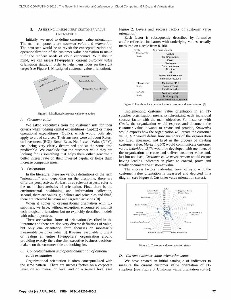
II. ASSESSING IT-SUPPLIERS´ CUSTOMER VALUE

ORIENTATION

Initially, we need to define customer value orientation. The main components are customer value and orientation. The next step would be to revisit the conceptualization and operationalization of the customer value orientation to make it fit the modern needs of cloud economics. With this in mind, we can assess IT-suppliers´ current customer value orientation status, in order to help them focus on the right target (see Figure 1. Misaligned customer value orientation).

Figure 1. Misaligned customer value orientation

A. Customer value

We asked executives from the customer side for their criteria when judging capital expenditures (CapEx) or major operational expenditures (OpEx), which would both also apply to cloud services. Their answers were all about Return on Investment (ROI), Break Even, Net Present Value (NPV), etc., being very clearly determined and at the same time predictable. We conclude that the customer value they are looking for is something that helps them either generate a better interest rate on their invested capital or helps them increase competitiveness.

B. Orientation

In the literature, there are various definitions of the term “orientation” and, depending on the discipline, there are different perspectives. At least three relevant aspects refer to the main characteristics of orientation. First, there is the environmental positioning and information collection, second, there are values, guidelines and principles and third, there are intended behavior and targeted activities [8].

When it comes to organizational orientation with IT-suppliers, we have, without exception, encountered implicit technological orientations but no explicitly described models with other objectives.

There are various forms of orientation described in the literature and there are also very diverse definitions of value, but only one orientation form focusses on monetarily measurable customer value [8]. It seems reasonable to orient or realign an entire IT-suppliers´ organization around providing exactly the value that executive business decision- makers on the customer side are looking for.

C. Conceptualization and operationalization of customer

value orientation

Organizational orientation is often conceptualized with the same pattern. There are success factors on a corporate level, on an interaction level and on a service level (see

Figure 2. Levels and success factors of customer value orientation).

Each factor is subsequently described by formative and/or reflective indicators with underlying values, usually measured on a scale from 0-100.

Figure 2. Levels and success factors of customer value orientation [8]

Implementing customer value orientation in an IT-supplier organization means synchronizing each individual success factor with the main objective. For instance, with Goals, the organization would express and document the customer value it wants to create and provide, Strategies would express how the organization will create the customer value, HR would define how members of the organization are hired, measured and fired in the process of creating customer value, Marketing/PR would communicate customer value, Individual skills would be developed with members of the organization to create and deliver customer value and, last but not least, Customer value measurement would ensure having leading indicators in place to control, prove and finally document the customer value.

The success factors´ individual level of sync with the customer value orientation is measured and depicted in a diagram (see Figure 3. Customer value orientation status).

Figure 3. Customer value orientation status

D. Current customer value orientation status

We have created an initial catalogue of indicators to measure the current customer value orientation of IT-suppliers (see Figure 3. Customer value orientation status).



90 / 157

The results reveal the enormous potential for IT-suppliers to grow their businesses because typically, we encounter values below 50 for all success factors. Whenever we had the opportunity to conduct such measurement with members of different hierarchical levels within an organization, we could also observe that higher-ranking people would rate the orientation status more positively than the lower levels.

Finally, we found, with all IT-suppliers that they do not measure the customer value potentially obtained from using their solutions.

III. BUSINESS POTENTIAL REFERENCE MODEL

A “business potential” is a chance to generate a higher operating cash flow, either by reducing outgoing cash flows or increasing incoming ones. Investing and financing cash flows are designed to leverage the operating cash flow. Therefore, they are not important to the genuine business potential. Basically there are inhibitors (I) from I1 to In, preventing this currently happening. To unleash the business potential, these inhibitors need to be addressed individually and appropriately with enablers (E) from E1 to En. The total monetary value of both inhibitors and enablers can be calculated with the following formula: resources x time x value (in any freely convertible currency). This way, the total value of a business potential is the sum of the values that each Inhibitor (I1 to In) generates on the one side. On the other side, the total value of the offering is the sum of the values that each enabler (E1 to En) generates. Altogether, this constitutes a solution (see Figure 4. Business potential reference model).

The real value of this solution is the total value of the inhibitors minus the total value of the enablers. If this value is positive, it indicates that the solution generates a positive impact on the operating cash flow of the owner of the business potential. Ideally, this is the customer, but the IT-supplier should also be able to generate a higher operating cash flow for himself, if he is able to determine the customer value.

Figure 4. Business potential reference model

Looking at elements of a business potential, reveals the

lever for making cloud services more effective and efficient. The customer business potential, with its current inhibitors, needs to be revealed and examined, making this the common denominator between IT-suppliers and customers. By

contrast, our observation from over 12 years of working with over 11.000 people from over 450 IT-suppliers, is that suppliers and customers use technologies as a common denominator, although none of them has properly analyzed the inhibitors or even a defined business potential as a target. Looking at the web sites and marketing collateral of IT-suppliers and requests for proposals (RFP) or requests for information (RFI) from customers, it is evident that this has not changed at all over time. We will not try to figure out which side is responsible for such dysfunctional behavior. Instead, we will establish the business potential, with its inhibitors and enablers, as the most effective common denominator. Understanding, analyzing and quantifying the individual inhibitors of a business potential is crucial to defining appropriate individual enablers and to specifically addressing the inhibitors. Only this way can both sides of a solution be measured and controlled. Finally, a solution is intended to help the customer generate more operating cash flow and hence increase his competitiveness. The advantage for the supplier would be a value-added pricing approach.

We conclude that the current state of play requires both parties to fundamentally change the way they approach and create cloud services as intended solutions. A challenge is that leaders on both sides are not prepared. Neither transformational leadership, nor transformation methodology, nor innovation methodology, nor innovation processes, were taught at university or other training to the majority of people who are currently in leading positions on either side. There is a massive skill gap to close.

IV. TRANSFORMATION PROCESS

IT-suppliers are able to manage the complexity of IT, but are still unable to map it to customers´ business potentials, because they do not have insight into their target customers´ business processes. Fundamentally changing their approach to innovation management (creating, communicating/selling, implementing and controlling) of Cloud-Services is what we perceive as the core of the so-called cloud transformation, in order to boost cloud economics in our target countries.

A. The need for innovation processes

Cloud technology itself is not a solution and does not provide value. Identifying business challenges or desired results is essential before modifying technologies. IT-suppliers in our focus countries are still technology oriented. Innovative is, ex post, what has successfully penetrated a market. We recommend integrating the customers into the innovation process (Open Innovation) of cloud services. According to our conversations with the executives of IT-suppliers, this needs to be the focus of our research. From over 300 CEO conversations, we have observed that IT-suppliers do not have an innovation process in place. It may seem incredible, but while process management and process modeling techniques [10] have impacted on a lot of processes even in the academic world (see Figure 5. The Nobel price process), for example, by making them visible,



91 / 157

repeatable, measurable and controllable, the innovation process still evidently remains a black box.

Figure 5. The Nobel price process [9]

In the literature, innovation processes [11][12] are only

described as a series of specified sub-processes [13] and rarely end-to end [14][15], which ultimately contributes to failure in innovation [16][17]. There is a demand for new management priorities [18], management responsibilities [14], management models [19], core processes [20][21][22], process activities, process roles and process resources [16][23].

Designing a simple innovation process that IT-suppliers can use to create cloud-based hybrid service bundles is a research gap and thus the subject of our future research and publications.

B. Conducting successful transformation

The term change is used so variously in the literature that some misunderstanding is inevitable. There is no copyright on expressions like “Organizational Development”, “Evolution”, “Change Management” or “Transformation Management” [1][7]. An early version of a change management model introduced in 1947 proposed that change in an organization requires unfreezing, changing/moving and (re)freezing [4]. Although the theory was criticized for being too simplistic and for not being operationalizable, Lewin´s model still is relevant and can be found at the cores of many major approaches to change.

We will therefore introduce the major concepts (Transformation management, Enterprise Transformation and Transformation of Management) before introducing our own transformation model. In addition, the success of a transformation is fundamentally determined by its extent. Too big could make it too long and costly, whereas too small could mean failing to achieve the objectives. In general, there are three types of transformation (see Figure 6. Types of transformation)

Type 1: Transforming the organization as an entity

Type 2: Having a small team pilot and role model the transformation within the organization

Type 3: Establishing a new entity outside the organization and starting from scratch [5].

Figure 6. Types of transformation

We will have to analyze and develop recommendations,

and determine with IT-suppliers which type of transformation will be most effective/efficient and under which circumstances. Also, we would need to define the three dimensions of transformation, Ends: Describing objectives that need to be achieved through initiatives, Means: Describing resources needed to achieve objectives, Scope: Describing the extent and direction of the transformation (see Figure 7. Dimensions of transformation)

Figure 7. Dimensions of transformation [6]

The transformation approaches in both the literature and in practice have matured over the past decades. Nevertheless, leading or managing transformation is still not common in the curricula of graduate and post-graduate studies. When conducting transformations in the past, the author has identified this issue and already introduced a new stage in Kotter´s transformation process [3] “Stage 3: Empowering the guiding coalition” (Figure 8). Educating the key people in transformation methodology and about the original core of their transformation, has already helped hundreds of people to drive their transformations successfully.

Figure 8. The 9-Stage process [8]



92 / 157

V. SUMMARY AND RECOMMENDATIONS

Customers of cloud solutions want to achieve positive, monetarily measurable results. Making them aware of their business potentials would leverage the sale and use of cloud solutions. IT-suppliers do yet not speak the language of business. They are talking bits and bytes, which currently leads to poor business in the focal area. Business potential is the most effective common denominator for customers and suppliers of cloud solutions. The major objective of our research is therfore to create a methodology and tools, enabling IT-suppliers to conduct their transformation successfully, which will in turn contribute to driving cloud economics.

VI. FUTURE RESEARCH

On the one hand, we strongly recommend conducting future research on innovation processes in order to enable customers and suppliers to measurably and repetitively create innovations. An alignment of these processes would together lead to better and faster results. On the other hand, it is questionable whether the majority of suppliers and customers are really able to transform with a reasonable scope of objectives, within a reasonable period of time and at an acceptable level of costs. The critical element is time to market. Therefore, we recommend future research in methodology and cloud-based technology to help both parties exploit business potential as the most effective common denominator.

REFERENCES

[1] A. Janes et al., “Transformation-Management – Changing Organisations Inside Out,“ Vienna: Springer, 2001.

[2] W. B. Rouse, “Enterprise Transformation - Understanding and Enabling Fundamental Change,” Wiley, 2006.

[3] J. P. Kotter, “Leading Change,” Boston: Harvard Business Review Press, 1996.

[4] K. Lewin, “Change Management Model,” New York: McGraw Hill.

[5] J. P. Kotter, “Accelerate: Building Strategic Agility for a Faster Moving World (XLR8),” Boston: Harvard Business Review Press, 2013.

[6] W. B. Rouse, “Enterprise Transformation - Understanding and Enabling Fundamental Change,” Wiley, 2006, p. 39.

[7] R. Lessem et al., “Transformation Management - Towards the Integral Enterprise,” Farnham: Gower, 2009.

[8] F. Keßler, “Enterprise Transformation Management – Development of a Concept of Customer Value Orientation for IT_Companies, B2B, as a Path to Longterm Profitable Growth ”, 2011.

[9] Author not named, in http://www.omg.org/spec/BPMN/20100601/10-06-02.pdf, p. 26, retr.: Feb. 2016

[10] G. Schewe et al., „Innovation for Medium Size Companies – A Process Oriented Guideline for SME,“ Wiesbaden: Gabler, 2009, pp. 124.

[11] Fraunhofer Institut für Arbeitswissenschaft und Organisation “Cross-Industry Innovation,“ in http://wiki.iao.fraunhofer.de/index.php/Cross_Industry-Innovation, 2012, retrieved: Oct. 2012.

[12] Author not named, Gabler Wirtschaftslexikon, “Open Innovation,“ in http://wirtschaftslexikon.gabler.de/Archiv/81584/open-innovation-v3.html, 2012, retrieved: Oct. 2012.

[13] B. Wirtz, “Business Model Management – Design – Instrumente – Success Factors of Business Models,“ Wiesbaden: Gabler, 2011, pp. 214.

[14] J. Hauschildt et al., “Innovation Management,“ 5. überarb., erg. und akt. Aufl., Munich: Vahlen, 2011.

[15] T. Stern et al., “Successful Innovation Management – Success Factors, Basic Patterns, Cases,“ 4., überarb. Aufl., Wiesbaden: Gabler, 2010, p. 18.

[16] M. Disselkamp, “Innovation Management - Instruments and Methods for Implementation in Companies,“ 2., überarb. Aufl., Munich: Springer Gabler, 2012, pp. 56.

[17] M. Zollenkop, “Business Model Innovation,“ Wiesbaden: Deutscher Universitäts-Verlag, 2006, p. 49.

[18] T. Bieger et al., “Innovative Business Models - Fundamental Concepts, Creative Areas and Entrepreneurial Practice,“ Heidelberg: Springer, 2011, pp. 81.

[19] N. Tomaschek et al., “Management & Consulting in Transformation- und Innovation-Processes - Research in Progress,“ Munich: Rainer Hampp, 2010.

[20] C. Hentschel, et al., “TRIZ – Systematic Innovation,“ Munich: Hanser, 2010.

[21] B. Maurer et al., “World Champions in Innovation – How our Companies become Unbeatable,“ Weinheim: Wiley, 2011.

[22] J. O. Meissner, “Introduction to systemic Innovation-Management,“ Heidelberg: Carl-Auer-Systeme, 2011.

[23] O. Gassmann et al., “Practical Knowledge Innovation Management – From Idea to Market Success,“ 2. erw. und überarb. Aufl., München: Hanser, 2011.

[24] H. Österle et al., “Memorandum for Creation Oriented Wirtschaftsinformatik, in Österle et al.: Creation Oriented Wirtschaftsinformatik: A Pleadoyer for Rigor und Relevance,“ infowerk Verlag, 2010, pp. 1 – 6.

[25] A. R. Hevner et al., “Design Science in Information Systems Research,” in MIS Quarterly, Vol. 28, No. 1, (2004)3

[26] A. R. Hevner, “A Three Cycle View of Design Science Research,” Scandinavian Journal of Information Systems, 19(2007)2, pp. 87 – 92.

[27] M. Yamartino, “The Economics Of The Cloud,” in http://news.microsoft.com/download/archived/presskits/cloud/docs/the-economics-of-the-cloud.pdf, 2010, (retr. Feb. 2016)

[28] H. Okin, “Cloud Economics,” in https://www.kpmg-institutes.com/institutes/advisory-institute/events/2014/09- /podcast-cloud-economics.html, 2014, retr.: Feb. 2016

[29] D. Reeves et al., “The Truth About Cloud Economics,” in https://hbr.org/2012/04/the-truth-about-cloud-economic/, 2012, retr.: Feb. 2016

[30] o. V. TechTarget, in http://searchcio.techtarget.com/ definition/ cloud-economics, 2013, retr.: Feb. 2016



93 / 157

How to Synchronize Large-Scale Ultra-Fine-GrainedProcessors in Optimum-Time

Hiroshi UmeoSchool of Information Engineering

University of Osaka Electro-CommunicationNeyagawa-shi, Hastu-cho, 18-8, Osaka


Abstract—We introduce a new class of FSSP (firing squad syn-chronization problem) algorithms based on recursive-halving andconstruct a survey on recent developments in FSSP algorithms forone-dimensional cellular arrays. We present herein a comparisonof the quantitative aspects of the optimum-time FSSP algorithmsdeveloped so far. Several state-efficient new implementationsand new insights into synchronization algorithms and multi-dimensional expansions are also given.

Keywords—cellular automata, synchronization

I. INTRODUCTION

Synchronization of large-scale networks is an importantand fundamental computing primitive in parallel and dis-tributed systems. The synchronization in ultra-fine grainedparallel computational model of cellular automata, knownas firing squad synchronization problem (FSSP), has beenstudied extensively for more than fifty years, and a richvariety of synchronization algorithms has been proposed. In thepresent paper, we introduce a new class of FSSP algorithmsbased on recursive-halving and construct a survey on recentdevelopments in FSSP algorithms for one-dimensional cellulararrays. The algorithms being compared are Balzer [1], Gerken[2], Waksman [20], a number of revised versions thereof, andtheir generalized versions such as Moore and Langdon [8],Settle and Simon [10], Szwerinski [11], all included in theproposed new class of FSSP algorithms. We present herein asurvey and a comparison of the quantitative aspects of theoptimum-time synchronization algorithms developed so far.Several state-efficient new implementations, new insights intosynchronization algorithms and multi-dimensional expansionsare also given.

Specifically, we attempt to answer the following questions:

• First, are all previously presented transition rule setscorrect?

• Do these sets contain redundant rules? If so, what isthe exact rule set?

• How do the algorithms compare with each other?

• Can we expand those 1D FSSP algorithms proposedso far to 2D, 3D arrays, or more generally to multi-dimensional arrays?

• How can we synchronize multi-dimensional arrays inoptimum-time?

In Section 2 we give a description of the FSSP and reviewsome basic results on the FSSP for 1D arrays. Section 3introduces a new class of FSSP algorithms based on recursive-halving and presents multi-dimensional generalizations of thealgorithms. In the last section we give a summary of the paper.

II. FIRING SQUAD SYNCHRONIZATION PROBLEM

In this section, we define the FSSP and introduce somebasic results on FSSP.

A. Firing Squad Synchronization Problem

Figure 1 illustrates a finite one-dimensional (1D) cellulararray consisting of n cells. Each cell is an identical finite-stateautomaton. The array operates in lock-step mode in such away that the next state of each cell is determined by both itsown present state and the present states of its left and rightneighbors. All cells (soldiers), except one general, are initiallyin the quiescent state at time t = 0 with the property that thenext state of a quiescent cell with quiescent neighbors is thequiescent state again. At time t = 0, one general cell C1 isin the fire-when-ready state, which is the initiation signal forthe synchronization of the array. The FSSP is to determinea description (state set and next-state function) for cells thatensures all cells enter the fire state at exactly the same time andfor the first time. The set of states and the next-state functionmust be independent of n.

C1 C2 C4 Cn

...

C3

Soldiers

Genaral

Fig. 1. One-dimensional cellular automaton

A formal definition of the FSSP is as follows: A cellularautomaton M is a pair M = (Q, δ), where

1) Q is a finite set of states with three distinguishedstates G, Q, and F. G is an initial general state, Q isa quiescent state, and F is a firing state, respectively.

2) δ is a next state function such that δ : Q∪{∗}×Q×Q ∪ {∗} → Q. The state * /∈ Q is a pseudo state ofthe border of the array.

3) The quiescent state Q must satisfy the followingconditions: δ(Q, Q, Q) = δ(∗, Q, Q) = δ(Q,Q, ∗) = Q.

A cellular automaton of length n, Mn consisting of ncopies of M is a 1D array of M, numbered from 1 to n.



94 / 157

Each M is referred to as a cell and denoted by Ci, where1 ≤ i ≤ n. We denote a state of Ci at time (step) t by St

i, wheret ≥ 0, 1 ≤ i ≤ n. A configuration of Mn at time t is a functionCt : [1, n] → Q and denoted as St

1St2 .... St

n. A computation ofMn is a sequence of configurations of Mn, C0, C1, C2, ...., Ct,..., where C0 is a given initial configuration. The configurationat time t + 1, Ct+1, is computed by synchronous applicationsof the next transition function δ to each cell of Mn in Ct suchthat:

St+11 = δ(∗, St

1, St2), S

t+1i = δ(St

i−1, Sti, S

ti+1), and St+1

n =δ(St

n−1, Stn, ∗).

A synchronized configuration of Mn at time t is a config-uration Ct, St

i = F, for any 1 ≤ i ≤ n.

The FSSP is to obtain an M such that, for any n ≥ 2,

1) A synchronized configuration at time t = T (n),

CT (n) =

n︷︸︸︷F, · · · , F can be computed from an initial

configuration C0 = G

n−1︷︸︸︷Q, · · · , Q.

2) For any t, i such that 1 ≤ t ≤ T (n) − 1, 1 ≤ i ≤n, St

i �= F.

The generalized FSSP (GFSSP) is to obtain an M suchthat, for any n ≥ 2 and for any k such that 1 ≤ k ≤ n,

1) A synchronized configuration at time t = T (n),

CT (n) =

n︷︸︸︷F, · · · , F can be computed from an initial

configuration C0 =

k−1︷︸︸︷Q, · · · , Q G

n−k︷︸︸︷Q, · · · , Q.

2) For any t, i, such that 1 ≤ t ≤ T (n) − 1, 1 ≤ i ≤n, St

i �= F.

No cells fire before time t = T (n). We say that Mn issynchronized at time t = T (n) and the function T (n) is atime complexity for the synchronization.

B. A Brief History of the Developments of Optimum-TimeFSSP Algorithms

The problem known as the firing squad synchronizationproblem was devised in 1957 by J. Myhill, and first appearedin print in a paper by E. F. Moore [7]. This problem hasbeen widely circulated, and has attracted much attention. Thefiring squad synchronization problem first arose in connectionwith the need to simultaneously turn on all parts of a self-reproducing machine. The problem was first solved by J.McCarthy and M. Minsky who presented a 3n-step algo-rithm. In 1962, the first optimum-time, i.e., (2n − 2)-step,synchronization algorithm was presented by Goto [3], witheach cell having several thousands of states. Waksman [20]presented a 16-state optimum-time synchronization algorithm.Afterward, Balzer [1] and Gerken [2] developed an eight-state algorithm and a seven-state synchronization algorithm,respectively, thus decreasing the number of states requiredfor the synchronization. In 1987, Mazoyer [5] developed asix-state synchronization algorithm which, at present, is thealgorithm having the fewest states.

C. Complexity Measures for FSSP Algorithms

• TimeAny solution to the original FSSP with a general atone end can be easily shown to require (2n− 2) stepsfor synchronizing n cells, since signals on the arraycan propagate no faster than one cell per one step, andthe time from the general’s instruction until the finalsynchronization must be at least 2n − 2.

Theorem 1 The minimum time in which the firingsquad synchronization could occur is 2n − 2 steps,where the general is located on the left end.

Theorem 2 There exists a cellular automaton that cansynchronize any 1D array of length n in optimum 2n−2 steps, where the general is located on the left end.

• Number of StatesThe following three distinct states: the quiescent state,the general state, and the firing state, are required inorder to define any cellular automaton that can solvethe FSSP. Note that the boundary state for C0 andCn+1 is not generally counted as an internal state.Balzer [1] and Sanders [9] showed that no four-stateoptimum-time solution exists. Umeo and Yanagihara[17], Yunes [21], and Umeo, Kamikawa, and Yunes[14] gave some 5- and 4-state partial solutions thatcan solve the synchronization problem for infinitelymany sizes n, but not all, respectively. The solutionis referred to as partial solution, which is comparedwith usual full solutions that can solve the problem forall cells. Concerning the optimum-time full solutions,Waksman [20] presented a 16-state optimum-timesynchronization algorithm. Afterward, Balzer [1] andGerken [2] developed an eight-state algorithm anda seven-state synchronization algorithm, respectively,thus decreasing the number of states required for thesynchronization. Mazoyer [5] developed a six-statesynchronization algorithm which, at present, is thealgorithm having the fewest states for 1D arrays.

Theorem 3 There exists a 6-state full solution to theFSSP.

Theorem 4 There is no four-state full solution thatcan synchronize n cells.

Yunes [21] and Umeo, Yunes, and Kamikawa [14]developed 4-state partial solutions based on Wolfram’srules 60 and 150. They can synchronize any array/ringof length n = 2k for any positive integer k. Detailscan be found in Yunes [21] and Umeo, Kamikawa,and Yunes [14].

Theorem 5 There exist 4-state partial solutions to theFSSP.

• Number of Transition RulesAny k-state (excluding the boundary state) transitiontable for the synchronization has at most (k − 1)k2

entries in (k − 1) matrices of size k × k. The numberof transition rules reflects a complexity of synchro-nization algorithms.



95 / 157

• State-Change ComplexityVollmar [18,19] introduced a state-change complexityin order to measure the efficiency of cellular automata,motivated by energy consumption in certain SRAM-type memory systems. The state-change complexityis defined as the sum of proper state changes ofthe cellular space during the computations. A formaldefinition is as follows: Consider an FSSP algorithmoperating on n cells. Let T (n) be synchronizationsteps of the FSSP algorithm. We define a matrix Cof size T (n)×n (T (n) rows, n columns) over {0, 1},where each element ci,j on ith row, jth column of thematrix is defined:

ci,j ={

1 Sji �= Sj−1

i

0 otherwise.(1)

The state-change complexity SC(n) of the FSSPalgorithm is the sum of 1’s elements in C definedas:

SC(n) =T (n)∑j=1

n∑i=1

ci,j. (2)

Vollmar [19] showed that Ω(n log n) state-changes arerequired for synchronizing n cells in (2n − 2) steps.

Theorem 6 Ω(n log n) state-change is necessary forsynchronizing n cells in minimum-steps.

Gerken [2] presented a minimum-time, Θ(n log n)minimum-state-change FSSP algorithm with a generalat one end.

Theorem 7 Θ(n log n) state-change is sufficient forsynchronizing n cells in 2n− 2 steps.

III. A CLASS OF FSSP ALGORITHMS BASED ONRECURSIVE-HALVING

Here we introduce a new class of FSSP algorithms basedon recursive halving.

A. Recursive-Halving Marking

In this section, we develop a marking schema for 1D arraysreferred to as recursive-halving marking. The marking schemaprints a special mark on cells in a cellular space defined bythe recursive-halving marking. It is based on a 1D FSSP syn-chronization algorithm. The marking will be effectively usedfor constructing multi-dimensional FSSP algorithms operatingin optimum-time.

Let S be a 1D cellular space consisting of cells Ci, Ci+1,..., Cj , denoted by [i...j], where j > i. Let |S| denote thenumber of cells in S, that is |S| = j − i + 1. A center cell(s)Cx of S is defined by

x ={

(i + j)/2 |S|: odd(i + j − 1)/2, (i + j + 1)/2 |S|: even.

(3)

The recursive-halving marking for a given cellular space S= [1...n] is defined as follows:

Recursive-Halving Marking: RHM

Algorithm RHM(S)begin

if |S| ≥ 2 thenif |S| is odd then

mark center cell Cx in SSL:= [1...x]; SR:= [x...n]RHML(SL); RHMR(SR);

elsemark center cells Cx and Cx+1 in SSL:= [1...x]; SR:= [x + 1...n]RHML(SL); RHMR(SR);

end

Left-Side Recursive-Halving Marking: RHML

Algorithm RHML(S)begin

while |S| > 2 doif |S| is odd then

mark center cell Cx in SSL:= [1...x]; RHML(SL);

elsemark center cells Cx and Cx+1 in SSL:= [1...x]; RHML(SL);

end

The marking RHMR for the right-side space can be definedin a similar way. As an example, we consider a cellular spaceS = [1...15] consisting of 15 cells. The first center cell is C8,then the second one is C4, C5 and C11, C12, and the last oneis C2, C3, C13, C14, respectively. In case S = [1...17], we getC9, C5, C13, C3, C15, and C2, C16 after four iterations.

1 2 3 4 5 6 7 8 9 10 11 12 13 14 15 16 17 18 19 20 21 22 23 24 25 26 27 28 29 30 31 32 33 34 35 36 37 38 39 40 41 42 43 44 45 46 47 48 49 50 51 52 53 54 55 56 57 58 59 60 61 62 63 64 65 66 67 68 69 70 71

0 G Q Q Q Q Q Q Q Q Q Q Q Q Q Q Q Q Q Q Q Q Q Q Q Q Q Q Q Q Q Q Q Q Q Q Q Q Q Q Q Q Q Q Q Q Q Q Q Q Q Q Q Q Q Q Q Q Q Q Q Q Q Q Q Q Q Q Q Q Q Q

1 G B Q Q Q Q Q Q Q Q Q Q Q Q Q Q Q Q Q Q Q Q Q Q Q Q Q Q Q Q Q Q Q Q Q Q Q Q Q Q Q Q Q Q Q Q Q Q Q Q Q Q Q Q Q Q Q Q Q Q Q Q Q Q Q Q Q Q Q Q Q

2 G O B Q Q Q Q Q Q Q Q Q Q Q Q Q Q Q Q Q Q Q Q Q Q Q Q Q Q Q Q Q Q Q Q Q Q Q Q Q Q Q Q Q Q Q Q Q Q Q Q Q Q Q Q Q Q Q Q Q Q Q Q Q Q Q Q Q Q Q Q

3 G O K B Q Q Q Q Q Q Q Q Q Q Q Q Q Q Q Q Q Q Q Q Q Q Q Q Q Q Q Q Q Q Q Q Q Q Q Q Q Q Q Q Q Q Q Q Q Q Q Q Q Q Q Q Q Q Q Q Q Q Q Q Q Q Q Q Q Q Q

4 G O K C B Q Q Q Q Q Q Q Q Q Q Q Q Q Q Q Q Q Q Q Q Q Q Q Q Q Q Q Q Q Q Q Q Q Q Q Q Q Q Q Q Q Q Q Q Q Q Q Q Q Q Q Q Q Q Q Q Q Q Q Q Q Q Q Q Q Q

5 G O O C K B Q Q Q Q Q Q Q Q Q Q Q Q Q Q Q Q Q Q Q Q Q Q Q Q Q Q Q Q Q Q Q Q Q Q Q Q Q Q Q Q Q Q Q Q Q Q Q Q Q Q Q Q Q Q Q Q Q Q Q Q Q Q Q Q Q

6 G E O Q K C B Q Q Q Q Q Q Q Q Q Q Q Q Q Q Q Q Q Q Q Q Q Q Q Q Q Q Q Q Q Q Q Q Q Q Q Q Q Q Q Q Q Q Q Q Q Q Q Q Q Q Q Q Q Q Q Q Q Q Q Q Q Q Q Q

7 G E O Q C C K B Q Q Q Q Q Q Q Q Q Q Q Q Q Q Q Q Q Q Q Q Q Q Q Q Q Q Q Q Q Q Q Q Q Q Q Q Q Q Q Q Q Q Q Q Q Q Q Q Q Q Q Q Q Q Q Q Q Q Q Q Q Q Q

8 G E O O C Q K C B Q Q Q Q Q Q Q Q Q Q Q Q Q Q Q Q Q Q Q Q Q Q Q Q Q Q Q Q Q Q Q Q Q Q Q Q Q Q Q Q Q Q Q Q Q Q Q Q Q Q Q Q Q Q Q Q Q Q Q Q Q Q

9 G E K O Q Q C C K B Q Q Q Q Q Q Q Q Q Q Q Q Q Q Q Q Q Q Q Q Q Q Q Q Q Q Q Q Q Q Q Q Q Q Q Q Q Q Q Q Q Q Q Q Q Q Q Q Q Q Q Q Q Q Q Q Q Q Q Q Q

10 G E K O Q C C Q K C B Q Q Q Q Q Q Q Q Q Q Q Q Q Q Q Q Q Q Q Q Q Q Q Q Q Q Q Q Q Q Q Q Q Q Q Q Q Q Q Q Q Q Q Q Q Q Q Q Q Q Q Q Q Q Q Q Q Q Q Q

11 G E K O O C Q Q C C K B Q Q Q Q Q Q Q Q Q Q Q Q Q Q Q Q Q Q Q Q Q Q Q Q Q Q Q Q Q Q Q Q Q Q Q Q Q Q Q Q Q Q Q Q Q Q Q Q Q Q Q Q Q Q Q Q Q Q Q

12 G E K C O Q Q C C Q K C B Q Q Q Q Q Q Q Q Q Q Q Q Q Q Q Q Q Q Q Q Q Q Q Q Q Q Q Q Q Q Q Q Q Q Q Q Q Q Q Q Q Q Q Q Q Q Q Q Q Q Q Q Q Q Q Q Q Q

13 G E E C O Q C C Q Q C C K B Q Q Q Q Q Q Q Q Q Q Q Q Q Q Q Q Q Q Q Q Q Q Q Q Q Q Q Q Q Q Q Q Q Q Q Q Q Q Q Q Q Q Q Q Q Q Q Q Q Q Q Q Q Q Q Q Q

14 G E E C O O C Q Q C C Q K C B Q Q Q Q Q Q Q Q Q Q Q Q Q Q Q Q Q Q Q Q Q Q Q Q Q Q Q Q Q Q Q Q Q Q Q Q Q Q Q Q Q Q Q Q Q Q Q Q Q Q Q Q Q Q Q Q

15 G E E C K O Q Q C C Q Q C C K B Q Q Q Q Q Q Q Q Q Q Q Q Q Q Q Q Q Q Q Q Q Q Q Q Q Q Q Q Q Q Q Q Q Q Q Q Q Q Q Q Q Q Q Q Q Q Q Q Q Q Q Q Q Q Q

16 G E E Q K O Q C C Q Q C C Q K C B Q Q Q Q Q Q Q Q Q Q Q Q Q Q Q Q Q Q Q Q Q Q Q Q Q Q Q Q Q Q Q Q Q Q Q Q Q Q Q Q Q Q Q Q Q Q Q Q Q Q Q Q Q Q

17 G E E Q K O O C Q Q C C Q Q C C K B Q Q Q Q Q Q Q Q Q Q Q Q Q Q Q Q Q Q Q Q Q Q Q Q Q Q Q Q Q Q Q Q Q Q Q Q Q Q Q Q Q Q Q Q Q Q Q Q Q Q Q Q Q

18 G E E Q K C O Q Q C C Q Q C C Q K C B Q Q Q Q Q Q Q Q Q Q Q Q Q Q Q Q Q Q Q Q Q Q Q Q Q Q Q Q Q Q Q Q Q Q Q Q Q Q Q Q Q Q Q Q Q Q Q Q Q Q Q Q

19 G E E Q C C O Q C C Q Q C C Q Q C C K B Q Q Q Q Q Q Q Q Q Q Q Q Q Q Q Q Q Q Q Q Q Q Q Q Q Q Q Q Q Q Q Q Q Q Q Q Q Q Q Q Q Q Q Q Q Q Q Q Q Q Q

20 G E E E C C O O C Q Q C C Q Q C C Q K C B Q Q Q Q Q Q Q Q Q Q Q Q Q Q Q Q Q Q Q Q Q Q Q Q Q Q Q Q Q Q Q Q Q Q Q Q Q Q Q Q Q Q Q Q Q Q Q Q Q Q

21 G E K E C C K O Q Q C C Q Q C C Q Q C C K B Q Q Q Q Q Q Q Q Q Q Q Q Q Q Q Q Q Q Q Q Q Q Q Q Q Q Q Q Q Q Q Q Q Q Q Q Q Q Q Q Q Q Q Q Q Q Q Q Q

22 G E K E C Q K O Q C C Q Q C C Q Q C C Q K C B Q Q Q Q Q Q Q Q Q Q Q Q Q Q Q Q Q Q Q Q Q Q Q Q Q Q Q Q Q Q Q Q Q Q Q Q Q Q Q Q Q Q Q Q Q Q Q Q

23 G E K E Q Q K O O C Q Q C C Q Q C C Q Q C C K B Q Q Q Q Q Q Q Q Q Q Q Q Q Q Q Q Q Q Q Q Q Q Q Q Q Q Q Q Q Q Q Q Q Q Q Q Q Q Q Q Q Q Q Q Q Q Q

24 G E K E Q Q K C O Q Q C C Q Q C C Q Q C C Q K C B Q Q Q Q Q Q Q Q Q Q Q Q Q Q Q Q Q Q Q Q Q Q Q Q Q Q Q Q Q Q Q Q Q Q Q Q Q Q Q Q Q Q Q Q Q Q

25 G E K E Q Q C C O Q C C Q Q C C Q Q C C Q Q C C K B Q Q Q Q Q Q Q Q Q Q Q Q Q Q Q Q Q Q Q Q Q Q Q Q Q Q Q Q Q Q Q Q Q Q Q Q Q Q Q Q Q Q Q Q Q

26 G E K E Q C C C O O C Q Q C C Q Q C C Q Q C C Q K C B Q Q Q Q Q Q Q Q Q Q Q Q Q Q Q Q Q Q Q Q Q Q Q Q Q Q Q Q Q Q Q Q Q Q Q Q Q Q Q Q Q Q Q Q

27 G E K E E C C C K O Q Q C C Q Q C C Q Q C C Q Q C C K B Q Q Q Q Q Q Q Q Q Q Q Q Q Q Q Q Q Q Q Q Q Q Q Q Q Q Q Q Q Q Q Q Q Q Q Q Q Q Q Q Q Q Q

28 G E K C E C C Q K O Q C C Q Q C C Q Q C C Q Q C C Q K C B Q Q Q Q Q Q Q Q Q Q Q Q Q Q Q Q Q Q Q Q Q Q Q Q Q Q Q Q Q Q Q Q Q Q Q Q Q Q Q Q Q Q

29 G E E C E C Q Q K O O C Q Q C C Q Q C C Q Q C C Q Q C C K B Q Q Q Q Q Q Q Q Q Q Q Q Q Q Q Q Q Q Q Q Q Q Q Q Q Q Q Q Q Q Q Q Q Q Q Q Q Q Q Q Q

30 G E E C E Q Q Q K C O Q Q C C Q Q C C Q Q C C Q Q C C Q K C B Q Q Q Q Q Q Q Q Q Q Q Q Q Q Q Q Q Q Q Q Q Q Q Q Q Q Q Q Q Q Q Q Q Q Q Q Q Q Q Q

31 G E E C E Q Q Q C C O Q C C Q Q C C Q Q C C Q Q C C Q Q C C K B Q Q Q Q Q Q Q Q Q Q Q Q Q Q Q Q Q Q Q Q Q Q Q Q Q Q Q Q Q Q Q Q Q Q Q Q Q Q Q

32 G E E C E Q Q C C C O O C Q Q C C Q Q C C Q Q C C Q Q C C Q K C B Q Q Q Q Q Q Q Q Q Q Q Q Q Q Q Q Q Q Q Q Q Q Q Q Q Q Q Q Q Q Q Q Q Q Q Q Q Q

33 G E E C E Q C C C C K O Q Q C C Q Q C C Q Q C C Q Q C C Q Q C C K B Q Q Q Q Q Q Q Q Q Q Q Q Q Q Q Q Q Q Q Q Q Q Q Q Q Q Q Q Q Q Q Q Q Q Q Q Q

34 G E E C E E C C C Q K O Q C C Q Q C C Q Q C C Q Q C C Q Q C C Q K C B Q Q Q Q Q Q Q Q Q Q Q Q Q Q Q Q Q Q Q Q Q Q Q Q Q Q Q Q Q Q Q Q Q Q Q Q

35 G E E C K E C C Q Q K O O C Q Q C C Q Q C C Q Q C C Q Q C C Q Q C C K B Q Q Q Q Q Q Q Q Q Q Q Q Q Q Q Q Q Q Q Q Q Q Q Q Q Q Q Q Q Q Q Q Q Q Q

36 G E E Q K E C Q Q Q K C O Q Q C C Q Q C C Q Q C C Q Q C C Q Q C C Q K C B Q Q Q Q Q Q Q Q Q Q Q Q Q Q Q Q Q Q Q Q Q Q Q Q Q Q Q Q Q Q Q Q Q Q

37 G E E Q K E Q Q Q Q C C O Q C C Q Q C C Q Q C C Q Q C C Q Q C C Q Q C C K B Q Q Q Q Q Q Q Q Q Q Q Q Q Q Q Q Q Q Q Q Q Q Q Q Q Q Q Q Q Q Q Q Q

38 G E E Q K E Q Q Q C C C O O C Q Q C C Q Q C C Q Q C C Q Q C C Q Q C C Q K C B Q Q Q Q Q Q Q Q Q Q Q Q Q Q Q Q Q Q Q Q Q Q Q Q Q Q Q Q Q Q Q Q

39 G E E Q K E Q Q C C C C K O Q Q C C Q Q C C Q Q C C Q Q C C Q Q C C Q Q C C K B Q Q Q Q Q Q Q Q Q Q Q Q Q Q Q Q Q Q Q Q Q Q Q Q Q Q Q Q Q Q Q

40 G E E Q K E Q C C C C Q K O Q C C Q Q C C Q Q C C Q Q C C Q Q C C Q Q C C Q K C B Q Q Q Q Q Q Q Q Q Q Q Q Q Q Q Q Q Q Q Q Q Q Q Q Q Q Q Q Q Q

41 G E E Q K E E C C C Q Q K O O C Q Q C C Q Q C C Q Q C C Q Q C C Q Q C C Q Q C C K B Q Q Q Q Q Q Q Q Q Q Q Q Q Q Q Q Q Q Q Q Q Q Q Q Q Q Q Q Q

42 G E E Q K C E C C Q Q Q K C O Q Q C C Q Q C C Q Q C C Q Q C C Q Q C C Q Q C C Q K C B Q Q Q Q Q Q Q Q Q Q Q Q Q Q Q Q Q Q Q Q Q Q Q Q Q Q Q Q

43 G E E Q C C E C Q Q Q Q C C O Q C C Q Q C C Q Q C C Q Q C C Q Q C C Q Q C C Q Q C C K B Q Q Q Q Q Q Q Q Q Q Q Q Q Q Q Q Q Q Q Q Q Q Q Q Q Q Q

44 G E E E C C E Q Q Q Q C C C O O C Q Q C C Q Q C C Q Q C C Q Q C C Q Q C C Q Q C C Q K C B Q Q Q Q Q Q Q Q Q Q Q Q Q Q Q Q Q Q Q Q Q Q Q Q Q Q

45 G E K E C C E Q Q Q C C C C K O Q Q C C Q Q C C Q Q C C Q Q C C Q Q C C Q Q C C Q Q C C K B Q Q Q Q Q Q Q Q Q Q Q Q Q Q Q Q Q Q Q Q Q Q Q Q Q

46 G E K E C C E Q Q C C C C Q K O Q C C Q Q C C Q Q C C Q Q C C Q Q C C Q Q C C Q Q C C Q K C B Q Q Q Q Q Q Q Q Q Q Q Q Q Q Q Q Q Q Q Q Q Q Q Q

47 G E K E C C E Q C C C C Q Q K O O C Q Q C C Q Q C C Q Q C C Q Q C C Q Q C C Q Q C C Q Q C C K B Q Q Q Q Q Q Q Q Q Q Q Q Q Q Q Q Q Q Q Q Q Q Q

48 G E K E C C E E C C C Q Q Q K C O Q Q C C Q Q C C Q Q C C Q Q C C Q Q C C Q Q C C Q Q C C Q K C B Q Q Q Q Q Q Q Q Q Q Q Q Q Q Q Q Q Q Q Q Q Q

49 G E K E C C K E C C Q Q Q Q C C O Q C C Q Q C C Q Q C C Q Q C C Q Q C C Q Q C C Q Q C C Q Q C C K B Q Q Q Q Q Q Q Q Q Q Q Q Q Q Q Q Q Q Q Q Q

50 G E K E C Q K E C Q Q Q Q C C C O O C Q Q C C Q Q C C Q Q C C Q Q C C Q Q C C Q Q C C Q Q C C Q K C B Q Q Q Q Q Q Q Q Q Q Q Q Q Q Q Q Q Q Q Q

51 G E K E Q Q K E Q Q Q Q C C C C K O Q Q C C Q Q C C Q Q C C Q Q C C Q Q C C Q Q C C Q Q C C Q Q C C K B Q Q Q Q Q Q Q Q Q Q Q Q Q Q Q Q Q Q Q

52 G E K E Q Q K E Q Q Q C C C C Q K O Q C C Q Q C C Q Q C C Q Q C C Q Q C C Q Q C C Q Q C C Q Q C C Q K C B Q Q Q Q Q Q Q Q Q Q Q Q Q Q Q Q Q Q

53 G E K E Q Q K E Q Q C C C C Q Q K O O C Q Q C C Q Q C C Q Q C C Q Q C C Q Q C C Q Q C C Q Q C C Q Q C C K B Q Q Q Q Q Q Q Q Q Q Q Q Q Q Q Q Q

54 G E K E Q Q K E Q C C C C Q Q Q K C O Q Q C C Q Q C C Q Q C C Q Q C C Q Q C C Q Q C C Q Q C C Q Q C C Q K C B Q Q Q Q Q Q Q Q Q Q Q Q Q Q Q Q

55 G E K E Q Q K E E C C C Q Q Q Q C C O Q C C Q Q C C Q Q C C Q Q C C Q Q C C Q Q C C Q Q C C Q Q C C Q Q C C K B Q Q Q Q Q Q Q Q Q Q Q Q Q Q Q

56 G E K E Q Q K C E C C Q Q Q Q C C C O O C Q Q C C Q Q C C Q Q C C Q Q C C Q Q C C Q Q C C Q Q C C Q Q C C Q K C B Q Q Q Q Q Q Q Q Q Q Q Q Q Q

57 G E K E Q Q C C E C Q Q Q Q C C C C K O Q Q C C Q Q C C Q Q C C Q Q C C Q Q C C Q Q C C Q Q C C Q Q C C Q Q C C K B Q Q Q Q Q Q Q Q Q Q Q Q Q

58 G E K E Q C C C E Q Q Q Q C C C C Q K O Q C C Q Q C C Q Q C C Q Q C C Q Q C C Q Q C C Q Q C C Q Q C C Q Q C C Q K C B Q Q Q Q Q Q Q Q Q Q Q Q

59 G E K E E C C C E Q Q Q C C C C Q Q K O O C Q Q C C Q Q C C Q Q C C Q Q C C Q Q C C Q Q C C Q Q C C Q Q C C Q Q C C K B Q Q Q Q Q Q Q Q Q Q Q

60 G E K C E C C C E Q Q C C C C Q Q Q K C O Q Q C C Q Q C C Q Q C C Q Q C C Q Q C C Q Q C C Q Q C C Q Q C C Q Q C C Q K C B Q Q Q Q Q Q Q Q Q Q

61 G E E C E C C C E Q C C C C Q Q Q Q C C O Q C C Q Q C C Q Q C C Q Q C C Q Q C C Q Q C C Q Q C C Q Q C C Q Q C C Q Q C C K B Q Q Q Q Q Q Q Q Q

62 G E E C E C C C E E C C C Q Q Q Q C C C O O C Q Q C C Q Q C C Q Q C C Q Q C C Q Q C C Q Q C C Q Q C C Q Q C C Q Q C C Q K C B Q Q Q Q Q Q Q Q

63 G E E C E C C C K E C C Q Q Q Q C C C C K O Q Q C C Q Q C C Q Q C C Q Q C C Q Q C C Q Q C C Q Q C C Q Q C C Q Q C C Q Q C C K B Q Q Q Q Q Q Q

64 G E E C E C C Q K E C Q Q Q Q C C C C Q K O Q C C Q Q C C Q Q C C Q Q C C Q Q C C Q Q C C Q Q C C Q Q C C Q Q C C Q Q C C Q K C B Q Q Q Q Q Q

65 G E E C E C Q Q K E Q Q Q Q C C C C Q Q K O O C Q Q C C Q Q C C Q Q C C Q Q C C Q Q C C Q Q C C Q Q C C Q Q C C Q Q C C Q Q C C K B Q Q Q Q Q

66 G E E C E Q Q Q K E Q Q Q C C C C Q Q Q K C O Q Q C C Q Q C C Q Q C C Q Q C C Q Q C C Q Q C C Q Q C C Q Q C C Q Q C C Q Q C C Q K C B Q Q Q Q

67 G E E C E Q Q Q K E Q Q C C C C Q Q Q Q C C O Q C C Q Q C C Q Q C C Q Q C C Q Q C C Q Q C C Q Q C C Q Q C C Q Q C C Q Q C C Q Q C C K B Q Q Q

68 G E E C E Q Q Q K E Q C C C C Q Q Q Q C C C O O C Q Q C C Q Q C C Q Q C C Q Q C C Q Q C C Q Q C C Q Q C C Q Q C C Q Q C C Q Q C C Q K C B Q Q

69 G E E C E Q Q Q K E E C C C Q Q Q Q C C C C K O Q Q C C Q Q C C Q Q C C Q Q C C Q Q C C Q Q C C Q Q C C Q Q C C Q Q C C Q Q C C Q Q C C K B Q

70 G E E C E Q Q Q K C E C C Q Q Q Q C C C C Q K O Q C C Q Q C C Q Q C C Q Q C C Q Q C C Q Q C C Q Q C C Q Q C C Q Q C C Q Q C C Q Q C C Q K C G

71 G E E C E Q Q Q C C E C Q Q Q Q C C C C Q Q K O O C Q Q C C Q Q C C Q Q C C Q Q C C Q Q C C Q Q C C Q Q C C Q Q C C Q Q C C Q Q C C Q Q C B G

72 G E E C E Q Q C C C E Q Q Q Q C C C C Q Q Q K C O Q Q C C Q Q C C Q Q C C Q Q C C Q Q C C Q Q C C Q Q C C Q Q C C Q Q C C Q Q C C Q Q C B D G

73 G E E C E Q C C C C E Q Q Q C C C C Q Q Q Q C C O Q C C Q Q C C Q Q C C Q Q C C Q Q C C Q Q C C Q Q C C Q Q C C Q Q C C Q Q C C Q Q C B K E G

74 G E E C E E C C C C E Q Q C C C C Q Q Q Q C C C O O C Q Q C C Q Q C C Q Q C C Q Q C C Q Q C C Q Q C C Q Q C C Q Q C C Q Q C C Q Q C B D K E G

75 G E E C K E C C C C E Q C C C C Q Q Q Q C C C C K O Q Q C C Q Q C C Q Q C C Q Q C C Q Q C C Q Q C C Q Q C C Q Q C C Q Q C C Q Q C B K D E E G

76 G E E Q K E C C C C E E C C C Q Q Q Q C C C C Q K O Q C C Q Q C C Q Q C C Q Q C C Q Q C C Q Q C C Q Q C C Q Q C C Q Q C C Q Q C B D K Q E E G

77 G E E Q K E C C C C K E C C Q Q Q Q C C C C Q Q K O O C Q Q C C Q Q C C Q Q C C Q Q C C Q Q C C Q Q C C Q Q C C Q Q C C Q Q C B K D D Q E E G

78 G E E Q K E C C C Q K E C Q Q Q Q C C C C Q Q Q K C O Q Q C C Q Q C C Q Q C C Q Q C C Q Q C C Q Q C C Q Q C C Q Q C C Q Q C B D K Q D E E E G

79 G E E Q K E C C Q Q K E Q Q Q Q C C C C Q Q Q Q C C O Q C C Q Q C C Q Q C C Q Q C C Q Q C C Q Q C C Q Q C C Q Q C C Q Q C B K D D Q Q E K E G

80 G E E Q K E C Q Q Q K E Q Q Q C C C C Q Q Q Q C C C O O C Q Q C C Q Q C C Q Q C C Q Q C C Q Q C C Q Q C C Q Q C C Q Q C B D K Q D D Q E K E G

81 G E E Q K E Q Q Q Q K E Q Q C C C C Q Q Q Q C C C C K O Q Q C C Q Q C C Q Q C C Q Q C C Q Q C C Q Q C C Q Q C C Q Q C B K D D Q Q D E E K E G

82 G E E Q K E Q Q Q Q K E Q C C C C Q Q Q Q C C C C Q K O Q C C Q Q C C Q Q C C Q Q C C Q Q C C Q Q C C Q Q C C Q Q C B D K Q D D Q Q E D K E G

83 G E E Q K E Q Q Q Q K E E C C C Q Q Q Q C C C C Q Q K O O C Q Q C C Q Q C C Q Q C C Q Q C C Q Q C C Q Q C C Q Q C B K D D Q Q D D Q E D E E G

84 G E E Q K E Q Q Q Q K C E C C Q Q Q Q C C C C Q Q Q K C O Q Q C C Q Q C C Q Q C C Q Q C C Q Q C C Q Q C C Q Q C B D K Q D D Q Q D E E D E E G

85 G E E Q K E Q Q Q Q C C E C Q Q Q Q C C C C Q Q Q Q C C O Q C C Q Q C C Q Q C C Q Q C C Q Q C C Q Q C C Q Q C B K D D Q Q D D Q Q E K D E E G

86 G E E Q K E Q Q Q C C C E Q Q Q Q C C C C Q Q Q Q C C C O O C Q Q C C Q Q C C Q Q C C Q Q C C Q Q C C Q Q C B D K Q D D Q Q D D Q E K Q E E G

87 G E E Q K E Q Q C C C C E Q Q Q C C C C Q Q Q Q C C C C K O Q Q C C Q Q C C Q Q C C Q Q C C Q Q C C Q Q C B K D D Q Q D D Q Q D E E K Q E E G

88 G E E Q K E Q C C C C C E Q Q C C C C Q Q Q Q C C C C Q K O Q C C Q Q C C Q Q C C Q Q C C Q Q C C Q Q C B D K Q D D Q Q D D Q Q E D K Q E E G

89 G E E Q K E E C C C C C E Q C C C C Q Q Q Q C C C C Q Q K O O C Q Q C C Q Q C C Q Q C C Q Q C C Q Q C B K D D Q Q D D Q Q D D Q E D D Q E E G

90 G E E Q K C E C C C C C E E C C C Q Q Q Q C C C C Q Q Q K C O Q Q C C Q Q C C Q Q C C Q Q C C Q Q C B D K Q D D Q Q D D Q Q D E E D D E E E G

91 G E E Q C C E C C C C C K E C C Q Q Q Q C C C C Q Q Q Q C C O Q C C Q Q C C Q Q C C Q Q C C Q Q C B K D D Q Q D D Q Q D D Q Q E K D D E K E G

92 G E E E C C E C C C C Q K E C Q Q Q Q C C C C Q Q Q Q C C C O O C Q Q C C Q Q C C Q Q C C Q Q C B D K Q D D Q Q D D Q Q D D Q E K Q D E K E G

93 G E K E C C E C C C Q Q K E Q Q Q Q C C C C Q Q Q Q C C C C K O Q Q C C Q Q C C Q Q C C Q Q C B K D D Q Q D D Q Q D D Q Q D E E K Q Q E K E G

94 G E K E C C E C C Q Q Q K E Q Q Q C C C C Q Q Q Q C C C C Q K O Q C C Q Q C C Q Q C C Q Q C B D K Q D D Q Q D D Q Q D D Q Q E D K Q Q E K E G

95 G E K E C C E C Q Q Q Q K E Q Q C C C C Q Q Q Q C C C C Q Q K O O C Q Q C C Q Q C C Q Q C B K D D Q Q D D Q Q D D Q Q D D Q E D D Q Q E K E G

96 G E K E C C E Q Q Q Q Q K E Q C C C C Q Q Q Q C C C C Q Q Q K C O Q Q C C Q Q C C Q Q C B D K Q D D Q Q D D Q Q D D Q Q D E E D D D Q E K E G

97 G E K E C C E Q Q Q Q Q K E E C C C Q Q Q Q C C C C Q Q Q Q C C O Q C C Q Q C C Q Q C B K D D Q Q D D Q Q D D Q Q D D Q Q E K D D D E E K E G

98 G E K E C C E Q Q Q Q Q K C E C C Q Q Q Q C C C C Q Q Q Q C C C O O C Q Q C C Q Q C B D K Q D D Q Q D D Q Q D D Q Q D D Q E K Q D D E D K E G

99 G E K E C C E Q Q Q Q Q C C E C Q Q Q Q C C C C Q Q Q Q C C C C K O Q Q C C Q Q C B K D D Q Q D D Q Q D D Q Q D D Q Q D E E K Q Q D E D E E G

100 G E K E C C E Q Q Q Q C C C E Q Q Q Q C C C C Q Q Q Q C C C C Q K O Q C C Q Q C B D K Q D D Q Q D D Q Q D D Q Q D D Q Q E D K Q Q Q E D E E G

101 G E K E C C E Q Q Q C C C C E Q Q Q C C C C Q Q Q Q C C C C Q Q K O O C Q Q C B K D D Q Q D D Q Q D D Q Q D D Q Q D D Q E D D Q Q Q E D E E G

102 G E K E C C E Q Q C C C C C E Q Q C C C C Q Q Q Q C C C C Q Q Q K C O Q Q C B D K Q D D Q Q D D Q Q D D Q Q D D Q Q D E E D D D Q Q E D E E G

103 G E K E C C E Q C C C C C C E Q C C C C Q Q Q Q C C C C Q Q Q Q C C O Q C B K D D Q Q D D Q Q D D Q Q D D Q Q D D Q Q E K D D D D Q E D E E G

104 G E K E C C E E C C C C C C E E C C C Q Q Q Q C C C C Q Q Q Q C C C O O B D K Q D D Q Q D D Q Q D D Q Q D D Q Q D D Q E K Q D D D E E D E E G

105 G E K E C C K E C C C C C C K E C C Q Q Q Q C C C C Q Q Q Q C C C C K M K D D Q Q D D Q Q D D Q Q D D Q Q D D Q Q D E E K Q Q D D E K D E E G

106 G E K E C Q K E C C C C C Q K E C Q Q Q Q C C C C Q Q Q Q C C C C Q A M A Q D D Q Q D D Q Q D D Q Q D D Q Q D D Q Q E D K Q Q Q D E K Q E E G

107 G E K E Q Q K E C C C C Q Q K E Q Q Q Q C C C C Q Q Q Q C C C C Q A C M D A Q D D Q Q D D Q Q D D Q Q D D Q Q D D Q E D D Q Q Q Q E K Q E E G

108 G E K E Q Q K E C C C Q Q Q K E Q Q Q C C C C Q Q Q Q C C C C Q A C Q M Q D A Q D D Q Q D D Q Q D D Q Q D D Q Q D E E D D D Q Q Q E K Q E E G

109 G E K E Q Q K E C C Q Q Q Q K E Q Q C C C C Q Q Q Q C C C C Q A C Q Q M Q Q D A Q D D Q Q D D Q Q D D Q Q D D Q Q E K D D D D Q Q E K Q E E G

110 G E K E Q Q K E C Q Q Q Q Q K E Q C C C C Q Q Q Q C C C C Q A C Q Q Q M Q Q Q D A Q D D Q Q D D Q Q D D Q Q D D Q E K Q D D D D Q E K Q E E G

111 G E K E Q Q K E Q Q Q Q Q Q K E E C C C Q Q Q Q C C C C Q A C Q Q Q Q M Q Q Q Q D A Q D D Q Q D D Q Q D D Q Q D E E K Q Q D D D E E K Q E E G

112 G E K E Q Q K E Q Q Q Q Q Q K C E C C Q Q Q Q C C C C Q A C Q Q Q Q Q M Q Q Q Q Q D A Q D D Q Q D D Q Q D D Q Q E D K Q Q Q D D E D K Q E E G

113 G E K E Q Q K E Q Q Q Q Q Q C C E C Q Q Q Q C C C C Q A C Q Q Q Q Q Q M Q Q Q Q Q Q D A Q D D Q Q D D Q Q D D Q E D D Q Q Q Q D E D D Q E E G

114 G E K E Q Q K E Q Q Q Q Q C C C E Q Q Q Q C C C C Q A C Q Q Q Q Q Q Q M Q Q Q Q Q Q Q D A Q D D Q Q D D Q Q D E E D D D Q Q Q Q E D D E E E G

115 G E K E Q Q K E Q Q Q Q C C C C E Q Q Q C C C C Q A C Q Q Q Q Q Q Q Q M Q Q Q Q Q Q Q Q D A Q D D Q Q D D Q Q E K D D D D Q Q Q E D D E K E G

116 G E K E Q Q K E Q Q Q C C C C C E Q Q C C C C Q A C Q Q Q Q Q Q Q Q Q M Q Q Q Q Q Q Q Q Q D A Q D D Q Q D D Q E K Q D D D D Q Q E D D E K E G

117 G E K E Q Q K E Q Q C C C C C C E Q C C C C Q A C Q Q Q Q Q Q Q Q Q Q M Q Q Q Q Q Q Q Q Q Q D A Q D D Q Q D E E K Q Q D D D D Q E D D E K E G

118 G E K E Q Q K E Q C C C C C C C E E C C C Q A C Q Q Q Q Q Q Q Q Q Q Q M Q Q Q Q Q Q Q Q Q Q Q D A Q D D Q Q E D K Q Q Q D D D E E D D E K E G

119 G E K E Q Q K E E C C C C C C C K E C C Q A C Q Q Q Q Q Q Q Q Q Q Q Q M Q Q Q Q Q Q Q Q Q Q Q Q D A Q D D Q E D D Q Q Q Q D D E K D D E K E G

120 G E K E Q Q K C E C C C C C C Q K E C Q A C Q Q Q Q Q Q Q Q Q Q Q Q Q M Q Q Q Q Q Q Q Q Q Q Q Q Q D A Q D E E D D D Q Q Q Q D E K Q D E K E G

121 G E K E Q Q C C E C C C C C Q Q K E Q A C Q Q Q Q Q Q Q Q Q Q Q Q Q Q M Q Q Q Q Q Q Q Q Q Q Q Q Q Q D A Q E K D D D D Q Q Q Q E K Q Q E K E G

122 G E K E Q C C C E C C C C Q Q Q K E A C Q Q Q Q Q Q Q Q Q Q Q Q Q Q Q M Q Q Q Q Q Q Q Q Q Q Q Q Q Q Q D A E K Q D D D D Q Q Q E K Q Q E K E G

123 G E K E E C C C E C C C Q Q Q Q K U U Q Q Q Q Q Q Q Q Q Q Q Q Q Q Q Q M Q Q Q Q Q Q Q Q Q Q Q Q Q Q Q Q U U K Q Q D D D D Q Q E K Q Q E K E G

124 G E K C E C C C E C C Q Q Q Q Q A U U Q Q Q Q Q Q Q Q Q Q Q Q Q Q Q Q M Q Q Q Q Q Q Q Q Q Q Q Q Q Q Q Q U U A Q Q Q D D D D Q E K Q Q E K E G

125 G E E C E C C C E C Q Q Q Q Q A C U U Q Q Q Q Q Q Q Q Q Q Q Q Q Q Q Q M Q Q Q Q Q Q Q Q Q Q Q Q Q Q Q Q U U D A Q Q Q D D D E E K Q Q E K E G

126 G E E C E C C C E Q Q Q Q Q A C Q U U Q Q Q Q Q Q Q Q Q Q Q Q Q Q Q Q M Q Q Q Q Q Q Q Q Q Q Q Q Q Q Q Q U U Q D A Q Q Q D D E D K Q Q E K E G

127 G E E C E C C C E Q Q Q Q A C Q Q U U Q Q Q Q Q Q Q Q Q Q Q Q Q Q Q Q M Q Q Q Q Q Q Q Q Q Q Q Q Q Q Q Q U U Q Q D A Q Q Q D E D D Q Q E K E G

128 G E E C E C C C E Q Q Q A C Q Q Q U U Q Q Q Q Q Q Q Q Q Q Q Q Q Q Q Q M Q Q Q Q Q Q Q Q Q Q Q Q Q Q Q Q U U Q Q Q D A Q Q Q E D D D Q E K E G

129 G E E C E C C C E Q Q A C Q Q Q Q U U Q Q Q Q Q Q Q Q Q Q Q Q Q Q Q Q M Q Q Q Q Q Q Q Q Q Q Q Q Q Q Q Q U U Q Q Q Q D A Q Q E D D D E E K E G

130 G E E C E C C C E Q A C Q Q Q Q Q U U Q Q Q Q Q Q Q Q Q Q Q Q Q Q Q Q M Q Q Q Q Q Q Q Q Q Q Q Q Q Q Q Q U U Q Q Q Q Q D A Q E D D D E D K E G

131 G E E C E C C C E A C Q Q Q Q Q Q U U Q Q Q Q Q Q Q Q Q Q Q Q Q Q Q Q M Q Q Q Q Q Q Q Q Q Q Q Q Q Q Q Q U U Q Q Q Q Q Q D A E D D D E D E E G

132 G E E C E C C C U U Q Q Q Q Q Q Q U U Q Q Q Q Q Q Q Q Q Q Q Q Q Q Q Q M Q Q Q Q Q Q Q Q Q Q Q Q Q Q Q Q U U Q Q Q Q Q Q Q U U D D D E D E E G

133 G E E C E C C B U U Q Q Q Q Q Q Q U U Q Q Q Q Q Q Q Q Q Q Q Q Q Q Q Q M Q Q Q Q Q Q Q Q Q Q Q Q Q Q Q Q U U Q Q Q Q Q Q Q U U B D D E D E E G

134 G E E C E C B C U U Q Q Q Q Q Q Q U U Q Q Q Q Q Q Q Q Q Q Q Q Q Q Q Q M Q Q Q Q Q Q Q Q Q Q Q Q Q Q Q Q U U Q Q Q Q Q Q Q U U D B D E D E E G

135 G E E C E B C Q U U Q Q Q Q Q Q Q U U Q Q Q Q Q Q Q Q Q Q Q Q Q Q Q Q M Q Q Q Q Q Q Q Q Q Q Q Q Q Q Q Q U U Q Q Q Q Q Q Q U U Q D B E D E E G

136 G E E C I Q Q Q U U Q Q Q Q Q Q Q U U Q Q Q Q Q Q Q Q Q Q Q Q Q Q Q Q M Q Q Q Q Q Q Q Q Q Q Q Q Q Q Q Q U U Q Q Q Q Q Q Q U U Q Q Q I D E E G

137 G E E B I Q Q Q U U Q Q Q Q Q Q Q U U Q Q Q Q Q Q Q Q Q Q Q Q Q Q Q Q M Q Q Q Q Q Q Q Q Q Q Q Q Q Q Q Q U U Q Q Q Q Q Q Q U U Q Q Q I B E E G

138 G E I Q I Q Q Q U U Q Q Q Q Q Q Q U U Q Q Q Q Q Q Q Q Q Q Q Q Q Q Q Q M Q Q Q Q Q Q Q Q Q Q Q Q Q Q Q Q U U Q Q Q Q Q Q Q U U Q Q Q I Q I E G

139 G I I Q I Q Q Q U U Q Q Q Q Q Q Q U U Q Q Q Q Q Q Q Q Q Q Q Q Q Q Q Q M Q Q Q Q Q Q Q Q Q Q Q Q Q Q Q Q U U Q Q Q Q Q Q Q U U Q Q Q I Q I I G

140 I I I Q I Q Q Q U U Q Q Q Q Q Q Q U U Q Q Q Q Q Q Q Q Q Q Q Q Q Q Q Q M Q Q Q Q Q Q Q Q Q Q Q Q Q Q Q Q U U Q Q Q Q Q Q Q U U Q Q Q I Q I I I

1 2 3 4 5 6 7 8 9 10 11 12 13 14 15 16 17 18 19 20 21 22 23 24 25 26 27 28 29 30 31 32 33 34 35 36 37 38 39 40 41 42

0 G Q Q Q Q Q Q Q Q Q Q Q Q Q Q Q Q Q Q Q Q Q Q Q Q Q Q Q Q Q Q Q Q Q Q Q Q Q Q Q Q Q

1 G B Q Q Q Q Q Q Q Q Q Q Q Q Q Q Q Q Q Q Q Q Q Q Q Q Q Q Q Q Q Q Q Q Q Q Q Q Q Q Q Q

2 G O B Q Q Q Q Q Q Q Q Q Q Q Q Q Q Q Q Q Q Q Q Q Q Q Q Q Q Q Q Q Q Q Q Q Q Q Q Q Q Q

3 G O K B Q Q Q Q Q Q Q Q Q Q Q Q Q Q Q Q Q Q Q Q Q Q Q Q Q Q Q Q Q Q Q Q Q Q Q Q Q Q

4 G O K C B Q Q Q Q Q Q Q Q Q Q Q Q Q Q Q Q Q Q Q Q Q Q Q Q Q Q Q Q Q Q Q Q Q Q Q Q Q

5 G O O C K B Q Q Q Q Q Q Q Q Q Q Q Q Q Q Q Q Q Q Q Q Q Q Q Q Q Q Q Q Q Q Q Q Q Q Q Q

6 G E O Q K C B Q Q Q Q Q Q Q Q Q Q Q Q Q Q Q Q Q Q Q Q Q Q Q Q Q Q Q Q Q Q Q Q Q Q Q

7 G E O Q C C K B Q Q Q Q Q Q Q Q Q Q Q Q Q Q Q Q Q Q Q Q Q Q Q Q Q Q Q Q Q Q Q Q Q Q

8 G E O O C Q K C B Q Q Q Q Q Q Q Q Q Q Q Q Q Q Q Q Q Q Q Q Q Q Q Q Q Q Q Q Q Q Q Q Q

9 G E K O Q Q C C K B Q Q Q Q Q Q Q Q Q Q Q Q Q Q Q Q Q Q Q Q Q Q Q Q Q Q Q Q Q Q Q Q

10 G E K O Q C C Q K C B Q Q Q Q Q Q Q Q Q Q Q Q Q Q Q Q Q Q Q Q Q Q Q Q Q Q Q Q Q Q Q

11 G E K O O C Q Q C C K B Q Q Q Q Q Q Q Q Q Q Q Q Q Q Q Q Q Q Q Q Q Q Q Q Q Q Q Q Q Q

12 G E K C O Q Q C C Q K C B Q Q Q Q Q Q Q Q Q Q Q Q Q Q Q Q Q Q Q Q Q Q Q Q Q Q Q Q Q

13 G E E C O Q C C Q Q C C K B Q Q Q Q Q Q Q Q Q Q Q Q Q Q Q Q Q Q Q Q Q Q Q Q Q Q Q Q

14 G E E C O O C Q Q C C Q K C B Q Q Q Q Q Q Q Q Q Q Q Q Q Q Q Q Q Q Q Q Q Q Q Q Q Q Q

15 G E E C K O Q Q C C Q Q C C K B Q Q Q Q Q Q Q Q Q Q Q Q Q Q Q Q Q Q Q Q Q Q Q Q Q Q

16 G E E Q K O Q C C Q Q C C Q K C B Q Q Q Q Q Q Q Q Q Q Q Q Q Q Q Q Q Q Q Q Q Q Q Q Q

17 G E E Q K O O C Q Q C C Q Q C C K B Q Q Q Q Q Q Q Q Q Q Q Q Q Q Q Q Q Q Q Q Q Q Q Q

18 G E E Q K C O Q Q C C Q Q C C Q K C B Q Q Q Q Q Q Q Q Q Q Q Q Q Q Q Q Q Q Q Q Q Q Q

19 G E E Q C C O Q C C Q Q C C Q Q C C K B Q Q Q Q Q Q Q Q Q Q Q Q Q Q Q Q Q Q Q Q Q Q

20 G E E E C C O O C Q Q C C Q Q C C Q K C B Q Q Q Q Q Q Q Q Q Q Q Q Q Q Q Q Q Q Q Q Q

21 G E K E C C K O Q Q C C Q Q C C Q Q C C K B Q Q Q Q Q Q Q Q Q Q Q Q Q Q Q Q Q Q Q Q

22 G E K E C Q K O Q C C Q Q C C Q Q C C Q K C B Q Q Q Q Q Q Q Q Q Q Q Q Q Q Q Q Q Q Q

23 G E K E Q Q K O O C Q Q C C Q Q C C Q Q C C K B Q Q Q Q Q Q Q Q Q Q Q Q Q Q Q Q Q Q

24 G E K E Q Q K C O Q Q C C Q Q C C Q Q C C Q K C B Q Q Q Q Q Q Q Q Q Q Q Q Q Q Q Q Q

25 G E K E Q Q C C O Q C C Q Q C C Q Q C C Q Q C C K B Q Q Q Q Q Q Q Q Q Q Q Q Q Q Q Q

26 G E K E Q C C C O O C Q Q C C Q Q C C Q Q C C Q K C B Q Q Q Q Q Q Q Q Q Q Q Q Q Q Q

27 G E K E E C C C K O Q Q C C Q Q C C Q Q C C Q Q C C K B Q Q Q Q Q Q Q Q Q Q Q Q Q Q

28 G E K C E C C Q K O Q C C Q Q C C Q Q C C Q Q C C Q K C B Q Q Q Q Q Q Q Q Q Q Q Q Q

29 G E E C E C Q Q K O O C Q Q C C Q Q C C Q Q C C Q Q C C K B Q Q Q Q Q Q Q Q Q Q Q Q

30 G E E C E Q Q Q K C O Q Q C C Q Q C C Q Q C C Q Q C C Q K C B Q Q Q Q Q Q Q Q Q Q Q

31 G E E C E Q Q Q C C O Q C C Q Q C C Q Q C C Q Q C C Q Q C C K B Q Q Q Q Q Q Q Q Q Q

32 G E E C E Q Q C C C O O C Q Q C C Q Q C C Q Q C C Q Q C C Q K C B Q Q Q Q Q Q Q Q Q

33 G E E C E Q C C C C K O Q Q C C Q Q C C Q Q C C Q Q C C Q Q C C K B Q Q Q Q Q Q Q Q

34 G E E C E E C C C Q K O Q C C Q Q C C Q Q C C Q Q C C Q Q C C Q K C B Q Q Q Q Q Q Q

35 G E E C K E C C Q Q K O O C Q Q C C Q Q C C Q Q C C Q Q C C Q Q C C K B Q Q Q Q Q Q

36 G E E Q K E C Q Q Q K C O Q Q C C Q Q C C Q Q C C Q Q C C Q Q C C Q K C B Q Q Q Q Q

37 G E E Q K E Q Q Q Q C C O Q C C Q Q C C Q Q C C Q Q C C Q Q C C Q Q C C K B Q Q Q Q

38 G E E Q K E Q Q Q C C C O O C Q Q C C Q Q C C Q Q C C Q Q C C Q Q C C Q K C B Q Q Q

39 G E E Q K E Q Q C C C C K O Q Q C C Q Q C C Q Q C C Q Q C C Q Q C C Q Q C C K B Q Q

40 G E E Q K E Q C C C C Q K O Q C C Q Q C C Q Q C C Q Q C C Q Q C C Q Q C C Q K C B Q

41 G E E Q K E E C C C Q Q K O O C Q Q C C Q Q C C Q Q C C Q Q C C Q Q C C Q Q C C K G

42 G E E Q K C E C C Q Q Q K C O Q Q C C Q Q C C Q Q C C Q Q C C Q Q C C Q Q C C Q A G

43 G E E Q C C E C Q Q Q Q C C O Q C C Q Q C C Q Q C C Q Q C C Q Q C C Q Q C C Q A D G

44 G E E E C C E Q Q Q Q C C C O O C Q Q C C Q Q C C Q Q C C Q Q C C Q Q C C Q A K E G

45 G E K E C C E Q Q Q C C C C K O Q Q C C Q Q C C Q Q C C Q Q C C Q Q C C Q A D K E G

46 G E K E C C E Q Q C C C C Q K O Q C C Q Q C C Q Q C C Q Q C C Q Q C C Q A K D E E G

47 G E K E C C E Q C C C C Q Q K O O C Q Q C C Q Q C C Q Q C C Q Q C C Q A D K Q E E G

48 G E K E C C E E C C C Q Q Q K C O Q Q C C Q Q C C Q Q C C Q Q C C Q A K D D Q E E G

49 G E K E C C K E C C Q Q Q Q C C O Q C C Q Q C C Q Q C C Q Q C C Q A D K Q D E E E G

50 G E K E C Q K E C Q Q Q Q C C C O O C Q Q C C Q Q C C Q Q C C Q A K D D Q Q E K E G

51 G E K E Q Q K E Q Q Q Q C C C C K O Q Q C C Q Q C C Q Q C C Q A D K Q D D Q E K E G

52 G E K E Q Q K E Q Q Q C C C C Q K O Q C C Q Q C C Q Q C C Q A K D D Q Q D E E K E G

53 G E K E Q Q K E Q Q C C C C Q Q K O O C Q Q C C Q Q C C Q A D K Q D D Q Q E D K E G

54 G E K E Q Q K E Q C C C C Q Q Q K C O Q Q C C Q Q C C Q A K D D Q Q D D Q E D E E G

55 G E K E Q Q K E E C C C Q Q Q Q C C O Q C C Q Q C C Q A D K Q D D Q Q D E E D E E G

56 G E K E Q Q K C E C C Q Q Q Q C C C O O C Q Q C C Q A K D D Q Q D D Q Q E K D E E G

57 G E K E Q Q C C E C Q Q Q Q C C C C K O Q Q C C Q A D K Q D D Q Q D D Q E K Q E E G

58 G E K E Q C C C E Q Q Q Q C C C C Q K O Q C C Q A K D D Q Q D D Q Q D E E K Q E E G

59 G E K E E C C C E Q Q Q C C C C Q Q K O O C Q A D K Q D D Q Q D D Q Q E D K Q E E G

60 G E K C E C C C E Q Q C C C C Q Q Q K C O Q A K D D Q Q D D Q Q D D Q E D D Q E E G

61 G E E C E C C C E Q C C C C Q Q Q Q C C O A D K Q D D Q Q D D Q Q D E E D D E E E G

62 G E E C E C C C E E C C C Q Q Q Q C C C W W D D Q Q D D Q Q D D Q Q E K D D E K E G

63 G E E C E C C C K E C C Q Q Q Q C C C B W W B D D Q Q D D Q Q D D Q E K Q D E K E G

64 G E E C E C C Q K E C Q Q Q Q C C C B C W W D B D D Q Q D D Q Q D E E K Q Q E K E G

65 G E E C E C Q Q K E Q Q Q Q C C C B C Q W W Q D B D D Q Q D D Q Q E D K Q Q E K E G

66 G E E C E Q Q Q K E Q Q Q C C C B C Q Q W W Q Q D B D D Q Q D D Q E D D Q Q E K E G

67 G E E C E Q Q Q K E Q Q C C C B C Q Q Q W W Q Q Q D B D D Q Q D E E D D D Q E K E G

68 G E E C E Q Q Q K E Q C C C B C Q Q Q Q W W Q Q Q Q D B D D Q Q E K D D D E E K E G

69 G E E C E Q Q Q K E E C C B C Q Q Q Q Q W W Q Q Q Q Q D B D D Q E K Q D D E D K E G

70 G E E C E Q Q Q K C E C B C Q Q Q Q Q Q W W Q Q Q Q Q Q D B D E E K Q Q D E D E E G

71 G E E C E Q Q Q C C E B C Q Q Q Q Q Q Q W W Q Q Q Q Q Q Q D B E D K Q Q Q E D E E G

72 G E E C E Q Q C C C I Q Q Q Q Q Q Q Q Q W W Q Q Q Q Q Q Q Q Q I D D Q Q Q E D E E G

73 G E E C E Q C C C B I Q Q Q Q Q Q Q Q Q W W Q Q Q Q Q Q Q Q Q I B D D Q Q E D E E G

74 G E E C E E C C B C I Q Q Q Q Q Q Q Q Q W W Q Q Q Q Q Q Q Q Q I D B D D Q E D E E G

75 G E E C K E C B C Q I Q Q Q Q Q Q Q Q Q W W Q Q Q Q Q Q Q Q Q I Q D B D E E D E E G

76 G E E Q K E B C Q Q I Q Q Q Q Q Q Q Q Q W W Q Q Q Q Q Q Q Q Q I Q Q D B E K D E E G

77 G E E Q K I Q Q Q Q I Q Q Q Q Q Q Q Q Q W W Q Q Q Q Q Q Q Q Q I Q Q Q Q I K Q E E G

78 G E E Q A I Q Q Q Q I Q Q Q Q Q Q Q Q Q W W Q Q Q Q Q Q Q Q Q I Q Q Q Q I A Q E E G

79 G E E A C I Q Q Q Q I Q Q Q Q Q Q Q Q Q W W Q Q Q Q Q Q Q Q Q I Q Q Q Q I D A E E G

80 G E U U Q I Q Q Q Q I Q Q Q Q Q Q Q Q Q W W Q Q Q Q Q Q Q Q Q I Q Q Q Q I Q U U E G

81 G I U U Q I Q Q Q Q I Q Q Q Q Q Q Q Q Q W W Q Q Q Q Q Q Q Q Q I Q Q Q Q I Q U U I G

82 I I U U Q I Q Q Q Q I Q Q Q Q Q Q Q Q Q W W Q Q Q Q Q Q Q Q Q I Q Q Q Q I Q U U I I

1 . . . . n

1/1

1/3

1/7

t = 0

t = 2n-2

1/1

1/1

w1

w3

w2

w1

w2

w3

1/7

1/15

w4

1/3

1/1

1/1

1/1

t = n-1

t = -1 n+n1

Fig. 2. Recursive-halving marking

Figure 2 (left) shows a space-time diagram for the marking.At time t = 0, the leftmost cell C1 generates a set of signalsw1, w2, ..., wk, .., each propagating in the right direction at1/(2k−1) speed, where k = 1, 2, 3, ..., . The 1/1-speed signalw1 arrives at Cn at time t = n − 1. Then, the rightmost cellCn also emits an infinite set of signals w1, w2, ..., wk, .., eachpropagating in the left direction at 1/(2k − 1) speed, wherek = 1, 2, 3, ..., . The readers can find that each crossing oftwo signals, shown in Figure 2 (left), enables the marking atmiddle points defined by the recursive-halving. A finite staterealization for generating the infinite set of signals above is awell-known technique employed in Balzer [1], Gerken [2], andWaksman [20] for the implementations of the optimum-timesynchronization algorithms on 1D arrays.

We have developed a simple implementation of therecursive-halving marking on a 13-state, 314-rule cellularautomaton. In Figure 2 (middle and right) we present several



96 / 157

snapshots for the marking on 42 and 71 cells, respectively. Wehave:

Lemma 8 There exists a 1D 13-state, 314-rule cellular au-tomaton that can print the recursive-halving marking in anycellular space of length n in 2n − 2 steps.

An optimum-time complexity 2n − 2 needed for synchro-nizing cellular space of length n in the classical WBG-type(Waksman [20], Balzer [1], and Gerken [2]) FSSP algorithmscan be interpreted as follows: Let S be a cellular space oflength n = 2n1+1, where n1 ≥ 1. The first center mark in S isprinted on cell Cn1+1 at time t1D−center = 3n1. Additional n1

steps are required for the markings thereafter, yielding a finalsynchronization at time t1D−opt = 3n1 + n1 = 4n1 = 2n− 2.In the case n = 2n1, where n1 ≥ 1, the first center markis printed simultaneously on cells Cn1 and Cn1+1 at timet1D−center = 3n1 − 1. Additional n1 − 1 steps are requiredfor the marking thereafter, yielding the final synchronizationat time t1D−opt = 3n1 − 1 + n1 − 1 = 4n1 − 2 = 2n − 2.

t1D−center ={

3n1 |S| = 2n1 + 1,3n1 − 1 |S| = 2n1.

(4)

Thus, additional tsync steps are required for the synchro-nization for a cellular space with the recursive-halving marks:

tsync ={

n1 |S| = 2n1 + 1,n1 − 1 |S| = 2n1.

(5)

1 n

1/1

1/1

t = 0

1/1

1/1

1/11/1

1/1

1/1

1/1

1/1

G

1/1

1/1

1/1

1/1

1/11/1

1/1

1/1

1/1

1/1

t = tsync

1 2 3 4 5 6 7 8 9 10 11 12 13 14 15 16 17

0 G I I Q I Q Q Q M2 Q Q Q I Q I I G

1 G I I Q I Q Q Q2 M2 C2 Q Q I Q I I G

2 G I I Q I Q Q2 Q2 M2 C2 C2 Q I Q I I G

3 G I I Q I Q2 L2 Q2 M2 C2 R2 C2 I Q I I G

4 G I I Q M2 A2 L2 Q2 M2 C2 R2 B2 M2 Q I I G

5 G I I Q2 M2 B2 Q2 Q2 M2 C2 C2 A2 M2 C2 I I G

6 G I M2 Q2 M2 C2 M2 Q2 M2 C2 M2 Q2 M2 C2 M2 I G

7 G M2 M2 M2 M2 M2 M2 M2 M2 M2 M2 M2 M2 M2 M2 M2 G

8 F F F F F F F F F F F F F F F F F

1 2 3 4 5 6 7 8 9 10 11 12 13 14 15 16 17 18 19 20 21 22 23 24 25 26 27 28 29 30 31 32

0 G U U U U Q Q U U Q Q Q Q Q Q M2 M2 Q Q Q Q Q Q U U Q Q U U U U G

1 G U U U U Q Q U U Q Q Q Q Q Q2 M2 M2 C2 Q Q Q Q Q U U Q Q U U U U G

2 G U U U U Q Q U U Q Q Q Q Q2 Q2 M2 M2 C2 C2 Q Q Q Q U U Q Q U U U U G

3 G U U U U Q Q U U Q Q Q Q2 L2 Q2 M2 M2 C2 R2 C2 Q Q Q U U Q Q U U U U G

4 G U U U U Q Q U U Q Q Q2 A2 L2 Q2 M2 M2 C2 R2 B2 C2 Q Q U U Q Q U U U U G

5 G U U U U Q Q U U Q Q2 L2 A2 Q2 Q2 M2 M2 C2 C2 B2 R2 C2 Q U U Q Q U U U U G

6 G U U U U Q Q U U Q2 A2 L2 L2 Q2 Q2 M2 M2 C2 C2 R2 R2 B2 C2 U U Q Q U U U U G

7 G U U U U Q Q U MM L2 A2 A2 L2 Q2 Q2 M2 M2 C2 C2 R2 B2 B2 R2 MM U Q Q U U U U G

8 G U U U U Q Q M2 M2 L2 L2 A2 Q2 Q2 Q2 M2 M2 C2 C2 C2 B2 R2 R2 M2 M2 Q Q U U U U G

9 G U U U U Q Q2 M2 M2 C2 L2 L2 Q2 L2 Q2 M2 M2 C2 R2 C2 R2 R2 Q2 M2 M2 C2 Q U U U U G

10 G U U U U Q2 Q2 M2 M2 C2 C2 L2 Q2 L2 Q2 M2 M2 C2 R2 C2 R2 Q2 Q2 M2 M2 C2 C2 U U U U G

11 G U U U MM L2 Q2 M2 M2 C2 R2 C2 Q2 L2 Q2 M2 M2 C2 R2 C2 Q2 L2 Q2 M2 M2 C2 R2 MM U U U G

12 G U U M2 M2 L2 Q2 M2 M2 C2 R2 M2 M2 L2 Q2 M2 M2 C2 R2 M2 M2 L2 Q2 M2 M2 C2 R2 M2 M2 U U G

13 G U MM M2 M2 C2 Q2 M2 M2 C2 Q2 M2 M2 C2 Q2 M2 M2 C2 Q2 M2 M2 C2 Q2 M2 M2 C2 Q2 M2 M2 MM U G

14 G M2 M2 M2 M2 M2 M2 M2 M2 M2 M2 M2 M2 M2 M2 M2 M2 M2 M2 M2 M2 M2 M2 M2 M2 M2 M2 M2 M2 M2 M2 G

15 F F F F F F F F F F F F F F F F F F F F F F F F F F F F F F F F

Fig. 3. Synchronization based on recursive-halving

In this way, it can be easily seen that any cellular spaceof length n with the recursive-halving marking initially witha general on a center cell or two generals on adjacent centercells can be synchronized in n/2 − 1 optimum-steps.

Lemma 9 Any 1D cellular space S of length n with therecursive-halving marking initially with a general(s) on acenter cell(s) in S can be synchronized in n/2−1 optimum-steps.

In Figure 3, we illustrate a space-time diagram for synchro-nizing a cellular space with recursive-halving marking (left)and some snapshots for the synchronization on 17 (middle)and 32 (right) cells, respectively.

As was seen, the first marking of center cell(s) playsan important role. In order to use the marking scheme forthe design of multi-dimensional FSSP algorithms, we print aspecial mark only on the first center cell(s) of a given cellularspace, where the center cells thereafter will be marked with adifferent symbol from the first one.

Q State

1: Q Q Q Q2: Q Q B0 Q3: Q Q B1 Q4: Q Q R0 R05: Q Q R1 Q6: Q Q P0 A0007: Q Q P1 A1008: Q Q A000 A0019: Q Q A001 A000

10: Q Q A100 A10111: Q Q A101 A10012: Q Q A010 R013: Q Q A110 Q14: Q Q * Q15: B0 Q Q Q16: B0 Q B0 Q17: B0 Q R0 R018: B0 Q P1 A10019: B0 Q A000 A00120: B0 Q A101 A10021: B0 Q A010 R022: B0 Q A110 Q23: B1 Q Q Q24: B1 Q B1 Q25: B1 Q R0 R026: B1 Q R1 Q27: B1 Q P0 A00028: B1 Q A001 A00029: B1 Q A100 A10130: R0 Q Q Q31: R0 Q B1 Q32: R0 Q P0 A00033: R0 Q A000 A00134: R0 Q A001 A00035: R0 Q A011 Q36: R1 Q Q R137: R1 Q B0 R138: R1 Q B1 R139: P0 Q Q A01040: P0 Q B1 A01041: P0 Q R1 A01042: P0 Q * P143: P1 Q Q A11044: P1 Q B0 A11045: A000Q Q R146: A000Q B0 R147: A001Q R1 Q48: A100Q Q Q

49: A100Q B0 Q50: A010Q Q A01151: A010Q B0 A01152: A010Q R1 A01153: A010Q * P054: A011Q Q A01055: A011Q B1 A01056: A011Q R1 A01057: A011Q * P158: A110Q Q A11159: A110Q B1 A11160: A111Q Q A11061: A111Q B0 A110

B0 State

62: Q B0 Q B063: Q B0 R0 R064: Q B0 P0 B065: Q B0 P1 B066: Q B0 A001 P167: Q B0 A100 P168: B1 B0 P0 B069: B1 B0 P1 B070: R1 B0 Q R171: R1 B0 P0 R172: R1 B0 P1 R173: P0 B0 Q B074: P0 B0 B1 B075: P0 B0 R0 R076: P0 B0 P0 P077: P0 B0 P1 P078: P0 B0 A100 P179: P0 B0 A011 B080: P1 B0 Q B081: P1 B0 B1 B082: P1 B0 R0 R083: P1 B0 P0 P084: P1 B0 A100 P185: A001B0 P0 B086: A011B0 Q P187: A110B0 Q P188: A110B0 P0 P189: A110B0 P1 P1

B1 State

90: Q B1 Q B191: Q B1 B0 B192: Q B1 R0 Q

93: Q B1 R1 B194: Q B1 A000 P095: Q B1 A101 P096: B0 B1 Q B197: B0 B1 R0 Q98: B0 B1 A000 P099: B0 B1 A101 P0

100: R0 B1 Q B1101: R0 B1 A000 P0102: R1 B1 Q Q103: R1 B1 B0 Q104: A010B1 Q P0105: A010B1 B0 P0106: A010B1 R1 P0107: A111B1 Q P0108: A111B1 B0 P0

R0 State

109: Q R0 Q Q110: Q R0 B1 Q111: Q R0 A111 Q112: B0 R0 Q B1113: B1 R0 Q B0114: P0 R0 B1 B0115: P1 R0 B1 B0116: P1 R0 A111 B0

R1 State

117: Q R1 Q Q118: Q R1 B0 B1119: Q R1 B1 B0120: B1 R1 Q Q121: B1 R1 P0 B0122: B1 R1 P1 B0123: A101R1 Q Q124: A101R1 P1 B0

P0 State

125: Q P0 Q P0126: Q P0 P0 P0127: Q P0 * P0128: B0 P0 B0 P0129: B0 P0 P0 P0130: B0 P0 * P0131: R1 P0 R0 P0132: R1 P0 P0 P0133: R1 P0 * P0

134: P0 P0 Q P0135: P0 P0 B0 P0136: P0 P0 R0 P0137: P0 P0 P0 T138: P0 P0 P1 T139: P0 P0 A010 P0140: P0 P0 * T141: P1 P0 P0 T142: P1 P0 P1 T143: P1 P0 * T144: A000P0 P0 P0145: A000P0 A010 P0146: A000P0 * P0147: * P0 Q P0148: * P0 B0 P0149: * P0 R0 P0150: * P0 P0 T151: * P0 P1 T152: * P0 A010 P0

P1 State

153: Q P1 Q P1154: Q P1 P1 P1155: Q P1 * P1156: B0 P1 B0 P1157: B0 P1 P1 P1158: B0 P1 * P1159: R1 P1 R0 P1160: R1 P1 P1 P1161: R1 P1 * P1162: P0 P1 P0 T163: P0 P1 P1 T164: P0 P1 * T165: P1 P1 Q P1166: P1 P1 B0 P1167: P1 P1 R0 P1168: P1 P1 P0 T169: P1 P1 P1 T170: P1 P1 A110 P1171: P1 P1 * T172: A100P1 P1 P1173: A100P1 A110 P1174: A100P1 * P1

A000 State

175: Q A000Q Q176: Q A000P0 B0177: B1 A000Q Q

178: B1 A000P0 B0

A001 State

179: Q A001Q Q180: Q A001B0 Q181: B0 A001Q Q182: B0 A001B0 Q

A100 State

183: Q A100Q R1184: Q A100P1 R1185: B0 A100Q P1186: B0 A100P1 P1

A101 State

187: Q A101R1 Q188: B1 A101R1 P0

A010 State

189: Q A010Q Q190: Q A010B1 Q191: P0 A010Q B0192: P0 A010B1 B0

A011 State

193: Q A011Q Q194: Q A011B0 Q195: B0 A011Q Q196: B0 A011B0 Q

A110 State

197: Q A110Q R0198: Q A110B0 P1199: P1 A110Q R0200: P1 A110B0 P1

A111 State

201: R0 A111Q Q202: R0 A111B1 P0

Fig. 4. Waksman’s FSSP

L Right StateL A B C M Q R *

Left State

L L L L LA A QB R QC C C R Q C MM C C C M C MQ L L LR A B A Q*

A Right StateL A B C M Q R *

Left State

L L LA A A AB C C R CC C C Q CM B B BQ A A Q AR L L*

C Right StateL A B C M Q R *

Left State

L L LAB R C R M CC R M C R M CM C L C M M CQR B C B M C*

M Right StateL A B C M Q R *

Left State

L M M MA M M M MB M M MC M M M MM M M M M F M FQ M M M MR M M M M* M M M M F M F

B Right StateL A B C M Q R *

Left State

LAB R Q B B A Q RC R Q B B A Q RM L C CQR Q B B A Q*

Q Right StateL A B C M Q R *

Left State

L Q Q Q QA Q Q QB R M RC M M M M RM MQ A L Q LR A L Q L*

R Right StateL A B C M Q R *

Left State

LAB R Q Q RC C C R Q Q RM B C M CQ A L Q LR B B R Q Q R* M M R

Fig. 5. Balzer’s FSSP

B. Waksman’s 16-state Algorithm

Waksman [20] proposed a 16-state firing squad synchro-nization algorithm. Umeo, Hisaoka, and Sogabe [13] correctedall errors in Waksman’s original transition table. In Figure 4,we give a snapshot of the synchronization processes on 20 celland a list of transition rules for Waksman’s algorithm. The listis a revised version presented in Umeo, Hisaoka, and Sogabe[13]. The state-change complexity of the algorithm is O(n2).

C. Balzer’s Eight-state Algorithm

Balzer [1] constructed an eight-state, 182-rule synchro-nization algorithm and the structure of which is completelyidentical to that of Waksman [20]. In Figure 5, we give



97 / 157

1 2 3 4 5 6 7 8 9 10 11 12 13 14 15 16 17 18 19 20

0 > / / / / / / / / / / / / / / / / / / /

1 > ] / / / / / / / / / / / / / / / / / /

2 > ] > / / / / / / / / / / / / / / / / /

3 > ] ^ ] / / / / / / / / / / / / / / / /

4 > ] ^ / > / / / / / / / / / / / / / / /

5 > ] > ^ ^ ] / / / / / / / / / / / / / /

6 > ] > ^ ^ / > / / / / / / / / / / / / /

7 > ] > ^ / ^ ^ ] / / / / / / / / / / / /

8 > ] > ] ^ ^ ^ / > / / / / / / / / / / /

9 > ] ^ ] ^ ^ / ^ ^ ] / / / / / / / / / /

10 > ] ^ ] ^ / ^ ^ ^ / > / / / / / / / / /

11 > ] ^ ] > ^ ^ ^ / ^ ^ ] / / / / / / / /

12 > ] ^ / > ^ ^ / ^ ^ ^ / > / / / / / / /

13 > ] > ^ > ^ / ^ ^ ^ / ^ ^ ] / / / / / /

14 > ] > ^ > ] ^ ^ ^ / ^ ^ ^ / > / / / / /

15 > ] > ^ ^ ] ^ ^ / ^ ^ ^ / ^ ^ ] / / / /

16 > ] > ^ ^ ] ^ / ^ ^ ^ / ^ ^ ^ / > / / /

17 > ] > ^ ^ ] > ^ ^ ^ / ^ ^ ^ / ^ ^ ] / /

18 > ] > ^ ^ / > ^ ^ / ^ ^ ^ / ^ ^ ^ / > /

19 > ] > ^ / ^ > ^ / ^ ^ ^ / ^ ^ ^ / ^ ^ <

20 > ] > ] ^ ^ > ] ^ ^ ^ / ^ ^ ^ / ^ ^ [ <

21 > ] ^ ] ^ ^ ^ ] ^ ^ / ^ ^ ^ / ^ ^ < [ <

22 > ] ^ ] ^ ^ ^ ] ^ / ^ ^ ^ / ^ ^ [ / [ <

23 > ] ^ ] ^ ^ ^ ] > ^ ^ ^ / ^ ^ < ^ / [ <

24 > ] ^ ] ^ ^ ^ / > ^ ^ / ^ ^ [ / / < [ <

25 > ] ^ ] ^ ^ / ^ > ^ / ^ ^ < ^ / / < [ <

26 > ] ^ ] ^ / ^ ^ > ] ^ ^ [ / / ^ / < [ <

27 > ] ^ ] > ^ ^ ^ ^ ] ^ < ^ / / / [ < [ <

28 > ] ^ / > ^ ^ ^ ^ ] [ / / ^ / / [ / [ <

29 > ] > ^ > ^ ^ ^ ^ < > / / / ^ / [ / [ <

30 > ] > ^ > ^ ^ ^ [ < > ] / / / < [ / [ <

31 > ] > ^ > ^ ^ < [ < > ] > / / < ^ / [ <

32 > ] > ^ > ^ [ / [ < > ] ^ ] / < / < [ <

33 > ] > ^ > < ^ / [ < > ] ^ / > < / < [ <

34 > ] > ^ [ ] / < [ < > ] > ^ [ ] / < [ <

35 > ] > < [ ] > < [ < > ] > < [ ] > < [ <

36 > ] [ ] [ ] [ ] [ < > ] [ ] [ ] [ ] [ <

37 > < > < > < > < > < > < > < > < > < > <

38 F F F F F F F F F F F F F F F F F F F F

Fig. 6. Gerken’s FSSP

a snapshot of the algorithm and a list of transition rulesfor Balzer’s algorithm. The state-change complexity of thealgorithm is O(n2).

D. Gerken’s Seven-state Algorithm

Gerken [2] reduced the number of states realizing Balzer’salgorithm and constructed a seven-state, 118-rule synchroniza-tion algorithm. In Figure 6, we give a list of the transition rulesfor Gerken’s algorithm and its snapshots. The state-changecomplexity of the algorithm is O(n2).

E. An Optimum-Time 2D FSSP Algorithm AWe assume that an initial general G is on the north-west

corner cell C1,1 of a given array of size m×n. The algorithmconsists of three phases: a marking start phase for 2D arrays,pre-synchronization phase and a final synchronization phase.An overview of the 2D synchronization algorithm A is asfollows:

Step 1. Start the recursive-halving marking for cells on eachrow and column, find a center cell(s) of the 2D array, andgenerate a new general(s) on the center cell(s). Note that acrossing(s) of the center column(s) with the center row(s) is acenter cell(s) of the array.

Step 2. Pre-synchronize the center column(s) using Lemma6, which is initiated by the general in step 1. Every cell(s) onthe center column(s) acts as a general at the next Step 3.

Step 3. Synchronize each row using Lemma 6, initiatedby the general generated in Step 2. This yields the finalsynchronization of the array.

Thus, we have:

Theorem 10 The synchronization algorithm A can synchro-nize any m × n rectangular array in optimum m + n +max(m, n) − 3 steps.

Theorem 11 There exists an optimum-time synchronizationalgorithm that can synchronize any three-dimensional array ofsize m× n × � with a general at C1,1,1 in optimum m + n +� + max(m, n, �) − 4 steps.

Theorem 12 There exists an optimum-time synchronizationalgorithm that can synchronize any kD array of size n1 ×n2 × ... × nk with a general at C1,1,...,1 in optimum n1 +n2+, ..., +nk + max(n1, n2, ..., nk) − k − 1 steps.

F. A Comparison of Quantitative Aspects of Optimum-TimeSynchronization Algorithms

Here, we present a table based on a quantitative comparisonof optimum-time synchronization algorithms and their tran-sition tables discussed above with respect to the number ofinternal states of each finite state automaton, the number oftransition rules realizing the synchronization, and the numberof state-changes on the array.

TABLE I. COMPARISON OF FSSP ALGORITHMS

Algorithm # of states # of transition State changerules complexity

Goto [3] many thousands — Θ(n log n)

Waksman [20] 16 202 O(n2)Balzer [1] 8 165 O(n2)

Gerken I [2] 7 105 O(n2)Mazoyer [5] 6 119 O(n2)Gerken II [2] 155 2371 Θ(n log n)

G. O(1)-bit vs. 1-bit Communication FSSP

In the study of cellular automata, the amount of bit-information exchanged at one step between neighboring cellshas been assumed to be O(1)-bit data. An O(1)-bit CA isa conventional CA in which the number of communicationbits exchanged at one step between neighboring cells is as-sumed to be O(1)-bit, however, such inter-cell bit-informationexchange has been hidden behind the definition of conventionalautomata-theoretic finite state description. On the other hand,the 1-bit inter-cell communication model is a new CA in whichinter-cell communication is restricted to 1-bit data, referredto as the 1-bit CA model. The number of internal states ofthe 1-bit CA is assumed to be finite in the usual sense. Thenext state of each cell is determined by the present state ofthat cell and two binary 1-bit inputs from its left and rightneighbor cells. Thus, the 1-bit CA can be thought of as oneof the most powerless and the simplest models in a varietyof CA’s. A precise definition of the 1-bit CA can be foundin Umeo and Yanagihara [17]. Umeo and Yanagihara [17]constructed an optimum-time synchronization algorithm on a1-bit CA model, based on Waksman’s algorithm. In Figure 7,we show a configuration of the 1-bit synchronization algorithmon 15 cells. Each cell has 78 internal states and 208 transitionrules. The small black triangles � and � indicate a 1-bit signaltransfer in the right or left direction, respectively, betweenneighboring cells. A symbol in a cell shows internal state ofthe cell.

[Theorem 13] There exists a 1-bit CA that can synchronize ncells in optimum 2n − 2 steps.



98 / 157

1 2 3 4 5 6 7 8 9 10 11 12 13 14 15

0 PW Q Q Q Q Q Q Q Q Q Q Q Q Q QW

1 PW AR’ Q Q Q Q Q Q Q Q Q Q Q Q QW

2 PW BR01 AR’ Q Q Q Q Q Q Q Q Q Q Q QW

3 PW BR00 sub AR’ Q Q Q Q Q Q Q Q Q Q QW

4 PW BR0S odd sub AR’ Q Q Q Q Q Q Q Q Q QW

5 PW QR0S BR11 QRB sub AR’ Q Q Q Q Q Q Q Q QW

6 PW BR0u1 BR10 QRC odd sub AR’ Q Q Q Q Q Q Q QW

7 PW BR0u0 BR1S QRD QRC QRB sub AR’ Q Q Q Q Q Q QW

8 PW BR0uS QR10 BR01 QRD QRC odd sub AR’ Q Q Q Q Q QW

9 PW BR0v0 QR11 BR00 QRA QRD QRC QRB sub AR’ Q Q Q Q QW

10 PW BR0v1 QR10 BR0S QRB QRA QRD QRC odd sub AR’ Q Q Q QW

11 PW BR0v0 RL1 QR00 BR11 QRB QRA QRD QRC QRB sub AR’ Q Q QW

12 PW BR0vS QR1S QR01 BR10 QRC QRB QRA QRD QRC odd sub AR’ Q QW

13 PW QR0S BR1u1 QR00 BR1S QRD QRC QRB QRA QRD QRC QRB sub AR’ QW

14 PW BR0u1 BR1u0 RL0 QR10 BR01 QRD QRC QRB QRA QRD QRC odd sub PW

15 PW BR0u0 BR1uS QR0S QR11 BR00 QRA QRD QRC QRB QRA QRD QRC AL0 PW

16 PW BR0u1 BR1v0 QR01 QR10 BR0S QRB QRA QRD QRC QRB QRA AL BL01 PW

17 PW BR0u0 BR1v1 QR00 RL1 QR00 BR11 QRB QRA QRD QRC AL QLA BL00 PW

18 PW BR0u1 BR1v0 RL0 QR1S QR01 BR10 QRC QRB QRA AL QLA QLB BL0S PW

19 PW BR0u0 BR1vS QR0S QR11 QR00 BR1S QRD QRC AL QLA QLB BL11 QL0S PW

20 PW BR0uS QR10 BR0u1 QR10 RL0 QR10 BR01 AL QLA QLB QLC BL10 BL0u1 PW

21 PW BR0v0 QR11 BR0u0 RL1 QR0S QR11 P1s QLA QLB QLC QLD BL1S BL0u0 PW

22 PW BR0v1 QR10 BR0uS QR1S QR01 AL P1 AR QLC QLD BL01 QL10 BL0uS PW

23 PW BR0v0 QR11 BR0v0 QR11 AL QLA P1 QRA AR QLA BL00 QL11 BL0v0 PW

24 PW BR0v1 QR10 BR0v1 AL QLA BL01 P1 BR01 QRA AR BL0S QL10 BL0v1 PW

25 PW BR0v0 QR11 P1d PA QLB BL00 P1 BR00 QRB PA P1d RR1 BL0v0 PW

26 PW BR0v1 AL P1 P1 AR BL0S P1 BR0S AL P1 P1 AR BL0vS PW

27 PW P1 PA P1 P1 PA P1 P1 P1 PA P1 P1 PA P1 PW

28 T T T T T T T T T T T T T T T

Fig. 7. FSSP on 1-bit CA

IV. CONCLUSION AND FUTURE WORK

In the present paper, we have given a survey on recentdevelopments in FSSP algorithms for one-dimensional cellulararrays. We focus our attention on a new class of FSSPalgorithms based on recursive-halving. It is shown that therecursive-halving marking has been used in the design of manyoptimum-time FSSP algorithms and can be generalized and ex-panded to multi-dimensional arrays. Several multi-dimensionalgeneralizations of the algorithms are also given. As a futurework an FSSP for growing multi-dimensional arrays would beinteresting.

REFERENCES

[1] R. Balzer: An 8-state minimal time solution to the firing squad synchro-nization problem. Information and Control, vol. 10, pp. 22-42, 1967.

[2] Hans-D. Gerken: Uber Synchronisations - Probleme bei Zellularauto-maten. Diplomarbeit, Institut fur Theoretische Informatik, TechnischeUniversitat Braunschweig, pp. 50, 1987.

[3] E. Goto: A minimal time solution of the firing squad problem. Dittoedcourse notes for Applied Mathematics 298, Harvard University, pp. 52-59, with an illustration in color, 1962.

[4] J. Mazoyer: An overview of the firing squad synchronization problem.Lecture Notes on Computer Science, Springer-Verlag, vol. 316, pp. 82-93, 1986.

[5] J. Mazoyer: A six-state minimal time solution to the firing squadsynchronization problem. Theoretical Computer Science, vol. 50, pp.183-238, 1987.

[6] M. Minsky: Computation: Finite and infinite machines. Prentice Hall,pp. 28-29, 1967.

[7] E. F. Moore: The firing squad synchronization problem. in SequentialMachines, Selected Papers (E. F. Moore, ed.), Addison-Wesley, ReadingMA., pp. 213-214, 1964.

[8] F. R. Moore and G. G. Langdon: A generalized firing squad problem.Information and Control, 12, pp. 212-220, 1968.

[9] P. Sanders: Massively parallel search for transition-tables of polyau-tomata. In Proc. of the VI International Workshop on Parallel Process-ing by Cellular Automata and Arrays, (C. Jesshope, V. Jossifov and W.Wilhelmi (editors)), Akademie, 99-108, 1994.

[10] A. Settle and J. Simon: Smaller solutions for the firing squad. Theoret-ical Computer Science, 276, 83-109, 2002.

[11] H. Szwerinski: Time-optimum solution of the firing squad synchro-nization problem for n-dimensional rectangles with the general at anarbitrary position. Theoretical Computer Science, vol. 19, pp. 305-320,1982.

[12] H. Umeo: Firing squad synchronization problem in cellular automata.In Encyclopedia of Complexity and System Science, R. A. Meyers (Ed.),Springer, Vol.4, pp.3537-3574, 2009.

[13] H. Umeo, M. Hisaoka, and T. Sogabe: A survey on optimum-timefiring squad synchronization algorithms for one-dimensional cellularautomata. Int. J. of Unconventional Computing, vol. 1, pp.403-426,2005.

[14] H. Umeo, N. Kamikawa, and J.-B. Yunes: A family of smallestsymmetrical four-state firing squad synchronization protocols for ringarrays. Parallel Processing Letters, Vol.19, No.2, pp.299-313, 2009.

[15] H. Umeo, N. Kamikawa, K. Nishioka, and S. Akiguchi: GeneralizedFiring Squad Synchronization Protocols for One-Dimensional CellularAutomata - A Survey. Acta Physica Polonica B, Proceedings Supple-ment. Vol.3, pp.267-289, 2010.

[16] H. Umeo, K. Kubo, and K. Nishide: A class of time-optimum FSSPalgorithms for multi-dimensional cellular arrays. Communications inNonlinear Science and Numerical Simulation, 21, pp.200-209, 2015.

[17] H. Umeo and T. Yanagihara: Smallest implementations of optimum-time firing squad synchronization algorithms for one-bit-communicationcellular automata. Proc. of the 2011 International Conference onParallel Computing and Technology, PaCT 2011, LNCS 6873, pp. 210-223, 2011.

[18] R. Vollmar: On Cellular Automata with a Finite Number of StateChange. Computing, Supplementum, vol. 3, pp. 181-191, 1981.

[19] R. Vollmar: Some remarks about the “Efficiency” of polyautomata.International Journal of Theoretical Physics, vol. 21, no. 12, pp. 1007-1015, 1982.

[20] A. Waksman: An optimum solution to the firing squad synchronizationproblem. Information and Control, vol. 9, pp. 66-78, 1966.

[21] J. B. Yunes: A 4-states algebraic solution to linear cellular automatasynchronization. Information Processing Letters, Vol. 19, Issue 2, pp.71-75, 2008.



99 / 157

Dynamic Power Simulator Utilizing Computational Fluid Dynamics andMachine Learning for Proposing Task Allocation in a Data Center

Kazumasa Kitada∗, Yutaka Nakamura†, Kazuhiro Matsuda‡ and Morito Matsuoka‡ §∗School of Information Science and Technology, Osaka University, Osaka, Japan

Email: [email protected]†Graduate School of Engineering Science, Osaka University, Osaka, Japan

Email: [email protected]‡Cybermedia Center, Osaka University, Osaka, Japan

Email: [email protected]§Advanced Telecommunications Research Institute International, Kyoto, Japan


Abstract—A dynamic power simulator for a data center wasdemonstrated by combining computational fluid dynamics (CFD)and machine learning. The total power consumption of the datacenter was simulated. The sensitivity of the temperature distri-bution along the virtual machine (VM) allocation was analyzedusing a non-parametric process for the CFD. An allocation ofserver tasks was proposed for reducing the power consumptionof the air conditioner installed in the data center. This simulationshowed that the optimum operating temperature increases withthe power usage effectiveness. These results indicate that thepower simulator developed in this study is a powerful tool fordynamic power simulation and for estimation of better operationparameters, including VM allocation, from the aspect of powerconsumption.

Keywords–Data center; power simulator; computational fluiddynamics; virtual machine allocation; machine learning.

I. INTRODUCTIONIn recent years, many data centers have been built to

support the increased popularity of services such as video ondemand and cloud storage. In line with this trend, the powerconsumption of data centers has increased sharply [1]. As aresult, the power consumption of data centers has become aserious social problem, and studies on energy-efficient datacenters have attracted considerable attention [2]–[6]. Variousproposals have been put forward for reducing the powerconsumption of data center equipment such as air conditioners,power supply units, and servers [7]–[9]. Considering the totalpower consumption of a server, Khuller et al. proposed anenergy management system in which the workload of allservers was concentrated in a portion of the servers and theother servers were turned off [10]. Iyengar et al. improved theenergy efficiency of data centers by configuring the fan speedof air conditioners or shutting off air conditioners according tothe temperature distribution in the data center [11]. However,reducing the power consumption of individual units withoutcoordination among them is insufficient for reducing the totalpower consumption of the data center, in which various typesof equipment operate in a strongly interrelated way.

ICT equipment and air conditioners account for mostof the power consumption in a data center [12]. Therefore,cooperative control, such as simultaneous optimization of theserver workload assignment and air conditioners, is essentialfor improving the energy efficiency of the data center. Thepower consumption of each piece of equipment depends notonly on its own operational conditions but also on those of

others. For example, the server power consumption dependson the inlet air temperature, which is in turn affected by theair-conditioner setting. The server workload assignment andoperation set points of the air conditioners must be controlledin a coordinated manner to minimize the total energy consump-tion of the data center. To reduce the total power consumption,it is necessary to predict the state of the data center, such asits temperature distribution, given by the operational conditionssuch as virtual machine allocation. Because the heat emittedfrom the servers accounts for most of the heat emitted fromthe data center, it is essential to predict the temperature of theexhaust heat from the servers for predicting the total powerconsumption of the data center. However, predicting the heatemitted from the servers is difficult because many factors areinterdependent. For example, the temperature of the exhaustheat from the server depends on the air volume passing throughthe server and the server’s power consumption. Moreover, asthe intake temperature and air volume vary according to theposition of the server in the data center, the temperature of theexhaust from the server changes with the location even whenthe same workload is assigned to servers with the same powerconsumption.

Computational fluid dynamics (CFD) is a representativetechnique for simulating the temperature distribution whenvarious parameters are interrelated [13]–[15]. However, CFDestimates only the temperature distribution and normally doesnot simulate the power consumption directly.

In this study, we developed a novel simulator that estimatesthe power consumption of the data center. This simulatorwas demonstrated by combining the temperature distributionsimulation using CFD and machine learning techniques to pre-dict the power consumption of the server and air conditioner.Power consumption of the servers and the air conditioner wasestimated by regression models, such as a neural network.Their parameters were trained so that the estimates fit theexact power consumption of the data center in operation. Theair temperature and fan rotational speed of the air conditionerwere measured as learning data to build the power consumptionmodel of the air conditioners. The procedure for estimatingthe total power consumption of the data center is as follows.First, the exhaust temperature for the servers is simulatedusing a CFD simulator with a task. Then, the total powerconsumption of the data center is calculated as a summation ofthe individual equipment power consumptions obtained fromthe CFD simulation results and the power consumption model



100 / 157

of each equipment.By combining the proposed simulator and a sensitivity

analysis of CFD, VM allocation optimization from the aspectof power consumption was demonstrated to equalize the ex-haust temperature in the rack plane. Through VM allocation,we increased the blowing temperature of the air conditionerand reduced its power consumption. In addition, we evaluatedthe optimum temperature set point of the air conditioner tominimize the total power consumption of the data center withseveral power usage effectiveness (PUE) [12] values.

The remainder of this paper is organized as follows. SectionII describes the power consumption simulator. Section III de-scribes the procedure for VM allocation. Section IV discussesthe evaluation of the proposed power consumption simulator.Finally, Section V presents our conclusions and possible areasof future work.

II. ENERGY SIMULATOR

Our research group manages an experimental data centeras a test bed to demonstrate energy-saving technologies fora green data center. Figure 1(a) shows a general view of thetestbed data center. In this data center, a system that reusesexhaust heat from the servers is implemented to reduce powerconsumption efficiency [16]. Figure 1(b) shows the equipmentarrangement and airflow of a conventional data center with onehot aisle (HA) and one cold aisle (CA). On the other hand, thetestbed data center has a conventional arrangement with coldand hot aisles and an additional super-hot aisle (SHA) to raisethe exhaust heat temperature to around 50◦C. The heat reuseefficiency reaches practical levels at this temperature.

A. Summary of power simulatorFigure 2(a) shows a conceptual diagram of the power simu-

lator for the data center. In our previous study, the temperatureprediction and power estimation were demonstrated using onlythe machine-learning-based power simulator [17] [18]. In thatsystem, sensor data are required for temperature prediction aswell as estimation of the power consumption of the data center.

In this study, the power consumption simulator consistsof the CFD simulator and external programs to estimate thepower consumption of individual pieces of equipment in thedata center. Figure 2(b) shows a conceptual diagram of thepower simulator, which comprises CFD and a power predictor,for the data center. It is not necessary to install sensorsacross the entire data center because the sensor data are notrequired for estimating the power consumption. As a result,this system is more practical than a power simulator basedon machine learning alone. The server’s power consumptionis estimated by a neural network whose inputs are the CPUusage, intake temperature, and rotational speed of the fan ofthe air conditioner. The exhaust temperature of each server isestimated by the CFD simulator according to the predictedheating value. The power consumption of each server andthat of the air conditioner are estimated using the calculationresult of the CFD simulation. By using the CFD simulationresult, the power consumption is estimated by the power modelfor the server and CFD simulation. The CFD simulation andpower consumption estimation are performed in turn. The totalpower consumption of the data center is estimated by thepower consumption of the servers and air conditioners. Thepower consumption of the air conditioner is also estimated by

(a) Tandem arrangement with cold aisle, hot aisle, and super-hot aisle to reuseexhaust heat from servers

(b) Conventional arrangement with cold aisle and hot aisle

Figure 1. Equipment arrangement in data center

using the learning data on the total power consumption of theservers, temperature from the air conditioner, air conditionerfan rotational speed, and fresh air temperature and humidity.After estimating the power consumption of all servers, thepower consumption of the air conditioner is estimated usingthe air conditioner model. As a result, the power consumptionof the entire data center and the temperature distribution in thedata center were determined.

B. CFD simulation

CFD is an analytical technique for numerically solving ahydrodynamic governing equation [19]. For the CFD simula-tion, we follow the steps described below. First, the simulation



101 / 157

Power Predictor

Temperature Predictor

Total Power Simulator

Air Condi3oner Power Model

Server Power Model

Equipment Power Modeler

(a) Machine-learning-based power simulator

Power Predictor

CFD simulator

Total Power Simulator

Air Condi5oner Power Model

Server Power Model

Equipment Power Modeler

(b) CFD-based power simulator (this study)

Figure 2. Block diagrams of the power consumption simulator for a datacenter constructed using only machine learning and using the hybrid CFD

and machine learning method

model is built, in which servers acting as heat sources andan air conditioner are emulated. Next, parameters includingthe heat value of the server, intake air temperature, and airvolume are set. Then, the required estimation is done using theCFD simulator (Flow Designer Ver. 12; Advanced KnowledgeLab., Inc.). As a result of the simulation, the temperature atany point in the entire analysis domain can be evaluated. Twomodels are used for CFD analysis: steady-state analysis for thestate in which the temperature is stable and unsteady analysisfor the transition state before converging to a steady state.In this study, a simulation based on steady-state analysis isdemonstrated.

C. Server power consumption model

This section describes the construction of the server powerconsumption model. The CPUs, Memory, hard disc drive(HDD) and internal fans account for most of the powerconsumption of a server. The power consumption of an HDDis almost constant, and additional power consumption occurswhen the HDD is accessed. Memory also consumes a certainamount of energy only when it is accessed. As a result ofour experiment to analyze the server power consumption, wefound that the power consumption was around 4 W at mostwhen 1 GB of memory is accessed. The change in the powerconsumption of the HDD is almost negligible even when thedrive is accessed. Therefore, we assumed that the change inthe server power consumption mainly depends on the CPUand internal fan in this case, because the amount of memoryinstalled in each server was 1 GB at most.

The power consumption of the CPU changes with the usageratio and its temperature. The CPU temperature depends on theCPU usage ratio, intake temperature of the server, and air speedpassing through the server. The air speed passing through theserver mainly depends on the rotational speed of the internal

TABLE I. SERVER INFORMAITON FOR POWER MODEL

CPU Intel(R) Xeon(TM) CPU 3.80 GHzMemory 1 GBStorage 500 GB

0 20

40 60

80 100

15 20

25 30

150

200

250

300

Serv

er p

ower

(W)

Server CPU usage (%)Server intake temperature (°C)

Serv

er p

ower

(W)

Figure 3. A typical server power model constructed by the neural networkmethod

fans. The rotational speed of the internal fan is controlledby using the CPU temperature and intake temperature of theserver. In this way, the power consumption of the server isdetermined by several parameters that depend on each other.As a result, a simple linear regression model is not suitablefor constructing the power model in the data center.

In this study, we use a neural network to construct theserver power consumption model. The parameters of the neuralnetwork were determined by using the operation data of aserver in the testbed data center. Table I shows the specifica-tions of the server’s measured operation data. The CPU usageratio and intake temperature were adopted as the explanatoryvariables to estimate the server power consumption. We alsoadopt the blowing temperature and fan rotational speed of theair conditioner as explanatory variables. The network shapeand hyperparameters of learning are optimized. As a result, theserver power consumption model is constructed. The root meansquare error (RMSE) between the measured and the estimatedvalues of the test data set is 8.41 kW. Figure 3 shows a serverpower model constructed by the neural network method. Thisfigure shows the typical relationships among the measuredpower consumption of the server, its CPU usage ratio, andits intake temperature. The estimated error of the server powerconsumption reaches 6.7% for the test data.

D. Air-conditioner power modelCoefficient of performance (COP) is an index that indicates

the power consumption efficiency of an air conditioner [20],and it is defined as follows:

COP =c

Pconsume(1)

where c and Pconsume are the coolability and total powerconsumption of the data center, respectively. Figure 4 showsthe COP against the operational parameters of outlet airtemperature and fan speed of the air conditioner as estimatedby a support vector regression model. This support vector



102 / 157

COP

Fan

spee

d (%

)

Air temperature (˚C)

Figure 4. Air-conditioner power model constructed by support vectorregression method

regression model is trained by using the recorded data fromour experimental data center [21] [22]. From this figure, it isclear that the COP dynamically changes against the operationalparameters of the air conditioner. Therefore, this suggests thatcontrolling the air conditioner using the prediction methodenables the power consumption to be reduced.

III. TASK ALLOCATION

A. Procedure for Task Allocation

This section describes the procedure for determining thequantity of tasks to assign to each server when some workloadis assigned to the entire data center. A VM is assigned andmoved to each server as a task unit. We do not distinguishbetween different types of VMs, and we assume that thereis no difference in the load between VMs. Turning off serverswith no assigned task to reduce power consumption is not donein this allocation method.

VM allocation follows the steps described below.

1) Calculate the temperature distribution subject to agiven initial allocation of workloads by order analysisof CFD simulation.

2) Conduct sensitivity analysis against the given ob-jective with respect to the generated heat at eachserver. In this study, the objective is to achieve auniform exhaust temperature distribution, and thus,the objective function is defined using the varianceof the exhaust temperatures.

3) Find the “local optimal” heat pattern to minimize thevariance using the sensitivity analysis result.

4) Find the VM allocation pattern that produces a gener-ated heat pattern that is closest to the local optimum.

5) Reallocate VMs to realize the allocation pattern.

The VM allocation procedure for the data center model witha conventional arrangement is described in the followingsubsections.

Figure 5. Temperature distribution in the exhaust-side plane of the rackwhen VMs are assigned to servers randomly

Sensitivity

Figure 6. Sensitivity map of each server for temperature distribution in thecase of the randomly assigned VM shown in Fig. 5

B. Order analysis of the initial pattern of generated heatAs preparation for sensitivity analysis, order analysis for

the initial workload is demonstrated. The initial pattern ofgenerated heat is obtained for the VM allocation randomlyassigned to the servers. Figure 5 shows the temperature distri-bution in the exhaust-side plane of the rack. CFD simulationis applied for the initial pattern of generated heat.

C. Sensitivity analysis for exhaust temperature in rack planeA sensitivity analysis is a non-parametric process to es-

timate the intensity of the influence (sensitivity) of a smallchange in each parameter [23]. In this process, the variancewith the temperature of each server in the exhaust-side planeis used as an objective function. The sensitivity analysis for theobjective function is demonstrated, and then, the sensitivitiesfor the variance in the rack exhaust temperature of each serverare obtained. Figure 6 shows the value of the sensitivity ofeach server in a color bar. This sensitivity shows exhausttemperature variance in the rack plane when the heating valueincreases to 1 W.

D. Calculate target pattern of generated heatBy using the sensitivity, we find the servers’ allocation

pattern of generated heat that equalizes the exhaust temperaturein the rack plane. The local optimal generated heat pattern thatdoes not require VM reallocation is the target pattern. Thetarget amount of generated heat target Poweri of server i



103 / 157

TABLE II. EXHAUST TEMPERATURE VARIANCE WHEN USING FIVECOEFFICIENTS FOR PATTERN OF GENERATED HEAT

Coefficient Variance0 (initial ) 0.17515000 0.47930000 0.25645000 0.10760000 0.103

is calculated, and it changes in proportion to the sensitivityof the current amount of generated heat Poweri, as shown in(2). After finding the local optimum, we do not recalculate tofind a better allocation pattern because the exhaust temperaturedistribution hardly improves from the viewpoint of the powerconsumption.

target Poweri = Poweri + Sensitivityi × α (2)

Here, coefficient α in (2) is a proportionality constant. Thecoefficient α is set to an appropriate value, and a patternof generated heat that reduces the rack exhaust temperaturevariance is obtained.

The difference between the intake and the exhaust airtemperature is ∆Tempi, and it depends on the heating value ofa server Poweri, speed of air passing over a server AirSpeedi,and the heat transfer coefficient between the air and the serverηheat transfar, as shown in (3) [24].

∆Tempi =Poweri

Air Speedi× ηheat transfar (3)

Assuming that the speed of air passing over a serveris constant, ∆Tempi is proportional to the server heatingvalue. The exhaust temperature variance in the rack plane isalmost proportional to the square of the server heating value.As with the temperature, the objective function of sensitivityanalysis is proportional to the square of the coefficient α. Theorder analysis for the patterns of generated heat calculatedusing two values of α is shown, and the exhaust temperaturevariance in the rack plane is calculated. Table II shows theexhaust temperature variance in the rack plane as estimatedby order analyses using at least three patterns of generatedheat, including the initial pattern. A quadratic function ofthe exhaust temperature variances in the rack plane and acoefficient using at least three pairs of variances are calculated.As a result, a coefficient is estimated so that the quadraticfunction approaches a local minimum. Figure 7 shows thequadratic curve for the five points shown in Table II and thelocal minimum of the quadratic curve. Here, an appropriatevalue for α is 57676 in the initial pattern of generated heat.Then, the target heating value of each server using this valueof α and equation (2) is obtained.

E. VM reallocation

VM reallocation is demonstrated to make each server’samount of generated heat close to the target pattern. Thedifference between them is shown in equation (4).

diff i = Poweri − target Poweri (4)

0

0.2

0.4

0.6

0.8

1

0 15000 30000 45000 60000 75000

Var

ianc

e

CoefficientSimulation result Fitted line Minimum point

Figure 7. Quadratic function of rack exhaust temperature variances andcoefficient

∑|diff i| (5)

Here, serverj means that the decrease in diff i becomes amaximum when one VM is removed from the server. serverkmeans that the decrease in diff i becomes a maximum whenone VM from the server is moved using the server powermodel. Then, a VM is moved from serverj to serverk. Thisprocedure is repeated until (5) does not decrease. As a result,this procedure greedily assigns server VMs.

IV. EVALUATION

A. Power estimation using proposed simulatorWe estimated the power consumption of the data center

by using the developed power simulation with the measuredCPU usage ratio of each server and the air-conditioner settingin the testbed data center. We compared the result of thepower simulation with the measured power consumption ofthe testbed data center. Our testbed data center includes manytypes of servers, including the servers for which a powermodel was constructed. Table III shows information aboutthese servers. The power model of each server was constructedin the same manner as in the previous section. Table IVshows the power consumption of each piece of equipment,total power consumption estimated for the data center, andpower consumption measured in the testbed data center. Thepower simulator estimated the power consumption of the datacenter with an average error rate of 5.34%.

B. VM allocation in data centerWe describe the VM allocation procedure for the data

center model with a conventional arrangement (Fig. 1(b)).This data center model comprises six racks with 40 serversper rack and air conditioners. RX300S4 servers in tableI areconstructed in this data center model. The maximum number ofVMs maxVM that each server runs is eight. The CPU usagecpu usagei of serveri was calculated by using the assignednumber of VMs VMi and (6).

cpuusagei =inVMi

maxVM× 100 (6)



104 / 157

TABLE III. SERVER INFORMATION FOR THE TESTBED DATA CENTER

Server CPU Memory HDD storageServer A Intel(R) Xeon(R) CPU 2.40 GHz 1 GB 200 GBServer B Intel(R) Xeon(TM) CPU 3.20 GHz 1 GB 200 GBServer C Intel(R) Xeon(TM) CPU 3.80 GHz 1 GB 500 GBServer D Intel(R) Xeon(R) CPU 1.60 GHz 1 GB 250 GBServer E Intel(R) Xeon(R) CPU 2.00 GHz 1 GB 400 GBServer F Intel(R) Xeon(TM) CPU 3.80 GHz 1 GB 400 GBServer G Intel(R) Xeon(R) CPU 3.00 GHz 1 GB 1 TBServer H Intel(R) Xeon(TM) CPU 3.80 GHz 1 GB 500 GB

TABLE IV. POWER CONSUMPTION OF EACH DEVICE ESTIMATED BY SIMULATION AND MEASUREMENT IN TESTBED DATA CENTER

Server power Air-conditioner power Data center total powerTestbed data center 57.15 kW 5.85 kW 65.70 kWSimulation result 56.63 kW 5.74 kW 62.37 kW

Temp

Figure 8. Air temperature distribution of the data center with random patternof generated heat (RMSE: 0.82)

The average utilization rate of the data center is 20%–30%;therefore, 650 VMs are assigned to 240 servers for the initialpattern of generated heat so that the mean utilization rate ofthe servers is 33%. Figure 8 shows the temperature distributionof the rack exhaust side as obtained from a CFD simulationusing this pattern of generated heat. The rack exhaust tem-perature variance for this temperature distribution was 0.76.The proposed VM allocation procedure was implemented forthis initial pattern of generated heat. 140 VMs were migrated,and a new pattern was obtained. Then, a CFD simulationwas conducted using the newly obtained pattern of generatedheat. The new temperature distribution of the rack exhaustside was obtained, and then the rack exhaust temperaturevariance decreased to 0.23. Figure 9 shows this temperaturedistribution. Table V shows the temperature distribution ofthe rack exhaust side from the analysis results before andafter reallocation. The maximum rack exhaust temperaturedecreased from 38.4◦C to 36.2◦C by using the proposed VMallocation procedure. This indicates that the air-conditionertemperature can increase by 2.2◦C relatively in comparisonwith that before the VM reallocation, and then the powerconsumption of the air conditioner might decrease by around5%.

C. Minimizing total power consumption of data center1) Suitable operation point of air conditioner: The power

consumption of a server depends on its CPU usage, its intake

Temp

Figure 9. Air temperature distribution of the data center after VMreallocation (RMSE: 0.23)

TABLE V. RACK EXHAUST TEMPERATURE VARIANCE ANDMAXIMUM RACK EXHAUST TEMPERATURE BEFORE AND AFTER

VM REALLOCATION

Initial (random) After reallocationExhaust temperature variance 0.82 0.23Maximum exhaust heat temperature 38.4◦C 36.2◦C

temperature, and other factors, and it increases when theintake temperature increases. The power consumption of theair conditioner depends on its blowing temperature and fanrotational speed, and it increases when the blowing temperatureis reduced. Therefore, increasing the air conditioner’s blowingtemperature reduces its power consumption. On the otherhand, as the intake temperature of the servers increases, thetotal power consumption of the servers increases because theleakage current at the processors or rotational speed of theinternal fans increase. Therefore, it is expected that operationaltemperature has the most suitable operation point from theaspect of power consumption of the data center which isthe sum of the power consumption of all servers and airconditioners. A reduction in the power consumption of theentire data center is expected by operating the air conditionerat the abovementioned blowing temperature. Figure 10 showsthe total power consumption of the servers, power consumptionof the air conditioner, and total power consumption of the datacenter as described in when the air temperature is varied from15◦C to 30◦C and the air conditioner is operated. Figure 11



105 / 157

0

10

20

30

40

50

16 18 20 22 24 26 28 30

Pow

er(k

W)

Blowing temperature (°)Server power AC power Total power

Figure 10. Power consumption of servers, power consumption of airconditioner, and total power consumption of data center versus

air-conditioner blowing temperature

40

41

42

43

44

45

16 18 20 22 24 26 28 30

Pow

er(k

W)

Blowing temperature (°C)Total power

Figure 11. Total power consumption of data center versus air temperature,showing the temperature that minimizes the power consumption

shows an enlarged view of the total power consumption of thedata center shown in Figure 10. The total power consumptionof the data center is given by a concave function, and itreaches a minimum when the air blowing temperature of the airconditioner is set to 20.5◦C and operated. In this manner, theair-conditioner blowing temperature that minimizes the powerconsumption of the data center was calculated by the powerconsumption simulator. A reduction in the power consumptionof the data center is expected by using the abovementionedvalue of the air blowing temperature.

2) Change in operation point of air conditioner for PUE:We evaluate the change in the air conditioner’s blowingtemperature that minimizes the total power consumption ofthe data center for different PUE values. The PUE is an indexthat indicates the power consumption efficiency of the datacenter, and it is calculated by using the power consumption ofall servers Powerserver and the total power consumption ofthe data center PowerDC , as given in (7).

PUE =PowerDC

Powerserver(7)

According to the power simulation result, when the airtemperature was set to 20.5◦C as calculated in IV-C1, the PUE

0

10

20

30

40

50

16 18 20 22 24 26 28 30

AC P

ower

(kW

)

Blowing temperature (°C)PUE=1.2 PUE=1.3 PUE=1.5 PUE=1.7 PUE=2.0

Figure 12. Power consumption of the air conditioner for PUE values of 1.2,1.3, 1.5, 1.7, and 2.0

35

40

45

50

55

60

65

70

75

80

16 18 20 22 24 26 28 30

Tota

l dat

a ce

nter

pow

er(k

W)

Blowing temperature (°C)PUE=1.2 PUE=1.3 PUE=1.5 PUE=1.7 PUE=2.0

Figure 13. Total power of the data center and the air temperature thatminimizes the power consumption of the data center for PUE values of 1.2,

1.3, 1.5, 1.7, and 2.0

was 1.18. We estimate and compare the power consumption ofthe data center for PUE values of 1.3, 1.5, 1.7, or 2.0 when theair conditioner blowing temperature was set to 20.5◦C. Figure12 shows the power consumption of the air conditioner foreach PUE value when the air conditioner blowing temperaturewas varied.

The air-conditioning power that gives each PUE was cal-culated on the assumption that the power to give the PUE(1.18 at 20.5◦) obtained in an actual data center varies inproportion to each temperature. It is assumed that the serverpower did not change in this case. In addition, Figure 13 showsthe change in the total power consumption of the data centerat each PUE versus the air-conditioner blowing temperatureusing the air-conditioner power shown in Fig. 12. The redpoints show the operating temperature point at which the datacenter’s total power is minimized for each PUE. In this manner,an air conditioner’s operation point that minimizes the totalpower consumption of the data center changes with the PUE.Moreover, it was found that the air temperature that minimizesthe power decreases so that the PUE value is small. In otherwords, it is advantageous from the viewpoint of the powerconsumption to set a lower air temperature when the powerefficiency is high. Thus, the developed power simulator is apowerful tool for VM allocation to reduce an air conditioner’s



106 / 157

power consumption. Furthermore, it can be used to determinethe most suitable operation point from the viewpoint of thepower consumption of the data center through the dynamicsimulation of the power consumption.

V. CONCLUSION AND FUTURE WORK

A novel power simulator was developed for the dynamicand real-time estimation of the power consumption of a datacenter. This simulator estimates the data center’s power con-sumption through a combination of CFD and machine learning.The prediction error was suppressed to around 5.3% for thepower consumption. A VM assignment policy was proposedto reduce the power consumption of the air conditioners bynarrowing the distribution of exhaust heat from the servers. Inaddition, the optimum operation temperature was proposed toreduce the power consumption by using the power simulator.

These results indicate that the power simulator developedin this study shows promise as a real-time and dynamic powersimulation tool.

In this study, learning data were obtained from a real serverlocated in a data center. However, several interactions occurbetween servers in a real environment. In future work, it isnecessary for the power simulator to take the relationshipsamong the servers.

ACKNOWLEDGMENT

This work was supported by a CO2 emission reductionproject of the Japanese Ministry of the Environment and NICT.A part of this work was collaborative research with NTTNetwork Innovation Laboratories. We thank Advanced Knowl-edge Laboratory, Inc., for support with the CFD techniques.We thank Takasago Thermal Engineering Inc. for supportwith the air conditioner and aisle arrangement. We also thankFujitsu Ltd. for supporting server management and sharinginformation about the characteristics of the servers.

REFERENCES

[1] J. Koomey, “Growth in data center electricity use 2005 to 2010,” Areport by Analytical Press, completed at the request of The New YorkTimes, Aug. 2011.

[2] A. Banerjee, T. Mukherjee, G. Varsamopoulos, and S. Gupta, “Cooling-aware and thermal-aware workload placement for green hpc datacenters,” in Proceedings of International Green Computing Conference,Aug. 2010, pp. 245–256.

[3] T. D. Boucher, D. M. Auslander, C. E. Bash, C. C. Federspiel, andC. D. Patel, “Viability of dynamic cooling control in a data centerenvironment,” Journal of electronic packaging, vol. 128, no. 2, Jun.2006, pp. 137–144.

[4] A. Beloglazov, J. Abawajy, and R. Buyya, “Energy-aware resourceallocation heuristics for efficient management of data centers for cloudcomputing,” Future generation computer systems, vol. 28, no. 5, May2012, pp. 755–768.

[5] B. Battles, C. Belleville, S. Grabau, and J. Maurier, “Reducing datacenter power consumption through efficient storage,” NetApp TechnicalReport, Feb. 2007.

[6] L. Parolini, B. Sinopoli, and B. H. Krogh, “Reducing data centerenergy consumption via coordinated cooling and load management,”in Proceedings of the Conference on Power Aware Computing andSystems, Dec. 2008.

[7] M. Norota, H. Hayama, M. Enai, T. Mori, and M. Kishita, “Research onefficiency of air conditioning system for data-center,” in Proceedings ofInternational Telecommunications Energy Conference 2003, Oct. 2003,pp. 147–151.

[8] C. Ge, Z. Sun, and N. Wang, “A survey of power-saving techniqueson data centers and content delivery networks,” IEEE CommunicationsSurveys Tutorials, vol. 15, no. 3, Jul. 2013, pp. 1334–1354.

[9] D. Cavdar and F. Alagoz, “A survey of research on greening data cen-ters,” in Proceedings of Global Communications Conference Exhibitionand Industry Forum 2012, Dec. 2012, pp. 3237–3242.

[10] S. Khuller, J. Li, and B. Saha, “Energy efficient scheduling via par-tial shutdown,” in Proceedings of Society for Industrial and AppliedMathematics 2010, Jan. 2010, pp. 1360–1372.

[11] M. Iyengar, R. Schmidt, and J. Caricari, “Reducing energy usagein data centers through control of room air conditioning units,” inProceedings of 12th IEEE Intersociety Conference on Thermal andThermomechanical Phenomena in Electronic Systems, Jun. 2010, pp.1–11.

[12] The Green Grid, “Guidelines for energy-efficient data centers,” avail-able at http://www.thegreengrid.org/ .

[13] C. D. Patel, C. E. Bash, C. Belady, L. Stahl, and D. Sullivan, “Compu-tational fluid dynamics modeling of high compute density data centersto assure system inlet air specifications,” in Proceedings of The PacificRim/ASME International Electronic Packaging Technical Conferenceand Exhibition, Jul. 2001, pp. 1–9.

[14] C. Patel, R. Sharma, C. Bash, and A. Beitelmal, “Thermal consid-erations in cooling large scale high compute density data centers,”in Proceedings of Proceedings of IEEE Intersociety Conference onThermal and Thermomechanical Phenomena in Electronic Systems,June 2002, pp. 767–776.

[15] U. Sing, A. Singh, and A. Sivasubramaiam, “CFD-based operationalthermal efficiency improvement of a production data center,” in Pro-ceedings of the First USENIX Conference on Sustainable InformationTechnology, ser. SustainIT’10, Feb. 2010, pp. 6–6.

[16] Y. Taniguchi and et al., “Tandem equipment arranged architecture withexhaust heat reuse system for software-defined data center infrastruc-ture,” IEEE Transactions on Cloud Computing, vol. PP, no. 99, June2015, pp. 1–13.

[17] Y. Tarutani and et al., “Temperature distribution prediction in datacenters for decreasing power consumption by machine learning,” inProceedings of IEEE 7th International Conference on Cloud ComputingTechnology and Science, Dec. 2015.

[18] S. Tashiro and et al., “A network model for prediction of temperaturedistribution in data centers,” in Proceedings of IEEE 4th InternationalConference on Cloud Networking (CloudNet), Oct. 2015, pp. 261–266.

[19] J. D. Anderson and J. Wendt, Computational fluid dynamics. Springer,1995, vol. 206.

[20] J. D. Moore, J. S. Chase, P. Ranganathan, and R. K. Sharma, “Makingscheduling” cool”: Temperature-aware workload placement in datacenters.” in USENIX annual technical conference, General Track, 2005,pp. 61–75.

[21] T. Deguchi and et al, “Impact of workload assignment on power con-sumption in software-defined data center infrastructure,” in Proceedingsof IEEE CloudNet 2014, Oct 2014, pp. 440–445.

[22] T. Deguchi and et al., “A workload assignment policy for reducingpower consumption in software-defined data center infrastructure,”IEICE Transactions on Communications, vol. E99B, no. 2, Feb. 2016,pp. 347–355.

[23] K. Momose and K. Ikejima, “Development of sensitivity-based decisionsupport system for heat and fluid flow design : Variational approach tosensitivity analysis,” in The society of Heating, Air-Conditioning andSanitary Engineers of Japan, vol. 18, no. 1, 2006, pp. 403–406.

[24] Y. Cengel, Ed., Heat transfer: a practical approach 2nd edition.Mcgraw-Hill, Oct. 2003, ISBN: 978-0072458930.



107 / 157

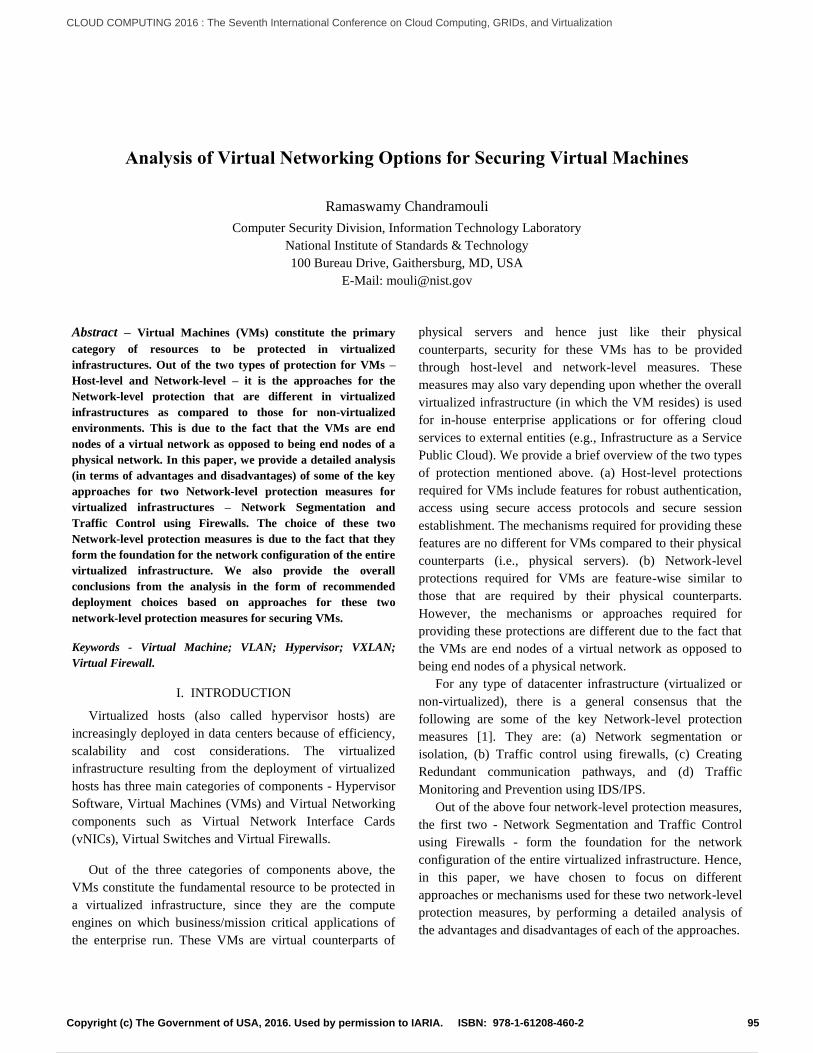
Analysis of Virtual Networking Options for Securing Virtual Machines

Ramaswamy Chandramouli

Computer Security Division, Information Technology Laboratory

National Institute of Standards & Technology

100 Bureau Drive, Gaithersburg, MD, USA

E-Mail: [email protected]

Abstract – Virtual Machines (VMs) constitute the primary

category of resources to be protected in virtualized

infrastructures. Out of the two types of protection for VMs –

Host-level and Network-level – it is the approaches for the

Network-level protection that are different in virtualized

infrastructures as compared to those for non-virtualized

environments. This is due to the fact that the VMs are end

nodes of a virtual network as opposed to being end nodes of a

physical network. In this paper, we provide a detailed analysis

(in terms of advantages and disadvantages) of some of the key

approaches for two Network-level protection measures for

virtualized infrastructures – Network Segmentation and

Traffic Control using Firewalls. The choice of these two

Network-level protection measures is due to the fact that they

form the foundation for the network configuration of the entire

virtualized infrastructure. We also provide the overall

conclusions from the analysis in the form of recommended

deployment choices based on approaches for these two

network-level protection measures for securing VMs.

Keywords - Virtual Machine; VLAN; Hypervisor; VXLAN;

Virtual Firewall.

I. INTRODUCTION

Virtualized hosts (also called hypervisor hosts) are

increasingly deployed in data centers because of efficiency,

scalability and cost considerations. The virtualized

infrastructure resulting from the deployment of virtualized

hosts has three main categories of components - Hypervisor

Software, Virtual Machines (VMs) and Virtual Networking

components such as Virtual Network Interface Cards

(vNICs), Virtual Switches and Virtual Firewalls.

Out of the three categories of components above, the

VMs constitute the fundamental resource to be protected in

a virtualized infrastructure, since they are the compute

engines on which business/mission critical applications of

the enterprise run. These VMs are virtual counterparts of

physical servers and hence just like their physical

counterparts, security for these VMs has to be provided

through host-level and network-level measures. These

measures may also vary depending upon whether the overall

virtualized infrastructure (in which the VM resides) is used

for in-house enterprise applications or for offering cloud

services to external entities (e.g., Infrastructure as a Service

Public Cloud). We provide a brief overview of the two types

of protection mentioned above. (a) Host-level protections

required for VMs include features for robust authentication,

access using secure access protocols and secure session

establishment. The mechanisms required for providing these

features are no different for VMs compared to their physical

counterparts (i.e., physical servers). (b) Network-level

protections required for VMs are feature-wise similar to

those that are required by their physical counterparts.

However, the mechanisms or approaches required for

providing these protections are different due to the fact that

the VMs are end nodes of a virtual network as opposed to

being end nodes of a physical network.

For any type of datacenter infrastructure (virtualized or

non-virtualized), there is a general consensus that the

following are some of the key Network-level protection

measures [1]. They are: (a) Network segmentation or

isolation, (b) Traffic control using firewalls, (c) Creating

Redundant communication pathways, and (d) Traffic

Monitoring and Prevention using IDS/IPS.

Out of the above four network-level protection measures,

the first two - Network Segmentation and Traffic Control

using Firewalls - form the foundation for the network

configuration of the entire virtualized infrastructure. Hence,

in this paper, we have chosen to focus on different

approaches or mechanisms used for these two network-level

protection measures, by performing a detailed analysis of

the advantages and disadvantages of each of the approaches.

95Copyright (c) The Government of USA, 2016. Used by permission to IARIA. ISBN: 978-1-61208-460-2


108 / 157

Before we describe the organization of the rest of the

paper, a few observations regarding our chosen network-

level protection measures in the context of virtualized

infrastructure are in order. In a virtualized infrastructure, the

distinguishing networking environment is the virtual

network. Hence the network segmentation approaches

discussed in this paper have to involve some virtual network

components such as virtual switches. Similarly, a viable

approach for traffic control using firewalls has to use a

virtual firewall instead of a physical firewall. In Section II,

we focus on two network segmentation approaches and

discuss the advantages and disadvantages of each. Control

of virtual network traffic using two different types of virtual

firewalls and the advantages and disadvantages of each are

analyzed in Section III. In Section IV, we provide the

overall conclusions from the analysis, in the form of

deployment choices based on approaches for the two

network-level protection measures for securing VMs.

II. NETWORK SEGMENTATION IN VIRTUAL

NETWORKS

The approaches to network segmentation in the context

of virtualized infrastructures are the same as those used in

physical network with some variations (these variations are

underlined in our description below): (a) Using a

combination of firewalls – the firewalls used are virtual

firewalls (as opposed to a physical firewall) and are

implemented as Virtual Security Appliance (VSA) and

hosted on security hardened VMs with multiple Virtual

Network Interface cards (vNICs). Each vNIC may be

connected to a different network segment [2]. (b) Isolated

network segments created as logical segments on top of a

physical network segment – one is the VLAN approach that

is based on tagging packets and switch ports with a unique

identifier called VLAN ID, and the other is overlay-based

virtual networking technology that creates an overlay

network by encapsulating packets with IDs depending upon

the type of overlay technology. Both approaches (VLAN

and Overlay) rely on the capabilities in virtual switches of

the virtualized host.

The three approaches for network segmentation in

virtualized infrastructures outlined above are discussed in

Sections A, B and C below. After a brief description of each

approach, an analysis of each approach is provided with the

relative advantages and disadvantages. Where ever

applicable, the distinct advantage of a particular approach is

also brought out.

A. Network Segmentation Using a Combination of Firewalls

Let us now consider a virtualized host with 4 VMs –

VM1, VM2, VM3 & VM4. We can form a network segment

(say a DMZ) using two virtual firewalls, one each on any

two VMs - say VM1 & VM4. These firewalls are VM-based

Virtual Security Appliances residing on VMs defined with

multiple vNICs – each one connected to a different network

segment. The firewall in VM1 then will have one vNIC

connected to an external network (say the public Internet)

of the enterprise and the other vNIC connected to the DMZ

segment in the virtualized network within a virtualized host.

Correspondingly the firewall in VM4 has to have one vNIC

connected to the internal network of the enterprise and the

other vNIC connected to the DMZ. The vNIC connection to

the DMZ (from both firewall VMs - VM1 & VM4) is

established by their pathway to an internal-only virtual

switch. This internal-only virtual switch has no uplink

connection to any physical NIC of the virtualized host and

hence traffic from any VM connected to it cannot travel

directly outside the virtual network segment (not to speak of

outside the virtualized host). The internal-only switch can

only forward traffic directly to VMs connected to it - say

VM2 &, VM3. All incoming and outgoing traffic into the

VMs connected to the internal-only virtual switch whose

source/target is an internal/external network, has to go

through the firewall in VM1 or in VM4. The firewalls in

VM1 & VM4 thus form the gatekeepers for the virtual

network segment (i.e., DMZ).

A.1 Analysis

The advantages of network segmentation within the

virtualized network of a virtualized host using a

combination of virtual firewalls are: (a) Simplicity of

Configuration: It can be configured with commodity

firewall VSAs hosted on multi-vNIC VMs. (b) Flexibility

within a Virtualized host: More than one isolated network

segment can be created within the virtual network of the

virtualized host by simply adding another firewall VM.

The limitations of this approach to network segmentation

in a virtualized network are the following: (a) The logical

network segment created inside a virtualized host can

neither be extended to the physical network of the data

center nor to the virtual network in another virtualized host

(since segmentation is obtained by virtual firewalls inside

the virtualized host). This makes the approach to network

segmentation non-scalable. (b) A consequence of creating a

non-scalable network segment is that the migration of a VM

in the network segment to any other virtualized host (due to



109 / 157

performance or availability or load balancing reasons) is out

of the question, unless a network segment (with identical

configuration) exists on the target virtualized host.

B. Network Segmentation Using Virtual LAN (VLAN)

Technology

The second approach to network segmentation in

virtualized infrastructures is broadcast-containment

networking technologies, such as VLAN. The requirement

for this is that the hypervisor should have capabilities to

define virtual switches that are VLAN-aware [3][4]. The

segmentation is obtained by assignment of an identifier

called the VLAN ID to one or more ports of a switch and

connecting the VMs designated for that VLAN segment to

those ports. VMs on one VLAN can only communicate

directly with VMs on the same VLAN and a router is

needed for communication between VMs on different

VLANs [5]. Assignment of a VM to a particular VLAN can

be based on the application tier it is hosting (e.g., Web

Server, DBMS server, etc.) or the client to which the VM

belongs (in cloud data centers). These VLAN-capable

virtual switches (VS) can perform tagging of all packets

going out of a VM with a VLAN tag (depending upon

which port it has received the packet from) and can route an

incoming packet with a specific VLAN tag and MAC

address to the appropriate VM by sending it through a port

whose VLAN ID assignment equals the VLAN tag of the

packet. An example of a VLAN-based virtual network

segmentation inside a virtualized host is given in Figure 1.

B.1 Analysis

The advantages of a VLAN-based network segmentation

approach are: (a) Network segments can extend beyond a

single virtualized host (unlike the segment defined using

virtual firewalls) since the same VLAN ID can be assigned

to ports of virtual switches in different virtualized hosts. (b)

The number of network segments that can be configured is

reasonably large since a single virtual switch can typically

support 64 ports and the 12-bit VLAN ID address space

enables creation of 4000 VLAN segments.

The disadvantages of VLAN-based network

segmentation approach are: (a) The configuration of the

ports in the physical switch attached to a virtualized host

must exactly match the VLANs defined on the virtual

switches inside that virtualized hosts. This results in tight

coupling between virtual network and physical network of

the data center. The consequence of this tight coupling is

that the port configuration of the physical switches has to be

frequently updated since the VLAN configuration of the

virtual network of the attached virtualized host may

frequently change due to migration of VMs among VLANs

as well as among virtualized hosts. (b) Another consequence

of frequent migration of VMs among VLANs, as well as

among virtualized hosts is that the VLAN configuration of

ports in the physical switch may not match with that of the

connected virtualized host. This may result in a situation

where a particular hypervisor (or a virtualized host) may end

up processing messages for every VLAN on the network,

even when it is not hosting any active VM belonging to that

VLAN [6] and (c) Segments created using broadcast-

containment technologies cannot be allowed to have a large

span since they will result in greater traffic in the overall

data center due to multicast and broadcast traffic. But

greater VM mobility (due to load balancing and availability

reasons) may require VLANs with a large span resulting in

an undesirable phenomena called VLAN sprawl [6].

C. Network Segmentation Using Overlay-based Virtual

Networking Technology

In the VLAN-based approach, the logical network

segments were created on a physical LAN using portgroups

of virtual switches inside virtualized hosts. These logical

network segments did span multiple virtualized hosts. The

total number of these segments possible is limited to around

4000 due to the 12 bit address space of VLAN ID. Another

limitation is the lack of independence between the physical

and virtual networking infrastructure, since the port

configuration of the physical switches attached to the

virtualized hosts have to be consistent with the VLANs

defined on the port groups of virtual switches inside those

virtualized hosts. The overlay-based virtual networking

approach to network segmentation overcomes these two

limitations in the following two ways [7].



110 / 157

Figure 1 - VLAN-based Network Segmentation

(a) Overlay-based virtual networking technologies have a

larger address space enabling larger number of virtual

network segments. An example is the 24 bit VXLAN ID of

the VXLAN overlay scheme that can enable 16 million

virtual network segments to be defined, and (b) The overlay

schemes by their definition, create a logical Layer 2 network

(called the overlay network) over the physical Layer 3

backbone of the data center (called the underlay network).

Since this scheme does not warrant any modifications to the

physical network, it provides physical-logical network

independence. As already alluded to, overlay-based virtual

networking schemes achieve segmentation by creating a

logical Layer 2 network over the physical Layer 3 network.

The overlay network is created by encapsulating a native

Layer 2 packet with another Layer 2 identifier. There are

three common encapsulation schemes – VXLAN, GRE and

STT [8].

Let us now look at the encapsulation process in VXLAN

[9] through components shown in Figure 2. The Ethernet

frame originating from a VM, that just holds the MAC

address of the destination VM is encapsulated in two stages:

(a) First with the 24 bit VXLAN ID (virtual Layer 2 (L2)

segment) to which the sending/receiving VM belongs and

(b) Second, with the source/destination IP address of the

VXLAN tunnel endpoints called VTEPs. [10]. VTEPs are

logical network endpoints (nodes) for the encapsulated

VXLAN packets and they reside in the kernel of a

hypervisor. A VXLAN-encapsulated packet originates at the

VTEP in the kernel of the hypervisor where the source VM

resides (carrying the VTEP’s address as the source IP

address) and terminates at the VTEP in the kernel of the

hypervisor where the destination VM resides (carrying this

VTEP’s address as the destination IP address). Thus, we see

that VXLAN encapsulation enables creation of a virtual

Layer 2 segment that can span not only different hypervisor

hosts but also different IP subnets within the data center.

C.1 Analysis

The advantages of a network segmentation approach

based on Overlay-based networking technology are: (a)



111 / 157

Figure 2 – Overlay-based Virtual Network Segmentation

Because of independence between the virtual network and

the physical network, there is greater VM mobility

compared to a VLAN- based virtual network environment,

(b) The physical-logical network independence, together

with the bigger overlay segment ID address space (e.g., a

VXLAN ID is 24 bits as opposed to 12 bit VLAN ID

allowing for 16 million segments compared to 4096 for

VLAN), makes the overlay based network segmentation

infinitely scalable. Another factor contributing to scalability

of the overlay scheme is that the encapsulating frame is an

IP/UDP packet. Hence, the number of virtual network

segments is limited only by the size of IP subnets that can be

defined within the data center and not by the number of

ports in virtual switches as in the case of VLAN-based

network segmentation. Further, by using internal, non-

routable IP addresses for VMs (using DHCP and NAT

capabilities) running within virtualized hosts, the number of

virtual networks that can be realized is even higher and (c)

The VLAN scheme uses the Spanning Tree Routing

Protocol to forward packets, VXLANs can use the ECMP

protocol of Layer 3 [11], thus efficiently utilizing all

available network links in the network fabric of the data

center.

The disadvantage of a network segmentation approach

based on Overlay-based networking technology is that it

requires large mapping tables in each virtual switch level in

order to generate overlay packets – since the MAC address

of the destination VM could be located in any IP subnet and

any host in the data center. Building these mapping tables

using just a flooding technique is inefficient. Hence, a

control plane needs to be deployed in the virtualized

infrastructure to populate the mapping tables for use by the

overlay packet generation module in the hypervisor. This

creates an additional layer of control and adds to the

complexity of network management [11].

III. TRAFFIC CONTROL IN A VIRTUAL NETWORK

Traffic control in a virtual network can be performed

using either a virtual firewall or a physical firewall.

However, in a virtualized infrastructure, the computing

nodes (whose incoming/outgoing traffic needs to be

controlled) are VMs and are end nodes of a virtual network.

Hence, the deployment of a physical firewall will require the

traffic from the virtual network to be diverted into the

physical network (where the physical firewall resides) and



112 / 157

then back into the virtual network. This extra route travelled

by communication packets will result in latency and

consequently reduced performance of applications hosted on

VMs. Hence, in this paper, we consider only virtual

firewall-based solutions for traffic control in virtual

networks for securing VMs.

Earlier in this paper (Section 2), we saw that two or more

virtual firewalls can be used to create network segments in a

virtual network. Since the focus of this Section is on traffic

control, we are going to analyze the use of virtual firewalls

only for controlling inter-VM traffic.

Inter-VM traffic can be of two kinds: the traffic between

two VMs residing on the same virtualized host (either

connected to the same or different virtual switches) and

traffic between two VMs hosted on different virtualized

hosts. Traffic between two VMs residing on the same

virtualized host can only be enabled if each VM has at least

one vNIC (a VM can have multiple vNICs just like a

physical server can have multiple physical network interface

cards or network adapters) connected to a common virtual

switch. This is due to the fact that two virtual switches in a

virtualized host cannot be connected to each other.

Although, theoretically, a pathway between two VMs on the

same virtualized host can be establishing by routing the

traffic from one VM (say VM1) to the physical network

(through one physical NIC) and back into the same

virtualized host (through another physical NIC) to the target

VM (say VM2), this is not a viable option in most

situations, due to the latency issue referred to above. Of

course, for enabling traffic between two VMs residing on

two different virtualized hosts, the traffic has to travel from

the virtual network (in the originating virtualized host)

where the originating VM resides, through the physical

network of the data center and back again into the virtual

network of the target VM (in the target virtualized host).

Virtual firewalls come in two flavors: (a) VM-based –

this class of virtual firewalls, comes packaged as a virtual

security appliance on a specially-configured VM and (b)

Hypervisor Kernel-based – this class of firewalls operates as

a kernel loadable module in the kernel of the hypervisor.

A. Traffic Control using VM-based Firewalls

A VM-based firewall, as the name indicates, is a firewall

software that runs in a VM. It can be installed as a software

module on a guest VM already running in a virtualized host

or it can be packaged as a virtual security appliance on a

specially prepared VM instance. Its location within the

virtual network of a virtualized host is critical as its function

is to monitor, drop or forward packets between sets of VMs

belonging to different security zones. This is the reason that

this class of firewalls is called bridge-mode firewalls as it

also acts as a bridge between zones (since the only link

between VMs connected to two different virtual switches is

through a VM with vNICs connected to both virtual

switches).

A.1 Analysis

The advantage of VM-based firewall for traffic control is

that since it is available as a Virtual Security Appliance, it is

easy to deploy and configure in a virtualized host. Its initial

location within the virtual network of the virtualized host is

relatively easy as it is dictated by the layout of the security

zones based on the various virtual switches and this type of

firewall only monitors and filters packet flows between one

virtual switch and another.

The disadvantages of VM-based firewalls are: (a) It

cannot monitor and filter traffic flowing between two VMs

connected to the same virtual switch, (b) Its performance is

limited by the number of virtual CPU cores allocated to the

VM it is residing or packaged in, and (c) All traffic flowing

into and out of all portgroups and virtual switches associated

with zones pertaining to this firewall, has to be redirected to

this firewall causing unnecessary traffic (a phenomena

called Traffic Trambones [12]).

B. Traffic Control using Hypervisor Kernel-based Firewalls

Hypervisor kernel-based firewalls are also called

hypervisor-mode firewalls and VM NIC firewalls. These

firewalls install as a hypervisor module along with a VSA,

the latter used purely for initial configuration (and re-

configuration) for the hypervisor module. Hence, the main

firewall functions of monitoring and packet filtering are

done in the hypervisor kernel-module with the VM hosting

the VSA portion playing the role of a Control or Service

VM. Logically residing between a VM vNIC and the

hypervisor virtual switch, this type of firewall provides a

vNIC-level firewall enforcement point for traffic to and

from VMs. Thus they can be used for selectively protecting

a given subset or all the VMs in a host or a cluster. Because

of the visibility at the vNIC level, these firewalls can protect

traffic flowing between two VMs connected to the same

virtual switch, unlike the bridge-mode firewalls. Another

distinguishing feature of this type of firewalls is that the

firewall does not require any changes



113 / 157

to the virtual network configuration inside a virtualized host

(such as additional network pathways for redirecting traffic

to the VM hosting firewall) or modification to IP addresses

of VMs.

B.1 Analysis

The advantages of hypervisor kernel-based firewalls are:

(a) Their performance is of an order of magnitude much

higher than bridge-mode firewalls since they perform packet

inspection from within the kernel at native hardware speeds

rather in a VM where the performance is limited by the

capacity of virtual CPU allocated to it [13], (b) These

perform monitoring at the VM NIC (vNIC) level and hence

all firewall rules (or ACLs) and state are logically attached

to the VM interface. Hence these rules and state move with

the VM when it migrates from one virtualized host to

another, thus providing continuity of security protection for

a VM irrespective of its location [12], and (c)

Implementations that support firewall rules at a higher level

of abstraction than IP addresses or ports, can be used to

filter packets at data center, host cluster and port group

levels.

The disadvantages of hypervisor kernel-based firewalls

are: (a) This class of firewalls works as a managed kernel

process and is therefore neither a VM resident program nor

is part of the virtual network of the hypervisor. Hence

conventional management tools having access only to VMs

or virtual networks cannot be used to monitor this class of

firewalls and (b) Some of the implementations of this class

of firewall support only 5-tuple based rules (Source and

Destination IP Address, Source and Destination Ports and

Protocol). They do not support higher level abstractions

such as Security Groups, Zones or Containers. However,

some of the latest offerings do support firewall rules based

On higher level abstractions and flow statistics as well.

IV. SUMMARY & CONCLUSIONS

In this paper, we performed a detailed analysis of two

network segmentation approaches and two virtual firewall

types for the protection of VMs in virtualized

infrastructures. Comparing the features of the two network

segmentation techniques, we find that the only distinct

advantage that overlay-based network segmentation (such as

VXLAN) holds over the VLAN-based approach is its

infinite scalability. Hence, unless the number of VMs in the

data center is in the order of thousands, the VLAN-based

approach provides a satisfactory outcome in terms of

performance and for meeting the goal of securing VMs.

Because of this, the VLAN approach is economically

justifiable in many environments. Further justification

comes from the fact that overlay-based network

segmentation schemes require sophisticated virtual switches,

large mapping tables and the overhead of creating a control

plane using SDN controllers.

Analyzing the relative advantages and disadvantages of

the two firewall types – VM-based and hypervisor kernel-

based – we find that the hypervisor kernel-based firewall is

superior to the VM-based one in terms of three features.

They are: (a) Performance (executes in the hypervisor kernel

instead of in a VM), (b) Reduced network traffic (no

diversion of traffic needed from various switches to the VM

hosting the firewall) and, (c) Firewall rules are associated

with the VM interface (since it is placed between a VM NIC

and the virtual switch) and move with VM. The third feature

is very critical from the point of view of the security of the

VM, since it provides continued protection to it even when

it migrates to different virtualized hosts or host clusters

within the data center, without any additional re-

configuration. It is this overwhelming security assurance

feature that makes the hypervisor kernel-based firewall, the

security software of choice in many virtualized

infrastructures.

REFERENCES

[1] D. Shackleford, Virtualization Security – Protecting Virtualized

Environments, Wiley Publishing Inc, Indianapolis, IA, USA, 2013

[2] “DMZ Virtualization with VMware Infrastructure”. [Online].

http://www.vmware.com/files/pdf/dmz_virtualization_vmware_inf

ra_wp.pdf [retrieved: Jan, 2016].

[3] “MAC Bridges and Virtual Bridged LANs”. [Online].

https://www.ietf.org/meeting/86/tutorials/86-IEEE-8021-

Thaler.pdf [retrieved: Dec, 2015].

[4] “IEEE 802.1Q Virtual LANs (VLANs)”. [Online].

http://www.ieee802.org/1/pages/802.1Q.html

[retrieved: Dec, 2015].

[5] A. Hameed, and A. N. Mian, “Finding Efficient VLAN

Topology for better broadcast containment,”

Third International Conference on the Network of the Future

(NOF), Gammarth, Nov 2012, pp.1-6.

[6] Introduction to Virtualized Networking. [Online].

http://www.ipspace.net/Introduction_to_Virtualized_Networking


[7] Overlay Virtual Networking. [Online].

http://www.ipspace.net/Overlay_Virtual_Networking




114 / 157

[8] “Overlay Virtual Networking and SDDC”. [Online].

http://my.ipspace.net/bin/list?id=xSDNOverlay

[retrieved: Jan, 2016].

[9] “Virtual eXtensible Local Area Network (VXLAN): A

Framework for Overlaying Virtualized Layer 2 Networks over

Layer 3 Networks”. [Online]. https://tools.ietf.org/html/rfc7348


[10] “VXLAN Overview: Cisco Nexus 9000 Series Switches”.

[Online].

http://www.cisco.com/c/en/us/products/collateral/switches/nexus-

9000-series-switches/white-paper-c11-729383.pdf


[11] “Scaling Overlay Virtual Networks”. [Online].

http://content.ipspace.net/get/Scaling%20Overlay%20Virtual%20

Networks.pdf


[12] Virtual Firewalls. [Online].

http://www.ipspace.net/Virtual_Firewalls [retrieved: Dec, 2015].

[13] Virtual Firewall. [Online].

https://en.wikipedia.org/wiki/Virtual_firewall




115 / 157

Profiling and Predicting Task Execution Time Variation ofConsolidated Virtual Machines

Maruf Ahmed, Albert Y. ZomayaSchool of Information Technologies, The University of Sydney, Australia

Email: [email protected], [email protected]

Abstract—The task execution time variation (TETV) due toconsolidation of virtual machines (vm), is an important issuefor data centers. This work, critically examines the natureand impact of performance variation from a new angle. Itintroduces a simple and feasibly implementable method of usingmicro and syntactic benchmarks to profile vms. It is called,the Incremental Consolidation Benchmarking Method (ICBM). Inthis method, server resources are systematically incremented,in order to quantitatively profile the effects of consolidation.Resource contention due to basic resources, like CPU, memoryand I/O, have been examined separately. Extended experimentshave been done on the combinations of those basic resources,too.All experiments have been done and data are collected from realvirtualized systems, without using any simulator. Theleast squareregression (LSR) is used on the profiled data, in order to predictthe TETV of vms. To profile the TETV data, the server has beenconsolidated with different types and levels of resource loads. Theprediction process, introduced here is straightforward and haslow overhead, making it suitable to be applied on a wide varietyof systems. The experimental results show that, the LSR modelscan reasonably well predict TETV of vms under different levels ofconsolidation. Theroot mean square error (RMSE) of predictionfor combination of resources, like CPU-Memory, CPU-I/O andMemory-I/O, are within 2.19, 2.47 and 3.08, respectively.

Keywords–virtualization; consolidation; performance; variation;prediction.

I. I NTRODUCTION

The virtualization is an essential part of modern datacenters. It is required for running many day-to-day operations,like deploying a fault tolerance scheme, or providingCloudservices. A virtual machine (vm) is a self-contained unitof execution, usually created with the help of a hypervisorrunning on top of a physicalhost. The vms are immenselyimportant for data centers, as they help to implement the pay-as-you-go model for the Cloud. Usually, a number of vmsare run on a host to reduce the operational cost. All thesimultaneously running vms of a physical host are collectivelyknown, as theco-located vms. The Cloud users can rent vmsand have complete control over the rented vms. However, theydo not have access to the underlaying physical hardware.

Theconsolidation of vms, is generally done to increase theresource utilization of virtualized servers. However, it imposesa performance penalty, which manifest itself through thetask execution time variation (TETV) of co-located vms [1]–[3]. This performance variation happens because of resourcecontention among the vms. It is an obstacle to efficientlyscheduling parallel applications on virtualized systems,forseveral reasons: (i) The variation depends on the server loadand resource contention among the vms. The result is that, thesame task may take different amount of time to be completedon different vms. At present there is no well accepted methodto predict this variation; (ii)To schedule a task of any parallel

application, the execution finish time of all the parents tasksmust be known. It becomes difficult due to the TETV. Thus,it is an important issue to address, if parallel applications areto be scheduled on virtualized clusters, efficiently.

Most of the previous works on this area fall into two maincategories. The first one, is to explore the cost-performancemodels of parallel applications on public Clouds [4]–[13].The other one, is virtualized server consolidation benchmark-ing [14]–[19]. Nonetheless, one can easily identify severalweaknesses of those works: (i) They do not explore theresource contention and performance variation of co-locatedvms explicitly; (ii) Experiments have been done, mainly withparallel applications. Those have complex internal structure oftheir own, usually represented by a task graph. The virtual-ization involves so many layers of abstraction and hardwareindirection. The complex internal structures of an applicationcan make it difficult to accurately capture the relationshipamong the co-located vms; (iii) They do not provide theoption to control usages of different computing resources,either individually or granularly during experiments. In thiscase such an ability is very desirable; (iv) Consolidationbenchmarks are designed to provide an overall average pointofsome combination of tests, not details about different levels ofconsolidation; (v) The consolidation benchmarks are hugelydependent on vendors and their applicability for comparingdifferent virtualization technologies are not well defined. Forexample, theVMmark benchmark is designed for VMwareESX servers; (vi) Most works use complex mathematicaloptimization tools, which have high overhead. The perfor-mance modeling greatly depends on system configuration, andchanges to system configuration may require model retraining,which in turn becomes hugely time consuming process dueto high overhead; (vii) Many works deal with theoreticallyderived model of the Cloud and simulation is used for verifi-cation. Those simulations often do not take virtualizationintoconsideration, hence does not always portray the reality.

It is clear that, a new design for the consolidation bench-mark is required, to address above limitations. TheIncremen-tal Consolidation Benchmarking Method (ICBM) overcomesabove issues, using micro and syntactic benchmarks. Some ofthe design features of the ICBM are discussed next, in orderto explain how does it overcome above issues:

1) Micro and syntactic benchmarks suites have been usedinstead of parallel applications. This gives the ability tomanipulate basic resources, like CPU, memory and I/O, bothindividually and granularly during experiments. This makes itpossible to analyze the effect of consolidation on each resourcetype more discretely than the previous works;

2) The ICBM, at its core is agnostic to both virtualizationtechnology and system configuration. First and foremost, itis



116 / 157

a methodology that can be applied to any system in general,making it suitable to compare a wide range of systems;

3) The TETV prediction models for combinations of re-sources have been built from profiled vm data. Separatelycollected TETV data due to basic resources, like CPU, memoryand I/O, have been used to predict TETV for combination ofresources, like CPU-Memory, CPU-I/O and Memory-I/O. Theprediction results have a good level of accuracy, demonstratingthat profiling for every combination of resource load is notnecessary. It can potentially save a huge amount of time whileprofiling a large data center;

5) All experiments have been done on actual virtualizedservers rather than using simulators. All results presented hereare real system data. The results show that, the ICBM canpredict TETV of real virtualized systems quite accurately;

4) Prediction models have been built using theLeast SquareRegression (LSR), which has very low overhead. Use of LSRinstead of a complex mathematical tool, makes the trainingand prediction process much faster. Often, changes in systemconfiguration may require retraining of models, in such casesa low overhead process can save a lot of time;

5) Analysis of profiled data reveals some interesting pat-terns. For example, it shows that certain types of resourcecombinations can cause the task execution time of consolidatedvms to degrade more rapidly than the others. This indicatesthat resource contention is one of the main factors, behind theaverage utilization of virtualized servers being so low.

The micro and syntactic benchmarks suites play an impor-tant part in the design of the ICBM. They are important toolsfor server performance analysis, and a lot of studies have beendone on their design. These benchmarks are the result of longtime analysis of commercially successful applications. Theyare inspired by an interesting phenomenon that, the applica-tions spend both 80% of their time and resources, executingjust 20% of the code [20]. The micro and syntactic benchmarksuites are carefully crafted to mimic such important parts ratherthan running the entire application. Each benchmark suiteconsists of several individual applications. These applicationsare grouped together in a well-thought-out pattern.

The benchmarks suites are used here, to get a finer controlon the individual server resource types. Without using thesebenchmark suites, such controlling of resources is not possible.Experimental results show that, the benchmark suites can causesignificant amount of resource contention and TETV on vms.Thus, the benchmark suites can be a set of powerful tools forstudying the performance variation of virtualized servers. Theexperiments that are done here, are very comprehensive andprovide some interesting results.

Rest of the paper is structured as follows. The mainobjectives of experiments are discussed in the Section II,followed by the methodology described in the Section III. Sec-tions III-B and III-A briefly discuss the benchmarks used in theexperiments and experiential setup, respectively. Detailresultsof experiments and prediction are given in the Section IV.Finally, Section V concludes the paper, with an overview ofthe future work.

II. PROBLEM DESCRIPTION

This section describes the objectives of the experiments.The first objective, is to quantitatively measure the effectof

consolidation on the task execution time of vms. The logicalview of a virtualized server is shown in the Figure 1a. Here,a typical situation has been considered. Usually, a physicalserver hosts vms of the same configuration, however number ofsimultaneously running vms may change over time. Differentvms may also have different types of resource requirements.Some of them may be CPU or memory intensive, while othersmay be multiple resources intensive. As the number of vmsincrease or decrease on a physical host, it is important to knowthe TETV of individual vms. The objective here, is to offer asystematic way to record the TETV due to different numbersof vms, and find a way to predict the TETV.

The second objective, is to establish a relationship betweenTETV due to basic types of resource contention and that ofcombination of resources. Figure 1b depicts the situation of aserver from resource usages point of view. In each graph, thex-axis represents the number of vms simultaneously runningon the host. The y-axis represent the task execution time ofa vm. As the number of co-located vms increase, the taskexecution time starts to vary.

The actual amount of variation depends on types andamount of resource loads. For three basic resources types,namely CPU, memory and I/O (Figure 1b(i-iii)), the amountof TETV are excepted to be different. Again for combinationof resources, like CPU-memory, CPU-I/O and memory-I/O(Figure 1b(iv-vi)), the TETV would be different, too. Profilinga virtualized system is difficult for many reasons. A server maybe running different number of vms, with different amountof loads at different points. That makes it impractical, toprofile all vms, for all combination of resources. Establishing arelation, among the TETV due to basic resource types and thatof combination of resources, would save a lot of time whileprofiling a large data center. Next, the procedure used in theICBM is discusses in details.

III. M ETHODOLOGY

This section introduces the terminologies and methodologythat have been used for rest of the paper. One of the vmsof host, is designated as the target vm (vt), while rest aredesignated as co-located (vco) vms. Thevt has been used torun different tasks to record their TETV. On the other hand,vco have been used to collectively create resource contention.

In Cloud, the data is generally stored on dedicated nodesover the network. However, before processing, all data isretrieved into the local node. For example, a MapReduceworker node performs all the mapping and reducing steps onlocal data. In fact, MapReduce nodes rely more on local data,and try to consume as little bandwidth as possible [21]. Thatway, local I/O contention has much more impact comparedto that of network I/O. What is more, in order to address theoverall I/O contention issue, it is necessary to address thelocalI/O contention first [22]. This work provides a quantitativewayto measure the I/O contention of vms of a node. The networkI/O system consists of several such nodes. Taking this work asa basis, the issue of network I/O contention can be addressedthrough extended experiments.

A parallel application can have many different data flowpaths. As mentioned in the introduction, such an applicationcan be decomposed into a set of tasks. Then, those tasks needto be scheduled on different vms individually. This work laysground, for understanding the effect of consolidation at vm



117 / 157

Stage 7

Vco Vco Vco Vco VcoVco VcoVco Vco Vco Vco VcoVt

1 4 5 10 11 122 3 6 7 8 9Hypervisor

Stage 1

Stage 2

Stage 3

Stage 4

Stage 5

Stage 6

(a) Stages of the ICBM.

(iv) Combined resources: CPU & Mem (v) Combined resources: CPU & I/O (vi) Combined resources: Mem & I/O

cococo

t

Exe

ctu

ion

Tim

e o

f V

Exe

ctu

ion

Tim

e o

f V

Exe

ctu

ion

Tim

e o

f V

Exe

ctu

ion

Tim

e o

f V

Exe

ctu

ion

Tim

e o

f V

Basic resource on VM : I/O Basic resource on VM : Mem Basic resource on VM : CPU

Exe

ctu

ion

Tim

e o

f V

ttt

tt

(iii)(i) (ii)

(b) Task time variation from resource point of view.

Figure 1. Experimental setup and objective of ICBM.

level. Without this understanding, it is not possible to formulatethe effect on consolidation at a higher level.

The micro and syntactic benchmarks used here, are actuallyapplication suites. They are combinations of several appli-cations, patterned together to execute such a way that theyput maximum pressure on a particular system resource. Forexample, the Filebench includes several different categories oftests, including a file-server test [23]. Similarly, the Unixbenchconsists of many tests, including the System Call Overhead,Pipe-based Context Switching and Execl Throughput test [24].The Nbench includes, a task allocation algorithm, Huffmancompression, IDEA encryption, Neural Net and LU Decom-position test [25]. There are many more test components onthose suites, and all of them are designed to mimic the steps ofcommercial applications. Thus, together they can put the vmsunder stress like a real application. Also the experimentalre-sults from real systems show that, these benchmarks cause thetask execution time to vary significantly. Thus, they are wellcapable of creating resource contention like a real application.

Initially, vt run one task alone on the host (stage 1 inFigure 1a) and execution finish time is recorded. In successivestages, co-located vms are added in a particular pattern tocreate resource contention. Manipulating each co-locatedvm,independently at each step, makes it possible to increase aparticular type of resource load at a desired quantity. In theexperimental setup, twovco are added at each stage until theserver reaches the saturation point. Depending on the configu-ration, a host can simultaneously run only a certain number ofvms, without becoming unresponsive. That is considered to bethe saturation point. As co-located vms with different resourcetypes are added at each stage the TETV of all vms are profiled.

Figure 2 provides the pseudo code of ICBM for basicresource types. The ICBM repeats the same steps for eachresource type, on co-located vms. Therefore, it is not necessaryto explain the steps, for each resource type. Next, these stepsare explained for one type of resource load, the CPU load.

Let t be a task whose TETV due to CPU intensive co-located vms is going to be investigated. First, thet is runalone on a single vm (vt) of the host (stage 1 of Figure 1a),in order to obtain the execution finished time, without anyinterference from co-located vms. Next, (stage 2) thet is runagain, this time along with two simultaneously running co-

T ← A set of tasks.Bcpu ← A set of CPU intensive benchmarks.Bmem ← A set of memory intensive benchmarks.Bi/o ← A set of I/O intensive benchmarks.vt ← A target vm.vco ← A set of co-located vms.for Each taskt ∈ T do

Add vt to the host.Run t on vt alone and record the execution finish time.for Each benchmark type B← Bcpu, Bmem, Bi/o do

while All the vms of host are respondingdoAdd two extravco with benchmark of type B to host.Run vt simultaneously with the addedvco, andrecord the execution finish time of each.

end whileRemove allvco and free related system resources.

end forend for

Figure 2. Basic steps of ICBM.

located vms (v1co and v2co). Both the new vms, run oneBcpu

type benchmark each, thus only increasing CPU intensive loadon the system. This gives the execution time oft on vt, whichis now consolidated with two co-located CPU intensive vms.Afterwards, two more CPU intensivevco are added (stage 3),increasing the number of CPU intensive co-located vms tofour. The execution finish time ofvt is profiled again for thissetting. This way, two newvco are added at each stage, untilthe co-located vms stop responding.

The maximum number of vms, that can be simultaneouslyrun on a host without making it non-responsive, is dependenton the system configuration. In the experiments, the host hadoneIntel i7-3770 processor, with four cores and eight hardwarethreads. Assigning, a logical CPU to each vm, the system couldrun maximum of fourteen such vms, simultaneously. Addinganymore vm, would made the whole system non-responsive.With one vm designated asvt, and two more newvco addedat each stage, the final stage (stage 7) of the experimenthad thirteen simultaneously running vms (onevt along withtwelve vco). The vms are created with least possible subset ofCPU resources, so that CPU load can be increased with finegranularity. However, vms with larger number of logical CPU



118 / 157

can be also created, if such is required.The same steps are repeated for memory intensivevco, too.

However, in this case memory intensive benchmarks are runon co-located vms instead of CPU intensive benchmarks. Allvms are configured to have 1 GB of RAM. The experimentstarts (stage 1) with a single vm (vt) running the task, whoseTETV due to memory intensive co-located vms is going tobe investigated. Next, (stage 2)vt is run again, along withtwo new co-located vms (v1co and v

2co), each running one

memory intensive benchmark. Similarly, two more vms (vico

and vi+1co ) are added at each stage until the system reaches

a predetermined point of memory load. In this case, addinga newvco makes the host memory load to be increased by 1GB. It was done so that, the host memory load can be changedgranularly. The host has 16 GB of RAM. By restricting thenumber of vms to thirteen at the final stage, maximum of 13GB RAM is allocated to the co-located vms, leaving rest forthe hypervisor. As with the CPU load, this predetermined loadis also not a fixed number. Afterwards, for I/O load the samesteps are repeated by adding two I/O intensive benchmarks ontwo vco, at each stage. Thus, the TETV for three basic resourcetypes (CPU, memory and I/O) are collected.

Next, the procedure is repeated forresource combinations.The combinations are made by choosing two resource typesat a time, from previously mentioned basic three. Those areCPU-Memory, Memory-I/O and I/O-CPU. Experiments forcombination of loads are done exactly the same way. That is,start with one vm (vt), and at each stage add two co-locatedvms (vico and v

i+1co ) to increase the load. Difference is that,

now two new vms run two different types of benchmarks. Bothof them, together create the effect of load combinations. Forexample, to increase CPU-Memory load, twovco are added ateach stage. One (vico) runs a CPU intensive benchmark, whilethe other one (vi+1

co ) runs a memory intensive benchmark.Above experiments demonstrate, how the execution time of

vt is varied due to co-located vms (vico). However, there is an-

other angle to this problem, that is how thevco are collectivelyeffect the execution times of each other. To examine this, theexecution finish times of all thevico, are also recorded at eachstage. Finally, the whole procedure is repeated without thevt

altogether. That is, all the experimental steps are repeated, byadding only load (onvico) at each stage.

Advantage of the ICBM is that, the server load can bechanged granularly, for each basic resource type or their com-binations. Furthermore, there is no need to know the internalstructure of a complex application, which is running on the vm.Establishing a relationship between task execution time andthe server load would be helpful for a virtualized data-centerin many ways, including designing heuristic algorithms forscheduling, consolidation and live-migration of vms [26][27].

A. Experimental setupA Dell XPS-8500 system has been used in the experiments.

It has one Intel i7-3770 processor and 16GB of RAM. The i7-3770, has four cores and eight hardware threads, each clockedat 3.4 GHz. The host is deployed with Xen 4.2 over Fedora 17core. Fourteen vms have been setup, one to acts asvt, while therest arevico. Each vm run Fedora 16, have one logical CPU, 1GB of RAM and 30 GB virtual disk. The vms are not pinned tothe logical cores. Total of 13 GB RAM is allocated to the vms,rest are available for the hypervisor. All the benchmarks are

installed on vms beforehand, and a concurrent java applicationmanages all benchmarks and vms from a remote node.

B. Benchmarks used

This section gives an overview of the benchmark suites,used in the experiments. A data center may be runningthousands of servers. While designing an algorithm for consol-idation or live migration scheme, the internal structures of allthe parallel applications may not be known. It is more realisticto characterize the servers by their loads. Micro and syntacticbenchmark suites are well suited for such purposes.

Three different categories of benchmarks have been usedfor three categories of resources, namely CPU, memory andI/O. The Nbench [25] and Unixbench [24], are the two CPUintensive benchmark suites used here. Two memory benchmarksuites used here, are theCachebench [28] andStream [29][30].Finally, three I/O benchmark suites have been used, they arethe Dbench [31], Filebench [23] and Iozone [32]. For eachbenchmark, several different parameters are need to be set.Owing to the space limitation, it is not possible to list all theparameters here. A fuller discussion about the benchmarks,isout of scope for this paper. Interested readers are encouraged torefer to the citations of respective benchmark suites for details.

IV. RESULTS

The results for prediction are given in the Section IV-C.However, to interpret the prediction results, it is necessary todiscuss some observations of the experimental results. It willalso help to clarify the training and testing data format, whichhas been used during the training and prediction phrases.

A. Execution time variations of the target vm (vt)

Three graphs of Figure 3, show the TETV ofvt due tothree basic types of resource loads. They are being, CPU(Figure 3a), memory (Figure 3b) and I/O (Figure 3c). In eachgraph, the x-axis shows the total number of vms running onthe system, while y-axis presents the task completion time onvt. First point of the graph, shows the execution time ofvt,when it is run alone on the server. At this stagevt is freefrom any interference from co-located vms. As explained in theSection III, two co-located vms (vco) are added to the serverat successive stages. In the final stage, there were twelvevco,simultaneously running besides thevt. In other words, fromleft to right along the x-axis, the interference from co-locatedvms increases. The first point of each graph, gives executiontime of the task without any interference from co-located vms.On the other hand, the last point gives the execution time withmaximum interference from co-located vms. Results clearlyshow that different types and number ofvco, make the taskexecution time to vary at a different rate.

Figure 3a shows that, the TETV ofvt with the increaseof CPU intensivevico, is the minimum among all types ofworkloads. On the other hand, for memory intensivevco(Figure 3b), two CPU intensive tasks (Nbench and Unixbench)on vt show less variation compared two memory intensivetasks (Cachebench and Stream) under the same situation. As anexample, in isolation the Nbench takes 10.1 minute to executeon vt. With other 12 memory intensive co-located vms (vco)it extends to 12.83 minutes, which is only 27.02% longer. Incontrast, the Cachebench under the exact same setup takes587.58% longer to execute (execution time goes from 11.76



119 / 157

min to 80.68 min). Figure 3c shows the TETV due to I/Ointensivevco. Here, CPU intensive tasks do not show muchperformance degradation, while both the memory and I/Ointensive tasks do. For example, the Cachebench (a memoryintensive task) have 1057.311% increase in execution time,while Iozone (an I/O intensive task) have 1482.93%.

Next, Figure 4 shows the TETV onvt, when combinationof loads have been used onvco. The combinations are beingCPU-Memory (Figure 4a), CPU-I/O (Figure 4b) and Memory-I/O (Figure 4c). Figure 4a shows the TETV onvt due to a

0

20

40

60

80

100

120

140

160

180

200

220

240

vt(stage 1)

vt + 2 vco(stage 2)

vt + 4 vco(stage 3)

vt + 6 vco(stage 4)

vt + 8 vco(stage 5)

vt + 10 vco(stage 6)


Exe

cutio

n tim

e of

vt (

min

)

No of vm with CPU load

NbenchUnixbench

CachebenchStream

DbenchFilebench

IozoneMean of all vm

(a) Basic resource type: CPU.

0

20

40

60

80

100

120

140

160

180

200

220

240

vt(stage 1)

vt + 2 vco(stage 2)

vt + 4 vco(stage 3)

vt + 6 vco(stage 4)

vt + 8 vco(stage 5)



Exe

cutio

n tim

e of

vt (

min

)

No of vm with Memory load

NbenchUnixbench

CachebenchStream

DbenchFilebench


(b) Basic resource type: Memory.

0

20

40

60

80

100

120

140

160

180

200

220

240

vt(stage 1)

vt + 2 vco(stage 2)

vt + 4 vco(stage 3)

vt + 6 vco(stage 4)

vt + 8 vco(stage 5)



Exe

cutio

n tim

e of

vt (

min

)

No of vm with I/O load

NbenchUnixbench

CachebenchStream

DbenchFilebench


(c) Basic resource type: I/O.

Figure 3. The TETV ofvt due to various basic types of resource load onvco.

0

20

40

60

80

100

120

140

160

180

200

220

240

vt(stage 1)

vt + 2 vco(stage 2)

vt + 4 vco(stage 3)

vt + 6 vco(stage 4)

vt + 8 vco(stage 5)



Exe

cutio

n tim

e of

vt (

min

)

No of vm with both CPU and Mem load

NbenchUnixbench

CachebenchStream

DbenchFilebench


(a) Combination of resources: CPU-Memory.

0

20

40

60

80

100

120

140

160

180

200

220

240

vt(stage 1)

vt + 2 vco(stage 2)

vt + 4 vco(stage 3)

vt + 6 vco(stage 4)

vt + 8 vco(stage 5)



Exe

cutio

n tim

e of

vt (

min

)

No of vm with both Mem and I/O load

NbenchUnixbench

CachebenchStream

DbenchFilebench


(b) Combination of resources: Memory-I/O.

0

20

40

60

80

100

120

140

160

180

200

220

240

vt(stage 1)

vt + 2 vco(stage 2)

vt + 4 vco(stage 3)

vt + 6 vco(stage 4)

vt + 8 vco(stage 5)



Exe

cutio

n tim

e of

vt (

min

)

No of vm with both CPU and I/O load

NbenchUnixbench

CachebenchStream

DbenchFilebench


(c) Combination of resources: CPU-I/O.

Figure 4. The TETV ofvt due to different combinations of resource load onvco.

mix of CPU and memory intensivevco. Here, CPU intensivetasks onvt show least amount of degradation just as observedpreviously. Among the memory intensive benchmarks, theCachebench shows highest rate of performance degradation(542.74%). However, for I/O intensive tasks the effect of CPU-Memoryvco combination, is less adverse compared to memoryintensive tasks. Figures 4c and 4b, show the performancedegradation ofvt, when I/O intensivevco is coupled with CPUand memory intensivevco, respectively.

In both cases, memory and I/O intensive tasks onvt

show comparatively more performance degradation. In the case



120 / 157

of CPU-I/O load (Figure 4c), the Cachebench and Iozoneshow increase of execution time by 1907.21% and 1991.67%,respectively. Again for Memory-I/O load (Figure 4b), thesame two benchmarks show worse performance degradation(1100.09% and 1502.56%, respectively). Table I shows thestandard deviation (SD) of execution times of all seven taskson vt through stage 1 to 7.

TABLE I. STANDARD DEVIATION OF TASK EXECUTION TIMES (MIN ).

Tasktype

CPU intensive Mem. intensive I/O intensive

Loa

dty

pe

Nbe

nch

Uni

xbe

nch

Ca

che

benc

h

Str

ea

m

Dbe

nch

File

benc

h

Iozo

ne

CPU 3.66 0.05 0.99 2.42 0.00 0.41 1.51

Ba

sic Memory 2.58 0.05 25.28 16.89 0.01 2.97 14.18

I/O 0.01 0.15 46.59 0.12 0.02 15.16 54.70

CPU-Memory

4.12 0.05 23.51 1.43 0.00 3.06 9.89

Com

bine

d

CPU-I/O 0.88 0.08 83.85 0.35 0.01 17.33 71.62

Memory-I/O

3.82 0.06 49.40 0.82 0.01 13.17 56.62

The results of this section show, how the degradation oftask execution time for each resource can be presented ina quantitative way. At present, there is no standard way tocompare the effect of consolidation, for different types ofresources or different classes of servers. The straightforwardmethod presented here, can be used to compare the effect ofconsolidation on wide varieties of systems.

B. Execution time variations of the co-located vms (vico)

Execution finish time of all the co-located vms, at eachstage are also profiled. This data is used for predicting theTETV of vt. Figures 5 and 6 show the arithmetic mean ofexecution times of allvico, at each stage, separately. Duringexperiments, it was observed that, the arithmetic mean ofexecution time of all thevico follow a pattern, for each resourcetype. Even though, individualvico execution time might nothave such characteristic. This, clearly indicates that overallresource usages of all vms, is what ultimately shapes theperformance degradation curve during consolidation.

Both in Figures 5 and 6, the first point of each graph isalways zero, as there is novico running on the host at stage1 (see Figure 1a). At stage 2, twovico are running, thereforesecond point is the arithmetic mean of task execution timesof two vms (v1co, v2co). Similarly, third point is the arithmeticmean of values of four vms (v1co, v2co, v3co andv4co) and so on.

Using above procedure, each subgraph has seven arithmeticmean variation plotting ofvco, for seven different tasks runningon vt. Furthermore, arithmetic mean of those seven values arealso shown (in black). Increase of different types of workloadscauses the arithmetic mean of execution times to changedifferently. It can be seen that, the variation is the minimumfor CPU intensive load (Figure 5a), among all three basic typesof resources. Among the three combination of resources, theCPU-Memory (Figure 6a) intensivevco combination showsleast amount of performance degradation. On the other hand,the combination of Memory-I/O intensivevco (Figure 6b) have

0

20

40

60

80

100

120

140

160

180

200

220

240

vt(stage 1)

vt + 2 vco(stage 2)

vt + 4 vco(stage 3)

vt + 6 vco(stage 4)

vt + 8 vco(stage 5)



Avg

. exe

cutio

n tim

e of

vco

(min

)

No of vm with CPU load

NbenchUnixbench

CachebenchStreamDbench

FilebenchIozone

Mean of all vmMean of load only

(a) Basic resource type: CPU.

0

20

40

60

80

100

120

140

160

180

200

220

240

vt(stage 1)

vt + 2 vco(stage 2)

vt + 4 vco(stage 3)

vt + 6 vco(stage 4)

vt + 8 vco(stage 5)



Avg

. exe

cutio

n tim

e of

vco

(min

)

No of vm with Memory load

NbenchUnixbench


FilebenchIozone


(b) Basic resource type: Memory.

0

20

40

60

80

100

120

140

160

180

200

220

240

vt(stage 1)

vt + 2 vco(stage 2)

vt + 4 vco(stage 3)

vt + 6 vco(stage 4)

vt + 8 vco(stage 5)



Avg

. exe

cutio

n tim

e of

vco

(min

)

No of vm with I/O load

NbenchUnixbench


FilebenchIozone


(c) Basic resource type: I/O.

Figure 5. Arithmetic mean of TETV ofvco with respect to three basicresource types load changes.

debilitating effect on the system as the arithmetic mean ofexecution time rises rather quickly, compared to other cases.

In order to obtain above execution time values, eachexperiment has been repeated at least three times. The orderof adding vms has been shuffled, in order to observe theireffect. However, no significant difference between the resultshave been observed. Two vms are added at each stage, only toconduct the experiments in a uniform way. In our observation,the order of adding vms do not change the results ultimately,rather it depends on the cumulative resource usages of vms.



121 / 157

0

20

40

60

80

100

120

140

160

180

200

220

240

vt(stage 1)

vt + 2 vco(stage 2)

vt + 4 vco(stage 3)

vt + 6 vco(stage 4)

vt + 8 vco(stage 5)



Avg

. exe

cutio

n tim

e of

vco

(min

)

No of vm with both CPU and Mem load

NbenchUnixbench


FilebenchIozone


(a) Combination of resources: CPU-Memory.

0

20

40

60

80

100

120

140

160

180

200

220

240

vt(stage 1)

vt + 2 vco(stage 2)

vt + 4 vco(stage 3)

vt + 6 vco(stage 4)

vt + 8 vco(stage 5)



Avg

. exe

cutio

n tim

e of

vco

(min

)

No of vm with both Mem and I/O load

NbenchUnixbench


FilebenchIozone


(b) Combination of resources: Memory-I/O.

0

20

40

60

80

100

120

140

160

180

200

220

240

vt(stage 1)

vt + 2 vco(stage 2)

vt + 4 vco(stage 3)

vt + 6 vco(stage 4)

vt + 8 vco(stage 5)



Avg

. exe

cutio

n tim

e of

vco

(min

)

No of vm with both CPU and I/O load

NbenchUnixbench


FilebenchIozone


(c) Combination of resources: CPU-I/O.

Figure 6. Arithmetic mean of TETV ofvco with respect to threecombinations of resource load changes.

C. Task execution time variation predictionFour benchmarks have been used as tasks for training. They

are the Nbench, Unixbench, Cachebench and Stream. Threeother benchmarks have been used for testing. They are theDbench, Filebench and Iozone. All of the test benchmarks havedifferent levels of performance degradation. Therefore, theycan help to evaluate the prediction process better. Training andtesting have been done on different sets of data. No trainingdata have been used for testing, and vice versa.

The nine subgraphs of Figure 8, separately show predictionresults for three resources of three test tasks onvt. Each

subgraph, contains two sets of predictions, obtained fromtwo separate data sets, which are described next. First set ofpredictions, are shown in blue on Figure 8. In this case, theTETV data ofvt for basic resource types, has been used topredict TETV of vt for combination of resources. First, theTETV data ofvt for CPU (Figure 3a), Memory (Figure 3b) andI/O (Figure 3c) intensivevco are recorded, separately. Thoseare used as inputs. Then, three resource combinations havebeen used as three separate targets, which are CPU-Memory(Figure 4a), CPU-I/O (Figure 4c) and Memory-I/O (Figure 4b).

0

20

40

60

80

100

120

140

160

180

200

220

vt(stage 1)

vt + 2 vco(stage 2)

vt + 4 vco(stage 3)

vt + 6 vco(stage 4)

vt + 8 vco(stage 5)



Cac

hebe

nch

exec

utio

n tim

e on

vt (

min

)No of co-located vm

CPU loadMem load

I/O load

CPU-Mem loadMem-I/O loadCPU-I/O load

(a) Vt training data: Cachebench.

0

10

20

30

40

50

60

70

80

90

100

vt(stage 1)

vt + 2 vco(stage 2)

vt + 4 vco(stage 3)

vt + 6 vco(stage 4)

vt + 8 vco(stage 5)



File

benc

h ex

ecut

ion

time

on v

t (m

in)

No of co-located vm

CPU loadMem load

I/O load


(b) Vt & Vco testing data: Filebench.

0

20

40

60

80

100

120

140

160

180

200

220

vt(stage 1)

vt + 2 vco(stage 2)

vt + 4 vco(stage 3)

vt + 6 vco(stage 4)

vt + 8 vco(stage 5)



Cac

hebe

nch:

Avg

. exe

cutio

n tim

e of

all

v co

(min

)

No of co-located vm

CPU loadMem load

I/O load


(c) Vco training data: Cachebench.

Figure 7. Examples of input and target data used for both training andtesting.



122 / 157

0

5

10

15

20

25

30

35

40

45

50

55

60

vt vt + 2 vco vt + 4 vco vt + 6 vco vt + 8 vco vt + 10 vco vt + 12 vco

Exe

cutio

n tim

e of

vt (

min

)

No of vm

Prediction using vt dataPrediction using vco data

Dbench CPU-Mem

(a) Prediction for Dbench: CPU-Mem load.

0

10

20

30

40

50

60


Exe

cutio

n tim

e of

vt (

min

)

No of vm


Filebench CPU-Mem

(b) Prediction for Filebench: CPU-Mem load.

0

10

20

30

40

50

60


Exe

cutio

n tim

e of

vt (

min

)

No of vm


Iozone CPU-Mem

(c) Prediction for Iozone: CPU-Mem load.

0

10

20

30

40

50

60


Exe

cutio

n tim

e of

vt (

min

)

No of vm


Dbench Mem-I/O

(d) Prediction for Dbench: Mem-I/O load.

0

10

20

30

40

50

60


Exe

cutio

n tim

e of

vt (

min

)

No of vm


Filebench Mem-I/O

(e) Prediction for Filebench: Mem-I/O load.

0

25

50

75

100

125

150

175

200


Exe

cutio

n tim

e of

vt (

min

)

No of vm


Iozone Mem-I/O

(f) Prediction for Iozone: Mem-I/O load.

0

25

50


Exe

cutio

n tim

e of

vt (

min

)

No of vm


Dbench CPU-I/O

(g) Prediction for Dbench: CPU-I/O load.

0

10

20

30

40

50

60


Exe

cutio

n tim

e of

vt (

min

)

No of vm


Filebench CPU-I/O

(h) Prediction for Filebench: CPU-I/O load.

0

25

50

75

100

125

150

175

200


Exe

cutio

n tim

e of

vt (

min

)

No of vm


Iozone CPU-I/O

(i) Prediction for Iozone: CPU-I/O load.

Figure 8. Task execution time prediction fromvt andvco data.

Input & target data example. In above Figures 3 and 4,data is grouped according to resource loads. It is done todemonstrate that, different types of resources influence the taskexecution time differently. Thus, it is important to study theeffect of each resource type separately. However, for trainingand prediction, input data needs to be grouped benchmarkwise. It is required, because during training, the TETV datadue to basic resources of a task, needs to be linked to theTETV data due to combination of resources of the same task.Otherwise, training would not be done with a consistent data.

Figure 7a shows an example, of this rearranged inputand target data set that is used for training. It combines theTETV data of the Cachebench onvt, for three basic and threecombined types ofvco loads from Figures 3 and 4, respectively.All benchmarks data are rearranged similarly. During training,three basic resources data (CPU, Memory and I/O) are used asinputs and three combination of resources data (CPU-Memory,CPU-I/O and Memory-I/O) as targets. From the training dataset, three sperate models have been generated, for three setsof target data (CPU-Memory, CPU-I/O and Memory-I/O). Allthree targets use the same three basic resources data as inputs.

An example of test data set is shown in Figure 7b. Itcombines six TETV data of the Filebench, from Figures 3and 4. Prediction results for three resources (CPU, Memoryand I/O) of three test benchmarks (Dbench, Filebench andIozone) are shown in Figure 8. Theroot mean square error(RMSE) for this set of predictions are shown in Table II.

Training with cco data. The second set of predictions(shown in red on Figure 8), are obtained by training themodels only withvco data. This demonstrates an interestingphenomenon, that models generated through use of co-locatedvm (vco) data only, can predict the execution time variationsof target vm (vt), too. During training the CPU (Figure 5a),memory (Figure 5b) and I/O (Figure 5c) data ofvco are usedas inputs, while CPU-Mem (Figure 6a), Mem-I/O (Figure 6b)and CPU-I/O (Figure 6c) data ofvco used as targets. On theother hand, during testing thevt data are used as both inputand target. All testing have been done with the same threebenchmarks (Dbench, Filebench and Iozone), that have beenused in the previous section for testing. That is, in this casemodels are generated using only co-located vms data, whiletesting is done with target vm data.



123 / 157

T t

cpu−mem,i = −20.415 + 4.795 ∗ (T t

cpu,i)0.7 + 0.752 ∗ (T t

mem,i)0.9 + 0.579 ∗ (T t

io,i)

−0.119 ∗ (T t

cpu,i)0.7

∗ (T t

mem,i)0.9

− 0.035 ∗ (T t

cpu,i)0.7

∗ (T t

io,i) + 0.002 ∗ (T t

mem,i)0.9

∗ (T t

io,i)(1)

T t

cpu−io,i = −16.393527 + 0.802 ∗ (T t

cpu,i) + 0.282 ∗ (T t

mem,i) + 1.769 ∗ (T t

io,i)

−0.020 ∗ (T t

cpu,i) ∗ (T t

mem,i) − 0.023 ∗ (T t

cpu,i) ∗ (T t

io,i) + 0.003 ∗ (T t

mem,i) ∗ (T t

io,i)(2)

T t

mem−io,i = −16.549 + 2.104 ∗ (T t

cpu,i) + 7.920 ∗ (T t

mem,i)0.2

− 0.169 ∗ (T t

io,i)0.96

−0.957 ∗ (T t

cpu,i) ∗ (T t

mem,i)0.2 + 0.031 ∗ (T t

cpu,i) ∗ (T t

io,i)0.96 + 0.455 ∗ (T t

mem,i)0.2

∗ (T t

io,i)0.96

(3)

Figure 9.TETV models for resource combinations (CPU-Memory, CPU-I/O & Memory-I/O) built from vt data.

T t

cpu−mem,i = −0.009 + 0.190 ∗ (T co

cpu,i)1.2 + 0.220 ∗ (T co

mem,i)1.2 + 0.250 ∗ (T co

io,i) (4)

T t

cpu−io,i = −0.102 + 4.217 ∗ (T co

cpu,i)3.25

− 0.034 ∗ (T co

mem,i) + 1.383 ∗ (T co

io,i)0.7

+0.544 ∗ (T co

cpu,i)3.25

∗ (T co

mem,i) − 5.394 ∗ (T co

cpu,i)3.25

∗ (T co

io,i)0.7 + 0.163 ∗ (T co

mem,i) ∗ IO0.7(5)

Tt

mem−io,i = 3.720 ∗ (Tco

cpu,i)0.325

+ 2.376 ∗ (Tco

mem,i) − 0.020 ∗ (Tco

io,i)0.05

+1.079 ∗ (T co

cpu,i)0.325

∗ (T co

mem,i) − 4.394 ∗ (T co

cpu,i)0.325

∗ (T co

io,i)0.05

− 3.144 ∗ (T co

mem,i) ∗ (T co

io,i)0.05

(6)

Figure 10.TETV models for resource combinations (CPU-Memory, CPU-I/O & Memory-I/O) built from vco data.

An example of the training data, used here is shown onFigure 7c. It is a collection of six differentvco workload TETVdata of the Cachebench, from six graphs of Figures 5 and 6.During training, the variation of arithmetic mean ofvco TETVdue to CPU, memory and I/O are used as inputs. The CPU-Memory, Memory-I/O and CPU-I/O data are used as targets.Three models have been generated in this way, with threevco

target data set. However, testing is done withvt test data like,the example shown in the Figure 7b. Recall that, it was alsoused for testing in the previous section. Table III shows theRMSE for this set of prediction. It shows that, the predictionresults have a good level of accuracy.

Root mean square error (RMSE) for prediction. TheRMSE of predictions for above two sets of data, are shownseparately on Table II and Table III. To the best knowledge ofthe authors, there exist no approximation algorithm to estimatethe TETV of co-located vms. Therefore, there is no acceptabletheoretical bound for the RMSE values [33]. Generally, a lowervalue of RMSE means better prediction accuracy.

In each case, the prediction is better, when all three basicresources have been used to generate the model rather thantwo. For example, while predicting the TETV of CPU-Memoryload combination, the model build using CPU, memory and I/O(all 3 basic resources) data produces better results, than thatgenerated by using only CPU and memory (2 resources) data.

Parametric model. Lastly, the Figures 9 and 10 showmodel parameters and coefficients, as they are trained fromprofiled vt and vco data, respectively. They demonstrate therelation between input and prediction data formats. Threeequations of the Figure 9, are for three resource combina-tion targets. The terms are self-explanatory. For example,T

tcpu−mem,i denotes predicted task execution time of a task

on vt, when it is consolidated with total ofi number of CPUand memory intensive co-located vms. Similarly,T

tcpu−io,i

and Ttmem−io,i represent the predicted task execution time

for CPU-I/O and Memory-I/O load combinations, respectively.

The same input parameters have been used for all equations.T

tcpu,i represents the task execution time onvt when server

is consolidated withi number of CPU intensive co-locatedvms. Similarly,T t

mem,i andT tio,i represent the task execution

time when the server is consolidated with the same number ofmemory and I/O intensive co-located vms, respectively.

The equations of Figure 10 have the same targets, howeverinputs are different. Here, arithmetic mean of execution timesof co-located vms have been used as inputs. For example,T

cocpu,i represents the arithmetic mean of execution times of

i number of CPU intensive co-located vms. In this case,arithmetic mean of execution times of co-located vms havebeen used to predict the TETV of target vm.

TABLE II. ROOT MEAN SQUARE ERROR(RMSE)FOR PREDICTIONUSING TARGET VM (vt) DATA .

CPU-Memory CPU-I/O Mem-I/OPrediction Prediction Prediction

Bench

mar

ks With all 3 Only 2 With all 3 Only 2 With all 3 Only 2resources:resources: resources:resources: resources:resources:CPU, CPU, CPU, CPU, CPU, Mem,Mem, I/O Mem Mem, I/O I/O Mem, I/O I/O

Dbench 0.036 2.516 0.146 0.506 0.011 0.468Filebench 0.771 2.628 2.131 11.933 2.605 3.022Iozone 2.193 10.505 2.475 21.566 3.083 3.588

TABLE III. ROOT MEAN SQUARE ERROR(RMSE)FORPREDICTION USING CO-LOCATED VM (vco) DATA .

CPU-Memory CPU-I/O Mem-I/OPrediction Prediction Prediction

Bench

mar

ks With all 3 Only 2 With all 3 Only 2 With all 3 Only 2resources:resources: resources:resources: resources:resources:CPU, CPU, CPU, CPU, CPU, Mem,Mem, I/O Mem Mem, I/O I/O Mem, I/O I/O

Dbench 0.006 0.317 0.020 17.621 0.014 20.182Filebench 0.657 4.515 1.841 10.607 1.475 47.797Iozone 2.083 43.546 4.572 87.725 3.898 59.863



124 / 157

Changes in basic configuration of vms, may require somemodification of model parameters. The public Cloud offersvms for renting in certain number of predefined configurations.Therefore, number of such models required in reality, arelimited. What is more, since LSR has low overhead, buildingor rebuilding of a limited number of such models would notbe time consuming.

V. CONCLUSION AND FUTURE WORK

This work addresses an important issue of virtualization,the performance variations due to consolidation. A straight-forward methodology has been introduced here, that is prac-tically feasible to implement. It is different from most of thecomplementary works on virtualization, that employ complexmathematical tools and rely on simulation. In contrast, thiswork introduces a low overhead prediction process, and resultsare collected from real virtualized systems.

Micro and syntactic benchmark suites have been usedhere in a step by step process, to manipulate various vmresources individually. The methodology introduced here isunique, and results prove the effectiveness of this method.Experimental results from real virtualized systems show that,in this way it is possible to predict the TETV of vms quiteaccurately. It provides a new and quantitative way to explorethe mutual performance interference of co-located vms. Theresults also provide some valuable inside into the nature ofresource contention due to consolidation of vms.

The experimental results encourages one to continue work-ing along this direction. For future work, experiments wouldneed to be extended to a wider range of virtualization tech-niques and server configurations, to derive a more generalizedmodel. More questions related to this method, can be addressedin details in future works.

REFERENCES

[1] T. Janpan, V. Visoottiviseth, and R. Takano, “A virtual machine con-solidation framework for CloudStack platforms,” in ICOIN,2014, pp.28–33.

[2] F. Farahnakian, T. Pahikkala, P. Liljeberg, J. Plosila,and H. Tenhunen,“Utilization Prediction Aware VM Consolidation Approach for GreenCloud Computing,” in CLOUD, 2015, pp. 381–388.

[3] A. Tchana, N. D. Palma, I. Safieddine, D. Hagimont, B. Diot, andN. Vuillerme, “Software Consolidation as an Efficient Energy and CostSaving Solution for a SaaS/PaaS Cloud Model,” in Euro-Par, 2015, pp.305–316.

[4] M. Dobber, R. D. van der Mei, and G. Koole, “Effective Prediction ofJob Processing Times in a Large-Scale Grid Environment,” inHPDC,2006, pp. 359–360.

[5] V. E. Taylor, X. Wu, J. Geisler, and R. L. Stevens, “Using KernelCouplings to Predict Parallel Application Performance.” in HPDC,2002, pp. 125–134.

[6] W. Gao, Y. Li, H. Lu, T. Wang, and C. Liu, “On Exploiting DynamicExecution Patterns for Workload Offloading in Mobile Cloud Applica-tions,” in ICNP, 2014, pp. 1–12.

[7] A. Gupta, L. V. Kale, F. Gioachin, V. March, C. H. Suen, B.Lee,P. Faraboschi, R. Kaufmann, and D. S. Milojicic, “The who, what, why,and how of high performance computing in the cloud,” in CloudCom,Volume 1, 2013, pp. 306–314.

[8] J. Simao and L. Veiga, “Flexible SLAs in the Cloud with a PartialUtility-Driven Scheduling Architecture,” in CloudCom, Volume 1, 2013,pp. 274–281.

[9] S. Xi, M. Xu, C. Lu, L. T. X. Phan, C. D. Gill, O. Sokolsky, and I. Lee,“Real-time multi-core virtual machine scheduling in Xen,”in EMSOFT,2014, pp. 27:1–27:10.

[10] J. Zhao, J. Tao, L. Wang, and A. Wirooks, “A Toolchain ForProfilingVirtual Machines,” in ECMS, 2013, pp. 497–503.

[11] A. Iosup, “IaaS Cloud Benchmarking: Approaches, Challenges, andExperience,” in HotTopiCS, 2013, pp. 1–2.

[12] B. F. Cooper, A. Silberstein, E. Tam, R. Ramakrishnan, and R. Sears,“Benchmarking Cloud Serving Systems with YCSB,” in SoCC, 2010,pp. 143–154.

[13] A. V. Do, J. Chen, C. Wang, Y. C. Lee, A. Y. Zomaya, and B. B.Zhou,“Profiling Applications for Virtual Machine Placement in Clouds,” inCLOUD, 2011, pp. 660–667.

[14] R. McDougall and J. Anderson, “Virtualization performance: Perspec-tives and challenges ahead,” SIGOPS Oper. Syst. Rev., vol. 44, no. 4,Dec. 2010, pp. 40–56.

[15] V. Makhija, B. Herndon, P. Smith, E. Zamost, and J. Anderson,“VMmark: A Scalable Benchmark for Virtualized Systems,” VMware,Tech. Rep. TR-2006-002, 2006.

[16] T. Deshane, Z. Shepherd, J. Matthews, M. Ben-Yehuda, A.Shah, andB. Rao, “Quantitative comparison of Xen and KVM,” in Xen summit.Berkeley, CA, USA: USENIX association, Jun. 2008.

[17] P. Apparao, R. Iyer, and D. Newell, “Towards Modeling & Analysis ofConsolidated CMP Servers,” SIGARCH Comput. Archit. News, vol. 36,no. 2, May 2008, pp. 38–45.

[18] O. Tickoo, R. Iyer, R. Illikkal, and D. Newell, “Modeling VirtualMachine Performance: Challenges and Approaches,” SIGMETRICSPerform. Eval. Rev., vol. 37, no. 3, Jan. 2010, pp. 55–60.

[19] H. Jin, W. Cao, P. Yuan, and X. Xie, “VSCBenchmark: Benchmark forDynamic Server Performance of Virtualization Technology,” in IFMT’08, 2008, pp. 5:1–5:8.

[20] G. G. Shulmeyer and T. J. McCabe, “Handbook of Software QualityAssurance (3rd Ed.),” G. G. Schulmeyer and J. I. McManus, Eds.Upper Saddle River, NJ, USA: Prentice Hall PTR, 1999, ch. TheParetoPrinciple Applied to Software Quality Assurance, pp. 291–328.

[21] J. Dean and S. Ghemawat, “MapReduce: simplified data processingon large clusters,” Commun. ACM, vol. 51, no. 1, 2008, pp. 107–113.[Online]. Available: http://doi.acm.org/10.1145/1327452.1327492

[22] S. Ma, X.-H. Sun, and I. Raicu, “I/O throttling and coordination forMapReduce,” Illinois Institute of Technology, Tech. Rep.,2012.

[23] OpenSolaris Project, “Filebench,” URL:http://filebench.sourceforge.net/wiki/index.php/Main_Page, Retrieved: February, 2016.

[24] “Unixbench: BYTE UNIX benchmark suite,” URL:http://github.com/kdlucas/byte-unixbench, Retrieved:February, 2016.

[25] C. C. Eglantine, NBench. TypPRESS, 2012, iSBN: 9786136257211.

[26] W. Hu, A. Hicks, L. Zhang, E. M. Dow, V. Soni, H. Jiang, R. Bull,and J. N. Matthews, “A Quantitative Study of Virtual MachineLiveMigration,” in CAC, 2013, pp. 11:1–11:10.

[27] S. Nathan, P. Kulkarni, and U. Bellur, “Resource Availability BasedPerformance Benchmarking of Virtual Machine Migrations,”in ICPE,2013, pp. 387–398.

[28] P. J. Mucci, K. London, and P. J. Mucci, “The CacheBench Report,”URL: www.earth.lsa.umich.edu/ keken/benchmarks/cachebench.pdf, Retrieved: February, 2016.

[29] J. D. McCalpin, “Memory Bandwidth and Machine Balance in CurrentHigh Performance Computers,” IEEE CS TCCA Newsletter, Dec.1995,pp. 19–25.

[30] ——, “STREAM: Sustainable Memory Bandwidth in High Perfor-mance Computers,” University of Virginia, Charlottesville, Virginia,Tech. Rep., 2007.

[31] A. Tridgell, “The dbench benchmark,” URL:http://samba.org/ftp/tridge/dbench/README, 2007, Retrieved: February, 2016.

[32] W. Norcott and D. Capps, “IOzone Filesystem Benchmark,” URL:www.iozone.org, Retrieved: February, 2016.

[33] Z. A. Mann, “Allocation of Virtual Machines in Cloud Data Cen-ters&Mdash;A Survey of Problem Models and Optimization Algo-rithms,” ACM Comput. Surv., vol. 48, no. 1, Aug. 2015, pp. 11:1–11:34.



125 / 157

Data Locality via Coordinated Cachingfor Distributed Processing

Max Fischer and Eileen KuehnKarlsruhe Institute of Technology

76344 Karlsruhe, GermanyEmail: {max.fischer, eileen.kuehn}@kit.edu

Abstract—Modern data analysis methods often rely on datalocality. Processing applications are executed directly where datais stored. Frameworks enabling this require their own specialisedenvironment and modifications. We propose an alternative ap-proach using coordinated caching integrated into classic batchsystems. A custom middleware layer provides relevant data locallyon worker nodes. Most importantly no modifications are neededto add data locality to existing workflows. However, considerablymore factors must be addressed by distributed caches comparedto isolated ones. We investigated our approach with theoreticmodelling, simulations, and a prototype implementation. Ourevaluations show promising results for both applicability andperformance.

Keywords–Cooperative caching; Coordinated caching; Dis-

tributed caching; Batch production systems; Distributed processing.

I. INTRODUCTION

Caching as an enabler for data locality is an importanttopic for distributed data processing. As workflows usuallyprocess only a fraction of data frequently. It is thus inefficientto provide all data locally. In addition, changing workflow re-quirements in batch systems require a dynamic but coordinatedcaching approach.

Motivated by this, our approach enables data locality forbatch systems with minimal requirements. The basis for ourefforts are batch clusters which read data via network fromdedicated fileservers. To make remote data available locally,a series of caches on worker nodes can be used. We proposea coordination layer that combines individual caches into asingle pool.

Our approach stands out from existing caches by its scopeand subject: for one, individual caches work on the scale ofsingle machines. We target the entire batch system as a sin-gle entity. Also, distributed caches commonly target resourceproviders, e.g. web caches. In contrast, our approach targetsthe batch system as a resource consumer.

In this paper, we exemplarily consider the High EnergyPhysics (HEP) data analysis workflows of groups at the Karl-sruhe Institute of Technology [1]. In general, HEP experimentsof the Large Hadron Collider [2] are amongst the largestproducers of scientific data in terms of data volume. Handlingthis data is performed in iterative workflows at different scopes.This ranges from reconstruction of raw data at a globalscope [3] to the analysis of subsets of data at the scope ofuniversity groups.

In theory, HEP analyses conform to principles of datalocality based processing. Analysis workflows execute multiple

instances of an analysis application in a distributed environ-ment. Each instance extracts the same set of variables fromits share of an input data set. All sets of extracted variablesare then merged. This corresponds to the map reduce methodemployed by frameworks such as Hadoop.

However, the wide range of HEP workflows and numberof collaborating scientists dictate the use of established appli-cations and frameworks. This also implies constraints, whichare not satisfied by modern analysis frameworks. For example,HEP data is commonly stored in the ROOT binary file format.This format cannot be easily split or read from a stream, asis common in the Hadoop framework. The largest volume ofdata is used infrequently for validation and crosschecking.

We have performed modelling (Section II) and simulationsof the situation (Section III). The estimates on architectureand scale are motivated by our own working experiences withthe HEP analysis groups. From this, we conclude that classicbatch processing can be considerably improved with cachebased data locality. Our approach for data locality is basedon a concept for coordinated caching (Section IV). To testour conclusions, we implemented a prototype of a cachingmiddleware for batch systems (Section V). First experiencesshow promising improvements regarding performance andthroughput (Section VI).

A. Related WorkMany individual sub-topics of our work have been focus

of past research. In general, the approaches show considerableadvantages over naive caching. However, no existing workmatches the scope and applicability that is needed for HEPworkflows.

Distributed caching has been studied extensively. For ex-ample, simulations on distributed caching with centralisedcontrol [4] show considerable improvements in hit ratio andthroughput compared to independent caches. However, re-search usually focuses on the perspective of data providers,not consumers. Usage metadata is thus not taken into account,limiting the granularity required for data locality.

The CernVM File System (CVMFS) uses independentcaches for software provisioning [5]. It is used to make sharedsoftware frameworks available in grid and cloud environments.The prototypical CacheD service of the HTCondor batchsystem caches binaries executed by jobs [6]. This minimisestraffic, considerably speeding up deployment of multiple jobson low-throughput networks. Both of these approaches showthat caching is beneficial for batch processing. It improvesthroughput and allows deployment on resources without high



126 / 157

throughput network. However, these approaches target onlyitems which are the same for all jobs.

User communities have made attempts to introduce data lo-cality and/or caching to their workflows. On the one hand, theATLAS collaboration demonstrated analysis speedup by usinga central SSD cache for network attached HDD storage [7].In this setup, data locality is improved but the cache is stillaccessed remotely.

On the other hand, attempts have been made to deployHEP workflows on Hadoop [8], [9]. This provides advancedperformance and scalability. However, extensive compromiseshave to be made. For example, applications have to be adaptedto the I/O model and jobs may access only single files. Theautomatic distribution of data by the infrastructure is severelylimited to ensure data integrity.

II. MODELLING DISTRIBUTED CACHING

The modelling of distributed caches involves more aspectsthan using local caches on a single host. It therefore increasesthe complexity. Though the data to cache remain the same,factors such as location, replication, or even splitting, andgrouping need to be considered.

We model caching statistically to estimate the probabilityof cache hits, following cache hit rate. Using a factorisedapproach, we describe issues individually and combine themto a single probability. This allows to assess a detailed cost ofnaively applying caching to a distributed system.

As shown in Figure 1, a distributed cache can be fun-damentally viewed as a single entity. This is an ideal case,where a fraction of the global data volume is replicated on thecache volume. However, each worker node (WN) is actuallylimited to its local scope. In addition, jobs in a batch systemare scheduled without knowledge about cache content. In theworst case, data and job placement may be perpendicular.

Figure 1. Scopes of distributed caching

To simplify the model, we make two assumptions: First, thevolume of individual caches is large compared to items that arecached. Second, the volume of all items is large compared toboth the individual and total cache volume. This allows us totreat volumes as continuous, avoiding quantisation and fringeeffects. These assumptions mainly simplify the mathematicaldescription. The general conclusions are not changed by this.

A. A Priori Hit RateAs with regular caches, we employ a general probability

that an item is cached. The choice of this is arbitrary andmainly serves for expressiveness. Without loss of generality,we assume a naive caching approach: the cache is filled withan equal fraction of all data. Thus the probability of an itembeing cached P base

cache is the fraction of cache volume Vcache anddata volume Vdata.

P basecache /

Vcache

Vdata(1)

B. Item LocalityA distributed cache has no single cache volume but actually

several separate ones. Cached items can only be accessedefficiently on the host they are located on. We thereforeintroduce a second probability for item locality, namely thatan item is cached on the host it is accessed from, the local hitrate P item

local.If the batch system is not aware of the contents of indi-

vidual caches, job scheduling is random in relation to itemplacement. The probability of executing on the correct hostis inversely proportional to the number of hosts Nhosts. Incontrast, creating a number of replicas Nreplica on multiple hostsautomatically increases the local hit rate. However, replicasreduce the effective total cache volume and thus the overallcache hit rate. Both hit rates combine to the expected hit rateP item

expect.

P itemlocal /

Nreplica

NhostsNreplica Nhosts (2a)

P itemcache /

1

Nreplica(2b)

P itemexpect = P item

cache · P itemlocal /

1

Nhosts(2c)

For naive caching of individual items and no alignedscheduling, we thus expect neither positive nor negative effectfrom replication. There is no naive approach to mitigate thepenalty from distribution over multiple hosts.

In contrast, if we actively align job scheduling and cachelocality, the local hit rate becomes a constant – the effec-tiveness of scheduling. In this case, the positive effect ofreplication is reduced and ideally eliminated with perfectscheduling. The negative effect of reducing the effective cachevolume remains, however. Therefore, the penalty from dis-tributed execution can be mitigated by active scheduling andavoiding replication.

C. Item GroupingFor efficiency, it is common for any single batch job to

process groups of files. In classic batch systems, this groupingis done externally on job submission.

The benefit for each job is proportional to the number ofprocessed items cached locally. We can express the expectedefficiency Ejob

local as the fraction of expected local files⌦N local

items↵

to total processed files Nitems. This resolves directly to the localhit rate without aligned scheduling.

Ejoblocal =

DP job

local

E/

⌦N local

items↵

Nitems=

1

Nitems

X

items

P itemlocal (3a)

= P itemlocal (3b)

For naive caching with unrelated items, this result is trivial.There are implications if aligned job scheduling is attempted,



127 / 157

however. Even when directing jobs to cached items, the frac-tion of locally available items limits the achievable efficiency.In this context, aligned job scheduling and replication are onlyuseful if cache content is aligned as well.

D. Access ConcurrencyFor the scope of our work, a common caching assumption

does not hold true: cache access is not always superior toremote access. For example, modern SSDs provide throughputat the same order as a 10Gbit/s network. The difference isconcurrency of accesses: caches are accessed only by localprocesses, whereas remote data sources can be accessed by allprocesses.

Modelling accesses for a distributed system in general isbeyond the scope of this paper. However, the fact that bothlocal and shared data sources have limited throughput allow forsome basic statements. Ideally, both local and shared resourcesare used to their limit. This automatically implies that perfectcache hit rates are not desirable: a fraction of accesses shouldalways make use of the shared resources available.

III. ESTIMATES AND SIMULATION

To estimate the benefit of coordinated caching, we havesimulated multiple circumstances. The scope and estimatescorrespond to that of our associated HEP analysis groups.

We model the workflow as a set of application instances,each reading the same amount of data. We have benchmarkedcommon HEP analysis applications to assess realistic limi-tations. The measurements show a maximum throughput of20MB/s for each instance. This is a technical limit inducedby the software frameworks and data formats in use. The totalinput volume is estimated as 640GB. This corresponds to thevolume of a 2 months data taking period.

For the processing environment, we model our currentanalysis infrastructure: a set of worker nodes connected to a setof fileservers via a dedicated network, as shown in Figure 2.We assume infinite bandwidth for the fileservers, but modelthe shared network with its limited throughput of 10Gbit/s.For processing, we model a number of worker nodes of equalconfiguration: 32 execution slots, a 4Gbit/s SSD cache and a10Gbit/s network connection to the fileservers. For simplicity,we assume that as many instances as execution slots aredeployed.

Figure 2. Simulated infrastructure

The results of the simulation can be seen in Figure 3.To rate performance, we have chosen the total processingtime. For this observable, lower values are desirable. Thecache hit rate to the local cache is used as a free parameterin the simulation. This is motivated by assuming adequateselection of cache content by existing algorithms. Thus, thehit rate is only determined by the scheduling of data and

.

Figure 3. Simulation of workflow runtime

jobs. Dashed, vertical lines indicate the expected local hit ratewithout coordination.

There are two major results from our simulations (see Fig-ure 3): on the one hand, caching enables to scale the infras-tructure horizontally. This is especially important since remoteaccess is a bottleneck even with few worker nodes. On theother hand, perfect cache hit rate is actually not desirable.Instead, there is a range of cache hit rates that give bestperformance. This range is defined by the points where eitherlocal or remote throughput is maximized.

Notably, even for perfect caching the expected local hit rateP item

expect is in this range only for the smallest setup. Therefore,we must coordinate caches to benefit from data locality.

IV. CONCEPT FOR COORDINATED CACHING

Our approach for coordinated caching distinguishes be-tween local and global view as known from batch systems. Thelocal view refers to the individual worker nodes where batchjobs are running. The global view is given by the managinglayer where queuing and scheduling of batch jobs is performed.

Based on this scheme, the functionality of a cache can besplit into three layers, illustrated in Figure 4:

• the data provisioning on local scale,• the data access on global as well as local scale, and• the caching algorithm and distribution logic on global

scale.

Figure 4. Layers of the distributed cache concept

A. Provisioning LayerThe provisioning layer handles the actual data on worker

nodes. The worker nodes are the only elements with guaranteed



128 / 157

access to remote source data. They are therefore the logicalplace to retrieve and store both actual data and its metadata.

The provisioning layer implements the data provisioningassociated with caches: remote items are copied to local cachedevices, periodically validated, and potentially removed asneeded. In addition, metadata of items, such as size andcreation time, can only be collected on the worker node.

Since cache content is by design volatile, the layer alsohandles content metadata. This ensures that content metadatais as volatile as the actual content: the provisioning layer is thefirst to notice changes and invalidation of items. In the contextof opportunistic resources, worker nodes shutting down neatlyremove their allocation information as well.

Every worker node of the provisioning layer is limited toits local scope. Thus, major decisions are outsourced to theglobal scale. Every worker node exposes information requiredfor cache decisions. The information are composed of its ownmetadata, such as size of caches, and metadata of items. Inreturn, worker nodes rely on being notified of new items tocache and their relevance.

B. Coordination Layer

The coordination layer is responsible for decision making.Since it is not co-located with any active component, there areno restrictions on resource usage. It can thus fetch, aggregate,and process metadata without impacting other components.

The most important task of the layer is the selection ofitems to cache. This is fundamentally the same as in othercaches. For example, scores can be calculated from accesstimes. Given that arbitrary processing power can be provided,algorithms may be more complex than common. Both metadataand processing resources can be extended as needed.

The additional responsibility of the coordination layer isitem placement. This means the deliberate assignment ofitems to elements of the provision layer. Common featuresof distributed systems, such as load balancing, must be takeninto account. In addition, item relations must be considered forthis. For example, common input groups should be assignedtogether.

C. Access Layer

The benefit of caches depends on low overhead for ac-cessing items. Obviously, executed applications require localaccess to cached items. On the global scale, the batch systemmust receive information on item location.

Implementing access to cached items for executed appli-cations on worker nodes depends on the actual setup of batchjobs. Primarily, the access protocol is the deciding factor. Inprinciple, local redirection to cached items is sufficient.

Similarly, details of integrating with a batch system aresetup specific. In any case, information on item location mustbe provided to the batch system. This is the responsibility ofthin front ends, which forward information from coordinationand cache layer. Functionally, this is similar to lookup servicesin distributed file systems, e.g. the NameNode of Hadoop FS.However, since all information originates in coordination andcache layer, our front ends are expendable.

V. HTDA MIDDLEWARE PROTOTYPE

We have implemented a prototype of the coordinatedcaching concept: the High Throughput Data Analysis (HTDA)middleware [10]. The test environment and community arethe HEP analysis groups of our university. We have delib-erately kept dependencies on HEP software small, however.The prototype supports the HTCondor batch system [11] andapplications performing POSIX I/O.

Architecturally, we build on a general purpose frameworkfor a pool of worker nodes. Every instance of our applicationrepresents an individual node. The nodes are loosely coupled.They form a pool using stateless communication. Every nodehosts component plugins, which collaborate in the abstractedpool. The component plugins implement the actual layersdescribed in the previous chapter.

We currently use three node types that directly correspondto each layer:

• Provisioning nodes represent the provisioning layer.They stage, maintain, and validate cached files onworker nodes.

• Coordinator nodes represent the coordination layer.They aggregate metadata, and select and assign filesfor caching.

• Locator nodes provide locality information for theaccess layer. They act as proxies to the provisioningnodes.

In addition, we enforce access with hooks in the batch systemand a redirection layer in each worker node’s virtual filesystem.

A. Coordination of Provisioning NodesCoordination of provisioning nodes is based on the scoring

mechanism of files. We use a 1-dimensional score to expressthe relevance for caching. The score is simple to transmit,unambiguous to interpret, and simplifies many algorithms withclear break conditions.

The file score caries an implicit command: files ratedhigher are assigned with higher priority to provisioning nodes.If space is required for new files, existing files with lowscores are discarded first. However, relations between files arenot apparent from the score. They are purely handled at thecoordination level.

The score of files is calculated inside the coordinatornode. A factorised approach is used to express multiple per-spectives. Usage prediction is performed using a Least Re-cently/Frequently Used (LRFU) algorithm [12]. The algorithmis staged as a plugin. Other scoring algorithms can be usedif needed. Additionally, we exemplarily model adequacy forcaching: exceptionally small and large files are penalised toease allocation and overhead.

Assignment of files to provisioning nodes is performedseparately. Files accessed by the same job are grouped together.These groups are spread evenly amongst all provisioningnodes. Since files may belong to multiple groups, approachessuch as distributed hash tables are not adequate. Instead, weexploit that grouping is deterministic and certain groupings aremore likely to occur. This allows us to use a heuristic approach,which has proven itself adequate for our target community.



129 / 157

Groups scored highest are allocated first. If any files ofa group are already allocated, the node with the highest filecount is chosen. Otherwise, a node is chosen at random. Thisis performed until all files are allocated or no free space isleft. Finally, the allocated files and their scores are pushed toeach provisioning node individually.

Provisioning nodes only operate on the limited set ofassigned files. Since they perform the actual data access, theyare the final authority for staging files. This requires limitedautonomy for internal allocation and rearranging of files. Thusprovisioning nodes expose their allocation to the coordinationlayer. This allows to iteratively adjust local allocation andglobal distribution.

B. Application AccessA major motivation for our development is to preserve ex-

isting workflows. Therefore, all accesses must be implementedin a transparent way. To be generally applicable, we must alsoavoid dependencies on HEP specific software.

The HTCondor batch system natively allows to inserthooks into batch job handling. On batch job submission andfinalisation, various job metadata is extracted: this includesinput files, resource usage, owner and workflow identifiers.During handling of the batch job, job requirements are updatedto prefer hosts caching required input files. This entire processis completely transparent to users.

We exploit HTCondor’s rank based scheduling. Users canprovide rating functions for worker nodes, e.g. to prefer fastermachines. We add our own rating, based on file locality. Thus,locality is preferred in general but can still be overruled byusers if hosts are not interchangeable. In addition, we usedynamic requirements to avoid jobs waiting indefinitely fora perfect host. We require worker nodes to satisfy a specificlocality rating, which decreases over time.

Application file access on worker nodes is performed usingPOSIX system calls. Therefore, accesses must be redirected inthe virtual file system layer of the operating system. We usea union file system, specifically AUFS [13], to squash cachefile systems on top of network file systems. This redirects readaccess preferably to caches, with write-through to the networkstorage.

VI. BENCHMARKING AND EXPERIENCES

We made overall positive experiences with our conceptand prototype. Our test deployment is in operation since 6months. The integration into infrastructure and workflows isfully transparent. Applications subject to caching show notableimprovements in runtime.

Our test cluster features four worker nodes (see Table I).Each has 32 logical cores, 512GB SSD cache and a 10Gbit/snetwork interface. A total of 7 fileservers is available on eachworker node. The global services for the middleware and batchsystem are on separate machines.

A. Middleware and InfrastructureThe overhead from our middleware is well acceptable. On

worker nodes, the software consumes (20± 5)% of a singleCPU. We consider this to be a reliable worst case estimate:first, the frequency of file validation and allocation is very highfor testing purposes. This is the majority of actions performed

TABLE I. TEST CLUSTER WORKER NODE

OS Scientific Linux 6 (Kernel 2.6.32)CPU 2x Intel Xeon E5-2650v2 @ 2.66GHz

( 8 cores, 16 threads)Memory 8x 8GB RAM

SSD 1x Samsung SSD 840 PRO 512GB or2x Samsung SSD 840 EVO 256GB

HDD 4x WDC WD4000 4TBNetwork 1x Intel X540-T1 (10GigE/RJ45)

on worker nodes. A factor 2 to 10 less is reasonable forproduction. Second, our prototype is written in python 2.7 andinterpreted with CPython. An optimised implementation in acompiled language is guaranteed to be faster in production. Wealso investigate other interpreters, e.g. pypy, which provide 3to 5 times better efficiency in our tests.

The metadata is negligible compared to the actual data. A500GB cache with 7000 cached files has (3.0± 0.5)MB ofpersistent metadata. The memory footprint of the applicationis of the same magnitude. The metadata aggregated in thecoordination layer is on the order of 250MB. Communicationoverhead between nodes is unnoticeable compared to datatransfers.

The experience with the access layer using AUFS ismixed. There is virtually no overhead on reading performancecompared to direct access. Even during concurrent accesses thefull cache device performance is available. However, we haverepeatedly observed spontaneous performance degradation andcrashes of the union mount service.

We assume the deficiencies to be caused by the old kernelof the Scientific Linux 6 [14] operating system required by ourtarget community. To validate this assumption, we performedtests on the same hardware using CentOS 7 [15] with kernel4.4.1. The tests revealed none of the deficiencies experiencedwith Scientific Linux 6. Still, a redirection layer tailoredto our access pattern may be more suitable for productiondeployment.

B. Integration and PerformanceOur prototype operates transparently to users. Applications

executed on our worker nodes require no changes. Workflowsneed to be adapted in one single point: required input fileshave to be reported explicitly to the batch system to benefitfrom caching. Since users delegate job submission to tools, weare able to automatise this.

The number of metrics which can be used to assessperformance are numerous. A simple and illustrative methodis to track individual reference workflows. These are regularend user analyses, extended to collect lightweight performancestatistics. Figure 5 shows the distribution of execution timesof individual jobs for one workflow. Lower execution timesare better. The blue area represents jobs run with the cachedisabled. The green area represents jobs run with the cacheenabled.

Considerable improvements in execution time indicate ap-propriate data provisioning and batch job scheduling. Indeedwe observe consistently improved execution times when ourHTDA middleware is enabled. Highly data driven workflowshave been sped up by a factor of 4. Workflows without cached



130 / 157

data also benefit from this, as cluster and network utilisationis lower.

Figure 5. Performance of reference analysis

VII. CONCLUSION AND OUTLOOK

Modern science is able to collect vast amounts of data.Analysing the increasing volumes is a challenge in itself,however. Solutions exist but are not necessarily applicable.We have therefore investigated an alternative to transparentlyprovide data locality, specifically in batch systems.

We propose a dedicated cache on the scope of an entirebatch system. Modelling shows that using individual cacheson worker nodes is not efficient. Simulations reveal that highcache hit rates do allow for improved throughput. This is onlyfeasible when actively coordinating individual caches.

Our approach to coordinated caches uses three layers. Theprovisioning layer is composed of agents on worker nodes,handling data directly. The coordination layer acts on a globalscale, coordinating caches based on available metadata. Theaccess layer wraps around workflows on both scales to providean interface to our system.

To test our estimations and concept, we implemented aprototype of the proposed system – the HTDA middleware.The current implementation handles several aspects of ourconsiderations. This system has already proven to speed updata analysis by a notable factor.

The concept allows room for further research. As oursimulations show, perfect hit rate is not desirable. This may beconsidered in the selection or distribution algorithm to increaseeffective cache volume. Compared to other cache solutions,our scope is at magnitudes more of processing resources andmagnitudes less of turnaround time. Data selection algorithmsmay therefore be drastically expanded. Furthermore, arbitrarysources for local and external metadata can be considered.

ACKNOWLEDGMENT

The authors would like to thank all people and institu-tions involved in the project Large Scale Data Managementand Analysis (LSDMA), as well as the German HelmholtzAssociation, and the Karlsruhe School of Elementary Particleand Astroparticle Physics (KSETA) for supporting and fundingthe work.

REFERENCES[1] J. Berger, F. Colombo, R. Friese, D. Haitz, T. Hauth, T. Muller,

G. Quast, and G. Sieber, “ARTUS - A Framework for Event-basedData Analysis in High Energy Physics,” ArXiv e-prints, Nov. 2015.

[2] The Large Hadron Collider. [Online]. Available: http://home.cern/topics/large-hadron-collider [retrieved: Nov 12, 2015]

[3] The Worldwide LHC Computing Grid. [Online]. Available: http://wlcg-public.web.cern.ch [retrieved: Nov 13, 2015]

[4] S. Paul and Z. Fei, “Distributed caching with centralized control,”Computer Communications, vol. 24, no. 2, 2001, pp. 256 –268. [Online]. Available: http://www.sciencedirect.com/science/article/pii/S0140366400003224

[5] J. Blomer and T. Fuhrmann, “A fully decentralized file system cache forthe cernvm-fs,” in Computer Communications and Networks (ICCCN),2010 Proceedings of 19th International Conference on, Aug 2010, pp.1–6.

[6] D. Weitzel, B. Bockelman, and D. Swanson, “Distributed caching usingthe htcondor cached,” in Proceedings for Conference on Parallel andDistributed Processing Techniques and Applications, 2015. [Online].Available: http://stacks.iop.org/1742-6596/513/i=3/a=032054

[7] W. Yang, A. B. Hanushevsky, R. P. Mount, and the Atlas Collaboration,“Using solid state disk array as a cache for lhc atlas data analysis,”Journal of Physics: Conference Series, vol. 513, no. 4, 2014, p. 042035.[Online]. Available: http://stacks.iop.org/1742-6596/513/i=4/a=042035

[8] S. A. Russo, M. Pinamonti, and M. Cobal, “Running a typical roothep analysis on hadoop mapreduce,” Journal of Physics: ConferenceSeries, vol. 513, no. 3, 2014, p. 032080. [Online]. Available:http://stacks.iop.org/1742-6596/513/i=3/a=032080

[9] S. Lehrack, G. Duckeck, and J. Ebke, “Evaluation of apache hadoopfor parallel data analysis with root,” Journal of Physics: ConferenceSeries, vol. 513, no. 3, 2014, p. 032054. [Online]. Available:http://stacks.iop.org/1742-6596/513/i=3/a=032054

[10] M. Fischer, C. Metzlaff, and M. Giffels. HPDA middlewarerepository. [Online]. Available: https://bitbucket.org/kitcmscomputing/hpda [retrieved: Nov 12, 2015]

[11] D. Thain, T. Tannenbaum, and M. Livny, “Distributed computingin practice: The condor experience,” Concurrency and Computation:Practice and Experience, vol. 17, 2005, pp. 2–4.

[12] D. Lee, J. Choi, J.-H. Kim, S. Noh, S. L. Min, Y. Cho, and C. S. Kim,“LRFU: a spectrum of policies that subsumes the least recently usedand least frequently used policies,” Computers, IEEE Transactions on,vol. 50, no. 12, Dec 2001, pp. 1352–1361.

[13] J. R. Okajima. AUFS project homepage. [Online]. Available:http://aufs.sourceforge.net [retrieved: Nov 12, 2015]

[14] S. Linux. Scientific linux. [Online]. Available: {https://www.scientificlinux.org} [retrieved: Feb 10, 2016]

[15] C. Project. Centos project. [Online]. Available: {https://www.centos.org} [retrieved: Feb 10, 2016]



131 / 157

Enhancing Cloud Security and Privacy: The Cloud Audit Problem

Bob DuncanComputer Science

University of AberdeenAberdeen, UK


Mark WhittingtonAccounting and FinanceUniversity of Aberdeen

Aberdeen, UKEmail: [email protected]

Abstract—Many people assume that cloud audit is no moredifficult than IT audit in general. We provide an outline of theevolution of cloud, providing an explanation of how it differsfrom conventional IT. We then discuss some of the benefitsand drawbacks of cloud, particularly in connection to auditchallenges, highlighting the dangers and shortcomings of manyapproaches.

Keywords—security; privacy; standards; compliance; audit.

I. INTRODUCTION

Cloud computing offers the possibility of a substantialeconomic benefit to firms and governments, yet at the sametime, increases complexity and risk. This results in an inter-esting dilemma. On the one hand, potential cost savings of50 - 90% [1] are possible, which is highly attractive, but onthe other hand, complexity can increase exponentially, placingsignificant increasing risk on business and government alike.

In previous work [2] on enhancing cloud security andprivacy, we addressed issues of the cloud service provider’s(CSP) lack of accountability in the standard service levelagreement (SLA). We mentioned the importance of the roleassurance plays, and the two main mechanisms used to achievethis, namely compliance and audit. In this paper, we willaddress some of the issues relating to audit. In order tounderstand how the use of cloud impacts on the audit process,and how it differs from conventional IT audit, we need to firstunderstand what audit is, why we need to do it, who should bedoing it and how it should be done. We must also understandwhat special difficulties the use of cloud brings to audit. Wetherefore revisit our definition of audit.

Audit (OED [3]: “To make an official systematic examina-tion of (accounts), so as to ascertain their accuracy”) requiresoutsiders who are deemed to be both objective and expert toform their own opinion of what is being audited and then topublicly state their confidence (or otherwise) in the reliabilityof what they have investigated. Auditing is not straightforwardor easy. Just as with accounting auditors, objectivity is difficultwhen companies pay auditors directly and auditors wouldalso like to be retained for the following year. Audit is alsopotentially very expensive if done well by the best experts inthe field and there is a temptation to reduce the experts’ roleto one of advising, often writing checklists to be administeredby qualified technicians.

We start by considering the purpose of audit, who should becarrying it out, and how it should be done, which we address inSection II. The remainder of the paper is organised as follows:Looking at past corporate computing models, Section IIIprovides us with an understanding of how corporate computinghas evolved over recent years, how these stages of evolution

have developed, and how they compare and impact on cloudcomputing. In Section IV, we look at how audit is currentlyperformed. In Section V, we question whether there are anyweaknesses in this approach and; in Section VI, we touch onsome of the cloud security compliance issues. Section VII,considers how to tackle these weaknesses; and finally, inSection VIII, we discuss our conclusions.

II. THE PURPOSE OF AUDIT

We consider three main purposes of audit, the most widelyunderstood of which is the statutory requirement for financialstatements to be audited by an independent external auditor,which has been a cornerstone of confidence in global financialsystems since auditing was introduced. It provides assurancethat company managers have presented a “true and fair” viewof a company’s financial performance and position, underpin-ning the trust and obligation of stewardship between companymanagement and the owners of the company, the shareholders.

A second purpose of audit is IT systems audit. Traditionalaudit approaches often involved treating IT systems as “blackbox” systems, meaning trust was placed in the IT systems, andlooking at the functioning of the IT system was not consideredpart of the statutory audit. The obvious shortcoming of thisapproach was addressed by conducting a specific IT basedaudit of the IT systems, to ensure these systems performedexactly as expected. These audits are usually conducted byIT specialists, often in conjunction with accounting auditprofessionals to ensure the functioning of these systems areproperly understood. However, these are not mandated understatute, which presents a weakness. In addition, there is norequirement for an annual audit to be undertaken.

A third purpose of audit is compliance, either with regula-tions, or more often with standards. This is often undertakento assure shareholders and other stakeholders that the companyis using best practice in its operations. This is particularlythe case in cloud computing, where systems are operated bythird parties beyond the control of the cloud user. Currently,the difficulties associated with performing an adequate cloudaudit present one of the key barriers to cloud adoption [33].These audits are not mandated under statute, which presents aweakness, and there is no requirement for an annual audit tobe undertaken.

Statutory audit is an area which is well understood andwhich benefits from over a century of research and experience.Despite this, there remain differences of opinion and a numberof problems are yet to be resolved. Duncan and Whittingtonprovide some useful background in [5]. One of the main issuesconcerns the independence of the auditor. The auditor is meantto be independent, yet is paid by the firm they are auditing.



132 / 157

There may also be additional links between the auditor andthe firm, such as other non-audit consulting work undertakenby the auditor. An audit firm is keen to remain auditor of thefirm for a long period of time to ensure continuity of incomeand enhancement of profit. The firm is often keen not to changeauditor too frequently, lest their reputation suffer damage bybeing unable to retain an auditor, as well as trying to keep coststo a reasonable level. Audit firms are keen to undertake non-audit consultancy work in order to further maximise revenueand profits. The firm is generally keen for this practice totake place, due to perceived cost savings to the firm. Thesearrangements can potentially create tensions, which in somecases might affect the impartiality of the auditor, hence somejurisdictions seek to limit consultancy by auditors. Despiteissues, financial auditors are heavily regulated, audits aremandatory and must be carried out every year.

Some industries are regulated and often the regulator willassure themselves of compliance with regulations through theuse of audit. In the UK, organisations such as The Office ofGas and Electricity Markets (Ofgem); The Office of Water Ser-vices (Ofwat); The Office of Telecommunications (Oftel); ThePostal Services Commission (Postcomm); The Civil AviationAuthority (CAA); The Office of the Rail Regulator (ORR); TheOffice for the Regulation of Electricity and Gas in NorthernIreland (Ofreg); and The Office of Communications Ofcom)will often use reports given by the company’s auditor. Thesewill generally be carried out based on the requirements ofthe licence granted by the regulator. The Financial ConductAuthority (FCA) and the Prudential Regulation Authority(PRA) usually take this view, although requirements here areoften more onerous. Some regulators, such as those responsiblefor the regulation of professional services, may conduct theaudit using their own auditors, and frequency of audit is usuallyless regular than with financial accounting.

Cloud audit difficulties have long been seen as a potentialbarrier to cloud adoption [33] [6], and there is certainly a beliefthat trust and privacy issues [7] [8] [9] [10] also need to beborne in mind. A common theme is the recognition that cloudaudit is far harder to perform than for non-cloud systems.

Audit may be required to test internal control systems,particularly where they involve financial reporting. This canextend to IT audit, where rather than treat the IT systemsas black box components of the company systems, the ITsystems themselves are audited to provide assurance that theyare capable of delivering what is needed by the company. Auditmay also be required where a company is involved in a jointventure project with another company or companies. The auditrequirements will usually be built in to the terms of the jointventure agreement, specifying who will have what rights toconduct the audit. Audit will not necessarily be mandatory, norwill the auditors and audit process necessarily be regulated.

Another facet of audit is internal audit, where a companyseeks to assure itself of how well its internal processes arerunning. Often this is continuous in nature, rather than spo-radic. It is not mandatory and there is no regulation of theauditors or the audit process. In previous work with Pym [11],we developed a cloud assurance model which uses continuousinternal audit to help achieve the required security goals.Audit can be used to test for fraud. Forensic audit is usedif fraud is discovered, to find and collect suitable evidence forpresentation in a court case, whether criminal or civil.

While auditing in the accountancy world has enjoyed thebenefit of over a century of practice and experience, cloudcomputing audit can not be considered a mature field, andthere will be some way to go before it can catch up withthe reflection and rigour of work done in the accountingprofession. An obvious area of weakness arises when takingaudit professionals from the accounting world out of theircomfort zone, and placing them in a more technical field.Whilst the use of people with a computing background canovercome some of these issues, their lack of audit backgroundpresents another weakness. Clearly further research will beneeded in this area.

Thus we see that there is more than one purpose forconducting audit. We can have: statutory audit, which mightextend to audit of internal control over financial reporting andfraud audit; IT audit, which covers the audit of IT systems; andcompliance audit, which will include regulatory compliance,standards compliance, joint venture compliance, internal auditand forensic audit. This list is not exhaustive. Of all thepurposes of audit, statutory audit is the most rigorous andhighly regulated, and for cloud, we could do well to learnfrom this wealth of experience and rigour. In today’s world,information can be just as valuable as money. The impactof compromise, leakage, or theft of information can have acatastrophic impact on cloud users, thus it makes sense toconsider applying equal rigour to the protection of information.

III. HOW DID CLOUD COMPUTING EVOLVE?Corporates have long understood the potential benefits to be

gained from embracing information technology ever since theearly days of computing, when expensive mainframes were theonly option — open only to the largest corporates. Since thosedays, modern information systems have evolved considerably,leading to the development of complex, highly distributedinformation systems and the need to police them properly. Theneed to address traditional security issues of confidentiality,integrity and availability (CIA) has increased this complexityfurther, due to the need for scalability and redundancy. We haveseen a relentless explosion in performance, cost reductions andwider accessibility for more and more corporates. Massive cap-ital and operating costs no longer present the barrier they oncedid. Technology has brought about major change in operationalefficiency. The invention of the internet has provided newopportunities and increased exposure to new markets, yet atthe same time, threats to security and privacy have increased ata frightening rate. The following list highlights nine evolutionsof corporate computing, with a brief explanation on each:

• Distributed Systems• Business Process Management• Service Oriented Architecture• Grid Computing• Utility Computing• Virtualization• Corporate Outsourcing• Cloud Computing• Economics of Cloud Computing

Distributed systems can be described as a software systemin which components located on networked computers com-municate and coordinate their actions by passing messages, inorder to achieve a common goal. Early interest from military



133 / 157

and defence agencies has contributed greatly to the benefits toindustry [12]. Early research effort from industry [13] [14] hasalso been evident. This is still an active research area today,with Lenk and Tai [15] addressing disaster recovery, Orgerie etal. [16] seeking to reduce energy costs of distributed systems,and Gottinger [17] who addresses the management issues ofimproving economic mechanism design of distributed systems.

Business process management (BPM) is a subset of op-erations management, which focuses on improving corpo-rate performance by managing and optimising a company’sbusiness processes. Information technology (IT) can play animportant role in helping with this continual process of im-provement, in which three basic elements are involved —people, process and technology. This interaction between thethree elements perfectly describes the business architecture ofa company. Instead of adapting business processes to fit rigidand intractable software, software could now be developedto align with business practices. This allowed a better fit tothe way a firm did business, ensuring greater efficiencies. Arich area of research for over three decades, from the earlywork of Zachman [18], Norman et al. [19] through to laterwork by Zhu et al. [20] and Herzberg et al. [21], it hasattracted great interest from a wide range of disciplines. Theopportunities offered by the development of business processarchitecture would lead to issues in trying to communicate withdifferent computing systems. This lead to the development ofthe term “Service Oriented Architecture (SOA)” [22]. SOAwas defined as “a software architecture that starts with aninterface definition and builds the entire application topologyas a topology of interfaces, interface implementations andinterface calls”. SOA didn’t get much traction until 2001 whenweb services technology became widely adopted. In manyrespects, web services gave SOA the foundation it needed tobecome widely accepted. Again a healthy research area, stillvery much active today, with Girbea et al. [23] addressingoptimisation of industrial manufacturing processes and Picardet al. [24] presenting several alternative systems for enhancingcollaboration at inter-organisational level.

Grid computing is a varied collection of computer re-sources spread over multiple locations designed to achieve acommon goal. Grid computing differs from conventional highperformance computing systems such as cluster computing.Grid computers have each node loosely coupled and highlydistributed over a wide geographical area, whereas high perfor-mance cluster computing generally has all the nodes physicallyconnected in the one location. Grid computers tend to be highlyheterogeneous, whereas a cluster will usually comprise a setof identical hardware. Grid computing nodes can be ownedby a diverse range of organisations who share access to theseresources, whereas a cluster tends to be owned by a singleorganisation. Grid computing started to gain traction in themid to late 1990s. Utility computing is a service provisioningmodel in which a service provider makes computing resourcesand infrastructure management available to the customer asneeded, and charges them for specific usage rather than a flatrate. This model differs from grid computing as the serviceprovision comes from a single service provider, rather thanfrom a network of service providers. The model is not new,evolving during the 1960s and 1970s. To facilitate this businessmodel, mainframe operating systems evolved to include pro-cess control facilities, security, and user metering. The model

re-surfaced in the late 1990s with a number of large playersoffering their own flavour. The development of virtualisationsoftware helped move the model towards cloud computing.

Virtualisation is the creation of a virtual (rather thanactual) version of something, such as an operating system,a server, a storage device or network resources. It began in1960s mainframe computers as a means of logically dividingsystem resources provided by mainframes between differentapplications, although its meaning has considerably broadenedin scope since then. Virtualisation allows spare capacity inlarge server systems to be partitioned into self standing virtualservers, which can provide “Chinese walls” between instancesto improve security where different customers use each of thevirtual instances. By 2003, the process of virtualisation hadbecome much more developed, yet few had offered resourceisolation or performance guarantees; most provided only best-effort provisioning, risking denial of service. Large corporateshave traditionally had a high focus on efficiency and maximis-ing profits. Consequently, they have long explored the potentialfor cost savings to be had from outsourcing non core activities.Indeed, they have also used extended outsourcing techniquessuch as off-shoring which allow them to potentially reap fargreater cost savings than with normal outsourcing methods.In the early days of mainframe computing, with no internetto worry about, security was much less of an issue. However,this would radically change with the arrival of the internet.

Cloud computing offers the possibility of a substantialeconomic benefit to firms, yet at the same time, increasescomplexity and risk further. This results in an interestingdilemma. On the one hand, potential cost savings of 50 -90% [1] are possible, which is highly attractive, but on theother hand, complexity can increase exponentially, placingsignificant increasing risk on business and government alike.

It will be useful to understand how the economics ofcloud computing has helped it to achieve such rapid marketpenetration and deployment. While the incentives to use cloudare very attractive, it brings with it other issues, such asaccountability, assurance, audit, availability, confidentiality,compliance, integrity, privacy, responsibility and security, allof which need to be properly addressed. Cloud computingis the most agile of these systems, yet the most technicallychallenging to secure, due to the multiplicity of relationshipswithin the cloud ecosystem.

IV. HOW IS AUDIT CURRENTLY PERFORMED?We provide a brief outline here of how the approach to

financial audit evolved over the past century. Then, vouchingwas the common mechanism utilised to conduct an audit. Here,the auditor checked every single transaction in the companybooks to vouch its authenticity. This was extremely cumber-some, and expensive, to conduct, and in ignoring managementcontrol systems, proved to be very inefficient. As companiesgrew larger, this technique could no longer be supported.

A move to statistical sampling of transactions, togetherwith consideration of the effectiveness of internal controls,allowed for a more efficient approach to the audit of largercompanies. Sometimes, fraud audit would also be carried outto detect the possibility of fraud having occurred, whether fromexternal or internal sources. The use of checklists becamepopular. Eventually companies started to use IT for theirfinancial systems. At first, the IT systems were treated as black



134 / 157

box systems, where auditors merely considered how the inputwas transformed into the expected output. Ultimately, this ledto the need to check the integrity of the systems themselvesand these too, were audited, creating a need for auditors tobroaden the scope of their learning. Over time, there wasa move towards a more risk based approach, with a greateremphasis on performing due diligence, and less emphasis onthe use of the checklist. Discussing financial audit in moredetail is impossible within the constraints of this paper, butprovides a brief outline of how things have changed.

IT audit is not the same as financial audit. Financial audit’spurpose is to evaluate whether an organisation is adheringto standard accounting practices, and to ensure the financialstatements present a true and fair view of the informationcontained in the financial reports. The purpose of an ITaudit is to evaluate the system’s internal control design andeffectiveness, through studying and evaluating controls andtesting their effectiveness. IT audit can be carried out by thecompany’s internal audit department, an external agency, orby the company’s own auditors. IT auditors are not regulatedto the same extent as financial auditors. Many of the largeauditing firms have set up specialised departments to handleIT audits, with the benefit that they have access to the financialaudit expertise of the firm. Many IT audit firms do not havefinancial audit experience. In general, there is a greater movetowards a checklist based approach in performing IT audits,as with compliance audit, including security standards audit,which traditionally use the checklist approach.

Joint venture audit is conducted in accordance with theterms of the joint venture agreement, often by the internal auditdepartment of the partners, although some will use their exter-nal auditors for this. Internal audit is sometimes performed byemployees with limited experience of how external financialaudit is conducted, resulting in a less risk based approach. Thiscan be useful in that their work can better inform the externalauditors when they arrive to carry out their audit. Forensicaudit will usually be carried out in response to the discoveryof a systems breach, usually by forensic IT specialists.

V. ARE THERE ANY WEAKNESSES IN THIS APPROACH?

We address some of the cloud security standards issues inSection VI. The frequency of compliance auditing is generallyquite relaxed, in that reassessment need take place only whensystem changes take place, or every few years, otherwise.This completely fails to grasp the rapidly evolving nature ofsecurity threats. There exists a clear need to employ somemethod of continuous monitoring when it comes to securitymanagement. Reports from global security companies, whichdo not differentiate between cloud and non-cloud using com-panies [25]–[27], suggest that over 85% of security breachesinvolve a low level of technical competence, facilitated in-stead by lack of understanding, lack of competence, or poorconfiguration of systems on the part of victims. It wouldbe very useful to the research community if security breachreporting companies were to publish cloud specific data. WhileCSPs are very reluctant to publicise security breaches, lastyear’s cloud breaches on iCloud, Target, Home Depot, Sonyand the US Internal Revenue Service (IRS) may have moreto do with slack security culture and poor internal controlprocesses than cloud security weaknesses. Nonetheless, this

clearly illustrates the importance of the link between people,process and technology.

Vouk [28] suggests a key element of SOA is an ability toaudit processes, data and results, i.e. the ability to collect anduse provenance information. Since SOA is not always includedin what is run on the cloud, there is a possibility that thismay present a weakness if steps are not taken to address thisshortcoming. Both Leavitt [29] and Wang et al. [30] suggestthe use of third party auditors, yet many CSPs to this dayare reluctant to offer this service. Armbrust et al. [33] suggestlack of cloud audit-ability presents the number three barrierto cloud take-up, and that more needs to be done to ensurecompliance with new legislation such as Sarbanes-Oxley Act(SOX) and the Health and Human Services Health InsurancePortability and Accountability Act (HIPAA) regulations.

Chen and Yoon [31] suggest that an exceptionally robustapproach to cloud audit is required in order to ensure compli-ance with all necessary legislation, regulation and standards.Ramgovind et al. [32] suggest the question of whether the CSPis willing to undergo audit represents a key security issue forcloud use. Wang et al. [34] propose a publicly audited cloudenvironment to ensure proper privacy is maintained. Zhou etal. [35] in conducting a survey of CSPs and SLAs suggestavailability, audit, confidentiality, control, and data integrityshould be added to standard SLAs.

Grobauer et al. [36] suggest that without proper auditprovisions in SLAs, security and privacy will be compromised.Doelitzscher et al. [37] propose a technical solution to thisissue using Security Audit as a Service (SAaaS) in conjunctionwith software agents and a neural network to detect anomaliesand misuse of systems. Early results are promising, althoughthe system has yet to run live. Ruebsamen and Reich [38]propose the use of audit agents to patrol a cloud environmentto ensure proper accountability. Lopez et al. [39] propose theuse of Somewhat Homomorphic Encryption (SHE) and Public-Key Searchable Encryption (PEKS) in conjunction with auditagents to ensure proper accountability in the cloud.

The approaches to financial audit and IT audit are wellunderstood, subject to our earlier comments, and are generallyperceived as fit for purpose. But, when using cloud computing,everything changes. Instead of working on systems under thecontrol of the company being audited, these systems belongto others, such as the CSP and any one of a number of otheractors involved in the cloud ecosystem. In previous work [2]on enhancing cloud security and privacy, we drew attention tothe shortcomings in the standard SLA offerings of many CSPs.Most lack any serious level of accountability, assurance, audit,confidentiality, compliance, integrity, privacy, responsibilityor security, merely concentrating on availability as the onlymeasure of performance provided. Many are reluctant to allowthird party auditors into their premises, making effective auditdifficult, if not impossible.

One of the fundamental benefits of cloud computing,agility, presents auditors with a very difficult challenge. Main-taining an effective audit trail presents a serious challengewhen cloud instances are spooled up or down, sometimes bythe thousand, as needed. We address this specific issue in [40].

VI. CLOUD SECURITY STANDARDS COMPLIANCE ISSUES

Cloud security standards compliance presents a number ofinteresting issues. First, in today’s global economy, an effective



135 / 157

standard needs to be internationally accepted, which introducesjurisdictional problems to the mix, coupled with the fact thatthe pace of evolution of new technology far outstrips thecapability of international standards organisations to keep upwith the changes [41]. Second, standards compliance is notmandatory, but merely a voluntary practice. While many largeorganizations are keen to be compliant in order to provideassurance to their clients, there is no legal obligation to do so.Third, compliance with standards is also generally not requiredby regulators, although there are signs that this attitude maybe changing. Fourth, compliance procedures will usually allowa degree of latitude to the compliant company in respectof the level of compliance they wish to achieve. Fifth, theaudit mechanisms used by compliance auditors can be flawed[42]. Sixth, compliance auditors are not heavily regulated, asthey are for financial audit. Seventh, there are a great manycloud security standards organisations in existence, often withdiffering agendas, or merely concerning themselves with anarea of narrow focus. Eighth, no complete cloud securitystandard yet exists. Nine, very few early standards took arisk based approach, relying instead on the checklist approachto compliance. Ten, knowing that a prospective company iscompliant is not enough. It is necessary to understand exactlywhat level of compliance has been achieved, and this detailedlevel of information is seldom disclosed.

Will compliance with a standard ensure security? In [5] weargued that compliance with a cloud security standard is morelikely to ensure compliance with a security standard, ratherthan achieve a meaningful level of security. We take a brieflook at some of the larger standards organisations.

The International Standards Organization (ISO) have doneexcellent work on global standards, yet the benefit of thisapproach is also a weakness. Seeking agreement across theglobe, prevents them from keeping standards fully up to date,taking up to eight years to publish a fully agreed new standard.It has taken some time, but it is encouraging that the ISO haschanged approach on ISO 27000 series standards to a riskbased approach, which started to filter through in 2014, andthis is very welcome. A few cloud standards are also starting tofilter through, but a full range of cloud standards is still someway off. It is also encouraging to note that as new standardsare published, they are adopting a risk based approach.

The National Institute of Standards and Technology(NIST), who produced one of the earliest clear definitions ofwhat cloud computing is, have long been of the view that arisk based approach to cloud security would be more effective.The US government finally accepted last year that this was asensible approach [43], and NIST have developed an excellentrisk based security standard. NIST produce excellent work,but compliance with NIST standards often only extends to UScompanies and those doing business with the US.

The Cloud Security Alliance (CSA) have been very activein promoting cloud security standards. Their work is good,but the weakness lies in the approach used for the method ofachieving compliance.

AICPA have produced a number of standards, including forcloud. Their SOC2 standard for cloud has seen many CSPsattain compliance, including across the globe. However, thisdoes not cover the case where the cloud service will potentiallyaffect the statement of financial information, for which a SOC

1 will be required. Where assurance on trust is required, aSOC 3 report should be sought. While these standards applythe same criteria for both cloud and non-cloud situations, itwould be naıve to believe that non-cloud security measureswould be suitable for a cloud deployment.

Considerable work has been done on addressing legalissues with cloud deployment [44] [45] [46] [47] [48]. Withthe global reach of both cloud users and CSPs, this will helpto tackle outstanding issues of sovereignty and jurisdiction.

VII. HOW DO WE TACKLE THESE WEAKNESSES?There needs to be a proper understanding of precisely why

a cloud audit is being performed. Different types of auditrequire different approaches and it is important not to forgetthe fundamental rationale for an audit. No matter what typeof audit is being carried out for whatever purpose, the auditorneeds to keep the fundamental requirements of the audit firmlyin mind throughout the audit.

The cloud security standards issue is a particularly difficultchallenge. We address this challenge in future work and makesome helpful suggestions here to address this problem.

The CSP problem with the standard SLA needs to beaddressed as an area of added risk. It is important to realisejust what this additional risk will mean to the company underreview. While it can be said that the standard SLA can offer abetter level of security than is available to the average small tomedium sized enterprise (SME) [49], it cannot be consideredfoolproof. Companies, and their auditors, should recognise theweaknesses inherent in the standard SLA and address thesespecifically as an added risk to the company. We hope that, intime, the changes we seek in [2] will come to pass.

The audit trail issue requires companies and their auditorsto recognise that the problem exists. In [40], we address thisissue and make some useful suggestions on how to tackle theseweaknesses.

VIII. CONCLUSION

Even centuries of experience of financial audit have notsolved all the problems of conflict of interest, or the clearunderstanding and interpretation of the role of audit, hence theneed to consider some of the more fundamental issues facingcompanies today. We must bear in mind that information isnow as valuable to companies as money, and deserves seriousthought and action to safeguard it.

We have looked at some of the challenges facing companieswho seek to obtain good cloud security assurance through au-dit. We have seen how weaknesses in standard CSP SLAs canimpact on cloud security. We have identified issues with cloudsecurity standards, and how that might impact on cloud secu-rity. Achieving compliance with cloud security standards is aworthwhile goal, but success will only guarantee compliancewith the standard, not necessarily a useful level of security.We have considered how the lack of accountability can impacton security. We have also considered how misconceptions inthe purpose and scope of audit can also impact on security.

We have touched on how these difficult areas of securitymight be approached as part of a comprehensive securitysolution based on our proposed framework. Clearly, companiescould benefit from further research in several of these areas. Inparticular, cloud audit could benefit from applying the rigour



136 / 157

used by auditors in the accounting world when carrying outstatutory audit. However, we would caution that action isneeded now, not several years down the line when researchreaches a more complete level of success in these areas. Thethreat environment is too dangerous. Companies have to actnow to try to close the door, otherwise it may be too late.

REFERENCES[1] P. Mell and T. Grance, “Effectively and Securely Using the Cloud

Computing Paradigm,” Tech. Rep., 2009.[2] B. Duncan and M. Whittington, “Enhancing Cloud Security and

Privacy: Broadening the Service Level Agreement,” in Trust-com/BigDataSE/ISPA, 2015 IEEE. Vol. 1. IEEE, 2015, pp. 1–6.

[3] OED, “Oxford English Dictionary,” 1989. [Online]. Available: www.oed.com [Retrieved: Feb 2016].

[4] M. Armbrust et al., “A view of cloud computing,”Commun. ACM,vol. 53, no. 4, 2010, pp. 50–58.

[5] B. Duncan and M. Whittington, “Compliance with Standards, Assuranceand Audit: Does this Equal Security?” in Proc. 7th Int. Conf. Secur. Inf.Networks. Glasgow: ACM, 2014, pp. 77–84.

[6] H. S. Herath and T. C. Herath, “IT security auditing: A performanceevaluation decision model,” Dec. Supp. Sys., vol. 57, 2014, pp. 54–63.

[7] R. K. L. Ko, P. Jagadpramana, and B. S. Lee, “Flogger: A File-Centric Logger for Monitoring File Access and Transfers Within CloudComputing Environments,” Proc. 10th IEEE Int. Conf. Trst. Sec. Priv.Comp. Com. Trst., 8th IEEE Int. Conf. Emb. Soft. Sys. ICESS, 6th Int.Conf. FCST 2011, pp. 765–771.

[8] R. K. L. Ko, B. S. Lee, and S. Pearson, “Towards achieving accountabil-ity, auditability and trust in cloud computing,” Commun. Comput. Inf.Sci., vol. 193 CCIS, no. Part 4, 2011, pp. 432–444.

[9] S. Pearson, “Taking Account of Privacy when Designing Cloud Comput-ing Services 2 . Why is it important to take privacy into,” Chall. CloudComp., 2009, pp. 44–52.

[10] S. Pearson and A. Benameur, “Privacy, Security and Trust Issues Arisingfrom Cloud Computing,” 2010 IEEE Second Int. Conf. Cloud Comput.Technol. Sci., 2010, pp. 693–702.

[11] B. Duncan, D. J. Pym, and M. Whittington, “Developing a ConceptualFramework for Cloud Security Assurance,” in Cloud Comput. Technol.Sci. (CloudCom), 5th Int. Conf. (Vol. 2). IEEE, 2013, pp. 120–125.

[12] J. Parker et al., “Detection of Mutual Inconsistency in DistributedSystems,” in IEEE Tra. Soft. Eng., vol. SE-9, no. 3, 1983, pp. 240–248.

[13] J. Kramer and J. Magee, “Dynamic Configuration for DistributedSystems,” IEEE Trans. Softw. Eng., vol. SE-11, no. 4, 1985, pp. 424–436.

[14] F. Mattern, “Virtual Time and Global States of Distributed Systems,”Event London, vol. pages, no. 23, 1989, pp. 215–226.

[15] A. Lenk and S. Tai, “Cloud Standby: Disaster Recovery of DistributedSystems in the Cloud,” Serv. Cloud Comput., 2014, pp. 32–46.

[16] A.-C. Orgerie, M. Dias de Assuncao, and L. Lefevre, “A Surveyon Techniques for Improving the Energy Efficiency of Large ScaleDistributed Systems,” ACM Comput. Surv., vol. 46, no. 4-47, 2013, pp.1–35.

[17] H. W. Gottinger, “Internet Economics of Distributed Systems,” in Soc.Sci. Educ., vol. 2, no. 6, 2015, pp. 55–70.

[18] J. A. Zachman, “A Framework for Information Systems Architecture,”IBM Syst. J., vol. 26, no. 3, 1987, pp. 454–470.

[19] T. J. Norman, N. R. Jennings, P. Faratin, and E. H. Mamdani, “Design-ing and Implementing a Multi-Agent Architecture for Business ProcessManagement,” in PreProceedings ECAI96 Work. Agent Theor. Archit.Lang. ATAL96, N. R. Muller, Jorg P and Wooldridge, Michael J andJennings, Ed., vol. 1193. New York: Springer, 1997, pp. 261–275.

[20] W. Zhu, L. Vizenor, and A. Srinivasan, “Towards a Reference Ar-chitecture for Service-Oriented Cross Domain Security Infrastructures,”Internet Distrib. Comput. Syst., 2014, pp. 275–284.

[21] S. Bulow, M. Backmann, and N. Herzberg, “Monitoring of BusinessProcesses with Complex Event Processing,” Bus. Process Manag. Work.,2014, pp. 277–290.

[22] W. R. Schulte and Y. V. Natis, “Service Oriented Architectures, Part 1,”Gartner, SSA Res. Note SPA-401-068, 1996.

[23] A. Girbea, C. Suciu, S. Nechifor, and F. Sisak, “Design and Imple-mentation of a Service-Oriented Architecture for the Optimization ofIndustrial Applications,” IEEE Trans. Ind. Informatics, vol. 10, no. 1,2014, pp. 185–196.

[24] W. Picard, Z. Paszkiewicz, S. Strykowski, R. Wojciechowski, andW. Cellary, “Application of the service-oriented architecture at the inter-organizational level,” Stud. Comput. Intell., vol. 499, 2014, pp. 125–201.

[25] PWC, “UK Information Security Breaches Survey - Technical Report2012,” PWC2012, Tech. Rep. April, 2012.

[26] Trend, “2012 Annual Security Roundup: Evolved Threats in a ‘Post-PC’World,” Trend Micro, Tech. Rep., 2012.

[27] Verizon, “2013 Data Breach Investigation Report: A study conductedby the Verizon business risk team.” Tech. Rep., 2013.

[28] M. Vouk, “Cloud computing - Issues, research and implementations,”ITI 2008 - 30th Int. Conf. Inf. Technol. Interfaces, vol. 16, no. 4, 2008,pp. 235–246.

[29] N. Leavitt, “Is Cloud Computing Really Ready for Prime Time?”Computer (Long. Beach. Calif)., vol. 42, no. January, 2009, pp. 15–20.

[30] Q. Wang, C. Wang, K. Ren, W. Lou, and J. Li, “Enabling publicauditability and data dynamics for storage security in cloud computing,”in IEEE Trans. Parallel Distrib. Syst., vol. 22, no. 5, 2011, pp. 847–859.

[31] Z. Chen and J. Yoon, “IT Auditing to Assure a Secure Cloud Comput-ing,” in 2010 6th World Congr. Serv., 2010, pp. 253–259.

[32] S. Ramgovind, M. M. Eloff, and E. Smith, “The management[33] M. Armbrust et al., “A view of cloud computing,”Commun. ACM,

vol. 53, no. 4, 2010, pp. 50–58.of security in cloud computing,” in Proc.2010 Inf. Secur. South Africa Conf. ISSA 2010, 2010, pp. 1–7.

[34] C. Wang, S. Chow, Q. Wang, K. Ren, and W. Lou, “Privacy-PreservingPublic Auditing for Secure Cloud Storage in Cloud Computing,” in IEEETrans. Comput., vol. PP, no. 99, 2012, pp. 1–14.

[35] M. Zhou, R. Zhang, W. Xie, W. Qian, and A. Zhou, “Security andPrivacy in Cloud Computing: A Survey,” in 2010 Sixth Int. Conf. Semant.Knowl. Grids, 2010, pp. 105–112.

[36] B. Grobauer, T. Walloschek, and E. Stocker, “Understanding cloudcomputing vulnerabilities,” IEEE Secur. Priv., vol. 9, no. 2, 2011, pp.50–57.

[37] F. Doelitzscher, M. Knahl, C. Reich, and N. Clarke, “Anomaly Detec-tion In IaaS Clouds,” in CloudCom, 2013, pp. 387–394.

[38] T. Ruebsamen and C. Reich, “Supporting cloud accountability by col-lecting evidence using audit agents,” in Proc. Int. Conf. Cloud Comput.Technol. Sci. CloudCom, vol. 1, 2013, pp. 185–190.

[39] J. M. Lopez, T. Ruebsamen, and D. Westhoff, “Privacy-Friendly CloudAudits with Somewhat Homomorphic and Searchable Encryption,” inInnov. Com. Serv. (I4CS), 14th Int. Conf., 2014, pp. 95–103.

[40] B. Duncan and M. Whittington, “Enhancing Cloud Security and Pri-vacy: The Power and the Weakness of the Audit Trail,” in press.

[41] G. T. Willingmyre, “Standards at the Crossroads,” StandardView, vol. 5,no. 4, 1997, pp. 190–194.

[42] B. Duncan and M. Whittington, “Reflecting on Whether ChecklistsCan Tick the Box for Cloud Security.” in Cloud Comp. Tech. Sci.(CloudCom), IEEE 6th Int. Conf. Singapore: IEEE, 2014, pp. 805–810.

[43] R. Holland et al., “Quick Take : 12 Lessons For Security & Risk ProsFrom The US OPM Breach,” 2015, pp. 1–10.

[44] C. Millard, K. Hon, and I. Walden, “The Problem of ’ Personal Data ’in Cloud Computing - What Information is Regulated ?” 2011.

[45] W. K. Hon, C. Millard, and I. Walden, “Who is Responsible for’Personal Data’ in Cloud Computing? The Cloud of Unknowing, Part2,”Leg. Stud., no. 77, 2011, pp. 1–31.

[46] W. K. Hon, J. Hornle, and C. Millard, “Data Protection Jurisdiction andCloud Computing When are Cloud Users and Providers Subject to EUData Protection Law?” Leg. Stud., 2011, pp. 1–40.

[47] J. Prufer, “How to govern the cloud? Characterizing the optimalenforcement institution that supports accountability in cloud computing,”Proc. Int. Conf. Cloud Comp. Tech. Sci., vol. 2, pp. 33–38, 2013.

[48] J. Prufer, “Trusting Privacy in the Cloud,” 2014.[49] M. Quinn, E. Strauss, and G. Kristandl, “The effects of cloud technology

on management accounting and business decision-making,” Fin. Man.,vol. 10, 2014, pp. 54–55.



137 / 157

Enhancing Cloud Security and Privacy: The Power and the Weakness of the Audit Trail

Bob DuncanComputer Science

University of AberdeenAberdeen, UK


Mark WhittingtonAccounting and FinanceUniversity of Aberdeen

Aberdeen, UKEmail: [email protected]

Abstract—Information security in the cloud presents a seriouschallenge. We have identified fundamental weaknesses whenundertaking cloud audit, namely the misconceptions surroundingthe purpose of audit, what comprises a proper audit trail, whatshould be included, and how it should be achieved and main-tained. A properly specified audit trail can provide a powerfultool in the armoury against cyber-crime, yet it is all too easyto throw away the benefits offered by this simple tool throughlack of understanding, incompetence, mis-configuration or sheerlaziness. Of course, merely having an effective audit trail is notenough — we actually have to examine it regularly to realise thepotential benefits it offers.

Keywords—security; privacy; audit; audit trail.

I. INTRODUCTION

Achieving information security is not a trivial process.When this involves a cloud setting, the problem intensifiesexponentially. Let us first consider how we go about achievingsecurity. Usually, it is achieved by means of compliancewith standards, assurance or audit. We provide some usefulbackground on this in [1]. In a non-cloud setting, we havea range of established standards which are well understoodby industry. However, when we move to cloud, everythingchanges. There are an extensive range of cloud standard settingbodies, yet there remains no definitive cloud security standard.

Assurance in non-cloud settings is well understood, butassurance in a cloud setting is less well understood. There aremany challenges to overcome and, with Pym, we addressedsome of those in earlier work [2] developing a conceptualframework for cloud security assurance, where we addressed:standards, proposed management method and complexity.

One of the fundamental tools that can be used to helpensure cloud security is the simple audit trail. There are,of course, many other challenges, and we revisit these inSection II, where we look at the definition of security goals,compliance with cloud security standards, audit issues, theimpact of management approaches on security, and how com-plexity, the lack of responsibility and accountability affectcloud security. The remainder of the paper is organized asfollows: in Section III, we discuss cloud audit, state of the art;in Section IV, we consider misconceptions prevalent acrossdifferent disciplines of what exactly the audit trail is; inSection V, we discuss how we might improve audit trails in acloud setting. In Section VI, we discuss our conclusions.

II. CLOUD SECURITY CHALLENGES

A number of challenges need to be addressed in orderto achieve the goal of good security. The fundamental con-cepts of information security are confidentiality, integrity, and

availability (CIA), a concept developed in an environmentusing agency theory to manage director self-interest and inter-corporate transactions. Agency theory recognizes the need toalign the objective of agent with principal, though this has beenshown to be difficult to achieve in practice. Cloud security isno different, which suggests a different approach is needed.

Ten key security issues have been identified, namely:

• The definition of security goals;• Compliance with standards;• Audit issues;• Management approach;• Technical complexity of cloud;• Lack of responsibility and accountability;• Measurement and monitoring;• Management attitude to security;• Security culture in the company;• The threat environment.

Looking at the definition of security goals, we recog-nise that the business environment is constantly changing,as are corporate governance rules and this would clearlyimply changing security measures are required to keep upto date. More emphasis is now placed on responsibility andaccountability [3], social conscience [4], sustainability [5] [6],resilience [7] and ethics [8]. Responsibility and accountabilityare, in effect, mechanisms we can use to help achieve all theother security goals. As social conscience and ethics are veryclosely related, we can expand the traditional CIA triad toinclude sustainability, resilience and ethics. This expansion ofCIA can help address some of the shortcomings of agencytheory, but also provides a perfect fit to stewardship theory.Stewardship carries a broader acceptance of responsibility thanthe self-interest embedded in agency, extending to acting in theinterests of company owners, society and the environment asa whole. Broadening the definition of security goals gives amore effective way to achieve successful cloud audit, but theadded complexity cloud brings may complicate the audit trail.

In earlier work with Pym [2], we developed a conceptualframework to address cloud security. We identified three barri-ers to good cloud security: standards compliance, managementmethod and complexity. We addressed compliance with stan-dards in [1]. The lack of coherent cloud standards underminesthe effectiveness of cloud audit and highlights a fundamentalweakness in that process [9] — the use of checklists.

We also considered management method [10], where weaddressed the cloud security issue with management method,arguing that historic reliance on agency theory to run compa-nies can undermine effective security. We addressed complex-ity along with the difficulties in addressing measurement [11],



138 / 157

which can complicate effective audit. In [12], we addressedthe lack of responsibility and accountability in standard servicelevel agreements (SLAs). This area has been much neglected,but there are signs that it is being taken more seriously.

On the matter of achieving compliance with standards inpractice, we have identified the use of assurance to achievesecurity through compliance and audit. Turning first to com-pliance, there are a number of challenges to address. Sincethe evolution of cloud computing, a number of cloud securitystandards have evolved, but the problem is that there is still nostandard which offers complete security — there is no “onesize covers all”, which is a limitation. Even compliance with allstandards will not guarantee complete security, which, presentsanother disadvantage [1]. The pace of evolution of new tech-nology far outstrips the capability of international standardsorganisations to keep up with the changes [13], adding to theproblem and meaning it may not be resolved any time soon.We have argued that companies need to take account of thesegaps in the standards when addressing compliance. Reliance oncompliance alone will undermine effective security. Some keyareas above we will not address here. Management attitude tosecurity, the importance of developing a strong security culturein the company, and looking at the threat environment are allareas that merit more extensive and specific research.

We have also considered weaknesses in the approach tocloud audit [14], and we expand on that work here. It iscertainly the case that cloud audit is not a mature field, andmuch early work on cloud audit has focussed on addressingtechnical issues. We have long held the view that focussingon technical issues alone can never solve cloud security. Thebusiness architecture of a company comprises people, processand technology [15], not technology alone, thus focussing ona technical solution alone is likely to undermine security.

III. CLOUD AUDIT, THE STATE OF THE ART

Vouk [16], in an early description of cloud computingissues, suggests there must be an ability to audit processes, dataand processing results, but does not propose a solution. Wanget al. [17] address how the cloud paradigm brings about manynew security challenges, which have not been well understood.The authors study the problem of ensuring the integrity of datastorage in cloud computing, in particular, the task of allowinga third party auditor (TPA), working on behalf of the cloudclient, to verify the integrity of the dynamic data stored in thecloud. The authors identify the difficulties, potential securityproblems and show how to construct an elegant verificationscheme for seamless integration of these features into protocoldesign, but this relies on the willingness of the cloud serviceprovider (CSP) to permit the TPA entry to their systems.

Leavitt [18] suggests CSPs will not be able to passcustomer audits if they cannot demonstrate who has accessto their data and how they prevent unauthorised personnelfrom retrieving information. Again, there is no detail givenon how to address this. Some CSPs address this by appointingTPAs to audit their systems in advance, and by documentingprocedures designed to address customers’ data security needs.Bernstein et al. [19] are excited by the prospect of a “cloud ofclouds”, but are worried about the security processes used toensure connectivity to the correct server on the other clouds,suggesting some kind of audit-ability would be needed. The

authors stress the need for cloud systems to provide strong andsecure audit trails, but do not suggest how this might be done.

Pearson and Benameur [20] recognise that achieving properaudit trails in the cloud is an unresolved issue. Wang et al.[21] address privacy preserving public auditing for data storagesecurity in cloud, and are keen to prevent TPA introducedweaknesses to the system, presenting a mechanism to enable amore secure approach to public audit by TPAs. Developmentof the algorithms is at an early stage and the authors notefurther improvement needs to take place. Zhou et al. [22]carry out a survey on security and privacy in cloud computing,investigating several CSPs about their concerns on securityand privacy issues, and find those concerns are inadequate.The authors suggest more should be added in terms of fiveaspects (i.e., availability, confidentiality, data integrity, controland audit) for security, but do not provide any detail. Chen andYoon [23] present a framework for secure cloud computingthrough IT auditing by establishing a general frameworkusing checklists by following data flow and its life-cycle. Thechecklists are made based on the cloud deployment models andcloud services models, see [9] for our views on checklists.

Armbrust et al. [24] present a detailed description of whatcloud computing is, and note that the possible lack of audit-ability presents the number three barrier to implementation,without proposing any solution. Ramgovind et al. [25] providean overall security perspective of cloud computing with the aimof highlighting the security concerns that should properly beaddressed and managed to realise the full potential of cloudcomputing. The authors note that possible unwillingness ofCSPs to undergo audit presents a real barrier to acceptance andtake up. Grobauer et al. [26] note that discussions about cloudcomputing security often fail to distinguish general issues fromcloud-specific issues. The authors express concern that manyCSPs do not do enough to ensure the provision of good cloudaudit practice and hence evidence proper security.

Doelitzscher et al. [27] present a prototype demonstrationof Security Audit as a Service (SAaaS) architecture, a cloudaudit system which aims to increase trust in cloud infrastruc-tures by introducing more transparency to both user and cloudprovider on what is happening in the cloud. This system aimsto keep track of changes to the infrastructure as VMs aredeployed, moved or shut down. Hale and Gamble [28] notethat current SLAs focus on quality of service metrics and lackthe semantics needed to express security constraints that couldbe used to measure risk. The authors present a framework,called SecAgreement (SecAg), that extends the current SLAnegotiation standard to allow security metrics to be expressedon service description terms and service level objectives. Theframework seeks to provide a lightweight approach, which canleave some weaknesses not fully addressed.

Pappas et al. [29] present CloudFence, a framework that al-lows users to independently audit the treatment of their privatedata by third-party online services, through the interventionof the cloud provider that hosts these services. The authorsdemonstrate that CloudFence requires just a few changes toexisting application code, while it can detect and prevent awide range of security breaches, ranging from data leakageattacks using SQL injection, to personal data disclosure due tomissing or erroneously implemented access control checks. Itaddresses data held by a CSP, but does not claim to providea complete audit trail. Xie and Gamble [30] outline a tiered



139 / 157

approach to auditing information in the cloud, but with littledetail provided. The approach provides perspectives on audit-able events that may include compositions of independentlyformed audit trails. Zhu et al. [30] propose the use of provabledata possession (PDP), a cryptographic technique for verifyingthe integrity of data, without retrieving it, as part of a means ofcarrying out audit on the data. This tool can prove the integrityof data, but does not consider who has accessed the data.

Ruebsamen and Reich [31] propose the use of softwareagents to carry out continuous audit processing and report-ing. The authors propose continuous audit to address thedynamically changing nature of cloud use, so as to ensureevidence concerning vital periods of use are not missed. Theuse of a separate evidence store is a major plus, and the toolsdeveloped look very interesting. The authors note that an auditof the cloud layer alone will not be enough. Doelitzscheret al. [32] propose the use of neural networks to analyseand learn the normal usage behaviour of cloud customers, sothat anomalies which originate from a cloud security incidentcaused by a compromised virtual machine can be detected.While retrospective tests on collected data have proved veryeffective, the system has yet to reach a sufficient level ofmaturity to be deployed in a live environment.

Doelitzscher et al. [33] present a cloud audit policy lan-guage for their SAaaS architecture. The authors describe thedesign and implementation of the automated audit system ofvirtual machine images, which ensures legal and companypolicies are complied with. They also discuss how on-demandsoftware audit agents that maintain and validate the securitycompliance of running cloud services are deployed. Thorpe etal. [34] present a framework for forensic based auditing ofcloud logs. The authors explore the requirements of a cloudlog forensics service oriented architecture (SOA) frameworkfor performing effective digital investigation examinations inthese abstract web services environments. Of course, theseservices need to be activated and protected before these toolscan be deployed. Wang et al. [35] propose a secure cloudstorage system supporting privacy-preserving public auditing.The authors further extend their proposal to enable the TPAto perform audits for multiple users simultaneously and effi-ciently, an improvement on earlier work.

Lopez et al. [36] propose privacy-friendly cloud auditsby applying Somewhat Homomorphic Encryption (SHE) andPublic-Key Searchable Encryption (PEKS) to the collectionof digital evidence. The authors show that their solution canprovide client privacy preserving audit data to cloud auditors.Whilst good for privacy, this does not cover all angles.Shameli-Sendi and Cheriet [37] propose a framework forassessing the security risks associated with cloud computingplatforms, but propose no solution on how to achieve ahigh standard of audit. Xiong and Chen [38] consider howto allocate sufficient computing resources, but not to over-provision them, to process and analyse audit logs for ensuringthe guarantee of security of an SLA, referred to as the SLA-based resource allocation problem, for high-performance cloudauditing. This is interesting because of the tools developed.However, it is geared toward enforcement of SLAs in highperformance computing, rather than for security auditing.

The common theme running through much of this work isthat there is a recognition of the need for proper audit, butlittle idea of how to go about it. Where tools are developed,

many are excellent for what they are designed for, but do notoffer a complete solution to the problem. It is clear that theconsistent lack of input from the accounting profession is nothelping advance the state of the art, and we would call for moreinput from the accounting profession. Cloud computing is sucha radical change from traditional computing approaches, thatwe now need to involve a wider range of disciplines, workingtogether to try to address what represents a major challenge.

IV. THE AUDIT TRAIL

Auditing in the accountancy world has enjoyed the benefitof over a century of practice and experience, yet there re-main differences of opinion with a number of problems yetto be resolved. Duncan and Whittington [1] provide somebackground on this issue. Cloud computing audit can not beconsidered a mature field, and there will be some way to gobefore it can catch up with the reflection and rigour of theaccounting profession. An obvious area of weakness ariseswhen taking audit professionals from the accounting world outof their comfort zone, and placing them in a more technicalfield. Equally, the use of people with a computing backgroundcan overcome some of these issues, but their lack of auditbackground presents another weakness.

A fundamental element of the audit process is the audittrail, and having two disciplines involved in providing cloudaudit services means we have two different disciplines tocontend with, namely accounting professionals and securityprofessionals. An obvious concern is what is meant by the term“audit trail”. It is easy to assume that everyone is talking aboutthe same thing, but is that actually the case? To an accountingprofessional, the meaning of an audit trail is very clear.

The Oxford English Dictionary (OED) [39] has two usefuldefinitions of an audit trail: “(a) Accounting: a means ofverifying the detailed transactions underlying any item in anaccounting record; (b) Computing: a record of the computingprocesses which have been applied to a particular set ofsource data, showing each stage of processing and allowing theoriginal data to be reconstituted; a record of the transactionsto which a database or a file has been subjected”. Thissuggests common understanding, but often this is not evidentin computing research.

Some 20 years ago, the National Institute of Standards andTechnology (NIST) [40] provided, in the context of computingsecurity, a very detailed description of what an audit trail is,and this is wholly consistent with the OED definition. Whenwe look at the definitions in use in some cloud audit researchpapers, we start to see a less rigorous understanding of whatan audit trail is. For example, Bernstein [19] suggests the audittrail comprises: events, logs, and analysis thereof, Chaula [41]suggests: raw data, analysis notes, preliminary developmentand analysis information, processes notes, etc.

Pearson et al. [20] recognise that achieving proper audittrails in the cloud is an unresolved issue. Ko et al. [42]explicitly note that steps need to be taken to prevent audittrails disappearing after a cloud instance is shut down. Ko[43] recognises the need to collect a multiplicity of layers oflog data, including transactional audit trails in order to ensureaccountability in the cloud. The EU Article 29 Working Party[44] raises several cloud-specific security risks, such as loss ofgovernance, insecure or incomplete data deletion, insufficient



140 / 157

audit trails or isolation failures, which are not sufficientlyaddressed by existing Safe Harbor principles on data security.

The audit trail can be a very powerful tool in the fightagainst attack. Just as the audit trail offers forensic accountantsa means to track down fraudulent behaviour in a company, sothe audit trail in a cloud setting, providing it can be properlyprotected against attack, offers forensic scientists an excellentbasis to track intrusions and other wrongdoing. In the eventof a catastrophic attack, it should be possible to reconstructthe system that has been attacked, in order to either prove theintegrity of the system values, or in a worst case scenario,reconstruct the system from scratch. The redundancy offeredby the simple audit trail, often seen by many as an unnecessaryduplication, will prove invaluable in the event of compromise.

Many cloud users are punctilious about setting up properaudit trails, but sometimes forget that when a virtual machine(VM) running in the cloud is shut down, everything, includ-ing the audit trail data they have so assiduously collected,disappears as soon as the VM shuts down [42], unless stepsare taken to prevent this loss. In real world conditions, mostdatabase software ships with inadequate audit trail provisionin the default settings. Anderson [45] states that the audit trailshould only be capable of being read by users. While it issimple enough to restrict users to read-only access, this doesnot apply to the system administrators. This presents an issuewhere an intruder gets into a system, escalates privileges untilroot access is obtained, and is then free to manipulate, or deletethe audit trail entries in order to cover their tracks.

Cloud users often assume that the VMs they are runningwill be under their sole control. However, the VMs run onsomeone else’s hardware — the CSP’s, who also employsystem administrators, and sometimes employ temporary staff,some of whom are also system administrators. While the CSPmay vet their own staff to a high level, this is often overlookedwith temporary employees. Network connections too are oftenvirtualised, opening up yet more avenues of attack.

A cloud user can take as many steps to secure their businessas they wish, but a key ingredient in the equation is the factthat all cloud processes run on somebody else’s hardware, andoften software too — the CSP’s. The cloud relationship needsto include the CSP as a key partner in the pursuit of achievingsecurity [12]. Unless and until CSPs are willing to share thisgoal, technical solutions will be doomed to failure.

V. HOW CAN WE IMPROVE THE AUDIT TRAIL?These vulnerabilities are not new, and are well known

to security professionals, and while many companies do usesecurity professionals, many do not. Regardless, companiescontinue to be breached. As stated in the introduction, achiev-ing information security is not a trivial process, but in acloud setting, this becomes far more difficult, due to thecomplexity of relationships between myriad actors involvedin cloud ecosystems, as well as the other issues discussed inSection II. Audit is difficult. Cloud audit is far more difficult,with far more weaknesses to overcome. Proper audit trailsalone will not solve cloud security, but will go a long wayto helping with this goal if some simple steps are taken.

In the accounting world, an understanding of exactly whatis meant by an audit trail, and its importance, is a fundamentalpart of the training every accountant undertakes. Looking at the

literature on cloud audit, it is obvious that there is a need forinput from the accounting profession, and the authors wouldwish to encourage and see more input from that source. It isclear that there is no shortage of input on the technical side, butthe authors believe there is room for a valuable contributionto be made by the accounting profession, with many lessonslearned over many decades. There is also no doubt that furtherwork is needed, and work on audit trails can prove to be bothcost effective and productive in helping with security.

Some interesting work is being done on information flowcontrol and legal issues in cloud [46] [47] [48] [49] [50] [51]which we believe, while a little light on the audit side, has thepotential to offer good improvements to cloud users to enhancetheir security and privacy, and to achieve compliance.

In looking at the current approach to the use of the audittrail, there are three fundamental weaknesses which need tobe addressed, yet which are relatively simple to address. First,inadequate default logging options can result in insufficientdata being collected for the audit trail. Second, there is a lackof recognition that the audit trail data can be accessed by amalicious user gaining root privileges, which can lead to theremoval of key data showing who compromised the system,and what they did once they had control of it. Third, failure toensure log data is properly collected and moved to permanentstorage can lead to loss of audit trail data, either when aninstance is shut down, or when it is compromised. Theseweaknesses apply equally to cloud and non-cloud systems.

On the first point, we look at one of the most popularopen source database programmes in general use today —MySQL. The vast majority of implementations use standarddefault settings on installation, or install the programme as partof a standard Linux, Apache, MySQL and PHP (LAMP) server.With a LAMP server, all four of the constituent elements areset up using the default settings. This works very well foreasy functionality “out of the box”, which is the aim of aLAMP server. But, this does not adequately address securityin the four elements of the LAMP server, and applies equallyto cloud and non-cloud systems.

MySQL offers the following audit trail options:

• Error log — Problems encountered starting, running, orstopping mysqld;

• General query log — Established client connections andstatements received from clients;

• Binary log — Statements that change data (also used forreplication);

• Relay log — Data changes received from a replicationmaster server;

• Slow query log — Queries that took more thanlong query time seconds to execute;

• DDL log (metadata log) — Metadata operations per-formed by Data Definition Language (DDL) statements.

By default, no logs are enabled, except the error log onWindows. Some versions of Linux send the Error log to syslog.

Oracle offer an audit plugin for Enterprise (paid) Editionsof MySQL. This allows a range of events to be logged,but again, by default, most are not enabled. The MariaDBcompany, whose author originally wrote MySQL, have theirown open source audit plug-in, and offer a version suitable forMySQL. It has the following functionality:



141 / 157

• CONNECTION — Logs connects, disconnects and failedconnects (including the error code);

• QUERY — Queries issued and their results (in plaintext), including failed queries due to syntax or permissionerrors;

• TABLE — Which tables were affected by query execu-tion;

• QUERY DDL — Works as the ‘QUERY’ value, butfilters only DDL-type queries (CREATE, ALTER, etc);

• QUERY DML — Works as the ‘QUERY’ value, butfilters only Data Manipulation Language (DML) DML-type queries (INSERT, UPDATE, etc).

By default, logging is set to off. Thus, those users who relyon default settings for their systems are immediately puttingthemselves at a severe disadvantage.

On the second point, as Anderson [45] states, the audit trailshould only be capable of being read by users. This presentsa problem in a cloud setting, where the software being usedis running on someone else’s hardware. There is a risk ofcompromise from an outside user with malicious intent. Thereis also a risk of compromise by someone working for the CSP.While the CSP may well take vetting of staff seriously, theremay be situations that arise where a temporary contract workeris engaged at short notice who is subject to lesser scrutiny. Thisapplies equally to cloud and non-cloud systems.

Looking at the third point, where MySQL data logging isactually switched on, all data is logged to the running instance.This means the data remains accessible to any intruder whosuccessfully breaches the system, allowing them to covertheir own tracks by deleting any entries which relate to theirintrusion of the system, or to simply delete the entire audittrail files. And, when the running instance is shut down, allthe data disappears anyway. In a non-cloud situation, the datais still visible to the attacker, but the forensic trail may still beleft for investigation. However, in a cloud instance, if the datais not safely stored and the running instance is shut down, theforensic trail is more likely to be permanently lost.

These three points are not generally considered, yet theypresent a serious weakness to the success of maintaining theaudit trail. Yet, these are relatively trivial to address by simplyturning on data logging and sending all log output to anindependent secure server under the control of the cloud user.Adding an Intrusion Detection system (IDS) is also a usefuladditional precaution to take, and this should be run on anindependent secure server under the control of the cloud user.Using an audit plug-in in addition to all the basic loggingcapabilities, is also a useful thing to do. While there may besome double processing involved, it is better to have more datathan none at all. Where the MySQL instance forms part of aLAMP server, it would be prudent to make some elementarysecurity changes to the setup of the Linux operating system,the Apache web server, and to harden the PHP installation.

It is rather worrying that in 2012, [52] report an average of6 months between breach and discovery, a clear indication thatvery few firms scrutinise their server logs, with most discoverybeing advised by external bodies, such as customers, financialinstitutions or fraud agencies. It is encouraging to see thatthree years later [53], the time between breach to discoveryhas been drastically reduced. This still leaves a large gapwhere compromised systems may still be under the control of

malicious users, which is a worry. Thus, in addition to makingthe simple suggestions we propose above, cloud users shouldalso make sure they actually review their audit trail logs. It isvital to understand when a security breach has occurred, whichrecords have been accessed, compromised or stolen. While thisis not a foolproof method of achieving cloud security, it is aneffective first step to help deliver far higher affordable securitythan many companies currently achieve.

The authors have over 50 years of experience of audit andinternal audit in industry between them, and this knowledgehas been brought to bear in addressing this work. This initialreview of the state of the art raises serious concerns over howlittle is being done. With some input from and partnershipwith the accounting profession, it may be possible to work toachieve far more effective levels of cloud audit, which in turn,can lead to better levels of security being achieved.

VI. CONCLUSION

We have looked at some of the challenges facing companieswho seek to obtain good cloud security assurance. We haveseen how weaknesses in standard CSP SLAs can impact oncloud security. We have identified cloud security standardsissues, and how that might impact cloud security. We haveconsidered how the lack of accountability can impact security.We have discussed how these issues must also be addressed.

The practice of using default settings when installingsoftware in a cloud environment is clearly asking for trouble,yet still persists. The simple steps proposed by the authorsare relatively easy to implement, need not be particularlyexpensive to implement and maintain, and providing some on-going monitoring of the audit trail logs is carried out, willcertainly prove beneficial. Inspecting the logs need not bechallenging or costly — there are many software solutionsavailable to address this task. Complicated solutions generallylead to complex problems, as the more complex the solution,the more the risk of ineffective configuration and maintenancecan lead to compromise in security. Yet all too often, the simplesteps that can really help improve security are ignored.

We certainly believe that more work needs to be donein this area, and it would be beneficial to encourage theaccounting audit profession to get involved. After all, it istheir neck on the block when they sign off an audit, andanything that can reduce risk to themselves, as well as theirclients, has to be a good thing. We have touched on howthese difficult areas of security might easily be approachedas part of a comprehensive security solution using simpleand inexpensive methods. Clearly, companies could benefitfrom further research in several of these areas. It is alsoclear that no one profession is equipped to deal with thischallenge. However, we would caution that action is needednow, not several years down the line when research reachesa more complete level of success in these areas. The threatenvironment is too dangerous. Companies have to act now totry to close the door, otherwise it may be too late.

REFERENCES

[1] B. Duncan and M. Whittington, “Compliance with Standards, Assuranceand Audit: Does this Equal Security?” in Proc. 7th Int. Conf. Secur. Inf.Networks. Glasgow: ACM, 2014, pp. 77–84.



142 / 157

[2] B. Duncan, D. J. Pym, and M. Whittington, “Developing a ConceptualFramework for Cloud Security Assurance,” in Cloud Comp. Tech. Sci.(CloudCom), 2013 IEEE 5th Int. Conf. (Vol. 2). Bristol: IEEE, 2013,pp. 120–125.

[3] M. Huse, “Accountability and Creating Accountability: a Frameworkfor Exploring Behavioural Perspectives of Corporate Governance,” Br.J. Manag., vol. 16, no. S1, 2005, pp. S65–S79.

[4] A. Gill, “Corporate Governance as Social Responsibility: A ResearchAgenda,” Berkeley J. Int’l L., vol. 26, no. 2, 2008, pp. 452–478.

[5] C. Ioannidis, D. Pym, and J. Williams, “Sustainability in informationstewardship: Time Preferences, Externalities and Social Co-Ordination,”in Weis 2013, pp. 1–24.

[6] A. Kolk, “Sustainability, accountability and corporate governance: Ex-ploring multinationals’ reporting practices.” Bus. Strateg. Environ.,vol. 17, no. 1, 2008, pp. 1–15.

[7] F. S. Chapin, G. P. Kofinas, and C. Folke, Principles of ecosystem stew-ardship: Resilience-based natural resource management in a changingworld. Springer, 2009.

[8] S. Arjoon, “Corporate Governance: An Ethical Perspective,” J. Bus.Ethics, vol. 61, no. 4, 2012, pp. 343–352.

[9] B. Duncan and M. Whittington, “Reflecting on Whether ChecklistsCan Tick the Box for Cloud Security.” in Cloud Comp. Tech. Sci.(CloudCom), IEEE 6th Int. Conf., Singapore: IEEE, 2014, pp. 805–810.

[10] B. Duncan and M. Whittington, “Company Management Approaches- Stewardship or Agency: Which Promotes Better Security in CloudEcosystems?” in Cloud Comput. 2015, Nice: IEEE, 2015, pp. 1–6.

[11] B. Duncan and M. Whittington, “The Importance of Proper Measure-ment for a Cloud Security Assurance Model,” in Cloud Comp. Tech. Sci.(CloudCom), 2015 IEEE 7th Int. Conf., Vancouver, 2015, pp. 1–6.

[12] B. Duncan and M. Whittington, “Enhancing Cloud Securityand Privacy: Broadening the Service Level Agreement,” in Trust-com/BigDataSE/ISPA, IEEE. Vol. 1. IEEE, Helsinki, 2015, pp. 1–6.

[13] G. T. Willingmyre, “Standards at the Crossroads,”StandardView, vol. 5,no. 4, 1997, pp. 190–194.

[14] B. Duncan and M. Whittington, “Enhancing Cloud Security and Pri-vacy: The Cloud Audit Problem,” in press.

[15] PWC, “UK Information Security Breaches Survey - Technical Report2012,” PWC Tech. Rep. April, 2012.

[16] M. Vouk, “Cloud computing- Issues, research and implementations,”ITI 2008 - 30th Int. Conf. Inf. Technol. Interfaces, vol. 16, no. 4, 2008,pp. 235–246.

[17] L. Wang, J. Zhan, W. Shi, Y. Liang, and L. Yuan, “In cloud, do MTC orHTC service providers benefit from the economies of scale?” Proc. 2ndWork. Many-Task Comp. Grids Supcomp. - MTAGS, 2009, pp. 1–10.

[18] N. Leavitt, “Is Cloud Computing Really Ready for Prime Time?”Computer (Long. Beach. Calif)., vol. 42, no. January, 2009, pp. 15–20.

[19] D. Bernstein, E. Ludvigson, K. Sankar, S. Diamond, and M. Morrow,“Blueprint for the intercloud - Protocols and formats for cloud computinginteroperability,” in Proc. 2009 4th Int. Conf. Internet Web Appl. Serv.ICIW 2009, 2009, pp. 328–336.

[20] S. Pearson and A. Benameur, “Privacy, Security and Trust Issues Arisingfrom Cloud Computing,” 2010 IEEE Second Int. Conf. Cloud Comput.Technol. Sci., 2010, pp. 693–702.

[21] C. Wang, S. Chow, Q. Wang, K. Ren, and W. Lou, “Privacy-PreservingPublic Auditing for Secure Cloud Storage in Cloud Computing,” in IEEETrans. Comput., vol. PP, no. 99, 2012, pp. 1–14.

[22] M. Zhou, R. Zhang, W. Xie, W. Qian, and A. Zhou, “Security andPrivacy in Cloud Computing: A Survey,” in 2010 Sixth Int. Conf. Semant.Knowl. Grids, 2010, pp. 105–112.

[23] Z. Chen and J. Yoon, “IT Auditing to Assure a Secure Cloud Comput-ing,” in 2010 6th World Congr. Serv., 2010, pp. 253–259.

[24] M. Armbrust et al., “A view of cloud computing,” Commun. ACM,vol. 53, no. 4, 2010 pp. 50–58.

[25] S. Ramgovind, M. M. Eloff, and E. Smith, “The management of securityin cloud computing,” in Proc. Inf. Sec. S. A. Conf. ISSA, 2010, pp. 1–7.

[26] B. Grobauer, T. Walloschek, and E. Stocker, “Understanding cloudcomputing vulnerabilities,” IEEE Secur. Priv., vol. 9, no. 2, 2011, pp.50–57.

[27] F. Doelitzscher et al., “Validating cloud infrastructure changes by cloudaudits,” in Proc. - 2012 IEEE 8th World Congr. Serv. Serv. 2012, 2012,pp. 377–384.

[28] M. L. Hale and R. Gamble, “SecAgreement: Advancing security riskcalculations in cloud services,” in Proc. - 2012 IEEE 8th World Congr.Serv., 2012, pp. 133–140.

[29] V. Pappas, V. Kemerlis, A. Zavou, M. Polychronakis, and A. D.Keromytis, “CloudFence: Enabling Users to Audit the Use of theirCloud-Resident Data,” 2012.

[30] Y. Zhu, H. Hu, G.-J. Ahn, and S. S. Yau, “Efficient audit serviceoutsourcing for data integrity in clouds,” J. Syst. Softw., vol. 85, no. 5,2012, pp. 1083–1095.

[31] T. Ruebsamen and C. Reich, “Supporting cloud accountability by col-lecting evidence using audit agents,” in Proc. Int. Conf. Cloud Comput.Technol. Sci. CloudCom, vol. 1, 2013, pp. 185–190.

[32] F. Doelitzscher, M. Knahl, C. Reich, and N. Clarke, “Anomaly Detec-tion In IaaS Clouds,” in CloudCom, 2013, pp. 387–394.

[33] F. Doelitzscher et al., “[DRKK+13] Sun Behind Clouds - On AutomaticCloud Security Audits and a Cloud Audit Policy Language,” J. Adv.vol. 6, no. 1, 2013, pp. 1–16.

[34] S. Thorpe et al., “Towards a forensic-based service oriented architectureframework for auditing of cloud logs,” in Proc. - 2013 IEEE 9th WorldCongr. Serv. Serv. 2013, 2013, pp. 75–83.

[35] C. Wang, S. S. M. Chow, Q. Wang, K. Ren, and W. Lou, “Privacy-preserving public auditing for secure cloud storage,” IEEE Trans. Com-put., vol. 62, no. 2, 2013, pp. 362–375.

[36] J. M. Lopez, T. Ruebsamen, and D. Westhoff, “Privacy-Friendly CloudAudits with Somewhat Homomorphic and Searchable Encryption,” inInnov. Com. Serv. (I4CS), 14th Int. Conf., 2014, pp. 95–103.

[37] A. Shameli-Sendi and M. Cheriet, “Cloud Computing: A Risk Assess-ment Model,” Cloud Eng. (IC2E), IEEE Int. Conf., 2014, pp. 147–152.

[38] K. Xiong and X. Chen, “Ensuring Cloud Service Guarantees Via ServiceLevel Agreement (SLA) -based Resource Allocation,” in Dist. Comp.Sys. Work. (ICDCSW), IEEE 35th Int. Conf., 2015, pp. 35–41.

[39] OED, “Oxford English Dictionary,” 1989. [Online]. Available: www.oed.com [Retrieved: Feb 2016]

[40] D. Gollmann, “Computer Security,” NIST, Tech. Rep. 800, 2011.[41] J. Chaula, “A Socio-Technical Analysis of Information Systems Secu-

rity Assurance: A Case Study for Effective Assurance,” Ph.D. thesis,2006.

[42] R. K. L. Ko et al., “TrustCloud: A framework for accountability andtrust in cloud computing,” Proc. - IEEE World Cong. Serv., 2011, pp.584–588.

[43] L. F. B. Soares, D. A. B. Fernandes, J. V. Gomes, M. M. Freire, andP. R. M. Inacio, “Security, Privacy and Trust in Cloud Systems,” in Secur.Priv. Trust Cloud Syst. Springer, 2014, ch. Data Accou, 2014, pp. 3–44.

[44] Eu, “Unleashing the Potential of Cloud Computing in Europe,” 2012.[45] R. J. Anderson, Security Engineering: A Guide to Building Dependable

Distributed Systems, C. A. Long, Ed. Wiley, 2008, vol. 50, no. 5.[46] T. Pasquier, B. Shand, and J. Bacon, “Information Flow Control for a

Medical Records Web Portal,” Cl.Cam.Ac.Uk, 2013, pp. 1–8.[47] J. Bacon et al., “Information flow control for secure cloud computing,”

IEEE Trans. Netw. Serv. Manag., vol. 11, no. 1, 2014, pp. 76–89.[48] T. F. J. Pasquier, J. Singh, J. Bacon, and O. Hermant, “Managing Big

Data with Information Flow Control,” in Cloud Comput. Technol. Sci.(CloudCom), 2015 IEEE 7th Int. Conf., vol. 2, 2015, pp. 1–8.

[49] J. Singh et al., “Regional Clouds: Technical Considerations,” no.UCAM-CL-TR-863, 2014.

[50] J. Singh, J. Powles, T. Pasquier, and J. Bacon, “Seeing through theclouds: Management, control and compliance for cloud computing,”Cloud Comput., 2015, pp. 1–12.

[51] W. Hon, E. Kosta, C. Millard, and D. Stefanatou, “Cloud Accountabil-ity: The Likely Impact of the Proposed EU Data Protection Regulation,”Queen Mary Sch. Law Leg. Stud. Res. Pap., no. 172, 2014, pp. 1–54.

[52] Trustwave, “2012 Global Security Report,” Tech. Rep., 2012.[53] Verizon, “Verizon 2015 Data Breach Investigation Report,” Tech. Rep.,

2015.



143 / 157

Online Traffic Classification Based on Swarm Intelligence

Takumi Sue, Yuichi Ohsita, and Masayuki MurataGraduate School of Information Science and Technology, Osaka University

Osaka, Japan{t-sue, y-ohsita, murata}@ist.osaka-u.ac.jp

Abstract—In this paper, we propose a new traffic classificationmethod which constructs hierarchical clusters using the featuresof uncompleted flows. By constructing the hierarchical groups,we can identify the similarity of the groups. If flows of anew application construct a new group in the lower layer, butthey are classified in an existing group in the upper layer, themanager can estimate the characteristic of the new applicationfrom the characteristic of the existing group. In our method,the hierarchical groups are constructed based on the clusteringmethod called AntTree; the each flow moves over the tree and findthe nodes whose similarity to the nodes exceeds the threshold. Bysetting the threshold based on the number of monitored packetsof the flow, we classify the flow if the features of the flow becomesufficiently accurate. Otherwise we wait another packets thatimprove the accuracy of the features.

Keywords—Traffic Classification; Hierarchical Clustering;Swarm Intelligence

I. INTRODUCTION

As the Internet has become playing an important role in oursociety, the number of types of services provided through theInternet increases. The requirements to the network dependon the type of the service. The video streaming applicationrequires enough bandwidth according to the bit rate of thevideo. On the other hand, the interactive application such asonline game requires the communication with low latencyinstead of the large bandwidth.

The network managers should manage their network so as toprovide sufficient network performance required by each ser-vice. For example, Miyamura et al. [1] proposed a method thatconstructs a virtual network for each service. In this method,each virtual network is dynamically reconfigured so as toprovide a performance required by the service correspondingto the network. To manage the network based on the typesof the service, we need to classify the traffic based on theapplication.

The traditional classification of the traffic uses the portnumbers [2]. However, in recent years, a large number of typesof the applications, such as YouTube and network game, havebecome provided through HTTP [3]. All of these applicationsuses 80 or 443 port. As a result, the traffic classification usingthe port numbers is no longer applicable in the Internet.

Therefore, the traffic classification methods based on thefeatures of the traffic have been proposed [2], [4]–[6]. Thepacket sizes and packet arrival intervals depend on the types ofthe application, and the protocol used by the application. Thetraffic classification methods based on the features monitorsthe packet size or packet arrival intervals for each flow. Then,they classify the flows based on the monitored features by

using the clustering methods, in which the flows are groupedso that the flows with the similar features belongs to the samegroup.

The traffic classification should be performed as soon aspossible after the flow arrives. Even if the network managersets the rule to relay the flow according to the types of theapplication, the rule cannot work before the classification ofthe flow is completed. The existing method, however, cannotclassify the flow before monitoring the flow is completed. Oneapproach is to classify the flow after the predefined numberof packets are monitored. By setting the required number ofpackets to the small value, we can classify the flow soon afterthe flow arrives. However, the features of the flow obtained bymonitoring the small number of packets may be inaccurate,and some application may be difficult to classify based onsuch inaccurate information.

Another problem in the existing traffic classification is thatthe group constructed by the classification methods does notimply the characteristic of the group. When flows of a newapplication comes, the flows are classified into a new group.However, the existing classification methods do not providethe information whether the newly constructed group has thesimilar characteristic to the existing other groups. As a result, itis difficult to estimate the characteristic of the new application.

In this paper, we propose a new traffic classification methodto solve the above problems. Our method is based on thehierarchical clustering [7]. In the hierarchical clustering, thegroups of the flows are hierarchically constructed; the flowsare clustered into a small number of groups in the upperlayer, and the flows belonging to the same group in the upperlayers are clustered into several groups in the lower layer.By constructing the hierarchical groups, we can identify thesimilarity of the groups. If flows of a new application constructa new group in the lower layer, but they are classified in anexisting group in the upper layer, the manager can estimate thecharacteristic of the new application from the characteristic ofthe existing group.

In our method, the hierarchical groups are constructedbased on the clustering method called AntTree [8]. AntTreeis inspired by the behavior of ants constructing the tree. Inthe AntTree, an ant, which corresponds to an item requiredto be classified, walks on the tree constructed by the otherants. Then, if the ant find the ant whose similarity exceeds thethreshold, the ant is connected to the similar ant. If the nearbyants do not have the similarity exceeding the threshold, the antupdates the threshold and goes to another place on the tree.By continuing this process, the hierarchical tree, where similar



144 / 157

ants are connected, is constructed.In our method, we extend AntTree to consider the accuracy

of the features. The features of the flow become accurate asthe number of monitored packets increases. We classify theflow if the features of the flow become sufficiently accurate.Otherwise we wait another packets that improve the accuracyof the features. To achieve this, we extend the AntTree bysetting the threshold of the similarity to connect the antsconsidering the number of monitored packets. By doing so,if the quite similar group to the newly arrived flow exists,the flow is classified soon after the flow starts. Otherwise, ourmethod waits another packet to improve the accuracy, and theflow is classified after the sufficient packets are monitored.

The rest of this paper is organized as follows. Section IIexplains the related work. Section III explains our onlinehierarchical traffic classification method. In Section IV , weconduct an experiment with real traffic data. The conclusionand future work are mentioned in Section V.

II. RELATED WORK

This section explains the related work.

A. Traffic Classification

There are several papers proposing a method to classify thetraffic using the features of the monitored traffic.

Roughan et al. proposed a method to classify the trafficthrough the supervised machine learning [4]. In this method,the newly obtained data is classified as the class of its nearestneighbor from the training data set. Zhang et al. improved theaccuracy of the nearest neighbor approach when the number ofthe training data set is small by incorporating the correlationinformation of the flows [9]. Moore et al. also proposed amethod to classify the traffic based on the supervised machinelearning [5]. In this method, the traffic is classified by usingthe Naıve Bayes classifier. Nguyen et al. also used the NaıveBayes to classify the traffic [10]. This method uses the featuresof a small number of most recent packets to obtain thefeatures. Then, applying the Naıve Bayes, this method classifythe current flows. Zhang et al. also used the Naıve Bayesclassifier [11]. In this method, flow correlation informationis modeled by bag-of-flow. Then, the features are extractedfor the represent traffic flows. The traffic is classified byaggregating the output of the Naıve Bayes classifiers using theextracted features. Li et al. proposed a method to construct thedecision tree from the training data set [12]. Then the trafficis classified based on the constructed decision tree. Jin et al.proposed a traffic classification method using multiple simplelinear binary classifiers [13]. In this method, each classifiercan be easily trained. Then, combining the multiple classifiers,we can accurately classify the traffic.

The supervised machine learning methods described aboverequire the training data set. However, as we discussed inSection I, it is difficult to prepare the training data set includingthe suitable labels for the traffic, because the new applications,which are unknown when the system to classify the trafficstarts, emerge.

The methods to classify the traffic based on the clusteringhave also been proposed.

Erman et al. applied the clustering method to the traffic clas-sification [14]. They used the K-means method, DBSCAN, andAutoClass, and demonstrated that these clustering algorithmscan classify the traffic accurately. Bernaille et al. proposeda method to classify the traffic online using the K-meansmethod [6]. In this method, the clusters are constructed offlineby using the training data set. Then, flows are classified onlineby searching the cluster corresponding to the flow. However,this approach cannot classify the traffic which corresponds tothe application, which was not included in the training dataset. The clustering method can be used to solve this problem.Zhang et al used the K-means method to detect the unknownflows [15].

Recently, Wang et al. extended the K-means method toimprove the accuracy of the traffic classification [16]. Inthis method, the accuracy is improved by considering theinformation of the flow inferred from the packet headers asthe constraint on the clustering.

However, the existing traffic classification methods basedon the clustering have the following two problems. (1) Thesemethods do not consider the case that the new applicationsemerges. Though the method proposed by Zhang et al [15] candetect the unknown flows, it cannot estimate the characteristicof the new flow. (2) These methods assume that the accuratefeatures of the flow are obtained before classifying the traffic.However, the accurate features may not be able to be obtainedbefore the flow is completed.

In this paper, we propose a clustering method which solvesthe above problems. Our clustering method can be applicableto the existing traffic classification method based on theclustering; our clustering method can be run by using anyfeatures of the flows.

B. Clustering

There are many algorithms to construct the clusters.K-means is one of the most popular clustering algorithms.

In the K-means method, the number of clusters k is givenas a parameter. Then, the k clusters are constructed so as tominimize the distance from each data point to the center ofthe cluster the data point belongs to, which is defined by themean of the data points within the cluster. However, the resultof the K-means only indicates the cluster which each datapoint belongs to. Thus, we cannot understand the similarity ofthe data points belonging to different clusters.

The hierarchical clustering methods can solve the aboveproblem. In the hierarchical clustering methods, the data pointsare clustered into a small number of groups in the upper layer,and the data points belonging to the same group in the upperlayers are clustered into several groups in the lower layer.By constructing the hierarchical groups, we can identify thesimilarity of the groups.

The ClusTree is one of the hierarchical clustering methods,which allow to update the clusters online [7]. This methodconstructs the tree, including two kinds of nodes, inner node



145 / 157

and leaf node. The leaf node indicates a fine-grained cluster,and has the pointer to the feature values of the correspondingdata points. The inner node corresponds to the coarse-grainedcluster, which includes the data points included in its childrennodes. The inner node has the pointer to the aggregatedfeatures of the data points included in its children nodes. Inthe ClusTree, the clusters can be updated by (1) searching theleaf node corresponding to the new data point from the rootnode, and (2) updating the features on the path from the rootnode to the leaf node.

The ClusTree can be updated online, but does not considerthe case that the features are inaccurate. Therefore, in thispaper, we propose a new clustering method based on theClusTree, considering the case that the features are inaccurate.

AntTree [8] is another hierarchical clustering method.AntTree is a method inspired by the behavior of the antsconstructing a tree. In this process, each data point acts as anant; each data point walks around the tree to find the nodesimilar to the flow, and connects it to the found node. Inthe AntTree, the nodes in the constructed tree are the datapoints. Therefore, it is difficult to interpret the constructedtree hierarchically; we need to determine the data pointscorresponding to the inner nodes when constructing the fine-grained flow. However, the idea of the AntTree is useful tohandle the inaccuracy of the features. In the AntTree, eachdata point has a threshold to determine whether the other datapoints are similar to it. Then, each data point walks aroundthe tree based on the threshold. Though the original AntTreeupdates the threshold based on the number of nodes the datapoints visited, we can consider the inaccuracy of the featuresby setting the threshold based on the accuracy of the features.Therefore, in this paper, we introduce the method based onthe AntTree to search the cluster each data point belongs to.

III. ONLINE HIERARCHICAL TRAFFIC CLASSIFICATIONMETHOD

This section explains our online hierarchical traffic classifi-cation method.

A. Overview

In this paper, we develop the traffic classifier, which clas-sifies the flow passing the classifier. The flow is defined bythe set of packets between the same IP address pairs usingthe same server port. We regard the well-known ports as theserver ports, and the other ports as the client ports. In thispaper, the packets using the same server port is regarded asthe packets belonging to the same flow even if the packetshave the different client port, because some application suchas Web browser uses the multiple TCP connections for thesame transaction.

The traffic classifier monitors the flows. When the trafficclassifier receive a packet, it identifies the flow the packetbelongs to. Then, it stores the information of the packet. Thetraffic classifier updates the features of the flow each time apacket of the flow are monitored.

The traffic classifier classifies the flow based on its features.To classify the flow, we use the hierarchical clustering meth-ods. In the hierarchical clustering, the groups of the flows arehierarchically constructed; the flows are clustered into a smallnumber of groups in the upper layer, and the flows belongingto the same group in the upper layers are clustered into severalgroups in the lower layer. By constructing the hierarchicalgroups, we can identify the similarity of the groups.

Each time the features of the flow is updated, the trafficclassifier runs the clustering method. That is, the clustering isperformed before the flow completed by using the inaccuratefeatures, which leads to wrong classification. Therefore, weuse the clustering method considering the accuracy of thefeatures. The accuracy of the features of the flow increasesas the number of monitored packets becomes large. Thus, weclassify the flow if the features of the flow become sufficientlyaccurate. Otherwise we wait another packets that improve theaccuracy of the features.

To achieve this, we extend the AntTree. In the AntTree, anant, which corresponds to an item required to be classified,walks on the tree constructed by the other ants. Then, if theant find the ant whose similarity exceeds the threshold, the antis connected to the similar ant.

If the nearby ants do not have the similarity exceeding thethreshold, the ant updates the threshold and goes to anotherplace on the tree. By continuing this process, the hierarchicaltree, where similar ants are connected, is constructed.

In this paper, we set the threshold of the AntTree based onthe number of received packets; the flow with a small numberof monitored packets is connected to the node only if the verysimilar node exists. On the other hand, the flow with a largenumber of monitored packets is easier to be connected.

B. Data structure

In this paper, we construct the hierarchical cluster basedon ClusTree [7]. Figure 1 shows the data structure of theconstructed cluster.

In this data structure, the feature values of the flows arestored in a table, and updated each time a packet correspondingthe flow arrives. We denote the feature value of the flow f asthe vector Ff .

This cluster has two kinds of nodes, inner node and leafnode. The leaf node indicates a fine-grained cluster, andincludes l toL flows. Each leaf node has the pointer to thefeature values of the corresponding flows.

The inner node corresponds to the coarse-grained cluster,which includes the flows included in its children nodes.That is, by constructing the tree of inner nodes, we canhierarchically construct clusters; the inner node near root nodecorresponds to the coarser-grained cluster, and the node nearleaf corresponds to the finer grained node.

The inner node construct the tree structure by connectingit tom to M children. Each inner node has the entriescorresponding to its children. Each entry has the abstractedclustering features and the pointer to the corresponding child.



146 / 157

The abstracted clustering features corresponding to the childnode c have the following values.

• The number of flows included in the abstracted featuresnc

• The sum of the features Slinear, which is calculated by

Slinearc =

∑f∈Fc

Ff

where Fc is the set of flows included in cluster of thenode c.

In our method, there are flows that have not been classifiedinto any clusters. We maintain such flows in a list calledunclassified flows.

A flow feature

Clustering feature

Figure 1. Data structure of the hierarchical cluster

C. Process to update the tree

When the traffic classifier receives a packet, it identifies theflow of the packet, and stores the packets. Each time a packetof the flow arrive, the features of the flow are updated. At thesame time, the data structure of the tree is updated.

The process to update the tree depends on whether the flowis already classified into one of the clusters or included in theunclassified flows.

1) Update the data of the flows that is included in theunclassified flows: We denote the flow finding the cluster byfnew, the location of fnew by pfnew , the node whose featureis the most similar to fnew among the children of pfnew bycpfnew . T sim

f and T dissimf are the thresholds for the flow f .

Sim(f, c) indicates the similarity between the flow f and thenode c, which is calculated by

Sim(f, c) = 1− distance(f, c)− distancemin

distancemax − distancemin(1)

where distance(f, c) is defined by

distance(f, c) =

∣∣∣∣Ff +Slinearn

nc

∣∣∣∣ .In this paper, the flow fnew moves over the tree by per-

forming the following rule once per one arrival packet.• If pfnew is the root node

1) if the root node has no children, make a leaf nodeand insert the pointer to fnew to the newly addednode

2) Otherwise, go to cpfnew

• If pfnew is not the root node1) If Sim(fnew, cpfnew ) ≥ T sim

fnew ,a) Go to cpfnew

b) If cpfnew is a leaf node,i) Insert the pointer to fnew to cpfnew

ii) Update the abstracted clustering features ofthe ancestors a of cpfnew by adding Ff toSlineara and 1 to na

iii) If there exists a node whose number ofchildren exceeds the upper limit (L or M ),add new a node

2) If Sim(fnew, cpfnew ) < T simfnew

a) Sim(fnew, cpfnew ) < T dissimfnew , go back to the

parent node of cpfnew

b) Otherwise, stay at cpfnew

In the above steps, T simfnew and T dissim

fnew is updated by

Tsim(ai) = Tsim(ai)× α1, (2)

andTdissim(ai) = Tdissim(ai)× α2, (3)

where α1 and α2 are the parameters.Addition of the new node in the above steps is done by the

following steps. First, we calculate∑

c∈Ca

Slinearn

ncwhere a is a

node whose number of entries exceeds the upper limit, and Ca

is a set of the children of a. Then, we select the cmax whoseSlinearn

ncmaxis the most different from

∑c∈Ca

Slinearn

nc. Finally, we

remove the entry for cmax from a and add the node includingthe entry for cmax. The parent of the newly added node is setto the parent of a. If the parent of a also has more entries thanthe upper limit after the above process, we perform the sameprocess for the parent again.

IV. EXPERIMENT

In this paper, we used our traffic classifier to classify theflows from one computer in our laboratory, where 43 flows aremonitored. The computer accessed Web servers, an Exchangeserver, and so on through the 80 or 443 port. To classify theflows, we use the features shown in Table I. In this features, wedefine the downstream packets as the packets from the serverswhose port number is a well-known port, and the upstreampackets as the packets to the servers.

In this experiment, we set the initial values of Tsim(ai)and Tdissim(ai) to 1.0. We set α1 and α2 to 0.7. We startedthe classification after 5 packets per flow were received. Thefeatures of each flow were updated until more than 100 packetsof the flow were received. We stopped updating the featuresafter 100 packets were received, because the features do notchange significantly after a sufficient number of packets aremonitored.

Figure 2 shows the tree constructed by our classification.Table II shows the features of the flow grouped by the clusterin the lowest layer. Tables III and IV show the abstractedclustering features divided by the number of flows included in



147 / 157

TABLE IFEATURES USED IN OUR EXPERIMENT

Name Description

E(sdown) Average of the size of the downstream packetsE(sup) Average of the size of the upstream packetsσ(sdown) Standard deviation of the size of the downstream packetsσ(sup) Standard deviation of the size of the upstream packetsE(idown) Average of the interval of the arrival of the downstream packetsE(iup) Average of the interval of the arrival of the upstream packetsσ(idown) Standard deviation of the interval of the arrival

of the downstream packetsσ(idown) Standard deviation of the interval of the arrival

of the upstream packets

the abstracted clustering features. To illustrate the result of theclustering, we plot the scatter graph of the clustering featuresof each flow. In Figures 3 and 4, we colored the flows basedon the group constructed in the 2nd layer and the 3rd layer ofthe tree, respectively.

These figures show that our clustering method can groupflows into clusters so that the flows with the similar feature areincluded in the same cluster, in any layers. That is, our methodcan classify the flows even before the flow is completed.

These figure also indicates that the constructed clusters aremainly based on the packet sizes, and packet arrival intervaldoes not have a large impact on the cluster.

Node 0Node 1Node 2 Node 3Node 4Node 5 Node 10Node 9Node 7Node 8Node 6 Node 11Node 12Node 13Node 14Node 15Node 16

Depth 4

Depth 3

Depth 2

Depth 1

Node 3

Node 1 Node 2Node 4

Node 0

Node 5

Node 6

Node 0 Node 1 Node 2

Root

Figure 2. Tree constructed by our classification

V. CONCLUSION

In this paper, we proposed a new traffic classificationmethod that construct hierarchical groups of the similar flows.Through the experiment, we demonstrated that our classifi-cation method enables grouping similar flows into the sameclusters. That is, our method can classify the flows evenbefore the flow is completed. Results also indicates that theconstructed clusters are mainly based on the packet sizes, andpacket arrival interval does not have a large impact on thecluster.

Our future work includes further verification of our methodusing larger traffic data and discussion on more appropriatefeatures calculated from packet information.

REFERENCES

[1] Takashi Miyamura, Yuichi Ohsita, Shin’ichi Arakawa, Yuki Koizumi,Akeo Masuda, Kohei Shiomoto, and Masayuki Murata, “Network vir-tualization server for adaptive network control,” in Proceedings of20th ITC Specialist Seminar on Network Virtualization - Concept andPerformance Aspects, May 2009.

[2] A. Callado, C. Kamienski, G. Szabo, B. P. Gero, J. Kelner, S. Fernandes,and D. Sadok, “A survey on internet traffic identification,” Communica-tions Surveys & Tutorials, IEEE, vol. 11, pp. 37–52, Aug. 2009.

[3] L. Popa, A. Ghodsi, and I. Stoica, “Http as the narrow waist of the futureinternet,” in Proceedings of the 9th ACM SIGCOMM Workshop on HotTopics in Networks, Hotnets-IX, (New York, NY, USA), pp. 6:1–6:6,ACM, 2010.

[4] M. Roughan, S. Sen, O. Spatscheck, and N. Duffield, “Class-of-servicemapping for QoS: A statistical signature-based approach to IP trafficclassification,” in Proceedings of the 4th ACM SIGCOMM Conferenceon Internet Measurement, IMC ’04, (New York, NY, USA), pp. 135–148, ACM, 2004.

[5] A. W. Moore and D. Zuev, “Internet traffic classification using bayesiananalysis techniques,” ACM SIGMETRICS Performance Evaluation Re-view, vol. 33, pp. 50–60, June 2005.

[6] L. Bernaille, R. Teixeira, and K. Salamatian, “Early application iden-tification,” in Proceedings of the 2006 ACM CoNEXT Conference,CoNEXT ’06, (New York, NY, USA), pp. 6:1–6:12, ACM, 2006.

[7] P. Kranen, I. Assent, C. Baldauf, and T. Seidl, “The ClusTree: indexingmicro-clusters for anytime stream mining,” Knowledge and InformationSystems, vol. 29, no. 2, pp. 249–272, 2011.

[8] H. Azzag, N. Monmarche, M. Slimane, and G. Venturini, “AntTree: anew model for clustering with artificial ants,” Evolutionary Computation,2003. CEC ’03. The 2003 Congress on, vol. 4, pp. 2642–2647, Dec.2003.

[9] J. Zhang, Y. Xiang, Y. Wang, W. Zhou, Y. Xiang, and Y. Guan,“Network traffic classification using correlation information,” Paralleland Distributed Systems, IEEE Transactions on, vol. 24, pp. 104–117,Jan 2013.

[10] T. T. T. Nguyen, G. Armitage, P. Branch, and S. Zander, “Timelyand continuous machine-learning-based classification for interactive iptraffic,” IEEE/ACM Trans. Netw., vol. 20, pp. 1880–1894, Dec. 2012.

[11] J. Zhang, C. Chen, Y. Xiang, W. Zhou, and Y. Xiang, “Internettraffic classification by aggregating correlated naive bayes predictions,”Information Forensics and Security, IEEE Transactions on, vol. 8, pp. 5–15, Jan 2013.

[12] W. Li, M. Canini, A. W. Moore, and R. Bolla, “Efficient applicationidentification and the temporal and spatial stability of classificationschema,” Comput. Netw., vol. 53, pp. 790–809, Apr. 2009.

[13] Y. Jin, N. Duffield, J. Erman, P. Haffner, S. Sen, and Z.-L. Zhang, “Amodular machine learning system for flow-level traffic classification inlarge networks,” ACM Trans. Knowl. Discov. Data, vol. 6, pp. 4:1–4:34,Mar. 2012.

[14] J. Erman, M. Arlitt, and A. Mahanti, “Traffic classification usingclustering algorithms,” in Proceedings of the 2006 SIGCOMM workshopon Mining network data, pp. 281–286, 2006.

[15] J. Zhang, C. Chen, Y. Xiang, W. Zhou, and A. Vasilakos, “An effectivenetwork traffic classification method with unknown flow detection,”Network and Service Management, IEEE Transactions on, vol. 10,pp. 133–147, June 2013.

[16] Y. Wang, Y. Xiang, J. Zhang, W. Zhou, G. Wei, and L. Yang, “In-ternet traffic classification using constrained clustering,” Parallel andDistributed Systems, IEEE Transactions on, vol. 25, pp. 2932–2943,Nov 2014.



148 / 157

TABLE IIFEATURES OF THE FLOWS: DEPTH 4

flow number E(sdown) E(sup) σ(sdown) σ(sup) E(idown) E(iup) σ(idown) σ(iup)Node 01 0.72084 0.0982946 0.42354 0.114737 1.01073e-005 1.51213e-005 3.37173e-005 3.97892e-0052 0.627727 0.106697 0.426203 0.126686 5.652e-005 0.000123704 9.43008e-005 0.0001068263 0.713851 0.0930637 0.381509 0.123607 0.000609879 0.000972389 0.00136518 0.001547264 0.804338 0.0884975 0.378517 0.112426 2.81074e-005 6.92139e-005 6.58568e-005 8.45793e-0055 0.763775 0.116724 0.386436 0.159844 0.0123994 0.0198522 0.0582105 0.072384Node 16 0.546043 0.101218 0.4561 0.115731 5.26767e-005 0.000108162 8.91574e-005 8.57252e-0057 0.547945 0.104547 0.454592 0.128433 0.000902717 0.00128282 0.00165487 0.00184167Node 28 0.715821 0.144243 0.396433 0.246516 2.88237e-005 3.63364e-005 8.34268e-005 9.56236e-005Node 39 0.427973 0.293015 0.349902 0.284289 3.13866e-005 3.08145e-005 5.17207e-005 4.05901e-00510 0.541256 0.504292 0.431807 0.441602 0.0011992 0.000964186 0.00186101 0.00159072Node 411 0.361422 0.248002 0.384193 0.309865 0.000404118 0.000285903 0.000602977 0.00035465112 0.335109 0.277778 0.378048 0.320403 0.000174889 0.000145212 0.000162109 0.000161237Node 513 0.463263 0.20624 0.429613 0.281791 0.00074491 0.000975223 0.00158266 0.001843614 0.463263 0.226884 0.429613 0.292398 0.000326853 0.000513898 0.000358468 0.000505234Node 615 0.378691 0.0986175 0.412466 0.0966242 9.41781e-005 7.83116e-005 0.000343073 0.00021405916 0.384721 0.0927376 0.397592 0.0789838 1.71589e-005 1.75337e-005 5.07459e-005 4.32654e-00517 0.32715 0.165906 0.398255 0.151882 0.00278449 0.00313977 0.00231127 0.0020356818 0.406562 0.102182 0.422961 0.0993938 0.000132655 0.000113818 0.000257254 0.00023246519 0.402588 0.143075 0.437178 0.194868 6.77042e-005 0.00115388 0.00010484 0.0017407Node 720 0.274734 0.109589 0.369642 0.132467 0.000220875 0.000434846 0.000330604 0.00039426Node 821 0.479959 0.10624 0.441488 0.125773 0.0506274 0.0633271 0.101089 0.109396Node 922 0.0570776 0.0593607 0.0114155 0 0.0222335 0.0500198 0.0248326 6.13253e-00623 0.105784 0.0410959 0 0 0.250259 0.250248 3.545e-006 6.00934e-00524 0.105784 0.0410959 0 0 0.250257 0.250257 7.90377e-006 0.00021912925 0.167047 0.328767 0.121385 0 0.323694 0.727734 0.36831 0.121438Node 1026 0.0456621 0.0410959 0 0 0.0105705 0.00906027 0.022708 0.0213338Node 1127 0.1207 0.0628615 0.0339138 0.0021309 0.00817775 0.00833702 0.00765219 0.00837687Node 1228 0.293715 0.10136 0.342828 0.0946878 0.000162252 0.000128599 0.000429047 0.00029370529 0.3431 0.128742 0.420671 0.191927 0.000136547 0.00013721 0.000158327 8.46613e-00530 0.256722 0.0967783 0.350721 0.120472 0.00795401 0.00795477 0.00984362 0.009764331 0.222 0.107827 0.309717 0.0900621 0.000672249 0.000859237 0.00212733 0.00252721Node 1332 0.153349 0.174458 0.190907 0.148768 2.02533e-005 2.86792e-005 5.66575e-005 6.71647e-00533 0.102055 0.181602 0.0811775 0.176932 9.99759e-005 7.07622e-005 0.000182625 0.00014292334 0.140665 0.171487 0.131139 0.178177 2.1e-005 1.51033e-005 2.84602e-005 1.38837e-00535 0.150158 0.132479 0.151779 0.146517 8.32722e-005 8.31819e-005 0.000175796 0.00021506936 0.100761 0.199391 0.107929 0.277773 0.0292866 0.023471 0.0504462 0.0461822Node 1437 0.122273 0.129427 0.0958468 0.102736 0.044121 0.0536464 0.127781 0.138994Node 1538 0.226636 0.0888128 0.170655 0.0909378 0.0431425 0.0196648 0.0638903 0.0455347Node 1639 0.946356 0.0748792 0.208481 0.156522 3.45042e-005 0.000112505 6.80385e-005 0.00020122540 0.756059 0.0831219 0.380303 0.112472 0.000272307 0.000536175 0.000593526 0.00096379641 0.895826 0.0653595 0.278181 0.0857372 7.59293e-005 0.000120305 0.000233297 0.00027957842 0.862609 0.0769847 0.324408 0.0999886 6.9086e-006 1.35787e-005 1.75598e-005 2.69238e-00543 0.899784 0.088946 0.292179 0.123184 3.14463e-005 7.06452e-005 5.85814e-005 6.59837e-005



149 / 157

TABLE IIIFEATURES OF THE FLOWS: DEPTH 3

flow number E(sdown) E(sup) σ(sdown) σ(sup) E(idown) E(iup) σ(idown) σ(iup)Node 01-5 0.726106 0.100655 0.399241 0.12746 0.0026208 0.00420653 0.0119539 0.01483256-7 0.546994 0.102882 0.455346 0.122082 0.000477697 0.00069549 0.000872014 0.0009636988 0.715821 0.144243 0.396433 0.246516 2.88237e-005 3.63364e-005 8.34268e-005 9.56236e-005Node 19-10 0.484614 0.398653 0.390854 0.362946 0.000615291 0.0004975 0.000956365 0.00081565311-12 0.348266 0.26289 0.38112 0.315134 0.000289504 0.000215557 0.000382543 0.00025794413-14 0.463263 0.216562 0.429613 0.287094 0.000535882 0.00074456 0.000970564 0.00117442Node 215-19 0.379942 0.120503 0.41369 0.12435 0.000619237 0.000900662 0.000613436 0.00085323420 0.274734 0.109589 0.369642 0.132467 0.000220875 0.000434846 0.000330604 0.0003942621 0.479959 0.10624 0.441488 0.125773 0.0506274 0.0633271 0.101089 0.109396Node 322-25 0.108923 0.11758 0.0332002 0 0.211611 0.319565 0.0982885 0.030430926 0.0456621 0.0410959 0 0 0.0105705 0.00906027 0.022708 0.021333827 0.1207 0.0628615 0.0339138 0.0021309 0.00817775 0.00833702 0.00765219 0.00837687Node 428-31 0.278884 0.108677 0.355984 0.124287 0.00223127 0.00226995 0.00313958 0.00316747Node 532-36 0.129397 0.171883 0.132586 0.185633 0.00590221 0.00473374 0.0101779 0.0093242437 0.122273 0.129427 0.0958468 0.102736 0.044121 0.0536464 0.127781 0.13899438 0.226636 0.0888128 0.170655 0.0909378 0.0431425 0.0196648 0.0638903 0.0455347Node 639-43 0.872127 0.0778583 0.29671 0.115581 8.42191e-005 0.000170642 0.0001942 0.000307501

TABLE IVFEATURES OF THE FLOWS: DEPTH 2

flow number E(sdown) E(sup) σ(sdown) σ(sup) E(idown) E(iup) σ(idown) σ(iup)Node 01-8 0.680042 0.106661 0.412916 0.140997 0.00176102 0.0028075 0.00769962 0.009523199-14 0.432048 0.292702 0.400529 0.321725 0.000480226 0.000485873 0.000769824 0.00074933815-21 0.379201 0.116907 0.411369 0.125713 0.00770635 0.00975218 0.0149268 0.0162938Node 122-27 0.100342 0.0957128 0.0277857 0.00035515 0.144199 0.215943 0.0705857 0.02523928-31 0.278884 0.108677 0.355984 0.124287 0.00223127 0.00226995 0.00313958 0.0031674732-38 0.142271 0.153951 0.132776 0.160263 0.0166821 0.0138543 0.0346516 0.0330214Node 239-43 0.872127 0.0778583 0.29671 0.115581 8.42191e-005 0.000170642 0.0001942 0.000307501



150 / 157

0

0.1

0.2

0.3

0.4

0.5

0.6

0.7

0.8

0.9

1

0 0.1 0.2 0.3 0.4 0.5 0.6 0.7 0.8 0.9 1

up

down

Node 0 Node 1 Node 2 Node 3 Node 4 Node 5 Node 6

(a) E(sup) vs. E(sdown)

0

0.1

0.2

0.3

0.4

0.5

0.6

0.7

0.8

0.9

1

0 0.1 0.2 0.3 0.4 0.5 0.6 0.7 0.8 0.9 1

up

down


(b) σ(sup) vs. σ(sdown)

0

0.1

0.2

0.3

0.4

0.5

0.6

0.7

0.8

0.9

1

0 0.1 0.2 0.3 0.4 0.5 0.6 0.7 0.8 0.9 1

up

down


(c) E(iup) vs. E(idown)

0

0.1

0.2

0.3

0.4

0.5

0.6

0.7

0.8

0.9

1

0 0.1 0.2 0.3 0.4 0.5 0.6 0.7 0.8 0.9 1

up

down


(d) σ(iup) vs. σ(idown)

Figure 3. Features distribution: depth 3

0

0.1

0.2

0.3

0.4

0.5

0.6

0.7

0.8

0.9

1

0 0.1 0.2 0.3 0.4 0.5 0.6 0.7 0.8 0.9 1

up

down

node 0 node 1 node 2

(a) E(sup) vs. E(sdown)

0

0.1

0.2

0.3

0.4

0.5

0.6

0.7

0.8

0.9

1

0 0.1 0.2 0.3 0.4 0.5 0.6 0.7 0.8 0.9 1up

down


(b) σ(sup) vs. σ(sdown)

0

0.1

0.2

0.3

0.4

0.5

0.6

0.7

0.8

0.9

1

0 0.1 0.2 0.3 0.4 0.5 0.6 0.7 0.8 0.9 1

up

down


(c) E(iup) vs. E(idown)

0

0.1

0.2

0.3

0.4

0.5

0.6

0.7

0.8

0.9

1

0 0.1 0.2 0.3 0.4 0.5 0.6 0.7 0.8 0.9 1

up

down


(d) σ(iup) vs. σ(idown)

Figure 4. Features disribution: depth 2



151 / 157

Comparing Replication Strategies for Financial Data on Openstackbased Private Cloud

Deepak Bajpai, Ruppa K. ThulasiramComputer Science department

University of ManitobaWinnipeg, Canada

Email: {bajpaid, tulsi}@cs.umanitoba.ca

Abstract—Private Cloud has substituted the traditional in-frastructure due to its flexible model and privacy in the formof administration control and supervision. In this study, wehave built a private Cloud using openstack Cloud based open-source software solution. We deployed financial application onVMs and generated a disaster recovery solution using openstackcomponent Cinder and Swift. We presented an experimentalanalysis of two strategies, block storage and object storage, toderive the best solution for an organization using private Cloud.From the set of experiments considered Cinder proved preferableover Swift.

Keywords- Cloud Computing, Private Cloud, Replication, Disas-ter Recovery, Block Storage, Object Storage

I. INTRODUCTION

With the exponential growth of Information Technology (IT)Infrastructure and increasing cost of IT from small scale tohigh end enterprise sectors, a workaround to effectively reducethe cost associated with infrastructure has become essential.Also, as the uncontrolled data growth raised concerns for theenterprise environment, storage moved outside the servers toindividual identity that provided a significant solution [1].Integration of Virtual Machines (VM) in the virtualizationlayer to the operating system environment added a robustand effective measure to share the CPU load and processingtime [2]. With more advancement in technology, more costeffective solutions were required. It was this time when Cloudcomputing came into emergence.

Cloud computing is a major shift on how the informationis stored and shared on the distributed platform to provideservices to customer as per customer demand. Cloud has beendefined as ”pay-as-you-go” architecture where customer paysfor the resources when used. Introduction of Cloud service byAmazon, Microsoft and other Cloud service providers inducedleading technology hubs like Oracle, HP, IBM, Adobe, etc.,to expand their service areas for Cloud technology. Whenit comes to financial, health and defense services, publicClouds have several vulnerabilities, including security andprivacy issues, and this is where private Cloud comes intothe picture. Private Cloud has shown reliable solutions forthese components of business and hence many organizationshave jumped into private Cloud [3]. A private Cloud is moreindependent as the organisation build their own infrastructure,use their own data storage blocks and servers, and at times

private Cloud owners may also outsource their requirement tothe third party.

In public Clouds, the service provider has control of the ITinfrastructure and, eventually, they control customers sensitivedata which reside in their datacenter. Even though there couldbe regulatory procedures (such as Service Level Agreement)in place that ensures fair management and supervision of thecustomers privacy, this condition can still be perceived asa threat or as an unacceptable risk that some organizationsare not willing to take. In particular, institutions such asgovernment and military agencies will not consider publicClouds as an option for processing or storing their sensitivedata [4]. When we put financial application and operations inpublic Cloud then there is severe threat of vulnerability as allthe data is stored with third party Cloud vendor. To address thisissue we built private Cloud and deployed financial applicationto provide security and privacy.

The main problem in the market of Cloud services is im-plementation and performance evaluation for the critical data.IT infrastructure organization has a central data repositorythat contains all the important data required for the properfunctioning of the organization. This data can be classifiedas critical on the basis of usage by the users. In a Cloudenvironment, data remains at different geo-locations; VMs atdifferent geo-locations hold that data which can be migratedfrom one host to another host as per the requirement of loadbalancing [5].

Some of the replication techniques which are used bymarket leaders are object storage or block storage replication.A cost effective dynamic replication management (CDRM)scheme has been introduced for storage clusters in Cloud [6]which has used Hadoop data filesystem. However, in CDRM,filesystem should be in a mounted state for initiating thereplication. Various object storage replication techniques havebeen in market [7] and they are efficient, but for block storagereplication in Cloud storage cluster, there is still demand forcutting edge strategy.

In this paper, we have proposed a new replication strategyfor the duplication of data in openstack based private Cloud.In this strategy, we created the VM using the block storagecomponent of openstack called Cinder. After the testing ofVM on a financial application, we created snapshots and usedthem for later recovery process. This strategy is new, and we



152 / 157

show that this is 53% better in time than object storage basedreplication technique. Rest of the paper describes the attributesof openstack, the deployment of private Cloud and the empir-ical analysis of the replication strategy all in the related worksection. Implementation and disaster recovery mechanism aredescribed in Section III. We did experimental comparison withobject based replication using Swift component of openstackas described in Section IV. After comparing these actionplans, we have analyzed the results on the basis of beststrategy available in Section V. We present our conclusionsin Section VI. One of the financial applications we haveconsidered is option pricing. Note that due to space limitationwe are not describing the financial option pricing applicationand the data related to this application, brief description onwhich are available in [2].

II. RELATED WORK

There are multiple software sources available to build aCloud. CloudStack is an open source software that allowsfor a Private Cloud and Hybrid Cloud deployment [8]. Themain functionality of CloudStack is to operate a large scaledeployment of a virtual infrastructure by managing a largenumber of virtual machines. Eucalyptus is an open sourcesoftware used to build Private Clouds and Hybrid Clouds thatare compatible with Amazon Web Services [9]. Eucalyptusmanages resources that allow for some dynamic allocation ofresources. OpenNebula is an open source software that allowsfor the deployment of Public Clouds, Private Clouds, andHybrid Clouds [10]. The main functionality of OpenNebulais to manage data that is distributed among datacenters and toensure that these datacenters are able to exchange informationwith each other regardless of their infrastructure. OpenStack isan open source software that is primarily used to manage a vir-tual infrastructure using the Dashboard or the OpenStack API.What makes OpenStack advantageous compared to the otheroptions is that OpenStack supports small scale deployment.OpenStack supports deployment onto a single, local machinefor rapid application development and testing with minimalsetup required. For this reason, OpenStack was selected inthis study as the Cloud computing software to develop thedisaster recovery application.

A. Openstack

Originally OpenStack was a project which was developedby Rackspace and NASA [11]. In 2010, OpenStack wasreleased under the name Austin. Austin initially had verylimited features. At the time Austin had support for objectstorage only. Companies started to contribute to OpenStackbecause they began to see its potential in the virtualizationmarket. As contributors added more features to OpenStack,eventually in 2012 support for Cinder was integrated [3].OpenStack provides a means for small companies to providetheir customers with services without the need of a significantinvestment initially. It became easier for new service providersto start out who did not have a lot of investors. At the same

time, OpenStack provided a means for big organizations toimplement private clouds within their corporation without theneed of big investments into physical hardware. OpenStackis currently an open source project and has hundreds ofcontributors. What makes OpenStack so advantageous is that ifthere is a need for a feature there are contributors constantlyavailable to implement them and fix them if any bugs arediscovered. Another reason OpenStack is advantageous is thatit is an open source project and it does not require anysubscription or an annual fee to use.

All of the modules contribute various components to Open-Stack. Of the nine modules listed in Figure.1, only three ofthose modules provide storage mechanisms for OpenStack.Each of these three modules provide a different storagemechanism. The three modules are, Swift, Cinder, and Glance.Swift provides an object storage capability, Cinder providesa block storage capability, and Glance provides a repositoryto store the virtual machines a user creates in OpenStack ordownloads them from the internet.

1) Cinder: Block storage was a fundamental milestone forCloud computing because it provides the capability to storevirtual machines along with the data those virtual machinesuse. Before block storage was integrated into OpenStack vir-tual machines used something called ephemeral storage [11].Virtual machines using ephemeral storage have a significant,fundamental flaw. The flaw is that when the virtual machinepowers down, all of the data and contents of the virtualmachine are lost. This is a problem because a virtual machinemay contain important data required to provide services tocustomers. Say the service being provided is banking transac-tions. If the virtual machine powers down, all of the customersbanking information is lost. The organization wont knowwhat the last balance on the customers account was if thatinformation wasnt backed up. Simply powering on the virtualmachine wouldnt solve the problem because even though wehave the environment to provide the service, we need the dataof past transactions. Finding a solution to ensure a virtualmachine never powers down is not a realistic answer to theproblem.

There was a need to provide a mechanism that allowsdata to persist in the event a virtual machine powers down.Block storage provides one possible solution to this problem.The data persists within the volume even though the virtualmachine may power down and the data is available the nexttime the virtual machine powers up. Cinder was developed andintegrated into OpenStack to provide access to and manage-ment of a block storage created by a user.

2) Swift: In OpenStack, the module named Swift providesthe object storage component in the application. Swift is usedto implement something called an OpenStack cluster. TheOpenStack cluster is used to provide a distributed object store.The object store uses HTTP protocols PUT to update an objector GET to retrieve the most recent version of the object. Swiftimplements something called an OpenStack ring. This ringconsists of a proxy server and a storage node. These two



153 / 157

components are used to store and retrieve objects upon ausers request. The main functionality of the proxy server isto track the location of the most recent version of the objectand to determine which storage server it should send the mostrecent version of the object. These OpenStack rings can bedivided in various ways. The reason for the division is if in theevent a request for an object fails, then there is another entityavailable who can fulfill this request. Four common divisionsof OpenStack rings are by disk drive, server, zone, or region.

Within each of these divisions the data is replicated in theevent one of the providers has a failure so another entity canfulfill the request. Through various testing it was determinedmaintaining three replicas was sufficient for reliability so bydefault OpenStack maintains three replicas of the data [3].Swift implements eventual consistency. This means that whenan object is updated not all of the storage servers are updatedimmediately to contain the most recent version of the object.Only one of the storage servers receives the most recentversion of the object from the proxy server and then thestorage server propagates that object to the rest of the storageservers as a background task. A risk with eventual consistencyis that a storage server may receive an updated object butthen may fail before it has a chance to propagate that updatedobject to another storage server. In a future updated versionsof OpenStack, code named Grizzly, allowed users to maintainas many replicas as they wanted within the OpenStack ring.Another feature implemented was time based sorting where theproxy server would request the most recently updated objectfrom the fastest responding storage server. The main reasontime based sorting was implemented was because storageservers were beginning to be distributed over larger areas, forexample, the other side of the country. A major advantageSwift provided was that it allows the capability to store objectson different platforms for example, Cleversafe, Scality, andAmazon S3[5].

Figure. 1. Internal component connection in openstack.

III. DISASTER RECOVERY AND IMPLEMENTATION

”Disaster recovery (DR) is defined as the use of alternativenetwork circuits to re-establish communications channels in

the event that the primary channels are disconnected or mal-functioning, and The methods and procedures for returning adata center to full operation after a catastrophic interruption(e.g., including recovery of lost data). Disaster recovery in-volves in restoring the technology aspect of a service. In 1978,Sun Information Systems was the first American company toprovide a hot site to organizations [12]. A hot site is a facilitythat an organization can relocate to in the event of a systemfailure due to a natural disaster or a human induced disasterto resume the operation of a service.

As businesses became more reliant on their IT infrastructureduring the late 20th century, there was pressure for organiza-tions to have a disaster recovery plan in place in the event aservice becomes unavailable. As a result different mechanismswere being provided as solutions. Data centers were being builtbecause on site recovery was no longer necessary due to thedevelopment of the internet. It has been statistically proventhat spending one dollar on disaster recovery planning willsave you four dollars in the long run when trying to recoveryfrom a disaster[12]. An important step in disaster recoveryplanning is to identify which services are considered vital foran organization, how long can they afford to keep the serviceunavailable and identify which systems are associated withproviding the service [12].

There are multiple strategies in designing an efficient disas-ter recovery plan, here are a few strategies. Backups of systemscan be made and transported to an offsite location. A secondalternative is to only forward data to an offsite location insteadof copying the entire system. A third alternative is to use aPrivate Cloud to replicate virtual machines, disks, templatesand store them in the Private Cloud. A fourth alternative isto use a Hybrid Cloud to back up the data stored onsite andoffsite and in the event of a disaster launch the system fromwithin the Cloud. A fifth alternative is to backup both thesystem and the data at an offsite location. For the purposes ofthis current study, a backup will be made of both the state ofthe system and the data it contains.

Implementation of private Cloud is a complex andcumbersome process. Its architecture is same as distributedsystem but the association of various components to makeit service oriented architecture brings the complexity indesign. After the implementation it is important to testthe performance on the basis of various performanceparameters such as response time, replication status, dataintegrity, accessibility on the data critical and time constraintapplication. The most suitable application are financialapplication where data is critical and time is also a bigconstraint. We built Openstack private cloud on three nodearchitecture as shown in Figure 2. Below are the descriptionof each nodes.

1) Controller node- Controller node is responsible for run-ning the basic openstack services required for private Cloudenvironment to function. These nodes: (a) Access to APIwhich is accessible by user for various functionality. It is also



154 / 157

entry point for the accessibility; (b) Run numerous servicesin high availability, utilizing components such as Pacemakerand HAProxy to provide a load-balancing and virtual serverallocation functions so the controller node is being used;(c) Provide highly available ”infrastructure” services, suchas MySQL and RabbitMQ that combine all the services; (d)Provide what is known as ”persistent storage” through servicesruns on the host as well. This persistent storage is backed ontothe storage nodes for reliability.2) Compute Node- Compute nodes host the virtual machineinstances in OpenStack environment. They: (a) Run the min-imum of services required to run these instances; (b) Uselocal defined storage on the nodes for the VM so that disasterrecovery in case of node failure is possible.3) Network Node- Network nodes provide communicationchannel and the virtual networking needed for users to createpublic or private networks. It also provide uplink to theirvirtual machines into external networks. (a) Form the onlyingress and egress point for access and security feature ofthe Openstack running instance; (b) Run the environment’snetworking services other than networking API service. Virtual

Figure. 2. Architecture of Openstack based Cloud.

machine provisioning is an important step for the privateCloud. Following are the basic components required for theVM provisioning:1) Block Storage (Cinder)- Provides persis-tence block storage for running VMs and create VMs as wellusing images, 2) Object Storage (Swift)-Stores and retrievearbitrary unstructured data objects via a RESTful, Http basedAPI, 3) Network (Neutron)-Provide communication channel asa service for Openstack services, such as Openstack compute,4) Authorization(Keystone)-Provides an authorization and au-thentication service for all Openstack services, 5) VM Image(Glance)-Stores and retrieve VM disk images, 6) Provisioning(Nova-Compute, KVM hypervisor integrated), 7) Controllerprovisioning (Nova-Controller). Openstack provide all these asseparate components as shown in Figure 1. These componentshelp to establish services within the framework. The VMson the compute nodes are working on arbitrary computationalgorithms which is be memory intensive. After that, we usedsnapshot based technology to capture the state of VM imageand these snapshots are scheduled to be triggered in a timely

manner [13]. Along with the snapshots, block replication isinitiated on the VMs, which captures the raw data on thedata blocks and store them on other passive systems. Thesedata blocks can be retrieved in case of disaster and whichwill provide same data as an active node. With snapshot andsynchronous replication, data will be more secure.

IV. EXPERIMENTS

To build a private Cloud, we used Dell R420 servers withmultiple Ethernet ports. All servers have 4GB RAM and 8Intel Xeon processors on each of them. Ubuntu 14.04 serverwas used as the operating system running on each of them.After the setup of virtual machines, IP association is done andtesting for the connection is done using Address resolutionprotocol (ARP). Java runtime environment and MYSQL aredeployed on all the nodes for multiple operations. After thesetup of all three nodes using Openstack with VMs, we run thearbitrary computation tasks on the multiple VMs hosted on thecompute node. The snapshots are captured as per pre-definedschedule using scripts. After that extensive testing is performedon financial application, where one of the VMs are triggeredwith configuration errors that is followed by powering off thatVM. At that point, snapshot are retrieved for that VM andpassive data block are activated. This produce a replicatedsystem of powered off VM. By using this method, we are ableto test the reliability of time constraint data and data criticalapplication.

In our disaster recovery experiments, we checked if the datacan be retrieved by using snapshot and volume replicationtechnique then it will generate the model for disaster recoverywithin the Cloud. On the basis of data retrieval following theVM failures, we also analysed the best replication strategy thatcan be used in Cloud environment. A typical comparison ofsnapshot and volume replication will be part of the evaluationprocess that will yield best disaster recovery solution. Thebaseline used to check the best replication strategy would besynchronous data recovery.

There were four VMs deployed in the Cloud. Three ofthem were virtual machines instances and the fourth systemwas an instance being launched using a volume block createdcontaining the Ubuntu image. Of the three virtual machineinstances deployed, two of them were clients and the third wasa server. The fourth instance was used as a server as well, butdeployed using a volume block. Cinder would be used to takea snapshot of the instance deployed from the volume block andSwift would be used to take a snapshot of the server virtualmachine instance. After the systems were deployed, a simpleRMI application was developed and deployed on the instancesto ensure they could communicate and transfer data betweeneach other.

We created multiple shell scripts for automation of snapshotand recovery process. These scripts were helpful to generatetimely triggers to create and delete snapshots. We also createdscript for meaningful data generation on Linux system. Scriptsthat take snapshots of each instance at timed intervals and



155 / 157

maintain a specified number of backups were needed toperform the experiment. For object storage, there were threescripts created for taking a snapshot of the instance. The firstscript would maintain the iterations, decide which instance totarget for the snapshot, and finally launch the other two scriptsover every iteration which performed the actual snapshot. Thesecond script would first delete any old snapshots exceedingtheir lifespan and then create a new snapshot. The third scriptwas used to force the data to be written into memory andprevent the instance from accepting input while the snapshotis taken to prevent any data inconsistencies as this wasdocumented as best practice in the OpenStack documentation[14]. For taking a snapshot using block storage, there weretwo scripts associated with the process.

Again, one script was used to maintain the iterations,which volume to target, and to launch the other script attimed intervals. The second script would delete old snapshotsexceeding their lifespan and then create a new snapshot ofthe volume. Generating data for the experiment manuallywould have been a time consuming process. For this reason ascript was developed in order to create text files with readableinformation within in order to have sample data during eachiteration. Due to the time it took to create the script forgenerating the data, a snapshot was taken every two hoursinstead of every three hours. Here is a tabular form of thedata collected during the experiment.

TABLE IVM ACCESS AND PREPARATION

Iteration Test-Mem Mem-G ST VT SD VDI-1 100 MB 105.4 MB 108 1 143 13I-2 200 MB 207.6 MB 128 2 147 13I-3 300 MB 309.8 MB 151 2 150 13I-4 400 MB 411.0 MB 170 3 153 13I-5 500 MB 513.2 MB 193 3 155 13

Table-1 is used to determine which methodology, objectstorage or block storage, is faster in terms of the time it takesto create a snapshot, the time it takes to deploy a snapshot andthe amount of data associated with each iteration. Here Test-Mem denotes Test memory used as financial data block size,Mem-G denotes memory generated after taking snapshot, STrefers to time taken to create VM snaphsot(in seconds), VTis time taken to create Volume snapshot(in seconds), SD andVT are the time taken to deploy Vm and volume snapshotrespectively.

TABLE IIVM RECOVERY DATA

Iteration Tot-Bytes V-Snap Lost-Vm V-vm Lost-volI-1 10538598 10538598 0 10538598 0I-2 20762214 20762214 0 20762214 0I-3 25480806 25480806 0 25480806 0I-4 15257190 15257190 0 15257190 0I-5 26929875 26929875 0 26929875 0

Table-2 is used to determine which methodology, objectstorage or block storage, is better at preserving consistent

data by measuring how many bytes of data are lost at eachiteration.In this table, V-snap refers to bytes in Vm snapshot,Lost-Vm denotes bytes lost in Vm snapshot after deploying asnew Vm, V-Vm refers to bytes in volume snapshot and Lost-V as bytes lost after deployment of new Vm using volumesnapshot.

V. RESULTS

Analyzing the results from Figure 3. we can see that interms of creating a backup, and deploying the backup, blockstorage (Cinder) is much faster than object storage (Swift). Foran organization, this is a significant factor to consider whencreating a disaster recovery plan because we want to makebackups quickly to minimize overhead on the system so thereis minimal interference with service quality. The system canbe recovered a lot quicker using Cinder instead of Swift whichmeans the system will be down for shorter periods of time.After some statistical calculations it was determined that usingCinder to deploy a backup is approximately 53 times fasterthan deploying a backup using Swift. As more data is storedon these systems we can expect the time to create a backupand backup deployment to increase. Let us assume the ratiocalculated holds for various sizes of data. If it takes one minuteto deploy a backup using block storage, then we can expecta deployment using object storage to take approximately 53minutes. This is a significant difference and having a servicedown for approximately an hour may not be acceptable to anorganization who relies heavily on their IT infrastructure. Interms of recovering a system from a disaster, it appears usingblock storage is the better option.

Figure. 3. VM preparation analysis

Analyzing the results in Figure 4. we can observe that bothcomponents, Cinder and Swift, experienced no data loss. Asthe amount of data increases on each system, it would beexpected Swift and Cinder would begin to experience somedata loss. Therefore we can conclude, based on the results, thatboth Cinder and Swift are effective in preserving small sets ofdata. In future experiments, bigger sizes of data would be usedto test how much data we can have before we experience lossfrom using Cinder and Swift. We would expect to lose datawhen more data is stored on the system when using Swift or



156 / 157

Cinder but the goal would be to determine which componentprovides more consistent data when it gets large. In terms ofproviding consistent data, for this experiment, both Swift andCinder performed equally well.

Figure. 4. VM data recovery analysis

Based on the results from Table 1 and 2, we can concludethat if our main objective of a disaster recovery plan is torestore service as quickly as possible then Cinder would bethe correct path to go down. We can also conclude that bothcomponents function with equal reliability if our system issmall. At the beginning all systems begin relatively smalltherefore if we have 2 options with both providing equalreliability and Cinder being 53 times faster than Swift, thenCinder would be the optimal choice at that particular pointin time. As the system grows, more experiments could beperformed to help determine which provides more consistentdata as the size of the data grows and determine the trade-offsif any.

VI. CONCLUSION

This paper shows how private cloud built on Openstackplatform was used to identify new unique strategy of vol-ume replication. It provides efficient storage mechanism incomparison to object based replication. In consideration withstrategies used in recent times, this study can help derivean effective replication solution for openstack private cloud.Given the following mechanism, we can implement simi-lar strategies in different private Cloud platforms such asCloudstack, OpenNebula and Eucalyptus. We can see somelimitations in public clouds as datacenters can be situated indifferent geo-locations which can add to hop count wait timeand produce delay in replication.

In conclusion, the experiment was a success for the reasonbeing that we wanted to find which method, block storageor object storage, provided the best disaster recovery plan.In this particular environment with a relatively small datasetCinder was proven to be the preferable choice as it held noadditional advantage over Swift in terms of data consistencybut it had a significant advantage in terms of the time it takes tocreate a backup and deploy it. Overall, we have achieved bothgoals for this study. We were able to build an environment

for the purposes of deploying a Private Cloud, deploying afinancial application utilizing RMI, and creating scripts forthe purpose of managing backups of systems deployed in thePrivate Cloud. This work can be explored in future for theother private Clouds and Inter-Clouds. This strategy can alsobe used on Bigdata, which can produce interesting result.

ACKNOWLEDGMENT

The first author acknowledges graduate enhancement of tri-council stipends (GETS) from the Faculty of Graduate Studies,University of Manitoba. The second author acknowledgesNatural Sciences and Engineering Research Council (NSERC)Canada and University of Manitoba for partial financial sup-port for this research through Discovery Grant and UniversityResearch Grant Programs.

REFERENCES

[1] M. Mesnier, G. R. Ganger, and E. Riedel, “Object-based storage,”Communications Magazine, IEEE, vol. 41, no. 8, pp. 84–90, 2003.

[2] A. N. Toosi, R. K. Thulasiram, and R. Buyya, “Financial optionmarket model for federated cloud environments,” in Proceedings of the2012 IEEE/ACM Fifth International Conference on Utility and CloudComputing. IEEE Computer Society, 2012, pp. 3–12.

[3] G. Suciu, E. G. Ularu, and R. Craciunescu, “Public versus privatecloud adoptiona case study based on open source cloud platforms,” inTelecommunications Forum (TELFOR), 2012 20th. IEEE, 2012, pp.494–497.

[4] S. Srirama, O. Batrashev, and E. Vainikko, “Scicloud: scientific com-puting on the cloud,” in Proceedings of the 2010 10th IEEE/ACMInternational Conference on Cluster, Cloud and Grid Computing. IEEEComputer Society, 2010, pp. 579–580.

[5] J. Hu, J. Gu, G. Sun, and T. Zhao, “A scheduling strategy on load bal-ancing of virtual machine resources in cloud computing environment,”in Parallel Architectures, Algorithms and Programming (PAAP), 2010Third International Symposium on. IEEE, 2010, pp. 89–96.

[6] Q. Wei, B. Veeravalli, B. Gong, L. Zeng, and D. Feng, “Cdrm: A cost-effective dynamic replication management scheme for cloud storagecluster,” in Cluster Computing (CLUSTER), 2010 IEEE InternationalConference on. IEEE, 2010, pp. 188–196.

[7] M. J. Brim, D. A. Dillow, S. Oral, B. W. Settlemyer, and F. Wang,“Asynchronous object storage with qos for scientific and commercialbig data,” in Proceedings of the 8th Parallel Data Storage Workshop.ACM, 2013, pp. 7–13.

[8] B. Sotomayor, R. S. Montero, I. M. Llorente, and I. Foster, “Virtualinfrastructure management in private and hybrid clouds,” Internet com-puting, IEEE, vol. 13, no. 5, pp. 14–22, 2009.

[9] D. Nurmi, R. Wolski, C. Grzegorczyk, G. Obertelli, S. Soman, L. Yous-eff, and D. Zagorodnov, “The eucalyptus open-source cloud-computingsystem,” in Cluster Computing and the Grid, 2009. CCGRID’09. 9thIEEE/ACM International Symposium on. IEEE, 2009, pp. 124–131.

[10] D. Milojicic, I. M. Llorente, and R. S. Montero, “Opennebula: A cloudmanagement tool,” IEEE Internet Computing, no. 2, pp. 11–14, 2011.

[11] O. Sefraoui, M. Aissaoui, and M. Eleuldj, “Openstack: toward an open-source solution for cloud computing,” International Journal of ComputerApplications, vol. 55, no. 3, pp. 38–42, 2012.

[12] V. Chang, “Towards a big data system disaster recovery in a privatecloud,” Ad Hoc Networks, vol. 35, pp. 65–82, 2015.

[13] V. Padhye and A. Tripathi, “Scalable transaction management with snap-shot isolation on cloud data management systems,” in Cloud computing(CLOUD), 2012 IEEE 5th International Conference on. IEEE, 2012,pp. 542–549.

[14] K. Pepple, Deploying openstack. ” O’Reilly Media, Inc.”, 2011.



Powered by TCPDF (www.tcpdf.org)

157 / 157

http://www.tcpdf.org

CLOUD COMPUTING 2016 Proceedings - ThinkMind

Documents

Transcript of CLOUD COMPUTING 2016 Proceedings - ThinkMind