Climate Dynamics (1993) 8 : 189-200

( limm¢ Uynumlw

© Springer-Verlag 1993

Climatic controls on Holocene lake-level changes in Europe

Sandy P Harrison 1, I Colin Prentice 2, Joi~l Guiot 3

1 Department of Earth Sciences, Uppsala University, Box 554, S-75122 Uppsala, Sweden 2 Department of Plant Ecology, Lund University, 13. Vallgatan 14, S-223 61 Lund, Sweden 3 Laboratoire de Botanique Historique et Palynologie, Facult6 des Sciences St J6r6me, CNRS UA 1152, F-13397 Marseillc Cedex 13, France

Received January 31, 1992/Accepted June 15, 1992

Abstract. Sensitivity experiments with a simple water- balance model were used to constrain the possible cli- matic causes of distinct Holocene patterns of lake-level variation in different regions of Europe. Lakes in S Sweden were low at 9 ka, high around 6.5 ka, low again around 4 ka and are high now. Lakes in Estonia show similar but weaker trends. Lakes in S France were high- est around 9 ka, lowest around 4 ka, intermediate now. Lakes in Greece were also high around 9 ka but contin- ued rising until 7.5 ka, then fell gradually from 5 ka with a brief high phase around 3 ka, and are low now. The model was forced with insolation anomalies de- duced from orbital variations, temperature anomalies inferred from the pollen record and cloudiness anomal- ies derived from changes in the position of the subtropi- cal anticyclone (inferred from reconstructed changes in the equator-to-pole temperature gradient), in order to evaluate the effects of resultant evaporation changes on catchment water balance. The resulting simulated changes in runoff (precipitation minus actual evapo- transpiration) were slight, and frequently opposite to the observed trends. Larger changes in precipitation are plausible and are required to explain the data. The re- quired precipitation increase in N Europe from 9 ka (low) to 6 ka (high) is suggested by GCM experiments to have been a consequence of interacting insolation and residual ice-sheet effects on the atmospheric circulation over the North Atlantic. The explanation of other ob- served changes, including the drying trend during the Holocene in S Europe, has not been provided by GCM experiments to date. Explanations may lie in changes in mesoscale circulation, sea-surface temperature patterns and the coupling between these phenomena that may not follow orbital changes in any simple way.

Introduction

The late Quaternary climatic history of Europe has been studied for decades, yet much remains unexplained in terms of forcing factors and climatological mechanisms

Correspondence to: SP Harrison

(Huntley and Prentice 1992). The most direct evidence for hydrological changes comes from sediment-based re- constructions of lake-level changes (Harrison and Diger- feldt submitted). This paper demonstrates consistent lake-level changes shown by multiple lakes within sev- eral regions of Europe during the Holocene, and con- trasts the patterns shown in the different regions. Sensi- tivity experiments with a simple water-balance model are used to narrow down the range of plausible explanations for these patterns.

Lakes vary in size in response to changes in the water budget over their surface and catchment areas. If most of the lakes in a region change in a similar way, the tem- poral pattern can only be interpreted as a response to regional climate change (Harrison and Digerfeldt sub- mitted). On a late Quaternary time scale, lake levels can be considered to be in equilibrium with the changing cli- mate (Street-Perrott and Harrison 1985) and therefore to be indicators of past climate. Lake-level records have been widely used as indicators of changes in annual wa- ter balance in semi-arid regions but they are proving equally valuable in humid regions, particularly because pollen records from humid climates reflect primarily seasonal temperatures and only secondarily the annual water balance (Guiot et al. submitted). Compilations of lac-dated changes in lake level have been used to make qualitative, spatial reconstructions of late Quaternary changes in regional water budgets (e.g. Street and Grove 1976, 1979; Street-Perrott and Harrison 1985; Harrison 1988; Street-Perrott et al. 1989). The patterns have been interpreted in terms of changes in atmospheric circula- tion and regional climates (e.g. Harrison and Metcalfe 1985; Harrison and Dodson 1992). Comparisons with general circulation model (GCM) simulations have sug- gested explanations in terms of changes in global climat- ic forcings including orbital variations, sea-surface tem- peratures and ice sheet extent and height. This data- model comparison approach has yielded insights into the causes of late Quaternary climate changes in both tropical and temperate regions (Kutzbach and Street- Perrott 1985; COHMAP Members 1988; Harrison 1989).

190 Harrison et al.: European Holocene lake-level changes

Quantitative applications of lake-level data require a more explicit model for the lake water budget. Modell- ing has previously concentrated on closed lakes in semi- arid regions (Kutzbach 1980; Benson 1981; Hastenrath and Kutzbach 1983; Adams and Tetzlaff 1985; Adams 1987; Hostetler and Bartlein 1990; Hostetler and Benson 1990). Such lakes tend towards an equilibrium area such that runoff from the catchment is balanced by the excess of evaporation over precipitation from the lake surface (Street-Perrott and Harrison 1985). One conclusion from several of these modelling studies (e.g. Hostetler and Benson 1990) is that closed-basin lakes can be sensi- tive to changes in cloudiness and surface air tempera- ture. Lakes in humid regions behave somewhat differ- ently. In humid regions, lakes tend towards an equili- brium level such that runoff plus the positive water bal- ance over the lake surface are balanced by discharge. Discharge is a monotonically increasing function of lake level, the form of the function depending on the mor- phometry of the lake and its outlet. The water balance over the lake surface is generally of less importance in humid climates relative to the contribution from runoff because the equilibrium lake area is usually a small frac- tion of the area of the basin as a whole. Increasing ru- noff will generally produce an increase in lake level and it is reasonable to assume that both lake level and dis- charge are monotonically increasing functions of ru- noff. The expected relationship between lake level and runoff is further strengthened by the fact that catchment and lake-surface water balance are highly correlated in climates where precipitation is considerably in excess of evaporation, either from the catchment or from the lake.

Runoff, in turn, depends on climatic factors (precipi- tation and potential evapotranspiration) and hydrologi- cal characteristics (principally soil-moisture storage ca- pacity) of the catchment. Here we estimate runoff using a model related to the "bucket model" used in many GCMs but with a more explicit formulation of actual evapotranspiration as the lesser of a supply (determined by current soil moisture) and a demand (equivalent to potential evapotranspiration, and determined by net ra- diation and temperature). Runoff is considered to be the difference between precipitation and actual evapotrans- piration over the catchment surface. Because this differ- ence is determined in part by potential evapotranspira- tion, we considered a number of possible contributions to changes in runoff from factors influencing potential evapotranspiration: orbital changes (changing the sea- sonal and latitudinal pattern of insolation and therefore also affecting solar and net radiation), temperature changes, and plausible changes in the zonal cloudiness pattern (affecting solar and net radiation independently of the direct orbital effects). A series of sensitivity ex- periments was used to assess the magnitude and direc- tion of these various effects. The aim of these experi- ments was to show to what extent the Holocene lake- level records from different parts of Europe could be ex- plained by these effects on the evaporation side of the water balance.

The lake-level data

Most of the evidence for lake-level changes in temperate regions is from sediment stratigraphy. Precise recon- structions can be made using transects of sediment cores (e.g. Digerfeldt 1972, 1986). Lake-level changes can also be reconstructed from single cores by inference from se- diment lithology and biostratigraphy of aquatic and tel- matic biota (Harrison 1987, 1988; Harrison and Diger- feldt submitted). The single-core method allows pub- lished sediment stratigraphic data to be used to recon- struct lake-level changes at an appropriate scale for pal- aeoclimatology. There is a great deal of such published, but previously unexploited, data from Europe.

The data used here (Table 1) are from eleven lake ba- sins in S Sweden, ten in Estonia, eleven from S France and five from Greece. These regions were chosen be- cause there were enough well-dated sites within limited areas to derive a regionally consistent pattern, and to provide contrasts in climate history. The data from S Sweden are transect-based reconstructions made by Di- gerfeldt and co-workers (Harrison et al. 1991; Harrison and Digerfeldt submitted). The data for the other re- gions were derived by analysis of published geologic and biostratigraphic data, as part of a project to construct a data base of late Quaternary lake-level changes in Eu- rope (Harrison et al. 1991; Harrison and Digerfeldt sub- mitted; Saarse and Harrison 1992; Harrison in prepara- tion). Site chronologies are provided by 14C-dating, or pollen correlation with a ~4C-dated regional pollen stra- tigraphy. Basins where the lake-level record appears to be influenced by tectonism, changes in the course of a river, changes in the threshold of the lake overflow, or glacier fluctuations are excluded. In cases where the lake has been drained during the past thousand years, the re- cord for "present" is taken to be the level before drai- nage.

To facilitate comparisons between sites, the records were categorized into status classes (high, intermediate and low). Status assignments were made for 500-year in- tervals. Various conventions have been used to define the boundaries of status classes. Here the boundaries were set so that for each lake record, the class "high" corresponded approximately to the upper quartile and "low" to the lower quartile of that lake's variation in level during the Holocene. This new convention recog- nizes that the palaeoclimatic interpretation of these re- cords rests on changes in level, rather than on absolute levels.

Reconstructed changes in regional water budgets

The lake-level records from S Sweden are dated either by multiple 14C-dates or by pollen correlation with the well-established, 14C-dated regional pollen chronology from AgerOds mosse. The lakes show broadly synchron- ous changes (Fig. la) although the details vary (Diger- feldt 1988; Gaillard and Digerfeldt 1990; Harrison et al. 1991; Harrison and Digerfeldt submitted). The lakes

Harrison et al.: European Holocene lake-level changes

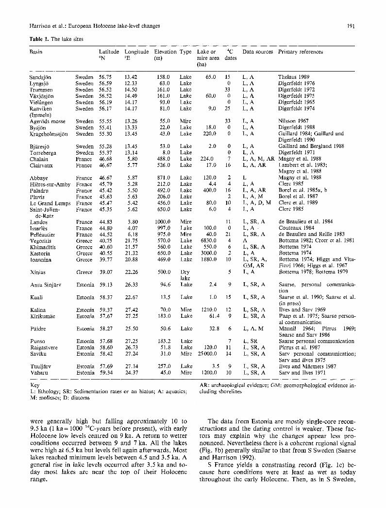
Table 1. The lake sites

191

Basin Latitude Longitude Elevation Type Lake or 14C °N °E (m) mire area dates

(ha)

Data sources Primary references

Sandsj6n Sweden 56.75 13.42 158.0 Lake 65.0 15 L, A Lyngsj6 Sweden 56.59 12.33 63.0 Lake 0 L, A Trummen Sweden 56.52 14.50 161.0 Lake 33 L, A Vfixj6sjOn Sweden 56.52 14.49 161.0 Lake 60.0 0 L, A Vielgngen Sweden 56.19 14.17 93.0 Lake 0 L, A Ranviken Sweden 56.17 14.17 81.0 Lake 9.0 25 L, A (Immeln) AgerOds mosse Sweden 55.55 13.26 55.0 Mire 33 L, A Bysj0n Sweden 55.41 13.33 22.0 Lake 18.0 0 L, A Krageholmssj0n Sweden 55.30 13.45 43.0 Lake 220.0 0 L, A

Bj~iresj6 Sweden 55.28 13.45 53.0 Lake 2.0 0 L, A Torreberga Sweden 55.37 13.14 8.0 Lake 0 L, A Chalain France 46.68 5.80 488.0 Lake 224.0 7 L, A, M, AR Clairvaux France 46.67 5.77 526.0 Lake 17.0 16 L, A, AR

Abbaye France 46.67 5.87 871.0 Lake 120.0 2 L HiOres-sur-Amby France 45.79 5.28 212.0 Lake 4.4 4 L, A Paladru France 45.42 5.50 492.0 Lake 400.0 16 L, A, AR Pluvis France 45.63 5.63 206.0 Lake 2 L, A, M Le Grand Lemps France 45.47 5.42 456.0 Lake 80.0 10 L, A, D, M Saint-Julien. France 45.35 5.62 650.0 Lake 6.0 4 L, A

de-Ratz Landos France 44.83 3.80 1000.0 Mire 11 L, SR, A Issarl~s France 44.80 4.07 997.0 Lake 100.0 0 L, A Pell6autier France 44.52 6.18 975.0 Mire 40.0 21 L, SR, A Vegoritis Greece 40.75 21.75 570.0 Lake 6830.0 4 A Khimaditis Greece 40.60 21.57 560.0 Lake 550.0 6 L, SR, A Kastoria Greece 40.55 21.32 650.0 Lake 3000.0 2 L, A Ioannina Greece 39.77 20.88 469.0 Lake 1880.0 10 L, SR, A,

GM, AR Xinias Greece 39.07 22.26 500.0 Dry 5 L, A

lake Antu Sinj~trv Estonia 59.13 26.33 94.6 Lake 2.4 9 L, SR, A

Kaali Estonia 58.37 22.67 13.5 Lake 1.0 15 L, SR, A

Kalina Estonia 59.37 27.42 70.0 Mire 1210.0 12 L, SR, A Kirikum~te Estonia 57.67 27.25 183.0 Lake 61.4 9 L, SR, A

P~tidre Estonia 58.27 25.50 50.6 Lake 32.8 6 L, A, M

Punso Estonia 57.68 27.25 183.2 Lake 7 L, SR Raigastvere Estonia 58.60 26.73 51.8 Lake 120.0 11 L, SR, A Saviku Estonia 58.42 27.24 31.0 Mire 25000.0 14 L, SR, A

Tuulj~trv Estonia 57.69 27.14 257.0 Lake 3.5 9 L, SR, A Vaharu Estonia 59.34 24.37 45.0 Mire 1200.0 10 L, SR, A

Thelaus 1989 Digerfeldt 1976 Digerfeldt 1972 Digerfeldt 1975 Digerfeldt 1965 Digerfeldt 1974

Nilsson 1967 Digerfeldt 1988 Gaillard 1984; Gaillard and Digerfeldt 1990 Galliard and Berglund 1988 Digerfeldt 1971 Magny et al. 1988 Lambert et al. 1983; Magny et al. 1988 Magny et al. 1988 Clerc 1985 Borel et al. 1985a, b Borel et al. 1987 Clerc et al. 1989 Clerc 1985

de Beaulieu et al. 1984 Couteaux 1984 de Beaulieu and Reille 1983 Bottema 1982; Creer et al. 1981 Bottema 1974 Bottema 1974 Bottema 1974; Higgs and Vita- Finzi 1966; Higgs et al. 1967 Bottema 1978; Bottema 1979

Saarse, personal communica- tion Saarse et al. 1990; Saarse et al. (in press) Ilves and Sarv 1969 Paap et al. 1975; Saarse person- al communication M/annil 1964; Pirrus 1969; Saarse and Sarv 1986 Saarse personal communication Pirrus et al. 1987 Sarv personal communication; Sarv and Ilves 1975 Ilves and M~temets 1987 Sarv and Ilves 1971

Key L: lithology; SR: Sedimentation rates or an hiatus; A: aquatics; M: molluscs; D: diatoms

AR: archaeological evidence; GM: geomorphological evidence in- cluding shorelines

were generally high but fall ing approximate ly 10 to 9.5 ka (1 ka = 1000 ~4C-years before present), with early Holocene low levels centred on 9 ka. A re turn to wetter condi t ions occurred between 9 and 7 ka. All the lakes were high at 6.5 ka bu t levels fell again afterwards. Most lakes reached m i n i m u m levels between 4.5 and 3.5 ka. A general rise in lake levels occurred after 3.5 ka and to- day most lakes are near the top of their Holocene range.

The data f rom Estonia are most ly single-core recon- structions and the dating control is weaker. These fac- tors may explain why the changes appear less pro- nounced . Nevertheless there is a coherent regional signal (Fig. lb ) generally similar to that f rom S Sweden (Saarse and Har r i son 1992).

S France yields a constras t ing record (Fig. lc) be- cause here condi t ions were at least as wet as today th roughou t the early HOlocene. Then, as in S Sweden,

100%

80%

60%

40%

20%

0%

b

100%

80%

60%

40%

20%

0%

Harrison et al.: European Holocene lake-level changes

Estonia

C

0 0.5 1 1.5 2 2.5 3 3.5 4 4.5 5 5.5 6 6.5 7 7.5 8 8.5 9 9.5 10

southern Sweden

Time (yr BP)

southern France

100%

80%

d

100%

80%

Greece

0 0.5 1 1.5 2 2.5 3 3.5 4 4.5 5 5.5 6 6.5 7 7.5 8 8.5 9 9.5 10

Time (yr BP)

192

a

60%

40%

20%

0%

%low

0 0.5 1 1.5 2 2.5 3 3.5 4 4.5 5 5.5 6 6.5 7 7.5 8 8.5 9 9.5 10

Time (yr BP)

%int ~i~ %high

60%

40%

20%

0%

0 0.5 1 1.5 2 2.5 3 3.5 4 4.5 5 5.5 6 6.5 7 7.5 8 8.5 9 9.5 10

Time (yr BP)

Fig. 1 a-d. Holocene lake-level changes in a S Sweden; b Estonia; e S France and d Greece

conditions became dried after about 6.5 ka and most lakes had a low stand between 4.5 and 3.5 ka, followed by a general rise in level after 3.5 ka.

The records from Greece (Fig. ld) show yet another pattern with a gradual increase in lake levels throughout the early Holocene to a maximum with all the lakes high between 7.5 and 5.5 ka, then rapid drying at 5 ka. There was a brief return to somewhat wetter conditions be- tween 4 and 3 ka, after which the lakes fell to their pres- ent, generally low, levels.

The contrasts beween regions as shown in Fig. 1 can be summarized as lake-level "anomalies" (differences from present) at the 3000-year intervals adopted by COHMAP Members (1988). At 9 ka, lake levels were lower than present in the north but higher than present in the south. At 6 ka, lake levels were similar to or high- er than present in the north and in S France and much higher than present in Greece. At 3 ka, lake levels were similar to or lower than present in the north and in S France, but remained higher than present in Greece.

The water-balance model

The model simulates the seasonal course of land-surface evapotranspiration and soil moisture that is consistent

with supplied long-term monthly average climate data for a given orbital configuration and latitude. The in- stantaneous (actual) evapotranspiration is taken to be the lesser of a supply function proportional to soil mois- ture (Federer 1982) and a demand function set to equal the "equilibrium evapotranspiration", a function of net radiation and temperature (Jarvis and MacNaughton 1986). Net radiation is obtained as a semi-empirical function of insolation, cloudiness and temperature and varies sinusoidally during the day, allowing daily actual and potential evapotranspiration to be obtained by inte- gration (Prentice et al. 1991a, b).

Cloudiness is indexed by sunshine hours, expressed as a proportion of the maximum possible sunshine hours for any given latitude and month. The input data to the model are thus monthly values of total precipitation ZPi (ram), temperature Ti (°C) and proportional sunshine hours hi; latitude ;.; and orbital parameters. The orbital parameters are eccentricity e, obliquity e, and a phase angle ep that indicates the timing of perihelion relative to the equinoxes (Kutzbach and Gallimore 1988).

The basic model timestep is one month. The change in soil moisture during each month is calculated on a daily timestep:

f2i. k = min { [O;. k- 1 Jr- (Pi-El. k)], ~'2max} (1)

Harrison et al.: European Holocene lake-level changes 193

where (2~,k and E~,k are the soil moisture and actual evapotranspiration on day k, month i, (2max is the soil water-holding capacity (150 mm) and P; is the monthly mean precipitation rate given by

P~ = EPJlength; (2)

where lengthi is the length of the month in a year of 365 days. Soil moisture is initialized to g2max and the proce- dure is iterated until January 1 soil moisture is constant, allowing an equilibrium to be established between soil moisture and evapotranspiration. If soil moisture re- turns to saturation on January 1 then one iteration is sufficient.

Daily actual evapotranspiration is given in mm by

E~,e=F,,k(R~JL) [sJ(s,+ y)] (3)

where L is the latent heat of vaporization of water (2.5* 106 J kg-1), si is the slope of the relationship be- tween the saturation vapour pressure of water and tem- perature (evaluated at the mean monthly temperature) obtained by differentiating the expression in Murray (1967):

si = 2.503 * 1 0 6 exp [17.269 7"//(237.3 + Ti)]/ (237.3 + Ti) 2 Pa K -1 (4)

is the psychrometer constant (65 Pa K - l ) , R,; is the daily integral of effective (i.e. positive) net radiation R~ evaluated at the mid-month, and Fe, k is the ratio of ac- tual to potential evapotranspiration for the day. Net ra- diation at time h (in radians from solar noon) is given by:

R~ =R~-Rt (5)

The net downward shortwave component R~ in Eq. (5) is approximated as a function of insolation q~g, sun- shine hours ni and a standard surface reflectance o~ (0.17):

Rs = (0.23 + 0.5ni) (1 - c~) q~i (6)

as in Linacre (1986). Insolation is calculated from celes- tial longitude (4~e) and orbital parameters (Kutzbach and Gallimore 1988):

~i : ~0 (ELF*) - 2 (sin~ sin fi + cos 2 cos ~ cos h) (7)

r/r* = 1 + e sin (4~i - ~bp) (8)

= e sin ~i (9)

where ~bo is the solar constant (1360 W m -2). The value of 4~ used to calculate each month's insolation corre- sponds to the mid-month value under present orbital conditions (Kutzbach and Gallimore 1988). The net up- ward longwave component R1 in Eq. (5) is approximated as a function of sunshine hours n,- and temperature 7"-:

Rt= (0.2+ 0.8n3 (107 - 7,-) W m -z (10)

as in Linacre (1986). The total daily effective net radia- tion is then

Rni = (86400/~r)(uho + v sinho) (11)

where

u =fiO~o(r/r*)-2 sin2 s i n 0 - R t (12)

v =J~o(r/r*) -2 cos2 cos0 (13)

f i being the coefficient of ~b~ in Eq. (6), and

ho = cos - 1 ( _ u/v) (14)

i.e. the time of day when Rn equals zero. Soil moisture supply may become limiting during a part of the day when Rn exceeds the critical value given by:

Si, k = Cwi (~'2i, k/ff~rnax) ( 1 5 )

where Cwi is the net radiation corresponding to an evap- otranspiration rate of 1 mm h -a at temperature Ti (Fed- erer 1982). F,.,~ is obtaind by accounting for the "unused" net radiation in excess of Si, k:

Fi, k = l - [ ( u - S i , k)hl+vsinhl]/[uho+vsinho] (16)

with

h I = COS - 1 [(Si, k - u ) / v ] ( 1 7 )

i.e. the time of day when R, = S~,k. In the calculation of ho and hi, arguments of cos- 1 lying outside the interval ( - 1 , 1) are set to - 1 or 1 as appropriate. These cases arise e.g. when net radiation is always negative, or soil moisture supply is non-limiting.

The outputs of the model are monthly totals of actual evapotranspiration (E) and potential evapotranspiration (PE) which are summed to give annual values. PE is de- fined as the total evaporative demand, i.e. the value of E that would result if soil moisture supply was never limiting.

Model sensitivity experiments

The model was used to evaluate the possible effects of different climate forcings on regional water budgets in different parts of Europe at 9, 6 and 3 ka. We consid- ered the direct effects of changes in orbital parameters, temperature and cloudiness on total annual potential evapotranspiration (PE) and runoff (P-E). Because changing orbital parameters also changes the lengths of the months, we also allowed for the effect of this change on the total annual precipitation (P) if the daily precipi- tation rate for each month is assumed to stay constant.

Baseline climate data were derived from the 0.5 ° grid- ded data set of Leemans and Cramer (1991) for refer- ence points located centrally in each of the four data re- gions: 56°N 13.5°E (S Sweden), 58°N 27°E (Estonia), 45.5°N 5°E (S France) and 40°N 21.5°E (Greece). We carried out a series of experiments varying orbital pa- rameters alone, orbital parameters plus temperature, or- bital parameters plus sunshine, and orbital parameters plus temperature and sunshine. Two sunshine scenarios were used as alternatives corresponding to different as- sumptions about the latitudinal temperature gradient at 9 ka and 6 ka (Table 3). Apart from the small effect of orbitally induced changes in the length of the months on the total annual precipitation, no precipitation changes were considered in these experiments. Although precipi- tation changes can be reconstructed from the pollen re-

194

cord, the sensitivity of vegetation to precipitation in the more humid regions of Europe is slight (Huntley and Prentice 1992) and confidence intervals on annual preci- pitation derived by the analog method can be as wide as 200 m m if no additional constraint is imposed (Guiot et al. submitted). For this reason our strategy was first to establish the possible effects of factors other than preci- pitation.

Orbital changes

At 9 ka perihelion was in N-hemisphere summer (rather than in N-hemisphere winter as it is today) and the tilt was near its maximum (Berger 1978). The combined ef- fects of the precession and tilt difference affected the seasonal and latitudinal distribution of insolation. N- hemisphere summer insolation was about 8% greater than today and because of the high tilt this anomaly was greatest at high latitudes. N-hemisphere winter insola- tion was correspondingly less, but this difference was larger in the mid-latitudes than in the high latitudes where winters are always dark.

The Earth 's orbital speed is greatest when near peri- helion. Thus, summer perihelion also implies a longer period between the autumnal and vernal equinoxes (the climatological winter) and a correspondingly shorter cli- matological summer, which can be expressed, for mod- elling purposes, as longer winter months and shorter summer months. The overall effects of the 9 ka orbital anomaly were therefore: high summer insolation (espe- cially at high latitudes) during a shorter summer, low winter insolation (especially at lower latitudes) during a longer winter, a reduced latitudinal gradient of insola- tion in both seasons, and a high seasonal insolation con- trast at all latitudes. These anomalies gradually decayed during the Holocene as the tilt decreased and perihelion shifted through autumn to winter.

Orbital parameters for 3, 6 and 9 ka were calculated for 3000, 7000 and 10500 astronomical years ago fol- lowing the U / T h calibration of the 14C time scale (Berg- er 1978; Bard et al. 1990). Lengths of each month under each orbital configuration were calculated by a proce-

Harrison et al.: European Holocene lake-level changes

dure similar to that of Kutzbach and Gallimore (1988). In experiment series L (for "length") the altered lengths of months were input to the model for each region, keeping each month ' s mean temperature, precipitation rate and cloudiness as present. Thus, experiment L pro- vides a way to assess the effects of our underlying as- sumption that (irrespective of other changes) the dura- tions of each month ' s climate would shift in step with the changes in the durations of each "celestial" month, defined as a range of celestial longitudes rather than as a fixed period of days (Berger 1978). In experiment O (for "orbital") the insolation too was altered, giving the full effect of the changes in orbital parameters.

Temperature

Fossil pollen data were taken f rom the data base com- piled by B. Huntley (Huntley and Birks 1983). These data are proport ional pollen counts of major taxa in samples of lake or mire sediment for about 400 sites, in the region between 40 ° and 75°N and 10°W to 45°E, and covering part or all of the time since 13 ka. Sixty- five per cent of the sites are 14C-dated. The rest were dated by pollen-correlation with nearby 14C-dated sites, or by comparison with 14C-dated regional pollen strati- graphies. The surface pollen-sample data base includes samples f rom a larger region (Huntley et al. 1989; Guiot 1990) to include a wider range of modern analogs for past climates.

Fossil pollen data for 3, 6 and 9 ka were interpolated to the reference points and compared with the surface sample data base using the method of Guiot (1990; 1991; Guiot et al. submitted) to reconstruct mean monthly temperatures. This method is based on locating the clo- sest modern analogs of each fossil pollen spectrum in a large set of surface samples using the chord distance measure to indicate degree of analogy. The distance measure is modified by taxon weightings derived f rom a multivariate analysis of the fossil pollen data set. Greater weight is given to those taxa that show strong spatio-temporal coherence and that, therefore, are likely to be good indicators of climatic (as opposed to local

Table 2. Pollen-based reconstructions of mean monthly temperature anomalies

Jan Feb Mar Apr May June July Aug Sept Oct Nov Dec

S Sweden 9 ka 0.1 0.2 0.2 0.1 -0.4 -1.5 -1.8 -1.4 -0.8 -0.3 0.1 0.0 6 ka -2.4 -2.1 - 1.6 -0.3 0.4 0.0 -0.3 -0.4 0.5 -0.8 - 1.2 -2.0 3 ka 0.9 1.0 0.7 0.0 -0.9 - 1.6 -2.3 -2.0 - 1.2 0.4 0.1 0.4

Estonia 9 ka -0.4 -1.0 -2.3 -4.6 -5.9 -5.3 -4.7 -4.7 -4.1 -3.6 -2.5 -1.3 6 ka 0.4 0.5 0.6 0.9 0.9 1.2 1.2 1.2 1.2 1.0 0.8 0.5 3 ka 1.2 1.2 1.3 1.4 1.2 1.4 1.2 1.4 1.4 1.4 1.3 1.1

S France 9 ka 3.7 3.2 2.5 2.0 1.8 1.0 0.5 0.3 1.0 1.9 2.8 3.5 6 ka -2.9 -3.3 -3.1 -1.1 0.3 -0.2 -1.2 -1.4 -1.4 -1.4 -1.4 -1.9 3 ka -2.4 -2.8 -3.1 -3.2 -2.9 -3.1 -3.6 -3.6 -3.2 -3.0 -2.8 -2.9

Greece 9 ka - 1.0 -0.8 -0.7 0.6 1.2 1.5 1.6 1.8 1.1 0.6 0.6 0.0 6 ka -0.2 -0.3 -0.3 -0.3 -0.3 -0.2 -0.3 -0.3 -0.2 -0.3 -0.2 -0.1 3 ka -1.0 -0.7 -0.7 -0.2 0.0 0.0 0.0 0.0 0.0 -0.3 -0.3 -0.6

Harrison etal.: European Holocene lake-level changes 195

environmental) change. Table 2 gives these results as anomalies, i.e. differences from the modern (baseline) climate. In experiment series OT, designed to show the effects of orbital variations (O) plus temperature (T), the orbital parameters were changed as appropriate and the reconstructed temperatures were supplied to the model in place of the baseline temperatures.

Cloudiness

The latitudes of the sub-tropical anticyclone belts (STA) in both hemispheres show seasonal migrations related to the equator-to-pole temperature gradient in each hemis- phere:

cot STAi = 0.0245 6Ti + 0.7245 (18)

where STAi is the latitude of the STA in month i and fiTi is the equator-to-pole temperature gradient for the pre- vious month (Korff and Flohn 1969). Tropical sea-sur- face temperatures (SSTs) were little different from today during the early and mid-Holocene (see e.g. Ruddiman, in Webb 1985) while reconstructions from the Green- land, Iceland and Norwegian Seas suggest that SSTs there were about 4°C greater than today (Koc Karpuz and Schrader 1990; Veum etal. submitted; Janssen, per- sonal communication) as a consequence of the greater than present total annual insolation received at those la- titudes. The change in SST may have been even larger nearer the pole because of the thermal feedback effect of reduced sea-ice in the Arctic (Kutzbach and Galli- more 1988). We hypothesized that the equator-to-pole temperature gradient at 9 and 6 ka was reduced by either 4 ° or 6°C throughout the year and applied Korff and Flohn's relationship to estimate a corresponding pole- ward shift of the mean position of the STA in each month. The resulting poleward shift varies through the year from 1.7 ° in January to 2.7 ° in July for a 4 ° C gra- dient reduction, or 2.5 ° to 4.1 ° for a 6°C reduction. These estimates are conservative compared with the cor- responding shifts calculated for 6 ka and 9 ka insolation conditions by GCM experiments (Kutzbach and Guetter 1986; Harrison et al. 1992).

Sunshine data for Europe show a strong latitudinal gradient in all seasons. The sunshine belts shift in phase with the seasonal migrations of the STA, with a maxi- mum at approximately the latitude of the STA. We used these observations to derive latitudinal anomalies for each month, corresponding to our estimates of past changes in the latitude of the STA. The relationship

i n n i = ai + bi,~ (19)

was found by inspection of scatterplots to be an appro- priate description of the zonal pattern in sunshine data for Europe west of 30°E (Leemans and Cramer 1991). The constants ai and be were estimated for each month i by linear regression, with correlation coefficients (r) ranging from -0 .58 (April) to -0 .85 (October). These constants were then used to calculate the latitude (Ls3 at which sunshine equals 1 - 1 / e (= 63o7o) of total sunshine

hours in each month. This latitude was used to fit a sec- ond linear regression,

Ls i= - 13.9 + 1.4 STAi (20)

with r= 0.81. To apply this regression in the past we as- sumed that the b~ would not change but that the ai, re- flecting the latitudinal positions of the sunshine belts, would shift the same distance poleward as the STA. These assumptions lead to an expression for the ratio of past and present monthly sunshine:

n~/ni = exp [ - 1.4 b~(STA~-STAi)] (21)

where the primes denote past values. January and July values of these ratios were 1.14 for a 4°C reduction in the latitudinal temperature gradient, and 1.22 for a 6°C reduction. These ratios were used to modify present-day sunshine data in experiment series OS4, OS6, OTS4 and OTS6 where O denotes that orbital parameters were changed, T denotes that temperatures were changed, S denotes that cloudiness (sunshine) was changed, and the numerals refer to a 4°C or 6°C change in the tempera- ture gradient.

Model results (Table 3, Fig. 2)

The main effect of lengthening the winter months (L) was to decrease PE and increase runoff everywhere. Higher midsummer insolation (O) more than compen- sated for the decrease in PE; all regions experienced a small increase in annual PE. However, even with this in- crease in PE, the net effect of the orbital changes was to increase runoff. This counterintuitive result arose be- cause of the seasonality of the orbitally induced change in PE. In climates where soils are saturated in winter but not in summer, decreasing PE during winter has a greater effect on runoff than increasing PE by the same amount during summer because evapotranspiration rep- resents only a fraction of PE when the soil is dry. This effect was greatest at 9 ka and declined towards the present.

The additional effects of temperature (OT) were con- sistent with the expectation that increasing either winter or summer temperature should both increase PE and re- duce runoff. For example, cool summers in N Europe at 9 ka enhanced the orbitally induced increase in runoff, while warm winters at 9 ka in S France lessened the in- crease. The temperature effects were strongest where the largest temperature anomalies were applied, and were generally similar in magnitude to the orbital effects with a sensitivity to annual mean temperature on the order of - 4 to - 8 m m ° C - ' .

Simulated cloudiness effects (OS4, OS6, OTS4, OTS6) were again of a similar magnitude. Cross-com- parisons of the results obtained for the 4°C and 6°C scenarios, with and without temperature effects, for 6 ka and 9 ka show that the different effects were more or less additive. The approximate sensitivity of simu- lated runoff to the zonal temperature gradient according to these experiments ranges from approximately 1 mm o C - ' in N Europe to > 2 mm ° C - ' in Greece. In

196 Harrison et al.: European Holocene lake-level changes

Table 3. Results of sensitivity analyses (mm) for annual values of precipitation (P), potential evapotranspiration (PE) and runoff (P-E)

P PE P-E

Modern control S Sweden 687 533 159 Estonia 581 485 116 S France 924 721 230 Greece 876 891 206

Experiment L (lengths of climatic seasons changed; insolation as present)

S Sweden 9 ka 683 511 172 6 ka 682 519 165 3 ka 684 531 160

Estonia 9 ka 576 462 126 6 ka 575 470 121 3 ka 578 482 117

S France 9 ka 924 696 246 6 ka 922 704 239 3 ka 923 718 233

Greece 9 ka 885 863 222 6 ka 882 871 216 3 ka 877 887 209

Experiment O changed)

S Sweden

Estonia

S France

Greece

(lengths of climatic seasons and insolation

9 ka 683 543 168 6 ka 682 541 161 3.ka 684 536 158 9 ka 576 496 124 6 ka 575 494 118 3 ka 578 488 115 9 ka 924 729 250 6 ka 922 727 242 3 ka 923 723 233 9 ka 885 898 235 6 ka 882 897 225 3 ka 877 893 212

Experiment OT (orbital parameters and temperature changed)

S Sweden 9 ka 683 531 170 6 ka 682 536 165 3 ka 684 528 161

Estonia 9 ka 576 432 143 6 ka 575 508 115 3 ka 578 506 110

S France 9 ka 924 756 237 6 ka 922 705 257 3 ka 923 664 265

Greece 9 ka 885 917 236 6 ka 882 891 227 3 ka 877 889 216

Experiment OS4 (orbital parameters 4°C reduction in temperature gradient)

and sunshine hours changed:

S Sweden 9 ka 683 565 162 6 ka 682 563 155

Estonia 9 ka 576 517 121 6 ka 575 515 115

S France 9 ka 924 763 243 6 ka 922 761 234

Greece 9 ka 885 947 226 6 ka 882 945 217

Table 3. (continued)

Experiment OTS4 (orbital parameters, temperature and sunshine hours changed: 4 ° C reduction in temperature gradient)

S Sweden 9 ka 683 552 164 6 ka 682 558 159

Estonia 9 ka 576 451 135 6 ka 575 529 112

S France 9 ka 924 791 230 6 ka 922 738 248

Greece 9 ka 885 967 227 6 ka 882 939 218

Experiment OS6 (orbital parameters and sunshine hours changed: 6°C reduction in temperature gradient)

S Sweden 9 ka 683 578 159 6 ka 682 576 152

Estonia 9 ka 576 529 118 6 ka 575 527 112

S France 9 ka 924 782 239 6 ka 922 780 230

Greece 9 ka 885 975 220 6 ka 882 973 211

Experiment OTS6 (orbital parameters, temperature and sunshine hours changed: 6 ° C reduction in temperature gradient)

S Sweden 9 ka 683 565 160 6 ka 682 570 156

Estonia 9 ka 576 561 131 6 ka 575 542 109

S France 9 ka 924 811 225 6 ka 922 756 243

Greece 9 ka 885 995 222 6 ka 882 967 213

N Europe the effect of the cloudiness changes over- whelms the other effects at 6 ka so that the combined scenarios have a little less runo f f than present, bu t this is not so at 9 ka when the orbi tal effects were stronger and temperatures low.

Discussion and conclusions

The sensitivity experiments reported here provide a quant i f ica t ion of the evaporat ive effects of changes in insolat ion, temperature and cloudiness on catchment ru- no f f in different regions of Europe. For plausible Holo- cene scenarios, these three factors produced effects of similar magni tude , producing small negative or positive net changes in annua l runof f . In all the regions investi- gated, the early Holocene insola t ion anomaly produced greater than present annua l PE but also greater than present runof f , due to the non- l inear in teract ion of soil mois ture and PE.

The magni tude of the individual and combined ef- fects of these changes is small; these effects could easily be overwhelmed by minor changes in precipi ta t ion re- gime, corresponding to spatial shifts of a few tens of kilometres in the present climate. The tempera ture and cloudiness changes would presumably not have occurred wi thout some associated changes in precipi ta t ion pat-

Harrison et al.: European Holocene lake-level changes

35

3O

25

~° t E 1 5 -

io

5

< 0

-10

3 5

30

25

E 20 >-.

N 5

-5

-10

0TS4

197

d 3 5

O 3O

25 E E

20 >-.

~ 15

5

.sj -10

35-

30

25 E

-.&E 2o

E 15

10 z

5

0

-5

-10

0S6

m • --m i J

35 q

30

25 E E

20 o s '15 o

o t ~ 10

~ 5

-5

-10

35

30

25 E E

20 >.,

~ 5

N 0

-5

-10

OT 35

OTS6

,! ~ . 25

N 5

- - "< 0

-5

4 0

3ka 6ka 9ka 3ka 6ka 9ka 3ka 6ka 9ka 3ka 6ka 9ka Estonia Sweden France Greece

OS4

, . . j j 3ka 6ka 9ka 3ka 6ka 9ka 3ka 6ka 9ka 3ka 6ka 9ka

Estonia Sweden France Greece

Fig. 2. Changes in annual runoff obtained in model experiments (see Table 3 for definitions). Note that experiments involving changing cloudiness (S) were carried out for 9 ka and 6 ka only

198 Harrison et al.: European Holocene lake-level changes

terns. The small numbers involved suggest that, in such cases, the direct effects of adding or subtracting precipi- tation, especially winter precipitation, would have been decisive.

Furthermore, the experiments show that evaporative effects on runoff can explain very little of the patterns shown by the lake-level data. Table 4 compares simu- lated runoff anomalies with regional water-balance ano- malies inferred f rom the lake-level data. Although the direct effects of the orbital changes on runoff are in the right direction to have contributed to the appearance of wetter conditions in S Europe at 9 ka, these changes do not explain why lake levels in Greece became still higher after 9 ka. In N Europe, the direct effects of the orbital changes are in the wrong direction to explain the appear- ance of drier than present conditions at 9 ka. A small net reduction in runoff was produced by adding the cloudiness effect of a poleward-shifted STA at 6 ka, but this effect is not strong enough to overwhelm the oppos- ing effects at 9 ka; whereas the lakes were high at 6 ka, low at 9 ka. The experiments similarly give no clue as to

T a b l e 4. Changes in annual runoff (mm) obtained in model exper- iments (see Table 3 for definitions), compared with regional wa- ter-balance anomalies implied by the lake-level record. The ob- served anomalies are indicated qualitatively on a scale from - - (much lower than present) to + + (much higher than present)

S Sweden Estonia S France Greece

9 ka

Lake data: - -

M o d e l experiments:

L +13 O + 9 OT + 11

OS4 + 3 OTS4 + 5

OS6 0 OTS6 + 1

6 ka

Lake data: 0

Model experiments:

L + 6 O + 2 OT + 6

OS4 - 4

OTS4 0

OS6 - 7 OTS6 - 3

3 ka

Lake data:

Model experiments:

L + I O - 1 OT + 2

+ +

+10 +16 +16 + 8 +20 +29 +27 + 7 +30

+ 5 +13 +20 +19 0 +11

+ 2 + 9 +14 +15 - 5 +16

(+) 0 + +

+ 5 + 9 +10 + 2 +12 +19 - 1 +22 +21

- 1 + 4 +11 4 + 18 + 12

- 4 0 + 5 - 7 +13 + 7

0 - +

+ 1 + 3 + 3 - 1 + 3 + 6 - 6 +35 +10

the cause of the changes in water-balance between 6 ka and 3 ka, or 3 ka and present. Thus, the records cannot be explained to any plausible degree without invoking Holocene changes in the distribution of precipitation across Europe. A similar conclusion was reached by

H a s t e n r a t h and Kutzbach (1983) concerning Holocene lake-level changes in east Africa, which are now general- ly explained as consequences of orbitally induced changes in the strength and extent of the monsoons.

Hypotheses have been put forward that might ac- count for some changes in the distribution of prec!pita- tion across Europe. For example, a poleward-shifted STA would not only have reduced cloudiness but would also be expected to have reduced precipitation in N Eu- rope (Harrison and Digerfeldt submitted), explaining low lake levels in N Europe at 9 ka. GCM experiments (Kutzbach and Guetter 1986) suggest that both the strength and the position of the STA changed during the Holocene. The July STA was shifted as much as 10 ° northward in the GCM experiments for 9ka , due to a synergistic downstream effect of the residual Laurentide ice sheet (Harrison et al. 1992). This shift produced net offshore winds f rom Europe at 50°N. By 6 ka, with the ice sheet gone and the insolation anomaly less, the simu- lated July STA was only slightly north of its present po- sition while remaining stronger than at present, produc- ing strong onshore winds at 50°N. These circulation shifts are in the right direction to produce dry conditions in N Europe at 9 ka, giving way to wet conditions at 6 ka (Harrison and Digerfeldt submitted; Huntley and Prentice 1992).

The sustained Holocene drying trend shown by the records f rom S Europe could conceivably be a conse- quence of orbital changes, but the climatological mecha- nism is unknown: GCM experiments for 9 ka and 6 ka consistently show less than present runoff for grid cells around the Mediterranean, contrary to the palaeoeco- logical and lake-level evidence (Harrison and Digerfeldt submitted; Huntley and Prentice 1992). Possible expla- nations for the discrepancy invoke atmospheric circula- tion features associated with the Mediterranean (Hunt- ley and Prentice 1992) which are not resolved by GCMs. No insolation-based mechanism seems able to explain the dry phase centred on 4 ka that appears in the records both f rom S Sweden and S France, nor the brief wet phase centred on 3 ka in the records f rom Greece. Such phenomena suggest the involvement of forcings not con- sidered in the GCM experiments, for example associated with ocean circulation changes. A more complete under- standing of the Holocene climatic history of Europe may emerge f rom a more detailed analysis of the rela- tionship between large-scale circulation features and specific regional climates, and a comparison of the land records with high-resolution palaeotemperature records f rom the adjacent North Atlantic.

Acknowledgements. This research was provoked by discussions with Pat Bartlein. It was supported by the Swedish Natural Science Research Council (NFR) and the Royal Swedish Academy of Sciences. Collaboration was facilitated by a grant from the Mission des Relations Internationales du CNRS. We thank Brian Huntley for supplying the p611en data set and Pat Bartlein, Steve

Harrison et al.: European Holocene lake-level changes 199

Hostetler and Tom Webb for helpful comments on the manu- script.

References

Adams LJ (1987) Ein Wasser- und Energiebilanz~Modell von ab- flusslosen Seen und seine Anwendung in der Pal~oklimatologie yon Nordwest-Afrika. Ber Inst Meteorol Klimatol Universit~t Hannover, 29, IV

Adams L J, Tetzlaff G (1985) The extension of Lake Chad at about 18000 years BP. Z Gletscher Glazialgeol 21 : 115-123

Bard E, Hamelin B, Fairbanks RG, Zindler A (1990) Calibration of the I4C timescale over the past 30000 years using mass spec- trometric U-Th ages from Barbados corals. Nature 345:405- 410

Benson LV (1981) Paleoclimatic significance of lake-level fluctua- tions in the Lahontan Basin. Quat Res 16:390-403

Berger AL (1978) Long-term variations of daily insolation and Quaternary climatic changes. J Atmos Sci 35:2362-2367

Borel JL, Brochier JL, Lundstrom-Baudais K (1985a) Water level fluctuations of the lake Paladru (Is~re, France) in the Xth and XIth centuries AD. Ecol Medit 11 : 179-183

Borel JL, Brochier JL, Lundstrom-Baudais K (1985b) Une expe- rience de recherche concert6e sur le pal6oenvironnement de l'habitat m6di6val immerg6 de Colleti~re (Charavines-Les- Bains, Isbre): s6dimentologie, pollens, macrorestes v6g6taux. Actes Journ6es, Palynol Arch6ol CNRS, pp 313-330

Borel JL, Damblon F, Montjuvent G, Mouthon J, Yates G (1987) Le lac de Pluvis (Bas-Bugey): pal6o6cologie et variations de niveau durant l'Holocbne d'apr~s le sondage 4. Trav Doc G6ogr Trop 59: 25. (R6sum6s des communications, Xe Sympo- sium, Associations des Palynologues de Langue Fran~aise, Bordeaux-Talence.) Cent Etudes G6ogr Trop, CNRS

Bottema S (1974) Late Quaternary vegetation history of northwes- tern Greece. Proefschrift, University of Groningen

Bottema S (1978) The Late Glacial in the eastern Mediterranean and the Near East. In: Brice WC (ed) Ur: the environmental history of the Near and Middle East since the last Ice Age. pp 15-28

Bottema S (1979) Pollen analytical investigations in Thessaly (Greece). Palaeohist 21 : 19-40

Bottema'S (1982) Palynological investigations in Greece with spe- cial reference to pollen as an indicator of human activity. Pal- aeohist 24: 257-289

Clerc J (1985) Premi6re contribution /t l'6tude de la v6g6tation Tardiglaciaire et Holoc~ne du Pi6mont Dauphinois. Doc Car- togr Ecol (Grenoble) 28:65-83

Clerc J, Magny M, Mouthon J (1989) Histoire d'un milieu la- custre du Bas-Dauphin6: Le Grand Lemps. Etude palynologi- que des remplissages Tardiglaciaires et Holoc~ne, et mise en 6vidence de fluctuations lacustres/~ l'aide d'analyses s6dimen- tologiques et malacologiques. Rev Pal6obiol (G6n6ve) 8 : 1-19

COHMAP Members (1988) Climatic changes of the last 18000 years: observations and model simulations. Science 241 : 1043- 1052

Couteaux M (1984) Recherches pollenanalytiques au lac d'Issarl~s (Ardbche, France): 6volution de la v6g6tation et fluctuations lacustres. Bull Soc Roy Bot Belg 117:197-217

Creer KM, Readman PW, Papamarinopoulos S (1981) Geomag- netic secular variations in Greece through the last 6000 years obtained from lake sediment studies. Geophys J R Astron Soc 66 : 193-219

de Beaulieu JL, Reille M (1983) Pal6oenvironnement tardiglaciaire et holoc~ne des lacs de Pell6autier et Siguret (Hautes-Alpes, France). Histoire de la v6g6tation d'apr~s les analyses pollini- ques. Ecol Medit'9: 19-36

de Beaulieu JL, Pons A, Reille M (1984) Recherches pollenanalti- ques sur l'histoire de la v6g6tation des Monts du Valey (Massif Central, France). Diss Bot 72:45-70

Digerfeldt G (1965) Vielfingen and Farlgmgen - an investigation of historical lake development [in Swedish]. Skgmes Natur 52:162-183

Digerfeldt G (1971) The Post-Glacial development of the ancient lake at Torreberga, Scania, South Sweden. Geol FOren Stock- holm F6rh 93:601-624

Digerfeldt G (1972) The Post-Glacial development of Lake Trum- men. Regional vegetation history, water-level changes and pal- aeolimnology. Folia Limnol Scand 16:1-96

Digerfeldt G (1974) The Post-Glacial development of the Ranvik- en Bay in Lake Immeln. I. The history of the regional vegeta- tion, and II. The water-level changes. Geol F6ren Stockholm F6rh 96 : 3-32

Digerfeldt G (1975) Post-Glacial water-level changes in Lake V~x- j6sjOn, central southern Sweden. Geol FOren Stockholm F6rh 97:167-173

Digerfeldt G (1976) A Pre-Boreal water-level change in Lake Lyngsj6, central Halland. Geol FOren Stockholm F6rh 98 : 329-336

Digerfeldt G (1986) Studies on past lake-level fluctuations. In: Berglund BE (ed) Handbook of Holocene Palaeoecology and palaeohydrology. John Wiley, Chichester, pp 127-143

Digerfeldt G (1988) Reconstruction and regional correlation of Holocene lake-level fluctuations in Lake Bysj6n, South Swed- en. Boreas 17:165-182

Federer CA (1982) Transpirational supply and demand: plant, soil, and atmospheric effects evaluated by simulation. Water Resour Res 18: 355-362

Gaillard M-J (1984) A palaeohydrological study of Krageholmss- jOn (Scania, South Sweden): regional vegetation history and water-level changes. Lundqua Rep 25 : 1-40

Gaillard M-J, Berglund BE (1988) Land-use history during the last 2700 years in the area of Bj~resj6, southern Sweden. In: Birks HH, Birks HJB, Kaland PE, Moe D (eds) The cultural land- scape - past, present and future. Cambridge University Press, Cambridge, pp 409-428

Gaillard M-J, Digerfeldt G (1990) Palaeohydrological studies and their contribution to palaeoecological and palaeoclimatic re- constructions. In: Berglund BE (ed) The cultural landscape during 6000 years in S Sweden. Ecol Bull (Copenhagen) 41

Guiot J (1990) Methodology of the last climatic cycle reconstruc- tion in France from pollen data. Palaeogeogr, Palaeoclim, Pal- aeoecol 80: 49-69

Guiot J (1991) Structural characteristics of proxy data and meth- ods for quantitative climate reconstruction. Pal~oklimaforsch 6: 271-284

Harrison SP (1987) Temperate lake levels as palaeoclimatic indica- tors: reconstructing the Late Quaternary climate of Europe. Lundqua Report (Lund University, Dept Quat Geol) 27:25- 26

Harrison SP (1988) Lake-level records from Canada and the east- ern USA. Lundqua Rep 29

Harrison SP (1989) Lake levels and climatic change in eastern North America. Clim Dyn 3 : 157-167

Harrison SP, Dodson J (1992) Climates of Australia and New Guinea since 18000 yr BP. In: Wright HE Jr, Kutzbach JE, Webb T I I I , Street-Perrott FA, Ruddiman WF, Bartlein PJ (eds) Global climates since the last Glacial Maximum. Univer- sity of Minnesota, Minneapolis (in press)

Harrison SP, Metcalfe SE (1985) Variations in lake levels during the Holocene in North America: an indicator of changes in at- mospheric circulation patterns. G6ogr Phys Quat 39 : 141-150

Harrison SP, Saarse L, Digerfeldt G (1991) Holocene changes in lake levels as climate proxydata in Europe. Pal~toklimaforsch 6:159-170

Harrison SP, Prentice IC, Bartlein PJ (1992) Influence of insola- tion and glaciation on atmospheric circulation in the North At- lantic sector: implications of general circulation model experi- ments for the late Quaternary climatology of Europe. Quat Sci Rev 11 : 283-299

200 Harrison et al.: European Holocene lake-level changes

Hastenrath S, Kutzbach JE (1983) Paleoclimatic estimates from water and energy budgets of East African lakes. Quat Res 19:141-153

Higgs ES, Vita-Finzi C (1966) The climate, environment and in- dustries of Stone Age Greece, Part II. Proc Prehist Soc 32: 1- 29

Higgs ES, Vita-Finzi C, Harris DR, Fagg AE (1967) The climate, environment and industries of Stone Age Greece, Part III. Proc Prehist Soc 33 : 1-29

Hostetler SW, Bartlein PJ (1990) Simulation of lake evaporation with application to modeling lake-level variations of Harney- Malheur, Oregon. Water Resour Res 26:2603-2612

Hostetler SW, Benson LV (1990) Paleoclimatic implications of the high stand of Lake Lahontan derived from models of evapora- tion and lake level. Clim Dyn 4:207-217

Huntley B, Birks HJB (1983) An atlas of past and present pollen maps for Europe 0-13000 years ago. Cambridge University Press, Cambridge

Huntley B, Prentice IC (1992) Holocene climate and vegetation of Europe. In: Wright HE Jr, Kutzbach JE, Webb T III, Street- Perrott FA, Ruddiman WF, Bartlein PJ (eds) Global climates since the last Glacial Maximum. University of Minnesota, Minneapolis (in press)

Huntley B, Bartlein P J, Prentice IC (1989) Climatic control of the distribution and abundance of beech (Fagus L.) in Europe and North America. J Biogeog 16:551-560

Ilves E, Sarv A (1969) Stratigraphy and chronology of the lacus- trine-mire deposits of mire Kalina. Proc Acad Sci, ESSR 4: 377-384

Ilves E, M~iemets H (1987) Results of radiocarbon and palynolog- ical analyses of coastal deposits of Lake Tuulj~trv and Vaskna. In: Raukas A, Saarse L (eds) Palaeohydrology of the temper- ate zone III. Mires and Lakes. Tallinn, Valgus, pp 108-130

Jarvis PG, MacNaughton KG (1986) Stomatal control of transpi- ration: scaling up from leaf to region. Adv Ecol Res 15:1-49

Koc Karpuz N, Schrader H (1990) Surface sediment distribution and Holocene paleotemperature variations in the Greenland, Iceland and Norwegian Sea. Paleoceanog 5:557-580

Korff HC, Flohn H (1969) Zusammenhang zwischen den Tempe- ratur-Gef~tllen ~quator-Pol und den planetarischen Luftdruck- gtirteln. Ann Meteorol NF 4:163-164

Kutzbach JE (1980) Estimates of past climate at Paleolake Chad, North Africa, based on a hydrological and energy-balance model. Quat Res 14:210-223

Kutzbach JE, Gallimore RG (1988) Sensitivity of a coupled atmo- sphere/mixed layer ocean model to changes in orbital forcing at 9000 years BP. J Geophys Res 93 : 803-821

Kutzbach JE, Guetter PJ (1986) The influence of changing orbital parameters and surface boundary conditions on climate simu- lations for the past 18000 years. J Atmos Sci 43 : 1726-1759

Kutzbach JE, Street-Perrott FA (1985) Milankovitch forcing of fluctuations in the level of tropical lakes from 18 to 0 kyr BP. Nature 317 : 130-134

Lambert G, Petrequin P, Richard H (1983) P6riodicit6 de l'habitat lacustre n6olithique et rythmes agricoles. L'Anthropologie (Paris) 87 : 393-411

Linacre ET (1986) Estimating the net-radiation flux. Agr Meteorol 5 : 49-63

Leemans R, Cramer W (1991) The IIASA climate database for mean monthly values of temperature, precipitation and cloudi- ness on a terrestrial grid. Int Inst Appl Syst Anal Res Rep RR- 91-18

Magny M, Richard H, Evin J (1988) Nouvelle contribution ~ l'his- toire holoc~ne des lacs du Jura frangais: recherches s6dimento- logiques et palynologiques sur les lacs de Chalain, de Clairvaux et de l'Abbaye. Rev Pal6obiol 7:11-23

M~innil R (1964) Distribution and stratigraphy of the carbona- ceous lacustrine deposits in Estonia. Doctoral Thesis. Tallinn, Institute of Geology (in Russian)

Murray FW (I 967) On the computation of saturation vapour pres- sure. J Appl Meteorol 6:203-204

Nilsson T (1967) Pollenanalytische Datierung mesolitischer Sied- lungen im Randgebiet des Ager6ds mosse im mittleren Schon- en. Acta Univ Lund II 16:1-80

Paap t], Saarse L, Ilomets Met al. (1975) Sediment rate, progno- sis and complex utilization of mire and lake deposits. Tallinn, Institute of Geology. Manuscript in the Archive of Estonian Academy of Sciences (in Russian)

Pirrus R (1969) Stratigraphic division of south Estonian late gla- cial deposits by means of pollen analyses. Proc Acad Sci ESSR. Chem Geol 18:181-190 (in Russian)

Pirrus R, R6uk A-M, Liiva A (1987) Geology and stratigraphy of reference site of Lake Raigastvere in Saadj~irv drumlin field. In: Raukas A and Saarse L (eds) Palaeohydrology of the tem- perate zone II. Lakes. Tallinn, Valgus, p 101-122

Prentice IC, Sykes MT, Cramer W (1992a) A simulation model for the transient effects of climate change on forest land- scapes. Ecol Model (in press)

Prentice IC, Cramer W, Harrison SP, Leemans R, Monserud RA, Solomon AM (1992b) A global biome model based on plant physiology and dominance, soil properties and climate. J Bio- geogr 19 : 117-134

Saarse L, Harrison SP (1992) Holocene lake-level changes in the eastern Baltic region. Eston Acad Sci, Spec Vol Int Geogr Union Cong (in press)

Saarse L, Sarv A (1986) Geology of the valley lakes on the Sakala Uplands. In: Studies of lake and mire formations in the pur- poses of palaeogeographic reconstructions. Abstr Tallinn, pp 106-108

Saarse L, Rajam~ie R, Heinsalu A, Vassiljev J (1990) Formation of the meteor crater lake Kaali (Island Saaremaa, Estonia). In: Pesonen L J, Niemisara H (eds) Symposium Fennoscandian impact structures. Abstr Espoo. p 55

Saarse L, Rajam~ie R, Heinsalu A, Vassiljev J (in press) On the biostratigraphy of the sediments deposited in the impact struc- ture, Saaremaa island, Estonia. Tallinn, Valgus

Sarv AA, Eves EO (1971) Radiocarbon dated lacustrine and mire deposits of Vaharu Mire (NW Estonia). In: Palynological in- vestigations in Prebaltic. Riga, Zinatne, pp 143-149

Sarv A, Ilves E (1975) On the age of the Holocene deposits at the mouth of Emaj6gi River (based on material from Saviku). Proc Acad Sci, ESSR 1 : 64-69

Street FA, Grove AT (1976) Environmental and climatic implica- tions of Late Quaternary lake-level fluctuations in Africa. Na- ture 261 : 385-390

Street FA, Grove AT (1979) Global maps of lake-level fluctua- tions since 30000 BP. Quat Res 12:83-118

Street-Perrott FA, Harrison SP (1985) Lake levels and climate re- construction. In: Hecht AD (ed) Paleoclimate analysis and modeling. John Wiley, New York, pp 291-340

Street-Perrott FA, Marchand DS, Roberts N, Harrison SP (1989) Global lake-level variations from 18000 to 0 years ago: a pal- aeoclimatic analysis. US DOE/ER/60304-H1 TR046. US Dep Energy, Techn Rep

Thelaus M (1989) Late Quaternary vegetation history and palaeo- hydrology of the Sandsj6n-Arshult area, southwestern Swed- en. Lundqua Thesis (Department of Quaternary Geology, Lund University) 26: 1-78

Webb T I I I (1985) A global paleoclimatic data base for 6 ka. US DOE/EV/lO097-6 TRO18. US Dep Energy, Techn Rep