classification of classical orthogonal polynomials kil h. kwon ...

J. Korean Math. Soc.34 (1997), No. 4, pp. 973–1008

CLASSIFICATION OF CLASSICAL

ORTHOGONAL POLYNOMIALS

KIL H. KWON AND LANCE L. LITTLEJOHN

ABSTRACT. We reconsider the problem of classifying all classical orthogo-nal polynomial sequences which are solutions to a second-order differentialequation of the form

`2(x)y′′(x)+ `1(x)y

′(x) = λny(x).

We first obtain new (algebraic) necessary and sufficient conditions on the coef-ficients`1(x) and`2(x) for the above differential equation to have orthogonalpolynomial solutions. Using this result, we then obtain a complete classifi-cation of all classical orthogonal polynomials : up to areal linear change ofvariable, there are the six distinct orthogonal polynomial sets of Jacobi, Bessel,Laguerre, Hermite, twisted Hermite, and twisted Jacobi.

1. Introduction

All polynomials in this work are assumed to be real polynomials in thereal variablex and we letP be the space of all these real polynomials.We denote the degree of a polynomialπ(x) by deg(π) with the conventionthat deg(0) = −1. By a polynomial system (PS), we mean a sequence ofpolynomials{φn(x)}∞n=0 with deg(φn) = n, n ≥ 0. Note that a PS forms abasis forP.

A PS{φn(x)}∞n=0 is called orthogonal if there is a functionµ : R→ R ofbounded variation on the real lineR such that

(1.1)∫R

xn dµ(x)

is finite for all n = 0, 1, . . . and

(1.2)∫Rφm(x)φn(x) dµ(x) = Knδmn (m andn ≥ 0),

Received June 25, 1997.1991 Mathematics Subject Classification: Primary 33A65.Key words and phrases: classical orthogonal polynomials, second-order differential equations.

974 Kil H. Kwon and Lance L. Littlejohn

whereKn are non-zero real constants andδmn is the Kronecker delta function.Furthermore, we shall say that{φn(x)}∞n=0 is classicalif eachφn(x) (n ≥ 0)satisfies a fixed second-order differential equation of the form

(1.3) L[y](x) = `2(x)y′′(x)+ `1(x)y

′(x) = λny(x),

where`2(x) and`1(x) are real-valued functions independent ofn andλn is areal constant depending only onn. The classification of classical orthogonalpolynomials is generally attributed to Bochner [3]. In fact, Bochner [3]considered a general second-order Sturm-Liouville differential equation ofthe form

(1.4) a2(x)y′′(x)+ a1(x)y

′(x)+ a0(x)y(x)+ λy(x) = 0,

whereai (x) (i = 0, 1, 2) are real- or complex-valued functions andλ is aconstant. He then raised and solved the problem : determine all cases suchthat for each integern ≥ 0, there is an eigenvalueλ = λn for which thereis a corresponding polynomial solution of degreen. He first observed that ifthe differential equation (1.4) has polynomial solutions of degree 0, 1, and2, thenai (x) must be a polynomial of degree≤ i , i = 0, 1, 2. He thenconsidered cases according to the degree ofa2(x) and, in each case, reducedthe differential equation into a normal form by a suitable complex linearchange of variable. Then, through a detailed analysis of each case, Bochnershowed that up to a complex linear change of variable, the only PS’s that ariseas eigensolutions of the differential equation (1.4) are the following (apartfrom non-zero constant factors) :

(a) Jacobi polynomials{P(α,β)n (x)}∞n=0 (α, β, α + β + 1 /∈ {−1,−2,

. . . }) ;(b) Laguerre polynomials{L(α)n (x)}∞n=0 (α /∈ {−1,−2, . . . }) ;(c) Hermite polynomials{Hn(x)}∞n=0 ;(d) {xn}∞n=0 ;(e) Bessel polynomials{B(α,β)n (x)}∞n=0 (α /∈ {0,−1,−2, . . . } andβ 6=

0).

The orthogonality of the Jacobi polynomials forα andβ > −1, Laguerrepolynomials forα > −1, and Hermite polynomials was known long beforeBochner’s work. In fact, Bochner [3] did not mention the orthogonality ofthe PS’s that he found. The problem of classifying all classical orthogonal

Classical orthogonal polynomials 975

polynomials was handled by many authors thereafter : see, for example, [1],[5], [6], [11], [27], and [31]. The problem was settled by Lesky [27] in 1962 atleast for classical orthogonal polynomials satisfying the orthogonality relation(1.2) in which the functionµ(x) is non-decreasing. Lesky [27] showed thatthe only such orthogonal polynomials are Jacobi polynomials withα andβ > −1, Laguerre polynomials withα > −1, and Hermite polynomials.

It is easy to see that the PS{xn}∞n=0 in case (d) above cannot be orthogonal.The orthogonality of the Bessel polynomials was first observed by H.L. Krall[18] and later investigated in depth by Krall and Frink [19]. Bochner [3]observed the relation between the PS in case (e) above and the half-integerBessel functions and it is this relation which motivates the name Besselpolynomials in [19]. The orthogonality of the Jacobi polynomials forα orβ < −1 and Laguerre polynomials forα < −1 was recently treated byMorton and Krall [32].

A natural question arises : are these four PS’s of Jacobi, Laguerre, Hermite,and Bessel the only classical orthogonal polynomials? Of course, if we allowfor a complex linear change of variable, as Bochner does in [3], the answer isyes. However, if we restrict our attention to areal linear change of variable, aswe shall do in this paper, are there any more classical orthogonal polynomials?As far as the authors know, no previous work on this classification problemreally exhausts all possibilities.

After obtaining necessary and sufficient conditions (see Theorem 2.9) forthe differential equation (1.3) to have orthogonal polynomials of solutionsin section two, we give a complete classification of classical orthogonalpolynomials in section three. Finally, in section four, we will discuss theintegral or distributional representation of orthogonality for each classicalorthogonal polynomial system found in section three.

2. Necessary and sufficient conditions

We call any linear functionalσ onP a moment functional and denote itsaction on a polynomialπ(x) by 〈σ, π〉. We define thenth moment ofσ by〈σ, xn〉 (n = 0, 1, . . . ).

We shall remind the reader in section four below that any moment func-tionalσ has a representation of the form

〈σ, π〉 =∫Rπ(x) dµ(x) (π ∈ P),


or

〈σ, π〉 =∫Rπ(x)φ(x) dx (π ∈ P),

whereµ(x) is, in general, a function of bounded variation onR and whereφ(x) is aC∞-function of the Schwartz class. Hence, the orthogonality relationin (1.2) can be expressed in terms of moment functionals. As we shall see,it is very convenient and advantageous to use moment functionals instead ofusing their integral representations in discussing orthogonal polynomials.

We say that a moment functionalσ is quasi-definite (respectively, positive-definite) if its moments{σn}∞n=0 satisfy the Hamburger condition

(2.1) 1n(σ ) = det[σi+ j ]ni, j=0 6= 0 (respectively,1n(σ ) > 0)

for everyn ≥ 0.Any PS {Pn(x)}∞n=0 determines a moment functionalσ (uniquely up to

a non-zero constant multiple), called a canonical moment functional for{Pn(x)}∞n=0, by the conditions

(2.2) 〈σ, P0〉 6= 0 and 〈σ, Pn〉 = 0, n ≥ 1.

DEFINITION 2.1. A PS{Pn(x)}∞n=0 is called a weak orthogonal polynomialsystem (WOPS) if there is a non-trivial moment functionalσ such that

(2.3) 〈σ, PmPn〉 = 0 if m 6= n (m andn ≥ 0).

If we further have

(2.4) 〈σ, PmPn〉 = Knδmn,

whereKn are non-zero real constants, then we call{Pn(x)}∞n=0 an orthogonalpolynomial system (OPS). If eachKn > 0, then we call{Pn(x)}∞n=0 a positive-definite OPS. In either case, we say that{Pn(x)}∞n=0 is a WOPS or an OPSrelative toσ and callσ an orthogonalizing moment functional of{Pn(x)}∞n=0.

It is immediate from the orthogonality (2.3) that for any WOPS{Pn(x)}∞n=0,its orthogonalizing moment functional must be a canonical moment functionalfor {Pn(x)}∞n=0 so that it is unique up to a non-zero constant multiple.


It is well known (for example, see [4, Chapter 1]) that a moment functionalσ is quasi-definite (respectively, positive-definite) if and only if there is anOPS (respectively, a positive-definite OPS) relative toσ . It is clear thatif {Pn(x)}∞n=0 is an OPS relative toσ , then so is{Cn Pn(x)}∞n=0 for everysequence of non-zero constantsCn. Conversely ifσ is any quasi-definitemoment functional and{Pn(x)}∞n=0 is an OPS relative toσ , then eachPn(x)is uniquely determined up to an arbitrary non-zero factor. In particular, forany quasi-definite moment functionalσ , there is a unique monic OPS relativeto σ given by

(2.5) Pn(x) = 1

1n−1(σ )det

σ0 σ1 . . . σn

σ1 σ2 . . . σn+1...

.... . .

...

σn−1 σn . . . σ2n−1

1 x . . . xn

(n ≥ 0),

where1−1(σ ) = 1 (see [4, Chapter 1]).We shall call an OPS{Pn(x)}∞n=0 a classical OPSif for each n ≥ 0,

Pn(x) satisfies the differential equation (1.3) for some eigenparameterλn. Asmentioned in the introduction, if the differential equation (1.3) has a PS ofsolutions, then it is necessary that the coefficients`2(x), `1(x), andλn begiven by

(2.6)`i (x) =

i∑j=0

`i j xj (i = 1, 2),

λn = n(n− 1)`22+ n`11 (n ≥ 0),

where`211+ `2

22 6= 0.From here on, we shall assume that the differential equation (1.3) has

coefficients given by (2.6).In 1938, H.L. Krall [17] obtained necessary and sufficient conditions for

an OPS to satisfy a Sturm-Liouville type differential equation of any order.In case of the second-order differential equation (1.3), Krall’s result can bestated as :

THEOREM2.1. A PS{Pn(x)}∞n=0 is an OPS(respectively, a positive-definiteOPS) satisfying the differential equation(1.3) if and only if its canonical


moment functionalσ is quasi-definite(respectively, positive-definite) and themoments{σn}∞n=0 of σ satisfy the recurrence relation(2.7)(n`22+ `11)σn+1 + (n`21+ `10)σn + n`20σn−1 = 0 (n ≥ 0 ; σ−1 = 0).

For a new and somewhat simpler proof of Theorem 2.1, see [23] ; foranother proof of the general Krall characterization theorem, see [20] and[25].

We call the recurrence relation (2.7) themoment equationfor the dif-ferential equation (1.3). We may use Theorem 2.1 to classify all possibleclassical OPS’s. However it is very difficult, in general, to solve the momentequation (2.7) and to see whether the corresponding moment functional isquasi-definite or not. The disadvantage of the conditions in Theorem 2.1 isthat the equation (2.7) contains not only the coefficients of (1.3) but also themoments of a canonical moment functional of a classical OPS of which theexistence is not known apriori.

Below, we shall first obtain a necessary condition (see Theorem 2.5) andthen necessary and sufficient conditions (see Theorem 2.9) for the differentialequation (1.3) to have an OPS of solutions. Unlike those in Theorem 2.1,these conditions involve only the coefficients of the differential equation (1.3).

We begin with introducing some formal calculus on moment functionals.For a moment functionalσ andπ ∈ P, we letσ ′, the derivative ofσ andπσ ,multiplication ofσ by a polynomial, be those moment functionals defined by

〈σ ′, p〉 = −〈σ, p′〉 (p ∈ P)(2.8)

and

〈πσ, p〉 = 〈σ, πp〉 (p ∈ P).(2.9)

It is then easy to obtain the following Leibnitz rule for any moment functionalσ and polynomialπ(x) :

(2.10) (πσ)′ = π ′σ + πσ ′.LEMMA 2.2. Let σ be a moment functional andπ(x) a polynomial.

(i) Thenσ = 0 if and only if σ ′ = 0.(ii) If σ is quasi-definite, thenπ(x)σ = 0 if and only if π(x) = 0.


Proof. (i) If σ ′ = 0, then

〈σ, xn〉 = 〈σ, 1

n+ 1(xn+1)′〉 = −1

n+ 1〈σ, xn+1〉 = 0

for everyn ≥ 0 so thatσ = 0. The converse is trivial.(ii) Assumeσ is quasi-definite andπ(x)σ = 0. Let {Pn(x)}∞n=0 be an

OPS relative toσ . Supposeπ(x) 6≡ 0 so that deg(π) = N ≥ 0 and write

π(x) =N∑

k=0

Ck Pk(x) with CN 6= 0. Then we have

0= 〈πσ, PN〉 =K∑

k=0

Ck〈σ, Pk PN〉 = CN〈σ, P2N〉

so thatCN = 0 since〈σ, P2N〉 6= 0, contradicting our assumption. The

converse is trivial.

LEMMA 2.3. If the differential equation(1.3) has a PS of solutions, thenany canonical moment functionalσ of this PS satisfies the functional equation

(2.11) (`2(x)σ )′ − `1(x)σ = 0.

Proof. Suppose that{Pn(x)}∞n=0 is a PS of solutions of the differentialequation (1.3). Letσ be a canonical moment functional for this PS. Then wehave for each integern ≥ 1,

0= λn〈σ, Pn〉 = 〈σ, λn Pn〉 = 〈σ, `2P′′n + `1P′n〉 = 〈`1σ − (`2σ)′, P′n〉,

which implies (2.11) since{P′n(x)}∞n=1 is also a PS.

Note that the zero in the right hand side of the equation (2.11) means thezero moment functional. In other words, the equation (2.11) means

〈(`2σ)′ − `1σ, xn〉 = 0 (n ≥ 0),

which is exactly the moment equation (2.7) when it is expressed in terms ofthe moments{σn}∞n=0 of σ .

We call the equation (2.11) the weight equation for the differential equation(1.3).


REMARK 2.1. If we view the equation (2.11) as a classical differentialequation:

(2.12) (`2(x)s)′ − `1(x)s= 0,

then any non-trivial solutions(x) of (2.12) is asymmetry f actor(see [29])of the differential expressionL[·] in (1.3). In this sense, we call the equation(2.12) thesymmetry equationof the differential expressionL[·]. For moredetails on symmetry factors, symmetry equations, and their applications toorthogonal polynomials, see [16], [25], [28], and [29].

It is natural to ask if the differential equation (1.3) always has a PS ofsolutions. By direct calculation, it is easy to see that (1.3) has a unique monicpolynomial solution of degreen for each integern ≥ 0 except possibly fora finite number of values ofn and, for those exceptional cases ofn (if thereis any), there may be no polynomial solution of degreen or there will beinfinitely many monic polynomial solutions of degreen.

EXAMPLE. Consider the following second-order differential equation :

(2.13) L[y](x) = (1+ x2)y′′(x)+ [(1− k)x + b]y′(x) = n(n− k)y(x),

wherek ≥ 1 is an integer andb is a real constant. Now it is easy to see thatthe equation (2.13) has a PS of solutions if and only ifk is odd andb = 0.Moreover whenk = 2 j+1, j ≥ 0 andb = 0, the equation (2.13) has a uniquemonic polynomial solution of degreen for n /∈ { j + 1, j + 2, . . . , 2 j + 1}.Forn ∈ { j + 1, j + 2, . . . , 2 j + 1}, it has infinitely many monic polynomialsolutions of degreen.

DEFINITION 2.2 (Krall and Sheffer [21]). The differential expressionL[·]in (1.3) (or the differential equation (1.3) itself) is called admissible if

(2.13) λm 6= λn for m 6= n (m andn ≥ 0).

LEMMA 2.4. For the differential expressionL[·] in (1.3), the following areequivalent :

(i) L[·] is admissible ;(ii) λn = n(n− 1)`22+ n`11 6= 0 (n ≥ 1) ;(iii) `11 /∈ {−n`22 | n = 0, 1, 2, . . . } ;(iv) The moment equation(2.7) (or equivalently the weight equation

(2.11))has only one linearly independent solution ;(v) For eachn ≥ 0, the differential equation(1.3) has a unique monic

polynomial solution of degreen.


Proof. The proofs of (i)⇒(ii) and (ii)⇔(iii)⇔(iv) are trivial.(ii)⇒(i) : This follows from the identity

(n+m)(λn−λm) = (n−m)(n+m)(`22(n+m−1)+ `11) = (n−m)λn+m.

(i)⇒(v) : For any integern ≥ 1, let

Pn(x) =n∑

k=0

Cnk xk (Cn

n = 1)

be a monic polynomial of degreen. ThenPn(x) satisfies (1.3) if and only if

(2.14) `20(k+2)(k+1)Cnk+2+ (k+1)(`21k+`10)C

nk+1+ (λk−λn)C

nk = 0

(k = 0, 1, . . . , n − 1), whereCnn+1 = 0. If L[·] is admissible, then all

Cnk (k = 0, 1, . . . , n − 1) are uniquely and successively determined by the

equation (2.14) and our assumption thatCnn = 1.

(v)⇒(i) : Assume that the differential equation (1.3) has a unique monicPS{Pn(x)}∞n=0 of solutions butL[·] is not admissible. Hence from (ii), wehaveλN = λ0 = 0 for some integerN ≥ 1. But then

L[ PN + k P0] = λN PN + kλ0P0 = 0= λN(PN + k P0)

for any constantk. HenceL[y] = λN y has infinitely many monic polynomialsolutions of degreeN, which contradicts our assumption.

REMARK 2.2. Let N ≥ 0 be the largest integer such thatλN = 0. Thenfor any n > N the differential equation (1.3) can have only one linearlyindependent polynomial solution of degreen.

REMARK 2.3. When 2(x) ≡ 0, the differential equation (1.3) reduces tothe first-order equation

(`11x + `10)y′(x) = n`11y(x),

which is admissible if and only if 11 6= 0. In this case, the correspondingweight equation is

(`11x + `10)σ = 0,


of which the general solution is

σ = cδ(`11x + `10),

wherec is an arbitrary constant andδ(`11x + `10) is the Dirac delta momentfunctional defined by

〈δ(`11x + `10), π(x)〉 = π(−`10/`11) (π ∈ P).

Sinceσ is not quasi-definite, we can conclude that the above first-orderdifferential equation can never have an OPS of solutions (see Theorem 2.1).

By Remark 2.3, we may assume`2(x) 6≡ 0 in the differential equation(1.3). Now we are ready to give a necessary condition for the differentialequation (1.3) to have an OPS of solutions, which will be very useful in ourclassification in the next section.

THEOREM 2.5. If the differential equation(1.3) has anOPS{Pn(x)}∞n=0 ofsolutions, thenL[·] is admissible.

Proof. Assume that (1.3) has an OPS{Pn(x)}∞n=0 of solutions and letσ bean orthogonalizing moment functional of{Pn(x)}∞n=0. Thenσ is a canonicalmoment functional of{Pn(x)}∞n=0 and, by Lemma 2.3,σ satisfies the weightequation (2.11). IfL[·] is not admissible, then, by Lemma 2.4 (ii), there is anintegerN ≥ 1 such thatλN = 0. Consequently, we have

0= λN PNσ = (`2P′′N + `1P′N)σ

= (`2P′Nσ)′ − P′N(`2σ)

′ + P′N(`1σ) = (`2P′Nσ)′.

Hence, by Lemma 2.2, we have2P′N ≡ 0. However,`2(x) 6≡ 0 (seeRemark 2.3) so thatP′N(x) ≡ 0, which impliesN = 0 contradicting the factthat N ≥ 1.

Theorem 2.5 was first proved by Lesky [27] only for positive-definiteclassical OPS’s. However his method of proof cannot be extended to generalclassical OPS’s since he used the following fact which holds only for positive-definite OPS’s : for any positive-definite OPS{Pn(x)}∞n=0, the zeros ofPn(x),n ≥ 1, are real and distinct and no two polynomials from{Pn(x)}∞n=0 canhave common zeros (see Chihara [4]).


The converse of Theorem 2.5 does not hold in general. For example, thePS{xn}∞n=0 satisfies the admissible differential equation

x2y′′(x)+ xy′(x) = n2y(x)

but {xn}∞n=0 is not an OPS. However, we have the following partial converseof Theorem 2.5.

THEOREM2.6. If the differential operatorL[·] in (1.3) is admissible, thenany PS{Pn(x)}∞n=0 of solutions to the differential equation(1.3) is a WOPS.

Proof. By Lemma 2.4, we may assume that{Pn(x)}∞n=0 is the uniquemonic PS of solutions to (1.3). Letσ be a canonical moment functional of{Pn(x)}∞n=0. Thenσ 6= 0 by definition and, by Lemma 2.3,σ satisfies theweight equation (2.11). Then we have form andn ≥ 0

(λm − λn)PmPn = `2(P′mPn − PmP′n)

′ + `1(P′mPn − PmP′n)

= `2W′m,n + `1Wm,n,

whereWm,n = P′mPn − PmP′n is the Wronskian ofPm and Pn. Hence, by(2.11), we have

(λm − λn)〈σ, PmPn〉 = 〈σ, `2W′m,n + `1Wm,n〉= 〈`1σ − (`2σ)

′,Wm,n〉 = 0.

Consequently,〈σ, PmPn〉 = 0 for m 6= n if L[·] is admissible.

REMARK 2.4. In fact we can prove, by the same reasoning as in the proofof Theorem 2.6, something more than Theorem 2.6. IfL[ p] = λp andL[q] = µq for some polynomialsp(x) andq(x) andλ 6= µ, then〈σ, pq〉 = 0for any moment functional solutionσ of the weight equation (2.11). Here wedo not need to assumeL[·] is admissible.

We now seek a criterion for when a WOPS{Pn(x)}∞n=0 is an OPS, whichdoes not involve a canonical moment functional of{Pn(x)}∞n=0.

For any monic PS{Pn(x)}∞n=0, there are constants{αn}∞n=1 and {βn}∞n=1such that

(2.15) Pn+1(x)− (x − αn)Pn(x)+ βn Pn−1(x) (n ≥ 1)


is a polynomial of degree≤ n− 2. In fact if Pn(x) =∑n

k=0 Cnk xk (Cn

n = 1 ;n ≥ 1), then

αn = Cnn−1− Cn+1

n

(2.16)

and

βn = Cnn−2− (Cn

n−1− Cn+1n )Cn

n−1 −Cn+1n−1 (C1

−1 = 0).

(2.17)

At this moment, we need to recall Favard’s theorem (see [10]) which assertsthat a monic PS{Pn(x)}∞n=0 is an OPS (respectively, a positive-definite OPS)if and only if {Pn(x)}∞n=0 satisfies a three term recurrence relation

(2.18) Pn+1(x) = (x − αn)Pn(x)− βn Pn−1(x) (n ≥ 1),

where eachβn 6= 0 (respectively,βn > 0).

In the case of WOPS’s, Favard’s theorem can be improved as follows.

PROPOSITION2.7 (Krall and Sheffer [21]).A monic WOPS{Pn(x)}∞n=0 is anOPS(respectively, a positive-definite OPS) if and only if

(2.19) βn 6= 0 (respectively,βn > 0)

for n ≥ 1, whereβn is the constant given in(2.15).

Proof. See Lemma 1.1 in [21].

Once we know a PS{Pn(x)}∞n=0 is a WOPS (it is so if{Pn(x)}∞n=0 satisfiesan admissible equation (1.3) : see Theorem 2.6), the advantage of applyingProposition 2.7 over Favard’s theorem is evident. In order to check condition(2.19), we only need to know the coefficients ofxn−1 andxn−2 of eachPn(x)from a monic WOPS{Pn(x)}∞n=0. More precisely, we have the followingresult from Proposition 2.7 and equation (2.17).


COROLLARY 2.8. Let {Pn(x)}∞n=0 be a WOPS andPn(x) =∞∑

k=0

Cnk xk

(Cnn = 1) for n ≥ 0. Then{Pn(x)}∞n=0 is an OPS(respectively, a positive-

definite OPS) if and only if(2.20)βn = Cn

n−2 − (Cnn−1 − Cn+1

n )Cnn−1− Cn+1

n−1 6= 0 (respectively,βn > 0)

for n ≥ 1, whereC1−1 = 0.

Now combining Theorem 2.5, Theorem 2.6, and Corollary 2.8, we canobtain necessary and sufficient conditions for the differential equation (1.3)to have an OPS of solutions in terms of only the coefficients of the differentialexpressionL[·].

THEOREM2.9. The differential equation(1.3)has an OPS(respectively,a positive-definite OPS) of solutions if and only if

(i) `11 /∈ {−n`22 | n = 0, 1, 2, . . . }and

(ii) the condition(2.20) holds; i.e. βn 6= 0 (respectively, βn > 0),where

(2.21) Cnn−1 =

n[`10+ `21(n− 1)]

`11+ 2`22(n− 1)

and

(2.22) Cnn−2 =

n(n− 1)[`20(`11+ 2`22(n− 1))+ (`10+ `21(n− 2))(`10+ `21(n− 1)]

2[`11+ 2`22(n− 1)][`11+ `22(2n− 3)]

(n ≥ 1 ; C1−1 = 0).

Proof. By Lemma 2.4, the above condition (i) is just the admissibility ofL[·] which is also equivalent to the fact that the differential equation (1.3) has a

unique monic PS{Pn(x)}∞n=0 of solutions. If we setPn(x) =n∑

k=0

Cnk xk (Cn

n =1 ; n ≥ 0), thenCn

n−1 andCnn−2 are given by (2.21) and (2.22), respectively, by

solving the equation (2.14) fork = n−1 andk = n−2. Hence, Theorem 2.9follows from Theorem 2.5, Theorem 2.6, and Corollary 2.8.

We end this section by the following remark.


REMARK 2.5. If we assume that the differential equation (1.3) has a monicPS {Pn(x)}∞n=0 of solutions, then{Pn(x)}∞n=0 is an OPS if and only if thecondition (2.20) holds. For a proof of this statement, see [24, Proposition 3.7].Note here that apriori we do not assume that{Pn(x)}∞n=0 is a WOPS (as inProposition 2.7) orL[·] is admissible (as in Theorem 2.9). Furthermore, onlycondition (2.2) must be checked but not with the conditions given in (2.21)and (2.22). In general, these latter two equations are not well defined unlessthe expressionL[·] is admissible.

3. Classification

We say that any two OPS’s are equivalent if either one differs from theother by non-zero constant factors or one is obtained from the other by a reallinear change of variable.

In this section, we will classify all classical OPS’s up to equivalence classesusing Theorem 2.9.

In the following, we letN be the set of all positive integers and use thenotation (

α

0

)= 1 and

(α

k

)= α(α − 1) · · · (α − k+ 1)

k!

for any complex numberα and any integerk in N. As with Bochner, wedivide the cases according to the roots of the leading coefficient`2(x) of thedifferential expressionL[·] in (1.3).

Cases 1: Jacobi polynomialsWe assume22 6= 0 and`2

21− 4`22`20 > 0. Then, by a real linear changeof variable, the equation (1.3) can be transformed into

(3.1)L[y](x) = (1− x2)y′′(x)+ [(β − α)− (α + β + 2)x]y′(x)

= − n(n+ α + β + 1)y(x).

We assume−(α + β + 1) /∈ N so thatL[·] in (3.1) is admissible. Then theequation (3.1) has a unique monic PS{P(α,β)

n (x)}∞n=0, called the Jacobi PS, ofsolutions :(3.2)

P(α,β)n (x) =

(2n+ α + β

n

)−1 n∑k=0

(n+ α

k

)(n+ βn− k

)(x − 1)n−k(x + 1)k

(n ≥ 0).


PROPOSITION3.1. The Jacobi PS{P(α,β)n (x)}∞n=0 is

(i) a WOPS if−(α + β + 1) /∈ N ;(ii) an OPS if and only if−α,−β, and−(α + β + 1) /∈ N :(iii) a positive-definite OPS if and only ifα andβ > −1.

Proof. The proof of (i) follows from Theorem 2.6. Now we assume−(α + β + 1) /∈ N. We then have, from (2.20), (2.21), (2.22), and (3.1),(3.3)

βn = 4n(α + β + n)(α + n)(β + n)

(α + β + 2n− 1)(α + β + 2n)2(α + β + 2n+ 1)(n ≥ 1).

Hence,βn 6= 0 for n ≥ 1 if and only ifα+n 6= 0 andβ+n 6= 0 for n ≥ 1 sothat (ii) follows from Theorem 2.9. To prove (iii), it suffices to showβn > 0for n ≥ 1 if and only ifα andβ > −1. If α andβ > −1, then every factorin (3.3) is positive so thatβn > 0 for n ≥ 1. Conversely, assumeβn > 0for n ≥ 1 butα < −1 (whenβ < −1, the proof is essentially the same).Then, fromβ1 > 0, we have(β + 1)(α + β + 3) < 0. If β + 1 < 0 andα+β+3> 0, thenα+β+2< 0 and 0< α+2, β+2< 1 so thatβ2 < 0,which is a contradiction. Ifβ + 1 > 0 andα + β + 3 < 0, thenα < −2.Then, fromβ2 > 0, we haveα + β + 5 < 0 and soα < −4. Continuingthe same process, we have thatα < −2k for any integerk ≥ 1, which isimpossible.

The explicit orthogonality of the Jacobi PS{P(α,β)n (x)}∞n=0 for α orβ < −1

(but−α and−β /∈ N) has been treated by Morton and Krall [32].

Case 2: Bessel polynomialsWe assume22 6= 0 and`2

21− 4`22`20 = 0. Then, by a real linear changeof variable, the equation (1.3) can be transformed into

(3.4) L[y](x) = x2y′′(x)+ (αx + β)y′(x) = n(n+ α − 1)y(x).

We assume−(α−1) /∈ N so thatL[·] in (3.4) is admissible. Then the equation(3.4) has a unique monic PS{B(α,β)n (x)}∞n=0 of solutions :

(3.5) B(α,β)n (x) =

xn if β = 0

1

βn0(α + 2n− 1)

n∑k=0

n! 0(α + n+ k− 1)

(n− k)! k!

(x

β

)k

if β 6= 0

(n ≥ 0). Whenβ 6= 0, we call{B(α,β)n (x)}∞n=0 the Bessel PS. The PS{xn}∞n=0is a WOPS by Theorem 2.6 but it cannot be an OPS.


PROPOSITION 3.2. The Bessel PS{B(α,β)n (x)}∞n=0 is an OPS(but not apositive-definite OPS) if and only if−(α − 1) /∈ N andβ 6= 0.

Proof. We assume−(α − 1) /∈ N. We then have, from (2.20), (2.21),(2.22), and (3.4),

(3.6) βn = −nβ2(α + n− 2)

(α + 2n− 3)(α + 2n− 2)2(α + 2n− 1)(n ≥ 1).

Henceβn 6= 0 for n ≥ 0 if and only ifβ 6= 0 andβn < 0 for n large enough.Therefore, we have the proposition by Theorem 2.9.

The Bessel PS, as an OPS, was first observed by H.L. Krall [18]. Earlierthese polynomials were discussed by Romanovski [33] and Bochner [3]. In[19], Krall and Frink studied the Bessel polynomials in detail and found,explicitly, their complex orthogonality.

Case 3: Laguerre polynomials

We assume22 = 0 and`21 6= 0. Then by a real linear change of variable,the equation (1.3) can be transformed into

(3.7) L[y](x) = xy′′(x)+ (α + 1− x)y′(x) = −ny(x).

The differential expressionL[·] in (3.7) is admissible and so the equation(3.7) has a unique monic PS{L (α)n }∞n=0, called the Laguerre polynomials, ofsolutions :

(3.8) L(α)n (x) = (−1)nn!n∑

k=0

(n+ αn− k

)(−x)k

k!(n ≥ 0).

PROPOSITION3.3. The Laguerre PS{L(α)n (x)}∞n=0 is

(i) a WOPS for everyα ;(ii) an OPS if and only if−α /∈ N ;(iii) a positive-definite OPS if and only ifα > −1.


Proof. (i) follows from Theorem 2.6. We have from (2.20), (2.21), (2.22),and (3.7)

(3.9) βn = n(α + n) (n ≥ 1).

Henceβn 6= 0 (respectively,βn > 0) for n ≥ 1 if and only ifα + n 6= 0 forn ≥ 1 (respectively,α > −1) so that (ii) and (iii) follow from Theorem 2.9.

The caseα = 0 is the one originally studied by Laguerre [26]. The caseα > −1 is due to Sonine [34] and the generalized Laguerre PS forα < −1and−α /∈ N has been recently studied by Morton and Krall [32].

Case 4: Hermite polynomials

We assume22 = `21 = 0, `20 6= 0, and`11 < 0. Then, by a real linearchange of variable, the equation (1.3) can be transformed into

(3.10) L[y](x) = y′′(x)− 2xy′(x) = −2ny(x).

The differential expressionL[·] in (3.10) is admissible and so the equation(3.10) has a unique monic PS{Hn(x)}∞n=0 of solutions called the Hermitepolynomials :

(3.11) Hn(x) = n![n/2]∑k=0

(−1)k

k! (n− 2k)!

xn−2k

4k(n ≥ 0),

where [x] is the integer part ofx.

PROPOSITION3.4. The Hermite PS{Hn(x)}∞n=0 is a positive-definite OPS.

Proof. We have from (2.20), (2.21), (2.22), and (3.10)

(3.12) βn = n

2(n ≥ 0).

Hence, the proposition follows from Theorem 2.9.

Case 5: Twisted Hermite polynomials

Assume`22 = `21 = 0, `20 6= 0, and`11 > 0. Then, by a real linearchange of variable, the equation (1.3) can be transformed into

(3.13) L[y](x) = y′′(x)+ 2xy′(x) = 2ny(x).


The differential expressionL[·] in (3.13) is admissible and so the equation(3.13) has a unique monic PS{Hn(x)}∞n=0 of solutions. We call{Hn(x)}∞n=0

the twisted HermitePS. In order to findHn(x) explicitly, we setx = i tand Hn(x) = Hn(i t ) = i nZn(t) with i = √−1. ThenZn(t) is a monicpolynomial of degreen and satisfies the Hermite differential equation (3.10)so thatZn(t) = Hn(t). Hence, we have

(3.14) Hn(x) = i nHn(−i x) = n![n/2]∑k=0

1

k! (n− 2k)!

xn−2k

4k(n ≥ 0).

PROPOSITION3.5. The twisted Hermite PS{Hn(x)}∞n=0 is an OPS but nota positive-definite OPS.

Proof. We have from (2.20), (2.21), (2.22), and (3.13)

(3.15) βn = −n

2(n ≥ 1).

Hence, the proposition follows from Theorem 2.9.

Case 6: Twisted Jacobi polynomials

We assume22 6= 0 and`221− 4`22`20 < 0. Then, by a real linear change

of variable, the equation (1.3) can be transformed into

(3.16) L[y](x) = (1+ x2)y′′(x)+ (dx+ e)y′(x) = n(n+ d − 1)y(x).

We assume−(d − 1) /∈ N so thatL[·] in (3.16) is admissible. Then theequation (3.16) has a unique monic PS{Pn(x; d, e)}∞n=0 of solutions. We call{Pn(x; d, e)}∞n=0 thetwisted JacobiPS. In order to findPn(x; d, e)explicitly,we setx = i t and Pn(x; d, e) = Pn(i t ; d, e) = i nZn(t). Then Zn(t) is amonic polynomial of degreen and satisfies

(1− t2)y′′(t)+ (ie− dt)y′(t) = −n(n+ d − 1)y(t),

which is the Jacobi differential equation (3.1) when

ie = β − α and d = α + β + 2.


Hence we haveZn(t) = P(α,β)n (t) and P(α,β)

n (x) = i n P(α,β)n (−i x) so that

(3.17)

P(α,β)n (x) =

(2n+ α + β

n

)−1 n∑k=0

(n+ α

k

)(n+ βn− k

)(x − i )n−k(x + i )k

(n ≥ 0), wherePn(x; d, e) = Pn(x; α+ β + 2, i (α− β)) = P(α,β)n (x). Note

that even though the expression forP(α,β)n (x) in (3.17) involvesi , P(α,β)

n (x)is a real polynomial of degreen sinceβ = α.

PROPOSITION3.6. The twisted Jacobi PS{P(α,β)n (x)}∞n=0 is an OPS(but

not a positive-definite OPS) if and only if−(α + β + 1) /∈ N.

Proof. We have, from (2.20), (2.21), (2.22), and (3.16),(3.18)

βn = −4n(α + β + n)(α + n)(β + n)

(α + β + 2n− 1)(α + β + 2n)2(α + β + 2n+ 1)(n ≥ 1).

Sinceβ = α, βn 6= 0 for n ≥ 1 if and only ifα + β + n 6= 0 for n ≥ 2 andβn < 0 forn large enough. Hence, the proposition follows from Theorem 2.9.

The twisted Jacobi PS first appeared in the paper [33] of Romanovski as aPS satisfying the differential equation

(x2+ a2)y′′(x)+ [2(1−m)x − va]y′(x)− n(n+ 1− 2m)y(x) = 0,

wherea, m, v > 0. He provided identities for the twisted Jacobi PS includ-ing the three term recurrence relation, the differentiation formula, and theorthogonality (with an incorrect weight function ; see section four).

As discussed in the introduction, Bochner [3] classified the so-calledSturm-Liouville polynomial systems that can arise as eigenfunctions of thedifferential equation (1.3). His analysis allowed a complex linear change ofvariable in his classification. Consequently, he identified the Hermite PS withthe twisted Hermite PS, and the Jacobi PS with the twisted Jacobi PS.

Later, Cryer [5] found the twisted Jacobi PS as the Jacobi PS with com-plex parameters in his characterization of the classical OPS’s through theRodrigues’ type formula.

Lastly in this section, we discuss briefly the problem of finding momentsof the classical OPS’s.


For each classical OPS, we can compute the moments{σn}∞n=0 of its canoni-cal moment functionalσ by solving the corresponding moment equation (2.7)successively starting from any non-zero value forσ0. However, the momentequation is, in general, a three term recurrence relation, which is not easy tosolve. Morton and Krall [32] introduced an idea by which we can alwaysreduce a three term recurrence relation to a two term recurrence relation. Lett = x − x0, wherex0 is a constant, possibly complex, that will be chosenlater. Then, in terms of the new variablet , the differential equation (1.3) andthe corresponding moment equation (2.7) become

(3.19)[`22t

2+ (2`22x0+ `21)t + `22x20 + `21x0+ `20]y

′′(t)

+ [`11t + (`11x0+ `10)]y′(t) = λny(t),

and

(3.20)(`11+ n`22)σn+1(x0)+ [`11x0+ `10+ n(2`22x0+ `21)]σn(x0)

+ n(`22x20 + `21x0+ `20)σn−1(x0) = 0 (n ≥ 0),

whereσn(x0) = 〈σ, (x− x0)n〉 is thenth moment ofσ aboutx0. If we choose

x0 so that 22x20 + `21x0 + `20 = 0, then the equation (3.20) becomes a two

term recurrence relation and we have(3.21)

σn = 〈σ, xn〉 = 〈σ, [(x − x0)+ x0]n〉 =n∑

k=0

(n

k

)xn−k

0 σk(x0) (n ≥ 0).

We illustrate the above procedure for the twisted Jacobi polynomials; seeMorton and Krall [32] for a similar discussion of the moments for the otherclassical OPS’s, except the twisted Hermite PS. The moment equation for thetwisted Hermite PS is a two-term recurrence relation, which can be solvedeasily.

Let σ = σ (α,β) be the canonical moment functional of the twisted Jacobi PS{P(α,β)

n (x)}∞n=0 with σ0 = 〈σ , 1〉 = 1. The corresponding moment equationis

(3.22) (α + β + n+ 2)σn+1 + i (α − β)σn + nσn−1 = 0 (n ≥ 0),

which is a three-term recurrence relation unlessα = β. If we choosex0 to bei and let{σn(i )}∞n=0 be the moments ofσ abouti , then{σn(i )}∞n=0 satisfies atwo-term recurrence relation

(α + β + n+ 2)σn+1(i )+ 2i (α + n+ 1)σn(i ) = 0 (n ≥ 0),


from which it follows that

σn(i ) = (−1)n(2i )n(α + 1)n(α + β + 2)n

(n ≥ 0),

where(α)0 = 1 and(α)k = α(α+1) · · · (α+k−1) for any complex numberα and integerk ≥ 1. We now obtain, from (3.21),

(3.23) σn = i nn∑

j=0

(nj

)(−2) j (α + 1)j

(α + β + 2)j(n ≥ 0).

Similarly, if we useσn(−i ) instead ofσn(i ), we then obtain

(3.24) σn = (−i )nn∑

j=0

(nj

)(−2) j (β + 1)j

(α + β + 2)j(n ≥ 0).

Note that allσn are real since the complex conjugate ofσn (recallβ = α) in(3.23) is exactlyσn in (3.24).

4. Integral representation of orthogonality

Although using moment functionals to introduce orthogonality has manyadvantages as we have seen in previous sections, it is still desirable to expressthe orthogonality as an integral with respect to a suitable measure. Such anintegral representation of orthogonality is always possible due to the followingclassical results on the moment problem .

Given any sequence{σn}∞n=0 of real numbers,

(i) (Boas [2]) there is a functionµ: R→ R of bounded variation onRsuch that

(4.1) σn =∫R

xn dµ(x) (n ≥ 0);

(ii) (Duran [7]) there is aC∞-functionφ: R→ R in the Schwartz spaceSsuch that

(4.2) σn =∫R

xnφ(x) dx (n ≥ 0).


Hence for any moment functionalσ , there is a distributionwσ(x) onR (forexample, we may takewσ (x) to beφ(x) in (4.2)) such that

(4.3) 〈σ, π〉 = 〈wσ , π〉 (π ∈ P),where〈wσ , π〉 is the action of the distributionwσ (x) on the test functionπ(x). In particular, ifσ is an orthogonalizing moment functional of an OPS{Pn(x)}∞n=0, we callwσ(x) in (4.3) an orthogonalizing weight for{Pn(x)}∞n=0.

Recently, there have been several attempts of effectively finding orthogo-nalizing weights for various classes of OPS’s. Morton and Krall [32] intro-duced a formalδ-series expansion of a moment functionalσ :

σ ≈∞∑

n=0

(−1)nσnδ(n)(x)/n!

and found, via the Fourier transform, orthogonalizing weights for the Jacobi,Laguerre, and Hermite PS’s. This formalδ-series expansion was also used inKim and Kwon [14] to produce an orthogonalizing hyperfunctional weightfor the Bessel PS{B(2,2)n (x)}∞n=0.

In case of a classical OPS{Pn(x)}∞n=0 satisfying the differential equation(1.3), we may use the corresponding weight equation (2.11) to find an or-thogonalizing weight for{Pn(x)}∞n=0. To do this, however, we must interpret(2.11) as a classical differential equation with the right-hand side of (2.11)replaced by a function (not necessarily identically zero) having zero moments.

To be precise we have the following Theorem, which is a special caseof Theorem 2.3 in [22] for second-order differential equations (see also [28,Theorem 5.6]).

THEOREM 4.1. Let {Pn(x)}∞n=0 be a classical OPS satisfying the differ-ential equation(1.3). If w(x) is an orthogonalizing weight distribution for{Pn(x)}∞n=0, thenw(x) satisfies the distributional differential equation

(4.4) (`2(x)w(x))′ − `1(x)w(x) = g(x),

whereg(x) is a distribution having zero moments; that is,

(4.5) 〈g(x), xn〉 = 0 (n ≥ 0).

Conversely, ifw(x) is a distribution such that

(i) w(x) decays rapidly at infinity so that< w, xn > exists and is finitefor all n ≥ 0 ;

(ii) w(x) is a solution to equation(4.4)onR distributionally ;


and

(iii) w(x) is non-trivial as a moment functional,

thenw(x) is an orthogonalizing weight distribution for{Pn(x)}∞n=0.

Condition (iii) in the above Theorem 4.1 means that〈w, xn〉 6= 0 for somen ≥ 0. For any classical OPS, there always exists a distributional orthogo-nalizing weightw(x) satisfying the conditions (i), (ii), (iii) in Theorem 4.1.In fact, it is enough to takew(x) to beφ(x) in (4.2) where{σn}∞n=0 are themoments of any canonical moment functionalσ of the given classical OPS.

We call the equation (4.4) the non-homogeneous weight equation for thedifferential equation (1.3). Wheng(x) ≡ 0, the homogeneous weight equa-tion

(4.6) (`2(x)w(x))′ − `1(x)w(x) = 0

is exactly the symmetry equation (2.12) of (1.3) (see Remark 2.1).Although it turns out that it is enough to solve classically thehomogeneous

weight equation (4.6) for an orthogonalizing weight for any positive-definiteclassical OPS (as shown by Lesky [27]), we must, in general, consider thenon-homogeneousweight equation (4.4) in the space of distributions; see,for example, Kwon, Kim, and Han [22] for the case of the Bessel PS andLittlejohn [28] and Krall and Littlejohn [16] for other classical OPS’s as wellas non-classical OPS’s satisfying higher order differential equations.

There are several examples of non-trivial continuous functions having zeromoments available. For example, the functiong(x) given by

(4.7) g(x) ={

0 if x ≤ 0

exp(−x14 ) sin(x

14 ) if x > 0

is continuous onR and has zero moments. This function was found byStieltjes [35]. For more such examples, we refer to Hardy [12] and Maroni[30].

Once an orthogonalizing weightw(x) (or any orthogonalizing momentfunctionalσ ) of an OPS{Pn(x)}∞n=0 is chosen, the squared norms〈w, P2

n 〉can be computed most easily from the three-term recurrence relation (2.18).In fact, we have (see [4, Theorem 4.2 in Chap. 1])

(4.8) 〈w(x), P2n 〉 =

n∏j=0

βj ,


whereβ0 = 〈w, P20 〉 = 〈w, 1〉 andβn (n ≥ 1) are the constants in (2.18).

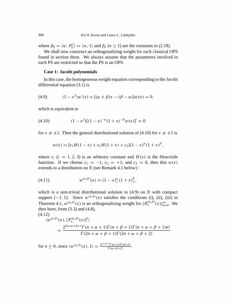
We shall now construct an orthogonalizing weight for each classical OPSfound in section three. We always assume that the parameters involved ineach PS are restricted so that the PS is an OPS.

Case 1: Jacobi polynomials

In this case, the homogeneous weight equation corresponding to the Jacobidifferential equation (3.1) is

(4.9) (1− x2)w′(x)+ [(α + β)x − (β − α)]w(x) = 0,

which is equivalent to

(4.10) (1− x2)[(1− x)−α(1+ x)−βw(x)]′ = 0

for x 6= ±1. Then the general distributional solution of (4.10) forx 6= ±1 is

w(x) = [c1H(1− x)+ c2H(1+ x)+ c3](1− x)α(1+ x)β,

whereci (i = 1, 2, 3) is an arbitrary constant andH(x) is the Heavisidefunction. If we choosec1 = −1, c2 = +1, andc3 = 0, then thisw(x)extends to a distribution onR (see Remark 4.1 below) :

(4.11) w(α,β)(x) = (1− x)α+(1+ x)β+,

which is a non-trivial distributional solution to (4.9) onR with compactsupport [−1, 1]. Sincew(α,β)(x) satisfies the conditions (i), (ii), (iii) inTheorem 4.1,w(α,β)(x) is an orthogonalizing weight for{P(α,β)

n (x)}∞n=0. Wethen have, from (3.3) and (4.8),(4.12)〈w(α,β)(x), [ P(α,β)

n (x)]2〉

= 22n+α+β+10(n+ α + 1)0(n+ β + 1)0(n+ α + β + 1)n!

0(2n+ α + β + 1)0(2n+ α + β + 2)

for n ≥ 0, since〈w(α,β)(x), 1〉 = 2α+β+10(α+1)0(β+1)0(α+β+2) .


REMARK 4.1. For any complex numbera, consider the functionfa: R→C defined by

fa(x) ={

0 if x ≤ 0

xa if x > 0,

where we take logx to be real forx > 0 so thatxa is defined uniquelyfor x > 0. The function fa(x) always extends to a distributionxa

+ on Rwith support in [0,∞). For Rea > −1, fa(x) is locally integrable onR sothat xa

+ = fa(x) and for Rea ≤ −1, xa+ is obtained fromfa(x) by analytic

continuation and regularization. For details on the distributionxa+, we refer to

Hormander [13, Chap. 3.3.2]; see also Morton and Krall [32] for an explicitintegral representation of the distributionw(α,β)(x) in (4.11).

Case 2: Bessel polynomials

In this case, it is more convenient to replacex by βx2 andα by α + 2 so

that the equation (3.4) becomes

(4.13) L[y](x) = x2y′′(x)+ [(α + 2)x + 2]y′(x) = n(n+ α + 1)y(x),

where−(α + 1) /∈ N. We then denoteB(α+2,2)n (x) by B(α)n (x). Now, the

homogeneous weight equation corresponding to (4.13) is

(4.14) x2w′(x)− (αx + 2)w(x) = 0,

of which the only one linearly independent distributional solution with supportin [0,∞) is

(4.15) w0(x) ={

0 if x ≤ 0

xα exp(−2/x) if x > 0.

Romanovski [33] usedw0(x) as an orthogonalizing weight for Bessel PS, butw0(x) cannot be an orthogonalizing weight since it does not decay rapidly atinfinity. In fact, we have

limx→∞ xnw0(x) = ∞

for n+ α > 0. We now consider the non-homogeneous weight equation

(4.16) x2w′(x)− (αx + 2)w(x) = g(x),


whereg(x) is a function with zero moments. Forx 6= 0, the general solutionof (4.16) is

w(x) ={

c1(−x)αe−2/x if x < 0

xαe−2/x∫ x

0 e2/t t−2−αg(t) dt + c2xαe−2/x if x > 0,

where c1 and c2 are arbitrary constants. With concern for the boundarycondition (i) in Theorem 4.1, we choosec1 = 0 andc2 = −

∫∞0 e2/t t−2−α

g(t) dt to obtain

(4.17) w(α)(x) ={

0 if x ≤ 0

−xαe−2/x∫∞

x e2/t t−2−αg(t) dt if x > 0.

If we further takeg(x) to be the function given in (4.7), thenw(α) in (4.17) is acontinuous function onR satisfying the conditions (i) and (ii) in Theorem 4.1(see [9], [22], and [30]). Hence,w(α)(x) in (4.17) (withg(x) in (4.7)) is anorthogonalizing weight for Bessel PS{B(α)n (x)}∞n=0 if and only if

(4.18) 〈w(α)(x), 1〉 = −∫ ∞

0xαe−2/x

[∫ ∞x

e2/t t−2−αg(t) dt

]dx 6= 0.

Condition (4.18) was first proved in [22] forα = 0 and, recently, Maroni [30]proved (4.18) for allα ≥ 12( 2

π)4− 2.

If we let σ (α) be the canonical moment functional of{B(α)n (x)}∞n=0 withσ(α)

0 = 1, then we have from (3.6) and (4.8)

(4.19) 〈σ (α), [B(α)n (x)]2〉 = (−4)nn!0(α + 2)0(α + n+ 1)

0(α + 2n+ 1)0(α + 2n+ 2)(n ≥ 0).

REMARK 4.2. Krall and Frink [19] found the complex orthogonality (nowcalled the Bessel orthogonality) of the Bessel PS through the contour integralalong the unit circle in the complex plane. Although the homogeneous weightequation (4.14) cannot yield a distributional orthogonalizing weight for theBessel PS, it has a non-trivial hyperfunctional solution with support at{0}with respect to which the Bessel PS is orthogonal (see [9], [14], and [15]).

Later in this section, we will discuss again real orthogonalizing weightsfor {B(α)n (x)}∞n=0 for anyα with −(α + 1) /∈ N.


Case 3: Laguerre polynomials

In this case, the homogeneous weight equation corresponding to the La-guerre differential equation (3.7) is

(4.20) xw′(x)+ (x − α)w(x) = 0.

If we setv(x) = exw(x), thenv(x) satisfies the Euler equation

xv′(x)− αv(x) = 0,

of which the general distributional solution is

v(x) = c1xα+ + c2xα−,

wherec1 andc2 are arbitrary constants andxα− is the distribution onR withsupport in(−∞, 0] (defined similarly asxα+; see Remark 4.1 and Hormander[13, Chap. 3.3.2]). Hence, the general solution of (4.20) is

w(x) = c1xα+e−x + c2xα−e−x.

For thisw(x) to vanish at infinity,c2 must be zero. Then by takingc1 = 1,we obtain

(4.21) w(α)(x) = xα+e−x.

Sincew(α)(x) in (4.21) satisfies the conditions (i), (ii), (iii) in Theorem 4.1,w(α)(x) is an orthogonalizing weight for{L(α)n (x)}∞n=0. Since

〈xα+e−x, 1〉 = 0(α + 1)

we have, from (3.9) and (4.8),

(4.22) 〈w(α)(x), [L(α)n (x)]2〉 = n! 0(n+ α + 1).

Case 4: Hermite polynomials

In this case, the homogeneous weight equation corresponding to the Her-mite differential equation (3.10) is

(4.23) w′(x)+ 2xw(x) = 0,


of which the only one linearly independent distributional solution is

(4.24) w(x) = exp(−x2).

Sincew(x) in (4.24) satisfies the conditions (i), (ii), (iii) in Theorem 4.1,w(x) is an orthogonalizing weight for{Hn(x)}∞n=0. We then have, from (3.12)and (4.8),(4.25)

〈w(x), H2n (x)〉 =

∫ ∞−∞

H2n (x) exp(−x2) dx = √πn! 2−n (n ≥ 0).

Case 5: Twisted Hermite polynomials

In this case, the homogeneous weight equation corresponding to the twistedHermite differential equation (3.13) is

(4.26) w′(x)− 2xw(x) = 0,

of which the only one linearly independent distributional solution is

w0(x) = exp(x2),

which cannot be an orthogonalizing weight. However, from (3.14) and (4.25),we can obtain the complex orthogonality :(4.27)∫ i∞

−i∞Hm(x)Hn(x) exp(x2) dx = (−1)n

√πn! 2−ni δmn (m andn ≥ 0).

Let us now consider the non-homogeneous weight equation

(4.28) w′(x)− 2xw(x) = g(x),

whereg(x) is a non-trivial continuous function onR with zero moments andsupport in [0,∞). Then the general solution of (4.28) is

w(x) = cex2 + ex2∫ x

0e−t2

g(t) dt,


wherec is an arbitrary constant. For thisw(x) to vanish at infinity,c must bezero and

(4.29)∫ ∞

0e−x2

g(x) dx = 0.

Then we have

(4.30) w(x) ={

0 if x ≤ 0

ex2 ∫ x0 e−t2

g(t) dt if x > 0.

Note thatw(x) in (4.30) is a classical solution to (4.26) onR. If we furtherassume

(4.31) limx→∞ xng(x) = 0 (n ≥ 0),

then it is easy to see that

limx→∞ xnw(x) = 0 (n ≥ 0),

and sow(x) satisfies the conditions (i), (ii) in Theorem 4.1. Consequently,w(x) in (4.30) is a real orthogonalizing weight for{Hn(x)}∞n=0 if and only if

(4.32) 〈w(x), 1〉 =∫ ∞

0ex2

[∫ x

0e−t2

g(t) dt

]dx 6= 0.

The existence of a weightw(x) for the twisted Hermite PS, of the formgiven in (4.30) and satisfying (4.29), is discussed below in Remark 4.3.

If we let σ be the orthogonalizing moment functional for{Hn(x)}∞n=0 withσ0 = √π , then we have, from (3.15) and (4.8),

(4.33) 〈σ, [ Hn(x)]2〉 = (−1)n

√πn!2−n (n ≥ 0).

REMARK 4.3. We can easily see that there is a non-trivial functiong(x)with zero moments, which also satisfies the condition (4.29). Choose anytwo linearly independent continuous functionsg1(x) and g2(x) with zeromoments and support in [0,∞). Set

Ai =∫ ∞

0e−x2

gi (x) dx (i = 1, 2).


If Ai 6= 0 (i = 1, 2), then

g(x) = A2g1(x)− A1g2(x)

satisfies the condition (4.29) and has zero moments.

Case 6: Twisted Jacobi polynomials

In this case, the homogeneous weight equation corresponding to the twistedJacobi differential equation (3.16) is

(4.34) (1+ x2)w′(x)+ [(d − 2)x + e]w(x) = 0,

of which the only linearly independent distributional solution is

f (x) = (1+ x2)2−d

2 exp(−earctanx).

Romanovski [33] usedf (x) as an orthogonalizing weight for the twistedJacobi PS, butf (x) cannot be an orthogonalizing weight since it does notdecay rapidly at infinity. In fact, we have

limx→∞ xn f (x) = ∞

for n + 2− d > 0. However, from (3.17) and (4.12), we can obtain thecomplex orthogonality(4.35)〈(1− x)α+(1+ x)β+, P(α,β)

m (i x)P(α,β)n (i x)〉

= (−1)n22n+α+β+10(n+ α + 1)0(n+ β + 1)0(n+ α + β + 1)n!

0(2n+ α + β + 1)0(2n+ α + β + 2)δmn

(m andn ≥ 0), whereie= β − α andd = α + β + 2.Let us now consider the non-homogeneous weight equation

(4.36) (1+ x2)w′(x)+ [(d − 2)x + e]w(x) = g(x),

whereg(x) is a non-trivial continuous function onR with zero moments andsupport in [0,∞). Then the general solution of (4.36) is

w(x) = ef (x)[c+∫ x

0e− f (t)(1+ t2)−1g(t) dt],


wherec is an arbitrary constant. For thisw(x) to vanish at infinity,c must bezero and

(4.37)∫ ∞

0e− f (t)(1+ t2)−1g(t) dt = 0.

Then we have

(4.38) w(x) ={

0 if x ≤ 0

ef (x)∫ x

0 e− f (t)(1+ t2)−1g(t) dt if x > 0.

Note thatw(x) in (4.38) is a classical solution to (4.36). Ifg(x) satisfiesthe condition (4.31), thenw(x) satisfies the conditions (i) and (ii) in Theo-rem 4.1. Consequently,w(x) in (4.38) is a real orthogonalizing weight for{P(α,β)

n (x)}∞n=0 if and only if

(4.39) 〈w(x), 1〉 =∫ ∞

0ef (x)

[∫ x

0e− f (t)(1+ t2)−1g(t) dt

]dx 6= 0.

If we let σ be the orthogonalizing moment functional of{P(α,β)n (x)}∞n=0

with

σ0 = 2α+β+10(α + 1)0(β + 1)

0(α + β + 2),

then we have, from (3.18) and (4.8),(4.40)〈σ ,[ P(α,β)

n (x)]2〉

= (−1)n22n+α+β+10(n+ α + 1)0(n+ β + 1)0(n+ α + β + 1)n!

0(2n+ α + β + 1)0(2n+ α + β + 2).

(n ≥ 0)

REMARK 4.4. In the formula (4.12), the parametersα and β are realnumbers with−(α + β + 1), −α, and−β /∈ N. However, by analyticcontinuation, the same formula holds for complex parametersα andβ as longas−Re(α + β + 1), −Reα, and−Reβ /∈ −N. This fact is used in (4.35),whereβ = α, Reα = Reβ = d−2

2 , and−(d − 1) = −(α + β + 1) /∈ N.

Constructing explicit real orthogonalizing weights for classical OPS’s bysolving the non-homogeneous weight equation (4.4) has been successful ex-cept, at the moment, for the Bessel PS{B(α)n (x)}∞n=0 when 0 6= α < 12( 2

π)4−2,


the twisted Hermite PS{Hn(x)}∞n=0, and the twisted Jacobi PS{P(α,β)n (x)}∞n=0.

For any OPS (classical or not), its real orthogonalizing weight can be explic-itly constructed by the following remarkable result on the general momentproblem.

THEOREM4.2 (Duran [8]). For any sequence of real or complex numbers{σn}∞n=0, define a functionw(x) by

(4.41) w(x) ={

0 if x ≤ 012

∫∞0 (∑∞

n=0 σncntnh(λnt))J0(√

xt) dt if x > 0,

wherecn = (−1)n

22n+1(n!)2 , λn = n+∑nk=0 cn, J0(x) is the Bessel function of the

first kind, andh(x) is a C∞-function onR with compact support satisfyingh(0) = 1 andh(n)(0) = 0 (n ≥ 1). Then,w(x) is a function in the SchwartzspaceSand satisfies∫ ∞

−∞xnw(x) dx =

∫ ∞0

xnw(x) dx = σn (n ≥ 0).

In particular, if we take{σn}∞n=0 in Theorem 4.2 to be the moments of acanonical moment functional of any classical OPS, then the functionw(x)in (4.41) is a real orthogonalizing weight for the OPS. Moreover, by Theo-rem 4.1, the function

g(x) = (`2(x)w(x))′ − `1(x)w(x)

is a function, in the Schwartz spaceS with zero moments and support in[0,∞), satisfying the condition (4.31). In the case of the twisted Hermite orthe twisted Jacobi polynomials, thisg(x) also satisfies (4.29) and (4.32) or(4.37) and (4.39) respectively.

REMARK 4.5. In the case of the Bessel, the twisted Hermite, and the twistedJacobi polynomials, their complex orthogonality seems more natural thantheir real orthogonality. In fact, through the hyperfunctional representationsof orthogonalizing weights, we can see that any OPS has both real andcomplex orthogonality : see, for example, [14].

ACKNOWLEDGEMENTS. The first author (KHK) thanks Professor L. DuaneLoveland of the Department of Mathematics and Statistics at Utah StateUniversity for the opportunity to visit Utah State during the 1992-93 academicyear. In addition, he thanks the Korea Science and Engineering Foundation(95-0701-02-01-3), GARC, and Korea Ministry of Education(BSRI 1420) fortheir research support.


References

[1] J. Aczel, Eine Bemerkunguber die Characterisierung der klassischen orthogonale Poly-nome, Acta Math. Sci. Hung.4 (1953), 315–321.

[2] R. P. Boas,The Stieltjes moment problem for functions of bounded variation, Bull. Amer.Math. Soc.45 (1939), 399–404.

[3] S. Bochner,Uber Sturm-Liouvillesche Polynomsysteme, Math. Z.29 (1929), 730–736.[4] T. S. Chihara,An introduction to orthogonal polynomials, Gordon and Breach, New York,

1977.[5] C. W. Cryer,Rodrigues’ formulas and the classical orthogonal polynomials, Boll. Unione

Mat. Ital. 25 (1970), 1–11.[6] A. Csaszar, Sur les polynomes orthogonaux classiques, Annales Univ. Sci. Budapest Sec.

Math.1 (1958), 33–39.[7] A. J. Duran,The Stieltjes moment problem for rapidly decreasing functions, Proc. Amer.

Math. Soc.107(3) (1989), 731–741.[8] , Functions with given moments and weight functions for orthogonal polynomials,

Rocky Mountain J. Math.23(1) (1993), 87–104.[9] W. D. Evans, W. N. Everitt, K. H. Kwon, and L. L. Littlejohn,Real orthogonalizing weights

for Bessel polynomials, J. Comp. Appl. Math.49 (1993), 51-57.[10] J. Favard,Sur les polynomes de Tchebicheff, C.R. Acad. Sci. Paris200(1935), 2052–2053.[11] J. Feldmann,On a characterization of classical orthogonal polynomials, Acta. Sc. Math.

17 (1956), 129–133.[12] G. H. Hardy,On Stieltjes’ “Probleme des Moments", Messenger of Math.4 (1917), 175–182.[13] L. Hormander,The analysis of linear partial differential operators I, Springer-Verlag, New

York, 1983.[14] S. S. Kim and K. H. Kwon,Hyperfunctional weights for orthogonal polynomials, Results

in Math.18 (1990), 273–281.[15] , Generalized weights for orthogonal polynomials, Diff. and Int. Equations4 (1991),

601–608.[16] A. M. Krall and L. L. Littlejohn, On the classification of differential equations having

orthogonal polynomial solutions II, Ann. Mat. Pura Appl.4 (1987), 77–102.[17] H. L. Krall, Certain differential equations for Tchebychev polynomials, Duke Math. J.4

(1938), 705–719.[18] , On derivatives of orthogonal polynomials II, Bull. Amer. Math. Soc.47 (1941),

261–264.[19] H. L. Krall and O. Frink,A new class of orthogonal polynomials : The Bessel polynomials,

Trans. Amer. Math. Soc.65 (1949), 100–115.[20] H. L. Krall and I. M. Sheffer,A characterization of orthogonal polynomials, J. Math. Anal.

Appl. 8 (1964), 232–244.[21] , Differential equations of infinite order for orthogonal polynomials, Ann. Mat. Pura

Appl. 4 (1966), 135–172.[22] K. H. Kwon, S. S. Kim, and S. S. Han,Orthogonalizing weights for Tchebychev sets of

polynomials, Bull. London Math. Soc.24 (1992), 361–367.[23] K. H. Kwon, J. K. Lee, and B. H. Yoo,Characterizations of classical orthogonal polynomi-

als, Results in Math.24 (1993), 119-128.


[24] K. H. Kwon and L. L. Littlejohn,Sobolev orthogonal polynomials and second-order differ-ential equations, Rocky Mt. J. Math. (to appear).

[25] K. H. Kwon, L. L. Littlejohn, and B. H. Yoo,Characterizations of orthogonal polynomialssatisfying differential equations, SIAM J. Math. Anal.25(3)(1994), 976–990.

[26] E. N. Laguerre,Sur l’integrale∫∞

x x−1e−x dx, Bull. de la Societe Math. de France7 (1879),72–81.

[27] P. Lesky,Die Charakterisierung der klassischen orthogonalen Polynome durch Sturm-Liouvillesche Differentialgleichungen, Arch. Rat. Mech. Anal.10 (1962), 341–352.

[28] L. L. Littlejohn, On the classification of differential equations having orthogonal polynomialsolutions, Ann. Mat. Pura Appl.4 (1984), 35–53.

[29] L. L. Littlejohn and D. Race,Symmetric and symmetrisable ordinary differential expressions,Proc. London Math. Soc.1 (1990), 334–356.

[30] P. Maroni,An integral representation for the Bessel form, J. Comp. Appl. Math.57 (1995),251–260.

[31] M. Mikol as,Common characterization of the Jacobi, Laguerre and Hermite-like polynomi-als (in Hungarian), Mate. Lapok7 (1956), 238–248.

[32] R. D. Morton and A. M. Krall,Distributional weight functions for orthogonal polynomials,SIAM J. Math. Anal.9(4) (1978), 604–626.

[33] M. V. Romanovski,Sur quelques classes nouvelle de polynomes orthogonaux, C.R. Acad.Sci. Paris188(1929), 1023–1025.

[34] N. J. Sonine,Recherches sur les fonctions cylindriques et le developpment des fonctionscontinues en series, Math. Ann.16 (1880), 1–80.

[35] T. J. Stieltjes,Recherches sur les fractions continues, Ann. de la Faculte des Sci. de Toulouse8 (1894), J1–122;9 (1895), A1–47; Oeuvres2, 398–566.

K. H. KwonDepartment of MathematicsKAISTTaejon 305-701, KoreaE-mail: khkwon@ jacobi.kaist.ac.kr

L. L. LittlejohnDepartment of Mathematics and StatisticsUtah State UniversityLogan, Utah, 84322-3900E-mail: [email protected]

classification of classical orthogonal polynomials kil h. kwon ...

Documents

Transcript of classification of classical orthogonal polynomials kil h. kwon ...