INSTITUTE OF PHYSICS PUBLISHING JOURNAL OF PHYSICS A: MATHEMATICAL AND GENERAL

J. Phys. A: Math. Gen. 37 (2004) 8045–8063 PII: S0305-4470(04)74861-1

Recurrences and explicit formulae for the expansionand connection coefficients in series of Besselpolynomials

E H Doha1 and H M Ahmed2

1 Department of Mathematics, Faculty of Science, Cairo University, Giza, Egypt2 Department of Mathematics, Faculty of Industrial Education, Amiria, Cairo, Egypt

E-mail: eiddoha@frcu.eun.eg

Received 17 January 2004, in final form 22 June 2004Published 4 August 2004Online at stacks.iop.org/JPhysA/37/8045doi:10.1088/0305-4470/37/33/006

AbstractA formula expressing explicitly the derivatives of Bessel polynomials of anydegree and for any order in terms of the Bessel polynomials themselves isproved. Another explicit formula, which expresses the Bessel expansioncoefficients of a general-order derivative of an infinitely differentiable functionin terms of its original Bessel coefficients, is also given. A formula for theBessel coefficients of the moments of one single Bessel polynomial of certaindegree is proved. A formula for the Bessel coefficients of the moments of ageneral-order derivative of an infinitely differentiable function in terms of itsBessel coefficients is also obtained. Application of these formulae for solvingordinary differential equations with varying coefficients, by reducing them torecurrence relations in the expansion coefficients of the solution, is explained.An algebraic symbolic approach (using Mathematica) in order to build and solverecursively for the connection coefficients between Bessel–Bessel polynomialsis described. An explicit formula for these coefficients between Jacobi andBessel polynomials is given, of which the ultraspherical polynomial and itsconsequences are important special cases. Two analytical formulae for theconnection coefficients between Laguerre–Bessel and Hermite–Bessel are alsodeveloped.

PACS numbers: 02.30.Gp, 02.30.Nw, 02.30.HqMathematics Subject Classification: 42C10, 33A50, 65L50, 65L10

1. Introduction

Techniques for finding approximate solutions for differential equations, based on classicalorthogonal polynomials, are popularly known as spectral methods. Approximating functions

0305-4470/04/338045+19$30.00 © 2004 IOP Publishing Ltd Printed in the UK 8045

8046 E H Doha and H M Ahmed

in spectral methods are related to polynomial solutions of eigenvalue problems in ordinarydifferential equations, known as Sturm–Liouville problems. In the past few decades, therehas been growing interest in this subject. As a matter of fact, spectral methods providea competitive alternative to other standard approximation techniques, for a large variety ofproblems. Initial applications were concerned with the investigation of periodic solutions ofboundary value problems using trigonometric polynomials. Subsequently, the analysis wasextended to algebraic polynomials. Expansions in orthogonal basis functions were performed,due to their high accuracy and flexibility in computations. Different basis functions leadto different spectral approximations; for instance, trigonometric polynomials for periodicproblems, Chebyshev, Legendre, ultraspherical and Jacobi polynomials for non-periodicproblems, Laguerre polynomials for problems on the half line, and Hermite polynomialsfor problems on the whole line.

Chebyshev, Legendre and ultraspherical polynomials are examples of three classes ofsingular Sturm–Liouville eigenfunctions that have been used in both the solution of boundaryvalue problems (see, for instance, Ben-Yu (1998), Coutsias et al (1996), Doha (1990, 2000,2002a, 2002b, 2003a), Doha and Al-kholi (2001), Doha and Abd-Elhameed (2002), Doha andHelal (1997), Haidvogel and Zang (1979), Siyyam and Syam (1997)) and in computationalfluid dynamics (see Canuto et al (1988), Helal (2001), Voigt et al (1984)). In most ofthese applications, formulae relating the expansion coefficients of derivatives appearing in thedifferential equation with those of the function itself are used.

Formulae for the expansion coefficients of a general-order derivative of an infinitelydifferentiable function in terms of those of the function are available for expansions inChebyshev (Karageorghis 1988a), Legendre (Phillips 1988), ultraspherical (Karageorghis andPhillips 1989, 1992, Doha 1991), Jacobi (Doha 2002a), Laguerre (Doha 2003b) and Hermite(Doha 2004a) polynomials.

A more general situation which often arises in the numerical solution of differentialequations with polynomial coefficients in spectral and pseudospectral methods is theevaluation of the expansion coefficients of the moments of high-order derivatives of infinitelydifferentiable functions. A formula for the shifted Chebyshev coefficients of the moments ofthe general-order derivatives of an infinitely differentiable function is given in Karageorghis(1988b). Corresponding results for Chebyshev polynomials of the first and second kinds,Legendre, ultraspherical, Hermite, Laguerre and Jacobi polynomials are given in Doha (1994),Doha and El-Soubhy (1995), Doha (1998, 2003b, 2004a, 2004b) respectively.

Up to now, and to the best of our knowledge, many formulae corresponding to thosementioned previously are not known and are traceless in the literature for the Bessel expansions.This partially motivates our interest in such polynomials. Another motivation is that thetheoretical and numerical analysis of numerous physical and mathematical problems veryoften requires the expansion of an arbitrary polynomial or the expansion of an arbitraryfunction with its derivatives and moments into a set of orthogonal polynomials. This is, inparticular, true for Bessel polynomials. To be precise, the Bessel polynomials form a set oforthogonal polynomials on the unit circle in the complex plane. They are important in certainproblems of mathematical physics; for example, they arise in the study of electrical networksand when the wave equation is considered in spherical coordinates.

The paper is organized as follows. In section 2, we give some relevant properties ofBessel polynomials. In section 3, we prove a theorem which relates the Bessel expansioncoefficients of the derivatives of a function in terms of its original expansion coefficients. Anexplicit expression for the derivatives of Bessel polynomials of any degree and for any orderas a linear combination of suitable Bessel polynomials themselves is also deduced. In section4, we prove a theorem which gives the Bessel coefficients of the moments of one single Bessel

Recurrences and explicit formulae for the expansion and connection coefficients 8047

polynomial of any degree. Another theorem which expresses the Bessel coefficients of themoments of a general-order derivative of an infinitely differentiable function in terms of itsBessel coefficients is proved in section 5. In section 6, we give an application of these theoremswhich provides an algebraic symbolic approach (using Mathematica) in order to build andsolve recursively for the connection coefficients between Bessel and different polynomialsystems.

2. Some properties of Bessel polynomials

The classical sets of orthogonal polynomials of Jacobi, Laguerre and Hermite satisfy second-order differential equations, and also have the property that their derivatives form orthogonalsystems. The Bessel polynomials, a fourth class of orthogonal polynomials with these twoproperties, were introduced by Krall and Frink (1949) in connection with the solution of thewave equation in spherical coordinates.

They define the generalized Bessel polynomial yn(x, a, b) to be the polynomial of degreen, and with constant term equal to unity, which satisfies the differential equation

x2y ′′(x) + [ax + b]y ′(x) − n(n + a − 1)y(x) = 0, b �= 0, a �= 0,−1,−2, . . . , (1)

where n is a non-negative integer, provided a is not a negative integer or zero, and b is notzero.

It is easy to see that yn(bx, a, b) is independent of b. Thus it seems preferable to adoptthe notation (Al-Salam 1957)

Y (α)n (x) = yn(x, α + 2, 2),

so that Y (0)n (x) = yn(x), the ordinary Bessel polynomial. Y (α)

n (x) satisfy the differentialequation

x2y ′′(x) + [(α + 2)x + 2]y ′(x) − n(n + α + 1)y(x) = 0, α �= −2,−3, . . . . (2)

These polynomials are orthogonal on the unit circle with respect to the weight function

ρα(x) =∞∑

k=0

�(α + 2)

�(k + α + 1)

(−2

x

)k

,

satisfying the orthogonality relation

1

4π i

∫C

Y (α)n (z)Y (α)

m (z)ρα(z) dz = (−1)n+1n!�(α + 2)

(2n + α + 1)�(n + α + 1)δnm,

where the integration is around the unit circle surrounding the zero point. Y (α)n (x) may be

generated by using the Rodrigues formula

Y (α)n (x) = 2−nx−α e2/x Dn[x2n+α e−2/x],

where D ≡ d/dx, and explicitly by the formula

Y (α)n (x) =

n∑k=0

(n

k

)(n + α + 1)k

(x

2

)k

, (3)

(for more detail see, for instance, Chihara (1978) and Sanchez-Ruiz and Dehesa (1998)).Several other authors have contributed to the study of Bessel polynomials, among them

are Agarwal (1954), Al-Salam (1957), Carlitz (1957), Evans et al (1993), Grosswald (1978),Han and Kwon (1991), and Luke (1969, vol 2).

8048 E H Doha and H M Ahmed

The following two recurrence relations (which may be found in Koepf and Schmersau(1998)) are of fundamental importance in developing the present work. These are

2(n + α + 1)(2n + α)Y(α)n+1(x) = (2n + α + 1)[(2n + α)(2n + α + 2)x + 2α]Y (α)

n (x)

+ 2n(2n + α + 2)Y(α)n−1(x), n � 1, (4)

Y (α)n (x) = 2(n + α + 1)

(2n + α + 1)(2n + α + 2)(n + 1)DY

(α)n+1(x) +

4

(2n + α + 2)(2n + α)DY (α)

n (x)

+2n

(n + α)(2n + α)(2n + α + 1)DY

(α)n−1(x). (5)

Note that the recurrence relation (4) may be used to generate the Bessel polynomials startingfrom Y

(α)0 (x) = 1 and Y

(α)1 (x) = α+2

2 x + 1.

Theorem 1. Let f (x) be a function regular (i.e. analytic) in |x − a| � R, where R > 0and a is any point of the plane. Then f (x) can be expanded in a series of generalized Besselpolynomials of the form f (x) ∼

∑cnY

(α)n (x − a), where

cn = 2n

n!(2n + α + 1)�(n + α + 1)

∞∑ν=0

(−2)ν

ν!�(2n + ν + α + 2)f (n+ν)(a),

and the series is convergent uniformly in |x − a| � R.

Proof. We first suppose that f (x) is regular in |x| � R and prove that f (x) can be expandedin a series

∑∞n=0 γnY

(α)n (x) where

γn = 2n

n!(2n + α + 1)�(n + α + 1)

∞∑ν=0

(−2)ν

ν!�(2n + ν + α + 2)f (n+ν)(0), (6)

and that the series is uniformly convergent in |x| � R. Theorem 1 follows readily when x − a

is written for x.

We have (see Sanchez-Ruiz and Dehesa (1998), equation (2.32))

xn =n∑

i=0

πniY(α)i (x), n � 0, (7)

where

πni =(

ni

)(−1)n−i2n(2i + α + 1)�(i + α + 1)

�(n + i + α + 2). (8)

We now substitute for xn from (7) in the Taylor expansion∑∞

n=0(f(n)(0)/n!)xn of f (x)

about the origin to get formally the series∑∞

n=0 γnY(α)n (x), where

γn =∞∑

ν=0

πn+ν,nf(n+ν)(0)/(n + ν)!.

Hence inserting the value of πn+ν,n from (8), equation (6) follows at once.In order to prove that the series

∑∞n=0 γnY

(α)n (x) is convergent in |x| � R we form the

sum (see Whittaker (1949), chapters II and III)

ωn(R) =∑

i

|πni |Mi(R),

Recurrences and explicit formulae for the expansion and connection coefficients 8049

where Mi(R) ≡ max|x|=R

∣∣Y (α)i (x)

∣∣ = ∑ik=0 2−k

(ik

)|(i + α + 1)k|Rk. Applying (8) we obtain

after some reduction

ωn(R) = 2n

n∑k=0

(n

k

)(R/2)k

n−k∑j=0

(n − k

j

) ∣∣∣∣ (2j + 2k + α + 1)�(2k + j + α + 1)

�(n + k + j + α + 2)

∣∣∣∣< |2n + α + 1||�(α + 1)|Rn

n∑k=0

(n

k

)(4/R)k/|�(k + α + 1)|

< |2n + α + 1|RnBn, (9)

where Bn = ∑nk=0

(nk

)(4/R′)k

k! , R′ = Rµ(α), 0 < µ(α) < minm∈Z+1m

|α + m|. Effecting the

transformation y = x(1 + x)−1 on the function x exp(4x/R′) = ∑∞n=0(4/R′)nxn+1/n! it

follows that

F(y) ≡ (y/(1 − y)) exp{4y/R′(1 − y)} =∞∑

n=0

Bnyn+1.

This function is regular in |y| < 1; hence by Cauchy’s inequality we have

Bn < K/βn+1, 0 < β < 1,

where K = max|y|=β |F(y)| < ∞. Inserting this in (9) and making n tend to infinity we obtain

λ(R) ≡ limn→∞ sup{ωn(R)}1/n � R/β,

and since β can be taken as near 1 as we please we conclude that λ(R) = R. According toCannon (1937) (see also Whittaker (1949), p 11), we infer that the series

∑∞n=0 γnY

(α)n (x) is

uniformly convergent in |x| � R, as required. �

Remark 1. It is to be noted that the theorem of Nassif (1954, p 408) can be obtained directlyfrom our theorem by taking α = 0.

Suppose now we are given a regular function f (x) which is formally expanded in aninfinite series of Bessel polynomials,

f (x) =∞∑

n=0

anY(α)n (x), (10)

and for the qth derivatives of f (x),

Dqf (x) =∞∑

n=0

a(q)n Y (α)

n (x), a(0)n = an, (11)

it is possible to derive a recurrence relation involving the Bessel coefficients of successivederivative of f (x). Let us write

D

[ ∞∑n=0

a(q−1)n Y (α)

n (x)

]=

∞∑n=0

a(q)n Y (α)

n (x),

then using identity (5) leads to the recurrence relation

a(q−1)n = 2(n + α)

n(2n + α − 1)(2n + α)a

(q)

n−1 +4

(2n + α + 2)(2n + α)a(q)

n

+2(n + 1)

(n + α + 1)(2n + α + 2)(2n + α + 3)a

(q)

n+1, q � 1, n � 1. (12)

8050 E H Doha and H M Ahmed

For computing purpose, we see that this equation is not easy to use, since the coefficientson the right-hand side are functions of n. No obvious direct way is available for solving thisequation, therefore we resort to the following alternative method that enables one to expressa

(q)n in terms of the original expansion coefficients ak, k = 0, 1, . . . .

3. The derivatives of Y (α)n (x) and the relation between the coefficients a(q)

n and an

The main result of this section is to prove the following theorem which expresses explicitly theBessel expansion coefficients, a

(q)n , of a general-order derivative of an infinitely differentiable

function in terms of its original Bessel coefficients, an.

Theorem 2. Suppose that a function f (x) and its qth derivative are formally expanded as in(10) and (11), then

a(q)n = 2−q

∞∑i=0

(n + i + 1)q(n + q + i + α + 1)qMn(α + 2q, α, n + i)an+q+i ,

n � 0, q � 1, (13)

where

Mi(α, β, n) = (−1)n(2i + β + 1)(α − β)n−i (−n)i(α + n + 1)i

i!(β + i + 1)n+1. (14)

The following two lemmas are needed to proceed with the proof of the theorem.

Lemma 1 (Sanchez-Ruiz and Dehesa 1998). The connection problem between Besselpolynomials with different parameters is

Y (α)n (x) =

n∑i=0

Mi(α, β, n)Y(β)

i (x),

where the connection coefficients Mi(α, β, n) are given as in (14).

Lemma 2. The derivatives of Bessel polynomials of any degree in terms of Bessel polynomialswith the same parameter are given by

DqY (α)n (x) = 2−q(n − q + 1)q(n + α + 1)q

n−q∑i=0

Mi(α + 2q, α, n − q)Y(α)i (x). (15)

Proof. Al-Salam (1957) has proved that

DY (α)n (x) = 1

2n(n + α + 1)Y(α+2)n−1 (x), n � 1, (16)

and therefore

DqY (α)n (x) = 2−q(n − q + 1)q(n + α + 1)qY

(α+2q)n−q (x). (17)

From lemma 1 and identity (17), we obtain (15). �

Proof of theorem 2. Now, on differentiating (10) q times and making use of (15), we find

Dqf (x) =∞∑

n=q

anDqY (α)

n (x)

= 2−q

∞∑n=q

an(n − q + 1)q(n + α + 1)q

n−q∑i=0

Mi(α + 2q, α, n − q)Y(α)i (x), (18)

Recurrences and explicit formulae for the expansion and connection coefficients 8051

expanding (18) and collecting similar terms, we obtain (13) which completes the proof oftheorem 2. �

Remark 2. It is to be noted here that the formula for a(q)n given by (13) is the exact solution of

the difference equation (12), and it also worth noting that based on theorem 1, one can showthat the series (13) is convergent.

4. Bessel coefficients of the moments of one single Bessel polynomial of any degree

For the evaluation of Bessel coefficients of the moments of higher order derivatives of aninfinitely differentiable function, the following theorem is needed.

Theorem 3

xmY(α)j (x) =

2m∑n=0

amn(j)Y(α)j+m−n(x), m � 0, j � 0, (19)

where

amn(j) = (−1)j−n2mm!j !(2j + 2m − 2n + α + 1)�(j + m − n + α + 1)

(j + m − n)!(2m − n)!�(j + α + 1)�(2j + 2m − n + α + 2)

×min(j+m−n,j)∑k=max(0,j−n)

(j + m − n

k

)(−1)k�(j + k + α + 1)�(j + 2m − n − k + 1)

(j − k)!(n + k − j)!.

(20)

Proof. We use the induction principle to prove this theorem. In view of recurrence relation

xY(α)j (x) = 2(j + α + 1)

(2j + α + 1)(2j + α + 2)Y

(α)j+1(x)

− 2α

(2j + α)(2j + α + 2)Y

(α)j (x) − 2j

(2j + α)(2j + α + 1)Y

(α)j−1(x), j � 0,

we may write

xY(α)j (x) = a10(j)Y

(α)j+1(x) + a11(j)Y

(α)j (x) + a12(j)Y

(α)j−1(x), (21)

and this in turn shows that (19) is true for m = 1. Proceeding by induction, assuming that (19)is valid for m, we want to prove that

xm+1Y(α)j (x) =

2m+2∑n=0

am+1,n(j)Y(α)j+m−n+1(x). (22)

From (21) and assuming the validity for m, we have

xm+1Y(α)j (x) =

2m∑n=0

amn(j)[a10(j + m − n)Y

(α)j+m−n+1(x) + a11(j + m − n)Y

(α)j+m−n(x)

+ a12(j + m − n)Y(α)j+m−n−1(x)

].

Collecting similar terms, we get

xm+1Y(α)j (x) = am0(j)a10(j + m)Y

(α)j+m+1(x) + [am1(j)a10(j + m − 1)

+ am0(j)a11(j + m)]Y (α)j+m(x) +

2m∑n=2

[amn(j)a10(j + m − n)

8052 E H Doha and H M Ahmed

+ am,n−1(j)a11(j + m − n + 1) + am,n−2(j)a12(j + m − n + 2)]Y (α)j+m−n+1(x)

+ [am,2m(j)a11(j − m) + am,2m−1(j)a12(j − m + 1)]Y (α)j−m(x)

+ am,2m(j)a12(j − m)Y(α)j−m−1(x). (23)

It can be easily shown that

am+1,0(j) = am0(j)a10(j + m),

am+1,1(j) = am1(j)a10(j + m − 1) + am0(j)a11(j + m),

am+1,n(j) = amn(j)a10(j + m − n) + am,n−1(j)a11(j + m − n + 1)

+ am,n−2(j)a12(j + m − n + 2),

am+1,2m+1(j) = am,2m(j)a11(j − m) + am,2m−1(j)a12(j − m + 1),

am+1,2m+2(j) = am,2m(j)a12(j − m),

and accordingly, formula (23) becomes

xm+1Y(α)j (x) =

2m+2∑n=0

am+1,n(j)Y(α)j+m−n+1(x),

which completes the induction and proves the theorem. �

Corollary 1. It can be easily shown that the expansion coefficients amn(j) of theorem 3 satisfythe recurrence relation

amn(j) =2∑

k=0

am−1,n+k−2(j)a1,2−k(j + m − n − k + 1), n = 0, 1, . . . , 2m, (24)

where

a1k(j) =

2(j + α + 1)

(2j + α + 1)(2j + α + 2), k = 0,

− 2α

(2j + α)(2j + α + 2), k = 1,

− 2j

(2j + α)(2j + α + 1), k = 2,

a00(j) = 1 (25)

with

am−1,−�(j) = 0, ∀� > 0, am−1,r (j) = 0, r = 2m − 1, 2m.

Corollary 2. One can show that

xmY(α)j (x) =

j+m∑n=0

am,j+m−n(j)Y (α)n (x), j � 0, m � 0, (26)

and

xm =m∑

n=0

am,m−n(0)Y (α)n (x), m � 0, (27)

where

am,m−n(0) =(

m

n

)(−1)m−n2m(2n + α + 1)�(n + α + 1)

�(m + n + α + 2). (28)

Formula (27) is in complete agreement with Sanchez-Ruiz and Dehesa (1998) and Zarzoet al (1997).

Recurrences and explicit formulae for the expansion and connection coefficients 8053

5. Bessel coefficients of the moments of a general-order derivative of an infinitelydifferentiable function

In this section, we state and prove a theorem which relates the Bessel coefficients of themoments of a general-order derivative of an infinitely differentiable function in terms of itsBessel coefficients.

Theorem 4. Assume that f (x), Dqf (x) and x�Y(α)j (x) have the Bessel expansions (10), (11)

and (19) respectively, and assume also that

x�

( ∞∑i=0

a(q)

i Y(α)i (x)

)=

∞∑i=0

bq,�

i Y(α)i (x) = I q,�, (29)

then the connection coefficients bq,�

i are given by

bq,�

i =

�−1∑k=0

a�,k+�−i (k)a(q)

k +i∑

k=0

a�,k+2�−i (k + �)a(q)

k+�, 0 � i � �,

�−1∑k=i−�

a�,k+�−i (k)a(q)

k +i∑

k=0

a�,k+2�−i (k + �)a(q)

k+�, � + 1 � i � 2� − 1,

i∑k=i−2�

a�,k+2�−i (k + �)a(q)

k+�, i � 2�,

(30)

where the coefficients amn(k) are as defined in (20).

Proof. Equations (11), (19) and (29) give

I q,� =∞∑

k=0

a(q)

k

2�∑j=0

a�,j (k)Y(α)k+�−j (x). (31)

By letting i = k + � − j, then (31) may be written in the form

I q,� =�−1∑k=0

a(q)

k

k+�∑i=k−�

a�,k+�−i (k)Y(α)i (x) +

∞∑k=�

a(q)

k

k+�∑i=k−�

a�,k+�−i (k)Y(α)i (x)

=∑

1

+∑

2

, (32)

where

∑1

=�−1∑k=0

a(q)

k

k+�∑i=k−�

a�,k+�−i (k)Y(α)i (x),

∑2

=∞∑

k=�

a(q)

k

k+�∑i=k−�

a�,k+�−i (k)Y(α)i (x).

Considering∑

1 first,

∑1

=�−1∑k=0

a(q)

k

−1∑i=k−�

a�,k+�−i (k)Y(α)i (x) +

�−1∑k=0

a(q)

k

k+�∑i=0

a�,k+�−i (k)Y(α)i (x)

=∑

11

+∑

12

. (33)

8054 E H Doha and H M Ahmed

Clearly,

∑11

=�−1∑k=0

a(q)

k

−1∑i=k−�

a�,k+�−i (k)Y(α)i (x) =

�−1∑k=0

a(q)

k

�−k∑i=1

a�,k+�+i (k)Y(α)−i (x),

hence ∑11

= 0. (34)

Now,

∑12

=�−1∑k=0

a(q)

k

k+�∑i=0

a�,k+�−i (k)Y(α)i (x)

=�∑

i=0

�−1∑k=0

a(q)

k a�,k+�−i (k)Y(α)i (x) +

2�−1∑i=�+1

�−1∑k=i−�

a(q)

k a�,k+�−i (k)Y(α)i (x),

hence ∑12

=2�−1∑i=0

�−1∑k=max(0,i−�)

a(q)

k a�,k+�−i (k)Y(α)i (x). (35)

Substitution of (34) and (35) into (33) yields

∑1

=2�−1∑i=0

�−1∑k=max(0,i−�)

a(q)

k a�,k+�−i (k)Y(α)i (x). (36)

If when considering∑

2, one takes k + � instead of k, then it is not difficult to show that

∑2

=∞∑i=0

i∑k=max(0,i−2�)

a(q)

k+�a�,k+2�−i (k + �)Y(α)i (x). (37)

Substitution of (36) and (37) into (32) gives the required results of (30) and completes theproof of theorem 4. �

6. Recurrence relations for connection coefficients between Bessel and differentpolynomial systems

Let f (x) have the Bessel expansion (10), and assume that it satisfies the linear non-homogeneous differential equation of order n

n∑i=0

pi(x)f (i)(x) = g(x), (38)

where p0, p1, . . . , pn �= 0 are polynomials in x, and the coefficients of Bessel series of thefunction g(x) are known, then formulae (13), (19) and (30) enable one to construct in view ofequation (38) the linear recurrence relation of order r,

r∑j=0

αj (k)ak+j = β(k), k � 0, (39)

where α0, α1, . . . , αr (α0 �= 0, αr �= 0) are polynomials of the variable k.In this section, we consider the problem of determining the connection coefficients

between different polynomial systems. An interesting question is how to transform the

Recurrences and explicit formulae for the expansion and connection coefficients 8055

Fourier coefficients of a given polynomial corresponding to an assigned orthogonal basis, intothe coefficients of another basis orthogonal with respect to a different weight function. Theaim is to determine the so-called connection coefficients of the expansion of any element ofthe first basis in terms of the elements of the second basis. Suppose V is a vector space of allpolynomials over the real or complex numbers and Vm is the subspace of polynomials ofdegree less than or equal to m. Suppose p0(x), p1(x), p2(x), . . . is a sequence of polynomialssuch that pn(x) is of exact degree n; let q0(x), q1(x), q2(x), . . . be another such sequence.Clearly, these sequences form a basis for V . It is also evident that p0(x), p1(x), . . . , pm(x)

and q0(x), q1(x), . . . , qm(x) give two bases for Vm. While working with finite-dimensionalvector spaces, it is often necessary to find the matrix that transforms a basis of a given spaceto another basis. This means that one is interested in the connection coefficients ai(n) thatsatisfy

qn(ax + b) =n∑

i=0

ai(n)pi(x), (40)

where a and b are constants. The choice of pn(x) and qn(ax + b) depends on the situation.For example, suppose

pn(x) = xn, qn(x) = x(x − 1) · · · (x − n + 1) = (−1)n(−x)n = �(x + 1)

�(x − n + 1),

then the connection coefficients ai(n) are Stirling numbers of the first kind. If the role of thesepn(x) and qn(x) are interchanged, then we get Stirling numbers of the second kind. Thesenumbers are useful in some combinatorial polynomials (see Abramowitz and Stegun (1970)pp 824–5).

The connection coefficients between many of the classical orthogonal polynomial systemshave been determined by different kinds of methods (see, e.g., Szego (1985), Rainville (1960)and Andrews et al (1999)). The aim of this section is to describe a simple procedure (based onthe results of theorem 4) in order to find recurrence relations, sometimes easy to solve, betweenthe coefficients ai(n) when pi(x) = Y

(α)i (x) and qi(x) = Y

(β)

i (x). This gives an alternativeand different way to be compared to the approaches of Askey and Gasper (1971), Ronveauxet al (1995, 1996), Area et al (1998), Godoy et al (1997), Koepf and Schmersau (1998),Lewanowicz (2002), Lewanowicz and Wozny (2001), Lewanowicz et al (2000), and Sanchez-Ruiz and Dehesa (1998). A nonrecursive way to approach the problem in the case of classicalorthogonal polynomials of a discrete variable can be found in Gasper (1974). Moreover, otherauthors have considered the problem from a recursive point of view (see Koepf and Schmersau(1998)), or even in the classical discrete and q-analogues (cf, Alvarez-Nodarse et al (1998)and Alvarez-Nodarse and Ronveaux (1996)). Since the connection coefficients ai(n) dependon two parameters i and n, the most interesting recurrence relations are those which leave oneof the parameters fixed. In the cases when the order of the resulting recurrence relation is 1, itdefines a hypergeometric term which can be given explicitly in terms of Pochhammer symbol(a)k = �(a+k)

�(a).

6.1. The Bessel–Bessel connection problem

The link between Y (α)n (ax + b) and Y

(β)

i (x) given by (40) can easily be replaced by a linearrelation involving only Y

(β)

i (x) using the Bessel differential equation, namely

[(ax + b)2D2 + a[(α + 2)(ax + b) + 2]D − a2n(n + α + 1)]Y (α)n (ax + b) = 0, (41)

8056 E H Doha and H M Ahmed

by substituting

Y (α)n (ax + b) =

n∑i=0

ai(n)Y(β)

i (x), (42)

with an+1(n) = an+2(n) = · · · = 0, and by virtue of formula (29), equation (41) takes the form

a2I 2,2 + 2abI 2,1 + b2I 2,0 + a2(α + 2)I 1,1 + [ab(α + 2) + 2]I 1,0 − a2n(n + α + 1)I 0,0 = 0,

or

a2b2,2i + 2abb

2,1i + b2b

2,0i + a2(α + 2)b

1,1i + [ab(α + 2) + 2]b1,0

i − a2n(n + α + 1)b0,0i = 0.

By making use of formulae (20) and (30), we obtain

a2n(n + α + 1)ai(n) − 2a2(α + 2)(i + α)

(2i + α − 1)(2i + α)a

(1)i−1(n)

+ a

[−b(α + 2) +

2(−4i2 − 4i(α + 1) + (a − 1)α(α + 2))

(2i + α)(2i + α + 2)

]a

(1)i (n)

+2a2(i + 1)(α + 2)

(2i + α + 2)2a

(1)i+1(n) − 4a2(i + α − 1)2

(2i + α − 3)4a

(2)i−2(n)

+4a(i + α)(2aα − b(2i + α − 2)(2i + α + 2))

(2i + α − 2)3(2i + α + 2)a

(2)i−1(n)

+

[−b2 +

4abα

(2i + α)(2i + α + 2)+

4a2(2i(i + 1) + α + 2iα − α2)

(2i + α − 1)2(2i + α + 2)2

]a

(2)i (n)

+4a(i + 1)(2aα − b(2i + α)(2i + α + 4))

(2i + α)(2i + α + 2)3a

(2)i+1(n)

− 4a2(i + 1)(i + 2)

(2i + α + 2)4a

(2)i+2(n) = 0, i � 0, (43)

using formula (13) with (43)—and after some manipulation obtain the following recurrencerelation,

δi0ai(n) + δi1ai+1(n) + δi2ai+2(n) + δi3ai+3(n) + δi4ai+4(n) = 0,

i = n − 1, n − 2, . . . , 0, (44)

where

δi0 = a2(n − i)(i + n + α + 1)(i + β + 1)4

(2i + β + 1)4,

δi1 = −a(i + 1)(i + β + 2)3

(2i + β + 3)2

[1 +

b

2(α + 2i + 2)

− a(β(2i + 1) + 2(3i + 1) + 4n(n + α + 1) + (2 − 2i + β)(α + 1))

(2i + β + 2)(2i + β + 6)

],

δi2 = (i + 1)2(β + i + 3)2

[−b2

4+

a((β − α + 2)b − 2)

(β + i + 4)(β + i + 6)

+a2(2i2 + 2(β + 5)i + (3 + β)(3α − β + 2) + 6n(n + α + 1))

(β + i + 3)2(β + i + 6)2

],

δi3 = −a(i + 1)3(i + β + 4)

(2i + β + 6)2

[1 − b

2(2i + 2β − α + 8)

+a(2(β − α + 2)i − (4 + β)(3α − 2β − 4) − 4n(n + α + 1))

(β + i + 3)2(β + i + 6)2

],

Recurrences and explicit formulae for the expansion and connection coefficients 8057

δi4 = a2(i + 1)4(i + β + n + 5)(n − i + α − β − 4)

(2i + β + 6)4,

with an+s(n) = 0, s = 1, 2, 3, and an(n) = an(n+α+1)n(n+β+1)n

. The solution of (44) is

ai(n) = (−a)i(−n)i(n + α + 1)i

(i + β + 1)i i!

n−i∑k=0

ak(−n + i)k(n + α + i + 1)k

k!(2i + β + 2)k

× 2F0

[−k,−2i − k − β − 1–

;− b

2a

], i = 0, 1, . . . , n. (45)

Corollary 3. In the connection problem

Y (α)n (ax) =

n∑i=0

ai(n)Y(β)

i (x), (46)

the coefficients ai(n) are given by

ai(n) = (−a)i(−n)i(n + α + 1)i

(i + β + 1)i i!2F1

[−n + i, n + α + i + 12i + β + 2

; a

], i = 0, 1, . . . , n. (47)

In the particular case a = 1, and if we use the Chu–Vandemonde formula

2F1

[−n, c

d; 1

]= (d − c)n

(d)n,

we find that the expansion coefficients (47) take the form of Mi(α, β, n) given by formula (14).

Remark 3. The two connected problems considered by Godoy et al (1997, sections 2.1, 2.2,pp 267–8) can be obtained from our problem as two direct special cases.

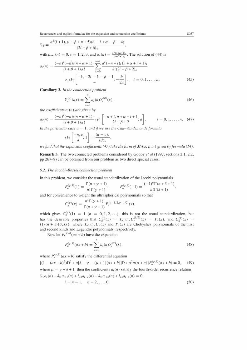
6.2. The Jacobi–Bessel connection problem

In this problem, we consider the usual standardization of the Jacobi polynomials

P (γ,δ)n (1) = �(n + γ + 1)

n!�(γ + 1), P (γ,δ)

n (−1) = (−1)n�(n + δ + 1)

n!�(δ + 1),

and for convenience to weight the ultraspherical polynomials so that

C(γ )n (x) = n!�(γ + 1)

�(n + γ + 1)P (γ−1/2,γ−1/2)

n (x),

which gives C(γ )n (1) = 1 (n = 0, 1, 2, . . .); this is not the usual standardization, but

has the desirable properties that C(0)n (x) = Tn(x), C

(1/2)n (x) = Pn(x), and C(1)

n (x) =(1/(n + 1))Un(x), where Tn(x), Un(x) and Pn(x) are Chebyshev polynomials of the firstand second kinds and Legendre polynomials, respectively.

Now let P(γ,δ)n (ax + b) have the expansion

P (γ,δ)n (ax + b) =

n∑i=0

ai(n)Y(α)i (x), (48)

where P(γ,δ)n (ax + b) satisfy the differential equation

[(1 − (ax + b)2)D2 + a[δ − γ − (µ + 1)(ax + b)]D + a2n(µ + n)]P (γ,δ)n (ax + b) = 0, (49)

where µ = γ + δ + 1, then the coefficients ai(n) satisfy the fourth-order recurrence relation

δi0ai(n) + δi1ai+1(n) + δi2ai+2(n) + δi3ai+3(n) + δi4ai+4(n) = 0,

i = n − 1, n − 2, . . . , 0, (50)

8058 E H Doha and H M Ahmed

where

δi0 = a2(n − i)(i + n + µ + 1)(i + α + 1)4

4(2i + α + 1)4,

δi1 = a(i + 1)(i + α + 2)3

4(2i + α + 3)2

[(1 − b

2

)(µ + 2i + 1) + (i + γ + 1)

+a[α(2i + 1) + 2(3i + 1) + 4n(n + µ) + (2 − 2i + α)µ]

(2i + α + 2)(2i + α + 6)

],

δi2 = 1

4(i + 1)2(α + i + 3)2

[(1 − b2

4

)− a((α − µ + 3)(1 − b) − α + 2γ − 2)

(α + 2i + 4)(α + 2i + 6)

+a2[2i2 + 2(α + 5)i + (3 + α)(3µ − α − 1) + 6n(n + µ)]

(α + 2i + 3)2(α + 2i + 6)2

],

δi3 = a(i + 1)3(i + α + 4)

4(2i + α + 6)2

[−

(1 − b

2

)(2i + 2α − µ + 9) + (i + α − γ + 4)

+a(2(α − µ + 3)i − (4 + α)(3µ − 2α − 7) − 4n(n + µ))

(α + 2i + 3)2(α + 2i + 6)2

],

δi4 = −a2(i + 1)4(i + α + n + 5)(i + α − n − µ + 5)

4(2i + α + 6)4,

with an+s(n) = 0, s = 1, 2, 3 and an(n) = an(n+µ)nn!(n+α+1)n

. The solution of (50) is

ai(n) = (γ + 1)n(−a)i

(i + α + 1)i i!n!

(−n)i(n + µ)i

(γ + 1)i

n−i∑k=0

ak

k!

(−n + i)k(n + µ + i)k

(γ + i + 1)k(2i + α + 2)k

× 2F0

[−k,−2i − k − α − 1; 1 − b

2a

], i = 0, 1, . . . , n. (51)

Corollary 4. In the connection problem

P (γ,δ)n (x) =

n∑i=0

ai(n)Y(α)i (x), (52)

the coefficients ai(n) are given by

ai(n) = (n + µ)i(γ + 1)n

i!(n − i)!(γ + 1)i(i + α + 1)i

n−i∑k=0

1

k!

(−n + i)k(n + µ + i)k

(γ + i + 1)k(2i + α + 2)k

× 2F0

[−k,−k − 2i − α − 1; 1

2

], i = 0, 1, . . . , n. (53)

Corollary 5. The link between ultraspherical–Bessel connection problem is given by

C(ν)n (x) =

n∑i=0

ai(n)Y(α)i (x), (54)

where the coefficients ai(n) are given by

ai(n) = n!(n + 2ν)i

i!(n − i)!(ν + 1/2)i(i + α + 1)i

n−i∑k=0

1

k!

(−n + i)k(n + 2ν + i)k

(ν + i + 1/2)k(2i + α + 2)k

× 2F0

[−k,−k − 2i − α − 1–

; 1

2

], i = 0, 1, . . . , n. (55)

Recurrences and explicit formulae for the expansion and connection coefficients 8059

Remark 4. It is worth noting that all the connection problems between the three orthogonalpolynomials, Chebyshev polynomials of the first and second kinds and Legendre polynomialsand Bessel polynomials can be easily deduced by taking ν = 0, 1, 1/2 in relations (54) and(55), respectively.

6.3. The Laguerre–Bessel connection problem

In this problem

L(γ )n (ax + b) =

n∑i=0

ai(n)Y(α)i (x), (56)

where L(γ )n (ax + b) are Laguerre polynomials, which satisfy the differential equation

[(ax + b)D2 + a(1 + γ − (ax + b))D + a2n]L(γ )n (ax + b) = 0. (57)

The coefficients ai(n) satisfy the recurrence relation

δi0ai(n) + δi1ai+1(n) + δi2ai+2(n) + δi3ai+3(n) + δi4ai+4(n) = 0,

i = n − 1, n − 2, . . . , 0, (58)

where

δi0 = a2(n − i)(i + α + 1)4

(2i + α + 1)4,

δi1 = −a(i + 1)(i + α + 2)3

2(2i + α + 3)2

[(b − i − γ − 1) +

2a(2i + 4n − 2 − α)

(2i + α + 2)(2i + α + 6)

],

δi2 = 1

4(i + 1)2(α + i + 3)2

[b − 2a(2b + α − 2γ + 2)

(α + 2i + 4)(α + 2i + 6)+

12a2(α + 2n + 3)

(α + 2i + 3)2(α + 2i + 6)2

],

δi3 = a(i + 1)3(i + α + 4)

2(2i + α + 6)2

[−(i + α + b − γ + 4) +

2a(2i + 3α + 4n + 12)

(α + 2i + 4)(α + 2i + 8)

],

δi4 = a2(i + 1)4(i + α + n + 5)

(2i + α + 6)4,

with an+s(n) = 0, s = 1, 2, 3 and an(n) = an(−2)n

n!(n+α+1)n. The solution of (58) is

ai(n) = (2a)i

(i + α + 1)i i!

(−n)i(γ + 1)n

n!(γ + 1)i

n−i∑k=0

(−2a)k

k!(2i + α + 2)k

(−(n − i))k

(γ + i + 1)k

× 2F0

[−k,−2i − k − α − 1–

;− b

2a

], i = 0, 1, . . . , n. (59)

Corollary 6. In the connection problem

L(γ )n (ax) =

n∑i=0

ai(n)Y(α)i (x),

the coefficients ai(n) are given by

ai(n) = (2a)i

(i + α + 1)i i!

(−n)i(γ + 1)n

n!(γ + 1)i1F2

[ −(n − i)

2i + α + 2, γ + i + 1;−2a

],

i = 0, 1, . . . , n. (60)

8060 E H Doha and H M Ahmed

6.4. The Hermite–Bessel connection problem

In this problem

Hn(ax + b) =n∑

i=0

ai(n)Y(α)i (x),

where Hn(x) are Hermite polynomials, which satisfy the differential equation

[D2 − 2a(ax + b)D + 2a2n]Hn(ax + b) = 0. (61)

The coefficients ai(n) satisfy the recurrence relation

δi0ai(n) + δi1ai+1(n) + δi2ai+2(n) + δi3ai+3(n) + δi4ai+4(n) = 0,

i = n − 1, n − 2, . . . , 0, (62)

where

δi0 = 2a2(i + α + 1)4(n − i)

(2i + α + 1)5,

δi1 = −a(i + 1)(i + α + 2)3

[b

(2i + α + 3)3− 2a(4n − 2i + α + 2)

(2i + α + 2)5

],

δi2 = 1

4(i + 1)2(i + α + 3)2

[1

(2i + α + 5)− 8ab

(2i + α + 4)3+

24a2(2n + α + 3)

(2i + α + 3)5

],

δi3 = a(i + α + 4)(i + 1)3

[− b

(2i + α + 5)3+

2a(4n + 2i + 3α + 12)

(2i + α + 4)5

],

δi4 = 2a2(i + 1)4(n + i + α + 5)

(2i + α + 5)5,

with an+s(n) = 0, s = 1, 2, 3 and an(n) = an22n

(n+α+1)n. The solution of (62) is

ai(n) = (2a)in!

(i + α + 1)i i!

[ n−i2 ]∑

k=0

(−1)k2n−2kbn−2k−i

k!(n − 2k − i)!1F1

[−(n − 2k − i)

2i + α + 2; 2a

b

],

i = 0, 1, . . . , n. (63)

Corollary 7. In the connection problem

Hn(ax) =n∑

i=0

ai(n)Y(α)i (x),

the coefficients ai(n) are given by

ai(n) = (−1)n−in!

(i + α + 1)i i!

[ n−i2 ]∑

k=0

(−1)k

k!(n − 2k − i)!

(4a)n−2k

(2i + α + 2)n−2k−i

, i = 0, 1, . . . , n. (64)

Remark 5. The expansions and connection coefficients in series of ordinary Besselpolynomials yn(x) can be obtained directly from those of the generalized Bessel polynomialsY (α)

n (x), by taking α = 0.

Recurrences and explicit formulae for the expansion and connection coefficients 8061

Remark 6. It is to be noted that one of our goals is to emphasize the systematic character andsimplicity of our algorithm, which allows one to implement it in any computer algebra (herethe Mathematica (1999)) symbolic language used.

To end this paper, we wish to report that this work deals with formulae associated with theBessel coefficients for the moments of a general-order derivative of differentiable functionsand with the connection coefficients between Bessel–Bessel, Jacobi–Bessel, Laguerre–Besseland Hermite–Bessel and other combinations with different parameters. These formulae can beused to facilitate greatly the setting up of the algebraic systems to be obtained by applying thespectral methods for solving differential equations with polynomial coefficients of any order.

Acknowledgments

The authors are grateful to the anonymous referees for their valuable comments andsuggestions.

References

Abramowitz M and Stegun I A (ed) 1970 Handbook of Mathematical Functions (Appl. Maths Series vol 55) (NewYork: National Bureau of Standards)

Agarwal R P 1954 On Bessel polynomials Can. J. Math. 6 410–5Alvarez-Nodarse R and Ronveaux A 1996 Recurrence relations for connection coefficients between q-orthogonal

polynomials of discrete variables in the non uniform lattice x(s) = q2s J. Phys. A: Math. Gen. 29 7165–75Al-Salam W 1957 The Bessel polynomials Duke Math. J. 24 529–45Alvarez-Nodarse, Yanez R J and Dehesa J S 1998 Modified Clebsch–Gordan-type expansions for products of discrete

hypergeometric polynomials J. Comput. Appl. Math. 89 171–97Andrews G E, Askey R and Roy R 1999 Special Functions (Cambridge: Cambridge University Press)Area I, Godoy E, Ronveaux A and Zarzo A 1998 Minimal recurrence relations for connection coefficients between

classical orthogonal polynomials: discrete case J. Comput. Appl. Math. 89 309–25Askey R and Gasper G 1971 Jacobi polynomials expansions of Jacobi polynomials with non-negative coefficients

Proc. Camb. Phil. Soc. 70 243–55Ben-Yu G 1998 Spectral Methods and Their Applications (London: World Scientific)Cannon B 1937 On the convergence of series of polynomials Proc. London Math. Soc. 43 348–64Canuto C, Hussaini M Y, Quarteroni A and Zang T A 1988 Spectral Methods in Fluid Dynamics (Berlin: Springer)Carlitz L 1957 On the Bessel polynomials Duke Math. J. 24 151–62Chihara T S 1978 An Introduction to Orthogonal Polynomials (New York: Gordon and Breach)Coutsias E A, Hagstorm T and Torres D 1996 An efficient spectral methods for ordinary differential equations with

rational function coefficients Math. Comput. 65 611–35Doha E H 1990 An accurate solution of parabolic equations by expansion in ultraspherical polynomials J. Comput.

Math. Appl. 19 75–88Doha E H 1991 The coefficients of differentiated expansions and derivatives of ultraspherical polynomials J. Comput.

Math. Appl. 21 115–22Doha E H 1994 The first and second kinds Chebyshev coefficients of the moments of the general-order derivative of

an infinitely differentiable function Int. J. Comput. Math. 51 21–35Doha E H 1998 The ultraspherical coefficients of the moments of a general-order derivative of an infinitely

differentiable function J. Comput. Appl. Math. 89 53–72Doha E H 2000 The coefficients of differentiated expansions of double and triple ultraspherical polynomials Ann.

Univ. Sci. Budapest, Sect. Comput. 19 57–73Doha E H 2002a On the coefficients of differentiated expansions and derivatives of Jacobi polynomials J. Phys. A:

Math. Gen. 35 3467–78Doha E H 2002b On the coefficients of integrated expansions and integrals of ultraspherical polynomials and their

applications for solving differential equations J. Comput. Appl. Math. 139 275–98Doha E H 2003a Explicit formulae for the coefficients of integrated expansions for Jacobi polynomials and their

integrals Integral Transforms Spec. Funct. 14 69–86

8062 E H Doha and H M Ahmed

Doha E H 2003b On the connection coefficients and recurrence relations arising from expansions in series of Laguerrepolynomials J. Phys. A: Math. Gen. 36 5449–62

Doha E H 2004a On the connection coefficients and recurrence relations arising from expansions in series of Hermitepolynomials Integral Transforms Spec. Funct. 15 13–29

Doha E H 2004b On the construction of recurrence relations for the expansion and connection coefficients in seriesof Jacobi polynomials J. Phys. A: Math. Gen. 37 657–75

Doha E H and Abd-Elhameed W M 2002 Efficient spectral Galerkin-algorithms for direct solution of second-orderequations using ultraspherical polynomials SIAM J. Sci. Comput. 24 548–71

Doha E H and Al-Kholi F M R 2001 An efficient double Legendre spectral method for parabolic and elliptic partialdifferential equations Int. J. Comput. Math. 78 413–32

Doha E H and El-Soubhy S I 1995 On the Legendre coefficients of the moments of general-order derivative of aninfinitely differentiable function Int. J. Comput. Math. 56 107–22

Doha E H and Helal M A 1997 An accurate double Chebyshev spectral approximation for parabolic partial differentialequations J. Egypt. Math. Soc. 5 83–101

Evans W D, Everitt W N, Kwon K H and Littlejohn L L 1993 Real orthogonalizing weights for Bessel polynomialsJ. Comput. Appl. Math. 49 51–7

Gasper G 1974 Project formulas for orthogonal polynomials of a discrete variable J. Math. Anal. Appl. 45 176–98Godoy E, Ronveaux A, Zarzo A and Area I 1997 Minimal recurrence relations for connection coefficients between

classical orthogonal polynomials: continuous case J. Comput. Appl. Math. 84 257–75Grosswald E 1978 Bessel polynomials Lecture Notes Math. 698 1–182Haidvogel D B and Zang T 1979 The accurate solution of Poisson’s equation by Chebyshev polynomials J. Comput.

Phys. 30 167–80Han S S and Kwon K H 1991 Spectral analysis of Bessel polynomials in Krein space Quaest. Math. 14 327–35Helal M A 2001 A Chebyshev spectral method for solving Korteweg–de Vries equation with hydrodynamical

application Chaos Solitons Fractals 12 943–50Karageorghis A 1988a A note on the Chebyshev coefficients of the general-order derivative of an infinitely

differentiable function J. Comput. Appl. Math. 21 129–32Karageorghis A 1988b A note on the Chebyshev coefficients of the moments of the general-order derivative of an

infinitely differentiable function J. Comput. Appl. Math. 21 383–6Karageorghis A and Phillips T N 1989 On the coefficients of differentiated expansions of ultraspherical polynomials

ICASE Report no 89-65 NASA Langley Research Center, Hampton, VAKarageorghis A and Phillips T N 1992 Appl. Numer. Math. 9 133–41Koepf W and Schmersau D 1998 Representations of orthogonal polynomials J. Comput. Appl. Math. 90 57–94Krall H L and Frink O 1949 A new class of orthogonal polynomials : the Bessel polynomials Trans. Am. Math. Soc.

65 100–5Lewanowicz S 2002 Recurrences of coefficients of series expansions with respect to classical orthogonal polynomials

Appl. Math. 29 97–116Lewanowicz S, Godoy E, Area I, Ronveaux A and Zarzo A 2000 Recurrence relations for coefficients of Fourier

series expansions with respect to q-classical orthogonal polynomials Numer. Algorithms 23 31–50Lewanowicz S and Wozny P 2001 Algorithms for construction of recurrence relations for the coefficients of expansions

in series of classical orthogonal polynomials Preprint Institute of Computer Science University of Wroclawonline at http://www.ii.uni.wroc.pl/sle/publ.html

Luke Y L 1969 The Special Functions and Their Approximations vols 1 and 2 (New York: Academic)Nassif M 1954 Note on the Bessel polynomials Trans. Am. Math. Soc. 77 408–12Phillips T N 1988 On the Legendre coefficients of a general-order derivative of an infinitely differentiable function

IMA. J. Numer. Anal. 8 455–9Rainville E D 1960 Special Functions (New York: Macmillan)Ronveaux A, Belmehdi S, Godoy E and Zarzo A 1996 Recurrence relation approach for connection coefficients.

Applications to classical discrete orthogonal polynomials CRM Proc. and Lecture notes vol 9 (Centre deResearches Mathematiques) pp 319–35

Ronveaux A, Zarzo A and Godoy E 1995 Recurrence relations for connection coefficients between two families oforthogonal polynomials J. Comput. Appl. Math. 62 67–73

Sanchez-Ruiz J and Dehesa J S 1998 Expansions in series of orthogonal polynomials J. Comput. Appl. Math. 89155–70

Siyyam H I and Syam M I 1997 An accurate solution of Poisson equation by the Chebyshev–Tau methods J. Comput.Appl. Math. 85 1–10

Szego G 1985 Orthogonal Polynomials (American Mathematical Society Colloquium Publications vol 23)(Providence, RI: American Mathematical Society)

Recurrences and explicit formulae for the expansion and connection coefficients 8063

Voigt R G, Gottlieb D and Hussaini M Y 1984 Spectral Methods for Partial Differential Equations (Philadelphia, PA:SIAM)

Whittaker J M 1949 Sur les series de base de polynomes quelconques (Paris: Gauthier-Villars)Wolfram Research Inc. 1999 Mathematica Version 4.0 (Wolfram Research Champaign)Zarzo A, Area I, Godoy E and Ronveaux A 1997 Results for some inversion problems for classical continuous and

discrete orthogonal polynomials J. Phys. A: Math. Gen. 30 35–40