Classical linear regression model assumptions and diagnostic ...
77
4 Classical linear regression model assumptions and diagnostic tests Learning Outcomes In this chapter, you will learn how to ● Describe the steps involved in testing regression residuals for heteroscedasticity and autocorrelation ● Explain the impact of heteroscedasticity or autocorrelation on the optimality of OLS parameter and standard error estimation ● Distinguish between the Durbin--Watson and Breusch--Godfrey tests for autocorrelation ● Highlight the advantages and disadvantages of dynamic models ● Test for whether the functional form of the model employed is appropriate ● Determine whether the residual distribution from a regression differs significantly from normality ● Investigate whether the model parameters are stable ● Appraise different philosophies of how to build an econometric model ● Conduct diagnostic tests in EViews 4.1 Introduction Recall that five assumptions were made relating to the classical linear re- gression model (CLRM). These were required to show that the estimation technique, ordinary least squares (OLS), had a number of desirable proper- ties, and also so that hypothesis tests regarding the coefficient estimates could validly be conducted. Specifically, it was assumed that: (1) E(u t ) = 0 (2) var(u t ) = σ 2 < ∞ (3) cov(u i ,u j ) = 0 129
-
Upload
khangminh22 -
Category
Documents
-
view
2 -
download
0
Transcript of Classical linear regression model assumptions and diagnostic ...
4Classical linear regression model assumptions
and diagnostic tests
Learning Outcomes
In this chapter, you will learn how to
● Describe the steps involved in testing regression residuals forheteroscedasticity and autocorrelation
● Explain the impact of heteroscedasticity or autocorrelation onthe optimality of OLS parameter and standard error estimation
● Distinguish between the Durbin--Watson and Breusch--Godfreytests for autocorrelation
● Highlight the advantages and disadvantages of dynamic models
● Test for whether the functional form of the model employed isappropriate
● Determine whether the residual distribution from a regressiondiffers significantly from normality
● Investigate whether the model parameters are stable
● Appraise different philosophies of how to build an econometricmodel
● Conduct diagnostic tests in EViews
4.1 Introduction
Recall that five assumptions were made relating to the classical linear re-
gression model (CLRM). These were required to show that the estimation
technique, ordinary least squares (OLS), had a number of desirable proper-
ties, and also so that hypothesis tests regarding the coefficient estimates
could validly be conducted. Specifically, it was assumed that:
(1) E(ut ) = 0
(2) var(ut ) = σ 2 < ∞
(3) cov(ui ,u j ) = 0
129
130 Introductory Econometrics for Finance
(4) cov(ut ,xt ) = 0
(5) ut ∼ N(0, σ 2)
These assumptions will now be studied further, in particular looking at
the following:
● How can violations of the assumptions be detected?
● What are the most likely causes of the violations in practice?
● What are the consequences for the model if an assumption is violated
but this fact is ignored and the researcher proceeds regardless?
The answer to the last of these questions is that, in general, the model
could encounter any combination of three problems:
● the coefficient estimates (βs) are wrong
● the associated standard errors are wrong
● the distributions that were assumed for the test statistics are inappro-
priate.
A pragmatic approach to ‘solving’ problems associated with the use of
models where one or more of the assumptions is not supported by the
data will then be adopted. Such solutions usually operate such that:
● the assumptions are no longer violated, or
● the problems are side-stepped, so that alternative techniques are used
which are still valid.
4.2 Statistical distributions for diagnostic tests
The text below discusses various regression diagnostic (misspecification)
tests that are based on the calculation of a test statistic. These tests can
be constructed in several ways, and the precise approach to constructing
the test statistic will determine the distribution that the test statistic is
assumed to follow. Two particular approaches are in common usage and
their results are given by the statistical packages: the LM test and the Wald
test. Further details concerning these procedures are given in chapter 8.
For now, all that readers require to know is that LM test statistics in the
context of the diagnostic tests presented here follow a χ2 distribution
with degrees of freedom equal to the number of restrictions placed
on the model, and denoted m. The Wald version of the test follows an
F-distribution with (m, T − k) degrees of freedom. Asymptotically, these
two tests are equivalent, although their results will differ somewhat
in small samples. They are equivalent as the sample size increases
towards infinity since there is a direct relationship between the χ2- and

Classical linear regression model assumptions and diagnostic tests 131
F-distributions. Taking a χ2 variate and dividing by its degrees of freedom
asymptotically gives an F -variate
χ2(m)
m→ F(m, T − k) as T → ∞
Computer packages typically present results using both approaches, al-
though only one of the two will be illustrated for each test below. They will
usually give the same conclusion, although if they do not, the F-version
is usually considered preferable for finite samples, since it is sensitive to
sample size (one of its degrees of freedom parameters depends on sample
size) in a way that the χ2-version is not.
4.3 Assumption 1: E(ut ) = 0
The first assumption required is that the average value of the errors is
zero. In fact, if a constant term is included in the regression equation, this
assumption will never be violated. But what if financial theory suggests
that, for a particular application, there should be no intercept so that
the regression line is forced through the origin? If the regression did
not include an intercept, and the average value of the errors was non-
zero, several undesirable consequences could arise. First, R2, defined as
ESS/TSS can be negative, implying that the sample average, y, ‘explains’
more of the variation in y than the explanatory variables. Second, and
more fundamentally, a regression with no intercept parameter could lead
to potentially severe biases in the slope coefficient estimates. To see this,
consider figure 4.1.
yt
x t
Figure 4.1
Effect of no
intercept on a
regression line

132 Introductory Econometrics for Finance
The solid line shows the regression estimated including a constant term,
while the dotted line shows the effect of suppressing (i.e. setting to zero)
the constant term. The effect is that the estimated line in this case is
forced through the origin, so that the estimate of the slope coefficient
(β) is biased. Additionally, R2 and R2 are usually meaningless in such a
context. This arises since the mean value of the dependent variable, y,
will not be equal to the mean of the fitted values from the model, i.e. the
mean of y if there is no constant in the regression.
4.4 Assumption 2: var(ut ) = σ2 < ∞
It has been assumed thus far that the variance of the errors is con-
stant, σ 2 -- this is known as the assumption of homoscedasticity. If the er-
rors do not have a constant variance, they are said to be heteroscedastic.
To consider one illustration of heteroscedasticity, suppose that a regres-
sion had been estimated and the residuals, ut , have been calculated and
then plotted against one of the explanatory variables, x2t , as shown in
figure 4.2.
It is clearly evident that the errors in figure 4.2 are heteroscedastic --
that is, although their mean value is roughly constant, their variance is
increasing systematically with x2t .
ût
x2t
+
–
Figure 4.2
Graphical
illustration of
heteroscedasticity

Classical linear regression model assumptions and diagnostic tests 133
4.4.1 Detection of heteroscedasticity
How can one tell whether the errors are heteroscedastic or not? It is pos-
sible to use a graphical method as above, but unfortunately one rarely
knows the cause or the form of the heteroscedasticity, so that a plot is
likely to reveal nothing. For example, if the variance of the errors was
an increasing function of x3t , and the researcher had plotted the residu-
als against x2t , he would be unlikely to see any pattern and would thus
wrongly conclude that the errors had constant variance. It is also possible
that the variance of the errors changes over time rather than systemati-
cally with one of the explanatory variables; this phenomenon is known
as ‘ARCH’ and is described in chapter 8.
Fortunately, there are a number of formal statistical tests for het-
eroscedasticity, and one of the simplest such methods is the Goldfeld--
Quandt (1965) test. Their approach is based on splitting the total sample
of length T into two sub-samples of length T1 and T2. The regression model
is estimated on each sub-sample and the two residual variances are cal-
culated as s21 = u′
1u1/(T1 − k) and s22 = u′
2u2/(T2 − k) respectively. The null
hypothesis is that the variances of the disturbances are equal, which can
be written H0 : σ 21 = σ 2
2 , against a two-sided alternative. The test statistic,
denoted GQ, is simply the ratio of the two residual variances where the
larger of the two variances must be placed in the numerator (i.e. s21 is the
higher sample variance for the sample with length T1, even if it comes
from the second sub-sample):
GQ =s2
1
s22
(4.1)
The test statistic is distributed as an F(T1 − k, T2 − k) under the null hy-
pothesis, and the null of a constant variance is rejected if the test statistic
exceeds the critical value.
The GQ test is simple to construct but its conclusions may be contin-
gent upon a particular, and probably arbitrary, choice of where to split
the sample. Clearly, the test is likely to be more powerful when this choice
is made on theoretical grounds -- for example, before and after a major
structural event. Suppose that it is thought that the variance of the dis-
turbances is related to some observable variable zt (which may or may not
be one of the regressors). A better way to perform the test would be to
order the sample according to values of zt (rather than through time) and
then to split the re-ordered sample into T1 and T2.
An alternative method that is sometimes used to sharpen the inferences
from the test and to increase its power is to omit some of the observations

134 Introductory Econometrics for Finance
from the centre of the sample so as to introduce a degree of separation
between the two sub-samples.
A further popular test is White’s (1980) general test for heteroscedas-
ticity. The test is particularly useful because it makes few assumptions
about the likely form of the heteroscedasticity. The test is carried out as
in box 4.1.
Box 4.1 Conducting White’s test
(1) Assume that the regression model estimated is of the standard linear form, e.g.
yt = β1 + β2x2t + β3x3t + ut (4.2)
To test var(ut ) = σ 2, estimate the model above, obtaining the residuals, ut
(2) Then run the auxiliary regression
u2t = α1 + α2x2t + α3x3t + α4x2
2t + α5x23t + α6x2t x3t + vt (4.3)
where vt is a normally distributed disturbance term independent of ut . This
regression is of the squared residuals on a constant, the original explanatory
variables, the squares of the explanatory variables and their cross-products. To see
why the squared residuals are the quantity of interest, recall that for a random
variable ut , the variance can be written
var(ut ) = E[(ut − E(ut ))2] (4.4)
Under the assumption that E(ut ) = 0, the second part of the RHS of this
expression disappears:
var(ut ) = E
[
u2t
]
(4.5)
Once again, it is not possible to know the squares of the population disturbances,
u2t , so their sample counterparts, the squared residuals, are used instead.
The reason that the auxiliary regression takes this form is that it is desirable to
investigate whether the variance of the residuals (embodied in u2t ) varies
systematically with any known variables relevant to the model. Relevant variables
will include the original explanatory variables, their squared values and their
cross-products. Note also that this regression should include a constant term,
even if the original regression did not. This is as a result of the fact that u2t will
always have a non-zero mean, even if ut has a zero mean.
(3) Given the auxiliary regression, as stated above, the test can be conducted using
two different approaches. First, it is possible to use the F-test framework described
in chapter 3. This would involve estimating (4.3) as the unrestricted regression and
then running a restricted regression of u2t on a constant only. The RSS from each
specification would then be used as inputs to the standard F-test formula.
With many diagnostic tests, an alternative approach can be adopted that does
not require the estimation of a second (restricted) regression. This approach is
known as a Lagrange Multiplier (LM) test, which centres around the value of R2 for
the auxiliary regression. If one or more coefficients in (4.3) is statistically
significant, the value of R2 for that equation will be relatively high, while if none of
the variables is significant, R2 will be relatively low. The LM test would thus operate

Classical linear regression model assumptions and diagnostic tests 135
by obtaining R2 from the auxiliary regression and multiplying it by the number of
observations, T . It can be shown that
TR2 ∼ χ2(m)
where m is the number of regressors in the auxiliary regression (excluding the
constant term), equivalent to the number of restrictions that would have to be
placed under the F-test approach.
(4) The test is one of the joint null hypothesis that α2 = 0, and α3 = 0, and α4 = 0,
and α5 = 0, and α6 = 0. For the LM test, if the χ2-test statistic from step 3 is
greater than the corresponding value from the statistical table then reject the null
hypothesis that the errors are homoscedastic.
Example 4.1
Suppose that the model (4.2) above has been estimated using 120 obser-
vations, and the R2 from the auxiliary regression (4.3) is 0.234. The test
statistic will be given by TR2 = 120 × 0.234 = 28.8, which will follow a
χ2(5) under the null hypothesis. The 5% critical value from the χ2 table is
11.07. The test statistic is therefore more than the critical value and hence
the null hypothesis is rejected. It would be concluded that there is signif-
icant evidence of heteroscedasticity, so that it would not be plausible to
assume that the variance of the errors is constant in this case.
4.4.2 Consequences of using OLS in the presence of heteroscedasticity
What happens if the errors are heteroscedastic, but this fact is ignored
and the researcher proceeds with estimation and inference? In this case,
OLS estimators will still give unbiased (and also consistent) coefficient
estimates, but they are no longer BLUE -- that is, they no longer have the
minimum variance among the class of unbiased estimators. The reason
is that the error variance, σ 2, plays no part in the proof that the OLS
estimator is consistent and unbiased, but σ 2 does appear in the formulae
for the coefficient variances. If the errors are heteroscedastic, the formulae
presented for the coefficient standard errors no longer hold. For a very
accessible algebraic treatment of the consequences of heteroscedasticity,
see Hill, Griffiths and Judge (1997, pp. 217--18).
So, the upshot is that if OLS is still used in the presence of heteroscedas-
ticity, the standard errors could be wrong and hence any inferences made
could be misleading. In general, the OLS standard errors will be too
large for the intercept when the errors are heteroscedastic. The effect of
heteroscedasticity on the slope standard errors will depend on its form.
For example, if the variance of the errors is positively related to the
136 Introductory Econometrics for Finance
square of an explanatory variable (which is often the case in practice), the
OLS standard error for the slope will be too low. On the other hand, the
OLS slope standard errors will be too big when the variance of the errors
is inversely related to an explanatory variable.
4.4.3 Dealing with heteroscedasticity
If the form (i.e. the cause) of the heteroscedasticity is known, then an alter-
native estimation method which takes this into account can be used. One
possibility is called generalised least squares (GLS). For example, suppose
that the error variance was related to zt by the expression
var(ut ) = σ 2z2t (4.6)
All that would be required to remove the heteroscedasticity would be to
divide the regression equation through by zt
yt
zt
= β1
1
zt
+ β2
x2t
zt
+ β3
x3t
zt
+ vt (4.7)
where vt =ut
zt
is an error term.
Now, if var(ut ) = σ 2z2t , var(vt ) = var
(
ut
zt
)
=var(ut )
z2t
=σ 2z2
t
z2t
= σ 2 for
known z.
Therefore, the disturbances from (4.7) will be homoscedastic. Note that
this latter regression does not include a constant since β1 is multiplied by
(1/zt ). GLS can be viewed as OLS applied to transformed data that satisfy
the OLS assumptions. GLS is also known as weighted least squares (WLS),
since under GLS a weighted sum of the squared residuals is minimised,
whereas under OLS it is an unweighted sum.
However, researchers are typically unsure of the exact cause of the het-
eroscedasticity, and hence this technique is usually infeasible in practice.
Two other possible ‘solutions’ for heteroscedasticity are shown in box 4.2.
Examples of tests for heteroscedasticity in the context of the single in-
dex market model are given in Fabozzi and Francis (1980). Their results are
strongly suggestive of the presence of heteroscedasticity, and they examine
various factors that may constitute the form of the heteroscedasticity.
4.4.4 Testing for heteroscedasticity using EViews
Re-open the Microsoft Workfile that was examined in the previous chap-
ter and the regression that included all the macroeconomic explanatory
variables. First, plot the residuals by selecting View/Actual, Fitted, Residu-
als/Residual Graph. If the residuals of the regression have systematically
changing variability over the sample, that is a sign of heteroscedasticity.

Classical linear regression model assumptions and diagnostic tests 137
In this case, it is hard to see any clear pattern, so we need to run the
formal statistical test. To test for heteroscedasticity using White’s test,
click on the View button in the regression window and select Residual
Tests/Heteroscedasticity Tests. You will see a large number of different
tests available, including the ARCH test that will be discussed in chapter
8. For now, select the White specification. You can also select whether
to include the cross-product terms or not (i.e. each variable multiplied by
each other variable) or include only the squares of the variables in the
auxiliary regression. Uncheck the ‘Include White cross terms’ given the
relatively large number of variables in this regression and then click OK.
The results of the test will appear as follows.
Heteroskedasticity Test: White
F-statistic 0.626761 Prob. F(7,244) 0.7336Obs∗R-squared 4.451138 Prob. Chi-Square(7) 0.7266Scaled explained SS 21.98760 Prob. Chi-Square(7) 0.0026
Test Equation:Dependent Variable: RESID∧2
Method: Least SquaresDate: 08/27/07 Time: 11:49Sample: 1986M05 2007M04Included observations: 252
Coefficient Std. Error t-Statistic Prob.
C 259.9542 65.85955 3.947099 0.0001ERSANDP∧2 −0.130762 0.826291 −0.158252 0.8744DPROD∧2 −7.465850 7.461475 −1.000586 0.3180
DCREDIT∧2 −1.65E-07 3.72E-07 −0.443367 0.6579DINFLATION∧2 −137.6317 227.2283 −0.605698 0.5453
DMONEY∧2 12.79797 13.66363 0.936645 0.3499DSPREAD∧2 −650.6570 3144.176 −0.20694 0.8362RTERM∧2 −491.0652 418.2860 −1.173994 0.2415
R-squared 0.017663 Mean dependent var 188.4152Adjusted R-squared −0.010519 S.D. dependent var 612.8558S.E. of regression 616.0706 Akaike info criterion 15.71583Sum squared resid 92608485 Schwarz criterion 15.82788Log likelihood −1972.195 Hannan-Quinn criter. 15.76092F-statistic 0.626761 Durbin-Watson stat 2.068099Prob(F-statistic) 0.733596
EViews presents three different types of tests for heteroscedasticity and
then the auxiliary regression in the first results table displayed. The test
statistics give us the information we need to determine whether the
assumption of homoscedasticity is valid or not, but seeing the actual

138 Introductory Econometrics for Finance
Box 4.2 ‘Solutions’ for heteroscedasticity
(1) Transforming the variables into logs or reducing by some other measure of ‘size’. This
has the effect of re-scaling the data to ‘pull in’ extreme observations. The regression
would then be conducted upon the natural logarithms or the transformed data. Taking
logarithms also has the effect of making a previously multiplicative model, such as
the exponential regression model discussed previously (with a multiplicative error
term), into an additive one. However, logarithms of a variable cannot be taken in
situations where the variable can take on zero or negative values, for the log will not
be defined in such cases.
(2) Using heteroscedasticity-consistent standard error estimates. Most standard econo-
metrics software packages have an option (usually called something like ‘robust’)
that allows the user to employ standard error estimates that have been modified to
account for the heteroscedasticity following White (1980). The effect of using the
correction is that, if the variance of the errors is positively related to the square of
an explanatory variable, the standard errors for the slope coefficients are increased
relative to the usual OLS standard errors, which would make hypothesis testing more
‘conservative’, so that more evidence would be required against the null hypothesis
before it would be rejected.
auxiliary regression in the second table can provide useful additional in-
formation on the source of the heteroscedasticity if any is found. In this
case, both the F - and χ2 (‘LM’) versions of the test statistic give the same
conclusion that there is no evidence for the presence of heteroscedasticity,
since the p-values are considerably in excess of 0.05. The third version of
the test statistic, ‘Scaled explained SS’, which as the name suggests is based
on a normalised version of the explained sum of squares from the auxil-
iary regression, suggests in this case that there is evidence of heteroscedas-
ticity. Thus the conclusion of the test is somewhat ambiguous here.
4.4.5 Using White’s modified standard error estimates in EViews
In order to estimate the regression with heteroscedasticity-robust standard
errors in EViews, select this from the option button in the regression entry
window. In other words, close the heteroscedasticity test window and click
on the original ‘Msoftreg’ regression results, then click on the Estimate
button and in the Equation Estimation window, choose the Options tab
and screenshot 4.1 will appear.
Check the ‘Heteroskedasticity consistent coefficient variance’ box and
click OK. Comparing the results of the regression using heteroscedasticity-
robust standard errors with those using the ordinary standard er-
rors, the changes in the significances of the parameters are only
marginal. Of course, only the standard errors have changed and the
parameter estimates have remained identical to those from before. The

Classical linear regression model assumptions and diagnostic tests 139
Screenshot 4.1
Regression options
window
heteroscedasticity-consistent standard errors are smaller for all variables
except for money supply, resulting in the p-values being smaller. The main
changes in the conclusions reached are that the term structure variable,
which was previously significant only at the 10% level, is now significant
at 5%, and the unexpected inflation variable is now significant at the 10%
level.
4.5 Assumption 3: cov(ui , u j ) = 0 for i �= j
Assumption 3 that is made of the CLRM’s disturbance terms is that the
covariance between the error terms over time (or cross-sectionally, for
that type of data) is zero. In other words, it is assumed that the errors are
uncorrelated with one another. If the errors are not uncorrelated with
one another, it would be stated that they are ‘autocorrelated’ or that they
are ‘serially correlated’. A test of this assumption is therefore required.
Again, the population disturbances cannot be observed, so tests for
autocorrelation are conducted on the residuals, u. Before one can proceed
to see how formal tests for autocorrelation are formulated, the concept
of the lagged value of a variable needs to be defined.

140 Introductory Econometrics for Finance
Table 4.1 Constructing a series of lagged values and first differences
t yt yt−1 �yt
2006M09 0.8 − −
2006M10 1.3 0.8 (1.3 − 0.8) = 0.52006M11 −0.9 1.3 (−0.9 − 1.3) = −2.22006M12 0.2 −0.9 (0.2 − −0.9) = 1.12007M01 −1.7 0.2 (−1.7 −0.2) = −1.92007M02 2.3 −1.7 (2.3 − −1.7) = 4.02007M03 0.1 2.3 (0.1 − 2.3) = −2.22007M04 0.0 0.1 (0.0 − 0.1) = −0.1. . . .. . . .. . . .
4.5.1 The concept of a lagged value
The lagged value of a variable (which may be yt , xt , or ut ) is simply the
value that the variable took during a previous period. So for example, the
value of yt lagged one period, written yt−1, can be constructed by shifting
all of the observations forward one period in a spreadsheet, as illustrated
in table 4.1.
So, the value in the 2006M10 row and the yt−1 column shows the value
that yt took in the previous period, 2006M09, which was 0.8. The last
column in table 4.1 shows another quantity relating to y, namely the
‘first difference’. The first difference of y, also known as the change in y,
and denoted �yt , is calculated as the difference between the values of y
in this period and in the previous period. This is calculated as
�yt = yt − yt−1 (4.8)
Note that when one-period lags or first differences of a variable are con-
structed, the first observation is lost. Thus a regression of �yt using the
above data would begin with the October 2006 data point. It is also possi-
ble to produce two-period lags, three-period lags, and so on. These would
be accomplished in the obvious way.
4.5.2 Graphical tests for autocorrelation
In order to test for autocorrelation, it is necessary to investigate whether
any relationships exist between the current value of u, ut , and any of
its previous values, ut−1, ut−2, . . . The first step is to consider possible

Classical linear regression model assumptions and diagnostic tests 141
ût
û t–1
+
–
+–
Figure 4.3
Plot of ut against
ut−1, showing
positive
autocorrelation
relationships between the current residual and the immediately previ-
ous one, ut−1, via a graphical exploration. Thus ut is plotted against ut−1,
and ut is plotted over time. Some stereotypical patterns that may be found
in the residuals are discussed below.
Figures 4.3 and 4.4 show positive autocorrelation in the residuals, which
is indicated by a cyclical residual plot over time. This case is known as pos-
itive autocorrelation since on average if the residual at time t − 1 is positive,
the residual at time t is likely to be also positive; similarly, if the residual
at t − 1 is negative, the residual at t is also likely to be negative. Figure 4.3
shows that most of the dots representing observations are in the first and
third quadrants, while figure 4.4 shows that a positively autocorrelated
series of residuals will not cross the time-axis very frequently.
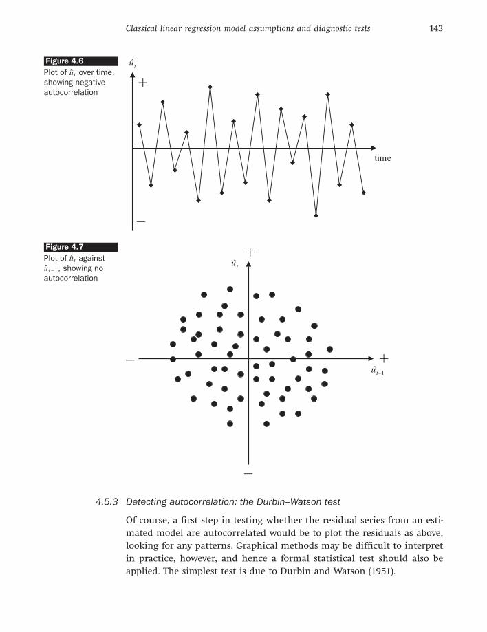
Figures 4.5 and 4.6 show negative autocorrelation, indicated by an
alternating pattern in the residuals. This case is known as negative
autocorrelation since on average if the residual at time t − 1 is positive,
the residual at time t is likely to be negative; similarly, if the residual
at t − 1 is negative, the residual at t is likely to be positive. Figure 4.5
shows that most of the dots are in the second and fourth quadrants,
while figure 4.6 shows that a negatively autocorrelated series of residu-
als will cross the time-axis more frequently than if they were distributed
randomly.

142 Introductory Econometrics for Finance
ût
+
–
time
Figure 4.4
Plot of ut over time,
showing positive
autocorrelation
ût
û t–1
+
–
+–
Figure 4.5
Plot of ut against
ut−1, showing
negative
autocorrelation
Finally, figures 4.7 and 4.8 show no pattern in residuals at all: this is
what is desirable to see. In the plot of ut against ut−1 (figure 4.7), the points
are randomly spread across all four quadrants, and the time series plot of
the residuals (figure 4.8) does not cross the x -axis either too frequently or
too little.
Classical linear regression model assumptions and diagnostic tests 143
ût
+
–
time
Figure 4.6
Plot of ut over time,
showing negative
autocorrelation
ût
û t–1
+
–
+–
Figure 4.7
Plot of ut against
ut−1, showing no
autocorrelation
4.5.3 Detecting autocorrelation: the Durbin–Watson test
Of course, a first step in testing whether the residual series from an esti-
mated model are autocorrelated would be to plot the residuals as above,
looking for any patterns. Graphical methods may be difficult to interpret
in practice, however, and hence a formal statistical test should also be
applied. The simplest test is due to Durbin and Watson (1951).

144 Introductory Econometrics for Finance
ût
+
–
time
Figure 4.8
Plot of ut over time,
showing no
autocorrelation
Durbin--Watson (DW) is a test for first order autocorrelation -- i.e. it tests
only for a relationship between an error and its immediately previous
value. One way to motivate the test and to interpret the test statistic
would be in the context of a regression of the time t error on its previous
value
ut = ρut−1 + vt (4.9)
where vt ∼ N (0, σ 2v ). The DW test statistic has as its null and alternative
hypotheses
H0 : ρ = 0 and H1 : ρ �= 0
Thus, under the null hypothesis, the errors at time t − 1 and t are indepen-
dent of one another, and if this null were rejected, it would be concluded
that there was evidence of a relationship between successive residuals. In
fact, it is not necessary to run the regression given by (4.9) since the test
statistic can be calculated using quantities that are already available after
the first regression has been run
DW =
T∑
t=2
(ut − ut−1)2
T∑
t=2
u2t
(4.10)
The denominator of the test statistic is simply (the number of observations
−1) × the variance of the residuals. This arises since if the average of the

Classical linear regression model assumptions and diagnostic tests 145
residuals is zero
var(ut ) = E(u2t ) =
1
T − 1
T∑
t=2
u2t
so thatT
∑
t=2
u2t = var(ut ) × (T − 1)
The numerator ‘compares’ the values of the error at times t − 1 and t .
If there is positive autocorrelation in the errors, this difference in the
numerator will be relatively small, while if there is negative autocorrela-
tion, with the sign of the error changing very frequently, the numerator
will be relatively large. No autocorrelation would result in a value for the
numerator between small and large.
It is also possible to express the DW statistic as an approximate function
of the estimated value of ρ
DW ≈ 2(1 − ρ) (4.11)
where ρ is the estimated correlation coefficient that would have been
obtained from an estimation of (4.9). To see why this is the case, consider
that the numerator of (4.10) can be written as the parts of a quadratic
T∑
t=2
(ut − ut−1)2 =
T∑
t=2
u2t +
T∑
t=2
u2t−1 − 2
T∑
t=2
ut ut−1 (4.12)
Consider now the composition of the first two summations on the RHS of
(4.12). The first of these is
T∑
t=2
u2t = u2
2 + u23 + u2
4 + · · · + u2T
while the second is
T∑
t=2
u2t−1 = u2
1 + u22 + u2
3 + · · · + u2T −1
Thus, the only difference between them is that they differ in the first and
last terms in the summation
T∑
t=2
u2t
contains u2T but not u2
1, while
T∑
t=2
u2t−1

146 Introductory Econometrics for Finance
contains u21 but not u2
T . As the sample size, T , increases towards infin-
ity, the difference between these two will become negligible. Hence, the
expression in (4.12), the numerator of (4.10), is approximately
2
T∑
t=2
u2t − 2
T∑
t=2
ut ut−1
Replacing the numerator of (4.10) with this expression leads to
DW ≈
2
T∑
t=2
u2t − 2
T∑
t=2
ut ut−1
T∑
t=2
u2t
= 2
⎛
⎜
⎜
⎜
⎜
⎝
1 −
T∑
t=2
ut ut−1
T∑
t=2
u2t
⎞
⎟
⎟
⎟
⎟
⎠
(4.13)
The covariance between ut and ut−1 can be written as E[(ut − E(ut ))(ut−1 −
E(ut−1))]. Under the assumption that E(ut ) = 0 (and therefore that E(ut−1) =
0), the covariance will be E[ut ut−1]. For the sample residuals, this covari-
ance will be evaluated as
1
T − 1
T∑
t=2
ut ut−1
Thus, the sum in the numerator of the expression on the right of (4.13)
can be seen as T − 1 times the covariance between ut and ut−1, while the
sum in the denominator of the expression on the right of (4.13) can be
seen from the previous exposition as T − 1 times the variance of ut . Thus,
it is possible to write
DW ≈ 2
(
1 −T − 1 cov(ut , ut−1)
T − 1 var(ut )
)
= 2
(
1 −cov(ut , ut−1)
var(ut )
)
= 2 (1 − corr(ut , ut−1)) (4.14)
so that the DW test statistic is approximately equal to 2(1 − ρ). Since ρ
is a correlation, it implies that −1 ≤ ρ ≤ 1. That is, ρ is bounded to lie
between −1 and +1. Substituting in these limits for ρ to calculate DW
from (4.11) would give the corresponding limits for DW as 0 ≤ DW ≤ 4.
Consider now the implication of DW taking one of three important values
(0, 2, and 4):
● ρ = 0, DW = 2 This is the case where there is no autocorrelation in
the residuals. So roughly speaking, the null hypothesis would not be
rejected if DW is near 2 → i.e. there is little evidence of autocorrelation.
● ρ = 1, DW = 0 This corresponds to the case where there is perfect pos-
itive autocorrelation in the residuals.

Classical linear regression model assumptions and diagnostic tests 147
Reject H0:
positive
autocorrelation
Inconclusive
Do not reject
H0: No evidence
of autocorrelation
Inconclusive
Reject H0:
negative
autocorrelation
0 dL dU 4-dU2 4-dL 4
Figure 4.9 Rejection and non-rejection regions for DW test
● ρ = −1, DW = 4 This corresponds to the case where there is perfect
negative autocorrelation in the residuals.
The DW test does not follow a standard statistical distribution such as a
t , F , or χ2. DW has 2 critical values: an upper critical value (dU) and a
lower critical value (dL ), and there is also an intermediate region where
the null hypothesis of no autocorrelation can neither be rejected nor not
rejected! The rejection, non-rejection, and inconclusive regions are shown
on the number line in figure 4.9.
So, to reiterate, the null hypothesis is rejected and the existence of pos-
itive autocorrelation presumed if DW is less than the lower critical value;
the null hypothesis is rejected and the existence of negative autocorrela-
tion presumed if DW is greater than 4 minus the lower critical value; the
null hypothesis is not rejected and no significant residual autocorrelation
is presumed if DW is between the upper and 4 minus the upper limits.
Example 4.2
A researcher wishes to test for first order serial correlation in the residuals
from a linear regression. The DW test statistic value is 0.86. There are 80
quarterly observations in the regression, and the regression is of the form
yt = β1 + β2x2t + β3x3t + β4x4t + ut (4.15)
The relevant critical values for the test (see table A2.6 in the appendix of
statistical distributions at the end of this book), are dL = 1.42, dU = 1.57, so
4 − dU = 2.43 and 4 − dL = 2.58. The test statistic is clearly lower than the
lower critical value and hence the null hypothesis of no autocorrelation
is rejected and it would be concluded that the residuals from the model
appear to be positively autocorrelated.
4.5.4 Conditions which must be fulfilled for DW to be a valid test
In order for the DW test to be valid for application, three conditions must
be fulfilled (box 4.3).
148 Introductory Econometrics for Finance
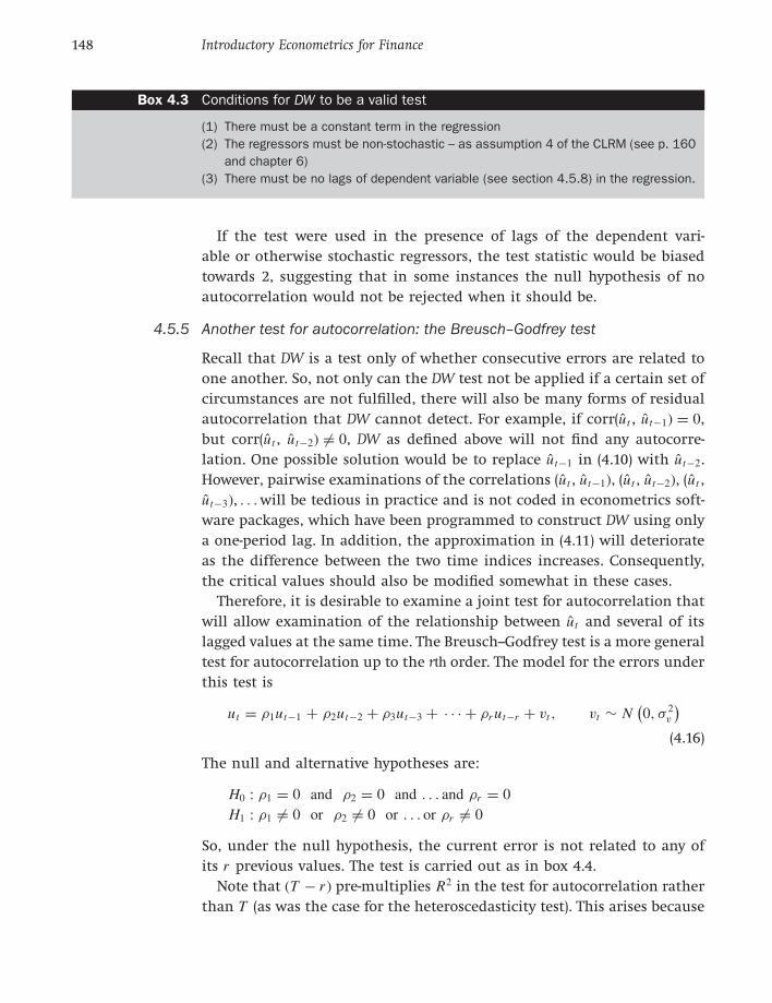
Box 4.3 Conditions for DW to be a valid test
(1) There must be a constant term in the regression
(2) The regressors must be non-stochastic – as assumption 4 of the CLRM (see p. 160
and chapter 6)
(3) There must be no lags of dependent variable (see section 4.5.8) in the regression.
If the test were used in the presence of lags of the dependent vari-
able or otherwise stochastic regressors, the test statistic would be biased
towards 2, suggesting that in some instances the null hypothesis of no
autocorrelation would not be rejected when it should be.
4.5.5 Another test for autocorrelation: the Breusch–Godfrey test
Recall that DW is a test only of whether consecutive errors are related to
one another. So, not only can the DW test not be applied if a certain set of
circumstances are not fulfilled, there will also be many forms of residual
autocorrelation that DW cannot detect. For example, if corr(ut , ut−1) = 0,
but corr(ut , ut−2) �= 0, DW as defined above will not find any autocorre-
lation. One possible solution would be to replace ut−1 in (4.10) with ut−2.
However, pairwise examinations of the correlations (ut , ut−1), (ut , ut−2), (ut ,
ut−3), . . . will be tedious in practice and is not coded in econometrics soft-
ware packages, which have been programmed to construct DW using only
a one-period lag. In addition, the approximation in (4.11) will deteriorate
as the difference between the two time indices increases. Consequently,
the critical values should also be modified somewhat in these cases.
Therefore, it is desirable to examine a joint test for autocorrelation that
will allow examination of the relationship between ut and several of its
lagged values at the same time. The Breusch--Godfrey test is a more general
test for autocorrelation up to the rth order. The model for the errors under
this test is
ut = ρ1ut−1 + ρ2ut−2 + ρ3ut−3 + · · · + ρr ut−r + vt , vt ∼ N(
0, σ 2v
)
(4.16)
The null and alternative hypotheses are:
H0 : ρ1 = 0 and ρ2 = 0 and . . . and ρr = 0
H1 : ρ1 �= 0 or ρ2 �= 0 or . . . or ρr �= 0
So, under the null hypothesis, the current error is not related to any of
its r previous values. The test is carried out as in box 4.4.
Note that (T − r ) pre-multiplies R2 in the test for autocorrelation rather
than T (as was the case for the heteroscedasticity test). This arises because

Classical linear regression model assumptions and diagnostic tests 149
Box 4.4 Conducting a Breusch–Godfrey test
(1) Estimate the linear regression using OLS and obtain the residuals, ut
(2) Regress ut on all of the regressors from stage 1 (the xs) plus ut−1, ut−2, . . . , ut−r ;
the regression will thus be
ut = γ1 + γ2x2t + γ3x3t + γ4x4t + ρ1ut−1 + ρ2ut−2 + ρ3ut−3
+ · · · + ρr ut−r + vt , vt ∼ N(
0, σ 2v
)
(4.17)
Obtain R2 from this auxiliary regression
(3) Letting T denote the number of observations, the test statistic is given by
(T − r )R2 ∼ χ2r
the first r observations will effectively have been lost from the sample
in order to obtain the r lags used in the test regression, leaving (T − r )
observations from which to estimate the auxiliary regression. If the test
statistic exceeds the critical value from the Chi-squared statistical tables,
reject the null hypothesis of no autocorrelation. As with any joint test,
only one part of the null hypothesis has to be rejected to lead to rejection
of the hypothesis as a whole. So the error at time t has to be significantly
related only to one of its previous r values in the sample for the null of
no autocorrelation to be rejected. The test is more general than the DW
test, and can be applied in a wider variety of circumstances since it does
not impose the DW restrictions on the format of the first stage regression.
One potential difficulty with Breusch--Godfrey, however, is in determin-
ing an appropriate value of r , the number of lags of the residuals, to use
in computing the test. There is no obvious answer to this, so it is typical
to experiment with a range of values, and also to use the frequency of the
data to decide. So, for example, if the data is monthly or quarterly, set r
equal to 12 or 4, respectively. The argument would then be that errors at
any given time would be expected to be related only to those errors in the
previous year. Obviously, if the model is statistically adequate, no evidence
of autocorrelation should be found in the residuals whatever value of r is
chosen.
4.5.6 Consequences of ignoring autocorrelation if it is present
In fact, the consequences of ignoring autocorrelation when it is present
are similar to those of ignoring heteroscedasticity. The coefficient esti-
mates derived using OLS are still unbiased, but they are inefficient, i.e.
they are not BLUE, even at large sample sizes, so that the standard er-
ror estimates could be wrong. There thus exists the possibility that the
wrong inferences could be made about whether a variable is or is not

150 Introductory Econometrics for Finance
an important determinant of variations in y. In the case of positive
serial correlation in the residuals, the OLS standard error estimates will
be biased downwards relative to the true standard errors. That is, OLS
will understate their true variability. This would lead to an increase in
the probability of type I error -- that is, a tendency to reject the null hy-
pothesis sometimes when it is correct. Furthermore, R2 is likely to be
inflated relative to its ‘correct’ value if autocorrelation is present but ig-
nored, since residual autocorrelation will lead to an underestimate of the
true error variance (for positive autocorrelation).
4.5.7 Dealing with autocorrelation
If the form of the autocorrelation is known, it would be possible to use
a GLS procedure. One approach, which was once fairly popular, is known
as the Cochrane--Orcutt procedure (see box 4.5). Such methods work by as-
suming a particular form for the structure of the autocorrelation (usually
a first order autoregressive process -- see chapter 5 for a general description
of these models). The model would thus be specified as follows:
yt = β1 + β2x2t + β3x3t + ut , ut = ρut−1 + vt (4.18)
Note that a constant is not required in the specification for the errors
since E(ut ) = 0. If this model holds at time t , it is assumed to also hold
for time t − 1, so that the model in (4.18) is lagged one period
yt−1 = β1 + β2x2t−1 + β3x3t−1 + ut−1 (4.19)
Multiplying (4.19) by ρ
ρyt−1 = ρβ1 + ρβ2x2t−1 + ρβ3x3t−1 + ρut−1 (4.20)
Subtracting (4.20) from (4.18) would give
yt − ρyt−1 = β1 − ρβ1 + β2x2t − ρβ2x2t−1 + β3x3t − ρβ3x3t−1 + ut − ρut−1
(4.21)
Factorising, and noting that vt = ut − ρut−1
(yt − ρyt−1) = (1 − ρ)β1 + β2(x2t − ρx2t−1) + β3(x3t − ρx3t−1) + vt
(4.22)
Setting y∗t = yt − ρyt−1, β
∗1 = (1 − ρ)β1, x∗
2t = (x2t − ρx2t−1), and x∗3t = (x3t −
ρx3t−1), the model in (4.22) can be written
y∗t = β∗
1 + β2x∗2t + β3x∗
3t + vt (4.23)
Classical linear regression model assumptions and diagnostic tests 151
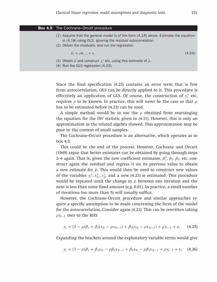
Box 4.5 The Cochrane–Orcutt procedure
(1) Assume that the general model is of the form (4.18) above. Estimate the equation
in (4.18) using OLS, ignoring the residual autocorrelation.
(2) Obtain the residuals, and run the regression
ut = ρut−1 + vt (4.24)
(3) Obtain ρ and construct y∗t etc. using this estimate of ρ.
(4) Run the GLS regression (4.23).
Since the final specification (4.23) contains an error term that is free
from autocorrelation, OLS can be directly applied to it. This procedure is
effectively an application of GLS. Of course, the construction of y∗t etc.
requires ρ to be known. In practice, this will never be the case so that ρ
has to be estimated before (4.23) can be used.
A simple method would be to use the ρ obtained from rearranging
the equation for the DW statistic given in (4.11). However, this is only an
approximation as the related algebra showed. This approximation may be
poor in the context of small samples.
The Cochrane--Orcutt procedure is an alternative, which operates as in
box 4.5.
This could be the end of the process. However, Cochrane and Orcutt
(1949) argue that better estimates can be obtained by going through steps
2--4 again. That is, given the new coefficient estimates, β∗1 , β2, β3, etc. con-
struct again the residual and regress it on its previous value to obtain
a new estimate for ρ. This would then be used to construct new values
of the variables y∗t , x∗
2t , x∗3t and a new (4.23) is estimated. This procedure
would be repeated until the change in ρ between one iteration and the
next is less than some fixed amount (e.g. 0.01). In practice, a small number
of iterations (no more than 5) will usually suffice.
However, the Cochrane--Orcutt procedure and similar approaches re-
quire a specific assumption to be made concerning the form of the model
for the autocorrelation. Consider again (4.22). This can be rewritten taking
ρyt−1 over to the RHS
yt = (1 − ρ)β1 + β2(x2t − ρx2t−1) + β3(x3t − ρx3t−1) + ρyt−1 + vt (4.25)
Expanding the brackets around the explanatory variable terms would give
yt = (1 − ρ)β1 + β2x2t − ρβ2x2t−1 + β3x3t − ρβ3x3t−1 + ρyt−1 + vt (4.26)

152 Introductory Econometrics for Finance
Now, suppose that an equation containing the same variables as (4.26)
were estimated using OLS
yt = γ1 + γ2x2t + γ3x2t−1 + γ4x3t + γ5x3t−1 + γ6 yt−1 + vt (4.27)
It can be seen that (4.26) is a restricted version of (4.27), with the re-
strictions imposed that the coefficient on x2t in (4.26) multiplied by the
negative of the coefficient on yt−1 gives the coefficient on x2t−1, and that
the coefficient on x3t multiplied by the negative of the coefficient on yt−1
gives the coefficient on x3t−1. Thus, the restrictions implied for (4.27) to
get (4.26) are
γ2γ6 = −γ3 and γ4γ6 = −γ5
These are known as the common factor restrictions, and they should be tested
before the Cochrane--Orcutt or similar procedure is implemented. If the
restrictions hold, Cochrane--Orcutt can be validly applied. If not, however,
Cochrane--Orcutt and similar techniques would be inappropriate, and the
appropriate step would be to estimate an equation such as (4.27) directly
using OLS. Note that in general there will be a common factor restriction
for every explanatory variable (excluding a constant) x2t , x3t , . . . , xkt in the
regression. Hendry and Mizon (1978) argued that the restrictions are likely
to be invalid in practice and therefore a dynamic model that allows for
the structure of y should be used rather than a residual correction on a
static model -- see also Hendry (1980).
The White variance--covariance matrix of the coefficients (that is, calcu-
lation of the standard errors using the White correction for heteroscedas-
ticity) is appropriate when the residuals of the estimated equation are
heteroscedastic but serially uncorrelated. Newey and West (1987) develop
a variance--covariance estimator that is consistent in the presence of both
heteroscedasticity and autocorrelation. So an alternative approach to deal-
ing with residual autocorrelation would be to use appropriately modified
standard error estimates.
While White’s correction to standard errors for heteroscedasticity as dis-
cussed above does not require any user input, the Newey--West procedure
requires the specification of a truncation lag length to determine the num-
ber of lagged residuals used to evaluate the autocorrelation. EViews uses
INTEGER[4(T/100)2/9]. In EViews, the Newey--West procedure for estimat-
ing the standard errors is employed by invoking it from the same place
as the White heteroscedasticity correction. That is, click the Estimate but-
ton and in the Equation Estimation window, choose the Options tab and
then instead of checking the ‘White’ box, check Newey-West. While this
option is listed under ‘Heteroskedasticity consistent coefficient variance’,

Classical linear regression model assumptions and diagnostic tests 153
the Newey-West procedure in fact produces ‘HAC’ (Heteroscedasticity and
Autocorrelation Consistent) standard errors that correct for both autocor-
relation and heteroscedasticity that may be present.
A more ‘modern’ view concerning autocorrelation is that it presents
an opportunity rather than a problem! This view, associated with Sargan,
Hendry and Mizon, suggests that serial correlation in the errors arises as
a consequence of ‘misspecified dynamics’. For another explanation of the
reason why this stance is taken, recall that it is possible to express the
dependent variable as the sum of the parts that can be explained using
the model, and a part which cannot (the residuals)
yt = yt + ut (4.28)
where yt are the fitted values from the model (= β1 + β2x2t + β3x3t + · · · +
βk xkt ). Autocorrelation in the residuals is often caused by a dynamic struc-
ture in y that has not been modelled and so has not been captured in
the fitted values. In other words, there exists a richer structure in the
dependent variable y and more information in the sample about that
structure than has been captured by the models previously estimated.
What is required is a dynamic model that allows for this extra structure
in y.
4.5.8 Dynamic models
All of the models considered so far have been static in nature, e.g.
yt = β1 + β2x2t + β3x3t + β4x4t + β5x5t + ut (4.29)
In other words, these models have allowed for only a contemporaneous re-
lationship between the variables, so that a change in one or more of the
explanatory variables at time t causes an instant change in the depen-
dent variable at time t . But this analysis can easily be extended to the
case where the current value of yt depends on previous values of y or on
previous values of one or more of the variables, e.g.
yt = β1 + β2 x2t + β3 x3t + β4 x4t + β5 x5t + γ1 yt−1 + γ2x2t−1
+ · · · + γk xkt−1 + ut (4.30)
It is of course possible to extend the model even more by adding further
lags, e.g. x2t−2, yt−3. Models containing lags of the explanatory variables
(but no lags of the explained variable) are known as distributed lag models.
Specifications with lags of both explanatory and explained variables are
known as autoregressive distributed lag (ADL) models.
How many lags and of which variables should be included in a dy-
namic regression model? This is a tricky question to answer, but hopefully

154 Introductory Econometrics for Finance
recourse to financial theory will help to provide an answer; for another
response (see section 4.13).
Another potential ‘remedy’ for autocorrelated residuals would be to
switch to a model in first differences rather than in levels. As explained
previously, the first difference of yt , i.e. yt − yt−1 is denoted �yt ; similarly,
one can construct a series of first differences for each of the explanatory
variables, e.g. �x2t = x2t − x2t−1, etc. Such a model has a number of other
useful features (see chapter 7 for more details) and could be expressed as
�yt = β1 + β2�x2t + β3�x3t + ut (4.31)
Sometimes the change in y is purported to depend on previous values
of the level of y or xi (i = 2, . . . , k) as well as changes in the explanatory
variables
�yt = β1 + β2�x2t + β3�x3t + β4x2t−1 + β5 yt−1 + ut (4.32)
4.5.9 Why might lags be required in a regression?
Lagged values of the explanatory variables or of the dependent variable (or
both) may capture important dynamic structure in the dependent variable
that might be caused by a number of factors. Two possibilities that are
relevant in finance are as follows:
● Inertia of the dependent variable Often a change in the value of one
of the explanatory variables will not affect the dependent variable im-
mediately during one time period, but rather with a lag over several
time periods. For example, the effect of a change in market microstruc-
ture or government policy may take a few months or longer to work
through since agents may be initially unsure of what the implications
for asset pricing are, and so on. More generally, many variables in eco-
nomics and finance will change only slowly. This phenomenon arises
partly as a result of pure psychological factors -- for example, in finan-
cial markets, agents may not fully comprehend the effects of a particu-
lar news announcement immediately, or they may not even believe the
news. The speed and extent of reaction will also depend on whether the
change in the variable is expected to be permanent or transitory. Delays
in response may also arise as a result of technological or institutional
factors. For example, the speed of technology will limit how quickly
investors’ buy or sell orders can be executed. Similarly, many investors
have savings plans or other financial products where they are ‘locked in’
and therefore unable to act for a fixed period. It is also worth noting that
Classical linear regression model assumptions and diagnostic tests 155
dynamic structure is likely to be stronger and more prevalent the higher
is the frequency of observation of the data.
● Overreactions It is sometimes argued that financial markets overre-
act to good and to bad news. So, for example, if a firm makes a profit
warning, implying that its profits are likely to be down when formally
reported later in the year, the markets might be anticipated to perceive
this as implying that the value of the firm is less than was previously
thought, and hence that the price of its shares will fall. If there is
an overreaction, the price will initially fall below that which is appro-
priate for the firm given this bad news, before subsequently bouncing
back up to a new level (albeit lower than the initial level before the
announcement).
Moving from a purely static model to one which allows for lagged ef-
fects is likely to reduce, and possibly remove, serial correlation which was
present in the static model’s residuals. However, other problems with the
regression could cause the null hypothesis of no autocorrelation to be
rejected, and these would not be remedied by adding lagged variables to
the model:
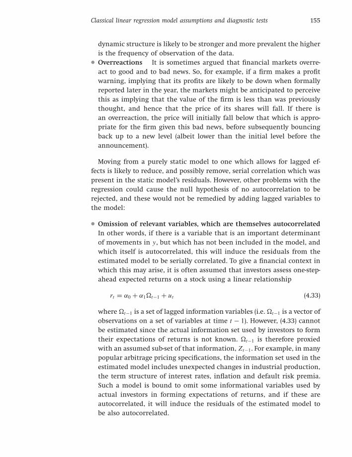
● Omission of relevant variables, which are themselves autocorrelated
In other words, if there is a variable that is an important determinant
of movements in y, but which has not been included in the model, and
which itself is autocorrelated, this will induce the residuals from the
estimated model to be serially correlated. To give a financial context in
which this may arise, it is often assumed that investors assess one-step-
ahead expected returns on a stock using a linear relationship
rt = α0 + α1t−1 + ut (4.33)
where t−1 is a set of lagged information variables (i.e. t−1 is a vector of
observations on a set of variables at time t − 1). However, (4.33) cannot
be estimated since the actual information set used by investors to form
their expectations of returns is not known. t−1 is therefore proxied
with an assumed sub-set of that information, Z t−1. For example, in many
popular arbitrage pricing specifications, the information set used in the
estimated model includes unexpected changes in industrial production,
the term structure of interest rates, inflation and default risk premia.
Such a model is bound to omit some informational variables used by
actual investors in forming expectations of returns, and if these are
autocorrelated, it will induce the residuals of the estimated model to
be also autocorrelated.

156 Introductory Econometrics for Finance
● Autocorrelation owing to unparameterised seasonality Suppose that
the dependent variable contains a seasonal or cyclical pattern, where
certain features periodically occur. This may arise, for example, in the
context of sales of gloves, where sales will be higher in the autumn
and winter than in the spring or summer. Such phenomena are likely
to lead to a positively autocorrelated residual structure that is cyclical
in shape, such as that of figure 4.4, unless the seasonal patterns are
captured by the model. See chapter 9 for a discussion of seasonality
and how to deal with it.
● If ‘misspecification’ error has been committed by using an inappro-
priate functional form For example, if the relationship between y and
the explanatory variables was a non-linear one, but the researcher had
specified a linear regression model, this may again induce the residuals
from the estimated model to be serially correlated.
4.5.10 The long-run static equilibrium solution
Once a general model of the form given in (4.32) has been found, it may
contain many differenced and lagged terms that make it difficult to in-
terpret from a theoretical perspective. For example, if the value of x2
were to increase in period t , what would be the effect on y in periods,
t, t + 1, t + 2, and so on? One interesting property of a dynamic model
that can be calculated is its long-run or static equilibrium solution.
The relevant definition of ‘equilibrium’ in this context is that a system
has reached equilibrium if the variables have attained some steady state
values and are no longer changing, i.e. if y and x are in equilibrium, it is
possible to write
yt = yt+1 = . . . = y and x2t = x2t+1 = . . . = x2, and so on.
Consequently, �yt = yt − yt−1 = y − y = 0, �x2t = x2t − x2t−1 = x2 − x2 =
0, etc. since the values of the variables are no longer changing. So the
way to obtain a long-run static solution from a given empirical model
such as (4.32) is:
(1) Remove all time subscripts from the variables
(2) Set error terms equal to their expected values of zero, i.e E(ut ) = 0
(3) Remove differenced terms (e.g. �yt ) altogether
(4) Gather terms in x together and gather terms in y together
(5) Rearrange the resulting equation if necessary so that the dependent
variable y is on the left-hand side (LHS) and is expressed as a function
of the independent variables.
Classical linear regression model assumptions and diagnostic tests 157
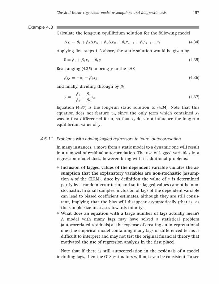
Example 4.3
Calculate the long-run equilibrium solution for the following model
�yt = β1 + β2�x2t + β3�x3t + β4x2t−1 + β5 yt−1 + ut (4.34)
Applying first steps 1--3 above, the static solution would be given by
0 = β1 + β4x2 + β5 y (4.35)
Rearranging (4.35) to bring y to the LHS
β5 y = −β1 − β4x2 (4.36)
and finally, dividing through by β5
y = −β1
β5
−β4
β5
x2 (4.37)
Equation (4.37) is the long-run static solution to (4.34). Note that this
equation does not feature x3, since the only term which contained x3
was in first differenced form, so that x3 does not influence the long-run
equilibrium value of y.
4.5.11 Problems with adding lagged regressors to ‘cure’ autocorrelation
In many instances, a move from a static model to a dynamic one will result
in a removal of residual autocorrelation. The use of lagged variables in a
regression model does, however, bring with it additional problems:
● Inclusion of lagged values of the dependent variable violates the as-
sumption that the explanatory variables are non-stochastic (assump-
tion 4 of the CLRM), since by definition the value of y is determined
partly by a random error term, and so its lagged values cannot be non-
stochastic. In small samples, inclusion of lags of the dependent variable
can lead to biased coefficient estimates, although they are still consis-
tent, implying that the bias will disappear asymptotically (that is, as
the sample size increases towards infinity).
● What does an equation with a large number of lags actually mean?
A model with many lags may have solved a statistical problem
(autocorrelated residuals) at the expense of creating an interpretational
one (the empirical model containing many lags or differenced terms is
difficult to interpret and may not test the original financial theory that
motivated the use of regression analysis in the first place).
Note that if there is still autocorrelation in the residuals of a model
including lags, then the OLS estimators will not even be consistent. To see

158 Introductory Econometrics for Finance
why this occurs, consider the following regression model
yt = β1 + β2x2t + β3x3t + β4 yt−1 + ut (4.38)
where the errors, ut , follow a first order autoregressive process
ut = ρut−1 + vt (4.39)
Substituting into (4.38) for ut from (4.39)
yt = β1 + β2x2t + β3x3t + β4 yt−1 + ρut−1 + vt (4.40)
Now, clearly yt depends upon yt−1. Taking (4.38) and lagging it one period
(i.e. subtracting one from each time index)
yt−1 = β1 + β2x2t−1 + β3x3t−1 + β4 yt−2 + ut−1 (4.41)
It is clear from (4.41) that yt−1 is related to ut−1 since they both appear
in that equation. Thus, the assumption that E(X ′u) = 0 is not satisfied
for (4.41) and therefore for (4.38). Thus the OLS estimator will not be
consistent, so that even with an infinite quantity of data, the coefficient
estimates would be biased.
4.5.12 Autocorrelation and dynamic models in EViews
In EViews, the lagged values of variables can be used as regressors or for
other purposes by using the notation x(−1) for a one-period lag, x(−5)
for a five-period lag, and so on, where x is the variable name. EViews
will automatically adjust the sample period used for estimation to take
into account the observations that are lost in constructing the lags. For
example, if the regression contains five lags of the dependent variable, five
observations will be lost and estimation will commence with observation
six.
In EViews, the DW statistic is calculated automatically, and was given in
the general estimation output screens that result from estimating any re-
gression model. To view the results screen again, click on the View button
in the regression window and select Estimation output. For the Microsoft
macroeconomic regression that included all of the explanatory variables,
the value of the DW statistic was 2.156. What is the appropriate conclu-
sion regarding the presence or otherwise of first order autocorrelation in
this case?
The Breusch--Godfrey test can be conducted by selecting View; Residual
Tests; Serial Correlation LM Test . . . In the new window, type again the
number of lagged residuals you want to include in the test and click on
OK. Assuming that you selected to employ ten lags in the test, the results
would be as given in the following table.

Classical linear regression model assumptions and diagnostic tests 159
Breusch-Godfrey Serial Correlation LM Test:
F-statistic 1.497460 Prob. F(10,234) 0.1410Obs*R-squared 15.15657 Prob. Chi-Square(10) 0.1265
Test Equation:Dependent Variable: RESIDMethod: Least SquaresDate: 08/27/07 Time: 13:26Sample: 1986M05 2007M04Included observations: 252Presample missing value lagged residuals set to zero.
Coefficient Std. Error t-Statistic Prob.
C 0.087053 1.461517 0.059563 0.9526ERSANDP −0.021725 0.204588 −0.106187 0.9155DPROD −0.036054 0.510873 −0.070573 0.9438
DCREDIT −9.64E-06 0.000162 −0.059419 0.9527DINFLATION −0.364149 3.010661 −0.120953 0.9038
DMONEY 0.225441 0.718175 0.313909 0.7539DSPREAD 0.202672 13.70006 0.014794 0.9882RTERM −0.19964 3.363238 −0.059360 0.9527
RESID(−1) −0.12678 0.065774 −1.927509 0.0551RESID(−2) −0.063949 0.066995 −0.954537 0.3408RESID(−3) −0.038450 0.065536 −0.586694 0.5580RESID(−4) −0.120761 0.065906 −1.832335 0.0682RESID(−5) −0.126731 0.065253 −1.942152 0.0533RESID(−6) −0.090371 0.066169 −1.365755 0.1733RESID(−7) −0.071404 0.065761 −1.085803 0.2787RESID(−8) −0.119176 0.065926 −1.807717 0.0719RESID(−9) −0.138430 0.066121 −2.093571 0.0374RESID(−10) −0.060578 0.065682 −0.922301 0.3573
R-squared 0.060145 Mean dependent var 8.11E-17Adjusted R-squared −0.008135 S.D. dependent var 13.75376S.E. of regression 13.80959 Akaike info criterion 8.157352Sum squared resid 44624.90 Schwarz criterion 8.409454Log likelihood −1009.826 Hannan-Quinn criter. 8.258793F-statistic 0.880859 Durbin-Watson stat 2.013727Prob(F-statistic) 0.597301
In the first table of output, EViews offers two versions of the test -- an
F -version and a χ2 version, while the second table presents the estimates
from the auxiliary regression. The conclusion from both versions of the
test in this case is that the null hypothesis of no autocorrelation should
not be rejected. Does this agree with the DW test result?

160 Introductory Econometrics for Finance
4.5.13 Autocorrelation in cross-sectional data
The possibility that autocorrelation may occur in the context of a time
series regression is quite intuitive. However, it is also plausible that auto-
correlation could be present in certain types of cross-sectional data. For
example, if the cross-sectional data comprise the profitability of banks in
different regions of the US, autocorrelation may arise in a spatial sense,
if there is a regional dimension to bank profitability that is not captured
by the model. Thus the residuals from banks of the same region or in
neighbouring regions may be correlated. Testing for autocorrelation in
this case would be rather more complex than in the time series context,
and would involve the construction of a square, symmetric ‘spatial con-
tiguity matrix’ or a ‘distance matrix’. Both of these matrices would be
N × N , where N is the sample size. The former would be a matrix of ze-
ros and ones, with one for element i , j when observation i occurred for
a bank in the same region to, or sufficiently close to, region j and zero
otherwise (i, j = 1, . . . , N ). The distance matrix would comprise elements
that measured the distance (or the inverse of the distance) between bank
i and bank j . A potential solution to a finding of autocorrelated residuals
in such a model would be again to use a model containing a lag struc-
ture, in this case known as a ‘spatial lag’. Further details are contained in
Anselin (1988).
4.6 Assumption 4: the xt are non-stochastic
Fortunately, it turns out that the OLS estimator is consistent and unbiased
in the presence of stochastic regressors, provided that the regressors are
not correlated with the error term of the estimated equation. To see this,
recall that
β = (X ′ X )−1 X ′y and y = Xβ + u (4.42)
Thus
β = (X ′ X )−1 X ′(Xβ + u) (4.43)
β = (X ′ X )−1 X ′ Xβ + (X ′ X )−1 X ′u (4.44)
β = β + (X ′ X )−1 X ′u (4.45)
Taking expectations, and provided that X and u are independent,1
E(β) = E(β) + E((X ′ X )−1 X ′u) (4.46)
E(β) = β + E[(X ′ X )−1 X ′]E(u) (4.47)
1 A situation where X and u are not independent is discussed at length in chapter 6.

Classical linear regression model assumptions and diagnostic tests 161
Since E(u) = 0, this expression will be zero and therefore the estimator is
still unbiased, even if the regressors are stochastic.
However, if one or more of the explanatory variables is contemporane-
ously correlated with the disturbance term, the OLS estimator will not
even be consistent. This results from the estimator assigning explanatory
power to the variables where in reality it is arising from the correlation
between the error term and yt . Suppose for illustration that x2t and ut
are positively correlated. When the disturbance term happens to take a
high value, yt will also be high (because yt = β1 + β2x2t + · · · + ut ). But if
x2t is positively correlated with ut , then x2t is also likely to be high. Thus
the OLS estimator will incorrectly attribute the high value of yt to a high
value of x2t , where in reality yt is high simply because ut is high, which
will result in biased and inconsistent parameter estimates and a fitted
line that appears to capture the features of the data much better than it
does in reality.
4.7 Assumption 5: the disturbances are normally distributed
Recall that the normality assumption (ut ∼ N(0, σ 2)) is required in order
to conduct single or joint hypothesis tests about the model parameters.
4.7.1 Testing for departures from normality
One of the most commonly applied tests for normality is the Bera--Jarque
(hereafter BJ) test. BJ uses the property of a normally distributed random
variable that the entire distribution is characterised by the first two mo-
ments -- the mean and the variance. The standardised third and fourth
moments of a distribution are known as its skewness and kurtosis. Skewness
measures the extent to which a distribution is not symmetric about its
mean value and kurtosis measures how fat the tails of the distribution are.
A normal distribution is not skewed and is defined to have a coefficient
of kurtosis of 3. It is possible to define a coefficient of excess kurtosis,
equal to the coefficient of kurtosis minus 3; a normal distribution will
thus have a coefficient of excess kurtosis of zero. A normal distribution is
symmetric and said to be mesokurtic. To give some illustrations of what a
series having specific departures from normality may look like, consider
figures 4.10 and 4.11.
A normal distribution is symmetric about its mean, while a skewed
distribution will not be, but will have one tail longer than the other, such
as in the right hand part of figure 4.10.

162 Introductory Econometrics for Finance
x x
xf ( ) xf ( )
Figure 4.10 A normal versus a skewed distribution
0.5
0.4
0.3
0.2
0.1
0.0
–5.4 –3.6 –1.8 0.0 1.8 3.6 5.4
Figure 4.11
A leptokurtic versus
a normal distribution
A leptokurtic distribution is one which has fatter tails and is more
peaked at the mean than a normally distributed random variable with
the same mean and variance, while a platykurtic distribution will be less
peaked in the mean, will have thinner tails, and more of the distribution
in the shoulders than a normal. In practice, a leptokurtic distribution
is far more likely to characterise financial (and economic) time series,
and to characterise the residuals from a financial time series model. In
figure 4.11, the leptokurtic distribution is shown by the bold line, with
the normal by the faint line.

Classical linear regression model assumptions and diagnostic tests 163
Bera and Jarque (1981) formalise these ideas by testing whether the co-
efficient of skewness and the coefficient of excess kurtosis are jointly zero.
Denoting the errors by u and their variance by σ 2, it can be proved that
the coefficients of skewness and kurtosis can be expressed respectively as
b1 =E[u3]
(
σ 2)3/2
and b2 =E[u4](
σ 2)2
(4.48)
The kurtosis of the normal distribution is 3 so its excess kurtosis (b2 − 3)
is zero.
The Bera--Jarque test statistic is given by
W = T
[
b21
6+
(b2 − 3)2
24
]
(4.49)
where T is the sample size. The test statistic asymptotically follows a χ2(2)
under the null hypothesis that the distribution of the series is symmetric
and mesokurtic.
b1 and b2 can be estimated using the residuals from the OLS regression,
u. The null hypothesis is of normality, and this would be rejected if the
residuals from the model were either significantly skewed or leptokurtic/
platykurtic (or both).
4.7.2 Testing for non-normality using EViews
The Bera--Jarque normality tests results can be viewed by selecting
View/Residual Tests/Histogram – Normality Test. The statistic has a χ2
distribution with 2 degrees of freedom under the null hypothesis of nor-
mally distributed errors. If the residuals are normally distributed, the
histogram should be bell-shaped and the Bera--Jarque statistic would not
be significant. This means that the p-value given at the bottom of the
normality test screen should be bigger than 0.05 to not reject the null of
normality at the 5% level. In the example of the Microsoft regression, the
screen would appear as in screenshot 4.2.
In this case, the residuals are very negatively skewed and are leptokurtic.
Hence the null hypothesis for residual normality is rejected very strongly
(the p-value for the BJ test is zero to six decimal places), implying that
the inferences we make about the coefficient estimates could be wrong,
although the sample is probably just about large enough that we need be
less concerned than we would be with a small sample. The non-normality
in this case appears to have been caused by a small number of very
large negative residuals representing monthly stock price falls of more
than −25%.

164 Introductory Econometrics for Finance
Screenshot 4.2
Non-normality test
results
4.7.3 What should be done if evidence of non-normality is found?
It is not obvious what should be done! It is, of course, possible to em-
ploy an estimation method that does not assume normality, but such a
method may be difficult to implement, and one can be less sure of its
properties. It is thus desirable to stick with OLS if possible, since its be-
haviour in a variety of circumstances has been well researched. For sample
sizes that are sufficiently large, violation of the normality assumption is
virtually inconsequential. Appealing to a central limit theorem, the test
statistics will asymptotically follow the appropriate distributions even in
the absence of error normality.2
In economic or financial modelling, it is quite often the case that one
or two very extreme residuals cause a rejection of the normality assump-
tion. Such observations would appear in the tails of the distribution, and
would therefore lead u4, which enters into the definition of kurtosis, to
be very large. Such observations that do not fit in with the pattern of the
remainder of the data are known as outliers. If this is the case, one way
2 The law of large numbers states that the average of a sample (which is a random
variable) will converge to the population mean (which is fixed), and the central limit
theorem states that the sample mean converges to a normal distribution.
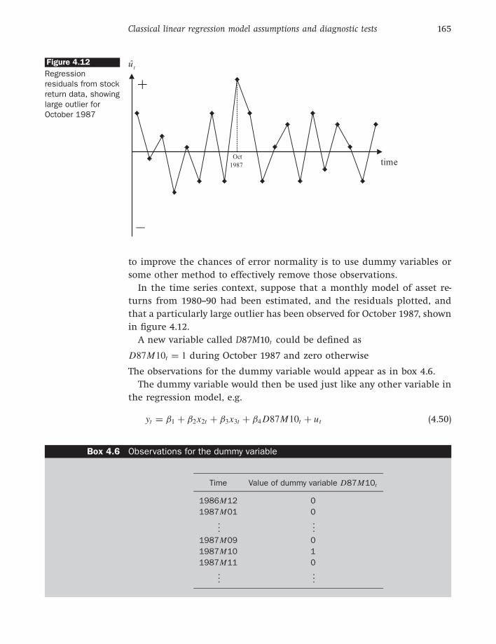
Classical linear regression model assumptions and diagnostic tests 165
ût
+
–
timeOct
1987
Figure 4.12
Regression
residuals from stock
return data, showing
large outlier for
October 1987
to improve the chances of error normality is to use dummy variables or
some other method to effectively remove those observations.
In the time series context, suppose that a monthly model of asset re-
turns from 1980--90 had been estimated, and the residuals plotted, and
that a particularly large outlier has been observed for October 1987, shown
in figure 4.12.
A new variable called D87M10t could be defined as
D87M10t = 1 during October 1987 and zero otherwise
The observations for the dummy variable would appear as in box 4.6.
The dummy variable would then be used just like any other variable in
the regression model, e.g.
yt = β1 + β2x2t + β3x3t + β4 D87M10t + ut (4.50)
Box 4.6 Observations for the dummy variable
Time Value of dummy variable D87M10t
1986M12 0
1987M01 0
......
1987M09 0
1987M10 1
1987M11 0
..
....

166 Introductory Econometrics for Finance
yt
x t
Figure 4.13
Possible effect of an
outlier on OLS
estimation
This type of dummy variable that takes the value one for only a single
observation has an effect exactly equivalent to knocking out that obser-
vation from the sample altogether, by forcing the residual for that obser-
vation to zero. The estimated coefficient on the dummy variable will be
equal to the residual that the dummied observation would have taken if
the dummy variable had not been included.
However, many econometricians would argue that dummy variables to
remove outlying residuals can be used to artificially improve the charac-
teristics of the model -- in essence fudging the results. Removing outlying
observations will reduce standard errors, reduce the RSS, and therefore
increase R2, thus improving the apparent fit of the model to the data.
The removal of observations is also hard to reconcile with the notion in
statistics that each data point represents a useful piece of information.
The other side of this argument is that observations that are ‘a long
way away’ from the rest, and seem not to fit in with the general pattern
of the rest of the data are known as outliers. Outliers can have a serious
effect on coefficient estimates, since by definition, OLS will receive a big
penalty, in the form of an increased RSS, for points that are a long way
from the fitted line. Consequently, OLS will try extra hard to minimise
the distances of points that would have otherwise been a long way from
the line. A graphical depiction of the possible effect of an outlier on OLS
estimation, is given in figure 4.13.
In figure 4.13, one point is a long way away from the rest. If this point
is included in the estimation sample, the fitted line will be the dotted
one, which has a slight positive slope. If this observation were removed,
the full line would be the one fitted. Clearly, the slope is now large and
negative. OLS would not select this line if the outlier is included since the

Classical linear regression model assumptions and diagnostic tests 167
observation is a long way from the others and hence when the residual
(the distance from the point to the fitted line) is squared, it would lead to
a big increase in the RSS. Note that outliers could be detected by plotting
y against x only in the context of a bivariate regression. In the case where
there are more explanatory variables, outliers are easiest identified by
plotting the residuals over time, as in figure 4.12, etc.
So, it can be seen that a trade-off potentially exists between the need
to remove outlying observations that could have an undue impact on the
OLS estimates and cause residual non-normality on the one hand, and the
notion that each data point represents a useful piece of information on
the other. The latter is coupled with the fact that removing observations
at will could artificially improve the fit of the model. A sensible way to
proceed is by introducing dummy variables to the model only if there is
both a statistical need to do so and a theoretical justification for their
inclusion. This justification would normally come from the researcher’s
knowledge of the historical events that relate to the dependent variable
and the model over the relevant sample period. Dummy variables may
be justifiably used to remove observations corresponding to ‘one-off’ or
extreme events that are considered highly unlikely to be repeated, and
the information content of which is deemed of no relevance for the data
as a whole. Examples may include stock market crashes, financial panics,
government crises, and so on.
Non-normality in financial data could also arise from certain types of
heteroscedasticity, known as ARCH -- see chapter 8. In this case, the non-
normality is intrinsic to all of the data and therefore outlier removal
would not make the residuals of such a model normal.
Another important use of dummy variables is in the modelling of sea-
sonality in financial data, and accounting for so-called ‘calendar anoma-
lies’, such as day-of-the-week effects and weekend effects. These are dis-
cussed in chapter 9.
4.7.4 Dummy variable construction and use in EViews
As we saw from the plot of the distribution above, the non-normality in
the residuals from the Microsoft regression appears to have been caused
by a small number of outliers in the regression residuals. Such events
can be identified if it is present by plotting the actual values, the fitted
values and the residuals of the regression. This can be achieved in EViews
by selecting View/Actual, Fitted, Residual/Actual, Fitted, Residual Graph.
The plot should look as in screenshot 4.3.
From the graph, it can be seen that there are several large (negative)
outliers, but the largest of all occur in early 1998 and early 2003. All of the

168 Introductory Econometrics for Finance
Screenshot 4.3
Regression
residuals, actual
values and fitted
series
large outliers correspond to months where the actual return was much
smaller (i.e. more negative) than the model would have predicted. Inter-
estingly, the residual in October 1987 is not quite so prominent because
even though the stock price fell, the market index value fell as well, so
that the stock price fall was at least in part predicted (this can be seen by
comparing the actual and fitted values during that month).
In order to identify the exact dates that the biggest outliers were re-
alised, we could use the shading option by right clicking on the graph
and selecting the ‘add lines & shading’ option. But it is probably easier to
just examine a table of values for the residuals, which can be achieved by
selecting View/Actual, Fitted, Residual/Actual, Fitted, Residual Table. If we
do this, it is evident that the two most extreme residuals (with values to
the nearest integer) were in February 1998 (−68) and February 2003 (−67).
As stated above, one way to remove big outliers in the data is by using
dummy variables. It would be tempting, but incorrect, to construct one
dummy variable that takes the value 1 for both Feb 98 and Feb 03, but
this would not have the desired effect of setting both residuals to zero. In-
stead, to remove two outliers requires us to construct two separate dummy

Classical linear regression model assumptions and diagnostic tests 169
variables. In order to create the Feb 98 dummy first, we generate a series
called ‘FEB98DUM’ that will initially contain only zeros. Generate this se-
ries (hint: you can use ‘Quick/Generate Series’ and then type in the box
‘FEB98DUM = 0’). Double click on the new object to open the spreadsheet
and turn on the editing mode by clicking ‘Edit +/−’ and input a single 1
in the cell that corresponds to February 1998. Leave all other cell entries
as zeros.
Once this dummy variable has been created, repeat the process above to
create another dummy variable called ‘FEB03DUM’ that takes the value
1 in February 2003 and zero elsewhere and then rerun the regression
including all the previous variables plus these two dummy variables. This
can most easily be achieved by clicking on the ‘Msoftreg’ results object,
then the Estimate button and adding the dummy variables to the end of
the variable list. The full list of variables is
ermsoft c ersandp dprod dcredit dinflation dmoney dspread rterm
feb98dum feb03dum
and the results of this regression are as in the following table.
Dependent Variable: ERMSOFTMethod: Least SquaresDate: 08/29/07 Time: 09:11Sample (adjusted): 1986M05 2007M04Included observations: 252 after adjustments
Coefficient Std. Error t-Statistic Prob.
C −0.086606 1.315194 −0.065850 0.9476ERSANDP 1.547971 0.183945 8.415420 0.0000DPROD 0.455015 0.451875 1.006948 0.315
DCREDIT −5.92E-05 0.000145 −0.409065 0.6829DINFLATION 4.913297 2.685659 1.829457 0.0686
DMONEY −1.430608 0.644601 −2.219369 0.0274DSPREAD 8.624895 12.22705 0.705395 0.4812RTERM 6.893754 2.993982 2.302537 0.0222
FEB98DUM −69.14177 12.68402 −5.451093 0.0000FEB03DUM −68.24391 12.65390 −5.393113 0.0000
R-squared 0.358962 Mean dependent var −0.420803Adjusted R-squared 0.335122 S.D. dependent var 15.41135S.E. of regression 12.56643 Akaike info criterion 7.938808Sum squared resid 38215.45 Schwarz criterion 8.078865Log likelihood −990.2898 Hannan-Quinn criter. 7.995164F-statistic 15.05697 Durbin-Watson stat 2.142031Prob(F-statistic) 0.000000

170 Introductory Econometrics for Finance
Note that the dummy variable parameters are both highly significant and
take approximately the values that the corresponding residuals would
have taken if the dummy variables had not been included in the model.3
By comparing the results with those of the regression above that excluded
the dummy variables, it can be seen that the coefficient estimates on the
remaining variables change quite a bit in this instance and the signifi-
cances improve considerably. The term structure and money supply pa-
rameters are now both significant at the 5% level, and the unexpected
inflation parameter is now significant at the 10% level. The R2 value has
risen from 0.20 to 0.36 because of the perfect fit of the dummy variables
to those two extreme outlying observations.
Finally, if we re-examine the normality test results by clicking
View/Residual Tests/Histogram – Normality Test, we will see that while
the skewness and kurtosis are both slightly closer to the values that they
would take under normality, the Bera--Jarque test statistic still takes a
value of 829 (compared with over 1000 previously). We would thus con-
clude that the residuals are still a long way from following a normal
distribution. While it would be possible to continue to generate dummy
variables, there is a limit to the extent to which it would be desirable to do
so. With this particular regression, we are unlikely to be able to achieve a
residual distribution that is close to normality without using an excessive
number of dummy variables. As a rule of thumb, in a monthly sample
with 252 observations, it is reasonable to include, perhaps, two or three
dummy variables, but more would probably be excessive.
4.8 Multicollinearity
An implicit assumption that is made when using the OLS estimation
method is that the explanatory variables are not correlated with one an-
other. If there is no relationship between the explanatory variables, they
would be said to be orthogonal to one another. If the explanatory variables
were orthogonal to one another, adding or removing a variable from a
regression equation would not cause the values of the coefficients on the
other variables to change.
In any practical context, the correlation between explanatory variables
will be non-zero, although this will generally be relatively benign in the
3 Note the inexact correspondence between the values of the residuals and the values of
the dummy variable parameters because two dummies are being used together; had we
included only one dummy, the value of the dummy variable coefficient and that which
the residual would have taken would be identical.

Classical linear regression model assumptions and diagnostic tests 171
sense that a small degree of association between explanatory variables
will almost always occur but will not cause too much loss of precision.
However, a problem occurs when the explanatory variables are very highly
correlated with each other, and this problem is known as multicollinearity.
It is possible to distinguish between two classes of multicollinearity: per-
fect multicollinearity and near multicollinearity.
Perfect multicollinearity occurs when there is an exact relationship be-
tween two or more variables. In this case, it is not possible to estimate all
of the coefficients in the model. Perfect multicollinearity will usually be
observed only when the same explanatory variable is inadvertently used
twice in a regression. For illustration, suppose that two variables were
employed in a regression function such that the value of one variable was
always twice that of the other (e.g. suppose x3 = 2x2). If both x3 and x2
were used as explanatory variables in the same regression, then the model
parameters cannot be estimated. Since the two variables are perfectly re-
lated to one another, together they contain only enough information to
estimate one parameter, not two. Technically, the difficulty would occur
in trying to invert the (X ′ X ) matrix since it would not be of full rank
(two of the columns would be linearly dependent on one another), so
that the inverse of (X ′ X ) would not exist and hence the OLS estimates
β = (X ′ X )−1 X ′y could not be calculated.
Near multicollinearity is much more likely to occur in practice, and would
arise when there was a non-negligible, but not perfect, relationship be-
tween two or more of the explanatory variables. Note that a high correla-
tion between the dependent variable and one of the independent variables
is not multicollinearity.
Visually, we could think of the difference between near and perfect
multicollinearity as follows. Suppose that the variables x2t and x3t were
highly correlated. If we produced a scatter plot of x2t against x3t , then
perfect multicollinearity would correspond to all of the points lying ex-
actly on a straight line, while near multicollinearity would correspond to
the points lying close to the line, and the closer they were to the line
(taken altogether), the stronger would be the relationship between the
two variables.
4.8.1 Measuring near multicollinearity
Testing for multicollinearity is surprisingly difficult, and hence all that
is presented here is a simple method to investigate the presence or
otherwise of the most easily detected forms of near multicollinear-
ity. This method simply involves looking at the matrix of correlations

172 Introductory Econometrics for Finance
between the individual variables. Suppose that a regression equation has
three explanatory variables (plus a constant term), and that the pair-wise
correlations between these explanatory variables are.
corr x2 x3 x4
x2 -- 0.2 0.8
x3 0.2 -- 0.3
x4 0.8 0.3 --
Clearly, if multicollinearity was suspected, the most likely culprit would
be a high correlation between x2 and x4. Of course, if the relationship
involves three or more variables that are collinear -- e.g. x2 + x3 ≈ x4 --
then multicollinearity would be very difficult to detect.
4.8.2 Problems if near multicollinearity is present but ignored
First, R2 will be high but the individual coefficients will have high stan-
dard errors, so that the regression ‘looks good’ as a whole4, but the in-
dividual variables are not significant. This arises in the context of very
closely related explanatory variables as a consequence of the difficulty in
observing the individual contribution of each variable to the overall fit
of the regression. Second, the regression becomes very sensitive to small
changes in the specification, so that adding or removing an explanatory
variable leads to large changes in the coefficient values or significances of
the other variables. Finally, near multicollinearity will thus make confi-
dence intervals for the parameters very wide, and significance tests might
therefore give inappropriate conclusions, and so make it difficult to draw
sharp inferences.
4.8.3 Solutions to the problem of multicollinearity
A number of alternative estimation techniques have been proposed that
are valid in the presence of multicollinearity -- for example, ridge re-
gression, or principal components. Principal components analysis was dis-
cussed briefly in an appendix to the previous chapter. Many researchers
do not use these techniques, however, as they can be complex, their prop-
erties are less well understood than those of the OLS estimator and, above
all, many econometricians would argue that multicollinearity is more a
problem with the data than with the model or estimation method.
4 Note that multicollinearity does not affect the value of R2 in a regression.

Classical linear regression model assumptions and diagnostic tests 173
Other, more ad hoc methods for dealing with the possible existence of
near multicollinearity include:
● Ignore it, if the model is otherwise adequate, i.e. statistically and in
terms of each coefficient being of a plausible magnitude and having an
appropriate sign. Sometimes, the existence of multicollinearity does not
reduce the t -ratios on variables that would have been significant without
the multicollinearity sufficiently to make them insignificant. It is worth
stating that the presence of near multicollinearity does not affect the
BLUE properties of the OLS estimator -- i.e. it will still be consistent,
unbiased and efficient since the presence of near multicollinearity does
not violate any of the CLRM assumptions 1--4. However, in the presence
of near multicollinearity, it will be hard to obtain small standard errors.
This will not matter if the aim of the model-building exercise is to
produce forecasts from the estimated model, since the forecasts will
be unaffected by the presence of near multicollinearity so long as this
relationship between the explanatory variables continues to hold over
the forecasted sample.
● Drop one of the collinear variables, so that the problem disappears.
However, this may be unacceptable to the researcher if there were strong
a priori theoretical reasons for including both variables in the model.
Also, if the removed variable was relevant in the data generating process
for y, an omitted variable bias would result (see section 4.10).
● Transform the highly correlated variables into a ratio and include
only the ratio and not the individual variables in the regression.
Again, this may be unacceptable if financial theory suggests that
changes in the dependent variable should occur following changes in
the individual explanatory variables, and not a ratio of them.
● Finally, as stated above, it is also often said that near multicollinear-
ity is more a problem with the data than with the model, so that there
is insufficient information in the sample to obtain estimates for all
of the coefficients. This is why near multicollinearity leads coefficient
estimates to have wide standard errors, which is exactly what would
happen if the sample size were small. An increase in the sample size
will usually lead to an increase in the accuracy of coefficient estimation
and consequently a reduction in the coefficient standard errors, thus
enabling the model to better dissect the effects of the various explana-
tory variables on the explained variable. A further possibility, therefore,
is for the researcher to go out and collect more data -- for example,
by taking a longer run of data, or switching to a higher frequency of
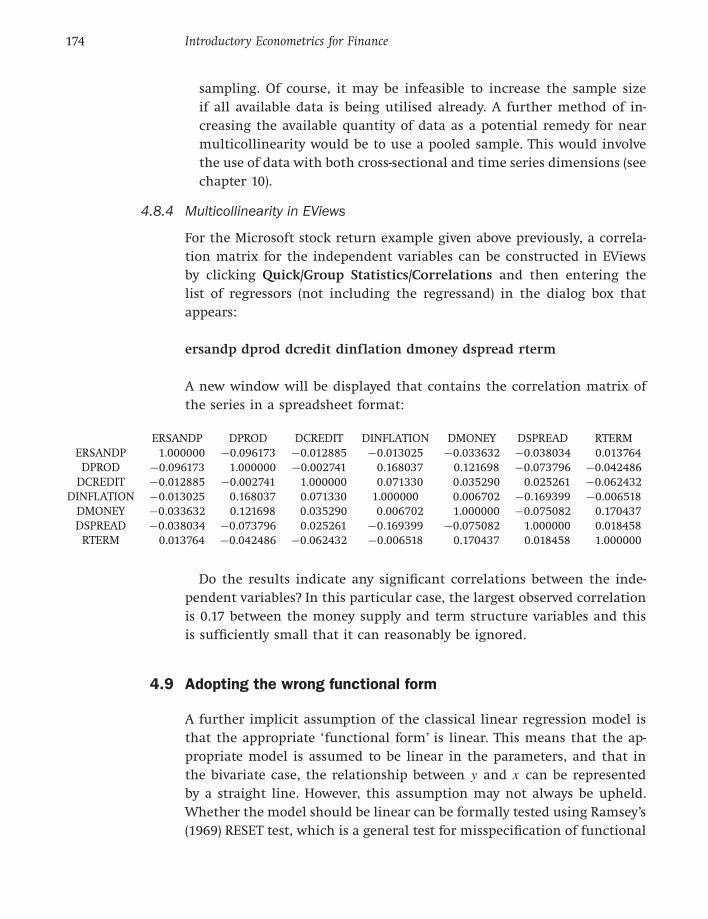
174 Introductory Econometrics for Finance
sampling. Of course, it may be infeasible to increase the sample size
if all available data is being utilised already. A further method of in-
creasing the available quantity of data as a potential remedy for near
multicollinearity would be to use a pooled sample. This would involve
the use of data with both cross-sectional and time series dimensions (see
chapter 10).
4.8.4 Multicollinearity in EViews
For the Microsoft stock return example given above previously, a correla-
tion matrix for the independent variables can be constructed in EViews
by clicking Quick/Group Statistics/Correlations and then entering the
list of regressors (not including the regressand) in the dialog box that
appears:
ersandp dprod dcredit dinflation dmoney dspread rterm
A new window will be displayed that contains the correlation matrix of
the series in a spreadsheet format:
ERSANDP DPROD DCREDIT DINFLATION DMONEY DSPREAD RTERM
ERSANDP 1.000000 −0.096173 −0.012885 −0.013025 −0.033632 −0.038034 0.013764
DPROD −0.096173 1.000000 −0.002741 0.168037 0.121698 −0.073796 −0.042486
DCREDIT −0.012885 −0.002741 1.000000 0.071330 0.035290 0.025261 −0.062432
DINFLATION −0.013025 0.168037 0.071330 1.000000 0.006702 −0.169399 −0.006518
DMONEY −0.033632 0.121698 0.035290 0.006702 1.000000 −0.075082 0.170437
DSPREAD −0.038034 −0.073796 0.025261 −0.169399 −0.075082 1.000000 0.018458
RTERM 0.013764 −0.042486 −0.062432 −0.006518 0.170437 0.018458 1.000000
Do the results indicate any significant correlations between the inde-
pendent variables? In this particular case, the largest observed correlation
is 0.17 between the money supply and term structure variables and this
is sufficiently small that it can reasonably be ignored.
4.9 Adopting the wrong functional form
A further implicit assumption of the classical linear regression model is
that the appropriate ‘functional form’ is linear. This means that the ap-
propriate model is assumed to be linear in the parameters, and that in
the bivariate case, the relationship between y and x can be represented
by a straight line. However, this assumption may not always be upheld.
Whether the model should be linear can be formally tested using Ramsey’s
(1969) RESET test, which is a general test for misspecification of functional
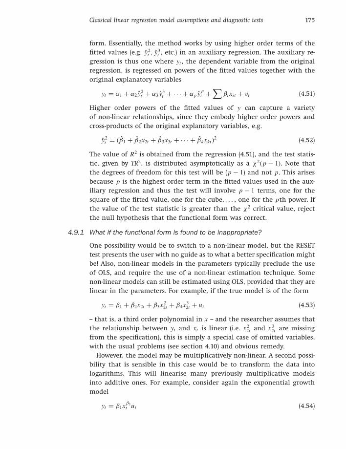
Classical linear regression model assumptions and diagnostic tests 175
form. Essentially, the method works by using higher order terms of the
fitted values (e.g. y2t , y3
t , etc.) in an auxiliary regression. The auxiliary re-
gression is thus one where yt , the dependent variable from the original
regression, is regressed on powers of the fitted values together with the
original explanatory variables
yt = α1 + α2 y2t + α3 y3
t + · · · + αp ypt +
∑
βi xi t + vt (4.51)
Higher order powers of the fitted values of y can capture a variety
of non-linear relationships, since they embody higher order powers and
cross-products of the original explanatory variables, e.g.
y2t = (β1 + β2x2t + β3x3t + · · · + βk xkt )
2 (4.52)
The value of R2 is obtained from the regression (4.51), and the test statis-
tic, given by TR2, is distributed asymptotically as a χ2(p − 1). Note that
the degrees of freedom for this test will be (p − 1) and not p. This arises
because p is the highest order term in the fitted values used in the aux-
iliary regression and thus the test will involve p − 1 terms, one for the
square of the fitted value, one for the cube, . . . , one for the pth power. If
the value of the test statistic is greater than the χ2 critical value, reject
the null hypothesis that the functional form was correct.
4.9.1 What if the functional form is found to be inappropriate?
One possibility would be to switch to a non-linear model, but the RESET
test presents the user with no guide as to what a better specification might
be! Also, non-linear models in the parameters typically preclude the use
of OLS, and require the use of a non-linear estimation technique. Some
non-linear models can still be estimated using OLS, provided that they are
linear in the parameters. For example, if the true model is of the form
yt = β1 + β2x2t + β3x22t + β4x3
2t + ut (4.53)
-- that is, a third order polynomial in x -- and the researcher assumes that
the relationship between yt and xt is linear (i.e. x22t and x3
2t are missing
from the specification), this is simply a special case of omitted variables,
with the usual problems (see section 4.10) and obvious remedy.
However, the model may be multiplicatively non-linear. A second possi-
bility that is sensible in this case would be to transform the data into
logarithms. This will linearise many previously multiplicative models
into additive ones. For example, consider again the exponential growth
model
yt = β1xβ2
t ut (4.54)

176 Introductory Econometrics for Finance
Taking logs, this becomes
ln(yt ) = ln(β1) + β2 ln(xt ) + ln(ut ) (4.55)
or
Yt = α + β2 X t + vt (4.56)
where Yt = ln(yt ), α = ln(β1), X t = ln(xt ), vt = ln(ut ). Thus a simple loga-
rithmic transformation makes this model a standard linear bivariate re-
gression equation that can be estimated using OLS.
Loosely following the treatment given in Stock and Watson (2006), the
following list shows four different functional forms for models that are
either linear or can be made linear following a logarithmic transformation
to one or more of the dependent or independent variables, examining only
a bivariate specification for simplicity. Care is needed when interpreting
the coefficient values in each case.
(1) Linear model: yt = β1 + β2x2t + ut ; a 1-unit increase in x2t causes a β2-
unit increase in yt .
x2t
yt
(2) Log-linear: ln(yt ) = β1 + β2x2t + ut ; a 1-unit increase in x2t causes a
100 × β2% increase in yt .
x2t
ln yt
x2t
yt
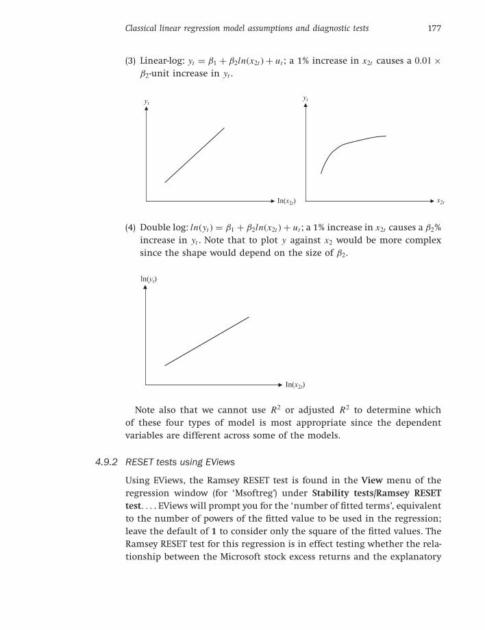
Classical linear regression model assumptions and diagnostic tests 177
(3) Linear-log: yt = β1 + β2ln(x2t ) + ut ; a 1% increase in x2t causes a 0.01 ×
β2-unit increase in yt .
yt
In(x2t) x2t
yt
(4) Double log: ln(yt ) = β1 + β2ln(x2t ) + ut ; a 1% increase in x2t causes a β2%
increase in yt . Note that to plot y against x2 would be more complex
since the shape would depend on the size of β2.
ln(yt)
In(x2t)
Note also that we cannot use R2 or adjusted R2 to determine which
of these four types of model is most appropriate since the dependent
variables are different across some of the models.
4.9.2 RESET tests using EViews
Using EViews, the Ramsey RESET test is found in the View menu of the
regression window (for ‘Msoftreg’) under Stability tests/Ramsey RESET
test. . . . EViews will prompt you for the ‘number of fitted terms’, equivalent
to the number of powers of the fitted value to be used in the regression;
leave the default of 1 to consider only the square of the fitted values. The
Ramsey RESET test for this regression is in effect testing whether the rela-
tionship between the Microsoft stock excess returns and the explanatory

178 Introductory Econometrics for Finance
variables is linear or not. The results of this test for one fitted term are
shown in the following table.
Ramsey RESET Test:
F-statistic 1.603573 Prob. F(1,241) 0.2066Log likelihood ratio 1.671212 Prob. Chi-Square(1) 0.1961
Test Equation:Dependent Variable: ERMSOFTMethod: Least SquaresDate: 08/29/07 Time: 09:54Sample: 1986M05 2007M04Included observations: 252
Coefficient Std. Error t-Statistic Prob.
C −0.531288 1.359686 −0.390743 0.6963ERSANDP 1.639661 0.197469 8.303368 0.0000DPROD 0.487139 0.452025 1.077681 0.2823
DCREDIT −5.99E-05 0.000144 −0.414772 0.6787DINFLATION 5.030282 2.683906 1.874239 0.0621
DMONEY −1.413747 0.643937 −2.195475 0.0291DSPREAD 8.488655 12.21231 0.695090 0.4877RTERM 6.692483 2.994476 2.234943 0.0263
FEB89DUM −94.39106 23.62309 −3.995712 0.0001FEB03DUM −105.0831 31.71804 −3.313037 0.0011FITTED∧2 0.007732 0.006106 1.266323 0.2066
R-squared 0.363199 Mean dependent var −0.420803Adjusted R-squared 0.336776 S.D. dependent var 15.41135S.E. of regression 12.55078 Akaike info criterion 7.940113Sum squared resid 37962.85 Schwarz criterion 8.094175Log likelihood −989.4542 Hannan-Quinn criter. 8.002104F-statistic 13.74543 Durbin-Watson stat 2.090304Prob(F-statistic) 0.000000
Both F− and χ2 versions of the test are presented, and it can be seen
that there is no apparent non-linearity in the regression equation and so
it would be concluded that the linear model for the Microsoft returns is
appropriate.
4.10 Omission of an important variable
What would be the effects of excluding from the estimated regression a
variable that is a determinant of the dependent variable? For example,

Classical linear regression model assumptions and diagnostic tests 179
suppose that the true, but unknown, data generating process is repre-
sented by
yt = β1 + β2 x2t + β3 x3t + β4 x4t + β5 x5t + ut (4.57)
but the researcher estimated a model of the form
yt = β1 + β2 x2t + β3 x3t + β4 x4t + ut (4.58)
so that the variable x5t is omitted from the model. The consequence would
be that the estimated coefficients on all the other variables will be biased
and inconsistent unless the excluded variable is uncorrelated with all
the included variables. Even if this condition is satisfied, the estimate of
the coefficient on the constant term will be biased, which would imply
that any forecasts made from the model would be biased. The standard
errors will also be biased (upwards), and hence hypothesis tests could yield
inappropriate inferences. Further intuition is offered in Dougherty (1992,
pp. 168--73).
4.11 Inclusion of an irrelevant variable
Suppose now that the researcher makes the opposite error to section 4.10,
i.e. that the true DGP was represented by
yt = β1 + β2 x2t + β3 x3t + β4 x4t + ut (4.59)
but the researcher estimates a model of the form
yt = β1 + β2 x2t + β3 x3t + β4 x4t + β5 x5t + ut (4.60)
thus incorporating the superfluous or irrelevant variable x5t . As x5t is
irrelevant, the expected value of β5 is zero, although in any practical
application, its estimated value is very unlikely to be exactly zero. The
consequence of including an irrelevant variable would be that the coeffi-
cient estimators would still be consistent and unbiased, but the estima-
tors would be inefficient. This would imply that the standard errors for
the coefficients are likely to be inflated relative to the values which they
would have taken if the irrelevant variable had not been included. Vari-
ables which would otherwise have been marginally significant may no
longer be so in the presence of irrelevant variables. In general, it can also
be stated that the extent of the loss of efficiency will depend positively
on the absolute value of the correlation between the included irrelevant
variable and the other explanatory variables.

180 Introductory Econometrics for Finance
Summarising the last two sections it is evident that when trying to
determine whether to err on the side of including too many or too few
variables in a regression model, there is an implicit trade-off between in-
consistency and efficiency; many researchers would argue that while in an
ideal world, the model will incorporate precisely the correct variables -- no
more and no less -- the former problem is more serious than the latter and
therefore in the real world, one should err on the side of incorporating
marginally significant variables.
4.12 Parameter stability tests
So far, regressions of a form such as
yt = β1 + β2x2t + β3x3t + ut (4.61)
have been estimated. These regressions embody the implicit assumption
that the parameters (β1, β2 and β3) are constant for the entire sample, both
for the data period used to estimate the model, and for any subsequent
period used in the construction of forecasts.
This implicit assumption can be tested using parameter stability tests.
The idea is essentially to split the data into sub-periods and then to esti-
mate up to three models, for each of the sub-parts and for all the data
and then to ‘compare’ the RSS of each of the models. There are two types
of test that will be considered, namely the Chow (analysis of variance) test
and predictive failure tests.
4.12.1 The Chow test
The steps involved are shown in box 4.7.
Box 4.7 Conducting a Chow test
(1) Split the data into two sub-periods. Estimate the regression over the whole period
and then for the two sub-periods separately (3 regressions). Obtain the RSS for
each regression.
(2) The restricted regression is now the regression for the whole period while the
‘unrestricted regression’ comes in two parts: one for each of the sub-samples. It is
thus possible to form an F-test, which is based on the difference between the
RSSs. The statistic is
test statistic =RSS − ( RSS1 + RSS2)
RSS1 + RSS2
×T − 2k
k(4.62)
where RSS = residual sum of squares for whole sample

Classical linear regression model assumptions and diagnostic tests 181
RSS1 = residual sum of squares for sub-sample 1
RSS2 = residual sum of squares for sub-sample 2
T = number of observations
2k = number of regressors in the ‘unrestricted’ regression (since it comes in two
parts)
k = number of regressors in (each) ‘unrestricted’ regression
The unrestricted regression is the one where the restriction has not been imposed
on the model. Since the restriction is that the coefficients are equal across the
sub-samples, the restricted regression will be the single regression for the whole
sample. Thus, the test is one of how much the residual sum of squares for
the whole sample (RSS) is bigger than the sum of the residual sums of squares for
the two sub-samples (RSS1 + RSS2). If the coefficients do not change much
between the samples, the residual sum of squares will not rise much upon
imposing the restriction. Thus the test statistic in (4.62) can be considered a
straightforward application of the standard F-test formula discussed in chapter 3.
The restricted residual sum of squares in (4.62) is RSS, while the unrestricted
residual sum of squares is (RSS1 + RSS2). The number of restrictions is equal to the
number of coefficients that are estimated for each of the regressions, i.e. k. The
number of regressors in the unrestricted regression (including the constants) is 2k,
since the unrestricted regression comes in two parts, each with k regressors.
(3) Perform the test. If the value of the test statistic is greater than the critical value
from the F-distribution, which is an F(k, T −2k), then reject the null hypothesis that
the parameters are stable over time.
Note that it is also possible to use a dummy variables approach to calcu-
lating both Chow and predictive failure tests. In the case of the Chow test,
the unrestricted regression would contain dummy variables for the inter-
cept and for all of the slope coefficients (see also chapter 9). For example,
suppose that the regression is of the form
yt = β1 + β2x2t + β3x3t + ut (4.63)
If the split of the total of T observations is made so that the sub-samples
contain T1 and T2 observations (where T1 + T2 = T ), the unrestricted re-
gression would be given by
yt = β1 + β2x2t + β3x3t + β4 Dt + β5 Dt x2t + β6 Dt x3t + vt (4.64)
where Dt = 1 for t ∈ T1 and zero otherwise. In other words, Dt takes the
value one for observations in the first sub-sample and zero for observations
in the second sub-sample. The Chow test viewed in this way would then be
a standard F-test of the joint restriction H0: β4 = 0 and β5 = 0 and β6 = 0,
with (4.64) and (4.63) being the unrestricted and restricted regressions,
respectively.
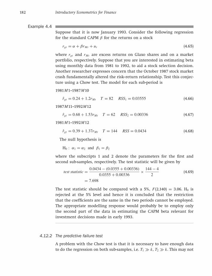
182 Introductory Econometrics for Finance
Example 4.4
Suppose that it is now January 1993. Consider the following regression
for the standard CAPM β for the returns on a stock
rgt = α + βrMt + ut (4.65)
where rgt and rMt are excess returns on Glaxo shares and on a market
portfolio, respectively. Suppose that you are interested in estimating beta
using monthly data from 1981 to 1992, to aid a stock selection decision.
Another researcher expresses concern that the October 1987 stock market
crash fundamentally altered the risk--return relationship. Test this conjec-
ture using a Chow test. The model for each sub-period is
1981M1--1987M10
rgt = 0.24 + 1.2rMt T = 82 RSS1 = 0.03555 (4.66)
1987M11--1992M12
rgt = 0.68 + 1.53rMt T = 62 RSS2 = 0.00336 (4.67)
1981M1--1992M12
rgt = 0.39 + 1.37rMt T = 144 RSS = 0.0434 (4.68)
The null hypothesis is
H0 : α1 = α2 and β1 = β2
where the subscripts 1 and 2 denote the parameters for the first and
second sub-samples, respectively. The test statistic will be given by
test statistic =0.0434 − (0.0355 + 0.00336)
0.0355 + 0.00336×
144 − 4
2(4.69)
= 7.698
The test statistic should be compared with a 5%, F (2,140) = 3.06. H0 is
rejected at the 5% level and hence it is concluded that the restriction
that the coefficients are the same in the two periods cannot be employed.
The appropriate modelling response would probably be to employ only
the second part of the data in estimating the CAPM beta relevant for
investment decisions made in early 1993.
4.12.2 The predictive failure test
A problem with the Chow test is that it is necessary to have enough data
to do the regression on both sub-samples, i.e. T1 ≫ k, T2 ≫ k. This may not

Classical linear regression model assumptions and diagnostic tests 183
hold in the situation where the total number of observations available is
small. Even more likely is the situation where the researcher would like
to examine the effect of splitting the sample at some point very close to
the start or very close to the end of the sample. An alternative formula-
tion of a test for the stability of the model is the predictive failure test,
which requires estimation for the full sample and one of the sub-samples
only. The predictive failure test works by estimating the regression over a
‘long’ sub-period (i.e. most of the data) and then using those coefficient
estimates for predicting values of y for the other period. These predic-
tions for y are then implicitly compared with the actual values. Although
it can be expressed in several different ways, the null hypothesis for this
test is that the prediction errors for all of the forecasted observations are
zero.
To calculate the test:
● Run the regression for the whole period (the restricted regression) and
obtain the RSS.
● Run the regression for the ‘large’ sub-period and obtain the RSS (called
RSS1). Note that in this book, the number of observations for the long
estimation sub-period will be denoted by T1 (even though it may come
second). The test statistic is given by
test statistic =RSS − RSS1
RSS1
×T1 − k
T2
(4.70)
where T2 = number of observations that the model is attempting to
‘predict’. The test statistic will follow an F(T2, T1 − k).
For an intuitive interpretation of the predictive failure test statistic for-
mulation, consider an alternative way to test for predictive failure using a
regression containing dummy variables. A separate dummy variable would
be used for each observation that was in the prediction sample. The un-
restricted regression would then be the one that includes the dummy
variables, which will be estimated using all T observations, and will have
(k + T2) regressors (the k original explanatory variables, and a dummy
variable for each prediction observation, i.e. a total of T2 dummy vari-
ables). Thus the numerator of the last part of (4.70) would be the total
number of observations (T ) minus the number of regressors in the unre-
stricted regression (k + T2). Noting also that T − (k + T2) = (T1 − k), since
T1 + T2 = T, this gives the numerator of the last term in (4.70). The re-
stricted regression would then be the original regression containing the
explanatory variables but none of the dummy variables. Thus the number

184 Introductory Econometrics for Finance
of restrictions would be the number of observations in the prediction
period, which would be equivalent to the number of dummy variables
included in the unrestricted regression, T2.
To offer an illustration, suppose that the regression is again of the form
of (4.63), and that the last three observations in the sample are used for
a predictive failure test. The unrestricted regression would include three
dummy variables, one for each of the observations in T2
rgt = α + βrMt + γ1 D1t + γ2 D2t + γ3 D3t + ut (4.71)
where D1t = 1 for observation T − 2 and zero otherwise, D2t = 1 for
observation T − 1 and zero otherwise, D3t = 1 for observation T and zero
otherwise. In this case, k = 2, and T2 = 3. The null hypothesis for the
predictive failure test in this regression is that the coefficients on all of
the dummy variables are zero (i.e. H0 : γ1 = 0 and γ2 = 0 and γ3 = 0). Both
approaches to conducting the predictive failure test described above are
equivalent, although the dummy variable regression is likely to take more
time to set up.
However, for both the Chow and the predictive failure tests, the dummy
variables approach has the one major advantage that it provides the
user with more information. This additional information comes from
the fact that one can examine the significances of the coefficients on
the individual dummy variables to see which part of the joint null hy-
pothesis is causing a rejection. For example, in the context of the Chow
regression, is it the intercept or the slope coefficients that are signifi-
cantly different across the two sub-samples? In the context of the pre-
dictive failure test, use of the dummy variables approach would show
for which period(s) the prediction errors are significantly different from
zero.
4.12.3 Backward versus forward predictive failure tests
There are two types of predictive failure tests -- forward tests and back-
wards tests. Forward predictive failure tests are where the last few obser-
vations are kept back for forecast testing. For example, suppose that obser-
vations for 1980Q1--2004Q4 are available. A forward predictive failure test
could involve estimating the model over 1980Q1--2003Q4 and forecasting
2004Q1--2004Q4. Backward predictive failure tests attempt to ‘back-cast’
the first few observations, e.g. if data for 1980Q1--2004Q4 are available,
and the model is estimated over 1971Q1--2004Q4 and back-cast 1980Q1--
1980Q4. Both types of test offer further evidence on the stability of the
regression relationship over the whole sample period.

Classical linear regression model assumptions and diagnostic tests 185
Example 4.5
Suppose that the researcher decided to determine the stability of the
estimated model for stock returns over the whole sample in example 4.4
by using a predictive failure test of the last two years of observations. The
following models would be estimated:
1981M1--1992M12 (whole sample)
rgt = 0.39 + 1.37rMt T = 144 RSS = 0.0434 (4.72)
1981M1--1990M12 (‘long sub-sample’)
rgt = 0.32 + 1.31rMt T = 120 RSS1 = 0.0420 (4.73)
Can this regression adequately ‘forecast’ the values for the last two years?
The test statistic would be given by
test statistic =0.0434 − 0.0420
0.0420×
120 − 2
24(4.74)
= 0.164
Compare the test statistic with an F (24,118) = 1.66 at the 5% level. So
the null hypothesis that the model can adequately predict the last few
observations would not be rejected. It would thus be concluded that the
model did not suffer from predictive failure during the 1991M1--1992M12
period.
4.12.4 How can the appropriate sub-parts to use be decided?
As a rule of thumb, some or all of the following methods for selecting
where the overall sample split occurs could be used:
● Plot the dependent variable over time and split the data accordingly to
any obvious structural changes in the series, as illustrated in figure 4.14.
1400
1200
1000
800
600
400
200
0
Observation number
y t
1
33
65
97
12
9
161
19
3
225
257
289
32
1
353
385
417
449
Figure 4.14
Plot of a variable
showing suggestion
for break date
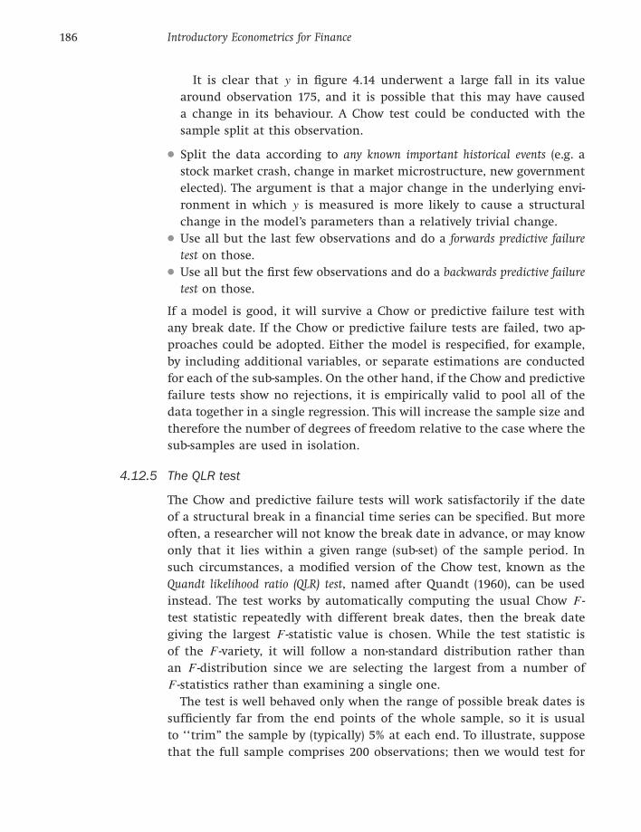
186 Introductory Econometrics for Finance
It is clear that y in figure 4.14 underwent a large fall in its value
around observation 175, and it is possible that this may have caused
a change in its behaviour. A Chow test could be conducted with the
sample split at this observation.
● Split the data according to any known important historical events (e.g. a
stock market crash, change in market microstructure, new government
elected). The argument is that a major change in the underlying envi-
ronment in which y is measured is more likely to cause a structural
change in the model’s parameters than a relatively trivial change.
● Use all but the last few observations and do a forwards predictive failure
test on those.
● Use all but the first few observations and do a backwards predictive failure
test on those.
If a model is good, it will survive a Chow or predictive failure test with
any break date. If the Chow or predictive failure tests are failed, two ap-
proaches could be adopted. Either the model is respecified, for example,
by including additional variables, or separate estimations are conducted
for each of the sub-samples. On the other hand, if the Chow and predictive
failure tests show no rejections, it is empirically valid to pool all of the
data together in a single regression. This will increase the sample size and
therefore the number of degrees of freedom relative to the case where the
sub-samples are used in isolation.
4.12.5 The QLR test
The Chow and predictive failure tests will work satisfactorily if the date
of a structural break in a financial time series can be specified. But more
often, a researcher will not know the break date in advance, or may know
only that it lies within a given range (sub-set) of the sample period. In
such circumstances, a modified version of the Chow test, known as the
Quandt likelihood ratio (QLR) test, named after Quandt (1960), can be used
instead. The test works by automatically computing the usual Chow F -
test statistic repeatedly with different break dates, then the break date
giving the largest F -statistic value is chosen. While the test statistic is
of the F -variety, it will follow a non-standard distribution rather than
an F -distribution since we are selecting the largest from a number of
F -statistics rather than examining a single one.
The test is well behaved only when the range of possible break dates is
sufficiently far from the end points of the whole sample, so it is usual
to ‘‘trim’’ the sample by (typically) 5% at each end. To illustrate, suppose
that the full sample comprises 200 observations; then we would test for

Classical linear regression model assumptions and diagnostic tests 187
a structural break between observations 31 and 170 inclusive. The criti-
cal values will depend on how much of the sample is trimmed away, the
number of restrictions under the null hypothesis (the number of regres-
sors in the original regression as this is effectively a Chow test) and the
significance level.
4.12.6 Stability tests based on recursive estimation
An alternative to the QLR test for use in the situation where a researcher
believes that a series may contain a structural break but is unsure of
the date is to perform a recursive estimation. This is sometimes known
as recursive least squares (RLS). The procedure is appropriate only for time-
series data or cross-sectional data that have been ordered in some sensible
way (for example, a sample of annual stock returns, ordered by market
capitalisation). Recursive estimation simply involves starting with a sub-
sample of the data, estimating the regression, then sequentially adding
one observation at a time and re-running the regression until the end of
the sample is reached. It is common to begin the initial estimation with
the very minimum number of observations possible, which will be k + 1.
So at the first step, the model is estimated using observations 1 to k + 1;
at the second step, observations 1 to k + 2 are used and so on; at the final
step, observations 1 to T are used. The final result will be the production
of T − k separate estimates of every parameter in the regression model.
It is to be expected that the parameter estimates produced near the
start of the recursive procedure will appear rather unstable since these
estimates are being produced using so few observations, but the key ques-
tion is whether they then gradually settle down or whether the volatility
continues through the whole sample. Seeing the latter would be an indi-
cation of parameter instability.
It should be evident that RLS in itself is not a statistical test for parame-
ter stability as such, but rather it provides qualitative information which
can be plotted and thus gives a very visual impression of how stable the
parameters appear to be. But two important stability tests, known as the
CUSUM and CUSUMSQ tests, are derived from the residuals of the recur-
sive estimation (known as the recursive residuals).5 The CUSUM statistic
is based on a normalised (i.e. scaled) version of the cumulative sums of
the residuals. Under the null hypothesis of perfect parameter stability, the
CUSUM statistic is zero however many residuals are included in the sum
5 Strictly, the CUSUM and CUSUMSQ statistics are based on the one-step ahead prediction
errors -- i.e. the differences between yt and its predicted value based on the parameters
estimated at time t − 1. See Greene (2002, chapter 7) for full technical details.
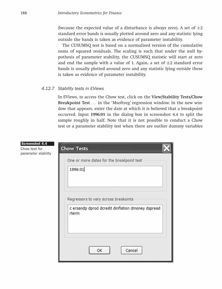
188 Introductory Econometrics for Finance
(because the expected value of a disturbance is always zero). A set of ±2
standard error bands is usually plotted around zero and any statistic lying
outside the bands is taken as evidence of parameter instability.
The CUSUMSQ test is based on a normalised version of the cumulative
sums of squared residuals. The scaling is such that under the null hy-
pothesis of parameter stability, the CUSUMSQ statistic will start at zero
and end the sample with a value of 1. Again, a set of ±2 standard error
bands is usually plotted around zero and any statistic lying outside these
is taken as evidence of parameter instability.
4.12.7 Stability tests in EViews
In EViews, to access the Chow test, click on the View/Stability Tests/Chow
Breakpoint Test . . . in the ‘Msoftreg’ regression window. In the new win-
dow that appears, enter the date at which it is believed that a breakpoint
occurred. Input 1996:01 in the dialog box in screenshot 4.4 to split the
sample roughly in half. Note that it is not possible to conduct a Chow
test or a parameter stability test when there are outlier dummy variables
Screenshot 4.4
Chow test for
parameter stability

Classical linear regression model assumptions and diagnostic tests 189
in the regression. This occurs because when the sample is split into two
parts, the dummy variable for one of the parts will have values of zero for
all observations, which would thus cause perfect multicollinearity with
the column of ones that is used for the constant term. So ensure that the
Chow test is performed using the regression containing all of the explana-
tory variables except the dummies. By default, EViews allows the values of
all the parameters to vary across the two sub-samples in the unrestricted
regressions, although if we wanted, we could force some of the parameters
to be fixed across the two sub-samples.
EViews gives three versions of the test statistics, as shown in the follow-
ing table.
Chow Breakpoint Test: 1996M01Null Hypothesis: No breaks at specified breakpointsVarying regressors: All equation variablesEquation Sample: 1986M05 2007M04
F-statistic 0.581302 Prob. F(8,236) 0.7929Log likelihood ratio 4.917407 Prob. Chi-Square(8) 0.7664Wald Statistic 4.650416 Prob. Chi-Square(8) 0.7942
The first version of the test is the familiar F -test, which computes a
restricted version and an unrestricted version of the auxiliary regression
and ‘compares’ the residual sums of squares, while the second and third
versions are based on χ2 formulations. In this case, all three test statistics
are smaller than their critical values and so the null hypothesis that
the parameters are constant across the two sub-samples is not rejected.
Note that the Chow forecast (i.e. the predictive failure) test could also be
employed by clicking on the View/Stability Tests/Chow Forecast Test . . .
in the regression window. Determine whether the model can predict the
last four observations by entering 2007:01 in the dialog box. The results
of this test are given in the following table.
Chow Forecast Test: Forecast from 2007M01 to 2007M04
F-statistic 0.056576 Prob. F(4,240) 0.9940Log likelihood ratio 0.237522 Prob. Chi-Square(4) 0.9935
The table indicates that the model can indeed adequately predict the
2007 observations. Thus the conclusions from both forms of the test are
that there is no evidence of parameter instability. However, the conclusion
should really be that the parameters are stable with respect to these partic-
ular break dates. It is important to note that for the model to be deemed

190 Introductory Econometrics for Finance
adequate, it needs to be stable with respect to any break dates that we
may choose. A good way to test this is to use one of the tests based on
recursive estimation.
Click on View/Stability Tests/Recursive Estimates (OLS Only). . . . You will
be presented with a menu as shown in screenshot 4.5 containing a number
of options including the CUSUM and CUSUMSQ tests described above and
also the opportunity to plot the recursively estimated coefficients.
Screenshot 4.5
Plotting recursive
coefficient
estimates
First, check the box next to Recursive coefficients and then recur-
sive estimates will be given for all those parameters listed in the ‘Co-
efficient display list’ box, which by default is all of them. Click OK and
you will be presented with eight small figures, one for each parameter,
showing the recursive estimates and ±2 standard error bands around
them. As discussed above, it is bound to take some time for the co-
efficients to stabilise since the first few sets are estimated using such
small samples. Given this, the parameter estimates in all cases are re-
markably stable over time. Now go back to View/Stability Tests/Recursive
Estimates (OLS Only) . . . . and choose CUSUM Test. The resulting graph is in
screenshot 4.6.
Since the line is well within the confidence bands, the conclusion would
be again that the null hypothesis of stability is not rejected. Now repeat
the above but using the CUSUMSQ test rather than CUSUM. Do we retain
the same conclusion? (No) Why?

Classical linear regression model assumptions and diagnostic tests 191
60
40
20
0
−20
−40
−6088 90 9492 96 98 00 02 04 06
CUSUM 5% Significance
Screenshot 4.6
CUSUM test graph
4.13 A strategy for constructing econometric models and adiscussion of model-building philosophies
The objective of many econometric model-building exercises is to build a
statistically adequate empirical model which satisfies the assumptions of
the CLRM, is parsimonious, has the appropriate theoretical interpretation,
and has the right ‘shape’ (i.e. all signs on coefficients are ‘correct’ and all
sizes of coefficients are ‘correct’).
But how might a researcher go about achieving this objective? A com-
mon approach to model building is the ‘LSE’ or general-to-specific method-
ology associated with Sargan and Hendry. This approach essentially in-
volves starting with a large model which is statistically adequate and re-
stricting and rearranging the model to arrive at a parsimonious final for-
mulation. Hendry’s approach (see Gilbert, 1986) argues that a good model
is consistent with the data and with theory. A good model will also encom-
pass rival models, which means that it can explain all that rival models
can and more. The Hendry methodology suggests the extensive use of
diagnostic tests to ensure the statistical adequacy of the model.
An alternative philosophy of econometric model-building, which pre-
dates Hendry’s research, is that of starting with the simplest model and
adding to it sequentially so that it gradually becomes more complex
and a better description of reality. This approach, associated principally
with Koopmans (1937), is sometimes known as a ‘specific-to-general’ or
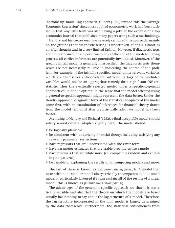
192 Introductory Econometrics for Finance
‘bottoms-up’ modelling approach. Gilbert (1986) termed this the ‘Average
Economic Regression’ since most applied econometric work had been tack-
led in that way. This term was also having a joke at the expense of a top
economics journal that published many papers using such a methodology.
Hendry and his co-workers have severely criticised this approach, mainly
on the grounds that diagnostic testing is undertaken, if at all, almost as
an after-thought and in a very limited fashion. However, if diagnostic tests
are not performed, or are performed only at the end of the model-building
process, all earlier inferences are potentially invalidated. Moreover, if the
specific initial model is generally misspecified, the diagnostic tests them-
selves are not necessarily reliable in indicating the source of the prob-
lem. For example, if the initially specified model omits relevant variables
which are themselves autocorrelated, introducing lags of the included
variables would not be an appropriate remedy for a significant DW test
statistic. Thus the eventually selected model under a specific-to-general
approach could be sub-optimal in the sense that the model selected using
a general-to-specific approach might represent the data better. Under the
Hendry approach, diagnostic tests of the statistical adequacy of the model
come first, with an examination of inferences for financial theory drawn
from the model left until after a statistically adequate model has been
found.
According to Hendry and Richard (1982), a final acceptable model should
satisfy several criteria (adapted slightly here). The model should:
● be logically plausible
● be consistent with underlying financial theory, including satisfying any
relevant parameter restrictions
● have regressors that are uncorrelated with the error term
● have parameter estimates that are stable over the entire sample
● have residuals that are white noise (i.e. completely random and exhibit-
ing no patterns)
● be capable of explaining the results of all competing models and more.
The last of these is known as the encompassing principle. A model that
nests within it a smaller model always trivially encompasses it. But a small
model is particularly favoured if it can explain all of the results of a larger
model; this is known as parsimonious encompassing.
The advantages of the general-to-specific approach are that it is statis-
tically sensible and also that the theory on which the models are based
usually has nothing to say about the lag structure of a model. Therefore,
the lag structure incorporated in the final model is largely determined
by the data themselves. Furthermore, the statistical consequences from

Classical linear regression model assumptions and diagnostic tests 193
excluding relevant variables are usually considered more serious than
those from including irrelevant variables.
The general-to-specific methodology is conducted as follows. The first
step is to form a ‘large’ model with lots of variables on the RHS. This is
known as a generalised unrestricted model (GUM), which should originate
from financial theory, and which should contain all variables thought to
influence the dependent variable. At this stage, the researcher is required
to ensure that the model satisfies all of the assumptions of the CLRM.
If the assumptions are violated, appropriate actions should be taken to
address or allow for this, e.g. taking logs, adding lags, adding dummy
variables.
It is important that the steps above are conducted prior to any hypoth-
esis testing. It should also be noted that the diagnostic tests presented
above should be cautiously interpreted as general rather than specific
tests. In other words, rejection of a particular diagnostic test null hypoth-
esis should be interpreted as showing that there is something wrong with
the model. So, for example, if the RESET test or White’s test show a rejec-
tion of the null, such results should not be immediately interpreted as
implying that the appropriate response is to find a solution for inappro-
priate functional form or heteroscedastic residuals, respectively. It is quite
often the case that one problem with the model could cause several as-
sumptions to be violated simultaneously. For example, an omitted variable
could cause failures of the RESET, heteroscedasticity and autocorrelation
tests. Equally, a small number of large outliers could cause non-normality
and residual autocorrelation (if they occur close together in the sample)
and heteroscedasticity (if the outliers occur for a narrow range of the
explanatory variables). Moreover, the diagnostic tests themselves do not
operate optimally in the presence of other types of misspecification since
they essentially assume that the model is correctly specified in all other
respects. For example, it is not clear that tests for heteroscedasticity will
behave well if the residuals are autocorrelated.
Once a model that satisfies the assumptions of the CLRM has been ob-
tained, it could be very big, with large numbers of lags and indepen-
dent variables. The next stage is therefore to reparameterise the model by
knocking out very insignificant regressors. Also, some coefficients may be
insignificantly different from each other, so that they can be combined.
At each stage, it should be checked whether the assumptions of the CLRM
are still upheld. If this is the case, the researcher should have arrived
at a statistically adequate empirical model that can be used for testing
underlying financial theories, forecasting future values of the dependent
variable, or for formulating policies.
194 Introductory Econometrics for Finance
However, needless to say, the general-to-specific approach also has its
critics. For small or moderate sample sizes, it may be impractical. In such
instances, the large number of explanatory variables will imply a small
number of degrees of freedom. This could mean that none of the variables
is significant, especially if they are highly correlated. This being the case, it
would not be clear which of the original long list of candidate regressors
should subsequently be dropped. Moreover, in any case the decision on
which variables to drop may have profound implications for the final
specification of the model. A variable whose coefficient was not significant
might have become significant at a later stage if other variables had been
dropped instead.
In theory, sensitivity of the final specification to the various possible
paths of variable deletion should be carefully checked. However, this could
imply checking many (perhaps even hundreds) of possible specifications. It
could also lead to several final models, none of which appears noticeably
better than the others.
The general-to-specific approach, if followed faithfully to the end, will
hopefully lead to a statistically valid model that passes all of the usual
model diagnostic tests and contains only statistically significant regres-
sors. However, the final model could also be a bizarre creature that is
devoid of any theoretical interpretation. There would also be more than
just a passing chance that such a model could be the product of a statisti-
cally vindicated data mining exercise. Such a model would closely fit the
sample of data at hand, but could fail miserably when applied to other
samples if it is not based soundly on theory.
There now follows another example of the use of the classical linear
regression model in finance, based on an examination of the determinants
of sovereign credit ratings by Cantor and Packer (1996).
4.14 Determinants of sovereign credit ratings
4.14.1 Background
Sovereign credit ratings are an assessment of the riskiness of debt issued
by governments. They embody an estimate of the probability that the bor-
rower will default on her obligation. Two famous US ratings agencies,
Moody’s and Standard and Poor’s, provide ratings for many governments.
Although the two agencies use different symbols to denote the given risk-
iness of a particular borrower, the ratings of the two agencies are com-
parable. Gradings are split into two broad categories: investment grade
and speculative grade. Investment grade issuers have good or adequate
payment capacity, while speculative grade issuers either have a high

Classical linear regression model assumptions and diagnostic tests 195
degree of uncertainty about whether they will make their payments, or
are already in default. The highest grade offered by the agencies, for the
highest quality of payment capacity, is ‘triple A’, which Moody’s denotes
‘Aaa’ and Standard and Poor’s denotes ‘AAA’. The lowest grade issued to a
sovereign in the Cantor and Packer sample was B3 (Moody’s) or B− (Stan-
dard and Poor’s). Thus the number of grades of debt quality from the
highest to the lowest given to governments in their sample is 16.
The central aim of Cantor and Packer’s paper is an attempt to explain
and model how the agencies arrived at their ratings. Although the ratings
themselves are publicly available, the models or methods used to arrive
at them are shrouded in secrecy. The agencies also provide virtually no
explanation as to what the relative weights of the factors that make up the
rating are. Thus, a model of the determinants of sovereign credit ratings
could be useful in assessing whether the ratings agencies appear to have
acted rationally. Such a model could also be employed to try to predict
the rating that would be awarded to a sovereign that has not previously
been rated and when a re-rating is likely to occur. The paper continues,
among other things, to consider whether ratings add to publicly available
information, and whether it is possible to determine what factors affect
how the sovereign yields react to ratings announcements.
4.14.2 Data
Cantor and Packer (1996) obtain a sample of government debt ratings for
49 countries as of September 1995 that range between the above grad-
ings. The ratings variable is quantified, so that the highest credit quality
(Aaa/AAA) in the sample is given a score of 16, while the lowest rated
sovereign in the sample is given a score of 1 (B3/B−). This score forms the
dependent variable. The factors that are used to explain the variability
in the ratings scores are macroeconomic variables. All of these variables
embody factors that are likely to influence a government’s ability and
willingness to service its debt costs. Ideally, the model would also include
proxies for socio-political factors, but these are difficult to measure ob-
jectively and so are not included. It is not clear in the paper from where
the list of factors was drawn. The included variables (with their units of
measurement) are:
● Per capita income (in 1994 thousand US dollars). Cantor and Packer ar-
gue that per capita income determines the tax base, which in turn in-
fluences the government’s ability to raise revenue.
● GDP growth (annual 1991--4 average, %). The growth rate of increase in
GDP is argued to measure how much easier it will become to service
debt costs in the future.

196 Introductory Econometrics for Finance
● Inflation (annual 1992--4 average, %). Cantor and Packer argue that high
inflation suggests that inflationary money financing will be used to
service debt when the government is unwilling or unable to raise the
required revenue through the tax system.
● Fiscal balance (average annual government budget surplus as a propor-
tion of GDP 1992--4, %). Again, a large fiscal deficit shows that the
government has a relatively weak capacity to raise additional revenue
and to service debt costs.
● External balance (average annual current account surplus as a proportion
of GDP 1992--4, %). Cantor and Packer argue that a persistent current
account deficit leads to increasing foreign indebtedness, which may be
unsustainable in the long run.
● External debt (foreign currency debt as a proportion of exports in 1994,
%). Reasoning as for external balance (which is the change in external
debt over time).
● Dummy for economic development (=1 for a country classified by the IMF as
developed, 0 otherwise). Cantor and Packer argue that credit ratings
agencies perceive developing countries as relatively more risky beyond
that suggested by the values of the other factors listed above.
● Dummy for default history (=1 if a country has defaulted, 0 otherwise).
It is argued that countries that have previously defaulted experience a
large fall in their credit rating.
The income and inflation variables are transformed to their logarithms.
The model is linear and estimated using OLS. Some readers of this book
who have a background in econometrics will note that strictly, OLS is not
an appropriate technique when the dependent variable can take on only
one of a certain limited set of values (in this case, 1, 2, 3, . . . 16). In such
applications, a technique such as ordered probit (not covered in this text)
would usually be more appropriate. Cantor and Packer argue that any
approach other than OLS is infeasible given the relatively small sample
size (49), and the large number (16) of ratings categories.
The results from regressing the rating value on the variables listed above
are presented in their exhibit 5, adapted and presented here as table 4.2.
Four regressions are conducted, each with identical independent vari-
ables but a different dependent variable. Regressions are conducted for
the rating score given by each agency separately, with results presented
in columns (4) and (5) of table 4.2. Occasionally, the ratings agencies give
different scores to a country -- for example, in the case of Italy, Moody’s
gives a rating of ‘A1’, which would generate a score of 12 on a 16-scale.
Standard and Poor’s (S and P), on the other hand, gives a rating of ‘AA’,

Classical linear regression model assumptions and diagnostic tests 197
Table 4.2 Determinants and impacts of sovereign credit ratings
Dependent variable
Explanatory Expected Average Moody’s S&P Differencevariable sign rating rating rating Moody’s/S&P(1) (2) (3) (4) (5) (6)
Intercept ? 1.442 3.408 −0.524 3.932∗∗
(0.663) (1.379) (−0.223) (2.521)
Per capita income + 1.242∗∗∗ 1.027∗∗∗ 1.458∗∗∗ −0.431∗∗∗
(5.302) (4.041) (6.048) (−2.688)
GDP growth + 0.151 0.130 0.171∗∗ −0.040(1.935) (1.545) (2.132) (0.756)
Inflation − −0.611∗∗∗ −0.630∗∗∗ −0.591∗∗∗ −0.039(−2.839) (−2.701) (−2.671) (−0.265)
Fiscal balance + 0.073 0.049 0.097∗ −0.048(1.324) (0.818) (1.71) (−1.274)
External balance + 0.003 0.006 0.001 0.006(0.314) (0.535) (0.046) (0.779)
External debt − −0.013∗∗∗ −0.015∗∗∗ −0.011∗∗∗ −0.004∗∗∗
(−5.088) (−5.365) (−4.236) (−2.133)
Development dummy + 2.776∗∗∗ 2.957∗∗∗ 2.595∗∗∗ 0.362(4.25) (4.175) (3.861) (0.81)
Default dummy − −2.042∗∗∗ −1.63∗∗ −2.622∗∗∗ 1.159∗∗∗
(−3.175) (−2.097) (−3.962) (2.632)
Adjusted R2 0.924 0.905 0.926 0.836
Notes: t -ratios in parentheses; ∗, ∗∗ and ∗∗∗ indicate significance at the 10%, 5% and
1% levels, respectively.
Source: Cantor and Packer (1996). Reprinted with permission from Institutional
Investor.
which would score 14 on the 16-scale, two gradings higher. Thus a regres-
sion with the average score across the two agencies, and with the differ-
ence between the two scores as dependent variables, is also conducted,
and presented in columns (3) and (6), respectively of table 4.2.
4.14.3 Interpreting the models
The models are difficult to interpret in terms of their statistical adequacy,
since virtually no diagnostic tests have been undertaken. The values of
the adjusted R2, at over 90% for each of the three ratings regressions,
are high for cross-sectional regressions, indicating that the model seems
able to capture almost all of the variability of the ratings about their
198 Introductory Econometrics for Finance
mean values across the sample. There does not appear to be any attempt
at reparameterisation presented in the paper, so it is assumed that the
authors reached this set of models after some searching.
In this particular application, the residuals have an interesting interpre-
tation as the difference between the actual and fitted ratings. The actual
ratings will be integers from 1 to 16, although the fitted values from the
regression and therefore the residuals can take on any real value. Cantor
and Packer argue that the model is working well as no residual is bigger
than 3, so that no fitted rating is more than three categories out from the
actual rating, and only four countries have residuals bigger than two cat-
egories. Furthermore, 70% of the countries have ratings predicted exactly
(i.e. the residuals are less than 0.5 in absolute value).
Now, turning to interpret the models from a financial perspective, it is
of interest to investigate whether the coefficients have their expected signs
and sizes. The expected signs for the regression results of columns (3)--(5)
are displayed in column (2) of table 4.2 (as determined by this author).
As can be seen, all of the coefficients have their expected signs, although
the fiscal balance and external balance variables are not significant or are
only very marginally significant in all three cases. The coefficients can be
interpreted as the average change in the rating score that would result
from a unit change in the variable. So, for example, a rise in per capita
income of $1,000 will on average increase the rating by 1.0 units according
to Moody’s and 1.5 units according to Standard & Poor’s. The development
dummy suggests that, on average, a developed country will have a rating
three notches higher than an otherwise identical developing country. And
everything else equal, a country that has defaulted in the past will have
a rating two notches lower than one that has always kept its obligation.
By and large, the ratings agencies appear to place similar weights on
each of the variables, as evidenced by the similar coefficients and signif-
icances across columns (4) and (5) of table 4.2. This is formally tested in
column (6) of the table, where the dependent variable is the difference be-
tween Moody’s and Standard and Poor’s ratings. Only three variables are
statistically significantly differently weighted by the two agencies. Stan-
dard & Poor’s places higher weights on income and default history, while
Moody’s places more emphasis on external debt.
4.14.4 The relationship between ratings and yields
In this section of the paper, Cantor and Packer try to determine whether
ratings have any additional information useful for modelling the cross-
sectional variability of sovereign yield spreads over and above that con-
tained in publicly available macroeconomic data. The dependent variable

Classical linear regression model assumptions and diagnostic tests 199
Table 4.3 Do ratings add to public information?
Dependent variable: ln (yield spread)
Variable Expected sign (1) (2) (3)
Intercept ? 2.105∗∗∗ 0.466 0.074(16.148) (0.345) (0.071)
Average rating − −0.221∗∗∗ −0.218∗∗∗
(−19.175) (−4.276)
Per capita − −0.144 0.226income (−0.927) (1.523)
GDP growth − −0.004 0.029(−0.142) (1.227)
Inflation + 0.108 −0.004(1.393) (−0.068)
Fiscal balance − −0.037 −0.02(−1.557) (−1.045)
External balance − −0.038 −0.023(−1.29) (−1.008)
External debt + 0.003∗∗∗ 0.000(2.651) (0.095)
Development − −0.723∗∗∗ −0.38dummy (−2.059) (−1.341)
Default dummy + 0.612∗∗∗ 0.085(2.577) (0.385)
Adjusted R2 0.919 0.857 0.914
Notes: t -ratios in parentheses; ∗, ∗∗and ∗∗∗ indicate significance at the 10%, 5% and 1%
levels, respectively.
Source: Cantor and Packer (1996). Reprinted with permission from Institutional Investor.
is now the log of the yield spread, i.e.
ln(Yield on the sovereign bond -- Yield on a US Treasury Bond)
One may argue that such a measure of the spread is imprecise, for the
true credit spread should be defined by the entire credit quality curve
rather than by just two points on it. However, leaving this issue aside, the
results are presented in table 4.3.
Three regressions are presented in table 4.3, denoted specifications (1),
(2) and (3). The first of these is a regression of the ln(spread) on only a
constant and the average rating (column (1)), and this shows that ratings
have a highly significant inverse impact on the spread. Specification (2)
200 Introductory Econometrics for Finance
is a regression of the ln(spread) on the macroeconomic variables used in
the previous analysis. The expected signs are given (as determined by this
author) in column (2). As can be seen, all coefficients have their expected
signs, although now only the coefficients belonging to the external debt
and the two dummy variables are statistically significant. Specification
(3) is a regression on both the average rating and the macroeconomic
variables. When the rating is included with the macroeconomic factors,
none of the latter is any longer significant -- only the rating coefficient
is statistically significantly different from zero. This message is also por-
trayed by the adjusted R2 values, which are highest for the regression
containing only the rating, and slightly lower for the regression contain-
ing the macroeconomic variables and the rating. One may also observe
that, under specification (3), the coefficients on the per capita income,
GDP growth and inflation variables now have the wrong sign. This is, in
fact, never really an issue, for if a coefficient is not statistically significant,
it is indistinguishable from zero in the context of hypothesis testing, and
therefore it does not matter whether it is actually insignificant and pos-
itive or insignificant and negative. Only coefficients that are both of the
wrong sign and statistically significant imply that there is a problem with
the regression.
It would thus be concluded from this part of the paper that there is no
more incremental information in the publicly available macroeconomic
variables that is useful for predicting the yield spread than that embodied
in the rating. The information contained in the ratings encompasses that
contained in the macroeconomic variables.
4.14.5 What determines how the market reacts to ratings announcements?
Cantor and Packer also consider whether it is possible to build a model
to predict how the market will react to ratings announcements, in terms
of the resulting change in the yield spread. The dependent variable for
this set of regressions is now the change in the log of the relative spread,
i.e. log[(yield -- treasury yield)/treasury yield], over a two-day period at the
time of the announcement. The sample employed for estimation comprises
every announcement of a ratings change that occurred between 1987 and
1994; 79 such announcements were made, spread over 18 countries. Of
these, 39 were actual ratings changes by one or more of the agencies,
and 40 were listed as likely in the near future to experience a regrad-
ing. Moody’s calls this a ‘watchlist’, while Standard and Poor’s term it
their ‘outlook’ list. The explanatory variables are mainly dummy variables
for:

Classical linear regression model assumptions and diagnostic tests 201
● whether the announcement was positive -- i.e. an upgrade
● whether there was an actual ratings change or just listing for probable
regrading
● whether the bond was speculative grade or investment grade
● whether there had been another ratings announcement in the previous
60 days
● the ratings gap between the announcing and the other agency.
The following cardinal variable was also employed:
● the change in the spread over the previous 60 days.
The results are presented in table 4.4, but in this text, only the final
specification (numbered 5 in Cantor and Packer’s exhibit 11) containing
all of the variables described above is included.
As can be seen from table 4.4, the models appear to do a relatively poor
job of explaining how the market will react to ratings announcements.
The adjusted R2 value is only 12%, and this is the highest of the five
Table 4.4 What determines reactions to ratings announcements?
Dependent variable: log relative spread
Independent variable Coefficient (t-ratio)
Intercept −0.02(−1.4)
Positive announcements 0.01(0.34)
Ratings changes −0.01(−0.37)
Moody’s announcements 0.02(1.51)
Speculative grade 0.03∗∗
(2.33)
Change in relative spreads from day −60 to day −1 −0.06(−1.1)
Rating gap 0.03∗
(1.7)
Other rating announcements from day −60 to day −1 0.05∗∗
(2.15)
Adjusted R2 0.12
Note: ∗ and ∗∗ denote significance at the 10% and 5% levels, respectively.
Source: Cantor and Packer (1996). Reprinted with permission from Institutional Investor.

202 Introductory Econometrics for Finance
specifications tested by the authors. Further, only two variables are signif-
icant and one marginally significant of the seven employed in the model.
It can therefore be stated that yield changes are significantly higher fol-
lowing a ratings announcement for speculative than investment grade
bonds, and that ratings changes have a bigger impact on yield spreads if
there is an agreement between the ratings agencies at the time the an-
nouncement is made. Further, yields change significantly more if there
has been a previous announcement in the past 60 days than if not. On
the other hand, neither whether the announcement is an upgrade or
downgrade, nor whether it is an actual ratings change or a name on the
watchlist, nor whether the announcement is made by Moody’s or Stan-
dard & Poor’s, nor the amount by which the relative spread has already
changed over the past 60 days, has any significant impact on how the
market reacts to ratings announcements.
4.14.6 Conclusions
● To summarise, six factors appear to play a big role in determining
sovereign credit ratings -- incomes, GDP growth, inflation, external debt,
industrialised or not and default history
● The ratings provide more information on yields than all of the macro-
economic factors put together
● One cannot determine with any degree of confidence what factors de-
termine how the markets will react to ratings announcements.
Key conceptsThe key terms to be able to define and explain from this chapter are● homoscedasticity ● heteroscedasticity
● autocorrelation ● dynamic model
● equilibrium solution ● robust standard errors
● skewness ● kurtosis
● outlier ● functional form
● multicollinearity ● omitted variable
● irrelevant variable ● parameter stability
● recursive least squares ● general-to-specific approach
Review questions
1. Are assumptions made concerning the unobservable error terms (ut ) or
about their sample counterparts, the estimated residuals (ut )? Explain
your answer.

Classical linear regression model assumptions and diagnostic tests 203
2. What pattern(s) would one like to see in a residual plot and why?
3. A researcher estimates the following model for stock market returns,
but thinks that there may be a problem with it. By calculating the
t -ratios, and considering their significance and by examining the value
of R2 or otherwise, suggest what the problem might be.
yt = 0.638 + 0.402x2t − 0.891x3t R2 = 0.96, R2 = 0.89
(4.75)(0.436) (0.291) (0.763)
How might you go about solving the perceived problem?
4. (a) State in algebraic notation and explain the assumption about the
CLRM’s disturbances that is referred to by the term
‘homoscedasticity’.
(b) What would the consequence be for a regression model if the
errors were not homoscedastic?
(c) How might you proceed if you found that (b) were actually the case?
5. (a) What do you understand by the term ‘autocorrelation’?
(b) An econometrician suspects that the residuals of her model might
be autocorrelated. Explain the steps involved in testing this theory
using the Durbin–Watson (DW) test.
(c) The econometrician follows your guidance (!!!) in part (b) and
calculates a value for the Durbin–Watson statistic of 0.95. The
regression has 60 quarterly observations and three explanatory
variables (plus a constant term). Perform the test. What is your
conclusion?
(d) In order to allow for autocorrelation, the econometrician decides to
use a model in first differences with a constant
�yt = β1 + β2�x2t + β3�x3t + β4�x4t + ut (4.76)
By attempting to calculate the long-run solution to this model,
explain what might be a problem with estimating models entirely in
first differences.
(e) The econometrician finally settles on a model with both first
differences and lagged levels terms of the variables
�yt = β1 + β2�x2t + β3�x3t + β4�x4t + β5x2t−1
+ β6x3t−1 + β7x4t−1 + vt (4.77)
Can the Durbin–Watson test still validly be used in this case?
6. Calculate the long-run static equilibrium solution to the following
dynamic econometric model
�yt = β1 + β2�x2t + β3�x3t + β4 yt−1 + β5x2t−1
+ β6x3t−1 + β7x3t−4 + ut (4.78)

204 Introductory Econometrics for Finance
7. What might Ramsey’s RESET test be used for? What could be done if it
were found that the RESET test has been failed?
8. (a) Why is it necessary to assume that the disturbances of a
regression model are normally distributed?
(b) In a practical econometric modelling situation, how might the
problem that the residuals are not normally distributed be
addressed?
9. (a) Explain the term ‘parameter structural stability’?
(b) A financial econometrician thinks that the stock market crash of
October 1987 fundamentally changed the risk–return relationship
given by the CAPM equation. He decides to test this hypothesis
using a Chow test. The model is estimated using monthly data from
January 1980–December 1995, and then two separate regressions
are run for the sub-periods corresponding to data before and after
the crash. The model is
rt = α + β Rmt + ut (4.79)
so that the excess return on a security at time t is regressed upon
the excess return on a proxy for the market portfolio at time t . The
results for the three models estimated for shares in British Airways
(BA) are as follows:
1981M1–1995M12
rt = 0.0215 + 1.491 rmt RSS = 0.189 T = 180 (4.80)
1981M1–1987M10
rt = 0.0163 + 1.308 rmt RSS = 0.079 T = 82 (4.81)
1987M11–1995M12
rt = 0.0360 + 1.613 rmt RSS = 0.082 T = 98 (4.82)
(c) What are the null and alternative hypotheses that are being tested
here, in terms of α and β?
(d) Perform the test. What is your conclusion?
10. For the same model as above, and given the following results, do a
forward and backward predictive failure test:
1981M1–1995M12
rt = 0.0215 + 1.491 rmt RSS = 0.189 T = 180 (4.83)
1981M1–1994M12
rt = 0.0212 + 1.478 rmt RSS = 0.148 T = 168 (4.84)

Classical linear regression model assumptions and diagnostic tests 205
1982M1–1995M12
rt = 0.0217 + 1.523 rmt RSS = 0.182 T = 168 (4.85)
What is your conclusion?
11. Why is it desirable to remove insignificant variables from a regression?
12. Explain why it is not possible to include an outlier dummy variable in a
regression model when you are conducting a Chow test for parameter
stability. Will the same problem arise if you were to conduct a predictive
failure test? Why or why not?
13. Re-open the ‘macro.wf1’ and apply the stepwise procedure including all
of the explanatory variables as listed above, i.e. ersandp dprod dcredit
dinflation dmoney dspread rterm with a strict 5% threshold criterion for
inclusion in the model. Then examine the resulting model both
financially and statistically by investigating the signs, sizes and
significances of the parameter estimates and by conducting all of the
diagnostic tests for model adequacy.