Chemometric Classification Techniques as a Tool for Solving Problems in Analytical Chemistry

Bevilacqua et al.: Journal of aoac international vol. 97, no. 1, 2014 19

Chemometric Classification Techniques as a Tool for Solving Problems in Analytical ChemistryMarta Bevilacqua, riccardo Nescatelli, reMo Bucci, aNdrea d. Magrì, aNtoNio l. Magrì, and Federico MariNi

1

University of Rome “La Sapienza,” Department of Chemistry, Rome, Italy

Guest edited as a special report on “Chemometrics in Analytical Process Workflow” by Ivana Stanimirova and Lukasz Komsta.

1 Corresponding author’s e-mail: [email protected]; [email protected]

DOI: 10.5740/jaoacint.SGEBevilacqua

SPECIAL GUEST EDITOR SECTION

Supervised pattern recognition (classification) techniques, i.e., the family of chemometric methods whose aim is the prediction of a qualitative response on a set of samples, represent a very important assortment of tools for solving problems in several areas of applied analytical chemistry. This paper describes the theory behind the chemometric classification techniques most frequently used in analytical chemistry together with some examples of their application to real-world problems.

Analytical chemistry can be considered as the scientific discipline that develops, optimizes, and applies measuring processes to provide reliable answers to

real-world problems (1). In this framework, the answers that are sought are often of a qualitative nature, i.e., they do not assume any numerical value, but instead can be expressed as nominal attributes, such as good, bad, within specification, anomalous, etc. In real-world applications, especially in QC, there are many examples of this kind of problem. For instance, in the context of analytical chemistry applied to process monitoring, one can be interested to detect whether the process is under control or not (2). On the other hand, when chemical analyses constitute the basis for medical diagnosis, attention is focused on the possibility of predicting whether an individual is healthy or ill, based on experimental data and, if enough information is available, to identify biomarkers that can account for the observed differences (3, 4). Similar considerations can be made in the case of metabolomics (or of other -omics disciplines) where samples are analyzed using different experimental platforms to understand the effects of a treatment or diet, or the evolution of a disease (5–8). In the context of food authentication, traceability is another issue where the final goal of chemical analysis is to assist in formulating an answer that is qualitative in nature. When tracing the origin of a foodstuff, one looks for a method that is able to assess whether the source of a product complies to what is declared on the label (9–11). Together with these examples, many more could be listed in different areas of analytical chemistry where a qualitative answer is involved.

Whatever the problem, there is the need to use mathematical and statistical tools to extract the desired information from experimental data, which are almost always multivariate. The

missing link between the data and the answer that is sought is provided by chemometrics, i.e., by the chemical discipline that makes use of mathematics, statistics, logic, and computer science to extract the maximum information from chemical data. When the answer to be predicted is of a qualitative nature, such as in all the examples listed above, the family of chemometric tools involved is gathered under the name of supervised pattern recognition or, more specifically, classification techniques. By the term classification one indicates the procedure of building a model that is able to assign an individual to a category based on the data that have been collected to describe it. In this context, a category (or class) is a group of objects sharing similar characteristics such as samples from a process that is under control or from healthy patients, to recall some of the examples illustrated above. In this paper, some of the most frequently used chemometric classification techniques are described, and examples of their application to solve real world problems in different areas of applied analytical chemistry are provided.

A Brief Survey of Classification Techniques in Chemometrics

Classification techniques aim at predicting a qualitative response, which codifies for belonging to a particular category (y = 1, 2, 3,…,G; G being the total number of classes) of analyzed samples based on the measured data X. For instance, if the classification problem involves the authentication of wine samples, the category “Pinot Noir” can be associated to the value y = 1, “Shiraz” to y = 2, and “Cabernet Sauvignon” to y = 3, if only these three classes are studied. Different from what happens with other methods aimed at identifying grouping within the data, such as cluster analysis, classification techniques are so-called supervised methods, i.e., they need a set of samples for which the category is known (training set) because this information is actively used for model building. From a geometrical standpoint, since each sample can be represented as a point in the multivariate space of the variables, one can also think of classification as the definition of surfaces in the multidimensional space, which define regions where the samples of a particular category are likely to be found. In this respect, a first and fundamental separation of the available techniques into two groups, which correspond to two different ways of approaching classification model building, can be made; accordingly, one can speak of discriminant or class-modeling methods.

Discriminant classification methods operate by partitioning all the multidimensional space of the variable in as many regions as the number of classes represented in the training set, so that if a sample falls within the region of space associated to a particular category it is uniquely assigned to it. As a consequence, an

20 Bevilacqua et al.: Journal of aoac international vol. 97, no. 1, 2014

unknown sample is always assigned, and can be assigned only to one of the classes given in the training set. On the other hand, the class-modeling approach is more flexible, as it considers only one category at a time. Class-modeling techniques operate by identifying the enclosed region of space corresponding to a particular category; accordingly, if an unknown sample falls within that region, it is accepted by the category, otherwise it is rejected. Then, the first difference with discriminant techniques is that class-modeling can be used also in cases where training samples from a single category are available. On the other hand, when more than one class is represented in the training set, the spaces of the different categories are modeled independently of one another, so that they can be partly overlapping, or there can be portions of space where no class is mapped. As a consequence, different situations can occur whenever an unknown sample is analyzed by these methods. It can be accepted by the model of only one category and therefore be univocally assigned to that class; it can be rejected by the models of all the categories and considered an outlier, or it can be accepted by more than one class model and therefore be recognized as confused. It must be stressed that when a sample is confused, obtaining a unique classification is still possible by evaluating to which of the classes the individual is most similar. The theory behind the main discriminant and class-modeling techniques will be described.

Discriminant Classification Techniques

Discriminant classification techniques result in models that assign any unknown sample to one out of G given classes, based on the vector of measurements used to describe it. Using a more rigorous mathematical formulation, defining xi the v-dimensional vector made up of the experimental data measured on the ith sample, discriminant classification methods operate by finding a relationship between the vector and a qualitative variable y coding for belonging to the available categories:

yi = f xi( ) with yi = 1...G (1)

The functional relationship in Equation 1 is called a classification rule, as it represents the criterion used to assign a sample to one of the categories; since this general expression holds for all the discriminant methods, it is clear that what differs among the available techniques is the way the classification rule is mathematically defined. A general concept that is always valid is the so-called Bayes’ rule, which prescribes that whatever the technique chosen, a sample should always be assigned to the class to which it has the highest probability of belonging. Accordingly, whenever possible, the definition of the classification rule in Equation 1 explicitly involves the calculation of the probability that a sample belongs to the different classes. Methods that operate in this way are called probabilistic. On the other hand, there can be techniques in which, even if Bayes’ rule still holds as an underlying assumption, the definition of the classification rule does not rely on a step where probabilities are explicitly computed; therefore, other criteria such as distance or similarity are used.

Linear and quadratic discriminant analysis.—Historically, the first classification method to be proposed in the literature was linear discriminant analysis (LDA), introduced by Fisher in 1936 (12). According to the definition given above, it is a probabilistic method; it assumes that the probability that a

sample belongs to a particular class follows a multivariate Gaussian distribution and, as the formulation of the classification rule, requires the explicit calculation of this probability. In the definition of the multivariate normal probability density, it is hypothesized that the within-class scatter matrix S is the same for all the categories, so that it can be practically estimated as the pooled sample variance-covariance matrix. Under these hypotheses the hypersurfaces separating the regions of the multidimensional space corresponding to the different classes are linear (hyperplanes), which explains the name.

In more rigorous terms, LDA assumes that the probability that a sample i, characterized by the vector of measurements xi, belongs to class g, p(g xi ) , can be expressed as:

p g p g ei vi g

Ti g( ) ( )x

S

x x S x x=( )

− −( ) −( )−0

2

12

2

1

π

(2)

where xg is the centroid of class g (the vector collecting the mean experimental profile for the training samples of that category), while p0(g) is the a priori probability of observing an individual from class g, i.e., the probability that one would estimate before performing any measurement on the system. According to Bayes’ rule, LDA operates the classification of unknown samples by calculating the probability that it belongs to any of the given classes, according to Equation 2, and assigning it to the category corresponding to the highest value. From a geometrical standpoint, this corresponds to defining the decision surfaces, which divide the v-dimensional hyperspace, into the G regions corresponding to the different classes according to the equation:

p a x( ) = p b x( ) (3)

where p(a|x) and p(b|x) are the probability that a sample belongs to class a and b, respectively, where a and b can be any pair of categories involved in the problem. Substituting Equation 2 into Equation 3 and taking the logarithm of both sides, one finds that in the case of LDA, the decision surfaces separating any pair of classes in the multidimensional space take the form:

x x S xa b

T c−( ) + =−1 0 (4)

which is linear in the experimental variables and represents the equation of a hyperplane. In Equation 4, xa and xb are the centroids of class a and b, respectively, while c is a constant term.

When the assumption of equality of the covariance matrixes S for all the given categories is released, therefore considering an individual scatter matrix Sg for each class, in calculating the decision boundaries according to Equation 3, some terms cannot be canceled anymore, and the hypersurfaces are defined by:

− −( ) + −( ) + =− − − −12

01 1 1 1x S S x x S x S xTa b a

Ta b

Tb c (5)

which represents a family of quadratic boundaries (hyperellipsoids, hyperspheres, hyperparaboloids, etc.), so that, in this case, one speaks of quadratic discriminant analysis (QDA; 13, 14).

Both LDA and QDA are robust with respect to violation of their underlying statistical assumptions, but because estimation of the model parameters relies on the inversion of variance-covariance matrixes, they cannot be used in all those situations where these matrixes are ill-conditioned. The practical


translation of this mathematical constraint is that both methods suffer from the severe drawback of requiring that the number of training samples is significantly higher than the number of variables, and that the variables themselves are not correlated (conditions that are rarely met by most of the instrumental fingerprints often used to characterize the samples).

Partial least squares-discriminant analysis (PLS-DA).—As discussed above, LDA and QDA suffer from severe limitations in terms of the kind of data that can be analyzed; there are very strict conditions that the X matrix should meet to obtain reliable solutions. One way of overcoming these limitations is to use latent (abstract) variables instead of those experimentally measured to describe the samples and to be used as predictors to build the classification model. When the data set is projected onto a set of latent variables, such as in the case of principal component analysis (PCA; 15), one obtains a representation of the samples in a subspace of reduced dimensionality spanned by orthogonal (i.e., not correlated) axes. This is exactly what happens in the case of PLS-DA (16, 17), which represents a modification of the PLS method (18) normally used in regression to deal with classification problems.

The starting point of PLS-DA is the general consideration that by suitably coding the information on class belonging into a dependent matrix Y, any regression method can be turned into a classification method. A dummy binary coding is introduced, so that each training sample is associated to a G-dimensional vector y, G being the total number of categories whose components are all zeros except for those in the position corresponding to the class it belongs to, which is equal to 1. For instance, if three classes are represented in the training set, all the samples belonging to class 2 will be associated to the y vector:

y = [ 0 1 0 ] (6)

Therefore, if r training samples are available, their class information will be coded into an r × G-dependent matrix Y. Accordingly, the classification problem can be reformulated as finding the best regression model linking the experimental data measured on the samples X to the binary-coded dummy matrix Y:

Y = XB + EY (7)

where B is the matrix of regression coefficients and EY the residuals. As the name suggests, in the case of PLS-DA, the PLS algorithm is used to calculate the regression model in Equation 7, which makes the model applicable also to the cases where the predictor matrix is ill-conditioned (highly correlated variables and/or high variable to samples ratio, which is the common case for instrumental analytical fingerprints). This is possible because the PLS algorithm operates by finding a low-dimensional representation of both the X- and Y-blocks, so that the corresponding scores have maximum covariance. In mathematical terms, this concept can be summarized by the following set of equations:

X = TPT + EX

Y = UQT + EY (8)

U = TC

where T, U, P, and Q are the X- and Y-scores and loadings, respectively, EX and EY represent the portion of the variability in X and Y not fitted by the bilinear model, and C is the diagonal matrix collecting the regression coefficients of the linear relation between the two set of scores (inner relation). By combining the three equations with some additional geometric considerations, it is possible to obtain the matrix of regression coefficients B in Equation 7. Calculation of B is fundamental as it allows prediction of the values of the dependent vector ynew for new (unknown) samples, described by the vector of

measurements xnew:

ynew = xnewB (9)

However, differently from the case of the binary-coded Y used to train the model, the components of the predicted vector ynew are real-valued and therefore can also assume values different from zero and one. Accordingly, different criteria have been proposed in the literature for the classification of unknown samples based on the calculated values of ynew (19, 20). In in the simplest case, classification of the samples is accomplished by assigning the individuals to the category corresponding to the highest value of the predicted response. For instance, if in a problem involving four categories the predicted response for a sample is

y = [0.07 –0.13 0.92 0.02]then the object would be assigned to class 3, because the third element of y is the one having the highest value.

Nonlinear PLS-DA.—The PLS-DA algorithm is a linear classifier, i.e., its classification rule results in linear hypersurfaces separating the regions of the hyperspace of the variables corresponding to the different categories. However, not all real-world classification problems are linearly separable, and sometimes more complex decision boundaries are needed. Accordingly, different nonlinear classification techniques have been proposed in the literature, starting from QDA, which was discussed above, and arriving at potential functions (21), neural networks (22, 23), or nonlinear support vector machines (24). Most of these methods, however, have very strict requirements in terms of samples to variable ratio and cannot deal with correlated predictors. Therefore, to extend the advantages already discussed to the case of nonlinear modeling, some modifications to PLS-DA have been proposed, namely, kernel (25) and dissimilarity PLS-DA (26). In both cases, the idea is to operate a nonlinear transformation of the original data by means of a pair-wise representation that can take the form of a kernel (25) or a more general dissimilarity matrix (26) and then apply the PLS-DA algorithm on the transformed input.

k-Nearest neighbors (kNN).—kNN (27) is a conceptually and algorithmically very simple method that allows operation of nonlinear classification and that despite its simplicity, in many cases can provide reliable results even when more complex methods fail (28). The method is a distance-based nonparametric procedure which assigns any unknown object to the category to which the majority of its k closest training samples (nearest neighbors) belong. The concept of neighborhood is mathematically expressed by some similarity measure, the most common being Euclidean distance in the multivariate space:

dst s tT

s t= −( ) −( )x x x x (10)

where xs and xt are the row vectors representing the coordinates


of samples s and t in the multidimensional space, respectively. Given the nature of the classification rule, it is apparent that the choice of the number of nearest neighbors, k, plays a fundamental role as it implicitly defines which form the decision boundaries assume. In particular, small values of k correspond to a rougher shape of the decision surface; on the other hand, increasing the number of nearest neighbors results in a smoother boundary. Accordingly, cross-validation is normally used to determine the optimal value of k, and it is widely accepted that small values of this parameter k (3 or 5) are preferred.

This method works quite well in many situations but can suffer from severe drawbacks when the number of training samples in the given categories is significantly different. In such cases, an unknown object will more likely be assigned to the class with the highest number of samples. To overcome this drawback, alternative voting rules have been proposed in the literature (29).

Class-Modeling Techniques

Discriminant classification, as discussed above, operates in such a way that samples are assigned to one and only one of the categories represented in the training set. Therefore, this approach cannot be the best one to deal with situations where new classes are continuously emerging (e.g., food traceability, in which an increasing number of products has been labeled with protected designations of origin over the years) or in the so-called asymmetric classification, where one is interested in a single category and the other is loosely defined as everything not belonging to that class. In all these cases, class modeling represents a very effective approach to classification, which is an alternative to the discriminant one (30, 31). Attention is focused on one category at a time, and model building results in identifying the portion of the multivariate space where one is likely to find samples coming from that particular class. The definition of the so-called class space, i.e., the region associated with samples of a particular category, is based on identifying the normal range of variability for the experimental data measured on individuals of that class. Verifying whether a sample is accepted by the model of a category is analogous to outlier identification and is always carried out using the same instruments. With respect to the discriminant case, the number of class-modeling techniques proposed in the literature is significantly lower, the oldest and most commonly used being soft independent modeling of class analogies (SIMCA; 32, 33), which is discussed below in detail. Apart from SIMCA, even if their use is less frequent, other methods include unequal class spaces (34) or the use of potential functions (35).

SIMCA.—Originally proposed by Wold in 1976 (32), SIMCA assumes that the systematic variability which accounts for the similarity among samples from the same category can be captured by a principal component model (15, 36) of opportune dimensionality Fg. Mathematically, by defining Xg the matrix collecting the data measured on the training samples of class g, this concept can be expressed by the equation:

Xg = TgPg

T +Eg (11)

where Tg and Pg are the matrixes collecting the scores and loadings for the first Fg components, respectively, and Eg is the residual matrix, i.e., the matrix containing the unmodeled

variability in Xg. A measure of distance to the latent variable model is introduced to assess the degree of outlyingness of new observations and, accordingly, to decide whether unknown samples are accepted by the category. Since a bilinear model of the systematic variability is assumed, as expressed by Equation 11, there are two ways an observation i can be outlying, and both have to be taken into account in defining its distance to the model of class g, dig, which takes the general form:

dig = ODig( )2

+ SDig( )2 (12)

where ODig and SDig represent the so-called orthogonal and score distances, respectively. Orthogonal distance is a measure of how well the experimental data measured on the sample are fitted by the principal component model, and it is related to the entity of the residuals. On the other hand, the score distance gives an account of how far the observation is from the bulk of samples of the particular class, and, as the name suggests, is linked to the value of the scores. Starting from this general concept, several ways of defining the terms in Equation 12 have been proposed (33, 37–39). Among these, one of the most frequently used relies on statistics borrowed from multivariate statistical process control (MSPC; 40), and defines ODig and SDig using the two variables T2 and Q, which represent the squared Mahalanobis distance of a sample to the center of the score space and the sum of the squared residuals, respectively. Accordingly, the distance dig in Equation 12 becomes:

dig = Tredig

2( )2+ Qredig( )2( ) (13)

where the subscript red indicates that the variables are normalized by dividing each term by the 95th percentile of the corresponding distribution under the null hypothesis. Decision on acceptance or rejection of a sample by the class model is then operated by setting a threshold to the value of the distance dig; because both statistical variables are divided by their respective critical limits, a value of 2 is normally used (41, 42). Therefore, if dig ≤ 2 the ith sample is accepted by the model of category g; otherwise it is rejected.

Validation

Before discussing in detail the results of applying the different techniques to the data sets chosen as benchmarks, it is important to introduce the concept of validation (43) in the context of chemometrics and classification. Whenever a chemometric technique is used to make predictions of a quantitative or, as in this case, qualitative property of unknown samples, it is important to have an idea of how reliable the predictions made by the models are. Thus, it is always advisable that whatever the method chosen, the model-building step is always accompanied and/or followed by a so-called validation step. Briefly stated, the name validation gathers the different diagnostic procedures, which aim at assessing the reliability and validity of a chemometric model. In this framework, the most obvious use of validation is to confirm that the model built is appropriate for the kind of data analyzed and that the results obtained are appropriate, accurate, and generalizable. Operationally, this is usually done by verifying the performances of the model on a second set of data (the test set), which has the characteristics of being treated as unknown by the model but for which the values of the properties to be predicted (in the case of classification,


the “true” categories to which the objects belong) are known by the user and can be used to compute any kind of error measure. Since the test set is completely external to the model (none of its samples has been used for computing parameters that are eventually used for preprocessing training samples or for model building), the estimate of the prediction error made on these individuals can be used to evaluate the accuracy of the model and its generalization ability on new samples.

Apart from this confirmatory role after model selection and interpretation, validation can also be important during the model-building phase to guide the choice of model parameters or model complexity or to suggest whether some data analytical steps (e.g., pretreatment or signal processing) are needed. Also, most of the considerations and/or decisions that are involved should be based on the results obtained on samples not used to build the models. However, as the number of available observations is generally not high, and to avoid using the test set in the model-building/selection stage, so as to keep it really independent, this exploratory role is normally accomplished through a procedure called cross-validation (44). Cross-validation consists of dividing the set of samples selected for model building (the training set) in a certain number, L, of segments (called cancelation groups), and using samples in any of these groups as unknowns to the model, which is then built using the individuals in the remaining L-1 splits. Accordingly, L models are computed on as many different training sets so that consistency of the model parameters, e.g., loadings or regression coefficients, can also be estimated; moreover, each training object is analyzed once and only once as if it were an unknown sample.

Classification in Practice

In the section on Survey of Classification Techniques above, the theory of chemometric pattern recognition was presented together with a short description of some of the most commonly used techniques. Here, those concepts will be exemplified through the use of selected data sets, to show how classification methods can be applied to solve real-world problems in the framework of analytical chemistry.

Italian Wines Data Set

To illustrate how LDA, QDA, and kNN work in practice, a benchmark data set made up of the measurements collected on Italian wine samples for the authentication of their protected origin (45) will be used. This data set comes from a study where 35 chemical indices (total acidity, alcohol grade, SO2, Cu, Zn, Pb, and the concentration of some phenolic substances) were measured on 180 samples coming from seven different Italian-controlled designations of origin (CDOs), Montepulciano d’Abruzzo, Nero d’Avola, Pinerolese Freisa, Rosso di Montalcino, Sagrantino, Solopaca, and Terrano, to check whether they could allow the verification of label compliance, i.e., to assess whether a sample that was declared to come from a particular protected denomination was effectively what it claimed to be. The aim of the study was to build a classification model that on the basis of the measured data, could assign samples to one of the categories involved. Considering the answer that was sought, seven classes were defined, each corresponding to a particular CDO. In the original study,

different chemometric methods were tested and compared; here, this data set is used to illustrate how the problem could be faced by three of the discriminant techniques discussed in the Discriminant Classification Techniques section above, namely, LDA, QDA, and kNN.

Based on the general considerations discussed in the Validation section above, prior to the application of the different classification techniques, the wine data set has to be split to constitute the training and test sets for model building and validation. To guarantee representativeness, i.e., that the same diversity is present in both sets, selection of the samples to be included in the test set was made through the use of the duplex algorithm (46). Accordingly, the training set comprised 143 samples (10 Montepulciano d’Abruzzo, 20 Nero d’Avola, 14 Solopaca, 28 Pinerolese Freisa, 27 Terrano, 25 Rosso di Montalcino, and 19 Sagrantino), while the test set included the remaining 37 samples (three Montepulciano d’Abruzzo, five Nero d’Avola, four Solopaca, seven Pinerolese Freisa, seven Terrano, six Rosso di Montalcino, and five Sagrantino).

LDA and QDA

The first technique to be applied to the wine data set was LDA. As described above, LDA uses linear surfaces to divide the multivariate space defined by the measured variables into a number of regions equal to the number of given classes. In the case of the wine data set, since there are seven categories, the multivariate space was divided into seven regions using hyperplanes, defined as in Equation 4, where the values of the centroids xg and of the covariance matrix S were computed on the basis of the experimental data collected on the training samples. The corresponding classification rule is graphically displayed in Figure 1, where the samples and the decision hyperplanes are projected onto the space spanned by the first three principal components.

Figure 1 shows that the classification rule computed using LDA results in a good separation for most of the classes. To quantitatively evaluate the quality of a classification method, a first figure of merit that can be used is the classification accuracy, i.e., the percentage of samples correctly classified by the model. According to the Discriminate Classification Techniques section above, a sample is correctly classified when it falls in the region corresponding to its true category, otherwise it is wrongly predicted. Classification accuracies for both the training and the test sets, based on the model represented in Figure 1, are reported in Table 1.

Table 1 shows that the LDA model provides very accurate predictions for samples coming from the CDOs Montepulciano d’Abruzzo, Nero d’Avola, Pinerolese Freisa, and Sagrantino, while classification of individuals from the other three categories are significantly worse, especially on test objects. To better interpret these results and understand the nature of the classification errors made by the model, i.e., to which category a sample that is wrongly classified is assigned, a valid instrument is the so-called confusion matrix which, in the case of test objects analyzed by LDA, is reported in Table 2.

A confusion matrix is a G x G array representing how the samples coming from the various categories are predicted; the (i,j) element of the matrix is the number of samples from class i predicted to belong to class j. Table 2 shows a consistency in the observed misclassification; wrongly classified samples from


Terrano are always predicted as Montepulciano d’Abruzzo and vice versa. A reason for this result can be found by observing the distribution of samples in Figure 1; the distributions of the samples from the classes Terrano and Rosso di Montalcino appear to be partly overlapped, and a linear boundary is not able to separate individuals coming from the two categories.

It is important to stress that because LDA (as QDA and kNN) is a discriminant method, its applicability on unknown samples relies on the assumption that they will come only from one of the seven classes represented in the training set. If the model is applied to a sample coming from a different category (e.g., Chianti or Barolo), the object can still be classified—wrongly—as belonging only to one of the modeled classes.

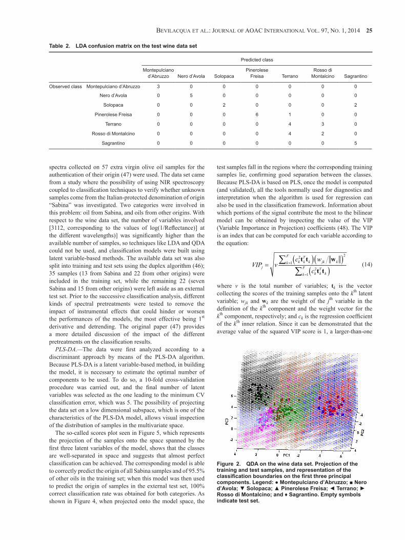
To see whether the use of quadratic decision surfaces instead of linear ones could improve the predictions, QDA was applied on the data set. The corresponding classification rule is graphically shown in Figure 2, where the quadratic hypersurfaces separating the regions of space associated to the different categories are projected together with the training and test samples onto the space spanned by the first three principal components. It can be seen that introduction of more complex decision boundaries results in a greater number of samples from the categories that were confused in LDA falling into the regions associated with their true categories. A direct consequence of

this observation is that the classification accuracy for these classes, which is reported in Table 1, is better than that obtained using LDA. As far as the nature of the misclassifications is concerned, inspection of the confusion matrix for QDA (not shown) confirms that the direction of the wrong predictions is the same as in LDA.

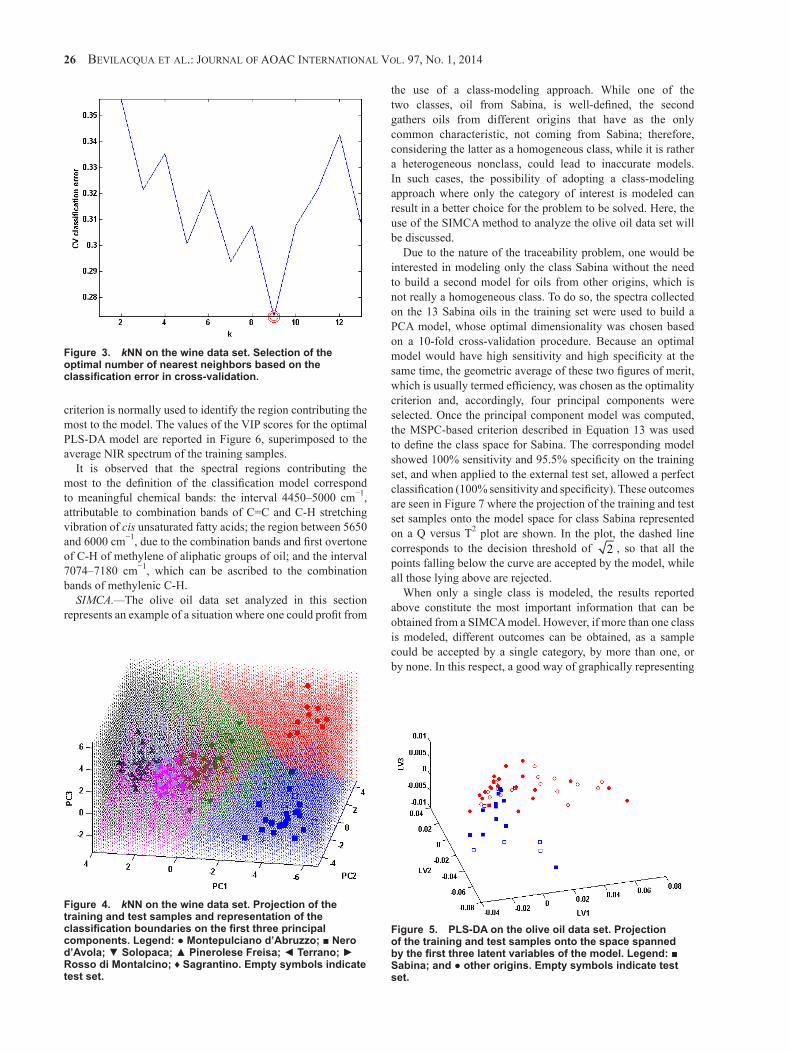
kNN.—kNN was applied to the same data set to investigate whether the use of a method involving an even more complex decision boundary could lead to further improvement in the results. Different from the case of LDA and QDA, where once the data set is defined there is only one solution, kNN modeling requires choosing the optimal value of an adjustable parameter, namely, the number of the nearest neighbors, k. Following what is described in the subsection immediately above, this choice was made on the basis of a cross-validation procedure with 10 cancelation groups; the optimal number of nearest neighbors was selected as the one leading to the minimum classification error in cross-validation and, as evident from Figure 3, was nine. It must be stressed that while in LDA and QDA column data scaling is embedded in the methods (through the normalization by the inverse of the variance-covariance matrixes), the outcomes of kNN, a distance-based method, heavily depend on the relative weighting of variables. Accordingly, because the 35 measured variables have a different nature, data were autoscaled prior to kNN classification.

The final model was built using k = 9, and its performances in modeling and validation are reported in Table 1. The table shows that the possibility of having decision boundaries with a higher extent of nonlinearity (more irregularity) generally does not result in improving the accuracy of the predictions, with the exception of only one of the two classes that appeared to be confused, i.e., Rosso di Montalcino, for which the correct classification rate on the test set increases to 83.3%. These results can be better understood considering that the selected value of k, which is relatively high, produces decision boundaries that even if nonlinear are rather smooth and, for some pairs of classes, almost coincident with those estimated by QDA. This can also be seen in Figure 4 where, analogous to what was already done for LDA and QDA, the kNN hypersurfaces separating the regions of space associated with the different categories are projected, together with the training and test samples, onto the space spanned by the first three principal components.

Olive Oil Data Set

To illustrate how PLS-DA and SIMCA can be used in practice and to show the differences between a modeling and a discriminant approach, a data set made up of the near IR (NIR)

Figure 1. LDA on the wine data set. Projection of the training and test samples, and representation of the classification boundaries on the first three principal components. Legend: ● Montepulciano d’Abruzzo; ■ Nero d’Avola; ▼ Solopaca; ▲ Pinerolese Freisa; ◄ Terrano; ► Rosso di Montalcino; and ♦ Sagrantino. Empty symbols indicate test set.

Table 1. Correct classification rates for the wine data set

Method Montepulciano d’Abruzzo, %

Nero d’Avola, % Solopaca, %

Pinerolese Freisa, % Terrano, %

Rosso di Montalcino, % Sagrantino, %

LDA Modeling 100.0 100.0 78.6 100.0 48.1 52.0 78.9

Validation 100.0 100.0 50.0 85.7 57.2 33.3 100.0

QDA Modeling 100.0 100.0 85.7 100.0 51.2 60.0 84.2

Validation 100.0 100.0 75.0 100.0 85.7 66.7 80.0

kNN Modeling 100.0 100.0 42.9 96.4 40.7 24.0 73.7

Validation 100.0 100.0 25.0 85.7 71.4 83.3 100.0


spectra collected on 57 extra virgin olive oil samples for the authentication of their origin (47) were used. The data set came from a study where the possibility of using NIR spectroscopy coupled to classification techniques to verify whether unknown samples come from the Italian-protected denomination of origin “Sabina” was investigated. Two categories were involved in this problem: oil from Sabina, and oils from other origins. With respect to the wine data set, the number of variables involved [3112, corresponding to the values of log(1/Reflectance)] at the different wavelengths)] was significantly higher than the available number of samples, so techniques like LDA and QDA could not be used, and classification models were built using latent variable-based methods. The available data set was also split into training and test sets using the duplex algorithm (46); 35 samples (13 from Sabina and 22 from other origins) were included in the training set, while the remaining 22 (seven Sabina and 15 from other origins) were left aside as an external test set. Prior to the successive classification analysis, different kinds of spectral pretreatments were tested to remove the impact of instrumental effects that could hinder or worsen the performances of the models, the most effective being 1st derivative and detrending. The original paper (47) provides a more detailed discussion of the impact of the different pretreatments on the classification results.

PLS-DA.—The data were first analyzed according to a discriminant approach by means of the PLS-DA algorithm. Because PLS-DA is a latent variable-based method, in building the model, it is necessary to estimate the optimal number of components to be used. To do so, a 10-fold cross-validation procedure was carried out, and the final number of latent variables was selected as the one leading to the minimum CV classification error, which was 5. The possibility of projecting the data set on a low dimensional subspace, which is one of the characteristics of the PLS-DA model, allows visual inspection of the distribution of samples in the multivariate space.

The so-called scores plot seen in Figure 5, which represents the projection of the samples onto the space spanned by the first three latent variables of the model, shows that the classes are well-separated in space and suggests that almost perfect classification can be achieved. The corresponding model is able to correctly predict the origin of all Sabina samples and of 95.5% of other oils in the training set; when this model was then used to predict the origin of samples in the external test set, 100% correct classification rate was obtained for both categories. As shown in Figure 4, when projected onto the model space, the

test samples fall in the regions where the corresponding training samples lie, confirming good separation between the classes. Because PLS-DA is based on PLS, once the model is computed (and validated), all the tools normally used for diagnostics and interpretation when the algorithm is used for regression can also be used in the classification framework. Information about which portions of the signal contribute the most to the bilinear model can be obtained by inspecting the value of the VIP (Variable Importance in Projection) coefficients (48). The VIP is an index that can be computed for each variable according to the equation:

VIP v

c w

cj

k kTk jk kk

F

k kTkk

F=( )( )

( )=

=

∑∑

2 2

12

1

t t w

t t

(14)

where v is the total number of variables; tk is the vector collecting the scores of the training samples onto the kth latent variable; wjk and wk are the weight of the jth variable in the definition of the kth component and the weight vector for the kth component, respectively; and ck is the regression coefficient of the kth inner relation. Since it can be demonstrated that the average value of the squared VIP score is 1, a larger-than-one

Figure 2. QDA on the wine data set. Projection of the training and test samples, and representation of the classification boundaries on the first three principal components. Legend: ● Montepulciano d’Abruzzo; ■ Nero d’Avola; ▼ Solopaca; ▲ Pinerolese Freisa; ◄ Terrano; ► Rosso di Montalcino; and ♦ Sagrantino. Empty symbols indicate test set.

Table 2. LDA confusion matrix on the test wine data set

Predicted class

Montepulciano

d’Abruzzo Nero d’Avola SolopacaPinerolese

Freisa TerranoRosso di

Montalcino Sagrantino

Observed class Montepulciano d’Abruzzo 3 0 0 0 0 0 0

Nero d’Avola 0 5 0 0 0 0 0

Solopaca 0 0 2 0 0 0 2

Pinerolese Freisa 0 0 0 6 1 0 0

Terrano 0 0 0 0 4 3 0

Rosso di Montalcino 0 0 0 0 4 2 0

Sagrantino 0 0 0 0 0 0 5


criterion is normally used to identify the region contributing the most to the model. The values of the VIP scores for the optimal PLS-DA model are reported in Figure 6, superimposed to the average NIR spectrum of the training samples.

It is observed that the spectral regions contributing the most to the definition of the classification model correspond to meaningful chemical bands: the interval 4450–5000 cm−1, attributable to combination bands of C=C and C-H stretching vibration of cis unsaturated fatty acids; the region between 5650 and 6000 cm−1, due to the combination bands and first overtone of C-H of methylene of aliphatic groups of oil; and the interval 7074–7180 cm−1, which can be ascribed to the combination bands of methylenic C-H.

SIMCA.—The olive oil data set analyzed in this section represents an example of a situation where one could profit from

the use of a class-modeling approach. While one of the two classes, oil from Sabina, is well-defined, the second gathers oils from different origins that have as the only common characteristic, not coming from Sabina; therefore, considering the latter as a homogeneous class, while it is rather a heterogeneous nonclass, could lead to inaccurate models. In such cases, the possibility of adopting a class-modeling approach where only the category of interest is modeled can result in a better choice for the problem to be solved. Here, the use of the SIMCA method to analyze the olive oil data set will be discussed.

Due to the nature of the traceability problem, one would be interested in modeling only the class Sabina without the need to build a second model for oils from other origins, which is not really a homogeneous class. To do so, the spectra collected on the 13 Sabina oils in the training set were used to build a PCA model, whose optimal dimensionality was chosen based on a 10-fold cross-validation procedure. Because an optimal model would have high sensitivity and high specificity at the same time, the geometric average of these two figures of merit, which is usually termed efficiency, was chosen as the optimality criterion and, accordingly, four principal components were selected. Once the principal component model was computed, the MSPC-based criterion described in Equation 13 was used to define the class space for Sabina. The corresponding model showed 100% sensitivity and 95.5% specificity on the training set, and when applied to the external test set, allowed a perfect classification (100% sensitivity and specificity). These outcomes are seen in Figure 7 where the projection of the training and test set samples onto the model space for class Sabina represented on a Q versus T2 plot are shown. In the plot, the dashed line corresponds to the decision threshold of 2 , so that all the points falling below the curve are accepted by the model, while all those lying above are rejected.

When only a single class is modeled, the results reported above constitute the most important information that can be obtained from a SIMCA model. However, if more than one class is modeled, different outcomes can be obtained, as a sample could be accepted by a single category, by more than one, or by none. In this respect, a good way of graphically representing

Figure 3. kNN on the wine data set. Selection of the optimal number of nearest neighbors based on the classification error in cross-validation.

Figure 4. kNN on the wine data set. Projection of the training and test samples and representation of the classification boundaries on the first three principal components. Legend: ● Montepulciano d’Abruzzo; ■ Nero d’Avola; ▼ Solopaca; ▲ Pinerolese Freisa; ◄ Terrano; ► Rosso di Montalcino; ♦ Sagrantino. Empty symbols indicate test set.

Figure 5. PLS-DA on the olive oil data set. Projection of the training and test samples onto the space spanned by the first three latent variables of the model. Legend: ■ Sabina; and ● other origins. Empty symbols indicate test set.


the results would be the so-called Coomans plot (49), in which the models of two categories are compared so that each sample is described by its distance to the two models investigated. To better illustrate how a Coomans plot can be interpreted, a model was built for the class of oils from other origins, so that the two categories could be compared. Accordingly, the Coomans plot obtained by comparing the models for Sabina and other origins is shown in Figure 8.

Figure 8 shows that the model is divided in four regions by two lines corresponding to the threshold value of 2 for the two distances. The left uppermost region corresponds to observations that are accepted only by the model of the other origins class, while the right lowermost one corresponds to those accepted only by the Sabina class. The lower leftmost part contains those samples that are accepted by both class models, while the right uppermost contains the observations rejected by both. Figure 8 shows that the high efficiency of the model is reflected also in the distribution of the samples in the plot. Additionally, even if SIMCA is a modeling technique, it can always be transformed to a discriminant one by assigning a sample to the category to which it is closest. Accordingly, the diagonal line in the plot represents the decision boundary when a classification approach is adopted; samples falling above the line are classified as Sabina and samples below the line as oils from other origins. As seen in Figure 8, when used as a discriminant classification technique on this data set, SIMCA would have provided the same results as PLS-DA.

Conclusions

Classification methods represent a valid and valuable tool for analytical chemists dealing with problems where a qualitative answer is sought. The availability of various methods with different characteristics and different degrees of complexity allows the operator to choose the one(s) most suitable for dealing with the specific issue to be solved. Moreover, the possibility of following a class-modeling approach, rather than a discriminant one, permits building reliable models in cases where an asymmetric classification is needed or when attention is focused on one class only.

References

(1) Valcárcel, M. (1997) Trends Anal. Chem. 16, 124–131. http://dx.doi.org/10.1016/S0165-9936(97)00010-1

(2) Qin, S.J. (2003) J. Chemometr. 17, 480–502. http://dx.doi.org/10.1002/cem.800

(3) Coomans, D., Broeckaert, I., Jonckheer, M., Blockx, P., & Massart, D.L. (1978) Anal. Chim. Acta 103, 409–415. http://dx.doi.org/10.1016/S0003-2670(01)83105-6

(4) West-Nørager, M., Bro, R., Marini, F., Høgdall, E.V., Høgdall, C.K., Nedergaard, L., & Heegaard, N.H.H. (2009) Anal. Chem. 81, 1907–1913. http://dx.doi.org/10.1021/ac802293g

(5) Miccheli, A., Marini, F., Capuani, G., Tomassini Miccheli, A., Delfini, M., Di Cocco, M.E., Puccetti, C., Paci, M., Rizzo, M., & Spataro, A. (2009) J. Am. Coll. Nutr. 28, 553–564. http://dx.doi.org/10.1080/07315724.2009.10719787

(6) Ritota, M., Marini, F., Sequi, P., & Valentini, M. (2010) J. Agric. Food Chem. 58, 9675–9684. http://dx.doi.org/10.1021/jf1015957

(7) Hendriks, M.M.W.B., Smit, S., Akkermans, W.L.M.W., Reijmers, T.H., Eilers, P.H.C., Hoefsloot, H.C.J., Rubingh, C.M., de Koster, C.G., Aerts, J.M., & Smilde,

Figure 7. SIMCA on the olive oil data set. Projection of the training and test samples onto the Tred

2 -Qred model space of class Sabina. Legend: ■ Sabina; and ● other origins. Empty symbols indicate test set.

Figure 8. SIMCA on the olive oil data set. Coomans plot. Legend: ■ Sabina; and ● other origins. Empty symbols indicate test set.

Figure 6. PLS-DA on the olive oil data set. VIP scores (bars) superimposed to the average NIR spectrum recorded on the data set (line). The dashed line indicates the threshold value of 1.


A.K. (2007) Proteomics 7, 3672–3680. http://dx.doi.org/10.1002/pmic.200700046

(8) Hendriks, M.M.W.B., van Eeuwijk, F.A., Jellema, R.H., Westerhuis, J.A., Reijmers, T.H., Hoefsloot, H.C.J., & Smilde, A.K. (2011) Trends Anal. Chem. 30, 1685–1698. http://dx.doi.org/10.1016/j.trac.2011.04.019

(9) Mannina, L., Marini, F., Gobbino, M., Sobolev, A.P., & Capitani, D. (2010) Talanta 80, 2141–2148. http://dx.doi.org/10.1016/j.talanta.2009.11.021

(10) Oliveri, P., Casale, M., Casolino, M.C, Baldo, M.A., Nizzi Grifi, F., & Forina, M. (2011) Anal. Bioanal. Chem. 399, 2105–2113. http://dx.doi.org/10.1007/s00216-010-4377-1

(11) Stanimirova, I., Üstün, B., Cajka, T., Riddellova, K., Hajslova, J., Buydens, L.M.C., & Walczak, B. (2010) Food Chem. 118, 171–176. http://dx.doi.org/10.1016/j.foodchem.2009.04.079

(12) Fisher, R.A. (1936) Ann. Eugen. 7, 179–188. http://dx.doi.org/10.1111/j.1469-1809.1936.tb02137.x

(13) Rao, C.R. (1948) J. R. Statist. Soc. B 10, 159–193(14) McLachlan, G.J. (1992) Discriminant Analysis and Statistical

Pattern Recognition, John Wiley & Sons, New York, NY. http://dx.doi.org/10.1002/0471725293

(15) Wold, S., Esbensen, K., & Geladi, P. (1987) Chemometr. Intell. Lab. Syst. 2, 37–52. http://dx.doi.org/10.1016/0169-7439(87)80084-9

(16) Ståhle, L., & Wold, S. (1987) J. Chemometr. 1, 185–196. http://dx.doi.org/10.1002/cem.1180010306

(17) Barker, M., & Rayens, W. (2003) J. Chemometr. 17, 166–173. http://dx.doi.org/10.1002/cem.785

(18) Wold, S., Martens, H., & Wold, H. (1983) in Proceedings of the Conference on Matrix Pencils, Lecture Notes in Mathematics, A. Ruhe & B. Kågström (Eds), Springer Verlag, Heidelberg, Germany, pp 286–293

(19) Indahl, U.G., Martens, H., & Næs, T. (2007) J. Chemometr. 21, 529–536. http://dx.doi.org/10.1002/cem.1061

(20) Nocairi, H., Qannari, E.M., Vigneau, E., & Bertrand, D. (2005) Comput. Stat. Data Anal. 48, 139–147. http://dx.doi.org/10.1016/j.csda.2003.09.008

(21) Coomans, D., & Broeckaert, I. (1986) Potential Pattern Recognition in Chemical and Medical Decision Making, Research Studies Press, Letchworth, UK

(22) Marini, F. (2009) in Comprehensive Chemometrics, Vol. 3, S.D. Brown, R. Tauler & B. Walczak (Eds), Elsevier, Oxford, UK, pp 477–505. http://dx.doi.org/10.1016/B978-044452701-1.00128-9

(23) Zupan, J., & Gasteiger, J. (1999) Neural Networks in Chemistry and Drug Design, 2nd Ed., Wiley VCH, Weinheim, Germany

(24) Brereton, R.G., & Lloyd, G.R. (2010) Analyst 135, 230–267. http://dx.doi.org/10.1039/b918972f

(25) Walczak, B., & Massart, D.L. (1996) Anal. Chim. Acta 331, 187–193. http://dx.doi.org/10.1016/0003-2670(96)00206-1

(26) Zerzucha, P., Daszykowski, M., & Walczak, B. (2012) Chemometr. Intell. Lab. Syst. 110, 156–162. http://dx.doi.org/10.1016/j.chemolab.2011.11.005

(27) Cover, T.M., & Hart, P.E. (1967) IEEE Trans. Inform. Theory 13, 21–27. http://dx.doi.org/10.1109/TIT.1967.1053964

(28) Collantes, E.R., Duta, R., Welsh, W.J., Zielinski, W.L., & Brower, J. (1997) Anal. Chem. 69, 1392–1397. http://dx.doi.org/10.1021/ac9608836

(29) Coomans, D., & Massart, D.L. (1982) Anal. Chim. Acta 136, 15–27. http://dx.doi.org/10.1016/S0003-2670(01)95359-0

(30) Forina, M., Oliveri, P., Lanteri, S., & Casale, M. (2008) Chemometr. Intell. Lab. Syst. 93, 132–148. http://dx.doi.org/10.1016/j.chemolab.2008.05.003

(31) Oliveri, P., Di Egidio, V., Woodcock, T., & Downey, G. (2011) Food Chem. 125, 1450–1456. http://dx.doi.org/10.1016/j.foodchem.2010.10.047

(32) Wold, S. (1976) Pattern Recogn. 8, 127–139. http://dx.doi.org/10.1016/0031-3203(76)90014-5

(33) Wold, S., & Sjöström, M. (1977) in Chemometrics, Theory and Application, B.R. Kowalski (Ed.), American Chemical Society, Washington, DC, pp 243–282. http://dx.doi.org/10.1021/bk-1977-0052.ch012

(34) Derde, M.P., & Massart, D.L. (1986) Anal. Chim. Acta 184, 33–51. http://dx.doi.org/10.1016/S0003-2670(00)86468-5

(35) Forina, M., Armanino, C., Leardi, R., & Drava, G. (1991) J. Chemometr. 5, 435–453. http://dx.doi.org/10.1002/cem.1180050504

(36) Jolliffe, I.T. (2002) Principal Component Analysis, 2nd Ed., Springer, New York, NY

(37) De Maesschalck, R., Caldolfi, A., Massart, D.L., & Heuerding, S. (1999) Chemometr. Intell. Lab. Syst. 47, 65–77. http://dx.doi.org/10.1016/S0169-7439(98)00159-2

(38) Daszykowski, M., Kaczmarek, K., Stanimirova, I., Vander Heyden, Y., & Walczak, B. (2007) Chemometr. Intell. Lab. Syst. 87, 95–103. http://dx.doi.org/10.1016/j.chemolab.2006.10.003

(39) Pomerantsev, A.L. (2008) J. Chemometr. 22, (2008) 601–609. http://dx.doi.org/10.1002/cem.1147

(40) Nomikos, P., & MacGregor, J.F. (1995) Technometrics 37, 41–59. http://dx.doi.org/10.1080/00401706.1995.10485888

(41) Durante, C., Bro, R., & Cocchi, M. (2011) Chemometr. Intell. Lab. Syst. 106, 73–85. http://dx.doi.org/10.1016/j.chemolab.2010.09.004

(42) PLS–Toolbox Manual 4.0 for MATLAB, distributed by Eigenvector Research, Wenatchee, WA

(43) Harshman, R.A. (1984) in Research Methods for Multimode Data Analysis, H.G. Law, C.W. Snyder Jr, J. Hattie, & R.P. McDonald (Eds), Praeger, New York, NY, pp 566–591

(44) Stone, M. (1974) J. Royal Stat. Soc. B 36, 111–147(45) Marini, F., Bucci, R., Magrì, A.L., & Magrì, A.D. (2006)

Chemometr. Intell. Lab. Syst. 84, 164–171. http://dx.doi.org/10.1016/j.chemolab.2006.04.017

(46) Snee, R.D. (1977) Technometrics 19, 415–428. http://dx.doi.org/10.1080/00401706.1977.10489581

(47) Bevilacqua, M., Bucci, R., Magrì, A.D., Magrì, A.L., & Marini, F. (2012) Anal. Chim. Acta 717, 39–51. http://dx.doi.org/10.1016/j.aca.2011.12.035

(48) Wold, S., Johansson, E., & Cocchi, M. (1993) in 3D QSAR In Drug Design: Theory, Methods And Applications, H. Kubinyi (Ed.), Escom Science Publishers, Leiden, The Netherlands, pp 523–550

(49) Coomans, D., Broeckaert, I., Derde, M.P., Tassin, A., Massart, D.L., & Wold, S. (1984) Comp. Biomed. Res. 17, 1–14. http://dx.doi.org/10.1016/0010-4809(84)90002-8

Chemometric Classification Techniques as a Tool for Solving Problems in Analytical Chemistry

Documents

Transcript of Chemometric Classification Techniques as a Tool for Solving Problems in Analytical Chemistry