HAL Id: hal-02615395https://hal.inria.fr/hal-02615395

Submitted on 22 May 2020

HAL is a multi-disciplinary open accessarchive for the deposit and dissemination of sci-entific research documents, whether they are pub-lished or not. The documents may come fromteaching and research institutions in France orabroad, or from public or private research centers.

L’archive ouverte pluridisciplinaire HAL, estdestinée au dépôt et à la diffusion de documentsscientifiques de niveau recherche, publiés ou non,émanant des établissements d’enseignement et derecherche français ou étrangers, des laboratoirespublics ou privés.

Chemoinformatics approaches to help antibacterialdiscovery

Clément Bellanger, Jane Hung, Nyoman Juniarta, Vincent Leroux, BernardMaigret, Amedeo Napoli

To cite this version:Clément Bellanger, Jane Hung, Nyoman Juniarta, Vincent Leroux, Bernard Maigret, et al.. Chemoin-formatics approaches to help antibacterial discovery. [Technical Report] Inria Nancy - Grand Est.2020. �hal-02615395�

Chemoinformatics approaches to help antibacterial discovery

Clément Bellanger∗, Jane Hung§, Nyoman Juniarta∗, Vincent Leroux∗, Bernard Maigret∗, AmedeoNapoli∗

∗Université de Lorraine, CNRS, Inria, LORIA. F-54000, Nancy, France§Broad Institute, Harvard / Massachusetts Institute of Technology. 02142 Cambridge, USA

corresponding author email: amedeo.napoli@loria.fr

ABSTRACTMany bacteria are acquiring more resistance to usual treatmentsworldwide, to the point that the possible advent of pathogens resis-tant to the entire current arsenal is a true concern. Therefore, thereis an urgent need for finding new effective antibacterial drugs. As-sociated to data mining methods, in silico ligand-based drug designtechniques may extract the most relevant molecular features andeventually lead to the discovery of innovative potent antibacterialmolecules. In this work, we use feature selection techniques to buildmolecular filters with demonstrated ability to discriminate betweenantibacterial and non-antibacterial small molecules. A very largenumber of molecular properties translated into molecular descrip-tors, being simultaneously diverse and redundant, were processedusing various feature selection techniques.

It is shown that this approach was efficient in decreasing themodels complexity by identifyingmost relevant features for antibac-terial activity. For reducing the number of considered descriptors,we have trained multiple machine learning algorithms until result-ing models performance in virtual screening could not be optimizedfurther. We also discuss the interest of using log-linear analysisto improve our data-driven process and to increase the chance topredict efficiently new antibacterials.

1 INTRODUCTIONBacterial and parasitic diseases are the second leading cause of deathworldwide, according to reports on antibiotic research released re-cently [5, 25, 34]. Currently, a pressing public health concern origi-nates from bacterial resistance to the available arsenal of antibiotics.This natural phenomenon is occurring more and more frequently,probably due to evolutionary pressure fueled by mis-use/over-useof current drugs. The emergence of “superbugs” resistant to en-tire antibiotic classes may render traditional antibiotics obsoletein the coming years, with potentially dramatic consequences [25].Consequently, new antibiotics are desperately needed, preferablyfeaturing novel mechanisms of action in order to successfully fightmultidrug-resistant strains [12, 14, 27].

Unfortunately, the amount of money being spent in antibioticsR&D is woefully inadequate as major pharmaceutical companiesmostly focus on different pathologies according to their pipelines.Drugs against chronic diseases highly common in modern devel-oped countries (e.g cardiovascular deficiencies, diabetes, obesity)certainly promise higher and faster returns to the shareholders,yet there are certainly a lot of profits to be potentially made withantibiotics. For instance, once the death toll for hospital-acquired in-fections of multidrug-resistant strains of the likes of Staphylococcusaureus become unacceptable (and that will happen too soon if no

progress is made), a new efficient antibiotic class could eventuallyturn out to be the only option to save lives.

In this context, in order to make progress in this field, resorting tomore modern techniques, even if those have not demonstrated sim-ilar success rates so far in classical drug discovery programs, lookslike a rational choice. Computer-aided techniques have alreadyproven their usefulness to save time and money in the drug discov-ery process [39]. In particular, ligand-based drug design calculations(i.e. QSAR) are now well-recognized as fast and efficient approachesin the hit-to-lead early drug discovery phase. Knowledge discoveryapproaches (e.g machine learning, data mining, neural networks)are less mature in the context of drug design but their success inother applied computing fields make them increasingly promising.They are also especially popular in academia since provided theyare combined with very strong interdisciplinary expertise; theymay allow overcoming the lack of experimental data useful formedicinal chemistry projects compared to what is existing in theindustry. Furthermore, one hope is that progress in the chemoin-formatics field [4] could eventually allow finding possible “hiddengems” amongst the millions of available chemicals from providers,companies or laboratory collections, and even established drugs.

Here, we present an in silico strategy targeting antibacterialmolecules identification in a virtual screening context. Our finalgoal is to be able to highlight molecules within existing chemicalcollections with a high probability of being potential antibacterialsand that could not be found using most of the existing similarapproaches.

Considering the huge variety of molecular descriptors that canbe used [43] in order to describe molecular properties, the prob-lem is how to achieve an optimal selection of molecular attributesets in order to analyze, with highest accuracy, chemical diver-sity/similarity among large (>1M objects) chemical libraries. Such“optimally-selected descriptors” should provide the most efficientrules which can be used next to describe molecules with a com-mon behavior, in this case antibacterial potency. Dimensionalityreduction in the descriptors space has already been considered asan important issue in QSAR methods [19, 22, 24, 35, 38]. The knowl-edge discovery phase would then next allow to extract, among largechemical datasets, compounds presenting all the same required ac-tion.

2 DESCRIPTION SPACE REDUCTION ANDTRAINING PROCESSES

In this section, we apply and compare several well-establishedmachine learning algorithms against the same training datasetsappropriate for the problem of antibacterial molecules identification.

It is demonstrated that the resulting filters are efficient, and thosewill serve as references to evaluate future new knowledge extractionmethods we are currently investigating.

2.1 Methods2.1.1 Molecular data sets. In order to train feature selection tech-niques for discriminating antibacterials and non-antibacterials, webuilt several molecular training sets of both antibacterial and non-antibacterial molecules from different sources.

• Set P1 (positive) is constituted by 150 antibacterials that arepart of the current standards of care in France [44].

• Set P2 is the antibacterials subset of the MDDR 2016 data-base [3]. It comprises 2854molecules annotated as possessingantibacterial potency and not already referenced in the P1set.

• Set P3 is the Life Chemicals [1] supplier’s antibacterial library.As retrieved for this study, it contains 38907 small-molecule,drug-like compounds available for purchase, that have beenselected from the full supplier catalog using proprietary clas-sifiers.

• Sets N1 (negative), N2, N3 and N4 are built from MDDRmolecules that are not tagged as antibacterials but havingcompletely different known activities. N1 has 1519 analgesiccompounds, N2 has 3654 compounds targeted at cardiovas-cular diseases, N3 comprises 17796 compounds marked as“antagonist” and N4 34210 marked as “inhibitor”.

• Set N5 is an ensemble of Life Chemicals molecules availablefor purchase not found in P2 nor in N1–N4. It comprises52604 molecules from the cancer-, central nervous system-and analgesic-focused libraries.

To focus our study on small molecules, all molecules in our datasets were imposed to have molecular weight less than 600 Daltons.A single 3D conformation of all these compounds was obtainedfrom Corina [36].

2.1.2 Attribute sets. For eachmolecule, a set of 4885 attributes werecalculated from the Dragon software [19] describing constitutional,topological and geometrical properties.While molecular descriptorscalculations are available in several QSAR platforms [2], Dragoncombines a particularly large choice and diversity with a clear anddetailed technical documentation. Attributes where values weremissing were removed. Some of the attributes were found perfectlycorrelated; in such cases we removed all but one attribute fromeach group. This resulted in a baseline number of 4532 attributes.

Models were run on data sets with 5 different attribute sets thatwill be referred to as F0, F1, F2, F3 and F4 next. F0 contains thebaseline 4532 attributes while F1–F4 have filters applied in orderto limit the number of attributes; such restrictions may positivelyimpact the final classifier performance. All filters are based onthresholds about computed values. F1 eliminates attributes thatresult in a data distribution with standard deviation σ < 0.01 andwith pair correlation ρ ≥ 0.4. F2 excludes σ < 0.01 and ρ ≥ 8. F3excludes σ < 0.001 and ρ ≥ 8. F4 excludes σ < 0.1 and ρ ≥ 8.

2.1.3 Classification algorithms. We applied the following popularclassification techniques: support vector machines (SVM) [11] withlinear kernel, random forest (RF) [6], logistic regression (LR) [40],

gradient boosted trees (GBT) [16], naive Bayes (NB) [26], and de-cision trees (DT) [26]. Besides predicting classes, most of thesemethods output a measure for feature importance that can be usedto infer relationships between specific molecular properties and ac-tivity (here: identification as antibacterial). All classifications wereimplemented in Python language using Scikit-learn [7, 28]. SVMwas implemented using the LIBSVM package [10] with a linear ker-nel. For SVM and LR, the testing data was normalized based on thetraining data, regularization parameter C was varied by factors of10 from 10−6 to 10. Regularization is a process of introducing extraterms to reduce overfitting by discouraging complexity. For RF andGBT, 1000 estimators were used because there was no significantimprovement using more. Tuning the C parameter was found toimprove performance (as measured by precision) so by averagingthe results of the first step for each value ofC . The best performingC was chosen for each data set.

2.1.4 Training process methological details. Different scoring meth-ods like precision (probability of a positively classified elementbeing positive), recall (probability of a positive element being posi-tively classified), accuracy (probability of a correct classification),f 1score (harmonic mean of precision and recall) and AUC (areaunder the ROC curve) were calculated. The most relevant score forour purposes and our main metric is precision because we want ahigh probability of our predicted antibacterial molecules being trueantibacterial molecules. For screens involving a large number ofmolecules, of which only a few are to be chosen for closer study, itis important to choose compounds with the maximum likelihood ofbeing antibacterial. However, recall must be high enough to obtainenough molecules to test. When looking for new potential antibac-terial molecules, it is very important that after classification weobtain a list of molecules that is reliable rather than a more ambigu-ous list containing both more antibacterials and non-antibacterials.ANOVA and Tukey’s Honest Significant Difference (HSD) wereused to identify which means were significantly different (withsignificance for p < 0.05).

At each phase of the validation/optimization process, differentindependent runs are done. A discriminating parameter α wastherefore introduced to derive the molecule final classification,which may not be consistent. The α is defined as follows: a moleculeis being considered antibacterial if it was classified as such in atleast α% of the runs.

2.2 Results and discussion2.2.1 Summary of starting datasets. As explained in Section 2.1.1,the molecules were collected from market, MDDR, and Life Chemi-cals. This set of molecules is illustrated in Figure 1.

From those molecules, five data sets are constructed. Each ofthem has the same set of molecules, but different attributes, ac-cording to standard deviation and pair correlation explained inSection 2.1.2. The resulting number of attributes on each data set isdetailed in Table 1.

2.2.2 Training and testing strategy. Three distinct training/testingstages were implemented:

(1) Our first step was to evaluate all classifiers performance. Forthat, we trained all methods (SVM, LR, RF, GBT, DT, NB)

2

Figure 1: Diagram showing the intersections betweenmolecules from market, MDDR, and Life Chemicals.

Table 1: Rules and number of attributes of each filter

Filter Stddev Pair correlation Selected attributes

1 ≥ 0.010 < 0.4 872 ≥ 0.010 < 0.8 5763 ≥ 0.001 < 0.8 5884 ≥ 0.100 < 0.8 524

against the on-market antibacterials set P1 as the positiveset and Life Chemicals non-antibacterials N5 as the negativeset. Because the non-antibacterial class is over-represented,we randomly undersampled this class to do cross validation.Therefore, a random set of 150 N5 molecules was generated.Next, 100 randomP1 andN5molecules were used for trainingand the remaining 100 (50 in each set) formed a test set. Thisprocess was repeated 50 times. The aim of this first stage isto allow the identification of the most appropriate attributeset and filter out the least interesting classifiers.

(2) Next, the three top-performing classifiers from the first stageare retained and applied to an independent set of data. The F0descriptor set (4532 unfiltered attributes) is trained against P1and a set of 150 randomN5molecules, then the resulting clas-sifier tested on an ensemble composed of P2, N1, N2, N3 andN4 (all from the MDDR database) assuming all P2 moleculesare actual antibacterials and that there is no antibacterialin N1, N2, N3 and N4. This training process is repeated 10times and the number of times each molecule was classifiedas non-antibacterial and antibacterial was recorded. Thenwe calculated the total combined precision and recall withthe antibacterial being the positive class. Because there were10 runs, we decided on molecules’ “final” classification byusing the α parameter defined before.

(3) For our third step, we applied the models from the secondstep to the P1 and N4 MDDR set. We trained the classifieron the 2854 P2 MDDR antibacterials and 2854 randomlychosen MDDR N1, N2, N3. The training was repeated 10

times and the number of times each molecule was classifiedas non-antibacterial and antibacterial was recorded.

2.2.3 Attribute set comparison and initial classifier evaluation. Inthe first step described above, we have tested all classifiers againstall attribute sets. The results are summarized in Table 7.

All classifiers perform better than chance regarding our mainmetric precision. SVM, LR, RF, and GBT have better precision thanNB and DT across the 5 different attribute sets. SVM appears to bethe best performer with respect to our main metric precision for alldata sets, though it is not significantly different from RF for attributeset F1 and from LR for F2 and F3. Over 99% precision is reachedwith SVM for all sets except F1, but it suffers from lower accuracyand recall, meaning it only correctly classifies a small percentage ofantibacterials but those that are classified as antibacterial are correct.This can be seen most clearly in the F0 case, where accuracy andf 1score are 67.7% and 52.1%, respectively, compared to > 90% forLR, RF, and GBT; the relatively low accuracy and f 1score , as well aslow training accuracy (68.2%) and f 1score (53.2%), are indicationsof under-fitting by this model.

The precision results with F2, F3, and F4 are comparable to F0.In particular, the SVM precision with F0, F2, F3, and F4 is not sig-nificantly different, but the accuracy, f 1score , and AUC are worsewith F0. The improved performance of some of the classifiers withreduced attribute sets may be due to some sensitivity to highly-correlated attributes or over-fitting to irrelevant attributes. F1 stillresults in > 90% precision for SVM, LR, RF, GBT, but the results aresignificantly worse than with F0, F2, F3, and F4, probably becauseimportant attributes were eliminated by the low correlation thresh-old. Definitions for F2, F3, and F4 do not result in such a problem,since metric scores are similar for all classifiers.

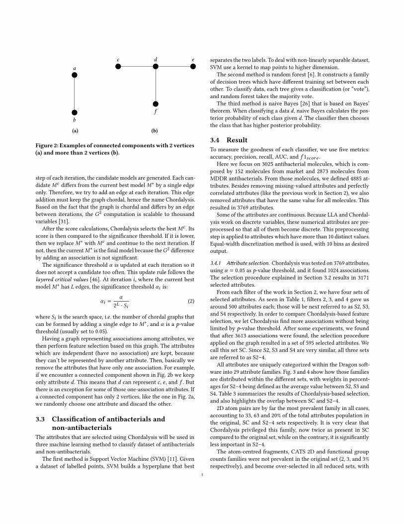
2.2.4 Final classifier selection. In our final step, we took the bestperforming models–SVM, LR, and RF–trained on the P1 and N5sets to test the MDDR data. Separately testing on the MDDR P2antibacterials and non-antibacterials (i.e. N1 analgesic, N2 cardio-vascular, N3 antagonist, N4 inhibitor), we calculated the propor-tion of molecules correctly classified where molecules classifiedas antibacterial in at least α percent of runs were classified as an-tibacterial; for each classifier, we also combined the MDDR dataand calculated the precision and recall with respect to antibacterialwhere a molecule was classified as antibacterial if it was (Table 8). Alow value of α (less than 50%) can be used if we want a permissivedefinition of antibacterial, but generally we are most interested invalues above 50%.

Similar to previous results, SVM shows higher precision butlower recall. The MDDR non-antibacterials (N1-N4) have high per-centage of correct classifications for all α values while less than20% of MDDR antibacterials are classified correctly. Despite this,because the proportion of non-antibacterials compared to antibac-terials is 20:1, precision ranges from 8% to 100% while recall staysbelow 20%. SVM with moderate α may be used as a model that out-puts a small list of molecules that are very likely to be antibacterials;however, this list could also be too small for efficient experimentaltesting.

LR shows very erratic results with varying α . For low α values,most antibacterials in the test set are retrieved, while for high α(less stringent screening), most non-antibacterials are correctly

3

found. Around α = 80%, the non-antibacterials show a steep rise inproportion of correct classifications and precision jumps from 6%to 23%, achieving a maximum of 48%. Most non-antibacterials wereclassified as antibacterial between 1 and 7 times out of 10 runs. Thisinconsistency makes LR an untrustworthy model for our purposes.

As expected from an ensemble model, RF shows more consistentresults. Precision stays around 10-12%, which is far smaller than thehighest precisions achieved by SVM and LR. Although RF classifiesmost non-antibacterials as such, a large number of them are falsepositives compared to the number of true positives. RF’s recall ismuch better than SVM, so RF could be used as an alternative incase it is worth sacrificing the precision of SVM for higher recall.To maximize precision, we choose SVM for the last training stage.

3 KNOWLEDGE DISCOVERYWITHDECOMPOSABLE MODELS

In Section 2, we inspected a number of chemical molecules to knowwhich features could characterize antibacterials. To do that, weused the properties of each molecule, summing up to thousands ofmolecular attributes providing a significant amount of data to beanalyzed for knowledge discovery.

In order to minimize the required time and space, before wemine the data, we should reduce the dimension of the data set, as atransformation step according to the basic steps of KDD [13]. It isperformed by combining some attributes into one, or by completelyeliminating some of them.

Within the thousands attributes for each molecule, we can iden-tify some redundancies and therefore, we can ignore an attribute ifit can be merged or replaced with another attribute. The selectedattributes should be able to define the molecules without significantloss of information. Beside the redundancies, we should also ignorethe attributes which are not informative.

3.1 Log-linear analysisLog-linear analysis (LLA) can find any associations among attributes,allowing feature selection according to those associations.

Suppose that we have a data setWAR of certain molecules withthree variables: molecular weight (W ), number of atoms (A) and ringperimeter (R). Relationship between two variables can be studiedwith two-way χ2 test of association. However, if we have morethan two variables, we need to do a multiway frequency analysisto study the two- and three-way associations. LLA is an extensionof multiway frequency analysis, and tries to discover any statisticalrelationships between three or more non-continuous variables. Itwill create a model (like the one in Eq. 1) to find the log of expectedfrequencies.

For theWAR, LLA tries to answer some relationship questions. Isa molecule’s weight related to its number of atoms? Is a molecule’snumber of atoms related to its ring perimeter? Is there a three-wayrelationship among molecular weight, number of atoms, and ringperimeter? By knowing ring perimeter of a molecule, can we predictits weight?

To do a multiway frequency analysis with LLA, we develop a lin-ear model of the logarithm of expected cell frequencies. An exampleof such model is shown in Eq. 1, with each term representing an

association. As the number of variables increases, the number of as-sociations also increases. With three variables in data setWAR, wehave seven possible associations: one three-way associations, threetwo-way associations, and three one-way associations. The modelin Eq. 1 contains all possible associations. To keep the simplicity of amodel, LLA tries to find which association will be kept or removed.To do that, we should determine the significance of an associationby examining the goodness-of-fit of the model containing it.

Eventually, with thousands of variables, the number of possibleassociations will be so large that it would be impractical to testeach association. This limitation can be solved by Chordalysis.

3.1.1 Log-linear model. Log-linear model is represented as an equa-tion to find a logarithm of E (expected frequency of a combinationof variables’ values). From data set WAR, we can generate a modelthat contains all possible associations. This is the saturated model,which can be written as:

lnEwar = θ + λW (w) + λA(a) + λR (r )

+ λWA(wa) + λWR (wr ) + λAR (ar )

+ λWAR (war ) (1)

where θ is a constant, and λ term represents an effect. Each λ hasvalues as many as the number of levels, and these values sum tozero. For example, since we define three levels of molecular weight:light,medium, and heavy, λW (w) has three possible non-zero values:for light (λW (lig)),medium (λW (med)), and heavy (λW (hvy)), withλW (lig) + λW (med) + λW (hvy) = 0.

A log-linear model can be hierarchical or non-hierarchical. Ahierarchical model can be represented by its highest-order associ-ation in square brackets. For example, a model [WA][R] containsλWA(wa) and λR (r ), as well as λW (w) and λA(a).

Furthermore, if a model is a sub-model of another, theirG2 differ-ence is itself aG2. Therefore, [WA][R] is a sub-model of [WA][WR],i.e. we can find all λ terms of [WA][R] in [WA][WR]. By comparingtheirG2 to χ2 table, we can obtain their significance. If both modelsare significant, we can choose the less complex one ([WA][R]) iftheir G2 difference is not significant.

3.2 ChordalysisThere are two ways to select which associations to include in alog-linear model, backward elimination and forward selection. Back-ward elimination starts from a saturated model and eliminatesnon-significant associations one by one. On the other hand, for-ward selection starts from an empty model and iteratively adds anassociation until the difference is not significant. The existing LLAconsiders all possible associations to determine which one to beadded or removed. This becomes infeasible when the number ofattributes increases, since the number of associations is exponentialw.r.t. it.

Chordalysis tries to guide the existing LLA in selecting whichassociations are significant enough to be included in the model [30,32]. This method is focusing on decomposable log-linear models,whose G2 can be calculated by inspecting the maximal cliques andminimal separators of the corresponding graph.

As a forward approach, Chordalysis starts with an empty graphas initial model. It has neither vertex nor edges. Then at the first

4

a

b

(a)

c d

f

e

(b)

Figure 2: Examples of connected components with 2 vertices(a) and more than 2 vertices (b).

step of each iteration, the candidate models are generated. Each can-didateMc differs from the current best modelM∗ by a single edgeonly. Therefore, we try to add an edge at each iteration. This edgeaddition must keep the graph chordal, hence the name Chordalysis.Based on the fact that the graph is chordal and differs by an edgebetween iterations, the G2 computation is scalable to thousandvariables [31].

After the score calculations, Chordalysis selects the bestMc . Itsscore is then compared to the significance threshold. If it is lower,then we replaceM∗ withMc and continue to the next iteration. Ifnot, then the currentM∗ is the final model because theG2 differenceby adding an association is not significant.

The significance threshold α is updated at each iteration so itdoes not accept a candidate too often. This update rule follows thelayered critical values [46]. At iteration i , where the current bestmodelM∗ has L edges, the significance threshold αi is:

αi =α

2L · Si(2)

where Si is the search space, i.e. the number of chordal graphs thatcan be formed by adding a single edge to M∗, and α is a p-valuethreshold (usually set to 0.05).

Having a graph representing associations among attributes, wethen perform feature selection based on this graph. The attributeswhich are independent (have no association) are kept, becausethey can’t be represented by another attribute. Then, basically weremove the attributes that have only one association. For example,if we encounter a connected component shown in Fig. 2b we keeponly attribute d . This means that d can represent c , e , and f . Butthere is an exception for some of those one-association attributes. Ifa connected component has only 2 vertices, like the one in Fig. 2a,we randomly choose one attribute and discard the other.

3.3 Classification of antibacterials andnon-antibacterials

The attributes that are selected using Chordalysis will be used inthree machine learning method to classify dataset of antibacterialsand non-antibacterials.

The first method is Support Vector Machine (SVM) [11]. Givena dataset of labelled points, SVM builds a hyperplane that best

separates the two labels. To deal with non-linearly separable dataset,SVM use a kernel to map points to higher dimension.

The second method is random forest [6]. It constructs a familyof decision trees which have different training set between eachother. To classify data, each tree gives a classification (or “vote”),and random forest takes the majority vote.

The third method is naive Bayes [26] that is based on Bayes’theorem. When classifying a data d , naive Bayes calculates the pos-terior probability of each class given d . The classifier then choosesthe class that has higher posterior probability.

3.4 ResultTo measure the goodness of each classifier, we use five metrics:accuracy, precision, recall, AUC, and f 1score .

Here we focus on 3025 antibacterial molecules, which is com-posed by 152 molecules from market and 2873 molecules fromMDDR antibacterials. From those molecules, we defined 4885 at-tributes. Besides removing missing-valued attributes and perfectlycorrelated attributes (like the previous work in Section 2), we alsoremoved attributes that have the same value for all molecules. Thisresulted in 3769 attributes.

Some of the attributes are continuous. Because LLA and Chordal-ysis work on discrete variables, these numerical attributes are pre-processed so that all of them become discrete. This preprocessingstep is applied to attributes which have more than 10 distinct values.Equal-width discretization method is used, with 10 bins as desiredoutput.

3.4.1 Attribute selection. Chordalysis was tested on 3769 attributes,using α = 0.05 as p-value threshold, and it found 1024 associations.The selection procedure explained in Section 3.2 results in 3171selected attributes.

From each filter of the work in Section 2, we have four sets ofselected attributes. As seen in Table 1, filters 2, 3, and 4 gave usaround 500 attributes each; those will be next referred to as S2, S3,and S4 respectively. In order to compare Chordalysis-based featureselection, we let Chordalysis find more associations without beinglimited by p-value threshold. After some experiments, we foundthat after 3613 associations were found, the selection procedureapplied on the graph resulted in a set of 595 selected attributes. Wecall this set SC. Since S2, S3 and S4 are very similar, all three setsare referred to as S2–4.

All attributes are uniquely categorized within the Dragon soft-ware into 29 attribute families. Fig. 3 and 4 show how those familiesare distributed within the different sets, with weights in percent-ages for S2–4 being defined as the average value between S2, S3 andS4. Table 3 summarizes the results of Chordalysis-based selection,and also highlights the overlap between SC and S2–4.

2D atom pairs are by far the most prevalent family in all cases,accounting to 33, 63 and 20% of the total attributes population inthe original, SC and S2–4 sets respectively. It is very clear thatChordalysis privileged this family, now twice as present in SCcompared to the original set, while on the contrary, it is significantlyless important in S2–4.

The atom-centred fragments, CATS 2D and functional groupcounts families were not prevalent in the original set (2, 3, and 3%respectively), and become over-selected in all reduced sets, with

5

Figure 3: The distribution of families in 4885 original attributes, 595 attributes of SC, and around 500 attributes of S2–4.

Table 2: Intersections of the sets of attributes from three fil-ters and from Chordalysis.

Set S2 S3 S4SC (595 attr.) 153 154 146S2 (576 attr.) 569 497S3 (588 attr.) 496S4 (524 attr.)

CATS 2D being more prevalent in S2–4 compared to SC. These 3sets account for 23% of SC, so with the addition of 2D atom pairsonly 15% is remaining.

The relative diversity of the different sets can be compared byfocusing on the number of families accounting for more than 5%of the total number of attributes and on their total weight (seeFigure 8). Only the 4 aforementioned families obey these criteriain SC, totaling 85% of the set. There are 7 families with more inS2–4 (73%); 4 in the original set (56%). Therefore, three attributefamilies are seen significantly more prevalent in S2–4 compared tothe original set (26% / 15%), but are almost completely filtered outby Chordalysis: 2D autocorrelations, 3D-MoRSE and GETAWAYdescriptors.

Table 3: Population of most relevant attribute families. Lastcolumn is the number of attributes present in all sets (SC,S2, S3 and S4). Percentages correspond to the number of re-tained attributes from the original set.

Attribute family Original set SC Overlap2D atom pairs 1596 373 (23%) 802D matrix-based 550 2 1Edge adjacency ind. 324 2 1GATEWAY 273 7 1Functional group cnt. 154 66 (43%) 24CATS 2D 150 31 (21%) 19Atom-centered frag. 115 38 (33%) 10Drug-like indices 27 15 (56%) 1TOTAL 4885 595 (12%) 144 (3%)

Apart from these families, there is a consensus between S2–4and SC regarding the removal of some attribute families from theoriginal set, with SC appearing more stringent than S2–4. Indeed,the 2D matrix-based descriptors, edge adjacency indices and RDFdescriptors account together for 22, <1 and 5% in the original, SCand S2–4 sets respectively. This suggests that those descriptors

6

2D atom pairs

32.67

2D matrix-based descriptors

11.26Edge adjecency indices

6.63

GATEWAY descriptors5.59

1-5%: 12 families

34.62<1%: 13 families

9.23

(a) Original set: 29 families, 4885 attributes

2D atom pairs

62.69

Functional group counts

11.09

Atom-centered fragments

6.39

CATS 2D

5.211-5%: 6 families

12.10<1%: 10 families

2.52

(b) SC set: 20 families, 595 attributes

2D atom pairs

19.71

CATS 2D

12.693D-MoRSE descriptors

11.10

Functional group counts8.62

2D autocorrelations

8.43

GATEWAY descriptors

6.50

Atom-centred fragments

5.64

1-5%: 12 families

22.16

<1%: 13 families5.25

(c) S2-4 set: 26 families, 563 attributes on average

Figure 4: Distribution of major attribute families in (a) theoriginal set, (b) set SC, and (c) average of S2, S3, and S4. Allvalues in percentages. Only sets weighting >5% are repre-sented. Categories in green are the 4most-represented in SC.Those in orange with description in italic aremostly filteredout of both SC and S2–4. Grey ones summarize remainingfamilies (1–5% and <1%).

are not of much value for modeling the probability that a givenchemical compound would possess antibacterial properties.

Eventually, it should be noticed that while SC size comparedto the original set is 12%, only a single attribute family has beenfiltered less than 50%: drug-like indices. This is specific to SC (5attributes are retained by S2, S3 and S4). There were only 27 residuesof this kind in the original set, which is not significant enough todetermine that there could be a correlation between drug-likeness

Table 4: Means and standard deviations of classifiers’ met-rics on the test set. All data in percentages.

Metric SVM (C = 0.01) Random Forest Naive BayesAccuracy 97.0 ± 2.5 96.6 ± 1.5 55.7 ± 1.4Recall 98.9 ± 2.0 95.6 ± 1.5 21.2 ± 0.6Precision 95.9 ± 3.5 98.3 ± 2.2 93.7 ± 9.1AUC 99.3 ± 1.1 99.5 ± 0.4 65.3 ± 4.5f 1score 97.3 ± 2.2 96.9 ± 1.3 34.5 ± 1.0

Table 5: Precision and recall of random forest classifier onthe test set. All values in percentages.

α 4532 attributes SCPrecision Recall Precision Recall

10 10.0 71.2 11.6 65.420 10.7 68.4 11.8 64.530 11.8 65.4 12.2 63.540 11.8 65.4 12.2 63.550 12.3 64.3 12.3 63.060 13.3 61.5 12.6 62.470 14.1 60.1 12.8 61.880 14.1 60.1 12.8 61.890 15.1 59.1 13.0 61.2100 16.6 56.3 13.3 60.1

and antibacterial potency that would be most efficiently selectedby Chordalysis.

Table 2 lists the number of overlapping selected attributes fromS2, S3 and S4 with SC. Table 3 summarizes SC-related data formost-relevant attribute families identified above, and highlights thenumber of consensus attributes i.e. attributes found in all sets.

3.4.2 Training/testing strategy. Using attributes in SC, we trainedSVM, random forest, and naive Bayes on data from market antibac-terials, MDDR antibacterials, Life Chemicals non-antibacterials, andMDDR non-antibacterials. After the training process, the three clas-sifiers are tested on Life Chemicals list of predicted antibacterials.The results are summarized in Table 4. By tuning the parameter Cfor SVM, we get the best result for C = 0.01.

Based on the values of all metrics used to evaluate classifierperformance, it appears that SVM and RF perform significantlybetter than naive Bayes. The two best performing model –SVM andrandom forest– were then trained on the market antibacterials andLife Chemical antibacterials to test the MDDR data. We regardeda molecule as an antibacterial if it is classified as such in at leastα percent of runs. The precision and recall of the two models areshown in Table 5–6. SVM has better recall on the majority of alphas,and it has higher precision for α ≥ 20.

4 CONCLUDING REMARKSWe evaluated several popular classification methods, includingSVM, LR, and RF, for classifying molecules as antibacterial or non-antibacterial. Such machine learning approaches were already suc-cessfully used for drug/non-drug classification [8, 17, 21, 29], but

7

Table 6: Precision and recall of SVM classifier on the test set.All values in percentages.

α 4532 attributes SCPrecision Recall Precision Recall

10 21.3 16.4 11.1 82.720 24.0 15.2 13.3 78.130 25.9 12.8 17.0 71.940 25.9 12.8 17.0 71.950 26.6 12.5 19.0 69.960 27.4 11.8 23.8 65.170 27.9 11.4 27.2 62.480 27.9 11.4 27.2 62.490 27.7 10.0 31.8 58.7100 32.4 9.2 39.9 53.4

none were applied to antibacterials. Along with our initial 4532 at-tribute data set (F0), we tested 4 reduced sets (F1-F4), filtered on thebasis of data variance and correlation. Using those was not foundto improve performance. When looking at precision as our mainmetric, our results show that the SVM classifier with a tuned Cparameter ranks first but has much lower accuracy and f 1score . Fora dataset of potential antibacterial molecules, SVM could be usedto find a reliable list of antibacterial molecules. Another methodlike RF with lower precision but better accuracy and f 1score maybe used if a greater number of classified antibacterials is desired.

Previous investigations of the merit and drawbacks of severallearning methods [20, 23, 33, 37, 45] are in good general agreementwith our own observations. In future work, we should favor the useof SVM and RF over the other classifiers evaluated here in order toperform virtual screening of chemical databases for finding mostprobable antibacterials.

One important finding of this work is that for such a task, thechoice of the classifier appears to have much more impact thanthe selection of molecular descriptors. We have chosen to evaluateall available descriptors from the Dragon software, without anyconsideration of the relative relevance of each of those. This “blind”approach has the advantage of being totally unbiased, but putsmore stress on the classifiers.

Furthermore, in Section 3, we describe the application of theChordalysis technique for molecular attribute set reduction. Weshow that it leads to improved performance when a machine learn-ing technique is used next to discriminate between antibacterialsand compounds with no antibacterial activity. It is suggested thata two-step strategy, with a Chordalysis-refined attribute set beingfed to a SVM classifier could be highly efficient for antibacterialsidentification. An alternate techniques for selecting an optimal at-tribute set [42], such as recursive feature elimination [18, 47], RFvariable importance [9], SVM variable selection [10], tabu search[41, 48], and evolutionary algorithms [15] should be further studied.In the process, precise clues on implementing new attributes thatcould be more efficient for our purpose (antibacterials selection)than the broad generic reference set of molecular attributes thatis available in the Dragon software could be obtained. When wereach a state where no clear methodological improvement could be

reached, we will apply the optimized methodology to mine chemi-cal space for possible new antibacterials. A limited number of hitsfrom this virtual screening process will be tested experimentally.Only interesting results backed up by the resulting experimentaldata will validate the ongoing chemoinformatics approach.

REFERENCES[1] 2004. Life Chemicals. http://www.lifechemicals.com/.[2] 2007. Molecular Descriptors. http://www.moleculardescriptors.eu/.[3] 2016. BIOVIA Databases | Bioactivity Databases: MDDR.

http://accelrys.com/products/collaborative-science/databases/bioactivity-databases/mddr.html.

[4] Jürgen Bajorath. 2013. Chemoinformatics for Drug Discovery. John Wiley & Sons.[5] Theresa Braine. 2011. Race against time to develop new antibiotics. World Health

Organization.[6] Leo Breiman. 2001. Random forests. Machine Learning 45, 1 (2001), 5–32.[7] L Buitinck, G Louppe, M Blondel, F Pedregosa, A Mueller, O Grisel, V Niculae,

P Prettenhofer, A Gramfort, J Grobler, et al. 2013. ECML PKDD Workshop:Languages for Data Mining and Machine Learning. API Design for MachineLearning Software: Experiences from the Scikit-Learn Project (2013), 108–122.

[8] Evgeny Byvatov, Uli Fechner, Jens Sadowski, and Gisbert Schneider. 2003. Com-parison of support vector machine and artificial neural network systems fordrug/nondrug classification. Journal of Chemical Information and ComputerSciences 43, 6 (2003), 1882–1889.

[9] Gaspar Cano, Jose Garcia-Rodriguez, Alberto Garcia-Garcia, Horacio Perez-Sanchez, Jón Atli Benediktsson, Anil Thapa, and Alastair Barr. 2017. Automaticselection of molecular descriptors using random forest: Application to drugdiscovery. Expert Systems with Applications 72 (2017), 151–159.

[10] Chih-Chung Chang and Chih-Jen Lin. 2011. LIBSVM: A library for support vectormachines. ACM Transactions on Intelligent Systems and Technology (TIST) 2, 3(2011), 1–27.

[11] Corinna Cortes and Vladimir Vapnik. 1995. Support-vector networks. MachineLearning 20, 3 (1995), 273–297.

[12] Ezekiel J Emanuel. 2015. How to Develop New Antibiotics. New York Times,February 24th.

[13] Usama Fayyad, Gregory Piatetsky-Shapiro, and Padhraic Smyth. 1996. From datamining to knowledge discovery in databases. AI Magazine 17, 3 (1996), 37–37.

[14] Prabhavathi Fernandes. 2015. The global challenge of new classes of antibacterialagents: an industry perspective. Current Opinion in Pharmacology 24 (2015),7–11.

[15] Alex A. Freitas. 2003. Advances in Evolutionary Computing.[16] Jerome H Friedman. 2001. Greedy function approximation: a gradient boosting

machine. Annals of Statistics (2001), 1189–1232.[17] Alireza Givehchi and Gisbert Schneider. 2004. Impact of descriptor vector scal-

ing on the classification of drugs and nondrugs with artificial neural networks.Journal of Molecular Modeling 10, 3 (2004), 204–211.

[18] Isabelle Guyon, Jason Weston, Stephen Barnhill, and Vladimir Vapnik. 2002.Gene selection for cancer classification using support vector machines. MachineLearning 46, 1-3 (2002), 389–422.

[19] Trevor J Howe, Guy Mahieu, Patrick Marichal, Tom Tabruyn, and Pieter Vugts.2007. Data reduction and representation in drug discovery. Drug Discovery Today12, 1-2 (2007), 45–53.

[20] Andreas Janecek. 2009. Efficient feature reduction and classification methods. Ph.D.Dissertation. University of Vienna.

[21] Selcuk Korkmaz, Gokmen Zararsiz, and Dincer Goksuluk. 2014. Drug/nondrugclassification using support vector machines with various feature selection strate-gies. Computer Methods and Programs in Biomedicine 117, 2 (2014), 51–60.

[22] P-J L’Heureux, Julie Carreau, Yoshua Bengio, Olivier Delalleau, and Shi Yi Yue.2004. Locally Linear Embedding for dimensionality reduction in QSAR. Journalof Computer-aided Molecular Design 18, 7-9 (2004), 475–482.

[23] Wenwen Lian, Jiansong Fang, Chao Li, Xiaocong Pang, Ai-Lin Liu, and Guan-HuaDu. 2016. Discovery of Influenza A virus neuraminidase inhibitors using supportvector machine and Naïve Bayesian models. Molecular Diversity 20, 2 (2016),439–451.

[24] Ying Liu. 2004. A comparative study on feature selection methods for drugdiscovery. Journal of Chemical Information and Computer Sciences 44, 5 (2004),1823–1828.

[25] Maryn McKenna. 2014. The coming cost of superbugs: 10 million deaths per year.https://www.wired.com/2014/12/oneill-rpt-amr/.

[26] Tom M Mitchell. 1997. Machine Learning. McGraw-Hill New York.[27] Carl Nathan and Otto Cars. 2014. Antibiotic resistance—problems, progress, and

prospects. New England Journal of Medicine 371, 19 (2014), 1761–1763.[28] Fabian Pedregosa, Gaël Varoquaux, Alexandre Gramfort, Vincent Michel,

Bertrand Thirion, Olivier Grisel, Mathieu Blondel, Peter Prettenhofer, Ron Weiss,Vincent Dubourg, et al. 2011. Scikit-learn: Machine learning in Python. The

8

Journal of Machine Learning Research 12 (2011), 2825–2830.[29] Ayca C Pehlivanli, Okan K Ersoy, and Turgay Ibrikci. 2008. Drug/nondrug

classification with consensual Self-Organising Map and Self-Organising GlobalRanking algorithms. International Journal of Computational Biology and DrugDesign 1, 4 (2008), 434–445.

[30] François Petitjean, Lloyd Allison, and Geoffrey I Webb. 2014. A statisticallyefficient and scalable method for log-linear analysis of high-dimensional data. In2014 IEEE International Conference on Data Mining. IEEE, 480–489.

[31] François Petitjean and Geoffrey I Webb. 2015. Scaling log-linear analysis todatasets with thousands of variables. In Proceedings of the 2015 SIAM InternationalConference on Data Mining. SIAM, 469–477.

[32] François Petitjean, Geoffrey I Webb, and Ann E Nicholson. 2013. Scaling log-linear analysis to high-dimensional data. In 2013 IEEE International Conferenceon Data Mining. IEEE, 597–606.

[33] Vijay Rathod, Vilas Belekar, Prabha Garg, and Abhay T Sangamwar. 2016. Classi-fication of Human Pregnane X Receptor (hPXR) Activators and Non-Activatorsby Machine Learning Techniques: A Multifaceted Approach. CombinatorialChemistry & High Throughput Screening 19, 4 (2016), 307–318.

[34] Matthew J Renwick, David M Brogan, and Elias Mossialos. 2014. A CriticalAssessment of Incentive Strategies for Development of Novel Antibiotics. LSEHealth, London School of Economics and Political Science.

[35] Michael Reutlinger and Gisbert Schneider. 2012. Nonlinear dimensionality reduc-tion and mapping of compound libraries for drug discovery. Journal of MolecularGraphics and Modelling 34 (2012), 108–117.

[36] Jens Sadowski, Johann Gasteiger, and Gerhard Klebe. 1994. Comparison ofautomatic three-dimensional model builders using 639 X-ray structures. Journalof Chemical Information and Computer Sciences 34, 4 (1994), 1000–1008.

[37] Mohammad Shahid, Muhammad Shahzad Cheema, Alexander Klenner, ErfanYounesi, and Martin Hofmann-Apitius. 2013. SVM based descriptor selection andclassification of neurodegenerative disease drugs for pharmacological modeling.Molecular Informatics 32, 3 (2013), 241–249.

[38] S Sirois, CM Tsoukas, Kuo-Chen Chou, Dongqing Wei, C Boucher, and GE Hatza-kis. 2005. Selection of molecular descriptors with artificial intelligence for theunderstanding of HIV-1 protease peptidomimetic inhibitors-activity. MedicinalChemistry 1, 2 (2005), 173–184.

[39] Brad Spellberg. 2014. The future of antibiotics. Critical care 18, 3 (2014), 228.[40] Barbara G Tabachnick, Linda S Fidell, and Jodie B Ullman. 2007. UsingMultivariate

Statistics. Vol. 5. Pearson Boston, MA.[41] Muhammad Atif Tahir, Ahmed Bouridane, and Fatih Kurugollu. 2007. Simultane-

ous feature selection and feature weighting using Hybrid Tabu Search/K-nearestneighbor classifier. Pattern Recognition Letters 28, 4 (2007), 438–446.

[42] Jiliang Tang, Salem Alelyani, and Huan Liu. 2014. Feature selection for clas-sification: A review. Data Classification: Algorithms and Applications (2014),37.

[43] Roberto Todeschini and Viviana Consonni. 2009. Molecular Descriptors forChemoinformatics. Vol. 41. John Wiley & Sons.

[44] L Vidal. 2016. Dictionnaire Vidal 2016 (French PDR - Physician’s Desk Reference).French and European Publications Inc., New York City.

[45] Renu Vyas, Sanket Bapat, Esha Jain, Sanjeev S Tambe, MuthukumarasamyKarthikeyan, and Bhaskar D Kulkarni. 2015. A study of applications of machinelearning based classification methods for virtual screening of lead molecules.Combinatorial Chemistry & High Throughput Screening 18, 7 (2015), 658–672.

[46] Geoffrey I Webb. 2008. Layered critical values: a powerful direct-adjustmentapproach to discovering significant patterns. Machine Learning 71, 2-3 (2008),307–323.

[47] Y. Xue, Z. R. Li, C. W. Yap, L. Z. Sun, X. Chen, and Y. Z. Chen. 2004. Effect ofmolecular descriptor feature selection in support vector machine classificationof pharmacokinetic and toxicological properties of chemical agents. Journal ofChemical Information and Computer Sciences 44, 5 (2004), 1630–1638.

[48] Hongbin Zhang and Guangyu Sun. 2002. Feature selection using tabu searchmethod. Pattern Recognition 35, 3 (2002), 701–711.

9

Table 7: Means and standard deviations of precision metrics of all classifiers. All values are in percentages.

Attribute set F0 (full Dragon set)SVM (C = 10−5) LR (C = 10−2) RF GBT DT NB

Precision 100.0 ± 0.0 97.2 ± 2.5 97.1 ± 25 94.6 ± 3.6 89.3 ± 3.8 83.6 ± 5.2Accuracy 67.7 ± 2.8 95.0 ± 2.2 95.2 ± 20 94.2 ± 2.4 89.2 ± 3.0 87.1 ± 4.1f 1score 52.1 ± 5.9 94.8 ± 2.5 95.1 ± 21 94.2 ± 2.4 89.2 ± 3.1 87.8 ± 3.5AUC 86.3 ± 5.1 97.9 ± 1.6 98.9 ± 07 98.5 ± 1.3 89.2 ± 3.0 87.3 ± 4.1

F1SVM (C = 10−3) LR (C = 10−3) RF GBT DT NB

Precision 95.1 ± 2.8 92.8 ± 3.6 94.6 ± 4.1 92.1 ± 3.4 79.1 ± 4.3 92.5 ± 5.0Accuracy 88.2 ± 2.5 88.7 ± 2.5 91.9 ± 3.0 90.4 ± 3.0 78.9 ± 3.8 77.5 ± 4.2f 1score 87.2 ± 3.0 88.1 ± 2.9 91.7 ± 3.1 90.2 ± 3.1 78.8 ± 4.2 72.5 ± 6.2AUC 94.8 ± 2.0 94.5 ± 1.9 97.3 ± 1.3 96.4 ± 1.9 78.9 ± 3.8 90.0 ± 3.6

F2SVM (C = 10−4) LR (C = 10−6) RF GBT DT NB

Precision 99.6 ± 1.1 98.8 ± 1.5 97.0 ± 2.7 96.5 ± 2.5 89.2 ± 4.8 85.5 ± 4.7Accuracy 86.9 ± 3.2 89.3 ± 3.9 95.1 ± 2.5 95.3 ± 1.9 88.7 ± 4.0 88.5 ± 3.7f 1score 84.8 ± 4.2 88.0 ± 4.1 95.0 ± 2.6 95.3 ± 1.9 88.6 ± 4.2 89.0 ± 3.5AUC 96.0 ± 1.8 95.7 ± 2.2 98.9 ± 0.9 98.8 ± 0.9 88.7 ± 4.0 89.7 ± 3.9

F3SVM (C = 10−4) LR (C = 10−6) RF GBT DT NB

Precision 99.3 ± 1.5 98.3 ± 2.2 96.5 ± 2.3 96.2 ± 2.4 88.6 ± 5.0 86.6 ± 4.8Accuracy 87.3 ± 2.7 88.9 ± 3.1 94.8 ± 2.3 95.2 ± 1.8 88.6 ± 3.8 89.0 ± 3.3f 1score 85.4 ± 3.4 87.6 ± 3.8 94.7 ± 1.8 95.1 ± 1.9 88.7 ± 3.8 89.4 ± 3.2AUC 96.4 ± 1.5 95.6 ± 1.9 98.6 ± 0.9 98.8 ± 0.8 88.6 ± 3.9 91.0 ± 3.3

F4SVM (C = 10−4) LR (C = 10−5) RF GBT DT NB

Precision 99.6 ± 1.0 98.7 ± 1.8 97.4 ± 2.1 96.3 ± 2.3 88.4 ± 5.0 86.3 ± 5.4Accuracy 86.2 ± 2.5 88.5 ± 3.4 95.3 ± 2.0 95.1 ± 1.8 88.0 ± 3.5 88.6 ± 4.3f 1score 83.9 ± 3.3 87.0 ± 4.3 95.2 ± 2.1 95.0 ± 1.9 88.0 ± 3.4 89.1 ± 4.0AUC 96.4 ± 1.9 95.5 ± 2.2 98.8 ± 0.8 98.9 ± 0.7 88.0 ± 3.5 90.5 ± 3.8

10

Table 8: The proportion, precision, and recall of MDDRmolecules correctly classified1 using SVM, LR, and RF.All values are in percentages.

SVMα P22 N12 N22 N32 N42 Precision Recall10 16.2 98 88.9 94.4 90.4 8.7 16.220 15.1 98.6 96.4 98.7 98.1 29.4 15.130 13.5 100 100 100 100 100 13.540 13.5 100 100 100 100 100 13.550 13.2 100 100 100 100 100 13.260 11.4 100 100 100 100 100 11.470 17 100 100 100 100 100 1780 17 100 100 100 100 100 1790 10.2 100 100 100 100 100 10.2100 9.5 100 100 100 100 100 9.5

Logistic Regressionα P2 N1 N2 N3 N4 Precision Recall10 70 0 0 0 0 3.4 7020 66.6 0 0 0 0 3.2 66.630 63.2 0 0 0 0 3.1 63.240 63.2 0 0 0 0 3.1 63.250 61.7 0 0 0 0 3.0 61.760 59.1 0 0 0 0.2 3.0 59.170 57.4 0 0 0 93.5 6.1 57.480 57.4 0.2 0.1 0.1 100 6.7 57.490 55.1 69.1 68.6 80 100 23.3 55.1100 51.2 91.3 88.2 94.5 100 48.7 51.2

Random Forestα P2 N1 N2 N3 N4 Precision Recall10 71.5 77.2 70.5 76.2 67.4 18 71.520 68.9 79.9 67.7 73.3 67.4 10.2 68.930 65.6 84.3 74.4 79.6 77 11.2 65.640 65.6 84.3 74.4 79.6 77 11.2 65.650 64.4 85.4 76 87 73 11.8 64.460 61.7 87.6 80.6 84.3 74.9 12.5 61.770 60.4 88.6 80.6 84.3 74.9 12.3 60.480 60.4 88.6 79.1 83.1 74.9 12.3 60.490 58.5 90 84.2 87.6 76.6 13.2 58.5100 54.9 91.1 82.2 85.7 76.6 12.1 54.91 A molecule is regarded as an antibacterial if it is classifiedas such in at least α% of runs.

2 P2, N1, N2, N3, and N4 refer to the antibacterial, analgesic,cardio, antagonist, and inhibitor MDDR subsets respec-tively.

11