Chemical Engineering Technology IV: Unit operations MODULE C Only study guide for...
158
Chemical Engineering Technology IV: Unit operations MODULE C Only study guide for CEM4M3CE–E/1/2006–2008 Complied by H.G.J. Potgieter Moderated by: Dr. M Smit UNIVERSITY OF SOUTH AFRICA PRETORIA
-
Upload
unisouthafr -
Category
Documents
-
view
0 -
download
0
Transcript of Chemical Engineering Technology IV: Unit operations MODULE C Only study guide for...
Chemical Engineering Technology IV:
Unit operations
MODULE C
Only study guide for
CEM4M3CE±E/1/2006±2008
Complied by H.G.J. Potgieter
Moderated by: Dr. M Smit
UNIVERSITY OF SOUTH AFRICA
PRETORIA
# 2005 University of South Africa
All rights reserved
Printed and published by theUniversity of South AfricaMuckleneuk, Pretoria
CEM4M3C±E/1/2006±2008
97732354
3B2
In accordance with the Copyright Act 98 of 1978 no part of this material may be reproduced,
republished, redistributed, transmitted, screened or used in any form without prior written permission
form UNISA. Where materials have been used from other sources permission must be obtained
directly for the original source.
A4 6 pica Style
Contents
Chapter Page
1 DISTILLATION 00
2 MULTICOMPONENT DISTILLATION 00
3 RIGORIOUS DISTILLATION DESIGN METHOD 00
4 EVAPORATION 00
5 ADSORPTION 00
6 CRYSTALLISATION 00
8 MULTICOMPONENT ABSORPTION/STRIPPING 00
REFERENCES 00
SUPPLYMENTARY MATERIAL 00
(iii) LCP409-R/2/2006-2008

1 CEM4M3-C/1
CHAPTER 1
Distillation
CONTENTS
1.1 INTRODUCTION 00
1.1.1 Objectives 00
1.1.2 McCabe ± Thiele Method 00
1.1.3 Minimum Reflux Ratio, Rm 00
1.1.4 Number of stages at total reflux 00
1.1.5 Batch Distillation 00
12 MULTIPLE FEED AND SIDE STREAMS 00
1.2.1 Objectives 00
1.3 PONCHON ± SAVARIT METHOD FOR TRAY TOWERS(2) 00
1.3.1 Objective 00
1.1 INTRODUCTION
1.1.1 Objectives
Brief revisions of the McCabe ± Thiele method and batch distillation are given in this
section
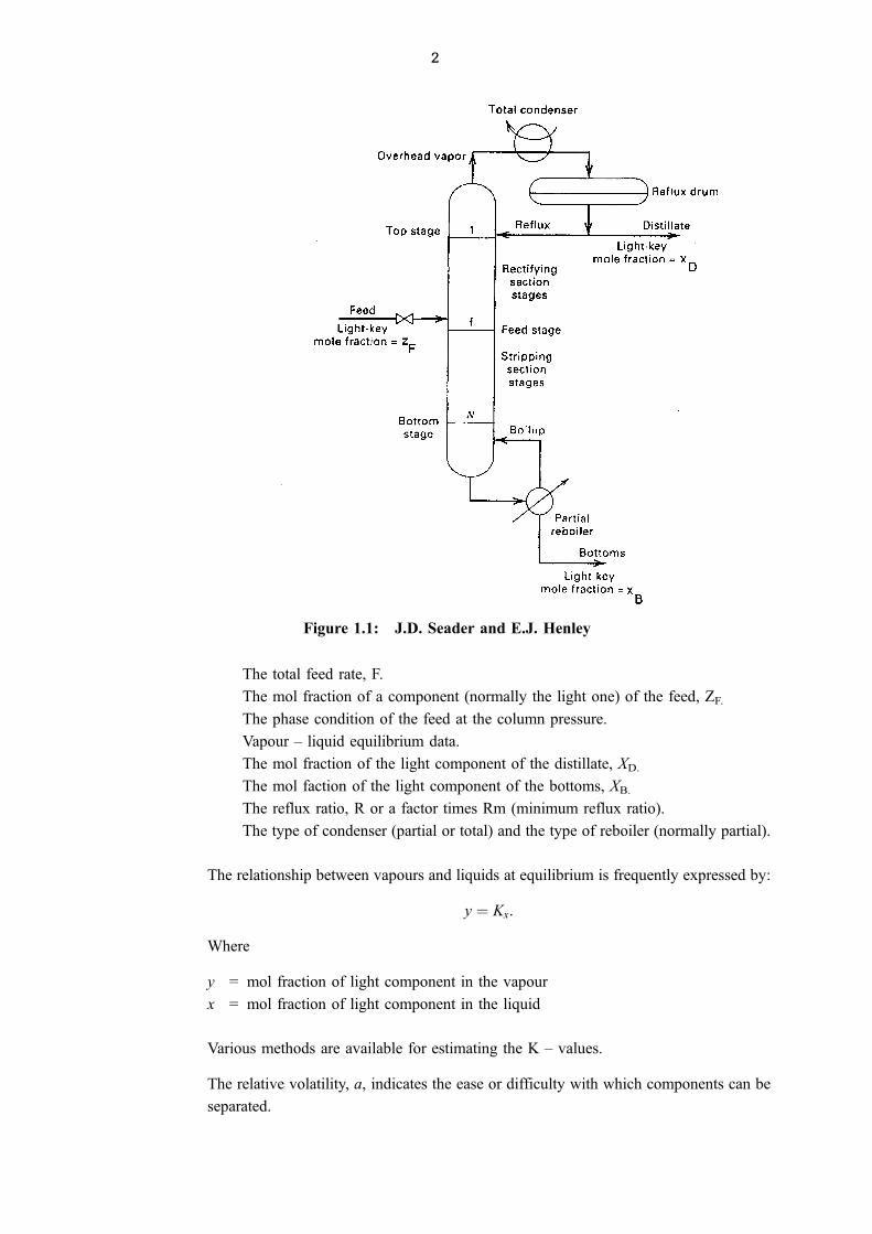
Refer to the following sketch (1) of a distillation column that operates with a total
condenser and a reboiler that vapourises a part of the liquid that leaves the bottom stage.
When a partial condenser is used the top product would be mixture of vapour and liquid.
In the sketch the more volatile component is referred to as the light key (LK) and the less
volatile component as the heavey key (HK). In multi component systems the LK is the
most volatile component in the bottom product (bottoms) and the HK the least volatile
component in the top product (distillate).
1.1.2 McCabe ± Thiele Method
This method is based on the assumption of constant ± molar ± overflow (equi ± molar
overflow). The liquid and vapour molar flow rates in the top part of the column (the
rectification section) do not change from stage to stage. This is also the case for the
bottom part (the stripping section) but the flow rates can be different from that in the
rectification section.
It is assumed that equilibrium is attained in each stage and such a stage is called an
equilibrium stage. The vapour that leaves the partial reboiler is also assumed to be in
equilibrium with the liquid that leaves it. The reboiler is thus considered to be a n
equilibrium stage. The vapour leaving the reboiler is called the boilup.
The following specifications are required to use this method successfully:
2
The total feed rate, F.
The mol fraction of a component (normally the light one) of the feed, ZF.
The phase condition of the feed at the column pressure.
Vapour ± liquid equilibrium data.
The mol fraction of the light component of the distillate, XD.
The mol faction of the light component of the bottoms, XB.
The reflux ratio, R or a factor times Rm (minimum reflux ratio).
The type of condenser (partial or total) and the type of reboiler (normally partial).
The relationship between vapours and liquids at equilibrium is frequently expressed by:
y � Kx.
Where
y = mol fraction of light component in the vapour
x = mol fraction of light component in the liquid
Various methods are available for estimating the K ± values.
The relative volatility, a, indicates the ease or difficulty with which components can be
separated.
Figure 1.1: J.D. Seader and E.J. Henley
3 CEM4M3-C/1
a1;2 � K1
K2
where 1 refers to light key
and 2 to the heavey key
The closer a is to 1 the more difficult the separation.
It can be assumed that Raoult's law applies when the components form ideal solutions
and ideal gas law applies in the vapour phase ± thus:
K1 � Ps1
Pand K2 � Ps
2P
and a1;2 � Ps1
Ps2
where Ps1 and Ps
2 are the vapour pres-
sures.
It can be shown that:
y1 � a1;2x1
1� x1�a1;2 ÿ 1� (1)
The amounts of distillate, D and bottoms, B are found by doing a molar balance.
The reflux ratio, R = Ln/S determines the liquid flow rate, Ln which remains constant in
the rectification section.
The vapour flow rate is given by Ln + D which also remains constant in the rectification
section.
It can be shown that the top operating line is given by:
yn � Ln
Vn
xn�1 � D
Vn
xD or yn � R
R� 1xn�1 � xD
R� 1(2)
Equation (2) is a straight line passing through (xD; xD) and�
0;xD
R� 1
�The bottom operating line is given by:
ym � Lm
Vm
xm�1 ÿ B
VM
xB (3)
Equation (3) is also a straight line passing through (xB; xB) with a slope of LmVm
.
It is worth remembering that: the compositions of the vapour and liquid leaving a stage
is obtained from the equilibrium curve and that the composition of the vapour entering
a stage in terms of the liquid leaving stage is given by the operating line. the physical
condition of the feed determines the flow rate of the liquid flowing from the feed tray to
the stripping section. If the feed is for instance a liquid at its boiling point
Lm � Ln � F.
The quantity, q is defined asheat to vapourise 1 mol of feedmolar latent heat of the feed
.
It can be shown that the equation of the q ± line is given by:
yq � q
qÿ 1xq ÿ zf
qÿ 1(4)
Equation (4) passes through (xf ; xf ) with a slope ofq
qÿ 1:
When the feed is
(a) a cold liquor q > 1 slope is positive
(b) liquor at boiling point q = 1 slope is vertical
4
(c) partly vapour 0 < q < 1 slope is negative
(d) saturated vapour q = 0 slope is horizontal
(e) superheated vapour q < 0 slope is positive
Procedure
1. Plot equilibrium curve
2. Draw 458 line
3. Draw top ooperating line
4. Draw q ± line
5. Draw bottom operating line by connecting (xB; xB) with the intersection of the top
operatiang line and the q ± line.
6. Draw a horizontal line from (xD; xD) to the equilibrium curve ± drop a vertical line
from this intersection to the top operating line. This completes the determination of
the first stage. Repeat this procedure until a vertical line from the equilibrium curve
has to be dropped to the bottom operating line (past (xf ; xf ).
7. The above procedure is carried out till a vertical line from the equilibrium curve
passes (xB; xB).
8. Count the number of theoretical stages.
9. Number of theoretical stages/efficiency = number of actual stages.
10. Number of actual stages ± 1 = number of actual trays.
Example 1
200 k mol/h of a mixture containing 55 mol% benzene and 45 mol% toluene is fed to a
continuous distillation column. The feed is at its boiling point. a = 3,09 and the reflux
ration is 1,6. The distillate must contain 95 mol% benzene and the bottoms 5 mol%
benzene.
Determine:
(a) the number of theoretical stages
(b) the feed stage
(c) the number of actual trays if the overall efficiency is 60%.
F = 200 = D + B (1)
200 6 0,55 = 110 = 0,95 D + 0,05 B (2)
Substitute (1) in (2) B = 88,9 D = 111,1
y � 3; 09x
1� 2; 09x
x y
0 0
0,2 0,435
0,4 0,67
0,6 0,82
0,8 0,92
1,0 1,0
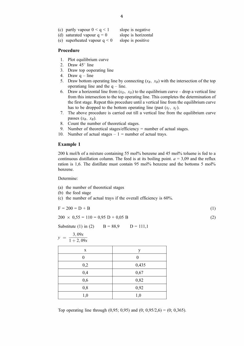
Top operating line through (0,95; 0,95) and (0; 0,95/2,6) = (0; 0,365).
q ± line is vertical through (0,55; 0,55).
Bottom operating line throught (o,55; 0,05) and intersection of q ± line and the top
operating line.
The construction is shown below.
(a) 9 theoretical stages are required
(b) the theoretical feed stage is number 4 from the top
(c) 9/0,6 ± 1 = 14 actual trays
1.1.3 Minimum Reflux Ration, Rm
The minimum reflux ration is determined by drawing a top operating line from (xD; xD)
to the intersection of the q ± line and the equilibrium curve.
A separation requires an infinite number of stages at Rm and can thus not be used in
practice. Rm is, however, used as a starting point and an actual R would be Rm
multiplied by a factor that is much bigger than one.
In the above example the line passes through (0,95; 0,95) and (0,55; 0,78).
The slope of the top operating line is given by:R
R� 1.
The slope of this line isRm
Rm � 1� 0; 95ÿ 0; 78
0; 95ÿ 0; 55� 0; 425 thus Rm � 0; 74.
5 CEM4M3-C/1
6
Problems
1. Repeat the above example but with a feed that is 60% vapour.
Answer: 9+ theoretical stages; 5 theoretical feed stage.
2. A mixture that contains 40 mass % benzene and 60 mass % ethyl- benzene must be
separated into a distillate containing 95 mol % benzene and a bottoms containing 5
mol % benzene. The feed is a liquid at 308C. The bubble point of the feed is 1048Cits latent heat of vapourisation is 36300 KJ/kmol and its specific heat is 160 kJ/kmol
K.
Determine Rm and the number of actual trays if the efficiency of the trays is 55%
and R = 1,5 Rm. a = 6,8
Answer: Rm = 0,318; number of trays = 12
1.1.4 Number of stages at total reflux
It is implied in this case that no products are withdrawn and is thus of no practical value.
It can, however, be used as a starting point in distillation calculations.
The two operating lines merge with the 458 line and stages are stepped off from xD to xB.
1.1.5 Batch distillation
This is an unsteady state distillation process that is frequently used for small scale
operations.
This type of column consists of a boiler (also called the still) on top of which a
distillation column is installed. A whole batch is charged to the boiler. The vapour is
condensed and part of the condensate is returned as reflux.
As the distillation process proceeds the composition in the boiler changes continuously.
This results in the decrease of the lighter component in the distillate. In order to maintain
a constant distillate composition the reflux ration can be adjusted continuously or the
column can be operated initially with a higher concentration of the light component at a
given reflux ratio. This ratio is kept constant which will result in a lower concentration
of the light component. The distillation is stopped when the required distillate
composition is given by the average.
A batch distillation column is only fitted with a rectification section. The operating line
of a rectification section thus applies.
Only the constant reflux method will be considered here.
Consider the boiler to be initially charged with S1 mols of liqid with a mol fraction x1 of
the light component. The composition of the distillate is xD with R1 the reflux ratio. The
distillation is stopped when S2 mols remain with mol fraction x2, It is necessary to
increase the reflux ratio to R2 in order to maintain the distillate composition at xD if the
number of trays remains the same.
A total mol balance gives: S1 ÿ S2 � D
A light component balance gives: S1 xs1 ÿ S2 xs2 � D xD
From these equations it follows that D � S1
h xs1 ÿ xs2
xD ÿ xs2
i(5)
The intercept of the operating line on the Y ± axis is xDR�1
= A(say).
7 CEM4M3-C/1
Thus R � xD
Aÿ 1 (6)
Equations (5) and (6) allows one to determine the final reflux ratio that is required to
obtain a given final concentration in the boiler and the quantity of distillate.
It can also be shown that: InS1
S2
�Z xs2
xs1
dxs
xD ÿ xs
.
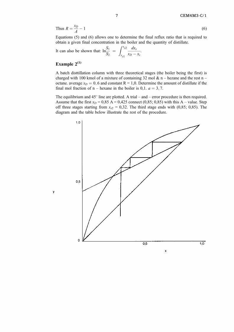
Example 2(1)
A batch disttillation column with three theoretical stages (the boiler being the first) is
charged with 100 kmol of a mixture of containing 32 mol & n ± hezane and the rest n ±
octane. average xD � 0; 6 and constant R = 1,0. Determine the amount of distillate if the
final mol fraction of n ± hexane in the boiler is 0,1. a � 3; 7.
The equilibrium and 458 line are plotted. A trial ± and ± error procedure is then required.
Assume that the first xD = 0,85 A = 0,425 connect (0,85; 0,85) with this A ± value. Step
off three stages starting from xs2 = 0,32. The third stage ends with (0,85; 0,85). The
diagram and the table below illustrate the rest of the procedure.
8
xs xD A1
xD ÿ xs
0,32 0,85 0,425 1,9
0,16 0,6 0,3 2,3
0,1 0,5 0,25 2,5
0,05 0,3 0,15 4
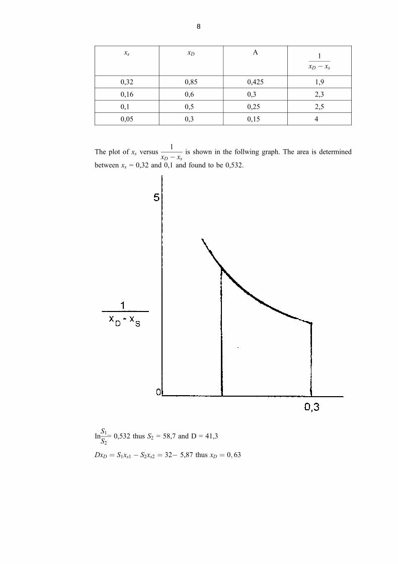
The plot of xs versus1
xD ÿ xs
is shown in the follwing graph. The area is determined
between xs = 0,32 and 0,1 and found to be 0,532.
InS1
S2
= 0,532 thus S2 = 58,7 and D = 41,3
DxD � S1xs1 ÿ S2xs2 � 32ÿ 5,87 thus xD � 0; 63
9 CEM4M3-C/1
1.2 MUTIPLE FEED AND SIDE STREAMS
1.2.1 Objectives
The methods that are required to solve these types of problems are presented here.
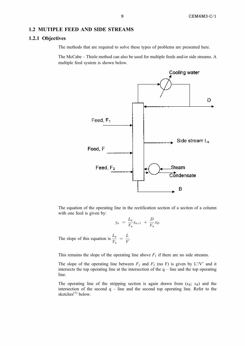
The McCabe ± Thiele method can also be used for multiple feeds and/or side streams. A
multiple feed system is shown below.
The equation of the operating line in the rectification section of a seciton of a column
with one feed is given by:
yn � Ln
Vn
xn�1 � D
Vn
xD
The slope of this equation isLn
Vn
� L
V.
This remains the slope of the operating line above F1 if there are no side streams.
The slope of the operating line between F1 and F2 (no F) is given by L'/V' and it
intersects the top operating line at the intersection of the q ± line and the top operating
line.
The operating line of the stripping section is again drawn from (xB; xB) and the
intersection of the second q ± line and the second top operating line. Refer to the
sketches(1) below.
10
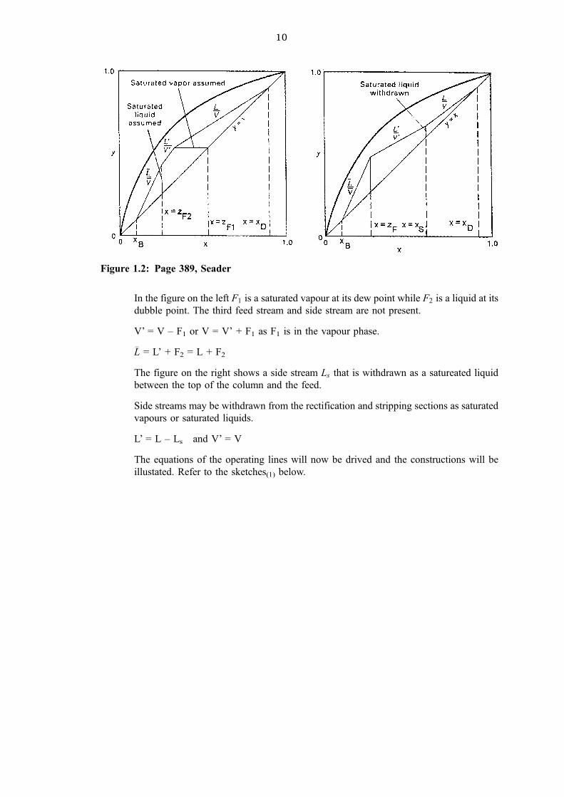
In the figure on the left F1 is a saturated vapour at its dew point while F2 is a liquid at its
dubble point. The third feed stream and side stream are not present.
V' = V ± F1 or V = V' + F1 as F1 is in the vapour phase.
�L = L' + F2 = L + F2
The figure on the right shows a side stream Ls that is withdrawn as a satureated liquid
between the top of the column and the feed.
Side streams may be withdrawn from the rectification and stripping sections as saturated
vapours or saturated liquids.
L' = L ± Ls and V' = V
The equations of the operating lines will now be drived and the constructions will be
illustated. Refer to the sketches(1) below.
Figure 1.2: Page 389, Seader
11 CEM4M3-C/1
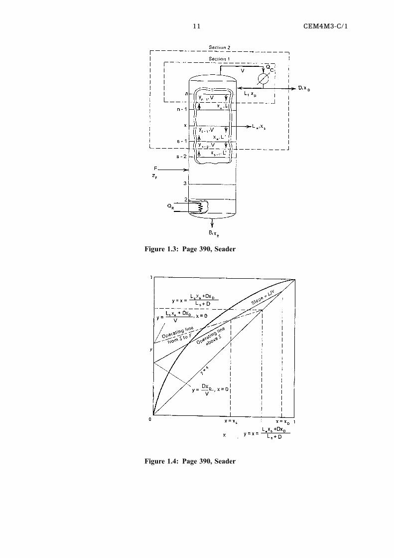
Figure 1.3: Page 390, Seader
Figure 1.4: Page 390, Seader
12
A material balance over section 1 gives:
Vnÿ1 Ynÿ1 � Lnxn � DxD (7)
A material balance over section 2 gives:
Vsÿ1 Ysÿ1 � L0sÿ1xsÿ1 � Lsxs � DxD (8)
These equations can be simplified to:
y � L0
Vx � Lsxs � DxD
Vand y � L
Vx � D
VxD (9)
By equating the two equations of (9) the intersection of the two operating lines are found
to be at x � xs
The intersection of y � x and y � L0
Vx � Lsxs � DxD
Voccurs at
x � Ls xs � DxDLs � D
(10)
Example 3(2)
A mixture of H2O and ethyl alcohol (EtOH) contianing 0,16 mol fraction EtOH is
continuously distilled in a tray fractionation column to give a product containing 0,77
mol faction EtOH and a wast containing 0,02 mol fraction EtOH. It is proposed to
withdraw 25% of the EtOH in the feed as a liquid side stream with a mol fraction of 0,5
EtOH.
Determine the number of theoretical trays required and the tray from which the side
stream should be withdrawn if the feed is a liquid at its bubble point and the reflux ratio
is 2.
x 0,019 ,072 ,097 ,124 ,166 ,234 ,261 ,327 ,396 ,508 ,52 ,57 ,676 ,747 ,894
y 0,17 ,389 ,437 ,47 ,509 ,544 ,558 ,583 ,612 ,656 ,66 ,68 ,738 ,781 ,894
Basis 100 kmol feed
EtOH in feed = 1006 0,16 = 16 kmol
25% of EtOH in side stream = 4 kmol
; Water in side stream = 4 kmol
Thus Ls = 8 kmol and xs = 0,5
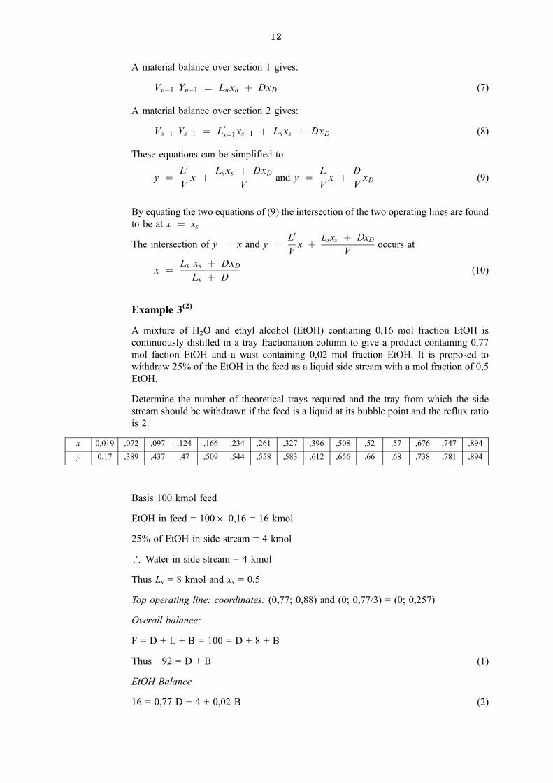
Top operating line: coordinates: (0,77; 0,88) and (0; 0,77/3) = (0; 0,257)
Overall balance:
F = D + L + B = 100 = D + 8 + B
Thus 92 = D + B (1)
EtOH Balance
16 = 0,77 D + 4 + 0,02 B (2)
13 CEM4M3-C/1
With (1) and (2) it is found that B = 78,45 kmol
D = 13,55 kmol
L = 2 D = 2 6 13,55 = 27,1 kmol
V= D + L + 13,55 + 27,1 = 40,65 kmol = V'
L' = L ± Ls = 27,1 ± 8 = 18,1 kmol
Second Operating Line:
y � s � Lsxs � DxD
Ls � D� 8 � 0; 5 � 13; 55 � 0; 77
8 � 13; 55� 0; 67
Second coordinate where xs = 0,5 intersects the top operating line
Bottom Operating Line:
Coordinates (0,02; 0,02) and where x � zF = 0,16 intersects the second operating ling.
From the construction below one finds that the number of theoretical trays are 9 and the
side steam is withdrawn from the 6th theoretical tray from the top.
14
Problems
3.(1) Two feed streams containing water and acetic acid are fed to a continuous
distillation column. Feed 1 enters as a liquid at its bubble point relatively high up in the
column and contains 75 kmol/h water (W) and 25 kmol/h acetic acid (A).
The second feed, F2 enters lower down, is 50% vapour and contains 50 kmol/h W and 50
kmol/h A.
The column is operated at a reflux ratio of 3,0 Rm. The distillate contains 95 mol % W
while the bottom product contains 95 mol % A.
Determine the number of theoretical trays and the feed trays.
x ,0055 ,053 ,125 ,206 ,297 ,51 ,649 ,803 ,9594
y ,0112 ,133 ,24 ,338 ,437 ,63 ,751 ,866 ,972
Answer: 16; 9; 13
4. Repeat example 2 by using the relevant equations. That is the equilibrium and
operating line equations.
Answer: D = 38,3; S2 = 61,7; xD = 0,67
5.(1) Determine the number of theoretical stages and the locations of the feed and side
stream when 100 kmol/h of a mixture of A and B is distilled at atmospheric
pressure. The mol fraction of A in the feed is 0,26. The distillate contains 95 mol %
A and the bottoms 95 mol % B. The side stream is withdrawn as a liquid from the
rectification section at a rate of 10 kmol/h that contains 40 mol % A.
Relative volatility is 2,23 and reflux ratio is 5.
Answer: 14; 6; 9±10
1.3 PONCHON ± SAVARIT METHOD FOR TRAY TOWERS(2)
1.3.1 Objective
This method can be used to design distillation columns for binary, non ± ideal systems
where equimolar overflow is invalid.
The McCabe ± Thiele method assumes constant molar overflow which implies that the
molar latent heats are constant and that heat of mixing is negligible.
For non-ideal systems where the above assumptions are not valid, energy as well as
material balances and phase equilibrium relationships have to be utilized to do a proper
design. This can be a very tedious process (except that rigorous computer aided design
packages are presently quite freely available).
The Ponchon ± Savarit method employs a graphical method for binary non-ideal
mixtures that is based on an enthalphy ± composition diagram.
Consider the following sketch that shows the relationship between the enthalpy of a
liquid and a vapour as functions of the liquid and vapour mol fractions.
15 CEM4M3-C/1
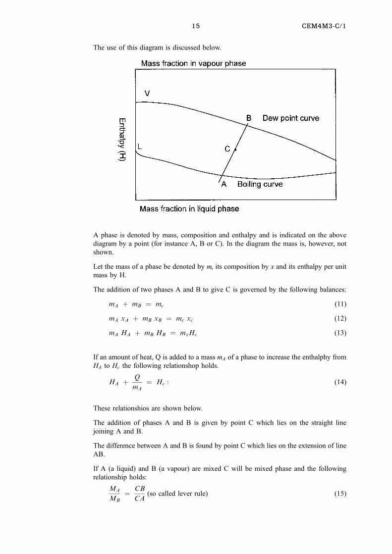
The use of this diagram is discussed below.
A phase is denoted by mass, composition and enthalpy and is indicated on the above
diagram by a point (for instance A, B or C). In the diagram the mass is, however, not
shown.
Let the mass of a phase be denoted by m, its composition by x and its enthalpy per unit
mass by H.
The addition of two phases A and B to give C is governed by the following balances:
mA � mB � mc (11)
mA xA � mB xB � mc xc (12)
mA HA � mB HB � mxHc (13)
If an amount of heat, Q is added to a mass mA of a phase to increase the enthalphy from
HA to Hc the following relationshop holds.
HA � Q
mA� Hc : (14)
These relationshios are shown below.
The addition of phases A and B is given by point C which lies on the straight line
joining A and B.
The difference between A and B is found by point C which lies on the extension of line
AB.
If A (a liquid) and B (a vapour) are mixed C will be mixed phase and the following
relationship holds:
MA
MB� CB
CA(so called lever rule) (15)

16
The figure(2) below represents a continuous distillation column. The trays are numbered
from the bottom upwards.
HV and HL represent the enthalphy of the vapour and liquid respectively while QC is the
heat removed in the condenser (no subcooling) and QB is the heat supplied by the
reboiler.
Figure 1.5: Page 461 C & R
17 CEM4M3-C/1
Vn � Ln�1 � D thus Vn ÿ Ln�1 � D (16)
Vn yn � Ln�1 xn�1 � Dxd thus Vn yn � Ln�1 xn�1 � Dxd (17)
Vn HVn � Ln�1HL
n�1 � DHLd � Qc thus VnHV
n ÿ Ln�1HLn�1 � DHL
d � Qc (18)
Let H 0d � HLd � Qc=D
Equation (18) thus becomes: VnHVn ÿ Ln�1HL
n�1 � DH 0d (19)
Substitute (16) and (17)
thus
�Ln�1 � D�yn ÿ Ln�1n� 1 � Dxd
Ln�1 �yn ÿ xn�1� � D�xd ÿ yn�thus
Ln�1
D� xd ÿ y
n
yn ÿ Xn�1
(20)
Substitute (16) in (19) �Ln�1 � D�HVn ÿ Ln�1H 0n�1 � DH 0d
Thus Ln�1�HVn ÿ HL
n�1� � D�H 0d ÿ HVn �
ThusLn�1
D� H 0d ÿ HV
n
HVn ÿ HL
n�1
(21)
Equate equations (20) and (21)
ThusH 0d ÿ HV
n
HVn ÿ HL
n�1
� xd ÿ yn
yn ÿ xn�1
(22)
From the above follows: yn �"
H 0d ÿ HVn
H 0d ÿ HLn�1
#xn�1 �
"HV
n ÿ HLn�1
H 0d ÿ HLn�1
#xd (23)
Equation (23) is that of the operating line above the feed tray and it is the relationship
between the composition of the vapour yn rising from a tray to the composition of the
liquid entering a tray.
It is clear from equation (22) that xd and H 0d are common to all the operatiang lines above
the feed tray. These operating lines pass through a common pole N with coordinates xd
and H 0d. Vn, Ln�1 and N lie on a straight line.
It can be shown in a similar manner that all the operating lines in the stripping section
pass through a common pole, M with coordinates:
xw ; Lm�1 where H0w � HLw ÿ
QB
W(24)
It can be shown that F, M and N also lie on a straight line.
Vm; Lm�1 and M lie on another straightline
Procedure to determine the number of trays
18
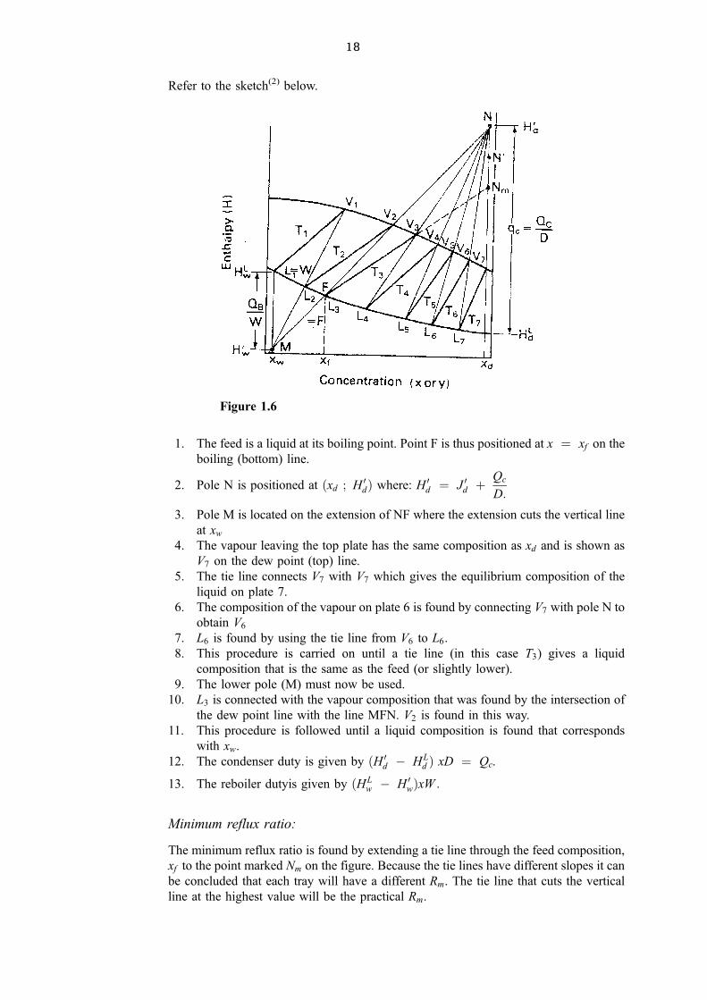
Refer to the sketch(2) below.
1. The feed is a liquid at its boiling point. Point F is thus positioned at x � xf on the
boiling (bottom) line.
2. Pole N is positioned at �xd ; H 0d� where: H 0d � J 0d �Qc
D:
3. Pole M is located on the extension of NF where the extension cuts the vertical line
at xw
4. The vapour leaving the top plate has the same composition as xd and is shown as
V7 on the dew point (top) line.
5. The tie line connects V7 with V7 which gives the equilibrium composition of the
liquid on plate 7.
6. The composition of the vapour on plate 6 is found by connecting V7 with pole N to
obtain V6
7. L6 is found by using the tie line from V6 to L6.
8. This procedure is carried on until a tie line (in this case T3) gives a liquid
composition that is the same as the feed (or slightly lower).
9. The lower pole (M) must now be used.
10. L3 is connected with the vapour composition that was found by the intersection of
the dew point line with the line MFN. V2 is found in this way.
11. This procedure is followed until a liquid composition is found that corresponds
with xw.
12. The condenser duty is given by �H 0d ÿ HLd � xD � Qc.
13. The reboiler dutyis given by �HLw ÿ H 0w�xW :
Minimum reflux ratio:
The minimum reflux ratio is found by extending a tie line through the feed composition,
xf to the point marked Nm on the figure. Because the tie lines have different slopes it can
be concluded that each tray will have a different Rm. The tie line that cuts the vertical
line at the highest value will be the practical Rm.
Figure 1.6
19 CEM4M3-C/1
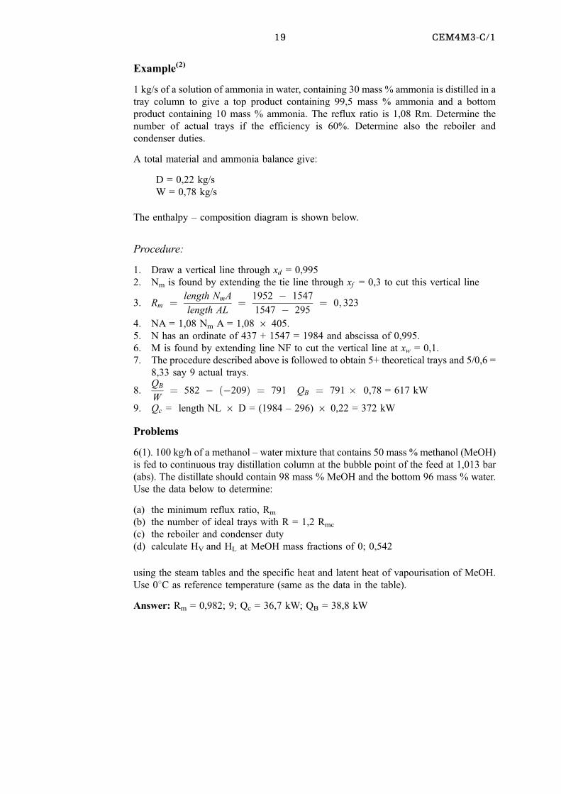
Example(2)
1 kg/s of a solution of ammonia in water, containing 30 mass % ammonia is distilled in a
tray column to give a top product containing 99,5 mass % ammonia and a bottom
product containing 10 mass % ammonia. The reflux ratio is 1,08 Rm. Determine the
number of actual trays if the efficiency is 60%. Determine also the reboiler and
condenser duties.
A total material and ammonia balance give:
D = 0,22 kg/s
W = 0,78 kg/s
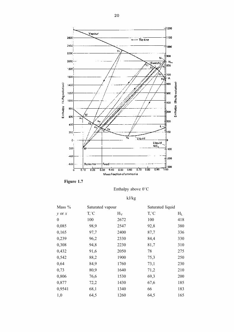
The enthalpy ± composition diagram is shown below.
Procedure:
1. Draw a vertical line through xd = 0,995
2. Nm is found by extending the tie line through xf = 0,3 to cut this vertical line
3. Rm � length NmA
length AL� 1952 ÿ 1547
1547 ÿ 295� 0; 323
4. NA = 1,08 Nm A = 1,08 6 405.
5. N has an ordinate of 437 + 1547 = 1984 and abscissa of 0,995.
6. M is found by extending line NF to cut the vertical line at xw = 0,1.
7. The procedure described above is followed to obtain 5+ theoretical trays and 5/0,6 =
8,33 say 9 actual trays.
8.QB
W� 582 ÿ �ÿ209� � 791 QB � 791 � 0,78 = 617 kW
9. Qc = length NL 6 D = (1984 ± 296) 6 0,22 = 372 kW
Problems
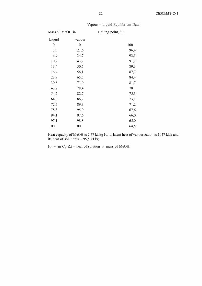
6(1). 100 kg/h of a methanol ± water mixture that contains 50 mass % methanol (MeOH)
is fed to continuous tray distillation column at the bubble point of the feed at 1,013 bar
(abs). The distillate should contain 98 mass % MeOH and the bottom 96 mass % water.
Use the data below to determine:
(a) the minimum reflux ratio, Rm
(b) the number of ideal trays with R = 1,2 Rmc
(c) the reboiler and condenser duty
(d) calculate HV and HL at MeOH mass fractions of 0; 0,542
using the steam tables and the specific heat and latent heat of vapourisation of MeOH.
Use 08C as reference temperature (same as the data in the table).
Answer: Rm = 0,982; 9; Qc = 36,7 kW; QB = 38,8 kW
20
Enthalpy above 08C
kJ/kg
Mass % Saturated vapour Saturated liquid
y or x T,8C HV T,8C HL
0 100 2672 100 418
0,085 98,9 2547 92,8 380
0,165 97,7 2400 87,7 336
0,239 96,2 2330 84,4 330
0,308 94,8 2230 81,7 310
0,432 91,6 2050 78 275
0,542 88,2 1900 75,3 250
0,64 84,9 1760 73,1 230
0,73 80,9 1640 71,2 210
0,806 76,6 1530 69,3 200
0,877 72,2 1430 67,6 185
0,9541 68,1 1340 66 183
1,0 64,5 1260 64,5 165
Figure 1.7
21 CEM4M3-C/1
Vapour ± Liquid Equilibrium Data
Mass % MeOH in Boiling point, 8C
Liquid vapour
0 0 100
3,5 21,6 96,4
6,9 34,7 93,5
10,2 43,7 91,2
13,4 50,5 89,3
16,4 56,1 87,7
23,9 65,5 84,4
30,8 71,0 81,7
43,2 78,4 78
54,2 82,7 75,3
64,0 86,2 73,1
72,7 89,3 71,2
78,8 95,0 67,6
94,1 97,6 66,0
97,1 98,8 65,0
100 100 64,5
Heat capacity of MeOH is 2,77 kJ/kg K, its latent heat of vapourization is 1047 kJ/k and
its heat of solutionis ± 95,5 kJ.kg.
HL = m Cp �t + heat of solution 6 mass of MeOH.
22
CHAPTER 2
Multicomponent distillation
CONTENTS
2.1 LEARNING OUTCOMES 00
2.1.1 Required Specifications(3) 00
2.1.3 Multicomponent Flash, Bubble and Dew Points(1) 00
2.1.4 Isothermal Flash Calculation
2.1.5 Adiaabatic Flash calculation 00
2.1.6 Key components 00
2.1.7 Minimum Reflux Ratio 00
2.1.8 Colburn's Method for Minimum Reflux(2) 00
2.1.9 Underwood's Method for Rm 00
2.2 SHORT CUT METHODS 00
2.2.1 Number of Trays (Lewis-Matheson)(2 & 3) 00
2.2.2 Feed Tray Location(3) 00
2.2.3 Recap 00
2.2.4 Evaluation 00
2.1 LEARNING OUTCOMES
After completion of this section the student should be able to do the following.
. Be able to determine the dew points and bubble points, at given pressures, of mixtures
of vapours and liquids respectively.
. Be able to do an isothermal flash calculation
. Be able to determine the minimum reflux ratio of multicomponent mixtures
. Be able to use the Lewis ± Matheson method to determine the number of theoretical
trays required to achieve a given separation
. Be able to determine the feed tray location for the separation of multicomponent
mixtures.
2.1.1 Objectives
Approximate methods to solve multicomponent, multistage distillation problems will be
discussed. This will be preceded by a discussion of the bubble and dew points of
mixtures and a method is given that enables the student to do an isothermal flash
calculation.
2.1.2 Required Specifications(3)
The following must be established to design a distillation column:
1. Temperature, pressure, composition and flow rate of the feed.
23 CEM4M3-C/1
2. Pressure at which the distillation must be carried out. This is frequently determined
by the temperature of the cooling medium that will be used in the condenser.
3. The feed should be introduced at the optimum feed tray location.
4. Heat losses are assumed to be negligible.
If the above items are established only three of the following can be specified.
1. Total number of trays.
2. Reflux ratio.
3. Ratio of vapour to bottom product produced in the reboiler (reboil rate).
4. Concentration of one component (maximum two) in one product.
5. Split of a component between the distillate and the bottoms (maximum of two).
6. Ratio of distillate to bottoms.
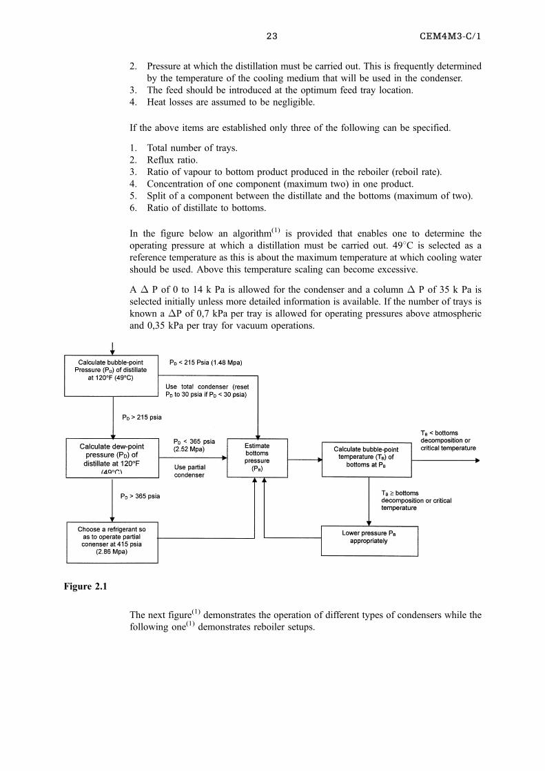
In the figure below an algorithm(1) is provided that enables one to determine the
operating pressure at which a distillation must be carried out. 498C is selected as a
reference temperature as this is about the maximum temperature at which cooling water
should be used. Above this temperature scaling can become excessive.
A � P of 0 to 14 k Pa is allowed for the condenser and a column � P of 35 k Pa is
selected initially unless more detailed information is available. If the number of trays is
known a �P of 0,7 kPa per tray is allowed for operating pressures above atmospheric
and 0,35 kPa per tray for vacuum operations.
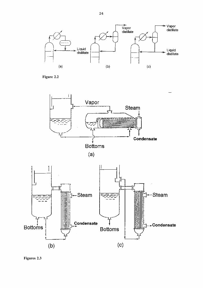
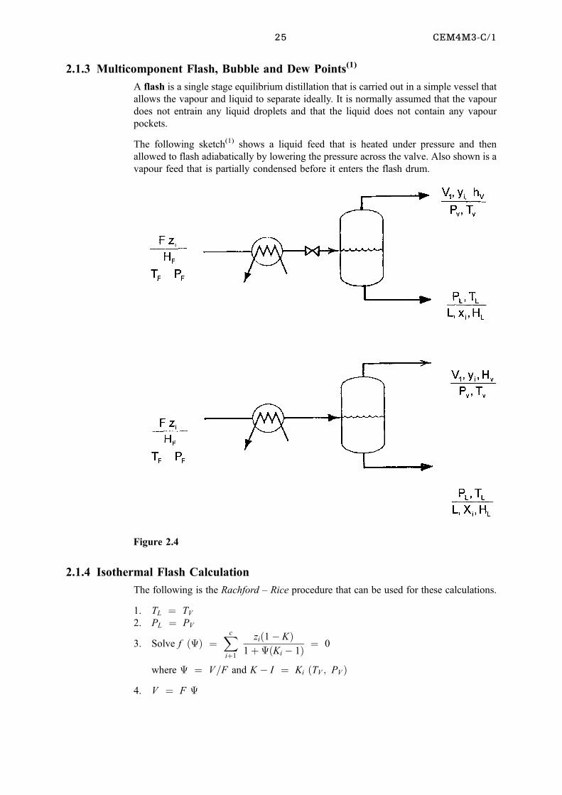
The next figure(1) demonstrates the operation of different types of condensers while the
following one(1) demonstrates reboiler setups.
Figure 2.1
24
Figure 2.2
Figures 2.3
25 CEM4M3-C/1
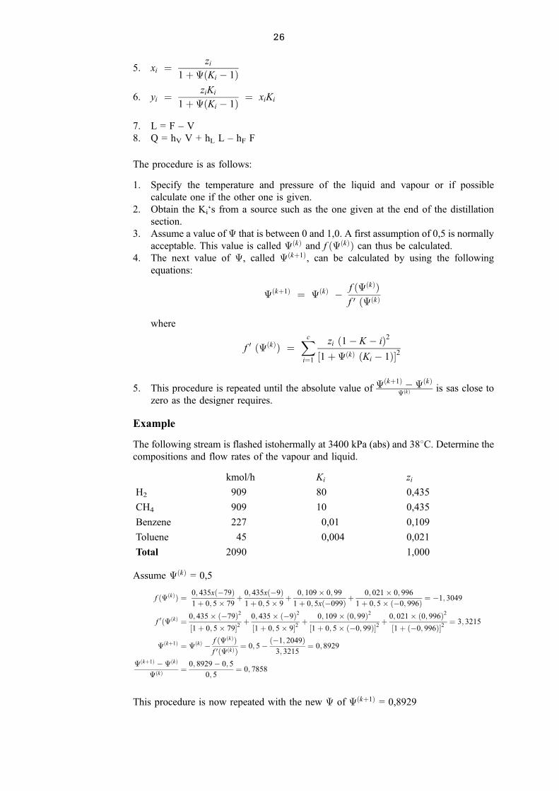
2.1.3 Multicomponent Flash, Bubble and Dew Points(1)
A flash is a single stage equilibrium distillation that is carried out in a simple vessel that
allows the vapour and liquid to separate ideally. It is normally assumed that the vapour
does not entrain any liquid droplets and that the liquid does not contain any vapour
pockets.
The following sketch(1) shows a liquid feed that is heated under pressure and then
allowed to flash adiabatically by lowering the pressure across the valve. Also shown is a
vapour feed that is partially condensed before it enters the flash drum.
2.1.4 Isothermal Flash Calculation
The following is the Rachford ± Rice procedure that can be used for these calculations.
1. TL � TV
2. PL � PV
3. Solve f �� �Xc
i�1
zi�1ÿ K�1��Ki ÿ 1� � 0
where � V=F and K ÿ I � Ki �TV ; PV �4. V � F
Figure 2.4
26
5. xi � zi
1��Ki ÿ 1�6. yi � ziKi
1��Ki ÿ 1� � xiKi
7. L = F ± V
8. Q = hV V + hL L ± hF F
The procedure is as follows:
1. Specify the temperature and pressure of the liquid and vapour or if possible
calculate one if the other one is given.
2. Obtain the Ki`s from a source such as the one given at the end of the distillation
section.
3. Assume a value of that is between 0 and 1,0. A first assumption of 0,5 is normally
acceptable. This value is called �k� and f ��k�� can thus be calculated.
4. The next value of , called �k�1�, can be calculated by using the following
equations:
�k�1� � �k� ÿ f ��k��f 0 ��k�
where
f 0 ��k�� �Xc
i�1
zi �1ÿ K ÿ i�2�1��k� �Ki ÿ 1��2
5. This procedure is repeated until the absolute value of �k�1� ÿ�k��k� is sas close to
zero as the designer requires.
Example
The following stream is flashed istohermally at 3400 kPa (abs) and 388C. Determine the
compositions and flow rates of the vapour and liquid.
kmol/h Ki zi
H2 909 80 0,435
CH4 909 10 0,435
Benzene 227 0,01 0,109
Toluene 45 0,004 0,021
Total 2090 1,000
Assume �k� = 0,5
f ��k�� � 0; 435x�ÿ79�1� 0; 5� 79
� 0; 435x�ÿ9�1� 0; 5� 9
� 0; 109� 0; 99
1� 0; 5x�ÿ099� �0; 021� 0; 996
1� 0; 5� �ÿ0; 996� � ÿ1; 3049
f 0��k� � 0; 435� �ÿ79�2�1� 0; 5� 79�2 �
0; 435� �ÿ9�2�1� 0; 5� 9�2 �
0; 109� �0; 99�2�1� 0; 5� �ÿ0; 99��2 �
0; 021� �0; 996�2�1� �ÿ0; 996��2 � 3; 3215
�k�1� � �k� ÿ f ��k��f 0��k�� � 0; 5ÿ �ÿ1; 2049�
3; 3215� 0; 8929
�k�1� ÿ�k�
�k�� 0; 8929ÿ 0; 5
0; 5� 0; 7858
This procedure is now repeated with the new of �k�1� = 0,8929
27 CEM4M3-C/1
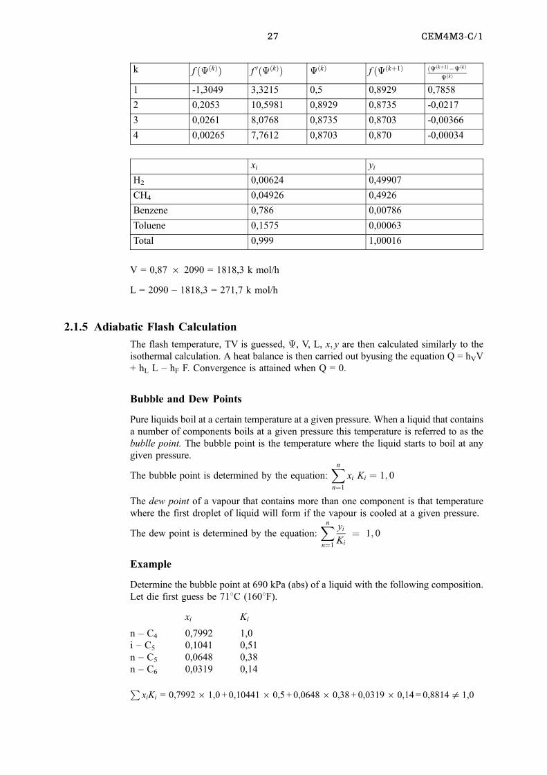
k f ��k�� f 0��k�� �k� f ��k�1� ��k�1�ÿ�k�
�k�
1 -1,3049 3,3215 0,5 0,8929 0,7858
2 0,2053 10,5981 0,8929 0,8735 -0,0217
3 0,0261 8,0768 0,8735 0,8703 -0,00366
4 0,00265 7,7612 0,8703 0,870 -0,00034
xi yi
H2 0,00624 0,49907
CH4 0,04926 0,4926
Benzene 0,786 0,00786
Toluene 0,1575 0,00063
Total 0,999 1,00016
V = 0,87 6 2090 = 1818,3 k mol/h
L = 2090 ± 1818,3 = 271,7 k mol/h
2.1.5 Adiabatic Flash Calculation
The flash temperature, TV is guessed, , V, L, x; y are then calculated similarly to the
isothermal calculation. A heat balance is then carried out byusing the equation Q = hVV
+ hL L ± hF F. Convergence is attained when Q = 0.
Bubble and Dew Points
Pure liquids boil at a certain temperature at a given pressure. When a liquid that contains
a number of components boils at a given pressure this temperature is referred to as the
bublle point. The bubble point is the temperature where the liquid starts to boil at any
given pressure.
The bubble point is determined by the equation:Xn
n�1
xi Ki � 1; 0
The dew point of a vapour that contains more than one component is that temperature
where the first droplet of liquid will form if the vapour is cooled at a given pressure.
The dew point is determined by the equation:Xn
n�1
yi
Ki
� 1; 0
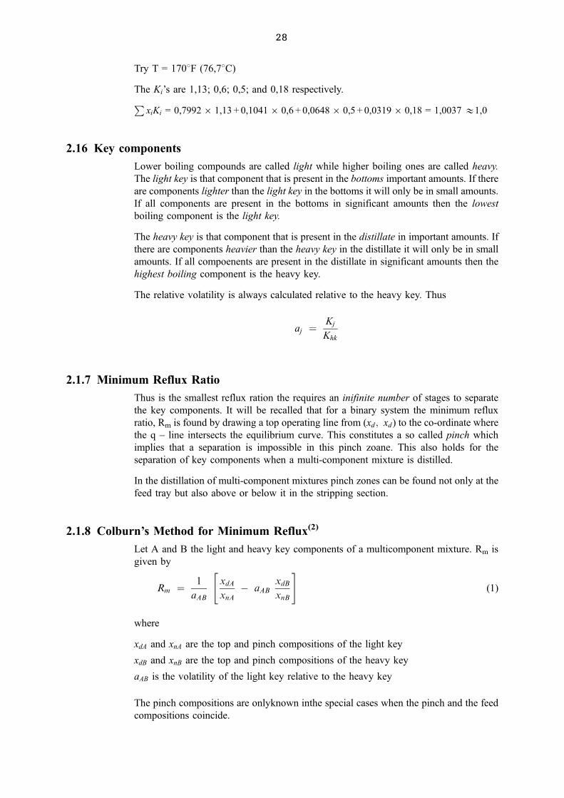
Example
Determine the bubble point at 690 kPa (abs) of a liquid with the following composition.
Let die first guess be 718C (1608F).
xi Ki
n ± C4 0,7992 1,0
i ± C5 0,1041 0,51
n ± C5 0,0648 0,38
n ± C6 0,0319 0,14
PxiKi = 0,79926 1,0 + 0,104416 0,5 + 0,06486 0,38 + 0,03196 0,14 = 0,8814= 1,0
28
Try T = 1708F (76,78C)
The Ki's are 1,13; 0,6; 0,5; and 0,18 respectively.PxiKi = 0,79926 1,13 + 0,10416 0,6 + 0,06486 0,5 + 0,03196 0,18 = 1,0037 &1,0
2.16 Key components
Lower boiling compounds are called light while higher boiling ones are called heavy.
The light key is that component that is present in the bottoms important amounts. If there
are components lighter than the light key in the bottoms it will only be in small amounts.
If all components are present in the bottoms in significant amounts then the lowest
boiling component is the light key.
The heavy key is that component that is present in the distillate in important amounts. If
there are components heavier than the heavy key in the distillate it will only be in small
amounts. If all compoenents are present in the distillate in significant amounts then the
highest boiling component is the heavy key.
The relative volatility is always calculated relative to the heavy key. Thus
aj � Kj
Khk
2.1.7 Minimum Reflux Ratio
Thus is the smallest reflux ration the requires an inifinite number of stages to separate
the key components. It will be recalled that for a binary system the minimum reflux
ratio, Rm is found by drawing a top operating line from (xd; xd) to the co-ordinate where
the q ± line intersects the equilibrium curve. This constitutes a so called pinch which
implies that a separation is impossible in this pinch zoane. This also holds for the
separation of key components when a multi-component mixture is distilled.
In the distillation of multi-component mixtures pinch zones can be found not only at the
feed tray but also above or below it in the stripping section.
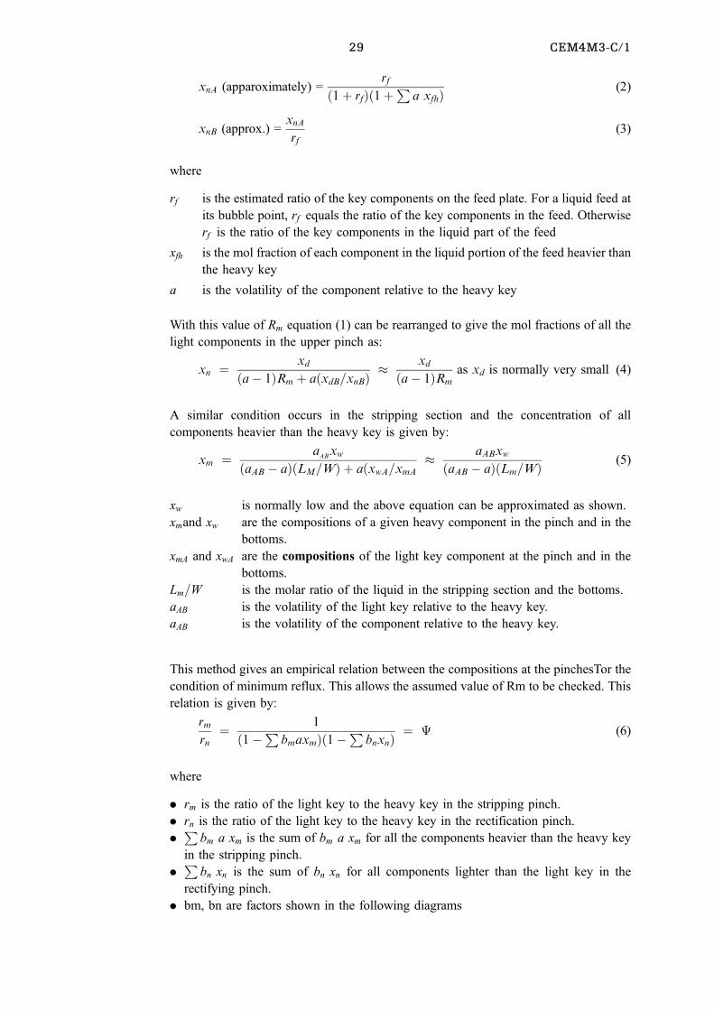
2.1.8 Colburn's Method for Minimum Reflux(2)
Let A and B the light and heavy key components of a multicomponent mixture. Rm is
given by
Rm � 1
aAB
"xdAxnA
ÿ aABxdBxnB
#(1)
where
xdA and xnA are the top and pinch compositions of the light key
xdB and xnB are the top and pinch compositions of the heavy key
aAB is the volatility of the light key relative to the heavy key
The pinch compositions are onlyknown inthe special cases when the pinch and the feed
compositions coincide.
29 CEM4M3-C/1
xnA (apparoximately) =rf
�1� rf��1�P
a xfh� (2)
xnB (approx.) =xnArf
(3)
where
rf is the estimated ratio of the key components on the feed plate. For a liquid feed at
its bubble point, rf equals the ratio of the key components in the feed. Otherwise
rf is the ratio of the key components in the liquid part of the feed
xfh is the mol fraction of each component in the liquid portion of the feed heavier than
the heavy key
a is the volatility of the component relative to the heavy key
With this value of Rm equation (1) can be rearranged to give the mol fractions of all the
light components in the upper pinch as:
xn � xd�aÿ 1�Rm � a�xdB=xnB� �
xd�aÿ 1�Rm
as xd is normally very small (4)
A similar condition occurs in the stripping section and the concentration of all
components heavier than the heavy key is given by:
xm � aABxw
�aAB ÿ a��LM=W� � a�xwA=xmA� aABxw�aAB ÿ a��Lm=W� (5)
xw is normally low and the above equation can be approximated as shown.
xmand xw are the compositions of a given heavy component in the pinch and in the
bottoms.
xmA and xwA are the compositions of the light key component at the pinch and in the
bottoms.
Lm=W is the molar ratio of the liquid in the stripping section and the bottoms.
aAB is the volatility of the light key relative to the heavy key.
aAB is the volatility of the component relative to the heavy key.
This method gives an empirical relation between the compositions at the pinchesTor the
condition of minimum reflux. This allows the assumed value of Rm to be checked. This
relation is given by:
rmrn� 1
�1ÿP bmaxm��1ÿP
bnxn� � (6)
where
. rm is the ratio of the light key to the heavy key in the stripping pinch.
. rn is the ratio of the light key to the heavy key in the rectification pinch.
.P
bm a xm is the sum of bm a xm for all the components heavier than the heavy key
in the stripping pinch.
.P
bn xn is the sum of bn xn for all components lighter than the light key in the
rectifying pinch.
. bm, bn are factors shown in the following diagrams
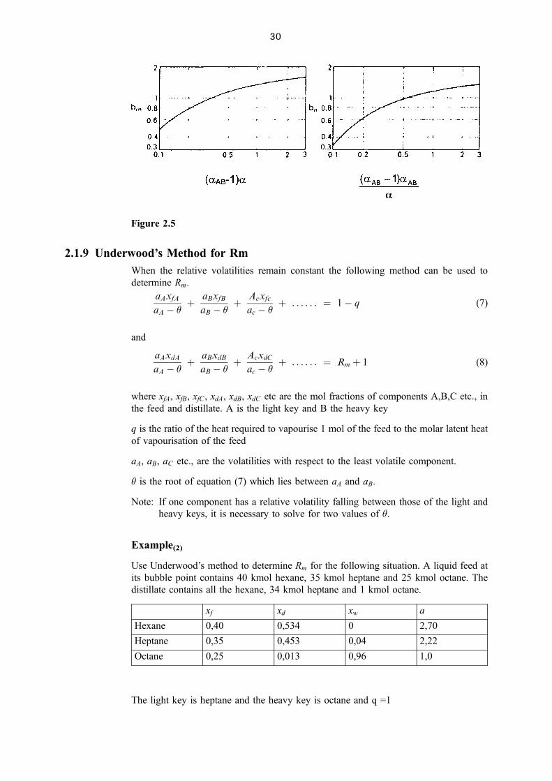
30
2.1.9 Underwood's Method for Rm
When the relative volatilities remain constant the following method can be used to
determine Rm.
aAxfAaA ÿ � �
aBxfBaB ÿ � �
Acxfcac ÿ � � . . . . . . � 1ÿ q (7)
and
aAxdAaA ÿ � �
aBxdBaB ÿ � �
AcxdCac ÿ � � . . . . . . � Rm � 1 (8)
where xfA, xfB, xfC, xdA, xdB, xdC etc are the mol fractions of components A,B,C etc., in
the feed and distillate. A is the light key and B the heavy key
q is the ratio of the heat required to vapourise 1 mol of the feed to the molar latent heat
of vapourisation of the feed
aA, aB, aC etc., are the volatilities with respect to the least volatile component.
� is the root of equation (7) which lies between aA and aB.
Note: If one component has a relative volatility falling between those of the light and
heavy keys, it is necessary to solve for two values of �.
Example(2)
Use Underwood's method to determine Rm for the following situation. A liquid feed at
its bubble point contains 40 kmol hexane, 35 kmol heptane and 25 kmol octane. The
distillate contains all the hexane, 34 kmol heptane and 1 kmol octane.
xf xd xw a
Hexane 0,40 0,534 0 2,70
Heptane 0,35 0,453 0,04 2,22
Octane 0,25 0,013 0,96 1,0
The light key is heptane and the heavy key is octane and q =1
Figure 2.5
31 CEM4M3-C/1
Use equation (7).
2; 7 � 0; 4
2; 7ÿ � � 2; 22 � 0; 35
2; 22ÿ � � 1 � 0; 25
1ÿ � � 0
The required value of � must lie between aB and aA
thus
1,0 < 0 < 2,22.
Solve the equation by trial and error.
With � =1,15, the left hand side of the equation is ± 0,243.
With � = 1,17, the left hand side of the equation is ± 0,024.
Substitute � =1,17 in equation (8)
thus
2; 7 � 0; 534
2; 70ÿ 1; 17� 2; 22 � 0; 453
2; 22ÿ 1; 17� 1 � 0; 013
1ÿ 1; 17� 1; 827 � Rm � 1
Thus Rm � 0; 827
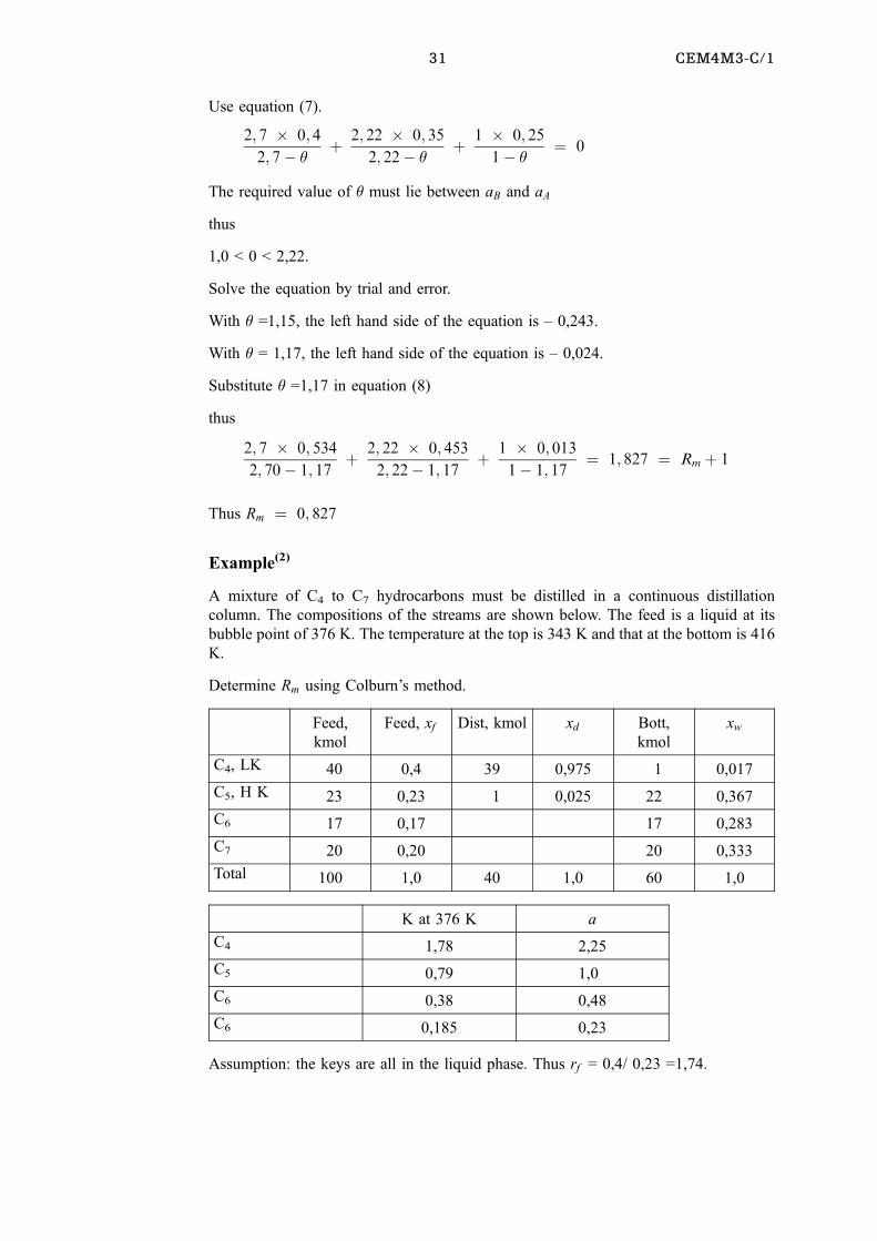
Example(2)
A mixture of C4 to C7 hydrocarbons must be distilled in a continuous distillation
column. The compositions of the streams are shown below. The feed is a liquid at its
bubble point of 376 K. The temperature at the top is 343 K and that at the bottom is 416
K.
Determine Rm using Colburn's method.
Feed,
kmol
Feed, xf Dist, kmol xd Bott,
kmol
xw
C4, LK 40 0,4 39 0,975 1 0,017
C5, H K 23 0,23 1 0,025 22 0,367
C6 17 0,17 17 0,283
C7 20 0,20 20 0,333
Total 100 1,0 40 1,0 60 1,0
K at 376 K a
C4 1,78 2,25
C5 0,79 1,0
C6 0,38 0,48
C6 0,185 0,23
Assumption: the keys are all in the liquid phase. Thus rf = 0,4/ 0,23 =1,74.
32
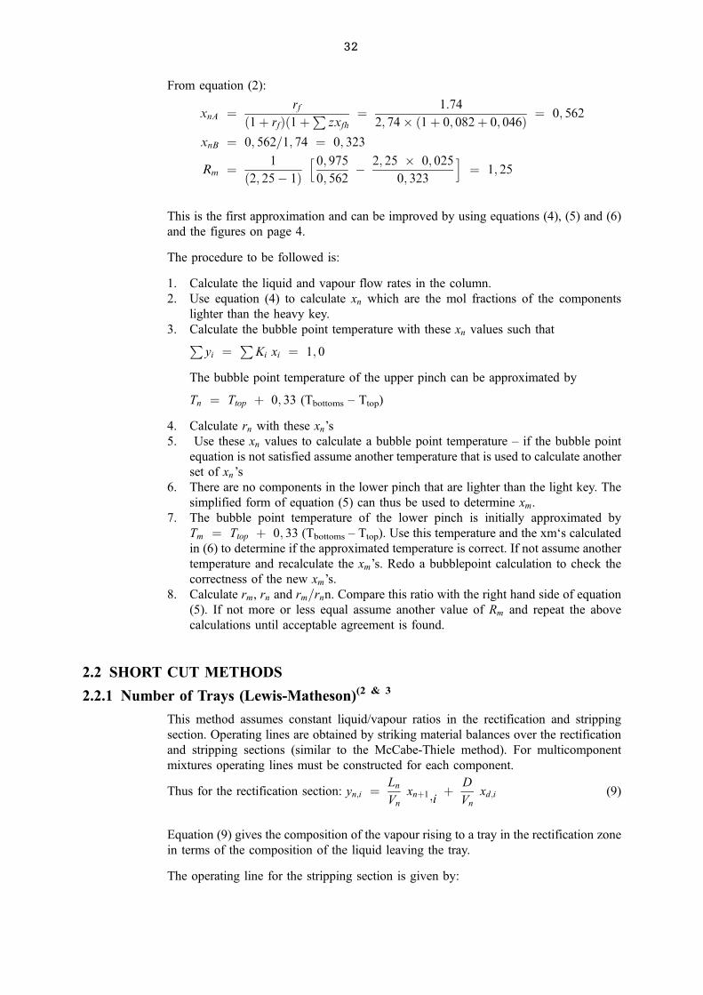
From equation (2):
xnA � rf�1� rf��1�
Pzxfh
� 1:74
2; 74� �1� 0; 082� 0; 046� � 0; 562
xnB � 0; 562=1; 74 � 0; 323
Rm � 1
�2; 25ÿ 1�h 0; 9750; 562
ÿ 2; 25 � 0; 025
0; 323
i� 1; 25
This is the first approximation and can be improved by using equations (4), (5) and (6)
and the figures on page 4.
The procedure to be followed is:
1. Calculate the liquid and vapour flow rates in the column.
2. Use equation (4) to calculate xn which are the mol fractions of the components
lighter than the heavy key.
3. Calculate the bubble point temperature with these xn values such thatPyi �
PKi xi � 1; 0
The bubble point temperature of the upper pinch can be approximated by
Tn � Ttop � 0; 33 (Tbottoms ± Ttop)
4. Calculate rn with these xn's
5. Use these xn values to calculate a bubble point temperature ± if the bubble point
equation is not satisfied assume another temperature that is used to calculate another
set of xn's
6. There are no components in the lower pinch that are lighter than the light key. The
simplified form of equation (5) can thus be used to determine xm.
7. The bubble point temperature of the lower pinch is initially approximated by
Tm � Ttop � 0; 33 (Tbottoms ± Ttop). Use this temperature and the xm`s calculated
in (6) to determine if the approximated temperature is correct. If not assume another
temperature and recalculate the xm's. Redo a bubblepoint calculation to check the
correctness of the new xm's.
8. Calculate rm, rn and rm=rnn. Compare this ratio with the right hand side of equation
(5). If not more or less equal assume another value of Rm and repeat the above
calculations until acceptable agreement is found.
2.2 SHORT CUT METHODS
2.2.1 Number of Trays (Lewis-Matheson)(2 & 3
This method assumes constant liquid/vapour ratios in the rectification and stripping
section. Operating lines are obtained by striking material balances over the rectification
and stripping sections (similar to the McCabe-Thiele method). For multicomponent
mixtures operating lines must be constructed for each component.
Thus for the rectification section: yn;i � Ln
Vn
xn�1;i� D
Vn
xd;i (9)
Equation (9) gives the composition of the vapour rising to a tray in the rectification zone
in terms of the composition of the liquid leaving the tray.
The operating line for the stripping section is given by:
33 CEM4M3-C/1
ym;i � Lm
Vmxm�1;i ÿ W
Vmxw;i (10)
Equation (10) gives the composition of the vapour rising to a tray in the stripping zone
in terms of the composition of the liquid leaving the tray.
Equilibrium relationships are also required with equations (9) and (10) in order to carry
out these calculations.
Let a mixture consist of components A, B, C and D, Let the mol fractions in the liquid
phase be denoted by xA, xB, xC and xD and in the vapour by yA, yB, yc and yD.
Then: yA � yB � yc � yD � 1 divide by yB
yA
yB
� yb
yB
� yc
yB
� yD
yB
� 1
yB
(11)
Also yA � kA xA and yB � KB xB
ThusyA
yB
� KA xX
KB xB
� aAB
xA
xB
substitute in (11)
aAB
xA
xB
� aBB
xB
xB
� aCB
xc
xB
� aDB
xD
xB
� 1
yB
(12)
aABxA � aBB xB � aCB xc � aDB xD � xB
yB
thusX�aAB xA� � xB
yB
(13)
And yc � aCB xcP�aAB xA� and yS � aDB xDP�AAB xA� (14)
It can be shown in a similar manner that:
xB � YBPYA
aAB
xA � YA=aABPYA
aAB
xc � Yc=aCBPYA
aAB
etc. (15)
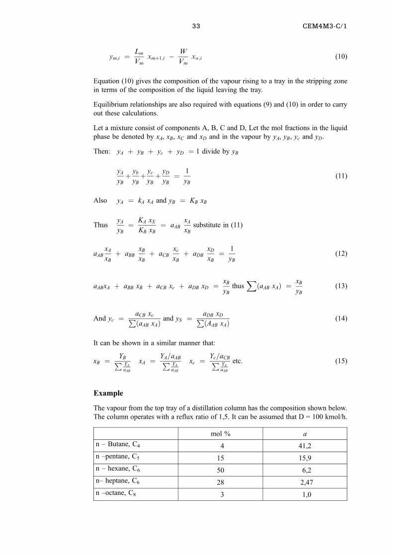
Example
The vapour from the top tray of a distillation column has the composition shown below.
The column operates with a reflux ratio of 1,5. It can be assumed that D = 100 kmol/h.
mol % a
n ± Butane, C4 4 41,2
n ±pentane, C5 15 15,9
n ± hexane, C6 50 6,2
n± heptane, C6 28 2,47
n ±octane, C8 3 1,0
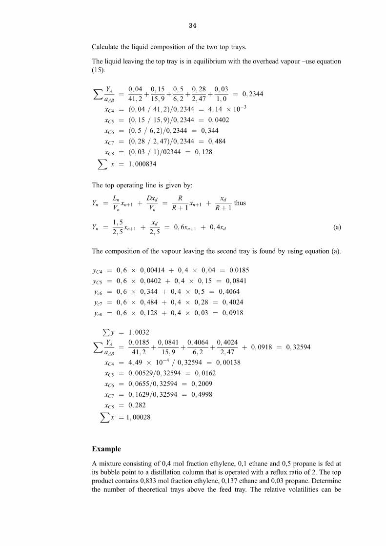
34
Calculate the liquid composition of the two top trays.
The liquid leaving the top tray is in equilibrium with the overhead vapour ±use equation
(15).
X YA
aAB
� 0; 04
41; 2� 0; 15
15; 9� 0; 5
6; 2� 0; 28
2; 47� 0; 03
1; 0� 0; 2344
xC4 � �0; 04 = 41; 2�=0; 2344 � 4; 14 � 10ÿ3
xC5 � �0; 15 = 15; 9�=0; 2344 � 0; 0402
xC6 � �0; 5 = 6; 2�=0; 2344 � 0; 344
xC7 � �0; 28 = 2; 47�=0; 2344 � 0; 484
xC8 � �0; 03 = 1�=02344 � 0; 128Xx � 1; 000834
The top operating line is given by:
Yn � Ln
Vn
xn�1 � Dxd
Vn
� R
R� 1xn�1 � xd
R� 1thus
Yn � 1; 5
2; 5xn�1 � xd
2; 5� 0; 6xn�1 � 0; 4xd (a)
The composition of the vapour leaving the second tray is found by using equation (a).
yC4 � 0; 6 � 0; 00414 � 0; 4 � 0; 04 � 0:0185
yC5 � 0; 6 � 0; 0402 � 0; 4 � 0; 15 � 0; 0841
yc6 � 0; 6 � 0; 344 � 0; 4 � 0; 5 � 0; 4064
yc7 � 0; 6 � 0; 484 � 0; 4 � 0; 28 � 0; 4024
yc8 � 0; 6 � 0; 128 � 0; 4 � 0; 03 � 0; 0918
Py � 1; 0032X YA
aAB
� 0; 0185
41; 2� 0; 0841
15; 9� 0; 4064
6; 2� 0; 4024
2; 47� 0; 0918 � 0; 32594
xC4 � 4; 49 � 10ÿ4 = 0; 32594 � 0; 00138
xC5 � 0; 00529=0; 32594 � 0; 0162
xC6 � 0; 0655=0; 32594 � 0; 2009
xC7 � 0; 1629=0; 32594 � 0; 4998
xC8 � 0; 282Xx � 1; 00028
Example
A mixture consisting of 0,4 mol fraction ethylene, 0,1 ethane and 0,5 propane is fed at
its bubble point to a distillation column that is operated with a reflux ratio of 2. The top
product contains 0,833 mol fraction ethylene, 0,137 ethane and 0,03 propane. Determine
the number of theoretical trays above the feed tray. The relative volatilities can be
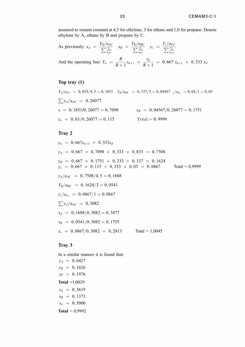
35 CEM4M3-C/1
assumed to remain constant at 4,5 for ethylene, 3 for ethane and 1,0 for propane. Denote
ethylene by A, ethane by B and propane by C.
As previously: xA � YB=aACPYA
aAC
xB � YB=aBCPYA
aAC
yc � Yc=aCCPYA
aAC
And the operating line: Yn � R
R� 1xn�1 � xd
R� 1� 0; 667 xn�1 � 0; 333 xd
Top tray (1)
YA=aAC � 0; 833=4; 5 � 0; 1851 YB=aBC � 0; 137=3 � 0; 04567 c=acc � 0; 03=1 � 0; 03PyA=aAC � 0; 26077
x � 0; 1851l0; 26077 � 0; 7098 xB � 0; 04567=0; 26077 � 0; 1751
xc � 0; 03=0; 26077 � 0; 115 Total � 0; 9999
Tray 2
yn � 0; 667xn�1 � 0; 333xd
yA � 0; 667 � 0; 7098 � 0; 333 � 0; 833 � 0; 7508
yB � 0; 667 � 0; 1751 � 0; 333 � 0; 137 � 0; 1624
yc � 0; 667 � 0; 115 � 0; 333 � 0; 03 � 0; 0867 Total = 0,9999
yA=aAC � 0; 7508=4; 5 � 0; 1668
YB=aBC � 0; 1624=3 � 0; 0541
yc=acc � 0; 0867=1 � 0; 0867PyA=aAC � 0; 3082
xA � 0; 1688=0; 3082 � 0; 5477
xB � 0; 0541=0; 3082 � 0; 1755
xc � 0; 0867=0; 3082 � 0; 2813 Total = 1,0045
Tray 3
In a similar manner it is found that:
yA � 0; 6427
yB � 0; 1626
yc � 0; 1976
Total =1,0029
xA � 0; 3619
xB � 0; 1373
xc � 0; 5000
Total = 0,9992
36
Tray 4
yA � 0; 5188
yB � 0; 137
yc � 0; 3435
Total = 0.9993
xA � 0; 2285
xB � 0; 0905
xc � 0; 6809
Total = 0,9999
The liquid compositions of trays 3 and 4 can be compared with the feed composition. It
can be concluded that the composition of tray 3 is closest to that of the feed and this tray
will thus be selected as the feed tray.
2.2.2 Feed Tray Location(3)
This method also assumes constant liquid/vapour ratios in the rectification and stripping
sections. A further assumption is that the optimum feed tray location occurs at the
intersection of the operating lines.
The operating lines are given by:
yn � Ln
Vn
xn�1 � D
Vn
xd and ym � Lm
Vm
xm�1 ÿ W
Vm
xw
The first equation can be rearranged as:
xn�1 � yN
Vn
Ln
ÿ D
Ln
xd
By omitting the tray numbers this equation can be written for each key as follows:
xLK � yLK
V
Lÿ D
LxLK;d and xHK � yHK
V
Lÿ D
LxHK;d
Rearrange these equations.
L � YLK
xLK
V ÿ DxLK;d
xLK
and L � YHK
xHKV ÿ D
xHK;d
XHK
By equating these two equations and rearranging it is found that:
YLK � xLKxHK
"YHK ÿ D
VxHK;d
#� D
VxLK;d (16)
37 CEM4M3-C/1
!
!!
!
!
In a similar manner can it be shown that for the stripping section:
YLK � xLK
xHK
"YHK � W
�VxHK;w
#ÿ W
�VxLK;w (17)
At the intersection of the operating lines YLK , YHK and XLKIXHK are the same from (16)
and (17) and the right hand side of these equations can be equated.
It then follows that:� aLK
xHK
�intersection
� WxLK;w=V � DxLK;d=V
WxHK;w=V � DxHK;d=V(18)
An overall LK balance gives: Fxf ;LK � DxLk;d �WXLK;w (19)
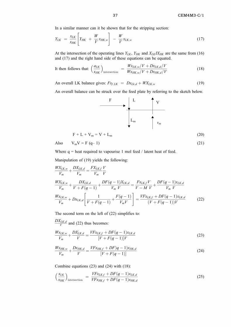
An overall balance can be struck over the feed plate by referring to the sketch below.
F LV
Lm vm
F + L + Vm = V + Lm (20)
Also VmV = F (q± 1) (21)
Where q = heat required to vapourise 1 mol feed / latent heat of feed.
Manipulation of (19) yields the following:
WXLK;w
Vm
� DXLK;d
Vm
� FXLK;f
Vm
V
V
WXLK;w
Vm
� DXLK;d
V � F�qÿ 1� �DF�qÿ 1�XLK;d
Vm V� FxLK;f V
V ÿM V� DF�qÿ 1�xLK;d
Vm V
WxLK;w
Vm
� DxLK;d
"1
V � F�qÿ 1� �F�qÿ 1�
VmV
#� VFxLK;f � DF�qÿ 1�xLK;d
�V � F�qÿ 1��V (22)
The second term on the left of (22) simplifies to:
DXLK;dV
and (22) thus becomes:
WxLK;w
Vm
� DXLK;d
V� VFxLK;f � DF�qÿ 1�xLK;d
�V � F�qÿ 1��V (23)
WxHK;w
Vm
� DxHK;d
V� VFxHK;f � DF�qÿ 1�xHK;d
�V � F�qÿ 1�� (24)
Combine equations (23) and (24) with (18):� xLK
xHK
�intersection
� VFxLK;f � DF�qÿ 1�xLK;d
VFxHK;f � DF�qÿ 1�xHK;d(25)
38
But V = L + D and V / D = L / D + 1 = R + 1 substitute in (25)� xLK
xHK
�intersection
� �R� 1�xLK;f � qÿ 1�xLK;d
�R� 1�xHK;f � �qÿ 1�xHK;d(26)
The feed tray location is then given by:� xLK
xHK
�fÿ1�� xLK
xHK
�intersection
�� xLK
x�HK
�f
(27)
Example
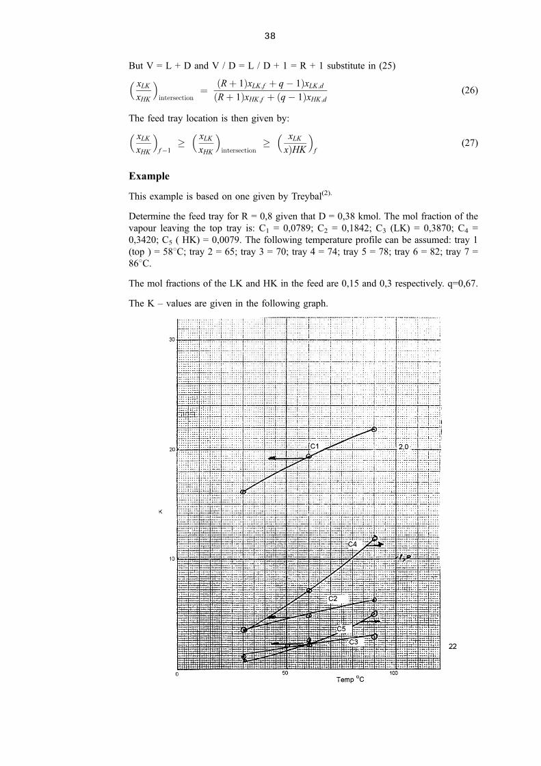
This example is based on one given by Treybal(2).
Determine the feed tray for R = 0,8 given that D = 0,38 kmol. The mol fraction of the
vapour leaving the top tray is: C1 = 0,0789; C2 = 0,1842; C3 (LK) = 0,3870; C4 =
0,3420; C5 ( HK) = 0,0079. The following temperature profile can be assumed: tray 1
(top ) = 588C; tray 2 = 65; tray 3 = 70; tray 4 = 74; tray 5 = 78; tray 6 = 82; tray 7 =
868C.
The mol fractions of the LK and HK in the feed are 0,15 and 0,3 respectively. q=0,67.
The K ± values are given in the following graph.
39 CEM4M3-C/1
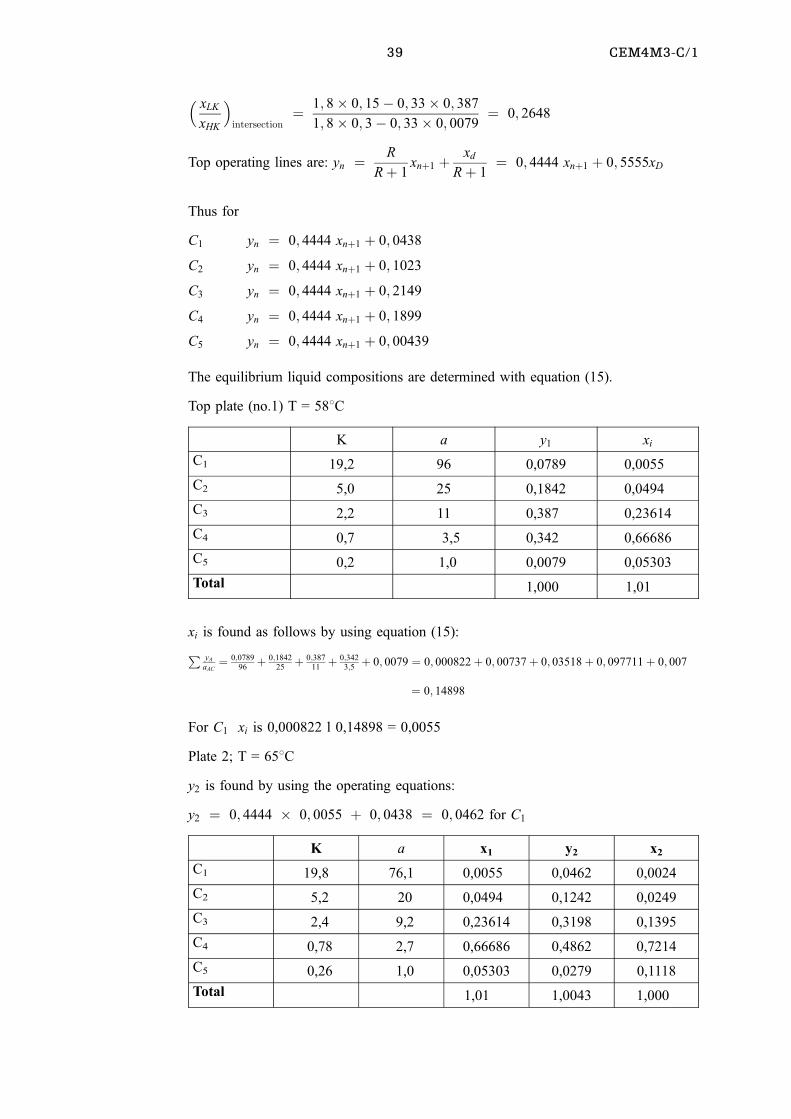
� xLK
xHK
�intersection
� 1; 8� 0; 15ÿ 0; 33� 0; 387
1; 8� 0; 3ÿ 0; 33� 0; 0079� 0; 2648
Top operating lines are: yn � R
R� 1xn�1 � xd
R� 1� 0; 4444 xn�1 � 0; 5555xD
Thus for
C1 yn � 0; 4444 xn�1 � 0; 0438
C2 yn � 0; 4444 xn�1 � 0; 1023
C3 yn � 0; 4444 xn�1 � 0; 2149
C4 yn � 0; 4444 xn�1 � 0; 1899
C5 yn � 0; 4444 xn�1 � 0; 00439
The equilibrium liquid compositions are determined with equation (15).
Top plate (no.1) T = 588C
K a y1 xi
C1 19,2 96 0,0789 0,0055
C2 5,0 25 0,1842 0,0494
C3 2,2 11 0,387 0,23614
C4 0,7 3,5 0,342 0,66686
C5 0,2 1,0 0,0079 0,05303
Total 1,000 1,01
xi is found as follows by using equation (15):P yA
aAC� 0;0789
96� 0;1842
25� 0;387
11� 0;342
3;5 � 0; 0079 � 0; 000822� 0; 00737� 0; 03518� 0; 097711� 0; 007
� 0; 14898
For C1 xi is 0,000822 l 0,14898 = 0,0055
Plate 2; T = 658C
y2 is found by using the operating equations:
y2 � 0; 4444 � 0; 0055 � 0; 0438 � 0; 0462 for C1
K a x1 y2 x2
C1 19,8 76,1 0,0055 0,0462 0,0024
C2 5,2 20 0,0494 0,1242 0,0249
C3 2,4 9,2 0,23614 0,3198 0,1395
C4 0,78 2,7 0,66686 0,4862 0,7214
C5 0,26 1,0 0,05303 0,0279 0,1118
Total 1,01 1,0043 1,000
40
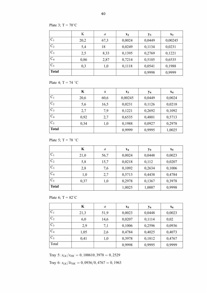
Plate 3; T = 708C
K a x2 y3 x3
C1 20,2 67,3 0,0024 0,0449 0,00245
C2 5,4 18 0,0249 0,1134 0,0231
C3 2,5 8,33 0,1395 0,2769 0,1221
C4 0,86 2,87 0,7214 0,5105 0,6535
C5 0,3 1,0 0,1118 0,0541 0,1988
Total 0,9998 0,9999
Plate 4; T = 74 8C
K a x3 y4 x4
C1 20,6 60,6 0,00245 0,0449 0,0024
C2 5,6 16,5 0,0231 0,1126 0,0218
C3 2,7 7,9 0,1221 0,2692 0,1092
C4 0,92 2,7 0,6535 0,4801 0,5713
C5 0,34 1,0 0,1988 0,0927 0,2978
Total 0,9999 0,9995 1,0025
Plate 5; T = 78 8C
K a x4 y5 x5
C1 21,0 56,7 0,0024 0,0448 0,0023
C2 5,8 15,7 0,0218 0,112 0,0207
C3 2,8 7,6 0,1092 0,2634 0,1006
C4 1,0 2,7 0,5713 0,4438 0,4784
C5 0,37 1,0 0,2978 0,1367 0,3978
Total 1,0025 1,0007 0,9998
Plate 6; T = 828C
K a x5 y6 x6
C1 21,3 51,9 0,0023 0,0448 0,0023
C2 6,0 14,6 0,0207 0,1114 0,02
C3 2,9 7,1 0,1006 0,2596 0,0936
C4 1,05 2,6 0,4784 0,4025 0,4073
C5 0,41 1,0 0,3978 0,1812 0,4767
Total 0,9998 0,9995 0,9999
Tray 5: xLK=xHK � 0; 100610; 3978 � 0; 2529
Tray 6: xLK=IxHK � 0; 0936=0; 4767 � 0; 1963
41 CEM4M3-C/1
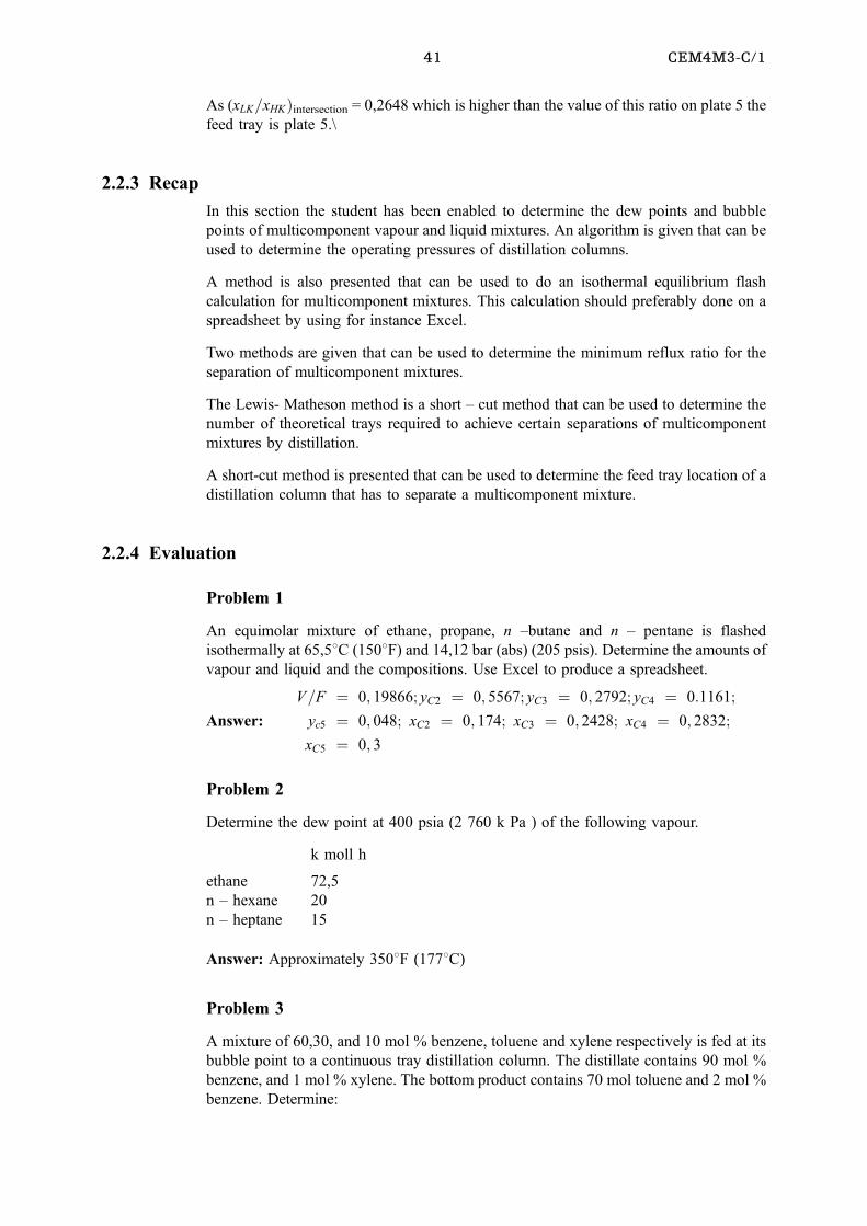
As (xLK=xHK�intersection = 0,2648 which is higher than the value of this ratio on plate 5 the
feed tray is plate 5.\
2.2.3 Recap
In this section the student has been enabled to determine the dew points and bubble
points of multicomponent vapour and liquid mixtures. An algorithm is given that can be
used to determine the operating pressures of distillation columns.
A method is also presented that can be used to do an isothermal equilibrium flash
calculation for multicomponent mixtures. This calculation should preferably done on a
spreadsheet by using for instance Excel.
Two methods are given that can be used to determine the minimum reflux ratio for the
separation of multicomponent mixtures.
The Lewis- Matheson method is a short ± cut method that can be used to determine the
number of theoretical trays required to achieve certain separations of multicomponent
mixtures by distillation.
A short-cut method is presented that can be used to determine the feed tray location of a
distillation column that has to separate a multicomponent mixture.
2.2.4 Evaluation
Problem 1
An equimolar mixture of ethane, propane, n ±butane and n ± pentane is flashed
isothermally at 65,58C (1508F) and 14,12 bar (abs) (205 psis). Determine the amounts of
vapour and liquid and the compositions. Use Excel to produce a spreadsheet.
Answer:
V=F � 0; 19866; yC2 � 0; 5567; yC3 � 0; 2792; yC4 � 0:1161;
yc5 � 0; 048; xC2 � 0; 174; xC3 � 0; 2428; xC4 � 0; 2832;
xC5 � 0; 3
Problem 2
Determine the dew point at 400 psia (2 760 k Pa ) of the following vapour.
k moll h
ethane 72,5
n ± hexane 20
n ± heptane 15
Answer: Approximately 3508F (1778C)
Problem 3
A mixture of 60,30, and 10 mol % benzene, toluene and xylene respectively is fed at its
bubble point to a continuous tray distillation column. The distillate contains 90 mol %
benzene, and 1 mol % xylene. The bottom product contains 70 mol toluene and 2 mol %
benzene. Determine:
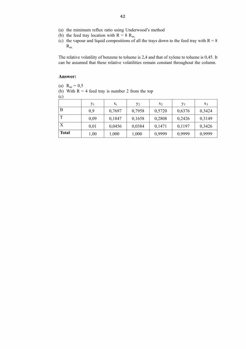
42
(a) the minimum reflux ratio using Underwood's method
(b) the feed tray location with R = 8 Rm.
(c) the vapour and liquid compositions of all the trays down to the feed tray with R = 8
Rm.
The relative volatility of benzene to toluene is 2,4 and that of xylene to toluene is 0,45. It
can be assumed that these relative volatilities remain constant throughout the column.
Answer:
(a) Rm = 0,5
(b) With R = 4 feed tray is number 2 from the top
(c)
y1 xi y2 x2 y3 x3
B 0,9 0,7697 0,7958 0,5720 0,6376 0,3424
T 0,09 0,1847 0,1658 0,2808 0,2426 0,3149
X 0,01 0,0456 0,0384 0,1471 0,1197 0,3426
Total 1,00 1,000 1,000 0,9999 0,9999 0,9999
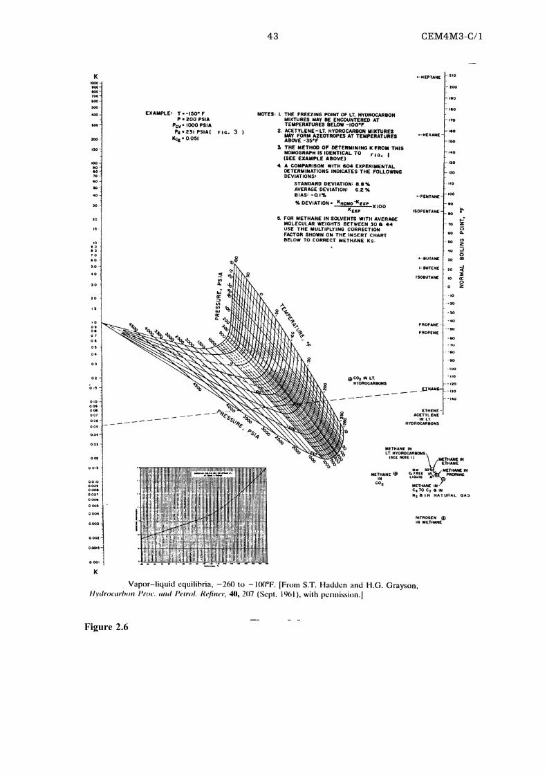
43 CEM4M3-C/1
Figure 2.6
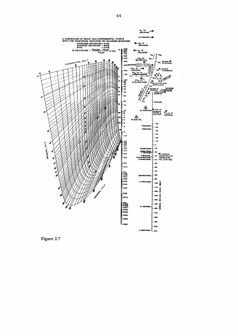
44
Figure 2.7
45 CEM4M3-C/1
CHAPTER 3
Rigorous distillation design method
CONTENTS
3.1 LEARNING OUTCOMES 73
3.2 A RIGOROUS DESIGN METHOD 74
3.3 TRAY EFFICIENCY 83
3.4 RECAP 85
3.5 EVALUATION 85
3.1 LEARNING OUTCOMES
After completion of this section the student should be able to:
. Do at least a first iteration of a multi-component distillation design using the rigorous
method that is discussed here. The calculation should be done by using a spread sheet.
Excel is ideally suitable for this calculation.
. Calculate the bubble points, based on the calculated compositions, by using the
method given earlier.
. Calculate the overall efficiency of a tray.
3.2 A RIGOROUS DESIGN METHOD
The methods that have been discussed, although very useful, cannot be used for final
design purposes. They can, however, be used to determine initial values for the rigorous
methods.
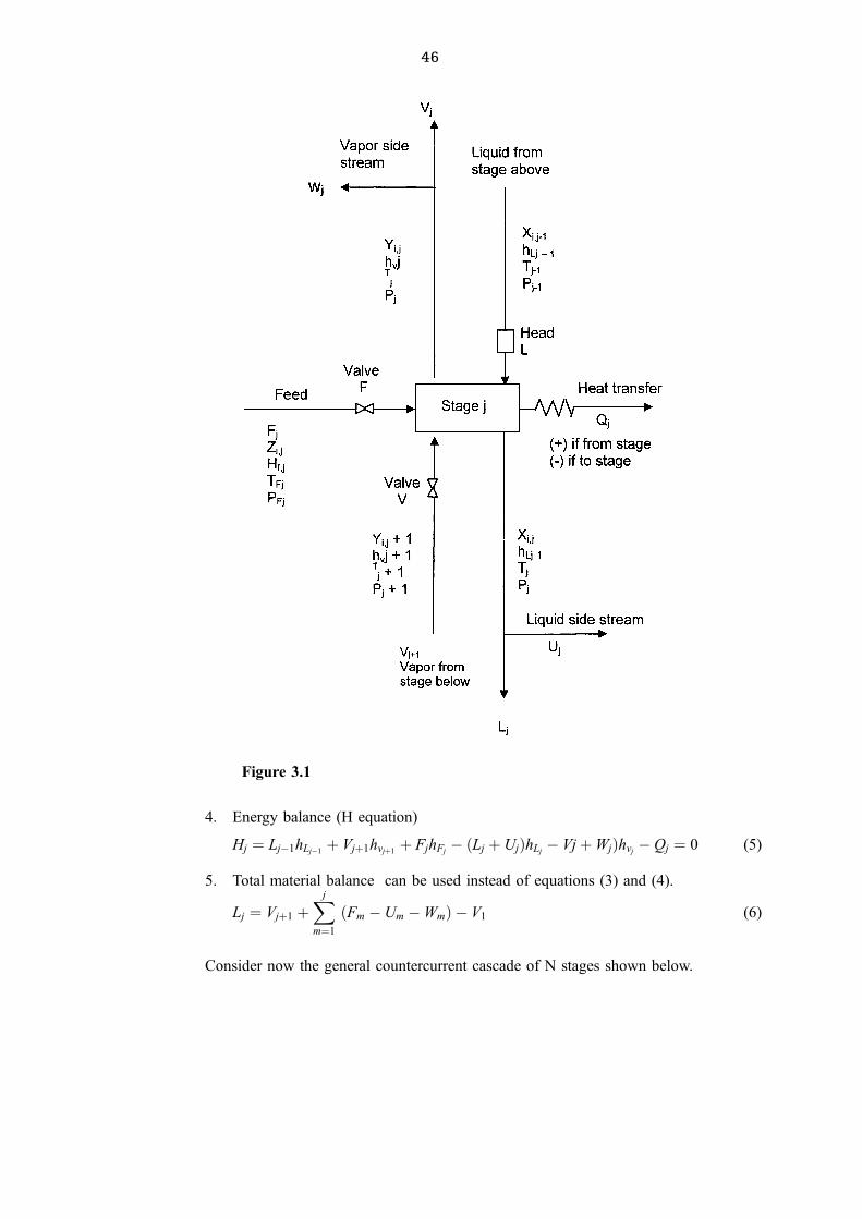
Consider the following sketch(1) of a general equilibrium stage.
The following equations are valid for each equilibrium stage.
1. Material balances (M equations):
Mij � Ljÿ1 � Vj�1yi;j�1 � Fjzi;j ÿ �L� Uj�xi;j ÿ �Vj �W�jyi;j � 0 (1)
2. Phase equilibrium relations (E equations)
Ei;j � yi;j ÿ Ki;jxi;j � 0 (2)
3. Mol fraction summations (S equations)
�Sy�j �Xc
i�1
yi;j ÿ 1; 0 � 0 (3)
�Sy�j �Xc
i�1
xi;j ÿ 1; 0 � 0 (4)
46
4. Energy balance (H equation)
Hj � Ljÿ1hLjÿ1� Vj�1hvj�1
� FjhFjÿ �Lj � Uj�hLj
ÿ Vj�Wj�hvjÿ Qj � 0 (5)
5. Total material balance can be used instead of equations (3) and (4).
Lj � Vj�1 �Xj
m�1
�Fm ÿ Um ÿWm� ÿ V1 (6)
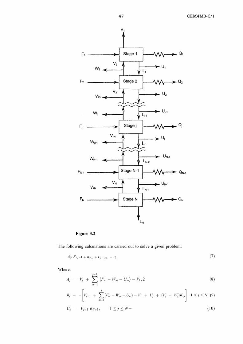
Consider now the general countercurrent cascade of N stages shown below.
Figure 3.1
47 CEM4M3-C/1
The following calculations are carried out to solve a given problem:
Aj xi;jÿ1 � Bjxi;j � Cj xi;j�1 � Dj(7)
Where:
Aj � Vj �Xjÿ1
m�1
�Fm ÿWm ÿ Um� ÿ V1; 2 (8)
Bj � ÿ"
Vj�1 �Xj
m�1
�Fm ÿWm ÿ Um� ÿ V1 � Uj � �Vj � Wj�Ki;j
#; 1 � j � N (9)
CJ � Vj�1 Kij�1; 1 � j � Nÿ (10)
Figure 3.2
48
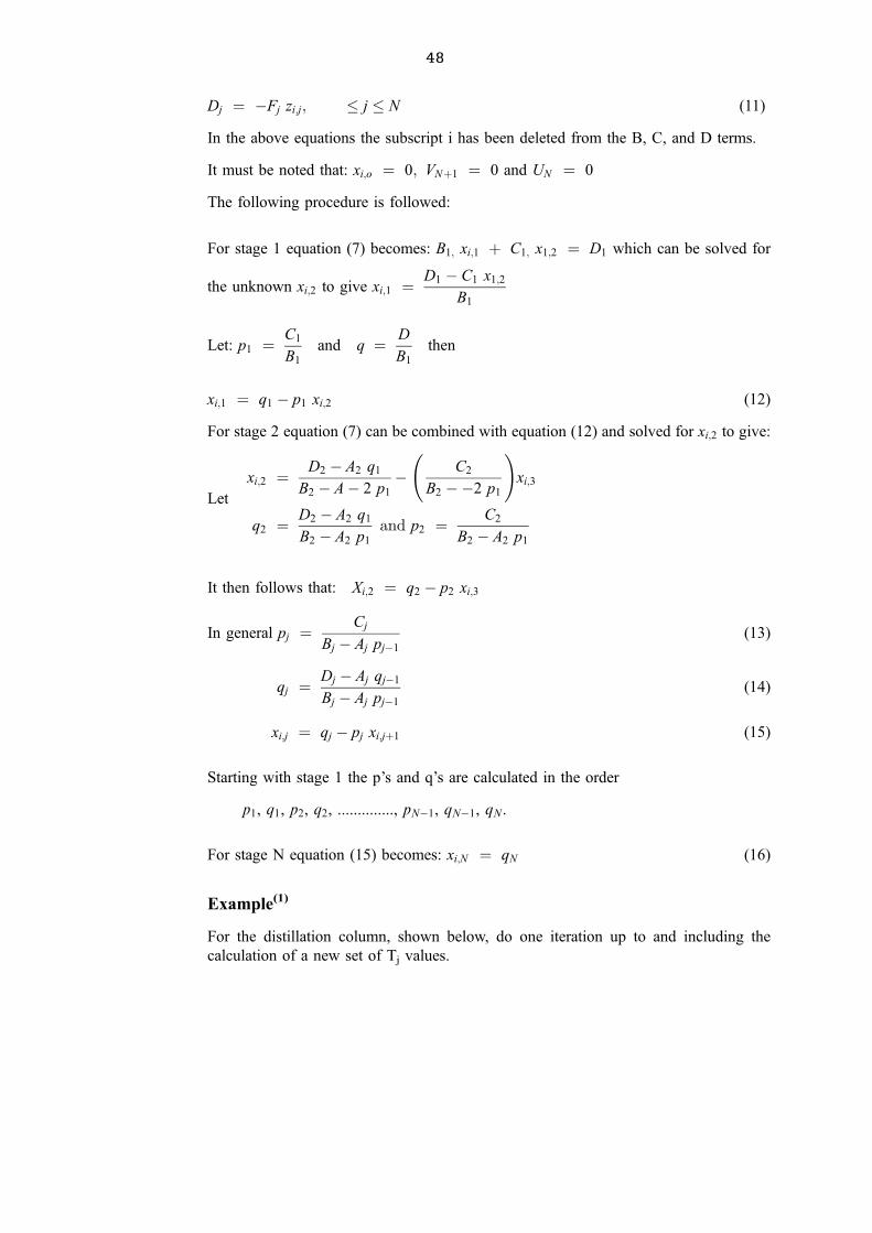
Dj � ÿFj zi;j; � j � N (11)
In the above equations the subscript i has been deleted from the B, C, and D terms.
It must be noted that: xi;o � 0; VN�1 � 0 and UN � 0
The following procedure is followed:
For stage 1 equation (7) becomes: B1; xi;1 � C1; x1;2 � D1 which can be solved for
the unknown xi;2 to give xi;1 � D1 ÿ C1 x1;2
B1
Let: p1 � C1
B1
and q � D
B1
then
xi;1 � q1 ÿ p1 xi;2 (12)
For stage 2 equation (7) can be combined with equation (12) and solved for xi;2 to give:
Let
xi;2 � D2 ÿ A2 q1
B2 ÿ Aÿ 2 p1
ÿ
C2
B2 ÿÿ2 p1
!xi;3
q2 � D2 ÿ A2 q1
B2 ÿ A2 p1
and p2 � C2
B2 ÿ A2 p1
It then follows that: Xi;2 � q2 ÿ p2 xi;3
In general pj � Cj
Bj ÿ Aj pjÿ1
(13)
qj � Dj ÿ Aj qjÿ1
Bj ÿ Aj pjÿ1
(14)
xi;j � qj ÿ pj xi;j�1 (15)
Starting with stage 1 the p's and q's are calculated in the order
p1, q1, p2, q2, .............., pNÿ1, qNÿ1, qN.
For stage N equation (15) becomes: xi;N � qN (16)
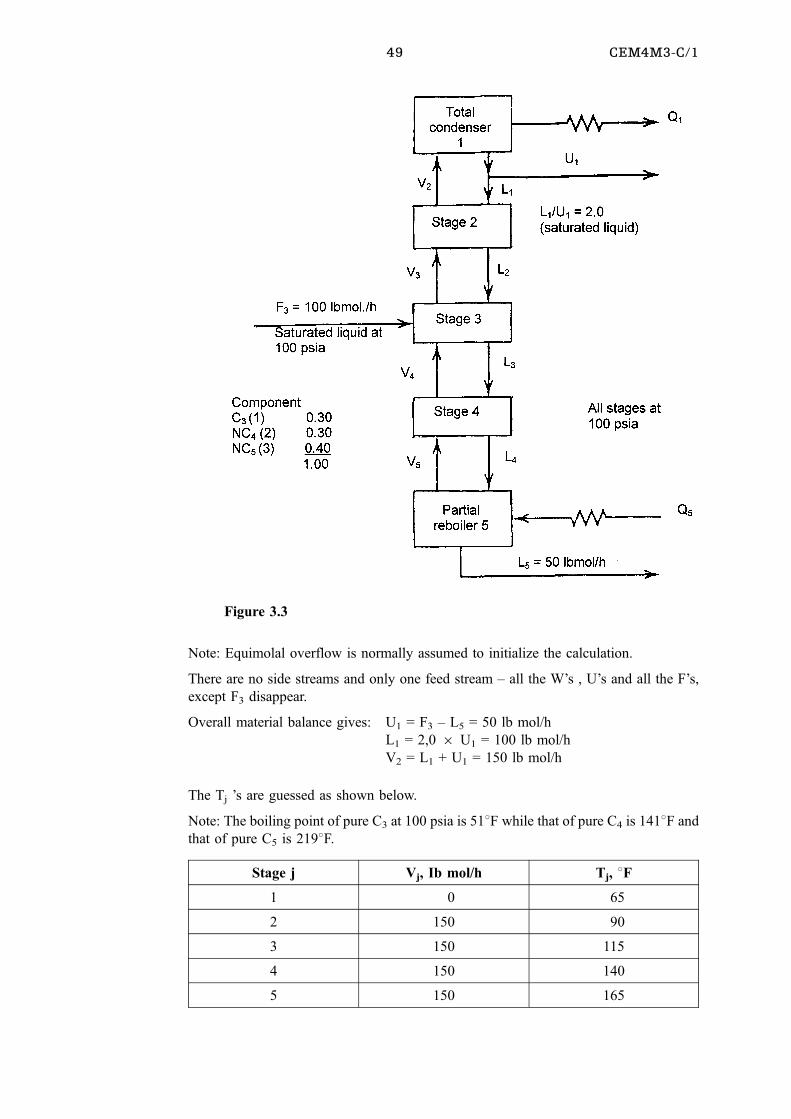
Example(1)
For the distillation column, shown below, do one iteration up to and including the
calculation of a new set of Tj values.
49 CEM4M3-C/1
Note: Equimolal overflow is normally assumed to initialize the calculation.
There are no side streams and only one feed stream ± all the W's , U's and all the F's,
except F3 disappear.
Overall material balance gives: U1 = F3 ± L5 = 50 lb mol/h
L1 = 2,0 6 U1 = 100 lb mol/h
V2 = L1 + U1 = 150 lb mol/h
The Tj 's are guessed as shown below.
Note: The boiling point of pure C3 at 100 psia is 518F while that of pure C4 is 1418F and
that of pure C5 is 2198F.
Stage j Vj, Ib mol/h Tj, 8F
1 0 65
2 150 90
3 150 115
4 150 140
5 150 165
Figure 3.3
50
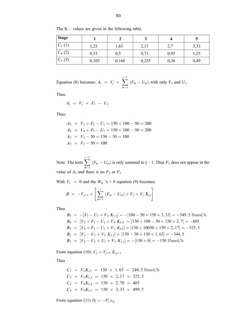
The K ± values are given in the following table.
Stage 1 2 3 4 5
C3 (1) 1,23 1,63 2,17 2,7 3,33
C4 (2) 0,33 0,5 0,71 0,95 1,25
C5 (3) 0,103 0,166 0,255 0,36 0,49
Equation (8) becomes: Ai � Vj �Xjÿ1
m�1
�Fm ÿ Um� with only F3 and U1.
Thus:
Aj � Vj � F3 ÿ U1
Thus:
A5 � V5 � F3 ÿU1 � 150� 100ÿ 50 � 200
A4 � V4 � F3 ÿU1 � 150� 100ÿ 50 � 200
A3 � V3 ÿ 50 � 150ÿ 50 � 100
A2 � V2 ÿ 50 � 100
Note: The termXjÿ1
m�1
�Fm ÿ Um� is only summed to j ± 1. Thus F3 does not appear in the
value of A3 and there is no F2 or F1.
With V1 � 0 and the Wm 's = 0 equation (9) becomes:
B � ÿVj�1 �"Xj
m�1�Fm ÿUm� �Uj � Vj Ki;j
#
Thus
B5 � ÿ�F3 ÿU1 � V5 K1;5� � ÿ�100ÿ 50� 150� 3; 33� � ÿ549; 5 lbmol=h
B4 � �V5 � F3 ÿU1 � V4 K1;4 � �150� 100ÿ 50� 150� 2; 7� � ÿ605B3 � �V4 � F3 ÿU1 � V3 KI;3� � �150� 10050� 150� 2; 17� � ÿ525; 5B2 � �V3 ÿU1 � V2 K1;2� � �150ÿ 50� 150� 1; 63� � ÿ344; 5B1 � �V2 ÿU1 �U1 � V1 K1;1� � ÿ�150� 0� � ÿ150 1bmol=h
From equation (10): Cj � Vj�1 Ki;j�1
Thus
C1 � V2Ki;2 � 150 � 1; 63 � 244; 5 lbmol=h
C2 � V3K1;3 � 150 � 2; 17 � 325; 5
C3 � V4K1;4 � 150 � 2; 70 � 405
C4 � V5K1;5 � 150 � 3; 33 � 499; 5
From equation (11) Dj � ÿFj zi;j
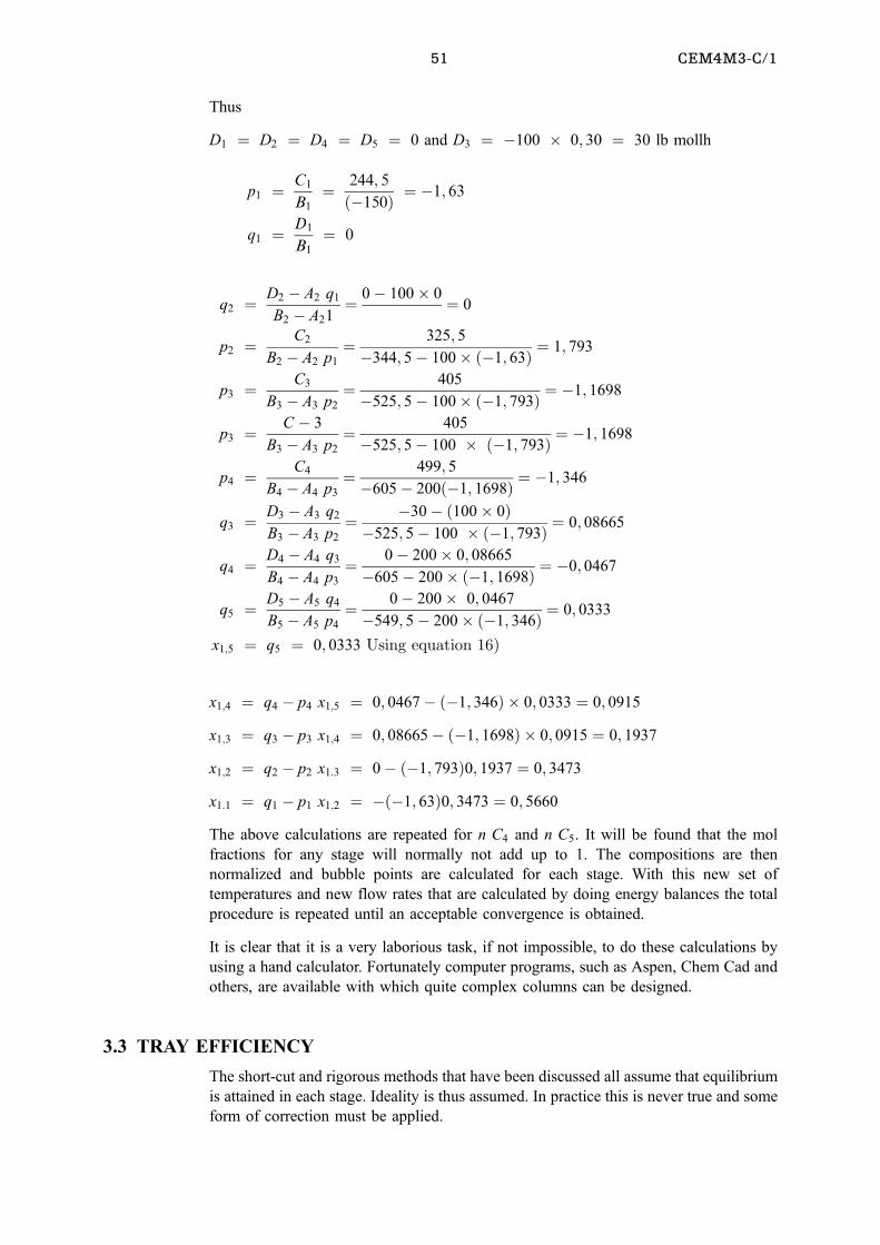
51 CEM4M3-C/1
Thus
D1 � D2 � D4 � D5 � 0 and D3 � ÿ100 � 0; 30 � 30 lb mollh
p1 � C1
B1� 244; 5
�ÿ150� � ÿ1; 63
q1 � D1
B1� 0
q2 � D2 ÿ A2 q1
B2 ÿ A21� 0ÿ 100� 0 � 0
p2 � C2
B2 ÿ A2 p1
� 325; 5
ÿ344; 5ÿ 100� �ÿ1; 63� � 1; 793
p3 � C3
B3 ÿ A3 p2
� 405
ÿ525; 5ÿ 100� �ÿ1; 793� � ÿ1; 1698
p3 � C ÿ 3
B3 ÿ A3 p2
� 405
ÿ525; 5ÿ 100 � �ÿ1; 793� � ÿ1; 1698
p4 � C4
B4 ÿ A4 p3
� 499; 5
ÿ605ÿ 200�ÿ1; 1698� � ÿ1; 346
q3 � D3 ÿ A3 q2
B3 ÿ A3 p2
� ÿ30ÿ �100� 0�ÿ525; 5ÿ 100 � �ÿ1; 793� � 0; 08665
q4 � D4 ÿ A4 q3
B4 ÿ A4 p3
� 0ÿ 200� 0; 08665
ÿ605ÿ 200� �ÿ1; 1698� � ÿ0; 0467
q5 � D5 ÿ A5 q4
B5 ÿ A5 p4
� 0ÿ 200� 0; 0467
ÿ549; 5ÿ 200� �ÿ1; 346� � 0; 0333
x1;5 � q5 � 0; 0333 Using equation 16�
x1;4 � q4 ÿ p4 x1;5 � 0; 0467ÿ �ÿ1; 346� � 0; 0333 � 0; 0915
x1;3 � q3 ÿ p3 x1;4 � 0; 08665ÿ �ÿ1; 1698� � 0; 0915 � 0; 1937
x1;2 � q2 ÿ p2 x1:3 � 0ÿ �ÿ1; 793�0; 1937 � 0; 3473
x1:1 � q1 ÿ p1 x1;2 � ÿ�ÿ1; 63�0; 3473 � 0; 5660
The above calculations are repeated for n C4 and n C5. It will be found that the mol
fractions for any stage will normally not add up to 1. The compositions are then
normalized and bubble points are calculated for each stage. With this new set of
temperatures and new flow rates that are calculated by doing energy balances the total
procedure is repeated until an acceptable convergence is obtained.
It is clear that it is a very laborious task, if not impossible, to do these calculations by
using a hand calculator. Fortunately computer programs, such as Aspen, Chem Cad and
others, are available with which quite complex columns can be designed.
3.3 TRAY EFFICIENCY
The short-cut and rigorous methods that have been discussed all assume that equilibrium
is attained in each stage. Ideality is thus assumed. In practice this is never true and some
form of correction must be applied.
52
The overall tray efficiency is such a correction.
The overall tray efficiency, Eo is defined as:
Eo � number of ideal trays required
number of real trays required
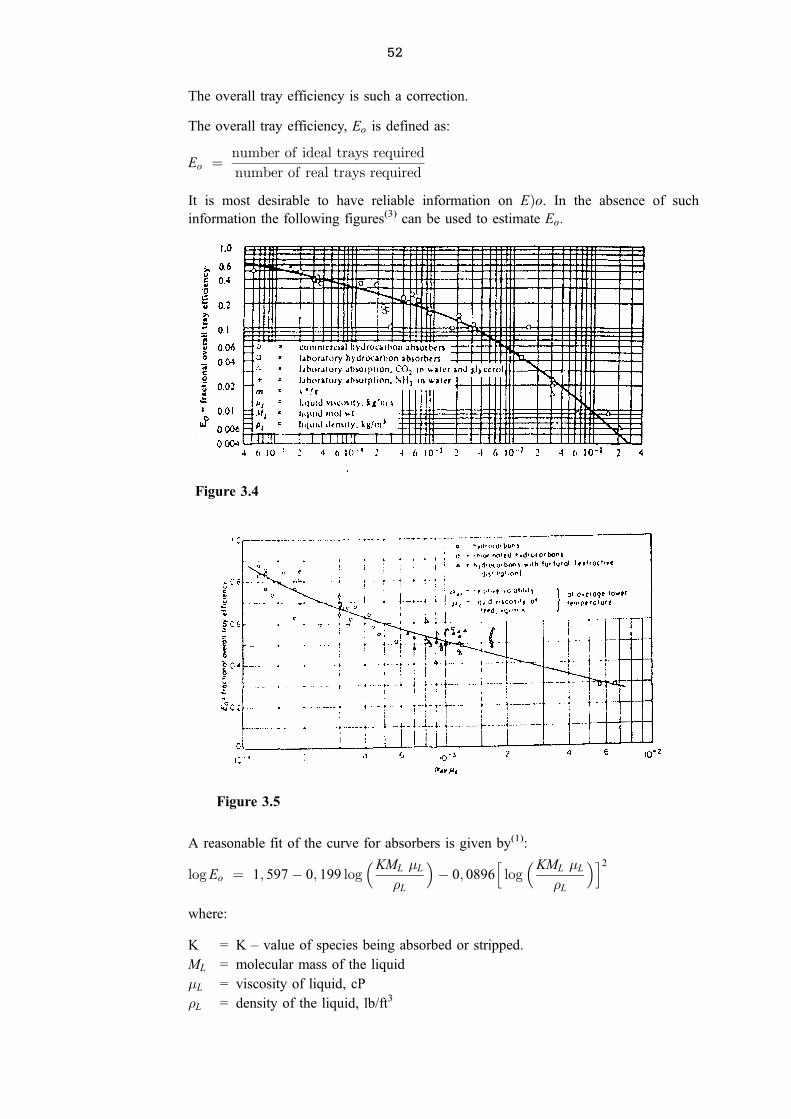
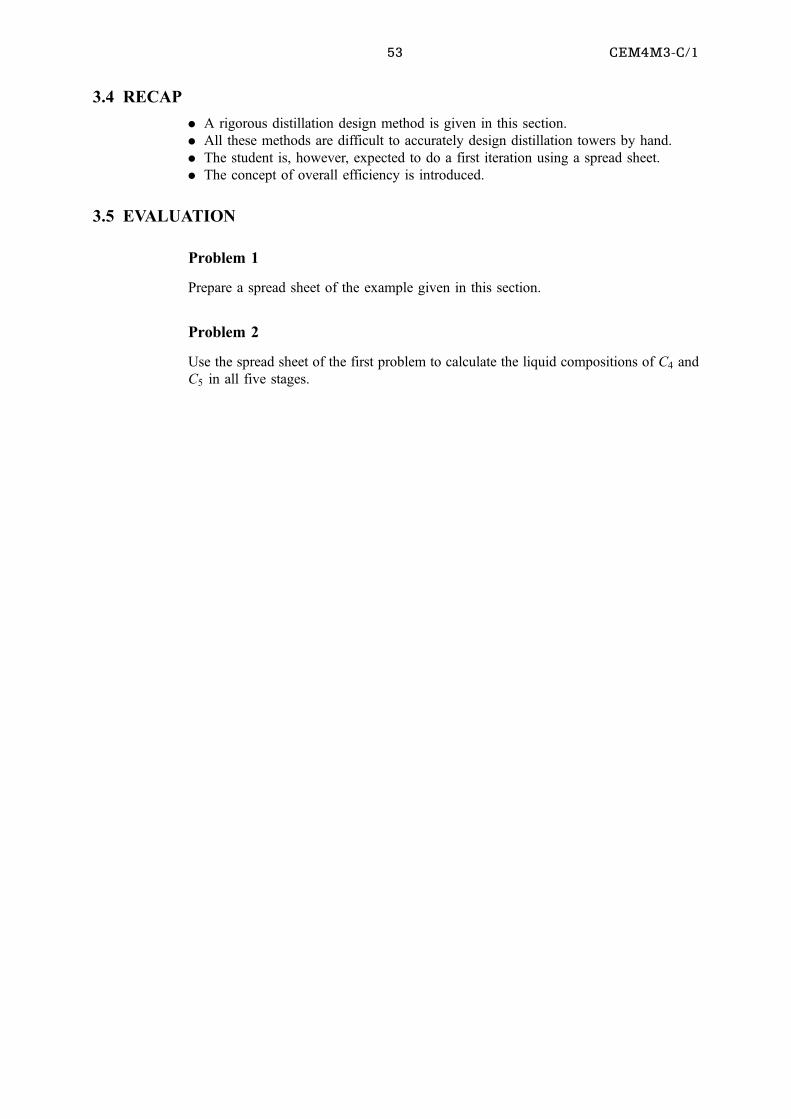
It is most desirable to have reliable information on E�o. In the absence of such
information the following figures(3) can be used to estimate Eo.
A reasonable fit of the curve for absorbers is given by(1):
log Eo � 1; 597ÿ 0; 199 log�KML �L
�L
�ÿ 0; 0896
hlog�KML �L
�L
�i2
where:
K = K ± value of species being absorbed or stripped.
ML = molecular mass of the liquid
�L = viscosity of liquid, cP
�L = density of the liquid, lb/ft3
Figure 3.4
Figure 3.5
53 CEM4M3-C/1
3.4 RECAP
. A rigorous distillation design method is given in this section.
. All these methods are difficult to accurately design distillation towers by hand.
. The student is, however, expected to do a first iteration using a spread sheet.
. The concept of overall efficiency is introduced.
3.5 EVALUATION
Problem 1
Prepare a spread sheet of the example given in this section.
Problem 2
Use the spread sheet of the first problem to calculate the liquid compositions of C4 and
C5 in all five stages.
54
CHAPTER 4
Evaporation
CONTENTS
4.1 OUTCOMES 00
4.2 INTRODUCTION 00
4.2.1 Factors Affecting Evaporation 00
4.2.2 Single ±Effect Evaporators(4) 00
4.2.3 Effect of Process Variables on the Operation of Evaporators(4) 00
4.2.4 Boiling Point Rise ( BPR ) 00
4.3 MULTIPLE ± EFFECT EVAPORATORS 00
4.3.1 Forward Feed 00
4.3.2 Backward Feed 00
4.3.3 Parallel Feed 00
4.3.4 Steam Economy 00
4.3.5 Vapour Recompression(2) , (4) 00
4.4 RECAP 00
4.5 EVALUATION 00
4.1 OUTCOMES
. The student should be able to solve problems involving single ±effect evaporators
. The student should know the factors that are effecting the evaporation of solvents as
well as the process variables that are important in the evaporation process
. The student must be able to determine the boiling point rise of a solution for a given
solute
. The student must know the types of multiple ± effect evaporators
. The student must understand the concept of steam economy and be able to determine
it
. The student must be able to solve multi ± effect evaporator problems
. The student must understand the vapour recompression process and be able to
determine the power requirements of compressors used in this process
4.2 INTRODUCTION
Evaporation is one of the main methods that is used to concentrate aqueous solutions.
Inorganic salts are normally not heat sensitive and solutions containing such solutes can
be heated to relatively high temperatures. Food products are, however, extremely heat
sensitive and care must be taken to prevent overheating. This is usually accomplished by
using short residence times and relatively low temperatures.
It is advisable that the student should read the section on Evaporation in the study guide
of Chemical Engineering Technology Ill ( CEM 321 BE).
55 CEM4M3-C/1
4.2.1 Factors Affecting Evaporation
1. Solute Concentration
The density and viscosity of the solution increase with the amount of solute that is
dissolved until the solution becomes saturated. When the solution becomes too
viscous the heat transfer is affected. Crystals form when saturated solutions are
heated with the result that the heat exchanger tubes might be blocked, reducing even
further the heat transfer rate.
Most, but not all, solutes cause the boiling point of the solution to be higher than
that of the solvent alone. This is called the boiling point rise (BPR) and it is a
function of the concentration of solute.
2. Temperature Sensitivity
Inorganic solutes are not really heat sensitive and will not be degraded at the
temperatures that are normally used in the evaporation process. Food products, such
as milk and fruit juices and pharmaceutical products are, however, extremely heat
sensitive. Great care must be exercised not to overheat such products and
evaporation is normally carried out under vacuum and the residence time must also
be kept to a minimum.
3. Foaming
Many organic compounds foam during the evaporation process and some of the
liquid in the evaporator can be carried over with the vapour. Compounds that
depress the foaming can sometimes be used to limit this carry over.
4. Pressure and Temperature
The boiling point of a solvent, and thus also the solution, is a function of the
pressure. The higher the pressure the higher is the boiling point. This relationship
must be kept in mind when evaporating heat sensitive solutes.
5. Scale Formation
Solids may be deposited on the heat transfer surfaces in the form of scale. This scale
reduces the heat transfer rate significantly and must be removed regularly.
6. Materials of Construction
The proper materials must be used to prevent corrosion and in the case of food
products discolouration.
4.2.2 Single ± Effect Evaporators(4)
Refer to the following sketch.
The following equation is used to determine the capacity of a single effect evaporator.
q � UA�T (1)
Where
q = heat transfer rate, W
U = Overall heat transfer coefficient, W/m2 K
A = heat transfer surface, m2
�T = temperature difference between the condensing steam and the boiling liquid, K
56
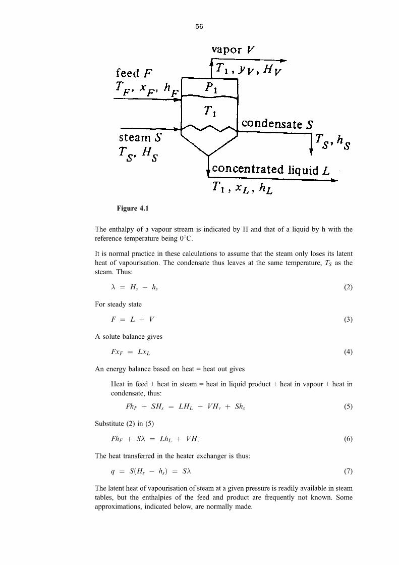
The enthalpy of a vapour stream is indicated by H and that of a liquid by h with the
reference temperature being 08C.
It is normal practice in these calculations to assume that the steam only loses its latent
heat of vapourisation. The condensate thus leaves at the same temperature, TS as the
steam. Thus:
� � Hs ÿ hs (2)
For steady state
F � L � V (3)
A solute balance gives
FxF � LxL (4)
An energy balance based on heat = heat out gives
Heat in feed + heat in steam = heat in liquid product + heat in vapour + heat in
condensate, thus:
FhF � SHs � LHL � VHv � Shs (5)
Substitute (2) in (5)
FhF � S� � LhL � VHv (6)
The heat transferred in the heater exchanger is thus:
q � S�Hs ÿ hs� � S� (7)
The latent heat of vapourisation of steam at a given pressure is readily available in steam
tables, but the enthalpies of the feed and product are frequently not known. Some
approximations, indicated below, are normally made.
Figure 4.1
57 CEM4M3-C/1
1. The latent heat of vaporization of the steam is determined at the boiling point of the
liquid, T1, and not at the operating pressure, P1 (the equilibrium presssure of pure
water).
2. The heat capacities of the feed CPF and the liquid product CPL are used to calculate
the corresponding enthalpies. By doing this the heat of solution is excluded but it is
in many cases not known.
Example 1(4)
A continuous single ± effect evaporator is fed with 9070 kg/h of a solution containing
1,0 mass % salt at 311 K. The liquid product leaves as a 1,5% solution. The vapour
space in the evaporator is at 101,3 kPa (abs) and saturated steam is supplied at 150,0 kPa
(abs).
U = 1 704 W/m2 K. The heat capacity of the feed and liquid product can be taken as that
of water, i.e. 4,18 kJ/kg K.
The following data are taken from the steam tables:
At 101,3 kPa T = 100 8C hg = 2676 lJ/kg hf = 417 kJ/kg
At 150 kPa Ts = 111 8C hg = 2694 kJ/kg hf = 467 kJ/kg
Overall material balance: 9070 = L + V
Solute balance: 9070 6 0,01 = 90,7 = L xL = 0,015 L
L = 90,7/0,015 = 6 047 kg/h
hf = CPF (TF ± Tbase) = 4,18 (38 ± 0) = 158,6kJ/kg
hL =CPL (TL ± Tbase) = 4,18 6 100 = 418 kJ/kg
FhF + SHs = LhL + VHv + Shs equation (5)
9080 6 158,8 + S(2694 ± 467) = 6047 6 418 + 3023 6 2676
S = 4121 kg/h
q � UA�T
�T � 111ÿ 100 � 11
A � q
U�T� 4121� �2694ÿ 467�
1; 704� 11� 3600� 136m2
These calculations can be simplified somewhat by choosing a different base
temperature. Choose 1008C (temperature of the vapour product and in this case also
the liquid product ) as base.
9070 6 4,18 6 (38 ± 100) + 2227S = 6047 6 4,18 6 (100 ± 100) + 3023 6 2259
S = 4122 kg/h
4.2.3 Effect of Process Variables on the Operation of Evaporator(4)
1. Feed temperature
The temperature at which the feed enters an evaporator has a significant effect on
the steam requirement and thus also the size of the heat exchanger.
58
2. Effect of Pressure
Lower temperatures in the evaporation chamber can be obtained by operating the
evaporator under vacuum. This leads to a large temperature difference and thus a
smaller heat exchanger.
3. Effect of Steam Pressure
The higher the steam pressure the higher will the temperature difference be resulting
in a smaller heat exchanger. The cost of high pressure steam is, however, much
higher than low pressure steam and these additional costs should be considered.
4.2.4 Boiling Point Rise (BPR)
This aspect is covered in the study guide of CEN321BE but will be very briefly
discussed here.
Strong solutions of dissolved solutes can cause significant BPR's and this cannot be
ignored in the design of evaporators in which such solutions are concentrated.
Duhring's rule can be used to determine the BPR of solutions containing certain solutes.
Example 2(4)
A 30% NaOH solution is boiled at 25 kPa (abs). Determine the boiling temperature of
the solution and the BPR by using the Duhring plot below.
From the steam tables is found that the boiling point of water at 25 kPa (abs ) is 658C(1498F).
From the plot boiling point of the solution is 1758F = 79,48C.
BPR = 79,4 65 = 14,48C
A very useful plot(5) to determine the BPR's of a number of solutes is given below.
Example 3(4)
4 500 kg/h of a 20% solution of NaOH in water is fed to a single effect evaporator at
608C. The liquid product contains 50% NaOH. Saturated steam at 175 kPa (abs) is fed to
the heat exchanger. The vapour space of the evaporator is operated at 15 kPa (abs). The
overall heat transfer coefficient is 1 560 W/m2K. The specific heat of the feed is 3,57 kJ/
kg8C and that of the liquid product is 5,64 kJ/kg8C. Calculate the steam usage, the heat
transfer surface and the steam economy.
From the steam tables: at 175 kPa T= 116 8C; hg = 2701 kJ/kg; hfg = 487and hf =
2214
At 15kPa: T=548C
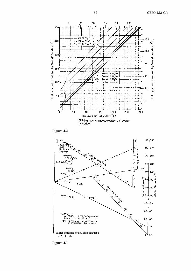
59 CEM4M3-C/1
Figure 4.2
Figure 4.3
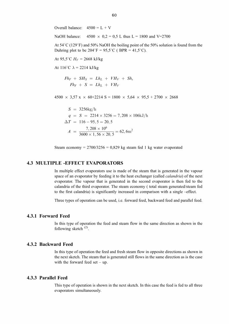
60
Overall balance: 4500 = L + V
NaOH balance: 4500 6 0,2 = 0,5 L thus L = 1800 and V=2700
At 548C (1298F) and 50% NaOH the boiling point of the 50% solution is found from the
Duhring plot to be 2048F = 95,58C ( BPR = 41,58C).
At 95,58C HV = 2668 kJ/kg
At 1168C � = 2214 kJ/kg
FhF � SHS � LhL � VHV � Shs
FhF � S � LhL � VHV
4500 6 3,57 x 6 60+2214 S = 1800 6 5,64 6 95,5 + 2700 6 2668
S � 3256kg=h
q � S � 2214� 3256 � 7; 208� 106kJ=h
�T � 116ÿ 95; 5 � 20; 5
A � 7; 208� 106
3600� 1; 56� 20; 5� 62; 6m2
Steam economy = 2700/3256 = 0,829 kg steam fed 1 kg water evaporated
4.3 MULTIPLE -EFFECT EVAPORATORS
In multiple effect evaporators use is made of the steam that is generated in the vapour
space of an evaporator by feeding it to the heat exchanger (called calandria) of the next
evaporator. The vapour that is generated in the second evaporator is then fed to the
calandria of the third evaporator. The steam economy ( total steam generated/steam fed
to the first calandria) is significantly increased in comparison with a single ±effect.
Three types of operation can be used, i.e. forward feed, backward feed and parallel feed.
4.3.1 Forward Feed
In this type of operation the feed and steam flow in the same direction as shown in the
following sketch (2).
4.3.2 Backward Feed
In this type of operation the feed and fresh steam flow in opposite directions as shown in
the next sketch. The steam that is generated still flows in the same direction as is the case
with the forward feed set ± up.
4.3.3 Parallel Feed
This type of operation is shown in the next sketch. In this case the feed is fed to all three
evaporators simultaneously.
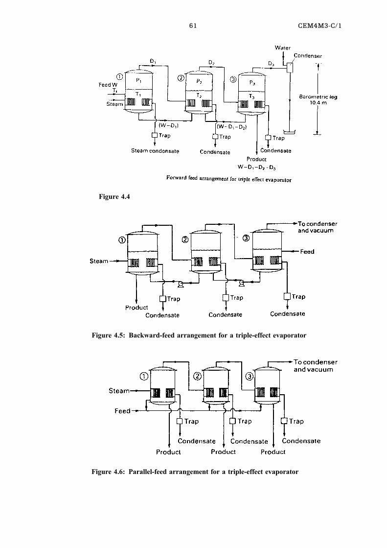
61 CEM4M3-C/1
Figure 4.4
Figure 4.5: Backward-feed arrangement for a triple-effect evaporator
Figure 4.6: Parallel-feed arrangement for a triple-effect evaporator
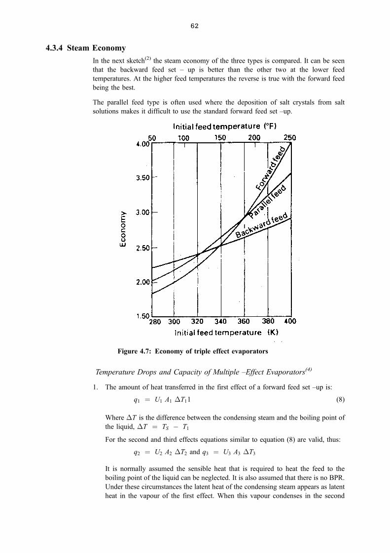
62
4.3.4 Steam Economy
In the next sketch(2) the steam economy of the three types is compared. It can be seen
that the backward feed set ± up is better than the other two at the lower feed
temperatures. At the higher feed temperatures the reverse is true with the forward feed
being the best.
The parallel feed type is often used where the deposition of salt crystals from salt
solutions makes it difficult to use the standard forward feed set ±up.
Temperature Drops and Capacity of Multiple ±Effect Evaporators(4)
1. The amount of heat transferred in the first effect of a forward feed set ±up is:
q1 � U1 A1 �T11 (8)
Where �T is the difference between the condensing steam and the boiling point of
the liquid, �T � TS ÿ T1
For the second and third effects equations similar to equation (8) are valid, thus:
q2 � U2 A2 �T2 and q3 � U3 A3 �T3
It is normally assumed the sensible heat that is required to heat the feed to the
boiling point of the liquid can be neglected. It is also assumed that there is no BPR.
Under these circumstances the latent heat of the condensing steam appears as latent
heat in the vapour of the first effect. When this vapour condenses in the second
Figure 4.7: Economy of triple effect evaporators
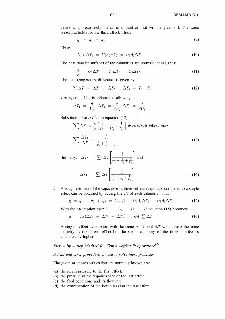
63 CEM4M3-C/1
calandria approximately the same amount of heat will be given off. The same
reasoning holds for the third effect. Thus:
q1 � q2 � q3 (9)
Thus:
U1A1�T1 � U2A2�T2 � U3A3�T3 (10)
The heat transfer surfaces of the calandrias are normally equal, thus:
q
A� U1�T1 � U2�T2 � U3�T3 (11)
The total temperature difference is given by:P�T � �T1 � �T2 � �T3 � Ts ÿ T3 (12)
Use equation (11) to obtain the following:
�T1 � q
AU1
�T2 � q
AU2
�T3 � q
AU3
Substitute these �T 's oin equation (12). Thus:X�T � q
A
h 1
U1
� 1
U2
� 1
U3
ifrom which follow that:
X �T1
�T�
1U1
1U1� 1
U1� 1
U3
(13)
Similarly: �T2 �P
�T
"1
U2
1U1� 1
U2� 1
U3
#and
�T3 �P
�T
"1
U3
1U1� 1
U2� 1
U3
#(14)
2. A rough estimate of the capacity of a three ±effect evaporator compared to a single
effect can be obtained by adding the q's of each calandria. Thus:
g � q1 � q2 � q3 � U1A11 � U2A2�T2 � U3A3�T3 (15)
With the assumption that: U1 � U2 � U3 � U equation (15) becomes:
q � UA��T1 � �T2 � �T3� � UAP
�T (16)
A single ±effect evaporator, with the same A, U, and �T would have the same
capacity as the three ±effect but the steam economy of the three ± effect is
considerably higher.
Step ± by ± step Method for Triple ±effect Evaporatore(4)
A trial and error procedure is used to solve these problems.
The given or known values that are normally known are:
(a) the steam pressure to the first effect.
(b) the pressure in the vapour space of the last effect.
(c) the feed conditions and its flow rate.
(d) the concentration of the liquid leaving the last effect.
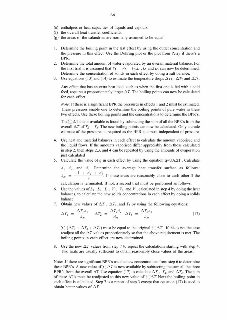
64
(e) enthalpies or heat capacities of liquids and vapours.
(f) the overall heat transfer coefficients.
(g) the areas of the calandrias are normally assumed to be equal.
1. Determine the boiling point in the last effect by using the outlet concentration and
the pressure in this effect. Use the Duhring plot or the plot from Perry if there's a
BPR.
2. Determine the total amount of water evaporated by an overall material balance. For
the first trial it is assumed that V1 � V2 � V3:L1; L2 and L3 can now be determined.
Determine the concentration of solids in each effect by doing a salt balance.
3. Use equations (13) and (14) to estimate the temperature drops �T1; �T2 and �T3.
Any effect that has an extra heat load, such as when the first one is fed with a cold
feed, requires a proportionately larger �T. The boiling points can now be calculated
for each effect.
Note: If there is a significant BPR the pressures in effects 1 and 2 must be estimated.
These pressures enable one to determine the boiling points of pure water in these
two effects. Use these boiling points and the concentrations to determine the BPR's.
TheP
�T that is available is found by subtracting the sum of all the BPR's from the
overall �T of TS ÿ T3. The new boiling points can now be calculated. Only a crude
estimate of the pressures is required as the BPR is almost independent of pressure.
4. Use heat and material balances in each effect to calculate the amount vaporised and
the liquid flows. If the amounts vaporised differ appreciably from those calculated
in step 2, then steps 2,3, and 4 can be repeated by using the amounts of evaporation
just calculated
5. Calculate the value of q in each effect by using the equation q=UA�T . Calculate
A1; A2, and A3. Determine the average heat transfer surface as follows:
Am � ÿ1 � A2 � A3
3. If these areas are reasonably close to each other 3 the
calculation is terminated. If not, a second trial must be performed as follows.
6. Use the values of L1; L2; L3; V1; V2, and V3, calculated in step 4 by doing the heat
balances, to calculate the new solids concentrations in each effect by doing a solids
balance.
7. Obtain new values of �T1; �T2, and T3 by using the following equations:
�T1 � �T1A1
Am
�T2 � �T2A2
Am
�T3 � �T3A3
Am
(17)
P ��T1 ��T2 ��T3� must be equal to the originalP
�T . If this is not the case
readjust all the �T values proportionately so that the above requirement is met. The
boiling points in each effect are now determined.
8. Use the new �T values from step 7 to repeat the calculations starting with step 4.
Two trials are usually sufficient to obtain reasonably close values of the areas.
Note: If there are significant BPR's use the new concentrations from step 6 to determine
these BPR's. A new value ofP
�T is now available by subtracting the sum all the three
BPR's from the overall AT. Use equation (17) to calculate �T1; T2, and �T3. The sum
of these AT's must be readjusted to this new value ofP
�T Next the boiling point in
each effect is calculated. Step 7 is a repeat of step 3 except that equation (17) is used to
obtain better values of �T .
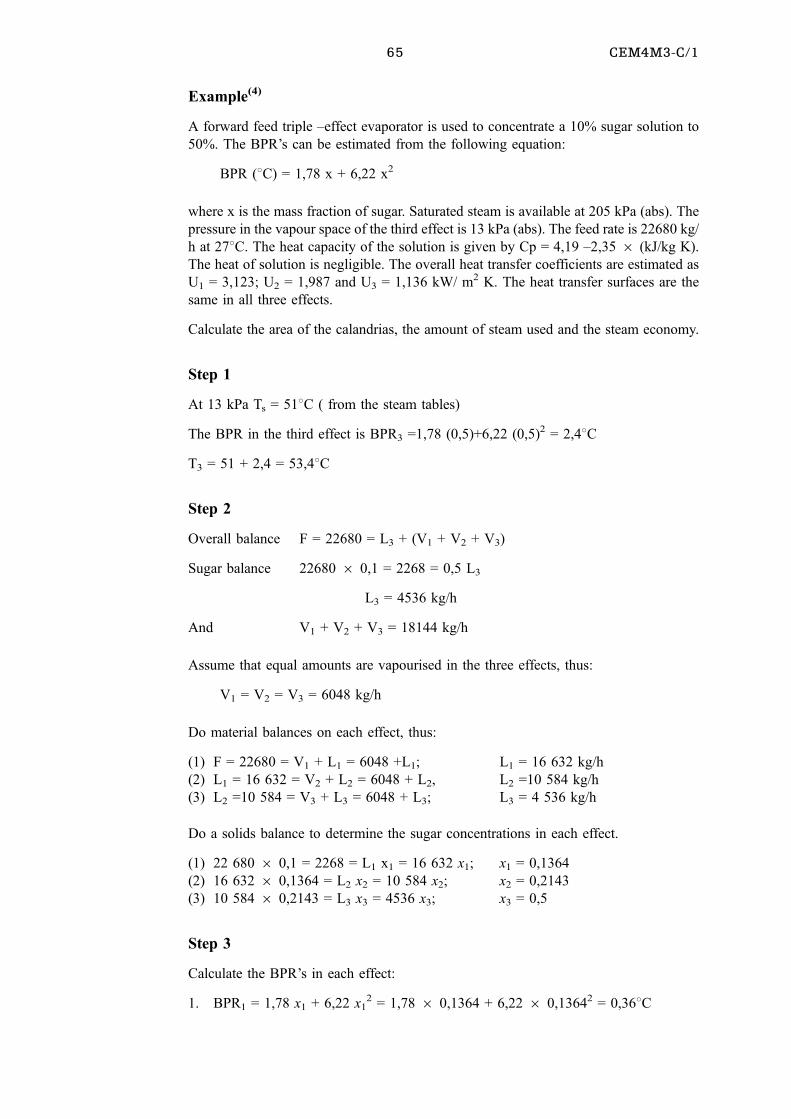
65 CEM4M3-C/1
Example(4)
A forward feed triple ±effect evaporator is used to concentrate a 10% sugar solution to
50%. The BPR's can be estimated from the following equation:
BPR (8C) = 1,78 x + 6,22 x2
where x is the mass fraction of sugar. Saturated steam is available at 205 kPa (abs). The
pressure in the vapour space of the third effect is 13 kPa (abs). The feed rate is 22680 kg/
h at 278C. The heat capacity of the solution is given by Cp = 4,19 ±2,35 6 (kJ/kg K).
The heat of solution is negligible. The overall heat transfer coefficients are estimated as
U1 = 3,123; U2 = 1,987 and U3 = 1,136 kW/ m2 K. The heat transfer surfaces are the
same in all three effects.
Calculate the area of the calandrias, the amount of steam used and the steam economy.
Step 1
At 13 kPa Ts = 518C ( from the steam tables)
The BPR in the third effect is BPR3 =1,78 (0,5)+6,22 (0,5)2 = 2,48C
T3 = 51 + 2,4 = 53,48C
Step 2
Overall balance F = 22680 = L3 + (V1 + V2 + V3)
Sugar balance 22680 6 0,1 = 2268 = 0,5 L3
L3 = 4536 kg/h
And V1 + V2 + V3 = 18144 kg/h
Assume that equal amounts are vapourised in the three effects, thus:
V1 = V2 = V3 = 6048 kg/h
Do material balances on each effect, thus:
(1) F = 22680 = V1 + L1 = 6048 +L1; L1 = 16 632 kg/h
(2) L1 = 16 632 = V2 + L2 = 6048 + L2, L2 =10 584 kg/h
(3) L2 =10 584 = V3 + L3 = 6048 + L3; L3 = 4 536 kg/h
Do a solids balance to determine the sugar concentrations in each effect.
(1) 22 680 6 0,1 = 2268 = L1 x1 = 16 632 x1; x1 = 0,1364
(2) 16 632 6 0,1364 = L2 x2 = 10 584 x2; x2 = 0,2143
(3) 10 584 6 0,2143 = L3 x3 = 4536 x3; x3 = 0,5
Step 3
Calculate the BPR's in each effect:
1. BPR1 = 1,78 x1 + 6,22 x12 = 1,78 6 0,1364 + 6,22 6 0,13642 = 0,368C
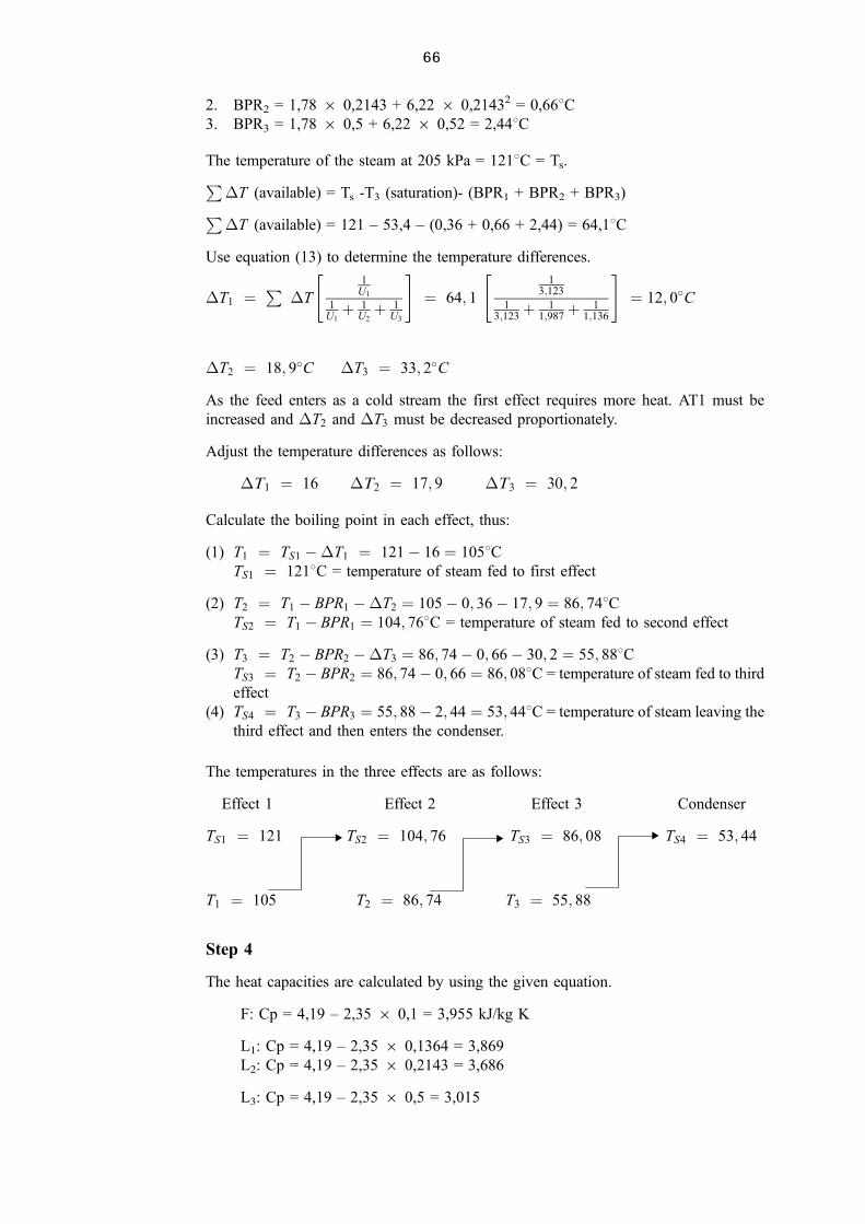
66
! ! !
2. BPR2 = 1,78 6 0,2143 + 6,22 6 0,21432 = 0,668C3. BPR3 = 1,78 6 0,5 + 6,22 6 0,52 = 2,448C
The temperature of the steam at 205 kPa = 1218C = Ts.P�T (available) = Ts -T3 (saturation)- (BPR1 + BPR2 + BPR3)P�T (available) = 121 ± 53,4 ± (0,36 + 0,66 + 2,44) = 64,18C
Use equation (13) to determine the temperature differences.
�T1 �P
�T
"1
U1
1U1� 1
U2� 1
U3
#� 64; 1
"1
3;123
13;123� 1
1;987� 1
1;136
#� 12; 0�C
�T2 � 18; 9�C �T3 � 33; 2�C
As the feed enters as a cold stream the first effect requires more heat. AT1 must be
increased and �T2 and �T3 must be decreased proportionately.
Adjust the temperature differences as follows:
�T1 � 16 �T2 � 17; 9 �T3 � 30; 2
Calculate the boiling point in each effect, thus:
(1) T1 � TS1 ÿ�T1 � 121ÿ 16 � 1058CTS1 � 1218C = temperature of steam fed to first effect
(2) T2 � T1 ÿ BPR1 ÿ�T2 � 105ÿ 0; 36ÿ 17; 9 � 86; 748CTS2 � T1 ÿ BPR1 � 104; 768C = temperature of steam fed to second effect
(3) T3 � T2 ÿ BPR2 ÿ�T3 � 86; 74ÿ 0; 66ÿ 30; 2 � 55; 888CTS3 � T2 ÿ BPR2 � 86; 74ÿ 0; 66 � 86; 088C = temperature of steam fed to third
effect
(4) TS4 � T3 ÿ BPR3 � 55; 88ÿ 2; 44 � 53; 448C = temperature of steam leaving the
third effect and then enters the condenser.
The temperatures in the three effects are as follows:
Effect 1 Effect 2 Effect 3 Condenser
TS1 � 121 TS2 � 104; 76 TS3 � 86; 08 TS4 � 53; 44
T1 � 105 T2 � 86; 74 T3 � 55; 88
Step 4
The heat capacities are calculated by using the given equation.
F: Cp = 4,19 ± 2,35 6 0,1 = 3,955 kJ/kg K
L1: Cp = 4,19 ± 2,35 6 0,1364 = 3,869
L2: Cp = 4,19 ± 2,35 6 0,2143 = 3,686
L3: Cp = 4,19 ± 2,35 6 0,5 = 3,015
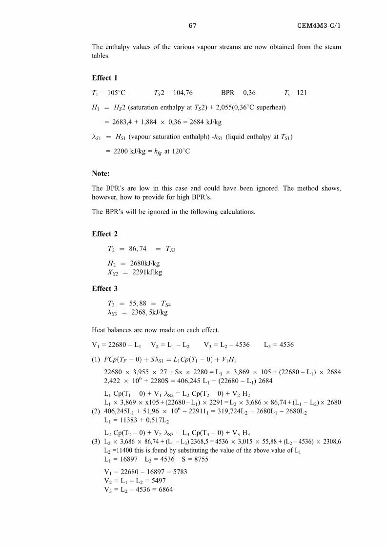
67 CEM4M3-C/1
The enthalpy values of the various vapour streams are now obtained from the steam
tables.
Effect 1
T1 = 1058C TS2 = 104,76 BPR = 0,36 Ts =121
H1 � HS2 (saturation enthalpy at TS2) + 2,055(0,368C superheat)
= 2683,4 + 1,884 6 0,36 = 2684 kJ/kg
�S1 � HS1 (vapour saturation enthalph) -hS1 (liquid enthalpy at TS1)
= 2200 kJ/kg = hfg at 1208C
Note:
The BPR's are low in this case and could have been ignored. The method shows,
however, how to provide for high BPR's.
The BPR's will be ignored in the following calculations.
Effect 2
T2 � 86; 74 � TS3
H2 � 2680kJ/kg
XS2 � 2291kJlkg
Effect 3
T3 � 55; 88 � TS4
�S3 � 2368; 5kJ/kg
Heat balances are now made on each effect.
V1 = 22680 ± L1 V2 = L1 ± L2 V3 = L2 ± 4536 L3 = 4536
(1) FCp�TF ÿ 0� � S�S1 � L1Cp�T1 ÿ 0� � V1H1
22680 6 3,955 6 27 + Sx 6 2280 = L1 6 3,869 6 105 + (22680 ± L1) 6 2684
2,422 6 106 + 2280S = 406,245 L1 + (22680 ± L1) 2684
L1 Cp(T1 ± 0) + V1 �S2 = L2 Cp(T2 ± 0) + V2 H2
L16 3,8696 x10⁵ + (22680 ± L1)6 2291 = L26 3,6866 86,74 + (L1 ± L2)6 2680
(2) 406,245L1 + 51,96 6 106 ± 229111 = 319,724L2 + 2680L1 ± 2680L2
L1 = 11383 + 0,517L2
L2 Cp(T2 ± 0) + V2 �S3 = L3 Cp(T3 ± 0) + V3 H3
(3) L2 6 3,686 6 86,74 + (L1 ± L3) 2368,5 = 4536 6 3,015 6 55,88 + (L2 ± 4536) 6 2308,6
L2 =11400 this is found by substituting the value of the above value of L1
L1 = 16897 L3 = 4536 S = 8755
V1 = 22680 ± 16897 = 5783
V2 = L1 ± L2 = 5497
V3 = L2 ± 4536 = 6864
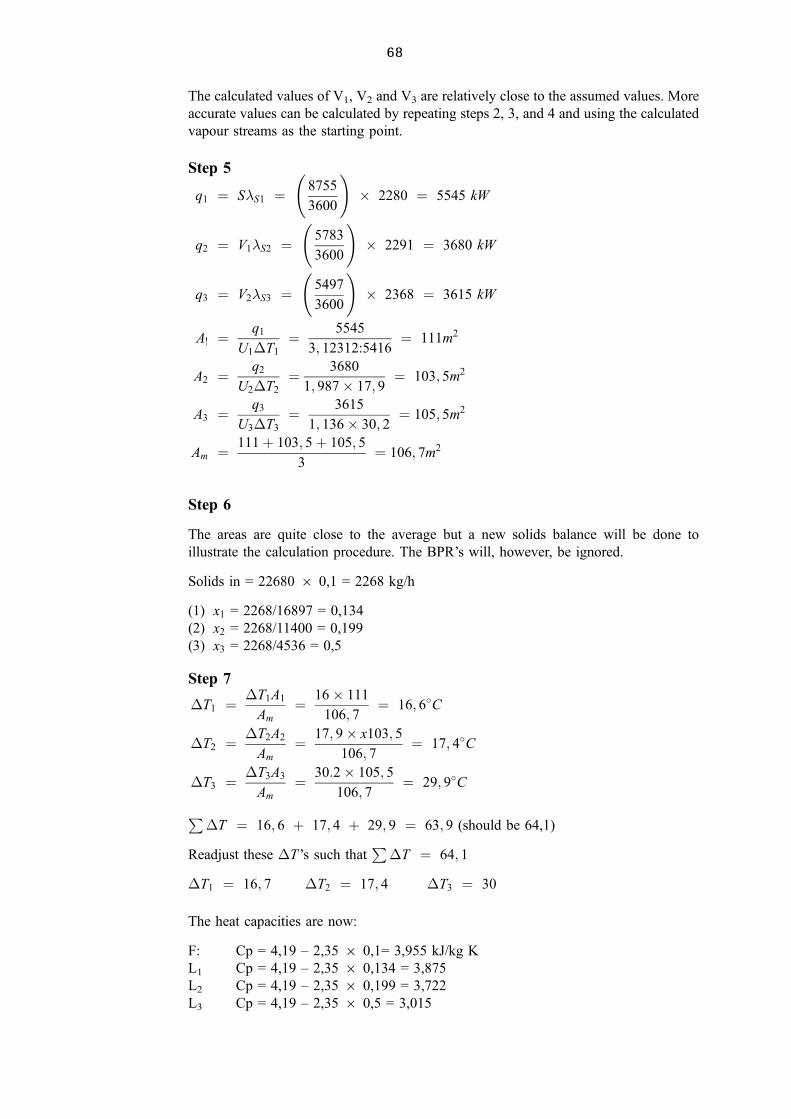
68
The calculated values of V1, V2 and V3 are relatively close to the assumed values. More
accurate values can be calculated by repeating steps 2, 3, and 4 and using the calculated
vapour streams as the starting point.
Step 5
q1 � S�S1 �
8755
3600
!� 2280 � 5545 kW
q2 � V1�S2 �
5783
3600
!� 2291 � 3680 kW
q3 � V2�S3 �
5497
3600
!� 2368 � 3615 kW
A! � q1
U1�T1
� 5545
3; 12312:5416� 111m2
A2 � q2
U2�T2
� 3680
1; 987� 17; 9� 103; 5m2
A3 � q3
U3�T3
� 3615
1; 136� 30; 2� 105; 5m2
Am � 111� 103; 5� 105; 5
3� 106; 7m2
Step 6
The areas are quite close to the average but a new solids balance will be done to
illustrate the calculation procedure. The BPR's will, however, be ignored.
Solids in = 22680 6 0,1 = 2268 kg/h
(1) x1 = 2268/16897 = 0,134
(2) x2 = 2268/11400 = 0,199
(3) x3 = 2268/4536 = 0,5
Step 7
�T1 � �T1A1
Am
� 16� 111
106; 7� 16; 6�C
�T2 � �T2A2
Am
� 17; 9� x103; 5
106; 7� 17; 4�C
�T3 � �T3A3
Am
� 30:2� 105; 5
106; 7� 29; 9�C
P�T � 16; 6 � 17; 4 � 29; 9 � 63; 9 (should be 64,1)
Readjust these �T 's such thatP
�T � 64; 1
�T1 � 16; 7 �T2 � 17; 4 �T3 � 30
The heat capacities are now:
F: Cp = 4,19 ± 2,35 6 0,1= 3,955 kJ/kg K
L1 Cp = 4,19 ± 2,35 6 0,134 = 3,875
L2 Cp = 4,19 ± 2,35 6 0,199 = 3,722
L3 Cp = 4,19 ± 2,35 6 0,5 = 3,015
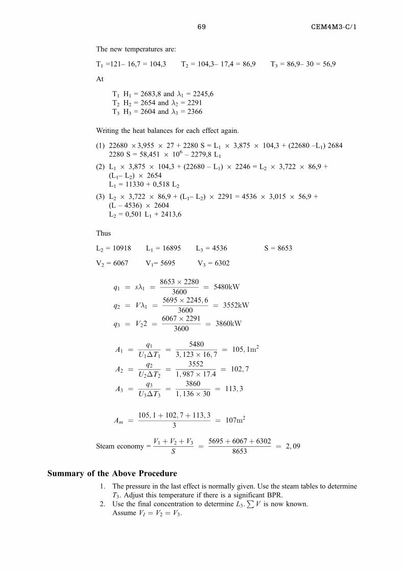
69 CEM4M3-C/1
The new temperatures are:
T1 =121± 16,7 = 104,3 T2 = 104,3± 17,4 = 86,9 T3 = 86,9± 30 = 56,9
At
T1 H1 = 2683,8 and �1 = 2245,6
T2 H2 = 2654 and �2 = 2291
T3 H3 = 2604 and �3 = 2366
Writing the heat balances for each effect again.
(1) 22680 63,955 6 27 + 2280 S = L1 6 3,875 6 104,3 + (22680 ±L1) 2684
2280 S = 58,451 6 106 ± 2279,8 L1
(2) L1 6 3,875 6 104,3 + (22680 ± L1) 6 2246 = L2 6 3,722 6 86,9 +
(L1± L2) 6 2654
L1 = 11330 + 0,518 L2
(3) L2 6 3,722 6 86,9 + (L1± L2) 6 2291 = 4536 6 3,015 6 56,9 +
(L ± 4536) 6 2604
L2 = 0,501 L1 + 2413,6
Thus
L2 = 10918 L1 = 16895 L3 = 4536 S = 8653
V2 = 6067 V1= 5695 V3 = 6302
q1 � s�1 � 8653� 2280
3600� 5480kW
q2 � V�1 � 5695� 2245; 6
3600� 3552kW
q3 � V22 � 6067� 2291
3600� 3860kW
A1 � q1U1�T1
� 5480
3; 123� 16; 7� 105; 1m2
A2 � q2U2�T2
� 3552
1; 987� 17:4� 102; 7
A3 � q3U3�T3
� 3860
1; 136� 30� 113; 3
Am � 105; 1� 102; 7� 113; 3
3� 107m2
Steam economy =V1 � V2 � V3
S� 5695� 6067� 6302
8653� 2; 09
Summary of the Above Procedure
1. The pressure in the last effect is normally given. Use the steam tables to determine
T3. Adjust this temperature if there is a significant BPR.
2. Use the final concentration to determine L3:P
V is now known.
Assume VI � V2 � V3.
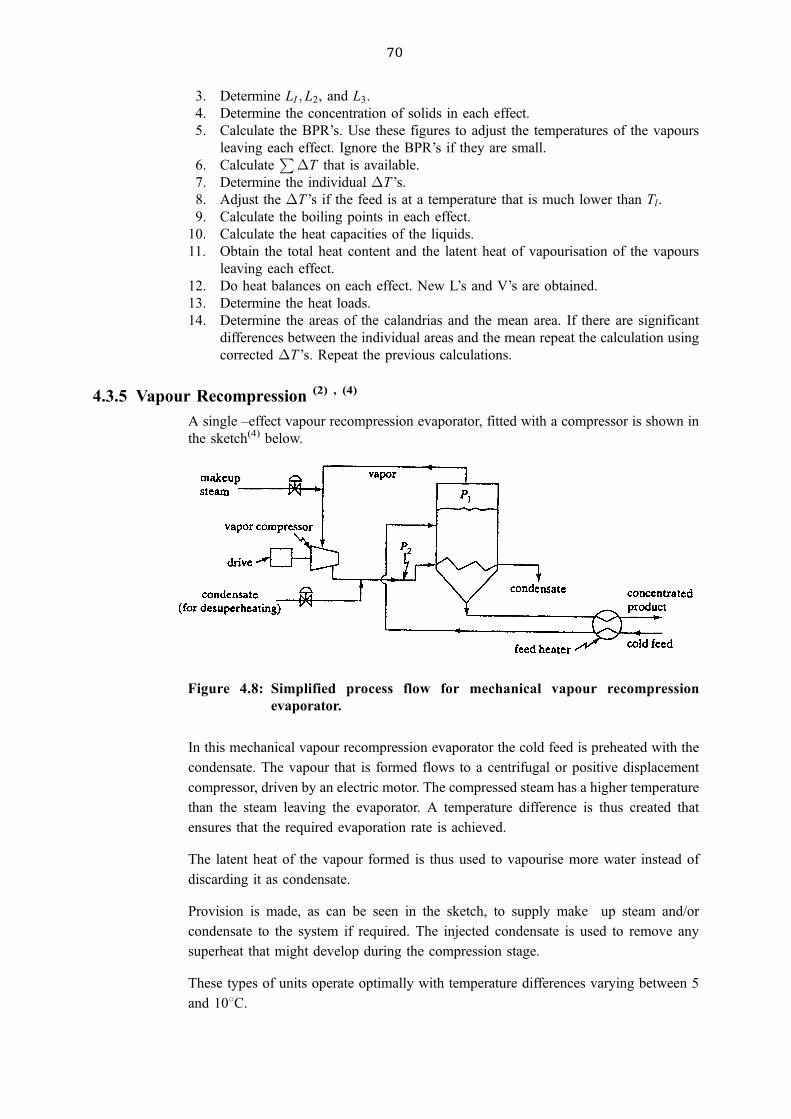
70
3. Determine LI ;L2, and L3.
4. Determine the concentration of solids in each effect.
5. Calculate the BPR's. Use these figures to adjust the temperatures of the vapours
leaving each effect. Ignore the BPR's if they are small.
6. CalculateP
�T that is available.
7. Determine the individual �T 's.
8. Adjust the �T 's if the feed is at a temperature that is much lower than Tl.
9. Calculate the boiling points in each effect.
10. Calculate the heat capacities of the liquids.
11. Obtain the total heat content and the latent heat of vapourisation of the vapours
leaving each effect.
12. Do heat balances on each effect. New L's and V's are obtained.
13. Determine the heat loads.
14. Determine the areas of the calandrias and the mean area. If there are significant
differences between the individual areas and the mean repeat the calculation using
corrected �T 's. Repeat the previous calculations.
4.3.5 Vapour Recompression (2) , (4)
A single ±effect vapour recompression evaporator, fitted with a compressor is shown in
the sketch(4) below.
In this mechanical vapour recompression evaporator the cold feed is preheated with the
condensate. The vapour that is formed flows to a centrifugal or positive displacement
compressor, driven by an electric motor. The compressed steam has a higher temperature
than the steam leaving the evaporator. A temperature difference is thus created that
ensures that the required evaporation rate is achieved.
The latent heat of the vapour formed is thus used to vapourise more water instead of
discarding it as condensate.
Provision is made, as can be seen in the sketch, to supply make up steam and/or
condensate to the system if required. The injected condensate is used to remove any
superheat that might develop during the compression stage.
These types of units operate optimally with temperature differences varying between 5
and 108C.
Figure 4.8: Simplified process flow for mechanical vapour recompression
evaporator.
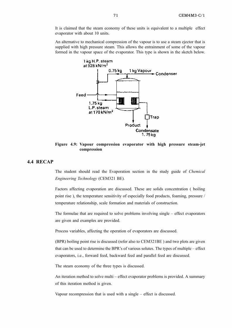
71 CEM4M3-C/1
It is claimed that the steam economy of these units is equivalent to a multiple effect
evaporator with about 10 units.
An alternative to mechanical compression of the vapour is to use a steam ejector that is
supplied with high pressure steam. This allows the entrainment of some of the vapour
formed in the vapour space of the evaporator. This type is shown in the sketch below.
4.4 RECAP
The student should read the Evaporation section in the study guide of Chemical
Engineering Technology (CEM321 BE).
Factors affecting evaporation are discussed. These are solids concentration ( boiling
point rise ), the temperature sensitivity of especially food products, foaming, pressure /
temperature relationship, scale formation and materials of construction.
The formulae that are required to solve problems involving single ± effect evaporators
are given and examples are provided.
Process variables, affecting the operation of evaporators are discussed.
(BPR) boiling point rise is discussed (refer also to CEM321BE ) and two plots are given
that can be used to determine the BPR's of various solutes. The types of multiple ± effect
evaporators, i.e., forward feed, backward feed and parallel feed are discussed.
The steam economy of the three types is discussed.
An iteration method to solve multi ± effect evaporator problems is provided. A summary
of this iteration method is given.
Vapour recompression that is used with a single ± effect is discussed.
Figure 4.9: Vapour compression evaporator with high pressure steam-jet
compression
72
4.5 EVALUATION
Problem 1(4)
A solution with a negligible BPR is being evaporated in a triple ± effect evaporator using
saturated steam at 121,18C. The pressure in the vapour space of the last effect is 25,6
kPa (abs). The overall heat transfer coefficients are U1 = 2,84, U2 = 1,988 and U3 = 1,42
kW/m2K. The heat transfer areas are equal. Estimate the boiling points in all three
effects.
Answer
T1 = 108,68C T2 = 90,78C T3 = 65,68C
Problem 2(4)
A triple ± effect forward feed evaporator concentrates a sugar solution from 5 mass % to
25%. Any BPR can be neglected. The feed enters at 22 680 kg/h at 300 K and the
pressure in the vapour space of the third effect is 13,65 kPa (abs). The fresh saturated
steam is available at 205 kPa (abs). The liquid heat capacity is given by: Cp = 4,19 ±
2,35 6 where 6 is the mass fraction of sugar. The heat transfer coefficients are U1 =
3,123, U2 = 1,987 and U3 = 1,136 kW/m2K. Calculate the heat transfer surface of each
effect if all areas are equal, the steam rate and the steam economy.
Do only one iteration.
Answer
100 m2; S = 8976 kg/h Steam economy = 2,02
Problem 3(4)
An aqueous solution containing 2 mass % organic solids is fed at 388C to a double ±
effect backward feed evaporator. The BPR's can be ignored and the product contains
25% solids. Each effect has a heat transfer area of 93 m2 and the heat transfer
coefficients are U1 = 2,837 and U2 = 3,972 kW/m2 K.
The feed enters effect no. 2 and saturated steam is fed to number 1 at 690 kPa (abs). The
pressure in the vapour space of number 2 is 21 kPa (abs). The hoÄat capacities of all the
liquids = 4,19 kJ/kg K. Calculate the feed rate and the product rate. Use as basis a feed
rate of 1000 kg / h to calculate the area. Use the given areas to prorate the feed and L1.
Do only one iteration.
Answer
F = .55 000 kg/h and L1 = 4 300 kg/h (these values are obtained if the �T's are not
adjusted ± with adjusted �T's F will be closer to 60 000 and L1 closer to 4800 kWh)
Problem 4
2 kg/s of an aqueous solution containing 10 mass % solids is fed to a triple ± effect
73 CEM4M3-C/1
backward feed evaporator at 218C. The solution that is withdrawn from the first effect
contains 50 % solids. The third effect is operated at 13 kPa (abs) while the dry saturated
steam fed to the first effect is at 205 kPa (abs). The specific heat of all liquids can be
assumed to be 4,18 kJ/kg K. It can also be assumed that there is no BPR.
Estimate the heat transfer areas assuming that they are equal in size, the temperatures in
each effect and the steam consumption. The overall heat transfer coefficients are U1 =
2,5; U2 = 2,0 and U3 =1,6 kW/m2 K
Do only one iteration.
Answer
Am = 31 m2; s = 0,7 kg/s
74
CHAPTER 5
Adsorption
CONTENTS
5.1 LEARNING OUTCOMES 00
5.2 INTRODUCTION 00
5.2.1 Physical Properties of Adsorbents 00
5.2.2 The Adsorption Process 00
5.2.3 Equilibrium Relations 00
5.2.4 Batch Adsorption (4) 00
5.3 DESIGN OF FIXED BED COLUMNS(4) 00
5.3.1 Breakthrough Concentration Curve(4) 00
5.3.2 Capacity of Column and Scale ± up Design Method(4) 00
5.4 DESIGN OF COUNTERCURRENT FLOW OF SOLIDS 00
5.4.1 Design Method for Countercurrent Flow 00
5.5 RECAP 00
5.6 EVALUATION 00
5.1 LEARNING OUTCOMES
. The student should be able to identify practical applications of adsorption.
. The student should understand the similarities between adsorption and absorption
processes.
. The student must be able to use some equilibrium equations and be able to determine
the break ± through times for batch and fixed bed operations as well the bed heights.
. The student must be able to determine the number and height of the transfer units and
the bed heights of countercurrent adsorption processes.
5.2 INTRODUCTION
In adsorption processes one or more components are removed from a gas or liquid
stream by contact with a solid phase.
The adsorbent is usually in the form of small particles with a high surface area. The
internal surface area of a particle is usually significantly larger than its external surface
area.
To obtain a very large surface area per unit volume of solid requires that the solid is very
porous. The pores must have small diameters and be interconnected.
The adsorbed solute is referred to as the adsorbate while the solid is referred to as the
adsorbent.
In an adsorption process the molecules diffuse into the pores of the solid where they
bond with the solid surface by physical or chemical forces. The latter process is referred
to as chemisorption.
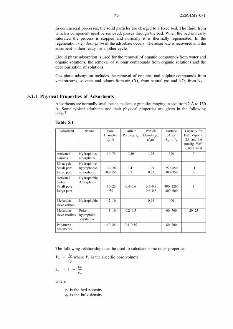
75 CEM4M3-C/1
In commercial processes, the solid particles are charged to a fixed bed. The fluid, from
which a component must be removed, passes through the bed. When the bed is nearly
saturated the process is stopped and normally it is thermally regenerated. In the
regeneration step desorption of the adsorbate occurs. The adsorbate is recovered and the
adsorbent is then ready for another cycle.
Liquid phase adsorption is used for the removal of organic compounds from water and
organic solutions, the removal of sulphur compounds from organic solutions and the
decolourisation of solutions.
Gas phase adsorption includes the removal of organics and sulphur compounds from
vent streams, solvents and odours from air, CO2 from natural gas and NOx from N2.
5.2.1 Physical Properties of Adsorbents
Adsorbents are normally small beads, pellets or granules ranging in size from 2 AG to 150
AG . Some typical adorbents and their physical properties are given in the following
table(1).
Table 5.1
Adsorbent Nature Pore
Diameter
dp; AG
Particle
Porosity "p
Particle
Density �p;
g/cm3
Surface
Area
Sg, m2/g
Capacity for
H2O Vapor at
258 and 4,6
mmHg. Wt%
(Dry Basis)
Activated
alumina
Hydrophilic,
amorphous
10±75 0.50 1.25 320 7
Silica gel:
Small pore
Large pore
Hydrophilic/
hydrophobic,
amorphous
22±26
100±150
0.47
0.71
1.09
0.62
750±850
300±350
11
±
Activated
carbon:
Small pore
Large pore
Hydrophobic,
Amorphous
10±25
>30
0.4±0.6
±
0.5±0.9
0.6±0.8
400±1200
200±600
1
±
Molecular-
sieve carbon
Hydrophobic 2±10 ± 0.98 400 ±
Molecular-
sieve zeolites
Polar-
hydrophilic
crystalline
3±10 0.2±0.5 ± 60±700 20±25
Polymeric
absorbents
± 40±25 0.4±0.55 ± 80±700 ±
The following relationships can be used to calculate some other properties.
Vp � "p
�p
where Vp is the specific pore volume
"b � 1 ÿ �b
�p
where
"b is the bed porosity
�b is the bulk density
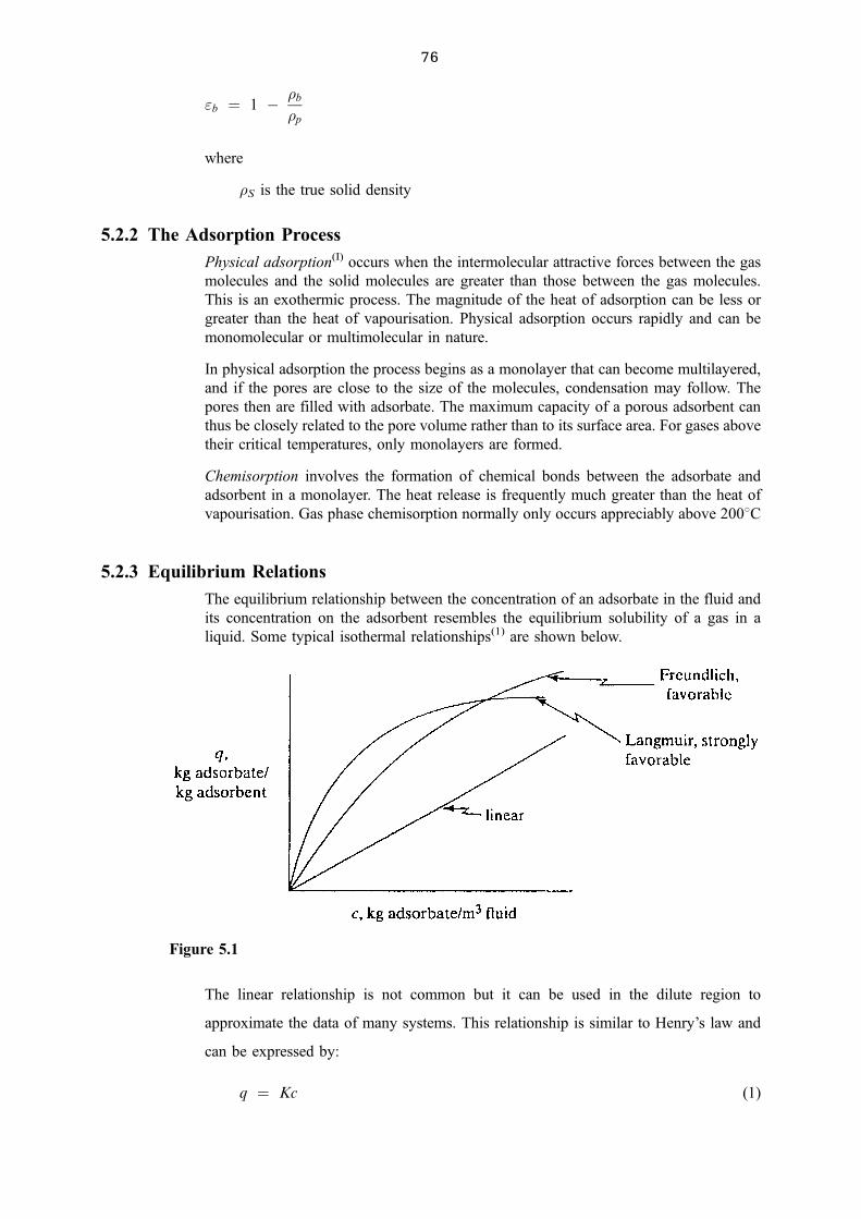
76
"b � 1 ÿ �b
�p
where
�S is the true solid density
5.2.2 The Adsorption Process
Physical adsorption(I) occurs when the intermolecular attractive forces between the gas
molecules and the solid molecules are greater than those between the gas molecules.
This is an exothermic process. The magnitude of the heat of adsorption can be less or
greater than the heat of vapourisation. Physical adsorption occurs rapidly and can be
monomolecular or multimolecular in nature.
In physical adsorption the process begins as a monolayer that can become multilayered,
and if the pores are close to the size of the molecules, condensation may follow. The
pores then are filled with adsorbate. The maximum capacity of a porous adsorbent can
thus be closely related to the pore volume rather than to its surface area. For gases above
their critical temperatures, only monolayers are formed.
Chemisorption involves the formation of chemical bonds between the adsorbate and
adsorbent in a monolayer. The heat release is frequently much greater than the heat of
vapourisation. Gas phase chemisorption normally only occurs appreciably above 2008C
5.2.3 Equilibrium Relations
The equilibrium relationship between the concentration of an adsorbate in the fluid and
its concentration on the adsorbent resembles the equilibrium solubility of a gas in a
liquid. Some typical isothermal relationships(1) are shown below.
The linear relationship is not common but it can be used in the dilute region to
approximate the data of many systems. This relationship is similar to Henry's law and
can be expressed by:
q � Kc (1)
Figure 5.1
77 CEM4M3-C/1
where
K has the dimension of m3/kg adsorbent.
The Freundlich empirical equation apparently often approximates the data for many
systems and is very useful for liquids. This equation is given by:
q � Kcn (2)
where
K and n are constants that must be determined experimentally.
The Langmuir equation is given by:
q � qo c
K� c(3)
where
qo is a constant with kg adsorbate/kg adsorbent as unit
K is a constant, kg/m3.
Equation (3) can be rearranged to:
1
q� K� c
qoc� K
qoc� 1qo (4)
This is the equation of a straight line and when 1q
is plotted vs. 1c
the slope is given by: Kqo
and the intercept by: 1qo
.
Example 1(4)
In batch experiments solutions of phenol in water were contacted with granular activated
carbon. The following results were obtained at room temperature.
c, kg phenol/m3 solution q, kg phenol/kg carbon
0,322 0,15
0,117 0,122
0,039 0,094
0,0061 0,059
0,0011 0,045
Assume that the Freundlich isotherm can be used to model this system. Determine the
constants.
A log ± log plot shows that the data are on a straight line.
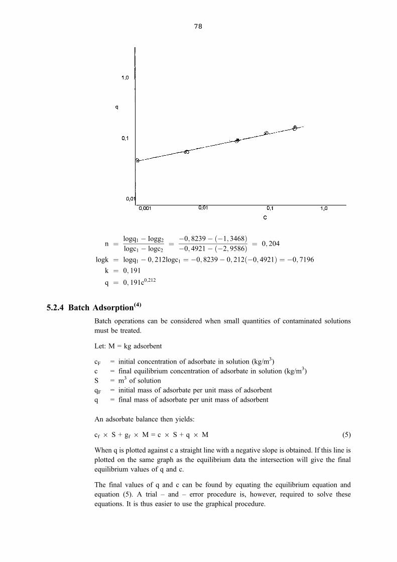
78
n � logq1 ÿ Iogg2
logc1 ÿ logc2
� ÿ0; 8239ÿ �ÿ1; 3468�ÿ0; 4921ÿ �ÿ2; 9586� � 0; 204
logk � logq1 ÿ 0; 212logc1 � ÿ0; 8239ÿ 0; 212�ÿ0; 4921� � ÿ0; 7196
k � 0; 191
q � 0; 191c0;212
5.2.4 Batch Adsorption(4)
Batch operations can be considered when small quantities of contaminated solutions
must be treated.
Let: M = kg adsorbent
cF = initial concentration of adsorbate in solution (kg/m3)
c = final equilibrium concentration of adsorbate in solution (kg/m3)
S = m3 of solution
qF = initial mass of adsorbate per unit mass of adsorbent
q = final mass of adsorbate per unit mass of adsorbent
An adsorbate balance then yields:
cf 6 S + gf 6 M = c 6 S + q 6 M (5)
When q is plotted against c a straight line with a negative slope is obtained. If this line is
plotted on the same graph as the equilibrium data the intersection will give the final
equilibrium values of q and c.
The final values of q and c can be found by equating the equilibrium equation and
equation (5). A trial ± and ± error procedure is, however, required to solve these
equations. It is thus easier to use the graphical procedure.
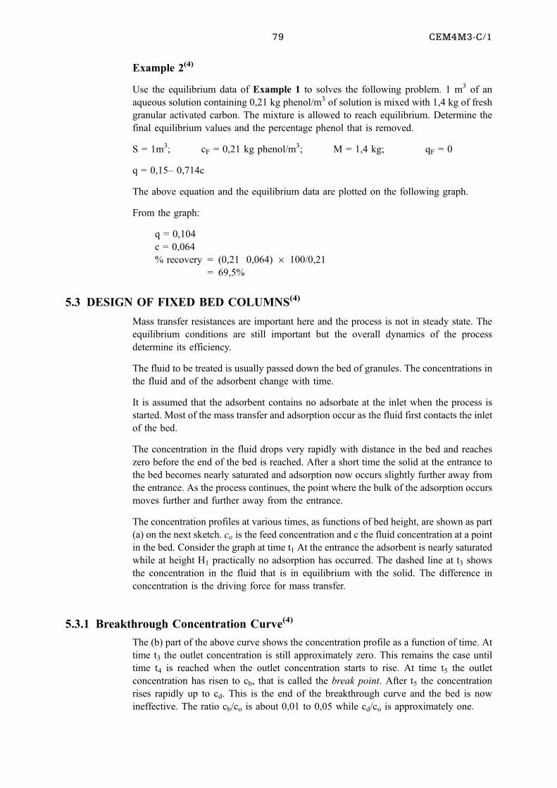
79 CEM4M3-C/1
Example 2(4)
Use the equilibrium data of Example 1 to solves the following problem. 1 m3 of an
aqueous solution containing 0,21 kg phenol/m3 of solution is mixed with 1,4 kg of fresh
granular activated carbon. The mixture is allowed to reach equilibrium. Determine the
final equilibrium values and the percentage phenol that is removed.
S = 1m3; cF = 0,21 kg phenol/m3; M = 1,4 kg; qF = 0
q = 0,15± 0,714c
The above equation and the equilibrium data are plotted on the following graph.
From the graph:
q = 0,104
c = 0,064
% recovery = (0,21 0,064) 6 100/0,21
= 69,5%
5.3 DESIGN OF FIXED BED COLUMNS(4)
Mass transfer resistances are important here and the process is not in steady state. The
equilibrium conditions are still important but the overall dynamics of the process
determine its efficiency.
The fluid to be treated is usually passed down the bed of granules. The concentrations in
the fluid and of the adsorbent change with time.
It is assumed that the adsorbent contains no adsorbate at the inlet when the process is
started. Most of the mass transfer and adsorption occur as the fluid first contacts the inlet
of the bed.
The concentration in the fluid drops very rapidly with distance in the bed and reaches
zero before the end of the bed is reached. After a short time the solid at the entrance to
the bed becomes nearly saturated and adsorption now occurs slightly further away from
the entrance. As the process continues, the point where the bulk of the adsorption occurs
moves further and further away from the entrance.
The concentration profiles at various times, as functions of bed height, are shown as part
(a) on the next sketch. co is the feed concentration and c the fluid concentration at a point
in the bed. Consider the graph at time t1 At the entrance the adsorbent is nearly saturated
while at height H1 practically no adsorption has occurred. The dashed line at t3 shows
the concentration in the fluid that is in equilibrium with the solid. The difference in
concentration is the driving force for mass transfer.
5.3.1 Breakthrough Concentration Curve(4)
The (b) part of the above curve shows the concentration profile as a function of time. At
time t3 the outlet concentration is still approximately zero. This remains the case until
time t4 is reached when the outlet concentration starts to rise. At time t5 the outlet
concentration has risen to cb, that is called the break point. After t5 the concentration
rises rapidly up to cd. This is the end of the breakthrough curve and the bed is now
ineffective. The ratio cb/co is about 0,01 to 0,05 while cd/co is approximately one.
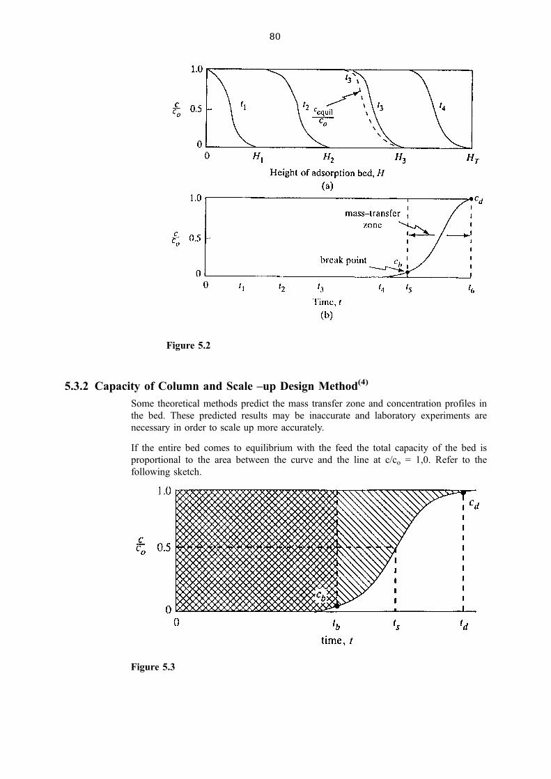
80
5.3.2 Capacity of Column and Scale ±up Design Method(4)
Some theoretical methods predict the mass transfer zone and concentration profiles in
the bed. These predicted results may be inaccurate and laboratory experiments are
necessary in order to scale up more accurately.
If the entire bed comes to equilibrium with the feed the total capacity of the bed is
proportional to the area between the curve and the line at c/co = 1,0. Refer to the
following sketch.
Figure 5.2
Figure 5.3
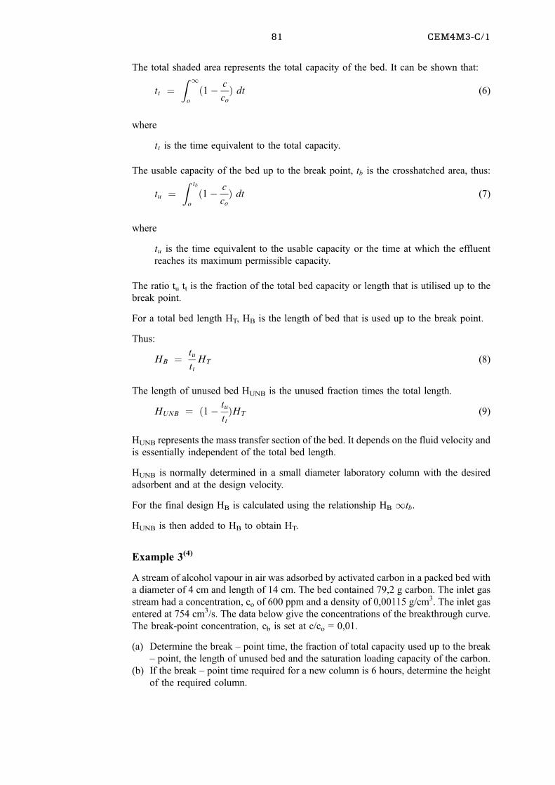
81 CEM4M3-C/1
The total shaded area represents the total capacity of the bed. It can be shown that:
tt �Z 1o
�1ÿ c
co� dt (6)
where
tt is the time equivalent to the total capacity.
The usable capacity of the bed up to the break point, tb is the crosshatched area, thus:
tu �Z tb
o
�1ÿ c
co� dt (7)
where
tu is the time equivalent to the usable capacity or the time at which the effluent
reaches its maximum permissible capacity.
The ratio tu tt is the fraction of the total bed capacity or length that is utilised up to the
break point.
For a total bed length HT, HB is the length of bed that is used up to the break point.
Thus:
HB � tuttHT (8)
The length of unused bed HUNB is the unused fraction times the total length.
HUNB � �1ÿ tutt�HT (9)
HUNB represents the mass transfer section of the bed. It depends on the fluid velocity and
is essentially independent of the total bed length.
HUNB is normally determined in a small diameter laboratory column with the desired
adsorbent and at the design velocity.
For the final design HB is calculated using the relationship HB 1tb.
HUNB is then added to HB to obtain HT.
Example 3(4)
A stream of alcohol vapour in air was adsorbed by activated carbon in a packed bed with
a diameter of 4 cm and length of 14 cm. The bed contained 79,2 g carbon. The inlet gas
stream had a concentration, co of 600 ppm and a density of 0,00115 g/cm3. The inlet gas
entered at 754 cm3/s. The data below give the concentrations of the breakthrough curve.
The break-point concentration, cb is set at c/co = 0,01.
(a) Determine the break ± point time, the fraction of total capacity used up to the break
± point, the length of unused bed and the saturation loading capacity of the carbon.
(b) If the break ± point time required for a new column is 6 hours, determine the height
of the required column.
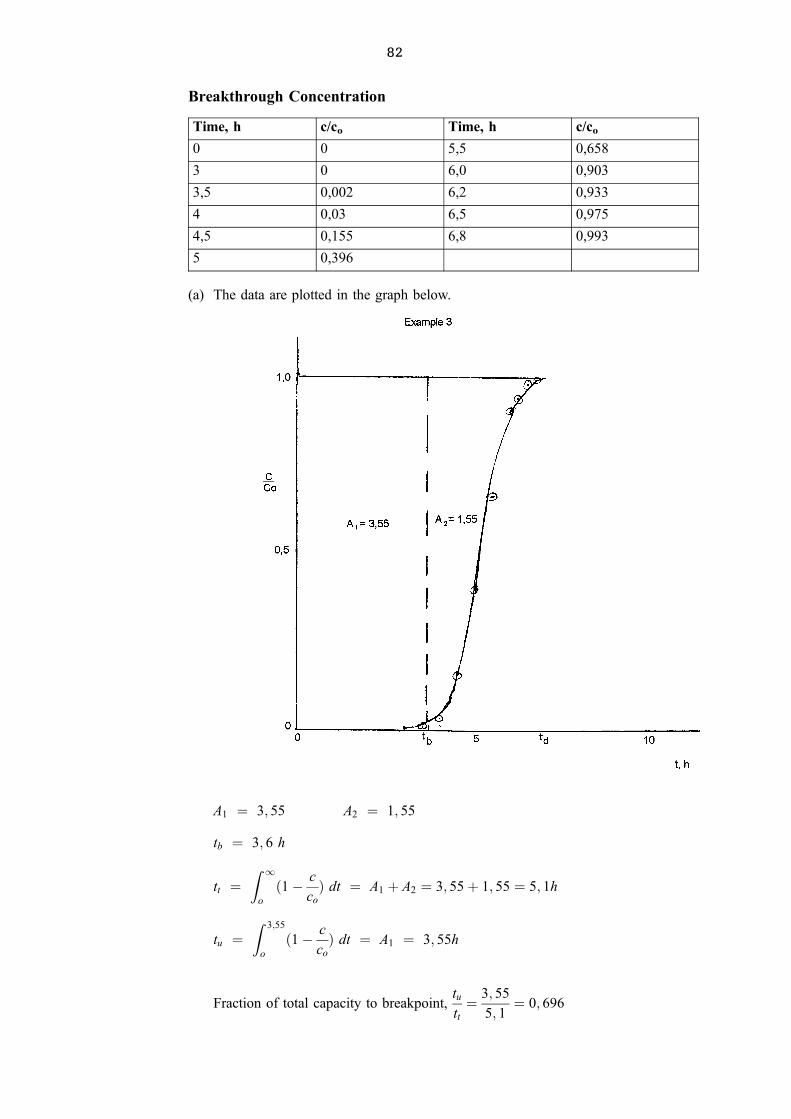
82
Breakthrough Concentration
Time, h c/co Time, h c/co
0 0 5,5 0,658
3 0 6,0 0,903
3,5 0,002 6,2 0,933
4 0,03 6,5 0,975
4,5 0,155 6,8 0,993
5 0,396
(a) The data are plotted in the graph below.
A1 � 3; 55 A2 � 1; 55
tb � 3; 6 h
tt �Z 1
o
�1ÿ c
co
� dt � A1 � A2 � 3; 55� 1; 55 � 5; 1h
tu �Z 3;55
o
�1ÿ c
co
� dt � A1 � 3; 55h
Fraction of total capacity to breakpoint,tu
tt� 3; 55
5; 1� 0; 696
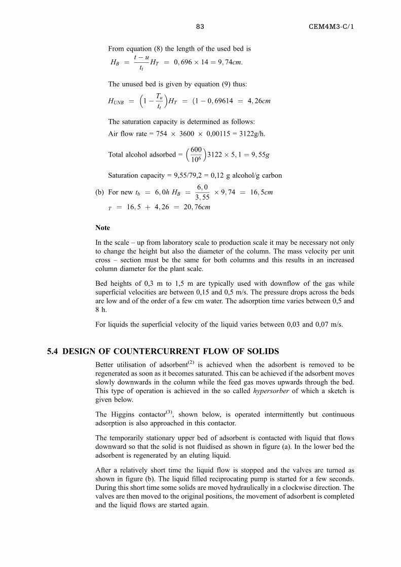
83 CEM4M3-C/1
From equation (8) the length of the used bed is
HB � t ÿ u
ttHT � 0; 696� 14 � 9; 74cm.
The unused bed is given by equation (9) thus:
HUNB ��
1ÿ Tu
tt
�HT � �1ÿ 0; 69614 � 4; 26cm
The saturation capacity is determined as follows:
Air flow rate = 754 6 3600 6 0,00115 = 3122g/h.
Total alcohol adsorbed =� 600
106
�3122� 5; 1 � 9; 55g
Saturation capacity = 9,55/79,2 = 0,12 g alcohol/g carbon
(b) For new tb � 6; 0h HB � 6; 0
3; 55� 9; 74 � 16; 5cm
T � 16; 5 � 4; 26 � 20; 76cm
Note
In the scale ± up from laboratory scale to production scale it may be necessary not only
to change the height but also the diameter of the column. The mass velocity per unit
cross ± section must be the same for both columns and this results in an increased
column diameter for the plant scale.
Bed heights of 0,3 m to 1,5 m are typically used with downflow of the gas while
superficial velocities are between 0,15 and 0,5 m/s. The pressure drops across the beds
are low and of the order of a few cm water. The adsorption time varies between 0,5 and
8 h.
For liquids the superficial velocity of the liquid varies between 0,03 and 0,07 m/s.
5.4 DESIGN OF COUNTERCURRENT FLOW OF SOLIDS
Better utilisation of adsorbent(2) is achieved when the adsorbent is removed to be
regenerated as soon as it becomes saturated. This can be achieved if the adsorbent moves
slowly downwards in the column while the feed gas moves upwards through the bed.
This type of operation is achieved in the so called hypersorber of which a sketch is
given below.
The Higgins contactor(3), shown below, is operated intermittently but continuous
adsorption is also approached in this contactor.
The temporarily stationary upper bed of adsorbent is contacted with liquid that flows
downward so that the solid is not fluidised as shown in figure (a). In the lower bed the
adsorbent is regenerated by an eluting liquid.
After a relatively short time the liquid flow is stopped and the valves are turned as
shown in figure (b). The liquid filled reciprocating pump is started for a few seconds.
During this short time some solids are moved hydraulically in a clockwise direction. The
valves are then moved to the original positions, the movement of adsorbent is completed
and the liquid flows are started again.
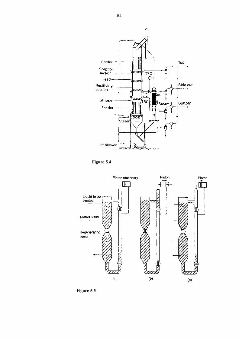
84
Figure 5.4
Figure 5.5
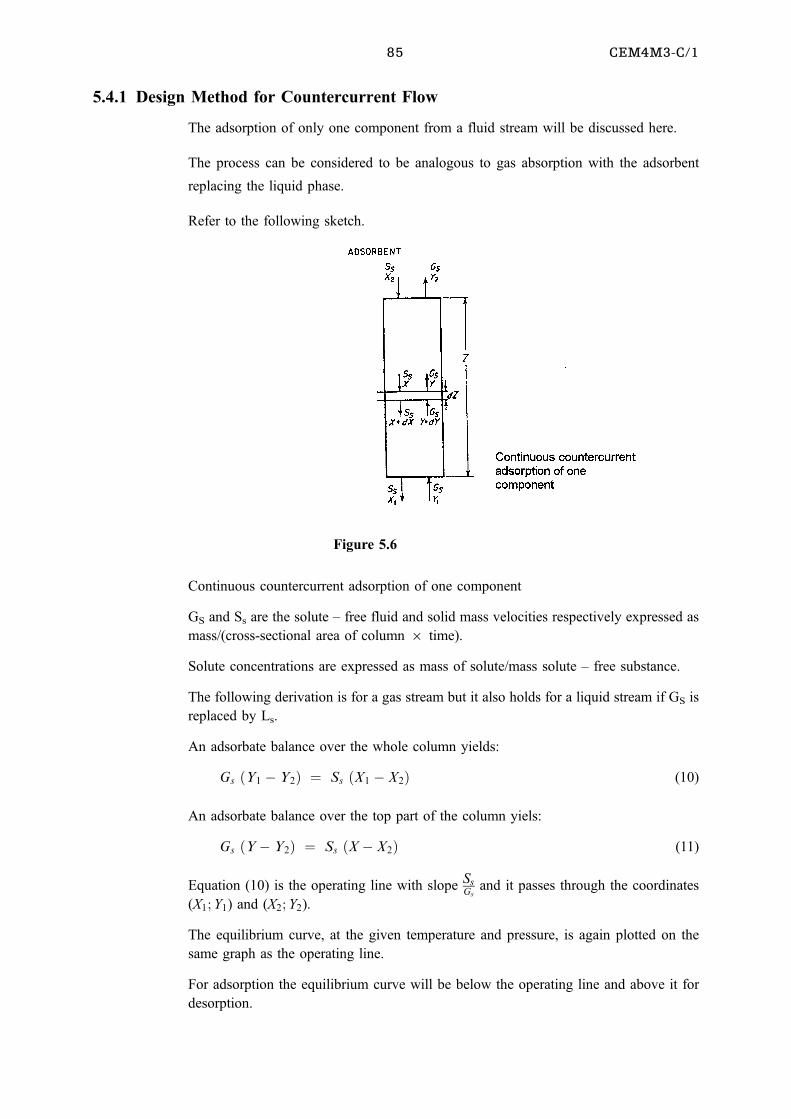
85 CEM4M3-C/1
5.4.1 Design Method for Countercurrent Flow
The adsorption of only one component from a fluid stream will be discussed here.
The process can be considered to be analogous to gas absorption with the adsorbent
replacing the liquid phase.
Refer to the following sketch.
Continuous countercurrent adsorption of one component
GS and Ss are the solute ± free fluid and solid mass velocities respectively expressed as
mass/(cross-sectional area of column 6 time).
Solute concentrations are expressed as mass of solute/mass solute ± free substance.
The following derivation is for a gas stream but it also holds for a liquid stream if GS is
replaced by Ls.
An adsorbate balance over the whole column yields:
Gs �Y1 ÿ Y2� � Ss �X1 ÿ X2� (10)
An adsorbate balance over the top part of the column yiels:
Gs �Yÿ Y2� � Ss �Xÿ X2� (11)
Equation (10) is the operating line with slope SsGs
and it passes through the coordinates
(X1; Y1) and (X2; Y2).
The equilibrium curve, at the given temperature and pressure, is again plotted on the
same graph as the operating line.
For adsorption the equilibrium curve will be below the operating line and above it for
desorption.
Figure 5.6
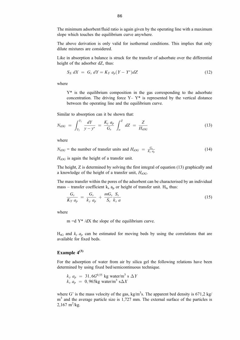
86
The minimum adsorbent/fluid ratio is again given by the operating line with a maximum
slope which touches the equilibrium curve anywhere.
The above derivation is only valid for isothermal conditions. This implies that only
dilute mixtures are considered.
Like in absorption a balance is struck for the transfer of adsorbate over the differential
height of the adsorber dZ, thus:
SS dX � Gs dY � KY ap�Yÿ Y��dZ (12)
where
Y* is the equilibrium composition in the gas corresponding to the adsorbate
concentration. The driving force Y± Y* is represented by the vertical distance
between the operating line and the equilibrium curve.
Similar to absorption can it be shown that:
NtOG �Z Y1
Y2
dY
yÿ y�� Ky ap
Gs
Z Z
o
dZ � Z
HtOG
(13)
where
NtOG = the number of transfer units and HtOG � Gs
Ky ap(14)
HtOG is again the height of a transfer unit.
The height, Z is determined by solving the first integral of equation (13) graphically and
a knowledge of the height of a transfer unit, HtOG.
The mass transfer within the pores of the adsorbent can be characterised by an individual
mass ± transfer coefficient ks ap or height of transfer unit. Hts thus:
Gs
KY ap� Gs
ky ap� mGs
Ss
Ss
ks a(15)
where
m =d Y* /dX the slope of the equilibrium curve.
HtG and ky ap can be estimated for moving beds by using the correlations that are
available for fixed beds.
Example 4(3)
For the adsorption of water from air by silica gel the following relations have been
determined by using fixed bed/semicontinuous technique.
ky ap � 31; 6G0;55 kg water/m3 s �Yks ap � 0; 965kg water/m3 s�X
where G' is the mass velocity of the gas, kg/m3s. The apparent bed density is 671,2 kg/
m3 and the average particle size is 1,727 mm. The external surface of the particles is
2,167 m2/kg.
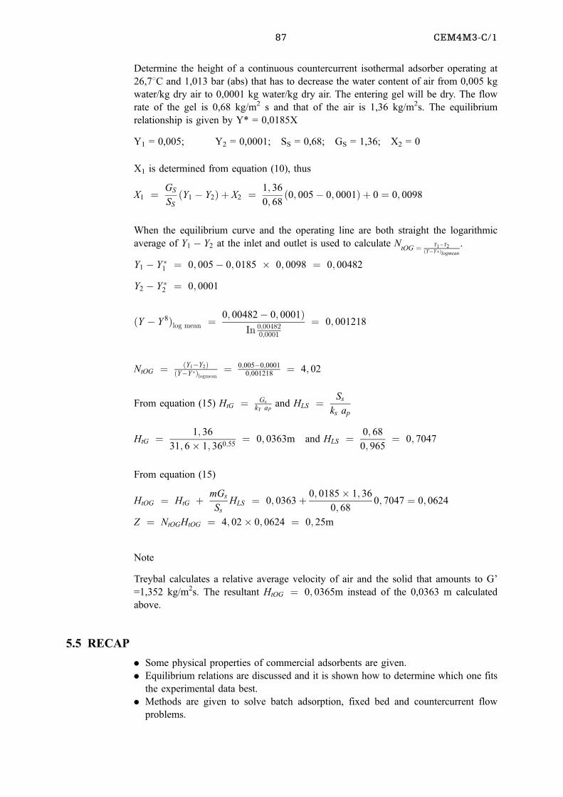
87 CEM4M3-C/1
Determine the height of a continuous countercurrent isothermal adsorber operating at
26,78C and 1,013 bar (abs) that has to decrease the water content of air from 0,005 kg
water/kg dry air to 0,0001 kg water/kg dry air. The entering gel will be dry. The flow
rate of the gel is 0,68 kg/m2 s and that of the air is 1,36 kg/m2s. The equilibrium
relationship is given by Y* = 0,0185X
Y1 = 0,005; Y2 = 0,0001; SS = 0,68; GS = 1,36; X2 = 0
X1 is determined from equation (10), thus
X1 � GS
SS
�Y1 ÿ Y2� � X2 � 1; 36
0; 68�0; 005ÿ 0; 0001� � 0 � 0; 0098
When the equilibrium curve and the operating line are both straight the logarithmic
average of Y1 ÿ Y2 at the inlet and outlet is used to calculate NtOG � Y1ÿY2
�YÿY��logmean
.
Y1 ÿ Y �1 � 0; 005ÿ 0; 0185 � 0; 0098 � 0; 00482
Y2 ÿ Y �2 � 0; 0001
�Y ÿ Y 8�log mean �0; 00482ÿ 0; 0001�
In 0;004820;0001
� 0; 001218
NtOG � �Y1ÿY2��YÿY ��logmean
� 0;005ÿ0;00010;001218
� 4; 02
From equation (15) HtG � Gs
kY aPand HLS � Ss
ks ap
HtG � 1; 36
31; 6� 1; 360;55� 0; 0363m and HLS � 0; 68
0; 965� 0; 7047
From equation (15)
HtOG � HtG � mGs
Ss
HLS � 0; 0363� 0; 0185� 1; 36
0; 680; 7047 � 0; 0624
Z � NtOGHtOG � 4; 02� 0; 0624 � 0; 25m
Note
Treybal calculates a relative average velocity of air and the solid that amounts to G'
=1,352 kg/m2s. The resultant HtOG � 0; 0365m instead of the 0,0363 m calculated
above.
5.5 RECAP
. Some physical properties of commercial adsorbents are given.
. Equilibrium relations are discussed and it is shown how to determine which one fits
the experimental data best.
. Methods are given to solve batch adsorption, fixed bed and countercurrent flow
problems.
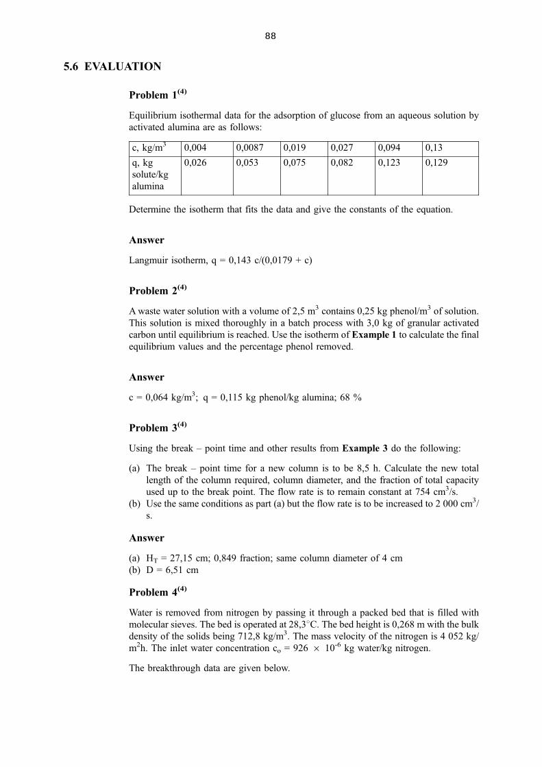
88
5.6 EVALUATION
Problem 1(4)
Equilibrium isothermal data for the adsorption of glucose from an aqueous solution by
activated alumina are as follows:
c, kg/m3 0,004 0,0087 0,019 0,027 0,094 0,13
q, kg
solute/kg
alumina
0,026 0,053 0,075 0,082 0,123 0,129
Determine the isotherm that fits the data and give the constants of the equation.
Answer
Langmuir isotherm, q = 0,143 c/(0,0179 + c)
Problem 2(4)
A waste water solution with a volume of 2,5 m3 contains 0,25 kg phenol/m3 of solution.
This solution is mixed thoroughly in a batch process with 3,0 kg of granular activated
carbon until equilibrium is reached. Use the isotherm of Example 1 to calculate the final
equilibrium values and the percentage phenol removed.
Answer
c = 0,064 kg/m3; q = 0,115 kg phenol/kg alumina; 68 %
Problem 3(4)
Using the break ± point time and other results from Example 3 do the following:
(a) The break ± point time for a new column is to be 8,5 h. Calculate the new total
length of the column required, column diameter, and the fraction of total capacity
used up to the break point. The flow rate is to remain constant at 754 cm3/s.
(b) Use the same conditions as part (a) but the flow rate is to be increased to 2 000 cm3/
s.
Answer
(a) HT = 27,15 cm; 0,849 fraction; same column diameter of 4 cm
(b) D = 6,51 cm
Problem 4(4)
Water is removed from nitrogen by passing it through a packed bed that is filled with
molecular sieves. The bed is operated at 28,38C. The bed height is 0,268 m with the bulk
density of the solids being 712,8 kg/m3. The mass velocity of the nitrogen is 4 052 kg/
m2h. The inlet water concentration co = 926 6 10-6 kg water/kg nitrogen.
The breakthrough data are given below.
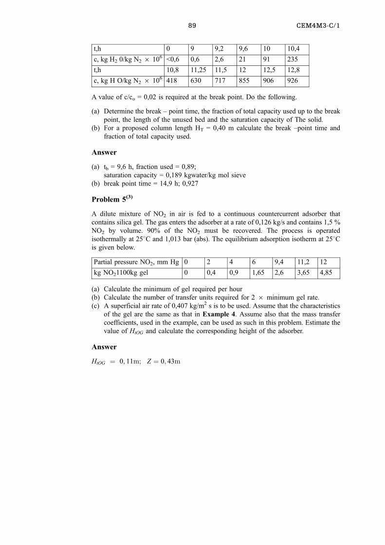
89 CEM4M3-C/1
t,h 0 9 9,2 9,6 10 10,4
c, kg H2 0/kg N2 6 106 <0,6 0,6 2,6 21 91 235
t,h 10,8 11,25 11,5 12 12,5 12,8
c, kg H O/kg N2 6 106 418 630 717 855 906 926
A value of c/co = 0,02 is required at the break point. Do the following.
(a) Determine the break ± point time, the fraction of total capacity used up to the break
point, the length of the unused bed and the saturation capacity of The solid.
(b) For a proposed column length HT = 0,40 m calculate the break ±point time and
fraction of total capacity used.
Answer
(a) tb = 9,6 h, fraction used = 0,89;
saturation capacity = 0,189 kgwater/kg mol sieve
(b) break point time = 14,9 h; 0,927
Problem 5(3)
A dilute mixture of NO2 in air is fed to a continuous countercurrent adsorber that
contains silica gel. The gas enters the adsorber at a rate of 0,126 kg/s and contains 1,5 %
NO2 by volume. 90% of the NO2 must be recovered. The process is operated
isothermally at 258C and 1,013 bar (abs). The equilibrium adsorption isotherm at 258Cis given below.
Partial pressure NO2, mm Hg 0 2 4 6 9,4 11,2 12
kg NO21100kg gel 0 0,4 0,9 1,65 2,6 3,65 4,85
(a) Calculate the minimum of gel required per hour
(b) Calculate the number of transfer units required for 2 6 minimum gel rate.
(c) A superficial air rate of 0,407 kg/m2 s is to be used. Assume that the characteristics
of the gel are the same as that in Example 4. Assume also that the mass transfer
coefficients, used in the example, can be used as such in this problem. Estimate the
value of HtOG and calculate the corresponding height of the adsorber.
Answer
HtOG � 0; 11m; Z � 0; 43m
90
CHAPTER 6
Crystallisation
CONTENTS
6.1 LEARNING OUTCOMES 00
6.2 INTRODUCTION 00
6.2.1 Effect of Temperature on the Solubility of Solutes 00
6.2.2 Fractional Crystallisation 00
6.2.3 Yield of Crystals 00
6.2.4 Vacuum Operation 00
6.2.5 Some Types of Crystallisers 00
6.3 RECAP 00
6.4 EVALUATION 00
6.1 LEARNING OUTCOMES
After completion of this section a student should know how some common types of
crystallisers look and how they function.
. Be able to do solute and solvent balances
. Be able to determine the energy requirements of crystallisers.
. Be able to use equilibrium diagrams
6.2 INTRODUCTION
Crystallisation is an operation which allows a solute to be recovered as solid crystals
from a solution. It can be used to purify mixtures or to produce crystals with the desired
size range.
The production of sugar from sugar cane or beetroot is an example of a large scale
crystallisation process.
Crystallisation is effected by either lowering the temperature of a solution or by
evaporating some of the solvent. The energy that is required during a cooling process
includes the sensible heat of the solution and the heat of crystallisation. In the
evaporative process the major energy requirement is the latent heat of vapourisation of
the solvent. Benzene's heat of crystallization is 126 kJ/kg while its latent heat of
vapourisation is 394 kJ/kg. It is thus clear that, from an energy point of view, cooling is
the preferred process.
The crystallization process consists essentially of two stages which proceed
simultaneously. The first is the formation of nuclei, which must exist in the solution
before crystallization will commence. This is followed by the growth of the crystals.
Normally a degree of super ± cooling is required before crystallization will commence.
A metastable condition thus exists at temperatures that are slightly below the
temperature where nucleation should start.
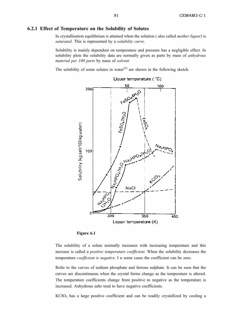
91 CEM4M3-C/1
6.2.1 Effect of Temperature on the Solubility of Solutes
In crystallisation equilibrium is attained when the solution ( also called mother liquor) is
saturated. This is represented by a solubility curve.
Solubility is mainly dependent on temperature and pressure has a negligible effect. In
solubility plots the solubility data are normally given as parts by mass of anhydrous
material per 100 parts by mass of solvent
The solubility of some solutes in water(2) are shown in the following sketch.
The solubility of a solute normally increases with increasing temperature and this
increase is called a positive temperature coefficient. When the solubility decreases the
temperature coefficient is negative. I n some cases the coefficient can be zero.
Refer to the curves of sodium phosphate and ferrous sulphate. It can be seen that the
curves are discontinuous when the crystal forms change as the temperature is altered.
The temperature coefficients change from positive to negative as the temperature is
increased. Anhydrous salts tend to have negative coefficients.
KCIO3 has a large positive coefficient and can be readily crystallized by cooling a
Figure 6.1
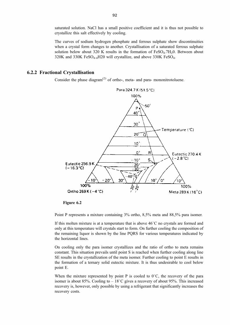
92
saturated solution. NaCl has a small positive coefficient and it is thus not possible to
crystallize this salt effectively by cooling.
The curves of sodium hydrogen phosphate and ferrous sulphate show discontinuities
when a crystal form changes to another. Crystallisation of a saturated ferrous sulphate
solution below about 320 K results in the formation of FeSO4.7H20. Between about
320K and 330K FeSO4.4H20 will crystallize, and above 330K FeSO4.
6.2.2 Fractional Crystallisation
Consider the phase diagram(2) of ortho-, meta- and para- mononitrotoluene.
Point P represents a mixture containing 3% ortho, 8,5% meta and 88,5% para isomer.
If this molten mixture is at a temperature that is above 468C no crystals are formed and
only at this temperature will crystals start to form. On further cooling the composition of
the remaining liquor is shown by the line PQRS for various temperatures indicated by
the horizontal lines.
On cooling only the para isomer crystallizes and the ratio of ortho to meta remains
constant. This situation prevails until point S is reached when further cooling along line
SE results in the crystallization of the meta isomer. Further cooling to point E results in
the formation of a ternary solid eutectic mixture. It is thus undesirable to cool below
point E.
When the mixture represented by point P is cooled to 08C, the recovery of the para
isomer is about 85%. Cooling to ± 188C gives a recovery of about 95%. This increased
recovery is, however, only possible by using a refrigerant that significantly increases the
recovery costs.
Figure 6.2
93 CEM4M3-C/1
Note: An eutectic mixture is defined as one in which the constituents are in such
proportions as to solidify at one temperature.
6.2.3 Yield of Crystals
The yield of crystals can be calculated by doing solvent and solute balances. The initial
and final concentrations of the solute must be known.
When the solvent is water hydrated salts can form at certain temperatures, and this
aspect must be taken account of. The initial solvent present is then equal to the sum of
the final solvent in the mother liquor, the crystal water in the hydrated salts and any
water that has evaporated.
A water balance is then: w1 � w2 � �yÿ Y
R� � w1 E (1)
where: w, ,w2 are the initial and final masses of solvent (water)
y is the yield of crystals
R is the ratio of the molecular mass of the hydrate / molecular mass of anhydrous
salt
E ratio of mass of solvent evaporated 1 mass of solvent initially present
A solute balance gives: w1 C1 � w2 C2 � Y
R(2)
where c1; c2 are the initial and final concentrations of the anhydrous salt expressed as
mass of anhydrous salt/unit mass of solvent.
From equation (1)
w2 � w1�1ÿ E� ÿ y�Rÿ 1�R
(3)
It can be shown that by substituting (3) in (2) that:
y � Rw1�c1 ÿ c2 �1ÿ E���1ÿ c2 �Rÿ 1�� (4)
Note: mother liquor is a term frequently used instead of solution.
Example 1(2)
A solution of 500 kg Na2 SO4 in 2500 kg of water is cooled from 333 K to 283 K in an
agitated mild steel crystalliser. At 283 K the stable crystalline form is ...
Na2 SO4.10 H2O. During cooling 2 mass % of water is lost by evaporation. Estimate the
yield of crystals. At 283 K the solubility of Na2 SO4 is 8,9 kg/100 kg water.
R = 322/142 = 2,27
c1 = 500/2500 = 0,2 kg/kg water
c2 = 8,9/100 = 0,089
w1 = 2 500 kg water
E = 0,02 kg/kg water
Equation (4) then gives:
94
y � 2; 27� 2500� �0; 2ÿ 0; 089�1ÿ 0; 02���1ÿ 0; 089�2; 27ÿ 1�� � 722kg
Example 2
Determine the heat that must be removed for the above example given the following:
mass of mild steel crystalliser = 750 kg
specific heat of mild steel = 0,5 kJ/kg K
heat of solution of Na2 SO4.10 H20 = ±78,5 MJ/kmol
specific heat of solution = 3,6 kJ/kg K
latent heat of vapourisation = 2 400 kJ/kg
Heat of crystallization is the opposite of the heat of solution
= + 78,5 MJ/kmol = 78500/322 = 243,8 kJ/kg
Thus heat of crystallization = 243,8 6 723 =176 267 kJ
Heat removed to cool crystalliser = 750 6 0,5 (333 ± 283) =18750 kJ
Heat removed by cooling the solution = (500 + 2500) 6 3,6 6 50 = 540000 kJ
Heat lost by vapourisation of 2% water = 2500 6 0,02 6 2400 = 120000 kJ
Heat to be removed = 176267 + 18750 + 540000 ± 120000 = 615017 Kj
6.2.4 Vacuum Operation
Crystallisers are frequently operated under a vacuum. The amount of evaporation(2) can
be calculated by using the following formula that is based on a heat balance.
Heat balance:
Solvent evaporated 6 latent heat = drop in sensible heat +heat of crystallisation
Thus:
Ew1 � � Cp�T1 ÿ T2�W1 �1� c1� � qc y (5)
where:
� is the latent heat per unit mass
qc is the heat of crystallisation
Cp is the mean heat capacity of the solution
T1 and T2 are the initial and final temperature of the solution
w1 is the initial mass of solvent in the liquor
c1 is the initial concentration of the solution (mass of anhydrous salt per unit
mass of solvent)
Substituting equation (4) in (5) yields:
E � qcR�c1 ÿ c2� � CP�T1 ÿ T2��1� c1��1ÿ c2�Rÿ 1����I ÿ c2�Rÿ 1�� ÿ qcRc2
(6)
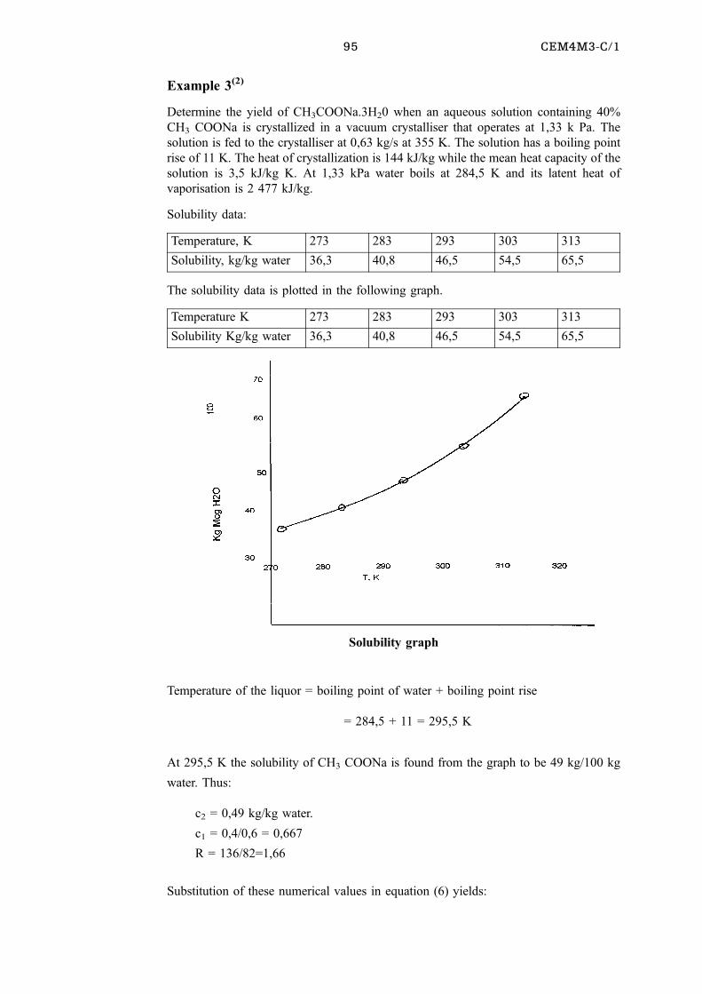
95 CEM4M3-C/1
Example 3(2)
Determine the yield of CH3COONa.3H20 when an aqueous solution containing 40%
CH3 COONa is crystallized in a vacuum crystalliser that operates at 1,33 k Pa. The
solution is fed to the crystalliser at 0,63 kg/s at 355 K. The solution has a boiling point
rise of 11 K. The heat of crystallization is 144 kJ/kg while the mean heat capacity of the
solution is 3,5 kJ/kg K. At 1,33 kPa water boils at 284,5 K and its latent heat of
vaporisation is 2 477 kJ/kg.
Solubility data:
Temperature, K 273 283 293 303 313
Solubility, kg/kg water 36,3 40,8 46,5 54,5 65,5
The solubility data is plotted in the following graph.
Temperature K 273 283 293 303 313
Solubility Kg/kg water 36,3 40,8 46,5 54,5 65,5
Solubility graph
Temperature of the liquor = boiling point of water + boiling point rise
= 284,5 + 11 = 295,5 K
At 295,5 K the solubility of CH3 COONa is found from the graph to be 49 kg/100 kg
water. Thus:
c2 = 0,49 kg/kg water.
c1 = 0,4/0,6 = 0,667
R = 136/82=1,66
Substitution of these numerical values in equation (6) yields:
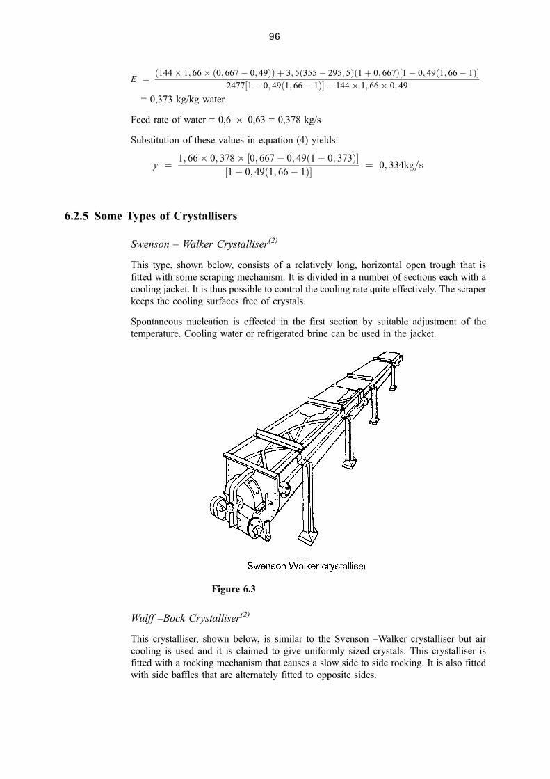
96
E � �144� 1; 66� �0; 667ÿ 0; 49�� � 3; 5�355ÿ 295; 5��1� 0; 667��1ÿ 0; 49�1; 66ÿ 1��2477�1ÿ 0; 49�1; 66ÿ 1�� ÿ 144� 1; 66� 0; 49
= 0,373 kg/kg water
Feed rate of water = 0,6 6 0,63 = 0,378 kg/s
Substitution of these values in equation (4) yields:
y � 1; 66� 0; 378� �0; 667ÿ 0; 49�1ÿ 0; 373���1ÿ 0; 49�1; 66ÿ 1�� � 0; 334kg=s
6.2.5 Some Types of Crystallisers
Swenson ± Walker Crystalliser(2)
This type, shown below, consists of a relatively long, horizontal open trough that is
fitted with some scraping mechanism. It is divided in a number of sections each with a
cooling jacket. It is thus possible to control the cooling rate quite effectively. The scraper
keeps the cooling surfaces free of crystals.
Spontaneous nucleation is effected in the first section by suitable adjustment of the
temperature. Cooling water or refrigerated brine can be used in the jacket.
Wulff ±Bock Crystalliser(2)
This crystalliser, shown below, is similar to the Svenson ±Walker crystalliser but air
cooling is used and it is claimed to give uniformly sized crystals. This crystalliser is
fitted with a rocking mechanism that causes a slow side to side rocking. It is also fitted
with side baffles that are alternately fitted to opposite sides.
Figure 6.3
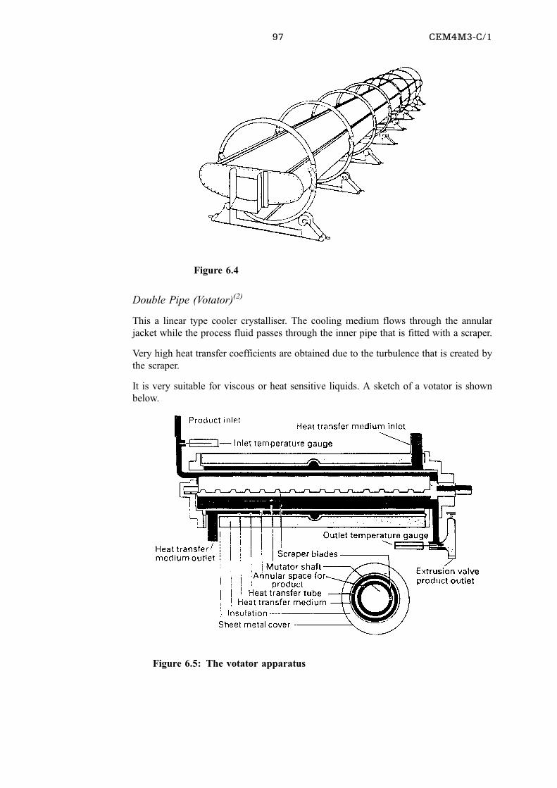
97 CEM4M3-C/1
Double Pipe (Votator)(2)
This a linear type cooler crystalliser. The cooling medium flows through the annular
jacket while the process fluid passes through the inner pipe that is fitted with a scraper.
Very high heat transfer coefficients are obtained due to the turbulence that is created by
the scraper.
It is very suitable for viscous or heat sensitive liquids. A sketch of a votator is shown
below.
Figure 6.4
Figure 6.5: The votator apparatus
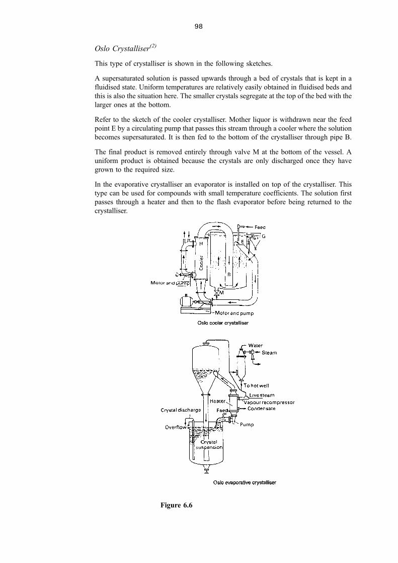
98
Oslo Crystalliser(2)
This type of crystalliser is shown in the following sketches.
A supersaturated solution is passed upwards through a bed of crystals that is kept in a
fluidised state. Uniform temperatures are relatively easily obtained in fluidised beds and
this is also the situation here. The smaller crystals segregate at the top of the bed with the
larger ones at the bottom.
Refer to the sketch of the cooler crystalliser. Mother liquor is withdrawn near the feed
point E by a circulating pump that passes this stream through a cooler where the solution
becomes supersaturated. It is then fed to the bottom of the crystalliser through pipe B.
The final product is removed entirely through valve M at the bottom of the vessel. A
uniform product is obtained because the crystals are only discharged once they have
grown to the required size.
In the evaporative crystalliser an evaporator is installed on top of the crystalliser. This
type can be used for compounds with small temperature coefficients. The solution first
passes through a heater and then to the flash evaporator before being returned to the
crystalliser.
Figure 6.6
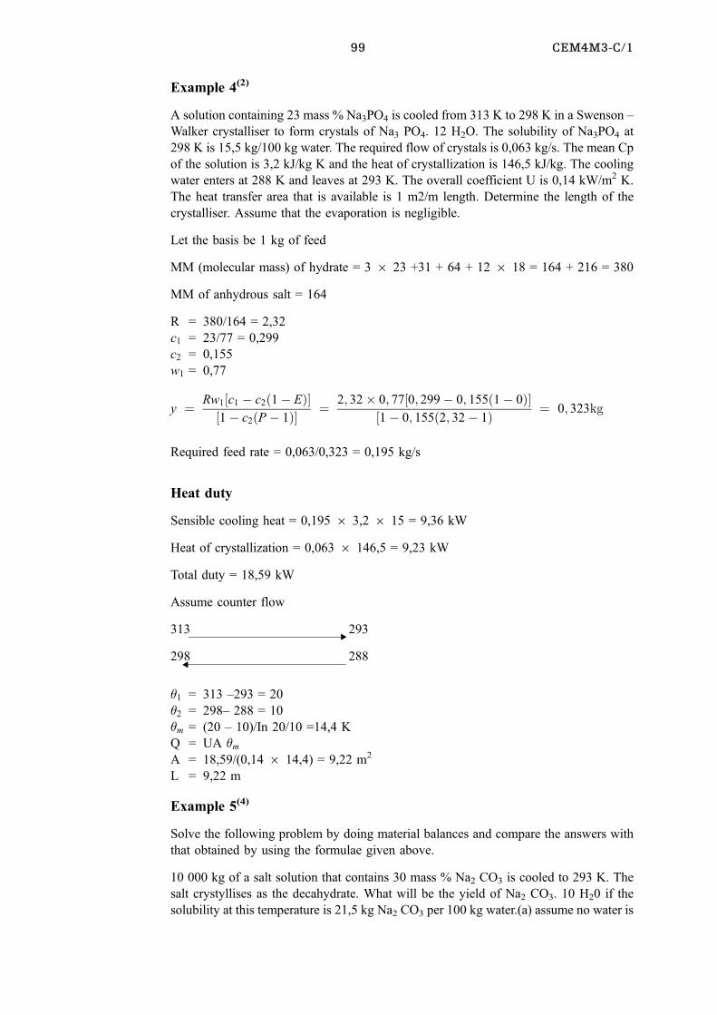
99 CEM4M3-C/1
!
!
Example 4(2)
A solution containing 23 mass % Na3PO4 is cooled from 313 K to 298 K in a Swenson ±
Walker crystalliser to form crystals of Na3 PO4. 12 H2O. The solubility of Na3PO4 at
298 K is 15,5 kg/100 kg water. The required flow of crystals is 0,063 kg/s. The mean Cp
of the solution is 3,2 kJ/kg K and the heat of crystallization is 146,5 kJ/kg. The cooling
water enters at 288 K and leaves at 293 K. The overall coefficient U is 0,14 kW/m2 K.
The heat transfer area that is available is 1 m2/m length. Determine the length of the
crystalliser. Assume that the evaporation is negligible.
Let the basis be 1 kg of feed
MM (molecular mass) of hydrate = 3 6 23 +31 + 64 + 12 6 18 = 164 + 216 = 380
MM of anhydrous salt = 164
R = 380/164 = 2,32
c1 = 23/77 = 0,299
c2 = 0,155
w1 = 0,77
y � Rw1�c1 ÿ c2�1ÿ E���1ÿ c2�P ÿ 1�� � 2; 32� 0; 77�0; 299ÿ 0; 155�1ÿ 0��
�1ÿ 0; 155�2; 32ÿ 1� � 0; 323kg
Required feed rate = 0,063/0,323 = 0,195 kg/s
Heat duty
Sensible cooling heat = 0,195 6 3,2 6 15 = 9,36 kW
Heat of crystallization = 0,063 6 146,5 = 9,23 kW
Total duty = 18,59 kW
Assume counter flow
313 293
298 288
�1 = 313 ±293 = 20
�2 = 298± 288 = 10
�m = (20 ± 10)/In 20/10 =14,4 K
Q = UA �m
A = 18,59/(0,14 6 14,4) = 9,22 m2
L = 9,22 m
Example 5(4)
Solve the following problem by doing material balances and compare the answers with
that obtained by using the formulae given above.
10 000 kg of a salt solution that contains 30 mass % Na2 CO3 is cooled to 293 K. The
salt crystyllises as the decahydrate. What will be the yield of Na2 CO3. 10 H20 if the
solubility at this temperature is 21,5 kg Na2 CO3 per 100 kg water.(a) assume no water is
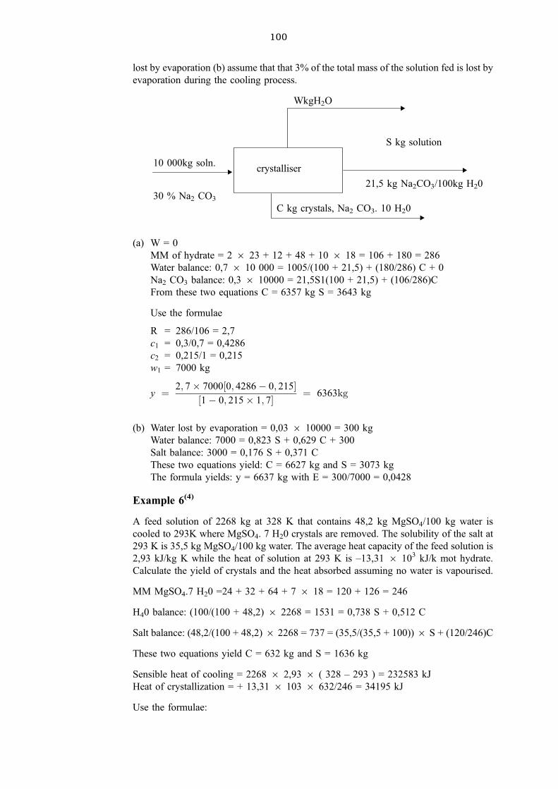
100
!
!
!
!
lost by evaporation (b) assume that that 3% of the total mass of the solution fed is lost by
evaporation during the cooling process.
WkgH2O
S kg solution
10 000kg soln.crystalliser
21,5 kg Na2CO3/100kg H20
30 % Na2 CO3
C kg crystals, Na2 CO3. 10 H20
(a) W = 0
MM of hydrate = 2 6 23 + 12 + 48 + 10 6 18 = 106 + 180 = 286
Water balance: 0,7 6 10 000 = 1005/(100 + 21,5) + (180/286) C + 0
Na2 CO3 balance: 0,3 6 10000 = 21,5S1(100 + 21,5) + (106/286)C
From these two equations C = 6357 kg S = 3643 kg
Use the formulae
R = 286/106 = 2,7
c1 = 0,3/0,7 = 0,4286
c2 = 0,215/1 = 0,215
w1 = 7000 kg
y � 2; 7� 7000�0; 4286ÿ 0; 215��1ÿ 0; 215� 1; 7� � 6363kg
(b) Water lost by evaporation = 0,03 6 10000 = 300 kg
Water balance: 7000 = 0,823 S + 0,629 C + 300
Salt balance: 3000 = 0,176 S + 0,371 C
These two equations yield: C = 6627 kg and S = 3073 kg
The formula yields: y = 6637 kg with E = 300/7000 = 0,0428
Example 6(4)
A feed solution of 2268 kg at 328 K that contains 48,2 kg MgSO4/100 kg water is
cooled to 293K where MgSO4. 7 H20 crystals are removed. The solubility of the salt at
293 K is 35,5 kg MgSO4/100 kg water. The average heat capacity of the feed solution is
2,93 kJ/kg K while the heat of solution at 293 K is ±13,31 6 103 kJ/k mot hydrate.
Calculate the yield of crystals and the heat absorbed assuming no water is vapourised.
MM MgSO4.7 H20 =24 + 32 + 64 + 7 6 18 = 120 + 126 = 246
H40 balance: (100/(100 + 48,2) 6 2268 = 1531 = 0,738 S + 0,512 C
Salt balance: (48,2/(100 + 48,2) 6 2268 = 737 = (35,5/(35,5 + 100)) 6 S + (120/246)C
These two equations yield C = 632 kg and S = 1636 kg
Sensible heat of cooling = 2268 6 2,93 6 ( 328 ± 293 ) = 232583 kJ
Heat of crystallization = + 13,31 6 103 6 632/246 = 34195 kJ
Use the formulae:
101 CEM4M3-C/1
R = 46/120 = 2,05
w1 = 2268 6 (100/(100 + 48,2)) = 1531 kg
c1 = 0,482
c2 = 0,325
y � 2; 05� 1531� f0; 482ÿ 0; 355��1ÿ 0; 355� 1; 05� � 635 kg and S = 2268± 635=1633 kg
Sensible heat of cooling = 2268 6 2,93 6 (328 ± 293) = 232583 kJ
Heat of crystallization = + 13,31 6 103 6 632/246 = 34194 kJ
Heat to be removed = 232583 + 34194 = 266777 say 266800 kJ
6.3 RECAP
. Crystallisation is introduced to the student
. Some typical equilibrium diagrams are discussed
. The fractional crystallisation of an isomer from a mixture of isomers is discussed
. Equations are derived that can be used to do material balances of the solvent and the
solute
. It is shown how energy balances can be made for crystallisers
. Some types of crystallisers and their operation are discussed
6.4 EVALUATION
Problem 1(4)
1 000 kg of KCI is dissolved in sufficient water to make a saturated solution at 363 K. At
this temperature the solubility of KCI is 35 mass %. The solution is cooled to 293 K at
which temperature the solubility is 25,4 mass %.
Determine:
(a) the mass of water required to obtain the required solution and the mass of KCI
crystals formed after the solution has been cooled to 293 K and what is the amount
of crystals obtained if no water evaporates?
(b) What is the mass of crystals obtained if 5% of the original water evaporates on
cooling?
Answer
(a) 1857 kg water, 368 kg crystals
(b) 399 kg crystals
Problem 2(4)
A feed solution of 4500 kg at 548C containing 47 kg FeSO4/100 kg water is cooled to
278C where FeSO4. 7 H20 crystals are removed. At 278C the solubility is 30,5 kg
FeSO4/1 00 kg water. The average heat capacity of the feed solution is 2,92 kJ/kg K. The
heat of solution is ±18400 kJ/k mol FeSO4.7H2O. Calculate the yield of crystals and
determine the amount of heat that must be removed. Assume that no water is vapourised.
102
Answer
1233 kg FeSO4.7H2O; heat to be removed = 436 400 kJ.
Problem 3(4)
A hot aqueous solution of Ba (NO3)2 contains 30,6 kg Ba(NO3)2/100 kg water. This
stream is fed to a crystalliser where the solution is cooled and Ba (NO3)2 crystallises. On
cooling 10% of the original water present evaporates. For a feed solution of 100 kg
calculate:
(a) the yield of crystals if the solution is cooled to 290 K where the solubility is 8,6 kg
Ba (NO3)2 /100 kg water
(b) the yield if the solution is cooled to 283 K where the solubility is 7,0 kg Ba (NO3)2/
100 kg water.
Answer:
(a) 17,51 kg Ba (NO3)2 crystals
(b) 18,6 kg Ba (NO3)2 crystals
Problem 4(2)
Na2 SO4.10 H2O is to be produced in a Swenson ±Walker crystalliser by cooling an
aqueous solution of Na2SO4 to 290 K which saturates at 300 K. Cooling water enters
and leaves the unit at 280 K and 290 K respectively. How many sections of crystalliser,
each 3 m long, will be required to process 0,25 kg/s of the product? The solubilities of
anhydrous Na2 SO4 in water are 40 and 14 kg/100 kg water at 300 K and 290 K
respectively. The mean heat capacity of the liquor is 3,8 kJ/kg K and the heat of
crystallisation is 230 kJ/kg. For this crystalliser the available heat transfer area is 3 m2/m
length. The overall heat transfer coefficient is 0,15 kW/m2K. The molecular masses are:
Na2SO4.10 H2O = 322 kg/kmol and Na2SO4 = 142 kg/k mol. Assume no evaporation.
Answer: about 9
Problem 5(2)
What is the evaporation rate and yield of CH3COONa.3H2O from a continuous
evaporative crystalliser operating at 1 kPa when it is fed with 1 kg/s of a 50 mass %
aqueous solution of CH3COONa at 350 K? The boiling point rise of the solution is 10 K
and the heat of crystallisation is 150 kJ/kg. The mean heat capacity of the solution is 3,5
kJ/kg K and 1 kPa water boils at 280 K at which temperature the latent heat of
vapourisation is 2 482 kJ/kg. Over the temperature range 270 to 305 K the solubility of
CH3OOONa in water s at T (K) is given by s = 0,61 T 132,4; kg/100 kg water.
MM of CH3COONa.3 H2O =136 kg/k mol and that of CH3COONa = 82 kg/k mol.
Answer
Evaporation rate, E = 0,265 kg/kg water (0,132 kg/s); y = 0,79 kg/s
103 CEM4M3-C/1
CHAPTER 7
Fluidisation
CONTENTS
7.1 OUTCOMES 00
7.2 INTRODUCTION(2) 00
7.2.1 Effect of Fluid Velocity and Pressure Gradient 00
7.2.2 Pressure Drop(2), (4) 00
7.2.3 Minimum Fluidising Velocity 00
7.2.4 Minimum Fluidising Velocity for Non ±spherical Particles(4) 00
7.2.5 Relation Between Bed Height and Porosity 00
7.2.6 Effective Mean Diameter of Particles With Different Sizes 00
7.2.7 Expansion of Fluidised Bede) 00
7.2.8 Heat Transfer From or To a Surface 00
7.2.9 Heat Transfer Between Fluid and Particles 00
7.2.10 Mass Transfer Between Fluid and Particle 00
7.2.11 Fluidised Bed Applications 00
7.3 RECAP 00
7.4 EVALUATION 00
7.1 OUTCOMES
. The student should have a good understanding of this process that is gaining
importance in a range of industrial applications.
. The student should be able to calculate the pressure drop at calculated fluid velocity
through the bed.
. The student should be able to determine the minimum fluidising velocity.
. The student should be able to calculate the bed height at given fluidising velocities.
. The student should be able to distinguish the two types of fluidisation.
7.2 INTRODUCTION(2)
When a fluid passes downwards through a bed of solids particles, called a packed bed,
there is no movement of the particles relative to each other.
This is not necessarily the case when the flow is upwards. At low linear velocities there
will still be no movement of the particles and the pressure drop will be same for both
cases.
As the flow is increased the frictional drag on the particles becomes equal to their weight
less buoyancy and they become rearranged. They then offer less resistance to the flow of
the fluid and the bed starts to expand.
This process continues as the linear velocity of the fluid is increased until the bed has
assumed the loosest stable form of packing. If the velocity of the fluid is further
increased the individual particles are separated and the bed has reached the fluidized
state.
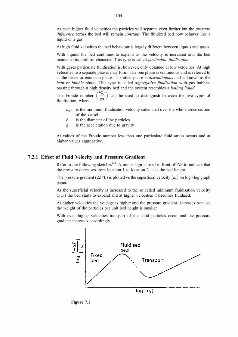
104
At even higher fluid velocities the particles will separate even further but the pressure
difference across the bed will remain constant. The fluidized bed now behaves like a
liquid or a gas.
At high fluid velocities the bed behaviour is largely different between liquids and gases.
With liquids the bed continues to expand as the velocity is increased and the bed
maintains its uniform character. This type is called particulate fluidisation.
With gases particulate fluidisation is, however, only obtained at low velocities. At high
velocities two separate phases may form. The one phase is continuous and is referred to
as the dense or emulsion phase. The other phase is discontinuous and is known as the
lean or bubble phase. This type is called aggregative fluidisation with gas bubbles
passing through a high density bed and the system resembles a boiling liquid.
The Froude number� u2
mf
gd
�can be used to distinguish between the two types of
fluidisation, where
umf is the minimum fluidisation velocity calculated over the whole cross section
of the vessel
d is the diameter of the particles
g is the acceleration due to gravity
At values of the Froude number less than one particulate fluidisation occurs and at
higher values aggregative.
7.2.1 Effect of Fluid Velocity and Pressure Gradient
Refer to the following sketches(2). A minus sign is used in front of �P to indicate that
the pressure decreases from location 1 to location 2. L is the bed height.
The pressure gradient (�P/L) is plotted vs the superficial velocity �uc� on log ±log graph
paper.
As the superficial velocity is increased to the so called minimum fluidisation velocity
�umf � the bed starts to expand and at higher velocities it becomes fluidised.
At higher velocities the voidage is higher and the pressure gradient decreases because
the weight of the particles per unit bed height is smaller.
With even higher velocities transport of the solid particles occur and the pressure
gradient increases accordingly.
Figure 7.1
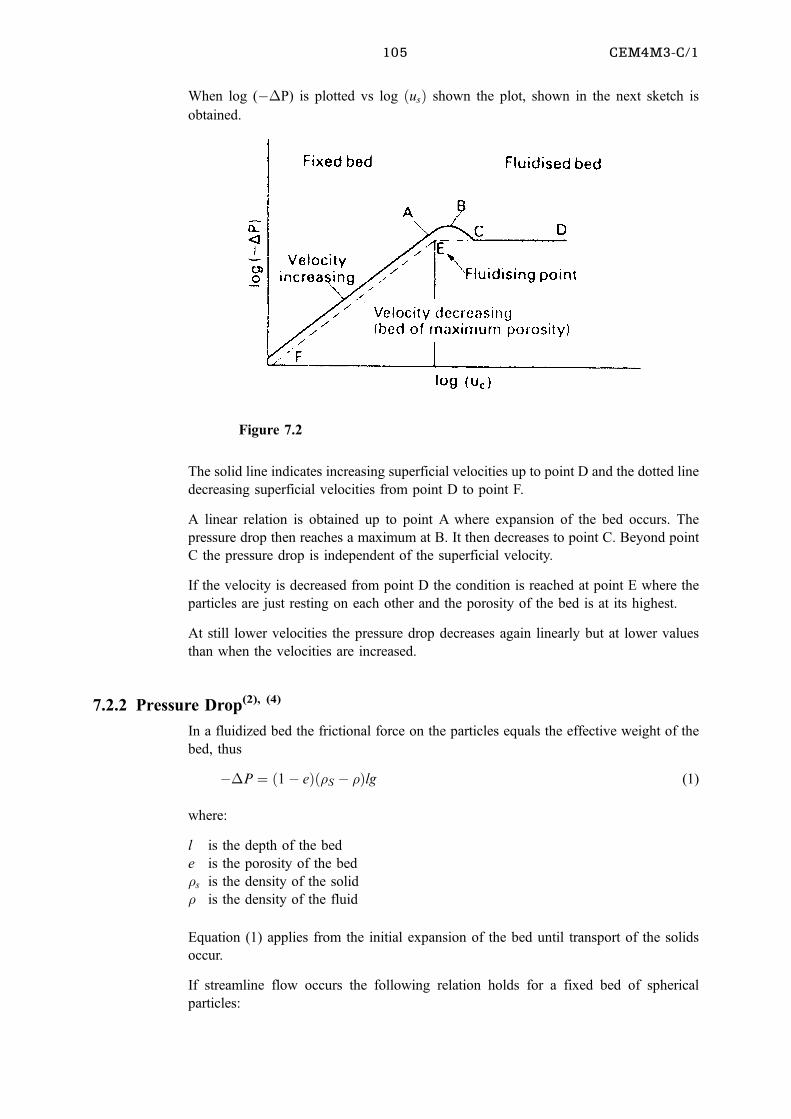
105 CEM4M3-C/1
When log (ÿ�P) is plotted vs log �us� shown the plot, shown in the next sketch is
obtained.
The solid line indicates increasing superficial velocities up to point D and the dotted line
decreasing superficial velocities from point D to point F.
A linear relation is obtained up to point A where expansion of the bed occurs. The
pressure drop then reaches a maximum at B. It then decreases to point C. Beyond point
C the pressure drop is independent of the superficial velocity.
If the velocity is decreased from point D the condition is reached at point E where the
particles are just resting on each other and the porosity of the bed is at its highest.
At still lower velocities the pressure drop decreases again linearly but at lower values
than when the velocities are increased.
7.2.2 Pressure Drop(2), (4)
In a fluidized bed the frictional force on the particles equals the effective weight of the
bed, thus
ÿ�P � �1ÿ e���S ÿ ��lg (1)
where:
l is the depth of the bed
e is the porosity of the bed
�s is the density of the solid
� is the density of the fluid
Equation (1) applies from the initial expansion of the bed until transport of the solids
occur.
If streamline flow occurs the following relation holds for a fixed bed of spherical
particles:
Figure 7.2
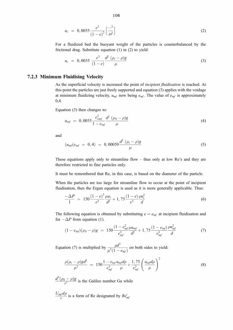
106
uc � 0; 0055e3
�1ÿ e�2hÿ2
�l
i(2)
For a fluidized bed the buoyant weight of the particles is counterbalanced by the
frictional drag. Substitute equation (1) in (2) to yield:
uc � 0; 0055e3
�1ÿ e�d2 ��s ÿ ��g
�(3)
7.2.3 Minimum Fluidising Velocity
As the superficial velocity is increased the point of incipient fluidisation is reached. At
this point the particles are just freely supported and equation (3) applies with the voidage
at minimum fluidizing velocity, umf now being emf . The value of emf is approximately
0,4.
Equation (3) then changes to:
umf � 0; 0055e3emf
1ÿ emf
d2 ��S ÿ ��g�
(4)
and
�umf�emf � 0; 4� � 0; 00059d2 ��s ÿ ��g
�(5)
These equations apply only to streamline flow ± thus only at low Re's and they are
therefore restricted to fine particles only.
It must be remembered that Re, in this case, is based on the diameter of the particle.
When the particles are too large for streamline flow to occur at the point of incipient
fluidisation, then the Ergun equation is used as it is more generally applicable. Thus:
ÿ�P
1� 150
�1ÿ e�2e3
�ucd2� 1; 75
�1ÿ e�e3
�u2cd
(6)
The following equation is obtained by substituting e � emf at incipient fluidisation and
for ÿ�P from equation (1).
�1ÿ emf���S ÿ ��g � 150�1ÿ e2mf
e3mf
�umf
d2� 1; 75
�1ÿ emf�e3mf
�u2mf
d(7)
Equation (7) is multiplied by�d3
�2�1ÿ emf � on both sides to yield:
���s ÿ ��gd3�2
� 1501ÿ emf
e3mf
umfd�
�� 1; 75
e3mf
umfd�
�
!2
(8)
d3��S ÿ ��g�2 is the Galileo number Ga while
Umf d�� is a form of Re designated by Re0mf
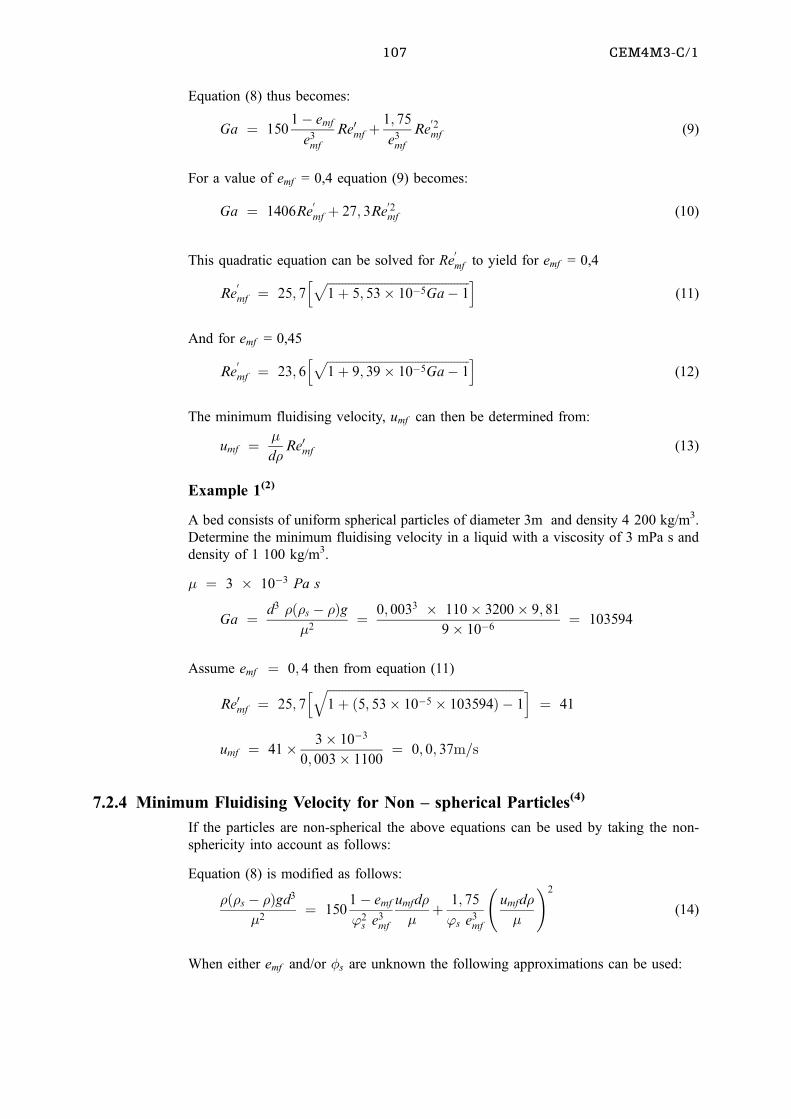
107 CEM4M3-C/1
Equation (8) thus becomes:
Ga � 1501ÿ emf
e3mf
Re0mf �1; 75
e3mf
Re02mf (9)
For a value of emf = 0,4 equation (9) becomes:
Ga � 1406Re0mf � 27; 3Re
02mf (10)
This quadratic equation can be solved for Re0mf to yield for emf = 0,4
Re0mf � 25; 7
h �����������������������������������������������1� 5; 53� 10ÿ5Gaÿ 1
p i(11)
And for emf = 0,45
Re0mf � 23; 6
h �����������������������������������������������1� 9; 39� 10ÿ5Gaÿ 1
p i(12)
The minimum fluidising velocity, umf can then be determined from:
umf � �
d�Re0mf (13)
Example 1(2)
A bed consists of uniform spherical particles of diameter 3m and density 4 200 kg/m3.
Determine the minimum fluidising velocity in a liquid with a viscosity of 3 mPa s and
density of 1 100 kg/m3.
� � 3 � 10ÿ3 Pa s
Ga � d3 ���s ÿ ��g�2
� 0; 0033 � 110� 3200� 9; 81
9� 10ÿ6� 103594
Assume emf � 0; 4 then from equation (11)
Re0mf � 25; 7h �����������������������������������������������������������������
1� �5; 53� 10ÿ5 � 103594� ÿ 1q i
� 41
umf � 41� 3� 10ÿ3
0; 003� 1100� 0; 0; 37m=s
7.2.4 Minimum Fluidising Velocity for Non ± spherical Particles(4)
If the particles are non-spherical the above equations can be used by taking the non-
sphericity into account as follows:
Equation (8) is modified as follows:
���s ÿ ��gd3�2
� 1501ÿ emf
'2s e3mf
umfd�
�� 1; 75
's e3mf
umfd�
�
!2
(14)
When either emf and/or �s are unknown the following approximations can be used:
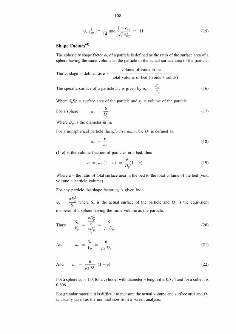
108
's e3mf �
1
14and
1ÿ emf
'2s e3mf
� 11 (15)
Shape Factors(4)
The sphericity shape factor �s of a particle is defined as the ratio of the surface area of a
sphere having the same volume as the particle to the actual surface area of the particle.
volume of voids in bedThe voidage is defined as e = ÐÐÐÐÐÐÐÐÐÐÐÐÐÐÐÐ
total volume of bed ( voids + solids)
The specific surface of a particle av, is given by av � Sp
Vp
(16)
Where SpSp = surface area of the particle and vp = volume of the particle
For a sphere av � 6
Dp
(17)
Where Dp is the diameter in m.
For a nonspherical particle the effective diameter, Dp is defined as:
av � 6
av(18)
(1±e) is the volume fraction of particles in a bed, thus
a � av �1ÿ e� � 6
Dp�1ÿ e� (19)
Where a = the ratio of total surface area in the bed to the total volume of the bed (void
volume + particle volume).
For any particle the shape factor 's is given by:
's ��D2
p
Sp
where Sp is the actual surface of the particle and Dp is the equivalent
diameter of a sphere having the same volume as the particle.
Thus:Sp
Vp
��D2
p's
�D3p
6
� 6
's Dp
(20)
And av � Sp
Vp
� 6
'2 Dp
(21)
And av � 6
'2 Dp
�1ÿ e� (22)
For a sphere �s is 1,0, for a cylinder with diameter = length it is 0,874 and for a cube it is
0,806.
For granular material it is difficult to measure the actual volume and surface area and Dp
is usually taken as the nominal size from a screen analysis.
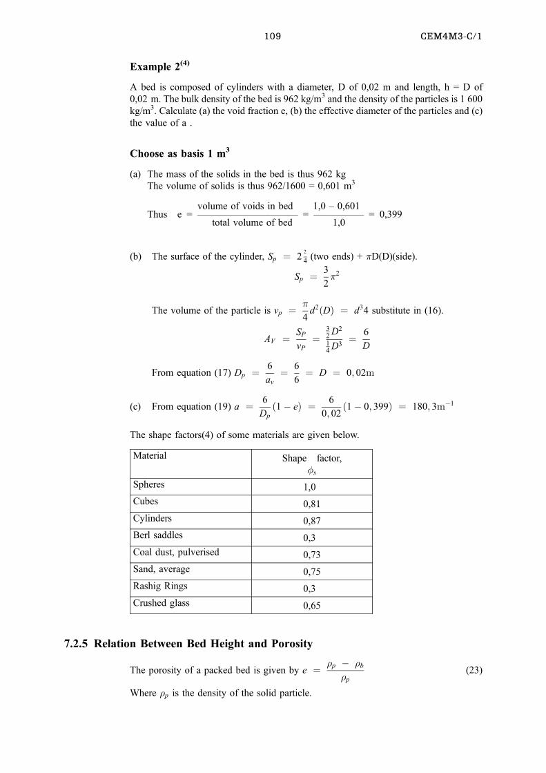
109 CEM4M3-C/1
Example 2(4)
A bed is composed of cylinders with a diameter, D of 0,02 m and length, h = D of
0,02 m. The bulk density of the bed is 962 kg/m3 and the density of the particles is 1 600
kg/m3. Calculate (a) the void fraction e, (b) the effective diameter of the particles and (c)
the value of a .
Choose as basis 1 m3
(a) The mass of the solids in the bed is thus 962 kg
The volume of solids is thus 962/1600 = 0,601 m3
volume of voids in bed 1,0 ± 0,601Thus e = ÐÐÐÐÐÐÐÐÐÐ = ÐÐÐÐÐ = 0,399
total volume of bed 1,0
(b) The surface of the cylinder, Sp � 22
4(two ends) + �D(D)(side).
Sp � 3
2�2
The volume of the particle is vp � �
4d2�D� � d34 substitute in (16).
AV � SP
vP
�32
D2
14
D3� 6
D
From equation (17) Dp � 6
av
� 6
6� D � 0; 02m
(c) From equation (19) a � 6
Dp
�1ÿ e� � 6
0; 02�1ÿ 0; 399� � 180; 3mÿ1
The shape factors(4) of some materials are given below.
Material Shape factor,
�s
Spheres 1,0
Cubes 0,81
Cylinders 0,87
Berl saddles 0,3
Coal dust, pulverised 0,73
Sand, average 0,75
Rashig Rings 0,3
Crushed glass 0,65
7.2.5 Relation Between Bed Height and Porosity
The porosity of a packed bed is given by e � �p ÿ �b
�p
(23)
Where �p is the density of the solid particle.
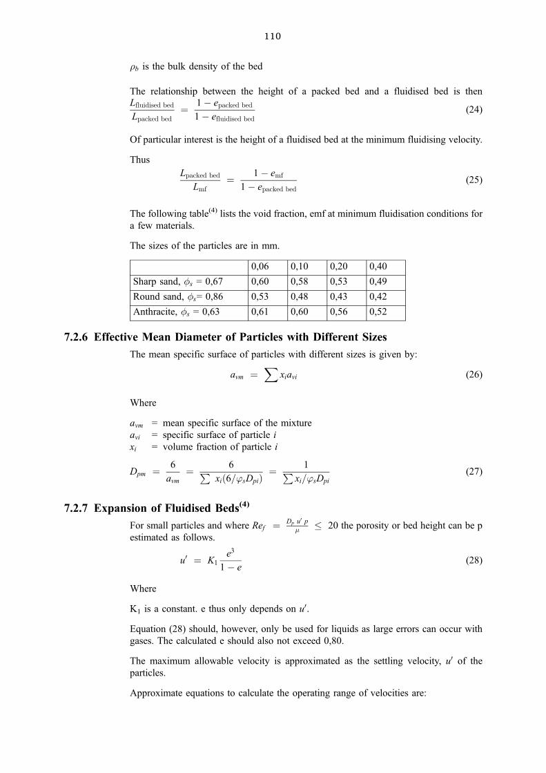
110
�b is the bulk density of the bed
The relationship between the height of a packed bed and a fluidised bed is thenLfluidised bed
Lpacked bed� 1ÿ epacked bed
1ÿ efluidised bed(24)
Of particular interest is the height of a fluidised bed at the minimum fluidising velocity.
Thus
Lpacked bed
Lmf� 1ÿ emf
1ÿ epacked bed(25)
The following table(4) lists the void fraction, emf at minimum fluidisation conditions for
a few materials.
The sizes of the particles are in mm.
0,06 0,10 0,20 0,40
Sharp sand, �s = 0,67 0,60 0,58 0,53 0,49
Round sand, �s= 0,86 0,53 0,48 0,43 0,42
Anthracite, �s = 0,63 0,61 0,60 0,56 0,52
7.2.6 Effective Mean Diameter of Particles with Different Sizes
The mean specific surface of particles with different sizes is given by:
avm �X
xiavi (26)
Where
avm = mean specific surface of the mixture
avi = specific surface of particle i
xi = volume fraction of particle i
Dpm � 6
avm
� 6Pxi�6='sDpi� �
1Pxi='sDpi
(27)
7.2.7 Expansion of Fluidised Beds(4)
For small particles and where Ref � Dp u0 p
� � 20 the porosity or bed height can be p
estimated as follows.
u0 � K1
e3
1ÿ e(28)
Where
K1 is a constant. e thus only depends on u0.
Equation (28) should, however, only be used for liquids as large errors can occur with
gases. The calculated e should also not exceed 0,80.
The maximum allowable velocity is approximated as the settling velocity, u0 of the
particles.
Approximate equations to calculate the operating range of velocities are:
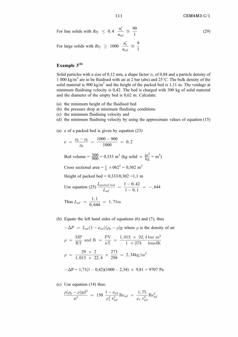
111 CEM4M3-C/1
For line solids with Ref � 0; 4u0t
umf� 90
1(29)
For large solids with Ref � 1000u0t
umf� 9
1
Example 3(4)
Solid particles with a size of 0,12 mm, a shape factor �s of 0,88 and a particle density of
1 000 kg/m3 are to be fluidised with air at 2 bar (abs) and 258C. The bulk density of the
solid material is 900 kg/m3 and the height of the packed bed is 1,11 m. The voidage at
minimum fluidising velocity is 0,42. The bed is charged with 300 kg of solid material
and the diameter of the empty bed is 0,62 m. Calculate:
(a) the minimum height of the fluidised bed
(b) the pressure drop at minimum fluidising conditions
(c) the minimum fluidising velocity and
(d) the minimum fluidising velocity by using the approximate values of equation (15)
(a) e of a packed bed is given by equation (23)
e � �p ÿ �p
�p
� 1000ÿ 900
1000� 0; 2
Bed volume = 300900
= 0,333 m3 (kg solid 6 m3
kg = m3)
Cross sectional area = �460622 = 0,302 m2
Height of packed bed = 0,333/0,302 =1,1 m
Use equation (25)Lpacked bed
Lmf� 1ÿ 0; 42
1ÿ 0; 1� ÿ; 644
Thus Lmf � 1; 1
0; 644� 1; 71m
(b) Equate the left hand sides of equations (6) and (7), thus
ÿ�P � Lmf�1ÿ emf���p ÿ ��g where � is the density of air
� � MP
RTand R � PV
nT� 1; 013 � 22; 4
1 � 273
bar m3
kmolK
� � 29 � 2
1; 013 � 22; 4� 273
298� 2; 34kg=m3
ÿ�P = 1,71(1 ± 0,42)(1000 ± 2,34) 6 9,81 = 9707 Pa
(c) Use equation (14) thus:
���p ÿ ��gd3
�2� 150
1ÿ emf
'2s e3
mf
Remf � 1; 75
's e3mf
Re2mf
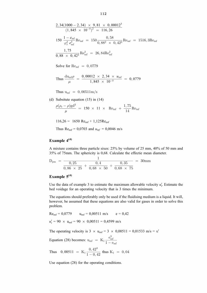
112
2; 34�1000ÿ 2; 34� � 9; 81 � 0; 000123
�1; 845 � 10ÿ5�2 � 116; 26
1501ÿ emf
'2s e3
mf
Remf � 1500; 58
0; 882 � 0; 423Remf � 1516; 3Remf
1; 75
0; 88 � 0; 423Re2
mf � 26; 84Re2mf
Solve for Remf � 0; 0779
Thusdumf�
�� 0; 00012 � 2; 34 � umf
1; 845 � 10ÿ5� 0; 0779
Thus umf � 0; 00511m=s
(d) Subsitute equation (15) in (14)
���s ÿ ��gd3
�� 150 � 11 � Remf � 1; 75
14Remf
116,26 = 1650 Remf + 1,125Remf
Thus Remf = 0,0703 and umf = 0,0046 m/s
Example 4(4)
A mixture contains three particle sixes: 25% by volume of 25 mm, 40% of 50 mm and
35% of 75mm. The sphericity is 0,68. Calculate the effectie mean diameter.
Dpm � 10; 25
0; 86 � 25� 0; 4
0; 68 � 50� 0; 35
0; 68 � 75
� 30mm
Example 5(4)
Use the data of example 3 to estimate the maximum allowable velocity u0t. Estimate the
bed voidage for an operating velocity that is 3 times the minimum.
The equations should preferably only be used if the fluidising medium is a liquid. It will,
however, be assumed that these equations are also valid for gases in order to solve this
problem.
Remf = 0,0779 umf = 0,00511 m/s e = 0,42
u0t = 90 6 umf = 90 6 0,00511 = 0,4599 m/s
The operating velocity is 3 6 umf = 3 6 0,00511 = 0,01533 m/s = u0
Equation (28) becomes: umf � K1e3
mf
1ÿ emf
Thus 0; 00511 � K10; 423
1ÿ 0; 42thus K1 � 0; 04
Use equation (28) for the operating conditions.
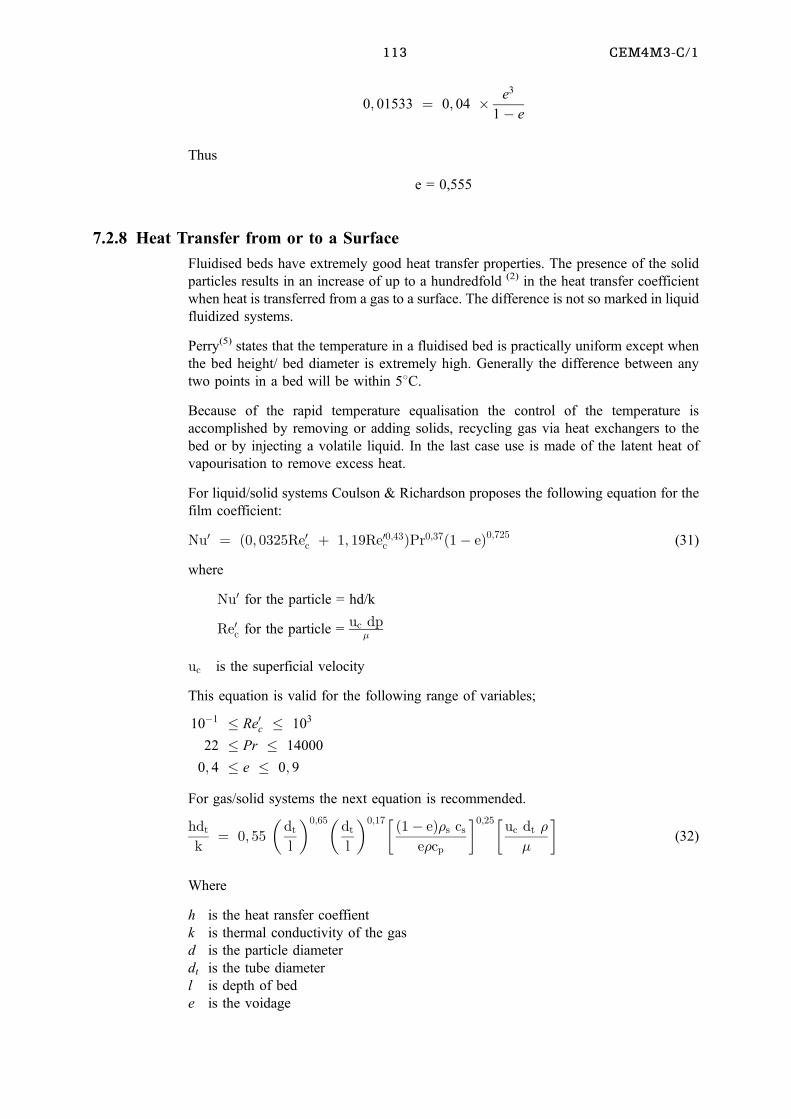
113 CEM4M3-C/1
0; 01533 � 0; 04 � e3
1ÿ e
Thus
e = 0,555
7.2.8 Heat Transfer from or to a Surface
Fluidised beds have extremely good heat transfer properties. The presence of the solid
particles results in an increase of up to a hundredfold (2) in the heat transfer coefficient
when heat is transferred from a gas to a surface. The difference is not so marked in liquid
fluidized systems.
Perry(5) states that the temperature in a fluidised bed is practically uniform except when
the bed height/ bed diameter is extremely high. Generally the difference between any
two points in a bed will be within 58C.
Because of the rapid temperature equalisation the control of the temperature is
accomplished by removing or adding solids, recycling gas via heat exchangers to the
bed or by injecting a volatile liquid. In the last case use is made of the latent heat of
vapourisation to remove excess heat.
For liquid/solid systems Coulson & Richardson proposes the following equation for the
film coefficient:
Nu0 � �0; 0325Re0c � 1; 19Re00;43c �Pr0;37�1ÿ e�0;725
(31)
where
Nu0 for the particle = hd/k
Re0c for the particle =uc dp
�
uc is the superficial velocity
This equation is valid for the following range of variables;
10ÿ1 � Re0c � 103
22 � Pr � 14000
0; 4 � e � 0; 9
For gas/solid systems the next equation is recommended.
hdt
k� 0; 55
�dt
l
�0;65�dt
l
�0;17� �1ÿ e��s cs
e�cp
�0;25�uc dt �
�
�(32)
Where
h is the heat ransfer coeffient
k is thermal conductivity of the gas
d is the particle diameter
dt is the tube diameter
l is depth of bed
e is the voidage
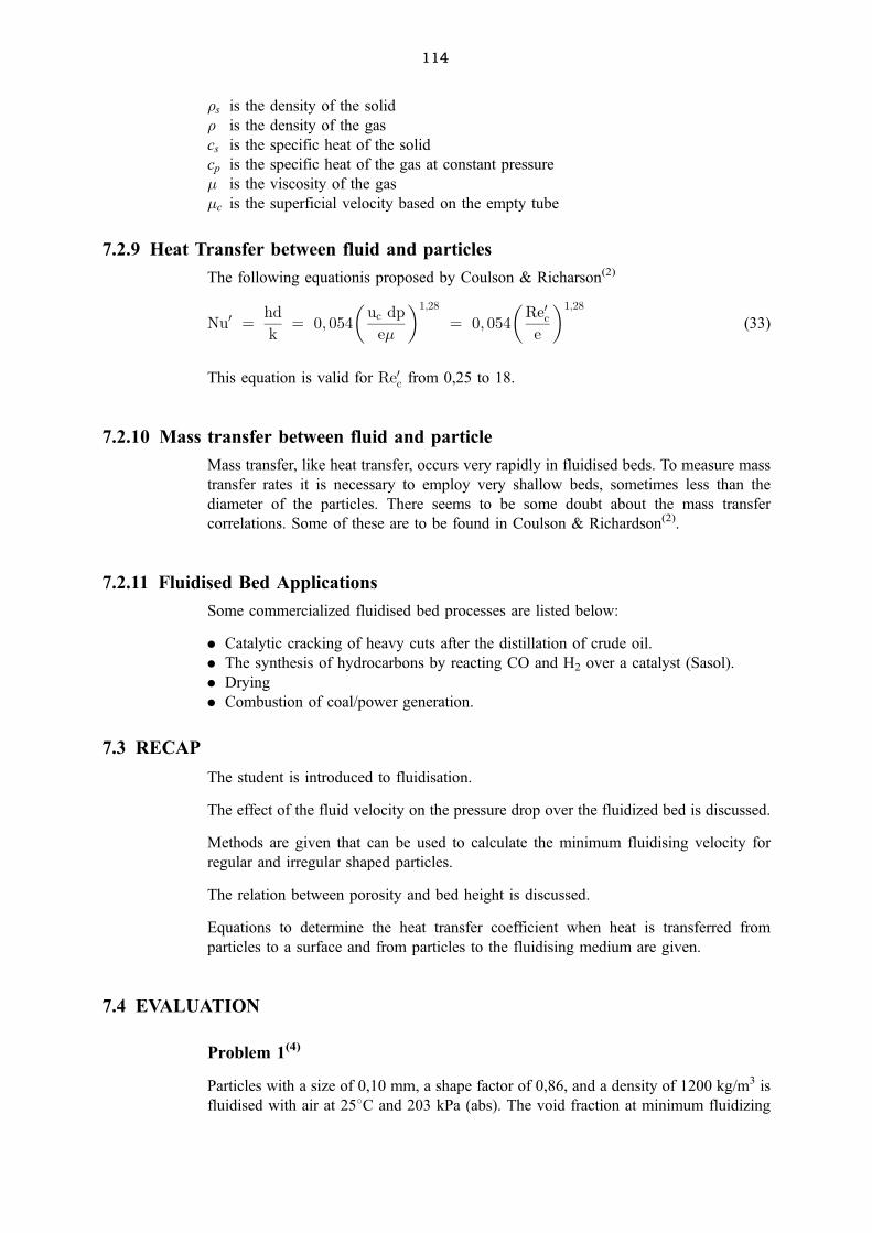
114
�s is the density of the solid
� is the density of the gas
cs is the specific heat of the solid
cp is the specific heat of the gas at constant pressure
� is the viscosity of the gas
�c is the superficial velocity based on the empty tube
7.2.9 Heat Transfer between fluid and particles
The following equationis proposed by Coulson & Richarson(2)
Nu0 � hd
k� 0; 054
�uc dp
e�
�1;28
� 0; 054
�Re0ce
�1;28
(33)
This equation is valid for Re0c from 0,25 to 18.
7.2.10 Mass transfer between fluid and particle
Mass transfer, like heat transfer, occurs very rapidly in fluidised beds. To measure mass
transfer rates it is necessary to employ very shallow beds, sometimes less than the
diameter of the particles. There seems to be some doubt about the mass transfer
correlations. Some of these are to be found in Coulson & Richardson(2).
7.2.11 Fluidised Bed Applications
Some commercialized fluidised bed processes are listed below:
. Catalytic cracking of heavy cuts after the distillation of crude oil.
. The synthesis of hydrocarbons by reacting CO and H2 over a catalyst (Sasol).
. Drying
. Combustion of coal/power generation.
7.3 RECAP
The student is introduced to fluidisation.
The effect of the fluid velocity on the pressure drop over the fluidized bed is discussed.
Methods are given that can be used to calculate the minimum fluidising velocity for
regular and irregular shaped particles.
The relation between porosity and bed height is discussed.
Equations to determine the heat transfer coefficient when heat is transferred from
particles to a surface and from particles to the fluidising medium are given.
7.4 EVALUATION
Problem 1(4)
Particles with a size of 0,10 mm, a shape factor of 0,86, and a density of 1200 kg/m3 is
fluidised with air at 258C and 203 kPa (abs). The void fraction at minimum fluidizing
115 CEM4M3-C/1
conditions is 0,43. The bed diameter is 0,60 m and it contains 350 kg of solids. The bulk
density of the solids, �b is 1150 kg/m3 and the viscosity of air is 1,845 6 10-5 Pa s.
Calculate:
(a) the minimum height of the bed
(b) the pressure drop at minimum fluidising conditions
(c) the minimum fluidising velocity
(d) estimate the porosity of the bed at 4,0 times the minimum velocity.
Answer
(a) Lmf = 1,88m
(b) �P = 12590 Pa
(c) umf = 0,00437m/s
(d) e = 0,605.
Problem 2(4)
A bed with a diameter of 0,1524m is being fluidised with water 208C. The uniform
spherical beads in the bed have a diameter of 4,42mm and a density of 1603kg/m3.
Estimate the minimum fluidising velocity and compare it with the experimenatal value
of 0,02307 m/s.
Answer
umf = 0,026 m/s
Problem 3(2)
A packed bed consisting of uniform spherical particles (diameter, d = 3mm and density,
�s = 4200 kg/m3) is fluidised by means of a liquid with viscosity, � = 0,003 Pa s and
density, � = 1100 kg/m3. Calculate (±�P) through a bed of depth/and voidage e and the
minimum fluidising velocity.
Answer
ÿ�Pl� 17790 Pa=m uMf � 0; 04m=s
Problem 4(2)
Oil with SG = 0,9 and viscosity = 0,003 Pa s passes vertically upwards through a bed of
catalyst consisting of spherical particles with a diameter of 0,1 mm and SG of 2,6. The
viscosity of the oil is 0,8 cp. Determine
(a) the minimum fluidising velocity and
(b) the pressure drop per unit bed height at a velocity of 4 6 umf.
Answer
umf � 0; 00017m=sÿ�P
l� 6920Pa=m
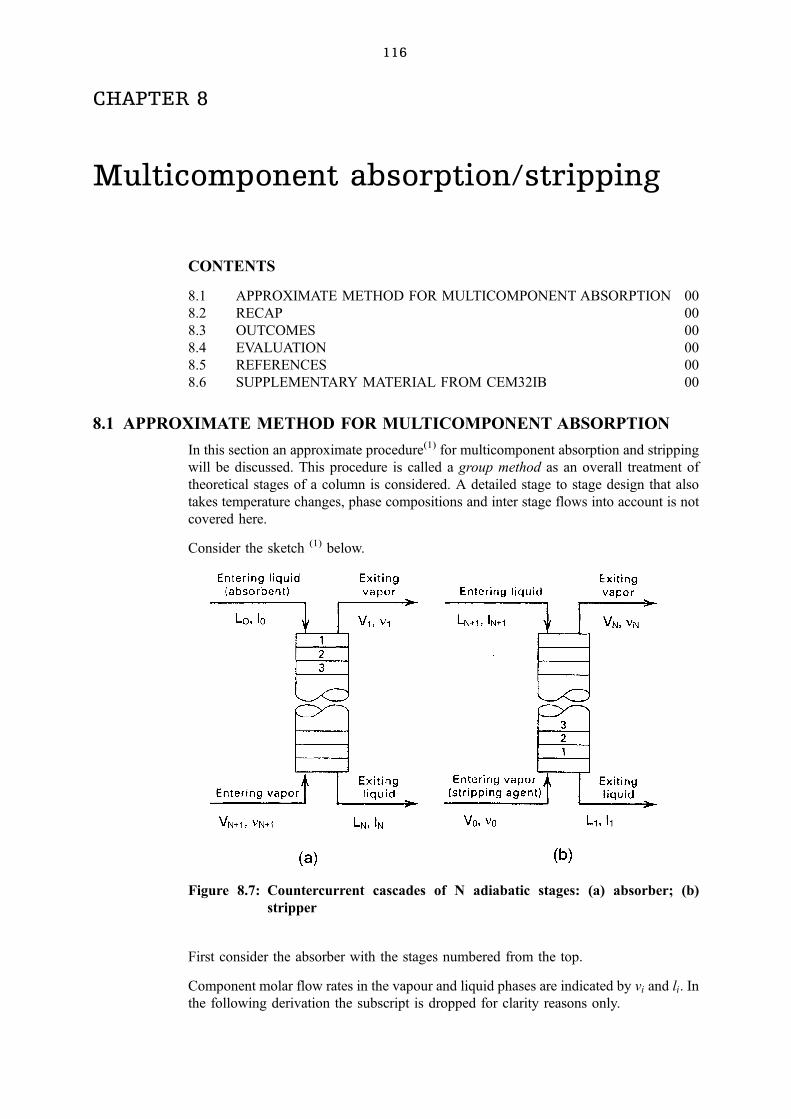
116
CHAPTER 8
Multicomponent absorption/stripping
CONTENTS
8.1 APPROXIMATE METHOD FOR MULTICOMPONENT ABSORPTION 00
8.2 RECAP 00
8.3 OUTCOMES 00
8.4 EVALUATION 00
8.5 REFERENCES 00
8.6 SUPPLEMENTARY MATERIAL FROM CEM32IB 00
8.1 APPROXIMATE METHOD FOR MULTICOMPONENT ABSORPTION
In this section an approximate procedure(1) for multicomponent absorption and stripping
will be discussed. This procedure is called a group method as an overall treatment of
theoretical stages of a column is considered. A detailed stage to stage design that also
takes temperature changes, phase compositions and inter stage flows into account is not
covered here.
Consider the sketch (1) below.
Figure 8.7: Countercurrent cascades of N adiabatic stages: (a) absorber; (b)
stripper
First consider the absorber with the stages numbered from the top.
Component molar flow rates in the vapour and liquid phases are indicated by vi and li. In
the following derivation the subscript is dropped for clarity reasons only.
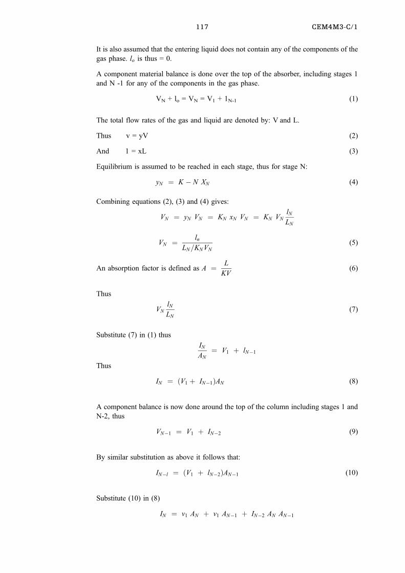
117 CEM4M3-C/1
It is also assumed that the entering liquid does not contain any of the components of the
gas phase. lo is thus = 0.
A component material balance is done over the top of the absorber, including stages 1
and N -1 for any of the components in the gas phase.
VN + lo = VN = V1 + 1N-1 (1)
The total flow rates of the gas and liquid are denoted by: V and L.
Thus v = yV (2)
And 1 = xL (3)
Equilibrium is assumed to be reached in each stage, thus for stage N:
yN � K ÿ N XN (4)
Combining equations (2), (3) and (4) gives:
VN � yN VN � KN xN VN � KN VN
lN
LN
VN � ln
LN=KN VN
(5)
An absorption factor is defined as A � L
KV(6)
Thus
VN
lN
LN
(7)
Substitute (7) in (1) thus
IN
AN
� V1 � lNÿ1
Thus
IN � �V1 � INÿ1�AN (8)
A component balance is now done around the top of the column including stages 1 and
N-2, thus
VNÿ1 � V1 � INÿ2 (9)
By similar substitution as above it follows that:
INÿl � �V1 � lNÿ2�ANÿ1 (10)
Substitute (10) in (8)
IN � v1 AN � v1 ANÿ1 � INÿ2 AN ANÿ1
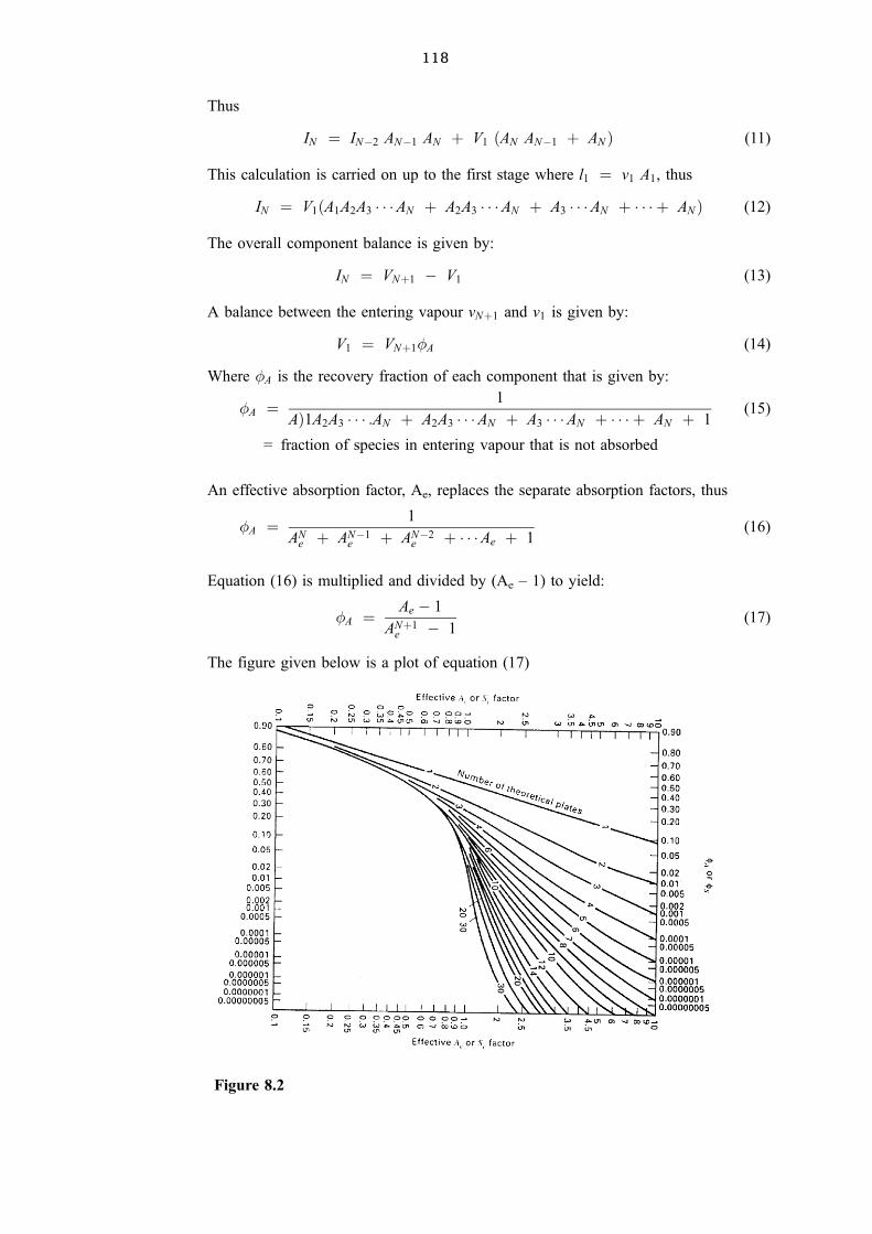
118
Thus
IN � INÿ2 ANÿ1 AN � V1 �AN ANÿ1 � AN � (11)
This calculation is carried on up to the first stage where l1 � v1 A1, thus
IN � V1�A1A2A3 � � �AN � A2A3 � � �AN � A3 � � �AN � � � � � AN � (12)
The overall component balance is given by:
IN � VN�1 ÿ V1 (13)
A balance between the entering vapour vN�1 and v1 is given by:
V1 � VN�1�A (14)
Where �A is the recovery fraction of each component that is given by:
�A � 1
A�1A2A3 � � � :AN � A2A3 � � �AN � A3 � � �AN � � � � � AN � 1(15)
= fraction of species in entering vapour that is not absorbed
An effective absorption factor, Ae, replaces the separate absorption factors, thus
�A � 1
ANe � ANÿ1
e � ANÿ2e � � � �Ae � 1
(16)
Equation (16) is multiplied and divided by (Ae ± 1) to yield:
�A � Ae ÿ 1
AN�1e ÿ 1
(17)
The figure given below is a plot of equation (17)
Figure 8.2
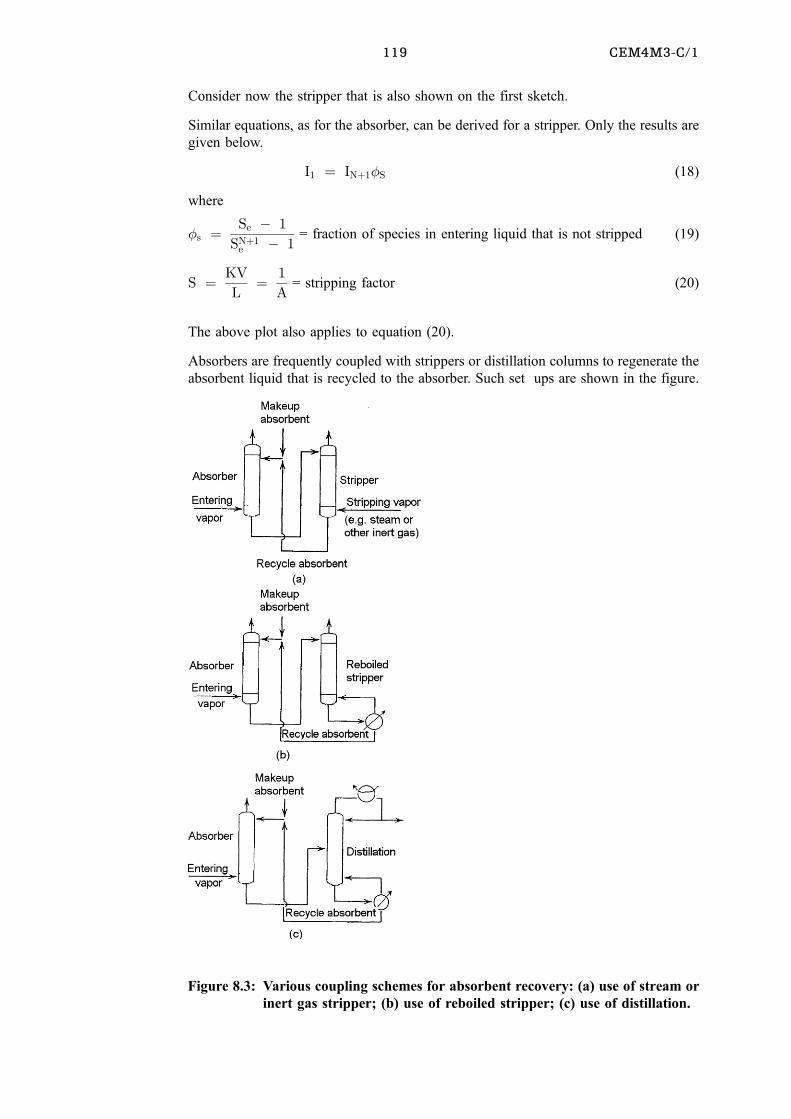
119 CEM4M3-C/1
Consider now the stripper that is also shown on the first sketch.
Similar equations, as for the absorber, can be derived for a stripper. Only the results are
given below.
I1 � IN�1�S (18)
where
�s � Se ÿ 1
SN�1e ÿ 1
= fraction of species in entering liquid that is not stripped (19)
S � KV
L� 1
A= stripping factor (20)
The above plot also applies to equation (20).
Absorbers are frequently coupled with strippers or distillation columns to regenerate the
absorbent liquid that is recycled to the absorber. Such set ups are shown in the figure.
Figure 8.3: Various coupling schemes for absorbent recovery: (a) use of stream or
inert gas stripper; (b) use of reboiled stripper; (c) use of distillation.
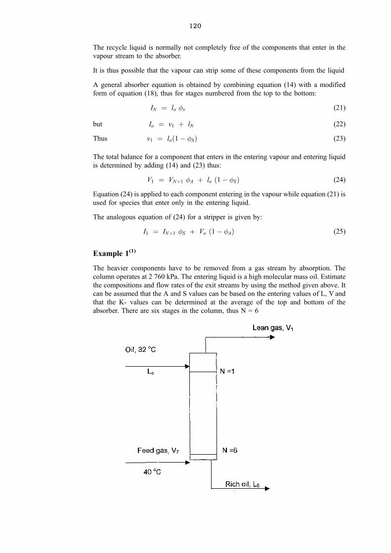
120
The recycle liquid is normally not completely free of the components that enter in the
vapour stream to the absorber.
It is thus possible that the vapour can strip some of these components from the liquid
A general absorber equation is obtained by combining equation (14) with a modified
form of equation (18), thus for stages numbered from the top to the bottom:
IN � lo �s (21)
but Io � v1 � lN (22)
Thus v1 � lo�1ÿ �S� (23)
The total balance for a component that enters in the entering vapour and entering liquid
is determined by adding (14) and (23) thus:
V1 � VN�1 �A � lo �1ÿ �S� (24)
Equation (24) is applied to each component entering in the vapour while equation (21) is
used for species that enter only in the entering liquid.
The analogous equation of (24) for a stripper is given by:
I1 � IN�1 �S � Vo �1ÿ �A� (25)
Example 1(1)
The heavier components have to be removed from a gas stream by absorption. The
column operates at 2 760 kPa. The entering liquid is a high molecular mass oil. Estimate
the compositions and flow rates of the exit streams by using the method given above. It
can be assumed that the A and S values can be based on the entering values of L, V and
that the K- values can be determined at the average of the top and bottom of the
absorber. There are six stages in the column, thus N = 6
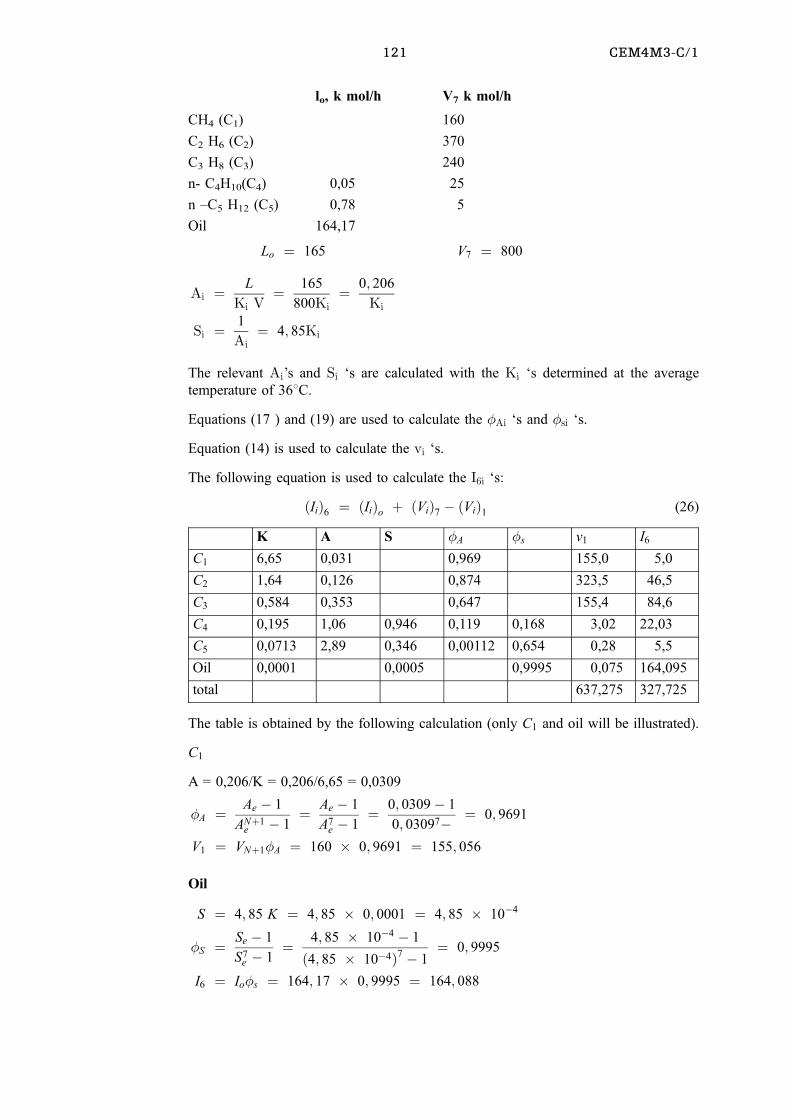
121 CEM4M3-C/1
lo, k mol/h V7 k mol/h
CH4 (C1) 160
C2 H6 (C2) 370
C3 H8 (C3) 240
n- C4H10(C4) 0,05 25
n ±C5 H12 (C5) 0,78 5
Oil 164,17
Lo � 165 V7 � 800
Ai � L
Ki V� 165
800Ki� 0; 206
Ki
Si � 1
Ai� 4; 85Ki
The relevant Ai's and Si `s are calculated with the Ki `s determined at the average
temperature of 368C.
Equations (17 ) and (19) are used to calculate the �Ai `s and �si `s.
Equation (14) is used to calculate the vi `s.
The following equation is used to calculate the I6i `s:
�Ii�6 � �Ii�o � �Vi�7 ÿ �Vi�1 (26)
K A S �A �s v1 I6
C1 6,65 0,031 0,969 155,0 5,0
C2 1,64 0,126 0,874 323,5 46,5
C3 0,584 0,353 0,647 155,4 84,6
C4 0,195 1,06 0,946 0,119 0,168 3,02 22,03
C5 0,0713 2,89 0,346 0,00112 0,654 0,28 5,5
Oil 0,0001 0,0005 0,9995 0,075 164,095
total 637,275 327,725
The table is obtained by the following calculation (only C1 and oil will be illustrated).
C1
A = 0,206/K = 0,206/6,65 = 0,0309
�A � Ae ÿ 1
AN�1e ÿ 1
� Ae ÿ 1
A7e ÿ 1
� 0; 0309ÿ 1
0; 03097ÿ � 0; 9691
V1 � VN�1�A � 160 � 0; 9691 � 155; 056
Oil
S � 4; 85 K � 4; 85 � 0; 0001 � 4; 85 � 10ÿ4
�S � Se ÿ 1
S7e ÿ 1
� 4; 85 � 10ÿ4 ÿ 1
�4; 85 � 10ÿ4�7 ÿ 1� 0; 9995
I6 � Io�s � 164; 17 � 0; 9995 � 164; 088
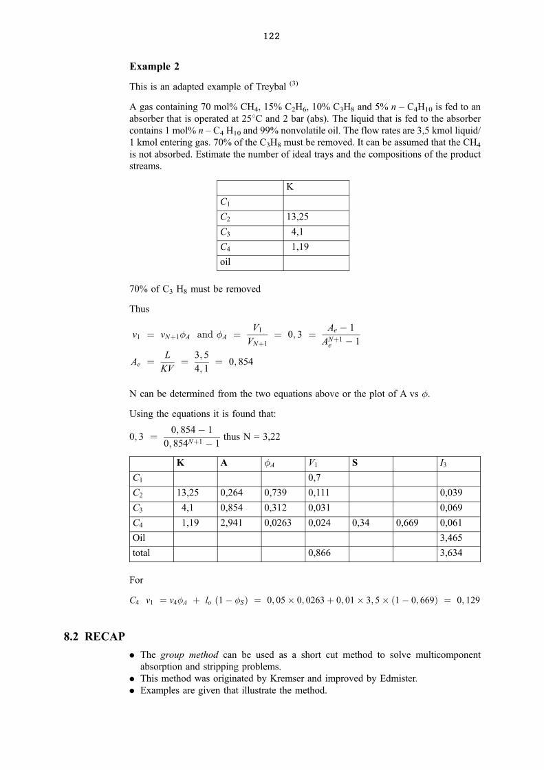
122
Example 2
This is an adapted example of Treybal (3)
A gas containing 70 mol% CH4, 15% C2H6, 10% C3H8 and 5% n ± C4H10 is fed to an
absorber that is operated at 258C and 2 bar (abs). The liquid that is fed to the absorber
contains 1 mol% n ± C4 H10 and 99% nonvolatile oil. The flow rates are 3,5 kmol liquid/
1 kmol entering gas. 70% of the C3H8 must be removed. It can be assumed that the CH4
is not absorbed. Estimate the number of ideal trays and the compositions of the product
streams.
K
C1
C2 13,25
C3 4,1
C4 1,19
oil
70% of C3 H8 must be removed
Thus
v1 � vN�1�A and �A � V1
VN�1
� 0; 3 � Ae ÿ 1
AN�1e ÿ 1
Ae � L
KV� 3; 5
4; 1� 0; 854
N can be determined from the two equations above or the plot of A vs �.
Using the equations it is found that:
0; 3 � 0; 854ÿ 1
0; 854N�1 ÿ 1thus N = 3,22
K A �A V1 S I3
C1 0,7
C2 13,25 0,264 0,739 0,111 0,039
C3 4,1 0,854 0,312 0,031 0,069
C4 1,19 2,941 0,0263 0,024 0,34 0,669 0,061
Oil 3,465
total 0,866 3,634
For
C4 v1 � v4�A � lo �1ÿ �S� � 0; 05� 0; 0263� 0; 01� 3; 5� �1ÿ 0; 669� � 0; 129
8.2 RECAP
. The group method can be used as a short cut method to solve multicomponent
absorption and stripping problems.
. This method was originated by Kremser and improved by Edmister.
. Examples are given that illustrate the method.
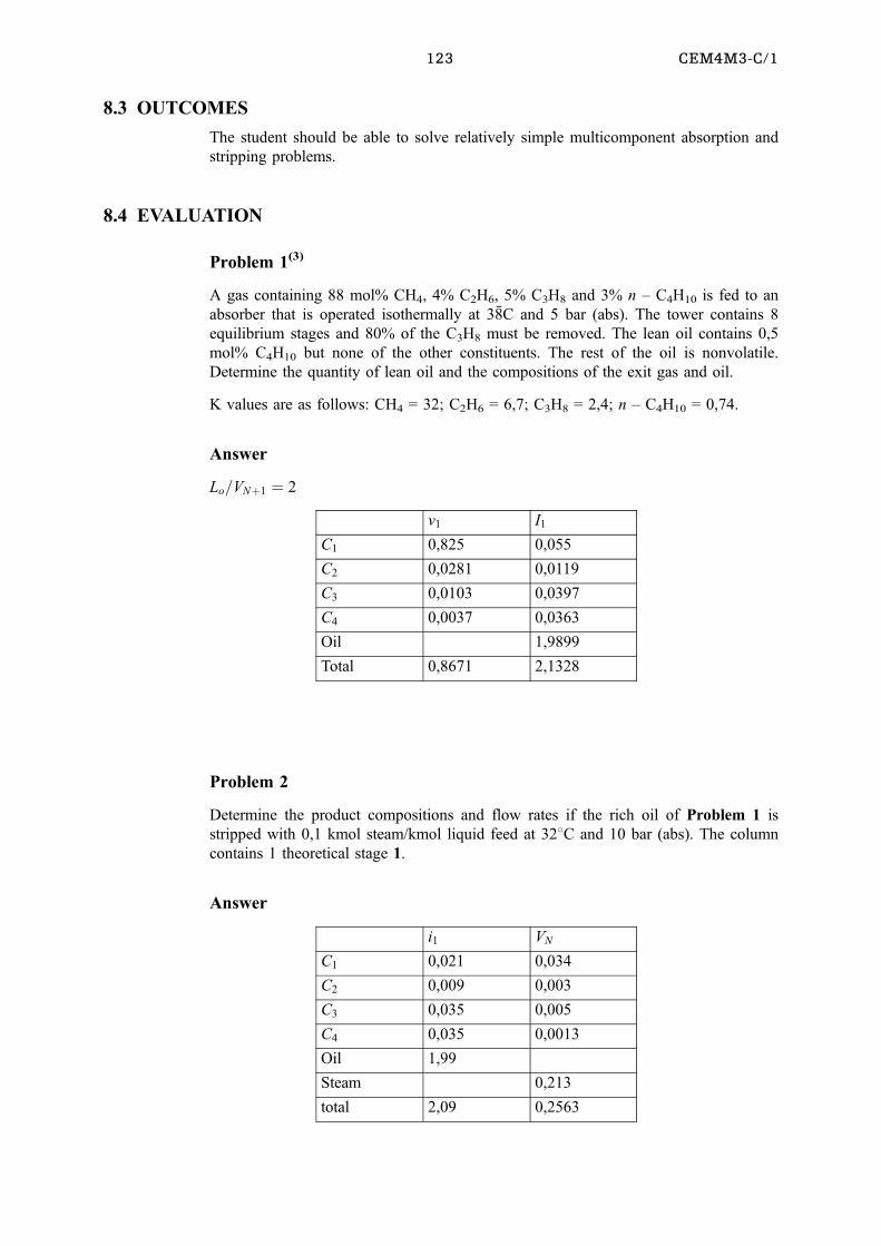
123 CEM4M3-C/1
8.3 OUTCOMES
The student should be able to solve relatively simple multicomponent absorption and
stripping problems.
8.4 EVALUATION
Problem 1(3)
A gas containing 88 mol% CH4, 4% C2H6, 5% C3H8 and 3% n ± C4H10 is fed to an
absorber that is operated isothermally at 38ÅC and 5 bar (abs). The tower contains 8
equilibrium stages and 80% of the C3H8 must be removed. The lean oil contains 0,5
mol% C4H10 but none of the other constituents. The rest of the oil is nonvolatile.
Determine the quantity of lean oil and the compositions of the exit gas and oil.
K values are as follows: CH4 = 32; C2H6 = 6,7; C3H8 = 2,4; n ± C4H10 = 0,74.
Answer
Lo=VN�1 � 2
v1 I1
C1 0,825 0,055
C2 0,0281 0,0119
C3 0,0103 0,0397
C4 0,0037 0,0363
Oil 1,9899
Total 0,8671 2,1328
Problem 2
Determine the product compositions and flow rates if the rich oil of Problem 1 is
stripped with 0,1 kmol steam/kmol liquid feed at 328C and 10 bar (abs). The column
contains 1 theoretical stage 1.
Answer
i1 VN
C1 0,021 0,034
C2 0,009 0,003
C3 0,035 0,005
C4 0,035 0,0013
Oil 1,99
Steam 0,213
total 2,09 0,2563
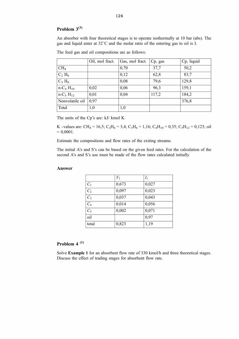
124
Problem 3(3)
An absorber with four theoretical stages is to operate isothermally at 10 bar (abs). The
gas and liquid enter at 328C and the molar ratio of the entering gas to oil is I.
The feed gas and oil compositions are as follows:
Oil, mol fract. Gas, mol fract. Cp, gas Cp, liquid
CH4 0,70 37,7 50,2
C2 H6 0,12 62,8 83,7
C3 H8 0,08 79,6 129,8
n-C4 H10 0,02 0,06 96,3 159,1
n-C5 H12 0,01 0,04 117,2 184,2
Nonvolatile oil 0,97 376,8
Total 1,0 1,0
The units of the Cp's are: kJ/ kmol K
K ±values are: CH4 = 16,5; C2H6 = 3,4; C3H6 = 1,16; C4H10 = 0,35; C5H12 = 0,123; oil
= 0,0001.
Estimate the compositions and flow rates of the exiting streams.
The initial A's and S's can be based on the given feed rates. For the calculation of the
second A's and S's use must be made of the flow rates calculated initially
Answer
V1 l1
C1 0,673 0,027
C2 0,097 0,023
C3 0,037 0,043
C4 0,014 0,056
C5 0,002 0,071
oil 0,97
total 0,823 1,19
Problem 4 (1)
Solve Example 1 for an absorbent flow rate of 330 kmol/h and three theoretical stages.
Discuss the effect of trading stages for absorbent flow rate.
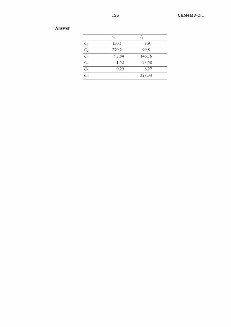
125 CEM4M3-C/1
Answer
v1 l3
C1 150,1 9,9
C2 270,2 99,8
C3 93,84 146,16
C4 1,52 23,58
C5 0,29 6,27
oil 328,34
126
REFERENCES
Seader, J.D. and Henley, E.J. Separation Process Principles. (John Wiley & Sons, Inc
New York, 1988).
Coulson, J.M. and Richardson, J.F. Chemical Engineering, Volume 2, Fourth Edition,
(Butterworth Heinemann, 1991)
Treybal, R.E. Mass Transfer Operations, (McGraw ±Hill Book Company, 1981).
Geankoplis, C.G. Transport Process and Unit Operations, Third Edition, (Prentice-Hall
International Inc, 1978).
Perry, R.H. and Green, D.W. Perry's Chemical Engineer's Handbook, 50th edition.
(McGraw ±Hill Book Company, New York, 1984).
127 CEM4M3-C/1
SUPPLEMENTARY MATERIAL
Absorption
CONTENTS
4.1 LEARNING OUTCOMES 00
4.2 INTRODUCTION 00
4.3 COLUMN OPERATION 00
4.4 EQUILIBRIUM BETWEEN LIQUID AND GAS 00
4.5 MECHANISM OF ABSORPTION 00
4.5.1 Two-film Theory 00
4.6 RATE OF ABSORPTION 00
4.6.1 Influence of Solubility on the Transfer Coefficients 00
4.7 MASS BALANCE OVER ABSORPTION AND STRIPPING COLUMNS 00
4.7.1 Equilibrium line a straight line 00
4.7.2 Number of Transfer Units and Height of a Transfer Unit 00
4.8 GRAPHICAL DESIGN METHOD 00
4.8.1 Gas absorption 00
4.8.2 Gas stripping 00
4.9 TYPES OF ABSORPTION EQUIPMENT 00
4.9.1 Selection of Columns 00
4.9.2 Packed columns 00
4.9.3 Plate Columns 00
4.9.4 Centrifugal Absorber 00
4.10 SUMMARY OF EQUATIONS 00
4.1 LEARNING OUTCOMES
After the completion of this chapter the learner should be able to do the following:
. Name the considerations for the choice of solvent.
. Describe the mechanism of absorption.
. Define the rate of absorption.
. Explain the effect of level of solubility of gas on the driving forces.
. Calculate column height, number of transfer units, height of transfer unit. Use
graphical method to determine the number of transfer units.
. Explain operation of packed columns, plate columns and centrifugal absorbers.
4.2 INTRODUCTION
Absorption is defined as the removal of selected components from a mixture of gases
into a suitable liquid. Two types may occur, namely those which are solely a physical
process and those where a chemical reaction is occurring. An example of the first is the
recovery of acetone from an acetone-air mixture by absorption in water. An example of
the latter is the absorption of carbon dioxide into a sodium hydroxide solution.
For an absorption column to operate efficiently, the gas and liquid phases should be
128
brought in close contact with another. Although packed and plate columns are used, as
in distillation, the method of operation differs. In the case of absorption, the gas is
introduced at the bottom of the column and the liquid at the top of the column, therefore
a counter-current operation.
4.3 COLUMN OPERATION
Different types of configurations can be used, i.e. plate columns, packed columns etc.
All types of configurations have the following in common, namely:
(i) The component removed from the feed mixture is in the gas phase;
(ii) The liquid is charged at the top of the column and recovered at the bottom with the
desired component;
(iii) Some sort of packing is used to increase the surface area between the liquid and
gas phase.
The choice of solvent is determined by the following considerations:
(i) Gas solubility: The gas solubility should be high, thus increasing the rate of
absorption and decreasing the quantity of solvent required. Solvents of a chemical
nature similar to that of the solute to be absorbed will provide good solubility. In
the case of chemical reactions where the solute has to be reused, the reaction
should be reversible. Hydrogen sulfide may be removed from gas mixtures by
ethanolamine solutions since the sulfide is readily absorbed at low temperatures
and easily stripped at high temperatures.
(ii) Volatility: The solvent should have a low vapour pressure since the gas leaving an
absorption operation is ordinarily saturated with the solvent and much may thereby
be lost. In the case where a liquid has superior solubility but a high volatility, a
second non-volatile liquid may be used to recover the volatilized solvent.
(iii) Corrosiveness: The liquid should be non-corrosive to prevent the use of expensive
materials of construction.
(iv) Cost: The solvent should be inexpensive, so that losses are not costly, and should
be readily available.
(v) Viscosity: A liquid with low viscosity is preferred for reasons of rapid absorption
rates, low pressure drops on pumping and good heat transfer characteristics.
(vi) Other: The solvent should also be, if possible, nontoxic, nonflammable,
chemically stable and have a low freezing point.
4.4 EQUILIBRIUM BETWEEN LIQUID AND GAS
When two phases are brought into contact with one another, they will eventually reach
equilibrium. Water in contact with air evaporates until the air is saturated with water
vapor and the air is absorbed by the water until saturated with the individual gases. The
extent to which the gas is absorbed by the liquid is determined by the partial pressure at
a given temperature and concentration. With an increase in temperature the solubility
decreases.
For dilute concentrations of most gases the relationship between the dissolvoÄd
component and component in the gas phase is given by Henry's law:
PA � HCA (Eq 1)
where PA partial pressure of component A in the gas phase;
CA concentration of the component in the liquid
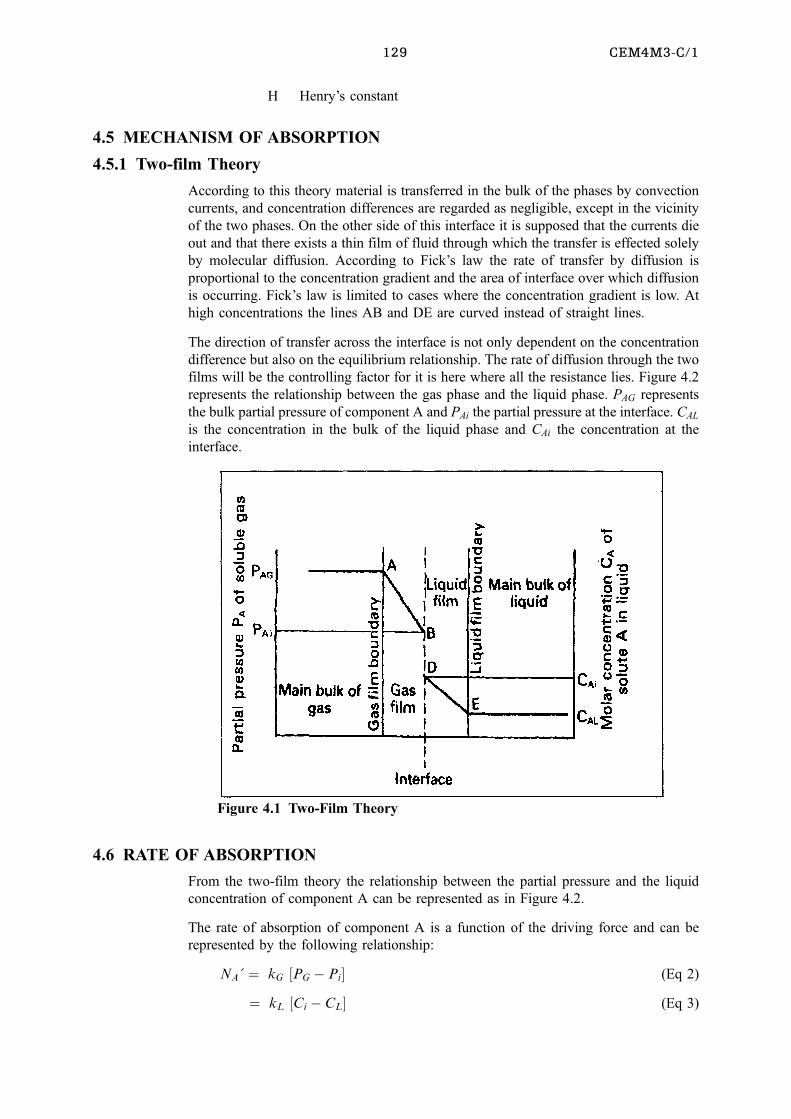
129 CEM4M3-C/1
H Henry's constant
4.5 MECHANISM OF ABSORPTION
4.5.1 Two-film Theory
According to this theory material is transferred in the bulk of the phases by convection
currents, and concentration differences are regarded as negligible, except in the vicinity
of the two phases. On the other side of this interface it is supposed that the currents die
out and that there exists a thin film of fluid through which the transfer is effected solely
by molecular diffusion. According to Fick's law the rate of transfer by diffusion is
proportional to the concentration gradient and the area of interface over which diffusion
is occurring. Fick's law is limited to cases where the concentration gradient is low. At
high concentrations the lines AB and DE are curved instead of straight lines.
The direction of transfer across the interface is not only dependent on the concentration
difference but also on the equilibrium relationship. The rate of diffusion through the two
films will be the controlling factor for it is here where all the resistance lies. Figure 4.2
represents the relationship between the gas phase and the liquid phase. PAG represents
the bulk partial pressure of component A and PAi the partial pressure at the interface. CAL
is the concentration in the bulk of the liquid phase and CAi the concentration at the
interface.
Figure 4.1 Two-Film Theory
4.6 RATE OF ABSORPTION
From the two-film theory the relationship between the partial pressure and the liquid
concentration of component A can be represented as in Figure 4.2.
The rate of absorption of component A is a function of the driving force and can be
represented by the following relationship:
NA�� kG �PG ÿ Pi� (Eq 2)
� kL �Ci ÿ CL� (Eq 3)
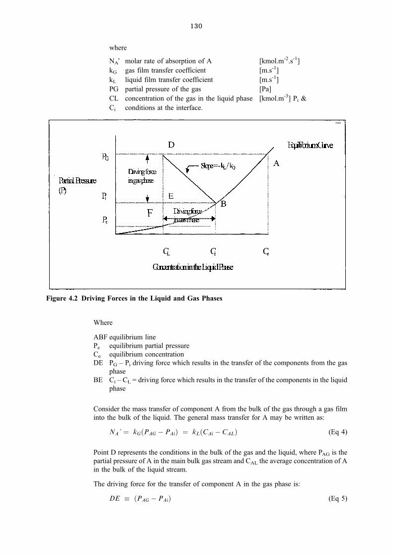
130
where
NA' molar rate of absorption of A [kmol.m-2.s-1]
kG gas film transfer coefficient [m.s-1]
kL liquid film transfer coefficient [m.s-1]
PG partial pressure of the gas [Pa]
CL concentration of the gas in the liquid phase [kmol.m-3] Pi &
Ci conditions at the interface.
Figure 4.2 Driving Forces in the Liquid and Gas Phases
Where
ABF equilibrium line
Pe equilibrium partial pressure
Ce equilibrium concentration
DE PG ± Pi driving force which results in the transfer of the components from the gas
phase
BE Ci ± CL = driving force which results in the transfer of the components in the liquid
phase
Consider the mass transfer of component A from the bulk of the gas through a gas film
into the bulk of the liquid. The general mass transfer for A may be written as:
NA�� kG�PAG ÿ PAi� � kL�CAi ÿ CAL� (Eq 4)
Point D represents the conditions in the bulk of the gas and the liquid, where PAG is the
partial pressure of A in the main bulk gas stream and CAL the average concentration of A
in the bulk of the liquid stream.
The driving force for the transfer of component A in the gas phase is:
DE � �PAG ÿ PAi� (Eq 5)
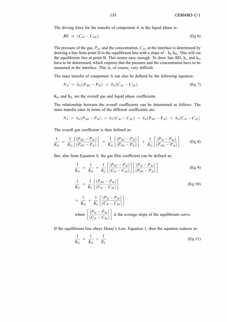
131 CEM4M3-C/1
The driving force for the transfer of component A in the liquid phase is:
BE � �CAi ÿ CAL� (Eq 6)
The pressure of the gas, PAi, and the concentration, CAi, at the interface is determined by
drawing a line from point D to the equilibrium line with a slope of ± kL/kG. This will cut
the equilibrium line at point B. This seems easy enough. To draw line BD, kL and kG
have to be determined, which requires that the pressure and the concentration have to be
measured at the interface. This is, of course, very difficult.
The mass transfer of component A can also be defined by the following equation:
NA�� kG�PAG ÿ PAi� � kL�CAe ÿ CAL� (Eq 7)
KG and KL are the overall gas and liquid phase coefficients
The relationship between the overall coefficients can be determined as follows. The
mass transfer rates in terms of the different coefficients are:
NA�� kG�PAG ÿ PAe� � kL�CAe ÿ CAL� � kG�PAG ÿ PAi� � kL�CAi ÿ CAL�
The overall gas coefficient is then defined as:
1
KG
� 1
KG
� �PAG ÿ PAe��PAG ÿ PAi�
�� 1
KG
� �PAG ÿ PAi��PAG ÿ PAi�
�� 1
KG
� �PAi ÿ PAe��PAiG ÿ PAi�
�(Eq 8)
But, also from Equation 8, the gas film coefficient can be defined as:
1
KG
� 1
KG
� 1
KL
� �PAG ÿ PAi��CAi ÿ CAL�
�� �PAi ÿ PAe��PAG ÿ PAi�
�(Eq 9)
1
KG
� 1
KL
� �PAG ÿ PAi��CAi ÿ CAL�
�(Eq 10)
� 1
KG
� 1
KL
� �PAi ÿ PAe��CAi ÿ CAL�
�
where
� �PAi ÿ PAe��CAi ÿ CAL�
�is the average slope of the equilibrium curve.
If the equilibrium line obeys Henry's Law, Equation 1, then the equation reduces to:
1
KG
� 1
KG
� 1
KL
(Eq 11)
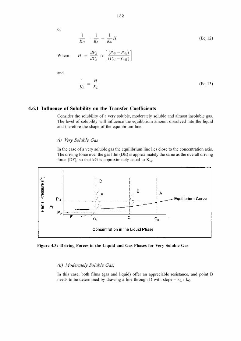
132
or
1
KG
� 1
KL
� 1
KG
H (Eq 12)
Where H � dPA
dCA
�� �PAi ÿ PAe��CAi ÿ CAL�
�
and
1
KL
� H
KL
(Eq 13)
4.6.1 Influence of Solubility on the Transfer Coefficients
Consider the solubility of a very soluble, moderately soluble and almost insoluble gas.
The level of solubility will influence the equilibrium amount dissolved into the liquid
and therefore the shape of the equilibrium line.
(i) Very Soluble Gas
In the case of a very soluble gas the equilibrium line lies close to the concentration axis.
The driving force over the gas film (DE) is approximately the same as the overall driving
force (DF), so that kG is approximately equal to KG.
Figure 4.3: Driving Forces in the Liquid and Gas Phases for Very Soluble Gas
(ii) Moderately Soluble Gas:
In this case, both films (gas and liquid) offer an appreciable resistance, and point B
needs to be determined by drawing a line through D with slope ± kL / kG.
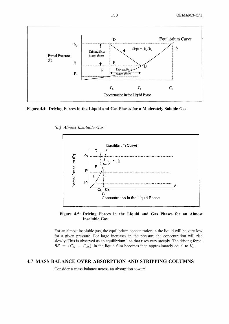
133 CEM4M3-C/1
Figure 4.4: Driving Forces in the Liquid and Gas Phases for a Moderately Soluble Gas
(iii) Almost Insoluble Gas:
For an almost insoluble gas, the equilibrium concentration in the liquid will be very low
for a given pressure. For large increases in the pressure the concentration will rise
slowly. This is observed as an equilibrium line that rises very steeply. The driving force,
BE � �CAi ÿ CAL�, in the liquid film becomes then approximately equal to KL.
4.7 MASS BALANCE OVER ABSORPTION AND STRIPPING COLUMNS
Consider a mass balance across an absorption tower:
Figure 4.5: Driving Forces in the Liquid and Gas Phases for an Almost
Insoluble Gas
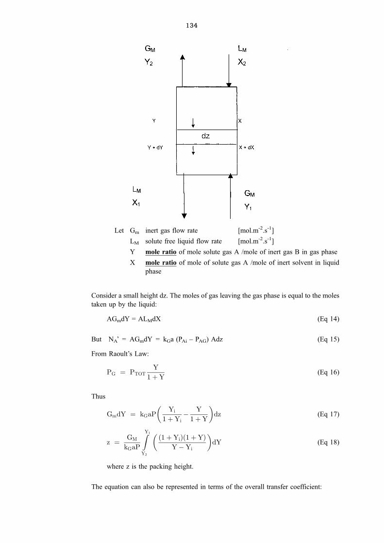
134
Let Gm inert gas flow rate [mol.m-2.s-1]
LM solute free liquid flow rate [mol.m-2.s-1]
Y mole ratio of mole solute gas A /mole of inert gas B in gas phase
X mole ratio of mole of solute gas A /mole of inert solvent in liquid
phase
Consider a small height dz. The moles of gas leaving the gas phase is equal to the moles
taken up by the liquid:
AGmdY = ALMdX (Eq 14)
But NA' = AGmdY = kGa (PAi ± PAG) Adz (Eq 15)
From Raoult's Law:
PG � PTOTY
1�Y(Eq 16)
Thus
GmdY � kGaP
�Yi
1�Yiÿ Y
1�Y
�dz (Eq 17)
z � GM
kGaP
ZY1
Y2
� �1�Yi��1�Y�YÿYi
�dY (Eq 18)
where z is the packing height.
The equation can also be represented in terms of the overall transfer coefficient:
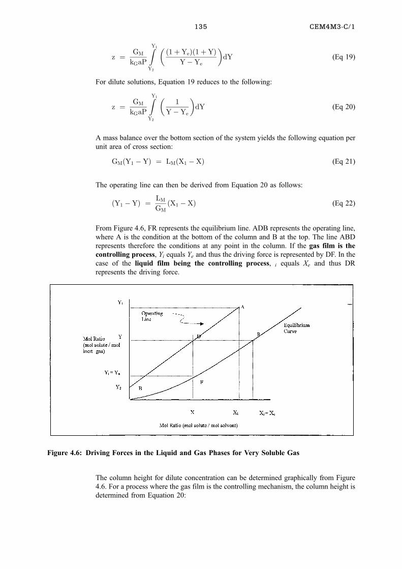
135 CEM4M3-C/1
z � GM
kGaP
ZY1
Y2
� �1�Ye��1�Y�YÿYe
�dY (Eq 19)
For dilute solutions, Equation 19 reduces to the following:
z � GM
kGaP
ZY1
Y2
�1
YÿYe
�dY (Eq 20)
A mass balance over the bottom section of the system yields the following equation per
unit area of cross section:
GM�Y1 ÿY� � LM�X1 ÿX� (Eq 21)
The operating line can then be derived from Equation 20 as follows:
�Y1 ÿY� � LM
GM�X1 ÿX� (Eq 22)
From Figure 4.6, FR represents the equilibrium line. ADB represents the operating line,
where A is the condition at the bottom of the column and B at the top. The line ABD
represents therefore the conditions at any point in the column. If the gas film is the
controlling process, Yi equals Ye and thus the driving force is represented by DF. In the
case of the liquid film being the controlling process, i equals Xe and thus DR
represents the driving force.
Figure 4.6: Driving Forces in the Liquid and Gas Phases for Very Soluble Gas
The column height for dilute concentration can be determined graphically from Figure
4.6. For a process where the gas film is the controlling mechanism, the column height is
determined from Equation 20:
136
z � GM
kGaP
ZY1
Y2
�1
YÿYe
�dY (Eq 20)
4.7.1 Equilibrium line a straight line
Consider the transfer of component A from the gas phase to the liquid phase. This can be
represented by Equation 23:
NA' (adV) = AGMdY = KGaPTOT (Ye ± Y) Adz (Eq 23)
The equilibrium line is given by the following:
Ye = mX + c (Eq 24)
And
Ye2 = mX2 + c (Eq 25)
From this follows:
m � Ye1 ÿYe2
X1 ÿX2(Eq 27)
A material balance over the bottom section of the tower will yield the following:
GM�Y1 ÿY� � LM�X1 ÿX� (Eq 28)
X � X1 ÿGM
LM�Y1 ÿY� (Eq 29)
Equation 29 can then be presented as follows:Zz
O
kGaPTOT
GMdz �
ZY2
Y1
dY
�Ye ÿY� (Eq 30)
Substituting Equations 12 and 16 in 17:
aAZNA�� GM�Y1 ÿY2�A � KGaPTOT�YÿYe�ImAZ (Eq 31)
where
�YÿYe�lm ��Y1 ÿY1e� ÿ �Y2 ÿY2e�
ln
� �Y1 ÿY1e��Y2 ÿY2e�
� (Eq 32)
The above equation can also be written in terms of the mole fraction by using the
following relationship:
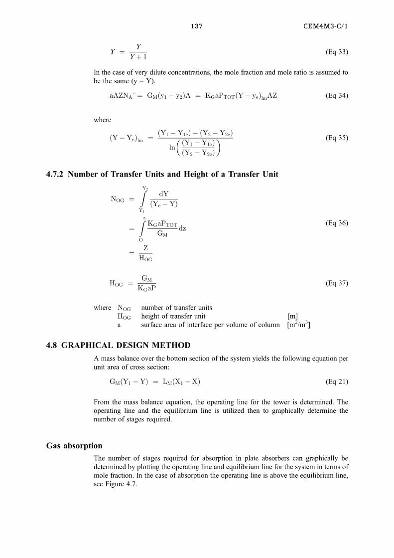
137 CEM4M3-C/1
Y � Y
Y� 1(Eq 33)
In the case of very dilute concentrations, the mole fraction and mole ratio is assumed to
be the same (y = Y).
aAZNA�� GM�y1 ÿ y2�A � KGaPTOT�Yÿ ye�lmAZ (Eq 34)
where
�YÿYe�lm ��Y1 ÿY1e� ÿ �Y2 ÿY2e�
ln
� �Y1 ÿY1e��Y2 ÿY2e�
� (Eq 35)
4.7.2 Number of Transfer Units and Height of a Transfer Unit
NOG �ZY2
Y1
dY
�Ye ÿY�
�Zz
O
KGaPTOT
GMdz
� Z
HOG
(Eq 36)
HOG � GM
KGaP(Eq 37)
where NOG number of transfer units
HOG height of transfer unit [m]
a surface area of interface per volume of column [m2/m3]
4.8 GRAPHICAL DESIGN METHOD
A mass balance over the bottom section of the system yields the following equation per
unit area of cross section:
GM�Y1 ÿY� � LM�X1 ÿX� (Eq 21)
From the mass balance equation, the operating line for the tower is determined. The
operating line and the equilibrium line is utilized then to graphically determine the
number of stages required.
Gas absorption
The number of stages required for absorption in plate absorbers can graphically be
determined by plotting the operating line and equilibrium line for the system in terms of
mole fraction. In the case of absorption the operating line is above the equilibrium line,
see Figure 4.7.
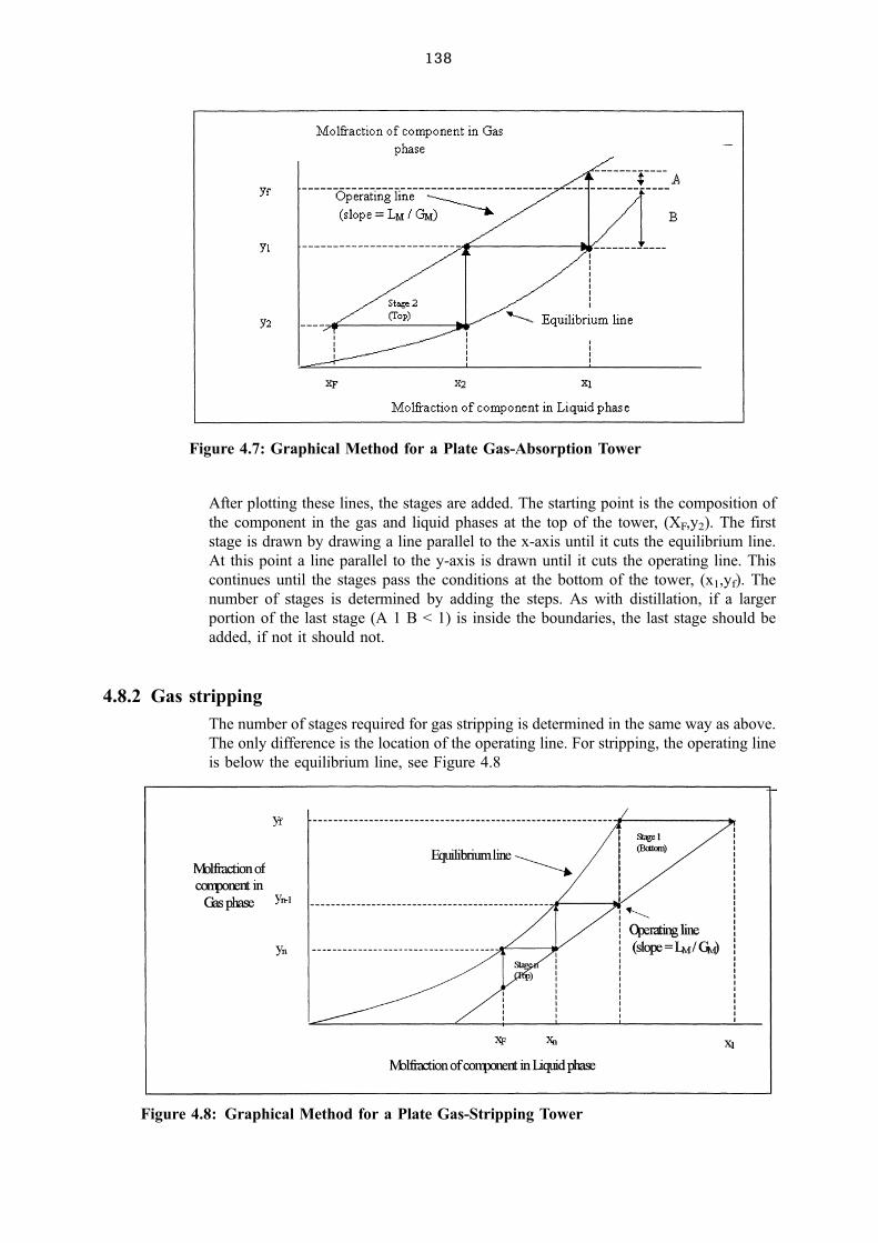
138
Figure 4.7: Graphical Method for a Plate Gas-Absorption Tower
After plotting these lines, the stages are added. The starting point is the composition of
the component in the gas and liquid phases at the top of the tower, (XF,y2). The first
stage is drawn by drawing a line parallel to the x-axis until it cuts the equilibrium line.
At this point a line parallel to the y-axis is drawn until it cuts the operating line. This
continues until the stages pass the conditions at the bottom of the tower, (x1,yf). The
number of stages is determined by adding the steps. As with distillation, if a larger
portion of the last stage (A 1 B < 1) is inside the boundaries, the last stage should be
added, if not it should not.
4.8.2 Gas stripping
The number of stages required for gas stripping is determined in the same way as above.
The only difference is the location of the operating line. For stripping, the operating line
is below the equilibrium line, see Figure 4.8
Figure 4.8: Graphical Method for a Plate Gas-Stripping Tower
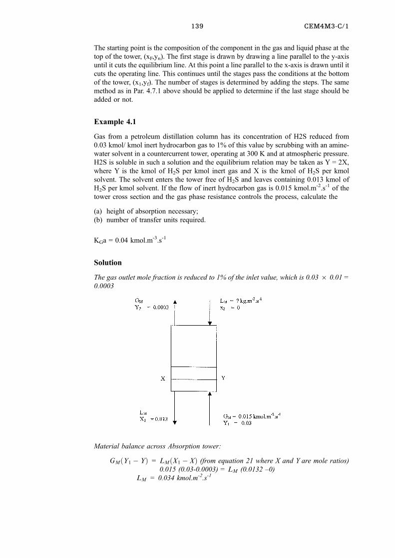
139 CEM4M3-C/1
The starting point is the composition of the component in the gas and liquid phase at the
top of the tower, (xF,yn). The first stage is drawn by drawing a line parallel to the y-axis
until it cuts the equilibrium line. At this point a line parallel to the x-axis is drawn until it
cuts the operating line. This continues until the stages pass the conditions at the bottom
of the tower, (x1,yf). The number of stages is determined by adding the steps. The same
method as in Par. 4.7.1 above should be applied to determine if the last stage should be
added or not.
Example 4.1
Gas from a petroleum distillation column has its concentration of H2S reduced from
0.03 kmol/ kmol inert hydrocarbon gas to 1% of this value by scrubbing with an amine-
water solvent in a countercurrent tower, operating at 300 K and at atmospheric pressure.
H2S is soluble in such a solution and the equilibrium relation may be taken as Y = 2X,
where Y is the kmol of H2S per kmol inert gas and X is the kmol of H2S per kmol
solvent. The solvent enters the tower free of H2S and leaves containing 0.013 kmol of
H2S per kmol solvent. If the flow of inert hydrocarbon gas is 0.015 kmol.m-2.s-1 of the
tower cross section and the gas phase resistance controls the process, calculate the
(a) height of absorption necessary;
(b) number of transfer units required.
KGa = 0.04 kmol.m-3.s-1
Solution
The gas outlet mole fraction is reduced to 1% of the inlet value, which is 0.03 6 0.01 =
0.0003
Material balance across Absorption tower:
GM�Y1 ÿ Y� = LM�X1 ÿ X� (from equation 21 where X and Y are mole ratios)
0.015 (0.03-0.0003) = LM (0.0132 ±0)
LM = 0.034 kmol.m-2.s-1
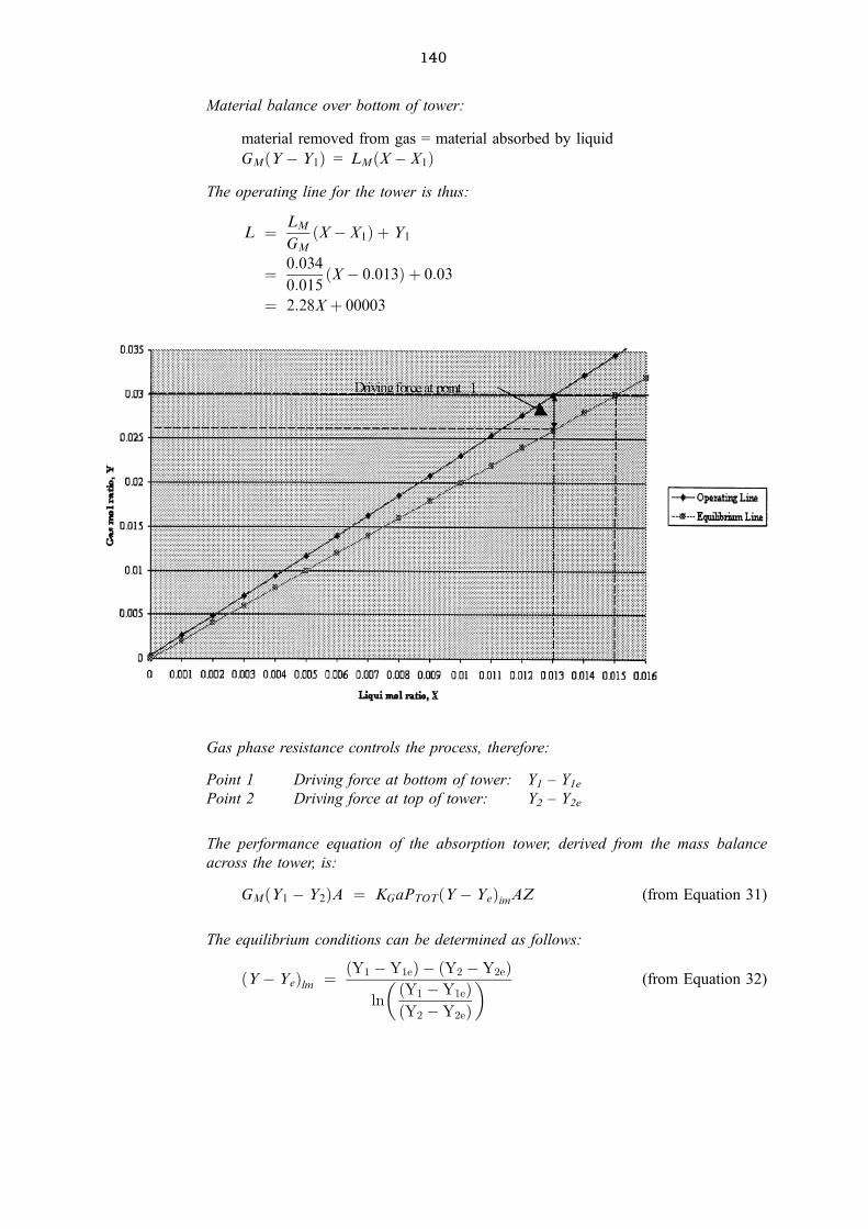
140
Material balance over bottom of tower:
material removed from gas = material absorbed by liquid
GM�Yÿ Y1� = LM�Xÿ X1�The operating line for the tower is thus:
L � LM
GM�Xÿ X1� � Y1
� 0:034
0:015�Xÿ 0:013� � 0:03
� 2:28X� 00003
Gas phase resistance controls the process, therefore:
Point 1 Driving force at bottom of tower: Y1 ± Y1e
Point 2 Driving force at top of tower: Y2 ± Y2e
The performance equation of the absorption tower, derived from the mass balance
across the tower, is:
GM�Y1 ÿ Y2�A � KGaPTOT�Yÿ Ye�imAZ (from Equation 31)
The equilibrium conditions can be determined as follows:
�Yÿ Ye�lm ��Y1 ÿY1e� ÿ �Y2 ÿY2e�
ln
� �Y1 ÿY1e��Y2 ÿY2e�
� (from Equation 32)
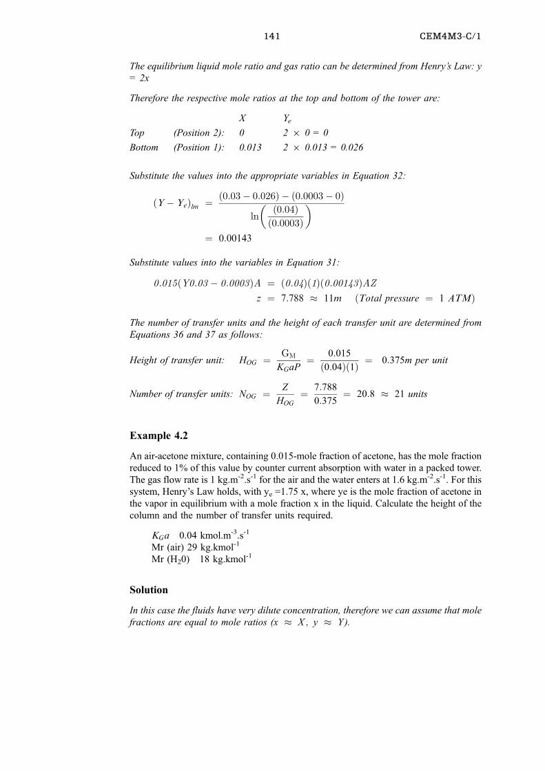
141 CEM4M3-C/1
The equilibrium liquid mole ratio and gas ratio can be determined from Henry's Law: y
= 2x
Therefore the respective mole ratios at the top and bottom of the tower are:
X Ye
Top (Position 2): 0 2 6 0 = 0
Bottom (Position 1): 0.013 2 6 0.013 = 0.026
Substitute the values into the appropriate variables in Equation 32:
�Yÿ Ye�lm ��0:03ÿ 0:026� ÿ �0:0003ÿ 0�
ln
� �0:04��0:0003�
�� 0:00143
Substitute values into the variables in Equation 31:
0:015�Y0:03 ÿ 0:0003�A � �0:04��1��0:00143�AZ
z � 7:788 � 11m �Total pressure � 1 ATM�
The number of transfer units and the height of each transfer unit are determined from
Equations 36 and 37 as follows:
Height of transfer unit: HOG � GM
KGaP� 0:015
�0:04��1� � 0:375m per unit
Number of transfer units: NOG � Z
HOG
� 7:788
0:375� 20:8 � 21 units
Example 4.2
An air-acetone mixture, containing 0.015-mole fraction of acetone, has the mole fraction
reduced to 1% of this value by counter current absorption with water in a packed tower.
The gas flow rate is 1 kg.m-2.s-1 for the air and the water enters at 1.6 kg.m-2.s-1. For this
system, Henry's Law holds, with ye =1.75 x, where ye is the mole fraction of acetone in
the vapor in equilibrium with a mole fraction x in the liquid. Calculate the height of the
column and the number of transfer units required.
KGa 0.04 kmol.m-3.s-1
Mr (air) 29 kg.kmol-1
Mr (H20) 18 kg.kmol-1
Solution
In this case the fluids have very dilute concentration, therefore we can assume that mole
fractions are equal to mole ratios (x � X ; y � Y).
142
Material balance across absorption tower:
GM�Y1 ÿ Y� � LM�Xÿ 1ÿ X� (from equation 21 where X and Y are mole
ratios)
GM�y1 ÿ Y2� � LM�X1 ÿ X2�
GM � G
Mr�gas� �1
29� 0:03448 kmol:mÿ2:sÿ1.
LM � G
Mr�liquid� �1:6
18� 0:0889 kmol:mÿ2:sÿ1.
Thus 0.03448(0.015 ± 0.00015) = 0.0889�x1 ÿ 0�v�
x1 = 0.00576
The performance equation of the absorption tower, derived from the mass balance
across the tower, is:
GM�Y1 ÿ Y2�A � KGaPTOT�Yÿ Ye�lmAZ (from Equation 31)
The equilibrium conditions can be determined as follows:
�Yÿ Ye�lm ��Y1 ÿY1e� ÿ �Y2 ÿY2e�
ln
� �Y1 ÿY1e��Y2 ÿY2e�
� (from Equation 32)
The equilibrium liquid mole ratio and gas ratio can be determined from Henry's Law:
y=1.75x
Therefore the respective mole ratios at the top and bottom of the tower are:
ÐÐÐÐÐÐÐÐÐÐÐv�1 % of inlet gas concentration
143 CEM4M3-C/1
x ye
Top (Position 2): 0 1.75 6 0 = 0
Bottom (Position 1): 0.00576 1.75 6 0.00576 = 0.0101
Substitute the values into the appropriate variables in Equation 32:
�Yÿ Ye�lm ��0:015ÿ 0:0101� ÿ �0:00015ÿ 0�
ln
� �0:049��0:00015�
�
Substitute values into the variables in Equation 31:
0.03448(0.015 ± 0.00015)A = (0.04)(1)(0.00136)AZ
z � 10:46 � 11m (Assume total pressure 1 atm)
The number of transfer units and the height of each transfer unit are determined from
Equations 36 and 37 as follows:
Height of transfer unit: HOG � GM
KGaP� 0:03448
0:04� 0:862m per unit
Number of transfer: NOG � Z
HOG
� 10:46
0:862� 12:13 � 13 units
4.9 TYPES OF ABSORPTION EQUIPMENT
From the performance equation derived, it is observed that the interfacial area between
the gas and liquid phases should be maximized. This can be done by several methods of
which the packed column and the plate column are the most common.
4.9.1 Selection of Columns
Packed columns are used for liquids that foam excessively, very corrosive materials and
for columns where only very low pressure drops are allowed. The type of packing
applied is determined by its mechanical strength, resistance to corrosion, capacity for
handling the required flows, mass-transfer efficiency and cost.
Plate columns are used for large-scale operations and are used when the liquid flow rate
is too low to wet the packing material sufficiently. Furthermore, it is used when the gas
velocity is low (high LIG), which can result in gas being mixed back down the column.
It is also used if the fluid has to be cooled intermediately.
The following design parameters have to be kept in mind.
Column Diameter and Pressure Drop
The minimum diameter of an absorption column is determined by the flooding point
(which is the maximum allowable velocity), usually 60% to 80% of the flooding
velocity. The maximum allowable pressure drop may be determined by cost of energy
for compression of the feed gas. In the case of systems that foam, the maximum
allowable velocity is lower than the flooding velocity.
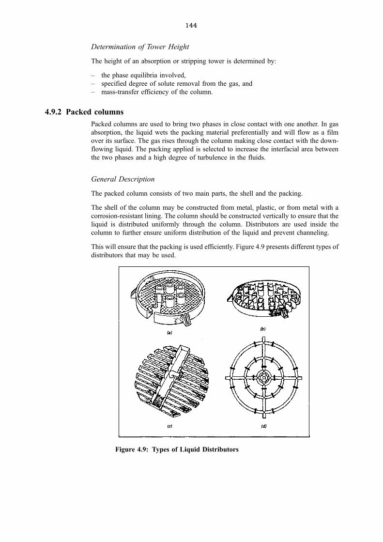
144
Determination of Tower Height
The height of an absorption or stripping tower is determined by:
± the phase equilibria involved,
± specified degree of solute removal from the gas, and
± mass-transfer efficiency of the column.
4.9.2 Packed columns
Packed columns are used to bring two phases in close contact with one another. In gas
absorption, the liquid wets the packing material preferentially and will flow as a film
over its surface. The gas rises through the column making close contact with the down-
flowing liquid. The packing applied is selected to increase the interfacial area between
the two phases and a high degree of turbulence in the fluids.
General Description
The packed column consists of two main parts, the shell and the packing.
The shell of the column may be constructed from metal, plastic, or from metal with a
corrosion-resistant lining. The column should be constructed vertically to ensure that the
liquid is distributed uniformly through the column. Distributors are used inside the
column to further ensure uniform distribution of the liquid and prevent channeling.
This will ensure that the packing is used efficiently. Figure 4.9 presents different types of
distributors that may be used.
Figure 4.9: Types of Liquid Distributors
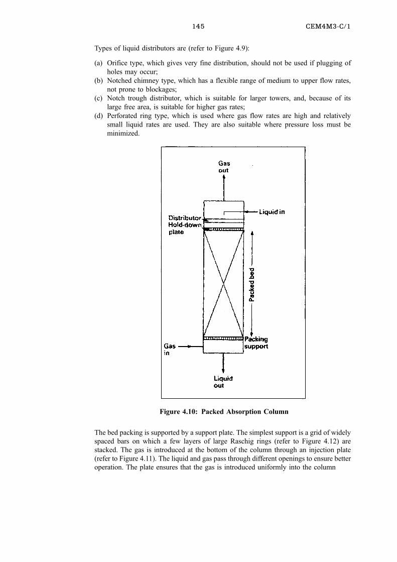
145 CEM4M3-C/1
Types of liquid distributors are (refer to Figure 4.9):
(a) Orifice type, which gives very fine distribution, should not be used if plugging of
holes may occur;
(b) Notched chimney type, which has a flexible range of medium to upper flow rates,
not prone to blockages;
(c) Notch trough distributor, which is suitable for larger towers, and, because of its
large free area, is suitable for higher gas rates;
(d) Perforated ring type, which is used where gas flow rates are high and relatively
small liquid rates are used. They are also suitable where pressure loss must be
minimized.
The bed packing is supported by a support plate. The simplest support is a grid of widely
spaced bars on which a few layers of large Raschig rings (refer to Figure 4.12) are
stacked. The gas is introduced at the bottom of the column through an injection plate
(refer to Figure 4.11). The liquid and gas pass through different openings to ensure better
operation. The plate ensures that the gas is introduced uniformly into the column
Figure 4.10: Packed Absorption Column
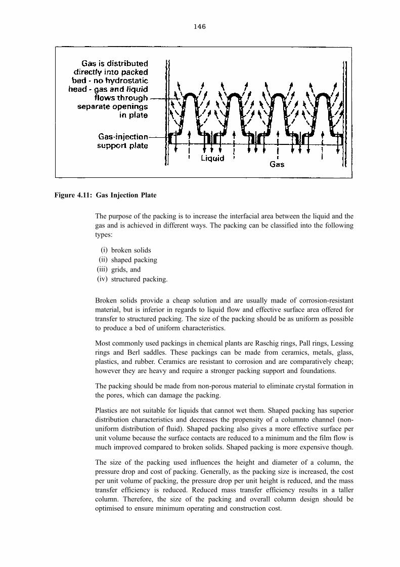
146
The purpose of the packing is to increase the interfacial area between the liquid and the
gas and is achieved in different ways. The packing can be classified into the following
types:
(i) broken solids
(ii) shaped packing
(iii) grids, and
(iv) structured packing.
Broken solids provide a cheap solution and are usually made of corrosion-resistant
material, but is inferior in regards to liquid flow and effective surface area offered for
transfer to structured packing. The size of the packing should be as uniform as possible
to produce a bed of uniform characteristics.
Most commonly used packings in chemical plants are Raschig rings, Pall rings, Lessing
rings and Berl saddles. These packings can be made from ceramics, metals, glass,
plastics, and rubber. Ceramics are resistant to corrosion and are comparatively cheap;
however they are heavy and require a stronger packing support and foundations.
The packing should be made from non-porous material to eliminate crystal formation in
the pores, which can damage the packing.
Plastics are not suitable for liquids that cannot wet them. Shaped packing has superior
distribution characteristics and decreases the propensity of a columnto channel (non-
uniform distribution of fluid). Shaped packing also gives a more effective surface per
unit volume because the surface contacts are reduced to a minimum and the film flow is
much improved compared to broken solids. Shaped packing is more expensive though.
The size of the packing used influences the height and diameter of a column, the
pressure drop and cost of packing. Generally, as the packing size is increased, the cost
per unit volume of packing, the pressure drop per unit height is reduced, and the mass
transfer efficiency is reduced. Reduced mass transfer efficiency results in a taller
column. Therefore, the size of the packing and overall column design should be
optimised to ensure minimum operating and construction cost.
Figure 4.11: Gas Injection Plate
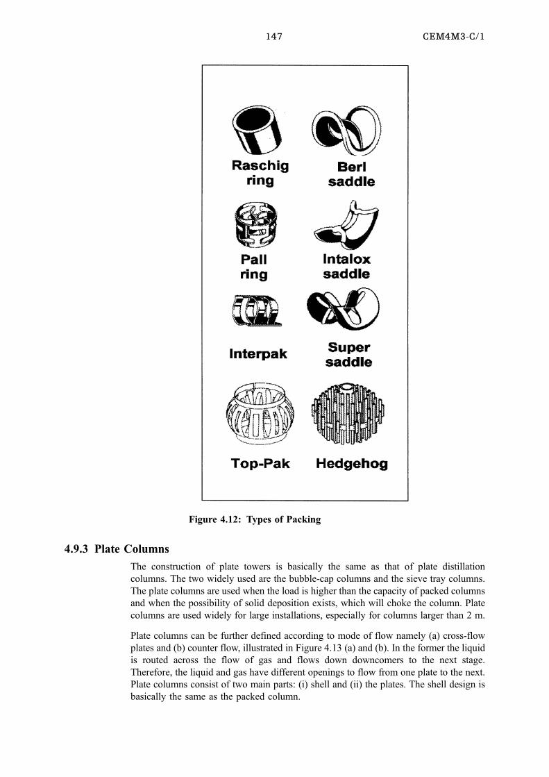
147 CEM4M3-C/1
4.9.3 Plate Columns
The construction of plate towers is basically the same as that of plate distillation
columns. The two widely used are the bubble-cap columns and the sieve tray columns.
The plate columns are used when the load is higher than the capacity of packed columns
and when the possibility of solid deposition exists, which will choke the column. Plate
columns are used widely for large installations, especially for columns larger than 2 m.
Plate columns can be further defined according to mode of flow namely (a) cross-flow
plates and (b) counter flow, illustrated in Figure 4.13 (a) and (b). In the former the liquid
is routed across the flow of gas and flows down downcomers to the next stage.
Therefore, the liquid and gas have different openings to flow from one plate to the next.
Plate columns consist of two main parts: (i) shell and (ii) the plates. The shell design is
basically the same as the packed column.
Figure 4.12: Types of Packing
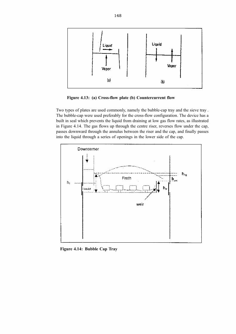
148
Two types of plates are used commonly, namely the bubble-cap tray and the sieve tray .
The bubble-cap were used preferably for the cross-flow configuration. The device has a
built in seal which prevents the liquid from draining at low gas flow rates, as illustrated
in Figure 4.14. The gas flows up through the centre riser, reverses flow under the cap,
passes downward through the annulus between the riser and the cap, and finally passes
into the liquid through a series of openings in the lower side of the cap.
Figure 4.13: (a) Cross-flow plate (b) Countercurrent flow
Figure 4.14: Bubble Cap Tray
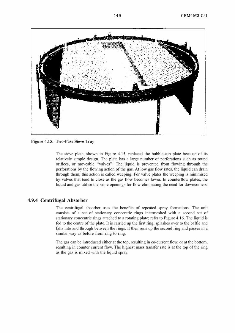
149 CEM4M3-C/1
The sieve plate, shown in Figure 4.15, replaced the bubble-cap plate because of its
relatively simple design. The plate has a large number of perforations such as round
orifices, or moveable `̀ valves''. The liquid is prevented from flowing through the
perforations by the flowing action of the gas. At low gas flow rates, the liquid can drain
through them; this action is called weeping. For valve plates the weeping is minimised
by valves that tend to close as the gas flow becomes lower. In counterflow plates, the
liquid and gas utilise the same openings for flow eliminating the need for downcomers.
4.9.4 Centrifugal Absorber
The centrifugal absorber uses the benefits of repeated spray formations. The unit
consists of a set of stationary concentric rings intermeshed with a second set of
stationary concentric rings attached to a rotating plate; refer to Figure 4.16. The liquid is
fed to the centre of the plate. It is carried up the first ring, splashes over to the baffle and
falls into and through between the rings. It then runs up the second ring and passes in a
similar way as before from ring to ring.
The gas can be introduced either at the top, resulting in co-current flow, or at the bottom,
resulting in counter current flow. The highest mass transfer rate is at the top of the ring
as the gas is mixed with the liquid spray.
Figure 4.15: Two-Pass Sieve Tray
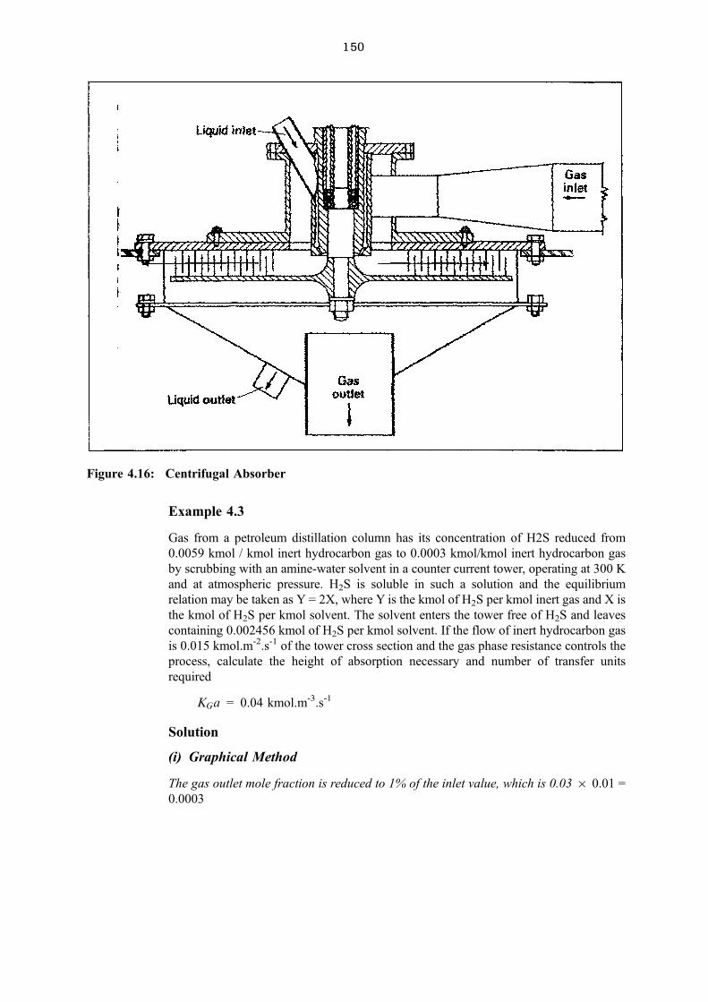
150
Example 4.3
Gas from a petroleum distillation column has its concentration of H2S reduced from
0.0059 kmol / kmol inert hydrocarbon gas to 0.0003 kmol/kmol inert hydrocarbon gas
by scrubbing with an amine-water solvent in a counter current tower, operating at 300 K
and at atmospheric pressure. H2S is soluble in such a solution and the equilibrium
relation may be taken as Y = 2X, where Y is the kmol of H2S per kmol inert gas and X is
the kmol of H2S per kmol solvent. The solvent enters the tower free of H2S and leaves
containing 0.002456 kmol of H2S per kmol solvent. If the flow of inert hydrocarbon gas
is 0.015 kmol.m-2.s-1 of the tower cross section and the gas phase resistance controls the
process, calculate the height of absorption necessary and number of transfer units
required
KGa = 0.04 kmol.m-3.s-1
Solution
(i) Graphical Method
The gas outlet mole fraction is reduced to 1% of the inlet value, which is 0.03 6 0.01 =
0.0003
Figure 4.16: Centrifugal Absorber
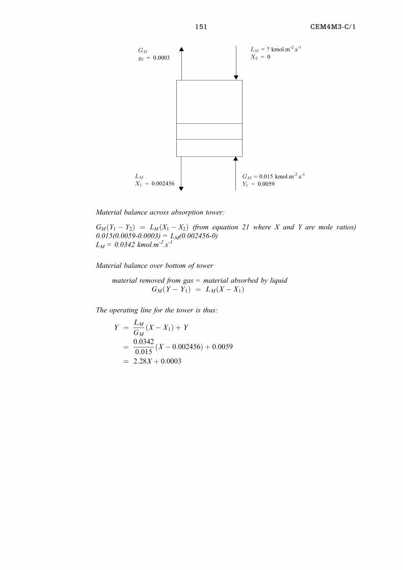
151 CEM4M3-C/1
GM
y2 = 0.0003
GM = 0.015 kmol.m-2.s-1
Y1 = 0.0059
LM = ? kmol.m-2.s-1
X2 = 0
LMX1 = 0.002456
!
!
!
!
Material balance across absorption tower:
GM �Y1 ÿ Y2� � LM �X1 ÿ X2� (from equation 21 where X and Y are mole ratios)
0.015(0.0059-0.0003) = LM(0.002456-0)
LM = 0.0342 kmol.m-2.s-1
Material balance over bottom of tower
material removed from gas = material absorbed by liquid
GM�Yÿ Y1� � LM�Xÿ X1�
The operating line for the tower is thus:
Y � LM
GM�Xÿ X1� � Y
� 0:0342
0:015�Xÿ 0:002456� � 0:0059
� 2:28X� 0:0003
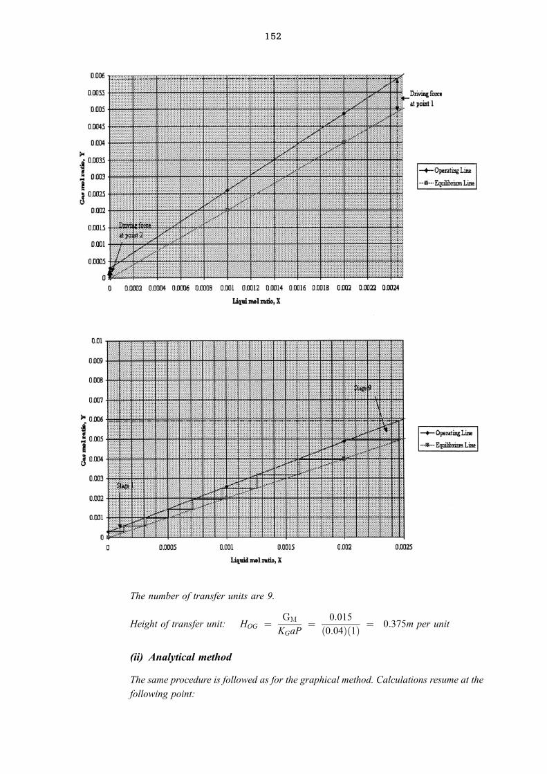
152
The number of transfer units are 9.
Height of transfer unit: HOG � GM
KGaP� 0:015
�0:04��1� � 0:375m per unit
(ii) Analytical method
The same procedure is followed as for the graphical method. Calculations resume at the
following point:
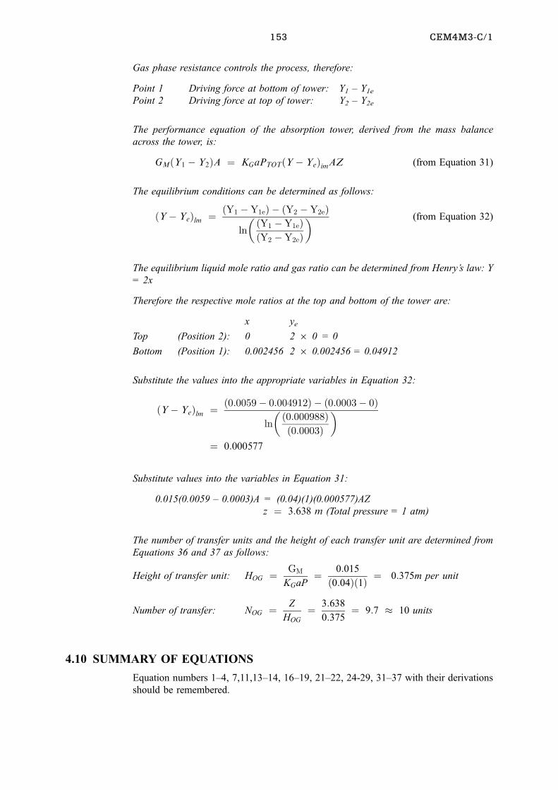
153 CEM4M3-C/1
Gas phase resistance controls the process, therefore:
Point 1 Driving force at bottom of tower: Y1 ± Y1e
Point 2 Driving force at top of tower: Y2 ± Y2e
The performance equation of the absorption tower, derived from the mass balance
across the tower, is:
GM�Y1 ÿ Y2�A � KGaPTOT�Yÿ Ye�imAZ (from Equation 31)
The equilibrium conditions can be determined as follows:
�Yÿ Ye�lm ��Y1 ÿY1e� ÿ �Y2 ÿY2e�
ln
� �Y1 ÿY1e��Y2 ÿY2e�
� (from Equation 32)
The equilibrium liquid mole ratio and gas ratio can be determined from Henry's law: Y
= 2x
Therefore the respective mole ratios at the top and bottom of the tower are:
x ye
Top (Position 2): 0 2 6 0 = 0
Bottom (Position 1): 0.002456 2 6 0.002456 = 0.04912
Substitute the values into the appropriate variables in Equation 32:
�Yÿ Ye�lm ��0:0059ÿ 0:004912� ÿ �0:0003ÿ 0�
ln
� �0:000988��0:0003�
�� 0:000577
Substitute values into the variables in Equation 31:
0.015(0.0059 ± 0.0003)A = (0.04)(1)(0.000577)AZ
z � 3:638 m (Total pressure = 1 atm)
The number of transfer units and the height of each transfer unit are determined from
Equations 36 and 37 as follows:
Height of transfer unit: HOG � GM
KGaP� 0:015
�0:04��1� � 0:375m per unit
Number of transfer: NOG � Z
HOG
� 3:638
0:375� 9:7 � 10 units
4.10 SUMMARY OF EQUATIONS
Equation numbers 1±4, 7,11,13±14, 16±19, 21±22, 24-29, 31±37 with their derivations
should be remembered.
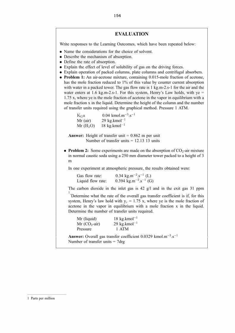
154
EVALUATION
Write responses to the Learning Outcomes, which have been repeated below:
. Name the considerations for the choice of solvent.
. Describe the mechanism of absorption.
. Define the rate of absorption.
. Explain the effect of level of solubility of gas on the driving forces.
. Explain operation of packed columns, plate columns and centrifugal absorbers.
. Problem 1: An air-acetone mixture, containing 0.015-mole fraction of acetone,
has the mole fraction reduced to 1% of this value by counter current absorption
with water in a packed tower. The gas flow rate is 1 kg.m-2.s-1 for the air and the
water enters at 1.6 kg.m-2.s-1. For this system, Henry's Law holds, with ye =
1.75 x, where ye is the mole fraction of acetone in the vapor in equilibrium with a
mole fraction x in the liquid. Determine the height of the column and the number
of transfer units required using the graphical method. Pressure 1 ATM.
KGa 0.04 kmol.mÿ3.sÿ1
Mr (air) 29 kg.kmolÿ1
Mr (H2O) 18 kg.kmolÿ1
Answer: Height of transfer unit = 0.862 m per unit
Number of transfer units = 12.13 13 units
. Problem 2: Some experiments are made on the absorption of CO2-air mixture
in normal caustic soda using a 250 mm diameter tower packed to a height of 3
m
In one experiment at atmospheric pressure, the results obtained were:
Gas flow rate: 0.34 kg.mÿ2.sÿ1 (L)
Liquid flow rate: 0.394 kg.mÿ2.sÿ1 (G)
The carbon dioxide in the inlet gas is 42 g/l and in the exit gas 31 ppm1.
Determine what the rate of the overall gas transfer coefficient is if, for this
system, Henry's law hold with ye = 1.75 x, where ye is the mole fraction of
acetone in the vapor in equilibrium with a mole fraction x in the liquid.
Determine the number of transfer units required.
Mr (liquid) 18 kg.kmolÿ1
Mr (CO2-air) 29 kg.kmolÿ1
Pressure 1 ATM
Answer: Overall gas transfer coefficient 0.0329 kmol.mÿ3.sÿ1
Number of transfer units = 7drg
ÐÐÐÐÐÐÐÐÐÐÐ1 Parts per million


![sequential.ppt [Read-Only]](https://static.fdokumen.com/doc/165x107/6319ca5fc51d6b41aa04902b/sequentialppt-read-only.jpg)