CHC3100 CHEMICAL REACTION ENGINEERING -I

CHC3100

CHEMICAL REACTION ENGINEERING -I

QAZI NAVED AHMAD

ASSISTANT PROFESSOR

DEPARTMENT OF CHEMICAL ENGINEERING

AMU, ALIGARH

Course Objective and Outcomes:

Course Objective Application of basic Chemical Engineering Principles to understand the chemical

kinetics and reactor design.

Course Outcomes

Students will be able to

Understand the basic laws of Reaction Engineering, kinetics and design of reactors.

Understand the kinetics of multiple reaction and multiple reaction design.

Comprehend and to apply temperature and pressure effects in reactor design.

UnderstandTRD in ideal and non-ideal reactors.

SYLLABUS

Unit I

Overview of Chemical Reaction Engineering. Reaction mechanism. Interpretation of batch reactor data. Ideal

reactors.Reactor design for single reaction.

Unit II

Multiple reactor systems, optimum reactor scheme, recycle reactor. Multiple Reactions: parallel and series reactions,

contacting pattern and product distribution, series- parallel reactions in mixed and plug flow reactors, optimum yield

of desired product.

Unit III

Temperature and pressure effects on equilibrium conversion, exothermic and endothermic reactions, optimum

temperature progression

Unit IV

Residence Time Distribution: stimulus response techniques, the RTD, E and F curves, RTD for ideal and non ideal

reactors,conversion in non-ideal reactors.

Text Books and Reference Books

Text Books:

1. Levenspiel,Octave,Chemical Reaction Engineering,3rd Edition (2005), JohnWiley & Sons,Singapore.

2. Fogler,Scott H.,Elements of Chemical Reaction Engineering,4th Edition (2008),Prentice-Hall of India,New Delhi.

Reference Books:

1. Smith, J.M.,Chemical Engineering Kinetics, 5th Edition (2002),McGraw-Hill,NewYork.

2. Schmidt, Lanny D., the Engineering of Chemical Reactions, 2nd Edition (2005), Oxford University Press, Oxford,NewYork.

3. Froment,G. F. and K.B.Bischoff,Chemical ReactorAnalysis and Design, JohnWiley & Sons,NewYork (1990).

4. Hill, Charles, G. Jr., An Introduction to Chemical Engineering Kinetics and Reactor Design, John Wiley & Sons, NewYork (1977).

5. Holland, Charles D., and R.G. Anthony, Fundamentals of Chemical Reaction Engineering, 2nd Edition (1989), Prentice-Hall Inc,New Jersey.

UNIT I:

OVERVIEW OF CHEMICAL REACTION ENGINEERING

Figure 1.1: Typical Chemical Process

• CRE is concerned with chemical treatment of the above shown typical chemical process.

• This chemical step is mainly consisted of inconsequential unit, or simply a mixing tank (or reactor) that makes or

breaks the process economically.

• Reactor design pre-requisites – chemical kinetics, thermodynamics, fluid mechanics, heat and mass transfers, and

economics.

• Chemical reaction engineering is the synthesis of all these factors with the aim of properly designing a chemical

reactor.

To know what a reactor can do, one must know the kinetics, the contacting patterns, and the performance

equation,as shown by figure 1.2.

Output = f [input, kinetics,contacting pattern]

The above equation is known as performance

equation.

It relates input and output of the system

(reactor).

It can be used to

compare different designs and conditions,

Find which is best, and then scale up to larger units.


Figure 1.2: Information needed to know what a Reactor can do.

-------- (1)

Homogeneous and Heterogeneous Reactions:

In CRE, the classification of reactions can be made on the basis of types/number of phases involved in a reaction.

A homogeneous reaction is the reaction in which the reaction takes place in the same phase i.e., either solid, or

liquid, or gas.

A reaction is said to be heterogeneous if the reaction takes place with at least two phases involved.


Table 1.1: Classification of Chemical Reactions useful in Reactor Design

Rate of Reaction:

Selecting one reaction component “i” and defining the rate of reaction in terms of i.

Number of ways in which rate of reaction can be defined are as follows –

1. Rate of Reaction based on Volume of the Reacting Fluid:

2. Based on Unit Mass of Solid in Solid-Fluid System:

3. Based on Unit Interfacial Surface in two-fluids system or on Unit Surface of solid in solid-fluid system:


-------- (2)

-------- (3)

-------- (4)

4. Based on UnitVolume of Solid in Gas-Solid System:

5. Based on UnitVolume of Reactor (if rate based on volume of reacting fluid is different):

For homogeneous systems, volume of fluid is often identical to volume of reactor therefore, in that case equations

(2) and (6) can be used interchangeably.

In heterogeneous systems,all of the above equation can be encountered.

Equations (2) to (6) are interconnected to each other in the following manner –


-------- (5)

-------- (6)

or,

Variables affecting Reaction Rate:

In homogeneous systems, the temperature, pressure and compositions are the parameters which affects the rate

of reaction.

In heterogeneous systems, since the reaction takes place in multiphase therefore the affecting parameters are

difficult to find.Two of the most important parameters are heat and mass transfers which takes place between the

multiple phases. E.g., amount of oxygen required for burning coal (mass transfer), an exothermic reaction with

heat extraction system (heat transfer),burning of gas, etc.

For heterogeneous systems,mass and heat transfers play important role in determining the rate of reaction.

-------- (7)


Speed of Chemical Reactions:

Reactions may occur at rapid speed or at a very, very slow rate. This speed generally depends on the end

product. For example in case of production gasoline from crude oil,we want the reaction to get completed in less

than a second.

Figure 1.3 shows different reactions with their typical speeds of progression.


KINETICS/REACTION MECHANISM OF HOMOGENEOUS REACTIONS

Simple Reactors:

Figure 2.1: Types of Ideal Reactors

The Rate Equation:

For a single-phase reaction,

the rate of reaction for reactant A can be given as –

Also, the rates of reaction of all the elements are related to each other as –


From experience, it is observed that –

Rate of reaction is a function of two terms, temperature and concentration.


Concentration DependentTerm:

1. Single and Multiple Reactions: Reactions, where only one stoichiometric equation and one rate equation is involved

in representing the progress of an ongoing reaction, is known as Single Reaction.

Where more than one stoichiometric equation is involved then more than one kinetic expressions are needed to

express the changes in ongoing reactions,these are called Multiple Reactions.They may be further classified as –

Series reaction –

Parallel reactions – they can be further classified into two types

Both series and parallel simultaneously –


2. Elementary and Non-Elementary Reactions: Reactions, in which rate equation corresponds to stoichiometric

equation of the system, are known as Elementary Reactions. For example, for a given single reaction, the

stoichiometric equation can be given as –

therefore,the rate of reaction can be written as,

When there is no direct correspondence between stoichiometry and rate, then the reactions are known as non-

elementary reactions. The classical example of a non-elementary reaction is that between hydrogen and bromine,


The rate expression of given stoichiometric equation is given as –

The non-elementary reactions can be explained as a sequence of single reactions or elementary reactions.

3. Molecularity and Order of Reaction:

Molecularity of an elementary reaction refers to the number of molecules taking part in the reaction.

It can have a value of 1, 2, 3,… which means molecularity will have only integral value.

Molecularity is defined only for elementary reactions.

For a reaction,rate is given as –

Where a, b, .., d are not necessarily related to stoichiometry of the reaction.


The power, to which the concentration term in the reaction rate is raised to, is known as Order of the Reaction with

respect to that element/molecule.

Thus,the reaction is

ath order with respect to A.

bth order with respect to B.

nth order overall.

Since the order refers to the empirically found rate expression, it can have a fractional value and need not be an

integer.

4. Rate Constant,k:

For a homogeneous chemical reactions with rate equation given as

The dimensions of the rate constant,k, for nth order reaction can be given as


For first order reaction, the rate constant has the following dimensions

5. Representation of an Elementary Reaction:

Rate equation can also be written in terms of pressure which is equivalent measure to the concentration term.Therefore,

Writing the rate equation in terms of equivalent measures does not have any affect on its order but will affect therate constant,k.

Elementary reactions are represented by equations that contain molecularity as well as rate constant in it.

The rate expression for this elementary reaction –


In some cases, where there is an ambiguity due to more number of components taking part in a reaction, the rate

constant may be written in terms of the component, with respect to which rate constant is mentioned. For example

–

Also, from stoichiometry –

Therefore,


6. Kinetic Models for Non-Elementary Reactions:

In non-elementary reactions, the stoichiometry does not match with the kinetics of the reaction therefore, a

multistep reaction model is developed to explain the kinetics.

A non-elementary reaction can be simplified as series of single elementary reactions to identify the kinetics easily.

For example –

where * refers to the unobserved intermediates.These intermediates can be grouped as –

a) Free Radicals: Free atoms or larger fragments of stable molecules that contain one or more unpaired electrons

are called free radicals.The unpaired electron is represented by a dot in the chemical symbol of the substance.


b) Ions and Polar Substances: These are electrically charged atoms, molecules, or fragments of molecules known as

ions.They may acts as active intermediates in reactions. For example –

c) Molecules:For the following reaction in series,

R is said to be the active intermediate but if its activity is increased then its quantity becomes very small or

unobservable as it reacts to form B very fast therefore in such situations,R is referred to as reactive intermediate.


Postulated reaction schemes involving these three kinds of intermediates can be of two types.

Non-chain Reactions: In the non-chain reaction the intermediate is formed in the first reaction and thendisappears as it reacts further to give the product.Thus,

Chain Reactions: In chain reactions the intermediate is formed in a first reaction, called the chain initiation step. Itthen combines with reactant to form product and more intermediate in the chain propagation step. Occasionally theintermediate is destroyed in the chain termination step.Thus,

The essential feature of the chain reaction is the propagation step. In this step the intermediate is not consumed butacts simply as a catalyst for the conversion of material. Thus, each molecule of intermediate can catalyze a long chainof reactions, even thousands,before being finally destroyed.


Examples pertaining to the above mentioned mechanisms are:

a. Free Radicals,Chain Reaction Mechanism:The reaction

with experimental rate,

and can be explained by the following scheme which introduces and involves the intermediates H2. and Br2.,


b. Molecular intermediates,Non-chain mechanism:The general class of enzyme- catalyzed fermentation reactions

with experimental rate

is viewed to proceed with intermediate (A.enzyme)* as follows:

In such reactions the concentration of intermediate may become more than negligible, in which case a special

analysis, first proposed by Michaelis and Menten (1913), is required.


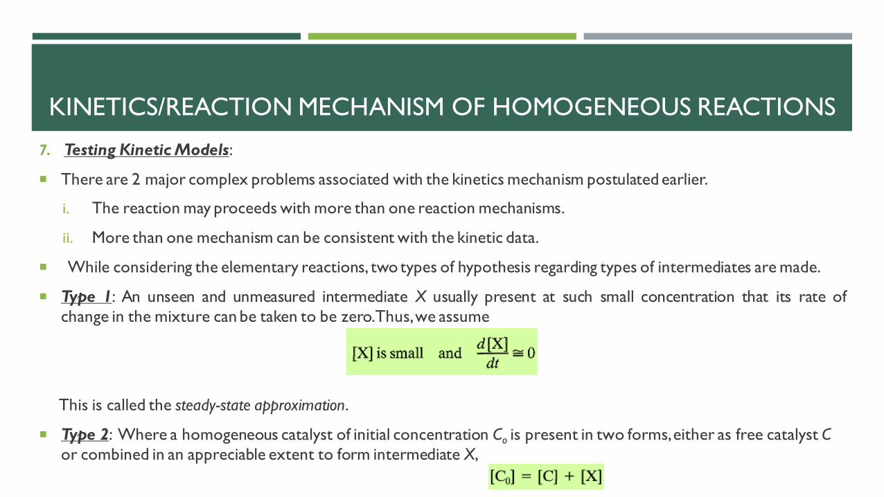
7. Testing Kinetic Models:

There are 2 major complex problems associated with the kinetics mechanism postulated earlier.

i. The reaction may proceeds with more than one reaction mechanisms.

ii. More than one mechanism can be consistent with the kinetic data.

While considering the elementary reactions, two types of hypothesis regarding types of intermediates are made.

Type 1: An unseen and unmeasured intermediate X usually present at such small concentration that its rate of

change in the mixture can be taken to be zero.Thus,we assume

This is called the steady-state approximation.

Type 2: Where a homogeneous catalyst of initial concentration Co is present in two forms, either as free catalyst C

or combined in an appreciable extent to form intermediate X,


Also, assuming –

or that the intermediate is in equilibrium with its reactants; thus,

where,


Temperature DependentTerm:

1. Temperature dependency from Arrhenius’ Law: For many reactions, and particularly elementary reactions, the rate

expression can be written as a product of a temperature-dependent term and a composition- dependent term,

or –

ri = f1(temperature) . f2(composition)

ri = k . f2(composition)

where,k in most of the cases,as predicted experimentally, is given byArrhenius’ equation –

Where, k0 is the frequency or pre exponential factor, E is the activation energy of reaction and, R is the universal

gas constant.


At the same concentration but different temperatures and at constantE,Arrhenius’ law indicates that –

2. Comparison of theories with Arrhenius’Law:

a) From Arrhenius’ plot of ln k vs 1/T gives a straight line,with large slopefor large E and small slope for small E,

b) Reactions with high activation energies are very temperature-sensitive;reactions with low activation energies are relatively temperature-insensitive.

c) Any given reaction is much more temperature sensitive at a lowtemperature than a high temperature.

d) From the Arrhenius’ law, the value of the frequency factor k0 does notaffect the temperature sensitivity.


The Reaction Mechanism:

There are three areas of investigation of a reaction, the stoichiometry, the kinetics, and the mechanism. In general,

the stoichiometry is studied first, and when this is far enough along, the kinetics is then investigated. With

empirical rate expressions available,the mechanism is then looked into.

Several clues that are often used in such experimentation can be mentioned.

1. Stoichiometry can tell whether we have a single reaction or not. Thus, a complicated stoichiometry or one that

changes with reaction conditions or extent of reaction is clear evidence of multiple reactions.

2. Stoichiometry can suggest whether a single reaction is elementary or not because molecularity of an elementary

reaction cannot increase by three.

3. A comparison of the stoichiometric equation and experimental kinetic expression can be made in order to find

the reaction to be elementary.

4. A large difference in the order of magnitude between the experimentally found frequency factor of a reaction

and that calculated from collision theory or transition-state theory may suggest a nonelementary reaction.


5. For two alternative available paths for a simple reversible reaction, if one of these paths is preferred for the

forward reaction, the same path must also be preferred for the reverse reaction. This is called the principle of

microscopic reversibility.Consider, for example,the forward reaction of

At a first sight this could very well be an elementary biomolecular reaction with two molecules of ammonia

combining to yield directly the four product molecules. From this principle, however, the reverse reaction would

then also have to be an elementary reaction involving the direct combination of three molecules of hydrogen with

one of nitrogen. Because such a process is rejected as improbable, the bimolecular forward mechanism must also

be rejected.

6. For multiple reactions a change in the observed activation energy with temperature indicates a shift in the

controlling mechanism of reaction. Thus, for an increase in temperature Eobs rises for reactions or steps in

parallel, Eobs falls for reactions or steps in series. Conversely, for a decrease in temperature Eobs falls for reactions

in parallel,Eobs rises for reactions in series.These findings are illustrated in Fig. 2.3.


KINETICS/REACTION MECHANISM OF HOMOGENEOUS

REACTIONS

Figure 2.3 A change in activation energy indicates a shift in controlling mechanism of reaction.

The determination of the rate equation is usually a two step procedure:

1. The concentration dependent term is found at fixed temperature then,

2. The temperature dependent term is found yielding the complete rate equation.

Equipment by which empirical information is obtained can also be divided into two categories: the batch and flow

reactors.

Batch reactor is a simple container which holds the contents while they react with each other.

To get the empirical information, extent of reaction at various times is to be calculated. This can be done in the

following ways –

1. By following the concentration of a given component.

2. By following change in some physical property of the fluid (example refractive index, electrical conductivity etc.).

3. For a constant-volume system, a change in total pressure can be followed.

4. For a constant-pressure system,a change in volume can be followed.

CHAPTER 3:

INTERPRETATION OF BATCH REACTOR DATA

Experimentally, the batch reactor operates at isothermal and constant volume process conditions as it is easy to

interpret homogeneous kinetic data for batch reactor at these conditions.

It is a simple device adaptable to small-scale lab set-ups with very little auxiliary equipment or instrumentation.

There are two methods for interpreting kinetic data of a batch reactor – the integral and the differential.

In the integral method of analysis we guess a particular form of rate equation and, after appropriate integration

and mathematical manipulation, predict that the plot of a certain concentration function versus time should yield a

straight line. The data are plotted, and if a reasonably good straight line is obtained, then the rate equation is said

to satisfactorily fit the data.

In the differential method of analysis we test the fit of the rate expression to the data directly and without any

integration. However, since the rate expression is a differential equation, we must first find (1/V)(dN/dt) from the

data before attempting the fitting procedure.

The integral method is easy to use and is recommended when testing specific mechanisms, or relatively simple

rate expressions, or when the data are so scattered that we cannot reliably find the derivatives needed in the

differential method.


The differential method is useful in more complicated situations but requires more accurate or larger amounts of

data.

The integral method can only test this or that particular mechanism or rate form; the differential method can be

used to develop or build up a rate equation to fit the data.

In general, integral analysis is to be attempted first, and, if not successful, then the differential method can be tried.

Constant Volume Batch Reactor:

In a constant volume batch reactor , the term volume refers to the volume of the reacting mixture and not the

volume of reactor.

A constant volume system may also be referred to as Constant Density Reaction System.

Mostly, liquid phase as well as gas phase reactions falls under the category of constant volume reaction system.

For a constant volume system,, the reaction rate equations becomes –


-------- (3.1)

and for ideal gas system, where C = p/RT,

It is evident from the above equations that rate of reaction of any component is given by the rate of change of its

concentration or partial pressure (only for constant volume systems).

For gas reactions with changing numbers of moles, rate of reaction can be obtained by following the change in

total pressure of the system.

1. Analysis of Total Pressure Data Obtained in a Constant-Volume System: For isothermal gas reactions, writing

the general stoichiometric equation, and under each term indicating the number of moles of that component:


-------- (3.2)

Total number of moles present in the system initially –

Total number of moles present after time, t –

where,

Assuming Ideal gas law and writing for reactantA in terms of system volume V –

Combining eqns. 3.3 and 3.4, we get –

or


-------- (3.3)

-------- (3.4)

-------- (3.5)

Equation 3.5 gives the concentration or partial pressure of reactant A as a function of the total pressure π at time t,

initial partial pressure of A, pA0, and initial total pressure of the system, π0.

Similarly, for any product R we can find –

Equations 3.5 and 3.6 are the desired relationships between total pressure of the system and the partial pressure of

reacting materials.

If in case, the precise stoichiometry is not known, or if more than one stoichiometric equation is needed to

represent the reaction, then the "total pressure" procedure cannot be used.

2. The Conversion: Also known as fractional conversion, or the fraction of any reactant, say A, converted to

product, or the fraction of A reacted away.

In simple words, it can be called out as, conversion of A, with symbol XA.


-------- (3.6)

Suppose that NA0 is the initial amount of A in the reactor at time t = 0, and that NA is the amount present at time t.

Then the conversion of Ain the constant volume system is given by:

and,

Integral Method of Analysis:

The integral method of analysis always puts a particular rate equation to the test by integrating and comparing the

predicted C versus t curve with the experimental C versus t data.

If the fit is unsatisfactory, another rate equation is guessed and tested.

Integral method is especially useful for fitting simple reaction types corresponding to elementary reactions.


-------- (3.7)

-------- (3.8)

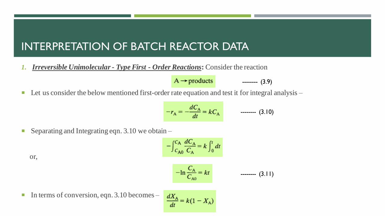
1. Irreversible Unimolecular - Type First - Order Reactions: Consider the reaction

Let us consider the below mentioned first-order rate equation and test it for integral analysis –

Separating and Integrating eqn. 3.10 we obtain –

or,

In terms of conversion, eqn. 3.10 becomes –


-------- (3.9)

-------- (3.10)

-------- (3.11)

On rearranging and integration, previous

equation becomes:

or,

A plot of ln(1 – XA) or ln(CA/CA0) vs. t, as

shown in Fig. 3.1, gives a straight line

through the origin for this form of rate of

equation.

If the experimental data seems to be better

fitted by a curve than by a straight line, try

another rate form because the first-order

reaction does not satisfactorily fit the data.


-------- (3.12)

Not all first-order reactions can be treated as shown above. For example, the equations of below mentioned type is

not worthy of this type of analysis –

2. Irreversible Bimolecular-Type Second-Order Reactions: Consider the bimolecular reaction –

with corresponding rate equation,

The amounts of A and B that have reacted at any time t are equal and given by CA0XA, we may write Eqs. 3.13a and

3.13b in terms of XA as –


-------- (3.13a)

-------- (3.13b)

Letting M = CB0/CA0 be the initial molar ratio of reactants, we obtain –

which on separation and integration becomes –

After breakdown into partial fractions, integration, and rearrangement, the final result in a number of different

forms is

Figure 3.2 shows two equivalent ways of obtaining a linear plot between the concentration function and time for

this second-order rate law.


-------- (3.14)

Figure 3.2: Test for Bimolecular Mechanism with CA0 does not equals to CB0, or for the second-order reaction


If CB0 is much larger than CA0, CB remains approximately constant at all times, and Eq. 3.14 approaches Eq. 3.11

or 3.12 for the first-order reaction. Thus, the second- order reaction becomes a pseudo first-order reaction.

Case 1: for the second-order reaction with equal initial concentrationsof A and B, or for the reaction

the defining second-order differential equation becomes

which on integration yields –

Figure 3.3 provides a test for this rate expression.

In practice, we should choose reactant ratios either equal to or widely different from the stoichiometric ratio.


-------- (3.15a)

-------- (3.16)

-------- (3.15b)

Figure 3.3: Test for Bimolecular Mechanism with CA0 equals to CB0, or for the second-order reaction


Case 1I: If the reaction is first order with respect to both A and B, hence second order overall, or

which on integration yields –

When a stoichiometric reactant ratio is used the integrated form is –

These two cases apply to all reaction types. Thus, special forms for the integrated expressions appear whenever

reactants are used in stoichiometric ratios, or when the reaction is not elementary.


-------- (3.17a)

-------- (3.18)

-------- (3.17b)

-------- (3.19)

3. Irreversible Trimolecular-Type Third-Order Reactions: Consider the trimolecular reaction –

with corresponding rate equation,

in terms of XA as –

On separation of variables, breakdown into partial fractions, and integration, we obtain after manipulation


-------- (3.20a)

-------- (3.20b)

-------- (3.21)

Now if CD0 is much larger than both CA0 and CB0 the reaction becomes second order and Eq. 3.21 reduces to Eq.

3.14.

All trimolecular reactions found so far are of the form of Eq. 3.22 or 3.25. Thus,

With,

In terms of conversions the rate of reaction becomes,

where M = CB0/CA0. On integration this gives –

or,


-------- (3.22)

-------- (3.23)

-------- (3.24)

Similarly, for the given reaction –

Which on integration gives,

or,


-------- (3.25)

-------- (3.26)

-------- (3.27)

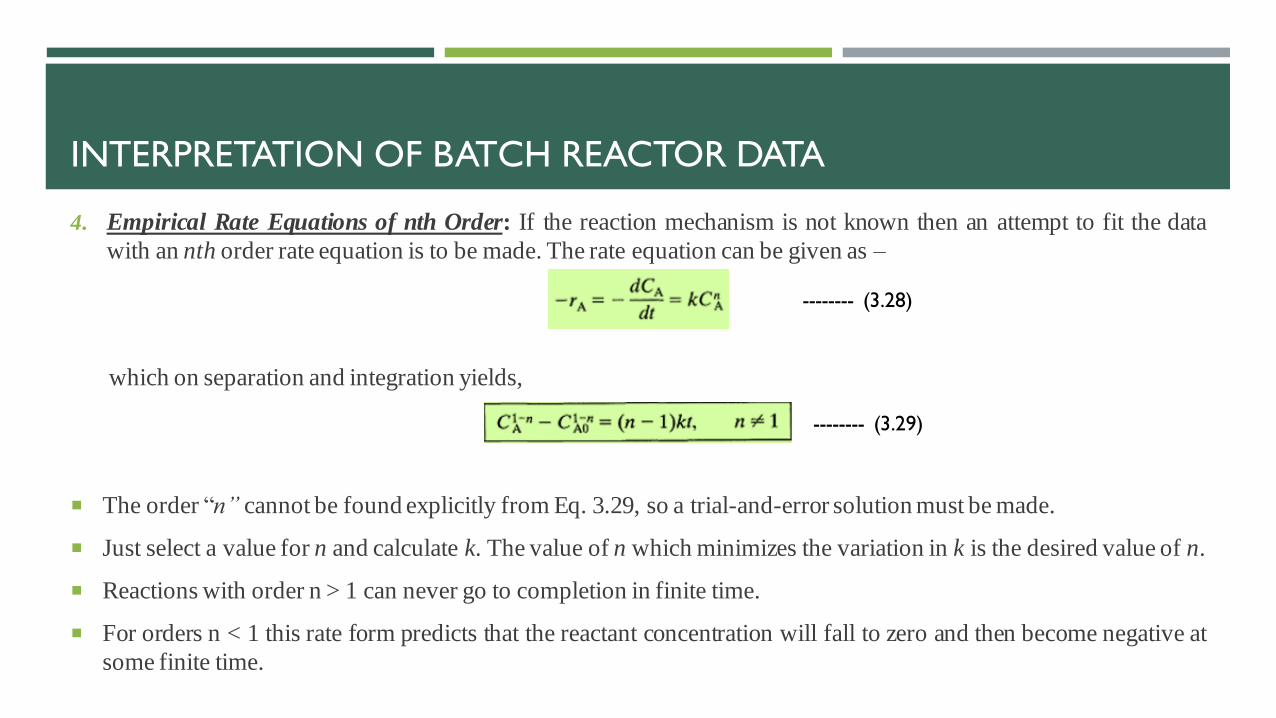
4. Empirical Rate Equations of nth Order: If the reaction mechanism is not known then an attempt to fit the data

with an nth order rate equation is to be made. The rate equation can be given as –

which on separation and integration yields,

The order “n” cannot be found explicitly from Eq. 3.29, so a trial-and-error solution must be made.

Just select a value for n and calculate k. The value of n which minimizes the variation in k is the desired value of n.

Reactions with order n > 1 can never go to completion in finite time.

For orders n < 1 this rate form predicts that the reactant concentration will fall to zero and then become negative at

some finite time.


-------- (3.28)

-------- (3.29)

Since the real concentration cannot fall below zero we should not carry out the integration beyond this time for n

< 1. Also, as a consequence of this feature, in real systems the observed fractional order will shift upward to unity

as reactant is depleted.

5. Zero Order Reactions: A reaction is said to be of zero order when the rate of reaction is independent of the

concentration of materials, that is –

Integrating the above equation in the light that CA can never becomes negative we will get –


-------- (3.30)

-------- (3.31)

The above equation can be plotted as follows:

This implies that the conversion is dependent on time.

As a rule, reactions are of zero order only in certain concentration ranges-the higher concentrations.


If the concentration is lowered far enough, then the reaction becomes concentration-dependent, in which case theorder rises from zero.

In general, zero-order reactions are those whose rates are determined by some factor other than the concentrationof the reacting materials, e.g., the intensity of radiation within the vat for photochemical reactions, or the surfaceavailable in certain solid catalyzed gas reactions.

6. Overall Order of Irreversible Reactions from the Half-Life t1/2: Consider an irreversible reaction as follows –

Writing rate of reaction for this equation will yield –

If the reactants are present in their stoichiometric ratios, they will remain at that ratio throughout the reaction.


Thus, for reactants A and B at any time CB/CA = β/α, and we may write –

Or,

Integrating for n ≠ 1 gives,

Defining the half-life of the reaction, t1/2, as the time needed for the concentration of reactants to drop to one-half

the original value, we obtain –


-------- (3.32)

-------- (3.33a)

This expression shows that a plot of log t,, vs. log CA0 gives a straight line of slope 1 - n, as shown in Fig. 3.5.

Figure 3.5: Overall order of reaction from a series of half-life experiments,

each at a different initial concentration of reactant.

From the above figure, it can be concluded that the fractional conversion in a given time:

rises with increased concentration for orders greater than one,

drops with increased concentration for orders less than one, and

is independent of initial concentration for reactions of first order.


6. Fractional Life Method tF:

The half-life method can be extended to any fractional life method in which the concentration of reactant drops to

any fractional value F = CA/CA0 in time tF .

7. Irreversible Reactions in Parallel: Consider the simplest case, A decomposing by two competing paths, both

elementary reactions:

The rates of change of the three components are given by –


-------- (3.33b)

-------- (3.34)

The k values are found using all three differential rate equations. First of all, Eq. 34, which is of simple first order, is integrated to give –

The above eqn. when plotted yields, (k1 +k2) as slope, as shown in figure 3.6.

Now taking eqns. 3.35 and 3.36 and dividing them will results in the following ratio:

Which on integration gives –


-------- (3.35)

-------- (3.36)

-------- (3.37)

The slope of a plot (figure 3.6) of CR versus CS gives the ratio k1/k2. Knowing k1/k2 as well as k1 + k2, gives k1 and

k2. Typical concentration-time curves of the three components in a batch reactor for the case where CR0 = CS0 = 0

and k1 > k2 are shown in Fig. 3.7.


-------- (3.38)

Figure 3.6: Evaluation of the Rate Constants for two competing

Elementary First Order Reactions

Figure 3.7: Typical Concentration-Time curves for Competing

Reactions

8. Homogeneous Catalyzed Reactions: Consider the reaction rate for a homogeneous catalyzed system as the sum of

rates of both the uncatalyzed and catalyzed reactions –

With corresponding reaction rates as –

The overall rate of disappearance of A is given as –


-------- (3.39)

On integrating eqn. 3.39 with taking the fact into consideration that the catalyst concentration remains unchanged

throughout the reaction, yields –

Making a series of runs with different catalyst concentrations allows us to find k1 and k2.

Plot the observed k value against the catalyst concentrations as shown in Fig. 3.8. The slope of such a plot is k2

and the intercept k1.


-------- (3.40)

Figure 3.7: Rate constants for a homogeneous catalyzed reaction

from a series of runs with different catalyst concentrations.

9. Autocatalytic Reactions: A reaction in which one of the products of reaction acts as a catalyst is called an

autocatalytic reaction. Consider the simplest from of these types of reaction as:

With corresponding rate equation as –

If there is no change in the number of moles of A and R, we may write that at any time:

Therefore, the rate equation becomes,

Rearranging and breaking into partial fractions, we obtain –


-------- (3.41a)

-------- (3.41b)

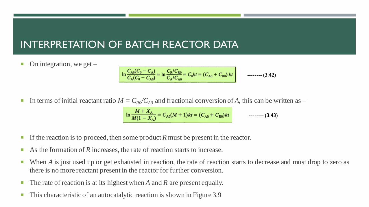
On integration, we get –

In terms of initial reactant ratio M = CR0/CA0 and fractional conversion of A, this can be written as –

If the reaction is to proceed, then some product R must be present in the reactor.

As the formation of R increases, the rate of reaction starts to increase.

When A is just used up or get exhausted in reaction, the rate of reaction starts to decrease and must drop to zero as

there is no more reactant present in the reactor for further conversion.

The rate of reaction is at its highest when A and R are present equally.

This characteristic of an autocatalytic reaction is shown in Figure 3.9


-------- (3.42)

-------- (3.43)

The test for an autocatalytic reaction includes the plotting of

time and concentration coordinates in eqns. 3.42 or 3.43 and

observe that whether a straight line passes through origin or

not as shown in Figure 3.10.


Figure 3.9: Conversion-time and rate-concentration curves for autocatalytic

reaction. This shape is typical for this type of reaction.

Figure 3.9: Test for the autocatalytic reaction of

Eqn. 3.41

10. Irreversible Reactions in Series:. Consider the simplest from of unimolecular type first order reactions as:

With corresponding rate equation for the three components as –

Starting with a concentration CA0 of A, no R or S present, and by integration of eqn. 3.44 the concentration of A is

found to be:


-------- (3.44)

-------- (3.45)

-------- (3.46)

-------- (3.47)

To get the changing concentration of R, insert the value of CA from eqn. 3.47 in to eqn. 3.45 and rearrange the eqn.

Eqn. 3.48 is a first-order linear differential equation of the form –

By multiplying through with the integrating factor, the solution can be obtained as follows:

Applying this general procedure to the integration of Eqn. 3.48, the integrating factor is found to be ek2t.

The constant of integration is found to be –k1CA0/(k2 – k1) from the initial conditions CR0 = 0 at t = 0, and the final

expression for the changing concentration of R is given as –


-------- (3.48)

If there is no change in total number of moles, then –

CA0 = CA + CR +CS

Which with eqns. 3.47 & 3.49 gives:

Thus eqns. 3.47, 3.49, and 3.50 gives the variation of concentrations of components A, R, and S with time t.

Case I: If k2 much larger then k1, then eqn. 3.50 reduces to –

Or, the rate is determined by k1 or the first step of the two-step reaction.


-------- (3.49)

-------- (3.50)

Case I: If k1 much larger then k2, then eqn. 3.50 reduces to –

Or, the rate is determined by k2 or the second step of the two-step reaction, which is the slowest step.

In general, for any number of reactions in series it is the slowest step that has the greatest influence on the overall

reaction rate.

The maximum concentration of R may be found out by differentiating eqn. 3.49 and setting dCR/dt = 0. Therefore,

the time at which the maximum concentration of R occurs is gives by –

Therefore, the maximum concentration of R is found by combining eqns. 3.49 & 3.51 as –


-------- (3.51)

-------- (3.52)

Figure 3.11 shows the general characteristics of the

concentration-time curves for the three components.

A decreases exponentially, R rises to a maximum and then

falls, and S rises continuously, the greatest rate of increase of

S occurring where R is a maximum.

In particular, this figure shows that one can evaluate k1 and k2

by noting the maximum concentration of intermediate and the

time when this maximum is reached.


Figure 3.11: Typical concentration-time curves

for consecutive first-order reactions.

For a longer chain of reactions,

the treatment is similar, though more

cumbersome than the two-step reaction just

considered. Figure 3.12 illustrates typical

concentration-time curves for this situation.


Figure 3.12: Concentration-time curves for a chain of successive first-order

reactions.

11. First Order Reversible Reactions:. Consider the simplest from of unimolecular type first order reactions as:

Starting with a concentration ratio M = CB0/CA0 the corresponding rate equation can be given as –

Now at equilibrium dCA/dt = 0. Hence from Eqn. 3.53b we find the fractional conversion of A at equilibrium

conditions to be –

And the equilibrium constant to be –


-------- (3.53a)

-------- (3.53b)

Combining the above three equations we obtain, in terms of the equilibrium

conversion,

With conversions measured in terms of XAe, this may be looked on as a pseudo first-

order irreversible reaction which on integration gives

A plot between concentration and time yields a straight line.

The similarity between eqns. for the first-order irreversible and reversible reactions

can be seen by comparing eqn. 3.12 with eqn. 3.54 or by comparing fig. 3.1 with fig.

3.13.

Thus, the irreversible reaction is simply the special case of the reversible reaction in

which CAe = 0, or XAe = 1, or KC = infinity.


-------- (3.54)

-------- (3.53b)

Figure 3.13: Test for the unimolecular type

reversible reactions of Eq. 3.53.

12. Second Order Reversible Reactions:. Consider the bimolecular type

second order reactions as:

With restrictions that CA0 = CB0 and CR0 = CS0 = 0, the integrated form of

the final eqns. Can be given as –

A plot between conversion and time is shown in fig. 3.14.


-------- (3.55a) -------- (3.55b)

-------- (3.55d)

-------- (3.56)

-------- (3.55c)

Figure 3.14: Test for the bimolecular type

reversible reactions of Eq. 3.55.

13. Reversible Reactions in General:. For orders other than one or two, integration of the rate equation becomes

cumbersome. Then search for an adequate rate equation is best done by the differential method.

14. Reactions of Shifting Orders:. In searching for a kinetic equation it may be found that the data are well fitted by

one reaction order at high concentrations but by another order at low concentrations. Consider the reaction

From the above rate eqn. one can observe that (fig. 3.15)

I. At high CA (or k2CA is much larger than 1)– the reaction is of zero order with rate constant k1/k2.

II. At low CA (or k2CA is much lower than 1) – the reaction is of first order with rate constant k1.

To apply the integral method, separate variables and integrate eqn. 3.57 which gives –


-------- (3.57)

-------- (3.58a)

On rearranging, eqn. 3.58a can be re-written as –

or,


-------- (3.58b)

-------- (3.58c)


Figure 3.16: Test for the rate equation,

Eq. 3.57, by integral analysis.

The general rate form can be given as –

-------- (3.59)

Equation 3.59 shifts from order m – n at high concentration to order m at low concentration, with the transition

taking place at k2Cn

A ≈ 1. this type of equation can then be used to fit data of any two orders.

Another form of equation which can account for this shift is –

or,

Example 3.1 from the book.


-------- (3.60)

Differential Method of Analysis of Data

The differential method of analysis deals directly with the differential rate equation to be tested, evaluating all terms

in the equation including the derivative dCi/dt, and testing the goodness of fit of the equation with experiment.

The procedure include is as follows:

1. Plot the CA vs. t data, and then carefully draw a smooth curve to represent the data. This curve most likely will not

pass through all the experimental points.

2. Determine the slope of this curve at suitably selected concentration values. These slopes dCi/dt = rA are the rates

of reaction at these compositions.

3. Now search for a rate expression to represent this rA vs. CA data, either by

(a) picking and testing a particular rate form, -rA = kf (CA), Fig. 3.17, or

(b) testing an nth-order form -rA = kCnA by taking logarithms of the rate equation (Fig. 3.18).


Differential Method of Analysis of Data


Figure 3.17: Test for the particular rate form –rA =

kf(CA) by the differential method.

Figure 3.18: Test for an nth – order rate form by the

differential method.

For graphical testing in differential analysis, some mathematical manipulations are required to get the straight line

curve.

For example, consider a set of CA vs t data to which we have to fit M-M equation:

Eqn. 3.57 has already been treated by integral analysis. However to perform graphical testing the above eqn. can

be manipulated by taking reciprocals as –

And a plot of 1/(-rA) vs. 1/CA is linear, as shown in figure 3.19.

Alternatively, a different manipulation (multiply Eq. 61 by k1(-rA)/k2) yields another form –


-------- (3.61)

-------- (3.57)

-------- (3.62)

A plot of -rA vs. (-rA)/CA is linear, as shown in Fig. 3.19.

Example 3.2 from the book.


Varying Volume Batch Reactor:

These reactors are much more complex than simple constant-volume batch reactor.

Their main use would be in the micro-processing field where a capillary tube with a movable bead would represent

the reactor (Fig. 3.20).

The progress of the reaction is followed by noting the movement of the bead with time, a much simpler procedure

than trying to measure the composition of the mixture, especially for microreactors. Thus,

V0 = initial volume of the reactor

V = the volume at time t.


This kind of reactor can be used for isothermal constant pressure operations, of reactions having a single

stoichiometry. For such systems the volume is linearly related to the conversion, or –

Or,

Where, ƐA is the fractional change in volume of the system between no conversion and complete conversion of

reactant A. Therefore,

For example, consider the isothermal gas-phase reaction –


-------- (3.63a)

-------- (3.63b)

-------- (3.64)

By taking pure reactantA into consideration, eqn. 3.64 will give –

But with 50% inerts into consideration will change the fractional change in volume as two volumes of reactant

mixture yield, on complete conversion, five volumes of product mixture –

ƐA accounts for both the reaction stoichiometry and the presence of inerts.

Now,


-------- (3.65)

Therefore,

Eqn. 3.66 is the relationship between conversion and concentration for isothermal varying-volume (or varying-

density) systems satisfying the linearity assumption of eqn. 3.63.

Now, the rate of reaction in general is given by –

Replacing V from eqn. 3.63a and NA from eqn. 3.65 we will get final rate equation as –

Or in terms of volume, using eqns. 3.63


-------- (3.66)

-------- (3.67)

1. Differential Method Analysis: The procedure for differential analysis of isothermal varying volume data is the

same as for the constant-volume situation except that we replace

And a plot of ln V vs. t will be plotted.

2. Integral Method Analysis: Only a few of the simpler rate forms integrate to give manageable V vs. t expressions.

They are as follows –

a) Zero order Reactions: For a homogeneous zero-order reaction the rate of change of any reactant A is independent

of the concentration of materials, or

On integration, it gives,


-------- (3.68)

-------- (3.69)

-------- (3.70)

As shown in Fig. 3.21, the logarithm of the fractional change in volume versus time yields a straight line of slope

kƐA/CA0 .


b) First order Reactions: For a unimolecular type first-order

reaction the rate of change of any reactant A is given as:

Replacing XA by V from eqns. 3.63 and on integration, it

gives,

A semi-logarithmic plot of eqn. 3.72 yields a straight line

of slope k.


-------- (3.71)

-------- (3.72)

c) Second order Reactions: For a bimolecular type

second order reaction –

Or,

The rate is given by,

Replacing XA by V from eqns. 3.63 and on integration,

it gives,


-------- (3.73)

nth-Order: For all rate forms other than zero-, first-, and second-order the integral method of analysis is not useful.

Temperature and Reaction Rate:

So far we have studied the effect of concentration of reactants and products on the rate of reaction, all at a given

temperature.

To obtain the complete rate equation, we also need to know the role of temperature on reaction rate.

The concentration dependent terms f(C) usually remain unchanged at different temperature.

Chemical theory predicts that the rate constant should be temperature-dependent in the following manner:

However, since the exponential term is much more temperature-sensitive than the power term, therefore we can

reasonably consider the rate constants to vary approximately as e-E/RT.

Thus we can examine for the variation of the rate constant with temperature by an Arrhenius-type relationship –


-------- (2.34 or 3.74)

Temperature and Reaction Rate:

Eqn. 3.74 can be plotted by plotting ln k vs. 1/T.

If the rate constant is found at two different temperatures we have:

Summary:

In chemistry, reaction rates and activation energies are developed in

terms of concentration.

For homogeneous reactions, E and –rA normally depends on

concentrations as the rate constants unit are often written as s-1,

liter/mole.sec, etc., without pressure appearing in the units.

It is better to convert p values into C values while making runs at

different temperatures.


-------- (2.35 or 3.75)

The Search for a Rate Equation:

All the rate equations are manipulated mathematically into a linearizedform because of the simplicity of family of straight lines that allows it tobe tested and rejected.

Three methods are commonly used to test for the linearity of a set ofpoints. These are as follows:

Calculation of k from Individual Data Points: For a given rate equation, therate constant can be determined for each experimental point by eitherintegral or differential method. If there is no appreciable trend in k valuesthen the equation is said to be satisfactory and the k values are averaged.

k values are calculated by taking the slopes of the lines connectingindividual data point to the origin. So for the same magnitude, k valuescalculated near the origin (low conversion) will vary widely as comparedto the k values calculated farther from the origin. This will create confusionabout being the k value, a constant.


In reactor design, generally the

study perform is to know what size

and type of reactor and method of

operation are best for a given job.

There are many factors which must

be accounted for in predicting the

performance of a reactor.

Equipment in which homogeneous

reactions are carried out can be one

of the three general types; the batch,

the steady-state flow, and the

unsteady-state flow or semibatch

reactor. The semibatch reactor

includes all reactors that do not fall

into the first two categories.

4. INTRODUCTION TO REACTOR DESIGN

Batch Reactor Steady State Flow Reactor Semi-batch Reactor

• Simple

• Needs little supporting equipment

• Ideal for small-scale experimental

studies on reaction kinetics

• Industrially, used only for relatively

small amounts of material

• Ideal for industrial purposes when

large quantities of materials are to

be processed

• Ideal when the rate of reaction is

fairly high to extremely high

• Supporting equipment needs are

great

• Extremely good product quality

control can be obtained

• Widely used in the oil industry

• More flexible system

• More difficult to analyze than

other reactor types

• Good control of reaction speed

because reaction proceeds as

reactants are added.

• Are generally used in variety of

applications like from calorimetric

titrations in the lab to the large

open hearth furnaces for steel

producction


The starting point for all design is the material balance expressed for any reactant or product. Therefore –

(rate of reactant flow into element of volume) = (rate of reactant flow out of element of volume) + (rate of loss due to

chemical reaction within the element of volume) + (rate of

accumulation of reactant in element of volume) ---- (4.1)


For uniform reactor composition (independent of position), the balance can be made over the whole reactor.

For non-uniform reactor composition, the balance must be made over a differential element of volume and then

integrated across the whole reactor for the appropriate flow and concentration conditions.

For various reactors, eqn. 4.1 ca be simplified and integrated so that the resultant expression gives the basic

performance equation of that particular type of reactor.

In batch reactor, the first two terms of eqn. 4.1 equals to zero as there is no inflow and outflow of the materials.

Similarly for steady state flow reactors, the last term of accumulation disappears and, for semi-batch reactor, all of

the four terms of the equation have to be considered.

For non-isothermal operations/processes an energy balances are used in addition to the material balances.

Therefore –

(rate of heat flow into element of volume) = (rate of heat flow out of element of volume) + (rate of disappearance of

heat by reaction within the element of volume) + (rate of accumulation of

heat within element of volume) ---- (4.2)


A satisfactory design for a given problem is achieved only when –

a) We can predict the response of the reacting system to changes in operating conditions (how rates and equilibrium conversion

change with temperature and pressure),

b) We are able to compare yields for alternative designs (adiabatic vs. isothermal operations, single vs. multiple reactors, flow

vs. batch system), and

c) We can estimate the economics of these different alternatives.

Symbols and Realtionship between CA and XA:

For the given reaction, with inerts iI

There are two related measures of the extent of reaction, the concentration CA and the conversion XA.

The relationship between these two measures depends on a number of factors. Consider the three special cases in

order to understand this relationship.


Special Case 1: Constant Density Batch and Flow Systems

Includes most liquid reactions and also gas reactions (which runs at constant temperature and density).

CA and XA are related to each other as:

The changes in B and R to A is related as –


-------- (4.3)

-------- (4.4)

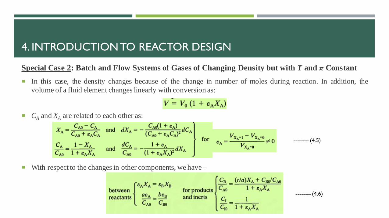
Special Case 2: Batch and Flow Systems of Gases of Changing Density but with T and π Constant

In this case, the density changes because of the change in number of moles during reaction. In addition, the

volume of a fluid element changes linearly with conversion as:

CA and XA are related to each other as:

With respect to the changes in other components, we have –


-------- (4.6)

-------- (4.5)

Special Case 3: Batch and Flow Systems of Gases in General (varying density, T, and π)

In this case, consider the following reaction which react according to –

Pick one reactant (called as key reactant) as the basis for determining the conversion. Let A be the key reactant,

then for the ideal gas behavior,

For high pressure non-ideal gas behavior replace


Special Case 3: Batch and Flow Systems of Gases in General (varying density, T, and π)

If key component is changed from Ato B then the following relationship can be used –

For liquids or isothermal gases with no change in pressure and density–


In the batch reactor, of Fig. 5.la the reactants are initiallycharged into a container, are well mixed, and are left toreact for a certain period. The resultant mixture is thendischarged. This is an unsteady-state operation wherecomposition changes with time; however, at any instantthe composition throughout the reactor is uniform.

Fig. 5.lb shows the first of the two ideal steady-state flowreactors is variously known as the plug flow, slug flow,piston flow, ideal tubular, and unmixed flow reactor. Thepattern of flow as plug flow. The flow of fluid through thereactor is orderly with no element of fluid overtaking ormixing with any other element ahead or behind. Theremay be lateral (side) mixing of fluid in a plug flowreactor; however, there must be no mixing or diffusionalong the flow path. The necessary and sufficientcondition for plug flow is for the residence time in thereactor to be the same for all elements of fluid.

5. IDEAL REACTORS FOR A SINGLE REACTION

The other ideal steady-state flow reactor is called the mixed flow reactor, the back-mix reactor,

the ideal stirred tank reactor, the C* (meaning C-star), CSTR, or the CFSTR (constant flow

stirred tank reactor), and, as its names suggest, it is a reactor in which the contents are well

stirred and uniform throughout. The exit stream from this reactor has the same composition as

the fluid within the reactor.

These three ideals are relatively easy to treat and also one or other usually represents the best

way of contacting the reactants for any given operation. Therefore real reactors are often

designed in such a way so that their flows approach these ideals.


I. IDEAL BATCH REACTOR

Applying material balance equation 4.1 for any component A (usually the limiting component) on the whole

reactor (as composition at any instance is same all over the reactor) will give:

Input (= 0) = Output (= 0) + Disappearance + Accumulation

Or

Evaluating the terms in eqn. 5.1 we have –

Disappearance of A by reaction, moles/time = (-rA)V = [moles A reacting/(time)(volume of fluid)] (volume of fluid)

Accumulation of A, moles/time = dNA/dt = d[NA0(1 – XA)]/dt = -NA0 (dXA/dt)

Putting above two terms in eqn. 5.1 will give:


-------- (5.1)

-------- (5.2)

Rearranging and integrating the above equation yields in –

This is the general equation showing the time required to achieve a conversion XA for either isothermal or non-

isothermal operation. The volume of reacting fluid and the reaction rate remain under the integral sign, for in

general they both change as reaction proceeds.

This equation may be simplified for a number of situations. If the density of the fluid remains constant, we obtain:

For all reactions in which the volume of reacting mixture changes proportionately with conversion, such as in

single gas-phase reactions with significant density changes, eqn. 5.3 becomes –


-------- (5.3)

-------- (5.4)

-------- (5.5)

Eqns. 5.2 – 5.5 are applicable to both isothermal and non-isothermal operations.

For the non-isothermal operations, the variation of rate with temperature, and the variation of temperature with

conversion, must be known before solution is possible.

Figure 5.2 is a graphical representation of two of these equations.


Space time and Space velocity:

Just as the reaction time t is the natural performance measure for a batch reactor, so are the space-time and space-

velocity the proper performance measures of flow reactors. These terms are defined as follows:

Space time:

Space velocity:

Thus, a space-velocity of 5 hr-l means that five reactor volumes of feed at specified conditions are being fed into

the reactor per hour. A space-time of 2 min means that every 2 min one reactor volume of feed at specified

conditions is being treated by the reactor.


-------- (5.6)

-------- (5.7)

Space time and Space velocity:

We may arbitrarily select the temperature, pressure, and state (gas, liquid, or solid) at which we choose to measure

the volume of material being fed to the reactor.

If they are of the stream entering the reactor, the relation between s and r and the other pertinent variables is

It may be more convenient to measure the volumetric feed rate at some standard state, especially when the reactor

is to operate at a number of temperatures. For example, the material is gaseous when fed to the reactor at high

temperature but is liquid at the standard state, care must be taken to specify precisely what state has been chosen.


-------- (5.8)

The relation between the space-velocity and space-time for actual feed conditions (unprimed symbols) and atstandard conditions (designated by primes) is given by

II. STEADY STATE MIXED FLOW REACTOR:

For a CSTR, since the composition is uniform throughout, the accounting may be made about the reactor as awhole and eqn. 1 of material balance can be written as:

Now, evaluating each term of eqn. 5.10, if FA0 = v0CA0 is the molar feed rate of component A to the reactor, thenconsidering the reactor as a whole we have –

Input of A, moles/time = FA0(1 – XA) = FA0

Output of A, moles/time = FA0(1 – XA)


-------- (5.9)

-------- (5.10)

Disappearance of A by reaction, moles/time = (–rA)V

Introducing the above evaluated terms in eqn. 3.10 we get:

Which on rearrangement and for any fractional change in volume, Ɛ, gives,

More generally, if the feed on which conversion is based, subscript 0, enters the reactor partially converted,

subscript i, and leaves at conditions given by subscript f, we have

or


-------- (5.12)

For any ƐA -------- (5.11)

For the special case of constant-density systems XA = 1 – CA/CA0, in which case the performance equation for mixed

reactors can also be written in terms of concentrations or,

These expressions relate in a simple way the four terms XA, -rA, V, FA0; thus, knowing any three allows the fourth to be

found directly.

In design, then, the size of reactor needed for a given duty or the extent of conversion in a reactor of given size is found

directly.

In kinetic studies each steady-state run gives, without integration, the reaction rate for the conditions within the reactor.

The ease of interpretation of data from a mixed flow reactor makes its use very attractive in kinetic studies, in particular

with messy reactions (e.g., multiple reactions and solid catalyzed reactions). Figure 5.4 is a graphical representation of

these mixed flow performance equations. For any specific kinetic form the equations can be written out directly.


For ƐA = 0 -------- (5.13)

Figure 5.4 is a graphical representation of these mixed flow performance equations. For any specific kinetic form

the equations can be written out directly.


As an example, for constant density systems CA/CA0 = 1 – XA, thus the performance expression for first-order

reaction becomes –

For variable volume systems,

Therefore, first order reaction with variable volume condition, the performance 5.11 can be rewritten as:

For second-order reaction,A→ products, -rA, = kC2A, ƐA = 0, the performance equation of eqn. 5.11 becomes


-------- (5.14a)

-------- (5.14b)

-------- (5.15)

Similar expressions can be written for any other form of rate equation. These expressions can be written either in

terms of concentrations or conversions.

Using conversions is simpler for systems of changing density, while either form can be used for systems of

constant density.

Example 5.1

Example 5.2

Example 5.3


III. STEADY STATE PLUG FLOW REACTOR:

In a plug flow reactor the composition of the fluid varies from point to point along a flow path; consequently, the

material balance for a reaction component must be made for a differential element of volume dV. Thus for reactant

A, eqn. 4.1 becomes


-------- (5.10)

From figure 5.5, for a elemental volume dV we can write

Input of A, moles/time = FA

Output of A, moles/time = FA + dFA

Disappearance of A by reaction, moles/time = (–rA)V

Introducing the above evaluated terms in eqn. 3.10 we get:

Also,

Therefore, on replacement in above eqn.

For the reactor as a whole the expression must be integrated. Therefore, we obtain


-------- (5.16)

Thus,

Equation 5.17 allows the determination of reactor size for a given feed rate and required conversion.

Compare Eqns. 5.11 and 5.17. The difference is that in plug flow rA varies, whereas in mixed flow rA is constant.

As a more general expression for plug flow reactors, if the feed on which conversion is based, subscript 0, enters

the reactor partially converted, subscript i, and leaves at a conversion designated by subscript f, we have

or


For ƐA -------- (5.17)

-------- (5.18)

For the special case of constant-density systems XA = 1 – CA/CA0 and dXA = - dCA/CA0 in which case the

performance equation can also be written in terms of concentrations or,

These performance equations, Eqns. 5.17 to 5.19, can be written either in terms of concentrations or conversions.

For systems of changing density it is more convenient to use conversions; however, there is no particular

preference for constant density systems.

Whatever its form, the performance equations interrelate the rate of reaction, the extent of reaction, the reactor

volume, and the feed rate, and if any one of these quantities is unknown it can be found from the other three.


For ƐA = 0 -------- (5.19)

Figure 5.6 displays these performance equations and shows that the spacetime needed for any particular duty can

always be found by numerical or graphical integration. However, for certain simple kinetic forms analytic

integration is possible-and convenient. To do this, insert the kinetic expression for r, in Eq. 17 and integrate.


Some of the simpler integrated forms for plug flow are as follows:

a) Zero-order homogeneous reaction, any constant ƐA,

b) First-order irreversible reaction, A→ products, any constant ƐA,

c) First-order reversible reaction, CR0/CA0 = M, kinetics approximated or fitted by –rA = k1CA – k2CR with an

observed equilibrium conversion XAe, any constant ƐA,

d) Second-order irreversible reaction, A+ B→ products with equimolar feed or 2A→ products, any constant ƐA,


-------- (5.20)

-------- (5.21)

-------- (5.22)

-------- (5.23)

Where the density is constant, put ƐA = 0 to obtain the simplified performance equation.

By comparing the batch expressions of derived earlier with these plug flow expressions we find:

1. For systems of constant density (constant-volume batch and constant-density plug flow) the performance equations are

identical, τ for plug flow is equivalent to t for the batch reactor, and the equations can be used interchangeably.

2. For systems of changing density there is no direct correspondence between the batch and the plug flow equations and the

correct equation must be used for each particular situation. In this case the performance equations cannot be used

interchangeably.

Example 5.4

Example 5.5

Example 5.6


Holding time and Space Time for Flow Reactors:

They are defined as:

Space time:

Holding Time:

For constant density systems (all liquids and constant density gases)

For changing density systems τ ≠ t and t ≠ V/v0 in which case it becomes difficult to find how these terms arerelated.


-------- (5.6 or 5.8)

-------- (5.24)

As a simple illustration of the difference between these 2, consider two cases of the steady-flow popcorn popper of

which takes in 1 liter/min of raw corn and produces 28 liters/min of product popcorn.

Consider three cases, called X, Y, and Z, which are shown in Fig. 5.7.


In the first case (case X) all the popping occurs at the back end of the reactor.

In the second case (case Y) all the popping occurs at the front end of the reactor.

In the third case (case Z) the popping occurs somewhere between entrance and exit.

In all three cases, irrespective f where the popping occurs –

However, we see that the residence time in the three cases is very different, or


This shows that, the value of t depends on what happens in the reactor, while the value of τ is independent of what

happens in the reactor.

This example shows that t and τ are not, in general, identical.

For batch systems, the proper performance measure is the time of reaction.

However, for flow systems, τ or V/FA0 is the proper performance measure.

The above simple example shows that in the special case of constant fluid density the space-time is equivalent to

the holding time;hence, these terms can be used interchangeably.

This special case includes practically all liquid phase reactions.

However, for fluids of changing density, e.g., non-isothermal gas reactions or gas reactions with changing number

of moles, a distinction should be made between t and τ and the correct measure should be used in each situation.


With the wide choice of systems available and with the many factors to be considered, no neat formula can be

expected to give the optimum setup.

Experience, engineering judgment, and a sound knowledge of the characteristics of the various reactor systems are

all needed in selecting a reasonably good design and, the choice in the last analysis will be dictated by the

economics of the overall process.

Single reactions are reactions whose progress can be described and followed adequately by using one and only one

rate expression coupled with the necessary stoichiometric and equilibrium expressions.

For such reactions product distribution is fixed; hence, the important factor in comparing designs is the reactor

size.

A. Size Comparison of Single Reactors:

1. Batch Reactor:

The batch reactor has the advantage of small instrumentation cost and flexibility of operation (may be shut down

easily and quickly).

6. DESIGN FOR SINGLE REACTIONS

1. Batch Reactor:

It has the disadvantage of high labor and handling cost, often considerable shutdown time to empty, clean out, and

refill, and poorer quality control of the product.

Hence the batch reactor is well suited to produce small amounts of material and to produce many different

products from one piece of equipment.

Regarding reactor sizes, on comparing eqns. 5.4 – 5.19 for a given duty and for ε = 0 shows that an element of

fluid reacts for the same length of time in the batch and in the plug flow reactor.

Thus, the same volume of these reactors is needed to do a given job.

On a long-term production basis one must correct the size requirement estimate to account for the shutdown time

between batches.

Still, it is easy to relate the performance capabilities of the batch reactor with the plug flow reactor.


2. Mixed Versus Plug Flow Reactors, First and Second OrderReactions:

For a given duty the ratio of sizes of mixed and plug flow reactors will depend on the extent of reaction, the

stoichiometry, and the form of the rate equation.

For the general case, a comparison of eqns. 5.11 and 5.17 will give this size ratio. Consider this comparison for the

large class of reactions approximated by the simple nth-order rate law:

Where n varies anywhere from 0 to 3. For mixed flow, eqn. 5.11 gives

Whereas, for plug flow, eqn. 5.17 gives


Dividing the above 2 eqns. We get

For constant density, or ε = 0, the expression reduces to

Or,

Equations 1 and 2 are displayed in graphical form in Fig. 6.1 to provide a quick comparison of the performance of

plug flow with mixed flow reactors.


-------- (6.1)

n ≠ 1 n = 1 -------- (6.2)

For

The ordinate becomes the volume ratio Vm,/Vp or space-time ratio τm/τp if the same quantities of identical feed are

used.

For identical feed composition CA0 and flow rate FA0, the ordinate of this figure gives directly the volume ratio

required for any specified conversion. Figure 6.1 shows the following.

1. For any particular duty and for all positive reaction orders the mixed reactor is always larger than the plug flow reactor. The

ratio of volumes increases with reaction order.

2. When conversion is small, the reactor performance is only slightly affected by flow type. The performance ratio increases

very rapidly at high conversion; consequently, a proper representation of the flow becomes very important in this range of

conversion.

3. Density variation during reaction affects design; however, it is normally of secondary importance compared to the difference

in flow type.


3. Variation of Reactant Ratio for Second Order Reactions:

Second order reactions of two components and of the type:

Can behave as second order reactions of one component when the reactant ratio is unity. Therefore,

For the second case, when a large excess of reactant B is used then its concentration does not change appreciably

(CB ≈ CB0) and the reaction approaches first-order behavior with respect to the limiting componentA, or

Thus in Fig. 6.1, and in terms of the limiting component A, the size ratio of mixed to plug flow reactors is

represented by the region between the first-order and the second-order curves.


-------- (3.13)

-------- (6.3)

-------- (6.4)

4. GeneralGraphicalComparison:

For reactions with arbitrary but known rate the

performance capabilities of mixed and plug flow

reactors are best illustrated in Fig. 6.2.

The ratio of shaded and of hatched areas gives the

ratio of space-times needed in these two reactors.

From Fig. 6.2, for all nth-order reactions, n > 0, it can

be seen that mixed flow always needs a larger volume

than does plug flow for any given duty.


CHC3100 CHEMICAL REACTION ENGINEERING -I

Documents

Transcript of CHC3100 CHEMICAL REACTION ENGINEERING -I