Towards High-Quality Black-Box Chemical Reaction Rates ...
307
Towards High-Quality Black-Box Chemical Reaction Rates with System-Specific Potential Energy Surfaces Dissertation in partial fulfillment of the requirements for the degree Dr. rer. nat. of the Faculty of Mathematics and Natural Sciences at Kiel University submitted by Julien Steffen Kiel, December 2019
-
Upload
khangminh22 -
Category
Documents
-
view
1 -
download
0
Transcript of Towards High-Quality Black-Box Chemical Reaction Rates ...
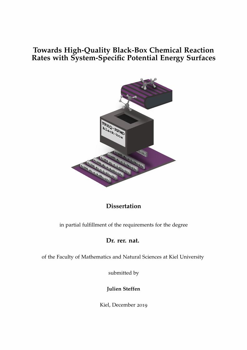
Towards High-Quality Black-Box Chemical ReactionRates with System-Specific Potential Energy Surfaces
Dissertation
in partial fulfillment of the requirements for the degree
Dr. rer. nat.
of the Faculty of Mathematics and Natural Sciences at Kiel University
submitted by
Julien Steffen
Kiel, December 2019


Towards High-Quality Black-Box Chemical Reaction Rateswith System-Specific Potential Energy SurfacesDissertation, submitted by Julien SteffenKiel, December 03, 2020
First referee: Prof. Dr. Bernd HartkeSecond referee: Prof. Dr. Carolin König
Date of the oral examination: 20.02.2020
Approved for publication: 20.02.2020


Meiner Mutter

Abstract
The calculation of highly-accurate reaction rate constants (k(T)) is one of the central topics intheoretical chemical kinetics. Two approaches for doing this are dominant in literature: applicationof heuristic corrections of the transition state theory (TST) and wave packet propagation withthe aim to represent exact quantum mechanical dynamics. While the first approach is easy tohandle but suffers from intrinsic approximations and limited accuracy, the second approach enablesconvergence towards the exact result, but at the expense of a complex handling and massive costs.This limits its application to a small circle of highly-specialized theoreticians.
A new method that might be able to bridge the gap between easy application and convergencetowards the exact result is the ring polymer molecular dynamics (RPMD) method. It is basedon the isomorphism between quantum statistical mechanics and classical statistical mechanics ofa fictitious ring polymer. With this, configurational state sums and free energy surfaces can beobtained from probabilistic samplings of the system’s accessible phase space with classical MDof ring polymers. Based on these free energy surfaces reaction rate constants can be obtainedthat converge towards the results of wave packet propagations, if the size of the ring polymer isadequate.
In order to conduct RPMD calculations, a sufficiently accurate representation of the thermallyaccessible potential energy surface (PES) of the system on which the ring polymers are propagatedis needed. In principle, this surface could be represented by ad hoc calculations of energies andgradients based on quantum chemical methods like density functional theory (DFT) or secondorder Møller-Plesset perturbation theory (MP2). However, since many millions of single gradientcalculations are needed to converge a free energy surface and the associated k(T) value, thisapproach is impractical. Instead, analytical representations of PESs that are fitted to DFT or MP2
results are commonly used. The parametrization of these representations is quite demanding,though, thus being a task for experts.
The present thesis deals with new methods for the automated parametrization of analyticalPES representations of reactive systems and the successive k(T) calculations based on RPMD.These representations are built on a combination of the quantum mechanical derived force field(QMDFF) method by Grimme and the empirical valence bond method (EVB) by Warshel, beingplugged together recently by Hartke and Grimme (EVB-QMDFF). In line with this thesis a crucialimprovement of this combination of methods was done, complementing it with newly developedEVB concepts. For practical usage a new program package was developed, which enables theautomated generation of an EVB-QMDFF-PES representation and calculations of RPMD-free-energysurfaces, recrossing corrections as well as k(T) values and Arrhenius parameters for comparisonwith experimental data, based on the preoptimized reaction path of an arbitrary thermal groundstate system.
The abilities of the new methods and the associated implementation were thoroughly bench-marked in different kinds of applications. These are calculations of k(T) values and Arrheniusparameters of arbitrary systems from a reaction data base and their comparison to literature values,theoretical molecular force experiments with quantitative investigations of force-dependent reactiv-ities for different systems, a thorough study of urethane synthesis being part of our cooperationwith Covestro AG and finally a combination of calculated rate constants of several elementaryreactions for describing the dynamics of larger systems based on the kinetic Monte Carlo (KMC)method.

Kurzzusammenfassung
Die Berechnung von hochgenauen Reaktionsgeschwindigkeitskonstanten (k(T)) ist eines der zen-tralen Themenfelder in der theoretisch-chemischen Kinetik. Bisher dominieren zwei Ansätze inder Literatur: die Anwendungen von heuristischen Korrekturen der Übergangszustandstheorie(TST) und die Wellenpaketpropagation mit dem Ziel der exakten Darstellung von quantenmecha-nischer Dynamik. Während der erste Ansatz leicht anzuwenden ist, aber dafür mit intrinsischenNäherungen und Genauigkeitsbeschränkungen zu kämpfen hat, ist es mit dem zweiten Ansatzmöglich, Konvergenz zum exakten Resultat zu erreichen, allerdings mittels einer sehr komplexenHandhabung und immenser Kosten, die ihn letzten Endes auf einen Kreis hochspezialisierterTheoretiker beschränkt.
Eine neue Methode mit dem Potential die Lücke zwischen leichter Anwendbarkeit und Kon-vergenz zum exakten Resultat zu überbrücken, ist die Ringpolymer-Moleküldynamik (RPMD).Sie basiert of dem Isomorphismus zwischen quantenmechanischer Statistik und der klassischenMechanik eines fiktiven Ringpolymers. Damit können Zustandssummen und Flächen freier Energieunter Berücksichtigung quantenmechanischer Effekte aus probabilistischen Erkundungen des ther-misch zugänglichen Phasenraums eines Systems mittels klassicher MD von Ringpolymeren erhaltenwerden. Aus den Flächen freier Energie werden wiederum chemische Reaktionsgeschwindigkeits-konstanten erhalten, welche bei genügender Größe der zugrundeliegenden Ringpolymere zumErgebnis von Wellenpaketpropagationsrechnungen konvergieren.
Zur Durchführung von RPMD-Rechnungen ist eine möglichst präzise Darstellung der thermischzugänglichen Potentialenergiefläche (PES) des Systems notwendig, auf welcher die Ringpolymerepropagiert werden können. Prinzipiell könnte diese durch ad-hoc-Berechnungen von Energienund Gradienten auf Basis quantenchemischer Methoden wie Dichtefunktionaltheorie (DFT) oderMøller-Plesset Störungstheorie 2. Ordnung (MP2) dargestellt werden. Da jedoch viele Millioneneinzelner Gradientenberechnungen zur Konvergenz der erhaltenen Fläche freier Energie und eineszuverlässigen k(T)-Wertes notwendig sind, ist diese Herangehensweise zeitlich nicht zu bewerkstel-ligen. Stattdessen greift man für gewöhnlich auf analytische Darstellungen der PES zurück, die anDFT- oder MP2-Resultate gefittet wurden. Die Parametrisierung solcher Darstellungen für neueSysteme ist jedoch erneut eine äußerst anspruchsvolle Aufgabe für Experten.
Die vorliegende Arbeit beschäftigt sich mit neuartigen Verfahren zur automatisierten Para-metrisierung analytischer PES-Darstellungen von reaktiven System und daran anschließendek(T)-Berechnungen auf Basis von RPMD. Die Darstellungen beruhen auf einer Verknüpfung derquantenmechanisch-abgeleiteten Kraftfeldmethode (QMDFF) von Grimme und der empirischenValenzbindungsmethode (EVB) von Warshel, welche unlängst von Hartke und Grimme ent-wickelt wurde (EVB-QMDFF). Im Rahmen dieser Arbeit wurde diese Methodenkombinationentscheidend weiterenwickelt und um neuentwickelte EVB-Konzepte ergänzt. Zur praktischenHandhabung wurde ein neues Programmpaket verfasst, welches automatisiert auf Basis desvoroptimierten Reaktionspfades eines beliebigen thermischen Grundzustandsssystems eine PES-Darstellung mit der EVB-QMDFF-Methode erstellt und auf dieser mittels RPMD Flächen freierEnerge, Rückkreuzungskorrekturen und k(T)-Werte, sowie Arrheniusparameter berechnet, welchedirekt mit experimentellen Resultaten verglichen werden können.
Die Fähigkeiten der neuen Methoden und der sie enthaltenden Implementation wurden anhandverschiedener Anwendungen ausführlich getestet. Enthalten sind hierbei Berechnungen von k(T)-Werten und Arrheniusparametern zufällig ausgewählter Systeme aus einer Reaktionsdatenbankund deren Vergleich mit Literaturwerten, theoretische Molekularkraftexperimente mit quantitativerUntersuchung der Reaktivität von Systemen abhängig von angelegten Kräften, ausführliche Unter-suchungen von Urethanbildungsreaktionen als Teil unserer Zusammenarbeit mit der Covestro AGund schließlich die Kombination von berechneten Geschwindigkeiten einzelner Teilreaktionen zurDynamik größerer Systeme auf Basis der kinetischen-Monte-Carlo-Methode (KMC).

Contents
List of Acronyms xv
List of Figures xvi
List of Tables xix
1 Introduction 1
2 Theoretical Background 52.1 Chemical Reaction Rates . . . . . . . . . . . . . . . . . . . . . . . . . . . . . . . . . . . 5
2.1.1 Transition State Theory . . . . . . . . . . . . . . . . . . . . . . . . . . . . . . . 6
2.1.2 Handling of TST-Problems . . . . . . . . . . . . . . . . . . . . . . . . . . . . . 9
2.1.3 Configurational Samplings . . . . . . . . . . . . . . . . . . . . . . . . . . . . . 16
2.1.4 Rigorous Quantum Theories . . . . . . . . . . . . . . . . . . . . . . . . . . . . 25
2.1.5 Path Integral Formulation of Quantum Mechanics . . . . . . . . . . . . . . . 29
2.1.6 Ring Polymer Molecular Dynamics . . . . . . . . . . . . . . . . . . . . . . . . 33
2.2 Potential Energy Surfaces . . . . . . . . . . . . . . . . . . . . . . . . . . . . . . . . . . 40
2.2.1 System-Specific Parametrizations . . . . . . . . . . . . . . . . . . . . . . . . . . 42
2.2.2 Generalized Potential Functions . . . . . . . . . . . . . . . . . . . . . . . . . . 44
2.2.3 Black-Box Approaches . . . . . . . . . . . . . . . . . . . . . . . . . . . . . . . . 46
2.3 Quantum Mechanically Derived Force Field . . . . . . . . . . . . . . . . . . . . . . . 47
2.3.1 Idea . . . . . . . . . . . . . . . . . . . . . . . . . . . . . . . . . . . . . . . . . . . 47
2.3.2 The QMDFF Potential Function . . . . . . . . . . . . . . . . . . . . . . . . . . 48
2.3.3 Optimization of Parameters . . . . . . . . . . . . . . . . . . . . . . . . . . . . . 51
2.3.4 Properties . . . . . . . . . . . . . . . . . . . . . . . . . . . . . . . . . . . . . . . 51
2.4 Empirical Valence Bond . . . . . . . . . . . . . . . . . . . . . . . . . . . . . . . . . . . 53
2.4.1 Valence Bond or Molecular Orbital Theory? . . . . . . . . . . . . . . . . . . . 53
2.4.2 EVB-Foundations . . . . . . . . . . . . . . . . . . . . . . . . . . . . . . . . . . . 55
2.4.3 Simple EVB Coupling Terms . . . . . . . . . . . . . . . . . . . . . . . . . . . . 58
2.4.4 Chang-Miller EVB . . . . . . . . . . . . . . . . . . . . . . . . . . . . . . . . . . 59
2.4.5 Distributed Gaussian (DG)-EVB . . . . . . . . . . . . . . . . . . . . . . . . . . 61
2.4.6 Reaction Path (RP)-EVB with Corrections . . . . . . . . . . . . . . . . . . . . . 66
2.4.7 Summary or Jacob’s Ladder of EVB . . . . . . . . . . . . . . . . . . . . . . . . 68
3 Program Development 713.1 History . . . . . . . . . . . . . . . . . . . . . . . . . . . . . . . . . . . . . . . . . . . . . 71
3.1.1 Version 1: The Origins . . . . . . . . . . . . . . . . . . . . . . . . . . . . . . . . 71
3.1.2 Version 2: EVB-QMDFF-Tinker . . . . . . . . . . . . . . . . . . . . . . . . . . . 72
3.1.3 Version 3: EVB-QMDFF+RPMDrate . . . . . . . . . . . . . . . . . . . . . . . . 74
3.1.4 Version 4: Unification . . . . . . . . . . . . . . . . . . . . . . . . . . . . . . . . 74
3.2 General Statistics . . . . . . . . . . . . . . . . . . . . . . . . . . . . . . . . . . . . . . . 75
3.3 Program Descriptions . . . . . . . . . . . . . . . . . . . . . . . . . . . . . . . . . . . . 76
3.3.1 qmdffgen . . . . . . . . . . . . . . . . . . . . . . . . . . . . . . . . . . . . . . . 76
3.3.2 evbopt . . . . . . . . . . . . . . . . . . . . . . . . . . . . . . . . . . . . . . . . . 76
3.3.3 egrad . . . . . . . . . . . . . . . . . . . . . . . . . . . . . . . . . . . . . . . . . . 78
xii Contents
3.3.4 evb_qmdff . . . . . . . . . . . . . . . . . . . . . . . . . . . . . . . . . . . . . . . 80
3.3.5 irc . . . . . . . . . . . . . . . . . . . . . . . . . . . . . . . . . . . . . . . . . . . . 80
3.3.6 dynamic . . . . . . . . . . . . . . . . . . . . . . . . . . . . . . . . . . . . . . . . 81
3.3.7 rpmd . . . . . . . . . . . . . . . . . . . . . . . . . . . . . . . . . . . . . . . . . . 82
3.3.8 evb_kt_driver . . . . . . . . . . . . . . . . . . . . . . . . . . . . . . . . . . . . . 91
4 Publication: (DG-)EVB-QMDFF-RPMD 974.1 Scope of the Project . . . . . . . . . . . . . . . . . . . . . . . . . . . . . . . . . . . . . . 97
4.2 Publication Data and Reprint . . . . . . . . . . . . . . . . . . . . . . . . . . . . . . . . 98
5 Publication: TREQ - Development and Benchmark 995.1 Scope of the Project . . . . . . . . . . . . . . . . . . . . . . . . . . . . . . . . . . . . . . 99
5.2 Publication Data and Reprint . . . . . . . . . . . . . . . . . . . . . . . . . . . . . . . . 100
6 Black-Box k(T) Calculations 1016.1 General Procedure . . . . . . . . . . . . . . . . . . . . . . . . . . . . . . . . . . . . . . 101
6.2 Example Reactions . . . . . . . . . . . . . . . . . . . . . . . . . . . . . . . . . . . . . . 103
6.2.1 The I2 + H → HI + I Reaction . . . . . . . . . . . . . . . . . . . . . . . . . . . 103
6.2.2 The CN + H2 → HCN + H Reaction . . . . . . . . . . . . . . . . . . . . . . . 105
6.2.3 The PH3 + H → PH2 + H2 Reaction . . . . . . . . . . . . . . . . . . . . . . . 108
6.2.4 The CH3NC → CH3CN Reaction . . . . . . . . . . . . . . . . . . . . . . . . . 108
6.2.5 The CH3Cl + Cl → CH2Cl + HCl Reaction . . . . . . . . . . . . . . . . . . . 108
6.2.6 The CH2Cl2 + Cl → CHCl2 + HCl Reaction . . . . . . . . . . . . . . . . . . . 112
6.2.7 The SiH4 + Cl → SiH3 + HCl Reaction . . . . . . . . . . . . . . . . . . . . . . 113
6.2.8 The GeH4 + H → GeH3 + H2 Reaction . . . . . . . . . . . . . . . . . . . . . 113
6.2.9 The C2H4 + H → C2H5 Reaction . . . . . . . . . . . . . . . . . . . . . . . . . 113
6.2.10 The CH3OH + Cl → CH2OH + HCl Reaction . . . . . . . . . . . . . . . . . . 116
6.2.11 The C2H6 → C2H4 + H2 Reaction . . . . . . . . . . . . . . . . . . . . . . . . 117
6.2.12 The CH4 + CH3 → CH3 + CH4 Reaction . . . . . . . . . . . . . . . . . . . . 118
6.2.13 The C2H6 + NH → C2H5 + H2N Reaction . . . . . . . . . . . . . . . . . . . . 120
6.2.14 The CF3O + CH4 → CF3OH+CH3 Reaction . . . . . . . . . . . . . . . . . . . 121
6.2.15 The Bicyclo[2.2.1]hept-2-ene → C2H4 + Cyclopentadiene Reaction . . . . . 122
6.3 Evaluation and Summary . . . . . . . . . . . . . . . . . . . . . . . . . . . . . . . . . . 124
7 Covalent Mechanochemistry 1277.1 Theoretical Background . . . . . . . . . . . . . . . . . . . . . . . . . . . . . . . . . . . 128
7.2 Implementations . . . . . . . . . . . . . . . . . . . . . . . . . . . . . . . . . . . . . . . 130
7.2.1 The Constant Force Experiment . . . . . . . . . . . . . . . . . . . . . . . . . . 130
7.2.2 The AFM Simulation Experiment . . . . . . . . . . . . . . . . . . . . . . . . . 131
7.2.3 Calculation of Rate Constants . . . . . . . . . . . . . . . . . . . . . . . . . . . . 133
7.3 Basic Mechanochemical Processes . . . . . . . . . . . . . . . . . . . . . . . . . . . . . 134
7.3.1 Choice of Systems . . . . . . . . . . . . . . . . . . . . . . . . . . . . . . . . . . 134
7.3.2 Constant Force Simulations . . . . . . . . . . . . . . . . . . . . . . . . . . . . . 135
7.3.3 AFM Simulations . . . . . . . . . . . . . . . . . . . . . . . . . . . . . . . . . . . 136
7.4 Other Examples . . . . . . . . . . . . . . . . . . . . . . . . . . . . . . . . . . . . . . . . 141
7.4.1 The Bridged Disulfide Molecule . . . . . . . . . . . . . . . . . . . . . . . . . . 141
7.4.2 The Ruthenium-Terpyridine Complex . . . . . . . . . . . . . . . . . . . . . . . 144
7.4.3 The Diels-Alder Reaction . . . . . . . . . . . . . . . . . . . . . . . . . . . . . . 145
7.5 Calculating Rate Constants . . . . . . . . . . . . . . . . . . . . . . . . . . . . . . . . . 147
7.5.1 Free Energy Profiles . . . . . . . . . . . . . . . . . . . . . . . . . . . . . . . . . 148
7.5.2 Force-Dependent Lifetimes . . . . . . . . . . . . . . . . . . . . . . . . . . . . . 148
7.5.3 The Diels-Alder Reaction . . . . . . . . . . . . . . . . . . . . . . . . . . . . . . 152
Contents xiii
8 Urethane Synthesis 1558.1 Synthesis of Urethanes - a Long Story Short . . . . . . . . . . . . . . . . . . . . . . . 155
8.1.1 Basic Mechanism . . . . . . . . . . . . . . . . . . . . . . . . . . . . . . . . . . . 156
8.1.2 Catalysis . . . . . . . . . . . . . . . . . . . . . . . . . . . . . . . . . . . . . . . . 156
8.1.3 Sequenctial Reactivity . . . . . . . . . . . . . . . . . . . . . . . . . . . . . . . . 158
8.2 Benchmark of QM Reference Methods . . . . . . . . . . . . . . . . . . . . . . . . . . . 159
8.2.1 Settings and Strategy . . . . . . . . . . . . . . . . . . . . . . . . . . . . . . . . . 159
8.2.2 Computational Details . . . . . . . . . . . . . . . . . . . . . . . . . . . . . . . . 161
8.2.3 Results . . . . . . . . . . . . . . . . . . . . . . . . . . . . . . . . . . . . . . . . . 161
8.3 RPMD Rate Constant Calculations . . . . . . . . . . . . . . . . . . . . . . . . . . . . . 164
8.3.1 TREQ Setup . . . . . . . . . . . . . . . . . . . . . . . . . . . . . . . . . . . . . . 164
8.3.2 Special Settings for RPMD . . . . . . . . . . . . . . . . . . . . . . . . . . . . . 164
8.3.3 Rate Constant Calculations . . . . . . . . . . . . . . . . . . . . . . . . . . . . . 168
8.3.4 Arrhenius and Eyring Fits . . . . . . . . . . . . . . . . . . . . . . . . . . . . . . 169
8.4 Influence of Prior Reactions . . . . . . . . . . . . . . . . . . . . . . . . . . . . . . . . . 170
9 Kinetic Monte Carlo 1759.1 Foundations . . . . . . . . . . . . . . . . . . . . . . . . . . . . . . . . . . . . . . . . . . 176
9.1.1 Integrating the Master Equation . . . . . . . . . . . . . . . . . . . . . . . . . . 178
9.1.2 KMC as a Probabilistic Approximation . . . . . . . . . . . . . . . . . . . . . . 179
9.1.3 Implementation . . . . . . . . . . . . . . . . . . . . . . . . . . . . . . . . . . . . 180
9.2 Abstract Model Systems . . . . . . . . . . . . . . . . . . . . . . . . . . . . . . . . . . . 180
9.2.1 Properties . . . . . . . . . . . . . . . . . . . . . . . . . . . . . . . . . . . . . . . 180
9.2.2 Diffusion Calculations . . . . . . . . . . . . . . . . . . . . . . . . . . . . . . . . 181
9.3 Hydrogen Diffusion on a Cu(001) Surface . . . . . . . . . . . . . . . . . . . . . . . . . 188
9.3.1 Quantum Chemical Reference . . . . . . . . . . . . . . . . . . . . . . . . . . . 189
9.3.2 EVB-QMDFF Setup . . . . . . . . . . . . . . . . . . . . . . . . . . . . . . . . . . 190
9.3.3 RPMD Calculations . . . . . . . . . . . . . . . . . . . . . . . . . . . . . . . . . 192
9.3.4 Diffusion Coefficients . . . . . . . . . . . . . . . . . . . . . . . . . . . . . . . . 201
9.4 Copper Diffusion on a Cu(001) Surface . . . . . . . . . . . . . . . . . . . . . . . . . . 205
9.4.1 Reference and EVB Setup . . . . . . . . . . . . . . . . . . . . . . . . . . . . . . 205
9.4.2 Rate Constant Calculations . . . . . . . . . . . . . . . . . . . . . . . . . . . . . 207
9.4.3 KMC Simulations . . . . . . . . . . . . . . . . . . . . . . . . . . . . . . . . . . . 209
10 Future Challenges 213
11 Appendix 21911.1 Supervised Projects . . . . . . . . . . . . . . . . . . . . . . . . . . . . . . . . . . . . . . 219
11.1.1 Jan-Moritz Adam . . . . . . . . . . . . . . . . . . . . . . . . . . . . . . . . . . . 219
11.1.2 Jennifer Müller . . . . . . . . . . . . . . . . . . . . . . . . . . . . . . . . . . . . 219
11.1.3 Michael Schulz . . . . . . . . . . . . . . . . . . . . . . . . . . . . . . . . . . . . 222
11.1.4 Sven Schultzke . . . . . . . . . . . . . . . . . . . . . . . . . . . . . . . . . . . . 222
11.2 Theoretical Details and Derivations . . . . . . . . . . . . . . . . . . . . . . . . . . . . 223
11.2.1 Schrödinger Equation from Path Integrals . . . . . . . . . . . . . . . . . . . . 223
11.2.2 The RPMD Reaction Rate . . . . . . . . . . . . . . . . . . . . . . . . . . . . . . 225
11.3 Internal Coordinates . . . . . . . . . . . . . . . . . . . . . . . . . . . . . . . . . . . . . 228
11.3.1 General Formalism . . . . . . . . . . . . . . . . . . . . . . . . . . . . . . . . . . 229
11.3.2 Coordinate Types and Metric . . . . . . . . . . . . . . . . . . . . . . . . . . . . 230
11.3.3 Wilson Matrix Elements . . . . . . . . . . . . . . . . . . . . . . . . . . . . . . . 231
11.3.4 Wilson Matrix Derivatives . . . . . . . . . . . . . . . . . . . . . . . . . . . . . . 234

xiv Contents
11.4 DG-EVB Details . . . . . . . . . . . . . . . . . . . . . . . . . . . . . . . . . . . . . . . . 240
11.4.1 The f-Vector . . . . . . . . . . . . . . . . . . . . . . . . . . . . . . . . . . . . . . 240
11.4.2 The D-Matrix . . . . . . . . . . . . . . . . . . . . . . . . . . . . . . . . . . . . . 241
11.4.3 Analytical Gradients . . . . . . . . . . . . . . . . . . . . . . . . . . . . . . . . . 243
11.5 Program Handling . . . . . . . . . . . . . . . . . . . . . . . . . . . . . . . . . . . . . . 244
11.5.1 List of Keywords . . . . . . . . . . . . . . . . . . . . . . . . . . . . . . . . . . . 244
11.5.2 Example Input Files . . . . . . . . . . . . . . . . . . . . . . . . . . . . . . . . . 252
11.6 Supplementary Information . . . . . . . . . . . . . . . . . . . . . . . . . . . . . . . . . 257
11.6.1 First EVB-QMDFF Publication . . . . . . . . . . . . . . . . . . . . . . . . . . . 257
11.6.2 RPMD Rate Constants with (DG-)EVB-QMDFF . . . . . . . . . . . . . . . . . 257
11.6.3 TREQ - Development and Benchmark . . . . . . . . . . . . . . . . . . . . . . . 257
12 Bibliography 259
Curriculum Vitae I
Acknowledgements V
Declaration VII

List of Acronyms
AFM Atomic Force MicroscopeAIMD Ab Initio Molecular DynamicsAO Atomic OrbitalBJ Becke-JohnsonCOM Center Of MassCUS Canonical Unified Statistical ModelCV Collective VariableCVT Canonical Variational TheoryDFT Density Functional TheoryDG Distributed GaussianEHT Extended Hückel TheoryEVB Empirical Valence BondFCI Full Configuration InteractionFF Force FieldGA Genetic AlgorithmGUI Graphical User InterfaceGVB Generalized Valence BondHF Hartree-FockHL Heitler-LondonICVT Improved Canonical Variational TheoryIRC Intrinsic Reaction CoordinateKMC Kinetic Monte Carlok(T) Chemical Reaction Rate ConstantLCAO Linear Combination of Atomic OrbitalsLCT Large Curvature TunnelingLEPS London-Eyring-Polanyi-SatoLM Levenberg-MarquardtLQA Local Quadratic ApproximationMC Monte CarloMCSI Multi-Configuration Shepard-InterpolationMDI Methylene Diphenyl IsocyanateMM Molecular MechanicsMO Molecular OrbitalMOF Metal Organic FrameworkMP2 Møller-Plesset Perturbation Theory 2nd. OrderMPI Message Passing InterfaceMS Multi-StateMSLS Multi-Start Local SearchµVT Microcanonical Variational TheoryNDI 1,5-Naphtyl-DiIsocynaateNEB Nudged Elastic BandNN Neural NetworkNR Newton-Raphson
xvi List of Acronyms
PES Potential Energy SurfacePI Path IntegralPIMC Path Integral Monte CarloPIMD Path Integral Molecular DynamicsPMF Potential of Mean ForceQM Quantum MechanicsQMDFF Quantum Mechanically Derived Force FieldQTST Quantum Transition State TheoryRF Reactive FluxRP Reaction PathRPMD Ring Polymer Molecular DynamicsSC Solvent ComplexSCT Small Curvature TunnelingSTM Scanning Tunneling MicroscopeSVD Singular Value DecompositionTDI Toluene DiIsocynaateTDSE Time-Dependent Schrödinger EquationTISE Time-Independent Schrödinger EquationTREQ Transition Region Corrected RP-EVB-QMDFFTS Transition StateTST Transition State TheoryUFF Universal Force FieldUI Umbrella IntegrationUS Unified Statistical ModelVB Valence BondVTST Variational Transition State TheoryWHAM Weighted Histogram Analysis MethodZCT Zero Curvature Tunneling
List of Figures
2.1 Schematic overview of the inherent approximations of TST. . . . . . . . . . . . . . . 10
2.2 Overview of different TST-correction schemes. . . . . . . . . . . . . . . . . . . . . . . 15
2.3 Effect of an umbrella bias potential on a MD sampling trajectory. . . . . . . . . . . . 19
2.4 Combination of single biased probability distributions to a global one. . . . . . . . . 21
2.5 Simplified illustration of a recrossing calculation. . . . . . . . . . . . . . . . . . . . . 26
2.6 Schematic derivation of exact path integrals for one-dimensional systems. . . . . . . 32
2.7 Demonstration of how partition functions can be calculated with path integrals. . . 35
2.8 Schematic picture of an approximated imaginary time path integral. . . . . . . . . . 38
2.9 Schematic exemplification of the RPMD Hamiltonian in the case of a water molecule. 39
2.10 Comparison between classical and RPMD dynamics for the sampling of a reactionbarrier. . . . . . . . . . . . . . . . . . . . . . . . . . . . . . . . . . . . . . . . . . . . . . 41
2.11 Overview of the QMDFF generation from needed reference data. . . . . . . . . . . . 52
2.12 Illustration of the general EVB concept. . . . . . . . . . . . . . . . . . . . . . . . . . . 56
2.13 Comparison between the Chang-Miller and the DG-EVB coupling terms. . . . . . . 62
2.14 Illustration of the linear equation needed for DG-EVB parametrization. . . . . . . . 65
2.15 Schematic presentation of the RP-EVB method. . . . . . . . . . . . . . . . . . . . . . 67
2.16 Illustration of the different regions along the reaction path being allocated in TREQ. 69
3.1 Overview of the four major program development steps since the invention ofEVB-QMDFF. . . . . . . . . . . . . . . . . . . . . . . . . . . . . . . . . . . . . . . . . . 73
3.2 Illustration of the MSLS algorithm for EVB optimizations. . . . . . . . . . . . . . . . 79
3.3 Illustration of the umbrella sampling coordinate expressed based on two dividingsurfaces. . . . . . . . . . . . . . . . . . . . . . . . . . . . . . . . . . . . . . . . . . . . . 85
3.4 Simpified structure of the rpmd.x program. . . . . . . . . . . . . . . . . . . . . . . . . 90
3.5 Illustration of automated QMDFF energy shifts applied during black-box calculations. 93
3.6 Example of how the positions of TREQ gradient/Hessian reference points aredetermined automatically. . . . . . . . . . . . . . . . . . . . . . . . . . . . . . . . . . . 94
3.7 Example for the automated choice of internal coordinates within TREQ. . . . . . . . 95
3.8 Automated determination of the reaction type for RPMD rate constant calculations. 96
6.1 Overview of the black-box calculation for the I2 + H → HI + I reaction. . . . . . . . . 106
6.2 Overview of the black-box calculation for the CN + H2 → HCN + H reaction. . . . 107
6.3 Overview of the black-box calculation for the PH3 + H → PH2 + H2 reaction. . . . . 109
6.4 Overview of the black-box calculation for the CH3NC → CH3CN reaction. . . . . . 110
6.5 Overview of the black-box calculation for the CH3Cl + Cl → CH2Cl + HCl reaction. 111
6.6 Overview of the black-box calculation for the CH2Cl2 + Cl → CHCl2 + HCl reaction. 112
6.7 Overview of the black-box calculation for the SiH4 + Cl → SiH3 + HCl reaction. . . 114
6.8 Overview of the black-box calculation for the GeH4 + H → GeH3 + H2 reaction. . . 115
6.9 Overview of the black-box calculation for the C2H4 + H → C2H5 reaction. . . . . . 116
6.10 Overview of the black-box calculation for the CH3OH + Cl → CH2OH + HC reaction.117
6.11 Overview of the black-box calculation for the C2H6 → C2H4 + H2 reaction. . . . . . 119
6.12 Overview of the black-box calculation for the CH4OH + CH3 → CH3 + CH4 reaction.120
6.13 Overview of the black-box calculation for the C2H6 + NH → C2H5 + H2 reaction. . 121
6.14 Overview of the black-box calculation for the CF3O + CH4 → CF3OH + CH3 reaction.122
xviii List of Figures
6.15 Overview of the black-box calculation for the Norbornene → C2H4 + Cyclopentadienereaction. . . . . . . . . . . . . . . . . . . . . . . . . . . . . . . . . . . . . . . . . . . . . 123
7.1 Illustration of an AFM experiment. . . . . . . . . . . . . . . . . . . . . . . . . . . . . . 128
7.2 Illustration of the effect of an applied force to a chemical bond. . . . . . . . . . . . . 129
7.3 Illustration of a constant force mechanochemistry simulation with dynamic.x. . . . 130
7.4 Illustration of an AFM mechanochemistry simulation with dynamic.x. . . . . . . . . 132
7.5 Structures of five different molecules used for bond-strength measurements. . . . . 134
7.6 Reactivity of five different bond types for various rupture forces. . . . . . . . . . . . 135
7.7 Temperature-dependence of constant-force simulations for five different bond types. 136
7.8 Example trajectory of the C-C bond AFM experiment. . . . . . . . . . . . . . . . . . 137
7.9 Scatter-plots of AFM rupture events for five different ruptured bonds. . . . . . . . . 138
7.10 Temperature-dependence of average AFM rupture forces for five different systems. 139
7.11 Influence of quantum effects on the results of AFM simulation trajectories . . . . . . 140
7.12 Structures of three larger mechanophores to be studied with (EVB-)QMDFF. . . . . 141
7.13 Illustration of an AFM experiment for the disulfide system. . . . . . . . . . . . . . . 142
7.14 Force-dependent reactivities of S-S and C-C bonds in the bridged disulfide. . . . . . 143
7.15 Temperature-dependent AFM simulations of the bridged disulfide molecule. . . . . 144
7.16 Observed AFM reaction events in the Terpyridine and Diels-Alder systems dependingon the anchor atoms. . . . . . . . . . . . . . . . . . . . . . . . . . . . . . . . . . . . . . 146
7.17 Reaction path of the Diels-Alder example reaction. . . . . . . . . . . . . . . . . . . . 146
7.18 Temperature-dependent AFM rupture forces for the Terpyridine and the Diels-Aldersystems. . . . . . . . . . . . . . . . . . . . . . . . . . . . . . . . . . . . . . . . . . . . . 147
7.19 Calculated free energy profiles for bond dissociations under influence of externalforces. . . . . . . . . . . . . . . . . . . . . . . . . . . . . . . . . . . . . . . . . . . . . . . 149
7.20 Force-dependent RPMD rate constants for different bond dissociations. . . . . . . . 151
7.21 Force-dependent rate constant calculations for the Diels-Alder example system. . . 154
8.1 Snapshots of TS structures for six investigated urethane reactive complexes. . . . . 160
8.2 RP-EVB gradient and Hessian reference points for different urethane reactions. . . 166
8.3 Illustration of the difference between tetramolecular and bimolecular reactions. . . 168
8.4 Illustration of the dividing surface definition for k(T) calculations of urethane reactions.169
8.5 Eyring plots for different urethane reaction systems. . . . . . . . . . . . . . . . . . . 172
8.6 TS structures for two-step urethanations of NDI. . . . . . . . . . . . . . . . . . . . . . 173
9.1 The general idea of KMC for a simple gas-phase diffusion process. . . . . . . . . . . 177
9.2 Model for the investigated surface diffusions in the rest of this chapter. . . . . . . . 181
9.3 List of all possible configurations for an upwards diffusion step on a metal surface. 182
9.4 Illustration of the simplified KMC site plot. . . . . . . . . . . . . . . . . . . . . . . . . 183
9.5 Six snapshots of a KMC trajectory simulated without neighbor interactions. . . . . . 184
9.6 Six snapshots of a KMC trajectory simulated with attactive interactions. . . . . . . . 186
9.7 Six snapshots of a KMC trajectory simulated with repulsive interactions. . . . . . . 187
9.8 Time-dependent gas absorbance for the different interaction models. . . . . . . . . . 189
9.9 The surface section used as unit cell in a periodic DFT reference calculation. . . . . 190
9.10 Overlay image of all RP structures for the H@Cu(001) reaction. . . . . . . . . . . . . 191
9.11 EVB-QMDFF quality along the RP of the H@Cu(001) system. . . . . . . . . . . . . . 192
9.12 Three-dimensional QM reference energy scan for the H@Cu(001) reaction. . . . . . 193
9.13 Three-dimensional EVB-QMDFF quality scan for the H@Cu(001) reaction. . . . . . . 194
9.14 Screenshots of RPMD umbrella trajectories for different beads and the H@Cu(001)system. . . . . . . . . . . . . . . . . . . . . . . . . . . . . . . . . . . . . . . . . . . . . . 197
List of Figures xix
9.15 Time-dependent RPMD transmission coefficients for the H@Cu(001) and D@Cu(001)diffusion reactions. . . . . . . . . . . . . . . . . . . . . . . . . . . . . . . . . . . . . . . 199
9.16 Calculated diffusion rate constants for the H@Cu(001) reaction. . . . . . . . . . . . . 200
9.17 Comparison of H@Cu001 and D@Cu001 diffusion rate constant with experimentalvalues and determination of tunneling crossover temperatures. . . . . . . . . . . . . 201
9.18 Example trajectories for the random movement of a particle on a regular surface. . 203
9.19 Histograms for the two-dimensional random walker model. . . . . . . . . . . . . . . 204
9.20 Overlay structure screenshots of different diffusion paths for the Cu@Cu(001) reaction.206
9.21 Optimized NEB reaction paths for the different diffusion reaction of Cu@Cu(001). . 207
9.22 Four example EVB-QMDFF energy plots of diffusion reaction paths. . . . . . . . . . 208
9.23 Snapshots of a KMC trajectory for the Cu@Cu(001) system. . . . . . . . . . . . . . . 211
9.24 Time-dependent KMC simulation results for the Cu@Cu(001) system. . . . . . . . . 212
11.1 List of reactions that were investigated within the work of Jennifer Müller. . . . . . 221
11.2 Flux-side correlation time profiles for classical and quantum calculations. . . . . . . 226
11.3 Schematic representation of coordinate types used in this thesis. . . . . . . . . . . . 230
11.4 Detailed structure of the D-matrix used for DG-EVB parametrization. . . . . . . . . 242

List of Tables
2.1 List of different EVB coupling term approaches (“Jacobs ladder of EVB”). . . . . . . 70
3.1 List of energy-gap (dE)-coupling terms as implemented in the EVB-QMDFF program 77
3.3 List of the coordinate-dependent (dQ)-coupling terms as implemented in the EVB-QMDFF program. . . . . . . . . . . . . . . . . . . . . . . . . . . . . . . . . . . . . . . . 78
3.4 List of reaction types that can be simulated with rpmd.x. . . . . . . . . . . . . . . . . 83
6.1 List of chosen reactions for the benchmark of evb_kt_driver.x. . . . . . . . . . . . . 102
6.3 Input parameters for RPMD k(T) calculations of all black-box examples. . . . . . . . 104
6.4 Comparison of calculated Arrhenius parameters for the different black-box systemswith literature values. . . . . . . . . . . . . . . . . . . . . . . . . . . . . . . . . . . . . 124
7.1 Illustration of force-dependent bond lifetimes calculated from RPMD k(T) values. . 152
7.2 Calculated Arrhenius parameters of bond-dissociations with attached forces. . . . . 153
8.1 DFT and semiempirics benchmark for different urethane reactive systems based onthe TS frequencies. . . . . . . . . . . . . . . . . . . . . . . . . . . . . . . . . . . . . . . 162
8.3 DFT and semiempirics benchmark for different urethane reactive systems based onIRC calculations. . . . . . . . . . . . . . . . . . . . . . . . . . . . . . . . . . . . . . . . 163
8.5 Results of the DFT and semiempirics benchmark of different urethane reactions. . . 165
8.7 Calculated RPMD reaction rate constants for different urethane reaction systems. . 170
8.9 Arrhenius and Eyring parameters for different urethane reactions with several numbers.171
8.10 Barrier heights for urethane reactions with NDI as isocyanate. . . . . . . . . . . . . . 174
9.1 List of reactive processes and their chosen rate constants for model system KMCsimulations. . . . . . . . . . . . . . . . . . . . . . . . . . . . . . . . . . . . . . . . . . . 185
9.2 RPMD k(T) calculation input parameters for the H@Cu(001) and D@Cu(001) reactions.196
9.3 Reaction rates, diffusion coefficients and lattice stays for the H@Cu(001) and D@Cu(001)systems. . . . . . . . . . . . . . . . . . . . . . . . . . . . . . . . . . . . . . . . . . . . . 205
9.4 Reaction path barriers and calculated rate constants for different diffusion steps ofCu@Cu(001). . . . . . . . . . . . . . . . . . . . . . . . . . . . . . . . . . . . . . . . . . . 210
11.1 DG-EVB-QMDFF rate constants calculated by Jennifer Müller. . . . . . . . . . . . . . 222
11.2 List of keywords implemented in the EVB-QMDFF program package. . . . . . . . . 244

1
Ch
ap
te
r
Introduction
This is your last chance. After this, there is noturning back. You take the blue pill – the storyends, you wake up in your bed and believewhatever you want to believe. You take the redpill – you stay in Wonderland and I show youhow deep the rabbit-hole goes.
(Morpheus)
The description of time-dependent processes is an important part of chemistry. There is abunch of quite different phenomena that can be described time-dependently, e.g., phase changes,changes of protein tertiary structures, reactions facilitated by collisions between reactive partners(mostly bimolecular reactions) or reactions inside one single molecule, such as decompositions orrearrangements, also called unimolecular reactions.
Most of them can be described either in terms of thermodynamics, by looking at differentequilibria and chemical potentials, or in terms of kinetics, i.e., investigating what the particlesdo during the reactive processes. The field of kinetics itself can be further subdivided intocontinuum kinetics and particle kinetics [1]. In continuum kinetics time-dependent partial pressuresor concentrations of different species are measured. The aim of the theoretical description isthen to find a suitable model consisting of different rate constants that describes the apparentchanges by simultaneously giving some insight into the interplay of various involved reactions. Inparticle kinetics, we want to calculate rate constants based on simulations of what single atoms andmolecules actually do during their reactions. Since reaction rate constants appear in both pictures,they provide a link between these two concepts. It is, e.g., possible to calculate rate constants forvarious processes on the particle level and parametrize macroscopic continuum equations withthem.
An important utility for kinetical descriptions of processes are therefore chemical reaction rateconstants (k(T)). Since chemical reactions are mostly rare events, they can be described at a level inwhich surrounding processes like thermal vibrations only enter as averages without any atomisticdetails. These averages are narrowly associated with the temperature of the system [2].
Historically, the systematic calculation of rate constants was made possible with the developmentof transition state theory (TST) [3–5]. Based on TST, two opposite approaches of calculating chemicalreaction rates were developed in the last couple of decades. The first direction constitutes thefield of parametric TST corrections. These are heuristic methods that try to overcome differentTST-limitations with as simple as possible correction schemes [6], e.g., by trying to add a correctionfactor that accounts for quantum effects like tunneling. The second direction is to do quantum TST
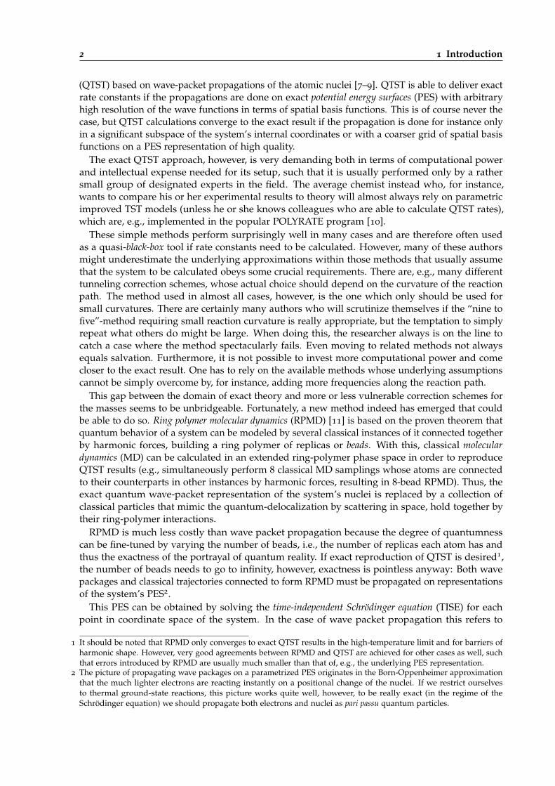
2 1 Introduction
(QTST) based on wave-packet propagations of the atomic nuclei [7–9]. QTST is able to deliver exactrate constants if the propagations are done on exact potential energy surfaces (PES) with arbitraryhigh resolution of the wave functions in terms of spatial basis functions. This is of course never thecase, but QTST calculations converge to the exact result if the propagation is done for instance onlyin a significant subspace of the system’s internal coordinates or with a coarser grid of spatial basisfunctions on a PES representation of high quality.
The exact QTST approach, however, is very demanding both in terms of computational powerand intellectual expense needed for its setup, such that it is usually performed only by a rathersmall group of designated experts in the field. The average chemist instead who, for instance,wants to compare his or her experimental results to theory will almost always rely on parametricimproved TST models (unless he or she knows colleagues who are able to calculate QTST rates),which are, e.g., implemented in the popular POLYRATE program [10].
These simple methods perform surprisingly well in many cases and are therefore often usedas a quasi-black-box tool if rate constants need to be calculated. However, many of these authorsmight underestimate the underlying approximations within those methods that usually assumethat the system to be calculated obeys some crucial requirements. There are, e.g., many differenttunneling correction schemes, whose actual choice should depend on the curvature of the reactionpath. The method used in almost all cases, however, is the one which only should be used forsmall curvatures. There are certainly many authors who will scrutinize themselves if the “nine tofive”-method requiring small reaction curvature is really appropriate, but the temptation to simplyrepeat what others do might be large. When doing this, the researcher always is on the line tocatch a case where the method spectacularly fails. Even moving to related methods not alwaysequals salvation. Furthermore, it is not possible to invest more computational power and comecloser to the exact result. One has to rely on the available methods whose underlying assumptionscannot be simply overcome by, for instance, adding more frequencies along the reaction path.
This gap between the domain of exact theory and more or less vulnerable correction schemes forthe masses seems to be unbridgeable. Fortunately, a new method indeed has emerged that couldbe able to do so. Ring polymer molecular dynamics (RPMD) [11] is based on the proven theorem thatquantum behavior of a system can be modeled by several classical instances of it connected togetherby harmonic forces, building a ring polymer of replicas or beads. With this, classical moleculardynamics (MD) can be calculated in an extended ring-polymer phase space in order to reproduceQTST results (e.g., simultaneously perform 8 classical MD samplings whose atoms are connectedto their counterparts in other instances by harmonic forces, resulting in 8-bead RPMD). Thus, theexact quantum wave-packet representation of the system’s nuclei is replaced by a collection ofclassical particles that mimic the quantum-delocalization by scattering in space, hold together bytheir ring-polymer interactions.
RPMD is much less costly than wave packet propagation because the degree of quantumnesscan be fine-tuned by varying the number of beads, i.e., the number of replicas each atom has andthus the exactness of the portrayal of quantum reality. If exact reproduction of QTST is desired1,the number of beads needs to go to infinity, however, exactness is pointless anyway: Both wavepackages and classical trajectories connected to form RPMD must be propagated on representationsof the system’s PES2.
This PES can be obtained by solving the time-independent Schrödinger equation (TISE) for eachpoint in coordinate space of the system. In the case of wave packet propagation this refers to
1 It should be noted that RPMD only converges to exact QTST results in the high-temperature limit and for barriers ofharmonic shape. However, very good agreements between RPMD and QTST are achieved for other cases as well, suchthat errors introduced by RPMD are usually much smaller than that of, e.g., the underlying PES representation.
2 The picture of propagating wave packages on a parametrized PES originates in the Born-Oppenheimer approximationthat the much lighter electrons are reacting instantly on a positional change of the nuclei. If we restrict ourselvesto thermal ground-state reactions, this picture works quite well, however, to be really exact (in the regime of theSchrödinger equation) we should propagate both electrons and nuclei as pari passu quantum particles.
3
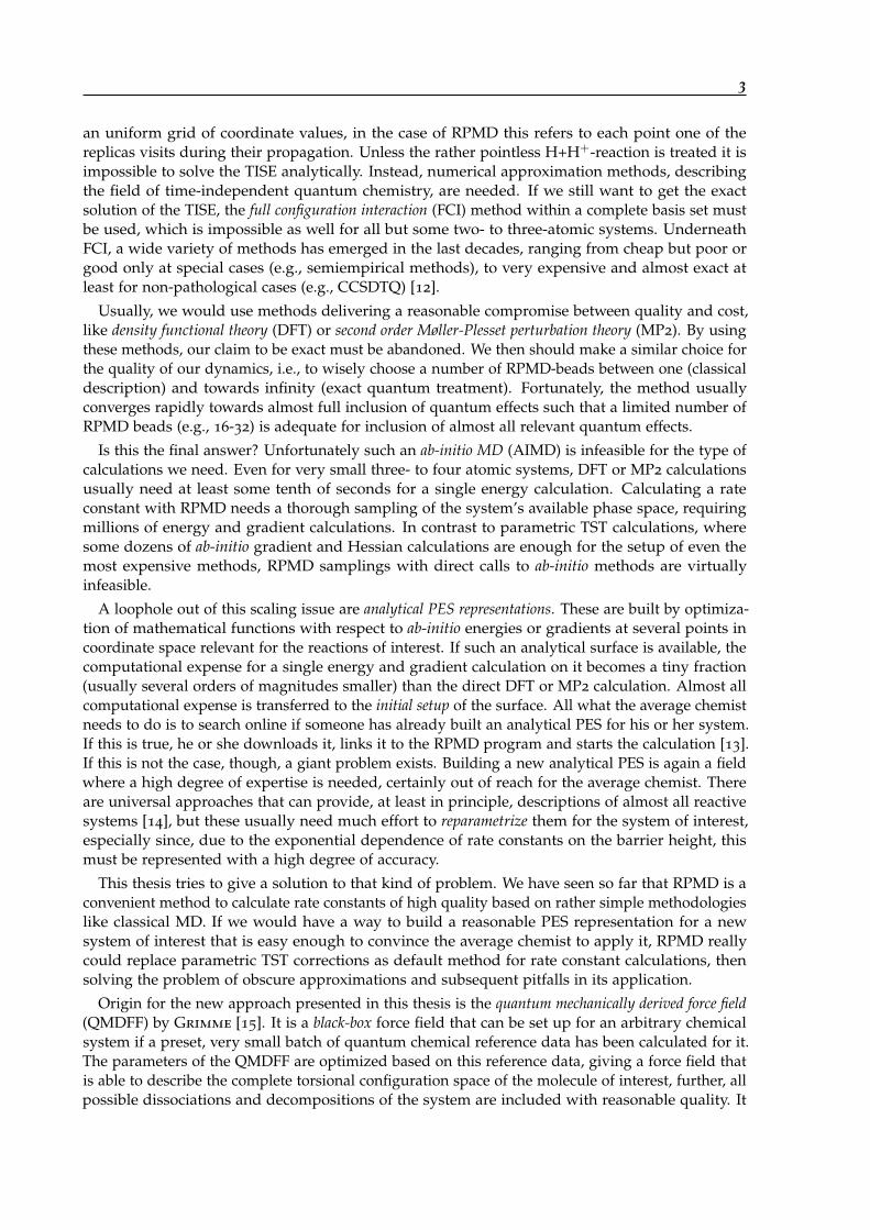
an uniform grid of coordinate values, in the case of RPMD this refers to each point one of thereplicas visits during their propagation. Unless the rather pointless H+H+-reaction is treated it isimpossible to solve the TISE analytically. Instead, numerical approximation methods, describingthe field of time-independent quantum chemistry, are needed. If we still want to get the exactsolution of the TISE, the full configuration interaction (FCI) method within a complete basis set mustbe used, which is impossible as well for all but some two- to three-atomic systems. UnderneathFCI, a wide variety of methods has emerged in the last decades, ranging from cheap but poor orgood only at special cases (e.g., semiempirical methods), to very expensive and almost exact atleast for non-pathological cases (e.g., CCSDTQ) [12].
Usually, we would use methods delivering a reasonable compromise between quality and cost,like density functional theory (DFT) or second order Møller-Plesset perturbation theory (MP2). By usingthese methods, our claim to be exact must be abandoned. We then should make a similar choice forthe quality of our dynamics, i.e., to wisely choose a number of RPMD-beads between one (classicaldescription) and towards infinity (exact quantum treatment). Fortunately, the method usuallyconverges rapidly towards almost full inclusion of quantum effects such that a limited number ofRPMD beads (e.g., 16-32) is adequate for inclusion of almost all relevant quantum effects.
Is this the final answer? Unfortunately such an ab-initio MD (AIMD) is infeasible for the type ofcalculations we need. Even for very small three- to four atomic systems, DFT or MP2 calculationsusually need at least some tenth of seconds for a single energy calculation. Calculating a rateconstant with RPMD needs a thorough sampling of the system’s available phase space, requiringmillions of energy and gradient calculations. In contrast to parametric TST calculations, wheresome dozens of ab-initio gradient and Hessian calculations are enough for the setup of even themost expensive methods, RPMD samplings with direct calls to ab-initio methods are virtuallyinfeasible.
A loophole out of this scaling issue are analytical PES representations. These are built by optimiza-tion of mathematical functions with respect to ab-initio energies or gradients at several points incoordinate space relevant for the reactions of interest. If such an analytical surface is available, thecomputational expense for a single energy and gradient calculation on it becomes a tiny fraction(usually several orders of magnitudes smaller) than the direct DFT or MP2 calculation. Almost allcomputational expense is transferred to the initial setup of the surface. All what the average chemistneeds to do is to search online if someone has already built an analytical PES for his or her system.If this is true, he or she downloads it, links it to the RPMD program and starts the calculation [13].If this is not the case, though, a giant problem exists. Building a new analytical PES is again a fieldwhere a high degree of expertise is needed, certainly out of reach for the average chemist. Thereare universal approaches that can provide, at least in principle, descriptions of almost all reactivesystems [14], but these usually need much effort to reparametrize them for the system of interest,especially since, due to the exponential dependence of rate constants on the barrier height, thismust be represented with a high degree of accuracy.
This thesis tries to give a solution to that kind of problem. We have seen so far that RPMD is aconvenient method to calculate rate constants of high quality based on rather simple methodologieslike classical MD. If we would have a way to build a reasonable PES representation for a newsystem of interest that is easy enough to convince the average chemist to apply it, RPMD reallycould replace parametric TST corrections as default method for rate constant calculations, thensolving the problem of obscure approximations and subsequent pitfalls in its application.
Origin for the new approach presented in this thesis is the quantum mechanically derived force field(QMDFF) by Grimme [15]. It is a black-box force field that can be set up for an arbitrary chemicalsystem if a preset, very small batch of quantum chemical reference data has been calculated for it.The parameters of the QMDFF are optimized based on this reference data, giving a force field thatis able to describe the complete torsional configuration space of the molecule of interest, further, allpossible dissociations and decompositions of the system are included with reasonable quality. It
4 1 Introduction
cannot, however, describe the formation of new bonds that have not already existed in the referencestructure.
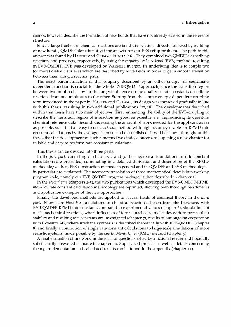
Since a large fraction of chemical reactions are bond dissociations directly followed by buildingof new bonds, QMDFF alone is not yet the answer for our PES setup problem. The path to thisanswer was found by Hartke and Grimme in 2015 [16]. They combined two QMDFFs describingreactants and products, respectively, by using the empirical valence bond (EVB) method, resultingin EVB-QMDFF. EVB was developed by Warshel in 1980. Its underlying idea is to couple two(or more) diabatic surfaces which are described by force fields in order to get a smooth transitionbetween them along a reaction path.
The exact parametrization of this coupling described by an either energy- or coordinate-dependent function is crucial for the whole EVB-QMDFF approach, since the transition regionbetween two minima has by far the largest influence on the quality of rate constants describingreactions from one minimum to the other. Starting from the simple energy-dependent couplingterm introduced in the paper by Hartke and Grimme, its design was improved gradually in linewith this thesis, resulting in two additional publications [17, 18]. The developments describedwithin this thesis have two main objectives: First, enhancing the ability of the EVB-coupling todescribe the transition region of a reaction as good as possible, i.e., reproducing its quantumchemical reference data. Second, decreasing the amount of work needed for the applicant as faras possible, such that an easy to use black-box method with high accuracy usable for RPMD rateconstant calculations by the average chemist can be established. It will be shown throughout thisthesis that the development of such a method was indeed successful, opening a new chapter forreliable and easy to perform rate constant calculations.
This thesis can be divided into three parts.In the first part, consisting of chapters 2 and 3, the theoretical foundations of rate constant
calculations are presented, culminating in a detailed derivation and description of the RPMD-methodology. Then, PES construction methods in general and the QMDFF and EVB methodologiesin particular are explained. The necessary translation of those mathematical details into workingprogram code, namely our EVB-QMDFF program package, is then described in chapter 3.
In the second part (chapters 4-5), the two publications which developed the EVB-QMDFF-RPMDblack-box rate constant calculation methodology are reprinted, showing both thorough benchmarksand application examples of the new approaches.
Finally, the developed methods are applied to several fields of chemical theory in the thirdpart. Shown are black-box calculations of chemical reactions chosen from the literature, withEVB-QMDFF-RPMD rate constants compared to experimental values (chapter 6), simulations ofmechanochemical reactions, where influences of forces attached to molecules with respect to theirstability and resulting rate constants are investigated (chapter 7), results of our ongoing cooperationwith Covestro AG, where urethane synthesis is described theoretically with EVB-QMDFF (chapter8) and finally a connection of single rate constant calculations to large-scale simulations of morerealistic systems, made possible by the kinetic Monte Carlo (KMC) method (chapter 9).
A final evaluation of my work, in the form of questions asked by a fictional reader and hopefullysatisfactorily answered, is made in chapter 10. Supervised projects as well as details concerningtheory, implementation and calculated results can be found in the appendix (chapter 11).
2
Ch
ap
te
r
Theoretical Background
A philosopher once said, “It is necessary forthe very existence of science that the sameconditions always produce the same results”.Well, they don’t!
(Richard Feynman)
2.1 Chemical Reaction Rates
As will be shown in this thesis, chemical reaction rates can be calculated for a whole range ofmolecular systems and situations, and in connection with methods like KMC, much larger systemsof almost real-world size can be simulated with manageable usage of resources but neverthelesshigh accuracy.
Since a comprehensive review of the rich field of quantitative reaction dynamics culminating inthe calculation of reaction rates would need several volumes of textbooks, it cannot be given evenapproximately in the scope of this thesis.
Nevertheless, I will try to lead through a little theorist’s journey starting from the foundationslike TST, continuing through improved transition state theory as well as sampling methods ofthe relevant configuration space and exact quantum mechanical treatments, and finally ending atmethods of calculating reaction rates with quantum corrections using classical trajectory sampling,which will be used extensively in the presented applications throughout this work.
Of course this journey cannot admit any claim to give a representative overview of the field, wewill essentially focus on all what is needed to calculate the results presented in the course of thisthesis. Further, mathematical foundations of TST, lying in flux-flux autocorrelations and others, aretreated rather shortly and at later stages, which could irritate some designated experts of the field.In order to understand ordinary TST as an average chemist, this background is not needed; it isneeded, however, to understand why RPMD can be used to calculate k(T) values with quantumcorrections.
Since only gas phase reactions1 of rather small systems in their electronic ground state areinvestigated in this thesis, the whole treatment will focus on this subtopic, ignoring the rich varietyof methods designed for the description of, for instance, reactions in solutions or surrounded by
1 In chapter 9 rate constants for diffusions on surfaces are calculated and fitted into KMC-schemes. However, their rateconstants are also calculated on the assumption of a gas phase reaction, treating the surface atom and the subjacentsurface slab as a single molecule.

6 2 Theoretical Background
protein backbones influencing the reaction mechanism. A better overview of the whole topic ispresented, e.g., in the book by Peters [1].
2.1.1 Transition State Theory
Perhaps one of the earliest quantitative observations in the field of chemical kinetics was that therates of most chemical reactions roughly double if the system’s temperature is increased by acertain amount, e.g., 10 K. More precisely, it was noticed that chemical reaction rates usually showexponential dependence on the temperature. This behavior is also known as Arrhenius’ law [19], andthe respective mathematical formulation is usually:
k(T) = A exp[−Ea
RT
], (2.1)
where A is the preexponential factor, Ea is the activation energy of the reaction, T is the temperatureand R is the universal gas constant.
If we take the logarithm of rate constants measured at different temperatures and plots themagainst the reciprocal temperatures, both A and Ea can be obtained from a linear fit2. SinceA can be interpreted as the number of collisions between possible reactants per time unit andthe exponential term picks the fraction of collisions that lead to reactions (depending on theheight of the activation barrier), we are able to determine information on the molecular level frommacroscopic experiments.
Surprisingly, in spite of its simplicity, Arrhenius law, i.e., exponential increase of reaction rateswith temperature, is valid to a high degree of accuracy in the largest fraction of systems andreactions, even if they were treated with much more elaborate methods as is shown in subsequentchapters.
In principle, we could go along the opposite direction: calculate the collision number via kinetictheory of gases to get A and the energy barrier Ea via quantum chemistry and insert it to calculatethe reaction rate [20]. Unfortunately, in most cases the results will be rather poor [3].
In the 1930s, efforts to get more rigorous formulations of microscopic chemical rate theory leadto transition-state theory, as formulated by Eyring, Evans and Polanyi [4, 5].
Derivation
We look at a standard second order reaction of two molecules A and B, reacting to one or moreproduct molecules P without any detailed specification of them [1]. Reactive trajectories passthrough transition states (TSs) ‡, being located at the barrier between reactant and product basins.Just for mathematical reasons it is assumed that these transition states are located within aninterval δξ centered at a central position ξ‡ with respect to the reaction coordinate ξ(q) (where qis a suitable set of internal coordinates), defining a a transition region at ξ‡ − δξ
2 < ξ(q) < ξ‡ +δξ2 .
It is further supposed that an equilibrium exists between reactants and transition states but notbetween transition states and products, i.e., no products can react back to transition states. Hence,the mechanism is:
A + B ‡→ P. (2.2)
Since no equilibrium exists between transition states and products all trajectories headed to theproducts in the transition region will have no chance of coming back and contribute to the reactionrate. These are half of the trajectories in the transition region, since they are in equilibrium with
2 It should be noted that the van’t Hoff equation emerged even before the approach by Arrhenius. Its differential form is(∂lnKc
∂T
)P= ∆Uo
RT2 , where Kc is the concentration equilibrium constant and ∆Uo is the standard internal energy change uponreaction. Similar to Arrhenius, a logarithmic plot can be done to determine the unknown quantities.
2.1 Chemical Reaction Rates 7
the reactants and are moving into both directions with equal probability. With this, the frequencyof transition states exiting to the product region ν‡ and contributing to the reaction rate can beexpressed as:
ν‡ =1
2δξ〈|ξ|〉‡, (2.3)
where 〈|ξ|〉‡ is the average velocity along the reaction coordinate at position ξ. In order to get anabsolute rate, the concentration of transition states to be multiplied with their exit-frequency needsto be calculated. According to the law of mass action, this concentration can be obtained from eq.2.2, being:
[‡] = K′‡[A][B]. (2.4)
As it is well known from statistical mechanics [21], chemical equilibria can be expressed in termsof the partition functions Q of their participants:
K′‡ =δξ
λT,ξ
Q‡
QAQBexp
(−∆Ea
RT
), (2.5)
where ∆Ea is the activation energy (e.g., the zero point energy difference between reactants andTS), QA, QB are the partition functions of both reactants and δξ
λT,qQ‡ is the partition function of
the TS. The latter is separated into two factors since the reaction coordinate ξ plays a special role:Unlike all other bound vibrational modes at the TS, it plays the role of a translation from reactantsto products3. Hence, its contribution to the total partition sum needs to be that of a translation,which can be expressed in terms of a de Broglie wavelength:
λT,ξ =h√
2πµξkBT, (2.6)
with µξ being the reduced mass for the motion along ξ, h the Planck constant and kB the Boltzmannconstant. The total rate of the reaction in eq. 2.2 is the product of the TS concentration expressed asin eq. 2.4 and the conversion frequency (eq. 2.3):
kTST [A][B] = K′‡ν‡[A][B]
kTST = K′‡ν‡
=δξ
λT,ξ
Q‡
QAQBexp
(−∆Ea
RT
)1
2δξ〈|ξ|〉‡
=12〈|ξ|〉‡λT,ξ
Q‡
QAQBexp
(−∆Ea
RT
).
(2.7)
The average velocity along the reaction coordinate at the TS 〈|ξ|〉‡ can be calculated by means ofthe Maxwell-Boltzmann velocity distribution:
〈|q|〉‡ =
∫ ∞
−∞exp
(− βµξ ξ2
2
)|ξ|dξ∫ ∞
−∞exp
(− βµξ ξ2
2
)dξ
=
√2kBTπµξ
. (2.8)
3 Partition functions of ideal gases with internal degrees of freedom usually contain translational, rotational,electronic and vibrational contributions as well as the zero-point potential energy VX
zp, resulting in QX =
QXtransQX
rotQXelQ
Xvib exp(− 1
kBT VXzp). The vibrational mode of the reaction coordinate at the TS is treated as a trans-
lation in TST, therefore contributing to QXtrans instead of QX
vib.
8 2 Theoretical Background
This expression and eq. 2.6 can be inserted into eq. 2.7, resulting in:
kTST =12
√2kBTπµξ
√2πµξkBT
hQ‡
QAQBexp
(−∆Ea
RT
)=
kBTh
Q‡
QAQBexp
(−∆Ea
RT
).
(2.9)
It can be seen that neither the width of the transition region δξ nor the reduced mass of thetranslation along the reaction coordinate µξ remain. Now we have obtained the TST rate expression.Usually, an additional prefactor κ containing additional corrections (as will be explained below) isadded, resulting in the famous statistical formulation of TST:
k(T) = κkBT
hQ‡
QAQBexp
[−∆Ea
RT
]. (2.10)
Thus, by knowing the partition functions of reactants and TS as well as the potential energybarrier of the reaction, we can directly calculate the rate of the whole reaction, without knowinganything about other areas in configuration space at all. This fact is quite impressive given that thewhole available coordinate space of the system scales exponentially with the number of particles,thus quickly becoming huge. Then the vicinities of the two points needed for TST shrink to a tinysection of the whole space, ignoring almost everything else of it. Nevertheless at least qualitativeestimates of reaction rates can be obtained for most systems if only this two tiny regions areincluded in the description. Besides the statistical formulation of TST, the perhaps even morerenowned thermodynamic formulation (also termed Eyring-Polanyi equation) can be used [22]:
k(T) =kBT
hK0 exp
[−∆G‡,0
RT
]=
kBTh
K0 exp[−∆S‡,0
R
]exp
[−∆H‡,0
R
], (2.11)
with K0 the reciprocal standard concentration and ∆G‡,0, ∆S‡,0 and ∆H‡,0 the free energy, entropy andenthalpy barriers at standard conditions, respectively. Now, transition state theory is again quitesimilar to the Arrhenius equation (eq. 2.1), however, the potential energy barrier Ea is replaced bythe free energy barrier ∆G‡,0, indicating the fact that entropic effects are also needed if a reliabledescription of reaction rates shall be achieved4.
Shortcomings
Reviewing the derivation of TST shown above some of its limitations are becoming obvious. Inthe underlying model (eq. 2.2) reactants and TS are assumed to be equilibrated, whereas onlyreactions in the direction TS to products are possible. The second assumption is deficient in practice:trajectories going through the TS region on their way to the products might turn back, e.g., due tothermal fluctuations and recross to reactants, in opposition to the assumption made in eq. 2.3. It istherefore called the no recrossing assumption. Even without thermal fluctuations recrossings arequite common if we look at the underlying PES of the system. For the simple case of a system witha linear or near-linear reaction path and negligible coupling between the reaction path and othervibrational modes, successful reactive trajectories will pass the TS and accomplish the reaction byreaching the products basin. Then, however, the story is not finished. If coupling between reactioncoordinate and other vibrations is low, there will be almost no vibrational energy distribution suchthat the system performs a pendulum motion through the products minimum, climbs the otherside and then turns back to the TS. Due to the small coupling the energy in the reaction coordinatewill often be still high enough to cross the TS again, now directed to the reactants, thus generating
4 The thermodynamic formulation of TST builds the base for Eyring-plots well known in experimental (and theoretical)kinetics. They are conducted similar to Arrhenius-plots with the distinction that the parameters ∆G‡,0, ∆S‡,0 and ∆H‡,0
for the actual reaction can be obtained from them. Eyring-plots are used in chapter 8
2.1 Chemical Reaction Rates 9
a recrossing event. If the reaction coordinate is curved near the TS, a reactive trajectory will usuallyclimb up the potential wall beyond the TS after it has reacted. If it comes back, the probability islarge that it recrosses the TS in a pendulum motion unless vibrational couplings will guide thetrajectory from this hillslope straight into the product region.
Moreover, the reaction coordinate ξ plays an exceptional role in the whole TST-concept. Itspartition function is treated separately (eq. 2.6) and its time derivative is used to calculate theturnover frequency at the TS (eq. 2.3). In reality, it is difficult to treat a single internal coordinate ofa molecule independently from all others, since the vibrational modes are usually coupled duringinternal motions.
The TS-region, in which all motions towards the products are assumed to be reactive, is locatedaround the TS position ξ‡ and has a width δξ. Since δξ does not appear in the final TST rateexpression, its actual extent does not play any role. It is therefore possible to make it infinitesi-mal, then resulting in a N − 1 dimensional hypersurface perpendicular to the reaction coordinate,incorporating the full space of all other coordinates at the actual TS-position. This surface is calleddividing surface, since all trajectories that cross it are classified as reactive in TST, thus effectivelydividing the coordinate space in reactants and products sections. This surface is located at ξ‡, thepoint along the reaction coordinate with the highest potential energy, hence the TS with respect topotential energy. We will see below that the position must actually be determined with respect tothe free energy along the reaction coordinate, hence showing the deficiency of the location in TST.
As it can be seen from eq. 2.10, only information about the reactants minimum and the TSis needed for the whole theory. Usually, the harmonic approximation is used to calculate thesepartition functions, thus anharmonic shapes of the PES, as they always exist in real systems, arenot recognized.
Further, the derivation of TST uses classical trajectories moving along the system’s PES asunderlying model, hence ignoring all quantum mechanical effects such as tunneling or zero pointenergies5. This leads to five major pitfalls of TST, also shown in fig. 2.1.
1. Separability of the reaction coordinate from all others.
2. No recrossing of the dividing surface.
3. The diving surface is always located at the TS of the potential energy.
4. Harmonic approximation in the calculation of partition functions.
5. Classical behavior of the system is assumed.
In practice, the significance of these shortcomings strongly depends on the chosen system andthe temperature, e.g., tunneling will get more important at lower temperatures, whereas theno-recrossing assumption is less valid at higher temperatures. For systems that approximately obeyall TST-assumptions and thus circumvent all its pitfalls, very accurate k(T) values can be obtained,whereas the theory might fail spectacularly for others [23, 24].
2.1.2 Handling of TST-Problems
Since its foundation in the 1930s, TST has become a widely used tool for k(T) calculations. Inparallel, several authors tried to solve or at least diminish TST’s intrinsic problems listed above [6].
5 Interestingly, quantum mechanical models like the harmonic oscillator (for vibrations), the rigid rotator (for rotations)and the particle in the box (for translations) are used for the calculation of the partition sums for the reactants and theTS, thus incorporating quantum mechanics indirectly.

10 2 Theoretical Background
Separated reaction coordinate
dividing surface, N-1 dimensional
Harmonic approximation for partition sums
Classical mechanicsdescription
No recrossing possible
Figure 2.1: Schematic overview of the inherent approximations of TST, for a two-dimensional model system.The reaction coordinate ξ(q) is shown in the base plane, the dividing surface is perpendicular toit, positioned at the potential energy TS (large scarlet dot). The partition sums of reactants (2dimensional) as well as the TS (one dimensional, due to the separated reaction coordinate) arecalculated with the harmonic approximation. Reactive trajectories show no recrossing and endalways on the products side of the dividing surface.
2.1 Chemical Reaction Rates 11
Variational TST
The first important improvement is the variational TST (VTST), also called canonical variational theory(CVT) [25, 26]. Conventional TST as discussed above leads usually to an overestimation of the rateconstant. The reason is that in eq. 2.10 the dividing surface, representing the bottleneck the systemmust overcome during a reaction, is placed at the potential energy maximum along the reactioncoordinate.
In reality, however, the activation criterion is not the potential energy but the free energy, sinceentropic effects play a significant role during reactions (what is already included in thermodynamicTST (eq. 2.11), but not with the correct position of the free energy barrier).
Therefore, the free energy maximum along the reaction coordinate needs to be taken as positionof the dividing surface (fig. 2.2 (a)). Usually this is viewed from another perspective: Since therate constant depends exponentially on the free energy activation barrier (eq. 2.11), the resultingrate constant (or the reactive flux) needs to be minimized, with respect to the reaction coordinateξ. In line with that, the number of recrossings becomes minimal at the correct TS-position, thusmaximizing the effective reactive flux6:
kCVT(T) = minξ
(kTST(T, ξ)). (2.12)
The minimum can be determined variationally, i.e., by setting the first derivative with respect toξ to zero:
∂
∂ξ[kTST(T, ξ)]
!= 0. (2.13)
Since TST and CVT provide an upper bound for the exact k(T) value in case of classical systemsand known PES functions [27], CVT is always an improvement over TST7. The drawback of thisimprovement is that much more calculation effort is needed. Instead of only three frequencycalculations (TST, first and second reactant) a number of additional frequency calculations alongthe interpolated reaction path is needed in order to parametrize a free energy surface based onpartition sums and then determine k(T, ξ) as well as the minimum of its derivative [10, 29].
In spite of the larger computational expense, CVT rate constants are usually calculated besidesTST rates in present publications (chapter 6). Though CVT/VTST is an important step forward andfrequently used, it has only solved issue 3 of the TST shortcomings!
Recrossing
The issues of recrossing and quantum effects are usually handled together by inserting a singleprefactor in the TST or CVT rate constants: The transmission coefficient κ.
As stated in the last section, TST assumes that trajectories crossing the dividing surface alwaysend in the product region. In reality, the system can be pushed back, for instance, by thermalor geometric effects such it only stays a short time in the product side before returning to the
6 The VTST method presented here is still an approximation since only the position of the dividing surface with respectto the reaction coordinate is altered, but not the shape of the surface itself. In reality, the correct dividing surface(i.e., the one that corresponds to the “global minimum” of the rate constant and thus also the global minimum forthe recrossing) might have a complicated rugged shape, depending on the couplings between the different internalcoordinates of the system. Of course, such an exact parametrization of the dividing surface is impossible at leastanalytically for all but the smallest systems [1]. Even if it is known, recrossings still can happen.
7 Besides usual CVT, where the free energy needs to be calculated along the reaction coordinate, some improved but alsomore tedious approaches are known in the literature: microcanonical variational theory (µVT) [28] uses a microcanonicalensemble instead of a canonical one for optimization of ξ, which involves calculations of accessible states dependingon the path progress and the total energy (phase space integration), improved canonical variational theory (ICVT) uses amixture of canonical and microcanonical optimizations depending on threshold energies [22], which reduces the phasespace integration effort.
12 2 Theoretical Background
reactants. This effect is called recrossing. Since TST ignores it by construction, its rate constant valuewill be always too large (the effective reactive flux should be diminished by recrossing). It can beshown that the location of the dividing surface at maximum free energy of activation minimizesthe recrossing, i.e., recrossing appears more often if the dividing surface is placed at the potentialenergy bottleneck instead of the free energy one. If the exact dividing surface would be known, therecrossing could be diminished further (see above).
For real systems, recrossing can still be an important factor, especially if reactions with broadbarriers are calculated, where the trajectories remain a significant amount of time in the transitionregion and high temperatures are used, where, e.g., thermal motions can push the system backthrough the bottleneck more easily.
Exact calculations of classical transmission coefficients (i.e., exclusion of quantum effects) requireactual sampling of trajectories and calculation of correlation functions, as it will be shown in thenext section. For static calculations, though, a bunch of approximate models was developed. Twoof them are the unified statistical model (US) for TST [30] and the canonical US (CUS) [31] for CVTcalculations.
The general assumption for US and CUS is that recrossing becomes important if more thanone bottleneck, i.e., local free energy maximum, is located along the reaction path. If two localmaxima are present, the dividing surface will be located at the higher one for CVT (since the globalmaximum of free energy is used as the position), but the system might be trapped in the highenergy region between this and the slightly lower second maximum some amount of time, suchthat it could oscillate back and forth, increasing the possibility for recrossings (fig. 2.2 (b)).
The partition function for the bound degrees of freedom (excluding the reaction coordinate) at acertain value ξ of the reaction path progress can be expressed as:
q(T, ξ) = e−βVMEP(ξ)Q(T, ξ), (2.14)
where β = 1kBT is the inverse temperature, Q(T, ξ) denotes the partition function of a dividing
surface located at ξ and the exponential provides an energy shift with respect to the reactantsminimum.
If we calculate the partition function for the global free energy maximum qCVT(T), for the secondlocal maximum qmax(T) and for the local minimum between both maxima qmin(T) , the CUSrecrossing coefficient can be expressed as:
κCUS(T) =qmax(T)qCVT(T)
qmax(T) + qCVT(T)− qmax(T)qCVT(T)qmin(T)
. (2.15)
This empirical correction delivers good results for some cases, but it cannot describe situations,where recrossing occurs even if the free energy profile only has one maximum (which is the case inmost reactions). In those cases κCUS becomes unity [31]. In general, analytical recrossing correctionsare rarely used.
Tunneling Corrections
More common are tunneling corrections to TST or CVT. In contrast to recrossing, which typicallyimposes a correction factor between 0.99 and 0.6 to reaction rates, slightly growing in importancewith raising temperature, tunneling can enhance reactions even more radical, up to more than tenorders of magnitude for proton transfers at very low temperatures [6, 23, 32–34]8.
8 In general, tunneling and recrossing corrections can be seen to be of similar importance, since recrossings alwaysinfluence the rate constant, where tunneling only causes the huge accelerations over many orders of magnitude if it isfavored and the classical rate is extremely small, what is usually the case for very low temperatures and systems werehydrogen or deuterium are transferred (see chapter 9).

2.1 Chemical Reaction Rates 13
One of the simplest but still widely known tunneling models is the semiclassical Wigner correction[35]. Here, the shape of the potential barrier is modeled as an inverted parabola, i.e., a Taylor seriesat the TS of the reaction coordinate, truncated after the second term:
κW(T) = 1 +124
∣∣∣βhω‡∣∣∣ , (2.16)
with ω‡ being the imaginary frequency of the (potential energy) transition state, i.e., the curvatureof the reaction coordinate, and h the reduced Planck constant ( h
2π ). Unsurprisingly, this model hardlydelivers quantitative results, if at all it should be used for barriers with near parabolic shape attemperatures where the expected tunneling coefficient is small (less than 1.2) [22]. Nevertheless, itcan serve as a first rule-of-thumb estimate for the importance of tunneling: If the temperature issmall and ω‡ is large, i.e., the barrier is sharp, large tunneling contributions can be expected andmore sophisticated tunneling corrections should be applied.
If rate constants are calculated with corrected TST nowadays, two tunneling approximations arethe most popular ones: zero curvature tunneling (ZCT) [36] and small curvature tunneling (SCT) [37].
As the terminology may indicate, the actual choice of the method depends on the curvature of thereaction path. It is the second derivative of the cartesian geometry x(ξ) with respect to the reactioncoordinate ξ:
γ(ξ) =d2xdξ2 . (2.17)
If the curvature is low, i.e., the reaction path appears nearly linear in the coordinate space underconsideration, the ZCT method can be applied. Both ZCT and SCT are one-dimensional models.Their common assumption is that the motion along the reaction coordinate can be separated fromthe motion of the bound degrees of freedom orthogonal to them, i.e., similar to TST. The motionalong the reaction coordinate is considered as slow with respect to the bound degrees of freedom,due to the similarity to quantum dynamics this is also called the vibrationally adiabatic model.
In the resulting one-dimensional system, the transmission coefficient for CVT is then evaluatedby integration over all energies present in the thermal ground state, populated according to aBoltzmann distribution (the largest part of the derivation is identical for ZCT and SCT):
κ(T) =
∫ ∞0 P(E)eβEdE∫ ∞
0 PC(E)eβEdE. (2.18)
Both numerator and denominator are essentially calculating transmission probabilities P(E) forall energies E, weighted by the actual population, expressed with the Boltzmann factor. In thenumerator, the approximated quantum mechanical transmission probabilities are integrated, whereasin the denominator, the classical transmission probabilities as already included into usual CVT areintegrated. Therefore, the division accounts for the remaining transmission prefactor not alreadyincluded into CVT itself9.
In the classical picture, the system can only overcome the barrier if its energy is higher than thebarrier height:
Pc(E) = Θ {E− (VMEP(ξ∗) + EZPE(ξ∗))} , (2.19)
where Θ is the Heaviside function, ξ∗ is the variationally corrected position of the dividing surface,VMEP is the potential energy of the reaction path and EZPE are the vibrational ground state energiesof the bound degrees of freedom.
9 This point might get clearer if we recall that the definition of the transmission coefficient can be written as the relationbetween the CVT rate constant (kCVT(T)) and the desired exact one (k(T)): κ = k(T)
kCVT(T).
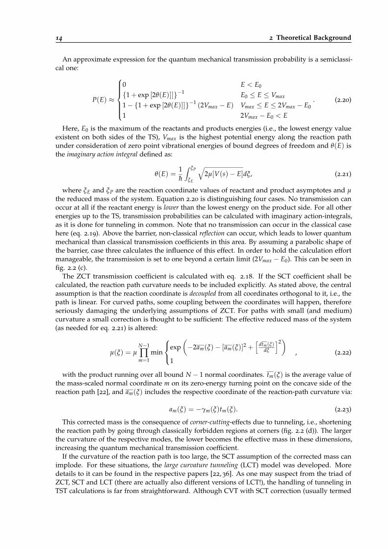
14 2 Theoretical Background
An approximate expression for the quantum mechanical transmission probability is a semiclassi-cal one:
P(E) ≈
0 E < E0
{1 + exp [2θ(E)]]}−1 E0 ≤ E ≤ Vmax
1− {1 + exp [2θ(E)]]}−1 (2Vmax − E) Vmax ≤ E ≤ 2Vmax − E0
1 2Vmax − E0 < E
. (2.20)
Here, E0 is the maximum of the reactants and products energies (i.e., the lowest energy valueexistent on both sides of the TS), Vmax is the highest potential energy along the reaction pathunder consideration of zero point vibrational energies of bound degrees of freedom and θ(E) isthe imaginary action integral defined as:
θ(E) =1h
∫ ξP
ξE
√2µ[V(s)− E]dξ, (2.21)
where ξE and ξP are the reaction coordinate values of reactant and product asymptotes and µthe reduced mass of the system. Equation 2.20 is distinguishing four cases. No transmission canoccur at all if the reactant energy is lower than the lowest energy on the product side. For all otherenergies up to the TS, transmission probabilities can be calculated with imaginary action-integrals,as it is done for tunneling in common. Note that no transmission can occur in the classical casehere (eq. 2.19). Above the barrier, non-classical reflection can occur, which leads to lower quantummechanical than classical transmission coefficients in this area. By assuming a parabolic shape ofthe barrier, case three calculates the influence of this effect. In order to hold the calculation effortmanageable, the transmission is set to one beyond a certain limit (2Vmax − E0). This can be seen infig. 2.2 (c).
The ZCT transmission coefficient is calculated with eq. 2.18. If the SCT coefficient shall becalculated, the reaction path curvature needs to be included explicitly. As stated above, the centralassumption is that the reaction coordinate is decoupled from all coordinates orthogonal to it, i.e., thepath is linear. For curved paths, some coupling between the coordinates will happen, thereforeseriously damaging the underlying assumptions of ZCT. For paths with small (and medium)curvature a small correction is thought to be sufficient: The effective reduced mass of the system(as needed for eq. 2.21) is altered:
µ(ξ) = µN−1
∏m=1
min
exp(−2am(ξ)− [am(ξ)]2 +
[dtm(ξ)
dξ
]2)
1, (2.22)
with the product running over all bound N− 1 normal coordinates. tm(ξ) is the average value ofthe mass-scaled normal coordinate m on its zero-energy turning point on the concave side of thereaction path [22], and am(ξ) includes the respective coordinate of the reaction-path curvature via:
am(ξ) = −γm(ξ)tm(ξ). (2.23)
This corrected mass is the consequence of corner-cutting-effects due to tunneling, i.e., shorteningthe reaction path by going through classically forbidden regions at corners (fig. 2.2 (d)). The largerthe curvature of the respective modes, the lower becomes the effective mass in these dimensions,increasing the quantum mechanical transmission coefficient.
If the curvature of the reaction path is too large, the SCT assumption of the corrected mass canimplode. For these situations, the large curvature tunneling (LCT) model was developed. Moredetails to it can be found in the respective papers [22, 36]. As one may suspect from the triad ofZCT, SCT and LCT (there are actually also different versions of LCT!), the handling of tunneling inTST calculations is far from straightforward. Although CVT with SCT correction (usually termed
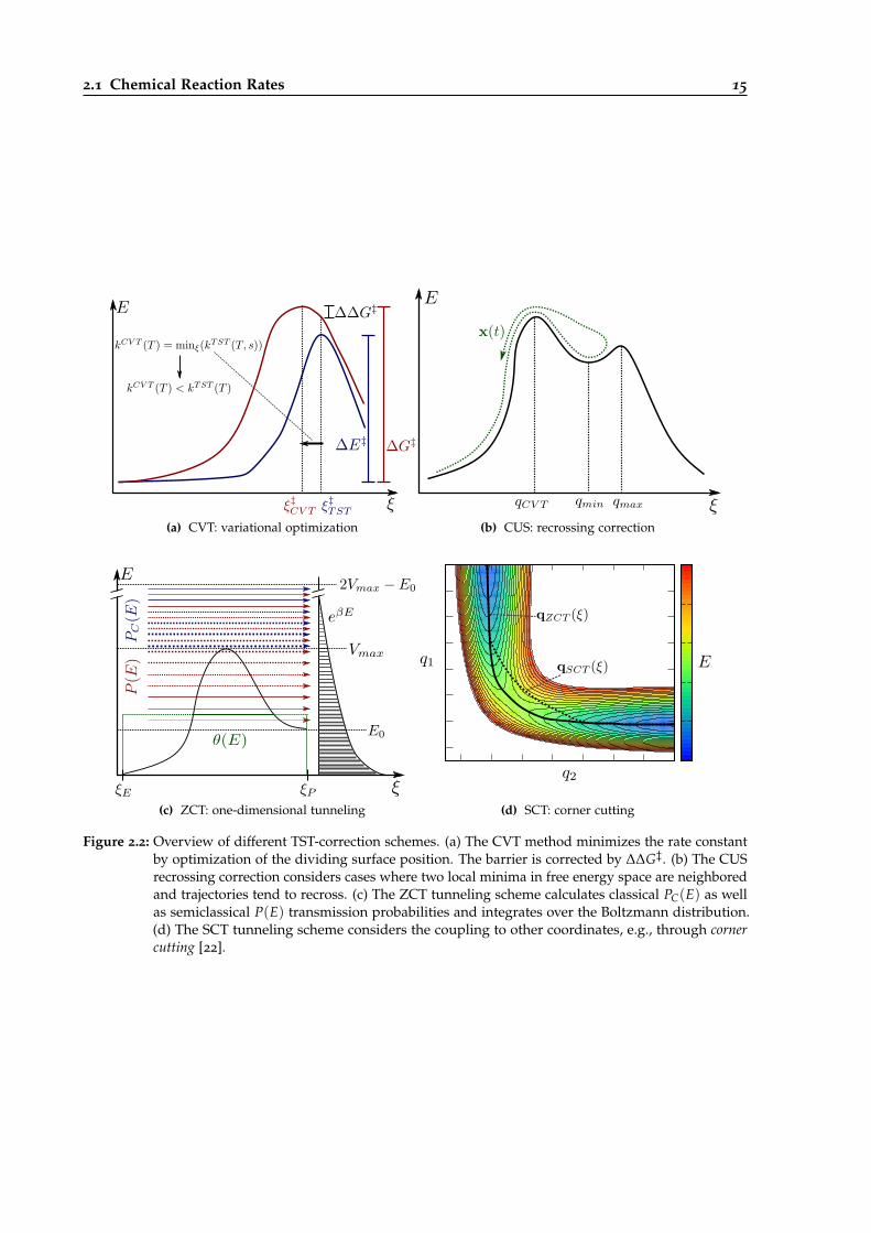
2.1 Chemical Reaction Rates 15
(a) CVT: variational optimization (b) CUS: recrossing correction
(c) ZCT: one-dimensional tunneling (d) SCT: corner cutting
Figure 2.2: Overview of different TST-correction schemes. (a) The CVT method minimizes the rate constantby optimization of the dividing surface position. The barrier is corrected by ∆∆G‡. (b) The CUSrecrossing correction considers cases where two local minima in free energy space are neighboredand trajectories tend to recross. (c) The ZCT tunneling scheme calculates classical PC(E) as wellas semiclassical P(E) transmission probabilities and integrates over the Boltzmann distribution.(d) The SCT tunneling scheme considers the coupling to other coordinates, e.g., through cornercutting [22].
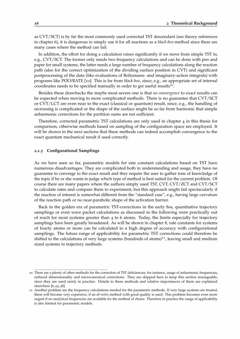
16 2 Theoretical Background
as CVT/SCT) is by far the most commonly used corrected TST descendant (see theory referencesin chapter 6), it is dangerous to simply use it for all reactions as a black-box-method since there aremany cases where the method can fail.
In addition, the effort for doing a calculation raises significantly if we move from simple TST to,e.g., CVT/SCT. The former only needs two frequency calculations and can be done with pen andpaper for small systems, the latter needs a large number of frequency calculations along the reactionpath (also for the correct optimization of the dividing surface position in CVT) and significantpostprocessing of the data (like evaluations of Boltzmann- and imaginary-action integrals) withprograms like POLYRATE [10]. This is far from black-box, since, e.g., an appropriate set of internalcoordinates needs to be specified manually in order to get useful results10.
Besides these drawbacks the maybe most severe one is that no convergence to exact results canbe expected when moving to more complicated methods. There is no guarantee that CVT/SCTor CVT/LCT are even near to the exact (classical or quantum) result, since, e.g., the handling ofrecrossing is complicated or the shape of the surface might be so far from harmonic that simpleanharmonic corrections for the partition sums are not sufficient.
Therefore, corrected parametric TST calculations are only used in chapter 4 in this thesis forcomparison, otherwise methods based on sampling of the configuration space are employed. Itwill be shown in the next sections that these methods can indeed accomplish convergence to theexact quantum mechanical result if used correctly.
2.1.3 Configurational Samplings
As we have seen so far, parametric models for rate constant calculations based on TST havenumerous disadvantages. They are complicated both in understanding and usage, they have noguarantee to converge to the exact result and they require the user to gather tons of knowledge ofthe topic if he or she wants to judge which type of method is best suited for the current problem. Ofcourse there are many papers where the authors simply used TST, CVT, CVT/ZCT and CVT/SCTto calculate rates and compare them to experiment, but this approach might fail spectacularly ifthe reaction of interest is somewhat different from the “standard case”, e.g., having large curvatureof the reaction path or no near-parabolic shape of the activation barrier.
Back in the golden era of parametric TST-corrections in the early 80s, quantitative trajectorysamplings or even wave packet calculations as discussed in the following were practically outof reach for most systems greater than 4 to 6 atoms. Today, the limits especially for trajectorysamplings have been greatly broadened. As will be shown in chapter 8, rate constants for systemsof fourty atoms or more can be calculated to a high degree of accuracy with configurationalsamplings. The future range of applicability for parametric TST corrections could therefore beshifted to the calculations of very large systems (hundreds of atoms)11, leaving small and mediumsized systems to trajectory methods.
10 There are a plenty of other methods for the correction of TST deficiencies, for instance, usage of anharmonic frequencies,reduced dimensionality and microcanonical corrections. They are skipped here to keep this section manageable,since they are used rarely in practice. Details to these methods and relative importances of them are explainedelsewhere [6, 22, 38].
11 Another problem are the frequency calculations needed for the parametric methods. If very large systems are treated,these will become very expensive, if an ab-initio method with good quality is used. This problem becomes even moreurgent if no analytical frequencies are available for the method of choice. Therefore in practice the range of applicabilityis also limited for parametric models.
2.1 Chemical Reaction Rates 17
Statistical Definition of Free Energy
The connection between parametric and sampling methods is the free energy12. As seen in eqs.2.10-2.11, the TST rate constant can be calculated either with respect to the partition functions ofreactants and the transition state or with respect to the free energy difference between them.
The canonical partition function of a system can be integrated above its full coordinate space [39]:
Q =∫
e−βE(q)dNq, (2.24)
with N being the number of degrees of freedom in the system. Here and in the following, theintegrals are meant to run over all space, corresponding to limits of −∞ to +∞ in all N dimensions.This is assumed also in the following.
The Helmholtz free energy13 can be calculated directly from this partition function:
A = −kBT ln Q. (2.25)
This definition is valid for each system but has no use in rate constant calculations since itincludes all coordinate space, i.e., the whole reactive process and it is not possible to calculatereaction barriers.
The solution is to include a reaction coordinate ξ, also called collective variable (CV). Now alldegrees of freedom but ξ can be integrated out, resulting in a ξ-dependent partition function:
Q(ξ) =
∫δ [ξ(q)− ξ] eβEdNq∫
eβEdNq, (2.26)
with δ [ξ(q)− ξ] being the Dirac delta function, thus for each value of ξ(q) only contributionswith the exact value of ξ are included into the partition sum. Now a free energy profile along ξ canbe calculated as needed for VTST14:
A(ξ) = −kBT ln Q(ξ). (2.27)
Unfortunately it is still impossible to calculate the integrals over space as needed in eq. 2.26,since an infinite number of potential energy calculations would be needed. The loophole and alsothe step towards trajectory samplings is the assumption that the system of interest is ergodic i.e.,that every point in space is visited during a MD simulation if the simulated time interval goes to
12 This equivalence is only approximate, since the reactive flux formulation of TST is the basis for TST rates calculatedfrom trajectory samplings. Within this formulation, a number of trajectories originating at the reactants basin arepropagated and those who get beyond the dividing surface contribute to the actual rate. More details are shown in therecrossing section and further below in the RPMD section. However, in practice, this conceptual difference only affectsthe TST prefactor.
13 It is important to distinct between the Gibbs free energy G, the Helmholtz free energy A and the Landau free energyF. The Helmholtz free energy can be calculated as F = U − TS with U being the internal energy and S being theentropy, whereas the Gibbs free energy can be calculated as G = U + PV − TS, where PV is the pressure-volumeproduct. Thus the Gibbs free energy describes a system with constant pressure and temperature (the common case forchemical reactions in test tubes), whereas the Helmholtz free energy describes a system with constant volume andtemperature. In the forthcoming of this work, only gas phase systems are treated and it is assumed that G ≈ F, i.e.,that the pressure-volume product PV can be neglected. The Landau free energy parametrically depends on a reactioncoordinate but is calculated in the same way as the Helmholtz free energy in practice. Therefore, the letters G, A and Fare used here as synonyms, unless noted explicitly, depending in which community with type of free energy is usedconventionally.
14 TST-correction methods like CVT calculate the free energy surface by means of interpolation between a number offrequency calculations along the given reaction path. In the case of sampling methods, this surface is obtained fromexploration of the thermally accessible coordinate space of the system.
18 2 Theoretical Background
infinity. An equivalent expression is that in the limit of infinite simulation time the time averageP(ξ) becomes equal to the ensemble average Q(ξ):
limt 7→∞
(P(ξ)) = Q(ξ). (2.28)
Of course, infinite simulations are impossible, therefore finite simulations are done and canceledafter some time. Then, eq. 2.28 is still approximately true. If the PES of the system would be flat inthe interesting area, a probabilistic sampling could indeed result in a representative description ofit. In the usual case of a PES with local minima and high-energy transitions between them, thisapproach is much less convenient, since the probability that a trajectory visits a certain area incoordinate space decreases exponentially with the energy of the respective space section. It is saidthat visits of these regions with high energy like transition areas between minima are rare events. Inorder to do a meaningful sampling also at those areas, extremely long MD runs would be needed.
Umbrella Sampling
To overcome the rare-event-problem, several enhanced sampling techniques were developed [40]. Forour application of sampling a one-dimensional reaction path ξ((q) the umbrella sampling method [41]is the best suited one. In order to enforce samplings at a certain value of the CV ξ (we could say ofthe dividing surface orthogonal to ξ), a bias potential only depending on the reaction coordinate isadded to the potential energy function of the system:
Eb(q) = E(q) + w(ξ), (2.29)
where Eb is the biased potential energy, E is the unbiased potential energy and w(ξ) is the biaspotential, usually of parabolic shape:
w(ξ) = K(ξ − ξ0)2, (2.30)
with K being the applied bias force constant. We can now, for instance, add a bias potential atthe transition state and get a reliable sampling distribution Pb(ξ)15, what would have neededenormous amount of calculation time if only rare events were used to sample the critical region(fig. 2.3). Of course this biased distribution cannot simply be plugged into eq. 2.26 since then thefree energy of the transition state could be lower than that of the minima.
Fortunately, the effect of the umbrella potential can be integrated out. First, the bias potentialw(ξ) can be added directly to the energy expressions appearing in the time average, resulting inthe biased average:
Pb(ξ) =
∫δ [ξ(q)− ξ] exp [β(E(q) + w(ξ(q)))] dNq∫
exp [β(E(q) + w(ξ(q)))] dNq. (2.31)
By disassembling the exponential in the numerator into two factors, the one solely depending onthe bias potential (and not the actual energy) can be factored out and set before the integral:
Pb(ξ) = eβw(ξ(q)) ·
∫δ [ξ(q)− ξ] eβE(q)dNq∫
exp [β(E(q) + w(ξ(q)))] dNq. (2.32)
15 A time average P(ξ) can also be seen as a probability distribution with respect to ξ. This enables practical calculationsof the time average and thus the desired free energy profile A(ξ).
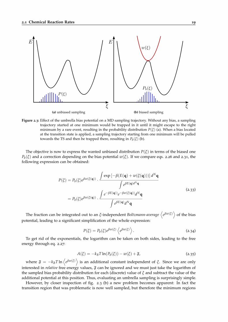
2.1 Chemical Reaction Rates 19
(a) unbiased sampling (b) biased sampling
Figure 2.3: Effect of the umbrella bias potential on a MD sampling trajectory. Without any bias, a samplingtrajectory started at one minimum would be trapped in it until it might escape to the rightminimum by a rare event, resulting in the probability distribution P(ξ) (a). When a bias locatedat the transition state is applied, a sampling trajectory starting from one minimum will be pulledtowards the TS and then be trapped there, resulting in Pb(ξ) (b).
The objective is now to express the wanted unbiased distribution P(ξ) in terms of the biased onePb(ξ) and a correction depending on the bias potential w(ξ). If we compare eqs. 2.26 and 2.31, thefollowing expression can be obtained:
P(ξ) = Pb(ξ)eβw(ξ(q)) ·
∫exp [−β(E(q) + w(ξ(q)))] dNq∫
eβE(q)dNq
= Pb(ξ)eβw(ξ(q)) ·
∫e−βE(q))e−βw(ξ(q))dNq∫
eβE(q)dNq
(2.33)
The fraction can be integrated out to an ξ-independent Boltzmann-average⟨
eβw(ξ)⟩
of the biaspotential, leading to a significant simplification of the whole expression:
P(ξ) = Pb(ξ)eβw(ξ)⟨
eβw(ξ)⟩
. (2.34)
To get rid of the exponentials, the logarithm can be taken on both sides, leading to the freeenergy through eq. 2.27:
A(ξ) = −kBT ln(Pb(ξ))− w(ξ) + F, (2.35)
where F = −kBT ln⟨
eβw(ξ)⟩
is an additional constant independent of ξ. Since we are onlyinterested in relative free energy values, F can be ignored and we must just take the logarithm ofthe sampled bias probability distribution for each (discrete) value of ξ and subtract the value of theadditional potential at this position. Thus, evaluating an umbrella sampling is surprisingly simple.
However, by closer inspection of fig. 2.3 (b) a new problem becomes apparent: In fact thetransition region that was problematic is now well sampled, but therefore the minimum regions
20 2 Theoretical Background
are almost completely neglected! Hence the rare event problem only has shifted from the transitionstate to the minima. Of course we could argue that the strength of the potential simply needs tobe reduced such that also regions farther away from the TS are sampled more often. But then theeffect of the potential in the direct vicinity of the TS might become too loose, so that the originalproblem returns. It might be possible in certain cases to find an ideal bias potential (either in termsof the force constant or the mathematical expression of the term itself) such that the whole regionof interest is sampled with similar probability. At least if more than one barrier is present in thecoordinate space of interest this ansatz becomes impractical. In general, another strategy is used:connection of several independent umbrella samplings scattered along the reaction coordinate.
WHAM
One quite prominent method for combining umbrella samplings at different positions along areaction coordinate is the weighted histogram analysis method (WHAM) [42]. It constructs a totalunbiased probability distribution P(ξ) as a sum of weighted histograms obtained from the singlesamplings conducted with different positions of the biasing potential (also called umbrella windows):
P(ξ) =W
∑i
pi(ξ)Pi(ξ), (2.36)
where W is the number of sampled distributions to combine, Pi(ξ) and pi(ξ) the i’th samplingdistribution and its ξ-dependent weighting factor, respectively. For each distribution, the i’thunbiased free energy surface can be calculated as:
Ai(ξ) = −kBT ln(Pb,i(ξ))− wi(ξ) + Fi, (2.37)
which is identical to eq. 2.35, apart from the indices i. However, now Fi cannot be simply ignoredas it was done for the single sampling because this constant is different for each sampling and dueto this different offsets the correct weighting of the single distributions is not obvious. Hence, ifdifferent samplings shall be combined, the Fi’s need to be determined somehow. It is practicallyimpossible to explicitly integrate the average values they represent, but fortunately an iterativemethod exists: WHAM.
In order to understand how this method works it is useful to translate the rather abstractformulation used so far into the language of applied numerics. As already explained and indicatedin fig. 2.3, the needed time averages or probability functions (Pi(ξ)) are obtained by trajectorysamplings from which the number of hits in different bins along the reaction coordinate are counted,i.e., the full ξ-range is divided into a number of sections and for each sampled structure the actualξ-value is assigned to the correct section or bin. This results in multiple ξ-dependent histograms,one for each umbrella sampling. After some derivation [42], the WHAM equations are obtained:
P(ξ j) =∑N
i=1 Pi(ξ j)
∑Ni=1 ni exp
[β(Fi − wi(ξ j)
] , (2.38)
Fi = −kBT ln
[M
∑j=1
P(ξ j)e−βwi(ξ j)
]. (2.39)
Here, N is the total number of individual umbrella samplings with i being the actual sampling,M the total number of bins per sampling with j being the actual bin and ni the total numberof sampling steps per umbrella window. Equation 2.38 calculates the total unbiased probabilitydistribution P(ξ) for each discrete ξ-value by summing up all single biased distributions, dividedthrough an Fi-dependent term. Equation 2.39 calculates the needed Fi-terms by summing over thetotal unbiased distribution and weighting it by the i’th bias term. Both Fi and P(ξ) are unknownand are itself needed to calculate the other. Therefore, an iterative procedure is needed to solve these
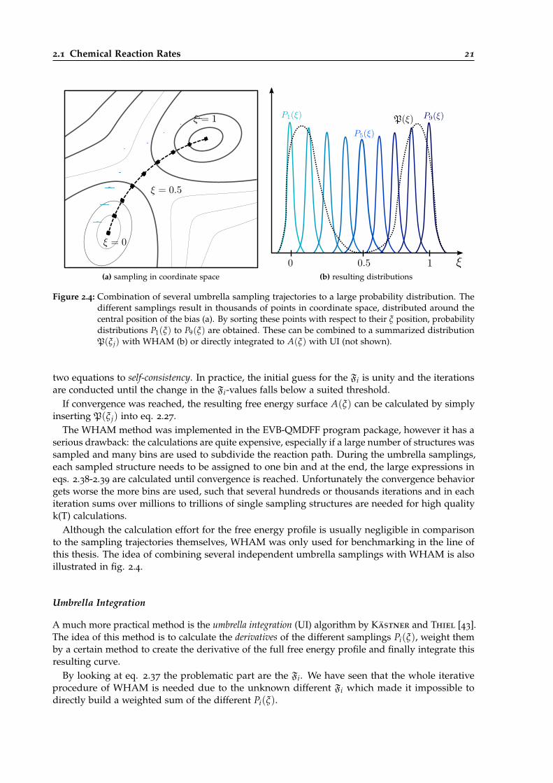
2.1 Chemical Reaction Rates 21
(a) sampling in coordinate space (b) resulting distributions
Figure 2.4: Combination of several umbrella sampling trajectories to a large probability distribution. Thedifferent samplings result in thousands of points in coordinate space, distributed around thecentral position of the bias (a). By sorting these points with respect to their ξ position, probabilitydistributions P1(ξ) to P9(ξ) are obtained. These can be combined to a summarized distributionP(ξ j) with WHAM (b) or directly integrated to A(ξ) with UI (not shown).
two equations to self-consistency. In practice, the initial guess for the Fi is unity and the iterationsare conducted until the change in the Fi-values falls below a suited threshold.
If convergence was reached, the resulting free energy surface A(ξ) can be calculated by simplyinserting P(ξ j) into eq. 2.27.
The WHAM method was implemented in the EVB-QMDFF program package, however it has aserious drawback: the calculations are quite expensive, especially if a large number of structures wassampled and many bins are used to subdivide the reaction path. During the umbrella samplings,each sampled structure needs to be assigned to one bin and at the end, the large expressions ineqs. 2.38-2.39 are calculated until convergence is reached. Unfortunately the convergence behaviorgets worse the more bins are used, such that several hundreds or thousands iterations and in eachiteration sums over millions to trillions of single sampling structures are needed for high qualityk(T) calculations.
Although the calculation effort for the free energy profile is usually negligible in comparisonto the sampling trajectories themselves, WHAM was only used for benchmarking in the line ofthis thesis. The idea of combining several independent umbrella samplings with WHAM is alsoillustrated in fig. 2.4.
Umbrella Integration
A much more practical method is the umbrella integration (UI) algorithm by Kästner and Thiel [43].The idea of this method is to calculate the derivatives of the different samplings Pi(ξ), weight themby a certain method to create the derivative of the full free energy profile and finally integrate thisresulting curve.
By looking at eq. 2.37 the problematic part are the Fi. We have seen that the whole iterativeprocedure of WHAM is needed due to the unknown different Fi which made it impossible todirectly build a weighted sum of the different Pi(ξ).
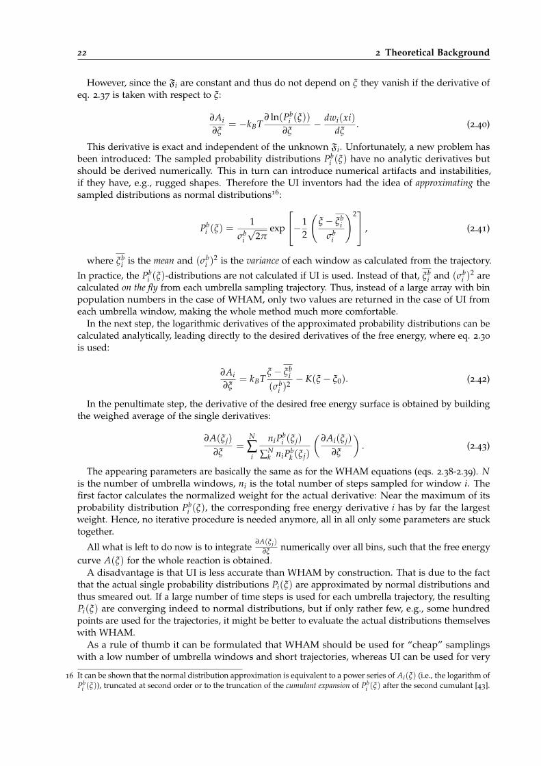
22 2 Theoretical Background
However, since the Fi are constant and thus do not depend on ξ they vanish if the derivative ofeq. 2.37 is taken with respect to ξ:
∂Ai∂ξ
= −kBT∂ ln(Pb
i (ξ))
∂ξ− dwi(xi)
dξ. (2.40)
This derivative is exact and independent of the unknown Fi. Unfortunately, a new problem hasbeen introduced: The sampled probability distributions Pb
i (ξ) have no analytic derivatives butshould be derived numerically. This in turn can introduce numerical artifacts and instabilities,if they have, e.g., rugged shapes. Therefore the UI inventors had the idea of approximating thesampled distributions as normal distributions16:
Pbi (ξ) =
1σb
i
√2π
exp
−12
(ξ − ξb
i
σbi
)2 , (2.41)
where ξbi is the mean and (σb
i )2 is the variance of each window as calculated from the trajectory.
In practice, the Pbi (ξ)-distributions are not calculated if UI is used. Instead of that, ξb
i and (σbi )
2 arecalculated on the fly from each umbrella sampling trajectory. Thus, instead of a large array with binpopulation numbers in the case of WHAM, only two values are returned in the case of UI fromeach umbrella window, making the whole method much more comfortable.
In the next step, the logarithmic derivatives of the approximated probability distributions can becalculated analytically, leading directly to the desired derivatives of the free energy, where eq. 2.30
is used:
∂Ai∂ξ
= kBTξ − ξb
i
(σbi )
2− K(ξ − ξ0). (2.42)
In the penultimate step, the derivative of the desired free energy surface is obtained by buildingthe weighed average of the single derivatives:
∂A(ξ j)
∂ξ=
N
∑i
niPbi (ξ j)
∑Nk niPb
k (ξ j)
(∂Ai(ξ j)
∂ξ
). (2.43)
The appearing parameters are basically the same as for the WHAM equations (eqs. 2.38-2.39). Nis the number of umbrella windows, ni is the total number of steps sampled for window i. Thefirst factor calculates the normalized weight for the actual derivative: Near the maximum of itsprobability distribution Pb
i (ξ), the corresponding free energy derivative i has by far the largestweight. Hence, no iterative procedure is needed anymore, all in all only some parameters are stucktogether.
All what is left to do now is to integrate∂A(ξ j)
∂ξ numerically over all bins, such that the free energycurve A(ξ) for the whole reaction is obtained.
A disadvantage is that UI is less accurate than WHAM by construction. That is due to the factthat the actual single probability distributions Pi(ξ) are approximated by normal distributions andthus smeared out. If a large number of time steps is used for each umbrella trajectory, the resultingPi(ξ) are converging indeed to normal distributions, but if only rather few, e.g., some hundredpoints are used for the trajectories, it might be better to evaluate the actual distributions themselveswith WHAM.
As a rule of thumb it can be formulated that WHAM should be used for “cheap” samplingswith a low number of umbrella windows and short trajectories, whereas UI can be used for very
16 It can be shown that the normal distribution approximation is equivalent to a power series of Ai(ξ) (i.e., the logarithm ofPb
i (ξ)), truncated at second order or to the truncation of the cumulant expansion of Pbi (ξ) after the second cumulant [43].
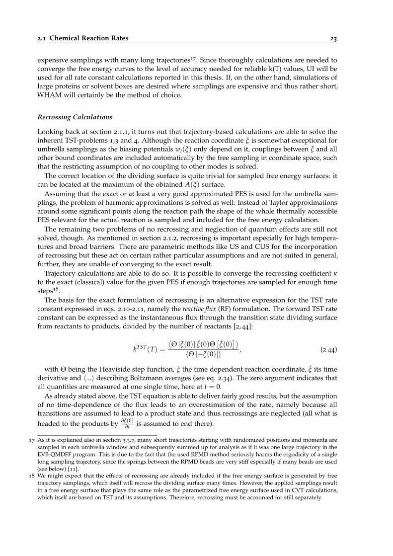
2.1 Chemical Reaction Rates 23
expensive samplings with many long trajectories17. Since thoroughly calculations are needed toconverge the free energy curves to the level of accuracy needed for reliable k(T) values, UI will beused for all rate constant calculations reported in this thesis. If, on the other hand, simulations oflarge proteins or solvent boxes are desired where samplings are expensive and thus rather short,WHAM will certainly be the method of choice.
Recrossing Calculations
Looking back at section 2.1.1, it turns out that trajectory-based calculations are able to solve theinherent TST-problems 1,3 and 4. Although the reaction coordinate ξ is somewhat exceptional forumbrella samplings as the biasing potentials wi(ξ) only depend on it, couplings between ξ and allother bound coordinates are included automatically by the free sampling in coordinate space, suchthat the restricting assumption of no coupling to other modes is solved.
The correct location of the dividing surface is quite trivial for sampled free energy surfaces: itcan be located at the maximum of the obtained A(ξ) surface.
Assuming that the exact or at least a very good approximated PES is used for the umbrella sam-plings, the problem of harmonic approximations is solved as well: Instead of Taylor approximationsaround some significant points along the reaction path the shape of the whole thermally accessiblePES relevant for the actual reaction is sampled and included for the free energy calculation.
The remaining two problems of no recrossing and neglection of quantum effects are still notsolved, though. As mentioned in section 2.1.2, recrossing is important especially for high tempera-tures and broad barriers. There are parametric methods like US and CUS for the incorporationof recrossing but these act on certain rather particular assumptions and are not suited in general,further, they are unable of converging to the exact result.
Trajectory calculations are able to do so. It is possible to converge the recrossing coefficient κto the exact (classical) value for the given PES if enough trajectories are sampled for enough timesteps18.
The basis for the exact formulation of recrossing is an alternative expression for the TST rateconstant expressed in eqs. 2.10-2.11, namely the reactive flux (RF) formulation. The forward TST rateconstant can be expressed as the instantaneous flux through the transition state dividing surfacefrom reactants to products, divided by the number of reactants [2, 44]:
kTST(T) =⟨Θ [ξ(0)] ξ(0)Θ
[ξ(0)
]⟩〈Θ [−ξ(0)]〉 , (2.44)
with Θ being the Heaviside step function, ξ the time dependent reaction coordinate, ξ its timederivative and 〈...〉 describing Boltzmann averages (see eq. 2.34). The zero argument indicates thatall quantities are measured at one single time, here at t = 0.
As already stated above, the TST equation is able to deliver fairly good results, but the assumptionof no time-dependence of the flux leads to an overestimation of the rate, namely because alltransitions are assumed to lead to a product state and thus recrossings are neglected (all what isheaded to the products by ∂ξ(0)
∂t is assumed to end there).
17 As it is explained also in section 3.3.7, many short trajectories starting with randomized positions and momenta aresampled in each umbrella window and subsequently summed up for analysis as if it was one large trajectory in theEVB-QMDFF program. This is due to the fact that the used RPMD method seriously harms the ergodicity of a singlelong sampling trajectory, since the springs between the RPMD beads are very stiff especially if many beads are used(see below) [11].
18 We might expect that the effects of recrossing are already included if the free energy surface is generated by freetrajectory samplings, which itself will recross the dividing surface many times. However, the applied samplings resultin a free energy surface that plays the same role as the parametrized free energy surface used in CVT calculations,which itself are based on TST and its assumptions. Therefore, recrossing must be accounted for still separately.
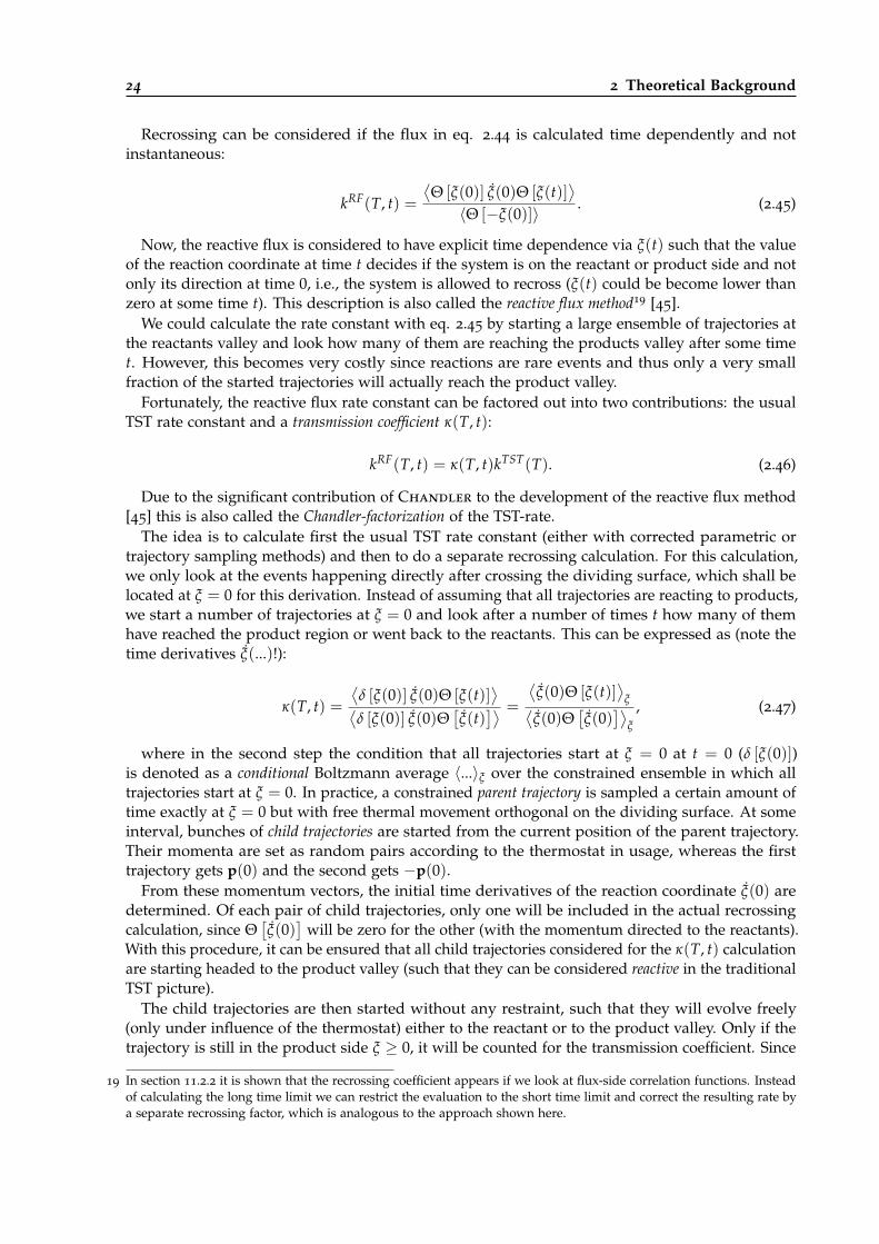
24 2 Theoretical Background
Recrossing can be considered if the flux in eq. 2.44 is calculated time dependently and notinstantaneous:
kRF(T, t) =⟨Θ [ξ(0)] ξ(0)Θ [ξ(t)]
⟩〈Θ [−ξ(0)]〉 . (2.45)
Now, the reactive flux is considered to have explicit time dependence via ξ(t) such that the valueof the reaction coordinate at time t decides if the system is on the reactant or product side and notonly its direction at time 0, i.e., the system is allowed to recross (ξ(t) could be become lower thanzero at some time t). This description is also called the reactive flux method19 [45].
We could calculate the rate constant with eq. 2.45 by starting a large ensemble of trajectories atthe reactants valley and look how many of them are reaching the products valley after some timet. However, this becomes very costly since reactions are rare events and thus only a very smallfraction of the started trajectories will actually reach the product valley.
Fortunately, the reactive flux rate constant can be factored out into two contributions: the usualTST rate constant and a transmission coefficient κ(T, t):
kRF(T, t) = κ(T, t)kTST(T). (2.46)
Due to the significant contribution of Chandler to the development of the reactive flux method[45] this is also called the Chandler-factorization of the TST-rate.
The idea is to calculate first the usual TST rate constant (either with corrected parametric ortrajectory sampling methods) and then to do a separate recrossing calculation. For this calculation,we only look at the events happening directly after crossing the dividing surface, which shall belocated at ξ = 0 for this derivation. Instead of assuming that all trajectories are reacting to products,we start a number of trajectories at ξ = 0 and look after a number of times t how many of themhave reached the product region or went back to the reactants. This can be expressed as (note thetime derivatives ξ(...)!):
κ(T, t) =⟨δ [ξ(0)] ξ(0)Θ [ξ(t)]
⟩⟨δ [ξ(0)] ξ(0)Θ
[ξ(t)
]⟩ =
⟨ξ(0)Θ [ξ(t)]
⟩ξ⟨
ξ(0)Θ[ξ(0)
]⟩ξ
, (2.47)
where in the second step the condition that all trajectories start at ξ = 0 at t = 0 (δ [ξ(0)])is denoted as a conditional Boltzmann average 〈...〉ξ over the constrained ensemble in which alltrajectories start at ξ = 0. In practice, a constrained parent trajectory is sampled a certain amount oftime exactly at ξ = 0 but with free thermal movement orthogonal on the dividing surface. At someinterval, bunches of child trajectories are started from the current position of the parent trajectory.Their momenta are set as random pairs according to the thermostat in usage, whereas the firsttrajectory gets p(0) and the second gets −p(0).
From these momentum vectors, the initial time derivatives of the reaction coordinate ξ(0) aredetermined. Of each pair of child trajectories, only one will be included in the actual recrossingcalculation, since Θ
[ξ(0)
]will be zero for the other (with the momentum directed to the reactants).
With this procedure, it can be ensured that all child trajectories considered for the κ(T, t) calculationare starting headed to the product valley (such that they can be considered reactive in the traditionalTST picture).
The child trajectories are then started without any restraint, such that they will evolve freely(only under influence of the thermostat) either to the reactant or to the product valley. Only if thetrajectory is still in the product side ξ ≥ 0, it will be counted for the transmission coefficient. Since
19 In section 11.2.2 it is shown that the recrossing coefficient appears if we look at flux-side correlation functions. Insteadof calculating the long time limit we can restrict the evaluation to the short time limit and correct the resulting rate bya separate recrossing factor, which is analogous to the approach shown here.
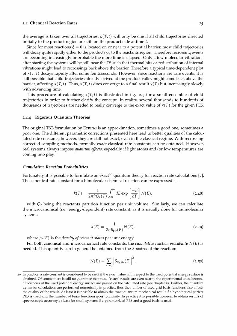
2.1 Chemical Reaction Rates 25
the average is taken over all trajectories, κ(T, t) will only be one if all child trajectories directedinitially to the product region are still on the product side at time t.
Since for most reactions ξ = 0 is located on or near to a potential barrier, most child trajectorieswill decay quite rapidly either to the products or to the reactants region. Therefore recrossing eventsare becoming increasingly improbable the more time is elapsed. Only a few molecular vibrationsafter starting the systems will be still near the TS such that thermal hits or redistribution of internalvibrations might lead to recrossings back above the barrier. Therefore a typical time-dependent plotof κ(T, t) decays rapidly after some femtoseconds. However, since reactions are rare events, it isstill possible that child trajectories already arrived at the product valley might come back above thebarrier, affecting κ(T, t). Thus, κ(T, t) does converge to a final result κ(T) but increasingly slowlywith advancing time.
This procedure of calculating κ(T, t) is illustrated in fig. 2.5 for a small ensemble of childtrajectories in order to further clarify the concept. In reality, several thousands to hundreds ofthousands of trajectories are needed to really converge to the exact value of κ(T) for the given PES.
2.1.4 Rigorous Quantum Theories
The original TST-formulation by Eyring is an approximation, sometimes a good one, sometimes apoor one. The different parametric corrections presented here lead to better qualities of the calcu-lated rate constants, however, they are still not exact, even in the classical regime. With recrossingcorrected sampling methods, formally exact classical rate constants can be obtained. However,real systems always impose quantum effects, especially if light atoms and/or low temperatures arecoming into play.
Cumulative Reaction Probabilities
Fortunately, it is possible to formulate an exact20 quantum theory for reaction rate calculations [7].The canonical rate constant for a bimolecular chemical reaction can be expressed as:
k(T) =1
2πhQr(T)
∫ ∞
∞dE exp
[−EkT
]N(E), (2.48)
with Qr being the reactants partition function per unit volume. Similarly, we can calculatethe microcanonical (i.e., energy-dependent) rate constant, as it is usually done for unimolecularsystems:
k(E) =1
2πhρr(E)N(E), (2.49)
where ρr(E) is the density of reactant states per unit energy.For both canonical and microcanonical rate constants, the cumulative reaction probability N(E) is
needed. This quantity can in general be obtained from the S-matrix of the reaction:
N(E) = ∑nrnp
∣∣∣Snp,nr(E)∣∣∣2 . (2.50)
20 In practice, a rate constant is considered to be exact if the exact value with respect to the used potential energy surface isobtained. Of course there is still no guarantee that these “exact” results are even near to the experimental ones, becausedeficiencies of the used potential energy surface are passed on the calculated rate (see chapter 5). Further, the quantumdynamics calculations are performed numerically in practice, thus the number of used grid basis functions also affectsthe quality of the result. At least it is possible to obtain the exact quantum mechanical result if a hypothetical perfectPES is used and the number of basis functions goes to infinity. In practice it is possible however to obtain results ofspectroscopic accuracy at least for small systems if a parametrized PES and a good basis is used.
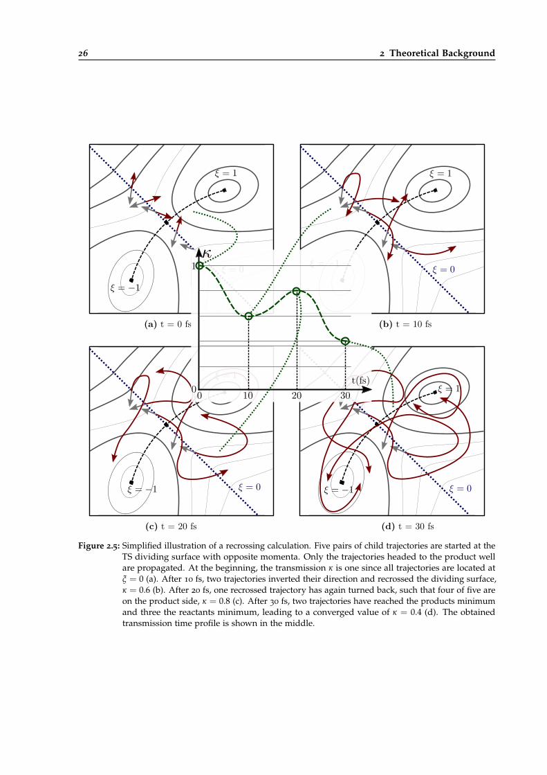
26 2 Theoretical Background
(a) t = 0 fs (b) t = 10 fs
(c) t = 20 fs (d) t = 30 fs
0 10 20 300
1
Figure 2.5: Simplified illustration of a recrossing calculation. Five pairs of child trajectories are started at theTS dividing surface with opposite momenta. Only the trajectories headed to the product wellare propagated. At the beginning, the transmission κ is one since all trajectories are located atξ = 0 (a). After 10 fs, two trajectories inverted their direction and recrossed the dividing surface,κ = 0.6 (b). After 20 fs, one recrossed trajectory has again turned back, such that four of five areon the product side, κ = 0.8 (c). After 30 fs, two trajectories have reached the products minimumand three the reactants minimum, leading to a converged value of κ = 0.4 (d). The obtainedtransmission time profile is shown in the middle.
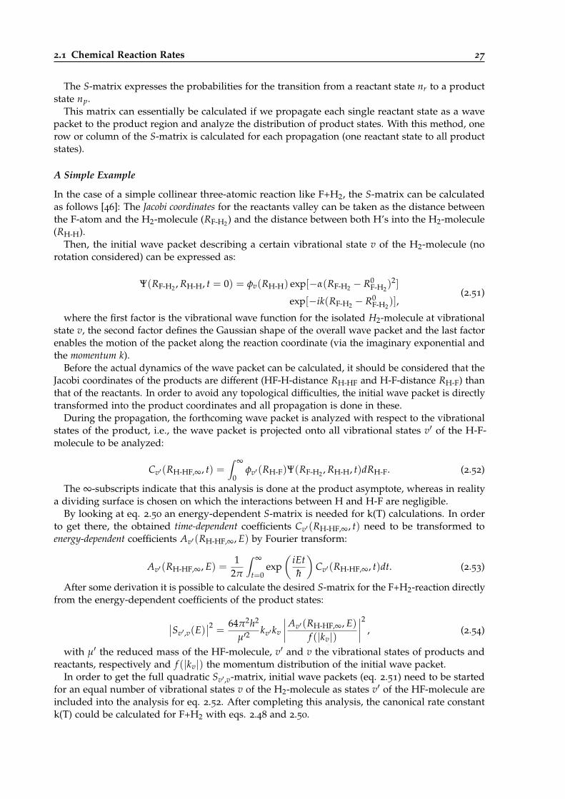
2.1 Chemical Reaction Rates 27
The S-matrix expresses the probabilities for the transition from a reactant state nr to a productstate np.
This matrix can essentially be calculated if we propagate each single reactant state as a wavepacket to the product region and analyze the distribution of product states. With this method, onerow or column of the S-matrix is calculated for each propagation (one reactant state to all productstates).
A Simple Example
In the case of a simple collinear three-atomic reaction like F+H2, the S-matrix can be calculatedas follows [46]: The Jacobi coordinates for the reactants valley can be taken as the distance betweenthe F-atom and the H2-molecule (RF-H2) and the distance between both H’s into the H2-molecule(RH-H).
Then, the initial wave packet describing a certain vibrational state v of the H2-molecule (norotation considered) can be expressed as:
Ψ(RF-H2 , RH-H, t = 0) = φv(RH-H) exp[−α(RF-H2 − R0F-H2
)2]
exp[−ik(RF-H2 − R0F-H2
)],(2.51)
where the first factor is the vibrational wave function for the isolated H2-molecule at vibrationalstate v, the second factor defines the Gaussian shape of the overall wave packet and the last factorenables the motion of the packet along the reaction coordinate (via the imaginary exponential andthe momentum k).
Before the actual dynamics of the wave packet can be calculated, it should be considered that theJacobi coordinates of the products are different (HF-H-distance RH-HF and H-F-distance RH-F) thanthat of the reactants. In order to avoid any topological difficulties, the initial wave packet is directlytransformed into the product coordinates and all propagation is done in these.
During the propagation, the forthcoming wave packet is analyzed with respect to the vibrationalstates of the product, i.e., the wave packet is projected onto all vibrational states v′ of the H-F-molecule to be analyzed:
Cv′(RH-HF,∞, t) =∫ ∞
0φv′(RH-F)Ψ(RF-H2 , RH-H, t)dRH-F. (2.52)
The ∞-subscripts indicate that this analysis is done at the product asymptote, whereas in realitya dividing surface is chosen on which the interactions between H and H-F are negligible.
By looking at eq. 2.50 an energy-dependent S-matrix is needed for k(T) calculations. In orderto get there, the obtained time-dependent coefficients Cv′(RH-HF,∞, t) need to be transformed toenergy-dependent coefficients Av′(RH-HF,∞, E) by Fourier transform:
Av′(RH-HF,∞, E) =1
2π
∫ ∞
t=0exp
(iEth
)Cv′(RH-HF,∞, t)dt. (2.53)
After some derivation it is possible to calculate the desired S-matrix for the F+H2-reaction directlyfrom the energy-dependent coefficients of the product states:
∣∣Sv′,v(E)∣∣2 =
64π2h2
µ′2kv′kv
∣∣∣∣Av′(RH-HF,∞, E)f (|kv|)
∣∣∣∣2 , (2.54)
with µ′ the reduced mass of the HF-molecule, v′ and v the vibrational states of products andreactants, respectively and f (|kv|) the momentum distribution of the initial wave packet.
In order to get the full quadratic Sv′,v-matrix, initial wave packets (eq. 2.51) need to be startedfor an equal number of vibrational states v of the H2-molecule as states v′ of the HF-molecule areincluded into the analysis for eq. 2.52. After completing this analysis, the canonical rate constantk(T) could be calculated for F+H2 with eqs. 2.48 and 2.50.
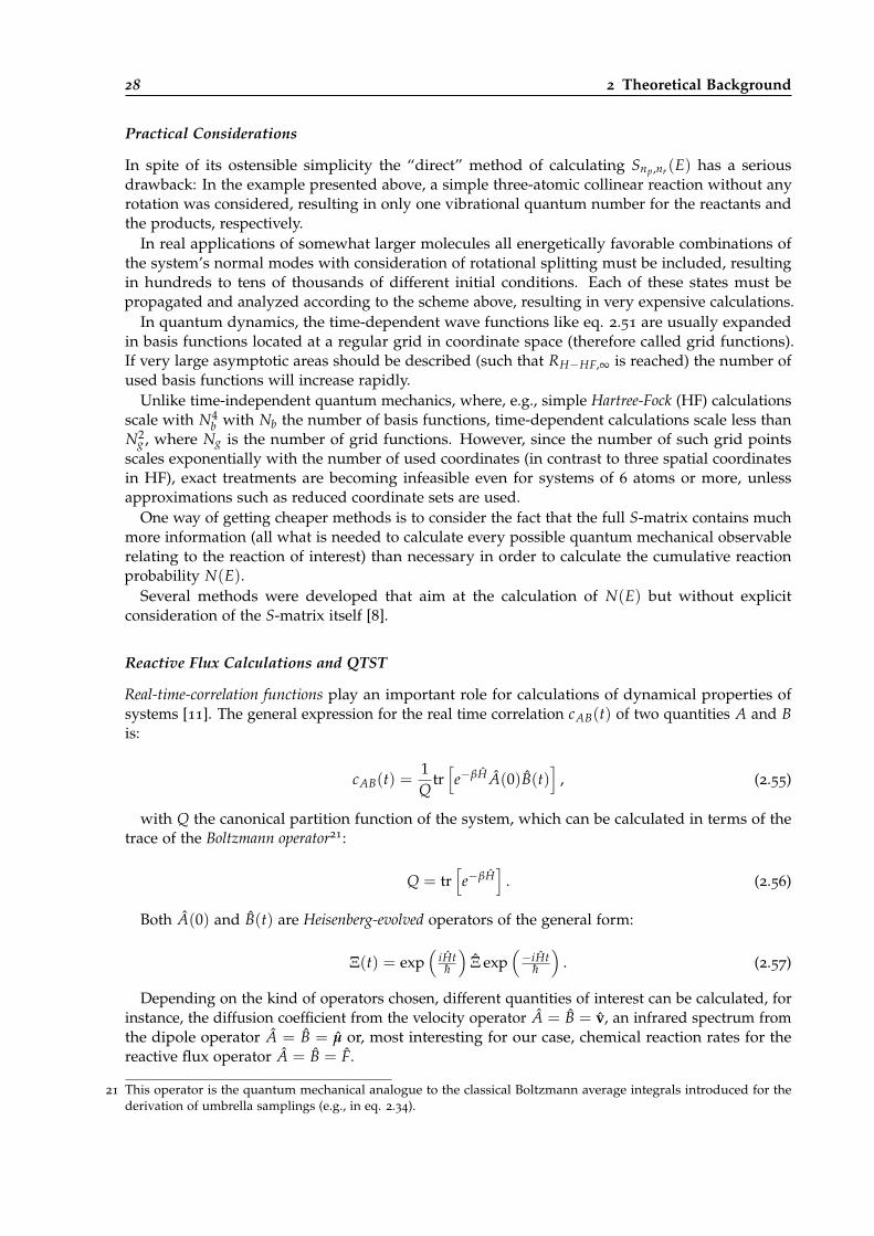
28 2 Theoretical Background
Practical Considerations
In spite of its ostensible simplicity the “direct” method of calculating Snp,nr(E) has a seriousdrawback: In the example presented above, a simple three-atomic collinear reaction without anyrotation was considered, resulting in only one vibrational quantum number for the reactants andthe products, respectively.
In real applications of somewhat larger molecules all energetically favorable combinations ofthe system’s normal modes with consideration of rotational splitting must be included, resultingin hundreds to tens of thousands of different initial conditions. Each of these states must bepropagated and analyzed according to the scheme above, resulting in very expensive calculations.
In quantum dynamics, the time-dependent wave functions like eq. 2.51 are usually expandedin basis functions located at a regular grid in coordinate space (therefore called grid functions).If very large asymptotic areas should be described (such that RH−HF,∞ is reached) the number ofused basis functions will increase rapidly.
Unlike time-independent quantum mechanics, where, e.g., simple Hartree-Fock (HF) calculationsscale with N4
b with Nb the number of basis functions, time-dependent calculations scale less thanN2
g , where Ng is the number of grid functions. However, since the number of such grid pointsscales exponentially with the number of used coordinates (in contrast to three spatial coordinatesin HF), exact treatments are becoming infeasible even for systems of 6 atoms or more, unlessapproximations such as reduced coordinate sets are used.
One way of getting cheaper methods is to consider the fact that the full S-matrix contains muchmore information (all what is needed to calculate every possible quantum mechanical observablerelating to the reaction of interest) than necessary in order to calculate the cumulative reactionprobability N(E).
Several methods were developed that aim at the calculation of N(E) but without explicitconsideration of the S-matrix itself [8].
Reactive Flux Calculations and QTST
Real-time-correlation functions play an important role for calculations of dynamical properties ofsystems [11]. The general expression for the real time correlation cAB(t) of two quantities A and Bis:
cAB(t) =1Q
tr[e−βH A(0)B(t)
], (2.55)
with Q the canonical partition function of the system, which can be calculated in terms of thetrace of the Boltzmann operator21:
Q = tr[e−βH
]. (2.56)
Both A(0) and B(t) are Heisenberg-evolved operators of the general form:
Ξ(t) = exp(
iHth
)Ξ exp
(−iHt
h
). (2.57)
Depending on the kind of operators chosen, different quantities of interest can be calculated, forinstance, the diffusion coefficient from the velocity operator A = B = v, an infrared spectrum fromthe dipole operator A = B = µ or, most interesting for our case, chemical reaction rates for thereactive flux operator A = B = F.
21 This operator is the quantum mechanical analogue to the classical Boltzmann average integrals introduced for thederivation of umbrella samplings (e.g., in eq. 2.34).

2.1 Chemical Reaction Rates 29
In order to calculate them, the flux-flux autocorrelation time profile needs to be integrated for alltimes [47]:
k(T) =1
Qr(T)
∫ ∞
0tr[e−βH F exp
(iHt
h
)F exp
(−iHt
h
)]dt. (2.58)
Since this method closely resembles the reactive flux formulation of TST given in eq. 2.44, itis also called quantum transition state theory (QTST) [9]. An important difference is, however, thatQTST is at least formally exact, in contrast to classical TST. In practice, these calculations worksimilar to trajectory recrossing calculations. Wave packets are started in the TS region (whereastheir delocalization in phase space is considered by the quantum Boltzmann operator e−βH) andpropagated some time, whereas the flux-flux-correlation time-profile is recorded [48]. By integratingthis profile, the rate constant can be obtained. Since the correlation function reaches an asymptoticvalue quite fast, almost no propagations into the reactants/product valleys are needed, instead,absorbing potentials are placed in their directions in order to avoid artifacts. The total number ofgrid points to set up is greatly reduced to the TS area, which of course lowers the costs significantly.
Further, as it will be seen below, this method of calculating k(T) values plays a pivotal role forthe conceptual ground of the RPMD-approach used throughout this thesis22.
There are a plenty of other methods that aim at reducing the computational expense of wavepacket k(T)-calculations, either in the way the rate is calculated or the way the propagation itself isdone, but even a short description of them would blow up the extent of this thesis. The interestedreader is referred to the respective literature [7, 8, 49].
2.1.5 Path Integral Formulation of Quantum Mechanics
In order to bridge the gap between cheap classical calculations that are unable to include quantumeffects and (at least in principle) exact but too expensive exact quantum calculations, the pathintegral (PI) formulation of quantum mechanics (QM) turned out to be quite useful. Developed byFeynman and others, it is an alternative formulation of quantum mechanics that can be shownto be equivalent to the usual Schrödinger picture and turns out to be quite advantageous fordeveloping approximate time-dependent QM-calculations based on classical trajectory samplings.
After giving a short introduction to the field, we will see in the next section how PIs can be usedto develop the RPMD-method, which is able to consider quantum effects yet is based on classicaldynamics.
It is of course not my demand to give a comprehensive review of PI-QM, thus I will only showthe very basics needed for understanding RPMD. For a deeper treatment of the field the famousbook of Feynman and Hibbs [50] is recommended.
Foundations
In our days, quantum mechanics is usually treated within the Schrödinger picture, i.e., by solvingthe Schrödinger equation for different situations, either analytically or, especially in theoreticalchemistry, numerically in order to get the wave function of a system23. Because the time-dependent
22 A closer look at the relation between RPMD and QTST is made in the derivation of the bimolecular RPMD reaction rateshown in section 11.2.2. There, we switch from flux-flux-autocorrelation functions to flux-side-correlation functions, byretention of the concept of looking at time-dependent correlation profiles of wave packets started in the TS region (fig.11.2).
23 In fact, there are several different formulations of quantum mechanics, which all can be shown to be equivalent. Someof the most important ones are [51]:
1. The Schrödinger picture, or wave mechanics.
2. The Heisenberg representation, also called matrix mechanics.
3. The Feynman path integral formulation, as it will be presented here.
30 2 Theoretical Background
Schrödinger equation (TDSE) is a partial differential equation, this description is also called thedifferential formulation of quantum mechanics.
Besides this, it is as well possible to describe quantum mechanics in an integral formulation. There,instead of differential equations integral equations need to be solved in order to obtain descriptionsand predictions for certain systems. This integral formulation is also called the path-integralformulation of quantum mechanics.
In classical mechanics, similar correspondences exist. Besides the Newtonian equations ofmotion, which are differential equations, we can, e.g., solve the motion of a one-dimensionalparticle between two points a and b by calculating its action:
S [b, a] =∫ tb
taL(x, x, t)dt, (2.59)
with ta and tb start and end points of the time interval to be examined and L the Lagrangian ofthe system, defined as:
L =m2
x2 −V(x, t), (2.60)
with m the mass of the system, for the case if an arbitrary time-dependent potential energyV(x, t) is existent.
We can now calculate the path the system will tread between ta and tb (x(t)) by applying theprinciple of least action: The quantity S [b, a] has a minimum value for the classical motion of thesystem in the time interval of interest. This can also be expressed variationally: S [b, a] should havean extremum for the extremum path x(t):
δS = S [x + δx]− S [x] = 0, (2.61)
i.e., the action remains unchanged to first order if the extremum path is changed infinitesimally.If this condition is inserted into eq. 2.59, we obtain:
S [x + δx] =∫ tb
taL(x + δx, x + δx, t)dt =
∫ tb
ta
[L(x, x, t) + δx
∂L∂x
+ δx∂L∂x
]dt. (2.62)
The resulting integral can be split up into the action and its variation:
S [x + δx] = S [x] +∫ tb
ta
[δx
∂L∂x
+ δx∂L∂x
]dt. (2.63)
The remaining integral can be evaluated by integration of parts, resulting in the expression forthe variation in S :
δS =
[δx
∂L∂x
]tb
ta
−∫ tb
taδx[
ddt
(∂L∂x
)− ∂L
∂x
]dt. (2.64)
The first term becomes zero since all possible paths have the same starting and ending points,respectively. Therefore, the derivative of L is zero at ta and tb. All what remains is the secondfactor in the integral. If the whole expression for δS should be zero, it leads to the condition:
ddt
(∂L∂x
)− ∂L
∂x= 0. (2.65)
This expression is well known in classical mechanics, namely it is the classical Lagrangian equationof motion.
4. The Dirac representation, or the interaction picture.
5. The phase space formulation, also called Wigner representation.
2.1 Chemical Reaction Rates 31
The quintessence of this derivation is that in the classical picture exactly one single path describesthe motion of a particle between two endpoints for given potential and kinetic energy, henceposition and momentum are known exactly during the whole motion.
In quantum mechanics this is of course no longer the case. Here, not only the single path ofleast action is important for the motion of the particle, but all possible paths contribute to theactual motion, corresponding to a smeared-out time-dependent probability distribution betweenthe points a and b. The probability to go from point a to b in space can be expressed as:
P(b, a) = |K(b, a)|2, (2.66)
where K(b, a) is the amplitude to go from a to b, obtained if all possible paths x(t) (no matter howabsurd they might appear) the system could take are summed up:
K(b, a) = ∑all x(t) from a to b
φ[x(t)] (2.67)
As for the classical case, the action S is an important measure for each path x(t), but now itinfects only the phase of each possible path:
φ[x(t)] = C exp(
ih
S[x(t)])
, (2.68)
with C being a suitable normalization constant. At first sight, we could think that all possiblepaths contribute equally to the total amplitude, since their prefactors are equal and only theirphases are different. However, in practice all paths will be integrated and especially for large valuesof S far offside the classical extremum path neighbored paths will cancel out each other due totheir heavily fluctuating phases. In the classical limit, with h going to zero, the phases will oscillatesignificantly for neighbored paths for all but the direct vicinity of the classical optimum x, wherethe change in S and thus of the phase is zero in first order. Thus, the single classical optimum pathis obtained if either S is becoming large or h is going to zero24.
So far, the amplitude for a certain quantum mechanical motion is given only qualitatively in eqs.2.67-2.68. How does this work in practice? Even in the simplest case of one dimension x we havean infinite number of possible paths, each of it needs to be integrated from a to b.
One way of doing this is to divide each path into a finite number of linear slices connectedtogether. If the number of these discrete steps per path is N, we can integrate over all paths foreach of the obtained xi values25. Because all paths are identical for the first xi at a and the last at b,we get:
K(b, a) ∼∫
. . .∫ ∫
φ[x(t)]dx1dx2 . . . dxN−1, (2.69)
where the first (x0) and the last (xN) are omitted. At this stage, the result is far from exact,because we only have a finite number of steps on which the different paths are evaluated. In orderto get the exact limit, the number of intersections must go to infinity, which corresponds to thedistances ε between them going to zero. Further, the whole integral needs to be normalized, whereA is a suitable normalization constant, depending on ε:
K(b, a) = limε→0
1A
∫. . .∫ ∫
exp(
ih
∫ tb
taL(x, x, t)dt
)dx1
Adx2
A. . .
dxNA
. (2.70)
24 The value of the action will become large for all possible paths if, e.g., a large particle (heavy atoms or molecules) isconsidered, since the m
2 part of L will become huge in units of h.25 Considering all possible paths means that for each time, every point in space is part of one path. Therefore, for each
slice considered, the integral must be taken over the whole space, i.e., here the x dimension in which the particle canmove.
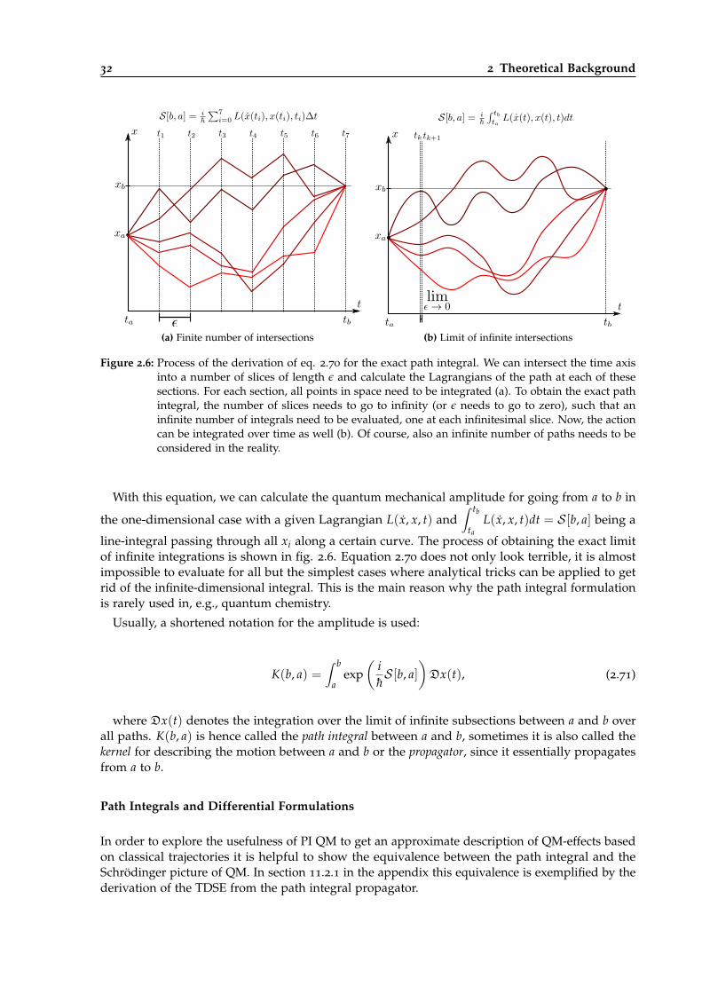
32 2 Theoretical Background
(a) Finite number of intersections (b) Limit of infinite intersections
Figure 2.6: Process of the derivation of eq. 2.70 for the exact path integral. We can intersect the time axisinto a number of slices of length ε and calculate the Lagrangians of the path at each of thesesections. For each section, all points in space need to be integrated (a). To obtain the exact pathintegral, the number of slices needs to go to infinity (or ε needs to go to zero), such that aninfinite number of integrals need to be evaluated, one at each infinitesimal slice. Now, the actioncan be integrated over time as well (b). Of course, also an infinite number of paths needs to beconsidered in the reality.
With this equation, we can calculate the quantum mechanical amplitude for going from a to b in
the one-dimensional case with a given Lagrangian L(x, x, t) and∫ tb
taL(x, x, t)dt = S [b, a] being a
line-integral passing through all xi along a certain curve. The process of obtaining the exact limitof infinite integrations is shown in fig. 2.6. Equation 2.70 does not only look terrible, it is almostimpossible to evaluate for all but the simplest cases where analytical tricks can be applied to getrid of the infinite-dimensional integral. This is the main reason why the path integral formulationis rarely used in, e.g., quantum chemistry.
Usually, a shortened notation for the amplitude is used:
K(b, a) =∫ b
aexp
(ihS [b, a]
)Dx(t), (2.71)
where Dx(t) denotes the integration over the limit of infinite subsections between a and b overall paths. K(b, a) is hence called the path integral between a and b, sometimes it is also called thekernel for describing the motion between a and b or the propagator, since it essentially propagatesfrom a to b.
Path Integrals and Differential Formulations
In order to explore the usefulness of PI QM to get an approximate description of QM-effects basedon classical trajectories it is helpful to show the equivalence between the path integral and theSchrödinger picture of QM. In section 11.2.1 in the appendix this equivalence is exemplified by thederivation of the TDSE from the path integral propagator.
2.1 Chemical Reaction Rates 33
The time propagation of a wave function can be described in the Schrödinger picture as atime-dependent superposition of the eigenstates of the respective Hamiltonian26:
ψ(x, t) =∞
∑n=1
cn exp(− i
hEnt)
φn(x). (2.72)
It can be shown that a kernel can be expressed in terms of eigenstates as well, but now of therespective states of the origin (xa, ta) and the endpoint (xb, tb):
K(xb, tb; xamta) =∞
∑n=1
φn(xb)φ∗n(xa) exp
(− i
hEn(tb − ta)
), (2.73)
where tb > ta. Now, the kernel representing a path integral is expressed in terms of solutionsof the TISE, a differential equation! It will be seen that this differential representation plays animportant role for the following derivations.
2.1.6 Ring Polymer Molecular Dynamics
As shown so far, exact quantum treatment of dynamics is expensive and almost impossible forall but quite small systems unless some subtle tricks are used. We also have seen that the PIformulation of quantum mechanics is even more expensive than the differential treatment, whichis the foundation for all direct quantum dynamics methods. It seems to be ridiculous to even try todevelop a numerical method based on path integrals.
However, as will become clear in the next section, the path integral approach is well suited forthe analytical calculations of quantum mechanical partition functions. As we have seen for examplein eq. 2.27, the free energy is defined in terms of the system’s partition function. Similarly, allother thermodynamical observables of a system can be calculated in terms of the partition function,which is discussed in larger detail in textbooks on statistical thermodynamics [21].
For our purpose, the determination of free energy profiles turned out to be essential for chemicalreaction rate calculations. We will now see how it is possible to obtain a quantum mechanicalprocedure of calculating partition functions and next how this can be approximated in a classicalmanner.
Path Integrals and Partition Functions
Physical systems are rarely isolated in nature. In fact, if we want to get a physical descriptionof realistic systems containing large numbers of particles a statistical description is needed. Thisimplies that the actual state of the system is not known but several states could occur with differentprobabilities. The probability of a state to occur depends on its energy:
pn =1Q
e−βEn , (2.74)
where the normalization constant is itself the partition sum of the system:
Q = ∑n
e−βEn . (2.75)
Thus, a sum over all states with exponential weighting of their energies is done. In order toswitch to the quantum mechanical picture, the definition of a state needs to be clarified: If a
26 These eigenstates are the solution of the TISE of the system: Hφn(x) = Enφn(x).
34 2 Theoretical Background
one-dimensional particle is considered, the probability of finding the particle at x is the sum overall of its possible states, taken as absolute square:
P(x) =1Q ∑
nφ∗n(x)φn(x)e−βEn . (2.76)
In the general case, the expectation value of an arbitrary operator A shall be described statistically.Then, its expected value can be given as:
A =1Q ∑
nAne−βEn =
1Q ∑
n
∫φ∗n(x)Aφn(x)dxe−βEn . (2.77)
In general, the expected value depends on a function called the statistical density matrix, or densitymatrix in short:
ρ(x′, x) = ∑n
φn(x′)φ∗n(x) exp (−βEn) . (2.78)
In order to calculate the probability to find the system at x, the density matrix can be used:
P(x) =1Q
ρ(x, x). (2.79)
The partition sum can now be calculated to normalize the total probability distribution to 1, thenwe get its expression:
Q =∫
ρ(x, x)dx ≡ tr(ρ). (2.80)
Thus, we need to calculate the trace of the density matrix of a system in order to get its partitionsum. But where are the path integrals? If we compare eqs. 2.78 and 2.73, we see that theyare surprisingly similar. The density matrix expression has the exponent βEn, the eigenfunctionrepresentation of the kernel has the exponent − i
h En(tb − ta), whereas the rest is identical.We can expand this similarity if the density matrix element ρ(x, x′) is expressed as a “pseudo
kernel”, a kernel working in imaginary time:
k(xb, ub, xa, ua) = ∑n
φn(xb)φ∗n(xa) exp
(−ub − ua
hEn
), (2.81)
with xb = x′, xa = x, ub = hβ and ua = 0. Now, we have transformed the Boltzmann factor ofthe density matrix into an imaginary time difference between 0 and hβ. Starting at this expression,it can be shown that the whole density matrix element ρ(xb, xa) is equivalent to a path integralover the imaginary time variable u. This results in:
ρ(xb, xa) =∫
exp[−1
h
∫ βh
0
(m2
x2(u) + V(x(u)))
du]Dx(u). (2.82)
Now, we can evaluate partition functions in terms of path integrals! In contrast to the general PIexpression given in eq. 2.70, no imaginary unit i appears in the exponent. Therefore, neighboredpaths do not cancel out another like for real dynamics, instead, paths of high potential and/orkinetic energy also add to the partition function but only with small amounts, since the (negative)exponential becomes small for large values in the bracket.
As the calculation of partition functions only needs the diagonal elements of the density matrix,xa = xb can be set. This means that start and end points of all paths calculated by eq. 2.82 areidentical. To calculate the coordinate-dependent partition function of the system we evaluate allpossible paths or motions the system can make at any point in coordinate space to start, travel foran imaginary time hβ and come back before this interval has ended. The longer these cyclic pathsare, the larger the kinetic energy will be and hence the lower this path’s contribution. Further, if the
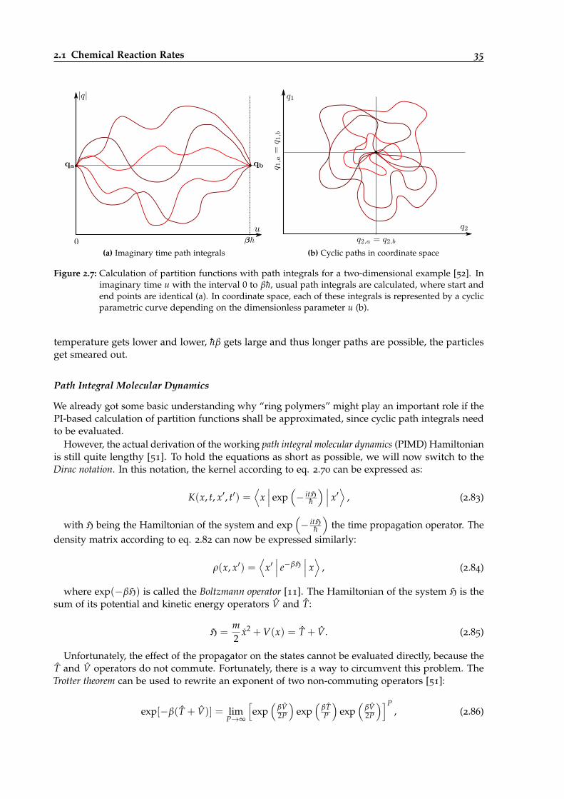
2.1 Chemical Reaction Rates 35
(a) Imaginary time path integrals (b) Cyclic paths in coordinate space
Figure 2.7: Calculation of partition functions with path integrals for a two-dimensional example [52]. Inimaginary time u with the interval 0 to βh, usual path integrals are calculated, where start andend points are identical (a). In coordinate space, each of these integrals is represented by a cyclicparametric curve depending on the dimensionless parameter u (b).
temperature gets lower and lower, hβ gets large and thus longer paths are possible, the particlesget smeared out.
Path Integral Molecular Dynamics
We already got some basic understanding why “ring polymers” might play an important role if thePI-based calculation of partition functions shall be approximated, since cyclic path integrals needto be evaluated.
However, the actual derivation of the working path integral molecular dynamics (PIMD) Hamiltonianis still quite lengthy [51]. To hold the equations as short as possible, we will now switch to theDirac notation. In this notation, the kernel according to eq. 2.70 can be expressed as:
K(x, t, x′, t′) =⟨
x∣∣∣ exp
(− itH
h
) ∣∣∣ x′⟩
, (2.83)
with H being the Hamiltonian of the system and exp(− itH
h
)the time propagation operator. The
density matrix according to eq. 2.82 can now be expressed similarly:
ρ(x, x′) =⟨
x′∣∣∣ e−βH
∣∣∣ x⟩
, (2.84)
where exp(−βH) is called the Boltzmann operator [11]. The Hamiltonian of the system H is thesum of its potential and kinetic energy operators V and T:
H =m2
x2 + V(x) = T + V. (2.85)
Unfortunately, the effect of the propagator on the states cannot be evaluated directly, because theT and V operators do not commute. Fortunately, there is a way to circumvent this problem. TheTrotter theorem can be used to rewrite an exponent of two non-commuting operators [51]:
exp[−β(T + V)] = limP→∞
[exp
(βV2P
)exp
(βTP
)exp
(βV2P
)]P, (2.86)
36 2 Theoretical Background
with P being the Trotter number. The evaluated propagator can now be reinserted into the densitymatrix expression:
ρ(x, x′) = limP→∞
⟨x′∣∣∣∣ [exp
(βV2P
)exp
(βTP
)exp
(βV2P
)]P∣∣∣∣ x⟩
. (2.87)
Now, we have single exponential operators that could be evaluated, however, there is still aninfinite product of them:
ρ(x, x′) = limP→∞
⟨x′∣∣∣∣∣ P
∏k=1
exp(
βV2P
)exp
(βTP
)exp
(βV2P
) ∣∣∣∣∣ x
⟩. (2.88)
It is possible to introduce the identity operator expressed in the space of possible position
eigenstates I =∫|x〉 〈x| dx, here we write them between each pair of operators, resulting in an
P− 1 dimensional integral:
ρ(x, x′) = limP→∞
∫ P
∏k=1
⟨xk+1
∣∣∣ exp(
βV2P
)exp
(βTP
)exp
(βV2P
) ∣∣∣ xk
⟩dx2 . . . dxP, (2.89)
where x1 = x and xP+1 = x′. Each of the brackets can be evaluated separately. The potentialenergy operator takes effect on the actual position and calculates its potential, therefore, they canbe evaluated on both positional states:
⟨xk+1
∣∣∣ exp(
βV2P
)exp
(βTP
)exp
(βV2P
) ∣∣∣ xk
⟩=
exp(− βV(xk+1)
2P
) ⟨xk+1
∣∣∣ exp(
βTP
) ∣∣∣ xk
⟩exp
(− βV(xk)
2P
).
(2.90)
Thus, only the kinetic energy operators remain to be evaluated. Its energy operator can be
expressed in terms of the momentum operator: T = p2
2m , with m the mass of the system. Now,similar to eq. 2.89, the identity operator expressed in the space of possible momentum eigenstates
I =∫|p〉 〈p| dp can be inserted:
⟨xk+1
∣∣∣ exp(
βTP
) ∣∣∣ xk
⟩=∫〈xk+1|p〉 〈p| exp
(βTP
)|xk〉 dp
=∫
exp(− βp2
2mP
)〈xk+1|p〉 〈p|xk〉 ,
(2.91)
where the kinetic energy operator was applied on the momentum eigenstate from the left. Theoverlap between a position and a momentum eigenstate can be expressed as:
〈x|p〉 = 1√2πh
exp(− ipx
h
). (2.92)
Now, the kinetic energy operator can finally be evaluated:
⟨xk+1
∣∣∣ exp(
βTP
) ∣∣∣ xk
⟩=∫
exp(− βp2
2mP
) 12πh
exp(− ipxk+1
h
)exp
(ipxk
h
)dp
=1
2πh
∫exp
(ip(xk+1−xk)
h
)exp
(− βp2
2mP
)dp.
(2.93)
2.1 Chemical Reaction Rates 37
The integral over the momentum is solvable, if some tricks concerning the Gaussian form of thesecond factor are done 27, which results in:
⟨xk+1
∣∣∣ exp(
βTP
) ∣∣∣ xk
⟩=
√mP
2πβh2 exp
(− mP
2βh2 (xk+1 − xk)2
). (2.94)
Now, all state vectors disappear, the remaining expressions are simple functions of the singlepoints in space! This result can be inserted into eq. 2.90, such that the expectation values ofthe single multiplied operators can now be noted. These can be inserted into eq. 2.89 wherethe integral over the whole coordinate space x is calculated over a product of P approximatedoperators. Since all of these are themselves products of exponentials, all can be summarized intoone large exponential, with the exponents being summed up:
ρ(x, x′) = limP→∞
(mP
2πβh2
) ∫exp
{−1
h
P
∑k=1
[mP
2βh2 (xk+1 − xk)2 +
βh2P
[V(xk+1) + V(xk)]
]}dx2 . . . dxP,
(2.95)
with xP+1 = x′ and x1 = x. At this stage, we can return to the initial expression for the partitionsum given in eq. 2.80:
Q = limP→∞
(mP
2πβh2
) P2 ∫
exp
{−1
h
P
∑k=1
[mP
2βh2 (xk+1 − xk)2 +
βhP
V(xk)
]}dx1 . . . dxP,
(2.96)
where now the integration is also over all points x, x′ of real space included into the densitymatrix expression of eq. 2.80, with x1 = x = x′. Since in eq. 2.89 the states x and x′ are includedonce, the states x2 to xP−1 are included twice and x = x′ for our special case, each state appearstwice in the potential energy term. Therefore, the sum runs over V(xk), with an additional prefactorof two, where x1 = xP.
In practice, the integrals needed for evaluation of the partition function can be evaluated by pathintegral Monte Carlo (PIMC) samplings. In order to perform PIMD, i.e., running trajectories in orderto sample the coordinate space, momenta need to be added to the effective potential in eq. 2.96.Then, integration must also be done in momentum space, thus being extended to the full phasespace of the system. Thereafter, also kinetic energy contributions of all particles can be added, with
T = p2
2m [8]. With this, we get an effective classical partition function, being an approximation tothe exact path integral one, which can be evaluated by PIMD samplings:
Q = limP→∞
(mP
2πβh2
) P2 ∫
e−βHeff(x,p)dxdp, (2.97)
27 Equation 2.93 can be rewritten such that only one exponential depends on the momentum:⟨
xk+1
∣∣∣ exp(
βTP
) ∣∣∣ xk
⟩=
12πh
∫exp
(− β
2mP
[p− imP
βh (xk+1 − xk)])2
dp exp(− mP
2βh2 (xk+1 − xk)2)
. The integral needs only to be done over the
first factor, where a substitution can be made: p′ = p− imP(xk+1−xk)βh . The resulting simple Gaussian integral can be
solved similar to eq. 11.18. Then, the second exponential remains, whereas the integration over momentum gives aconstant prefactor.
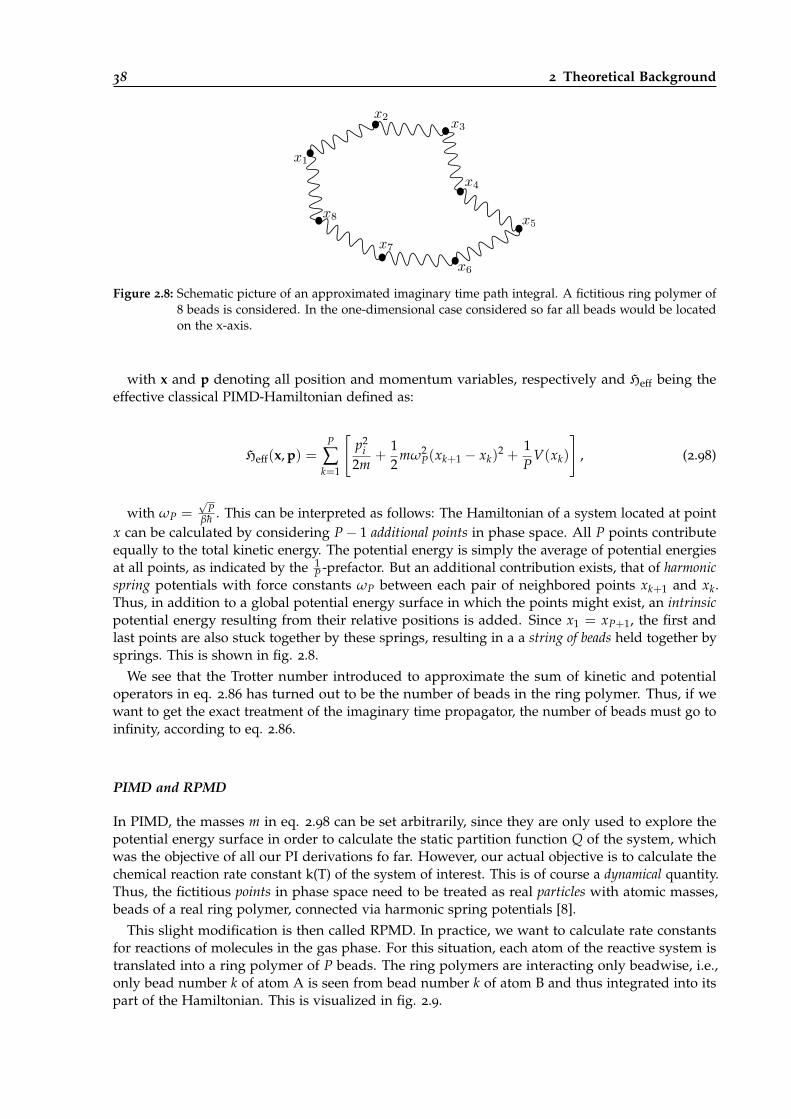
38 2 Theoretical Background
Figure 2.8: Schematic picture of an approximated imaginary time path integral. A fictitious ring polymer of8 beads is considered. In the one-dimensional case considered so far all beads would be locatedon the x-axis.
with x and p denoting all position and momentum variables, respectively and Heff being theeffective classical PIMD-Hamiltonian defined as:
Heff(x, p) =P
∑k=1
[p2
i2m
+12
mω2P(xk+1 − xk)
2 +1P
V(xk)
], (2.98)
with ωP =√
Pβh . This can be interpreted as follows: The Hamiltonian of a system located at point
x can be calculated by considering P− 1 additional points in phase space. All P points contributeequally to the total kinetic energy. The potential energy is simply the average of potential energiesat all points, as indicated by the 1
P -prefactor. But an additional contribution exists, that of harmonicspring potentials with force constants ωP between each pair of neighbored points xk+1 and xk.Thus, in addition to a global potential energy surface in which the points might exist, an intrinsicpotential energy resulting from their relative positions is added. Since x1 = xP+1, the first andlast points are also stuck together by these springs, resulting in a a string of beads held together bysprings. This is shown in fig. 2.8.
We see that the Trotter number introduced to approximate the sum of kinetic and potentialoperators in eq. 2.86 has turned out to be the number of beads in the ring polymer. Thus, if wewant to get the exact treatment of the imaginary time propagator, the number of beads must go toinfinity, according to eq. 2.86.
PIMD and RPMD
In PIMD, the masses m in eq. 2.98 can be set arbitrarily, since they are only used to explore thepotential energy surface in order to calculate the static partition function Q of the system, whichwas the objective of all our PI derivations fo far. However, our actual objective is to calculate thechemical reaction rate constant k(T) of the system of interest. This is of course a dynamical quantity.Thus, the fictitious points in phase space need to be treated as real particles with atomic masses,beads of a real ring polymer, connected via harmonic spring potentials [8].
This slight modification is then called RPMD. In practice, we want to calculate rate constantsfor reactions of molecules in the gas phase. For this situation, each atom of the reactive system istranslated into a ring polymer of P beads. The ring polymers are interacting only beadwise, i.e.,only bead number k of atom A is seen from bead number k of atom B and thus integrated into itspart of the Hamiltonian. This is visualized in fig. 2.9.
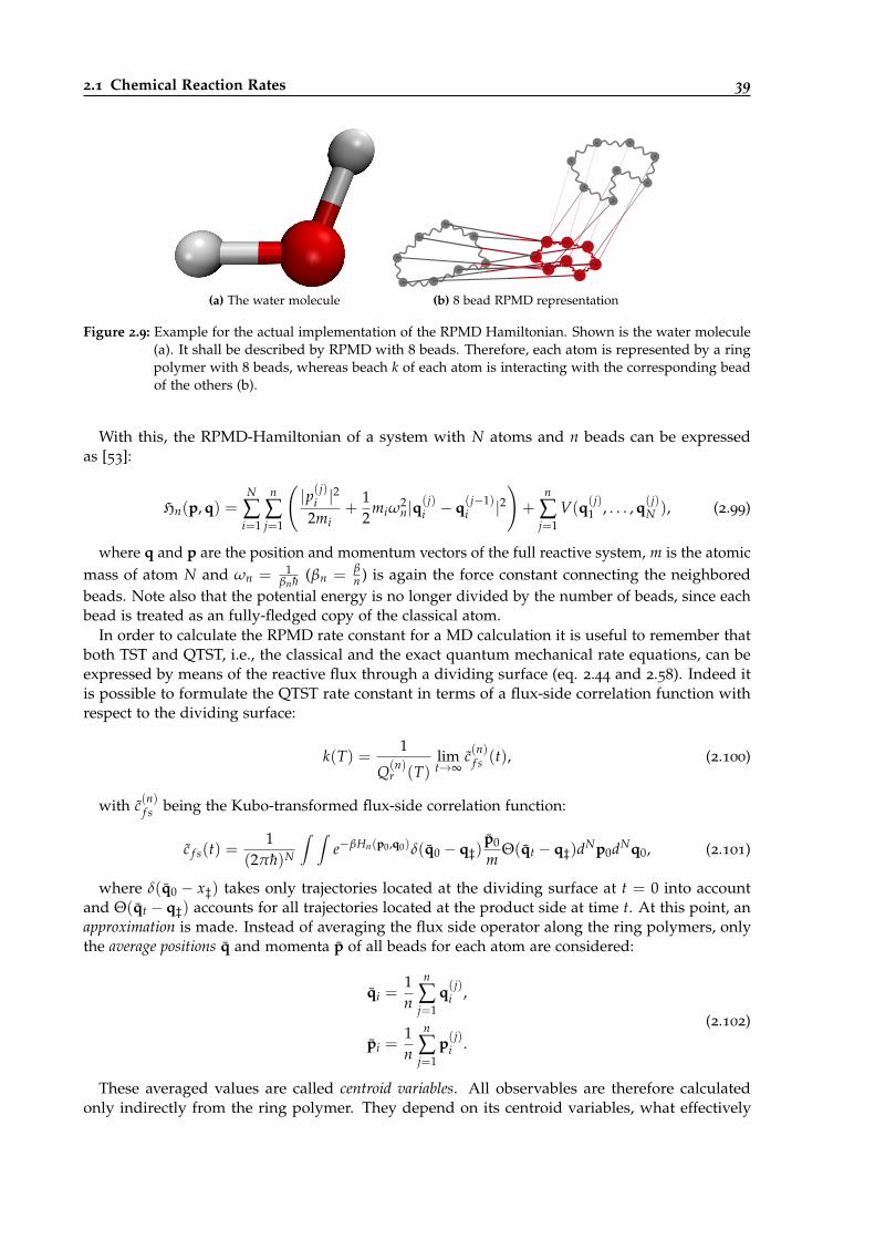
2.1 Chemical Reaction Rates 39
(a) The water molecule (b) 8 bead RPMD representation
Figure 2.9: Example for the actual implementation of the RPMD Hamiltonian. Shown is the water molecule(a). It shall be described by RPMD with 8 beads. Therefore, each atom is represented by a ringpolymer with 8 beads, whereas beach k of each atom is interacting with the corresponding beadof the others (b).
With this, the RPMD-Hamiltonian of a system with N atoms and n beads can be expressedas [53]:
Hn(p, q) =N
∑i=1
n
∑j=1
(|p(j)
i |2
2mi+
12
miω2n|q
(j)i − q(j−1)
i |2)+
n
∑j=1
V(q(j)1 , . . . , q(j)
N ), (2.99)
where q and p are the position and momentum vectors of the full reactive system, m is the atomicmass of atom N and ωn = 1
βn h (βn = βn ) is again the force constant connecting the neighbored
beads. Note also that the potential energy is no longer divided by the number of beads, since eachbead is treated as an fully-fledged copy of the classical atom.
In order to calculate the RPMD rate constant for a MD calculation it is useful to remember thatboth TST and QTST, i.e., the classical and the exact quantum mechanical rate equations, can beexpressed by means of the reactive flux through a dividing surface (eq. 2.44 and 2.58). Indeed itis possible to formulate the QTST rate constant in terms of a flux-side correlation function withrespect to the dividing surface:
k(T) =1
Q(n)r (T)
limt→∞
c(n)f s (t), (2.100)
with c(n)f s being the Kubo-transformed flux-side correlation function:
c f s(t) =1
(2πh)N
∫ ∫e−βHn(p0,q0)δ(q0 − q‡)
p0
mΘ(qt − q‡)dNp0dNq0, (2.101)
where δ(q0 − x‡) takes only trajectories located at the dividing surface at t = 0 into accountand Θ(qt − q‡) accounts for all trajectories located at the product side at time t. At this point, anapproximation is made. Instead of averaging the flux side operator along the ring polymers, onlythe average positions q and momenta p of all beads for each atom are considered:
qi =1n
n
∑j=1
q(j)i ,
pi =1n
n
∑j=1
p(j)i .
(2.102)
These averaged values are called centroid variables. All observables are therefore calculatedonly indirectly from the ring polymer. They depend on its centroid variables, what effectively
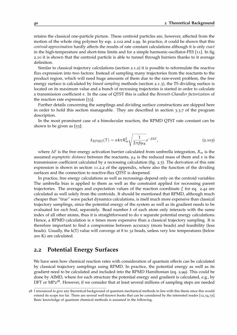
40 2 Theoretical Background
retains the classical one-particle picture. These centroid particles are, however, affected from themotion of the whole ring polymer by eqs. 2.102 and 2.99. In practice, it could be shown that thiscentroid-approximation hardly affects the results of rate constant calculations although it is only exactin the high-temperature and short-time limits and for a simple harmonic-oscillator-PES [11]. In fig.2.10 it is shown that the centroid particle is able to tunnel through barriers thanks to it averagedefinition.
Similar to classical trajectory calculations (section 2.1.2) it is possible to reformulate the reactiveflux expression into two factors: Instead of sampling many trajectories from the reactants to theproduct region, which will need huge amounts of them due to the rare-event problem, the freeenergy surface is calculated by biased sampling methods (section 2.1.3), the TS dividing surface islocated on its maximum value and a bunch of recrossing trajectories is started in order to calculatea transmission coefficient κ. In the case of QTST this is called the Bennett-Chandler factorization ofthe reaction rate expression [53].
Further details concerning the samplings and dividing surface constructions are skipped herein order to hold this section manageable. They are described in section 3.3.7 of the programdescription.
In the most prominent case of a bimolecular reaction, the RPMD QTST rate constant can beshown to be given as [53]:
kRPMD(T) = κ4πR2∞
√1
2πβµRe−β∆F, (2.103)
where ∆F is the free energy activation barrier calculated from umbrella integration, R∞ is theassumed asymptotic distance between the reactants, µR is the reduced mass of them and κ is thetransmission coefficient calculated by a recrossing calculation (fig. 2.5). The derivation of this rateexpression is shown in section 11.2.2 of the appendix, where also the function of the dividingsurfaces and the connection to reactive-flux QTST is deepened.
In practice, free energy calculations as well as recrossings depend only on the centroid variables:The umbrella bias is applied to them as well as the constraint applied for recrossing parenttrajectories. The averages and expectation values of the reaction coordinate ξ for eq. 2.42 arecalculated as well solely from the centroids. It should be mentioned that RPMD, although muchcheaper than “true” wave packet dynamics calculations, is itself much more expensive than classicaltrajectory samplings, since the potential energy of the system as well as its gradient needs to beevaluated for each bead, separately. Bead number k of each atom only interacts with the sameindex of all other atoms, thus it is straightforward to do n separate potential energy calculations.Hence, a RPMD calculation is n times more expensive than a classical trajectory sampling. It istherefore important to find a compromise between accuracy (more beads) and feasibility (lessbeads). Usually, the k(T) value will converge at 8 to 32 beads, unless very low temperatures (below200 K) are calculated.
2.2 Potential Energy Surfaces
We have seen how chemical reaction rates with consideration of quantum effects can be calculatedby classical trajectory samplings using RPMD. In practice, the potential energy as well as itsgradient need to be calculated and included into the RPMD Hamiltonian (eq. 2.99). This could bedone by AIMD, where for each structure the potential energy and gradient is calculated, e.g., byDFT or MP2
28. However, if we consider that at least several millions of sampling steps are needed
28 I renounced to give any theoretical background of quantum mechanical methods in line with this thesis since this wouldextend its scope too far. There are several well-known books that can be considered by the interested reader [12, 54, 55].Basic knowledge of quantum chemical methods is assumed in the following.
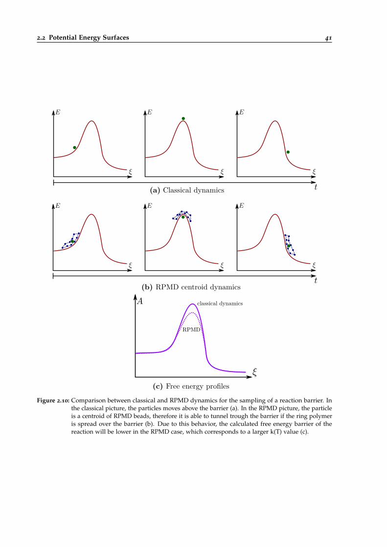
2.2 Potential Energy Surfaces 41
(a) Classical dynamics
(b) RPMD centroid dynamics
(c) Free energy profiles
classical dynamics
RPMD
Figure 2.10: Comparison between classical and RPMD dynamics for the sampling of a reaction barrier. Inthe classical picture, the particles moves above the barrier (a). In the RPMD picture, the particleis a centroid of RPMD beads, therefore it is able to tunnel trough the barrier if the ring polymeris spread over the barrier (b). Due to this behavior, the calculated free energy barrier of thereaction will be lower in the RPMD case, which corresponds to a larger k(T) value (c).

42 2 Theoretical Background
to converge the free energy profile of medium-sized systems, it becomes clear that this approach isunfeasible, even if semiempirical methods are used.
Therefore, reaction rate constants are usually calculated with parametrized potential energysurfaces, whose potential energies and gradients can be calculated very fast. The usual procedureis to set up a function defining the potential energy and its gradient in the region of interest forthe reactive system under consideration. Since the description should be as accurate as possible,several schemes were developed to calculate high-level ab-initio reference data and fit empiricalfunctions to them and sometimes also to experimental data.
In line with this thesis, the EVB-QMDFF method founded by Hartke and Grimme [16] wasused to express the potential energy surfaces of the reactions. Since the overall aim is to developreliable high-quality black-box methods for reaction rate calculations of arbitrary systems, it willbe explained why EVB-QMDFF is at least one of the best PES representations to be used in thiscontext. To make this point clear, a short review of popular approaches for setting up reactive PESswill be given, by describing their advantages and disadvantages the path to EVB-QMDFF will bedepicted.
In order to do a fair and comprehensible judgment, three conditions will be applied:
1. Simple parametrization (both intellectual and computational)
2. General applicability
3. High quality in the vicinity of the reaction path
Our method of choice should fulfill all three. Therefore, all approaches that are shortly explainedin the following will be evaluated with respect to these conditions. In order to make things clearer,the methods are assigned to a number of categories and subcategories. In reality there is of coursea methodological continuum such that the assignment of a method to a category is not definite.
2.2.1 System-Specific Parametrizations
The idea of parametrizing PESs of molecular systems in order to avoid direct ab-intio calculations fordynamics or other purposes was recognized already in the early days of computational chemistry29.Perhaps the first usable PES representation was built for the H + H2-reaction in 1955: The London-Eyring-Polanyi-Sato (LEPS) surface [56, 57]. It is based on the Heitler-London (HL) method (eq. 2.122)for the H2-molecule, when the third H-atom is in infinite separation to them. Within HL, thebonding energy is given by a simple Morse function, whereas the antibonding energy is expressedby a slightly changed Morse function. To obtain the whole surface, essentially three HL-typesurfaces (for each permutation of H-pairs) are combined and weighted according to the actualHi − Hj-distances.
Early Approaches
Though originally designed for H + H2-systems, generalized LEPS-surfaces can be built for arbitrarythree-atomic systems and advanced versions of them are still in use today [58, 59]. Since its originsuntil the early 90s, the field of PES-publications for new systems has grown steadily [60]. Thoseold but still frequently used surfaces can be classified into three branches:
(a) System-specific static global expressions with individual functions, fitted to ab-initio referencedata. Since the intellectual effort for this individual construction of PES-functions steeplyincreases with system size, very small systems are the main area of application. For three-atomic systems, they are often based on the LEPS surface type, e.g., the H+H2-surface byTruhlar and Horowitz [61] as it is used in chapter 5.
29 The essentials of this first section are also included in the introduction of chapter 5.
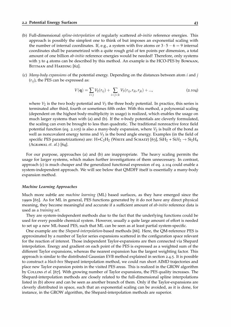
2.2 Potential Energy Surfaces 43
(b) Full-dimensional spline-interpolation of regularly scattered ab-initio reference energies. Thisapproach is possibly the simplest one to think of but imposes an exponential scaling withthe number of internal coordinates. If, e.g., a system with five atoms or 3 · 5− 6 = 9 internalcoordinates shall be parametrized with a quite rough grid of ten points per dimension, a totalamount of one billion ab-initio reference energies would be needed! Therefore, only systemswith 3 to 4 atoms can be described by this method. An example is the HCO-PES by Bowman,Bittman and Harding [62].
(c) Many-body expansions of the potential energy. Depending on the distances between atom i and j(rij), the PES can be expressed as:
V(q) = ∑i<j
V2(rij) + ∑i<j<k
V3(rij, rik, rjk) + ..., (2.104)
where V2 is the two body potential and V3 the three body potential. In practice, this series isterminated after third, fourth or sometimes fifth order. With this method, a polynomial scaling(dependent on the highest body-multiplicity in usage) is realized, which enables the usage onmuch larger systems than with (a) and (b). If the n-body potentials are cleverly formulated,the scaling can even be brought to less than quadratic. The traditional nonreactive force fieldpotential function (eq. 2.105) is also a many-body expansion, where V2 is built of the bond aswell as noncovalent energy terms and V3 is the bond angle energy. Examples (in the field ofspecific PES parametrizations) are: H+C2H2 (White and Schatz) [63], SiH2 + SiH2 → Si2H4(Agrawal et. al.) [64].
For our purpose, approaches (a) and (b) are inappropriate. The heavy scaling permits theusage for larger systems, which makes further investigations of them unnecessary. In contrast,approach (c) is much cheaper and the generalized functional expression of eq. 2.104 could enable asystem-independent approach. We will see below that QMDFF itself is essentially a many-bodyexpansion method.
Machine Learning Approaches
Much more subtle are machine learning (ML) based surfaces, as they have emerged since the1990s [65]. As for ML in general, PES functions generated by it do not have any direct physicalmeaning, they become meaningful and accurate if a sufficient amount of ab-initio reference data isused as a training set.
They are system-independent methods due to the fact that the underlying functions could beused for every possible chemical system. However, usually a quite large amount of effort is neededto set up a new ML-based PES, such that ML can be seen as at least partial system-specific.
One example are the Shepard-interpolation-based methods [66]. Here, the QM-reference PES isapproximated by a number of Taylor series expansions scattered in the configuration space relevantfor the reaction of interest. Those independent Taylor-expansions are then connected via Shepardinterpolation. Energy and gradient on each point of the PES is expressed as a weighted sum of thedifferent Taylor expansions, whereas the nearest expansion has the largest weighting factor. Thisapproach is similar to the distributed Gaussian EVB method explained in section 2.4.5. It is possibleto construct a black-box Shepard interpolation method, we could run short AIMD trajectories andplace new Taylor expansion points in the visited PES areas. This is realized in the GROW algorithmby Collins et al. [67]. With growing number of Taylor expansions, the PES quality increases. TheShepard-interpolation methods are closely related to the full-dimensional spline interpolationslisted in (b) above and can be seen as another branch of them. Only if the Taylor-expansions arecleverly distributed in space, such that an exponential scaling can be avoided, as it is done, forinstance, in the GROW algorithm, the Shepard-interpolation methods are superior.
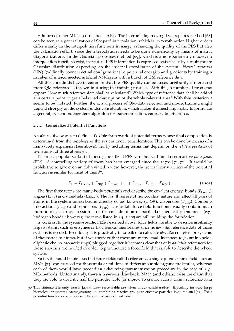
44 2 Theoretical Background
A bunch of other ML-based methods exists. The interpolating moving least-squares method [68]can be seen as a generalization of Shepard interpolation, which is its zeroth order. Higher ordersdiffer mainly in the interpolation functions in usage, enhancing the quality of the PES but alsothe calculation effort, since the interpolation needs to be done numerically by means of matrixdiagonalizations. In the Gaussian processes method [69], which is a non-parametric model, nointerpolation functions exist, instead all PES information is expressed statistically by a multivariateGaussian distribution depending on the internal coordinates of the system. Neural networks(NN) [70] finally connect actual configurations to potential energies and gradients by training anumber of interconnected artificial NN-layers with a bunch of QM reference data.
All those methods have in common that the PES quality can be raised arbitrarily if more andmore QM reference is thrown in during the training process. With this, a number of problemsappear. How much reference data shall be calculated? Which type of reference data shall be addedat a certain point to get a balanced description of the whole relevant area? With this, criterion 1
seems to be violated. Further, the actual process of QM-data selection and model training mightdepend strongly on the system under consideration, which makes it almost impossible to formulatea general, system-independent algorithm for parametrization, contrary to criterion 2.
2.2.2 Generalized Potential Functions
An alternative way is to define a flexible framework of potential terms whose final composition isdetermined from the topology of the system under consideration. This can be done by means of amany-body expansion (see above), i.e., by including terms that depend on the relative positions oftwo atoms, of three atoms etc.
The most popular variant of those generalized PESs are the traditional non-reactive force fields(FFs). A compelling variety of them has been emerged since the 1970s [71, 72]. It would beprohibitive to give even an abbreviated review, however, the general construction of the potentialfunction is similar for most of them30:
Eff = Ebonds + Eang + Edihed + ... + Edisp + Ecoul + Erep + ... . (2.105)
The first three terms are many-body potentials and describe the covalent energy: bonds (Ebonds),angles (Eang) and dihedrals (Edihed). The last three are of noncovalent nature and affect all pairs ofatoms in the system unless bound directly or too far away (cutoff ): dispersion (Edisp), Coulombinteractions (Ecoul) and repulsions (Erep). Up-to-date force field functions usually contain muchmore terms, such as crossterms or for consideration of particular chemical phenomena (e.g.,hydrogen bonds); however, the terms listed in eq. 2.105 are still building the foundation.
In contrast to the system-specific PESs described above, force fields are able to describe arbitrarilylarge systems, such as enzymes or biochemical membranes since no ab-initio reference data of thosesystems is needed. Even today it is practically impossible to calculate ab-initio energies for systemsof thousands of atoms, but if we consider that these are many small instances (e.g., amino acids,aliphatic chains, aromatic rings) plugged together it becomes clear that only ab-initio references forthose subunits are needed in order to parametrize a force field that is able to describe the wholesystem.
So far, it should be obvious that force fields fulfill criterion 2, a single popular force field such asMM3 [73] can be used for thousands or millions of different simple organic molecules, whereaseach of them would have needed an exhausting parametrization procedure in the case of, e.g.,ML-methods. Unfortunately, there is a serious drawback: MM3 (and others) raise the claim thatthey are able to describe half the periodic table (or more). To ensure such a claim, reference data
30 This statement is only true if just all-atom force fields are taken under consideration. Especially for very largebiomolecular systems, coarse-graining, i.e., combining reactive groups to effective particles, is quite usual [12]. Theirpotential functions are of course different, and are skipped here.
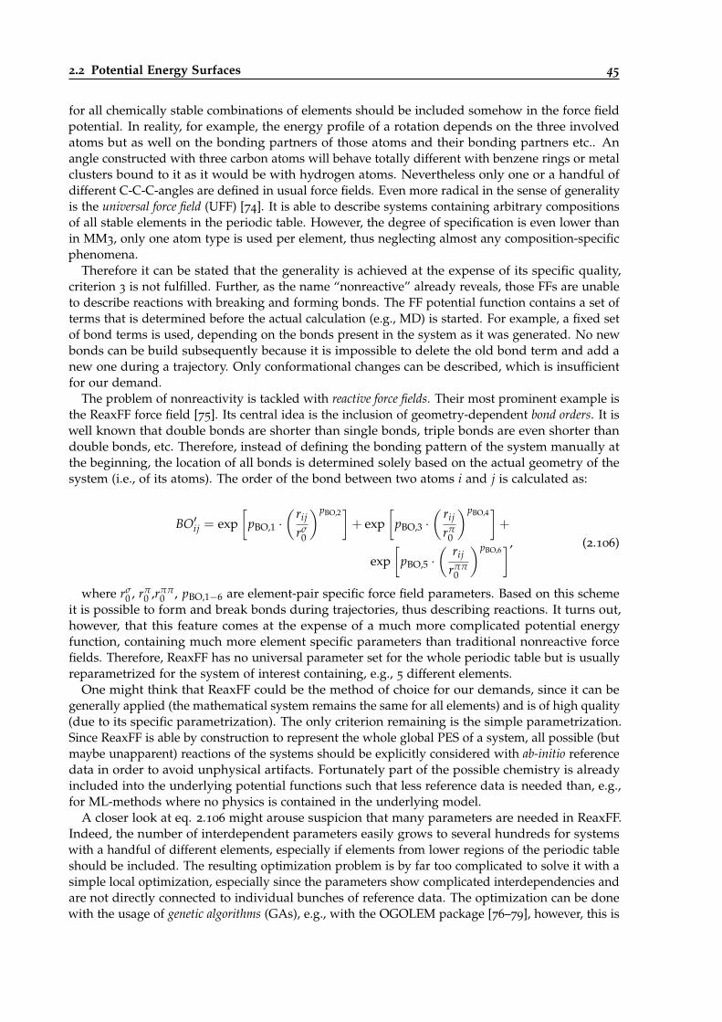
2.2 Potential Energy Surfaces 45
for all chemically stable combinations of elements should be included somehow in the force fieldpotential. In reality, for example, the energy profile of a rotation depends on the three involvedatoms but as well on the bonding partners of those atoms and their bonding partners etc.. Anangle constructed with three carbon atoms will behave totally different with benzene rings or metalclusters bound to it as it would be with hydrogen atoms. Nevertheless only one or a handful ofdifferent C-C-C-angles are defined in usual force fields. Even more radical in the sense of generalityis the universal force field (UFF) [74]. It is able to describe systems containing arbitrary compositionsof all stable elements in the periodic table. However, the degree of specification is even lower thanin MM3, only one atom type is used per element, thus neglecting almost any composition-specificphenomena.
Therefore it can be stated that the generality is achieved at the expense of its specific quality,criterion 3 is not fulfilled. Further, as the name “nonreactive” already reveals, those FFs are unableto describe reactions with breaking and forming bonds. The FF potential function contains a set ofterms that is determined before the actual calculation (e.g., MD) is started. For example, a fixed setof bond terms is used, depending on the bonds present in the system as it was generated. No newbonds can be build subsequently because it is impossible to delete the old bond term and add anew one during a trajectory. Only conformational changes can be described, which is insufficientfor our demand.
The problem of nonreactivity is tackled with reactive force fields. Their most prominent example isthe ReaxFF force field [75]. Its central idea is the inclusion of geometry-dependent bond orders. It iswell known that double bonds are shorter than single bonds, triple bonds are even shorter thandouble bonds, etc. Therefore, instead of defining the bonding pattern of the system manually atthe beginning, the location of all bonds is determined solely based on the actual geometry of thesystem (i.e., of its atoms). The order of the bond between two atoms i and j is calculated as:
BO′ij = exp[
pBO,1 ·( rij
rσ0
)pBO,2]+ exp
[pBO,3 ·
( rij
rπ0
)pBO,4]+
exp[
pBO,5 ·( rij
rππ0
)pBO,6], (2.106)
where rσ0 , rπ
0 ,rππ0 , pBO,1−6 are element-pair specific force field parameters. Based on this scheme
it is possible to form and break bonds during trajectories, thus describing reactions. It turns out,however, that this feature comes at the expense of a much more complicated potential energyfunction, containing much more element specific parameters than traditional nonreactive forcefields. Therefore, ReaxFF has no universal parameter set for the whole periodic table but is usuallyreparametrized for the system of interest containing, e.g., 5 different elements.
One might think that ReaxFF could be the method of choice for our demands, since it can begenerally applied (the mathematical system remains the same for all elements) and is of high quality(due to its specific parametrization). The only criterion remaining is the simple parametrization.Since ReaxFF is able by construction to represent the whole global PES of a system, all possible (butmaybe unapparent) reactions of the systems should be explicitly considered with ab-initio referencedata in order to avoid unphysical artifacts. Fortunately part of the possible chemistry is alreadyincluded into the underlying potential functions such that less reference data is needed than, e.g.,for ML-methods where no physics is contained in the underlying model.
A closer look at eq. 2.106 might arouse suspicion that many parameters are needed in ReaxFF.Indeed, the number of interdependent parameters easily grows to several hundreds for systemswith a handful of different elements, especially if elements from lower regions of the periodic tableshould be included. The resulting optimization problem is by far too complicated to solve it with asimple local optimization, especially since the parameters show complicated interdependencies andare not directly connected to individual bunches of reference data. The optimization can be donewith the usage of genetic algorithms (GAs), e.g., with the OGOLEM package [76–79], however, this is
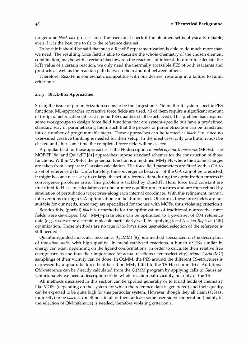
46 2 Theoretical Background
no genuine black-box process since the user must check if the obtained set is physically reliable,even if it is the best one to fit to the reference data set.
To be fair it should be said that such a ReaxFF reparametrization is able to do much more thanwe need. The resulting force field is able to describe the whole chemistry of the chosen elementcombination, maybe with a certain bias towards the reactions of interest. In order to calculate thek(T) value of a certain reaction, we only need the thermally accessible PES of both reactants andproducts as well as the reaction path between them and not between others.
Therefore, ReaxFF is somewhat incompatible with our desires, resulting in a failure to fulfillcriterion 1.
2.2.3 Black-Box Approaches
So far, the issue of parametrization seems to be the largest one. No matter if system-specific PESfunctions, ML-approaches or reactive force fields are used, all of them require a significant amountof (re-)parameterization (at least if good PES qualities shall be achieved). This problem has inspiredsome workgroups to design force field functions that are system-specific but have a predefinedstandard way of parametrizing them, such that the process of parametrization can be translatedinto a number of programmable steps. These approaches can be termed as black-box, since nouser-sided creative thinking is needed for their setup. In the ideal case, only one button must beclicked and after some time the completed force field will be ejected.
A popular field for those approaches is the FF-description of metal organic frameworks (MOFs). TheMOF-FF [80] and QuickFF [81] approaches impose standard schemes for the construction of thosefunctions. Within MOF-FF, the potential function is a modified MM3 FF, where the atomic chargesare taken from a separate Gaussian calculation. The force field parameters are fitted with a GA toa set of reference data. Unfortunately, the convergence behavior of the GA cannot be predicted,it might become necessary to enlarge the set of reference data during the optimization process ifconvergence problems arise. This problem is tackled by QuickFF. Here, force field constant arefirst fitted to Hessian calculations of one or more equilibrium structures and are then refined bysimulation of perturbation trajectories along each internal coordinate. With this refinement, manualinterventions during a GA optimization can be diminished. Of course, these force fields are notsuitable for our needs, since they are specialized for the use with MOFs, thus violating criterion 2.
Besides this, (partial) black-box methods for the optimization of traditional nonreactive forcefields were developed [82]. MM3-parameters can be optimized to a given set of QM referencedata (e.g., to describe a certain molecule particularly well) by applying local Newton-Raphson (NR)optimization. Those methods are no true black-boxes since user-sided selection of the reference isstill needed.
Quantum-guided molecular mechanics (Q2MM) [83] is a method specialized on the descriptionof transition states with high quality. In metal-catalyzed reactions, a bunch of TSs similar inenergy can exist, depending on the ligand conformations. In order to calculate their relative freeenergy barriers and thus their importance for actual reactions (stereoselectivity), Monte Carlo (MC)samplings of their vicinity can be done. In Q2MM, the PES around the different TS-structures isexpressed by a quadratic force field based on MM3 fitted to the TS Hessian matrix. AdditionalQM-reference can be directly calculated from the Q2MM program by applying calls to Gaussian.Unfortunately we need a description of the whole reaction path vicinity, not only of the TS.
All methods discussed in this section can be applied generally or to broad fields of chemistrylike MOFs (depending on the system for which the reference data is generated) and their qualitycan be expected to be quite high for this particular system. However, though they all claim (at leastindirectly) to be black-box methods, in all of them at least some user-sided cooperation (mainly inthe selection of QM reference) is needed, therefore violating criterion 1.
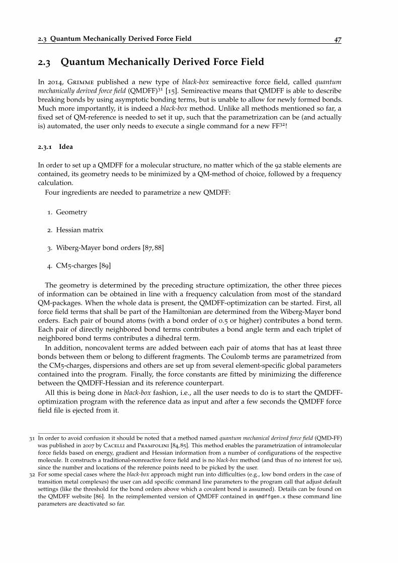
2.3 Quantum Mechanically Derived Force Field 47
2.3 Quantum Mechanically Derived Force Field
In 2014, Grimme published a new type of black-box semireactive force field, called quantummechanically derived force field (QMDFF)31 [15]. Semireactive means that QMDFF is able to describebreaking bonds by using asymptotic bonding terms, but is unable to allow for newly formed bonds.Much more importantly, it is indeed a black-box method. Unlike all methods mentioned so far, afixed set of QM-reference is needed to set it up, such that the parametrization can be (and actuallyis) automated, the user only needs to execute a single command for a new FF32!
2.3.1 Idea
In order to set up a QMDFF for a molecular structure, no matter which of the 92 stable elements arecontained, its geometry needs to be minimized by a QM-method of choice, followed by a frequencycalculation.
Four ingredients are needed to parametrize a new QMDFF:
1. Geometry
2. Hessian matrix
3. Wiberg-Mayer bond orders [87, 88]
4. CM5-charges [89]
The geometry is determined by the preceding structure optimization, the other three piecesof information can be obtained in line with a frequency calculation from most of the standardQM-packages. When the whole data is present, the QMDFF-optimization can be started. First, allforce field terms that shall be part of the Hamiltonian are determined from the Wiberg-Mayer bondorders. Each pair of bound atoms (with a bond order of 0.5 or higher) contributes a bond term.Each pair of directly neighbored bond terms contributes a bond angle term and each triplet ofneighbored bond terms contributes a dihedral term.
In addition, noncovalent terms are added between each pair of atoms that has at least threebonds between them or belong to different fragments. The Coulomb terms are parametrized fromthe CM5-charges, dispersions and others are set up from several element-specific global parameterscontained into the program. Finally, the force constants are fitted by minimizing the differencebetween the QMDFF-Hessian and its reference counterpart.
All this is being done in black-box fashion, i.e., all the user needs to do is to start the QMDFF-optimization program with the reference data as input and after a few seconds the QMDFF forcefield file is ejected from it.
31 In order to avoid confusion it should be noted that a method named quantum mechanical derived force field (QMD-FF)was published in 2007 by Cacelli and Prampolini [84,85]. This method enables the parametrization of intramolecularforce fields based on energy, gradient and Hessian information from a number of configurations of the respectivemolecule. It constructs a traditional-nonreactive force field and is no black-box method (and thus of no interest for us),since the number and locations of the reference points need to be picked by the user.
32 For some special cases where the black-box approach might run into difficulties (e.g., low bond orders in the case oftransition metal complexes) the user can add specific command line parameters to the program call that adjust defaultsettings (like the threshold for the bond orders above which a covalent bond is assumed). Details can be found onthe QMDFF website [86]. In the reimplemented version of QMDFF contained in qmdffgen.x these command lineparameters are deactivated so far.
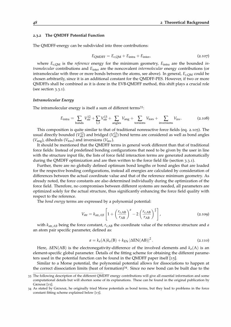
48 2 Theoretical Background
2.3.2 The QMDFF Potential Function
The QMDFF-energy can be subdivided into three contributions:
EQMDFF = Ee,QM + Eintra + Einter, (2.107)
where Ee,QM is the reference energy for the minimum geometry, Eintra are the bounded in-tramolecular contributions and Einter are the noncovalent intermolecular energy contributions (orintramolecular with three or more bonds between the atoms, see above). In general, Ee,QM could bechosen arbitrarily, since it is an additional constant for the QMDFF-PES. However, if two or moreQMDFFs shall be combined as it is done in the EVB-QMDFF method, this shift plays a crucial role(see section 3.3.1).
Intramolecular Energy
The intramolecular energy is itself a sum of different terms33:
Eintra = ∑bonds
V12str + ∑
1,3V13
str + ∑angles
Vang + ∑torsions
Vtors + ∑inversions
Vinv. (2.108)
This composition is quite similar to that of traditional nonreactive force fields (eq. 2.105). Theusual directly bounded (V12
str) and bridged (V13str) bond terms are considered as well as bond angles
(Vang), dihedrals (Vtors) and inversions (Vinv).It should be mentioned that the QMDFF terms in general work different than that of traditional
force fields: Instead of predefined bonding configurations that need to be given by the user in linewith the structure input file, the lists of force field interaction terms are generated automaticallyduring the QMDFF optimization and are then written to the force field file (section 3.3.1).
Further, there are no globally defined optimum bond lengths or bond angles that are loadedfor the respective bonding configurations, instead all energies are calculated by consideration ofdifferences between the actual coordinate value and that of the reference minimum geometry. Asalready noted, the force constants are also determined individually during the optimization of theforce field. Therefore, no compromises between different systems are needed, all parameters areoptimized solely for the actual structure, thus significantly enhancing the force field quality withrespect to the reference.
The bond energy terms are expressed by a polynomial potential:
Vstr = kstr,AB
[1 +
(re,AB
rAB
)a− 2
(re,AB
rAB
) a2]
, (2.109)
with kstr,AB being the force constant, re,AB the coordinate value of the reference structure and aan atom pair specific parameter, defined as:
a = ka(A)ka(B) + kEN |∆EN(AB)|2 . (2.110)
Here, ∆EN(AB) is the electronegativity-difference of the involved elements and ka(A) is anelement-specific global parameter. Details of the fitting scheme for obtaining the different parame-ters used in the potential function can be found in the QMDFF paper itself [15].
Similar to a Morse potential, the polynomial potential allows for dissociations to happen atthe correct dissociation limits (heat of formation)34. Since no new bond can be built due to the
33 The following description of the different QMDFF energy contributions will give all essential information and somecomputational details but will shorten some of its explanations. These can be found in the original publication byGrimme [15].
34 As stated by Grimme, he originally tried Morse potentials as bond terms, but they lead to problems in the forceconstant fitting scheme explained below [15].
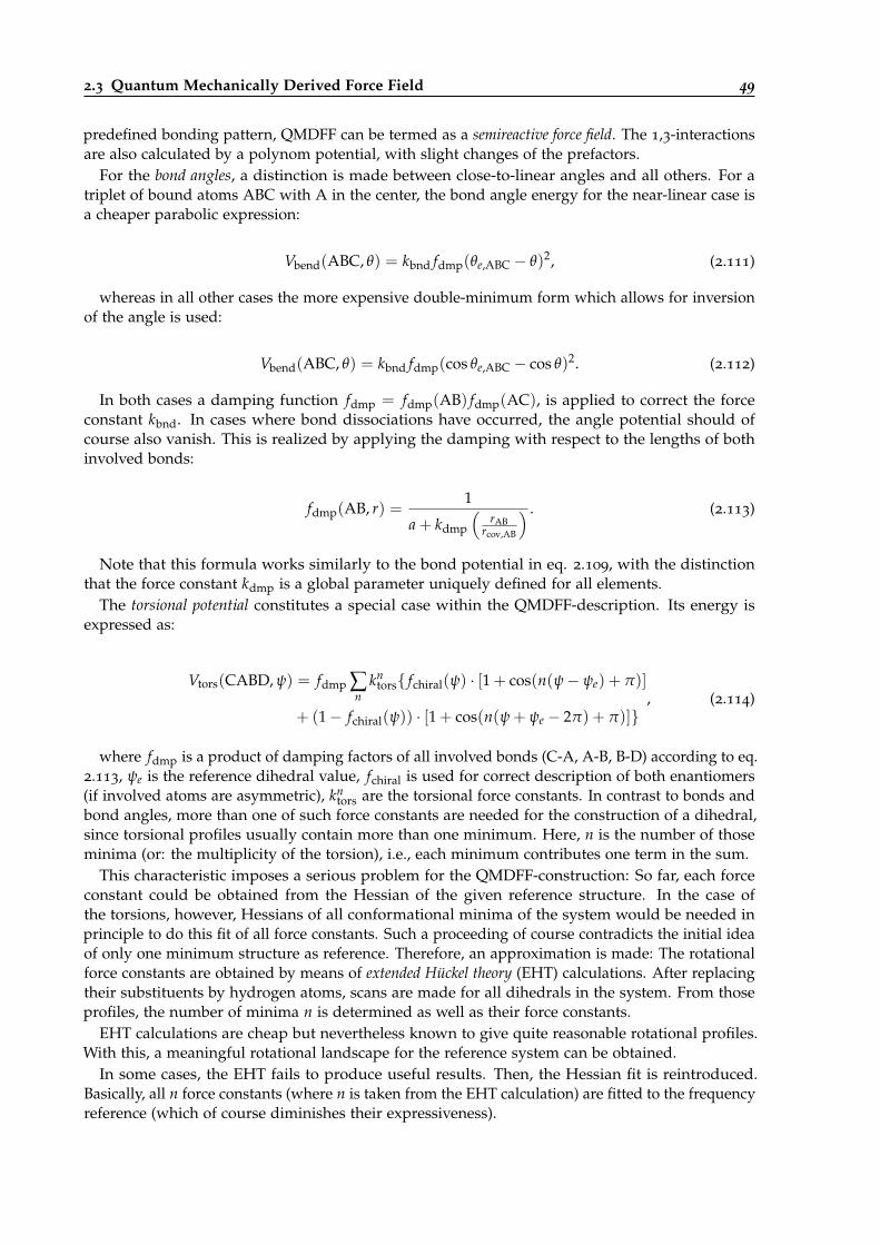
2.3 Quantum Mechanically Derived Force Field 49
predefined bonding pattern, QMDFF can be termed as a semireactive force field. The 1,3-interactionsare also calculated by a polynom potential, with slight changes of the prefactors.
For the bond angles, a distinction is made between close-to-linear angles and all others. For atriplet of bound atoms ABC with A in the center, the bond angle energy for the near-linear case isa cheaper parabolic expression:
Vbend(ABC, θ) = kbnd fdmp(θe,ABC − θ)2, (2.111)
whereas in all other cases the more expensive double-minimum form which allows for inversionof the angle is used:
Vbend(ABC, θ) = kbnd fdmp(cos θe,ABC − cos θ)2. (2.112)
In both cases a damping function fdmp = fdmp(AB) fdmp(AC), is applied to correct the forceconstant kbnd. In cases where bond dissociations have occurred, the angle potential should ofcourse also vanish. This is realized by applying the damping with respect to the lengths of bothinvolved bonds:
fdmp(AB, r) =1
a + kdmp
(rAB
rcov,AB
) . (2.113)
Note that this formula works similarly to the bond potential in eq. 2.109, with the distinctionthat the force constant kdmp is a global parameter uniquely defined for all elements.
The torsional potential constitutes a special case within the QMDFF-description. Its energy isexpressed as:
Vtors(CABD, ψ) = fdmp ∑n
kntors{ fchiral(ψ) · [1 + cos(n(ψ− ψe) + π)]
+ (1− fchiral(ψ)) · [1 + cos(n(ψ + ψe − 2π) + π)]}, (2.114)
where fdmp is a product of damping factors of all involved bonds (C-A, A-B, B-D) according to eq.2.113, ψe is the reference dihedral value, fchiral is used for correct description of both enantiomers(if involved atoms are asymmetric), kn
tors are the torsional force constants. In contrast to bonds andbond angles, more than one of such force constants are needed for the construction of a dihedral,since torsional profiles usually contain more than one minimum. Here, n is the number of thoseminima (or: the multiplicity of the torsion), i.e., each minimum contributes one term in the sum.
This characteristic imposes a serious problem for the QMDFF-construction: So far, each forceconstant could be obtained from the Hessian of the given reference structure. In the case ofthe torsions, however, Hessians of all conformational minima of the system would be needed inprinciple to do this fit of all force constants. Such a proceeding of course contradicts the initial ideaof only one minimum structure as reference. Therefore, an approximation is made: The rotationalforce constants are obtained by means of extended Hückel theory (EHT) calculations. After replacingtheir substituents by hydrogen atoms, scans are made for all dihedrals in the system. From thoseprofiles, the number of minima n is determined as well as their force constants.
EHT calculations are cheap but nevertheless known to give quite reasonable rotational profiles.With this, a meaningful rotational landscape for the reference system can be obtained.
In some cases, the EHT fails to produce useful results. Then, the Hessian fit is reintroduced.Basically, all n force constants (where n is taken from the EHT calculation) are fitted to the frequencyreference (which of course diminishes their expressiveness).
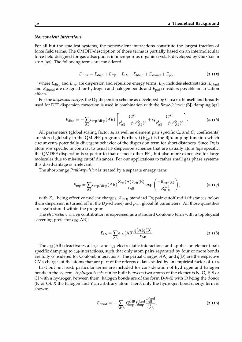
50 2 Theoretical Background
Noncovalent Interations
For all but the smallest systems, the noncovalent interactions constitute the largest fraction offorce field terms. The QMDFF-description of those terms is partially based on an intermolecularforce field designed for gas adsorptions in microporous organic crystals developed by Grimme in2012 [90]. The following terms are considered:
Einter = Edisp + Erep + EES + Ehbnd + Exbond + Epol, (2.115)
where Edisp and Erep are dispersion and repulsion energy terms, EES includes electrostatics, Ehbndand Exbond are designed for hydrogen and halogen bonds and Epol considers possible polarizationeffects.
For the dispersion energy, the D3-dispersion scheme as developed by Grimme himself and broadlyused for DFT dispersion correction is used in combination with the Becke-Johnson (BJ) damping [91]:
Edisp = −∑AB
εrep/disp(AB)
[CAB
6
r6AB + f (R0
AB)6+ s8
CAB8
r8AB + f (R0
AB)8
]. (2.116)
All parameters (global scaling factor s8 as well as element pair specific C6 and C8 coefficients)are stored globally in the QMDFF program. Further, f (R0
AB) is the BJ-damping function whichcircumvents potentially divergent behavior of the dispersion term for short distances. Since D3 isatom pair specific in contrast to usual FF dispersion schemes that are usually atom type specific,the QMDFF dispersion is superior to that of most other FFs, but also more expensive for largemolecules due to missing cutoff distances. For our applications to rather small gas phase systems,this disadvantage is irrelevant.
The short-range Pauli-repulsion is treated by a separate energy term:
Erep = ∑AB
εrep/disp(AB)Zeff(A)Zeff(B)
rABexp
(−βreprAB
R3/20,D3
), (2.117)
with Zeff being effective nuclear charges, R0,D3 standard D3 pair-cutoff-radii (distances belowthem dispersion is turned off in the D3-scheme) and βrep global fit parameters. All those quantitiesare again stored within the program.
The electrostatic energy contribution is expressed as a standard Coulomb term with a topologicalscreening prefactor εES(AB):
EES = ∑AB
εES(AB)q(A)q(B)
rAB. (2.118)
The εES(AB) deactivates all 1,2- and 1,3-electrostatic interactions and applies an element pairspecific damping to 1,4-interactions, such that only atom pairs separated by four or more bondsare fully considered for Coulomb interactions. The partial charges q(A) and q(B) are the respectiveCM5-charges of the atoms that are part of the reference data, scaled by an empirical factor of 1.15.
Last but not least, particular terms are included for consideration of hydrogen and halogenbonds in the system. Hydrogen bonds can be built between two atoms of the elements N, O, F, S orCl with a hydrogen between them, halogen bonds are of the form D-X-Y, with D being the donor(N or O), X the halogen and Y an arbitrary atom. Here, only the hydrogen bond energy term isshown:
Ehbnd = − ∑AHB
f AHBdmp f hbnd
dmpchbnd
ABr3
AB, (2.119)
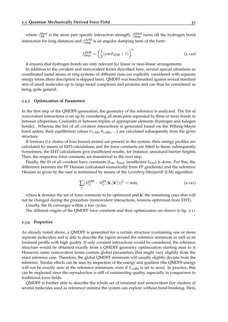
2.3 Quantum Mechanically Derived Force Field 51
where chbndAB is the atom pair specific interaction strength, f hbnd
dmp turns off the hydrogen bond
interaction for long distances and f AHBdmp is an angular damping term of the form:
f AHBdmp =
(12(cos θAHB + 1)
)6. (2.120)
It ensures that hydrogen bonds are only relevant for linear or near-linear arrangements.In addition to the covalent and noncovalent terms described here, several special situations as
coordinated metal atoms or ring-systems of different sizes are explicitly considered with separateenergy terms (their description is skipped here). QMDFF was benchmarked against several standardsets of small molecules up to large metal complexes and proteins and can thus be considered asbeing quite general.
2.3.3 Optimization of Parameters
In the first step of the QMDFF-generation, the geometry of the reference is analyzed. The list ofnoncovalent interactions is set up by considering all atom-pairs separated by three or more bonds inbetween (dispersion, Coulomb) or between triplets of appropriate elements (hydrogen and halogenbonds). Whereas the list of all covalent interactions is generated based on the Wiberg-Mayerbond orders, their equilibrium values (re,AB, θe,ABC, ...) are calculated subsequently from the givenstructure.
If torsions (i.e chains of four bound atoms) are present in the system, their energy profiles arecalculated by means of EHT-calculations and the force constants are fitted to these, subsequently.Sometimes, the EHT-calculations give insufficient results, for instance, unnatural barrier heights.Then, the respective force constants are transferred to the next step.
Finally, the fit of all covalent force constants (kstr, kbnd, insufficient ktors) is done. For this, thedifference between the FF Hessian (calculated numerically from FF gradients) and the referenceHessian as given by the user is minimized by means of the Levenberg-Marquardt (LM) algorithm:
∑ij(HQM
ij − HFFij (k, [k′]))2 → min, (2.121)
where k denotes the set of force constants to be optimized and k′ the remaining ones that willnot be changed during the procedure (noncovalent interactions, torsions optimized from EHT).
Usually, the fit converges within a few cycles.The different origins of the QMDFF force constants and their optimization are shown in fig. 2.11.
2.3.4 Properties
As already noted above, a QMDFF is generated for a certain structure (containing one or moreseparate molecules) and is able to describe the region around the reference minimum as well as itstorsional profile with high quality. If only covalent interactions would be considered, the referencestructure would be obtained exactly from a QMDFF geometry optimization starting near to it.However, some noncovalent terms contain global parameters that might vary slightly from theexact reference case. Therefore, the global QMDFF minimum will usually slightly deviate from thereference. Similar effects can be seen by inspection of the energy and gradient (the QMDFF-energywill not be exactly zero at the reference minimum, even if Ee,QM is set to zero). In practice, thiscan be neglected since the reproduction is still of outstanding quality, especially in comparison totraditional force fields.
QMDFF is further able to describe the whole set of torsional and noncovalent (for clusters ofseveral molecules used as reference) minima the system can explore without bond-breaking. Here,
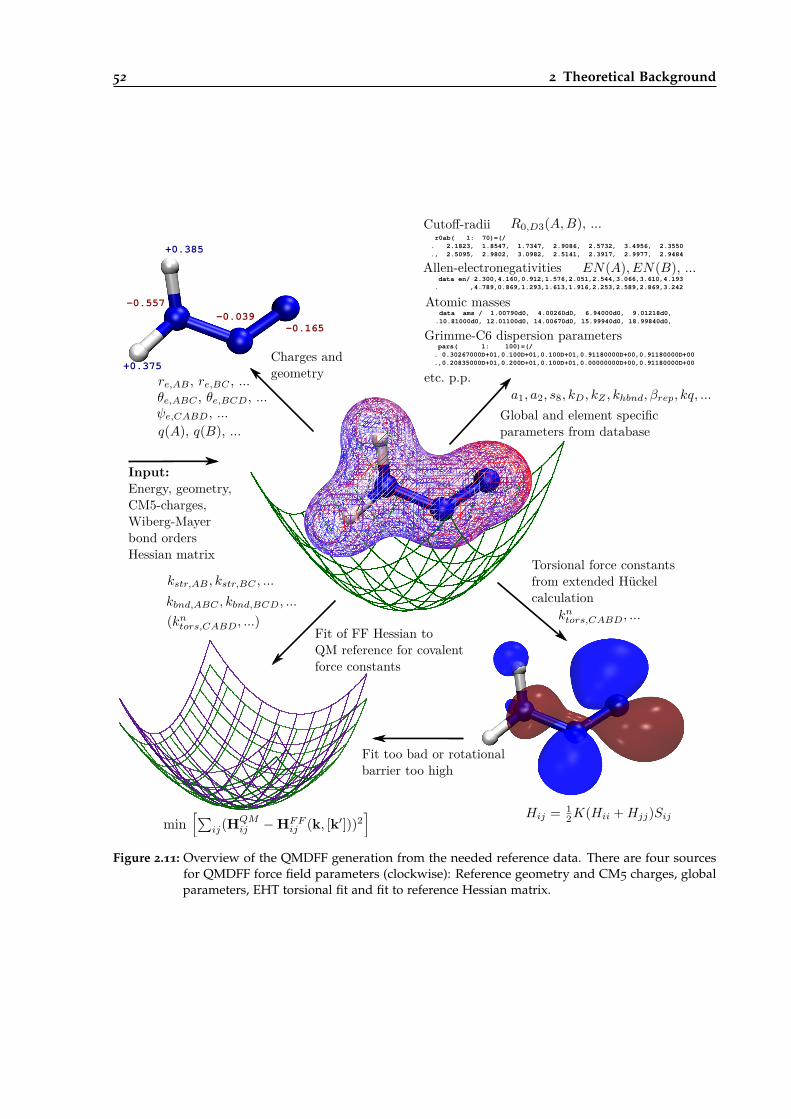
52 2 Theoretical Background
r0ab( 1: 70)=(/ . 2.1823, 1.8547, 1.7347, 2.9086, 2.5732, 3.4956, 2.3550 ., 2.5095, 2.9802, 3.0982, 2.5141, 2.3917, 2.9977, 2.9484 data en/ 2.300,4.160,0.912,1.576,2.051,2.544,3.066,3.610,4.193 . ,4.789,0.869,1.293,1.613,1.916,2.253,2.589,2.869,3.242
data ams / 1.00790d0, 4.00260d0, 6.94000d0, 9.01218d0, .10.81000d0, 12.01100d0, 14.00670d0, 15.99940d0, 18.99840d0,
pars( 1: 100)=(/ . 0.30267000D+01,0.100D+01,0.100D+01,0.91180000D+00,0.91180000D+00 .,0.20835000D+01,0.200D+01,0.100D+01,0.00000000D+00,0.91180000D+00
Cutoff-radii
Allen-electronegativities
Atomic masses
Grimme-C6 dispersion parameters
etc. p.p.
+0.385
+0.375
-0.557
-0.039
-0.165 Charges and
geometry
Global and element specific parameters from database
Torsional force constants from extended Hückel calculation
Fit of FF Hessian toQM reference for covalent force constants
Fit too bad or rotationalbarrier too high
Input:Energy, geometry,CM5-charges,Wiberg-Mayer bond orders Hessian matrix
Figure 2.11: Overview of the QMDFF generation from the needed reference data. There are four sourcesfor QMDFF force field parameters (clockwise): Reference geometry and CM5 charges, globalparameters, EHT torsional fit and fit to reference Hessian matrix.
2.4 Empirical Valence Bond 53
the QMDFF quality is slightly worse in comparison to the direct vicinity of the reference minimumbut still very good in comparison to traditional force fields.
With this, we can state that QMDFF fulfills criteria 1 and 2, i.e., it is generally applicable andcan be optimized in a black-box fashion. It further partly fulfills criterion 3: The quality of QMDFFin reproducing the reference PES is very encouraging for the whole configuration space of eitherthe reactants or products area. All what remains is the region between them, i.e., the reactionchannel35. This challenge is tackled in the next section.
2.4 Empirical Valence Bond
We have learned so far that QMDFF is perhaps the single PES description method that deservesthe label black-box more than all others. Unfortunately it is semireactive, thus unable to representPESs of reactive systems (disregarding simple diffusions, cis-trans isomerizations or other purelynoncovalent reactions). To make QMDFF reactive, empirical valence bond (EVB) is the method ofchoice.
Originally formulated by Warshel in 1980 [92], the EVB-method is a surprisingly simple way ofconstructing reactive force fields by connecting traditional nonreactive force fields or even simplerformulations with an individually designed coupling term. Since its invention, a multiplicity ofEVB-coupling terms has been emerged in the literature. Since the implementation and constructionof EVB-coupling terms was one of my main working fields, a thorough review of those terms willbe given, culminating in the description of those that are best suited for construction of high-qualityblack-box PESs.
2.4.1 Valence Bond or Molecular Orbital Theory?
Looking back to the origins of modern applied quantum mechanics, two concurring theories werein play many decades. Molecular orbital (MO) and valence bond (VB) theory. Since the 50s andespecially since computer power has raised significantly such that quantum chemical calculationsof large molecular systems became routine, MO theory is the dominant theory in practice [93].
VB still serves an important role for understanding of chemical bonding situations and molecularstructures, mainly due to the localized VB orbitals, resembling bonds or resonance in π-systems.However, although quantum chemical programs based on VB are available [94], modern computa-tional chemistry almost exclusively relies on MO.
The differences of VB- and MO-concepts can be explained quite well in the simplest possiblecase of the H2-molecule [95]: It consists of (at least) two atomic orbitals (AO), one located at eachH atom: χa and χb.
In the VB-picture, the wave function of H2 is made of a linear combination of both the covalentand the possible ionic structures. The covalent structure is expressed by:
|χaχb| − |χaχb|. (2.122)
Each term in this Heitler-London [96] wave function consists of a Slater determinant:
|χaχb| =1√2[χa(1)α(1)χb(2)β(2)− χa(2)α(2)χb(2)β(1)],
|χaχb| =1√2[χa(1)β(1)χb(2)α(2)− χa(2)β(2)χb(2)α(1)].
(2.123)
35 In chapter 7 it is shown that a single QMDFF is able to deliver a PES-description that can be used to do accuratecovalent mechanochemistry simulations, since there only bond dissociations must be described with high quality.
54 2 Theoretical Background
It becomes clear that the linear combination consists of all possibilities to distribute the α and βspin electrons on both AOs. However, it is also possible that both electrons are located in the sameAO, leading to the ionic contributions |χaχa| and |χbχb|.
The total VB wave function consists of four determinants, two covalent and two ionic ones:
ΨVB = λ(|χaχb| − |χaχb|) + µ(|χaχa|+ |χbχb|), (2.124)
where the two parameters λ and µ are to be optimized variationally. For small bond distancesnear the equilibrium value, the covalent part is dominant, corresponding to a large λ-value. Duringbond breaking, µ increases, since ionic configurations are needed for its description. If the bond isbroken homolytically and the atoms were moved far away, λ will converge to one, correspondingto two separated H radicals [55].
In the case of MO-theory, the molecular orbitals are built by linear combination of atomic orbitals(LCAO):
φ1 = χa + χb,
φ2 = χa − χb.(2.125)
In the simplest case, both electrons are located in the bonding orbital φ1. Building the Slaterdeterminant results in:
ΨMO = |φ1φ1| = (|χaχb| − |χaχb|) + (|χaχa|+ |χbχb|). (2.126)
If we compare ΨMO to ΨVB, both wave functions are almost identical with the exception of λ andµ in the VB case. Therefore the VB wave function is much more flexible than the MO one, whichconsists of always 50 % covalent and ionic components.
This deficiency of MO theory can also be seen in many dissociation curves calculated with HF,which show qualitatively wrong shapes [12, 55]. To correct this deficiency, inclusion of electroncorrelation is needed.
In the simple H2-case, configuration interaction (CI) needs to be applied, i.e., the wave function isitself a linear combination of two Slater determinants, the ground state and the exited state:
ΨMO−CI = c1|φ1φ1| − c2|φ2φ2|. (2.127)
Evaluating both Slater determinants and simplifying, the wave function can be expresseddepending on the atomic orbitals:
ΨMO−CI = (c1 + c2)(|χaχb| − |χaχb|) + (c1 − c2)(|χaχa|+ |χbχb|). (2.128)
Now, additional prefactors c1 + c2 and c1 − c2 are present. Compared to the VB expression, it isclear that λ = c1 + c2 and µ = c1 − c2. The surprising result is that in this simple system a FCI MOwave function is needed to reproduce the VB wave function.
Further, it can be seen that both VB- and MO-theory come to the same result, if all configurationsare included and all electron correlation is considered.
Why MO theory is still superior in practice?The main reason is that the VB orbitals are nonorthogonal, which raises the needed computational
amount significantly in comparison to MO, where the molecular orbitals are orthogonal [97].Further, for larger systems, the number of needed configurations, especially ionic ones similar to eq.2.124, grows heavily, which leads to both large computational demand and obscured conceptualclarity. Another important aspect is that in VB CI- and MO-coefficients are always optimizedsimultaneously (corresponding to a FCI calculation in the H2-example). This apparent advantagewas indeed a huge disadvantage in the early days of computational chemistry. Then, calculations ofreactions involving bond dissociations where out of reach for most systems and usual applications

2.4 Empirical Valence Bond 55
were restricted to near-equilibrium geometries, where a single electronic configuration is sufficient.Methods like HF are of satisfying quality for those regions by simultaneously being much chapterthan VB. Even if today’s computational resources are enough to perform VB-calculations for manysystems, this historical mortgage constitutes another inhibiting factor.
Since the 1980s, a small but nevertheless visible renaissance of VB can be seen, at least in theeyes of VB enthusiasts36. This is mainly due to new implementations like Generalized Valence Bond(GVB) [98], which can, e.g., also be used with the Gaussian program suite [99]. In GVB, somesimplifications are introduced in order to accelerate both user sided setup and computational timeof a calculation. The wave function is expressed as a product of the HL function type (eq. 2.122)with the condition that two different of such functions are orthogonal to each other. With thisprerequisite, the demand of calculating overlap integrals is reduced significantly.
There are many other published VB-methods, which makes it quite cumbersome to know whichone could be needed for a specific situation. Therefore, MO-methods are still widely superior interms of high quality (near-)black-box calculations of arbitrary molecules executed by the averagechemist [94].
2.4.2 EVB-Foundations
What is needed to go from VB to EVB? One central advantage of VB is that the wave functionis a superposition of orbitals that can be constructed by chemical intuition. In the H2-examplepresented above these orbitals are the covalent HL wave function and the two ionic configurations.
During the (homolytic) dissociation of the H2-bond the relative weights of these configurationschange, from roughly 3 to 1 covalent to ionic at equilibrium distance over almost equal distributionat intermediary distances up to exclusively covalent at long distances.
The concept of expressing a reaction as a coordinate-dependent superposition of differentchemical configurations can also be used apart from wave-function methods like VB. For theH2-example, we could equally well describe both the covalent and the ionic states with fittedpotential energy surfaces like force fields, if the parameters are chosen such that they reproducethe quantum mechanical energies and gradients.
Now, the total PES of the system could be expressed again as a superposition of these forcefields, resulting in a superposition FF. This is the central idea of the EVB approach first developedby Warshel in his groundbreaking paper [92].
All concepts shown in this first publication are still valid for all EVB applications, thereforethey will be shown here in some detail. The simplest (and mostly used) case is a superpositionof two configurations, like the covalent and one of the ionic ones at the H2 example. This closelyresembles the famous two-state problem of quantum mechanics [100]. For this, the EVB-energy canbe expressed as:
H =
(F1(q) C(q)C(q) F2(q)
). (2.129)
Here, F1(q) and F2(q) are the coordinate-dependent potentials of both configurations and C(q)is the resonance integral or coupling term. If no coupling is present, the EVB energy would be alwaysthe energy of the lower lying state, without any smooth transition between them. Of course this isnot true for nearly any real system, therefore the exact formulation of this coupling term becomesa central aspect in EVB, as will be shown below.
The general idea of 2x2-EVB is also illustrated in fig. 2.12.
36 Reason for the success of some new invented VB-methods is also the partial mixing with MO-concepts. In order toat least partially avoid the problem of nonorthogonal orbitals, the VB orbitals are allowed in some approaches todelocalize somehow such that orthogonality of neighbored orbitals can be achieved. More details to this can be foundin [94].
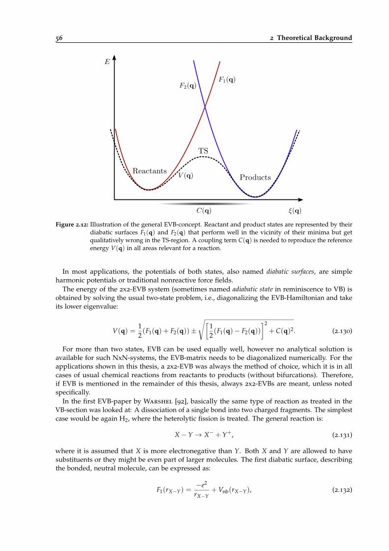
56 2 Theoretical Background
ReactantsProducts
TS
Figure 2.12: Illustration of the general EVB-concept. Reactant and product states are represented by theirdiabatic surfaces F1(q) and F2(q) that perform well in the vicinity of their minima but getqualitatively wrong in the TS-region. A coupling term C(q) is needed to reproduce the referenceenergy V(q) in all areas relevant for a reaction.
In most applications, the potentials of both states, also named diabatic surfaces, are simpleharmonic potentials or traditional nonreactive force fields.
The energy of the 2x2-EVB system (sometimes named adiabatic state in reminiscence to VB) isobtained by solving the usual two-state problem, i.e., diagonalizing the EVB-Hamiltonian and takeits lower eigenvalue:
V(q) =12(F1(q) + F2(q))±
√[12(F1(q)− F2(q))
]2+ C(q)2. (2.130)
For more than two states, EVB can be used equally well, however no analytical solution isavailable for such NxN-systems, the EVB-matrix needs to be diagonalized numerically. For theapplications shown in this thesis, a 2x2-EVB was always the method of choice, which it is in allcases of usual chemical reactions from reactants to products (without bifurcations). Therefore,if EVB is mentioned in the remainder of this thesis, always 2x2-EVBs are meant, unless notedspecifically.
In the first EVB-paper by Warshel [92], basically the same type of reaction as treated in theVB-section was looked at: A dissociation of a single bond into two charged fragments. The simplestcase would be again H2, where the heterolytic fission is treated. The general reaction is:
X−Y → X− + Y+, (2.131)
where it is assumed that X is more electronegative than Y. Both X and Y are allowed to havesubstituents or they might be even part of larger molecules. The first diabatic surface, describingthe bonded, neutral molecule, can be expressed as:
F1(rX−Y) =−e2
rX−Y+ Vnb(rX−Y), (2.132)
2.4 Empirical Valence Bond 57
where −e2
rX−Yis the Coulomb force between both (partially) charged atoms and Vnb(rX−Y) are
additional nonbonded interactions like dispersion forces.The second diabatic surface is similar to the first, however it is shifted by the formation-energy
of X−Y+ from X.Y. at infinite separation (∆)37:
F2(rX−Y) =−e2
rX−Y+ Vnb(rX−Y) + ∆. (2.133)
The EVB resonance integral can be constructed by looking back at eq. 2.130. If this equation issolved for C(q), the result is:
C(q)2 = [F1(q)−V(q)][F2(q)−V(q)]. (2.134)
Applied to our simple two-atom problem, the only relevant internal coordinate is the separationof both atoms rX−Y:
C(rX−Y)2 = [F1(rX−Y)−V(rX−Y)][F2(rX−Y)−V(rX−Y)]. (2.135)
Warshel and Weiss assumed that the “true” potential energy surface of the reacting system canbe modeled by a simple Morse-oscillator, depending solely on the bond length between atoms Xand Y:
V(q) = M(rX−Y). (2.136)
The total EVB-surface is obtained by inserting F1(rX−Y), F2(rX−Y) and C(rX−Y)2 (calculated
from eq. 2.135) into eq. 2.130. In the transition-region between both diabatic surfaces, the couplingterm dominates the shape of the whole EVB-surface. Therefore, if C(rX−Y)
2 is constructed suchthat the whole EVB-term resembles a Morse-oscillator, this will actually be the case for the surfaceitself in the critical region. Near the covalent and ionic minima, the usual shapes of F1(rX−Y) andF2(rX−Y) will be resembled, but in the transition region they both will converge to the desiredMorse-oscillator shape.
An important feature of EVB is the (near) independence of the coupling term C(q) from themolecular environment38. With this, is is possible to parametrize the coupling term with gasphase calculations (especially if methods like distributed Gaussian EVB (see below), where thecosts of QM-reference calculations are important are utilized) and use it in solutions or proteinenvironments. Only the diabatic states need to be set up with inclusion of the whole environment.Since these states are force fields in most cases, the total expense of the EVB calculation should beaffected only slightly (i.e., with modest scaling).
Having this property of partial solvent-independence, EVB is well suited for multiscale calcula-tions, i.e., combinations of a small reactive system with the environment that – although passivewith respect to the actual reaction – might have a significant influence on it. Warshel received hisNobel prize of 1992 together with Karplus and Lewitt “for the development of multiscale modelsfor complex chemical systems” [104].
37 The gas phase formation-energy of X−Y+ from X.Y. can be expressed in terms of the electron affinity of X (EAX) andthe ionization potential of Y (IY): ∆ = IY − EAX .
38 This independence of the coupling term from the molecular environment was proven numerically in a paper byWarshel et al. [101]. There, the Cl−+CH3Cl symmetric nucleophilic substitution was taken as benchmark reaction.Energies of diabatic states as well as the adiabatic state were calculated with frozen density functional theory (FDFT)both in presence and absence of solvents calculated with QM/MM methods. Using eq. 2.134 it could be shown thatthe needed coupling was almost identical for the whole reaction path with and without solvent. Similar tests weredone in [102] and [103].
58 2 Theoretical Background
2.4.3 Simple EVB Coupling Terms
Since the invention of EVB in 1980 a huge number of publications spanning a large range ofapplications has been published. I will give no comprehensive review of EVB in a whole, this isdone elsewhere [95, 105]. However, especially the construction of the resonance integral C(q) is ofcentral importance and a wide range of concepts for it is known, therefore it seems to be useful togive a short overview of successful approaches, starting with the most simple ones and successivelygoing to quite comprehensive ideas.
The simplest case would be a constant coupling term:
C(q) = a. (2.137)
This quite primitive formulation leads indeed to a significant improvement over no coupling at allbut it is nevertheless not suited for real applications with desired quantitative accuracy [106]. Thereason is that the reactant and product areas are usually described well by their diabatic surfaces(i.e., force fields). If a coupling disturbs the diabatic surfaces in those areas, their description willoften become worse although there is a general tendency that a global constant coupling usuallydisturbs the areas near the minima less than the transition region39. Even if the influence on theminima can be made small, one single parameter is usually not sufficient to guarantee a high-levelquantitative description of the transition region. Hence, to the best of my knowledge, the constantcoupling was so far never used for actual EVB-applications. However, in the supplementaryinformation of the first EVB-QMDFF paper [16] (section 11.6.1), one example for this term is shown.
The next step on the path to better EVB coupling terms is the energy-gap reaction coordinate[107–109]. In this case, the coupling itself is dependent on the energies of both diabatic surfaces:
C(q) = g(F1(q)− F2(q)). (2.138)
Here, g might be any kind of useful functional expression. An obvious choice is a Gaussianlocated at zero energy difference [108]:
C(q) = a exp(−b(F1(q)− F2(q))2
). (2.139)
In this case, the coupling has maximum strength in the TS region (where both diabatic surfacesusually cross) and decays to zero in the reactant and product areas. Then, the diabatic energies inthose regions are preserved. This is illustrated in fig. 2.12. The actual functional expressions usedfor energy gaps in this thesis are listed in table 3.1 of the program chapter.
Another formulation is by far the most common one: the coordinate-dependent coupling. This typewas already used in the original paper by Warshel, there it was a Morse potential dependent onthe length of the broken bond (eqs. 2.135, 2.136).
Since a large part of chemical reactions consists essentially of breaking or formation of one ormore bonds, this type of coordinate-dependence, despite being quite simple, has been applied tomany published systems. The general formula for the coupling term is:
C(q) = ag1(q1)g2(q2)...gn(qn). (2.140)
One famous application is the multistate (MS)-EVB model by Voth et al. [102, 110], which wasconstructed to simulate alternating hydrogen bond networks between water molecules with excessprotons. Since each bonding configuration can be represented by its own diabatic surface, more
39 This behavior can be explained by looking back at eq. 2.130. There, the square root consists of two summands: thesquared difference between both diabatic energies and the squared coupling. Near the TS-region, the first term is nearlyzero, such that the coupling determines the square root term almost exclusively. Near the reactants and products,however, the difference between both diabatic surfaces becomes large, marginalizing the effect of the coupling in theargument of the root.
2.4 Empirical Valence Bond 59
than two of these surfaces are needed. In practice, for each oxygen atom in the system, oneadditional EVB is needed. Reactions with more than 30 states (corresponding to a 30x30-EVB term)were done [111].
In spite of this rather general nxn-EVB approach, the used type of coupling term is also wellsuited for our case of 2x2-EVB terms:
C(q)ij = (Vijconst + Vij
ex) f (ROO)g(q), (2.141)
where Vijex = ∑7
m=1 ∑NH2O−1k=1 ∑3
nk=1qnk ,H2Oqex
mRmnk
represents the electrostatic interactions with nearby
point charges of H5O+2 dimers (Rmnk is the cartesian distance to the atoms of such structures),
f (ROO) is an oxygen-oxygen distance-dependent damping function and g(q) = exp(−γq2) withq = ROO
2 − ROH is an asymmetric stretch coordinate of the actual H5O+2 -dimer.
In spite of the rather complicated functional expressions, all depends on distances between theH- and O-atoms, therefore the MS-EVB coupling term is a prominent example of the coordinate-dependent coupling.
Very similar to MS-EVB is the approach by Villeumier and Borgis [112,113], which also handlesthe description of excess protons in hydrogen bonding networks. A special feature of this approachis that the diabatic surfaces participating in the nxn-EVB matrix are updated in each dynamic stepduring a proton transport trajectory. Thus, only neighbored water molecules will be included intothe EVB-description. The coupling term is much simpler than in the MS-EVB case:
C(q)ij = V12 exp(
αROO − γq2)
. (2.142)
Here, q = qH − 12 (qO1 + qO2) is the distance between the position of the transferred proton and
the middle of the actual O-O bond. The coordinate-dependent coupling terms used in this thesisare listed in table 3.3 of the program chapter.
2.4.4 Chang-Miller EVB
All EVB coupling methods discussed so far are quite successful in their specific applications butthey lack general applicability as it is needed for our desired black-box method. The MS-EVBformulation by Voth et al. is, although the name sounds quite general, only applicable to excess-protons solved in water. Even small variations of the system of interest, e.g., if water should bereplaced by ethanol, are not possible without at least partial rethinking of the whole mathematicalstructure.
The energy-gap couplings are much simpler, but, as will be shown below, they often give quitebad results for larger systems or asymmetric reaction paths.
Additionally, the concrete parametrization of the coupling terms listed above is not clear from thebeginning. Are prefactors chosen such that a compromise between several reaction paths is reachedor shall one specific path be optimized such that a bunch of reference energies are reproduced aswell as possible?
A solution for this problems of either no general applicability or bad quality is already givenimplicitly in the original EVB-paper by Warshel (eq. 2.134). We can calculate the needed couplingfor reproduction of a certain energy at q by inserting this reference energy and the energies of bothdiabatic surfaces in eq. 2.134.
Starting from this idea, Chang and Miller developed their Taylor expansion of reference dataaround the TS, the so called Chang-Miller coupling term [114].
We know that the coupling can be expressed as:
C(q)2 = [F1(q)−V(q)][F2(q)−V(q)]. (2.143)
60 2 Theoretical Background
Near the transition state, we can develop the reference energy in a Taylor series up to secondorder, with ∆q = q− q0:
V(q) = V0 +12
∆q · ∂2V(q)∂q2 · ∆q, (2.144)
where only the constant and quadratic terms appear since the gradient at a saddle point is zero.Similarly, the energies of both diabatic states can be expressed in Taylor series. Now, the linear
term (generally) does not vanish because the diabatic states usually have no stationary point at thesaddle point of the reference. Their expressions are:
Fi(q) = Fi +∂Fi(q)
∂q· ∆q +
12
∆q · ∂2Fi(q)∂q2 · ∆q, (2.145)
where i is 1 or 2, depending on the actual diabatic state.These Taylor series can be inserted into the formula for the squared coupling (eq. 2.143), resulting
in a quite lengthy expression:
C(q)2 = (F1 −V)(F2 −V) + (F2 −V)∂F1(q)
∂q· ∆q + (F1 −V)
∂F2(q)∂q
· ∆q+
12(F1 −V)∆q ·
(∂2F2(q)∂q2 − ∂2V(q)
∂q2
)+
12(F2 −V)∆q ·
(∂2F1(q)∂q2 − ∂2V(q)
∂q2
)+
(∂F1(q)
∂q· ∆q
)(∂F2(q)
∂q· ∆q
). (2.146)
Now, the coupling near the TS can be described with this expression of combined Taylor series,if energies, gradients of Hessians of both the reference and the diabatic states at the TS are known.However, it has been shown that a cumulant resummation40 gives better extrapolation properties.Applying this, a generalized Gaussian is obtained:
C(q)2 = A exp(
B · ∆q− 12
∆q ·C · ∆q)
. (2.147)
Here, the constant A is similar to the initial coupling strength expression:
A = (F1 −V)(F2 −V), (2.148)
the vector B depends on the energies and gradients of reference and diabatic states:
B =1
F1 −V∂F1(q)
∂q+
1F2 −V
∂F2(q)∂q
(2.149)
and the matrix C depends on the Hessians, gradients and energies of all three potentials:
C =1
(F1 −V)2
(∂F1(q)
∂q
)2
+1
(F2 −V)2
(∂F2(q)
∂q
)2
+
1F1 −V
(∂2V(q)
∂q2 − ∂2F1(q)∂q2
)+
1F2 −V
(∂2V(q)
∂q2 − ∂2F2(q)∂q2
). (2.150)
40 Cumulant resummations are well known in mathematical statistics [115]. A probability density function can becharacterized by its moments, where the zeroth moment is the mean, the first is the variance, the second is the skewnessand so forth. Depending on moments, the density function can be developed in a Taylor series (where the n’th Taylorexpansion term depends on the n’th moment of the distribution). A cumulant resummation links this Taylor expansionto the more common Gaussian-shape density function.
2.4 Empirical Valence Bond 61
This type of coupling performs quite well for reactions with simple reaction paths, where theTS-region converges fast to the reactants- and products-regions. However, other small and simplesystems are described much worse. The reason is that the Taylor expansions around the TS arevalid only close to it. If the distance between TS and reactant/product valleys is larger or thereference PES exposes significant anharmonicity, the whole approach fails (fig. 2.13).
Chang and Miller themselves proposed a fairly self-evident way to improve their couplingterm: inclusion of higher-order Taylor series elements [116]. Of course the coupling term wouldbe exact in the limit of an infinite number of Taylor series elements, but even inclusion of thirdor fourth order becomes very expensive. It would be no big deal to calculate numerical thirdand fourth derivatives of the diabatic terms represented by force fields, but calculation of suchderivatives with the quantum chemical reference is nearly impossible in terms of computationalexpense, considering the fact that they must be calculated numerically based on Hessians or evengradients.
Further, eqs. 2.147 to 2.150 need to be evaluated for each energy calculation. With the initialversion, this scales with N2, where N is the number of internal coordinates used to express thecoupling. Adding, for instance, up to fourth order, a scaling of N4 with system size would beachieved, which is the same scaling as for, e.g., HF!
2.4.5 Distributed Gaussian (DG)-EVB
A way to solve this problem of the insufficient Taylor expansion was proposed by Sonnenberg
and Schlegel in 2006 [117]. Their ansatz is to combine several Taylor expansions in the relevantareas of the PES such that the whole accessible surface might be covered. Similar to eq. 2.147, thesingle Taylor series can be expressed by Gaussians. Thus, instead of using one giant expansion, anarbitrary large number of modest expansions distributed along, e.g., the reaction path is employed41.This idea is illustrated in fig. 2.13 with schematic energy plots which are similar to actual resultsobtained during the work on this thesis.
In order to translate this idea into a valid mathematical structure, the expression for the coupling(eq. 2.147) needs to be partially reformulated. Instead of a generalized Gaussian with all gradientand Hessian parameters in the exponent and thus coordinate-dependent decay behavior, a muchsimpler spherical Gaussian times a polynomial prefactor is used:
C(q)2 = A[
1 + B · ∆q +12
∆q · (C + αI) · ∆q]
exp[−1
2|∆q|2
], (2.151)
where I is the unit matrix. The A and B parameters are the same as for Chang-Miller, but C isslightly altered:
C =1A
(∂F1(q)
∂q· ∂F2(q)
∂q
T+
∂F2(q)∂q
· ∂F1(q)∂q
T)+
1F1 −V
∂2F1(q)∂q2 +
1F2 −V
∂2F2(q)∂q2
. (2.152)
Eq. 2.151 can be seen as a Taylor expansion with Gaussian-damping applied, i.e., for largerdistances the coupling decays to zero (if α > 0). Another way of seeing it is to factorize the
41 A similar approach is the multiconfigurational Shepard interpolation (MCSI) method by Truhlar et al. [118, 119], whichitself is closely related to the Shepard interpolation methods for PES construction discussed in section 2.2.1. Here,several quadratic Taylor expansions are located in the transition region of the PES of interest. The relevant coupling isconstructed applying a Shepard interpolation between those reference points such that a smooth coupling surface isconstructed. In spite of its similarity to DG-EVB, Truhlar claimed that he has invented a new method superior toEVB, which lead to a public argument with Warshel [120].
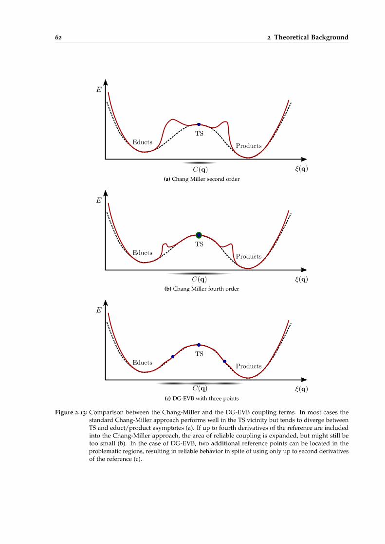
62 2 Theoretical Background
EductsTS
Products
(a) Chang Miller second order
EductsTS
Products
(b) Chang Miller fourth order
EductsTS
Products
(c) DG-EVB with three points
Figure 2.13: Comparison between the Chang-Miller and the DG-EVB coupling terms. In most cases thestandard Chang-Miller approach performs well in the TS vicinity but tends to diverge betweenTS and educt/product asymptotes (a). If up to fourth derivatives of the reference are includedinto the Chang-Miller approach, the area of reliable coupling is expanded, but might still betoo small (b). In the case of DG-EVB, two additional reference points can be located in theproblematic regions, resulting in reliable behavior in spite of using only up to second derivativesof the reference (c).
2.4 Empirical Valence Bond 63
polynomial prefactor. Then, we get three Gaussians, with prefactors A (constant), AB · ∆q (linear)and A 1
2 ∆q · (C + αI) · ∆q (quadratic). This can be compared to Gaussian-type basis functions asused in quantum chemistry. Those are usually expressed in cartesian coordinates:
Gi,j,k(x, α, a) = xiayj
azkae−αr2
a , (2.153)
where x is the actual position in cartesian space, α the exponential prefactor, a the position andL = i + j + k the angular momentum of the basis function. As it is well known from quantumchemistry, functions with L = 0 are s-functions, those with L = 1 are p-functions etc. .
In quantum chemistry, the MOs are expressed as LCAO, which themselves are simply theGaussian basis functions or fixed linear combinations of them.
For this distributed Gaussian (DG)-EVB, the same idea can be utilized. Instead of MOs we want toexpress the coupling term C(q) as linear combination of the basis functions. The MOs are locatedin the three dimensional cartesian space, but C(q) depends on all N chosen internal coordinates42.Therefore, the number of basis functions for a given angular momentum value L is different, itdepends on the used set of internal coordinates. In quantum chemistry, there are one s-function,three p-functions and five/six d-functions43, for DG-EVB, there are one s-function, N p-functionsand N(N−1)
2 d-functions per reference point. The s-functions in DG-EVB are defined as:
g(q, qK, 0, 0, αK) =
[1 +
12
αK|∆qK|2]
exp[
12
αK|∆qK|2]
, (2.154)
where q is the actual point in internal coordinate space, qK the position of the basis function,∆qK = q− qK and αK the exponential prefactor of the function. Instead of simply using 1 as globalprefactor, the squared distance is taken in order to improve the behavior of the coefficient matrix(see below).
p-functions are defined as:
g(q, qK, i, 0, αK) = (∆qK)i exp[
12
αK|∆qK|2]
, (2.155)
with i being the internal coordinate whose angular momentum is 1. In the case of d-functions,the unit matrix from eq. 2.151 is applied:
g(q, qK, i, j, αK) =
(1− 1
2δij
)(∆qK)i(∆qK)j exp
[12
αK|∆qK|2]
. (2.156)
A general linear combination consists of s-, p- and d-functions at different points in coordinatespace, the DG-coupling term can be expressed as:
C(q)2 =M
∑K
N
∑i=j=0
bijKg(q, qK, i, j, αK), (2.157)
with M being the number of DG-EVB points. By comparing eq. 11.109 with eq. 2.151, onecan see that the parameters A, B and C were exchanged with the bijk-coefficients that are so farunknown.
42 In principle, DG-EVB could also be implemented with usage of cartesian coordinates. However, since the molecularsystem will move and rotate during MD simulations, the coupling needs to be independent of overall translations androtations, which is achieved with internal coordinates. The actual choice of internals for DG-EVB is far from trivial (seechapter 4 and section 11.6.2). Detailed descriptions of the internal coordinates used within the EVB-QMDFF programpackages are presented in section 11.3.2.
43 According to eq. 2.153, s-functions are uniquely defined by i = j = k = 0, for p-functions one of the prefactors is 1,with all others zero (x, y, z), for d-functions there are 9 possible permutations. Imposing symmetry, 6 of them remain(x2,y2,z2,xy,xz,yz). These are used for some basis sets. Others use linear combinations (x2 − y2 instead of x2, y2),reducing the total number of d-functions to 5 [12]
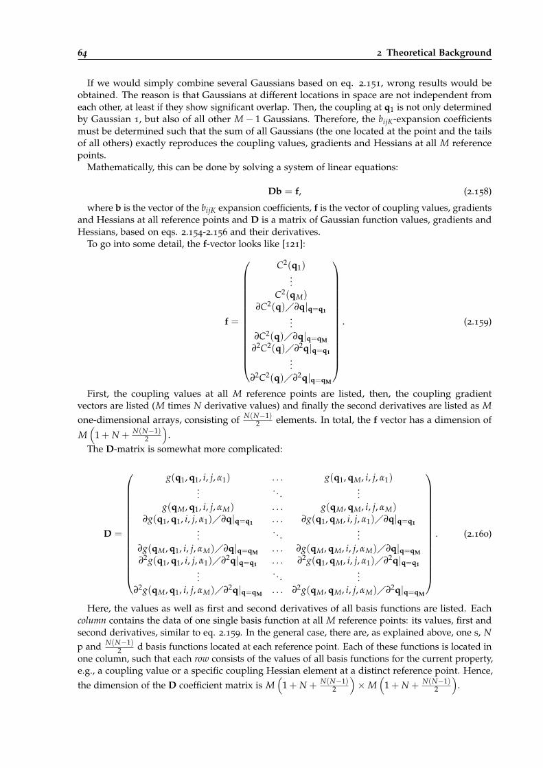
64 2 Theoretical Background
If we would simply combine several Gaussians based on eq. 2.151, wrong results would beobtained. The reason is that Gaussians at different locations in space are not independent fromeach other, at least if they show significant overlap. Then, the coupling at q1 is not only determinedby Gaussian 1, but also of all other M− 1 Gaussians. Therefore, the bijK-expansion coefficientsmust be determined such that the sum of all Gaussians (the one located at the point and the tailsof all others) exactly reproduces the coupling values, gradients and Hessians at all M referencepoints.
Mathematically, this can be done by solving a system of linear equations:
Db = f, (2.158)
where b is the vector of the bijK expansion coefficients, f is the vector of coupling values, gradientsand Hessians at all reference points and D is a matrix of Gaussian function values, gradients andHessians, based on eqs. 2.154-2.156 and their derivatives.
To go into some detail, the f-vector looks like [121]:
f =
C2(q1)...
C2(qM)∂C2(q)�∂q|q=q1
...∂C2(q)�∂q|q=qM
∂2C2(q)�∂2q|q=q1...
∂2C2(q)�∂2q|q=qM
. (2.159)
First, the coupling values at all M reference points are listed, then, the coupling gradientvectors are listed (M times N derivative values) and finally the second derivatives are listed as Mone-dimensional arrays, consisting of N(N−1)
2 elements. In total, the f vector has a dimension of
M(
1 + N + N(N−1)2
).
The D-matrix is somewhat more complicated:
D =
g(q1, q1, i, j, α1) . . . g(q1, qM, i, j, α1)...
. . ....
g(qM, q1, i, j, αM) . . . g(qM, qM, i, j, αM)∂g(q1, q1, i, j, α1)�∂q|q=q1 . . . ∂g(q1, qM, i, j, α1)�∂q|q=q1
.... . .
...∂g(qM, q1, i, j, αM)�∂q|q=qM . . . ∂g(qM, qM, i, j, αM)�∂q|q=qM
∂2g(q1, q1, i, j, α1)�∂2q|q=q1 . . . ∂2g(q1, qM, i, j, α1)�∂2q|q=q1...
. . ....
∂2g(qM, q1, i, j, αM)�∂2q|q=qM . . . ∂2g(qM, qM, i, j, αM)�∂2q|q=qM
. (2.160)
Here, the values as well as first and second derivatives of all basis functions are listed. Eachcolumn contains the data of one single basis function at all M reference points: its values, first andsecond derivatives, similar to eq. 2.159. In the general case, there are, as explained above, one s, Np and N(N−1)
2 d basis functions located at each reference point. Each of these functions is located inone column, such that each row consists of the values of all basis functions for the current property,e.g., a coupling value or a specific coupling Hessian element at a distinct reference point. Hence,the dimension of the D coefficient matrix is M
(1 + N + N(N−1)
2
)×M
(1 + N + N(N−1)
2
).
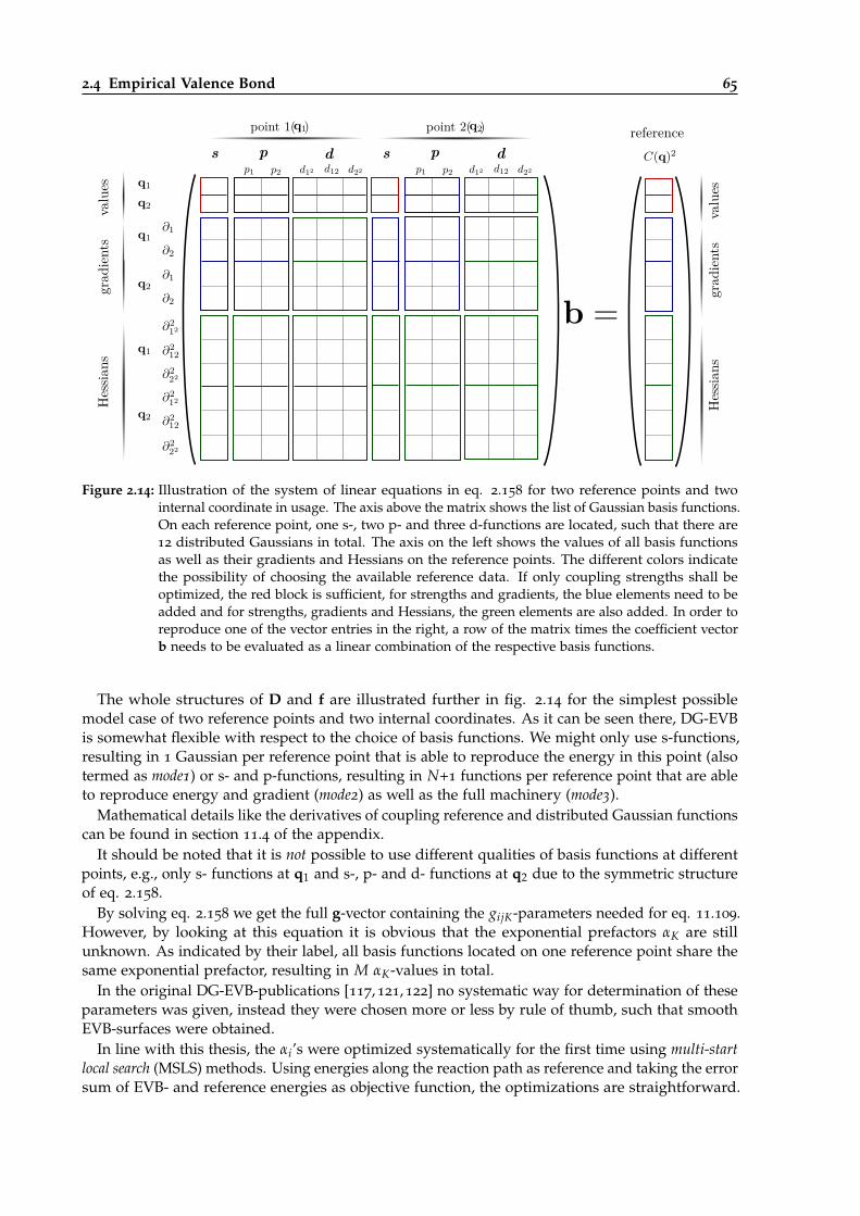
2.4 Empirical Valence Bond 65
s p d s p d
valu
esgr
adie
nts
Hes
sians
point 1( ) point 2( ) reference
valu
esgr
adie
nts
Hes
sians
Figure 2.14: Illustration of the system of linear equations in eq. 2.158 for two reference points and twointernal coordinate in usage. The axis above the matrix shows the list of Gaussian basis functions.On each reference point, one s-, two p- and three d-functions are located, such that there are12 distributed Gaussians in total. The axis on the left shows the values of all basis functionsas well as their gradients and Hessians on the reference points. The different colors indicatethe possibility of choosing the available reference data. If only coupling strengths shall beoptimized, the red block is sufficient, for strengths and gradients, the blue elements need to beadded and for strengths, gradients and Hessians, the green elements are also added. In order toreproduce one of the vector entries in the right, a row of the matrix times the coefficient vectorb needs to be evaluated as a linear combination of the respective basis functions.
The whole structures of D and f are illustrated further in fig. 2.14 for the simplest possiblemodel case of two reference points and two internal coordinates. As it can be seen there, DG-EVBis somewhat flexible with respect to the choice of basis functions. We might only use s-functions,resulting in 1 Gaussian per reference point that is able to reproduce the energy in this point (alsotermed as mode1) or s- and p-functions, resulting in N+1 functions per reference point that are ableto reproduce energy and gradient (mode2) as well as the full machinery (mode3).
Mathematical details like the derivatives of coupling reference and distributed Gaussian functionscan be found in section 11.4 of the appendix.
It should be noted that it is not possible to use different qualities of basis functions at differentpoints, e.g., only s- functions at q1 and s-, p- and d- functions at q2 due to the symmetric structureof eq. 2.158.
By solving eq. 2.158 we get the full g-vector containing the gijK-parameters needed for eq. 11.109.However, by looking at this equation it is obvious that the exponential prefactors αK are stillunknown. As indicated by their label, all basis functions located on one reference point share thesame exponential prefactor, resulting in M αK-values in total.
In the original DG-EVB-publications [117, 121, 122] no systematic way for determination of theseparameters was given, instead they were chosen more or less by rule of thumb, such that smoothEVB-surfaces were obtained.
In line with this thesis, the αi’s were optimized systematically for the first time using multi-startlocal search (MSLS) methods. Using energies along the reaction path as reference and taking the errorsum of EVB- and reference energies as objective function, the optimizations are straightforward.
66 2 Theoretical Background
More details concerning this procedure and the general DG-EVB-methodology can be found inchapter 4.
The DG-EVB-method is one of the central topics in this thesis. In chapters 4 and 5, furtherexperiments done with DG-EVB are presented.
2.4.6 Reaction Path (RP)-EVB with Corrections
The DG-EVB method as exposed in the last section in connection with QMDFF as diabatic surfaceshas been shown to be quite a reliable foundation for partially automated generations of PESssuitable for chemical rate constant calculations [17].
It was indeed the hope that DG-EVB-QMDFF could be a suitable method for general automatedk(T) calculations as it is the overall aim of this thesis. However, unexpected problems arose shortlyafter it became established. Details of the problems are shown in upcoming chapters but in short itseems that the connection of several Taylor expansions along the reaction path is still not sufficientin many cases where the convergence radii of the Taylor series are too small and/or the diabaticsurfaces (i.e., the QMDFFs) show bad behavior, largely reducing the viability of eq. 2.143.
In line with the efforts to solve those problems, a new EVB coupling term was developed in thescope of this thesis [18]. Theoretical background as well as benchmarking results are presented inchapter 5 with great detail. Therefore, only a short-as-possible overview of the method is givenhere.
The main idea is to make the reaction path itself, a one-dimensional curve in the N-dimensionalspace of internal coordinates, the central part for the description of the coupling. Since we areinterested in the calculation of k(T)-values and other properties related to them, an as-good-aspossible description of this path and its accessible vicinity is crucial for the method of choice.
In DG-EVB, a good description of the reaction path can be achieved by optimizing the αK-valuesin order to minimize the error sum with respect to a reference path. In combination with thedistributed Gaussians themselves, quite a good description of the relevant regions is possible inmany cases. But a good description of regions between two DG-EVB points and only slightly awayfrom the optimized path cannot be guaranteed. Therefore, the method fails in many seeminglysimple cases: The system’s trajectory could, for instance, be trapped in holes or chasms existent inthe PES near the reaction path.
In reaction path (RP)-EVB this path becomes a central part of the coupling formulation. Essentially,a given reference reaction path is modeled via cubic spline interpolation and then a Taylor expansionis built around it:
C(q)2 = C(s)2 + ∆q∂C(s)2
∂q+
12
∆q∂2C(s)2
∂q2 ∆q. (2.161)
There, C(s) is the coupling strength along the reaction path, dependent on the parameter s ofthe cubic spline curve. In practice, internal coordinates of the path structures as well as couplingstrengths calculated according to eq. 11.109 are interpolated as a one-dimensional parametric curve
in N + 1-dimensional space. The gradients ∂C(s)2
∂q and Hessians ∂2C(s)2
∂q2 of the coupling are alsointerpolated between a smaller number of energy-, gradient- and Hessian-reference points on thepath, based on the s-parameter. This is illustrated in fig. 2.15.
During a MD calculation, the value of the s-parameter has to be calculated first, this is doneby numerical minimization of the distance between the current structure and the reaction pathcurve, such that the current structure is projected on the reaction path. With the known valueof s, the nearest structure on the reaction path curve as well as its coupling value C(s) can becalculated. With this information, the projection vector ∆q from the current structure to the pathcan be determined and finally C(q) is calculated with eq. 2.161.
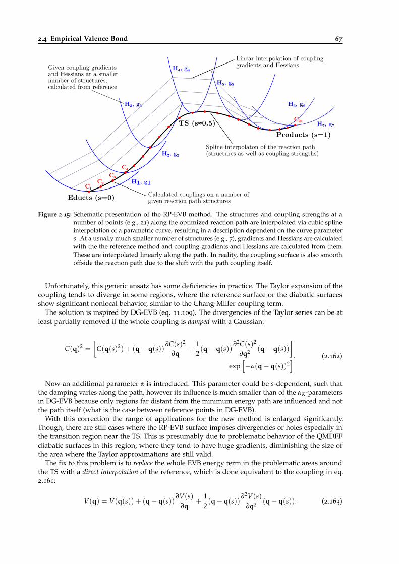
2.4 Empirical Valence Bond 67
H1, g1
H2, g2
H3, g3
H4, g4
H5, g5
H6, g6
H7, g7
C1C2
C3
C4
C21
Calculated couplings on a number of given reaction path structures
Spline interpolaton of the reaction path (structures as well as coupling strengths)
Linear interpolation of couplinggradients and HessiansGiven coupling gradients
and Hessians at a smaller number of structures,calculated from reference
Educts (s=0)
Products (s=1)TS (s≈0.5)
Figure 2.15: Schematic presentation of the RP-EVB method. The structures and coupling strengths at anumber of points (e.g., 21) along the optimized reaction path are interpolated via cubic splineinterpolation of a parametric curve, resulting in a description dependent on the curve parameters. At a usually much smaller number of structures (e.g., 7), gradients and Hessians are calculatedwith the the reference method and coupling gradients and Hessians are calculated from them.These are interpolated linearly along the path. In reality, the coupling surface is also smoothoffside the reaction path due to the shift with the path coupling itself.
Unfortunately, this generic ansatz has some deficiencies in practice. The Taylor expansion of thecoupling tends to diverge in some regions, where the reference surface or the diabatic surfacesshow significant nonlocal behavior, similar to the Chang-Miller coupling term.
The solution is inspired by DG-EVB (eq. 11.109). The divergencies of the Taylor series can be atleast partially removed if the whole coupling is damped with a Gaussian:
C(q)2 =
[C(q(s)2) + (q− q(s))
∂C(s)2
∂q+
12(q− q(s))
∂2C(s)2
∂q2 (q− q(s))]
exp[−α(q− q(s))2
]. (2.162)
Now an additional parameter α is introduced. This parameter could be s-dependent, such thatthe damping varies along the path, however its influence is much smaller than of the αK-parametersin DG-EVB because only regions far distant from the minimum energy path are influenced and notthe path itself (what is the case between reference points in DG-EVB).
With this correction the range of applications for the new method is enlarged significantly.Though, there are still cases where the RP-EVB surface imposes divergencies or holes especially inthe transition region near the TS. This is presumably due to problematic behavior of the QMDFFdiabatic surfaces in this region, where they tend to have huge gradients, diminishing the size ofthe area where the Taylor approximations are still valid.
The fix to this problem is to replace the whole EVB energy term in the problematic areas aroundthe TS with a direct interpolation of the reference, which is done equivalent to the coupling in eq.2.161:
V(q) = V(q(s)) + (q− q(s))∂V(s)
∂q+
12(q− q(s))
∂2V(s)∂q2 (q− q(s)). (2.163)
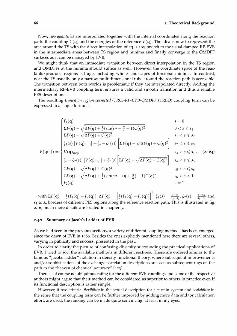
68 2 Theoretical Background
Now, two quantities are interpolated together with the internal coordinates along the reactionpath: the coupling C(q) and the energies of the reference V(q). The idea is now to represent thearea around the TS with the direct interpolation of eq. 2.163, switch to the usual damped RP-EVBin the intermediate areas between TS region and minima and finally converge to the QMDFFsurfaces as it can be managed by EVB.
We might think that an immediate transition between direct interpolation in the TS regionand QMDFFs at the minima should suffice as well. However, the coordinate space of the reac-tants/products regions is huge, including whole landscapes of torsional minima. In contrast,near the TS usually only a narrow multidimensional tube around the reaction path is accessible.The transition between both worlds is problematic if they are interpolated directly. Adding theintermediary RP-EVB coupling term ensures a valid and smooth transition and thus a reliablePES-description.
The resulting transition region corrected (TRC)-RP-EVB-QMDFF (TREQ) coupling term can beexpressed in a single formula:
V(q(s)) =
F1(q) s = 0
ΣF(q)−√
∆F(q) + 12 (sin(sη − π
2 + 1)C(q)2 0 < s 6 s1
ΣF(q)−√
∆F(q) + C(q)2 s1 < s 6 s2
ζ1(s)[V(q)intp
]+ [1− ζ1(s)]
[ΣF(q)−
√∆F(q) + C(q)2
]s2 < s 6 s3
V(q)intp s3 < s 6 s4
[1− ζ2(s)][V(q)intp
]+ ζ2(s)
[ΣF(q)−
√∆F(q) + C(q)2
]s4 < s 6 s5
ΣF(q)−√
∆F(q) + C(q)2 s5 < s 6 s6
ΣF(q)−√
∆F(q) + 12 (sin(sη − (η + π
2 ) + 1)C(q)2 s6 < s < 1
F2(q) s = 1
, (2.164)
with ΣF(q) = 12 (F1(q) + F2(q)), ∆F(q) =
[12 (F1(q)− F2(q))
]2, ζ1(s) =
s−s2s3−s2
, ζ2(s) =s−s4s5−s4
ands1 to s6 borders of different PES regions along the reference reaction path. This is illustrated in fig.2.16, much more details are located in chapter 5.
2.4.7 Summary or Jacob’s Ladder of EVB
As we had seen in the previous sections, a variety of different coupling methods has been emergedsince the dawn of EVB in 1980. Besides the ones explicitly mentioned here there are several others,varying in publicity and success, presented in the past.
In order to clarify the picture of confusing diversity surrounding the practical applications ofEVB, I tried to sort the available methods in different sections. These are ordered similar to thefamous “Jacobs ladder” notation in density functional theory, where subsequent improvementsand/or sophistications of the exchange correlation descriptions are seen as subsequent rugs on thepath to the “heaven of chemical accuracy” [123].
There is of course no ubiquitous rating for the different EVB-couplings and some of the respectiveauthors might argue that their method can be considered as superior to others in practice even ifits functional description is rather simple.
However, if two criteria, flexibility in the actual description for a certain system and scalability inthe sense that the coupling term can be further improved by adding more data and/or calculationeffort, are used, the ranking can be made quite convincing, at least in my eyes.
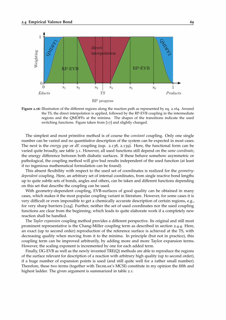
2.4 Empirical Valence Bond 69
Wei
ghtin
g1
010 s2 s3 s4 s5
QMDF
F1
QMDFF2
RP-EVB RP-EVB
TS
direct interpolation
RP progress
Educts Productss6s1
Figure 2.16: Illustration of the different regions along the reaction path as represented by eq. 2.164. Aroundthe TS, the direct interpolation is applied, followed by the RP-EVB coupling in the intermediateregions and the QMDFFs at the minima. The shapes of the transitions indicate the usedswitching functions. Figure taken from [17] and slightly changed.
The simplest and most primitive method is of course the constant coupling. Only one singlenumber can be varied and no quantitative description of the system can be expected in most cases.The next is the energy gap or dE coupling (eqs. 2.138, 2.139). Here, the functional form can bevaried quite broadly, see table 3.1. However, all used functions still depend on the same coordinate,the energy difference between both diabatic surfaces. If these behave somehow asymmetric orpathological, the coupling method will give bad results independent of the used function (at leastif no ingenious mathematical formulation can be found).
This absent flexibility with respect to the used set of coordinates is realized for the geometry-dependent coupling. Here, an arbitrary set of internal coordinates, from single reactive bond lengthsup to quite subtle sets of bonds, angles and others, can be taken and different functions dependingon this set that describe the coupling can be used.
With geometry-dependent coupling, EVB-surfaces of good quality can be obtained in manycases, which makes it the most popular coupling variant in literature. However, for some cases it isvery difficult or even impossible to get a chemically accurate description of certain regions, e.g.,for very sharp barriers [124]. Further, neither the set of used coordinates nor the used couplingfunctions are clear from the beginning, which leads to quite elaborate work if a completely newreaction shall be handled.
The Taylor expansion coupling method provides a different perspective. Its original and still mostprominent representative is the Chang-Miller coupling term as described in section 2.4.4. Here,an exact (up to second order) reproduction of the reference surface is achieved at the TS, withdecreasing quality when moving from it to the minima. In principle (but not in practice), thiscoupling term can be improved arbitrarily, by adding more and more Taylor expansion terms.However, the scaling exponent is incremented by one for each added term.
Finally, DG-EVB as well as the newly invented TRE(Q) methods are able to reproduce the regionsof the surface relevant for description of a reaction with arbitrary high quality (up to second order),if a huge number of expansion points is used (and still quite well for a rather small number).Therefore, these two terms (together with Truhlar’s MCSI) constitute in my opinion the fifth andhighest ladder. The given argument is summarized in table 2.1.
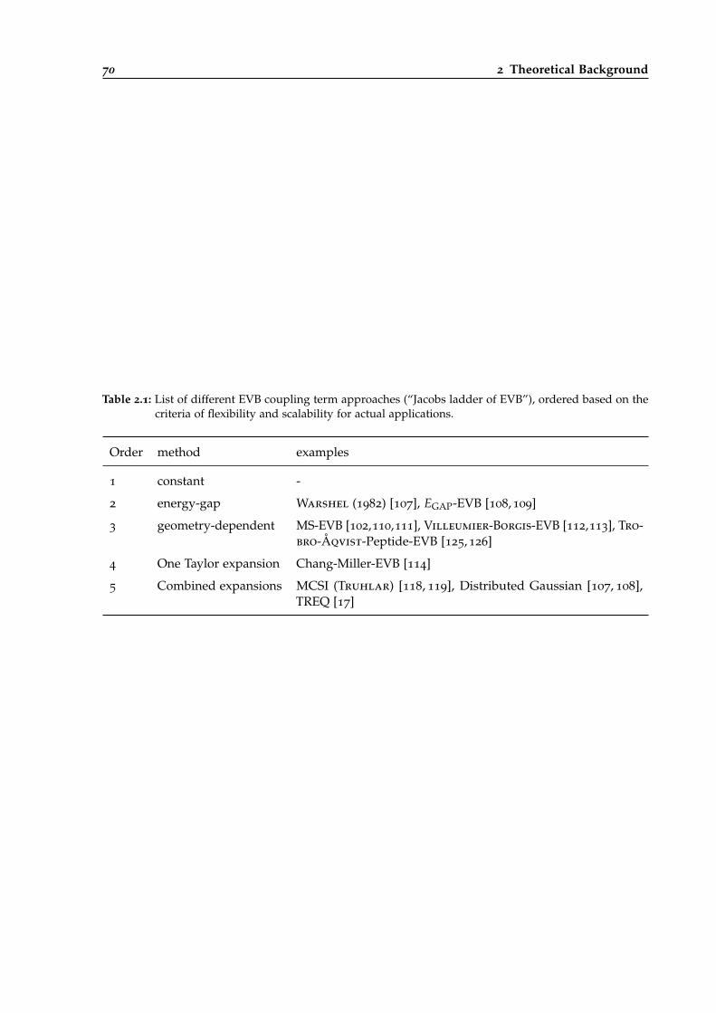
70 2 Theoretical Background
Table 2.1: List of different EVB coupling term approaches (“Jacobs ladder of EVB”), ordered based on thecriteria of flexibility and scalability for actual applications.
Order method examples
1 constant -
2 energy-gap Warshel (1982) [107], EGAP-EVB [108, 109]
3 geometry-dependent MS-EVB [102,110,111], Villeumier-Borgis-EVB [112,113], Tro-bro-Åqvist-Peptide-EVB [125, 126]
4 One Taylor expansion Chang-Miller-EVB [114]
5 Combined expansions MCSI (Truhlar) [118, 119], Distributed Gaussian [107, 108],TREQ [17]
3
Ch
ap
te
r
Program Development
In line with this thesis, a program package named EVB-QMDFF was developed to be used for thecalculations presented in the following sections.
Before going to concrete applications, the general structure of this program package shall beoutlined. A detailed discussion of all contained subroutines is impractical, since it would probablyneed several hundred pages, while no real insight for the average reader can be gained.
Therefore a rather coarse description will be given, first outlining the history, general structureand idea of the whole package, then going into some detail concerning the different programs thatare designed to perform a number of frequently needed tasks with EVB-QMDFF.
3.1 History
Before turning to a comprehensive description of the actual implementation and its handlingin practice, a short history of EVB-QMDFF programming shall be givenin order to clarify somepeculiarities that might irritate the reader at some point.
I have subdivided the program development into four stages. Of course, the changes were donesuccessively during my work, some improvements were made as deficiencies became apparent atcertain applications or as colleagues or my supervisor had ideas to make things easier.
Nevertheless, four milestones can be clearly identified, without them the applications presentedwithin this thesis would have been simply impossible to do. An overview of this four developmentmilestones is given in fig. 3.1.
3.1.1 Version 1: The Origins
EVB-QMDFF was invented by Hartke [16], who also wrote its first implementation. He obtainedthe QMDFF program by Grimme which itself was able to calculate energies and gradients as wellas performing geometry optimizations and MD with QMDFF. Hartke wrote a new program whichcalled the internal energy and gradient routines of QMDFF (Up to three instances of them, since2x2- and 3x3-EVB could be used) and coupled them with EVB. Two simple coupling terms wereavailable: constant coupling (eq. 2.137) as well as the Gaussian energy-gap coupling (eq. 2.139).
The parameters of the coupling terms were given by the user in the input file. This programcould calculate energies and gradients for a trajectory of structures, e.g., in order to perform surfacescans. Before doing the EVB-calculation, both QMDFFs needed to be set up with the QMDFFoptimization program, their relative energies were calculated from the QM reference energies of thereactants/products minima, corrected by the QMDFF energy deviation, introduced by noncovalentinteractions (section 2.3.4).
72 3 Program Development
With this first version, the general concept of coupling two QMDFFs with simple EVB terms wasintroduced, however, it was unable to do more sophisticated tasks like running MD, doing k(T)calculations, optimize more complicated EVB terms and so forth.
3.1.2 Version 2: EVB-QMDFF-Tinker
During my Master’s thesis [124], the next program version was developed. Originally, the aimwas to check whether EVB-QMDFF is able to represent the PES also offside the reaction pathused for parametrization of EVB in the transition region. There is no guarantee at all that regionsslightly offside this path are reproduced even qualitatively if the simple constant or energy-gap EVBmethods are used. The first step of investigating this was to perform two-dimensional scans forseveral combinations of internal coordinates. This was done with the first version of EVB-QMDFF( [16], supporting information (section 11.6.1)).
For three-atomic systems, a three-dimensional coordinate scan would be needed in order to fullydiscover the configuration space and hence get a complete picture of the EVB-QMDFF quality.Even in the case of still quite small four- or five-atomic systems, this approach of full-dimensionalscanning becomes infeasible due to its exponential scaling. Furthermore, a large fraction of thescanned coordinate-space is needless as only regions of low energy are relevant in practice. Analternative is to utilize the ergodic theorem and perform coordinate samplings. From those, free-energy profiles can be obtained (section 2.1.3) and compared with AIMD samplings (at least wherea sufficiently cheap ab-initio method is used).
However, in order to simulate biased sampling trajectories, new program code had to be added.Instead of writing it myself, I chose to utilize existent program packages.
This led to the EVB-QMDFF-Tinker program package. The existing EVB-QMDFF program wascoupled to the well known Tinker FF-MD program package [127], which is also written in Fortran.The gradient routine in Tinker was replaced by the EVB-QMDFF gradient routine such that a coupleof Tinker features, for instance, molecular dynamics, geometry optimization, TS optimization andmany others, could be applied for EVB-QMDFF.
Because biased samplings are not included in Tinker, a MD addon particularly designed forthose tasks was added: Plumed [128]. It enables a whole range of different collective variables (CV)for application of bias potentials.
Finally, free energy profiles were calculated by combination of several biased samplings. Again,a separate program was used: WHAM by Grossfield [129]. As the name says, it applies theWHAM-equations (eqs. 2.38-2.39) for calculation of free energy surfaces.
In order to investigate the overall quality of EVB-QMDFF, free energy surfaces were calculatedwith AIMD (by implementing a call to an Orca [130, 131] gradient calculation in the modifiedTinker program) as well as with EVB-QMDFF and compared to each other. Since information ofthe whole thermally accessible surface is accumulated in both cases, a good agreement of the freeenergy surfaces implies an EVB-QMDFF of high quality.
Besides the ability of calculating free energy surfaces, different energy-gap as well as simplecoordinate-dependent EVB-coupling terms were implemented, with automated optimization oftheir parameters. The quadratic Chang-Miller coupling term (section 2.4.4) was implemented aswell for benchmark purposes (no dynamics was possible since this coupling term was constructedbased on cartesian coordinates). Further, the relative energy-adjustment of both QMDFFs previousto the EVB-optimization was automated.
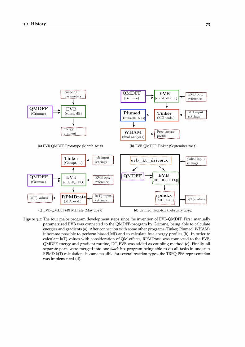
3.1 History 73
QMDFF EVB (const, dE)
coupling parameters
(Grimme)
energy +gradient
(a) EVB-QMDFF Prototype (March 2015)
QMDFF EVB (const, dE, dQ) (Grimme)
TinkerPlumed
WHAM Free energyprofile
MD input settings (MD trajs.) (Umbrella bias)
(final analysis)
EVB opt.reference
(b) EVB-QMDFF-Tinker (September 2015)
QMDFF EVB (dE, dQ, DG) (Grimme)
Tinker (Geoopt, ...)
RPMDrate (MD, eval.)
k(T)-values
EVB opt.reference
k(T) input settings
job input settings
(c) EVB-QMDFF+RPMDrate (May 2017)
global inputsettings
k(T)-values
QMDFF EVB (dE, DG,TREQ)
rpmd.x
evb_kt_driver.x
(MD, eval.)
(d) Unified black-box (February 2019)
Figure 3.1: The four major program development steps since the invention of EVB-QMDFF. First, manuallyparametrized EVB was connected to the QMDFF-program by Grimme, being able to calculateenergies and gradients (a). After connection with some other programs (Tinker, Plumed, WHAM),it became possible to perform biased MD and to calculate free energy profiles (b). In order tocalculate k(T)-values with consideration of QM-effects, RPMDrate was connected to the EVB-QMDFF energy and gradient routine, DG-EVB was added as coupling method (c). Finally, allseparate parts were merged into one black-box program being able to do all tasks in one step.RPMD k(T) calculations became possible for several reaction types, the TREQ PES representationwas implemented (d).
74 3 Program Development
3.1.3 Version 3: EVB-QMDFF+RPMDrate
In the Master’s thesis, the ability of EVB-QMDFF to reproduce all relevant areas along a reactionpath with at least acceptable quality was verified for two example reactions. The next step was tomake the method useful in practice.
Free energy profiles are used to calculate several quantities, for small gas phase systems upto large solvated enzymes or metal clusters. As explained in section 2.1, chemical reaction rateconstants are of central importance for the quantification of reactions.
Therefore, it was the objective to implement a method for the calculation of k(T)-values based ontrajectory samplings.
Fortunately, we discovered the RPMDrate program [13] which is designed to calculate bimolecularreaction rate constants based on RPMD samplings (eq. 2.103). Its concept is suited almost perfectlyto EVB-QMDFF: A potential function expressed as Fortran subroutine needs to be supplied by theuser such that RPMDrate is able to request energy and gradient for each dynamics step.
Instead of the rather complicated combination of EVB-QMDFF, Tinker, Plumed and WHAM, onlyEVB-QMDFF and RPMDrate are needed to perform the whole calculation. In addition, quantumeffects can be considered with the RPMD method (section 2.1.6).
Shortly after establishing k(T)-calculations, it became clear that the rather simple EVB-couplingmethods used so far were mostly unable to provide the degree of accuracy needed to obtainreasonable rate constants. Due to the exponential dependence of the free energy barrier in thecase of k(T)-calculations, small errors in the EVB-QMDFF representation are magnified into largek(T)-errors. Therefore, an EVB-coupling method located much higher on the Jacobs ladder of EVB(table 2.1) was needed. DG-EVB was the method of choice. Its quality can be raised arbitrarily highif enough reference points with gradient and Hessian reference information are taken into account.The method was implemented in the EVB-QMDFF code, further, an automated optimization of theαi-parameters (eq. 11.109) was introduced in order to make the whole process more convenient.
With this program version, the results presented in the second EVB-QMDFF paper [17] (chapter4) were produced.
3.1.4 Version 4: Unification
The initial point for the next program development step was the cooperation with Covestro initiatedin 2017 (chapter 8). During this cooperation the kinetics of polyurethane systems should be studied.Polyurethanes are formed by a polyaddition reaction of isocyanates and alcohols.
The program structure so far, i.e., k(T)-calculations by RPMDrate based on the EVB-QMDFFPES, was unable to deliver such rate constants: RPMDrate is designed to calculate only rates ofbimolecular reactions with two reactants and two products, whereas in a polyadditon two reactantsare merged into one product. Another disadvantage of RPMDrate was that it is based on Pythoncode, which lead to problems with the needed Python-libraries on the computer clusters used forhigh-throughput calculations of k(T)-values.
In order to solve these problems, I decided to reimplement the RPMD code similar to RPMDratebut with the capability of handling a broader range of reaction types and to lower the dependencyon external libraries. Therefore, the RPMD code was rewritten in Fortran90. In parallel, theremaining parts of the Tinker code were eliminated (apart from the input section). Finally, also theQMDFF code by Grimme was reimplemented into Fortran90, mainly to improve the convenienceof generating new QMDFFs.
With these changes, the program was able to calculate rate constants for the polyadditionprocesses of interest. However, the quality of those rate constants (especially their degree ofconvergence, i.e., the difference between k(T) values of several independent runs) was rather bad.The reason was the DG-EVB coupling used to represent the PESs. At this time, I got the idea for
3.2 General Statistics 75
constructing a new coupling term named TREQ (section 2.4.6) which was able to improve theconvergence and reliability of the k(T) calculations significantly.
Since TREQ needs no parameter optimization (apart from the α-damping factor of the RP-EVBpart (eq. 2.162), where a default value works well in many cases), it became clear that a black-boxcalculation of reaction rates was possible with it. All calculations, from the QMDFF- and EVB-parametrizations up to the k(T)-calculations, are done with the same program package, only amaster program (or driver) was needed to call the different programs with the correct parameters.The latest significant change of the program code was therefore the addition of such a driverprogram, named evb_kt_driver.x.
Over the years, the initial collection of several independent programs needed for the calculationof free energy profiles therefore merged to one large program package which is able to do all tasksconducted in this thesis. Another advantage is that the user only needs to compile one large bunchof Fortran programs, subroutines and functions which is done by a single make command insteadof installing several independent program packages from the literature.
3.2 General Statistics
Before going to a detailed description of the interactions between the several executables, subrou-tines and functions contained into EVB-QMDFF, it might be interesting to see its overall dimensionin terms of some numbers (status: September 2019):
• No. of bytes (uncompiled): 6496256
• No. of bytes (compiled): 19992576
• No. of source code files: 331
• Source code lines (including comments): 133262
• No. of programs: 8
• No. of modules: 6
• No. of subroutines: 409
• No. of functions: 34
• No. of subroutine calls: 2337
Approximately 95% of this code is written in Fortran90, with Fortran77 code forming the other5%. The Fortran77 subroutines are mainly the embedded PES functions for the analytical surfacestaken from the literature (see section 3.3.3).
In total, 148 functions and subroutines originate in the QMDFF program by Grimme. Theywere translated from Fortran77 to Fortran90 and slightly changed in some parts concerning theread-in of QM reference data (see below). Another bunch of approx. 50 functions and subroutinesis inspired from RPMDrate, concerning trajectory samplings, biasing potentials, as well as freeenergy and recrossing calculations. Here, the biasing part was altered to a more general form inorder to make k(T)-calculations for a larger range of cases possible (more complex bimolecular aswell as unimolecular reactions with almost arbitrary mechanisms). Further, WHAM calculationsof free energy profiles were implemented in addition to the UI contained in RPMDrate. Theparallelization was completely redone with usage of the message passing interface (MPI) instead ofthe original Python approach. The recrossing part was parallelized as well, which was not the casein RPMDrate, therefore further accelerating the rate constant calculations.
76 3 Program Development
The method of reading user input was inspired by Tinker, yet almost no unaltered Tinker coderemained in EVB-QMDFF.
All other functions and subroutines were implemented over the years, they are described in sec.3.3 with some detail.
3.3 Program Descriptions
In the following, the eight different programs contained in the EVB-QMDFF package are inspectedmore closely. Details concerning the actual executions of calculations (list of all keywords as wellas example input files) are presented in section 11.5 of the appendix. If a black-box k(T) calculationshall be done, only program evb_kt_driver.x (section 3.3.8) must be executed, which itself callsall other programs if needed.
3.3.1 qmdffgen
This program needs to be started first when a new system shall be investigated with EVB-QMDFF.It is able to generate up to three QMDFFs1 and calculate their correct relative energy shift suchthat the EVB coupling can be applied in the next step.
Reference data calculated by four different QM-program packages can be used: Gaussian [99],Orca [130, 131], Turbomole [132] and CP2K [133, 134]. For all but Gaussian and CP2K, geometryoptimization as well as calculation of all reference data can be done with one single program call,whereas Gaussian needs a separate geometry optimization2 and CP2K only calculates CM5-chargesfor separate geometry optimizations. Besides these QM-programs, also EVB-QMDFF calculationscan be done as reference. This is mainly for benchmark reasons (chapter 5).
After the QM-calculations are done, their logfiles should be copied into a QMDFF folder, thenqmdff.x can be started.
After finishing, the QMDFF force field files (name.qmdff) as well as logfiles with detailed informa-tion about the parametrization processes (name_qmdff.log) are written. Further, a qmdff.key file iswritten which serves as initial point for all following calculations. In this file, the energy-shifts ofboth QMDFFs are noted. These can be calculated as
Eshift = Eref − Emin,QMDFF, (3.1)
with Eref the QM reference energy of the structure and Emin,QMDFF its (usually very small)QMDFF energy.
3.3.2 evbopt
For all EVB-methods but TREQ, coupling parameters need to be optimized before, e.g., a dynamiccalculation can be done. Currently, four different EVB-methods are implemented for optimization:constant, energy-gap, coordinate-dependent and DG-EVB (table 2.1).
The aim of the parameter optimization is to minimize the error sum χ2 between EVB-QMDFFand ab-initio reference energies for a number of structures:
χ2(α) = ∑i
(Eref(xi)− EEVB(α, xi))2
σ7−→ min, (3.2)
1 For all applications presented in this thesis two QMDFFs were used, further, DG-EVB and TREQ (currently) only workfor two QMDFFs, such that the possibility to parametrize three QMDFFs is of little use in practice.
2 According to the Gaussian manual it should be possible to do all this at a time. But unfortunately the cartesian Hessianitself is not printed to file (only the normal mode vibrations) in the case of combined optimization and frequencycalculations.
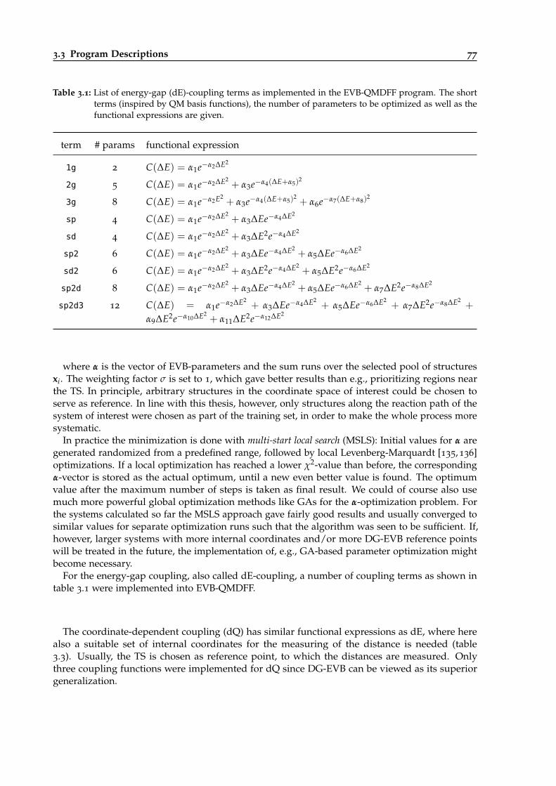
3.3 Program Descriptions 77
Table 3.1: List of energy-gap (dE)-coupling terms as implemented in the EVB-QMDFF program. The shortterms (inspired by QM basis functions), the number of parameters to be optimized as well as thefunctional expressions are given.
term # params functional expression
1g 2 C(∆E) = α1e−α2∆E2
2g 5 C(∆E) = α1e−α2∆E2+ α3e−α4(∆E+α5)
2
3g 8 C(∆E) = α1e−α2E2+ α3e−α4(∆E+α5)
2+ α6e−α7(∆E+α8)
2
sp 4 C(∆E) = α1e−α2∆E2+ α3∆Ee−α4∆E2
sd 4 C(∆E) = α1e−α2∆E2+ α3∆E2e−α4∆E2
sp2 6 C(∆E) = α1e−α2∆E2+ α3∆Ee−α4∆E2
+ α5∆Ee−α6∆E2
sd2 6 C(∆E) = α1e−α2∆E2+ α3∆E2e−α4∆E2
+ α5∆E2e−α6∆E2
sp2d 8 C(∆E) = α1e−α2∆E2+ α3∆Ee−α4∆E2
+ α5∆Ee−α6∆E2+ α7∆E2e−α8∆E2
sp2d3 12 C(∆E) = α1e−α2∆E2+ α3∆Ee−α4∆E2
+ α5∆Ee−α6∆E2+ α7∆E2e−α8∆E2
+
α9∆E2e−α10∆E2+ α11∆E2e−α12∆E2
where α is the vector of EVB-parameters and the sum runs over the selected pool of structuresxi. The weighting factor σ is set to 1, which gave better results than e.g., prioritizing regions nearthe TS. In principle, arbitrary structures in the coordinate space of interest could be chosen toserve as reference. In line with this thesis, however, only structures along the reaction path of thesystem of interest were chosen as part of the training set, in order to make the whole process moresystematic.
In practice the minimization is done with multi-start local search (MSLS): Initial values for α aregenerated randomized from a predefined range, followed by local Levenberg-Marquardt [135, 136]optimizations. If a local optimization has reached a lower χ2-value than before, the correspondingα-vector is stored as the actual optimum, until a new even better value is found. The optimumvalue after the maximum number of steps is taken as final result. We could of course also usemuch more powerful global optimization methods like GAs for the α-optimization problem. Forthe systems calculated so far the MSLS approach gave fairly good results and usually converged tosimilar values for separate optimization runs such that the algorithm was seen to be sufficient. If,however, larger systems with more internal coordinates and/or more DG-EVB reference pointswill be treated in the future, the implementation of, e.g., GA-based parameter optimization mightbecome necessary.
For the energy-gap coupling, also called dE-coupling, a number of coupling terms as shown intable 3.1 were implemented into EVB-QMDFF.
The coordinate-dependent coupling (dQ) has similar functional expressions as dE, where herealso a suitable set of internal coordinates for the measuring of the distance is needed (table3.3). Usually, the TS is chosen as reference point, to which the distances are measured. Onlythree coupling functions were implemented for dQ since DG-EVB can be viewed as its superiorgeneralization.
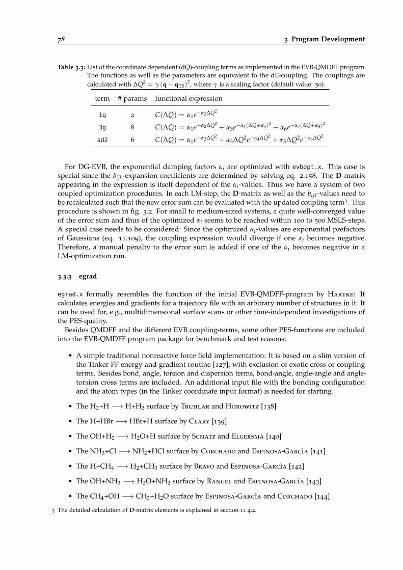
78 3 Program Development
Table 3.3: List of the coordinate dependent (dQ)-coupling terms as implemented in the EVB-QMDFF program.The functions as well as the parameters are equivalent to the dE-coupling. The couplings arecalculated with ∆Q2 = γ (q− qTS)
2, where γ is a scaling factor (default value: 50).
term # params functional expression
1g 2 C(∆Q) = α1e−α2∆Q2
3g 8 C(∆Q) = α1e−α2∆Q2+ α3e−α4(∆Q+α5)
2+ α6e−α7(∆Q+α8)
2
sd2 6 C(∆Q) = α1e−α2∆Q2+ α3∆Q2e−α4∆Q2
+ α5∆Q2e−α6∆Q2
For DG-EVB, the exponential damping factors αi are optimized with evbopt.x. This case isspecial since the bijk-expansion coefficients are determined by solving eq. 2.158. The D-matrixappearing in the expression is itself dependent of the αi-values. Thus we have a system of twocoupled optimization procedures. In each LM-step, the D-matrix as well as the bijk-values need tobe recalculated such that the new error sum can be evaluated with the updated coupling term3. Thisprocedure is shown in fig. 3.2. For small to medium-sized systems, a quite well-converged valueof the error sum and thus of the optimized αi seems to be reached within 100 to 500 MSLS-steps.A special case needs to be considered: Since the optimized αi-values are exponential prefactorsof Gaussians (eq. 11.109), the coupling expression would diverge if one αi becomes negative.Therefore, a manual penalty to the error sum is added if one of the αi becomes negative in aLM-optimization run.
3.3.3 egrad
egrad.x formally resembles the function of the initial EVB-QMDFF-program by Hartke: Itcalculates energies and gradients for a trajectory file with an arbitrary number of structures in it. Itcan be used for, e.g., multidimensional surface scans or other time-independent investigations ofthe PES-quality.
Besides QMDFF and the different EVB coupling-terms, some other PES-functions are includedinto the EVB-QMDFF program package for benchmark and test reasons:
• A simple traditional nonreactive force field implementation: It is based on a slim version ofthe Tinker FF energy and gradient routine [127], with exclusion of exotic cross or couplingterms. Besides bond, angle, torsion and dispersion terms, bond-angle, angle-angle and angle-torsion cross terms are included. An additional input file with the bonding configurationand the atom types (in the Tinker coordinate input format) is needed for starting.
• The H2+H −→ H+H2 surface by Truhlar and Horowitz [138]
• The H+HBr −→ HBr+H surface by Clary [139]
• The OH+H2 −→ H2O+H surface by Schatz and Elgersma [140]
• The NH3+Cl −→ NH2+HCl surface by Corchado and Espinosa-Garcìa [141]
• The H+CH4 −→ H2+CH3 surface by Bravo and Espinosa-Garcìa [142]
• The OH+NH3 −→ H2O+NH2 surface by Rangel and Espinosa-Garcìa [143]
• The CH4+OH −→ CH3+H2O surface by Espinosa-Garcìa and Corchado [144]
3 The detailed calculation of D-matrix elements is explained in section 11.4.2.
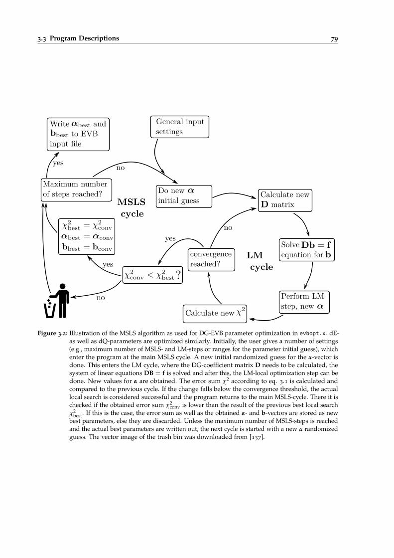
3.3 Program Descriptions 79
General input settings
Do new initial guess
convergence reached?
Calculate new matrix
Solve equation for
Perform LM step, new
Maximum number of steps reached?
Calculate new
no
?
Write and to EVB input file
LM cycle
no
yes
yes
no yes
MSLS cycle
Figure 3.2: Illustration of the MSLS algorithm as used for DG-EVB parameter optimization in evbopt.x. dE-as well as dQ-parameters are optimized similarly. Initially, the user gives a number of settings(e.g., maximum number of MSLS- and LM-steps or ranges for the parameter initial guess), whichenter the program at the main MSLS cycle. A new initial randomized guess for the α-vector isdone. This enters the LM cycle, where the DG-coefficient matrix D needs to be calculated, thesystem of linear equations DB = f is solved and after this, the LM-local optimization step can bedone. New values for α are obtained. The error sum χ2 according to eq. 3.1 is calculated andcompared to the previous cycle. If the change falls below the convergence threshold, the actuallocal search is considered successful and the program returns to the main MSLS-cycle. There it ischecked if the obtained error sum χ2
conv is lower than the result of the previous best local searchχ2
best. If this is the case, the error sum as well as the obtained α- and b-vectors are stored as newbest parameters, else they are discarded. Unless the maximum number of MSLS-steps is reachedand the actual best parameters are written out, the next cycle is started with a new α randomizedguess. The vector image of the trash bin was downloaded from [137].
80 3 Program Development
• The GeH4+OH −→ GeH3+H2O surface by Rangel and Espinosa-Garcìa [145]
• The CH4+CN −→ CH3+HCN surface by Espinosa-Garcìa and Rangel [146]
• The H+C2H6 −→ H2+C2H5 surface by Chakraborty and Truhlar [147]
There is no difference in the handling of all other programs. We can, for instance, calculategradients with egrad.x or rate constants with rpmd.x with EVB-QMDFF or with any of the surfacesmentioned above (calculations of chemical reactions involving bond breakings are of course notpossible with the traditional nonreactive FF). Instead of the QMDFF energy shifts and EVB couplingparameters the keywords trad_ff or pot_ana with a descriptor of the desired surfaces must begiven. No parameter optimization is needed.
We can, e.g., test the quality of an EVB-QMDFF surface by performing a k(T) calculation onone of the surfaces listed above, parametrize an EVB-QMDFF with the program itself as providerof reference information (performing Hessian calculations with evb_qmdff.x, charges and bondorder calculations with a simple ab-initio method, optimizing the QMDFFs based on these data,optimize the IRC with irc.x, calculate additional reference data on it and run evbopt.x) and redothe k(T) calculation. Both reaction rates will be very similar if the relevant areas of the referencePES are reproduced well with EVB-QMDFF. This strategy was used for the benchmarking of TREQpresented in chapter 5.
3.3.4 evb_qmdff
evb_qmdff.x is able to calculate several quantities of a single structure provided by the user. Similarto, e.g., a quantum chemistry program package, the user can give keywords for the calculation ofthe energy, the gradient and the Hessian as well as to do a geometry optimization. The well knownBFGS algorithm [148] was implemented and is used for geometry optimizations.
A special feature is that we can do the calculations as well for parts or fragments of the system. If,e.g., the EVB-QMDFF PES of a bimolecular reaction is given and we want to calculate frequenciesof both separate reactants, e.g., in order to do a TST calculation based on their partition sums, thecalc_frag keyword in combination with a file named fragment.inp that contains the atom indicesof the desired fragments must be added (see table 11.2).
3.3.5 irc
Calculations of reaction paths using the internal reaction coordinate (IRC) algorithm [149] are integralparts of the QM reference calculations for EVB-QMDFF. Therefore, a separate program (irc.x) waswritten to perform such calculations with EVB-QMDFF or the other PES-descriptions provided bythe EVB-QMDFF program package (section 3.3.3).
With this, EVB-QMDFF-benchmarks against other analytical PESs descriptions as mentionedabove are possible. Alternatively, we could, for instance, check how good the reference RP isactually reproduced by the parametrized EVB-QMDFF surface.
In order to start irc.x, an initial guess structure of the TS along the desired IRC is needed.Since the IRC-calculation needs to be started from the imaginary TS-mode, a TS-structure must beoptimized first. The simple NR-algorithm is implemented for TS-optimization.
NR converges always to the nearest stationary point on the PES, therefore a good initial guess ofthe structure is needed in order to converge to the correct TS (and not to, e.g., a local minimum).The method originates in a Taylor expansion around the current position on the PES:
V = V0 + gth +12
htHh + ..., (3.3)
3.3 Program Descriptions 81
where h is the difference vector between the current and the desired points on the PES incartesian coordinates, gt the gradient and H the Hessian at the current position. Going the reversedirection, the step from an elongated structure to the extremum is:
h = −H−1g. (3.4)
This simple algorithm is known to be unstable, since the inverse of the Hessian might be ill-defined due to translational and rotational as well as small vibrational eigenvalues. Therefore, theoptimization is done in a suitable set of internal coordinates, and the step is expressed in terms ofthe eigenvectors (V) and -values (b) of the Hessian matrix H:
h =N
∑i−FiVi
bi, (3.5)
with F = Vg. Only sufficiently large Hessian-eigenvalues are included into the sum. In practice,the same set of internal coordinates as later used for TREQ-couplings can be used for NR, at it wasdone in [17].
When the TS was found, the IRC can be calculated. Since all PES-descriptions in EVB-QMDFFare cheap, a simple but quite expensive IRC algorithm was implemented: the Euler algorithm inmass-weighted cartesian coordinates:
x′k+1 = x′k − ∆sgk||gk||
, (3.6)
with ∆s being the IRC step size chosen by the user and gk the cartesian gradient at point x′k and
x′β,i =√
mβxβ,i (3.7)
describes the mass-weighting of cartesian coordinate i of atom β.The IRC can be followed in two directions (reactants and products), depending on the initial
gradient. Both directions are started at the optimized TS-structure, where the gradient is thecartesian eigenvector of the imaginary TS-eigenmode v or its negative counterpart:
x0 = xTS, g0 = v1 ∨ g0 = −v1. (3.8)
All following IRC steps for both directions are simply calculated with eq. 3.6. Convergence isreached for both sides of the IRC, if ||gk|| or the energy difference EkEk1 falls below a user givenvalue.
In order to get a good description of the path, the step size ∆s should be quite small. However,this results in IRCs containing thousands or tens of thousands of structures that are quite bulky inhandling for, e.g., EVB optimizations. Therefore, a new step is only written after a covered distanceof ∆ς, where ∆ς is by default twenty times larger than the intrinsic Euler distance ∆s. In practice,the optimization might fail in some cases because the energy increases for one direction after thefirst step in eq. 3.8. Presumably this happens because the respective TS optimization was not exactenough, such that the true TS is located near the optimized TS and the first eigenvector-followingstep “climbs the hill” of that true TS. In these cases, ∆s of the first step is increased automaticallyin integer steps until the energy decreases for the reached second structure. After this, the usualstep size is restored.
3.3.6 dynamic
This program performs single MD-trajectores, propagated with the usual velocity Verlet algorithm.Temperature can be applied via the Andersen thermostat [150]. In contrast to usual classical MDprograms, RPMD trajectories with arbitrary bead numbers can be calculated as well.
82 3 Program Development
If trajectories are run with RPMD (no matter if dynamic.x or rpmd.x are used), problems withthe connected beads could arise. Since the force constants between the beads of an atom are muchlarger than force constants of usual chemical bonds (at least for temperatures around 300 K), muchsmaller Verlet time steps would be needed to ensure a reliable dynamics. This would of coursemake the whole calculation much more expensive. Fortunately, we can bypass this problem bytranslating the RPMD-bead propagation into the normal mode space of the harmonic interactionsbetween the beads as it was done in the RPMDrate program as well [13]. This free ring polymer stepis then calculated by intermediary fast Fourier transform, application of the harmonic interactionsin normal mode space and finally transform back the updated bead positions.dynamic.x was so far mainly used for benchmarks and stability tests of new EVB coupling terms.
Alternatively, steered MD or molecular force simulations can be conducted (see chapter 7). Therespective strategies and keywords are explained there.
3.3.7 rpmd
Main objective of this thesis is to calculate rate constants of chemical reactions, therefore rpmd.x,which is able to do this, is the most important part of EVB-QMDFF. The structure of rpmd.x islargely borrowed from the RPMDrate program by Suleymanov. However, a number of differencesbetween those programs exist: RPMDrate is a Fortran/Python hybrid, whereas rpmd.x is pureFortran90. The parallelization was implemented with MPI instead of the Python-specific parallelprocessing scheme. Now, also recrossing calculations can be done in parallel. Further, mostimportantly, only k(T) values of bimolecular substitutions with two separated products could becalculated with RPMDrate, whereas rpmd.x is able to calculate k(T)-values for arbitrary uni- andbimolecular reactions owing to a generalized dividing surface implementation4.
Needed Input
What is needed to start a rpmd.x calculation? Essentially, five batches of information must beprovided:
• The fully parametrized EVB-QMDFF surface
• Umbrella bias settings, depending on the type of the reaction
• Biased sampling settings, number of trajectories, time steps etc.
• Free energy evaluation settings: WHAM or UI, number of bins etc.
• Recrossing calculation settings: number and length of child trajectories
The reaction type and thus the dividing surface definitions as well as the biasing potentials canbe determined based on three pieces of information: (1) How many reactant molecules are present(Ned), (2) How many bonds are formed (Nf) and (3) how many bonds are broken (Nb) during thereaction. The classification of reaction types based on these criteria is listed in table 3.4.
4 The term dividing surface might be confusing if we look back to the TST-derivation in section 2.1.1, where the dividingsurface was a central part of the whole formalism. For the RPMD k(T)-calculations, dividing surfaces play a doublerole: They can be seen simply as geometric constructions (lower dimensional subspaces orthogonal to the reactioncoordinate located at certain values of it) needed for more convenient umbrella samplings or as conceptual ground forthe derivation of the RPMD rate constant presented in section 11.2.2, similar to TST.

3.3 Program Descriptions 83
Table 3.4: List of reaction types that can be simulated with rpmd.x. The actual type can be determineduniquely if the number of reactants, forming and breaking bonds is known. The first type (atom-shift) represents a special case in which a single atom is moved a certain distance in cartesian spacewithout any specification of formed or broken bonds. This type is needed for KMC simulationson metal surfaces (chapter 9). The last two types refer to solvent complex (SC) stabilized reactions.There, all but one reactant molecule are stabilized by a hydrogen bond complex, only the lastreactant approaches from asymptotic distance.
Reaction type No. of educts (Ned) forming bonds (Nf) breaking bonds (Nb)
atom-shift 1 n.A. n.A.
dissociation 1 0 1
cycloreversion 1 0 2
rearrangement 1 1 1
elimination 1 1 2
merging 2 1 0
bimolecular substitution 2 1 1
addition 2 2 1
cycloaddition 2 2 0
3 reactant cyclic addition 3 3 2
4 reactant cyclic addition 4 4 3
3 reactant cyclic addition(SC)
2 3 2
4 reactant cyclic addition(SC)
2 4 3
84 3 Program Development
Umbrella Sampling
The most time consuming part of a usual k(T) calculation are the biased sampling trajectoriesalong the reaction coordinate. As we have seen in section 2.1.3 (eq. 2.30), umbrella samplingsare conducted by adding a bias potential which depends solely on the reaction path variable ξ.In order so sample the whole relevant area from the reactants up to the TS and beyond, severalumbrella samplings with force constants placed at different ξ values must be conducted.
But how are those reaction coordinates actually defined? There are several possibilities ofconstructing collective variables (CV) along which umbrella samplings can be done, the Plumedpackage [128] used within the second program version allows for a wide variability of them.For our task of doing reaction path samplings for several different reaction types (table 3.4) thisapproach of sampling along specific coordinates, e.g., placing the umbrella potential at differentlengths of a certain bond in the system, is rather inappropriate since each reaction type would needits own CV definition.
Therefore, another concept based on dividing surfaces is used. As we have seen, e.g., in theTST derivation (section 2.1.1), we can define a subspace of reduced dimensionality orthogonal tothe reaction path. For TST, the TS dividing surface was placed at the TS of the system and alltrajectories that crossed this surface from the reactants to the products side were assumed to bereactive.
In the case of umbrella sampling, the system is restrained to a narrow range around a certainξ-value by imposing a harmonic biasing potential depending on ξ. If ξ would be a single bondlength and a certain sampling would be done with the biasing potential at ξ = 1, the systemwould oscillate around this value, but all other coordinates, e.g., other bond lengths or angles,are unbiased and thus able to move freely. Thus, the accessible coordinate space of the system isnarrowed in one dimension, by simultaneously maintaining its extent in all other dimensions. Ifwe now strengthen the umbrella force constant, the accessible interval along ξ becomes narrower,in the limit case of an infinite force constant the restraint becomes a constraint which reduces thesystem’s dimensionality by one.
In such a case, this reduced accessible space is called a dividing surface. Since the limittowards dividing surfaces exists for umbrella samplings, it is valid to define the biasing potentialdepending on those surfaces. One can define a TS dividing surface and a reactants dividing surfaceindependently, for instance, by taking bond lengths of forming and breaking bonds at the TS asdefinition for the TS surface and taking the distance of both reactant molecules as definition forthe reactants surface for bimolecular reactions. As shown in section 11.2.2 of the appendix, theadditional definition of a reactants dividing surface is also needed to derive a simple expression forthe bimolecular RPMD rate constant dependent on free energy differences. All the space betweenboth surfaces can now be sampled by setting up a potential that depends on a linear interpolationbetween both dividing surfaces:
ξact(q) =ξ0(q)
ξ0(q)− ξ1(q), (3.9)
where ξ0(q) and ξ1(q) are functions describing the distance of the actual systems RPMD centroidposition q (eq. 2.102) to the reactants and TS dividing surfaces, respectively5. If the system islocated at the reactants dividing surface, the distance ξ0(q) becomes zero, as well as the numeratorof eq. 3.9, thus resulting in ξact = 0. If it is located at the TS, ξ1(q) becomes zero, resulting inξact(q) =
ξ0(q)ξ0(q)
= 1, no matter what the value of ξ0 is. Thus in the limiting case of very strongumbrella potentials the coordinate space would be sampled by cutting it into a number of thinslices orthogonal to the reaction path. This is illustrated in fig. 3.3. If, e.g., the sampling shall be
5 If classical trajectories shall be calculated, one RPMD bead is used and thus q = q. In the following, always the generalcase of more RPMD beads is assumed.
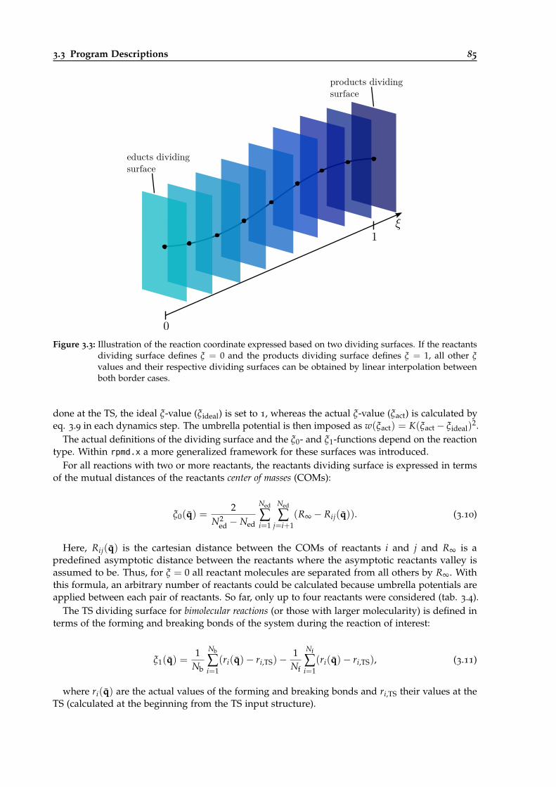
3.3 Program Descriptions 85
educts dividing surface
products dividing surface
Figure 3.3: Illustration of the reaction coordinate expressed based on two dividing surfaces. If the reactantsdividing surface defines ξ = 0 and the products dividing surface defines ξ = 1, all other ξvalues and their respective dividing surfaces can be obtained by linear interpolation betweenboth border cases.
done at the TS, the ideal ξ-value (ξideal) is set to 1, whereas the actual ξ-value (ξact) is calculated byeq. 3.9 in each dynamics step. The umbrella potential is then imposed as w(ξact) = K(ξact− ξideal)
2.The actual definitions of the dividing surface and the ξ0- and ξ1-functions depend on the reaction
type. Within rpmd.x a more generalized framework for these surfaces was introduced.For all reactions with two or more reactants, the reactants dividing surface is expressed in terms
of the mutual distances of the reactants center of masses (COMs):
ξ0(q) =2
N2ed − Ned
Ned
∑i=1
Ned
∑j=i+1
(R∞ − Rij(q)). (3.10)
Here, Rij(q) is the cartesian distance between the COMs of reactants i and j and R∞ is apredefined asymptotic distance between the reactants where the asymptotic reactants valley isassumed to be. Thus, for ξ = 0 all reactant molecules are separated from all others by R∞. Withthis formula, an arbitrary number of reactants could be calculated because umbrella potentials areapplied between each pair of reactants. So far, only up to four reactants were considered (tab. 3.4).
The TS dividing surface for bimolecular reactions (or those with larger molecularity) is defined interms of the forming and breaking bonds of the system during the reaction of interest:
ξ1(q) =1
Nb
Nb
∑i=1
(ri(q)− ri,TS)−1Nf
Nf
∑i=1
(ri(q)− ri,TS), (3.11)
where ri(q) are the actual values of the forming and breaking bonds and ri,TS their values at theTS (calculated at the beginning from the TS input structure).
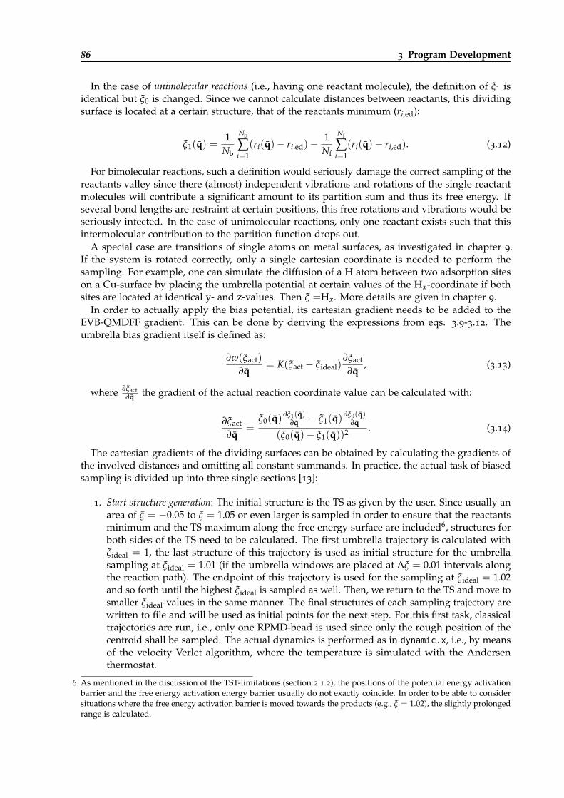
86 3 Program Development
In the case of unimolecular reactions (i.e., having one reactant molecule), the definition of ξ1 isidentical but ξ0 is changed. Since we cannot calculate distances between reactants, this dividingsurface is located at a certain structure, that of the reactants minimum (ri,ed):
ξ1(q) =1
Nb
Nb
∑i=1
(ri(q)− ri,ed)−1Nf
Nf
∑i=1
(ri(q)− ri,ed). (3.12)
For bimolecular reactions, such a definition would seriously damage the correct sampling of thereactants valley since there (almost) independent vibrations and rotations of the single reactantmolecules will contribute a significant amount to its partition sum and thus its free energy. Ifseveral bond lengths are restraint at certain positions, this free rotations and vibrations would beseriously infected. In the case of unimolecular reactions, only one reactant exists such that thisintermolecular contribution to the partition function drops out.
A special case are transitions of single atoms on metal surfaces, as investigated in chapter 9.If the system is rotated correctly, only a single cartesian coordinate is needed to perform thesampling. For example, one can simulate the diffusion of a H atom between two adsorption siteson a Cu-surface by placing the umbrella potential at certain values of the Hx-coordinate if bothsites are located at identical y- and z-values. Then ξ =Hx. More details are given in chapter 9.
In order to actually apply the bias potential, its cartesian gradient needs to be added to theEVB-QMDFF gradient. This can be done by deriving the expressions from eqs. 3.9-3.12. Theumbrella bias gradient itself is defined as:
∂w(ξact)
∂q= K(ξact − ξideal)
∂ξact
∂q, (3.13)
where ∂ξact∂q the gradient of the actual reaction coordinate value can be calculated with:
∂ξact
∂q=
ξ0(q)∂ξ1(q)
∂q − ξ1(q)∂ξ0(q)
∂q
(ξ0(q)− ξ1(q))2 . (3.14)
The cartesian gradients of the dividing surfaces can be obtained by calculating the gradients ofthe involved distances and omitting all constant summands. In practice, the actual task of biasedsampling is divided up into three single sections [13]:
1. Start structure generation: The initial structure is the TS as given by the user. Since usually anarea of ξ = −0.05 to ξ = 1.05 or even larger is sampled in order to ensure that the reactantsminimum and the TS maximum along the free energy surface are included6, structures forboth sides of the TS need to be calculated. The first umbrella trajectory is calculated withξideal = 1, the last structure of this trajectory is used as initial structure for the umbrellasampling at ξideal = 1.01 (if the umbrella windows are placed at ∆ξ = 0.01 intervals alongthe reaction path). The endpoint of this trajectory is used for the sampling at ξideal = 1.02and so forth until the highest ξideal is sampled as well. Then, we return to the TS and move tosmaller ξideal-values in the same manner. The final structures of each sampling trajectory arewritten to file and will be used as initial points for the next step. For this first task, classicaltrajectories are run, i.e., only one RPMD-bead is used since only the rough position of thecentroid shall be sampled. The actual dynamics is performed as in dynamic.x, i.e., by meansof the velocity Verlet algorithm, where the temperature is simulated with the Andersenthermostat.
6 As mentioned in the discussion of the TST-limitations (section 2.1.2), the positions of the potential energy activationbarrier and the free energy activation energy barrier usually do not exactly coincide. In order to be able to considersituations where the free energy activation barrier is moved towards the products (e.g., ξ = 1.02), the slightly prolongedrange is calculated.
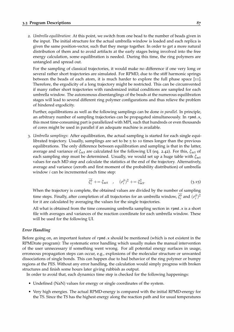
3.3 Program Descriptions 87
2. Umbrella equilibration: At this point, we switch from one bead to the number of beads given inthe input. The initial structure for the actual umbrella window is loaded and each replica isgiven the same position-vector, such that they merge together. In order to get a more naturaldistribution of them and to avoid artifacts at the early stages being involved into the freeenergy calculation, some equilibration is needed. During this time, the ring polymers areuntangled and spread out.
For the sampling of classical trajectories, it would make no difference if one very long orseveral rather short trajectories are simulated. For RPMD, due to the stiff harmonic springsbetween the beads of each atom, it is much harder to explore the full phase space [11].Therefore, the ergodicity of a long trajectory might be restricted. This can be circumventedif many rather short trajectories with randomized initial conditions are sampled for eachumbrella window. The autonomous disentanglings of the beads at the numerous equilibrationstages will lead to several different ring polymer configurations and thus relieve the problemof hindered ergodicity.
Further, equilibrations as well as the following samplings can be done in parallel. In principle,an arbitrary number of sampling trajectories can be propagated simultaneously. In rpmd.x,this most time-consuming part is parallelized with MPI, such that hundreds or even thousandsof cores might be used in parallel if an adequate machine is available.
3. Umbrella samplings: After equilibration, the actual sampling is started for each single equi-librated trajectory. Usually, samplings are set to be 5 to 10 times longer than the previousequilibrations. The only difference between equilibration and sampling is that in the latter,average and variance of ξact are calculated for the following UI (eq. 2.42). For this, ξact ofeach sampling step must be determined. Usually, we would set up a huge table with ξactvalues for each MD step and calculate the statistics at the end of the trajectory. Alternatively,average and variance (zeroth and first moment of the probability distribution) of umbrellawindow i can be incremented each time step:
ξbi += ξact , (σb
i )2 += ξ2
act. (3.15)
When the trajectory is complete, the obtained values are divided by the number of samplingtime steps. Finally, after completion of all trajectories for an umbrella window, ξb
i and (σbi )
2
for it are calculated by averaging the values for the single trajectories.
All what is obtained from the time consuming umbrella sampling section in rpmd.x is a shortfile with averages and variances of the reaction coordinate for each umbrella window. Thesewill be used for the following UI.
Error Handling
Before going on, an important feature of rpmd.x should be mentioned (which is not existent in theRPMDrate program): The systematic error handling which usually makes the manual interventionof the user unnecessary if something went wrong. For all potential energy surfaces in usage,erroneous propagation steps can occur, e.g., explosions of the molecular structure or unwanteddissociations of single bonds. This can happen due to bad behavior of the ring polymer or bumpyregions at the PES. Without any error handling, the calculation would simply progress with brokenstructures and finish some hours later giving rubbish as output.
In order to avoid that, each dynamics time step is checked for the following happenings:
• Undefined (NaN) values for energy or single coordinates of the system.
• Very high energies. The actual RPMD-energy is compared with the initial RPMD-energy forthe TS. Since the TS has the highest energy along the reaction path and for usual temperatures
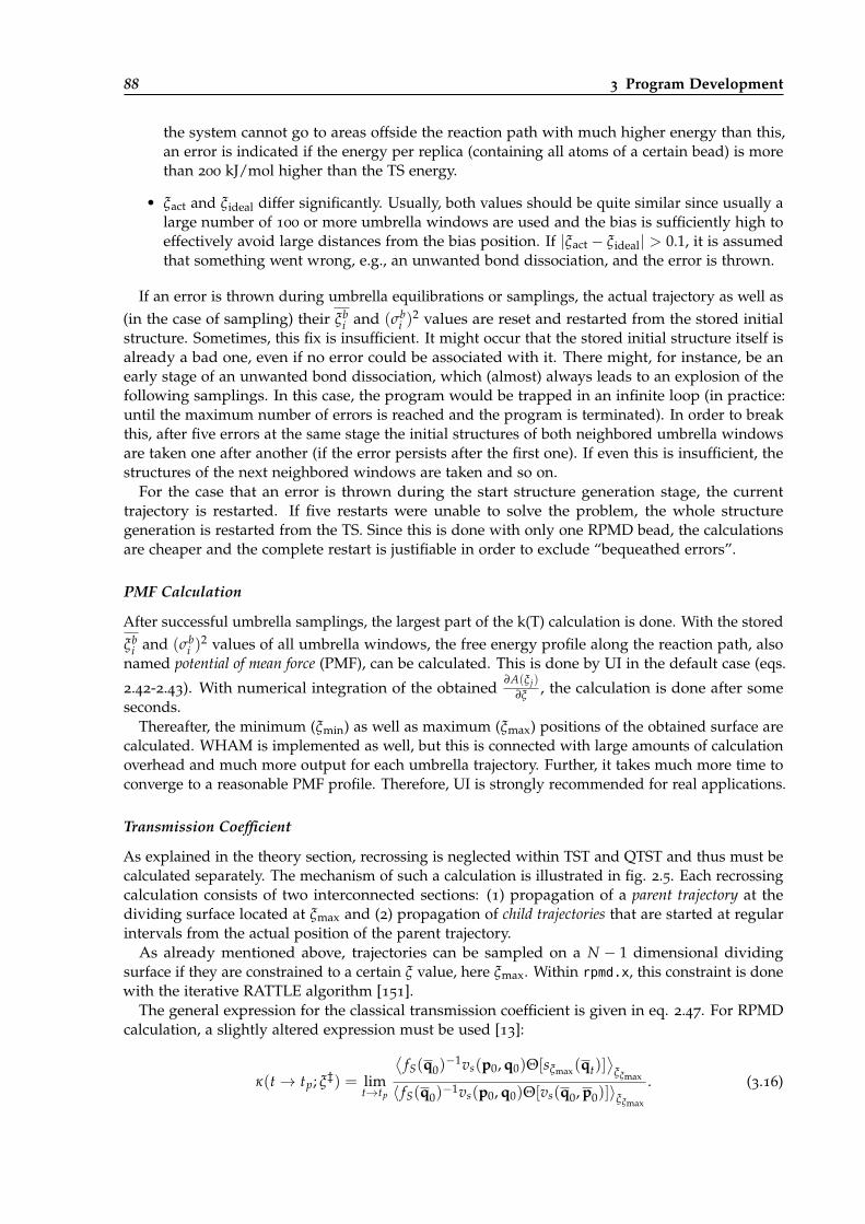
88 3 Program Development
the system cannot go to areas offside the reaction path with much higher energy than this,an error is indicated if the energy per replica (containing all atoms of a certain bead) is morethan 200 kJ/mol higher than the TS energy.
• ξact and ξideal differ significantly. Usually, both values should be quite similar since usually alarge number of 100 or more umbrella windows are used and the bias is sufficiently high toeffectively avoid large distances from the bias position. If |ξact − ξideal| > 0.1, it is assumedthat something went wrong, e.g., an unwanted bond dissociation, and the error is thrown.
If an error is thrown during umbrella equilibrations or samplings, the actual trajectory as well as(in the case of sampling) their ξb
i and (σbi )
2 values are reset and restarted from the stored initialstructure. Sometimes, this fix is insufficient. It might occur that the stored initial structure itself isalready a bad one, even if no error could be associated with it. There might, for instance, be anearly stage of an unwanted bond dissociation, which (almost) always leads to an explosion of thefollowing samplings. In this case, the program would be trapped in an infinite loop (in practice:until the maximum number of errors is reached and the program is terminated). In order to breakthis, after five errors at the same stage the initial structures of both neighbored umbrella windowsare taken one after another (if the error persists after the first one). If even this is insufficient, thestructures of the next neighbored windows are taken and so on.
For the case that an error is thrown during the start structure generation stage, the currenttrajectory is restarted. If five restarts were unable to solve the problem, the whole structuregeneration is restarted from the TS. Since this is done with only one RPMD bead, the calculationsare cheaper and the complete restart is justifiable in order to exclude “bequeathed errors”.
PMF Calculation
After successful umbrella samplings, the largest part of the k(T) calculation is done. With the storedξb
i and (σbi )
2 values of all umbrella windows, the free energy profile along the reaction path, alsonamed potential of mean force (PMF), can be calculated. This is done by UI in the default case (eqs.
2.42-2.43). With numerical integration of the obtained∂A(ξ j)
∂ξ , the calculation is done after someseconds.
Thereafter, the minimum (ξmin) as well as maximum (ξmax) positions of the obtained surface arecalculated. WHAM is implemented as well, but this is connected with large amounts of calculationoverhead and much more output for each umbrella trajectory. Further, it takes much more time toconverge to a reasonable PMF profile. Therefore, UI is strongly recommended for real applications.
Transmission Coefficient
As explained in the theory section, recrossing is neglected within TST and QTST and thus must becalculated separately. The mechanism of such a calculation is illustrated in fig. 2.5. Each recrossingcalculation consists of two interconnected sections: (1) propagation of a parent trajectory at thedividing surface located at ξmax and (2) propagation of child trajectories that are started at regularintervals from the actual position of the parent trajectory.
As already mentioned above, trajectories can be sampled on a N − 1 dimensional dividingsurface if they are constrained to a certain ξ value, here ξmax. Within rpmd.x, this constraint is donewith the iterative RATTLE algorithm [151].
The general expression for the classical transmission coefficient is given in eq. 2.47. For RPMDcalculation, a slightly altered expression must be used [13]:
κ(t→ tp; ξ‡) = limt→tp
⟨fS(q0)
−1vs(p0, q0)Θ[sξmax(qt)]⟩
ξξmax
〈 fS(q0)−1vs(p0, q0)Θ[vs(q0, p0)]〉ξξmax
. (3.16)
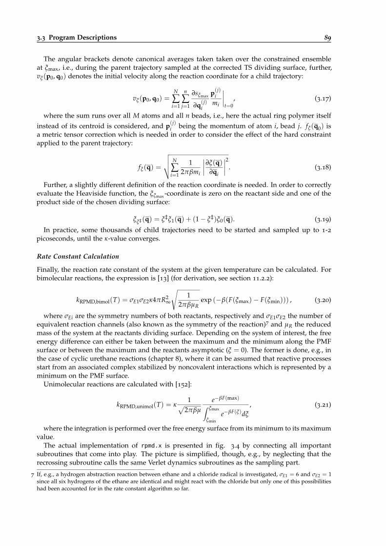
3.3 Program Descriptions 89
The angular brackets denote canonical averages taken taken over the constrained ensembleat ξmax, i.e., during the parent trajectory sampled at the corrected TS dividing surface, further,vξ(p0, q0) denotes the initial velocity along the reaction coordinate for a child trajectory:
vξ(p0, q0) =N
∑i=1
n
∑j=1
∂sξmax
∂q(j)i
p(j)i
mi
∣∣∣∣t=0
, (3.17)
where the sum runs over all M atoms and all n beads, i.e., here the actual ring polymer itselfinstead of its centroid is considered, and p(j)
i being the momentum of atom i, bead j. fξ(q0) isa metric tensor correction which is needed in order to consider the effect of the hard constraintapplied to the parent trajectory:
fξ(q) =
√√√√ N
∑i=1
12πβmi
∣∣∣∣∂ξ(q)∂qi
∣∣∣∣2. (3.18)
Further, a slightly different definition of the reaction coordinate is needed. In order to correctlyevaluate the Heaviside function, the ξξmax-coordinate is zero on the reactant side and one of theproduct side of the chosen dividing surface:
ξξ‡(q) = ξ‡ξ1(q) + (1− ξ‡)ξ0(q). (3.19)
In practice, some thousands of child trajectories need to be started and sampled up to 1-2picoseconds, until the κ-value converges.
Rate Constant Calculation
Finally, the reaction rate constant of the system at the given temperature can be calculated. Forbimolecular reactions, the expression is [13] (for derivation, see section 11.2.2):
kRPMD,bimol(T) = σE1σE2κ4πR2∞
√1
2πβµRexp (−β(F(ξmax)− F(ξmin))) , (3.20)
where σEi are the symmetry numbers of both reactants, respectively and σE1σE2 the number ofequivalent reaction channels (also known as the symmetry of the reaction)7 and µR the reducedmass of the system at the reactants dividing surface. Depending on the system of interest, the freeenergy difference can either be taken between the maximum and the minimum along the PMFsurface or between the maximum and the reactants asymptotic (ξ = 0). The former is done, e.g., inthe case of cyclic urethane reactions (chapter 8), where it can be assumed that reactive processesstart from an associated complex stabilized by noncovalent interactions which is represented by aminimum on the PMF surface.
Unimolecular reactions are calculated with [152]:
kRPMD,unimol(T) = κ1√
2πβµ
e−βF(max)∫ ξmax
ξmin
e−βF(ξ)dξ
, (3.21)
where the integration is performed over the free energy surface from its minimum to its maximumvalue.
The actual implementation of rpmd.x is presented in fig. 3.4 by connecting all importantsubroutines that come into play. The picture is simplified, though, e.g., by neglecting that therecrossing subroutine calls the same Verlet dynamics subroutines as the sampling part.
7 If, e.g., a hydrogen abstraction reaction between ethane and a chloride radical is investigated, σE1 = 6 and σE2 = 1since all six hydrogens of the ethane are identical and might react with the chloride but only one of this possibilitieshad been accounted for in the rate constant algorithm so far.
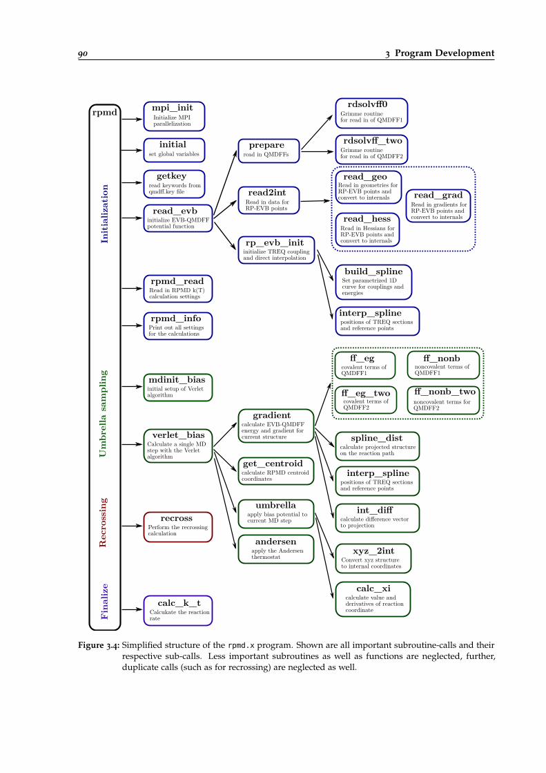
90 3 Program Development
mpi_initInitialize MPI parallelization
initialset global variables
getkeyread keywords from qmdff.key file
read_evbinitialize EVB-QMDFFpotential function
prepareread in QMDFFs
rdsolvff0Grimme routine for read in of QMDFF1
rdsolvff_twoGrimme routine for read in of QMDFF2
read2intRead in data for RP-EVB points
read_geoRead in geometries for RP-EVB points and convert to internals read_grad
Read in gradients for RP-EVB points and convert to internalsread_hess
Read in Hessians for RP-EVB points and convert to internals rp_evb_init
initialize TREQ couplingand direct interpolation
build_splineSet parametrized 1D curve for couplings and energies
interp_splinepositions of TREQ sections and reference points
rpmd_readRead in RPMD k(T) calculation settings
rpmd_infoPrint out all settings for the calculations
mdinit_biasinitial setup of Verlet algorithm
verlet_biasCalculate a single MDstep with the Verlet algorithm
get_centroidcalculate RPMD centroidcoordinates
umbrellaapply bias potential to current MD step
xyz_2intConvert xyz structure to internal coordinates
calc_xicalculate value andderivatives of reaction coordinate
andersenapply the Andersen thermostat
gradientcalculate EVB-QMDFFenergy and gradient for current structure
ff_egcovalent terms of QMDFF1
ff_nonbnoncovalent terms of QMDFF1
ff_eg_twocovalent terms of QMDFF2
ff_nonb_twononcovalent terms for QMDFF2
interp_splinepositions of TREQ sections and reference points
spline_distcalculate projected structure on the reaction path
int_diffcalculate difference vector to projection
recrossPerform the recrossing calculation
calc_k_tCalcukate the reactionrate
rpmdIn
itia
lizat
ion
Um
brel
la s
ampl
ing
Rec
ross
ing
Fin
aliz
e
Figure 3.4: Simplified structure of the rpmd.x program. Shown are all important subroutine-calls and theirrespective sub-calls. Less important subroutines as well as functions are neglected, further,duplicate calls (such as for recrossing) are neglected as well.
3.3 Program Descriptions 91
3.3.8 evb_kt_driver
This program enables the black-box calculation of reaction rate constants. The underlying idea isthat a specific elementary chemical reaction can be fully described if its minimum energy path hasbeen calculated. Therefore it should be possible to calculate the rate constant of a reaction if thispath is supplied by the user.
So far, a couple of steps was needed to go from the reaction path to a rate constant finally ejectedfrom a RPMD calculation:
1. Optimize structures of both reactants and products minima, with the endpoints of the reactionpath as origins.
2. Calculate sets of reference data needed for QMDFF generations.
3. Run the qmdffgen.x program for the generation of the QMDFF force field files.
4. If DG-EVB or TREQ shall be used as EVB-coupling method, calculate gradient and Hessianreference data for a manually chosen set of points along the reaction path.
5. Unless TREQ is used as EVB method, optimize the EVB-coupling term with evbopt.x
6. Determine settings needed for the following RPMD-run: reaction type, dividing surfaces,number of sampling steps etc. .
7. Execute rpmd.x for calculation of k(T)-value(s).
8. If the temperature-dependence of rate constants shall be investigated, e.g., by doing anArrhenius or Eyring plot, calculate several k(T)-values and do the fit with a suitable script.
As will be shown in the following, all this can be fully automatized, under the condition thatTREQ is used as EVB coupling method8.
Needed Input
Since it is the aim that one single program execution shall be enough to do all steps depictedabove, all information that might be needed at some point should be provided at the beginning (orcalculated on-the-fly based on the results of preceding steps, if possible). Besides the reaction pathstructures and energies (provided in a xyz and an energy list file), only one additional input file(qmdff.key) is needed. Keywords were designed that allow the user to give all needed parameters:
• The used software package for ab-initio reference calculations (Currently, Gaussian and Orcaare supported).
• The direction of the reaction (with respect to the IRC). Unless a symmetric reaction isconsidered, rate constants could be calculated for the forward and backward process.
• The used ab-initio reference method (as well as basis set and other settings such as DFTdispersion corrections etc.) for geometry optimizations, QMDFF reference calculations, TREQreference calculations and an optional improvement of the path energies by a higher levelmethod. Usually, all tasks except the last are done with the same method (e.g., MP2), whereasthe last can be done with a much more expensive method (e.g., CCSD(T)) and possibly evenwith another software package.
8 Indeed, the black-box procedure can also be done with DG-EVB as coupling method, since no user intervention isneeded for the DG-EVB parameter optimization in general. However, it turned out that the actual choice of DG-EVBcoupling coordinates as well as the DG-EVB mode might affect the overall quality significantly. So far, no stringentmethod of predicting the best settings could be developed, thus excluding DG-EVB for usage within a true black-boxapproach.
92 3 Program Development
• Calculation settings for the reference: Number of cores for QMDFF- as well as TREQ-referencecalculations and the available memory per core. Further, symlinks to the program executables(QM program, qmdffgen.x, rpmd.x) must be given. With this, the calculations can be doneon external calculation clusters as well.
• Number of TREQ gradient and frequency reference points along the reaction path (if nodefault values shall be used).
• Settings for RPMD calculations: temperatures as well as runs per temperature that shall beaveraged.
All other settings (e.g., time steps for RPMD structure generation trajectories) are set by defaultfrom the program. If the user wants to change some of them manually, he or she can add thestandard keywords with the preferred settings to the main qmdff.key input file.
QMDFF Generation
Depending on the choice regarding the direction of the reaction, the first and last structures ofthe reaction path are taken as initial points for reactants and products geometries, respectively.Starting from these structures, geometry optimizations are done with the chosen QM programpackage. Input files are generated in separate folders and the calculations are started, either serialor in parallel, depending on the total number of cores available and the chosen number of coresper calculation. The output files are monitored during the calculations, such that the main programwaits until the program-package-dependent lines indicating a successful finishing appear. Afterthis, the output files with the optimized structures are read in.
In the next step, new input files, now for QMDFF reference calculations, are written in separatefolders. The program-package-specific keywords for frequency, CM5 charges etc. are added tothe method and basis set chosen by the user. Now, the same procedure as with the geometryoptimizations is repeated.
When all reference was calculated successfully, qmdffgen.x can be executed. Since this is alsoa black-box program, only one command is needed. After completion, the QMDFF-shift energiesare slightly changed: Sometimes the QMDFF energy curves deviate quite significantly from theasymptotic ab-initio reference of the reaction path. Therefore, they are manually corrected such thatthe first and last energy of the RP are reproduced exactly by the reactants and products QMDFFs,respectively. This is illustrated in fig. 3.5 for the CF3O+CH4-reaction.
EVB Reference Calculations
Now, the EVB-part must be parametrized. No matter if DG-EVB or TREQ are used, gradientand Hessian reference information is needed on a number of points along the RP. The procedureof locating those points is usually far from black-box. So far, the user had to choose each pointmanually, usually by inspecting the RP energies and picking single points from them. It has turnedout that better DG-EVB qualities (with respect to the reproduction of the reaction path) could beobtained if a denser grid of points was picked at regions with higher slope of the RP. Further, theTS was always chosen since the exact information of the RP turning point should be included. ForTREQ, also the very first and very last point of the IRC must be chosen in order to make lineargradient and frequency interpolations along the whole path possible (chapter 5, section 2).
With these prerequisites, a heuristic algorithm for the automated location of those referencepoints was developed. First, the ideal total number of reference points Mtot should be determined.At least three points are needed (TS as being the structure along the RP with the highest energy andboth ends of the RP), but of course much more are preferable in almost all cases. It was assumedthat the number of needed reference points grows with system size since the accessible coordinate
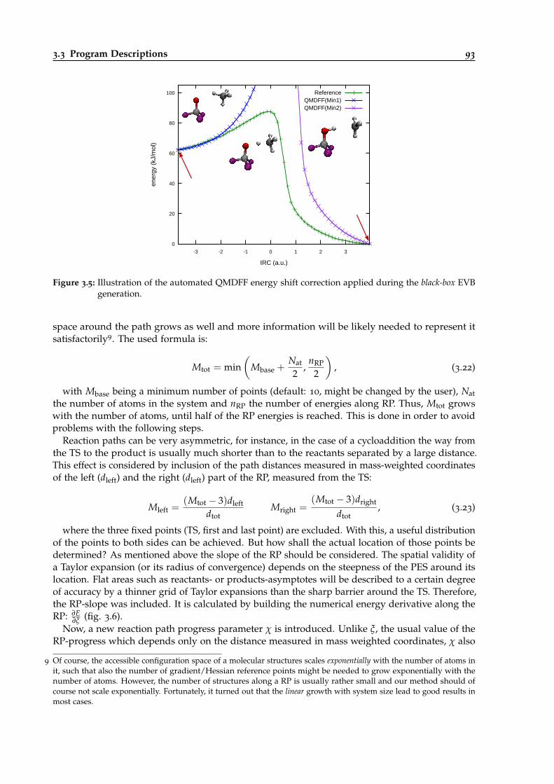
3.3 Program Descriptions 93
0
20
40
60
80
100
-3 -2 -1 0 1 2 3
ener
gy
(kJ/
mol
)
IRC (a.u.)
ReferenceQMDFF(Min1)QMDFF(Min2)
Figure 3.5: Illustration of the automated QMDFF energy shift correction applied during the black-box EVBgeneration.
space around the path grows as well and more information will be likely needed to represent itsatisfactorily9. The used formula is:
Mtot = min(
Mbase +Nat
2,
nRP
2
), (3.22)
with Mbase being a minimum number of points (default: 10, might be changed by the user), Natthe number of atoms in the system and nRP the number of energies along RP. Thus, Mtot growswith the number of atoms, until half of the RP energies is reached. This is done in order to avoidproblems with the following steps.
Reaction paths can be very asymmetric, for instance, in the case of a cycloaddition the way fromthe TS to the product is usually much shorter than to the reactants separated by a large distance.This effect is considered by inclusion of the path distances measured in mass-weighted coordinatesof the left (dleft) and the right (dleft) part of the RP, measured from the TS:
Mleft =(Mtot − 3)dleft
dtotMright =
(Mtot − 3)dright
dtot, (3.23)
where the three fixed points (TS, first and last point) are excluded. With this, a useful distributionof the points to both sides can be achieved. But how shall the actual location of those points bedetermined? As mentioned above the slope of the RP should be considered. The spatial validity ofa Taylor expansion (or its radius of convergence) depends on the steepness of the PES around itslocation. Flat areas such as reactants- or products-asymptotes will be described to a certain degreeof accuracy by a thinner grid of Taylor expansions than the sharp barrier around the TS. Therefore,the RP-slope was included. It is calculated by building the numerical energy derivative along theRP: ∂E
∂ξ (fig. 3.6).Now, a new reaction path progress parameter χ is introduced. Unlike ξ, the usual value of the
RP-progress which depends only on the distance measured in mass weighted coordinates, χ also
9 Of course, the accessible configuration space of a molecular structures scales exponentially with the number of atoms init, such that also the number of gradient/Hessian reference points might be needed to grow exponentially with thenumber of atoms. However, the number of structures along a RP is usually rather small and our method should ofcourse not scale exponentially. Fortunately, it turned out that the linear growth with system size lead to good results inmost cases.
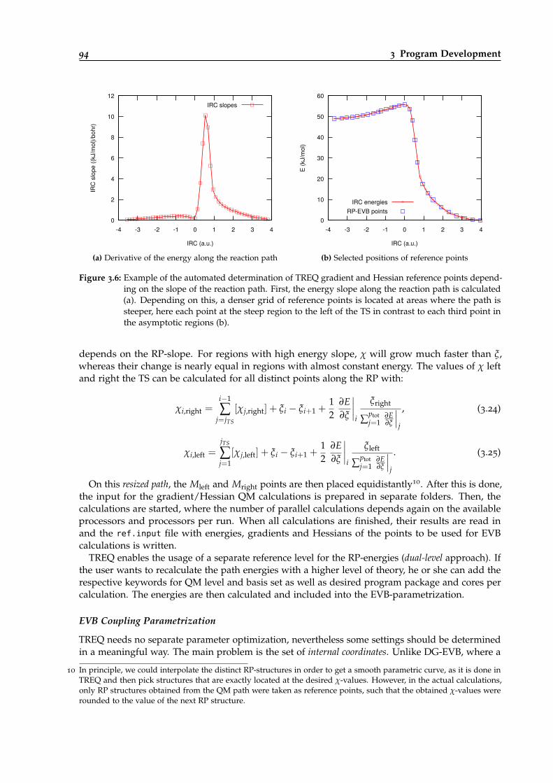
94 3 Program Development
0
2
4
6
8
10
12
-4 -3 -2 -1 0 1 2 3 4
IRC
slop
e((k
J/m
ol)/b
ohr)
IRC (a.u.)
IRC slopes
(a) Derivative of the energy along the reaction path
0
10
20
30
40
50
60
-4 -3 -2 -1 0 1 2 3 4
E(k
J/m
ol)
IRC (a.u.)
IRC energiesRP-EVB points
(b) Selected positions of reference points
Figure 3.6: Example of the automated determination of TREQ gradient and Hessian reference points depend-ing on the slope of the reaction path. First, the energy slope along the reaction path is calculated(a). Depending on this, a denser grid of reference points is located at areas where the path issteeper, here each point at the steep region to the left of the TS in contrast to each third point inthe asymptotic regions (b).
depends on the RP-slope. For regions with high energy slope, χ will grow much faster than ξ,whereas their change is nearly equal in regions with almost constant energy. The values of χ leftand right the TS can be calculated for all distinct points along the RP with:
χi,right =i−1
∑j=jTS
[χj,right] + ξi − ξi+1 +12
∂E∂ξ
∣∣∣∣i
ξright
∑ptotj=1
∂E∂ξ
∣∣∣j
, (3.24)
χi,left =jTS
∑j=1
[χj,left] + ξi − ξi+1 +12
∂E∂ξ
∣∣∣∣i
ξleft
∑ptotj=1
∂E∂ξ
∣∣∣j
. (3.25)
On this resized path, the Mleft and Mright points are then placed equidistantly10. After this is done,the input for the gradient/Hessian QM calculations is prepared in separate folders. Then, thecalculations are started, where the number of parallel calculations depends again on the availableprocessors and processors per run. When all calculations are finished, their results are read inand the ref.input file with energies, gradients and Hessians of the points to be used for EVBcalculations is written.
TREQ enables the usage of a separate reference level for the RP-energies (dual-level approach). Ifthe user wants to recalculate the path energies with a higher level of theory, he or she can add therespective keywords for QM level and basis set as well as desired program package and cores percalculation. The energies are then calculated and included into the EVB-parametrization.
EVB Coupling Parametrization
TREQ needs no separate parameter optimization, nevertheless some settings should be determinedin a meaningful way. The main problem is the set of internal coordinates. Unlike DG-EVB, where a
10 In principle, we could interpolate the distinct RP-structures in order to get a smooth parametric curve, as it is done inTREQ and then pick structures that are exactly located at the desired χ-values. However, in the actual calculations,only RP structures obtained from the QM path were taken as reference points, such that the obtained χ-values wererounded to the value of the next RP structure.
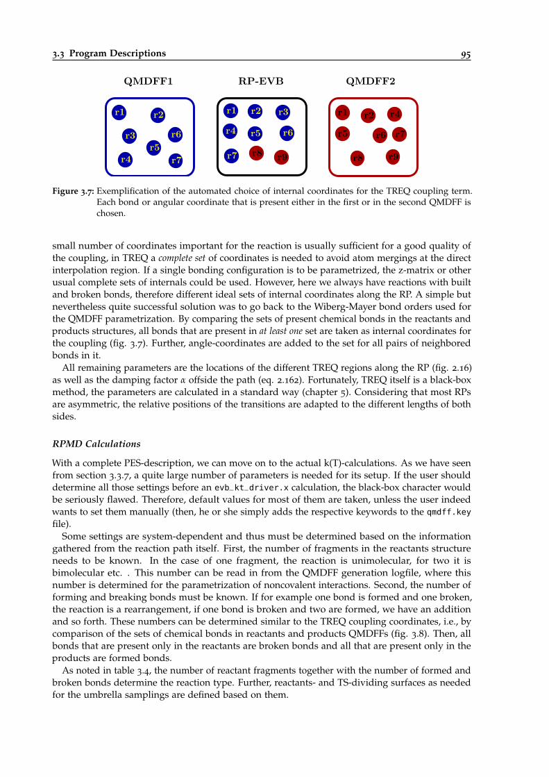
3.3 Program Descriptions 95
r1
r3
r2
r6
r7r5
r4
r1 r4r2
r5 r7r6
r8 r9
QMDFF1 QMDFF2RP-EVB
r1 r3r2
r6
r7
r5r4
r8 r9
Figure 3.7: Exemplification of the automated choice of internal coordinates for the TREQ coupling term.Each bond or angular coordinate that is present either in the first or in the second QMDFF ischosen.
small number of coordinates important for the reaction is usually sufficient for a good quality ofthe coupling, in TREQ a complete set of coordinates is needed to avoid atom mergings at the directinterpolation region. If a single bonding configuration is to be parametrized, the z-matrix or otherusual complete sets of internals could be used. However, here we always have reactions with builtand broken bonds, therefore different ideal sets of internal coordinates along the RP. A simple butnevertheless quite successful solution was to go back to the Wiberg-Mayer bond orders used forthe QMDFF parametrization. By comparing the sets of present chemical bonds in the reactants andproducts structures, all bonds that are present in at least one set are taken as internal coordinates forthe coupling (fig. 3.7). Further, angle-coordinates are added to the set for all pairs of neighboredbonds in it.
All remaining parameters are the locations of the different TREQ regions along the RP (fig. 2.16)as well as the damping factor α offside the path (eq. 2.162). Fortunately, TREQ itself is a black-boxmethod, the parameters are calculated in a standard way (chapter 5). Considering that most RPsare asymmetric, the relative positions of the transitions are adapted to the different lengths of bothsides.
RPMD Calculations
With a complete PES-description, we can move on to the actual k(T)-calculations. As we have seenfrom section 3.3.7, a quite large number of parameters is needed for its setup. If the user shoulddetermine all those settings before an evb_kt_driver.x calculation, the black-box character wouldbe seriously flawed. Therefore, default values for most of them are taken, unless the user indeedwants to set them manually (then, he or she simply adds the respective keywords to the qmdff.key
file).Some settings are system-dependent and thus must be determined based on the information
gathered from the reaction path itself. First, the number of fragments in the reactants structureneeds to be known. In the case of one fragment, the reaction is unimolecular, for two it isbimolecular etc. . This number can be read in from the QMDFF generation logfile, where thisnumber is determined for the parametrization of noncovalent interactions. Second, the number offorming and breaking bonds must be known. If for example one bond is formed and one broken,the reaction is a rearrangement, if one bond is broken and two are formed, we have an additionand so forth. These numbers can be determined similar to the TREQ coupling coordinates, i.e., bycomparison of the sets of chemical bonds in reactants and products QMDFFs (fig. 3.8). Then, allbonds that are present only in the reactants are broken bonds and all that are present only in theproducts are formed bonds.
As noted in table 3.4, the number of reactant fragments together with the number of formed andbroken bonds determine the reaction type. Further, reactants- and TS-dividing surfaces as neededfor the umbrella samplings are defined based on them.
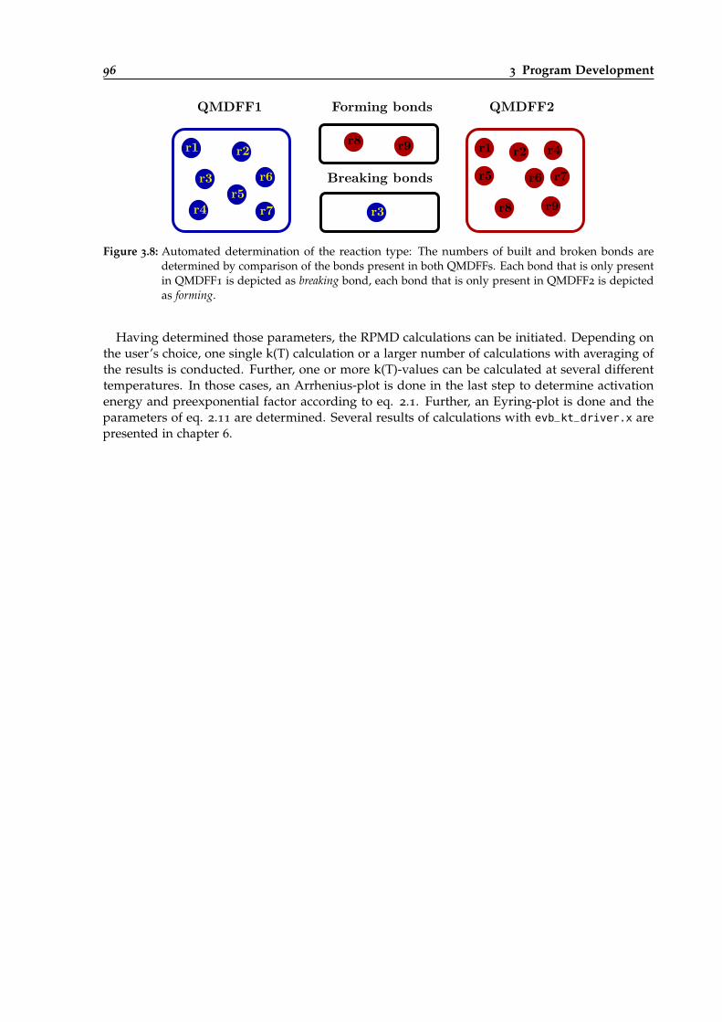
96 3 Program Development
r1
r3
r2
r6
r7r5
r4
r1 r4r2
r5 r7r6
r8 r9
QMDFF1 QMDFF2Forming bonds
r3
r8 r9
Breaking bonds
Figure 3.8: Automated determination of the reaction type: The numbers of built and broken bonds aredetermined by comparison of the bonds present in both QMDFFs. Each bond that is only presentin QMDFF1 is depicted as breaking bond, each bond that is only present in QMDFF2 is depictedas forming.
Having determined those parameters, the RPMD calculations can be initiated. Depending onthe user’s choice, one single k(T) calculation or a larger number of calculations with averaging ofthe results is conducted. Further, one or more k(T)-values can be calculated at several differenttemperatures. In those cases, an Arrhenius-plot is done in the last step to determine activationenergy and preexponential factor according to eq. 2.1. Further, an Eyring-plot is done and theparameters of eq. 2.11 are determined. Several results of calculations with evb_kt_driver.x arepresented in chapter 6.

4
Ch
ap
te
r
Publication: (DG-)EVB-QMDFF-RPMD
4.1 Scope of the Project
This project covers a significant period of the whole work for this thesis. As already explained insection 3.1.3 of the program chapter, it was our desire to enable reaction rate constant calculationson EVB-QMDFF surfaces. By coupling our EVB-QMDFF code with the RPMDrate programby Suleymanov [13] it became possible to calculate bimolecular rate constants with the RPMDformalism, such that also quantum effects could be considered in a MD based manner.
The present paper was designed to fulfill two purposes: First, it should show that the energy-gap(dE)-EVB as well as the distributed Gaussian (DG)-EVB coupling terms in connection with QMDFFsas diabatic surfaces are able to describe a reference PES based on an ab-initio reaction path in allregions relevant for a reactive sampling with good quality, shown by rate constants that coincidewell with experimental references. Second, the much reduced effort for setting up an EVB-QMDFFPES description compared to traditional parametric surfaces should show that black-box calculationsof reaction rate constants are already nearly possible and might become routine in the near futureif the EVB-QMDFF formalism is further improved (with respect to the time the paper was written).
Three example reactions are presented, for which reaction rate constants were calculated withEVB-QMDFF-RPMD as well as with “traditional” parametric TST corrections in the POLYRATE [10]program package. A final comparison of both methods was made.
98 4 Publication: (DG-)EVB-QMDFF-RPMD
4.2 Publication Data and Reprint
Authors Julien Steffen and Bernd Hartke
Title Cheap but accurate calculation of chemical reaction rate constants from abinitio data, via system-specific, black-box force fields
Submitted February 1, 2017
Accepted March 10, 2017
Reference J. Steffen and B. Hartke, J. Chem. Phys., 147 (2017), 161701.DOI: 10.1063/1.4979712
Contribution Implementation of the EVB-QMDFF program, especially of the DG-EVB cou-pling term, connection with RPMDrate. Parametrization of the PES descrip-tions for the example reactions, running and evaluating the rate constant calcu-lations. Further: Doing parametric rate constant calculations with POLYRATEin order to compare them with the EVB-QMDFF-RPMD values. Major Contri-butions to writing the article.
5
Ch
ap
te
r
Publication: TREQ - Development and Benchmark
5.1 Scope of the Project
Shortly after the establishment of the DG-EVB method for rate constant calculations with RPMDrateit became clear that the provided PES description was insufficient for many even rather simplesystems. The umbrella sampling trajectories became trapped in artificial minima offside the reactionpath, leading to distorted free energy curves and absurd rate constants. Several approaches forsolving these problems inside the DG-EVB network failed, such as optimization of internalcoordinates and positions of DG-EVB reference points.
Therefore, the decision was made to develop an entirely new EVB coupling method, designedespecially for high quality descriptions of reaction paths and their direct vicinity. The new couplingterm was named Reaction Path (RP)-EVB. During first benchmarks, the new term, althoughsuperior to DG-EVB, showed problems in other examples.
This lead to the development of the Transition Region Corrected (TRC)-RP-EVB-QMDFF (TREQ)method, where the EVB-QMDFF construction is replaced by a direct Taylor series expansion ofthe QM-reference in the TS region. The presented publication shows the development and the(mathematical as well as algorithmic) construction of the TREQ method in great detail. Additionally,a thorough benchmark of the new method is conducted in order to prove its quality for relevantexamples. For this, analytic potential energy functions from the literature for a number of smallreactive systems were coupled to the EVB-QMDFF program package. The benchmark was thendone as follows: On the analytic potential energy surfaces, reaction paths and the needed TREQreference data were calculated similar to QM methods. Then, TREQ surfaces were parametrizedbased on this “pseudo-QM” reference. Finally, RPMD rate constant calculations were done bothon the analytic surfaces and the TREQ surfaces derived from them, the results were comparedthoroughly.
It turned out that TREQ is indeed able to provide quantitatively correct descriptions of referencesurfaces, hence able to calculate high-quality rate constants. Additionally, TREQ was constructedsuch that no optimization procedure is needed for its setup which makes the development of ablack-box algorithm for k(T) calculations possible (see chapter 6).

100 5 Publication: TREQ - Development and Benchmark
5.2 Publication Data and Reprint
Authors Julien Steffen
Title A new class of reaction path based potential energy surfaces enabling accurateblack box chemical rate constant calculations
Submitted February 12, 2019
Accepted March 26, 2019
Reference J. Steffen, J. Chem. Phys., 150 (2019), 154105.DOI: 10.1063/1.5092589
Contribution All what is shown in the paper, further the implementation of the EVB-QMDFFprogram package.
6
Ch
ap
te
r
Black-Box k(T) Calculations
We have seen in the last chapter that the TREQ method is well suited for performing black-box rateconstant calculations since no ambiguous parameter optimization or system-specific choices by theuser are needed for its setup. As explained in section 3.3.8 of the program chapter, this propertywas used to develop a program named evb_kt_driver.x that is able to calculate rate constants andArrhenius parameters for an arbitrary elementary reaction if its reaction path is given by the user.
In this chapter, a first benchmark of evb_kt_driver.x is presented: Fifteen different reactionswere chosen, their reaction paths were optimized and black-box rate constant calculations based onthem were started. Then, the resulting rate constants and Arrhenius parameters were comparedwith (both theoretical and experimental) literature values as reference.
6.1 General Procedure
The first task was to find a suitable set of example reactions for the test of the program. In the idealcase, we should choose a wide variety of different system sizes, involved chemical elements andreaction mechanisms (uni- and bimolecular). In the reality, the desired reactions should furtherfulfill three requirements in order to be suited as easy-to-calculate black-box systems:
1. It should be a small to medium-sized thermally activated gas phase reaction in the groundstate (due to the construction of the TREQ PES).
2. Experimental reference data for rate constants and Arrhenius parameters should be available.
3. To limit the effort for the QM-reference calculations, the reaction path needs to be of single-reference character.
A suitable place for the search of gas-phase reactions with available experimental data is the NISTChemical Kinetics Database [153]. The idea was to randomly choose some handful of reactionsfrom there and to calculate black-box rate constants. It turned out that this task was far from easy.In order to ensure that single-reference methods are able to calculate a reliable reaction path, onlyreactions with theoretical papers where, e.g., a TS-optimization was done (and reported with somedetail) could be considered.
Therefore, reactions for which experimental and theoretical (containing detailed descriptions ofQM-reference calculations) studies are available were chosen. Ideally, more than one experimentalstudy should be available as well since their results tend to differ significantly in some cases (seebelow). These prerequisites excluded approximately 95-98 % of the reactions listed in the database.From the remaining ones, fifteen reactions were finally chosen, still offering a large variety both inthe involved elements and in the reaction mechanisms. Unfortunately, the vast majority of reactionslisted in NIST with enough references available are simple bimolecular exchanges.
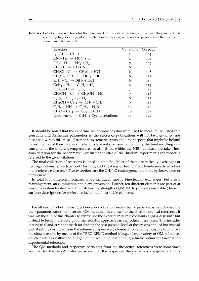
102 6 Black-Box k(T) Calculations
Table 6.1: List of chosen reactions for the benchmark of the evb_kt_driver.x program. They are orderedaccording to (ascending) atom numbers in the system, references to pages where the results areshown are listed as well.
Reaction No. atoms On pageI2 + H → HI + I 3 103
CN + H2 → HCN + H 4 108
PH3 + H → PH2 + H2 5 105
CH3NC → CH3CN 6 108
CH3Cl + Cl → CH2Cl + HCl 6 108
CH2Cl2 + Cl → CHCl2 + HCl 6 112
SiH4 + Cl → SiH3 + HCl 6 113
GeH4 + H → GeH3 + H2 6 113
C2H4 + H → C2H5 7 113
CH3OH + Cl → CH2OH + HCl 7 116
C2H6 → C2H4 + H2 8 117
CH4OH + CH3 → CH3 + CH4 9 118
C2H6 + NH → C2H5 + H2N 10 120
CF3O + CH4 → CF3OH+CH3 10 121
Norbornene → C2H4 + Cyclopentadiene 17 122
It should be noted that the experimental approaches that were used to measure the listed rateconstants and Arrhenius parameters in the reference publications will not be mentioned nordiscussed within this thesis. Error bars, systematic errors and other aspects that might be helpfulfor estimation of their degree of reliability are not discussed either, only the final resulting rateconstants at the different temperatures as also listed within the NIST database are taken intoconsideration for the benchmark. For further studies of the different experiments the reader isreferred to the given citations.
The final collection of reactions is listed in table 6.1. Most of them are basically exchanges ofhydrogen atoms, since (covalent) forming and breaking of heavy atom bonds mostly involvesmulti-reference character. Two exceptions are the CH3NC-rearrangement and the cycloreversion ofnorbornene.
In total four different mechanisms are included: mostly bimolecular exchanges, but also arearrangement, an eliminiation and a cycloreversion. Further, ten different elements are part of atleast one system treated, which illustrates the strength of QMDFF to provide reasonable (diabaticsurface) descriptions for molecules including all 92 stable elements.
For all reactions but the last (cycloreversion of norbornene) theory papers exist which describetheir parametrization with certain QM methods. In contrast to the cited theoretical references itwas not the aim of this chapter to reproduce the experimental rate constants as good as possible butinstead to benchmark how good the black-box approach can reproduce these rates. This includesthat no trial-and-error approach for finding the best possible level of theory was applied but insteadglobal settings or those from the reference papers were chosen. It is certainly possible to improvethe shown results by means of the TREQ-RPMD method if, e.g., a large variety of QM-referencesor other settings within the TREQ method would be tested and gradually optimized towards theexperimental reference.
The QM methods and respective basis sets from the theoretical references were sometimesadopted for the black-box studies as well. If the respective theory papers are quite old, thus
6.2 Example Reactions 103
containing rather cheap QM methods (e.g., HF with a small basis set), superior methods werechosen. In addition, a higher QM level was adapted for the calculation of IRC energies as neededfor the dual-level approach (see section 3.3.8). This level is in all cases DLPNO-CCSD(T) [154, 155]in order to reduce the amount of calculation effort in comparison to, e.g., CCSD(T), especially forlarger systems. In practice, the TS structure of the system was optimized first; if its imaginaryeigenmode seemed to describe the reaction properly, the IRC optimization was started from the TSstructure1.
For the RPMD calculations, the same settings were used for all 15 examples. Since Arrheniusparameters should be calculated and compared to values obtained from literature references toget a distinct comparison between single numbers, k(T) calculations at several temperatures weredone for all reported systems. The actual calculated temperatures depend on the ones at whichexperimental measurements were made. In total, a span between 200 and 2000 K is bridged bythese calculations, showing the ability of the TREQ-RPMD approach to handle wide ranges ofchemical reality (at least with respect to the temperature).
Two settings must be determined individually for each reaction. The first one is the symmetry ofthe reaction, i.e., if more than one path can be taken to get to the result. One example is a moleculewith several identical hydrogen atoms undergoing a hydrogen abstraction reaction. The secondsetting is the required number of beads for sufficient consideration of quantum effects2.
In order to get a balance between low costs and satisfying quality, a compromise was made:Instead of running one expensive k(T) calculation for one single temperature and hoping that it willbe sufficiently well converged, five rather cheap k(T) calculations are done at each temperature withfinal averaging of their results. The single calculated values are plotted together with their averagesand variances in the next section to enable a visual evaluation of the degree of convergence in theRPMD calculations. Finally, the Arrhenius parameters are determined by doing a fit through theaveraged rate constant results of each temperature.
The used RPMD calculation settings are listed in table 6.3.
6.2 Example Reactions
6.2.1 The I2 + H → HI + I Reaction
This reaction plays an important role for the translation of iodine in the gaseous phase. A theoreticalstudy of it was done by Canneux and Cantrel as part of a larger study that should reveal thedynamics of bringing radioactive iodine into the environment in the case of a Pressured WaterReactor incident [157].
1 Initially, an even larger set of reactions was gathered (around 30 systems). However, TS and IRC calculationsonly worked for approximately one half of them, in the other cases convergence problems arose mostly in the IRCcalculations, even if the same level of theory was used already in a reference paper. Since elaborate workarounds tosolve these problems would have seriously harmed the desired black-box character, those systems were discarded. Allsystems for which TS and IRC calculations were successful are presented in this chapter.
2 Theoretically, both settings could also be determined in an automated manner: The reaction symmetry σ could beobtained by topological analysis of the reactants in comparison to the reaction path. If, e.g., a hydrogen abstractionreaction is handled, determine the initial bonding pattern of the hydrogen to be abstracted and search for hydrogenswith identical patterns in the same reactant molecule, e.g., all hydrogens in ethane. The number of beads might bedetermined by doing a simple Wigner calculation of the transmission coefficient (eq. 2.16) for all temperatures. Theneeded imaginary frequency at the TS can, e.g., be obtained from the given data for the RP-EVB reference points.Depending on the magnitude of the tunneling correction the required number of beads could be estimated, e.g., byrunning a set of benchmarks with systems like the ones listed here and determine a correlation between the Wignertunneling correction and the “asymptotic” number of RPMD beads above which no relevant change of the calculatedreaction rate appears. However, since the choice of both settings can easily be made in a few seconds for most cases,the manual method was preserved so far.
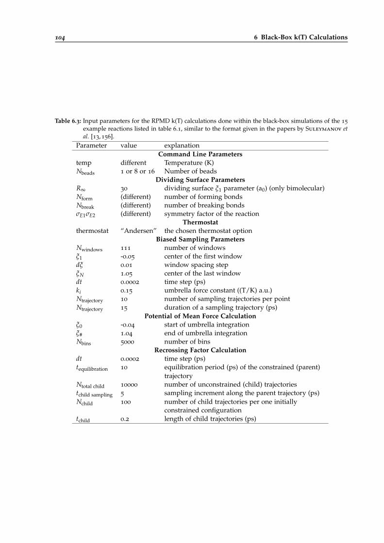
104 6 Black-Box k(T) Calculations
Table 6.3: Input parameters for the RPMD k(T) calculations done within the black-box simulations of the 15
example reactions listed in table 6.1, similar to the format given in the papers by Suleymanov etal. [13, 156].
Parameter value explanationCommand Line Parameters
temp different Temperature (K)Nbeads 1 or 8 or 16 Number of beads
Dividing Surface ParametersR∞ 30 dividing surface ξ1 parameter (a0) (only bimolecular)Nform (different) number of forming bondsNbreak (different) number of breaking bondsσE1σE2 (different) symmetry factor of the reaction
Thermostatthermostat “Andersen” the chosen thermostat option
Biased Sampling ParametersNwindows 111 number of windowsξ1 -0.05 center of the first windowdξ 0.01 window spacing stepξN 1.05 center of the last windowdt 0.0002 time step (ps)ki 0.15 umbrella force constant ((T/K) a.u.)Ntrajectory 10 number of sampling trajectories per pointNtrajectory 15 duration of a sampling trajectory (ps)
Potential of Mean Force Calculationξ0 -0.04 start of umbrella integrationξ# 1.04 end of umbrella integrationNbins 5000 number of bins
Recrossing Factor Calculationdt 0.0002 time step (ps)tequilibration 10 equilibration period (ps) of the constrained (parent)
trajectoryNtotal child 10000 number of unconstrained (child) trajectoriestchild sampling 5 sampling increment along the parent trajectory (ps)Nchild 100 number of child trajectories per one initially
constrained configurationtchild 0.2 length of child trajectories (ps)

6.2 Example Reactions 105
In the cited study, the IRC of the reaction was optimized with several different ab-initio andDFT methods. Frequencies of reactants and the TS were also calculated in order to perform TSTrate constant calculations with the simple Wigner tunneling correction. Energies of the stationarypoints were calculated with CCSD(T) using several different basis sets. Since the combinationof MP2/cc-pVTZ [158] IRC and CCSD(T)/cc-pVTZ energies of stationary points (CCSD(T)/cc-pVTZ//MP2/cc-pVTZ) led to (in the eyes of the authors) reasonable TST results, similar settingswere used for the black-box method presented here: Because the cc-pVTZ basis set is not availablefor iodine in Gaussian16, the def2-TZVPP basis set which also has triple-zeta quality was choseninstead. For the energy corrections, the DLPNO-CCSD(T) method was used in place of “usual”CCSD(T).
The obtained structures of stationary points along the reaction path are shown in fig. 6.1 (a),the IRC itself in part (b)3. Starting from the IRC, the black-box calculations were done withoutcomplications. Their results are shown in fig. 6.1, (c). It can be seen that the experimental reference(LZ1979) obtained a (nearly) temperature-independent rate constant, corresponding to an Arrheniusactivation energy of only 0.17 kJ mol−1 (table 6.4), whereas inverse temperature dependenciescorresponding to negative activation energies of roughly -4 kJ mol−1 were obtained both from theblack-box procedure and the theoretical reference (CC2010). Overall, the RPMD rates coincide wellwith both experimental and theoretical values in the investigated temperature range.
6.2.2 The CN + H2 → HCN + H Reaction
This process has been well studied in theoretical kinetics over many decades [160,161], the stationarypoints along the RP are shown in fig. 6.2 (a). In the first theory paper at hand (ter Horst, Schatz,1996 (HS1996) [160]), the authors used the CASSCF method for optimization of the reaction pathand further scans of the available PES of the system. The GVB method [94] was used in the secondpaper by Wagner and Bair [161]. Since the deviations of barrier heights between the CAS andusual Restricted HF (RHF) calculations in HS1996 were smaller than for different basis sets, it wasassumed that usual MP2 is able to handle this calculation as well. A look at the IRC optimizedwith MP2/aug-cc-pVTZ (fig. 6.2 (a)) fortifies this assumption because a smooth curve could beenobtained. The IRC energies were recalculated with DLPNO-CCSD(T) as usual.
The symmetry factor of the reaction is σE1σE2 = 2; since the temperatures between 300 and 700 Kwere calculated, a number of 16 RPMD bead was considered to be suitable.
The resulting k(T) values of the TREQ-RPMD samplings are plotted in part (c), together withexperimental results of three authors and the TST rate constants with Wigner tunneling correctionof the second mentioned theory paper (WB1986). It becomes obvious that the rate constants of therather old theory paper deviate more than one order of magnitude from all experiments that are atclose quarters to each other. The TREQ-RPMD values are close to the experimental ones especiallyat higher temperatures but have a too large slope. This corresponds to an Arrhenius activationenergy Ea which is 4.5 kJ mol−1 larger than that of BM1981 and even more than 15 kJ mol−1 largerthan that of SS1988 (table 6.4). It becomes clear that the activation energies (and prefactors) of thedifferent experimental works differ from each other quite significantly, in spite of their similar rateconstants in the investigated area. The theory paper WB1986 underestimates both activation energyand exponential prefactor.
3 It should be noted that the shown IRC energies in this and all following figures are the energies of the IRC optimizationmethod (here: MP2) and not of the subsequent higher-level energy correction method, mainly in order to fairly showthe quality of the QMDFFs which are themselves optimized from the lower level of theory.
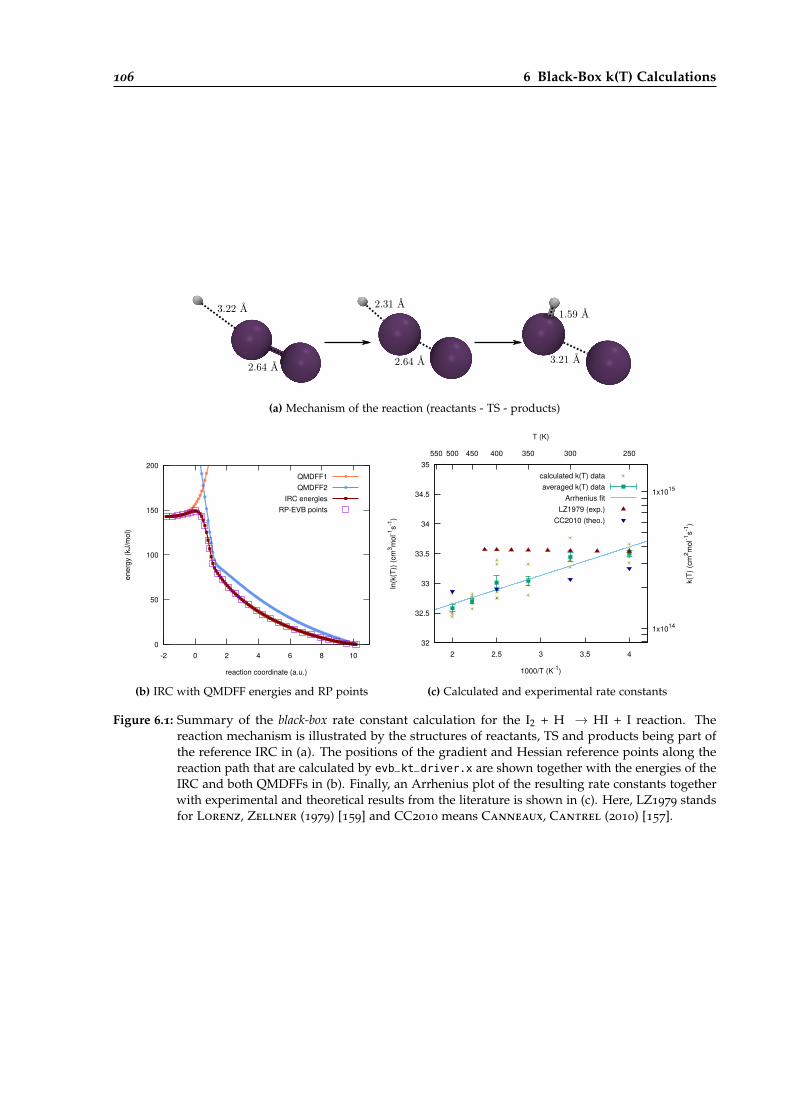
106 6 Black-Box k(T) Calculations
3.22 Å
2.64 Å
2.31 Å
2.64 Å
1.59 Å
3.21 Å
(a) Mechanism of the reaction (reactants - TS - products)
0
50
100
150
200
-2 0 2 4 6 8 10
ener
gy (k
J/m
ol)
reaction coordinate (a.u.)
QMDFF1QMDFF2
IRC energiesRP-EVB points
(b) IRC with QMDFF energies and RP points
32
32.5
33
33.5
34
34.5
35
2 2.5 3 3.5 4
1x10¹⁴
1x10¹⁵
250300350400450500550
ln(k
(T))
(cm
3 mol
-1s-1
)
k(T)
(cm
2 mol
-1s-1
)
1000/T (K-1)
T (K)
calculated k(T) dataaveraged k(T) data
Arrhenius fitLZ1979 (exp.)
CC2010 (theo.)
(c) Calculated and experimental rate constants
Figure 6.1: Summary of the black-box rate constant calculation for the I2 + H → HI + I reaction. Thereaction mechanism is illustrated by the structures of reactants, TS and products being part ofthe reference IRC in (a). The positions of the gradient and Hessian reference points along thereaction path that are calculated by evb_kt_driver.x are shown together with the energies of theIRC and both QMDFFs in (b). Finally, an Arrhenius plot of the resulting rate constants togetherwith experimental and theoretical results from the literature is shown in (c). Here, LZ1979 standsfor Lorenz, Zellner (1979) [159] and CC2010 means Canneaux, Cantrel (2010) [157].
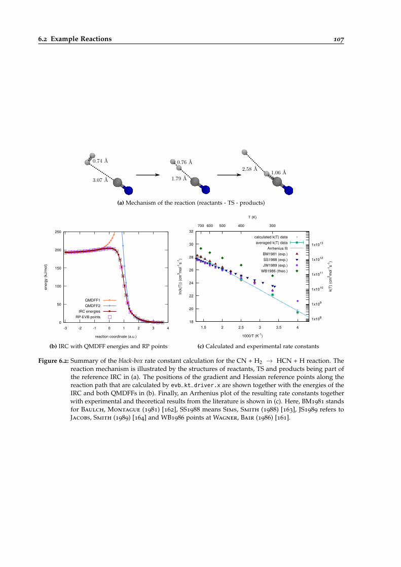
6.2 Example Reactions 107
0.74 Å
3.07 Å 1.79 Å
0.76 Å2.58 Å 1.06 Å
(a) Mechanism of the reaction (reactants - TS - products)
0
50
100
150
200
250
-3 -2 -1 0 1 2 3 4
ener
gy (k
J/m
ol)
reaction coordinate (a.u.)
QMDFF1QMDFF2
IRC energiesRP-EVB points
(b) IRC with QMDFF energies and RP points
18
20
22
24
26
28
30
32
1.5 2 2.5 3 3.5 4
1x10⁸
1x10⁹
1x10¹⁰
1x10¹¹
1x10¹²
1x10¹³
300400500600700
ln(k
(T))
(cm
3 mol
-1s-1
)
k(T)
(cm
2 mol
-1s-1
)1000/T (K-1)
T (K)
calculated k(T) dataaveraged k(T) data
Arrhenius fitBM1981 (exp.)SS1988 (exp.)JW1989 (exp.)
WB1986 (theo.)
(c) Calculated and experimental rate constants
Figure 6.2: Summary of the black-box rate constant calculation for the CN + H2 → HCN + H reaction. Thereaction mechanism is illustrated by the structures of reactants, TS and products being part ofthe reference IRC in (a). The positions of the gradient and Hessian reference points along thereaction path that are calculated by evb_kt_driver.x are shown together with the energies of theIRC and both QMDFFs in (b). Finally, an Arrhenius plot of the resulting rate constants togetherwith experimental and theoretical results from the literature is shown in (c). Here, BM1981 standsfor Baulch, Montague (1981) [162], SS1988 means Sims, Smith (1988) [163], JS1989 refers toJacobs, Smith (1989) [164] and WB1986 points at Wagner, Bair (1986) [161].
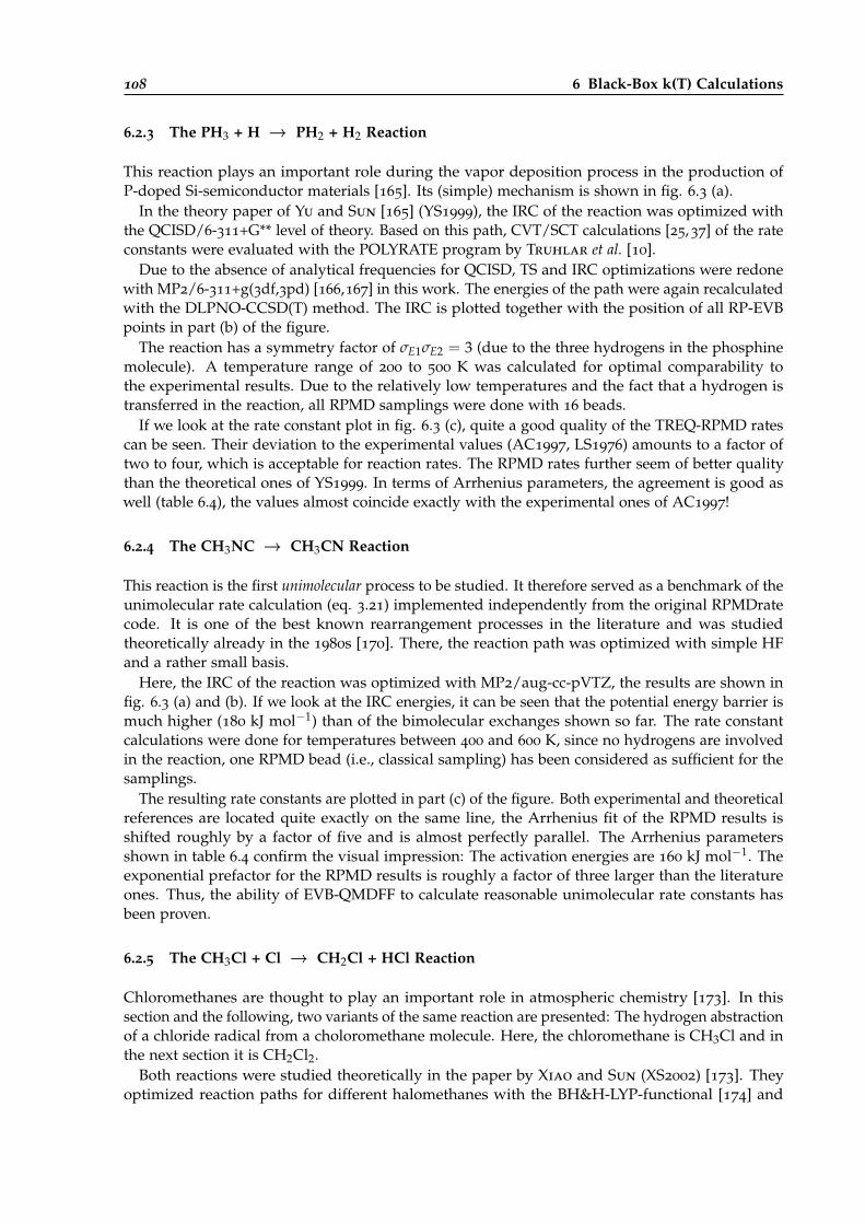
108 6 Black-Box k(T) Calculations
6.2.3 The PH3 + H → PH2 + H2 Reaction
This reaction plays an important role during the vapor deposition process in the production ofP-doped Si-semiconductor materials [165]. Its (simple) mechanism is shown in fig. 6.3 (a).
In the theory paper of Yu and Sun [165] (YS1999), the IRC of the reaction was optimized withthe QCISD/6-311+G** level of theory. Based on this path, CVT/SCT calculations [25, 37] of the rateconstants were evaluated with the POLYRATE program by Truhlar et al. [10].
Due to the absence of analytical frequencies for QCISD, TS and IRC optimizations were redonewith MP2/6-311+g(3df,3pd) [166,167] in this work. The energies of the path were again recalculatedwith the DLPNO-CCSD(T) method. The IRC is plotted together with the position of all RP-EVBpoints in part (b) of the figure.
The reaction has a symmetry factor of σE1σE2 = 3 (due to the three hydrogens in the phosphinemolecule). A temperature range of 200 to 500 K was calculated for optimal comparability tothe experimental results. Due to the relatively low temperatures and the fact that a hydrogen istransferred in the reaction, all RPMD samplings were done with 16 beads.
If we look at the rate constant plot in fig. 6.3 (c), quite a good quality of the TREQ-RPMD ratescan be seen. Their deviation to the experimental values (AC1997, LS1976) amounts to a factor oftwo to four, which is acceptable for reaction rates. The RPMD rates further seem of better qualitythan the theoretical ones of YS1999. In terms of Arrhenius parameters, the agreement is good aswell (table 6.4), the values almost coincide exactly with the experimental ones of AC1997!
6.2.4 The CH3NC → CH3CN Reaction
This reaction is the first unimolecular process to be studied. It therefore served as a benchmark of theunimolecular rate calculation (eq. 3.21) implemented independently from the original RPMDratecode. It is one of the best known rearrangement processes in the literature and was studiedtheoretically already in the 1980s [170]. There, the reaction path was optimized with simple HFand a rather small basis.
Here, the IRC of the reaction was optimized with MP2/aug-cc-pVTZ, the results are shown infig. 6.3 (a) and (b). If we look at the IRC energies, it can be seen that the potential energy barrier ismuch higher (180 kJ mol−1) than of the bimolecular exchanges shown so far. The rate constantcalculations were done for temperatures between 400 and 600 K, since no hydrogens are involvedin the reaction, one RPMD bead (i.e., classical sampling) has been considered as sufficient for thesamplings.
The resulting rate constants are plotted in part (c) of the figure. Both experimental and theoreticalreferences are located quite exactly on the same line, the Arrhenius fit of the RPMD results isshifted roughly by a factor of five and is almost perfectly parallel. The Arrhenius parametersshown in table 6.4 confirm the visual impression: The activation energies are 160 kJ mol−1. Theexponential prefactor for the RPMD results is roughly a factor of three larger than the literatureones. Thus, the ability of EVB-QMDFF to calculate reasonable unimolecular rate constants hasbeen proven.
6.2.5 The CH3Cl + Cl → CH2Cl + HCl Reaction
Chloromethanes are thought to play an important role in atmospheric chemistry [173]. In thissection and the following, two variants of the same reaction are presented: The hydrogen abstractionof a chloride radical from a choloromethane molecule. Here, the chloromethane is CH3Cl and inthe next section it is CH2Cl2.
Both reactions were studied theoretically in the paper by Xiao and Sun (XS2002) [173]. Theyoptimized reaction paths for different halomethanes with the BH&H-LYP-functional [174] and
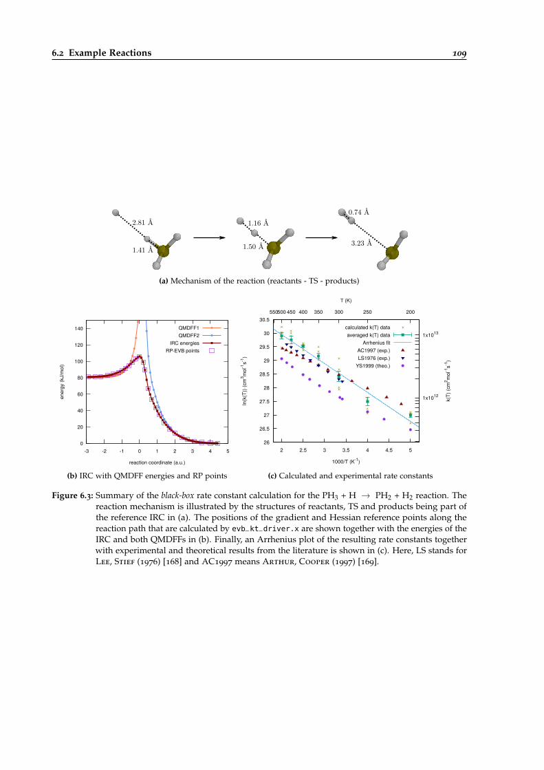
6.2 Example Reactions 109
2.81 Å
1.41 Å
1.16 Å
1.50 Å 3.23 Å
0.74 Å
(a) Mechanism of the reaction (reactants - TS - products)
0
20
40
60
80
100
120
140
-3 -2 -1 0 1 2 3 4 5
ener
gy (k
J/m
ol)
reaction coordinate (a.u.)
QMDFF1QMDFF2
IRC energiesRP-EVB points
(b) IRC with QMDFF energies and RP points
26
26.5
27
27.5
28
28.5
29
29.5
30
30.5
2 2.5 3 3.5 4 4.5 5
1x10¹²
1x10¹³
200250300350400450500550
ln(k
(T))
(cm
3 mol
-1s-1
)
k(T)
(cm
2 mol
-1s-1
)
1000/T (K-1)
T (K)
calculated k(T) dataaveraged k(T) data
Arrhenius fitAC1997 (exp.)LS1976 (exp.)
YS1999 (theo.)
(c) Calculated and experimental rate constants
Figure 6.3: Summary of the black-box rate constant calculation for the PH3 + H → PH2 + H2 reaction. Thereaction mechanism is illustrated by the structures of reactants, TS and products being part ofthe reference IRC in (a). The positions of the gradient and Hessian reference points along thereaction path that are calculated by evb_kt_driver.x are shown together with the energies of theIRC and both QMDFFs in (b). Finally, an Arrhenius plot of the resulting rate constants togetherwith experimental and theoretical results from the literature is shown in (c). Here, LS stands forLee, Stief (1976) [168] and AC1997 means Arthur, Cooper (1997) [169].
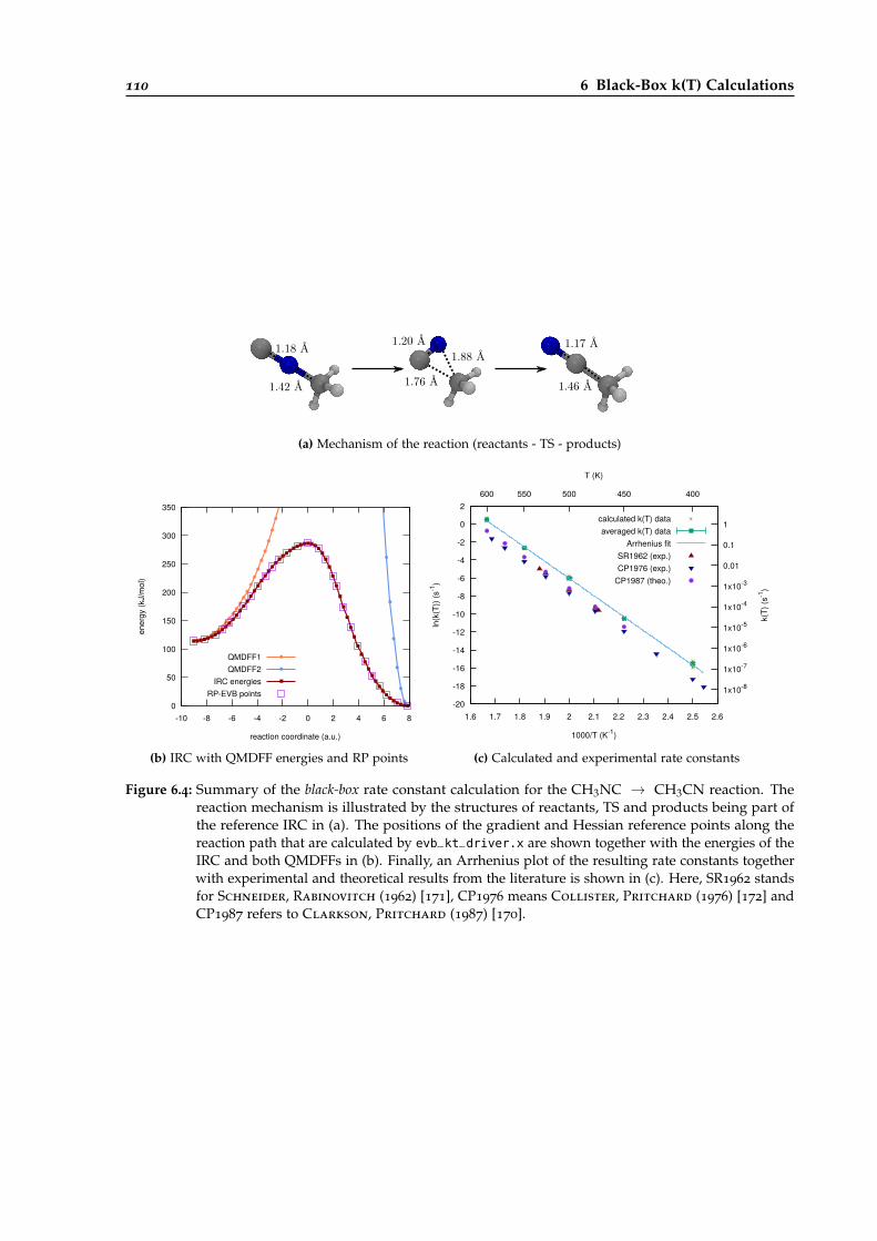
110 6 Black-Box k(T) Calculations
1.18 Å
1.42 Å
1.88 Å1.20 Å
1.76 Å
1.17 Å
1.46 Å
(a) Mechanism of the reaction (reactants - TS - products)
0
50
100
150
200
250
300
350
-10 -8 -6 -4 -2 0 2 4 6 8
ener
gy (k
J/m
ol)
reaction coordinate (a.u.)
QMDFF1QMDFF2
IRC energiesRP-EVB points
(b) IRC with QMDFF energies and RP points
-20
-18
-16
-14
-12
-10
-8
-6
-4
-2
0
2
1.6 1.7 1.8 1.9 2 2.1 2.2 2.3 2.4 2.5 2.6
1x10⁻⁸
1x10⁻⁷
1x10⁻⁶
1x10⁻⁵
1x10⁻⁴
1x10⁻³
0.01
0.1
1
400450500550600
ln(k
(T))
(s-1
)
k(T)
(s-1
)
1000/T (K-1)
T (K)
calculated k(T) dataaveraged k(T) data
Arrhenius fitSR1962 (exp.)CP1976 (exp.)
CP1987 (theo.)
(c) Calculated and experimental rate constants
Figure 6.4: Summary of the black-box rate constant calculation for the CH3NC → CH3CN reaction. Thereaction mechanism is illustrated by the structures of reactants, TS and products being part ofthe reference IRC in (a). The positions of the gradient and Hessian reference points along thereaction path that are calculated by evb_kt_driver.x are shown together with the energies of theIRC and both QMDFFs in (b). Finally, an Arrhenius plot of the resulting rate constants togetherwith experimental and theoretical results from the literature is shown in (c). Here, SR1962 standsfor Schneider, Rabinovitch (1962) [171], CP1976 means Collister, Pritchard (1976) [172] andCP1987 refers to Clarkson, Pritchard (1987) [170].

6.2 Example Reactions 111
3.21 Å
1.09 Å
1.48 Å
1.31 Å
1.28 Å
2.34 Å
(a) Mechanism of the reaction (reactants - TS - products)
0
10
20
30
40
50
60
-12 -10 -8 -6 -4 -2 0 2 4 6
ener
gy (k
J/m
ol)
reaction coordinate (a.u.)
QMDFF1QMDFF2
IRC energiesRP-EVB points
(b) IRC with QMDFF energies and RP points
20
22
24
26
28
30
32
34
36
1.6 1.8 2 2.2 2.4 2.6 2.8 3 3.2 3.4
1x10⁹
1x10¹⁰
1x10¹¹
1x10¹²
1x10¹³
1x10¹⁴
300350400450500550600
ln(k
(T))
(cm
3 mol
-1s-1
)
k(T)
(cm
2 mol
-1s-1
)
1000/T (K-1)
T (K)
calculated k(T) dataaveraged k(T) data
Arrhenius fitBK2002 (exp.)
CW1973 (exp.)GM1961 (exp.)XS2002 (theo.)
(c) Calculated and experimental rate constants
Figure 6.5: Summary of the black-box rate constant calculation for the CH3Cl + Cl → CH2Cl + HCl reaction.The reaction mechanism is illustrated by the structures of reactants, TS and products being partof the reference IRC in (a). The positions of the gradient and Hessian reference points along thereaction path that are calculated by evb_kt_driver.x are shown together with the energies of theIRC and both QMDFFs in (b). Finally, an Arrhenius plot of the resulting rate constants togetherwith experimental and theoretical results from the literature is shown in (c). Here, GM1961 standsfor Goldfinger, Martens (1961) [175], CW1973 means Clyne, Walker (1973) [176], BK2002
refers to Bryakov, Knyazev (2002) [177] and XS2002 means Xu, Sun (2002) [173] .
calculated its energies with the QCISD(T) method. The rate constants of the different processes werecalculated with the usual static CVT/SCT-method using POLYRATE. For the black-box calculations,the IRC was again optimized with MP2, now with the same basis set as used in the reference paper(6-311g(d,p)). The energies of the path were again recalculated with the DLPNO-CCSD(T) method.Structures and energies of the IRC are presented in fig. 6.5.
The rate constant calculations were done at temperatures from 300 to 600 K, 16 beads were usedsince significant quantum effects can be expected if a hydrogen atom is transferred; the reactionhas a symmetry factor of three.
In part (c) of the figure the resulting rate constants are compared with two experimental papersand the CVT/SCT results of XS2002. The RPMD values are near the experimental ones for highertemperatures but show larger deviations from them for lower temperatures. Corresponding to thisoverestimated slope of the Arrhenius curve, the RPMD activation energy (30.1 kJ mol−1, table 6.4)is much too high in comparison to that of experiments, which are between 6.6 and 14.9 kJ mol−1.The same trend can be seen for the exponential prefactors. A possible reason for the deviationsmight be, e.g., an insufficient performance of the DLPNO-CCSD(T) energy correction method inreproducing the reaction barrier.
112 6 Black-Box k(T) Calculations
3.06 Å
1.09 Å
1.54 Å
1.25 Å
1.28 Å
2.31 Å
(a) Mechanism of the reaction (reactants - TS - products)
0
10
20
30
40
50
60
-8 -6 -4 -2 0 2 4 6 8
ener
gy (k
J/m
ol)
reaction coordinate (a.u.)
QMDFF1QMDFF2
IRC energiesRP-EVB points
(b) IRC with QMDFF energies and RP points
22
24
26
28
30
32
34
1.6 1.8 2 2.2 2.4 2.6 2.8 3 3.2 3.4
1x10¹⁰
1x10¹¹
1x10¹²
1x10¹³
1x10¹⁴
300350400450500550600
ln(k
(T))
(cm
3 mol
-1s-1
)
k(T)
(cm
2 mol
-1s-1
)
1000/T (K-1)
T (K)
calculated k(T) dataaveraged k(T) data
Arrhenius fitGM1961 (exp.)CW1973 (exp.)BK2002 (exp.)
XS2002 (theo.)
(c) Calculated and experimental rate constants
Figure 6.6: Summary of the black-box rate constant calculation for the CH2Cl2 + Cl → CHCl2 + HCl reaction.The reaction mechanism is illustrated by the structures of reactants, TS and products being partof the reference IRC in (a). The positions of the gradient and Hessian reference points along thereaction path that are calculated by evb_kt_driver.x are shown together with the energies of theIRC and both QMDFFs in (b). Finally, an Arrhenius plot of the resulting rate constants togetherwith experimental and theoretical results from the literature is shown in (c). Here, GM1961 standsfor Goldfinger, Martens (1961) [175], CW1973 means Clyne, Walker (1973) [176], BK2002
refers to Bryakov, Knyazev (2002) [177] and XS2002 links to Xu, Sun (2002) [173].
6.2.6 The CH2Cl2 + Cl → CHCl2 + HCl Reaction
This reaction is a small variation of the last one: one hydrogen in the chloromethane has beenreplaced by another chlorine atom. All calculation settings of reference and RPMD were the sameas for the previous reaction. The symmetry factor is now two instead of three.
By looking at the results presented in fig. 6.6 an improvement of the RPMD quality withrespect to the experiments in comparison to the CH3Cl + Cl system can be seen: The determinedArrhenius fit of the TREQ-RPMD rate constants coincides almost exactly with the rates of GM1961.The deviations to CW1972 and BK2002 are smaller than one order of magnitude for the wholeinvestigated temperature range. The Arrhenius parameters show a similar trend (table 6.4):The RPMD ones are very similar to GM1961 and CW1973 (there with a larger deviation ofpreexponential factors). The BK2002 value of the activation energy again deviates substantiallyfrom the others.
If we do now the final comparison between the CH3Cl + Cl and CH2Cl2 + Cl reactions, thegeneral trend is reproduced correctly: The potential energy barrier expressed in part (b) of figs.6.5-6.6 is higher for the CH3Cl + Cl reaction, which results in smaller rate constants and Arrheniusparameters for it. TREQ-RPMD is able to reproduce this trend, nevertheless its results deviate quitesignificantly for the CH3Cl + Cl reaction.
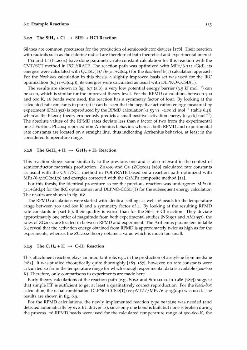
6.2 Example Reactions 113
6.2.7 The SiH4 + Cl → SiH3 + HCl Reaction
Silanes are common precursors for the production of semiconductor devices [178]. Their reactionwith radicals such as the chlorine radical are therefore of both theoretical and experimental interest.
Pei and Li (PL2004) have done parametric rate constant calculation for this reaction with theCVT/SCT method in POLYRATE. The reaction path was optimized with MP2/6-311+G(d), itsenergies were calculated with QCISD(T)//6-311+G(d,p) for the dual-level k(T) calculation approach.For the black-box calculation in this thesis, a slightly improved basis set was used for the IRCoptimization (6.311+G(d,p)), its energies were calculated as usual with DLPNO-CCSD(T).
The results are shown in fig. 6.7 (a,b), a very low potential energy barrier (3.5 kJ mol−1) canbe seen, which is similar for the improved theory level. For the RPMD calculations between 300
and 600 K, 16 beads were used, the reaction has a symmetry factor of four. By looking at thecalculated rate constants in part (c) it can be seen that the negative activation energy measured byexperiment (DM1992) is reproduced by the RPMD calculation(-2.53 vs. -2.00 kJ mol−1 (table 6.4)),whereas the PL2004-theory erroneously predicts a small positive activation energy (0.93 kJ mol−1).The absolute values of the RPMD rates deviate less than a factor of two from the experimentalones! Further, PL2004 reported non-Arrhenius behavior, whereas both RPMD and experimentalrate constants are located on a straight line, thus indicating Arrhenius behavior, at least in theconsidered temperature range.
6.2.8 The GeH4 + H → GeH3 + H2 Reaction
This reaction shows some similarity to the previous one and is also relevant in the context ofsemiconductor materials production. Zhang and Gu (ZG2002) [180] calculated rate constantsas usual with the CVT/SCT method in POLYRATE based on a reaction path optimized withMP2/6-311G(2df,p) and energies corrected with the G2MP2 composite method [12].
For this thesis, the identical procedure as for the previous reaction was undergone: MP2/6-311+G(d,p) for the IRC optimization and DLPNO-CCSD(T) for the subsequent energy calculation.The results are shown in fig. 6.8.
The RPMD calculations were started with identical settings as well: 16 beads for the temperaturerange between 300 and 600 K and a symmetry factor of 4. By looking at the resulting RPMDrate constants in part (c), their quality is worse than for the SiH4 + Cl reaction. They deviateapproximately one order of magnitude from both experimental studies (NS1993 and AM1997), therates of ZG2002 are located in between RPMD and experiment. The Arrhenius parameters in table6.4 reveal that the activation energy obtained from RPMD is approximately twice as high as for theexperiments, whereas the ZG2002 theory obtains a value which is much too small.
6.2.9 The C2H4 + H → C2H5 Reaction
This attachment reaction plays an important role, e.g., in the production of acetylene from methane[183]. It was studied theoretically quite thoroughly [183–187], however, no rate constants werecalculated so far in the temperature range for which enough experimental data is available (300-600
K). Therefore, only comparisons to experiments are made here.Early theory calculations of the reaction path (e.g., Sosa and Schlegel in 1986 [187]) suggest
that simple HF is sufficient to get at least a qualitatively correct reproduction. For the black-boxcalculation, the usual combination DLPNO-CCSD(T)/cc-pVTZ//MP2/6-311g(d,p) was used. Theresults are shown in fig. 6.9.
For the RPMD calculations, the newly implemented reaction type merging was needed (anddetected automatically by evb_kt_driver.x), since only one bond is built but none is broken duringthe process. 16 RPMD beads were used for the calculated temperature range of 300-600 K, the
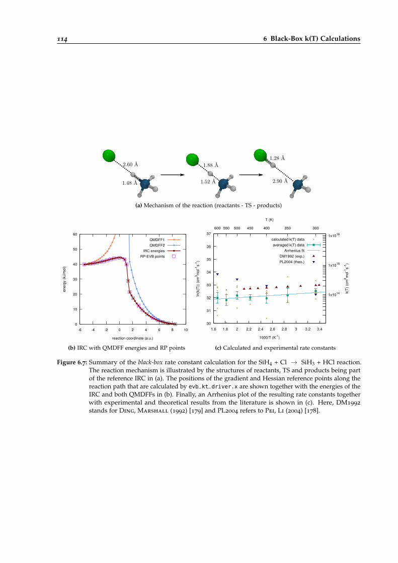
114 6 Black-Box k(T) Calculations
2.60 Å
1.48 Å
1.88 Å
1.52 Å
1.28 Å
2.90 Å
(a) Mechanism of the reaction (reactants - TS - products)
0
10
20
30
40
50
60
-6 -4 -2 0 2 4 6 8 10
ener
gy (k
J/m
ol)
reaction coordinate (a.u.)
QMDFF1QMDFF2
IRC energiesRP-EVB points
(b) IRC with QMDFF energies and RP points
30
31
32
33
34
35
36
37
1.6 1.8 2 2.2 2.4 2.6 2.8 3 3.2 3.4
1x10¹⁴
1x10¹⁵
1x10¹⁶
300350400450500550600
ln(k
(T))
(cm
3 mol
-1s-1
)
k(T)
(cm
2 mol
-1s-1
)
1000/T (K-1)
T (K)
calculated k(T) dataaveraged k(T) data
Arrhenius fitDM1992 (exp.)PL2004 (theo.)
(c) Calculated and experimental rate constants
Figure 6.7: Summary of the black-box rate constant calculation for the SiH4 + Cl → SiH3 + HCl reaction.The reaction mechanism is illustrated by the structures of reactants, TS and products being partof the reference IRC in (a). The positions of the gradient and Hessian reference points along thereaction path that are calculated by evb_kt_driver.x are shown together with the energies of theIRC and both QMDFFs in (b). Finally, an Arrhenius plot of the resulting rate constants togetherwith experimental and theoretical results from the literature is shown in (c). Here, DM1992
stands for Ding, Marshall (1992) [179] and PL2004 refers to Pei, Li (2004) [178].
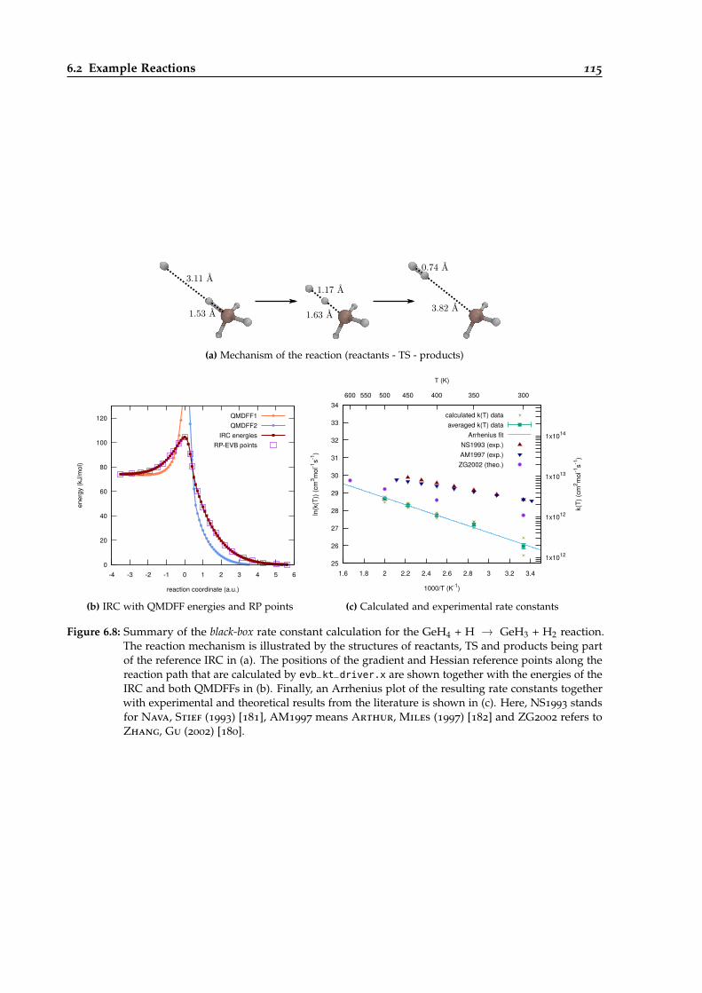
6.2 Example Reactions 115
3.11 Å
1.53 Å
1.17 Å
1.63 Å
0.74 Å
3.82 Å
(a) Mechanism of the reaction (reactants - TS - products)
0
20
40
60
80
100
120
-4 -3 -2 -1 0 1 2 3 4 5 6
ener
gy (k
J/m
ol)
reaction coordinate (a.u.)
QMDFF1QMDFF2
IRC energiesRP-EVB points
(b) IRC with QMDFF energies and RP points
25
26
27
28
29
30
31
32
33
34
1.6 1.8 2 2.2 2.4 2.6 2.8 3 3.2 3.4
1x10¹²
1x10¹²
1x10¹³
1x10¹⁴
300350400450500550600
ln(k
(T))
(cm
3 mol
-1s-1
)
k(T)
(cm
2 mol
-1s-1
)1000/T (K-1)
T (K)
calculated k(T) dataaveraged k(T) data
Arrhenius fitNS1993 (exp.)AM1997 (exp.)ZG2002 (theo.)
(c) Calculated and experimental rate constants
Figure 6.8: Summary of the black-box rate constant calculation for the GeH4 + H → GeH3 + H2 reaction.The reaction mechanism is illustrated by the structures of reactants, TS and products being partof the reference IRC in (a). The positions of the gradient and Hessian reference points along thereaction path that are calculated by evb_kt_driver.x are shown together with the energies of theIRC and both QMDFFs in (b). Finally, an Arrhenius plot of the resulting rate constants togetherwith experimental and theoretical results from the literature is shown in (c). Here, NS1993 standsfor Nava, Stief (1993) [181], AM1997 means Arthur, Miles (1997) [182] and ZG2002 refers toZhang, Gu (2002) [180].
116 6 Black-Box k(T) Calculations
4.02 Å
1.33 Å
1.87 Å
1.33 Å
1.10 Å
1.49 Å
(a) Mechanism of the reaction (reactants - TS - products)
0
50
100
150
200
250
-4 -3 -2 -1 0 1 2
ener
gy (k
J/m
ol)
reaction coordinate (a.u.)
QMDFF1QMDFF2
IRC energiesRP-EVB points
(b) IRC with QMDFF energies and RP points
26
27
28
29
30
31
32
33
1.6 1.8 2 2.2 2.4 2.6 2.8 3 3.2 3.4 3.6
1x10¹²
1x10¹³
1x10¹⁴
300350400450500550600
ln(k
(T))
(cm
3 mol
-1s-1
)
k(T)
(cm
2 mol
-1s-1
)
1000/T (K-1)
T (K)
calculated k(T) dataaveraged k(T) data
Arrhenius fitDT1969 (exp.)TJ1972 (exp.)LP1987 (exp.)
(c) Calculated and experimental rate constants
Figure 6.9: Summary of the black-box rate constant calculation for the C2H4 + H → C2H5 reaction. Thereaction mechanism is illustrated by the structures of reactants, TS and products being part ofthe reference IRC in (a). The positions of the gradient and Hessian reference points along thereaction path that are calculated by evb_kt_driver.x are shown together with the energies of theIRC and both QMDFFs in (b). Finally, an Arrhenius plot of the resulting rate constants togetherwith experimental and theoretical results from the literature is shown in (c). Here, DT1969 standsfor Dodonov, Talroze (1969) [188], TJ1972 means Teng, Jones (1972) [189] and LP1987 refers toLightfood, Piling 1987 [190].
symmetry factor of the reaction is two (both carbon atoms). With this, bimolecular rate constantswere calculated and fitted to get the Arrhenius parameters, the results are shown in part (c) ofthe figure. The three experimental studies differ quite largely from each other, TJ1972 obtainedmuch lower rates than the other two. The RPMD rates are estimated too large. By looking at theArrhenius parameters (table 6.4), we can see that LP1987 coincides quite well with RPMD at leastfor the Ea-values. Both parameters of TJ1972 are much smaller than of the others.
6.2.10 The CH3OH + Cl → CH2OH + HCl Reaction
This reaction of methanol with a chlorine radical is believed to play an important role duringthe combustion of methanol [191]. It is one of two possible reaction pathways (in the other, thehydroxyl hydrogen is abstracted). Jodkowski and Rayes (JR1998) [191] optimized the IRC ofthe reaction with different theory levels (HF, MP2, MP4) and calculated the rate constants of theprocess with a method based on state sums for different possible reaction channels developed bythemselves [191].
For the black-box method, the DLPNO-CCSD(T)/cc-pVTZ//MP2/6-311g(d,p) combination ofmethods was again used to get the needed QM reference information (fig. 6.10).
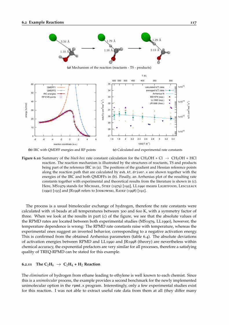
6.2 Example Reactions 117
3.34 Å
1.10 Å
1.79 Å
1.16 Å
1.29 Å
2.13 Å
(a) Mechanism of the reaction (reactants - TS - products)
0
10
20
30
40
50
60
-8 -6 -4 -2 0 2 4 6
ener
gy (k
J/m
ol)
reaction coordinate (a.u.)
QMDFF1QMDFF2
IRC energiesRP-EVB points
(b) IRC with QMDFF energies and RP points
27
28
29
30
31
32
33
34
35
1.6 1.8 2 2.2 2.4 2.6 2.8 3 3.2 3.4
1x10¹²
1x10¹³
1x10¹⁴
1x10¹⁵
300350400450500550600
ln(k
(T))
(cm
3 mol
-1s-1
)
k(T)
(cm
2 mol
-1s-1
)
1000/T (K-1)
T (K)
calculated k(T) dataaveraged k(T) data
Arrhenius fitMS1979 (exp.)LL1990 (exp.)
JR1998 (theo.)
(c) Calculated and experimental rate constants
Figure 6.10: Summary of the black-box rate constant calculation for the CH3OH + Cl → CH2OH + HClreaction. The reaction mechanism is illustrated by the structures of reactants, TS and productsbeing part of the reference IRC in (a). The positions of the gradient and Hessian reference pointsalong the reaction path that are calculated by evb_kt_driver.x are shown together with theenergies of the IRC and both QMDFFs in (b). Finally, an Arrhenius plot of the resulting rateconstants together with experimental and theoretical results from the literature is shown in (c).Here, MS1979 stands for Michael, Stief (1979) [192], LL1990 means Lightfood, Lescleaux
(1990) [193] and JR1998 refers to Jodkowski, Rayez (1998) [191].
The process is a usual bimolecular exchange of hydrogen, therefore the rate constants werecalculated with 16 beads at all temperatures between 300 and 600 K, with a symmetry factor ofthree. When we look at the results in part (c) of the figure, we see that the absolute values ofthe RPMD rates are located between both experimental studies (MS1979, LL1990), however, thetemperature dependence is wrong: The RPMD rate constants raise with temperature, whereas theexperimental ones suggest an inverted behavior, corresponding to a negative activation energy.This is confirmed from the obtained Arrhenius parameters (table 6.4). The absolute deviationsof activation energies between RPMD and LL1990 and JR1998 (theory) are nevertheless withinchemical accuracy, the exponential prefactors are very similar for all processes, therefore a satisfyingquality of TREQ-RPMD can be stated for this example.
6.2.11 The C2H6 → C2H4 + H2 Reaction
The elimination of hydrogen from ethane leading to ethylene is well known to each chemist. Sincethis is a unimolecular process, the example provides a second benchmark for the newly implementedunimolecular option in the rpmd.x program. Interestingly, only a few experimental studies existfor this reaction. I was not able to extract useful rate data from them at all (they differ many
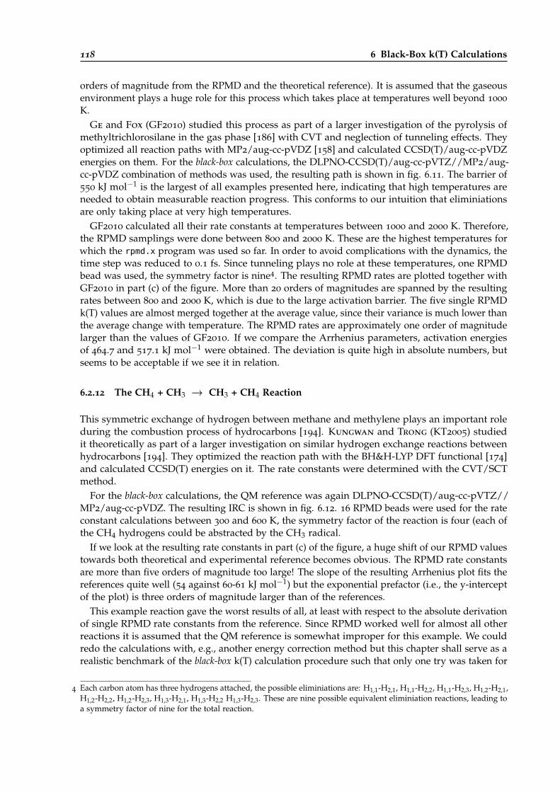
118 6 Black-Box k(T) Calculations
orders of magnitude from the RPMD and the theoretical reference). It is assumed that the gaseousenvironment plays a huge role for this process which takes place at temperatures well beyond 1000
K.Ge and Fox (GF2010) studied this process as part of a larger investigation of the pyrolysis of
methyltrichlorosilane in the gas phase [186] with CVT and neglection of tunneling effects. Theyoptimized all reaction paths with MP2/aug-cc-pVDZ [158] and calculated CCSD(T)/aug-cc-pVDZenergies on them. For the black-box calculations, the DLPNO-CCSD(T)/aug-cc-pVTZ//MP2/aug-cc-pVDZ combination of methods was used, the resulting path is shown in fig. 6.11. The barrier of550 kJ mol−1 is the largest of all examples presented here, indicating that high temperatures areneeded to obtain measurable reaction progress. This conforms to our intuition that eliminiationsare only taking place at very high temperatures.
GF2010 calculated all their rate constants at temperatures between 1000 and 2000 K. Therefore,the RPMD samplings were done between 800 and 2000 K. These are the highest temperatures forwhich the rpmd.x program was used so far. In order to avoid complications with the dynamics, thetime step was reduced to 0.1 fs. Since tunneling plays no role at these temperatures, one RPMDbead was used, the symmetry factor is nine4. The resulting RPMD rates are plotted together withGF2010 in part (c) of the figure. More than 20 orders of magnitudes are spanned by the resultingrates between 800 and 2000 K, which is due to the large activation barrier. The five single RPMDk(T) values are almost merged together at the average value, since their variance is much lower thanthe average change with temperature. The RPMD rates are approximately one order of magnitudelarger than the values of GF2010. If we compare the Arrhenius parameters, activation energiesof 464.7 and 517.1 kJ mol−1 were obtained. The deviation is quite high in absolute numbers, butseems to be acceptable if we see it in relation.
6.2.12 The CH4 + CH3 → CH3 + CH4 Reaction
This symmetric exchange of hydrogen between methane and methylene plays an important roleduring the combustion process of hydrocarbons [194]. Kungwan and Trong (KT2005) studiedit theoretically as part of a larger investigation on similar hydrogen exchange reactions betweenhydrocarbons [194]. They optimized the reaction path with the BH&H-LYP DFT functional [174]and calculated CCSD(T) energies on it. The rate constants were determined with the CVT/SCTmethod.
For the black-box calculations, the QM reference was again DLPNO-CCSD(T)/aug-cc-pVTZ//MP2/aug-cc-pVDZ. The resulting IRC is shown in fig. 6.12. 16 RPMD beads were used for the rateconstant calculations between 300 and 600 K, the symmetry factor of the reaction is four (each ofthe CH4 hydrogens could be abstracted by the CH3 radical.
If we look at the resulting rate constants in part (c) of the figure, a huge shift of our RPMD valuestowards both theoretical and experimental reference becomes obvious. The RPMD rate constantsare more than five orders of magnitude too large! The slope of the resulting Arrhenius plot fits thereferences quite well (54 against 60-61 kJ mol−1) but the exponential prefactor (i.e., the y-interceptof the plot) is three orders of magnitude larger than of the references.
This example reaction gave the worst results of all, at least with respect to the absolute derivationof single RPMD rate constants from the reference. Since RPMD worked well for almost all otherreactions it is assumed that the QM reference is somewhat improper for this example. We couldredo the calculations with, e.g., another energy correction method but this chapter shall serve as arealistic benchmark of the black-box k(T) calculation procedure such that only one try was taken for
4 Each carbon atom has three hydrogens attached, the possible eliminiations are: H1,1-H2,1, H1,1-H2,2, H1,1-H2,3, H1,2-H2,1,H1,2-H2,2, H1,2-H2,3, H1,3-H2,1, H1,3-H2,2 H1,3-H2,3. These are nine possible equivalent eliminiation reactions, leading toa symmetry factor of nine for the total reaction.
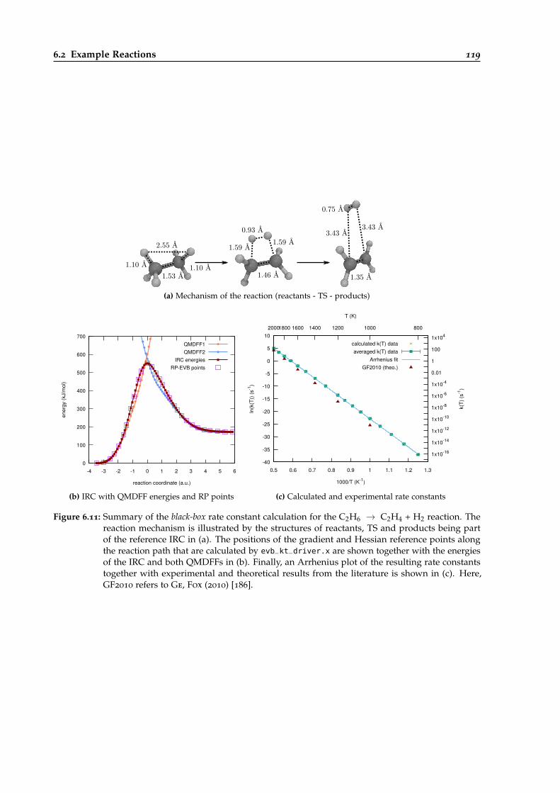
6.2 Example Reactions 119
1.53 Å
2.55 Å
1.10 Å 1.10 Å
1.59 Å1.59 Å
0.93 Å
1.46 Å
3.43 Å3.43 Å
0.75 Å
1.35 Å
(a) Mechanism of the reaction (reactants - TS - products)
0
100
200
300
400
500
600
700
-4 -3 -2 -1 0 1 2 3 4 5 6
ener
gy (k
J/m
ol)
reaction coordinate (a.u.)
QMDFF1QMDFF2
IRC energiesRP-EVB points
(b) IRC with QMDFF energies and RP points
-40
-35
-30
-25
-20
-15
-10
-5
0
5
10
0.5 0.6 0.7 0.8 0.9 1 1.1 1.2 1.3
1x10-16
1x10-14
1x10-12
1x10⁻¹⁰
1x10⁻⁸
1x10⁻⁶
1x10⁻⁴
0.01
1
100
1x104800100012001400160018002000
ln(k
(T))
(s-1
)
k(T)
(s-1
)
1000/T (K-1)
T (K)
calculated k(T) dataaveraged k(T) data
Arrhenius fitGF2010 (theo.)
(c) Calculated and experimental rate constants
Figure 6.11: Summary of the black-box rate constant calculation for the C2H6 → C2H4 + H2 reaction. Thereaction mechanism is illustrated by the structures of reactants, TS and products being partof the reference IRC in (a). The positions of the gradient and Hessian reference points alongthe reaction path that are calculated by evb_kt_driver.x are shown together with the energiesof the IRC and both QMDFFs in (b). Finally, an Arrhenius plot of the resulting rate constantstogether with experimental and theoretical results from the literature is shown in (c). Here,GF2010 refers to Ge, Fox (2010) [186].

120 6 Black-Box k(T) Calculations
2.92 Å
1.10 Å
1.33 Å
1.33 Å
1.10 Å
2.92 Å
(a) Mechanism of the reaction (reactants - TS - products)
0
20
40
60
80
100
120
-8 -6 -4 -2 0 2 4 6 8
ener
gy (k
J/m
ol)
reaction coordinate (a.u.)
QMDFF1QMDFF2
IRC energiesRP-EVB points
(b) IRC with QMDFF energies and RP points
5
10
15
20
25
1.6 1.8 2 2.2 2.4 2.6 2.8 3 3.2 3.4
1x10³
1x10⁴
1x10⁵
1x10⁶
1x10⁷
1x10⁸
1x10⁹
1x10¹⁰
1x10¹¹
1x1012300350400450500550600
ln(k
(T))
(cm
3 mol
-1s-1
)
k(T)
(cm
2 mol
-1s-1
)
1000/T (K-1)
T (K)
calculated k(T) dataaveraged k(T) data
Arrhenius fitDW1959 (exp.)AB1978 (exp.)
KT2005 (theo.)
(c) Calculated and experimental rate constants
Figure 6.12: Summary of the black-box rate constant calculation for the CH4OH + CH3 → CH3 + CH4reaction. The reaction mechanism is illustrated by the structures of reactants, TS and productsbeing part of the reference IRC in (a). The positions of the gradient and Hessian reference pointsalong the reaction path that are calculated by evb_kt_driver.x are shown together with theenergies of the IRC and both QMDFFs in (b). Finally, an Arrhenius plot of the resulting rateconstants together with experimental and theoretical results from the literature is shown in (c).Here, DW1959 stands for Dainton, Wilkinson (1959) [195], AB1978 refers to Arthur, Bell
(1978) [196] and KT2005 refers to Kungwan, Trong (2005) [194].
each system and no variation of the reference or other settings was done until we would “movetowards” the experiment.
6.2.13 The C2H6 + NH → C2H5 + H2N Reaction
This process is relevant in the combustion mechanism of energetic materials [197]. Xu and Sun
(XS2002) [197] have studied it with the CVT/SCT method as implemented in POLYRATE. Theyoptimized the reaction path at different levels of theory and basis set sizes (HF, MP2, Pople basissets [166, 167]).
For the black-box procedure the popular dual-level approach with DLPNO-CCSD(T)/cc-pVTZ//MP2/6-311g(d,p) was used again. The resulting reaction path is plotted in fig. 6.13. On the relatedTREQ PES, RPMD samplings were done with 16 beads for temperatures between 300 and 600 K,whereas the symmetry factor was chosen to be six (each hydrogen of the ethane).
The results are shown in part (c) of the figure together with the theoretical results of XS2002.It can be seen that both sets are located quite exactly on the same linear curve, indicating avery good agreement between both. This impression is confirmed if we look at the Arrheniusparameters (table 6.4). The activation energies of RPMD calculations and theoretical referenceare almost identical; the preexponential factors deviate by roughly one order of magnitude. In
6.2 Example Reactions 121
1.09 Å
3.94 Å 1.26 Å
1.32 Å
1.03 Å
2.52 Å
(a) Mechanism of the reaction (reactants - TS - products)
0
20
40
60
80
100
120
140
-10 -8 -6 -4 -2 0 2 4 6 8
ener
gy (k
J/m
ol)
reaction coordinate (a.u.)
QMDFF1QMDFF2
IRC energiesRP-EVB points
(b) IRC with QMDFF energies and RP points
-4
-2
0
2
4
6
8
10
12
14
16
1.6 1.8 2 2.2 2.4 2.6 2.8 3 3.2 3.4
0.1
1
10
100
1x10³
1x10⁴
1x10⁵
1x10⁶
300350400450500550600
ln(k
(T))
(cm
3 mol
-1s-1
)
k(T)
(cm
2 mol
-1s-1
)
1000/T (K-1)
T (K)
calculated k(T) dataaveraged k(T) data
Arrhenius fitXS1999 (theo.)
(c) Calculated and experimental rate constants
Figure 6.13: Summary of the black-box rate constant calculation for the C2H6 + NH → C2H5 + H2N reaction.The reaction mechanism is illustrated by the structures of reactants, TS and products being partof the reference IRC in (a). The positions of the gradient and Hessian reference points alongthe reaction path that are calculated by evb_kt_driver.x are shown together with the energiesof the IRC and both QMDFFs in (b). Finally, an Arrhenius plot of the resulting rate constantstogether with experimental and theoretical results from the literature is shown in (c). Here,XS1999 refers to Xu, Sun (1999) [197].
the table an experimental reference (Rohrig, Wagner 1994 [198]) is added. They measured ratesbetween 1010 and 1170 K, nevertheless the activation barrier fits both theoretical ones quite well.The preexponential factor of the experiment is one order of magnitude smaller than the RPMDone and two orders smaller than XS1999, indicating that RPMD performs better with respect tothe experiment (if we assume that near-ideal Arrhenius behavior is preserved along the wholetemperature range).
6.2.14 The CF3O + CH4 → CF3OH+CH3 Reaction
The CF3O-molecule has been proposed as eco-friendlier alternative to cholorocarbons since it seemsto have less impact on ozone layer destruction and the greenhouse effect [199]. Jing and Sun
(JS2005) [199] have studied the kinetics of this reaction with CVT/SCT. They optimized the reactionpath with both B3LYP [200, 201] and MP2; energies were then calculated with the QCISD method.
Due to the larger number of heavy atoms in this system, DLPNO-CCSD(T)/cc-pVTZ//B3LYP/6-311g(d,p) was used as black-box QM method (i.e., DFT instead of MP2 for the IRC optimizationand frequencies). The optimized reaction path is shown in fig. 6.14.
RPMD rate constant calculations were done at 300-600 K with 16 RPMD beads each, thesymmetry factor is four. The results are plotted together with the CVT/SCT values of JS2005 and
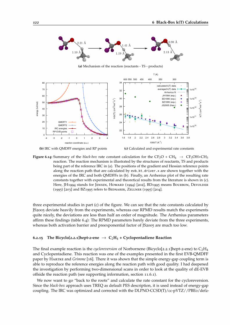
122 6 Black-Box k(T) Calculations
2.21 Å
1.10 Å
1.41 Å
1.19 Å
0.98 Å
2.13 Å
(a) Mechanism of the reaction (reactants - TS - products)
0
10
20
30
40
50
60
70
80
-4 -3 -2 -1 0 1 2 3 4
ener
gy (k
J/m
ol)
reaction coordinate (a.u.)
QMDFF1QMDFF2
IRC energiesRP-EVB points
(b) IRC with QMDFF energies and RP points
22
24
26
28
30
32
34
1.6 1.8 2 2.2 2.4 2.6 2.8 3 3.2 3.4 3.6 3.8
1x10¹⁰
1x10¹¹
1x10¹²
1x10¹³
1x10¹⁴
300350400450500550600
ln(k
(T))
(cm
3 mol
-1s-1
)
k(T)
(cm
2 mol
-1s-1
)
1000/T (K-1)
T (K)
calculated k(T) dataaveraged k(T) data
Arrhenius fitJH1994 (exp.)BD1995 (exp.)BZ1995 (exp.)JS2005 (theo.)
(c) Calculated and experimental rate constants
Figure 6.14: Summary of the black-box rate constant calculation for the CF3O + CH4 → CF3OH+CH3reaction. The reaction mechanism is illustrated by the structures of reactants, TS and productsbeing part of the reference IRC in (a). The positions of the gradient and Hessian reference pointsalong the reaction path that are calculated by evb_kt_driver.x are shown together with theenergies of the IRC and both QMDFFs in (b). Finally, an Arrhenius plot of the resulting rateconstants together with experimental and theoretical results from the literature is shown in (c).Here, JH1994 stands for Jensen, Howard (1994) [202], BD1995 means Bourbon, Devolder
(1995) [203] and BZ1995 refers to Bednarek, Zellner (1995) [204].
three experimental studies in part (c) of the figure. We can see that the rate constants calculated byJS2005 deviate heavily from the experiments, whereas our RPMD results match the experimentsquite nicely, the deviations are less than half an order of magnitude. The Arrhenius parametersaffirm these findings (table 6.4): The RPMD parameters barely deviate from the three experiments,whereas both activation barrier and preexponential factor of JS2005 are much too low.
6.2.15 The Bicyclo[2.2.1]hept-2-ene → C2H4 + Cyclopentadiene Reaction
The final example reaction is the cycloreversion of Norbornene (Bicyclo[2.2.1]hept-2-ene) to C2H4and Cyclopentadiene. This reaction was one of the examples presented in the first EVB-QMDFFpaper by Hartke and Grimme [16]. There it was shown that the simple energy-gap coupling term isable to reproduce the reference energies along the reaction path with good quality. I had deepenedthe investigation by performing two-dimensional scans in order to look at the quality of dE-EVBoffside the reaction path (see supporting information, section 11.6.1).
We now want to go “back to the roots” and calculate the rate constant for the cycloreversion.Since the black-box approach uses TREQ as default PES description, it is used instead of energy-gapcoupling. The IRC was optimized and corrected with the DLPNO-CCSD(T)/cc-pVTZ//PBE0/def2-
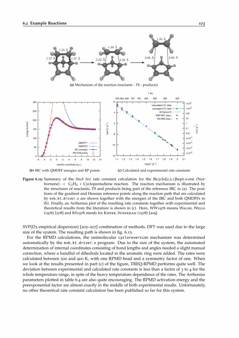
6.2 Example Reactions 123
1.57 Å 1.57 Å
1.55 Å
2.22 Å 2.22 Å
1.39 Å
3.68 Å 3.68 Å
1.33 Å
(a) Mechanism of the reaction (reactants - TS - products)
0
50
100
150
200
250
300
-6 -4 -2 0 2 4 6 8 10 12 14
ener
gy (k
J/m
ol)
reaction coordinate (a.u.)
QMDFF1QMDFF2
IRC energiesRP-EVB points
(b) IRC with QMDFF energies and RP points
-15
-10
-5
0
5
10
1.1 1.2 1.3 1.4 1.5 1.6 1.7 1.8 1.9 2 2.1
1x10⁻⁶
1x10⁻⁵
1x10⁻⁴
1x10⁻³
0.01
0.1
1
10
100
1x10³
1x10⁴
500550600650700750800850900
ln(k
(T))
(s-1
)
k(T)
(s-1
)
1000/T (K-1)
T (K)
calculated k(T) dataaveraged k(T) data
Arrhenius fitWW1967 (exp.)
KS1993 (exp.)
(c) Calculated and experimental rate constants
Figure 6.15: Summary of the black box rate constant calculation for the Bicyclo[2.2.1]hept-2-ene (Nor-bornene) → C2H4 + Cyclopentadiene reaction. The reaction mechanism is illustrated bythe structures of reactants, TS and products being part of the reference IRC in (a). The posi-tions of the gradient and Hessian reference points along the reaction path that are calculatedby evb_kt_driver.x are shown together with the energies of the IRC and both QMDFFs in(b). Finally, an Arrhenius plot of the resulting rate constants together with experimental andtheoretical results from the literature is shown in (c). Here, WW1976 means Walsh, Wells
(1976) [208] and KS1978 stands for Kiefer, Sunderam (1978) [209].
SVP(D3 empirical dispersion) [205–207] combination of methods, DFT was used due to the largesize of the system. The resulting path is shown in fig. 6.15.
For the RPMD calculations, the unimolecular cycloreversion mechanism was determinedautomatically by the evb_kt_driver.x program. Due to the size of the system, the automateddetermination of internal coordinates consisting of bond lengths and angles needed a slight manualcorrection, where a handful of dihedrals located in the aromatic ring were added. The rates werecalculated between 500 and 900 K, with one RPMD bead and a symmetry factor of one. Whenwe look at the results presented in part (c) of the figure, TREQ-RPMD performs quite well. Thedeviation between experimental and calculated rate constants is less than a factor of 3 to 4 for thewhole temperature range, in spite of the heavy temperature dependence of the rates. The Arrheniusparameters plotted in table 6.4 are also quite encouraging. The RPMD activation energy and thepreexponential factor are almost exactly in the middle of both experimental results. Unfortunately,no other theoretical rate constant calculation has been published so far for this system.
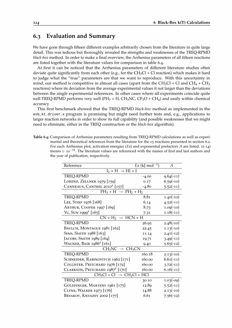
124 6 Black-Box k(T) Calculations
6.3 Evaluation and Summary
We have gone through fifteen different examples arbitrarily chosen from the literature in quite largedetail. This was tedious but thoroughly revealed the strengths and weaknesses of the TREQ-RPMDblack-box method. In order to make a final overview, the Arrhenius parameters of all fifteen reactionsare listed together with the literature values for comparison in table 6.4.
At first it can be noticed that the Arrhenius parameters of different literature studies oftendeviate quite significantly from each other (e.g., for the CH3Cl + Cl reaction) which makes it hardto judge what the “true” parameters are that we want to reproduce. With this uncertainty inmind, our method is competitive in almost all cases (apart from the CH3Cl + Cl and CH4 + CH3reactions) where its deviation from the average experimental values it not larger than the deviationsbetween the single experimental references. In other cases where all experiments coincide quitewell TREQ-RPMD performs very well (PH3 + H, CH3NC, CF3O + CH4) and easily within chemicalaccuracy.
This first benchmark showed that the TREQ-RPMD black-box method as implemented in theevb_kt_driver.x program is promising but might need further tests and, e.g., applications tolarger reaction networks in order to show its full capability (and possible weaknesses that we mightneed to eliminate, either in the TREQ construction or the black-box algorithm).
Table 6.4: Comparison of Arrhenius parameters resulting from TREQ-RPMD calculations as well as experi-mental and theoretical references from the literature for the 15 reactions presented in section 6.2.For each Arrhenius plot, activation energies (Ea) and exponential prefactors A are listed. 1(-14)means 1· 10
−14. The literature values are referenced with the names of first and last authors andthe year of publication, respectively.
Reference Ea (kJ mol−1) AI2 + H → HI + I
TREQ-RPMD -4.00 9.64(-11)Lorenz, Zellner 1979 [159] 0.17 6.59(-10)Canneaux, Cantrel 2010
a [157] -4.80 5.52(-11)PH3 + H → PH2 + H2
TREQ-RPMD 8.81 1.40(-10)Lee, Stief 1976 [168] 6.14 4.52(-11)Arthur, Cooper 1997 [169] 8.73 1.09(-10)Yu, Sun 1999
a [165] 7.31 1.18(-11)CN + H2 → HCN + H
TREQ-RPMD 26.95 2.48(-10)Baulch, Montague 1981 [162] 22.45 1.13(-10)Sims, Smith 1988 [163] 11.14 2.41(-12)Jacobs, Smith 1989 [164] 19.71 3.49(-11)Wagner, Bair 1986
a [161] 9.40 5.65(-12)CH3NC → CH3CN
TREQ-RPMD 160.18 2.13(-10)Schneider, Rabinovitch 1962 [171] 160.00 6.61(-11)Collister, Pritchard 1976 [172] 160.00 3.72(-11)Clarkson, Pritchard 1987
a [170] 160.00 6.16(-11)CH3Cl + Cl → CH2Cl + HCl
TREQ-RPMD 30.10 1.03(-09)Goldfinger, Martens 1961 [175] 12.89 5.52(-11)Clyne, Walker 1973 [176] 14.88 2.13(-10)Bryakov, Knyazev 2002 [177] 6.61 7.56(-12)
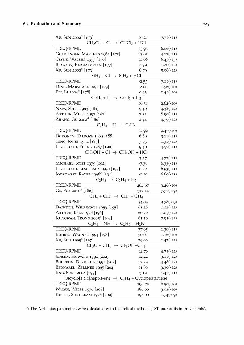
6.3 Evaluation and Summary 125
Xu, Sun 2002a [173] 16.21 7.71(-11)
CH2Cl2 + Cl → CHCl2 + HClTREQ-RPMD 15.95 6.96(-11)Goldfinger, Martens 1961 [175] 13.05 4.17(-11)Clyne, Walker 1973 [176] 12.06 6.45(-13)Bryakov, Knyazev 2002 [177] 2.99 1.20(-12)Xu, Sun 2002
a [173] 6.79 5.96(-12)SiH4 + Cl → SiH3 + HCl
TREQ-RPMD -2.53 7.11(-11)Ding, Marshall 1992 [179] -2.00 1.56(-10)Pei, Li 2004
a [178] 0.93 2.41(-10)GeH4 + H → GeH3 + H2
TREQ-RPMD 16.51 2.64(-10)Nava, Stief 1993 [181] 9.40 4.38(-12)Arthur, Miles 1997 [182] 7.31 8.90(-11)Zhang, Gu 2002
a [180] 2.44 4.79(-12)C2H4 + H → C2H5
TREQ-RPMD 12.99 9.47(-10)Dodonov, Talroze 1969 [188] 6.69 3.11(-11)Teng, Jones 1972 [189] 3.05 1.31(-12)Lightfood, Piling 1987 [190] 9.40 4.57(-11)
CH3OH + Cl → CH2OH + HClTREQ-RPMD 3.37 4.77(-11)Michael, Stief 1979 [192] -7.38 6.33(-11)Lightfood, Lescleaux 1990 [193] 0.27 6.93(-11)Jodkowski, Rayez 1998
a [191] -0.19 6.60(-11)C2H6 → C2H4 + H2
TREQ-RPMD 464.67 3.46(-10)Ge, Fox 2010
a [186] 517.14 7.71(-09)CH4 + CH3 → CH3 + CH4
TREQ-RPMD 54.09 3.78(-09)Dainton, Wilkinson 1959 [195] 61.28 1.12(-12)Arthur, Bell 1978 [196] 60.70 1.05(-12)Kungwan, Trong 2005
a [194] 61.10 7.95(-13)C2H6 + NH → C2H5 + H2N
TREQ-RPMD 77.65 1.36(-11)Rohrig, Wagner 1994 [198] 70.01 1.16(-10)Xu, Sun 1999
a [197] 79.00 1.47(-12)CF3O + CH4 → CF3OH+CH3
TREQ-RPMD 14.70 4.73(-12)Jensen, Howard 1994 [202] 12.22 3.11(-12)Bourbon, Devolder 1995 [203] 13.39 4.48(-12)Bednarek, Zellner 1995 [204] 11.89 3.30(-12)Jing, Sun
a2008 [199] 5.12 1.41(-11)
Bicyclo[2.2.1]hept-2-ene → C2H4 + CyclopentadieneTREQ-RPMD 190.75 6.50(-10)Walsh, Wells 1976 [208] 186.00 3.02(-10)Kiefer, Sunderam 1978 [209] 194.00 1.74(-09)
a: The Arrhenius parameters were calculated with theoretical methods (TST and/or its improvements).

126 6 Black-Box k(T) Calculations
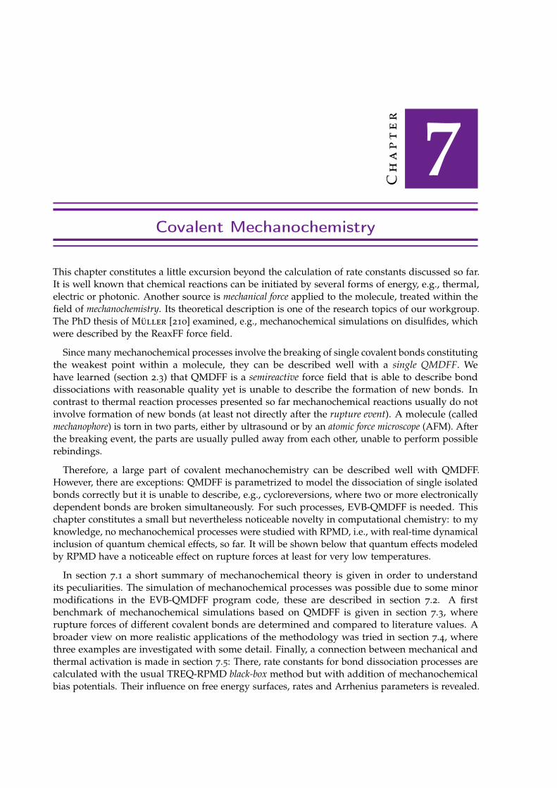
7
Ch
ap
te
r
Covalent Mechanochemistry
This chapter constitutes a little excursion beyond the calculation of rate constants discussed so far.It is well known that chemical reactions can be initiated by several forms of energy, e.g., thermal,electric or photonic. Another source is mechanical force applied to the molecule, treated within thefield of mechanochemistry. Its theoretical description is one of the research topics of our workgroup.The PhD thesis of Müller [210] examined, e.g., mechanochemical simulations on disulfides, whichwere described by the ReaxFF force field.
Since many mechanochemical processes involve the breaking of single covalent bonds constitutingthe weakest point within a molecule, they can be described well with a single QMDFF. Wehave learned (section 2.3) that QMDFF is a semireactive force field that is able to describe bonddissociations with reasonable quality yet is unable to describe the formation of new bonds. Incontrast to thermal reaction processes presented so far mechanochemical reactions usually do notinvolve formation of new bonds (at least not directly after the rupture event). A molecule (calledmechanophore) is torn in two parts, either by ultrasound or by an atomic force microscope (AFM). Afterthe breaking event, the parts are usually pulled away from each other, unable to perform possiblerebindings.
Therefore, a large part of covalent mechanochemistry can be described well with QMDFF.However, there are exceptions: QMDFF is parametrized to model the dissociation of single isolatedbonds correctly but it is unable to describe, e.g., cycloreversions, where two or more electronicallydependent bonds are broken simultaneously. For such processes, EVB-QMDFF is needed. Thischapter constitutes a small but nevertheless noticeable novelty in computational chemistry: to myknowledge, no mechanochemical processes were studied with RPMD, i.e., with real-time dynamicalinclusion of quantum chemical effects, so far. It will be shown below that quantum effects modeledby RPMD have a noticeable effect on rupture forces at least for very low temperatures.
In section 7.1 a short summary of mechanochemical theory is given in order to understandits peculiarities. The simulation of mechanochemical processes was possible due to some minormodifications in the EVB-QMDFF program code, these are described in section 7.2. A firstbenchmark of mechanochemical simulations based on QMDFF is given in section 7.3, whererupture forces of different covalent bonds are determined and compared to literature values. Abroader view on more realistic applications of the methodology was tried in section 7.4, wherethree examples are investigated with some detail. Finally, a connection between mechanical andthermal activation is made in section 7.5: There, rate constants for bond dissociation processes arecalculated with the usual TREQ-RPMD black-box method but with addition of mechanochemicalbias potentials. Their influence on free energy surfaces, rates and Arrhenius parameters is revealed.
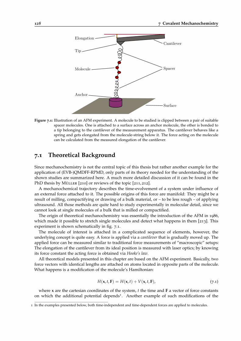
128 7 Covalent Mechanochemistry
Spacer
Cantilever
Molecule
Surface
Anchor
Tip
Elongation
Figure 7.1: Illustration of an AFM experiment. A molecule to be studied is clipped between a pair of suitablespacer molecules. One is attached to a surface across an anchor molecule, the other is bonded toa tip belonging to the cantilever of the measurement apparatus. The cantilever behaves like aspring and gets elongated from the molecule-string below it. The force acting on the moleculecan be calculated from the measured elongation of the cantilever.
7.1 Theoretical Background
Since mechanochemistry is not the central topic of this thesis but rather another example for theapplication of (EVB-)QMDFF-RPMD, only parts of its theory needed for the understanding of theshown studies are summarized here. A much more detailed discussion of it can be found in thePhD thesis by Müller [210] or reviews of the topic [211, 212].
A mechanochemical trajectory describes the time-evolvement of a system under influence ofan external force attached to it. The possible origins of this force are manifold: They might be aresult of milling, compactifying or drawing of a bulk material, or – to be less rough – of applyingultrasound. All those methods are quite hard to study experimentally in molecular detail, since wecannot look at single molecules of a bulk that is milled or compactified.
The origin of theoretical mechanochemistry was essentially the introduction of the AFM in 1986,which made it possible to stretch single molecules and detect what happens in them [213]. Thisexperiment is shown schematically in fig. 7.1.
The molecule of interest is attached in a complicated sequence of elements, however, theunderlying concept is quite easy. A force is applied via a cantilever that is gradually moved up. Theapplied force can be measured similar to traditional force measurements of “macroscopic” setups:The elongation of the cantilever from its ideal position is measured with laser optics; by knowingits force constant the acting force is obtained via Hooke’s law.
All theoretical models presented in this chapter are based on the AFM experiment. Basically, twoforce vectors with identical lengths are attached on atoms located in opposite parts of the molecule.What happens is a modification of the molecule’s Hamiltonian:
H(x, t, F) = H(x, t) + V(x, t, F), (7.1)
where x are the cartesian coordinates of the system, t the time and F a vector of force constantson which the additional potential depends1. Another example of such modifications of the
1 In the examples presented below, both time-independent and time-dependent forces are applied to molecules.
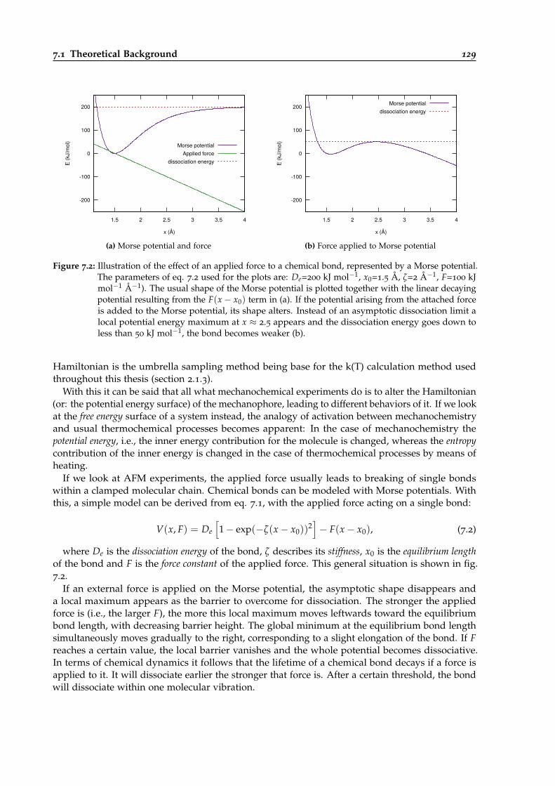
7.1 Theoretical Background 129
-200
-100
0
100
200
1.5 2 2.5 3 3.5 4
E (k
J/m
ol)
x (Å)
Morse potentialApplied force
dissociation energy
(a) Morse potential and force
-200
-100
0
100
200
1.5 2 2.5 3 3.5 4
E (k
J/m
ol)
x (Å)
Morse potentialdissociation energy
(b) Force applied to Morse potential
Figure 7.2: Illustration of the effect of an applied force to a chemical bond, represented by a Morse potential.The parameters of eq. 7.2 used for the plots are: De=200 kJ mol−1, x0=1.5 Å, ζ=2 Å−1, F=100 kJmol−1 Å−1). The usual shape of the Morse potential is plotted together with the linear decayingpotential resulting from the F(x− x0) term in (a). If the potential arising from the attached forceis added to the Morse potential, its shape alters. Instead of an asymptotic dissociation limit alocal potential energy maximum at x ≈ 2.5 appears and the dissociation energy goes down toless than 50 kJ mol−1, the bond becomes weaker (b).
Hamiltonian is the umbrella sampling method being base for the k(T) calculation method usedthroughout this thesis (section 2.1.3).
With this it can be said that all what mechanochemical experiments do is to alter the Hamiltonian(or: the potential energy surface) of the mechanophore, leading to different behaviors of it. If we lookat the free energy surface of a system instead, the analogy of activation between mechanochemistryand usual thermochemical processes becomes apparent: In the case of mechanochemistry thepotential energy, i.e., the inner energy contribution for the molecule is changed, whereas the entropycontribution of the inner energy is changed in the case of thermochemical processes by means ofheating.
If we look at AFM experiments, the applied force usually leads to breaking of single bondswithin a clamped molecular chain. Chemical bonds can be modeled with Morse potentials. Withthis, a simple model can be derived from eq. 7.1, with the applied force acting on a single bond:
V(x, F) = De
[1− exp(−ζ(x− x0))
2]− F(x− x0), (7.2)
where De is the dissociation energy of the bond, ζ describes its stiffness, x0 is the equilibrium lengthof the bond and F is the force constant of the applied force. This general situation is shown in fig.7.2.
If an external force is applied on the Morse potential, the asymptotic shape disappears anda local maximum appears as the barrier to overcome for dissociation. The stronger the appliedforce is (i.e., the larger F), the more this local maximum moves leftwards toward the equilibriumbond length, with decreasing barrier height. The global minimum at the equilibrium bond lengthsimultaneously moves gradually to the right, corresponding to a slight elongation of the bond. If Freaches a certain value, the local barrier vanishes and the whole potential becomes dissociative.In terms of chemical dynamics it follows that the lifetime of a chemical bond decays if a force isapplied to it. It will dissociate earlier the stronger that force is. After a certain threshold, the bondwill dissociate within one molecular vibration.
130 7 Covalent Mechanochemistry
Figure 7.3: Illustration of a constant force mechanochemistry simulation to be done with dynamic.x. Twoatoms of the molecule are chosen to be anchors for the attached force (blue circles). Force vectorsof opposite direction and identical absolute value are added to their gradients throughout thesimulation. At some time a bond-breaking event might happen, resulting in two separatedfragments (last picture).
7.2 Implementations
Within this thesis, mechanochemical processes were studied with three different types of simulationsetups. All three are implemented into EVB-QMDFF and can be called with their respectivekeywords that are noted here as well.
7.2.1 The Constant Force Experiment
This is the simplest possible way of attaching an external force to a molecule: A constant forcevector is added to two atoms. In order to avoid movements of the whole system towards infinityequally strong forces need to be applied in opposite directions, such that the total force applied istwice the force applied per side and no overall translation of the system is caused.
Such an experiment can be invoked for the dynamic.x program if the following program linesare added to the qmdff.key file2:
add_force
force1 [atom] [strength (N)] [vector (x, y, z)]
force1 [atom] [strength (N)] [vector (x, y, z)]
Now a dynamics trajectory with the ordered number of time steps is started, with a constant forceof the specified directions and strengths added to the chosen atoms. This experiment essentiallytests the lifetime of a bond since only two events can happen: (1) nothing (besides some stretching)and (2) a bond breaks. If the second event happens, both fragments begin to move apart in thedirections of the opposite force vectors. This behavior is illustrated in fig. 7.3.
For most forces attached either nothing happens or the bond breaks always after some time steps.There exists, however, a narrow transition region between both cases: There, for an ensemble of,e.g., 10 simulation trajectories started from the same initial structures, e.g., only six bond breakshappen, with the other four remaining intact.
With this in mind, we can estimate the critical force that is needed at least to break the bond aftera desired time: We must do a force strength scan. We could, for instance, scan the range between 0
and 10 nN with an increment of 0.1 nN and run 100 trajectories for each force strength. For most
2 Indeed it is possible with the current setup to pull both atoms in arbitrary directions, causing overall translations.Therefore, it might be useful for future program versions to, e.g., only choose the atom numbers and the strength ofthe force and then to calculate the vectors automatically from the cartesian difference vector of both atoms’ positions.
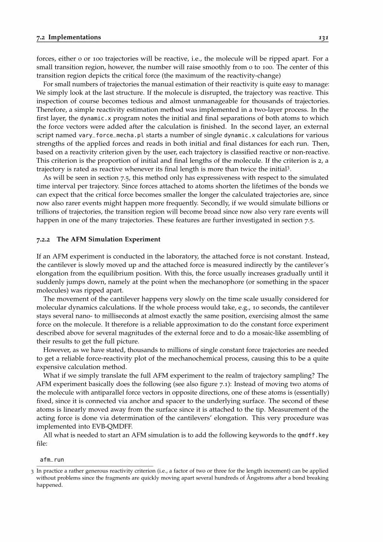
7.2 Implementations 131
forces, either 0 or 100 trajectories will be reactive, i.e., the molecule will be ripped apart. For asmall transition region, however, the number will raise smoothly from 0 to 100. The center of thistransition region depicts the critical force (the maximum of the reactivity-change)
For small numbers of trajectories the manual estimation of their reactivity is quite easy to manage:We simply look at the last structure. If the molecule is disrupted, the trajectory was reactive. Thisinspection of course becomes tedious and almost unmanageable for thousands of trajectories.Therefore, a simple reactivity estimation method was implemented in a two-layer process. In thefirst layer, the dynamic.x program notes the initial and final separations of both atoms to whichthe force vectors were added after the calculation is finished. In the second layer, an externalscript named vary_force_mecha.pl starts a number of single dynamic.x calculations for variousstrengths of the applied forces and reads in both initial and final distances for each run. Then,based on a reactivity criterion given by the user, each trajectory is classified reactive or non-reactive.This criterion is the proportion of initial and final lengths of the molecule. If the criterion is 2, atrajectory is rated as reactive whenever its final length is more than twice the initial3.
As will be seen in section 7.5, this method only has expressiveness with respect to the simulatedtime interval per trajectory. Since forces attached to atoms shorten the lifetimes of the bonds wecan expect that the critical force becomes smaller the longer the calculated trajectories are, sincenow also rarer events might happen more frequently. Secondly, if we would simulate billions ortrillions of trajectories, the transition region will become broad since now also very rare events willhappen in one of the many trajectories. These features are further investigated in section 7.5.
7.2.2 The AFM Simulation Experiment
If an AFM experiment is conducted in the laboratory, the attached force is not constant. Instead,the cantilever is slowly moved up and the attached force is measured indirectly by the cantilever’selongation from the equilibrium position. With this, the force usually increases gradually until itsuddenly jumps down, namely at the point when the mechanophore (or something in the spacermolecules) was ripped apart.
The movement of the cantilever happens very slowly on the time scale usually considered formolecular dynamics calculations. If the whole process would take, e.g., 10 seconds, the cantileverstays several nano- to milliseconds at almost exactly the same position, exercising almost the sameforce on the molecule. It therefore is a reliable approximation to do the constant force experimentdescribed above for several magnitudes of the external force and to do a mosaic-like assembling oftheir results to get the full picture.
However, as we have stated, thousands to millions of single constant force trajectories are neededto get a reliable force-reactivity plot of the mechanochemical process, causing this to be a quiteexpensive calculation method.
What if we simply translate the full AFM experiment to the realm of trajectory sampling? TheAFM experiment basically does the following (see also figure 7.1): Instead of moving two atoms ofthe molecule with antiparallel force vectors in opposite directions, one of these atoms is (essentially)fixed, since it is connected via anchor and spacer to the underlying surface. The second of theseatoms is linearly moved away from the surface since it is attached to the tip. Measurement of theacting force is done via determination of the cantilevers’ elongation. This very procedure wasimplemented into EVB-QMDFF.
All what is needed to start an AFM simulation is to add the following keywords to the qmdff.key
file:
afm_run
3 In practice a rather generous reactivity criterion (i.e., a factor of two or three for the length increment) can be appliedwithout problems since the fragments are quickly moving apart several hundreds of Ångstroms after a bond breakinghappened.
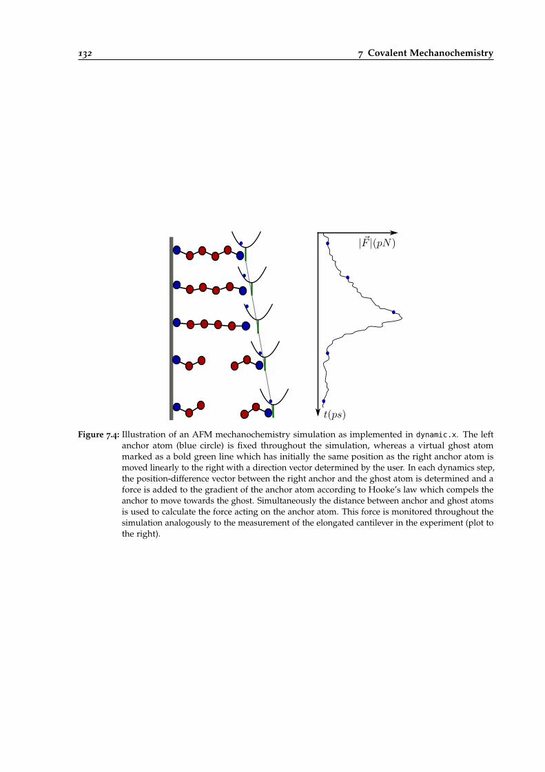
132 7 Covalent Mechanochemistry
Figure 7.4: Illustration of an AFM mechanochemistry simulation as implemented in dynamic.x. The leftanchor atom (blue circle) is fixed throughout the simulation, whereas a virtual ghost atommarked as a bold green line which has initially the same position as the right anchor atom ismoved linearly to the right with a direction vector determined by the user. In each dynamics step,the position-difference vector between the right anchor and the ghost atom is determined and aforce is added to the gradient of the anchor atom according to Hooke’s law which compels theanchor to move towards the ghost. Simultaneously the distance between anchor and ghost atomsis used to calculate the force acting on the anchor atom. This force is monitored throughout thesimulation analogously to the measurement of the elongated cantilever in the experiment (plot tothe right).
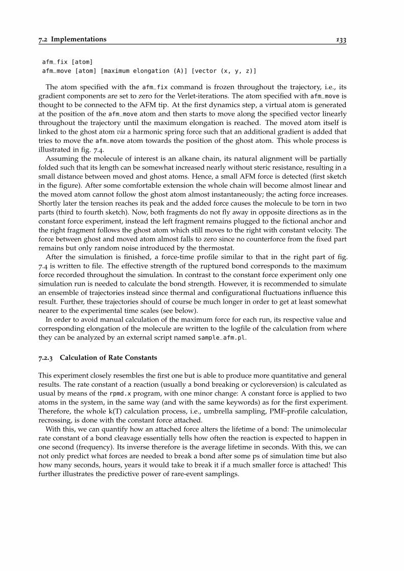
7.2 Implementations 133
afm_fix [atom]
afm_move [atom] [maximum elongation (A)] [vector (x, y, z)]
The atom specified with the afm_fix command is frozen throughout the trajectory, i.e., itsgradient components are set to zero for the Verlet-iterations. The atom specified with afm_move isthought to be connected to the AFM tip. At the first dynamics step, a virtual atom is generatedat the position of the afm_move atom and then starts to move along the specified vector linearlythroughout the trajectory until the maximum elongation is reached. The moved atom itself islinked to the ghost atom via a harmonic spring force such that an additional gradient is added thattries to move the afm_move atom towards the position of the ghost atom. This whole process isillustrated in fig. 7.4.
Assuming the molecule of interest is an alkane chain, its natural alignment will be partiallyfolded such that its length can be somewhat increased nearly without steric resistance, resulting in asmall distance between moved and ghost atoms. Hence, a small AFM force is detected (first sketchin the figure). After some comfortable extension the whole chain will become almost linear andthe moved atom cannot follow the ghost atom almost instantaneously; the acting force increases.Shortly later the tension reaches its peak and the added force causes the molecule to be torn in twoparts (third to fourth sketch). Now, both fragments do not fly away in opposite directions as in theconstant force experiment, instead the left fragment remains plugged to the fictional anchor andthe right fragment follows the ghost atom which still moves to the right with constant velocity. Theforce between ghost and moved atom almost falls to zero since no counterforce from the fixed partremains but only random noise introduced by the thermostat.
After the simulation is finished, a force-time profile similar to that in the right part of fig.7.4 is written to file. The effective strength of the ruptured bond corresponds to the maximumforce recorded throughout the simulation. In contrast to the constant force experiment only onesimulation run is needed to calculate the bond strength. However, it is recommended to simulatean ensemble of trajectories instead since thermal and configurational fluctuations influence thisresult. Further, these trajectories should of course be much longer in order to get at least somewhatnearer to the experimental time scales (see below).
In order to avoid manual calculation of the maximum force for each run, its respective value andcorresponding elongation of the molecule are written to the logfile of the calculation from wherethey can be analyzed by an external script named sample_afm.pl.
7.2.3 Calculation of Rate Constants
This experiment closely resembles the first one but is able to produce more quantitative and generalresults. The rate constant of a reaction (usually a bond breaking or cycloreversion) is calculated asusual by means of the rpmd.x program, with one minor change: A constant force is applied to twoatoms in the system, in the same way (and with the same keywords) as for the first experiment.Therefore, the whole k(T) calculation process, i.e., umbrella sampling, PMF-profile calculation,recrossing, is done with the constant force attached.
With this, we can quantify how an attached force alters the lifetime of a bond: The unimolecularrate constant of a bond cleavage essentially tells how often the reaction is expected to happen inone second (frequency). Its inverse therefore is the average lifetime in seconds. With this, we cannot only predict what forces are needed to break a bond after some ps of simulation time but alsohow many seconds, hours, years it would take to break it if a much smaller force is attached! Thisfurther illustrates the predictive power of rare-event samplings.
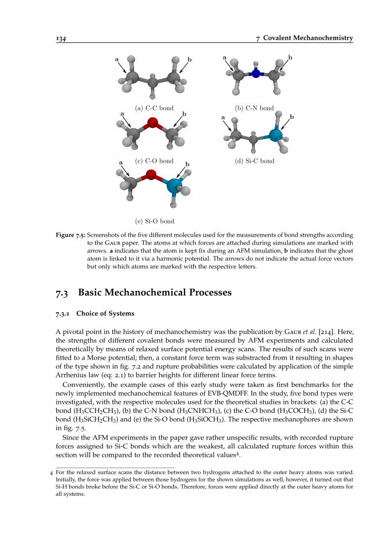
134 7 Covalent Mechanochemistry
(a) C-C bond (b) C-N bond
(c) C-O bond (d) Si-C bond
(e) Si-O bond
a b
a
a
a
a
b
b
b
b
Figure 7.5: Screenshots of the five different molecules used for the measurements of bond strengths accordingto the Gaub paper. The atoms at which forces are attached during simulations are marked witharrows. a indicates that the atom is kept fix during an AFM simulation, b indicates that the ghostatom is linked to it via a harmonic potential. The arrows do not indicate the actual force vectorsbut only which atoms are marked with the respective letters.
7.3 Basic Mechanochemical Processes
7.3.1 Choice of Systems
A pivotal point in the history of mechanochemistry was the publication by Gaub et al. [214]. Here,the strengths of different covalent bonds were measured by AFM experiments and calculatedtheoretically by means of relaxed surface potential energy scans. The results of such scans werefitted to a Morse potential; then, a constant force term was substracted from it resulting in shapesof the type shown in fig. 7.2 and rupture probabilities were calculated by application of the simpleArrhenius law (eq: 2.1) to barrier heights for different linear force terms.
Conveniently, the example cases of this early study were taken as first benchmarks for thenewly implemented mechanochemical features of EVB-QMDFF. In the study, five bond types wereinvestigated, with the respective molecules used for the theoretical studies in brackets: (a) the C-Cbond (H3CCH2CH3), (b) the C-N bond (H3CNHCH3), (c) the C-O bond (H3COCH3), (d) the Si-Cbond (H3SiCH2CH3) and (e) the Si-O bond (H3SiOCH3). The respective mechanophores are shownin fig. 7.5.
Since the AFM experiments in the paper gave rather unspecific results, with recorded ruptureforces assigned to Si-C bonds which are the weakest, all calculated rupture forces within thissection will be compared to the recorded theoretical values4.
4 For the relaxed surface scans the distance between two hydrogens attached to the outer heavy atoms was varied.Initially, the force was applied between those hydrogens for the shown simulations as well, however, it turned out thatSi-H bonds broke before the Si-C or Si-O bonds. Therefore, forces were applied directly at the outer heavy atoms forall systems.
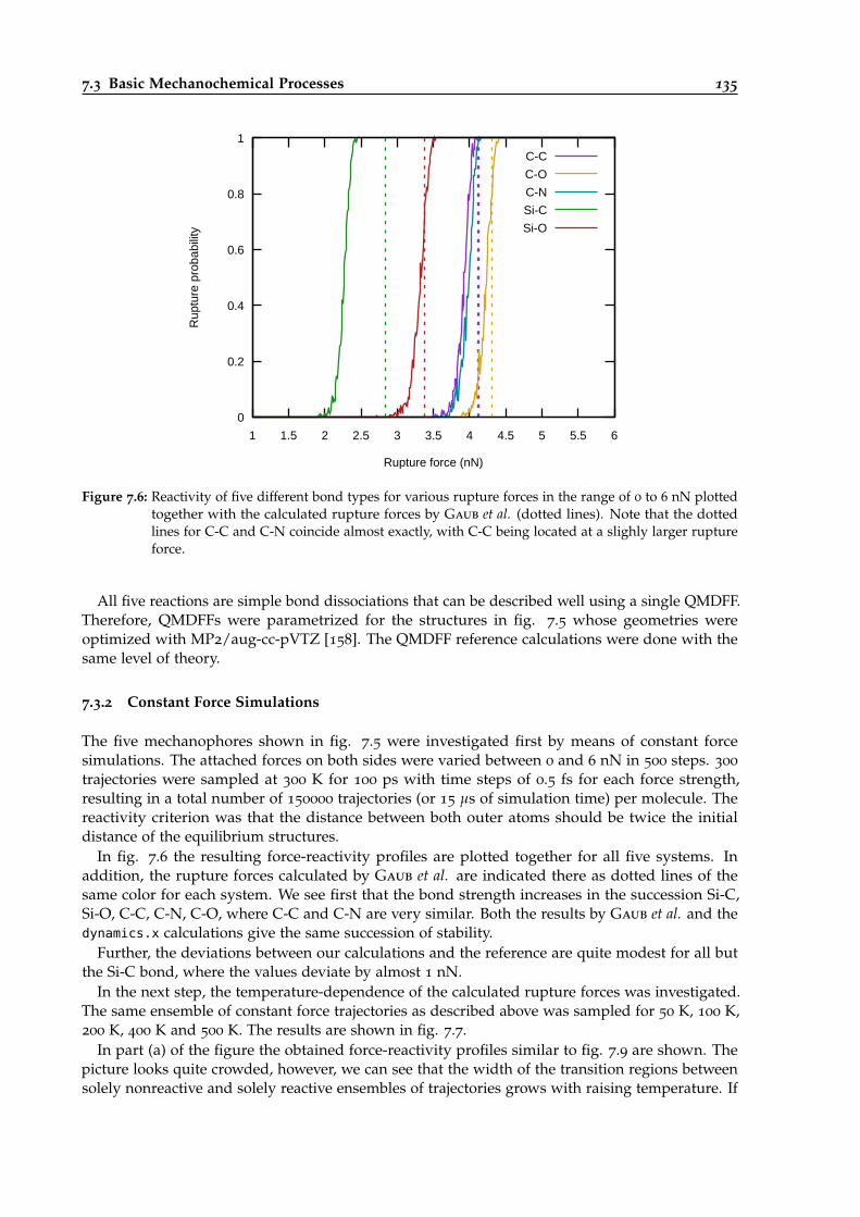
7.3 Basic Mechanochemical Processes 135
0
0.2
0.4
0.6
0.8
1
1 1.5 2 2.5 3 3.5 4 4.5 5 5.5 6
Rup
ture
prob
abili
ty
Rupture force (nN)
C-C
C-O
C-N
Si-C
Si-O
Figure 7.6: Reactivity of five different bond types for various rupture forces in the range of 0 to 6 nN plottedtogether with the calculated rupture forces by Gaub et al. (dotted lines). Note that the dottedlines for C-C and C-N coincide almost exactly, with C-C being located at a slighly larger ruptureforce.
All five reactions are simple bond dissociations that can be described well using a single QMDFF.Therefore, QMDFFs were parametrized for the structures in fig. 7.5 whose geometries wereoptimized with MP2/aug-cc-pVTZ [158]. The QMDFF reference calculations were done with thesame level of theory.
7.3.2 Constant Force Simulations
The five mechanophores shown in fig. 7.5 were investigated first by means of constant forcesimulations. The attached forces on both sides were varied between 0 and 6 nN in 500 steps. 300
trajectories were sampled at 300 K for 100 ps with time steps of 0.5 fs for each force strength,resulting in a total number of 150000 trajectories (or 15 µs of simulation time) per molecule. Thereactivity criterion was that the distance between both outer atoms should be twice the initialdistance of the equilibrium structures.
In fig. 7.6 the resulting force-reactivity profiles are plotted together for all five systems. Inaddition, the rupture forces calculated by Gaub et al. are indicated there as dotted lines of thesame color for each system. We see first that the bond strength increases in the succession Si-C,Si-O, C-C, C-N, C-O, where C-C and C-N are very similar. Both the results by Gaub et al. and thedynamics.x calculations give the same succession of stability.
Further, the deviations between our calculations and the reference are quite modest for all butthe Si-C bond, where the values deviate by almost 1 nN.
In the next step, the temperature-dependence of the calculated rupture forces was investigated.The same ensemble of constant force trajectories as described above was sampled for 50 K, 100 K,200 K, 400 K and 500 K. The results are shown in fig. 7.7.
In part (a) of the figure the obtained force-reactivity profiles similar to fig. 7.9 are shown. Thepicture looks quite crowded, however, we can see that the width of the transition regions betweensolely nonreactive and solely reactive ensembles of trajectories grows with raising temperature. If
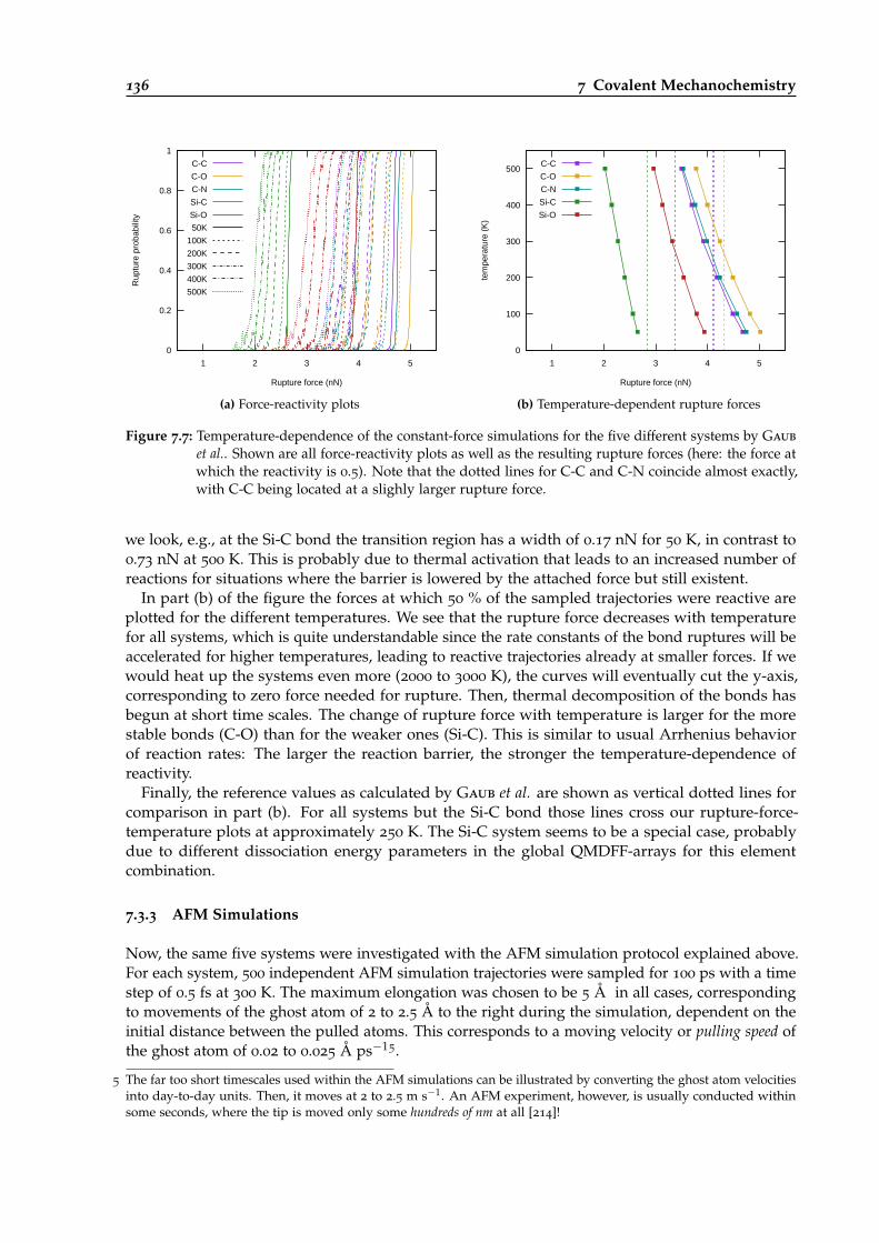
136 7 Covalent Mechanochemistry
0
0.2
0.4
0.6
0.8
1
1 2 3 4 5
Rup
ture
prob
abili
ty
Rupture force (nN)
C-C
C-O
C-N
Si-C
Si-O
50K
100K
200K
300K
400K
500K
(a) Force-reactivity plots
0
100
200
300
400
500
1 2 3 4 5
tem
pera
ture
(K)
Rupture force (nN)
C-C
C-O
C-N
Si-C
Si-O
(b) Temperature-dependent rupture forces
Figure 7.7: Temperature-dependence of the constant-force simulations for the five different systems by Gaub
et al.. Shown are all force-reactivity plots as well as the resulting rupture forces (here: the force atwhich the reactivity is 0.5). Note that the dotted lines for C-C and C-N coincide almost exactly,with C-C being located at a slighly larger rupture force.
we look, e.g., at the Si-C bond the transition region has a width of 0.17 nN for 50 K, in contrast to0.73 nN at 500 K. This is probably due to thermal activation that leads to an increased number ofreactions for situations where the barrier is lowered by the attached force but still existent.
In part (b) of the figure the forces at which 50 % of the sampled trajectories were reactive areplotted for the different temperatures. We see that the rupture force decreases with temperaturefor all systems, which is quite understandable since the rate constants of the bond ruptures will beaccelerated for higher temperatures, leading to reactive trajectories already at smaller forces. If wewould heat up the systems even more (2000 to 3000 K), the curves will eventually cut the y-axis,corresponding to zero force needed for rupture. Then, thermal decomposition of the bonds hasbegun at short time scales. The change of rupture force with temperature is larger for the morestable bonds (C-O) than for the weaker ones (Si-C). This is similar to usual Arrhenius behaviorof reaction rates: The larger the reaction barrier, the stronger the temperature-dependence ofreactivity.
Finally, the reference values as calculated by Gaub et al. are shown as vertical dotted lines forcomparison in part (b). For all systems but the Si-C bond those lines cross our rupture-force-temperature plots at approximately 250 K. The Si-C system seems to be a special case, probablydue to different dissociation energy parameters in the global QMDFF-arrays for this elementcombination.
7.3.3 AFM Simulations
Now, the same five systems were investigated with the AFM simulation protocol explained above.For each system, 500 independent AFM simulation trajectories were sampled for 100 ps with a timestep of 0.5 fs at 300 K. The maximum elongation was chosen to be 5 Å in all cases, correspondingto movements of the ghost atom of 2 to 2.5 Å to the right during the simulation, dependent on theinitial distance between the pulled atoms. This corresponds to a moving velocity or pulling speed ofthe ghost atom of 0.02 to 0.025 Å ps−15.
5 The far too short timescales used within the AFM simulations can be illustrated by converting the ghost atom velocitiesinto day-to-day units. Then, it moves at 2 to 2.5 m s−1. An AFM experiment, however, is usually conducted withinsome seconds, where the tip is moved only some hundreds of nm at all [214]!

7.3 Basic Mechanochemical Processes 137
t (ps)
0
15
30
50
90
LAFM (Å)
2.582.8
63.1
13.5
74.8
60
(a) Snapshots of trajectory keyframes
0
2
4
6
8
10
12
14
0 20 40 60 80 100
Mea
sure
d fo
rce
(nN
)
t (ps)
(b) Calculated forces for each MD step
0
2
4
6
8
10
12
14
0 20 40 60 80 100
Mea
sure
d fo
rce
(nN
)
t (ps)
(c) Averaged forces (reduced thermal noise)
Figure 7.8: Example trajectory of the C-C bond AFM experiment. Shown are some screenshots with therespective times and distances between the anchor atoms (a). The force-time plot of the sametrajectory is shown in (b). Since this is quite noisy, slices of 50 neighbored points were averaged,resulting in the plot shown in (c).
The maximum force throughout the simulation was recorded by the dynamic.x program andwritten out for each simulation. Since thermal fluctuations lead to short high peaks of the recordedforce-time profile, they were filtered out by averaging slices of 50 neighbored force values. Forcesand distances are written out every 10 fs, after removal of thermal fluctuations a value is thuswritten out every 0.5 ps, resulting into 200 values in total. This is shown for a C-C bond exampletrajectory in fig. 7.8.
The results of the AFM simulations are shown in fig. 7.9. The calculated rupture forces togetherwith the molecule length (also called AFM elongations) in the moment of rupture are illustrated asscattering plots containing 500 points, the averaged rupture forces are plotted as straight verticallines. We see that the AFM elongations are different for the systems, since the included bondlengths are different for all combinations. Further, the same ordering of bond strengths as in theconstant force experiments can be found, with increasing bond lengths in the succession Si-C,Si-O, C-C, C-N, C-O. It should be noted that the resulting forces (e.g., plotted in fig. 7.8) of theAFM experiments are halved for this plot in order to establish comparability: In the constantforce experiments, force vectors of the depicted strengths are added to both sides of the molecule,resulting in a total force twice as large, whereas in the AFM experiment the whole (doubled) forceis applied to the moved atom.
The theoretical values of Gaub et al. were added again as comparison. We see that these aresmaller than the averaged AFM forces for all five systems, where the Si-C bond now has the bestaccordance (0.15 nN difference). The other systems show slightly larger differences of 0.3 to 0.5 nN.
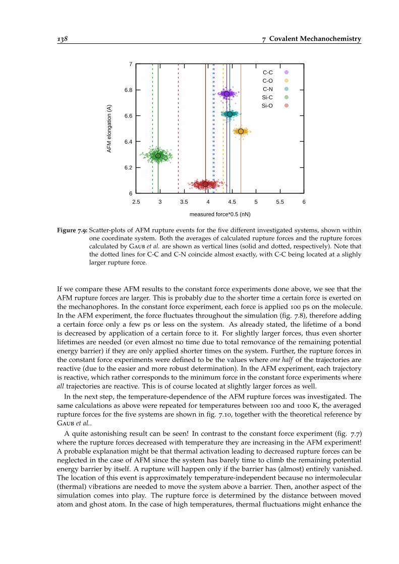
138 7 Covalent Mechanochemistry
6
6.2
6.4
6.6
6.8
7
2.5 3 3.5 4 4.5 5 5.5 6
AF
Mel
onga
tion
(A)
measured force*0.5 (nN)
C-C
C-O
C-N
Si-C
Si-O
Figure 7.9: Scatter-plots of AFM rupture events for the five different investigated systems, shown withinone coordinate system. Both the averages of calculated rupture forces and the rupture forcescalculated by Gaub et al. are shown as vertical lines (solid and dotted, respectively). Note thatthe dotted lines for C-C and C-N coincide almost exactly, with C-C being located at a slighlylarger rupture force.
If we compare these AFM results to the constant force experiments done above, we see that theAFM rupture forces are larger. This is probably due to the shorter time a certain force is exerted onthe mechanophores. In the constant force experiment, each force is applied 100 ps on the molecule.In the AFM experiment, the force fluctuates throughout the simulation (fig. 7.8), therefore addinga certain force only a few ps or less on the system. As already stated, the lifetime of a bondis decreased by application of a certain force to it. For slightly larger forces, thus even shorterlifetimes are needed (or even almost no time due to total removance of the remaining potentialenergy barrier) if they are only applied shorter times on the system. Further, the rupture forces inthe constant force experiments were defined to be the values where one half of the trajectories arereactive (due to the easier and more robust determination). In the AFM experiment, each trajectoryis reactive, which rather corresponds to the minimum force in the constant force experiments whereall trajectories are reactive. This is of course located at slightly larger forces as well.
In the next step, the temperature-dependence of the AFM rupture forces was investigated. Thesame calculations as above were repeated for temperatures between 100 and 1000 K, the averagedrupture forces for the five systems are shown in fig. 7.10, together with the theoretical reference byGaub et al..
A quite astonishing result can be seen! In contrast to the constant force experiment (fig. 7.7)where the rupture forces decreased with temperature they are increasing in the AFM experiment!A probable explanation might be that thermal activation leading to decreased rupture forces can beneglected in the case of AFM since the system has barely time to climb the remaining potentialenergy barrier by itself. A rupture will happen only if the barrier has (almost) entirely vanished.The location of this event is approximately temperature-independent because no intermolecular(thermal) vibrations are needed to move the system above a barrier. Then, another aspect of thesimulation comes into play. The rupture force is determined by the distance between movedatom and ghost atom. In the case of high temperatures, thermal fluctuations might enhance the
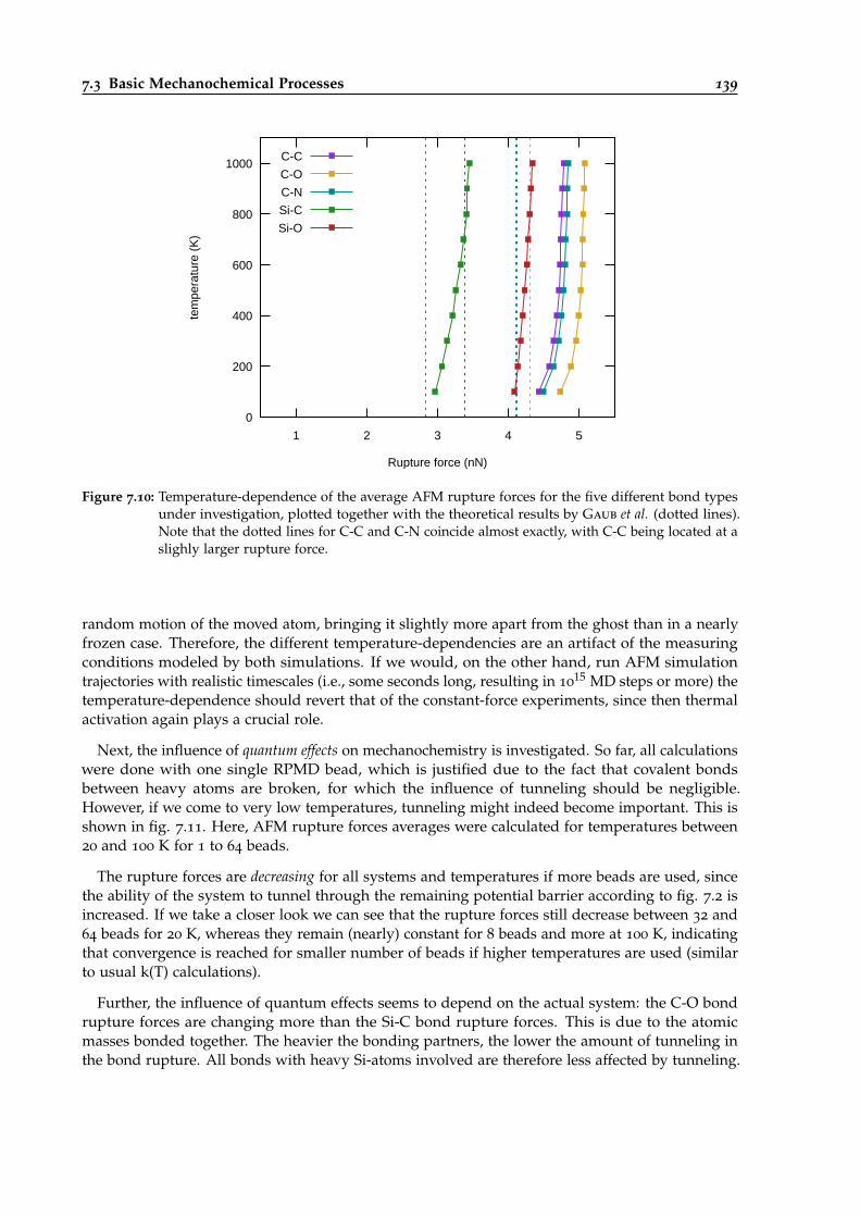
7.3 Basic Mechanochemical Processes 139
0
200
400
600
800
1000
1 2 3 4 5
tem
pera
ture
(K)
Rupture force (nN)
C-C
C-O
C-N
Si-C
Si-O
Figure 7.10: Temperature-dependence of the average AFM rupture forces for the five different bond typesunder investigation, plotted together with the theoretical results by Gaub et al. (dotted lines).Note that the dotted lines for C-C and C-N coincide almost exactly, with C-C being located at aslighly larger rupture force.
random motion of the moved atom, bringing it slightly more apart from the ghost than in a nearlyfrozen case. Therefore, the different temperature-dependencies are an artifact of the measuringconditions modeled by both simulations. If we would, on the other hand, run AFM simulationtrajectories with realistic timescales (i.e., some seconds long, resulting in 10
15 MD steps or more) thetemperature-dependence should revert that of the constant-force experiments, since then thermalactivation again plays a crucial role.
Next, the influence of quantum effects on mechanochemistry is investigated. So far, all calculationswere done with one single RPMD bead, which is justified due to the fact that covalent bondsbetween heavy atoms are broken, for which the influence of tunneling should be negligible.However, if we come to very low temperatures, tunneling might indeed become important. This isshown in fig. 7.11. Here, AFM rupture forces averages were calculated for temperatures between20 and 100 K for 1 to 64 beads.
The rupture forces are decreasing for all systems and temperatures if more beads are used, sincethe ability of the system to tunnel through the remaining potential barrier according to fig. 7.2 isincreased. If we take a closer look we can see that the rupture forces still decrease between 32 and64 beads for 20 K, whereas they remain (nearly) constant for 8 beads and more at 100 K, indicatingthat convergence is reached for smaller number of beads if higher temperatures are used (similarto usual k(T) calculations).
Further, the influence of quantum effects seems to depend on the actual system: the C-O bondrupture forces are changing more than the Si-C bond rupture forces. This is due to the atomicmasses bonded together. The heavier the bonding partners, the lower the amount of tunneling inthe bond rupture. All bonds with heavy Si-atoms involved are therefore less affected by tunneling.

140 7 Covalent Mechanochemistry
0
10
20
30
40
50
60
70
1 2 3 4 5
No.
ofbe
ads
Rupture force (nN)
C-C
C-O
C-N
Si-C
Si-O
(a) 20 K
0
10
20
30
40
50
60
70
1 2 3 4 5
No.
ofbe
ads
Rupture force (nN)
C-C
C-O
C-N
Si-C
Si-O
(b) 40 K
0
10
20
30
40
50
60
70
1 2 3 4 5
No.
ofbe
ads
Rupture force (nN)
C-C
C-O
C-N
Si-C
Si-O
(c) 70 K
0
10
20
30
40
50
60
70
1 2 3 4 5
No.
ofbe
ads
Rupture force (nN)
C-C
C-O
C-N
Si-C
Si-O
(d) 100 K
Figure 7.11: Influence of quantum effects on the results of AFM simulation trajectories. Shown are the RPMDbead-dependent averaged rupture forces for the five systems studied so far at four differenttemperatures between 20 and 100 K. Note that the dotted lines for C-C and C-N coincide almostexactly, with C-C being located at a slightly larger rupture force.

7.4 Other Examples 141
a b
(a) Disulfide
(b) Terpyridine (c) Diels-Alder
a a' b' bb
b'a'a
Figure 7.12: Optimized reactant minimum structures of the three mechanophores to be investigated with(EVB-)QMDFF mechanochemistry. Noted are the atoms on which the forces are applied (a andb) as well as those on which forces are applied due to unexpected bond ruptures (a’ and b’).The arrows do not indicate the actual force vectors but only which atoms are marked with therespective letters.
7.4 Other Examples
We have seen so far that the implemented mechanochemical methods are able to reproduce thetheoretical results by Gaub et al. quite well. In the next step three more realistic cases were chosenfrom the literature. The respective molecules are presented in fig. 7.12.
Molecule (a) is a bridged disulfide system with aromatic anchor. It was studied both exper-imentally and theoretically within the University of Kiel, with the theoretical studies done byMüller [215, 216]. Structure (b) contains a Ru2+-ion coordinated by two terpyridine molecules.The force needed to rip both terpyridines apart was measured by Gaub et al. in 2003 [217]. System(c) has no experimental example; it was chosen in order to study a Diels-Alder reaction by meansof mechanochemistry.
Both geometry optimizations and QMDFF reference calculations were done with the B3LYP(D3
empirical dispersion)/cc-pVDZ level of theory [158, 201, 207].
7.4.1 The Bridged Disulfide Molecule
This system was designed to be a two-stage mechanophore: If a force is applied on both anchoratoms shown in fig. 7.12, the shorter chain with the disulfide bond in the middle will be stretchedfirst. Since the S-S bond is much weaker than all other bonds in the line, it will break at someforce value during the AFM experiment. But the story is not over yet: Both fragments are stillconnected via the longer ether bridge in the background. The anchor atoms will be moved much
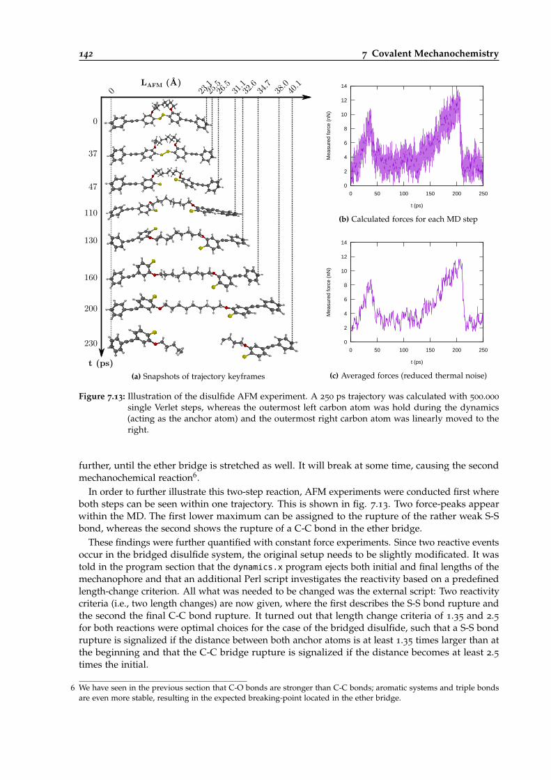
142 7 Covalent Mechanochemistry
t (ps)
0
37
47
110
130
160
200
230
LAFM (Å)23.
125.
526.
531.
134.
738.
032.
640.
10
(a) Snapshots of trajectory keyframes
0
2
4
6
8
10
12
14
0 50 100 150 200 250
Mea
sure
d fo
rce
(nN
)
t (ps)
(b) Calculated forces for each MD step
0
2
4
6
8
10
12
14
0 50 100 150 200 250
Mea
sure
d fo
rce
(nN
)
t (ps)
(c) Averaged forces (reduced thermal noise)
Figure 7.13: Illustration of the disulfide AFM experiment. A 250 ps trajectory was calculated with 500.000
single Verlet steps, whereas the outermost left carbon atom was hold during the dynamics(acting as the anchor atom) and the outermost right carbon atom was linearly moved to theright.
further, until the ether bridge is stretched as well. It will break at some time, causing the secondmechanochemical reaction6.
In order to further illustrate this two-step reaction, AFM experiments were conducted first whereboth steps can be seen within one trajectory. This is shown in fig. 7.13. Two force-peaks appearwithin the MD. The first lower maximum can be assigned to the rupture of the rather weak S-Sbond, whereas the second shows the rupture of a C-C bond in the ether bridge.
These findings were further quantified with constant force experiments. Since two reactive eventsoccur in the bridged disulfide system, the original setup needs to be slightly modificated. It wastold in the program section that the dynamics.x program ejects both initial and final lengths of themechanophore and that an additional Perl script investigates the reactivity based on a predefinedlength-change criterion. All what was needed to be changed was the external script: Two reactivitycriteria (i.e., two length changes) are now given, where the first describes the S-S bond rupture andthe second the final C-C bond rupture. It turned out that length change criteria of 1.35 and 2.5for both reactions were optimal choices for the case of the bridged disulfide, such that a S-S bondrupture is signalized if the distance between both anchor atoms is at least 1.35 times larger than atthe beginning and that the C-C bridge rupture is signalized if the distance becomes at least 2.5times the initial.
6 We have seen in the previous section that C-O bonds are stronger than C-C bonds; aromatic systems and triple bondsare even more stable, resulting in the expected breaking-point located in the ether bridge.
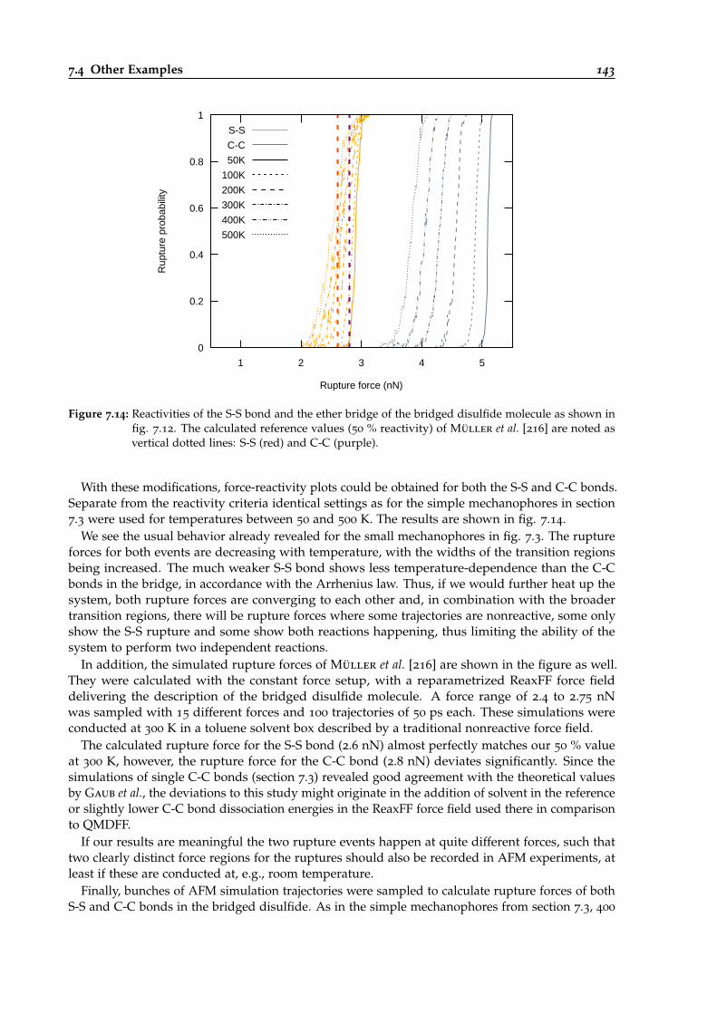
7.4 Other Examples 143
0
0.2
0.4
0.6
0.8
1
1 2 3 4 5
Rup
ture
prob
abili
ty
Rupture force (nN)
S-S
C-C
50K
100K
200K
300K
400K
500K
Figure 7.14: Reactivities of the S-S bond and the ether bridge of the bridged disulfide molecule as shown infig. 7.12. The calculated reference values (50 % reactivity) of Müller et al. [216] are noted asvertical dotted lines: S-S (red) and C-C (purple).
With these modifications, force-reactivity plots could be obtained for both the S-S and C-C bonds.Separate from the reactivity criteria identical settings as for the simple mechanophores in section7.3 were used for temperatures between 50 and 500 K. The results are shown in fig. 7.14.
We see the usual behavior already revealed for the small mechanophores in fig. 7.3. The ruptureforces for both events are decreasing with temperature, with the widths of the transition regionsbeing increased. The much weaker S-S bond shows less temperature-dependence than the C-Cbonds in the bridge, in accordance with the Arrhenius law. Thus, if we would further heat up thesystem, both rupture forces are converging to each other and, in combination with the broadertransition regions, there will be rupture forces where some trajectories are nonreactive, some onlyshow the S-S rupture and some show both reactions happening, thus limiting the ability of thesystem to perform two independent reactions.
In addition, the simulated rupture forces of Müller et al. [216] are shown in the figure as well.They were calculated with the constant force setup, with a reparametrized ReaxFF force fielddelivering the description of the bridged disulfide molecule. A force range of 2.4 to 2.75 nNwas sampled with 15 different forces and 100 trajectories of 50 ps each. These simulations wereconducted at 300 K in a toluene solvent box described by a traditional nonreactive force field.
The calculated rupture force for the S-S bond (2.6 nN) almost perfectly matches our 50 % valueat 300 K, however, the rupture force for the C-C bond (2.8 nN) deviates significantly. Since thesimulations of single C-C bonds (section 7.3) revealed good agreement with the theoretical valuesby Gaub et al., the deviations to this study might originate in the addition of solvent in the referenceor slightly lower C-C bond dissociation energies in the ReaxFF force field used there in comparisonto QMDFF.
If our results are meaningful the two rupture events happen at quite different forces, such thattwo clearly distinct force regions for the ruptures should also be recorded in AFM experiments, atleast if these are conducted at, e.g., room temperature.
Finally, bunches of AFM simulation trajectories were sampled to calculate rupture forces of bothS-S and C-C bonds in the bridged disulfide. As in the simple mechanophores from section 7.3, 400

144 7 Covalent Mechanochemistry
28
30
32
34
36
38
40
42
2.5 3 3.5 4 4.5 5 5.5 6 6.5 7
AF
Mel
onga
tion
(A)
measured force*0.5 (nN)
S-S
C-C
(a) Rupture forces and positions
0
100
200
300
400
500
600
700
800
3 4 5 6 7 8
T(K
)
measured force*0.5 (nN)
S-S
C-C
(b) Temperature-dependent rupture forces
Figure 7.15: AFM simulation experiments for the bridged disulfide molecule. The rupture forces and anchoratom distances (S-S and C-C bonds) for simulations at 300 K are shown in (a), whereas thetemperature dependence of the rupture forces is illustrated in (b).
single AFM trajectories were started at different temperatures (100 to 700 K). The ghost atom wasmoved a distance of approximately 23 Å during the simulation, resulting in a velocity of 0.092
Å ps−1, thus roughly four times faster than in the case of the small systems presented in section7.3. In order to monitor both reactive events (S-S and bridge ruptures), a special setting was addedfor dynamic.x. If the keyword
afm_second [number of MD steps]
is added, the final evaluation of the force-time curve will divide it into two parts at the givennumber of MD steps. Since all disulfide AFM trajectories were 500.000 steps (250 ps) long, thedivision was made at 250.000 steps (125 ps). For each part, its local maximum will be determinedand written out. When we look back at fig. 7.13, we see that the S-S rupture happens roughly at 40
ps and the final bridge rupture at 200 ps, thus justifying the division between both events at 125 ps.The AFM results are shown in fig. 7.15.The rupture forces and anchor atom distances for both reactive events at 300 K are shown in part
(a). We see that the anchor atom distances (a.k.a. AFM elongations) show very modest variation,whereas the rupture forces fluctuate much more. This impression is fortified if we look at part(b), where the temperature-dependent rupture forces for all trajectories are plotted. The variationof this force becomes so significant at 300 K and above that both S-S-bond and ether-bridge arebreaking at similar or reversed forces at a number of runs.
By looking at the average forces a similar picture as in fig. 7.10 is received: They are growing forhigher temperatures, in contrast to the constant force simulations.
7.4.2 The Ruthenium-Terpyridine Complex
In the reference paper of Gaub et al. [217] molecule (b) of fig. 7.12 was put between two longpoly(ethylene oxide) spacers. Several AFM runs with force loading rates of 1 nN s−1 were done,with recorded rupture forces of ca. 0.1 nN. Since these are much smaller than those needed torupture covalent bonds it was supposed that the recorded events were caused by openings of themetallo-supramolecular complex, i.e., separations of both terpyridines, where the Ru2+-ion is takenby one of them.

7.4 Other Examples 145
This experimental setting was recronstructed by means of the AFM simulation method indynamics.x. The outer carbon atom termed a was frozen and its counterpart b coupled to themoved ghost atom. An ensemble of AFM trajectories was sampled at 300 K with each trajectorybeing 250 ps long. Unfortunately all of them showed another reaction than expected: The methylor ethyl group containing atom b was torn apart, with the main ruthenium complex remainingintact (fig. 7.16). The observed rupture forces were around 4-4.5 nN, thus similar to our results forthe C-C model system.
The Ru-N bonds in the complex are apparently much stronger than they should be if QMDFFis used to model them. The situation within this complex is of course much more complicatedthan for single covalent bonds described so far, it seems that the global fitting approach withinQMDFF is not sufficient for this reaction. Another possible reason is that two of the three bondsfrom each terpyridine molecule are almost perpendicular towards the applied force vector. Onlya small fraction of the rupture force is effective on them. A similar discussion is made for theDiels-Alder system in the next section.
Nevertheless the force needed to break this complex was calculated: Instead of using peripheralcarbon atoms as anchors aromatic carbons in the terpyridines were chosen (a’ and b’ in fig. 7.16).Now, the desired reaction happens: The Ruthenium complex gets cracked, the Ru2+-ion remainsbonded to one ruthenium, with the other one moving away alone. More than 8 nN was needed totrigger this event, i.e., twice the C-C rupture force and almost 100 times the experimental value byGaub et al. (actually almost 200 times since the total force exerted by the “AFM” moving atom isactually twice as large (see above)).
In spite of this wrong mechanistic prediction, series of AFM trajectories were started for the a’-b’anchor atoms at temperatures between 100 and 700 K (250 ps each, with the ghost atom movedapprox. 5 Å, resulting in a velocity of 0.02 Å ps−1). The results are presented in fig. 7.18 (a). Asimilar behavior to the model systems in fig. 7.9 can be seen, with both variances and expectationvalues of the rupture forces increasing with temperature.
If theory and experiment should be compared directly, an EVB-QMFFF (probably TREQ) ofthe reaction should be parametrized, which is quite tricky due to the presumptive multireferencecharacter of the Ru-N bond breakings requiring demanding QM reference calculations and the verysize of the system making both an accurate choice of TREQ internal coordinates and the calculationof reference frequencies etc. very demanding.
7.4.3 The Diels-Alder Reaction
We have seen that the mechanochemistry of the ruthenium terpyridine complex cannot be describedproperly with one single QMDFF. A similar case is a cycloreversion. QMDFF is parametrized forsingle covalent bond ruptures but not for cycloreversions involving electronic influence of thewhole aromatic system. Therefore, EVB-QMDFF should be used here as well. A simple example isthe basic Diels-Alder reaction (1,3-butadiene and ethylene), with ethyl substituents for applicationof the rupture forces. The reaction path of this system was calculated starting from the TS. Then, ablack-box rate constant calculation with evb_kt_driver.x was done. In fig. 7.17 the reaction pathis shown together with the positions of the RP-EVB reference points and the energies of bothQMDFFs. Structure inlets show the actual mechanism of the reaction.
After the black-box setup was finished, the resulting TREQ force field can be used equally wellfor other tasks such as AFM simulation trajectories. Atoms a and b shown in fig. 7.12 were used inthe same way as for the terpyridine system. Again one of the outer C-C bonds was ruptured first,as can be seen in fig. 7.16.
This behavior is quite interesting since we now know the potential energy barriers of bothC-C bond rupture (ca. 500 kJ mol−1) and cycloreversion (ca. 250 kJ mol−1). From this simplecomparison we should assume that cycloreversions are largely preferred in this case. However, if the
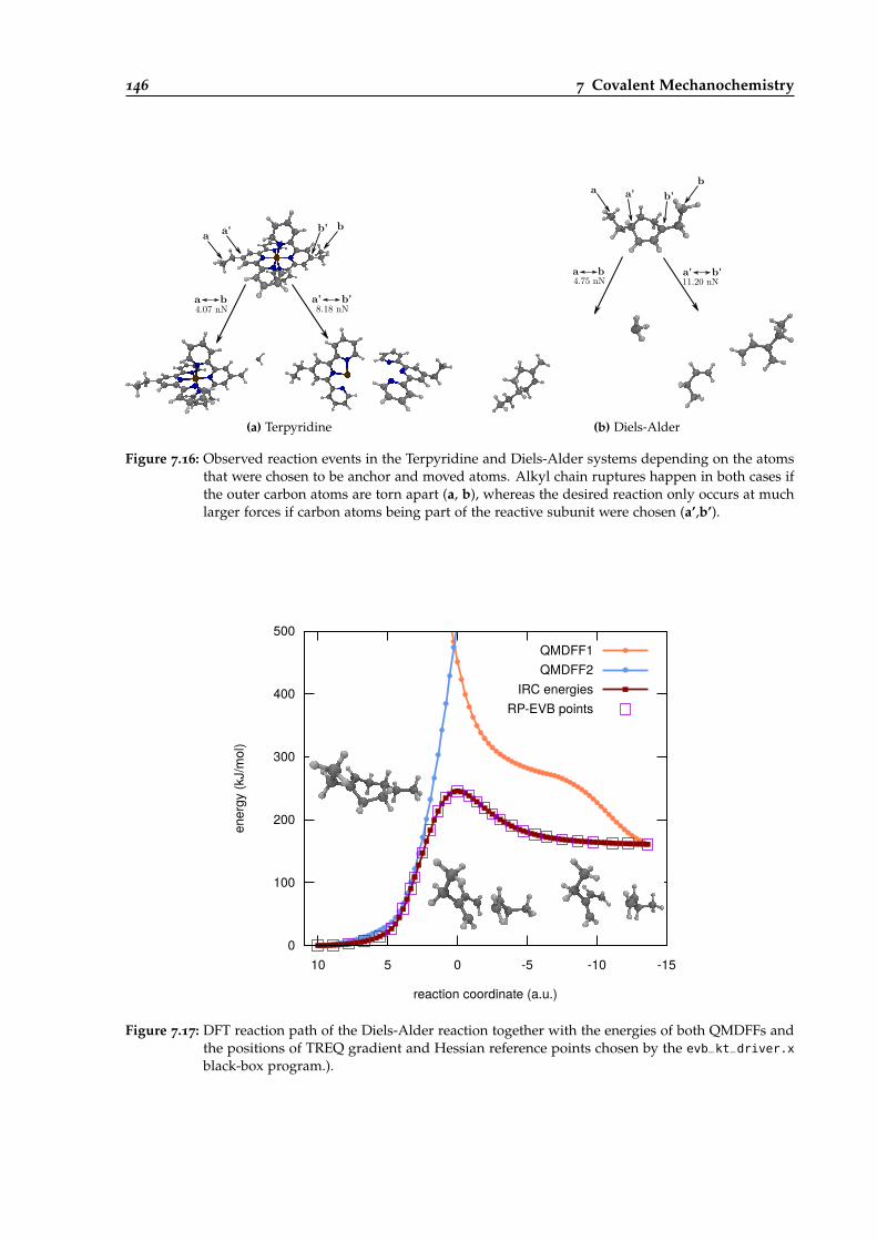
146 7 Covalent Mechanochemistry
a a' b' b
a b4.07 nN
a' b'8.18 nN
(a) Terpyridine
bb'a'
a b4.75 nN
a' b'11.20 nN
a
(b) Diels-Alder
Figure 7.16: Observed reaction events in the Terpyridine and Diels-Alder systems depending on the atomsthat were chosen to be anchor and moved atoms. Alkyl chain ruptures happen in both cases ifthe outer carbon atoms are torn apart (a, b), whereas the desired reaction only occurs at muchlarger forces if carbon atoms being part of the reactive subunit were chosen (a’,b’).
0
100
200
300
400
500
-15-10-50510
ener
gy (k
J/m
ol)
reaction coordinate (a.u.)
QMDFF1QMDFF2
IRC energiesRP-EVB points
Figure 7.17: DFT reaction path of the Diels-Alder reaction together with the energies of both QMDFFs andthe positions of TREQ gradient and Hessian reference points chosen by the evb_kt_driver.x
black-box program.).
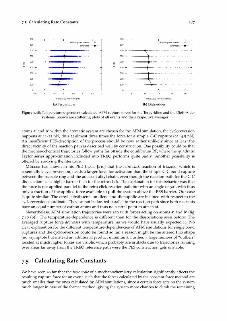
7.5 Calculating Rate Constants 147
0
100
200
300
400
500
600
700
800
900
6.5 7 7.5 8 8.5 9 9.5 10
T(K
)
measured force*0.5 (nN)
AFM rupture events
averages
(a) Terpyridine
0
100
200
300
400
500
600
700
800
900
8 10 12 14 16
T(K
)
measured force*0.5 (nN)
AFM rupture events
averages
(b) Diels-Alder
Figure 7.18: Temperature-dependent calculated AFM rupture forces for the Terpyridine and the Diels-Aldersystems. Shown are scattering plots of all events and their respective averages.
atoms a’ and b’ within the aromatic system are chosen for the AFM simulation, the cycloreversionhappens at 11-12 nN, thus at almost three times the force for a simple C-C rupture (ca. 4.5 nN).An insufficient PES-description of the process should be now rather unlikely since at least thedirect vicinity of the reaction path is described well by construction. One possibility could be thatthe mechanochemical trajectories follow paths far offside the equilibrium RP, where the quadraticTaylor series approximation included into TREQ performs quite badly. Another possibility isoffered by studying the literature.
Müller has shown in his PhD thesis [210] that the retro-click reaction of triazole, which isessentially a cycloreversion, needs a larger force for activation than the simple C-C bond rupturebetween the triazole ring and the adjacent alkyl chain, even though the reaction path for the C-Cdissociation has a higher barrier than for the retro-click. The explanation for this behavior was thatthe force is not applied parallel to the retro-click reaction path but with an angle of 50
◦, with thusonly a fraction of the applied force available to pull the system above the PES barrier. Our caseis quite similar: The ethyl substituents on diene and dienophile are inclined with respect to thecycloreversion coordinate. They cannot be located parallel to the reaction path since both reactantshave an equal number of carbon atoms and thus no central point to attach at.
Nevertheless, AFM simulation trajectories were ran with forces acting on atoms a’ and b’ (fig.7.18 (b)). The temperature-dependence is different than for the dissociations seen before: Theaveraged rupture force decreases with temperature, as we would have usually expected it. Noclear explanation for the different temperature-dependencies of AFM simulations for single bondruptures and the cycloreversion could be found so far, a reason might be the altered PES shape(no asymptote but instead an additional product minimum). Further, a large number of “outliers”located at much higher forces are visible, which probably are artifacts due to trajectories runningover areas far away from the TREQ reference path were the PES construction gets unstable.
7.5 Calculating Rate Constants
We have seen so far that the time scale of a mechanochemistry calculation significantly affects theresulting rupture force for an event, such that the forces calculated by the constant force method aremuch smaller than the ones calculated by AFM simulations, since a certain force acts on the systemmuch longer in case of the former method, giving the system more chances to climb the remaining
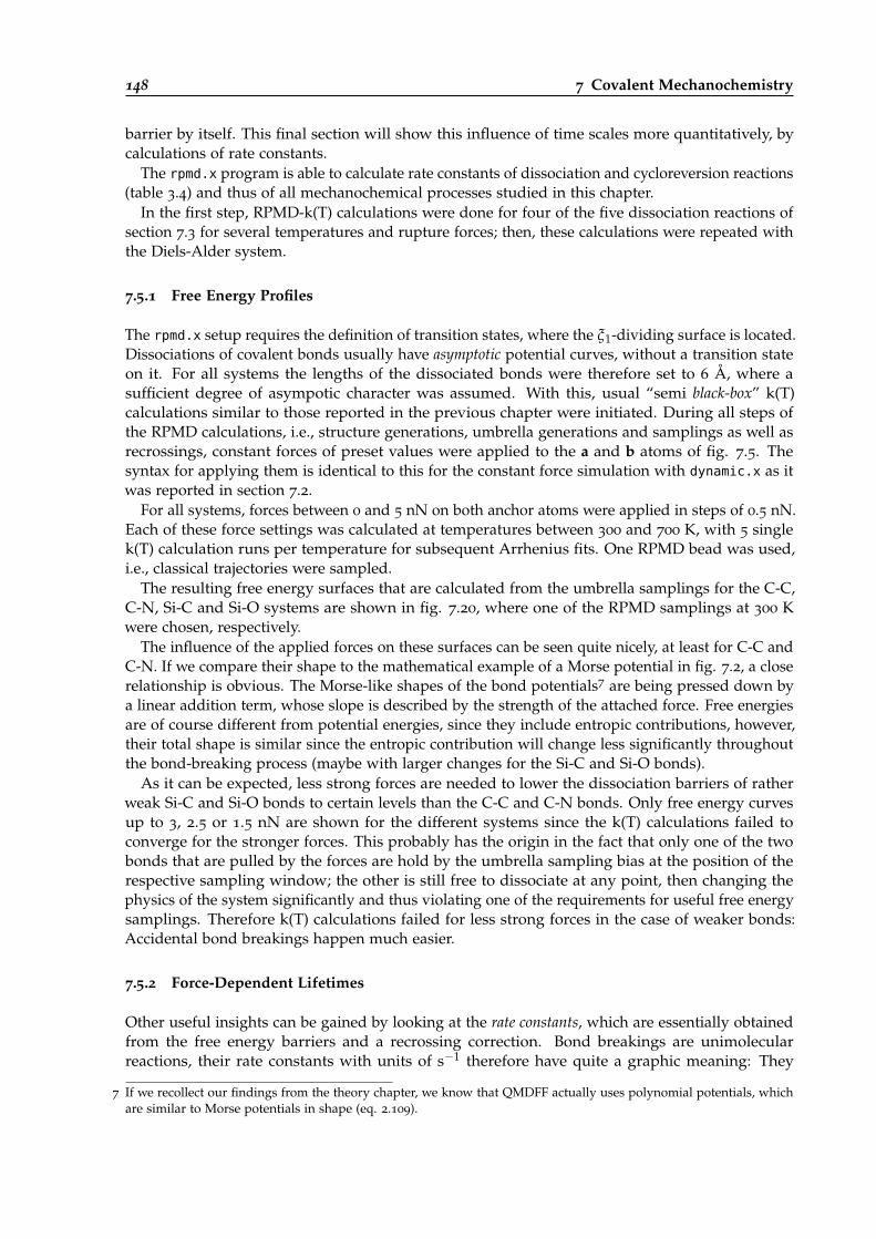
148 7 Covalent Mechanochemistry
barrier by itself. This final section will show this influence of time scales more quantitatively, bycalculations of rate constants.
The rpmd.x program is able to calculate rate constants of dissociation and cycloreversion reactions(table 3.4) and thus of all mechanochemical processes studied in this chapter.
In the first step, RPMD-k(T) calculations were done for four of the five dissociation reactions ofsection 7.3 for several temperatures and rupture forces; then, these calculations were repeated withthe Diels-Alder system.
7.5.1 Free Energy Profiles
The rpmd.x setup requires the definition of transition states, where the ξ1-dividing surface is located.Dissociations of covalent bonds usually have asymptotic potential curves, without a transition stateon it. For all systems the lengths of the dissociated bonds were therefore set to 6 Å, where asufficient degree of asympotic character was assumed. With this, usual “semi black-box” k(T)calculations similar to those reported in the previous chapter were initiated. During all steps ofthe RPMD calculations, i.e., structure generations, umbrella generations and samplings as well asrecrossings, constant forces of preset values were applied to the a and b atoms of fig. 7.5. Thesyntax for applying them is identical to this for the constant force simulation with dynamic.x as itwas reported in section 7.2.
For all systems, forces between 0 and 5 nN on both anchor atoms were applied in steps of 0.5 nN.Each of these force settings was calculated at temperatures between 300 and 700 K, with 5 singlek(T) calculation runs per temperature for subsequent Arrhenius fits. One RPMD bead was used,i.e., classical trajectories were sampled.
The resulting free energy surfaces that are calculated from the umbrella samplings for the C-C,C-N, Si-C and Si-O systems are shown in fig. 7.20, where one of the RPMD samplings at 300 Kwere chosen, respectively.
The influence of the applied forces on these surfaces can be seen quite nicely, at least for C-C andC-N. If we compare their shape to the mathematical example of a Morse potential in fig. 7.2, a closerelationship is obvious. The Morse-like shapes of the bond potentials7 are being pressed down bya linear addition term, whose slope is described by the strength of the attached force. Free energiesare of course different from potential energies, since they include entropic contributions, however,their total shape is similar since the entropic contribution will change less significantly throughoutthe bond-breaking process (maybe with larger changes for the Si-C and Si-O bonds).
As it can be expected, less strong forces are needed to lower the dissociation barriers of ratherweak Si-C and Si-O bonds to certain levels than the C-C and C-N bonds. Only free energy curvesup to 3, 2.5 or 1.5 nN are shown for the different systems since the k(T) calculations failed toconverge for the stronger forces. This probably has the origin in the fact that only one of the twobonds that are pulled by the forces are hold by the umbrella sampling bias at the position of therespective sampling window; the other is still free to dissociate at any point, then changing thephysics of the system significantly and thus violating one of the requirements for useful free energysamplings. Therefore k(T) calculations failed for less strong forces in the case of weaker bonds:Accidental bond breakings happen much easier.
7.5.2 Force-Dependent Lifetimes
Other useful insights can be gained by looking at the rate constants, which are essentially obtainedfrom the free energy barriers and a recrossing correction. Bond breakings are unimolecularreactions, their rate constants with units of s−1 therefore have quite a graphic meaning: They
7 If we recollect our findings from the theory chapter, we know that QMDFF actually uses polynomial potentials, whichare similar to Morse potentials in shape (eq. 2.109).
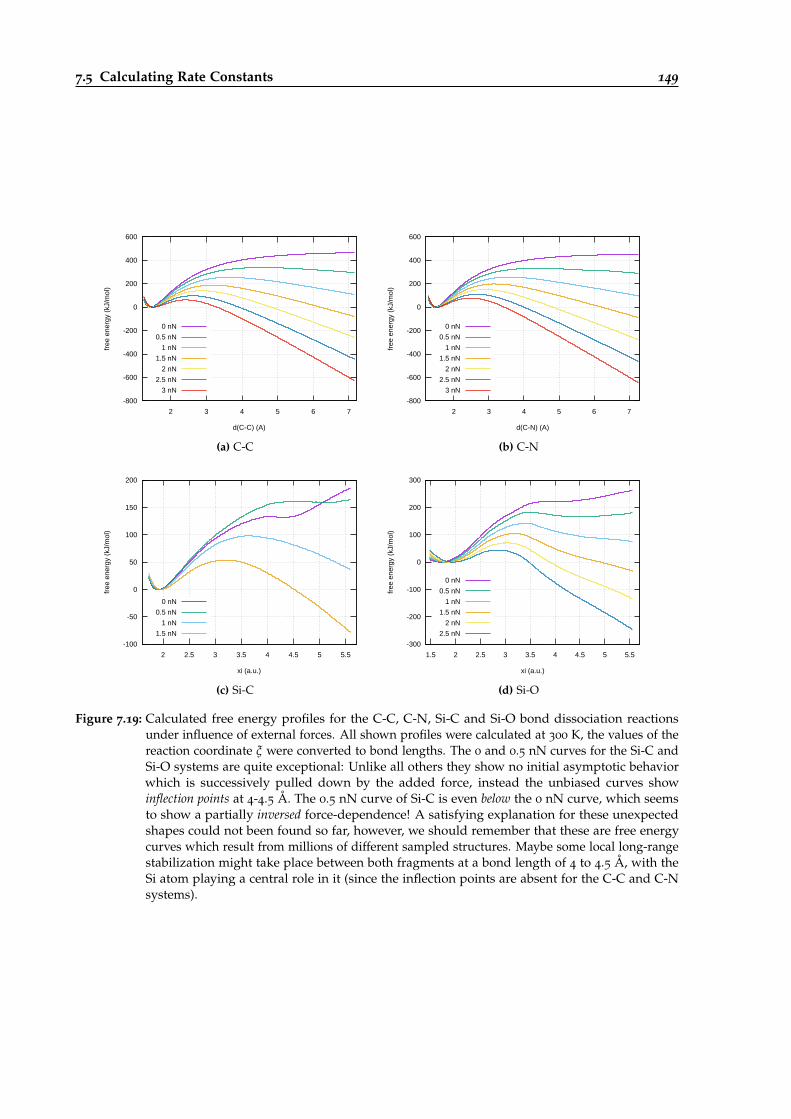
7.5 Calculating Rate Constants 149
-800
-600
-400
-200
0
200
400
600
2 3 4 5 6 7
free
ene
rgy
(kJ/
mol
)
d(C-C) (A)
0 nN
0.5 nN
1 nN
1.5 nN
2 nN
2.5 nN
3 nN
(a) C-C
-800
-600
-400
-200
0
200
400
600
2 3 4 5 6 7
free
ene
rgy
(kJ/
mol
)
d(C-N) (A)
0 nN
0.5 nN
1 nN
1.5 nN
2 nN
2.5 nN
3 nN
(b) C-N
-100
-50
0
50
100
150
200
2 2.5 3 3.5 4 4.5 5 5.5
free
ene
rgy
(kJ/
mol
)
xi (a.u.)
0 nN
0.5 nN
1 nN
1.5 nN
(c) Si-C
-300
-200
-100
0
100
200
300
1.5 2 2.5 3 3.5 4 4.5 5 5.5
free
ene
rgy
(kJ/
mol
)
xi (a.u.)
0 nN
0.5 nN
1 nN
1.5 nN
2 nN
2.5 nN
(d) Si-O
Figure 7.19: Calculated free energy profiles for the C-C, C-N, Si-C and Si-O bond dissociation reactionsunder influence of external forces. All shown profiles were calculated at 300 K, the values of thereaction coordinate ξ were converted to bond lengths. The 0 and 0.5 nN curves for the Si-C andSi-O systems are quite exceptional: Unlike all others they show no initial asymptotic behaviorwhich is successively pulled down by the added force, instead the unbiased curves showinflection points at 4-4.5 Å. The 0.5 nN curve of Si-C is even below the 0 nN curve, which seemsto show a partially inversed force-dependence! A satisfying explanation for these unexpectedshapes could not been found so far, however, we should remember that these are free energycurves which result from millions of different sampled structures. Maybe some local long-rangestabilization might take place between both fragments at a bond length of 4 to 4.5 Å, with theSi atom playing a central role in it (since the inflection points are absent for the C-C and C-Nsystems).
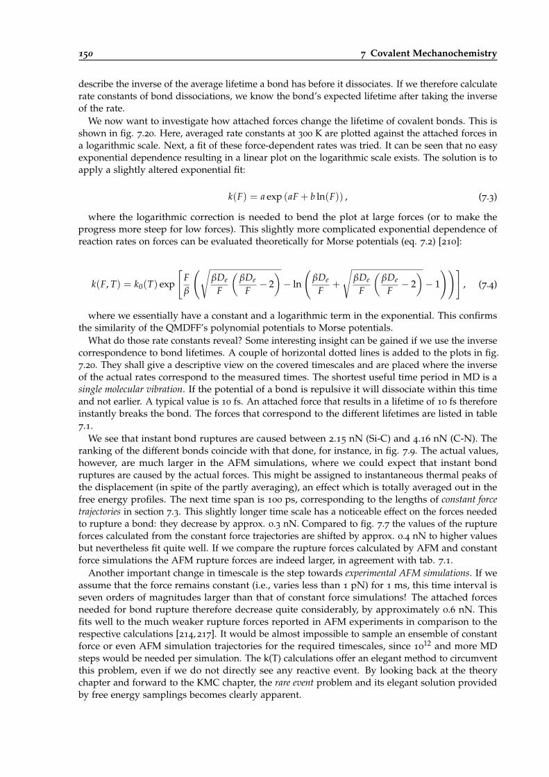
150 7 Covalent Mechanochemistry
describe the inverse of the average lifetime a bond has before it dissociates. If we therefore calculaterate constants of bond dissociations, we know the bond’s expected lifetime after taking the inverseof the rate.
We now want to investigate how attached forces change the lifetime of covalent bonds. This isshown in fig. 7.20. Here, averaged rate constants at 300 K are plotted against the attached forces ina logarithmic scale. Next, a fit of these force-dependent rates was tried. It can be seen that no easyexponential dependence resulting in a linear plot on the logarithmic scale exists. The solution is toapply a slightly altered exponential fit:
k(F) = a exp (aF + b ln(F)) , (7.3)
where the logarithmic correction is needed to bend the plot at large forces (or to make theprogress more steep for low forces). This slightly more complicated exponential dependence ofreaction rates on forces can be evaluated theoretically for Morse potentials (eq. 7.2) [210]:
k(F, T) = k0(T) exp
[Fβ
(√βDe
F
(βDe
F− 2)− ln
(βDe
F+
√βDe
F
(βDe
F− 2)− 1
))], (7.4)
where we essentially have a constant and a logarithmic term in the exponential. This confirmsthe similarity of the QMDFF’s polynomial potentials to Morse potentials.
What do those rate constants reveal? Some interesting insight can be gained if we use the inversecorrespondence to bond lifetimes. A couple of horizontal dotted lines is added to the plots in fig.7.20. They shall give a descriptive view on the covered timescales and are placed where the inverseof the actual rates correspond to the measured times. The shortest useful time period in MD is asingle molecular vibration. If the potential of a bond is repulsive it will dissociate within this timeand not earlier. A typical value is 10 fs. An attached force that results in a lifetime of 10 fs thereforeinstantly breaks the bond. The forces that correspond to the different lifetimes are listed in table7.1.
We see that instant bond ruptures are caused between 2.15 nN (Si-C) and 4.16 nN (C-N). Theranking of the different bonds coincide with that done, for instance, in fig. 7.9. The actual values,however, are much larger in the AFM simulations, where we could expect that instant bondruptures are caused by the actual forces. This might be assigned to instantaneous thermal peaks ofthe displacement (in spite of the partly averaging), an effect which is totally averaged out in thefree energy profiles. The next time span is 100 ps, corresponding to the lengths of constant forcetrajectories in section 7.3. This slightly longer time scale has a noticeable effect on the forces neededto rupture a bond: they decrease by approx. 0.3 nN. Compared to fig. 7.7 the values of the ruptureforces calculated from the constant force trajectories are shifted by approx. 0.4 nN to higher valuesbut nevertheless fit quite well. If we compare the rupture forces calculated by AFM and constantforce simulations the AFM rupture forces are indeed larger, in agreement with tab. 7.1.
Another important change in timescale is the step towards experimental AFM simulations. If weassume that the force remains constant (i.e., varies less than 1 pN) for 1 ms, this time interval isseven orders of magnitudes larger than that of constant force simulations! The attached forcesneeded for bond rupture therefore decrease quite considerably, by approximately 0.6 nN. Thisfits well to the much weaker rupture forces reported in AFM experiments in comparison to therespective calculations [214, 217]. It would be almost impossible to sample an ensemble of constantforce or even AFM simulation trajectories for the required timescales, since 10
12 and more MDsteps would be needed per simulation. The k(T) calculations offer an elegant method to circumventthis problem, even if we do not directly see any reactive event. By looking back at the theorychapter and forward to the KMC chapter, the rare event problem and its elegant solution providedby free energy samplings becomes clearly apparent.
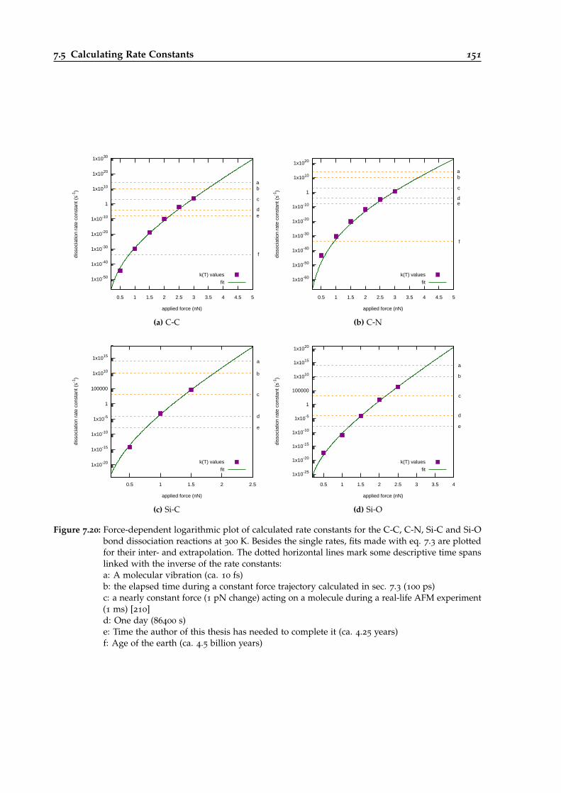
7.5 Calculating Rate Constants 151
1x10-50
1x10-40
1x10-30
1x10-20
1x10⁻¹⁰
1
1x10¹⁰
1x10²⁰
1x1030
0.5 1 1.5 2 2.5 3 3.5 4 4.5 5
diss
ocia
tion
rate
con
stan
t (s-1
)
applied force (nN)
k(T) values
fit
ab
c
de
f
(a) C-C
1x10-60
1x10-50
1x10-40
1x10-30
1x10-20
1x10⁻¹⁰
1
1x10¹⁰
1x10²⁰
0.5 1 1.5 2 2.5 3 3.5 4 4.5 5
diss
ocia
tion
rate
con
stan
t (s-1
)
applied force (nN)
k(T) values
fit
ab
c
de
f
(b) C-N
1x10-20
1x10-15
1x10⁻¹⁰
1x10⁻⁵
1
100000
1x10¹⁰
1x10¹⁵
0.5 1 1.5 2 2.5
diss
ocia
tion
rate
con
stan
t (s-1
)
applied force (nN)
k(T) values
fit
a
b
c
d
e
(c) Si-C
1x10-25
1x10-20
1x10-15
1x10⁻¹⁰
1x10⁻⁵
1
100000
1x10¹⁰
1x10¹⁵
1x10²⁰
0.5 1 1.5 2 2.5 3 3.5 4
diss
ocia
tion
rate
con
stan
t (s-1
)
applied force (nN)
k(T) values
fit
a
b
c
d
e
(d) Si-O
Figure 7.20: Force-dependent logarithmic plot of calculated rate constants for the C-C, C-N, Si-C and Si-Obond dissociation reactions at 300 K. Besides the single rates, fits made with eq. 7.3 are plottedfor their inter- and extrapolation. The dotted horizontal lines mark some descriptive time spanslinked with the inverse of the rate constants:a: A molecular vibration (ca. 10 fs)b: the elapsed time during a constant force trajectory calculated in sec. 7.3 (100 ps)c: a nearly constant force (1 pN change) acting on a molecule during a real-life AFM experiment(1 ms) [210]d: One day (86400 s)e: Time the author of this thesis has needed to complete it (ca. 4.25 years)f: Age of the earth (ca. 4.5 billion years)
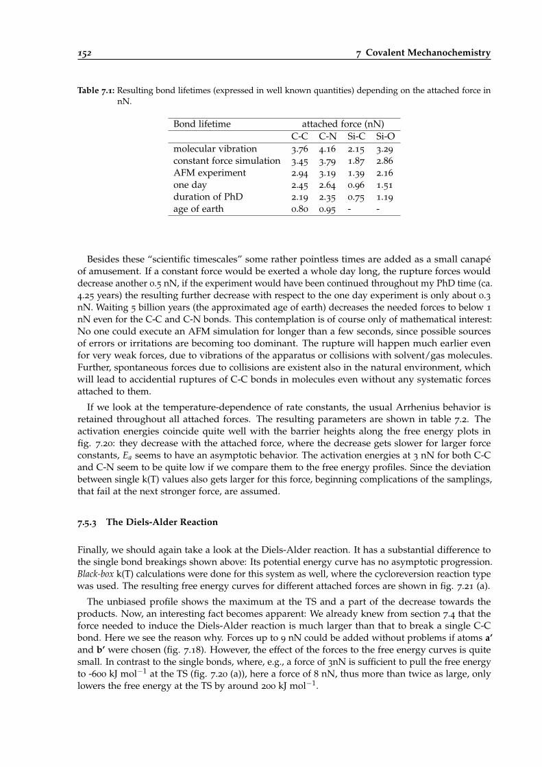
152 7 Covalent Mechanochemistry
Table 7.1: Resulting bond lifetimes (expressed in well known quantities) depending on the attached force innN.
Bond lifetime attached force (nN)C-C C-N Si-C Si-O
molecular vibration 3.76 4.16 2.15 3.29
constant force simulation 3.45 3.79 1.87 2.86
AFM experiment 2.94 3.19 1.39 2.16
one day 2.45 2.64 0.96 1.51
duration of PhD 2.19 2.35 0.75 1.19
age of earth 0.80 0.95 - -
Besides these “scientific timescales” some rather pointless times are added as a small canapéof amusement. If a constant force would be exerted a whole day long, the rupture forces woulddecrease another 0.5 nN, if the experiment would have been continued throughout my PhD time (ca.4.25 years) the resulting further decrease with respect to the one day experiment is only about 0.3nN. Waiting 5 billion years (the approximated age of earth) decreases the needed forces to below 1
nN even for the C-C and C-N bonds. This contemplation is of course only of mathematical interest:No one could execute an AFM simulation for longer than a few seconds, since possible sourcesof errors or irritations are becoming too dominant. The rupture will happen much earlier evenfor very weak forces, due to vibrations of the apparatus or collisions with solvent/gas molecules.Further, spontaneous forces due to collisions are existent also in the natural environment, whichwill lead to accidential ruptures of C-C bonds in molecules even without any systematic forcesattached to them.
If we look at the temperature-dependence of rate constants, the usual Arrhenius behavior isretained throughout all attached forces. The resulting parameters are shown in table 7.2. Theactivation energies coincide quite well with the barrier heights along the free energy plots infig. 7.20: they decrease with the attached force, where the decrease gets slower for larger forceconstants, Ea seems to have an asymptotic behavior. The activation energies at 3 nN for both C-Cand C-N seem to be quite low if we compare them to the free energy profiles. Since the deviationbetween single k(T) values also gets larger for this force, beginning complications of the samplings,that fail at the next stronger force, are assumed.
7.5.3 The Diels-Alder Reaction
Finally, we should again take a look at the Diels-Alder reaction. It has a substantial difference tothe single bond breakings shown above: Its potential energy curve has no asymptotic progression.Black-box k(T) calculations were done for this system as well, where the cycloreversion reaction typewas used. The resulting free energy curves for different attached forces are shown in fig. 7.21 (a).
The unbiased profile shows the maximum at the TS and a part of the decrease towards theproducts. Now, an interesting fact becomes apparent: We already knew from section 7.4 that theforce needed to induce the Diels-Alder reaction is much larger than that to break a single C-Cbond. Here we see the reason why. Forces up to 9 nN could be added without problems if atoms a’and b’ were chosen (fig. 7.18). However, the effect of the forces to the free energy curves is quitesmall. In contrast to the single bonds, where, e.g., a force of 3nN is sufficient to pull the free energyto -600 kJ mol−1 at the TS (fig. 7.20 (a)), here a force of 8 nN, thus more than twice as large, onlylowers the free energy at the TS by around 200 kJ mol−1.
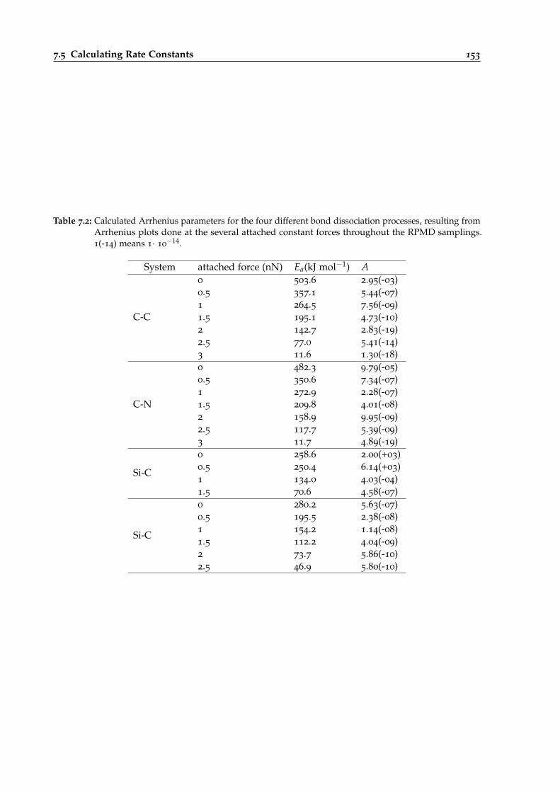
7.5 Calculating Rate Constants 153
Table 7.2: Calculated Arrhenius parameters for the four different bond dissociation processes, resulting fromArrhenius plots done at the several attached constant forces throughout the RPMD samplings.1(-14) means 1· 10
−14.
System attached force (nN) Ea(kJ mol−1) A
C-C
0 503.6 2.95(-03)0.5 357.1 5.44(-07)1 264.5 7.56(-09)1.5 195.1 4.73(-10)2 142.7 2.83(-19)2.5 77.0 5.41(-14)3 11.6 1.30(-18)
C-N
0 482.3 9.79(-05)0.5 350.6 7.34(-07)1 272.9 2.28(-07)1.5 209.8 4.01(-08)2 158.9 9.95(-09)2.5 117.7 5.39(-09)3 11.7 4.89(-19)
Si-C
0 258.6 2.00(+03)0.5 250.4 6.14(+03)1 134.0 4.03(-04)1.5 70.6 4.58(-07)
Si-C
0 280.2 5.63(-07)0.5 195.5 2.38(-08)1 154.2 1.14(-08)1.5 112.2 4.04(-09)2 73.7 5.86(-10)2.5 46.9 5.80(-10)
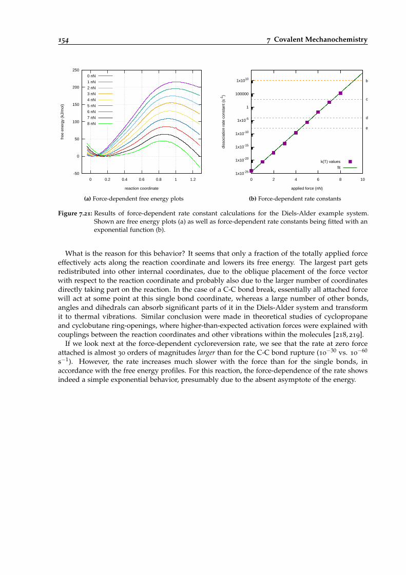
154 7 Covalent Mechanochemistry
-50
0
50
100
150
200
250
0 0.2 0.4 0.6 0.8 1 1.2
free
ene
rgy
(kJ/
mol
)
reaction coordinate
0 nN
1 nN
2 nN
3 nN
4 nN
5 nN
6 nN
7 nN
8 nN
(a) Force-dependent free energy plots
1x10-25
1x10-20
1x10-15
1x10⁻¹⁰
1x10⁻⁵
1
100000
1x10¹⁰
0 2 4 6 8 10
diss
ocia
tion
rate
con
stan
t (s-1
)
applied force (nN)
k(T) values
fit
b
c
d
e
(b) Force-dependent rate constants
Figure 7.21: Results of force-dependent rate constant calculations for the Diels-Alder example system.Shown are free energy plots (a) as well as force-dependent rate constants being fitted with anexponential function (b).
What is the reason for this behavior? It seems that only a fraction of the totally applied forceeffectively acts along the reaction coordinate and lowers its free energy. The largest part getsredistributed into other internal coordinates, due to the oblique placement of the force vectorwith respect to the reaction coordinate and probably also due to the larger number of coordinatesdirectly taking part on the reaction. In the case of a C-C bond break, essentially all attached forcewill act at some point at this single bond coordinate, whereas a large number of other bonds,angles and dihedrals can absorb significant parts of it in the Diels-Alder system and transformit to thermal vibrations. Similar conclusion were made in theoretical studies of cyclopropaneand cyclobutane ring-openings, where higher-than-expected activation forces were explained withcouplings between the reaction coordinates and other vibrations within the molecules [218, 219].
If we look next at the force-dependent cycloreversion rate, we see that the rate at zero forceattached is almost 30 orders of magnitudes larger than for the C-C bond rupture (10
−30 vs. 10−60
s−1). However, the rate increases much slower with the force than for the single bonds, inaccordance with the free energy profiles. For this reaction, the force-dependence of the rate showsindeed a simple exponential behavior, presumably due to the absent asymptote of the energy.
8
Ch
ap
te
r
Urethane Synthesis
A significant part of my work during the last years was spent on a cooperation with Covestro AG,which is still active at the time this thesis was finished. Since one of Covestro’s main occupationfields is the production of polyurethane materials, their theoretical chemistry section has builta significant expertise on this field. Soon after publication of the second EVB-QMDFF paper in2017 [17], we were contacted by the Covestro researchers and a cooperation was initiated.
The aim was to do rate constant calculations for (poly-)urethane synthesis reactions with EVB-QMDFF-RPMD in order to enable large-scale modeling of its synthesis with methods like KMC. Ina first step, rate constants of different autocatalytic mechanisms were calculated to benchmark theability of the method to simulate this kind of reactions. So far, only parametric k(T) calculationsbased on TST with tunneling corrections had been done. This study therefore constitutes to thebest of my knowledge the first ever RPMD study of urethane synthesis. In order to make thecalculations possible, the initial approach of connecting the RPMDrate program by Suleymanov
with an EVB-QMDFF PES function was revised with a global black-box approach uniting PESdescription and flexible RPMD rate constant calculation within one program package (see section3.1).
Publication of the results presented in this chapter is under preparation at the time this thesiswas completed [220]. Due to privacy concerns regarding the theoretical and experimental resultsproduced by Covestro, these will not be revealed before our cooperation paper has been published.In the actual publication, only results for suitable model reactions will be revealed, whereasapplications to actual industrial synthesis done by Covestro will not be disclosed at all. In order tonevertheless give a rough estimation of the EVB-QMDFF result‘s quality, they will be compared toother theoretical papers that handle the topic of urethane autocatalysis.
In section 8.1 a short review of the urethane chemistry will be given such that the importanceof our results for this topic can be better understood. In section 8.2 a benchmark study withselected DFT functionals is presented from which a method of high quality and modest scalingfor future calculations of larger systems can be proposed. This is followed by the actual RPMDcalculations, both settings and results, that are presented in section 8.3. A short excursion on thetopic of subsequent urethanation is presented in section 8.4.
8.1 Synthesis of Urethanes - a Long Story Short
Polyurethanes are one of the most important synthetic materials [221]. In contrast to most otherplastics like polyethylene or polystyrene, the properties of polyurethanes can be widely varied.This is due to the mechanism from which they are formed. They are not built by adding the samemonomer to growing monotonous chains but instead by combining isocyanates and alcohols thatreact to the urethane group. Whereas toluene diisocynaate (TDI) and methylene diphenyl isocyanate
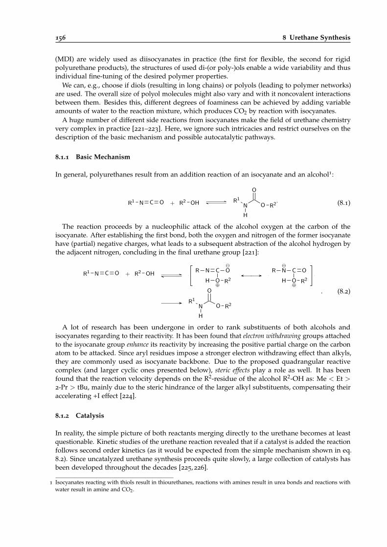
156 8 Urethane Synthesis
(MDI) are widely used as diisocyanates in practice (the first for flexible, the second for rigidpolyurethane products), the structures of used di-(or poly-)ols enable a wide variability and thusindividual fine-tuning of the desired polymer properties.
We can, e.g., choose if diols (resulting in long chains) or polyols (leading to polymer networks)are used. The overall size of polyol molecules might also vary and with it noncovalent interactionsbetween them. Besides this, different degrees of foaminess can be achieved by adding variableamounts of water to the reaction mixture, which produces CO2 by reaction with isocyanates.
A huge number of different side reactions from isocyanates make the field of urethane chemistryvery complex in practice [221–223]. Here, we ignore such intricacies and restrict ourselves on thedescription of the basic mechanism and possible autocatalytic pathways.
8.1.1 Basic Mechanism
In general, polyurethanes result from an addition reaction of an isocyanate and an alcohol1:
R1 N C O + R2 OH R1
N
H
O
O R2. (8.1)
The reaction proceeds by a nucleophilic attack of the alcohol oxygen at the carbon of theisocyanate. After establishing the first bond, both the oxygen and nitrogen of the former isocyanatehave (partial) negative charges, what leads to a subsequent abstraction of the alcohol hydrogen bythe adjacent nitrogen, concluding in the final urethane group [221]:
R1 N C O + R2 OH
[R N C
O⊕
H R2
O R
N C
O⊕
H R2
O]
R1
N
H
O
O R2
. (8.2)
A lot of research has been undergone in order to rank substituents of both alcohols andisocyanates regarding to their reactivity. It has been found that electron withdrawing groups attachedto the isyocanate group enhance its reactivity by increasing the positive partial charge on the carbonatom to be attacked. Since aryl residues impose a stronger electron withdrawing effect than alkyls,they are commonly used as isocyanate backbone. Due to the proposed quadrangular reactivecomplex (and larger cyclic ones presented below), steric effects play a role as well. It has beenfound that the reaction velocity depends on the R2-residue of the alcohol R2-OH as: Me < Et >2-Pr > tBu, mainly due to the steric hindrance of the larger alkyl substituents, compensating theiraccelerating +I effect [224].
8.1.2 Catalysis
In reality, the simple picture of both reactants merging directly to the urethane becomes at leastquestionable. Kinetic studies of the urethane reaction revealed that if a catalyst is added the reactionfollows second order kinetics (as it would be expected from the simple mechanism shown in eq.8.2). Since uncatalyzed urethane synthesis proceeds quite slowly, a large collection of catalysts hasbeen developed throughout the decades [225, 226].
1 Isocyanates reacting with thiols result in thiourethanes, reactions with amines result in urea bonds and reactions withwater result in amine and CO2.
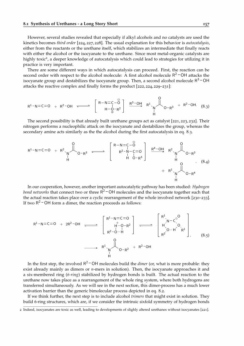
8.1 Synthesis of Urethanes - a Long Story Short 157
However, several studies revealed that especially if alkyl alcohols and no catalysts are used thekinetics becomes third order [224, 227, 228]. The usual explanation for this behavior is autocatalysis,either from the reactants or the urethane itself, which stabilizes an intermediate that finally reactswith either the alcohol or the isocyanate to the urethane. Since most metal-organic catalysts arehighly toxic2, a deeper knowledge of autocatalysis which could lead to strategies for utilizing it inpractice is very important.
There are some different ways in which autocatalysis can proceed. First, the reaction can besecond order with respect to the alcohol molecule: A first alcohol molecule R2 OH attacks theisocyanate group and destabilizes the isocyanate group. Then, a second alcohol molecule R3 OHattacks the reactive complex and finally forms the product [222, 224, 229–231]:
R1 N C O + R2 OH
[R N C
O⊕
H R2
O]
R3 OH R1
N
H
O
O R3 + R2 OH. (8.3)
The second possibility is that already built urethane groups act as catalyst [221, 223, 232]. Theirnitrogen performs a nucleophilic attack on the isocyanate and destabilizes the group, whereas thesecondary amine acts similarly as the the alcohol during the first autocatalysis in eq. 8.3.
R1 N C O + R2
N
H
O
O R3
R N C
NR2 C
O R3
O
H
O
R4 OH R2
N
H
O
O R3
+ R1
N
H
O
O R4
. (8.4)
In our cooperation, however, another important autocatalytic pathway has been studied: Hydrogenbond networks that connect two or three R2 OH molecules and the isocyanate together such thatthe actual reaction takes place over a cyclic rearrangement of the whole involved network [230–233].If two R2 OH form a dimer, the reaction proceeds as follows:
R1 N C O + 2R2 OH
R1
H
OR2 H
O R2
N+
C O
R1
NH
OR2
H
CO
OR1
R1
N
H
O
O R2 + R2 OH
. (8.5)
In the first step, the involved R2 OH molecules build the dimer (or, what is more probable: theyexist already mainly as dimers or n-mers in solution). Then, the isocyanate approaches it anda six-membered ring (6-ring) stabilized by hydrogen bonds is built. The actual reaction to theurethane now takes place as a rearrangement of the whole ring system, where both hydrogens aretransferred simultaneously. As we will see in the next section, this dimer-process has a much loweractivation barrier than the generic bimolecular process depicted in eq. 8.2.
If we think further, the next step is to include alcohol trimers that might exist in solution. Theybuild 6-ring structures, which are, if we consider the intrinsic sixfold symmetry of hydrogen bonds
2 Indeed, isocyanates are toxic as well, leading to developments of slighly altered urethanes without isocyanates [221].
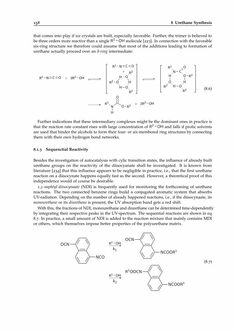
158 8 Urethane Synthesis
that comes into play if ice crystals are built, especially favorable. Further, the trimer is believed tobe three orders more reactive than a single R2 OH molecule [223]. In connection with the favorablesix-ring structure we therefore could assume that most of the additions leading to formation ofurethane actually proceed over an 8-ring intermediate:
R1 N C O + 3R2 OH
R1
HOR2
H OR2
HO
R2
N+
C O
R1
NH
OR2 H O
R2
H
CO
O R2
R1
N
H
O
O R2 + 2R2 OH
. (8.6)
Further indications that these intermediary complexes might be the dominant ones in practice isthat the reaction rate constant rises with large concentration of R2 OH and falls if protic solventsare used that hinder the alcohols to form their four- or six-membered ring structures by connectingthem with their own hydrogen bond networks.
8.1.3 Sequenctial Reactivity
Besides the investigation of autocatalysis with cylic transition states, the influence of already builturethane groups on the reactivity of the diisocyanate shall be investigated. It is known fromliterature [234] that this influence appears to be negligible in practice, i.e., that the first urethanereaction on a diisocynate happens equally fast as the second. However, a theoretical proof of thisindependence would of course be desirable.
1,5-naphtyl-diisocynaate (NDI) is frequently used for monitoring the forthcoming of urethanereactions. The two connected benzene rings build a conjugated aromatic system that absorbsUV-radiation. Depending on the number of already happened reactions, i.e., if the diisocynaate, itsmonourethane or its diurethane is present, the UV absorption band gets a red shift.
With this, the fractions of NDI, monourethane and diurethane can be determined time-dependentlyby integrating their respective peaks in the UV-spectrum. The sequential reactions are shown in eq.8.7. In practice, a small amount of NDI is added to the reaction mixture that mainly contains MDIor others, which themselves impose better properties of the polyurethane matrix.
OCN
NCO
R1 OH
k1
OCN
NCOOR1
R1 OH
k2
R1OOCN
NCOOR1
(8.7)
8.2 Benchmark of QM Reference Methods 159
8.2 Benchmark of QM Reference Methods
As usual, the calculation of QM reference data was the first step of the EVB-QMDFF setup in thisstudy. In contrast to the other examples presented so far in this thesis, a wise choice of the QMreference is essential, since we want to be able to calculate the urethane reaction rate constants withhigh quality. Further, we want to have a method that imposes modest scaling since applicationsto k(T) calculations of even larger systems (i.e., larger substituents of both alcohol and isocyanatemolecules) are scheduled for the future.
8.2.1 Settings and Strategy
The present study covers six different systems: The basic bimolecular urethane reaction (eq.8.2) as well as the autocatalytic cyclic rearrangement pathways (eqs. 8.5-8.6) were studied withtwo different alcohol molecules each: The simplest possible methanol (MeOH) as well as the2-methoxyethanol (MeOCH2CH2OH) constituting a more realistic sidechain for real synthesis 3.
Even if the chosen systems are still quite small model cases, their size (up to 46 atoms) isnevertheless much larger than anything treated before with EVB-QMDFF (exceptions are the KMCcalculations presented in the next chapter, where most atoms are located in the passive metalbulk). Therefore it became clear in advance that very expensive QM methods like CCSD(T) wereout of reach even for calculations of energy corrections. Another strategy was pursued: MP2 willusually be a reliable method for the cases presented here, however it becomes much too expensivefor even larger systems than the ones presented here. Alternatively, DFT-based methods imposemodest scaling with system size by simultaneously being able to permit high-quality descriptions.However, the actual quality strongly depends on the chosen DFT functional. A whole bunch ofthem has been emerged since the 90s, and for one specific type of reaction DFT performance maydiffer from the average performance determined in huge, general benchmarks [235, 236]. Therefore,a benchmark for this particular purpose was performed. MP2 calculations of all six systems wereperformed (with the cc-pVTZ basis set [237] for the MeOH-substituents and the cc-pVDZ basis setfor the MeOCH2CH2OH-substituents), which serves as reference. Since the TREQ method shallbe used for PES setup it is useful to calculate the energies of the reaction path with a separateQM method of higher quality (dual-level approach, see chapter 5). Therefore, the energies of theMP2 RP were calculated with DLPNO-CCSD(T)4 [154, 155] and the def2-TZVP basis set [158] usingOrca [130, 131]. Then, these calculations were done with 17 different popular functionals as well,using the cc-pVDZ basis set for all of them. The D3 empirical dispersion correction by Grimme [91]was applied. In addition, three different semiempirical methods, constituting an even cheaperalternative, were investigated as well.
For all methods, TS and IRC optimizations were done with Gaussian 16 [99], the frequencies ofthe imaginary TS modes that describe the shape of the reaction path at the transition state as wellas the total potential energy barrier heights obtained from the IRCs were taken as quality criteria.A DFT method is assumed to perform well in this case if its TS imaginary frequency is similarto that of MP2, the barrier heights are compared with the DLPNO-CCSD(T) energies, calculatedon IRC paths optimized with MP2. The TS structures of the six systems optimized with MP2 areshown in fig. 8.1.
3 In reality, much longer chains with at least two hydroxyl groups are of course in usage. The pattern of ether groupsconnecting a sequence of rather small alkyl fragments is quite common, though, therefore making these calculationscomparable to real world systems at least in the first place. Calculations of longer chains are the logical next step (seechapter 10).
4 The DLPNO-CCSD(T)-method claims to provide similar quality as “real” CCSD(T) calculations by simultaneouslyimpose much more favorable scaling.
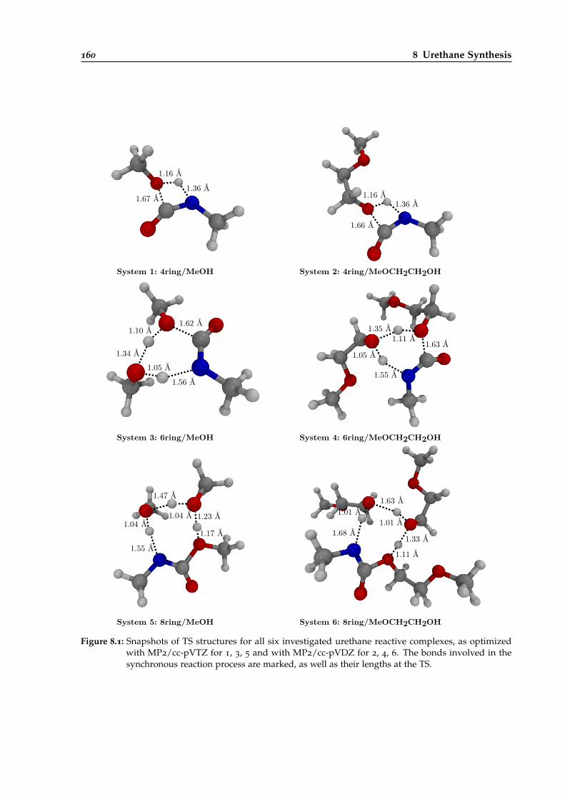
160 8 Urethane Synthesis
System 5: 8ring/MeOH System 6: 8ring/MeOCH2CH2OH
System 3: 6ring/MeOH System 4: 6ring/MeOCH2CH2OH
System 1: 4ring/MeOH System 2: 4ring/MeOCH2CH2OH
1.36 Å
1.16 Å
1.67 Å 1.36 Å1.16 Å
1.66 Å
1.56 Å
1.34 Å
1.10 Å1.62 Å
1.05 Å
1.35 Å
1.63 Å1.11 Å
1.55 Å
1.05 Å
1.04 Å
1.47 Å
1.23 Å
1.17 Å1.04 Å
1.55 Å
1.63 Å
1.01 Å
1.33 Å
1.11 Å
1.68 Å
1.01 Å
Figure 8.1: Snapshots of TS structures for all six investigated urethane reactive complexes, as optimizedwith MP2/cc-pVTZ for 1, 3, 5 and with MP2/cc-pVDZ for 2, 4, 6. The bonds involved in thesynchronous reaction process are marked, as well as their lengths at the TS.
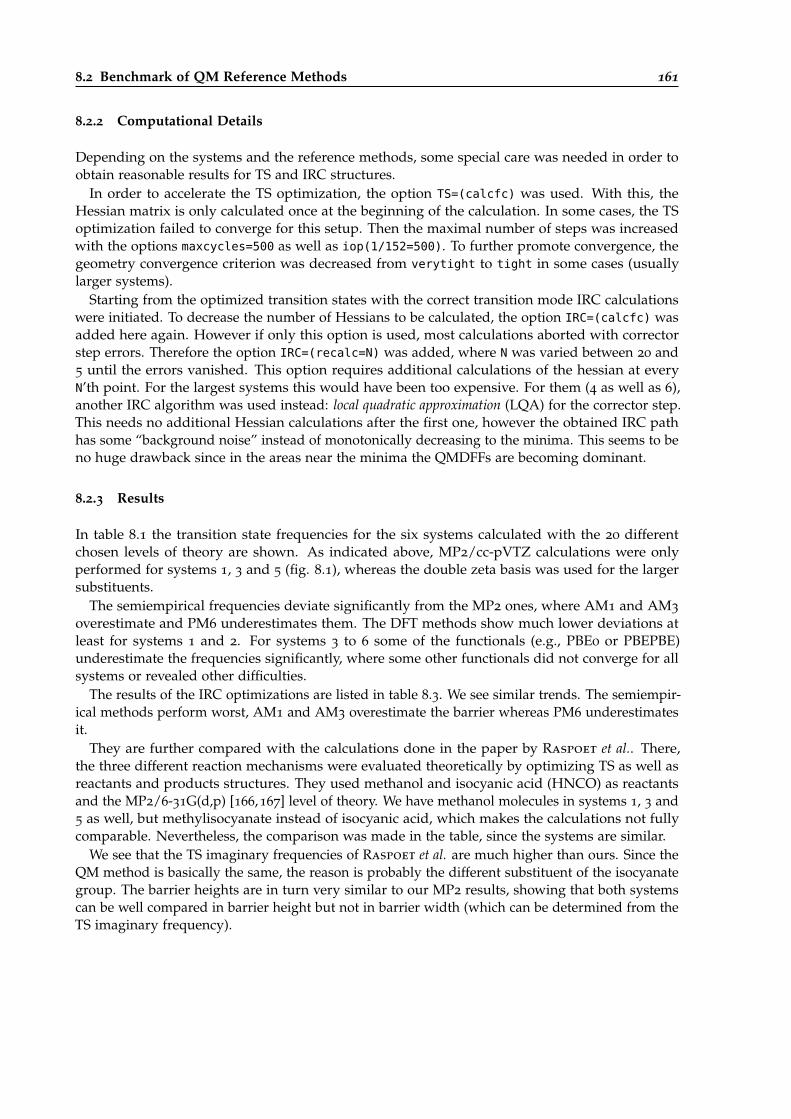
8.2 Benchmark of QM Reference Methods 161
8.2.2 Computational Details
Depending on the systems and the reference methods, some special care was needed in order toobtain reasonable results for TS and IRC structures.
In order to accelerate the TS optimization, the option TS=(calcfc) was used. With this, theHessian matrix is only calculated once at the beginning of the calculation. In some cases, the TSoptimization failed to converge for this setup. Then the maximal number of steps was increasedwith the options maxcycles=500 as well as iop(1/152=500). To further promote convergence, thegeometry convergence criterion was decreased from verytight to tight in some cases (usuallylarger systems).
Starting from the optimized transition states with the correct transition mode IRC calculationswere initiated. To decrease the number of Hessians to be calculated, the option IRC=(calcfc) wasadded here again. However if only this option is used, most calculations aborted with correctorstep errors. Therefore the option IRC=(recalc=N) was added, where N was varied between 20 and5 until the errors vanished. This option requires additional calculations of the hessian at everyN’th point. For the largest systems this would have been too expensive. For them (4 as well as 6),another IRC algorithm was used instead: local quadratic approximation (LQA) for the corrector step.This needs no additional Hessian calculations after the first one, however the obtained IRC pathhas some “background noise” instead of monotonically decreasing to the minima. This seems to beno huge drawback since in the areas near the minima the QMDFFs are becoming dominant.
8.2.3 Results
In table 8.1 the transition state frequencies for the six systems calculated with the 20 differentchosen levels of theory are shown. As indicated above, MP2/cc-pVTZ calculations were onlyperformed for systems 1, 3 and 5 (fig. 8.1), whereas the double zeta basis was used for the largersubstituents.
The semiempirical frequencies deviate significantly from the MP2 ones, where AM1 and AM3
overestimate and PM6 underestimates them. The DFT methods show much lower deviations atleast for systems 1 and 2. For systems 3 to 6 some of the functionals (e.g., PBE0 or PBEPBE)underestimate the frequencies significantly, where some other functionals did not converge for allsystems or revealed other difficulties.
The results of the IRC optimizations are listed in table 8.3. We see similar trends. The semiempir-ical methods perform worst, AM1 and AM3 overestimate the barrier whereas PM6 underestimatesit.
They are further compared with the calculations done in the paper by Raspoet et al.. There,the three different reaction mechanisms were evaluated theoretically by optimizing TS as well asreactants and products structures. They used methanol and isocyanic acid (HNCO) as reactantsand the MP2/6-31G(d,p) [166,167] level of theory. We have methanol molecules in systems 1, 3 and5 as well, but methylisocyanate instead of isocyanic acid, which makes the calculations not fullycomparable. Nevertheless, the comparison was made in the table, since the systems are similar.
We see that the TS imaginary frequencies of Raspoet et al. are much higher than ours. Since theQM method is basically the same, the reason is probably the different substituent of the isocyanategroup. The barrier heights are in turn very similar to our MP2 results, showing that both systemscan be well compared in barrier height but not in barrier width (which can be determined from theTS imaginary frequency).
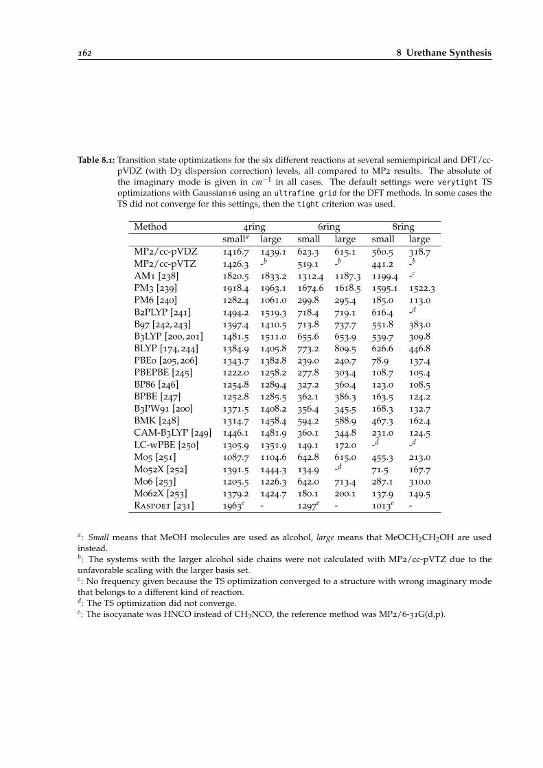
162 8 Urethane Synthesis
Table 8.1: Transition state optimizations for the six different reactions at several semiempirical and DFT/cc-pVDZ (with D3 dispersion correction) levels, all compared to MP2 results. The absolute ofthe imaginary mode is given in cm−1 in all cases. The default settings were verytight TSoptimizations with Gaussian16 using an ultrafine grid for the DFT methods. In some cases theTS did not converge for this settings, then the tight criterion was used.
Method 4ring 6ring 8ringsmalla large small large small large
MP2/cc-pVDZ 1416.7 1439.1 623.3 615.1 560.5 318.7MP2/cc-pVTZ 1426.3 -b
519.1 -b441.2 -b
AM1 [238] 1820.5 1833.2 1312.4 1187.3 1199.4 -c
PM3 [239] 1918.4 1963.1 1674.6 1618.5 1595.1 1522.3PM6 [240] 1282.4 1061.0 299.8 295.4 185.0 113.0B2PLYP [241] 1494.2 1519.3 718.4 719.1 616.4 -d
B97 [242, 243] 1397.4 1410.5 713.8 737.7 551.8 383.0B3LYP [200, 201] 1481.5 1511.0 655.6 653.9 539.7 309.8BLYP [174, 244] 1384.9 1405.8 773.2 809.5 626.6 446.8PBE0 [205, 206] 1343.7 1382.8 239.0 240.7 78.9 137.4PBEPBE [245] 1222.0 1258.2 277.8 303.4 108.7 105.4BP86 [246] 1254.8 1289.4 327.2 360.4 123.0 108.5BPBE [247] 1252.8 1285.5 362.1 386.3 163.5 124.2B3PW91 [200] 1371.5 1408.2 356.4 345.5 168.3 132.7BMK [248] 1314.7 1458.4 594.2 588.9 467.3 162.4CAM-B3LYP [249] 1446.1 1481.9 360.1 344.8 231.0 124.5LC-wPBE [250] 1305.9 1351.9 149.1 172.0 -d -d
M05 [251] 1087.7 1104.6 642.8 615.0 455.3 213.0M052X [252] 1391.5 1444.3 134.9 -d
71.5 167.7M06 [253] 1205.5 1226.3 642.0 713.4 287.1 310.0M062X [253] 1379.2 1424.7 180.1 200.1 137.9 149.5Raspoet [231] 1963
e - 1297e - 1013
e -
a: Small means that MeOH molecules are used as alcohol, large means that MeOCH2CH2OH are usedinstead.b: The systems with the larger alcohol side chains were not calculated with MP2/cc-pVTZ due to theunfavorable scaling with the larger basis set.c: No frequency given because the TS optimization converged to a structure with wrong imaginary modethat belongs to a different kind of reaction.d: The TS optimization did not converge.e: The isocyanate was HNCO instead of CH3NCO, the reference method was MP2/6-31G(d,p).
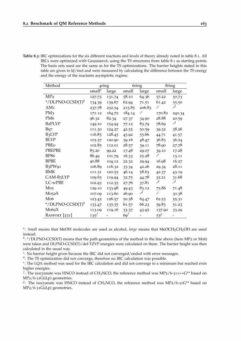
8.2 Benchmark of QM Reference Methods 163
Table 8.3: IRC optimizations for the six different reactions and levels of theory already noted in table 8.1. AllIRCs were optimized with Gaussian16, using the TS structures from table 8.1 as starting points.The basis sets used are the same as for the TS optimizations. The barrier heights stated in thistable are given in kJ/mol and were measured by calculating the difference between the TS energyand the energy of the reactants asymptotic regime.
Method 4ring 6ring 8ringsmalla large small large small large
MP2 127.73 131.74 58.10 64.36 57.22 50.73
*/DLPNO-CCSD(T)b134.39 139.67 62.94 71.51 61.42 55.50
AM1 237.78 232.54 215.85 206.83 -c -d
PM3 171.12 164.72 184.14 -c170.82 240.34
PM6 96.32 82.34 27.37 34.90 28.88 20.59
B2PLYP 149.10 154.94 77.12 83.79 78.69 -d
B97 111.30 124.27 42.52 50.59 39.32 38.26
B3LYP 116.85 128.45 45.92 55.66 44.71 41.57
BLYP 103.57 120.90 39.16 48.47 36.83 36.24
PBE0 102.85 112.01 28.57 39.11 78.90 27.78
PBEPBE 85.20 99.22 17.48 29.07 39.10 17.28
BP86 86.49 101.79 16.33 25.28 -e13.11
BPBE 90.88 104.12 22.32 29.94 16.98 16.27
B3PW91 106.89 116.32 33.34 42.26 29.34 28.11
BMK 111.31 120.55 46.14 58.63 42.37 43.19
CAM-B3LYP 109.65 119.94 32.75 44.78 32.21 31.68
LC-wPBE 102.93 112.35 27.76 37.81 -d -d
M05 129.10 133.98 49.43 83.12 75.86 71.48
M052X 107.09 113.60 26.90 -d -c30.38
M06 123.45 126.57 50.38 64.47 62.53 55.31
*/DLPNO-CCSD(T)b133.47 135.55 61.57 66.23 59.83 51.23
M062X 113.09 119.16 33.37 43.95 137.90 33.29
Raspoet [231] 135f - 69
f - 53g -
a: Small means that MeOH molecules are used as alcohol, large means that MeOCH2CH2OH are usedinstead.b: */DLPNO-CCSD(T) means that the path geometries of the method in the line above (here MP2 or M06)were taken and DLPNO-CCSD(T)/def-TZVP energies were calculated on them. The barrier height was thencalculated in the usual way.c: No barrier height given because the IRC did not converged/ended with error messages.d: The TS optimization did not converge, therefore no IRC calculation was possible.e: The LQA method was used for the IRC calculation and did not converge to a minimum but reached evenhigher energies.f : The isocyanate was HNCO instead of CH3NCO, the reference method was MP2/6-311++G** based onMP2/6-31G(d,p) geometries.g: The isocyanate was HNCO instead of CH3NCO, the reference method was MP2/6-31G** based onMP2/6-31G(d,p) geometries.
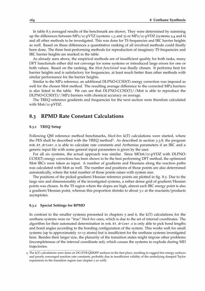
164 8 Urethane Synthesis
In table 8.5 averaged results of the benchmark are shown. They were determined by summingup the differences between MP2/cc-pVTZ (systems 1,3 and 5) or MP2/cc-pVDZ (systems 2,4 and 6)and all other methods to be investigated. This was done for TS frequencies and IRC barrier heightsas well. Based on these differences a quantitative ranking of all involved methods could finallybeen done. The three best-performing methods for reproduction of imaginary TS frequencies andIRC barrier heights are marked in the table.
As already seen above, the empirical methods are of insufficient quality for both tasks, manyDFT functionals either did not converge for some systems or introduced large errors for one orboth values. Based on the ranking, the M06 functional was finally chosen. It performs best forbarrier heights and is satisfactory for frequencies, at least much better than other methods withsimilar performance for the barrier heights.
Similar to the MP2 reference, an additional DLPNO-CCSD(T) energy correction was imposed aswell for the chosen M06 method. The resulting average difference to the corrected MP2 barriersis also listed in the table. We can see that DLPNO-CCSD(T)//M06 is able to reproduce theDLPNO-CCSD(T)//MP2 barriers with chemical accuracy on average.
The TREQ reference gradients and frequencies for the next section were therefore calculatedwith M06/cc-pVDZ.
8.3 RPMD Rate Constant Calculations
8.3.1 TREQ Setup
Following QM reference method benchmarks, black-box k(T) calculations were started, wherethe PES shall be described with the TREQ method5. As described in section 3.3.8, the programevb_kt_driver.x is able to calculate rate constants and Arrhenius parameters if an IRC and ageneric input file with some general input parameters is given by the user.
For all six systems, the actual approach was similar. Since MO06/cc-pVDZ with DLPNO-CCSD(T) energy corrections has been shown to be the best performing DFT method, the optimizedM06 IRCs were taken as input. A number of gradients and Hessians along the reaction pathswas calculated with M06 as well. The number and positions of those points are also determinedautomatically, where the total number of those points raises with system size.
The positions of the picked gradient/Hessian reference points are plotted in fig. 8.5. Due to thelarge size and dimensionality of the investigated systems, a rather dense grid of gradient/Hessianpoints was chosen. In the TS region where the slopes are high, almost each IRC energy point is alsoa gradient/Hessian point, whereas this proportion shrinks to about 3:1 at the reactants/productsasymptotes.
8.3.2 Special Settings for RPMD
In contrast to the smaller systems presented in chapters 5 and 6, the k(T) calculations for theurethane systems were no “true” black-box ones, which is due to the set of internal coordinates. Thealgorithm for their automated determination in evb_kt_driver.x is only able to pick bond lengthsand bond angles according to the bonding configuration of the system. This works well for smallsystems (up to approximately 10-15 atoms) but is insufficient for the urethane systems investigatedhere. Besides their larger size, the planarity of the transition states might impose other problems(incompleteness of the internal coordinate set), which causes the systems to explode during MDtrajectories.
5 The k(T) calculations were done on DG-EVB-QMDFF surfaces in the first place, resulting in rugged free energy surfacesand poorly converged reaction rate constants, probably due to insufficient validity of the underlying damped Taylorexpansions in the transition region (see chapter 5 as well).
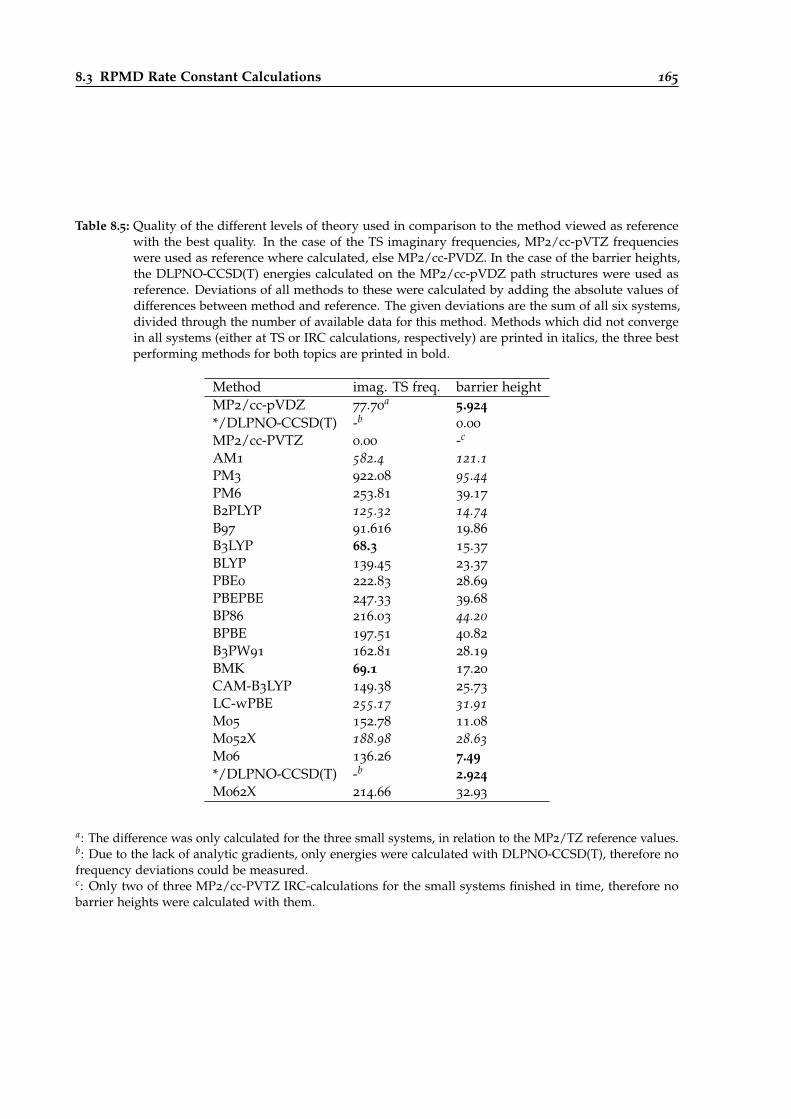
8.3 RPMD Rate Constant Calculations 165
Table 8.5: Quality of the different levels of theory used in comparison to the method viewed as referencewith the best quality. In the case of the TS imaginary frequencies, MP2/cc-pVTZ frequencieswere used as reference where calculated, else MP2/cc-PVDZ. In the case of the barrier heights,the DLPNO-CCSD(T) energies calculated on the MP2/cc-pVDZ path structures were used asreference. Deviations of all methods to these were calculated by adding the absolute values ofdifferences between method and reference. The given deviations are the sum of all six systems,divided through the number of available data for this method. Methods which did not convergein all systems (either at TS or IRC calculations, respectively) are printed in italics, the three bestperforming methods for both topics are printed in bold.
Method imag. TS freq. barrier heightMP2/cc-pVDZ 77.70
a 5.924*/DLPNO-CCSD(T) -b
0.00
MP2/cc-PVTZ 0.00 -c
AM1 582.4 121.1PM3 922.08 95.44PM6 253.81 39.17
B2PLYP 125.32 14.74B97 91.616 19.86
B3LYP 68.3 15.37
BLYP 139.45 23.37
PBE0 222.83 28.69
PBEPBE 247.33 39.68
BP86 216.03 44.20BPBE 197.51 40.82
B3PW91 162.81 28.19
BMK 69.1 17.20
CAM-B3LYP 149.38 25.73
LC-wPBE 255.17 31.91M05 152.78 11.08
M052X 188.98 28.63M06 136.26 7.49*/DLPNO-CCSD(T) -b 2.924M062X 214.66 32.93
a: The difference was only calculated for the three small systems, in relation to the MP2/TZ reference values.b: Due to the lack of analytic gradients, only energies were calculated with DLPNO-CCSD(T), therefore nofrequency deviations could be measured.c: Only two of three MP2/cc-PVTZ IRC-calculations for the small systems finished in time, therefore nobarrier heights were calculated with them.
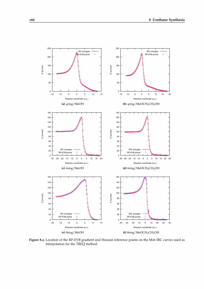
166 8 Urethane Synthesis
0
50
100
150
200
250
-15 -10 -5 0 5 10 15
E (k
J/m
ol)
Reaction coordinate (a.u.)
IRC energiesRP-EVB points
(a) 4ring/MeOH
0
50
100
150
200
250
-15 -10 -5 0 5 10 15 20
E (k
J/m
ol)
Reaction coordinate (a.u.)
IRC energiesRP-EVB points
(b) 4ring/MeOCH2CH2OH
0
20
40
60
80
100
120
140
160
180
-30 -25 -20 -15 -10 -5 0 5 10 15 20
E (k
J/m
ol)
Reaction coordinate (a.u.)
IRC energiesRP-EVB points
(c) 6ring/MeOH
0
20
40
60
80
100
120
140
160
180
-30 -25 -20 -15 -10 -5 0 5 10 15 20 25
E (k
J/m
ol)
Reaction coordinate (a.u.)
IRC energiesRP-EVB points
(d) 6ring/MeOCH2CH2OH
0
20
40
60
80
100
120
140
160
-20 -15 -10 -5 0 5 10
E (k
J/m
ol)
Reaction coordinate (a.u.)
IRC energiesRP-EVB points
(e) 8ring/MeOH
0
20
40
60
80
100
120
140
160
-40 -30 -20 -10 0 10 20 30 40
E (k
J/m
ol)
Reaction coordinate (a.u.)
IRC energiesRP-EVB points
(f) 8ring/MeOCH2CH2OH
Figure 8.2: Location of the RP-EVB gradient and Hessian reference points on the M06 IRC curves used asinterpolation for the TREQ method.
8.3 RPMD Rate Constant Calculations 167
This problem was solved by introduction of dihedral and out-of-plane angle coordinates. If we addsome of these coordinates to the atoms that become part of the cyclic TS during the reaction thebad behavior can be avoided. So far, no clever algorithm for the right choice of additional dihedraland out-of-plane coordinates was developed, therefore they were chosen manually.
Two changes concerning the RPMD k(T) calculations shall be mentioned as well. In the simplestcase (systems 1 and 2), the urethane is built by an addition reaction, where one bond is brokenand two are built. Since the RPMDrate program by Suleymanov is unable to calculate k(T) valuesfor such reactions, the rpmd.x program with a more general definition of the dividing surfacehas been developed (section 3.3.7). With this, the simple urethane reaction mechanism can betreated as a simple bimolecular addition reaction. However, things get more complicated whenwe look at the autocatalytic reaction mechanisms expressed by systems 3 to 6. Here, three or fourreactant molecules come together and react simultaneously at the TS. We might expect that theseare tri- or tetramolecular reactions, respectively, due to the number of reactants that come togethersimultaneously. This is shown in fig. 8.3, (a).
In reality, reaction orders of three or four are almost unknown since synchronous hits of threeor four molecules coming from different directions are extremely unlikely. Therefore, anothermechanism is calculated in the examples. As already shown above (eqs. 8.5-8.6) it is assumedin the literature that the alcohol molecules build dimers or trimers if no protic solvent is used.Urethane reactions with autocatalysis now start if the isocyanate molecule and an alcohol clusterapproach each other such that they can build the cyclic TS complex (fig. 8.1). This reaction thenis a bimolecular one where the alcohol cluster can be treated as a single molecule at least in theasymptote of distant approach.
In order to teach rpmd.x to calculate such a reaction, the definitions of reactants and TS dividingsurfaces must be set independently. The reactant dividing surface (eq. 3.10) is that of a bimolecularreaction (Ned = 2), since the alcohol cluster can be seen as a single molecule from afar. Theumbrella bias is therefore applied on the center of mass of all two or three alcohol molecules, lettingthem build a hydrogen bond network freely. If the molecules stick together and build the reactivecomplex, the simplified picture of two molecules must be broken at least partly. Depending on thenumber of molecules involved we have a larger number of built and broken bonds (according tothe reformed hydrogen bond network) than in the simplest case. Near the TS, the bias is appliedon all those bonds (eq. 3.11), thus treating all involved molecules as separate entities. Therefore,the TS dividing surface is rather that of a tetramolecular reaction than that of a bimolecular one.This composite reaction type has been introduced into rpmd.x with the descriptors 3 educt cyclicaddition (SC) and 4 educt cyclic addition (SC), where SC stands for solvent complex (table 3.4).
Experimental works obtained indications that the actual autocatalytic reaction has a reactionorder between two and three, according to a mixture of solvent complex reaction and “real” tri- ormaybe even tetramolecular reactions with separate approaching of the alcohol molecules. Here weassume that the reactions are fully bimolecular at least in the asymptotic limit, such that the usualbimolecular RPMD k(T) formula can be applied. This assumption seems to be legitimate, as willbe shown when the RPMD results are compared with experimental results from Covestro in theprepared publication.
The second change that needs to be applied on rpmd.x is the way in which the free energysurface is postprocessed for the final k(T) calculation (eq. 2.103). Usually, the free energy of thereactants is evaluated at the reactants asymptote (ξ =0). This scheme might be called the asymptotebarrier approach (see fig. 8.4). For the urethane reactions it turned out that the resulting Arrheniusparameters agree much better with the experimental ones if a slight change is made: Instead oftaking the free energy value at ξ =0 for the reactants, the global minimum of the calculated freeenergy curve is determined and the free energy of the reactants is calculated at this point, resultingin a larger barrier and a lower rate constant.
The reason why this modification leads to better agreement with experiment might be that themeasurements were done in solution and not in the gas phase as our calculations. In solution, the
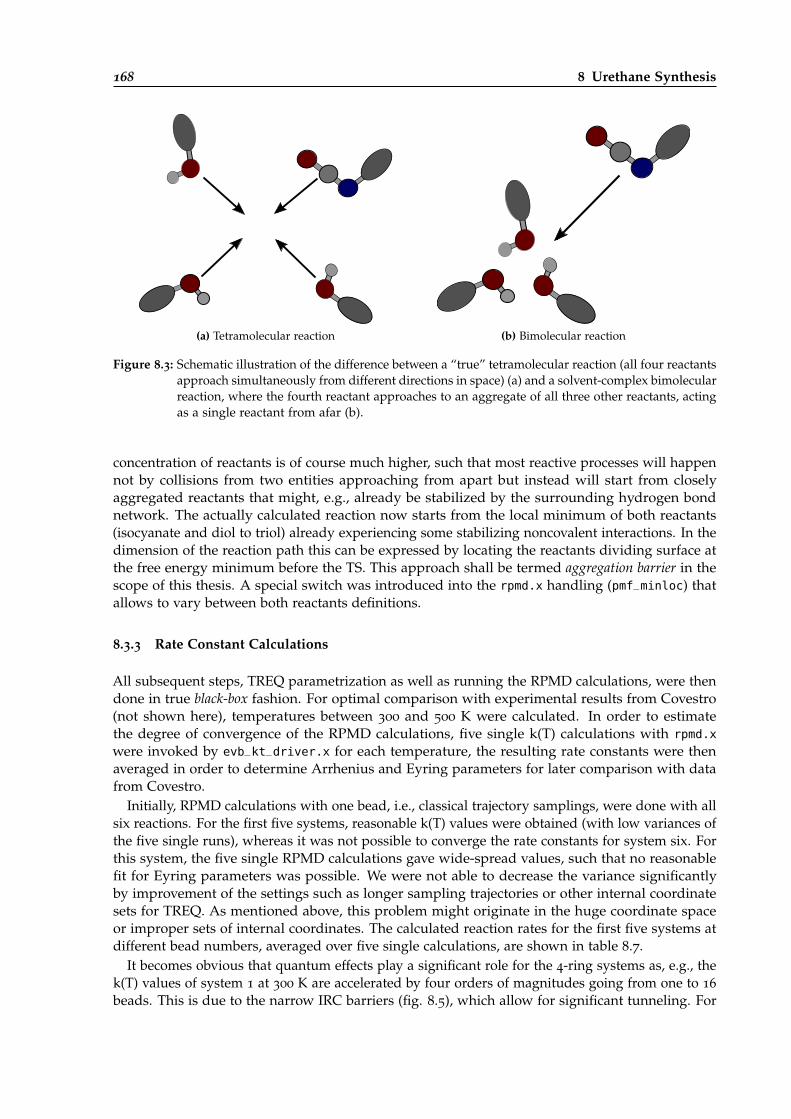
168 8 Urethane Synthesis
(a) Tetramolecular reaction (b) Bimolecular reaction
Figure 8.3: Schematic illustration of the difference between a “true” tetramolecular reaction (all four reactantsapproach simultaneously from different directions in space) (a) and a solvent-complex bimolecularreaction, where the fourth reactant approaches to an aggregate of all three other reactants, actingas a single reactant from afar (b).
concentration of reactants is of course much higher, such that most reactive processes will happennot by collisions from two entities approaching from apart but instead will start from closelyaggregated reactants that might, e.g., already be stabilized by the surrounding hydrogen bondnetwork. The actually calculated reaction now starts from the local minimum of both reactants(isocyanate and diol to triol) already experiencing some stabilizing noncovalent interactions. In thedimension of the reaction path this can be expressed by locating the reactants dividing surface atthe free energy minimum before the TS. This approach shall be termed aggregation barrier in thescope of this thesis. A special switch was introduced into the rpmd.x handling (pmf_minloc) thatallows to vary between both reactants definitions.
8.3.3 Rate Constant Calculations
All subsequent steps, TREQ parametrization as well as running the RPMD calculations, were thendone in true black-box fashion. For optimal comparison with experimental results from Covestro(not shown here), temperatures between 300 and 500 K were calculated. In order to estimatethe degree of convergence of the RPMD calculations, five single k(T) calculations with rpmd.x
were invoked by evb_kt_driver.x for each temperature, the resulting rate constants were thenaveraged in order to determine Arrhenius and Eyring parameters for later comparison with datafrom Covestro.
Initially, RPMD calculations with one bead, i.e., classical trajectory samplings, were done with allsix reactions. For the first five systems, reasonable k(T) values were obtained (with low variances ofthe five single runs), whereas it was not possible to converge the rate constants for system six. Forthis system, the five single RPMD calculations gave wide-spread values, such that no reasonablefit for Eyring parameters was possible. We were not able to decrease the variance significantlyby improvement of the settings such as longer sampling trajectories or other internal coordinatesets for TREQ. As mentioned above, this problem might originate in the huge coordinate spaceor improper sets of internal coordinates. The calculated reaction rates for the first five systems atdifferent bead numbers, averaged over five single calculations, are shown in table 8.7.
It becomes obvious that quantum effects play a significant role for the 4-ring systems as, e.g., thek(T) values of system 1 at 300 K are accelerated by four orders of magnitudes going from one to 16
beads. This is due to the narrow IRC barriers (fig. 8.5), which allow for significant tunneling. For
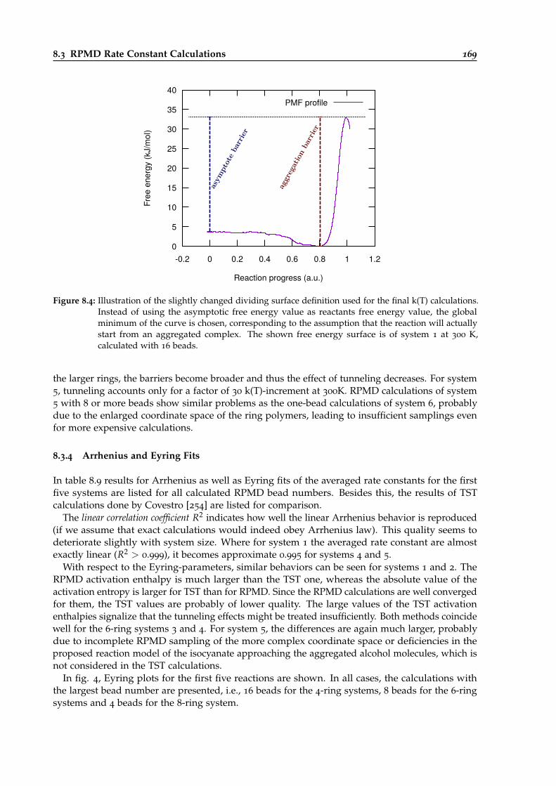
8.3 RPMD Rate Constant Calculations 169
0
5
10
15
20
25
30
35
40
-0.2 0 0.2 0.4 0.6 0.8 1 1.2
Free
ene
rgy
(kJ/
mol
)
Reaction progress (a.u.)
PMF profile
asym
ptot
e ba
rrier
aggr
egat
ion
barr
ier
Figure 8.4: Illustration of the slightly changed dividing surface definition used for the final k(T) calculations.Instead of using the asymptotic free energy value as reactants free energy value, the globalminimum of the curve is chosen, corresponding to the assumption that the reaction will actuallystart from an aggregated complex. The shown free energy surface is of system 1 at 300 K,calculated with 16 beads.
the larger rings, the barriers become broader and thus the effect of tunneling decreases. For system5, tunneling accounts only for a factor of 30 k(T)-increment at 300K. RPMD calculations of system5 with 8 or more beads show similar problems as the one-bead calculations of system 6, probablydue to the enlarged coordinate space of the ring polymers, leading to insufficient samplings evenfor more expensive calculations.
8.3.4 Arrhenius and Eyring Fits
In table 8.9 results for Arrhenius as well as Eyring fits of the averaged rate constants for the firstfive systems are listed for all calculated RPMD bead numbers. Besides this, the results of TSTcalculations done by Covestro [254] are listed for comparison.
The linear correlation coefficient R2 indicates how well the linear Arrhenius behavior is reproduced(if we assume that exact calculations would indeed obey Arrhenius law). This quality seems todeteriorate slightly with system size. Where for system 1 the averaged rate constant are almostexactly linear (R2 > 0.999), it becomes approximate 0.995 for systems 4 and 5.
With respect to the Eyring-parameters, similar behaviors can be seen for systems 1 and 2. TheRPMD activation enthalpy is much larger than the TST one, whereas the absolute value of theactivation entropy is larger for TST than for RPMD. Since the RPMD calculations are well convergedfor them, the TST values are probably of lower quality. The large values of the TST activationenthalpies signalize that the tunneling effects might be treated insufficiently. Both methods coincidewell for the 6-ring systems 3 and 4. For system 5, the differences are again much larger, probablydue to incomplete RPMD sampling of the more complex coordinate space or deficiencies in theproposed reaction model of the isocyanate approaching the aggregated alcohol molecules, which isnot considered in the TST calculations.
In fig. 4, Eyring plots for the first five reactions are shown. In all cases, the calculations withthe largest bead number are presented, i.e., 16 beads for the 4-ring systems, 8 beads for the 6-ringsystems and 4 beads for the 8-ring system.
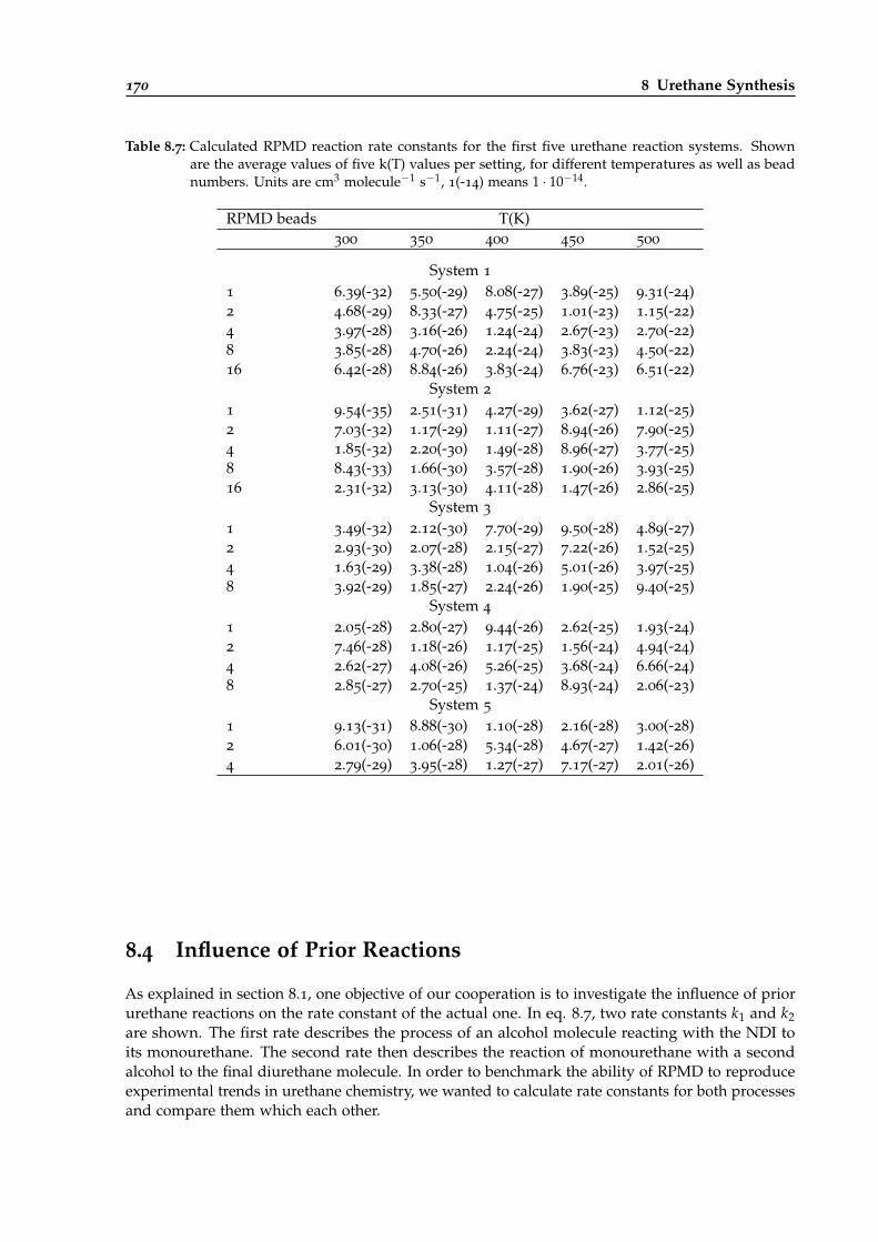
170 8 Urethane Synthesis
Table 8.7: Calculated RPMD reaction rate constants for the first five urethane reaction systems. Shownare the average values of five k(T) values per setting, for different temperatures as well as beadnumbers. Units are cm3 molecule−1 s−1, 1(-14) means 1 · 10−14.
RPMD beads T(K)300 350 400 450 500
System 1
1 6.39(-32) 5.50(-29) 8.08(-27) 3.89(-25) 9.31(-24)2 4.68(-29) 8.33(-27) 4.75(-25) 1.01(-23) 1.15(-22)4 3.97(-28) 3.16(-26) 1.24(-24) 2.67(-23) 2.70(-22)8 3.85(-28) 4.70(-26) 2.24(-24) 3.83(-23) 4.50(-22)16 6.42(-28) 8.84(-26) 3.83(-24) 6.76(-23) 6.51(-22)
System 2
1 9.54(-35) 2.51(-31) 4.27(-29) 3.62(-27) 1.12(-25)2 7.03(-32) 1.17(-29) 1.11(-27) 8.94(-26) 7.90(-25)4 1.85(-32) 2.20(-30) 1.49(-28) 8.96(-27) 3.77(-25)8 8.43(-33) 1.66(-30) 3.57(-28) 1.90(-26) 3.93(-25)16 2.31(-32) 3.13(-30) 4.11(-28) 1.47(-26) 2.86(-25)
System 3
1 3.49(-32) 2.12(-30) 7.70(-29) 9.50(-28) 4.89(-27)2 2.93(-30) 2.07(-28) 2.15(-27) 7.22(-26) 1.52(-25)4 1.63(-29) 3.38(-28) 1.04(-26) 5.01(-26) 3.97(-25)8 3.92(-29) 1.85(-27) 2.24(-26) 1.90(-25) 9.40(-25)
System 4
1 2.05(-28) 2.80(-27) 9.44(-26) 2.62(-25) 1.93(-24)2 7.46(-28) 1.18(-26) 1.17(-25) 1.56(-24) 4.94(-24)4 2.62(-27) 4.08(-26) 5.26(-25) 3.68(-24) 6.66(-24)8 2.85(-27) 2.70(-25) 1.37(-24) 8.93(-24) 2.06(-23)
System 5
1 9.13(-31) 8.88(-30) 1.10(-28) 2.16(-28) 3.00(-28)2 6.01(-30) 1.06(-28) 5.34(-28) 4.67(-27) 1.42(-26)4 2.79(-29) 3.95(-28) 1.27(-27) 7.17(-27) 2.01(-26)
8.4 Influence of Prior Reactions
As explained in section 8.1, one objective of our cooperation is to investigate the influence of priorurethane reactions on the rate constant of the actual one. In eq. 8.7, two rate constants k1 and k2are shown. The first rate describes the process of an alcohol molecule reacting with the NDI toits monourethane. The second rate then describes the reaction of monourethane with a secondalcohol to the final diurethane molecule. In order to benchmark the ability of RPMD to reproduceexperimental trends in urethane chemistry, we wanted to calculate rate constants for both processesand compare them which each other.
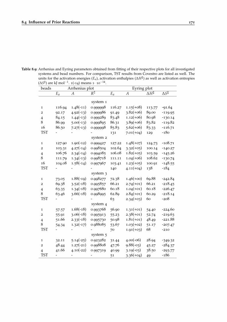
8.4 Influence of Prior Reactions 171
Table 8.9: Arrhenius and Eyring parameters obtained from fitting of their respective plots for all investigatedsystems and bead numbers. For comparison, TST results from Covestro are listed as well. Theunits for the activation energies (Ea), activation enthalpies (∆H‡) as well as activation entropies(∆S‡) are kJ mol−1. 1(-14) means 1· 10
−14.beads Arrhenius plot Eyring plot
Ea A R2 Ea A ∆H‡ ∆S‡
system 1
1 116.94 1.48(-11) 0.999998 116.27 1.15(+08) 113.77 -91.64
2 92.17 4.92(-13) 0.999986 91.49 3.82(+06) 89.00 -119.95
4 84.15 1.44(-13) 0.999289 83.48 1.12(+06) 80.98 -130.14
8 86.99 5.00(-13) 0.999895 86.31 3.89(+06) 83.82 -119.82
16 86.50 7.27(-13) 0.999998 85.83 5.62(+06) 83.33 -116.71
TST - - - 131 7.01(+04) 129 -180
system 2
1 127.90 1.90(-12) 0.999427 127.22 1.48(+07) 124.73 -108.71
2 103.31 4.27(-14) 0.998504 102.64 3.32(+05) 100.14 -140.27
4 106.76 2.34(-14) 0.994085 106.08 1.82(+05) 103.59 -145.26
8 111.79 1.34(-13) 0.998718 111.11 1.04(+06) 108.62 -130.74
16 104.08 1.58(-14) 0.997967 103.41 1.23(+05) 100.91 -148.55
TST - - - 140 4.11(+04) 138 -184
system 3
1 73.05 1.88(-19) 0.998277 72.38 1.46(+00) 69.88 -242.84
2 69.38 3.52(-18) 0.995857 66.21 2.74(+01) 66.21 -218.45
4 63.35 1.34(-18) 0.997680 60.18 1.04(+01) 60.18 -226.47
8 63.46 3.66(-18) 0.998995 62.89 2.84(+01) 60.29 -218.14
TST - - - 63 2.34(+03) 60 -208
system 4
1 57.57 1.68(-18) 0.993768 56.90 1.31(+01) 54.40 -224.60
2 55.91 3.06(-18) 0.995913 55.23 2.38(+01) 52.74 -219.63
4 51.66 2.33(-18) 0.995730 50.98 1.81(+01) 48.49 -221.88
8 54.34 1.32(-17) 0.988085 53.67 1.03(+02) 51.17 -207.47
TST - - - 70 1.91(+03) 68 -210
system 5
1 32.11 5.14(-25) 0.923282 31.44 4.00(-06) 28.94 -349.32
2 48.44 1.27(-21) 0.998808 47.76 9.88(-03) 45.27 -284.37
4 41.66 4.10(-22) 0.997319 40.99 3.19(-03) 38.50 -293.77
TST - - - 51 3.36(+04) 49 -186
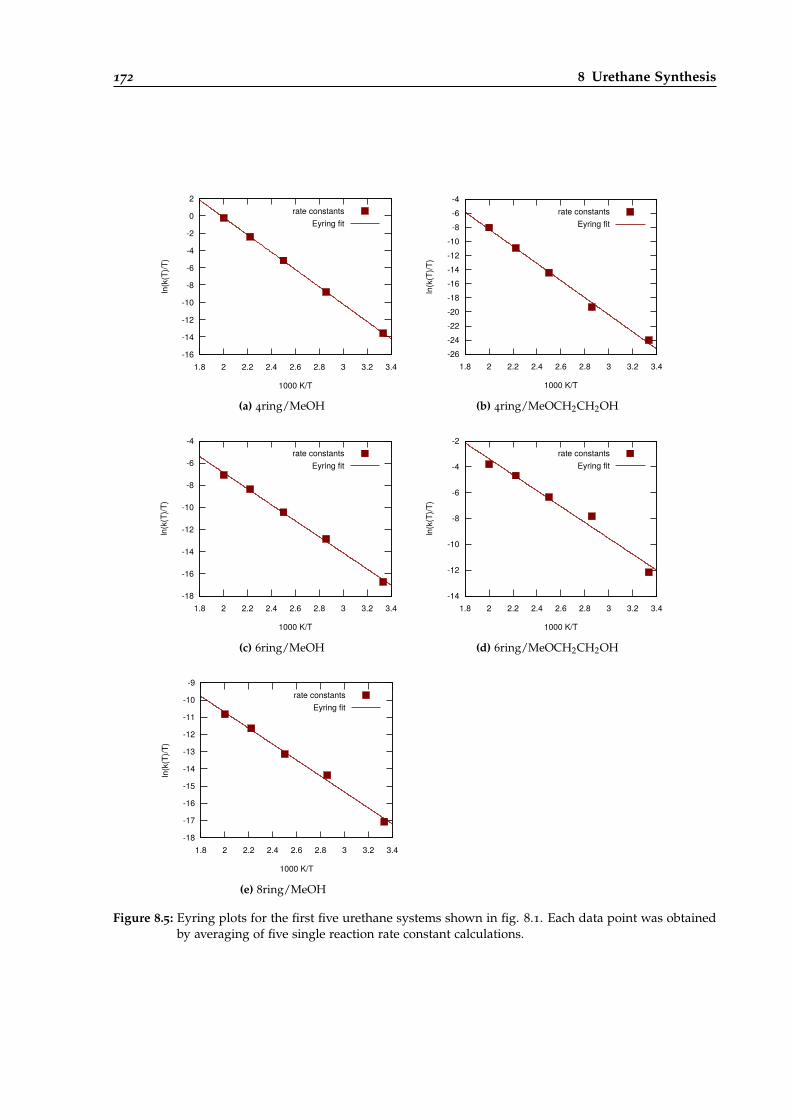
172 8 Urethane Synthesis
-16
-14
-12
-10
-8
-6
-4
-2
0
2
1.8 2 2.2 2.4 2.6 2.8 3 3.2 3.4
ln(k
(T)/T
)
1000 K/T
rate constantsEyring fit
(a) 4ring/MeOH
-26-24-22-20-18-16-14-12-10
-8-6-4
1.8 2 2.2 2.4 2.6 2.8 3 3.2 3.4
ln(k
(T)/T
)
1000 K/T
rate constantsEyring fit
(b) 4ring/MeOCH2CH2OH
-18
-16
-14
-12
-10
-8
-6
-4
1.8 2 2.2 2.4 2.6 2.8 3 3.2 3.4
ln(k
(T)/T
)
1000 K/T
rate constantsEyring fit
(c) 6ring/MeOH
-14
-12
-10
-8
-6
-4
-2
1.8 2 2.2 2.4 2.6 2.8 3 3.2 3.4
ln(k
(T)/T
)
1000 K/T
rate constantsEyring fit
(d) 6ring/MeOCH2CH2OH
-18
-17
-16
-15
-14
-13
-12
-11
-10
-9
1.8 2 2.2 2.4 2.6 2.8 3 3.2 3.4
ln(k
(T)/T
)
1000 K/T
rate constantsEyring fit
(e) 8ring/MeOH
Figure 8.5: Eyring plots for the first five urethane systems shown in fig. 8.1. Each data point was obtainedby averaging of five single reaction rate constant calculations.

8.4 Influence of Prior Reactions 173
System 7: 4ring/MeOH System 8: 4ring/MeOCH2CH2OH
System 9: 6ring/MeOH System 10: 6ring/MeOCH2CH2OH
1.61 Å
1.15 Å1.39 Å
1.38 Å 1.15 Å
1.61 Å
1.65 Å1.02 Å
1.11 Å
1.33 Å1.64 Å
1.03 Å
1.33 Å
1.11 Å1.59 Å
1.60 Å
Figure 8.6: Optimized TS structures for the four different reactions possible with the two-step urethanationof NDI. The structures were optimized with MP2/cc-pVDZ.
The first step is of course again to find a reliable QM method for the calculation of TREQreference data. As depicted above, the DFT benchmark done in section 8.2 has the claim that thebest method found there can be used for all urethane reactions.
Therefore, the M06/cc-pVDZ level of theory with D3 empirical dispersion correction was usedto calculate the reaction paths of first and second urethanations. These reactions can of course alsobe accelerated by autocatalysis. Interestingly we found out that the 8-ring cyclic process present inreactions 5 and 6 could not happen if NDI is the isocyanate, since the aromatic system is too bulkyfor the formation of a hydrogen bond system with three alkohols in its direct vicinity. With this,only four reactions could be studied in total: First and second urethanation with the 4-ring and6-ring mechanisms, respectively. Transition states of those reactions optimized with MP2/cc-pVDZare presented in fig. 8.6.
In order to check if the M06 method performs also well for the NDI reactions (i.e., gives similarresults to MP2), IRC optimizations were done with both methods for all four reactions. Finally,DLPNO-CCSD(T) energies for all IRC structures were calculated as well in order to use themfor the TREQ two-level approach. The results of these calculations are shown in table 8.10. If wecompare the MP2 activation barriers with the M06 ones, we see that they differ by less than 3
kJ/mol for all four systems. If the DLPNO-CCSD(T) calculations on the MP2 and M06 paths arecompared, the differences slightly shrink for the 4-ring reactions and grow for the 6-ring reactions.For all combinations, the differences are within chemical accuracy, thus indicating that M06 workswell also for this kind of urethane reactions.
By further comparing the activation barriers of the first and second reactions, the differences areeven smaller. For the 4-ring reactions, they are less than 1.5 kJ/mol, for the 6-ring reactions, they
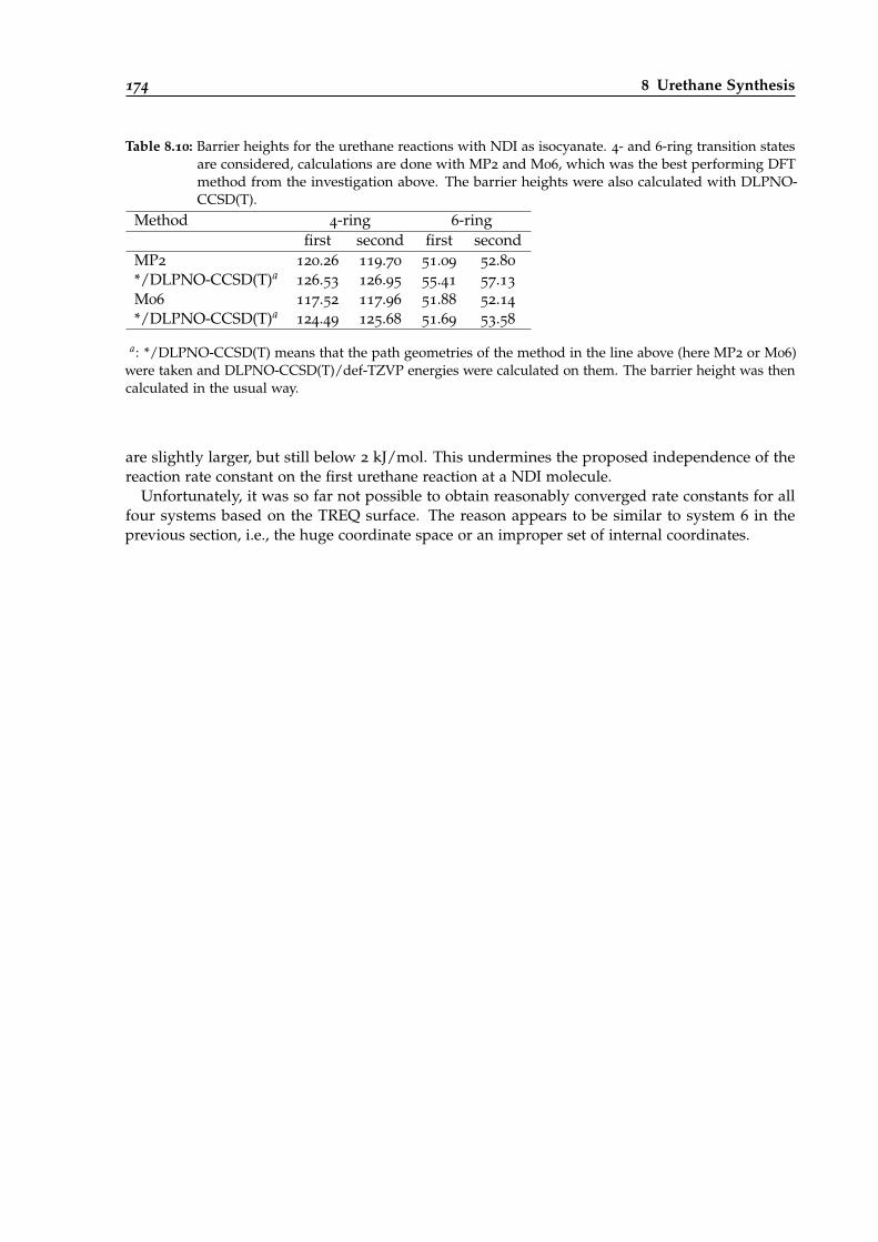
174 8 Urethane Synthesis
Table 8.10: Barrier heights for the urethane reactions with NDI as isocyanate. 4- and 6-ring transition statesare considered, calculations are done with MP2 and M06, which was the best performing DFTmethod from the investigation above. The barrier heights were also calculated with DLPNO-CCSD(T).
Method 4-ring 6-ringfirst second first second
MP2 120.26 119.70 51.09 52.80
*/DLPNO-CCSD(T)a126.53 126.95 55.41 57.13
M06 117.52 117.96 51.88 52.14
*/DLPNO-CCSD(T)a124.49 125.68 51.69 53.58
a: */DLPNO-CCSD(T) means that the path geometries of the method in the line above (here MP2 or M06)were taken and DLPNO-CCSD(T)/def-TZVP energies were calculated on them. The barrier height was thencalculated in the usual way.
are slightly larger, but still below 2 kJ/mol. This undermines the proposed independence of thereaction rate constant on the first urethane reaction at a NDI molecule.
Unfortunately, it was so far not possible to obtain reasonably converged rate constants for allfour systems based on the TREQ surface. The reason appears to be similar to system 6 in theprevious section, i.e., the huge coordinate space or an improper set of internal coordinates.
9
Ch
ap
te
r
Kinetic Monte Carlo
So far we have seen how the EVB-QMDFF methodology can be used to calculate k(T) values ofseveral reactive systems. By using the black-box procedure developed in this thesis the user-sidedeffort for setup and performing such calculations is almost set to zero, at least if the systems arenot too large or otherwise pathological.
However, in real chemical systems, several different reactions are usually taking place in parallel.Calculations of rates for single elementary reactions are of great importance for their understandingas well as benchmark of accurate theoretical methods, but of course it should be our demand aswell to study everyday chemical systems. For them, the aseptic picture of single independentgas-phase reactions becomes cracky: even for relatively simple systems (with respect to the numberof different elements involved) like the combustion of hydrogen, alkanes or alcohols, a wholezoo of dozens to hundreds of different elementary reactions can take place [255, 256]. If wefound out which of them are important, we can calculate all their k(T) values. But still it isnot clear how we can set them together in order to get the overall large-scale dynamics. Whendoes which reaction occur? There are many different continuum kinetic models for, e.g., certaincombustion processes, such as of H2 [257], Kerosene [258] and CO [259]. As it was mentioned inthe introduction, continuum and particle kinetics are two different concepts of modeling chemicalreality: in continuum kinetics we are unable by definition to look at the processes of interest withmolecular resolution. We can simulate systems of real-world size, but with no real existence of itin space. It is silently assumed that, for instance, reactants are distributed equally. In reality, wemight be interested in spatially varying reactant concentrations or in the fate of single moleculesduring the process, which can only be handled by particle kinetics. Therefore, continuum kineticapproaches are improper for our desires.
One alternative is to return to a real-time simulation of the whole system: Instead of calculatingk(T) values for a bunch of model reactions we could simply run reactive dynamics of a large vesselof, e.g., carbohydrate molecules and look what happens. Since most reactions are rare events evenat high temperatures, millions to trillions of time steps will be needed to consider the large-scalelow-frequency coupled reactive processes which might take milliseconds or even seconds. Further,several local reactions might be influenced by their neighborhood, e.g., if a needed reactant forreaction B is the product of reaction A, such that B can only occur if A has been completed someÅngstroms away. In order to model such interactions realistically and quantitatively, thousandsto millions of atoms must be propagated simultaneously. Such timescales are accessible if weuse simple MM methods specialized for biochemical systems, e.g., in order to study proteinfolding [260, 261].
176 9 Kinetic Monte Carlo
Unfortunately we need a PES description that is able to describe bond fissions and other reactiveprocesses with high quality, which requires the usage of ab-initio MD. This is of course unfeasibleeven if semiempirical models are used1.
One quite popular alternative is the ReaxFF force field (section 2.2.2) since it can describe allrelevant reactive processes and imposes a relatively moderate scaling located between traditionalnonreactive FFs and semiempirical methods. Large scale ReaxFF calculations were conducted, e.g.,for the simulation of hydrogen combustion [263], ignition front propagation [264] and combustionsof different coal brands [265, 266]2.
Unfortunately, the ReaxFF parametrization might become quite complicated, especially if complexcatalytic processes with hundreds to thousands of possible reactive pathways shall be treated.We need to choose a useful set of ab-initio information, further, the user must monitor the wholeparametrization process of the interdependent parameters thoroughly in order to avoid artifacts(like unphysical side reactions) that might diminish the quality of the FF [79].
It is almost impossible to parametrize a ReaxFF force field that is able to describe the PESsections of all relevant reactive processes with chemical accuracy, which is needed due to the heavydependence of k(T) values to the barrier heights and shapes (eq. 2.10)3.
An alternative is the Kinetic Monte Carlo method [267, 268], that is able to combine high-qualityk(T) values of several elementary reactions to a realistic simulation of the whole reactive system.
In section 9.1 the general idea and mathematical foundation of the method is presented, insection 9.2 a generic application of the method to a mathematical example system is shown. Thisgeneral procedure is translated to realistic chemical situations in the last two sections: The diffusionof hydrogen atoms on a Cu(001) surface (section 9.3), named H@Cu(001) and the diffusion andaggregation of copper atoms on the same surface (section 9.4), named Cu@Cu(001). Compared tothe combustion examples shown above the KMC applications presented here look quite primitive,however, they shall serve as a first proof-of-principle that it is possible to connect the EVB-QMDFF-RPMD k(T) calculation machinery to large scale chemical simulations.
9.1 Foundations
Since chemical reactions are rare events, the system’s trajectory will usually be trapped someamount of time in a potential energy minimum, corresponding to a certain molecular configuration,until it is finally able to cross the barrier to a neighbored minimum. The vibrational movementinside these local minima takes place in the range of femtoseconds, such that small MD timesteps are needed to describe them properly. However, if we are interested in chemical reactions,vibrations around local minima are of no importance at all, only transitions between neighboredminima are relevant for us. Good insights on the separated timescales of molecular vibrations andreactive events can be gained by reviewing the k(T) calculations in the covalent mechanochemistrychapter (section 7.5).
In KMC the coordinate space of the system is subdivided into different sites that contain thevicinity of a local minimum. The different sites border to each other at transition state dividingsurfaces (section 2.1.1).
1 There exist some prominent studies of ab-initio nanoreactors, e.g., by Martinez et al. [262], but these are very expensiveand rather small in scale (e.g., around 40 initial molecules in use). Several tricks like high temperature and pressureas well as modified dynamics that push reactants out of their local PES minima need to be utilized for them. Theyreveal, however, that hundreds of chemical species and reactions become important even if we start from rather simplemolecular species.
2 The last mentioned example of the combustion of Illinois no. 6 coal was simulated with 50000 atoms (728 molecules)over a evolved time of 250 ps, where a high temperature of 2000 K was used in order to accelerate the reactive processes.
3 If we rather want to simulate qualitatively what happens, for instance, which molecules can be built from an originalset of structures, ReaxFF is of course still very useful, since it usually provides at least a qualitatively correct picture ofthe reactions and their relative velocities.
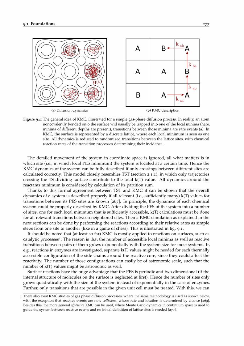
9.1 Foundations 177
q(t)
(a) Diffusion dynamics
A
BA
A
A
A
B
AB k aa
k ab
k ba
k ab
(b) KMC description
Figure 9.1: The general idea of KMC, illustrated for a simple gas-phase diffusion process. In reality, an atomnoncovalently bonded onto the surface will usually be trapped into one of the local minima (here,minima of different depths are present), transitions between those minima are rare events (a). InKMC, the surface is represented by a discrete lattice, where each local minimum is seen as onesite. All dynamics is reduced to randomized transitions between the lattice sites, with chemicalreaction rates of the transition processes determining their incidence.
The detailed movement of the system in coordinate space is ignored, all what matters is inwhich site (i.e., in which local PES minimum) the system is located at a certain time. Hence theKMC dynamics of the system can be fully described if only crossings between different sites arecalculated correctly. This model closely resembles TST (section 2.1.1), in which only trajectoriescrossing the TS dividing surface contribute to the total k(T) value. All dynamics around thereactants minimum is considered by calculation of its partition sum.
Thanks to this formal agreement between TST and KMC it can be shown that the overalldynamics of a system is described properly if all relevant (i.e., sufficiently many) k(T) values fortransitions between its PES sites are known [267]. In principle, the dynamics of each chemicalsystem could be properly described by KMC. After dividing the PES of the system into a numberof sites, one for each local minimum that is sufficiently accessible, k(T) calculations must be donefor all relevant transitions between neighbored sites. Then a KMC simulation as explained in thenext sections can be done by performing the reactions according to their relative rates as simplesteps from one site to another (like in a game of chess). This is illustrated in fig. 9.1.
It should be noted that (at least so far) KMC is mostly applied to reactions on surfaces, such ascatalytic processes4. The reason is that the number of accessible local minima as well as reactivetransitions between pairs of them grows exponentially with the system size for most systems. If,e.g., reactions in enzymes are investigated, separate k(T) values might be needed for each thermallyaccessible configuration of the side chains around the reactive core, since they could affect thereactivity. The number of those configurations can easily be of astronomic scale, such that thenumber of k(T) values might be astronomic as well.
Surface reactions have the huge advantage that the PES is periodic and two-dimensional (if theinternal structure of molecules on the surface is neglected at first). Hence the number of sites onlygrows quadratically with the size of the system instead of exponentially in the case of enzymes.Further, only transitions that are possible in the given unit cell must be treated. With this, we can
4 There also exist KMC studies of gas phase diffusion processes, where the same methodology is used as shown below,with the exception that reactive events are now collisions, whose rate and location is determined by chance [269].Besides this, the more general off-lattice KMC can be used, where Monte Carlo dynamics in continuum space is used toguide the system between reactive events and no initial definition of lattice sites is needed [270].
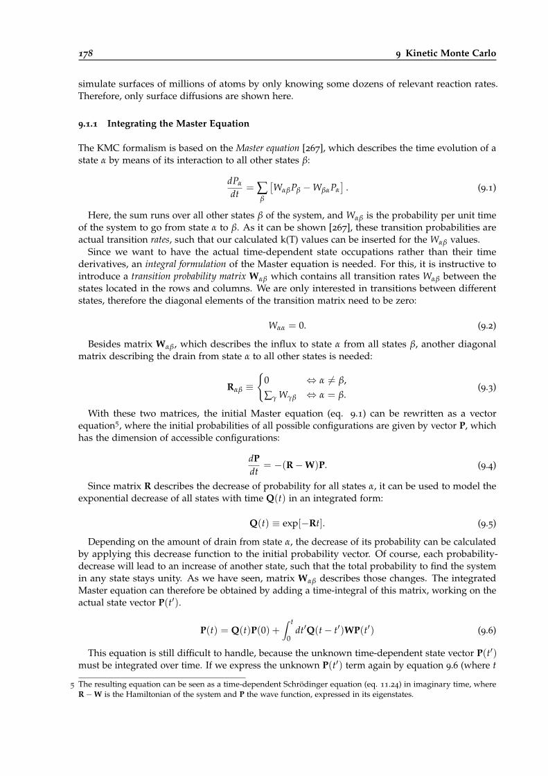
178 9 Kinetic Monte Carlo
simulate surfaces of millions of atoms by only knowing some dozens of relevant reaction rates.Therefore, only surface diffusions are shown here.
9.1.1 Integrating the Master Equation
The KMC formalism is based on the Master equation [267], which describes the time evolution of astate α by means of its interaction to all other states β:
dPα
dt= ∑
β
[WαβPβ −WβαPα
]. (9.1)
Here, the sum runs over all other states β of the system, and Wαβ is the probability per unit timeof the system to go from state α to β. As it can be shown [267], these transition probabilities areactual transition rates, such that our calculated k(T) values can be inserted for the Wαβ values.
Since we want to have the actual time-dependent state occupations rather than their timederivatives, an integral formulation of the Master equation is needed. For this, it is instructive tointroduce a transition probability matrix Wαβ which contains all transition rates Wαβ between thestates located in the rows and columns. We are only interested in transitions between differentstates, therefore the diagonal elements of the transition matrix need to be zero:
Wαα = 0. (9.2)
Besides matrix Wαβ, which describes the influx to state α from all states β, another diagonalmatrix describing the drain from state α to all other states is needed:
Rαβ ≡{
0 ⇔ α 6= β,
∑γ Wγβ ⇔ α = β.(9.3)
With these two matrices, the initial Master equation (eq. 9.1) can be rewritten as a vectorequation5, where the initial probabilities of all possible configurations are given by vector P, whichhas the dimension of accessible configurations:
dPdt
= −(R−W)P. (9.4)
Since matrix R describes the decrease of probability for all states α, it can be used to model theexponential decrease of all states with time Q(t) in an integrated form:
Q(t) ≡ exp[−Rt]. (9.5)
Depending on the amount of drain from state α, the decrease of its probability can be calculatedby applying this decrease function to the initial probability vector. Of course, each probability-decrease will lead to an increase of another state, such that the total probability to find the systemin any state stays unity. As we have seen, matrix Wαβ describes those changes. The integratedMaster equation can therefore be obtained by adding a time-integral of this matrix, working on theactual state vector P(t′).
P(t) = Q(t)P(0) +∫ t
0dt′Q(t− t′)WP(t′) (9.6)
This equation is still difficult to handle, because the unknown time-dependent state vector P(t′)must be integrated over time. If we express the unknown P(t′) term again by equation 9.6 (where t
5 The resulting equation can be seen as a time-dependent Schrödinger equation (eq. 11.24) in imaginary time, whereR−W is the Hamiltonian of the system and P the wave function, expressed in its eigenstates.
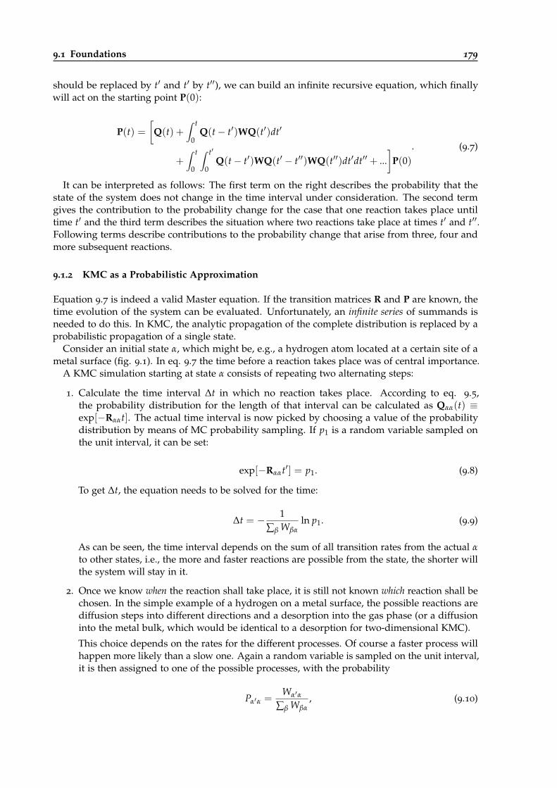
9.1 Foundations 179
should be replaced by t′ and t′ by t′′), we can build an infinite recursive equation, which finallywill act on the starting point P(0):
P(t) =[
Q(t) +∫ t
0Q(t− t′)WQ(t′)dt′
+∫ t
0
∫ t′
0Q(t− t′)WQ(t′ − t′′)WQ(t′′)dt′dt′′ + ...
]P(0)
. (9.7)
It can be interpreted as follows: The first term on the right describes the probability that thestate of the system does not change in the time interval under consideration. The second termgives the contribution to the probability change for the case that one reaction takes place untiltime t′ and the third term describes the situation where two reactions take place at times t′ and t′′.Following terms describe contributions to the probability change that arise from three, four andmore subsequent reactions.
9.1.2 KMC as a Probabilistic Approximation
Equation 9.7 is indeed a valid Master equation. If the transition matrices R and P are known, thetime evolution of the system can be evaluated. Unfortunately, an infinite series of summands isneeded to do this. In KMC, the analytic propagation of the complete distribution is replaced by aprobabilistic propagation of a single state.
Consider an initial state α, which might be, e.g., a hydrogen atom located at a certain site of ametal surface (fig. 9.1). In eq. 9.7 the time before a reaction takes place was of central importance.
A KMC simulation starting at state α consists of repeating two alternating steps:
1. Calculate the time interval ∆t in which no reaction takes place. According to eq. 9.5,the probability distribution for the length of that interval can be calculated as Qαα(t) ≡exp[−Rααt]. The actual time interval is now picked by choosing a value of the probabilitydistribution by means of MC probability sampling. If p1 is a random variable sampled onthe unit interval, it can be set:
exp[−Rααt′] = p1. (9.8)
To get ∆t, the equation needs to be solved for the time:
∆t = − 1∑β Wβα
ln p1. (9.9)
As can be seen, the time interval depends on the sum of all transition rates from the actual αto other states, i.e., the more and faster reactions are possible from the state, the shorter willthe system will stay in it.
2. Once we know when the reaction shall take place, it is still not known which reaction shall bechosen. In the simple example of a hydrogen on a metal surface, the possible reactions arediffusion steps into different directions and a desorption into the gas phase (or a diffusioninto the metal bulk, which would be identical to a desorption for two-dimensional KMC).
This choice depends on the rates for the different processes. Of course a faster process willhappen more likely than a slow one. Again a random variable is sampled on the unit interval,it is then assigned to one of the possible processes, with the probability
Pα′α =Wα′α
∑β Wβα, (9.10)
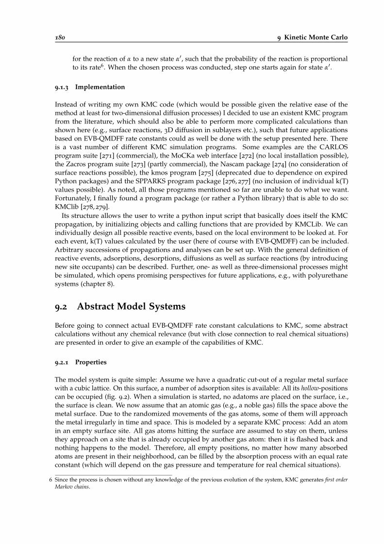
180 9 Kinetic Monte Carlo
for the reaction of α to a new state α′, such that the probability of the reaction is proportionalto its rate6. When the chosen process was conducted, step one starts again for state α′.
9.1.3 Implementation
Instead of writing my own KMC code (which would be possible given the relative ease of themethod at least for two-dimensional diffusion processes) I decided to use an existent KMC programfrom the literature, which should also be able to perform more complicated calculations thanshown here (e.g., surface reactions, 3D diffusion in sublayers etc.), such that future applicationsbased on EVB-QMDFF rate constants could as well be done with the setup presented here. Thereis a vast number of different KMC simulation programs. Some examples are the CARLOSprogram suite [271] (commercial), the MoCKa web interface [272] (no local installation possible),the Zacros program suite [273] (partly commercial), the Nascam package [274] (no consideration ofsurface reactions possible), the kmos program [275] (deprecated due to dependence on expiredPython packages) and the SPPARKS program package [276, 277] (no inclusion of individual k(T)values possible). As noted, all those programs mentioned so far are unable to do what we want.Fortunately, I finally found a program package (or rather a Python library) that is able to do so:KMClib [278, 279].
Its structure allows the user to write a python input script that basically does itself the KMCpropagation, by initializing objects and calling functions that are provided by KMCLib. We canindividually design all possible reactive events, based on the local environment to be looked at. Foreach event, k(T) values calculated by the user (here of course with EVB-QMDFF) can be included.Arbitrary successions of propagations and analyses can be set up. With the general definition ofreactive events, adsorptions, desorptions, diffusions as well as surface reactions (by introducingnew site occupants) can be described. Further, one- as well as three-dimensional processes mightbe simulated, which opens promising perspectives for future applications, e.g., with polyurethanesystems (chapter 8).
9.2 Abstract Model Systems
Before going to connect actual EVB-QMDFF rate constant calculations to KMC, some abstractcalculations without any chemical relevance (but with close connection to real chemical situations)are presented in order to give an example of the capabilities of KMC.
9.2.1 Properties
The model system is quite simple: Assume we have a quadratic cut-out of a regular metal surfacewith a cubic lattice. On this surface, a number of adsorption sites is available: All its hollow-positionscan be occupied (fig. 9.2). When a simulation is started, no adatoms are placed on the surface, i.e.,the surface is clean. We now assume that an atomic gas (e.g., a noble gas) fills the space above themetal surface. Due to the randomized movements of the gas atoms, some of them will approachthe metal irregularly in time and space. This is modeled by a separate KMC process: Add an atomin an empty surface site. All gas atoms hitting the surface are assumed to stay on them, unlessthey approach on a site that is already occupied by another gas atom: then it is flashed back andnothing happens to the model. Therefore, all empty positions, no matter how many absorbedatoms are present in their neighborhood, can be filled by the absorption process with an equal rateconstant (which will depend on the gas pressure and temperature for real chemical situations).
6 Since the process is chosen without any knowledge of the previous evolution of the system, KMC generates first orderMarkov chains.
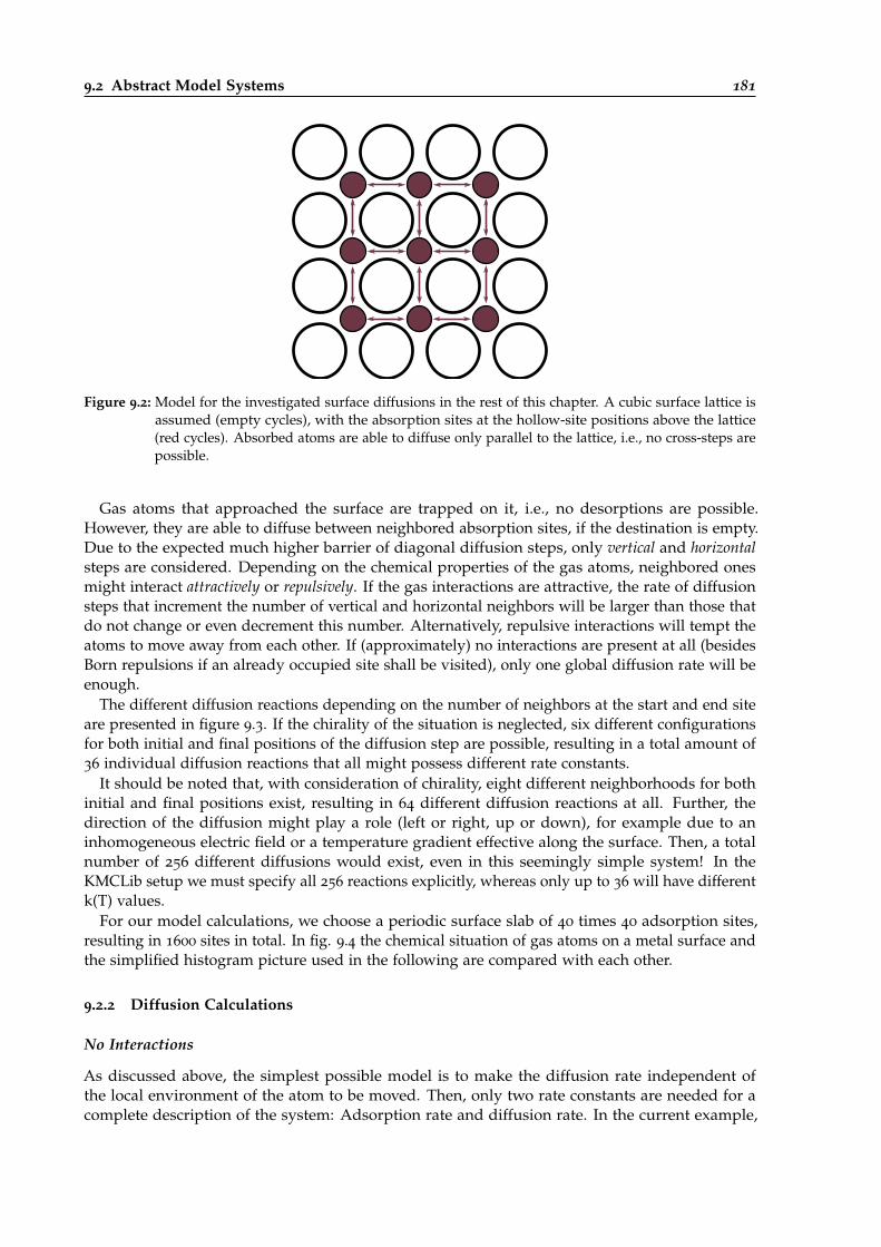
9.2 Abstract Model Systems 181
Figure 9.2: Model for the investigated surface diffusions in the rest of this chapter. A cubic surface lattice isassumed (empty cycles), with the absorption sites at the hollow-site positions above the lattice(red cycles). Absorbed atoms are able to diffuse only parallel to the lattice, i.e., no cross-steps arepossible.
Gas atoms that approached the surface are trapped on it, i.e., no desorptions are possible.However, they are able to diffuse between neighbored absorption sites, if the destination is empty.Due to the expected much higher barrier of diagonal diffusion steps, only vertical and horizontalsteps are considered. Depending on the chemical properties of the gas atoms, neighbored onesmight interact attractively or repulsively. If the gas interactions are attractive, the rate of diffusionsteps that increment the number of vertical and horizontal neighbors will be larger than those thatdo not change or even decrement this number. Alternatively, repulsive interactions will tempt theatoms to move away from each other. If (approximately) no interactions are present at all (besidesBorn repulsions if an already occupied site shall be visited), only one global diffusion rate will beenough.
The different diffusion reactions depending on the number of neighbors at the start and end siteare presented in figure 9.3. If the chirality of the situation is neglected, six different configurationsfor both initial and final positions of the diffusion step are possible, resulting in a total amount of36 individual diffusion reactions that all might possess different rate constants.
It should be noted that, with consideration of chirality, eight different neighborhoods for bothinitial and final positions exist, resulting in 64 different diffusion reactions at all. Further, thedirection of the diffusion might play a role (left or right, up or down), for example due to aninhomogeneous electric field or a temperature gradient effective along the surface. Then, a totalnumber of 256 different diffusions would exist, even in this seemingly simple system! In theKMCLib setup we must specify all 256 reactions explicitly, whereas only up to 36 will have differentk(T) values.
For our model calculations, we choose a periodic surface slab of 40 times 40 adsorption sites,resulting in 1600 sites in total. In fig. 9.4 the chemical situation of gas atoms on a metal surface andthe simplified histogram picture used in the following are compared with each other.
9.2.2 Diffusion Calculations
No Interactions
As discussed above, the simplest possible model is to make the diffusion rate independent ofthe local environment of the atom to be moved. Then, only two rate constants are needed for acomplete description of the system: Adsorption rate and diffusion rate. In the current example,

182 9 Kinetic Monte Carlo
(1) a-a (2) a-b (3) a-c (4) a-d (5) a-e (6) a-f
(7) b-a (8) b-b (9) b-c (10) b-d (11) b-e (12) b-f
(13) c-a (14) c-b (15) c-c (16) c-d (17) c-e (18) c-f
(19) d-a (20) d-b (21) d-c (22) d-d (23) d-e (24) d-f
(25) e-a (26) e-b (27) e-c (28) e-d (29) e-e (30) e-f
(31) f-a (32) f-b (33) f-c (34) f-d (35) f-e (36) f-f
Figure 9.3: List of all possible configurations for an upwards diffusion step of a gas molecule on a cubicmetal surface if any dependence on chirality is neglected (else, 64 combinations are possible).The labeling refers to the configurations of the neighbored sites at the initial and final positionsof the diffusion step, a-a for example means that no neighbors are present initially and finally,whereas a-f means that three atoms are present finally.
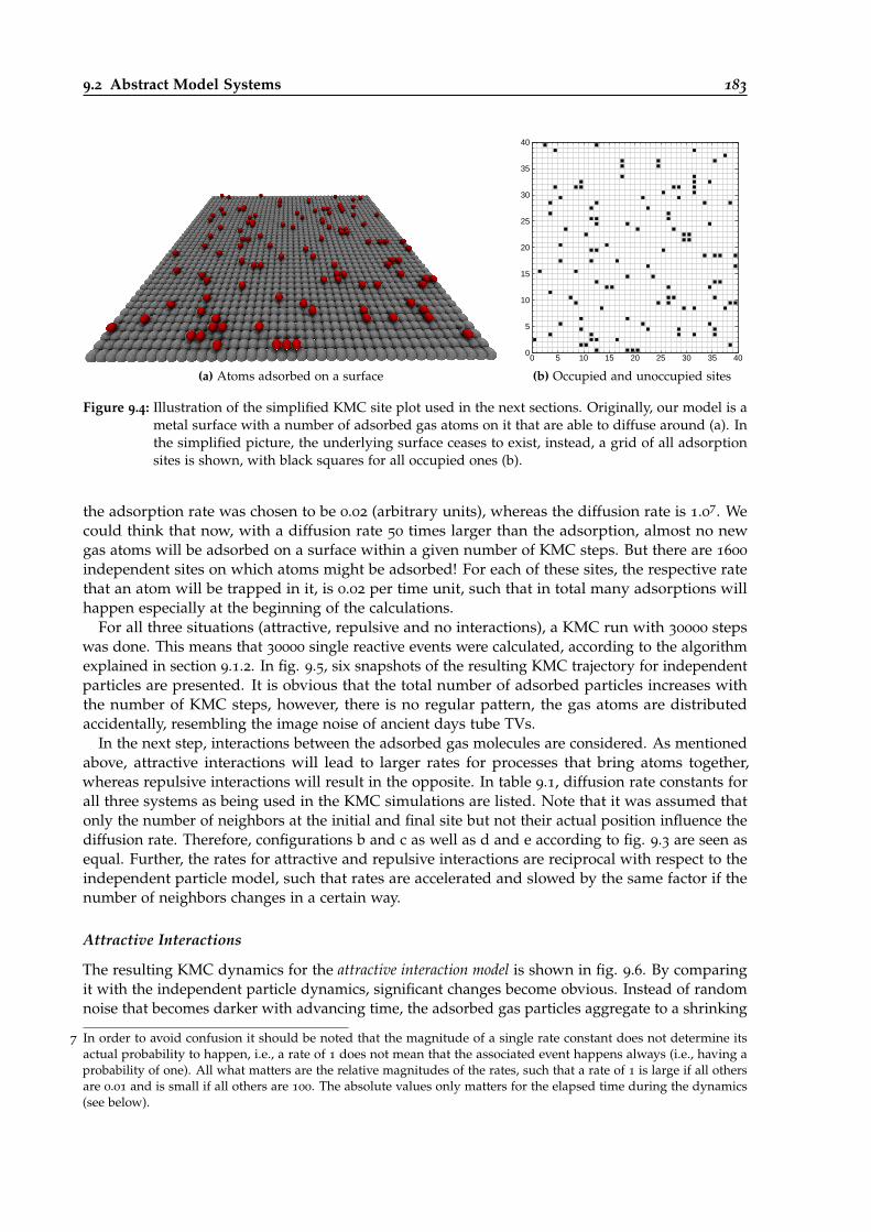
9.2 Abstract Model Systems 183
(a) Atoms adsorbed on a surface
0
5
10
15
20
25
30
35
40
0 5 10 15 20 25 30 35 40
(b) Occupied and unoccupied sites
Figure 9.4: Illustration of the simplified KMC site plot used in the next sections. Originally, our model is ametal surface with a number of adsorbed gas atoms on it that are able to diffuse around (a). Inthe simplified picture, the underlying surface ceases to exist, instead, a grid of all adsorptionsites is shown, with black squares for all occupied ones (b).
the adsorption rate was chosen to be 0.02 (arbitrary units), whereas the diffusion rate is 1.07. Wecould think that now, with a diffusion rate 50 times larger than the adsorption, almost no newgas atoms will be adsorbed on a surface within a given number of KMC steps. But there are 1600
independent sites on which atoms might be adsorbed! For each of these sites, the respective ratethat an atom will be trapped in it, is 0.02 per time unit, such that in total many adsorptions willhappen especially at the beginning of the calculations.
For all three situations (attractive, repulsive and no interactions), a KMC run with 30000 stepswas done. This means that 30000 single reactive events were calculated, according to the algorithmexplained in section 9.1.2. In fig. 9.5, six snapshots of the resulting KMC trajectory for independentparticles are presented. It is obvious that the total number of adsorbed particles increases withthe number of KMC steps, however, there is no regular pattern, the gas atoms are distributedaccidentally, resembling the image noise of ancient days tube TVs.
In the next step, interactions between the adsorbed gas molecules are considered. As mentionedabove, attractive interactions will lead to larger rates for processes that bring atoms together,whereas repulsive interactions will result in the opposite. In table 9.1, diffusion rate constants forall three systems as being used in the KMC simulations are listed. Note that it was assumed thatonly the number of neighbors at the initial and final site but not their actual position influence thediffusion rate. Therefore, configurations b and c as well as d and e according to fig. 9.3 are seen asequal. Further, the rates for attractive and repulsive interactions are reciprocal with respect to theindependent particle model, such that rates are accelerated and slowed by the same factor if thenumber of neighbors changes in a certain way.
Attractive Interactions
The resulting KMC dynamics for the attractive interaction model is shown in fig. 9.6. By comparingit with the independent particle dynamics, significant changes become obvious. Instead of randomnoise that becomes darker with advancing time, the adsorbed gas particles aggregate to a shrinking
7 In order to avoid confusion it should be noted that the magnitude of a single rate constant does not determine itsactual probability to happen, i.e., a rate of 1 does not mean that the associated event happens always (i.e., having aprobability of one). All what matters are the relative magnitudes of the rates, such that a rate of 1 is large if all othersare 0.01 and is small if all others are 100. The absolute values only matters for the elapsed time during the dynamics(see below).
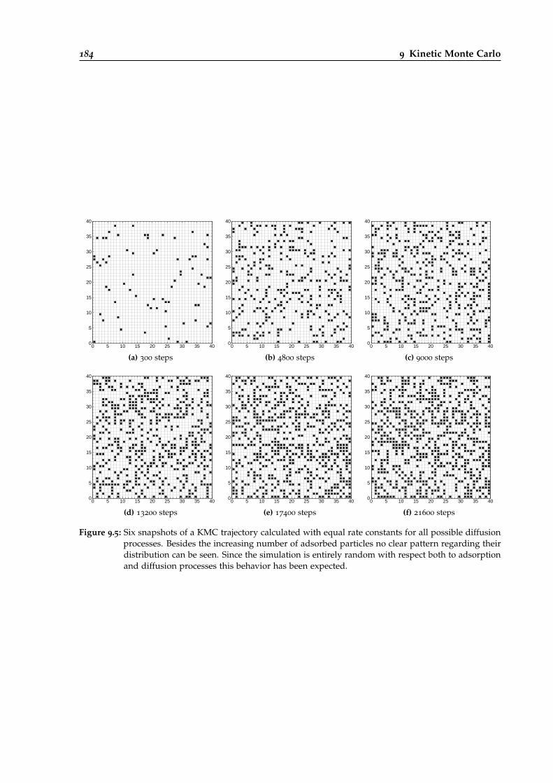
184 9 Kinetic Monte Carlo
0
5
10
15
20
25
30
35
40
0 5 10 15 20 25 30 35 40
(a) 300 steps
0
5
10
15
20
25
30
35
40
0 5 10 15 20 25 30 35 40
(b) 4800 steps
0
5
10
15
20
25
30
35
40
0 5 10 15 20 25 30 35 40
(c) 9000 steps
0
5
10
15
20
25
30
35
40
0 5 10 15 20 25 30 35 40
(d) 13200 steps
0
5
10
15
20
25
30
35
40
0 5 10 15 20 25 30 35 40
(e) 17400 steps
0
5
10
15
20
25
30
35
40
0 5 10 15 20 25 30 35 40
(f) 21600 steps
Figure 9.5: Six snapshots of a KMC trajectory calculated with equal rate constants for all possible diffusionprocesses. Besides the increasing number of adsorbed particles no clear pattern regarding theirdistribution can be seen. Since the simulation is entirely random with respect both to adsorptionand diffusion processes this behavior has been expected.
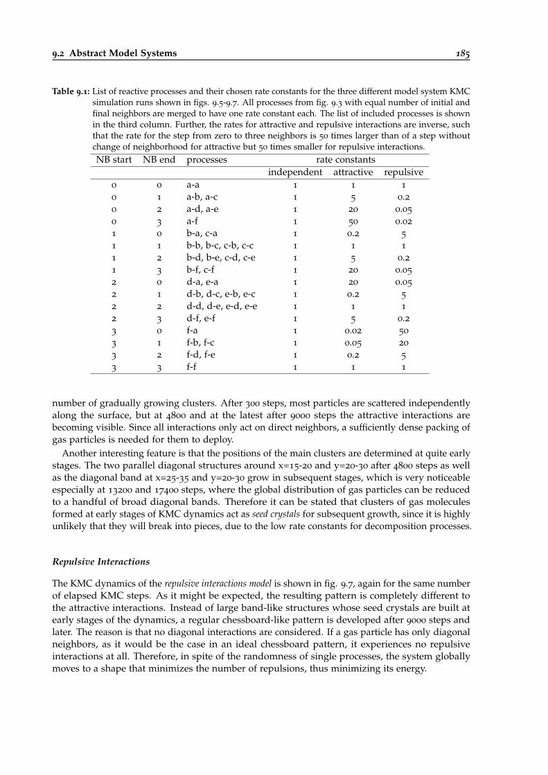
9.2 Abstract Model Systems 185
Table 9.1: List of reactive processes and their chosen rate constants for the three different model system KMCsimulation runs shown in figs. 9.5-9.7. All processes from fig. 9.3 with equal number of initial andfinal neighbors are merged to have one rate constant each. The list of included processes is shownin the third column. Further, the rates for attractive and repulsive interactions are inverse, suchthat the rate for the step from zero to three neighbors is 50 times larger than of a step withoutchange of neighborhood for attractive but 50 times smaller for repulsive interactions.NB start NB end processes rate constants
independent attractive repulsive0 0 a-a 1 1 1
0 1 a-b, a-c 1 5 0.20 2 a-d, a-e 1 20 0.05
0 3 a-f 1 50 0.02
1 0 b-a, c-a 1 0.2 5
1 1 b-b, b-c, c-b, c-c 1 1 1
1 2 b-d, b-e, c-d, c-e 1 5 0.21 3 b-f, c-f 1 20 0.05
2 0 d-a, e-a 1 20 0.05
2 1 d-b, d-c, e-b, e-c 1 0.2 5
2 2 d-d, d-e, e-d, e-e 1 1 1
2 3 d-f, e-f 1 5 0.23 0 f-a 1 0.02 50
3 1 f-b, f-c 1 0.05 20
3 2 f-d, f-e 1 0.2 5
3 3 f-f 1 1 1
number of gradually growing clusters. After 300 steps, most particles are scattered independentlyalong the surface, but at 4800 and at the latest after 9000 steps the attractive interactions arebecoming visible. Since all interactions only act on direct neighbors, a sufficiently dense packing ofgas particles is needed for them to deploy.
Another interesting feature is that the positions of the main clusters are determined at quite earlystages. The two parallel diagonal structures around x=15-20 and y=20-30 after 4800 steps as wellas the diagonal band at x=25-35 and y=20-30 grow in subsequent stages, which is very noticeableespecially at 13200 and 17400 steps, where the global distribution of gas particles can be reducedto a handful of broad diagonal bands. Therefore it can be stated that clusters of gas moleculesformed at early stages of KMC dynamics act as seed crystals for subsequent growth, since it is highlyunlikely that they will break into pieces, due to the low rate constants for decomposition processes.
Repulsive Interactions
The KMC dynamics of the repulsive interactions model is shown in fig. 9.7, again for the same numberof elapsed KMC steps. As it might be expected, the resulting pattern is completely different tothe attractive interactions. Instead of large band-like structures whose seed crystals are built atearly stages of the dynamics, a regular chessboard-like pattern is developed after 9000 steps andlater. The reason is that no diagonal interactions are considered. If a gas particle has only diagonalneighbors, as it would be the case in an ideal chessboard pattern, it experiences no repulsiveinteractions at all. Therefore, in spite of the randomness of single processes, the system globallymoves to a shape that minimizes the number of repulsions, thus minimizing its energy.
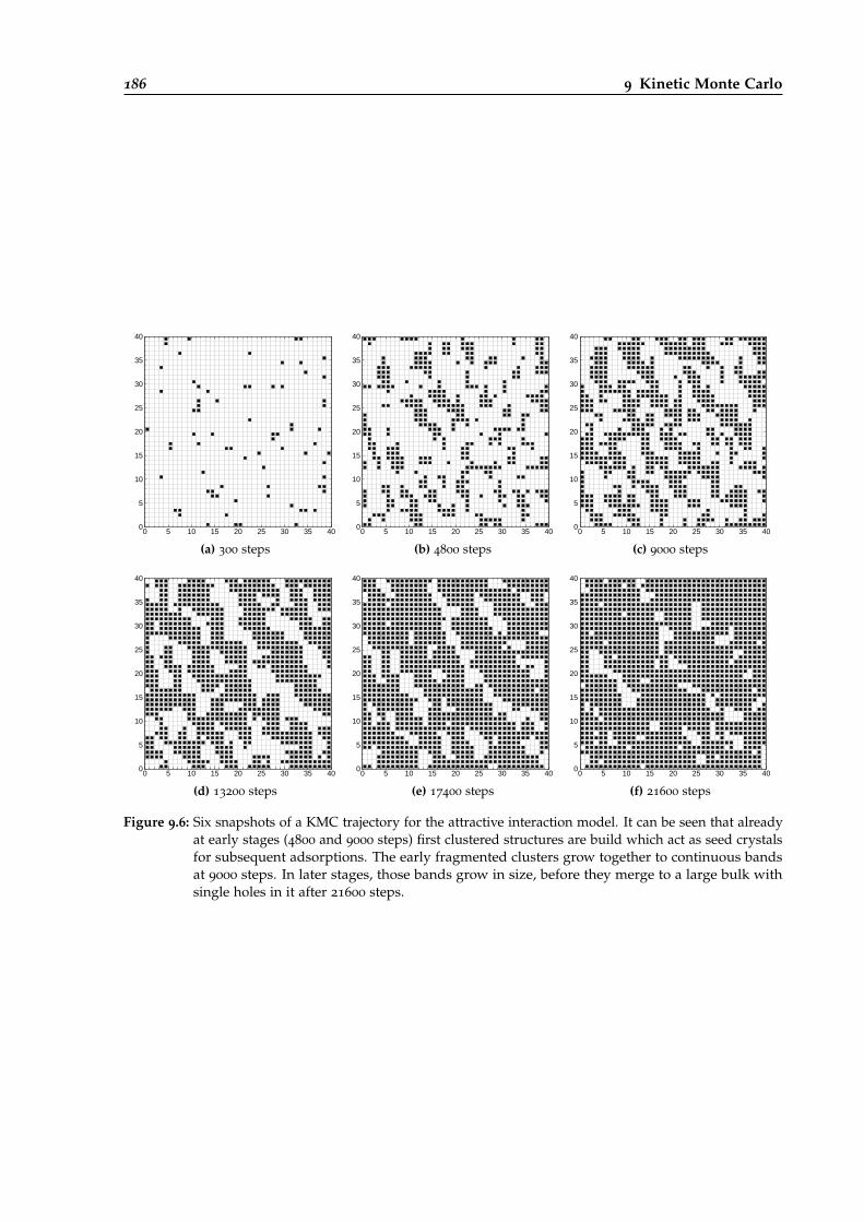
186 9 Kinetic Monte Carlo
0
5
10
15
20
25
30
35
40
0 5 10 15 20 25 30 35 40
(a) 300 steps
0
5
10
15
20
25
30
35
40
0 5 10 15 20 25 30 35 40
(b) 4800 steps
0
5
10
15
20
25
30
35
40
0 5 10 15 20 25 30 35 40
(c) 9000 steps
0
5
10
15
20
25
30
35
40
0 5 10 15 20 25 30 35 40
(d) 13200 steps
0
5
10
15
20
25
30
35
40
0 5 10 15 20 25 30 35 40
(e) 17400 steps
0
5
10
15
20
25
30
35
40
0 5 10 15 20 25 30 35 40
(f) 21600 steps
Figure 9.6: Six snapshots of a KMC trajectory for the attractive interaction model. It can be seen that alreadyat early stages (4800 and 9000 steps) first clustered structures are build which act as seed crystalsfor subsequent adsorptions. The early fragmented clusters grow together to continuous bandsat 9000 steps. In later stages, those bands grow in size, before they merge to a large bulk withsingle holes in it after 21600 steps.
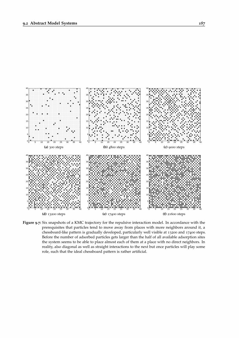
9.2 Abstract Model Systems 187
0
5
10
15
20
25
30
35
40
0 5 10 15 20 25 30 35 40
(a) 300 steps
0
5
10
15
20
25
30
35
40
0 5 10 15 20 25 30 35 40
(b) 4800 steps
0
5
10
15
20
25
30
35
40
0 5 10 15 20 25 30 35 40
(c) 9000 steps
0
5
10
15
20
25
30
35
40
0 5 10 15 20 25 30 35 40
(d) 13200 steps
0
5
10
15
20
25
30
35
40
0 5 10 15 20 25 30 35 40
(e) 17400 steps
0
5
10
15
20
25
30
35
40
0 5 10 15 20 25 30 35 40
(f) 21600 steps
Figure 9.7: Six snapshots of a KMC trajectory for the repulsive interaction model. In accordance with theprerequisites that particles tend to move away from places with more neighbors around it, achessboard-like pattern is gradually developed, particularly well visible at 13200 and 17400 steps.Before the number of adsorbed particles gets larger than the half of all available adsorption sitesthe system seems to be able to place almost each of them at a place with no direct neighbors. Inreality, also diagonal as well as straight interactions to the next but once particles will play somerole, such that the ideal chessboard pattern is rather artificial.
188 9 Kinetic Monte Carlo
Time Evolution
Besides the detailed surface structures presented above, the quantitative development of theoccupation number is a statistic quantity of great importance. In fig. 9.8 the number of adsorbedparticles during the three simulations is plotted dependent on the number of calculated KMC stepsas well as the elapsed time (summed up from all calculated time intervals ∆t).
The number of adsorbed particles after the given amount of KMC steps strongly depends onthe chosen model. At the end, approx. 800 particles were adsorbed in the independent particlesmodel, whereas for the attractive interactions this number is almost twice as large, with nearly allavailable sites populated. If the same results are plotted with respect to the elapsed time, it becomesclear that there is no fixed relation between a certain number of KMC steps and the actual time!Whereas almost 200 a.u. were simulated for the attractive interaction model, only less than 40
were simulated for the independent particle model. Since all three curves coincide quite well atthe beginning it seems that their differences in the KMC-step dependent plot arise solely due todifferent rates of progress.
But why one model evolves much faster than the other with respect to real time? This becomesclear if we consider what time actually means in KMC. In contrast to MD, where the time evolvesmonotonously and the total amount of elapsed time is determined by the number of MD steps, theelapsed time in KMC depends on the possible reactions (eq. 9.9). The equation is evaluated for eachKMC step. The more reactions with larger k(T) values are possible, the shorter the time intervaluntil the next event happens will be, since it is very unlikely that none of the many probable eventswill happen during a longer period.
In our calculations, the largest interval of time was spanned in the attractive interactions model.As we have seen in fig. 9.6, large clusters of adsorbed gas atoms are built. Inside these clusters,no diffusions are possible, since only gas atoms with three or less neighbors are able to take adiffusion step. Therefore, the number of possible reactions is reduced, with the remaining diffusions(starting from the cluster edges) being slow since they will reduce the number of neighbors. Thetotal number of possible adsorption events only depends on the free sites, no matter what theirenvironment might be. However, the rate for adsorptions is low (0.02), therefore the probability ofa reactive event in a certain time span is greatly reduced in the attractive interactions model, whichleads to a faster passage of time during a given number of KMC steps.
9.3 Hydrogen Diffusion on a Cu(001) Surface
We have seen how KMC works in principle for an artificial model system. However, our true desireis of course to simulate real chemical systems. Before going to a system similar to the abstractone of several gas atoms diffusing on a metal surface, a much simpler model will be looked at: Asingle hydrogen atom moving on a Cu(001) surface (H@Cu(001)). The reason why this system waschosen is that both theoretical and experimental studies were performed based on it, mainly inorder to investigate tunneling effects which impose corrections to the standard Arrhenius behaviorof chemical reactions [280–283].
Further, a similar study (hydrogen on a Ni(100) surface) was done by Suleymanov, imposingthe RPMD methodology [152]. That study was done with a separate RPMD program, which is notfreely available (since RPMDrate is only able to handle bimolecular gas phase reactions), however,the rpmd.x program developed in this thesis is able to calculate k(T) values for this kind of reactionsas well (section 3.3.7).
The original intention was indeed to simulate several hydrogen atoms on a Cu(001) surfacemoving simultaneously on it. Unfortunately it turned out that the standard pattern of hydrogensoccupying the hollow positions on the surface was only valid for low occupancies (at least for theused reference calculation, see below). If many neighbored lattice positions are occupied with
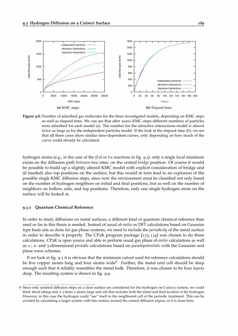
9.3 Hydrogen Diffusion on a Cu(001) Surface 189
0
500
1000
1500
2000
0 5000 10000 15000 20000 25000 30000
adso
rbed
gas
ato
ms
KMC steps
independent particlesattractive interactionsrepulsive interactions
(a) KMC steps
0
200
400
600
800
1000
1200
1400
1600
0 20 40 60 80 100 120 140 160 180 200
adso
rbed
gas
ato
ms
t (a.u.)
independent particlesattractive interactionsrepulsive interactions
(b) Elapsed time
Figure 9.8: Number of adsorbed gas molecules for the three investigated models, depending on KMC stepsas well as elapsed time. We can see that after 30000 KMC steps different numbers of particleswere adsorbed for each model (a). The number for the attractive interactions model is almosttwice as large as for the independent particles model. If the look at the elapsed time (b), we seethat all three cases show similar time-dependent curves, only depending on how much of thecurve could already be calculated.
hydrogen atoms (e.g., in the case of the (f-d or f-e reactions in fig. 9.3), only a single local minimumexists on the diffusion path between two sites: on the central bridge position. Of course it wouldbe possible to build up a slightly altered KMC model with explicit consideration of bridge and(if needed) also top positions on the surface, but this would in turn lead to an explosion of thepossible single KMC diffusion steps, since now the environment must be classified not only basedon the number of hydrogen neighbors on initial and final positions, but as well on the number ofneighbors on hollow, side, and top positions. Therefore, only one single hydrogen atom on thesurface will be looked at.
9.3.1 Quantum Chemical Reference
In order to study diffusions on metal surfaces, a different kind of quantum chemical reference thanused so far in this thesis is needed. Instead of usual ab-initio or DFT calculations based on Gaussiantype basis sets as done for gas phase systems, we need to include the periodicity of the metal surfacein order to describe it properly. The CP2K program package [133, 134] was chosen to do thesecalculations. CP2K is open source and able to perform usual gas phase ab-initio calculations as wellas 1-, 2- and 3-dimensional periodic calculations based on pseudopotentials with the Gaussian andplane wave schemes.
If we look at fig. 9.3 it is obvious that the minimum cutout used for reference calculations shouldbe five copper atoms long and four atoms wide8. Further, the metal unit cell should be deepenough such that it reliably resembles the metal bulk. Therefore, it was chosen to be four layersdeep. The resulting system is shown in fig. 9.9.
8 Since only isolated diffusion steps on a clear surface are considered for the hydrogen on Cu(001) system, we couldthink about taking only a 3 times 2 atoms large unit cell that includes both the initial and final location of the hydrogen.However, in this case the hydrogen could “see” itself in the neighbored cell of the periodic treatment. This can beavoided by calculating a larger system with free surface around the central diffusion region, as it is done here,
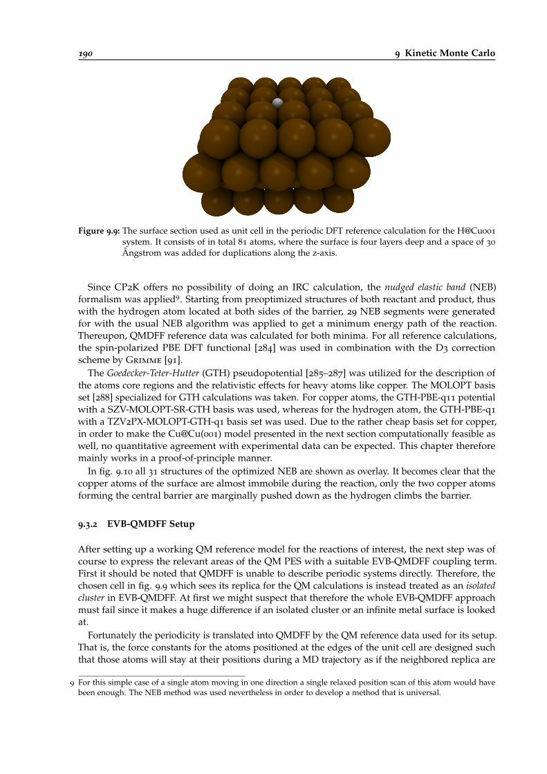
190 9 Kinetic Monte Carlo
Figure 9.9: The surface section used as unit cell in the periodic DFT reference calculation for the H@Cu001
system. It consists of in total 81 atoms, where the surface is four layers deep and a space of 30
Ångstrom was added for duplications along the z-axis.
Since CP2K offers no possibility of doing an IRC calculation, the nudged elastic band (NEB)formalism was applied9. Starting from preoptimized structures of both reactant and product, thuswith the hydrogen atom located at both sides of the barrier, 29 NEB segments were generatedfor with the usual NEB algorithm was applied to get a minimum energy path of the reaction.Thereupon, QMDFF reference data was calculated for both minima. For all reference calculations,the spin-polarized PBE DFT functional [284] was used in combination with the D3 correctionscheme by Grimme [91].
The Goedecker-Teter-Hutter (GTH) pseudopotential [285–287] was utilized for the description ofthe atoms core regions and the relativistic effects for heavy atoms like copper. The MOLOPT basisset [288] specialized for GTH calculations was taken. For copper atoms, the GTH-PBE-q11 potentialwith a SZV-MOLOPT-SR-GTH basis was used, whereas for the hydrogen atom, the GTH-PBE-q1
with a TZV2PX-MOLOPT-GTH-q1 basis set was used. Due to the rather cheap basis set for copper,in order to make the Cu@Cu(001) model presented in the next section computationally feasible aswell, no quantitative agreement with experimental data can be expected. This chapter thereforemainly works in a proof-of-principle manner.
In fig. 9.10 all 31 structures of the optimized NEB are shown as overlay. It becomes clear that thecopper atoms of the surface are almost immobile during the reaction, only the two copper atomsforming the central barrier are marginally pushed down as the hydrogen climbs the barrier.
9.3.2 EVB-QMDFF Setup
After setting up a working QM reference model for the reactions of interest, the next step was ofcourse to express the relevant areas of the QM PES with a suitable EVB-QMDFF coupling term.First it should be noted that QMDFF is unable to describe periodic systems directly. Therefore, thechosen cell in fig. 9.9 which sees its replica for the QM calculations is instead treated as an isolatedcluster in EVB-QMDFF. At first we might suspect that therefore the whole EVB-QMDFF approachmust fail since it makes a huge difference if an isolated cluster or an infinite metal surface is lookedat.
Fortunately the periodicity is translated into QMDFF by the QM reference data used for its setup.That is, the force constants for the atoms positioned at the edges of the unit cell are designed suchthat those atoms will stay at their positions during a MD trajectory as if the neighbored replica are
9 For this simple case of a single atom moving in one direction a single relaxed position scan of this atom would havebeen enough. The NEB method was used nevertheless in order to develop a method that is universal.
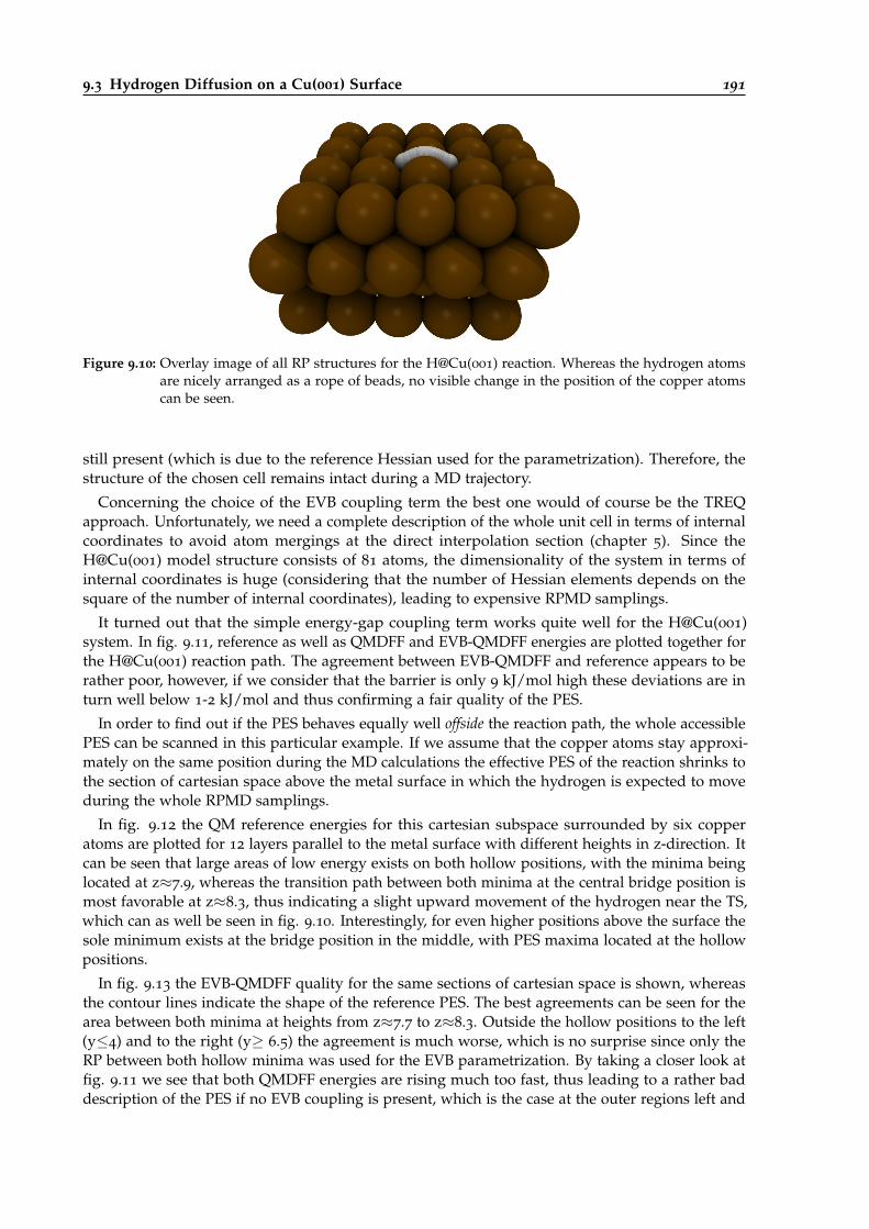
9.3 Hydrogen Diffusion on a Cu(001) Surface 191
Figure 9.10: Overlay image of all RP structures for the H@Cu(001) reaction. Whereas the hydrogen atomsare nicely arranged as a rope of beads, no visible change in the position of the copper atomscan be seen.
still present (which is due to the reference Hessian used for the parametrization). Therefore, thestructure of the chosen cell remains intact during a MD trajectory.
Concerning the choice of the EVB coupling term the best one would of course be the TREQapproach. Unfortunately, we need a complete description of the whole unit cell in terms of internalcoordinates to avoid atom mergings at the direct interpolation section (chapter 5). Since theH@Cu(001) model structure consists of 81 atoms, the dimensionality of the system in terms ofinternal coordinates is huge (considering that the number of Hessian elements depends on thesquare of the number of internal coordinates), leading to expensive RPMD samplings.
It turned out that the simple energy-gap coupling term works quite well for the H@Cu(001)system. In fig. 9.11, reference as well as QMDFF and EVB-QMDFF energies are plotted together forthe H@Cu(001) reaction path. The agreement between EVB-QMDFF and reference appears to berather poor, however, if we consider that the barrier is only 9 kJ/mol high these deviations are inturn well below 1-2 kJ/mol and thus confirming a fair quality of the PES.
In order to find out if the PES behaves equally well offside the reaction path, the whole accessiblePES can be scanned in this particular example. If we assume that the copper atoms stay approxi-mately on the same position during the MD calculations the effective PES of the reaction shrinks tothe section of cartesian space above the metal surface in which the hydrogen is expected to moveduring the whole RPMD samplings.
In fig. 9.12 the QM reference energies for this cartesian subspace surrounded by six copperatoms are plotted for 12 layers parallel to the metal surface with different heights in z-direction. Itcan be seen that large areas of low energy exists on both hollow positions, with the minima beinglocated at z≈7.9, whereas the transition path between both minima at the central bridge position ismost favorable at z≈8.3, thus indicating a slight upward movement of the hydrogen near the TS,which can as well be seen in fig. 9.10. Interestingly, for even higher positions above the surface thesole minimum exists at the bridge position in the middle, with PES maxima located at the hollowpositions.
In fig. 9.13 the EVB-QMDFF quality for the same sections of cartesian space is shown, whereasthe contour lines indicate the shape of the reference PES. The best agreements can be seen for thearea between both minima at heights from z≈7.7 to z≈8.3. Outside the hollow positions to the left(y≤4) and to the right (y≥ 6.5) the agreement is much worse, which is no surprise since only theRP between both hollow minima was used for the EVB parametrization. By taking a closer look atfig. 9.11 we see that both QMDFF energies are rising much too fast, thus leading to a rather baddescription of the PES if no EVB coupling is present, which is the case at the outer regions left and
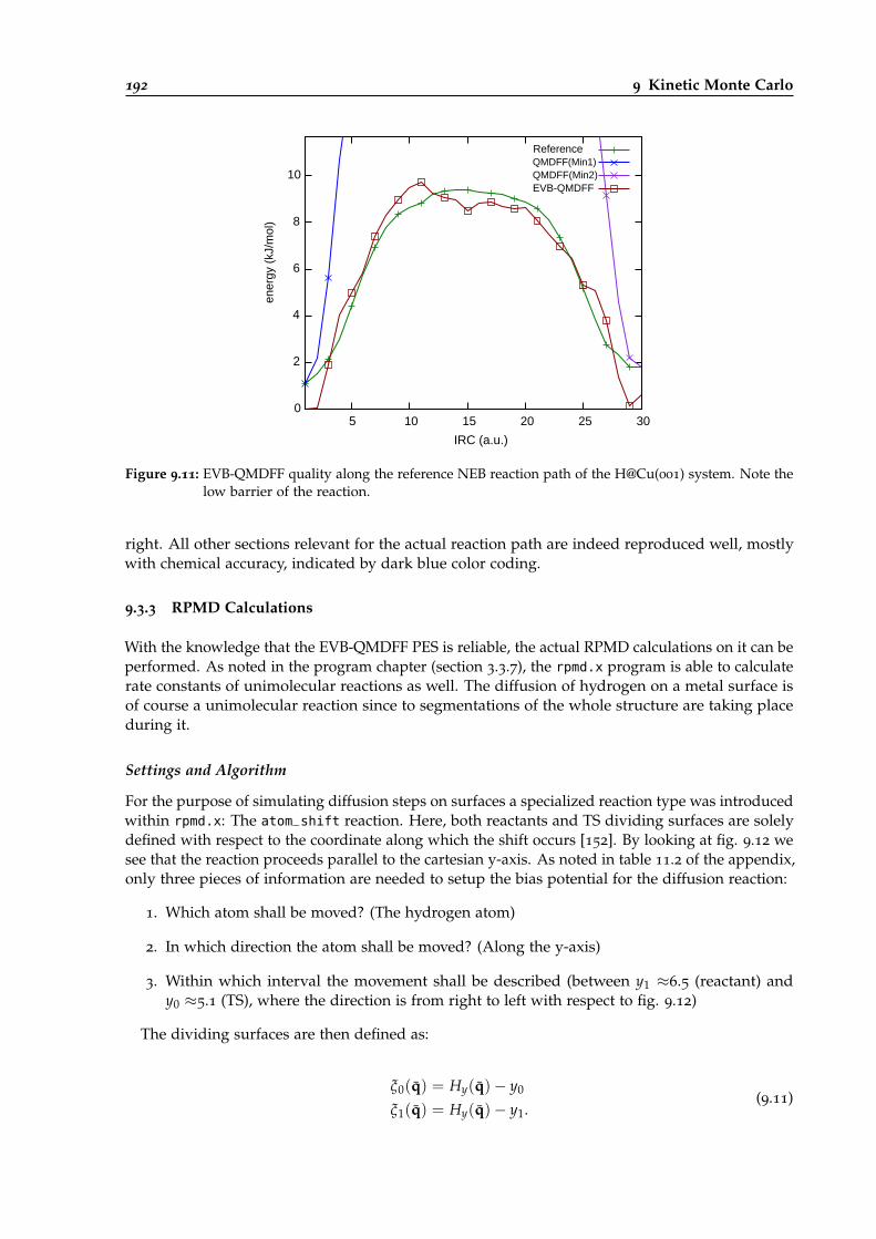
192 9 Kinetic Monte Carlo
0
2
4
6
8
10
5 10 15 20 25 30
ener
gy
(kJ/
mol
)
IRC (a.u.)
ReferenceQMDFF(Min1)QMDFF(Min2)EVB-QMDFF
Figure 9.11: EVB-QMDFF quality along the reference NEB reaction path of the H@Cu(001) system. Note thelow barrier of the reaction.
right. All other sections relevant for the actual reaction path are indeed reproduced well, mostlywith chemical accuracy, indicated by dark blue color coding.
9.3.3 RPMD Calculations
With the knowledge that the EVB-QMDFF PES is reliable, the actual RPMD calculations on it can beperformed. As noted in the program chapter (section 3.3.7), the rpmd.x program is able to calculaterate constants of unimolecular reactions as well. The diffusion of hydrogen on a metal surface isof course a unimolecular reaction since to segmentations of the whole structure are taking placeduring it.
Settings and Algorithm
For the purpose of simulating diffusion steps on surfaces a specialized reaction type was introducedwithin rpmd.x: The atom_shift reaction. Here, both reactants and TS dividing surfaces are solelydefined with respect to the coordinate along which the shift occurs [152]. By looking at fig. 9.12 wesee that the reaction proceeds parallel to the cartesian y-axis. As noted in table 11.2 of the appendix,only three pieces of information are needed to setup the bias potential for the diffusion reaction:
1. Which atom shall be moved? (The hydrogen atom)
2. In which direction the atom shall be moved? (Along the y-axis)
3. Within which interval the movement shall be described (between y1 ≈6.5 (reactant) andy0 ≈5.1 (TS), where the direction is from right to left with respect to fig. 9.12)
The dividing surfaces are then defined as:
ξ0(q) = Hy(q)− y0
ξ1(q) = Hy(q)− y1.(9.11)
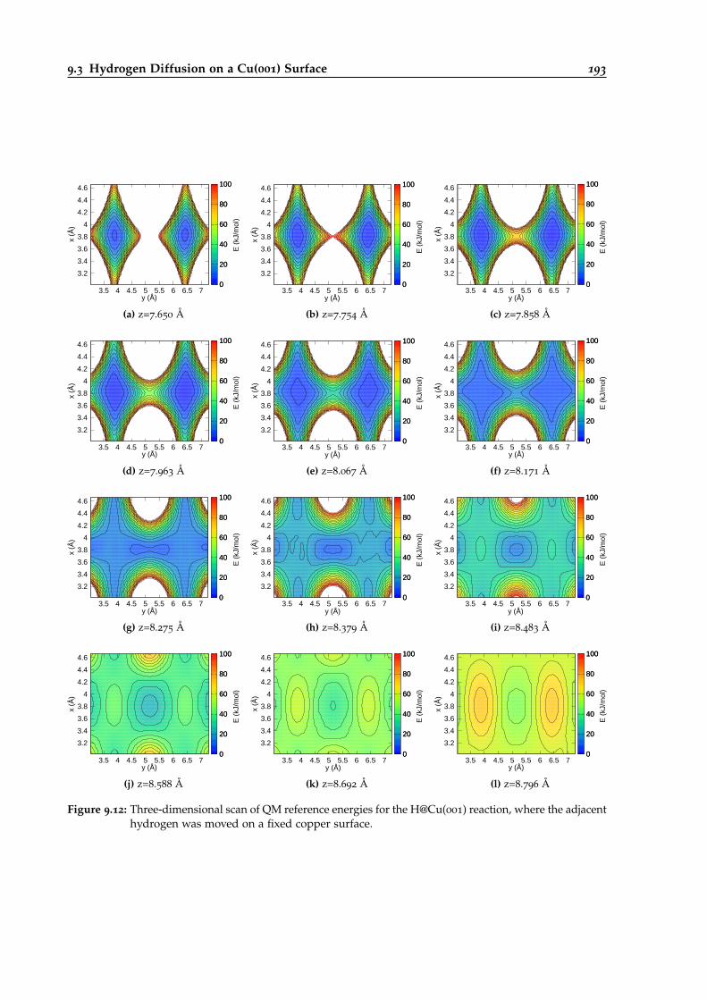
9.3 Hydrogen Diffusion on a Cu(001) Surface 193
3.5 4 4.5 5 5.5 6 6.5 7
3.2
3.4
3.6
3.8
4
4.2
4.4
4.6
x (Å
)
0
20
40
60
80
100
0
20
40
60
80
100
y (Å)
E (
kJ/m
ol)
(a) z=7.650 Å
3.5 4 4.5 5 5.5 6 6.5 7
3.2
3.4
3.6
3.8
4
4.2
4.4
4.6
x (Å
)
0
20
40
60
80
100
0
20
40
60
80
100
y (Å)
E (
kJ/m
ol)
(b) z=7.754 Å
3.5 4 4.5 5 5.5 6 6.5 7
3.2
3.4
3.6
3.8
4
4.2
4.4
4.6
x (Å
)
0
20
40
60
80
100
0
20
40
60
80
100
y (Å)
E (
kJ/m
ol)
(c) z=7.858 Å
3.5 4 4.5 5 5.5 6 6.5 7y (Å)
3.2
3.4
3.6
3.8
4
4.2
4.4
4.6
x (Å
)
0
20
40
60
80
100
0
20
40
60
80
100
E (
kJ/m
ol)
(d) z=7.963 Å
3.5 4 4.5 5 5.5 6 6.5 7
3.2
3.4
3.6
3.8
4
4.2
4.4
4.6
x (Å
)
0
20
40
60
80
100
0
20
40
60
80
100
y (Å)
E (
kJ/m
ol)
(e) z=8.067 Å
3.5 4 4.5 5 5.5 6 6.5 7
3.2
3.4
3.6
3.8
4
4.2
4.4
4.6
x (Å
)0
20
40
60
80
100
0
20
40
60
80
100
y (Å)
E (
kJ/m
ol)
(f) z=8.171 Å
3.5 4 4.5 5 5.5 6 6.5 7
3.2
3.4
3.6
3.8
4
4.2
4.4
4.6
x (Å
)
0
20
40
60
80
100
0
20
40
60
80
100
y (Å)
E (
kJ/m
ol)
(g) z=8.275 Å
3.5 4 4.5 5 5.5 6 6.5 7y (Å)
3.2
3.4
3.6
3.8
4
4.2
4.4
4.6
x (Å
)
0
20
40
60
80
100
0
20
40
60
80
100
E (
kJ/m
ol)
(h) z=8.379 Å
3.5 4 4.5 5 5.5 6 6.5 7
3.2
3.4
3.6
3.8
4
4.2
4.4
4.6
x (Å
)
0
20
40
60
80
100
0
20
40
60
80
100
y (Å)
E (
kJ/m
ol)
(i) z=8.483 Å
3.5 4 4.5 5 5.5 6 6.5 7
3.2
3.4
3.6
3.8
4
4.2
4.4
4.6
x (Å
)
0
20
40
60
80
100
0
20
40
60
80
100
y (Å)
E (
kJ/m
ol)
(j) z=8.588 Å
3.5 4 4.5 5 5.5 6 6.5 7
3.2
3.4
3.6
3.8
4
4.2
4.4
4.6
x (Å
)
0
20
40
60
80
100
0
20
40
60
80
100
y (Å)
E (
kJ/m
ol)
(k) z=8.692 Å
3.5 4 4.5 5 5.5 6 6.5 7
3.2
3.4
3.6
3.8
4
4.2
4.4
4.6
x (Å
)
0
20
40
60
80
100
0
20
40
60
80
100
y (Å)
E (
kJ/m
ol)
(l) z=8.796 Å
Figure 9.12: Three-dimensional scan of QM reference energies for the H@Cu(001) reaction, where the adjacenthydrogen was moved on a fixed copper surface.

194 9 Kinetic Monte Carlo
3.5 4 4.5 5 5.5 6 6.5 7
3.2
3.4
3.6
3.8
4
4.2
4.4
4.6
x (Å
)
0
10
20
30
40
50
0
10
20
30
40
50
y (Å)
ΔE
(kJ
/mol
)
(a) z=7.650 Å
3.5 4 4.5 5 5.5 6 6.5 7
3.2
3.4
3.6
3.8
4
4.2
4.4
4.6
x (Å
)0
10
20
30
40
50
0
10
20
30
40
50
y (Å)
ΔE
(kJ
/mol
)
(b) z=7.754 Å
3.5 4 4.5 5 5.5 6 6.5 7
3.2
3.4
3.6
3.8
4
4.2
4.4
4.6
x (Å
)
0
10
20
30
40
50
0
10
20
30
40
50
y (Å)
ΔE
(kJ
/mol
)
(c) z=7.858 Å
3.5 4 4.5 5 5.5 6 6.5 7
3.2
3.4
3.6
3.8
4
4.2
4.4
4.6
x (Å
)
0
10
20
30
40
50
0
10
20
30
40
50
y (Å)
ΔE
(kJ
/mol
)
(d) z=7.963 Å
3.5 4 4.5 5 5.5 6 6.5 7
3.2
3.4
3.6
3.8
4
4.2
4.4
4.6
x (Å
)
0
10
20
30
40
50
0
10
20
30
40
50
y (Å)Δ
E (
kJ/m
ol)
(e) z=8.067 Å
3.5 4 4.5 5 5.5 6 6.5 7
3.2
3.4
3.6
3.8
4
4.2
4.4
4.6
x (Å
)
0
10
20
30
40
50
0
10
20
30
40
50
y (Å)
ΔE
(kJ
/mol
)
(f) z=8.171 Å
3.5 4 4.5 5 5.5 6 6.5 7
3.2
3.4
3.6
3.8
4
4.2
4.4
4.6
x (Å
)
0
10
20
30
40
50
0
10
20
30
40
50
y (Å)
ΔE
(kJ
/mol
)
(g) z=8.275 Å
3.5 4 4.5 5 5.5 6 6.5 7y (Å)
ΔE
(kJ
/mol
)
3.2
3.4
3.6
3.8
4
4.2
4.4
4.6
x (Å
)
0
10
20
30
40
50
0
10
20
30
40
50
(h) z=8.379 Å
3.5 4 4.5 5 5.5 6 6.5 7y (Å)
ΔE
(kJ
/mol
)
3.2
3.4
3.6
3.8
4
4.2
4.4
4.6
x (Å
)
0
10
20
30
40
50
0
10
20
30
40
50
(i) z=8.483 Å
3.5 4 4.5 5 5.5 6 6.5 7
3.2
3.4
3.6
3.8
4
4.2
4.4
4.6
x (Å
)
0
10
20
30
40
50
0
10
20
30
40
50
y (Å)
ΔE
(kJ
/mol
)
(j) z=8.588 Å
3.5 4 4.5 5 5.5 6 6.5 7y (Å)
ΔE
(kJ
/mol
)
3.2
3.4
3.6
3.8
4
4.2
4.4
4.6
x (Å
)
0
10
20
30
40
50
0
10
20
30
40
50
(k) z=8.692 Å
3.5 4 4.5 5 5.5 6 6.5 7
3.2
3.4
3.6
3.8
4
4.2
4.4
4.6
x (Å
)
0
10
20
30
40
50
0
10
20
30
40
50
y (Å)
ΔE
(kJ
/mol
)
(l) z=8.796 Å
Figure 9.13: Quality of the energy-gap EVB coupling term used for parametrization of the EVB-QMDFF PESfor the H@Cu(001) reaction. Shown are the differences of reference and EVB-QMDFF energiesfor the same coordinate space as in fig. 9.12.
9.3 Hydrogen Diffusion on a Cu(001) Surface 195
After performing the sampling as well as umbrella integration and recrossing the unimolecularrate constant can be calculated with eq. 3.21.
Only one fix needs to be made for the samplings: If a bias potential is applied solely on theadjacent hydrogen atom during the RPMD k(T) calculations, it turns out that the whole unit cellstructure is gradually moved in this direction. If the hydrogen atom shall be moved from the rightminimum over the TS to the left minimum during the umbrella structure generation phase, the biasis applied on the absolute position of the atom in cartesian space, i.e., along the y-axis in our case.Then, the whole metal cluster can be moved together with the hydrogen to the left, leaving thehydrogen into its reactant minimum, since this overall translation (obviously) has a lower energybarrier than the local translation of the hydrogen over the fixed surface. This behavior can beprevented by artificial freezing of the lowest layer of copper atoms by setting its momentum to zeroduring the sampling trajectories. Since three additional layers exist between the frozen one and thehydrogen atom the introduced error will be small, by simultaneously solving the problem of globaltranslation.
In order to thoroughly investigate quantum effects at low temperatures, the samplings wereconducted between 20 and 120 K. Further, the calculations were repeated for the D@Cu(001) system,where the hydrogen is replaced by deuterium. For this case, the QM reference as well as theEVB-QMDFF stay the same but the rate constants change significantly (see below). The used RPMDsettings are summarized into table 9.2. Since the total internal coordinate space to be sampled isquite small in comparison to usual gas phase reactions, the chosen settings are rather cheap. Thenumber as well as the durations of the umbrella trajectories is rather short, nevertheless resultingin RPMD rates of good convergence.
The calculations were made with the objective to compare their results with those of Kua andLauhon [281] who calculated diffusion (or direct hopping) rates of H@Cu(001) and D@Cu(001)10
and compared them with experimental scanning tunneling microscope (STM) measurements, wherethe actual hopping rates were determined from diffusion coefficients of single tracked hydrogenand deuterium atoms. To make a direct comparison possible, RPMD calculations were performedfor very low temperatures between 10 and 120 K for both H@Cu(001) and D@Cu(001).
Illustration of RPMD
In order to illustrate the actual behavior of RPMD for very low temperatures where quantumeffects become important, trajectory snapshots are presented in fig. 9.14. There, structures ofumbrella sampling trajectories at 10 K with the bias potential located at the transition state arecompared with another for one to 256 beads. The positions of the copper atoms remain almostconstant; although they all are expressed as well with the respective number of RPMD beads, theirseparation seems to negligible.
Interestingly all hydrogen replicas are located in one of the minima for 2 to 16 beads in totaleven though the bias potential is located at the TS between them! This is due to the RPMD centroidassumption (eq. 2.102), where the bias potential is not applied on each bead directly but onlyindirectly over the centroid, i.e., the center of mass for all beads. If one half of the beads is locatedleft and the other half is located right, their center of mass is consequently located directly atthe TS as it should be. For 32 and more beads, the single replicas are scattered more regularlyalong the whole reaction path, such that basically all cartesian space with sufficiently low energy isfilled with hydrogen replicas at 256 beads; in narrow correspondence to a wave function of thehydrogen calculated for real quantum dynamics, where the density of replicas per space segment isrelated to the square of the wave function, i.e., the probability to find the particle there. The actual
10 The theoretical k(T) calculations of Kua and Lauhon basically consist of two parts: For the thermally activated regime(see below) simple TST was used, where for the quantum tunneling regime the Wentzel-Kramers-Brillouin (WKB)approximation was used in order to calculate a sole tunneling rate. Thus, tunneling was neglected in the first part andthe thermal rate in the second, resulting in a sharp transition between both parts, visible in fig. 9.17.
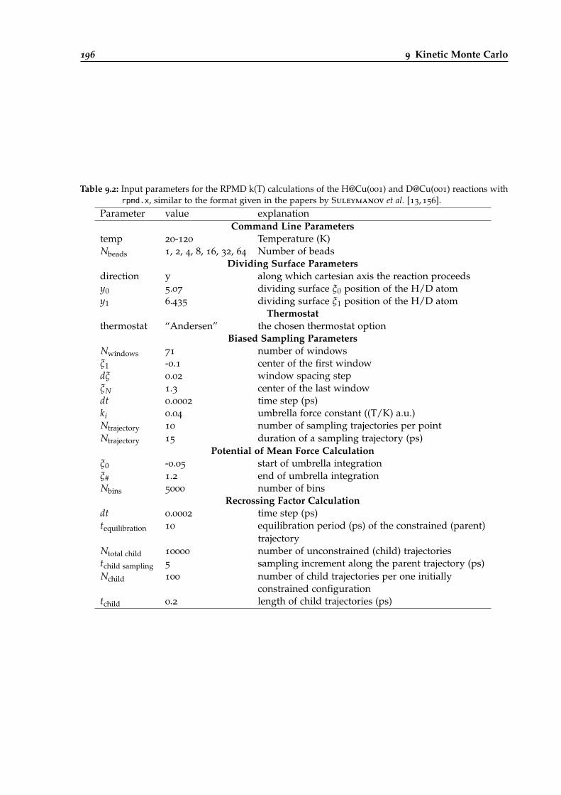
196 9 Kinetic Monte Carlo
Table 9.2: Input parameters for the RPMD k(T) calculations of the H@Cu(001) and D@Cu(001) reactions withrpmd.x, similar to the format given in the papers by Suleymanov et al. [13, 156].
Parameter value explanationCommand Line Parameters
temp 20-120 Temperature (K)Nbeads 1, 2, 4, 8, 16, 32, 64 Number of beads
Dividing Surface Parametersdirection y along which cartesian axis the reaction proceedsy0 5.07 dividing surface ξ0 position of the H/D atomy1 6.435 dividing surface ξ1 position of the H/D atom
Thermostatthermostat “Andersen” the chosen thermostat option
Biased Sampling ParametersNwindows 71 number of windowsξ1 -0.1 center of the first windowdξ 0.02 window spacing stepξN 1.3 center of the last windowdt 0.0002 time step (ps)ki 0.04 umbrella force constant ((T/K) a.u.)Ntrajectory 10 number of sampling trajectories per pointNtrajectory 15 duration of a sampling trajectory (ps)
Potential of Mean Force Calculationξ0 -0.05 start of umbrella integrationξ# 1.2 end of umbrella integrationNbins 5000 number of bins
Recrossing Factor Calculationdt 0.0002 time step (ps)tequilibration 10 equilibration period (ps) of the constrained (parent)
trajectoryNtotal child 10000 number of unconstrained (child) trajectoriestchild sampling 5 sampling increment along the parent trajectory (ps)Nchild 100 number of child trajectories per one initially
constrained configurationtchild 0.2 length of child trajectories (ps)
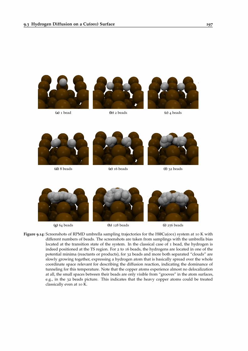
9.3 Hydrogen Diffusion on a Cu(001) Surface 197
(a) 1 bead (b) 2 beads (c) 4 beads
(d) 8 beads (e) 16 beads (f) 32 beads
(g) 64 beads (h) 128 beads (i) 256 beads
Figure 9.14: Screenshots of RPMD umbrella sampling trajectories for the H@Cu(001) system at 10 K withdifferent numbers of beads. The screenshots are taken from samplings with the umbrella biaslocated at the transition state of the system. In the classical case of 1 bead, the hydrogen isindeed positioned at the TS region. For 2 to 16 beads, the hydrogens are located in one of thepotential minima (reactants or products), for 32 beads and more both separated “clouds” areslowly growing together, expressing a hydrogen atom that is basically spread over the wholecoordinate space relevant for describing the diffusion reaction, indicating the dominance oftunneling for this temperature. Note that the copper atoms experience almost no delocalizationat all, the small spaces between their beads are only visible from “grooves” in the atom surfaces,e.g., in the 32 beads picture. This indicates that the heavy copper atoms could be treatedclassically even at 10 K.
198 9 Kinetic Monte Carlo
k(T)-calculations were performed with 1 to 64 beads, since even larger numbers, being expensiveto calculate, had nearly no effect on the calculated rates.
Transmission Coefficients
Before going to the final results of reaction rate calculations, it is interesting to investigate therecrossing calculations in more detail. In fig. 9.15 the time-dependent transmission coefficients κ(t)for the investigated temperatures of both H@Cu(001) and D@Cu(001) are plotted (see fig. 2.5 in thetheory part for better understanding of how κ(t) is calculated).
In both figures, the overall shape of the κ(t)-curves strongly depends on the calculated tem-perature. For H@Cu(001) the time-profile for 20 K shows a very flat shape near unity. Since thisis completely different to all other temperatures, problems of RPMD with the low temperatureare assumed (calculations for 10 K gave no useful results at all, see below). Further, the 20 Ktime-profile for D@Cu(001) shows no such peculiarity, probably due to the doubled masses thatlead to stiffer forces between the beads11. For 30 to 60 K, similar shapes can be seen. The finalvalue of κ(t) rises with temperature, further, quite eye-catching oscillations of κ(t) exist, whosestrength decreases with increasing temperature. If we compare these oscillations of hydrogen anddeuterium, we can further see that the “wavelength” of the first oscillation at 30 K is for deuteriumroughly one and a half times larger than for hydrogen, corresponding to the well known isotopeeffect in hydrogen/deuterium vibrations in molecules, where the exact proportion is
√2.
These oscillations exist also in similar low-temperature RPMD studies of hydrogen (or deuterium)transfers and can be attributed to vibrational motions of the ring polymer beads in the reactantand product minima as the centroid crosses the transition state in the recrossing calculations (seefig. 9.14) [152, 289]. Those vibrations lead to artificial back-and-forth movements of the centroidthrough the TS dividing surface, causing back-and-forth recrossings as well. Here we see indeedone of the deficiencies of the RPMD centroid approximation introduced in eq. 2.102.
For higher temperatures, the oscillations gradually disappear, presumably due to the strongerinter-bead forces that keep single beads from oscillating in the reactants or product basins whenthe centroid is located in the transition region. If we look at H@Cu(001) a substantial change canbe seen between 60 and 80 K. For low temperatures, the oscillations declined with time, leadingto quite well converged values of κ(t). For 80 K and above, however, a number of decreasing stepscan be seen in the κ(t) profile, for instance, at approximately 120, 200, 270 and 390 fs for 100 K.They were observed as well in the publication of Suleymanov where rates for the diffusion ofhydrogen on a Ni(001) surface were calculated [152]. The steps can be explained with recrossingsof trajectories that already reached the product basin, vibrate there and then climb the activationbarrier again from the other direction. The higher the temperature the earlier those steps appear,matching the fact that the vibrations in the minimum will have larger amplitudes if the temperatureis higher, such that the chance of leaving reactants or products basins increases. If we wouldrun much longer recrossing child trajectories, we should see that the steps are becoming smallerand shorter at later times, since the trajectories are becoming less and less correlated, ultimatelyresulting in a smoothly decaying curve. This decay should continue until κ(t) ≈0.5 is approached,at least if no complete vibrational redistribution to the underlying copper surface takes place in theinvestigated time scales. Then, due to the symmetric PES, half of the trajectories should be locatedin the reactants and the other in the products basin, with equal probability for both sides to react,thus holding up an equilibrium12.
11 An interesting feature of RPMD is that the masses of atoms have a direct influence on the force acting on them via theharmonic spring forces attached between the beads (see eq. 2.99). For classical MD simulations, the masses have noinfluence on the gradient and come only into play via the thermostat and the Verlet algorithm itself [40].
12 This stepwise decrease of κ(t) cannot be seen for usual gas-phase reactions studied so far, since there the energypresent in the reactive mode is quickly redistributed to all other vibrational modes of the product structure, thuspreventing it from coming back in almost all cases (even if a slow decrease of κ(t) for extremely long time intervalswill also be seen there, which can be accelerated by calculating much higher temperatures). For the H@Cu(001) model,
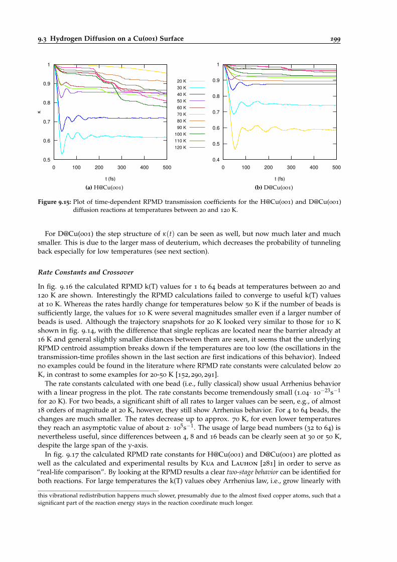
9.3 Hydrogen Diffusion on a Cu(001) Surface 199
0.5
0.6
0.7
0.8
0.9
1
0 100 200 300 400 500
κ
t (fs)(a) H@Cu(001)
20 K30 K40 K50 K60 K70 K80 K90 K
100 K110 K120 K
0.4
0.5
0.6
0.7
0.8
0.9
1
0 100 200 300 400 500
t (fs)(b) D@Cu(001)
Figure 9.15: Plot of time-dependent RPMD transmission coefficients for the H@Cu(001) and D@Cu(001)diffusion reactions at temperatures between 20 and 120 K.
For D@Cu(001) the step structure of κ(t) can be seen as well, but now much later and muchsmaller. This is due to the larger mass of deuterium, which decreases the probability of tunnelingback especially for low temperatures (see next section).
Rate Constants and Crossover
In fig. 9.16 the calculated RPMD k(T) values for 1 to 64 beads at temperatures between 20 and120 K are shown. Interestingly the RPMD calculations failed to converge to useful k(T) valuesat 10 K. Whereas the rates hardly change for temperatures below 50 K if the number of beads issufficiently large, the values for 10 K were several magnitudes smaller even if a larger number ofbeads is used. Although the trajectory snapshots for 20 K looked very similar to those for 10 Kshown in fig. 9.14, with the difference that single replicas are located near the barrier already at16 K and general slightly smaller distances between them are seen, it seems that the underlyingRPMD centroid assumption breaks down if the temperatures are too low (the oscillations in thetransmission-time profiles shown in the last section are first indications of this behavior). Indeedno examples could be found in the literature where RPMD rate constants were calculated below 20
K, in contrast to some examples for 20-50 K [152, 290, 291].The rate constants calculated with one bead (i.e., fully classical) show usual Arrhenius behavior
with a linear progress in the plot. The rate constants become tremendously small (1.04· 10−23s−1
for 20 K). For two beads, a significant shift of all rates to larger values can be seen, e.g., of almost18 orders of magnitude at 20 K, however, they still show Arrhenius behavior. For 4 to 64 beads, thechanges are much smaller. The rates decrease up to approx. 70 K, for even lower temperaturesthey reach an asymptotic value of about 2· 10
5s−1. The usage of large bead numbers (32 to 64) isnevertheless useful, since differences between 4, 8 and 16 beads can be clearly seen at 30 or 50 K,despite the large span of the y-axis.
In fig. 9.17 the calculated RPMD rate constants for H@Cu(001) and D@Cu(001) are plotted aswell as the calculated and experimental results by Kua and Lauhon [281] in order to serve as“real-life comparison”. By looking at the RPMD results a clear two-stage behavior can be identified forboth reactions. For large temperatures the k(T) values obey Arrhenius law, i.e., grow linearly with
this vibrational redistribution happens much slower, presumably due to the almost fixed copper atoms, such that asignificant part of the reaction energy stays in the reaction coordinate much longer.
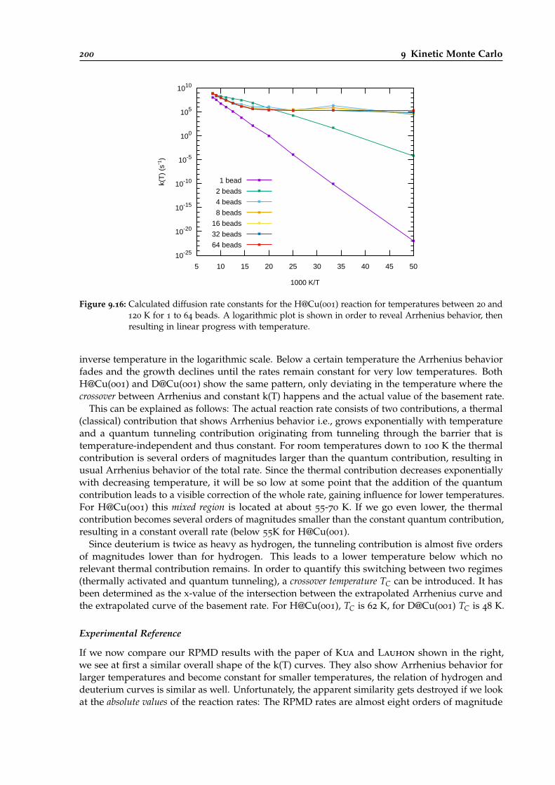
200 9 Kinetic Monte Carlo
10-25
10-20
10-15
10-10
10-5
100
105
1010
5 10 15 20 25 30 35 40 45 50
k(T
)(s
- 1)
1000 K/T
1 bead
2 beads
4 beads
8 beads
16 beads
32 beads
64 beads
Figure 9.16: Calculated diffusion rate constants for the H@Cu(001) reaction for temperatures between 20 and120 K for 1 to 64 beads. A logarithmic plot is shown in order to reveal Arrhenius behavior, thenresulting in linear progress with temperature.
inverse temperature in the logarithmic scale. Below a certain temperature the Arrhenius behaviorfades and the growth declines until the rates remain constant for very low temperatures. BothH@Cu(001) and D@Cu(001) show the same pattern, only deviating in the temperature where thecrossover between Arrhenius and constant k(T) happens and the actual value of the basement rate.
This can be explained as follows: The actual reaction rate consists of two contributions, a thermal(classical) contribution that shows Arrhenius behavior i.e., grows exponentially with temperatureand a quantum tunneling contribution originating from tunneling through the barrier that istemperature-independent and thus constant. For room temperatures down to 100 K the thermalcontribution is several orders of magnitudes larger than the quantum contribution, resulting inusual Arrhenius behavior of the total rate. Since the thermal contribution decreases exponentiallywith decreasing temperature, it will be so low at some point that the addition of the quantumcontribution leads to a visible correction of the whole rate, gaining influence for lower temperatures.For H@Cu(001) this mixed region is located at about 55-70 K. If we go even lower, the thermalcontribution becomes several orders of magnitudes smaller than the constant quantum contribution,resulting in a constant overall rate (below 55K for H@Cu(001).
Since deuterium is twice as heavy as hydrogen, the tunneling contribution is almost five ordersof magnitudes lower than for hydrogen. This leads to a lower temperature below which norelevant thermal contribution remains. In order to quantify this switching between two regimes(thermally activated and quantum tunneling), a crossover temperature TC can be introduced. It hasbeen determined as the x-value of the intersection between the extrapolated Arrhenius curve andthe extrapolated curve of the basement rate. For H@Cu(001), TC is 62 K, for D@Cu(001) TC is 48 K.
Experimental Reference
If we now compare our RPMD results with the paper of Kua and Lauhon shown in the right,we see at first a similar overall shape of the k(T) curves. They also show Arrhenius behavior forlarger temperatures and become constant for smaller temperatures, the relation of hydrogen anddeuterium curves is similar as well. Unfortunately, the apparent similarity gets destroyed if we lookat the absolute values of the reaction rates: The RPMD rates are almost eight orders of magnitude
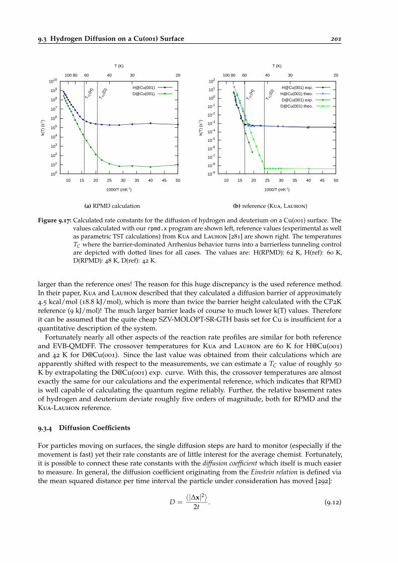
9.3 Hydrogen Diffusion on a Cu(001) Surface 201
100
101
102
103
104
105
106
107
108
109
1010
10 15 20 25 30 35 40 45 50
100 80 60 40 30 20
k(T
) (s
-1)
1000/T (mK-1)
T (K)
H@Cu(001)
D@Cu(001)
T TC(H
)
T TC(D
)
(a) RPMD calculation
10-9
10-8
10-7
10-6
10-5
10-4
10-3
10-2
10-1
100
101
102
10 15 20 25 30 35 40 45 50
100 80 60 40 30 20
k(T
) (s
-1)
1000/T (mK-1)
T (K)
H@Cu(001) exp.
H@Cu(001) theo.
D@Cu(001) exp.
D@Cu(001) theo.
T TC(H
)
T TC(D
)
(b) reference (Kua, Lauhon)
Figure 9.17: Calculated rate constants for the diffusion of hydrogen and deuterium on a Cu(001) surface. Thevalues calculated with our rpmd.x program are shown left, reference values (experimental as wellas parametric TST calculations) from Kua and Lauhon [281] are shown right. The temperaturesTC where the barrier-dominated Arrhenius behavior turns into a barrierless tunneling controlare depicted with dotted lines for all cases. The values are: H(RPMD): 62 K, H(ref): 60 K,D(RPMD): 48 K, D(ref): 42 K.
larger than the reference ones! The reason for this huge discrepancy is the used reference method.In their paper, Kua and Lauhon described that they calculated a diffusion barrier of approximately4.5 kcal/mol (18.8 kJ/mol), which is more than twice the barrier height calculated with the CP2Kreference (9 kJ/mol)! The much larger barrier leads of course to much lower k(T) values. Thereforeit can be assumed that the quite cheap SZV-MOLOPT-SR-GTH basis set for Cu is insufficient for aquantitative description of the system.
Fortunately nearly all other aspects of the reaction rate profiles are similar for both referenceand EVB-QMDFF. The crossover temperatures for Kua and Lauhon are 60 K for H@Cu(001)and 42 K for D@Cu(001). Since the last value was obtained from their calculations which areapparently shifted with respect to the measurements, we can estimate a TC value of roughly 50
K by extrapolating the D@Cu(001) exp. curve. With this, the crossover temperatures are almostexactly the same for our calculations and the experimental reference, which indicates that RPMDis well capable of calculating the quantum regime reliably. Further, the relative basement ratesof hydrogen and deuterium deviate roughly five orders of magnitude, both for RPMD and theKua-Lauhon reference.
9.3.4 Diffusion Coefficients
For particles moving on surfaces, the single diffusion steps are hard to monitor (especially if themovement is fast) yet their rate constants are of little interest for the average chemist. Fortunately,it is possible to connect these rate constants with the diffusion coefficient which itself is much easierto measure. In general, the diffusion coefficient originating from the Einstein relation is defined viathe mean squared distance per time interval the particle under consideration has moved [292]:
D =〈|∆x|2〉
2t. (9.12)
202 9 Kinetic Monte Carlo
For the simple case of particles moving on a two dimensional regular grid, an analytical solutionexists that connects the diffusion coefficient with the length of a single diffusion hop l, its rate k(T)and the symmetry factor of the reaction σ [152]:
D(T) =σ
2k(T)l2. (9.13)
In our case, the distance l covered by a proton during a single diffusion step is 2.564 Å, therelevant temperature-dependent rate constants are plotted into fig. 9.17 and the symmetry factorσ is four since four equivalent ways exist for a proton to reach a neighbored hollow site if novertical movements over copper atoms are considered. Therefore, we are able to get the diffusioncoefficients directly from our RPMD rates in this particular example by simply multiplying aconstant geometry-dependent prefactor.
However, in order to show that KMC is able to obtain the analytical result through probabilisticsamplings (and in order to give a simple but detailed example of its machinery), KMC runs werecalculated for a single hydrogen atom on the surface, where the aim is to calculate the covereddistance ∆x and the elapsed time t needed for determination of D(T), which in turn will becompared to the analytical results. Now, instead of 256 different reactions (or 36 per direction ifchirality is neglected, fig. 9.3) only four need to be considered: diffusions in in +x,-x,+y and -y,each having identical rate constants (fig. 9.2).
Therefore, the KMC runs are actually independent of the rate since all results simply need tobe multiplied by its actual value (the diffusion coefficient will be four times larger if the rate of asingle diffusion step is four times larger). In general, where different processes are considered (asin the previous section), this is of course not the case since the relative values of those rates willvary with temperature (see Cu@Cu(001) in the next section).
Due to this independence, the KMC runs were done with a generic diffusion rate of 1 and with adiffusion step length of 2. The particle was started at the origin and then propagated 10000 KMCsteps. According to eq. 9.9, the elapsed time is basically a random variable divided through thesum of all possible rates (here: 4 · 1 = 4). In the long time average, a reaction will therefore occureach quarter time unit. Which of the four possible processes occurs (i.e., in which direction theparticle will move) is of course determined by chance as well (eq. 9.10). The whole movementtherefore reduces to a simple two-dimensional random walker model13.
In fig. 9.18, four example KMC trajectories of the hydrogen on the abstract copper surface areshown, whereas the actual covered distance is indicated by a dotted line connecting initial andfinal positions.
As we see, it is clearly insufficient to simply calculate a dozen trajectories and determine theaverage value of ∆x, since the single runs deviate heavily. In fact, it became obvious that asignificantly higher number of trajectories was needed. Therefore, 10000 trajectories with 10000
KMC steps each were calculated; the covered distances as well as the elapsed times for all of themare shown in histograms (fig. 9.19), the calculated global average values are indicated there asvertical lines. The average covered distance (with a single diffusion step being 2 a.u. long) was176.819, the average elapsed time was 2499.994. Since the average time needed for a single diffusionstep is 0.25, after 10000 diffusion steps 2500 time units should be elapsed at average, which isalmost exactly the case here. We further see that single outliers tend to be 100 units shorter orlonger, corresponding to 2.5% of the total interval.
If the squared mean of covered distances 〈|∆x|2〉 is determined by averaging over all 10000 runs,the value is 39956.177, near to 40000, which would be obtained by adding all squared 10000 steplengths.
Now we know both t and 〈|∆x|2〉. In order to introduce actual physics, the abstract modeldimensions of transition times and diffusion step lengths need to be converted into the values
13 Since the KMClib program is rather slow, a separate Fortran program for the simple diffusion calculations of a singleparticle on a surface was written and used to produce the following results in this section.
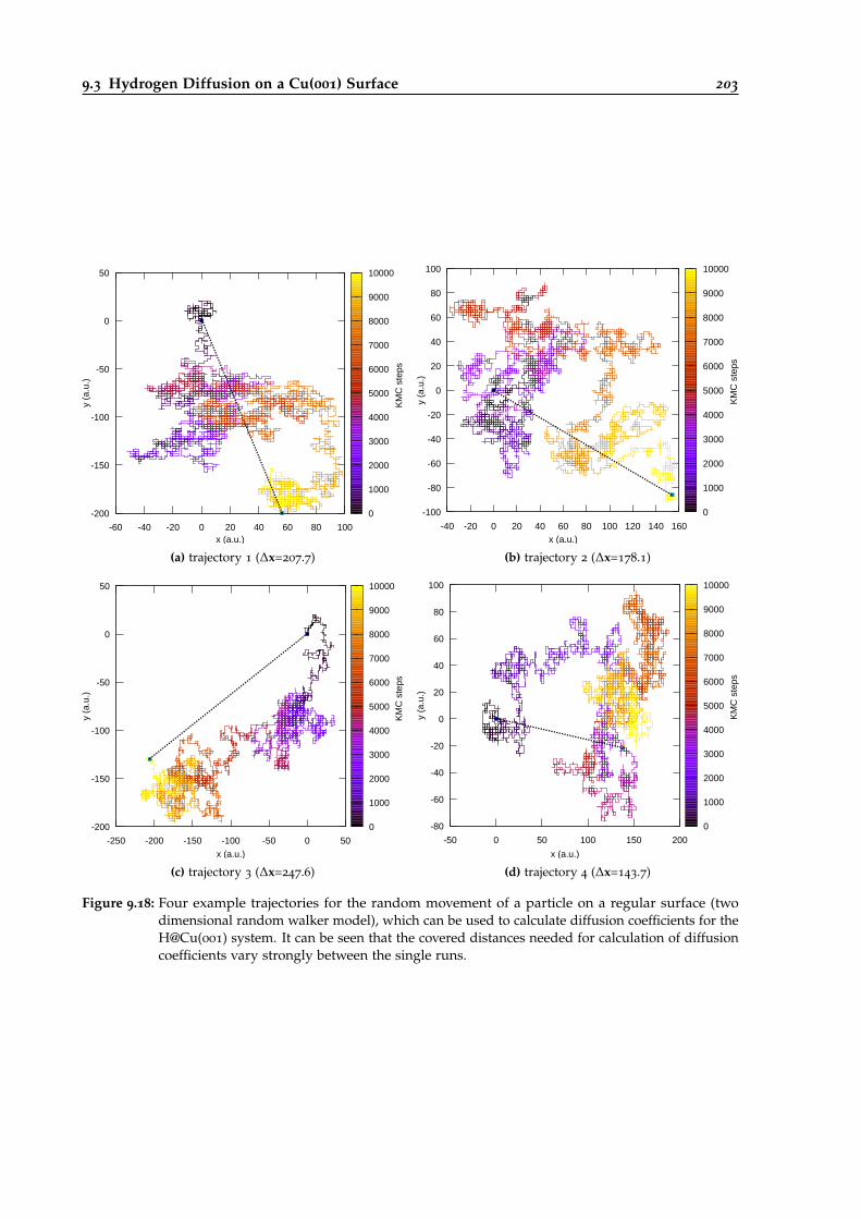
9.3 Hydrogen Diffusion on a Cu(001) Surface 203
-200
-150
-100
-50
0
50
-60 -40 -20 0 20 40 60 80 100
y (a
.u.)
x (a.u.)
0
1000
2000
3000
4000
5000
6000
7000
8000
9000
10000
KM
C s
teps
(a) trajectory 1 (∆x=207.7)
-100
-80
-60
-40
-20
0
20
40
60
80
100
-40 -20 0 20 40 60 80 100 120 140 160
y (a
.u.)
x (a.u.)
0
1000
2000
3000
4000
5000
6000
7000
8000
9000
10000
KM
C s
teps
(b) trajectory 2 (∆x=178.1)
-200
-150
-100
-50
0
50
-250 -200 -150 -100 -50 0 50
y (a
.u.)
x (a.u.)
0
1000
2000
3000
4000
5000
6000
7000
8000
9000
10000
KM
C s
teps
(c) trajectory 3 (∆x=247.6)
-80
-60
-40
-20
0
20
40
60
80
100
-50 0 50 100 150 200
y (a
.u.)
x (a.u.)
0
1000
2000
3000
4000
5000
6000
7000
8000
9000
10000
KM
C s
teps
(d) trajectory 4 (∆x=143.7)
Figure 9.18: Four example trajectories for the random movement of a particle on a regular surface (twodimensional random walker model), which can be used to calculate diffusion coefficients for theH@Cu(001) system. It can be seen that the covered distances needed for calculation of diffusioncoefficients vary strongly between the single runs.
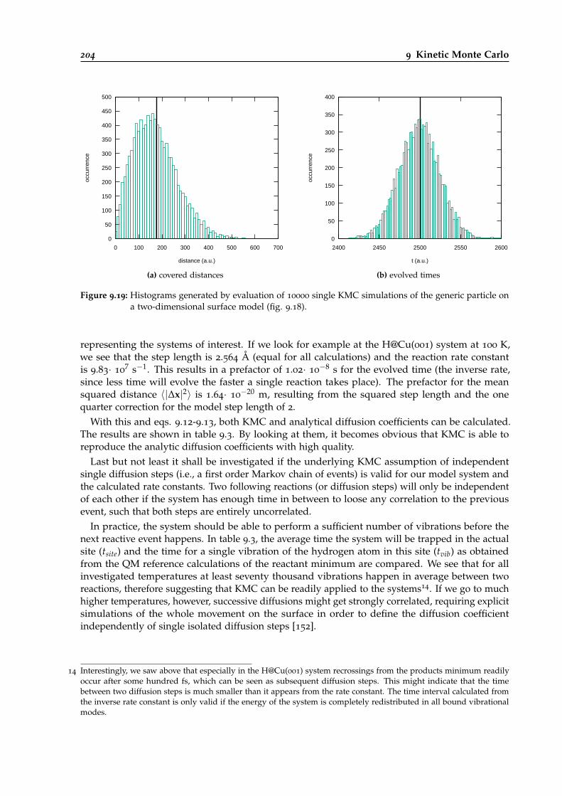
204 9 Kinetic Monte Carlo
0
50
100
150
200
250
300
350
400
450
500
0 100 200 300 400 500 600 700
occu
rren
ce
distance (a.u.)
(a) covered distances
0
50
100
150
200
250
300
350
400
2400 2450 2500 2550 2600
occu
rren
ce
t (a.u.)
(b) evolved times
Figure 9.19: Histograms generated by evaluation of 10000 single KMC simulations of the generic particle ona two-dimensional surface model (fig. 9.18).
representing the systems of interest. If we look for example at the H@Cu(001) system at 100 K,we see that the step length is 2.564 Å (equal for all calculations) and the reaction rate constantis 9.83· 10
7 s−1. This results in a prefactor of 1.02· 10−8 s for the evolved time (the inverse rate,
since less time will evolve the faster a single reaction takes place). The prefactor for the meansquared distance 〈|∆x|2〉 is 1.64· 10
−20 m, resulting from the squared step length and the onequarter correction for the model step length of 2.
With this and eqs. 9.12-9.13, both KMC and analytical diffusion coefficients can be calculated.The results are shown in table 9.3. By looking at them, it becomes obvious that KMC is able toreproduce the analytic diffusion coefficients with high quality.
Last but not least it shall be investigated if the underlying KMC assumption of independentsingle diffusion steps (i.e., a first order Markov chain of events) is valid for our model system andthe calculated rate constants. Two following reactions (or diffusion steps) will only be independentof each other if the system has enough time in between to loose any correlation to the previousevent, such that both steps are entirely uncorrelated.
In practice, the system should be able to perform a sufficient number of vibrations before thenext reactive event happens. In table 9.3, the average time the system will be trapped in the actualsite (tsite) and the time for a single vibration of the hydrogen atom in this site (tvib) as obtainedfrom the QM reference calculations of the reactant minimum are compared. We see that for allinvestigated temperatures at least seventy thousand vibrations happen in average between tworeactions, therefore suggesting that KMC can be readily applied to the systems14. If we go to muchhigher temperatures, however, successive diffusions might get strongly correlated, requiring explicitsimulations of the whole movement on the surface in order to define the diffusion coefficientindependently of single isolated diffusion steps [152].
14 Interestingly, we saw above that especially in the H@Cu(001) system recrossings from the products minimum readilyoccur after some hundred fs, which can be seen as subsequent diffusion steps. This might indicate that the timebetween two diffusion steps is much smaller than it appears from the rate constant. The time interval calculated fromthe inverse rate constant is only valid if the energy of the system is completely redistributed in all bound vibrationalmodes.
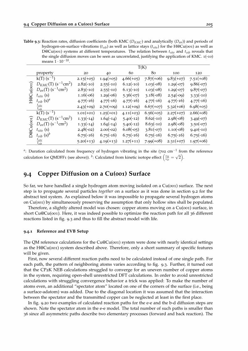
9.4 Copper Diffusion on a Cu(001) Surface 205
Table 9.3: Reaction rates, diffusion coefficients (both KMC (DKMC) and analytically (Dan)) and periods ofhydrogen-on-surface vibrations (tvib) as well as lattice stays (tsite) for the H@Cu(001) as well asD@Cu(001) systems at different temperatures. The relation between tsite and tvib reveals thatthe single diffusion moves can be seen as uncorrelated, justifying the application of KMC. 1(-10)means 1 · 10−10.
T(K)property 20 40 60 80 100 120
H@
Cu(
00
1)
k(T) (s−1) 2.15(+05) 1.94(+05) 4.66(+05) 7.87(+06) 9.83(+07) 7.51(+08)DKMC(T) (s−1cm2) 2.82(-10) 2.55(-10) 6.12(-10) 1.03(-08) 1.29(-07) 9.86(-07)Dan(T) (s−1cm2) 2.83(-10) 2.55(-10) 6.13(-10) 1.03(-08) 1.29(-07) 9.87(-07)tsite (s) 1.16(-06) 1.29(-06) 5.36(-07) 3.18(-08) 2.54(-09) 3.33(-10)tvib (s)a
4.77(-16) 4.77(-16) 4.77(-16) 4.77(-16) 4.77(-16) 4.77(-16)tsitetvib
2.43(+09) 2.70(+09) 1.12(+09) 6.67(+07) 5.32(+06) 6.98(+05)
D@
Cu(
00
1)
k(T) (s−1) 1.01(+01) 1.25(+01) 4.11(+03) 6.56(+05) 2.27(+07) 2.66(+08)DKMC(T) (s−1cm2) 1.33(-14) 1.64(-14) 5.40(-12) 8.62(-10) 2.98(-08) 3.49(-07)Dan(T) (s−1cm2) 1.33(-14) 1.64(-14) 5.40(-12) 8.63(-10) 2.98(-08) 3.50(-07)tsite (s) 2.48(-02) 2.00(-02) 6.08(-05) 3.81(-07) 1.10(-08) 9.40(-10)tvib (s)b
6.75(-16) 6.75(-16) 6.75(-16) 6.75(-16) 6.75(-16) 6.75(-16)tsitetvib
5.20(+13) 4.19(+13) 1.27(+11) 7.99(+08) 2.31(+07) 1.97(+06)
a: Duration calculated from frequency of hydrogen vibrating in the site (702 cm−1 from the reference
calculation for QMDFF1 (see above)). b: Calculated from kinetic isotope effect(
νHνD
=√
2)
.
9.4 Copper Diffusion on a Cu(001) Surface
So far, we have handled a single hydrogen atom moving isolated on a Cu(001) surface. The nextstep is to propagate several particles together on a surface as it was done in section 9.2 for theabstract test system. As explained below it was impossible to propagate several hydrogen atomson Cu(001) by simultaneously preserving the assumption that only hollow sites shall be populated.
Therefore, a slightly altered model was chosen: copper atoms moving on a Cu(001) surface, inshort Cu@Cu(001). Here, it was indeed possible to optimize the reaction path for all 36 differentreactions listed in fig. 9.3 and thus to fill the abstract model with life.
9.4.1 Reference and EVB Setup
The QM reference calculations for the Cu@Cu(001) system were done with nearly identical settingsas the H@Cu(001) system described above. Therefore, only a short summary of specific featureswill be given.
First, now several different reaction paths need to be calculated instead of one single path. Foreach path, the pattern of neighboring atoms varies according to fig. 9.3. Further, it turned outthat the CP2K NEB calculations struggled to converge for an uneven number of copper atomsin the system, requiring open-shell unrestricted DFT calculations. In order to avoid unrestrictedcalculations with struggling convergence behavior a trick was applied: To make the number ofatoms even, an additional “spectator atom” located on one of the corners of the surface (i.e., beinga surface-adatom) was added. Due to the diagonal location it was assumed that the interactionbetween the spectator and the transmitted copper can be neglected at least in the first place.
In fig. 9.20 two examples of calculated reaction paths for the e-e and the b-d diffusion steps areshown. Note the spectator atom in the e-e model. The total number of such paths is smaller than36 since all asymmetric paths describe two elementary processes (forward and back reaction). The
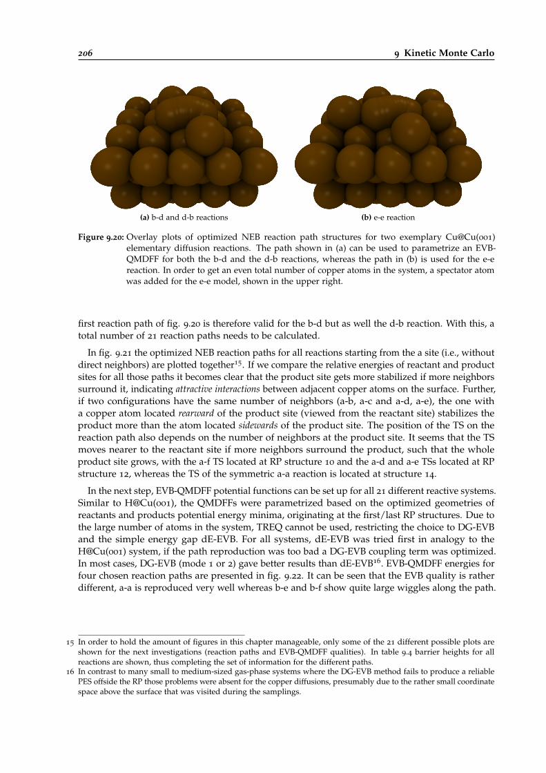
206 9 Kinetic Monte Carlo
(a) b-d and d-b reactions (b) e-e reaction
Figure 9.20: Overlay plots of optimized NEB reaction path structures for two exemplary Cu@Cu(001)elementary diffusion reactions. The path shown in (a) can be used to parametrize an EVB-QMDFF for both the b-d and the d-b reactions, whereas the path in (b) is used for the e-ereaction. In order to get an even total number of copper atoms in the system, a spectator atomwas added for the e-e model, shown in the upper right.
first reaction path of fig. 9.20 is therefore valid for the b-d but as well the d-b reaction. With this, atotal number of 21 reaction paths needs to be calculated.
In fig. 9.21 the optimized NEB reaction paths for all reactions starting from the a site (i.e., withoutdirect neighbors) are plotted together15. If we compare the relative energies of reactant and productsites for all those paths it becomes clear that the product site gets more stabilized if more neighborssurround it, indicating attractive interactions between adjacent copper atoms on the surface. Further,if two configurations have the same number of neighbors (a-b, a-c and a-d, a-e), the one witha copper atom located rearward of the product site (viewed from the reactant site) stabilizes theproduct more than the atom located sidewards of the product site. The position of the TS on thereaction path also depends on the number of neighbors at the product site. It seems that the TSmoves nearer to the reactant site if more neighbors surround the product, such that the wholeproduct site grows, with the a-f TS located at RP structure 10 and the a-d and a-e TSs located at RPstructure 12, whereas the TS of the symmetric a-a reaction is located at structure 14.
In the next step, EVB-QMDFF potential functions can be set up for all 21 different reactive systems.Similar to H@Cu(001), the QMDFFs were parametrized based on the optimized geometries ofreactants and products potential energy minima, originating at the first/last RP structures. Due tothe large number of atoms in the system, TREQ cannot be used, restricting the choice to DG-EVBand the simple energy gap dE-EVB. For all systems, dE-EVB was tried first in analogy to theH@Cu(001) system, if the path reproduction was too bad a DG-EVB coupling term was optimized.In most cases, DG-EVB (mode 1 or 2) gave better results than dE-EVB16. EVB-QMDFF energies forfour chosen reaction paths are presented in fig. 9.22. It can be seen that the EVB quality is ratherdifferent, a-a is reproduced very well whereas b-e and b-f show quite large wiggles along the path.
15 In order to hold the amount of figures in this chapter manageable, only some of the 21 different possible plots areshown for the next investigations (reaction paths and EVB-QMDFF qualities). In table 9.4 barrier heights for allreactions are shown, thus completing the set of information for the different paths.
16 In contrast to many small to medium-sized gas-phase systems where the DG-EVB method fails to produce a reliablePES offside the RP those problems were absent for the copper diffusions, presumably due to the rather small coordinatespace above the surface that was visited during the samplings.
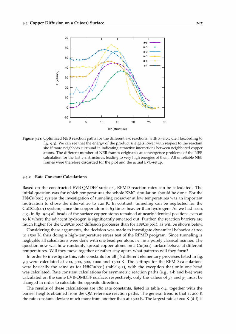
9.4 Copper Diffusion on a Cu(001) Surface 207
-10
0
10
20
30
40
50
60
70
0 5 10 15 20 25 30
E (k
J/m
ol)
RP (structure)
a-a
a-b
a-c
a-d
a-e
a-f
Figure 9.21: Optimized NEB reaction paths for the different a-x reactions, with x=a,b,c,d,e,f (according tofig. 9.3). We can see that the energy of the product site gets lower with respect to the reactantsite if more neighbors surround it, indicating attractive interactions between neighbored copperatoms. The different number of NEB frames originates at convergence problems of the NEBcalculation for the last 2-4 structures, leading to very high energies of them. All unreliable NEBframes were therefore discarded for the plot and the actual EVB-setup.
9.4.2 Rate Constant Calculations
Based on the constructed EVB-QMDFF surfaces, RPMD reaction rates can be calculated. Theinitial question was for which temperatures the whole KMC simulation should be done. For theH@Cu(001) system the investigation of tunneling crossover at low temperatures was an importantmotivation to chose the interval 20 to 120 K. In contrast, tunneling can be neglected for theCu@Cu(001) system, since the copper atom is 63 times heavier than hydrogen. As we had seen,e.g., in fig. 9.14 all beads of the surface copper atoms remained at nearly identical positions even at10 K where the adjacent hydrogen is significantly smeared out. Further, the reaction barriers aremuch higher for the Cu@Cu(001) diffusion processes than for H@Cu(001), as will be shown below.
Considering these arguments, the decision was made to investigate dynamical behavior at 200
to 1500 K, thus doing a high-temperature stress test of the RPMD program. Since tunneling isnegligible all calculations were done with one bead per atom, i.e., in a purely classical manner. Thequestion now was how randomly spread copper atoms on a Cu(001) surface behave at differenttemperatures. Will they move together or rather stay apart, what patterns will they form?
In order to investigate this, rate constants for all 36 different elementary processes listed in fig.9.3 were calculated at 200, 300, 500, 1000 and 1500 K. The settings for the RPMD calculationswere basically the same as for H@Cu(001) (table 9.2), with the exception that only one beadwas calculated. Rate constant calculations for asymmetric reaction paths (e.g., a-b and b-a) werecalculated on the same EVB-QMDFF surface, respectively, only the values of y0 and y1 must bechanged in order to calculate the opposite direction.
The results of these calculations are 180 rate constants, listed in table 9.4, together with thebarrier heights obtained from the QM reference reaction paths. The general trend is that at 200 Kthe rate constants deviate much more from another than at 1500 K. The largest rate at 200 K (d-f) is

208 9 Kinetic Monte Carlo
0
10
20
30
40
50
5 10 15 20 25
E (k
J/m
ol)
RP (a.u.)
ReferenceQMDFF(Min1)QMDFF(Min2)EVB-QMDFF
(a) a-a (DG-EVB, mode2)
0
10
20
30
40
50
60
5 10 15 20 25
E (k
J/m
ol)
RP (a.u.)
ReferenceQMDFF(Min1)QMDFF(Min2)EVB-QMDFF
(b) b-e (DG-EVB, mode1)
0
10
20
30
40
50
5 10 15 20 25
E (k
J/m
ol)
RP (a.u.)
ReferenceQMDFF(Min1)QMDFF(Min2)EVB-QMDFF
(c) b-f (DG-EVB, mode1)
0
10
20
30
40
50
60
5 10 15 20 25
E (k
J/m
ol)
RP (a.u.)
ReferenceQMDFF(Min1)QMDFF(Min2)EVB-QMDFF
(d) c-e (DG-EVB, mode1)
Figure 9.22: Four example EVB-QMDFF energy plots for arbitrarily chosen reaction paths, including noteswhich EVB coupling term was used.
9.4 Copper Diffusion on a Cu(001) Surface 209
13 orders of magnitude larger than the smallest one (e-a), whereas this difference shrinks downto less than two orders of magnitude at 1500 K. This means that the relative importance of the siteenvironment grows for lower temperatures, thus favoring more ordered structures than for highertemperatures.
9.4.3 KMC Simulations
After determination of diffusion rate constants for all 36 different processes existing in our model,we are able to do KMC simulations similar to those of section 9.2. The abstract gas atoms mentionedthere are now of course copper atoms distributed on a regular Cu(001) surface. Since gas phaseadsorption of copper seems to be rather implausible, a slightly different model was used: Insteadof starting with a clean surface that is successively populated with suddenly appearing copperatoms, the starting condition is a surface with randomly distributed atoms on it. The periodicsurface of 40 times 40 hollow sites, i.e., consisting of 1600 sites in total, is randomly populated with400 copper atoms at the beginning.
After starting the KMC simulation, no further adsorption or desorption is possible, only diffusionof the 400 present copper atoms until a clearly identifiable pattern is generated or no significantchanges happen after a certain stage of simulation.
In fig. 9.23 an example KMC trajectory of 450000 steps for the model at 300 K is shown. Shortlyafter the beginning the copper atoms are still distributed by chance (a). After 30000 steps aclear pattern can be seen, a number of small crystals has grown (b), clearly indicating attractiveinteractions, as already seen in fig. 9.21. In the following, these initial clusters merge, such that asmaller number of larger clusters dominates the surface. After 90000 steps only one cluster remains(with consideration of periodic boundaries). For the rest of the propagation, a steady state betweenthe large cluster and 10-30 single Copper atoms seems to be established.
The overall résumé is therefore that arbitrary distributed copper atoms on a Cu(001) surfacewill grow together to a large cluster behaving like an additional surface layer (if we would go toeven larger systems). This of course is no surprise since copper is solid at the temperatures andtherefore expected to build ordered and compact structures rather than single distributed atoms.
The next question is if and how this behavior changes for higher temperatures. In fig. 9.24 theresults of 400 randomly distributed copper atoms propagated for 450000 KMC steps at 200 to1500 K are shown. The resulting patterns are almost identical between 200 and 500 K: one largecluster is built, with almost all surface atoms united in it17. A significant change takes place at1000 K: Here, a rather pitted structure is built, with many atoms staying isolated around it. For1500 K, the pattern is completely burst. Here, some smaller, irregular clusters seem to be build butthey are not larger than 30-40 atoms in total. We could think that perhaps more steps are neededsince the cluster growth is slower than for lower temperatures. But even for twofold or threefoldstep numbers no significant change of this structure can be seen, indicating that this is indeed the“final” pattern the system aspires to build18.
Reviewing our insights concerning the reaction rate (table 9.4) this is of course no surprise sincethe rates for different steps resulting in cluster growth or shrinkage are becoming more and moresimilar the higher the systems temperature is. Ergo it is much less probable that all particles end inone large cluster for those higher temperatures since steps that move particles away from it willhappen much more frequent.
17 The pattern of cluster (a) in fig. 9.24 looks slightly irritating, since the right and upper boundaries are completelystraight, with irregular lower and left boundaries. Usually we would assume that no direction-specific changes in theshape should occur, because all KMC processes have the same rates for all space directions. The regular pattern in (a)might either origin in a kind of accidental seed crystal for a straight boundary, that has enlarged during the start, or ina bug of the KMC program.
18 Of course particles are still moving after a large number of steps, but now the built cluster structures are slowly movingand changing its shape, by simultaneously maintaining their characteristics, see fig. 9.23.
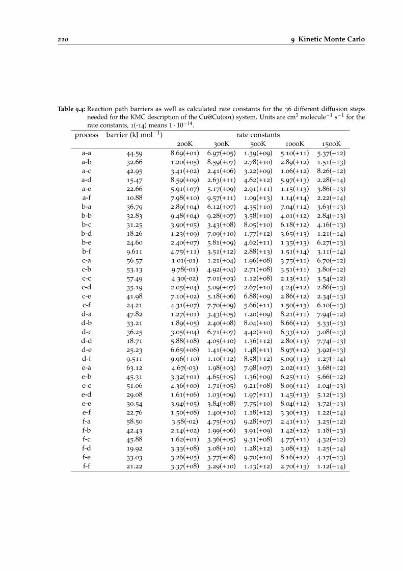
210 9 Kinetic Monte Carlo
Table 9.4: Reaction path barriers as well as calculated rate constants for the 36 different diffusion stepsneeded for the KMC description of the Cu@Cu(001) system. Units are cm3 molecule−1 s−1 for therate constants, 1(-14) means 1 · 10−14.
process barrier (kJ mol−1) rate constants200K 300K 500K 1000K 1500K
a-a 44.59 8.69(+01) 6.97(+05) 1.39(+09) 5.10(+11) 5.37(+12)a-b 32.66 1.20(+05) 8.59(+07) 2.78(+10) 2.89(+12) 1.51(+13)a-c 42.95 3.41(+02) 2.41(+06) 3.22(+09) 1.06(+12) 8.26(+12)a-d 15.47 8.59(+09) 2.63(+11) 4.62(+12) 5.97(+13) 2.28(+14)a-e 22.66 5.91(+07) 5.17(+09) 2.91(+11) 1.15(+13) 3.86(+13)a-f 10.88 7.98(+10) 9.57(+11) 1.09(+13) 1.14(+14) 2.22(+14)b-a 36.79 2.89(+04) 6.12(+07) 4.35(+10) 7.04(+12) 3.63(+13)b-b 32.83 9.48(+04) 9.28(+07) 3.58(+10) 4.01(+12) 2.84(+13)b-c 31.25 3.90(+05) 3.43(+08) 8.05(+10) 6.18(+12) 4.16(+13)b-d 18.26 1.23(+09) 7.09(+10) 1.77(+12) 3.65(+13) 1.21(+14)b-e 24.60 2.40(+07) 5.81(+09) 4.62(+11) 1.35(+13) 6.27(+13)b-f 9.611 4.75(+11) 3.51(+12) 2.88(+13) 1.51(+14) 3.11(+14)c-a 56.57 1.01(-01) 1.21(+04) 1.96(+08) 3.75(+11) 6.70(+12)c-b 53.13 9.78(-01) 4.92(+04) 2.71(+08) 3.51(+11) 3.80(+12)c-c 57.49 4.30(-02) 7.01(+03) 1.12(+08) 2.13(+11) 3.54(+12)c-d 35.19 2.05(+04) 5.09(+07) 2.67(+10) 4.24(+12) 2.86(+13)c-e 41.98 7.10(+02) 5.18(+06) 6.88(+09) 2.86(+12) 2.34(+13)c-f 24.21 4.31(+07) 7.70(+09) 5.66(+11) 1.50(+13) 6.10(+13)d-a 47.82 1.27(+01) 3.43(+05) 1.20(+09) 8.21(+11) 7.94(+12)d-b 33.21 1.89(+05) 2.40(+08) 8.04(+10) 8.66(+12) 5.33(+13)d-c 36.25 3.05(+04) 6.71(+07) 4.42(+10) 6.33(+12) 3.08(+13)d-d 18.71 5.88(+08) 4.05(+10) 1.36(+12) 2.80(+13) 7.74(+13)d-e 25.23 6.65(+06) 1.41(+09) 1.48(+11) 8.97(+12) 3.92(+13)d-f 9.511 9.96(+10) 1.10(+12) 8.58(+12) 5.09(+13) 1.27(+14)e-a 63.12 4.67(-03) 1.98(+03) 7.98(+07) 2.02(+11) 3.68(+12)e-b 45.31 3.32(+01) 4.65(+05) 1.36(+09) 6.25(+11) 5.66(+12)e-c 51.06 4.36(+00) 1.71(+05) 9.21(+08) 8.09(+11) 1.04(+13)e-d 29.08 1.61(+06) 1.03(+09) 1.97(+11) 1.45(+13) 5.12(+13)e-e 30.54 3.94(+05) 3.84(+08) 7.75(+10) 8.04(+12) 3.72(+13)e-f 22.76 1.50(+08) 1.40(+10) 1.18(+12) 3.30(+13) 1.22(+14)f-a 58.50 3.58(-02) 4.75(+03) 9.28(+07) 2.41(+11) 3.25(+12)f-b 42.43 2.14(+02) 1.99(+06) 3.91(+09) 1.42(+12) 1.18(+13)f-c 45.88 1.62(+01) 3.36(+05) 9.31(+08) 4.77(+11) 4.32(+12)f-d 19.92 3.33(+08) 3.08(+10) 1.28(+12) 3.08(+13) 1.25(+14)f-e 33.03 3.26(+05) 3.77(+08) 9.70(+10) 8.16(+12) 4.17(+13)f-f 21.22 3.37(+08) 3.29(+10) 1.13(+12) 2.70(+13) 1.12(+14)
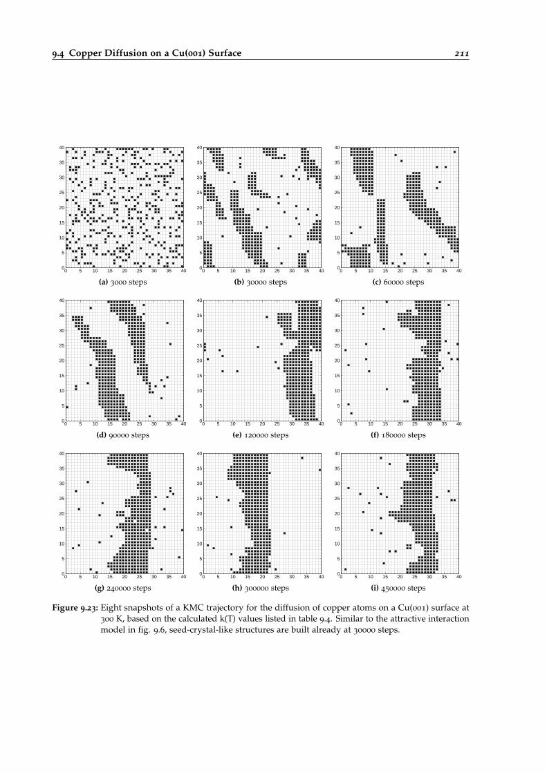
9.4 Copper Diffusion on a Cu(001) Surface 211
0
5
10
15
20
25
30
35
40
0 5 10 15 20 25 30 35 40
(a) 3000 steps
0
5
10
15
20
25
30
35
40
0 5 10 15 20 25 30 35 40
(b) 30000 steps
0
5
10
15
20
25
30
35
40
0 5 10 15 20 25 30 35 40
(c) 60000 steps
0
5
10
15
20
25
30
35
40
0 5 10 15 20 25 30 35 40
(d) 90000 steps
0
5
10
15
20
25
30
35
40
0 5 10 15 20 25 30 35 40
(e) 120000 steps
0
5
10
15
20
25
30
35
40
0 5 10 15 20 25 30 35 40
(f) 180000 steps
0
5
10
15
20
25
30
35
40
0 5 10 15 20 25 30 35 40
(g) 240000 steps
0
5
10
15
20
25
30
35
40
0 5 10 15 20 25 30 35 40
(h) 300000 steps
0
5
10
15
20
25
30
35
40
0 5 10 15 20 25 30 35 40
(i) 450000 steps
Figure 9.23: Eight snapshots of a KMC trajectory for the diffusion of copper atoms on a Cu(001) surface at300 K, based on the calculated k(T) values listed in table 9.4. Similar to the attractive interactionmodel in fig. 9.6, seed-crystal-like structures are built already at 30000 steps.
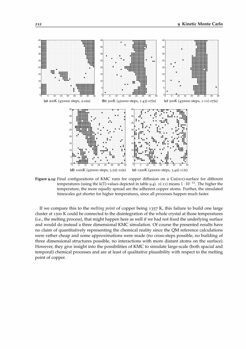
212 9 Kinetic Monte Carlo
0
5
10
15
20
25
30
35
40
0 5 10 15 20 25 30 35 40
(a) 200K (450000 steps, 2.02s)
0
5
10
15
20
25
30
35
40
0 5 10 15 20 25 30 35 40
(b) 300K (450000 steps, 1.43(-07)s)
0
5
10
15
20
25
30
35
40
0 5 10 15 20 25 30 35 40
(c) 500K (450000 steps, 1.11(-07)s)
0
5
10
15
20
25
30
35
40
0 5 10 15 20 25 30 35 40
(d) 1000K (450000 steps, 3.52(-10)s)
0
5
10
15
20
25
30
35
40
0 5 10 15 20 25 30 35 40
(e) 1500K (450000 steps, 3.42(-11)s)
Figure 9.24: Final configurations of KMC runs for copper diffusion on a Cu(001)-surface for differenttemperatures (using the k(T)-values depicted in table 9.4). 1(-11) means 1 · 10−11. The higher thetemperature, the more equally spread are the adherent copper atoms. Further, the simulatedtimescales get shorter for higher temperatures, since all processes happen much faster.
If we compare this to the melting point of copper being 1357 K, this failure to build one largecluster at 1500 K could be connected to the disintegration of the whole crystal at those temperatures(i.e., the melting process), that might happen here as well if we had not fixed the underlying surfaceand would do instead a three dimensional KMC simulation. Of course the presented results haveno claim of quantitatively representing the chemical reality since the QM reference calculationswere rather cheap and some approximations were made (no cross-steps possible, no building ofthree dimensional structures possible, no interactions with more distant atoms on the surface).However, they give insight into the possibilities of KMC to simulate large-scale (both spacial andtemporal) chemical processes and are at least of qualitative plausibility with respect to the meltingpoint of copper.
10
Ch
ap
te
r
Future Challenges
One of the basic rules of the universe is thatnothing is perfect. Perfection simply doesn’texist. Without imperfection, neither you nor Iwould exist.
(Stephen Hawking)
Instead of a summarized outlook, some of the obvious and less obvious challenges to be tackledin the future will be formulated in a handful of questions which the author (and hopefully theinterested reader too) might ask him or herself during a calm hour of intense EVB-QMDFF regardedsoul-searching.
Can we move to a true black-box method?
Looking back at chapter 6 we have seen that calculations with evb_kt_driver.x already are quitegood realizations of that what we call black-box: Once a reaction path and suitable QM methodsfor calculation of additional reference data are given, the program does the rest by itself andfinally ejects rate constants and Arrhenius parameters. But what about those first steps, namelythe calculations of reaction path and choice of suitable QM methods? By far the largest amount ofwork done for chapter 6 was invested to optimize TSs and IRCs, which often suffered from eitherwrong results (e.g., IRCs leading to other products than desired) or convergence problems.
Unfortunately, there is no way of avoiding those difficulties, since quantum chemical modelingof a new reactive system always needs some manual intervention and intellectual reflection: Areparts of the reaction path of multireference character? Should diffuse basis functions be added tocorrectly describe some dispersion interactions crucial for the mechanism? Many of those questionsneed to be answered before we can really be sure that the optimized reaction path offers a goodfoundation for a high-quality black-box calculation. Doing all this in black-box fashion seems tobe impossible, since such a black-box program should basically know everything what a goodcomputational chemist knows.
But is this really that bad? Even if the correct approach of multireference methods is far fromeasy, there are many easy to handle graphical user interface (GUI) based programs such as GaussViewavailable that try to make the correct application of QM methods possible for the average user.These utilities of course do not prevent the user from making popular mistakes like using B3LYP/6-31G(d,p) for each and every chemical system as a quasi black-box method, whose correction is
214 10 Future Challenges
certainly out of scope for the present project. The rather nasty part of setting up a rate constantcalculation, however, is now fully automated, therefore removing a large part of work.
Is TREQ really the final answer?
The TREQ method has indeed proven to be quite successful for black-box k(T) calculations at leastfor small and medium-sized systems. On the other hand we have seen that the description of thelarger urethane systems in chapter 8 was problematic. Either manual improvement of the internalcoordinate system was needed to stabilize the MD trajectories or the method was unable to describethem at all1.
Even though the definite reason for that failure is unclear so far, it can be assumed that theorthogonal projection of the actual point in coordinate space on the MEP needed for the followingTaylor series evaluation from there plays a central role. For small to medium-sized systems thisprojection should usually be clear, especially if the space of interest can be fully described interms of bond lengths and angles. If we, however, go to very large systems with high-dimensionalcoordinate space (remember the 3N− 6 scaling if N is the number of atoms!), the projection almostcertainly will become ambiguous or unstable. This might lead to sudden jumps of the projectedpositions on the MEP if the system itself moves only gradually within one time step. This jumpwill cause large changes in the gradient, potentially leading to explosions within the dynamics.
How can this deficiency be solved? If we do not want to change the mathematical foundations ofTREQ itself there seems to be little room to escape. One possibility could be to remember that thesize of the reactive center itself usually stays rather small. If we look back again to the urethanereactions in chapter 8 we have seen that the large systems still have the same reaction mechanismbut larger substituents around it. Long alkyl chains or benzene rings, however, usually do not havemuch influence on the reaction itself (some sterics and small electronic effects), but in usual TREQtheir whole coordinate space is included and complicates the projection algorithm on the MEP.
A possible solution therefore might be to subdivide the system into a reactive part which mustbe described by direct interpolation in the transition region and the remaining part (similar toQM/MM methods [294]), that could be described by either RP-EVB or the QMDFFs alone. Since thedescription of outer alkyl chains will stay identical for both reactants and products QMDFFs (i.e.,same connectivity and almost the same force constants), we also could assume that no high-leveldescription is needed for a reasonable modeling of the transition between them. The practicalimplementation might look like this: We define a subspace of internal coordinates which arelocated in the reactive part of the system. Then we project the reference gradients and Hessianson those as it is done for usual TREQ so far. Energy and gradient for the atoms in this part arefully defined by the direct interpolation. The neighbored atoms, however, are described by, e.g.,RP-EVB, where a small set of coordinates is enough since the QMDFFs act as a stable foundationof the surface. Possibly a smooth switching will be needed between the reactive part and the outeralkyl chains of the substituents.
Such a partitioning certainly will become quite complicated, we should, for instance, investigatefor each atom how much its gradient components change during the reaction in order to allocate itto a reactive or less reactive part of the system, however, we should remember that TREQ was notdesigned to be mathematically elegant or nice to look at. It was designed to avoid any manualintervention in its setup! Therefore, if we are able to automate a very complicated setup such thatit will work for (almost) any system, we do not need to worry about it.
If those problems are solved someday, another issue might be that of very high quality descriptions.So far, only a second order Taylor series is used to describe regions offside the reaction path. It is
1 Another possibility for those problems could be that the RPMD algorithm itself is proven to be unstable as well, aproblem that might get worse for large systems [293]. We will not discuss this point here in more detail, since there isno easy way to solve it.
215
not possible to improve this description so far, thus no convergence to exactness (with respect to theQM reference method) can be achieved even if large amounts of computational power are available.To enable such convergence the Taylor expansion perpendicular to the MEP could be expanded. Thestraightforward method would be to simply add the cubic term of the Taylor expansion. This term,however, needs the third derivatives of the QM method, which are very expensive to calculate evenfor rather small systems. The only reasonable way would be to avoid their full calculation butinstead to construct an approximated correction, e.g., by randomly calculating energies of pointsfarther offside the MEP and to optimize some internal coordinate specific correction terms to them.
Can we describe polymerization processes?
This question looks rather specific. It becomes relevant, however, if our cooperation with Covestrofor the theoretical description of urethane reactions is reconsidered (chapter 8). There we havecalculated rate constants for rather small urethane systems, i.e., of single monomers comingtogether and starting a new polymer chain. In reality those reactions will mainly occur at theends of already growing chains or even by merging of two large chains. One central questiontherefore is how the reaction rate constants are affected by the growing polymer chain. Does thepolymerization proceed with equal speed if the attached chain grows or is it accelerated or is itslowed down?
This problem reveals quite a broad field to be investigated: We have seen in the last sectionof the chapter that no 8-ring autocatalysis is possible for the reaction of NDI with methanol. Ifthe substituents of the alcohols grow, will the 6-ring reaction still be possible or could the sterichindrance of long polymer substituents become too large even for this mechanism? Besides thissteric problem at the reaction site, stabilizations via hydrogen bonds between urethane, isocyanateand alcohol groups of the substituents might as well play an important role. Further, electroniceffects (+I,-I) of the side chains might also influence the reaction by raising/lowering the reactionbarrier. If we consider in the first place a study of rate constants depending on growing side chainsof one involved alcohol molecule, we could repeat rate constants calculations for one monomer(e.g., butandiol), the monomer reacted with an diisocyanate (A-I), with the diisocyanate reactedwith another alcohol (A-I-A) and so forth. These calculations could be done from scratch, i.e.,optimizing TS and IRC for the different chains, parametrizing TREQ and do the k(T) calculationswith RPMD.
Considering the unfavorable scaling of QM methods with system size, it becomes clear that“direct” calculations of very long chains containing hundreds of atoms are essentially out of reacheven if DFT methods are used as reference. A possible loophole is to make the central property of apolymer chain (e.g., being a succession of identical subunits) part of the PES construction. Insteadof calculating the whole system and generate QMDFFs as well as EVB from its reference data,we might think of a modular approach. We then would calculate, for instance, the full set of QMreference data for the 6-ring reaction of an isocyanate with a diol molecule that itself already hasformed another urethane bond with an additional isocyanate. After calculation of QM referencedata and generation of QMDFF files, we take a further look at the QMDFFs.
As explained in section 2.3, the QM reference information from Hessian, bond orders, chargesand equilibrium geometry is transformed into a bunch of covalent force field terms, each consistingof involved atom indices, equilibrium values and force constants and some noncovalent ones,depending on distances, charges and global parameters. If we now pick the atoms of the alcohol-isocyanate side chain that shall be polymerized, we could build a polymer structure from them,e.g., by simply plugging the same unit many times together, with adequate cartesian translationof the single unit’s atoms. All partial charges stay identical for the units, as well as the forceconstants of their internal coordinates. We then must consider inter-unit interactions. These arefirst noncovalent interactions like dispersions. Their parameters are set by the QMDFF program
216 10 Future Challenges
itself such that we only need to specify all possible interaction pairs. Slightly more complicated arecovalent interactions in the transition regions between neighbored units. Here we could adopt forceconstants from other regions of the initial molecule. If, e.g., an urethane unit builds the transitionregion, we could take the force constants from the central urethane unit present in the productsQMDFF. It should be possible to automate this “QMDFF polymerization” with a separate script oras part of an EVB-QMDFF subroutine especially designed for description of polymer chains.
Besides the QMDFFs, the EVB coupling term itself should as well be polymerized. If we wouldtake the simple energy-gap coupling term, this would be trivial, since all needed changes werealready made in the QMDFFs on which the EVB term depends. Unfortunately the quality ofdE coupling has proven to be insufficient for reliable description of urethane reactions, thereforewe must use either DG-EVB or TREQ. For their treatment it is important to note that the spatialdistribution of the needed coupling strength is closely restricted to the sections of the moleculethat are taking part in the reaction. Therefore the polymerized side chains are negligible for thecoupling term. If we would use DG-EVB or RP-EVB without TS correction (or TREQ with QM-MM,see above) we usually operate in a reduced space of internal coordinates (see chapter 4), where,e.g., only built and broken bonds are included. Since all gradient and Hessian reference data isprojected onto this reduced set of internal coordinates before being used for the coupling setup, wereadily could use the QM reference data of the original system without polymerized sidechains,since all reactive coordinates will be located in it. Thus, the projection cartesian to internal operatesfrom a reduced set of cartesian information to an even further reduced set of internals. We nowcould argue that this treatment makes the whole experiment unnecessary, since the transitionregion (almost) solely depends on the coupling and this coupling is constructed to be independentof the added side chains. Since the rate constant largely depends on this transition region, noinfluence of the degree of polymerization in the side chain could be seen by construction.
Here, one central property of EVB proves to be quite helpful: The independence of the couplingterm from the molecular environment [101] (see section 2.4.2). If we parametrize an EVB-QMDFFfor a system in vacuum and now want to simulate it in a solvent, we only need to calculate theinfluence of the solvent on the diabatic surfaces, i.e., on the QMDFFs, whereas the coupling term canstay the same. If we assume that the polymer chains have similar (indirect) influence on the reactivecenter as a solvent, we therefore can indeed use reference data from the original unpolymerizedsystem for the parametrization of the coupling.
Is an online black-box k(T) portal possible?
As pointed out already in the introduction, the main objective of this thesis was to develop a methodsuitable for the average chemist. Since popular quantum chemistry programs like Gaussian [99] thatshould be known to almost every chemist in our days usually have nice GUIs (here: GaussView),the question seems to be legitimate if EVB-QMDFF itself should get a modern GUI to become moreattractive for everyone.
If we assume that most average chemists simply want to calculate rate constants and/or Arrheniusparameters for the system of interest, we can restrict that discussion to the evb_kt_driver.x
program. Looking back at its description in section 3.3.8 we saw that all needed settings canbe defined in a single qmdff.key input file. This type of handling certainly was the standardthroughout the last decades. However, it might be rather challenging to convince the average userthat obeying certain syntax for keywords or absolute paths to called programs is really up to date,especially if we look at the general development of, for instance, smartphones that try to hide asmuch “nerdy” details as possible from the user.
Therefore, it is certainly desirable to develop a program similar to GaussView where someclicks and entries in well-placed question boxes are sufficient to initiate a rate constant calculation.Similar to GaussView, which is a separate interface to the Gaussian program itself that can as well
217
be controlled in the classical way, i.e., by editing input files with text viewers, the GUI should be aseparate program, taking the role of evb_kt_driver.x, that calls the other single programs of theEVB-QMDFF program package when they are needed.
A possible design of a black-box k(T) GUI would be like that: After the user has opened it, theprogram asks for a calculated reaction path to be imported. Alternatively, it could be extendedsuch that also the TS and IRC optimization are managed with it. In this case, a molecule buildergets opened where a TS guess structure must be clicked together. Then, suitable QM programpackages are called to do the optimizations.
No matter if TS and IRC shall be calculated within the program package or not, it should searchthe system for existent QM program packages like Gaussian, Orca or Turbomole [99, 130, 132].After the IRC has been calculated or loaded, the user is asked for which direction of the path thek(T) values shall be determined. This decision is eased by animated visualizations of the reactionproceding in the chosen way. Then, the QM method for further TREQ reference calculationsmust be determined. Ideally, the program automatically reads in the level of theory used for thecalculation of the given IRC or, if the user does also the TS and IRC calculation with our program,he or she might get a drop-down menu similar to GaussView where usual methods (depending onthe availability in the located QM program packages) can be found. Such a menu is needed as wellfor higher-level energy corrections of the path.
After those settings are determined, the QM reference calculations (QMDFF minima as well asTREQ gradient/Hessian reference) can be started. Since those might take many hours or days,a progress-update indicating the quality of the single calculations might be very desirable. Aschematic picture of the reaction path might exist with little boxes on it representing the singlereference points. Their color might change from red to green if the reference calculation for one ofthem is finished, then offering to click on it, where, e.g., normal modes of the calculated Hessian canbe inspected in order to control if everything is alright. Similarly, the QMDFF optimizations can bemonitored, e.g., by automated evaluation of the QMDFF force constant fit (how large the deviationsbetween QMDFF and QM reference frequencies are). Settings for the RPMD calculations aredetermined in a fully automated fashion, such that the user must not care about it. Of course, theycan be altered as well, either during the QM reference calculations or after the RPMD calculationswhen, e.g., a too large variance of single k(T) values is monitored.
Moving further to the future, where cloud-computing gets more and more important, awebbrowser-based application (or an app on the smartphone) to start and manage the black-box k(T) calculations would be preferable to the local GUI, especially if probably very expensiveQM reference calculations are run that might take days on usual desktop computers. Locating thecalculations on high-performing computing centers allows the user to turn off his or her desktopPC and look on the progress via the webpage. Depending on the field of application (researchor industry) suitable models for accessing those central computing facilities should of course bedeveloped as well. To finally answer the question: Yes, online black-box k(T) calculations arecertainly possible.
What if we want to describe reactions in solution?
All reactions calculated in this thesis are thermal gas phase reactions on the electronic ground state.In chemical reality, however, most reactions of interest are taking place in solution. Therefore itwould be preferable to include the influence of solvents into our black-box protocol. There are twoways of doing this.
First, implicit solvation could be used [295]. Here, the surrounding solvent molecules areapproximated by modeling their electrostatic effects on the reaction of interest. Implicit solvationshould be included into the QM reference calculation by, e.g., using COSMO [296].
218 10 Future Challenges
Second, the solvent might be added explicitly by simulating the reaction in a solvent box. Thisleads to a multi scale model, where the reactive system itself (or maybe only its reactive center, seeabove) is described with TREQ and the solvent molecules around it with a traditional nonreactiveforce field. Further, we should restrict the RPMD description to the reactive system, such that thiswould be described by, e.g., 8 or 16 beads, whereas all solvent molecules are still described by onebead. Interactions between the RPMD beads and the solvent molecules are then simply summedup over all replicas, divided through the number of beads, i.e., the solvent sees, e.g., one eighth ofeach replica. Such RPMD-classical hybrid simulations, mostly for single particles like protons orelectrons in classical environments, were already done by several authors [152, 297, 298].
The main issue is how good TREQ can be combined with a solvent environment. We havelearned that EVB is able to include solvent interactions by modifying the diabatic surfaces (section2.4.2). Further studies should now made how the direct interpolation part in TREQ is affected byinteractions with solvent molecules.
How can we get to large-scale chemical systems?
The black-box rate constant methodology was applied to single elementary reactions so far. Inchapter 9, though, we have seen that the KMC method is able to describe a whole ensemble ofreactive sites by reducing single reactive events to state changes whose incidence is determined bythe pre-calculated rate constants.
There, only very simple diffusions of gas or metal atoms on metal surfaces were treated, with verylittle relevance for most kinetical descriptions. If we look on the field of heterogeneous catalysis,though, we see that reactions happening on metal surfaces can be indeed of great importance. TheKMC algorithm presented in chapter 9 is able to include those more complex events as well.
If we consider a metal surface which acts as a catalyst for the subsequent assembling of smallgas-phase molecules to the desired products, all reactions will still happen on the various sites ofthe metal surface. Depending on the partial pressure of the components (e.g., A, B and C), theywill randomly spawn on the surface with different probabilities. If two possible reactants (A and B)are located on neighbored sites, a reaction event will happen with a certain rate that merges bothto a new molecule (A+B −→ D) that will either occupy one of the sites or leave to the gas phase,changing its respective partial pressure and thus its probability to spawn on another free site. Thissimple model can of course be made much more complicated, for instance, by introducing morekinds of reactants and intermediates, different ways to react (depending on the relative locations ofthe occupied sites on the surface) and so forth. Rate constants for all possible processes can then becalculated with EVB-QMDFF-RPMD and subsequently added to the growing KMC model.
If we move to other kinds of reactions, e.g., polyurethane synthesis, the system is much morecomplicated: It is three-dimensional and has no discrete sites located in cartesian space betweenwhich the system can move or distinct reactions can happen. Instead, reactions might happeneverywhere where the reactive groups approach each other in space.
Fortunately, there also exist off-lattice KMC methods [270]. Here, the system is propagated incartesian space with usual Monte Carlo sampling until two molecular groups approach each other.Then, it is evaluated if a reaction takes place or not, depending on the calculated reaction rate.If the detected possible reaction is not listed in our global arrays so far, its rate constant mightbe calculated on the fly by the black-box program and added to the table. In the case of urethanereactions, only a limited number of reactions are interesting for us. Therefore we can calculatetheir rates in advance and propagate the system with off-lattice KMC, where this method should beoptimized for the usage with polymer chains in solution. Off-lattice KMC will of course also workfor several other kinds of reactive systems either in the gas phase or in solution.

11
Ch
ap
te
r
Appendix
11.1 Supervised Projects
In line with this thesis, four lab courses were supervised by me: two advanced lab courses intheoretical chemistry (“F3”), one lab course being part of the theoretical chemistry compulsoryelective core subject (“F2”) and one voluntary short-term course. Depending on the status my workhad at these points in time, different tasks were offered to the four participants, from which two ofthem wrote a protocol as well. The most important parts of their results, especially if they had animpact on the further development of my whole work, shall be described here briefly.
11.1.1 Jan-Moritz Adam
Jan-Moritz Adam did an advanced lab course between March and May 2016, i.e., quite shortlyafter I began my PhD. At this time, the EVB-QMDFF program was in the early stages of version 3
(section 3.1); the coupling to RPMDrate was not done yet and only DG-EVB version 1 (i.e., energiesas reference) was implemented. He tried to setup EVB-QMDFF for some small reactions which hechose from the NIST Chemical Kinetics Database [153].
Two of these reactions were NH3+OH −→ NH2+H2O and CH3F+CH2Cl −→ CH2F+CH3Cl.Besides the manual calculation of reference data for both QMDFF and DG-EVB, he wrote a firstscript that automated the choice of structures and energies along the reaction path to be used forthe DG-EVB setup. With different sets of internal coordinates he tried to reproduce the referenceenergies along the reaction paths as well as possible.
Unfortunately he aborted the lab course before final results were obtained. His automatedDG-EVB reference energy script however was indeed one of the first small early steps for that whatis now known as the black-box TREQ setup.
11.1.2 Jennifer Müller
Jennifer Müller did her advanced lab course between August and September 2017. At this time,program version 3 was completed and, after publication of the second EVB-QMDFF paper, I appliedthe DG-EVB-k(T) calculation method to as many example reactions as possible in order to researchits abilities and limitations (of which, sadly, many existed).
Jennifer assisted me in this task and chose a number of reactions for which experimental data wasavailable. She did the QM reference calculations and optimized the respective DG-EVB couplingterms, where the number of DG-EVB reference points, the set of internal coordinates for thecoupling and the DG-EVB mode were varied until the reference path was reproduced as well aspossible.
220 11 Appendix
The first set of reactions were radical hydrogen abstractions of hydroxyl from primary, secondaryand tertiary carbon atoms:
CH3CH3 + OH −→ CH3CH2 + H2O, (11.1)
(CH3)2CH3 + OH −→ (CH3)2CH2 + H2O, (11.2)
(CH3)3CH3 + OH −→ (CH3)3CH2 + H2O. (11.3)
QM references for all three reactions were calculated with MP2/cc-pVTZ. For reaction 11.1DG-EVB mode 2 with 9 reference points along the path was used, the forming O-H and breakingC-H bonds as well as two other distances in the reactive area were chosen as internal couplingcoordinates. In the case of reaction 11.2, DG-EVB mode 3 with 6 DG-EVB points and the formingO-H and breaking C-H bonds as internal coordinates gave good results. For all following reactions,the smallest possible internal coordinate set of breaking and forming bond was sufficient. Reaction11.3 was calculated with the same settings as 11.2. The resulting DG-EVB energies are plottedtogether with both QMDFF- and QM reference energies in fig. 11.1. We can see that DG-EVB isable to reproduce the reference path with high quality in all cases.
The second set of reactions were bimolecular nucleophilic substitutions of monocholormethanewith fluoride, cyanide and isocyanide anions:
CH3Cl + F− −→ CH3F + Cl−, (11.4)
CH3Cl + CN− −→ CH3CN + Cl−, (11.5)
CH3Cl + NC− −→ CH3NC + Cl−. (11.6)
Here, the calculation of QM reference data was slightly more demanding, both MP2/cc-pVTZand PBE0/aug-cc-pVTZ were used as methods of choice. For reaction 11.4 the IRC calculationsdid not converge, the reaction path was therefore parametrized with two bond length scans (ofboth breaking and forming bonds). DG-EVB mode 3 with 8 reference points gave the best results.The reactions 11.5 and 11.6 are very similar. IRC calculations failed for both of them, and weretherefore replaced with bond length scans. Parametrization of DG-EVB was done again with mode3, 8 reference points and the minimal set of internal coordinates. The resulting energies are shownin fig. 11.1, where for reaction 11.4 the parametrization with respect to the PBE0 path is taken,in contrast to the MP2 paths of both 11.5 and 11.6. Very good agreements between DG-EVB andreference can be seen again.
Based on these DG-EVB PESs, Jennifer did rate constant calculations with the RPMDrate programfor 300 K and 16 (reactions 11.1-11.3) or 8 (reactions 11.4-11.6) beads, depending on the amountof tunneling to be expected. The results are shown in table 11.1. Unfortunately the method onlygave useful results for three of six systems. For the others, severe complications in the umbrellasamplings, resulting in damaged free energy curves and thus useless rate constants, occurred.Presumable reasons were the difficulties of DG-EVB to guarantee a smooth description of the wholeaccessible PES offside the reaction path.
Jennifer’s work gave important insights into the apparent problems of DG-EVB: Even if reactionpaths are reproduced with very good quality, the whole PES accessible during RPMD umbrellasamplings might be insufficient. It constituted one of the motivations that led to the developmentof TREQ.
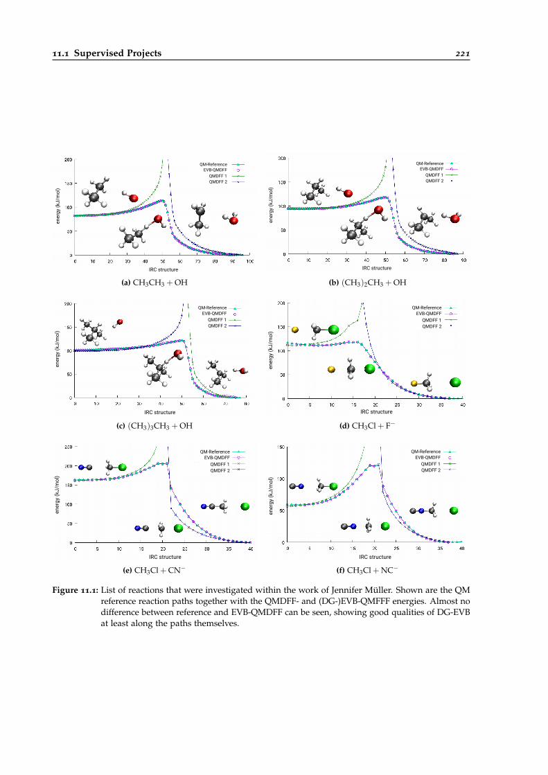
11.1 Supervised Projects 221
QM-ReferenceEVB-QMDFF
QMDFF 1 QMDFF 2
IRC structure
ener
gy (
kJ/m
ol)
(a) CH3CH3 + OH
QM-ReferenceEVB-QMDFF
QMDFF 1 QMDFF 2
IRC structureen
ergy
(kJ
/mol
)
(b) (CH3)2CH3 + OH
QM-ReferenceEVB-QMDFF
QMDFF 1 QMDFF 2
IRC structure
ener
gy (
kJ/m
ol)
(c) (CH3)3CH3 + OH
QM-ReferenceEVB-QMDFF
QMDFF 1 QMDFF 2
IRC structure
ener
gy (
kJ/m
ol)
(d) CH3Cl + F−
QM-ReferenceEVB-QMDFF
QMDFF 1 QMDFF 2
IRC structure
ener
gy (
kJ/m
ol)
(e) CH3Cl + CN−
QM-ReferenceEVB-QMDFF
QMDFF 1 QMDFF 2
IRC structure
ener
gy (
kJ/m
ol)
(f) CH3Cl + NC−
Figure 11.1: List of reactions that were investigated within the work of Jennifer Müller. Shown are the QMreference reaction paths together with the QMDFF- and (DG-)EVB-QMFFF energies. Almost nodifference between reference and EVB-QMDFF can be seen, showing good qualities of DG-EVBat least along the paths themselves.
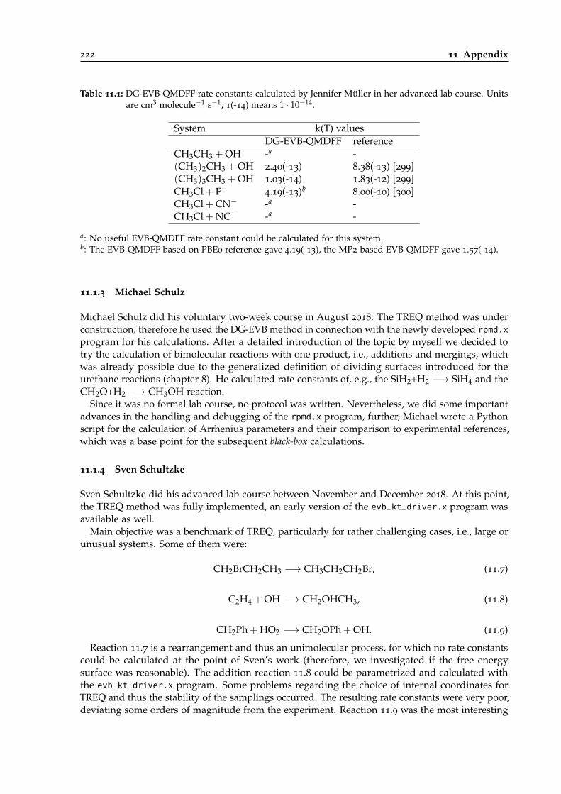
222 11 Appendix
Table 11.1: DG-EVB-QMDFF rate constants calculated by Jennifer Müller in her advanced lab course. Unitsare cm3 molecule−1 s−1, 1(-14) means 1 · 10−14.
System k(T) valuesDG-EVB-QMDFF reference
CH3CH3 + OH -a -(CH3)2CH3 + OH 2.40(-13) 8.38(-13) [299](CH3)3CH3 + OH 1.03(-14) 1.83(-12) [299]CH3Cl + F− 4.19(-13)b
8.00(-10) [300]CH3Cl + CN− -a -CH3Cl + NC− -a -
a: No useful EVB-QMDFF rate constant could be calculated for this system.b: The EVB-QMDFF based on PBE0 reference gave 4.19(-13), the MP2-based EVB-QMDFF gave 1.57(-14).
11.1.3 Michael Schulz
Michael Schulz did his voluntary two-week course in August 2018. The TREQ method was underconstruction, therefore he used the DG-EVB method in connection with the newly developed rpmd.x
program for his calculations. After a detailed introduction of the topic by myself we decided totry the calculation of bimolecular reactions with one product, i.e., additions and mergings, whichwas already possible due to the generalized definition of dividing surfaces introduced for theurethane reactions (chapter 8). He calculated rate constants of, e.g., the SiH2+H2 −→ SiH4 and theCH2O+H2 −→ CH3OH reaction.
Since it was no formal lab course, no protocol was written. Nevertheless, we did some importantadvances in the handling and debugging of the rpmd.x program, further, Michael wrote a Pythonscript for the calculation of Arrhenius parameters and their comparison to experimental references,which was a base point for the subsequent black-box calculations.
11.1.4 Sven Schultzke
Sven Schultzke did his advanced lab course between November and December 2018. At this point,the TREQ method was fully implemented, an early version of the evb_kt_driver.x program wasavailable as well.
Main objective was a benchmark of TREQ, particularly for rather challenging cases, i.e., large orunusual systems. Some of them were:
CH2BrCH2CH3 −→ CH3CH2CH2Br, (11.7)
C2H4 + OH −→ CH2OHCH3, (11.8)
CH2Ph + HO2 −→ CH2OPh + OH. (11.9)
Reaction 11.7 is a rearrangement and thus an unimolecular process, for which no rate constantscould be calculated at the point of Sven’s work (therefore, we investigated if the free energysurface was reasonable). The addition reaction 11.8 could be parametrized and calculated withthe evb_kt_driver.x program. Some problems regarding the choice of internal coordinates forTREQ and thus the stability of the samplings occurred. The resulting rate constants were very poor,deviating some orders of magnitude from the experiment. Reaction 11.9 was the most interesting

11.2 Theoretical Details and Derivations 223
one: Initially the RPMD dynamics exploded almost instantly and the reason was not clear. Laterwe found out that the standard choice of internal coordinates consisting of bond lengths andangles was insufficient to describe the benzene ring. Addition of newly implemented dihedralsand out-of-plane angles finally made it possible to do the samplings, the resulting rate constantat 300 K (4.0· 10
11 cm3 mol−1 s−1) was close to the experimental value (1.2· 1011 cm3 mol−1 s−1).
Samplings at higher temperatures still suffered from instability.This most recent lab course was important for the improvement of the TREQ method as well
as for the final implementation steps of evb_kt_driver.x. Further, the elaborate error-handlingfeatures of rpmd.x could be improved based on Sven’s findings concerning PES instabilities.
11.2 Theoretical Details and Derivations
11.2.1 Schrödinger Equation from Path Integrals
In order to clarify the correspondence between the path integral and the Schrödinger picture ofquantum mechanics, a short proof shall be given that the popular differential formulation of QMis indeed identical to the path PI introduced in section 2.1.5, by obtaining the time dependentSchrödinger equation from the PI propagator [50]. In order to get to the differential formulation, itis useful to introduce wave functions.
As noted in section 2.1.5, a kernel describes the probability of going from location a to b. If weinclude the time as parameter, the kernel for one dimension can be defined as: K(xb, tb, xa, ta).Thus, it describes the probability for a particle being at xb at time tb under the condition that it wasat xa at time ta. The wave function ψ(xb, tb) describes also a quantum mechanical amplitude ofbeing at xb at time tb, but no matter from which position the particle has actually started.
Both kernel and wave function are adequate for a complete description of a quantum mechanicalsystem, i.e., we can calculate its state for all future time if K(xb, tb, xa, ta) or ψ(xb, tb) are known.The kernel can also be used to propagate a wave function in time: The probability of arriving at xbat time tb can be calculated from the wave function ψ(xc, tc) (arriving at xc at time tc), multipliedby the amplitude to go from c to b, integrated over all possible values of xc:
ψ(xb, tb) =∫ ∞
−∞K(xb, tb, xc, tc)ψ(xc, tc)dxc. (11.10)
In order to get to the Schrödinger equation, which shall also describe the time evolution of awave function, but not by integrals, a differential description is needed. Our task is to transform anintegral equation into a differential equation. Therefore, an infinitesimal time step is considered, i.e.,tb = tc + ε.
Now, eq. 11.10 can be specified for this situation, where the particle shall be at y before thepropagation and at x after the propagation, when ε was added to the actual time:
ψ(x, t + ε) =1A
∫ ∞
−∞exp
[ih
εL(
x− yε
,x + y
2
)]ψ(y, t)dy. (11.11)
Here, the general expression for the kernel (eq. 2.70) was used and simplified: Since we only lookat an infinitesimal step, only one single intersection is evaluated for all paths, resulting in one singleintegral over all y. For the infinitesimal step, the action (i.e., the time integral of the Lagrangian) can
be approximated by a single box of height L(x, x) and width ε: S[a, b] =∫ tb
taL(x, x, t)dt ≈ εL(x, x).
Further, actual position x+y2 and velocity x−y
ε are approximated linearly in terms of start andend points.
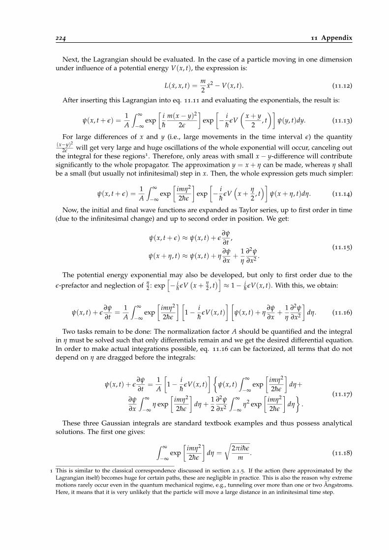
224 11 Appendix
Next, the Lagrangian should be evaluated. In the case of a particle moving in one dimensionunder influence of a potential energy V(x, t), the expression is:
L(x, x, t) =m2
x2 −V(x, t). (11.12)
After inserting this Lagrangian into eq. 11.11 and evaluating the exponentials, the result is:
ψ(x, t + ε) =1A
∫ ∞
−∞exp
[ih
m(x− y)2
2ε
]exp
[− i
hεV(
x + y2
, t)]
ψ(y, t)dy. (11.13)
For large differences of x and y (i.e., large movements in the time interval ε) the quantity(x−y)2
2ε will get very large and huge oscillations of the whole exponential will occur, canceling outthe integral for these regions1. Therefore, only areas with small x− y-difference will contributesignificantly to the whole propagator. The approximation y = x + η can be made, whereas η shallbe a small (but usually not infinitesimal) step in x. Then, the whole expression gets much simpler:
ψ(x, t + ε) =1A
∫ ∞
−∞exp
[imη2
2hε
]exp
[− i
hεV(
x +η
2, t)]
ψ(x + η, t)dη. (11.14)
Now, the initial and final wave functions are expanded as Taylor series, up to first order in time(due to the infinitesimal change) and up to second order in position. We get:
ψ(x, t + ε) ≈ ψ(x, t) + ε∂ψ
∂t,
ψ(x + η, t) ≈ ψ(x, t) + η∂ψ
∂x+
1η
∂2ψ
∂x2 .(11.15)
The potential energy exponential may also be developed, but only to first order due to theε-prefactor and neglection of η
2 : exp[− i
h εV(
x + η2 , t)]≈ 1− i
h εV(x, t). With this, we obtain:
ψ(x, t) + ε∂ψ
∂t=
1A
∫ ∞
−∞exp
[imη2
2hε
] [1− i
hεV(x, t)
] [ψ(x, t) + η
∂ψ
∂x+
1η
∂2ψ
∂x2
]dη. (11.16)
Two tasks remain to be done: The normalization factor A should be quantified and the integralin η must be solved such that only differentials remain and we get the desired differential equation.In order to make actual integrations possible, eq. 11.16 can be factorized, all terms that do notdepend on η are dragged before the integrals:
ψ(x, t) + ε∂ψ
∂t=
1A
[1− i
hεV(x, t)
]{ψ(x, t)
∫ ∞
−∞exp
[imη2
2hε
]dη+
∂ψ
∂x
∫ ∞
−∞η exp
[imη2
2hε
]dη +
12
∂2ψ
∂x2
∫ ∞
−∞η2 exp
[imη2
2hε
]dη
}.
(11.17)
These three Gaussian integrals are standard textbook examples and thus possess analyticalsolutions. The first one gives:
∫ ∞
−∞exp
[imη2
2hε
]dη =
√2πihε
m. (11.18)
1 This is similar to the classical correspondence discussed in section 2.1.5. If the action (here approximated by theLagrangian itself) becomes huge for certain paths, these are negligible in practice. This is also the reason why extrememotions rarely occur even in the quantum mechanical regime, e.g., tunneling over more than one or two Ångstroms.Here, it means that it is very unlikely that the particle will move a large distance in an infinitesimal time step.

11.2 Theoretical Details and Derivations 225
Now, the normalization factor A can already be determined. Consider the case that the infinites-imal time interval ε becomes zero. Then, eq. 11.17 must still be valid. On the left, only ψ(x, t)
remains. On the right, ψ(x, t) has the prefactor 1A
√2πihε
m . With this, it becomes clear that
A =
√2πihε
m. (11.19)
Two integrals remain. The second integral,∫ ∞
−∞η exp
[imη2
2hε
]dη is zero, since an uneven function
is integrated over a symmetric interval. The last integral becomes, with consideration of thenormalization factor:
1A
∫ ∞
−∞η2 exp
[imη2
2hε
]dη =
ihε
m. (11.20)
Inserting all this into eq. 11.17 results in:
ψ(x, t) + ε∂ψ
∂t=
[1− i
hεV(x, t)
]{ψ(x, t) +
ihε
2m∂2ψ
∂x2
}=
ψ(x, t)− ih
εV(x, t)ψ(x, t) +ihε
2m∂2ψ
∂x2 +ε2
2mV(x, t)
∂2ψ
∂x2 .
(11.21)
Since we only developed to first order in ε, the term containing ε2 can be neglected, such that weget as the final expression for the time development:
ψ + ε∂ψ
∂t= ψ +
ih
εVψ +ihε
2m∂2ψ
∂x2 . (11.22)
Solving for the time derivative of ψ results in the following equation, valid to order ε:
∂ψ
∂t= − i
h
[− h
2m∂2ψ
∂x2 + Vψ
]. (11.23)
This is finally the time dependent Schrödinger equation (TDSE). Perhaps more popular is itsslightly altered version:
ih∂ψ
∂t=
[− h
2m∂2
∂x2 + V]
ψ, (11.24)
where H = − h2m
∂2
∂x2 + V is the Hamiltonian for the one dimensional particle in the potentialV(x, t). Thus we have shown that the path integral propagator K(xb, tb, xc, tc) operating on a wavefunction can indeed be represented by the TDSE in the case of infinitesimal time differences2.
11.2.2 The RPMD Reaction Rate
In this section we want to explore how the expression for the RPMD reaction rate constant (eq.2.103) can be obtained from the reactive-flux formulation of QTST in connection with two dividingsurfaces constructed in the system’s coordinate space [301, 302].
2 Interestingly, we can also define a TDSE of the path integral, which as we have seen is very similar to a wave function.This TSDE is: ∂
∂tbK(b, a) = − i
h HbK(b, a), where Hb is a Hamiltonian only working on variable b (the endpoint of theparticle).
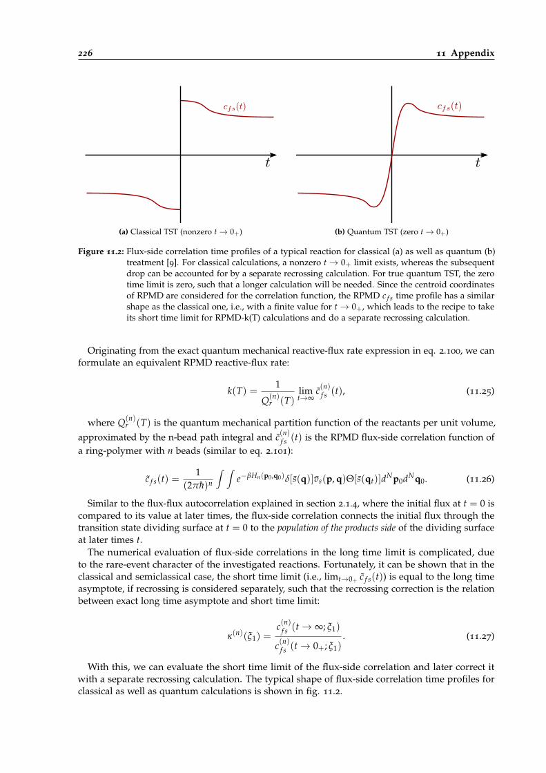
226 11 Appendix
(a) Classical TST (nonzero t→ 0+) (b) Quantum TST (zero t→ 0+)
Figure 11.2: Flux-side correlation time profiles of a typical reaction for classical (a) as well as quantum (b)treatment [9]. For classical calculations, a nonzero t→ 0+ limit exists, whereas the subsequentdrop can be accounted for by a separate recrossing calculation. For true quantum TST, the zerotime limit is zero, such that a longer calculation will be needed. Since the centroid coordinatesof RPMD are considered for the correlation function, the RPMD c f s time profile has a similarshape as the classical one, i.e., with a finite value for t→ 0+, which leads to the recipe to takeits short time limit for RPMD-k(T) calculations and do a separate recrossing calculation.
Originating from the exact quantum mechanical reactive-flux rate expression in eq. 2.100, we canformulate an equivalent RPMD reactive-flux rate:
k(T) =1
Q(n)r (T)
limt→∞
c(n)f s (t), (11.25)
where Q(n)r (T) is the quantum mechanical partition function of the reactants per unit volume,
approximated by the n-bead path integral and c(n)f s (t) is the RPMD flux-side correlation function ofa ring-polymer with n beads (similar to eq. 2.101):
c f s(t) =1
(2πh)n
∫ ∫e−βHn(p0,q0)δ[s(q)]vs(p, q)Θ[s(qt)]dNp0dNq0. (11.26)
Similar to the flux-flux autocorrelation explained in section 2.1.4, where the initial flux at t = 0 iscompared to its value at later times, the flux-side correlation connects the initial flux through thetransition state dividing surface at t = 0 to the population of the products side of the dividing surfaceat later times t.
The numerical evaluation of flux-side correlations in the long time limit is complicated, dueto the rare-event character of the investigated reactions. Fortunately, it can be shown that in theclassical and semiclassical case, the short time limit (i.e., limt→0+ c f s(t)) is equal to the long timeasymptote, if recrossing is considered separately, such that the recrossing correction is the relationbetween exact long time asymptote and short time limit:
κ(n)(ξ1) =c(n)f s (t→ ∞; ξ1)
c(n)f s (t→ 0+; ξ1). (11.27)
With this, we can evaluate the short time limit of the flux-side correlation and later correct itwith a separate recrossing calculation. The typical shape of flux-side correlation time profiles forclassical as well as quantum calculations is shown in fig. 11.2.
11.2 Theoretical Details and Derivations 227
The short time limit can be calculated as:
limt→0+
c f s(t) =f
∏i=1
(µi
2πβnh2
) n2 ∫
eβnVn(q)δ[ξ(q)] fξ(q)d f nq, (11.28)
where f is the number of degrees of freedom in the system and
fξ(q) =
√√√√ f
∑i=1
12πβnµi
[∂ξ(q)
∂qi
]2
. (11.29)
The evaluation of this integral is still very complicated. It can be simplified significantly if anotherdividing surface besides the first at the transition state is introduced. We choose a dividing surfacelocated at the asymptotic reactants valley (eq. 3.10):
ξ0(q) = R∞ − |R| = 0, (11.30)
where |R| is the cartesian distance between the reactants center of masses and R∞ is a manuallychosen asymptotic distance at which the interactions between the reactants are negligible. If wecalculate the short-time flux-side correlation function (eq. 11.28) with respect to this dividingsurface instead of the one located at the transition state, we get
fξ0(q) =
√1
2πβµR(11.31)
and subsequently for the flux-side correlation:
limt→0+
c f s(t; ξ0) = 4πR2∞
√1
2πβµRQn
r (T). (11.32)
If we compare this with eq. 11.25, we see that the same partition function Qnr (T) is located there
in the denominator, such that they can be cut to get the rate constant expression:
kQTST(ξ0) = 4πR2∞
√1
2πβµR. (11.33)
This expression is surprisingly simple, in fact, it depends only on a handful of predefinedparameters, we no longer need to evaluate any partition functions [302]. Further, it is quite
descriptive: The 4πR2∞-factor is the surface area of a sphere with radius R∞ and
√1
2πβµRis,
according to the kinetic theory of gases, the averaged speed of reactant molecules entering thissphere. Thus, a reaction with respect to the ξ0-dividing surface always happens if both reactantsapproach to R∞ distance from infinity, or, if one molecule is the frame of reference, the secondreactant enters the imaginary sphere with R∞ radius around it. However, if we want to achieve areasonable quantification of the whole reaction, we still need to include the transition state dividingsurface, which was the basis of the whole reactive-flux formulation so far. Or, more descriptive, wemust compute the probability that reactants approaching to R∞ actually react to the products. Foran arbitrary pair of dividing surfaces (here: ξ0 and ξ1), we can define the ratio of their respectiveflux-side correlation functions (i.e., the reaction rate at the first surface relative to the second) as:
p(n)(ξ1, ξ0) =c(n)f s (t→ 0+; ξ1)
c(n)f s (t→ 0+; ξ0). (11.34)
228 11 Appendix
This ratio can be expressed by means of canonical probabilities of the system to be at the respectivedividing surfaces, i.e., at ξ = 0 or ξ = 1 [302]:
p(n)(ξ1, ξ0) =P(n)(1)P(n)(0)
, (11.35)
with
P(n)(ξ) =
∫e−βn Hξ
n(p,q)δ[ξ(q)− ξ]d f npd f nq∫e−βn Hξ
n(p,q)d f npd f nq). (11.36)
We already learned something about these coordinate-dependent distributions in section 2.1.3,e.g., that they can be expressed by means of coordinate-dependent free energy curves. If we recalleq. 2.27 in connection with eq. 2.28, the free energy can be expressed as:
A(n)(ξ) = − 1βn
ln P(n)(ξ). (11.37)
Solving this equation for the probability distribution P(n)(ξ) gives:
P(n)(ξ) = e−βn A(n)(ξ). (11.38)
Now, the ratio between the flux-side correlation functions from eq. 11.34 can be expressed bymeans of free energies of the reaction coordinate at the dividing surfaces ξ0 and ξ1:
p(n)(ξ1, ξ0) = exp(−βn
[A(n)(1)− A(n)(0)
]). (11.39)
The bimolecular RPMD rate constant evaluated from the flux-side correlation at the transitionstate dividing surface can be obtained by connecting the rate at the reactants dividing surface (eq.11.33) with the ratio of flux-side correlation functions at reactants and transition state (eq. 11.39)as well as with the recrossing factor introduced by taking the short-time limit for the flux-sidecorrelation in eq. 11.27:
kRPMD(T) = κkQTST(ξ0)p(n)(ξ1, ξ0)
= κ4πR2∞
√1
2πβµRexp
(−βn
[A(n)(1)− A(n)(0)
]).
(11.40)
This finally is the bimolecular RPMD k(T) expression shown in eq. 2.103, with ∆A = A(n)(1)−A(n)(0).
11.3 Internal Coordinates
As briefly described in the theory part of this thesis, the more complex formulations of the EVB-coupling terms in the DG-EVB as well as the TREQ formulation rely on the usage of internalcoordinate systems.
Both directions of coordinate transformations are needed in practice: First, for DG-EVB andTREQ setup, reference gradients and Hessians given in cartesian coordinates need to be transformedto internals for their actual application in the Taylor expansions. Second, calculated gradients ofthe surfaces need to be transformed back to cartesian space such that they can be introduced intothe velocity Verlet algorithm.
11.3 Internal Coordinates 229
During the development of the EVB-QMDFF program package, four different kinds of internalswere adopted subsequently: bond lengths, bond angles, dihedral angles and out-of-plane angles.Whereas small systems (up to approximately 10-15 atoms) could be described well only using bondlengths and angles, larger systems, especially if they shall be described with TREQ, tend to needalso some dihedral and out-of-plane coordinates for reliable calculations.
In the first subsection, the general coordinate transformation algorithm as adopted from Pulay
and Fogarasi [303] is described, whereas in the second subsection all four coordinate types aredescribed in more detail. Based on these introduced coordinates, in the last two subsectionsformulations for their transformation matrix elements are given.
11.3.1 General Formalism
A molecular system is given, containing N atoms whose location in space can be fully describedvia a set x of 3N cartesian coordinates. If the total orientation of the system with respect to thelaboratory frame is neglected, it can also be fully described via a set q of internal coordinates. Thisset might as well be nonredundant (containing 3N − 6 coordinates) or redundant (containing a largerset), depending on the actual requirements.
If a given set of cartesian coordinates shall be converted into a corresponding set of internals, theWilson transformation matrix Bij =
∂qi∂xj
is needed:
q = B−1x. (11.41)
Similar to geometries, gradients can also be converted from cartesian to internal coordinates. Thishowever, requires the transposed inverse of the Wilson transformation matrix:
gq = (B−1)tgx. (11.42)
By taking the derivative of the whole transformation formula, the respective expression for thecartesian Hessian matrix can be found:
Hq = B−1(Hx − B′tgq)(B−1)t. (11.43)
For this operation, the tensor with the second cartesian derivatives of the internal coordinatesB′ijk =
∂qi∂xj∂xk
, that might be seen as the cartesian derivative of the Wilson matrix itself, is needed.If the numbers of internal and cartesian coordinates are different, which they will be in most
cases, the Wilson-matrix is no square matrix and an inverse cannot be build. Nevertheless, singularvalue decomposition (SVD) of the Wilson matrix
B = UΣVt (11.44)
might be applied in order to calculate its pseudoinverse thereafter, which fulfills the same task as aclassical inverse for the transformations. The pseudoinverse of a SVD is calculated by inverting thediagonal matrix Σ containing the singular values:
Σ =
σ1...
. . . · · · 0 · · ·
σr−1...
σr...
...· · · 0 · · · · · · 0 · · ·
......
. (11.45)
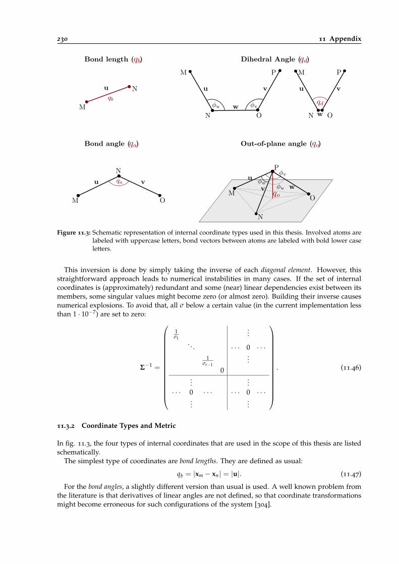
230 11 Appendix
Bond angle ( ) Out-of-plane angle ( )
Bond length ( ) Dihedral Angle ( )
M
N
M
N
O
N
M
O
P
N O
PM
M
N
O
P
u
u v
u v
w
u v
w
uv w
Figure 11.3: Schematic representation of internal coordinate types used in this thesis. Involved atoms arelabeled with uppercase letters, bond vectors between atoms are labeled with bold lower caseletters.
This inversion is done by simply taking the inverse of each diagonal element. However, thisstraightforward approach leads to numerical instabilities in many cases. If the set of internalcoordinates is (approximately) redundant and some (near) linear dependencies exist between itsmembers, some singular values might become zero (or almost zero). Building their inverse causesnumerical explosions. To avoid that, all σ below a certain value (in the current implementation lessthan 1 · 10−7) are set to zero:
Σ−1 =
1σ1
.... . . · · · 0 · · ·
1σr−1
...0
......
· · · 0 · · · · · · 0 · · ·...
...
. (11.46)
11.3.2 Coordinate Types and Metric
In fig. 11.3, the four types of internal coordinates that are used in the scope of this thesis are listedschematically.
The simplest type of coordinates are bond lengths. They are defined as usual:
qb = |xm − xn| = |u|. (11.47)
For the bond angles, a slightly different version than usual is used. A well known problem fromthe literature is that derivatives of linear angles are not defined, so that coordinate transformationsmight become erroneous for such configurations of the system [304].
11.3 Internal Coordinates 231
An alternative formulation for a bond angle is to calculate the distance between the outside atoms(M and O in fig. 11.3) of the bonds by simultaneously normalize both involved bond lengths [304]:
qa =12(
u′
λu− v′
λv) =
12(u− v) (11.48)
where u′ = ~xm −~xn, v′ = ~xo −~xn, and λu, λv their respective bond lengths calculated with eq.11.47. For the Wilson matrix elements shown below, normalized bond vectors are used almostexclusively, they are u and v in this case. Now, linear angles are no longer problematic.
Dihedral angles are defined as usual:
qd = arccos((u×w) · (v×w)
sin(φu) sin(φv)
), (11.49)
where u′ = ~xm − ~xn, w′ = ~xo − ~xn, v′ = ~xp − ~xo and u, w, v their normalized counterparts;further defined are sin(φu) =
√1− (u ·w)2 as well as sin(φv) =
√1− (v ·w)2. For this type
of definition, care needs to be taken for invalid angle arguments: if the argument of the arccosfunction gets smaller than −1 or larger than +1, it is set to its limit values automatically.
The definition of the out-of-plane coordinates is shown in fig. 11.3. It was taken from the paperof Krimm et al. [304] and has the advantage that in contrast to usual out-of-plane definitions nosingularities can appear if involved angles get linear. The coordinate is basically a normalizedtriple product:
qo =1ρ
u · (v×w). (11.50)
The normalization constant needed for calculation of the height is defined as:
ρ2 = 3− cos2 φu − cos2 φv − cos2 φw + 2[cos φu(cos φv − 1)
+ cos φv(cos φw − 1) + cos φw(cos φu − 1)],(11.51)
where the involved angles are defined as normalized dot products cos φu = v ·w, cos φv = u ·w,cos φw = u · v.
11.3.3 Wilson Matrix Elements
As noted above, coordinate transformation matrices, mostly called Wilson matrices, are of integralimportance for internal coordinate calculations. They consist of partial derivatives of internalcoordinates with respect to cartesians:
Bij =∂qi∂xj
. (11.52)
The elements of this matrix can be calculated numerically by imposing finite differences. However,especially for dihedrals and out-of-planes this results in a large calculation overhead: four atomsneed to be elongated in three cartesian directions with plus and minus, respectively, resulting in 24
coordinate calculations! During a MD calculation, a backwards coordinate transformation frominternals to cartesians is needed in each step in order to calculate the EVB-QMDFF gradient, whichmakes the coordinate transformation a critical step for the scaling of the whole method. Therefore,analytical derivatives should be implemented to avoid such overhead. In this section, the analyticalexpressions for the elements of eq. 11.52 are listed and explained.
Similar work was done already before in a paper of Helgaker [305], however, this was donethere only for bonds, angles and torsions. Further, the torsional Wilson elements contain someerrors which makes it problematic to implement (at least until all errors could be detected). Finally,the expression for the angle coordinate is different in my case.
232 11 Appendix
To the best of my knowledge, the compilation of Wilson matrix elements shown in the followingis the only one freely available for the collection of internal coordinates used in this paper. Anew formalism was used in order to generalize the different expressions as much as possible. Allderivatives are given as vector expressions, i.e., they constitute three entries in the Wilson matrix,the x-, y- and z- values.
The actual implementation of the coordinate transformation was made more effective by definingseveral intermediate vectors, dot- and cross-products in advance for each new Wilson matrixcalculation.
Bond Lengths
For bond lengths, the following expression is valid3:
∂qb∂xa,i
= ζaMNui ; a = M, N, (11.53)
where a sign factor was introduced similar to the paper of Helgaker:
ζamn =
1 a = M−1 a = N0 else
. (11.54)
Bond Angles
For the bond angles, cartesian derivatives of normalized bonds are needed. They can be defined ascomponents of a derivative vector, where each entry is itself a vector.
∂u∂x
=1
λ3u
u22 + u2
3−u1u2−u1u3
−u2u1u2
1 + u23
−u2u3
−u3u1−u3u2u2
1 + u22
T
. (11.55)
With this abbreviation, Wilson matrix elements for a bond angle coordinate can be written inclosed form:
∂qa
∂xa,i= − 1
4qaζaMNζaNO
((1− δaO)
∂u∂xi· v + (1− δaM)u · ∂v
∂xi
); a = M, N, O. (11.56)
Dihedral Angles
Dihedral angles result in much longer expressions, however these can still be expressed in termsof vectors and vector derivatives according to eq. 11.55.
With numerator θ = (u×w) · (v×w) and denominator κ = sin(φu) sin(φv) the Wilson matrixelements for the dihedral angles are:
∂qd∂xa,i
= −∂θ
∂xa,iκ − θ ∂κ
∂xa,i√1−
(θκ
)2κ2
. (11.57)
3 In the upcoming mathematical expressions, the following nomenclature is used (closely related to fig. 11.3): M, N, O, Pare the up to four atoms for which the coordinate is calculated, xa,i depicts that the current derivative is built withrespect to the i’th cartesian coordinate (x, y or z) of atom a (which can be M, N, O or P). Bold symbols u, v and wdescribe the bond vectors included in the current coordinate description.
11.3 Internal Coordinates 233
Now, the derivatives of the numerator and denominator of the dihedral expression are stillmissing. Although they might also be expressed in one closed formula (resulting in a long andnasty expression), I have decided to give them depending on the atom which coordinates arecalculated. For the numerator the derivatives are:
∂θ
∂xa,i=
(∂u∂xi×w
)· (v×w) a = M
−[(
∂u∂xi×w
)+(
u× ∂w∂xi
)]· (v×w)− (u×w) ·
(v× ∂w
∂xi
)a = N(
u× ∂w∂xi
)· (v×w) + (u×w) ·
[(v× ∂w
∂xi
)−(
∂v∂xi×w
)]a = O
(u×w) ·(
∂v∂xi×w
)a = P
. (11.58)
The derivatives of the denominator are:
∂κ
∂xa,i=
−(
∂u∂xi·w)(u ·w)
sin(φv)
sin(φu)a = m[(
∂u∂xi·w)+
(u · ∂w
∂xi
)](u ·w)
sin(φv)
sin(φu)
+sin(φu)
sin(φv)
(v · ∂w
∂xi
)(v ·w)
a = n
−(
u · ∂w∂xi
)(u ·w)
sin(φv)
sin(φu)
−[(
∂v∂xi·w)+
(v · ∂w
∂xi
)](v ·w)
sin(φu)
sin(φv)
a = o
−(
∂v∂xi·w)(v ·w)
sin(φv)
sin(φu)a = p
. (11.59)
Out-of-Plane Angles
For the out-of-plane-angles, the Wilson matrix elements can be given again in one closed formula:
∂qo
∂xa,i=
υ
ρ
(∂ρ
∂xa,i
υ
ρ+
∂υ
∂xa,i
)a = M, N, O
−(
∂qo
∂xM,i+
∂qo
∂xN,i+
∂qo
∂xO,i
)a = P
(11.60)
where υ = u · (v×w).The derivatives of the normalization factor with respect to the involved bond vectors can be
expressed as:
∂ρ
∂xa,i=
2ρ
∂u∂xi·[w (− cos(φ2)− 1 + cos(φ1) + cos(φ3)) +
v (− cos(φ3)− 1 + cos(φ1) + cos(φ2))] a = M
2ρ
∂v∂xi·[w (− cos(φ1)− 1 + cos(φ2) + cos(φ3)) +
u (− cos(φ3)− 1 + cos(φ1) + cos(φ2))] a = N
2ρ
∂w∂xi·[v (− cos(φ1)− 1 + cos(φ2) + cos(φ3)) +
u (− cos(φ2)− 1 + cos(φ1) + cos(φ3))] a = O
, (11.61)
where the angles φ1 to φ3 are shown in fig. 11.3.

234 11 Appendix
The derivatives of the triple product in eq. 11.50 (υ = u · (v×w)) are quite simple:
∂υ
∂xa,i=
∂u∂xi· (v×w) a = M
u ·(
∂v∂xi×w
)a = N
u ·(
v× ∂w∂xi
)a = O
. (11.62)
Evaluating the symmetry of eq. 11.60, it is obvious that the Wilson matrix elements for atom Pare basically the negative sum of the elements for all other atoms, due to the fact that P constitutesthe peak of a tripod, with M,N and O building its base.
11.3.4 Wilson Matrix Derivatives
Similar to the Wilson matrix elements (i.e., the first derivatives of the internal coordinates with re-spect to cartesians) the Wilson matrix derivatives (i.e., the second derivatives of internal coordinateswith respect to cartesians) can be simplified significantly if the expressions for bond-, dihedral-and out-of-plane angles are constructed in terms of bond derivatives.
Bond Lengths
The simplest case are again the bond lengths. Their Wilson matrix derivatives are given byHelgaker, they are:
∂2qb∂xa,i∂xb,j
= (−1)δabuiuj − δij
λu. (11.63)
Similar to the expression for the first derivative of a normalized bond in dot- or cross-productsin eq. 11.55, their second derivatives can be written as a symmetric second derivative matrix, witheach entry being a vector itself (eq. 11.64).
∂2u∂x∂x
=1
λ5u·
−3u1(u22 + u2
3)u2(2u2
1 − u22 − u2
3)u3(2u2
1 − u22 − u2
3)
. . . . . .−u2(−2u21 + u2
2 + u23)
−u1(u21 − 2u2
2 + u23)
3u1u2u3
u1(−u21 + 2u2
2 − u23)
−3u2(u21 + u2
3)u3(−u2
1 + 2u22 − u2
3)
. . .
−u3(−2u21 + u2
2 + u23)
3u1u2u3−u1(u2
1 − 2u22 + u2
3)
3u1u2u3−u3(u2
1 − 2u22 + u2
3)−u2(u2
1 + u22 − 2u2
3)
u1(−u21 − u2
2 + 2u23)
u2(−u21 − u2
2 + 2u23)
−3u3(u21 + u2
2)
(11.64)
Bond Angles
For the bond angles, the second derivatives can be written in one single expression if the firstderivatives of eq. 11.56 are used:
∂2qa
∂xa,i∂xb,j= − 1
4qa
(4
∂qa
∂xa,i
∂qa
∂xb,j+
∂2(u · v)∂xa,i∂xb,j
). (11.65)

11.3 Internal Coordinates 235
In this formula, the general second derivatives of the dot product of the u and v bond vectors(fig. 11.3) are needed. They can be expressed depending on the vector derivatives in eq. 11.64:
∂2(u · v)∂xa,i∂xb,j
=
∂2u∂xi∂xj
· v − ∂2u∂xi∂xj
· v− ∂u∂xi· ∂v
∂xj
∂u∂xi· ∂v
∂xj
− ∂2u∂xi∂xj
· v− ∂u∂xj· ∂v
∂xi
∂2u∂xi∂xj
· v +∂u∂xi· ∂v
∂xj∂u∂xj· ∂v
∂xi+ u · ∂2v
∂xi∂xj
∂u∂xj· ∂v
∂xi+ u · ∂2v
∂xi∂xj
∂u∂xj· ∂v
∂xi− ∂u
∂xj· ∂v
∂xi− u · ∂2v
∂xj∂xiu · ∂2v
∂xi∂xj
, (11.66)
where the dimensions of this matrix a and b run over the involved atoms M, N and O.
Dihedral Angles
For the dihedral angles the strategy for the first derivatives (eq. 11.57) is continued: In order toprevent one single extremely large expression, all is expressed depending on the numerator anddenominator of the original dihedral formula (eq. 11.49), these two are again denoted as θ and κ.
Introducing these variables, the whole second derivative expression for dihedrals is quitemanageable:
∂2qd∂xa,i∂xb,j
=
[θ3 ∂κ
∂xb,j
∂κ
∂xa,i− κθ3 ∂2κ
∂xa,i∂xb,j+ κ3
( ∂θ
∂xb,j
∂κ
∂xa,i+
∂κ
∂xb,j
∂θ
∂xa,i+
θ∂2κ
∂xa,i∂xb,j
)− κ4 ∂2θ
∂xa,i∂xb,j+ κ2θ
(−2
∂κ
∂xa,i
∂κ
∂xb,j− ∂θ
∂xa,i
∂θ
∂xb,j+
θ∂2θ
∂xa,i∂xb,j
][κ3(κ2 − θ2)
√1− θ2
κ2
]−1
. (11.67)
This equation contains first as well as second derivatives of both θ and κ. The first derivativeexpressions were already deduced for the first dihedral derivatives (eqs. 11.58, 11.59) and can bereused in perfect analogy. However, the second derivatives of both the numerator and denominatorare also needed. Since four atoms are involved in the dihedral, in total 16 different secondderivatives are possible. Similar to the bond angle expressions, the effective number of matrixelements reduces to 11 due to symmetry. In the following, all unique second derivatives of θ and κwith respect to the four involved atoms are listed.
These expressions become quite lengthy, therefore a shorthand notation is introduced for thepartial derivatives: ∂xi u means ∂u
∂xiand ∂xixj u means ∂2u
∂xi∂xj.
The diagonal elements of the second derivatives of θ are:
∂2θ
∂xM,i∂xM,j= (∂xixj u) · (v×w) , (11.68)
236 11 Appendix
∂2θ
∂xN,i∂xN,j= [(∂xixj u×w) + (∂xi u× ∂xj w) + (∂xj u× ∂xi w)+
(u× ∂xixj w)] · (v×w) + (∂xi u×w) · (v× ∂xj w)+
(u× ∂xi w) · (v× ∂xj w) + (∂xj u×w) · (v× ∂xi w)+
(∂xj u×w) · (v× ∂xi w) + (u×w) · (v× ∂xixj w)
, (11.69)
∂2θ
∂xO,i∂xO,j= [(v× ∂xixj w)− (∂xj v× ∂xi w)− (∂xi v× ∂xj w)+
(∂xixj v×w)] · (v×w) + (u× ∂xixj w) · (v×w)+
(u× ∂xi w) · (v× ∂xj w) + (u× ∂xi w) · (∂xj v×w)+
(u× ∂xj w) · (v× ∂xi w)− (u× ∂xj w) · (∂xi v×w)
, (11.70)
∂2θ
∂xP,i∂xP,j= ·(v×w) · (∂xixj v×w). (11.71)
The off-diagonal elements of the second derivatives of θ are:
∂2θ
∂xM,i∂xN,j= −[(∂xixj u×w) + (∂xi u× ∂xj w)] · (v×w)
−(∂xi u×w) · (v× ∂xj w)
, (11.72)
∂2θ
∂xM,i∂xO,j= (∂xi u×w) · [(v× ∂xj w)− (∂xj v×w)]+
(∂xj u× ∂xj w) · (v×w)
, (11.73)
∂2θ
∂xM,i∂xP,j= (∂xi u×w) · (∂xj v×w), (11.74)
∂2θ
∂xN,i∂xO,j= −[(∂xi u× ∂xj w) + (u× ∂xixj w)] · (v×w)−
[(∂xj v× ∂xi w)− (v× ∂xixj w)] · (u×w)−(∂xi u×w) · (v× ∂xj w) + (∂xi u×w) · (∂xj v×w)−(u× ∂xi w) · (v× ∂xj ]w) + (u× ∂xi w) · (∂xj v×w)−
(u× ∂xj w) · (v× ∂xi w)
, (11.75)
∂2θ
∂xN,i∂xP,j= −[(∂xi u×w) + (v× ∂xi w)] · (∂xj v×w)−
(u×w) · (∂xixj v×w)
, (11.76)
∂2θ
∂xP,i∂xP,j= −[(∂xj v× ∂xi w)− (∂xixj v×w)] · (u×w)+
(u× ∂xi w) · (∂xj v×w)
. (11.77)
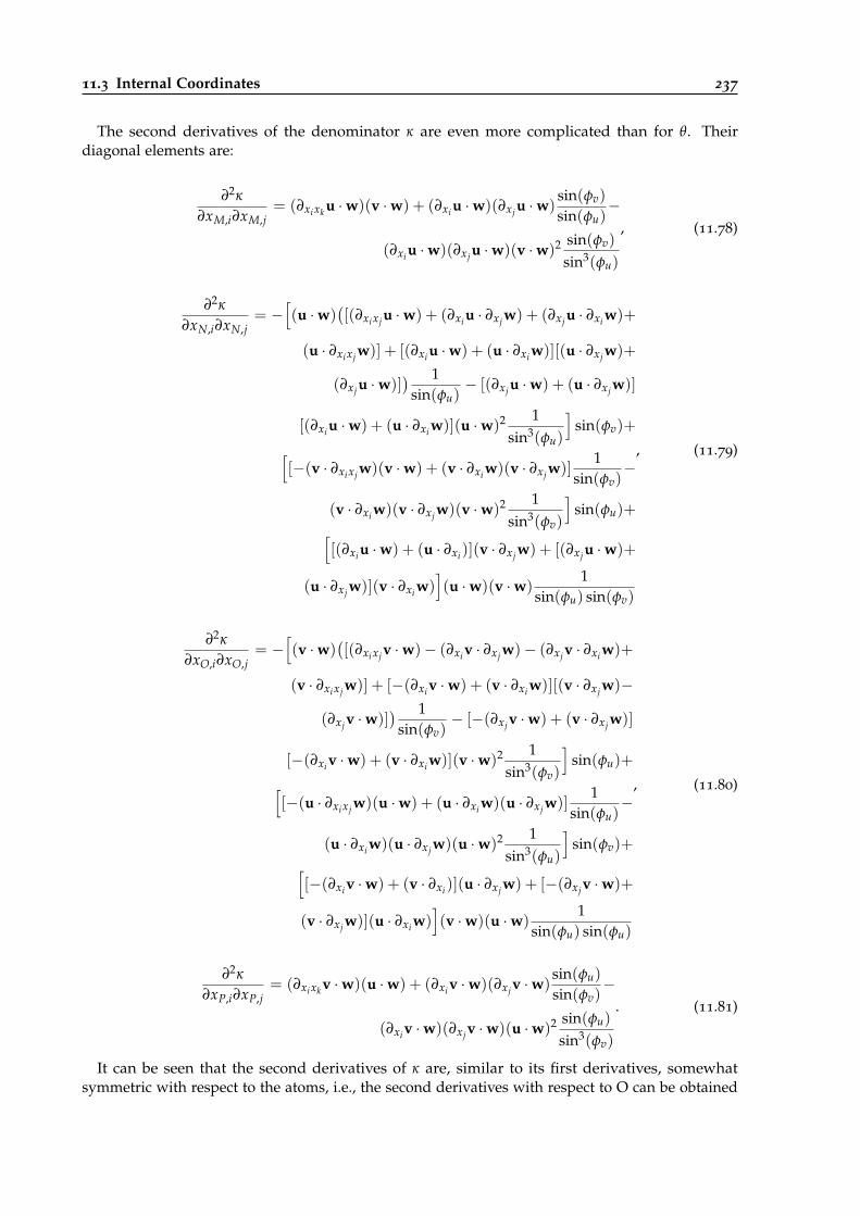
11.3 Internal Coordinates 237
The second derivatives of the denominator κ are even more complicated than for θ. Theirdiagonal elements are:
∂2κ
∂xM,i∂xM,j= (∂xixk u ·w)(v ·w) + (∂xi u ·w)(∂xj u ·w)
sin(φv)
sin(φu)−
(∂xi u ·w)(∂xj u ·w)(v ·w)2 sin(φv)
sin3(φu)
, (11.78)
∂2κ
∂xN,i∂xN,j= −
[(u ·w)
([(∂xixj u ·w) + (∂xi u · ∂xj w) + (∂xj u · ∂xi w)+
(u · ∂xixj w)] + [(∂xi u ·w) + (u · ∂xi w)][(u · ∂xj w)+
(∂xj u ·w)]) 1
sin(φu)− [(∂xj u ·w) + (u · ∂xj w)]
[(∂xi u ·w) + (u · ∂xi w)](u ·w)2 1sin3(φu)
]sin(φv)+[
[−(v · ∂xixj w)(v ·w) + (v · ∂xi w)(v · ∂xj w)]1
sin(φv)−
(v · ∂xi w)(v · ∂xj w)(v ·w)2 1sin3(φv)
]sin(φu)+[
[(∂xi u ·w) + (u · ∂xi)](v · ∂xj w) + [(∂xj u ·w)+
(u · ∂xj w)](v · ∂xi w)](u ·w)(v ·w)
1sin(φu) sin(φv)
, (11.79)
∂2κ
∂xO,i∂xO,j= −
[(v ·w)
([(∂xixj v ·w)− (∂xi v · ∂xj w)− (∂xj v · ∂xi w)+
(v · ∂xixj w)] + [−(∂xi v ·w) + (v · ∂xi w)][(v · ∂xj w)−
(∂xj v ·w)]) 1
sin(φv)− [−(∂xj v ·w) + (v · ∂xj w)]
[−(∂xi v ·w) + (v · ∂xi w)](v ·w)2 1sin3(φv)
]sin(φu)+[
[−(u · ∂xixj w)(u ·w) + (u · ∂xi w)(u · ∂xj w)]1
sin(φu)−
(u · ∂xi w)(u · ∂xj w)(u ·w)2 1sin3(φu)
]sin(φv)+[
[−(∂xi v ·w) + (v · ∂xi)](u · ∂xj w) + [−(∂xj v ·w)+
(v · ∂xj w)](u · ∂xi w)](v ·w)(u ·w)
1sin(φu) sin(φu)
, (11.80)
∂2κ
∂xP,i∂xP,j= (∂xixk v ·w)(u ·w) + (∂xi v ·w)(∂xj v ·w)
sin(φu)
sin(φv)−
(∂xi v ·w)(∂xj v ·w)(u ·w)2 sin(φu)
sin3(φv)
. (11.81)
It can be seen that the second derivatives of κ are, similar to its first derivatives, somewhatsymmetric with respect to the atoms, i.e., the second derivatives with respect to O can be obtained
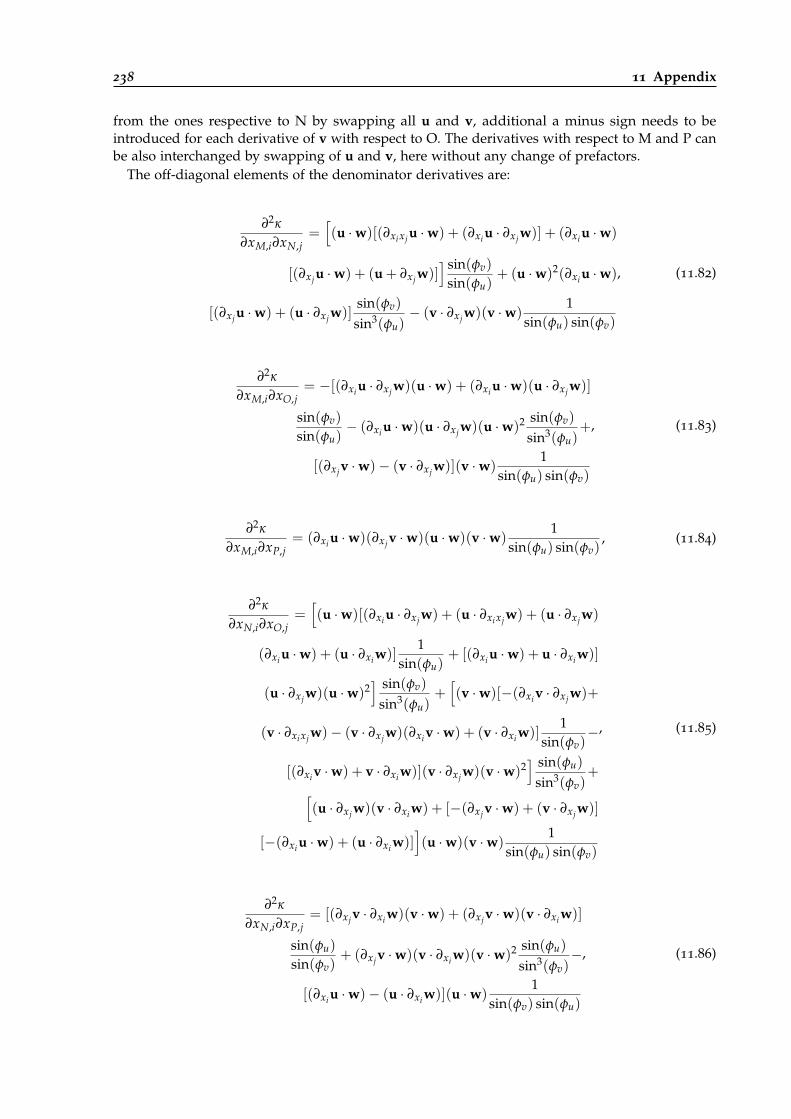
238 11 Appendix
from the ones respective to N by swapping all u and v, additional a minus sign needs to beintroduced for each derivative of v with respect to O. The derivatives with respect to M and P canbe also interchanged by swapping of u and v, here without any change of prefactors.
The off-diagonal elements of the denominator derivatives are:
∂2κ
∂xM,i∂xN,j=[(u ·w)[(∂xixj u ·w) + (∂xi u · ∂xj w)] + (∂xi u ·w)
[(∂xj u ·w) + (u + ∂xj w)]] sin(φv)
sin(φu)+ (u ·w)2(∂xi u ·w)
[(∂xj u ·w) + (u · ∂xj w)]sin(φv)
sin3(φu)− (v · ∂xj w)(v ·w)
1sin(φu) sin(φv)
, (11.82)
∂2κ
∂xM,i∂xO,j= −[(∂xi u · ∂xj w)(u ·w) + (∂xi u ·w)(u · ∂xj w)]
sin(φv)
sin(φu)− (∂xi u ·w)(u · ∂xj w)(u ·w)2 sin(φv)
sin3(φu)+
[(∂xj v ·w)− (v · ∂xj w)](v ·w)1
sin(φu) sin(φv)
, (11.83)
∂2κ
∂xM,i∂xP,j= (∂xi u ·w)(∂xj v ·w)(u ·w)(v ·w)
1sin(φu) sin(φv)
, (11.84)
∂2κ
∂xN,i∂xO,j=[(u ·w)[(∂xi u · ∂xj w) + (u · ∂xixj w) + (u · ∂xj w)
(∂xi u ·w) + (u · ∂xi w)]1
sin(φu)+ [(∂xi u ·w) + u · ∂xi w)]
(u · ∂xj w)(u ·w)2] sin(φv)
sin3(φu)+[(v ·w)[−(∂xi v · ∂xj w)+
(v · ∂xixj w)− (v · ∂xj w)(∂xi v ·w) + (v · ∂xi w)]1
sin(φv)−
[(∂xi v ·w) + v · ∂xi w)](v · ∂xj w)(v ·w)2] sin(φu)
sin3(φv)+[
(u · ∂xj w)(v · ∂xi w) + [−(∂xj v ·w) + (v · ∂xj w)]
[−(∂xi u ·w) + (u · ∂xi w)]](u ·w)(v ·w)
1sin(φu) sin(φv)
, (11.85)
∂2κ
∂xN,i∂xP,j= [(∂xj v · ∂xi w)(v ·w) + (∂xj v ·w)(v · ∂xi w)]
sin(φu)
sin(φv)+ (∂xj v ·w)(v · ∂xi w)(v ·w)2 sin(φu)
sin3(φv)−
[(∂xi u ·w)− (u · ∂xi w)](u ·w)1
sin(φv) sin(φu)
, (11.86)
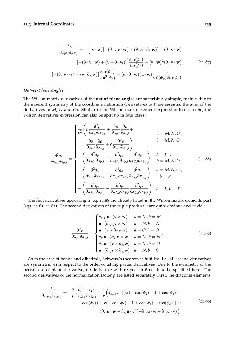
11.3 Internal Coordinates 239
∂2κ
∂xN,i∂xP,j= −
[(v ·w)[−(∂xixj v ·w) + (∂xj v · ∂xi w)] + (∂xj v ·w)
[−(∂xi v ·w) + (v + ∂xi w)]]sin(φu)
sin(φv)− (v ·w)2(∂xj v ·w)
[−(∂xi v ·w) + (v · ∂xi w)]sin(φu)
sin3(φv)− (u · ∂xi w)(u ·w)
1sin(φv) sin(φu)
. (11.87)
Out-of-Plane Angles
The Wilson matrix derivatives of the out-of-plane angles are surprisingly simple, mainly due tothe inherent symmetry of the coordinate definition (derivatives to P are essential the sum of thederivatives to M, N and O). Similar to the Wilson matrix element expression in eq. 11.60, theWilson derivatives expression can also be split up in four cases:
∂2qo
∂xa,i∂xb,j=
1ρ2
(υ
∂2ρ
∂xa,i∂xb,j+
∂ρ
∂xa,i
∂υ
∂xb,j+
∂υ
∂xa,i
∂ρ
∂xb,j+ ρ
∂2υ
∂xa,i∂xb,j
) a = M, N, O ,
b = M, N, O
−(
∂2qo
∂xM,i∂xb,j+
∂2qo
∂xN,i∂xb,j
∂2qo
∂xO,i∂xb,j
)a = P ,
b = M, N, O
−(
∂2qo
∂xa,i∂xM,j+
∂2qo
∂xa,i∂xN,j
∂2qo
∂xa,i∂xO,j
)a = M, N, O ,
b = P
−(
∂2qo
∂xM,i∂xP,j+
∂2qo
∂xN,i∂xP,j
∂2qo
∂xO,i∂xP,j
)a = P, b = P
. (11.88)
The first derivatives appearing in eq. 11.88 are already listed in the Wilson matrix elements part(eqs. 11.61, 11.62). The second derivatives of the triple product υ are quite obvious and trivial:
∂2υ
∂xa,i∂xb,j=
∂xixj u · (v×w) a = M, b = Mu · (∂xixj v×w) a = N, b = Nu · (v× ∂xixj w) a = O, b = O∂xi u · (∂xj v×w) a = M, b = N∂xi u · (v× ∂xj w) a = M, b = Ou · (∂xi v× ∂xj w) a = N, b = O
. (11.89)
As in the case of bonds and dihedrals, Schwarz’s theorem is fulfilled, i.e., all second derivativesare symmetric with respect to the order of taking partial derivatives. Due to the symmetry of theoverall out-of-plane derivative, no derivative with respect to P needs to be specified here. Thesecond derivatives of the normalization factor ρ are listed separately. First, the diagonal elements:
∂2ρ
∂xM,i∂xM,j= −3
ρ
∂ρ
∂xM,i
∂ρ
∂xM,j− 1
ρ
(∂xixj u · [(w(− cos(φ2)− 1 + cos(φ1)+
cos(φ3)) + v(− cos(φ3)− 1 + cos(φ1) + cos(φ2))]+
(∂xi u ·w− ∂xi u · v)(−∂xj u ·w + ∂xj u · v)), (11.90)
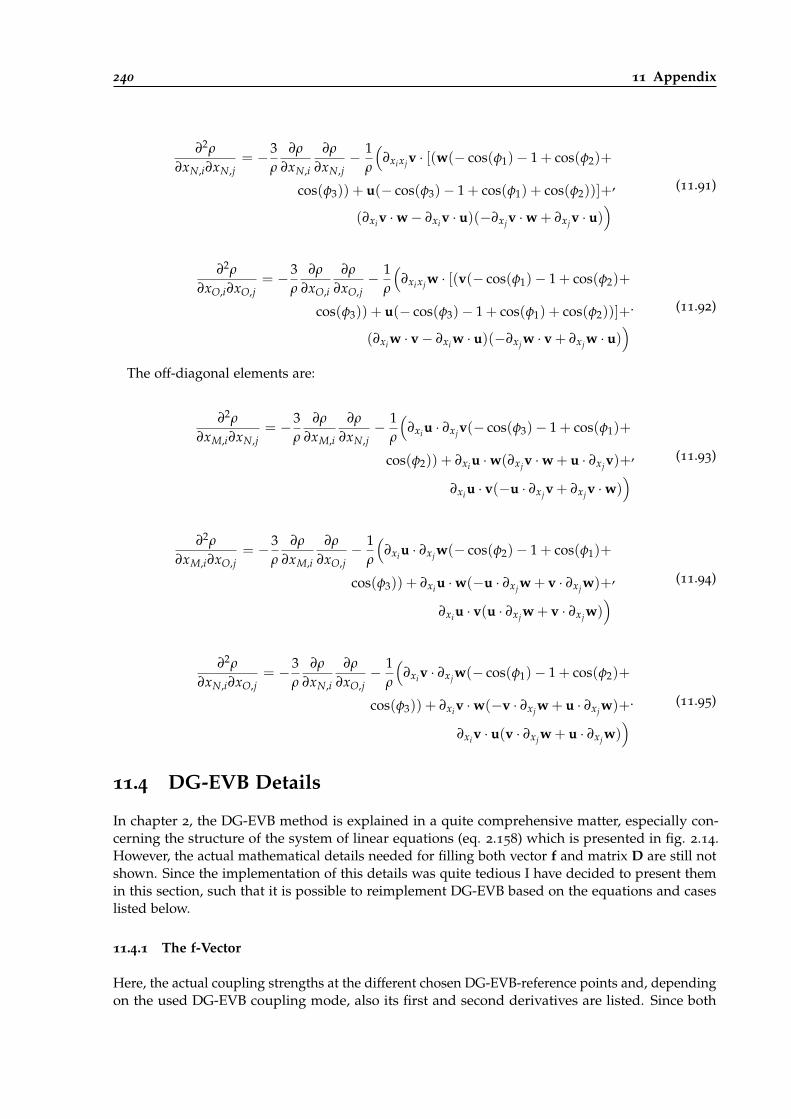
240 11 Appendix
∂2ρ
∂xN,i∂xN,j= −3
ρ
∂ρ
∂xN,i
∂ρ
∂xN,j− 1
ρ
(∂xixj v · [(w(− cos(φ1)− 1 + cos(φ2)+
cos(φ3)) + u(− cos(φ3)− 1 + cos(φ1) + cos(φ2))]+
(∂xi v ·w− ∂xi v · u)(−∂xj v ·w + ∂xj v · u)), (11.91)
∂2ρ
∂xO,i∂xO,j= −3
ρ
∂ρ
∂xO,i
∂ρ
∂xO,j− 1
ρ
(∂xixj w · [(v(− cos(φ1)− 1 + cos(φ2)+
cos(φ3)) + u(− cos(φ3)− 1 + cos(φ1) + cos(φ2))]+
(∂xi w · v− ∂xi w · u)(−∂xj w · v + ∂xj w · u)). (11.92)
The off-diagonal elements are:
∂2ρ
∂xM,i∂xN,j= −3
ρ
∂ρ
∂xM,i
∂ρ
∂xN,j− 1
ρ
(∂xi u · ∂xj v(− cos(φ3)− 1 + cos(φ1)+
cos(φ2)) + ∂xi u ·w(∂xj v ·w + u · ∂xj v)+
∂xi u · v(−u · ∂xj v + ∂xj v ·w)), (11.93)
∂2ρ
∂xM,i∂xO,j= −3
ρ
∂ρ
∂xM,i
∂ρ
∂xO,j− 1
ρ
(∂xi u · ∂xj w(− cos(φ2)− 1 + cos(φ1)+
cos(φ3)) + ∂xi u ·w(−u · ∂xj w + v · ∂xj w)+
∂xi u · v(u · ∂xj w + v · ∂xj w)), (11.94)
∂2ρ
∂xN,i∂xO,j= −3
ρ
∂ρ
∂xN,i
∂ρ
∂xO,j− 1
ρ
(∂xi v · ∂xj w(− cos(φ1)− 1 + cos(φ2)+
cos(φ3)) + ∂xi v ·w(−v · ∂xj w + u · ∂xj w)+
∂xi v · u(v · ∂xj w + u · ∂xj w)). (11.95)
11.4 DG-EVB Details
In chapter 2, the DG-EVB method is explained in a quite comprehensive matter, especially con-cerning the structure of the system of linear equations (eq. 2.158) which is presented in fig. 2.14.However, the actual mathematical details needed for filling both vector f and matrix D are still notshown. Since the implementation of this details was quite tedious I have decided to present themin this section, such that it is possible to reimplement DG-EVB based on the equations and caseslisted below.
11.4.1 The f-Vector
Here, the actual coupling strengths at the different chosen DG-EVB-reference points and, dependingon the used DG-EVB coupling mode, also its first and second derivatives are listed. Since both
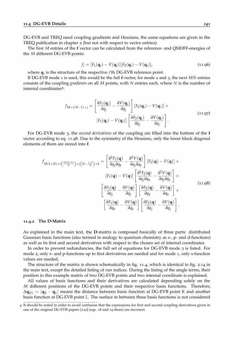
11.4 DG-EVB Details 241
DG-EVB and TREQ need coupling gradients and Hessians, the same equations are given in theTREQ publication in chapter 5 (but not with respect to vector entries).
The first M entries of the f vector can be calculated from the reference- and QMDFF-energies ofthe M different DG-EVB points:
fi = [F1(qi)−V(qi)][F2(qi)−V(qi)], (11.96)
where qi is the structure of the respective i’th DG-EVB reference point.If DG-EVB mode 1 is used, this would be the full f-vector, for mode 2 and 3, the next MN entries
consists of the coupling gradients on all M points, with N entries each, where N is the number ofinternal coordinates4:
fM+i(N−1)+j =
[∂F1(qi)
∂qj− ∂V(qi)
∂qj
][F2(qi)−V(qi)] +
[F1(qi)−V(qi)]
[∂F2(qi)
∂qj− ∂V(qi)
∂qj
].
(11.97)
For DG-EVB mode 3, the second derivatives of the coupling are filled into the bottom of the fvector according to eq. 11.98. Due to the symmetry of the Hessians, only the lower block diagonalelements of them are stored into f.
fM(1+N)+i
(N(N+1)
2
)+j(
N− j−12
)+k
=
[∂2F1(q)∂qj∂qk
− ∂2V(q)∂qj∂qk
][F2(q)−V(q)] +
[F1(q)−V(q)]
[∂2F2(q)∂qj∂qk
− ∂2V(q)∂qj∂qk
]+[
∂F1(q)∂qj
− ∂V(q)∂qj
] [∂F2(q)
∂qk− ∂V(q)
∂qk
]+
[∂F1(q)
∂qk− ∂V(q)
∂qk
] [∂F2(q)
∂qj− ∂V(q)
∂qj
].
(11.98)
11.4.2 The D-Matrix
As explained in the main text, the D-matrix is composed basically of three parts: distributedGaussian basis functions (also termed in analogy to quantum chemistry as s-, p- and d-functions)as well as its first and second derivatives with respect to the chosen set of internal coordinates.
In order to prevent redundancies, the full set of equations for DG-EVB mode 3 is listed. Formode 2, only s- and p-functions up to first derivatives are needed and for mode 1, only s-functionvalues are needed.
The structure of the matrix is shown schematically in fig. 11.4, which is identical to fig. 2.14 inthe main text, except the detailed listing of run indices. During the listing of the single terms, theirposition in this example matrix of two DG-EVB points and two internal coordinate is explained.
All values of basis functions and their derivatives are calculated depending solely on theM different positions of the DG-EVB points and their respective basis functions. Therefore,∆qKL = |qK − qL| means the distance between basis function at DG-EVB point K and anotherbasis function at DG-EVB point L. The surface in between these basis functions is not considered
4 It should be noted in order to avoid confusion that the expressions for first and second coupling derivatives given inone of the original DG-EVB papers [122] (eqs. 18 and 19 there) are incorrect.
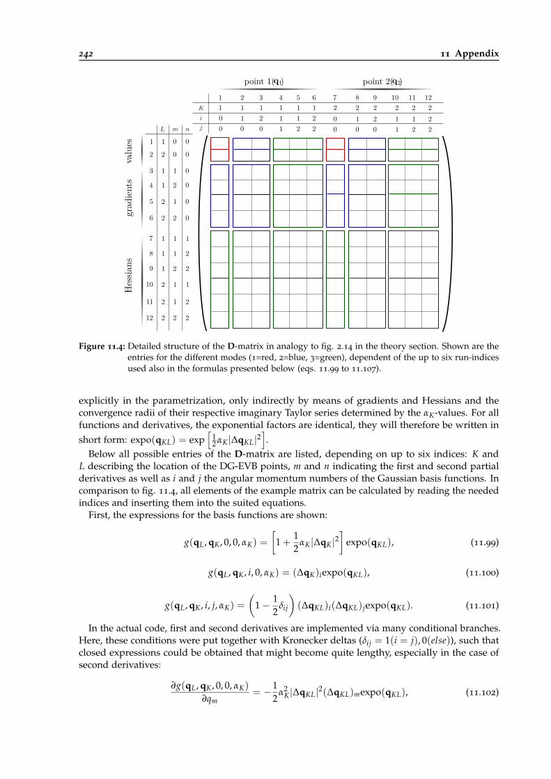
242 11 Appendix
valu
esgr
adie
nts
Hes
sians
point 1( ) point 2( )
1 2 3 4 5 6 7 8 9 10 11 121 1 1 1 1 1 2 2 2 2 2 200 0 0
1 2 1 1 21 2 2
00 0 0
1 2 1 1 21 2 2
1
2
3
4
5
6
7
8
9
10
11
12
1
2
1
1
2
2
1
1
1
2
2
2
0
0
1
2
1
2
1
1
2
1
1
2
0
0
0
0
0
0
1
2
2
1
2
2
Figure 11.4: Detailed structure of the D-matrix in analogy to fig. 2.14 in the theory section. Shown are theentries for the different modes (1=red, 2=blue, 3=green), dependent of the up to six run-indicesused also in the formulas presented below (eqs. 11.99 to 11.107).
explicitly in the parametrization, only indirectly by means of gradients and Hessians and theconvergence radii of their respective imaginary Taylor series determined by the αK-values. For allfunctions and derivatives, the exponential factors are identical, they will therefore be written inshort form: expo(qKL) = exp
[12 αK|∆qKL|2
].
Below all possible entries of the D-matrix are listed, depending on up to six indices: K andL describing the location of the DG-EVB points, m and n indicating the first and second partialderivatives as well as i and j the angular momentum numbers of the Gaussian basis functions. Incomparison to fig. 11.4, all elements of the example matrix can be calculated by reading the neededindices and inserting them into the suited equations.
First, the expressions for the basis functions are shown:
g(qL, qK, 0, 0, αK) =
[1 +
12
αK|∆qK|2]
expo(qKL), (11.99)
g(qL, qK, i, 0, αK) = (∆qK)iexpo(qKL), (11.100)
g(qL, qK, i, j, αK) =
(1− 1
2δij
)(∆qKL)i(∆qKL)jexpo(qKL). (11.101)
In the actual code, first and second derivatives are implemented via many conditional branches.Here, these conditions were put together with Kronecker deltas (δij = 1(i = j), 0(else)), such thatclosed expressions could be obtained that might become quite lengthy, especially in the case ofsecond derivatives:
∂g(qL, qK, 0, 0, αK)
∂qm= −1
2α2
K|∆qKL|2(∆qKL)mexpo(qKL), (11.102)

11.4 DG-EVB Details 243
∂g(qL, qK, i, 0, αK)
∂qm= − [αK(∆qKL)i(∆qKL)m − δmi] expo(qKL), (11.103)
∂g(qL, qK, i, j, αK)
∂qm= −
(1− 1
2δij
) [αK(∆qKL)i(∆qKL)j(∆qKL)m−
δmi(∆qKL)i − δmj(∆qKL)j
]expo(qKL).
(11.104)
The second derivatives depend on up to six indices:
∂2g(qL, qK, 0, 0, αK)
∂qm∂qn= −1
2α2
K
(αK|∆qKL|2(∆qKL)m(∆qKL)n − 3δmn|∆qKL|2−
2(1− δmn)(∆qKL)m(∆qKL)n
)expo(qKL)
, (11.105)
∂2g(qL, qK, i, 0, αK)
∂qm∂qn= αK
[αK(∆qKL)i(∆qKL)m(∆qKL)n − δmn(1 + 2δmi)(∆qKL)i−
(1− δmn)(δni(∆qKL)n + δmi(∆qKL)m)]expo(qKL)
, (11.106)
∂2g(qL, qK, i, j, αK)
∂qm∂qn=
(1− 1
2δij
)[α2
K(∆qKL)i(∆qKL)j(∆qKL)m(∆qKL)n−
δmnδmiαK(∆qKL)i(∆qKL)j − δij
{2αK(1− δmn)(∆qKL)i(δmi(∆qKL)n+
δni(∆qKL)m) + δmn(5αK(∆qKL)i(∆qKL)j − 2)}− (1− δij){
αK(1− δni)(1− δnj)[δmi(∆qKL)j(∆qKL)n + δmj(∆qKL)i(∆qKL)m]+
αK(1− δmi)(1− δmj)[δni(∆qKL)j(∆qKL)m + δnj(∆qKL)i(∆qKL)n]+
δmiδnj(αK(∆qKL)i(∆qKL)m + αK(∆qKL)j(∆qKL)n − 1)+
δniδmj(αK(∆qKL)j(∆qKL)m + αK(∆qKL)i(∆qKL)n − 1)+
3αK(∆qKL)i(∆qKL)j(δmiδni + δmjδnj)}]
expo(qKL)
. (11.107)
11.4.3 Analytical Gradients
The methodology for calculating the DG-EVB gradient is similar to that for the TREQ gradientshown in chapter 5. Since only the squared coupling C(q)2 is calculated from DG-EVB, the originalEVB gradient formula resulting from building the derivative of eq. 2.130 needs to be slightlymodified, as it is shown in the TREQ chapter.
The result is the following expression:
∂V(q)∂q
=12
{(∂F1(q)
∂q
)+
(∂F2(q)
∂q
)−
2(
∂C(q)2
∂q
)+ [F1(q)− F2(q)]
[(∂F1(q)
∂q
)−(
∂F2(q)∂q
)]√(F1(q)− F2(q))2 + 4C(q)2
}. (11.108)
244 11 Appendix
Almost all of this is known: the diabatic energies F1(q) and F2(q) as well as their gradients and
the squared coupling. The remaining part is the gradient of the squared coupling ∂C(q)2
∂q .By looking at the original DG-EVB coupling expression (eq. 11.109), it becomes clear that the first
derivatives of the single distributed Gaussian basis functions need to be built. The linear expansionprefactors bijK are coordinate-independent and thus remain identical, resulting in the followingexpression:
∂C(q)2
∂q=
M
∑K
N
∑i=j=0
bijK∂g(q, qK, i, j, αK)
∂q. (11.109)
The first derivatives of the Gaussian basis functions with respect to the used set of internalcoordinates ( ∂g(q,qK ,i,j,αK)
∂q ) are also needed for the setup of the D-matrix. Thus, the expressions ofeqs. 11.102-11.104 can be reused for the purpose of calculating the coupling gradients, with thesole exception that the position qL of the L’th reference point needs to be replaced by a genericposition vector q of the current system’s position in internal coordinate space.
11.5 Program Handling
In this section, some details concerning the application of the single programs contained intoEVB-QMDFF are presented. All eight programs listed in section 3.3 are handled similarly. Theneeded keywords are listed in a qmdff.key file, the programs are started by, e.g.,
rpmd.x qmdff.key. (11.110)
Other input files (e.g., DG-EVB reference data or the start structure for a calculation withdynamic.x) must be named with standard names. If the user wants to gather detailed informationabout the current program, he or she can execute the help command:
rpmd.x -h. (11.111)
In the next section, a complete list of keywords is presented. They are divided into generalkeywords for EVB-QMDFF setup valid for (almost) all programs and program specific keywords.Finally, example input files for all programs but qmdffgen.x (where no input file is needed) arelisted.
11.5.1 List of Keywords
Table 11.2: List of keywords currently (October 2019) in usage within the EVB-QMDFF program package.All used keywords need to be written in a qmdff.key file. Some of them are essential for theexecution of the respective program, others can alter predefined values of several programparameters and are thus optional. The list begins with general EVB-QMDFF PES keywordsthat might be used for several application programs, following with sections for all individualprograms. The parameter [value] indicates a real number parameter to be given, [number]an integer parameter and [word] or [filename] a character string. For the evb_kt_driver.x
program, all keywords of rpmd.x can be added to the input as well in order to alter default valuesgiven for all RPMD sampling settings initiated with the driver.
keyword [parameters] description
general keywords
ffname [qmdff1/2/3] Force field filenames for up to three QMDFFs.
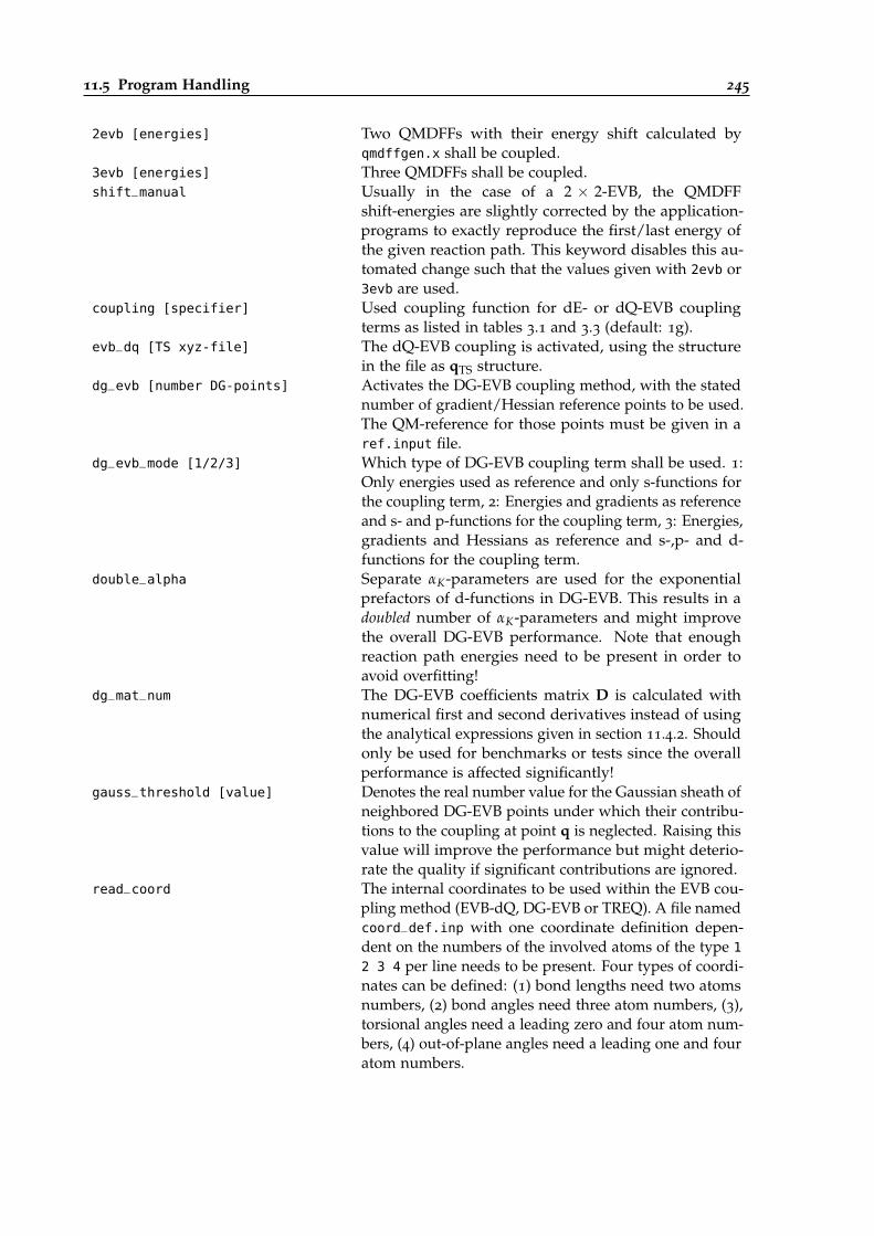
11.5 Program Handling 245
2evb [energies] Two QMDFFs with their energy shift calculated byqmdffgen.x shall be coupled.
3evb [energies] Three QMDFFs shall be coupled.shift_manual Usually in the case of a 2 × 2-EVB, the QMDFF
shift-energies are slightly corrected by the application-programs to exactly reproduce the first/last energy ofthe given reaction path. This keyword disables this au-tomated change such that the values given with 2evb or3evb are used.
coupling [specifier] Used coupling function for dE- or dQ-EVB couplingterms as listed in tables 3.1 and 3.3 (default: 1g).
evb_dq [TS xyz-file] The dQ-EVB coupling is activated, using the structurein the file as qTS structure.
dg_evb [number DG-points] Activates the DG-EVB coupling method, with the statednumber of gradient/Hessian reference points to be used.The QM-reference for those points must be given in aref.input file.
dg_evb_mode [1/2/3] Which type of DG-EVB coupling term shall be used. 1:Only energies used as reference and only s-functions forthe coupling term, 2: Energies and gradients as referenceand s- and p-functions for the coupling term, 3: Energies,gradients and Hessians as reference and s-,p- and d-functions for the coupling term.
double_alpha Separate αK-parameters are used for the exponentialprefactors of d-functions in DG-EVB. This results in adoubled number of αK-parameters and might improvethe overall DG-EVB performance. Note that enoughreaction path energies need to be present in order toavoid overfitting!
dg_mat_num The DG-EVB coefficients matrix D is calculated withnumerical first and second derivatives instead of usingthe analytical expressions given in section 11.4.2. Shouldonly be used for benchmarks or tests since the overallperformance is affected significantly!
gauss_threshold [value] Denotes the real number value for the Gaussian sheath ofneighbored DG-EVB points under which their contribu-tions to the coupling at point q is neglected. Raising thisvalue will improve the performance but might deterio-rate the quality if significant contributions are ignored.
read_coord The internal coordinates to be used within the EVB cou-pling method (EVB-dQ, DG-EVB or TREQ). A file namedcoord_def.inp with one coordinate definition depen-dent on the numbers of the involved atoms of the type 1
2 3 4 per line needs to be present. Four types of coordi-nates can be defined: (1) bond lengths need two atomsnumbers, (2) bond angles need three atom numbers, (3),torsional angles need a leading zero and four atom num-bers, (4) out-of-plane angles need a leading one and fouratom numbers.
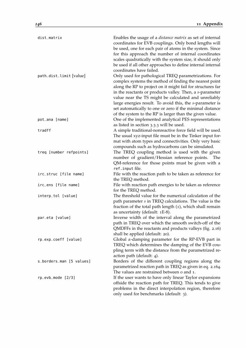
246 11 Appendix
dist_matrix Enables the usage of a distance matrix as set of internalcoordinates for EVB couplings. Only bond lengths willbe used, one for each pair of atoms in the system. Sincefor this approach the number of internal coordinatesscales quadratically with the system size, it should onlybe used if all other approaches to define internal internalcoordinates have failed.
path_dist_limit [value] Only used for pathological TREQ parametrizations. Forcomplex systems the method of finding the nearest pointalong the RP to project on it might fail for structures farin the reactants or products valley. Then, a s-parametervalue near the TS might be calculated and unreliablylarge energies result. To avoid this, the s-parameter isset automatically to one or zero if the minimal distanceof the system to the RP is larger than the given value.
pot_ana [name] One of the implemented analytical PES representationsas listed in section 3.3.3 will be used.
tradff A simple traditional-nonreactive force field will be used.The usual xyz-input file must be in the Tinker input for-mat with atom types and connectivities. Only very basiccompounds such as hydrocarbons can be simulated.
treq [number refpoints] The TREQ coupling method is used with the givennumber of gradient/Hessian reference points. TheQM-reference for those points must be given with aref.input file.
irc_struc [file name] File with the reaction path to be taken as reference forthe TREQ method.
irc_ens [file name] File with reaction path energies to be taken as referencefor the TREQ method.
interp_tol [value] The threshold value for the numerical calculation of thepath parameter s in TREQ calculations. The value is thefraction of the total path length (1), which shall remainas uncertainty (default: 1E-8).
par_eta [value] Inverse width of the interval along the parametrizedpath in TREQ over which the smooth switch-off of theQMDFFs in the reactants and products valleys (fig. 2.16)shall be applied (default: 20).
rp_exp_coeff [value] Global α-damping parameter for the RP-EVB part inTREQ which determines the damping of the EVB cou-pling term with the distance from the parametrized re-action path (default: 4).
s_borders_man [5 values] Borders of the different coupling regions along theparametrized reaction path in TREQ as given in eq. 2.164.The values are restrained between 0 and 1.
rp_evb_mode [2/3] If the user wants to have only linear Taylor expansionsoffside the reaction path for TREQ. This tends to giveproblems in the direct interpolation region, thereforeonly used for benchmarks (default: 3).
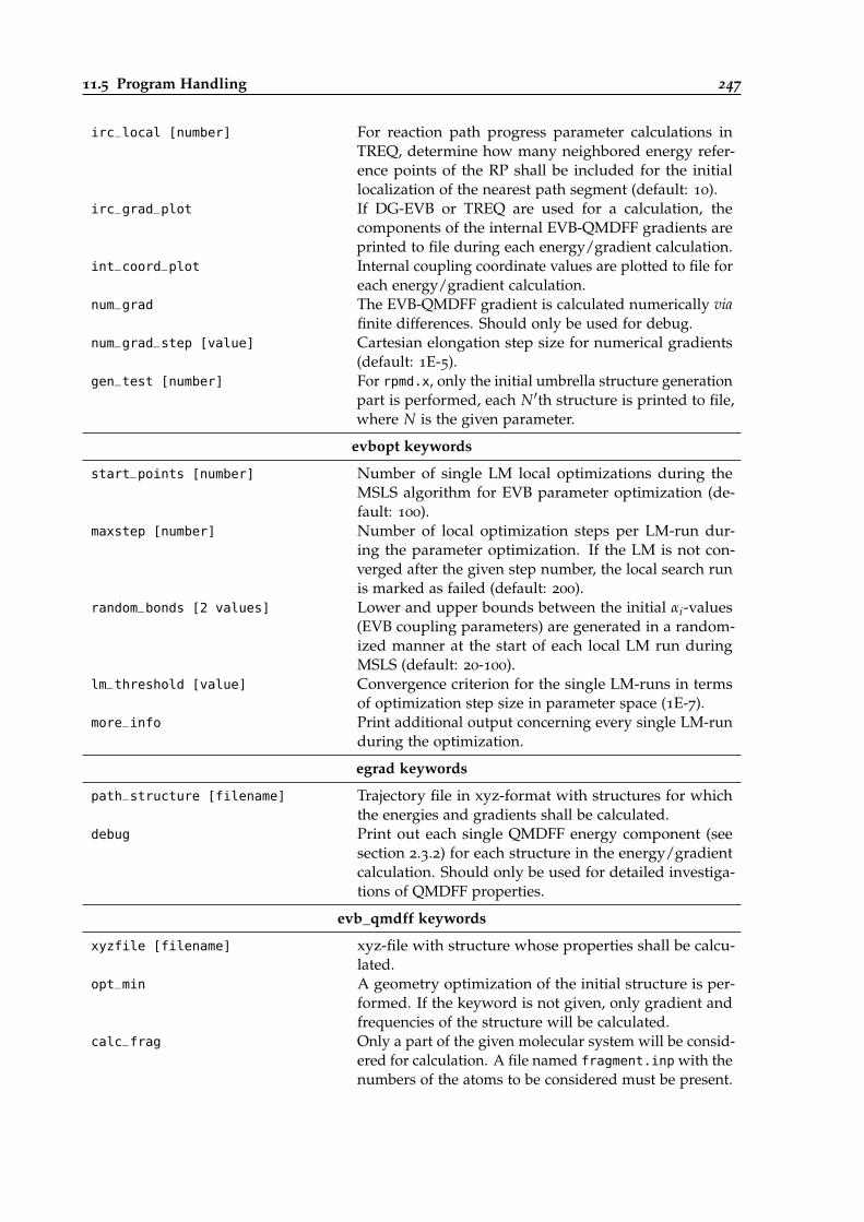
11.5 Program Handling 247
irc_local [number] For reaction path progress parameter calculations inTREQ, determine how many neighbored energy refer-ence points of the RP shall be included for the initiallocalization of the nearest path segment (default: 10).
irc_grad_plot If DG-EVB or TREQ are used for a calculation, thecomponents of the internal EVB-QMDFF gradients areprinted to file during each energy/gradient calculation.
int_coord_plot Internal coupling coordinate values are plotted to file foreach energy/gradient calculation.
num_grad The EVB-QMDFF gradient is calculated numerically viafinite differences. Should only be used for debug.
num_grad_step [value] Cartesian elongation step size for numerical gradients(default: 1E-5).
gen_test [number] For rpmd.x, only the initial umbrella structure generationpart is performed, each N′th structure is printed to file,where N is the given parameter.
evbopt keywords
start_points [number] Number of single LM local optimizations during theMSLS algorithm for EVB parameter optimization (de-fault: 100).
maxstep [number] Number of local optimization steps per LM-run dur-ing the parameter optimization. If the LM is not con-verged after the given step number, the local search runis marked as failed (default: 200).
random_bonds [2 values] Lower and upper bounds between the initial αi-values(EVB coupling parameters) are generated in a random-ized manner at the start of each local LM run duringMSLS (default: 20-100).
lm_threshold [value] Convergence criterion for the single LM-runs in termsof optimization step size in parameter space (1E-7).
more_info Print additional output concerning every single LM-runduring the optimization.
egrad keywords
path_structure [filename] Trajectory file in xyz-format with structures for whichthe energies and gradients shall be calculated.
debug Print out each single QMDFF energy component (seesection 2.3.2) for each structure in the energy/gradientcalculation. Should only be used for detailed investiga-tions of QMDFF properties.
evb_qmdff keywords
xyzfile [filename] xyz-file with structure whose properties shall be calcu-lated.
opt_min A geometry optimization of the initial structure is per-formed. If the keyword is not given, only gradient andfrequencies of the structure will be calculated.
calc_frag Only a part of the given molecular system will be consid-ered for calculation. A file named fragment.inp with thenumbers of the atoms to be considered must be present.
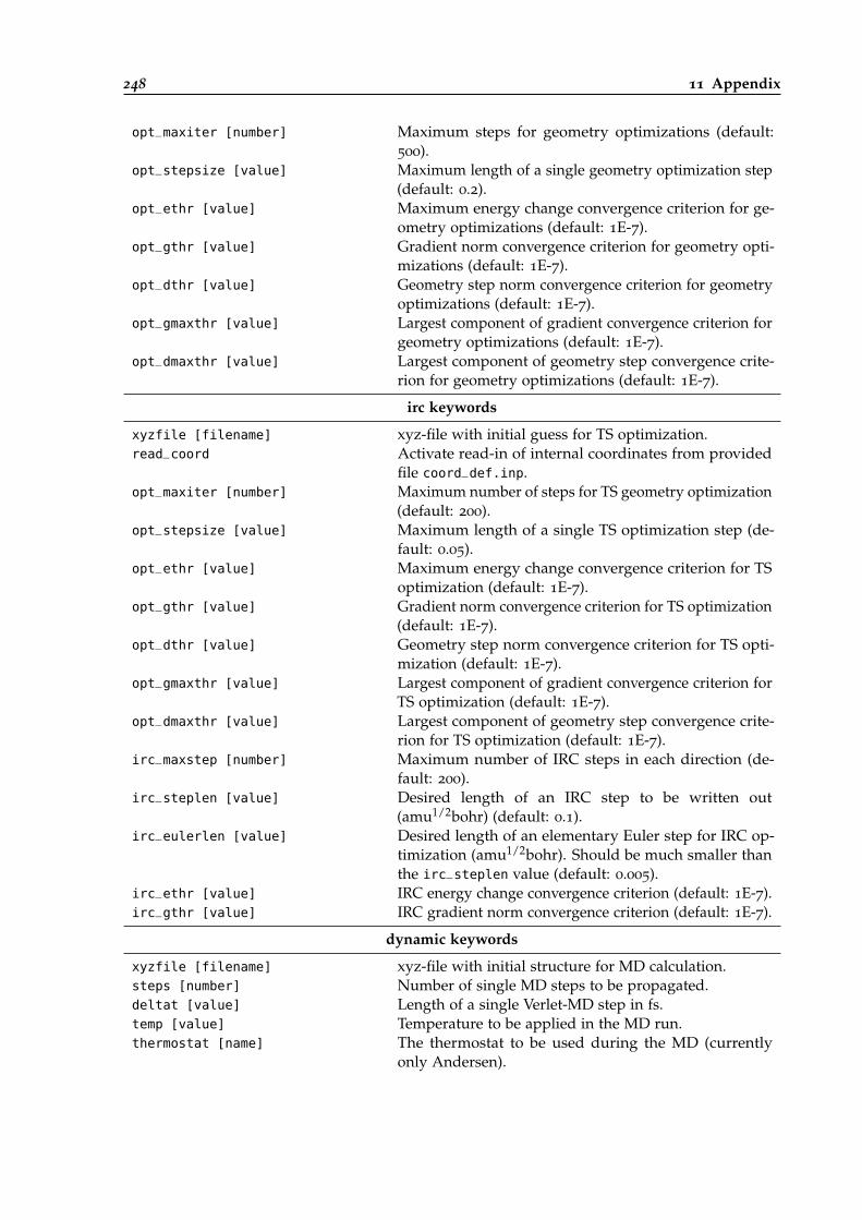
248 11 Appendix
opt_maxiter [number] Maximum steps for geometry optimizations (default:500).
opt_stepsize [value] Maximum length of a single geometry optimization step(default: 0.2).
opt_ethr [value] Maximum energy change convergence criterion for ge-ometry optimizations (default: 1E-7).
opt_gthr [value] Gradient norm convergence criterion for geometry opti-mizations (default: 1E-7).
opt_dthr [value] Geometry step norm convergence criterion for geometryoptimizations (default: 1E-7).
opt_gmaxthr [value] Largest component of gradient convergence criterion forgeometry optimizations (default: 1E-7).
opt_dmaxthr [value] Largest component of geometry step convergence crite-rion for geometry optimizations (default: 1E-7).
irc keywords
xyzfile [filename] xyz-file with initial guess for TS optimization.read_coord Activate read-in of internal coordinates from provided
file coord_def.inp.opt_maxiter [number] Maximum number of steps for TS geometry optimization
(default: 200).opt_stepsize [value] Maximum length of a single TS optimization step (de-
fault: 0.05).opt_ethr [value] Maximum energy change convergence criterion for TS
optimization (default: 1E-7).opt_gthr [value] Gradient norm convergence criterion for TS optimization
(default: 1E-7).opt_dthr [value] Geometry step norm convergence criterion for TS opti-
mization (default: 1E-7).opt_gmaxthr [value] Largest component of gradient convergence criterion for
TS optimization (default: 1E-7).opt_dmaxthr [value] Largest component of geometry step convergence crite-
rion for TS optimization (default: 1E-7).irc_maxstep [number] Maximum number of IRC steps in each direction (de-
fault: 200).irc_steplen [value] Desired length of an IRC step to be written out
(amu1/2bohr) (default: 0.1).irc_eulerlen [value] Desired length of an elementary Euler step for IRC op-
timization (amu1/2bohr). Should be much smaller thanthe irc_steplen value (default: 0.005).
irc_ethr [value] IRC energy change convergence criterion (default: 1E-7).irc_gthr [value] IRC gradient norm convergence criterion (default: 1E-7).
dynamic keywords
xyzfile [filename] xyz-file with initial structure for MD calculation.steps [number] Number of single MD steps to be propagated.deltat [value] Length of a single Verlet-MD step in fs.temp [value] Temperature to be applied in the MD run.thermostat [name] The thermostat to be used during the MD (currently
only Andersen).
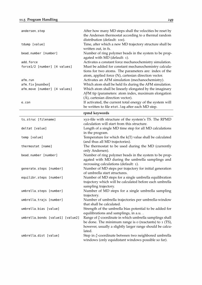
11.5 Program Handling 249
andersen_step After how many MD steps shall the velocities be reset bythe Andersen thermostat according to a thermal randomdistribution (default: 100).
tdump [value] Time, after which a new MD trajectory structure shall bewritten out, in fs.
bead_number [number] Number of ring polymer beads in the system to be prop-agated with MD (default: 1).
add_force Activates a constant force mechanochemistry simulation.force1/2 [number] [4 values] Must be added for constant mechanochemistry calcula-
tions for two atoms. The parameters are: index of theatom, applied force (N), cartesian direction vector.
afm_run Activates an AFM simulation (mechanochemistry).afm_fix [number] Which atom shall be held fix during the AFM simulation.afm_move [number] [4 values] Which atom shall be linearly elongated by the imaginary
AFM tip (parameters: atom index, maximum elongation(Å), cartesian direction vector).
e_con If activated, the current total energy of the system willbe written to file etot.log after each MD step.
rpmd keywords
ts_struc [filename] xyz-file with structure of the system’s TS. The RPMDcalculation will start from this structure.
deltat [value] Length of a single MD time step for all MD calculationsin the program.
temp [value] Temperature for which the k(T) value shall be calculated(and thus all MD trajectories).
thermostat [name] The thermostat to be used during the MD (currentlyonly Andersen).
bead_number [number] Number of ring polymer beads in the system to be prop-agated with MD during the umbrella samplings andrecrossing calculations (default: 1).
generate_steps [number] Number of MD steps per trajectory for initial generationof umbrella start structures.
equilibr_steps [number] Number of MD steps for a single umbrella equilibrationtrajectory which will be calculated before each umbrellasampling trajectory.
umbrella_steps [number] Number of MD steps for a single umbrella samplingtrajectory.
umbrella_trajs [number] Number of umbrella trajectories per umbrella-windowthat shall be calculated.
umbrella_bias [value] Strength of the umbrella bias potential to be added forequilibrations and samplings, in a.u. .
umbrella_bonds [value1] [value2] Range of ξ-coordinate in which umbrella samplings shallbe done. The minimum range is 0 (reactants) to 1 (TS),however, usually a slightly larger range should be calcu-lated.
umbrella_dist [value] Step in ξ-coordinate between two neighbored umbrellawindows (only equidistant windows possible so far).
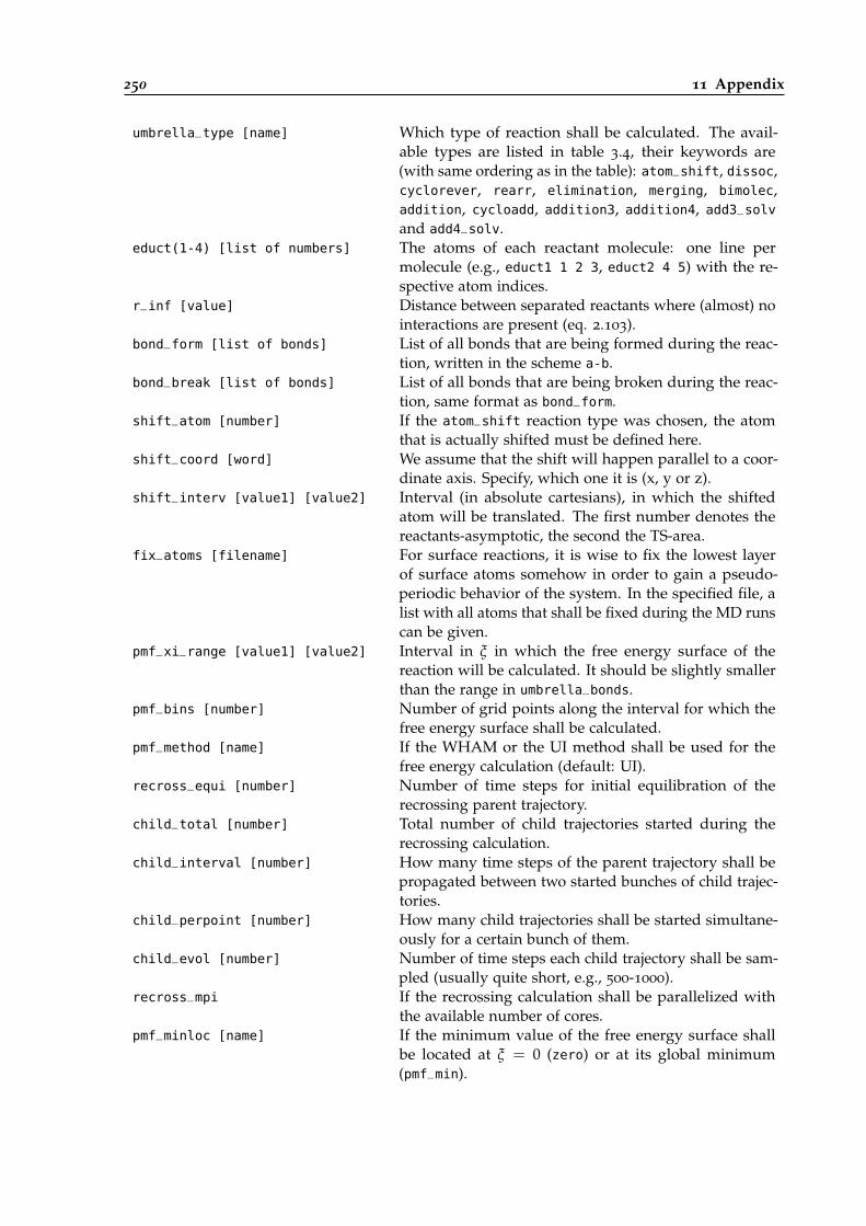
250 11 Appendix
umbrella_type [name] Which type of reaction shall be calculated. The avail-able types are listed in table 3.4, their keywords are(with same ordering as in the table): atom_shift, dissoc,cyclorever, rearr, elimination, merging, bimolec,addition, cycloadd, addition3, addition4, add3_solvand add4_solv.
educt(1-4) [list of numbers] The atoms of each reactant molecule: one line permolecule (e.g., educt1 1 2 3, educt2 4 5) with the re-spective atom indices.
r_inf [value] Distance between separated reactants where (almost) nointeractions are present (eq. 2.103).
bond_form [list of bonds] List of all bonds that are being formed during the reac-tion, written in the scheme a-b.
bond_break [list of bonds] List of all bonds that are being broken during the reac-tion, same format as bond_form.
shift_atom [number] If the atom_shift reaction type was chosen, the atomthat is actually shifted must be defined here.
shift_coord [word] We assume that the shift will happen parallel to a coor-dinate axis. Specify, which one it is (x, y or z).
shift_interv [value1] [value2] Interval (in absolute cartesians), in which the shiftedatom will be translated. The first number denotes thereactants-asymptotic, the second the TS-area.
fix_atoms [filename] For surface reactions, it is wise to fix the lowest layerof surface atoms somehow in order to gain a pseudo-periodic behavior of the system. In the specified file, alist with all atoms that shall be fixed during the MD runscan be given.
pmf_xi_range [value1] [value2] Interval in ξ in which the free energy surface of thereaction will be calculated. It should be slightly smallerthan the range in umbrella_bonds.
pmf_bins [number] Number of grid points along the interval for which thefree energy surface shall be calculated.
pmf_method [name] If the WHAM or the UI method shall be used for thefree energy calculation (default: UI).
recross_equi [number] Number of time steps for initial equilibration of therecrossing parent trajectory.
child_total [number] Total number of child trajectories started during therecrossing calculation.
child_interval [number] How many time steps of the parent trajectory shall bepropagated between two started bunches of child trajec-tories.
child_perpoint [number] How many child trajectories shall be started simultane-ously for a certain bunch of them.
child_evol [number] Number of time steps each child trajectory shall be sam-pled (usually quite short, e.g., 500-1000).
recross_mpi If the recrossing calculation shall be parallelized withthe available number of cores.
pmf_minloc [name] If the minimum value of the free energy surface shallbe located at ξ = 0 (zero) or at its global minimum(pmf_min).
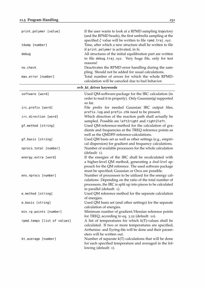
11.5 Program Handling 251
print_polymer [value] If the user wants to look at a RPMD sampling trajectory(and the RPMD beads), the first umbrella sampling at thespecified ξ value will be written to file rpmd_traj.xyz.
tdump [number] Time, after which a new structure shall be written to fileif print_polymer is activated, in fs.
debug All structures of the initial equilibration part are writtento file debug_traj.xyz. Very huge file, only for testreasons!
no_check Deactivates the RPMD error handling during the sam-pling. Should not be added for usual calculations.
max_error [number] Total number of errors for which the whole RPMD-calculation will be canceled due to bad behavior.
evb_kt_driver keywords
software [word] Used QM-software-package for the IRC calculation (inorder to read it in properly). Only Gaussian(g) supportedso far.
irc_prefix [word] File prefix for needed Gaussian IRC output files,prefix.log and prefix.chk need to be present.
irc_direction [word] Which direction of the reaction path shall actually besampled. Possible are left2right and right2left.
gf_method [string] Used QM-reference-method for the calculation of gra-dients and frequencies at the TREQ reference points aswell as the QMDFF-reference-calculations.
gf_basis [string] Used QM basis set as well as other settings (e.g., empiri-cal dispersion) for gradient and frequency calculations.
nprocs_total [number] Number of available processors for the whole calculation(default: 1).
energy_extra [word] If the energies of the IRC shall be recalculated witha higher-level QM method, generating a dual-level ap-proach for the QM reference. The used software packagemust be specified; Gaussian or Orca are possible.
ens_nprocs [number] Number of processors to be utilized for the energy cal-culations. Depending on the ratio of the total number ofprocessors, the IRC is split up into pieces to be calculatedin parallel (default: 1).
e_method [string] Used QM reference method for the separate calculationof energies.
e_basis [string] Used QM basis set (and other settings) for the separatecalculation of energies.
min_rp_points [number] Minimum number of gradient/Hessian reference pointsfor TREQ, according to eq. 3.22 (default: 10).
rpmd_temps [list of values] A list of temperatures for which k(T)-values shall becalculated. If two or more temperatures are specified,Arrhenius- and Eyring-fits will be done and their param-eters will be written out.
kt_average [number] Number of separate k(T) calculations that will be donefor each specified temperature and averaged in the fol-lowing (default: 1).
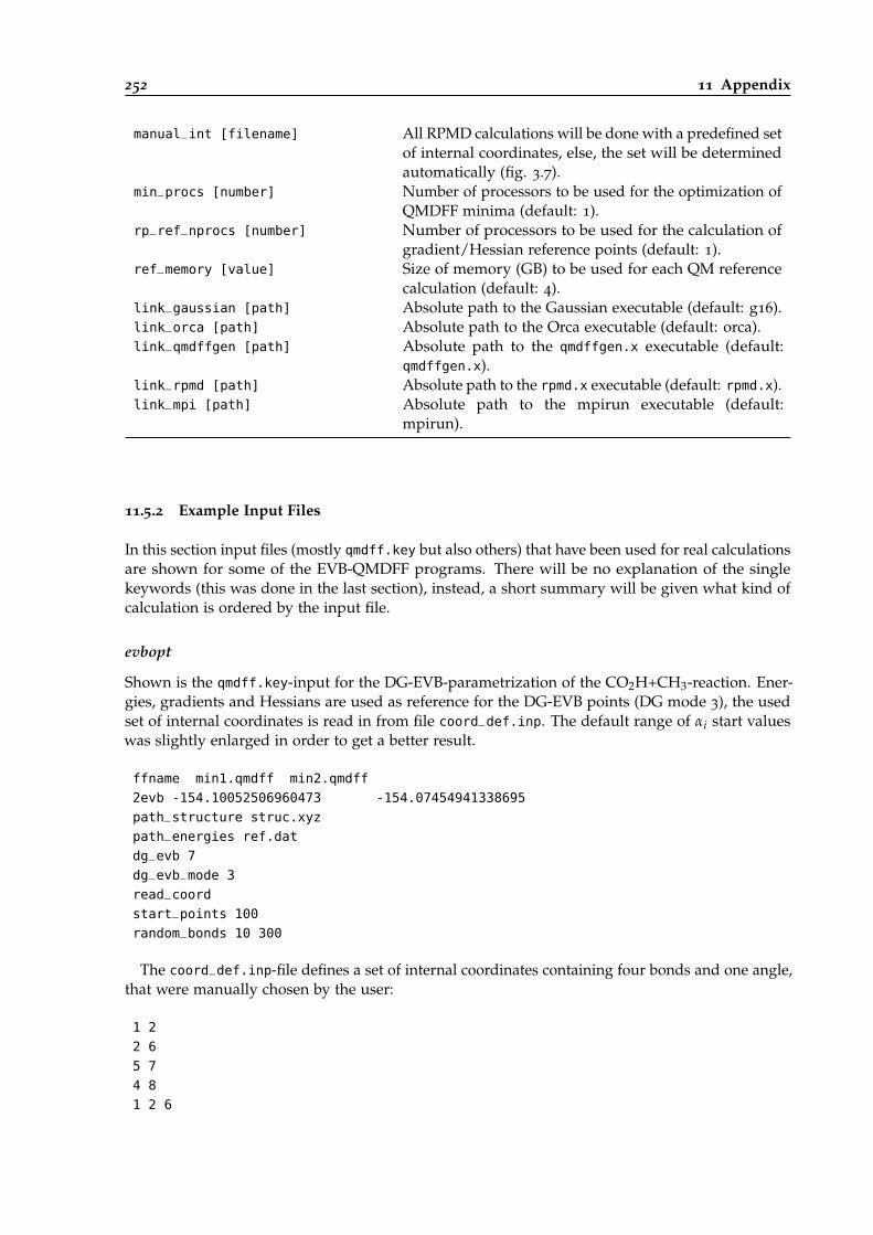
252 11 Appendix
manual_int [filename] All RPMD calculations will be done with a predefined setof internal coordinates, else, the set will be determinedautomatically (fig. 3.7).
min_procs [number] Number of processors to be used for the optimization ofQMDFF minima (default: 1).
rp_ref_nprocs [number] Number of processors to be used for the calculation ofgradient/Hessian reference points (default: 1).
ref_memory [value] Size of memory (GB) to be used for each QM referencecalculation (default: 4).
link_gaussian [path] Absolute path to the Gaussian executable (default: g16).link_orca [path] Absolute path to the Orca executable (default: orca).link_qmdffgen [path] Absolute path to the qmdffgen.x executable (default:
qmdffgen.x).link_rpmd [path] Absolute path to the rpmd.x executable (default: rpmd.x).link_mpi [path] Absolute path to the mpirun executable (default:
mpirun).
11.5.2 Example Input Files
In this section input files (mostly qmdff.key but also others) that have been used for real calculationsare shown for some of the EVB-QMDFF programs. There will be no explanation of the singlekeywords (this was done in the last section), instead, a short summary will be given what kind ofcalculation is ordered by the input file.
evbopt
Shown is the qmdff.key-input for the DG-EVB-parametrization of the CO2H+CH3-reaction. Ener-gies, gradients and Hessians are used as reference for the DG-EVB points (DG mode 3), the usedset of internal coordinates is read in from file coord_def.inp. The default range of αi start valueswas slightly enlarged in order to get a better result.
ffname min1.qmdff min2.qmdff
2evb -154.10052506960473 -154.07454941338695
path_structure struc.xyz
path_energies ref.dat
dg_evb 7
dg_evb_mode 3
read_coord
start_points 100
random_bonds 10 300
The coord_def.inp-file defines a set of internal coordinates containing four bonds and one angle,that were manually chosen by the user:
1 2
2 6
5 7
4 8
1 2 6
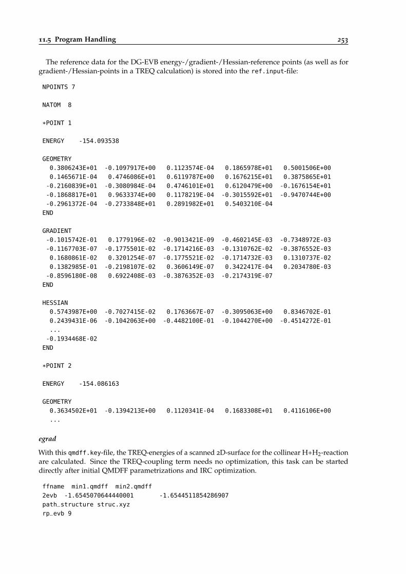
11.5 Program Handling 253
The reference data for the DG-EVB energy-/gradient-/Hessian-reference points (as well as forgradient-/Hessian-points in a TREQ calculation) is stored into the ref.input-file:
NPOINTS 7
NATOM 8
*POINT 1
ENERGY -154.093538
GEOMETRY
0.3806243E+01 -0.1097917E+00 0.1123574E-04 0.1865978E+01 0.5001506E+00
0.1465671E-04 0.4746086E+01 0.6119787E+00 0.1676215E+01 0.3875865E+01
-0.2160839E+01 -0.3080984E-04 0.4746101E+01 0.6120479E+00 -0.1676154E+01
-0.1868817E+01 0.9633374E+00 0.1178219E-04 -0.3015592E+01 -0.9470744E+00
-0.2961372E-04 -0.2733848E+01 0.2891982E+01 0.5403210E-04
END
GRADIENT
-0.1015742E-01 0.1779196E-02 -0.9013421E-09 -0.4602145E-03 -0.7348972E-03
-0.1167703E-07 -0.1775501E-02 -0.1714216E-03 -0.1310762E-02 -0.3876552E-03
0.1680861E-02 0.3201254E-07 -0.1775521E-02 -0.1714732E-03 0.1310737E-02
0.1382985E-01 -0.2198107E-02 0.3606149E-07 0.3422417E-04 0.2034780E-03
-0.8596180E-08 0.6922408E-03 -0.3876352E-03 -0.2174319E-07
END
HESSIAN
0.5743987E+00 -0.7027415E-02 0.1763667E-07 -0.3095063E+00 0.8346702E-01
0.2439431E-06 -0.1042063E+00 -0.4482100E-01 -0.1044270E+00 -0.4514272E-01
...
-0.1934468E-02
END
*POINT 2
ENERGY -154.086163
GEOMETRY
0.3634502E+01 -0.1394213E+00 0.1120341E-04 0.1683308E+01 0.4116106E+00
...
egrad
With this qmdff.key-file, the TREQ-energies of a scanned 2D-surface for the collinear H+H2-reactionare calculated. Since the TREQ-coupling term needs no optimization, this task can be starteddirectly after initial QMDFF parametrizations and IRC optimization.
ffname min1.qmdff min2.qmdff
2evb -1.6545070644440001 -1.6544511854286907
path_structure struc.xyz
rp_evb 9
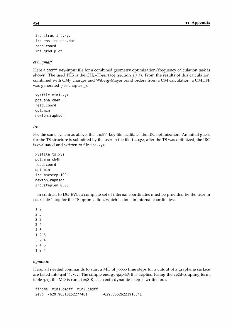
254 11 Appendix
irc_struc irc.xyz
irc_ens irc_ens.dat
read_coord
int_grad_plot
evb_qmdff
Here a qmdff.key-input file for a combined geometry optimization/frequency calculation task isshown. The used PES is the CH4+H-surface (section 3.3.3). From the results of this calculation,combined with CM5 charges and Wiberg-Mayer bond orders from a QM calculation, a QMDFFwas generated (see chapter 5).
xyzfile min1.xyz
pot_ana ch4h
read_coord
opt_min
newton_raphson
irc
For the same system as above, this qmdff.key-file facilitates the IRC optimization. An initial guessfor the TS structure is submitted by the user in the file ts.xyz, after the TS was optimized, the IRCis evaluated and written to file irc.xyz.
xyzfile ts.xyz
pot_ana ch4h
read_coord
opt_min
irc_maxstep 100
newton_raphson
irc_steplen 0.05
In contrast to DG-EVB, a complete set of internal coordinates must be provided by the user incoord_def.inp for the TS optimization, which is done in internal coordinates:
1 2
2 5
2 3
2 4
4 6
1 2 5
3 2 4
2 4 6
1 2 4
dynamic
Here, all needed commands to start a MD of 50000 time steps for a cutout of a graphene surfaceare listed into qmdff.key. The simple energy-gap-EVB is applied (using the sp2d-coupling term,table 3.1), the MD is run at 298 K, each 20th dynamics step is written out.
ffname min1.qmdff min2.qmdff
2evb -629.98510152277481 -629.86526221918541
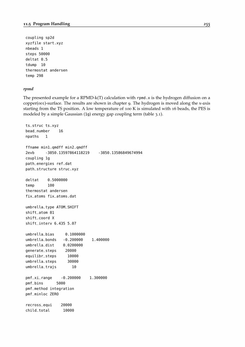
11.5 Program Handling 255
coupling sp2d
xyzfile start.xyz
nbeads 1
steps 50000
deltat 0.5
tdump 10
thermostat andersen
temp 298
rpmd
The presented example for a RPMD-k(T) calculation with rpmd.x is the hydrogen diffusion on acopper(001)-surface. The results are shown in chapter 9. The hydrogen is moved along the x-axisstarting from the TS position. A low temperature of 100 K is simulated with 16 beads, the PES ismodeled by a simple Gaussian (1g) energy gap coupling term (table 3.1).
ts_struc ts.xyz
bead_number 16
npaths 1
ffname min1.qmdff min2.qmdff
2evb -3850.13597864118219 -3850.13586849674994
coupling 1g
path_energies ref.dat
path_structure struc.xyz
deltat 0.5000000
temp 100
thermostat andersen
fix_atoms fix_atoms.dat
umbrella_type ATOM_SHIFT
shift_atom 81
shift_coord X
shift_interv 6.435 5.07
umbrella_bias 0.1000000
umbrella_bonds -0.200000 1.400000
umbrella_dist 0.0200000
generate_steps 20000
equilibr_steps 10000
umbrella_steps 30000
umbrella_trajs 10
pmf_xi_range -0.200000 1.300000
pmf_bins 5000
pmf_method integration
pmf_minloc ZERO
recross_equi 20000
child_total 10000
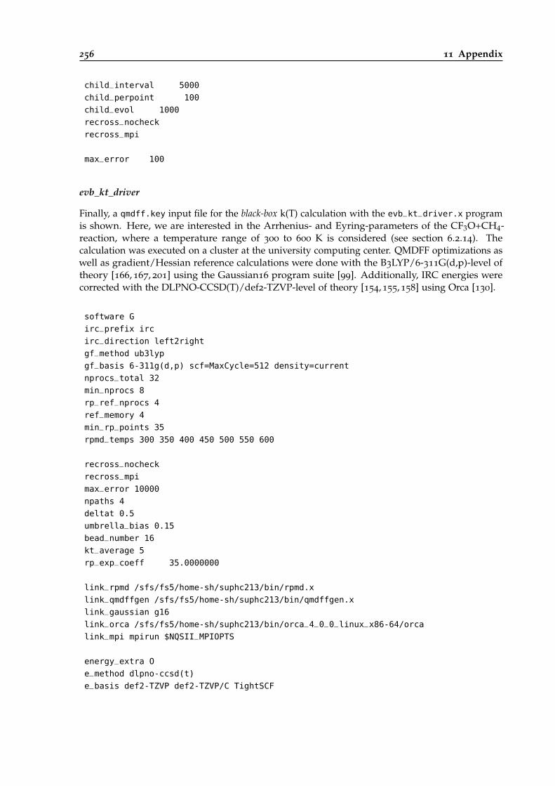
256 11 Appendix
child_interval 5000
child_perpoint 100
child_evol 1000
recross_nocheck
recross_mpi
max_error 100
evb_kt_driver
Finally, a qmdff.key input file for the black-box k(T) calculation with the evb_kt_driver.x programis shown. Here, we are interested in the Arrhenius- and Eyring-parameters of the CF3O+CH4-reaction, where a temperature range of 300 to 600 K is considered (see section 6.2.14). Thecalculation was executed on a cluster at the university computing center. QMDFF optimizations aswell as gradient/Hessian reference calculations were done with the B3LYP/6-311G(d,p)-level oftheory [166, 167, 201] using the Gaussian16 program suite [99]. Additionally, IRC energies werecorrected with the DLPNO-CCSD(T)/def2-TZVP-level of theory [154, 155, 158] using Orca [130].
software G
irc_prefix irc
irc_direction left2right
gf_method ub3lyp
gf_basis 6-311g(d,p) scf=MaxCycle=512 density=current
nprocs_total 32
min_nprocs 8
rp_ref_nprocs 4
ref_memory 4
min_rp_points 35
rpmd_temps 300 350 400 450 500 550 600
recross_nocheck
recross_mpi
max_error 10000
npaths 4
deltat 0.5
umbrella_bias 0.15
bead_number 16
kt_average 5
rp_exp_coeff 35.0000000
link_rpmd /sfs/fs5/home-sh/suphc213/bin/rpmd.x
link_qmdffgen /sfs/fs5/home-sh/suphc213/bin/qmdffgen.x
link_gaussian g16
link_orca /sfs/fs5/home-sh/suphc213/bin/orca_4_0_0_linux_x86-64/orca
link_mpi mpirun $NQSII_MPIOPTS
energy_extra O
e_method dlpno-ccsd(t)
e_basis def2-TZVP def2-TZVP/C TightSCF
11.6 Supplementary Information 257
11.6 Supplementary Information
For both publications that are part of this thesis, supplementary information sheets were createdthat provide some additional insight into calculation setups, choices made by the author(s) andfurther results complementing the ones shown in the main publications.
Besides the papers in chapters 4 and 5 I wrote a part of the supplementary information of thefirst EVB-QMDFF paper of Hartke and Grimme [16]. This is therefore shown here as well.
11.6.1 First EVB-QMDFF Publication
The publication by Hartke and Grimme [16] introduced the EVB-QMDFF methodology. Reactionpaths for three different systems were parametrized by using the simple 1g-energy-gap couplingterm.
The supporting information presents an example of the even simpler constant coupling term (seetable 3.1) in chapter 1. Further, it gives a first clue of how EVB-QMDFF is able to describe regionsoffside the reaction path in chapter 2, shown by two-dimensional sections of the potential energysurfaces for two example reactions. The results in chapter 2 were produced by myself.
11.6.2 RPMD Rate Constants with (DG-)EVB-QMDFF
This supplementary information shows further details for the second EVB-QMDFF publicationreprinted in chapter 4. Since the overall quality of DG-EVB force fields depends on quite a fewparameters, their influence on the force field is shown in chapter 1.
The tests were executed for both reactions that are calculated with DG-EVB in the main paper.Presented are different sets of internal coordinates as well as different numbers and positions ofDG-EVB gradient and Hessian reference points. Two-dimensional scans of both parameter setswere done, resulting in the insight that the “correct” choice of internal coordinates is crucial for theoverall force field quality and that the error sum converges to a minimum value if more than 8 or 9
DG-EVB reference points are used. In chapter 2, the number of energy reference points along theMEP is varied and its influence on the DG-EVB parameter optimization process can be seen.
The used RPMDrate settings are presented in chapter 3, whereas the influence of their variationon the calculated rate constants is shown in chapter 4. Convergence of the values with respect tobead number, lengths of MD time steps and the number of umbrella sampling trajectories exists.
Free energy curves and time-dependent transmission coefficients are presented in chapters 5 and6.
11.6.3 TREQ - Development and Benchmark
The following sheet contains many details regarding the TREQ benchmarks that were done for 6
different reactions (see chapter 5).Besides this, settings for the DG-EVB calculations used as a competitor are shown as well.A more detailed overview of the shown results is presented on the first reprinted page.


12
Ch
ap
te
r
Bibliography
[1] B. Peters, Reaction Rate Theory and Rare Events, Elsevier, 1st ed., 2017.
[2] W. K. den Otter and W. J. Briels, The Reactive Flux Method Applied to Complex IsomerizationReactions: Using the Unstable Normal Mode as a Reaction Coordinate, J. Chem. Phys., 106 (1997),pp. 5494–5508, DOI: 10.1063/1.473573.
[3] K. J. Laidler and M. C. King, Development of Transition-State Theory, J. Phys. Chem., 87
(1983), pp. 2657–2664, DOI: 10.1021/j100238a002.
[4] H. Eyring, Viscosity, Plasticity, and Diffusion as Examples of Absolute Reaction Rates, J. Chem.Phys., 4 (1936), pp. 283–291, DOI: 10.1063/1.1749836.
[5] M. G. Evans and M. Polanyi, Some Applications of the Transition State Method to the Calculationof Reaction Velocities, Especially in Solution, Trans. Faraday Soc., 31 (1935), pp. 875–894, DOI:10.1039/TF9353100875.
[6] J. A. Sansòn, M.-L. Sànchez, and J. C. Corchado, Importance of Anharmonicity, RecrossingEffects, and Quantum Mechanical Tunneling in Transition State Theory with Semiclassical Tunneling.A Test Case: The H2+Cl Hydrogen Abstraction Reaction, J. Phys. Chem. A, 110 (2006), pp. 589–599,DOI: 10.1021/jp052849d.
[7] U. Manthe and W. H. Miller, The Cumulative Reaction Probability as Eigenvalue Problem, J.Chem. Phys., 99 (1993), pp. 3411–3419, DOI: 10.1063/1.465151.
[8] G. Nyman, Computational Methods of Quantum Reaction Dynamics, Int. J. Quantum Chem., 114
(2014), pp. 1183–1198, DOI: 10.1002/qua.24661.
[9] T. J. H. Hele, Quantum Transition-State Theory, PhD thesis, University of Cambridge, 2014.
[10] J. Zheng, J. L. Bao, R. Maena-Pañeda, S. Zhang, B. J. Lynch, J. C. Corchado, Y.-Y. Chuang,P. L. Fast, W.-P. Hu, Y.-P. Liu, G. C. Lynch, K. A. Nguyen, C. F. Jackels, A. F. Ramos, B. A.Ellington, V. S. Melissas, J. Villá, I. Rossi, E. L. Coitniño, J. Pu, T. V. Albu, A. Ratkiewicz,R. Steckler, B. C. Garrett, A. D. Isaacson, and D. G. Truhlar, Polyrate-version 2017, 2017.
[11] S. Habershon, D. E. Manolopoulos, T. E. Markland, and T. F. Miller III, Ring-PolymerMolecular Dynamics: Quantum Effects in Chemical Dynamics from Classical Trajectories in anExtended Phase Space, Annu. Rev. Phys. Chem., 64 (2013), pp. 387–413, DOI: 10.1146/annurev-physchem-040412-110122.
[12] F. Jensen, Introduction to Computational Chemistry, Wiley, 3rd ed., 2017.
260 12 Bibliography
[13] Y. V. Suleymanov, J. W. Allen, and W. H. Green, RPMDrate: Bimolecular Chemical ReactionRates from Ring Polymer Molecular Dynamics, Comp. Phys. Comm., 184 (2013), pp. 833–840,DOI: 10.1016/j.cpc.2012.10.017.
[14] A. C. T. van Duin, S. Dasgupta, F. Lorant, and W. A. Goddard, III., ReaxFF: A Reactive ForceField for Hydrocarbons, J. Phys. Chem. A, 105 (2001), pp. 9396–9409, DOI: 10.1021/jp004368u.
[15] S. Grimme, A General Quantum Mechanically Derived Force Field (QMDFF) for Moleculesand Condensed Phase Simulations, J. Chem. Theory Comput., 10 (2014), pp. 4497–4514, DOI:10.1021/ct500573f.
[16] B. Hartke and S. Grimme, Reactive Force Fields Made Simple, Phys. Chem. Chem. Phys., 17
(2015), pp. 16715–16718, DOI: 10.1039/C5CP02580J.
[17] J. Steffen and B. Hartke, Cheap but Accurate Calculation of Chemical Reaction Rate Constantsfrom Ab Initio Data, via System-Specific, Black-Box Force Fields, J. Chem. Phys., 147 (2017),p. 161701, DOI: 10.1063/1.4979712.
[18] J. Steffen, A New Class of Reaction Path Based Potential Energy Surfaces Enabling AccurateBlack Box Chemical Rate Constant Calculations, J. Chem. Phys., 150 (2019), p. 154105, DOI:10.1063/1.5092589.
[19] K. J. Laidler, The Development of the Arrhenius Equation, J. Chem. Educ., 61 (1984), pp. 494–498,DOI: 10.1021/ed061p494.
[20] P. L. Houston, Chemical Kinetics and Reaction Dynamics, vol. 1st, Dover Publications, 1st ed.,2006.
[21] W. Göpel and H.-D. Wiemhöfer, Statistische Thermodynamik, Spektrum AkademischerVerlag, 1st ed., 2000.
[22] A. Fernàndez-Ramos, J. A. Miller, S. J. Klippenstein, and D. G. Truhlar, Modeling the Ki-netics of Bimolecular Reactions, Chem. Rev., 106 (2006), pp. 4518–4584, DOI: 10.1021/cr050205w.
[23] R. P. de Tudela, Y. V. Suleimanov, J. O. Richardson, V. S. Rábanos, W. H. Green, and
F. J. Aoiz, Stress Test for Quantum Dynamics Approximations: Deep Tunneling in the MuoniumExchange Reaction D+HMu −→ DMu+H, J. Phys. Chem., 5 (2014), pp. 4219–4224, DOI:10.1021/jz502216g.
[24] Y. V. Suleimanov, R. Pérez de Tudela, P. G. Jambrina, J. F. Castillo, V. Sáez-Rábanos,D. E. Manolopoulos, and F. J. Aoiz, A Ring Polymer Molecular Dynamics Study of theIsotopologues of the H+H2 Reaction, Phys. Chem. Chem. Phys., 15 (2013), pp. 3655–3665, DOI:10.1039/c2cp44364c.
[25] D. G. Truhlar and B. C. Garrett, Variational Transition-State Theory, Acc. Chem. Res., 13
(1980), pp. 440–448, DOI: 10.1021/ar50156a002.
[26] D. G. Truhlar and B. C. Garrett, Variational Transition State Theory, Ann. Rev. Phys. Chem.,35 (1984), pp. 159–189, DOI: 10.1146/annurev.pc.35.100184.001111.
[27] B. C. Garrett and D. G. Truhlar, Criterion of Minimum State Density in the Transi-tion State Theory of Bimolecular Reactions, J. Chem. Phys., 70 (1979), pp. 1593–1598, DOI:10.1063/1.437698.
[28] S. C. Tucker and E. Pollack, Microcanonical Variational Transition-State Theory for ReactionRates in Dissipative Systems, J. Stat. Phys., 66 (1992), pp. 975–990, DOI: 10.1007/BF01055711.
12 Bibliography 261
[29] D. G. Truhlar, A. D. Isaacson, and B. C. Garrett, Generalized Transition State Theory, CRCPress, 1985, pp. 65–137.
[30] W. H. Miller, Unified Statistical Model for "Complex" and "Direct" Reaction Mechanisms, J.Chem. Phys., 65 (1976), pp. 2216–2223, DOI: 10.1063/1.433379.
[31] B. C. Garrett and D. G. Truhlar, Canonical Unified Statistical Model. Classical MechanicalTheory and Applications to Collinear Reactions, J. Chem. Phys., 76 (1982), pp. 1853–1858, DOI:10.1063/1.443157.
[32] J. Meisner and J. Kästner, Atom Tunneling in Chemistry, Angew. Chem. Int. Ed., 55 (2016),pp. 5400–5413, DOI: 10.1002/anie.201511028.
[33] J. Pu, J. Gao, and D. G. Truhlar, Multidimensional Tunneling, Recrossing, and the Trans-mission Coefficient for Enzymatic Reactions, Chem. Rev., 106 (2006), pp. 3140–3169, DOI:10.1021/cr050308e.
[34] Y. V. Suleimanov and J. Espinosa-Garcìa, Recrossing and tunnelling in the kinetics studyof the OH+CH4 −→ H2O+CH3 reaction., J. Phys. Chem. B, 120 (2016), pp. 1418–1428, DOI:10.1021/acs.jpcb.5b02103.
[35] B. C. Garrett and D. G. Truhlar, Accuracy of Tunneling Corrections to Transition State Theoryfor Thermal Rate Constants of Atom Transfer Reactions, J. Phys. Chem., 83 (1979), pp. 200–203,DOI: 10.1021/j100464a026.
[36] B. C. Garrett, D. G. Truhlar, R. S. Grev, and A. W. Magnuson, Improved Treatmentof Threshold Contributions in Variational Transition-State Theory, J. Phys. Chem., 84 (1980),pp. 1730–1748, DOI: 10.1021/j100450a013.
[37] R. T. Skodje and D. G. Truhlar, A General Small-Curvature Approximation for Transition-State-Theory Transmission Coefficients, J. Phys. Chem., 85 (1981), pp. 3019–3023, DOI:10.1021/j150621a001.
[38] D. G. Truhlar, B. C. Garrett, and S. J. Klippenstein, Current Status of Transition-StateTheory, J. Phys. Chem., 100 (1996), pp. 12771–12800, DOI: 10.1021/jp953748q.
[39] J. Kästner, Umbrella Sampling, WIREs Comput. Mol. Sci., 1 (2011), pp. 932–942, DOI:10.1002/wcms.66.
[40] A. R. Leach, Molecular Modeling - Principles and Applications, Pearson, 2nd ed., 2001.
[41] G. M. Torrie and J. P. Valleau, Nonphysical Sampling Distributions in Monte Carlo Free-EnergyEstimation: Umbrella Sampling, J. Comput. Phys., 23 (1977), pp. 187–199, DOI: 10.1016/0021-9991(77)90121-8.
[42] S. Kumar, J. M. Rosenberg, D. Bouzida, R. H. Swendsen, and P. A. Kollman, The WeightedHistogram Analysis Method for Free-Energy Calculations on Biomolecules. I. The Method, J. Comput.Chem., 13 (1992), pp. 1011–1021, DOI: 10.1002/jcc.540130812.
[43] J. Kästner and W. Thiel, Bridging the Gap Between Thermodynamic Integration and UmbrellaSampling Provides a Novel Analysis Method: “Umbrella Integration”, J. Chem. Phys., 123 (2005),p. 144104, DOI: 10.1063/1.2052648.
[44] W. K. den Otter and W. J. Briels, Solvent Effect on the Isomerization Rate of Calix[4]areneStudied by Molecular Dynamics Simulations, J. Am. Chem. Soc., 120 (1998), pp. 13167–13175,DOI: 10.1021/ja9741739.
262 12 Bibliography
[45] D. Chandler, Statistical Mechanics of Isomerization Dynamics in Liquids and the Transition StateApproximation, J. Chem. Phys., 68 (1978), pp. 2959–2970, DOI: 10.1063/1.436049.
[46] C. C. Marston, G. G. Balint-Kurti, and R. N. Dixon, Time-Dependent Quantum Dynamicsof Reactive Scattering and the Calculation of Product Quantum State Distributions - A Study of theCollinear F+H2(v=0) −→ HF(v’)+H Reaction, Theor. Chim. Acta, 79 (1991), pp. 313–322, DOI:10.1007/BF01113699.
[47] W. H. Miller, "Direct" and "Correct" Calculation of Canonical and Microcanonical Rate Constantsfor Chemical Reactions, J. Phys. Chem. A, 105 (1992), pp. 793–806, DOI: 10.1021/jp973208o.
[48] T. Seidemann and W. H. Miller, Calculation of the Cumulative Reaction Probability via aDiscrete Variable Representation with Absorbing Boundary Conditions, J. Chem. Phys., 96 (1992),pp. 4412–4422, DOI: 10.1063/1.462832.
[49] M. H. Beck, A. Jäckle, G. A. Worth, and H.-D. Meyer, The Multiconfiguration Time-DependentHartree (MCTDH) Method: a Highly Efficient Algorithm for Propagating Wavepackets, Phys. Rep.,324 (2000), pp. 1–105, DOI: 10.1016/S0370-1573(99)00047-2.
[50] R. P. Feynman and A. R. Hibbs, Quantum Mechanics and Path Integrals, Dover Publications,amended edition ed., 2005.
[51] A. Agarwal, Path Integral Techniques in Molecular Dynamics Simulations of Open BoundarySystems, PhD thesis, Freie Universität Berlin, 2016.
[52] C. Gorgulla, Free Energy Methods Involving Quantum Physics, Path Integrals, and VirtualScreenings, PhD thesis, Freie Universität Berlin, 2018.
[53] Y. V. Suleimanov, R. Collepardo-Guevara, and D. E. Manolopoulos, Bimolecular ReactionRates from Ring Polymer Molecular Dynamics: Application to H+CH4 −→ H2+CH3, J. Chem.Phys., 134 (2011), p. 044131, DOI: 10.1063/1.3533275.
[54] I. N. Levine, Quantum Chemistry, Allyn and Bacon, 3rd ed., 1983.
[55] A. Szabo and N. S. Ostlund, Modern Quantum Chemistry, Dover, 2nd ed., 1989.
[56] S. Sato, On a New Method of Drawing the Potential Energy Surface, J. Chem. Phys., 23 (1955),pp. 592–593, DOI: 10.1063/1.1742043.
[57] S. Sato, Potential Energy Surface of the System of Three Atoms, J. Chem. Phys., 23 (1955),pp. 2465–2466, DOI: 10.1063/1.1741936.
[58] A. Persky and H. Kornweitz, Oscillating Reactivity of the Light Atom Transfer Reaction Cl+HCl−→ ClH+Cl: Dependence on the Nature of the Potential Energy Surface, J. Phys. Chem., 91 (1987),pp. 5496–5503, DOI: 10.1021/j100305a023.
[59] L. Martin-Gondre, C. Crespos, P. Larrègaray, J. C. Rayez, D. Conte, and B. van Ootegem,Detailed Description of the Flexible Periodic London–Eyring–Polanyi–Sato Potential Energy Function,Chem. Phys., 367 (2010), pp. 136–147, DOI: 10.1016/j.chemphys.2009.11.012.
[60] G. C. Schatz, The Analytical Representation of Electronic Potential-Energy Surfaces, Rev. Mod.Phys., 61 (1989), pp. 205–264, DOI: 10.1103/RevModPhys.61.669.
[61] D. G. Truhlar and C. J. Horowitz, Functional Representation of Liu and Siegbahn’s AccurateAb Initio Potential Energy Calculations for H+H2, J. Chem. Phys., 68 (1978), pp. 2466–2476, DOI:10.1063/1.436019.
12 Bibliography 263
[62] J. M. Bowman, J. S. Bittman, and L. B. Harding, Ab Initio Calculations of Electronic and Vibra-tional Energies of HCO and HOC, J. Chem. Phys., 85 (1986), pp. 911–921, DOI: 10.1063/1.451246.
[63] K. A. White and G. C. Schatz, Analytical Potential Energy Surfaces for Ethynyl, Acetylene, andVinyl, J. Phys. Chem., 88 (1984), pp. 2049–2057, DOI: 10.1021/j150654a023.
[64] P. M. Agrawal, D. L. Thompson, and L. M. Raff, Trajectory Studies of Unimolecular Reactionsof Si2H4 and SiH2 on a Global Potential Surface Fitted to Ab Initio and Experimental Data, J. Chem.Phys., 89 (1988), pp. 741–750, DOI: 10.1063/1.455197.
[65] C. M. Handly and J. Behler, Next Generation Interatomic Potentials for Condensed Systems,Eur. Phys. J. B, 87 (2014), p. 152, DOI: 10.1140/epjb/e2014-50070-0.
[66] M. A. Collins, Molecular Potential-Energy Surfaces for Chemical Reaction Dynamics, Theor.Chem. Acc., 108 (2002), pp. 313–324, DOI: 10.1007/s00214-002-0383-5.
[67] H. M. Netzloff, M. A. Collins, and M. S. Gordon, Growing Multiconfigurational PotentialEnergy Surfaces with Applications to X+H2(X = C, N, O) Reactions, J. Chem. Phys., 124 (2006),p. 154104, DOI: 10.1063/1.2185641.
[68] G. G. Maisuradze, D. L. Thompson, A. F. Wagner, and M. Minkoff, Interpolating MovingLeast-Squares Methods for Fitting Potential Energy Surfaces: Detailed Analysis of One-DimensionalApplications, J. Chem. Phys., 119 (2003), pp. 10002–10014, DOI: 10.1063/1.1617271.
[69] B. Kolb, P. Marshall, B. Zhao, B. Jiang, and H. Guo, Representing Global Reactive PotentialEnergy Surfaces Using Gaussian Processes, J. Phys. Chem. A, 121 (2017), pp. 2552–2557, DOI:10.1021/acs.jpca.7b01182.
[70] J. Behler, Constructing High-Dimensional Neural Network Potentials: A Tutorial Review, Int. J.Quantum Chem., 115 (2015), pp. 1032–1050, DOI: 10.1002/qua.24890.
[71] P. Dauber-Osguthorpe and A. T. Hagler, Biomolecular Force Fields: Where Have We Been,Where Are We Now, Where Do We Need to Go and How Do We Get There?, J. Comput.-Aided Mol.Des., 33 (2018), pp. 133–203, DOI: 10.1007/s10822-018-0111-4.
[72] A. T. Hagler, Force Field Development Phase II: Relaxation of Physics-Based Criteria... or Inclusionof More Rigorous Physics into the Representation of Molecular Energetics, J. Comput.-Aided Mol.Des., 33 (2018), pp. 205–264, DOI: 10.1007/s10822-018-0134-x.
[73] N. L. Allinger, Y. H. Yuh, and J. H. Lii, Molecular Mechanics. The MM3 Force Field forHydrocarbons. 1, J. Am. Chem. Soc., 111 (1989), pp. 8551–8566, DOI: 10.1021/ja00205a001.
[74] A. K. Rappe, C. J. Casewit, K. S. Colwell, W. A. Goddard, III, and W. M. Skiff, UFF, a FullPeriodic Table Force Field for Molecular Mechanics and Molecular Dynamics Simulations, J. Am.Chem. Soc., 114 (1992), pp. 10024–10035, DOI: 10.1021/ja00051a040.
[75] A. C. T. van Duin, S. Dasgupta, F. Lorant, and W. A. Goddard, III., ReaxFF: A Reactive ForceField for Hydrocarbons, J. Phys. Chem. A, 105 (2001), pp. 9396–9409, DOI: 10.1021/jp004368u.
[76] J. M. Dieterich and B. Hartke, OGOLEM: Global Cluster Structure Optimisation for ArbitraryMixtures of Flexible Molecules. A Multiscaling, Object-Oriented Approach, Mol. Phys., 108 (2010),pp. 279–291, DOI: 10.1080/00268970903446756.
[77] H. R. Larsson, A. C. T. van Duin, and B. Hartke, Global Optimization of Parameters inthe Reactive Force Field ReaxFF for SiOH, J. Comput. Chem., 34 (2013), pp. 2178–2189, DOI:10.1002/jcc.23382.
264 12 Bibliography
[78] M. Dittner, J. Müller, H. M. Aktulga, and B. Hartke, Efficient Global Optimization of Reac-tive Force–Field Parameters, J. Comput. Chem., 36 (2015), pp. 1550–1561, DOI: 10.1002/jcc.23966.
[79] J. Müller and B. Hartke, ReaxFF Reactive Force Field for Disulfide Mechanochemistry, Fittedto Multireference ab Initio Data, J. Chem. Theory Comput., 12 (2016), pp. 3913–3925, DOI:10.1021/acs.jctc.6b00461.
[80] S. Bureekaew, S. Amirjalayer, M. Tafipolsky, C. Spickermann, T. K. Roy, and R. Schmid,MOF-FF – A Flexible First-Principles Derived Force Field for Metal-Organic Frameworks, Phys.Status Solidi B, 250 (2013), pp. 1128–1141, DOI: 10.1002/pssb.201248460.
[81] L. Vanduyfhuys, S. Vandenbrande, T. Verstraelen, R. Schmid, M. Waroquier, and
V. van Speybroeck, QuickFF: A Program for a Quick and Easy Derivation of Force Fields forMetal-Organic Frameworks from Ab Initio Input, J. Comput. Chem., 36 (2015), pp. 1015–1027,DOI: 10.1002/jcc.23877.
[82] P.-O. Norrby and T. Liljefors, Automated Molecular Mechanics Parameterization with Simulta-neous Utilization of Experimental and Quantum Mechanical Data, J. Comput. Chem., 19 (1998),pp. 1146–1166, DOI: 10.1002/(SICI)1096-987X(19980730)19:10<1146::AID-JCC4>3.0.CO;2-M.
[83] E. Hansen, A. R. Rosales, B. Tutkowski, P.-O. Norrby, and O. Wiest, Predic-tion of Stereochemistry Using Q2MM, Acc. Chem. Res., 49 (2016), pp. 996–1005, DOI:10.1021/acs.accounts.6b00037.
[84] I. Cacelli and G. Prampolini, Parametrization and Validation of Intramolecular Force FieldsDerived from DFT Calculations, J. Chem. Theory Comput., 3 (2007), pp. 1803–1817, DOI:10.1021/ct700113h.
[85] G. Prampolini, P. R. Livotto, and I. Cacelli, Accuracy of Quantum Mechanically DerivedForce-Fields Parameterized from Dispersion-Corrected DFT Data: The Benzene Dimer as a Pro-totype for Aromatic Interactions, J. Chem. Theory Comput., 11 (2015), pp. 5182–5196, DOI:10.1021/acs.jctc.5b00642.
[86] S. Grimme, QMDFF - A General Quantum Mechanically Derived Force Field for Moleculesand Condensed Phase Simulations. https://www.chemie.uni-bonn.de/pctc/mulliken-center/software/qmdff/qmdff.
[87] K. B. Wiberg, Application of the Pople-Santry-Segal CNDO Method to the Cyclopropylcarbinyland Cyclobutyl Cation and to Bicyclobutane, Tetrahedron, 24 (1968), pp. 1083–1096, DOI:10.1016/0040-4020(68)88057-3.
[88] I. Mayer, Charge, Bond Order and Valence in the Ab Initio SCF Theory, Chem. Phys. Lett., 97
(1983), pp. 270–274, DOI: 10.1016/0009-2614(83)80005-0.
[89] A. V. Marenich, S. V. Jerome, C. J. Cramer, and D. G. Truhlar, Charge Model 5: AnExtension of Hirshfeld Population Analysis for the Accurate Description of Molecular Interactionsin Gaseous and Condensed Phases, J. Chem. Theory Comput., 8 (2012), pp. 527–541, DOI:10.1021/ct200866d.
[90] W. Li, S. Grimme, H. Krieg, J. Möllmann, and J. Zhang, Accurate Computation of Gas Uptakein Microporous Organic Molecular Crystals, J. Phys. Chem. C, 116 (2012), pp. 8865–8871, DOI:10.1021/jp2112632.
[91] S. Grimme, J. Antony, S. Ehrlich, and H. Krieg, A Consistent and Accurate Ab InitioParametrization of Density Functional Dispersion Correction (DFT-D) for the 94 Elements H-Pu, J.Chem. Phys., 132 (2010), p. 154104, DOI: 10.1063/1.3382344.
12 Bibliography 265
[92] A. Warshel and R. M. Weiss, An Empirical Valence Bond Approach for Comparing Re-actions in Solutions and in Enzymes, J. Am. Chem. Soc., 102 (1980), pp. 6218–6226, DOI:10.1021/ja00540a008.
[93] S. Shaik and P. C. Hiberty, Valence Bond Theory, Its History, Fundamentals, and Applications:A Primer, in Reviews in Computational Chemistry, vol. 20, Wiley-VCH, 2004.
[94] P. C. Hiberty and S. Shaik, A Survey of Recent Developments in Ab Initio Valence Bond Theory,J. Comp. Chem., 28 (2007), pp. 137–151, DOI: 10.1002/jcc.20478.
[95] F. Duarte and S. C. L. Kamerlin, Theory and Applications of the Empirical Valence BondApproach, Wiley, 1st ed., 2017.
[96] W. Heitler and F. London, Wechselwirkung neutraler Atome und homöopolare Bindung nachder Quantenmechanik, Z. Physik, 44 (1927), pp. 455–472, DOI: 10.1007/BF01397394.
[97] J. Gerratt, M. Raimondi, D. Cooper, and P. B. Karadakov, Modern Valence Bond Theory,Chem. Soc. Rev., 26 (1997), pp. 87–100, DOI: 10.1039/CS9972600087.
[98] W. A. Goddard, III., J. Thom H. Dunning, W. J. Hunt, and P. J. Hay, Generalized Valence BondDescription of Bonding in Low-Lying States of Molecules, Acc. Chem. Res., 6 (1973), pp. 368–376,DOI: 10.1021/ar50071a002.
[99] M. J. Frisch, G. W. Trucks, H. B. Schlegel, G. E. Scuseria, M. A. Robb, J. R. Cheeseman,G. Scalmani, V. Barone, G. A. Petersson, H. Nakatsuji, X. Li, M. Caricato, A. V.Marenich, J. Bloino, B. G. Janesko, R. Gomperts, B. Mennucci, H. P. Hratchian, J. V.Ortiz, A. F. Izmaylov, J. L. Sonnenberg, D. Williams-Young, F. Ding, F. Lipparini, F. Egidi,J. Goings, B. Peng, A. Petrone, T. Henderson, D. Ranasinghe, V. G. Zakrzewski, J. Gao,N. Rega, G. Zheng, W. Liang, M. Hada, M. Ehara, K. Toyota, R. Fukuda, J. Hasegawa,M. Ishida, T. Nakajima, Y. Honda, O. Kitao, H. Nakai, T. Vreven, K. Throssell, J. A.Montgomery, Jr., J. E. Peralta, F. Ogliaro, M. J. Bearpark, J. J. Heyd, E. N. Brothers,K. N. Kudin, V. N. Staroverov, T. A. Keith, R. Kobayashi, J. Normand, K. Raghavachari,A. P. Rendell, J. C. Burant, S. S. Iyengar, J. Tomasi, M. Cossi, J. M. Millam, M. Klene,C. Adamo, R. Cammi, J. W. Ochterski, R. L. Martin, K. Morokuma, O. Farkas, J. B.Foresman, and D. J. Fox, Gaussian 16 Revision B.01, 2016. Gaussian Inc. Wallingford CT.
[100] P. W. Atkins and R. S. Friedman, Molecular Quantum Mechanics, Oxford University Press,5th ed., 2010.
[101] G. Hong, E. Rosta, and A. Warshel, Using the Constrained DFT Approach in GeneratingDiabatic Surfaces and Off Diagonal Empirical Valence Bond Terms for Modeling Reactions inCondensed Phases, J. Phys. Chem. B, 110 (2006), pp. 19570–19574, DOI: 10.1021/jp0625199.
[102] U. W. Schmitt and G. A. Voth, Multistate Empirical Valence Bond Model for Proton Transportin Water, J. Phys. Chem. B, 102 (1998), pp. 5547–5551, DOI: 10.1021/jp9818131.
[103] Y. Mo and J. Gao, An Ab Initio Molecular Orbital - Valence Bond (MOVB) Method for Sim-ulating Chemical Reactions in Solution, J. Phys. Chem. A, 104 (2000), pp. 3012–3020, DOI:10.1021/jp994053i.
[104] The Nobel Prize in Chemistry 2013. https://www.nobelprize.org/prizes/chemistry/2013/
summary/.
[105] S. C. L. Kamerlin and A. Warshel, The Empirical Valence Bond Model: Theory and Applications,WIREs Comput. Mol. Sci., 1 (2011), pp. 30–45, DOI: 10.1002/wcms.10.
266 12 Bibliography
[106] F. Jensen and P.-O. Norrby, Transition States from Empirical Force Fields, Theor. Chem. Acc.,109 (2003), pp. 1–7, DOI: 10.1007/s00214-002-0382-6.
[107] A. Warshel, Dynamics of Reactions in Polar Solvents. Semiclassical Trajectory Studies ofElectron-Transfer and Proton-Transfer Reactions, J. Phys. Chem., 86 (1982), pp. 2218–2224, DOI:10.1021/j100209a016.
[108] L. Mones, P. Kulánek, I. Simon, A. Laio, and M. Fuxreiter, The Energy Gap as a UniversalReaction Coordinate for the Simulation of Chemical Reactions, J. Phys. Chem. B, 113 (2009),pp. 7867–7873, DOI: 10.1021/jp9000576.
[109] L. Mones and G. Cyányi, Topologically Invariant Reaction Coordinates for Simulating MultistateChemical Reactions, J. Phys. Chem. B, 116 (2012), pp. 14876–14885, DOI: 10.1021/jp307648s.
[110] T. J. F. Day, A. V. Soudackov, M. Cûma, U. W. Schmitt, and G. A. Voth, A Second GenerationMultistate Empirical Valence Bond Model for Proton Transport in Aqueous Systems, J. Chem. Phys.,117 (2002), pp. 5839–5849, DOI: 10.1063/1.1497157.
[111] C. M. Maupin, K. F. Wong, A. V. Soudackov, S. Kim, and G. A. Voth, A Multistate EmpiricalValence Bond Description of Protonatable Amino Acids, J. Phys. Chem. A, 110 (2006), pp. 631–639,DOI: 10.1021/jp053596r.
[112] R. Vuilleumier and D. Borgis, Quantum Dynamics of an Excess Proton in Water Using anExtended Empirical Valence-Bond Hamiltonian, J. Phys. Chem. B, 102 (1998), pp. 4261–4264, DOI:10.1021/jp9807423.
[113] R. Vuilleumier and D. Borgis, Transport and Spectroscopy of the Hydrated Proton: A molecularDynamics Study, J. Chem. Phys., 111 (1999), pp. 4251–4266, DOI: 10.1063/1.479723.
[114] Y.-T. Chang and W. H. Miller, An Empirical Valence Bond Model for Constructing GlobalPotential Energy Surfaces for Chemical Reactions of Polyatomic Molecular Systems, J. Phys. Chem.,94 (1990), pp. 5884–5888, DOI: 10.1021/j100378a052.
[115] A. Rodriguez and C. Tsallis, A Generalization of the Cumulant Expansion. Application to aScale-Invariant Probabilistic Model, J. Math. Phys., 51 (2010), p. 073301, DOI: 10.1063/1.3448944.
[116] Y.-T. Chang, C. Minichino, and W. H. Miller, Classical Trajectory Studies of the MolecularDissociation Dynamics of Formaldehyde: H2CO −→ H2+CO, J. Chem. Phys., 96 (1992), pp. 4341–4355, DOI: 10.1063/1.462826.
[117] H. B. Schlegel and J. L. Sonnenberg, Empirical Valence-Bond Models for Reactive PotentialEnergy Surfaces Using Distributed Gaussians, J. Chem. Theory Comput., 2 (2006), pp. 905–911,DOI: 10.1021/ct600084p.
[118] Y. Kim, J. C. Corchado, J. Villà, J. Xing, and D. G. Truhlar, Multiconfiguration MolecularMechanics Algorithm for Potential Energy Surfaces of Chemical Reactions, J. Chem. Phys., 112
(2000), pp. 2718–2735, DOI: 10.1063/1.480846.
[119] O. Tishchenko and D. G. Truhlar, Gradient-based Multiconfiguration Shepard Interpolationfor Generating Potential Energy Surfaces for Polyatomic Reactions, J. Chem. Phys., 132 (2010),p. 084109, DOI: 10.1063/1.3310296.
[120] S. C. L. Kamerlin, J. Cao, E. Rosta, and A. Warshel, On Unjustifiably Misrepresenting theEVB Approach While Simultaneously Adopting It, J. Phys. Chem. B, 113 (2009), pp. 10905–10915,DOI: 10.1021/jp901709f.
12 Bibliography 267
[121] J. L. Sonnenberg, K. F. Wong, G. A. Voth, and H. B. Schlegel, Distributed GaussianValence Bond Surface Derived from Ab Initio Calculations, J. Chem. Theory Comput., 5 (2009),pp. 949–961, DOI: 10.1021/ct800477y.
[122] K. F. Wong, J. L. Sonnenberg, F. Paesani, T. Yamamoto, J. Vanicek, W. Zhang, H. B.Schlegel, D. A. Case, T. E. Cheatham, III, W. H. Miller, and G. A. Voth, Proton TransferStudied Using a Combined Ab Initio Reactive Potential Energy Surface with Quantum Path IntegralMethodology, J. Chem. Theory Comput., 6 (2010), pp. 2566–2580, DOI: 10.1021/ct900579k.
[123] J. P. Perdew, A. Ruzsinszky, J. Tao, V. N. Staroverov, G. E. Scuseria, and G. I. Csonka,Prescription for the Design and Selection of Density Functional Approximations: More ConstraintSatisfaction with Fewer Fits, J. Chem. Phys., 123 (2005), p. 062201, DOI: 10.1063/1.1904565.
[124] J. Steffen, Reaktive Kraftfelder auf Basis quantenchemischer Rechnungen - Implementation undAnwendungen, Master’s thesis, University of Kiel, 2015.
[125] S. Trobro and J. Åqvist, Mechanism of Peptide Bond Synthesis on the Ribosome, Proc. Natl.Acad. Sci. U.S.A., 102 (2005), pp. 12395–12400, DOI: 10.1073/pnas.0504043102.
[126] S. Trobro and J. Åqvist, Analysis of Predictions for the Catalytic Mechanism of RibosomalPeptidyl Transfer, Biochemistry, 45 (2006), pp. 7049–7056, DOI: 10.1021/bi0605383.
[127] J. A. Rackers, Z. Wang, C. Lu, M. L. Laury, L. Lagardère, M. J. Schnieders, J.-P. Piquemal,P. Ren, and J. W. Ponder, Tinker 8: Software Tools for Molecular Design, J. Chem. TheoryComput., 14 (2018), pp. 5273–5289, DOI: 10.1021/acs.jctc.8b00529.
[128] G. A. Tribello, M. Bonomi, D. Branduardi, C. Camilloni, and G. Bussi, PLUMED2:New Feathers for an Old Bird, Comp. Phys. Comm., 185 (2013), pp. 604–613, DOI:10.1016/j.cpc.2013.09.018.
[129] A. Grossfield, WHAM: the Weighted Histogram Analysis Method. http://membrane.urmc.
rochester.edu/wordpress/?page_id=126.
[130] F. Neese, The ORCA Program System, WIREs Comput. Mol. Sci., 2 (2012), pp. 73–78, DOI:10.1002/wcms.81.
[131] F. Neese, Software Update: the ORCA Program System, Version 4.0, WIREs Comput. Mol. Sci., 8
(2018), p. e1327, DOI: 10.1002/wcms.1327.
[132] TURBOMOLE V6.2 2010, a Development of University of Karlsruhe and ForschungszentrumKarlsruhe GmbH, 1989-2007, TURBOMOLE GmbH, since 2007; Available Fromhttp://www.turbomole.com.
[133] CP2K: Open Source Molecular Dynamics. https://www.cp2k.org/.
[134] J. Hutter, M. Iannuzzi, F. Schiffmann, and J. VandeVondele, cp2k: Atomistic Simu-lations of Condensed Matter Systems, WIREs Comput. Mol. Sci., 4 (2014), pp. 15–25, DOI:10.1002/wcms.1159.
[135] K. Levenberg, A Method for the Solution of Certain Non-Linear Problems in Least Squares, Quart.Appl. Math., 2 (1944), pp. 164–168, DOI: 10.1090/qam/10666.
[136] D. W. Marquardt, An Algorithm for Least-Squares Estimation of Nonlinear Parameters, J. Soc.Indust. Appl. Math., 11 (1963), pp. 431–441, DOI: 10.1137/0111030.
[137] Free vector graphic on Pixabay - Litter Disposal Person. https://pixabay.com/vectors/
litter-disposal-person-trash-can-44039/.
268 12 Bibliography
[138] D. G. Truhlar and C. J. Horowitz, Functional Representation of Liu and Siegbahn’s AccurateAb Initio Potential Energy Calculations for H+H2, J. Chem. Phys., 68 (1978), pp. 2466–2476, DOI:10.1063/1.436019.
[139] D. C. Clary, Exchange Reactions of Hydrogen Halides with Hydrogenic Atoms, Chem. Phys., 71
(1982), pp. 117–125, DOI: 10.1016/0301-0104(82)87011-0.
[140] G. C. Schatz and H. Elgersma, A Quasi-Classical Trajectory Study of Product VibrationalDistributions in the OH+H2 −→ H2O+H Reaction, Chem. Phys. Lett., 73 (1980), pp. 21–25, DOI:10.1016/0009-2614(80)85193-1.
[141] M. Monge-Palacios, C. Rangel, J. C. Corchado, and J. Espinosa-Garcìa, AnalyticalPotential Energy Surface for the Reaction with Intermediate Complexes NH3+Cl −→ NH2+HCl:Application to the Kinetics Study, Int. J. Quantum Chem., 112 (2012), pp. 1887–1903, DOI:10.1002/qua.23165.
[142] J. C. Corchado, J. L. Bravo, and J. Espinosa-Garcìa, The Hydrogen Abstraction Reaction. I.New Analytical Potential Energy Surface Based on Fitting to Ab Initio Calculations, J. Chem. Phys.,130 (2009), p. 184314, DOI: 10.1063/1.3132223.
[143] M. Monge-Palacios, C. Rangel, and J. Espinosa-Garcìa, Ab Initio Based Potential EnergySurface and Kinetics Study of the OH+NH3 Hydrogen Abstraction Reaction, J. Chem. Phys., 138
(2013), p. 084305, DOI: 10.1063/1.4792719.
[144] J. Espinosa-Garcìa and J. C. Corchado, Potential Energy Surface for a Seven-Atom Reaction.Thermal Rate Constants and Kinetic Isotope Effects for CH4+OH, J. Chem. Phys., 112 (2000),pp. 5731–5739, DOI: 10.1063/1.481148.
[145] J. Espinosa-Garcìa, C. Rangel, and J. C. Corchado, Rate Constant Calculations of theGeH4+OH/OD −→ GeH3+H2O/HOD Reactions Using an Ab Initio Based Full-DimensionalPotential Energy Surface, Phys. Chem. Chem. Phys., 18 (2016), pp. 16941–16949, DOI:10.1039/c6cp02986h.
[146] J. Espinosa-Garcìa, C. Rangel, and Y. V. Suleimanov, Kinetics Study of the CN+CH4 Hydro-gen Abstraction Reaction Based on a New Ab Initio Analytical Full-Dimensional Potential EnergySurface, Phys. Chem. Chem. Phys., 19 (2017), pp. 19341–19351, DOI: 10.1039/c7cp03499g.
[147] A. Chakraborty, Y. Zhao, H. Lin, and D. G. Truhlar, Combined Valence Bond MolecularMechanics Potential Energy Surface and Direct Dynamics Study of Rate Constants and Kinetic IsotopeEffects for the H+C2H6 Reaction, J. Chem. Phys., 124 (2006), p. 044315, DOI: 10.1063/1.2132276.
[148] D. F. Shanno, Conditioning of Quasi-Newton Methods for Function Minimization, Math. Comp.,24 (1970), pp. 647–656, DOI: 10.1090/s0025-5718-1970-0274029-x.
[149] K. Fukui, The Path of Chemical Reactions - The IRC Approach, Acc. Chem. Res., 14 (1981),pp. 363–368, DOI: 10.1021/ar00072a001.
[150] Hans C. Andersen, Molecular Dynamics Simulations at Constant Pressure and/or Temperature, J.Chem. Phys., 72 (1980), pp. 2384–2393, DOI: 10.1063/1.439486.
[151] Hans C. Andersen, Rattle: A "Velocity" Version of the Shake Algorithm for Molecular DynamicsCalculations, J. Comput. Phys., 52 (1983), pp. 24–34, DOI: 10.1016/0021-9991(83)90014-1.
[152] Yury V. Suleimanov, Surface Diffusion of Hydrogen on Ni(100) from Ring Polymer MolecularDynamics, J. Phys. Chem. C, 116 (2012), pp. 11141–11153, DOI: 10.1021/jp302453z.
12 Bibliography 269
[153] National Institute of Standards and Technology (NIST): Chemical Kinetics Database. https://
kinetics.nist.gov/kinetics/index.jsp.
[154] C. Riplinger and F. Neese, An Efficient and Near Linear Scaling Pair Natural Orbital BasedLocal Coupled Cluster Method, J. Chem. Phys., 138 (2013), p. 034106, DOI: 10.1063/1.4773581.
[155] C. Rieplinger, B. Sandhoefer, A. Hansen, and F. Neese, Natural Triple Excitations in LocalCoupled Cluster Calculations with Pair Natural Orbitals, J. Chem. Phys., 139 (2013), p. 134101,DOI: 10.1063/1.4821834.
[156] E. Gonzalez-Lavado, J. C. Corchado, Y. V. Suleimanov, W. H. Green, and J. Espinosa-Garcìa, Theoretical Kinetics Study of the O(3P)+CH4/CD4 Hydrogen Abstraction Reaction: TheRole of Anharmonicity, Recrossing Effects, and Quantum Mechanical Tunneling, J. Phys. Chem. A,118 (2014), pp. 3243–3252, DOI: 10.1021/jp5028965.
[157] S. Canneaux, B. Xerri, F. Louis, and L. Cantrel, Theoretical Study of the Gas-Phase Reactionsof Iodine Atoms (2P3/2) with H2, H2O, HI and OH, J. Phys. Chem. A, 114 (2010), pp. 9270–9288,DOI: 10.1021/jp104163t.
[158] T. H. Dunning, Jr., Gaussian Basis Sets for Use in Correlated Molecular Calculations. I. TheAtoms Boron Through Neon and Hydrogen, J. Chem. Phys., 90 (1989), pp. 1007–1023, DOI:10.1063/1.456153.
[159] K. Lorenz, H. G. Wagner, and R. Zellner, Rate Measurements for the Reactions H+I2 −→HI+I and H+HI −→ H2+I by Lyman-α-Fluorescence, Ber. Bunsenges. Phys. Chem., 83 (1979),pp. 556–560, DOI: 10.1002/bbpc.19790830603.
[160] M. A. ter Horst, G. C. Schatz, and L. B. Harding, Potential Energy Surface and Quasiclas-sical Trajectory Studies of the CN+H2 Reaction, J. Chem. Phys., 105 (1996), pp. 558–571, DOI:10.1063/1.471909.
[161] A. F. Wagner and R. A. Bair, An Ab Initio Determination of the Rate Constant for H2+CN −→H+HCN, Int. J. Chem. Kinet., 18 (1986), pp. 473–486, DOI: 10.1002/kin.550180406.
[162] Q. Sun, D. L. Yang, N. S. Wang, J. M. Bowman, and M. C. Lin, Experimental and ReducedDimensionality Quantum Rate Coefficients for H2(D2)+CN −→ H(D)CN+H(D), J. Chem. Phys.,93 (1990), pp. 4730–4739, DOI: 10.1063/1.458663.
[163] I. R. Sims and I. W. M. Smith, Rate Constants for the Reactions CN(v=O), CN(v=1)+H2,D2−→ HCN, DCN+H,D Between 295 and 768 K, and Comparisons with Transition State TheoryCalculations, Chem. Phys. Lett., 149 (1988), pp. 565–571, DOI: 10.1016/0009-2614(88)80384-1.
[164] A. Jacobs, M. Wahl, R. Weller, and J. Wolfrum, Measurements of Absolute Rate Coefficientsfor the Reactions of CN Radicals with H2O, H2, and CO2 in the Temperature Range 295 K≤ T≤ 1027K, Symp. Int. Combust. Proc., 22 (1989), pp. 1093–1100, DOI: 10.1016/S0082-0784(89)80119-5.
[165] X. Yu, S.-M. Li, J.-Y. Liu, Z.-F. Xu, Z.-S. Li, and C.-C. Sun, Direct Dynamics Study on theHydrogen Abstraction Reaction PH3+H −→ PH2+H2, J. Chem. Phys. A, 103 (1999), pp. 6402–6405, DOI: 10.1021/jp990367u.
[166] W. J. Hehre, R. Ditchfield, and J. A. Pople, Self—Consistent Molecular Orbital Methods. XII.Further Extensions of Gaussian—Type Basis Sets for Use in Molecular Orbital Studies of OrganicMolecules, J. Chem. Phys., 56 (1972), pp. 2257–2261, DOI: 10.1063/1.1677527.
[167] R. Krishnan, J. S. Binkley, R. Seeger, and J. A. Pople, SelfâARConsistent Molecular OrbitalMethods. XX. A Basis Set for Correlated Wave Functions, J. Chem. Phys., 72 (1980), pp. 650–654,DOI: 10.1063/1.438955.
270 12 Bibliography
[168] J. H. Lee, J. V. Michael, W. A. Payne, D. A. Whytock, and L. J. Stief, Absolute Rate Constantfor the Reaction of Atomic Hydrogen with Phosphine over the Temperature Range 209 to 495 K, J.Chem. Phys., 65 (1976), pp. 3280–3283, DOI: 10.1063/1.433502.
[169] N. L. Arthur and I. A. Cooper, Arrhenius Parameters for the Reactions of H Atoms with PH3and AsH3, J. Chem. Soc. Faraday Trans., 93 (1997), pp. 521–524, DOI: 10.1039/a606454j.
[170] M. E. Clarkson and H. O. Pritchard, Partial State-to-State Calculation of the Infinite-PressureRate Constant for the Isomerization of Methyl Isocyanide, Chem. Phys., 117 (1987), pp. 29–37, DOI:10.1016/0301-0104(87)80094-0.
[171] F. W. Schneider and B. S. Rabinovitch, The Thermal Unimolecular Isomerization ofMethyl Isocyanide. Fall-Off Behavior, J. Am. Chem. Soc., 84 (1962), pp. 4215–4230, DOI:10.1021/ja00881a006.
[172] J. L. Collister and H. Q. Pritchard, The Thermal Isomerisation of Methyl Isocyanide in theTemperature Range 120-320 ◦C, Can. J. Chem., 54 (1976), pp. 2380–2384, DOI: 10.1139/v76-339.
[173] J.-F. Xiao, Z.-S. Li, Y.-H. Ding, J.-Y. Liu, X.-R. Huang, and C.-c. Sun, Density FunctionalTheory and ab Initio Direct Dynamics Studies on the Hydrogen Abstraction Reactions of ChlorineAtoms with CHCl3−nFn (n = 0, 1, and 2) and CH2Cl2, J. Phys. Chem. A, 106 (2002), pp. 320–325,DOI: 10.1021/jp013405u.
[174] C. Lee, W. Yang, and R. G. Parr, Development of the Colle-Salvetti Correlation-Energy For-mula into a Functional of the Electron Density, Phys. Rev. B, 37 (1988), pp. 785–789, DOI:10.1103/PhysRevB.37.785.
[175] P. Goldfinger, G. Huybrechts, and G. Martens, Elementary Rate Constants in AtomicChlorination reactions. Part 2.-Experiments in Competitive Systems, Trans. Faraday Soc., 57 (1961),pp. 2210–2219, DOI: 10.1039/tf9615702210.
[176] M. A. A. Clyne and R. F. Walker, Absolute Rate Constants for Elementary Reactions in theChlorination of CH4, CD4, CH3Cl, CH2Cl2, CHCl3, CDCl3 and CBrCl3, J. Chem. Soc. FaradayTrans. 1, 69 (1973), pp. 1547–1567, DOI: 10.1039/f19736901547.
[177] M. G. Bryukov, I. R. Slagle, and V. D. Knyadzev, Kinetics of Reactions of Cl Atoms withMethane and Chlorinated Methanes, J. Phys. Chem. A, 106 (2002), pp. 10532–10542, DOI:10.1021/jp0257909.
[178] K. Pei and H. Y. Li, Ab Initio and Kinetic Calculations for the Reactions of Cl with SiHnCl4−n (n= 1, 2, 3, 4), J. Chem. Phys., 121 (2004), pp. 6738–6742, DOI: 10.1063/1.1788651.
[179] L. Ding and P. Marshall, Kinetic Studies of the Reactions of Atomic Chlorine and Bromine withSilane, J. Phys. Chem., 96 (1992), pp. 2197–2201, DOI: 10.1021/j100184a031.
[180] Q. Zhang, D. Zhang, S. Wang, and Y. Gu, Ab Initio and Kinetic Calculations for the Reactionsof H with (CH3)(4−n)GeHn ( n = 1, 2, 3, 4), J. Phys. Chem. A, 106 (2002), pp. 122–129, DOI:10.1021/jp012730e.
[181] D. F. Nava, W. A. Payne, G. Marston, and L. J. Stief, The Reaction of Atomic Hydrogen withGermane: Temperature Dependence of the Rate Constant and Implications for Germane Photochemistryin the Atmospheres of Jupiter and Saturn, J. Geophys. Res., 98 (1993), pp. 5531–5537, DOI:10.1029/92je02806.
[182] N. L. Arthur, I. A. Cooper, and L. A. Miles, Kinetic Isotope Effect for the Reaction of H Atomswith GeH4 and GeD4, Int. J. Chem. Kinet., 29 (1997), pp. 237–243, DOI: 10.1002/(SICI)1097-4601(1997)29:4<237::AID-KIN1>3.0.CO;2-V.
12 Bibliography 271
[183] Y. Li, D. W. Brenner, X. Dong, and C. Sun, Ab Initio Study of the Role of Entropy in the Kineticsof Acetylene Production in Filament-Assisted Diamond Growth Environments, J. Phys. Chem. A,110 (2006), pp. 132–140, DOI: 10.1021/jp054914p.
[184] Y. Ge, M. S. Gordon, F. Battaglia, and R. O. Fox, Theoretical Study of the Pyrolysis ofMethyltrichlorosilane in the Gas Phase. 1. Thermodynamics, J. Phys. Chem. A, 111 (2007), pp. 1462–1474, DOI: 10.1021/jp065453q.
[185] Y. Ge, M. S. Gordon, F. Battaglia, and R. O. Fox, Theoretical Study of the Pyrolysis ofMethyltrichlorosilane in the Gas Phase. 2. Reaction Paths and Transition States, J. Phys. Chem. A,111 (2007), pp. 1475–1486, DOI: 10.1021/jp065455a.
[186] Y. Ge, M. S. Gordon, F. Battaglia, and R. O. Fox, Theoretical Study of the Pyrolysis ofMethyltrichlorosilane in the Gas Phase. 3. Reaction Rate Constant Calculations, J. Phys. Chem. A,114 (2010), pp. 2384–2392, DOI: 10.1021/jp911673h.
[187] C. Sosa and H. B. Schlegel, Ab Initio Calculations on the Barrier Height for the HydrogenAddition to Ethylene and Formaldehyde. The Importance of Spin Projection, Int. J. Quantum Chem.,29 (1986), pp. 1001–1015, DOI: 10.1002/qua.560290435.
[188] A. F. Dodonov and G. K. Lavrovskaya, Mass-Spectroscopic Determination of Rate Constantsfor Elementary Reactions. III. The Reactions H+C2H4, H+C3H6, and H+n-C4H8, Kinet. Catal., 10
(1969).
[189] L. Teng and W. E. Jones, Kinetics of the Reactions of Hydrogen Atoms with Ethylene and VinylFluoride, J. Chem. Soc. Faraday Trans. 1, 68 (1972), pp. 1267–1277, DOI: 10.1039/f19726801267.
[190] P. D. Lightfoot and M. J. Pilling, Temperature and Pressure Dependence of the Rate Constant forthe Addition of H to C2H4, J. Phys. Chem., 91 (1987), pp. 3373–3379, DOI: 10.1021/j100296a054.
[191] J. T. Jodkowski, M.-T. Rayez, and J.-C. Rayes, Theoretical Study of the Kinetics of the HydrogenAbstraction from Methanol. 2. Reaction of Methanol with Chlorine and Bromine Atoms, J. Phys.Chem. A, 102 (1998), pp. 9230–9243, DOI: 10.1021/jp980846d.
[192] J. V. Michael, D. F. Nava, W. A. Payne, and L. J. Stief, Rate Constants for the Reaction ofAtomic Chlorine with Methanol and Dimethyl Ether from 200 to 500 K, J. Chem. Phys., 70 (1979),pp. 3652–3656, DOI: 10.1063/1.437957.
[193] P. D. Lightfoot, B. Veyret, and R. Lesclaux, Flash Photolysis Study of the CH3O2+HO2 Reac-tion Between 248 and 573 K, J. Phys. Chem., 94 (1990), pp. 708–714, DOI: 10.1021/j100365a035.
[194] N. Kungwan and T. N. Truong, Kinetics of the Hydrogen Abstraction .CH3+Alkane −→CH4+Alkyl Reaction Class: An Application of the Reaction Class Transition State Theory, J. Phys.Chem. A, 109 (2005), pp. 7742–7750, DOI: 10.1021/jp051799.
[195] F. S. Dainton, K. J. Ivin, and F. Wilkinson, The Kinetics of the Exchange Reaction CH3+CH4−→ CH4+CH3 Using 14C as Tracer, Trans. Faraday Soc., 55 (1959), DOI: 10.1039/tf9595500929.
[196] N. L. Arthur and T. N. Bell, An Evaluation of the Kinetic Data for Hydrogen Abstraction fromSilanes in the Gas Phase, Rev. Chem. Intermed, 2 (1978), pp. 37–74, DOI: 10.1007/BF03055540.
[197] Z.-F. Xu, S.-M. Li, Y.-X. Yu, Z.-S. Li, and C. C. Sun, Theoretical Studies on the Reaction PathDynamics and Variational Transition-State Theory Rate Constants of the Hydrogen-AbstractionReactions of the NH(X3Σ−) Radical with Methane and Ethane, J. Phys. Chem. A, 103 (1999),pp. 4910–4917, DOI: 10.1021/jp984499j.
272 12 Bibliography
[198] M. Rohrig and H. G. Wagner, A Kinetic Study about the Reactions of NH(X3Σ−) withHydrocarbons. Part 1: Saturated Hydrocarbons and Acetaldehyde, Ber. Bunsenges. Phys. Chem.,98 (1994), pp. 858–863, DOI: 10.1002/bbpc.19940980615.
[199] B. Jing, J.-y. Liu, Z.-s. Li, Y. Wang, L. Wang, H.-q. He, and C.-c. Sun, Direct Dynamics Studieson the Hydrogen Abstraction Reactions CF3O+CH4(CD4) −→ CF3OH(CF3OD)+CCH3(CD3),Comput. Theor. Chem., 732 (2005), pp. 225–231, DOI: 10.1016/j.theochem.2005.07.018.
[200] A. D. Becke, Becke’s Three Parameter Hybrid Method Using the LYP Correlation Functional, J.Chem. Phys., 98 (1993), pp. 5648–5652.
[201] P. J. Stephens, F. J. Devlin, C. F. Chabalowski, and M. J. Frisch, Ab Initio Calculation ofVibrational Absorption and Circular Dichroism Spectra Using Density Functional Force Fields, J.Phys. Chem., 98 (1994), pp. 11623–11627, DOI: 10.1021/j100096a001.
[202] N. R. Jensen, D. R. Hanson, and C. J. Howard, Temperature Dependence of the GasPhase Reactions of CF3O with CH4 and NO, J. Phys. Chem., 98 (1994), pp. 8574–8579, DOI:10.1021/j100085a042.
[203] C. Bourbon, C. Fittschen, J. P. Sawerysyn, and P. Devolder, Temperature Dependence of theGas Phase Reaction Rates of CF3O with Methane, Ethane, and Isobutane, J. Phys. Chem., 99 (1995),pp. 15102–15107, DOI: 10.1021/j100041a028.
[204] G. Bednarek, J. P. Kohlmann, H. Saathoff, and R. Zellner, Temperature Dependence andProduct Distribution for the Reaction of CF3O Radicals with Methane, Z. Phys. Chem., 188 (1995),pp. 1–15, DOI: 10.1524/zpch.1995.188.Part_1_2.001.
[205] C. Adamo and V. Barone, Toward Reliable Density Functional Methods Without AdjustableParameters: The PBE0 Model, J. Phem. Phys., 110 (1999), pp. 6158–6170, DOI: 10.1063/1.478522.
[206] M. Ernzerhof and G. E. Scuseria, Assessment of the Perdew-Burke-Ernzerhof Exchange-Correlation Functional, J. Chem. Phys., 110 (1999), pp. 5029–5036, DOI: 10.1063/1.478401.
[207] S. Grimme, J. Anthony, S. Ehrlich, and H. Krieg, A Consistent and Accurate Ab InitioParametrization of Density Functional Dispersion Correction (DFT-D) for the 94 Elements H-Pu, J.Chem. Phys., 132 (2010), p. 154104, DOI: 10.1063/1.3382344.
[208] R. Walsh and J. M. Wells, The Kinetics of Reversible Diels-Alder Reactions in the Gas Phase.Part II. Cyclopentadiene and Ethylene, J. Chem. Soc. Perkin Trans. 2, 2 (1976), pp. 52–55, DOI:10.1039/P29760000052.
[209] J. H. Kiefer, S. S. Kumaran, and S. Sundaram, Vibrational Relaxation, Dissociation, andDissociation Incubation Times in Norbornene, J. Chem. Phys., 99 (1993), pp. 3531–3541, DOI:10.1063/1.466151.
[210] J. Müller, Theoretical Investigations of Covalent Mechanochemistry , PhD thesis, Christian-Albrechts Universität zu Kiel, 2017.
[211] J. Ribas-Arino and D. Marx, Covalent Mechanochemistry: Theoretical Concepts and Computa-tional Tools with Applications to Molecular Nanomechanics, Chem. Rev., 112 (2012), pp. 5412–5487,DOI: 10.1021/cr200399q.
[212] L. Takacs, The Historical Development of Mechanochemistry, Chem. Soc. Rev., 42 (2013),pp. 7649–7659, DOI: 10.1039/C2CS35442J.
[213] G. Binnig and C. F. Quate, Atomic Force Microscope, Phys. Rev. Lett., 56 (1986), pp. 930–933,DOI: 10.1103/PhysRevLett.56.930.
12 Bibliography 273
[214] M. Grandbois, M. K. Beyer, M. Rief, H. Clausen-Schaumann, and H. E. Gaub, How StrongIs a Covalent Bond?, Science, 283 (1999), pp. 1727–1730, DOI: 10.1126/science.283.5408.1727.
[215] D. Schütze, K. Holz, J. Müller, M. K. Beyer, U. Lüning, and B. Hartke, PinpointingMechanochemical Bond Rupture by Embedding the Mechanophore into a Macrocycle, Angew. Chem.Int. Ed., 54 (2015), pp. 2556–2559, DOI: 10.1002/anie.201409691.
[216] J. Müller and B. Hartke, ReaxFF Reactive Force Field for Disulfide Mechanochemistry, Fittedto Multireference Ab Initio Data, J. Chem. Theory Comput., 12 (2016), pp. 3913–3925, DOI:10.1021/acs.jctc.6b00461.
[217] M. Kudera, C. Eschbaumer, H. E. Gaub, and U. S. Schubert, Analysis of Metallo-Supramolecular Systems Using Single-Molecule Force Spectroscopy, Adv. Funct. Mater., 13 (2003),pp. 615–620, DOI: 10.1002/adfm.200304359.
[218] J. Ribas-Arino, S. Motoyuki, and D. Marx, Unravelling the Mechanism of Force-Induced Ring-Opening of Benzocyclobutenes, Chem. Eur. J., 15 (2009), pp. 13331–13335, DOI:10.1002/chem.200902573.
[219] J. Wang, T. B. Kouznetsova, Z. Niu, M. T. Ong, H. M. Klukovich, A. L. Rheingold, T. J.Martinez, and S. L. Craig, Inducing and quantifying forbidden reactivity with single-moleculepolymer mechanochemistry, Nature Chemistry, 7 (2015), pp. 323–327, DOI: 10.1038/nchem.2185.
[220] J. Steffen, J. Gamez, and B. Hartke, Theoretical Investigation of Urethane Synthesis Based onEVB-QMDFF-RPMD, in preparation.
[221] E. Delebecq, J.-P. Pascault, B. Boutevin, and F. Ganachaud, On the Versatility of Ure-thane/Urea Bonds: Reversibility, Blocked Isocyanate, and Non-isocyanate Polyurethane, Chem. Rev.,113 (2013), pp. 80–118, DOI: 10.1021/cr300195n.
[222] E. Sacher, A re-Examination of the Polyurethane Reaction, J. Macromol. Sci. B, 16 (1979),pp. 525–538, DOI: 10.1080/00222347908215180.
[223] A. A. Caraculacu and S. Coseri, Isocyanates in Polyaddition Processes. Structure and ReactionMechanisms, Prog. Polym. Sci., 26 (2001), pp. 799–851, DOI: 10.1016/s0079-6700(00)00033-2.
[224] J. W. Baker and J. Gaunt, 4. The Mechanism of the Reaction of Aryl isoCyanates with Alcoholsand Amines. Part III. The “Spontaneous” Reaction of Phenyl isoCyanate with Various Alcohols.Further Evidence Relating to the Anomalous Effect of Dialkylanilines in the Base-Catalysed Reaction.,J. Chem. Soc., (1949), pp. 19–24, DOI: 10.1039/jr9490000019.
[225] J. R. Fischer, Catalysis in the Preparation of Nitropolyurethanes, Tetrahedron, 19 (1963), pp. 97–104, DOI: 10.1016/s0040-4020(63)80045-9.
[226] M. Ako and J. P. Kennedy, Polyisobutylene-Based Urethane Foams, Polym. Bull., 19 (1988),pp. 137–143, DOI: 10.1007/bf00257006.
[227] M. Sato, The Rates of Reaction of 1-Alkenyl Isocyanates with Methanol, J. Am. Chem. Soc., 82
(1960), pp. 3893–3897, DOI: 10.1021/ja01500a027.
[228] J. L. Han, C. H. Yu, Y. H. Lin, and K. H. Hsieh, Kinetic Study of the Urethane and UreaReactions of Isophorone Diisocyanate, J. Appl. Polym. Sci., 107 (2008), pp. 3891–3902, DOI:10.1002/app.27421.
[229] J. W. Baker and J. B. Holdsworth, Kinetic Examination of the Reaction of Aryl Isocyanates withMethyl Alcohol, J. Chem. Soc., (1947), pp. 713–126.
274 12 Bibliography
[230] A. E. Oberth and R. S. Brunner, The Effect of Hydrogen Bonding on the Kinetics of the UrethaneReaction, J. Phys. Chem., 72 (1968), pp. 845–855, DOI: 10.1021/j100849a013.
[231] G. Raspoet and M. T. Nguyen, The Alcoholysis Reaction of Isocyanates Giving Urethanes:Evidence for a Multimolecular Mechanism, J. Org. Chem., 63 (1998), pp. 6878–6885, DOI:10.1021/jo9806411.
[232] M. Bertoldo, C. Cappelli, S. Catanorchi, V. Liuzzo, and S. Bronco, Understanding theAccelerating Effect of ε-Caprolactam on the Formation of Urethane Linkages, Macromolecules, 38
(2005), pp. 1385–1394, DOI: 10.1021/ma0480998.
[233] A. Y. Samuilov, L. A. Zenitova, Y. D. Samuilov, and A. I. Konovalov, Quantum-ChemicalStudy on the Reaction of Phenyl Isocyanate with Linear Methanol Associates. Addition at the C=NBond, Russ. J. Org. Chem., 44 (2008), pp. 1316–1322, DOI: 10.1134/s107042800809011x.
[234] X. Y. Huang, W. Yu, and C. S. P. Sung, Studies of Model Urethane Reactions and Cure inPolyurethanes by UV Absorption and Fluorescence Spectroscopy, Macromolecules, 23 (1990),pp. 390–398, DOI: 10.1021/ma00204a007.
[235] L. Goerigk, A. Hansen, C. Bauer, S. Ehrlich, A. Najibi, and S. Grimme, A Look at theDensity Functional Theory Zoo with the Advanced GMTKN55 Database for General Main GroupThermochemistry, Kinetics and Noncovalent Interactions, Phys. Chem. Chem. Phys., 19 (2017),pp. 32184–32215, DOI: 10.1039/c7cp04913g.
[236] N. Mardirossian and M. Head-Gordon, Thirty Years of Density Functional Theory inComputational Chemistry: an Overview and Extensive Assessment of 200 Density Functionals, Mol.Phys., 115 (2017), pp. 2315–2372, DOI: 10.1080/00268976.2017.1333644.
[237] F. Weigend and R. Ahlrichs, Balanced Basis Sets of Split Valence, Triple Zeta Valence andQuadruple Zeta Valence Quality for H to Rn: Design and Assessment of Accuracy, Phys. Chem.Chem. Phys., 7 (2005), pp. 3297–3305, DOI: 10.1039/b508541a.
[238] M. J. S. Dewar, E. G. Zoebisch, E. F. Healy, and J. J. P. Stewart, Development and Use ofQuantum Mechanical Molecular Models. 76. AM1: a New General Purpose Quantum MechanicalMolecular Model, J. Am. Chem. Soc., 107 (1985), pp. 3902–3909, DOI: 10.1021/ja00299a024.
[239] J. J. P. Stewart, Optimization of Parameters for Semiempirical Methods. I. Method, J. Comp.Chem., 10 (1989), pp. 209–220, DOI: 10.1002/jcc.540100208.
[240] J. J. P. Stewart, Optimization of Parameters for Semiempirical Methods. V. Modification of NDDOApproximations and Application to 70 Elements, J. Mol. Model., 13 (2007), pp. 1173–1213, DOI:10.1007/s00894-007-0233-4.
[241] S. Grimme, Semiempirical Hybrid Density Functional with Perturbative Second-Order Correlation,J. Chem. Phys., 124 (2006), p. 034108, DOI: 10.1063/1.2148954.
[242] F. A. Hamprecht, A. J. Cohen, D. J. Tozer, and N. C. Handy, Development and Assessmentof new Exchange-Correlation Functionals, J. Chem. Phys., 109 (1998), pp. 6264–6271, DOI:10.1063/1.477267.
[243] P. J. Wilson, T. J. Bradley, and D. J. Tozer, Hybrid Exchange-Correlation Functional Determinedfrom Thermochemical Data and Ab Initio Potentials, J. Chem. Phys., 115 (2001), p. 9233, DOI:10.1063/1.1412605.
[244] R. Miehlich, A. Savin, H. Stoll, and H. Preuss, Results Obtained with the Correlation energyDensity Functionals of Becke and Lee, Yang and Parr, Chem. Phys. Lett., 157 (1989), pp. 200–206,DOI: 10.1016/0009-2614(89)87234-3.
12 Bibliography 275
[245] J. P. Perdew, Generalized Gradient Approximation Made Simple, Phys. Rev. Lett., 77 (1996),pp. 3865–3868, DOI: 10.1103/PhysRevLett.77.3865.
[246] J. P. Perdew, Density-Functional Approximation for the Correlation Energy of the InhomogeneousElectron Gas, Phys. Rev. B, 33 (1986), pp. 8822–8824, DOI: 10.1103/PhysRevB.33.8822.
[247] A. D. Becke, Density-Functional Exchange-Energy Approximation with Correct AsymptoticBehavior, Phys. Rev. A, 38 (1988), pp. 3098–3100, DOI: 10.1103/PhysRevA.38.3098.
[248] A. D. Boese and J. M. L. Martin, Development of Density Functionals for ThermochemicalKinetics, J. Chem. Phys., 121 (2004), pp. 3405–3516, DOI: 10.1063/1.1774975.
[249] T. Yanai, D. Tew, and N. Handy, A New Hybrid Exchange-Correlation Functional Using theCoulomb-Attenuating Method (CAM-B3LYP), Chem. Phys. Lett., 393 (2004), pp. 51–57, DOI:10.1016/j.cplett.2004.06.011.
[250] T. M. Henderson, A. F. Izmaylov, G. Scalmani, and G. E. Scuseria, Can Short-RangeHybrids Describe Long-Range-Dependent Properties?, J. Chem. Phys., 131 (2009), p. 044108, DOI:10.1063/1.3185673.
[251] Y. Zhao, N. E. Schultz, and D. G. Truhlar, Exchange-Correlation Functional with BroadAccuracy for Metallic and Nonmetallic Compounds, Kinetics, and Noncovalent Interactions, J. Chem.Phys., 123 (2005), p. 161103, DOI: 10.1063/1.2126975.
[252] Y. Zhao, N. E. Schultz, and D. G. Truhlar, Design of Density Functionals by Combiningthe Method of Constraint Satisfaction with Parametrization for Thermochemistry, ThermochemicalKinetics, and Noncovalent Interactions, J. Chem. Theory and Comput., 2 (2006), pp. 364–382,DOI: 10.1021/ct0502763.
[253] Y. Zhao and D. G. Truhlar, The M06 Suite of Density Functionals for Main Group Ther-mochemistry, Thermochemical Kinetics, Noncovalent Interactions, Excited States, and TransitionElements: Two New Functionals and Systematic Testing of Four M06-Class Functionals and 12 OtherFunctionals, Theor. Chem. Acc., 120 (2008), pp. 215–241, DOI: 10.1007/s00214-007-0310-x.
[254] J. Gamez, unpublished.
[255] D. L. Baulch, C. J. Cobos, R. A. Cox, P. Frank, G. Hayman, T. Just, J. A. Kerr, T. Mur-rells, M. J. Pilling, J. Troe, R. W. Walker, and J. Warnatz, Evaluated Kinetic Data forCombustion Modeling. Supplement I, J. Phys. Chem. Ref. Data, 23 (1994), pp. 847–1033, DOI:10.1063/1.555953.
[256] D. L. Baulch, C. T. Bowman, C. J. Cobos, R. A. Cox, T. Just, J. A. Kerr, M. J. Pilling,D. Stocker, J. Troe, W. Tsang, R. W. Walker, and J. Warnatz, Evaluated Kinetic Data forCombustion Modeling: Supplement II, J. Phys. Chem. Ref. Data, 34 (2005), pp. 757–1397, DOI:10.1063/1.1748524.
[257] J. Li, Z. Zhao, A. Kazakov, and F. L. Dryer, An Updated Comprehensive Kinetic Model ofHydrogen Combustion, Int. J. Chem. Kinet., 36 (2004), pp. 566–575, DOI: 10.1002/kin.20026.
[258] P. Dagaut and M. Cathonnet, The Ignition, Oxidation, and Combustion of Kerosene: A Reviewof Experimental and Kinetic Modeling, Prog. Energy Combust. Sci., 32 (2006), pp. 48–92, DOI:10.1016/j.pecs.2005.10.003.
[259] S. G. Davis, A. V. Joshi, H. Wang, and F. Egolfopoulos, An Optimized Kinetic Model of H2/COCombustion, P. Combust. Inst., 30 (2005), pp. 1283–1292, DOI: 10.1016/j.proci.2004.08.252.
276 12 Bibliography
[260] T. J. Lane, D. Shukla, K. A. Beauchamp, and V. S. Pande, To Milliseconds and Beyond:Challenges in the Simulation of Protein Folding, Curr. Opin. Struct. Biol., 23 (2013), pp. 58–65,DOI: 10.1016/j.sbi.2012.11.002.
[261] S. Piana, J. L. Klepeis, and D. E. Shaw, Assessing the Accuracy of Physical Models Used inProtein-Folding Simulations: Quantitative Evidence from Long Molecular Dynamics Simulations,Curr. Opin. Struct. Biol., 24 (2014), pp. 98–105, DOI: 10.1016/j.sbi.2013.12.006.
[262] L.-P. Wang, A. Titov, R. McGibbon, F. Liu, V. S. Pande, and T. J. Martínez, DiscoveringChemistry with an Ab Initio Nanoreactor, Nature chemistry, 6 (2014), pp. 1283–1292.
[263] S. Agrawalla and A. C. T. van Duin, Development and Application of a ReaxFF Reac-tive Force Field for Hydrogen Combustion, J. Phys. Chem. A, 115 (2011), pp. 960–972, DOI:10.1021/jp108325e.
[264] C. Ashraf, A. Jain, Y. Xuan, and A. C. T. van Duin, ReaxFF Based Molecular DynamicsSimulations of Ignition Front Propagation in Hydrocarbon/Oxygen Mixtures Under High Tem-perature and Pressure Conditions, Phys. Chem. Chem. Phys., 19 (2017), pp. 5004–5017, DOI:10.1039/C6CP08164A.
[265] M. Gao, Xiaoxia, and L. Guo, Pyrolysis Simulations of Fugu Coal by Large-ScaleReaxFF Molecular Dynamics, Fuel Process. Technol., 178 (2018), pp. 197–205, DOI:10.1016/j.fuproc.2018.05.011.
[266] F. Castro-Marcano, M. F. Russo, Jr., A. C. T. van Duin, and J. P. Mathews, Pyrolysis of aLarge-Scale Molecular Model for Illinois No. 6 Coal Using the ReaxFF Reactive Force Field, J. Anal.Appl. Pyrolysis, 109 (2014), pp. 79–89, DOI: 10.1016/j.jaap.2014.07.011.
[267] A. P. J. Jansen, An Introduction to Monte Carlo Simulations of Surface Reactions, arXiv Preprint,cond-mat/0303028 (2003), DOI: 10.1007/978-3-642-29488-4.
[268] A. Chatterjee and D. G. Vlachos, An Overview of Spatial Microscopic and AcceleratedKinetic Monte Carlo Methods, J. Comput.-Aided Mol. Des., 14 (2007), pp. 253–308, DOI:10.1007/s10820-006-9042-9.
[269] E. M. Dietze and P. N. Plessow, Kinetic Monte Carlo Model for Gas Phase Diffusion in NanoscopicSystems, J. Phys. Chem. C, 122 (2018), pp. 11524–11531, DOI: 10.1021/acs.jpcc.8b01816.
[270] M. Trochet, N. Mousseau, L. K. Béland, and G. Henkelman, Off-Lattice Kinetic MonteCarlo Methods, Springer, 2019, pp. 1–29.
[271] J. J. Lukken, CARLOS: a General Purpose Program for the Simulation of Chemical Reactions TakingPlace at Crystal Surfaces. https://carlos.win.tue.nl/.
[272] L. Kunz and O. Deutschmann, MoCKa - Monte Carlo Karlsruhe . http://kmc-simulations.org/index.html.
[273] J. Hetherington, I. Christidi, R. Guichard, M. Stamakis, and M. Pineda, Zacros -Advanced lattice-KMC made easy. http://zacros.org/software.
[274] S. Lucas and P. Moskovkin, Simulation at High Temperature of Atomic Deposition, IslandsCoalescence, Ostwald and Inverse Ostwald Ripening with a General Simple Kinetic Monte CarloCode, Thin Solids Films, 518 (2010), pp. 5355–5361, DOI: 10.1016/j.tsf.2010.04.064.
[275] M. J. Hoffmann, M. Andersen, M. Bajdich, A. Garhammer, J. M. Lorenzi, and S. Matera,kmos - kMC on Steroids: A Vigorous Attempt to Make Lattice Kinetic Monte Carlo Modeling as Fastas Possible . http://mhoffman.github.io/kmos/.
12 Bibliography 277
[276] S. Plimpton, C. Battaile, M. Chandros, L. Holm, A. Thompson, V. Tikare, G. Wagner,E. Webb, X. Zhou, C. G. Cardona, and A. Slepoy, Crossing the Mesoscale No-Man’s Land viaParallel Kinetic Monte Carlo, tech. rep., 2009.
[277] S. Plimpton, A. Thompson, and A. Slepoy, SPPARKS Kinetic Monte Carlo Simulator. http://zacros.org/software.
[278] M. Leetma and N. V. Skorodumova, KMCLib: A General Framework for Lattice KineticMonte Carlo (KMC) Simulations, Comp. Phys. Comm., 185 (2014), pp. 2340–2349, DOI:10.1016/j.cpc.2014.04.017.
[279] M. Leetma and N. V. Skorodumova, KMCLib 1.1: Extended Random Number Support andTechnical Updates to the KMCLib General Framework for Kinetic Monte-Carlo Simulations, Comp.Phys. Comm., 196 (2015), pp. 611–613, DOI: 10.1016/j.cpc.2015.06.016.
[280] L. J. Lauhon and W. Ho, Direct Observation of the Quantum Tunneling of Single HydrogenAtoms with a Scanning Tunneling Microscope, Phys. Rev. Lett., 85 (2000), pp. 4566–4569, DOI:10.1103/PhysRevLett.85.4566.
[281] J. Kua, L. J. Lauhon, W. Ho, and W. A. Goddard, III., Direct Comparisons of Rates for LowTemperature Diffusion of Hydrogen and Deuterium on Cu(001) from Quantum Mechanical Calcula-tions and Scanning Tunneling Microscopy Experiments, J. Chem. Phys., 115 (2001), pp. 5620–5624,DOI: 10.1063/1.1396815.
[282] P. G. Sundell and G. Wahnström, Quantum Motion of Hydrogen on Cu(001) Using First-Principles Calculations, Phys. Rev. B, 70 (2004), p. 081403, DOI: 10.1103/PhysRevB.70.081403.
[283] P. G. Sundell and G. Wahnström, Hydrogen Tunneling on a Metal Surface: A Density-Functional Study of H and D Atoms on Cu(001), Surf. Sci., 593 (2005), pp. 102–109, DOI:10.1016/j.susc.2005.06.051.
[284] J. P. Perdew, K. Burke, and M. Ernzerhof, Generalized Gradient Approximation Made Simple,Phys. Rev. Lett., 77 (1996), pp. 3865–3868, DOI: 10.1103/PhysRevLett.77.3865.
[285] S. Goedecker, M. Teter, and J. Hutter, Separable Dual-Space Gaussian Pseudopotentials, Phys.Rev. B, 54 (1996), pp. 1703–1710, DOI: 10.1103/PhysRevB.54.1703.
[286] C. Hartwigsen, S. Goedecker, and J. Hutter, Relativistic Separable Dual-Space GaussianPseudopotentials from H to Rn, Phys. Rev. B, 58 (1998), pp. 3642–3662, DOI: 10.1103/Phys-RevB.58.3641.
[287] M. Krack, Pseudopotentials for H to Kr Optimized for Gradient-Corrected Exchange-CorrelationFunctionals, Theor. Chem. Acc., 114 (2005), pp. 145–152, DOI: 10.1007/s00214-005-0655-y.
[288] J. VandeVondele and J. Hutter, Gaussian Basis Sets for Accurate Calculations on Molecular Sys-tems in Gas and Condensed Phases, J. Chem. Phys., 127 (2007), p. 114105, DOI: 10.1063/1.2770708.
[289] T. E. Markland, S. Habershon, and D. E. Manolopoulos, Quantum Diffusion of Hydrogenand Muonium Atoms in Liquid Water and Hexagonal Ice, J. Chem. Phys., 128 (2008), p. 194506,DOI: 10.1063/1.2925792.
[290] S. Bhowmick, D. Bossion, Y. Scribano, and Y. V. Suleimanov, The Low Temperature D++H2−→ HD+H+ Reaction Rate Coefficient: a Ring Polymer Molecular Dynamics and Quasi-ClassicalTrajectory Study, Phys. Chem. Chem. Phys., 20 (2018), p. 26752, DOI: 10.1039/c8cp05398g.
278 12 Bibliography
[291] K. M. Hickson, J.-C. Loison, H. Guo, and Y. V. Suleimanov, Ring-Polymer MolecularDynamics for the Prediction of Low-Temperature Rates: An Investigation of the C(1D)+H2 Reaction,J. Phys. Chem. Lett., 6 (2015), pp. 4194–4199, DOI: 10.1021/acs.jpclett.5b02060.
[292] M. P. Allen and D. J. Tildesley, Computer Simulation of Liquids, Oxford University Press,2nd ed., 2017.
[293] R. Korol, N. Bou-Rabee, and T. F. Miller III, Cayley Modification for Strongly Stable Path-Integral and Ring-Polymer Molecular Dynamics, J. Chem. Phys., 151 (2019), p. 124103, DOI:10.1063/1.5120282.
[294] H. M. Senn and W. Thiel, QM/MM Methods for Biomolecular Systems, Angew. Chem. Int. Ed.,48 (2009), pp. 1198–1229, DOI: 10.1002/anie.200802019.
[295] C. J. Cramer and D. G. Truhlar, Implicit Solvation Models: Equilibria, Structure, Spectra, andDynamics, Chem. Rev., 99 (1999), pp. 2161–2200, DOI: 10.1021/cr960149m.
[296] A. Klamt, The COSMO and COSMO–RS Solvation Models, WIREs Comput. Mol. Sci., 1 (2011),pp. 699–709, DOI: 10.1002/wcms.56.
[297] R. Collepardo-Guevara, I. R. Craig, and D. E. Manolopoulos, Proton Transfer in a PolarSolvent from Ring Polymer Reaction Rate Theory, J. Chem. Phys., 128 (2008), p. 144502, DOI:10.1063/1.2883593.
[298] T. F. Miller III, Isomorphic Classical Molecular Dynamics Model for an Excess Electron in aSupercritical Fluid, J. Chem. Phys., 129 (2008), p. 194502, DOI: 10.1063/1.3013357.
[299] R. Atkinson, Kinetics and Mechanisms of the Gas-Phase Reactions of the NO3 Radical with OrganicCompounds, J. Phys. Chem. Ref. Data, 20 (1991), pp. 459–507, DOI: 10.1063/1.555887.
[300] W. N. Olmstead and J. I. Brauman, Gas-Phase Nucleophilic Displacement Reactions, J. Am.Chem. Soc., 99 (1977), pp. 4219–4228, DOI: 10.1021/ja00455a002.
[301] R. Collepardo-Guevara, Y. V. Suleymanov, and D. E. Manolopoulos, Bimolecular ReactionRates from Ring Polymer Molecular Dynamics, J. Chem. Phys., 130 (2009), p. 174713, DOI:10.1063/1.3127145.
[302] T. Yamamoto and W. H. Miller, On the Efficient Path Integral Evaluation of Thermal RateConstants Within the Quantum Instanton Approximation, J. Chem. Phys., 120 (2003), pp. 3086–3099, DOI: 10.1063/1.1641005.
[303] P. Pulay and G. Fogarasi, Geometry Optimization in Redundant Internal Coordinates, J. Chem.Phys., 96 (1992), pp. 2856–2860, DOI: 10.1063/1.462844.
[304] S.-H. Lee, K. Palmo, and S. Krimm, New Out-of-Plane Angle and Bond Angle Inter-nal Coordinates and Related Potential Energy Functions for Molecular Mechanics and Dy-namics Simulations, J. Comp. Chem., 20 (1999), pp. 1067–1084, DOI: 10.1002/(SICI)1096-987X(19990730)20:10<1067::AID-JCC9>3.0.CO;2-V.
[305] V. Bakken and T. Helgaker, The Efficient Optimization of Molecular Geometries Using RedundantInternal Coordinates, J. Chem. Phys., 117 (2002), pp. 9160–9174, DOI: 10.1063/1.1515483.
All webpages have been accessed on November 30, 2019.

Curriculum Vitae
Personal Data
Name Julien Steffen
Nationality german
Date of birth 14/09/1991
Place of birth Neumünster
Address Waitzstraße 86, 24118 Kiel
Education
since 10/2015 Doctoral candidate at University of Kiel, GermanyTopic: Towards High-Quality Black-Box Chemical Reaction Rates with System-Specific Potential Energy Surfaces with Prof. Dr. Bernd Hartke, Institute forPhysical Chemistry
10/2013-09/2015 Master of Science (Chemistry) studies at University of Kiel, GermanyMaster’s thesis: Reaktive Kraftfelder auf Basis quantenchemischer Rechnungen -Implementation und Anwendungen with Prof. Dr. Bernd Hartke, Institute forPhysical Chemistry
10/2010-09/2013 Bachelor of Science (Chemistry) studies at University of Kiel, GermanyBachelor’s thesis: QM/MM-Simulation der Photodynamik von Chromophoren inPolymeren with Prof. Dr. Bernd Hartke, Institute for Physical Chemistry
08/2002-06/2010 School education at Klaus Groth Schule Neumünster, Abitur majoring in Mathe-matics and Chemistry
Awards
12/2013 Award of the German Chemical Society (GDCh) for the Bachelor’s thesis
06/2010 Award of the German Chemical Society (GDCh) for the Abitur in Chemistry
Teaching Experience
10/2019-02/2020 Teaching assistant in Exercises Mathematics for Chemists I
03/2019-04/2019 Teaching assistant in Lab Course Introduction to Theoretical Chemistry
11/2018-12/2018 Lab course in the compulsory elective core subject Theoretical Chemistry with SvenSchultzke
10/2018-02/2019 Teaching assistant in Exercises Mathematics for Chemists I
10/2018 Teaching assistant in Exercises Mathematics for Chemists (Pre-Course)
08/2018 Voluntary short-term Lab course in Theoretical Chemistry with Michael Schulz
03/2018 Teaching assistant in Lab Course Introduction to Theoretical Chemistry
10/2017-02/2018 Teaching assistant in Exercises Mathematics for Chemists I
10/2017 Teaching assistant in Exercises Mathematics for Chemists (Pre-Course)
09/2017 Teaching assistant in Lab Course Introduction to Theoretical Chemistry
08/2017-09/2017 Advanced practical course in Theoretical Chemistry with Jennifer Müller
10/2016-02/2017 Teaching assistant in Exercises Mathematics for Chemists I
10/2016 Teaching assistant in Exercises Mathematics for Chemists (Pre-Course)
04/2016-09/2016 Teaching assistant in Exercises Mathematics for Chemists II
03/2016-05/2016 Advanced practical course in Theoretical Chemistry with Jan-Moritz Adam
10/2015-02/2016 Teaching assistant in Exercises Mathematics for Chemists I
10/2015 Teaching assistant in Exercises Mathematics for Chemists (Pre-Course)
04/2015-09/2015 Student assistant in Exercises Mathematics for Chemists II
10/2014-02/2015 Teaching assistant in Perle tutorium Mathematics for Chemists I
10/2014-02/2015 Teaching assistant in Exercises Mathematics for Chemists I
10/2014 Teaching assistant in Exercises Mathematics for Chemists (Pre-Course)
04/2014-09/2014 Student assistant in Exercises Physical Chemistry II
10/2013-02/2014 Teaching assistant in Exercises Mathematics for Chemists I
10/2013 Teaching assistant in Exercises Mathematics for Chemists (Pre-Course)
04/2013-09/2013 Student assistant in Exercises Physical Chemistry II

Posters, Talks and Cooperations
since 08/2017 Cooperation with Covestro AG on the topic Kinetical Theory of Urethane Synthesis.
08/2017 Poster at the Congress of the World Association of Theoretical and ComputationalChemists (WATOC), Munich, Germany
03/2017 Talk at the Physics department, University of Kiel, Germany
03/2016 Poster at the JCF Frühjahrssymposium, Kiel, Germany
10/2015 Talk at Software for Chemistry & Materials (SCM), Amsterdam, Netherlands
List of Publications
1. J. Steffen, A new class of reaction path based potential energy surfaces enabling accurate black boxchemical rate constant calculations, J. Chem. Phys., 150 (2019), 154105.
2. J. Steffen and B. Hartke, Cheap but accurate calculation of chemical reaction rate constants fromab initio data, via system-specific, black-box force fields, J. Chem. Phys., 147 (2017), 161701.


Acknowledgements
First and in particular I want to thank my supervisor Prof. Bernd Harte who made it possible towork on this topic (which he established) and to finish my PhD thesis. His relaxed and curiousnature helped me a lot to feel comfortable during my work in the last years. He always kept hisears open for my questions or suggestions, some of the central ideas within this thesis originatedeither from a thought of him or developed during a fruitful exchange between us.
Further I want to thank Prof. Carolin König for accepting to be my second referee.
I would like to thank Jose Gamez of Covestro for the interesting (and continuing) cooperation onthe field of polyurethane chemistry which widened my scientific horizon and gave some importantstimuli for the overall forthcoming of my work.
Further I want to thank my colleagues who created a pleasant working environment that wasalso important to keep me motivated throughout the years. Several funny events on- and offsidethe work will be kept in good memory.
I am grateful to Bernd Hartke and the other proofreaders for the patient search of the many smallmistakes and gaps within the text and for giving some suggestions for its overall improvement.
This whole work would of course not be possible without the steady support of my friends.I would like to thank Corvin, Atanur, Marco, Bente, Sven and many others for all the awesomeand sometimes weird experiences we had together and that were crucial to endure some ratherfrustrating periods during this work.
Finally I want to thank my mother and my father who always were my most important supportsince I can remember. Without their steady interest, acceptance and motivation it would have beencertainly impossible for me to go my way.


Declaration
I, Julien Steffen, hereby declare that the work presented in this thesis was done by me, under thesupervision of Prof. Dr. Bernd Hartke, with no other help than the referenced sources in the text.
This is my first dissertation and the work has never been used in any other dissertation attempts.I have never been deprived of an academic title.
The dissertation complies to the good scientific practice rules as proposed by the GermanResearch Foundation (DFG).
Kiel, December 03, 2019
Julien Steffen