
Cooperative Boolean systems with generically long attractors I
Upload
unimagdalenaCategory
view
2download
0
October 28, 2012 1:56 WSPC/S0218-1274 1230034
International Journal of Bifurcation and Chaos, Vol. 22, No. 10 (2012) 1230034 (34 pages)c© World Scientific Publishing CompanyDOI: 10.1142/S0218127412300340
CHARACTERIZATION OF CHAOTIC ATTRACTORSINSIDE BAND-MERGING SCENARIO
IN A ZAD-CONTROLLED BUCK CONVERTER
JOHN ALEXANDER TABORDAFaculty of Engineering, Electronics Engineering,
Universidad del Magdalena,Santa Marta, Magdalena, Colombia
FABIOLA ANGULO∗ and GERARD OLIVAR†Department of Electrical and Electronics Engineering,
and Computer Science,Universidad Nacional de Colombia Sede Manizales,
Campus La Nubia, Manizales, Colombia∗[email protected]†[email protected]
Received March 27, 2011
Zero Average Dynamics (ZAD) control strategy has been developed, applied and widely analyzedin the last decade. Numerous and interesting phenomena have been studied in systems controlledby ZAD strategy. In particular, the ZAD-controlled buck converter has been a source of nonlinearand nonsmooth phenomena, such as period-doubling, merging bands, period-doubling bands,torus destruction, fractal basins of attraction or codimension-2 bifurcations. In this paper, wereport a new bifurcation scenario found inside band-merging scenario of ZAD-controlled buckconverter. We use a novel qualitative framework named Dynamic Linkcounter (DLC ) approachto characterize chaotic attractors between consecutive crisis bifurcations. This approach comple-ments the results that can be obtained with Bandcounter approaches. Self-similar substructuresdenoted as Complex Dynamic Links (CDLs) are distinguished in multiband chaotic attractors.Geometrical changes in multiband chaotic attractors are detected when the control parameterof ZAD strategy is varied between two consecutive crisis bifurcations. Linkcount subtractingstaircases are defined inside band-merging scenario.
Keywords : Chaos; band-merging scenario; crisis bifurcations; buck converter; ZAD strategy.
1. Introduction
Nonlinear and nonsmooth circuits are a sourceof new knowledge on chaos. The most interestingresults on chaos have been obtained in thesesystems. The reasons of this fact are several. First,nonlinear circuits can be modeled by Ordinary
Differential Equations (ODEs) or maps with only afew variables. In the same way, nonsmooth circuitscan be represented by PieceWise-Smooth (PWS)flows or maps with very low dimension. Second,experimental validation is possible and setting theconditions of each experiment can be more precisely
†Author for correspondence
1230034-1

October 28, 2012 1:56 WSPC/S0218-1274 1230034
J. A. Taborda et al.
controlled than other types of dynamical systems.Third, the special and unique characteristics ofchaos such as bounded erratic oscillations, broad-band spectrum or extreme sensitivity to initialconditions have been exploited by the electronicsindustry in different devices [Olivar, 1997].
Researches in chaotic circuits have found manyphenomena which are then reported in other sci-entific disciplines. Possibly, the most representativecase in this sense is the Chua’s Circuit. A lot of non-linear phenomena have been studied in great detail,both experimentally and theoretically. With theappropriate choice of the parameters, this circuitcan be made to follow the classic period-doubling,intermittency and torus-breakdown routesto chaos.
In recent years, PWS dynamical theory hasadded new issues and challenges to chaos theory.Nonsmooth phenomena, such as impact, friction,hysteresis, saturation, switching or sliding haveadded new ingredients to chaos scenarios [Baner-jee & Verghese, 2001; Zhusubaliyev & Mosekilde,2003; di Bernardo et al., 2007; Alzate et al., 2007].Power converters and mechanical oscillators arethe most used model to study nonsmooth chaosscenarios.
Switched power converters are finding wideapplications in the area of electrical energy condi-tioning. Innumerable electronics devices have powerconverters to achieve high conversion efficiencyand therefore low waste heat. Some of them are:drivers for industrial motion control, battery charg-ers, Uninterruptible Power Supplies (UPS), elec-tric vehicles, laptops, gadgets and mobile phones.Therefore, the control of power converters in orderto optimize the conversion efficiency is a current andchallenging research topic. The PulseWidth Modu-lation (PWM) is the most used method to controlpower converters.
Digital-PWM controllers are a novel alternativeto control power converters. These controllers havemany advantages as programmability, high flexibil-ity, reliability and easy implementation of advancedcontrol algorithms. Digital-PWM controller basedon Zero Average Dynamics (ZAD) strategy hasbeen developed, applied and widely analyzed in thelast decade. This technique can be thought as aweak version of sliding-mode control.
Numerous interesting phenomena have beenstudied in ZAD-controlled systems [Taborda et al.,2009, 2010]. In particular, the ZAD-controlled buck
converter has been a source of nonlinear andnonsmooth phenomena, such as period-doubling,merging bands, period-doubling bands, torusdestruction, fractal basins of attraction orcodimension-2 bifurcations. One of the most studiedphenomena in the ZAD-controlled buck converter isthe border-collision period-doubling scenario whichis followed by an inverse band-merging cascade.Several papers report progress in understandingthe phenomena involved in this scenario. However,many aspects remain hidden.
In [Angulo et al., 2005] a deep study of the tran-sition from periodicity to chaos was performed. Inthis paper, the first four bifurcations were detectedanalytically. Then, a process was detected of merg-ing chaotic bands chaos and doubling chaotic bandsleading the system to one-band full chaos. In thispaper, it was also shown that chaos appeared inthe system with a stretching and folding mecha-nism which was observed in the one-dimensionalPoincare map of the inductor current. This Poincaremap converged to a tent map when the parameterks was varied.
In [Angulo et al., 2008a] the authors studiedthe continuation problem of high-periodic orbits forthe controlled buck converter, through their exis-tence and stability ranges. These orbits had differ-ent configuration and periodicity, and they endedin a transition to chaotic bands when the param-eter ks was varied. The analyzed orbits were of1T-, 2T-, 4T- and 8T-periodic type. Three assump-tions were done: (1) symmetry assumption, (2) zero-average assumption and (3) regulation assumption.All these assumptions allowed to predict existenceranges analytically; after, the stability of thesehigh-periodic orbits was checked through Floquetexponents.
In [Angulo et al., 2008b] numerical and analyti-cal evidence of the existence of an organizer higher-codimension point of nonsmooth bifurcations inthis system was reported. Such bifurcation eventwas stated for the first time and it correspondsto the simultaneous occurrence of a corner-collisionand a standard period-doubling bifurcations. Usingone- and two-dimensional bifurcation diagramsthe authors showed how this event leads to theonset of chaotic behavior in the system. The two-parameter bifurcation diagram was computed ana-lytically, showing that one-dimensional curves ofperiod-doubling and corner-collision bifurcationsmet in the parameter space at a higher-codimension
1230034-2

October 28, 2012 1:56 WSPC/S0218-1274 1230034
Chaotic Attractors Inside Band-Merging Scenario in a ZAD-Controlled Buck Converter
nonsmooth bifurcation point. In [D’Amico et al.,2012] the incidence of the first period-doublingbifurcation exhibited by the ZAD-controlled buckconverter is studied in detail and it is relatedto the appearance of border-collision bifurcations.This analysis is based considering the variation offour parameters: the sampling time T , the nor-malized time constant γ := 1/R
√L/C, the normal-
ized input voltage reference x1ref and the controlgain ks of the ZAD-strategy. For the analysisof period-doubling bifurcations the discrete-timenonlinear model of the ZAD-controlled buck con-verter is studied by using the frequency-domainmethod. The results presented there do not onlyfully agree with the previous contributions derivedwith totally different modeling and simulation tools,but they also add important information about thecharacteristics of the period-doubling bifurcations.
In [Avrutin et al., 2011] the authors describedanalytically some bifurcation structures in a ZAD-controlled buck converter when the transcendentalcondition was satisfied. In order to obtain analyt-ical results the authors made use of the theoremin [Fossas et al., 2009], which enabled to show thatthe period-doubling bifurcation in the system maybe both subcritical or supercritical. Even more,considering “virtual orbits”, i.e. periodic orbitsobtained assuming that the duty cycle saturationdid not exist, they showed how a saddle-node bifur-cation became feasible and how it was destroyedat a codimension-2 bifurcation point. At this pointthe subcritical period-doubling bifurcation becamesupercritical.
In this paper, we report a new bifurcationscenario found inside band-merging scenario ofZAD-controlled buck converter. We use a novelqualitative framework named Dynamic Linkcounter(DLC ) approach to characterize chaotic attractorsbetween consecutive crisis bifurcations.
Computer-assisted bifurcation analysis hasallowed to explore chaotic scenarios and to char-acterize topological and geometrical changes ofchaotic attractors using numerical-analytical meth-ods [Zhusubaliyev & Mosekilde, 2003]. For exam-ple, crisis bifurcations are the theoretical basisfor numerical approach to characterize multibandchaotic scenarios which count the number ofbands in each chaotic attractor. This approachknown as Bandcounter was reported by Avrutin,Ekstein and Schanz [Eckstein, 2006; Avrutin et al.,2007].
In [Avrutin et al., 2007] the authors have devel-oped the Bandcounter approach. The system inves-tigated is a one-dimensional discontinuous mapwhich is considered by many authors as some kindof one-dimensional canonical form for discontinu-ous maps and represents an approximation of gen-eral PWS maps in the neighborhood of the discon-tinuity point [Avrutin et al., 2008a; di Bernardoet al., 2007]. Complex self-similar structures of crisisbifurcations were found in two-dimensional param-eter space. Bandcount-adding, bandcount-doubling[Avrutin & Schanz, 2008] and bandcount-increment[Avrutin et al., 2008a, 2008b, 2009] scenarios werecharacterized using this approach.
However, other topological and/or geometri-cal changes of chaotic attractors cannot be charac-terized using Bandcounter approach. For example,bifurcations into a band of a multiband attractorwhere the number of bands is not modified, or bifur-cations in one-band chaotic attractor where topo-logical characteristics of the attractor change butthe number of bands remains in one. Therefore, itis necessary for an alternative approach to char-acterize complex (chaos and/or quasiperiodic) sce-narios in dynamical systems. In [Taborda, 2010]the author reported two novel approaches denomi-nated Dynamic Bandcounter (DBC ) and DynamicLinkcounter (DLC ). DBC approach is similar tothe Avrutin et al. methods but it allows a morecomplete characterization including qualities suchas domains of attraction, symmetries, rotations orrecurrent patterns.
DLC approach complements the results thatcan be obtained with Bandcounter approaches.In DLC approach, each complex (chaos and/orquasiperiodic) attractor is decomposed in sub-structures denominated Complex Dynamic Links(CDL). The change in the number of CDL definesa bifurcation. In [Taborda et al., 2011] bifur-cation scenarios characterized by period-addingcascades with alternating chaos in the ZAD-controlled buck converter was studied. Overlap-ping period-adding cascades interspersed with adynamic linkcount adding cascade were reported.Each Complex Dynamic Link (CDL) structure wasa fingered strange attractor where the number ofCDL or fingers increase in an arithmetic progres-sion as a bifurcation parameter is varied. Alterna-tive point of view based on tent-map-like structureswas given to illustrate the birth of fingered strangeattractors.
1230034-3
October 28, 2012 1:56 WSPC/S0218-1274 1230034
J. A. Taborda et al.
In this paper, CDLs are distinguished in multi-band chaotic attractors. Geometrical changes inmultiband chaotic attractors are detected whenthe control parameter of ZAD strategy is var-ied between two consecutive crisis bifurcations.Linkcount subtracting staircases are defined insideband-merging scenario.
The paper is organized as follows: in Sec. 2 wepresent the main concepts related to the buck con-verter and the ZAD strategy. Dynamic Bandcounterand Dynamic Linkcounter approaches are presentedin Sec. 3. Section 4 is devoted to characterize multi-band chaotic attractors inside band-merging sce-nario. Finally, conclusions are shown in Sec. 5.
2. Mathematical Model ofZAD-Controlled Buck Converter
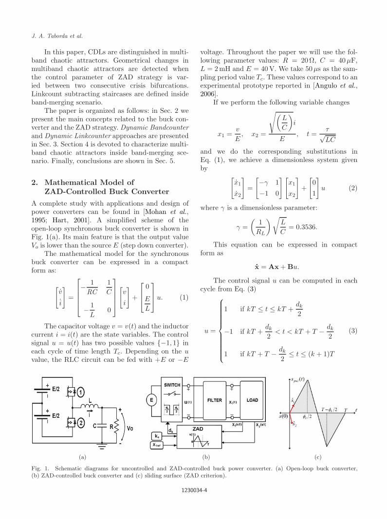
A complete study with applications and design ofpower converters can be found in [Mohan et al.,1995; Hart, 2001]. A simplified scheme of theopen-loop synchronous buck converter is shown inFig. 1(a). Its main feature is that the output valueVo is lower than the source E (step down converter).
The mathematical model for the synchronousbuck converter can be expressed in a compactform as:
[v
i
]=
− 1
RC1C
− 1L
0
[v
i
]+
0
E
L
u. (1)
The capacitor voltage v = v(t) and the inductorcurrent i = i(t) are the state variables. The controlsignal u = u(t) has two possible values −1, 1 ineach cycle of time length Tc. Depending on the uvalue, the RLC circuit can be fed with +E or −E
voltage. Throughout the paper we will use the fol-lowing parameter values: R = 20Ω, C = 40µF,L = 2mH and E = 40 V. We take 50µs as the sam-pling period value Tc. These values correspond to anexperimental prototype reported in [Angulo et al.,2006].
If we perform the following variable changes
x1 =v
E, x2 =
√(L
C
)i
E, t =
τ√LC
and we do the corresponding substitutions inEq. (1), we achieve a dimensionless system givenby [
x1
x2
]=
[−γ 1
−1 0
][x1
x2
]+
[0
1
]u (2)
where γ is a dimensionless parameter:
γ =(
1RL
)√L
C= 0.3536.
This equation can be expressed in compactform as
x = Ax + Bu.
The control signal u can be computed in eachcycle from Eq. (3)
u =
1 if kT ≤ t ≤ kT +dk
2
−1 if kT +dk
2< t < kT + T − dk
2
1 if kT + T − dk
2≤ t ≤ (k + 1)T
(3)
(a) (b) (c)
Fig. 1. Schematic diagrams for uncontrolled and ZAD-controlled buck power converter. (a) Open-loop buck converter,(b) ZAD-controlled buck converter and (c) sliding surface (ZAD criterion).
1230034-4

October 28, 2012 1:56 WSPC/S0218-1274 1230034
Chaotic Attractors Inside Band-Merging Scenario in a ZAD-Controlled Buck Converter
where T is the dimensionless sampling period
T =Tc√(LC)
= 0.1767,
and dk ∈ [0, T ] is the new duty cycle for the dimen-sionless system.
Thus we finally have the following compactform for the PWS
x =
Ax + B 0 ≤ t ≤ dk
2
Ax− Bdk
2< t <
(T − dk
2
)
Ax + B(
T − dk
2
)≤ t ≤ T.
(4)
For the ZAD strategy, the duty cycle φk (wheredk := sat(φk)) must be computed in order toachieve, in every T -cycle, a zero (integral) averageon the so-called sliding surface defined by
s(t) = x1 − x1ref + ks(x1 − x1ref), (5)
where x1 is the variable to be controlled, x1ref is thereference signal and ks is the time constant associ-ated to the first order dynamics. Zero average onthe surface guarantees that the output x1 followsthe reference x1ref . For the so-called regulation case,where the reference x1ref is constant, which is thecase we will study, we have x1ref = 0. In this paper,x1ref is fixed as 0.8. A closed-loop buck converterscheme is shown in Fig. 1(b).
Computing the duty cycle φk means that wehave to solve
∫ (k+1)T
kTs(t)dt = 0.
This implies, in each cycle, solving a transcen-dental equation
φk + KB(eAT (1−φk2
) − eATφk2 )KA = Kx
which is a serious problem for a practical prototype.In order to simplify the duty cycle computation,s(x(t)) can be approximated to a piecewise-linear function as in [Angulo, 2004]. This func-tion is shown in Fig. 1(b) and its mathematicalexpression is
spwl(t)
=
s1(kT )t + s1(kT ) if 0 ≤ t ≤ φk
2
s2(kT )t + s2(kT ) ifφk
2< t <
(T − φk
2
)
s1(kT )t + s3(kT ) if(
T − φk
2
)≤ t ≤ T
(6)
where s1 and s2 are the slopes computed from theexpression of s(t) [after Eq. (5)] using the state val-ues at the beginning of the cycle and the sign of thesignal control. Thus s1 is evaluated with u = 1 ands2 is evaluated with u = −1. Also,
s1(kT ) = s(kT )
is the value of s(t) at the sampling instant;
s2(kT ) = s(kT ) +(
φk
2
)(s1(kT ) − s2(kT ))
and
s3(kT ) = s(kT ) − (T − φk)(s1(kT ) − s2(kT )).
Therefore, the zero average criterion is slightlychanged in such a way that it is possible to find aneasy algebraic expression for computing φk, as it isshown in (8). Namely, we impose∫ (k+1)T
kTspwl(t)dt = 0 (7)
and we obtain
φk =2s(kT ) + T s2(kT )s2(kT ) − s1(kT )
. (8)
Equation (8) can be written as an expressiondepending on the state variables x1 and x2 at thesampling instant kT as
φk = c1x1(kT ) + c2x2(kT ) + c3
where
c1 =2 − 2γks + γ2ksT − γT − ksT
−2ks
c2 =2ks + T − γksT
−2ks
c3 =x1ref
ks+
T
2.
(9)
1230034-5
October 28, 2012 1:56 WSPC/S0218-1274 1230034
J. A. Taborda et al.
The duty cycle computed with ZAD strategy(φk) should be bounded to the range [0;T ]. Equa-tion (10) defines the duty cycle after saturation (dk)
dk :=
0 if φk ≤ 0
φk if 0 < φk < T
T if φk ≥ T.
(10)
The PWS map P of the T-periodic orbit of thesystem (4) can be obtained through direct integra-tion, and this leads to Eq. (11)
x((k + 1)T ) = Φx(kT ) + Γ(dk(x((k − 1)T ))),
(11)
where Φ = eAT and Γk = Γ(dk(x((k − 1)T ))) is avectorial function of dk, which is given in Eq. (12)with Γc = [eAT − I]A−1B and Γd = 2(eA(dkT/2) −eAT(1−dk)/2)A−1B
Γk =
ΓD0 = −Γc if dk = 0
ΓNS = Γc + Γd if 0 < dk < T
ΓD1 = Γc if dk = T.
(12)
Band-merging scenario of ZAD-controlled buckconverter is studied in the following sections. Thebehavior of chaotic attractors is influenced by turn-ing manifolds Λi with dimension (n− 1). Two mainturning manifolds (Λ1 and Λ2) can be defined in thestate-space.
Making dk = 0 and dk = 1, we obtain theboundary manifolds xd0
1 and xd11 , respectively:
xd01 = −c2x2 + c3
c1; xd1
1 =T − c2x2 − c3
c1. (13)
We define the main turning manifolds apply-ing (13) to the Poincare map P when dk = 0 anddk = T
Λ1 := Φ
[xd0
1
x2
]+ ΓD0
Λ2 := Φ
[xd1
1
x2
]+ ΓD1.
(14)
3. Computer-Assisted Approachesto Characterize Chaotic Scenarios
Chaos is a wide-spread phenomenon that it hasnow been reported in virtually every scientific
discipline: astronomy, biology, biophysics, chem-istry, engineering, geology, mathematics, medicine,meteorology, plasmas, physics and even the socialsciences [Olivar, 1997].
It is no coincidence that during the same threedecades, during which chaos has grown into an inde-pendent field of research, computers have perme-ated society. It is, in fact, the wide availabilityof inexpensive computing power that has spannedmuch of the research in chaotic dynamics.
The computer allows nonlinear and nons-mooth systems to be studied in a way that wasundreamt by the pioneers of nonlinear dynamics.Next, we synthesize two novel numerical-analyticalapproaches in order to characterize chaotic dynam-ics. These approaches were denominated DynamicBandcounter (DBC ) and Dynamic Linkcounter(DLC ).
3.1. Bandcounter approach
Bandcounter (BC) approach was initially reportedby Avrutin et al. [2007] to characterize multibandchaotic attractors formed by crisis bifurcations ina chaotic domain without periodic inclusions. Thistheoretical-based approach was implemented by thepioneers using automatic (nonsupervised) and effi-cient numerical algorithms in order to count bandsin a two-dimensional parameter space. They devel-oped two methods for the detection of the numberof bands denominated GCD-based Bandcounting(GCD-BC) and Boxcounting-based Bandcounting(Box-BC). GCD-BC computes the number of bandsas the Greatest Common Divisor (GCD) of a setof return times. Box-BC computes the number ofbands as the number of clusters on adjacent boxesseparated from each other by empty boxes.
Method GCD-BC was developed for dynamicalsystems with a continuous system function whileBox-BC could be used with continuous and discon-tinuous system functions. Eckstein [2006] concludedthat both bandcounting methods can generate goodresults, but GCD-BC method is much more elegant(and also much faster) and can be used to get reallyclean bandcount-diagrams.
Dynamic bandcounter approach was defined bythe decomposition of the band sets into periodicmaps [Taborda, 2010]. Although this approach issemi-automatic (or semi-supervised), it allows amore complete characterization including qualitiessuch as domains of attraction, symmetries, rota-tions or recurrent patterns.
1230034-6
October 28, 2012 1:56 WSPC/S0218-1274 1230034
Chaotic Attractors Inside Band-Merging Scenario in a ZAD-Controlled Buck Converter
Previous reported bandcounter approaches(GCD-BC, Box-BC and DBC) cannot be used todetect topological or geometrical changes in one-band complex scenarios or in a band of multibandcomplex scenarios.
Dynamic Bandcounter approach is used tocharacterize torus and chaos p-bands in smooth andpiecewise-smooth dynamical systems. The Poincaremap P is decomposed by a sequence of m mapsP p
1, . . . , Ppm (p = m · K with m,K ∈ Z
+) whereP p
i , i = 1, . . . ,m is the restriction of P to the Πpi
piece of the attractor as it is shown in Eq. (15)
P pi : Πp
i → Πpi+1 i = 1, . . . ,m − 1
P pm : Πp
m → Πp1.
(15)
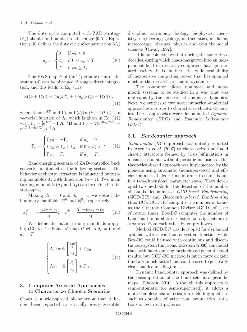
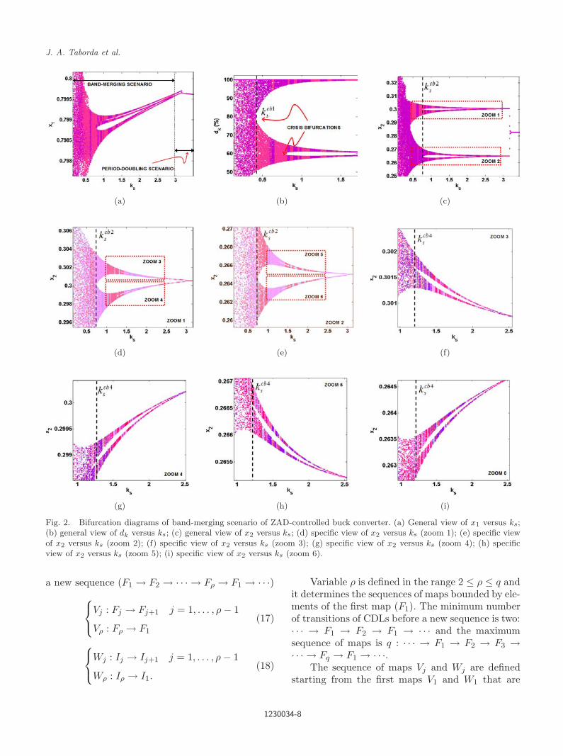
In order to distinguish from quasiperiodicorbits, chaotic bands or one-band chaos, we use thePoincare map decomposition in periodic sequences.High-order periodic orbits, chaotic bands and chaoscan be detected and characterized. Figure 2 showsbifurcation diagrams of band-merging scenarioanalyzed with DBC approach. Border-collisionperiod-doubling scenario is followed by an inverseband-merging cascade.
Poincare map P can be restricted to two sub-sets Π2
i i=1,2. Figures 2(a)–2(c) show the Poincaremap decomposition in two periodic sequences. Frac-tal basins of attraction of the maps P 2
1 and P 22 can
be observed when ks is varied. Each map P 2i has
an alternated but different domain of attraction forks > 0.4095. A collision between chaotic attractorand unstable T-periodic orbit takes place in ks ≈0.4095, i.e. crisis bifurcation (kcb1
s ) occurs in thisvalue. Intertwined domains of attraction of P 2
1 andP 2
2 are detected in one-band chaos ks < 0.4095.Poincare map P is restricted to four subsets
Π4i i=1,2,3,4 to analyze two-band to four-band tran-
sition. Figures 2(d) and 2(e) show the sets Π4i near
the second crisis bifurcation (ks := kcb2s ≈ 0.763).
Separated domains of attraction of P 41, P 4
2, P 43 and
P 44 for ks > kcb2
s and intertwined domains of P 4i for
ks < kcb2s can be distinguished. Fractal basins of
attraction persist in this range.Finally, Poincare map P is restricted to eight
subsets Π8i i=1,2,3,4,5,6,7,8 to analyze four-band to
eight-band transition. Figures 2(f)–2(i) show thesets Π8
i near the collision between chaotic attrac-tor and unstable 4T-periodic orbit (ks := kcb4
s ≈1.2144). DBC approach can detect the transitionbetween four-band chaos and eight-band chaos
defining the value when the domains of attractionof each map P 8
i intertwine.
3.2. Linkcounter approach
Dynamic Linkcounter (DLC ) approach was pro-posed to characterize one-band chaos, multibandchaos and torus-breakdown scenarios in dynamicalsystems where Bandcounter approach does not giverepresentative information of bifurcation behavior.DLC approach allows to make a more detailed anal-ysis of band-merging scenario of ZAD-controlledbuck converter than DBC approach.
The concept of Complex Dynamic Links (CDL)was created to characterize chaos and quasiperi-odic attractors in one-band complex scenarios orin multiband complex scenarios between consecu-tive crisis bifurcations. The change in the numberof CDL is used to characterize complex bifurca-tion scenarios. A change in the number of complexdynamic links due to a parameter change, impliesa geometrical or topological change in the complexbifurcation scenario. The quantity of CDL struc-tures is induced by adjacent periodic orbits in theparameter space.
First, we introduce the procedure to character-ize one-band chaotic attractors. Later, we general-ize the method for multiband chaotic attractors.DLC approach was initially reported in [Tabordaet al., 2011] to characterize a chaotic scenario withintermittency. That paper reported a new bifur-cation scenario characterized by chaotic attractorswith fingered strange shape in Linkcount-addingcascade. Each structure of CDL had a fingeredstrange attractor increasing in an arithmetic pro-gression the number of CDL or fingers when thebifurcation parameter (x1ref) was varied.
DLC approach allows to decompose one-bandchaotic attractors in self-similar substructures. LetΩq be a chaotic attractor composed by q substruc-tures Fj denominated CDL
Ωq =q⋃
j=1
Fj . (16)
Each CDL substructure Fj has an index set Ij whichis defined by the tuple of maps (Vj ,Wj), where Vj isthe restriction of P to the Fj piece of the attractorΩq and Wj is the restriction of I to the Ij subset.Equations (17) and (18) show expressions for therestrictions of state variables and indexes, where ρdefines the number of CDLs that are visited before
1230034-7
October 28, 2012 1:56 WSPC/S0218-1274 1230034
J. A. Taborda et al.
(a) (b) (c)
(d) (e) (f)
(g) (h) (i)
Fig. 2. Bifurcation diagrams of band-merging scenario of ZAD-controlled buck converter. (a) General view of x1 versus ks;(b) general view of dk versus ks; (c) general view of x2 versus ks; (d) specific view of x2 versus ks (zoom 1); (e) specific viewof x2 versus ks (zoom 2); (f) specific view of x2 versus ks (zoom 3); (g) specific view of x2 versus ks (zoom 4); (h) specificview of x2 versus ks (zoom 5); (i) specific view of x2 versus ks (zoom 6).
a new sequence (F1 → F2 → · · · → Fρ → F1 → · · ·)Vj : Fj → Fj+1 j = 1, . . . , ρ − 1
Vρ : Fρ → F1
(17)
Wj : Ij → Ij+1 j = 1, . . . , ρ − 1
Wρ : Iρ → I1.(18)
Variable ρ is defined in the range 2 ≤ ρ ≤ q andit determines the sequences of maps bounded by ele-ments of the first map (F1). The minimum numberof transitions of CDLs before a new sequence is two:· · · → F1 → F2 → F1 → · · · and the maximumsequence of maps is q : · · · → F1 → F2 → F3 →· · · → Fq → F1 → · · ·.
The sequence of maps Vj and Wj are definedstarting from the first maps V1 and W1 that are
1230034-8

October 28, 2012 1:56 WSPC/S0218-1274 1230034
Chaotic Attractors Inside Band-Merging Scenario in a ZAD-Controlled Buck Converter
determined by means of the evaluation of relative(or local) extrema in a discriminant function namedunlinking function ξ(k) := ξk.
The unlinking function ξ(k) for PWS maps withthree smooth zones (PWS3) defined by a satura-tion function dk = sat(φk) was defined in [Taborda,2010]. ZAD-controlled buck converter is a PWS3
where φk is the duty cycle computed by ZAD algo-rithm. The unlinking function ξ(k) is given by
ξk = φk − φk−1
ξk = c1e1 + c2e2 + c3
(19)
where e1 = x1(k) − x1(k − 1)
e2 = x2(k) − x2(k − 1),(20)
and c1, c2 and c3 are given by Eq. (9). Local maxi-mum (Lmax) or local minimum (Lmin) sets of ξk are
defined by Eqs. (21) and (22), respectively
Lmax =
ξk ∀ k
(ξ(k) > ξ(k − 1)) ∧ (ξ(k) > ξ(k + 1))
(21)
Lmin =
ξk ∀ k
(ξ(k) < ξ(k − 1)) ∧ (ξ(k) < ξ(k + 1))
.
(22)
The unlinking criterion (local maxima or localminima detection) depends on properties of thesystem and/or the unlinking function. Figure 3(a)shows an example of local maxima detection andLinkcount characterization for a chaotic attractorwith six CDLs. Each CDL set Fj is characterizedwith a different color. Local maxima points thatdefine the first CDL set (F1) are identified withblue.
(a) (b) (c)
(d) (e) (f)
Fig. 3. Dynamic Linkcounter Approach. (a) Unlinking function for six CDL chaotic attractors (Lmax detection); (b) indexmap (W1) of the first CDL versus k (W1 versus k); (c) index map (W1) of the first CDL versus i (W1 versus i); (d) variationof the first index map versus k (∆W1 versus k); (e) variation of the first index map versus i (∆W1 versus i); (f) CDL map ofthe first map (V1) (V1(x2) versus i).
1230034-9

October 28, 2012 1:56 WSPC/S0218-1274 1230034
J. A. Taborda et al.
Now, each CDL set (Fj) has associated a mapVj that is indexed by an independent index map Wj
contained in an index set Ij. The first CDL map (V1)is given by Eq. (23)
V1 : x(W1(i)) → x(W1(i + 1)) (23)
where
x ∈ F1
W1 ∈ I1 ∈ I
i ∈ Z+
with,
F1 =
x(k)ξk
∈ Lmax
I1 =
k
ξk∈ Lmax
.
Figures 3(b) and 3(c) show the evolution of thefirst CDL index map (W1) when the index variablesare k (used in the general map P ) or i (used in thefirst CDL map V1). The map W1(k) has jumps ink due to extreme point detections, while the mapW1(i) is defined for each i. Now, the maximum jumpof W1(k) is q iterations (where q is the numberof CDL sets) and this jump is determined by thedistance between two consecutive points containedin F1, i.e.
max(∆W1(i))
= max(W1(i + 1) − W1(i)) = q. (24)
An example of the computation of the maxi-mum jump of W1(k) is shown in Figs. 3(d) and 3(e).Note that for this example, the system has a sixCDL chaotic attractor.
Each sequence of maps bounded by two ele-ments of the first map F1 → F2 → · · · → Fρ → F1
is characterized by ρ transitions where ρ = ∆W1(i)
ρ = ∆W1(i) = W1(i + 1) − W1(i). (25)
Therefore, the index maps defined as functionsof the first index map (W1) are given by:
W2(k) = W1(k) + 1
...
Wρ(k) = W1(k) + ρ − 1.
(26)
The CDL maps Vj can be defined by using theindex maps Wj as presented in Eq. (27)
V1 : x(W1(i)) → x(W1(i + 1))
V2 : x(W2(i)) → x(W2(i + 1))...
Vq : x(Wq(i)) → x(Wq(i + 1)).
(27)
Figure 3(f) shows the state variable x2 for thefirst CDL map (V1(x2)) for the example of one-bandchaotic attractor with six CDLs.
4. Characterization ofBand-Merging Scenario
In this section, we present the results of the char-acterization of band-merging scenario in a ZAD-controlled buck converter. We use DLC approachto characterize one-band and multiband chaoticattractor inside band-merging scenario. Band-counter approaches cannot give extra information ofgeometrical changes between two consecutive crisisbifurcations.
4.1. Characterization of one-bandchaotic attractors
Figure 4 synthesizes the behavior of chaotic attrac-tors in one-band chaos. Linkcount subtracting stair-case can be defined when ks is varied in the range[0.1; 0.4095]. The number of CDLs decreases in thearithmetic sequence: (Ω9,Ω8,Ω7,Ω6,Ω5,Ω4,Ω3,Ω2)when ks is increased from ks = 0.1 to ks = 0.42.
Figure 4(b) presents a chaotic attractor with 9CDLs (Ω9) for ks = 0.105. Both turning manifoldsΛ1 and Λ2 are active. In this case, each CDL set Fj
has tangential contact points with one turning man-ifold. The first CDL set F1 has contact point withthe turning manifold Λ1 while the other CDL setshave tangential points in the turning manifold Λ2.
Turning manifolds Λ1 and Λ2 have an impor-tant role in the formation of chaotic attractors inZAD-controlled buck converter. CDL structures areinfluenced by turning manifolds. Turning manifoldΛ1 becomes inactive after the chaotic attractor with8 CDLs. Note that the first CDL set F1 has nocontact point with the turning manifold Λ1 for thechaotic attractor with 7 CDLs [see Fig. 4(d)]. Turn-ing manifold Λ2 results in activity in the otherchaotic attractors.
1230034-10

October 28, 2012 1:56 WSPC/S0218-1274 1230034
Chaotic Attractors Inside Band-Merging Scenario in a ZAD-Controlled Buck Converter
(a) (b) (c)
(d) (e) (f)
(g) (h) (i)
Fig. 4. Phase portraits of one-band chaotic attractors. (a) General scheme; (b) 9 CDLs for ks = 0.105; (c) 8 CDLs forks = 0.145; (d) 7 CDLs for ks = 0.1625; (e) 6 CDLs for ks = 0.17; (f) 5 CDLs for ks = 0.18; (g) 4 CDLs for ks = 0.195; (h) 3CDLs for ks = 0.25; (i) 2 CDLs for ks = 0.42.
One-band chaotic attractors have a fingeredshape. Each structure of CDL is a fingered strangeattractor increasing in arithmetic progression thenumber of CDL or fingers when the bifurcationparameter (ks) is varied.
The characteristic fingered shape of theseattractors, first reported in the work of Thomp-son and Ghaffari [1983], arises because the grazingmap stretches phase space strongly in one direc-tion and compresses it in the other direction. Thehigh stretching associated with grazing means thatchaotic behavior is observed in impact oscillators forwide ranges of the parameters. Often, the strange
attractors associated with grazing events have a fin-gered appearance.
Chaotic attractors decrease CDL sets while ks
is nearer crisis bifurcation kcb1s (ks ≈ 0.4095). Just
before the crisis bifurcation (ks < kcb1s ), the system
experiments a chaotic attractor with 3 CDL sets. Inkcb1
s , the third set F3 is empty and two-band chaosis created. Figure 4(i) shows an example of chaoticattractor after kcb1
s . Each set Fj corresponds to adifferent band Π2
i .Figure 5 and Table 1 show the distribution
of elements in each set Fj of one-band chaoticattractors. The sum of all percentages Fj(%) should
1230034-11

October 28, 2012 1:56 WSPC/S0218-1274 1230034
J. A. Taborda et al.
(a) (b) (c)
(d) (e) (f)
(g) (h) (i)
Fig. 5. Percentage distribution of each CDL in each one-band chaotic attractor. (a) General scheme; (b) 9 CDLs for ks = 0.105;(c) 8 CDLs for ks = 0.145; (d) 7 CDLs for ks = 0.1625; (e) 6 CDLs for ks = 0.17; (f) 5 CDLs for ks = 0.18; (g) 4 CDLs forks = 0.195; (h) 3 CDLs for ks = 0.25; (i) 2 CDLs for ks = 0.42.
Table 1. Linkcount adding cascade in one-band chaotic scenario. Percentage of state variables in each CDL.
ks KL F1(%) F2(%) F3(%) F4(%) F5(%) F6(%) F7(%) F8(%) F9(%)
0.1050 9 17.0066 17.0066 14.6593 12.9940 11.3422 9.5900 7.8780 6.2997 3.22340.1450 8 25.6039 25.6039 19.0578 13.9664 8.6681 4.3174 2.0286 0.75400.1625 7 30.0520 30.0520 20.5922 12.6010 5.1621 1.3165 0.22410.1700 6 31.5857 31.5857 20.6796 11.5945 3.8582 0.69640.1800 5 33.8633 33.8633 20.5703 9.7725 1.93050.1950 4 36.3418 36.3418 20.3771 6.93940.2500 3 41.3260 41.3260 17.34810.4200 2 50.0000 50.0000
1230034-12

October 28, 2012 1:56 WSPC/S0218-1274 1230034
Chaotic Attractors Inside Band-Merging Scenario in a ZAD-Controlled Buck Converter
be 100%. In each case, the last CDL Fq has the low-est percentage. For example, F9 set of Ω9 attractorhas 3.2234% of the total points [see Fig. 5(b)]. Theattractor Ω2 has half of the points in the set F1 andand the other half is in the set F2 [see Fig. 5(i)].
4.2. Characterization of two-bandchaotic attractors
In the same way, we can use Linkcounter approachto decompose multiband chaotic attractors in self-similar substructures. Let Ωp
q be a chaotic attrac-tor composed by q substructures F(p,i)
j denominatedCDL located in the Πp
i band
Ωpq =
q⋃j=1
(F (p,i)j |i=p
i=1). (28)
Two-band chaos is bounded by the crisis bifur-cations kcb1
s and kcb2s in the range [0.4095; 0.763).
Two groups of sets F(2,1)j and F(2,2)
j are defined.Figures 6 and 7 summarize the analysis of two-band
chaotic attractors. Linkcount subtracting stair-cases can be recognized in each band Π2
1 andΠ2
2 when ks is increased from ks = kcb1s to
ks = kcb2s . In each Π2
i piece, the number of CDLsets decreases in the arithmetic sequence: (F(2,i)
6 ,
F(2,i)5 ,F(2,i)
4 ,F(2,i)3 ,F(2,i)
2 ).The unlinking functions ξ
(p,i)k to discriminate
CDL inside two-band chaos are defined based onthe first index map (W1) and the second indexmap (W2). Equation (29) shows the definition ofeach unlinking function. Now, the discriminantinformation is obtained comparing the ZAD-controllaw (φk) between two consecutive points of the firstmap V1 (or the second map V2)
ξ(2,1)k = φk(W1(i)) − φk(W1(i − 1)) (29a)
ξ(2,2)k = φk(W2(i)) − φk(W2(i − 1)). (29b)
The unlinking criterion (local maxima or localminima detection) depends on geometrical proper-ties of the pieces Π2
1 and Π22. Equation (30) defines
the criteria of each case
L(2,1)min =
ξ(2,1)k ∀ k
(ξ(2,1)(k) < ξ(2,1)(k − 1)) ∧ (ξ(2,1)(k) < ξ(2,1)(k + 1))
(30a)
L(2,2)max =
ξ(2,2)k ∀ k
(ξ(2,2)(k) > ξ(2,2)(k − 1)) ∧ (ξ(2,2)(k) > ξ(2,2)(k + 1))
. (30b)
The pieces F1 and F2 are equivalent to thepieces Π2
1 and Π22, respectively, when the crisis
bifurcation kcb1s occurs. The map V1 is the same
P 21 and the map V2 is the same P 2
2 in the rangeks ∈ [kcb1
s , kcb2s ). Now, each CDL set (F (2,i)
j ) has
associated a map V(2,i)j that is indexed by an inde-
pendent index map W(2,i)j contained in an index
set I(2,i)j .Figure 6 shows the phase portraits of the Π2
1
piece. Each CDL structure F(2,1)j inside Π2
1 piecehas a tent-map-like pattern. Tent-map patterns isa classical mechanism of chaos formation in nons-mooth systems.
The first CDL map associated to the Π21 piece
denoted by V(2,1)1 is given by Eq. (31)
V(2,1)1 : x(W (2,1)
1 (i)) → x(W (2,1)1 (i + 1)) (31)
where
x ∈ F(2,1)1
W(2,1)1 ∈ I
(2,1)1 ∈ I
i ∈ Z+
with,
F(2,1)1 =
x(k)
ξ(2,1)k
∈ L(2,1)min
I(2,1)1 =
k
ξ(2,1)k
∈ L(2,1)min
.
Each sequence of maps bounded by two ele-ments of the first map F
(2,1)1 → F
(2,1)2 → · · · →
F(2,1)ρ → F
(2,1)1 is characterized by ρ transitions
1230034-13
October 28, 2012 1:56 WSPC/S0218-1274 1230034
J. A. Taborda et al.
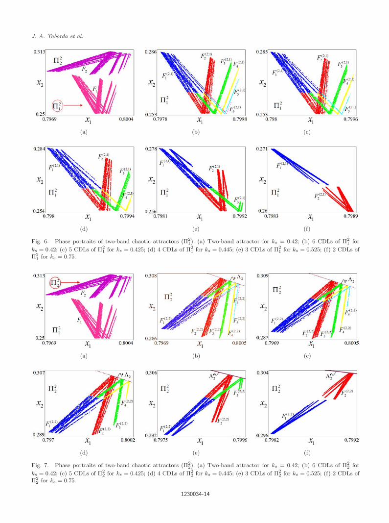
(a) (b) (c)
(d) (e) (f)
Fig. 6. Phase portraits of two-band chaotic attractors (Π21). (a) Two-band attractor for ks = 0.42; (b) 6 CDLs of Π2
1 for
ks = 0.42; (c) 5 CDLs of Π21 for ks = 0.425; (d) 4 CDLs of Π2
1 for ks = 0.445; (e) 3 CDLs of Π21 for ks = 0.525; (f) 2 CDLs of
Π21 for ks = 0.75.
(a) (b) (c)
(d) (e) (f)
Fig. 7. Phase portraits of two-band chaotic attractors (Π22). (a) Two-band attractor for ks = 0.42; (b) 6 CDLs of Π2
2 for
ks = 0.42; (c) 5 CDLs of Π22 for ks = 0.425; (d) 4 CDLs of Π2
2 for ks = 0.445; (e) 3 CDLs of Π22 for ks = 0.525; (f) 2 CDLs of
Π22 for ks = 0.75.
1230034-14

October 28, 2012 1:56 WSPC/S0218-1274 1230034
Chaotic Attractors Inside Band-Merging Scenario in a ZAD-Controlled Buck Converter
where ρ = ∆W(2,1)1 (i)
ρ = ∆W(2,1)1 (i) = W
(2,1)1 (i + 1) − W
(2,1)1 (i). (32)
Therefore, the index maps defined as functionsof the first index map (W (2,1)
1 ) are given by:
W(2,1)2 (k) = W
(2,1)1 (k) + 1
...
W(2,1)ρ (k) = W
(2,1)1 (k) + ρ − 1.
(33)
The CDL maps V(2,1)j can be defined by using
the index maps W(2,1)j as presented in Eq. (34)
V(2,1)1 : x(W (2,1)
1 (i)) → x(W (2,1)1 (i + 1))
V(2,1)2 : x(W (2,1)
2 (i)) → x(W (2,1)2 (i + 1))
...
V(2,1)q : x(W (2,1)
q (i)) → x(W (2,1)q (i + 1)).
(34)
Figure 7 shows the phase portraits of the Π22
piece. Each CDL structure F(2,2)j inside Π2
2 piecehas a tent-map-like pattern too.
The first CDL map associated to the Π22 piece
denoted by V(2,2)1 is given by Eq. (35)
V(2,2)1 : x(W (2,2)
1 (i)) → x(W (2,2)1 (i + 1)) (35)
where
x ∈ F(2,2)1
W(2,2)1 ∈ I
(2,2)1 ∈ I
i ∈ Z+
with,
F(2,2)1 =
x(k)
ξ(2,2)k
∈ L(2,2)max
I(2,2)1 =
k
ξ(2,2)k
∈ L(2,2)max
.
Each sequence of maps bounded by two ele-ments of the first map F
(2,2)1 → F
(2,2)2 → · · · →
F(2,2)ρ → F
(2,2)1 is characterized by ρ transitions
where ρ = ∆W(2,2)1 (i)
ρ = ∆W(2,2)1 (i) = W
(2,2)1 (i + 1) − W
(2,2)1 (i). (36)
Therefore, the index maps defined as functionsof the first index map (W (2,2)
1 ) are given by:
W(2,2)2 (k) = W
(2,2)1 (k) + 1
...
W(2,2)ρ (k) = W
(2,2)1 (k) + ρ − 1.
(37)
The CDL maps V(2,2)j can be defined by using
the index maps W(2,2)j as presented in Eq. (38)
V(2,2)1 : x(W (2,2)
1 (i)) → x(W (2,2)1 (i + 1))
V(2,2)2 : x(W (2,2)
2 (i)) → x(W (2,2)2 (i + 1))
...
V(2,2)q : x(W (2,2)
q (i)) → x(W (2,2)q (i + 1)).
(38)
Just before the crisis bifurcation (ks < kcb2s ),
each Π2i is composed of 3 CDL sets. In kcb2
s , the thirdsets F
(2,1)3 and F
(2,2)3 are empty and four-band chaos
is created. Figures 6(f) and 7(f) show the formationof four-band chaotic attractor after kcb2
s . Sets F(2,1)1 ,
F(2,1)2 , F
(2,2)1 and F
(2,2)2 correspond to a different
band Π4i .
Figure 8 and Table 2 show the percentages ofeach set F
(2,i)j of two-band chaotic attractors. Each
group of sets F(2,1)j and F
(2,2)j has symmetric behav-
ior. The sum of all percentages in each group ofsets (F (2,1)
j (%) or F(2,2)j (%)) should be 50%. In each
case, the last CDL F(2,i)q has the lowest percentage.
For example, F 2,16 and F 2,2
6 sets of Ω26 attrac-
tor have 0.2646% each one of the total points [seeFig. 8(b)]. The attractor Ω2
2 has a quarter of thepoints in each set F
(2,1)1 , F
(2,1)2 , F
(2,2)1 and F
(2,2)2
[see Fig. 8(f)].
4.3. Characterization of four-bandchaotic attractors
Four-band chaos is bounded by the crisis bifur-cations kcb2
s and kcb4s in the range [0.763; 1.144).
1230034-15

October 28, 2012 1:56 WSPC/S0218-1274 1230034
J. A. Taborda et al.
(a) (b) (c)
(d) (e) (f)
Fig. 8. Percentage distribution of each CDL in each two-band chaotic attractor. (a) General scheme; (b) 6 CDLs of eachband for ks = 0.42; (c) 5 CDLs of each band for ks = 0.425; (d) 4 CDLs of each band for ks = 0.445; (e) 3 CDLs of each bandfor ks = 0.525; (f) 2 CDLs of each band for ks = 0.75.
Four groups of sets F(4,1)j , F(4,2)
j , F(4,3)j and F(4,4)
jare defined. Figures 9–12 summarize the analysis offour-band chaotic attractors.
Linkcount subtracting staircases can be rec-ognized in each band Π4
1, Π42, Π4
3 and Π44 when
ks is increased from ks = kcb2s to ks = kcb4
s .In each Π4
i piece, the number of CDL setsdecreases in the arithmetic sequence: (F(4,i)
6 ,F(4,i)5 ,
F(4,i)4 ,F(4,i)
3 ,F(4,i)2 ).
The unlinking functions ξ(p,i)k to discriminate
CDL inside four-band chaos are defined basedon the first index maps (W (2,1)
1 and W(2,2)1 )
and the second index maps (W (2,1)2 and W
(2,2)2 ).
Equation (39) shows the definition of each unlink-ing function. Now, the discriminant informationis obtained comparing the ZAD control law (φk)between two consecutive points of the maps V
(2,i)j
for j = 1, 2 and i = 1, 2
ξ(4,1)k = φk(W
(2,1)2 (i)) − φk(W
(2,1)2 (i − 1)) (39a)
ξ(4,2)k = φk(W
(2,2)2 (i)) − φk(W
(2,2)2 (i − 1)) (39b)
ξ(4,3)k = φk(W
(2,1)1 (i)) − φk(W
(2,1)1 (i − 1)) (39c)
ξ(4,4)k = φk(W
(2,2)1 (i)) − φk(W
(2,2)1 (i − 1)). (39d)
Table 2. Linkcount adding cascade in two-band chaotic scenario. Percentage of state variables in each CDL.
ks KB KL F(2,i)1 (%) F
(2,i)2 (%) F
(2,i)3 (%) F
(2,i)4 (%) F
(2,i)5 (%) F
(2,i)6 (%) Total (%)
0.4200 2 6 18.0229 18.0229 8.5897 3.7876 1.3122 0.2646 500.4250 2 5 18.5167 18.5113 8.4929 3.4837 0.9953 500.4450 2 4 19.4938 19.4874 8.5330 2.4858 500.5250 2 3 21.5139 21.5139 6.9665 500.7500 2 2 25.0025 24.9975 50
1230034-16

October 28, 2012 1:56 WSPC/S0218-1274 1230034
Chaotic Attractors Inside Band-Merging Scenario in a ZAD-Controlled Buck Converter
The unlinking criterion (local maxima or local minima detection) depends on geometrical propertiesof the pieces Π4
i . Equation (40) defines the criteria of each case
L(4,1)min =
ξ(4,1)k ∀ k
(ξ(4,1)(k) < ξ(4,1)(k − 1)) ∧ (ξ(4,1)(k) < ξ(4,1)(k + 1))
(40a)
L(4,2)min =
ξ(4,2)k ∀ k
(ξ(4,2)(k) < ξ(4,2)(k − 1)) ∧ (ξ(4,2)(k) < ξ(4,2)(k + 1))
(40b)
L(4,3)max =
ξ(4,3)k ∀ k
(ξ(4,3)(k) > ξ(4,3)(k − 1)) ∧ (ξ(4,3)(k) > ξ(4,3)(k + 1))
(40c)
L(4,4)max =
ξ(4,4)k ∀ k
(ξ(4,4)(k) > ξ(4,4)(k − 1)) ∧ (ξ(4,4)(k) > ξ(4,4)(k + 1))
. (40d)
The pieces F(2,1)1 , F
(2,1)2 , F
(2,2)1 and F
(2,2)2 are
equivalent to the pieces Π4i , when the crisis bifur-
cation kcb2s occurs. Now, each CDL set (F (4,i)
j ) has
associated a map V(4,i)j that is indexed by an inde-
pendent index map W(4,i)j contained in an index
set I(4,i)j .Figure 9 shows the phase portraits of the Π4
1
piece. Each CDL structure F(4,1)j inside Π4
1 piecehas a tent-map-like pattern. Also, fractal patternscan be identified because the behavior of Π4
1 pieceis similar to the behavior of Π2
1. Π41 piece occurs
on a smaller scale than Π21 piece. This is the main
difference.The first CDL map associated to the Π4
1 piecedenoted by V
(4,1)1 is given by Eq. (41)
V(4,1)1 : x(W (4,1)
1 (i)) → x(W (4,1)1 (i + 1)) (41)
where
x ∈ F(4,1)1
W(4,1)1 ∈ I
(4,1)1 ∈ I
i ∈ Z+
with,
F(4,1)1 =
x(k)
ξ(4,1)k
∈ L(4,1)min
I(4,1)1 =
k
ξ(4,1)k ∈ L
(4,1)min
.
Each sequence of maps bounded by two ele-ments of the first map F
(4,1)1 → F
(4,1)2 → · · · →
F(4,1)ρ → F
(4,1)1 is characterized by ρ transitions
where ρ = ∆W(4,1)1 (i)
ρ = ∆W(4,1)1 (i) = W
(4,1)1 (i + 1) − W
(4,1)1 (i). (42)
Therefore, the index maps defined as functionsof the first index map (W (4,1)
1 ) are given by:
W(4,1)2 (k) = W
(4,1)1 (k) + 1
...
W(4,1)ρ (k) = W
(4,1)1 (k) + ρ − 1.
(43)
The CDL maps V(4,1)j can be defined by using
the index maps W(4,1)j as presented in Eq. (44)
V(4,1)1 : x(W (4,1)
1 (i)) → x(W (4,1)1 (i + 1))
V(4,1)2 : x(W (4,1)
2 (i)) → x(W (4,1)2 (i + 1))
...
V(4,1)q : x(W (4,1)
q (i)) → x(W (4,1)q (i + 1)).
(44)
Figure 10 shows the phase portraits of the Π42
piece. Fractal patterns begin to be recognized intwo-band chaotic attractors and four-band chaoticattractors.
The first CDL map associated to the Π42 piece
denoted by V(4,2)1 is given by Eq. (45)
V(4,2)1 : x(W (4,2)
1 (i)) → x(W (4,2)1 (i + 1)) (45)
1230034-17
October 28, 2012 1:56 WSPC/S0218-1274 1230034
J. A. Taborda et al.
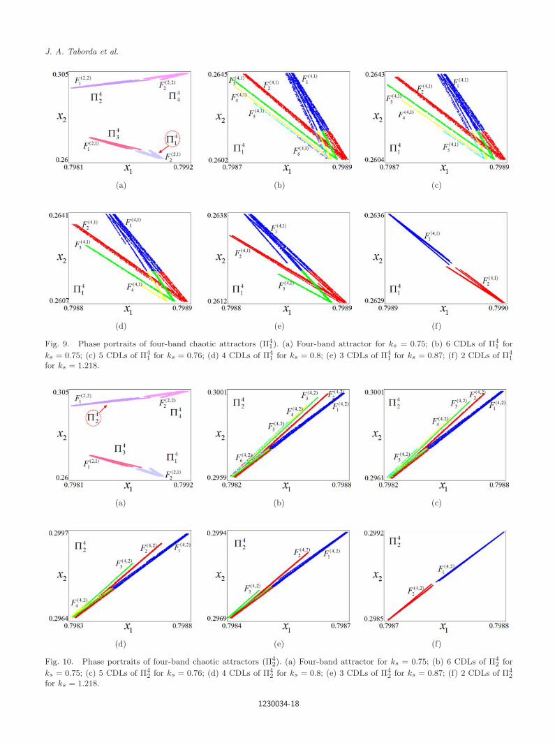
(a) (b) (c)
(d) (e) (f)
Fig. 9. Phase portraits of four-band chaotic attractors (Π41). (a) Four-band attractor for ks = 0.75; (b) 6 CDLs of Π4
1 for
ks = 0.75; (c) 5 CDLs of Π41 for ks = 0.76; (d) 4 CDLs of Π4
1 for ks = 0.8; (e) 3 CDLs of Π41 for ks = 0.87; (f) 2 CDLs of Π4
1
for ks = 1.218.
(a) (b) (c)
(d) (e) (f)
Fig. 10. Phase portraits of four-band chaotic attractors (Π42). (a) Four-band attractor for ks = 0.75; (b) 6 CDLs of Π4
2 for
ks = 0.75; (c) 5 CDLs of Π42 for ks = 0.76; (d) 4 CDLs of Π4
2 for ks = 0.8; (e) 3 CDLs of Π42 for ks = 0.87; (f) 2 CDLs of Π4
2
for ks = 1.218.
1230034-18

October 28, 2012 1:56 WSPC/S0218-1274 1230034
Chaotic Attractors Inside Band-Merging Scenario in a ZAD-Controlled Buck Converter
where
x ∈ F(4,2)1
W(4,2)1 ∈ I
(4,2)1 ∈ I
i ∈ Z+
with,
F(4,2)1 =
x(k)
ξ(4,2)k
∈ L(4,2)min
I(4,2)1 =
k
ξ(4,2)k
∈ L(4,2)min
.
Each sequence of maps bounded by two ele-ments of the first map F
(4,2)1 → F
(4,2)2 → · · · →
F(4,2)ρ → F
(4,2)1 is characterized by ρ transitions
where ρ = ∆W(4,2)1 (i)
ρ = ∆W(4,2)1 (i) = W
(4,2)1 (i + 1) − W
(4,2)1 (i). (46)
Therefore, the index maps defined as functionsof the first index map (W (4,2)
1 ) are given by:
W(4,2)2 (k) = W
(4,2)1 (k) + 1
...
W(4,2)ρ (k) = W
(4,2)1 (k) + ρ − 1.
(47)
The CDL maps V(4,2)j can be defined by using
the index maps W(4,2)j as presented in Eq. (48)
V(4,2)1 : x(W (4,2)
1 (i)) → x(W (4,2)1 (i + 1))
V(4,2)2 : x(W (4,2)
2 (i)) → x(W (4,2)2 (i + 1))
...
V(4,2)q : x(W (4,2)
q (i)) → x(W (4,2)q (i + 1)).
(48)
Figure 11 shows the phase portraits of the Π43
piece. The first CDL map associated to the Π43 piece
denoted by V(4,3)1 is given by Eq. (49)
V(4,3)1 : x(W (4,3)
1 (i)) → x(W (4,3)1 (i + 1)) (49)
where
x ∈ F(4,3)1
W(4,3)1 ∈ I
(4,3)1 ∈ I
i ∈ Z+
with,
F(4,3)1 =
x(k)
ξ(4,3)k
∈ L(4,3)max
I(4,3)1 =
k
ξ(4,3)k
∈ L(4,3)max
.
Each sequence of maps bounded by two ele-ments of the first map F
(4,3)1 → F
(4,3)2 → · · · →
F(4,3)ρ → F
(4,3)1 is characterized by ρ transitions
where ρ = ∆W(4,3)1 (i)
ρ = ∆W(4,3)1 (i) = W
(4,3)1 (i + 1) − W
(4,3)1 (i).
(50)
Therefore, the index maps defined as functionsof the first index map (W (4,3)
1 ) are given by:
W(4,3)2 (k) = W
(4,3)1 (k) + 1
...
W(4,3)ρ (k) = W
(4,3)1 (k) + ρ − 1.
(51)
The CDL maps V(4,3)j can be defined by using
the index maps W(4,3)j as presented in Eq. (52)
V(4,3)1 : x(W (4,3)
1 (i)) → x(W (4,3)1 (i + 1))
V(4,3)2 : x(W (4,3)
2 (i)) → x(W (4,3)2 (i + 1))
...
V(4,3)q : x(W (4,3)
q (i)) → x(W (4,3)q (i + 1)).
(52)
Figure 12 shows the phase portraits of the Π44
piece. The first CDL map associated to the Π44 piece
denoted by V(4,4)1 is given by Eq. (53)
V(4,4)1 : x(W (4,4)
1 (i)) → x(W (4,4)1 (i + 1)) (53)
1230034-19
October 28, 2012 1:56 WSPC/S0218-1274 1230034
J. A. Taborda et al.
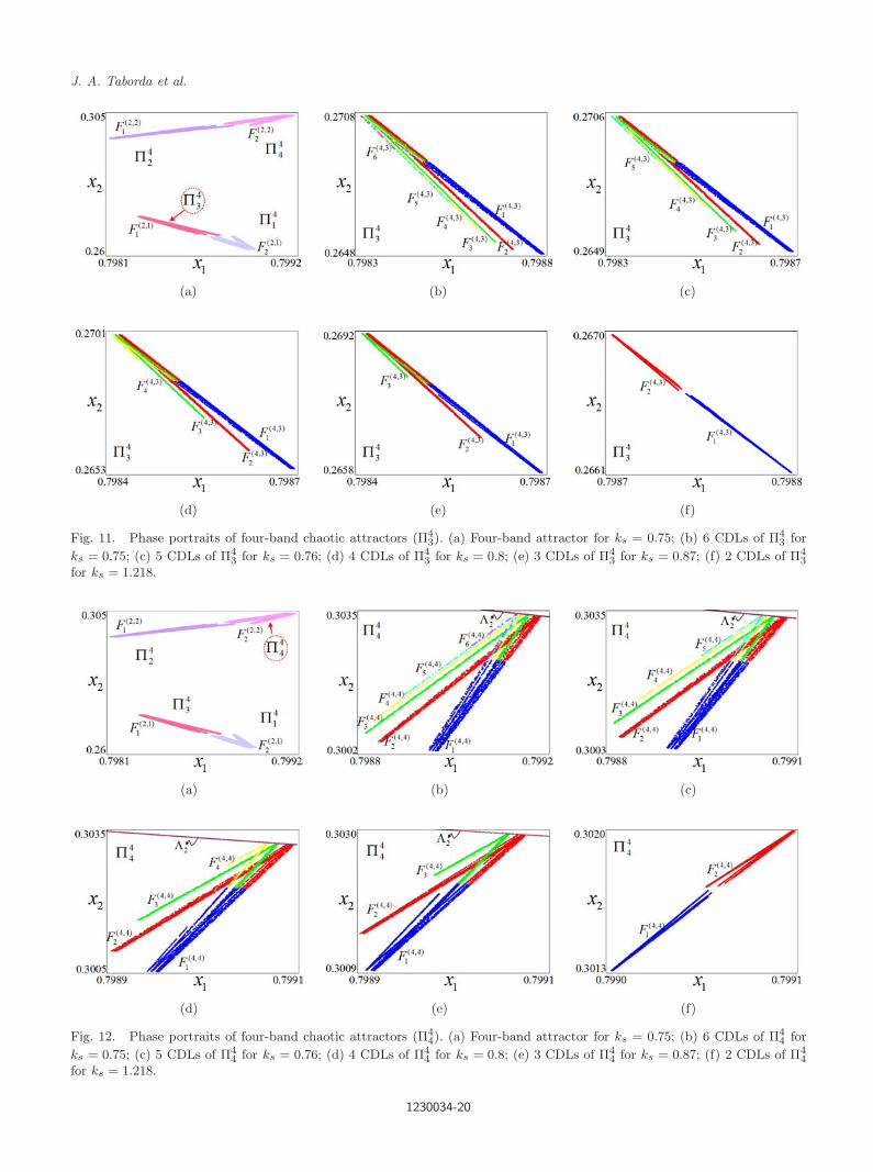
(a) (b) (c)
(d) (e) (f)
Fig. 11. Phase portraits of four-band chaotic attractors (Π43). (a) Four-band attractor for ks = 0.75; (b) 6 CDLs of Π4
3 for
ks = 0.75; (c) 5 CDLs of Π43 for ks = 0.76; (d) 4 CDLs of Π4
3 for ks = 0.8; (e) 3 CDLs of Π43 for ks = 0.87; (f) 2 CDLs of Π4
3
for ks = 1.218.
(a) (b) (c)
(d) (e) (f)
Fig. 12. Phase portraits of four-band chaotic attractors (Π44). (a) Four-band attractor for ks = 0.75; (b) 6 CDLs of Π4
4 for
ks = 0.75; (c) 5 CDLs of Π44 for ks = 0.76; (d) 4 CDLs of Π4
4 for ks = 0.8; (e) 3 CDLs of Π44 for ks = 0.87; (f) 2 CDLs of Π4
4
for ks = 1.218.
1230034-20

October 28, 2012 1:56 WSPC/S0218-1274 1230034
Chaotic Attractors Inside Band-Merging Scenario in a ZAD-Controlled Buck Converter
where
x ∈ F(4,4)1
W(4,4)1 ∈ I
(4,4)1 ∈ I
i ∈ Z+
with,
F(4,4)1 =
x(k)
ξ(4,4)k
∈ L(4,4)max
I(4,4)1 =
k
ξ(4,4)k
∈ L(4,4)max
.
Each sequence of maps bounded by two ele-ments of the first map F
(4,4)1 → F
(4,4)2 → · · · →
F(4,4)ρ → F
(4,4)1 is characterized by ρ transitions
where ρ = ∆W(4,4)1 (i)
ρ = ∆W(4,4)1 (i) = W
(4,4)1 (i + 1) − W
(4,4)1 (i).
(54)
Therefore, the index maps defined as functionsof the first index map (W (4,4)
1 ) are given by:
W(4,4)2 (k) = W
(4,4)1 (k) + 1
...
W(4,4)ρ (k) = W
(4,4)1 (k) + ρ − 1.
(55)
The CDL maps V(4,4)j can be defined by using
the index maps W(4,4)j as presented in Eq. (56)
V(4,4)1 : x(W (4,4)
1 (i)) → x(W (4,4)1 (i + 1))
V(4,4)2 : x(W (4,4)
2 (i)) → x(W (4,4)2 (i + 1))
...
V(4,4)q : x(W (4,4)
q (i)) → x(W (4,4)q (i + 1)).
(56)
Just before the crisis bifurcation (ks < kcb4s ),
each Π4i is composed of 3 CDL sets. In kcb4
s ,the third sets F
(4,1)3 , F
(4,2)3 , F
(4,3)3 and F
(4,4)3 are
empty and eight-band chaos is created. Figures 9(f),10(f), 11(f) and 12(f) show the formation of eight-band chaotic attractor after kcb4
s . Sets F(4,1)1 , F
(4,1)2 ,
F(4,2)1 , F
(4,2)2 , F
(4,3)1 , F
(4,3)2 , F
(4,4)1 and F
(4,4)2 corre-
spond to a different band Π8i .
Figure 13 and Table 3 show the percentagesof each set F
(4,i)j of four-band chaotic attractors.
Each group of sets F(4,1)j , F
(4,2)j , F
(4,3)j and F
(4,4)j
has symmetric behavior. The sum of all percentagesin each group of sets (F (4,i)
j (%)) should be 25%.
In each case, the last CDL F(4,i)q has the lowest
percentage.
4.4. Characterization of eight-bandchaotic attractors
Eight-band chaos is bounded by the crisis bifur-cations kcb4
s and kcb8s in the range [1.144; 1.75).
Eight groups of sets F(8,i)j are defined. Figures 14
to 21 summarize the analysis of eight-band chaoticattractors.
The unlinking functions ξ(p,i)k to discriminate
CDL inside eight-band chaos are defined based onthe first index maps (W (4,1)
1 , W(4,2)1 , W
(4,3)1 and
W(4,4)1 ) and the second index maps (W (4,1)
2 , W(4,2)2 ,
W(4,3)2 and W
(4,4)2 ). Equation (57) shows the defini-
tion of each unlinking function. Now, the discrim-inant information is obtained comparing the ZADcontrol law (φk) between two consecutive points ofthe maps V
(4,i)j for j = 1, 2 and i = 1, 2, 3, 4
ξ(8,1)k = φk(W
(4,1)1 (i)) − φk(W
(4,1)1 (i − 1))
(57a)
ξ(8,2)k = φk(W
(4,2)1 (i)) − φk(W
(4,2)1 (i − 1))
(57b)
ξ(8,3)k = φk(W
(4,3)1 (i)) − φk(W
(4,3)1 (i − 1))
(57c)
ξ(8,4)k = φk(W
(4,4)2 (i)) − φk(W
(4,4)2 (i − 1))
(57d)
ξ(8,5)k = φk(W
(4,1)2 (i)) − φk(W
(4,1)2 (i − 1))
(57e)
ξ(8,6)k = φk(W
(4,2)2 (i)) − φk(W
(4,2)2 (i − 1))
(57f)
ξ(8,7)k = φk(W
(4,3)2 (i)) − φk(W
(4,3)2 (i − 1))
(57g)
ξ(8,8)k = φk(W
(4,4)1 (i)) − φk(W
(4,4)1 (i − 1)).
(57h)
1230034-21
October 28, 2012 1:56 WSPC/S0218-1274 1230034
J. A. Taborda et al.
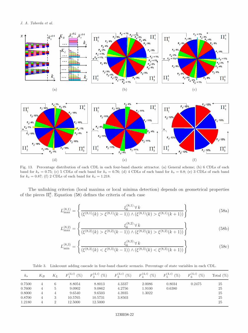
(a) (b) (c)
(d) (e) (f)
Fig. 13. Percentage distribution of each CDL in each four-band chaotic attractor. (a) General scheme; (b) 6 CDLs of eachband for ks = 0.75; (c) 5 CDLs of each band for ks = 0.76; (d) 4 CDLs of each band for ks = 0.8; (e) 3 CDLs of each bandfor ks = 0.87; (f) 2 CDLs of each band for ks = 1.218.
The unlinking criterion (local maxima or local minima detection) depends on geometrical propertiesof the pieces Π8
i . Equation (58) defines the criteria of each case
L(8,1)max =
ξ(8,1)k ∀ k
(ξ(8,1)(k) > ξ(8,1)(k − 1)) ∧ (ξ(8,1)(k) > ξ(8,1)(k + 1))
(58a)
L(8,2)max =
ξ(8,2)k ∀ k
(ξ(8,2)(k) > ξ(8,2)(k − 1)) ∧ (ξ(8,2)(k) > ξ(8,2)(k + 1))
(58b)
L(8,3)min =
ξ(8,3)k ∀ k
(ξ(8,3)(k) < ξ(8,3)(k − 1)) ∧ (ξ(8,3)(k) < ξ(8,3)(k + 1))
(58c)
Table 3. Linkcount adding cascade in four-band chaotic scenario. Percentage of state variables in each CDL.
ks KB KL F(4,i)1 (%) F
(4,i)2 (%) F
(4,i)3 (%) F
(4,i)4 (%) F
(4,i)5 (%) F
(4,i)6 (%) Total (%)
0.7500 4 6 8.8054 8.8013 4.3337 2.0086 0.8034 0.2475 250.7600 4 5 9.0902 9.0862 4.2756 1.9100 0.6380 250.8000 4 4 9.6540 9.6503 4.3935 1.3022 250.8700 4 3 10.5765 10.5731 3.8503 251.2180 4 2 12.5000 12.5000 25
1230034-22

October 28, 2012 1:56 WSPC/S0218-1274 1230034
Chaotic Attractors Inside Band-Merging Scenario in a ZAD-Controlled Buck Converter
L(8,4)max =
ξ(8,4)k ∀ k
(ξ(8,4)(k) > ξ(8,4)(k − 1)) ∧ (ξ(8,4)(k) > ξ(8,4)(k + 1))
(58d)
L(8,5)min =
ξ(8,5)k ∀ k
(ξ(8,5)(k) < ξ(8,5)(k − 1)) ∧ (ξ(8,5)(k) < ξ(8,5)(k + 1))
(58e)
L(8,6)min =
ξ(8,6)k ∀ k
(ξ(8,6)(k) < ξ(8,6)(k − 1)) ∧ (ξ(8,6)(k) < ξ(8,6)(k + 1))
(58f)
L(8,7)max =
ξ(8,7)k ∀ k
(ξ(8,7)(k) > ξ(8,7)(k − 1)) ∧ (ξ(8,7)(k) > ξ(8,7)(k + 1))
(58g)
L(8,8)min =
ξ(8,8)k ∀ k
(ξ(8,8)(k) < ξ(8,8)(k − 1)) ∧ (ξ(8,8)(k) < ξ(8,8)(k + 1))
. (58h)
Figure 14 shows the phase portraits of the Π81
piece. The first CDL map associated to the Π81 piece
denoted by V(8,1)1 is given by Eq. (59)
V(8,1)1 : x(W (8,1)
1 (i)) → x(W (8,1)1 (i + 1)) (59)
where
x ∈ F(8,1)1
W(8,1)1 ∈ I
(8,1)1 ∈ I
i ∈ Z+
with,
(a) (b) (c)
(d) (e) (f)
Fig. 14. Phase portraits of eight-band chaotic attractors (Π81). (a) Eight-band attractor for ks = 1.5; (b) 6 CDLs of Π8
1 for
ks = 1.218; (c) 5 CDLs of Π81 for ks = 1.25; (d) 4 CDLs of Π8
1 for ks = 1.3; (e) 3 CDLs of Π81 for ks = 1.5; (f) 2 CDLs of Π8
1
for ks = 1.78.
1230034-23
October 28, 2012 1:56 WSPC/S0218-1274 1230034
J. A. Taborda et al.
F(8,1)1 =
x(k)
ξ(8,1)k
∈ L(8,1)max
I(8,1)1 =
k
ξ(8,1)k
∈ L(8,1)max
.
Each sequence of maps bounded by two ele-ments of the first map F
(8,1)1 → F
(8,1)2 → · · · →
F(8,1)ρ → F
(8,1)1 is characterized by ρ transitions
where ρ = ∆W(8,1)1 (i)
ρ = ∆W(8,1)1 (i) = W
(8,1)1 (i + 1) − W
(8,1)1 (i). (60)
Therefore, the index maps defined as functionsof the first index map (W (8,1)
1 ) are given by:
W(8,1)2 (k) = W
(8,1)1 (k) + 1
...
W(8,1)ρ (k) = W
(8,1)1 (k) + ρ − 1.
(61)
The CDL maps V(8,1)j can be defined by using
the index maps W(8,1)j as presented in Eq. (62)
V(8,1)1 : x(W (8,1)
1 (i)) → x(W (8,1)1 (i + 1))
V(8,1)2 : x(W (8,1)
2 (i)) → x(W (8,1)2 (i + 1))
...
V(8,1)q : x(W (8,1)
q (i)) → x(W (8,1)q (i + 1)).
(62)
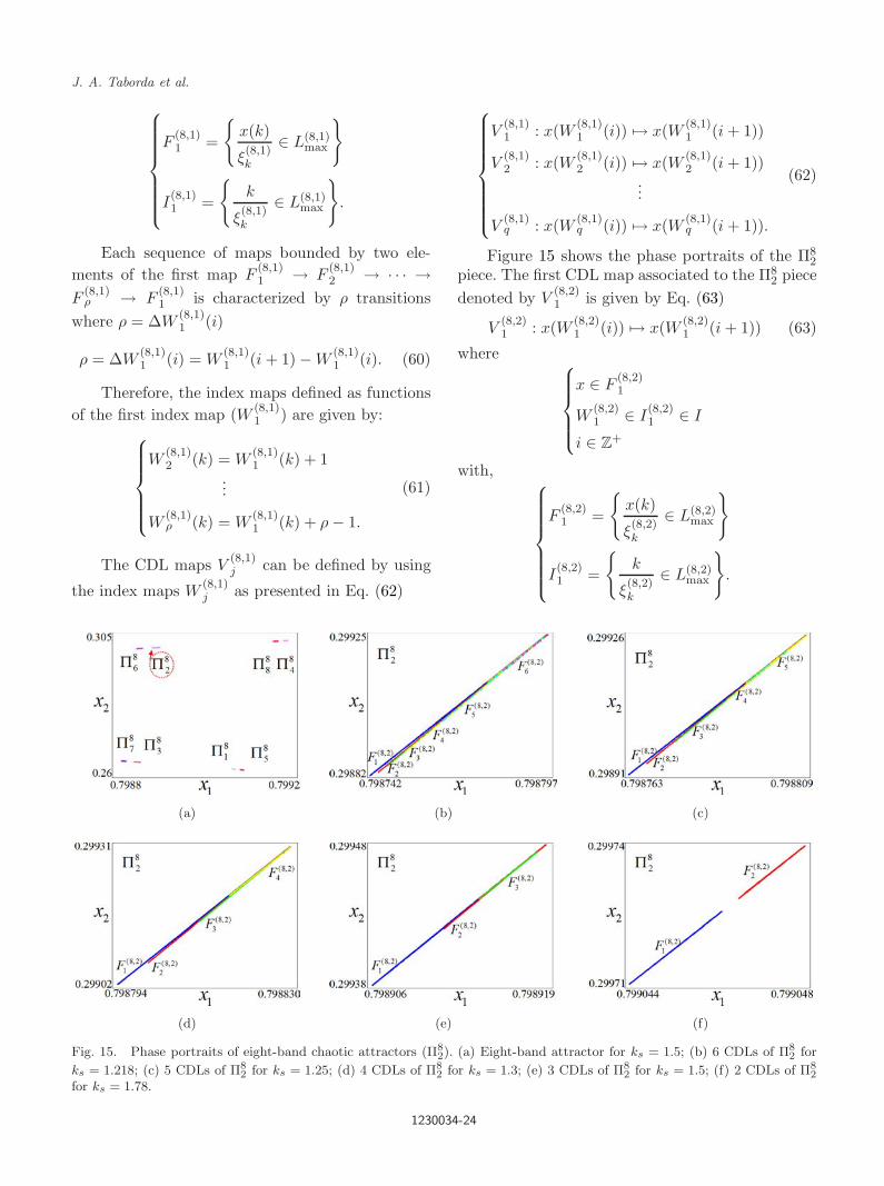
Figure 15 shows the phase portraits of the Π82
piece. The first CDL map associated to the Π82 piece
denoted by V(8,2)1 is given by Eq. (63)
V(8,2)1 : x(W (8,2)
1 (i)) → x(W (8,2)1 (i + 1)) (63)
where
x ∈ F(8,2)1
W(8,2)1 ∈ I
(8,2)1 ∈ I
i ∈ Z+
with,
F(8,2)1 =
x(k)
ξ(8,2)k
∈ L(8,2)max
I(8,2)1 =
k
ξ(8,2)k
∈ L(8,2)max
.
(a) (b) (c)
(d) (e) (f)
Fig. 15. Phase portraits of eight-band chaotic attractors (Π82). (a) Eight-band attractor for ks = 1.5; (b) 6 CDLs of Π8
2 for
ks = 1.218; (c) 5 CDLs of Π82 for ks = 1.25; (d) 4 CDLs of Π8
2 for ks = 1.3; (e) 3 CDLs of Π82 for ks = 1.5; (f) 2 CDLs of Π8
2
for ks = 1.78.
1230034-24
October 28, 2012 1:56 WSPC/S0218-1274 1230034
Chaotic Attractors Inside Band-Merging Scenario in a ZAD-Controlled Buck Converter
Each sequence of maps bounded by two ele-ments of the first map F
(8,2)1 → F
(8,2)2 → · · · →
F(8,2)ρ → F
(8,2)1 is characterized by ρ transitions
where ρ = ∆W(8,2)1 (i)
ρ = ∆W(8,2)1 (i) = W
(8,2)1 (i + 1) − W
(8,2)1 (i). (64)
Therefore, the index maps defined as functionsof the first index map (W (8,2)
1 ) are given by:
W(8,2)2 (k) = W
(8,2)1 (k) + 1
...
W(8,2)ρ (k) = W
(8,2)1 (k) + ρ − 1.
(65)
The CDL maps V(8,2)j can be defined by using
the index maps W(8,2)j as presented in Eq. (66)
V(8,2)1 : x(W (8,2)
1 (i)) → x(W (8,2)1 (i + 1))
V(8,2)2 : x(W (8,2)
2 (i)) → x(W (8,2)2 (i + 1))
...
V(8,2)q : x(W (8,2)
q (i)) → x(W (8,2)q (i + 1)).
(66)
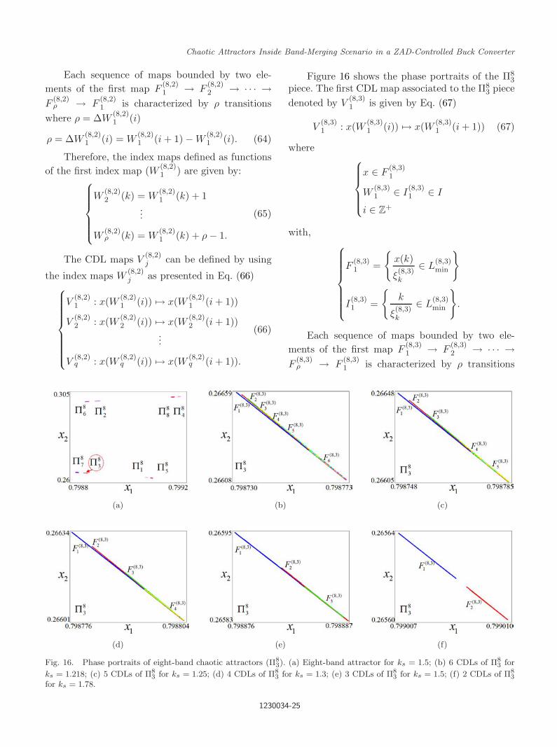
Figure 16 shows the phase portraits of the Π83
piece. The first CDL map associated to the Π83 piece
denoted by V(8,3)1 is given by Eq. (67)
V(8,3)1 : x(W (8,3)
1 (i)) → x(W (8,3)1 (i + 1)) (67)
where
x ∈ F(8,3)1
W(8,3)1 ∈ I
(8,3)1 ∈ I
i ∈ Z+
with,
F(8,3)1 =
x(k)
ξ(8,3)k
∈ L(8,3)min
I(8,3)1 =
k
ξ(8,3)k
∈ L(8,3)min
.
Each sequence of maps bounded by two ele-ments of the first map F
(8,3)1 → F
(8,3)2 → · · · →
F(8,3)ρ → F
(8,3)1 is characterized by ρ transitions
(a) (b) (c)
(d) (e) (f)
Fig. 16. Phase portraits of eight-band chaotic attractors (Π83). (a) Eight-band attractor for ks = 1.5; (b) 6 CDLs of Π8
3 for
ks = 1.218; (c) 5 CDLs of Π83 for ks = 1.25; (d) 4 CDLs of Π8
3 for ks = 1.3; (e) 3 CDLs of Π83 for ks = 1.5; (f) 2 CDLs of Π8
3
for ks = 1.78.
1230034-25
October 28, 2012 1:56 WSPC/S0218-1274 1230034
J. A. Taborda et al.
where ρ = ∆W(8,3)1 (i)
ρ = ∆W(8,3)1 (i) = W
(8,3)1 (i + 1) − W
(8,3)1 (i).
(68)
Therefore, the index maps defined as functionsof the first index map (W (8,3)
1 ) are given by:
W(8,3)2 (k) = W
(8,3)1 (k) + 1
...
W(8,3)ρ (k) = W
(8,3)1 (k) + ρ − 1.
(69)
The CDL maps V(8,3)j can be defined by using
the index maps W(8,3)j as presented in Eq. (70)
V(8,3)1 : x(W (8,3)
1 (i)) → x(W (8,3)1 (i + 1))
V(8,3)2 : x(W (8,3)
2 (i)) → x(W (8,3)2 (i + 1))
...
V(8,3)q : x(W (8,3)
q (i)) → x(W (8,3)q (i + 1)).
(70)
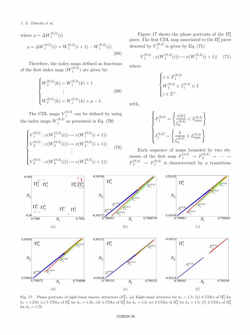
Figure 17 shows the phase portraits of the Π84
piece. The first CDL map associated to the Π84 piece
denoted by V(8,4)1 is given by Eq. (71)
V(8,4)1 : x(W (8,4)
1 (i)) → x(W (8,4)1 (i + 1)) (71)
where
x ∈ F(8,4)1
W(8,4)1 ∈ I
(8,4)1 ∈ I
i ∈ Z+
with,
F(8,4)1 =
x(k)
ξ(8,4)k
∈ L(8,4)max
I(8,4)1 =
k
ξ(8,4)k
∈ L(8,4)max
.
Each sequence of maps bounded by two ele-ments of the first map F
(8,4)1 → F
(8,4)2 → · · · →
F(8,4)ρ → F
(8,4)1 is characterized by ρ transitions
(a) (b) (c)
(d) (e) (f)
Fig. 17. Phase portraits of eight-band chaotic attractors (Π84). (a) Eight-band attractor for ks = 1.5; (b) 6 CDLs of Π8
4 for
ks = 1.218; (c) 5 CDLs of Π84 for ks = 1.25; (d) 4 CDLs of Π8
4 for ks = 1.3; (e) 3 CDLs of Π84 for ks = 1.5; (f) 2 CDLs of Π8
4
for ks = 1.78.
1230034-26

October 28, 2012 1:56 WSPC/S0218-1274 1230034
Chaotic Attractors Inside Band-Merging Scenario in a ZAD-Controlled Buck Converter
where ρ = ∆W(8,4)1 (i)
ρ = ∆W(8,4)1 (i) = W
(8,4)1 (i + 1) − W
(8,4)1 (i).
(72)
Therefore, the index maps defined as functionsof the first index map (W (8,4)
1 ) are given by:
W(8,4)2 (k) = W
(8,4)1 (k) + 1
...
W(8,4)ρ (k) = W
(8,4)1 (k) + ρ − 1.
(73)
The CDL maps V(8,4)j can be defined by using
the index maps W(8,4)j as presented in Eq. (74)
V(8,4)1 : x(W (8,4)
1 (i)) → x(W (8,4)1 (i + 1))
V(8,4)2 : x(W (8,4)
2 (i)) → x(W (8,4)2 (i + 1))
...
V(8,4)q : x(W (8,4)
q (i)) → x(W (8,4)q (i + 1)).
(74)
Figure 18 shows the phase portraits of the Π85
piece. The first CDL map associated to the Π85 piece
denoted by V(8,5)1 is given by Eq. (75)
V(8,5)1 : x(W (8,5)
1 (i)) → x(W (8,5)1 (i + 1)) (75)
where
x ∈ F(8,5)1
W(8,5)1 ∈ I
(8,5)1 ∈ I
i ∈ Z+
with,
F(8,5)1 =
x(k)
ξ(8,5)k
∈ L(8,5)min
I(8,5)1 =
k
ξ(8,5)k
∈ L(8,5)min
.
Each sequence of maps bounded by two ele-ments of the first map F
(8,5)1 → F
(8,5)2 → · · · →
F(8,5)ρ → F
(8,5)1 is characterized by ρ transitions
(a) (b) (c)
(d) (e) (f)
Fig. 18. Phase portraits of eight-band chaotic attractors (Π85). (a) Eight-band attractor for ks = 1.5; (b) 6 CDLs of Π8
5 for
ks = 1.218; (c) 5 CDLs of Π85 for ks = 1.25; (d) 4 CDLs of Π8
5 for ks = 1.3; (e) 3 CDLs of Π85 for ks = 1.5; (f) 2 CDLs of Π8
5
for ks = 1.78.
1230034-27
October 28, 2012 1:56 WSPC/S0218-1274 1230034
J. A. Taborda et al.
where ρ = ∆W(8,5)1 (i)
ρ = ∆W(8,5)1 (i) = W
(8,5)1 (i + 1) − W
(8,5)1 (i).
(76)
Therefore, the index maps defined as functionsof the first index map (W (8,5)
1 ) are given by:
W(8,5)2 (k) = W
(8,5)1 (k) + 1
...
W(8,5)ρ (k) = W
(8,5)1 (k) + ρ − 1.
(77)
The CDL maps V(8,5)j can be defined by using
the index maps W(8,5)j as presented in Eq. (78)
V(8,5)1 : x(W (8,5)
1 (i)) → x(W (8,5)1 (i + 1))
V(8,5)2 : x(W (8,5)
2 (i)) → x(W (8,5)2 (i + 1))
...
V(8,5)q : x(W (8,5)
q (i)) → x(W (8,5)q (i + 1)).
(78)
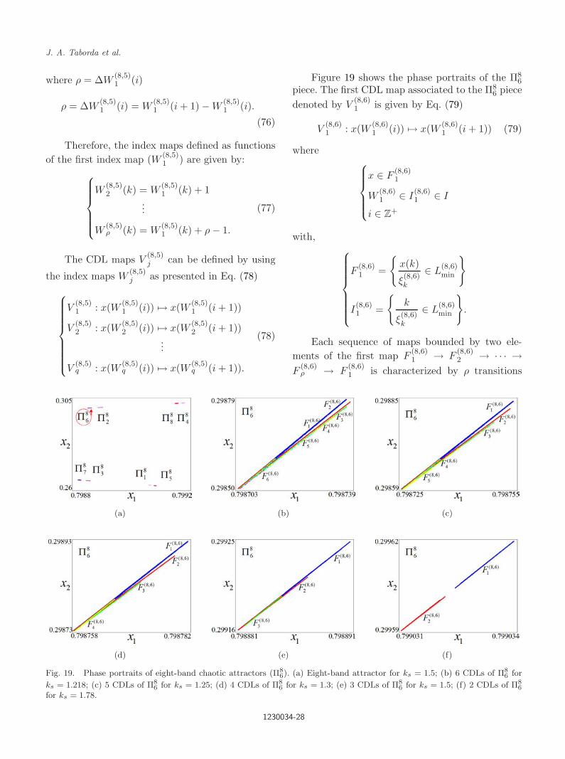
Figure 19 shows the phase portraits of the Π86
piece. The first CDL map associated to the Π86 piece
denoted by V(8,6)1 is given by Eq. (79)
V(8,6)1 : x(W (8,6)
1 (i)) → x(W (8,6)1 (i + 1)) (79)
where
x ∈ F(8,6)1
W(8,6)1 ∈ I
(8,6)1 ∈ I
i ∈ Z+
with,
F(8,6)1 =
x(k)
ξ(8,6)k
∈ L(8,6)min
I(8,6)1 =
k
ξ(8,6)k
∈ L(8,6)min
.
Each sequence of maps bounded by two ele-ments of the first map F
(8,6)1 → F
(8,6)2 → · · · →
F(8,6)ρ → F
(8,6)1 is characterized by ρ transitions
(a) (b) (c)
(d) (e) (f)
Fig. 19. Phase portraits of eight-band chaotic attractors (Π86). (a) Eight-band attractor for ks = 1.5; (b) 6 CDLs of Π8
6 for
ks = 1.218; (c) 5 CDLs of Π86 for ks = 1.25; (d) 4 CDLs of Π8
6 for ks = 1.3; (e) 3 CDLs of Π86 for ks = 1.5; (f) 2 CDLs of Π8
6
for ks = 1.78.
1230034-28
October 28, 2012 1:56 WSPC/S0218-1274 1230034
Chaotic Attractors Inside Band-Merging Scenario in a ZAD-Controlled Buck Converter
where ρ = ∆W(8,6)1 (i)
ρ = ∆W(8,6)1 (i) = W
(8,6)1 (i + 1) − W
(8,6)1 (i).
(80)
Therefore, the index maps defined as functionsof the first index map (W (8,6)
1 ) are given by:
W(8,6)2 (k) = W
(8,6)1 (k) + 1
...
W(8,6)ρ (k) = W
(8,6)1 (k) + ρ − 1.
(81)
The CDL maps V(8,6)j can be defined by using
the index maps W(8,6)j as presented in Eq. (82)
V(8,6)1 : x(W (8,6)
1 (i)) → x(W (8,6)1 (i + 1))
V(8,6)2 : x(W (8,6)
2 (i)) → x(W (8,6)2 (i + 1))
...
V(8,6)q : x(W (8,6)
q (i)) → x(W (8,6)q (i + 1)).
(82)
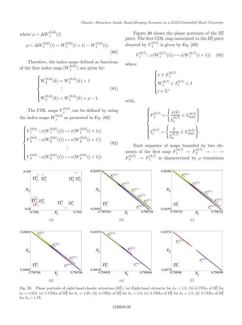
Figure 20 shows the phase portraits of the Π87
piece. The first CDL map associated to the Π87 piece
denoted by V(8,7)1 is given by Eq. (83)
V(8,7)1 : x(W (8,7)
1 (i)) → x(W (8,7)1 (i + 1)) (83)
where
x ∈ F(8,7)1
W(8,7)1 ∈ I
(8,7)1 ∈ I
i ∈ Z+
with,
F(8,7)1 =
x(k)
ξ(8,7)k
∈ L(8,7)max
I(8,7)1 =
k
ξ(8,7)k
∈ L(8,7)max
.
Each sequence of maps bounded by two ele-ments of the first map F
(8,7)1 → F
(8,7)2 → · · · →
F(8,7)ρ → F
(8,7)1 is characterized by ρ transitions
(a) (b) (c)
(d) (e) (f)
Fig. 20. Phase portraits of eight-band chaotic attractors (Π87). (a) Eight-band attractor for ks = 1.5; (b) 6 CDLs of Π8
7 for
ks = 1.218; (c) 5 CDLs of Π87 for ks = 1.25; (d) 4 CDLs of Π8
7 for ks = 1.3; (e) 3 CDLs of Π87 for ks = 1.5; (f) 2 CDLs of Π8
7
for ks = 1.78.
1230034-29
October 28, 2012 1:56 WSPC/S0218-1274 1230034
J. A. Taborda et al.
where ρ = ∆W(8,7)1 (i)
ρ = ∆W(8,7)1 (i) = W
(8,7)1 (i + 1) − W
(8,7)1 (i).
(84)
Therefore, the index maps defined as functionsof the first index map (W (8,7)
1 ) are given by:
W(8,7)2 (k) = W
(8,7)1 (k) + 1
...
W(8,7)ρ (k) = W
(8,7)1 (k) + ρ − 1.
(85)
The CDL maps V(8,7)j can be defined by using
the index maps W(8,7)j as presented in Eq. (86)
V(8,7)1 : x(W (8,7)
1 (i)) → x(W (8,7)1 (i + 1))
V(8,7)2 : x(W (8,7)
2 (i)) → x(W (8,7)2 (i + 1))
...
V(8,7)q : x(W (8,7)
q (i)) → x(W (8,7)q (i + 1)).
(86)
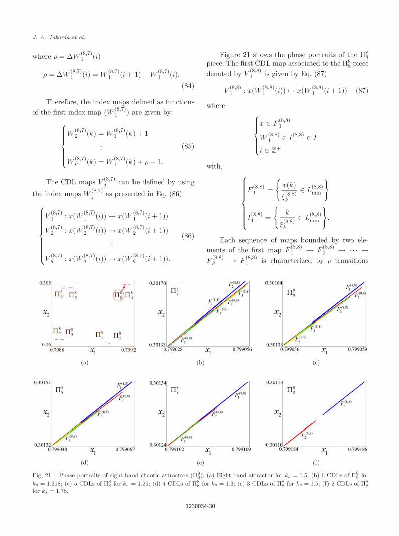
Figure 21 shows the phase portraits of the Π88
piece. The first CDL map associated to the Π88 piece
denoted by V(8,8)1 is given by Eq. (87)
V(8,8)1 : x(W (8,8)
1 (i)) → x(W (8,8)1 (i + 1)) (87)
where
x ∈ F(8,8)1
W(8,8)1 ∈ I
(8,8)1 ∈ I
i ∈ Z+
with,
F(8,8)1 =
x(k)
ξ(8,8)k
∈ L(8,8)min
I(8,8)1 =
k
ξ(8,8)k
∈ L(8,8)min
.
Each sequence of maps bounded by two ele-ments of the first map F
(8,8)1 → F
(8,8)2 → · · · →
F(8,8)ρ → F
(8,8)1 is characterized by ρ transitions
(a) (b) (c)
(d) (e) (f)
Fig. 21. Phase portraits of eight-band chaotic attractors (Π88). (a) Eight-band attractor for ks = 1.5; (b) 6 CDLs of Π8
8 for
ks = 1.218; (c) 5 CDLs of Π88 for ks = 1.25; (d) 4 CDLs of Π8
8 for ks = 1.3; (e) 3 CDLs of Π88 for ks = 1.5; (f) 2 CDLs of Π8
8
for ks = 1.78.
1230034-30
October 28, 2012 1:56 WSPC/S0218-1274 1230034
Chaotic Attractors Inside Band-Merging Scenario in a ZAD-Controlled Buck Converter
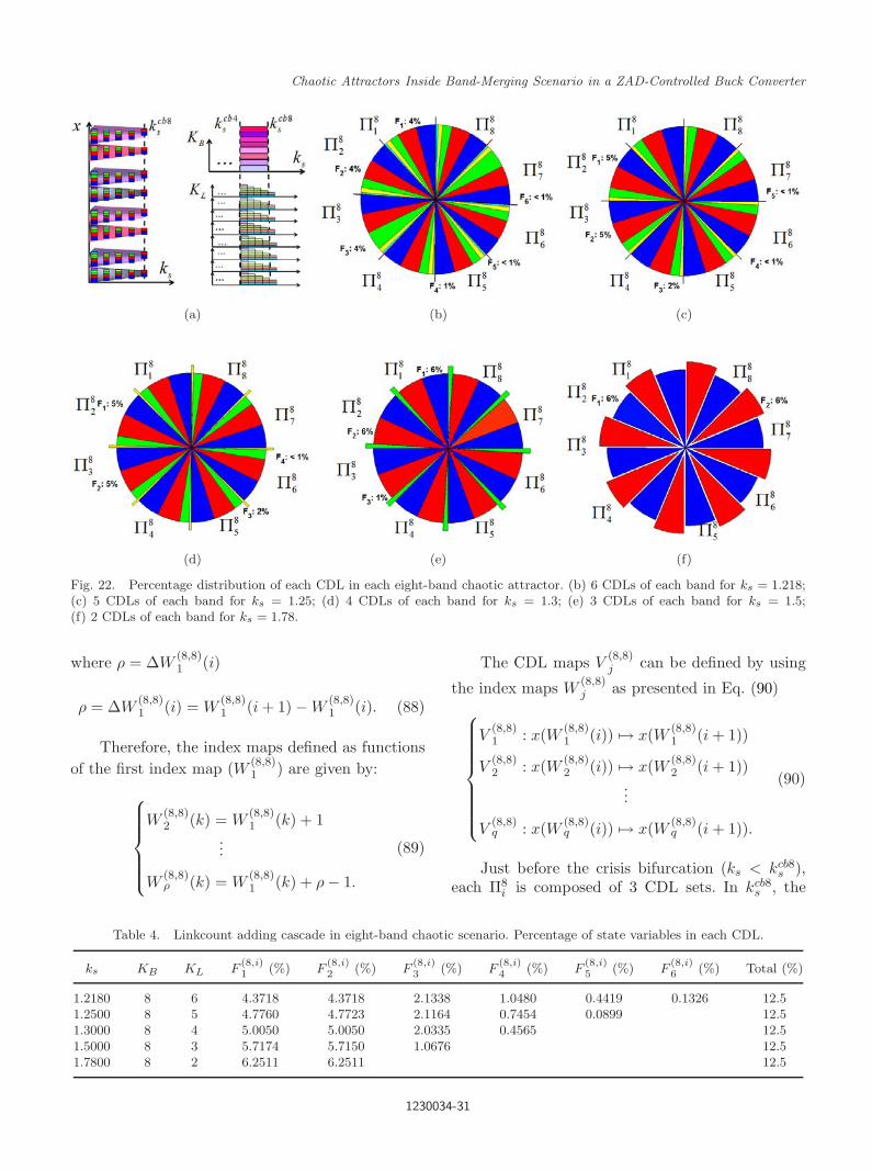
(a) (b) (c)
(d) (e) (f)
Fig. 22. Percentage distribution of each CDL in each eight-band chaotic attractor. (b) 6 CDLs of each band for ks = 1.218;(c) 5 CDLs of each band for ks = 1.25; (d) 4 CDLs of each band for ks = 1.3; (e) 3 CDLs of each band for ks = 1.5;(f) 2 CDLs of each band for ks = 1.78.
where ρ = ∆W(8,8)1 (i)
ρ = ∆W(8,8)1 (i) = W
(8,8)1 (i + 1) − W
(8,8)1 (i). (88)
Therefore, the index maps defined as functionsof the first index map (W (8,8)
1 ) are given by:
W(8,8)2 (k) = W
(8,8)1 (k) + 1
...
W(8,8)ρ (k) = W
(8,8)1 (k) + ρ − 1.
(89)
The CDL maps V(8,8)j can be defined by using
the index maps W(8,8)j as presented in Eq. (90)
V(8,8)1 : x(W (8,8)
1 (i)) → x(W (8,8)1 (i + 1))
V(8,8)2 : x(W (8,8)
2 (i)) → x(W (8,8)2 (i + 1))
...
V(8,8)q : x(W (8,8)
q (i)) → x(W (8,8)q (i + 1)).
(90)
Just before the crisis bifurcation (ks < kcb8s ),
each Π8i is composed of 3 CDL sets. In kcb8
s , the
Table 4. Linkcount adding cascade in eight-band chaotic scenario. Percentage of state variables in each CDL.
ks KB KL F(8,i)1 (%) F
(8,i)2 (%) F
(8,i)3 (%) F
(8,i)4 (%) F
(8,i)5 (%) F
(8,i)6 (%) Total (%)
1.2180 8 6 4.3718 4.3718 2.1338 1.0480 0.4419 0.1326 12.51.2500 8 5 4.7760 4.7723 2.1164 0.7454 0.0899 12.51.3000 8 4 5.0050 5.0050 2.0335 0.4565 12.51.5000 8 3 5.7174 5.7150 1.0676 12.51.7800 8 2 6.2511 6.2511 12.5
1230034-31

October 28, 2012 1:56 WSPC/S0218-1274 1230034
J. A. Taborda et al.
third sets F(8,i)3 are empty and sixteen-band chaos is
created. Figures 14(f)–21(f) show the formation ofsixteen-band chaotic attractor after kcb8
s . Sets F(8,i)1
and F(8,i)2 correspond to a different band Π16
i .Figure 22 and Table 4 show the percentages
of each set F(8,i)j of eight-band chaotic attractors.
Each group of sets F(8,1)j , F
(8,2)j , F
(8,3)j , F
(8,4)j ,
F(8,5)j , F
(8,6)j , F
(8,7)j , F
(8,8)j has symmetric behavior.
The sum of all percentages in each group of sets(F (8,i)
j (%)) should be 12.5%. In each case, the last
CDL F(8,i)q has the lowest percentage.
5. Conclusions and Future Work
We have reported a new bifurcation scenario foundinside band-merging scenario of ZAD-controlledbuck converter. We have used a novel qualitativeframework named Dynamic Linkcounter (DLC )approach to characterize chaotic attractors between
consecutive crisis bifurcations. This approach hascomplemented the results that can be obtained withBandcounter approaches. Self-similar substructuresdenoted as complex dynamic links (CDLs) were dis-tinguished in multiband chaotic attractors. Geo-metrical changes in multiband chaotic attractorswere detected when the control parameter of ZADstrategy was varied between two consecutive crisisbifurcations. Linkcount subtracting staircases weredefined inside band-merging scenario. Figure 23(a)shows a schematic bifurcation diagram of band-merging scenario with link-subtracting cascades.
Border-collision period-doubling cascade fol-lowed by inverse band-merging cascade is a non-smooth chaotic scenario that is widely studied.However, the study of topological changes inmultiband chaotic attractors was avoided. To ourknowledge, this work is the first attempt to charac-terize geometric and topological changes of multi-band chaotic attractors between two consecutivecrisis bifurcations.
Fig. 23. Summary diagrams of band-merging scenario. (a) Schematic bifurcation diagram; (b) adding-band staircase; (c)subtracting-link staircases; (d) tree diagram of multiband chaos and index maps for unlinking functions; (e) tree diagram ofmultiband chaos and unlinking criteria.
Table 5. Summary of notation used in Dynamic Bandcounter Approach (DBC) and Dynamic Linkcounter Approach (DLC).
Symbol Type Description
i Counter Can be used to index Vj and Wj maps (or V(p,i)j and W
(p,i)j maps)
k Counter Can be used to index the general maps P or I
m Parameter Number of maps used in the DBC approach
p Characteristic Number of bands in a multiband chaotic attractor
q Characteristic Number of self-similar substructures in a chaotic attractor
Fj Set of points Substructures (or CDL) of Ωq
F(p,i)j Set of points Substructures (or CDL) of Ωp
q located in the Πpi piece
I Index set General index set associated to the Poincare map P
Ij Index sets (j = 1, . . . , q) Set of indexes k that define the Fj piece of the attractor Ωq
I(p,i)j Index sets (j = 1, . . . , q) Set of indexes k that define the Fj piece in the Πp
i piece of the attractor Ωpq
1230034-32

October 28, 2012 1:56 WSPC/S0218-1274 1230034
Chaotic Attractors Inside Band-Merging Scenario in a ZAD-Controlled Buck Converter
Table 5. (Continued)
Symbol Type Description
Lmax Set of points Local maxima set of ξk that could define the first CDL (F1)
L(p,i)max Set of points Local maxima set of ξ
(p,i)k that could define the first CDL (F
(p,i)1 )
Lmin Set of points Local minima set of ξk that could define the first CDL (F1)
L(p,i)min Set of points Local minima set of ξ
(p,i)k that could define the first CDL (F
(p,i)1 )
P Map Poincare map
P pi Maps (i = 1, . . . , m) Restriction of P to the Πp
i piece of the attractor
Vj Maps (j = 1, . . . , q) Restriction of P to the Fj piece of the attractor Ωq
V(p,i)j Maps (j = 1, . . . , q) Restriction of P to the Fj piece in the Πp
i piece of the attractor Ωpq
Wj Index maps (j = 1, . . . , q) Restriction of I to the Ij subset that defines Fj
W(p,i)j Index maps (j = 1, . . . , q) Restriction of I to the I
(p,i)j subset that defines F
(p,i)j
ρ Variable Number of CDLs that are visited before a new sequence (F1 → · · ·Fρ → F1 · · ·)ξk Discrete function Discriminant function named unlinking function that defines the first CDL (F1)
ξ(p,i)k Discrete function Unlinking function that defines the first CDL (F
(p,i)1 ) in the Πp
i piece
Πpi Sets of points (i = 1, . . . , m) Piece of the attractor defined by the Pp
i map
Ωq Set of points One-band chaotic attractor composed by q CDLs
Ωpq Set of points p-band chaotic attractor composed by q CDLs
The principles of Dynamic Bandcounterapproach and Dynamic Linkcounter approach weregiven. Table 5 summarizes the notation used in eachapproach. We have defined an unlinking function foreach multiband attractor. Figure 23(b) shows a treediagram with the index maps W
(p,i)1 and W
(p,i)2 used
in each unlinking function.We have determined the unlinking criteria
(local maxima or local minima detection) to decom-pose multiband chaotic attractors in substructuresnamed Complex Dynamic Links (CDL). Each CDLset has a state variable map (V (p,i)
j ) and an index
map (W (p,i)j ) associated to it. Figure 23(c) shows
a tree diagram with the unlinking criteria L(p,i)min or
L(p,i)max used in each Πp
i piece.In our future research, we wish to apply the
same methodology of this paper in a multibandtorus-breakdown scenario.
References
Alzate, R., di Bernardo, M., Montanaro, U. & Santini, S.[2007] “Experimental and numerical verification ofbifurcations and chaos in cam-follower impactingsystems,” Nonlin. Dyn. 50, 409–429.
Angulo, F. [2004] “Dynamical analysis of PWM-controlled power electronic converters based on the
zero average dynamics (ZAD) strategy,” PhD thesis,Technical University of Catalonia (in Spanish).
Angulo, F., Fossas, E. & Olivar, G. [2005] “Transitionfrom periodicity to chaos in a PWM-controlled buckconverter with ZAD strategy,” Int. J. Bifurcation andChaos 15, 3245–3264.
Angulo, F., Ocampo, C., Olivar, G. & Ramos, R. [2006]“Nonlinear and nonsmooth dynamics in a DC-DCbuck converter: Two experimental set-ups,” Nonlin.Dyn. 46, 239–257.
Angulo, F., Olivar, G. & Taborda, J. A. [2008a] “Con-tinuation of periodic orbits in a ZAD-strategy con-trolled buck converter,” Chaos Solit. Fract. 38, 348–363.
Angulo, F., Olivar, G. & di Bernardo, M. [2008b] “Two-parameter discontinuity-induced bifurcation curves ina ZAD-strategy controlled DC-DC buck converter,”IEEE Trans. Circuits Syst.-I : Regular Papers 55,2392–2401.
Avrutin, V., Eckstein, B. & Schanz, M. [2007] “On detec-tion of multi-band chaotic attractors,” Proc. R. Soc.A 463, 1339–1358.
Avrutin, V., Eckstein, B. & Schanz, M. [2008a] “Thebandcount increment scenario. I. Basic structures,”Proc. R. Soc. A 464, 1867–1883.
Avrutin, V., Eckstein, B. & Schanz, M. [2008b] “Thebandcount increment scenario. II. Interior struc-tures,” Proc. R. Soc. A 464, 2247–2263.
Avrutin, V. & Schanz, M. [2008] “On the fully developedbandcount adding scenario,” Nonlinearity 21, 1077–1103.
1230034-33

October 28, 2012 1:56 WSPC/S0218-1274 1230034
J. A. Taborda et al.
Avrutin, V., Eckstein, B. & Schanz, M. [2009] “Thebandcount increment scenario. III. Deformed struc-tures,” Proc. R. Soc. A 465, 41–57.
Avrutin, V., Fossas, E., Granados, A. & Schanz, M.[2011] “Virtual orbits and two-parameter bifurcationanalysis in a ZAD-controlled buck converter,” Nonlin.Dyn. 63, 19–23.
Banerjee, S. & Verghese, G. [2001] Nonlinear Phenom-ena in Power Electronics — Attractors, Bifurcations,Chaos, and Nonlinear Control (IEEE Press, NY).
D’Amico, M. B., Angulo, F., Olivar, G., Paolini, E.& Moiola, J. L. [2012] “Influence of period-doublingbifurcations in the appearance of border collisionsfor a ZAD-strategy controlled buck converter,” Int.J. Circuit Th. Appl. 40, 77–91.
di Bernardo, M., Budd, C., Champneys, A. & Kowal-czyk, P. [2007] Piecewise-Smooth Dynamical Systems :Theory and Applications (Springer).
Eckstein, B. [2006] Bandcounter : Counting Bandsof Multiband Chaotic Attractors (University ofStuttgart).
Fossas, E., Hogan, S. J. & Seara, T. M. [2009] “Two-parameter bifurcation curves in power electronic con-verters,” Int. J. Bifurcation and Chaos 19, 349–357.
Hart, D. [2001] Electronica de Potencia (Prentice Hall,Madrid, Espana).
Mohan, N., Undeland, T. & Robbins, W. [1995] PowerElectronics : Converters, Applications and Design(John Wiley & Sons).
Olivar, G. [1997] “Chaos in the buck converter,” PhDthesis, Technical University of Catalonia, Barcelona,Spain.
Taborda, J. A., Angulo, F. & Olivar, G. [2009] “Bifur-cation analysis on nonsmooth torus destruction sce-nario of delayed-PWM switched buck converter,” Int.J. Bifurcation and Chaos 19, 2193–2212.
Taborda, J. A. [2010] “Characterization of complexbifurcation scenarios in piecewise-smooth dynami-cal systems,” PhD thesis, Universidad Nacional deColombia, 2010.
Taborda, J. A., Angulo, F. & Olivar, G. [2010]“Mandelbrot-like bifurcation structures in chaosband scenario of switched converter with delayed-PWM control,” Int. J. Bifurcation and Chaos20, 99–119.
Taborda, J. A., Angulo, F. & Olivar, G. [2011] “Charac-terization of chaos scenarios with periodic inclusionsfor one class of piecewise-smooth dynamical maps,”Int. J. Bifurcation and Chaos 21, 2427–2466.
Thompson, J. M. T. & Ghaffari, R. [1983] “Chaoticdynamics of an impact oscillator,” Phys. Rev. A 27,1741–1743.
Zhusubaliyev, Zh. T. & Mosekilde, E. [2003] Bifurcationsand Chaos in Piecewise-Smooth Dynamical Systems(World Scientific, Singapore).
1230034-34
Copyright © 2022 FDOKUMEN